Introduction to Automata Theory, Languages, and
Computation
John E, Hopcroft
Rajeev Motwani
Jeffrey D, Ullman
led., 2001

Senior Acquisitions EditX)r Maite Sttarez-Rivas
Project Editor Katherine Harutunian
Executive Marketing Manager Michael Hirsch
Cover Design Leslie Haimes
Art Direction Regina Hagen
Prepress and Manufacturing Caroline Fell
Access the latest information about Addison-Wesley titles from our World Wide
Web site: http://www.awLcom
The programs and applications presented in this book have been included for
their instructional value. They have been tested with care, but are not
guaranteed for any particular purpose. The publisher does not offer arxy warranties or
representations, not does it accept any liabilities with respect to the programs
or applications.
library of Congress Cataloging^in-Publlcation Data
Hopcroft, John E., 1939-
Introduction to automata theory, languages, and computation / John E.
Hopcroft, Rajeev Motwani, Jeffrey D. Ullman.—^2nd ed.
p. cm.
ISBN 0-201-44124-1
1. Machine theory. 2. Formal languages. 3. Computational complexity.
L Motwani, Rajeev. U. UUman, Jeffrey D., 1942-.
QA267 .H56 2001
511.3—dc21 00-064608
Copyright © 2001 by Addison-Wesley
All rights reserved. No part of this publication may be reproduced, stored in a
retrieval system, or transmitted, in any form or by arxy means, electronic,
mechanical, photocopying, recording, or otherwise, without the prior written
permission of the publisher. Printed in the United States of America.
345678910-MA-04030201
u

Preface
In the preface from the 1979 predecessor to this book, Hopcroft and Ulhnan
maxveled at the fact that the subject of automata had exploded, compared with
its state at the time they wrote their first book, in 1969. Truly, the 1979 book
contained many topics not found in the earlier work and was about twice its
size. If you compare this book with the 1979 book, you will find that, like the
automobiles of the 1970's, this book is "larger on the outside, but smaller on
the inside." That sounds like a retrograde step, but we are happy with the
changes for several reasons.
First, in 1979, automata and language theory was still an area of active
research. A purpose of that book was to encourage mathematically indined
students to make new contributions to the field. Today, there is little direct
research in automata theory (as opposed to its applications), and thus little
motivation for us to retain the succinct, highly mathematical tone of the 1979
book.
Second, the role of automata and language theory has changed over the
past two decades* In 1979, automata was largely a graduate-level subject, and
we imagined our reader was an advanced graduate student, especially those
using the later chapters of the book. Today, the subject is a staple of the
undergraduate curriculum. As such, the content of the book must assume less
in the way of prerequisites from the student, and therefore must provide more
of the background and details of arguments than did the earlier book,
A third change in the environment is that Computer Science has grown to
an almost unimaginable degree in the past two decades. While in 1979 it was
often a challenge to fill up a curriculum with materigJ that we felt would survive
the next wave of technology, today very many subdisciplines compete for the
limited amount of space in the undergraduate curriculum.
Fourthly, CS has become a more vocational subject, and there is a severe
pragmatism among many of its students. We continue to believe that aspects
of automata theory are essential tools in a variety of new disciplines, and we
believe that the theoretical, mind-expanding exercises embodied in the typical
automata course retain their value, no matter how much the student prefers to
learn only the most immediately monetizable technology. However, to assure
a continued place for the subject on the menu of topics avsdlable to the
computer science student, we believe it is necessary to emphasize the applications
* * ■

iv PREFACE
along with the mathematics. Thus, we have replaced a number of the more
abstinase topics in the earUer book with examples of how the ideas are used
today. While applications of automata and language theory to compUers are
now so well understood that they are normally covered in a compiler course,
there are a variety of more recent uses, including model-checking algorithms
to verify protocols and document-description languages that are patterned on
context-free grammars.
A final explanation for the simultaneous growth and shrinkage of the book
is that we were today able to take advantage of the T^ and I^TJgX typesetting
systems developed by Don Knuth and Les Lamport. The latter, especially,
encourages the "open" style of typesetting that makes books larger, but easier
to read. We appreciate the efforts of both men.
Use of the Book
This book is suitable for a quarter or semester course at the Junior level or
above. At Stanford, we have used the notes in CS154, the course in automata
and language theory. It is a one-quarter course, which both Rajeev and Jeff have
taught. Because of the limited time available. Chapter 11 is not covered, and
some of the later material, such as the more difficult polynomial-time reductions
in Section 10.4 are omitted as well. The book's Web site (see below) includes
notes and syllabi for several offerings of CS154.
Some years ago, we found that mfiny graduate students came to Stanford
with a course in automata theory that did not include the theory of
intractability. As the Stfinford faculty believes that these ideas are essential for every
computer scientist to know at more than the level of "NP-complete meajis it
takes too long," there is another course, CS154N, that students may take to
cover only Chapters 8, 9, and 10. They actually participate in roughly the last
third of CS154 to fulfill the CS154N requirement. Even today, we find several
students each quarter availing themselves of this option. Since it requires little
extra effort, we recommend the approach.
Prerequisites
To make best use of this book, students should have taken previously a course
covering discrete mathematics, e.g., graphs, trees, logic, and proof techniques.
We assume also that they have had several courses in programming, and are
familiar with common data structures, recursion, find the role of major system
components such as compilers. These prerequisites should be obtained in a
typical freshman-sophomore CS progr^n.

Exercises
The book contains extensive exercises, with some for almost every section. We
indic?ite harder exercises or parts of exercises with an exclamation point. The
hardest exercises have a double exclamation point.
Some of the exercises or parts are marked with a star. For these exercises,
we shall endeavor to maintain solutions accessible through the book's Web page.
These solutions are publicly available and should be used for self-testing. Note
that in a few cases, one exercise B asks for modification or adaptation of your
solution to another exercise A, If certain parts of A have solutions, then you
should expect the corresponding parts of B to have solutions as welL
Support on the World Wide Web
The book's home page is
http: //www-db. Stanford * edu/"Tillman/ialc. html
Here are solutions to starred exercises, errata as we learn of them, and backup
materials. We hope to make available the notes for each offering of CS154 as
we teach it, including homeworks, solutions, and exams.
Acknowledgements
A hfindout on "how to do proofe" by Craig Silverstein influenced some of the
material in Chapter 1. Comments and errata on drafts of this book were
received from: Zoe Abrams, George Candea, Haowen Chen, Byong-Gun Chun,
Jeffrey Shallit, Bret Taylor, Jason Townsend, and Erik Uzureau. They are
gratefully acknowledged. Remaining errors are ours, of course*
J. E. H.
R. M.
J. D. U.
Ithaca NY and Stanford CA
September, 2000

Table of Contents
1 Automata: The Methods and the Madness 1
1.1 Why Study Automata Theory? 2
1.1.1 Introduction to Finite Automata 2
1.1.2 Structural Representations 4
1.1*3 Automata and Complexity 5
1.2 hitroduction to Formal Proof 5
1.2.1 Deductive Proofs 6
1*2*2 Reduction to Definitions 8
1.2.3 Other Theorem Forms 10
1.2.4 Theorems That Appear Not to Be If-Then Statements . , 13
L3 Additional Forms of Proof 13
1.3.1 Proving Equivalences About Sets 14
1.3.2 The Contrapositive 14
1.3.3 Proof by Contradiction 16
1.3.4 Counterexamples 17
1.4 Inductive Proofs 19
1.4.1 Inductions on Integers 19
1.4.2 More (Jeneral Forms of Integer Inductions 22
1.4.3 Structural Inductions 23
1.4.4 Mutual Inductions 26
1*5 The Central Concepts of Automata Theory 28
1.5.1 Alphabets 28
1.5.2 Strings 29
1.5.3 Languages 30
1.5.4 Problems 31
1.6 Summary of Chapter 1 34
1.7 References for Chapter 1 35
2 Finite Automata 37
2.1 An Informal Picture of Finite Automata 38
2.1.1 The Ground Rules 38
2.1.2 The Protocol 39
2.1-3 Enabling the Automata to Ignore Actions 41
«■
vu

viu TABLE OF CONTENTS
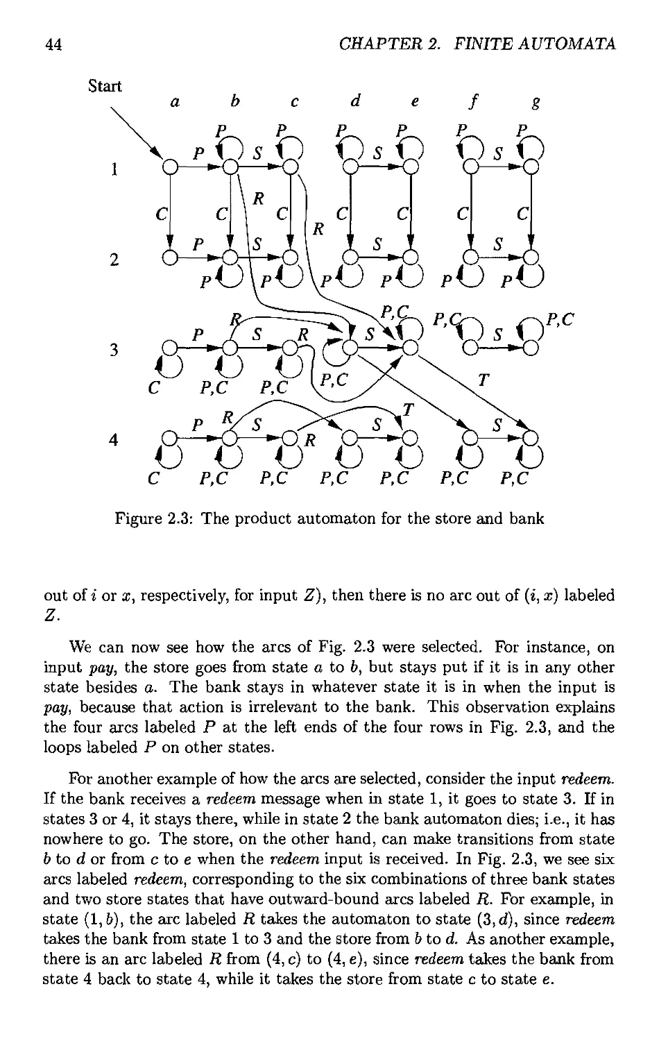
2.1.4 The Entire System as an Automaton 43
2.1.5 Using the Product Automaton to VaHdate the Protocol * 45
2.2 Deterministic Finite Automata 45
2.2.1 Definition of a Deterministic Finite Automaton 46
2.2.2 How a DFA Processes Strings 46
2.2.3 Simpler Notations for DFA's 48
2.2.4 Extending the Transition Function to Strings 49
2.2.5 The Language of a DFA 52
2.2.6 Exercises for Section 2,2 53
2.3 Nondeterministic Finite Automata 55
2.3.1 An Informal View of Nondeterministic Finite Automata . 56
2.3.2 Definition of Nondeterministic Finite Automata 57
2.3.3 The Extended Transition Function 58
2.3.4 The Language of an NFA 59
2.3.5 Equivalence of Deterministic and Nondeterministic Finite
Automata 60
2.3.6 A Bad Case for the Subset Construction 65
2.3.7 Exercises for Section 2.3 66
2.4 An Application: Text Search 68
2.4.1 Finding Strings in Text 68
2.4.2 Nondeterministic Finite Automata for Text Search .... 69
2.4.3 A DFA to Recognize a Set of Keywords 70
2.4.4 Exercises for Section 2.4 72
2.5 Finite Automata With Epsilon-IVansitions 72
2.5-1 Uses of c-Transitions 72
2.5.2 The Formal Notation for an e-NFA 74
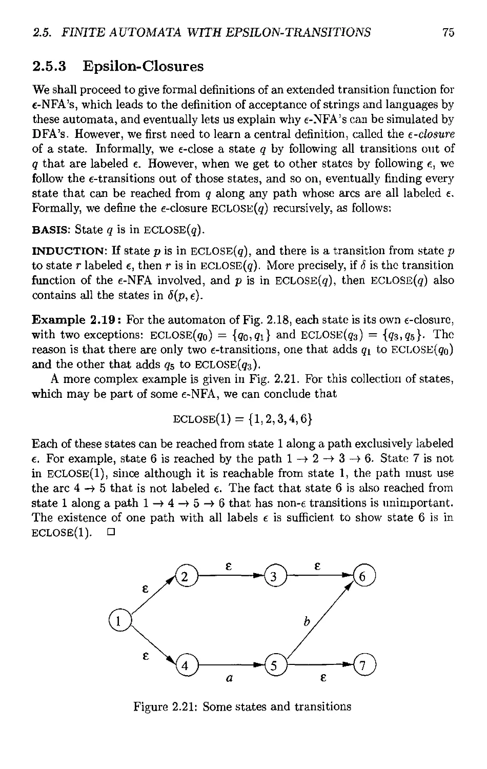
2.5.3 Epsilon-Closures 75
2.5.4 Extended Transitions and Languages for €-NFA'9 ..... 76
2.5.5 Eliminating ^-Transitions 77
2.5.6 Exercises for Section 2.5 80
2.6 Summary of Chapter 2 80
2.7 References for Chapter 2 81
3 Regular Expressions and Languages 83
3.1 Regular Expressions 83
3.1.1 The Operators of Regular Expressions 84
3.1.2 Building Regular Expressions 85
3.1.3 Precedence of Regular-Expression Operators 88
3.1.4 Exercises for Section 3.1 89
3.2 Finite Automata and Regular Expressions 90
3.2.1 Prom DFA's to Regular Expressions 91
3.2.2 Converting DFA's to Regular Expressions by Eliminating
States 96
3.2.3 Converting Regular Expressions to Automata 101
3.2.4 Exercises for Section 3.2 106

TABLE OF CONTENTS ix
3.3 Applications of Regular Expressions 108
3.3.1 Regular Expressions in UNIX 108
3.3.2 Le:dcal Analysis 109
3.3.3 Finding Patterns in Tfext Ill
3.3.4 Exercises for Section 3.3 113
3.4 Algebraic Laws for Regular Expressions 114
3.4.1 Associativity and Conimutativity 114
3.4.2 Identities and Annihilators 115
3.4.3 Distributive Laws 115
3.4.4 The Idempotent Law 116
3.4.5 Laws Involving Closures 117
3.4.6 Discovering Laws for Regular Expressions 117
3.4.7 The Test for a Regular-Expression Algebraic Law 119
3.4.8 Exercises for Section 3.4 120
3.5 Summary of Chapter 3 122
3.6 References for Chapter 3 122
4 Properties of Regular Languages 125
4.1 Proving Lfinguages not to be Regular 126
4.1.1 The Pumping Lemma for Regular Languages 126
4.1.2 Applications of the Pumping Lemma * 127
4.1.3 Exercises for Section 4.1 129
4.2 Closure Properties of Regular Languages 131
4.2.1 Closure of Regular Languages Under Boolean Operations 131
4.2.2 Reversal 137
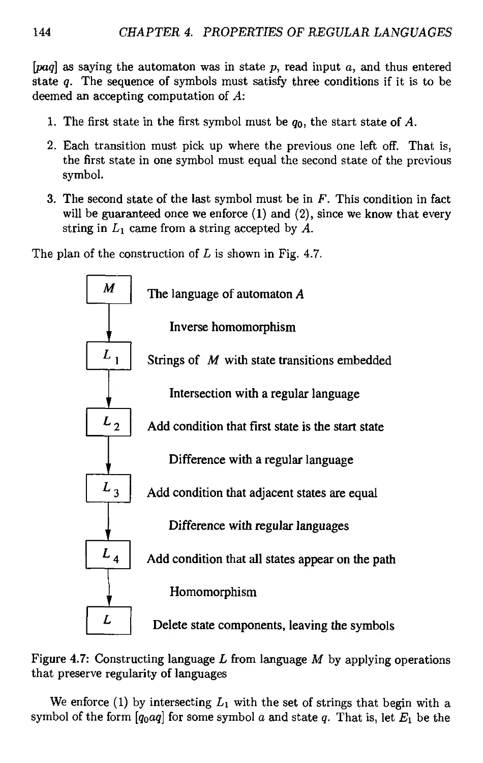
4.2.3 Homomorphisms 139
4.2.4 Inverse Homomorphisms 140
4.2.5 Exercises for Section 4.2 145
4.3 Decision Properties of Regular Languages 149
4.3.1 Converting Among Representations 149
4.3.2 Testing Emptiness of Regular Lfinguages 151
4.3.3 Testing Membership in a Regular Language 153
4.3*4 Exercises for Section 4.3 153
4.4 Equivalence and Minimization of Automata 154
4.4.1 Testing Equivalence of States 154
4.4.2 Testing Equivalence of Regular Languages 157
4.4.3 Minimization of DFA's 159
4.4.4 Why the Minimized DFA Can't Be Beaten 162
4.4.5 Exercises for Section 4.4 164
4.5 Summary of Chapter 4 165
4.6 References for Chapter 4 166

X TABLE OF CONTENTS
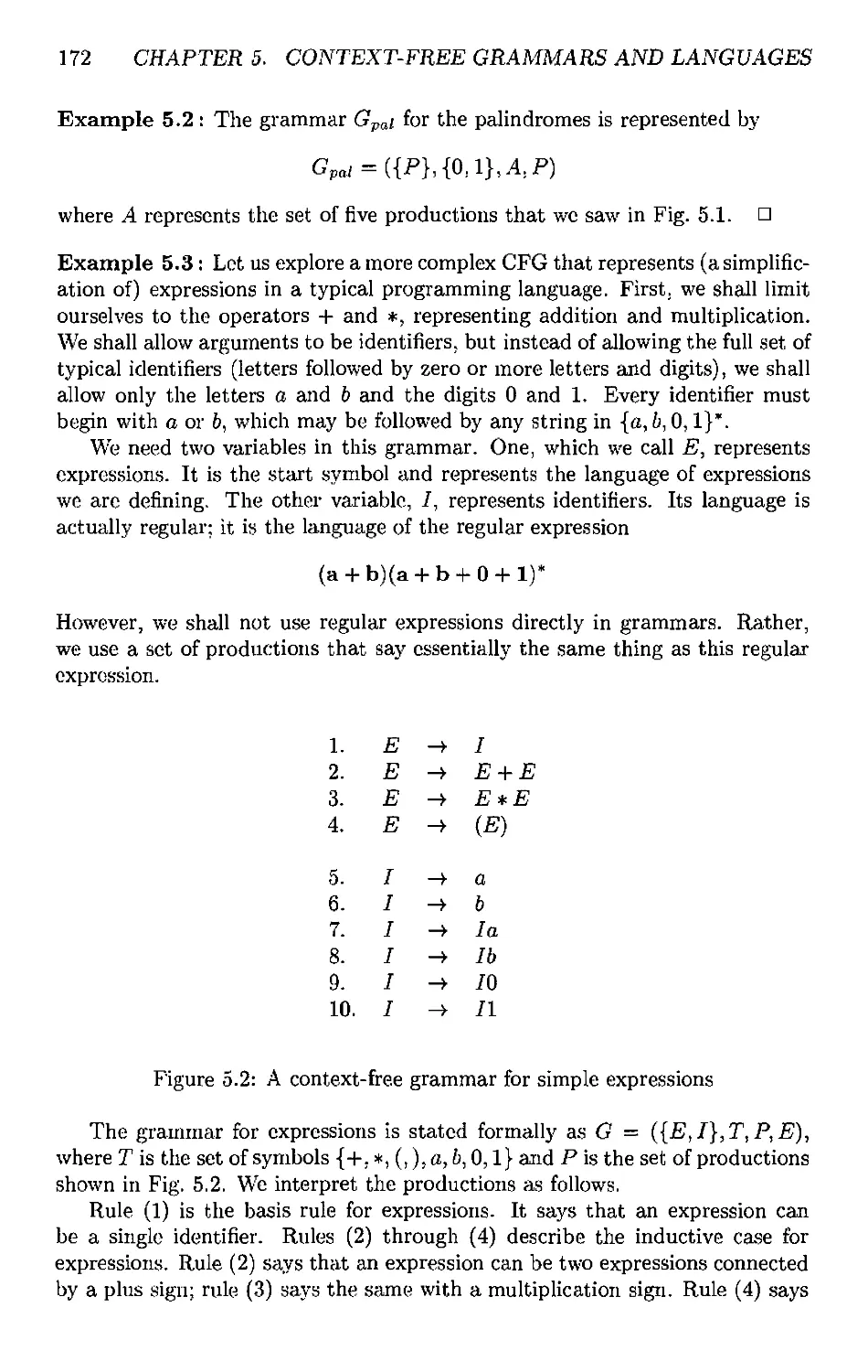
5 Context-Free Grammars and Languages 169
5.1 Context-Free Grammars 169
5.1.1 An Informal Example 170
5.1.2 Definition of Context-Free Grammars 171
5.1.3 Derivations Using a Grammar 173
5.1.4 Leftmost and Rightmost Derivations 175
5.1.5 The Language of a Grammar 177
5.1.6 Sentential Forms 178
5.1.7 Exercises for Section 5.1 179
5.2 Parse Trees 181
5.2.1 Constructing Parse Trees 181
5.2.2 The Yield of a Parse Tree 183
5.2.3 Inference, Derivations, and Parse Trees 184
5.2.4 Prom Inferences to Trees 185
5.2.5 FVom TVees to Derivations 187
5.2.6 FVom Derivations to Recursive Inferences 190
5.2.7 Exercises for Section 5.2 191
5.3 Applications of Context-FVee Grammars 191
5.3.1 Parsers 192
5.3.2 The YACC Parser-Generator 194
5.3.3 Markup Languages 196
5.3.4 XML and Document-Type Definitions 198
5.3.5 Exercises for Section 5.3 204
5.4 Ambiguity in Grammars and Languages 205
5.4.1 Ambiguous Grammars 205
5.4.2 R;emoving Ambiguity Prom Grammars 207
5.4.3 Leftmost Derivations as a Way to Express Ambiguity . . 211
5.4.4 Inherent Ambiguity 212
5.4.5 Exercises for Section 5.4 214
5.5 Summary of Chapter 5 215
5.6 References for Chapter 5 216
6 Pushdown Automata 219
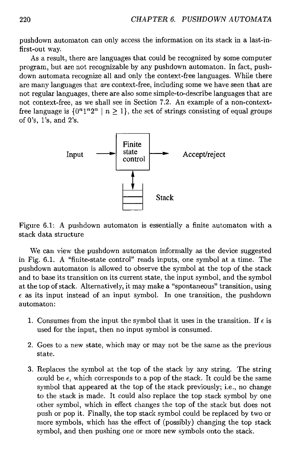
6.1 Definition of the Pushdown Automaton 219
6.1.1 Informal Introduction 219
6.1.2 The Formal Definition of Pushdown Automata 221
6.1.3 A Graphical Notation for PDA's 223
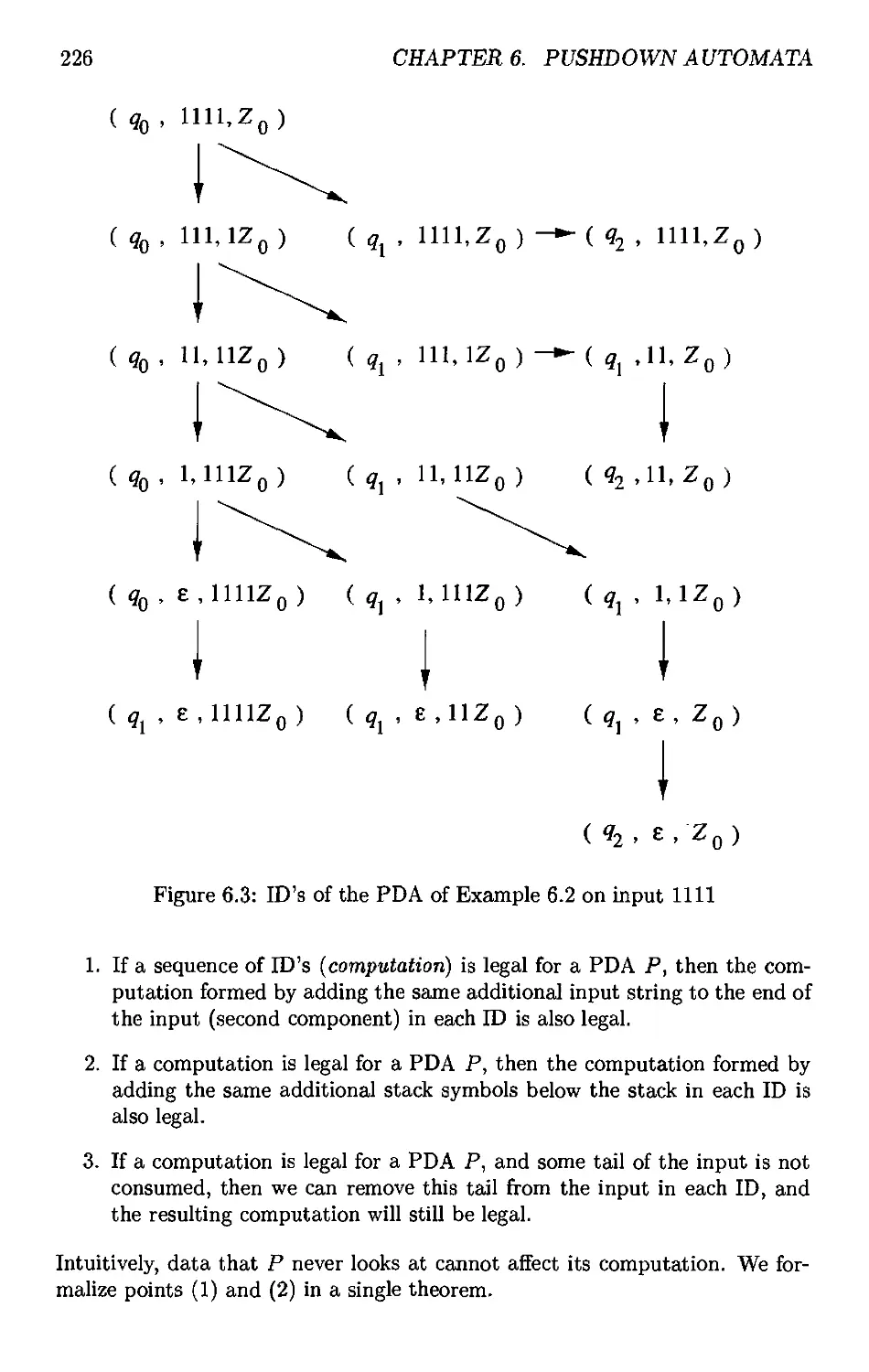
6.1.4 Instantaneous Descriptions of a PDA 224
6.1.5 Exercises for Section 6.1 228
6.2 The Languages of a PDA 229
6.2.1 Acceptance by Final State 229
6.2.2 Acceptance by Empty Stack 230
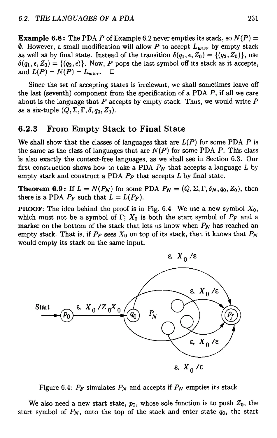
6.2.3 Prom Empty Stack to Final State 231
6.2.4 Prom Final State to Empty Stack 234
6.2.5 Exercises for Section 6.2 236

TABLE OF CONTENTS xi
6.3 Equivalence of PDA's and CFG's 237
6.3.1 From Grammars to Pushdown Automata 237
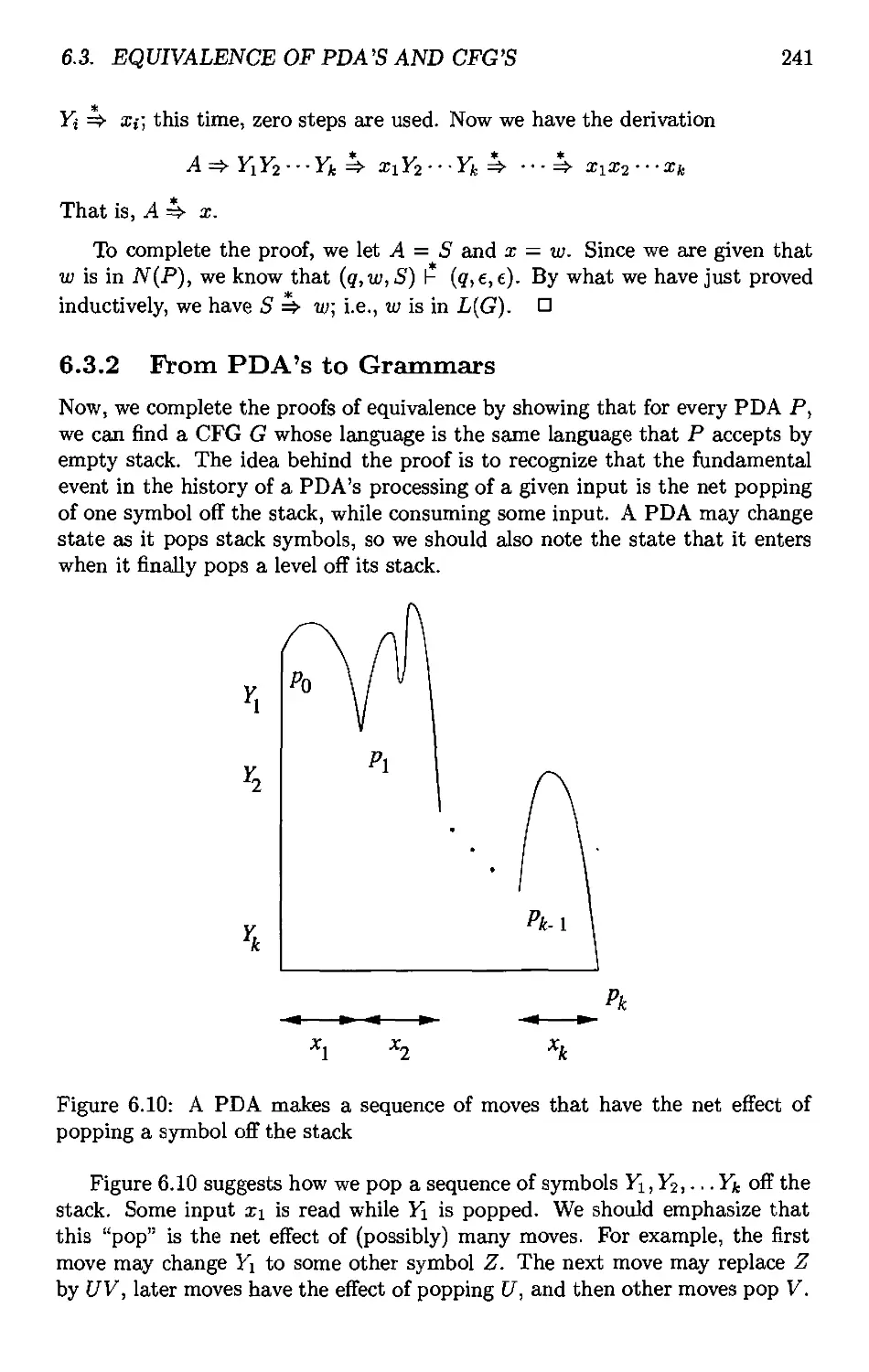
6.3.2 From PDA's to Grammars 241
6.3.3 Exercises for Section 6.3 245
6.4 Deterministic Pushdown Automata 246
6.4.1 Definition of a Deterministic PDA 247
6.4.2 Regular Languages and Deterministic PDA's 247
6.4.3 DPDA's £tnd Context-Free Languages 249
6.4.4 DPDA's and Ambiguous Grammars 249
6.4.5 Exercises for Section 6.4 251
6.5 Summary of Chapter 6 252
6.6 References for Chapter 6 253
7 Properties of Context-Free Languages 255
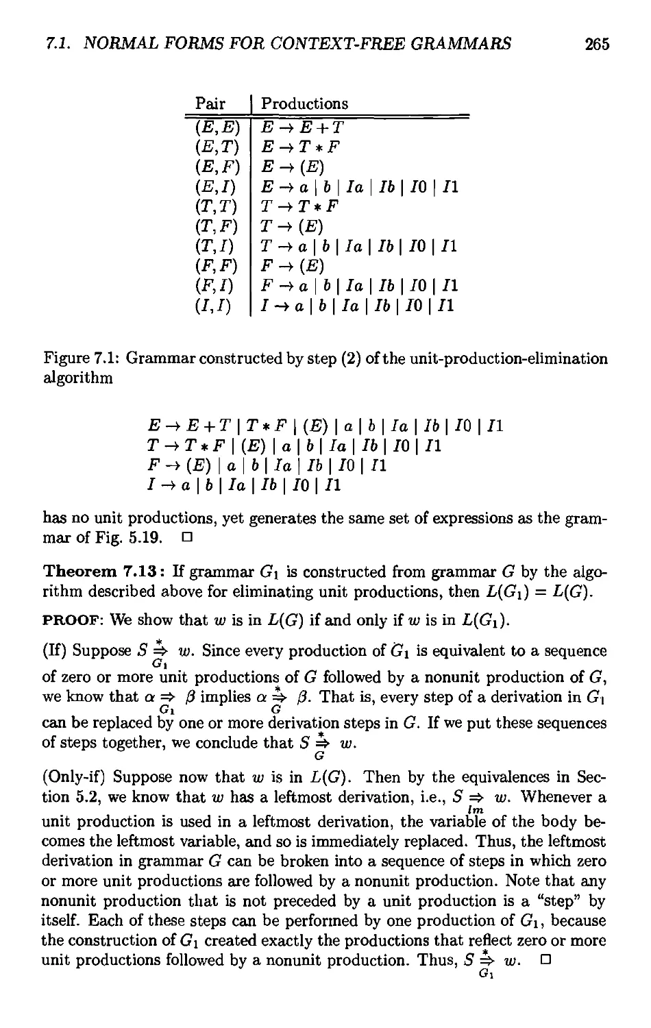
7.1 Normal Forms for Context-Free Grammars 255
7.1.1 Eliminating Useless Symbols 256
7.1.2 Computing the Generating and Reachable Symbols . . . .258
7.1.3 Eliminating ^-Productions 259
7.1.4 Eliminating Unit Productions 262
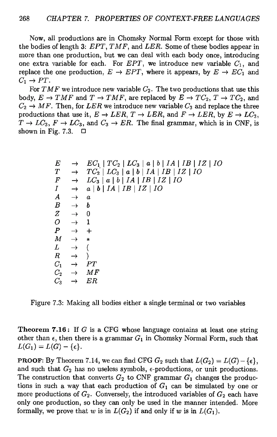
7.1.5 Chomsky Normal Form 266
7.1.6 Exercises for Section 7.1 269
7.2 The Pumping Lemma for Context-Free Languages 274
7.2.1 The Size of Parse Trees 274
7.2.2 Statement of the Pumping Lemma 275
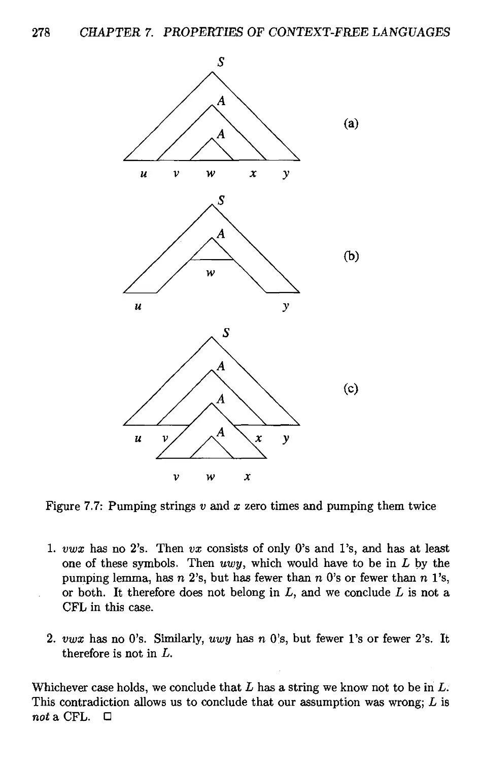
7.2.3 Applications of the Pumping Lemma for CFL's 276
7.2.4 Exercises for Section 7.2 280
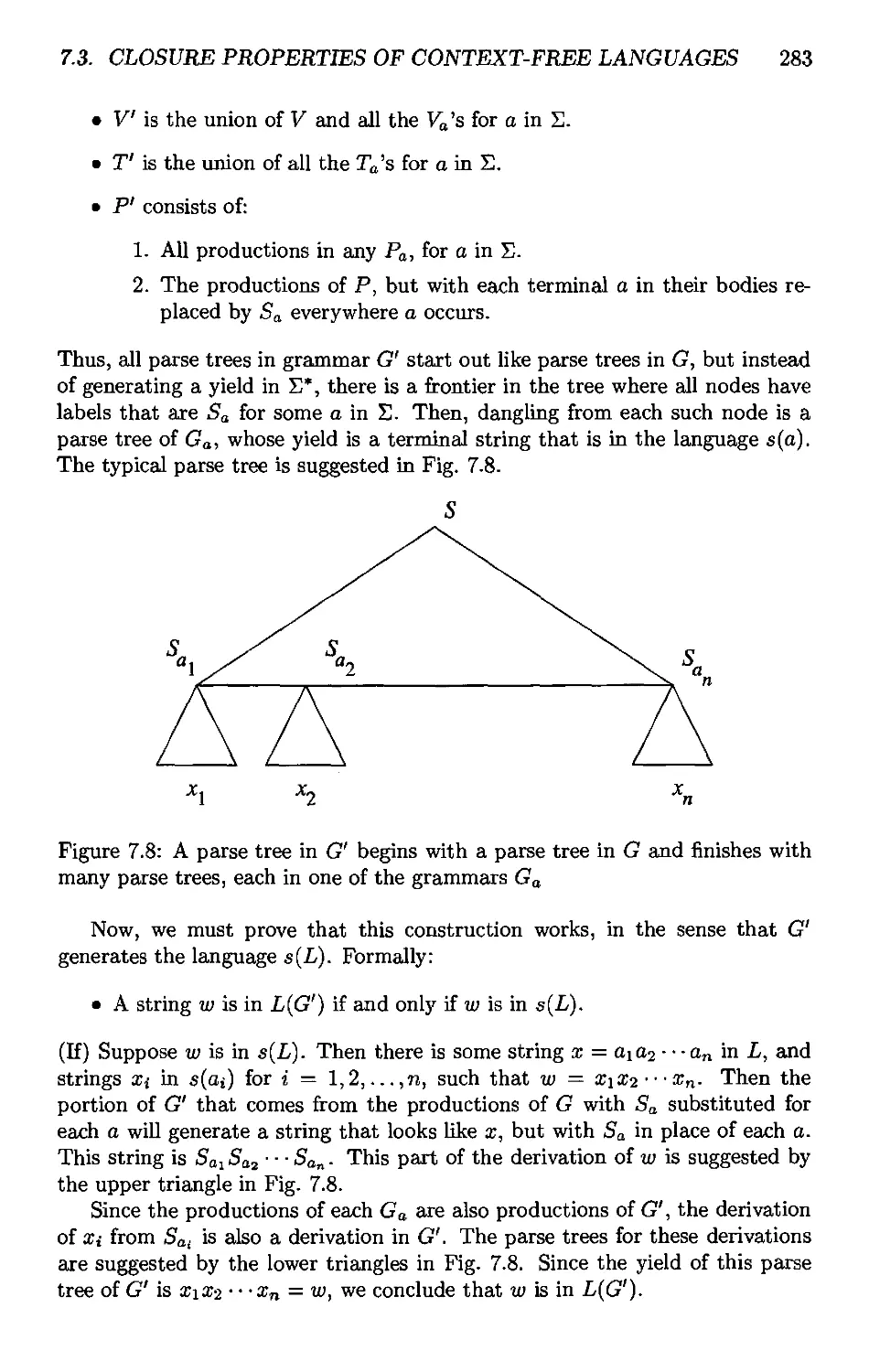
7.3 Closure Properties of Context-Free Languages 281
7.3.1 Substitutions 282
7.3.2 Applications of the Substitution Theorem 284
7.3.3 Reversal 285
7.3.4 Intersection With a Regular Language 285
7.3.5 Inverse Homomorphism 289
7.3.6 Exercises for Section 7.3 291
7.4 Decision Properties of CFL's 293
7.4.1 Complexity of Converting Among CFG's and PDA's ... 294
7.4.2 Running Time of Conversion to Chomsky Normal Form . 295
7.4.3 Testing Emptiness of CFL's 296
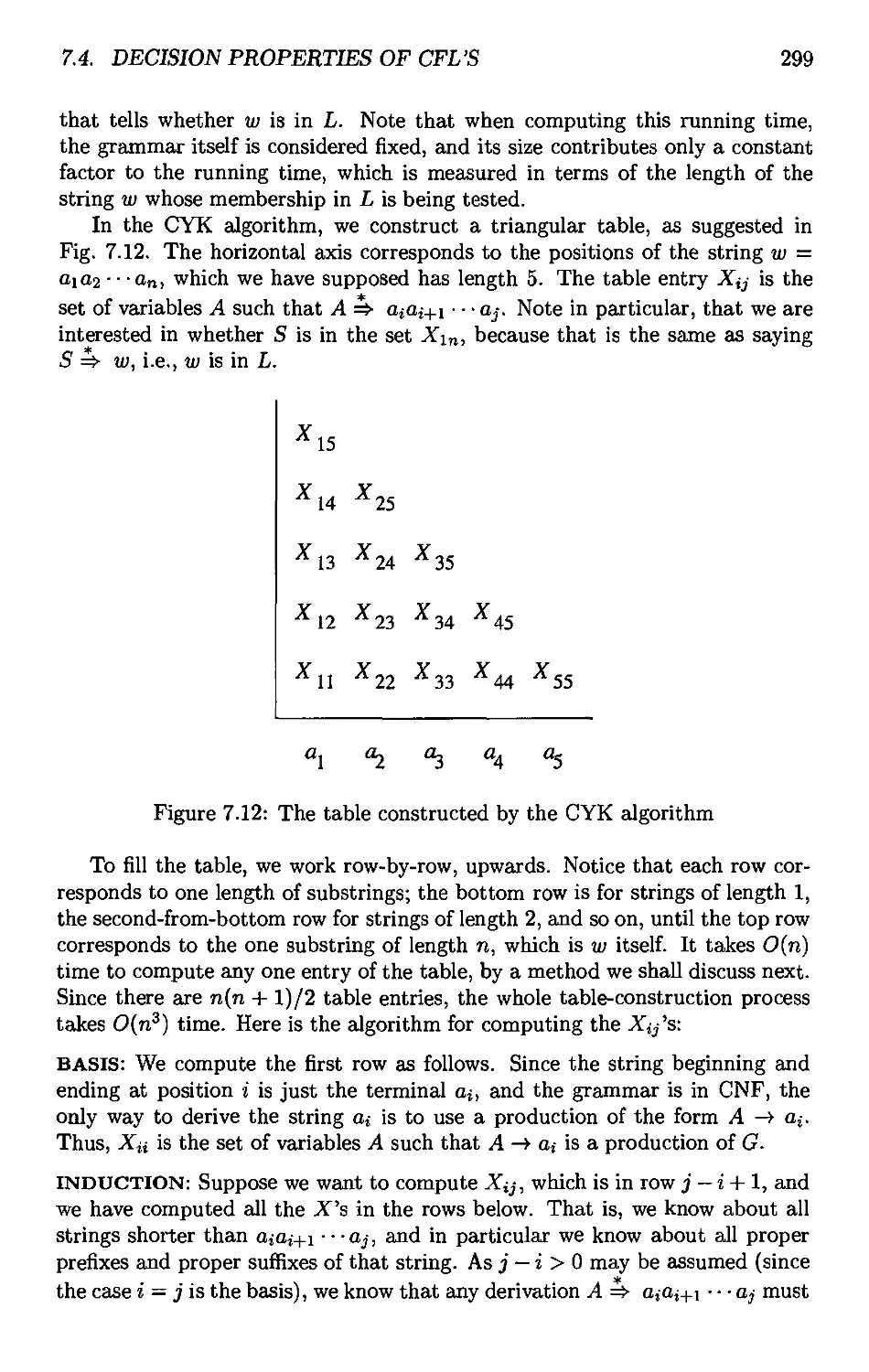
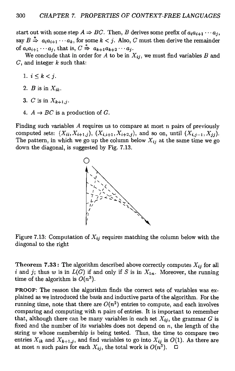
7.4.4 Testing Membership in a CFL 298
7.4.5 Preview of Undecidable CFL Problems 302
7.4.6 Exercises for Section 7.4 302
7.5 Summary of Chapter 7 303
7.6 References for Chapter 7 304

xii TABLE OF CONTENTS
8 Introduction to Turing Machines 307
8.1 Problems That Computers Cannot Solve 307
8.1.1 Programs that Print "Hello, World" 308
8.1.2 The Hypothetical "Hello, World" Tester 310
8.1.3 Reducing One Problem to Another 313
8.1.4 Exercises for Section 8.1 316
8.2 The Turing Machine 316
8.2.1 The Quest to Decide All Mathematical Questions 317
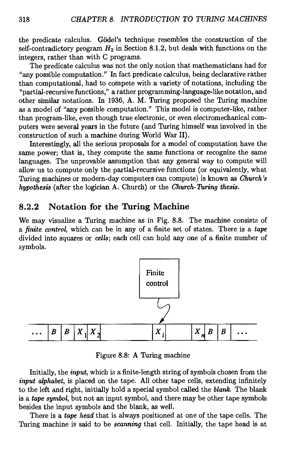
8.2.2 Notation for the Turing Machine 318
8.2.3 Instantaneous Descriptions for Turing Machines 320
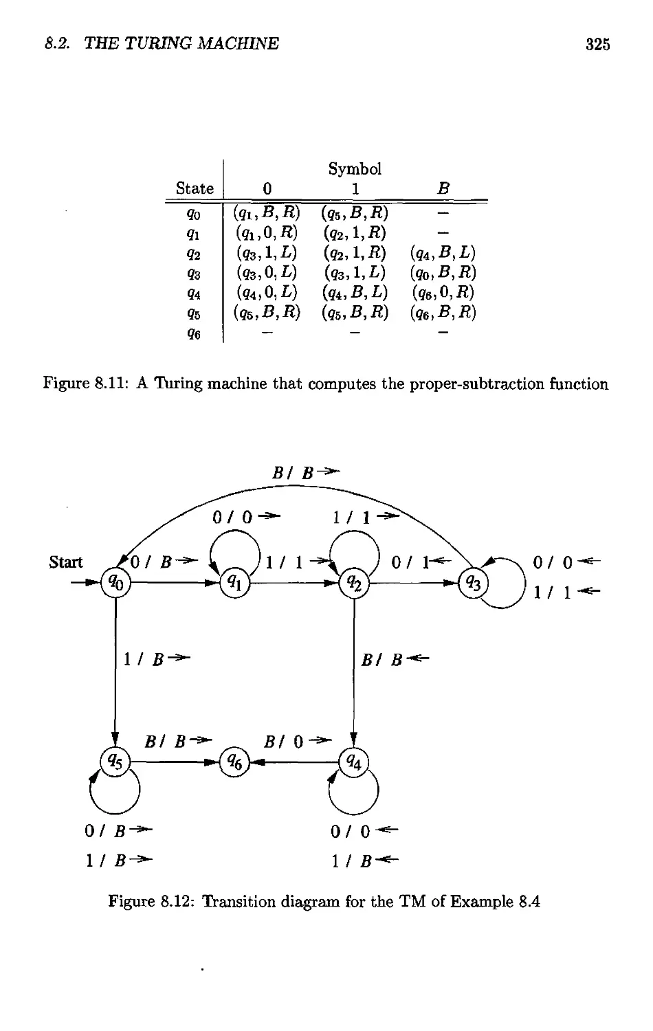
8.2.4 Transition Diagrams for Turing Machines 323
8.2.5 The Language of a Turing Machine 326
8.2.6 Turing Machines and Halting 327
8.2 J Exercises for Section 8.2 328
8.3 Programming Techniques for Taring Machines 329
8.3.1 Storage in the State 330
8.3.2 Multiple Tracks 331
8.3.3 Subroutines 333
8.3.4 Exercises for Section 8.3 334
8.4 Extensions to the Basic Taring Machine 336
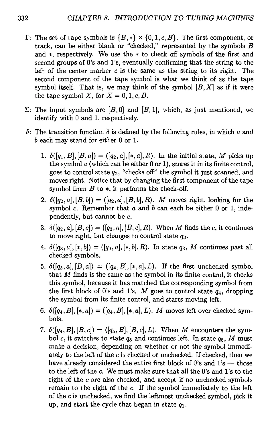
8.4.1 Multitape Turing Machines 336
8.4.2 Equivalence of One-Tape and Multitape TM's 337
8.4.3 Running Time and the Many-Tapes-to-One Construction 339
8.4.4 Nondeterministic Turing Machines 340
8.4.5 Exercises for Section 8.4 342
8.5 Restricted Turing Machines 345
8.5.1 Turing Machines With Semi-inifinite Tapes 345
8.5.2 Multistack Machines 348
8.5.3 Counter Machines 351
8.5.4 The Power of Counter Machines 352
8.5.5 Exercises for Section 8.5 354
8.6 Turing Machines and Computers 355
8.6.1 Simulating a Turing Machine by Computer 355
8.6.2 Simulating a Computer by a Turing Machine 356
8.6.3 Comparing the Running Times of Computers and Turing
Machines 361
8.7 Summary of Chapter 8 363
8.8 References for Chapter 8 365
9 Undecidability 367
9.1 A Language That Is Not Recursively Enumerable 368
9.1.1 Enumerating the Binary Strings 369
9.1.2 Codes for Turing MacJiines 369
9.1.3 The Diagonalization Language 370
9.1.4 Proof that Ld is not Recursively Enumerable 372

TABLE OF CONTENTS xiii
9.1,5 Exercises for Section 9.1 372
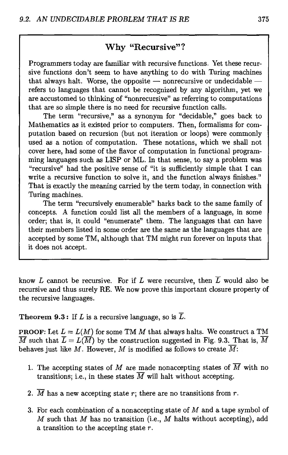
9.2 An Undecidable Problem That is RE 373
9.2.1 Recursive Languages 373
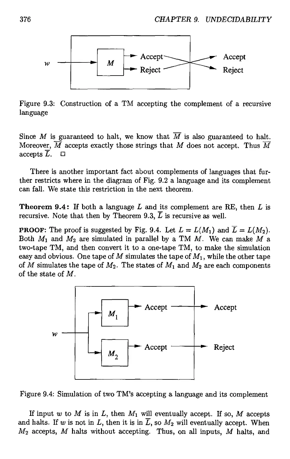
9.2.2 Complements of Recursive and RE languages 374
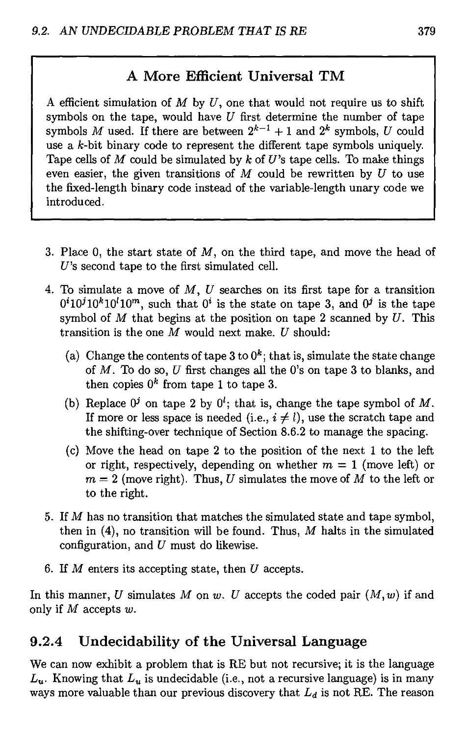
9.2.3 The Universal Language 377
9.2.4 Undecidability of the Universal Language 379
9.2.5 Exercises for Section 9.2 381
9.3 Undecidable Problems About Turing Machines 383
9.3.1 Reductions 383
9.3.2 Turing Machines That Accept the Empty Language . . . 384
9.3.3 Rice's Theorem and Properties of the RE Languages . . . 387
9.3.4 Problems about Turing-Machine Specifications 390
9.3.5 Exercises for Section 9.3 390
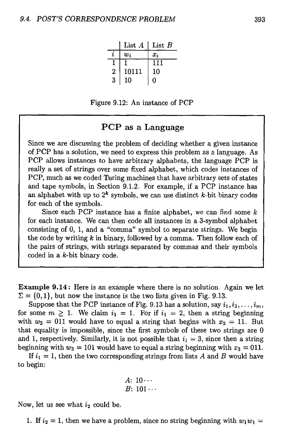
9.4 Post's Correspondence Problem 392
9.4.1 Definition of Post's Correspondence Problem 392
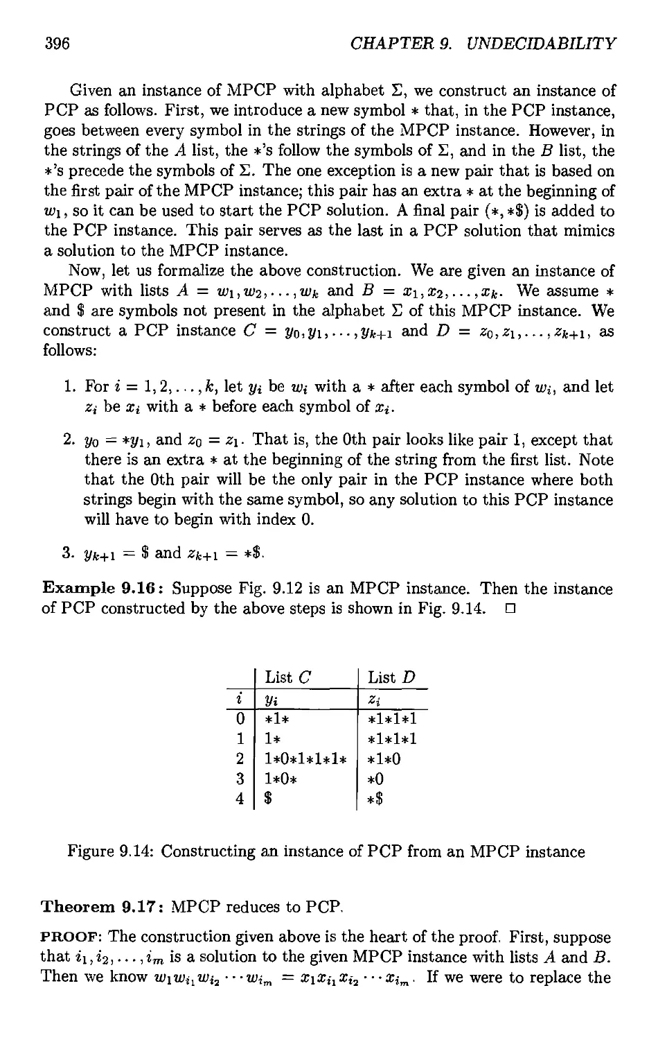
9.4.2 The "Modified" PC? 394
9.4.3 Completion of the Proof of PCP Undecidability 397
9.4.4 Exercises for Section 9.4 403
9.5 Other Undecidable Problems 403
9.5.1 Problems About Programs 403
9.5.2 UndecidabiUty of Ambiguity for CFG's 404
9.5.3 The Complement of a List Language 406
9.5.4 Exercises for Section 9.5 409
9.6 Summary of Chapter 9 410
9.7 References for Chapter 9 411
10 Intractable Problems 413
10.1 The Classes V smd J^T 414
10.1.1 Problems Solvable in Polynomial Time 414
10.1.2 An Example: Kruskal's Algorithm 414
10.1.3 Nondeterministic Polynomial Time 419
10.1.4 An ^fV Example: The Traveling Salesman Problem ... 419
10.1.5 Polynomial-Time Reductions 421
10.1.6 NP-Complete Problems 422
10.L7 Exercises for Section 10.1 423
10.2 An NP-Complete Problem 426
10.2.1 The Satisfiability Problem 426
10.2.2 Representing SAT Instances 427
10.2.3 NP-Completeness of the SAT Problem 428
10.2.4 Exercises for Section 10.2 434
10.3 A Restricted Satisfiability Problem 435
10.3.1 Normal Forms for Boolean Expressions 436
10.3.2 Converting Expressions to CNF 437
10.3.3 NP-Completeness of CSAT 440
10.3.4 NP-Completeness of 3SAT 445
10.3.5 Exercises for Section 10.3 446

xiv TABLE OF CONTENTS
10.4 Additional NP-Complete Problems 447
10.4.1 Describing NP-complete Problems 447
10.4*2 The Problem of Independent Sets 448
10.4.3 The Node-Cover Problem 452
10.4.4 The Directed Hamilton-Circuit Problem 453
10.4.5 Undirected Hamilton Circuits and the TSP 460
10.4.6 Summary of NP-Complete Problems 461
10.4.7 Exercises for Section 10.4 462
10.5 Summary of Chapter 10 466
10.6 References for Chapter 10 467
11 Additional Classes of Problems 469
11.1 Complements of Languages in J\fT 470
11.1.1 The Class of Languages Co-^fT 470
11.1.2 NP-Complete Problems and Co-AfV 471
11.1.3 Exercises for Section 11,1 472
11.2 Problems Solvable in Polynomial Space 473
11.2.1 Polynomial-Space Turing Machines 473
11.2.2 Relationship ofVS and ^fVS to Previously Defined Classes474
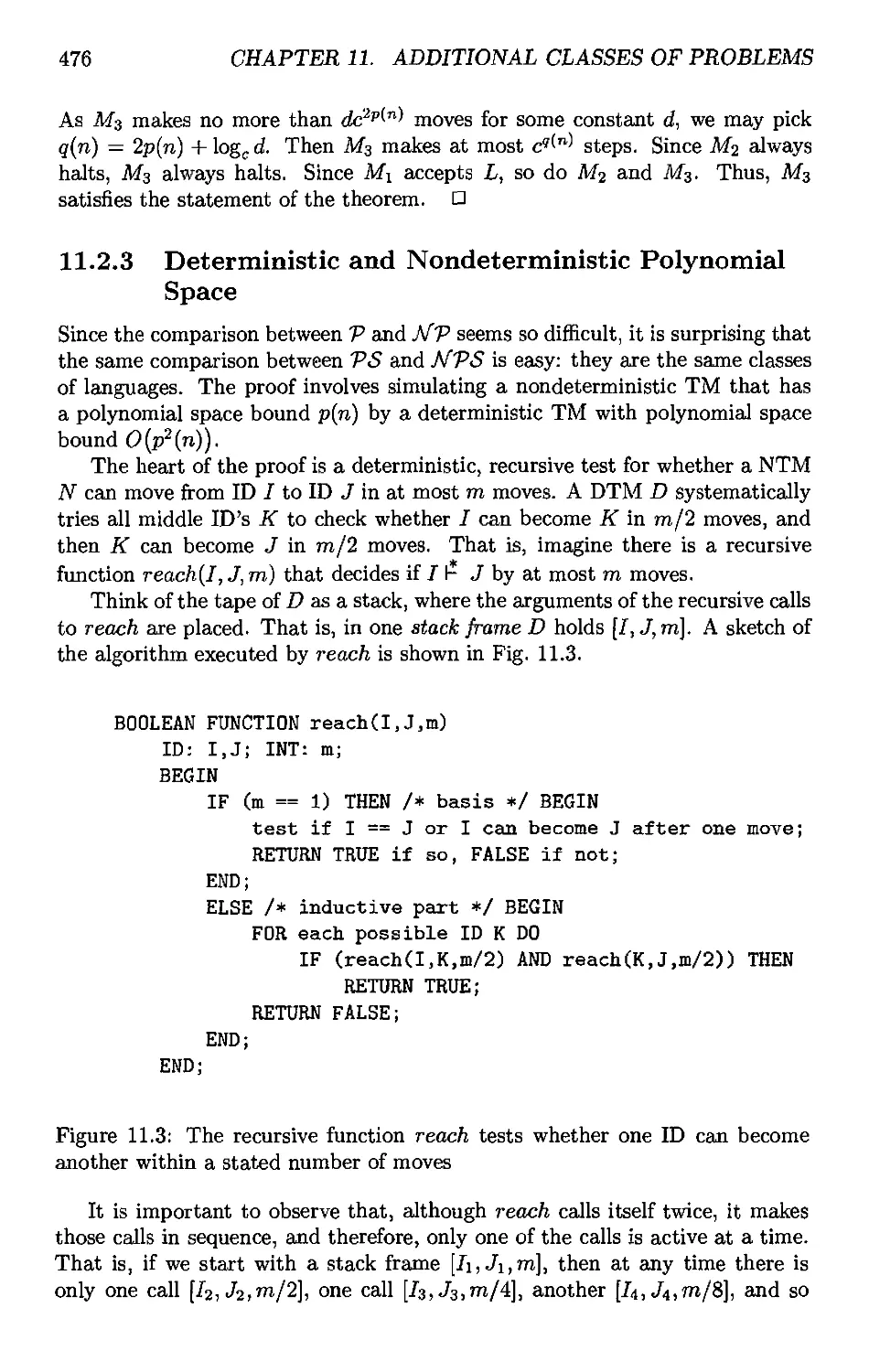
11.2.3 Deterministic and Nondeterministic Polynomial Space . . 476
11.3 A Problem That Is Complete fox VS 478
11.3.1 PS-Completeness 478
11.3.2 Quantified Boolean Formulas 479
11.3.3 Evaluating Quantified Boolean Formulas 480
11.3.4 PS-Completeness of the QBF Problem 482
11.3.5 Exercises for Section 11.3 487
11.4 Language Classes Based on Randomization 487
11.4.1 Quicksort: an Example of a Randomized Algorithm . , . 488
11.4.2 A Turing-Machine Model Using Randomization 489
11.4.3 The Language of a Randomized Turing Machine 490
11.4.4 The Class TIT 492
11.4.5 Recognizing Languages in 7?-7^ 494
11.4.6 The Class ZVV 495
11.4.7 Relationship Between HV and ZVV . 496
11.4.8 Relationships to the Classes 7^ and A/'T^ . . 497
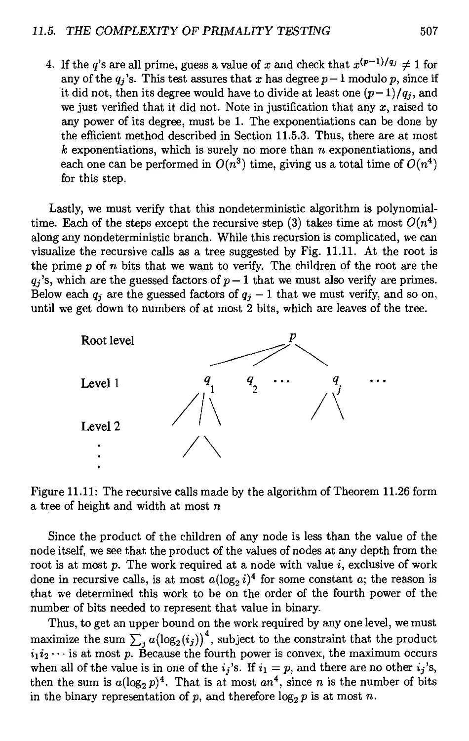
11.5 The Complexity of Primality Testing 498
11.5.1 The Importamce of Testing PrimaUty 499
11.5.2 Introduction to Modular Arithmetic .....*.,.... 501
11.5.3 The Complexity of Modular-Arithmetic Computations . . 503
11.5.4 Random-Polynomial Primality Testing 504
11.5.5 Nondeterministic Primality Tests 505
11.5.6 Exercises for Section 11.5 508
11.6 Summary of Ch^ter 11 . 508
11.7 References for Chapter 11 510
Index 513

Chapter 1
Automata: The Methods
and the Madness
Automata theory is the study of abstract computing devices, or "machines."
Before there were computers, in the 1930'Sj A. Turing studied an abstract
machine that had all the capabilities of today's computers, at least as far as in
what they could compute. Turing^s goal was to describe precisely the boundary
between what a computing machine could do and what it could not do; his
conclusions apply not only to his abstract Turing machines^ but to today's real
machines.
In the 1940's and 1950's, simpler kinds of machines, which w-e today call
"finite automata/' were studied by a number of researchers. These automata,
originally proposed to model brain function, turned out to be extremely useful
for a variety of other purposes, which we shall mention in Section LI. Also in
the late 1950's, the linguist N. Chomsky began the study of formal "grammars."
While not strictly machines, these graiiunars have close relationships to abstract
automata and serve today as the basis of some important software components,
including parts of compilers*
In 1969j S* Cook extended Turing's study of what could and what could
not be computed. Cook was able to separate those problems that can be solved
efficiently by computer from those problems that can in principle be solved, but
in practice take so much time tliat computers are useless for all but very small
instances of tlie problem. Tlie latter class of problems is called "intractable,"
or "NP-hard." It is highly unlikely that even the exponential improvement in
computing speed that computer hardwai^e has been following ("Moore's Law")
will h-dve significant impact on our ability to solve large instances of intractable
problems.
All of these theoretical developments bear directly on what computer
scientists do today. Some of the concepts, like finite automata and certain kinds of
formal grammars, are used in the design and construction of important kinds
of software* Other concepts, like the Turing machine, help us understand what
1

2 CHAPTER L AUTOMATA: THE METHODS AND THE MADNESS
we can expect from our software. Especially, the theory of intractable problems
lets us deduce whether we are likely to be able to meet a problem "head-on"
and write a program to solve it (because it is not in the intractable class), or
whether we have to find some way to work around the intractable problem:
find an approximation, use a heuristic, or use some other method to limit the
amount of time the program will spend solving the problem.
In this introductory chapter, we begin with a very high-level view of what
automata theory is about, and what its uses are. Much of the chapter is
devoted to a survey of proof techniques and tricks for discovering proofs. We cover
deductive proofs, reformulating statements, proofs by contradiction, proofs by
induction, and other important concepts. A final section introduces the
concepts that pervade automata theory: alphabets, strings, and languages.
1.1 W^hy study Automata Theory?
There are several reasons why the study of automata and complexity is an
important part of the core of Computer Science. This section serves to introduce
the reader to the principal motivation and also outlines the major topics covered
in this book.
1*1.1 Introduction to Finite Automata
Finite automata are a useful model for many important kinds of hardware and
software. We shall see, starting in Chapter 2. examples of how the concepts are
used. For the moment, let us just list some of the most important kinds:
1. Software for designing and checking the behavior of digital circuits.
2. The "lexical analyzer" of a typical compiler, that is, the compiler
component that breaks the input text into logical units, such as identifiers,
keywords, and punctuation.
3. Softw^are for scanning large bodies of text, such as collections of Web
pages, to find occurrences of words, phrases, or other patterns.
4. Software for verifying systems of all types that have a finite number of
distinct states, such as communications protocols or protocols for secure
exchange of information.
While we shall soon meet a precise definition of automata of various types,
let us begin our informal introduction with a sketch of what a finite automaton
is and does. There are many systems or components, such as those enumerated
above, that may be viewed as being at all times in one of a finite number
of "states." The purpose of a state is to remember the relevant portion of the
system's history. Since there are only a finite number of states, the entire history
generally cannot be remembered, so the system must be designed carefully, to

iJ. WHY STUDY AUTOMATA THEORY? 3
remember what is important and forget what is not. The advantage of having
only a finite number of states is that we can implement the system with a fixed
set of resources. For example, we could implement it in hardware as a circuit, or
as a simple form of program that can make decisions looking only at a limited
amount of data or using the position in the code itself to make the decision.
Example !♦!: Perhaps the simplest nontrivial finite automaton is an on/oif
switch. The device remembers whether it is in the "on" state or the "off state,
and it allows the user to press a button whose effect is different, depending on
the state of the switch. That is, if the switch is in the off state, then pressing
the button changes it to the on state, and if the switch is in the on state, then
pressing the same button turns it to the off state.
Push
—*-(off ) ( on )
Push
Figure 1.1: A finite automaton modeling an on/ofF switch
The finite-automaton model for the switch is shown in Fig. 1.1. As for all
finite automata; the states are represented by circles; in this example, we have
named the states on and off. Arcs between states are labeled by "inputs," which
represent external influences on the system. Here, both arcs are labeled by the
input Push, which represents a user pushing the button. The intent of the two
arcs is that whichever state the system is in, when the Push input is received
it goes to the other state.
One of the states is designated the "start state," the state in which the
system is placed initially. In our example, the start state is off^ and we
conventionally indicate the start state by the word Start and an arrow leading to that
state.
It is often necessary to indicate one or more states as "final" or "accepting"
states. Entering one of these states after a sequence of inputs indicates that
the input sequence is good in some way. For instance, we could have regarded
the state on in Fig. 1.1 as accepting, because in that state, the device being
controlled by the switch will operate. It is conventional to designate accepting
states by a double circle, although we have not made any such designation in
Fig. 1.1. □
Example 1.2: Sometimes, what is remembered by a state can be much more
complex than an on/off choice. Figure 1.2 shows another finite automaton that
could be part of a lexical analyzer. The job of this automaton is to recognize

4 CHAPTER 1. AUTOMATA: THE METHODS AND THE MADNESS
the keyword then. It thus needs five states, each of which represents a different
position in the word then that has been reached so far. These positions
correspond to the prefixes of the word, ranging from the empty string (i.e., nothing
of the word has been seen so far) to the complete word.
Start
Figure 1.2: A finite automaton modeling recognition of then
In Fig. 1.2j the five states are named by the prefix of then seen so far. Inputs
correspond to letters. We may imagine that the lexical analyzer examines one
character of the program that it is compiling at a time, and the next character
to be examined is the input to the automaton. The start state corresponds to
the empty string, and each state has a transition on the next letter of then to
the state that corresponds to the next-larger prefix. The state named then is
entered when the input has spelled the word then. Since it is the job of this
automaton to recognize w^hen then has been seen, we could consider that state
the lone accepting state. □
1.1.2 Structural Representations
There are two important notations that are not automaton-like, but plaj^ an
important role in the study of automata cind their applications.
1. Grammars are useful models when designing software that processes data
with a recursive structure. The best-known example is a "parser," the
component of a compiler that deals with the recursively nested features
of the typical programming language, such as expressions — arithmetic,
conditional, and so on. For instance, a grammatical rule like E =^ E + E
states that an expression can be formed by taking any two expressions
and connecting them by a plus sign; this rule is typical of how expressions
of real programming languages are formed. We introduce context-free
grammars, as they are usually called, in Chapter 5.
2. Regular Expressions also denote the structure of data, especially text
strings. As we shall see in Chapter 3, the patterns of strings they describe
are exactly the same as what can be described by finite automata. The
style of these expressions differs significantly from that of grammars, and
we shall content ourselves with a simple example here. The UNIX-style
regular expression ' [A-Z] [a-z]*[ ] [A-Z] [A-Z] ' represents capitalized
words followed by a space and two capital letters. This expression
represents patterns in text that could be a city cind state, e.g., Ithaca NY.
It misses multiword city names, such as Palo Alto CA, which could be
captured by the more complex expression

L2. INTRODUCTION TO FORMAL PROOF 5
'([A-Z][a-z]*[])*[][A-Z][A-Z]'
When interpreting such expressions, we only need to know that [A-Z]
represents a range of characters from capital "A" to capital "Z" (i.e., any
capital letter), and C ] is used to represent the blank character alone.
Also, the symbol * represents "any number of" the preceding expression.
Pai^entheses are used to group components of the expression; they do not
represent characters of the text described,
1.1 ♦S Automata and Complexity
Automata are essential for the study of the limits of computation. As we
mentioned in the introduction to the chapter, there are two important issues:
1. What can a computer do at all? This study is called "decidability," and
the problems that can be solved by computer are called "decidable/' This
topic is addressed in Chapter 9.
2. What can a computer do efficiently? This study is called
"intractability," and the problems that can be solved by a computer using no more
time than some slowly growing function of the size of the input are called
"tractable." Often, we take all polynomial functions to be "slowly
growing," while functions that grow faster than any polynomial are deemed to
gTOw too fast. The subject is studied in Chapter 10.
1.2 Introduction to Formal Proof
If you studied plane geometry in high school any time before the 1990's, you
most likely had to do some detailed "deductive proofs," where you showed
the truth of a statement by a detailed sequence of steps and reasons. While
geometry has its practical side (e.g., you need to know the rule for computing
the area of a rectangle if you need to buy the correct amount of carpet for a
room), the study of formal proof methodologies was at least as important a
reason for covering this branch of mathematics in high school.
In the USA of the 1990's it became popular to teach proof as a matter
of personal feelings about the statement. While it is good to feel the truth
of a statement you need to use, important techniques of proof are no longer
mastered in high school. Yet proof is something that every computer scientist
needs to understand. Some computer scientists take the extreme view that a
formal proof of the correctness of a program should go hand-in-hand with the
writing of the program itself- We doubt that doing so is productive. On the
other hand, there are those who say that proof has no place in the discipline of
programming* The slogan "if you are not sure your program is correct, run it
and see" is commonly offered by this camp.

6 CHAPTER 1. AUTOMATA: THE METHODS AND THE MADNESS
Our position is between these two extremes* Testing programs is surely
essential. However, testing goes only so far, since you cannot try your program
on every input* More importantly, if your program is complex — say a tricky
recursion or iteration — then if you don^t understand what is going on as you
go around a loop or call a function recursively, it is unlikely that you will write
the code correctly. When your testing tells you the code is incorrect, you still
need to get it right.
To make your iteration or recursion correct, you need to set up an inductive
hypothesis, and it is helpful to reason, formally or informally, that the
hypothesis is consistent with the iteration or recursion. This process of understanding
the workings of a correct program is essentially the same as the process of
proving theorems by induction. ThuS; in addition to giving you models that are
useful for certfun types of software, it has become traditional for a course on
automata theory to cover methodologies of formal proof. Perhaps more than
other core subjects of computer science, automata theory lends itself to natural
and interesting proofs, both of the deductive kind (a sequence of justified steps)
and the inductive kind (recursive proofs of a parameterized statement that use
the statement itself with "lower" values of the parameter).
1.2.1 Deductive Proofs
As mentioned above, a deductive proof consists of a sequence of statements
whose truth leads us from some initial statement, called the hypothesis or the
given statement(s)y to a conclusion statement. Each step in the proof must
follow, by some accepted logical principle, from either the given facts, or some
of the previous statements in the deductive proof, or a combination of these.
The hypothesis may be true or false, typically depending on values of its
parameters. Often, the hypothesis consists of several independent statements
connected by a logical AND. In those cases, we talk of each of these statements
as a hypothesis, or as a given statement.
The theorem that is proved when we go from a hypothesis i/ to a conclusion
C is the statement "if H then C." We say that C is deduced from H. An example
theorem of the form "if H then C will illustrate these points.
Theorem 1.3: If ar > 4, then 2^ > x'K □
It is not hard to convince ourselves informally that Theorem 1.3 is true,
although a formal proof requires induction and will be left for Example 1.17.
First, notice that the hypothesis H is "x > 4." This hypothesis has a parameter,
x, and thus is neither true nor false. Rather, its truth depends on the value of
the parameter x\ e.g., H is true for x = 6 and false for x = 2.
Likewise, the conclusion C is "2^ > x^." This statement also uses parameter
X and is true for certain \^ues of x and not others. For example, C is false for
X = 3, since 2*^ = 8, which is not as large as 3^ = 9. On the other hand, C is
true for a; = 4, since 2^ = 4^ = 16. For x = 5, the statement is also true, since
2^ = 32 is at least as large as S**^ = 25.

1.2. INTRODUCTION TO FORMAL PROOF 7
Perhaps you can see the intuitive argument tha.t tells us the conclusion
2^ > x'^ will be true whenever x > 4. We already saw that it is true for ar = 4.
As X grows larger than 4, the left side, 2^ doubles each time x increases by
1. However, the right side, x^, grows by the ratio {^^) • li x > 4, then
{x H- l)/x cannot be greater than 1.25, and therefore (^^)" cannot be bigger
than 1.5625. Since 1.5625 < 2, each time x increases above 4 the left side 2^
grows more than the right side ar^. Thus, as long as we start from a value like
X = 4 where the inequality 2^ > x^ is already satisfied, we can increase x as
much as we like, and the inequality will still be satisfied.
We have now completed an informal but accurate proof of Theorem 1.3. We
shall return to the proof and make it more precise in Example 1.17, after we
introduce "inductive" proofs.
Theorem 1.3, like all interesting theorems, involves an infinite number of
related facts, in this case the statement "if x > 4 then 2^ > x^" for all integers
X. In fact, we do not need to assume x is an integer, but the proof talked about
repeatedly increasing x by 1, starting at x = 4, so we really addressed only the
situation where x is an integer.
Theorem 1.3 can be used to help deduce other theorems. In the next
example, we consider a complete deductive proof of a simple theorem that uses
Theorem L3.
Theorem 1-4: If x is the sum of the squares of four positive integers, then
2=^ >x^.
PROOF: The intuitive idea of the proof is that if the hypothesis is true for x.
that is, X is the sum of the squares of four positive integers, then x must be at
least 4. Therefore, the hypothesis of Theorem 1.3 holds, and since we believe
that theorem, we may state that its conclusion is also true for x. The reasoning
can be expressed as a sequence of steps. Each step is either the hypothesis of
the theorem to be proved, part of that hypothesis, or a statement that follows
from one or more previous statements.
By "follows" we mean that if the hypothesis of some theorem is a previous
statement, then the conclusion of that theorem is true, and can be written down
as a statement of our proof. This logical rule is often called modus ponens; i.e.,
if we know H is true, and we know "if H then C" is true; we may conclude
that C is true. We also allow certain other logical steps to be used in creating
a statement that follows from one or more previous statements. For instance,
if A and B are two previous statements, then we can deduce and write down
the statement "A and B."
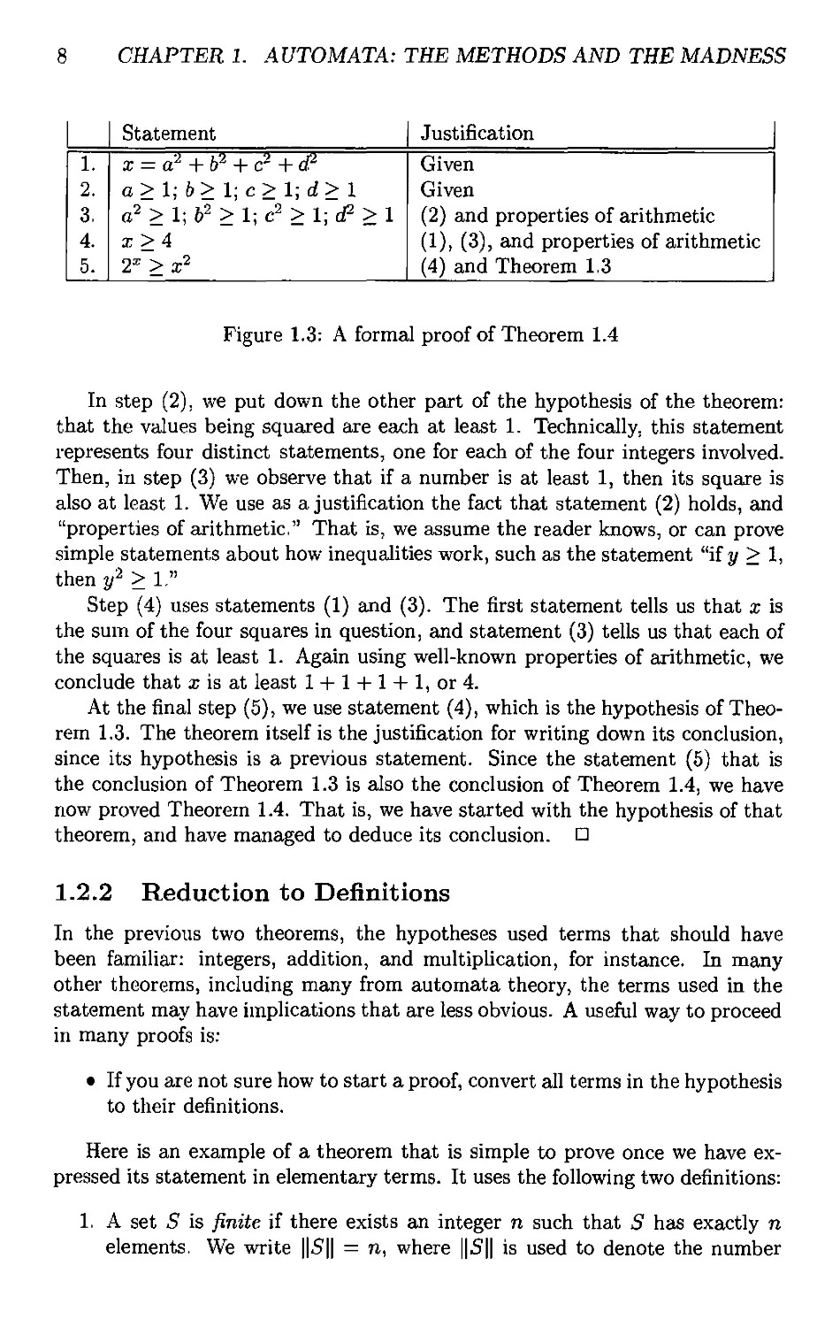
Figure 1.3 shows the sequence of statements we need to prove Theorem 1.4.
While we shall not generally prove theorems in such a stylized form, it helps to
think of proofs as very explicit lists of statements, each with a precise
justification. In step (1), we have repeated one of the given statements of the theorem:
that X is the sum of the squares of four integers. It often helps in proofs if we
name quantities that are referred to but not named, and we have done so here,
giving the four integers the names a, &, c, and d.

8
CHAPTER 1. AUTOMATA: THE METHODS AND THE MADNESS
1.
2,
3.
4.
5.
Statement
a: = a^ + &^ + c^ + d^
a>l;b>l;c>Ud>l
a'^>l;b^>l;c^>l;(f>l
x>4
2^ > x'^
Justification
Given
Given
(2) and properties of arithmetic
{l)y (3), and properties of arithmetic
(4) and Theorem 1.3
Figure 1.3: A formal proof of Theorem T4
In step (2), we put down the other part of the hypothesis of the theorem:
that the values being squared are each at least 1. Technically, this statement
represents four distinct statements, one for each of the four integers involved-
Then, in step (3) we observe that if a number is at least 1, then its square is
also at least L We use as a justification the fact that statement (2) holds, and
"properties of arithmetic." That is, we assume the reader knows, or can prove
simple statements about how inequalities w^ork, such as the statement "if j/ > 1,
then y^ > 1,"
Step (4) uses statements (1) and (3). The first statement tells us that x is
the sum of the four squares in question, and statement (3) tells us that each of
the squares is at least 1. Again using well-known properties of arithmetic, we
conclude that x is at least l + l + l-l-l, or4.
At the final step (5), we use statement (4), which is the hypothesis of
Theorem 1.3. The theorem itself is the justification for writing down its conclusion,
since its hypothesis is a previous statement. Since the statement (5) that is
the conclusion of Theorem 1.3 is also the conclusion of Theorem 1.4, we have
now proved Theorem 1.4. That is, we have started with the hypothesis of that
theorem, and have managed to deduce its conclusion. D
1.2.2 Reduction to Definitions
In the previous two theorems, the hypotheses used terms that should have
been familiar: integers, addition, and multiplicationj for instance. In many
other theorems, including many from automata theory, the terms used in the
statement may have implications that are less obvious. A useful way to proceed
in many proofs is;
• If you are not sure how to start a proof, convert all terms in the hypothesis
to their definitions.
Here is an example of a theorem that is simple to prove once we have
expressed its statement in elementary terms. It uses the following two definitions:
1. A set S is finite if there exists an integer n such that S has exactly n
elements. We write ||5|| = n, where ||5|| is used to denote the number

1.2. INTRODUCTION TO FORMAL PROOF
9
of elements in a set 5. If the set S is not finite, we say S is infinite*
Intuitively, an infinite set is a set that contains more than any integer
number of elements.
2. If 5 and T are both subsets of some set C/, then T is the complement of 5
(with respect to [/) if 5 U T = L^ and 5 fi T = 0. That is, each element
of U is in exax;tly one of S and T; put another way, T consists of exactly
those elements of U that are not in S.
Theorem 1,5: Let 5 be a finite subset of some infinite set U, Let T be the
complement of S with respect to U. Then T is infinite.
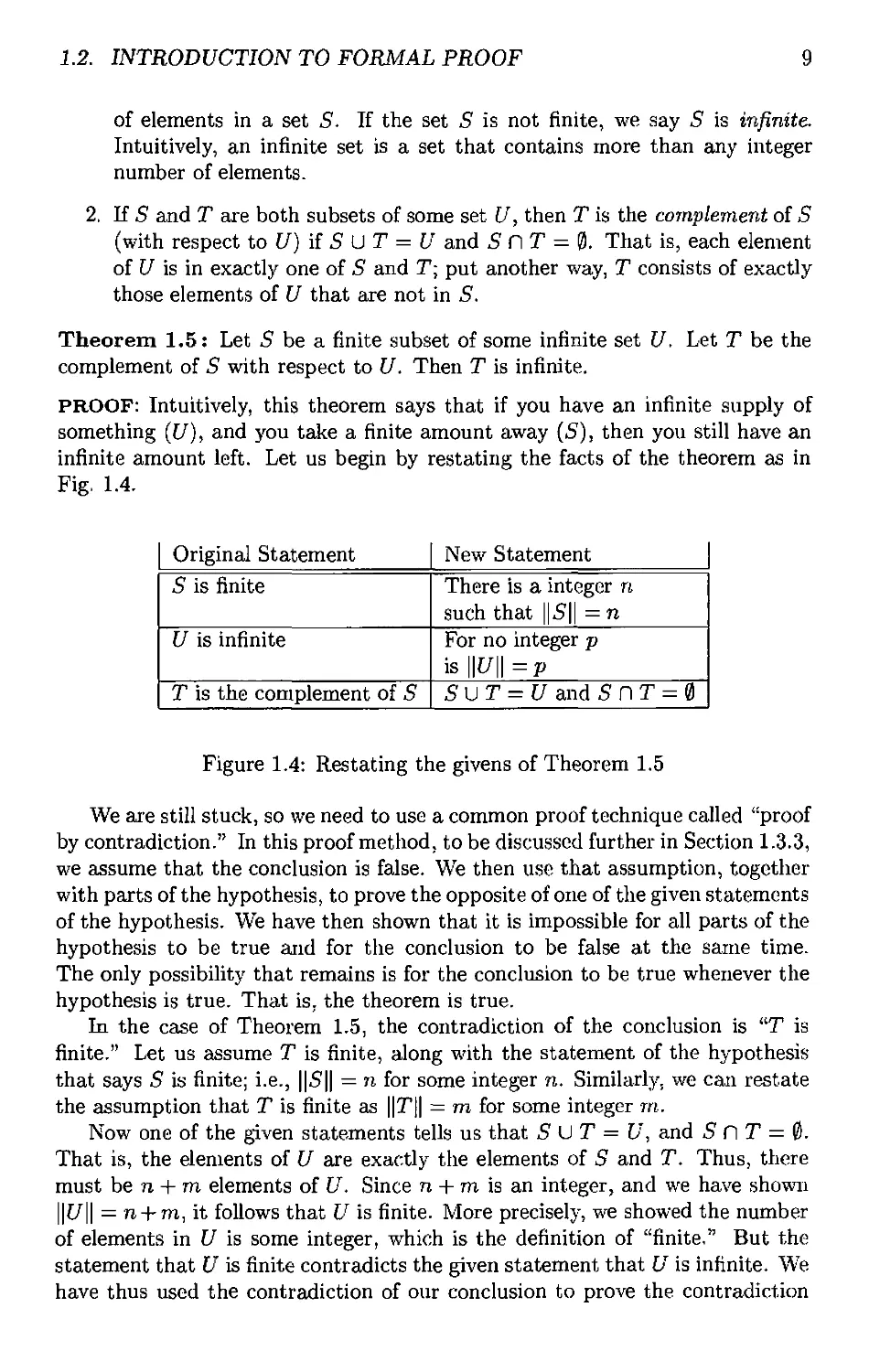
PROOF: Intuitively, this theorem says that if you have an infinite supply of
something ([/), and you take a finite amount away (5), then you still have an
infinite amount left. Let us begin by restating the facts of the theorem as in
Fig. 1.4.
Original Statement
S is finite
U is infinite
T is the complement of S
New Statement
There is a integer n
such that \\S\\ = n
For no integer p
is \U \='p
5 U T = [/ and 5 n T = 0
Figure 1.4: Restating the givens of Theorem 1.5
We ai'e still stuck, so we need to use a common proof technique called "proof
by contradiction." In this proof method, to be discussed further in Section 1.3.3,
we assume that the conclusion is false. We then use that assumption, together
with parts of the hypothesis, to prove the opposite of one of the given statements
of the hypothesis. We have then shown that it is impossible for all parts of the
hypothesis to be true and for the conclusion to be false at the same time.
The only possibility that remains is for the conclusion to be true whenever the
hypothesis is true. That is. the theorem is true.
In the case of Theorem 1.5, the contradiction of the conclusion is "T is
finite." Let us assume T is finite, along with the statement of the hypothesis
that says S is finite; i.e., ||5|| = n for some integer n. Similarly, we can restate
the assumption that T is finite as ||T|| — m for some integer m.
Now one of the given statements tells us that S yjT = U, and 5 n T = 0.
That is, the elements of U are exactly the elements of S and T. Thus, there
must be n + m elements of U. Since n + ru is an integer, and we have shown
\U\\ = n-f-m, it follows that U is finite. More precisely, t\^ showed the number
of elements in U is some integer, which is the definition of "finite," But the
statement that U is finite contradicts the given statement that U is infinite. We
have thus used the contradiction of our conclusion to prove the contradiction

10 CHAPTER L AUTOMATA: THE METHODS AND THE MADNESS
of one of the given statements of the hypothesis, and by the principle of "proof
by contradiction" we may conclude the theorem is true. □
Proofs do not have to be so wordy. Having seen the ideas behind the proof,
let us reprove the theorem in a few lines.
PROOF; (of Theorem Lo) We know that SuT = U and S and T are disjoint,
so ||5|| + ||T|| = \\U\\- Since S is finite, ||5|| = n for some integer n, and since U
is infinite, there is no integer p such that \\U\\ = p. So assume that T is finite;
that is, ||T|| = m for some integer m. Then \\U\\ = \\S\\ + ||T|| = n + m, which
contradicts the given statement that there is no integer p equal to \\U\\. □
1,2.3 Other Theorem Forms
The "if-then" form of theorem is most common in typical areas of mathematics.
However, we see other kinds of statements proved as theorems also. In this
section, we shall examine the most common forms of statement and what we
usually need to do to prove them.
Ways of Saying "If-Then"
First, there are a number of kinds of theorem statements that look different
from a simple "if H then (7" form, but are in fact saying the same thing: if
hypothesis H is true for a given value of the parameter(s), then the conclusion
C is true for the same value. Here are some of the other ways in which "if H
then C" might appear.
1. H implies C,
2. H only if C.
3. C if H.
4. Whenever H holds, C follows.
We also see many variants of form (4), such a^ "if H holds, then C follows," or
"whenever H holds, C holds."
Example 1.6: The statement of Theorem 1.3 would appear in these four forms
as:
1. X > 4 implies 2^ > x^,
2. a; > 4 only if 2=^ > x^
3. 2'^>x^iix> 4.
4. Whenever x > 4^ 2^ > x'^ follows.

L2. INTRODUCTION TO FORMAL PROOF 11
Statements With Quantifiers
Many theorems involve statements that use the quantifiers "for all" and
"there exists," or similar variations, such as "for every" instead of "for all."
The order in which these quantifiers appear affects what the statement
means. It is often helpful to see statements with more than one quantifier
as a "game" between two players — for-all and there-exists — who take
turns specifying values for the parameters mentioned in the theorem, "For-
all" must consider all possible choices, so for-all's choices are generally left
as variables. However, "there-exists" only has to pick one value, which
may depend on the values picked by the players previously. The order in
which the quantifiers appear in the statement determines who goes first.
If the last player to make a choice can always find some allowable value,
then the statement is true.
For example, consider an alternative definition of ^'infinite set'': set S
is infinite if and only if for all integers n, there exists a subset T of 5 with
exactly n members. Here, "for-all" precedes "there-exists." so we must
consider an arbitrary integer n. Now, "there-exists" gets to pick a subset
r, and may use the knowledge of n to do so. For instance, if S were the
set of integers, "there-exists" could pick the subset T = {1,2,... ,n} and
thereby succeed regardless of n. That is a proof that the set of integers is
infinite.
The following statement looks like the definition of "infinite." but is
incorr^ect because it reverses the order of the quantifiers: "there exists a
subset T of set S such that for all n, set T has exactly n members." Now.
given a set S such as the integers, player "there-exists" can pick any set
T; say {1,2,5} is picked. For this choice, player "for-all" must show that
T has n members for every possible n. However, "for-all" cannot do so.
For instance, it is false for n = 4, or in fax;t for any n / 3.
In addition, in formal logic one often see.*3 the operator -> in place of "if-
then." That is, the statement "if H then C" could appear as if ^ C in some
mathematical literature; we shall not use it here.
If-And-Only-If Statements
Sometimes, we find a statement of the form ''A if and only if S." Other forms
of this statement are "A iff B''^ "A is equivalent to 5," or "A exactly when
B" This statement is actually two if-then statements: "if A then 5," and "if
B then A." We prove "A if and only if i?" by proving these two statements:
^IfF, short for "if and only if," is a non-word that is used in some mathematical trealises
for succinctness.

12 CHAPTER L AUTOMATA: THE METHODS AND THE MADNESS
How Formal Do Proofs Have to Be?
The answer to this question is not easy^ The bottom line regarding proofs
is that their purpose is to convince someone, whether it is a grader of your
classwork or yourself, about the correctness of a strategy you are using in
your code. If it is convincing, then it is enough; if it fails to con\dnce the
"consumer" of the proof, then the proof has left out too much,
Part of the uncertainty regarding proofs comes from the different
knowledge that the consumer may have. Thus, in Theorem 1.4, we
assumed you knew all about arithmetic, and would beheve a statement like
"if 2/ > 1 then y^ > 1." If you were not familiar with arithmetic, we would
have to prove that statement by some steps in our deductive proof.
However, there are certain things that are required in proofs, and
omitting them surely makes the proof inadequate. For instance, any
deductive proof that uses statements whicli are not justified by the given or
previous statements, cannot be adequate. When doing a proof of an "if
and only if" statement, we must surely have one proof for the "if part and
another proof for the "oniy-iP part. As an additional example, inductive
proofs (discussed in Section 1.4) require proofs of the basis and induction
parts.
1. The if part; "if S then A,'' and
2. The only-if part: "if A then B," which is often stated in the equivalent
form "A only if S."
The proofs can be presented in either order. In many theorems, one part is
decidedly easier than the other, and it is customary to present the easy direction
first and get it out of the way.
In formal logic, one may see the operator f^ or = to denote an "if-and-only-
if" statement. That is, A = B and A f> B mean the same as "A if and only if
Br
When proving an if-and-only-if statement, it is important to remember that
you must prove both the "iP and "only-iP parts. Sometimes, you will find it
helpful to break an if-and-only-if into a succession of several equivalences. That
is, to prove "A if and only if B," you might first prove "A if and only if C," and
then prove '^C if cuul only if B," That method works, as long as you remember
that each if-and-only-if step must be proved in both directions. Proving any
one step in only one of the directions invalidates the entire proof.
The following is an example of a simple if-and-only-if proof. It uses the
notations:
. [xj, the floor of real number a:, is the greatest integer equal to or less than
1
X.

L3. ADDITIONAL FORMS OF PROOF 13
2. [a:]j the ceiling of real number x, is the least integer equal to or greater
than X.
Theorem 1-7: Let a: be a real number. Then [xj = \x] if and only if x is an
integer.
PROOF: (Only-if part) In this part, we assume [x\ — |"x] and try to prove x is
an integer. Using the definitions of the floor and ceiling, we notice that [x\ < x,
and \x] > X. However, we are given that [x\ = \x]. Thus, we may substitute
the floor for the ceiling in the first inequality to conclude \x] < x. Since
both \x] < X and \x] > x hold, we may conclude by properties of arithmetic
inequalities that \x] — x* Since |"x] is always an integer, x must also be an
integer in this case.
(If part) Now, we assume x is an integer and try to prove \x\ — \x\. This part
is easy. By the definitions of floor and ceiling, when x is an integer, both \_x\
and fx] are equal to x, and therefore equal to each other. D
1.2.4 Theorems That Appear Not to Be If-Then
Statements
Sometimes, we encounter a theorem that appears not to have a hypothesis. An
example is the well-known fact from trigonometry:
Theorem 1.8: sin^ ^ + cos^ 6 = 1. □
Actually, this statement does have a hypothesis, and the hypothesis consists
of all the statements you need to know to interpret the statement. In particular,
the hidden hypothesis is that 6 is an angle, and therefore the functions sine
and cosine have their usual meaning for angles. From the definitions of these
terms, and the Pythagorean Theorem (in a right triangle, the square of the
hypotenuse equals the sum of the squares of the other two sides), you could
prove the theorem. In essence, the if-then form of the theorem is really: "if 6
is an angle, then sin^ 6 -f cos^ ^ = 1."
1,3 Additional Forms of Proof
In this section, we take up several additional topics concerning how to construct
proofs:
1. Proofs about sets.
2. Proofs by contradiction.
3. Proofs by counterexample.

14 CHAPTER 1. AUTOMATA: THE METHODS AND THE MADNESS
1.3*1 Proving Equivalences About Sets
In automata theory, we axe frequently asked to prove a theorem which says that
the sets constructed in two different ways are the sairie sets. Often, these sets
are sets of character strings, and the sets are called "languages," but in this
section the nature of the sets is unimportant. If E and F are two expressions
representing sets, the statement E = F means that the two sets represented
are the same. More precisely, every element in the set represented by E is in
the set represented by F, and every element in the set represented by F is in
the set represented by E,
Example 1.9: The commutative law of union says that we can take the union
of two sets R and S in either order. That is, RU S = S U R. In this case, E is
the expression RU S and F is the expression S U R. The commutative law of
union says that E = F. D
We can write a set-equality £ = F as an if-and-only-if statement: an element
X is in £ if and only if x is in F, As a consequence, we see the outline of a
proof of any statement that asserts the equality of two sets E = F: it follows
the form of any if-and-only-if proof:
1. Proof that if x is in E, then x is in F,
2. Prove that if x is in F, then x is in E.
As an example of this proof process, let us prove the distributive law of
union over intersection:
Theorem 1.10: RU {S CiT) = (RU S) Ci {RU T),
PROOF: The two set-expressions involved are E — RU {S r\T) and
F = {R\jS)n{RUT)
We shall prove the two parts of the theorem in turn. In the "if" part we assume
element x is in E and show it is in F. This part, summarized in Fig. 1.5, uses
the definitions of union and intersection, with which we assume you are familiar.
Then, wc must prove the "only-if part of the theorem. Here, we assume x
is in F and show it is in E, The steps are summarized in Fig. 1.6. Since we
have now^ proved both parts of the if-and-only-if statement, the distributive law
of union over intersection is proved. □
1.3.2 The Contrapositive
Every if-then statement has an equivalent form that in some circumstances is
easier to prove. The contrapositive of the statement "if H then C" is "if not C
then not H.'' A statement and its contrapositive are either both true or both
false, so w^e can prove either to prove the other.
To see why "if if then C" and "if not C then not i?" are logically equivalent,
first observe that there are four cases to consider:

1.3. ADDITIONAL FORMS OF PROOF
15
1.
2.
3.
4.
5.
6.
Statement
xism Ru{SnT)
a: is in ii or a: is in 5 n r
a: is in ij or a: is in
both S and T
a: is in ij U 5
a: is in iJ U T
a: is in (RuS)r\ (RUT)
Justification
Given
(1) and definition of union
(2) and definition of intersection
(3) and definition of union
(3) and definition of union
(4), (5), and definition
of intersection
Figure 1.5: Steps in the "if" part of Theorem 1,10
1.
2.
3.
4.
5.
6.
Statement
X is in (J? U 5) n (J? U T)
a: is in i? U 5
a; is in i? U T
a: is in i? or X is in
both 5 and T
a: is in i? or X is in 5 n T
xlsin Ru{SnT)
Justification
Given
(1) and definition of intersection
(1) and definition of intersection
(2), (3), and reasoning
about unions
(4) and definition of intersection
(5) and definition of union
Figure 1.6: Steps in the "only-if" part of Theorem 1.10
1. H and C both true.
2. H true and C false.
3. C true and H false.
4. H and C both false.
There is only one way to make an if-then statement false; the hypothesis must
be true and the conclusion false, as in case (2). For the other three cases,
including case (4) where the conclusion is false, the if-then statement itself is
true.
Now, consider for which cases the contrapositive "if not C then not H" is
false. In order for this statement to be false, its hypothesis (which is "not C")
must be true, and its conclusion (which is "not ii"") must be false. But "not
C" is true exactly when C is false, and "not iif" is false exactly when H is true.
These two conditions are again case (2), which shows that in each of the four
cases, the original statement and its contrapositive are either both true or both
false; i.e., they are logically equivalent.

16 CHAPTER L AUTOMATA: THE METHODS AND THE MADNESS
Saying "If-And-Only-If" for Sets
As we mentioned, theorems that state equivalences of expressions about
sets are if-and-only-if statements. Thus, Theorem 1.10 could have been
stated: an element x is in /? U (5 fl T) if and only if x is in
{RuS)n{Ru T)
Another common expression of a set-equivalence is with the locution
"all-and-only." For instance, Theorem 1.10 could as well have been stated
"the elements of iZ U (5 fl T) are all and only the elements of
{RuS)n{Ru T)
The Converse
Do not confuse the terms "contrapositive" and "converse." The converse
of an if-then statement is the "other direction"; that is, the converse of "if
H then C" is "if C then i?." Unlike the contrapositive, which is logically
equivalent to the original, the converse is not equivalent to the original
statement- In fact, the two parts of an if-and-only-if proof are always
some statement and its converse.
Example 1.11: Recall Theorem 1.3, whose statement was: "if x > 4, then
2^ > x^." The contrapositive of this statement is "if not 2^ > x^ then not
X > 4." In more colloquial terms, making use of the fact that "not a >
the same as a < 6, the contrapositive is "if 2^ < x^ then x < 4." Q
> 6" is
When we £ure asked to prove an if-and-only-if theorem, the use of the
contrapositive in one of the parts allows us several options* For instance, suppose
we want to prove the set equivalence E = F, Instead of proving "if x is in £
then x is in F and if a: is in F then x is in £," we could also put one direction
in the contrapositive. One equivalent proof form is:
• If a: is in £ then x is in F, and if x is not in E then x is not in F.
We could also interchange E and F in the statement above.
1.3.3 Proof by Contradiction
Another way to prove a statement of the form "if H then (7" is to prove the
statement

1.3. ADDITIONAL FOBMS OF PROOF 17
• "ii" and not C implies falsehood."
That is, start by assuming both the hypothesis H and the negation of the
conclusion C. Complete the proof by showing that something known to be
false follows logically from H and not C. This form of proof is called proof by
contradiction.
Example 1.12: Recall Theorem 1.5, where we proved the if-then statement
with hypothesis H = ''U is an infinite set, 5 is a finite subset of U, and T is
the complement of S with respect to !7." The conclusion C was 'T is infinite."
We proceeded to prove this theorem by contradiction. We assumed "not C";
that is, we assumed T was finite.
Our proof was to derive a falsehood from H and not C We first showed
from the assumptions that S and T axe both finite, that U also must be finite.
But since U is stated in the hypothesis H to be infinite, and a set cannot be
both finite and infinite, we have proved the logical statement "false." In logical
terms, we have both a proposition p {U is finite) and its negation, not p (U
is infinite). We then use the fact that "p and not p" is logically equivalent to
"false." □
To see why proofs by contradiction are logically correct, reccill from
Section 1.3.2 that there are four combinations of truth values for H and C Only
the second case, H true and C false, makes the statement "if H then C"' false.
By showing that H and not C leads to falsehood, we are showing that case 2
cannot occur. Thus, the only possible combinations of truth values for H and
C are the three combinations that make "if H then C" true.
1.3,4 Counterexamples
In real life, we are not told to prove a theorem. Rather, we are faced with
something that seems true — a strategy for implementing a program for example —
and we need to decide whether or not the "theorem" is true. To resolve the
question, we may alternately try to prove the theorem, and if we cannot, try to
prove that its statement is false.
Theorems generally are statements about an infinite number of cases j
perhaps all values of its parameters. Indeed, strict mathematical convention will
only dignify a statement with the title "theorem" if it has an infinite number
of cases; statements that have no parameters, or that apply to only a finite
number of values of its parameter(s) are called observations. It is sufficient to
show that an alleged theorem is false in any one case in order to show it is not a
theorem. The situation is analogous to programs, since a program is generally
considered to have a bug if it fails to operate correctly for even one input on
which it was expected to work.
It often is easier to prove that a statement is not a theorem than to prove
it is a theorem. As we mentioned, if S is any statement, then the statement
"5 is not a theorem" is itself a statement without parameters, and thus can

18 CHAPTER 1. AUTOMATA: THE METHODS AND THE MADNESS
be regarded as an observation rather than a theorem. The following are two
examples, first of an obvious nontheorem, and the second a statement that just
misses being a theorem and that requires some investigation before resolving
the question of whether it is a theorem or not.
Alleged Theorem 1.13: All primes are odd. (More formally, we might say:
if integer a: is a prime, then x is odd.)
DISPROOF: The integer 2 is a prime, but 2 is even, □
Now, let us discuss a "theorem" involving modular arithmetic. There is an
essential definition that we must first establish. If a and b are positive integers,
then a mod b is the remainder when a is divided by 6, that is, the unique integer
r between 0 and 6-1 such that a = qb + r foi some integer q. For example,
8 mod 3 = 2, and 9 mod 3 = 0. Our first proposed theorem, which we shall
determine to be false, is:
Alleged Theorem 1.14: There is no pair of integers a and b such that
o mod 6 = 6 mod a
U
When asked to do things with pairs of objects, such as a and 6 here, it is
often possible to simplify the relationship between the two by taking advantage
of symmetry. In this case, we can focus on the case where a < 6, since if 6 < a
we can swap a and 6 and get the same equation as in Alleged Theorem 1.14.
we must be careful, however, not to forget the third case, where a = b. This
case turns out to be fatal to our proof attempts.
Let us assume a < 6. Then a mod 6 = o, since in the definition of a mod 6
we have q = 0 and r = a. That is, when o < 6 we have o = 0 x 6 + a. But
6 mod a < Qj since anything mod a is between 0 and a - 1. Thus, when a < 6,
6 mod a < a mod 6, so a mod 6 = 6 mod a is impossible. Using the argument
of symmetry above, we also know that o mod 6^6 mod a when 6 < a.
However, consider the third case: a = 6. Smce x mod a: = 0 for any integer
X, we do have a mod 6 = 6 mod a if a = 6. We thus have a disproof of the
alleged theorem:
DISPROOF: (of Alleged Theorem 1.14) Let a = 6 = 2. Then
a mod 6 = 6 mod o = 0
D
In the process of finding the counterexample, we have in fact discovered the
exact conditions under which the alleged theorem holds. Here is the correct
version of the theorem, and its proof.
Theorem 1*15: a mod 6 = 6 mod a if and only if o = 6,

J.4. INDUCTIVE PROOFS 19
PROOF: (If part) Assume a = 6, Then as we obsen^ed above, x mod x = 0 for
any integer x. Thus, a mod 6 = 6 mod a = 0 whenever a = b.
(Only-if part) Now, assume a mod 6 = 6 mod a. The best technique is a
proof by contradiction, so assume in addition the negation of the conclusion;
that is. assume a=^b. Then since a = 6 is eliminated^ we have only to consider
the cases a < b and b < a.
We already observed above that when a < b, we have a mod b = a and
b mod a < a. Thus, these statements, in conjunction with the hypothesis
a mod 6 = 6 mod a lets us derive a contradiction.
By symmetry, if 6 < a then 6 mod a = b and a mod 6 < 6. We again derive
a contradiction of the hypothesis, and conclude the only-if part is also true. We
have now proved both directions and conclude that the theorem is true. □
1.4 Inductive Proofs
There is a special form of proof, called "inductive," that is essential when dealing
with recursively defined objects. Many of the most familiar inductive proofs
deal with integers, but in automata theory, we also need inductive proofs about
such recursively defined concepts as trees and expressions of various sorts, such
as the regular expressions that were mentioned briefly in Section 1.1.2. In this
section, we shall introduce the subject of inductive proofs first with "simple"
inductions on integers, Then, we show how to perform "structural" inductions
on any recursively defined concept.
1.4.1 Inductions on Integers
Suppose we are given a statement S{n)^ about an integer n, to prove. One
common approach is to prove two things:
1. The basis, where we show S{i) for a particular integer i. Usually, i = 0
01 i — 1, but there are examples where we want to start at some higher
i, perhaps because the statement S is false for a few small integers.
2. The inductive step, where we assume n > i, where i is the basis integer,
and we show that "if S{n) then S{n +1)."
Intuitively, these two parts should convince us that S{n) is true for every
integer n that is equal to or greater than the basis integer i. We can argue as
follows. Suppose S{n) were false for one or more of those integers. Then there
would have to be a smallest value of n, say j, for which S{j) is false, and yet
j ^ i' ^'o^' j could not be i, because we prove in the basis part that S{i) is
true. Thus, j must be greater than i. We now know that j -l>i, and S{j — 1)
is true.
However, we proved in the inductive part that if n > i, then S{n) implies
5(n -h 1). Suppose we let n = j - 1. Then we know from the inductive step
that S{j - 1) implies S{j), Since we also know S{j - 1), we can conclude 5(j).

20 CHAPTER L AUTOMATA: THE METHODS AND THE MADNESS
We have assumed the negation of what we wanted to prove; that is, we
assumed S{j) was felse for some j > z. In each case, we derived a contradiction,
so we have a "proof by contradiction" that S{n) is true for all n > i.
Unfortunately, there is a subtle logical flaw in the above reasoning. Our
assumption that we can pick a least j > i for which S{j) is false depends on
our believing the principle of induction in the first place* That is, the only way
to prove that we can find such a j is to prove it by a method that is essentially
an inductive proof. However, the "proof" discussed above makes good intuitive
sense, and matches our understanding of the real world. Thus, we generally
take as an integral part of our logical reasoning system:
• The Induction Principle: If we prove S{i) and we prove that for all n > i,
S{n) implies S{n + 1), then we may conclude S{n) for all n > i.
The following two examples illustrate the use of the induction principle to prove
theorems about integers.
Theorem 1.16: For all n > 0:
n
n(n + l](2n+l)
"6
I = ^ (1-1)
PROOF: The proof is in two parts: the basis eind the inductive step; we prove
each in turn,
BASIS: For the basis, we pick n = 0. It might seem surprising that the theorem
even makes sense for n = 0, since the left side of Equation (1.1) is Yli=^\ when
n = 0. However, there is a general principle that when the upper limit of a sum
(0 in this case) is less than the lower limit (1 here), the sum is over no terms
and therefore the sum is 0, Thatis, l]i^ii^ = 0.
The right side of Equation (IJ) is also 0, since 0 x (0 +1) x (2 x 0 +1)/6 = 0,
Thus, Equation (LI) is true when n = 0.
INDUCTION: Now, assume n > 0. We must prove the inductive step, that
Equation (1.1) implies the same formula with n H- 1 substituted for n. The
latter formula is
'g^.,_[n + l]([n + l] + l)(2[n+ !] + !) ^j^)
We may simplify Equations (1.1) and (L2) by expanding the sums and products
on the right sides. These equations become:
n
^ i^ = (2n3 + Sn^ + n)/6 (1.3)
i=\

1.4. INDUCTIVE PROOFS 21
n-fl
^i^ = (2n3 + 9n2 + 13n + 6)/6 (1.4)
We need to prove (1,4) using (1.3), since in the induction principle, these are
statements S{n + 1) and S{n), respectively. The ^'trick" is to break the sum
to n + 1 on the right of (1,4) into a sum to n plus the (n + l)st term. In that
way, we can replace the sum to n by the left side of (1.3) and show that (1.4)
is true. These steps are as follows:
(2n^ + 3n^ + n)/6 -h (n^ + 2n + 1) = (2n^ + Qn'"^ + 13n + 6)/6 (1.6)
The final verification that (1.6) is true requires only simple polynomial algebra
on the left side to show it is identical to the right side. □
Example 1-17: In the next example, we prove Theorem 1.3 from Section 1.2.1.
Recall this theorem states that if a; > 4, then 2^ > x^. We gave an informal
proof based on the idea that the ratio x'^/2^ shrinks as x grows above 4. We
can make the idea precise if we prove the statement 2^ > x^ by induction on
X, starting with a basis of x = 4. Note that the statement is actually false for
X <4.
BASIS: K X = 4, then 2^ and x^ are both 16. Thus, 2^ > 4? holds.
INDUCTION: Suppose for some x > 4 that 2"^ > x^. With this statement as
the hypothesis, we need to prove the same statement, with x -h 1 in place of x,
that is, 2t=^+*J >[x-\- if. These are the statements 5(x) and 5(x + 1) in the
induction principle; the fact that we are using x instead of n as the parameter
should not be of concern; x orn is just a local variable.
As in Theorem 1.16, we should rewrite 5(x + 1) so it can make use of 5(x).
In this case, we can write 2l^'^^l as 2 x 2^. Since 5(x) tells us that 2^ > x^, we
can conclude that 2=^+^ = 2 x 2=^ > 2x^.
But we need something different; we need to show that 2^"^^ > (x + 1)^,
One way to prove this statement is to prove that 2x^ > (x + 1)^ and then use
the transitivity of > to show 2=""*'^ > 2x'^ >{x + 1)^. In our proof that
2x'^ >(x + l)2 (1.7)
we may use the assumption that x > 4. Begin by simplifying (1.7):
x^ >2x+l (L8)
Divide (1.8) by x, to get:

22 CHAPTER L AUTOMATA: THE METHODS AND THE MADNESS
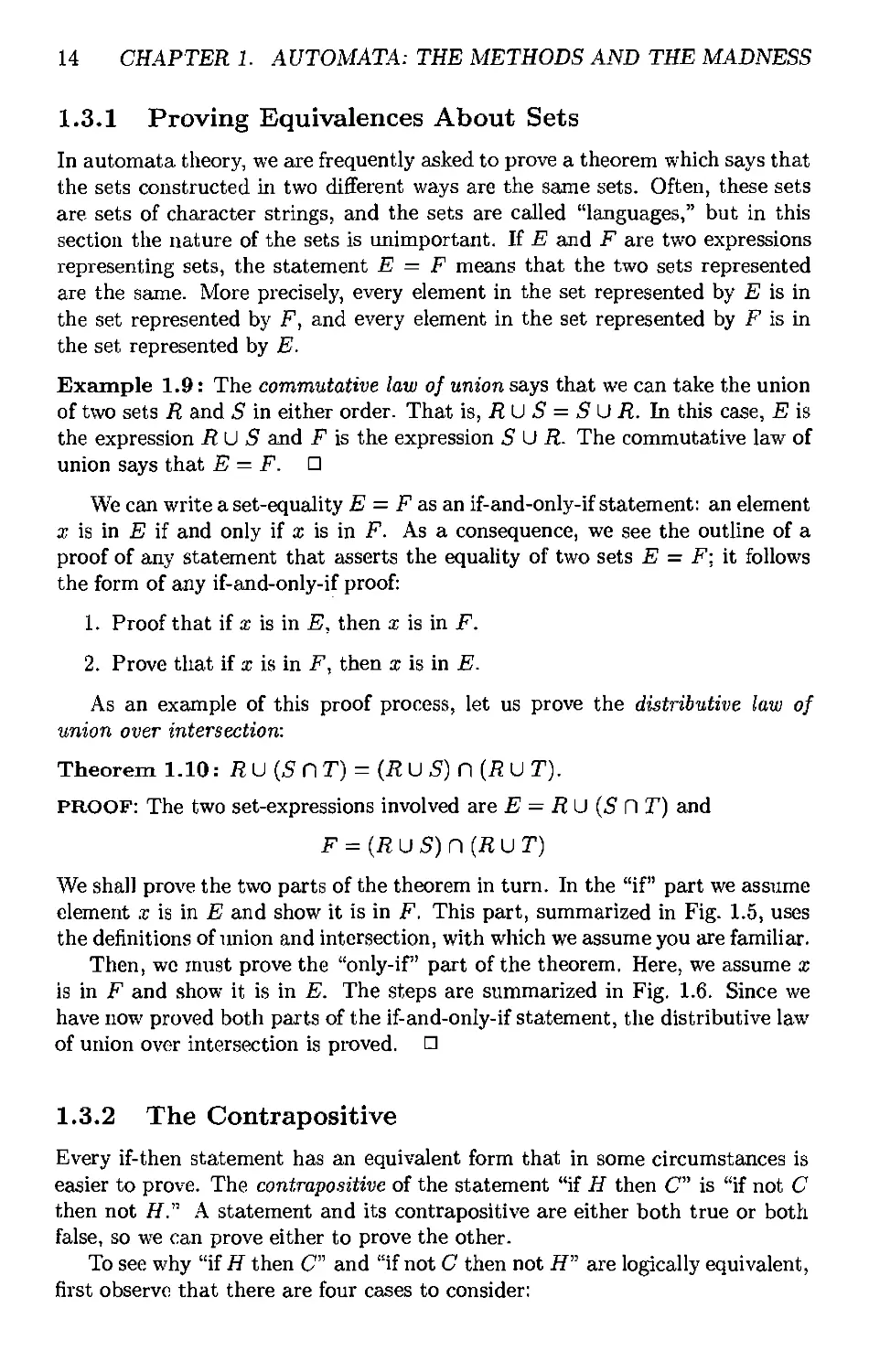
Integers as Recursively Defined Concepts
We mentioned that inductive proofs are useful when the subject matter is
recursively defined. However, our first examples were inductions on
integers, which we do not normally think of as "recursively defined." However,
there is a natural, recursive definition of when a number is a nonnegative
integer, and this definition does indeed match the way inductions on
integers proceed: from objects defined first, to those defined later.
BASIS: 0 is an integer.
INDUCTION: If n is an integer, then so is n + 1.
x>2+- (1.9)
X
Since x > 4, we know l/x < 1/4. Thus, the left side of (1.9) is at least
4, and the right side is at most 2.25. We have thus proved the truth of (1.9).
Therefore, Equations (1.8) and (1.7) are also true. Equation (1.7) in turn gives
us 2x^ > (2: + 1)^ for X > 4 and lets us prove statement 5(x + 1), which we
recall was 2^+^ >{x-\-lf. □
1.4.2 More General Forms of Integer Inductions
Sometimes an inductive proof is made possible only by using a more general
scheme than the one proposed in Section 1.4.1, where we proved a statement S
for one basis value and then proved that "if S{7i) then 5(n+1)." Two important
generalizations of this scheme are:
1. We can use several basis cases. That is, we prove 5(i), S{i + 1),,.., S{j)
for some j > i.
2. In proving S{n + 1), we can use the truth of all the statements
5(i),5(i + l),...,5(7z)
rather than just using S{n). Moreover, if we have proved basis cases up
to S{j), then we can assume n > j^ rather than just n>i.
The conclusion to be made from this basis and inductive step is that S{n) is
true for all n>i.
Example 1.18: The following example will illustrate the potential of both
principles. The statement S{n) we would like to prove is that if n > 8, then n
can be written as a sum of 3's and 5's. Notice, incidentally, that 7 cannot be
written as a sum of 3's and 5's.

1.4. INDUCTIVE PROOFS 23
BASIS: The basis cases are 5(8), 5(9), and 5(10). The proofs are 8 = 3 + 5,
9 = 3 + 3 + 3, and 10 = 5 + 5, respectively.
induction: Assume that n > 10 and that 5(8),5(9),.. .,5(n) are true. We
must prove S{n + 1) from these given facts. Our strategy is to subtract 3 from
n + 1, observe that this number must be writable as a sum of 3's and 5's, and
add one more 3 to the sum to get a way to write n + l.
More formally, observe that n - 2 > 8, so we may assume S{n — 2). That
is, n — 2 = 3a + 56 for some integers a and b. Then h -h 1 = 3 + 3a + 56, so
n + 1 can be written as the sum of a + 1 3's and b 5's. That proves S{n + 1)
and concludes the inductive step. D
1,4,3 Structural Inductions
In automata theory, there are several recursively defined structures about which
we need to prove statements. The familiar notions of trees and expressions
are important examples. Like inductions, all recursive definitions have a basis
case, where one or more elementary structures are defined, and an inductive
step, where more complex structures are defined in terms of previously defined
structures.
Example 1,19: Here is the recursive definition of a tree:
BASIS: A single node is a tree, and that node is the root of the tree.
INDUCTION: UTi^T2,... ,Tk axe trees, then we can form a new tree as follows:
1. Begin with a new node AT, which is the root of the tree.
2. Add copies of all the trees Ti, 72, - ■ -, 7"^.
3. Add edges from node A^ to the roots of each of the trees Ti, T2,..,, Tjt.
Figure 1.7 shows the inductive construction of a tree w-ith root N from k smaller
trees. D
Example 1-20: Here is another recursive definition. This time w^e define
expressions using the arithmetic operators + and *, with both numbers and
variables allowed as operands.
BASIS: Any number or letter (i.e.^ a variable) is an expression.
INDUCTION: If E and F are expressions, then so a^re E + F, E* F, and (E).
For example, both 2 and x are expressions by the basis* The inductive step
tells us ar + 2, (x + 2), and 2 * (x + 2) are all expressions. Notice how each of
these expressions depends on the previous ones being expressions. D

24 CHAPTER L AUTOMATA: THE METHODS AND THE MADNESS
Figure 1.7: Inductive construction of a tree
Intuition Behind Structural Induction
We can suggest informally why structural induction is a valid proof
method. Imagine the recursive definition establishing, one at a time, that
certain structures Xi, A's,... meet the definition. The basis elements come
first, and the fact that Xi is in the defined set of structures cgin only depend
on the membership in the defined set of structures that precede Xi on the
list. Viewed this way, a structural induction is nothing but an induction
on integer n of the statement S{Xn). This induction may be of the
generalized form discussed in Section 1.4.2, with multiple basis cases and an
inductive step that uses all previous instances of the statement. However,
we should remember, as explained in Section 1.4.1, that this intuition is
not a formal proof, and in fact we must assume the validity this induction
principle as we did the validity of the original induction principle of that
section.
When we have a recursive definition, we can prove theorems about it using
the following proof form, which is called structural induction. Let S(X) be a
statement about the structures X that are defined by some particular recursive
definition.
1. As a basis, prove S{X) for the basis structure(s) X.
2. For the inductive step, take a structure X that the recursive
definition says is formed from Yi,Y2^*.*jYk* Assume tliat the statements
5(yi), S{Y2),.. M S{Yk), and use these to prove S{X).
Our conclusion is that S{X) is true for all X. The next two theorems are
examples of facts that can be proved about trees and expressions.
Theorem 1.21: Every tree has one more node than it has edges.

L4, INDUCTIVE PROOFS 25
PROOF: The formal statement S{T) we need to prove by structural induction
is: "if T is a tree, and T has n nodes sind e edges, then n = e + 1."
BASIS: The basis case is when T is a single node. Then n = 1 and e = 0, so
the relationship n = e + 1 holds*
INDUCTION: Let T be a tree built by the inductive step of the definition,
from root node N and k smaller trees Ti, Ta,..., T^. We may assume that the
statements S{Ti) hold for i = 1,2,..., A:, That is, let Ti have n^ nodes and ei
edges; then n^ = e^ + 1.
The nodes of T are node N and all the nodes of the T^'s. There are thus
1 + ni + n2 H +nk nodes in T, The edges of T are the k edges we added
explicitly in the inductive definition step, plus the edges of the T^'s. Hence^ T
has
fc + ei +e2 + '---hefc (1.10)
edges. K we substitute e^ + 1 for n^ in the count of the number of nodes of T
we find that T has
1 + [ei + 1] + [62 + 1] + ' • - + [et + 1] (1.11)
nodes. Since there are k of the "+1" terms in (1.10), we can regroup (1.11) as
k + l + ei+e2 + '- + ek (1.12)
This expression is exactly 1 more than the expression of (1.10) that was given
for the number of edges of T. Thus, T has one more node than it has edges.
D
Theorem 1,22 : Every expression has an equal number of left and right paren-
theses*
PROOF: Formally, we prove the statement S{G) about any expression G that
is defined by the recursion of Example 1.20: the numbers of left and right
parentheses in G are the same.
BASIS: If G is defined by the basis, then (3 is a number or variable. These
expressions have 0 left parentheses and 0 right parentheses, so the numbers are
equal.
INDUCTION: There are three rules whereby expression G may have been
constructed according to the inductive step in the definition:
1. G = E + F.
2. G^E^F.
3. G^{E).

26 CHAPTER 1. AUTOMATA: THE METHODS AND THE MADNESS
We may assume that S{E) and S{F) are true; that is, E has the same number
of left and right parentheses, say n of each, and F likewise has the same number
of left and right parentheses, say m of each. Then we can compute the numbers
of left and right parentheses in G for each of the three cases, as follows:
1, If G = E + F, then G has n + m left parentheses and n + m right
parentheses; n of each come from E and m of each come from F.
2, li G = E * F, the count of parentheses for G is again n + m of each, for
the same reason as in case (1).
3, If G = (£■), then there are n+1 left parentheses in G — one left parenthesis
is explicitly shown, and the other n are present in E. Likewise, there are
n + 1 right parentheses in G; one is explicit and the other n are in E,
In each of the three cases, we see that the numbers of left and right parentheses
in G are the same. This observation completes the inductive step and completes
the proof. □
1.4.4 Mutual Inductions
Sometimes, we cannot prove a single statement by induction, but rather need
to prove a group of statements 5i(n),52(n),... ,5fc(n) together by induction
on n. Automata theory provides many such situations. In Example 1.23 w^e
sample the common situation where we need to explain what an automaton
does by proving a group of statements, one for each state. These statements
tell under what sequences of inputs the automaton gets into each of the states.
Strictly speaking, proving a group of statements is no different from proving
the conjunction (logical AND) of all the statements. For instance, the group
of statements Si (n) j 52(rt)j..., Sk{n) could be replaced by the single statement
51(72) AND 52(n) AND - ■ • AND Sk{n). However, when there are really several
independent statements to prove, it is generally less confusing to keep the statements
separate and to prove them all in their own parts of the basis and inductive
steps. We call this sort of proof mutual induction. An example will illustrate
the necessary steps for a mutual recursion.
Example 1-23: Let us revisit the on/off switch, which we represented as an
automaton in Example 1.1. The automaton itself is reproduced as Fig. 1.8.
Since pushing the button switches the state between on and off^ and the switch
starts out in the OjQ^ state, we expect that the following statements will together
explain the operation of the switch:
Si{n): The automaton is in state OjQ^after n pushes if and only if n is even.
52 (^): The automaton is in state on after n pushes if and only if n is odd.

L4, INDUCTIVE PROOFS 27
Push
Start
Push
Figure 1.8: Repeat of the automaton of Fig. 1.1
We might suppose that Si implies 52 and vice-versa, since we know that
a number n cannot be both even and odd. However, what is not always true
about an automaton is that it is in one and only one state. It happens that
the automaton of Fig. 1.8 is always in exactly one state, but that fact must be
proved as part of the mutual induction.
We give the basis and inductive parts of the proofs of statements Si (n) and
52(n) below. The proofs depend on several facts about odd and even integers:
if we add or subtract 1 from an even integer, we get an odd integer, and if we
add or subtract 1 from an odd integer we get an even integer.
BASIS: For the basis, we choose n = 0. Since there are two statements, each of
which must be proved in both directions (because Si and S2 are each "if-and-
only-if" statements), there are actually four cases to the basis, and four cases
to the induction as well.
1. [Si] If] Since 0 is in fact even, we must show that after 0 pushes, the
automaton of Fig. 1.8 is in state off. Since that is the start state, the
automaton is indeed in state off after 0 pushes.
2. [5i; Only-if] The automaton is in state off aStei 0 pushes, so we must
show that 0 is even. But 0 is even by definition of "even," so there is
nothing more to prove.
3. [52; If] The hypothesis of the "if" part of S2 is that 0 is odd. Since this
hypothesis H is false, any statement of the form "if H then C" is true, as
we discussed in Section 1.3.2. Thus, this part of the basis also holds.
4. [52; Only-if] The hypothesis, that the automaton is in state on after 0
pushes, is also false, since the only way to get to state on is by following
an arc labeled Pushy which requires that the button be pushed at least
once. Since the hypothesis is false, we can again conclude that the if-then
statement is true.
INDUCTION: Now, we assume that Si{n) and 52(n) are true, and try to prove
5i(Ti -h 1) and 52(n + 1). Again, the proof separates into four parts.

28 CHAPTER L AUTOMATA: THE METHODS AND THE MADNESS
1. [5i(n + 1); If] The hj-pothesis for this part is that n + 1 is even. Thus,
n is odd. The "if part of statement 82(71) says that after n pushes, the
automaton is in state on. The arc from on to off labeled Push tells us
that the (n + l)st push will cause the automaton to enter state off. That
completes the proof of the "if part of Si {n + 1).
2. [Si{n + 1); Only-if] The hypothesis is that the automaton is in state off
after n + 1 pushes. Lispecting the automaton of Fig. 1.8 tells us that the
only way to get to state offaiter one or more moves is to be in state on gind
receive an input Push. Thus, if we are in state offaStev n+ 1 pushes, we
must have been in state on after n pushes. Then, we may use the "only-if"
part of statement 52(w) to conclude that n is odd. Consequently, n + 1 is
even, which is the desired conclusion for the only-if portion of Si{n + 1).
3. [52(n-|-l); If] This part is essentially the same as part (1), with the roles of
statements Si and S2 exchanged, and with the roles of "odd" sind "even"
exchanged. The reader should be able to construct this part of the proof
easily.
4. [S2{n -h 1); Only-if] This part is essentially the same as part (2), with the
roles of statements Si and 52 exchanged, and with the roles of "odd" sind
"even" exchanged.
D
We can abstract from Example 1.23 the pattern for all mutual inductions:
• Each of the statements must be proved separately in the basis and in the
inductive step.
• If the statements are "if-and-only-if," then both directions of each
statement must be proved, both in the basis sind in the induction.
1.5 The Central Concepts of Automata Theory
In this section we shall introduce the most important definitions of terms that
pervade the theory of automata. These concepts include the ''alphabet" (a set
of symbols), "strings" (a list of symbols from an alphabet), and "language" (a
set of strings from the same alphabet).
1,5.1 Alphabets
An alphabet is a finite, nonempty set of symbols. Conventionally, we use the
symbol S for an alphabet. Common alphabets include:
1. E = {0,1}, the binary alphabet.

1.5. THE CENTRAL CONCEPTS OF AUTOMATA THEORY 29
2, S = {a, 6,... J z]^ the set of all lower-case letters,
3. The set of all ASCII characters, or the set of all printable ASCII
characters.
1,5.2 Strings
A string (or sometimes word) is a finite sequence of symbols chosen from some
alphabet. For example, 01101 is a string from the binary alphabet E = {0,1},
The string HI is another string chosen from this alphabet.
The Empty String
The empty string is the string with zero occurrences of symbols. This string,
denoted e, is a string that may be chosen from any alphabet whatsoever.
Length of a String
It is often useful to classif}' strings by their lengthy that is, the number of
positions for symbols in the string. For instance, 01101 has length 5. It is
common to say that the length of a string is "the number of symbols" in the
string; this statement is colloquially accepted but not strictly correct. Thus,
there are only two symbols, 0 and 1, in the string 01101, but there are five
positions for symbols, and its length is 5. However, you should generally expect
that "the number of symbols" can be used when "number of positions" is meant.
The standard notation for the length of a string w is \w\. For example,
|011| = 3 and |e| =0.
Powers of an Alphabet
If S is an alphabet^ we can express the set of all strings of a certain length from
that alphabet by using an exponential notation. We define E^ to be the set of
strings of length k, each of whose symbols is in E.
Example 1-24: Note that E^ = {e}, regardless of what alphabet E is. That
is, e is the only string whose length is 0.
K E ^ {0,1}, then E^ = {0,1}, E^ = {00,01,10,11},
E^ = {000,001,010,Oil, 100,101,110,111}
and so on. Note that there is a slight confusion between E and E^. The former
is an alphabet; its members 0 and 1 are symbols. The latter is a set of strings;
its members are the strings 0 and 1, each of which is of length 1. We shall not
try to use separate notations for the two sets, relying on context to make it
clear whether {0,1} or similar sets are alphabets or sets of strings. D

30 CHAPTER 1. AUTOMATA: THE METHODS AND THE MADNESS
Type Convention for Symbols and Strings
Commonly, we shall use lower-case letters at the beginning of the alphabet
(or digits) to denote symbols, and lower-case letters near the end of the
alphabet, typically w, x, y^ and z, to denote strings. You should try to get
used to this convention, to help remind you of the types of the elements
being discussed.
The set of all strings over an alphabet S is conventionallj'^ denoted E*. For
instance, {0,1}* = {e,0,1,00,01,10,11,000,., J, Put another way,
S* = S°US^ US^ U ■■•
Sometimes, we wish to exclude the empty string from the set of strings. The
set of nonempty strings from alphabet E is denoted E"*". Thus, two appropriate
equivalences are:
• E+ = E^ UE2 UE^U---.
• E* = E+ U {e}.
Concatenation of Strings
Let X and y be strings. Then xy denotes the concatenation of x and y, that
is, the string formed by making a copy of x and following it by a copy of y.
More precisely, if x is the string composed of i symbols x = aia2-"ai and y is
the string composed of j symbols y = bib2 • - - bj, then xy is the string of length
i -\- j: xy = aia-2 ■ ••a,:&i62 *• -bj.
Example 1.25: Let x = 01101 and y = 110. Then xy = 01101110 and
yx = 11001101. For any string w, the equations ew = we = w hold. That is,
e is the identity for concatenation, since when concatenated with any string it
yields the other string as a result (analogously to the way 0, the identity for
addition, can be added to any number x and yields x as a result), n
1,5,3 Languages
A set of strings all of which are chosen from some E*, where E is a particular
alphabet, is called a language. U E is an alphabet, and L C E*, then L is a
language over E. Notice that a language over E need not include strings with
all the symbols of E, so once we have established that L is a language over E,
we also know it is a language over any alphabet that is a superset of E.
The choice of the term "language" may seem strange. However, common
languages can be viewed as sets of strings. An example is English, where the

1.5. THE CENTRAL CONCEPTS OF AUTOMATA THEORY 31
collection of legal English words is a set of strings over the alphabet that consists
of all the letters. Another example is C, or any other programming language^
where the legal programs are a subset of the possible strings that can be formed
from the alphabet of the language. This alphabet is a subset of the ASCII
characters. The exact alphabet may differ slightly among different programming
languages, but generally includes the upper- and lower-case letters, the digits,
punctuation, and mathematical symbols.
However, there are also many other languages that appear when wo study
automata. Some are abstract examples, such as:
1. The language of all strings consisting of n O's followed by n Ts, for some
n>0: {e,01,0011,000111,...}.
2. The set of strings of O's and I's with an equal number of each:
{£,01,10,0011,0101,1001,...}
3. The set of binary numbers whose value is a prime:
{10,11,101,111,1011,...}
4. S' is a language for any alphabet S.
5. 0, the empty language, is a language over any alphabet.
6. {e}, the language consisting of only the empty string, is also a language
over any alphabet. Notice that 0 ^ {e}; the former has no strings and
the latter has one string.
The only important constraint on what can be a language is that all alphabets
are finite. Thus languages, although they can have an infinite number of strings,
are restricted to consist of strings drawn from one fixed, finite alphabet.
1,5.4 Problems
In automata theory^ a problem, is the question of deciding whether a given string
is a member of some particular language. It turns out, as we shall see, that
anything we more colloquially call a "problem" can be expressed as membership
in a language. More precisely, if E is an alphabet, and L is a language over E,
then the problem L is:
• Given a string w in E*, decide whether or not lu is in L.
Example 1.26: The problem of testing primality can be expressed by the
language Lp consisting of all binary strings whose value as a binary number is
a prime. That is. given a string of O's and I's, say "yes" if the string is the
binary representation of a prime and say "no" if not. For some strings, this

32 CHAPTER 1. AUTOMATA: THE METHODS AND THE MADNESS
Set-Formers as a Way to Define Languages
It is common to describe a language using a "set-former":
{w I something about w}
This expression is read "the set of words w such that (whatever is said
about w to the right of the vertical bar)." Examples are:
1. {w I w consists of an equal number of O's and Ts }.
2. (it; I It; is a binary integer that is prime }.
3. {ti? I ty is a syntactically correct C program }.
It is also common to replace w by some expression with parameters and
describe the strings in the language by stating conditions on the
parameters. Here are some examples; the first with parameter n, the second with
parameters i and j:
1. {O^l'^ \n> 1]. Read "the set of 0 to the n 1 to the n such that n
is greater than or equal to 1," this language consists of the strings
{01,0011,000111,...}. Notice that, as with alphabets, we can raise
a single symbol to a power n in order to represent n copies of that
symbol.
2. {O^V \ 0 < i < j}. This language consists of strings with some O's
(possibly none) followed by at least as many Ts.
decision is easy. For instance, 0011101 cannot be the representation of a prime,
for the simple reason that every integer except 0 has a binary representation
that begins with 1. However, it is less obvious whether the string 11101 belongs
to Lp^ so any solution to this problem will have to use significant computational
resources of some kind: time and/or space, for example. □
One potentially unsatisfactory aspect of our definition of "problem" is that
one commonly thinks of problems not as decision questions (is or is not the
following true?) but as requests to compute or transform some input (find the
best way to do this task). For instance, the task of the parser in a C compiler
can be thought of as a problem in our formal sense, where one is given an ASCII
string and asked to decide whether or not the string is a member of Lcj the set
of valid C programs. However, the parser does more than decide. It produces a
parse tree, entries in a symbol table and perhaps more. Worse, the compiler as
a whole solves the problem of turning a C program into object code for some

L5, THE CENTRAL CONCEPTS OF AUTOMATA THEORY 33
Is It a Language or a Problem?
Languages aiid problems are really the same thing. Which term we prefer
to use depends on our point of view. When we caxe only about strings for
their own szike, e.g., in the set {0"1" | n > 1}, then we tend to think of
the set of strings as a language. In the last chapters of this book, we shall
tend to assign "semantics" to the strings, e.g., think of strings as coding
graphs, logical expressions, or even integers. In those cases, where we care
more about the thing represented by the string than the string itself, we
shall tend to think of a set of strings as a problem.
machine, which is far from simply answering "y^s" or "no" about the validity
of a program.
Nevertheless, the definition of "problems" as languages has stood the test
of time as the appropriate way to deal with the importcint questions of
complexity theory. In this theory, we are interested in proving lower bounds on
the complexity of certain problems. Especially important are techniques for
proving that certain problems cannot be solved in an amount of time that is
less than exponential in the size of their input. It turns out that the yes/no
or language-based version of known problems axe just as hard in this sense, as
their "solve this" versions.
That is, if we can prove it is hard to decide whether a given string belongs to
the language Lx of valid strings in programming language X, then it stands to
reason that it will not be easier to translate programs in language X to object
code. For if it were easy to generate code, then we could run the translator, and
conclude that the input was a valid member of Lx exactly when the translator
succeeded in producing object code. Since the final step of determining whether
object code has been produced cannot be hard, we can use the fast algorithm
for generating the object code to decide membership in Lx efficiently. We thus
contradict the assumption that testing membership in Lx is hai*d. We have a
proof by contrgidiction of the statement "if testing membership in Lx is hard,
then compiling programs in programming language X is hard."
This technique, showing one problem hard by using its supposed efficient
algorithm to solve efficiently another problem that is already known to be hard,
is called a "reduction" of the second problem to the first. It is an essential tool
in the study of the complexity of problems, and it is facilitated greatly by our
notion that problems are questions about membership in a language, rather
than more general kinds of questions.

34 CHAPTER L AUTOMATA: THE METHODS AND THE MADNESS
1.6 Summary of Chapter 1
-¥ Finite Automata: Finite automata involve states and transitions among
states in response to inputs. They are useful for building several different
kinds of software, including the lexical analysis component of a compiler
and systems for verifying the correctness of circuits or protocols, for
example.
-¥ Regular Expressions: These are a structural notation for describing the
same patterns that can be represented by finite automata. They are used
in many common types of software, including tools to search for patterns
in text or in file names, for instance.
4- Context-Free Grammars: These are an important notation for describing
the structure of programming languages and related sets of strings; they
are used to build the parser component of a compiler.
^ Turing Machines: These are automata that model the power of real
computers. They allow us to study decidabilty, the question of what can or
cannot be done by a computer. They also let us distinguish tractable
problems — those that can be solved in polynomial time — from the
intractable problems — those that cannot.
-¥ Deductive Proofs: This basic method of proof proceeds by listing
statements that are either given to be true, or that follow logically from some
of the previous statements.
-¥ Proving If~Then Statements: Many theorems are of the form "if
(something) then (something else)." The statement or statements following the
"if are the hypothesis, and what follows "then" is the conclusion.
Deductive proofs of if-then statements begin with the hypothesis, and continue
with statements that follow logically from the hypothesis and previous
statements, until the conclusion is proved as one of the statements.
-¥ Proving If-And-Only-If Statements: There are other theorems of the form
"(something) if and only if (something else)." They are proved by showing
if-then statements in both directions. A similar kind of theorem claims
the equality of the sets described in two different ways; these are proved
by showing that each of the two sets is contained in the other.
-♦- Proving the Contrapositive: Sometimes, it is easier to prove a statement
of the form "if H then C" by proving the equivalent statement: "if not
C then not iJ." The latter is called the contrapositive of the former.
4- Proof by Contradiction: Other times, it is more convenient to prove the
statement "if H then C" by proving "if H and not C then (something
known to be false)." A proof of this type is called proof by contradiction.

L7. REFERENCES FOR CHAPTER 1 35
4- Counterexamples: Sometiiries we are asked to show that a certain
statement is not true. K the statement has one or more parameters, then we
can show it is false as a generality by providing just one
counterexample, that is, one assignment of values to the parameters that makes the
statement false.
■^ Inductive Proofs: A statement that has an integer parameter n can often
by proved by induction on n. We prove the statement is true for the
basis, a finite number of cases for particular values of n, and then prove
the inductive step: that if the statement is true for values up to n, then
it is true for n -f 1.
■♦■ Structural Inductions: In some situations, including many in this book,
the theorem to be proved inductively is about some recursively defined
construct, such as trees. We may prove a theorem about the constructed
objects by induction on the number of steps used in its construction. This
type of induction is referred to as structural.
■♦■ Alphabets: An alphabet is any finite set of symbols.
4- Strings: A string is a finite-length sequence of symbols.
4- Languages and Problems: A language is a (possibly infinite) set of strings,
all of which choose their symbols from some one alphabet. When the
strings of a language axe to be interpreted in some wayj the question of
whether a string is in the language is sometimes called a problem.
1.7 References for Chapter 1
For extended coverage of the material of this chapter, including mathematical
concepts underlying Computer Science, we recommend [1].
1. A. V. Aho and J, D. Ullmaiij Foundations of Computer Science^ Computer
Science Press, New York, 1994.

Chapter 2
Finite Automata
This chapter introduces the class of languages known as "regular languages."
These languages are exactly the ones that can be described by finite automata,
which we sampled briefly in Section 1.1.1. After an extended example that will
provide motivation for the study to follow, we define finite automata formally.
As was mentioned earlier, a finite automaton has a set of states, and its
"control" moves from state to state in response to external "inputs." One of
the crucial distinctions among classes of finite automata is whether that
control is "deterministic," meaning that the automaton cannot be m more than
one state at any one time, or "nondeterministic," meaning that it may be in
several states at once. We shall discover that adding nondeterminism does
not let us define any language that cannot be defined by a deterministic finite
automaton, but there can be substantial efficiency in describing an apphcation
using a nondeterministic automaton. In effect, nondeterminism allows us to
"program" solutions to problems using a higher-level language. The
nondeterministic finite automaton is then "compiled," by an algorithm we shall learn
in this chapter, into a deterministic automaton that can be "executed" on a
conventional computer.
We conclude the chapter with a study of an extended nondeterministic
automaton that has the additional choice of making a transition from one state to
another spontaneously, i.e., on the empty string as "input." These automata
also accept nothing but the regular languages. However, we shall find them
quite important in Chapter 3, when we study regular expressions and their
equivalence to automata.
The study of the regular languages continues in Chapter 3. There, we
introduce another important way to describe regular languages: the algebraic
notation known as regular expressions. After discussing regular expressions,
and showing their equivalence to finite automata, we use both automata and
regular expressions as tools in Chapter 4 to show certain important properties
of the regular languages. Examples of such properties are the "closure"
properties, which allow us to claim that one language is regular because one or more
37

38 CHAPTER 2. FINITE AUTOMATA
other languages are known to be regular, and "decision" properties. The latter
are algorithms to answer questions about automata or regular expressions, e.g.,
whether two automata or expressions represent the same language.
2.1 An Informal Picture of Finite Automata
In this section, we shall study an extended example of a real-world problem
whose solution uses finite automata in an important role. We investigate
protocols that support "electronic money" — files that a customer can use to pay
for goods on the internet, and that the seller can receive with assurance that
the "money" is real. The seller must know that the file has not been forged,
nor has it been copied and sent to the seller, while the customer retains a copy
of the same file to spend again.
The nonforgeability of the file is something that must be assured by a bank
and by a cryptography policy. That is, a third player, the bank, must issue and
encrypt the "money" files, so that forgery is not a problem. However, the bank
has a second important job: it must keep a database of all the valid money
that it has issued, so that it can verify to a store that the file it has received
represents real money and can be credited to the store's account. We shall not
address the cryptographic aspects of the problem, nor shall we worry about
how the bank can store and retrieve what could be billions of "electronic dollar
bills." These problems are not likely to represent long-term impediments to the
concept of electronic money, and examples of its small-scale use have existed
since the late 1990's.
However, in order to use electronic money, protocols need to be devised to
allow the manipulation of the money in a variety of ways that the users want.
Because monetary systems always invite fraud, we must verify whatever policy
we adopt regarding how money is used. That is, we need to prove the only
things that can happen are things we intend to happen — things that do not
allow an unscrupulous user to steal from others or to "manufacture" money.
In the balance of this section, we shall introduce a very simple example of a
(bad) electronic-money protocol, model it with finite automata, and show how
constructions on automata can be used to verify protocols (or, in this case, to
discover that the protocol has a bug).
2.1.1 The Ground Rules
There are three participants: the customer, the store, and the bank. We assume
for simplicity that there is only one "money" file in existence. The customer
may decide to transfer this money file to the store, which will then redeem the
file from the bank (i.e., get the bank to issue a new money file belonging to the
store rather than the customer) and ship goods to the customer. In addition,
the customer has the option to cancel the file. That is, the customer may ask
the bank to place the money back in the customer's account, making the money

2.1. AN INFORMAL PICTURE OF FINITE AUTOMATA 39
no longer spendable. Interaction among the three participants is thus limited
to five events:
1. The customer may decide to pay. That is, the customer sends the money
to the store.
2. The customer may decide to cancel The money is sent to the bank with
a message that the value of the money is to be added to the customer's
bank account.
3. The store may ship goods to the customer.
4. The store may redeem the money. That is, the money is sent to the bank
with a request that its value be given to the store.
5. The bank may transfer the money by creating a new, suitably encrypted
money file and sending it to the store.
2.1.2 The Protocol
The three participants must design their behaviors carefully, or the wrong things
may happen. In our example, we make the reasonable assumption that the
customer cannot be relied upon to act responsibly. In particular, the customer
may try to copy the money file, use it to pay several times, or both pay and
cancel the money, thus getting the goods "for free,"
The bank must behave responsibly, or it cannot be a bank. In particular, it
must make sure that two stores cannot both redeem the same money file, and
it must not allow money to be both canceled and redeemed. The store should
be careful as well. In particular, it should not ship goods until it is sure it has
been given valid money for the goods.
Protocols of this type can be represented as finite automata. Each state
represents a situation that one of the participants could be in. That is, the state
"remembers" that certain important events have happened and that others have
not yet happened. Transitions between states occur when one of the five events
described above occur. We shall think of these events as "external" to the
automata representing the three participants, even though each participant is
responsible for initiating one or more of the events. It turns out that what is
important about the problem is what sequences of events can happen, not who
is allowed to initiate them.
Figure 2.1 represents the three paiticipants by automata. In that diagram,
we show only the events that affect a participant. For example, the action pay
affects only the customer and store. The bank does not know that the money
has been sent by the customer to the store; it discovers that fact only when the
store executes the action redeem.
Let us examine first the automaton (c) for the bank. The start state is
state 1; it represents the situation where the bank has issued the money file in
question but has not been requested either to redeem it or to cancel it. If a

40
CHAPTER 2. FINITE AUTOMATA
Start ^..^^ pay ^..^ redeem^,.^ transfer...,^
KD—K^>—-0—-©
(a) Store
c } '^^ '\g
redeem transfer
cancel
cancel
redeem transfer
Start
Start
(b) Customer
(c) Bank
Figure 2.1: Finite automata representing a customer, a store, and a bank
cancel request is sent to the bank by the customer, then the bank restores the
money to the customer's account and enters state 2. The latter state represents
the situation where the money has been cancelled. The bank, being responsible,
will not leave state 2 once it is entered, since the bank must not allow the same
money to be cancelled again or spent by the customer.^
Alternatively, when in state 1 the bank may receive a redeem request from
the store. If so, it goes to state 3, and shortly sends the store a irans/er message,
with a new money file that now belongs to the store. After sending the transfer
message^ the bank goes to state 4. In that state, it will neither accept cancel or
redeem requests nor will it perform any other actions regarding this particular
money file.
Now, let us consider Fig. 2.1(a), the automaton representing the actions of
the store. While the bank always does the right thing, the store's system has
some defects. Imagine that the shipping and financial operations are done by
^ You should remember that this entire discussion is about one single money file. The bank
will in fact be running the same protocol with a large number of electronic pieces of money,
but the workings of the protocol are the same for each of them, so we can discuss the problem
as if there were only one piece of electronic money in existence.

2,1, AN INFORMAL PICTURE OF FINITE AUTOMATA 41
separate processes, so there is the opportunity for the ship action to be done
either before, after, or during the redemption of the electronic money. That
policy allows the store to get into a situation where it has already shipped the
goods and then finds out the money was bogus.
The store starts out in state a. When the customer orders the goods by
performing the pay action, the store enters state b. In this state, the store
begins both the shipping and redemption processes. If the goods are shipped
first, then the store enters state c, where it must still redeem the money from
the bank and receive the transfer of an equivalent money file from the bank.
Alternatively, the store may send the redeem message first, entering state d.
From state d, the store might next ship, entering state e, or it might next
receive the transfer of money from the bank, entering state /. R:om state /, we
expect that the store will eventually ship, putting the store in state g, where the
transaction is complete and nothing more will happen. In state e, the store is
waiting for the transfer from the bank. Unfortunately, the goods have already
been shipped, and if the transfer never occurs, the store is out of luck.
Last, observe the automaton for the customer, Fig. 2.1(b). This automaton
has only one state, reflecting the fact that the customer "can do anything."
The customer can perform the pay and cancel actions any number of times, in
any order, and stays in the lone state after each action.
2.1.3 Enabling the Automata to Ignore Actions
While the three automata of Fig. 2.1 reflect the behaviors of the three
participants independently, there are certain transitions that are missing. For example,
the store is not affected by a cance/message, so if the cance/action is performed
by the customer, the store should remain in whatever state it is in. However, in
the formal definition of a finite automaton, which we shall study in Section 2.2,
whenever an input X is received by an automaton, the automaton must follow
an arc labeled X from the state it is in to some new state. Thus, the automaton
for the store needs an additional axe from each state to itself, labeled cancel.
Then, whenever the cancel action is executed, the store automaton can make a
"transition" on that input, with the effect that it stays in the same state it was
in. Without these additional arcs, whenever the cancel action was executed the
store automaton would "die"; that is, the automaton would be in no state at
all, and further actions by that automaton would be impossible.
Another potential problem is that one of the participants may, intentionally
or erroneously, send an unexpected message, and we do not want this action to
cause one of the automata to die. For instance, suppose the customer decided
to execute the pay action a second time, while the store was in state e. Since
that state has no arc out with label pay^ the store's automaton would die before
it could receive the transfer from the bank. In summary, we must add to the
automata of Fig. 2.1 loops on certain states, with labels for all those actions
that must be ignored when in that state; the complete automata are shown
in Fig. 2.2. To save space, we combine the labels onto one arc, rather than

42
CHAPTER 2, FINITE AUTOMATA
showing several arcs with the same heads and tails but different labels. The
two kinds of actions that must be ignored axe:
cancel
Start |CA
(a) Store
ship, redeem, transfer,
pay, cancel
pay,cancel pay,cancel pay,cancel
- ^^^ransfer Y
ship
redeeny-Str^isfery^
pay,cancel pay,cancel pay,cancel
pay, ship
pay,redeem, pay,redeem,
cancel, ship cancel, ship
ni;
redeem transfer
Start
Start
(b) Customer
(c) Bank
Figure 2.2: The complete sets of transitions for the three automata
h Actions that are irrelevant to the participant involved. As we saw, the
only irrelevant action for the store is cancel^ so each of its seven states
has a loop labeled cancel For the bank, both pay and ship are irrelevant,
so we have put at each of the bank's states an arc labeled pay, ship. For
the customer, ship^ redeem and transfer axe all irrelevant, so we add arcs
with these labels. In effect, it stays in its one state on any sequence of
inputs, so the customer automaton has no effect on the operation of the
overall system. Of course, the customer is still a participant, since it is
the customer who initiates the pay and cancel actions. However, as we
mentioned, the matter of who initiates actions has nothing to do with the
behavior of the automata.
2. Actions that must not be allowed to kill an automaton. As mentioned, we
must not cdlow the customer to kill the store's automaton by executing pay

2.1. AN INFORMAL PICTURE OF FINITE AUTOMATA 43
again, so we have added loops with label pay to all but state a (where the
pay ax;tion is expected and relevant). We have also added loops with labels
cancel to states 3 and 4 of the bank, in order to prevent the customer from
killing the bank's automaton by trying to cancel money that has already
been redeemed. The bank properly ignores such a request. Likewise,
states 3 and 4 have loops on redeem. The store should not try to redeem
the same money twice, but if it does, the bank properly ignores the second
request.
2.1.4 The Entire System as an Automaton
While we now have models for how the three participants behave, we do not
yet have a representation for the interaction of the three pai'ticipants. As
mentioned, because the customer has no constraints on behavior, that automaton
has only one state, and any sequence of events lets it stay in that state; i.e.. it is
not possible for the system as a whole to "die" because the customer automaton
has no response to an action. However, both the store and bank behave in a
complex way, and it is not immediately obvious in what combinations of states
these two automata can be.
The normal way to explore the interaction of automata such as these is to
construct the product automaton. That automaton's states represent a pair of
states, one from the store and one from the bank. For instance, the state (3jd)
of the product automaton represents the situation where the bank is in state
3, and the store is in state d. Since the bank has four states and the store has
seven, the product automaton has 4 x 7 = 28 states.
We show the product automaton in Fig. 2.3. For clarity, we have arranged
the 28 states in an array. The row corresponds to the state of the bank and
the column to the state of the store. To save space, we have also abbreviated
the labels on the arcs, with P, 5, C, R, and T standing for pay, ship, cancel,
redeem, and transfer, respectively.
To construct the arcs of the product automaton, we need to run the bank
and store automata "in parallel." Each of the two components of the product
automaton independently makes transitions on the various inputs. However, it
is important to notice that if an input action is received, and one of the two
automata has no state to go to on that input; then the product automaton
"dies"; it has no state to go to.
To make this rule for state transitions precise, suppose the product
automaton is in state (i,x). That state corresponds to the situation where the bank
is in state i and the store in state x. Let Z be one of the input actions. We
look at the automaton for the bank, and see whether there is a transition out
of state i with label Z. Suppose there is, and it leads to state j (which might
be the same as i if the bank loops on input Z), Then, we look at the store and
see if there is an arc labeled Z leading to some state y. If both j and y exist,
then the product automaton has an arc from state (i,x) to state (j,?/), labeled
Z. If either of states j or y do not exist (because the bank or store has no arc

44
CHAPTER 2. FINITE AUTOMATA
Start
a
f
g
p p p p
p p
Figure 2.3: The product automaton for the store and bank
out of i or x, respectively, for input Z), then there is no arc out of (i, x) labeled
Z.
We can now see how the arcs of Fig. 2.3 were selected. For instance, on
input pay^ the store goes from state a to fe, but stays put if it is in any other
state besides a. The bank stays in whatever state it is in when the input is
pay^ because that action is irrelevant to the bank. This observation explains
the four arcs labeled P at the left ends of the four rows in Fig. 2.3, and the
loops labeled P on other states.
For another example of how the arcs are selected, consider the input redeem.
If the bank receives a redeem message when in state 1, it goes to state 3. If in
states 3 or 4, it stays there, while in state 2 the bank automaton dies; i.e., it has
nowhere to go. The store, on the other hand, can make transitions from state
fe to d or from c to e when the redeem input is received. In Fig. 2.3, we see six
arcs labeled redeem, corresponding to the six combinations of three bank states
and two store states that have outward-bound arcs labeled R. For example, in
state (1, b)y the arc labeled R takes the automaton to state (3,d), since redeem
takes the bank from state 1 to 3 and the store from b to d. As another example,
there is an arc labeled R from (4, c) to (4, e), since redeem takes the bank from
state 4 back to state 4, while it takes the store from state c to state e.

2.2. DETERMINISTIC FINITE AUTOMATA 45
2.1.5 Using the Product Automaton to Validate the
Protocol
Figure 2.3 tells us somt; interesting things. For instanc^j of the 28 states, only
ten of them can be reached from the start state, which is (l,a) — the
combination of the start states of the bank and store automata. Notice that states
like (2,e) and (4,c/) are not accessible, that is, there is no path to them from
the start, state. Inaccessible states need not be included in the automaton, and
we did so in this example just to be systematic.
Howeverj the real purpose of analyzing a protocol such as this one using
automata is to ask and answer questions that mean "can the following tyi)e
of error occur?" In the example at handj we might ask w-hether it is possible
that the store can ship goods and never get paid. That is. can the product
automaton get into a state in which the store has shipped (that is, th(} state is
in column c, e, or g), and yet no transition on input T was ever iiiadc or will
be made?
For instance, in state (3,e), the goods have shipped, but there will
eventually be a transition on input T to state (4,^). In terms of what the bank is
doing, once it has gotten to state 3, it has received the redeem request and
processed it. That means it must have been in state 1 before receiving the redeem
and therefore the cancel message had not been received and will be ignorcKl if
received in the future. Thus, the bank will evc^ntually perform the transfer of
money to the store.
However, state {2,c) is a problem. The state is accessible, but the only arc
out leads back to that state. This state corresponds to a situation where the
bank received a cancel message before a redeem message. However, the store
received a pay message; i.e., the customer was being duplicitous and has both
spent and canceled the same money. The store foolishly shippc^d before trying
to redeem the money, and when the store does execute the redeem action, the
bank will not even acknowledge the message, because it is in state 2, where it
has canceled the money and will not process a redeew- request,
2.2 Deterministic Finite Automata
Now it is time to present the formal notion of a finite automaton, so that we
may start to make precise some of the informal arguments and descriptions that
we saw in Sections 1.1.1 and 2.1. We begin by introducing the formalism of a
deterministic finite automaton, one that is in a single state after reading any
sequence of inputs. The term "deterministic" refers to the fact that on each
input there is one and only one state to which the automaton can transition from
its current state. In contrast, "nondeterministic" finite automata, the subject of
Section 2.3, can be in several states at once. The term "finite automaton" will
refer to the deterministic vai'iety, although we shall use ''deterministic" or the
abbreviation DFA normally, to remind the reader of which kind of automaton
we are talking about.

46 CHAPTER 2. FINITE AUTOMATA
2.2.1 Definition of a Deterministic Finite Automaton
A detej-rninistic finite automaton consists of:
1. A finite set of states, often denoted Q.
2. A finite set of input symbols, often denoted D.
3. A transition function that takes as arguments a state and an input symbol
and returns a state. The transition function will commonly be denoted 6.
In our informal graph representation of automata, 6 was represented by
arcs between states and the labels on the arcs. If g- is a state, and a is an
input symbol, then 6{q, a) is that state p such that there is an arc labeled
a from q to p.^
4. A start state, one of the states in Q.
5. A set of final or accepting states F. The set F is a subset of Q.
A deterministic finite automaton will often be referred to by its acronym: DFA.
The most succinct representation of a DFA is a listing of the five components
above. In proofs we often talk about a DFA in "five-tuple" notation:
A={Q,i:,6,qo,F)
where A is the name of the DFA. Q is its set of states, S its input symbols, 6
its transition function, ^o its start state, and F its set of accepting states.
2.2.2 How a DFA Processes Strings
The first thing we need to understand about a DFA is how the DFA decides
whether or not to "accept" a sequence of input symbols. The "language" of
the DFA is the set of all strings that the DFA accepts. Suppose ai^a • — a„ is a
sequence of input symbols. We start out with the DFA in its start state, ^o- We
consult the transition function 6^ say S{qQ,ai) = qi to find the state that the
DFA A enters after processing the first input symbol ai. We process the next
input symbol, 0-2, by evaluating 6{qiya2); let us suppose this state is q2* We
continue in this manner, finding states q'3jQ'4, ^^ - ^qn such that 6{qi-i,ai) = q^
for each i. If qn is a member of F, then the input aia^ * ■ -Un is accepted, and
if not then it is "rejected."
Example 2.1: Let us formally specify a DFA that accepts all and only the
strings of O's and I's that have the sequence 01 somewhere in the string. We
can write this language L as:
{v}\w\s of the form xQ\y for some strings
X and y consisting of O's and I's only}
^More accurately, the graph is a picture of some transition function J, and the arcs of the
graph are constructed to reflect the transitions specified by d.

2.2. DETERMINISTIC FINITE AUTOMATA 47
Another (?quivaloiit clnsc^riiJtion, using parameters x and y to the left of the
vertical bar, is:
{xOiy I X and y are any strings of O's and r.s}
Examples of strings in the language inchide 01, 11010, and 100011. ExMuipk^s
of strings not in the language include €, 0, and 111000.
What do we know about an automaton that caii accept this languagt^ L?
First, its hiput alphabet is S = {0,1}. It haH some set of states, Q, of which
one, say go*, is the start state. This automaton has to rememb(*r th{; important
facts about what inputs it ha.s seen so far. To decide whether 01 is a substring
of the input, A needs to remember:
1. Has it already seen 01? Tf sO; then it accepts every sequence* of further
inputs; i.e., it will only be in accepting states from now an.
2. Has it never seen 01, but its most njcoiit input was 0. so if it now sees a
1, it will have seen 01 and can accept everything it sckis from here on?
3. Has it never seen 01, but its last input was either nonexistent (it just
started) or it last aaw^ a 1? In this case, A cannot accept until it first sees
ci 0 and then sees a 1 immediately after.
Thc>se throe conditions can each be representc^d by a state. Condition (3) is
represented by the start state, qo- Surely, when just starting, we need to se(^
a 0 and then a 1. But if in state qo w^e next see a 1, then we are no c^losc^r to
seeing 01, and so wo must stay in state qq. That is, S{qQ^ 1) — (/cj.
However, if we arc in state qo and we next sec a 0, we are in coiidition (2).
That is, we have never seen 01, but we have our 0, Thus, let us use q^ to
represent condition (2). Our transition from qo on input 0 is 6{q[),0) = q2.
Now, let us consider the transitions from state (/a- If wo see a 0, we are no
better off than we were, but no worse cither. We have not seen 01, but 0 wa'?
the last syniboh so we are still waiting for a 1. State q^ d(^s(Tibes this situation
perfectly, so we want Siqz.O) = (Ji* If we are in state f/2 and we see a 1 input,
we now know there is a 0 followed by a T We can go to an accepting statc\
which w'e shall call q\, and which corresponds to condition (1) above. That is,
Finally, we must design the transitions for state ^i- In this stat(\ we have
already Ke(^n a 01 sequence, so regardless of what happens, w(; shall still bo in
a situation where we've seen 01. That is, S{q\,0) = 6{qi, I) = q\.
Thus, Q = {qo:<h,<l2}' As we said, qty is the start statO; and the only
accepting state is ^i; that is, F = {q^}. The complete spcjcification of the
automaton .4 that accepts the language L of strings that liavc^ a. 01 substring,
is
A= ({(/o,^i,^2},{0, \}.S,qo,{qi})
where 6 is the transiticm function described above. □

48 CHAPTER 2. FINITE AUTOMATA
2.2.3 Simpler Notations for DFA's
Specifying a DFA as a five-tuple with a detailed description of the 6 transition
function is both tedious and hard to read. There are two preferred notations
for describing automata:
L A transition diagram^ which is a graph such as the ones we saw in
Section 2.h
2. A transition table, which is a tabular listing of the 6 function, which by
implication tells us the set of states and the input alphabet.
Transition Diagrams
A transition diagram for a DFA A= {Qj'S,S.qojF)\sa> graph defined as follows:
a) For each state in Q there is a node.
b) For each state ^ in Q and each input symbol a in S, let Siq^a) = p.
Then the transition diagram has an arc from node q to node p, labeled
a. If there are several input symbols that cause transitions from q to p,
then the transition diagram can have one arc, labeled by the list of these
symbols.
c) There is an arrow into the start state goj labeled Start. This arrow does
not originate at any node.
d) Nodes corresponding to accepting states (those in F) are marked by a
double circle. States not in F have a single circle.
Example 2.2: Figure 2.4 shows the transition diagram for the DFA that we
designed in Example 2.1. We see in that diagram the three nodes that
correspond to the three states. There is a Start arrow entering the start state,
gO) and the one accepting state, gi, is represented by a double circle. Out of
each state is one arc labeled 0 and one arc labeled 1 (although the two arcs
are combined into one with a double label in the case of gi). The arcs each
correspond to one of the 6 facts developed in Example 2.1. D
0
0 Q 1
►(§^^K® 0,1
Figure 2.4: The transition diagram for the DFA accepting all strings with a
substring 01

2.2. DETERMINISTIC FINITE AUTOMATA
49
Transition Tables
A transition table is a conventional, tabular representation of a function like 6
that takes two arguments and returns a value. The rows of the table correspond
to the states, and the columns correspond to the inputs. The entry for the row
corresponding to state q and the column corresponding to input a is the state
5{q,a).
Example 2.3: The transition table corresponding to the function 6 of
Example 2.1 is shown in Fig. 2.5. We have ^ilso shown two other features of a
transition tabic. The start state is marked with an arrow, and the accepting
states are marked with a star. Since we can deduce the sets of states and
input symbols by looking at the row and column heads, we can now read from
the transition table all the information we need to specify the finite automaton
uniquely. D
-^ f/0
*<?]
Q2
0
^2
</l
</2
I
Qo
Qi
(li
Figure 2.5: Transition table for the DFA of Example 2.1
2.2.4 Extending the Transition Function to Strings
We have explaintul informally that the DFA defines a language: the set of all
strings that result in a sequence of state tr^msitions from the start state to an
accepting state. In terms of the transition diagram, the language of a DFA
is the set of labels along all the paths that lead from the start state to any
accepting state.
Now, we need to make the notion of the language of a DFA precise. To do
so, we define an extended transition function that describes what happens when
we start in any state and follow any sequence of inputs. If 6 is our transition
function, then the extended transition function constructed from 6 will be called
6. The extended transition function is a function that takes a state q cuid a
string w and returns a state p — the state that the automaton reaches when
starting in state q and proceKsing the sequence of inputs w^ We define 6 by
induction on the length of the input string, as follows;
BASIS: 6{q,c) ~ q. That iSj if we are in state q and read no inputs, then we
are still in state q.

50 CHAPTERS. FINITE AUTOMATA
INDUCTION: Suppose wj is a string of the form xa\ that is, a is the last symbol
of vj^ and x is the string consisting of all but the last symbol.^ For example,
vj = 1101 is broken into x = 110 and a = 1. Then
6{q,w) = 6{6{q,x),a) (2.1)
Now (2.1) may seem like a lot to take in, but the idea is simple. To compute
6{q, w). first compute 6{q, x), the state that the automaton is in after processing
all but the last symbol of w. Suppose this state is p; that is, 6(q, x) = p. Then
6{q,w) is what we get by making a transition from state p on input a, the last
symbol oft/;. That is^ S{q,w) = S{p,a),
Example 2.4: Let us design a DFA to accept the language
L = {w \w has both an even number of O's and an even number of I's}
It should not be surprising that the job of the states of this DFA is to count
both the number of O's and the number of I's, but count them modulo 2. That
iSj the state is used to remember whether the number of O's seen so far is even or
odd, and also to remember whether the number of I's seen so far is even or odd.
There are thus four states, which can be given the following interpretations:
go- Both the number of O's seen so far and the number of I's seen so far are
even.
qi: The number of O's seen so far is even, but the number of I's seen so far is
odd.
ga: The number of I's seen so far is even, but the number of O's seen so far is
odd.
qs: Both the number of O's seen so far and the number of I's seen so far are
odd.
State qo is both the start state and the lone accepting state. It is the start
state, because before reading any inputs, the numbers of O's and I's seen so
far are both zero, and zero is even. It is the only accepting state, because it
describes exactly the condition for a sequence of O's and I's to be in language
I.
We now know almost how to specify the DFA for language L, It is
^ = ({0^0,^1,^2,^3}, {0,1}, (J, go, {go})
'*Recall our convention that letters at the beginning of the alphabet are symbols, and those
near the end of the alphabet are strings. We need that convention to make sense of the phrase
"of the form xa"

2,2, DETERMINISTIC FINITE AUTOMATA
51
Start
Figure 2.6: Transition diagram for the DFA of Example 2.4
where the transition function S is described by the transition diagram of Fig. 2.6.
Notice how each input 0 causes the state to cross the horizontal, dashed line.
Thus, after seeing an even number of O's we are always above the line, in state
go or Qi while after seeing an odd number of O's we are always below the line,
in state ga or q^. Likewise, every 1 causes the state to cross the vertical, dashed
line. Thus, after seeing an even number of l^s, we are always to the left, in state
% 01* Q2j while after seeing an odd number of I's we are to the right, in state qi
or qs. These observations are an informal proof that the four states have the
interpretations attributed to them. However, one could prove the correctness
of our claims about the states formally, by a mutual induction in the spirit of
Example 1.23.
We can also represent this DFA by a transition table. Figure 2.7 shows this
table. However, we are not just concerned with the design of this DFA; we
want to use it to illustrate the construction of 5 from its transition function S.
Suppose the input is 110101. Since this string has even numbers of O's and l*s
both, we expect it is in the language. Thus, we expect that S{qo^ 110101) = qo^
since go is the only accepting state. Let us now verify that claim.
* -> go
9i
92
93
0
92
93
90
91
1
91
9o
93
92
Figure 2.7: Transition table for the DFA of Example 2.4
The check involves computing S{qo,w) for each prefix w of 110101, starting
at e and going in increasing size. The summary of this calculation is:

52 CHAPTER 2, FINITE AUTOMATA
Standard Notation and Local Variables
After reading this section, you might imagine that our customary notation
is required; that is, you must use S for the transition function, use A for
the name of a DFA, and so on. We tend to use the same variables to
denote the same thing ax:ross all examples, because it helps to remind you
of the types of variables, much the way a variable i in a program is almost
always of integer type. However, we are free to call the components of an
automaton, or anything else, anything we wish. Thus, you are free to call
a DFA M and its transition function T if you like.
Moreover, you should not be surprised that the same variable means
different things in different contexts. For example, the DFA's of Examples
2.1 and 2.4 both were given a transition function called 5, However, the
two transition functions are each local variables, belonging only to their
examples. These two transition functions are very different and bear no
relationship to one another.
• 6{qo,e) = qo.
• 6{qo,'\.) = 5{6{qo,€),l) =%o,l) = gi.
. 6{qo,n) = S{6{qo,l),l) = 6{qul) ^ qo.
• 6{Qo, 110) = 6{5{qo, 11),0) = 6{qo,0) - 92-
. Siqo, 1101) = 6{6{qo, HO), l) = 6{q2,1) = 93-
. 5(90,11010) = J(5(go,1101),0) = 5(93,0) - 9,.
• 5(90,110101) = 5(5(90,11010), l) = 5(91,1) - 90-
n
2.2.5 The Language of a DFA
Now, we can define the language of a DFA A — {Q, E, S, qo,F). This language
is denoted L{A), and is defined by
L{A) = {w I S{qojw) is in F}
That is, the language of A is the set of strings w that take the start state go to
one of the accepting states. If L is L{A) for some DFA -4, then we say i is a
regular language.

2,2. DETERMINISTIC FINITE AUTOMATA
53
Example 2.5: As we mentioned earlier, if .4 is the DFA of Example 2.1, then
L{A) is the set of all strings of O's and l'*s that contain a substring 01. If A is
instead the DFA of Example 2.4, then L{A) is the set of all strings of O's and
I's whose numbers of O's and l^s are both even. □
2.2.6 Exercises for Section 2.2
Exercise 2.2.1: In Fig. 2.8 is a marblc-roUing toy. A marble is dropped at
A or B. Levers xi, X2-, and X3 cause the marble to fall either to the left or to
the right. Whenever a marble encounters a lever, it causes the lever to reverse
after the marble passes, so the next marble will take the opposite branch.
A
B
C
D
Figure 2.8: A marble-rolling toy
* a) Model this toy by a finite automaton. Let the inputs A and B represent
the input into which the marble is dropped. Let acceptance correspond
to the marble exiting at D: nonacceptance represents a marble exiting at
C,
! b) Informcilly describe the language of the automaton.
c) Suppose that instead the levers switched before allowing the marble to
pass. How would your answers to parts (a) and (b) change?
ft
Exercise 2.2.2: We defined S by breaking the input string into any string
follow^od by a single symbol (in the inductive part, Equation 2.1). However, we
informally think of S as describing what happens along a path with a certain

54 CHAPTER 2. FINITE AUTOMATA
string of labels, and if so, then it should not matter how we break the input
string in the definition of 5. Show that in fact, 5{q,xy) = 6[5{q,x)^y) for any
state q and strings x and y. Hint: Perform an induction on \y\.
Exercise 2.2.3: Show that for any state q, string x, and input symbol o,
5{q,ax) = S{S{qja),x). Hint: Use Exercise 2.2.2.
Exercise 2.2.4: Give DFA's accepting the following languages over the
alphabet {0,1}:
* a) The set of all strings ending in 00.
b) The set of all strings with three consecutive O's (not necessarily at the
end).
c) The set of strings with Oil as a substring.
Exercise 2,2.5: Give DFA's accepting the following languages over the
alphabet {0,1}:
a) The set of all strings such that each block of five consecutive symbols
contains at least two O's.
b) The set of all strings whose tenth symbol from the right end is a 1.
c) The set of strings that either begin or end (or both) with 01.
d) The set of strings such that the number of O's is divisible by five, and the
number of I's is divisible by 3.
Exercise 2.2.6: Give DFA's accepting the following languages over the
alphabet {0,1}:
* a) The set of all strings beginning with a 1 that, when interpreted as a binary
integer, is a multiple of 5. For example, strings lOli 1010, and 1111 axe
in the language; 0, 100, and 111 are not.
b) The set of all strings that, when interpreted in reverse as a binary
integer, is divisible by 5. Examples of strings in the language are 0, 10011,
1001100, and 0101.
Exercise 2.2.7: Let >1 be a DFA and q a particular state of A, such that
5{q, a) = g for all input symbols a. Show by induction on the length of the
input that for all input strings w, S{q,w) = q.
Exercise 2.2.8: Let >1 be a DFA and a a particular input symbol of A, such
that for all states q of A we have S{q^ a) = q,
a) Show by induction on n that for all n > 0, S{q,a^) = q, where a" is the
string consisting of n a's.

2.3. NONDETERMINISTIC FINITE AUTOMATA
55
b) Show that either {a}* C L{A) or {a}' n L{A) = 0.
Exercise 2.2,9 : Let ,4 — {Q, S, 6, qo, {?/}) be a DFA, and suppose that for all
a in E we have d{qo, a) = S{qf.a).
a) Show that for all w ^ e we have d{qo, iv) — S{qf, vj),
b) Show that if a: is a nonempty string in L{A), then for all fc > 0, x^ (i.e.,
X written k times) is also in L{A),
Exercise 2.2.10: Consider the DFA with the following transition table:
-^A
1 0
.4
B
1
B
A
Informally describe the language accepted by this DFA, and prove by induction
on the length of an input string that your description is correct. Hint\ When
setting up the inductive hypothesis, it is wise to make a statement about what
inputs get you to each state, not JTist w^hat inputs get you to the accepting
state.
Exercise 2.2,11: Repeat Exercise 2.2.10 for the following transition table:
-J- +.4
*B
C
0
B
C
C
1
A
A
C
2,3 Nondeterministic Finite Automata
A "nondotornunistic" finite automaton {NFA) has the pow(n^ to bo in several
states at once. This ability is often expressed as an ability to "guess" something
about its input. For instance, when the automaton is used to search for certain
sequences of charactexs (c.g,, keywords) in a long text string, it is helpful to
"guess" that we are at the begimiing of one of those strings and use a sequence of
states to do nothing but check that the string appears, chciracter by character.
Wo shall see an example of this type of application in Section 2.4.
Before examining applit:ations, we need to define nondeterministic finite
automata and show^ that each one accepts a language that is also ac:c:opted by
some DFA, That is, the NFA's accept exactly the regular languages, just as
DFA's do. However, there are reasons to think about NFA's, Thev are often
more succinct and easier to design than DFA's, Moreovt^r. while we can always
convert an NFA to a DFA. the latter may have exponentially more states than
the NFA; fortunately, causes of this type an^ rare.

56 CHAPTER 2, FINITE AUTOMATA
2.3,1 An Informal View of Nondeterministic Finite
Automata
Like the DFA, an NFA has a finite set of states, a finite set of input symbols,
one start state and a set of accepting states. It also has a transition function,
which we shall commonly call 5. The difference between the DFA and the NFA
is in the type of 5. For the NFA, 5 is a function that takes a state and input
symbol as arguments (like the DFA's transition function), but returns a set
of zero, one, or more states (rather than returning exactly one state, as the
DFA must). We shall start with an example of an NFA, and then make the
definitions precise.
Example 2.6: Figure 2.9 shows a nondeterministic finite automaton, whose
job is to accept all and only the strings of O's and I's that end in 01. State
qo is the start state, and we can think of the automaton as being in state ^o
(perhaps among other states) whenever it has not yet "guessed" that the final
01 has begun. It is always possible that the next symbol does not begin the
final 01, even if that symbol is 0. Thus, state qo may transition to itself on both
0 and 1.
Start r/Tx) 0 /-\ 1
KS)
Figure 2.9: An NFA accepting all strings that end in 01
However, if the next symbol is 0, this NFA also guesses that the final 01 has
begun. An arc labeled 0 thus leads from qo to state qi. Notice that there are
two arcs labeled 0 out of qo. The NFA has the option of going either to qo or
to qi, and in fact it does both, as we shall see when we make the definitions
precise. In state qi, the NFA checks that the next symbol is 1, and if so, it goes
to state ^2 aJ^d accepts.
Notice that there is no arc out of qi labeled 0. and there are no arcs at all
out of ^2- In these situations, the thread of the NFA's existence corresponding
to those states simply "dies," although other threads may continue to exist.
While a DFA has exactly one arc out of each state for each input symbol, an
NFA has no such constraint; we have seen in Fig. 2.9 cases where the number
of arcs is zero, one, and two, for example.
Figure 2.10 suggests how an NFA processes inputs. We have shown what
happens when the automaton of Fig. 2.9 receives the input sequence OOIOL It
starts in only its start state, go- When the first 0 is read, the NFA may go to
either state qo or state gi, so it does both. These two threads are suggested by
the second column in Fig. 2.10.
Then, the second 0 is read. State qo may again go to both qo and qi.
However, state qi has no transition on 0, so it "dies." When the third input, a

2,3, NONDETERMINISTIC FINITE AUTOMATA 57
% ^ % ^ % ^ % ^ ^0 ^ %
9, ^1 9l
(stuck) \
(stuck)
0 0 10 1
Figure 2,10: The states an NFA is in during the processing of input sequence
00101
Ij occurs, we must consider transitions from both qq and Qi. We find that go
goes only to go on 1, while qi goes only to ^2- Thus, after reading 001, the NFA
is in states go and g2- Since q2 is an accepting state, the NFA accepts 001.
However, the input is not finished* The fourth input, a 0, causes ga's thread
to die, while go goes to both go and gi. The last input, a 1, sends go to go and
gi to g2. Since we are again in an accepting state, 00101 is accepted. □
2.3,2 Definition of Nondeterministic Finite Automata
Now, let us introduce the formal notions associated with nondeterministic finite
automata. The differences between DFA's and NFA's will be pointed out as w^e
do. An NFA is represented essentially like a DFA:
A = (Q,E,5,go,F)
where:
1. Q is a finite set of states.
2. E is a finite set of input symbols.
3. go, a member of Q, is the start state,
4. F, a subset of Q^ is the set of final (or accepting) states.
5. 5j the transition function is a function that takes a state in Q and an
input symbol in E as arguments and returns a subset of Q. Notice that
the only difference between an NFA and a DFA is in the type of value
that S returns: a set of states in the case of an NFA and a single state in
the case of a DFA,
Example 2.7: The NFA of Fig, 2.9 can be specified formally as
({'?o,Gfii92},{0, l},5,go,{g2})

58 CHAPTER 2. FINITE AUTOMATA
^Q2
0
0
0
1
0
Figure 2.11: Transition table for an NFA that accepts all strings ending in 01
where the transition function 5 is given by the transition table of Fig. 2.11. □
Notice that transition tables can be used to specify the transition function
for an NFA as well as for a DFA. The only difference is that each entry in the
table for the NFA is a set, even if the set is a singleton (has one member). Also
notice that when there is no transition at all from a given state on a given input
symbol, the proper entry is 0, the empty set.
2,3,3 The Extended Transition Function
As for DF.4's, we need to extend the transition function 5 of an NFA to a
function S that takes a state q and a string of input symbols w, and returns the
set of states that the NFA is in if it starts in state q and processes the string w.
The idea was suggested by Fig. 2.10; in essence S{q,w) is the column of states
found after reading ty, if g is the lone state in the first column. For instance,
Fig, 2,10 suggests that S{qo,001) = {90,92}- Formally, we define S for an NFA's
transition function S by;
BASIS: S{q,e) — {9}. That is, without reading any input symbols, we are only
in the state we began in.
INDUCTION: Suppose w is of the form w = xa, where a is the final symbol of
w and X is the rest of w- Also suppose that 6{q^x) = {pi,P2? - • - ^Pk}* Let
k
i=l
Then 6{q^w) — {ri^r2T *- ^Tm}- Less formally, we compute S{qjW) by first
computing S{q^ x), and by then following any transition from any of these states
that is labeled a.
Example 2.8: Let us use 6 to describe the processing of input 00101 by the
NFA of Fig. 2.9. A summary of the steps is:
1- ^(<?o,e) = {go}-
2. ^(go,0)-%o,0) = {go,gi}

2.3. NONDETERMINISTIC FINITE AUTOMATA 59
3. %o,00) = %o,0) U 6{qu0) = {qo.q^}U 0 = {qo^Qi},
4. S{qo,00l) = %o,l) U%i,l) = {qo} U fe} = {90,^2}.
5. %o,0010) = %o,0) U (5(92,0) = {qo^qi} U 0 = {go,gi}.
6. %o,00101) = %o, 1) U %i,l) = {90} U {q^} = {90,92}.
Line (1) is the basis rule. We obtain line (2) by applying S to the lone state, 901
that is in the previous set, and get {qo^qi} as a result. Line (3) is obtained by
taking the union over the two states in the previous set of what we get when we
apply 6 to them with input 0. That is, 6{qo,0) = {9o,9i}i while 6{qi,0) = 0.
For line (4), we take the union of 6{qoj 1) = {90} and 6{qi, 1) = {92}- Lines (5)
cmd (6) are similar to lines (3) and (4). n
2.3.4 The Language of an NFA
As we have suggested, an NFA accepts a string w if it is possible to make any
sequence of choices of next state, while reading the characters oiw, and go from
the start state to any accepting state. The fact that other choices using the
input symbols of w lead to a nonaccepting state, or do not lead to cmy state at
all (i.e., the sequence of states "dies"), does not prevent w from being accepted
by the NFA as a whole. Formally, if ^ = (Q, S, S, qo, F) is an NFA, then
L{A)^{w\6{qoMnF^9}
That is, L{A) is the set of strings w in S* such that 6{qo^w) contains at least
one accepting state.
Example 2.9: As an example, let us prove formally that the NFA of Fig. 2.9
accepts the language L = {w \w ends in 01}. The proof is a mutual induction
of the following three statements that characterize the three states:
1. S{qo,w) contains qo for every w.
2. S{qoiV)) contains qi if and only if w ends in 0.
3. S{qo^w) contains 92 if and only if w ends in 01.
To prove these statements, we need to consider how A can reach each state; i.e.,
what was the last input symbol, and in what state was A just before reading
that symbol?
Since the language of this automaton is the set of strings w such that 5{qo, w)
contains qo (because qo is the only accepting state), the proof of these three
statements, in particular the proof of (3), guarantees that the Icmguage of this
NFA is the set of strings ending in 01. The proof of the theorem is an induction
on \w\y the length of u;, starting with length 0.

60 CHAPTER 2. FINITE AUTOMATA
BASIS: If |w;| — 0, then w — e. Statement (1) says that S{qo^e) contains qoj
which it does by the basis part of the definition of S. For statement (2), we
know that e does not end in 0, and we also know that 5((?0] e) does not contain
gi, again by the basis part of the definition of S, Thus, the hypotheses of both
directions of the if-and-only-if statement are false, and therefore both directions
of the statement are true. The proof of statement (3) for ^/j = e is essentially
the same as the above proof for statement (2).
INDUCTION: Assume that w = xa, where a is a symbol, either 0 or L We
may assume statements (1) through (3) hold for a;, and we need to prove them
for w- That is, we assume 1^1 — n + 1, so \x\ — n. We assume the inductive
hypothesis for n and prove it for n + 1.
1. We know that S{qo,x) contains qo- Since there are transitions on both
0 and 1 from qo to itself, it follows that S{qojW) also contains go, so
statement (1) is proved for w.
2. (If) Assume that w ends in 0; i.e., a = 0. By statement (1) applied to x,
we know that S{qo^x) contains qo. Since there is a transition from qo to
qi on input 0, we conclude that S{qo,w) contains qi.
(Only-if) Suppose ^(^o,^^) contains qi. If we look at the diagram of
Fig. 2.9, we see that the only way to get into state qi is if the input
sequence w is of the form rcO. That is enough to prove the "only-if"
portion of statement (2).
3. (If) Assume that w ends in 01. Then if tt; = xa, we know that a = 1 and
re ends in 0. By statement (2) applied to re, we know that S{qo,x) contains
qi. Since there is a transition from qi to q2 on input 1, we conclude that
S{qo,w) contains 92-
(Only-if) Suppose S{qoyW) contains qo. Looking at the diagram of Fig. 2.9,
we discover that the only way to get to state ^2 is for w to be of the form
xl, where S{qo^x) contains qi- By statement (2) applied to x, we know
that X ends in 0. Thus, xu ends in 01, and we have proved statement (3).
n
2,3.5 Equivalence of Deterministic and Nondeterministic
Finite Automata
Although there are many languages for which an NFA is easier to construct
than a DFA, such as the language (Example 2.6) of strings that end in 01, it is
a surprising fact that every language that can be described by some NFA can
also be described by some DFA. Moreover, the DFA in practice has about as
many states as the NFA, although it often has more transitions. In the worst
case, however, the smallest DFA can have 2'^ states while the smallest NFA for
the same language has only n states.

2.3. NONDETERMINISTIC FINITE AUTOMATA
61
The proof that DFA's can do whatever NFA's can do involves an important
"construction" called the subset construction because it involves constructing all
subsets of the set of states of the NFA. In general, mcuiy proofs about automata
involve constructing one automaton from another. It is important for us to
observe the subset construction as an example of how one formally describes one
automaton in terms of the states and transitions of another, without knowing
the specifics of the latter automaton.
The subset construction starts from an NFA N = (QatjH,5^,90)^n)- Its
goal is the description of a DFA D = (Qr>)2,(JDi {9o})-Pr>) such that L{D) =
L{N). Notice that the input alphabets of the two automata are the same, and
the start state of D is the set containing only the start state of N. The other
components of D are constructed as follows.
• Qd is the set of subsets of Qn\ i^e., Qd is the power set of Qjy. Note
that if Qn has n states, then Qd will have 2^ states. Often, not all these
states are accessible from the start state of Qd- Inaccessible states can
be **thrown away," so effectively, the number of states of D may be much
smaller than 2".
• Fd is the set of subsets S of Qn such that S C\ Fj^ ^^. That is, Fd is
all sets of A'"'s states that include at least one accepting state of A^.
• For each set S C Qj^ and for each input symbol a in S,
SoiS.a) = y 6N{P',a)
p in 5
That is, to compute Sn{S,a) we look at all the states p in 5, see what
states TV goes to from p on input a, and take the union of all those states.
0
-^{90}
{Qi]
*{Q2}
{Qo,gi}
*{<10,Q2}
*{9i,92}
*{Qq,Qi,Q2}
0
0
{90,91}
0
0
{qo,Qi}
{90,91}
0
{90,91}
1
0
{90}
{92}
0
{90,92}
{90}
{92}
{90,92}
Figure 2.12: The complete subset construction from Fig. 2.9
Example 2.10: Let N be the automaton of Fig, 2.9 that accepts all strings
that end in 01. Since N^s set of states is {90)9i)^2}i the subset construction

62
CHAPTER 2. FINITE AUTOMATA
produces a DFA with 2^ = 8 states, corresponding to all the subsets of these
three states. Figure 2.12 shows the transition table for these eight states; we
shall show shortly the details of how some of these entries are computed.
Notice that this transition table belongs to a deterministic finite automaton.
Even though the entries in the table are sets, the states of the constructed DFA
are sets. To make the point clearer, we can invent new names for these states,
e.g., A for 0, B for {qo}, and so on. The DFA transition table of Fig 2.13 defines
exactly the same automaton as Fig. 2.12. but makes clear the point that the
entries in the table are single states of the DFA.
A
-^B
C
*D
E
*F
*G
*H
0
A
E
A
A
E
E
A
E
1
A
B
D
A
F
B
D
F
Figure 2.13: Renaming the states of Fig. 2.12
Of the eight states in Fig. 2.13, starting in the start state B. we can only
reach states B, E^ and F. The other five states are inaccessible from the start
state and may as well not be there. We often can avoid the exponential-time step
of constructing transition-table entries for every subset of states if we perform
"lazy evaluation" on the subsets, as follows,
BASIS: We know for certain that the singleton set consisting only of N's start
state is accessible.
INDUCTION: Suppose we have determined that set S of states is accessible.
Then for each input symbol a, compute the set of states 6o{Sya)] we know that
these sets of states will also be accessible*
For the example at handj we know that {qq} is a state of the DFA D. We
find that SoiiQajyO) = {9o?9i} and 6o{{qo}^l) = {qo}- Both these facts are
established by looking at the transition diagram of Fig. 2.9 and observing that
on 0 there axe arcs out of ^o to both ^o s^d qi, while on 1 there is an arc only
to qo. We thus have one row of the transition table for the DFA: the second
row in Fig. 2.12.
One of the two sets we computed is "old"; {qo} has already been considered*
However, the other — {qo^qi} — is new and its transitions must be computed.
We find Soi{qo,q\},0) = {qo,q\} and Soiiqo.qijyl) = {90,^2}* For instance,
to see the latter calculation, we know that

2,3, NONDETERMINISTIC FINITE AUTOMATA
63
<JD({go,9i},l) = Sp<f{qo,l) U5!^{qul) = {go} U {^2} = {^0,^2}
We now have the fifth row of Fig. 2.12, and we have discovered one new
state of Dj which is {^Oj^a}- A similar calculation tells us
SD{{qo.Q2},0) = S^riqo,0) U 5^(^2,0) = {go,9i} U 0 = {qo.Qi}
6D{{qo^q2}y 1) = Sr^iqoy 1) U 5iv(g2,l) = {^o} U 0 = {qo}
These calculations give us the sixth row of Fig. 2.12. but it gives us only sets
of states that we have already seen.
Thus, the subset construction has converged; we know all the accessible
states and their transitions. The entire DFA is shown in Fig. 2.14. Notice that
it has only three states, which is, by coincidence, exactly the same number of
states as the NFA of Fig. 2.9, from which it was constructed. However, the DFA
of Fig. 2.14 has six transitions, compared with the four transitions in Fig. 2.9.
n
Start
Figure 2.14: The DFA constructed from the NFA of Fig 2.9
We need to show formally that the subset construction works, although
the intuition was suggested by the examples. After reading sequence of input
symbols to, the constructed DFA is in one state that is the set of NFA states
that the NFA would be in after reading w^ Since the accepting states of the
DFA are those sets that include at least one accepting state of the NFA, and the
NFA also accepts if it gets into at least one of its accepting states, we may then
conclude that the DFA and NFA accept exactly the same strings, and therefore
accept the same language.
Theorem 2.11: If D = (Qd,S, 5/?, {^oIj-Fz?) is the DFA constructed from
NFA N = {QN,^,S^^,qo,F^-) by the subset construction, then L{D) — L{N),
PROOF: What we actually prove first, by induction on \w\. is that
Notice that each of the S functions returns a set of states from Qjv, but 60
interprets this set as one of the states of Qd (which is the power set of Qn),
while Jat interprets this set as a subset of Qn*

64 CHAPTER 2. FINITE AUTOMATA
BASIS: Let |«;| = 0; that is, w = t. By the basis definitions of S for DFA's and
NFA's, both 6D{{qo}i^) and 5iv(70)€) are {^o}-
INDUCTION: Let w be of length n H- 1, and assume the statement for length
n. Break w up as w = rra, where a is the final symbol of w. By the indue-
tive hypothesis, SdHqo},^) = Sj^{qQ,x). Let both these sets of A'''s states be
{Pl^P2,--,Pk}-
A
The inductive part of the definition of 6 for NFA's tells us
k
SNiqo,'^) = (J SNipuo) (2.2)
The subset constnictionj on the other hand, tells us that
k
Sd{{puP2, ... ,Pa}, ^) = U ^Nipu a) (2.3)
1=1
Now, let us use (2.3) and the fact that 6p{{qo}^x) = {pijP2j-• • ?Pfc} in the
inductive part of the definition of S for DFA's:
k
SD{{qo},i^) =SD{SD{{qo},x),a) =6D{{pi,p2,...,Pk}^a) = [JSi^ipua)
1=1
(2.4)
A A
Thus, Equations (2.2) and (2.4) demonstrate that SDi{qo}^io) = S^iqa^'^)-
When we observe that D and N both accept w if and only if Snilqo}^'^) or
^Niqa^y^), respectively, contain a state in Fn^ we have a complete proof that
L{D) =: L{N). D
Theorem 2.12: A language L is accepted by some DFA if smd only if L is
accepted by some NFA.
PROOF; (If) The "if" part is the subset construction and Theorem 2.11.
(Only-if) This part is easy; we have only to convert a DFA into an identical NFA.
Put intuitively, if we have the transition diagram for a DFA, we can also
interpret it as the transition diagram of an NFA, which happens to have exactly one
choice of transition in any situation. More formally, let D = ((3,S,5i),90)-P')
be a DFA. Define TV = (<3,S,57V,gO)^) to be the equivalent NFA, where Sn is
defined by the rule:
• If Soiq^a) = p, then S^iq^a) = {p}.
A
It is then easy to show by induction on |ti;|, that if Soiqa^ w) = p then
SN{qo,i^) = {p}
We leave the proof to the reader. As a consequence, w is accepted by D if and
only if it is accepted by N; i.e., L{D) = L{N). □

2,3. NONDETERMINISTIC FINITE AUTOMATA 65
2.3.6 A Bad Case for the Subset Construction
In Example 2.10 we found that the DFA had no more states than the NFA.
As we mentioned, it is quite common in practice for the DFA to have roughly
the same number of states as the NFA from which it is constructed. However,
exponential growth in the number of states is possible; all the 2" DFA states
that we could construct from an n-state NFA may turn out to be accessible* The
following example does not quite reach that bound, but it is an understandable
way to reach 2" states in the smallest DFA that is equivalent to an n -I- l-state
NFA.
Example 2.13: Consider the NFA N of Fig. 2 J5. L{N) is the set of all strings
of O's and I's such that the nth symbol from the end is 1. Intuitively, a DFA
D that accepts this language must remember the last n symbols it has read.
Since any of 2^ subsets of the last n symbols could have been 1, if D has fewer
than 2" states^ then there would be some state q such that D can be hi state q
after reading two different sequences of n bits, say aia2 • ■ ■ a^i and 6162 *' • &n-
Since the sequences are different, they must differ in some position, say
cii 7^ bi. Suppose (by symmetry) that a^ = 1 and 6i = 0. If ^ = 1, then q
must be both £in accepting state and a nonaccepting state, since aia2 ■ • *«« is
accepted (the nth symbol from the end is 1) and 6162 ■■•^n is not. If i > 1,
then consider the state p that D enters after reading i — 1 O's. Then p must
be both accepting and nonaccepting, since ajai+i - ■ ■ a„00 ■ • - 0 is accepted and
bibi.\.i •• 'bnOO-- -0 is not.
Start
Figure 2.15: This NFA has no equivalent DFA with fewer than 2" states
Now, let us see how the NFA N of Fig. 2.15 works. There is a state qo that
the NFA is always in, regardless of what inputs have been read. If the next
input is 1, A/' may also "guess" that this 1 will be the nth symbol from the end,
so it goes to state qi as well as qo. From state 71, any input takes N to q2^
the next input takes it to 73, and so on, until n — 1 inputs later, it is in the
accepting state 7^. The formal statement of what the states of A'" do is:
1. A'" is in state qo after reading any sequence of inputs v).
2. N is in state g£, for i = 1,2,... ,n, after reading input sequence w if and
only if the ith symbol from the end of «; is 1; that is, w is of the form
xlaia2 • ■ ■ ai_i, where the a/s are each input symbols.
We shall not prove these statements formally; the proof is an easy induction
on \w\, mimicking Example 2.9. To complete the proof that the automaton

66
CHAPTER 2. FINITE AUTOMATA
The Pigeonhole Principle
In Example 2.13 we used an important reasoning technique called the
pigeonhole principle. Colloquially, if you have more pigeons than
pigeonholes, and each pigeon flies into some pigeonhole, then there must be at
least one hole that has more than one pigeon. In our example, the '*pi-
geons" are the sequences of n bits, and the "pigeonholes" are the states.
Since there are fewer states than sequences, one state must be assigned
two sequences.
The pigeonhole principle may appear obvious, but it actually depends
on the number of pigeonholes being finite. Thus, it works for finite-state
automata, with the states as pigeonholes, but does not apply to other
kinds of automata that have an infinite number of states.
To see why the finiteness of the number of pigeonholes is essential,
consider the infinite situation where the pigeonholes correspond to integers
1,2,... . Number the pigeons 0,1,2,..., so there is one more pigeon than
there are pigeonholes. However, we can send pigeon i to hole z + 1 for all
i > 0. Then each of the infinite number of pigeons gets a pigeonhole, and
no two pigeons have to share a pigeonhole.
accepts exactly those strings with a 1 in the nth position from the end, we
consider statement (2) with i = n. That says N is in state q^ if and only if
the nth symbol from the end is 1. But Qn is the only accepting state, so that
condition also characterizes exactly the set of strings accepted by A''. D
2.3.7 Exercises for Section 2.3
Exercise 2.3.1: Convert to a DFA the following NFA:
^P
Q
r
*s
0
{P>9}
{r}
{^}
{^}
1
M
{r}
0
M
Exercise 2.3.2 : Convert to a DFA the following NFA:
^p
*q
r
*s
0
{q,s}
{r}
{^}
0
1
{q]
{9,r}
{p}
{p}

2.3. NONDETERMINISTIC FINITE AUTOMATA
67
Dead States and DFA's Missing Some Transitions
We have formally defined a DFA to have a transition from any state,
on any input symbol, to exactly one state. However, sometimes, it is
more convenient to design the DFA to "die" in situations where we know
it is impossible for any extension of the input sequence to be accepted.
For instance, observe the automaton of Fig. 1.2, which did its job by
recognizing a single keyword, then, and nothing else. Technically, this
automaton is not a DFA, because it lacks transitions on most symbols
from each of its states.
However, such £in automaton is an NFA. If we use the subset
construction to convert it to a DFA, the automaton looks almost the same, but it
includes a dead state., that is, a nonaccepting state that goes to itself on
every possible input symbol. The dead state corresponds to 0, the empty
set of states of the automaton of Fig. 1.2.
In general, we can add a dead state to any automaton that has no
more than one transition for any state and input symbol. Then, add a
transition to the dead state from each other state 7, on all input symbols
for which q has no other transition. The result will be a DFA in the strict
sense. Thus, we shall sometimes refer to an automaton as a DFA if it has
at most one transition out of any state on any symbol, rather than if it
has exactly one transition.
Exercise 2,3.3: Convert the following NFA to a DFA and informally describe
the language it accepts.
-4p
1
r
*s
*t
0
{p.?}
{r,s}
{P,r}
0
0
1
{P}
{t}
m
0
0
Exercise 2.3,4: Give nondeterministic finite automata to accept the following
languages. Try to take advantage of nondeterminisni as much as possible.
* a) The set of strings over alphabet {0,1,..., 9} such that the final digit has
appeared before.
b) The set of strings over alphabet {0,1,..., 9} such that the final digit has
not appeared before.
c) The set of strings of O's and I's such that there are two O's separated by
a number of positions that iis a multiple of 4. Note that 0 is an allowable
multiple of 4.

68 CHAPTER 2. FINITE AUTOMATA
Exercise 2.3,5: In the only-if portion of Theorem 2.12 we omitted the proof
by induction on |u^| that if So{qo,w) — p then 6r^{qo,w) = {p}. Supply this
proof.
Exercise 2.3,6: In the box on "Dead States and DFA's Missing Some
Transitions," we cl£dm that if N is an NFA that has at most one choice of state for
any state and input symbol (i.e., 6{q, a) never has size greater than 1), then the
DFA D constructed from N by the subset construction has exactly the states
and transitions of A^ plus transitions to a new dead state whenever N is missing
a transition for a given state and input symbol. Prove this contention.
Exercise 2.3.7: In Example 2.13 we claimed that the NFA N is in state Qi,
for ^ = 1,2,..., n, after reading input sequence w if and only if the ith symbol
from the end of w is 1. Prove this clcdm.
2.4 An Application: Text Search
In this section, we shall see that the abstract study of the previous section,
where we considered the "problem" of deciding whether a sequence of bits ends
in 01, is actually an excellent model for several real problems that appear in
applications such as Web search and extraction of information from text.
2,4,1 Finding Strings in Text
A common problem in the age of the Web and other on-line text repositories
is the following. Given a set of words, find all documents that contain one
(or all) of those words. A search engine is a popular example of this process.
The search engine uses a particular teclmology; called inverted indexes^ where
for each word appearing on the Web (there are 100,000,000 different words),
a list of all the places where that word occurs is stored. Machines with very
large amounts of main memory keep the most common of these lists available,
allowing many people to search for documents at once.
Inverted-index techniques do not make use of finite automata, but they also
take very large amounts of time for crawlers to copy the Web and set up the
indexes. There are a number of related applications that are unsuited for
inverted indexes, but are good applications for automaton-based techniques. The
characteristics that make an application suitable for searches that use automata
are:
1. The repository on which the search is conducted is rapidly changing. For
example:
(a) Every day, news analysts want to search the day's on-line news
articles for relevant topics. For example, a financial analyst might search
for certain stock ticker symbols or names of companies.

2.4. AN APPLICATION: TEXT SEARCH 69
(b) A "shopping robot" wants to search for the current prices charged
for the items that its clients request. The robot will retrieve current
catalog pages from the Web and then search those pages for words
that suggest a price for a particular item.
2. The documents to be searched cajinot be cataloged. For example,
Amazon.com does not maJte it easy for crawlers to find all the pages for all the
books that the company sells. Rather, these pages are generated "on the
fly" in response to queries. Howeverj we could send a query for books on
a certain topic, say "finite automata," and then search the pages retrieved
for certain words, e.g., "excellent" in a review portion.
2,4*2 Nondeterministic Finite Automata for Text Search
Suppose we are given a set of words, which we shall call the keywords^ and we
want to find occurrences of any of these words. In applications such as these, a
useful way to proceed is to design a nondeterministic finite automaton, which
signals, by entering an accepting state, that it has seen one of the keywords.
The text of a document is fed, one character at a time to this NFA, which then
recognizes occurrences of the keywords in this text. There is a simple form to
an NFA that recognizes a set of keywords.
1. There is a start state with a transition to itself on every input symbol,
e.g. every printable ASCII character if we are examining text. Intuitively,
the start state represents a "guess" that we have not yet begun to see one
of the keywords, even if we have seen some letters of one of these words.
2. For each keyword aia2 • • • ajfc, there are k states, say q\,q2,* ^ • yQk- There
is a transition from the start state to q\ on symbol a\, a transition from
gi to q'2 on symbol a2, and so on. The state gjt is an accepting state and
indicates that the keyword aia2'* -ak has been found.
Example 2.14: Suppose we want to design an NFA to recognize occurrences
of the words web and ebay. The transition diagram for the NFA designed using
the rules above is in Fig. 2.16. State 1 is the start state, and we use S to stand
for the set of all printable ASCII characters. States 2 through 4 have the job
of recognizing web, while states 5 through 8 recognize ebay. D
Of course the NFA is not a program. We have two major choices for an
implementation of this NFA.
1. Write a program that simulates this NFA by computing the set of states
it is in after reading each input symbol. The simulation was suggested in
Fig. 2.10.
2. Convert the NFA to an equivalent DFA using the subset construction.
Then simulate the DFA directly.

70
CHAPTER 2, FINITE AUTOMATA
Start
a
Figure 2.16: An NFA that searches for the words web and ebay
Some text-processing programs, such as advanced forms of the UNIX grep
command (egrep and f grep) actually use a mixture of these two approaches.
However, for our purposes, conversion to a DFA is easy and is guaranteed not
to increase the number of states.
2.4,3 A DFA to Recognize a Set of Keywords
We can apply the subset construction to any NFA. However, when we apply that
construction to an NFA that was designed from a set of keywords, according to
the strategy of Section 2.4.2, we find that the number of states of the DFA is
never greater than the number of states of the NFA. Since in the worst case the
number of states exponentiates as we go to the DFA, this observation is good
news and explains why the method of designing an NFA for keywords and then
constructing a DFA from it is used frequently. The rules for constructing the
set of DFA states is as follows.
a) If Qo is the start state of the NFA, then {go} is one of the states of the
DFA.
b) Suppose p is one of the NFA states, and it is reached from the start state
along a path whose symbols are aia2 • • ■ a^. Then one of the DFA states
is the set of NFA states consisting of:
1.
2,
3,
Every other state of the NFA that is reachable from qo by following
a path whose labels are a suffix of aia2 • • -ay^, that is, any sequence
of symbols of the form cXjaj+i • • • a^.
Note that in general, there will be one DFA state for each NFA state p. However,
in step (b), two states may actually yield the same set of NFA states, and thus
become one state of the DFA. For example, if two of the keywords begin with
the same letter, say a, then the two NFA states that are reached from qq by an

2.4, AN APPLICATION: TEXT SEARCH
71
arc labeled a will yield the same set of NFA states and thus get merged in the
DFA.
Z-e-
Start
Figure 2.17: Conversion of the NFA from Fig. 2.16 to a DFA
Example 2.15 : The construction of a DFA from the NFA of Fig. 2.16 is shown
in Fig. 2.17. Each of the states of the DFA is located in the same position as
the state p from which it is derived using rule (b) above. For example, consider
the state 135, which is our shorthand for {1,3,5}. This state was constructed
from state 3* It includes the start state, 1, because every set of the DFA states
does. It also includes state 5 because that state is reached from state 1 by a
suffix, e, of the string we that reaches state 3 in Fig. 2.16*
The transitions for each of the DFA states may be calculated according to
the subset construction. However, the rule is simple. From any set of states that
includes the start state go ^^^ some other states {pi,P2j • • * ^Pn}^ determine, for
each symbol x, where the p,:'s go in the NFA, and let this DFA state have a
transition labeled x to the DFA state consisting of go and all the targets of the

72 CHAPTER 2. FINITE AUTOMATA
Pi's on symbol x. On all symbols x such that there axe no transitions out of
any of the pi's on symbol x, let this DFA state have a transition on x to that
state of the DFA consisting of go and all states that are reached from go in the
NFA following an arc labeled x.
For instance, consider state 135 of Fig. 2.17. The NFA of Fig. 2.16 has
transitions on symbol b from states 3 and 5 to states 4 and 6, respectively.
Therefore, on symbol 6, 135 goes to 146. On symbol e, there are no transitions
of the NFA out of 3 or 5, but there is a transition from 1 to 5. Thus, in the
DFA, 135 goes to 15 on input e. Similarly, on input it;, 135 goes to 12.
On every other symbol x, there axe no transitions out or 3 or 5, and state 1
goes only to itself. Thus, there are transitions from 135 to 1 on every symbol
in S other than b. e, and w. We use the notation S — & — e — it; to represent
this set, and use similar representations of other sets in which a few symbols
are removed from S. n
2.4.4 Exercises for Section 2,4
Exercise 2A,1: Design NFA's to recognize the following sets of strings.
* a) abc, abd, and aacd. .A^ssume the alphabet is {a,6,c,d}.
b) 0101, iOi, and Oil.
c) ab, be. and ca. Assume the alphabet is {a, 6, c}.
Exercise 2.4.2 : Convert each of your NFA's from Exercise 2.4.1 to DFA's.
2.5 Finite Automata With Epsilon-Transitions
We shall now introduce another extension of the finite automaton. The new
"feature" is that we allow a transition on e, the empty string. In effect, an
NFA is allowed to make a transition spontaneously, without receiving an input
symbol. Like the nondeterminism added in Section 2.3, this new capability does
not expand the class of languages that can be accepted by finite automata, but it
does give us some added "programming convenience." We shall also see, when
we take up regular expressions in Section 3.1, how NFA's with e-transitions,
which we call e-NFA's, are closely related to regular expressions and useful
in proving the equivalence between the classes of languages accepted by finite
automata and by regular expressions.
2,5*1 Uses of €-Transitions
We shall begin with an informal treatment of e-NFA's, using transition diagrams
with e allowed as a label. In the examples to follow, think of the automaton
as accepting those sequences of labels along paths from the start state to an
accepting state. However, each e along a path is "invisible"; i.e., it contributes
nothing to the string along the path.

2.5. FINITE AUTOMATA WITH EPSILON-TRANSITIONS
73
Example 2.16: In Fig. 2.18 is an e-NFA that accepts decimal numbers
consisting of:
1. An optional -I- or — sign,
2. A string of digits,
3. A decimal point, and
4. Another string of digits. Either this string of digits, or the string (2) can
be empty, but at least one of the two strings of digits must be nonempty.
Start
ai,...,9
0,1,...,9
Figure 2.18: An e-NFA accepting decimal numbers
Of particular interest is the transition from (/o to q\ on any of e, -I-, or —.
Thus, state q\ represents the situation in which we have seen the sign if there
is one, and perhaps some digits^ but not the decimal point. State q^ represents
the situation where we have just seen the decimal point, and may or may not
have seen prior digits. In q^ we have definitely seen at least one digit, but
not the decimal point. Thus, the interpretation of qz is that we have seen a
decimal point and at least one digit, either before or after the decimal point.
We may stay in q^ reading whatever digits there are, and also have the option
of "guessing" the string of digits is complete and going spontaneously to 75, the
accepting state, n
Example 2,17; The strategy we outlined in Example 2.14 for building an
NFA that recognizes a set of keywords can be simplified further if we allow
e-transitions. For instance, the NFA recognizing the keywords web and ebay,
which we saw in Fig. 2.16, can also be implemented with 6-transitions as in
Fig. 2.19. In general, we construct a complete sequence of states for each
keyword, as if it were the only word the automaton needed to recognize. Then,
we add a new start state (state 9 in Fig. 2.19), with e-transitions to the start-
states of the automata for each of the keywords. □

74
CHAPTER 2, FINITE AUTOMATA
Start
Figure 2.19: Using e-transitions to help recognize keywords
2,5.2 The Formal Notation for an e-NFA
We may represent an e-NFA exactly as we do an NFA, with one exception: the
transition function must include information about transitions on e. Formally,
we represent an e-NFA Ahy A = ((5jS,<5, goj^)i where all components have
their same interpretation as for an NFA, except that 6 is now a function that
takes as arguments:
1. A state in Q^ and
2. A member of S U {e}, that is, either an input symbol, or the symbol e.
We require that e, the symbol for the empty string, cannot be a member
of the alphabet S, so no confusion results.
Example 2.18: The e-NFA of Fig, 2,18 is represented formally as
E = {{qo^Qi,-",<l5}y{'y+,-,0,l,...,9},6,qQ,{q^})
where 6 is defined by the transition table in Fig. 2.20, □
Qo
Qi
Q2
Qs
Q4
Qb
e
{91}
0
0
{95}
0
0
+,-
{91}
0
0
0
0
0
4
0
{92}
0
0
{93}
0
\J* X y ' 1 ' \ \7
0
{91.94}
{93}
{93}
0
0
Figure 2.20: Transition table for Fig. 2.18

2.5. FINITE AUTOMATA WITH EPSILON-TRANSTTIONS
75
2.5.3 Epsilon- Closures
We shall proceed to give formal definitions of an extended transition function for
c-NFA's, which leads to the definition of acceptance of strings cuid languages by
these automata, and eventually lets us explain why e-NFA's can be simulated by
DFA's. However, we first need to learn a central definition, called the t-closure
of a state. Informally^ we e-close a state q by following all transitions out of
q that are labeled e. However, when we get to other states by following <;, we
follow the e-transitions out of those states, ^md so on, eventually finding every
state that can be reached from q along any path whose arcs are all labeled t.
Formally, we define the e-closure ECLOSe(^) recursively, as follows:
BASIS: State q is in ECLOSE(^).
INDUCTION: If State p is in ECLOSE(g), and there is a transition from state p
to state r labeled e, then r is in ECLOSE(g'). More precisely, if 6 is the transition
function of the e-NFA involved, and p is in ECLOSE(^), then ECLOSE(^) also
contains all the states in <5(p, e).
Example 2,19: For the automaton of Fig. 2,18, each state is its own e-clos\ire,
with two exceptions: ECLOSE(go) = {9o?9i} ^i^d ECLOSE(g'3) = {q'^.q^}. The
reason is that there are only two e-transitions, one that adds g-i to ECLOSE{go)
and the other that adds ^5 to ECLOSE(g3).
A more complex example is given in Fig, 2.21. For this collection of states,
which may be part of some e-NFA, we can conclude that
eclose(1) = {1,2,3,4,6}
Each of these states can be reached from state 1 along a path exclusively labeled
e. For example, state 6 is reached by the path 1-^2-^3-^6. State 7 is not
in ECLOSE(l), since although it is reachable from state 1, the path must use
the arc 4 -> 5 that is not labeled e. The fact that state 6 is ciiso reached from
state 1 along a path 1 -> 4 -> 5 -> 6 that has non-e transitions is unimportant.
The existence of one path with all labels e is sufficient to show state 6 is in
ECLOSE(l), □
a
Figure 2.21: Some states and transitions

76 CHAPTER 2. FINITE AUTOMATA
2,5.4 Extended Transitions and Languages for e-NFA's
The e-closure allows us to explain easily what the transitions of an e-NFA look
like when given a sequence of (non-e) inputs. Prom there, we can define what
it means for an e-NFA to accept its input.
Suppose that £ = (Q, S, 6,qo, F) is an e-NFA. We first define <5, the extended
transition function, to reflect what happens on a sequence of inputs. The intent
is that 6{qj w) is the set of states that can be reached along a path whose labels,
when concatenated, form the string w. As always, e's along this path do not
contribute to ti;. The appropriate recursive definition of 6 is;
BASIS: S{q,e) = ECLOSE(g). That is, if the label of the path is e. then we can
follow only e-labeled arcs extending from state g; that is exactly what ECLOSE
does.
INDUCTION: Suppose w is of the form xa, where a is the last symbol of w.
Note that a is a member of S; it cannot be e, which is not in S. We compute
6{qyw) as follows:
1. Let {pi,P2?' • -iPk} be 6(g,x). That is, the Pi's are all and only the states
that we can reach from q following a path labeled x. This path may end
with one or more transitions labeled e, and may have other e-transitions,
as well.
2. Let |J^_i <5(pi,a) be the set {ri,r2,.. ■ ,^Tn}. That is, follow all transitions
labeled a from states we can reach from q along paths labeled x. The
Tj's are some of the states we can reach from q along paths labeled w.
The additional states we can reach are found from the r^-'s by following
e-labeled arcs in step (3), below.
3. Then SCq^w) = U^i ECLOSE(rj), This additional closure step includes
all the paths from q labeled w, by considering the possibility that there
are additional e-labeled arcs that we can follow after making a transition
on the final "real" symbol, a.
Example 2.20: Let us compute d{qQ,5,6) for the e-NFA of Fig. 2.18. A
summary of the steps needed are as follows:
• ^(9o,e) = ECLOSE(go) = {qq,Qi}-
• Compute S{qQ,S) as follows:
1. First compute the transitions on input 5 from the states qo and qi
that we obtained in the calculation of 6{qo,c), above. That iSj we
compute d{qo,B) U d{qi,5) = {91,94}-
2, Next, e-close the members of the set computed in step (1). We get
ECLOSE(gi) U ECLOSE(g4) = {Qi} U {^4} = {Qi.Qa}* That set is
^(^0) 5)' This two-step pattern repeats for the next two symbols.

2.5. FINITE AUTOMATA WITH EPSILON-TILANSITIO^S 77
• Compute S(qQ,5*) as follows:
1. First compute <5(gi, .)uS{q4, ^) = {(12} ^ {q^) = {q-i^Q's}^
2. Then compute
^(go,5.) =ECLOSE(g2)UECLOSE(g3) = {^2} U {qs^qo} = {^2,^3,95}
• Compute <5(go)5.6) £is follows:
1. First compute S{q2,6) U S(q3,B) U <5(g5,6) = {qz} U {^73} U 0 =
{93}-
2. Then compute S{qo,B,6) = ECLOSE(qf3) = {</3.^5}-
a
Now, we can define the language of an c-NFA E = (Q, £,(5,^o,F) hi tlio
expected way: L{E) = {w \ S{qo,w) O F 7^ 0}. That is, the language of E is
the set of strings w that take the start state to at least one accepting state. For
instance, we saw in Example 2.20 that S{qo,5.6) contains the accepting .state
^5, so the string 5.6 is in the language of that e-NFA.
2.5.5 Eliminating 6-Transitions
Given any e-NFA E, we can find a DFA D that accepts tht* same language as £.
The construction we use is very close to the subset construction, as the states of
D are subsets of the states of E, The only difference is that we must incorporate
e-transitions of E, which we do through the mechanism of the f-closurc.
LrCt E = (Q/;,S,<5/i:,go»^£)- Then the ecjuivalent DFA
D = {QD^^^Sp.qD.Fo)
is defined as follows:
L <5d is the set of subsets of Q^. More precisely, we shall find that all
accessible states of D are e-closed subsets of Q/?, that is, sets 5 C Q/,-
such that S = ECLOSE(5). Put another way, the e-closed sets of states 5
axe those such that any e-transition out of one of the states in S leads to
a state that is also in S. Note that 0 is an f-closed set.
2. qo = ECLOSE(qfo); that is, we get the start state of D by closing the set
consisting of only the start state of £. Note that this rule differs from
the original subset construction, where the start state of the constructed
automaton was just the set containing the start state of the given NFA-
3. Fd is those sets of states that contain at least one accepting state of E.
That is, Fo = {S\S is in Qp mdSn Fe 7^ 0}.
4. (5£i(5, a) is computed, for all a in S and sets 5 in Qn by:

78
CHAPTER 2. FINITE AUTOMATA
(a) Let S = {p\,P2,-'-,Pk}'
(b) Compute |Ji=i ^EiPi.o); let this set be {ri,r2,.. -.Tm}'
(c) Then doiS.a) = UjLi ECLOSE(rj).
Example 2.21: Let us eliminate e-transitions from the e-NFA of Fig. 2.18,
which we shall call E in what follows. From E, we construct an DFA D, which
is shown in Fig. 2.22. However, to avoid clutter, we omitted from Fig. 2.22 the
dead state 0 and all transitions to the dead state. You should imagine that for
each state shown in Fig. 2.22 there are additional transitions from any state to
0 on any input symbols for which a transition is not indicated. Also, the state
0 has transitions to itself on all input symbols.
0,1,...,9
0,1,...,9
oa„..,9
0,1,...,9
Figure 2.22: The DFA D that eliminates e-transitions from Fig. 2.18
Since the start state of E \s qq^ the start state of D is ECLOSE(go), which
is {qo^qi}- Our first job is to find the successors of Qq and qi on the various
symbols in S; note that these symbols are the plus and minus signs, the dot,
and the digits 0 through 9. On + and —, q\ goes nowhere in Fig. 2.18, while
go goes to qi. Thus, to compute 6D{{qo,q\},+) we start with {qi} and e-close
it. Since there are no e-transitions out of gi, we have <5d({9o,9i}>+) = {qi}-
Similarly, <5d({90)9i}; ~) = {^i}- These two transitions are shown by one arc
in Fig. 2.22.
Next, we need to compute <5d({9o)9i}> ■)• Since qo goes nowhere on the
dot, and qi goes to qz in Fig. 2.18, we must e-close {q-z}- As there are no
e-transitions out of q2, this state is its own closure, so doHqQ^q\}^ •) = {92}-
Finally, we must compute <5d({9O)9i})0)) ^ ^^ example of the transitions
from {go> 9i} on all the digits. We find that qo goes nowhere on the digits, but
q\ goes to both qi and q^. Since neither of those states have e-transitions out,
we conclude do{{qQ, gi}, 0) = {q\, q^ji and likewise for the other digits.

2,5. FINITE AUTOMATA WITH EPSILON-TRANSITIONS 79
We have now explained the arcs out of {qo^qi} in Fig. 2.22. The other
transitions are computed similarly, cind we leave them for you to check. Since
^5 is the only accepting state of E, the accepting states of D are those accessible
states that contain q^. We see these two sets {93,95} and {92,93)95} indicated
by double circles in Fig. 2.22. □
Theorem 2-22: A language L is accepted by some e-NFA if and only if L is
accepted by some DFA.
PROOF: (If) This direction is easy. Suppose L = L{D) for some DFA. Turn
D into an e-DFA E by adding transitions 6{q,e) = 0 for all states 9 of D.
Technically, we must also convert the transitions of D on input symbols, e.g..
^oiqiO) = V into an NFA-transition to the set containing only p, that is
^E{q^o) = {p}- Thus, the transitions of E and D are the same, but E
explicitly states that there are no transitions out of any state on e.
(Only-if) Let E = (Qe, S,(5e,9o,^£:) be an e-NFA. Apply the modified
subset construction described above to produce the DFA
D = (QD^^jD^qD^Fo)
We need to show that L{D) = L{E), and we do so by showing that the extended
trcinsition functions of E and D are the same. Formally, we show <5£:(9o,uf) =
<5d(9D)U?) by induction on the length of ti;.
BASIS: If Iw] = 0, then w = e. We know ^£:(9o,e) - ECLOSe(9o). We also
know that qp = ECLOSE(9o), because that is how the start state of I? is defined.
Finally, for a DFA, we know that 6{p, t) = p for any state p, so in particular,
SoiqD^^) = ECLOSE(9o). We have thus proved that 6E{qo^^) = ^Diqa^^)-
INDUCTION: Suppose w = xa, where a is the final symbol of Wy and assume
that the statement holds for x. That is, <5jc;(9o,x) = doiqa-i^)' L^^ both these
sets of states be {pi,p2,-' ^Pk}-
■n. A
By the definition of (5 for eNFA's, we compute <5ii;(9o,t(;) by:
1. Let {ri,r2,...,r.m} be \Ji=\^E{Pi,o>).
2. Then 6E{qo,w) = U^i ECLOSE(rj).
If we examine the construction of DFA D in the modified subset construction
above, we see that SD{{piyP2y- -">Pk}->^) ^^ constructed by the same two steps
(1) and (2) above. Thus, Soiqo^'^), which is 5£)({pi,p2:.-- ,Pk}-,Q) is the same
setaS(5£;(go,^)' We have now proved that <5k(9o?'^) = <5d(9dj'«^') and completed
the inductive part. □

80
CHAPTER 2. FINITE AUTOMATA
2,5,6 Exercises for Section 2.5
Exercise 2-5.1: Consider the following e-NFA.
-^P
Q
*r
e
0
{p}
{q}
a
{p}
{q}
{t}
b
{q}
{t}
0
C
{r}
0
{P}
a) Compute the e-closure of each state.
b) Give all the strings of length three or less accepted by the automaton.
c) Convert the automaton to a DFA.
Exercise 2,5.2: Repeat Exercise 2.5.1 for the following e-NFA:
P
Q
0
0
a
0
{P}
0
{q}
{t}
0
{r}
{p^q}
0
Exercise 2.5.3: Design e-NFA's for the following languages. Try to use e-
transitions to simplify your design.
a) The set of strings consisting of zero or more a's followed by zero or more
b'Sj followed by zero or more c's.
! b) The set of strings that consist of either 01 repeated one or more times or
010 repeated one or more times.
! c) The set of strings of O's and I's such that at least one of the last ten
positions is a 1.
2.6 Summary of Chapter 2
-¥ Deterministic Finite Automata: A DFA has a finite set of states and a
finite set of input symbols. One state is designated the start state, and
zero or more states axe accepting states. A transition function determines
how the state changes each time an input symbol is processed.
-¥ Transition Diagrams*- It is convenient to represent automata by a graph
in which the nodes are the states, and arcs are labeled by input symbols,
indicating the transitions of that automaton. The start state is designated
by an arrow, and the accepting states by double circles.

2J. REFERENCES FOR CHAPTER 2 81
■^ Language of an Automaton: The automaton accepts strings. A string is
accepted if, starting in the start state, the transitions caused by processing
the symbols of that string one-at-a-time lead to an accepting state. In
terms of the transition diagram, a string is accepted if it is the label of a
path from the start state to some ax;cepting state.
■¥ Nondeterministic Finite Automata: The NFA differs from the DFA in
that the NFA can have any number of transitions (including zero) to next
states from a given state on a given input symbol.
4- The Subset Construction: By treating sets of states of an NFA as states
of a DFA, it is possible to convert any NFA to a DFA that accepts the
same language.
> e-Transitions: We can extend the NFA by allowing transitions on an
empty input, i.e., no input symbol at all. These extended NFA's can be
converted to DFA's accepting the same language.
4- Text-Searching Applications: Nondeterministic finite automata are a
useful way to represent a pattern matcher that scans a large body of text for
one or more keywords. These automata are either simulated directly in
software or are first converted to a DFA, which is then simulated.
2.7 References for Chapter 2
The formal study of finite-state systems is generally regarded as originating
with [2]. However, this work was based on a "neural nets" model of computing,
rather than the finite automaton we know today. The conventional DFA was
independently proposed, in several similar variations, by [1], [3], and [4]. The
nondeterministic finite automaton and the subset construction are from [5].
L D. A. Huffman, "The synthesis of sequential switching circuits," J,
Franklin Inst 257:3-4 (1954), pp. 161-190 and 275-303,
2. W. S. McCuUoch and W. Pitts, "A logical calculus of the ideas immanent
in nervious activity," Bull. Math. Biophysics 5 (1943), pp. 115-133,
3. G. H. Mealy, "A method for synthesizing sequential circuits," Bell Systein
Technical Jowmo/34:5 (1955), pp. 1045-1079.
4. E. F» Moore, "Gedanken experiments on sequential machines," in [6],
pp. 129-153.
5. M, O. Rabin and D, Scott, "Finite automata and their decision problems,"
IBM J. Research and Development 3:2 (1959), pp. 115-125,
6. C E. Shannon and J. McCarthy, Automata Studies, Princeton Univ,
Press, 1956.

Chapter 3
Regular Expressions and
Languages
We begin this chapter by introducing the notation called "regular expressions."
These expressions are another type of language-defining notation, which we
sampled briefly in Section 1.1.2. Regular expressions also may be thought of as
a "programming language," in which we express some important applications,
such as text-search applications or compiler components. Regular expressions
are closely related to nondeterministic finite automata and can be thought of
as a "user-friendly" alternative to the NFA notation for describing software
components.
In this chapter, after defining regular expressions, we show that they are
capable of defining all and only the regular languages. We discuss the way
that regular expressions are used in several software systems. Then, we
examine the algebraic laws that apply to regular expressions. They have significant
resemblance to the algebraic laws of arithmetic, yet there are also some
important differences between the algebras of regular expressions and arithmetic
expressions.
3.1 Regular Expressions
Now, we switch our attention from machine-like descriptions of languages —
deterministic and nondeterministic finite automata — to an algebraic
description: the "regular expression," We shall find that regular expressions can define
exactly the same languages that the various forms of automata describe: the
regular languages. However, regular expressions offer something that automata
do not: a declarative way to express the strings we want to accept. Thus,
regular expressions serve as the input language for many systems that process
strings. Examples include:
83

84 CHAPTER 3, REGULAR EXPRESSIONS AND LANGUAGES
1. Search commands such as the UNIX grep or equivalent commands for
finding strings that one sees in Web browsers or text-formatting systems.
These systems use a regular-expression-like notation for describing
patterns that the user wants to find in a file. Different search systems convert
the regular expression into either a DFA or an NFA, and simulate that
automaton on the file being searched.
2. Lexical-analyzer generators, such as Lex or Flex. Recall that a lexical
analyzer is the component of a compiler that breaks the source program
into logical units (called tokens) of one or more characters that have a
shared significance. Examples of tokens include keywords (e.g., while),
identifiers (e.g., any letter followed by zero or more letters and/or digits),
and signs, such as + or <=. A lexical-analyzer generator accepts
descriptions of the forms of tokens, which are essentially regular expressions, and
produces a DFA that recognizes which token appears next on the input.
3-1.1 The Operators of Regular Expressions
Regular expressions denote languages. For a simple example, the regular
expression 01* -(-10* denotes the language consisting of all strings that are either
a single 0 followed by any number of I's or a single 1 followed by any number
of O's. We do not expect you to know at this point how to interpret regular
expressions, so our statement about the language of this expression must be
accepted on faith for the moment. We shortly shall define all the symbols used
in this expression, so you can see why our interpretation of this regular
expression is the correct one. Before describing the regular-expression notation, we
need to learn the three operations on languages that the operators of regular
expressions represent. These operations are:
1. The union of two languages L and M, denoted L U M, is the set of strings
that are in either L or M, or both. For example, if L = {001,10,111} and
M = {e,001}, then LU M = {e, 10,001, 111}.
2. The concatenation of languages L and M is the set of strings that can
be formed by taking any string in L and concatenating it with any string
in M. Recall Section 1.5.2, where we defined the concatenation of a
pair of strings; one string is followed by the other to form the result of the
concatenation. We denote concatenation of languages either with a dot or
with no operator at all, although the concatenation operator is frequently
called "dot." For example, if L = {001,10,111} and M = {e,001}, then
L.M, or just LM, is {001,10,111,001001,10001,111001}. The first three
strings in LM are the strings in L concatenated with e. Since e is the
identity for concatenation, the resulting strings are the same as the strings
of L. However, the last three strings in LM are formed by taking each
string in L and concatenating it with the second string in M, which is
001. For instance, 10 from L concatenated with 001 from M gives us
10001 for LM.

3J. REGULAR EXPRESSIONS 85
3. The closure (or star^ or Kleene closure^ of a language L is denoted L*
and represents the set of those strings that can be formed by taking any
number of strings from L, possibly with repetitions (i.e., the same string
may be selected more than once) and concatenating all of them. For
instance, if L = {0,1}, then L* is all strings of O's and Ts. If L = {0,11},
then L* consists of those strings of O's and I's such that the I's come in
pairs, e.g. J Oil, 11110. and e, but not 01011 or 101. More formally, L* is
the infinite union iJi>o L*, where L^ = {e}, L^ = L, and L^ for t > 1 is
LL * " L (the concatenation of i copies of L).
Example 3,1: Since the idea of the closure of a language is somewhat tricky,
let us study a few examples. First, let L = {0,11}. L^ = {e}, independent of
what language L is; the 0th power represents the selection of zero strings from
L. L^ = L, which represents the choice of one string from L. Thus, the first
two terms in the expansion of L* give us {e,0,11}.
Next, consider L^. We pick two strings from L, with repetitions allowed, so
there axe four choices. These four selections give us L^ — {00,011,110,1111}.
Similarly, L^ is the set of strings that may be formed by making three choices
of the two strings in L and gives us
{000,0011,0110,1100,01111,11011,11110,111111}
To compute L*, we must compute L* for each i. and take the union of all these
languages. L^ has 2* members. Although each L* is finite, the union of the
infinite number of terms L* is generally an infinite language, as it is in our
example.
Now, let L be the set of all strings of O's. Note that L is infinitej unlike
our previous example, which is a finite language. However, it is not hard to
discover what L* is. L^ = {e}, as always. L^ = L. L^ is the set of strings that
can be formed by taking one string of O's and concatenating it with another
string of O's. The result is still a string of O's. In fact, every string of O's
can be written as the concatenation of two strings of O's (don't forget that e
is a "string of O's"; this string can always be one of the two strings that we
concatenate). Thus, L^ — L. Likewise, L^ — L, and so on. Thus, the infinite
union L* = L^ U L^ U L^ U • - • is L in the particular case that the language L
the set of all strings of O's.
For a final example, 0* — {e}. Note that 0^ — {e}, while 0% for any i > 1,
is empty, since we can't select any strings from the empty set. In fact, 0 is one
of only two languages whose closure is not infinite. D
3*1.2 Building Regular Expressions
Algebras of all kinds start with some elementary expressions, usually constants
and/or variables. Algebras then allow us to construct more expressions by
■^The term "Kleene closure" refers to S. C. Kleene, who originated the regular expression
notation and this operator.

86 CHAPTER 3, REGULAR EXPRESSIONS AND LANGUAGES
Use of the Star Operator
We saw the star operator first in Section L5.2, where we applied it to an
alphabet, e.g., S*. That operator formed all strings whose symbols were
chosen from alphabet S. The closure operator is essentially the same,
although there is a subtle distinction of types.
Suppose L is the language containing strings of length 1, and for each
symbol a in S there is a string a in L. Then, although L and S "look"
the same, they axe of different types; L is a set of strings, and S is a set
of symbols. On the other hand, L* denotes the same language as S*.
applying a certain set of operators to these elementary expressions and to
previously constructed expressions. Usually, some method of grouping operators
with their operands, such as parentheses, is required as well. For instance,
the familiar arithmetic algebra starts with constants such as integers and real
numbers, plus variables, and builds more complex expressions with arithmetic
operators such as -f and x.
The algebra of regular expressions follows this pattern, using constants and
variables that denote languages, and operators for the three operations of
Section 3.1.1 —union, dot, and star. We can describe the regular expressions
recursively, as follows. In this definition, we not only describe what the
legal regular expressions are, but for each regular expression E, we describe the
language it represents, which we denote L{E).
BASIS: The basis consists of three parts:
1. The constants e and 0 are regular expressions, denoting the languages {e}
and 0, respectively. That is, L(e) = {e}, and L(0) = 0.
2. If a is any symbol, then a is a regular expression. This expression denotes
the language {a}. That is, L(a) = {a}. Note that we use boldface font
to denote an expression corresponding to a symbol. The correspondence,
e.g. that a refers to a, should be obvious.
3. A variable, usually capitalized and italic such as L, is a variable,
representing any language.
INDUCTION: There are four parts to the inductive step, one for each of the
three operators and one for the introduction of parentheses.
1. If £ and F are regular expressions, then £? -h F is a regular expression
denoting the union oi L{E) and L{F). That is, L{E-\-F) = L{E) U L{F),
2. If E and F are regular expressions, then EF is a regular expression
denoting the concatenation of L{E) and L{F), That is, L{EF) = L{E)L{F).

3,1. REGULAR EXPRESSIONS 87
Expressions and Their Languages
Strictly speaking, a regular expression E is just an expression, not a
language. We should use L{E) when we want to refer to the language that E
denotes. However, it is common usage to refer to say "£^" when we really
mean "L(£^)." We shall use this convention as long as it is clear we are
talking about a language and not about a regular expression.
Note that the dot can optionally be used to denote the concatenation
operator, either as an operation on languages or as the operator in a regular
expression. For instance, 0.1 is a regular expression meaning the same as
01 and representing the language {01}. However, we shall avoid the dot
as concatenation in regular expressions.^
3. If £ is a regular expression, then E* is a regular expression, denoting the
closure of L(E). That is, L{E*) = {L{E))\
4. If E is a regular expression, then (E)^ a parenthesized E, is also a regular
expression, denoting the same language as E. Formally; L[{E)) = L{E).
Example 3.2: Let us write a regular expression for the set of strings that
consist of alternating O's and I's. First, let us develop a regular expression
for the language consisting of the single string 01. We can then use the star
operator to get an expression for all strings of the form 0101 • — 01.
The basis rule for regular expressions tells us that 0 and 1 ai*e expressions
denoting the languages {0} and {1}, respectively. If we concatenate the two
expressions, we get a regular expression for the language {01}; this expression is
01. As a general rule, if we want a regular expression for the language consisting
of only the string tu, we use w itself as the regular expression. Note that in the
regular expression, the symbols oi w will normally be written in boldface, but
the change of font is only to help you distinguish expressions from strings and
should not be taken as significant.
Now, to get all strings consisting of zero or more occurrences of 01, we use
the regular expression (01)*. Note that we first put parentheses around 01, to
avoid confusing with the expression 01*, whose language is all strings consisting
of a 0 and any number of I's. The reason for this interpretation is explained
in Section 3.1.3, but briefly, star takes precedence over dot, and therefore the
argument of the star is selected before performing any concatenations.
However, L((01)*) is not exactly the language that we want. It includes
only those strings of alternating O's and I's that begin with 0 and end with 1.
We also need to consider the possibility that there is a 1 at the beginning and/or
^Tn fact, UNIX regular expressions use the dot for an entirely different purpose:
representing any .A.SCII character.

88 CHAPTER 3. REGULAR EXPRESSIONS AND LANGUAGES
a 0 at the end. One approach is to construct three more regular expressions that
handle the other three possibilities. That is, (10)* represents those alternating
strings that begin with 1 and end with 0, while 0(10)* can be used for strings
that both begin and end with 0 and 1(01)* serves for strings that begin and
end with 1. The entire regular expression is
(01)"+ (10)* 4-0(10)"+ 1(01)"
Notice that we use the + operator to take the union of the four languages that
together give us all the strings with alternating O's and I's.
However, there is another approach that yields a regular expression that
looks rather different and is also somewhat more succinct. Start again with the
expression (01)*. We can add an optional 1 at the beginning if we concatenate
on the left with the expression e + 1. Likewise, we add an optional 0 at the end
with the expression e + 0, For instance, using the definition of the + operator:
L(e + 1) - L(e) U L(l) = {e} U {1} = {e, 1}
If we concatenate this language with any other language L, the e choice gives
us all the strings in L, while the 1 choice gives us Iw for every string w in L.
Thus, another expression for the set of strings that alternate O's and I's is:
(e+l)(Oir(e + 0)
Note that we need parentheses around each of the added expressions, to make
sure the operators group properly. □
3-1.3 Precedence of Regular-Expression Operators
Like other algebras, the regular-expression operators have an assumed order of
"precedence," which means that operators axe associated with their operands in
a particular order. We are familiar with the notion of precedence from ordinary
arithmetic expressions. For instance, we know that xy-^z groups the product xy
before the sum, so it is equivalent to the parenthesized expression {xy) + z and
not to the expression x{y + z). Similarly, we group two of the same operators
from the left in arithmetic, so a; — y — ^ is equivalent to (x — y) — z, and not to
^—{y~ ^)* For regular expressions, the following is the order of precedence for
the operators:
1. The star operator is of highest precedence. That is, it applies only to
the smallest sequence of symbols to its left that is a well-formed regular
expression.
2. Next in precedence comes the concatenation or "dot" operator. After
grouping all stars to their operands, we group concatenation operators
to their operands. That is, all expressions that axe juxtaposed (adjacent,
with no intervening operator) axe grouped together. Since concatenation

3J. REGULAR EXPRESSIONS 89
is an associative operator it does not matter in what order we group
consecutive concatenations, although if there is a choice to be madej you
should group them from the left. For instance, 012 is grouped (01)2.
3. Finallyj all unions (4- operators) axe grouped with their operands. Since
union is also associative, it again matters little in which order consecutive
unions axe grouped, but we shall assume grouping from the left.
Of course, sometimes we do not want the grouping in a regular expression
to be as required by the precedence of the operators. If so, we are free to use
parentheses to group operands exa<;tly as we choose. In addition, there is never
anything wrong with putting parentheses around operands that you want to
group, even if the desired grouping is implied by the rules of precedence.
Example 3.3: The expression 01* + 1 is grouped (0(1*)) 4- 1. The stai*
operator is grouped first. Since the symbol 1 immediately to its left is a legal
regular expression, that alone is the operand of the star. Next, we group the
concatenation between 0 and (1*), giving us the expression (0(1*)). Finally,
the union operator connects the latter expression and the expression to its right,
which is 1.
Notice that the language of the given expression, grouped according to the
precedence rules, is the string 1 plus all strings consisting of a 0 followed by any
number of I's (including none). Had we chosen to group the dot before the star,
we could have used parentheses, as (01)* -f 1. The language of this expression
is the string 1 and all strings that repeat 01. zero or more times. Had we wished
to gToup the union first, we could have added parentheses around the union to
make the expression 0(1* + 1). That expression's language is the set of strings
that begin with 0 and have any number of I's following, n
3.1.4 Exercises for Section 3.1
Exercise 3,1.1: Write regular expressions for the following languages:
* a) The set of strings over alphabet {a, &, c} containing at least one a and at
least one b.
b) The set of strings of O's and I's whose tenth symbol from the right end is
1.
c) The set of strings of O's and I's with at most one pair of consecutive I's.
Exercise 3.1.2: Write regular expressions for the following languages:
* a) The set of all strings of O's and I's such that every pair of adjacent O's
appears before any pair of adjacent I's.
b) The set of strings of O's and I's whose number of O's is divisible by five.

90 CHAPTER 3^ REGULAR EXPRESSIONS AND LANGUAGES
Exercise 3.1,3: Write regular expressions for the following languages:
a) The set of all strings of O's and I's not containing 101 as a substring.
b) The set of all strings with an equal number of O's and l^s, such that no
prefix has two more O's than l^Sj nor two more I's than O's.
c) The set of strings of O's and I's whose number of O's is divisible by five
and whose number of l^s is even.
Exercise 3.1.4: Give English descriptions of the languages of the following
regular expressions:
* a) (1 + €)(00*1)*0*.
b) (0"l")*000(0 + l)^
c) (0 + 10)*l".
Exercise 3.1.5: In Example 3.1 we pointed out that 0 is one of two languages
whose closure is finite. What is the other?
3.2 Finite Automata and Regular Expressions
While the regular-expression approach to describing languages is fundamentally
different from the finite-automaton approach, these two notations turn out to
represent exactly the same set of languages, which we have termed the
"regular languages." We have already shown that deterministic finite automata,
and the two kinds of nondeterministic finite automata — with and without
€-transitions — accept the same class of languages. In order to show that the
regular expressions define the same class, we must show that:
1. Every language defined by one of these automata is also defined by a
regular expression. For this proof, we can assume the language is accepted
by some DFA.
2. Every language defined by a regular expression is defined by one of these
automata. For this part of the proof, the easiest is to show that there is
an NFA with e-transitions accepting the same language.
Figure 3*1 shows all the equivalences we have proved or will prove. An arc from
class X to class Y means that we prove every language defined by class X is
also defined by class Y. Since the graph is strongly connected (i.e., we can get
from each of the four nodes to any other node) we see that all four classes are
really the same.

3.2. FINITE AUTOMATA AND REGULAR EXPRESSIONS
91
Figure 3.1: Plan for showing the equivalence of four different notations for
regular languages
3.2.1 From DFA's to Regular Expressions
The construction of a regular expression to define the language of any DFA is
surprisingly tricky. Roughly, we build expressions that describe sets of strings
that label certain paths in the DFA's transition diagram. However, the paths
are allowed to pass through only a limited subset of the states. In an inductive
definition of these expressions, we start with the simplest expressions that
describe paths that axe not allowed to pass through any states (i.e., they are single
nodes or single arcs), and inductively build the expressions that let the paths
go through progressively larger sets of states. Finally, the paths are allowed to
go through any state; i.e., the expressions we generate at the end represent all
possible paths. These ideas appear in the proof of the following theorem.
Theorem 3.4: If L = L{A) for some DFA A, then there is a regular expression
iisuch that L = L{R).
PROOF: Let us suppose that A's states are {1,2,..,, n} for some integer n. No
matter what the states of A actually are, there will be n of them for some finite
n, and by renaming the states, we can refer to the states in this manner, as if
they were the first n positive integers. Our first, and most difficult, task is to
construct a collection of regular expressions that describe progressively broader
sets of paths in the transition diagram of A.
Let us use Rip as the name of a regular expression whose language is the
set of strings iv such that w is the label of a path from state i to state j in A,
and that path has no intermediate node whose number is greater than k. Note
that the beginning and end points of the path are not "intermediate," so there
is no constraint that i ajid/or j be less than or equal to k.
Figure 3.2 suggests the requirement on the paths represented by Rjj - There,
the vertical dimension represents the state, from 1 at the bottom to n at the
top, and the horizontal dimension represents travel along the path. Notice that
in this diagram we have shown both i and j to be greater than fc, but either or
both could be k or less. Also notice that the path passes through node k twice,
but never goes through a state higher than ky except at the endpoints.

92
CHAPTER 3. REGULAR EXPRESSIONS AND LANGUAGES
J
ik)
Figure 3.2: A path whose label is in the language of regular expression iJ- •
u
To construct the expressions RijK we use the following inductive definition,
starting at fc = 0 and finally reaching k = n. Notice that when k = n^ there is
no restriction at all on the paths represented, since there are no states greater
than n.
BASIS: The basis is fc = 0. Since all states are numbered 1 or above, the
restriction on paths is that the path must have no intermediate states at all.
There are only two kinds of paths that meet such a condition:
1. An arc from node (state) i to node j.
2. A path of length 0 that consists of only some node ^.
If i ^ j, then only case (1) is possible. We must examine the DFA A and
find those input symbols a such that there is a transition from state i to state
j on symbol a.
a) If there is no such symbol a, then R\j = 0.
b) If there is exactly one such symbol a, then r\j = a.
c) If there are symbols 01,02,... ,ajt that label arcs from state i to state j,
then Rlf = ai + a2 + • • • + a^.
However, if i = j\ then the legal paths are the path of length 0 and all loops
from i to itself. The path of length 0 is represented by the regular expression
e, since that path has no symbols along it. Thus, we add e to the various
expressions devised in (a) through (c) above. That is, in case (a) [no symbol a]
the expression becomes e, in case (b) [one symbol a] the expression becomes e+a,
and in case (c) [multiple symbols] the expression becomes e + ai + ag H \-B.k*
INDUCTION: Suppose there is a path from state i to state j that goes through
no state higher than k. There are two possible cases to consider:

1
3Z FINITE AUTOMATA AND REGULAR EXPRESSIONS 93
1. The path does not go through state k at all. In this case, the label of the
path is in the language of B.\j~^K
2. The path goes through state k at least onc:e. Then we can break the path
into several pieces, as suggested by Fig. 3^3. The first goes from state
i to state k without passing through fe, the last piece goes from k to ;
without passing through k^ and all tho pieces in the middle go from k
to itself, without passing through fc- Note that if the path goes througl
state k only once, then there are no "middle" pieces, just a path from i
to k and a path from k to j. The set of labels for all paths of this type
is represented by the regular expression ^ife~^^(i?[4~ )*-^ij~^^* That is,
the first expression represents the part of the path that gets to state k
the first time, the second represents the portion that goes from k to itself,
zero times, once, or more than once, and th(! third expression represents
the part of the path that leaves k for the hist time and goes to state j\
Tn R (^-^^ In R ^^:^^
'^ Zero or more strings in R ^^"'^ ^^
Figure 3.3: A path from i to j can be broken into segments at each point where
it goes through state k
When we combine the expressions for the paths of the two types above, we
have the expression
for the labels of all paths from state i to state j that go through no state higher
than k. If wc construct these expressions in order of increasing superscript.
then since each i?-■ depends only on expressions with a sm^xller superscript,
then all expressions are available when we need them.
Eventually, we have i?,-" for all i and j. We may tissume that state 1 is the
start state, although the accepting states coxild be any set of the states. The
regular expression for the language of the automaton is then the sum (union)
of all expressions flj ■ such that state j is an accepting state. □
Example 3.5: Let us convert the DFA of Fig. 3.4 to a regular expression.
This DFA accepts all strings that have at least one 0 in them. To see w^hy, note
that the automaton goes from the start state 1 to accepting state 2 as soon as
it sees an input 0. The automaton then stays in state 2 on all input sequences.
Below^ are the basis expressions in the construction of Theorem 3.4.

94
CHAPTER 3. BEGULAR EXPRESSIONS AND LANGUAGES
1
Start
0
0,1
Figure 3.4: A DFA accepting all strings that have at least one 0
-f*'21
■^22
e + 1
0
0
(6 + 0 + 1)
For instajice, ij}/ has the term e because the beginning and ending states are
the same, state 1. It has the term 1 because there is an arc from state 1 to state
1 on input 1. As another examplej R[2 is 0 because there is an arc labeled 0
from state 1 to state 2. There is no e term because the beginning and ending
states are different. For a third example, /Z^j = 0, because there is no arc from
state 2 to state L
Now, we must do the induction part, building more complex expressions
that first take into account paths that go through state 1, and then paths that
can go through states 1 and 2, i.e., any path. The rule for computing the
expressions R], are instances of the general rule given in the inductive part of
Theorem 3.4:
4^ = <'+^r(^iiV< (3.1)
The table in Fig. 3.5 gives first the expressions computed by direct substitution
into the above formula, and then a simplified expression that we can show, by
ad-hoc reasoning, to represent the same language as the more complex
expression.
By direct substitution
Simplified
rS>
nil)
e + l + (€ + l)(e +!)*(€+1)
0 + (€ + l)(e + l)*O
0 + 0(e + l)*(6 + l)
e + O + l + 0(e + l)*O
1*0
0
e + 0 + 1
Figure 3.5: Regular expressions for paths that can go through only state 1
For example, consider R12 • Its expression is RI2 + -^n (-Ru )*M2 ? which
we get from (3.1) by substituting « = 1 and j = 2.
To understand the simplification, note the general principle that if R is any
regxilar expression, then (e + i?)* = R*. The justification is that both sides of

3.2. FINITE AUTOMATA AND REGULAR EXPRESSIONS
95
the equation describe the language consisting of any concatenation of zero or
more strings from L{R), In our case, we have (e + 1)^ = 1*; notice that both
expressions denote any number of I's. Further, (e + l)l* = 1*. Again, it can be
observed that both expressions denote "any number of I's." ThuSj the original
expression R[2 is equivalent to 0 + 1*0, This expression denotes the language
containing the string 0 and all strings consisting of a 0 preceded by any number
of I's. This language is also expressed by the simpler expression 1*0.
The simplification of R\i is similar to the simplification of R[2 that we just
considered. The simplification of R21 and i?22 depends on two rules about
how 0 operates. For any regular expression R:
1. 0i? = iJ0 = 0. That is, 0 is an annihilator for concatenation; it results in
itself when concatenated, either on the left or right, with any expression.
This rule makes sense, because for a string to be in the result of a
concatenation, we must find strings from both arguments of the concatenation.
Whenever one of the arguments is 0, it will be impossible to find a string
from that argument.
2, 0 + iJ = fl4-0 = ii. That is, 0 is the identity for union; it results in the
other expression whenever it appears in a union.
As a result, an expression like 0(€ + 1)*(€ + 1) can be replaced by 0. The last
two simplifications should now be clear.
Now, let us compute the expressions R^j - The inductive rule applied with
k = 2 gives us:
i^? = iiS^+ii^ii^rj^ (3.2)
If we substitute the simplified expressions Irom Yig, ^.b 'mto i^.^"), 'WB g^Y YYi^
expressions of Fig. 3.6. That figure also shows simplifications following the same
principles that we described for Fig. 3.5.
By direct substitution
Simplified
l* + l*O(e + O + l)*0
1*0 + l*0(e + 0 + l)*(e + 0 + 1)
0 + (e + O + l)(e + O + l)*0
e + 0+l + («; + 0 + l)(e + 0 + l)*(e + 0 + 1)
1'
1*0(0 + 1)
0
(0 + 1)*
Figure 3.6: Regnalar expressions for paths that can go through any state
The final regular expression equivalent to the automaton of Fig. 3.4 is
constructed by taking the union of all the expressions where the first state is the
start state and the second state is accepting. In this example, with 1 as the
start state and 2 as the only accepting state, we need only the expression HJ, .

96 CHAPTER 3. REGULAR EXPRESSIONS AND LANGUAGES
This expression is 1*0(0 + 1)*. It is simple to interpret this expression. Its
language consists of all strings that begin with zero or more I's, then have a 0,
and then any string of O's and I's. Put another way, the language is all strings
of O's and I's with at least one 0. □
3.2,2 Converting DFA's to Regular Expressions by
Eliminating States
The method of Section 3.2.1 for converting a DFA to a regular expression
always works. In fact, as you may have noticed, it doesn't really depend on the
automaton being deterministic, and could just as well have been applied to an
NFA or even an e-NFA. However, the construction of the regular expression
is expensive. Not only do we have to construct about n^ expressions for an
n-state automaton, but the length of the expression can grow by a factor of 4
on the average, with eax:h of the n inductive steps, if there is no simplification
of the expressions. Thus, the expressions themselves could reach on the order
of 4" symbols.
There is a similar approach that avoids dupUcating work at some points.
For example, all of the expressions with superscript {k + 1) in the construction
of Theorem 3.4 use the same subexpression (Rf-jl)*] the work of writing that
expression is therefore repeated n^ times.
The approach to constructing regular expressions that we shall now learn
involves eliminating states. When we eliminate a state s, all the paths that went
through s no longer exist in the automaton. If the language of the automaton
is not to change, we must include, on an arc that goes directly from q to p,
the labels of paths that went from some state q to state p, through s. Since
the label of this arc may now involve strings, rather than single symbols, and
there may even be an infinite number of such strings, we cannot simply list the
strings as a label. Fortunately, there is a simple, finite way to represent all such
strings: use a regular expression.
Thus, we are led to consider automata that have regular expressions as
labels. The language of the automaton is the union over all paths from the
start state to an accepting state of the language formed by concatenating the
languages of the regular expressions along that path. Note that this rule is
consistent with the definition of the language for any of the varieties of automata
we have considered so far. Eax:h symbol a, or e if it is allowed, can be thought
of as a regular expression whose language is a single string, either {a} or {e}.
We may regard this observation as the basis of a state-elimination procedure,
which w^e describe next.
Figure 3.7 shows a generic state s about to be eliminated. W^e suppose that
the automaton of which s is a state has predecessor states qi^q2^- "-iQk for a*
and successor states Pi,P2j • • • j Pm for s. It is possible that some of the q^s are
also p's, but we assume that s is not among the ^'s or p's, even if there is a loop
from s to itself, as suggested by Fig. 3.7. We also show a regular expression on
each arc from one of the ^'s to s; expression Qi labels the circ from qi. Likewise,

3.2. FINITE AUTOMATA AND REGULAR EXPRESSIONS
97
R
n
Figure 3.7: A state s about to be eliminated
we show a regular expression Pj labeling the arc from s to Pi, for all ^ We show
a loop on s with label 5. Finally, there is a regular expression Rij on the arc
from q.i to pj, for all i and j. Note that some of these arcs may not exist in the
automaton, in which case we take the expression on that arc to be 0.
Figure 3.8 shows what happens when we eliminate state s. All arcs involving
state s are deleted. To compensate, we introduce, for each predecessor qi of s
and each successor pj of s, a regular expression that represents all the paths
that start at qi, go to s, perhaps loop around s zero or more times, and finally
go to Pj. The expression for these paths is QiS*Pj. This expression is added
(with the union operator) to the arc from qi to pj. If there was no arc qi -^ pj,
then first introduce one with regular expression 0.
The strategy for constructing a regular expression from a finite automaton
is as follows:
1. For each accepting state q, apply the above reduction process to
produce an equivalent automaton with regxilar-expression labels on the arcs.
Eliminate all states except q and the start state ^o-
2. If ^ 7^ ^0, then we shall be left with a two-state automaton that looks like

98 CHAPTERS. REGULAR EXPRESSIONS AND LANGUAGES
R,,^Q,S*P,
®: ■ ^
Figure 3.8: Result of eliminating state s from Fig. 3.7
Fig. 3.9. The regular expression for the accepted strings can be described
in various ways. One is {R + SU*T)*SU*. In explanation, we can go
from the start state to itself any number of times, by foUowing a sequence
of paths whose labels are in either L{R) or L(SU*T). The expression
SU*T represents paths that go to the accepting state via a path in L{S),
perhaps return to the accepting state several times using a sequence of
paths with labels in L{U), and then return to the start state with a path
whose label is in L{T). Then we must go to the accepting state, never to
return to the start state, by following a path with a label in L{S). Once
in the accepting state, we can return to it as many times as we like, by
foUowing a path whose label is in L{U).
Start
Figure 3.9: A generic two-state automaton
3. If the start state is also an accepting state, then we must also perform
a state-elimination from the original automaton that gets rid of every
state but the start state. When we do so, we are left with a one-state
automaton that looks like Fig. 3.10. The regular expression denoting the

3.2. FINITE AUTOMATA AND REGULAR EXPRESSIONS 99
strings that it accepts is R*.
R
Start
Figure 3.10: A generic one-state automaton
4. The desired regular expression is the sum (union) of all the expressions
derived from the reduced automata for each accepting state, by rules (2)
and (3).
0,1
—Ha) -if)
Figure 3.11: An NFA accepting strings that have a 1 either two or three
positions from the end
Example 3.6: Let us consider the NFA in Fig. 3.11 that accepts all strings of
O's and I's such that either the second or third position from the end has a 1.
Our first step is to convert it to an automaton with regular expression labels.
Since no state elimination has been performed, aU we have to do is replace the
labels "0,1" with the equivalent regular expression 0 + 1. The result is shown
in Fig. 3.12.
0 + 1
Start ( ) 1 0 + 1 /cr\ 0 + 1
-^® Kfi)
Figure 3.12: The automaton of Fig. 3.11 with regular-expression labels
Let us first eliminate state B. Since this state is neither accepting nor
the start state, it will not be in any of the reduced automata. Thus, we save
work if we eliminate it first, before developing the two reduced automata that
correspond to the two accepting states.
State B has one predecessor, yl, and one successor, C. In terms of the
regular expressions in the diagram of Fig. 3.7: Qi = 1, Pi = 0 + 1, iZu = 0
(since the arc from A to C does not exist), and 5 = 0 (because there is no

100 CHAPTER 3. REGULAR EXPRESSIONS AND LANGUAGES
loop at state J5). As a resiilt, the expression on the new arc from yl to C is
0 + 10^(0 + 1).
To simplify, we first eliminate the initial 0, which may be ignored in a union.
The expression thus becomes 10*(0 + 1). Note that the regular expression 0"^
is equivalent to the regulai' expression e, since
L{r) = {e} U L(0) U L(0)L(0) U • • -
Since all the terms but the first are empty, we see that L(0*) = {e}, which
is the same as L{t). Thus, 10*(O + 1) is equi\^lent to 1(0 + 1), which is the
expression we use for the arc /I -> C in Fig. 3,13.
0 + 1
Start 4 ^ ) 1(0 + 1) /-r^ 0 + 1
Figure 3.13: Eliminating state B
Now, we must branch, eliminating states C and D in separate reductions.
To eliminate state C, the mechanics are similar to those we performed above
to eliminate state B, and the resulting automaton is shown in Fig. 3.14.
0 + 1
Start i } 1(0 + 1)(0 + 1)
Figure 3.14: A two-state automaton with states A and D
In terms of the generic two-state automaton of Fig. 3.9, the regular
expressions from Fig. 3.14 are: i? = 0 + 1, 5 = 1(0 + 1)(0 + 1), T = 0, and ?7 = 0.
The expression U* can be replaced by e, i*e*. eliminated in a concatenation;
the justification is that 0* = e, as we discussed above. Also, the expression
SU*T is equivalent to 0, since T, one of the terms of the concatenation, is 0.
The generic expression {R + SU*T)*SU* thus simplifies in this case to R*S,
or (0 + 1)*1(0 + 1)(0 + 1). In informal terms, the language of this expression
is any string ending in 1, followed by two symbols that are each either 0 or
1. That language is one portion of the strings accepted by the automaton of
Fig. 3.11: those strings whose third position from the end has a 1.
Now, we must start again at Fig. 3.13 and eliminate state D instead of C.
Since D has no successors^ an fnspection of Fig. 3.T tells us that there will be
no changes to arcs, and the arc from C to £* is eliminated, along with state £>.
The resulting two-state automaton is shown in Fig. 3.15.

3.2. FINITE AUTOMATA AND REGULAR EXPRESSIONS 101
Ordering the Elimination of States
As we observed in Example 3.6, when a state is neither the start state
nor an accepting state, it gets eliminated in all the derived automata.
Thus, one of the advantages of the state-elunination process compared
^nth the mechanical generati(m of regular expressions that we described
in Section 3.2.1 is that we can start by ehminating all the states that
are neither start nor accepting, once and for all. We only have to begin
duplicating the reduction effort when we need to eliminate some accepting
states.
Even there, wo can combine some of the effort. For instance, if there
are three accepting states p, q, and r, we can eliminate p and then branch
to eliminate either q or r. thus producing the automata for accepting states
r and q, respectively. We then start again with all three accepting states
and eliminate both q and r to get the automaton for p.
0 + 1
Figure 3-15: Two-state automaton resulting from the ehmination of D
This automaton is very much like that of Fig. 3.14; ozily the label on the arc
from the start state to the accepting state is different. Thus, we can apply the
rule for two-state automata and simplify the expres.sion to get (0 + 1)*1(0 + 1).
This exi)ression represents the other type of string the automaton accepts: those
with a 1 in the second position from the end.
All that remains is to sum the two expressions to get the expression for the
entire automaton of Fig. 3.11. This expression is
(0 + 1)^(0 + 1) + (0 + 1)*1(0 + 1)(0 + 1)
3,2.3 Converting Regular Expressions to Automata
W'k^. shall now^ complete the plan of Fig, 3.1 by showing that every language L
that is L{R) fur some regular (]xi)res8ion R, is also L{E) for some e-NFA E, The
proof is a structural induction on the exi)ression i?. We start by showing how
to construct automata for the basis expressions: single symbols, e, and 0, We
then .show how to combine these automata into larger automata that accept the
union, concatenation, or closure of the language accepted by smaller automata.

102
CHAPTER 3. REGULAR EXPRESSIONS AND LANGUAGES
All of the automata we construct are €-NFA's with a single accepting state.
Theorem 3-7: Every language defined by a regular expression is also defined
by a finite automaton.
PROOF: Suppose L = L{R) for a regular expression R. We show that L = L{E)
for some €-NFA E with:
1. Exactly one accepting state.
2. No arcs into the initial state.
3. No arcs out of the accepting state.
The proof is by structural induction on R, following the recursive definition of
regular expressions that we had in Section 3-1.2.
(a)
(b)
(c)
Figure 3.16: The basis of the construction of an automaton from a regular
expression
BASIS: There are three parts to the basis, shown in Fig. 3.16. In part (a) we
see how to handle the expression e. The language of the automaton is easily
seen to be {e}, since the only path from the start state to an accepting state
is labeled e. Part (b) shows the construction for 0. Clearly there are no paths
from start state to accepting state, so 0 is the language of this automaton.
Finally, part (c) gives the automaton for a regular expression a. The language
of this automaton evidently consists of the one string a, which is also L(a). It
is easy to check that these automata all satisfy conditions (1), (2), and (3) of
the inductive hypothesis-

3.2. FINITE AUTOMATA AND REGULAR EXPRESSIONS
103
-kd:
(a)
(b)
-KD
(c)
Figure 3.17: The inductive step in the regular-expression-to-£-NFA construction
INDUCTION: The three parts of the induction are shown in Fig. 3-17- We
assume that the statement of the theorem is true for the immediate
subexpressions of a given regular expression; that is. the languages of these subexpressions
are also the languages of €-NFA's with a single accepting state. The four cases
are:
1. The expression is i? + 5 for some smaller expressions R and 5. Then the
automaton of Fig. 3.17(a) serves. That is, starting at the new start state,
we can go to the start state of either the automaton for R or the
automaton for S, We then reach the accepting state of one of these automata,
following a path labeled by some string in L{R) or L(5), respectively.
Once we reach the accepting state of the automaton for R or 5, we can
follow one of the e-arcs to the accepting state of the new automaton.

104 CHAPTER 3. REGULAR EXPRESSIONS AND LANGUAGES
Thus, the language of the automaton in Fig. 3.17(a) is L{R) U L{S).
2. The expression is RS for some smsdler expressions R and S. The
automaton for the concatenation is shown in Fig- 3.17(b). Note that the start
state of the first automaton becomes the start state of the whole, and the
accepting state of the second automaton becomes the accepting state of
the whole. The idea is that the only paths from start to accepting state go
first through the automaton for /?, where it must follow a path labeled by
a string in L(/?), and then through the automaton for 5, where it follows
a path labeled by a string in L{S). Thus, the paths in the automaton of
Fig. 3.17(b) are all and only those labeled by strings in L{R)L{S).
3. The expression is R* for some smsdler expression R. Then we use the
automaton of Fig. 3,17(c). That automaton gdlows us to go either:
(a) Directly from the start state to the accepting state along a path
labeled e. That path lets us accept e, which is in L{R^) no matter
what expression R is.
(b) To the start state of the automaton for /J, through that automaton
one or more times, and then to the accepting state. This set of paths
allows us to accept strings in L{R), L{R)L{R), L{R)L{R)L{R), and
so on, thus covering all strings in L{R*) except perhaps e, which was
covered by the direct arc to the accepting state mentioned in (3a).
4. The expression is (R) for some smsdler expression R. The automaton
for R also serves as the automaton for (/?), since the parentheses do not
change the language defined by the expression.
It is a simple observation that the constructed automata satisfy the three
conditions given in the inductive hypothesis — one accepting state, with no arcs
into the initial state or out of the accepting state. □
Example 3.8: Let us convert the regular expression (0 -f 1)*1(0 -f 1) to an
€-NFA. Our first step is to construct an automaton for 0 -f 1. We use two
automata constructed according to Fig. 3.16(c), one with label 0 on the arc
and one with label 1. These two automata are then combined using the union
construction of Fig. 3.17(a). The result is shown in Fig. 3-18(a).
Next, we apply to Fig. 3.18(a) the star construction of Fig. 3.17(c). This
automaton is shown in Fig. 3.18(b). The last two steps involve applying the
concatenation construction of Fig. 3.17(b). First, we connect the automaton of
Fig. 3-18(b) to another automaton designed to accept only the string 1. This
automaton is another appUcation of the basis construction of Fig. 3-16(c) with
label 1 on the arc. Note that we must create a new automaton to recognize 1;
we must not use the automaton for 1 that was part of Fig. 3-18(a)- The third
automaton in the concatenation is another automaton for 0 + 1- Again, we
must create a copy of the automaton of Fig. 3.18(a); we must not use the same
copy that became part of Fig. 3-18(b). The complete automaton is shown in

3.2, FINITE AUTOMATA AND REGULAR EXPRESSIONS
105
(b)
Start
(c)
Figure 3-18: Automata constructed for Example 3-8

106
CHAPTERS. REGULAR EXPRESSIONS AND LANGUAGES
Fig. 3-18(c). Note that this e-NFA, when e-transitions are removed, looks just
like the much simpler automaton of Fig. 3.15 that also accepts the strings that
have a 1 in their next-to-last position. □
3.2.4 Exercises for Section 3,2
Exercise 3.2,1; Here is a transition table for a DFA:
-^^1
Q2
*q3
0
Q2
</3
^3
1
^1
^1
Q2
* a) Give all the regular expressions KjA Note: Think of state Qi as if it were
the state with integer number i.
* b) Give aU the regular expressions -R^,- . Try to simplify the expressions as
much as possible.
c) Give all the regular expressions R^j . Try to simplify the expressions as
much as possible.
d) Give a regular expression for the language of the automaton.
* e) Construct the transition diagram for the DFA and give a regular
expression for its language by eliminating state ^2-
Exercise 3,2.2: Repeat Exercise 3.2.1 for the following DFA:
-^^1
Q2
*Qd
0
Q2
Qi
Q2
1
^3
^3
^1
Note that solutions to parts (a), (b) and (e) are not available for this exercise.
Exercise 3.2.3: Convert the following DFA to a regular expression, using the
state-elimination technique of Section 3.2.2.
->■ *p
Q
r
s
0
s
P
r
Q
1
P
s
Q
r
Exercise 3,2,4: Convert the following regular expressions to NFA's with e-
transitions.

3.2, FINITE AUTOMATA AND REGULAR EXPRESSIONS 107
* a) 01*.
b) (0 + 1)01.
c) 00(0 + 1)*.
Exercise 3.2.5: Eliminate e-transitions from your e-NFA's of Exercise 3.2.4.
A solution to part (a) appears in the book's Web pages.
Exercise 3,2,6: Let A = (Q, E, 6, go? {Qf}) be an e-NFA such that there are no
transitions into qo and no transitions out of g/. Describe the language accepted
by each of the following modifications of A, in terms of L = L{A):
* a) The automaton constructed from A by adding an e-transition from q/ to
* b) The automaton constructed from A by adding an e-transition from qo
to every state reachable from qo (along a path whose labels may include
symbols of E as well as e).
c) The automaton constructed from A by adding an e-transition to q/ from
every state that can reach q/ along some path.
d) The automaton constructed from A by doing both (b) and (c).
Exercise 3.2.7: There are some simplifications to the constructions of
Theorem 3.7, where we converted a regular expression to an e-NFA. Here are three:
1. For the union operator, instead of creating new start ajid accepting states,
merge the two start states into one state with all the trajisitions of both
start states. Likewise, merge the two accepting states, having all
transitions to either go to the merged state instead.
2. For the concatenation operator, merge the accepting state of the first
automaton with the start state of the second.
3. For the closure operator, simply add e-transitions from the accepting state
to the start state and vice-versa.
Each of these simplifications, by themselves, still yield a correct construction;
that is, the resulting e-NFA for ajiy regular expression accepts the language of
the expression. Which subsets of changes (1), (2), and (3) may be made to the
construction together, while still yielding a correct automaton for every regular
expression?
Exercise 3.2.8: Give an algorithm that takes a DFA A and computes the
number of strings of length n (for some given n, not related to the number
of states of A) accepted by A. Your algorithm should be polynomial in both
n and the number of states of A. Hint: Use the technique suggested by the
construction of Theorem 3.4.

108 CHAPTER 3. REGULAR EXPRESSIONS AND LANGUAGES
3.3 Applications of Regular Expressions
A regular expression that gives a "picture" of the pattern we want to recognize
is the medium of choice for applications that search for patterns in text. The
regular expressions are then compiled, behind the scenes, into deterministic or
nondeterministic automata, which are then simulated to produce a program
that recognizes patterns in text. In this section, we shall consider two
important classes of regular-expression-based applications: lexical analyzers and text
search.
3.3.1 Regular Expressions in UNIX
Before seeing the applications, we shall introduce the UNIX notation for
extended regular expressions. This notation gives us a number of additional
capabilities. In fact, the UNIX extensions include certain features, especially the
ability to name and refer to previous strings that have matched a pattern, that
actually allow nonregular lajiguages to be recognized. We shall not consider
these features here; rather we shall only introduce the shorthands that allow
complex regular expressions to be written succinctly.
The first enhancement to the regular-expression notation concerns the fact
that most real applications deal with the ASCII character set. Our examples
have typically used a small alphabet, such as {0,1). The existence of only two
symbols allowed us to write succinct expressions like 0 + 1 for "any character."
However, if there were 128 characters, say, the same expression would involve
listing them all, and would be highly inconvenient to write. Thus, UNIX
regular expressions allow us to write character classes to represent large sets of
characters as succinctly as possible. The rules for character classes are:
• The symbol . (dot) stands for "any character."
• The sequence [aia2 • ■ • ctfel stands for the regular expression
ai + a2 H 1- aft
This notation saves about half the characters, since we don't have to write
the +-signs. For example, we could express the four characters used in C
comparison operators by [<>=! ].
• Between the square braces we can put a range of the form x-y to meaji all
the cliaxacters from x to 2/ in the ASCII sequence. Since the digits have
codes in order, as do the upper-case letters and the lower-case letters, we
can express many of the classes of characters that we really care about
with just a few keystrokes. For example, the digits caji be expressed
[0-9], the upper-case letters can be expressed [A-Z], ajid the set of all
letters and digits can be expressed [A-Za-zO-9]. If we want to include a
minus sign among a list of characters, we can place it first or last, so it is
not confused with its use to form a character range. For example, the set

3.3. APPLICATIONS OF REGULAR EXPRESSIONS 109
of digits, plus the dot, plus, and minus signs that axe used to form signed
decimal numbers may be expressed [-+.0-9]. Square brackets, or other
characters that have special meanings in UNIX regular expressions can
be represented as characters by preceding them with a backslash (\).
• There are special notations for several of the most common classes of
characters. For instance:
a) [:digit:] is the set of ten digits, the same as [0-9].^
b) [:alpha:] stands for any alphabetic character, as does [A-Za-z].
c) [ralnum;] stands for the digits and letters (alphabetic aiid numeric
characters), as does [A-Za-zO-9].
In addition, there are several operators that are used in UNIX regular
expressions that we have not encountered previously. None of these operators
extend what languages can be expressed, but they sometimes make it easier to
express what we want.
1. The operator | is used in place of + to denote union.
2. The operator ? means ''zero or one of." Thus, i?? in UNIX is the saine
as e + i? in this book's regular-expression notation.
3. The operator + means "one or more of." Thus, R+ in UNIX is shorthand
for RR* in our notation,
4. The operator {n} means "n copies of." Thus, R{5} in UNIX is shorthand
for RRRRR.
Note that UNIX regular expressions allow parentheses to group subexpressions,
just as for the regular expressions described in Section 3.1.2, and the same
operator precedence is used (with ?, + and {n} treated like * as far as precedence
is concerned). The star operator * is used in UNIX (without being a superscript,
of course) with the same meaning as we have used.
3.3.2 Lexical Analysis
One of the oldest applications of regular expressions was in specifying the
component of a compiler called a "lexical analyzer." This component scans the
source program ajid recognizes all tokens, those substrings of consecutive
characters that belong together logically. Keywords and identifiers are common
examples of tokens, but there are many others.
^The notation [:digif.] has the advantage that should some code other than ASCII be
used, including a code where the digits did not have consecutive codes, [:dlglt:] would still
represent [0123456789], while [0-9] would represent whatever characters had codes between
the codes for 0 and 9, inclusive.

110 CHAPTER 3. REGULAR EXPRESSIONS AND LANGUAGES
The Complete Story for UNIX Regular Expressions
The reader who wants to get the complete list of operators and
shorthands available in the UNIX regular-expression notation can find them
in the manual pages for various commands. There axe some differences
among the various versions of UNIX, but a command like man grep will
get you the notation used for the grep command, which is fundajnental.
"Grep" stands for "Global (search for) Regular Expression ajid Print,"
incidentally.
The UNIX command lex and its GNU version flex, accept as input a list of
regular expressions, in the UNIX style, each followed by a bracketed section of
code that indicates what the lexical analyzer is to do when it finds an instance
of that token. Such a facility is called a lexical-analyzer generator^ because it
takes as input a high-level description of a lexical analyzer and produces from
it a function that is a working lexical analyzer.
Commands such as lex and flex have been found extremely useful because
the regular-expression notation is exactly as powerful as we need to describe
tokens. These commands are able to use the regular-expression-to-DFA
conversion process to generate an efficient function that breaks source programs
into tokens. They make the implementation of a lexical analyzer an afternoon's
work, while before the development of these regular-expression-based tools, the
hand-generation of the lexical analyzer could take months. Further, if we need
to modify the lexical analyzer for any reason, it is often a simple matter to
change a regular expression or two, instead of having to go into mysterious
code to fix a bug.
Example 3.9: In Fig. 3.19 is an example of partial input to the lex command,
describing some of the tokens that are found in the language C. The first line
handles the keyword else and the action is to return a symbolic constant (ELSE
in this example) to the parser for further processing. The second line contains
a regular expression describing identifiers: a letter followed by zero or more
letters and/or digits. The action is first to enter that identifier in the symbol
table if not already there; lex isolates the token found in a buffer, so this piece
of code knows exactly what identifier was found. Finally, the lexical analyzer
returns the symbolic constant ID, which has been chosen in this example to
represent identifiers.
The third entry in Fig. 3.19 is for the sign >=, a two-character operator.
The last example we show is for the sign =, a one-character operator. There
would in practice appear expressions describing each of the keywords, each of
the signs and punctuation symbols fike commas and parentheses, and families
of constants such as numbers and strings. Many of these are very simple,
just a sequence of one or more specific characters. However, some have more

3.3. APPLICATIONS OF REGULAR EXPRESSIONS 111
else {return(ELSE);}
[A-Za-z] [A-Za-z0--9]* {code to enter the found identifier
in the symbol table;
return(ID);
}
>= {return(GE);}
{return(EQ);}
Figure 3.19: A sample of lex input
of the flavor of identifiers, requiring the full power of the regular-expression
notation to describe. The integers, floating-point numberSj character strings,
and comments are other examples of sets of strings that profit from the regular-
expression capabilities of commands like lex. □
The conversion of a collection of expressions, such as those suggested in
Fig. 3.19, to an automaton proceeds approximately as we have described
formally in the preceding sections. We start by building an automaton for the
union of aU the expressions. This automaton in principle tells us only that
some token has been recognized. However, if we follow the construction of
Theorem 3.7 for the union of expressions, the e-NFA state tells us exactly which
token has been recognized.
The only problem is that more than one token may be recognized at once;
for instance, the string else matches not only the regular expression else but
also the expression for identifiers. The standard resolution is for the lexical-
analyzer generator to give priority to the first expression listed. Thus, if we
want keywords like else to be reserved (not usable as identifiers), we simply
list them ahead of the expression for identifiers.
3.3-3 Finding Patterns in Text
In Section 2.4.1 we introduced the notion that automata could be used to search
eflaciently for a set of words in a large repository such as the Web. While the
tools and technology for doing so are not so well developed as that for lexical
analyzers, the regular-expression notation is valuable for describing searches
for interesting patterns. As for lexical analyzers, the capability to go from
the natural, descriptive regular-expression notation to an eflScient (automaton-
based) implementation offers substantial intellectual leverage.

112 CHAPTERS. REGULAR EXPRESSIONS AND LANGUAGES
The general problem for which regular-expression technology has been found
useful is the description of a vaguely defined class of patterns in text. The
vagueness of the description virtually guarantees that we shall not describe
the pattern correctly at first — perhaps we can never get exactly the right
description. By using regular-expression notation, it becomes easy to describe
the patterns at a high level, with little effort, and to modify the description
quickly when things go wrong. A "compiler" for regular expressions is useful
to turn the expressions we write into executable code.
Let us explore an extended example of the sort of problem that arises in
many Web applications. Suppose that we want to scan a very large number of
Web pages and detect addresses. We might simply want to create a mailing
list. Or. perhaps we are trying to classify businesses by their location so that
we can answer queries like "find me a restaurant witliin 10 minutes drive of
where I am now."
We shall focus on recognizing street addresses in particular. What is a street
address? We'll have to figure that out, and if, while testing the software, we
find we miss some cases, we*ll have to modify the expressions to capture what
we were missing. To begin, a street address will probably end in "Street" or its
abbreviation, "St." However, some people live on "Avenues" or "Roads," and
these might be abbreviated in the address as well. Thus, we might use as the
ending for our regular expression something like:
Street ISt\.|Avenue IAve\.I Road|Rd\.
In the above expression, we have used UNIX-style notation, with the vertical
bar, rather than +, as the union operator. Note also that the dots are escaped
with a preceding backslash, since dot has the special meaning of "any character"
in UNIX expressions, and in this case we really want only the period or "dot"
character to end the three abbreviations.
The designation such as Street must be preceded by the name of the street.
Usually, the name is a capital letter followed by some lower-case letters. We
can describe this pattern by the UNIX expression [A-Z][a-z]*. However,
some streets have a name consisting of more than one word, such as Rhode
Island Avenue in Washington DC. Thus, after discovering that we were missing
addresses of this form, we could revise our description of street names to be
^ [A-Z] [a-z] *( [A-Z][a-z]*)*'
The expression above starts with a group consisting of a capital and zero
or more lower-case letters. There follow zero or more groups consisting of a
blank, another capital letter, and zero or more lower-case letters. The blank
is an ordinary character in UNIX expressions, but to avoid having the above
expression look like two expressions separated by a blank in a UNIX command
line, we are required to place quotation marks axound the whole expression.
The quotes are not part of the expression itself.

3.3. APPLICATIONS OF REGULAR EXPRESSIONS 113
Now, we need to include the house number as part of the address. Most
house numbers are a string of digits. However, some will have a letter
following, as in "123A Main St." Thus, the expression we use for numbers has an
optional capital letter following: [0-9] + [A-Z]?. Notice that we use the UNIX
-h operator for "one or more" digits and the ? operator for "zero or one" capital
letter. The entire expression we have developed for street addresses is:
'[0-93 + CA-Z]? [A-Z][a-z]*( [A-Z] [a-z]*)*
(Street ISt\.I Avenue|Ave\.I Road IRd\.) '
If we work with this expression, we shall do fairly well. However, we shall
eventually discover that we are missing:
1. Streets that axe called something other than a street, avenue, or road. For
example, we shall miss "Boulevard," "Place." "Way," and their
abbreviations.
2. Street names that are numbers, or partially numbers, like "42nd Street."
3. Post-Oifice boxes and rural-delivery routes.
4. Street names that don't end in aiiytliing like "Street." An example is El
Camino Real in Silicon Valley. Being Spanish for "the royal road," saying
"El Camino Real Road" would be redundant, so one has to deal with
complete addresses like "2000 El Camino Real."
5. All sorts of strange things we can*t even imagine. Can you?
Thus, having a regular-expression compiler can make the process of slow
convergence to the complete recognizer for addresses much easier than if we had
to recode every change directly in a conventional programming language.
3.3.4 Exercises for Section 3.3
Exercise 3.3.1: Give a regular expression to describe phone numbers in all
the various forms you can think of. Consider international numbers as well as
the fact that different countries have different numbers of digits in area codes
and in local phone numbers.
Exercise 3.3.2: Give a regular expression to represent salaries as they might
appear in employment advertising. Consider that salaries might be given on
a per hour, week, month, or year basis. They may or may not appear with a
dollar sign, or other unit such as "K" following. There may be a word or words
nearby that identify a salary. Suggestion: look at classified ads in a newspaper,
or on-line jobs listings to get an idea of what patterns might be useful.
Exercise 3.3.3: At the end of Section 3.3.3 we gave some examples of
improvements that could be possible for the regular expression that describes addresses.
Modify the expression developed there to include all the mentioned options.

114 CHAPTERS. REGULAR EXPRESSIONS AND LANGUAGES
3.4 Algebraic Laws for Regular Expressions
In Example 3.5, we saw the need for simplifying regular expressions, in order to
keep the size of expressions manageable. There, we gave some ad-hoc arguments
why one expression could be replaced by another. In all cases, the basic issue
was that the two expressions were equivalent, in the sense that they defined
the same languages. In this section, wo shall offer a collection of algebraic
laws that bring to a higher level the issue of when two regular expressions are
equivalent. Instead of examining specific regular expressions, we shall consider
pairs of regular expressions with variables as arguments. Two expressions with
variables are equwale7it if whatever languages we substitute for the variables,
the results of the two expressions are the same language.
An example of this process in the algebra of arithmetic is as follows. It is
one matter to say that 1 + 2 = 2-h 1. That is an example of the commutative law
of addition, and it is easy to check by applying the addition operator on both
sides and getting 3 = 3. However, the commutative law of addition says more;
it says that x -\-y — y -^ x, where x and y aie variables that can be replaced
by any two numbers. That is, no matter what two numbers we add, we get the
same result regardless of the order in which we sum them.
Like arithmetic expressions, the regular expressions have a number of laws
that work for them. Many of these are similar to the laws for arithmetic, if we
think of union as addition and concatenation as multiplication. However, there
are a few places where the analogy breaks down, and there are also some laws
that apply to regular expressions but have no analog for arithmetic, especially
when the closure operator is involved. The next sections form a catalog of the
major laws. We conclude with a discussion of how one can check whether a
proposed law for regular expressions is indeed a law; i.e., it will hold for any
languages that we may substitute for the variables.
3.4.1 Associativity and Commutativity
Commutativity is the property of an operator that says we can switch the order
of its operands and get the same result. An example for arithmetic was given
above: x -h 2/ = 2/ + x. Associativity is the property of an operator that allows
us to regroup the operands when the operator is applied twice. For example,
the associative law of multiplication \s {x x y) x z = x x [y x z). Here are three
laws of these types that hold for regular expressions:
• L -\- M = M + L- This law, the commutative law for unionj says that we
may take the union of two languages in either order.
• (L -h M) -^ N — L+ (M + A'"). This law, the associative law for union,
says that we may take the union of three languages either by taking the
union of the first two initially, or taking the union of the last two initially.
Note that, together with the commutative law for union, we conclude
that we can take the union of any collection of languages with any order

3.4. ALGEBRAIC LAWS FOR REGULAR EXPRESSIONS 115
and grouping, and the result will be the same. Intuitively, a string is in
Li U L2 U • • ■ U Life if and only if it is in one or more of the Lj's.
• {LM)N = L{MN). This law, the associative law for concatenation, says
that we can concatenate three languages by concatenating either the first
two or the last two initially.
Missing from this list is the "law" LM = ML, which would say that
concatenation is commutative. However, this law is false.
Example 3.10: Consider the regular expressions 01 and 10. These
expressions denote the languages {01} and {10}, respectively. Since the languages are
different the general law LM = ML cannot hold. If it did, we could substitute
the regular expression 0 for L and 1 for M and conclude falsely that 01 = 10.
n
3.4.2 Identities and Annihilators
An identity for an operator is a value such that when the operator is applied to
the identity and some other value, the result is the other value. For instance,
0 is the identity for addition, since 0 + x = x-{-0 = x^ and 1 is the identity
for multiplication, since lxx = xxl = x. An annihilator for an operator
is a value such that when the operator is applied to the annihilator and some
other value, the result is the annihilator. For instance, 0 is an annihilator for
multiplication, since Oxx = xxO = 0. There is no annihilator for addition-
There are three laws for regular expressions involving these concepts; we list
them below.
• 0-}-L=L + 0 = L. This law asserts that 0 is the identity for union.
• eL — Le = L, This law asserts that e is the identity for concatenation.
• ^L = L^ ~ % This law asserts that 0 is the annihilator for concatenation.
These laws are powerful tools in simplifications. For example, if we have a
union of several expressions, some of which are, or have been simplified to 0,
then the 0's can be dropped from the union. Likewise, if we have a concatenation
of several expressions, some of which are, or have been simplified to €, we can
drop the e's from the concatenation. Finally, if we have a concatenation of any
number of expressions, and even one of them is 0, then the entire concatenation
can be replaced by 0.
3.4.3 Distributive Laws
A distributive law involves two operators, and asserts that one operator can be
pushed down to be applied to each argument of the other operator individually.
The most common example from arithmetic is the distributive law of
multiplication over addition, that is, x x (2/ + 2) = x x y + x x z. Since multiplication is

116 CHAPTER 3. REGULAR EXPRESSIONS AND LANGUAGES
commutative, it doesn't matter whether the multiplication is on the left or right
of the sum. However, there is an ansilogous law for regular expressions, that we
must state in two forms, since concatenation is not commutative. These laws
are:
• L{M -^ N) = LM -}- LN, This law, is the left distributive law of
concatenation over union.
• (M -{■ N)L = ML -\- NL, This law, is the right distributive law of
concatenation over union.
Let us prove the left distributive law; the other is proved similarly. The
proof will refer to languages only; it does not depend on the languages having
regular expressions.
Theorem 3.11: If L, M, and N are any languages, then
L{M \JN)=LMULN
PROOF: The proof is similar to another proof about a distributive law that we
saw in Theorem 1.10. We need first to show that a string w is in L{M U N) if
and only if it is in LM U LN,
(Only if) If w is in L{M U N)^ then w = xy, where x is in L and y is in either
M or N, If 2/ is in M, then xy is in LM^ and therefore in LM U LA''. Likewise,
if y is in A^ then xy is in LN and therefore in LM U LN,
(If) Suppose w is in LM U LN, Then w is in either LM or in LN, Suppose
first that w is in LM, Then w = xy, where x is in L and y is in M, As y is in
M, it is also \n M I) N. Thus, xy is in L{M UN). If ti; is not in LM^ then it
is surely in LN^ and a similar argument shows it is in L{M UN), n
Example 3.12: Consider the regular expression 0 + 01*. We can "factor out a
0" from the union, but first we have to recognize that the expression 0 by itself
is actually the concatenation of 0 with something, namely e. That is, we use
the identity law for concatenation to replace 0 by Oe, giving us the expression
Oe + 01*. Now, we can apply the left distributive law to replace this expression
by 0(6 + 1*). If we farther recognize that e is in L{1*), then we observe that
€ + 1* = 1*, and can simpUfy to 01*. D
3.4.4 The Idempotent Law
An operator is said to be idempotent if the result of applying it to two of the
same v£ilues as arguments is that value. The common arithmetic operators are
not idempotent; x + x 7^ x in gener£il and x x x ^ x in general (although there
are some values of x for which the equality holds, such as 0 + 0 = 0). However,
union and intersection are common examples of idempotent operators. Thus,
for regular expressions, we may assert the following law:

3.4. ALGEBRAIC LAWS FOR REGULAR EXPRESSIONS 117
• L-^- L = L. This law, the idempotence law for union, states that if we
take the union of two identical expressions, we can replace them by one
copy of the expression.
3.4.5 Laws Involving Closures
There are a number of laws involving the closure operators and its UNIX-style
variants "*" and ?. We shall list them here, and give some explanation for why
they are true.
• (L*)* = L*. This law says that closing an expression that is already
closed does not change the language. The language of (L*)* is all strings
created by concatenating strings in the language of L*. But those strings
are themselves composed of strings from L. Thus, the string in (L*)* is
also a concatenation of strings from L and is therefore in the language of
L\
• 0" = e. The closure of 0 contains only the string €, as we discussed in
Example 3.6.
• e* = 6. It is easy to check that the only string that can be formed by
concatenating any number of copies of the empty string is the empty
string itself-
• L-^ = LL* = L*L. Recall that L"^ is defined to be L + LL + LLL + • ■ ■ .
Also, L* =€-^L + LL-^ LLL + - • • . Thus,
LL* ^Le^LL^ LLL + LLLL + ■ ■ •
When we remember that Le = L, we see that the infinite expansions for
LL* and for L^ are the same. That proves L"*" = LL^. The proof that
L"^ = L*L is similar.'*
• L* = L^ +e. The proof is easy, since the expansion of L^ includes every
term in the expansion of L* except €. Note that if the language L contains
the string e, then the additional "H-e" term is not needed; that is, L"^ = L*
in this special case.
• LI = e + L. This rule is really the definition of the ? operator.
3.4.6 Discovering Laws for Regular Expressions
Each of the laws above was proved, formally or informally. However, there is
an infinite variety of laws about regular expressions that might be proposed.
Is there a general methodology that will make our proofs of the correct laws
'^Notice that, as a consequence, any language L commutes (under concatenation) with its
own closure; LL* = L*L. That rule does not contradict the fact that, in general,
concatenation is not commutative,

118 CHAPTER 3. REGULAR EXPRESSIONS AND LANGUAGES
easy? It turns out that the truth of a law reduces to a question of the equality
of two specific languages. Interestingly, the technique is closely tied to the
regular-expression operators, and cannot be extended to expressions involving
some other operators, such as intersection.
To see how this test works, let us consider a proposed law, such as
{L + M)* = {L^M^y
This law says that if we have any two languages L and M, and we close their
union, we get the same language as if we take the language L*M*^ that is,
all strings composed of zero or more choices from L followed by zero or more
choices from A/, and close that language.
To prove this law, suppose first that string w is in the language of {L~\'MY}
Then we can write m = witU2 • ■ "Wj^ for some fc, where each Wi is in either L or
M. It follows that each Wj, is in the language of L*Ai"*. To see why, if w is in
L, pick one string, wi^ from L; this string is also in L*. Pick no strings from
M; that is, pick e from M*. liwi is in M, the argument is similar. Once every
Wi is seen to be in L^M*^ it follows that w is in the closure of this language.
To complete the proof, we also have to prove the converse: that strings
in {L*M*)* are also in (L + M)*. We omit this part of the proof, since our
objective is not to prove the law, but to notice the following important property
of regular expressions.
Any regular expression with variables can be thought of as a concrete regulax
expression, one that has no variables, by thinking of each variable as if it were a
distinct symbol. For example, the expression (L + M)* can have variables L and
M replaced by symbols a and 6, respectively, giving us the regular expression
(a + b)*.
The language of the concrete expression guides us regarding the form of
strings in any language that is formed from the original expression when we
replace the variables by languages. Thus, in our analysis of (L -h M)*, we
observed that any string w composed of a sequence of choices from either L or
M, would be in the language of (L + M)*. We can arrive at that conclusion
by looking at the language of the concrete expression, L((a + b)*), which is
evidently the set of all strings of a's and 6's. We could substitute any string in
L for any occurrence of a in one of those strings, and we could substitute any
string in M for any occurrence of 6, with possibly different choices of strings for
different occurrences of a or 6, Those substitutions, applied to all the strings
in (a + b)*, gives us all strings formed by concatenating strings from L and/or
M, in any order.
The above statement may seem ob\dous, but as is pointed out in the box
on "Extensions of the Test Beyond Regular Expressions May Fail," it is not
even true when some other operators are added to the three regular-expression
operators. We prove the general principle for regular expressions in the next
theorem.
^For simplicity, we shall identify the regular expressions and their languages, and avoid
saying "the language of" in front of every regular exprevsslon.

3,4, ALGEBRAIC LAWS FOR REGULAR EXPRESSIONS 119
Theorem 3-13 : Let £? be a regular expression with variables LxjL2,... ,-^m-
Form concrete regular expression C by replacing each occurrence of Li by the
symbol ai, for i = 1,2,..,, m. Then for any languages Li, L2j..., Lm, every
string w in L{E) can be written w = tiJitiJa * "U^a:, where each Wi is in one of
the languages, say Lji, and the string aj^aj^ "'^jfe is in the language L{C).
Less formally, we can construct L{E) by starting with each string in L(C),
say aj^aj2 •••dj^^^ and substituting for each of the a^^.-'s any string from the
corresponding language Lj,.
PROOF: The proof is a structural induction on the expression E.
BASIS: The basis cases are where E is e, 0. or a variable L. In the first two
cases, there is nothing to prove, since the concrete expression C is the same as
E, If E is a variable L, then L{E) = L. The concrete expression C is just a.
where a is the symbol corresponding to L. Thus, L{C) = {a}. If we substitute
any string in L for the symbol a in this one stringj we get the language L, which
is also L{E).
INDUCTION: There are three cases, depending on the final operator of E.
Firstj suppose that E ^ F + Gi i.e., a union is the final operator. Let C and D
be the concrete expressions formed from F and G, respectively, by substituting
concrete symbols for the language-variables in these expressions. Note that the
same symbol must be substituted for all occurrences of the same variable, in
both F and G. Then the concrete expression that we get from .B is C + D, and
L{C + D) = L{C) + L{D).
Suppose that ii; is a string in L(£?). when the language variables of E ai'e
replaced by specific languages. Then w is in either L{F) or L{G). By the
inductive hypothesis, w is obtained by starting with a concrete string in L{C) or
L{D), respectively, and substituting for the symbols strings in the corresponding
languages. Thus, in either case, the string w can be constructed by starting
with a concrete string in L{C+D)j and making the same substitutions of strings
for symbols.
We must also consider the cases where E is FG or F^. However, the
arguments are similar to the union case above, and we leave them for you to
complete. Q
3-4.7 The Test for a Regular-Expression Algebraic Law
Now, we can state and prove the test for whether or not a law of regular
expressions is true. The test for whether E = F is true, where E and F are
two regular expressions with the same set of variables, is:
1. Convert E and F to concrete regular expressions C and D. respectively,
by replacing each variable by a concrete symbol.
2. Test whether L{C) — L{D). If so, then £ = F is a true law, and if not.
then the "law" is false. Note that we shall not see the test for whether two

120 CHAPTER 3. REGULAR EXPRESSIONS AND LANGUAGES
regular expressions denote the same language until Section 4.4. However,
we can use ad-hoc means to decide the equality of the pairs of languages
that we cictually care about. ReccJl that if the languages are not the same,
than it is sufficient to provide one counterexample: a single string that is
in one language but not the other.
Theorem 3.14; The above test correctly identifies the true laws for regular
expressions.
PROOF: We shall show that L{E) = L{F) for any languages in place of the
variables of E and F if and only if L{C) = L{D).
(Only-if) Suppose L{E) = L{F) for all choices of languages for the variables.
In particular, choose for every variable L the concrete symbol a that replaces L
in expressions C and D. Then for this choice, L{C) = L{E)^ and L{D) = L{F).
Since L{E) = L{F) is given, it follows that L{C) = L{D).
(If) Suppose L{C) = LiD). By Theorem 3.13, LiE) and L{F) are each
constructed by replacing the concrete symbols of strings in L{C) and L{D)y
respectively, by strings in the languages that correspond to those symbols. If
the strings of L{C) and L{D) are the same, then the two languages constructed
in this manner will also be the same; that is, L{E) = L{F), □
Example 3.15: Consider the prospective law (L + M)* = {L*M*)*. If we
replace variables L ajid M by concrete symbols a and b respectively, we get the
regular expressions (a + b)* and (a*b*)*. It is easy to check that both these
expressions denote the language with all strings of a's and 6's. Thus, the two
concrete expressions denote the same language, and the law holds.
For another example of a law, consider L* = L^L*, The concrete languages
are a* and a*a*, respectively, and each of these is the set of all strings of a's.
Again, the law is found to hold; that is, concatenation of a closed language with
itself yields that language.
Finally, consider the prospective law L + ML = {L + M)L. If we choose
symbols a and b for variables L and M, respectively, we have the two concrete
regular expressions a + ba and (a + b)a- However, the languages of these
expressions are not the same. For example, the string aa is in the second, but
not the first. Thus, the prospective law is false. □
3.4.8 Exercises for Section 3,4
Exercise 3.4.1: Verify the following identities involving regular expressions.
*a) R + S = S + R,
b) (/? + 5) + r = ij + (5 + r).
c) {RS)T^R{ST),

3.4. ALGEBRAIC LAWS FOR REGULAR EXPRESSIONS 121
Extensions of the Test Beyond Regular Expressions
May Fail
Let us consider an extended regular-expression algebra that includes
the intersection operator. Interestingly, adding fl to the three regular-
expression operators does not increase the set of languages we can
describe, as we shall see in Theorem 4.8. However, it does make the test for
algebraic laws invalid.
Consider the "law" LnMnN = LnM; that is, the intersection of
any three languages is the same as the intersection of the first two of these
languages. This "law" is patently false. For example, let L = M = {a}
and AT = 0, But the test based on concretizing the variables would fail to
see the difference. That is, if we replaced L, M, and A^ by the symbols a,
6, and c, respectively, we would test whether {a} n {b} H [c] = {a} fl {b}.
Since both sides arc the empty set, the equality of languages holds and
the test would imply that the "law" is true.
d) R{S + T) = RS + RT.
e) {R + S)T = RT + ST,
*f) (/?*)* = /?*.
g) i€ + Ry = R\
h) {R*S*y = {R + S)\
Exercise 3.4.2: Prove or disprove each of the following statements about
regular expressions.
*a) {R + Sy = R* + S\
b) {RS + RYR = R{SR + R)\
* c) (RS + RyRS = {RR*Sy.
d) {R + SyS={R*S)\
e) S{RS + SyR = RR*S{RR*Sy.
Exercise 3.4.3: In Example 3.6, we developed the regular exijression
(0 + 1)*1(0 + 1) + (0 + 1)*1(0 + 1)(0 + 1)
Use the distributive laws to develop two different, simpler, equivalent
expressions.

122 CHAPTERS. REGULAR EXPRESSIONS AND LANGUAGES
Exercise 3.4,4; At the beginning of Section 3-4.6, we gave part of a proof that
{L\M*y = (L + M)*. Complete the proof by showing that strings in (L*M*)*
are also in {L + M)*.
Exercise 3.4.5: Complete the proof of Theorem 3.13 by handling the cases
where regular expression E is of the form FG or of the form F*.
3,5 Summary of Chapter 3
4- Regular Expressions: This algebraic notation describes exactly the same
languages as finite automata: the regular languages. The
regular-expression operators are union, concatenation (or "dot''), and closure (or
"star").
-¥ Regular Expressions in Practice: Systems such as UNIX and various of
its commands use an extended regular-expression language that provides
shorthands for many common expressions. Character classes allow the
easy expression of sets of symbols, while operators such as one-or-more-of
and at-most-one-of augment the usual regular-expression operators.
■♦■ Equivalence of Regular Expressions and Finite Automata: We can
convert a DFA to a regular expression by an inductive construction in which
expressions for the labels of paths allowed to pass through increasingly
larger sets of states are constructed. Alternatively, we can use a state-
elimination procedure to build the regular expression for a DFA. In the
other direction, we can construct recursively an e-NFA firom regular
expressions, and then convert the e-NFA to a DFA, if we wish.
4' The Algebra of Regular Expressions: Regular expressions obey many of
the algebraic laws of arithmetic, although there are differences. Union
and concatenation ai'e associative, but only union is commutative.
Concatenation distributes over union. Union is idempotent.
-¥ Testing Algebraic Identities: We can tell whether a regular-expression
equivalence involving variables as arguments is true by replcicing the
variables by distinct constants and testing whether the resulting languages
are the same.
3.6 References for Chapter 3
The idea of regular expressions and the proof of their equivalence to finite
automata is the work of S. C. Kleene [3]. However, the construction of an e-
NFA firom a regular expression, as presented here, is the "McNaughton-Yajnada
construction," from [4]. The test for regular-expression identities by treating
variables as constants was written down by J. Gischer [2], Although thought to

3.6. REFERENCES FOR CHAPTER 3 123
be folklore, this report demonstrated how adding several other operations such
as intersection or shuffle (See Exercise 7.34) makes the test fail, even though
they do not extend the class of languages representable.
Even before developing UNIX, K. Thompson was investigating the use of
regular expressions in commands such as grep, and his algorithm for processing
such commands appears in [5]. The early development of UNIX produced
several other commands that make heavy use of the extended regular-expression
notation, such as M. Lesk's lex command. A description of this command and
other regular-expression techniques can be found in [1].
1. A. V. Aho, R. Sethi, and J. D. UUman, Compilers: Principles, Techniques^
and Tools^ Addison-Wesley, Reading MA, 1986.
2. J. L. Gischer, STAN-CS-TR-84-1033 (1984).
3. S. C. Kleene, "Representation of events in nerve nets and finite automata,"
In C. E. Shaimon and J. McCarthy, Automata Studies, Princeton Univ.
Press, 1956, pp. 3-42.
4. R. McNaughton and H. Yamada, "Regular expressions and state graphs
for automata," IEEE Trans. Electronic Computers 9:1 (Jan., 1960), pp.
39-47.
5. K. Thompson, "Regular expression search algorithm," Comm. ACM 11:6
(June, 1968), pp. 419-422.

Chapter 4
Properties of Regular
Languages
The chapter explores the properties of regular languages. Our first tool for
this exploration is a way to prove that certain languages are not regular. This
theorem, called the "pumping lemma," is introduced in Section 4.1.
One important kind of fact about the regular' languages is called a "closure
property." These properties let us build recognizers for languages that are
constructed from other languages by certain operations. As an example, the
intersection of two regular languages is also regular* Thus, given automata
that recognize two different regular languages, we can construct mechanically
an automaton that recognizes exactly the intersection of these two languages.
Since the automaton for the intersection may have many more states than either
of the two given automata, this "closure property" can be a useful tool for
building complex automata. Section 2.1 used this construction in an essential
way.
Some other important facts about regular languages are called "decision
properties." Our study of these properties gives us algorithms for answering
important questions about automata. A central example is an algorithm for
deciding whether two automata define the same language. A consequence of
our ability to decide this question is that we can "minimize" automata, that
is, find an equivalent to a given automaton that has as few states as possible.
This problem has been important in the design of switching circuits for decades,
since the cost of the circuit (area of a chip that the circuit occupies) tends to
decrease as the number of states of the automaton implemented by the circuit
decreases.
125

126 CHAPTER 4. PROPERTIES OF REGULAR LANGUAGES
4.1 Proving Languages not to be Regular
We have established that the class of languages known as the regular languages
has at least four different descriptions. They are the languages accepted by
DFA's, by NFA's, and by e-NFA's; they axe also the languages defined by regular
expressions.
Not every language is a regular language. In this section, we shall introduce
a powerful technique, known as the "pumping lemmaj" for showing certain
languages not to be regular. We then give several examples of nonregular
languages. In Section 4.2 we shall see how the pumping lemma can be used in
tandem with closure properties of the regular languages to prove other languages
not to be regular.
4.1.1 The Pumping Lemma for Regular Languages
Let us consider the language Loi = {0"1" | n > 1}, This language contains
^ill strings 01, 0011, 000111, and so on, that consist of one or more O's followed
by an equal number of I's. We claim that Lqi is not a regular language. The
intuitive argument is that if Lqi were regular, then Lqi would be the language
of some DFA A. This automaton has some particular number of states, say fc
states. Imagine this automaton receiving k O's as input. It is in some state after
consuming each of the k + 1 prefixes of the input; e, 0,00,..., O'^'. Since there
are only k diff'erent states, the pigeonhole principle tells us that after reading
two different prefixes, say 0^ and 0^. A must be in the same state, say state q.
However, suppose instead that after reading i or j O's, the automaton A
starts receiving I's as input. After receiving i I's, it must accept if it previously
received i O's, but not if it received j O's. Since it was in state q when the l^s
startedj it cannot "remember" whether it received i or j O's, so we can "fool"
A and make it do the wrong thing — accept if it should not, or fail to accept
when it should.
The above argument is informal, but can be made precise. However, the
same conclusion, that the language Lqi is not regular, can be reached using a
general result, as follows.
Theorem 4.1: (The pumping lemma for regular languages) Let L be a regular
language. Then there exists a constant n (which depends on L) such that for
every string w in L such that \w\ > n, we can break w into three strings,
w = xyz, such that:
1. y^e..
2* \xy\ < n.
3* For all A; > 0. the string xy^z is also in L.
That is, we can always find a nonempty string y not too far from the beginning
oiw that can be "pumped"; that is, repeating y any number of times, or deleting
it (the case k = 0), keeps the resulting string in the language L,

4A. PROVING LANGUAGES NOT TO BE REGULAR 127
PROOF: Suppose L is regular. Then L = L{A) for some DFA A. Suppose .4 has
n states. Now, consider any string w of length n or more, say w — aia-i * - • Om,
where rri > n and each a, is ixa input syniboL For i = 0,1,..., n define state
Pi to be ^((i'orfiia2 *'' «(■)) where ^ is the transition function of -4, and ^o is the
start state of A, Th^t i»s, p^ is the .state A is in after reading the first i symbols
of w. "Note that po = Qfo-
By th(; pigeonhole principle, it is not possible for the n + 1 different p,'s for
i = 0,1,..., 71 to be di.stinct, since there are only n different states. Thus, we
can find two different integers i and j, with 0 < i < j < n, such that pj = Pj.
Now, we can break w = xyz as follows:
1. X = a\a2 '' -ai.
That is, X takes us to pi once; y takes us from pi back to pi (since p.^ is also Pj),
and z is the balance of w. The relationships among the strings and states are
suggested by Fig. 4.L Note that x may be empty, in th(? case that i = 0. Also.
z may be empty if j = n = m. However, y can not be empty, since i is strictly
less than j.
, ' ' '»
X = Z =
Start _ aj ... a. \ ■ a.^j ... a^
-® ' ' ►©■
Figure 4.1: Every string longer than the number of states must cause a state
to repeat
Now. consider what happens if the automaton -4 reci^ives the input xy^z for
any A: > 0. If A: = 0, then the automaton goes from th(^ start state qo (which is
also Po) to Pi on input x. Since p,- is also pj, it must be that A goes from pi to
the accepting stat^ shown in Fig. 4.1 on input z. Thus, A accepts xz.
If A; > 0, then .4 goes from ^o to pj on iiii^ut x. circles from pi to pi k times
on injnit y^*, and then goes to the accepting state on input z. Thus, for any
A: > 0, xy^z is also accepted by A] that is, xy^z is in L. □
4.1.2 Applications of the Pumping Lemma
Let us see some examples of how the i)umping lemma is used, bi each case,
we shall propose a language and use th(^ pumping lemma to prove that the
language is not regular.

128 CHAPTER 4. PROPERTIES OF REGULAR LANGUAGES
The Pumping Lemma as an Adversarial Game
Recall our discussion from Section 1.2.3 where we pointed out that a
theorem whose statement involves several alternations of "for-all" and "there-
exists" quantifiers can be thought of as a game between two players. The
pumping lemma is an importajit example of this type of theorem, since it
in effect involves four different quantifiers: "for all regular Istnguages L
there exists n such that for all w in L with |zz;| > n there exists xyz
equal to w such that - ^ ." We can see the application of the pumping
lemma as a game, in which:
1. Player 1 picks the language L to be proved nonregular.
2. Player 2 picks n, but doesn't reveal to player 1 what n is; player 1
must devise a play for all possible n's.
3. Player 1 picks w, whicli may depend on n and which must be of
length at least n.
4. Player 2 divides w into x, j/, and z, obeying the constraints that
are stipulated in the pumping lemma; y ^ e and \xy\ < n. Again,
player 2 does not have to tell player 1 what x^ y, and z are, although
they must obey the constraints.
5. Player 1 "wins" by picking A:, which may be a function of n, x, j/,
and z, such that xy'^z is not in L.
Example 4.2: Let us show that the language Leg consisting of all strings with
an equal number of O's cind I's (not in £iny pgirticular order) is not a regular
language. In terms of the "two-player game" described in the box on "The
Pumping Lemma as an Adversarial Game," we shall be player 1 and we must
deal with whatever choices player 2 makes. Suppose n is the constsmt that must
exist if Lcq is regular, according to the pumping lemma; i.e., "player 2" picks
n. We shall pick w = 0"1", that is, n O's followed by n I's, a string that surely
is in Leg.
Now, "player 2" breaks our w up into xyz. All we know is that y ^ e, and
\xy\ < n. However, that information is very useful, and we "win" as follows.
Since \xy\ < n, and xy comes at the front of Wy we know that x and y consist
only of O's. The pumping lemma tells us that xz is in Leq, if L^q is regular.
This conclusion is the case fc = 0 in the pumping lemma. ^ However^ xz has n
I's, since all the I's of w are in z. But xz also has fewer than n O's, because we
^Observe in what follows that we could have also succeeded by picking A; = 2, or indeed
any value of k other than 1.

4.L PROVING LANGUAGES NOT TO BE REGULAR 129
lost the O's of y. Since y 7^ e we know that there can be no more than n - 1 O's
among x £tnd z. Thus, after assuming Leg is a regular language, we have proved
a fact known to be false, that xz is in Leg. We have a proof by contradiction
of the fact that Leg is not regular. D
Example 4.3: Let us show that the language Lpr consisting of all strings of
I's whose length is a prime is not a regular language. Suppose it were. Then
there would be a constant n satisfying the conditions of the pumping lemma.
Consider some prime p > n -f 2; there must be such a p, since there are an
infinity of primes. Let w = 1^.
By the pumping lemma, we can break w = xyz such that y ^ e and \xy\ < n.
Let \y\ = m. Then \xz\ = p — m. Now consider the string xy^'^z^ which must
be in Lpr by the pumping lemma, if Lpr really is regular. However,
\xy^~'^z\ - \xz\ -f (p -m)\y\ =p~m-\' (p-m)Tn = {m-h l)(p-m)
It looks like \xy^~^z\ is not a prime, since it has two factors m + 1 and
p — m. However, we must check that neither of these factors are 1, since then
(m + l)(p — m) might be a prime after all. But m + 1 > 1, since y ^ e tells us
m > 1. Also, p - m > 1, since p > n -f 2 was chosen, and m <n since
m=\y\< \xy\ < n
Thus, p - m > 2.
Again we have started by assuming the language in question was regular,
£md we derived a contradiction by showing that some string not in the language
was required by the pumping lemma to be in the language. Thus, we conclude
that Lpr is not a regulgir language. D
4.1.3 Exercises for Section 4.1
Exercise 4.1.1: Prove that the following are not regular Ismguages.
a) {0"1" I n > 1}. This language, consisting of a string of O's followed by an
equal-length string of I's, is the language ioi we considered informally at
the beginning of the section. Here, you should apply the pumping lemma
in the proof-
b) The set of strings of balanced parentheses. These are the strings of
characters "(" and ")" that Ccin appear in a well-formed girithmetic expression.
*c) {0"10" |n> 1}.
d) {0^1 "^2" I n and m are arbitrary integers}.
e) {0"!"* I n<m}.
f) {0"l2" I n> 1}.

130 CHAPTER 4. PROPERTIES OF REGULAR LANGUAGES
Exercise 4.1.2: Prove that the following are not regular languages.
* a) {0" I n is a perfect square}.
b) {0" I n is a perfect cube}.
c) {0^ I n is a power of 2).
d) The set of strings of O's and Ts whose length is a perfect square.
e) The set of strings of O's ajid I's that are of the form wwy that is, some
string repeated.
f) The set of strings of O's and I's that are of the form ww^, that is, some
string followed by its reverse. (See Section 4.2.2 for a formal definition of
the reversal of a string.)
g) The set of strings of O's £tnd Ts of the form ww^ where w is formed from
w by replacing all O's by I's, and vice-versa; e.g., Oil = 100, smd 011100
is an example of a string in the language.
h^ The set of strings of the form zwl", where lu is a string of O's and I's of
length n.
Exercise 4.1.3: Prove that the following are not regulsir languages.
a) The set of strings of O's and I's, beginning with a 1, such that when
interpreted as an integer, that integer is a prime.
b) The set of strings of the form 0*P such that the greatest common divisor
of i and j is 1.
Exercise 4.1.4: When we try to apply the pumping lemma to a regular
language, the "adversary wins," and we cannot complete the proof. Show what
goes wrong when we choose L to be one of the following languages:
* a) The empty set.
*b) {00,11}.
*c) (00-f 11)*.
d) 01*0*1.

4.2. CLOSURE PROPERTIES OF REGULAR LANGUAGES 131
4,2 Closure Properties of Regular Languages
In this section, we shall prove several theorems of the form "if certain lan^ages
are regular, £tnd a language L is formed from them by certain operations (e.g., L
is the union of two regular languages), then L is also regular." These theorems
are often called closure properties of the regular languages, since they show that
the class of regular languages is closed under the operation mentioned. Closure
properties express the idea that when one (or several) Ismguages are regular,
then certain related languages are also regular. They also serve as an
interesting illustration of how the equivalent representations of the regular languages
(automata and regular expressions) reinforce each other in our understanding
of the class of languages, since often one representation is far better than the
others in supporting a proof of a closure property. Here is a summary of the
principal closure properties for regular languages:
1. The union of two regular languages is regular.
2. The intersection of two regular languages is regulai*.
3. The complement of a regular language is regular.
4. The difference of two regular languages is regular.
5. The reversal of a regular language is regular.
6. The closure (star) of a regular language is regular.
7. The concatenation of regular languages is regular.
8. A homomorphism (substitution of strings for symbols) of a regular
language is regular.
9. The inverse homomorphism of a regular language is regular.
4.2.1 Closure of Regular Languages Under Boolean
Operations
Our first closure properties are the three boolean operations: union,
intersection, cind complementation:
1. Let L and M be languages over alphabet S. Then L U M is the Ismguage
that contains all strings that are in either or both of L and M.
2. Let L £md M be languages over alphabet E. Then L n M is the Icinguage
that contains all strings that are in both L and M.
3. Let L be a language over alphabet E. Then L, the complement of L, is
the set of strings in E* that are not in L.
It turns out that the regular languages are closed under all three of the
boolean operations. The proofs take rather different approaclies though, as we
shall see.

132 CHAPTER. 4. PROPERTIES OF REGULAR LANGUAGES
What if Languages Have Different Alphabets?
When we take the union or intersection of two languages L and M, they
might have different alphabets. For example, it iy possible that Li C {a, b}
while Ls C {6,c,d}. However, if a language L consists of strings with
symbols in S, then we can also think of L as a Jarjguage over any finite
alphabet that is a superset of E. Thus, for example, we can think of both
Li and Lo above as being languages over alphabet {a, 6,c, d}. The fact
that none of Li 's strings contain symbols c or d is irrelevant, as is the fact
that L2^s strings will not contain a.
Likewise, when taking the complement of a language L that is a subset
of EJ for some alphabet Ej, we may choose to t£ike the complement with
respect to some alphabet S2 that is a superset of Ei. If so, then the
complement of L will be ES — L: that is, the complement of L with respect
to E2 includes (among other strings) all those strings in E2 that have at
least one symbol that is in S2 but not in Ei. Had we taken the complement
of L with respect to Ei, then no string with symbols in E2 — Ei w^ould be in
L. Thus, to be strict, we should always state the alphabet with respect to
which a complement is taken. However, often it is obvious which alphabet
is meant; e.g., if L is defined by an automaton, then the specification of
that automaton includes the alphabet. Thus, we shall often speak of the
"complement" without specifying the alphabet.
Closure Under Union
Theorem 4,4: If L and M sxe regular languages, then so is L U M.
PROOF: This proof is simple. Since L and M are regular, they have regular
expressions; say L = L{R) and M = L{S)^ Then LV M = L{R + 5) by the
definition of the + operator for regular expressions. □
Closure Under Complementation
The theorem for union was made verj' easy by the use of the regular-expression
representation for the languages. However, let us next consider
complementation. Do you see how to take a regular expression and change it into one
that defines the complement language? Well neither do we. However, it can be
donej because as we shall see in Theorem 4.5, it is easy to start with a DFA and
construct a DFA that accepts the complement. Thus, starting with a regular
expression, we could find a regular expression for its complement as follows:
1. Convert the regular expression to an f-NFA.
2. Convert that e-NFA to a DFA by the subset construction.

4.2. CLOSURE PROPERTIES OF REGULAR LANGUAGES 133
Closure Under Regular Operations
The proof that regular languages are closed under union was exceptionally
easy because union is one of the three operations that define the regular
expressions- The same idea as Theorem 4.4 applies to concatenation and
closure as well. That is:
• If L and M are regular languages, then so is LM.
• If L is a regular language, then so is L*.
3. Complement the accepting states of that DFA.
4. Turn the complement DFA back into a regular expression using the
construction of Sections 3.2.1 or 3.2.2.
Theorem 4.5: If L is a regular language over alphabet E, then L = 71* — Lis
also a regular language.
PROOF: Let L = L{A) for some DFA A = {Q,I,,S,qo,F). Then I = L{B),
where B is the DFA {Q, E,5, qo, Q - F). That is, B is exactly like A, but the
accepting states of A have become nonacccpting states of B, and vice versa.
Then w is in L{B) if and only if 6{qo,w) is in Q - F, which occurs if and only
ifw is not in L{A). D
Notice that it is importcint for the above proof that Sigo^tv) is always some
state; i.e., there are no missing transitions in A, If there were, then certain
strings might lead neither to an accepting nor nonaccepting state of A, and
those strings would be missing from both L{A) and L{B). Fortunately, we
have defined a DFA to have a transition on every symbol of I! from every state,
so each string leads either to a state in F or a state in Q — F.
Example 4,6: Let A be the automaton of Fig, 2.14. Recall that DFA A
accepts all and only the strings of O's and I's that end in 01; in regular-expression
terms, L{A) = (0 + 1)*01. The complement of L{A) is therefore all strings
of O's and I's that do not end in 01. Figure 4.2 shows the automaton for
{0,1}* — L{A). It is the same as Fig. 2.14 but with the accepting state made
nonaccepting and the two nonaccepting states made accepting. D
Example 4,7: Li this example, we shall apply Theorem 4.5 to show a certain
language not to be regular. In Example 4.2 we showed that the language Leg
consisting of strings with an equal number of O's and I's and is not regular. This
proof was a straightforward application of the pumping lemma. Now consider

134 CHAPTER 4. PROPERTIES OF REGULAR LANGUAGES
Start
1
Figure 4.2: DFA accepting the complement of the language (0 + 1)*01
the language M consisting of those strings of O's and I's that have an unequal
number of O's and I's.
It would be hard to use the pumping lemma to show M is not regular.
Intuitively, if we start with some string w in M, break it into w = xyz^ and
"pump'' 2/: we might find that y itself was a string like 01 that had an equal
number of O's and I's. If so, then for no k will xy^z have an equal number of O's
and Ts, since xyz has an unequal number of O's and I's, and the numbers of O's
and I's change equally as we "pump" y. Thus, we can never use the pumping
lemma to contradict the assumption that M is regular.
However, M is still not regular. The reason is that M = L. Since the
complement of the complement is the set we started with, it also follows that
L = M. If M is regular, then by Theorem 4.5, L is regular. But we know L is
not regular, so we have a proof by contradiction that M is not regular. D
Closure Under Intersection
Now, let us consider the intersection of two regular languages. We actually
have little to do, since the three boolean operations are not independent. Once
we have ways of performing complementation and union, we can obtain the
intersection of languages L and M by the identity
LnM^LuM (4.1)
In general, the intersection of two sets is the set of elements that are not in
the complement of either set- That observation, which is what Equation (4.1)
says, is one of DeMorgan's laws. The other law is the same with union and
intersection interchanged; that \Sy L U M = L C] M,
However, we can also perform a direct construction of a DFA for the
intersection of two regular languages. This construction, which essentially runs
two DFA's in parallel, is useful in its own right. For instance, we used it to
construct the automaton in Fig\ 2-3 that represented the "product" of what
two participants — the bank and the store — were doing. We shall make the
product construction formal in the next theorem.

4.2, CLOSURE PROPERTIES OF REGULAR LANGUAGES
135
Theorem 4.8: If L and M are regular languages, then so is L fi M,
PROOF: Let L and M be the languages of automata Al = {Ql^ ^,^L,qL',Ei)
and Am — {Qm, ^,Sm,Qm^ Em)* Notice that we are assuming that the
alphabets of both automata are the same; that is, S is the union of the alphabets
of L and M, if those alphabets are different. The product construction
actually works for NFA's as well as DFA's, but to make the argument as simple as
possible, we assume that Al and Am are DFA's,
For L n M we shall construct an automaton A that simulates both Ac and
Ajif' The states of A are pairs of states, the first from Al and the second from
Am- To design the transitions of A, suppose A is in state (p, q), where p is the
state of Al and q is the state of Am- If a is the input symbol, we see what Ai
does on input a; say it goes to state 5. We also see what Am does on input
a; say it makes a transition to state t Then the next state of -4 will be (5,t).
In that manner, A has simulated the effect of both Al and Am^ The idea is
sketched in Fig. 4.3.
Input a
Start
Accept
Figure 4.3: An automaton simulating two other automata and accepting if and
only if both accept
The remaining details are simple. The start state of A is the pair of start
states of Al and Am- Since we want to accept if and only if both automata
accept, we select as the ciccepting states of A all those pairs {p<q) such that p
is an accepting state of Ai and g is an accepting state of A^i^ FormalW, we
define:
A = {QlX QM,^^S,{qL,qM),Fi X Fm)
where 5(0,g-),a) = {6LijP,a),8M{q,a)).

136
CHAPTER 4. PROPERTIES OF REGULAR LANGUAGES
To see why L{A) — L{Al) n L{Am), first observe that an easy induction
on \w\ proves that S[{qL,qM),'ii^) — {^rX(7/.i^)i^M(^Mj^))* But A accepts w if
and only if 6[iqL,qM)^ ^) i« a pair of accepting states. That is, S^iQL^ ^) i^ust
be in F^, and 5m(gM-,^) must be in Fm- Put another way, w is accepted by A
if and only if both Al aiid Aa/ accept w. Thus, A accepts the intersection of
L and M, □
Example 4.9: In Fig* 4.4 we see two DFA's, The automaton in Fig. 4,4(a)
accepts all those strings that have a 0, while the automaton in Fig. 4.4(b)
accepts all those strings that have a 1. We show in Fig. 4.4(c) the product of
these two automata. Its states are labeled by the pairs of states of the automata
in (a) and (b).
1
Start
0
Start
Start
0
0
(a)
(b)
1
0
(c)
Figure 4.4; The product construction
It is easy to argue that this automaton accepts the intersection of the first
two languages: those strings that have both a 0 and a 1. State pr represents
only the initial condition, in which we have seen neither 0 nor 1, State qr means
that we have seen only O's, while state ps represents the condition that we have

4.2. CLOSURE PROPERTIES OF REGULAR LANGUAGES 137
seen only I's, The accepting state qs represents the condition where we have
seen both O's and I's. □
Closure Under Difference
There is a fourth operation that is often applied to sets and is related to the
boolean operations: set difference. In terms of languages, L — M, the difference
of L and M. is the set of strings that are in language L but not in language
M. The regular languages are also closed under this operation, and the proof
follows easily from the theorems just proven.
Theorem 4.10; If L and M axe regular languages, then so is L - M.
PROOF: Observe that L — M = Lr\ M. By Theorem 4,5, M is regular, and
by Theorem 4,8 L fl M is regular. Therefore L — M is regular. □
4.2.2 Reversal
The reversal of a string ai a2 - • ■ On is the string written backwards, that is,
^n^n-\ * * * ^1 ■ We use w^ for the reversal of string w. Thus, 0010^ is 0100, and
e^ = €.
The reversal of a language L, written L^, is the language consisting of the
reversals of all its strings. For instance, if L = {001,10,111}, then L^ =
{100,01,111}.
Reversal is another operation that preserves regular languages; that is, if
L is a regular language, so is L^. There are two simple proofs, one based on
automata and one based on regular expressions. We shall give the automaton-
based proof informally, and let you fill in the details if you like. We then prove
the theorem formally using regular expressions.
Given a language L that is L{A) for some finite automaton, perhaps with
nondeterminism and e-transitions, we may construct an automaton for L^ by;
1. Reverse all the arcs in the transition diagram for A,
2. Make the start state of A be the only accepting state for the new
automaton.
3. Create a new start state po with transitions on e to all the accepting states
of-4.
The result is an automaton that simulates A "in reverse," and therefore accepts
a string w if and only if A accepts w^. Now, we prove the reversal theorem
formally.
Theorem 4.11: If L is a regular language, so is L^.

138 CHAPTER 4. PROPERTIES OF REGULAR LANGUAGES
PROOF: Assume L is defined by regular expression E, The proof is a structural
induction on the size of E, We show that there is another regular expression
E^ such that L{E^) = {L{E)) ; that is, the language of E^ is the reversal of
the language of E.
BASIS: If E is €, 0, or a, for some symbol a, then E^ is the same as E. That
is, we know {e}^ = {e}, 0^^ = 0, and {a}^ = {a}.
INDUCTION: There are three cases, depending on the form of E,
1. E = Ei-\-E2> Then E^ = E^^-E^. The justification is that the reversal
of the union of two languages is obtained by computing the reversals of
the two languages and taking the union of those languages.
2. E = EiE2^ Then E^ = E^E^. Note that we reverse the order of
the two languages, as well as reversing the languages themselves. For
instance, if L{Ei) = {01,111} and L(£^) = {00,10}, then L{EiE2) =
{0100, OHO, 11100,11110}. The reversal of the latter language is
{0010,0110,00111,01111}
If we concatenate the reversals of L(£^) and L{Ei) in that order, we get
{00,01}{10,111} = {0010,00111,0110,01111}
which is the same language as [L{E\E2)) . In general, if a word w in
L{E) is the concatenation of wi from L{Ei) and W2 from L{E2), then
3. E = EJ*. Then E^ = (E^)*. The justification is that any string w in
L{E) can be written as wiW2 ■ ■ -Wny where each Wi is in L{E), But
Each wf- is in L{E^), so w^ is in L((Ef )*), Conversely, any string in
L{{E^Y) is of the form wiW2-'*Wn^ where each wi is the reversal of a
string in L{Ei). The reversal of this string, w^w^_i • - • w;f, is therefore
a string in L{E{), which is L{E), We have thus shown that a string is in
L{E) if and only if its reversal is in L{{Ef^)*),
D
Example 4.12: Let L be defined by the regular expression (0 + 1)0*. Then
L^ is the language of (0*)^(0 +1)^, by the rule for concatenation. If we apply
the rules for closure and union to the two parts, and then apply the basis rule
that says the reversals of 0 and 1 are unchanged, we find that L^ has regular
expression 0*(0 + 1), □

4.2. CLOSURE PROPERTIES OF REGULAR LANGUAGES 139
4.2.3 Homomorphisms
A string homornorphism is a function on strings that works by substituting a
particular string for each symbol.
Example 4.13: The function h defined by /i(0) = ab and h(l) = e is a homo-
morphism. Given any string of O's and I's^ it replaces all 0*s by the string ab
and replaces all I's by the empty string. For example, h applied to the string
0011 IS abab, D
Formally, if /i is a homomorphism on alphabet S, and w = aiao'-On
is a string of symbols in S, then h{w) = h{a\)h{a2) -" h{an). That is, we
apply h to each symbol of w and concatenate the results, in order. For
instance, if h is the homomorphism in Example 4.13, and w = 0011, then
h{w) = h{0)h{0)h{l)h{l) = (a6)(a6)(e){e) = abab, as we claimed in that
example.
Further, we can apply a homomorphism to a language by applying it to
each of the strings in the language. That is, if L is a language over alphabet
Sj and /i is a homomorphism on S, then h{L) = {h{w) | «; is in L}. For
instance, if L is the language of regular expression 10*1, i.e,, any number of
O's surrounded by single I's, then h{L) is the language (ab)** The reason is
that h of Example 4.13 effectively drops the I's, since they are replaced by e,
and turns each 0 into ab. The same idea, applying the homomorphism directly
to the regular expression, can be used to prove that the regular languages are
closed under homomorphisms.
Theorem 4.14: If L is a regular language over alphabet S, and /i is a
homomorphism on S, then h{L) is also regular.
PROOF: Let L = L{R) for some regular expression R, In general, if E is a
regular expression with symbols in S, let h{E) be the expression we obtain by
replacing each symbol a of S in E by h{a). We claim that h{R) defines the
language h{L).
The proof is an easy structural induction that says whenever we take a
subexpression E o( R and apply h to it to get h{E), the language of h{E)
is the same language we get if we apply h to the language L{E). Formallv,
L{h{E))^h{L{E)).
BASIS: If £? is € or 0, then h{E) is the same as E, since h does not affect the
string e or the language 0. Thus, L[h{E)) = L{E). However, if J5 is 0 or e, then
L{E) contains either no strings or a string with no symbols, respectively. Thus
h{L{E)) = L{E) in either case. We conclude L{h{E)) = L{E) = h{L{E)).
The only other basis case is if £? = a for some symbol a in S. In this case,
L{E) = {a}, so h[L{E)) = {h{a)}. Also, h{E) is the regular expression that
is the string of symbols h{a). Thus, L[h{E)) is also {h{a)}, and we conclude
L{h{E)) =h{L{E)).

140 CHAPTER 4, PROPERTIES OF REGULAR LANGUAGES
INDUCTION: There are three cases, each of them simple. We shall prove only
the union case, where E = F+G. The way we apply homomorphisms to regular
expressions assures us that h{E) = h{F -\-G) = h{F) + h{G). We also know
that L{E) = L{F) U L{G) and
L{h{E)) = L{h{F) + h{G)) = L{h{F)) U L{h{G)) (4.2)
by the definition of what "+" means in regular expressions. Finally,
h{L{E)) = h{L{F) U L{G)) = h{L{F)) U h{L{G)) (4,3)
because h is appHed to a language by application to each of its strings
individually. Now we may invoke the inductive hypothesis to assert that L[h{F)) —
h{L{F)) and L{h{G)) = h{L{G)), Thus, the final expressions in (4,2) and
(4,3) are equivalent, and therefore so are their respective first terms; that is,
L{h{E)) =h{L{E))^
We shall not prove the cases where expression £ is a concatenation or
closure: the ideas are similar to the above in both cases. The conclusion is that
L{h{R)) is indeed h{L{R)); i.e,, applying the homornorphism h to the
regular expression for language L results in a regular expression that defines the
language h{L). n
4,2.4 Inverse Homomorphisins
Homomorphisms may also be apphed "backwards," and in this mode they also
preserve regular languages. That is, suppose /i is a homomorphism from some
alphabet E to strings in another (possibly the same) alphabet T.'^ Let L be
a language over alphabet T, Then h~^{L)y read "/i inverse of L," is the set
of strings w in £* such that h{w) is in L, Figure 4.5 suggests the effect of
a homomorphism on a language L in part (a), arid the effect of an inverse
homomorphism in part (b).
Example 4.15: Let L be the language of regular expression (00 + 1)*. That
is, L consists of all strings of O's and I's such that all the O's occur in adjacent
pairs. Thus, 0010011 and 10000111 are in L, but 000 and 10100 are not.
Let h be the homomorphism defined by h{a) = 01 and h{b) = 10. We claim
that h~^{L) is the language of regular expression (ba)*, that is, all strings of
repeating ba pairs. We shall prove that h{'w) is in L if and only if w is of the
form baba '-ba.
(If) Suppose w \^n repetitions of ba for some n > 0. Note that h{ba) = 100Ij
so h{w) is n repetitions of 1001, Since 1001 is composed of two I's and a pair of
O's, we know that 1001 is in L. Therefore any repetition of 1001 is also formed
from 1 and 00 segments and is in L. Thus, h{w) is in L.
2
That "7^' should be thought of as a Greek capital tan, the letter following sigma.

4.2. CLOSURE PROPERTIES OF REGULAR LANG UAGES
141
(a)
(b)
Figure 4.5: A homomorphism applied in the forward and inverse direction
(Only-if) Now, we must assume that h{w) is in L and show that u; is of the
form baba-- -ba. There are four conditions under which a string is not of that
form, and we shall show that if any of them hold then h{w) is not in L. That
is, we prove the contrapositive of the statement we set out to prove.
1. If w begins with a, then h{w) begins with 01. It therefore has an isolated
0, and is not in L.
2. If w ends in 6, then hlw) ends in 10, and again there is an isolated 0 in
h{w),
3. If'u; has two consecutive a's, then h{w) has a substring 0101. Here too.
there is an isolated Oinw.
4. Likewise, if w has two consecutive 6's, then h{w) has substring 1010 and
hcLs an isolated 0.
Thus, whenever one of the above cases hold, h{w) is not in L. However, unless
at least one of items (1) through (4) hold, then w is of the fonn babu'-ba.

142
CHAPTER 4. PROPERTIES OF REGULAR LANGUAGES
To see why, assume none of (1) through (4) hold. Then (1) tells us w must
begin with b, and (2) tells us w ends with a. Statements (3) and (4) tell us that
a's and 6's must alternate in w. Thus, the logical "OR" of (1) through (4) is
equivalent to the statement "u? is not of the form baba • • • 6a." We have proved
that the "OR" of (1) through (4) implies hiw) is not in L. That statement is
the contrapositive of the statement we wanted: "if h{w) is in L, then w is of
the form baba - • • 6a." □
We shall next prove that the inverse homomorphism of a regular language
is also regular, and then show how the theorem can be used.
Theorem 4.16: If /i is a homomorphism from alphabet S to alphabet T, and
L is a regular language over T, then h~^ (L) is also a regular language.
PROOF: The proof starts ^ith a DFA A for L. We construct from A and h a
DFA for h~'^{L) using the plan suggested by Fig. 4.6. This DFA uses the states
of-4 but translates the input symbol according to h before deciding on the next
state.
Input a
Start
Accept/reject
Figure 4.6: The DFA for h ^{L) applies h to its input, and then simulates the
DFA for L
Formally, let L be L{A), where DFA A = {Q,T,S,qo,F), Define a DFA
where transition function 7 is constructed by the rule 7(g, a) = S[q, h{a)). That
is, the transition B makes on input a is the result of the sequence of transitions
that A makes on the string of symbols h{a). Remember that h{a) could be e,
it could be one symbolj or it could be many symboJs, but S is properly defined
to take care of all these cases.

4.2. CLOSURE PROPERTIES OF REGULAR LANGUAGES 143
It is an easy induction on \w\ to show that 7(^0?^) = ^{qoi ^(^)) • Since the
accepting states of A and B are the same, B accepts w if and only if A accepts
h{w)^ Put another way, B accepts exactly those strings w that are in /i"^(L).
n
Example 4.17: In this example we shall use inverse homomorphism and
several other closure properties of regular sets to prove an odd fact about finite
automata. Suppose we required that a DFA visit every state at least once when
accepting its input. More precisely, suppose A = {QjT,.6^qQ,F) is a DFA, and
we are interested in the language L of all strings w in S* such that S{qojW)
is in F, and also for every state q in Q there is some prefix Xq of w such that
<5(9oi^g) = q- Is i regular? We can show it is, but the construction is complex.
First, start with the language M that is L{A), i.e., the set of strings that
A accepts in the usual way, without regard to what states it visits during the
processing of its input. Note that L C M, since the definition of L puts an
additional condition on the strings of L{A), Our proof that L is regular begins
by using an inverse homomorphism to, in effect, place the states of A into the
input symbols. More precisely, let us define a new alphabet T consisting of
symbols that we may think of as triples \paq]^ where:
1. p and q are states in Q.
2. a is a symbol in S, and
3. 6{p,q) = q.
That is, we may think of the symbols in T as representing transitions of the
automaton A, It is important to see that the notation [paq] is our way of
expressing a single symbol, not the concatenation of three symbols. We could
have given it a single letter as a name, but then its relationship to p, q, and a
would be hard to describe.
Now, define the homomorphism h{\paq]) = a for all p, a, and q. That is, h
removes the state components from each of the symbols of T and leaves only
the symbol from S. Our first step in showing L is regular is to construct the
language Li = h~^{M), Since M is regular, so is Li by Theorem 4.16. The
strings of Li are just the strings of M with a pair of states, representing a
transition, attached to each symbol.
As a very simple illustration, consider the two-state automaton of Fig.
4.4(a). The alphabet E is {0,1}, arid the alphabet T consists of the four
symbols [pOg], [qOq], [pip]) cind [qlq]- For instance, there is a transition from state
p to 7 on input 0, so [pOg] is one of the symbols of T. Since 101 is a string
accepted by the automaton, h~^ applied to this string will give us 2^ = 8 strings,
of which [plp][pOg][g^l^] and [9l9][90g][plp] are two examples-
We shall now construct L from Li by using a series of further operations
that preserve regular languages. Our first goal is to eliminate all those strings
of Li that deal incorrectly with states. That is, we can think of a symbol like

144
CHAPTER 4. PROPERTIES OF REGULAR LANGUAGES
Ipaq] as saying the automaton was in state p, read input a, and thus entered
state q. The sequence of symbols must satisfy three conditions if it is to be
deemed an accepting computation of A:
1. The first state in the first symbol must be qq, the start state of A.
2. Each transition must pick up where the previous one left off. That is,
the first state in one symbol must equal the second state of the previous
symbol.
3. The second state of the last symbol must be in F. This condition in fact
will be guaranteed once we enforce (1) and (2), since we know that every
string in Li came from a string accepted by A,
The plan of the construction of L is shown in Fig. 4.7.
The language of automaton A
Inverse homomorphism
Strings of M with state transitions embedded
Intersection with a regular language
Add condition that first state is the start state
Difference with a regular language
Add condition that adjacent states are equal
Difference with regular languages
Add condition that all states appear on the path
Homomorphism
Delete state components, leaving the symbols
Figure 4.7: Constructing language L from language M by applying operations
that preserve regularity of languages
We enforce (1) by intersecting Li with the set of strings that begin with a
symbol of the form [qoaq] for some symbol a and state q. That is, let Ei be the

4.2. CLOSURE PROPERTIES OF REGULAR LANGUAGES 145
expression [^o'^i^i] + [(?o<^292] H , where the pairs UiQi range over all pairs in
S X Q such that S{qo,ai) = qi^ Then let L^ = Li H L{EiT*), Since EiT* is
a regular expression denoting all strings in T* that begin with the start state
(treat T in the regular expression as the sum of its symbols), L-? is all strings
that are formed by applying h~^ to language M and that have the start state
as the first component of its first symbol; i.e.. it meets condition (1).
To enforce condition (2), it is easier to subtract from L2 (using the set-
difference operation) all those strings that violate it. Let E2 be the regular
expression consisting of the sum (union) of the concatenation of all pairs of
symbols that fail to match; that is, pairs of the form [pa^][rfe] where q ^ r.
Then T*E'2T* is a regular expression denoting all strings that fail to meet
condition (2).
We may now define L3 = L2 - L{T*E2T*). The strings of L3 satisfy
condition (1) because strings in L2 must begin with the start symbol. They satisfy
condition (2) because the subtraction of LiT^E^T*) removes any string that
violates that condition. Finally, they satisfy condition (3), that the last state
is accepting; because we started with only strings in M, all of which lead to
acceptance by A. The effect is that L3 consists of the strings in M with the
states of the accepting computation of that string embedded as part of each
symbol. Note that L3 is regular because it is the result of starting with the
regular language M^ and applying operations — inverse homomorphism,
intersection, and set difference — that yield regular sets when applied to regular
sets.
Recall that our goal was to accept only those strings in M that visited
every state in their accepting computation. We may enforce tliis condition by
additional applications of the set-difference operator. That is. for each state q,
let Eq be the regular expression that is the sum of all the symbols in T sudi
that q appears in neither its first or last position. If we subtract L{E*) from
L3 we have those strings that are an accepting computation of A and that visit
state q at least once. If we subtract from L3 all the languages L{E*) for q in
Q, then we have the accepting computations of A that visit all the states. Call
this language L4. By Theorem 4.10 w-e know L4 is also regular.
Our final step is to construct L from L4 by getting rid of the state
components. That is, L — /i(L4). Now-, L is the set of strings in S* that arc
accepted by .4 and that visit each state of A at least once during their
acceptance. Since regular languages are closed under homomorphisms, we conclude
that L is regular. □
4,2,5 Exercises for Section 4-2
Exercise 4.2.1: Suppose h is the homomorphism from the alphabet {0,1,2}
to the alphabet {a, 6} defined by: h{0) = a; h{l) = ab, and h{2) = ba.
* a) What is i^(0120)?
b) What is /i(21120)?

146 CHAPTER 4. PROPERTIES OF REGULAR LANGUAGES
* c) If L is the language L(01*2), what is h{L)?
d) If L is the language L(0 + 12), what is h{L)?
* e) Suppose L is the language {ababa}, that is. the language consisting of
only the one string ababa. What is h~^{L)l
! f) If L is the language L(a(ba)*), what is h~^{L)?
Exercise 4.2.2: If L is a language, and a is a sj^mbol, then L/a, the quotient
of L and a, is the set of strings w such that wa is in L, For example, if
L = {ajUabybaajy then L/a = {e,6a}. Prove that if L is regular, so is L/a,
Hint: Start with a DFA for L and consider the set of accepting states.
Exercise 4.2.3: Lf L is a language, and a is a symbol, then a\L is the set
of strings w such that mv is in L, For example, if L = [a^aab^baa], then
a\L — {c,ab}. Prove that if L is regular, so is a\L, Hint: Remember that the
regular languages are closed under reversal and under the quotient operation of
Exercise 4.2.2,
Exercise 4.2.4: Which of the following identities are true?
a) {L/a)a = L (the left side represents the concatenation of the languages
L/a and {a}).
b) a{a\L) = L (again, concatenation with {a}, this time on the left, is
intended).
c) {La)/a = L,
d) a\{aL) = L.
Exercise 4.2.5: The operation of Exercise 4.2.3 is sometimes viewed as a
"derivative," and a\L is written ^. These derivatives apply to regular expressions
in a manner similar to the way ordinary derivatives apply to arithmetic
expressions. Thus, if i? is a regular expression, we shall use ^ to mean the same as
f, if L-L(i?).
a)Showthat^(M = ^ + ^.
*! b) Give the rule for the "derivative" of RS. Hint: You need to consider two
cases: if L{R) does or does not contain e. This rule is not quite the same
as the "product rule" for ordinary derivatives, but is similar.
! c) Give the rule for the "derivative" of a closure, i.e., ^^-^.
d) Use the rules from (a)-(c) to find the "derivatives" of regular expression
(0 -i-1)*011 with respect to 0 and 1.
* e) Characterize those languages L for which ^ = 0-

4.2, CLOSURE PROPERTIES OF REGULAR LANGUAGES 147
*! f) Characterize those languages L for which ^ = L.
Exercise 4.2.6: Show that the regular languages are closed under the
following operations:
a) min{L) = {w \ w is in L, but no proper prefix of w is in L}.
b) max{L) =■ {w \w\B\n L and for no x other than e is wx in L}.
c) init{L) — {w \ for some x, wx is in L}.
Hint: Like Exercise 4.2.2, it is easiest to start with a DFA for L and perform a
construction to get the desired language.
Exercise 4.2.7: If ^ = aia2--a„ and x — 6i62***&m ^e strings of the
same length, define alt{WiX) to be the string in which the symbols of w and x
alternate, starting with w, that is, ai6ia2&2 * * * dnbn- If L and M are languages,
define aft(L, M) to be the set of strings of the form alt{wj x), where w is any
string in L and x is any string in M of the same length. Prove that if L and
M are regular, so is alt{L,M).
Exercise 4.2.8: Let L be a language. Define half{L) to be the set of first
halves of strings in L, that is, {w \ for some x such that |x| = \w\, we have wx
in L}. For example, if L = {e,0010,Oil,010110} then half{L) = {e,00,010}.
Notice that odd-length strings do not contribute to half{L). Prove that if L is
a regular language, so is half{L).
Exercise 4,2.9 : We can generalize Exercise 4.2.8 to a number of functions that
determine how much of the string we take. If / is a function of integers, define
f{L) to be {w I for some x, with |x| = f{\w\)y we have wx in L}, For instance,
the operation /io//corresponds to / being the identity function /(n) = n, since
half{L) is defined by having \x\ — \w\. Show that if L is a regular language,
then so is /(i), if / is one of the following functions:
a) /(n) = 2n (i.e., take the first thirds of strings).
b) /(n) = n^ (i.e., the amount we take has length equal to the square root
of what we do not take.
c) /(n) = 2" (i.e., what we take has length equal to the logarithm of what
we leave).
Exercise 4.2.10: Suppose that L is any language, not necessarily regular,
whose alphabet is {0}; i.e., the strings of L consist of O's only. Prove that L*^ is
regular. Hint: At first, this theorem sounds preposterous. However, an example
will help you see why it is true. Consider the language L = {0* | i is prime},
which we know is not regular by Example 4.3. Strings 00 and 000 are in L,
since 2 and 3 are both primes. Thus, if ^' > 2, we can show 0^ is in L*. If j is
even, use ij2 copies of 00, and if j is odd, use one copy of 000 and {j — 3)/2
copies of 00. Thus, L* = 000*.

148 CHAPTER 4, PROPERTIES OF REGULAR LANGUAGES
Exercise 4.2.11: Show that the regular languages are closed under the
following operation: cyde{L) = {it; | we can write ^ as ^ = xy^ such that yx is
in L], For example, if L = {01,011}, then cyde{L) ^ {01,10,011,110,101}.
Hint: Start with a DFA for L and construct an e-NFA for cycle{L).
Exercise 4.2.12: Let ^'i = Ooaoai, and Wi — Wi-iWi-iai for all i > 1.
For instance, u^s — aoaoaiaoaoaia'2aoaociiaQaQaia2a2. The shortest regular
expression for the language L„ — {wn}, i-e., the language consisting of the one
string Wn, is the string Wn itself, and the length of this expression is 2""^-^ — 1.
However, if we allow the intersection operator, we can write an expression for
Ln whose length is 0(71^^). Find such an expression. Hint: Find n languageSj
each with regular expressions of length 0{n), whose intersection is Ln-
Exercise 4.2.13: We can use closure properties to help prove certain
languages are not regular. Start with the fact that the language
LOnln = {0"l"|n>0}
is not a regular set. Prove the following languages not to be regular by
transforming them, \ising operations known to preserve regularity, to Lonin-
*a) {0'V\i^j].
b) {0'M/"2"-"' I n>m>0}.
Exercise 4.2,14: In Theorem 4.8, we described the "product construction"
that took two DFA's and constructed one DFA whose language is the
intersection of the languages of the first two.
a) Show how to perform the product construction on NFA's (without e-
transitions).
! b) Show how to perform the product construction on e-NFA's.
* c) Show how to modify the product construction so the resulting DFA
accepts the difference of the languages of the two given DFA's.
d) Show how to modify the product construction so the resulting DFA
accepts the union of the languages of the two given DFA's,
Exercise 4.2.15: In the proof of Theorem 4.8 we claimed that it could be
proved by induction on the length of w that
Give this inductive proof.
Exercise 4.2.16: Complete the proof of Theorem 4.14 by considering the Ccises
where expression jB is a concatenation of two subexpressions and where E is
the closure of an expression.
Exercise 4.2.17: In Theorem 4,16, we omitted a proof by induction on the
length of w that 7(^0^^) = <^(<70)/*(^))* Prove this statement.

4.3, DECISION PROPERTIES OF REGULAR LANGUAGES 149
4.3 Decision Properties of Regular Languages
In this section we consider how one answers important questions about regular
languages. First, we must consider what it means to ask a question about a
language. The typical language is infinite, so you cannot present the strings of
the language to someone and ask a question that requires them to inspect the
infinite set of strings. Rather, we present a language by giving one of the finite
representations for it that we have developed: a DFA, an NFA, an e-NFA, or a
regular expression.
Of course the language so described will be regular, and in fact there is no
way at all to represent completely arbitrary languages. In later chapters we
shall see finite ways to represent more than the regular languages, so we can
consider questions about languages in these more generaJ classes. However, for
many of the questions we ask. algorithms exist only for the clciss of regular
languages. The same questions become "undecidable" (no algorithm to answer
them exists) when posed using more "expressive" notations (i.e., notations that
can be used to express a larger set of languages) than the representations we
have developed for the regular languages.
We begin our study of algorithms for questions about regular languages by
reviewing the ways we can convert one representation into another for the same
language. In particular, we want to observe the time complexity of the
algorithms that perform the conversions. We then consider some of the fundamental
questions about languages:
1. Is the language described empty?
2. Is a particular string w in the described language?
3. Do two descriptions of a language actually describe the same language?
This question is often called "equivalence" of languages.
4,3,1 Converting Among Representations
We know that we can convert any of the four representations for regular
languages to any of the other three representations. Figure 3.1 gave paths from
any representation to any of the others. While there are algorithms for any
of the conversions, sometimes we are interested not only in the possibility of
making a conversion, but in the amount of time it takes. In particular, it is
important to distinguish between algorithms that take exponential time (as a
function of the size of their input), and therefore can be performed only for
relatively small instances, from those that take time that is a linear, quadratic,
or some small-degree polynomial of their input size. The latter algorithms are
"realistic," in the sense that we expect them to be executable for large instances
of the problem. We shall consider the time complexity of each of the conversions
we discussed.

150 CHAPTER 4, PROPERTIES OF REGULAR LANGUAGES
Converting NFA's to DFA's
When we start with either an NFA or and e-NFA and convert it to a DFA, the
time can be exponential in the number of states of the NFA. First, computing
the e-closure of n states takes 0{n^) time. We must search from each of the n
states along aJl arcs labeled e. If there are n states, there can be no more than
n^ arcs. Judicious bookkeeping and well-designed data structures will make
sure that we can explore from each state in O(n^) time. In fact, a transitive
closure algorithm such as Warshall's algorithm can be used to compute the
entire e-closure at once,^
Once the e-closure is computed, we can compute the equivalent DFA by the
subset construction. The dominant cost is, in principle, the number of states
of the DFA, which can be 2". For each state, we can compute the transitions
in 0{n^) time by consulting the e-closure information and the NFA*s transition
table for each of the input symbols. That is, suppose we want to compute
^{{Qi) 92) •'',Qk}) o) for the DFA. There may be as many as n states reachable
from each qi aJong e-labeled paths, and each of those states may have up to n
arcs labeled a. By creating an array indexed by states, we can compute the
union of up to n sets of up to n states in time proportional to n^.
In this way, we can compute, for each ^£, the set of states reachable from
qi along a path labeled a (possibly including e's). Since k < n, there are at
most n states to deal with. We compute the reachable states for each in 0{7i^)
time. Thus, the total time spent computing reachable states is 0{n^). The
union of the sets of reachable states requires only O(n^) additional time, and
we conclude that the computation of one DFA transition takes O(n^) time.
Note that the number of input sj^mbols is assumed constant, and does not
depend on n. Thus, in this and other estimates of running time, we do not
consider the number of input symbols as a factor. The size of the input
alphabet influences the constant factor that is hidden in the "big-oh" notation, but
nothing more.
Our conclusion is that the running time of NFA-to-DFA conversion,
including the case where the NFA has e-transitions, is 0(n^2"). Of course in practice
it is common that the number of states created is much less than 2", often only
n states. We could state the bound on the running time cis 0{n^3), where s is
the number of states the DFA actually has.
DFA-to-NFA Conversion
This conversion is simple, and takes 0{n) time on an n-state DFA. All that we
need to do is modify the transition table for the DFA by putting set-brackets
around states and, if the output is an e-NFA, adding a column for e. Since we
treat the number of input symbols (i.e., the width of the transition table) as a
constant, copying and processing the table takes 0{n) time.
^For a discussion of transitive closure algorithms, see A. V. Aho, J. E. Hopcroft, and J.
D. Ullman, Data Structures and Aigorithms, Addison-Wesley, 1984.

4.3. DECISION PROPERTIES OF REGULAR LANGUAGES 151
Automaton-to-Regular-Expression Conversion
If we examine the construction of Section 3.2.1 we observe that at each of n
rounds (where n is the number of states of the DFA) we can quadruple the size
of the regular expressions constructed^ since each is built from four expressions
of the previous round. Thus, simply writing down the n^ expressions can take
time 0(n^4"). The improved construction of Section 3.2.2 reduces the constant
factor, but does not affect the worst-case exponentiality of the problem.
The same construction works in the same running time if the input is an
NFA. or even an e-NFA, although we did not prove those facts. It is important
to use those constructions for NFA's, however. If we first convert an NFA to
a DFA and then convert the DFA to a regular expression, it could take time
0(n^4" ^ )j which is doubly exponential.
Regular-Expression-to-Automaton Conversion
Conversion of a regular expression to an e-NFA takes linear time. We need to
parse the expression efficiently, using a technique that takes only 0(n) time on
a regular expression of length n^ The result is an expression tree with one
node for each symbol of the regulai' expression (although parentheses do not
have to appear in the tree; they just guide the parsing of the expression).
Once we have an expression tree for the regular expression, we can work
up the tree, building the e-NFA for each node. The construction rules for the
conversion of a regular expression that we saw in Section 3.2.3 never add more
than two states and four arcs for any node of the expression tree. Thus, the
numbers of states and arcs of the resulting e-NFA are both 0{n). Moreover,
the work at each node of the parse tree in creating these elements is constant,
provided the function that processes each subtree returns pointers to the start
and accepting states of its automaton.
We conclude that construction of an e-NFA from a regular expression takes
time that is linear in the size of the expression. We can eliminate ^-transitions
from an n-state e-NFA, to make an ordinary NFA, in 0{n^) time, without
increasing the number of states. However, proceeding to a DFA can take
exponential time.
4.3*2 Testing Emptiness of Regular Languages
At first glance the answer to the question "is regular language L empty?" is
obvious: 0 is empty, and all other regular languages ai^e not. However; as we
discussed at the beginning of Section 4.3^ the problem is not stated with an
explicit list of the strings in L, Rather, we are given some representation for L
and need to decide whether that representation denotes the language 0.
■^Parsing methods capable of doing this task in 0{n) time arc discussed in A. V. Aho,
R. Sethi^ and J. D. Ullman, Compiler Design: Principles, TooiSy and Techniques, Addison-
Wesley, 1986.

152 CHAPTER 4. PROPERTIES OF REGULAR LANGUAGES
If our representation is any kind of finite automaton, the emptiness question
is whether there is any path whatsoever from the start state to some accepting
state. If so, the language is nonempty^ while if the accepting states are all
separated from the start state, then the language is empty. Deciding whether
we can reach an accepting state from the start state is a simple instance of
graph-reachability, similar in spirit to the calculation of the e-closure that we
discussed in Section 2.5.3. The algorithm can be summarized by this recursive
process.
BASIS: The start state is surely reachable from the start state.
INDUCTION: If State q is reachable from the start state, and there is an arc
from qtop with any label (an input symbol, or e if the automaton is an e-NFA),
then p is reachable.
In that manner we can compute the set of reachable states. If any accepting
state is among them, we answer "no" (the language of the automaton is not
empty), and otherwise we answer "yes." Note that the reachability calculation
takes no more time that 0{Tr) if the automaton has 7i states, and in fact it is
no worse than proportional to the number of arcs in the automaton's transition
diagram, which could be less than n^ and cannot be more than O(n-).
If we are given a regular expression representing the language L, rather
than an automaton, we could convert the expression to an e-NFA and proceed
as above. Since the automaton that results from a regular expression of length
n has at most 0{n) states and transitions, the algorithm takes 0{n) time.
However, we can also inspect the regular expression to decide whether it
is empty. Notice first that if the expression has no occurrence of 0, then its
language is surely not empty. If there are 0's, the language may or may not be
empty. The following recursive rules tell whether a regular expression denotes
the empty language.
BASIS: 0 denotes the empty language; e and a for any input symbol a do not.
INDUCTION: Suppose R is a regular expression. There are four cases to
consider, corresponding to the ways that R could be constructed.
1. H = i?i + i?2. Then L{R) is empty if and only if both L{Ri) and L(i?2)
are empty.
2. R = RiRo' Then L{R) is empty if and only if either L{Ri) or L{R2) is
empty.
3. /2= /2|. Then L{R) is not empty; it always includes at least e.
4. R— (i?i). Then L{R) is empty if and only if L{Ri) is empty, since they
are the same language.

4.3, DECISION PROPERTIES OF REGULAR LANGUAGES 153
4.3.3 Testing Membership in a Regular Language
The next question of importance is, given a string vj and a regular language L,
is w in L. While w is represented explicitly, L is represented by an automaton
or regular expression.
If L is represented by a DFA, the algorithm is simple. Simulate the DFA
processing the string of input symbols u», beginning in the start state. If the
DFA ends in an accepting state, the answer is "y^s"; otherwise the answer is
"no/' This algorithm is extremely fast. If |u;| = u, and the DFA is represented
by a suitable data structure, such as a two-dimensional array that ia the
transition table, then each transition requires constant time, and the entire test ttikes
0{n) time.
If L has any other representation besides a DFA, we could convert to a DFA
and run the test above. That approach could take time that is exponential
in the size of the representation; although it is liiiear in \w\. However, if the
representation is an NFA or e-NFA, it is simpler and more efficient to simulate
the NFA directly. That is, wo process symbols of lu one at a time, maintriining
the set of states the NFA can be in after following any path labeled with that
prefix of w. The idea was presented in Fig. 2 J0>
If rv is of length n, and the NFA has s states, then the runniiig time of this
algorithm is 0{ns^). Each input symbol can be processed by taking the previous
set of states, which numbers at most s states, and looking at the successors of
each of these states. We take the union of at most .s sets of at most s states
each, which requires 0{s^) time.
If the NFA has 6-transitions. then we must compute the €-closure before
starting the simulation. Then the processing of each input symbol a has two
stages, each of which requires 0{s^) time. First, we take the previous set of
states and find their successors on input symbol a. Next, we compute the e-
closure of this set of states. The initial set of states for the simulation is the
e-closure of the initial state of the NFA.
Lastly, if the representation of L is a regular expression of size s, we can
convert to an e-NFA with at most 2s states, in 0{s) time. We then perform
the simulation above, taking 0{ns^) time on an input w of length n.
4.3.4 Exercises for Section 4-3
Exercise 4,3.1: Give an algorithm to tell whether a regular language L is
infinite. Hint: Use the pumping lemma to show that if the language contains
any string whose length is above a certain lower limit, then the language must
be infinite.
Exercise 4.3.2: Give an algorithm to tell whether a regular language L
contains at lectst 100 strings.
Exercise 4,3.3: Suppose L is a regular language with alphabet E. Give an
algorithm to tell whether L = S*, i,e., all strings over its alphabet.

154 CHAPTER 4. PROPERTIES OF REGULAR LANGUAGES
Exercise 4.3.4: Give an algorithm to tell whether two regular languages Li
and 1/2 have at least one string in common.
Exercise 4.3.5: Give an algorithm to tell, for two regular languages Li and
1/2 over the same alphabet E, whether there is any string in E* that is in neither
L\ nor 1/2*
4.4 Equivalence and Minimization of Automata
In contrast to the previous questions — emptiness and membership — whose
algorithms were rather simple, the question of whether two descriptions of two
regular languages actually define the same language involves considerable
intellectual mechanics. In this section we discuss how to test whether two descriptors
for regular languages are equivalent^ in the sense that they define the same
language. An important consequence of this test is that there is a way to minimize
a DFA. That is, we can take any DFA and find an equivalent DFA that has
the minimum number of states. In fact, this DFA is essentially unique: given
any two minimum-state DFA's that are equivalent, we can always find a way
to rename the states so that the two DFA's become the same.
4.4,1 Testing Equivalence of States
We shall begin by asking a question about the states of a single DFA> Our goal
is to understand when two distinct states p and q can be replaced by a single
state that behaves like both p and q. We say that states p and q are equivalent
if:
• For all input strings w^ (5(p, w) is an accepting state if and only if (5(g, w)
is an accepting state.
Less formally, it is impossible to tell the difference between equivalent states
p and q merely by starting in one of the states and asking whether or not a
given input string leads to acceptance when the automaton is started in this
(unknown) state. Note we do not require that 5{p^w) and S{q,w) are the same
state, only that either both are accepting or both are nonaccepting.
If two states are not equivalent, then we say they are distinguishable. That
is, state p is distinguishable from state q if there is at least one string w such
that one of 5{p, w) and 5{q, w) is accepting, and the other is not accepting.
Example 4.18: Consider the DFA of Fig. 4.8, whose transition function we
shall refer to as 5 in this example. Certain pairs of states are obviously not
equivalent. For example, C and G are not equivalent because one is accepting
and the other is not. That is, the empty string distinguishes these two states,
because 5(0,e) is accepting and S{G^e) is not.
Consider states A and G. String e doesn't distinguish them, because they are
both nonaccepting states. String 0 doesn't distinguish them because they go to

4.4. EQUIVALENCE AND MINIMIZATION OF AUTOMATA
155
0
1
Start
0 /-N 1
'-^^
0
Figure 4.8; An automaton with equivalent states
states B and G, respectively on input 0, and both these states are nonaccepting.
Likewise, string 1 doesn't distinguish ^4 from G, because they go to F and Ej
respectively, and both axe nonaccepting. However, 01 distinguishes A from G,
because 5{A,01) = G, 5(G,01) = E, C is accepting, and E is not. Any input
string that takes A and G to states only one of which is accepting is sufficient
to prove that A and G are not equivalent.
In contrast, consider states A and E. Neither is accepting, so e does not
distinguish them. On input Ij they both go to state F. Thus, no input string
that begins with 1 can distinguish A from E^ since for any string x, S{A, Ix) =
6{E,lx),
Now consider the behavior of states A and E on inputs that begin with 0.
They go to states B and i?, respectively. Since neither is accepting, string 0
by itself does not distinguish A from E. However, B and H are no help. On
input 1 they both go to G, and on input 0 they both go to G. Thus, all inputs
that begin with 0 will fail to distinguish A from E, We conclude that no input
string whatsoever will distinguish A from E] i.e., they are equivalent states, n
To find states that are equivalent, we make our best efforts to find pairs
of states that are distinguishable. It is perhaps surprising, but true, that if
we try our best, according to the algorithm to be described below, then any
pair of states that we do not find distinguishable are equivalent. The
algorithm, which we refer to as the table-filling algorithm^ is a recursive discovery
of distinguishable pairs in a DFA A — {Q, S, 5, q^, F),
BASIS: If p is an accepting state and q is nonaccepting, then the pair {p^q} is
distinguishable.
INDUCTION: Let p and q be states such that for some input symbol a, r —
5(p,a) and s — 5{q^a) are a pair of states known to be distinguishable. Then

156
CHAPTER 4. PROPERTIES OF REGULAR LANGUAGES
{p^q} is a pair of distinguishable states. The reason this rule makes sense is
that there must be some string w that distinguishes r from s; that is, exactly
one of 5(r, w) and 6{Sy w) is accepting, Then string mu must distinguish p from
q. since (J(;?jaw;) and Siq^aw) is the same pair of states as 5{r,iv) and 5{s,w)-
Example 4«19: Let us oxocutc the table-filling algorithm on the DFA of
Fig 4.8. The final table is shown in Fig. 4.9, where an x indicates pairs of
distinguishable states, and the blank squares indicate those pairs that have
been found equivalent. Initially, there axe no x^'s in the table.
B
C
D
G
H
X
X X
XXX
XXX
XXX X
mf\f mf\f mf\f mf\f j\- mf\f
t\ ^ p^ -/V t\ i/V
A B C D E F G
Figure 4.9: Table of state inequivalences
For the basis, since C is the only accepting state, we put x's in each pair
that involves C, Now that we know some distinguishable pairs, we can discover
others. For instance, since {C, H] is distinguishable, and states E and F go to
H and C, respectively, on input 0, wo know that {E^F} is also a distinguishable
pair. In fact, all the a;'s in Fig. 4.9 with the exception of the pair {A, G} can be
discovered simply by looking at the transitions from the pair of states on either
0 or on 1, and observing that (for one of those inputs) one state goes to C and
the other does not. We can show {A^G} is distinguishable on the next rounds
since on input 1 they go to F and E. respectively, and we already established
that the pair {E,F} is distinguishable.
However, then we can discover no more distinguishable pairs. The three
remaining pairs, which ai'e therefore equivalent pairs, are {A.E), {B.if}, and
{D,F}, For example, consider why we can not infer that {A^E} is a
distinguishable pair. On input 0, A and £ go to B and H, respectively, and {B, H}
has not yet been shown distinguishable. On input 1, A and E both go to F, so
there is no hope of distinguishing them that way. The other two pairs, {j5, if}
and {D, F} will never be distinguished because they each have identical
transitions on 0 and identical transitions on 1. Thus, the table-filling algorithm
stops with the table as shown in Fig. 4.9, which is the correct determination of
equi\'cilent and distinguishable states. D

4.4. EQUIVALENCE AND MINIMIZATION OF AUTOMATA 157
Theorem 4.20: If two states are not distinguished by the table-filling
algorithm, then the states are equivalent.
PROOF: Let us again assume we are talking of the DFA A = {Q,T.^5,qo,F).
Suppose the theorem is false; that is, there is at least one pair of states {p, q}
sucli that
1. States p and q are distinguishable, in the sense that there is some string
w such that exactly one of 5{p.w) and 5{q^ w) is accepting, and yet
2. The table-filling algorithm does not find p and q to be distinguished.
Call such a pair of states a bad pair.
If there are bad pairs, then there must be some that are distinguished by the
shortest strings among all those strings that distinguish bad pairs. Let {p^q}
be one such bad pair, and let w; = aia^ - - * an be a string as short as any that
distinguishes p from g. Then exactly one of 5{p,w) and 5{qjW) is accepting.
Observe first that w cannot be e, since if e distinguishes a pair of states,
then that pair is marked by the basis part of the table-filling algorithm. Thus,
n> 1.
Consider the states r = 5{p^ai) and s = 5{q,ai). States r and s sae
distinguished by the string 020-3 ■ * * fln, since this string takes r and s to the states
(5(p, w) and 5{q, w). However, the string distinguishing r from 5 is shorter than
any string that distinguishes a bad pair. Thus, {r,s} cannot be a bad pair.
Rather, the table-filling algorithm must have discovered that they are
distinguishable.
But the inductive part of the table-filling algorithm will not stop until it has
also inferred that p and q are distinguishable, since it finds that S{pyai) = r is
distinguishable from 5{q,ai) = 5. We have contradicted our assumption that
bad pairs exist. If there are no bad pairs, then every pair of distinguishable
states is distinguished by the table-filling algorithm, and the theorem is true.
a
4.4.2 Testing Equivalence of Regular Languages
The table-filling algorithm gives us an easy way to test if two regular languages
are the same. Suppose languages L and M are each represented in some way,
e.g., one by a regular expression and one by an NFA. Convert each
representation to a DFA. Now, imagine one DFA whose states are the union of the
states of the DFA's for L and M. Technically, this DFA has two start states,
but actually the start state is irrelevant as far as testing state equivalence is
concerned, so make any state the lone start state.
Now, test if the start states of the two original DFA's are equivalent, using
the table-filling algorithm. If they are equivalent, then L — Af, and if not, then
Ly^M.

158
CHAPTER 4, PROPERTIES OF REGULAR LANGUAGES
0
Start
Start
0
1
0
Figure 4.10: Two equivalent DFA's
Example 4.21: Consider the two DFA's in Fig. 4.10. Each DFA accepts
the empty string and all strings that end in 0: that is the language of regular
expression e + (0 + 1)*0. We can imagine that Fig. 4.10 represents a single
DFA, with five states A through E. If we apply the table-filling algoritlmi to
that automaton, the result is a^ shown in Fig. 4.11.
B
D
X
X
X
A B C D
Figure 4.11: The table of distinguishabilities for Fig. 4.10
To see how the table is filled out, we start by placing x's in all pairs of
states where exactly one of the states is accepting. It turns out that there is
no more to do. The four remaining pairs, {A^C], {A,D}^ {C, D}, and {B,E}
are all equivalent pairs. You should check that no more distinguishable pairs
are discovered in the inductive part of the table-filling algorithm. For instance,
with th^ table as in Fig. 4.11, we cannot distinguish the pair {A,I>} because
on 0 they go to themselves, and on 1 they go to the pair {5,£?}, which has

4.4. EQUIVALENCE AND MINIMIZATION OF AUTOMATA 159
not yet been distinguished. Since .4 and C are found equivalent by this test,
and those states were the start states of the two original automata, we conclude
that these DFA's do accept the same language. D
The time to fill out the table, and thus to decide whether two states are
equi\^leiit is polynomial in the number of states. If there are n states, then
there are (^), or n(n - l)/2 pairs of states. In one round, we consider all pairs
of states, to see if one of their successor pairs has been found distinguishable,
so a round surely takes no more than 0{n^) time. Moreover, if on some round,
no additional x's are placed in the table, then the algorithm ends. Thus, there
can be no more than O(n^) rounds, and 0{n'^) is surely an upper bound on the
running time of the table-filling algorithm.
However, a more careful algorithm can fill the table in 0{n'~) time. The
idea is to initialize, for each pair of states {r, a}, a list of those pairs {p, q} that
"depend on" {r,s}. That is, if {r,5} is found distinguishable, then {p.q} is
distinguishable. We create the lists initially by examining each pair of states
{p, g), and for each of the fixed number of input symbols a, we put {p^q} on
the list for the pair of states {5{p, a), (5(g, a)}, which are the successor states for
p and q on input a.
If we ever find {r,s} to be distinguishable, then we go down the list for
{r, 5}. For each pair on that list that is not already distinguishable, we make
that pair distinguishable, and we put the pair on a queue of pairs whose lists
we must check similarly.
The total work of tliis algorithm is proportional to the sum of the lengths
of the lists, since w^e are at all times either adding something to the lists
(initialization) or examining a member of the list for the first and last time (when
we go down the list for a pair that has been found distinguishable) > Since the
size of the input alphabet is considered a constant, each pair of states is put on
0(1) lists. As there are O(n^) pairs, the total work is 0{n^).
4.4.3 Minimization of DFA's
Another important consequence of the test for equivalence of states is that we
can "minimize" DFA's. That is, for each DFA we can find an equivalent DFA
that has as few states as any DFA accepting the same language. Moreover,
except for our ability to call the states by whatever names we choose, this
minimum-state DFA is unique for the language. The algorithm is as follows:
1. First, eliminate any state that cannot be reached from the stai*t state.
2. Then, partition the remaining states into blocks, so that all states in the
same block are equivalent, and no pair of states from different blocks are
equivalent. Theoreni 4.24, below, shows that wo can always make such a
partition.
Example 4.22: Consider the table of Fig. 4.9, where we determined the state
equivalences and distinguishabilities for the states of Fig. 4.8. The partition

160 CHAPTER 4, PROPERTIES OF REGULAR LANGUAGES
of the states into equivalent blocks is {{A,E}, {B,H}, {C}, {D,F}, {G}).
Notice that the three pairs of states that are equivalent are each placed in a
block together, while the states that are distinguishable from all the other states
are each in a block alone.
For the automaton of Fig. 4.10, the partition is {{A,C,D}, {B,E}). This
example shows that we can have more than two states in a block. It may
appear fortuitous that A, C. and D can all live together in a block, because
every pair of them is equivalent, and none of them is equivalent to any other
state. Howeverj as we shall see in the next theorem to be proved, this situation
is guaranteed by our definition of "equivalence" for states, n
Theorem 4.23: The equivalence of states is transitive. That is, if in some
DFA A = (Q, E, 6, qo, F) we find that states p and q are equivalent, and we also
find that q and r are equivalent, then it must be that p and r are equivalent.
PROOF: Note that transitivity is a property we expect of any relationship called
"equivalence." However, simply calling something "equivalence" doesn't make
it transitive; we must prove that the name is justified.
Suppose that the pairs {p^q} and {q^r} are equivalent, but pair {p,r} is
distinguishable. Then there is some input string w such that exactly one of
S(j),w) and 6{ryW) is an accepting state. Suppose, by symmetry, that 6(pjw)
is the accepting state.
Now consider whether 6{q^ w) is accepting or not. If it is accepting, then
{q^r} is distinguishable, since 6{q^w) is accepting, and 6{r^w) is not. If 6{q,w)
is nonaccepting, then {p,^} is distinguishable for a similar reason. We conclude
by contradiction that {p,r} was not distinguishable, and therefore this pair is
equivalent. D
We can use Theorem 4.23 to justify the obvious algorithm for partitioning
states. For each state ^, construct a block that consists of q and all the states
that are equivalent to q. We must show that the resulting blocks are a partition;
that is, no state is in two distinct blocks.
First, observe that all states in any block are mutually equivalent. That is,
if p and r are two states in the block of states equivalent to q, then p and r are
equivalent to each other, by Theorem 4.23.
Suppose that there are two overlapping, but not identical blocks. That
is J there is a block B that includes states p and q, and another block C that
includes p but not q. Since p and q are in a block together, they are equivalent.
Consider how the block C was formed. If it was the block generated by p, then
q would be in C, because those states are equivalent. Thus, it must be that
there is some third state s that generated block C; i.e., C is the set of states
equivalent to s.
We know that p is equivalent to 5, because p is in block C We also know that
p is equivalent to q because they are together in block B. By the transitivity of
Theorem 4.23, q is equivalent to s. But then q belongs in block C, a
contradiction. We conclude that equivalence of states partitions the states; that is, two

4,4. EQUIVALENCE AND MINIMIZATION OF AUTOMATA 161
states either have the same set of equivalent states (including themselves), or
their equivalent states are disjoint. To conclude the above analysis:
Theorem 4.24: If we create for each state g of a DFA a block consisting of
q and all the states equivalent to q^ then the diiferent blocks of states form a
partition of the set of states.^ That is, each state is in exactly one block. All
members of a block are equivalent j and no pair of states chosen from different
blocks are equivalent, n
We are now able to state succinctly the algorithm for minimizing a DFA
A = {Q,i:,6,qo,F).
1. Use the table-filling algorithm to find all the pairs of equivalent states.
2. Partition the set of states Q into blocks of mutually equivalent states by
the method described above.
3. Construct the minimum-state equivalent DFA B by using the blocks a«
its states. Let 7 be the transition function of B. Suppose 5 is a set of
equivalent states of 4, and a is an input symbol. Then there must exist one
block T of states such that for all states q in 5, 6{q, a) is a member of block
T. For if not, then input symbol a takes two states p and ^ of 5 to states
in different blocks, and those states are distinguishable by Theorem 4.24.
That fact lets us conclude that p and q are not equivalent, and they did
not both belong in S. As a consequence, we can let 7(5', fl) = T, In
addition:
(a) The start state of B is the block containing the start state of A.
(b) The set of accepting states of B is the set of blocks containing
accepting states of A. Note that if one state of a block is accepting,
then all the states of that block must be accepting- The reason is
that any accepting state is distinguishable from any nonaccepting
state, so you can't have both accepting and nonaccepting states in
one block of equivalent states.
Example 4.25: Let us minimize the DFA from Fig. 4.8. We established the
blocks of the state partition in Example 4.22. Figure 4.12 shows the minimum-
state automaton. Its five states correspond to the five blocks of equivalent states
for the automaton of Fig. 4.8.
The start state is {A, £}, since A was the start state of Fig. 4.8. The only
accepting state is {C}. since C is the only accepting state of Fig. 4.8. Notice
that the transitions of Fig. 4.12 properly reflect the transitions of Fig. 4.8. For
instance, Fig. 4.12 has a transition on input 0 from {A,E} to {B^H}. That
^You should remember that the same block may be formed several times, starting from
different states. However, the partition consists of the different blocks, so this block appears
only once in the partition.

162
CHAPTER 4. PROPERTIES OF REGULAR LANGUAGES
Start
Figure 4.12: Minimum-state DFA equivalent to Fig. 4.8
makes sense, because in Fig. 4.8, A goes to B on input 0, and E goes to H.
Likewise, on input 1, {A.E} goes to {D,F}. K we examine Fig. 4.8, we find
that both A and E go to F on input 1, so the selection of the successor of
{A,E} on input 1 is also correct. Note that the fact neither A nor E goes to
D on input 1 is not important. You may check that all of the other transitions
are also proper. D
4.4.4 Why the Minimized DFA Can't Be Beaten
Suppose we have a DFA A, and we minimize it to construct a DFA iW, using the
partitioning method of Theorem 4.24. That theorem shows that we can't group
the states of A into fewer groups and stiU have an equivalent DFA. However,
could there be another DFA A^, unrelated to A, that accepts the same language
as A and M, yet has fewer states than M? We can prove by contradiction that
TV does not exist.
First J run the state-distinguishability process of Section 4.4.1 on the states of
M and TV together, as if they were one DFA. We may assume that the states of
M and A'' have no names in common, so the transition function of the combined
automaton is the union of the transition rules of M and A'', with no interaction.
States are accepting in the combined DFA if and only if they are accepting in
the DFA from which they come.
The start states of M and N are indistinguishable because L{M) — L{N).
Further, if {p^ q} are indistinguishable, then their successors on any one input

4.4. EQUIVALENCE AND MINIMIZATION OF AUTOMATA 163
Minimizing the States of an NFA
You might imagine that the same state-partition technique that minimizes
the states of a DFA could also be used to find a minimum-state NFA
equi\'alent to a given NFA or DFA. While we can, by a process of exhaustive
enumeration, find an NFA with as few states as possible accepting a given
regular language, we cannot simply group the states of some given NFA
for the language.
An example is in Fig. 4.13. None of the three states are equivalent.
Surely accepting state B is distinguishable from nonaccepting states A and
C However, A and C are distinguishable by input 0. The successors of C
are A alone, which does not include an accepting state, while the successors
of A are {A,B}, which does include an accepting state. Thus, grouping
equivalent states does not reduce the number of states of Fig. 4.13.
However, we can find a smaller NFA for the same language if we
simply remove state C Note that A and B alone accept all strings ending
in 0, while adding state C does not allow us to accept any other strings.
symbol are also indistinguishable. The reason is that if we could distinguish
the successors, then we could distinguish p from q.
Neither M nor N could have an insiccessible state, or else we could eliminate
that state and have an even smaller DFA for the same language. Thus, every
state of M is indistinguishable from at least one state of A'". To see why, suppose
p is a state of M. Then there is some string aia2 • * • cik that takes the start
state of M to state p. This string also takes the start state of N to some state
q. Since we know the start states are indistinguishable, we also know that their
successors under input symbol a\ are indistinguishable. Then, the successors
of those states on input 02 are indistinguishable, and so on, until we conclude
Figure 4.13: An NFA that cannot be minimized by state equivalence

164
CHAPTER 4, PROPERTIES OF REGULAR LANGUAGES
that p and q are indistinguishable.
Since A^ has fewer states than M, there are two states of M that are
indistinguishable from the same state of iV, and therefore indistinguishable from
each other. But M was designed so that all its states are distinguishable from
each other. We have a contradiction, so the assumption that N exists is wrong,
and M in fact has as few states as any equivalent DFA for A. Formally, we
have proved:
Theorem 4.26: If >1 is a DFA, and M the DFA constructed from A by the
algorithm described in the statement of Theorem 4.24, then M has as few states
as any DFA equi\^alent to A, D
In fact we can say something even stronger than Theorem 4.26. There must
be a one-to-one correspondence between the states of any other minimum-state
N and the DFA M. The reason is that we argued above how each state of M
must be equivalent to one state of N^ and no state of M can be equivalent to
two states of N, We can similarly argue that no state of AT can be equivalent
to two states of M, although each state of N must be equivalent to one of M's
states. Thus, the minimum-state DFA equivalent to A is miique except for a
possible renaming of the states.
-^A
B
C
*D
E
F
G
H
0
B
A
D
D
D
G
F
G
1
A
C
B
A
F
E
G
D
Figure 4.14: A DFA to be minimized
4,4.5 Exercises for Section 4,4
Exercise 4,4,1: In Fig. 4.14 is the transition table of a DFA.
a) Draw the table of distinguishabilities for this automaton.
b) Construct the minimum-state equivalent DFA.
Exercise 4.4.2: Repeat Exercise 4.4.1 for the DFA of Fig 4.15.
Exercise 4.4.3: Suppose that p are q are distinguishable states of a given DFA
A with n states. As a function of n^ what is the tightest upper bound on how
long the shortest string that distinguishes p from q can be?

4.5. SUMMARY OF CHAPTER 4
165
-^A
B
*C
D
E
*F
G
H
*I
0
B
C
D
E
F
G
H
I
A
1
E
F
H
H
I
B
B
C
E
Figure 4.15: Another DFA to minimize
4,5 Summary of Chapter 4
-¥ The Pumping Lemma; If a language is regulEir, then every sufficiently long
string in the language has a nonempty substring that can be "pumped,"
that is, repeated any number of times while the resulting strings are also
in the language. This fact can be used to prove that many different
languages are not regular.
-¥ Operations That Preserve the Property of Being a Regular Language:
There are many operations that^ when applied to regular languages, yield
a regular language as a result. Among these are union, concatenation,
closure, intersection, complementation, difference, reversal, homomorphism
(replacement of each symbol by an associated string) ^ and inverse
homomorphism.
-¥ Testing Emptiness of Regular Languages: There is an algorithm that,
given a representation of a regular language, such as an automaton or
regular expression, tells whether or not the represented language is the
empty set.
-¥ Testing Membership in a Regular Language; There is an algorithm that,
given a string and a representation of a regular language, tells whether or
not the string is in the language.
-¥ Testing Distinguishability of States: Two states of a DFA are
distinguishable if there is an input string that takes exactly one of the two states to
an accepting state. By starting with only the fact that pairs consisting of
one accepting and one iionaccepting state are distinguishable, arid trying
to discover addition pairs of distinguishable states by finding pairs whose
successors on one input symbol are distinguishable^ we can discover all
pairs of distinguishable states.

166 CHAPTER 4. PROPERTIES OF REGULAR LANGUAGES
4- Minimizing Deterministic Finite Automata: We can partition the states
of any DFA into groups of mutually indistinguishable states. Members of
two different groups are always distinguishable. If we replace each group
by a single state, we get an equivalent DFA that has as few states as auy
DFA for the same language.
4*6 References for Chapter 4
Except for the obvious closure properties of regular expressions — union,
concatenation, and star — that were shown by Kleene [6], almost all results about
closure properties of the regular languages mimic similar results about context-
free languages (the class of languages we study in the next chapters). Thus,
the pumping lemma for regular languages is a simplification of a
corresponding result for context-free languages by Bar-Hillel, Perles, and Shamir [1]. The
same paper indirectly gives us several of the other closure properties shown
here. However, the closure under inverse homomorphism is from [2].
The quotient operation introduced in Exercise4.2.2 is from [3]. In fact, that
paper talks about a more general operation where in place of a single symbol a
is any regular language. The series of operations of the "partial removal" type,
starting with Exercise 4.2.8 on the first halves of strings in a regular language,
began with [8]. Seiferas and McNaughton [9] worked out the general case of
when a removal operation pre.serves regular languages.
The original decision algorithms^ such as emptiness, finiteness, aiid
membership for regular languages, are from [7]. Algorithms for minimizing the states
of a DFA appear there and in [5]. The most efficient algorithm for finding the
minimum-state DFA is in [4].
1. Y. Bar-Hillel, M. Perles, and E. Shamir, "On formal properties of simple
phrase-structure grammars," Z. Fhonetik, Sprachwiss. Kommunikations-
forsclL 14 (1961), pp. 143-172.
2. S. Ginsburg and G- Rose, "Operations which preserve definability in
languages," J, ACM 10:2 (1963), pp. 175-195.
3. S. Ginsburg and E. H. Spanier, "Quotients of context-free languages," J.
ACMIO'A (1963), pp. 487-492.
4. J. E. Hopcroft, "An niogn algorithm for minimizing the states in a finite
automaton/' in Z. Kohavi (ed.) The Theory of Machines and
Computations, Academic Press, New York, pp. 189-196.
5. D. A. Huffman, "The synthesis of sequential switching circuits," J.
Franklin Inst. 257:3-4 (1954), pp. 161-190 and 275-303.
6. S. C. Kleene, "Representation of events in nerve nets and finite automata,"
in C. E. Shannon and J, McCarthy, Automata Studies^ Princeton Univ.
Press, 1956, pp. 3-42.

4.6. REFERENCES FOR CHAPTER 4 167
7. E. F. Moore, "Gedanken experiments on sequential machines," in C* E.
Shannon and J. McCarthy, Automata Studies^ Princeton Univ. Press,
1956, pp. 129-153.
8. R* E, Stearns and J< HaitmaniSj "Regularity-preserving modiiications of
regular expressions," Information a«d Control 6:1 (1963), pp. 55-69.
9. J. I. Seiferas and R, McNaughton, "Regularity-preserving modifications,''
Theoretical Computer Science 2:2 (1976), pp. 147-154.

Chapter 5
Context-Free Grammars
and Languages
We now turn our attention away from the regular languages to a larger class of
languages, called the "context-free languages." These languages have a
natural, recursive notation, called "context-free gTammars." Context-free grammars
have played a central role in compiler technology since the 1960's; they turned
the implementation of parsers (functions that discover the structure of a
program) from a time-consuming, ad-hoc implementation task into a routine job
that can be done in an afternoon. More recentlj^, the context-free grammar has
been used to describe document formats, via the so-called document-type
definition (DTD) that is used in the XML (extensible markup language) community
for information exchange on the Web.
In this chapter, we introduce the context-free grammar notation, and show
how grammars define languages. We discuss the "parse tree," a picture of the
structure that a grammar places on the strings of its language- The parse tree
is the product of a parser for a programming language and is the way that the
structure of programs is normally captured.
There is an automaton-like notation, called the "pushdown automaton,"
that also describes all and only the context-free languages; we introduce the
pushdown automaton in Chapter 6. While less important than finite automata,
we shall find the pushdown automaton, especially its equivalence to context-free
grammars as a language-defining mechanism, to be quite useful when we explore
the closure and decision properties of the context-free languages in Chapter 7.
5-1 Context-Free Grammars
We shall begin by introducing the context-free grammar notation informtilly.
After seeing some of the important capabUities of these grammars, we offer
formal definitions. We show how to define a grammar formally., and introduce
169

170 CHAPTER 5. CONTEXT-FREE GRAMMARS AND LANGUAGES
the process of "derivation," whereby it is determined which strings are in the
language of the grammar.
5-1,1 An Informal Example
Let us consider the language of palindromes. A palindrome is a string that reads
the same forward and backward, such as otto or madamimadam ("Madam, I'm
Adam," allegedly the first thing Eve heard in the Garden of Eden). Put another
way, string ju is a palindrome if and only ii w = w^. To make things simple,
we shall consider describing only the palindromes with alphabet {0,1). This
language includes strings like 0110, 11011, and e, but not Oil or 0101.
It is easy to verify that the language Lpai of palindromes of O's and I's is
not a regular language. To do so, we use the pumping lemma. If Lpai is a
regular language, let n be the associated constant, and consider the palindrome
w = 0^10"^ If Lpai is regular, then we can break w into w = xyZy such that
y consists of one or more O's from the first group. Thus, xz, which would also
have to be in Lpai if Lpai were regulai', would have fewer O's to the left of the
lone 1 than there are to the right of the 1. Therefore xz cannot be a palindrome.
We have now contradicted the assumption that Lp^i is a regular language.
There is a natural, recursive definition of when a string of O's and I's is in
Lpai. It starts with a basis saying that a few obvious strings are in Lpah and
then exploits the idea that if a string is a palindrome, it must begin and end
with the same symbol. Further, when the first and last symbols are removed,
the resulting string must also be a palindrome. That is:
BASIS: Cj 0, and 1 are palindromes.
INDUCTION: If «; is a palindrome, so are QwQ and Iwl. No string is a
palindrome of O's and I's, unless it follows from this basis and induction rule.
A context-free grammar is a formal notation for expressing such recursive
definitions of languages. A grammar consists of one or more variables that
represent classes of strings, i.e., languages. In this example we have need for
only one variable P, which represents the set of palindromes; that is the class of
strings forming the language Lpai. There are rules that say how the strings in
each class are constructed. The construction can use symbols of the alphabet,
strings that are alrea<:ly known to be in one of the classes, or both.
Example 5.1: The rules that define the palindromes, expressed in the context-
free grammar notation, are shown in Fig. 5.1. We shall see in Section 5.1.2 what
the rules mean.
The first three rules form the basis. They tell us that the class of palindromes
includes the strings e, 0, and 1. None of the right sides of these rules (the
portions following the arrows) contains a variable, which is why they form a
basis for the definition.
The last two rules form the inductive part of the definition* For instance,
rule 4 says that if we take any string w from the class P, then OwO is also in
class P. Rule 5 likewise tells us that Iwl is also in P. D

5.1. CONTEXT-FREE GRAMMARS 171
1.
2.
3.
4.
5.
P
P
P
P
P
-)■
->■
->■
->■
->■
e
0
1
OPO
IPX
Figure 5.1: A context-free grammar for palindromes
5.1.2 Definition of Context-Free Grammars
There axe four important components in a grammatical description of a
language:
1. There is a finite set of symbols that form the strings of the language being
defined- This set was {0,1} in the palindrome example we just saw. We
call this alphabet the terminals, or terminal symbols.
2. There is a finite set of variablesj also called sometimes nonterminals or
syntactic categories. Each variable represents a language; i.e., a set of
strings. In our example above, there was only one variable, P, which we
used to represent the class of palindromes over alphabet {0,1}.
3. One of the variables represents the language being defined; it is called the
start symbol. Other variables represent auxiliary classes of strings that
are used to help define the language of the start symbol. In our example,
P, the only variable, is the start symbol.
4. There is a finite set of productions or rules that represent the recursive
definition of a language. Each production consists of:
(a) A variable that is being (partially) defined by the production. This
variable is often called the head of the production.
(b) The production symbol -^.
(c) A string of zero or more terminals and variables. This string, called
the body oi the production, represents one way to form strings in the
language of the variable of the head. In so doing, we leave terminals
unchanged and substitute for each variable of the body any string
that is known to be in the language of that variable.
We saw an example of productions in Fig. 5.1.
The four components just described form a context-free grammar, or just
grammar, or CFG. We shall represent a CFG G by its four components, that is^
G = {V,TyP,S)j where V is the set of variables, T the terminals, P the set of
productions, and S the start symbol.

172 CHAPTER 5. CONTEXT-FREE GRAMMARS AND LANGUAGES
Example 5.2: The grammar Gpai for the pahndromes is represented by
G,ai = {{P}AOA}.A,P)
where A represents the set of five productions that we saw in Fig. 5.1. □
Example 5.3: Let us explore a more complex CFG that represents (a
simplification of) expressions in a typical programming language. First, we shall limit
ourselves to the operators -I- and *, representing addition and multiplication.
We shall allow arguments to be identifiers, but instead of allowing the full set of
typical identifiers (letters followed by zero or more letters aiid digits), we shall
allow only the letters a and b and the digits 0 and 1* Every identifier must
begin with a or 6, which may be followed by any string in {a, b, 0,1}*.
We need two variables in this grammar. One, which we call £?, represents
expressions. It is the start symbol and represents the language of expressions
we arc defining. The other variable, /, represents identifiers. Its language is
actually regular; it is the language of the regular expression
(a-l-b)(a-l-b-fO-l-l)*
However, we shall not use regular expressions directly in grammars. Rather,
we use a set of productions that sa}^ essentially the same thing as this regular
expression.
1.
2.
3.
4.
5.
6.
7.
8.
9.
10.
E
E
E
E
I
I
I
I
I
I
-)■
-)■
-)■
-)■
-)■
-)■
-)■
-)■
-)■
->•
/
E + E
E*E
(E)
a
b
la
lb
10
II
Figure 5.2: A context-free grammar for simple expressions
The grammar for expressions is stated formally as G = ({jB,/},T, P, £^),
where T is the set of symbols {-!-.*,(,), a, t, 0,1} and P is the set of productions
shown in Fig. 5.2. We interpret the productions as follows.
Rule (1) is the basis rule for expressions. It says that an expression can
be a single identifier. Rules (2) through (4) describe the inductive case for
expressions. Rule (2) says that an expression can be two expressions connected
by a plus sign; rule (3) says the same with a multiplication sign. Rule (4) says

5,L CONTEXT-FREE GRAMMARS 173
Compact Notation for Productions
It is convenient to think of a production as "belonging" to the variable
of its head. We shall often use remarks like "the productions for .4" or
"^-productions" to refer to the productions whose head is variable A. We
may write the productions for a grammar by listing each variable once, and
then listing all the bodies of the productions for that variable, separated by
vertical bars. That is^ the productions A-^ a\^ ^ ->■ a2,..., >1 ->■ (Xn can
be replaced by the notation A -> a\ |a'2| * - * \an- For instance, the grammar
for palindromes from Fig. 5.1 can bo written as P —)^ e | 0 | 1 | OPO | IPl.
that if we take any expression and put matching parentheses around it, the
result is also an expression.
Rules (5) through (10) describe identifiers /. The basis is rules (5) and (6);
they say that a and b are identifiers. The remaining four rules are the inductive
case. They say that if we have any identifier, we can follow it by a, b, 0, or 1,
and the result will be another identifier. D
5,1.3 Derivations Using a Grammar
We apply the productions of a CFG to infer that certain strings are in the
language of a certain variable. There are two approaches to this inference. The
more conventional approach is to use the rules from body to head. That is, we
take strings known to be in the language of each of the variables of the body,
concatenate them, in the proper order, with any terminals appearing in the
body, and infer that the resulting string is in the language of the variable in
the head. We shall refer to this procedure as recursive inference.
There is another approach to defining the language of a grammar, in which
we use the productions from head to body. We expand the start symbol using
one of its productions (i.e., using a production whose head is the start symbol).
We further expand the resulting string by replacing one of the variabltos by the
body of one of its productions, and so on, until we derive a string consisting
entirely of terminals. The language of the grammar is all strings of terminals
that we can obtain in this way. This use of grammars is called derivation.
We shall begin with an example of the first approach — recursive inference.
However, it is often more natural to think of grammars as used in derivations,
and we shall next develop the notation for describing these derivations.
Example 5.4: Let us consiider some of the iiiferences we can make using the
grammar for expressions in Fig. 5.2. Figure 5.3 summarizes these inferences.
For example, line (i) says that we can infer string a is in the language for
/ by using production 5. Lines (ii) through (ii;) say we can infer that 600

174 CHAPTER 5. CONTEXT-FREE GRAMMARS AND LANGUAGES
is an identifier by using production 6 once (to get the b) and then applying
production 9 twice (to attach the two O's).
H)
Hi)
{Hi)
{iv)
iv)
{vi)
{vii)
(viii)
{ix)
String
Inferred
a
b
60
600
a
600
a+ 600
(a + 600)
a*{a + 600)
For
language of
/
/
/
/
E
E
E
E
E
Production
used
5
6
9
9
1
1
2
4
3
String(s)
used
(n)
(m)
(i)
{iv)
{v),{vi)
{vii)
[v), {viii)
Figure 5*3: Inferring strings using the grammar of Fig. 5.2
Lines {v) and (m) exploit production 1 to infer that, since any identifier is
an expression, the strings a and 600, which we inferred in lines {%) and {iv) to
be identifiers, are also in the language of variable E. Line {vii) uses
production 2 to infer that the sum of these identifiers is an expression; line {viii) uses
production 4 to infer that the same string with parentheses around it is also an
expression, and line {ix) uses production 3 to multiply the identifier a by the
expression we had discovered in line {viii). □
The process of deriving strings by applying productions from head to body
requires the definition of a new relation symbol =>. Suppose G = (V, T, P, S) is
a CFG. Let aA^ be a string of terminals and variables, with A a variable. That
is, a and j3 are strings in (T^ U T)*, and A is in V. Let .4 ->■ 7 be a production
of G. Then we say aA^ => a'yP. If G is understood, we just say aAP => ajP.
G
Notice that one derivation step replaces any variable anywhere in the string by
the body of one of its productions.
We may extend the => relationship to represent zero, one, or many derivation
steps, much as the transition function 5 ol a. finite automaton was extended to
5. For derivations, we use a * to denote "zero or more steps," as follows:
BASIS: For any string a of terminals and variables, we say a => a. That is,
G
any string derives itself.
INDUCTION: If a => ^ and 5 => 7, then a => 7. That is, if a can become 3
G ' G G
by zero or more steps, and one more step takes j3 to 7, then a can become 7.
Put another way, a => /? means that there is a sequence of strings 7i, 02 j • • •) 7n ?
for some n > 1. such that
1. a = 7i,

5A, CONTEXT-FREE GRAMMARS 175
2. ^ = 7n5 and
3. For z = 1,2,... J u — 1, we have 7.; => jj^i.
If grammar G is understood, then we use => in place of => .
G
Example 5.5 : The inference that a^{a + 600) is in the language of variable E
can be reflected in a derivation of that string, starting with the string E, Here
is one such derivation:
E^E^E=>I^E^a^E^
a*{E)^ a^{E + E) =>a^{I + E) =>a^{a-^ E) =>
a * (a + /) ^ a * (a + 70) ^ a * (a + ZOO) ^ a*{a-^ 600)
At the first step, E is replaced by the body of production 3 (from Fig. 5.2).
At the second step, production 1 is used to replace the first E by /, and so
on. Notice that we have systematically adopted the policy of always replacing
the leftmost variable in the string. However, at each step we may choose which
variable to replace, and we can use any of the productions for that variable.
For instance, at the second step, we could have replaced the second E by (£),
using production 4. In that case, we would say E^E ^ E^{E). We could also
have chosen to make a replacement that would fail to lead to the same string
of terminals. A simple example would be if we used production 2 at the first
step, and said E =^ E -\- E. No replacements for the two E^s could ever turn
E-^E into a* (a+ 600).
if: 4
We can use the => relationship to condense the derivation. Wekiiow£=> E
by the basis. Repeated use of the inductive part gives us £ =>• E^E^E=> I^E,
and so on. until finally E => a^ {a-{- 600).
The two viewpoints — recursive inference and derivation — are equivalent.
That is. a string of terminals w is inferred to be in the language of some variable
A if and only if A => w. However, the proof of this fact requires some work,
and we leave it to Section 5.2. □
5-1.4 Leftmost and Rightmost Derivations
In order to restrict the number of choices we have in deriving a string, it is
often useful to require that at each step we replace the leftmost variable by one
of its production bodies. Such a derivation is called a leftmost derivation, and
we indicate that a derivation is leftmost by using the relations => cmd => , for
one or many steps, respectively. If the grammar G that is being used is not
obvious, we can place the name G below the arrow in either of these symbols.
Similarly, it is possible to require that at each step the rightmost variable
is replaced by one of its bodies. If so, we call the derivation rightmost and use

176 CHAPTER 5. CONTEXT-FREE GRAMMARS AND LANGUAGES
Notation for CFG Derivations
There are a number of conventions in common use that help us remember
the role of the symbols we use when discussing CFG's. Here are the
conventions we shall use:
1. Lower-case letters near the beginning of the alphabet, a, i, and so
on, are terminal symbols. We shall also assume that digits and other
characters such as + or parentheses are terminals,
2. Upper-case letters near the beginning of the alphabet. A, 5, and so
on, are variables.
3. Lower-case letters near the end of the alphabet, such as w or z, are
strings of terminals. This convention reminds us that the terminals
are analogous to the input symbols of an automaton.
4. Upper-case letters near the end of the alphabet, such as X or F, are
cither terminals or variables.
5. Lower-case Greek letters, such as a and /3, are strings consisting of
terminals and/or variables.
There is no special notation for strings that consist of variables only, since
this concept plays no important role. However, a string named a or
another Greek letter might happen to have only variables.
the symbols => and => to indicate one or many rightmost derivation steps,
nn rm
respectively. Again, the name of the grammar may appear below these symbols
if it is not clear which grammar is being used.
Example 5.6: The derivation of Example 5.5 was actually a leftmost
derivation. Thus, we c^m describe the same derivation by:
£=> E*E^ I* E^ a^E^
hn hn hn Im
a * (£) => a * (E 4- £) => a *(/ + £) => a * (a + £) =>
im Im Im Im
a * (a + /) => a * (a + /O) => a^{a + /OO) => a * (a + 600)
hn Im im
We can also summarize the leftmost derivation by saying E ^ a*{a-\- 600), or
express several steps of the derivation by expressions such as .E * £ => a * (.E).
Im

5.L CONTEXT-FREE GRAMMARS 111
There is a rightmost deri\^tion that uses the same replacements for each
variable, although it makes the replacements in different order. This rightmost
derivation is:
E=^ E^E^ E^{E)^ E*{E-^E)=>
rm. rm rm rm
E*{E+I)^ E*{E + IO)=> E*(E + 700) ^ E * {E + 600) ^
rm rm rm rm
E^{I -\- 600) => E * (a + 600) =^ / * (a + 600) ^ a * (a 4- 600)
7*7/1 rm rm
This derivation allows us to conclude E ^ a*{a + 600). □
rm
Any derivation has an equivalent leftmost and an equivalent rightmost der-
^_ ^
ivation. That is, if liJ is a terminal string, and A a variable, then A=> w; if and
only if ^ => w^ and A => w if and only if A^ w^ We shall also prove these
Im ml
claims in Section 5.2.
5,1.5 The Language of a Grammar
I{G{V,T,P,S) is a CFG, the languageoiG, denoted L(G), is theset of terminal
strings that have derivations from the start symbol. That is,
L{G) = {wmT* \S^ w]
G
If a language L is the language of some context-free grammar, then L is said to
be a context-fr-ee language^ or CFL. For instance, we asserted that the grammar
of Fig. 5.1 defined the language of palindromes over alphabet {0.1}. Thus, the
set of palindromes is a context-free language. We can prove that statement, as
follows.
Theorem 5-7: L{Gpai), where Gpai is the grammar of Example 5.1, is the set
of palindromes over {0,1).
PROOF: We shall prove that a string w in {0,1}'^ is in L{GpQi) if and only if it
is a palindrome; i.e., w = w^,
(If) Suppose ii; is a palindrome. We show by induction on \w\ that w is in
L{Gpal)^
BASIS: We use lengths 0 and 1 as the basis. If \w\ = 0 or \w\ = 1, then w is e,
0, or 1. Since there are productions P -> e, P -^ 0, and P -^ 1, we conclude
that P => vj m anv of these basis cases.
INDUCTION: Suppose \w\ > 2. Since w = w^^ iv must begin and end with the
same symbol That is, xo = 0x0 or w = 1x1. Moreover, x must be a palindrome;
that is, X = x^. Note that we need the fact that \w\ > 2 to infer that there are
two distinct O's or I's, at either end of w.

178 CHAPTER 5. CONTEXT-FREE GRAMMARS AND LANGUAGES
li w = 0x0, then we invoke the inductive hypothesis to claim that P => x.
Then there is a derivation of w from P, namely P => OPO => 0x0 = w. If
w — 1x1, the argument is the same, but we use the production P -¥ IPl at
the first step. In either case, we conclude that w is in L{GpQi) and complete
the proof.
(Onl^'-if) Now, we assume that w is in L(Gpaf); that is, P ^ w. We must
conclude that ly is a palindrome. The proof is an induction on the number of
steps in a derivation of w from P.
BASIS: If the derivation is one step, then it must use one of the three
productions that do not have P in the body. That is, the derivation is P => e, P => 0,
or P => 1. Since e, 0, and 1 are all palindromes, the basis is proven.
INDUCTION: Now, suppose that the derivation takes n-t-1 steps, where n > 1,
and the statement is true for all deri\'ations of n steps. That is, if P => x in n
steps, then x is a palindrome.
Consider an (n 4- l)-step derivation of w. which must be of the form
P => OPO ^ 0x0 = w
or P => IPl =^ 1x1 = ly, since n 4- 1 steps is at least two stepSj and the
productions P -> OPO and P -> IPl are the only productions whose use allows
additional steps of a derivation. Note that in either case, P =^ x in n steps.
By the inductive hypothesis, we know that x is a palindrome; that is, x = x^.
But if so, then 0x0 and 1x1 are also palindromes. For instance, (0x0)^ =
0x^0 — 0x0. We conclude that u; is a palindrome, which completes the proof.
D
5.1.6 Sentential Forms
Deri\^tions from the start symbol produce strings that have a special role. We
call these "sentential forms." That is, if G = {V,T,P,S) is a CFG, then any
string a in (V U T)* such that S => a is a sentential form. If 5 =^ a, then
tm
a is a left-sentential form, and if 5 =^ a, then a is a right-sentential form.
rm
Note that the language L{G) is those sentential forms that are in T*; i.e., they
consist solely of terminals.
Example 5.8: Consider the grammar for expressions from Fig. 5.2. For
example, E*{I -\- E) is a sentential form, since there is a derivation
E=>E*E^E*{E)^E*{E + E)=i^E*{I + E)
However this derivation is neither leftmost nor rightmost, since at the last step,
the middle E is replaced.
As an example of a left-sentential form, consider a* E, with the leftmost
derivation

5J. CONTEXT-FREE GRAMMARS 179
The Form of Proofs About Grammars
Theorem 5.7 is typical of proofe that show a grammar defines a particulaXj
informally defined language. We first develop an inductive hypothesis that
states what properties the strings derived from each variable have. In this
example, there was only one variable, P, so we had only to claim that its
strings were palindromes.
We prove the "iP part: that if a string w satisfies the informal
statement about the strings of one of the variables A, then ^4 =^ ly. In our
example, since P is the start symbol, we stated "F => w'' by saying that
w is in the language of the grammar. Typically, we prove the "if" part by
induction on the length of w. If there are k vfiriables, then the inductive
statement to be proved has k parts, which must be proved as a mutual
induction.
We must also prove the "only-if" part, that if ^ ^ w, then w
satisfies the informal statement about the strings derived from variable A.
Again, in our example, since we had to deal only with the start symbol
P, we assumed that w was in the language of Gpai as an equivalent to
P => w. The proof of this part is typically by induction on the number of
steps in the derivation. If the grammar has productions that allow two or
more variables to appear in derived strings, then we shall have to break
a derivation of n steps into several parts, one derivation from each of the
variables. These derivations may have fewer than n steps, so we have to
perform an induction assuming the statement for all values n or less, as
discussed in Section 1.4.2.
E^ E^E^ I*E=^ a^E
Im Im Im.
Additionally, the derivation
E^ E*E^ E*{E)=> E*{E + E)
rm rm rtn
shows that E ^ {E -^ E) is a right-sentential form. □
5.1*7 Exercises for Section 5.1
Exercise 5.1.1: Design context-free grammars for the following languages:
* a) The set {0"1^ I ^ > 1}) that is, the set of all strings of one or more O's
followed by an equal number of I's.
*! b) The set {a^b^c^ \i ^ J or j ^ k], that is, the set of strings of a's followed
by &'s followed by c'Sj such that there are either a different number of a^s
and &'s or a different number of b's and c'sj or both.

180 CHAPTER 5. CONTEXT-FREE GRAMMARS AND LANGUAGES
! c) The set of all strings of a's and 6's that axe not of the form ww, that is,
not equal to any string repeated.
!! d) The set of all strings with twice as many O's as Ts.
Exercise 5.1.2: The following grammar generates the language of regular
expression 0*1(0 + 1)*:
5
A
B
-)•
->
->
A\B
0A| e
05 1 15 1 e
Give leftmost and rightmost derivations of the following strings:
* a) 00101.
b) 1001.
c) 00011.
Exercise 5.1.3: Show that every regular language is a context-free language.
Hint: Construct a CFG by induction on the number of operators in the regular
expression.
Exercise 5.1.4: A CFG is said to be right-linear if each production body
has at most one variable, and that variable is at the right end. That is, all
productions of a right-linear grammar are of the form A -)• wB or A -^ w^
where A and B are variables and w some string of zero or more terminals.
a) Show that every right-linear grammar generates a regular language. Hint:
Construct an e-NFA that simulates leftmost derivations, using its state to
represent the lone variable in the current left-sentential form.
b) Show that every regular language has a right-linear grammar. Hint: Start
with a DFA and let the variables of the grammar represent states.
Exercise 5.1.5: Let T — {0,1, (.),+, *,0,e}. We may think of T as the set of
sj^mbols used by regular expressions over alphabet {0,1}; the only difference is
that we use e for symbol e, to avoid potential confusion in what follows. Your
task is to design a CFG with set of terminals T that generates exactly the
regular expressions with alphabet {0,1}.
Exercise 5.1.6; We defined the relation => with a basis "a => a" and an
induction that says "a => p and /3 ^ 7 imply a ^ 7. There are several other
ways to define ^ that also have the effect of saying that "=> is zero or more
=> steps." Prove that the following are true:
a) a ^ /3 if and only if there is a sequence of one or more strings
7l)72,...,7n
such that a = 7i, /3 = 7„, and for i = 1,2,..., ti - 1 we have 7^ => 7^+1 *

5.2. PARSE TREES 181
^ # lie
b) If a => 0, and ^ ^ 7, then a ^ 7. ffin^: use induction on the number
of steps in the derivation /3 ^ 7.
Exercise 5.1.7: Consider the CFG G defined by productions:
S -^aS\Sb\a\b
a) Prove by induction on the string length that no string in L(G) has ba as
a substring.
b) Describe L{G) informally. Justify your answer using part (a).
Exercise 5.1.8: Consider the CFG G defined by productions:
5 -^ aSbS I bSaS \ e
Prove that L{G) is the set of all strings with an equal number of a's and 6's.
5.2 Parse Trees
There is a tree representation for derivations that has proved extremely useful*
This tree shows us clearly how the symbols of a terminal string are grouped
into substrings, each of which belongs to the language of one of the variables of
the grammar. But perhaps more importantly, the tree, known as a "parse tree"
when used in a compiler, is the data structure of choice to represent the source
program. In a compiler, the tree structure of the source program facilitates
the translation of the source program into executable code by allowing natural,
recursive functions to perform this translation process.
In this section, we introduce the parse tree and show that the existence of
parse trees is tied closely to the existence of derivations and recursive inferences.
We shall later study the matter of ambiguity in grammars and languages, which
is an important application of parse trees. Certain grammars allow a terminal
string to have more than one parse tree. That situation makes the grammar
unsuitable for a programming language, since the compiler could not tell the
structure of certain source programs, and therefore could not with certainty
deduce what the proper executable code for the program was.
5.2.1 Constructing Parse Trees
Let us fix on a grammar G = {V,T, P, 5). The parse trees for G are trees with
the following conditions:
1. Each interior node is labeled by a variable in V,
2. Each leaf is labeled by either a variable, a terminal, or e. However, if the
leaf is labeled 6, then it must be the only child of its parent.

182 CHAPTER 5. CONTEXT-FREE GRAMMARS AND LANGUAGES
Review of Tree Terminology
We assume you have been introduced to the idea of a tree and are familiar
with the commonly used definitions for trees. However, the following will
serve as a review.
• Trees are collections of nodeSy with a parent-child relationship. A
node has at most one parent, drawn above the node, and zero or
more children, drawn below. Lines connect parents to their children.
Figures 5.4, 5.5, and 5.6 are examples of trees.
• There is one node, the root^ that has no parent; this node appears at
the top of the tree. Nodes with no children are called leaves. Nodes
that are not leaves are interior nodes.
• A child of a child of a • • node is a descendant of that node. A parent
of a parent of a •• * is an ancestor. lVi\aally, nodes are ancestors and
descendants of themselves.
• The children of a node are ordered "from the left," and drawn so. If
node N is to the left of node M, then all the descendants of N are
considered to be to the left of all the descendants of M.
3. If an interior node is labeled A, and its children are labeled
respectively, from the left, then A -^ X1X2 • • • A'jt is a production in P.
Note that the only time one of the X's can be e is if that is the label of
the only child, and A -^ e is a. production of G.
Example 5.9: Figure 5.4 shows a parse tree that uses the expression grammar
of Fig. 5.2. The root is labeled with the variable E, We see that the production
used at the root is E -> E -f E. since the three children of the root have labels
E, -f, and E, respectively, from the left. At the leftmost child of the root, the
production E -> / is used, since there is one child of that node, labeled /. □
Example 5.10: Figure 5.5 shows a parse tree for the palindrome grammar of
Fig. 5.1. The production used at the root is P -> OPOj and at the middle child
of the root it is P -> IPl. Note that at the bottom is a use of the production
P -> e. That use, where the node labeled by the head has one child, labeled e.
is the only time that a node labeled e can appear in a parse tree. □

5.2. PARSE TREES
183
Figure 5.4; A parse tree showing the derivation of / + £^ from E
0
0
1
1
Figuro 5.5: A parse troo showing the derivation P =!> 0110
5.2.2 The Yield of a Parse Tree
If wo look at the loaves of any parse tree and concatenate them from the left, we
get a string, called the yidd of the tree, which is always a string that is derived
from the root variable. The fact that the yield is derived from the root will be
proved shortly. Of special importance are those parse trees such that:
1. The yield is a terminal string. That is, all leaves are labeled either with
a termiiud or with e.
2. The root is labeled bv the start symbol.
These are the parse trees wliose yields are strings in the language of the
underlying grammar. We shall also prove shortly that another way to describe the
language of a grammar is as the set of yields of those parse trees having the
start symbol at the root and a terminal string as yield.
Example 5,11: Figure 5.6 is an example of a tree with a terminal string as
yield and the; start symbol at the root; it is based on tht^ grammar for expressions
that we introduced in Fig. 5.2, This tree's yield is the string a* (a + iOO) that
was derived in Example 5,5. In fact, as we shall see, this particular parse tree
is a representation of that derivation. □

184 CHAPTER 5. CONTEXT-FREE GRAMMARS AND LANGUAGES
E
E *
/ (
a I
I
E
E )
i 4
E
I
a
0
0
Figure 5.6: Parse tree showing a * (a -f 600) is in the language of our expression
grammar
5.2.3 Inference, Derivations, and Parse Trees
Each of the ideas that we have introduced so fax for describing how a grammar
works gives us essentially the same facts about strings. That is, given a grammar
G = (V,r,F,5), we shall show that the following are equivalent:
1. The recursive inference procedure determines that terminal string ur is in
the language of variable A,
2. AU w.
Z. A^ w.
Im
i. A^
w.
rm
5. There is a parse tree with root A and yield w.
In fact, except for the use of recursive inference, which we only defined for
terminal strings, all the other conditions — the existence of derivations, leftmost
or rightmost derivations, and parse trees — are also equivalent if w; is a string
that has some variables.

5.2. PARSE TREES 185
We need to prove these equivalences, and we do so iLSing the plan of Fig. 5.7.
That is, each arc in that diagram indicates that we prove a theorem that says
if w meets the condition at the tail, then it meets the condition at the head of
the arc. For instance, we shall show in Theorem 5,12 that if w is inferred to be
in the language of A by recursive inference, then there is a parse tree ^ith root
A and yield w.
^__^_ Parse
Leftmost -^ tree
derivation
Rightmost
Derivation -^ derivation Recursive
inference
Figure 5.7: Proving the equivalence of certain statements about grammars
Note that two of the arcs are very simple and will not be proved formally. If
w has a leftmost derivation from A^ then it surely has a derivation from A. since
a leftmost derivation is a derivation. Likewise, if w has a rightmost derivation,
then it surely has a derivation. We now proceed to prove the harder steps of
this equivalence.
5.2.4 Prom Inferences to Trees
Theorem 5-12: Let G = {V\T,P,S) be a CFG. If the recursive inference
procedure tells us that terminal string w is in the language of variable .4, then
there is a parse tree with root .4 and yield lu.
PROOF: The proof is an induction on the number of steps used to infer that w
is in the language of A.
BASIS: One step. Then only the basis of the inference procedure must have
been used. Thus, there must be a production A -> iv. The tree of Fig. 5.8,
where there is one leaf for each position of lu, meets the conditions to be a parse
tree for grammar G, and it evidently has yield u) and root A. In the special
case that w; = e, the tree has a single leaf labeled e and is a legal parse tree
with root A and yield w.
INDUCTION: Suppose that the fact w is in the language of A is inferred after
n4-1 inference steps, and that the statement of the theorem holds for all strings
X and variables B such that the membership of x in the language of B was
inferred using n or fewer inference steps. Consider the last step of the inference
that w is in the language of A, This inference uses some production for A^ say
A -^ X\X-2--Xk-, where each Xi is either a variable or a terminal*

186 CHAPTERS. CONTEXT-FREE GRAMMARS AND LANGUAGES
w
Figure 5^8: IVee constructed in the basis case of Theorem 5.12
We can break w n-p as w\W2- — Wk, where:
1. If Xi is a terminal, then wi — Xi\ i.e., Wf consists of only this one terminal
from the production.
2. If Xi is a variable, then Wi is a string that was previously inferred to be in
the language of Xi. That is, this inference about Wi took at most n of the
n-\-l steps of the inference that w is in the language of A. It cannot take
all n4-1 steps, because the final step, using production A -^ XiX2- --Xk,
is surely not part of the inference about Wi. Consequently, we may apply
the inductive hypothesis to Wi and X^, and conclude that there is a parse
tree with yield wi and root Xi.
Figure 5.9: Tree used in the inductive part of the proof of Theorem 5.12
We then construct a tree with root A and yield w, as suggested in Fig. 5.9.
There is a root labeled A, whose children are -XijX2j... ,Xi^. This choice is
valid, since A -^ X1X2 • ■ • Xjt is a production of G.
The node for each Xi is made the root of a subtree with yield Wi. In case (1),
where Xi is a terminal, this subtree is a trivial tree with a single node labeled
Xi. That is, the subtree consists of only this child of the root. Since wi = Xi
in case (1), we meet the condition that the yield of the subtree is wi.
In case (2), Xi is a variable. Then, we invoke the inductive hypothesis to
claim that there is some tree with root Xi and yield Wi. This tree is attached
to the node for Xi in Fig. 5,9.
The tree so constructed has root A. Its yield is the yields of the subtrees,
concatenated from left to right. That string is W1W2 ■ • ■ w^, which is w. Q

5,2. PARSE TREES 187
5.2.5 Prom Trees to Derivations
We shall now show how to construct a leftmost derivation from a pai'se tree,
The method for constructing a rightmost derivation uses the same ideas, and
we shall not explore the rightmost-derivation case. In order to understand how
derivations may be constructed, we need first to see how one derivation of a
string from a variable can be embedded within another derivation. An example
should illustrate the point.
Example 5,13: Let us again consider the expression grammar of Fig. 5.2. It
is easy to check that there is a derivation
E =^ I =^ Ib=^ ab
As a result, for any strings a and /3, it is also true that
aEp => aI0 => albp => aabp
The justification is that we can make the same replacements of production
bodies for heads in the context of a and P as we can in isolation.^
For instance, if we have a derivation that begins E=>E + E=^E + (£/),
we could apply the derivation of ab from the second E by treating "E 4- C^ as
a and ")" as 0. This derivation would then continue
E + {E)^E + iI)=f>E+ {lb) ^E + (ab)
D
We are now able to prove a theorem that lets us convert a parse tree to a
leftmost derivation. The proof is an induction on the height of the tree, which is
the maximum length of a path that starts at the root, and proceeds downward
through descendants, to a leaf. For instance, the height of the tree in Fig. 5,6 is
7. The longest root-to-leaf path in tWs tree goes to the leaf labeled b. Note that
path lengths conventionally count the edges, not the nodes, so a path consisting
of a single node is of length 0.
Theorem 5-14: Let G = (V^T^P,5) be a CFG, and suppose there is a parse
tree with root labeled by variable A and with yield w^ where w is in T*. Then
there is a leftmost derivation A ^ w in grammar G.
PROOF: We perform an induction on the height of the tree.
^In fact, it is this property of being able to make a string-for-variable substitution
regardless of context that gave rise originally to the term "context-free." There is a nnore powerful
classes of grammars, called "context-sensitive," where replacements are pernnitted only if
certain strings appear to the left and/or right. Context-sensitive grammars do not play a major
role in practice today.

188 CHAPTER 5. CONTEXT-FREE GRAMMARS AND LANGUAGES
BASIS: The basis is height 1, the least that a parse tree with a yield of terminals
can be. In this case^ the tree must look like Fig. 5.8, with a root labeled A and
children that read w, left-to-right. Since this tree is a parse tree, A ^ w must
be a production. Thus, A => w; is a one-step, leftmost derivation of w from A,
im
INDUCTION: If the height of the tree is n, where n > 1, it must look like
Fig 5.9. That is, there is a root labeled A, with children labeled Xi, X2, ^ ^., A't
from the left. The X'b may be either terminals or variables,
1, If Xi is a terminal, define Wi to be the string consisting of Xi alone,
2, If Xi is a variable, then it must be the root of some subtree with a yield
of terminals, which we shall call tVi^ Note that in this case, the subtree is
of height less than n, so the inductive hypothesis applies to it. That is,
there is a leftmost derivation Xi => Wj.
Note that w = wiW2 * • 'li^k-
We construct a leftmost derivation of lu as follows. We begin with the step
A ^ Xi X'z--- Xk. Then, for each i = 1,2,,.., Aj, in order, we show that
tin
A=^ Wl'W>2--- WiXi^iXi^'2 "-Xk
This proof is actually another induction, this time on i. For the basis, i = 0,
we already know that A =^ -X1X2 • ■ • Xk- For the induction, assume that
Im
A=^ WiW2'-"Wi^iX.iXi^i'-'Xk
a) If-Xi is a terminal, do nothing. However, we shall subsequently think of
Xi as the terminal string wi. Thus, we already have
A => 'WyW2 • ' * WiXi^iXi^2 '--Xk
b) \f Xi is a variable, continue with a derivation oiwi from Xi, in the context
of the derivation being constructed. That iSj if this derivation is
Xi => ai => a?- • ■ ^ 'Wi
Im im Im
we proceed with
2Vi'W2 - • • Wi^iXiXi-^i • • • Xjt =>
WitV2 '' -Wi-iaiXi^i • • • Xf. =>
im
W1W2 ••'Wi-ia2-X,+i •• -Xk =>
im.
• • *
10x102 ' * ' WiXi^i Xi^2 -'Xk

5.2. PARSE TREES 189
The result is a derivation A => wiW2' - WiXi^i • - • Xjt.
When i = k, the result is a leftmost derivation of w from A, Q
Example 5.15 : Let us construct the leftmost derivation for the tree of Fig. 5.6.
We shall show only the final step, where we construct the derivation from the
entire tree from derivations that correspond to the subtrees of the root. That is,
we shall assume that by recursive application of the technique in Theorem 5.14,
we have deduced that the subtree rooted at the first child of the root has
leftmost derivation E =^ / => a, while the subtree rooted at the third child of
the root has leftmost derivation
E => (£) => (E + E)^ (I + E)^ (a + E)^
im Im. Im Im Im
{a + I)^ (a + 10) ^ {a + 700) -> (a + 600)
Im Irn Im
To build a leftmost derivation for the entire tree, we start with the step at
the root: A =^ E * E. Then, we replace the first E according to its deriva-
Im
tioUj following each step by *E to account for the larger context in which that
derivation is used. The leftmost derivation so far is thus
E => E*E ^ I *E ^ a*E
im Im I Til
The * in the production used at the root requires no derivation, so the
above leftmost derivation also accoimts for the first two children of the root.
We complete the leftmost derivation by using the derivation of £" =^ (a + 600),
Im
in a context where it is preceded by a* and followed by the empty string. This
derivation actually appeared in Example b.6] it is:
E^ E*E^ I *E^ a*E^
Ivt Im Im /m
a * (E) => a*{E-\-E) => a *(/ + £?) =^ a*{a-\-E) =>
hn im im Irn
a^{a-\-I) ^ a * (a + /O) ^ a*ia + 700) => a*ia + 600)
Im tm Im
a
A similar theorem lets us convert a tree to a rightmost derivation. The
construction of a rightmost derivation from a tree is almost the same as the
construction of a leftmost derivation. However, after starting with the step
A => XiX2-*'Xk, we expand X^ first, using a rightmost derivation, then
rm
expand X^-i, and so on. down to Xi. Thus, we shall state without further
proof:
Theorem 5.16; Let G = {V,T, P, S) be a CFG, and suppose there is a parse
tree with root labeled by variable A and with yield w, where w is in T*, Then
there is a rightmost derivation A => w m grammar G. D
nn

190 CHAPTER 5. CONTEXT-FREE GRAMMARS AND LANGUAGES
5»2.6 From Derivations to Recursive Inferences
We now complete the loop suggested by Fig* 5.7 by showing that whenever
there is a derivation A =^ w; for some CFG, then the fact that iv is in the
language of A is discovered in the recursive inference procedure. Before giving
the theorem and proof, let us observe something important about derivations.
Suppose that we have a derivation A =^ X1X2 — * X^ ^ w. Then we can
break w into pieces ^u — W1W2 * • -Wf.. such that Xi => Wi. Note that if Xi is
a terminal, then Wi — X;, and the derivation is zero steps* The proof of this
observation is not liard. You can show by induction on the number of steps
of the derivation, that if -X'iA"2 '^'^k => «» then all the positions of a that
come from expansion of Xi are to the left of all the positions that come from
expansion of Xj, if i < j*
If Xi is a variable, we can obtain the derivation of Xi => wi by starting
with the derivation A => w, and stripping away:
a) All the positions of the sentential forms that are either to the left, or right
of the positions that are derived from Xj, and
b) All the steps that are not relevant to the derivation of wi from Xi.
An example should make this process clear.
Example 5.17: Using the expression grammar of Fig. 5.2, consider the
derivation
E^E*E=>E*E-\-E=>I*E + E=>T^I-\-E=^
/*/ + /=^a*/-l-/=^a*6-|-/=i^a*6 + a
Consider the tliird sentential form. E*E + E^ and the middle E in this form.^
Starting from E ^ E -\- E. we may follow the steps of the above derivation,
but strip away whatever positions are derived from the £?* to the left of the
central E or derived from the -\-E to its right. The steps of the derivation then
become E^E,I,I^I^b^b. That is, the next step does not change the central E^
the step after that changes it to /, the next two steps leave it as /. the next
changes it to &, and the final step does not change what is derived from the
central E.
If we take only the steps that change what comes from the central E, the
sequence of strings E^EjIjI,Ijbjb becomes the derivation E => I => b. That
derivation correctly describes how the central E evolves during the complete
derivation, n
Theorem 5.18: Let G = {V, T, P, S) be a CFG, and suppose there is a deriva-
tion .4 => w. where w is in T*. Then the recursive inference procedure applied
G
to G determines that lu is in the language of variable A.
^Our discussion of finding subderivations from larger derivations assumed we were
concerned with a variable in the second sentential form of some derivation. However, tlie idea
applies to a variable in any step of a derivation.

5.3. APPLICATIONS OF CONTEXT-FREE GRAMMARS 191
PROOF: The proof is an induction on the length of the derivation A => w,
BASIS: If the derivation is one-step, then A ^ w must be a production. Since
w consists of terminals only, the fact that w is in the language of .4 will be
discovered in the basis part of the recursive inference procedure.
INDUCTION: Suppose the derivation takes n + 1 steps, and assume that for
any derivation of n or fewer steps, the statement holds. Write the derivation
as A =^ X1X2 •' • Xk => ^. Then, as discussed prior to the theorem, we can
break w SiS w ^ W1W2 • • • Wky where:
a) If Xi is a terminal^ then Wi = Xi,
b) If Xi is a variable, then Xi => Wi, Since the first step of the derivation
A=>wis surely not part of the derivation Xi =» wtj we know that this
derivation is of n or fewer steps. Thus, the inductive hypothesis applies
to it, and we know that Wi is inferred to be in the language of Xi..
Now, we have a production A -> -X'iX2 "-Xk, with Wi either equal to Xi or
known to be in the language of Xi. In the next round of the recursive inference
procedure, we shall discover that W1W2 ••'iVf^ is in the language of ^4. Since
Win)2 - 'iVk =w, we have shown that w is inferred to be in the language of A.
D
5.2.7 Exercises for Section 5.2
Exercise 5.2,1: For the grammar and each of the strings in Exercise 5.1.2,
give parse trees.
Exercise 5.2.2: Suppose that G is a CFG without any productions that have
e as the right side. If w is in L(G), the length of w is n, and w has a derivation
of m steps, show that ly has a parse tree with n + m nodes.
Exercise 5*2.3: Suppose all is as in Exercise 5.2.2, but G may have some
productions with e as the right side. Show that a pai'se tree for a string tu other
than e may have as many as n + 2m — 1 nodes, but no more.
Exercise 5.2.4: In Section 5.2.6 we mentioned that if XiXo • • X}^ ^ a, then
all the positions of a that come from expansion of X-i are to the left of all the
positions that come from expansion of Xj, if i < j. Prove this fact. Hint:
Perform an induction on the number of steps in the derivation.
5.3 Applications of Context-Free Grammars
Context-free grammars were originally conceived by N. Chomsky as a way to
describe natural languages* That promise has not been fulfilled. However, as
uses for recursively defined concepts in Computer Science have multiplied, so
has the need for CFG's as a way to describe instances of these concepts. We
shall sketch two of these uses, one old and one new.

192 CHAPTER 5. CONTEXT-FREE GRAMMARS AND LANGUAGES
1. Grammars are used to describe programming languages. More
importantly, there is a mechanical way of turning the language description as
a CFG into a parser, the component of the compiler that discovers the
structure of the source program and represents that structure by a parse
tree. This application is one of the earliest uses of CFG's; in fact it is
one of the first ways in which theoretical ideas in Computer Science found
their way into practice.
2. The development of XML (Extensible Markup Language) is widely
predicted to facilitate electronic commerce by allowing participants to share
conventions regarding the format of orders, product descriptions, and
many other kinds of documents. An essential part of XML is the
Document Type Definition (DTD), which is essentially a context-free grammar
that describes the allowable tags and the ways in which these tags may
be nested. Tags are the familiar keywords with triangular brackets that
you may know from HTML, e.g., <EM> and </EM> to surround text that
needs to be emphasized. However, XML tags deal not with the formatting
of text, but with the meaning of text. For instance, one could surround
a sequence of characters that was intended to be interpreted as a phone
number by <PHONE> and </PHONE>.
5.3<1 Parsers
Many aspects of a programming language have a structure that may be
described by regular expressions* For instance, we discussed in Example 3.9 how
identifiers could be represented by regular expressions. However ^ there are also
some very important aspects of typical programming languages that cannot be
represented by regular expressions alone. The following are two examples.
Example 5.19 : Typical languages use parentheses and/or brackets in a nested
and balanced fashion. That is, we must be able to match some left parenthesis
against a right parenthesis that appears immediately to its right, remove both
of them, and repeat. If we eventually eliminate all the parentheses, then the
string was balanced, and if we cannot match parentheses in this way, then it is
unbalanced. Examples of strings of balanced parentheses are (()), ()(), (()()),
and e, while )( and (() are not.
A grammar Gbai — ({^l? {(OIj^j^) generates all and only the strings of
balanced parentheses, where P consists of the productions:
B^BB\{B)\e
The first production, B -> BB^ says that the concatenation of two strings of
balanced parentheses is balanced. That assertion makes sense, because we can
match the parentheses in the two strings independently. The second production,
B -> (jB), says that if we place a pair of parentheses around a balanced string,
then the result is balanced. Again, this rule makes senvSe. because if we match

5.3. APPLICATIONS OF CONTEXT-FREE GRAMMARS 193
the parentheses in the inner string, then they are all eliminated and we are then
allowed to match the first and last parentheses, which have become adjacent.
The third production, 5 -> e is the basis; it says that the empty string is
balanced.
The above informal arguments should convince us that Gbai generates all
strings of balanced parentheses. We need a proof of the converse — that every
string of balanced parentheses is generated by this grammar. However, a proof
by induction on the length of the balanced string is not hard and is left as an
exercise.
We mentioned that the set of strings of balanced parentheses is not a reg\ilar
language, and we shall now prove that fact. If L{Gbai) were regular, then there
would be a constant n for this language from the pumping lemma for regular
languages. Consider the balanced string w = C^)", that is, n left parentheses
followed by n matching right parentheses. If we break w = xyz according to
the pumping lemma, then y consists of only left parentheses, and therefore xz
has more right parentheses than left. This string is not balanced, contradicting
the assumption that the language of balanced parentheses is regular. D
Programming languages consist of more than parentheses, of course, but
parentheses are an essential part of arithmetic or conditional expressions. The
grammar of Fig, 5,2 is more typical of the structure of arithmetic expressions,
although we used only two operators, plus and times, and we included the
detailed structure of identifiers, which would more likely be handled by the lexical-
analyzer portion of the compiler, as we mentioned in Section 3.3,2. However,
the language described in Fig. 5.2 is not regular either. For instance, according
to this grammar, (^a)'^ is a legal expression. We can use the pumping lemma
to show that if the language were regular, then a string with some of the left
parentheses removed and the a and all right parentheses intact would also be a
legal expression, which it is not.
There are numerous aspects of a typical programming language that behave
hke balanced parentheses. There will usually be parentheses themselves, in
expressions of all types. Beginnings and endings of code blocks, such as begin
and end in Pascal, or the curly braces {. - <} of C; are examples. That is,
whatever curly braces appear in a C program must form a balanced sequence,
with { in place of the left parenthesis and } in place of the right parenthesis.
There is a related pattern that appears occasionally, where "parentheses"
can be balanced with the exception that there can be unbalanced left
parentheses. An example is the treatment of if and else in C. An if-clause can appear
unbalanced by any else-clausQ, or it may be balanced by a matching else-clause.
A grammar that generates the possible sequences of if and else (represented
by i and e, respectively) is:
e\ SS\iS\ iSeS
For instance, zeze, ne, and iei are possible sequences of if s and else's, and
each of these strings is generated by the above grammar. Some examples of
illegal sequences, not generated by the grammar, are ei and ieeii.

194 CHAPTER 5. CONTEXT-FREE GRAMMARS AND LANGUAGES
A simple test (whose correctness we leave as an exercise), for whether a
sequence of Vs and e's is generated by the grammar is to consider each e, in
turn from the left. Look for the first i to the left of the e being considered. If
there is none, the string fails the test and is not in the Icmguage. If there is such
an i, delete this i and the e being considered. Then, if there are no more e's
the string passes the test and is in the language. If there are more e's, proceed
to consider the next one.
Example 5.20: Consider the string iee. The first e is matched with the i to
its left. They are removed, leaving the string e. Since there are more e's we
consider the next. However, there is no i to its left, so the test fails; iee is not
in the language. Note that this conclusion is valid, since you cannot have more
else's than if s in a C prograni.
For another example, consider neie. Matching the first e with the i to its
left leaves He. Matching the remaining e with the i to its left leaves i. Now
there are no more e's, so the test succeeds. This conclusion also makes sense,
because the sequence iieie corresponds to a C program whose structure is like
that of Fig. 5.10. In fact, the matching algorithm also tells us (and the C
compiler) which if matches any given else. That knowledge is essential if the
compiler is to create the control-flow logic intended by the programmer, D
if (Condition) {
* • *
if (Condition) Statement;
else Statement;
• • •
if (Condition) Statement;
else Statement;
Figure 5.10: An if-else structure; the two else's match their previous if s, and
the first if is unmatched
5.3.2 The YACC Parser-Generator
The generation of a parser (function that creates parse trees from source
programs) has been institutionalized in the YACC command that appears in all
UNIX systems. The input to YACC is a CFG, in a notation that differs only
in details from the one we have used here. Associated with each production is
an action^ which is a fragment of C code that is performed whenever a node of
the parse tree that (with its children) corresponds to this production is created.
Typically, the action is code to construct that node, although in some YACC

5.3. APPLICATIONS OF CONTEXT-FREE GRAMMARS
195
applications the tree is not actually constructed, and the action does something
else, such as emit a piece of object code.
Example 5.21: In Fig. 5.11 is a sample of a CFG in the YACC notation.
The grammar is the same as that of Fig. 5.2. We have elided the actions, just
showing their (required) curly braces and their position in the YACC input.
Exp
Id
Id
Exp '+'
Exp '*'
'(' Exp
'a'
'b'
Id 'a'
Id 'b'
Id '0'
Id '1'
Exp
Exp
0'
{...}
{...}
{...}
{...}
{...}
{,..}
{...}
{...}
{..,}
{...}
Figure 5.11: An example of a grammar in the YACC notation
Notice the following correspondences between the YACC notation for
grammars and ours:
The colon is used as the production symbol, our
All the productions with a given head are grouped together, and their
bodies are separated by the vertical bar. We also allow this convention,
as an option.
The list of bodies for a given head ends with a semicolon. We have not
used a terminating symbol.
Terminals are quoted with single quotes. Several characters can appear
within a single pair of quotes. Although we have not shown it, YACC
allows its user to define symbolic terminals as well. The occurrence of these
terminals in the source program are detected by the lexical analyzer and
signaled, through the return-value of the lexical analyzer, to the parser.
Unquoted strings of letters and digits are variable names. We have taken
advantage of this capability to give our two variables more descriptive
names — Exp and Id — although E and / could have been used.
D

196 CHAPTER 5. CONTEXT-FREE GRAMMARS AND LANGUAGES
5.3<3 Markup Languages
We shall next consider a family of **languages" called markup languages. The
"strings'' in these languages are documents with certain marks (called tags) in
them. Tags tell us something about the semantics of various strings within the
document.
The markup language with which you are probably most familiar is HTML
(HyperTiext Markup Language). This language has two major functions:
creating links between documents and describing the format ("look") of the a
document. We shall offer only a simplified view of the structure of HTML,
but the following examples should suggest both its structure and how a CFG
could be used both to describe the legal HTML documents and to guide the
processing (i.e., the display on a monitor or printer) of a document.
Ex£iinple 5.22: Figure 5*12(a) shows a piece of text, comprising a list of items,
and Fig. 5,12(b) shows its expression in HTML. Notice from Fig. 5.12(b) that
HTML consists of ordinary text interspersed with tags. Matching tags are of
the form <x> and </x> for some string x.^ For instance, we see the matching
tags <EM> and </EM>, which indicate that the text between them should be
emphasized, that is, put in italics or another appropriate font. We also see the
matching tags <0L> and </0L>, indicating an ordered list, i,e,, an enumeration
of list items.
The things I hate:
1. Moldy bread.
2. People who drive too slow in the fast lane.
(a) The text as viewed
<P>The things I <EM>hate</EM>:
<0L>
<LI>Moldy bread.
<LI>People who drive too slow
in the fast lane,
</0L>
(b) The HTML source
Figure 5.12: An HTML document and its printed version
W^e also see two examples of unmatched tags: <P> and <LI>, which introduce
paragraphs and list items, respectively- HTML allows, indeed encourages, that
^Sometimes the introclucjng tag <x> \bs more m'iormaVion *m 'i\ t'han JUS^ VtiG TiS-T^^ 3; SoT
the tag. However, we shall not consider that possibihty in examples.

5.3. APPLICATIONS OF CONTEXT-FREE GRAMMARS 197
these tags be matched by </P> and </LI> at the ends of paragraphs and Hst
items, but it does not require the matching. We have therefore left the matching
tags off, to provide some complexity to the sample HTML grammar we shall
develop, □
There are a number of classes of strings that are associated with an HTML
document. We shall not try to list them all, but here are the ones essential to
the understanding of text like that of Example 5.22. For each class, we shall
introduce a variable with a descriptive name.
1. Text is any string of characters that can be literally interpreted; i,e., it
has no tags. An example of a Text element in Fig 5,12(a) is "Moldy
bread."
2. Char is any string consisting of a single character that is legal in HTML
text. Note that blanks are included as characters.
3. Doc represents documents, which are sequences of "elements." We define
elements next, and that definition is mutually recursive with the definition
of a Doc.
4. Element is either a Text string, or a pair of matching tags and the
document between them^ or an unmatched tag followed by a document.
5. Listltem is the <LI> tag followed by a document, which is a single list
item.
6. List is a sequence of zero or more list items.
L Char -^ a\ A\ ■-
2. Text -> e I Char Text
3. Doc -> € I EleTTient Doc
4. Element -^ Text \
<EM> Doc </EM> I
<P> Doc I
<0L> List </0L> I •'
5. Listltem -^ <LI> Doc
6. List -^ e I Listltem List
Figure 5.13: Part of an HTML grammar

198 CHAPTER 5. CONTEXT-FREE GRAMMARS AND LANGUAGES
Figure 5.13 is a CFG that describes as much of the structure of the HTML
language as we have covered. In line (1) it is suggested that a character can
be V or "A" or many other possible characters that are part of the HTML
character set. Line (2) says, using two productions, that Text can be either the
empty string, or any legal character followed by more text. Put another way,
Text is zero or more characters. Note that < and > are not legal characterSj
although they can be represented by the sequences &lt; and &gt;, respectively.
Thus, ivc cannot accidcntaUy get a tag into Text.
Line (3) says that a document is a sequence of zero or more "elements." An
element in turn, we learn at line (4). is either text, an emphasized document, a
paragraph-beginning followed by a document, or a list. We have also suggested
that there are other productions for Element, corresponding to the other kinds
of tags that appear in HTML. Then, in Hne (5) we find that a list item is the
<LI> tag followed by any document, and line (6) tells us that a list is a sequence
of zero or more list elements.
Some aspects of HTML do not require the power of context-free grammars;
regular expressions are adequate. For example, lines (1) and (2) of Fig. 5-13
simply say that Text represents the same language as does the regular
expression (a + A + ■ ■ ■)*. However, some aspects of HTML do require the power
of CFG's. For instance, each pair of tags that are a corresponding beginning
and ending pair, e.g., <EM> and </EM>, are like balanced parentheses, which we
already know are not regular.
5-3-4 XML and Document-Type Definitions
The fact that HTML is described by a grammar is not in itself remarkable.
Essentially all programming languages can be described by their own CFG's,
so it would be more surprising if we could not so describe HTML. However,
when we look at another important markup language, XML (extensible Markup
Language), we find that the CFG's play a more vital role, as part of the process
of using that language.
The purpose of XML is not to describe the formatting of the document;
that is the job for HTML. Rather, XML tries to describe the "semantics" of
the text. For example, text Hke "12 Maple St." looks like an address, but is
it? In XMLj tags would surround a phrase that represented an address; for
example;
<ADDR>12 Maple St.</ADDR>
However, it is not immediately obvious that <ADDR> means the address of a
building. For instance, if the document were about memory allocation, we might
expect that the <ADDR> tag would refer to a memory address. To make clear
what the different kinds of tags are, and what structures may appear between
matching pairs of these tags, people with a common interest are expected to
develop standards in the form of a DTD (Document-Type Definition).

5.3. APPLICATIONS OF CONTEXT-FREE GRAMMARS 199
A DTD is essentially a context-free grammar, with its own notation for
describing the variables and productions. In the next example, we shall show
a simple DTD and introduce some of the language used for describing DTD's,
The DTD language itself has a context-free grammar, but it is not that grammar
we are interested in describing. Rather, the language for describing DTD's is
essentially a CFG notation, and we want to see how CFG's are expressed in
this language.
The form of a DTD is
<!DOCTYPE name-of-DTD [
list of element definitions
]>
An element definition, in turn, has the form
<!ELEMENT element-name (description of the element)>
Element descriptions are essentially regular expressions. The basis of these
expressions are:
1, Other element names, representing the fact that elements of one type can
appear within elements of another type, just as in HTML we might find
emphasized text within a list.
2. The special term #PCDATA, standing for any text that does not uivolve
XML tags. This term plays the role of variable Text in Example 5,22.
The allowed operators are:
L I st^mding for union, as in the UNDC regular-expression notation discussed
in Section 3.3.1.
2. A comma, denoting concatenation.
3. Three variants of the closure operator, as in Section 3.3.L These are *,
the usual operator meaning "zero or more occurrences of," -h, meaning
"one or more occurrences of," and ?, meaning "zero or one occurrence
of."
Parentheses may group operators to their arguments; otherwise, the usual
precedence of regular-expression operators applies.
Example 5-23: Let us imagine that computer vendors get together to create
a standard DTD that they can use to publish, on the Webj descriptions of the
various PC's that they currently sell. Each description of a PC will have a
model number, and details about the features of the model, e,g,, the amount of
RAM, number and size of disks, and so on. Figure 5T4 shows a hypothetical,
very simple, DTD for personal computers.

200 CHAPTER 5, CONTEXT-FREE GRAMMARS AND LANGUAGES
<!DGCTYPE PcSpecs [
<
<
<
<
<
<
<
<
<
<
<
<
<
<
ELEMENT PCS (PC*)>
ELEMENT PC (MODEL, PRICE, PROCESSOR, RAM, DISK+)>
ELEMENT MODEL (\#PCDATA)>
ELEMENT PRICE (\#PCDATA)>
ELEMENT PROCESSOR (MANF, MODEL, SPEED)>
ELEMENT MANF (\#PCDATA)>
ELEMENT MODEL (\#PCDATA)>
ELEMENT SPEED (\#PCDATA)>
ELEMENT RAM (\#PCDATA)>
ELEMENT DISK (HARDDISK | CD | DVD)>
ELEMENT HARDDISK (MANF, MODEL, SIZE)
ELEMENT SIZE (\#PCDATA)>
ELEMENT CD (SPEED)>
ELEMENT DVD (SPEED)>
]>
Figure 5.14: A DTD for personal computers
The name of the DTD is PcSpecs, The first element, which is like the start
symbol of a CFG, is PCS (list of PC specifications). Its definition, PC*, says
that a PCS is zero or more PC entries.
We then see the definition of a PC element. It consists of the concatenation
of five things. The first four are other elements, corresponding to the model,
price, processor type, and RAM of the PC. Each of these must appear once,
in that order, since the comma represents concatenation. The last constituent,
DISK+j tells us that there will be one or more disk entries for a PC.
Many of the constituents are simply text; MODEL, PRICE, and RAM are of this
type. However, PROCESSOR has more structure. We see from its definition that
it consists of a manufacturer, model, and speed, in that order; each of these
elements is simple text,
A DISK entry is the most complex. First, a disk is either a hard disk, CD, or
DVD, as indicated by the rule for element DISK, which is the OR of three other
elements. Hard disks, in turn, have a structure in which the manufacturer,
model, and size are specified, while CD's and DVD's are represented only by
their speed.
Figure 5.15 is aii example of an XML document that conforms to the DTD
of Fig. 5.14. Notice that each element is represented in the document by a tag
with the name of that element and a matching tag at the end, with an extra
slash, just as in HTML. Thus, in Fig. 5.15 we see at the outermost level the tag
<PCS>. . .</PCS>. Inside these tags appears a list of entries, one for each PC
sold by this manufacturer; we have only shown one such entry explicitly.
Within the illustrated <PC> entry, we can easily see that the model number

5.3. APPLICATIONS OF CONTEXT-FREE GRAMMARS 201
<PCS>
<PC>
<MODEL>4560</MODEL>
<PRICE>$2295</PRICE>
<PR0CESSOR>
<MANF>Intel</MANF>
<MODEL>Peiitiuin</MODEL>
<SPEED>800MHz</SPEED>
</PROCESS0R>
<RAM>256</RAM>
<DISK><HARDDISK>
<MANF>Maxtor</MANF>
<MODEL>Diamoad</MODEL>
<SIZE>30.5Gb</SIZE>
</HARDDISK></DISK>
<DISK><CD>
<SPEED>32x</SPEED>
</CD></DISK>
</PC>
<PC>
■« •
</PC>
</PCS>
Figure 5.15: Part of a document obeying the structure of the DTD in Fig. 5.14
is 4560, the price is $2295, and it has an 800MHz Intel Pentium processor. It
has 256Mb of RAM, a 30.5Gb Maxtor Diamond hard disk, and a 32x CD-ROM
reader. What is important is not that we can read these facts, but that a
program could read the document, and guided by the grammar in the DTD
of Fig. 5.14 that it hcis also read, could interpret the numbers and names in
Fig. 5.15 properly. □
You may have noticed that the rules for the elements in DTD's like Fig. 5.14
are not quite like productions of context-free grammars. Many of the rules are
of the correct form. For instance,
<!ELEMENT PROCESSOR (MANF, MODEL, SPEED)>
Is analogous to the production
Processor -^ Manf Model Speed
However, the rule

202 CHAPTER 5. CONTEXT-FREE GRAMMARS AND LANGUAGES
<!ELEMENT DISK (HARDDISK | CD | DVD)>
does not have a definition for DISK that is like a production body. In this case,
the extension is simple: we may interpret this rule as three productions, with
the vertical bar playing the same role as it does in our shorthand for productions
having a common head. Thus, this rule is equivalent to the three productions
Disk -^ HardDisk \ Cd \ Dvd
The most difficult case is
<!ELEMENT PC (MODEL, PRICE, PROCESSOR, RAM, DISK+)>
where the "body" has a closure operator within it. The solution is to replace
DISK+ by a new variable, say Disks, that generates, via a pair of productions,
one or more instances of the variable Disk. The equivalent productions are
thiis:
Pc —> Model Price Processor Ram Disks
Disks —)■ Disk \ Disk Disks
There is a general technique for converting a CFG with regular expressions
as production bodies to an ordinary CFG. We shall give the idea informally;
you may wish to formalize both the meaning of CFG's with regular-expression
productions and a proof that the extension yields no new languages beyond
the CFL's- We show, inductively, how to convert a production with a regular-
expression body to a collection of equivalent ordinary productions. The
induction is on the size of the expression in the body.
BASIS: If the body is the concatenation of elements, then the production is
already in the legal form for CFG's, so we do nothing.
INDUCTION: Otherwise, there are five cases, depending on the final operator
used.
1. The production is of the form A-> E\-tE2y where Ei and £2 are
expressions permitted in the DTD language. This is the concatenation case.
Introduce two new variables, B and C, that appear nowhere else in the
grammar. Replace A -^ Ei^E2 by the productions
A
B
C
-)■
-)■
-)■
BC
El
E2
The first production, A -)■ J3C, is legal for CFG's. The last two may or
may not be legal. However, their bodies are shorter than the body of the
original production, so we may inductively convert them to CFG form.

5.3. APPLICATIONS OF CONTEXT-FREE GRAMMARS 203
2. The production is of the form A -^ Ei | E2- For this union operator,
replace this production by the pair of productions:
A^ Ei
A^ E2
Again, these productions may or may not be legal CFG productions, but
their bodies are shorter than the body of the original. We may therefore
apply the rules recursively and eventually convert these new productions
to CFG form.
3. The production is of the form A -^ (Ei)*. Introduce a new variable B
that appears nowhere else, and replace this production by:
A^BA
A ^ e
B^Ej
4. The production is of the form A -^ {Ei)~^. Introduce a new variable B
that appears nowhere else, and replace this production by:
A
A
B
-)■
-)■
-)■
BA
B
El
5. The production is of the form A -^ (Ei)?. Replace this production by:
A-> e
A^ El
Example 5.24: Let us consider how to convert the DTD rule
<!ELEMENT PC (MODEL, PRICE, PROCESSOR, RAM, DISK+)>
to legal CFG productions. First, we can view the body of this rule as the
concatenation of two expressions, the first of which is MODEL, PRICE, PROCESSOR,
RAM and the second of which is DISK+. If we create variables for these two
subexpressions, say A and J3, respectively, then we can use the productions:
Pc^ AB
A -^ Model Price Processor Ram
B -^ Disk^
Only the last of these is not in legal form. We introduce another variable C
and the productions:

204 CHAPTER 5. CONTEXT-FREE GRAMMARS AND LANGUAGES
B^CB\C
C -> Disk
In this special case, because the expression that A derives is just a
concatenation of variables, and Disk is a single variable; we actually have no need for
the variables .4 or C We could use the following productions instead:
Pc —)■ Model Price Processor Ram B
B -^ Disk B I Disk
5,3.5 Exercises for Section 5,3
Exercise 5.3.1: Prove that if a string of parentheses is balanced, in the sense
given in Example 5.19. then it is generated by the granimar B -^ BB \ (B) \ e.
Hint: Perform an induction on the length of the string.
Exercise 5.3.2 : Consider the set of all strings of balanced parentheses of two
types, round and square. An example of where these strings come from is as
follows. If we take expressions in C, which use round parentheses for grouping
and for arguments of function calls, and use square brackets for array indexes,
and drop out everything but the parentheses, we get all strings of balanced
parentheses of these two types. For example,
f(a[i]*(b[i][j],c[g(x)]),d[i])
becomes the balanced-parenthesis string ([]([] [] [()])[]). Design a
grammar for all and only the strings of round and square parentheses that are
balanced.
Exercise 5.3.3: In Section 5.3.1, we considered the grammar
S^e\SS\iS\ iSeS
and claimed that we could test for membership in its language L by repeatedly
doing the following, starting with a string w^ The string w changes during
repetitions.
1. If the current string begins with e, fail; w is not in L.
2. If the string currently has no e's (it may have i's), succeed; w is in L.
3. Otherwise, delete the first e and the i immediately to its left. Then repeat
these three steps on the new string.
Prove that this process correctly identifies the strings in L,
Exercise 5.3.4: Add the following forms to the HTML grammar of Fig. 5.13:

5.4. AMBIGUITY IN GRAMMARS AND LANGUAGES 205
* a) A list item must be ended by a closing tag </LI>.
b) An element can be an unordered list, as well as an ordered list. Unordered
lists are surrounded by the tag <UL> and its closing </UL>.
! c) An element can be a table. Tables are surrounded by <TABLE> and its
closer </TABLE>. Inside these tags are one or more rows, each of which
is surrounded by <TR> and </TR>. The first row is the header, with one
or more fields, each introduced by the <TH> tag (we'll assume these are
not closed, although they should be). Subsequent rows have their fields
introduced by the <TD> tag.
<!DOCTYPE CourseSpecs [
<!ELEMENT COURSES (COURSE+)>
<!ELEMENT COURSE (CNAME, PROF, STUDENT*, TA?)>
<!ELEMENT CNAME (#PCDATA)>
<!ELEMENT PROF (#PCDATA)>
<!ELEMENT STUDENT (#PCDATA)>
<!ELEMENT TA (#PCDATA)> ]>
Figure 5.16: A DTD for courses
Exercise 5.3.5: Convert the DTD of Fig. 5.16 to a context-free grammar.
5-4 Ambiguity in Grammars and Languages
As we have seen, applications of CFG's often rely on the grammar to provide
the structure of files. For instance, we saw in Section 5.3 how grammars can be
used to put structure on programs and documents. The tacit assumption was
that a grammar uniquely determines a structure for each string in its language.
However, we shall see that not every grammar does provide unique structures.
When a grammar fails to provide unique structures, it is sometimes possible
to redesign the grammar to make the structure unique for each string in the
language. Unfortunately, sometimes we cannot do so. That is, there are some
CFL's that are "inherently ambiguous"; every grammar for the language puts
more than one structure on some strings in the language.
5A.1 Ambiguous Grammars
Let us return to our running example: the expression grammar of Fig. 5.2. This
grammar lets us generate expressions with any sequence of * and + operators,
and the productions E -^ £-{- E \ E*E allow us to generate these expressions
in any order we choose.

206 CHAPTER 5. CONTEXT-FREE GRAMMARS AND LANGUAGES
Example 5.25: For instance, consider the sentential form £-{-£*£. It has
two derivations from E:
1. E=> E^E=> E-\-E:¥E
2. E => E^E =>E-\-E*E
Notice that in derivation (1), the second E is replaced by £^ * E, while in
derivation (2), the first E is replaced hy E -\- E, Figure 5.17 shows the two
parse trees, which we should note are distinct trees.
(a)
(b)
Figure 5.17: Two parse trees with the same yield
The difference between these two derivations is significant. As far as the
structure of the expressions is concerned, derivation (1) says that the second and
tliird expressions are multiplied, and the result is added to the first expression,
while derivation (2) adds the first two expressions and multiplies the result by
the third. In more concrete terms, the first derivation suggests that 1 + 2*3
should be grouped 1 + (2 * 3) = 7, while the second derivation suggests the
same expression should be grouped (1 + 2) * 3 = 9. Obviously, the first of
these, and not the second, matches our notion of correct grouping of arithmetic
expressions.
Since the grammar of Fig. 5.2 gives two different structures to any string
of terminals that is derived by replacing the three expressions in E -\- E ^ E by
identifiers, we see that this grammar is not a good one for providing unique
structure. In particular, while it can give strings the correct grouping as
arithmetic expressions, it also gives them incorrect groupings. To use this expression
grammar in a compiler, we would have to modify it to provide only the correct
groupings. □
On the other hand, the mere existence of different derivations for a string
(as opposed to different parse trees) does not imply a defect in the grammar.
The following is an example.
Example 5.26: Using the same expression grammar, we find that the string
a + b has many different derivations. Two examples are:

5.4, AMBIGUITY IN GRAMMARS AND LANGUAGES
207
1. E=>E + E=>I + E=>a + E=>a + I=^a + b
2. E=>E + E=^E^I^I^I=>I^b^a + b
However, there is no real difference between the structures provided by these
derivations; they each say that a and b are identifiers, and that their values are
to be added. In fact, both of these derivations produce the same parse tree if
the construction of Theorems 5.18 and 5.12 are applied. O
The two examples above suggest that it is not a multiplicity of derivations
that cause ambiguity, but rather the existence of two or more parse trees. Thus,
we say a CFG G = {V^T^P^S) is ambiguous if there is at least one string w
in r* for which we can find two different parse trees, each with root labeled S
and yield w. If each string has at most one parse tree in the grammar, then the
grammar is unambiguous.
For instance, Example 5.25 almost demonstrated the ambiguity of the
grammar of Fig. 5*2. We have only to show that the trees of Fig. 5.17 can be
completed to have terminal yields. Figure 5.18 is an example of that completion.
E
a
E
a
a
a
a
a
(a)
(b)
Figure 5.18: Trees with yield a -{- a '^ a^ demonstrating the ambiguity of our
expression grammar
5.4.2 Removing Ambiguity From Grammars
In an ideal world, we would be able to give you an algorithm to remove
ambiguity from CFG's, much as we were able to show an algorithm in Section 4.4 to
remove unnecessary states of a finite automaton. However, the surprising fact
is, as we shall show in Section 9.5.2, that there is no algorithm whatsoever that
can even tell us whether a CFG is ambiguous in the first place. Moreover, we

208 CHAPTER 5. CONTEXT-FREE GRAMMARS AND LANGUAGES
Ambiguity Resolution in YACC
If the expression grammar we have been using is ambiguous, we might
wonder whether the sample YACC program of Fig. 5.11 is realistic. True,
the underlying grammar is ambiguous, but much of the power of the YACC
parser-generator comes from providing the user with simple mechanisms
for resolving most of the common causes of ambiguity. For the expression
grammar, it is sufficient to insist that:
a) * takes precedence over +. That is, *'s must be grouped before
adjacent +'s on either side. This rule tells us to use derivation (1)
in Example 5.25, rather than derivation (2).
b) Both * and + are left-associative. That is, group sequences of
expressions, all of which are connected by *, from the left, and do the
same for sequences connected by +.
YACC allows us to state the precedence of operators by listing them
in order, from lowest to highest precedence. Technically, the precedence
of an operator applies to the use of any production of which that operator
is the rightmost terminal in the body. We can also declare operators to
be left- or right-associative with the keywords 7.1eft and Voright. For
instance, to declare that -h and * were both left associative, with * taking
precedence over +j we would put ahead of the grammar of Fig. 5.11 the
statements:
•/left ' + '
•/left '*'
shall see in Section 5.4.4 that there are context-free languages that have nothing
but ambiguous CFG's; for these languages, removal of ambiguity is impossible.
Fortunately, the situation in practice is not so grim. For the sorts of
constructs that appear in common programming languages, there are well-known
techniques for eliminating ambiguity. The problem with the expression
grammar of Fig. 5.2 is typical, and we shall explore the elimination of its ambiguity
as an important illustration.
First, let us note that there are two causes of ambiguity in the grammar of
Fig. 5.2:
1. The precedence of operators is not respected. While Fig. 5.17(a) properly
groups the * before the -h operator. Fig 5.17(b) is also a valid parse tree
and groups the + ahead of the *. We need to force only the structure of
Fig. 5.17(a) to be legal in an unambiguous grammar.

5A. AMBIGUITY IN GRAMMARS AND LANGUAGES 209
2. A sequence of identical operators can group either from the left or from the
right. For example, if the *'s in Fig. 5.17 were replaced by +'s, we would
see two different parse trees for the string E + E -{- E, Since addition
and multiplication are associative, it doesn't matter whether we group
from the left or the right, but to eliminate ambiguity, we must pick one.
The conventional approach is to insist on grouping from the left, so the
structure of Fig. 5.17(b) is the only correct grouping of two +-signs.
The solution to the problem of enforcing precedence is to introduce several
different variables, each of which represents those expressions that share a level
of "binding strength." Specifically:
1. A factor is an expression that cannot be broken apart by any adjacent
operator, either a * or a +. The only factors in our expression language
are:
(a) Identifiers. It is not possible to separate the letters of an identifier
by attaching an operator.
(b) Any parenthesized expression, no matter what appears inside the
parentheses. It is the purpose of parentheses to prevent what is inside
from becoming the operand of any operator outside the parentheses.
2. A term is an expression that cannot be broken by the + operator. In our
example, where + and * are the only operators, a term is a product of
one or more factors. For instance, the term a*b can be "broken" if we
use left associativity and place al* to its left. That is, al*a*& is grouped
(a 1 * a) * 6, which breaks apart the a*b. However, placing an additive
term, such as alH-, to its left or +al to its right cannot break a * 6. The
proper grouping of al + a * 6 is al + (a * 6), and the proper grouping of
a * & + al is (a * &) + al.
3. An expression will henceforth refer to any possible expression, including
those that can be broken by either an adjacent * or an adjacent +. Thus,
an expression for our example is a sum of one or more terms.
/ -^ a I & I /a I 76 I /O I /I
F -^ I\{E)
T -^ F\ T*F
E -^ T\ E^T
Figure 5.19: An unambiguous expression grammar
Exajnple 5.27: Figure 5.19 shows an unambiguous grammar that generates
the same language as the grammar of Fig. 5.2. Think of F, T, and E as the

210 CHAPTER 5. CONTEXT-FREE GRAMMARS AND LANGUAGES
variables whose languages are the factors, terms, and expressions. a5 defined
above. For instance, this grammar allows only one parse tree for the string
a + a * a; it is shown in Fig. 5.20.
+
a
a
a
Figure 5.20: The sole parse tree for a -h a * a
The fact that this grajnmax is unambiguous may be far from obvious. Here
are the key observations that explain why no string in the language can have
two different parse trees.
• Any string deri\^d from T, a term, must be a sequence of one or more
factors, connected by *'s. A factor, as we have defined it, and as follows
from the productions for F in Fig. 5.19, is either a single identifier or any
parenthesized expression.
• Because of the form of the two productions for T, the only parse tree for
a sequence of factors is the one that breaks /i * /2 * * * • * /m fo>^ ^ > 1 into
a term /i * /2 * • • • * fn-\ ^md a factor f^^. The reason is that F cannot
derive expressions like fn-i * fn without introducing parentheses around
them. Thus, it is not possible that when using the production T -^ T*F,
the F derives anything but the last of the factors. That is, the parse tree
for a term can only look like Fig. 5.21.
• Likewise, an expression is a sequence of terms connected by +. When
we use the production E ^ E -\-T to derive tj + ^2 + • • • + ^n, the T
must derive only tn-, and the E in the body derives ^1 + ^2 H \- ^n-i •
The reason, again, is that T cannot derive the sum of two or more terms
without putting parentheses around them*
□

5A, AMBIGUITY IN GRAMMARS AND LANGUAGES
211
Figure 5.21: The form of all parse trees for a term
5.4.3 Leftmost Derivations as a Way to Express
Ambiguity
While derivations are not necessarily unique, even if the grammar is
unambiguous, it turns out that, in an unambiguous grammar, leftmost derivations will
be unique, and rightmost derivations will be unique. We shall consider leftmost
derivations only, and state the result for rightmost derivations.
Example 5.28: As an example, notice the two parse trees of Fig. 5.18 that
each yield E + E * E. If we construct leftmost derivations from them we get
the following leftmost derivations from trees (a) and (b), respectively:
a) E^ E + E=> / + £?=> a-f-E=> a-f-£?*E=> a + /*E=^ a + a*jB=>
hn Im Im Im Im Im Im
Im
b) £?=> E^E =^ E + E^E ^ I + E^E =^ a + E*E=> a + /*jB=>
Im Im Im Im Im tm
a + a^E ^ a + a*I=^ a-\-a*a
Im Im
Note that these two leftmost derivations differ. This example does not prove
the theorem, but demonstrates how the differences in the trees force different
steps to be taken in the leftmost derivation. □
Theorem 5.29: For each grammar G = {V,T, P, 5) and string w in T*,w has
two distinct parse trees if and only if w has two distinct leftmost derivations
from 5.

212 CHAPTER 5. CONTEXT-FREE GRAMMARS AND LANGUAGES
PROOF: (Only-if) If we examine the construction of a leftmost derivation from
a parse tree in the proof of Theorem 5.14. we see that wherever the two parse
trees first have a node at which different productions are used, the leftmost
derivations constructed will also use different productions and thus be different
derivations.
(If) While we have not previously given a direct constl^lctioIl of a parse tree
from a leftmost derivation, the idea is not hard. Start constructing a tree with
only the root, labeled S. Examine the derivation one step at a time. At each
step, a variable will be replaced, and this variable will correspond to the leftmost
node in the tree being constructed that has no children but that has a variable
as its label. From the production used at this step of the leftmost derivation,
determine what the children of this node should be- If there are two distinct
derivations, then at the first step where the derivations diifer, the nodes being
constructed will get different fists of children, and this difference guarantees
that the parse trees are distinct, n
5.4.4 Inherent Ambiguity
A context-free language L is said to be inherently ambiguous if all its
grammars are ambiguous. If even one grammar for L is unambiguous, then L is an
unambiguous language- We saw, for example, that the language of expressions
generated by the grammar of Fig. 5.2 is actually unambiguous. Even though
that grammar is ambiguous, there is another grammar for the same language
that is unambiguous — the grammar of Fig. 5.19.
We shall not prove that there are inherently ambiguous languages. Rather
we shall discuss one example of a language that can be proved inherently
ambiguous, and we shall explain intuitively why every grammar for the language
must be ambiguous. The language L in question is:
L = {a"6^c"^d"' I n > l,m > 1} U {a^6"^c"^rf" I u > l,m > 1}
That is, L consists of strings in a"'"b"'"c"'"d"'" such that either:
1. There are as many a's as &'s and as many c's as d's, or
2. There are as many a's as d's and as many &'s as c's.
L is a context-free language- The obvious grammar for L is shown in
Fig. 5.22. It uses separate sets of productions to generate the two kinds of
strings in L.
This grammar is ambiguous. For example, the string aabbccdd has the two
leftmost derivations:
1- 5 => AB => aAbB => aabbB => aabbcBd => aabbccdd
Im. Im /m Itn Im
2. S => C => aCd => aaDdd ^ aabDcdd => aabbccdd
Im Im Im Im Im

5.4. AMBIGUITY IN GRAMMARS AND LANGUAGES
213
s
A
B
C
D
-^
-^
-^
-^
-^
AB 1 C
aAb 1 a&
c5d 1 cd
aCd \ aDd
bDc 1 be
Figure 5.22: A grammar for an inherently ambiguous language
B
a
B
a
a
a
D
D
(a)
(b)
Figure 5.23: Two parse trees for aabbccdd
and the two parse trees shown in Fig. 5.23.
The proof that all grammars for L must be ambiguous is complex. However,
the essence is as follows. We need to axgue that all but a finite number of the
strings whose counts of the four symbols a, b, c, and d, are all equal must be
generated in two different ways: one in which the a's and b are generated to be
equal and the c*s and d's are generated to be equal, and a second way, where
the a's and d's are generated to be equal and likewise the &'s and c's.
For instaxicej the only way to generate strings where the a's and &'s have
the same number is with a variable like A in the grammar of Fig. 5.22. There
are variations, of course, but these variations do not change the basic picture.
For instance:
Some small strings can be avoided, say by changing the basis production
A -> ab to A ^ aaabbb^ for instance.

214 CHAPTER 5. CONTEXT-FREE GRAMMARS AND LANGUAGES
• We could arrange that A shares its job with some other variables, e.g., by
using variables Ai and A2, with Ai generating the odd numbers of a's and
A2 generating the even numbers, as: Ai —> aA2b \ ab] A2 —> aAib \ ah.
• We could also axrange that the numbers of a's and Vs generated by A
are not exactly equalj but off by some finite number. For instance, we
could start with a production like S —> AbB and then use A —> aAb \ a
to generate one more a than &'s.
However, we cannot avoid some mechanism for generating a's in a way that
matches the count of &'s.
Likewise, we can axgue that there must be a variable like B that generates
matching c's and d's. Also, variables that play the roles of C (generate
matching a's and d's) and D (generate matching 6's and c's) must be available in
the grammar. The argument, when formalized, proves that no matter what
modifications we make to the basic grammar, it will generate at least some of
the strings of the form a^b^d^d^ in the two ways that the grammar of Fig. 5.22
does,
5.4.5 Exercises for Section 5.4
Exercise 5.4.1: Consider the grammar
aS I aShS I e
This grammar is ambiguous. Show in particular that the string aah has two:
a) Parse trees.
b) Leftmost derivations.
c) Rightmost derivations.
Exercise 5.4.2: Prove that the grammar of Exercise 5.4.1 generates all and
only the strings of a's and &'s such that every prefix has at least as many a's as
Exercise 5.4.3: Find an unambiguous grammar for the language of
Exercise 5.4.1.
Exercise 5.4.4: Some strings of a's and &'s have a unique parse tree in the
grammar of Exercise 5.4.1. Give an efficient test to tell whether a given string
is one of these. The test "try all parse trees to see how many yield the given
string" is not adequately efficient.
Exercise 5.4.5: This question concerns the grammar from Exercise 5.1.2,
which we reproduce here:

5.5, SUMMARY OF CHAPTER 5 215
5 -> A\B
A -> OA\e
B -^ OB I IS I e
a) Show that this grammar is unambiguous.
b) Find a grammar for the same language that is ambiguous, and
demonstrate its ambiguity.
Exercise 5.4.6: Is your grammar from Exercise 5.1.5 unambiguous? If not,
redesign it to be unambiguous.
Exercise 5.4.7: The following grammar generates prefix expressions with
operands x and y and binary operators +, —, and *:
E -)■ -\-EE I ^EE\ -EE\x\y
a) Find leftmost and rightmost derivations, and a derivation tree for the
string +*-xyxy,
! b) Prove that this grammar is unambiguous.
5,5 Summary of Chapter 5
4- Context-Free Grammars: A CFG is a way of describing languages by
recursive rules called productions, A CFG consists of a set of variables, a
set of terminal symbols, and a start variable, as well as the productions.
Each production consists of a head variable and a body consisting of a
string of zero or more variables and/or terminals.
4- Derivations and Languages: Beginning with the start symbol, we derive
terminal strings by repeatedly replacing a variable by the body of some
production with that variable in the head. The language of the CFG is
the set of terminal strings we can so derive; it is called a context-free
language.
■♦■ Leftmost and Rightmost Derivations: If we always replace the leftmost
(resp. rightmost) variable in a string, then the resulting derivation is a
leftmost (resp. rightmost) derivation. Every string in the language of a
CFG has at least one leftmost and at least one rightmost derivation.
■♦■ Sentential Forms: Any step in a derivation is a string of variables and/or
terminals. We call such a string a sentential form. If the derivation is
leftmost (resp. rightmost), then the string is a left- (resp. right-) sentential
form.

216 CHAPTER 5. CONTEXT-FREE GRAMMARS AND LANGUAGES
^ Parse Trees: A parse tree is a tree that shows the essentials of a derivation.
Interion nodes are labeled by variables, and leaves are labeled by terminals
or e. For each internal node, there must be a production such that the
head of the production is the label of the node, and the labels of its
children, read from left to right, form the body of that production,
>■ Equivalence of Parse Tr'ees and Derivations: A terminal string is in the
language of a grammar if and only if it is the yield of at least one parse
tree. Thus, the existence of leftmost derivations, rightmost derivations,
and parse trees are equivalent conditions that each define exactly the
strings in the language of a CFG.
>■ Ambiguous Grammars: For some CFG's, it is possible to find a terminal
string with more than one parse tree, or equivalently, more than one
leftmost derivation or more than one rightmost derivation. Such a grammar
is called ambiguous.
>■ Eliminating Ambiguity: For many useful grammars, such as those that
describe the structure of programs in a typical programming language,
it is possible to find an unambiguous grammar that generates the same
language. Unfortunately, the unambiguous grammar is frequently more
complex than the simplest ambiguous grammar for the language. There
are also some context-free languages, usually quite contrived, that are
inlierently ambiguous, meaning that every grammar for that language is
ambiguous.
■♦■ Parsers: The context-free grammar is an essential concept for the
implementation of compilers and other programming-language processors.
Tools such as YACC take a CFG as input and produce a parser, the
component of a compiler that deduces the structure of the program being
compiled.
^ Document Type Definitions: The emerging XML standard for sharing
information through Web documents has a notation, called the DTD,
for describing the structure of such documents, through the nesting of
semantic tags within the document. The DTD is in essence a context-free
grammar whose language is a class of related documents.
5.6 References for Chapter 5
The context-free grammar was first proposed as a description method for
natural languages by Chomsky [4]. A similar idea was used shortly thereafter to
describe computer languages — Foriiran by Backus [2] and Algol by Naur [7].
As a result, CFG's are sometimes referred to as "Backus-Naur form grammars."
Ambiguity in grammars was identified as a problem by Cantor [3] and Floyd
[5] at about the same time. Inherent ambiguity was first addressed by Gross
[6].

5,6, REFERENCES FOR CHAPTER 5 217
For applications of CFG's in compilers, see [1]. DTD's are defined in the
standards document for XML [8].
1. A. V. Aho, R. Sethi, and J. D. Ullman, Compilers: Principles, Techniques^
and Tools, Addison-Wesley, Reading MA, 1986.
2. J, W. Backus, "The syntax and semantics of the proposed international
algebraic language of the Zuricli ACM-GAMM conference," Proc, Intl.
Conf, on Information Processing (1959), UNESCO, pp. 125-132.
3. D. C. Cantor, "On the ambiguity problem of Backus systems/' J, ACM
9:4 (1962), pp. 477-479.
4. N. Chomsky, "Three models for the description of language," IRE Trans,
on Information Theory 2:3 (1956), pp. 113-124,
5. R. W. Floyd, "On ambiguity in phrase-structure languages," Comm. ACM
5:10 (1962), pp. 526-534,
6. M. GrosSj "Inherent ambiguity of minimal linear grammars," Information
and Control 7:3 (1964), pp. 366-368.
7. P. Naur et al.j "Report on the algorithmic language ALGOL 60," Comvi.
ACMZ:h (1960), pp. 299-314, See also Comm. ACM%:1 (1963), pp. 1-17.
8. World-Wide-Web Consortium, http://www.w3.org/TR/REC-xnil (1998),

Chapter 6
Pushdown Automata
The context-free languages have a type of automaton that defines them. This
automaton, called a "pushdown automaton," is an extension of the nondeter-
ministic finite automaton with e-transitions, which is one of the ways to define
the regular languages. The pushdown automaton is essentially an e-NFA with
the addition of a stack. The stack can be read, pushed, and popped only at the
top, just like the "stack" data structure.
hi this chapter, we define two different versions of the pushdown automaton:
one that accepts by entering an accepting state, hke finite automata do, and
another version that accepts by emptying its stack, regardless of the state it is in.
We show that these two variations accept exactly the context-free languages;
that is, grammars can be converted to equivalent pushdown automata, and
vice-versa. We also consider briefly the subclass of pushdown automata that is
deterministic. These accept all the regular languages, but only a proper subset
of the CFL's. Since they resemble closely the mechanics of the parser in a
typical compiler, it is important to observe what language constructs can and
cannot be recognized by deterministic pushdown automata.
6.1 Definition of the Pushdown Automaton
hi this section we introduce the pushdown automaton, first informally, then as
a formal construct.
6,1.1 Informal Introduction
The pushdown automaton is in essence a nondeterministic finite automaton
with €-transitions permitted and one additional capability; a stack on wliich it
can store a string of "stack vSymbols." The presence of a stack means that, unUke
the finite automaton, the pushdown automaton can "remember" an infinite
amount of information. However, unHke a general-purpose computer, which
also has the abihty to remember arbitrarily large amounts of information, the
219

220
CHAPTER 6. PUSHDOWN AUTOMATA
pushdown automaton can only access the information on its stack in a last-in-
first-out way.
As a resultj thero are languages that could be recognized by some computer
program, but are not recognizable by any pushdo^Ti automaton. In fact,
pushdown automata recognize all and only the context-free languages. While there
are many languages that ar-e context-free, including some we have seen that are
not regular languages, there are also some simple-to-describe languages that are
not context-free, as we shall see in Section 7.2, An example of a non-context-
fi-ee language is {0"r'^2'^ | ii > l), the set of strings consisting of equal groups
of O's, rs, and 2's.
Input
Finite
state
control
Accept/reject
I
Stack
Figure 6.1: A pushdown automaton is essentially a finite automaton with a
stack data structure
We can view the pushdown automaton informally cis the device suggested
in Fig. 6.1. A "finite-state control" reads inputs, one symbol at a time. The
pushdown automaton is allowed to observe the symbol at the top of the stack
and to base its transition on its current state, the input symbol, and the symbol
at the top of stack. Alternatively, it may make a "spontaneous" transition, using
e as its input instead of an input symbol. In one transition, the pushdown
automaton:
1. Consumes from the input the symbol that it uses in the transition. If e is
used for the input, then no input symbol is consumed.
2. Goes to a new state, which may or may not be the same as the previous
state.
3. Replaces the symbol at the top of the stack by any string. The string
could be e. which corresponds to a pop of the stack. It could be the same
symbol that appeared at the top of the stack previously; i.e., no change
to the stack is made. It could also replace the top stack symbol by one
other symbol, which in effect changes the top of the stack but does not
push or pop it. Finally, the top stack symbol could be replaced by two or
more symbols, which has the effect of (possibly) changing the top stack
symbol, and then pushing one or more new symbols onto the stack.

6,1. DEFINITION OF THE PUSHDO^^ AUTOMATON 221
Example 6.1: Let us consider the language
Lwwr = {ww^ I u; is in (0 + 1)*}
This language, often referred to as "ly-iy-reversed," is the even-length
palindromes over alphabet {0,1}. It is a CFL, generated by the grammar of Fig. 5.1,
with the productions P -^ 0 and P -^ 1 omitted.
We can design an informal pushdown automaton accepting Lxvwr-i ^s
follows-^
1* Start in a state go that represents a "guess" that we have not yet seen the
middle; i.e., we have not seen the end of the string w that is to be followed
by its own reverse. While in state goj we read symbols and store them on
the stack, by pushing a copy of each input symbol onto the stack, in turn.
2. At any time, we may guess that we have seen the middle, i.e., the end of
w* At this time, w will be on the stack, with the right end of w at the top
and the left end at the bottom. We signify this choice by spontaneously
going to state gi. Since the automaton is nondeterministic, we actually
make both guesses: we guess we have seen the end of u;, but we also stay
in state qq and continue to read inputs and store them on the stack*
3* Once in state qi, we compare input symbols with the symbol at the top
of the stack. If they match, we consume the input symbol, pop the stack,
and proceed. If they do not match, we have guessed wrong; our guessed
w was not followed by w^. This branch dies, although other branches
of the nondeterministic automaton may survive and eventually lead to
acceptance.
4. If we empty the stack, then we have indeed seen some input w followed
by w^. We accept the input that was read up to this point.
D
6.1.2 The Formal Definition of Pushdown Automata
Our formal notation for a pushdown automaton (PDA) involves seven
components. We write the specification of a PDA P as follows:
The components have the following meanings:
Q: A finite set of states, like the states of a finite automaton.
^We could also design a pushdown automaton for LpaU which is the language whose
grammar appeared in Fig. 5.1. However, L^jjwr is slightly simpler and will allow us to focus
on the important ideas regarding pushdown automata.

222 CHAPTER 6, PUSHDOWN AUTOMATA
No "Mixing and Matching**
There may be several pairs that are options for a PDA in some situation.
For instance, suppose 6{q, a, X) = {(/?, YZ)^ (r, e)}. When making a move
of the PDA, we have to chose one pair in its entirety; we cannot pick a
state from one and a stack-replacement string from another. Thus, in state
g, with X on the top of the stack, reading input a, we could go to state p
and replace X by YZ, or we could go to state r and pop X, However, we
cannot go to state p and pop X, and we cannot go to state r and replace
X by YZ,
E; A finite set of input symbols^ also analogous to the corresponding
component of a finite automaton.
F: A finite stack alphabet This component, which has no finite-automaton
analog, is the set of symbols that we are allowed to push onto the stack.
6: The transition function. As for a finite automaton, S governs the behavior
of the automaton. Formally, 6 takes as argument a triple <5(g, a, -X"), where:
1. g is a state in Q.
2. a is either an input symbol in E or a = e, the empty string, which is
assumed not to be an input symbol.
3. X is a stack symbol, that is, a member of F.
The output of 5 is a finite set of pairs (p, 7), where p is the new state, and
7 is the string of stack symbols that replaces X at the top of the stack.
For instance, if 7 = e, then the stack is popped, if 7 = X, then the stack
is unchanged, and if 7 = YZ^ then X is replaced by Z, and Y is pushed
onto the stack.
qq: The start state. The PDA is in this state before making any transitions.
Zo: The start symbol. Initially, the PDA's stack consists of one instance of
this symbol, and nothing else.
F: The set of accepting states^ or final states.
Example 6.2: Let us design a PDA P to accept the language Lyj^jr of
Example 6.1. First, there are a few details not present in that example that we need
to understand in order to manage the stack properly. We shall use a stack
symbol Zq to mark the bottom of the stax:k. We need to have this symbol present
so that, after we pop w off the stack and realize that we have seen ww^ on the

6,L DEFINITION OF THE PUSHDOWN AUTOMATON 223
input, we still have something on the stack to permit us to make a transition
to the accepting state, g2- Thus, our PDA for Lu^wr can be described as
P = ({<7o,gi,g2},{0,l}.{0.1,Zo},<5,go,2o,{g2})
where 6 is defined by the following rules:
1. <5(go,OjZo) = {(<7otOZo)} and 6{qi)A,Zo) = {(qo^Zo)}- One of these
rules applies initially, when wo are in state Qq and we see the start symbol
Zq at the top of the stack. We read the first input, and push it onto the
stack, leaving Zq below to mark the bottom.
2. %o,0,0) = {(go.00)},%o,0,l) = {(go,01)},<5(go,l,0) = {(go,10)},aiid
<5(goi 1:1) = {(^0,11)}- These four, similar rules allow us to stay in state
go aJid read inputs, pushing each onto the top of the stack and leaving
the previous top stack symbol alone,
3. 6{%,t,Zo) = {{quZq)}, S{qo,e,0) = {(QuO)}, and 6(qo,e,l) = {(f/i,l)}.
These three rules allow P to go from state go to state qi spontaneously
(on e input)J leaving intact whatever symbol is at the top of the stack.
4. 6{qi,0,0) — {{gi,e)}, and (5(gi51,1) = {(qi-,^)}* Now, in state gi we can
match input symbols against the top symbols on the stack, and pop when
the symbols match.
5. S{qi, e, Zq) = {{Q2^ ^o)}- Finally, if we expose the bottom-of-stack marker
Zq and we are in state q^, then we have found an input of the form ww^.
We go to state q2 and accept.
D
6.1.3 A Graphical Notation for PDA's
The list of 6 facts, as in Example 6.2, is not too easy to follow. Sometimes, a
diagram, generalizing the transition diagram of a finite automaton, will make
aspects of the behavior of a given PDA clearer. We shall therefore introduce
and subsequently use a transition diagram for PDA's in which:
a) The nodes correspond to the states of the PDA.
b) An arrow labeled Start indicates the start state, and doubly circled states
are ciccepting, as for finite automata.
c) The arcs correspond to transitions of the PDA in the following sense. An
arc labeled a^X/a from state q to .state p means that S{q,a,X) contains
the peiir (p, a), perhaps among other pairs. That is, the <irc label tolls
what input is used, and also gives the old and new tops of the stack.

224 CHAPTERS. PUSHDOWN AUTOMATA
0, Zq/OZq
1, Zq/IZq
0, 0/0 0
0, l/Ol
1,0/10 0, 0/ e
1,1/11 1 . 1/ e
K§)--——kS)
^t Z, Q f Zt Q ^ ^ Zf Q f Z, Q
£,0/0
£,1/1
Figure 6.2: Representing a PDA as a generalized transition diagram
The only thing that the diagram does not tell us is which stack symbol is the
start symbol. Conventionally, it is Zo, unless we indicate otherwise.
Example 6.3: The PDA of Example 6.2 is represented by the diagram shown
in Fig. 6.2. □
6,1.4 Instantaneous Descriptions of a PDA
To this point, we have only an informal notion of how a PDA "computes."
Intuitively, the PDA goes from configuration to configuration, in response to input
symbols (or sometimes e), but unlike the finite automaton, where the state is
the only thing that we need to know about the automaton, the PDA's
configuration involves both the state and the contents of the stack. Being arbitrarily
large, the stack is often the more important part of the total configuration of
the PDA at any time. It is £dso useful to represent as part of the configuration
the portion of the input that remains.
Thus, we shall represent the configuration of a PDA by a triple (g,ttf,7),
where
1. q IS the state,
2. w is the remaining input, and
3. 7 is the stack contents.
Conventionally, we show the top of the stack at the left end of 7 and the bottom
at the right end. Such a triple is called an instantaneous description, or ID, of
the pushdown automaton.
For finite automata, the 6 notation was sufficient to represent sequences
of instantaneous descriptions through which a finite automaton moved, since

6,1, DEFINITION OF THE PUSHDOWN AUTOMATON 225
the ID for a finite automaton is just its state. However, for PDA's we need a
notation that describes changes in the state, the input, and stack. Thus, we
adopt the "turnstile" notation for connecting pairs of ID's that represent one
or many moves of a PDA.
Let P = ((3,S,r,<5,(/oi2o,F) be a PDA. Define h , or just h when P is
understood, as follows. Suppose 6{q,a,X) contains (p,a). Then for all strings
win S* and j9inr*:
{q,aw,,XI3) h ip,w,,al3)
This move reflects the idea that, by consuming a (which may be e) from the
input and replcicing X on top of the stack by a, we can go from state q to state
p. Note that w^hat remains on the input, w, and what is below the top of the
stack, j9, do not influence the action of the PDA; they are merely carried aiong,
perhaps to influence events later.
We also use the symbol F , or F when the PDA P is understood, to represent
zero or more moves of the PDA. That is:
BASIS: / f^ /for any ID /.
INDUCTION: / f^ J if there exists some ID K such that I \- K and K ^ J.
That is, / F J if there is a sequence of ID's Ki, K2,. • -, -K'n such that / = K],
J = Kn, and for alH = 1,2,...,n — 1, we have Kj, F Ki.^i,
Example 6-4: Let us consider the action of the PDA of Example 6.2 on the
input lllL Since go is the start state and Zq is the start symbol^ the initial ID
is (go, 1111, Zo). On this input, the PDA has an opportunity to guess wrongly
several times. The entire sequence of ID's that the PDA can reach from the
initial ID (go, HH, Zq) is shown in Fig. 6.3. Arrows represent the h relation.
Prom the initial ID, there are two choices of move. The first guesses that
the middle has not been seen and leads to ID (go. Ill, IZq). In effect, a 1 has
been removed from the input and pushed onto the stack.
The second choice from the initial ID guesses that the middle has been
reached. Without consuming input, the PDA goes to state gi, leading to the
ID (gi, 1111,Zo). Since the PDA may accept if it is in state gi and sees Zq on
top of its stack, the PDA goes from there to ID (go, 1111, Zq), That ID is not
exactly an accepting ID, since the input has not been completely consumed.
Had the input been e rather than 1111, the same sequence of moves would have
led to ID (q'Zy^, ^0), which would show that e is accepted.
The PDA may also guess that it has seen the middle after reading one L. that
is, when it is in the ID (go,lll, IZo). That guess also leads to failure, since
the entire input cannot be consumed. The correct guess, that the middle is
reached after reading two I's, gives us the sequence of ID's (go,llll,2'o) F
(go,lll,lZo) I- (^0,11,11^0)'F (g,,lLllZo) I- (Quh'^Zo) ^ (g],f,2o) F
(g2,e,Zo). a
There are three important principles about ID's and their transitions that
we shall need in order to reason about PDA's:

226
CHAPTER 6. PUSHDOWN AUTOMATA
( q^, 1111,Zq)
t
( q^ , 111, IZq ) iq^, IUUZq ) -<-( q^ , 1111,2^ )
t
(q^, ll.llZo) ( ?j , lll,lZo)--( q^ .11, Zq)
t
t
t
t
(^Q,l, UIZq) (^j,11, IIZq) (<?2.11. Zq)
t
( ^Q, e,llllZo) (^j,l, UIZq) (^j,1,1Zq)
t
(^^,e,llllZo) (^j.e.UZq) (^j,e,ZQ)
t
(^2- e. Zq)
Figure 6.3: ID's of the PDA of Example 6.2 on input 1111
1. If a sequence of ID's (computation) is legal for a PDA P, then the
computation formed by adding the same additional input string to the end of
the input (second component) in each ID is also legal.
2. If a computation is legal for a PDA P, then the computation formed by
adding the same additional stack symbols below the stack in each ID is
also legal.
3. If a computation is legal for a PDA P, and some tail of the input is not
consumed, then we can remove this tail from the input in each ID, and
the resulting computation will still be legal.
Intuitively, data that P never looks at cannot affect its computation. We
formalize points (1) and (2) in a single theorem.

6A. DEFINITION OF THE PUSHDOWN AUTOMATON Til
Notational Conventions for PDA's
We shall continue using conventions regarding the use of symbols that
we introduced for finite automata and grammars. In carrying over the
notation, it is useful to realize that the stack symbols play a role analogous
to the union of the terminals and variables in a CFG* Thus:
1. Symbols of the input alphabet will be represented by lower-case
letters near the beginning of the alphabet, e,g., a, h,
2. States will be represented by q and p, typically, or other letters that
are nearby in alphabetical order.
3. Strings of input symbols will be represented by lower-case letters
near the end of the alphabet, e.g., w or z.
4. Stack symbols will be represented by capital letters near the end of
the alphabet, e.g., X oxY.
5. Strings of stack symbols will be represented by Greek letters, e.g., a
or 7.
Theorem 6.5: If P = {Q,S,r,(5,go,2o,F) is a PDA, and (-?,x,q) t^ (p,2/,/3),
then for any strings w in E* and 7 in F*, it is also true that
Note that if 7 = e, then we have a formal statement of principle (1) above, and
if ttf = e, then we have the second principle.
PROOF: The proof is actually a very simple induction on the number of steps
in the sequence of ID's that take (g,xttf,a7) to (p^yw^lSj). Each of the moves
in the sequence (g,x, a) h {p^y^0) is justified by the transitions of P without
p
using w and/or 7 in any way. Therefore, each move is still justified when these
strings are sitting on the input and stack. D
Incidentally, note that the converse of this theorem is false. There are things
that a PDA might be able to do by popping its stack, using some symbols of 7,
and then replacing them on the stack, that it couldn't do if it never looked at
7. However, as principle (3) states, we can remove unused input, since it is not
possible for a PDA to consume input symbols and then restore those symbols
to the input. We state principle (3) formally as:

228 CHAPTERS. PUSHDOWN AUTOMATA
ID'S for Finite Automata?
One might wonder why we did not introduce for finite automata a notation
like the ID's we use for PDA's. Although a FA has no stack, we could use
a pair (q^w)^ where q is the state and w the remaining input, as the ID of
a finite automaton.
While we could have done so, we would not glean any more informa-
tion from reachability among ID's than we obtain from the 6 notation.
That is, for any finite automaton, we could show that 6{q^w) = p if and
only if {q^wx) F (p,x) for all strings x. The fact that x can be anything
we wish without influencing the behavior of the FA is a theorem analogous
to Theorems 6.5 and 6.6.
Theorem 6-6: If P = (Q, E, F, 6, qo, Zq, F) is a PDA, and
then it is also true that (g, x, a) \- (p, y, /?). Q
6.1.5 Exercises for Section 6.1
Exercise 6.1.1: Suppose the PDA P = ({g,p}, {0,1}, {Zo,X},<5,g, Zq, {p})
has the following transition function:
1. 6{q,0,Zo) = {{q,XZo)}^
2. 6{q,0„X) = {{q,XX)}.
3. (5(^,l,X) = {(g,X)}.
4. 6{q,e,X) = {(p,e)}.
5- (5(p,e,X) = {{p,e)}-
6, 6{p,l,X) = {{p,XX)}.
7. 6(p,hZo) = {(p,€)],
Starting from the initial ID {q,w,Zo), show all the reachable ID's when the
input w is:
* a) 01.
b) 0011.
c) 010.

6,2, THE LANGUAGES OF A PDA 229
6.2 The Languages of a PDA
We have assumed that a PDA accepts its input by consuming it and entering
an accepting state. We call this approach "acceptance by final state." There
is a second approach to defining the language of a PDA that has important
applications. We may also define for any PDA the language "accepted by
empty stack," that is, the set of strings that cause the PDA to empty its stack,
starting from the initial ID,
These two methods are equivalent, in the sense that a language L has a
PDA that accepts it by final state if and only if L has a PDA that accepts it
by empty stack. However, for a given PDA P, the languages that P accepts
by final state and by empty stack are usually different. We shall show in this
section how to convert a PDA accepting L by final state into another PDA that
accepts L by empty stack, and vice-versa.
6-2.1 Acceptance by Final State
Let P = (<3iS,r,(5,goi ^Oi-F) be a PDA. Then L(P), the language accepted by
P by final state^ is
{w I [qo.w.Zq) ^ (g,e,a)}
for some state q in F and any stack string a. That is, starting in the initial
ID with w waiting on the input, P consumes w from the input and enters an
accepting state. The contents of the stack at that time is irrelevant.
Example 6.7: We have claimed that the PDA of Example 6,2 accepts the
language L^^jy^r^ the language of strings in {0,1}* that have the form ww^. Let
us see why that statement is true. The proof is an if-and-only-if statement: the
PDA P of Example 6.2 accepts string x by final state if and only if x is of the
form ww^^
(If) This part is easy; we have only to show the accepting computation of P. If
X = ww^, then observe that
iqo^ww^.Zo)^ {qo,w^,w^Zo)\- iqi,w'',w^Zo)^ {9i,e, Zo) I" (92,e, Zq)
That is, one option the PDA has is to read w from its input and store it on its
stackj in reverse. Next, it goes spontaneously to state q\ and matches w^ on
the input with the same string on its stack, and finally goes spontaneously to
state q2'
(Only-if) This part is harder. First, observe that the only way to enter accepting
state q2 is to be in state qi and have Zq at the top of the stack. Also, any
accepting computation of P will start in state goj make one transition to qi^
and never return to qo. Thus, it is sufficient to find the conditions on x such
that {qo.x, Zq) f (gi, e, Zq); these will be exactly the strings x that P accepts
by final state. We shall show by induction on |x| the slightly more general
statement:

230 CHAPTER 6. PUSHDOWN AUTOMATA
• If (^o^^jQ^) r- (gi,c,Q:), then X is of the form 2/;^/;^.
BASIS: If X = e, then x is of the form ww^ (with w = e). Thus, the conclusion is
true, so the statement is true. Note we do not have to argue that the hypothesis
{qQ^e^a) F (gi,e,a) is true, although it is.
INDUCTION: Suppose x = O1O2 - *an for some n > 0. There are two moves
that P can make from ID {q0i3:^a):
1. {qo,x,a) h (gijX,a). Now P can only pop the stack when it is in state
qi. P must pop the stack with every input symbol it reads, and |x| > 0.
Thus, if {gijX,a) h (gije,/3), then /3 will be shorter than a and cannot
be equal to a.
2. (^0) flift2 ' • ■ *^nj <^) l~ (90^a*2 • " ^n,oiCk). Now the only way a sequence of
moves can end in {qi,e^a) is if the last move is a pop:
(qi.an.aia) h (qiye.a)
In that case, it must be that a\ = an- We also know that
{qo^Q'2'-'an,aia)\- {gi,On,aiQ)
By Theorem 6.6, we can remove the symbol On from the end of the input,
since it is not used. Thus,
{qo,a2"-an-uaia)^ (gi,e,Oia)
Since the input for this sequence is shorter than n, we may apply the
inductive hypothesis and conclude that 02 • • ■ On-i is of the form yy^ for
some y. Since x = aiyy^any and we know a\ = a^, we conclude that x is
of the form ww^\ specifically w = aiy.
The above is the heart of the proof that the only way to accept x is for x
to be equal to ww^ for some w. Thus, we have the "only-if" part of the proof,
which, with the "if" part proved earlier, tells us that P accepts exactly those
strings in L^fwr- ^
6.2,2 Acceptance by Empty Stack
For each PDA P = {$> S,F, 6, qo, Zq.F), we also define
NiP) = {w\{qo,w,Zo)i^ {q,e,e)}
for any state q. That is, N{P) is the set of inputs w that P can consume and
at the same time empty its stack.^
^The iV in N(F) stands for "null stack," a synonym for "empty stack."

6,2, THE LANGUAGES OF A PDA
231
Example 6.8: The PDA P of Example 6.2 never empties its stack, so N{P) =
0. However, a small modification will allow P to accept L^jwr by empty stack
as well as by final state. Instead of the transition S{qi, e, Zq) = {(92? 2'o)}, use
S{q\, e, Zq) = {(g2) e)}. Now, P pops the last symbol off its stack as it accepts,
and L{P) = N{P) = Ly^^r- a
Since the set of accepting states is irrelevant, we shall sometimes leave off
the last (seventh) component from the specification of a PDA P, if all we care
about is the language that P accepts by empty stack. Thus, we would write P
as a six-tuple (Q, S, F, 5, goj 2'o).
6.2.3 From Empty Stack to Final State
We shall show that the classes of languages that are L{P) for some PDA P is
the same as the class of languages that are N{P) for some PDA P. This class
is also exactly the context-free languages, as we shall see in Section 6.3. Our
first construction shows how to take a PDA P^ that accepts a language L by
empty stack and construct a PDA Pp that accepts L by final state.
Theorem 6.9: If L = N{Pn) for some PDA Pjv = (<5,S,r,5jv,go,-^o), then
there is a PDA Pp such that L = L{Pf).
PROOF: The idea behind the proof is in Fig. 6,4, We use a new symbol Xo,
which must not be a symbol of F; Xq is both the start symbol of Pp and a
marker on the bottom of the stack that lets us know when Pp^ has reached an
empty stack. That is, if Pp sees Xq on top of its stack, then it knows that Pjsj
would empty its stack on the same input.
Start
e. X^/E
Figure 6.4; Pp simulates P,v and accepts if Pn empties its stack
We also need a new start state, po, whose sole function is to push Zq, the
start symbol of Fat, onto the top of the stack and enter state go) *^he start

232 CHAPTER 6. PUSHDOWN AUTOMATA
state of Ps. Then, Pp simulates P/v, until the stack of P/v is empty, which Pp
detects because it sees Xq on the top of the stack. Finally, we need another
new state, p/, which is the accepting state of Ff; this PDA transfers to state
Pf whenever it discovers that F/v would have emptied its stack.
The specification of Pp is as follows:
Pf = (Q U {i?o,P/},S,ru {Xo},5f,Po,^o,{p/})
where 6p is defined by;
L 6f{pqj€,Xq) = {(qo^ZoXo)}, In its start state, Pf makes a spontaneous
transition to the start state of P;v ? pushing its start symbol Zq onto the
stack,
2. For all states q in Q, inputs a in E or o = 6, and stack symbols Y in F,
5r{q,ajY) contains all the pairs in 6jsf{q,ayY),
3, In addition to rule (2), 5ir(g,e, Xq) contains (p/,e) for every state q in Q.
We must show that w is in L{Pf) if and only if w is in N{Ppf),
(If) We are given that (qo^w, Zq) h (^,€,€) for some state g. Theorem 6,5 lets
US insert Xq at the bottom of the stack and conclude (go, '^^ ZqXq) h (g, e, Xq),
Pn
Since by rule (2) above, Pf has all the moves of Ppf, we may also conclude that
(go J ^5 ZqXq) \- (g, e,Xo), If we put this sequence of moves together with the
initial and final moves from rules (1) and (3) above, we get:
{jPo,w,Xq)\- {qQ,w,ZQXQ)\^ (q^c^Xq)}- (pf,e,e) (6,1)
Pf Pf Pf
Thus, Pf accepts w by final state,
(Only-if) The converse requires only that we observe the additional transitions
of rules (1) and (3) give us very limited ways to accept w by final state. We must
use rule (3) at the last step, and we can only use that rule if the stack of Pf
contains only Xq, No Xo's ever appear on the stack except at the bottommost
position. Further, rule (1) is only used at the first step, and it must be used at
the first step.
Thus, any computation of Pf that accepts w must look like sequence (6.1),
Moreover, the middle of the computation — all but the first and last steps —
must also be a computation of Pyv with Xq below the stack. The reason is that,
except for the first and last steps, Pf cannot use any transition that is not also
a transition of P/v, and Xq cannot be exposed or the computation would end at
the next step. We conclude that (go,ti;,Zo) I- (g,e,e). That is, w is in N{Pisf),

6.2. THE LANGUAGES OF A PDA 233
Example 6.10: Let us design a PDA that processes sequences of if's and
else's in a C program, where i stands for if and e stands for else. Recall
from Section 5.3.1 that there is a problem whenever the number of else's in
any prefix exceeds the number of if's, because then we cannot match each
else against its previous if. Thus, we shall use a stack symbol Z to count the
difference between the number of i's seen so far and the number of e's. This
simple, one-state PDA, is suggested by the transition diagram of Fig. 6.5.
Start
Figure 6.5: A PDA that accepts the if/else errors by empty stack
We shall push another Z whenever we see an i and pop a Z whenever we see
an e. Since we start with one Z on the stack, we actually follow the rule that if
the stack is Z^\ then there have been n — 1 more z's than e's. In particular, if
the stack is empty, than we have seen one more e than i, and the input read so
far has just become illegal for the first time. It is these strings that our PDA
accepts by empty stack. The formal specification of Pw is:
PN = {{q},{he},{Z},6N,Q,Z)
where <Jjv is defined by:
1. 5j\;{q^i^Z) = {{q,ZZ)}, This rule pushes a Z when we see an i.
2, 6n{q, e, Z) = {(g, e)}. This rule pops a Z when we see an e.
St^ e,X^Q \ J e,X^/e
Figure 6.6: Construction of a PDA accepting by final state from the PDA of
Fig. 6.5
Now, let us construct from P^- a PDA Pp that accepts the same language
by final state; the transition diagram for Ff- is shown in Fig. 6.6/"* We introduce
^Do not be concerned that we aro using new states p and r here, while the construction
in Theorem 6.9 used po <ind p/. Names of states are arbitrary, of course.

234 CHAPTERS. PUSHDOWN AUTOMATA
a new start state p and an accepting state r. We shall use Xq as the bottom-of
stack marker. Pp is formally defined:
Pf ^{{p,q,r},{i,e},{Z,XQ},6F,p,XQ,{r})
where 6^ consists of:
1. SpiPj^yXo) = {(g, ZXq)]. This rule starts Pf simulating Pj^, with Xq as
a bottom-of-stack-marker.
2. SpiqAy 2) = {(<?? ZZ)}. This rule pushes a Z when we see an i; it
simulates Pa^-
3. Sp{q,e,Z) = {((Zs^)}. This rule pops a Z when we see an e; it also
simulates Pjv-
4. (5F(g,e,-^o) = {(^i^jO}- That is, Pf accepts when the simulated P/v
would have emptied its stack.
a
6.2.4 From Final State to Empty Stack
Now, let us go in the opposite direction: take a PDA Pf that accepts a language
L by final state and construct another PDA Pj^r that accepts L by empty stack.
The construction is simple and is suggested in Fig. 6.7. From each accepting
state of Pp, add a transition on 6 to a new state p. When in state p, Pat pops its
stack and does not consume any input. Thus, whenever Pp enters an accepting
state after consuming input w^ Pjv will empty its stack after consuming w.
To avoid simulating a situation where Pf accidentally empties its stack
without accepting, Pyv must also use a marker Xq on the bottom of its stack.
The marker is Pjv's start symbol, and like the construction of Theorem 6.9, P^r
must start in a new state poi whose sole function is to push the start symbol of
Pf on the stack and go to the start state of Pp. The construction is sketched
in Fig. 6.7, and we give it formally in the next theorem.
e, any/ e ^' ^y^ ^
Start e, X^/ZqX '
—K2o> ^ ,, ^, ^
e, any/ e
Figure 6.7: Pw simulates Pf and empties its stack when and only when P/v
enters an accepting state
Theorem 6.H: Let L be L{Pf) for some PDA Pf = (Q,S,r,<JF,go,-^0,-F).
Then there is a PDA Pjs; such that L = N{P!^),

6.2. THE LANGUAGES OF A PDA 235
PROOF: The construction is as suggested in Fig. 6.7. Let
Ps = {QU {po,p},S,ru {Xo},(Jyv,Po,^o)
where <J;v is defined by:
1. 6s(poj e,Xo) = {(^oj ^o-^o)}- We start by pushing the start symbol of P/?
onto the stack and going to the start state of Pp.
2. For all states q in Q, input symbols a in S or a = e, and Y in T, Srsf{q, a, Y)
contains every pair that is in Sp{q^ayY). That is, P/v simulates Pp.
3. For all accepting states g in P and stack symbols Y in T or Y ^ Xq,
^Niq^^jY) contains (p,e). By this rule, whenever Pp accepts, Pyv can
start emptying its stack without consuming any more input.
4. For all stack symbols F in F or F = Xq, 5r^{p,eyY) = {(p,e)}. Once in
state p, which only occurs when Pp has ax:cepted, Pjv pops every symbol
on its stack, until the stack is empty. No further input is consumed.
Now, we must prove that w is in N{Pn) if and only if w is in L{Pf).
The ideas are similar to the proof for Theorem 6.9. The 'iP part is a direct
simulation, and the 'only-iP part requires that we examine the limited number
of things that the constructed PDA P^ can do,
(If) Suppose (qo^Wj Zq) F (7,€,a) for some accepting state q gind stack string
Pf
a. Using the fact that every transition of Pp is a move of P^^, and invoking
Theorem 6.5 to allow us to keep Xq below the symbols of F on the stack, we
know that {qQ^w^ZoXo) \- {q^e^aXo). Then P^ can do the following:
Pn
{jPq,w,Xq)\- {qo^w^ZoXo)^ {q.e.aXa)^ (p,e,e)
P^ Pn Pn
The first move is by rule (1) of the construction of P/v, while the last sequence
of moves is by rules (3) and (4). Thus, w is accepted by P/v, by empty stack.
(Only-if) The only way P/v can empty its stack is by entering state p, since
Xo is sitting at the bottom of stack and Xo is not a symbol on which Pp has
any moves. The only way Pat can enter state p is if the simulated Pp enters
an accepting state. The first move of Pyv is surely the move given in rule (1).
Thus, every accepting computation of P/v looks like
[jPQ,w,Xo)\r {qo.'Vj.ZoXo)^ {q,c,aXo)^^ (p,f,e)
Pn Pn Pn
where ^ is an ax;cepting state of Pp.
Moreover, between ID's (tycti;, Zo-Yq) and (^,e, aXo), all the moves are
moves of Pp. In particular, X^ was never the top stack symbol prior to reaching
ID (9, e,aXo).^ Thus, we conclude that the same computation can occur in Pp,
without the Xo on the stack; that is, (^Oj^j^o) F {q^^^oc)- Now we see that
Pf
Pp accepts w by final state, so w is in L{Pp). □
* Although Q could be e, in which case Pf has emptied its stack at the same time it accepts.

236 CHAPTERS. PUSHDOWN AUTOMATA
6.2.5 Exercises for Section 6.2
Exercise 6.2.1: Design a PDA to accept each of the following languages. You
may accept cither by final state or by empty stack, whichever is more convenient,
* a) {0"1" \n>l}.
b) The set of all strings of O's and I's such that no prefix has more Ts than
O's.
c) The set of all strings of O's and I's with an equal number of O's and I's.
Exercise 6.2.2: Design a PDA to accept each of the following languages*
* a) {a^b^c^ \ i = J oi^ J = k}^ Note that this language is different from that
of Exercise 5.1.1(b),
b) The set of all strings with twice as many O's as Ts.
Exercise 6.2.3: Design a PDA to accept each of the following languages.
a) {a^b^c^ \i 7^ J ov j ^ k}.
b) The set of all strings of a's and 6's that are not of the form ww^ that is,
not equal to any string repeated.
Exercise 6.2.4: Let P be a PDA with empty-stack language L = N{P)^ and
suppose that e is not in L. Describe how you would modify P so that it accepts
L U {e} by empty stack.
Exercise 6.2.5: PDA P = {{qo,quQ2.q3j}A^.b},{Zo,A,B}J,qo,ZoAf})
has the following rules defining 5:
%o>a,Zo) = iqiyAAZo) 6{qo,b,Zo) = {q-i,BZo) 6{qo,e,,Zo) = (/,e)
6{qi,a,A) = {qi.AAA) 6{qi,b,A) = {que) 6{qi,e,Zo) = ((7o,^o)
5{q^,a,B) = {qs,e) 6{q2AB) = {q^.BB) %2,e,-^o) = {qo.Z^)
5iq3,e,B) = {q2,e) 5{q3,e,Zo) = (qi^AZa)
Note that, since each of the sets above hai> only one choice of move, we have
omitted the set brackets from each of the rules.
* a) Give an execution trace (sequence of ID's) showing that string bab is in
L{P).
b) Give an execution trace showing that abb is in L{P).
c) Give the contents of the stack after P has read b^a^ from its input,
! d) Informally describe L{P).
Exercise 6.2.6: Consider the PDA P from Exercise 6.1.1.

6.3. EQUIVALENCE OF PDA'S AND CFG'S 237
a) Convert P to another PDA P\ that accepts by empty stack th(^ same
language that P ac:copts by final state; i.e,, N{Pi) = L{P).
b) Find a PDA P^ such that L{P2) = N{P)] i.e., P2 accepts by final state
what P accepts by empty stack.
Exercise 6.2-7: Show that if F is a PDA, then there is a PDA Po with only
two stack symbols, such that ^(^2) = -^(^)- Hint: Binary-code the stack
alphabet of P.
Exercise 6.2.8: A PDA is called restrictcA if on anv transition it can increcise
the height of the stack by at most one symbol. That is, for any rule 6{q, a, Z)
contains (p, 7), it must be that I7I < 2. Show that if P is a PDA, then there is
a restricted PDA P3 such that L{P) = L{P^),
6.3 Equivalence of PDA's and CFG's
Now, we shall demonstrate that the languages defined by PDA's are exactly the
context-free languages. The plan of attack is suggested by Fig. 6.8. The goal
is to prove that the following three classes of languages:
1. The context.-free languages, i.e,. the languages defined by CFG's.
2. The languages that are accepted by final state by some PDA-
3. The languages that are accepted by empty stack by some PDA.
ai-e all the same <!biSH. We have already shown that (2) and (3) are the sam(i.
It turns out to be easiest next to show that (1) and (3) are the same, thus
implying the equivalence of all three.
Figure 6.8: Organization of constructions showing equivalence of thr(io ways of
defining the CFL's
6.3.1 From Grammars to Pushdown Automata
Given a CFG G. we construct a PDA that simulates the leftmost derivations
of G. Any left-sentential form that is not a terminal string can be written as
xAaj where A is the leftmost variable, x is whatever terminals appear to its
left, and a is the string of terminals and variables that appear to the right of A,

238 CHAPTER 6. PUSHDOWN AUTOMATA
We call Aa the tail of this left-sentential form. If a left-sentential form consists
of terminals only, then its tail is e.
The idea behind the construction of a PDA from a grammar is to have
the PDA simulate the sequence of left-sentential forms that the grammar uses
to generate a given terminal string w. The tail of each sentential form xAa
appears on the stack, with A at the top. At that time, x will be "represented"
by our having consumed x from the input, leaving whatever of tv follows its
prefix X, That is, ii w = xy^ then y will remain on the input.
Suppose the PDA is in an ID (g-, y, Aa), representing left-sentential form
xAa, It guesses the production to use to expand A, say A -^ p. The move of
the PDA is to replace A on the top of the stack by /?, entering ID {q,y,Pa).
Note that there is only one state, q^ for this PDA.
Now {q.y^Pa) may not be a representation of the next left-sentential form,
because 0 may have a prefix of terminals. In fact. ,3 may have no variables at
all. and a may have a prefix of terminals. Whatever terminals appear at the
beginning of 0a need to be removed, to expose the next variable at the top of
the stack. These terminals are compared against the next input symbols, to
make sure our guesses at the leftmost derivation of input string w are correct;
if not, this branch of the PDA dies.
If we succeed in this way to guess a leftmost derivation of w^ then we shall
eventually reach the left-sentential form ty. At that point, all the symbols on
the stack have either been expanded (if they are variables) or matched against
the input (if they are terminals). The stack is empty, and we accept by empty
stack.
The above informal construction can be made precise as follows. Let G =
(KT, <3, S) be a CFG. Construct the PDA P that accepts L{G) by empty stack
as follows;
P^i{q},T,VuT,5,q,S)
where transition function 5 is defined by:
1. For each variable A,
5{q,e,A) = {{q,0) | A -> ^ is a production of G}
2, For each terminal o, 5(g',a,a) — {(q',^)}.
Example 6.12: Let us convert the expression grammar of Fig. 5.2 to a PDA.
Recall this grammar is:
/ ^ a\b\Ia\ Ib\IO\Il
E -^ I \E^E\E + E\{E)
The set of terminals for the PDA is {a,6,0,1, (,),+,*}. These eight symbols
and the symbols / and E form the stack alphabet. The transition function for
the PDA is:

6.3. EQUIVALENCE OF PDA'S AND CFG'S 239
a) 5{q,eJ) = {{q,a), {q,b), iqJa), {q,Ib), {q,IO), (g./l)}.
b) 5iq,e,E) = {iq,I), {q,E + E), iq,E*E), (g, (E))}.
c) 5iq,a,a) = {iq,e)}; 5(g,6,6) = {(g,e)}; 5(g,0,0) = {(g,e)}; 5{q,l,l) =
{(9,e)}5 6{q,i,{) = {(g,e)}; 5(g,),)) = {(g,e)}; 5(9,+,+) = {{q,e)};
6{q,*,*) = {{q,e)].
Note that (a) and (b) come from rule (1), while the eight transitions of (c) come
from rule (2). Also, 5 is empty except as defined by (a) through (c). □
Theorem 6.13: If PDA P is constructed from CFG G by the construction
above, then N{P) = L{G).
PROOF: We shall prove that w is in N{P) if and only if w is in L{G).
(If) Suppose w is in L{G). Then w has a leftmost derivation
5 = 7i => 72 => • • • => 7n = If
Im Im Im
We show by induction on i that {q^w.S) F (^jj/ijai), where yi and q^ are a
representation of the left-sentential form 7^. That is, let ai be the tail of ji,
and let 7^ = a^tai. Then yi is that string such that Xiyi = ?/;; i.e., it is what
remains when xi is removed from the input.
BASIS: For i = 1. 71 — 5. Thus, xi = e, and 2/1 — w. Since (^, u;, 5) h (qf, u;, S)
by 0 moves, the basis is proved.
INDUCTION: Now we consider the case of the second and subsequent left-
sentential forms. We assume
iq,w,S) ^ {q.yuoti)
and prove (g,^/;,5) F (o'jj/i+ijai+i). Since at is a tail, it begins with a variable
A. Moreover, the step of the derivation 7^ => 7^+1 involves replacing A by one of
its production bodies, say /?, Rule (1) of the construction of P lets us replace A
at the top of the stack by /?, and rule (2) then allows us to match any terminals
on top of the stack with the next input symbols. As a result, we reach the ID
(Q')J/i-fii<^i-fi)> which represents the next left-sentential form 7£+i.
To complete the proof, we note that a^ = e, since the tail of 7^ (which is w)
is empty. Thus, [q^w^S) F (q',e,e), which proves that P accepts w by empty
stack.
(Only-if) We need to prove something more general: that if P executes a
sequence of moves that has the net effect of popping a variable A from the top of
its stack, without ever going below A on the stack, then A derives, in G,
whatever input string was consumed from the input during this process. Precisely:
• li {q.x.A)\- (Q'je,e), then A => x.
The proof is an induction on the number of moves taken by P.

240
CHAPTER 6. PUSHDOWN AUTOMATA
BASIS: One move. The only possibility is that A -^ e is a production of G, and
this production is used in a rule of type (1) by the PDA P. In this case, a; = e,
ajid we know that A=> e,
INDUCTION: Suppose P takes n moves, where n > 1. The first move must be
of type (1), where A is replaced by one of its production bodies on the top of
the stack. The reason is that a rule of type (2) can only be used when there is a
terminal on top of the stack. Suppose the production used is A -> F1I2 * * * yjt,
where each Yi is either a terminal or variable.
The next n - 1 moves of P must consume x from the input and have the
net effect of popping each of Fi, F2, and so on from the stack, one at a time.
We caji break x into X1X2 -"Xk^ where xi is the portion of the input consumed
until Yi is popped off the stack (i.e«, the stack first is as short as A; - 1 symbols).
Then X2 is the next portion of the input that is consumed while popping Y2 off
the stack, and so on.
Figure 6.9 suggests how the input x is broken up, and the corresponding
effects on the stack.. There, we suggest that 13 was BaCy so x is divided into
three parts X1X2X3, where X2 — a. Note that in general, if 1^- is a terminal, then
Xi must be that terminal.
B
a
Figure 6.9; The PDA P consumes x and pops BaC from its stack
Formally, we caji conclude that (q,XiXi-\.i • • • xjt, Fi) r {q,Xj+i * • *x^^,e) for
alH = 1,2,..., A;. Moreover, none of these sequences can be more than n — 1
moves, so the inductive hypothesis applies if Yi is a variable. That is, we may
conclude Fj => x^.
If Yi is a terminal, then there must be only one move involved, and it matches
the one symbol of Xi against Yf, which are the same. Again, we can conclude

6.3. EQ UIVALENCE OF PDA'S AND CFG'S
241
Yi => Xi] this time, zero steps axe used. Now we have the derivation
A =^ Y1Y2 • • • yjb ^ X1Y2 -'Yk^ • - 4 X1X2 • * *
Xk
That is, A ^ X.
To complete the proof, we let ^4 = 5 and x — w. Since we are given that
w is in N{P), we know that {q,w,S) \- {qy€,e). By what we have just proved
inductively, we have S => w; i.e., w is in L{G), □
6-3.2 From PDA's to Grammars
Now, we complete the proofs of equivalence by showing that for every PDA P,
we can find a CFG G whose language is the same language that P accepts by
empty stack. The idea behind the proof is to recognize that the fundamental
event in the history of a PDA's processing of a given input is the net popping
of one symbol off the stack, while consuming some input. A PDA may change
state as it pops stack symbols, so we should also note the state that it enters
when it finally pops a level off its stack.
Pk
Figure 6.10: A PDA makes a sequence of moves that have the net effect of
popping a symbol off the stack
Figure 6.10 suggests how we pop a sequence of symbols Yi,Y2,*.. Yk off the
stack. Some input xi is read while Yi is popped. We should emphasize that
this "pop" is the net effect of (possibly) many moves. For example, the first
move may change Yi to some other symbol Z. The next move may replace Z
by UV, later moves have the effect of popping f7, and then other moves pop V.

242 CHAPTER 6. PUSHDOWN AUTOMATA
The net effect is that Yi has been replciced by nothing; i.e«, it has been popped,
and all the input symbols consumed so far constitute xj.
We also show in Fig. 6.10 the net change of state. We suppose that the PDA
starts out in state po> with Yi at the top of the stack. After all the moves whose
net effect is to pop Fi, the PDA is in state pi. It then proceeds to (net) pop
F2) while reading input string X2 and winding up, perhaps after many moves,
in state p2 with Y2 off the stack. The computation proceeds until each of the
symbols on the stack is removed.
Our construction of an equivalent grammar uses variables each of which
represents an "event" consisting of:
1. The net popping of some symbol X from the stack, and
2. A change in state from some p at the beginning to q when X has finally
been replaced by e on the stack.
We represent such a.variable by the composite symbol [p-X'q']. Remember that
this sequence of characters is our way of describing one variable; it is not five
grammar symbols. The formal construction is given by the next theorem.
Theorem 6.14: Let P = {Q, S, T, 5, q^^^ Zo) be a PDA. Then there is a context-
free grammar G such that L{G) = N{P).
PROOF: We shall construct G = (V, S,i?, 5), where the set of variables V
consists of:
1. The special symbol 5, which is the start symbol, ajid
2. All symbols of the form [p-X'q'], where p and q are states in Q, and X is a
stack symbol, in F.
The productions of G are as follows:
a) For all states p, G has the production S -y [qoZop], Recall our intuition
that a symbol like [qoZop] is intended to generate all those strings w that
cause P to pop Zq from its stack while going from state qo to state p.
That is, (q'O) ^) ^0) r- (p, e, e). If so, then these productions say that start
symbol S will generate all strings w that cause P to empty its stack, after
starting in its initial ID.
b) Let 5{q,a,X) contain the pair (r, YiYz-'Yk)^ where:
1, a is either a symbol in E or a = e.
2. k can be any number, including 0, in which case the pair is (r, e).
Then for all lists of states ri, r2,..., rjb, G has the production
[qXrk] -)■ a[rFiri][rir27'2] * • • [rk-iYkVk]

6,3, EQUIVALENCE OF PDA'S AND CFG'S 243
This production says that one way to pop X and go from state q to state
Tk is to read a (which may be e), then use some input to pop Yi off the
stack while going from state r to state ri, then read some more input that
pops F2 off the stack and goes from state vi to r2, and so on.
We shall now prove that the informal interpretation of the variables [qXp] is
correct:
ik ik
• [q^p] =^ ^ if and only if {q^w,X) F (p,e,e)<
(If) Suppose {q,w,X) h (p,e, e). We shall show [qXp] => u; by induction on
the number of moves made by the PDA.
BASIS: One step. Then (p, e) must be in d{q,w,X)y and w is either a
single symbol or e. By the construction of G, [qXp] -¥ w is a, production, so
[qXp] =^ w.
INDUCTION: Suppose the sequence (q^w^X) r (p,e,e) takes n steps, and
n > 1. The first move must look like
iq,w,X)\-{ro,x,YiY2'-Yk)^ (p,e,e)
where w = ax for some a that is either e or a symbol in E. It follows that the
pair (ro,Fil2 -^-Yk) must be in d{q,ajX), Further, by the construction of G,
there is a production [o'Xrjt] ->• o[royiri][riy27'2]' • • [f^k-iYhTk], where:
1- f^k = Pi and
2. ri,r2,.. .,rjt_i are any states in Q.
In particular, we may observe, as was suggested in Fig. 6,10, that ecich of
the symbols Fi, F2) - • ? ^;fc gets popped off the stack in turn, and we may choose
Pi to be the state of the PDA when Yi is popped, for i = 1,2,..., A: — 1. Let
X = W1W2' *'Wk, where wi is the input consumed while Yi is popped off the
stack. Then we know that {vi-i^WijYi) h (ri,e,e).
As none of these sequences of moves can take as many as n moves, the
inductive hypothesis applies to them. We conclude that [ri-iFiri] => Wi. We
may put these derivations together with the first production used to conclude:
[qXrk] => a[roFiri][ririr2] * • • [rk-^iYkVk] =>
awi [riY2r2][r2Yzrz] • • • [rk-iYkVk] 4
awiW2[r2Y^r3] • * * [rk-iYkVk] =>
« > *
where r^ = p.
(Only-if) The proof is an induction on the number of steps in the derivation.

244 CHAPTER 6. PUSHDOWN AUTOMATA
BASIS: One step. Then [qXp] -y w must be a production. The only way for
this production to exist is if there is a transition of P in which X is popped
and state q becomes state p. That is, (p, e) must be in 5{q,a,X), and a = w.
But then (q^w^X) h (p,e, e).
INDUCTION: Suppose [qXp] => w hy n steps, where n > 1. Consider the first
sentential form explicitly, which must look like
[qXvk] => a[roYiri][riY2r2\ * - • [vk-iYkVk] 4 w
where r^ = p. This production must come from the fact that (ro, YiY2-'Yk)
is in 5{q,ayX),
We caji break w into w = aw\W2 — -Wk such that [ri_iFjri] => wi for all
i = 1,2,... J fe. By the inductive hypothesis, we know that for all z.
If we use Theorem 6.5 to put the correct strings beyond Wi on the input and
below Yi on the stack, we also know that
(r,--!, WiWiJ^i --Wk, YiYi+i --Yk)^ (r*, u;i+i - * * Wk,Yi^i --Yk)
If we put all these sequences together, we see that
{q,awiW2'-Wk,X) \- {ro,wiW2 - • Wk,YiY2 - -Yk) ^
{r},W2W3-'-Wk,Y2Yz--'Yk)\- ir2,wz-'-Wk.Yz--Yk) \- • ■ - h (rft,e,e)
Since rk = p, we have shown that (q^ w, X) h (p, e, e).
We complete the proof as follows. 5 =^ u; if and only if [qoZop] => w for some
p, because of the way the rules for start symbol 5 are constructed. We just
proved that [qoZop] => ly if and only if {q^w, Zo) l~ 0?>e,e), i.e., if and only if
P accepts X by empty stack. Thus, L{G) = N{P), □
Example 6.15: Let us convert the PDA P/v = {{q}^ {i> e}, {Z}, (5^', q, Z) from
Example 6.10 to a grammar. Recall that Pn accepts all strings that violate, for
the first time, the rule that every e (else) must correspond to some preceding
i (if). Since P^ has only one state ajid one stack symbol, the construction is
particularly simple. There are only two variables in the grammar G:
a) 5, the start symbol, which is in every grammar constructed by the method
of Theorem 6.14, and
b) [qZq\^ the only triple that can be assembled from the states and stack
symbols of Pn^
The productions of grammar G are as follows:

6,3, EQUIVALENCE OF PDA'S AND CFG'S 245
1. The only production for 5 is 5 -y [qZq]. However, if there were n states
of the PDA, then there would be n productions of this type, since the last
state could be any of the n states. The first state would have to be the
start state, and the stack symbol would have to be the start symbol, cis
in our production above.
2. From the fact that 6is^{q^ijZ) contains {q,ZZ), we get the production
[qZq] —^ "^[qZqllqZq]. Again, for this simple example, there is only one
production. However, if there were n states, then this one rule would
produce n^ productions, since the middle two states of the body could be
any one state p, and the last states of the head and body could also be
any one state. That is, if p and r were any two states of the PDA, then
production [qZp] -y i[qZr][rZp] would be produced.
3. Prom the fact that 5r^-{q, e. Z) contains (Q,e), we have production
[qZq] ^ e
Notice that in this case, the list of stack symbols by which Z is replaced
is empty, so the only symbol in the body is the input symbol that caused
the move.
We may, for convenience, replace the triple [qZq] by some less complex
symbol, say A. If we do, then the complete grammar consists of the productions:
A -y iAA I e
In fact, if we notice that A and 5 derive exactly the same strings, we may
identify them as one, and write the complete grainmax as
G = {{S},{i,e},{S^iSS\e],S)
n
6.3.3 Exercises for Section 6.3
Exercise 6.3-1: Convert the grammar
5 -► 051 I A
A -^ 1^0 I 5 I €
to a PDA that accepts the same language by empty stack.
Exercise 6.3.2: Convert the grammar
5 -^ aAA
A -^ aS \bS
a

246 CHAPTERS. PUSHDOWN AUTOMATA
to a PDA that accepts the same language by empty stack.
Exercise 6.3.3: Convert the PDA P = ({p,g},{0, l},{X,Zo},<J,g,Zo) to a
CFG, if 5 is given by:
2. 5{q,l,X) = {{q,XX)}.
3. %,0,X) = {(p,X)}.
4. 6{q,e,X) = {{q,e)},
5. 5(p,hX) = {(p,e)}.
6. 5ip,0,Zo) = {{q.Zo)Y
Exercise 6.3,4: Convert the PDA of Exercise 6.1.1 to a context-free grammar.
Exercise 6.3.5: Below are some context-free languages. For each, devise a
PDA that accepts the language by empty stack. You may, if you wish, first
construct a grammar for the language, and then convert to a PDA.
a) {a'*6"^c2('^+"*) I n > 0, m > 0}.
b) {a'b^c^ \i = 2j or j = 2k}.
!c) {0^1"^ \n<m<2n}.
Exercise 6.3.6: Show that if P is a PDA, then there is a one-state PDA Pi
such that A^(Pi) = N(P).
Exercise 6.3.7: Suppose we have a PDA with s states, t stack symbols, and
no rule in which a replacement stack string has length greater than u. Give a
tight upper bound on the number of variables in the CFG that we construct
for this PDA by the method of Section 6.3.2.
6.4 Deterministic Pushdown Automata
While PDA's are by definition allowed to be nondeterministic, the
deterministic subcase is quite important. In particular, parsers generally behave like
deterministic PDA's, so the class of languages that can be accepted by these
automata is interesting for the insights it gives us into what constructs are
suitable for use in programming languages. In this section, we shall define
deterministic PDA's and investigate some of the things they can and cannot
do.

6,4. DETERMINISTIC PUSHDOWN AUTOMATA 247
6.4.1 Definition of a Deterministic PDA
Intuitively, a PDA is deterministic if there is never a choice of move in any
situation. These choices axe of two kinds. If 6{q^a,X) contains more than one
pair, then surely the PDA is nondeterministic because we can choose among
these pairs when deciding on the next move. However, even if 6{q,a,X) is
always a singleton, we could still have a choice between using a real input symbol,
or making a move on e. Thus, we define a PDA P — (<5, S,r,5, goi^o,-?^) to
be deterministic (a deterministic PDA or DPDA), if and only if the following
conditions are met:
1. 6{q,ayX) has at most one member for any g in Q, a in S or a = e, and
XinP.
2. If Siq^a.X) is nonempty, for some a in S, then S{q,e^X) must be empty.
Example 6.16 : It turns out that the language L^wr of Example 6.2 is a CFL
that has no DPDA. However, by putting a "center-marker" c in the middle, we
can make the language recognizable by a DPDA. That is, we can recognize the
language Lu)cwr = {wcw^ | it; is in (0 4-1)*} by a deterministic PDA.
The strategy of the DPDA is to store O's and I's on its stack, until it sees
the center marker c. it then goes to another state, in which it matches input
symbols against stack symbols and pops the stfick if they match, K it ever finds
a nonmatch, it dies; its input cannot be of the form wcw^, K it succeeds in
popping its stack down to the initial symbol, which marks the bottom of the
stack, then it accepts its input-
The idea is very much like the PDA that we saw in Fig. 6.2. However, that
PDA is nondeterministic, because in state go it always has the choice of pushing
the next input symbol onto the stack or making a tran"sition on e to state qi\
i.e., it has to guess when it has reached the middle. The DPDA for L^cwr is
shown as a transition diagram in Fig. 6.11.
This PDA is clearly deterministic. It never has a choice of move in the same
state, using the same input and stack symbol. As for choices between using a
real input symbol or e, the only e-transition it makes is from q\ to q2 with Zq
at the top of the stcick. However, in state gi, there are no other moves when
Zo is at the stack top. D
6.4.2 Regular Languages and Deterministic PDA's
The DPDA's accept a class of languages that is between the regular languages
and the CFL's. We shall first prove that the DPDA languages include all the
regular languages.
Theorem 6.17: If L is a regular language, then L = L{P) for some DPDA P.

248 CHAPTER 6. PUSHDOWN AUTOMATA
0, Zq/OZq
1, Zq/IZq
0, 0/0 0
0, 1/0 1
1,0/10 0, 0/ e
1,1/11 1,1/8
'-iQ—Q—^
c, 0/ 0
c , 1 / 1
Figure 6,11: A deterministic PDA accepting L
WCWT
PROOF: Essentially, a DPDA can simulate a deterministic finite automaton.
The PDA keeps some stack symbol Zq on its stack, because a PDA has to have
a stack, but really the PDA ignores its stack and just uses its state. Formally,
let A = {Q,i:,6Ayqo->F) be a DFA. Construct DPDA
P = {Q,^,{ZQh5p,qQ,Zo,F)
by defining 6p{q,ayZQ) = {(p, Zq)} for all states p and q in (3, such that
SA{q,a) =p.
We claim that {qoyWy Zq) f (p, e, Zq) if and only if SAiQo,'^) = P^ That is,
P simulates A using its state. The proofs in both directions are easy inductions
on I It; I, and we leave them for the reader to complete. Since both A and P
accept by entering one of the states of F, we conclude that their languages are
the same, n
K we want the DPDA to accept by empty stEick, then we find that our
language-recognizing capability is rather limited. Say that a language L has
the prefix property if there are no two different strings x and y in L such that
X is a prefix of y.
Example 6.18: The language L^cwr of Example 6.16 has the prefix property.
That is, it is not possible for there to be two strings wcw^ and xcx^, one of
which is a prefix of the other, unless they are the same string. To see why,
suppose wcw^ is a prefix of xcx^, and w ^ x. Then w must be shorter than
X. Therefore, the c in wcw^ comes in a position where xcx^ has a 0 or 1; it is
a position in the first x. That point contradicts the assumption that wcw^ is
a prefix of xcx^.
On the other hand, there axe some very simple languages that do not have
the prefix property. Consider {0}*, i.e., the set of all strings of O^s. Clearly,

6A. DETERMINISTIC PUSHDOWN AUTOMATA 249
there are pairs of strings in this language one of which is a prefix of the other,
so this language does not have the prefix property. In fact, of any two strings,
one is a prefix of the other, although that condition is stronger than we need
to establish that the prefix property does not hold. D
Note that the language {0}* is a regular language. Thus, it is not even true
that every regular language is iV(P) for some DPDA P. We leave as an exercise
the following relationship:
Theorem 6*19: A language L is N{P) for some DPDA P if and only if L has
the prefix property and L is L(P') for some DPDA P'. □
6.4.3 DPDA's and Context-Free Languages
We have already seen that a DPDA can accept languages like L^cwr that are
not regular. To see this language is not regular, suppose it were, and use the
pumping lemma. If n is the constant of the pumping lemma, then consider the
string w = O^d)^, which is in Lwcwr* However, when we "pump" this string, it
is the first group of O's whose length must change, so we get in L^cwr strings
that have the "center" marker not in the center. Since these strings are not in
Lwcwr-i we have a contradiction and conclude that Lyjcwr is not regular.
On the other hand, there are CFL's like L^wr that cannot be L{P) for any
DPDA P. A formal proof is complex, but the intuition is transparent. If P is
a DPDA accepting Lyj^r, then given a sequence of O's. it must store them on
the stack, or do something equivalent to count an ai'bitrary number of O's. For
instance, it could store one X for every two O's it sees, and use the state to
remember whether the number was even or odd.
Suppose P has seen n O's and then sees 110". It must verify that there
were n 0*s after the 11, and to do so it must pop its stack.^ Now, P has seen
0"110". If it sees an identical string next, it must accept j because the complete
input is of the form zuzu^, with w — O^llO'^. However, if it sees 0"^110"^ for
some m^n^ P must not accept. Since its stack is empty, it cannot remember
what arbitrary integer n was, and must fail to recognize L^u^r correctly. Our
conclusion is that:
• The languages ciccepted by DPDA's by final state properly include the
regular languages, but are properly included in the CFL's.
6.4.4 DPDA's and Ambiguous Grammars
We can refine the power of the DPDA's by noting that the languages they accept
all have unambiguous grammars. Unfortunately, the DPDA languages are not
^This statement is the intuitive part that requires a (hard) formal proof; could there be
some other way for P to compare equal blocks of 0*s?

250 CHAPTER 6. PUSHDOWN AUTOMATA
exactly equal to the subset of the CFL's that are not inherently ambiguous.
For instance, L^y^r has an unambiguous grammar
5 -^ 050 I 151 I e
even though it is not a DPDA language. The following theorems refine the
bullet point above.
Theorem 6.20: If L = N{P) for some DPDA P, then L has an unambiguous
context-free grammar.
PROOF: We claim that the construction of Theorem 6.14 yields an unambiguous
CFG G when the PDA to which it is applied is deterministic. First recall from
Theorem 5.29 that it is sufficient to show that the grammar has unique leftmost
derivations in order to prove that G is unambiguous.
Suppose P accepts string w by empty stack. Then it does so by a unique
sequence of moves, because it is deterministic, and cannot move once its stack
is empty. Knowing this sequence of moves, we can determine the one choice of
production in a leftmost derivation whereby G derives w. There can never be a
choice of which rule of P motivated the production to use. However, a rule of
P, say 6{q, a, X) = {(r, Y1Y2 * * * 1^)} might cause many productions of G, with
different states in the positions that reflect the states of P cifter popping eexh
of Fi, ^2,..., Yjfe-i. Because P is deterministic, only one of these sequences of
choices will be consistent with what P actually does, and therefore, only one of
these productions will Eictually lead to derivation of lu. □
However, we can prove more: even those languages that DPDA^s accept by
final state have unambiguous grammars. Since we only know how to construct
grammars directly from PDA's that accept by empty stack, we need to change
the language involved to have the prefix property, and then modify the resulting
grammar to generate the original language. We do so by use of an "endmaxker"
symbol.
Theorem 6.21: If L = L{P) for some DPDA P, then L has an unambiguous
CFG.
PROOF: let $ be an "endmarker" symbol that does not appear in the strings of
L, and let U — L$- That is, the strings of L' are the strings of L, each followed
by the symbol $. Then L' surely has the prefix property, and by Theorem 6.19,
L' = 7V(P') for some DPDA P'.^ By Theorem 6.20, there is an unambiguous
grammar G' generating the language N{P'), which is L'.
Now, construct from G' a grammar G such that L{G) = L. To do so, we
have only to get rid of the endmarker $ from strings. Thus, treat $ as a variable
^The proof of Theorem 6.19 appears in Exercise 6-4.3, but we can easily see how to
construct P' from P- Add a new state q that P' enters whenever P is in aui accepting state
and the next input is $. In state q^ P' pops all symbols off its stack. Also, P' needs its own
bottom-of-stack marker to avoid accidentally emptying its stack as it simulates P.

6A. DETERMINISTIC PUSHDOWN AUTOMATA 251
of G, and introduce production $ -> e; otherwise, the productions of G' and G
are the same. Since L(G') = L\ it follows that L{G) — L.
We claim that G is unambiguous. In proof, the leftmost derivations in G are
exactly the same as the leftmost derivations in G'y except that the derivations
in G have a final step in which $ is replaced by e. Thus, if a terminal w string
had two leftmost derivations in G, then w$ would have two leftmost derivations
in G\ Since we know G' is unambiguous, so is G. □
6.4,5 Exercises for Section 6*4
Exercise 6.4.1: For each of the following PDA's, tell whether or not it is
deterministic. Either show that it meets the definition of a DPDA or find a
rule or rules that violate it,
a) The PDA of Example 6.2.
* b) The PDA of Exercise 6.1.1.
c) The PDA of Exercise 6.3.3.
Exercise 6.4.2: Give deterministic pushdown automata to accept the
following languages:
a) {0"1"* I n < m}.
b) {O'^l"* \n>m}.
c) {O'^l^^O" I n and m are arbitrary}.
Exercise 6.4.3: We can prove Theorem 6.19 in three parts:
* a) Show that if L = N{P) for some DPDA P, then L.has the prefix property.
! b) Show that if L = N{P) for some DPDA P, then there exists a DPDA P'
such that L = L{P').
*! c) Show that if L has the prefix property and is L{P') for some DPDA P\
then there exists a DPDA P such that L = N{P).
Exercise 6.4.4: Show that the language
L = {O'^r I n > 1} U {O^l^'' \n>l}
is a context-free language that is not accepted by any DPDA. Hint: Show that
there must be two strings of the form O^l'* for different values of n, say ni and
712 that cause a hypothetical DPDA for L to enter the same ID after reading
both strings. Intuitively, the DPDA must erase from its stack almost everything
it placed there on reading the O's, in order to check that it has seen the same
number of I's. Thus, the DPDA cannot tell whether or not to accept next after
seeing rii I's or after seeing n2 I's.

252 CHAPTER 6. PUSHDOWN AUTOMATA
6*5 Summary of Chapter 6
4 Pushdown Automata: A PDA is a nondeterministic finite automaton
coupled with a stack that can be used to store a string of arbitrary length.
The stack can be read and modified only at its top.
4 Moves of a Pushdown Automata: A PDA chooses its next move based
on its current state, the next input symbol, and the symbol at the top
of its stack. It may also choose to make a move independent of the
input symbol and without consuming that symbol from the input. Being
nondeterministic, the PDA may have some finite number of choices of
move; each is a new state and a string of stack symbols with which to
replace the symbol currently on top of the stack.
4 Acceptance by Pushdown Automata: There are two ways in which we
may allow the PDA to signal acceptance. One is by entering an accepting
state; the other, by emptying its stack. These methods are equivalent, in
the sense that any language accepted by one method is accepted (by some
other PDA) by the other method.
4 Instantaneous Descriptions: We use an ID consisting of the state,
remaining input, and stack contents to describe the "current condition" of
a PDA. A transition function h between ID's represents single moves of
a PDA.
4- Pushdown Automata and Grammars: The languages accepted by PDA's
either by final state or by empty stack, are exactly the context-free
languages.
4- Deterministic Pushdown Automata: A PDA is deterministic if it never
has a choice of move for a given state, input symbol (including €), and
stack symbol. Also, it never has a choice between making a move using a
true input and a move using € input.
4 Acceptance by Deterministic Pushdown Automata: The two modes of
acceptance — finaJ state and empty stack — are not the same for DPDA's,
Rather, the languages accepted by empty stack are exactly those of the
languages accepted by final state that have the prefix property: no string
in the language is a prefix of another word in the language.
4- The Languages Accepted by DPDA's: All the regular languages are
accepted (by final state) by DPDA's, and there axe nonregular languages
accepted by DPDA's. The DPDA languages are context-free languages,
and in fact are languages that have unambiguous CFG's* Thus, the DPDA
languages lie strictly between the regular languages and the context-free
languages.

6.6. REFERENCES FOR CHAPTER 6 253
6.6 References for Chapter 6
The idea of the pushdown automaton is attributed independently to Oettinger
[4] and Schutzenberger [5]. The equivalence between pushdown automata and
context-free languages was also the result of independent discoveries; it appears
in a 1961 MIT technical report by N. Chomsky but was first published by Evey
The deterministic PDA was first introduced by Fischer [2] and
Schutzenberger [5]. It gained significance later as a model for parsers. Notably, [3]
introduces the "LR(/;:) grammars," a subclass of CFG's that generate exactly
the DPDA languages. The LR(/;:) grammars, in turn, form the basis for YACC,
the parser-generating tool discussed in Section 5-3.2.
1. J. Evey, "Application of pushdown store machines," Proc. Fall Joint
Computer Conference (1963), AFIPS Press, Montvale, NJ, pp. 215-227.
2. P. C. Fischer, "On computability by certain classes of restricted Turing
machines," Proc. Fourth Annl Symposium on Switching Circuit Theory
and Logical Design (1963), pp. 23-32.
3. D. E. Knuth, "On the translation of languages from left to right,"
Information and Control 8:6 (1965), pp. 607-639.
4. A. G, Oettinger, "Automatic syntactic analysis and the pushdown store,"
Proc. Symposia on Applied Math, 12 (1961), American Mathematical
Society, Providence, RI.
5. M. P, Schutzenberger, "On context-free languages and pushdown
automata," Information and Control Q:3 (1963), pp. 246-264.

Chapter 7
Properties of Context-Free
Languages
We shall complete our study of context-free languages by learning some of
their properties. Our first task is to simplify context-free grammars; these
simplifications meike it easier to prove facts about CFL*s, since we can claim
that if a language is a CFL, then it has a grammcu: in some special form.
We then prove a "pumping lemma" for CFL's. This theorem is in the
same spirit as Theorem 4,1 for regular languages, but can be used to prove
a language not to be context-free. Next, we consider the sorts of properties
that we studied in Chapter 4 for the regular languages: closure properties and
decision properties. We shall see that some, but not all, of the closure properties
that the regular languages have are also possessed by the CFL's. Likewise, some
questions about CFL's can be decided by algorithms that generalize the tests
we developed for regular languages, but there are also certain questions about
CFL's that we cannot answer.
7.1 Normal Forms for Context-Free Grammars
The goal of this section is to show that every CFL (without e) is generated by a
CFG in which all productions are of the form A -> BC or ^4 -> a, where ^4, B,
and C are variables, and a is a terminal. This form is called Chomsky Normal
Form. To get there, we need to make a number of preliminary simplifications,
which are themselves useful in various ways:
1. We must eliminate useless symbols^ those variables or terminals that do
not appear in any derivation of a terminal string from the start symbol.
2. We must eliminate e-productions^ those of the form A -> eiov some
variable A,
255

256 CHAPTER 7. PROPERTIES OF CONTEXT-FREE LANGUAGES
3. We must eliminate unit productions, those of the form ^4 -> B for variables
A and B.
7.1<1 Eliminating Useless Symbols
We say a symbol X is useful for a grammar G = {V,T, P^S) if there is some
derivation of the form S => aX0 => w, where it; is in T*. Note that X may be
in either V or T, and the sentential form aX0 might be the first or last in the
derivation. If J^f is not useful, we say it is useless. Evidently, omitting useless
symbols from a grammar will not change the language generated, so we may as
well detect and eliminate all useless symbols.
Our approach to eliminating useless symbols begins by identifying the two
things a symbol has to be able to do to be useful:
1. We say X is generating if X ^ w for some terminal string w. Note that
every terminal is generating, since w can be that terminal itself, which is
derived by zero steps.
2. We say X is reachable if there is a derivation S => aX0 for some a and
0.
Surely a symbol that is useful will be both generating and reachable. If we
eliminate the symbols that are not generating first, and then eliminate from
the remaining grammar those symbols that are not reachable, we shall, as will
be proved, have only the useful symbols left.
Example 7.1: Consider the grammar:
S ^ AB \a
A^b
All symbols but B axe generating; a and b generate themselves; S generates
a, and A generates b. If we eliminate B, we must eliminate the production
S -> AB, leaving the grammar:
A^b
Now, we find that only S and a are reachable from S. Eliminating A and
b leaves only the production 5 -> a. That production by itself is a grammar
whose language is {a}, just as is the language of the original grammar.
Note that if we start by checking for reachability first, we find that all
symbols of the grammar
S ^ AB \a
A^b

7.1. NORMAL FORMS FOR CONTEXT-FREE GRAMMARS 257
are reachable. If we then eliminate the symbol B because it is not generating,
we axe left with a grammar that still has useless symbols, in particular, A and
6. □
Theorem 7.2: Let G = {V,T,P,S) be a CFG, and assume that L{G) ^ 0;
i.e., G generates at least one string. Let Gi = (Vi,ri,Pi,5) be the grammar
we obtain by the following steps:
1. First eliminate nongenerating symbols and all productions involving one
or more of those symbols. Let G2 = {Vi-^T^, P2->S) be this new grammai*.
Note that S must be generating, since we assume L{G) has at least one
string, so S has not been eliminated.
2. Second, eliminate all symbols that are not reachable in the grammar G2.
Then G\ has no useless symbols, and L{G\) = L{G).
PROOF: Suppose A" is a symbol that remsdns; i.e., X is in Vi U Ti. We know
that X =^ w ior some w inT*. Moreover, every symbol used in the derivation
of w from X is also generating* Thus, X => w.
Since X was not eliminated in the second step, we also know that there are
a and f3 such that S => aXf3. Further, every symbol used in this derivation is
G2
reachable, so 5 => aXB>
Gi
We know that every symbol in aX0 is reachable, and we also know that
all these symbols are in V2 U Ta, so each of them is generating in Ga- The
derivation of some terminal string, say aX0 => xwy^ involves only symbols
G2
that are reachable from 5, because they are reached by symbols in aXp. Thus,
this derivation is also a derivation of Gi; that is,
5 4- aX0 U xwy
Gi Gi
We conclude that X is useful in Gi. Since X is an arbitrary symbol of Gi, we
conclude that Gi has no useless symbols.
The last detfidl is that we must show L(Gi) = L{G)- As usual, to show two
sets the same, we show each is contained in the other,
L{Gi) C L{G): Since we have only eliminated symbols and productions from
G to get Gi, it follows that L(Gi) C L{G).
L{G) C L(Gi): We must prove that if w is in I'(G), then w is in L{Gi). If
w is in L{G)^ then S ^ w. Each symbol in this derivation is evidently both
G
reachable and generating, so it is also a derivation of Gi. That is, S ^ w, and
G\
thus w is in L(Gi). □

258 CHAPTER 7. PROPERTIES OF CONTEXT-FREE LANGUAGES
7.1.2 Computing the Generating and Reachable Symbols
Two points remain. How do we compute the set of generating symbols of a
grammar, and how do we compute the set of reachable symbols of a grammar?
For both problems, the algorithm we use tries its best to discover symbols of
these types. We shall show that if the proper inductive constructions of these
sets fails to discover a symbol to be generating or reachable, respectively, then
the symbol is not of these types.
Let G = (l/,r,P, 5) be a grammar* To compute the generating symbols of
G, we perform the following induction.
BASIS: Every symbol of T is obviously generating; it generates itself.
INDUCTION: Suppose there is a production A -^ a, and every symbol of a
is already known to be generating. Then A is generating. Note that this rule
includes the case where a = e; all variables that have € as a production body
axe surely generating.
Example 7.3: Consider the grammar of Example 7.1. By the basis, a and b
are generating. For the induction, we can use the production A-> bio conclude
that A is generating, and we can use the production 5 -> a to conclude that
S is generating. At that point, the induction is finished. We cannot use the
production S -> AB, because B has not been established to be generating.
Thus, the set of generating symbols is {a, 6, A, 5}. □
Theorem 7.4: The algorithm above finds all and only the generating symbols
ofG.
PROOF: For one direction, it is an easy induction on the order in which symbols
axe added to the set of generating symbols that each symbol added really is
generating. We leave to the reader this part of the proof.
For the other direction, suppose X is a generating symbol, say X =^ w,
G
We prove by induction on the length of this derivation that X is found to be
generating.
BASIS: Zero steps. Then X is a terminal, and X is found in the basis.
INDUCTION: If the derivation takes n steps for tz > 0, then X is a variable.
Let the derivation be X => a =>- w; that is, the first production used is -X" -> a.
Each symbol of a derives some terminal string that is a part of u;, and that
derivation must take fewer than n steps. By the inductive hypothesis, each
symbol of a is found to be generating. The inductive part of the algorithm
allows us to use production X -> a to infer that X is generating. D
Now, let us consider the inductive algorithm whereby we find the set of
reachable symbols for the grammar G = (y,T, P, 5). Again, we can show that
by trying our best to discover reachable symbols, any symbol we do not add to
the reachable set is really not reachable.

7.L NORMAL FORMS FOR CONTEXT-FREE GRAMMARS 259
BASIS: S is surely reachable.
INDUCTION: Suppose we have discovered that some variable A is reachable*
Then for all productions with A in the head, all the symbols of the bodies of
those productions are also reachable.
Example 7.5: Again start with the grammar of Example 7.1. By the basis,
S is reachable. Since S has production bodies AB and a, we conclude that
Ay Bj and a axe reachable. B has no productions, but A has A -¥ b. We
therefore conclude that b is reachable. Now, no more symbols can be added to
the reachable set, which is {5, A, B, a, b}. D
Theorem 7,6: The algorithm above finds all and only the reachable symbols
ofG.
PROOF: This proof is another pair of simple inductions akin to Theorem 7.4.
We leave these arguments as an exercise. □
7.1.3 Eliminating e-Productions
Now, we shall show that e-productions, while a convenience in many grammar-
design problems, are not essential. Of course without a production that has
an e body, it is impossible to generate the empty string as a member of the
language. Thus, what we actUcdly prove is that if language L has a CFG, then
L — {e} has a CFG without €-productions. If e is not in L, then L itself is
L — {€}, so L has a CFG with out e-productions.
Our strategy is to begin by discovering which variables are "nullable." A
variable A is unliable li A => e. If A is nullable, then whenever A appears in
a production body, say B -¥ CAD, A might (or might not) derive e. We make
two versions of the production, one without A in the body {B -> CD), which
corresponds to the case where A would have been used to derive €, and the
other with A still present {B -> CAD). However, if we use the version with A
present, then we cannot aUow A to derive e. That proves not to be a problem,
since we shall simply eliminate all productions with e bodies, thus preventing
any variable from deriving €.
Let G = {V, T, P, S) be a CFG. We can find all the nullable symbols of G by
the following iterative algorithm. We shall then show that there are no nullable
symbols except what the algorithm finds.
BASIS: If A -> € is a production of G, then A is nullable.
INDUCTION: If there is a production B -> GiC2***Gjfe, where each d is
nullable, then B is nullable. Note that each Ci must be a variable to be nullable,
so we only have to consider productions with all-variable bodies.
Theorem 7.7: In any grammar G, the only nullable symbols are the variables
found by the algorithm above.

260 CHAPTER 7, PROPERTIES OF CONTEXT-FREE LANGUAGES
PROOF: For the "if" direction of the implied "A is nullable if and only if
the algorithm identifies A as nullable," we simply observe that, by an easy
induction on the order in which nullable sjTnbols are discovered, that the each
such symbol truly derives e. For the "only-if" part, we can perform an induction
on the length of the shortest derivation A =^ e,
BASIS: One step. Then A -> e must be a production, and A is discovered in
the basis part of the algorithm.
INDUCTION: Suppose A => e by n steps, where n > 1. The first step must
look like A =^ (7iC2 "'<?*; =^ ^5 where each d derives e by a sequence of
fewer than n steps. By the inductive hypothesis, each Ci is discovered by
the algorithm to be nullable. Thus, by the inductive step, A, thanks to the
production A ->^ CiCa • • -Cfc, is found to be nullable. D
Now we give the construction of a grammar without €-productions. Let
G = (1/,T,P,5) be a CFG* Determine all the nullable symbols of G. We
construct a new grammar G\ — (ViT,Pi,5), whose set of productions Pi is
determined as follows*
For each production A -> X1X2 •" Xk of P^ where A: > 1, suppose that m
of the k Xi's are nullable symbols* The new grammar Gi will have 2"* versions
of this production, where the nullable Xi's^ in all possible combinations are
present or absent. There is one exception: if m = A;, i.e*, all symbols are
nullable, then we do not include the case where all -X"i's axe absent. Also, note
that if a production of the form A -> e is in P, we do not place this production
in Fi.
Example 7.8: Consider the grammar
S^AB
A -¥ aAA I €
B -> bBB I e
First, let us find the nullable symbols. A and B are directly nullable because
they have productions with € as the body. Then, we find that S is nullable,
because the production S -> AB has a body consisting of nullable symbols only*
Thus, all three variables are nullable.
Now, let us construct the productions of grammar Gi- First consider
S -> AB, All symbols of the body are nullable, so there are four ways we
could choose present or absent for A and B, independently. However, we axe
not allowed to choose to make all symbols absent, so there axe only three
productions:
S^AB\A\B
Next, consider production A -^ aAA. The second and third positions hold
nullable symbols, so again there are four choices of present/absent. In this case,

7,1. NORMAL FORMS FOR CONTEXT-FREE GRAMMARS 261
all four choices are allowable, since the nonnullable symbol a will be present in
any case. Our four choices yield productions:
A —^ aAA \ aA\ aA\ a
Note that the two middle choices happen to yield the same production, since it
doesn't matter which of the A's we eliminate if we decide to eliminate one of
them. Thus, the final grammar Gi will only have three productions for A.
Similarly, the production B yields for Gi:
B -> hBB \hB\h
The two e-productions of G yield nothing for Gi. Thus, the following
productions:
S^AB\A\B
A -> aAA \ aA\ a
B -> hBB \hB\h
constitute G\. □
We conclude our study of the elimination of e-productions by proving that
the construction given above does not change the language, except that e is no
longer present if it was in the language of G. Since the construction obviously
eliminates e-productions, we shall have a complete proof of the claim that for
every CFG G, there is a grammar G\ with no €-productions, such that
L{G,)^L{G)-{e}
Theorem 7-9: K the grammar G\ is constructed from G by the above
construction for eliminating e-productions, then L{G\) = L{G) — {e}.
PROOF: We must show that if w; 7^ €, then wis in L{G\) if and only if w
is in L{G). As is often the case, we find it easier to prove a more general
statement. In this case, we need to talk about the terminal strings that each
variable generates, even though we only caxe what the start sjonbol S generates.
Thus, we shall prove:
• A =^ w if and only if A ^ w and w ^ €*
Gi G
In each case, the proof is an induction on the length of the derivation.
(Only-if) Suppose that A =^ w. Then surely w; 7^ e, because Gi has no e-
Gi
productions. We must show by induction on the length of the derivation that
A=^ w.
G
BASIS: One step. Then there is a production A -¥ w inGi. The construction
of Gj tells us that there is some production A ->■ a of G, such that a is w, with
zero or more nullable variables interspersed. Then in G, A =» a =>- w, where
G G
the steps after the first, if any, derive e from whatever variables there are in a.

262 CHAPTER 7. PROPERTIES OF CONTEXT-FREE LANGUAGES
INDUCTION: Suppose the derivation takes n > 1 steps* Then the derivation
looks like A => X1X2" -Xk => w. The first production used must come from
Gi Gi
a production A -¥ Y1Y2 - -Ym, where the y's are the JC's, in order, with zero
or more additional, nullable variables interspersed. Also, we can break w into
'Wi'W2'* ^Wk, where Xi =>- w;^ for i = 1,2,.. ..A;* If Xi is a terminal, then
Wi = Xu and if Xi is a variable, then the derivation Xi =^ wi takes fewer than
G\
n steps. By the inductive hypothesis, we can conclude Xi => Wi,
G
Now, we construct a corresponding derivation in G as follows:
A =» Y1Y2 * - ^m =^ -^1-^2 "*Xk =^ W1W2 '-Wk =W
G G G
The first step is application of the production A -> YiY2***Yk that we know
exists in G, The next group of steps represents the derivation of e from each
of the Yj'^s that is not one of the Xis. The final group of steps represents the
derivations of the wis from the Xf's, which we know exist by the inductive
hypothesis.
(K) Suppose A^ w and w ^ e. We show by induction on the length n of the
G
derivation, that A=> w.
Gi
BASIS: One step. Then A ->■ w; is a production of G. Since w ^ t^ this
production is also a production of G\, and A'=> w.
Gx
INDUCTION: Suppose the derivation takes n> 1 steps. Then the derivation
looks like A^ Y\Yi'^ -Y^n ^ vj. We can break w = WiW2"-Wm, such that
G G
Yi =^ Wi for i = 1,2,*. *,m* Let Xi,X^^.., ,Xk be those of the Yj% in order,
G
such that Wj 7^ e. We must have A; > 1, since w ^ e. Thus, A -> J^iJC2 ' * 'X^
is a production of Gi.
We claim that X\X2 -•'Xf- =^ w, since the only Vy's that are not present
G
among the X's were used to derive e, and thus do not contribute to the deriva-
tion of w. Since each of the derivations Yj => Wj takes fewer than n steps, we
G
may apply the inductive hypothesis and conclude that, if Wj 7^ e, then Yj =>- Wj,
Gi
Thus, A=> XiX2"-Xk^ w,
Gi Gi
Now, we complete the proof as follows. We know w is in L{Gi) if and only if
S ^ w. Letting A = S in the above, we know that w is in -L(Gi) if and only
Gi
if 5 =>- w; and w ^ t. That is, w is in L{Gi) if and only if w is in X(G) and
w ^e. □
7.1.4 Eliminating Unit Productions
A unit production is a production of the form A -¥ B, where both A and B axe
variables. These productions can be useful. For instance, in Example 5*27, we

7.1, NORMAL FORMS FOR CONTEXT-FREE GRAMMARS 263
saw how using unit productions E -¥ T and T -¥ F allowed us to create an
unambiguous grammar for simple arithmetic expressions:
/
F
T
E
->
->
->
->
a 1 6 1 /a 1 /6 1 /O 1 /I
I\{E)
F 1 T*F
T 1 E + T
However, unit productions can complicate certain proofs, and they also
introduce extra steps into derivations that technically need not be there. For
instance, we could expand the T in production E -¥ T in both possible ways,
replacing it by the two productions E ^ F \T ^ F. That change still doesn't
eliminate unit productions, because we have introduced unit production E -¥ F
that was not previously part of the grammar. Rirther expanding E -¥ F hy
the two productions for F gives us E ^ I \ (E) \T * F. We still have a unit
production; it is F -> /. But if we further expand this / in aJl six possible ways,
we get
E^a\b\Ia\Ib\IO\Il\{E)\T^F
Now the unit production for E is gone. Note that E -¥ a \s not a unit
production, since the lone symbol in the body is a terminal, rather than a
variable as is required for unit productions.
The technique suggested above — expand unit productions until they
disappear — often works. However, it can fail if there is a cycle of unit productions,
such as A-> B, B -> C, and C -¥ A, The technique that is guaranteed to work
involves first finding all those pairs of variables A and B such that A =^ B
using a sequence of unit productions only* Note that it is possible for -4 =>- B to
be true even though no unit productions are involved* For instance, we might
have productions A -^ BC and C -¥ e.
Once we have determined all such pairs, we can replace any sequence of
derivation steps in which A ^ Bi =^ B2 => • * * =^ -B„ => a by a production
that uses the nonunit production Bn -^ oc directly from .4; that is, A -> a. To
begin, here is the inductive construction of the pairs (A, B) such that A=^B
using only unit productions* Call such a pair a unit pair.
BASIS: (>l, .4) is a unit pair for any variable A, That is, A=> A by zero steps,
INDUCTION: Suppose we have determined that {A,B) is a unit pair, and
B -> C is a production, where C is a variable. Then (A^C) is a unit pair*
Example 7-10: Consider the expression grammar of Example 5.27, which we
reproduced above* The basis gives us the unit pairs (£?, £?), {T^T), (F, F), and
(/,/). For the inductive step, we can make the following inferences:
1* (F, E) and the production E -¥T gives us unit pair {E,T),
2. (F,r) £ind the production T -¥ F gives us unit pair (F,F)*
3. (EyF) and the production F -¥ I gives us unit pair (£?,/),

264 CHAPTER 7. PROPERTIES OF CONTEXT-FREE LANGUAGES
4. {T,T) and the production T ^ F gives us unit pair (T, F).
5. (T, F) and the production F ^ I gives us unit pair (T, /).
6. (F, F) and the production F -> I gives us unit pair (F,/),
There are no more pairs that can be inferred, and in fact these ten pairs
represent all the derivations that use nothing but unit productions. D
The pattern of development should by now be famiJiax. There is an easy
proof that our proposed algorithm does get all the pairs we want. We then use
the knowledge of those pairs to remove unit productions from a grammar and
show that the language of the two grammars is the same.
Theorem 7.11: The algorithm above finds exactly the unit pairs for a CFG
G.
PROOF: In one direction, it is an easy induction on the order in which the pairs
are discovered, that if (A, B) is found to be a unit pair, then .4 =^ B using
G
only unit productions. We leave this part of the proof to you.
In the other direction, suppose that A =^ B using unit productions only,
G
We can show by induction on the length of the derivation that the pair {A^ B)
will be found.
BASIS; Zero steps. Then A = B, and the pair {A, B) is added in the basis,
INDUCTION: Suppose A =^ B using n steps, for some n> 0, each step being
the application of a unit production. Then the derivation looks like
A^ C=>B
The derivation A => C takes n - 1 steps, so by the inductive hypothesis, we
discover the pair (-4,(7). Then the inductive part of the algorithm combines
the pair (.4, C) with the production C -¥ B to infer the pair {A, B). □
To eliminate unit productions, we proceed as follows. Given a CFG G —
{V,T,P,S), construct CFG d = (y,T,Pi,5):
1. Find all the unit pairs of G,
2. For each unit pair (-4, B), add to Pi all the productions A -> a, where
B ^ a is a nonunit production in P. Note that A = B is possible; in
that way, Pi contains all the nonunit productions in P.
Example 7.12: Let us continue with Example 7.10, which performed step (1)
of the construction above for the expression grammar of Example 5.27.
Figure 7.1 summarizes step (2) of the algorithm, where we create the new set of
productions by using the first member of a pair as the head and all the nonunit
bodies for the second member of the pair as the production bodies.
The final step is to eliminate the unit productions from the grammar of
Fig. 7.1. The resulting grammar:

7.1. NORMAL FORMS FOR CONTEXT-FREE GRAMMARS
265
Pair
{E,E)
{E,T)
{E,F)
(EJ)
{T,T)
{T,F)
iT,I)
{F,F)
{F,I)
iU)
Productions
E-^E + T
E-^T*F
E^{E)
E -^ a\b\ la
T-^T*F
T^{E)
T -^a\b\Ia
F^{E)
F -^ a\b\ la
/ -> o 1 6 1 /o 1
\Ib
lb
\Ib
Ib\
1 10
10
I/O
10 \
1 ■''l
n
1 ■''i
n
Figure 7.1: Grammar constructed by step (2) of the unit-production-elimination
algorithm
E-^ E + T\ T*F
T^T*F\{E)\a
F'^{E)\a\b\Ia
I -^ a\b\ Ia\ Ib\
(E)
b\
lb
1 '^
Ia\
70
1 ^1
Ib\
1 ^1
Ia\
10
Ib\
11
70
71
70 1 71
has no unit productions, yet generates the same set of expressions as the
grammar of Fig. 5.19. □
Theorem 7.13: If grammar Gy is constructed from grammar G by the
algorithm described above for eliminating unit productions, then L{Gi) = L{G).
PROOF: We show that it; is in L{G) if find only if it; is in L{Gi).
(If) Suppose S ^ w. Since every production of Gi is equivalent to a sequence
of zero or more unit productions of G followed by a nonunit production of G,
we know that a ^ (3 implies a =>■ /3. That is, every step of a derivation in G\
Gi G
Ccin be replaced by one or more derivation steps in G. If we put these sequences
of steps together, we conclude that S ^ w.
a
(Only-if) Suppose now that it; is in L{G). Then by the equivalences in
Section 5.2, we know that it; has a leftmost derivation, i*e*, S ^ it;* Whenever a
/m
unit production is used in a leftmost derivation, the variable of the body
becomes the leftmost variable, smd so is immediately replaced. Thus, the leftmost
derivation in grammar G can be broken into a sequence of steps in which zero
or more unit productions are followed by a nonunit production. Note that any
nonunit production that is not preceded by a unit production is a "step" by
itself. Each of these steps Ccin be performed by one production of Gi, because
the construction of Gi created exactly the productions that reflect zero or more
unit productions followed by a nonunit production. Thus, 5 =^ it;. □
G\

266 CHAPTER?. PROPERTIES OF CONTEXT-FREE LANGUAGES
We can now summarize the various simplifications described so far. We want
to convert any CFG G into an equivalent CFG that has no useless symbols,
e-productions, or unit productions. Some care must be taken in the order of
application of the constructions* A safe order is:
1. Ehminate e-productions*
2. Eliminate unit productions.
3. Eliminate useless symbols.
You should notice that, just as in Section 7.1*1, where we had to order the
two steps properly or the result might have useless symbols, we must order the
three steps above as shown, or the restdt might still have some of the features
we thought we were eliminating*
Theorem 7.14: If G is a CFG generating a language that contains at least one
string other than e, then there is another CFG Gi such that L{Gi) = L{G)-{e},
and Gi has no e-productiotis, unit productions, or useless symbols.
PROOF: Start by eliminating the e-productions by the method of Section 7.L3*
If we then eliminate unit productions by the method of Section 7.1.4, we do
not introduce any e-productions, since the bodies of the new productions are
each identical to some body of an old production. Finally, we eliminate useless
symbols by the method of Section 7.1*1* As this transformation only eliminates
productions and symbols, never introducing a new production, the resulting
grammar will still be devoid of e-productions and unit productions. □
7.1.5 Chomsky Normal Form
We complete our study of grammatical simplifications by showing that every
nonempty CFL without e has a grammar G in which all productions are in one
of two simple forms, either:
1* ^ -^ BCy where A^ B, and C, are each variables, or
2. j4 -^ a, where A is a variable and a is a termingil.
Further, G has no useless symbols* Such a grammar is said to be in Chomsky
Normal Form, or CNF*^
To put a grammar in CNF, start with one that satisfies the restrictions of
Theorem 7.14; that is, the grammar has no e-productions, unit productions,
or useless symbols. Every production of such a grammar is either of the form
A -^ a, which is akeady in a form allowed by CNF, or it has a body of length
2 or more. Our tasks are to:
*N. Chomsky is the linguist who first proposed context-free grammars as a way to d^
scribe natural languages, and who proved that every CFG could be converted to this form.
Interestingly, CNF does not appear to have important uses in natural linguistics, although
we shall see it has several other uses, such as an efficient test for membership of a string in a
context-free language (Section 7*4.4)*

7.1. NORMAL FORMS FOR CONTEXT-FREE GRAMMARS 267
a) Arrcinge that all bodies of length 2 or more consist only of variables*
b) Break bodies of length 3 or more into a cascade of productions, each with
a body consisting of two variables.
The construction for (a) is as follows. For every terminal a that appears in
a body of length 2 or more, create a new variable, say A. This variable has only
one production, A -> a. Now, we use A in place of a everywhere a appears in
a body of length 2 or more. At this point, every production has a body that is
either a single terminal or at least two variables and no terminals.
For step (b), we must break those productions i4 -^ J3iJ32 • • ^ J3fc, for A: > 3,
into a group of productions with two variables in each body. We introduce
k — 2 new variables, Ci, C2,..., Cjt_2. The original production is replaced by
the A: — 1 productions
A -^ J3iCi, Ci -^ J32C2,.. *^Ck-^ -^ ■Bfc-2C'fc_25 Ck^2 -^ Bk-\Bk
Example 7.15: Let us convert the grammar of Example 7.12 to CNF. For
pfurt (a), notice that there are eight terminals, a, 6, 0, 1, +, *, (, and ), each of
which appears in a body that is not a single terminal. Thus, we must introduce
eight new variables, corresponding to these terminals, and eight productions in
which the new variable is replaced by its terminal. Using the obvious initials
as the new variables, we introduce:
A-^a B -^b Z-^0 0-^1
P-^+ M-^* L-^( R-^)
If we introduce these productions, and replace every terminal in a body that is
other thsm a single terminal by the corresponding variable, we get the grammar
shown in Fig. 7.2.
E -> EPT I TMF LER \ a\b\ IA\ IB \ IZ \ 10
T -^ TMF I LER a\b\ IA\ IB \ IZ \ 10
F -^ LER I a I 6 I /A I /J3 I /Z I /O
/ -^ a\b\IA\IB\IZ\IO
A -^ a
B ^ b
Z -^ 0
O -> 1
F -> +
M -^ *
L ^ (
R -> )
Figure 7.2: Making all bodies either a single terminal or several variables

268 CHAPTER 7. PROPERTIES OF CONTEXT-FREE LANGUAGES
Now, all productions are in Chomsky Normal Form except for those with
the bodies of length 3: EPT, TMF, and LER. Some of these bodies appear in
more than one production, but we can deal with each body once, introducing
one extra ^^able for each. For EPT^ we introduce new variable Ci, and
replace the one production, E -^ EPT^ where it appears, hy E -> EC\ and
Ci -^ PT.
For TMF we introduce new variable €2^ The two productions that use this
body, E -^ TMF and T -^ TMF, are replaced by E -^ rC2, T -^ TC2, and
C'l -> MF. Then, for LER we introduce new variable C^ and replace the three
productions that use it, £/ -> LER, T -^ LER, and F -^ LER, by £ -^ LC3,
T -^ LCs, F -^ LC3, and C^ -^ -EiZ. The final grammar, which is in CNF, is
shown in Fig. 7*3. □
E
T
F
I
A
B
Z
0
P
M
L
R
Ci
C2
Cz
-^
-^
-^
-^
-^
-^
-^
-^
-^
-^
-^
-^
-^
-^
-^
ECi
TC2
LCs
a b
a
b
0
1
+
*
(
)
PT
MP
ER
ECi \ TC2 \ LC3 \ a \ b \ lA \ IB \ IZ \ 10
LC3\a\b\IA\IB\IZ \I0
LC3\a\b\IA\IB\IZ \I0
lA \ IB IZ \ 10
Figure 7.3: Making all bodies either a single terminal or two \'ariables
Theorem 7.16: If G is a CFG whose language contains at least one string
other than e, then there is a grammar Gi in Chomsky Normal Form, such that
L(Gi)-L(G)-{6}.
PROOF: By Theorem 7.14, we can find CFG G2 such that L{G2) = L{G) - {e},
and such that G2 has no useless symbols, e-productions, or unit productions*
The construction that converts G2 to CNF grammar Gi changes the
productions in such a way that each production of Gi can be simulated by one or
more productions of G2* Conversely, the introduced variables of G2 each have
only one production, so they can only be used in the manner intended. More
formally, we prove that w is in L{G2) if and only if it; is in L{G\)^

7.L NORMAL FORMS FOR CONTEXT-FREE GRAMMARS 269
(Only-if) If w has a derivation in G2j it is easy to replace each production
used, say A -^ X1X2* * -X^, by a sequence of productions of Gi, That is,
one step in the derivation in G2 becomes one or more steps in the derivation
of w using the productions of Gi. First, if any Xi is a terminal, we know
Gi has a corresponding variable Bi and a production Bi -^ Xi. Then, if
fc > 2, Gi has productions A -^ BiCi^ Ci -^ ■B2G2, and so on, where Bi is
either the introduced variable for terminal Xi or Xf itself, if Xi is a variable*
These productions simulate in Gi one step of a derivation of G2 that iises
A -^ X\X2*-*Xk* We conclude that there is a derivation of it; in Gi, so xi; is
in L{Gi).
(If) Suppose w is in L{Gi). Then there is a parse tree in Gi, with S at the
root and yield it;. We convert this tree to a parse tree of G2 that also has root
S and yield it;*
First, we "undo" part (b) of the CNF construction. That is, suppose there
is a node labeled A^ with two children labeled B\ and Gi, where C\ is one of the
variables introduced in part (b). Then this portion of the parse tree must look
like Fig* 7*4(a)* That is, because these introduced variables each have only one
production, there is only one way that they can appear, and all the variables
introduced to handle the production A -^ B1B2*' * Bk must appear together,
as shown.
Any such cluster of nodes in the parse tree may be replaced by the
production that they represent* The parse-tree transformation is suggested by
Fig. 7.4(b).
The resulting parse tree is still not necessarily a parse tree of Gs- The
reason is that step (a) in the CNF construction introduced other variables that
derive single terminals. However, we can identify these in the current parse tree
and replax^e a node labeled by such a variable A and its one child labeled a,
by a single node labeled a. Now, every interior node of the parse tree forms a
production of G2* Since it; is the yield of a parse tree in G2, we conclude that
w is in L{G2)' ^
7,1,6 Exercises for Section 7.1
Exercise 7.1,1: Find a grammar equivalent to
S -^ AB\CA
A -^ a
B -^ BC\AB
C -^ aB\h
with no useless symbols.

7.L NORMAL FORMS FOR CONTEXT-FREE GRAMMARS
271
Greibach Normal Form
There is another interesting normal form for grammars that we shall not
prove. Every nonempty language without e is L{G) for some grammar G
each of whose productions are of the form A -^ aa, where a is a terminal
and a is a string of zero or more variables. Converting a grammar to
this form is complex, even if we simplify the task by, say, starting with a
Chomsky-Normal-Form grammar. Roughly, we expand the first variable
of each production, until we get a terminal. However, because there can
be cycles, where we never reach a terminal, it is necessary to "short-
circuit" the process, creating a production that introduces a terminal as
the first symbol of the body and has variables following it to generate all
the sequences of variables that might have been generated on the way to
generation of that terminal.
This form, called Greibach Normal Form, after Sheila Greibach, who
first gave a way to construct such grammars, ha^ several interesting
consequences. Since each use of a production introduces exactly one terminal
into a sentential form, a string of length n has a derivation of exactly
n steps. Also, if we apply the PDA construction of Theorem 6.13 to
a Greibach-Normal-Form grammar, then we get a PDA with no e-rules,
thus showing that it is always possible to eliminate such transitions of a
PDA.
Exercise 7,1.2: Begin with the grammar:
5 ^ ASB I e
A -)• aAS I a
B -^ SbS\ A bb
a) Eliminate e-productions.
b) Eliminate any unit productions in the resulting grammar.
c) Eliminate any useless symbols in the resulting grammar.
d) Put the resulting grammar into Chomsky normal form.
Exercise 7.1,3: Repeat Exercise 7.1.2 for the following grammar:
5
A
B
C
-^
->
->
-^
0^01151
c
S\A
S\e
BB
Exercise 7,1,4: Repeat Exercise 7,L2 for the following grammar:

272 CHAPTER?. PROPERTIES OF CONTEXT-FREE LANGUAGES
S -^ AAA I B
A -^ aA\ B
B -^ e
Exercise 7.1.5: Repeat Exercise 7.1.2 for the following grammar:
S -> aAa I hBb \ e
A ^ C I a
B -^ C\h
C -^ ODE I e
D -^ A\B\ah
Exercise 7.1.6: Design a CNF grammar for the set of strings of balanced
parentheses. You need not start from any particulax non-CNF grammar.
Exercise 7.1.7: Suppose G is a CFG with p productions, and no production
body longer than n. Show that if A =^ e, then there is a derivation of e from
G
A of no more than (n^ — l)/(n — 1) steps. How close can you actually come to
this bound?
Exercise 7.1.8: Suppose we have a grammar G with n productions, none of
them e-productions, and we we convert this grammar to CNF.
a) Show that the CNF grammar has at most O(n^) productions.
b) Show that it is possible for the CNF grammar to have a number of
productions proportional to n^. Hint: Consider the construction that eliminates
unit productions.
Exercise 7.1,9: Provide the inductive proofs needed to complete the following
theorems;
a) The part of Theorem 7.4 where we show that discovered symbols really
are generating.
b) Both directions of Theorem 7.6, where we show the correctness of the
algorithm in Section 7.1.2 for detecting the reachable symbols.
c) The part of Theorem 7.11 where we show that all pairs discovered really
are unit pairs.
Exercise 7.1,10: Is it possible to find, for every context-free language without
e, a granamar such that all its productions are either of the form A -^ BCD
(i.e., a body consisting of three variables), or A -> a (i.e., a body consisting of
a single terminal)? Give either a proof or a counterexample.
Exercise 7,1.11: In this exercise, we shall show that for every context-free
language L containing at least one string other than e, there is a CFG in Greibach
normal form that generates L- {e}. Recall that a Greibach normal form (GNF)
grammar is one where every production body starts with a terminal. The
construction will be done using a series of lemmas and constructions.

7.1. NORMAL FORMS FOR CONTEXT-FREE GRAMMARS 273
a) Suppose that a CFG G has a production A -)• aB^, and all the
productions for B are B -^ 7i I 72 I • • • ] jn* Then if we replace A -^ aB,3 by
all the productions we get by substituting some body of a B-production
for B, that is, A -)• oc^yiP \ a72/3 I ■•• | c^lnP, the resulting gTammar
generates the same language as ff.
In what follows, assume that the grammar G for L is in Chomsky Normal Form,
and that the variables are called >li, A2,..., A^-
*! b) Show that, by repeatedly using the transformation of part (a), we can
convert G to an equivalent grammar in which every production body for
Ai either starts with a terminal or starts with Aj, for some j > i. In either
case, all symbols after the iirst in any production body are variables.
! c) Suppose Gi is the grammar that we get by performing step (b) on G.
Suppose that Ai is any variable, and let A -^ Aiai | • • • | Aiam be all
the Ai-productions that have a body beginning with Ai. Let
Ai^Pil • • ■ \^p
be all the other ^^-productions. Note that each Pj must start with either a
terminal or a variable with index higher than j. Introduce a new variable
Bi, and replace the first group of m productions by
Ai^pyBi I •-• l^pBi
Bi -)• aiBi I ai I -- \ ajnBi \ Om
Prove that the resulting grammar generates the same language as G and
*! d) Let Go be the grammar that results from step (c). Note that all the Ai
productions have bodies that begin with either a terminal or an Aj for
j > i. Also, all the Bi productions have bodies that begin with either a
terminal or some Aj. Prove that G2 has an equivalent grammar in GNF.
Hint: First fix the productions for A^, then -4fc_i, and so on, down to
^i5 using part (a). Then fix the Bi productions in any order, again using
part (a).
Exercise 7,1.12: Use the construction of Exercise 7.1.11 to convert the
grammar
S -^ AA\0
A ^ 55 I 1
to GNF.

274 CHAPTER 7. PROPERTIES OF CONTEXT-FREE LANGUAGES
7.2 The Pumping Lemma for Context-Free
Languages
Now, we shall develop a tool for showing that certain languages are not context-
free. The theorem, called the "pumping lemma for context-free languages," says
that in any sufficiently long string in a CFL, it is possible to find at most two
short, nearby substrings, that we can "pump" in tandem. That is, we may
repeat both of the strings i times, for any integer «, and the resulting string will
still be in the language.
We may contrast this theorem with the analogous pumping lemma for
regular languages, Theorem 4.1, which says we can always find one small
string to pump. The difference is seen when we consider a language like
L — {0"1^ I ^ ^ !}• We can show it is not regular, by fixing n and pumping a
substring of O's, thus getting a string with more O's than I's. However, the CFL
pumping lemma states only that we can find two small strings, so we might be
forced to use a string of O's and a string of I's, thus generating only strings in
L when we "pump." That outcome is fortunate, because Z is a CFL, and thus
we should not be able to use the CFL pumping lemma to construct strings not
in L.
7.2.1 The Size of Parse Trees
Our first step in deriving a pumping lemma for CFL's is to examine the shape
and size of parse trees. One of the uses of CNF is to turn parse trees into
binary trees. These trees have some convenient properties, one of which we
exploit here.
Theorem 7,17: Suppose we have a parse tree according to a
Chomsky-Normal-Form grammar G = {V,T,P,S), and suppose that the yield of the tree is
a terminal string w. If the length of the longest path is n, then \w\ < 2""^.
PROOF: The proof is a simple induction on n.
BASIS: n = 1. Recall that the length of a path in a tree is the number of edges,
i.e., one less than the number of nodes. Thus, a tree with a maximum path
length of 1 consists of only a root and one leaf labeled by a terminal. String w
is this terminal, so \w\ = 1. Since 2"~^ = 2"^ = 1 in this case, we have proved
the basis.
INDUCTION: Suppose the longest path has length n, and n > 1. The root of
the tree uses a production, which must be of the form A —> BC, since n > Ij
i.e., we could not start the tree using a production with a terminal. No path
in the subtrees rooted at B and C can have length greater than n - 1, since
these paths exclude the edge from the root to its child labeled B or C. Thus,
by the inductive hypothesis, these two subtrees each have yields of length at
most 2"~^. The yield of the entire tree is the concatenation of these two yields,

7,2. THE PUMPING LEMMA FOR CONTEXT-FREE LANGUAGES 275
and therefore has length at most 2"~^ + 2"~^ = 2"~^. Thus, the inductive step
is proved. □
7,2.2 Statement of the Pumping Lemma
The pumping lemma for CFL's is quite similar to the pumping lemma for
regular languages, but we break each string z in the CFL L into five parts, and
we pump the second and fourth, in tandem.
Theorem 7.18: (The pumping lemma for context-free languages) Let L be
a CFL. Then there exists a constant n such that if z is any string in L such
that l^l is at least n, then we can write z = uvwxy^ subject to the following
conditions:
1. |z;u;a;| < n. That is, the middle portion is not too long.
2. vx j^ e. Since v and x are the pieces to be ''pumped," this condition says
that at least one of the strings we pump must not be empty.
3. For alH > 0, uv^wx^y is in L. That is, the two strings v and x may be
"pumped" any number of times, including 0, and the resulting string will
still be a member of jL.
PROOF: Our first step is to find a Chomsky-Normal-Form grammar G for L.
Technically, we cannot find such a grammar if L is the CFL 0 or {e}. However,
if jL = 0 then the statement of the theorem, which talks about a string z in L
surely cannot be violated, since there is no such z in 0. Also, the CNF grammar
G will actually generate L - {e}, but that is again not of importance, since we
shall surely pick n > 0, in which case z cannot be e anyway.
Now, starting with a CNF grammar G = {V,T,P,S) such that L{G) =
L - {e}, let G have m variables. Choose n = 2"*. Next, suppose that z in L is
of length at least n. By Theorem 7.17, any parse tree whose longest path is of
length m or less must have a yield of length 2^~^ = n/2 or less. Such a parse
tree cannot have yield z, because z is too long. Thus, any parse tree with yield
z has a path of length at least m H-1.
Figure 7.5 suggests the longest path in the tree for z, where k is at least m
and the path is of length fcH-1. Since k>m, there are at least m+1 occurrences
of variables i4o, Ai,..., Aj^ on the path. As there are only m different variables
in y, at least two of the last m -f 1 variables on the path (that is, Ak-m
through Ajb, inclusive) must be the same variable. Suppose Ai = Aj^ where
k — m <i < j < k.
Then it is possible to divide the tree as shown in Fig. 7.6. String w is the
yield of the subtree rooted at Aj. Strings v and x are the strings to the left and
right, respectively, of w in the yield of the larger subtree rooted at A^. Note
that, since there are no unit productions, v and x could not both be e, although
one could be. Finally, u and y are those portions of z that are to the left and
right, respectively, of the subtree rooted at Aj,

276 CHAPTER 7. PROPERTIES OF CONTEXT-FREE LANGUAGES
a
Figure 7.5: Every sufRciently long string in L must have a long path in its parse
tree
If Ai = Aj =■ A, then we can construct new parse trees from the original
tree, as suggested in Fig. 7,7(a). First, we may replace the subtree rooted
at Ai, which has yield vwx, by the subtree rooted at Aj^ which has yield w.
The reason we can do so is that both of these trees have root labeled A. The
resulting tree is suggested in Fig, 7.7(b); it has yield uwy and corresponds to
the case ^ = 0 in the pattern of strings uv^wx^y.
Another option is suggested by Fig. 7.7(c). There, we have replaced the
subtree rooted at Aj by the entire subtree rooted at Aj. Again, the justification
is that we are substituting one tree with root labeled A for another tree with
the same root label. The yield of this tree is uv^wx'^y. Were we to then replace
the subtree of Fig. 7.7(c) with yield w by the larger subtree with yield vwx, we
would have a tree with yield uv^wx^y, and so on, for any exponent i. Thus,
there are parse trees in G for all strings of the form uv^wx^y, and we have
almost proved the pumping lemma.
The remaining detail is condition (1), which says that \vwx\ < n< However,
we picked Ai to be close to the bottom of the tree; that is, fc — i < m. Thus,
the longest path in the subtree rooted at Ai is no greater than m H- 1< By
Theorem 7 J 7, the subtree rooted at Ai has a yield whose length is no greater
than 2"* = n. □
7.2.3 Applications of the Pumping Lemma for CFL's
Notice that, like the earlier pumping lemma for regular languages, we use the
CFl pumping lemma as an "adversary game, as follows."
1. We pick a language L that we want to show is not a CFL.

7.2. THE PUMPING LEMMA FOR CONTEXT-FREE LANGUAGES 277
U V W
Figure 7.6: Dividing the string w so it can be pumped
2. Our "adversary" gets to pick n, which we do not know, and we therefore
must plan for any possible n.
3. We get to pick z, and may use n as a parameter when we do so.
4. Our adversary gets to break z into uvwxy, subject only to the constraints
that |tJu;a;| < n and vx ^ e.
5. We "win" the game, if we can, by picking i and showing that uv^wx^y is
not in L.
We shall now see some examples of languages that we can prove, using the
pumping lemma, not to be context-free. Our first example shows that, while
context-free languages can match two groups of symbols for equality or
inequality, they cannot match three such groups.
Example 7.19 : Let L be the language {0"P2" | n > 1}. That is, L consists of
all strings in 0"*"1"*"2'*" with an equal number of each symbol, e.g., 012, 001122,
and so on. Suppose L were context-free. Then there is an integer n given to us
by the pumping lemma.^ Let us pick z = 0"1"2^.
Suppose the "adversary" breaks z os z = uvwxy, where \v'wx\ < n and v
and X are not both e. Then we know that vwx cannot involve both 0*s and
2's, since the last 0 and the first 2 are separated by n H- 1 positions. We shall
prove that L contains some string known not to be in L, thus contradicting the
assumption that L is a CFL. The cases are as follows:
^Remember that this n is the constant provided by the pumping lemma, and it has nothing
to do with the local variable n used in the definition of L itself.

278
CHAPTER 7. PROPERTIES OF CONTEXT-FREE LANGUAGES
(a)
(b)
u
(c)
V
w
Figure 7.7: Pumping strings v and x zero times and pumping them twice
1. vwx has no 2*s. Then vx consists of only O's and Ts, and has at least
one of these symbols. Then uwy, which would have to be in L by the
pumping lemma, has n 2% but has fewer than n O's or fewer than n I's,
or both. It therefore does not belong in jL, and we conclude L is not a
CFL in this case.
2, vwx has no 0*s. Similarly, uwy has n O's, but fewer I's or fewer 2's, It
therefore is not in L.
Whichever case holds, we conclude that L has a string we know not to be in jL.
This contradiction allows us to conclude that our assumption was wrong; L is
not a CFL. □

7.2. THE PUMPING LEMMA FOR CONTEXT-FREE LANGUAGES 279
Another thing that CFL's cannot do is match two pairs of equal numbers
of symbols, provided that the pairs interleave. The idea is made precise in the
following example of a proof of non-context-freeness using the pumping lemma.
Example 7.20: Let L be the language {0^P2*3^ | z > 1 and j > 1}. If L is
context-free, let n be the constant for L, and pick z = 0"1"2**3'*. We may write
z = uvwxy subject to the usual constraints \vwx\ < n and vx ^ e. Then vwx
is either contained in the substring of one symbol, or it straddles two adjacent
symbols.
If vwx consists of only one symbol, then uwy has n of three different symbols
and fewer than n of the fourth symbol. Thus, it cannot be in jL. Jivwx straddles
two symbols, say the I's and 2's, then uwy is missing either some I's or some
2's, or both. Suppose it is missing I's. As there are n 3's, this string cannot
be in L. Similarly, if it is missing 2's, then as it has n O's, uwy cannot be in jL.
We have contradicted the assumption that L is a CFL and conclude that it is
not. □
As a final example, we shall show that CFL's cannot match two strings
of arbitrary length, if the strings are chosen from an alphabet of more than
one symbol. An implication of this observation, incidentally, is that grammars
are not a suitable mechanism for enforcing certain ''semantic" constraints in
programming languages, such as the common requirement that an identifier be
declared before use. In practice, another mechanism, such as a ''symbol table"
is used to record declared identifiers, and we do not try to design a parser that,
by itself, checks for "definition prior to use."
Example 7.21: Let L = {u;u; | u; is in {0,1}*}. That is, L consists of repeating
strings, such as e, 0101, 00100010, or 110110. If L is context-free, then let n be
its pumping-lemma constant. Consider the string z = 0"1"0"1". This string is
0"1" repeated, so z is in L.
Following the pattern of the previous examples, we can break z — uvwxy,
such that \vwx\ < n and vx ^ e. We shall show that uwy is not in L, and thus
show L not to be a context-free language, by contradiction.
First, observe that, since \vwx\ < n, \uwy\ > 3n. Thus, if uwy is some
repeating string, say tt, then t is of length at least 3n/2. There are several
cases to consider, depending where vwx is within z.
1. Suppose vwx is within the first n O's. In particular, let vx consist of k
O's, where A; > 0. Then uwy begins with 0"~*1^. Since \uwy\ = 4n — k,
we know that if uwy = it, then \t\ = 2n — k/2. Thus, t does not end until
after the first block of I's; i.e., t ends in 0. But uwy ends in 1, and so it
cannot equal tt.
2. Suppose vwx straddles the first block of O's and the first block of I's. It
may be that vx consists only of O's, if a; = e. Then, the argument that
uwy is not of the form tt is the same as case (1). If vx has at least one

280 CHAPTER 7. PROPERTIES OF CONTEXT-FREE LANGUAGES
1, then we note that i, which is of length at least 3n/2, must end in 1^,
because uwy ends in 1". However, there is no block of n I's except the
final block, so t cannot repeat in uwy.
3. If vwx is contained in the first block of I's, then the argument that uwy
is not in L is like the second part of case (2).
4. Suppose vwx straddles the first block of I's and the second block of 0*s.
If vx actually has no O's, then the argument is the same as if vwx were
contained in the first block of I's. livx has at least one 0, then uwy starts
with a block of n O's, and so does t if uwy = tt. However, there is no
other block of n O's in uwy for the second copy of t. We conclude in this
case too, that uwy is not in L,
5. In the other cases, where vwx is in the second half of z, the argument is
symmetric to the cases where vwx is contained in the first half of z.
Thus, in no case is uwy in L, and we conclude that L is not context-free. □
7.2.4 Exercises for Section 7.2
Exercise 7.2.1: Use the CFL pumping lemma to show each of these languages
not to be context-free:
* a) {a'b^c^ \i<j< k}.
b) {a"6V \i<n}.
c) {0^ I p is a prime}. Hint: Adapt the same ideas used in Example 4.3,
which showed this language not to be regular.
*!d) {O'V \j = i^}.
!e) {a^'b^'c' \n<i<2n}.
! f) {ifif^if I u; is a string of O's and I's}. That is, the set of strings consisting
of some string w followed by the same string in reverse, and then the string
w again, such £ls 001100001.
Exercise 7.2.2: When we try to apply the pumping lemma to a CFL, the
**adversary wins," and we cannot complete the proof. Show what goes wrong
when we choose L to be one of the following languages:
a) {00,11}.
* b) {0*^1^ I n>l},
* c) The set of palindromes over alphabet {0,1}.

Z3. CLOSURE PROPERTIES OF CONTEXT-FREE LANGUAGES 281
! Exercise 7.2.3: There is a stronger version of the CFL pumping lemma known
as Ogden's lemma. It differs from the pumping lemma we proved by allowing
us to focus on any n "distinguished" positions of a string z and guaranteeing
that the strings to be pumped have between 1 and n distinguished positions.
The advantage of this ability is that a language may have strings consisting
of two parts, one of which can be pumped without producing strings not in
the language, while the other does produce strings outside the language when
pumped. Without being able to insist that the pumping take place in the latter
part, we cannot complete a proof of non-context-freeness. The formal statement
of Ogden's lemma is: If L is a CFL, then there is a constant n, such that if z
is any string of length at least n in L, in which we select at least n positions to
be distinguished, then we can write z = uvwxy^ such that:
1. vwx has at most n distinguished positions.
2. vx has at least one distinguished position.
3. For all i, uv^wx'^y is in L.
Prove Ogden's lemma. Hint: The proof is really the same as that of the
pumping lemma of Theorem 7.18 if we pretend that the nondistinguished positions
of z are not present as we select a long path in the parse tree for z.
Exercise 7.2,4: Use Ogden's lemma (Exercise 7.2.3) to simplify the proof
in Example 7.21 that L — {ww | it; is in {0,1}*} is not a CFL. Hint: With
z = 0"1"0"1^, make the two middle blocks distinguished.
Exercise 7.2.5: Use Ogden's lemma (Exercise 7.2.3) to show the following
languages are not CFL's:
! a) {OnJO'^ I j = max(z,fc)}.
!! b) {a^6^c* | i ^ n). Hint: If n is the constant for Ogden's lemma, consider
the string z = a"6"c^'.
7.3 Closure Properties of Context-Free
Languages
We shall now consider some of the operations on context-free languages that
are guaranteed to produce a CFL. Many of these closure properties will parallel
the theorems we had for regular languages in Section 4.2. However, there are
some dijfferences.
First, we introduce an operation called substitution, in which we replace each
symbol in the strings of one language by an entire language. This operation, a
generalization of the homomorphism that we studied in Section 4.2.3, is useful in
proving some other closure properties of CFL'5, such as the re^lar-expression
operations: union, concatenation, and closure. We show that CFL's axe closed

282 CHAPTER 7. PROPERTIES OF CONTEXT-FREE LANGUAGES
under homomorphisms and inverse homomorphisms. Unlike the regular
languages, the CFL's are not closed under intersection or difference. However, the
intersection or difference of a CFL and a regular language is always a CFL.
7.3.1 Substitutions
Let S be an alphabet, and suppose that for every symbol a in S, we choose a
language Lq. These chosen languages can be over any alphabets, not necessarily
S and not necessarily the same. This choice of languages defines a function s
(a substitution) on S, and we shall refer to La as s{a) for each symbol a.
If It; = flifla •'• an is a string in S*, then s{w) is the language of all strings
X1X2 •' • Xn such that string Xi is in the language s{ai), for i = 1,2,... ,n. Put
another way. s{w) is the concatenation of the languages s{ai)s{a2)" ^ s{an)^
We can further extend the definition of s to apply to languages: s{L) is the
union of s{w) for all strings w in L,
Example 7,22: Suppose 5(0) = {a'^fe" I "' > 1} ^^ s{l) = {aa.bb}. That is,
5 is a substitution on alphabet I! = {0,1}. Language 5(0) is the set of strings
with one or more a's followed by an equal number of 6's, while 5(1) is the finite
language consisting of the two strings aa and bb.
Let w — 01. Then siw) is the concatenation of the languages 5(0)5(1). To
be exact, s{w) consists of all strings of the forms a^b^aa and a'^b""^^, where
n> 1.
Now, suppose L = i(0*), that is, the set of all strings of O's. Then s{L) =
(5(0))*. This language is the set of all strings of the form
for some fc > 0 and any sequence of choices of positive integers rii, n2,... * rij^.
It includes strings such as e, aabbaaabbb, and abaabbabab. □
Theorem 7.23: If L is a context-free language over alphabet S, and 5 is a
substitution on S such that s[a) is a CFL for each a in S, then s{L) is a CFL.
PROOF: The essential idea is that we may take a CFG for L and replace each
terminal a by the start symbol of a CFG for language s{a). The result is a
single CFG that generates s{L). However, there are a few details that must be
gotten right to make this idea work.
More formally, start with grammars for each of the relevant languages, say
G — (V,E,P,S) for L and Ga — {Va^'^a^F^a-^Sa) for each a in S. Since we
can choose any names we wish for \'ariables. let us make sure that the sets of
variables are disjoint; that is, there is no symbol A that is in two or more of
V and any of the Va's. The purpose of this choice of names is to make sure
that when we combine the productions of the various grammars into one set
of productions, we cannot get accidental mixing of the productions from two
grammars and thus have derivations that do not resemble the derivations in
any of the given grammars.
We construct a new grammar G' = (F',T',F',5) for s{L)^ as follows:

7.3. CLOSURE PROPERTIES OF CONTEXT-FREE LANGUAGES 283
• V is the union of V and all the 14's for a in S.
• T' is the union of all the T^'s for a in S.
• P' consists of:
1. All productions in any Pa, for a in E.
2. The productions of P, but with each terminal a in their bodies
replaced by Sa everywhere a occurs.
Thus, all parse trees in grammar G' start out like parse trees in G, but instead
of generating a yield in E*, there is a frontier in the tree where all nodes have
labels that are Sa for some a in S. Then, dangling from each such node is a
parse tree of Ga^ whose yield is a terminal string that is in the language s{a).
The typical parse tree is suggested in Fig. 7.8.
n
Figure 7.8: A parse tree in G' begins with a parse tree in G and finishes with
many parse trees, each in one of the grammars Ga
Now, we must prove that this construction works, in the sense that G'
generates the language s{L), Formally:
• A string w is in L{G') if and only if it; is in s{L),
(If) Suppose w is in s{L). Then there is some string a; = aia2 • * • an in L, and
strings Xi in s{ai) fori = l,2,...,n, such that w = XiX2-"Xn- Then the
portion of G' that comes from the productions of G with Sa substituted for
each a will generate a string that looks like x, but with Sa in place of each a.
This string is Sai S^^ ''' San • This part of the derivation of w is suggested by
the upper triangle in Fig. 7.8.
Since the productions of each Ga are also productions of G', the derivation
of Xi from Sai is also a derivation in G'. The parse trees for these derivations
are suggested by the lower triangles in Fig. 7.8. Since the yield of this parse
tree of G' is Xix^ • • -x^ = ty, we conclude that it; is in L{G')^

284 CHAPTER 7, PROPERTIES OF CONTEXT-FREE LANGUAGES
(Only-if) Now suppose w is in L{G'). We claim that the parse tree for w
must look like the tree of Fig. 7.8. The reason is that the variables of each
of the grammars G and Ga for a in E are disjoint. Thus, the top of the tree,
starting from variable S, must use only productions of G until some symbol Sa
is derived, and below that Sa only productions of grammar Ga may be used.
As a result, whenever w has a parse tree T, we can identify a string aia2 * ■ * ^n
in L(G), and strings xi in language 5(a£), such that
1. ty = x\X2 •' 'Xm and
2. The string Sa^ Sa^'** Sa^ is the yield of a tree that is formed from T by
deleting some subtrees (as suggested by Fig. 7.8).
But the string X1.X2 • • • x„ is in s{L)j since it is formed by substituting strings
Xi for each of the a^'s. Thus, we conclude w is in s{L), n
7.3.2 Applications of the Substitution Theorem
There are several familiar closure properties, which we studied for regular Icin-
guages, that we can show for CFL's using Theorem 7.23. We shall list them all
in one theorem.
Theorem 7.24; The context-free languages are closed under the following
operations:
1. Union.
2. Concatenation.
3. Closure (*), and positive closure ("•").
4. Homomorphism.
PROOF: Each requires only that we set up the proper substitution. The proofs
below each involve substitution of context-free Icinguages into other context-free
languages, and therefore produce CFL's by Theorem 7.23.
1. Union: Let Li and L2 be CFL's. Then Li U L^ is the language s{L)^
where L is the language {1,2}, and s is the substitution defined by 5(1) =
Li and 5(2) = L2*
2. Concatenation: Again let Li and L2 be CFL's. Then L1L2 is the language
s{L)^ where L is the language {12}, and s is the same substitution as in
case (1).
3. Closure and positive closure: If Li is a CFL, L is the language {1}*, and
s is the substitution 5(1) = Liy then Lj = 5(L). Similarly, if L is instead
the language {1}"*", then Lf — s{L),

7.3, CLOSURE PROPERTIES OF CONTEXT-FREE LANGUAGES 285
4. Suppose L is a CFL over alphabet S, and his a. homomorphism on S. Let
s be the substitution that replaces each symbol a in S by the language
consisting of the one string that is h{a). That is, s{d) = {/i(a)}, for all a
inS. Then h{L) = s{L).
a
7.3-3 Reversal
The CFL's are also closed under reversal* We cannot use the substitution
theorem, but there is a simple construction using grammars.
Theorem 7.25: If L is a CFL, then so is L^.
PROOF: Let L = L{G) for some CFL G = {V,T,P,S). Construct G^ =
(V,r,P^,5), where P^ is the "reverse" of each production in P. That is, if
^ -> a is a production of G, then A —)• a^ is a production of G^. It is an easy
induction on the lengths of derivations in G and G^ to show that L{G^) = L^.
Essentially, all the sentential forms of G^ are reverses of sentential forms of G,
and vice-versa. We leave the formal proof as an exercise. □
7.3.4 Intersection With a Regular Language
The CFL's are not closed under intersection. Here is a simple example that
proves they are not.
Example 7.26; We learned in Example 7.19 that the language
i = {0"l"2^ \n>l}
is not a context-free language. However, the following two languages are
context-free:
Li = {0"1^2^ I n>l,2>l}
Ls = {0U^2" I n>l,2> 1}
A grammar for Li is:
S^AB
A^0A1\ 01
B^2B\2
In this grammar, A generates all strings of the form 0"1", and B generates all
strings of 2's. A grammar for La is:
S~^AB
A^OA\0
B^1B2\ 12

286
CHAPTER 7. PROPERTIES OF CONTEXT-FREE LANGUAGES
It works similarly, but with A generating any string of O's, and B generating
matching strings of I's and 2's.
However, L = Li fl L2- To see why, observe that Li requires that there be
the same number of O's and I's, while L2 requires the numbers of I's and 2's
to be equal. A string in both languages must have equal numbers of all three
symbols and thus be in L,
If the CFL^s were closed under intersection, then we could prove the false
statement that L is context-free. We conclude by contradiction that the CFL's
axe not closed under intersection, □
On the other hand, there is a weaJcer claim we can make about intersection.
The context-free languages axe closed under the operation of "intersection with
a regular language." The formal statement and proof is in the next theorem.
Theorem 7.27: If L is a CFL and i? is a regular language, then L fi i? is a
CFL.
PROOF: This proof requires the pushdown-automaton representation of CFL's,
as well as the finite-automaton representation of regulax languages, and
generalizes the proof of Theorem 4.8, where we ran two finite automata "in parallel"
to get the intersection of their languages. Here, we run a finite automaton "in
paxallel" with a PDA, and the result is another PDA, as suggested in Fig. 7.9-
Input
FA
state
PDA
state
ANDJ-
Accept/
reject
Stack
Figure 7.9: A PDA and a FA can run in parallel to create a new PDA
Formally, let
P = {Qp,i:,T,5p,qp,Zo,Fp)

7,3, CLOSURE PROPERTIES OF CONTEXT-FREE LANGUAGES 287
be a PDA that accepts L by final state, and let
be a DFA for i?. Construct PDA
P' - {Qp X Q^,S,r,5,(gp,g^),Zo,Fp X Fa)
where 5[{q,p)ya,X) is defined to be the set of all pairs ((r,s),7) such that:
1. s = Sa(p,(i), and
2. Pair (r,7) is in 5p{q,a,X),
That is, for each move of PDA F, we can maJce the same move in PDA P', and
in addition, we carry along the state of the DFA A in a second component of
the state of P'. Note that a may be a symbol of S, or a = e. In the former
Ccise, 5(p,a) = 5yi(p), while if a = e, then 5(p, a) — p; i.e., A does not change
state while P makes moves on e input.
It is an easy induction on the numbers of moves made by the PDA's that
{qp,w,Zo) ^ (g,€>7) if and only if {{qpyqA),'w,Zo) ^, ((g,p),€,7)) where
P = S(pa^w). We leave these inductions as exercises. Since (g,p) is an accepting
state of P' if and only if ^ is an accepting state of P, and p is an accepting state
of A, we conclude that P' accepts w if and only if both P and A do; i.e., w is
in L n i?. □
Example 7-28: In Fig. 6.6 we designed a PDA called F to accept by final
state the set of strings of i's and e^s that represent minimal violations of the
rule regarding how if's and else's may appear in C programs. Call this language
L, The PDA F was defined by
PF = ({p,g,r},{i,e},{Z,Xo},5F,P,Xo,{r})
where Sp consists of the rules:
1. 5/r(p,€,Xo) = {(g,ZXo)}.
2. SF{q,hZ) = {{q,ZZ)},
3. 5F{q,e,Z) = {{q,e)}.
4. Spiq^e^Xo) = {(r,€,€)}.
Now, let us introduce a finite automaton
A = ({s,«}, {i, e}, 5a, s, {«, 0)
that accepts the strings in the language of i*e*, that is, all strings of i's followed
by e's. Call this language iJ. Transition function 5a is given by the rules:

288 CHAPTER 7. PROPERTIES OF CONTEXT-FREE LANGUAGES
a) 5yi(s, i) = s.
b) SA{s,e) =t.
c) SA{t,e) -t.
Strictly speaJcing, A is not a DFA, as assumed in Theorem 7.27, because it is
missing a dead state for the Ccise that we see input i when in state t. However,
the same construction works even for an NFA, since the PDA that we construct
is allowed to be nondeterministic- In this case, the constructed PDA is actually
deterministic, although it will "die" on certain sequences of input.
We shall construct a PDA
The transitions of 8 are listed below and indexed by the rule of PDA F (a
number from 1 to 4) and the rule of DFA A (a letter a, 6, or c) that gives rise
to the rule. In the case that the PDA F makes an e-transition, there is no rule
of A used. Note that we construct these rules in a "lazy" way, starting with the
state of P that is the start states of F and A, and constructing rules for other
states only if we discover that P can enter that pair of states.
1: 5{{p,8U,Xo)={{{q,8),ZXo)}.
2a: 5((g,5),i,Z) = {((g,s),ZZ)}.
36: 5{{q,s),e,Z) = {{{q,t),e)}.
4: (J((g, s),€,Xq) = {{(r,s),€)}. Note: one can prove that this rule is never
exercised. The reason is that it is impossible to pop the stack without
seeing an e, and as soon as P sees an e the second component of its state
becomes t.
3c: 5{{q,t),e,Z)={{{q,t),e)},
4: 5((g,«),€,Jfo) = {((r,i),€)}.
The language Ln Ris the set of strings with some number of f s followed by
one more e, that is, {i^e""*"^ I « > 0}. This set is exactly those if-else violations
that consist of a block of if s followed by a block of else's. The language is
evidently a CFL, generated by the grammar with productions S -^ iSe \ e.
Note that the PDA P accepts this language L n R. After pushing Z onto
the stack, it pushes more Z's onto the stack in response to inputs i, staying in
state (^, s). As soon cis it sees and e, it goes to state (g, t) and starts popping
the stack. It dies if it sees an i until Xq is exposed on the stack. At that point,
it spontaneously transitions to state (r, t) and accepts. □

7,3. CLOSURE PROPERTIES OF CONTEXT-FREE LANGUAGES 289
Since we know that the CFL's are not closed under intersection, but axe
closed under intersection with a regular language, we also know about the set-
difference and complementation operations on CFL's. We summarize these
properties in one theorem.
Theorem 7,29: The following are true about a CFL's L, Li, and -L25 and a
regular language R,
1. L — iJ is a context-free language.
2. L is not necessarily a context-free language.
3. Li — L2 is not necessarily context-free.
PROOF: For (1), note that L — R^ LnlR. Ji Ris regular, so is S regular by
Theorem 4.5. Then L - Ris a CFL by Theorem 7.27.
For (2), suppose that L is always context-free when L is. Then since
LinL2 = Li\J L2
and the CFL's are closed under union, it would follow that the CFL's are closed
under intersection. However, we know they are not from Example 7.26.
Lastly, let us prove (3). We know S* is a CFL for every alphabet E;
designing a grammar or PDA for this regular language is easy. Thus, if Li — L2
were always a CFL when Li and La are, it would follow that S* — L was always
a CFL when L is. However, S* — L is L when we pick the proper alphabet
S. Thus, we would contradict (2) and we have proved by contradiction that
ii - Ir2 is not necessarily a CFL. D
7.3.5 Inverse Homomorphism
Let us review from Section 4.2.4 the operation called "inverse homomorphism."
If /i is a homomorphism, and L is any language, then h~^{L) is the set of
strings w such that h{w) is in L. The proof that regular languages are closed
under inverse homomorphism was suggested in Fig. 4.6. There, we showed how
to design a finite automaton that processes its input symbols a by applying a
homomorphism /i to it, and simulating another finite automaton on the sequence
of inputs h{a).
We can prove this closure property of CFL's in much the same way, by using
PDA's instead of finite automata. However, there is one problem that we face
with PDA's that did not arise when we were dealing with finite automata. The
action of a finite automaton on a sequence of inputs is a state transitiouj and
thus looks, as far as the constructed automaton is concerned, just like a move
that a finite automaton might make on a single input symbol.
When the automaton is a PDA, in contrast, a sequence of moves might not
look like a move on one input symbol In particular, in n moves, the PDA can
pop n symbols off its stack, while one move can only pop one symbol. Thus,

290
CHAPTER 7. PROPERTIES OF CONTEXT-FREE LANGUAGES
the construction for PDA's that is analogous to Fig. 4.6 is somewhat more
complex; it is sketched in Pig. 7.10. The key additional idea is that after input
a is read, h{a) is placed in a "buffer." The symbols of h{a) are used one at
a time, and fed to the PDA being simulated. Only when the buffer is empty
does the constructed PDA read another of its input symbols and apply the
homomorphism to it. We shall formalize this construction in the next theorem.
Input
^^ Accept/
reject
Stack
Figure 7.10: Constructing a PDA to accept the inverse homomorphism of what
a given PDA accepts
Theorem 7.30: Let L be a CFL and h a homomorphism. Then h~^{L) is a
CFL.
PROOF: Suppose h applies to symbols of alphabet S and produces strings in
T*. We also assume that L is a language over alphabet T. As suggested above,
we start with a PDA P = {Q,T,T,S,qo,Zo,F) that accepts L by final state.
We construct a new PDA
P' = {Q',i:,5',{qo,e),Zo,Fx{e})
(7.1)
where:
1, Q' is the set of pairs (g, x) such that:
(a) g is a state in Q, and
(b) a; is a suffix (not necessarily proper) of some string h{a) for some
input symbol a in S.

7,3, CLOSURE PROPERTIES OF CONTEXT-FREE LANGUAGES 291
That is, the first component of the state of P' is the state of P, and the
second component is the buffer. We assume that the buffer will
periodically be loaded with a string /i(a), and then allowed to shrink from the
front, as we use its symbols to feed the simulated PDA P. Note that since
S is finite, and h{a) is finite for all a, there are only a finite number of
states for P'.
2. 5* is defined by the following rules:
(a) 5'{{q,e),ayX) = {({q,h{a)),X]} for all symbols a in S, all states
q in Qy and stack symbols X in T. Note that a cannot be e here.
When the buffer is empty, P' can consume its next input symbol a
and place h{a) in the buffer.
(b) If 5{q^ b, X) contains (p, 7), where 6 is in T or 6 = €, then
5'((g,6x),€,X)
contains ((p, x),7). That is, P' always has the option of simulating
a move of P, using the front of its buffer. If 6 is a symbol in T, then
the buffer must not be empty, but if 6 = e, then the buffer Ccin be
empty.
3. Note that, as defined in (7.1), the start state of P' is {qo,€); i.e., P' starts
in the start state of P with an empty buffer.
4. Likewise, the accepting states of P', as per (7.1), are those states {q,e)
such that g is cin accepting state of P.
The following statement characterizes the relationship between P' and P:
• {Qo^h{w),Zo)^ (P,e,7) if andonly if ((go,€),t/;,Zo) ^, ((p,€),e,7).
The proofs in both directions are inductions on the number of moves made by
the two automata. In the "iP portion, one needs to observe that once the buffer
of F' is nonempty, it cannot read another input symbol and must simulate P,
until the buffer has become empty (although when the buffer is empty, it may
still simulate P). We leave further details cis an exercise.
Once we accept this relationship between P' and F, we note that P accepts
h{w) if and only if F' axicepts w^ because of the way the accepting states of P'
are defined. Thus, L(F') = h-^{L{P)). D
7,3.6 Exercises for Section 7.3
Exercise 7.3.1: Show that the CFL's are closed under the following
operations:
* a) init, defined in Exercise 4,2.6(c), Hint: Start with a CNF greunmar for
the language L.

292 CHAPTER 7. PROPERTIES OF CONTEXT-FREE LANGUAGES
*! b) The operation L/a, defined in Exercise 4,2,2, Hint: Again, start with a
CNF grammar for L.
!! c) cycle, defined in Exercise 4.2.11. Hint: Try a PDA-based construction.
Exercise 7.3.2: Consider the following two languages:
Li = {a'^62n^"^ |n,m>0}
Lo = {a^'b^'c^'^ \n,m>0}
a) Show that each of these languages is context-free by giving grammars for
each.
! b) Is Li n L2 a CFL? Justify your answer.
Exercise 7*3,3: Show that the CFL's are not closed under the following op-
erations:
* a) min^ as defined in Exercise 4,2,6(a).
b) max, as defined in Exercise 4,2,6(b).
c) half^ as defined in Exercise 4.2.8.
d) alt, as defined in Exercise 4.2.7.
Exercise 7*3.4: The shuffle of two strings w and x is the set of all strings that
one can get by interleaving the positions ofw and x in any way. More precisely,
shuffie(w, x) is the set of strings z such that
1. Each position of z can be assigned to w or x, but not both.
2. The positions of z assigned to w form w when read from left to right.
3. The positions of z assigned to x form x when read from left to right.
For example, if u; = 01 and x = 110, then shuffle{01^ 110) is the set of strings
(OHIO, 01101,10110,10101,11010,11001}. To illustrate the necessary
reasoning, the third string, 10110, is justified by assigning the second and fifth
positions to 01 and positions one, three, and four to 110. The first string, OHIO
has three justifications. Assign the first position and either the second, third,
or fourth to 01, and the other three to 110. We can also define the shuffle of
languages, shuffie{Li,L2) to the the union over all pairs of strings, w from Li
and X from L2, of shuffie{w,x).
a) Whatis5/iui^e(00,lll)?
* b) What is shuffieiLuL^) if Li = L(0*) and L2 = {0"1^ I n > 0}.
*! c) Show that if L\ and L2 are both regular languages, then so is

7A. DECISION PROPERTIES OF CPUS 293
shuffle{Li,L2)
Hint: Start with DFA's for Li and L2-
! d) Show that if X is a CFL and i? is a regular language, then shuffle{L, R)
is a CFL. Hint: start with a PDA for L and a DFA for R,
!! e) Give a counterexample to show that if Li and L2 are both CFL's, then
shuffle{Li,L2) need not be a CFL.
Exercise 7,3-5: A string y is said to be a permutation of the string x if the
symbols of y can be reordered to make x. For instance^ the permutations
of string x = Oil are 110, 101, and Oil. If L is a language, then perm{L)
is the set of strings that axe permutations of strings in L. For example, if
L = {O'^P I ^ > 0}, then perm{L) is the set of strings with equal numbers of
O's and I's.
a) Give an example of a regular language L over alphabet {0,1} such that
perm{L) is not regulcir. Justify your answer. Hint: Try to find a regular
language whose permutations are all strings with an equal ntimber of O's
and I's.
b) Give an example of a regular language L over alphabet {0,1,2} such that
perm{L) is not context-free.
c) Prove that for every regular language L over a two-symbol alphabet,
perm{L) is context-free.
Exercise 7,3.6: Give the formal proof of Theorem 7,25: that the CFL's axe
closed under reversal.
Exercise 7,3.7: Complete the proof of Theorem 7.27 by showing that
■*
{qp,w,Zo) h (g,€,7)
p
if and only if ((gp,g^),u;,Zo) h, ((g,p),e,7) and p = <5(p^,^z;).
7.4 Decision Properties of CFL's
Now, let us consider what kinds of questions we can answer about context-free
languages. In analogy with Section 4.3 about decision properties of the regular
languages, our starting point for a question is always some representation of a
CFL — either a grammar or a PDA. Since we know from Section 6.3 that we
can convert between grammars and PDA's, we may assume we are given either
representation of a CFL, whichever is more convenient.
We shall discover that very little can be decided about a CFL; the major
tests we are able to make are whether the language is empty and whether a given

294 CHAPTER 7. PROPERTIES OF CONTEXT-^FREE LANGUAGES
string is in the language. We thus close the section with a brief discussion of the
kinds of problems that we shall later show (in Chapter 9) are "undecidable,"
i.e., they have no algorithm. We begin this section with some observations
about the complexity of converting between the grammar and PDA notations
for a language. These calculations enter into any question of how eflSciently we
can decide a property of CFL^s with a given representation.
7.4.1 Complexity of Converting Among CFG's and PDA's
Before proceeding to the algorithms for deciding questions about CFL's, let
us consider the complexity of converting from one representation to another.
The running time of the conversion is a component of the cost of the decision
algorithm whenever the language is given in a form other than the one for which
the algorithm is designed.
In what follows, we shall let n be the length of the entire representation of
a PDA or CFG. Using this parameter as the representation of the size of the
gTammar or automaton is "coarse," in the sense that some algorithms have a
running time that could be described more precisely in terms of more specific
parameterSj such as the number of variables of a grammar or the sum of the
lengths of the stack strings that appear in the transition function of a PDA.
However, the total-length measure is sufficient to distinguish the most
important issues; is an algorithm linear in the length (i.e., does it take little more
time than it takes to read its input), is it exponential in the length (i.e., you can
perform the conversion only for rather small examples), or is it some nonlinear
polynomial (i.e., you can run the algorithm, even for large examples, but the
time is often quite significant).
There are several conversions we have seen so far that are linear in the size
of the input. Since they take linear time, the representation that they produce
as output is not only produced quickly, but it is of size comparable to the input
size. These conversions are:
1. Converting a CFG to a PDA, by the algorithm of Theorem 6.13,
2. Converting a PDA that accepts by final state to a PDA that accepts by
empty stack, using the construction of Theorem 6.11.
3. Converting a PDA that accepts by empty stack to a PDA that accepts
by final state, using the construction of Theorem 6.9.
On the other hand, the running time of the conversion from a PDA to a
grammar (Theorem 6.14) is much more complex. First, note that n, the total
length of the input, is surely an upper bound on the number of states and
stack symbols, so there cannot be more than n^ variables of the form \pXq]
constructed for the grammar. However, the running time of the conversion can
be exponential, if there is a transition of the PDA that puts a large number of
symbols on the stack. Note that one rule could place almost n symbols on the
stack.

7A. DECISION PROPERTIES OF CFUS 295
If we review the construction of grammar productions from a rule like
"5(g,a,-X') contains {TQ^Y\Y2"^Yk)^' we note that it gives rise to a
collection of productions of the form [qXvk] ^ [7'oi^i7'i][riy27'2] * * • [rfc-ilfcrfc] for all
lists of states ri, r2,.. *, ^fe- As A; could be close to n, and there could be close
to n states, the total number of productions grows as n". We cannot carry out
such a construction for reasonably sized PDA's if the PDA has even one long
stack string to write.
Fortunately, this worst case never has to occur. As was suggested by
Exercise 6.2.8, we can break the pushing of a long string of stack symbols into a
sequence of at most n steps that each pushes one symbol. That is, if 6{q^a^X)
contains (rojlila * "Yk)-, we may introduce new states P2)P3)- MpJt-i- Then,
we replace (ro,lil2 * "ilb) '^ 6{q^a,X) by {pk-i,Yk-\Yk)^ and introduce the
new transitions
6{pk-uYk-l) = {(Pfc-2,n-2n-l)}, 6{pk-2,Yk-2) = {{Pk^3,Yk-3Yk-2)}
and so on, down to 6{p2iY2) = {(ro,i^iF2)}-
Now, no transition has more than two stack symbols. We have added at
most n new states, and the total length of all the transition rules of 6 has grown
by at most a constant factor; i.e., it is still 0{n). There are 0{n) transition
rules, and each generates 0{n^) productions, since there are only two states
that need to be chosen in the productions that come from each rule. Thus, the
constructed grammar has length 0{n^) and can be constructed in cubic time.
We summarize this informal analysis in the theorem below.
Theorem 7*31: There is an 0{n^) algorithm that takes a PDA P whose
representation has length n and produces a CFG of length at most (9(n^). This
CFG generates the same language as P accepts by empty stack. Optionally, we
can cause G to generate the language that P accepts by final state. □
7,4.2 Running Time of Conversion to Chomsky Normal
Form
As decision algorithms may depend on first putting a CFG into Chomsky
Normal Form, we should also look at the running time of the various algorithms
that we used to convert an arbitrary grammar to a CNF grammar. Most of the
steps preserve, up to a constant factor, the length of the grammar's description;
that is, starting with a grammar of length n they produce another grammar of
length 0{n). The good news is summarized in the following list of observations:
1. Using the proper algorithm (See Section 7.4.3), detecting the reachable
and generating symbols of a grammar can be done in 0{n) time.
Eliminating the resulting useless symbols takes 0{n) time and does not increase
the size of the grammar.
2. Constructing the unit pairs and eliminating unit productions, as in
Section 7.1.4, takes 0{n^) time and the resulting grammar has length 0{n^),

296 CHAPTER 7. PROPERTIES OF CONTEXT-FREE LANGUAGES
3. The replacement of terminals by variables in production bodies, as in
Section 7.1.5 (Chomsky Normal Form), takes 0{n) time and results in a
grammar whose length is 0{n).
4. The breaking of production bodies of length 3 or more into bodies of
length 2, as carried out in Section 7.1.5 also tcikes 0{n) time and results
in a grammar of length 0{n).
The bad news concerns the construction of Section 7.1.3, where we eliminate
€-productions. If we have a production body of length A;, we could construct
from that one production 2^-1 productions for the new grammar. Since k
could be proportional to n, this part of the construction could take 0(2") time
and result in a grammar whose length is 0(2").
To avoid this exponential blowup, we need only to bound the length of
production bodies. The trick of Section 7.1.5 can be applied to any production
body, not just to one without terminals. Thus, we recommend, as a preliminary
step before eliminating c-productions, the breaking of all long production bodies
into a sequence of productions with bodies of length 2. This step takes 0(n)
time and grows the grammar only linearly. The construction of Section 7.1.3,
to eliminate e-productions, will work on bodies of length at most 2 in such a
way that the running time is 0{n) and the resulting grammar has length 0{n).
With this modification to the overall CNF construction, the only step that
is not linear is the elimination of unit productions. As that step is Oin^)^ we
conclude the following:
Theorem 7.32: Given a grammar G of length n, we can find an equivalent
Chomsky-Normal-Form grammar for G in time 0(1^^)1 the resulting grammar
has length 0(71^). □
7A.3 Testing Emptiness of CFL's
We have already seen the algorithm for testing whether a CFL L is empty.
Given a grammar G for the language L, use the algorithm of Section 7.1.2 to
decide whether the stcirt symbol 5 of G is generating, i.e., whether S derives
at least one string. L is empty if and only if S is not generating.
Because of the importance of this test, we shall consider in detail how much
time it takes to find all the generating symbols of a granmiar G. Suppose
the length of G is n. Then there could be on the order of n variables, and
each pass of the inductive discovery of generating variables could take 0{n)
time to examine all the productions of G. If only one new generating variable
is discovered on each pass, then there could be 0(n) passes. Thus, a naive
implementation of the generating-symbols test is 0{n'^)^
However, there is a more careful algorithm that sets up a data structure in
advance to make our discovery of generating symbols take 0{n) time only. The
data structure, suggested in Fig. 7.11, starts with an array indexed by the
variables, as shown on the left, which tells whether or not we have established that

7A. DECISION PROPERTIES OF CFL'S
297
the variable is generating. In Fig. 7.11, the array suggests that we have
discovered B is generating, but we do not know whether or not A is generating. At the
end of the algorithm, each question mark will become "no," since any variable
not discovered by the algorithm to be generating is in fact nongenerating.
Generating?
A
B
9
yes
'
/
•- ^ "^
Count
'"■-*■*
Figure 7.11: Data structtire for the linear-time emptiness test
The productions are preprocessed by setting up several kinds of useful links.
First, for each variable there is a chain of all the positions in which that
variable appears. For instance, the chain for variable B is suggested by the solid
lines. For each production, there is a count of the number of positions holding
variables whose ability to generate a terminal string has not yet been taken into
account. The dashed lines suggest links from the productions to their counts.
The counts shown in Fig. 7.11 suggests that we have not yet taken any of the
variables into account, even though we just established that B is generating.
Suppose that we have discovered that B is generating. We go down the list
of positions of the bodies holding 5. For each such position, we decrement the
count for that production by 1; there is now one fewer position we need to find
generating in order to conclude that the variable at the head is cdso generating.
If a count reaches 0, then we know the head variable is generating. A
link, suggested by the dotted Unes, gets us to the variable, and we may put
that variable on a queue of generating variables whose consequences need to be
explored (as we just did for variable B). This queue is not shown.
We must argue that this algorithm takes 0{ri) time. The important points
are as follows:
• Since there are at most n variables in a grammar of size n, creation and
initiadization of the array takes 0(p) time.
• There are at most n productions, and their toted length is at most n, so
initialization of the links and counts suggested in Fig. 7.11 can be done
in 0(ri) time.
• When we discover a production has count 0 (i.e., all positions of its body
are generating), the work involved can be put into two categories:

298 CHAPTER 7. PROPERTIES OF CONTEXT-FREE LANGUAGES
Other Uses for the Linecir Emptiness Test
The same data structure and accounting trick that we used in Section 7.4.3
to test whether a variable is generating can be used to make some of the
other tests of Section 7.1 linear-time. Two important examples are:
1. Which symbols are reachable?
2. Which symbols are nullable?
1. Work done for that production: discovering the count is 0, finding
which variable, say A, is at the head, checking whether it is already
known to be generating, and putting it on the queue if not. All these
steps are 0(1) for each production, and so at most 0{n) work of this
type is done in total.
2. Work done when visiting the positions of the production bodies that
have the head variable .4. This work is proportional to the number
of positions with A. Therefore, the aggregate amount of work done
processing all generating symbols is proportioned to the sum of the
lengths of the production bodies, and that is 0{n).
We conclude that the toted work done by this algorithm is 0{n),
7.4,4 Testing Membership in a CFL
We can also decide membership of a string it; in a CFL L. There are several
inefficient ways to make the test; they take time that is exponenticd in |w;|,
assuming a grammar or PDA for the language L is given and its size is treated
as a constant, independent of w. For instance, start by converting whatever
representation of L we are given into a CNF grammar for L. As the parse trees
of a Chomsky-Normal-Form grammar are binary trees, if w is of length n then
there will be exactly 2n — 1 nodes labeled by variables in the tree (that result
has an easy, inductive proof, which we leave to you). The number of possible
trees and node-labolings is thus "only" exponential in n, so in principle we can
list thorn all and check to see if any of them yields w.
There is a much more efiBcient technique based on the idea of "dynamic
programming," which may also be known to you as a "table-filling algorithm"
or "tabulation." This algorithm, known as the CYK Algorithm,^ starts with a
CNF grammar G = (V, T, P, 5) for a language L. The input to the algorithm is
a string u; = aia2 • ■ ■«« in T*. In 0{n^) time, the cdgorithm constructs a table
■''it is named after three people, each of whom independently discovered essentially the
same idea; J. Cocke, D. Younger, and T. Kaaami.

7.4. DECISION PROPERTIES OF CFL'S
299
that tells whether w is in L. Note that when computing this running time,
the grammar itself is considered fixed, and its size contributes only a constant
factor to the running time, which is measured in terms of the length of the
string w whose membership in L is being tested.
In the CYK algorithm, we construct a triangular table, as suggested in
Fig. 7.12. The horizontal axis corresponds to the positions of the string w =
0102 • • *On, which we have supposed has length 5. The table entry Xij is the
set of variables A such that A ^ 0^0^+1 • • • aj. Note in particular, that we are
interested in whether S is in the set Xin-, because that is the same as saying
5 =^ w;, i.e., w is in L.
^15
^14
■^13
^12
^11
^25
■^24
■^23
^22
■^35
^34
^33
^45
■^44 -^55
a.
^ ^
a.
a
Figure 7.12: The table constructed by the CYK cdgorithm
To fill the table, we work row-by-row, upwards. Notice that each row
corresponds to one length of substrings; the bottom row is for strings of length 1,
the second-from-bottom row for strings of length 2, and so on, until the top row
corresponds to the one substring of length n, which is w itself. It takes 0{n)
time to compute any one entry of the table, by a method we shall discuss next.
Since there are n{n + l)/2 table entries, the whole table-construction process
takes 0{n^) time. Here is the cdgorithm for computing the Xij^s:
BASIS: We compute the first row as follows. Since the string beginning and
ending at position i is just the terminal Oi, and the grammar is in CNF, the
only way to derive the string o^ is to use a production of the form i4 -> Oj.
Thus, Xii is the set of variables A such that A -> o^ is a production of G.
INDUCTION: Suppose we want to compute Xij, which is in row j — i + 1, and
we have computed cdl the X's in the rows below. That is, we know about all
strings shorter than OtO^+i • * *Oj, and in particular we know about all proper
prefixes and proper suffixes of that string. As j — i > 0 may be assumed (since
the case z = j is the basis), we know that any derivation A => OtOt+i - -aj must

300
CHAPTER 7. PROPERTIES OF CONTEXT-FREE LANGUAGES
start out with some step A => BC- Then, B derives some prefix of aja^+i • ■ * Oj,
say B => ajaj+i • • ■ Ojt, for some k < j^ Also, C must then derive the remainder
of aifli-i-i • •' CLjy that is, C ^ aA+iOjfc+2 ''' clj*
We conclude that in order for A to be in Xij^ we must find variables B and
C, and integer A: such that:
1. i < k < j.
2. B is in Xjj^.
3. C is in Xf.^ij,
4. A -^ BC is a production of G.
Finding such variables A requires us to compare at most n pairs of previously
computed sets: (Xu^Xi^ij), {Xi^i^i,Xi+2,j)i cind so on, until (Xi^j^i^Xjj),
The pattern, in which we go up the column below Xij at the same time we go
down the diagonal, is suggested by Fig. 7.13.
o
Figure 7.13: Computation oi Xij requires matching the column below with the
diagonal to the right
Theorem 7<33 : The algorithm described above correctly computes Xij for all
i and j; thus w is in L{G) if and only if 5 is in Xin- Moreover, the running
time of the cdgorithm is 0{n^)-
PROOF: The reason the algorithm finds the correct sets of variables was
explained as we introduced the basis and inductive parts of the algorithm. For the
running time, note that there are O(n^) entries to compute, and each involves
comparing and computing with n pairs of entries. It is import2tnt to remember
that, 2d though there can be many variables in each set X^j, the grammar G is
fixed and the number of its variables does not depend on n, the length of the
string li) whose membership is being tested. Thus, the time to compare two
entries Xik and Xk-\-ijj and find variables to go into X^j is 0(1). As there are
at most n such pairs for each Xij^ the total work is O(n^). □

7.4. DECISION PROPERTIES OF CFL'S
301
Example 7.34: The following are the productions of a CNF grammar G:
s
A
B
C
-)•
-)•
->
->
AB \BC
BA\a
CC\b
AB 1 a
We shall test for membership in L{G) the string baaba. Figure 7.14 shows the
table filled in for this string.
{S,A,Q
- {S.A,Q
{B} {B}
{SA} {B} [S.Q
{£} {A.Q {A,Q
{S.A}
{5}
{A,Q
a
a
a
Figure 7.14: The table for string baaba constructed by the CYK algorithm
To construct the first (lowest) row, we use the basis rule. We have only to
consider which variables have a production body a (those variables are A and
C) and which variables have body b (only B does). Thus, above those positions
holding a we see the entry {^4, C), and above the positions holding b we see
{B}. That is,Xii = X44 = {B}, and X22 = ^33 = ^55 = {A,C}.
In the second row we see the values of X12, X23, X34, and -X'45. For instance,
let us see how -X'12 is computed. There is only one way to break the string from
positions 1 to 2, which is ba, into two nonempty substrings. The first must be
position 1 and the second must be position 2. In order for a variable to generate
6a, it must have a body whose first variable is in Xn = {B} (i.e., it generates
the b) and whose second variable is in X22 = {^yC} (i.e., it generates the a).
This body can only be BA or BC, 1£ we inspect the grammar, we find that the
productions A -> BA and 5 -> BC are the only ones with these bodies. Thus,
the two heads, A and 5, constitute X12.
For a more complex example, consider the computation of -X'24. We can
break the string aab that occupies positions 2 through 4 by ending the first
string after position 2 or position 3. That is, we may choose A; = 2 or A; = 3 in
the definition of -X'24. Thus, we must consider all bodies in X22-X'34 U -X'23-^44-
This set of strings is {A, C}{5, C} U {B){B} = {AS, AC, CS, CC, BE). Of the

302 CHAPTER 7. PROPERTIES OF CONTEXT-FREE LANGUAGES
five strings in this set, only CC is a body, and its head is B. Thus, -X'24 = {B}.
n
7.4.5 Preview of Undecidable CFL Problems
In the next chapters we shall develop a remarkable theory that lets us prove
formally that there are problems we cannot solve by any algorithm that can
run on a computer. We shall use it to show that a number of simple-to-state
questions about grammars and CFL's have no algorithm; they are called
"undecidable problems." For now, we shall have to content ourselves with a list
of the most significant undecidable questions about context-free grammars and
languages. The following are undecidable:
1. Is a given CFG G ambiguous?
2. Is a given CFL inherently ambiguous?
3. Is the intersection of two CFL's empty?
4. Are two CFL's the same?
5. Is a given CFL equal to S*, where S is the alphabet of this language?
Notice that the flavor of question (1), about ambiguity, is somewhat diflferent
from the others, in that it is a question about a grammar, not a language. All
the other questions assume that the language is represented by a grammar or
PDA, but the question is about the language(s) defined by the grammar or
PDA. For instance, in contrast to question (1), the second question asks, given
a grammar G (or a PDA, for that matter), does there exist some equivalent
grammar G' that is unambiguous. If G is itself unambiguous, then the answer
is surely "y^s," but if G is ambiguous, there could still be some other grammar
G' for the same language that is unambiguous, as we learned about expression
grammars in Example 5.27.
7.4.6 Exercises for Section 7.4
Exercise 7.4-1: Give algorithms to decide the following:
* a) Is L{G) finite, for a given CFG G? Hint: Use the pumping lemma.
! b) Does L{G) contain at least 100 strings, for a given CFG G?
!! c) Given a CFG G and one of its variables A, is there any sentential form
in which A is the first symbol. Note: Remember that it is possible for A
to appear first in the middle of some sentential form but then for all the
symbols to its left to derive e.
Exercise 7,4-2: Use the technique described in Section 7.4.3 to develop linear-
time algorithms for the following questions about CFG's:

7,5. SUMMARY OF CHAPTER 7 303
a) Which symbols appear in some sentential form?
b) Which symbols axe nullable (derive e)?
Exercise 7.4<3: Using the grammar G of Example 7.34, use the CYK
algorithm to determine whether eajch of the following strings is in L{G):
* a) ababa.
b) baaab,
c) aabab.
Exercise 7,4.4: Show that in any CNF grammar, all parse trees for strings of
length n have 2n — 1 interior nodes (i.e., 2n — 1 nodes with variables for labels).
Exercise 7.4.5: Modify the CYK algorithm so can report the number of
distinct parse trees for the given input, rather than just reporting membership in
the language.
7.5 Summary of Chapter 7
4- Eliminating Useless Symbols: A variable can be eliminated from a CFG
unless it derives some string of terminals and also appears in at least
one string derived from the start symbol. To correctly eliminate such
useless symbols, we must first test whether a variable derives a terminal
string, and eliminate those that do not, along with all their productions.
Only then do we eliminate variables that are not derivable from the start
symbol.
4- Eliminating e- and Unit-productions: Given a CFG, we can find another
CFG that generates the same language, except for string e, yet has no e-
productions (those with body e) or unit productions (those with a single
variable as the body).
4- Chomsky Normal Form: Given a CFG that derives at least one nonempty
string, we can find another CFG that generates the same language, except
for €, and is in Chomsky Normal Form: there are no useless symbols, and
every production body consists of either two variables or one terminal.
4- The Pumping Lemma: In any CFL, it is possible to find, in any sufficiently
long string of the language, a short substring such that the two ends of
that substring can be "pumped" in tandem; i.e., each can be repeated any
desired number of times. The strings being pumped are not both e. This
lemma, and a more powerful version called Ogden's lemma mentioned in
Exercise 7.2.3, allow us to prove many languages not to be context-free.

304 CHAPTER 7, PROPERTIES OF CONTEXT-FREE LANGUAGES
4- Operations That Preserve Context-Free Languages: The CFL's axe closed
under substitution, union, concatenation, closure (star), reversal, and
inverse homomorphisms. CFL's are not closed under intersection or
complementation, but the intersection of a CFL and a regular language is
always a CFL.
4- Testing Emptiness of a CFL: Given a CFG, there is an algorithm to tell
whether it generates any strings at all. A careful implementation allows
this test to be conducted in time that is proportional to the size of the
grammar itself.
4- Testing Membership in a CFL: The Cocke-Yomiger-Kasami algorithm
tells whether a given string is in a given context-free language. For a
fixed CFL, this test takes time 0{n^), if n is the length of the string
being tested.
7.6 References for Chapter 7
Chomsky normal form comes from [2], Greibach normal form is from [4],
although the construction outlined in Exercise 7.1.11 is due to M. C. PauU.
Many of the fundamental properties of context-free languages come from [1].
These ideas include the pumping lemma, basic closure properties, and tests for
simple questions such as emptiness and finiteness of a CFL. In addition [6] is
the source for the nonclosure under intersection and complementation, and [3]
provides additional closure results, including closure of the CFL^s under inverse
homomorphism. Ogden^s lemma comes from [5].
The CYK algorithm has three known independent sources. J. Cocke's work
was circulated privately and never published. T. Kasami's rendition of
essentially the same algorithm appeared only in an internal US-Air-Force
memorandum. However, the work of D. Younger was published conventionally [7].
1. Y. Bax-Hillel, M. Perles, and E. Shamir, "On formal properties of simple
phrase-structure grammars," Z. Phonetik. Sprackwiss. Kommunikations-
forsch. 14 (1961), pp. 143-172.
2. N. Chomsky, "On certain formal properties of grammars," Information
and Control 2:2 (1959), pp. 137-167.
3. S. Ginsburg and G. Rose, "Operations which preserve definability in
languages," 7. ACM 10:2 (1963), pp. 175-195.
4. S- A. Greibach, "A new normal-form theorem for context-free phrase
structure grammars," J. ACM 12:1 (1965), pp. 42-52.
5. W. Ogden, "A helpful result for proving inherent ambiguity,"
Mathematical Systems Theory 2:3 (1969), pp. 31-42.

7.6. REFERENCES FOR CHAPTER 7 305
6. S. Scheinberg, "Note on the boolean properties of context-free languages,"
Information and Control S'A (1960), pp. 372-375.
7. D. H. Younger, "Recognition and parsing of context-free languages in time
n^," Information and Control 10:2 (1967), pp. 189-208.

Chapter 8
Introduction to Turing
Machines
In this chapter we change our direction significantly. Until now, we have been
interested primarily in simple classes of languages and the ways that they can
be used for relatively constrained problems, such as analyzing protocols,
searching text, or parsing programs. Now, we shall start looking at the question of
what languages can be defined by any computational device whatsoever. This
question is tantamount to the question of what computers can do, since
recognizing the strings in a language is a formed way of expressing any problem, and
solving a problem is a reasonable surrogate for what it is that computers do.
We begin with an informal argument, using an assumed knowledge of C
programming, to show that there are specific problems we cannot solve using
a computer. These problems are called "undecidable." We then introduce a
venerable formalism for computers ^ called the Turing machine. While a Turing
machine looks nothing like a PC, and would be grossly inefficient should some
startup company decide to manufacture and sell them, the Turing machine long
has been recognized as an accurate model for what any physical computing
device is capable of doing.
In Chapter 9, we use the Turing machine to develop a theory of "undecid-
able" problems, that is, problems that no computer can solve. We show that
a number of problems that axe easy to express axe in fact undecidable. An
example is telling whether a given grammar is ambiguous, and we shall see many
others.
8.1 Problems That Computers Cannot Solve
The purpose of this section is to provide an informal, C-programming-based
introduction to the proof of a specific problem that computers cannot solve.
The particular problem we discuss is whether the first thing a C program prints
307

308 CHAPTER 8. INTRODUCTION TO TURING MACHINES
is hello, world. Although we might imagine that simulation of the program
would allow us to tell what the program does, we must in reality contend with
programs that take an unimaginably long time before making any output at
all. This problem — not knowing when, if ever, something will occur — is the
ultimate cause of our inability to tell what a program does. However, proving
formally that there is no program to do a stated task is quite tricky, and we
need to develop some formal mechanics. In this section, we give the intuition
behind the formal proofs.
8,1,1 Programs that Print "Hello, World"
In Fig. 8.1 is the first C program met by students who read Kernighan and
Ritchie's classic book.^ It is rather easy to discover that this program prints
hello, world and terminates. This program is so transparent that it has
become a common practice to introduce languages by showing how to write a
program to print hello, world in those languages.
mainO
printf("hello, worldXn");
>
Figure 8.1: Kernighan and Ritchie's hello-world program
However, there axe other programs that also print hello, world; yet the
fact that they do so is fax from obvious. Figure 8.2 shows another program that
might print hello, world. It takes an input n, and looks for positive integer
solutions to the equation a:" -f y" = z^. If it finds one, it prints hello, world.
If it never finds integers x, y, and z to satisfy the equation, then it continues
seaxching forever, and never prints hello, world.
To understand what this program does, first observe that exp is an auxiliary
function to compute exponentials. The main program needs to seaxch through
triples {x, yyz)'maii order such that we are sure we get to every triple of positive
integers eventually. To organize the seaxch properly, we use a fourth variable,
total, that starts at 3 and, in the while-loop, is increased one unit at a time,
eventually reaching any finite integer. Inside the while-loop, we divide total
into three positive integers x, y, and z, by first allowing x to range from 1 to
total-2, and within that for-loop allowing y to range from 1 up to one less
than what x has not already taken from total. What remains, which must be
between 1 and total-2, is given to z.
In the innermost loop, the triple (x,2/, z) is tested to see if x^ +y^ = z^. If
so, the program prints hello, world, and if not, it prints nothing.
^B. W. Kernighan and D. M. Ritchie, The C Programming Language^ 1978, Prentice-Hall,
Bnglewood Cliffs, NJ.

8.1. PROBLEMS THAT COMPUTERS CANNOT SOLVE 309
int expCint i, n)
/* computes i to the power n */
{
int ans, j;
ans = 1;
for (j=i; j<=]i; j++) ans *= i;
return (aais);
>
main ()
{
int n, total, x, y, z;
scanf ('*y.d'*, &n) ;
total = 3;
while (1) {
for (x=l; x<=total-2; x++)
for (y=l; y<=total"X-l; y++) {
2 = total - X " y;
if (exp(x,n) + exp(y,n) == exp(2,n))
printf("hello, worldXn");
}
total++;
>
Figure 8.2: Fermat^s last theorem expressed as a hello-world program
ff the value of n that the program reads is 2, then it will eventually find
combinations of integers such as total = 12, a: = 3,2/ = 4, and z = 5^ for which
a;« -f y« = z^. Thus, for input 2^ the program does print hello, world.
However, for any integer n > 2, the program will never find a triple of
positive integers to satisfy x^ •■\- y^ = z^, and thus will fail to print hello,
world. Interestingly, until a few years ago, it was not known whether or not this
program would print hello, world for some large integer n. The claim that it
would not, i.e., that there axe no integer solutions to the equation x^-\-y^ = z^
if n > 2, was made by Fermat 300 years ago, but no proof was found until quite
recently. This statement is often referred to as "Fermat's last theorem."
Let us define the hello-world problem to be: determine whether a given C
program, with a given input, prints hello, world as the first 12 characters
that it prints. In what follows, we often use, as a shorthand, the statement
about a program that it prints hello, world to mean that it prints hello,
world as the first 12 characters that it prints.
It seems likely that, if it takes mathematicians 300 years to resolve a question

310 CHAPTER 8. INTRODUCTION TO TURING MACHINES
Why Undecidable Problems Must Exist
While it is tricky to prove that a specific problem, such as the "hello-
world problem" discussed here, must be undecidable, it is quite easy to
see why almost all problems must be undecidable by any system that
involves progrcunming. Recall that a "problem" is really membership of a
string in a language. The number of different languages over any edphabet
of more than one symbol is not countable. That is, there is no way to
assign integers to the languages such that every language has an integer,
and every integer is assigned to one language.
On the other hand programs, being finite strings over a finite alphabet
(typically a subset of the ASCII alphabet), are countable. That is, we can
order them by length, and for programs of the same length, order them
lexicographically. Thus, we can speak of the first program, the second
program, and in general, the ith program for any integer i.
As a result, we know there are infinitely fewer programs than there are
problems. If we picked a language at random, almost certainly it would be
an undecidable problem. The only reason that most problems appear to be
decidable is that we rarely are interested in random problems. Rather, we
tend to look at fairly simple, well-structured problems, and indeed these
are often decidable. However, even among the problems we are interested
in and can state clearly and succinctly, we find many that are undecidable;
the hello-world problem is a case in point.
about a single, 22-line program, then the general problem of telling whether a
given program, on a given input, prints hello, world must be hard indeed.
In fact, any of the problems that mathematicians have not yet been able to
resolve can be turned into a question of the form "does this program, with this
input, print hello, world? Thus, it would be remarkable indeed if we could
write a program that could examine any program P and input / for P, and tell
whether P, run with / as its input, would print hello, world. We shall prove
that no such program exists.
8-1.2 The Hypothetical "Hello, World" Tester
The proof of impossibility of making the hello-world test is a proof by
contradiction. That is, we assume there is a program, call it i?, that takes as input
a program P and an input /, and tells whether P with input / prints hello,
world. Figure 8.3 is a representation of what H does. In particular, the only
output H makes is either to print the three characters yes or to print the two
characters no. It always does one or the other.
If a problem has an algorithm like H^ that always tells correctly whether an
instance of the problem has answer "yes" or "no," then the problem is said to

8.L PROBLEMS THAT COMPUTERS CANNOT SOLVE
311
yes
no
Figure 8.3: A hypothetical program H that is a hello-world detector
be "decidable." Otherwise, the problem is "undecidable." Our goal is to prove
that H doesn't exist; i.e., the hello-world problem is undecidable.
In order to prove that statement by contradiction, we are going to maJce
several changes to H, eventually constructing a related program called H2 that
we show does not exist. Since the changes to H are simple transformations that
can be done to any C program, the only questionable statement is the existence
of H, so it is that assumption we have contradicted.
To simplify our discussion, we shall make a few assumptions about C
programs. These assumptions make if's job easier, not harder, so if we can show
a "hello-world tester" for these restricted programs does not exist, then surely
there is no such tester that could work for a broader class of programs. Our
assumptions are:
1. All output is character-based, e.g., we are not using a graphics package
or any other facility to make output that is not in the form of characters.
2. All character-based output is performed using printf, rather than put-
char () or another character-based output function.
We now assume that the program H exists. Our first modification is to
change the output no, which is the response that H makes when its input
program P does not print hello, world as its first output in response to input
/. As soon as H prints "n," we know it will eventually follow with the "o."^
Thus, we can modify any printf statement in H that prints "n" to instead
print hello, world. Another printf statement that prints an "o" but not
the "n" is omitted. As a result, the new program, which we call H\j behaves
like if, except it prints hello, world exactly when H would print no. Hi is
suggested by Fig. 8.4.
Our next transformation on the program is a bit trickier; it is essentially
the insight that allowed Alan Turing to prove his undecidability result about
Turing machines. Since we are really interested in programs that take other
programs as input and tell something about them, we shall restrict Hi so it:
a) Takes only input P, not P and i.
-^Most likely, the program would put no in one printf, but it could print the "n" in one
printf and the "o" in another.

312
CHAPTER 8. INTRODUCTION TO TURING MACHINES
yes
hello, world
Figure 8.4: Hi behaves like H, but it says hello ^ world instead of no
b) Asks what P would do if its input were its own code, i.e., what would Hx
do on inputs P as program and P as input / as well?
The modifications we must perform on Hi to produce the program H2
suggested in Fig. 8.5 are as follows:
1. H2 first reads the entire input P and stores it in an array A, which it
"malloc's" for the purpose,^
2. H2 then simulates Hi, but whenever Hi would read input from P or /,
H2 reads from the stored copy in A. To keep track of how much of P and
/ Hi has read, H2 can maintain two cursors that mark positions in A.
yes
hello, world
Figure 8.5: H2 behaves like ifi, but uses its input P as both P and /
We are now ready to prove H2 cannot exist. Thus, Hi does not exist, and
likewise, H does not exist. The heart of the argument is to envision what H2
does when given itself as input. This situation is suggested in Fig. 8.6. Recall
that if2) given any program P as input, makes output yes if P prints hello,
world when given itself as input. Also, H2 prints hello, world if F, given
itself as input, does not print hello, world as its first output.
Suppose that the H2 represented by the box in Fig. 8.6 makes the output
yes. Then the H2 in the box is saying about its input H2 that i?2, given itself
^The UNIX malloc system function allocates a block of memory of a size specified in
the call to malloc. This function is used when the amount of storage needed cannot be
determined until the program is run, as would be the case If an Input of arbitrary length were
read. Typically, malloc would be called several times, as more and more input is read and
progressively more space is needed.

8.1. PROBLEMS THAT COMPUTERS CANNOT SOLVE 313
yes
H
2
hello, world
Figure 8.6: What does H2 do when given itself as input?
as input, prints hello, world as its first output. But we just supposed that
the first output H^ makes in this situation is yes rather than hello, world.
Thus, it appears that in Fig. 8.6 the output of the box is hello, world,
since it must be one or the other. But if H2, given itself as input, prints hello,
world first, then the output of the box in Fig. 8.6 must be yes. Whichever
output we suppose H2 makes, we can argue that it makes the other output.
This situation is paradoxical, and we conclude that H2 cannot exist. As a
result, we have contradicted the assumption that H exists. That is, we have
proved that no program H can tell whether or not a given program P with
input / prints hello, world as its first output.
8.1.3 Reducing One Problem to Another
Now, we have one problem — does a given program with given input print
hello, world as the first thing it prints? — that we know no computer program
can solve. A problem that cannot be solved by computer is called undecidable.
We shall give the formal definition of "undecidable" in Section 9.3, but for the
moment, let us use the term informally. Suppose we want to determine whether
or not some other problem is solvable by a computer. We can try to write a
program to solve it, but if we cannot figure out how to do so, then we might
try a proof that there is no such program.
Perhaps we could prove this new problem undecidable by a technique similar
to what we did for the hello-world problem: assume there is a program to solve
it and develop a paradoxical program that must do two contradictory things,
like the program H2. However, once we have one problem that we know is
undecidable, we no longer have to prove the existence of a paradoxical situation.
It is sufficient to show that if we could solve the new problem, then we could use
that solution to solve a problem we already know is undecidable. The strategy
is suggested in Fig. 8.7; the technique is called the reduction of Pi to F2-
Suppose that we know problem Fi is undecidable, and Pa is a new problem
that we would like to prove is undecidable as well. We suppose that there is a
program represented in Fig. 8.7 by the diamond labeled "decide"; this program
prints yes or no, depending on whether its input instance of problem P2 is or
is not in the language of that problem.'*
''Recall that a problem is really a language. When we talked of the problem of deciding

314 CHAPTER 8. INTRODUCTION TO TURING MACHINES
P. —^ Construct —^ P. *^ Decide/—^ yes
instance instance
no
Figure 8.7: If we could solve problem P2, then we could use its solution to solve
problem Pi
In order to make a proof that problem P2 is undecidable, we have to invent a
construction, represented by the square box in Fig. 8.7, that converts instances
of Pi to instances of P2 that have the same answer. That is, any string in the
language Pi is converted to some string in the language P2, and any string over
the alphabet of Pi that is not in the language Pi is converted to a string that
is not in the language P2. Once we have this construction, we can solve Pi as
follows:
1. Given an instance of Pi, that is, given a string m that may or may not be
in the language Pi, apply the construction algorithm to produce a string
X.
2. Test whether x is in P2, and give the same answer about w and Pi.
ff w; is in Pi, then x is in P2, so this algorithm says yes. If w is not in Pi,
then X is not in P2, and the algorithm says no. Either way, it says the truth
about w. Since we assumed that no algorithm to decide membership of a string
in Pi exists, we have a proof by contradiction that the hypothesized decision
algorithm for P2 does not exist; i.e., P2 is undecidable.
Example 8.1: Let us use this methodology to show that the question "does
program Q, given input y, ever call function f 00" is undecidable. Note that Q
may not have a function f 00, in which case the problem is easy, but the hard
cases are when Q has a function f 00 but may or may not reach a call to f 00 with
input y. Since we only know one undecidable problem, the role of Pi in Fig. 8.7
will be played by the hello-world problem. P2 will be the calls-foo problem ^nst
mentioned. We suppose there is a program that solves the calls-foo problem.
Our job is to design an algorithm that converts the hello-world problem into
the calls-foo problem.
That is, given program Q and its input 3/, we must construct a program R
and an input z such that iJ, with input 2, calls f 00 if and only if Q with input
y prints hello, world. The construction is not hard:
whether a given program and input results in hello, world as the first output, we were really
talking about strings consisting of a C source program followed by whatever input file(s) the
program reads. This set of strings is a language over the alphabet of ASCII characters.

8.1, PROBLEMS THAT COMPUTERS CANNOT SOLVE 315
Can a Computer Really Do All That?
ff we examine a program such as Fig. 8.2, we might ask whether it really
searches for counterexamples to Fermat's last theorem. After all, integers
are only 32 bits long in the typical computer, and if the smallest
counterexample involved integers in the billions, there would be an overflow error
before the solution was found. In fact, one could axgue that a computer
with 128 megabytes of main memory and a 30 gigabyte disk, has "only"
25630128000000 states, and is thus a finite automaton.
However, treating computers as finite automata (or treating brains
as finite automata, which is where the FA idea originated), is
unproductive. The number of states involved is so large, and the limits so unclear,
that you don't draw any useful conclusions. In fact, there is every reason
to believe that, if we wanted to, we could expand the set of states of a
computer arbitrarily.
For instance, we can represent integers as linked lists of digits, of
arbitrary length. If we run out of memory, the program can print a request
for a human to dismount its disk, store it, and replace it by an empty disk.
As time goes on, the computer could print requests to swap among as many
disks as the computer needs. This program would be far more complex
than that of Fig. 8.2, but not beyond our capabilities to write. Similar
tricks would allow any other program to avoid finite limitations on the size
of memory or on the size of integers or other data items.
1. If Q has a function called f oo, rename it and all calls to that function.
Clearly the new program Qi does exa<:tly what Q does.
2. Add to Q\ a function f oo. This function does nothing, and is not called.
The resulting program is Q2.
3. Modify Q2 to remember the first 12 characters that it prints, storing them
in a global array A. Let the resulting program be Q3.
4. Modify Q3 so that whenever it executes any output statement, it then
checks in the array A to see if it has written 12 characters or more, and
if so, whether hello, world axe the first 12 characters. In that case, call
the new function f 00 that was added in item (2). The resulting program
is ii, and input z is the same as y.
Suppose that Q with input y prints hello, world as its first output. Then
R as constructed will call f 00. However, if Q with input y does not print
hello, world as its first output, then R will never call f 00, If we can decide
whether R with input z calls f oo, then we also know whether Q with input y
(remember y — z) prints hello, world. Since we know that no algorithm to

316 CHAPTER 8. INTRODUCTION TO TURING MACHINES
The Direction of a Reduction Is Important
It is a common mistake to try to prove a problem P2 undecidable by-
reducing P2 to some known undecidable problem Pi; i.e., showing the
statement "if Pi is decidable, then P-z is decidable." That statement,
although surely true, is useless, since its hypothesis "Pi is decidable" is
false.
The only way to prove a new problem P2 to be undecidable is to
reduce a known undecidable problem Pi to P2. That way, we prove the
statement "if P2 is decidable, then Pi is decidable," The contrapositive of
that statement is "if Pi is undecidable, then P2 is undecidable," Since we
know that Pi undecidable, we can deduce that P2 is undecidable.
decide the hello-world problem exists, and all four steps of the construction of
R from Q could be carried out by a program that edited the code of programs,
our assumption that there was a calls-foo tester is wrong. No such program
exists, and the calls-foo problem is undecidable, D
8.1,4 Exercises for Section 8,1
Exercise 8.1.1: Give reductions from the hello-world problem to each of the
problems below. Use the informal style of this section for describing
plausible program transformations, and do not worry about the real limits such as
maximum file size or memory size that real computers impose.
*! a) Given a progi'am and an input, does the program eventually halt; i,e,,
does the program not loop forever on the input?
b) Given a program and an input, does the program ever produce any
output?
! c) Given two programs and an input, do the programs produce the same
output for the given input?
8.2 The Turing Machine
The purpose of the theory of undecidable problems is not only to establish the
existence of such problems — an intellectually exciting idea in its own right —
but to provide guidance to programmers about what they might or might not be
able to accomplish through programming. The theory also has great pragmatic
impact when we discuss, as we shall in Chapter 10, problems that although
decidable, require large amounts of time to solve them. These problems, called
"intractable problems," tend to present greater difficulty to the programmer

5,2, THE TURING MACHINE 317
and system designer than do the undecidable problems. The reason is that,
while undecidable problems are usually quite obviously so, and their solutions
are rarely attempted in practice, the intr2ictable problems are faced every day.
Moreover, they often yield to small modifications in the requirements or to
heuristic solutions. Thus, the designer is faced quite frequently with having to
decide whether or not a problem is in the intrcictable class, and what to do
about it, if so.
We need tools that will allow us to prove everyday questions undecidable or
intractable. The technology introduced in Section 8.1 is useful for questions that
deal with programs, but it does not translate easily to problems in unrelated
domains. For example, we would have great difficulty reducing the hello-world
problem to the question of whether a grammar is ambiguous.
As a result, we need to rebuild our theory of undecidability, based not on
programs in C or another language, but based on a very simple model of a
computer, called the Turing ma<:hine. This device is essentially a finite automaton
that has a single tape of infinite length on which it may read and write data.
One advantage of the Turing machine over programs as representation of what
can be computed is that the Turing machine is sufficiently simple that we can
represent its configuration precisely, using a simple notation much like the ID's
of a PDA, In comparison, while C programs have a state, involving all the
variables in whatever sequence of function calls have been made, the notation for
describing these states is far too complex to allow us to make understandable,
formal proofs.
Using the Turing machine notation, we shall prove undecidable certain
problems that appear unrelated to programming. For instance, we shall show in
Section 9,4 that "Post's Correspondence Problem," a simple question involving
two lists of strings, is undecidable, and this problem makes it easy to show
questions about grammars, such as ambiguity, to be undecidable. Likewise,
when we introduce intractable problems we shall find that certain questions,
seemingly having little to do with computation (e,g,, satisfiability of boolean
formulas), axe intr2ictable.
8.2.1 The Quest to Decide All Mathematical Questions
At the turn of the 20th century, the mathematician D, Hilbert asked whether
it was possible to find an algorithm for determining the truth or falsehood of
any mathematical proposition. In particular, he asked if there was a way to
determine whether any formula in the first-order predicate calculus, applied
to integers, was true. Since the first-order predicate calculus of integers is
sufficiently powerful to express statements like "this grammar is ambiguous,"
or "this program prints hello, world," had Hilbert been successful, these
problems would have algorithms that we now know do not exist.
However, in 1931, K, Godel pubhshed his famous incompleteness theorem.
He constructed a formula in the predicate calculus applied to integers, which
asserted that the formula itself could be neither proved nor disproved within

318
CHAPTER 8. INTRODUCTION TO TURING MACHINES
the predicate calculus. Godel's technique resembles the construction of the
self-contradictory program H2 in Section 8.L2, but deals with functions on the
integers, rather than with C programs.
The predicate calculus was not the only notion that mathematicians had for
"any possible computation." In fact predicate calculus, being declarative rather
than computational, had to compete with a variety of notations, including the
"partial-recursive functions," a rather programming-language-like notation, and
other similar notations. In 1936, A. M. Turing proposed the Turing machine
as a model of "any possible computation." This model is computer-like, rather
than program-like, even though true electronic, or even electromechaxiical
computers were several years in the future (and Turing himself was involved in the
construction of such a machine during World War II).
Interestingly, all the serious proposals for a model of computation have the
same power; that is, they compute the same functions or recognize the same
languages. The unprovable assumption that any general way to compute will
allow us to compute only the partial-recursive functions (or equivalently, what
Turing machines or modern-day computers can compute) is known as Church's
hypothesis (after the logician A. Church) or the Churvh-Turing tiiesis.
8.2.2 Notation for the Turing Machine
We may visualize a Turing mcichine as in Fig. 8.8. The machine consists of
a finite control, which can be in any of a finite set of states. There is a tape
divided into squares or cells; each cell can hold any one of a finite number of
symbols.
3
B
B
X
X
X.,
X\B
B
• •
Figure 8.8: A Turing machine
Initially, the input, which is a finite-length string of symbols chosen from the
input alphabet, is placed on the tape. All other tape cells, extending infinitely
to the left and right, initially hold a special symbol called the blank. The blank
is a tape symbol, but not an input symbol, and there may be other tape symbols
besides the input symbols and the blank, as well.
There is a tape head that is always positioned at one of the tape cells. The
Turing m2ichine is said to be scanning that cell. Initially, the tape head is at

8.2. THE TURING MACHINE 319
the leftmost cell that holds the input,
A move of the Turing mcichine is a function of the state of the finite control
and the tape symbol scanned. In one move, the Turing machine will;
1, Chaxige state. The next state optionally may be the same as the current
state,
2, Write a tape symbol in the cell scanned. This tape symbol replaces
whatever symbol was in that cell. Optionally, the symbol written may be the
same as the symbol currently there.
3, Move the tape head left or right. In our formalism we require a move,
and do not allow the head to remain stationary. This restriction does
not constrain what a Turing m2ichine can compute, since any sequence of
moves with a stationary head could be condensed, along with the next
tape-head move, into a single state change, a new tape symbol, and a
move left or right.
The formal notation we shall use for a Turing machine (TM) is similar to
that used for finite automata or PDA's. We describe a TM by the 7-tuple
M = (Q,S,r,(J,go,5,F)
whose components have the following meanings:
Q: The finite set of states of the finite control.
S: The finite set of input symbols,
F: The complete set of tape symbols', S is always a subset of F.
S: The transition function. The arguments of S{qyX) are a state q and a
tape sjonbol X. The value of 5{q^ X), if it is defined, is a triple (p, Y, D),
where:
1. p is the next state, in Q,
2. Y is the symbol, in F, written in the cell being scanned, replacing
whatever symbol was there.
3. D is a direction^ either L or iJ, standing for "left" or "right,"
respectively, and telling us the direction in which the head moves.
qo: The start state, a member of Q, in which the finite control is found initially.
B: The blank symhoL This symbol is in F but not in S; i.e., it is not an input
symbol. The blank appears initially in all but the finite number of initial
cells that hold input symbols.
F: The set of final or accepting states, a subset of Q.

320 CHAPTER 8. INTRODUCTION TO TURING MACHINES
8.2.3 Instantaneous Descriptions for Turing Machines
In order to describe formally what a Turing machine does, we need to develop
a notation for configurations or instantaneous descriptions (ID's), like the
notation we developed for PDA's. Since a TM, in principle, has an infinitely long
tape, we might imagine that it is impossible to describe the configurations of a
TM succinctly. However, after any finite number of moves, the TM can have
visited only a finite number of cells, even though the number of cells visited can
eventually grow beyond any finite limit. Thus, in every ID, there is an infinite
prefix and an infinite sufiix of cells that have never been visited. These cells
must all hold either blanks or one of the finite number of input symbols. We
thus show in an ID only the cells between the leftmost and the rightmost non-
blanks. Under special conditions, when the hesid is scanning one of the leading
or trailing blanks, a finite number of blanks to the left or right of the nonblank
portion of the tape must also be included in the ID.
In addition to representing the tape, we must represent the finite control and
the tape-head position. To do so, we embed the state in the tape, and place it
immediately to the left of the cell scanned. To disambiguate the tape-plus-state
string J we have to make sure that we do not use as a state any symbol that
is also a tape symbol. However, it is easy to change the names of the states
so they have nothing in common with the tape symbols, since the operation of
the TM does not depend on what the states are called. Thus, we shall use the
string X1X2 • •' Xi-iqXiXi^i - -Xn to represent an ID in which
1. q is the state of the Turing machine.
2. The tape head is scanning the ith symbol from the left.
3. X1X2 • • • Xn is the portion of the tape between the leftmost and the
rightmost nonblank. As an exception, if the head is to the left of the leftmost
nonblank or to the right of the rightmost nonblank, then some prefix or
suffix of X1X2 •' • Xn will be blank, and i will be 1 or n, respectively.
We describe moves of a Turing machine M = (Q, H, F, 5, QoyB, F) by the I-
M
notation that was used for PDA's. When the TM M is understood, we shall
^ lit
use just \- to reflect moves. As usual, F , or just F , will be used to indicate
M
zero, one, or more moves of the TM M.
Suppose 6{qyXi) = (p, Y", L); i.e., the next move is leftward. Then
X1X2 • •' Xi-iqXiXi^i • • • Xn F X1X2 * • • Xi-2pXi-iYXi^i "-Xn
M
Notice how this move reflects the change to state p and the fact that the tape
head is now positioned at cell i — 1. There axe two important exceptions:
1. If i = 1, then M moves to the blank to the left of Xi. In that case,
qXiX2-'Xn^ pBYX2-Xn
M

8.2. THE TURING MACHINE 321
2. If i = n and y = B, then the symbol B written over Xn joins the infinite
sequence of trailing blanks and does not appear in the next ID. Thus,
X1X2 ' "Xn-lQXn \- X\X2 ■ ■' Xn-2P^n-l
M
Now, suppose S{q^Xi) = (p,Y,R); i.e., the next move is rightward. Then
X1X2 • • • Xi^iqXiXi.^x * •' Xn f" XxX2' ■ * Xi-iYpXi.^\ • - - Xn
M
Here, the move reflects the fact that the head has moved to cell t 4-1. Again
there axe two important exceptions:
1. If i = n, then the i 4- 1st cell holds a blank, and that cell was not part of
the previous ID. Thus, we instead have
XiX2"'Xn-\qXny- XiX^'-Xn^iYpB
2. If i = 1 and Y = B^ then the symbol B written over Xi joins the infinite
sequence of leading blanks and does not appear in the next ID. Thus,
qXiX2 — Xn \~ pX2 ' '' Xn
M
Example 8.2: Let us design a Turing machine and see how it behaves on a
typical input. The TM we construct will accept the language {0"1" | n > 1}.
Initially, it is given a finite sequence of O^s and I's on its tape, preceded and
followed by an infinity of blanks. Alternately, the TM will change a 0 to an X
and then a 1 to a y, until all O^s and I's have been matched.
In more detail, starting at the left end of the input, it repeatedly changes
a 0 to an X and moves to the right over whatever O's and y's it sees, until it
comes to a 1. It changes the 1 to a y, and moves left, over y's and O's, until
it finds an X. At that point, it looks for a 0 immediately to the right, and if it
finds one, changes it to X and repeats the process, changing a matching 1 to a
y.
If the nonblank input is not in 0* 1*, then the TM will eventually fail to have
a next move and will die without accepting. However, if it finishes changing all
the O's to X's on the same round it changes the last 1 to a y, then it has found
its input to be of the form 0"1" and accepts. The formal specification of the
TM Mis
M = ({go,9i,92,g3,g4},{0,l},{0,l,X,y,B},<5,go,B,{g4})
where S is given by the table in Fig. 8.9.
As M performs its computation, the portion of the tape, where M's tape
head has visited, will always be a sequence of symbols described by the regular
expression X*0*Y*1*. That is, there will be some O's that have been changed

322 CHAPTERS. INTRODUCTION TO TURING MACHINES
State
Qo
Qi
12
Q3
94
(Qu
(91
(92
0
X,R)
,o,R)
,0,L)
—
—
(92
1
—
,Y,L)
—
—
—
Symbol
X
—
—
{qo,x,R)
—
—
(93
(91
(92
(93
Y
,Y,R)
Y,R)
,Y,L)
,Y,R)
—
(94
B
—
—
—
,B,
—
R)
Figure 8.9: A Turing machine to accept {O'^l'^ | ^i > 1}
to X's, followed by some O's that have not yet been changed to X's. Then there
are some I's that were changed to y's, and I's that have not yet been changed
to y's. There may or may not be some O's and Ts following.
State Qo is the initial state, and M also enters state qq every time it returns
to the leftmost remaining 0. If M is in state qq and scanning a 0, the rule in
the upper-left corner of Fig. 8.9 tells it to go to state qx, change the 0 to an X,
and move right. Once in state qj^ M keeps moving right over all O's and y's
that it finds on the tape, remaining in state qj. If M sees an X or a S, it dies.
However, if M sees a 1 when in state gi, it changes that 1 to a y, enters state
92) and staxts moving left.
In state 921 M moves left over O's and y's, remaining in state 92- When
M reaches the rightmost X, which marks the right end of the block of O's that
have already been changed to X, M returns to state qo and moves right. There
are two cases:
1. If M now sees a 0, then it repeats the matching cycle we have just
described.
2. If M sees a y, then it has changed all the O's to X's. If all the Ts have
been changed to y's, then the input was of the form 0"1", and M should
accept. Thus, M enters state 93, and starts moving right, over y's. If
the first symbol other than a Y that M sees is a blank, then indeed there
were an equal number of O's and I's, so M enters state 94 and accepts.
On the other hand, if M encounters another 1, then there axe too many
I'Sj so M dies without accepting. If it encounters a 0, then the input was
of the wrong form, and M also dies.
Here is an example of an accepting computation by M. Its input is 0011.
Initially, M is in state qo^ scanning the first 0, i.e., M's initial ID is goOOll.
The entire sequence of moves of M is:
goOOll h XqiOn h XOgill h Xq20Yl h q2X0Yl h
XqoOYl \- XXqiYl h XXYqil h XXq2YY h Xq2XYY h
XXqoYY \- XXYqzY h XXYYq^B h XXYYBq4B

S.2. THE TURmG MACHINE 323
For another example, consider what M does on the input 0010, which is not
in the language accepted.
goOOlO h XqiOIO h XO<7ilO h XQ2OYO h Q2XOYO h
XqoOYO \- XXqiYO h XXYqiO h XXyOgiB
The behavior of M on 0010 resembles the behavior on 0011, until in ID XXYqiO
M scans the final 0 for the first time. M must move right, staying in state gi,
which takes it to the ID XXYOqiB, However, in state qi M has no move on
tape symbol B\ thus M dies and does not accept its input. □
8.2.4 Transition Diagrams for Turing Machines
We can represent the transitions of a Turing machine pictorially, much as we
did for the PDA. A transition diagram consists of a set of nodes corresponding
to the states of the TM. An axe from state q to state p is labeled by one or
more items of the form X/YD, where X and Y are tape symbols, and D is
a direction, either L or R. That is, whenever S{q^X) = (p, Y", D), we find the
label X/YD on the arc from q to p. However, in our diagrams, the direction D
is represented pictorially by i- for "left" and -> for "right."
As for other kinds of transition diagrams, we represent the start state by the
word "Start" and an arrow entering that state. Accepting states are indicated
by double circles. Thus, the only information about the TM one cannot read
directly from the diagram is the symbol used for the blank. We shall assume
that symbol is B unless we state otherwise.
Example 8.3: Figure 8.10 shows the transition diagram for the Turing
machine of Example 8.2, whose transition function was given in Fig. 8.9. □
Example 8,4: While today we find it most convenient to think of Turing
machines as recognizers of languages, or equivalently, solvers of problems, Turing's
original view of his machine was as a computer of integer-valued functions. In
his scheme, integers were represented in unary, as blocks of a single character,
and the machine computed by changing the lengths of the blocks or by
constructing new blocks elsewhere on the tape. In this simple example, we shall
show how a Turing machine might compute the function —, which is called
monus or proper subtraction and is defined by ttz — n = max(m — n,0). That
is, m — n is m — n if m > n and 0 if m < n.
A TM that performs this operation is specified by
M = ({go,9i,-.^,96},{0,l},{0,l,B},<5,go,5)
Note that, since this TM is not used to accept inputs, we have omitted the
seventh component, which is the set of accepting states. M will start with a
tape consisting of O^'IO'^ surrounded by blanks. M halts with C""^^ on its tape,
surrounded by blanks.

324
CHAPTER 8. INTRODUCTION TO TURING MACHINES
Start ^^0/X
(S)
Y/ Y
XI X
Yl Y
Figure 8.10: Transition diagram for a TM that accepts strings of the form 0^1"
M repeatedly finds its leftmost remaimng 0 and replaces it by a blank. It
then searches right, looking for a 1. After finding a 1, it continues right, until it
comes to a 0, which it replaces by a 1. M then returns left, seeking the leftmost
0, which it identifies when it first meets a blank and then moves one cell to the
right. The repetition ends if either:
1. Searching right for a 0, M encounters a blank. Then the n O's in C^IO"
have all been changed to I's, and n + 1 of the m O's have been changed
to B. M replaces the n + 1 Ts by one 0 and n B's, leaving m — n O's on
the tape. Since m > n in this case, m — n^m — n,
2. Beginning the cycle, M cannot find a 0 to change to a blank, because the
first m O's already have been changed to B, Then n > ttz, so ttz — ti = 0.
M replaces all remaining I's and O's by B and ends with a completely
blank tape.
Figure 8.11 gives the rules of the transition function ^, and we have also
represented ^ as a transition diagram in Fig. 8.12. The following is a summary
of the role played by each of the seven states:
qq: This state begins the cycle, and also breaJcs the cycle when appropriate.
If M is scanning a 0, the cycle must repeat. The 0 is replaced by B, the
head moves right, and state q\ is entered. On the other hand, if M is

8.2. THE TURING MACHINE
325
State
Qo
Q\
Q2
Qd
Q4
Qb
96
0
iqi,B,R)
iQuO.R)
{QbA.L)
(QzAL)
(94,0, L)
iq^.B.R)
-—
Symbol
1
iq5,B,R)
(92,l,i?)
(92,1,-R)
(93,1,1')
(94, B, L)
(95, B, R)
—
B
—
—
{q4,B,L)
{qo,B,R)
(qsAR)
iq6>B,R)
—
Figure 8.11: A Turing meichine that computes the proper-subtraction function
B/ B
Start
1/ B
Bl B
Bl 5-^ 5/0
%\ K§>* i^4
Figure 8*12: Transition diagram for the TM of Example 8.4

326 CHAPTER 8. INTRODUCTION TO TURING MACHINES
scanning 1, then all possible matches between the two groups of O's on
the tape have been made, and M goes to state ^5 to make the tape blank.
^1: In this state, M searches right, through the initial block of O's, looking
for the leftmost 1. When found, M goes to state ^2.
^2: M moves right, skipping over I's, until it finds a 0. It changes that 0 to
a 1, turns leftward, and enters state qz* However, it is also possible that
there are no more O's left after the block of I's. In that case, M in state
q'2 encounters a blank. We have case (1) described above, where n O's in
the second block of O's have been used to cancel n of the m O's in the first
block, and the subtraction is complete. M enters state ^4, whose purpose
is to convert the l*s on the tape to blanks.
^3: M moves left, skipping over O's and I's, until it finds a blank. When it
finds j5, it moves right and returns to state Qo^ beginning the cycle again.
^4: Here, the subtraction is complete, but one unmatched 0 in the first block
was incorrectly changed to a B, M therefore moves left, changing I's to
S's, until it encounters a S on the tape. It changes that B back to 0, and
enters state ^g, wherein M halts.
^5; State ^5 is entered from ^0 when it is found that all O's in the first block
have been changed to B, In this case, described in (2) above, the result
of the proper subtraction is 0. M changes all remaining O's and I's to S
and enters state q^.
Qq: The sole purpose of this state is to allow M to halt when it has finished
its task. If the subtraction had been a subroutine of some more complex
function, then q^ would initiate the next step of that laxger computation.
8.2-5 The Language of a Turing Machine
We have intuitively suggested the way that a Turing machine accepts a
language. The input string is placed on the tape, and the tape head begins at the
leftmost input symbol. If the TM eventually enters an accepting state, then
the input is accepted, and otherwise not.
More formally, let M = {Q,^,T,S,qo,B,F) be a Turing machine. Then
L{M) is the set of strings w in E* such that ^0^ ^ <^pP for some state pin F
and any tape strings a and y3. This definition was assumed when we discussed
the Turing machine of Example 8,2, which accepts strings of the form O^l*^.
The set of languages we can accept using a Turing machine is often called
the recursively enumerable languages or RE languages, The term "recursively
enumerable" comes from computational formalisms that predate the Turing
machine but that define the same class of languages or arithmetic functions.
We discuss the origins of the term as an aside (box) in Section 9.2.1.

B.2. THE TURING MACHINE 327
Notational Conventions for Turing Machines
The symbols we normally use for Turing machines resemble those for the
other kinds of automata we have seen.
1. Lower-case letters at the beginning of the alphabet stand for input
symbols.
2. Capital letters, typically near the end of the alphabet, are used for
tape symbols that may or may not be input symbols. However, B is
generally used for the blank symbol.
3. Lower-case letters near the end of the alphabet are strings of input
symbols.
4. Greek letters are strings of tape symbols.
5. Letters such as Qj p, and nearby letters are states.
8-2.6 Turing Machines and Halting
There is another notion of "acceptance" that is commonly used for Taring
machines: acceptance by halting. We say a TM halts if it enters a state q,
scanning a tape symbol X, and there is no move in this situation; i.e., Siq^X)
is undefined.
Example 8.5: The Turing machine M of Example 8.4 was not designed to
accept a language; rather we viewed it as computing an arithmetic function.
Note, however, that M halts on all strings of O's and I's, since no matter what
string M finds on its tape, it will eventually cancel its second group of O's, if it
can find such a group, against its first group of O's, and thus must reach state
^6 and halt. D
We can always assume that a TM halts if it accepts. That is, without
changing the language accepted, we can make 6{qyX) undefined whenever q is
an accepting state. In general, without otherwise stating so:
• We assume that a TM always halts when it is in an accepting state.
Unfortunately, it is not always possible to require that a TM halts even
if it does not accept. Those languages with Turing machines that do halt
eventually, regardless of whether or not they accept, are called recursive^ and
we shall consider their important properties starting in Section 9,2.1. Turing
machines that always halt, regardless of whether or not they accept, are a good
model of an "algorithm." If an algorithm to solve a given problem exists, then

328 CHAPTER 8, INTRODUCTION TO TURING MACHINES
we say the problem is "decidable," so TM's that always halt figure importantly
into decidability theory in Chapter 9.
8.2.7 Exercises for Section 8.2
Exercise 8.2.1: Show the ID's of the Turing machine of Fig. 8.9 if the input
tape contains:
* a) 00.
b) 000111.
c) 00111.
Exercise 8.2.2: Design Turing machines for the following languages:
* a) The set of strings with an equal number of O's and I's.
b) {a^6^c" \n>l}.
c) {ww^ I w is any string of O's and I's}.
Exercise 8.2.3: Design a Turing machine that takes as input a number A^ and
adds 1 to it in binary. To be precise, the tape initially contains a $ followed by
A'' in binary. The tape head is initially scanning the $ in state ^o- Your TM
should halt with N+l, in binary, on its tape, scanning the leftmost symbol of
A^ + 1, in state qf. You may destroy the $ in creating A^ -f-1, if necessary. For
instance, (^oSlOOll 1^ $(]r/10100, and (^oSlllll ^^ c?/100000,
a) Give the transitions of your Turing machine, and explain the purpose of
each state.
b) Show the sequence of ID's of your TM when given input $111.
Exercise 8.2.4: In this exercise we explore the equivalence between function
computation and language recognition for Turing machines. For simplicity, we
shall consider only functions from nonnegative integers to nonnegative integers,
but the ideas of this problem apply to any computable functions. Here are the
two central definitions:
• Define the graph of a function / to be the set of all strings of the form
[x, fix)], where a: is a nonnegative integer in binary, and f{x) is the value
of function / with argument x, also written in binary.
• A Turing machine is said to compute function / if, started with any non-
negative integer x on its tape, in binary, it halts (in any state) with /(x),
in binary, on its tape.
Answer the following, with informal, but clear constructions*

8.3. PROGRAMMING TECHNIQUES FOR TURING MACHINES 329
a) Show how, given a TM that computes /, you can construct a TM that
accepts the graph of / as a language.
b) Show how, given a TM that accepts the graph of /, you can construct a
TM that computes /.
c) A function is said to be partial if it may be undefined for some arguments.
If we extend the ideas of this exercise to partial functions, then we do not
require that the TM computing / halts if its input x is one of the integers
for which f{x) is not defined. Do your constructions for parts (a) and (b)
work if the function / is partial? If not, explain how you could modify
the construction to make it work.
Exercise 8.2.5: Consider the Turing machine
M = ({^o,^i,^2,^/},{0,l},{0,l,S},(5,^o,-B,{^/})
Informally but clearly describe the language L{M) if 6 consists of the following
sets of rules:
* a) %o,0) = {QuhR); 6{qi,l) = (^o,0,ii); d{quB) = {qf,B,R).
b) %o,0) = (^o,-B,i?); %o, 1) = {quB.R); 6{qul) = {quB.R); 6{quB) =
{qf,B,R).
! c) %o,0) = (qiA^R); (5(^1,1) = (^2,0,L); (5(^2,1) = (^0,1,-^); Siq^B) =
{qf,B,R),
8.3 Programming Techniques for Turing
Machines
Our goal is to give you a sense of how a Taring machine can be used to compute
in a manner not unlike that of a conventional computer. Eventually, we want
to convince you that a TM is exactly as powerful as a conventional computer.
In particular, we shall learn that the Turing machine can perform the sort of
calculations on other Turing machines that we saw performed in Section 8.1.2 by
a program that examined other programs. This "introspective" ability of both
Turing machines and computer programs is what enables us to prove problems
undecidable.
To make the ability of a TM clearer, we shall present a number of examples
of how we might think of the tape and finite control of the Turing machine.
None of these tricks extend the basic model of the TM; they are only notational
conveniences. Later, we shall use them to simulate extended Turing-machine
models that have additional features — for instance, more than one tape — by
the basic TM model.

330
CHAPTER 8. INTRODUCTION TO TURING MACHINES
8.3-1 Storage in the State
We can use the finite control not only to represent a position in the "program"
of the Turing machine, but to hold a finite amount of data. Figure 8.13 suggests
this technique (as well as another idea: multiple tracks). There, we see the finite
control consisting of not only a "control" state q, but three data elements A,
j5, and C. The technique requires no extension to the TM model; we merely
think of the state as a tuple. In the case of Fig. 8.13, we should think of the
state as [q^ Ay B, C]. Regarding states this way allows us to describe transitions
in a more systematic way, often making the strategy behind the TM program
more transparent.
State
Storage
Track 1
Track 2
Track 3
X
Y
Z
Figure 8.13: A Turing machine viewed as having finite-control storage and
multiple tracks
Example 8.6: We shall design a TM
M-(Q,{0,l},{0,l,S},(5,[go,5],{[9i,5]})
that remembers in its finite control the first symbol (0 or 1) that it sees, and
checks that it does not appear elsewhere on its input. Thus, M accepts the
language 01* +10*. Accepting regular languages such as this one does not stress
the ability of Turing machines, but it will serve as a simple demonstration^
The set of states Q is {^oi ^i} x {0,1, S}. That is, the states may be thought
of as pairs with two components:
a) A control portion, ^o or ^i, that remembers what the TM is doing.
Control state ^0 indicates that M has not yet read its first symbol, while ^i
indicates that it has read the symbol, and is checking that it does not
appear elsewhere, by moving right and hoping to reach a blank cell.
b) A data portion, which remembers the first symbol seen, which must be 0
or 1. The symbol B in this component means that no symbol has been
read.

8.3. PROGRAMMING TECHNIQUES FOR TURING MACHINES 331
The trajisition function <J of M is as follows:
1* S{[QoyB]ya) = ([^i,a],a,-R) for a = 0 or a = 1. Initially, ^o is the control
state, and the data portion of the state is B* The symbol scanned is copied
into the second component of the state, and M moves right, entering
control state ^i as it does so,
2, 6{[qi,a],a) = {[qi,a],a, R) where a is the "complement" of a, that is, 0 if
a = 1 and 1 if a = 0. In state ^i, M skips over each symbol 0 or 1 that
is different from the one it has stored in its state, and continues moving
right.
3. d{[qi,a],B) = {[qi,B],B,R) for a = 0 or a = 1. If M reaches the first
blank, it enters the accepting state [^i,-B].
Notice that M has no definition for 6{[qiya]ya) for a = 0 or a = 1. Thus, if
M encounters a second occurrence of the symbol it stored initially in its finite
control, it halts without having entered the accepting state. D
8.3.2 Multiple Tracks
Another useful "trick" is to think of the tape of a Turing machine as composed
of several tracks. Each track can hold one symbol, and the tape alphabet of the
TM consists of tuples, with one component for each "track." Thus, for instance,
the cell scanned by the tape head in Fig. 8.13 contains the symbol [XyY,Z].
Like the technique of storage in the finite control, using multiple tracks does
not extend what the Turing machine can do. It is simply a way to view tape
symbols and to imagine that they have a useful structure.
Example 8.7: A common use of multiple tracks is to treat one track as holding
the data and a second track as holding a mark. We can check off each symbol
as we "use" it, or we can keep trax;k of a small number of positions within the
data by marking only those positions. Examples 8.2 and 8.4 were two instances
of this technique, but in neither example did we think explicitly of the tape as
if it were composed of tracks. In the present example, we shall use a second
track explicitly to recognize the non-context-free language
Lwcw — {y^ow I zi? is in (0 + 1)^}
The Turing machine we shall design is:
M = (Q,E,r,(5,[gi,5US,B],{[g9,S]})
where:
Q: The set of states is {gi,g2)--* j^o} x {0,1,5}, that is, pairs consisting
of a control state qi and a data component: 0, 1, or blank. We again
use the technique of storage in the finite control, as we allow the state to
remember an input symbol 0 or 1.

332 CHAPTER 8, INTRODUCTION TO TURING MACHINES
T: The set of tape symbols is {By *} x {0,1, c, B}. The first component, or
track, can be either blank or "checked," represented by the symbols B
and *, respectively. We use the * to check off symbols of the first and
second groups of O's and I's, eventually confirming that the string to the
left of the center marker c is the same as the string to its right. The
second component of the tape symbol is what we think of as the tape
symbol itself. That is, we may think of the symbol [B,X] as if it were
the tape symbol X, for X = 0,1, c, B.
E: The input symbols are [5,0] and [5,1], which, as just mentioned, we
identify with 0 and 1, respectively.
S: The transition function S is defined by the following rules, in which a and
b each may stand for either 0 or 1.
1. 6{[qi,B],[B,a]) = ([92)a]j[*,a],-R)- In the initial state, M picks up
the symbol a (which can be either 0 or 1), stores it in its finite control,
goes to control state g2i "checks off" the symbol it just scanned, and
moves right. Notice that by changing the first component of the tape
symbol from B to *, it performs the check-off.
2. S{[q2,a],[B,b]) = {[q2yo],[B,b],R). M moves right, looking for the
symbol c. Remember that a and b can each be either 0 or 1,
independently, but cannot be c.
3. 6{[q2^Q\^ [B,c]) = ([gs) o]^ [5,c],R), When M finds the c, it continues
to move right, but changes to control state q^.
4 ^([g3,a], [*5&]) = ([93,a], [*5&]3/2)- In state qz, M continues past all
checked symbols,
5. S{[q3ya],[B,a]) = {[q4,B]y[*,a],L). If the first unchecked symbol
that M finds is the same as the symbol in its finite control, it checks
this symbol, because it has matched the corresponding symbol from
the first block of O's and I's. M goes to control state g4, dropping
the symbol from its finite control, and starts moving left.
6. ^([94,5], [*,a]) = ([g4,S],[*,a],L). M moves left over checked
symbols.
7. d{[q4yB],[B,c]) = {[q5,B],[B,c],L), When M encounters the
symbol c, it switches to state q^ and continues left. In state gs, M must
make a decision, depending on whether or not the symbol
immediately to the left of the c is checked or unchecked. If checked, then we
have already considered the entire first block of O's and I's — those
to the left of the c. We must make sure that cdl the O's and I's to the
right of the c are cdso checked, and accept if no unchecked symbols
remain to the right of the c. If the symbol immediately to the left
of the c is unchecked, we find the leftmost unchecked symbol, pick it
up, and start the cycle that begcoi in state gi.

8.3- PROGRAMMING TECHNIQUES FOR TURING MACHINES 333
8. 5{[q5,B],[B,a]) = {[qe,B],[B,a],L). This branch covers the case
where the symbol to the left of c is unchecked. M goes to state qq
and continues left, looking for a checked symbol.
9. 6{[qe^B]y[Bja]) = {[qs^B]j[B^a]^L). As long as symbols are
unchecked, M remains in state q^ and proceeds left.
10. 5([(if6,-S]i [*)0]) = ([gi,S]j[*,a],i?). When the checked symbol is
found, M enters state qi and moves right to pick up the first
unchecked symbol.
11. ^([g5,-S])[*io]) = {[q7iB],[*^a]^R). Now, let us pick up the branch
from state q^ where we have just moved left from the c cind find a
checked symbol. We start moving right again, entering state qj,
12. d{[q7yB]y[B,c]) = {[q8,B],[B,c],R). In state qj we shall surely see
the c. We enter state q% as we do so, aind proceed right.
13. ^([gs^-SjJ+jO]) = {[qs,B],[*^a]^R). M moves right in state ggj
skipping over any checked O's or I's that it finds.
14. d{[q8,B],[B,B]) = {[q9,B],[B,B],R). If M reaches a blank cell is
state qs without encountering ciny unchecked 0 or 1, then M accepts.
If M first finds an unchecked 0 or 1, then the blocks before and after
the c do not match, and M halts without accepting.
D
8.3.3 S ubrout ines
As with programs in general, it helps to think of Turing machines as built from
a collection of interacting components, or "subroutines." A Turing-machine
subroutine is a set of states that perform some useful process. This set of states
includes a start state and another state that temporarily has no moves, cind
that serves as the "return" state to pass control to whatever other set of states
called the subroutine. The "ccdl" of a subroutine occurs whenever there is a
trainsition to its initial state. Since the TM has no mechanism for remembering
a "return address/' that is, a state to go to after it finishes, should our design
of a TM ccdl for one subroutine to be called from sever2d states, we can mcike
copies of the subroutine, using a new set of states for each copy. The "calls"
are made to the start states of different copies of the subroutine, and each copy
"returns" to a different state.
Example 8.8: We shall design a TM to implement the function
"multiplication." That is, our TM will start with O'^IO'U on its tape, and will end with
0*"" on the tape. An outline of the strategy is:
1. The tape will, in general, have one nonblank string of the form 0*10"10*"
for some k.

334 CHAPTERS. INTRODUCTION TO TURING MACHINES
2. In one basic step, we chcinge a 0 in the first group to B and add n O's to
the last group, giving us a string of the form 0*~^10"10^*'^^^".
3. As a result, we copy the group of n O's to the end m times, once each
time we change a 0 in the first group to B. When the first group of O's is
completely chcinged to blanks, there will be mn O's in the last group.
4. The fined step is to chainge the leading 10"! to blcinks, cind we are done.
The heart of this cdgorithm is a subroutine, which we call Copy. This
subroutine implements step (2) above, copying the block of n O's to the end.
More precisely. Copy converts an ID of the form 0"*~*lgiO"10^*^~^^" to ID
0"*~*lg50"10*". Figure 8.14 shows the transitions of subroutine Copy. This
subroutine marks the first 0 with an X^ moves right in state g2 until it finds a
blank, copies the 0 there, cind moves left in state qs to find the marker X, It
repeats this cycle until in state gi it finds a 1 instead of a 0. At that point, it
uses state g4 to change the X's back to O's, cind ends in state gs.
The complete multiplication Turing machine starts in state go- The first
thing it does is go, in several steps, from ID goO'^lO" to ID O^'-^giO'^l. The
transitions needed are shown in the portion of Fig. 8.15 to the left of the
subroutine Ccdl; these transitions involve states go and ge only.
Then, to the right of the subroutine call in Fig. 8.15 we see states g? through
gi2. The purpose of states g?, gs, and go is to take control after Copy has just
copied a block of n O's, and is in ID 0"*~*lg50"10*'*. Eventually, these states
bring us to state goO"*~*10'*10*'". At that point, the cycle starts again, and
Copy is called to copy the block of n O's again.
As an exception, in state gg the TM may find that cdl m O's have been
changed to blanks (i.e., fc = m). In that case, a trainsition to state gio occurs.
This state, with the help of state gn, changes the leading 10"1 to blanks cind
enters the hcdting state gi2. At this point, the TM is in ID gi20^*^j and its job
is done. □
8.3.4 Exercises for Section 8.3
Exercise 8.3.1: Redesign your Turing machines from Exercise 8.2.2 to tfike
advantage of the programming techniques discussed in Section 8.3.
Exercise 8.3.2: A common operation in Turing-machine programs involves
"shifting over." Idecdly, we would like to create an extra cell at the currev.^
head position, in which we could store some character. However, we cannot
edit the tape in this way. Rather, we need to move the contents of each of the
cells to the right of the current head position one cell right, and then find our
way back to the current head position. Show how to perform this operation
Hint: Leave a speci2d symbol to mark the position to which the head must
return.

8.3. PROGRAMMING TECHNIQUES FOR TURING MACHINES 335
1/1
0/0
1/1
0/0
Start
1/1
X/ X
1/1
-{%)
X/0
Start
Figure 8.14: The subroutine Copy
B/ B
%
0/0^
0/B
I
1/1
Copy
4®""'"
•<9l) (%>
I
0/0
*<s>
in-
0/0-^
-®
0/0
BfB
0/5
Figure 8.15: The complete multiplication program uses the subroutine Copy

336 CHAPTER 8. INTRODUCTION TO TURING MACHINES
Exercise 8.3.3: Design a subroutine to move a TM head from its current
position to the right, skipping over all O's, until reaching a 1 or a blank. If the
current position does not hold 0, then the TM should halt. You may assume
that there are no tape symbols other than 0, 1, and B (blank). Then, use this
subroutine to design a TM that accepts all strings of O's and I's that do not
have two I's in a row,
8.4 Extensions to the Basic Turing Machine
In this section we shall see certain computer models that are related to Turing
machines and have the same language-recognizing power as the basic model of
a TM with which we have been working. One of these, the multitape Turing
machine, is important because it is much easier to see how a multitape TM can
simulate real computers (or other kinds of Turing machines), compared with
the single-tape model we have been studying. Yet the extra tapes add no power
to the model, as far as the ability to accept Icinguages is concerned.
We then consider the nondeterministic Turing machine, an extension of the
basic model that is allowed to make any of a finite set of choices of move in
a given situation. This extension also makes "programming" Turing machines
easier in some circumstances, but adds no language-defining power to the basic
modeL
8.4.1 Multitape Turing Machines
A multitape TM is as suggested by Fig. 8.16. The device has a finite control
(state), and some finite number of tapes. Each tape is divided into cells, and
each cell can hold any symbol of the finite tape cdphabet. As in the single-tape
TM, the set of tape symbols includes a blank, and has a subset called the input
symbols, of which the blank is not a member. The set of states includes an
initial state and some accepting states. Initially:
1. The input, a finite sequence of input symbols, is placed on the first tape.
2. All other cells of all the tapes hold the blank.
3. The finite control is in the initicd state.
4. The head of the first tape is at the left end of the input.
5* All other tape heads are at some arbitrary cell. Since tapes other tham
the first tape are completely blank, it does not matter where the head is
placed initicdly; all cells of these tapes "look" the same.
A move of the multitape TM depends on the state and the symbol scanned
by each of the tape hecids. In one move, the multitape TM does the following:

8,4, EXTENSIONS TO THE BASIC TURING MACHINE
337
Figure 8*16: A multitape Turing machine
1. The control enters a new state, which could be the same as the previous
state.
2. On each tape, a new tape symbol is written on the cell scanned. Any of
these symbols may be the same as the symbol previously there.
3. Each of the tape heads makes a move, which can be either left, right, or
stationary. The heads move independently, so different heads may move
in different directions, and some may not move at all.
We shall not give the formal notation of transition rules, whose form is
a straightforward generalization of the notation for the one-tape TM, except
that directions are now indicated by a choice of L, R, or 5. For the one-
tape machine, we did not allow the head to remain stationary, so the 5 option
was not present. You should be able to imagine an appropriate notation for
instantaineous descriptions of the configuration of a multitape TM; we shall not
give this notation formally. Multitape Turing machines, like one-tape TM's,
accept by entering an accepting state.
8*4.2 Equivalence of One-Tape and Multitape TM's
Recall that the recursively enumerable lainguages are defined to be those
accepted by a one-tape TM. Surely, multitape TM's accept all the recursively
enumerable languages, since a one-tape TM is a multitape TM. However, are
there languages that are not recursively enumerable, yet are accepted by
multitape TM's? The answer is "no," and we prove this fact by showing how to
simulate a multitape TM by a one-tape TM.

338
CHAPTER 8, INTRODUCTION TO TURING MACHINES
Theorem 8-9: Every language accepted by a multitape TM is recursively
enumerable.
PROOF: The proof is suggested by Fig. 8.17. Suppose language L is accepted
by a fc-tape TM M. We simulate M with a one-tape TM N whose tape we
think of as having 2fc tracks. Half these tracks hold the tapes of M, and the
other half of the tracks each hold only a single marker that indicates where the
head for the corresponding tape of M is currently located. Figure 8.17 assumes
k = 2, The second and fourth tracks hold the contents of the first and second
tapes of M, track 1 holds the position of the head of tape 1, and track 3 holds
the position of the second tape head.
A.
A.
X
B
B
B.
I
B
Figure 8.17: Simulation of a two-tape Turing machine by a one-tape Turing
machine
To simulate a move of M, A'"'s head must visit the A; head markers. So that
N not get lost, it must remember how many head markers are to its left at all
times; that count is stored as a component of iV's finite control. After visiting
each head marker and storing the scanned symbol in a component of its finite
control, N knows what tape symbols are being scanned by each of M's heads.
N also knows the state of M, which it stores in TV's own finite control. Thus,
N knows what move M will make.
N now revisits each of the head markers on its tape, changes the symbol
in the track representing the corresponding tapes of M, and moves the head
markers left or right, if necessary. Finally, N changes the state of M as recorded
in its own finite control. At this point, A^ has simulated one move of M.
We select as TV's accepting states all those states that record M's state as
one of the accepting states of M. Thus, whenever the simulated M accepts. A''
also accepts, and N does not accept otherwise, n

8.4. EXTENSIONS TO THE BASIC TURING MACHINE 339
A Reminder About Finiteness
A common fallacy is to confuse a value that is finite at any time with a set
of values that is finite* The many-tapes-to-one construction may help us
appreciate the difference. In that construction, we used tracks on the tape
to record the positions of the tape hecids. Why could we not store these
positions as integers in the finite control? Carelessly, one could argue that
after n moves, the TM can have tape hecwl positions that must be within
n positions of original head positions, and so the head only has to store
integers up to n.
The problem is that, while the positions axe finite at any time, the
complete set of positions possible at any time is infinite. If the state is
to represent any head position, then there must be a data component of
the state that has any integer as vgtlue. This component forces the set of
states to be infinite, even if only a finite number of them can be used at
any finite time. The definition of a Turing machine requires that the set
of states be finite. Thus, it is not permissible to store a tape-head position
in the finite control.
8.4.3 Running Time and the Many-Tapes-to-One
Construction
Let us now introduce a concept that will become quite important later: the
"time complexity" or "running time" of a Turing machine. We say the running
time of TM M on input w is the number of steps that M makes before halting.
If M doesn't halt on w, then the running time of M on zi; is infinite. The time
complexity of TM M is the function T{n) that is the maximum, over all inputs
w of length n, of the running time of M on w. For Turing machines that do
not halt on all inputs, T{n) may be infinite for some or even all n. However, we
shall pay special attention to TM's that do halt on all inputs, and in particular,
those that have a polynomial time complexity T{n)] Section 10.1 initiates this
study.
The construction of Theorem 8,9 seems clumsy. In fact, the constructed one-
tape TM may take much more running time than the multitape TM. However,
the amounts of time taken by the two Turing machines are commensurate in
a weak sense: the one-tape TM takes time that is no more than the square of
the time taken by the other. While "squaring" is not a very strong guarantee,
it does preserve polynomial running time. We shall see in Chapter 10 that:
a) The difference between polynomial time and higher growth rates in
running time is really the divide between what we can solve by computer and
what is in practice not solvable.
b) Despite extensive research, the running time needed to solve many prob-

340 CHAPTER 8. INTRODUCTION TO TURING MACHINES
lems has not been resolved closer than to within some polynomial. Thus,
the question of whether we are using a one-tape or multitape TM to solve
the problem is not crucial when we examine the running time needed to
solve a particular problem.
The argument that the running times of the one-tape and multitape TM's are
within a square of each other is as follows.
Theorem 8.10: The time taken by the one-tape TM N of Theorem 8.9 to
simulate n moves of the fc-tape TM M is 0{n^).
PROOF: After n moves of M, the tape head markers cannot have separated by
more than 2n cells. Thus, if A'' starts at the leftmost marker, it has to move
no more than 2n cells right, to find all the head markers. It can then make
an excursion leftward, changing the contents of the simulated tapes of M, and
moving head markers left or right as needed. Doing so requires no more than
2n moves left, plus at most 2k moves to reverse direction and write a marker
X in the cell to the right (in the case that a tape head of M moves right).
Thus, the number of moves by N needed to simulate one of the first n moves
is no more than 4n + 2k, Since A is a constant, independent of the number of
moves simulated, this number of moves is 0(n). To simulate n moves requires
no more than n times this amount, or O(n^). □
8.4.4 Nondeterministic Turing Machines
A nondeterministic Turing machine (NTM) differs from the deterministic
variety we have been studying by having a transition function 5 such that for each
state q and tape symbol X, 6{q^X) is a set of triples
where A; is any finite integer. The NTM can choose, at each step, any of the
triples to be the next move. It cannot, however, pick a state from one, a tape
symbol from another, and the direction from yet another.
The language accepted by an NTM M is defined in the expected manner,
in analogy with the other nondeterministic devices, such as NFA's and PDA's,
that we have studied. That is, M accepts an input w if there is any sequence of
choices of move that leads from the initial ID with w as input, to an ID with an
accepting state. The existence of other choices that do not lead to an accepting
state is irrelevant, as it is for the NFA or PDA.
The NTM's accept no languages not accepted by a deterministic TM (or
DTM if we need to emphasize that it is deterministic). The proof involves
showing that for every NTM Mat, we can construct a DTM Md that explores
the ID'S that Mjv can reach by any sequence of its choices. If Mp finds one
that has an accepting state, then Mp enters an accepting state of its own, Md
must be systematic, putting new ID's on a queue, rather than a stack, so that
after some finite time Md has simulated all sequences of up to A; moves of Mn,
for fc = 1, 2,... .

8,4, EXTENSIONS TO THE BASIC TURING MACHINE
341
Theorem 8,11: If Mj^ is a nondeterministic Turing machine, then there is a
deterministic Turing machine Mp such that L{Mn) = L{Md)'
PROOF: Md will be designed as a multitape TM, sketched in Fig. 8.18. The
first tape of Mjj holds a sequence of ID^s of Miv, including the state of Mat.
One ID of Mj^ is marked as the "current" ID, whose successor ID's are in the
process of being discovered. In Fig. 8.18, the third ID is marked by an x along
with the inter-ID separator, which is the *. All ID's to the left of the current
one have been explored and can be ignored subsequently.
Queue
of ID'S
* ID2 * ID3
Scratch
tape
Figure 8.18: Simulation of an NTM by a DTM
To process the current ID, Mp does the following:
L Md examines the state and scanned symbol of the current ID. Built into
the finite control of Mp is the knowledge of what choices of move Mj^
has for each state and symbol. If the state in the current ID is accepting,
then Md accepts and simulates Mjv no further.
2. However, if the state is not accepting, and the state-symbol combination
has A; moves, then Mp uses its second tape to copy the ID and then make
A; copies of that ID at the end of the sequence of ID's on tape 1.
3. Md modifies each of those A; ID's according to a different one of the A;
choices of move that Mjv has from its current ID.
4. Md returns to the marked, current ID, erases the mark, and moves the
mark to the next ID to the right. The cycle then repeats with step (1).
It should be clear that the simulation is accurate, in the sense that Md will
only accept if it finds that Mj^ can enter an accepting ID. However, we need
to confirm that if Mjv enters an accepting ID after a sequence of n of its own
moves, then Md will eventually make that ID the current ID and will accept.

342 CHAPTER 5. INTRODUCTION TO TURING MACHINES
Suppose that m is the maximum number of choices Mj^ has in any
configuration. Then there is one initial ID of Myv, at most m ID's that Myv can reach
after one move, at most m^ ID's Mjv cajti reach after two moves, and so on.
Thus, after n moves, M]\/ can reach at most 1 + m + m^ H \- m^ ID's. This
number is at most rnnn^ ID's.
The order in which Mi^ explores ID's of Mn is "breadth first"; that is, it
explores all ID's reachable by 0 moves (i.e., the initial ID), then all ID's
reachable by one move, then those reachable by two moves, and so on. In particular,
Mif will make current, and consider the successors of, all ID's reachable by up
to n moves before considering any ID's that are only reachable by more than n
moves.
As a consequence, the accepting ID of Mjv will be considered by M^ among
the first nrn^ ID's that it considers. We only care that Md considers this ID
in some finite time, and this bound is suJQScient to assure us that the accepting
ID is considered eventually. Thus, if Mp^ accepts, then so does M/:). Since we
already observed that if Mi^ accepts it does so only because Mj^ accepts, we
conclude that L{Mjsf) = L{Md)* ^
Notice that the constructed deterministic TM may take exponentially more
time than the nondeterministic TM. It is unknown whether or not this
exponential slowdown is necessary. In fact. Chapter 10 is devoted to this question
and the consequences of someone discovering a better way to simulate NTM's
deterministically.
8.4.5 Exercises for Section 8.4
Exercise 8.4.1; Informally but clearly describe multitape Turing machines
that accept each of the languages of Exercise 8,2,2. TVy to make each of your
Turing machines run in time proportional to the input length.
Exercise 8.4.2: Here is the transition function of a nondeterministic TM M =
({go>gi,g2},{0,l},{0,l,-B},(5,go,S,{g2}):
6
12
0 1 B
{{qo,l,R)} {(91,0, J?)} 0
{iquO,R), iqo,0,L)} {(quhR), (qo,l,L)} {{q2,B,R)}
0 0 0
Show the id's reachable from the initial ID if the input is:
* a) 01.
b) Oil.
Exercise 8.4.3: Informally but clearly describe nondeterministic Turing ma^
chines — multitape if you like — that accept the following languages. Try to

8A. EXTENSIONS TO THE BASIC TURING MACHINE 343
take advantage of nondeterminism to avoid iteration and save time in the non-
deterministic sense. That is, prefer to have your NTM branch a lot, while each
branch is short.
* a) The language of all strings of O's and I's that have some string of length
100 that repeats, not necessarily consecutively. Formally, this language is
the set of strings of O's and I's of the form wxyxz, where |a:| = 100, and
w, y, and z axe of arbitrary length.
b) The language of all strings of the form ^i;i#w;2# • - • #wJn> for any n, such
that each Wim a string of O's and I's, and for some j, Wj is the integer j
in binary.
c) The language of all strings of the same form as (b), but for at least two
values of j, we have Wj equal to j in binary.
Exercise 8.4.4: Consider the nondeterministic Turing machine
M = ({go,gi,g2,g/},{0,l},{0,l,S},(5,go,S,{g/})
Informally but clearly describe the language L{M) if 6 consists of the following
sets of rules: 5{qo,0) = {{qo>l>R)y (gi,l,ii)}; %i,l) = {(g2,0,L)}; 5(^2,1) =
{{qoA.R)h d{quB) = {{qf,B,R)}.
Exercise 8.4.5: Consider a nondeterministic TM whose tape is infinite in
both directions. At some time, the tape is completely blank, except for one
cell, which holds the symbol $, The head is currently at some blank cell, and
the state is q.
a) Write transitions that will enable the NTM to enter state p, scanning the
! b) Suppose the TM were deterministic instead. How would you enable it to
find the $ and enter state p?
Exercise 8.4*6: Design the following 2-tape TM to accept the language of all
strings of O's and I's with an equal number of each. The first tape contains the
input, and is scanned from left to right. The second tape is used to store the
excess of O's over I's, or vice-versa, in the part of the input seen so fax. Specify
the states, transitions, and the intuitive purpose of each state.
Exercise 8.4.7: In this exercises, we shall implement a stack using a special
3-tape TM.
1. The first tape will be used only to hold and read the input. The input
alphabet consists of the symbol t) which we shall interpret as "pop the
stack," and the symbols a and 6, which are interpreted as "push an a
(respectively b) onto the stack."

344 CHAPTER 8. INTRODUCTION TO TURING MACHINES
2. The second tape is used to store the stack.
3. The third tape is the output tape. Every time a symbol is popped from
the stack, it must be written on the output tape, following all previously
written symbols.
The Turing machine is required to start with an empty stack and implement the
sequence of push and pop operations, as specified on the input, reading from
left to right. If the input causes the TM to try to pop and empty stack, then it
must halt in a special error state q^. If the entire input leaves the stack empty
at the end, then the input is accepted by going to the final state g/. Describe
the transition function of the TM informally but clearly. Also, give a summary
of the purpose of each state you use.
Exercise 8.4.8: In Fig. 8,17 we saw an example of the general simulation of
a fc-tape TM by a one-tape TM.
* a) Suppose this technique is used to simulate a 5-tape TM that had a tape
alphabet of seven symbols. How many tape symbols would the one-tape
TM have?
* b) An alternative way to simulate k tapes by one is to use a (A: + l)st track
to hold the head positions of all A: tapes, while the first k tracks simulate
the k tapes in the obvious manner. Note that in the {k + l)st track, we
must be careful to distinguish among the tape heads and to allow for the
possibility that two or more heads are at the same cell. Does this method
reduce the number of tape symbols needed for the one-tape TM?
c) Another way to simulate k tapes by 1 is to avoid storing the head positions
altogether. Rather, a. {k + l)st track is used only to mark one cell of the
tape. At all times, each simulated tape is positioned on its track so the
head is at the marked cell. If the k-tape TM moves the head of tape i, then
the simulating one-tape TM slides the entire nonblank contents of the ith
track one cell in the opposite direction, so the marked cell continues to
hold the cell scanned by the ith tape head of the k-ta.pe TM. Does this
method help reduce the number of tape symbols of the one-tape TM?
Does it have any drawbacks compared with the other methods discussed?
Exercise 8.4.9: A k-head Turing machine has k heads reading cells of one
tape. A move of this TM depends on the state and on the symbol scanned
by each head. In one move, the TM can change state, write a new symbol
on the cell scanned by each head, and can move each head left, right, or keep
it stationary. Since several heads may be scanning the same cell, we assume
the heads are numbered 1 through A;, and the symbol written by the highest
numbered head scanning a given cell is the one that actually gets written there*
Prove that the languages accepted by fc-head Turing machines are the same as
those accepted by ordinary TM's.

8.5. RESTRICTED TURING MACHINES 345
Exercise 8.4*10: A two-dimensional TvLving machine has the usual finite-state
control but a tape that is a two-dimensional grid of cells, infinite in all directions.
The input is placed on one row of the grid, with the head at the left end of the
input and the control in the start state, as usual. Acceptance is by entering a
final state, also as usual. Prove that the languages accepted by two-dimensional
Turing machines are the same as those accepted by ordinary TM's.
8.5 Restricted Turing Machines
We have seen seeming generalizations of the Turing machine that do not add any
language-recognizing power. Now, we shall consider some examples of apparent
restrictions on the TM that also give exactly the same language-recognizing
power. Our first restriction is minor but useful in a number of constructions
to be seen later: we replace the TM tape that is infinite in both directions by
a tape that is infinite only to the right. We also forbid this restricted TM to
print a blank as the replacement tape symbol. The value of these restrictions
is that we can assume ID's consist of only nonblank symbols, and that they
always begin at the left end of the input.
We then explore certain kinds of multitape Turing machines that are
generalized pushdown automata. First, we restrict the tapes of the TM to behave
like stacks. Then, we further restrict the tapes to be "counters," that is, they
can only represent one integer, and the TM can only distinguish a count of 0
firom any nonzero count. The impact of this discussion is that there are several
very simple kinds of automata that have the full power of any computer.
Moreover, undecidable problems about Turing machines, which we see in Chapter 9,
apply as well to these simple machines.
8,5.1 Turing Machines With Semi-infinite Tapes
While we have allowed the tape head of a Taring machine to move either left
or right from its initial position, it is only necessary that the TM's head be
allowed to move within the positions at and to the right of the initial head
position. In fact, we can assume the tape is semi-infinite^ that is, there are no
cells to the left of the initial head position. In the next theorem, we shall give a
construction that shows a TM with a semi-infinite tape can simulate one whose
tape iSj like our original TM model, infinite in both directions.
The trick behind the construction is to use two tracks on the semi-infinite
tape. The upper track represents the cells of the original TM that are at or to
the right of the initial head position. The lower track represents the positions
left of the initial position, but in reverse order. The exact arrangement is
suggested in Fig. 8.19. The upper track represents cells XcXi,... , where Xq
is the initial position of the head; Xi,X2, and so on, are the cells to its right.
Cells X_i,X_2, and so on, represent cells to the left of the initial position.
Notice the * on the leftmost celPs bottom track. This symbol serves as an

346
CHAPTER S. INTRODUCTION TO TURING MACHINES
endmarker and prevents the head of the semi-infinite TM from accidentcilly
falling off the left end of the tape.
^0
*
^1
^-1
^2
^-2
V * «
■ V «
Figure 8.19: A semi-infinite tape can simulate a two-way infinite tape
We shall make one more restriction to our Turing machine: it never writes a
blank. This simple restriction, coupled with the restriction that the tape is only
semi-infinite means that the tape is at all times a prefix of nonblank symbols
foUowed by an infinity of blanks. Further, the sequence of nonblanks always
begins at the initial tape position. We shall see in Theorem 9.19, and again in
Theorem 10.9, how useful it is to assume ID's have this form.
Theorem 8*12: Every language accepted by a TM M2 is also ax;cepted by a
TM Ml with the following restrictions:
1. Mi's head never moves left of its initial position.
2. Ml never writes a blank.
PROOF: Condition (2) is quite easy. Create a new tape symbol J5' that
functions as a blank, but is not the blank B. That is:
a) If M2 has a rule d2{qyX) = (p.B^D), change this rule to d2(q,X) =
b) Then, let ^2(^15') be the same as S2{q,B), for every state q.
Condition (1) requires more effort. Let
be the TM Ms as modified above, so it never writes the blank B. Construct
Mi=(Qi,Sx{S},ri,(5i,goJB,B],i^i)
where:
Qii The states of Mi are {qqjQi} U [Q2 x {U,L}), That is, the states of Mi
are the initial state Qq another state qi, and all the states of M2 with a
second data component that is either U ox L (upper or lower). The second
component tells us whether the upper or lower track, as in Fig. 8.19 is
being scanned by M2. Put another way, U means the head of M2 is at
or to the right of its initial position, and L means it is to the left of that
position.

8.5. RESTRICTED TURING MACHINES 347
Fi: The tape symbols of Mi are cill pairs of symbols from r2, that is, r2 x r2.
The input symbols of Mi are those pairs with an input symbol of M2 in
the first component and a blank in the second component, that is, pairs
of the form [a, B], where a is in S. The blank of Mi has blanks in both
components. Additionally, for every symbol X in r2, there is a pair [X, *]
in Fi. Here, * is a new symbol, not in F2, and serves to mark the left end
of Mi's tape.
5i: The transitions of Mi are as follows:
1- ^i(^Oi [^^B]) = {qi,[a,*],R), for any a in E. The first move of Mi
puts the * marker in the lower track of the leftmost cell. The state
becomes gi, and the head moves right, because it cannot move left
or remain stationary.
2. di{qu[X,B]) = {[q2,U], [X,B],L), for any X in F2. In state ^1, Mi
establishes the initial conditions of Ma, by returning the head to its
initial position and changing the state to fe? U]^ i-^., the initial state
of M2, with attention focused on the upper track of Mi.
3. Iid2{q,X) = (p,r,D), then for every Z in F2:
(a) 5i{[q,UUX,Z]) = {\p,UUY,ZlD) and
(b) d,i\q,Ll[Z,X]) = ([p,L],[Z,r],D),
where D is the direction opposite D, that iSy L ii D = R and R if
D = L, K Ml is not at its leftmost cell, then it simulates M2 on
the appropriate track — the upper track if the second component of
state is U and the lower track if the second component is L. Note,
however, that when working on the lower track, M2 moves in the
direction opposite that of M2* That choice makes sense, because the
left half of M2's tape has been folded, in reverse, along the lower
trajck of Mi's tape.
4 lid2{q,X) = {p,Y,R),then
di([g,L],[X,*]) = (5i([g,i7],[^,*])-([p,i7],[y,*],iJ)
This rule covers one case of how the left endmarker * is handled. If
M2 moves right from its initial position, then regardless of whether
it had previously been to the left or the right of that position (as
reflected in the fact that the second component of Mj 's state could
be L or U)y Mi must move right and focus on the upper track. That
is. Ml will next be at the position represented by Xi in Fig. 8.19.
5. Jfd2{q,X) = {j),Y,L),then
di{[q, Li [X, *]) = 6,([g, [/], [X, *]) = (b, LUY, *], R)
This rule is similar to the previous, but covers the case where M2
moves left from its initial position. Mi must move right from its

348
CHAPTER 8. INTRODUCTION TO TURING MACHINES
endmarker, but now focuses on the lower track, i.e., the cell indicated
by X-i in Fig. 8.19.
Fii The accepting states Fi are those states in F2 x {{7, L}, that is all states
of Ml whose first component is an accepting state of Af2. The attention
of Ml may be focused on either the upper or lower track at the time it
accepts.
The proof of the theorem is now essentially complete. We may observe by
induction on the number of moves made by M^ that Mi will mimic the ID of
M2 on its own tape, if you take the lower track, reverse it, and follow it by the
upper track. Also, we note that Mi enters one of its accepting states exactly
when M'z does. Thus, L{Mi) = L{M^). O
8.5.2 Multistack Machines
We now consider several computing models that are based on generalizations
of the pushdown automaton. First, we consider what happens when we give
the PDA several stacks. We already know^ from Example 8.7, that a Turing
machine can accept languages that are not accepted by any PDA with one
stack. It turns out that if we give the PDA two stacks, then it can accept any
language that a TM can accept.
We shall then consider a class of machines called "counter machines." These
machines have only the ability to store a finite number of integers ("counters"),
and to make different moves depending on which if any of the counters are
currently 0. The counter machine can only add or subtract one from the counter,
and cannot tell two different nonzero counts from each other. In effect, a counter
is like a stack on which we can place only two symbols: a bottom-of-stack marker
that appears only at the bottom, and one other symbol that may be pushed
and popped from the stack.
Input
Accept/reject
mKh
Figure 8.20: A machine with three stacks

8.5, RESTRICTED TURING MACHINES 349
We shall not give a formal treatment of the multistack machine, but the
idea is suggested by Fig* 8.20. A fe-stack machine is a deterministic PDA with
k stacks. It obtains its input, like the PDA does, from an input source, rather
than having the input placed on a tape or stack, as the TM does. The multistack
machine has a finite control, which is in one of a finite set of states. It has a
finite stack alphabet, which it uses for all its stacks. A move of the multistack
machine is based on:
1. The state of the finite control.
2. The input symbol read, which is chosen from the finite input alphabet.
Alternatively, the multistack machine can make a move using e input, but
to make the machine deterministic, there cannot be a choice of an e-move
or a non-6-move in any situation.
3. The top stack symbol on each of its stacks.
In one move, the multistack machine can:
a) Change to a new state.
b) Replace the top symbol of each stack with a string of zero or more stack
symbols. There can be (and usually is) a different replacement string for
each stack.
Thus, a typical transition rule for a A-stack machine looks like:
The interpretation of this rule is that in state q, with Xi on top of the ith stack,
for i = 1,2,..., fc, the machine may consume a (either an input symbol or e)
from its input, go to state p, and replace Xi on top of the ith stack by string
7t, for each i = 1,2,..., fc. The multistack machine accepts by entering a final
state.
We add one capability that simplifies input processing by this deterministic
machine: we assume there is a special symbol $, called the endmarker, that
appears only at the end of the input and is not part of that input. The presence
of the endmarker allows us to know when we have consumed all the available
input. We shall see in the next theorem how the endmarker makes it easy for the
multistack machine to simulate a Turing machine. Notice that the conventional
TM needs no special endmarker, because the first blank serves to mark the end
of the input.
Theorem 8.13; If a language L is accepted by a Turing machine, then L is
accepted by a two-stack machine.

350 CHAPTERS. INTRODUCTION TO TURING MACHINES
PROOF: The essential idea is that two stacks can simulate one Turing-machine
tape, with one stack holding what is to the left of the head and the other stack
holding what is to the right of the head, except for the infinite strings of blanks
beyond the leftmost and rightmost nonblanks. In more detail, let L be L{M)
for some (one-tape) TM M. Our two-stack machine S will do the following:
1. S begins with a bottom-of-stack marker on each stack. This marker can
be the start symbol for the stacks, and must not appear elsewhere on the
stacks. In what follows, we shall say that a "stack is empty" when it
contains only the bottom-of-stack marker.
2. Suppose that w$ is on the input of 5. S copies w onto its first stack,
ceasing to copy when it reads the endmarker on the input.
3. S pops each symbol in turn from its first stack and pushes it onto its
second stack. Now, the first stack is empty, and the second stack holds
w, with the left end of w at the top.
4. S enters the (simulated) start state of M. It has an empty first stack,
representing the fact that M has nothing but blanks to the left of the cell
scanned by its tape head. S has a second stack holding w^ representing
the fact that w appears at and to the right of the cell scanned by M's
head.
5. 5 simulates a move of M as follows.
(a) S knows the state of M, say §, because S simulates the state of M
in its own finite control.
(b) S knows the symbol X scanned by M's tape head; it is the top
of 5's second stack. As an exception, if the second stack has only
the bottom-of-stack marker, then M has just moved to a blank; S
interprets the symbol scanned by M as the blank.
(c) Thus, S knows the next move of M.
(d) The next state of M is recorded in a component of 5's finite control,
in place of the previous state.
(e) If M replaces X hy Y and moves right, then S pushes Y onto its
first stack, representing the fact that Y is now to the left of M's
head. X is popped off the second stack of S. However, there are two
exceptions;
i. If the second stack has ordy a bottom-of-stack marker (and
therefore, X is the blank), then the second stack is not changed; M
has moved to yet another blank further to the right.
ii. If Y is blank, and the first stack is empty, then that stack remains
empty. The reason is that there are still only blanks to the left
of M's head.

8.5. RESTRICTED TURING MACHINES 351
(f) If M replaces X by V and moves left, 5 pops the top of the first
stack, say Z, then replaces X by ZY on the second stack. This
change reflects the fact that what used to be one position left of the
head is now at the head. As an exception, if Z is the bottom-of-stack
m£irker, then M must push BY onto the second stack and not pop
the first stack.
6. S accepts if the new state of M is accepting. Otherwise, S simulates
another move of M in the same way.
D
8.5.3 Counter Machines
A counter machine may be thought of in one of two ways:
L The counter machine has the same structmre as the multistack machine
(Fig. 8.20), but in place of ecich stack is a counter. Counters hold any
nonnegative integer, but we can only distinguish between zero and nonzero
counters. That is, the move of the counter machine depends on its state,
input symbol, and which, if any, of the counters £ire zero. In one move,
the counter machine can:
(a) Change state,
(b) Add or subtract 1 from any of its counters, independently. However,
a counter is not aJlowed to become negative, so it cannot subtract 1
from a counter that is currently 0.
2. A counter machine may also be regarded as a restricted multistack
machine. The restrictions are as follows:
(a) There are only two stack symbols, which we shall refer to as Zo (the
bottom-of-stack marker), and X.
(b) Zq is initially on each stack.
(c) We may replace Zq only by a string of the form X^Zq, for some i > 0.
(d) We may replace X only by X* for some i > 0. That is, Zq appears
only on the bottom of each stack, and all other stack symbols, if any,
are X.
We shall use definition (1) for counter machines, but the two definitions clearly
define machines of equivalent power. The reason is that stack X^Zq can be
identified with the count i. In definition (2), we can tell count 0 from other
counts, because for count 0 we see Zq on top of the stack, and otherwise we see
X. However, we cannot distinguish two positive counts, since both have X on
top of the stack.

352 CHAPTER 8. INTRODUCTION TO TURING MACHINES
8.5.4 The Power of Counter Machines
There are a few observations about the languages accepted by counter machines
that are obvious but worth stating:
• Every language accepted by a counter machine is recursively enumerable.
The reason is that a counter machine is a special case of a stack machine,
and a stack machine is a special case of a multitape Turing machine, which
accepts only recursively enumerable languages by Theorem 8,9.
• Every language accepted by a one-counter machine is a CFL. Note that
a counter, in point-of-view (2), is a stack, so a one-counter machine is a
special case of a one-stack machine, i.e<, a PDA. In fact, the languages
of one-counter machines are accepted by deterministic PDA's, although
the proof is surprisingly complex. The difficulty in the proof stems from
the fact that the multistack and counter machines have cin endmarker $
at the end of their input. A nondeterministic PDA can guess that it has
seen the last input symbol and is about to see the $; thus it is clear that a
nondeterministic PDA without the endmarker can simulate a DPDA with
the endmarker. However, the hard proof, which we shall not attack, is
to show that a DPDA without the endmarker can simulate a DPDA with
the endmarker.
The surprising result about counter machines is that two counters are enough to
simulate a Turing machine and therefore to accept every recursively enumerable
language. It is this result we address now, first showing that three counters Eire
enough, and then simulating three counters by two counters.
Theorem 8.14: Every recursively enumerable language is accepted by a three-
counter machine.
PROOF: Begin with Theorem 8.13, which says that every recursively
enumerable language is accepted by a two-stack machine. We then need to show how
to simulate a stack with counters. Suppose there are r — 1 tape symbols used
by the stack machine. We may identify the symbols with the digits 1 through
r — 1, and think of a stack -X*iX2 * * *-X*n as an integer in base r. That is, this
stack (whose top is at the left end, as usual) is represented by the integer
We use two counters to hold the integers that represent each of the two
stacks. The third counter is used to adjust the other two counters. In particular,
we need the third counter when we either divide or multiply a count by r.
The operations on a stack can be broken into three kinds: pop the top
symbol, change the top symbol, and push a symbol onto the stack. A move of
the two-stack machine may involve several of these operations; in particular,
replacing the top stack symbol X by a string of symbols must be broken down
into replacing X and then pushing additional symbols onto the stack. We
perform these operations on a stack that is represented by a count i, as follows.

8.5. RESTRICTED TURING MACHINES 353
Note that it is possible to use the finite control of the multistack machine to do
each of the operations that requires counting up to r or less.
L To pop the stack, we must replace i by i/r, throwing away any remainder,
which is Xi. Starting with the third counter at 0, we repeatedly reduce
the count i by r, and increase the third counter by 1. When the counter
that originally held i reaches 0, we stop. Then, we repeatedly increase the
ori^nal counter by 1 and decrease the third counter by 1, until the third
counter becomes 0 again. At this time, the counter that used to hold i
holds i/r.
2, To change X to V on the top of a stack that is represented by count i,
we increment or decrement i by a small amount, stnrely no more than r.
liY > X, as digits, increment ihyY — X]iiY<X then decrement i by
X-Y.
3. To push X onto a stack that initially holds i, we need to replace i by
ir + X. We first multiply by r. To do so, repeatedly decrement the count
i by 1 and increase the third counter (which starts from 0, as always), by
r. When the original counter becomes 0, we have ir on the third counter.
Copy the third counter to the original counter and make the third counter
0 again, as we did in item (1). Finally, we increment the ori^nal counter
byX.
To complete the construction, we must initialize the counters to simulate the
stacks in their initial condition: holding only the steirt symbol of the two-stack
machine. This step is accomplished by incrementing the two counters involved
to some small integer, whichever integer from 1 to r — 1 corresponds to the start
symbol. □
Theorem 8.15: Every recursively enumerable language is accepted by a two-
counter machine.
PROOF: With the previous theorem, we only have to show how to simulate
three counters with two counters. The idea is to represent the three counters,
say i, j, and k, by a single integer. The integer we choose is m = 2*3^5^. One
counter will hold this number, while the other is used to help multiply or divide
m by one of the first three primes: 2, 3, and 5. To simulate the three-counter
machine, we need to perform the following operations:
L Increment f, j', and/or k. To increment i by 1, we multiply m by 2.
We already saw in the proof of Theorem 8.14 how to multiply a count
by any constant r, using a second counter. Likewise, we increment j by
multiplying m by 3, and we increment k by multiplying m by 5.
2. Tell which, if any, of i, j, and k are 0. To tell if i = 0, we must determine
whether m is divisible by 2. Copy m into the second counter, using the
state of the counter machine to remember whether we have decremented

354 CHAPTER 8. INTRODUCTION TO TURING MACHINES
Choice of Constants in the 3-to-2 Counter
Construction
Notice how important it is in the proof of Theorem 8.15 2, 3, and 5 are
distinct primes. If we had chosen, say m = 2*3^4*, then m = 12 could
represent either i = 0, i = 1, and fc = 1, or it could represent i = 2, j = 1,
and fc = 0. Thus, we could not tell whether i or k was 0, and thus could
not simulate the 3-counter machine reliably.
m an even or odd number of times. If we have decremented m an odd
number of times when it becomes 0, then i = 0. We then restore m
by copying the second counter to the first. Similarly, we test if _; = 0
by determining whether m is divisible by 3, and we test if fc = 0 by
determining whether m is divisible by 5.
3. Decrement i, j, and/or k. To do so, we divide m by 2, 3, or 5,
respectively. The proof of Theorem 8.14 tells us how to perform the division by
any constant, using an extra counter. Since the 3-counter machine cannot
decrease a count below 0, it is an error, and the simulating 2-counter
machine halts without accepting, if m is not evenly divisible by the constant
by which we are dividing.
D
8.5.5 Exercises for Section 8.5
Exercise 8.5.1: Informally but clearly describe counter machines that accept
the following languages. In each case, use as few counters as possible, but not
more than two counters.
* a) {0^1"* I n > m > 1}.
b) {0^1"* I l<m<n}.
*! c) {a'6^c*^ \ i = j or i = fc}.
!! d) {a^fr^c* \i = j or i = k or j = k}.
Exercise 8.5.2: The purpose of this exercise is to show that a one-stack
machine with an endmaxker on the input has no more power than a deterministic
PDA. L$ is the concatenation of language L with the language containing only
the one string $; that is, L$ is the set of all strings w$ such that w is in L. Show
that if L$ is a language accepted by a DPDA, where $ is the endmarker symbol,
not appearing in any string of L, then L is also accepted by some DPDA, Hint:

8.6. TUBJNG MACHINES AND COMPUTERS 355
This question is really one of showing that the DPDA languages are closed
under the operation L/a defined in Exercise 4.2.2. You must modify the DPDA
P for L$ by replacing each of its stack symbols X by all possible pairs (A", 5),
where 5 is a set of states. If P has stack X1X2 • • • Xm then the constructed
DPDA for L has stack (Xi, 5i)(X2, ^2) ■ ■ • (Xn, Sn), where each Si is the set of
states q such that P, started in ID (q^a^XiXi^i •■ -Xn) will accept.
8.6 Turing Machines and Computers
Now, let us compare the Turing machine and the common sort of computer
that we use daily. While these models appear rather different, they can accept
excu:tly the same languages — the recursively enumerable languages. Since
the notion of "a common computer" is not well defined mathematically, the
arguments in this section are necessarily informal. We must appeal to your
intuition about what computers can do, especially when the numbers involved
exceed normal limits that are built into the architecture of these machines (e.g.,
32-bit address spaces). The claims of this section can be divided into two parts:
1. A computer can simulate a Turing machine.
2. A Turing machine can simulate a computer, and can do so in an amount
of time that is at most some polynomial in the number of steps taken by
the computer.
8.6.1 Simulating a Turing Machine by Computer
Let us first examine how a computer can simulate a Turing machine. Given
a particular TM M, we must write a program that acts like M. One aspect
of M is its finite control. Since there are only a finite number of states and a
finite number of transition rules, our program can encode states as character
strings and use a table of transitions, which it looks up to determine each move.
Likewise, the tape symbols can be encoded as character strings of a fixed length,
since there axe only a finite number of tape symbols.
A serious question arises when we consider how our program is to simulate
the Turing-machine tape. This tape can grow infinitely long, but the computer's
memory — main memory, disk, and other storage devices — are finite. Can we
simulate an infinite tape with a fixed amount of memory?
If there is no opportunity to replace storage devices, then in fact we cannot;
a computer would then be a finite automaton, and the only languages it could
accept would we regular. However, common computers have swappable storage
devices, perhaps a "Zip" disk, for example. In fact, the typical hard disk is
removable and can be replaced by an empty, but otherwise identical disk.
Since there is no obvious limit on how many disks we could use, let us assume
that as many disks as the computer needs is available. We can thus arrange
that the disks are placed in two stacks, as suggested by Fig. 8.21. One steick

356
CHAPTER 8. INTRODUCTION TO TURING MACHINES
holds the data in cells of the Turing-machine tape that axe located significantly
to the left of the tape head, and the other stack holds data significantly to the
right of the tape head. The further down the stacks, the further away from the
tape head the data is.
Tape to
left of
the head
Tape to
right of
the head
Figure 8.21: Simulating a Turing machine with a common computer
If the tape head of the TM moves sufficiently far to the left that it reaches
cells that axe not represented by the disk currently mounted in the computer,
then it prints a message "swap left." The currently mounted disk is removed
by a human operator cind placed on the top of the right stack. The disk on top
of the left stack is mounted in the computer, and computation resumes.
Similarly, if the TM's tape head reaches cells so fax to the right that these
cells are not represented by the mounted disk, then a "swap right" message is
printed. The human operator moves the currently mounted disk to the top of
the left stack, and mounts the disk on top of the right stack in the computer.
If either stack is empty when the computer asks that a disk from that stack
be mounted, then the TM has entered an all-blank region of the tape. In that
case, the human operator must go to the store and buy a fresh disk to mount.
8.6.2 Simulating a Computer by a Turing Machine
We also need to consider the opposite comparison: are there things a common
computer can do that a Turing machine cannot. An important subordinate
question is whether the computer can do certain things much faster than a
Turing machine. In this section, we axgue that a TM can simulate a computer,
and in Section 8.6.3 we argue that the simulation can be done sufficiently fast
that "only" a polynomial separates the running times of the computer and TM

8.6. TURING MACHINES AND COMPUTERS 357
The Problem of Very Large Tape Alphabets
The argument of Section 8.6.1 becomes questionable if the number of tape
symbols is so large that the code for one tape symbol doesn't fit on a disk.
There would have to be very many tape symbols indeed, since a 30 gigabyte
disk, for instance, can represent any of 2^^^^*^^*^^^*^^^ symbols. Likewise, the
number of states could be so large that we could not represent the state
using the entire disk.
One resolution of this problem begins by limiting the number of tape
symbols a TM uses. We can always encode an arbitrary tape alphabet in
binary. Thus, any TM M can be simulated by another TM M' that uses
only tape symbols 0, 1, and B. However, M' needs many states, since to
simulate a move of M, the TM M' must scan its tape and remember, in its
finite control, all the bits that tell it what symbol M is scanning. In this
manner, we axe left with very large state sets, and the PC that simulates
M' may have to mount and dismount several disks when deciding what
the state of M' is and what the next move of M' should be. No one ever
thinks about computers performing tasks of this nature, so the typical
operating system has no support for a program of this type. However, if
we wished, we could program the raw computer and give it this capability.
Fortunately, the question of how to simulate a TM with a huge number
of states or tape symbols can be finessed. We shall see in Section 9.2.3
that one can design a TM that is in effect a "stored program" TM. This
TM, called "universal," takes the transition function of any TM, encoded
in binary on its tape, and simulates that TM. The universal TM has
quite reasonable numbers of states and tape symbols. By simulating the
universal TM, a common computer can be programmed to accept any
recursively enumerable language that we wish, without having to resort
to simulation of numbers of states that stress the limits of what can be
stored on a disk.
on a given problem. Again, let us remind the reader that there are
important reasons to think of all running times that lie within a polynomial of one
another to be similar, while exponential differences in running time are "too
much," We take up the theory of polynomial versus exponential running times
in Chapter 10.
To begin our study of how a TM simulates a computer, let us give a realistic
but informal model of how a typical computer operates.
a) First, we shall suppose that the storage of a computer consists of an
indefinitely long sequence of words^ each with an address. In a real computer,
words might be 32 or 64 bits long, but we shall not put a limit on the
length of a ^ven word. Addresses will be assumed to be integers 0, 1,

358 CHAPTER 8. INTRODUCTION TO TURING MACHINES
2, and so on. In a real computer, individual bytes would be numbered
by consecutive integers, so words would have addresses that are multiples
of 4 or 8, but this difference is unimportant. Also, in a real computer,
there would be a limit on the number of words in "memory," but since we
want to account for the content of an arbitrary number of disks or other
storage devices, we shall assume there is no limit to the number of words.
b) We assume that the program of the computer is stored in some of the
words of memory. These words each represent a simple instruction, as in
the machine or assembly language of a typical computer. Examples are
instructions that move data from one word to another or that add one
word to another. We assume that "indirect addressing" is permitted, so
one instruction could refer to another word and use the contents of that
word as the address of the word to which the operation is applied. This
capability, found in all modern computers, is needed to perform array
accesses, to follow links in a list, or to do pointer operations in general.
c) We assume that each instruction involves a limited (finite) number of
words, and that each instruction changes the value of at most one word.
d) A typical computer has registers^ which axe memory words with especially
fast access. Often, operations such as addition axe restricted to occur in
registers* We shall not make any such restrictions, but will allow any
operation to be performed on any word. The relative speed of operations
on different words will not be taken into account, nor need it be if we
are only comparing the language-recognizing abilities of computers and
Turing machines. Even if we are interested in running time to within a
polynomial, the relative speeds of different word accesses is unimportant,
since those differences are "only" a constant factor.
Figure 8.22 suggests how the Turing machine would be designed to simulate
a computer. This TM uses several tapes, but it could be converted to a one-tape
TM using the construction of Section 8.4.1, The first tape represents the entire
memory of the computer. We have used a code in which addresses of memory
words, in numerical order, alternate with the contents of those memory words.
Both addresses and contents axe written in binary. The marker symbols * and
# are used to make it easy to find the ends of addresses and contents, and to tell
whether a binary string is an address or contents. Another marker, $, indicates
the beginning of the sequence of addresses and contents.
The second tape is the "instruction counter." This tape holds one integer
in binary, which represents one of the memory locations on tape 1, The value
stored in this location will be interpreted as the next computer instruction to
be executed*
The third tape holds a "memory address" or the contents of that address
after the address has been located on tape 1, To execute an instruction, the
TM must find the contents of one or more memory addresses that hold data

8£. TURING MACHINES AND COMPUTERS
359
Finite
control
Memory $0 *Wq #1*w
Instruction
counter
Memory
address
Computer's
Input file
Scratch
Figure 8.22: A Turing machine that simulates a typical computer
involved in the computation. First, the desired address is copied onto tape 3 and
compared with the addresses on tape 1, until a match is found. The contents of
this address is copied onto the third tape and moved to wherever it is needed,
typically to one of the low-numbered addresses that represent the registers of
the computer.
Our TM will simulate the instruction cycle of the computer, as follows.
1. Search the first tape for an address that matches the instruction number
on tape 2. We start at the $ on the first tape, and move right, comparing
each address with the contents of tape 2. The comparison of addresses
on the two tapes is easy, since we need only move the tape heads right,
in tandem, checking that the symbols scanned are always the same,
2. When the instruction address is found, examine its value. Let us assume
that when a word is an instruction, its first few bits represent the action
to be taken (e.g., copy, add, branch), and the remaining bits code an
address or addresses that are involved in the action.
3. If the instruction requires the value of some address, then that address
will be part of the instruction. Copy that address onto the third tape, and

360 CHAPTER 8. INTRODUCTION TO TURING MACHINES
mark the position of the instruction, using a second track of the first tape
(not shown in Fig. 8.22), so we can find our way back to the instruction,
if necessary. Now, search for the memory address on the first tape, and
copy its value onto tape 3. the tape that holds the memory address.
4. Execute the instruction, or the part of the instruction involving this value.
Wo cannot go into all the possible machine instructions. However, a
sajiiple of the kinds of thing.s we might do with the new value are:
(a) Copy it to some other address. We get the second address from the
instruction, find this address by putting it on tape 3 and searching
for the address on tape 1, a« discussed previously. When we find
the second address, we copy the value into the space reserved for the
value of that address. If more space is needed for the new value, or
the new value uses less space than the old value, change the available
space by shifting ovcj\ That is:
i. Copy, onto a scratch tape the entire nonblaiik tape to the right
of where the new value goes.
ii. Write the new value, using the correct amount of space for that
value.
iii. Recopy the scratch tape onto tape 1. immediately to the right
of the new value.
As a special case, the addrc^ss may not yet appear on the first tape,
because it has not been used by the computer previously. In this
case, we find the place on the first tape where it belongSj shift-over
to make adequate room, and store both the address and the new
Vfilue there,
(b) Add the value just found to the value of some other address. Go
back to the instruction to locate the other address, find this address
on tape 1. Perform a binary addition of the value of that address
and the value stored on tape 3. By scanning the two values from
their right ends, a TM can perform a ripple-carry addition with
little difficulty. Should more space be needed for the result, use the
shifting-over technique to create space on tape L
(c) The instruction is a "jump," that is, a directive to take the next
instruction from the address that is the value now stored on tape 3.
Simply copy tape 3 to tape 2 and begin the instruction cycle again.
5. After performing the instruction, aiid determining that the instruction is
not a jump, add 1 to the instruction counter on tape 2 and begin the
instruction cycle again.
There are many other details of how the TM simulates a typical computer.
We have suggested in Fig. 8.22 a fourth tape holding the simulated input to the

8,6, TURING MACHINES AND COMPUTERS 361
computer, since the computer must read its input (the word whose membership
in a language it is testing) from a file. The TM can read from this tape instead.
A scratch tape is also shown. Simulation of some computer instructions
might make effective use of a scratch tape or tapes to compute arithmetic
operations such as multiplication.
Finally, we assume that the computer makes an output that tells whether
or not its input is accepted. To translate this action into terms that the Turing
machine can execute, we shall suppose that there is an "accept" instruction of
the computer, perhaps corresponding to a function call by the computer to put
yes on an output file. When the TM simulates the execution of this computer
instruction, it enters an accepting state of its own and halts.
While the above discussion is far from a complete, formal proof that a TM
can simulate a typical computer, it should provide you with enough detail to
convince you that a TM is a valid representation for what a computer can
do. Thus, in the future, we shall use only the Turing machine as the formal
representation of what can be computed by any kind of computing device.
8.6.3 Comparing the Running Times of Computers and
Turing Machines
We now must address the issue of running time for the Turing machine that
simulates a computer. As we have suggested previously:
• The issue of running time is important because we shall use the TM not
only to examine the question of what can be computed at all, but what
can be computed with enough efficiency that a problem's computer-based
solution can be used in practice.
• The dividing line between the tractable — that which can be solved
efficiently — from the intractable — problems that can be solved, but not
fast enough for the solution to be usable — is generally held to be between
what can be computed in polynomial time and what requires more than
any polynomial running time.
• Thus, we need to assure ourselves that if a problem can be solved in
polynomial time on a typical computer, then it can be solved in polynomial
time by a Turing machine, and conversely. Because of this polynomial
equivalence, our conclusions about what a Turing machine can or cannot
do with adequate efficiency apply equally well to a computer.
Recall that in Section 8.4.3 we determined that the difference in running
time between one-tape and multitape TM's was polynomial — quadratic, in
particular. Thus, it is sufficient to show that anything the computer can do,
the multitape TM described in Section 8.6.2 can do in an amount of time that
is polynomial in the amount of time the computer takes. We then know that
the same holds for a one-tape TM.

362 CHAPTER 8. INTRODUCTION TO TURING MACHINES
Before giving the proof that the Turing machine described above can
simulate n steps of a computer in O(n^) time, we need to confront the issue of
multiplication as a computer instruction. The problem is that we have not put
a limit on the number of bits that one computer word can hold. If, say, the
computer were to start with a word holding integer 2, and were to multiply that
word by itself for n consecutive steps, then the word would hold the number
2^". This number requires 2^ + 1 bits to represent, so the time the Turing
machine takes to simulate these n instructions would be exponential in n, at
least.
One approach is to insist that words retain a fixed maximum length, say
64 bits. Then, multiplications (or other operations) that produced a word too
long would cause the computer to halt, and the Turing machine would not have
to simulate it any further. We shall take a more liberal stance: the computer
may use words that grow to any length, but one computer instruction can only
produce a word that is one bit longer than the longer of its arguments.
Example 8,16: Under the above restriction, addition is allowed, since the
result can only be one bit longer than the maximum length of the addends.
Multiplication is not allowed, since two m-bit words can have a product of
length 2m, However, we can simulate a multiplication of m-bit integers by a
sequence of m additions, interspersed with shifts of the multiplicand one bit
left (which is another operation that only increases the length of the word by
1). Thus, we can still multiply arbitrarily long words, but the time taken by
the computer is proportional to the square of the length of the operands. □
Assuming one-bit maximum growth per computer instruction executed, we
can prove our polynomial relationship between the two running times. The
idea of the proof is to notice that after n instructions have been executed, the
number of words mentioned on the memory tape of the TM is 0(n), and each
computer word requires 0{n) Turing-machine cells to represent it. Thus, the
tape is O(n^) cells long, and the TM can locate the finite number of words
needed by one computer instruction in 0(n^) time.
There is, however, one additional requirement that must be placed on the
instructions. Even if the instruction does not produce a long word as a result,
it could take a great deal of time to compute the result. We therefore make the
additional assumption that the instruction itself, applied to words of length up
to A;, can be performed in 0{k^) steps by a multitape Turing machine. Surely
the typical computer operations, such as addition, shifting, and comparison of
values, can be done in 0{k) steps of a multitape TM, so we are being overly
liberal in what we allow a computer to do in one instruction.
Theorem 8.17: If a computer:
1. Has only instructions that increase the maximum word length by at most
1, and

8J. SUMMARY OF CHAPTER 8 363
2. Has only instructions that a multitape TM can perform on words of length
k in 0{k^) steps or less,
then the Turing machine described in Section 8.6.2 can simulate n steps of the
computer in O(n^) of its own steps.
PROOF: Begin by noticing that the first (memory) tape of the TM in Fig. 8.22
starts with only the computer's program. That program may be long, but it is
fixed and of constant length, independent of n, the number of instruction steps
the computer executes. Thus, there is some constant c that is the largest of
the computer's words and addresses appearing in the program. There is also a
constant d that is the number of words occupied by the program.
Thus J after executing n steps, the computer cannot have created any words
longer than c-\-n^ and therefore, it cannot have created or used any addresses
that axe longer than c~\-n bits either. Each instruction creates at most one new
address that gets a value, so the total number of addresses after n instructions
have been executed is at most d + n. Since each address-word combination
requires at most 2(c + n) + 2 bits, including the address, the contents, and two
marker symbols to separate them, the total number of TM tape cells occupied
after n instructions have been simulated is at most 2(d + n)(c + n + 1). As c
and d are constants, this number of cells is 0{'n?).
We now know that each of the fixed number of lookups of addresses involved
in one computer instruction can be done in 0{n^) time. Since words are 0{n)
in length, our second assumption tells us that the instructions themselves can
each be carried out by a TM in O(n^) time. The only significant, remaining
cost of an instruction is the time it takes the TM to create more space on its
tape to hold a new or expanded word. However, shifting-over involves copying
at most 0{ri^) data from tape 1 to the scratch tape and back again. Thus,
shifting-over also requires only 0{ri^) time per computer instruction.
We conclude that the TM simulates one step of the computer in 0{n^) of
its own steps. Thus, as we claimed in the theorem statement, n steps of the
computer can be simulated in 0{n^) steps of the Turing machine. □
As a final observation, we now see that cubing the number of steps lets a
multitape TM simulate a computer. We also know from Section 8.4.3 that a
one-tape TM can simulate a multitape TM by squaring the number of steps, at
most. Thus:
Theorem 8.18: A computer of the type described in Theorem 8.17 can be
simulated for n steps by a one-tape Turing machine, using at most 0{n^) steps
of the Turing machine. Q
8.7 Summary of Chapter 8
4- The Turing Machine: The TM is an abstract computing machine with
the power of both real computers and of other mathematical definitions

364 CHAPTER 8. INTRODUCTION TO TURING MACHINES
of what can be computed. The TM consists of a finite-state control and
an infinite tape divided into cells. Each cell holds one of a finite number
of tape symbols, and one cell is the current position of the tape head. The
TM makes moves based on its current state and the tape symbol at the
cell scanned by the tape head. In one move, it changes state, overwrites
the scanned cell with some tape symbol, and moves the head one cell left
or right.
•♦■ Acceptance by a Turing Machine: The TM starts with its input, a finite-
length string of tape symbols, on its tape, and the rest of the tape
containing the blank symbol on each cell. The blank is one of the tape symbols,
and the input is chosen from a subset of the tape symbols, not including
blank, called the input symbols. The TM accepts its input if it ever enters
an accepting state.
4^ Recursively Enumerable Languages: The languages accepted by TM's axe
called recursively enumerable (RE) languages. Thus, the RE languages
are those languages that can be recognized or accepted by any sort of
computing device.
4- Instantaneous Descriptions of a TM: We can describe the current
configuration of a TM by a finite-length string that includes all the tape cells
from the leftmost to the rightmost nonblank. The state and the position
of the head axe shown by placing the state within the sequence of tape
symbols, just to the left of the cell scanned.
•♦■ Storage in the Finite Control: Sometimes, it helps to design a TM for a
particular language if we imagine that the state has two or more
components. One component is the control component, and functions as a state
normally does. The other components hold data that the TM needs to
remember.
•♦■ Multiple Tracks: It also helps frequently if we think of the tape symbols
as vectors with a fixed number of components. We may visualize each
component as a separate track of the tape.
4^ Multitape Turing Machines: An extended TM model has some fixed
number of tapes greater than one. A move of this TM is based on the state
and on the vector of symbols scanned by the head on each of the tapes.
In a move, the multitape TM changes state, overwrites symbols on the
cells scanned by each of its tape heads, and moves any or all of its tape
heads one cell in either direction. Although able to recognize certain
languages faster than the conventional one-tape TM, the multitape TM
cannot recognize any language that is not RE.
4 Nondeterministic Turing Machines: The NTM has a finite number of
choices of next move (state, new symbol, and head move) for each state
and symbol scanned. It accepts an input if any sequence of choices leads

8.8. REFERENCES FOR CHAPTER 8 365
to an ID with an accepting state. Although seemingly more powerful than
the deterministic TM^ the NTM is not able to recognize any language that
is not RE.
4^ Semi-infinite-Tape Turing Machines: We can restrict a TM to have a tape
that is infinite only to the right, with no cells to the left of the initial head
position. Such a TM can accept any RE language.
4^ Multistack Machines: We can restrict the tapes of a multitape TM to
behave like a stack. The input is on a separate tape, which is read once
from left-to-right, mimicking the input mode for a finite automaton or
PDA. A one-stack machine is really a DPDA, while a machine with two
stacks can accept any RE language.
4^ Counter Machines: We may further restrict the stacks of a multistack
machine to have only one symbol other than a bottom-marker. Thus,
each stack functions as a counter, allowing us to store a nonnegative
integer, and to test whether the integer stored is 0, but nothing more, A
machine with two counters is sufficient to accept any RE language.
4- Simulating a Taring Machine by a real computer: It is possible, in
principle, to simulate a TM by a real computer if we accept that there is a
potentially infinite supply of a removable storage device such as a disk.
to simulate the nonblank portion of the TM tape. Since the physical
resources to make disks are not infinite, this arginnent is questionable.
However, since the limits on how much storage exists in the universe ai-e
unknown and undoubtedly vast, the assumption of an infinite resource,
as in the TM tape, is realistic in practice and generally accepted.
4^ Simulating a Computer by a Turing Machine: A TM can simulate the
storage and control of a real computer by using one tape to store all the
locations and their contents; registers, main memory, disks, and other
storage devices. Thus, we can be confident that something not doable by
a TM cannot be done by a real computer.
8.8 References for Chapter 8
The Turing machine is taken from [8]. At about the same time there were several
less machine-like proposals for characterizing what can be computed, including
the work of Church [1], Kleene [5], and Post [7]. All these were preceded by the
work of Godel [3], which in effect showed that there was no way for a computer
to answer all mathematical questions.
The study of multitape Turing machines, especially the matter of how their
running time compares with that of the one-tape model initiated with Hart-
manis and Stearns [4]. The examination of multistack and counter machines
comes from [6], although the construction given here is from [2].

366 CHAPTERS. INTRODUCTION TO TURING MACHINES
The approach in Section 8.1 of using "hello, world" as a surrogate for
acceptance or halting by a Turing machine appeared in unpublished notes of S.
Rudich.
1. A. Church, "An undecidable problem in elementary number theory,"
American J. Math. 58 (1936), pp. 345-363.
2. P, C. Fischer, "Turing machines with restricted memory access," Infor-
mation and Control 9:4 (1966), pp. 364-379.
3. K. Godel, "Uber formal unentscheidbaxe satze der Principia Mathematica
und verwander systeme," Monatschefte far Mathematik und Physik 38
(1931), pp. 173-198.
4. J. Hartmanis and R. E. Steams, "On the computational complexity of
algorithms," Transactions of the AMS 117 (1965), pp. 285-306.
5. S, C. Kleene, "General recursive functions of natural numbers," Mathe-
matische Annalen 112 (1936), pp. 727-742.
6. M. L. Minsky, "Recursive unsolvability of Post's problem of 'tag' and
other topics in the theory of Turing machines," Annals of Mathematics
74:3 (1961), pp. 437-455.
7. E. Post, "Finite combinatory processes-formulation," J. Symbolic Logic 1
(1936), pp. 103-105.
8. A. M. Turing, "On computable numbers with an application to the Ent-
scheidungsproblem," Proc, London Math. Society 2:42 (1936), pp. 230-
265. See also ibid. 2:43, pp. 544-546.

Chapter 9
Undecidability
This chapter begins by repeating, in the context of Turing machines, the
argument of Section 8.1, which was a plausibility argument for the existence of
problems that could not be solved by computer. The problem with the latter
"proof" was that we were forced to ignore the real limitations that every
implementation of C (or any other programming language) has on any real computer.
Yet these limitations, such as the size of the address space, are not fundamental
limits. Rather, as the yeeurs progress we expect computers will grow indefinitely
in measures such as address-space size, main-memory size, and others.
By focusing on the Turing machine, where these limitations do not exist,
we are better able to capture the essential idea of what some computing device
will be capable of doing, if not today, then at some time in the future. In this
chapter, we shall give a formal proof of the existence of a problem about Turing
machines that no Turing machine can solve. Since we know from Section 8.6
that Turing machines can simulate real computers, even those without the limits
that we know exist today, we shall have a rigorous argument that the following
problem:
• Does this Turing machine accept (the code for) itself as input?
cannot be solved by a computer, no matter how generously we relax those
practical limits.
We then divide problems that can be solved by a Turing machine into two
classes: those that have an algorithm (i.e., a Turing machine that halts whether
or not it accepts its input), and those that are only solved by Turing machines
that may run forever on inputs they do not accept. The latter form of
acceptance is problematic, since no matter how long the TM runs, we cannot know
whether the input is accepted or not. Thus, we shall concentrate on techniques
for showing problems to be "undecidable," i.e., to have no algorithm, regctrdless
of whether or not they are accepted by a Turing machine that fails to halt on
some inputs.
We prove undecidable the following problem:
367

368 CHAPTER 9. UNDECIDABILITY
• Does this Turing machine accept this input?
Then, we exploit this undecidabihty result to exhibit a number of other un-
decidable problems. For instance, we show that all nontrivial problems about
the language accepted by a Turing machine are undecidable, as are a number
of problems that have nothing at all to do with Turing machines j programs, or
computers.
9.1 A Language That Is Not Recursively
Enumerable
Recall that a language L is recursively enumerable (abbreviated RE) if L =
L{M) for some TM M. Also, we shall in Section 9.2 introduce "recursive"
or "decidable" languages that are not only recursively enumerable, but are
accepted by a TM that always halts, regardless of whether or not it accepts.
Our long-range goal is to prove undecidable the language consisting of pairs
(M, lu) such that:
1. M is a Turing machine (suitably coded, in binary) with input alphabet
{0,1},
2. It; is a string of O^s and I's, and
3. M accepts input w.
If this problem with inputs restricted to the binary alphabet is undecidable,
then surely the more general problem, where TM's may have any alphabet, is
undecidable.
Our first step is to set this question up as a true question about membership
in a particular language. Thus, we must give a coding for Turing machines that
uses only O's and I's, regardless of how many states the TM has. Once we have
this coding, we can treat any binary string as if it were a Turing machine. If the
string is not a well-formed representation of some TM, we may think of it as
representing a TM with no moves. Thus, we may think of every binary string
as some TM.
An intermediate goal, and the subject of this section, involves the language
Zd, the "diagonahzation language," which consists of all those strings w such
that the TM represented by w does not accept the input w. We shall show that
Ld has no Turing machine at all that accepts it. Remember that showing there
is no Turing machine at all for a language is showing something stronger than
that the language is undecidable (i.e., that it has no algorithm, or TM that
always halts).
The language L^ plays a role analogous to the hypothetical program H2
of Section 8.1.2, which prints hello, world whenever its input does not print
hello, world when given itself as input. More precisely, just as H2 cannot

9.1. A LANGUAGE THAT IS NOT RECURSIVELY ENUMERABLE 369
exist because its response when given itself as input is paradoxical, L^ cannot
be accepted by a Turing machinej because if it were^ then that Turing machine
would have to disagree with itself when given a code for itself as input.
9.1.1 Enumerating the Binary Strings
In what followSj we shall need to assign integers to all the binary strings so
that each string corresponds to one integer, and each integer corresponds to
one string. If lu is a binary string, treat lit; as a binary integer i. Then we
shall call w the ith string. That iSj e is the first string, 0 is the second, 1 the
third, 00 the fourth, 01 the fifth, and so on. Equivalently, strings are ordered
by length, and strings of equal length are ordered lexicographically. Hereafter,
we shall refer to the fth string as Wi.
9.1.2 Codes for Turing Machines
Our next goal is to devise a binary code for Turing machines so that each TM
with input alphabet {0,1} may be thought of as a binary string. Since we just
saw how to enumerate the binary strings, we shall then have an identification of
the Turing machines with the integers, and we can talk about "the ith Turing
machine, M^." To represent a TM M = (Q, {0, l},r,J,gi,5,F) as a binary
string, we must first assign integers to the states, tape symbols, and directions
L and R.
• We shall assume the states are qi,q2y-'>Qr for some r. The start state
will always be qi, and q2 will be the only accepting state. Note that, since
we may assume the TM halts whenever it enters an accepting state, there
is never any need for more than one accepting state.
• We shall assume the tape symbols are -X"i,X2, *.. ,Xs for some s. Xi
always will be the symbol 0, X2 will be 1, and X^ will be B, the blank.
However, other tape symbols can be assigned to the remaining integers
arbitrarily.
• We shall refer to direction L as Di and direction R as D2'
Since each TM M can have integers assigned to its states and tape symbols in
many different orders, there will be more than one encoding of the typical TM.
However, that fact is unimportant in what follows, since we shall show that no
encoding can represent a TM M such that L{M) = Ld-
Once we have established an integer to represent each state, symbol, and
direction, we can encode the transition function 6. Suppose one transition rule
is 6{qi,Xj) = iqkyXijDm), for some integers i, j, k, I, and m. We shall code
this rule by the string OUO^IO'^IO^IO"'. Notice that, since all of i, j, k, I, and m
are at least one, there are no occurrences of two or more consecutive l^s within
the code for a single transition.

370 CHAPTER 9. UNDECIDABILITY
A code for the entire TM M consists of all the codes for the transitions, in
some order, separated by pairs of I's:
CillCsll-'-Cn-illCn
where each of the Cs is the code for one transition of M.
Example 9.1: Let the TM in question be
M = i{quq2,q3}A0M{0.hB},6,qi,B,{q2})
where S consists of the rules:
6iqul) = {q3AR)
Siq3.0) = iquhR)
S{q3.B) = iq^,l,L)
The codes for each of these rules, respectively, are:
0100100010100
0001010100100
00010010010100
0001000100010010
For example, the first rule can be written as 6{qi^X2) = ($3,-X"i,D2), since
1 = JJ^s, 0 = Xi, and i? = D2. Thus, its code is 0^10=^10^10^10=^, as was
indicated above. A code for M is:
01001000101001100010101001001100010010010100110001000100010010
Note that there are many other possible codes for M. In particular, the codes
for the four transitions may be listed in any of 4! orders, giving us 24 codes for
M. n
In Section 9.2.3, we shall have need to code pairs consisting of a TM and a
string, {M,w). For this pair we use the code for M followed by 111, followed
by w. Note that, since no valid code for a TM contains three I's in a row, we
can be sure that the first occurrence of 111 separates the code for M from w.
For instance, if M were the TM of Example 9.1, and w were 1011, then the
code for (MyW) would be the string shown at the end of Example 9.1 followed
by 1111011.
9.1.3 The Diagonalization Language
In Section 9.1.2 we coded Turing machines so there is now a concrete notion of
Mi, the "ith Turing machine": that TM M whose code is Wi^ the ith binary
string. Many integers do not correspond to any TM at all. For instance, 11001

9,L A LANGUAGE THAT IS NOT RECURSIVELY ENUMERABLE 371
does not begin with 0, and 0010111010010100 is not valid because it has three
consecutive I's. If Wi is not a valid TM code, we shall take Mi to be the TM
with one state and no transitions. That is, for these values of i. Mi is a Turing
machine that immediately halts on any input. Thus, L{Mi) is 0 if Wi fails to
be a valid TM code.
Now, we can make a vital definition,
• The language L^^ the diagonalization language^ is the set of strings Wi
such that Wi is not in L{Mi),
That is, Ld consists of all strings w such that the TM M whose code is w does
not accept when given w as input.
The reason L^ is called a "diagonalization" language can be seen if we
consider Fig. 9,1, This table tells for all i and j, whether the TM Mi accepts
input string wj; 1 means "y^ it does" and 0 means "no it doesn't."^ We may
think of the ith row as the chamcteristic vector for the language L{Mi); that
is, the I's in this row indicate the strings that ai'e members of this language.
i
1
2
3
4
«
1
sQ^
1^
0
0
•
2
\^
\1^
0^
1
•
3
1
\Q
H^
o""
•
4 •
0 •
0 •
M '
•
>i * \.
Diagonal
Figure 9.1: The table that represents acceptance of strings by Turing machines
The diagonal values tell whether M{ accepts Wi. To construct L^, we
complement the diagonal. For instance, if Fig. 9.1 were the correct table, then
the complemented diagonal would begin 1,0,0,0,.,. . Thus, Ld would contain
1^1=6, not contain W2 through W4, which axe 0, 1, and 00, and so on.
The trick of complementing the diagonal to construct the characteristic
vector of a language that cannot be the language that appears in any row,
is called diagonalization. It works because the complement of the diagonal is
itself a characteristic vector describing membership in some language, namely
^You should note that the actual table does not look anything like the one suggested by
the figure. Since all low integers fail to represent a valid TM code, and thus represent the
trivial TM that makes no moves, the top rows of the table are in fact solid O's,

372 CHAPTER 9. UNDECIDABILITY
L^. This characteristic vector disagrees in some column with every row of the
table suggested by Fig. 9,1. Thus, the complement of the diagonal cannot be
the characteristic vector of any Turing machine.
9,1.4 Proof that Ld is not Recursively Enumerable
Following the above intuition about characteristic vectors and the diagonal, we
shall now prove formally a fundamental result about Turing machines: there is
no Turing machine that accepts the language Ld*
Theorem 9-2: Ld is not a recursively enumerable language. That is, there is
no Turing machine that accepts Ld-
PROOF: Suppose Ld were L{M) for some TM M. Since Ld is a language over
alphabet {0,1}, M would be in the list of Turing machines we have constructed,
since it includes all TM's with input alphabet {0,1}. Thus, there is at least
one code for M, say i\ that is, M — Mi.
Now, ask if wi is in Ld*
• Ifwi is in Ld, then Mi accepts Wi* But then, by definition of L^, Wi is not
in Ldi because Ld contains only those Wj such that Mj does not accept
Wj.
• Similarly, iiwi is not in Ld, then Mi does not accept wi^ Thus, by
definition of Ld, Wi is in Ld*
Since Wi can neither be in Ld nor fail to be in Ld, we conclude that there is a
contradiction of our assumption that M exists. That is, Ld is not a recursively
enumerable language. □
9.1.5 Exercises for Section 9,1
Exercise 9-1.1: What strings axe:
* a) 1^37?
b) luioo?
Exercise 9-1.2; Write one of the possible codes for the Turing machine of
Fig. 8.9.
Exercise 9-1.3: Here are two definitions of languages that are similar to the
definition of Ld, yet different from that language. For each, show that the
language is not accepted by a Turing machine, using a diagonalization-type
argument* Note that you cannot develop an argument based on the diagonal
itself, but must find another infinite sequence of points in the matrix suggested
by Fig. 9.1.
* a) The set of all wi such that Wi is not accepted by M2i.

9.2. AN UNDECIDABLE PROBLEM THAT IS RE 373
b) The set of all Wi such that W2i is not accepted by M^,
Exercise 9-1.4: We have considered only Turing machines that have input
alphabet {0,1}. Suppose that we wanted to assign an integer to all Turing
machines, regardless of their input alphabet. That is not quite possible because,
while the names of the states or noninput tape symbols are arbitrary, the
particular input symbols matter. For instance, the languages {O^l*^ | n > 1} and
{a"6" I H > l}i while similar in some sense, axe notthe same language, and they
axe accepted by different TM's. However, suppose that we have an infinite set
of symbols, {ai, a2, *. J from which all TM input alphabets are chosen. Show
how we could assign an integer to all TM's that had a finite subset of these
symbols as its input alphabet,
9.2 An Undecidable Problem That is RE
Now, we have seen a problem — the diagonalization language Ld — that has
no Turing machine to accept it. Our next goal is to refine the structure of the
recursively enumerable (RE) languages (those that are accepted by TM's) into
two classes. One class, which corresponds to what we commonly think of as an
algorithm, has a TM that not only recognizes the language, but it tells us when
it has decided the input string is not in the language. Such a Turing machine
always halts eventually, regaxdless of whether or not it reaches an accepting
state.
The second class of languages consists of those RE languages that are not
accepted by any Turing machine with the guaxantee of halting. These languages
are accepted in an inconvenient way: if the input is in the language, we'll
eventually know that, but if the input is not in the language, then the Turing
machine may run forever, and we shall never be sure the input won't be accepted
eventually. An example of this type of language, as we shall see, is the set of
coded pairs {M,w) such that TM M accepts input w.
9.2.1 Recursive Languages
We call a language L recursive if L = L{M) for some Turing machine M such
that:
1. If uj is in L, then M accepts (and therefore halts).
2. If w is not in L, then M eventually halts, although it never enters an
accepting state.
A TM of this type corresponds to our informal notion of an "algorithm," a
well-defined sequence of steps that always finishes and produces an answer.
If we think of the language L as a "problem," as will be the case frequently,
then problem L is called decidable if it is a recursive language, and it is called
undecidable if it is not a recursive language.

374
CHAPTER 9. UNDECIDABILITY
Not RE
Figure 9.2: Relationship between the recursive, RE, and non-RE languages
The existence or nonexistence of an algorithm to solve a problem is often
of more importance than the existence of some TM to solve the problem. As
mentioned above, the Turing machines that axe not guaranteed to halt may not
give us enough information ever to conclude that a string is not in the language,
so there is a sense in which they have not "solved the problem." Thus, dividing
problems or languages between the decidable — those that axe solved by an
algorithm — and those that are undecidable is often more important than the
division between the recursively enumerable languages (those that have TM's of
some sort) and the non-recursively-enumerable languages (which have no TM
at all). Figure 9.2 suggests the relationship among three classes of languages:
1. The recursive languages.
2. The languages that are recursively enumerable but not recursive.
3. The non-recursively-emmierable (non-RE) languages.
We have positioned the non-RE language Ld properly, and we also show the
language L^, or "universal language," that we shall prove shortly not to be
recursive, although it is RE.
9.2.2 Complements of Recursive and RE languages
A powerful tool in proving languages to belong in the second ring of Fig. 9.2 (i.e.,
to be RE, but not recursive) is consideration of the complement of the language.
We shall show that the recursive languages are closed under complementation.
Thus, if a language L is RE, but L, the complement of L^ is not RE, then we

9.2. AN UNDECIDABLE PROBLEM THAT IS RE 375
Why "Recursive"?
Programmers today axe familiar with recursive functions. Yet these
recursive functions don't seem to have anything to do with Turing machines
that always halt. Worse, the opposite — nonrecursive or undecidable —
refers to languages that cannot be recognized by any algorithm, yet we
axe accustomed to thinking of "nonrecursive" as referring to computations
that axe so simple there is no need for recursive function calls.
The term "recursive," a^ a synonym for "decidable," goes back to
Mathematics as it existed prior to computers. Then, formalisms for
computation based on recursion (but not iteration or loops) were commonly
used as a notion of computation. These notations, which we shall not
cover here, had some of the flavor of computation in functional
programming languages such as LISP or ML. In that sense, to say a problem was
"recursive" had the positive sense of "it is sufficiently simple that I can
write a recursive function to solve it, and the function always finishes."
That is exactly the meaning carried by the term today, in connection with
Turing machines.
The term "recursively enumerable" harks back to the same family of
concepts, A function could list all the members of a language, in some
order; that is, it could "enumerate" them. The languages that can have
their members listed in some order are the same as the languages that axe
accepted by some TM, although that TM might run forever on inputs that
it does not accept.
know L cannot be recursive. For if L were recursive, then L would also be
recursive and thus surely RE. We now prove this important closure property of
the recursive languages.
Theorem 9-3: If L is a recursive language, so is L.
PROOF: Let L = L{M) for some TM M that always halts. We construct a TM
M such that L = L{M) by the construction suggested in Fig. 9.3._That is, M
behaves just like M. However, M is modified as follows to create M:
1. The accepting states of M are made nonaccepting states of M with no
transitions; i.e., in these states M will halt without accepting.
2. M has a new accepting state r; there are no transitions from r.
3. For each combination of a nonaccepting state of M and a tape symbol of
M such that M has no transition (i.e., M halts without accepting), add
a transition to the accepting state r.

376
CHAPTER 9. UNDECIDABILITY
w
M
—**• Reject ^""^^
^^,,--^^ Accept
^""^ Reject
Figure 9.3: Construction of a TM accepting the complement of a recursive
language
Since M is guaranteed to halt, we know that M is also guaranteed to halt.
Moreoverj M accepts exactly those strings that M does not accept. Thus M
accepts L. D
There is another important fact about complements of languages that
further restricts where in the diagram of Fig. 9.2 a language and its complement
can fall. We state this restriction in the next theorem.
Theorem 9.4: ff both a language L and its complement are RE, then L is
recursive. Note that then by Theorem 9.3, L is recursive as well.
PROOF: The proof is suggested by Fig. 9.4. Let L = L{Mi) and L = L(M2).
Both Ml and M2 axe simulated in parallel by a TM Af. We can make M a
two-tape TM, and then convert it to a one-tape TM, to make the simulation
easy and obvious. One tape of M simulates the tape of M\, while the other tape
of M simulates the tape of M2. The states of Mi and M2 are each components
of the state of M.
w
Accept
^ Reject
Figure 9.4: Simulation of two TM's accepting a language and its complement
If input It; to M is in L, then Mi will eventually accept. E so, M accepts
and halts. If w is not in L, then it is in L, so M2 will eventually accept. When
M2 accepts, M halts without accepting. Thus, on all inputs, M halts, and

9,2, AN UNDECIDABLE PROBLEM THAT IS RE 377
L{M) is exactly L. Since M always halts, and L{M) = L, we conclude that L
is recursive. □
We may summarize Theorems 9.3 and 9.4 as follows. Of the nine possible
ways to place a language L and its complement L in the diagram of Fig. 9.2,
only the following four are possible:
1. Both L and L are recursive; i.e., both are in the inner ring.
2. Neither L nor L is RE; I.e., both are in the outer ring.
3. L is RE but not recursive, and L is not RE; i.e., one is in the middle ring
and the other is in the outer ring.
4. L is RE but not recursive, and L is not RE; i.e., the same as (3), but with
L and L swapped.
In proof of the above, Theorem 9.3 eliminates the possibility that one language
{L or L) is recursive and the other is in either of the other two classes.
Theorem 9.4 eliminates the possibility that both are RE but not recursive.
Example 9.5: As an example, consider the language L^, which we know is
not RE. Thus, L4 could not be recursive. It is, however, possible that L^ could
be either non-RE or RE-but-not-recursive. It is in fact the latter.
Ld is the set of strings wi such that Mi accepts Wf. This language is similar
to the universal language L^ consisting of all pairs (M, w) such that M accepts
w, which we shall show in Section 9.2.3 is RE. The same argument can be used
to show Ld is RE. D
9*2.3 The Universal Language
We already discussed informally in Section 8.6.2 how a Turing machine could be
used to simulate a computer that had been loaded with an arbitrary program.
That is to say, a single TM can be used as a "stored program computer,"
taking its program as well as its data from one or more tapes on which input is
placed. In this section, we shall repeat the idea with the additional formality
that comes with talking about the Turing machine as our representation of a
stored program.
We define L^, the universal language, to be the set of binary strings that
encode, in the notation of Section 9.1.2, a pair (M^m;), where M is a TM with
the binary input alphabet, and m; is a string in (0+1)*, such that w is in L(M).
That is, Lu is the set of strings representing a TM and an input accepted by
that TM. We shall show that there is a TM U, often called the universal Taring
machine, such that L^ = L{U), Since the input to i7 is a binary string, U is
in fact some Mj in the list of binary-input Turing machines we developed in
Section 9.1.2.

378
CHAPTER 9, UNDECIDABILITY
It is easiest to describe f7 as a multitape Turing machinej in the spirit of
Fig. 8*22. In the case of U, the transitions of M are stored initially on the first
tape, along with the string w^ A second tape will be used to hold the simulated
tape of M, using the same format as for the code of M. That is, tape symbol
Xi of M will be represented by 0\ and tape symbols will be separated by single
I's. The third tape of U holds the state of Af, with state Qi represented by i
O's. A sketch of U is in Fig. 9.5.
Input
Tape of M 0001000001010001 -'
/_
State of M 000 •*• QBB ••*
Scratch
Figure 9.5: Organization of a universal Turing machine
The operation of V can be summarized as follows:
1. Examine the input to make sure that the code for M is a legitimate code
for some TM. If not, U halts without accepting. Since invalid codes are
assumed to represent the TM with no moves, and such a TM accepts no
inputs, this action is correct*
2* Initialize the second tape to contain the input w, in its encoded form.
That is, for each 0 of w, place 10 on the second tape, and for each 1 of
m;, place 100 there. Note that the blanks on the simulated tape of M,
which are represented by 1000, will not actually appear on that tape; all
cells beyond those used for w will hold the blank of U. However, IJ knows
that, should it look for a simulated symbol of M and find its own blank,
it must replace that blank by the sequence 1000 to simulate the blank of

9,2, AN UNDECIDABLE PROBLEM THAT IS RE 379
A More Efficient Universal TM
A efficient simulation of M by {7, one that would not require us to shift
symbols on the tape, would have U first determine the number of tape
symbols M used. If there are between 2^~^ + 1 and 2^ symbols, U could
use a fc-bit binary code to represent the different tape symbols uniquely.
Tape cells of M could be simulated by k of J7's tape cells. To make things
even easier, the given transitions of M could be rewritten by U to use
the fixed-length binary code instead of the variable-length unary code we
introduced.
3. Place 0, the start state of M, on the third tape, and move the head of
t/'s second tape to the first simulated cell.
4. To simulate a move of M, U searches on its first tape for a transition
OUOnO^'lO'lO^, such that 0* is the state on tape 3, and (P is the tape
symbol of M that begins at the position on tape 2 scanned by U. This
transition is the one M would next make. U should:
(a) Change the contents of tape 3 to 0^; that is, simulate the state change
of M. To do so, U first changes all the O's on tape 3 to blanks, and
then copies O*' from tape 1 to tape 3.
(b) Replace [F on tape 2 by O'; that is, change the tape symbol of M.
If more or less space is needed (i.e., i / 0? use the scratch tape and
the shifting-over technique of Section 8.6.2 to manage the spacing.
(c) Move the head on tape 2 to the position of the next 1 to the left
or right, respectively, depending on whether m = 1 (move left) or
m ~2 (move right). Thus, U simulates the move of M to the left or
to the right.
5. If M has no transition that matches the simulated state and tape symbol,
then in (4), no transition will be found. Thus, M halts in the simulated
configuration, and U must do likewise.
6. If M enters its accepting state, then U accepts.
In this manner, U simulates M on w. U accepts the coded pair {M^w) if and
only if M accepts w.
9,2.4 Undecidability of the Universal Language
We can now exhibit a problem that is RE but not recursive; it is the language
Lti. Knowing that L^ is undecidable (i.e., not a recursive language) is in many
ways more valuable than our previous discovery that Ld is not HE. The reason

380
CHAPTER 9. UNDECIDABILITY
The Halting Problem
One often hears of the halting problem for Turing machines as a problem
similar to L^ — one that is RE but not recursive. In fact, the original
Turing machine of A. M. Turing accepted by halting, not by final state.
We could define H{M) for TM M to be the set of inputs w such that M
halts given input w, regardless of whether or not M accepts w. Then, the
halting problem is the set of pairs (M, w) such that w is in H(M). This
problem/language is another example of one that is RE but not recursive.
is that the reduction of Lu to another problem P can be used to show there
is no algorithm to solve P, regardless of whether or not P is RE. However,
reduction of L^ to P is only possible if P is not RE, so L^ cannot be used to
show undecidability for those problems that are RE but not recursive. On the
other hand J if we want to show a problem not to be RE, then only L^ can be
used; Ly, is useless since it is RE.
Theorem 9.6: L^ is RE but not recursive.
PROOF: We just proved in Section 9.2.3 that Lu is RE. Suppose L^ were
recursive. Then by Theorem 9.3, Ltz, the complement of L^, would also be
recursive. However, if we have a TM M to accept L^, then we can construct a
TM to accept Ld (by a method explained below). Since we already know that
Ld is not RE, we have a contradiction of our assumption that Lu is recursive.
w
Copy
w\\\ w
M' for L
Hypothetical
algorithm
Mfor L
u
Accept
Reject
-^ Accept
"*^ Reject
Figure 9.6: Reduction of Ld to L^
Suppose L{M) = Ly,. As suggested by Fig. 9.6, we can modify TM M into
a TM M' that accepts Ld as follows.
1. Given string w on its input, M' changes the input to wlllw. You may,
as an exercise, write a TM program to do this step on a single tape.
However, an easy argument that it can be done is to use a second tape to
copy w, and then convert the two-tape TM to a one-tape TM.

9.2. AN UNDECIDABLE PROBLEM THAT IS RE 381
2. M' simulates M on the new input. ]£ w is Wi in our enumeration, then
M' determines whether Mi accepts Wi. Since M accepts L^, it will accept
if and only if Mi does not accept w^ i.e., Wi is in L^.
Thus, M' accepts w if and only if w is in Lrf. Since we know M' cannot exist
by Theorem 9.2, we conclude that Lu is not recursive. □
9.2.5 Exercises for Section 9.2
Exercise 9.2.1: Show that the halting problem, the set of {M,w) pairs such
that M haJts (with or without accepting) when given input w is RE but not
recursive. (See the box on "The Halting Problem" in Section 9.2.4.)
Exercise 9.2.2: In the box "Why 'Recursive*?" in Section 9.2.1 we suggested
that there was a notion of "recursive function" that competed with the Turing
machine as a model for what can be computed. In this exercise, we shall
explore an example of the recursive-function notation. A recursive function
is a function F defined by a finite set of rules. Each rule specifies the value
of the function F for certain arguments; the specification can use variables,
nonnegative-integer constants, the successor (add one) function, the function
F itself, and expressions built from these by composition of functions. For
example, Ackermann^s function is defined by the rules:
1. A(0,2/) = 1 for any y >0.
2. A(l,0) = 2.
3. A{x,0) = a:+ 2 for a: > 2.
4. A(a: + 1,2/ + 1) = A{A{x,y-^l),y) for any a: > 0 and y > 0.
Answer the following:
* a) E^^uate A(2,l).
! b) What function of x is A{x,2)?
! c) E^^uate A(4,3).
Exercise 9.2,3: Informally describe multitape Turing machines that
enumerate the following sets of integers, in the sense that started with blank tapes, it
prints on one of its tapes 10*^10*^1-*- to represent the set {^1,^2,.. •}•
* a) The set of all perfect squares {1,4,9,...}.
b) The set of all primes {2,3,5,7,11,...}.

382 CHAPTER 9, UNDECIDABILITY
!! c) The set of all i such that Mi accepts wi. Hint: It is not possible to generate
all these Vs in numerical order. The reason is that this language, which
is Lrf, is RE but not recursive. In fact, a definition of the RE-but-not-
recursive languages is that they can be enumerated, but not in numerical
order. The "trick" to enumerating them at all is that we have to simulate
all M/s on Wi, but we cannot allow any Mi to run forever, since it would
preclude trying any other Mj for j ^ i as soon as we encountered some
Mi that does not halt on Wi. Thus, we need to operate in rounds, where
in the fcth round we try only a Umited set of Mi*s, and we do so for only
a limited number of steps. Thus, each round can be completed in finite
time. As long as for each TM Mi and for each number of steps s there is
some round such that Mi will be simulated for at least s steps, then we
shall eventually discover each Mi that accepts wi and enumerate ^.
Exercise 9.2*4: Let ii, L2,..., Lfc be a collection of languages over alphabet
E such that:
1. For alH 7^ j, Li fl Lj = 0; i.e., no string is in two of the languages.
2. Li U L2 U • ■ • U Lfc = E*; i.e., every string is in one of the languages.
3. Each of the languages L^, for ^ = 1,2,..., A; is recursively enumerable.
Prove that each of the languages is therefore recursive.
Exercise 9,2,5: Let L be recursively enumerable and let L be non-RE.
Consider the language
L' = {Ow I w is in L} U {Iw \ w is not in L]
Can you say for certain whether L' or its complement are recursive, RE, or
non-RE? Justify your answer.
Exercise 9.2.6: We have not discussed closure properties of the recursive
languages or the RE languages, other than our discussion of complementation
in Section 9.2.2. Tell whether the recursive languages and/or the RE languages
are closed under the following operations. You may give informal, but clear,
constructions to show closure.
* a) Union.
b) Intersection.
c) Concatenation.
d) Kleene closure (star).
* e) Homomorphism.
f) Inverse homomorphism.

9,3, UNDECIDABLE PROBLEMS ABOUT TURING MACHINES 383
9.3 Undecidable Problems About Turing
Machines
We shall now use the languages Lu and L^, whose status regarding decidability
and recursive enumerability we know, to exhibit other undecidable or non-RE
languages. The reduction technique will be exploited in each of these proofs.
Our first undecidable problems are all about Turing machines. In fact, our
discussion in this section culminates with the proof of "Rice's theorem," which
says that any nontriviaJ property of Turing machines that depends only on
the language the TM accepts must be undecidable. Section 9.4 will let us
investigate some undecidable problems that do not involve Turing machines or
their languages.
9-3-1 Reductions
We introduced the notion of a reduction in Section 8.1.3- In general, if we have
an algorithm to convert instances of a problem Pi to instances of a problem
P2 that have the same answer, then we say that Pi reduces to P2. We can
use this proof to show that P2 is at least as hard as Pi. Thus, if Pi is not
recursive, then Pa cannot be recursive. If Pi is non-RE, then P2 cannot be RE.
As we mentioned in Section 8.1.3, you must be careful to reduce a known hard
problem to one you wish to prove to be at least as hard, never the opposite.
p, p^
Figure 9.7: Reductions turn positive instances into positive, and negative to
negative
As suggested in Fig. 9.7, a reduction must turn any instance of Pi that has
a "yes" answer into an instance of P2 with a "yes" answer, and every instance
of Pi with a "no" answer must be turned into an instance of P2 with a "no"
answer. Note that it is not essential that every instance of P2 be the target of
one or more instances of Pi, and in fact it is quite common that only a small

384 CHAPTER 9. UNDECIDABILITY
fraction of P2 is a tcirget of the reduction.
Formally, a reduction from Pi to P2 is a Turing machine that takes an
instance of Pi written on its tape and halts with an instance of P2 on its tape.
In practice, we shall generally describe reductions as if they were computer
programs that taJce an instance of Pi as input and produce an instance of P2
as output. The equivalence of Turing machines and computer programs allows
us to describe the reduction by either means. The importance of reductions is
emphasized by the following theorem, of which we shall see numerous
applications.
Theorem 9,7: If there is a reduction from Pi to P2, then:
a) If Pi is undecidable then so is P2.
b) If Pi is non-RE, then so is P2.
PROOF: First suppose Pi is undecidable. If it is possible to decide P2, then we
can combine the reduction from Pi to P2 with the algorithm that decides P2
to construct an algorithm that decides Pi. The idea was suggested in Fig. 8.7.
In more detail, suppose we are given an instance w of Pi. Apply to w the
algorithm that converts w into an instance x of-J^^, Then apply the algorithm
that decides to P2 to a:. If that algorithm says "yes/Nthen x is in P2. Because
we reduced Pi to P2, we know the answer to w for Pi is "y^s"; i.e., w is in Pi.
Likewise, if x is not in P2 then w is not in Pi, and whatever answer we give to
the question "is x in P2?" is also the correct answer to "is w in Pi?"
We have thus contradicted the assumption that Pi is undecidable. Our
conclusion is that if Pi is undecidable, then P2 is also undecidable.
Now, consider part (b). Assume that Pi is non-RE, but P2 is RE. Now,
we have an algorithm to reduce Pi to P2, but we have only a procedure to
recognize P2; that is, there is a TM that says "yes" if its input is in P2 but may
not halt if its input is not in P2. As for part (a), starting with an instance w of
Pi, convert it by the reduction algorithm to an instance x of P2. Then apply
the TM for P2 to x. If x is accepted, then accept w.
This procedure describes a TM (which may not halt) whose language is Pi.
If w is in Pi, then x is in P2, so this TM will accept w. If m; is not in Pi, then x
is not in P2. Then, the TM may or may not halt, but will surely not accept w.
Since we assumed no TM for Pj exists, we have shown by contradiction that
no TM for P2 exists either; i.e., if Pi is non-RE, then P2 is non-RE. D
9.3.2 Turing Machines That Accept the Empty Language
As an example of reductions involving Turing machines, let us investigate two
languages called Le and Lne- Each consists of binary strings. K w is a binary
string, then it represents some TM, Mi, in the enumeration of Section 9.1.2.
If L{Mi) = 0, that is, Mi does not ax;cept any input, then w is in Le*
Thus, Le is the language consisting of all those encoded TM's whose language

9.3. UNDECIDABLE PROBLEMS ABOUT TURING MACHINES
385
is empty. On the other hand, if L{Mi) is not the empty language, then w is in
Lne- Thus, Lne is the language of all codes for Turing mcichines that accept at
least one input string.
In what follows, it is convenient to regard strings as the Turing machines
they represent. Thus, we may define the two languages just mentioned as:
• Le = {M\ L{M) = 0}
• Lne = {M I LiM) ^ 0}
Notice that L^ and Ln^ are both languages over the binary alphabet {0,1},
and that they are complements of one another. We shall see that Lne is the
"easier" of the two languages; it is RE but not recursive. On the other hand,
Le is non-RE.
Theorem 9.8: Lne is recursively enumerable.
PROOF: We have only to exhibit a TM that accepts Lne- It is easiest to describe
a nondeterministic TM M, whose plan is shown in Fig. 9.8. By Theorem 8.11,
M can be converted to a deterministic TM.
Af. V
I
Guessed
^~-
u
—*" Accept ~
M for L
ne
Accept
Figure 9.8: Construction of a NTM to accept L^e
The operation of M is as follows.
1. M takes as input a TM code Mi-
2. Using its nondeterministic capability, M guesses an input w that Mi might
accept.
3. M tests whether Mi accepts w* For this part, M can simulate the
universal TM U that accepts L^.
4. If Mi ax;cepts w^ then M accepts its own input, which is Mi,
In this manner, if Mi accepts even one string, M will guess that string (among
all others, of course), and accept M^. However, if L{Mi) = 0, then no guess w
leads to acceptance by Mi, so M does not accept Mj. Thus, L{M) — Lne- ^

386
CHAPTER 9. UNDECIDABILITY
Our next step is to prove that Lne is not recursive. To do so, we reduce
Lu to Lne, That is, we shall describe an aJgorithm that transforms an input
(Myw) into an output M', the code for another Turing mcichine, such that w
is in L{M) if and only if L{M') is not empty. That is, M accepts w if and
only if M' ciccepts at least one string. The trick is to have M' ignore its input,
and instead simulate M on input w. If M ax;cepts, then M' accepts its own
input; thus acceptance of tu by M is tantamount to L{M') being nonempty. If
Lne were recursive, then we would have an algorithm to tell whether or not M
accepts w: construct M' and see whether L{M') = 0.
Theorem 9.9: Lne is not recursive.
PROOF: We shall follow the outline of the proof given above. We must design
an algorithm that converts an input that is a binary-coded pair (M, w) into a
TM M' such that L{M') ^ 0 if and only if M ciccepts input w. The construction
of M' is sketched in Fig. 9.9. As we shall see, if M does not accept w, then M'
accepts none of its inputs; i.e., L{M') = 0. However, if M ax;cepts w^ then M'
ciccepts every input, and thus L(M^) surely is not 0.
^ Accept
Figure 9.9: Plan of the TM M' constructed from (M,w) in Theorem 9.9; M'
accepts arbitrary input if and only if M accepts w
M' is designed to do the following:
1. M' ignores its own input x. Rather, it replcices its input by the string
that represents TM M and input string w. Since M' is designed for a
specific pair {M,tu), which has some length n, we may construct M' to
have a sequence of states QOiQii^-^^Qm where qo is the start state.
(a) In state ^i, for i = 0,1,..., n — 1, M' writes the (i + 1)5^ bit of the
code for (M,tu), goes to state Qi+i, and moves right.
(b) In state Qn, M' moves right, if necessary, replacing any nonblanks
(which would be the tail of x, if that input to M' is longer than n)
by blanks.
2. When M' reaches a blank in state qn, it uses a similar collection of states
to reposition its head at the left end of the tape.
3. Now, using additional states, M' simulates a universal TM U on its
present tape.

9,3, UNDECIDABLE PROBLEMS ABOUT TURING MACHINES 387
4. If U accepts, then M' ax;cepts. If U never accepts, then M' never accepts
either.
The description of M' above should be sufficient to convince you that you could
design a Turing machine that would transform the code for M and the string
w into the code for M'. That is, there is an algorithm to perform the reduction
of L^ to Lne- We also see that if M accepts w^ then M' accepts whatever
input X was originally on its tape. The fact that x was ignored is irrelevant; the
definition of acceptance by a TM says that whatever was placed on the tape,
before commencing operation, is what the TM accepts. Thus, if M accepts w^
then the code for M' is in Lne-
Conversely, if M does not accept Wy then M' never accepts, no matter
what its input is. Hence, in this case the code for M' is not in Lne- We have
successfully reduced L^ to Lne by the algorithm that constructs M' from M and
w; we may conclude that, since L^ is not recursive, neither is Lne' The existence
of this reduction is sufficient to complete the proof. However, to illustrate the
impact of the reduction, we shall take this argument one step further. If Lne
were recursive, then we could develop an algorithm for L^ as follows:
1. Convert {M,w) to the TM M' as above.
2. Use the hypothetical algorithm for Lne to tell whether or not L{M') = 0.
If so, say M does not accept w; if L{M') ^ 0, say M does accept w.
Since we know by Theorem 9.6 that no such algorithm for L^ exists, we have
contradicted the assumption that Lne is recursive, and conclude that L^e is not
recursive. □
Now, we know the status of Lg. If Lg were RE, then by Theorem 9.4, both
it and Lne would be recursive. Since Lne is not recursive by Theorem 9.9, we
conclude that:
Theorem 9.10: L. is not RE. □
9.3.3 Rice's Theorem and Properties of the RE Languages
The fact that languages like Le and Lne are undecidable is cictually a special case
of a far more general theorem: all nontrivial properties of the RE languages are
undecidable, in the sense that it is impossible to recognize by a Turing max;hine
those binary strings that are codes for a TM whose language has the property.
An example of a property of the RE languages is "the language is context free."
It is undecidable whether a given TM accepts a context-free language, as a
special case of the general principle that all nontrivial properties of the RE
languages are undecidable.
A property of the RE languages is simply a set of RE languages. Thus, the
property of being context-free is formally the set of all CFL's. The property of
being empty is the set {0} consisting of only the empty language.

388 CHAPTER 9. UNDECIDABILITY
Why Problems and Their Complements are Different
Our intuition tells us that a problem and its complement are really the
same problem. To solve one, we can use an algorithm for the other, and
at the last step, complement the output: say "yes" instead of "no," and
vice-versa. That instinct is excictly right, as long as the problem and its
complement are recursive.
However, as we discussed in Section 9.2.2, there are two other
possibilities. First, neither the problem nor its complement are even RE. Then,
neither can be solved by any kind of TM at all, so in a sense the two are
again similar* However, the interesting case, typified by Le and Lno is
when one is RE and the other is non-RE.
For the language that is RE, we can design a TM that takes an input
w and searches for a reason why w is in the language. Thus, for Lne^
given a TM M as input, we set our TM looking for strings that the TM
M accepts, and as soon as we find one, we ax;cept M. E M is a TM with
an empty language, we never know for certain that M is not in Lney but
we never ax;cept M, and that is the correct response by the TM.
On the other hand, for the complement problem Le, which is not RE,
there is no way ever to accept all its strings. Suppose we are given a string
M that is a TM whose language is empty. We can test inputs to the TM
7W, and we may never find one that M accepts, yet we can never be sure
that there isn't some input we've not yet tested, that this TM accepts.
Thus, M can never be accepted, even if it should be.
A property is trivial if it is either empty (i.e., satisfied by no language at
ail), or is ail BE languages. Otherwise, it is nontrivial
• Note that the empty property, 0, is different from the property of being
an empty language, {0}.
We cannot recognize a set of languages as the languages themselves. The
reason Is that the typical language, being infinite, cannot be written down as
a finite-length string that could be input to a TM. Rather, we must recognize
the Turing machines that accept those languages; the TM code itself is finite,
even if the language it accepts is infinite. Thus, if 7^ is a property of the RE
languages, the language L^ is the set of codes for Turing machines Mi such that
L(Mi) is a language in P. When we talk about the decidability of a property
V, we mean the decidabihty of the language L^.
Theorem 9,11: (Rice's Theorem) Every nontrivial property of the RE
languages is undecidable.
PROOF: Let P be a nontrivial property of the RE languages. Assume to begin
that 0, the empty language, is not in V] we shall return later to the opposite

9,3. UNDECIDABLE PROBLEMS ABOUT TURING MACHINES
389
case* Since P is nontriviaJ, there must be some nonempty language L that is
in V* Let Mf, be a TM accepting L.
We shall reduce Lu to Lp, thus proving that L-p is undecidable, since L^
is undecidable. The algorithm to perform the reduction takes as input a pair
(M,u;) and produces a TM M*, The design of M' is suggested by Fig. 9.10;
L{M*) is 0 if M does not accept w, and L{M') = L if M ciccepts w.
Accept
Figure 9.10: Construction of M' for the proof of Rice's Theorem
M' is a two-tape TM. One tape is used to simulate M on u;. Remember
that the algorithm performing the reduction is given M and w as input, and
can use this input in designing the transitions of M'. Thus, the simulation of
M on ly is "built into" M'; the latter TM does not have to read the transitions
of M on a tape of its own.
The other tape of M' is used to simulate Mj, on the input x to M\ if
necessary. Again j the transitions of M^ are known to the reduction algorithm
and may be "built into" the transitions of M'. The TM M* is constructed to
do the following:
1. Simulate M on input w^ Note that w is not the input to M'; rather, M'
writes M and w onto one of its tapes and simulates the universal TM U
on that pair, as in the proof of Theorem 9*8.
2. E M does not accept w, then M' does nothing else. M' never ax;cepts its
own input, x, so L{M') ~ 0. Since we assume 0 is not in property 'P, that
means the code for M' is not in L7?.
3. If M accepts w^ then M' begins simulating Mi, on its own input x. Thus,
M' will ax;cept exactly the language L. Since L is in P, the code for M'
is in L-p.
You should observe that constructing M' from M and w can be carried out by
an algorithm. Since this algorithm turns (M, w) into an M' that is in L-p if and
only if (M,u;) is in i/u, this algorithm is a reduction of Ly^ to Lv^ and proves
that the property V is undecidable.
We are not quite done. We need to consider the case where 0 i5 in P. E
so, consider the complement property V^ the set of RE languages that do not
have property V^ By the foregoing, V is undecidable. However, since every TM

390 CHAPTER 9. UNDECIDABILITY
accepts an RE language, L-p^ the set of (codes for) Turing max;hines that do
not accept a language in V is the same as L^-, the set of TM^s that accept a
language in V. Suppose Lj> were decidable. Then so would be L^-, because the
complement of a recursive language is recursive (Theorem 9.3). □
9.3.4 Problems about Turing-Machine Specifications
All problems about Turing machines that involve only the language that the
TM accepts axe undecidable, by Theorem 9.11. Some of these problems are
interesting in their own right. For instance, the following are undecidable:
1. Whether the language accepted by a TM is empty (which we knew from
Theorems 9.9 and 9.3).
2. Whether the language accepted by a TM is finite.
3. Whether the language ax;cepted by a TM is a regular language.
4. Whether the language ax;cepted by a TM is a context-free language.
However, Rice's Theorem does not imply that everything about a TM is
undecidable. For instance, questions that ask about the states of the TM,
rather than about the language it accepts, could be decidable.
Example 9.12: It is decidable whether a TM has five states. The algorithm
to decide this question simply looks at the code for the TM and counts the
number of states that appear in any of its transitions.
As another example, it is decidable whether there exists some input such
that the TM makes at least five moves. The algorithm becomes obvious when
we remember that if a TM makes five moves, then it does so looking only at
the nine cells of its tape surrounding its initial head position. Thus, we may
simulate the TM for five moves on any of the finite number of tapes consisting
of five or fewer input symbols, preceded and followed by blanks. If any of these
simulations fails to reach a halting situation, then we conclude that the TM
makes at least five moves on some input, n
9.3.5 Exercises for Section 9.3
Exercise 9.3.1: Show that the set of Turing-machine codes for TM's that
accept all inputs that are palindromes (possibly along with some other inputs)
is undecidable.
Exercise 9.3.2: The Big Computer Corp. has decided to bolster its sagging
market share by manufacturing a high-tech version of the Turing machine, called
BWTM, that is equipped with bells and whistles. The BWTM is basically the
same as your ordinary Turing machine, except that each state of the machine is
labeled either a "bell-state" or a "whistle-state." Whenever the BWTM enters

9.3. UNDECIDABLE PROBLEMS ABOUT TURING MACHINES 391
a new state, it either rings the bell or blows the whistle, depending on which
type of state it has just entered. Prove that it is undecidable whether a given
BWTM M, on given input ly, ever blows the whistle.
Exercise 9.3.3: Show that the language of codes for TM's M that, when
started with blank tape, eventually write a 1 somewhere on the tape is
undecidable.
Exercise 9.3.4: We know by Rice's theorem that none of the following
problems are decidable. However, are they recursively enumerable, or non-RE?
a) Does L{M) contain at least two strings?
b) Is L{M) infinite?
c) Is L{M) a context-free language?
*d) Is L(M) = {L{M))^?
Exercise 9.3.5: Let L be the language consisting of pairs of TM codes plus
an integer, (Mi,M2,fc), such that L{Mi) n L(M2) contains at least k strings.
Show that L is RE, but not recursive.
Exercise 9.3.6: Show that the following questions are decidable:
* a) The set of codes for TM's M such that, when started with blank tape
will eventually write some nonblank symbol on its tape. Hint: If M has
m states, consider the first m transitions that it makes.
! b) The set of codes for TM's that never make a move left,
! c) The set of pairs {M,w) such that TM Af, started with input ly, never
scans any tape cell more than once.
Exercise 9.3.7: Show that the following problems are not recursively
enumerable:
* a) The set of pairs (M, w) such that TM M, started with input w, does not
halt.
b) The set of pairs (Mi, Ma) such that L(Mi) H L(JVf2) = 0.
c) The set of triples {Mi,M2,Mz) such that L(Mi) = L{M2)L{M^); i.e.,
the language of the first is the concatenation of the languages of the other
two TM's.
Exercise 9.3.8: Tell whether each of the following are recursive, RE-but-not-
recursive, or non-RE.
* a) The set of all TM codes for TM's that halt on every input.
b) The set of all TM codes for TM's that halt on no input.
c) The set of all TM codes for TM's that halt on at least one input.
* d) The set of all TM codes for TM's that fail to halt on at least one input.

392 CHAPTER 9. UNDECIDABILITY
9.4 Post's Correspondence Problem
In this section, we begin reducing undecidable questions about Turing machines
to undecidable questions about "real" things, that is, common matters that have
nothing to do with the abstraction of the Turing machine. We begin with a
problem called "Post's Correspondence Problem" (PCP), which is still abstract,
but it involves strings rather than Turing machines. Our goal is to prove this
problem about strings to be undecidable, and then use its undecidability to
prove other problems undecidable by reducing PC? to those.
We shall prove PCP undecidable by reducing L„ to PCP. To facilitate the
proofj we introduce a "modified" PCP, and reduce the modified problem to the
original PCP. Then, we reduce L^ to the modified PCP. The chain of reductions
is suggested by Fig. 9.11. Since the original L^ is known to be undecidable, we
conclude that PCP is undecidable.
L
u
an
algorithm
MPCP
an
algorithm
PCP
Figure 9.11: Reductions proving the undecidability of Post's Correspondence
Problem
9.4.1 Definition of Post's Correspondence Problem
An instance of Posies Correspondence Problem (PCP) consists of two lists of
strings over some alphabet S; the two lists must be of equal length. We generally
refer to the-4 and B lists, and write-4 = iyi,iy2,. - jW^a: and 5 = xi,X2,. ^. ,xjfe,
for some integer fc. For eadi i, the pair {wuxi) is said to be a corresponding
pair.
We say this instance of PCP has a solution^ if there is a sequence of one or
more integers u, ^2? - - j^m that, when interpreted as indexes for strings in the
A and B fists, yield the same string. That is, wi^ '^i^-- • wi^ = Xi^ a;^^ - • Xi^.
We say the sequence ii,i2, • - • j^m is a solution to this instance of PCP, if so.
The Post's correspondence problem is:
• Given an instance of PCP. tell whether this instance has a solution.
Example 9.13: Let S = {Ojl}, and let the A and B lists be as defined in
Fig. 9.12. In this case, PCP has a solution. For instance, let m = 4, ii = 2,
22 = 1, 23 = 1, and ^4 = 3; i.e., the solution is the list 2,1,1,3. We verify that
this list is a solution by concatenating the corresponding strings in order for
the two lists. That is, W2W1W1W3 = 0:22:1X1X3 = lOlllllIO, Note this solution
is not unique. For instance, 2,1,1,3,2,1,1,3 is another solution, n

9.4. POST'S CORRESPONDENCE PROBLEM
393
1
2
3
List A
Wi
1
10111
10
List 5
Xj,
111
10
0
Figure 9.12: An instance of PCP
PCP as a Language
Since we are discussing the problem of deciding whether a given instance
of PCP has a solution, we need to express this problem as a language. As
PCP allows instances to have arbitrai-y alphabets, the language PCP is
really a set of strings over some fixed alphabet, which codes instances of
PCP, much as we coded Turing machines that have arbitrary sets of states
and tape symbols, in Section 9*1.2. For example, if a PCP instance has
an alphabet with up to 2* symbols, we can use distinct fc-bit binary codes
for each of the symbols.
Since each PCP instance has a finite alphabet, we can find some k
for each instance. We can then code all instances in a 3-symbol alphabet
consisting of 0, 1, and a "comma" symbol to separate strings. We begin
the code by writing k in binary, followed by a comma. Then follow each of
the pairs of strings, with strings separated by commas and their symbols
coded in a k-hit binary code.
Exeunple 9.14; Here is an example where there is no solution. Again we let
S = {0,1}, but now the instance is the two lists given in Fig. 9.13.
Suppose that the PCP instance of Fig. 9.13 has a solution, say ii,i2,. •. yim^
for some m > 1. We claim ii = 1. For if ii — 2, then a string beginning
with w;2 = Oil would have to equal a string that begins with X2 — 11. But
that equality is impossible, since the first symbols of these two strings are 0
and 1, respectively. Similarly, it is not possible that ii = 3, since then a string
beginning with wz = 101 would have to equal a string beginning with x^ = Oil.
If ii = 1, then the two corresponding strings from lists A and B would have
to begin:
A: lO---
B: 101 ••
Now, let us see what ^2 could be.
1. If 42 = Ij then we have a problem, since no string beginning with wiW\ =

394
CHAPTER 9. UNDECIDABILITY
*
1
2
3
List A
Wi
10
Oil
101
Lists
Xi
101
11
Oil
Figure 9.13: Another PCP instance
1010 can match a string that begins with xia:i = 101101; they must
disagree at the fourth position.
2. If 12 = 2, we again have a problem, because no string that begins with
it;iit;2 — 10011 can match a string that begins with xiX2 = 10111; they
must differ at the third position.
3. Only 22 = 3 is possible.
If we choose 22 = 3, then the corresponding strings formed from list of integers
21,^3 are:
A: 10101-••
B: 101011 •••
There is nothing about these strings that immediately suggests we cannot
extend list 1,3 to a solution. However, we can argue that it is not possible to do
so. The reason is that we are in the same condition we were in after choosing
i\ = \. The string from the B list is the same as the string from the A list
except that in the B list there is an extra 1 at the end. Thus, we axe forced
to choose 23 = 3, u = 3, and so on, to avoid creating a mismatch. We can
never aUow the A string to catch up to the B string, and thus can never reach
a solution, n
9.4.2 The "Modified" PCP
It is easier to reduce Lu to PCP if we first introduce an intermediate version of
PCP, which we call the Modified Post's Correspondence ProblerUy or MPCR In
the modified PCP, there is the additional requirement on a solution that the first
pair on the A and B lists must be the first pair in the solution. More formally,
an instance of MPCP is two lists A = wi^W2,'~. yWk and B = xi,X2,.. .,a;jfe,
and a solution is a list of 0 or more integers ii,i2j^-^Jm such that
Notice that the pair {w\^x\) is forced to be at the beginning of the two
strings, even though the index 1 is not mentioned at the front of the list that

9.4. POSTS CORRESPONDENCE PROBLEM 395
Peirtial Solutions
In Example 9.14 we used a technique for analyzing PCP instances that
comes up frequently. We considered what the possible partial
solutions were, that is, sequences of indexes ii,i2)-*-iV such that one of
Wi^Wi^ " 'Wi^ and Xi^Xi^ " -xi^ is a prefix of the other, although the two
strings are not equal. Notice that if a sequence of integers is a solution,
then every prefix of that sequence must be a partial solution. Thus,
understanding what the partial solutions are allows us to argue about what
solutions there might be.
Note, however, that because PCP is undecidable, there is no algorithm
to compute all the partial solutions. There can be an infinite number of
them, and worse, there is no upper bound on how different the lengths of
the strings Wi^Wi^ " -wi^ and Xi^Xi^ "-Xi^ can be, even though the partial
solution leads to a solution.
is the solution. Also, unlike PCP, where the solution has to have at least one
integer on the solution list, in MFC?, the empty list could be a solution if
^1 — xi (but those instances are rather uninteresting and will not figure in our
useofMPCP),
Example 9.15: The lists of Fig. 9.12 may be regarded as an instance of MPCP.
However, as an instance of MPCP it has no solution. In proof, observe that
any partial solution has to begin with index 1, so the two strings of a solution
would begin:
A: 1 • ••
B\ 111---
The next integer could not be 2 or 3, since both W2 and 1^3 begin with 10 and
thus would produce a mismatch at the third position. Thus, the next index
would have to be 1, yielding:
A\ 11---
B: 111111-"
We can argue this way indefinitely. Only another 1 in the solution can avoid a
mismatch, but if we can only pick index 1, the B string remains three times as
long as the A string, and the two strings can never become equal. □
An important step in showing PCP is undecidable is reducing MPCP to
PCP. Later, we show MPCP is undecidable by reducing L^^ to MPCP. At that
point, we will have a proof that PCP is undecidable as well; if it were decidable,
then we could decide MPCP, and thus L^.

396
CHAPTER 9. UNDECIDABILITY
Given an instance of MPCP with alphabet E, we construct an instance of
POP as follows. Firstj we introduce a new symbol * that, in the POP instance,
goes between every symbol in the strings of the MPCP instance. However, in
the strings of the A list, the *'s follow the symbols of S, and in the B list, the
*'s precede the symbols of S. The one exception is a new pair that is based on
the first pair of the MPCP instance; this pair has an extra * at the beginning of
Wi J so it can be used to start the PCP solution. A final pair (*, *$) is added to
the PCP instance. This pair serves as the last in a PCP solution that mimics
a solution to the MPCP instance.
Now, let us formalize the above construction. We axe given an instance of
MPCP with lists A = w\,W2f' ^",Wk and B = xi,a:2j... jXfc. We assume *
and $ are symbols not present in the alphabet E of this MPCP instance. We
construct a PCP instance C = 2/o,2/i?---)2/Jk-i-i and D = zo,zi,... ^Zk^i, as
follows:
1. For i = 1,2,... J fc, let yi be Wi with a * after each symbol of Wi^ and let
Zi be Xi with a * before each symbol of Xi.
2. yo = *2/ij and zq =■ z\. That is, the 0th pair looks like pair 1, except that
there is an extra * at the beginning of the string from the first list. Note
that the 0th pair will be the only pair in the PCP instance where both
strings begin with the same symbol, so any solution to this PCP instance
will have to begin with index 0.
3. yjt+i — $ and Zk-^\ — *$.
Example 9,16: Suppose Fig. 9.12 is an MPCP instance. Then the instance
of PCP constructed by the above steps is shown in Fig, 9.14. n
I
0
1
2
3
4
List C
Vi
*1*
1*
1*0*1*1*1*
1*0*
$
List Z)
Zi
*1*1*1
*1*1*1
*1*0
*o
*$
Figure 9.14: Constructing an instance of PCP from an MPCP instance
Theorem 9.17: MPCP reduces to PCP.
PROOF: The construction given above is the heart of the proof. First, suppose
that ziy 22,...,im is a solution to the given MPCP instance with lists A and B.
Then we know WiWi^Wi^ * - • Wi^ = XiXi^Xi^ • • • Xi^. If we were to replace the

9A. POSTS CORRESPONDENCE PROBLEM 397
w's by y's and the x's by z% we would have two strings that were almost the
same: yiyi^yi^ - "Vim ^i^d z\Zi^Zi^ "' ^im- The difference is that the first string
would be missing a * at the beginning, and the second would be missing a * at
the end* That is,
However, ^o = *yi j and zq = zi^ so we can fix the initial * by replacing the
first index by 0. We then have:
We can take care of the final * by appending the index A; + 1. Since yk-\-i = $,
and ZAt+i = *$i we have:
yoyhyi2 ■ ■ ■ yi^Vk+i = z^zi^zi^ ■ ■ ■ Zi^z^+i
We have thus shown that 0,21,^2,. ■. ,«m) fc + 1 is a solution to the instance of
PCR
Now, we must show the converse, that if the constructed instance of PCP
has a solution, then the original MFC? instance has a solution as well. We
observe that a solution to the PCP instance must begin with index 0 and end
with index A: -|-1, since only the 0th pair has strings yo and zq that begin with
the same symbol, and only the (A; + l)st pair has strings that end with the same
symbol. Thus, the PCP solution can be written 0,ii,i2,. ■ ■ ,im)^ + 1*
We claim that Zi,fa,..., im is a solution to the MPCP instance. The reason
is that if we remove the *'s and the final $ from the string yoyhVi^ ' '*yimyk-¥i
we get the string WiWi^Wi^ - ■ • Wi^, Also, if we remove the *'s and $ from the
string ZQZi^zi^-*zi^^2:^+1 we get x\Xi^Xf^ -^-Xim* We know that
voyhyh' • • Vimyk-^i = ^oZhZi^ * • • Zi^z^^i
so it follows that
Thus, a solution to the PCP instance implies a solution to the MPCP instance.
We now see that the construction described prior to this theorem is an
algorithm that converts an instance of MPCP with a solution to an instance of
PCP with a solution, and also converts an instance of MPCP with no solution
to an instance of PCP with no solution. Thus, there is a reduction of MPCP
to PCP, which confirms that if PCP were decidable, MPCP would also be
decidable. □
9.4.3 Completion of the Proof of PCP Undecidability
We now complete the chain of reductions of Fig. 9.11 by reducing L.^ to MPCP.
That is, given a pair (MyW), we construct an instance {A,B) of MPCP such
that TM M accepts input w if and only if (.4, B) has a solution.

398 CHAPTER 9. UNDECIDABILITY
The essential idea is that MPCP instance (A, B) simulates, in its partial
solutions, the computation of M on input w^ That is, partial solutions will
consist of strings that are prefixes of the sequence of ID's of M: #ai #02 #a3# • -,
where ai is the initial ID of M with input ly, and ai h a^+i for all i. The string
from the B hst will always be one ID ahead of the string from the A list, unless
M enters an accepting state. In that case, there will be pairs to use that will
allow the A list to "catch up" to the B hst and eventually produce a solution.
However, without entering an ax:cepting state, there is no way that these pairs
can be used, and no solution exists.
To simplify the construction of an MPCP instance, we shall invoke
Theorem 8.12, which says that we may assume our TM never prints a blank, and
never moves left from its initial head position. In that case, an ID of the Turing
machine will always be a string of the form aq/3^ where a and 0 are strings of
nonblank tape symbols, £tnd g is a state. However, we shall allow /3 to be empty
if the head is at the blank immediately to the right of a, rather than placing a
blank to the right of the state. Thus, the symbols of a and /3 will correspond
exactly to the contents of the cells that held the input, plus any cells to the
right that the head has previously visited.
Let M = {Q,'E,r,6,qo,B,F) be a TM satisfying Theorem 8.12, and let w
in S* be an input string. We construct an instance of MPCP as follows. To
understand the motivation behind our choice of pairs, remember that the goal
is for the first list to be one ID behind the second list, unless M ax:cepts.
1. The first pair is:
List A List B
# #Qow#
This, pair, which must start any solution according to the rules of MPCP,
begins the simulation of M on input ly. Notice that initially, the B list is
a complete ID ahead of the A list.
2. Tape symbols and the separator # can be appended to both lists. The
pairs
List A List B
X X for each X in T
# #
allow symbols not involving the state to be "copied." In effect, choice of
these pairs lets us extend the A string to match the B string, £tnd at the
same time copy parts of the previous ID to the end of the B string. So
doing helps to form the next ID in the sequence of moves of M, at the
end of the B string.

9A. POSTS CORRESPONDENCE PROBLEM 399
3. To simulate a move of M, we have certain pairs that reflect those moves.
For all g in Q - F (i.e., g is a nonaccepting state), p in Q, and X, Y, and
Z in r we have:
List A List B
qX Yp ii5{q,X)^(j>,Y,R)
ZqX pZY if 5(g,X) = {p,Y,L); Z is any tape symbol
g# rp# if%,s) = (p,r,K)
Zg# pZYif^ if S{q, B) = (p, F, L); Z is any tape symbol
Like the pairs of (2), these pairs help extend the B string to add the next
ID, by extending the A string to match the B string. However, these pairs
use the state to determine the change in the current ED that is needed
to produce the next ID. These changes — a new state, tape symbol, and
head move — are reflected in the ID being constructed at the end of the
B string.
4. If the ID at the end of the B string has an accepting state, then we need
to allow the partial solution to become a complete solution. We do so by
extending with "ID's" that axe not really ID's of M, but represent what
would happen if the ciccepting state were allowed to consume all the tape
symbols to either side of it. Thus, if g is an accepting state, then for all
tape symbols X and F, there are pairs:
List A List B
XqY q
Xq q
qY q
5. Finally, once the accepting state has consumed all tape symbols, it stands
alone as the last ID on the B string. That is, the remainder of the two
strings (the suffix of the B string that must be appended to the A string
to match the B string) is q#. We use the final pair:
List A List B
q** #
to complete the solution.
In what follows, we refer to the five kinds of pairs generated above as the pairs
from rule (1), rule (2), and so on.
Example 9.18: Let us convert the TM
M = ({gi,g2,g3},{0,l},{0,l,S},(J,gi,S,{g3})
where 5 is given by:

400
CHAPTER 9. UNDECIDABILITY
Qi
Q2
93
6{quO)
(g2,l,i?)
(g3,o,L)
Kqu 1)
(g2,o,L)
[qi, 0, R)
SiquB)
(g2,i,L)
(g2,o,i?)
and input string u; = 01 to an instance of MPCP. To simplify, notice that M
never writes a blank, so we shall never have B in an ID. Thus, we shall omit
all the pairs that involve B. The entire list of pairs is in Fig. 9,15, along with
explanations about where each pair comes from.
Rule
(1)
(2)
(3)
(4)
(5)
List A
*
0
1
#
giO
Ogil
igil
Ogi#
OgaO
1^20
921
92 #
OggO
0931
I93O
I93I
O93
I93
93O
931
93##
List B
#9i01#
0
1
#
I92
9200
9210
9201#
92ll#
9300#
93l0#
O91
092#
93
93
93
93
93
93
93
93
#
Source
horn 5{qi,0) = (92,1,-R)
from%i,I) = (92,0,L)
from(J(gi,l)^(g2,0,L)
from %i,B) = (92,1,-^)
from%i,B) = (92,1,^)
from%2,0) = (g3,0,L)
from 5(^2,0) = (93,0,L)
from%2,l) ^{qi,0,R)
komSiq2,B) = iq2,0,R)
Figure 9.15: MPCP instance constructed from TM M of Example 9.18
Note that M accepts the input 01 by the sequence of moves
qiOl h 1^21 H lOqx h IgaOl h gslOl
Let us see the sequence of partial solutions that mimics this computation of M
and eventually leads to a solution. We must start with the first pair, as required
in any solution to MPCP:
A: #
B: #gi01#

9.4. POSTS CORRESPONDENCE PROBLEM 401
The only way to extend the partial solution is for the string from the A list
to be a prefix of the remgiinder, gi01#. Thus, we must next choose the pair
(giO, 1^2)) which is one of those move-simulating pairs that we got from rule (3).
The partial solution is thus:
A: #giO
B: #qi01#lq2
We may now further extend the partial solution using the "copying" pairs from
rule (2), until we get to the state in the second ID. The partial solution is then:
A: #gi01#l
B: #gi01#lg2l#l
At this point, we can use another of the rule-(3) pairs to simulate a move; the
appropriate pair is (g2l?0gi), and the resulting partial solution is:
A: #gi01#lg2l
B: #gi01#lg2l#10gi
We now could use rule-(2) pairs to "copy" the next three symbols: #, 1, and 0.
However, to go that far would be a mistake, since the next move of M moves
the head left, and the 0 just before the state is needed in the next rule-(3) pair.
Thus, we only "copy" the next two symbols, leaving partial solution:
A: #gi01#lg2l#l
B: #gi01#lg2l#10gi#l
The appropriate rule-(3) pair to use is (Ogi#, g201#), which gives us the partial
solution:
A: #gi01#lg2l#10gi#
B: #gi01#lg2l#10gi#lg201#
Now, we may use another rule-(3) pair, (1^20,^310), which leads to acceptance:
A: #gi01#lg2l#10gi#lg20
B: #gi01#lg2l#10gi#lg201#g3l0
At this point, we use pairs from rule (4) to eliminate all but gs from the ID. We
also need pairs from rule (2) to copy symbols as necessary. The continuation of
the partial solution is:
A: #gi01#lg2l#10gi#lg201#g3l01#g301#g3l#
B: #gi01#lg2l#10gi#lg201#g3l01#g301#g3l#g3#
With only g3 left in the ID, we can use the pair (g3##,#) from rule (5) to
finish the solution:

402 CHAPTER 9. UNDECIDABILITY
A: #gi01#lg2l#10gi#lg201#g3l01#g301#g3l#^3##
B: #gi01#lg2l#10gi#lg201#g3l0l#g301#g3l#g3##
n
Theorem 9.19: Post's Correspondence Problem is undecidable.
PROOF: We have almost completed the chain of reductions suggested by Fig.
9.11, The reduction of MPCP to PCP was shown in Theorem 9.17. The
construction of this section shows how to reduce L^ to MPCP. Thus, we complete
the proof of undecidability of PCP by proving that the construction is correct,
that is:
• M accepts w if and only if the constructed MPCP instance has a solution.
(Only-if) Example 9,18 gives the fundamental idea. If u; is in L{M), then we
can start with the pair from rule (1), and simulate the computation of M on
w. We use a pair from rule (3) to copy the state from each ID and simulate
one move of M, and we use the pairs from rule (2) to copy tape symbols and
the marker # as needed. If M reaches an accepting state, then the pairs from
rule (4) and a final use of the pair from rule (5) allow the A string to catch up
to the B string and form a solution.
(If) We need to argue that if the MPCP instance has a solution, it could only be
because M accepts w. First, because we are dealing with MPCP, any solution
must begin with the first pair, so a partial solution begins
A: #
B: #qoW#
As long as there is no accepting state in the partial solution, the pairs from
rules (4) and (5) are useless. States and one or two of their surrounding tape
symbols in an ID can only be handled by the pairs of rule (3), and all other
tape symbols and # must be handled by pairs from rule (2). Thus, unless M
reaches an accepting state, all partial solutions have the form
A: X
B\ xy
where x is a sequence of ID's of M representing a computation of M on input
w;, possibly followed by # and the beginning of the next ID a. The remainder
y is the completion of a, another #, and the beginning of the ID that follows
a, up to the point that x ended within a itself.
In particular, as long as M does not enter an accepting state, the partial
solution is not a solution; the B string is longer than the A string. Thus, if
there is a solution, M must at some point enter an ciccepting state; i.e., M
accepts w. □

9.5. OTHER UNDECIDABLE PROBLEMS 403
9.4.4 Exercises for Section 9.4
Exercise 9.4.1: Tell whether each of the followmg instances of PCP has a
solution. Each is presented as two lists A and B, and the ith strings on the two
lists correspond for each i = 1,2,
*a) A = (01,001,10); 5 = (011,10,00).
b) A = (01,001,10); 5 = (011,01,00).
c) >1 = (a6,a,6c, c); S = (6c,a6, ca,a).
Exercise 9.4.2: We showed that PCP was undecidable, but we assumed that
the alphabet S could be arbitrary. Show that PCP is undecidable even if we
limit the alphabet to E = {0,1} by reducing PCP to this special case of PCP.
Exercise 9.4.3: Suppose we limited PCP to a one-symbol alphabet, say S =
{0}. Would this restricted case of PCP still be undecidable?
Exercise 9.4.4: A Post tag system consists of a set of pairs of strings chosen
from some finite alphabet S and a start string. If (w^x) is a pair, and y is
any string over S, we say that wy h yx^ That is, on one move, we can remove
some prefix w of the "current" string wy and instead add at the end the second
component of a string x with which w is paired* Define r to mean zero or
more steps of h, just as for derivations in a context-free grammar. Show that
it is undecidable, given a set of pairs P and a start string z^ whether z \- e.
Hint: For each TM M and input w, let z be the initial ID of M with input w;,
followed by a separator symbol #. Select the pairs P such that any ID of M
must eventually become the ID that follows by one move of M. If M enters an
£iccepting state, arrange that the current string can eventually be erased, i.e.,
reduced to e.
9^5 Other Undecidable Problems
Now, we shall consider a variety of other problems that we can prove
undecidable. The principal technique is reducing PCP to the problem we wish to prove
undecidable.
9.5.1 Problems About Programs
Our first observation is that we can write a program, in any conventional
language, that takes as input an instance of PCP and searches for solutions some
systematic manner, e.g., in order of the length (number of pairs) of potential
solutions. Since PCP allows arbitraxy alphabets, we should encode the symbols
of its alphabet in binary or some other fixed alphabet, as discussed in the box
on "PCP as a Language" in Section 9.4.1.

404 CHAPTER 9. UNDECIDABILITY
We can have our program do any paxticulax thing we want, e*g*, halt or
print hello, world, when £tnd if it finds a solution* Otherwise, the program
will never perform that particulax action. Thus, it is undecidable whether a
program prints hello, world, whether it halts, whether it calls a particular
function, rings the console bell, or makes any other nontrivial action. In fact,
there is an analog of Rice's Theorem for programs: any nontrivial property that
involves what the program does (rather than a lexical or syntactic property of
the program itself) must be undecidable.
9.5.2 Undecidability of Ambiguity for CFG's
Programs axe sufficiently like Turing max:hines that the observations of
Section 9,5.1 axe unsurprising. Now, we shall see how to reduce PCP to a problem
that looks nothing like a question about computers: the question of whether a
given context-free grammax is ambiguous.
The key idea is to consider strings that represent a list of indexes (integers),
in reverse, and the corresponding strings according to one of the lists of a
PCP instance. These strings can be generated by a grammar. The similar set
of strings for the other list in the PCP instance can also be generated by a
grammar. If we talce the union of these grammars in the obvious way, then
there is a string generated through the productions of each original grammax if
and only if there is a solution to this PCP instance. Thus, there is a solution if
and only if there is ambiguity in the grammar for the union.
Let us now make these ideas more precise. Let the PCP instance consist of
Usts A = wiyW2,^^ ^,Wk and 5 = xi,0:2,.. *,x^. For list A we shall construct
a CFG with A as the only variable. The terminals are all the symbols of the
alphabet E used for this PCP instance, plus a distinct set of index symbols
ai,{Z2, • -. T^A that represent the choices of pairs of strings in a solution to the
PCP instance. That is, the index symbol at represents the choice of Wi from
the A list or Xi from the B list. The productions for the CFG for the A list are:
A -> wiAai I W2Aa2 | •• * | WkAa^ \
wiai I W2a2 I •" I w^fedft
We shall call tliis grammax Ga and its language La- In the future, we shall
refer to a language like La as the language for the list A,
Notice that the terminal strings derived by Ga are all those of the form
Wi^Wi^ ' • ■'Wi^ai^ • ■ -ai^ai^ for some m > 1 and list of integers ^1,^2,. ■. ,«m;
each integer is in the range 1 to k. The sentential forms of Ga all have a single
A between the strings (the w^s) and the index symbols (the a^s), until we use
one of the last group of k productions, none of which have an ^4 in the body.
Thus, parse trees look like the one suggested in Fig. 9.16.
Observe also that any terminal string derivable from A in Ga has a unique
derivation. The index symbols at the end of the string determine uniquely
which production must be used at each step. That is, only two production
bodies end with a given index symbol af, A -^ WiAai and A -¥ WiUi. We must

9.5. OTHER UNDECIDABLE PROBLEMS
405
w.
a.
'm-i
w, a .
nt nt
Figure 9.16: The form of parse trees in the grammar Ga
use the first of these if the derivation step is not the last, and we must use the
second production if it is the last step.
Now, let us consider the other part of the given PCP instance, the list
B = x\^X2,' " jXfe. For this list we develop another grajnmar Gb-
B —^ xiBa\ I X2Ba2
Xiai X2(l2 I • *
The language of this grammar will be referred to as Lb- The same observations
that we made for Ga apply also to Gb- In particular, a terminal string in Lb
has a unique derivation, which can be determined by the index symbols in the
tail of the string.
Finally, we combine the languages and grammars of the two lists to form a
grammar Gab for the entire PCP instance. Gab consists of:
1. Variables A^ B^ and 5; the latter is the start symbol.
2. Productions S ^ A\ B.
3. All the productions of G^.
4. All the productions of Gb-
We claim that Gab is ambiguous if and only if the instance (^4, B) of PCP has
a solution; that argument is the core of the next theorem.
Theorem 9.20: It is undecidable whether a CFG is ambiguous.

406 CHAPTER 9, UNDECIDABILITY
PROOF: We have already given most of the reduction of PCP to the question
of whether a CFG is ambiguous; that reduction proves the problem of CFG
ajnbiguity to be undecidable, since PCP is undecidable. We have only to show
that the above construction is correct; that is:
• Gab is ambiguous if and only if instance (^4, B) of PCP has a solution.
(If) Suppose ii solution to this instance of PCP. Consider the
two derivations in Gab'
S ^ A=> Wi^Aaii => Wi^Wi^Aai^ai^ =>...=>
S =^ B => Xi^Buii => Xi-^Xi^Bai^ai^ =>•-=>
Since ii solution, we know that Wi^ wt^-- Wi^ = xi^ Xj^ • • • Xi^.
Thus, these two derivations are derivations of the same terminal string. Since
the derivations themselves are clearly two distinct, leftmost derivations of the
sajne terminal string, we conclude that Gab is ambiguous.
(Only-if) We already observed that a given terminal string cannot have more
than one derivation in Ga and not more than one in Gb- So the only way that
a terminal string could have two leftmost derivations in Gab is if one of them
begins S =^ A and continues with a derivation in Ga, while the other begins
S => B and continues with a derivation of the same string in Gb-
The string with two derivations has a tail of indexes a^^ • • - cti^cih j for some
7n > 1. This tail must be a solution to the PCP instance, because what
precedes the tail in the string with two derivations is both wi^ wi^ • • • Wi^ and
o* ■ o* ■ . » . o*' I I
9.5.3 The Complement of a List Language
Having context-free languages like La for the list A lets us show a number of
problems about CFL's to be undecidable. More undecidability facts for CFL's
can be obtained by considering the complement language La- Notice that the
language La consists of all strings over the alphabet S U {ai, a2» — •»^fe} that
are not in L^, where S is the alphabet of some instance of PCP, and the a^'s
are distinct symbols representing the indexes of pairs in that PCP instance.
The interesting members of La are those strings consisting of a prefix in S*
that is the concatenation of some strings from the A list, followed by a suffix
of index symbols that does not match the strings from A, However, there are
also many strings in La that are simply of the wrong form: they are not in the
language of regular expression S*(ai + a2 H 1- Oft)*.
We claim that La is a CFL. Unlike L^, it is not very easy to design a
grammar for L^, but we can design a PDA, in fact a deterministic PDA, for
L^. The construction is in the next theorem.

9.5. OTHER UNDECIDABLE PROBLEMS 407
Theorem 9.21: If La is the language for list A^ then La is a context-free
language.
PROOF: Let S be the alphabet of the strings on list ^4 = t«i, u;2) - • t^Aj and
let / be the set of index symbols: / = {ai,a2? - - ,«&}' The DPDA P we design
to accept La works as follows.
1. As long as P sees symbols in S, it stores them on its stack. Since all
strings in S* are in L^, P accepts as it goes.
2. As soon as a P sees an index symbol in /, say a^, it pops its stack to see if
the top symbols form wf', that is, the reverse of the corresponding string.
(a) If not, then the input seen so far, and any continuation of this input
is in La^ Thus, P goes to an giccepting state in which it consumes
all future inputs without changing its stack.
(b) If wf- was popped from the stack, but the bottom-of-stack marker
is not yet exposed on the stack, then P accepts, but remembers, in
its state that it is looking for symbols in / only, and may yet see a
string in La (which P will not accept). P repeats step (2) as long
as the question of whether the input is in La is unresolved.
(c) If wf- was popped from the stax;k, and the bottom-of-stack marker
is exposed, then P has seen an input in L^. P does not accept this
input. However, since any input continuation cannot be in L^, P
goes to a state where it accepts all future inputs, leaving the stadc
unchanged.
3. If, after seeing one or more symbols of /, P sees another symbol of E,
then the input is not of the correct form to be in La- Thus, P goes to a
state in which it ax;cepts this and all future inputs, without changing its
stack.
D
We can use L^, Lb and their complements in various ways to show unde-
cidability results about context-free languages. The next theorem summarizes
some of these facts.
Theorem 9.22: Let G\ and Ga be context-free grammars, and let i? be a
regular expression. Then the following are undecidable:
a) IsL(Gi)nL(G2) = 0?
b) IsL(Gi)=L(G2)?
c) Is L{Gi) = L(i?)?
d) Is L{Gi) = T* for some alphabet T?

408 CHAPTER 9. UNDECIDABILITY
e) IsL(Gi)CL(G2)?
f) Is L{R) CL(Gi)?
PROOF: Each of the proofs is a reduction from PCR We show how to take
an instance {A,B) of PCP and convert it to a question about CFG's and/or
regular expressions that has answer "yes" if and only if the instance of PCP
has a solution. In some cases, we reduce PCP to the question as stated in the
theorem; in other cases we reduce it to the complement. It doesn't matter, since
if we show the complement of a problem to be undecidable, it is not possible
that the problem itself is decidable, since the recursive languages are closed
under complementation (Theorem 9.3).
We shall refer to the alphabet of the strings for this instance as E and the
alphabet of index symbols as /. Our reductions depend on the fact that L^,
Lb, La^ and Lb all have CFG's. We construct these CFG's either directly, as
in Section 9.5.2, or by the construction of a PDA for the complement languages
given in Theorem 9.21 coupled with the conversion from a PDA to a CFG by
Theorem 6.14.
a) Let L{Gi) = La and L{G2) = Lb^ Then L{Gi) D L(G2) is the set of
solutions to this instance of PCP. The intersection is empty if and only
if there is no solution. Note that, technically^ we have reduced PCP to
the language of pairs of CFG's whose intersection is nonempty; i.e.^ we
have shown the problem "is the intersection of two CFG's nonempty" to
be undecidable. However, as mentioned in the introduction to the proof,
showing the complement of a problem to be undecidable is tantamount
to showing the problem itself undecidable.
b) Since CFG^s are closed under union^ we can construct a CFG Gi for
La U Lb. Since (S U /)* is a regular set, we surely may construct for it a
CFG G2. Now L^ U L^ = L^ n Lb- Thus, L{Gi) is missing only those
strings that represent solutions to the instance of PCP. L{G2) is missing
no strings in (S U /)*. Thus, their languages are equal if and only if the
PCP instance has no solution.
c) The argument is the same as for (h), but we let R be the regular expression
(SU/)*.
d) The argument of (c) suffices, since S U / is the only alphabet of which
La U Lb could possibly be the closure.
e) Let Gi be a CFG for (S U /)*_aiid le^G2 be a CFG for I^ U I^. Then
L{Gi) C L{G2) if and only if L^ U Lb = (S U /)*, i.e., if and only if the
PCP instance has no solution.
f) The argument is the same as (e), but let .R be the regular expression
(S U /)*, and let L{Gi) be La U Lb^
D

9.5, OTHER UNDECIDABLE PROBLEMS 409
9.5.4 Exercises for Section 9.5
Exercise 9.5.1: Let L be the set of (codes for) context-free grammars G such
that L{G) contains at least one palindrome. Show that L is undecidable. Hint:
Reduce PCP to L by constructing, from each instance of PCP a grammar whose
language contains a palindrome if and only if the PCP instance has a solution.
Exercise 9.5.2: Show that the language La U Lb is a regular language if and
only if it is the set of all strings over its alphabet; i.e., if and only if the instance
{A,B) of PCP has no solution. Thus, prove that it is undecidable whether or
not a CFG generates a regular language. Hint Suppose there is a solution to
PCP; say the string wx is missing from La U Lb, where u; is a string from
the alphabet S of this PCP instance, and x is the reverse of the corresponding
string of index symbols. Define a homomorphism h{0) = w and h{l) = x. Then
what is h~^[LA U Lb)? Use the fact that regular sets are closed under inverse
homomorphism, complementation, and the pumping lemma for regular sets to
show that La U Lb is not regular.
Exercise 9.5.3: It is undecidable whether the complement of a CFL is also a
CFL. Exercise 9.5.2 can be used to show it is undecidable whether the
complement of a CFL is regular, but that is not the same thing. To prove our initial
claim, we need to define a different language that represents the nonsolutions to
an instance (^4, B) of PCP. Let Lab be the set of strings of the form w#x#yi^z
such that:
1. w and x axe strings over the alphabet S of the PCP instance.
2. y and z are strings over the index alphabet / for this instance.
3. # is a symbol in neither S nor /.
4. w ^ x^.
5. y^z^,
6. x^ is not what the index string y generates ax:cording to list 5.
7. w is not what the index string z^ generates according to the list A.
Notice that Lab consists of all strings in I]*#S*#/*#/* unless the instance
{A,B) has a solution, but Lab is a CFL regardless. Prove that Lab is a CFL
if and only if there is no solution. Hint: Use the inverse homomorphism trick
from Exercise 9.5.2 and use Ogden's lemma to force equality in the lengths of
certain substrings as in the hint to Exercise 7.2.5(b).

410 CHAPTER 9. UNDECIDABILITY
9,6 Summary of Chapter 9
4- Recursive and Recursively Enumerable Languages: The languages
accepted by Turing msLchines are called recursively enumerable (RE), £tnd
the subset of RE languages that are accepted by a TM that always halts
are called recursive.
4- Complements of Recursive and RE Languages: The recursive languages
are closed under complementation, and if a language and its complement
are both RE, then both languages are actually recursive. Thus, the
complement of an RE-but-not-recursive language can never be RE.
4- Decidability and Undecidability: "Decidable" is a synonym for
"recursive," although we tend to refer to languages as "recursive" and
problems (which are languages interpreted as a question) as "decidable." If
a language is not recursive, then we call the problem expressed by that
language "undecidable."
4- The Language L^^: This language is the set of strings of O's and I's that,
when interpreted as a TM, are not in the language of that TM. The
language Ld is a good example of a language that is not RE; i.e., no
Turing machine accepts it.
4- The Universal Language: The language Lu consists of strings that are
interpreted as a TM followed by an input for that TM. The string is in
Lu if the TM accepts that input. Ly, is a good example of a language that
is RE but not recursive.
4- Rice's Theorem: Any nontrivial property of the languages accepted by
Turing machines is undecidable. For instance, the set of codes for Turing
msLchines whose language is empty is undecidable by Rice's theorem. In
fact, this language is not RE, although its complement — the set of codes
for TM's that accept at least one string — is RE but not recursive.
4- Post's Correspondence Problem: This question asks, given two lists of the
same number of strings, whether we can pick a sequence of corresponding
strings from the two lists and form the same string by concatenation. PCP
is an important example of an undecidable problem. PCP is a good choice
for reducing to other problems and thereby proving them undecidable.
4- Undecidable Context-Free-Language Problems: By reduction from PCP,
we can show a number of questions about CFL's or their grammars to be
undecidable. For instancej it is undecidable whether a CFG is ambiguous,
whether one CFL is contained in another, or whether the intersection of
two CFL's is empty.

9,7, REFERENCES FOR CHAPTER 9 411
9.7 References for Chapter 9
The undecidability of the universal language is essentially the result of Turing
[9], although there it was expressed in terms of computation of arithmetic
functions and halting, rather than languages and acceptance by final state. Rice's
theorem is firom [8],
The undecidability of Post's Correspondence problem was shown in [7],
although the proof used here was devised by R. W. Floyd, in unpublished notes.
The undecidability of Post tag systems (defined in Exercise 9.4.4) is from [6].
The fundamental papers on undecidability of questions about context-firee
languages axe [1] and [5]. However, the fact that it is undecidable whether a
CFG is ambiguous was discovered independently by Cantor [2], Floyd [4], and
Chomsky and Schutzenberger [3].
1. Y. Bar-Hillel, M. Perles, and E. Shamir, "On formal properties of simple
phrase-structure grammars," Z, PhonetiL Sprachwiss, Kommunikations-
forsch. 14 (1961), pp. 143-172.
2. D. C. Cantor, "On the ambiguity problem in Backus systems," 7. ACM
9:4 (1962), pp. 477-479.
3. N. Chomsky and M. P. Schutzenberger, "The algebraic theory of
context-firee languages," Computer Programming and Formal Systems (1963),
North Holland, Amsterdam, pp. 118-161.
4. R. W. Floyd, "On ambiguity in phrase structure languages,"
Communications of the ^CM 5:10 (1962), pp. 526-534.
5. S. Ginsburg and G. F. Rose, "Some reciirsively unsolvable problems in
ALGOL-like languages," J. ^CM 10:1 (1963), pp. 29-47.
6. M. L. Minsky, "Recursive unsolvability of Post's problem of 'tag' and
other topics in the theory of Turing machines," Annals of Mathematics
74:3 (1961), pp. 437-455.
7. E. Post, "A variant of a recursively unsolvable problem," Bulletin of the
AMS52 (1946), pp. 264-268.
8. H. G. Rice, "Classes of recursively enumerable sets and their decision
problems," Tfansactions of the AMS 89 (1953), pp. 25-59.
9. A. M. Turing, "On computable numbers with aii application to the Ent-
scheidungsproblem," Proc, London Math. Society 2:42 (1936), pp. 230-
265.

Chapter 10
Intractable Problems
We now bring our discussion of what can or cannot be computed down to the
level of efficient versus inefficient computation. We focus on problems that are
decidable, and ask which of them can be computed by Turing machines that
run in an amount of time that is polynomial in the size of the input. You should
review in Section 8.6*3 two important points:
• The problems solvable in polynomial time on a typical computer are
exactly the same as the problems solvable in polynomial time on a Turing
machine.
• Experience has shown that the dividing line between problems that can be
solved in polynomial time and those that require exponential time or more
is quite fundamental. Practical problems requiring polynomial time are
almost always solvable in an amount of time that we can tolerate, while
those that require exponential time generally cannot be solved except for
small instances.
In this chapter we introduce the theory of "intractability," that is, techniques
for showing problems not to be solvable in polynomial time. We start with a
particular problem — the question of whether a boolean expression can be
satisfied^ that is, made true for some assignment of the truth values TRUE and
FALSE to its variables. This problem plays the role for intractable problems that
Lu or PCP played for undecidable problems. That is, we begin with "Cook's
Theorem," which implies that the satisfiabihty of boolean formulas cannot be
decided in polynomial time. We then show how to reduce this problem to many
other problems, which are therefore shown intractable as well.
Since we are dealing with whether problems can be solved in polynomial
time, our notion of a reduction must change. It is no longer sufficient that there
be an algorithm to transform instances of one problem to instances of another.
The algorithm itself must take at most polynomial time, or the reduction does
not let us conclude that the target problem is intractable, even if the source
413

414 CHAPTER 10. INTRACTABLE PROBLEMS
problem is. Thus, we introduce the notion of "polynomial-time reductions" in
the first section.
There is another important distinction between the kinds of conclusions we
drew in the theory of undecidability and those that intractability theory lets
us draw. The proofs of undecidability that we gave in Chapter 9 are
incontrovertible; they depend on nothing but the definition of a Turing machine and
common mathematics. In contrast, the results on intractable problems that we
give here are all predicated on an unproved, but strongly believed, assumption,
often referred to as the assumption V ^ MV.
That is, we assume the class of problems that can be solved by nondetermin-
istic TM's operating in polynomial time includes at least some problems that
cannot be solved by deterministic TM's operating in polynomial time (even if
we allow a higher degree polynomial for the deterministic TM). There are
literally thousands of problems that appear to be in this category, since they can
be solved easily by a polynomial time NTM, yet no polynomial-time DTM (or
computer program, which is the same thing) is known for their solution.
Moreover, an important consequence of intractability theory is that either all these
problems have polynomial-time deterministic solutions, which have eluded us
for centuries, or none do; i.e., they really require exponential time.
10.1 The Classes V and NV
In this section, we introduce the basic concepts of intractability theory: the
classes V and NV of problems solvable in polynomial time by deterministic
and nondeterministic TM's, respectively, and the technique of polynomial-time
reduction. We also define the notion of "NP-completeness," a property that
certain problems in NV have; they are at least as hard (to within a pol3Tiomial
in time) as any problem in MV.
10.1.1 Problems Solvable in Polynomial Time
A Turing machine M is said to be of time complexity T{n) [or to have '^running
time T{nY] if whenever M is given an input w of length n, M halts after making
at most T{n) moves, regardless of whether or not M accepts. This definition
applies to any function T'(n), such as T{n) = 50n^ or T{n) = 3" + 5n^; we
shall be interested predominantly in the case where T{n) is a polynomial in n.
We say a language L is in class V if there is some poljoaomial T{n) such that
L = L{M) for some deterministic TM M of time complexity T(n).
10.1.2 An Example: Kruskal's Algorithm
You are probably familiar with many problems that have efficient solutions;
perhaps you studied some in a course on data structures and algorithms. These
problems axe generally in V. We shall consider one such problem: finding a
minimum-weight spanning tree (MWST) for a graph.

mi. THE CLASSES V AND ^rv
415
Is There Anything Between Polynomials and
Exponentials?
In the introductory discussion, and subsequently, we shall often act as if
all progtcons either ran in polynomial time [time 0{n^) for some integer
k] or in exponential time [time 0(2'^'*) for some constant c > 0], or more.
In practice, the known algorithms for common problems generally do fall
into one of these two categories. However, there are running times that lie
between the polynomials and the exponentials. In all that we say about
exponentials, we really mean "any running time that is bigger than all the
polynomials."
An example of a function between the polynomials and exponentials
is n^°^2 ^. This function grows faster than any polynomial in n, since logn
eventually (for large n) becomes bigger than any constant k. On the other
hand, n}^^^^ = 2(*°«2'*) ; if you don't see why, take logarithms of both
sides. This function grows more slowly that 2^^ for any c> 0. That is, no
matter how small the positive constant c is, eventually en becomes bigger
than (log2n)^.
Informally, we think of graphs as diagrams such as that of Fig. 10.1. There
are nodes, which are numbered 1-4 in this example graph, and there are edges
between some pairs of nodes. Each edge has a weight, which is em integer. A
spanning tree is a subset of the edges such that all nodes are connected through
these edges, yet there are no cycles. An example of a spanning tree appears
in Fig. 10.1; it is the three edges drawn with heavy lines. A minimum-weight
spanning tree has the least possible total edge weight of all spanning trees.
Figure 10.1: A graph; its minimum-weight spanning tree is indicated by heavy
lines

416 CHAPTER 10, INTRACTABLE PROBLEMS
There is a well-known "greedy" algorithm, called KmskaVs Algorithm,^ for
finding a MWST. Here is an informal outline of the key ideas:
1. Maintain for each node the connected component in which the node
appears, using whatever edges of the tree have been selected so far. Initially,
no edges are selected, so every node is then in a connected component by
itself.
2. Consider the lowest-weight edge that has not yet been considered; break
ties any way you like. If this edge connects two nodes that are currently
in different connected components then:
(a) Select that edge for the spanning tree, and
(b) Merge the two connected components involved, by changing the
component number of all nodes in one of the two components to be the
same as the component number of the other.
If, on the other hand, the selected edge connects two nodes of the same
component, then this edge does not belong in the spanning tree; it would
create a cycle.
3. Continue considering edges until either all edges have been considered, or
the number of edges selected for the spanning tree is one less than the
number of nodes. Note that in the latter case, all nodes must be in one
connected component, and we can stop considering edges.
Example 10.1: In the graph of Fig. 10.1, we first consider the edge (1,3),
because it has the lowest weight, 10. Since 1 and 3 are initially in different
components, we accept this edge, and make 1 and 3 have the same component
number, say "component 1." The next edge in order of weights is (2,3), with
weight 12. Since 2 and 3 are in different components, we accept this edge and
merge node 2 into "component 1." The third edge is (1,2), with weight 15.
However, 1 and 2 are now in the same component, so we reject this edge and
proceed to the fourth edge, (3,4). Since 4 is not in "component 1," we accept
this edge. Now, we have three edges for the spanning tree of a 4-node graph,
and so may stop. □
It is possible to implement this algorithm (using a computer, not a Turing
machine) on a graph with m nodes and e edges in time 0{m + eloge). A
simpler, easier-to-foUow implementation proceeds in e rounds. A table gives
the current component of each node. We pick the lowest-weight remaining edge
in 0(e) time, and find the components of the two nodes connected by the edge
in 0{m) time. If they are in different components, merge all nodes with those
numbers in 0{m) time, by scanning the table of nodes. The total time taken
^J. B.KruskalJr., "On the shortest spanning subtree of a graph and the traveling salesman
problem," Proc, AMS 7:1 (1956), pp. 48-50.

mi. THE CLASSES V AND J\fV 417
by this algorithm is 0(e(e+m)). This running time is polynomial in the "size"
of the input, which we might informally take to be the sum of e and m.
When we translate the above ideas to Turing machines, we face several
issues:
• When we study algorithms, we encounter "problems" that ask for outputs
in a variety of forms, such as the list of edges in a MWST. When we deal
with Turing machines, we may only think of problems as languages, and
the only output is yes or no, i.e., accept or reject. For instance, the
MWST tree problem could be couched as: "given this graph G and limit
W, does G have a spanning tree of weight W or less?" That problem
may seem easier to answer than the MWST problem with which we are
familiaXj since we don't even learn what the spanning tree is. However,
in the theory of intractability, we generally want to argue that a problem
is hard, not easy, and the fact that a yes-no version of a problem is
hard implies that a more standard version, where a full answer must be
computed, is also hard.
• While we might think informally of the "size" of a graph as the number
of its nodes or edges, the input to a TM is a string over a finite alphabet.
Thus, problem elements such as nodes and edges must be encoded
suitably. The effect of this requirement is that inputs to Turing machines are
generally slightly longer than the intuitive "size" of the input. However,
there are two reasons why the difference is not significant:
1. The difference between the size as a TM input string and as an
informal problem input is never more than a small factor, usually the
logarithm of the input size. Thus, what can be done in polynomial
time using one measure can be done in polynomial time using the
other measure.
2. The length of a string representing the input is actually a more
accurate measure of the number of bytes a real computer has to read
to get its input. For instance, if a node is represented by an integer,
then the number of bytes needed to represent that integer is
proportional to the logarithm of the integer's size, and it is not "1 byte for
any node" cis we might imagine in an informal accounting for input
size.
Example 10.2 : Let us consider a possible code for the graphs and weight
limits that could be the input to the MWST problem. The code has five symbols,
0, 1, the left and right parentheses, and the comma.
1. Assign integers 1 through m to the nodes.
2. Begin the code with the value of m in binary and the weight limit W in
binary, separated by a comma.

418 CHAPTER 10, INTRACTABLE PROBLEMS
3. If there is an edge between nodes i and j with weight w^ place (i^j^w)
in the code. The integers i, j, and w are coded in binary. The order of
i and j within an edge, and the order of the edges within the code are
immaterial*
Thus, one of the possible codes for the graph of Fig. 10.1 with limit V7 = 40 is
100,101000(1,10,1111)(1,11,1010){10,11,1100)(10,100,10100)(11,100,10010)
D
If we represent inputs to the MWST problem as in Example 10.2, then
an input of length n can represent at most 0(n/log n) edges. It is possible
that m, the number of nodes, could be exponential in n, if there are very few
edges. However, unless the number of edges, e, is at least m - 1, the graph
cannot be connected and therefore will have no MWST, regardless of its edges.
Consequently, if the number of nodes is not at least some fraction of n/logn,
there is no need to run Kruskal's algorithm at all; we simply say "no; there is
no spanning tree of that weight."
Thus, if we have axi upper bound on the running time of Kruskal's algorithm
as a function of m and e, such as the upper bound 0{e(m+e)) developed above,
we can conservatively replace both m and e by n and say that the running time,
as a function of the input length n is 0[n{n + n)), or 0{n^), In fact, a better
implementation of Kruskal's algorithm takes time 0(n log n), but we need not
concern ourselves with that improvement here.
Of course, we are using a Turing machine as our model of computation, while
the algorithm we described was intended to be implemented in a programming
language with useful data structures such as arrays and pointers. However, we
claim that in 0{n^) steps we can implement the version of Kruskal's algorithm
described above on a multitape TM. The extra tapes are used for several jobs:
1. One tape caxi be used to store the nodes and their current component
numbers. The length of this table is 0{n).
2. A tape can be used, as we scaxi the edges on the input tape, to hold the
currently least edge-weight found, among those edges that have not been
marked "used." We could use a second track of the input tape to mark
those edges that were selected as the edge of least remaining weight in
some previous round of the algorithm. Scanning for the lowest-weight,
unmarked edge takes 0{n) time, since each edge is considered only once,
and comparisons of weight can be done by a linear, right-to-left scan of
the binary numbers.
3. When an edge is selected in a round, place its two nodes on a tape. Search
the table of nodes and components to find the components of these two
nodes. This ta^k takes 0{n) time.

lO.L THE CLASSES V AND J^V 419
4. A tape can be used to hold the two components, i and j, being merged
when an edge is found to connect two previously unconnected components.
We then scan the table of nodes and components, and each node found
to be in component i has its component number changed to j. This scan
also takes 0{n) time.
You should thus be able to complete the argument that says one round can
be executed in 0{n) time on a multitape TM. Since the number of rounds, e,
is at most n, we conclude that 0{7i^) time suffices on a multitape TM. Now,
remember Theorem 8.10, which says that whatever a multitape TM can do in
8 steps, a single-tape TM can do in O(s^) steps. Thus, if the multitape TM
takes 0{n^) steps, then we can construct a single-tape TM to do the same thing
in 0{{n^)^) = 0{n^) steps. Our conclusion is that the yes-no version of the
MWST problem, "does graph G have a MWST of total weight W or less," is
in 7^.
10.1.3 Nondeterministic Polynomial Time
A fundamental class of problems in the study of intrcictability is those problems
that can be solved by a nondeterministic TM that runs in polynomial time.
Formally, we say a language L is in the class AfV (nondeterministic polynomial)
if there is a nondeterministic TM M and a polynomial time complexity T{n)
such that L = L{M), and when M is given an input of length n, there are no
sequences of more than T{n) moves of M.
Our first observation is that, since every deterministic TM is a
nondeterministic TM that happens never to have a choice of moves, V C J\fV* However,
it appears that MV contains many problems not in V. The intuitive reason is
that a NTM running in polynomial time has the ability to guess an exponential
number of possible solutions to a problem and check each one in polynomial
time, "in parallel." However:
• It is one of the deepest open questions of Mathematics whether V = MV^
i.e., whether in fact everything that can be done in polynomial time by a
NTM can in fact be done by a DTM in polynomial time, perhaps with a
higher-degree polynomial.
10.1.4 An MV Example: The Traveling Salesman
Problem
To get a feel for the power oi AfV, we shall consider an example of a problem
that appears to be in AfV but not in V: the Traveling Salesman Problem (TSP),
The input to TSP is the same as to MWST, a graph with integer weights on
the edges such as that of Fig, 10.1, and a weight Umit W. The question asked
is whether the graph has a "Hamilton circuit" of total weight at most W, A
Hamilton circuit is a set of edges that connect the nodes into a single cycle.

420 CHAPTER 10, INTRACTABLE PROBLEMS
A Variant of Nondeter minis tic Acceptance
Notice that we have required of our NTM that it halt in polynomial time
along all branches, regardless of whether or not it accepts. We could just
as well have put the polynomial time bound T{n) on only those branches
that lead to acceptaxice; i.e., we could have defined AfV as those languages
that are accepted by a NTM such that if it accepts, does so by at least
one sequence of at most T{n) moves, for some polynomial T{n).
However, we would get the same class of languages had we done so.
For if we know that M accepts within T{n) moves if it accepts at all, then
we could modify M to count up to T{n) on a separate track of its tape and
halt without accepting if it exceeds count T{n). The modified M might
take 0{T^{n)) steps, but T'^{n) is a polynomial if T{n) is.
In fact, we could also have defined V through acceptance by TM*s
that accept within time T{n), for some polynomial T{n). These TM's
might not halt if they do not accept. However, by the same construction
as for NTM's, we could modify the DTM to count to T{n) and halt if the
limit is exceeded. The DTM would run in 0{T'^{n)) time.
with each node appearing exactly once. Note that the number of edges on a
Hamilton circuit must equal the number of nodes in the graph.
Example 10.3: The graph of Fig 10.1 actually has only one Hamilton circuit:
the cycle (1,2,4,3,1). The total weight of this cycle is 15 -f 20 -h 18 -h 10 = 63,
Thus, if W is 63 or more, the answer is "yes," and if W < 63 the answer is
"no."
However, the TSP on four-node graphs is deceptively simple, since there
caxi never be more than two different Hamilton circuits once we account for the
different nodes at which the same cycle can start, and for the direction in which
we traverse the cycle. In m-node graphs, the number of distinct cycles grows
as 0(m!), the factorial of m, which is more thaxi 2^^ for any constant c. D
It appears that all ways to solve the TSP involve trying essentially all cycles
and computing their total weight. By being clever, we can eliminate some
obviously bad choices. But it seems that no matter what we do, we must
examine an exponential number of cycles before we can conclude that there is
none with the desired weight limit W, or to find one if we axe unlucky in the
order in which we consider the cycles.
On the other hand, if we had a nondeterministic computer, we could guess a
permutation of the nodes, and compute the total weight for the cycle of nodes in
that order. If there were a real computer that was nondeterministic, no branch
would use more than 0{n) steps if the input was of length n. On a multitape
NTM, we can guess a permutation in O(n^) steps and check its total weight in

10,1. THE CLASSES V AND ^fV
421
a similar amount of time. Thus, a single-tape NTM can solve the TSP in O(n^)
time at most. We conclude that the TSP is in AfV.
10.1.5 Polynomial-Time Reductions
Our principal methodology for proving that a problem P2 cannot be solved in
polynomial time (i.e., P2 is not in V) is the reduction of a problem Pi, which is
known not to be in Vy to P2-^ The approach was suggested in Fig, 8.7, which
we reproduce here as Fig. 10.2.
instance
yes
mstance
no
Figure 10.2: Reprise of the picture of a reduction
Suppose we want to prove the statement "if P2 is in "P, then so is Pj." Since
we claim that Pi is not in "P, we could then claim that P2 is not in V either.
However, the mere existence of the algorithm labeled "Construct" in Fig. 10.2
is not sufficient to prove the desired statement.
For instance, suppose that when given an instance of Pi of length m, the
algorithm produced an output string of length 2"^, which it fed to the
hypothetical polynomial-time algorithm for P2. If that decision algorithm ran in,
say, time 0{n^)i then on an input of length 2"^ it would run in time 0(2^"*),
which is exponential in m. Thus, the decision algorithm for Pi takes, when
given an input of length m, time that is exponential in m. These facts are
entirely consistent with the situation where P2 is in V and Pi is not in P.
Even if the algorithm that constructs a P2 instance from a Pi instance
always produces an instance that is polynomial in the size of its input, we can
fail to reach our desired conclusion. For instance, suppose that the instance of
P2 constructed is of the same size, m, as the Pi instance, but the construction
algorithm itself takes time that is exponential in m, say 0(2"*). Now, a decision
algorithm for P2 that takes polynomial time 0{n^) on input of length n only
implies that there is a decision algorithm for Pi that takes time 0{2^ -f m'^) on
input of length m. This running time bound takes into account the fact that we
have to perform the translation to P2 as well as solve the resulting P2 instance.
Again it would be possible for P2 to be in V and Pi not.
^That statement is a slight lie. In practice, we only assume Pi is not in "P, using the very
strong evidence that Pi is "NP-complete," a concept we discuss in Section 10.1.6. We then
prove that Pa is also "NP-complete," and thus suggest just as strongly that Pi is not in V,

422 CHAPTER 10. INTRACTABLE PROBLEMS
The correct restriction to place on the translation from Pi to P2 is that it
requires time that is polynomial in the length of its input. Note that if the
translation takes time 0{m^) on input of length m, then the output instance
of P2 cannot be longer than the number of steps taken, i.e., it is at most cm^
for some constant c Now, we can prove that if P2 is in "P, then so is Pi.
For the proof, suppose that we can decide membership in P2 of a string of
length n in time 0{n^). Then we can decide membership in Pj of a string of
length m in time 0{m^ + {cm^)^) time; the term m^ accounts for the time to
do the translation, and the term {cm^)^ accounts for the time to decide the
resulting instance of P2. Simplifying the expression, we see that Pi can be
solved in time 0{m^ -h cvnP^), Since c, j, and k are all constants, this time is
polynomial in m, and we conclude Pi is in V.
Thus, in the theory of intractability we shall use polynomial-time reductions
only. A reduction from Pi to P2 is polynomial-time if it takes time that is some
polynomial in the length of the Pi instance. Note that as a consequence, the P2
instance will be of a length that is polynomial in the length of the Pi instance.
10-1.6 NP-Complete Problems
We shall next meet the family of problems that are the best-known candidates
for being in J\fV but not in V. Let L be a language (problem) in MV. We say
L is NP-complete if the following statements are true about L:
1. L is in WP.
2. For every language L' in ^fV there is a polynomial-time reduction of L'
to L,
An example of an NP-complete problem, as we shall see, is the Traveling
Salesman Problem, which we introduced in Section 10*1.4. Since it appears that
V 7^ J\fVj and in particular, all the NP-complete problems are in J^V — P, we
generally view a proof of NP-completeness for a problem as a proof that the
problem is not in V*
We shall prove our first problem, called SAT (for boolean satisfiability) to be
NP-complete by showing that the language of every polynomial-time NTM has
a polynomial-time reduction to SAT. However, once we have some NP-complete
problems, we can prove a new problem to be NP-complete by reducing some
known NP-complete problem to it, using a polynomial-time reduction. The
following theorem shows why such a reduction proves the target problem to be
NP-complete.
Theorem 10.4: If Pi is NP-complete, P2 is in AfV^ and there is a polynomial-
time reduction of Pi to P2. then P2 is NP-complete.
PROOF: We need to show that every language L in J\fV polynomial-time
reduces to P2. We know that there is a polynomial-time reduction of L to Pi;

10J. THE CLASSES V AND MV 423
NP-Hard Problems
Some problems L are so hard that although we can prove condition (2)
of the definition of NP-completeness (every language in NV reduces to
L in polynomial time), we cannot prove condition (1): that L is in J\fV*
If so, we call L NP-hard, We have previously used the informal term
"intractable" to refer to problems that appeared to require exponential
time. It is generally acceptable to use "intractable" to mean "NP-hard,"
although in principle there might be some problems that require
exponential time even though they are not NP-hard in the formal sense.
A proof that L is NP-hard is sufficient to show that L is very likely to
require exponential time, or worse. However, if L is not in MV, then its
apparent difficulty does not support the argument that all NP-complete
problems are difficult. That is, it could turn out that V = AfV, and yet L
still requires exponential time*
this reduction takes some polynomial time p{n). Thus, a string w in L of length
n is converted to a string x in Pi of length at most p{n).
We also know that there is a polynomial-time reduction of Pi to P2; let
this reduction take polynomial time q{m). Then this reduction transforms x to
some string y in P2, taking time at most q{p{n)). Thus, the transformation of
w to y takes time at most p{n) -f ^(p(?^)), which is a polynomial. We conclude
that L is polynomial-time reducible to Pg. Since L could be any language in
A/'P, we have shown that all of MV polynomial-time reduces to P2; i.e., P2 is
NP-complete. □
There is one more important theorem to be proven about NP-complete
problems: if any one of them is in P, then all of MV is in P. Since we believe
strongly that there are many problems in J\fV that are not in P, we thus consider
a proof that a problem is NP-complete to be tantamount to a proof that in has
no polynomial-time algorithm, and thus has no good computer solution.
Theorem 10.5 : If some NP-complete problem P is in P, then P = MV.
PROOF: Suppose P is both NP-complete and in V, Then all languages L in
J\fV reduce in polynomial-time to P. If P is in P, then L is in P, as we discussed
in Section 10.1.5. □
10,1.7 Exercises for Section 10.1
Exercise 10.1.1: Suppose we make the following changes to the weights of
the edges in Fig. 10.1. What would the resulting MWST be?
* a) Change the weight 10 on edge (1,3) to 25.

424 CHAPTER 10, INTRACTABLE PROBLEMS
Other Notions of NP-completeness
The goal of the study of NP-completeness is really Theorem 10.5, that is,
the identification of problems P for which their presence in the class V
implies V = MV. The definition of "NP-complete" we have used, which is
often called Karp-completeness because it was first used in a fundamental
paper on the subject by R. Karp, is adequate to capture every problem
that we have reason to believe satisfies Theorem 10.5. However, there
are other, broader notions of NP-completeness that also allow us to claim
Theorem 10.5.
For instance, S, Cook, in his original paper on the subject, defined
a problem P to be "NP-complete" if, given an oracle for the problem P
, i.e., a mechanism that in one unit of time would answer any question
about membership of a given string in P, it was possible to recognize
any language in J\fV in polynomial time. This type of NP-completeness
is called Cook-completeness. In a sense, Karp-completeness is the
special case where you ask only one question of the oracle. However, Cook-
completeness also allows complementation of the answer; e.g., you might
ask the oracle a question and then answer the opposite of what the oracle
says. A consequence of Cook's definition is that the complements of NP-
complete problems would also be NP-complete. Using the more restricted
notion of Karp-completeness, as we do, we are able to make an important
distinction between the NP-complete problems (in the Karp sense) and
their complements, in Section 11.1.
b) Instead, change the weight on edge (2,4) to 16.
Exercise 10.1.2: If we modify the graph of Fig* 10.1 by adding an edge of
weight 19 between nodes 1 and 4, what is the minimum-weight Hamilton circuit?
Exercise 10.1.3: Suppose that there is an NP-complete problem that has
a deterministic solution that takes time 0{n^^^^^). Note that this function
lies between the polynomials and the exponentials, and is in neither class of
functions. What could we say about the running time of any problem in MV?
Exercise 10.1.4: Consider the graphs whose nodes are grid points in an n-
dimensional cube of side m, that is, the nodes are vectors (ii, ^2? • * • ? ^n)? where
each ij is in the range 1 to m. There is an edge between two nodes if and only
if they differ by one in exactly one dimension. For instance, the case n — 2 and
7n = 2 is a square, n — 3 and m = 2 is a cube, and n — 2 and m = 3 is the graph
shown in Fig. 10.3. Some of these graphs have a Hamilton circuit, and some do
not. For instance, the square obviously does, and the cube does too, although it

10.1. THE CLASSES V AND MV
425
o—o
o
6—6
o
o—o
o
Figure 10.3: A graph with n = 2; m = 3
may not be obvious; one is (0,0,0), (0,0,1), (0,1,1), (0,1,0), (1,1,0), (1,1,1),
(1,0,1), (1,0,0), and back to (0,0,0). Figure 10.3 has no Hamilton circuit.
a) Prove that Fig. 10.3 has no Hamilton circuit. Hint: Consider what
happens when a hypothetical Hamilton circuit passes through the central
node. Where can in come from, and where can it go to, without cutting
off one piece of the graph from the Hamilton circuit?
b) For what values of n and m is there a Hamilton circuit?
Exercise 10.1.5: Suppose we have an encoding of context-free grammars
using some finite alphabet* Consider the following two languages:
1. Li = {{G.AjB) I G is a (coded) CFG, A and B are (coded) variables of
G, and the sets of terminal strings derived from A and B are the same}.
2. L2 = {(Gi,G2) I Gi and G2 axe (coded) CFG's, and L(Gi) = L(G2)}.
Answer the following:
* a) Show that Li is polynomial-time reducible to L2-
b) Show that L2 is polynomial-time reducible to Li*
* c) What do (a) and (b) say about whether or not Li and L2 are NP-
complete?
Exercise 10.1.6: As clcisses of languages, V and J\fV each have certain closure
properties. Show that V is closed under each of the following operations:
a) Reversal.
* b) Union.
*! c) Concatenation.
! d) Closure (star),
e) Inverse homomorphism.

426 CHAPTER 10. INTRACTABLE PROBLEMS
* f) Complementation*
Exercise 10.1.7: J\fV is also closed under each of the operations listed for V
in Exercise 10.1.6, with the (presumed) exception of (f) compleraentatiori. It is
not known whether or not J\fV is closed under complementation, an issue we
discuss further in Section 11.1. Prove that each of Exercise 10.1.6(a) through
(e) hold for MV.
10.2 An NP-Complete Problem
We now introduce you to the iSrst NP-complete problem. This problem —
whether a boolean expression is satisfiable — is proved NP-complete by
explicitly reducing the language of any nondeterministic, polynomial-time TM to the
satisjSability problem.
10.2.1 The Satisfiability Problem
The boolean expressions are built from:
1. Variables whose values are boolean; i.e., they either have the value 1 (true)
or 0 (false).
2. Binary operators A and V, standing for the logical AND and OR of two
expressions.
3. Unary operator -• standing for logical negation.
4. Parentheses to group operators and operands, if necessary to alter the
default precedence of operators: -« highest, then A, and finally V.
Example 10.6: An example of a boolean expression is a; A ->{y V z). The
subexpression y W z is true whenever either variable y or variable z has the
value true, but the subexpression is false whenever both y and z are false. The
larger subexpression -i(y V z) is true exactly when yWzis false, that is, when
both y and z are false. If either y or 2; or both are true, then -i(y W z) is false.
Finally, consider the entire expression. Since it is the logical AND of two
subexpressions, it is true exactly when both subexpressions are true. That is,
X A -'(y W z) IB true exeictly when x is true, y is false, and z is false. D
A truth assignment for a given boolean expression E assigns either true or
false to each of the variables mentioned in E, The value of expression E given
a truth assignment T, denoted £?(r), is the result of evaluating E with each
variable x replaced by the value T{x) (true or false) that T eissigns to x.
A truth assignment T satisfies boolean expression E if E{T) = 1; i.e., the
truth assignment T makes expression E true. A boolean expression E is said
to be satisfiable if there exists at least one truth assignment T that satisfies E.

10.2. AN NP^COMPLETE PROBLEM 427
Example 10.7: The expression x A -^{y V z) of Example 10,6 is satisfiable.
We saw that the truth assignment T defined by T{x) = 1, T{y) = 0, and
T{z) = 0 satisfies this expression, because it makes the value of the expression
true (1)* We also observed that T is the only satisfying assignment for this
expression, since the other seven combinations of values for the three variables
give the expression the value false (0).
For another example, consider the expression E = x A {-'X V y) A -ly. We
claim that E is not satisfiable. Since there are only two variables, the number
of truth cissignments is 2^ = 4, so it is easy for you to try all four assignments
and verify that E has value 0 for all of them. However, we can also argue as
follows. E is true only if all three terms connected by A are true. That means
X must be true (because of the first term) and y must be false (because of the
last term). But under that truth assignment, the middle term -ix V y is false.
Thus, E cannot be made true and is in fact unsatisfiable.
We have seen an example where an expression has exactly one satisfying
assignment and an example where it has none. There are also many examples
where an expression has more than one satisfying assignment. For a simple
example, consider F = xW -^y. The value of F is 1 for three assignments:
1. Ti(x) = 1; Ti{y) = 1.
2. T2{x) = l;T2{y) = 0.
3. T3(x) = 0',my) = 0.
F has value 0 only for the fourth assignment, where x = 0 and y = 1. Thus, F
is satisfiable. □
The satisfiability problem is:
• Given a boolean expression, is it satisfiable?
We shall generally refer to the satisfiability problem as SAT^ Stated as a
language, the problem SAT is the set of (coded) boolean expressions that are
satisfiable. Strings that either are not valid codes for a boolean expression or
that are codes for an unsatisfiable boolean expression are not in SAT.
10.2.2 Representing SAT Instances
The symbols in a boolean expression are A, V, -i, the left and right parentheses,
and symbols representing variables. The satisfiability of an expression does
not depend on the names of the variables, only on whether two occurrences of
variables are the same variable or different variables. Thus, we may assume
that the variables are xi, X2, *.. , although in examples we shall continue to use
variable names like y ov z,b>s well as x's. We shall also assume that variables are
renamed so we use the lowest possible subscripts for the variables. For instance,
we would not use x^ unless we also used xi through X4 in the same expression.

428 CHAPTER 10, INTRACTABLE PROBLEMS
Since there are an infinite number of symbols that could in principle,
appear in a boolean expression, we have a familiar problem of having to devise a
code with a fixed, finite alphabet to represent expressions with arbitrarily large
numbers of variables. Only then can we talk about SAT as a "problem," that
is, as a language over a fixed alphabet consisting of the codes for those boolean
expressions that are satisfiable. The code we shall use is as follows:
1. The symbols A, V, ->, (, and ) are represented by themselves.
2. The variable xi is represented by the symbol x followed by O's and l^s
that represent i in binary.
ThuSj the alphabet for the SAT problem/language has only eight symbols. All
instances of S.4T are strings in this fixed, finite alphabet.
Example 10.8: Consider the expression x A ->(y V z) from Example 10.6. Our
first step in coding it is to replace the variables by subscripted x's. Since there
are three variables, we must use xi, .^2, and ^3. We have freedom regarding
which of X, y^ and z is replaced by each of the xi's, and to be specific, let x = X}j
y = X2^ and z = X3. Then the expression becomes X] A --(xo V X3). The code
for this expression is:
xl A-.(xlO Vxll)
D
Notice that the lengt.h of a coded boolean expression i.s approximately the
same as the number of positions in the expression, counting each variable
occurrence as 1. The reason for the difference is that if the expression has m
positions, it can have 0{m) variables, so variables may take O(logm) symbols
to code. ThuSj an expression whose length is m positions can have a code as
long as n = (D(mlogm) symbols.
However, the difference between m and mlogm is surely limited by a
polynomial. Thus, as long as we only deal with the issue of whether or not a problem
can be solved in time that is polynomial in its input length, there is no need
to distinguish between the length of an expression's code and the number of
positions in the expression itself.
10.2.3 NP-Completeness of the SAT Problem
We now prove "Cook's Theorem," the fact that SAT is NP-complete. To prove
a problem is IN'P-complete, we need first to show that it is in A^V. Then, we
must show that every language in A''V reduces to the problem in question. In
general, we show the second part by offering a polynomial-time reduction from
some other NP-complete problem, and then invoking Theorem 10,5. But right
now, we don't know any NP-complete problems to reduce to SAT. Thus, the
only strategy available is to reduce absolutely every problem in ,^fV to SAT.
Theorem 10.9: (Cook's Theorem) SAT is NP-complete.

10.2. AN NP-COMPLETE PROBLEM 429
PROOF: The first part of the proof is showing that SAT is in MP. This part
is easy:
1. Use the nondeterministic ability of an NTM to guess a truth assignment
T for the given expression E. K the encoded E is of length n, then 0(n)
time sufEces on a multitape NTM. Note that this NTM has many choices
of move, and may have as many as 2" different ID's reached at the end of
the guessing process, where each branch represents the guess of a different
truth assignment.
2. Evaluate E for the truth assignment T. If E{T) = 1, then accept. Note
that this part is deterministic. The fact that other branches of the NTM
may not lead to acceptance has no bearing on the outcome, since if even
one satisfying truth assignment is found, the NTM accepts.
The evaluation can be done easily in 0{n^) time on a multitape NTM. Thus, the
entire recognition of SAT by the multitape NTM takes O(n^) time. Converting
to a single-tape NTM may square the amount of time, so O(n^) time suffices
on a single-tape NTM.
Now, we must prove the hard part: that if L is any language in J\fV, then
there is a polynomial-time reduction of L to SAT. We may assume that there
is some single-tape NTM M and a polynomial p{n) such that M takes no
more than p{n) steps on an input of length n, along any branch. Further, the
restrictions of Theorem 8.12, which we proved for DTM's, can be proved in the
same way for NTM's. Thus, we may assume that M never writes a blank, and
never moves its head left of its initial head position.
Thus, if M accepts an input w, and \w\ — n, then there is a sequence of
moves of M such that:
1. ao is the initial ID of M with input w^
2. ao I- tti H • - • h ajk, where k < pin).
3. ttjfe is an ID with an accepting state.
4. Each ai consists of nonblanks only (except if ai ends in a state and a
blank), and extends from the initial head position — the leftmost input
symbol — to the right.
Our strategy can be summairized as follows.
a) Ecich ai can be written as a sequence of symbols XioXa - - - -^i,p(n)' One
of these symbols is a state, and the others are tape symbols. As always,
w^e assume that the states emd tape symbols are disjoint, so we cem tell
which Xij is the state, and therefore tell where the tape head is. Note
that there is no reason to represent symbols to the right of the first p(n)
symbols on the tape [which with the state makes an ID of length p(n) 4-1],
because they cannot influence a move of M if M is guaranteed to halt
after p(n) moves or less.

430 CHAPTER 10. INTRACTABLE PROBLEMS
b) To describe the sequence of ID's in terms of boolean vciriables, we create
variable yijA to represent the proposition that Xij = A, Here, i and j axe
each integers in the range 0 to p(n), and A is either a tape symbol or a
state.
c) We express the condition that the sequence of ID's represents acceptance
of an input w by writing a boolean expression that is satisfiable if and
only if M accepts ly by a sequence of at most p{n) moves. The satisfying
assignment will be the one that "tells the truth" about the ID's; that is,
VijA will be true if and only if Xij = A. To make sure that the polynomial-
time reduction of L(M) to SAT is correct, we write this expression so that
it says the computation:
i. Starts right That is, the initial ID is qow followed by blanks.
ii. Next move is right (i.e., the move correctly follows the rules of the
TM), That is, each subsequent ID follows from the previous by one
of the possible legal moves of M,
Hi. Finishes right. That is, there is some ID that is an accepting state.
There are a few details that must be introduced before we can make the
construction of our boolean expression precise.
• First, we have specified ID's to end when the infinite tail of blanks begin.
However, it is more convenient when simulating a polynomial-time
computation to think of all ID's as having the same length, p{n) -|-1, Thus,
a tail of blanks may be present in an ID.
• Second, it is convenient to assume that all computations continue for
exactly p(n) moves [cind therefore havep(n) -|-1 ID's], even if acceptance
occurs earlier. We therefore allow each ID with an accepting state to be
its own successor. That is, if a has an accepting state, we allow a "move"
aha. Thus, we can assume that if there is an accepting computation,
then ap(„) will have an accepting ID, and that is all we have to check for
the condition "finishes right."
Figure 10.4 suggests what a polynomial-time computation of M looks like. The
rows correspond to the sequence of ID's, and the columns are the cells of the
tape that can be used in the computation. Notice that the number of squares
in Fig. 10.4 is {p{n) -k-1) , Also, the number of variables that represent each
square is finite, depending only on M\ it is the sum of the number of states and
tape symbols of M,
Let us now give cin algorithm to construct from M and w a boolean
expression £?M,ut' The overall form of Em,w is S A N A F^ where 5, A^, cind F axe
expressions that say M starts, moves, and finishes right.

10.2. AN NP-COMPLETE PROBLEM
431
ID
ao
ai
CXi
Q^i+i
o^pW
0
-Xoo
-X^io
^p(n).0
1
^01
^11
^vinU
♦ • ♦
Xij-i
■^i+lJ-1
^ij
■^i+i,i
■^i,i+i
-^i+ij+i
« » «
P(^)
^O.pfn)
-'^l^pCn)
^p(n),p{n)
Figure 10.4; Constructing the array of cell/ID facts
Starts Right
^00 niust be the start state qo of M, Xqi through Xon must be w (where n
is the length of w)^ and the remaining Xqj-, must be the blank, B, That is, if
w = fliOs ' • • ttn, then:
S = yoOgo A yoiat A yo2a2 A - " A yonan A yo,n+l,-B A yo,n+2,B A • - • A yo,p(n),B
Surely, given the encoding of M and given w, we can write 5 in 0{p{n)) time
on a second tape of a multitape TM.
Finishes Right
Since we assume that an accepting ID repeats forever, acceptance by M is the
same as finding an accepting state in ocp^^y Remember that we assume M is
an NTM that, if it accepts, does so within p{n) steps. Thus, F is the OR of
expressions Fj, for j = 0,1,,,. ,p(n), where Fj says that -X'p(n),j is an accepting
state. That is, Fj is yp(n)j,ai V yp{n)j,a2 V • - V yp{n)j,aky where ai,a2,. ■., a^
are all the accepting states of M, Then,
F = Fo V Fi V ' • ■ V Fp(^)

432 CHAPTER 10. INTRACTABLE PROBLEMS
Notice that each Fi uses a constant number of symbols, that depends on
M, but not on the length n of its input w. Thus, F has length 0{n), More
importantly, the time to write F, given £in encoding of M and the input w is
polynomial in n; actually, F can be written in 0{p{n)) time on a multitape
TM.
Next Move is Right
Assuring that the moves of M are correct is by far the most complicated part.
The expression N will be the AND of expressions A^i, for i = 0,1,.. ■ ,p(^) - 1,
and each Nf will be designed to assure that ID a^+i is one of the ID's that
M allows to follow ai. To begin the explanation of how to write Ni, observe
symbol Xi^ij in Fig, 10,4. We can always determine -^i+ij from:
1. The three symbols above it: Xij-i^ Xij, and ^ij+i, and
2. K one of these symbols is the state of a^, then the particular choice of
move by the NTM M.
We shall write Ni as the A of expressions Aij V Bij^ where y — 0,1,... ,p{n).
• Expression Aij says that:
a) The state of a^ is at position j (i.e., Xij is the state), and
b) There is a choice of move of M, where Xij is the state and Xij^i is
the symbol sccinned, such that this move transforms the sequence of
symbols Xij-iXijXij^i into Xi^ij-iXi^ijXi^ij^\. Note that if
Xij is an accepting state, there is the "choice" of making no move
at all, so all subsequent ID's are the same as the one that first led
to acceptance.
• Expression Bij says that:
a) The state of ai is sufficiently far away from Xij that it cannot
influence Xi^ij (i.e., neither Xij-i, Xij, nor Xij^i is a state).
b) Xi^ij = Xij.
Bij is the easier to write. Let qi,q2,---,Q7n be the states of M, and let
Zi,Z2,..., Zr be the tape symbols. Then:
Bij = iVid-hZ, V 2/i,j-i,Z2 V • • • V 2/i,i-i,zJ A
{Vij^zi V yij^z2 V • ■ • V yij,z^) A
{yid+i,Zi V 2/zj+i,Z2 V - ■ • V 2/ij+i,zJ A
{{yiJ.Zi A 2/i+iJ,Zi) V {yij,Z2 A 2/i+i,i,Z2) V •' • V (2/i,j,z. A 2/i+ij,z
r

10.2. AN NP-COMPLETE PROBLEM 433
The first line of Bij says that -X'»j-i is one of the tape symbols; the second
line says Xij is one of the tape symbols, and the third Une says the same about
Xtj+i- The final line says that Xij = -X'^+ij by enumerating all the possible
tape symbols Z and saying that either both are Zi, or both are Z2, and so on.
There are two important special cases: either j = 0 or j = p{n). In one case
there are no variables yij-i^Zy and in the other, no variables yij^i^z- However,
we know the head never moves to the left of its initial position, and we know it
will not have time to get more than p{n) cells to the right of where it started.
Thus, we may eliminate certain terms from Bio and 5j^p(,i); we leave you to
make the simplification.
Now, let us consider the expressions Aij. These expressions reflect all
possible relationships among the 2x3 rectangle of symbols in the array of Fig. 10.4:
Xij-i, Xij, Xij^i, Xi+ij_i, Xi^ijy and Xi^ij^i. An assignment of symbols
to each of these six variables is valid if:
1. Xij is a state, but Xij-i and Xij^i are tape symbols.
2. Exactly one of Xi+ij-i, Xj+i j, and Xi+ij+i is a state.
3. There is a move of M that explains how Xij-\XijXi^j-^i becomes
Xi^ij^iXi^ijXi^ij^i
There are thus a finite number of assignments of symbols to the six variables
that are valid. Let Aij be the OR of terms, one term for each set of six variables
that form a valid assignment.
For instance, suppose that one move of M comes from the fact that 6{q, A)
contains (p, C, L). Let D be some tape symbol of M. Then one valid assignment
is Xij^iXijXij^i = DqA and Xi^ij^iXi^ijXi^ij^i = pDC. Notice how
this assignment reflects the change in ID that is caused by making this move of
M. The term that reflects this possibility is
3/i,i-i,D A yij,q A yu~^i,A A 2/i+ij_i,p A 2/i+ij.D A 2/i+ij+i,c
K, instecid, 5{qyA) contains (p,C,R) (i.e., the move is the same, but the head
moves right), then the corresponding valid assignment is Xij^iXijXij^i =
DqA and Xi+ij-iXi+ijX^+ij+i = DCp. The term for this valid assignment
is
yiyj-\yD A 2/i,j,g A yuj^i.A A 2/2+ij-i,£) A 2/t+i,j,c A 2/i+i,j+i,p
Aij is the OR of all valid terms. In the special cases j = 0 and j = p(n),
we must make certain modifications to reflect the nonexistence of the variables
yijZ for j <0 or j > p{n), as we did for Aij. Finally,
Ni = {Aio V Bio) A {Ail V Sii) A •'' A {Ai^p^n) V Bi^^^n))
and then

434 CHAPTER 10. INTRACTABLE PROBLEMS
Although Aij and Bij can be very large if M has many states and/or tape
symbols, their size is actually a constant as far as the length of input w is
concerned; that is, their size is independent of n, the length of w. Thus, the
length of Ni is 0(p(n)), and the length of A'' is 0{p^{n)). More importantly,
we can write A'' on a tape of a multitape TM in an amount of time that is
proportional to its length, and that amount of time is polynomial in n, the
length of w^
Conclusion of the Proof of Cook's Theorem
Although we have described the construction of the expression
Em.^ = s an af
as a function of both M and w, the fact is that only the "starts right" part
S that depends on w^ and it does so in a simple way {w is on the tape of the
initial ID). The other parts, A'^ and F, depend on M and on n, the length of ?iJ,
only.
Thus, for any NTM M that runs in some polynomial time p(n), we can
devise an algorithm that takes an input w of length n, and produces Em,w^ The
running time of this algorithm on a multitape, deterministic TM is 0{p^{n)),
and that multitape TM can be converted to a single-tape TM that runs in time
0{p^{n)). The output of this algorithm is a boolean expression Em,'w that is
satisfiable if and only if M accepts w within p{n) moves. □
To emphasize the importance of Cook's Theorem 10.9, let us see how
Theorem 10.5 applies to it. Suppose SAT had a deterministic TM that recognized
its instances in polynomial time, say time q{n). Then every language accepted
by an NTM M that accepted within polynomial time p(n) would be accepted
in deterministic polynomial time by the DTM whose operation is suggested by
Fig. 10.5. The input w to M is converted to a boolean expression Em^w This
expression is fed to the SAT tester, and whatever this tester answers about
Em,w, our algorithm answers about w,
10.2.4 Exercises for Section 10.2
Exercise 10.2.1: How many satisfying truth assignments do the following
boolean expressions have? Which are in SAT?
* a) X A {y W -^x) A {z W -ty).
b) {xy y) A {-^{x y z)y {-'Z A -^y)).

10.3. A RESTRICTED SATISFIABILITY PROBLEM
435
w
Polynomial-
time
converter
for M
M,w
yes
no
Figure 10.5; If SAT is in 7^, then every language in J\fV could be shown to be
in P by a DTM designed in this manner
Exercise 10.2.2: Suppose G is a graph of four nodes: 1, 2, 3, and 4. Let
Xij, for 1 < i < J < 4 be a propositional variable that we interpret as saying
"there is an edge between nodes i and j. Any gxaph on these four nodes can
be represented by a truth assignment. For instance, the graph of Fig. 10.1
is represented by making xu false and the other five variables true. For any
property of the graph that involves only the existence or nonexistence of edges,
we can express that property as a boolean expression that is true if and only if
the truth assignment to the variables describes a graph that has the property.
Write expressions for the following properties:
* a) G has a Hamilton circuit.
b) G is connected.
c) G contains a clique of size 3, that is, a set of three nodes such that there
is an edge between every two of them (i.e., a triangle in the graph).
d) G contains at least one isolated node, that is, a node with no edges.
10.3 A Restricted Satisfiability Problem
Our plan is to demonstrate a wide variety of problems, such as the TSP problem
mentioned in Section 10.1.4, to be NP-complete. In principle, we do so by
finding poljTiomial-time reductions from the problem SAT to each problem of
interest. However, there is an important intermediate problem, called "3SAT,"
that is much easier than SAT to reduce to typical problems. 3SAT is still a
problem about satisfiability of boolean expressions, but these expressions have
a very regular form: they are the AND of "clauses," each of which is the OR
of exactly three variables or negated variables.
In this section we introduce some important terminology about boolean
expressions. We then reduce satisfiability for any expression to satisfiability
for expressions in the normal form for the 3SAT problem. It is interesting to
observe that, while every boolean expression E has an equivalent expression F
in the normal form of 3SAT, the size of F may be exponential in the size of

436 CHAPTER 10, INTRACTABLE PROBLEMS
E. Thus, our polynomial-time reduction of SAT to 3SAT must be more subtle
than simple boolean-algebra manipulation. We need to convert each expression
E in SAT to another expression F in the normal form for 3SAT. Yet F is not
necessarily equivalent to E. We can be sure only that F is satisfiable if and
only if £? is.
10.3.1 Normal Forms for Boolean Expressions
The following are three essential definitions:
• A literal is either a variable, or a negated variable. Examples are x and
-ty. To save space, we shall often use an overbar y in place of a literal
such as -12/.
• A clause is the logical OR of one or more literals. Examples are x, x V j/,
and xy yy z.
• A boolean expression is said to be in conjunctive normal forw? or CWF,
if it is the AND of clauses.
To further compress the expressions we write, we shall adopt the alternative
notation in which V is treated as a sum, using the -I- operator, and A is treated
as a product. For products, we normally use juxtaposition, i.e., no operator,
just as we do for concatenation in regular expressions. It is also then natural
to refer to a clause as a "sum of literals" and a CNF expression as a "product
of clauses."
Example 10.10: The expression {x V -^y) A (-ix V z) will be written in our
compressed notation as (x + y){x + z). It is in conjunctive normal form, since
it is the AND (product) of the clauses {x + y) and {x-^- z).
Expression (x ^^ y'z){x •¥ y-\- z){y +1) is not in CNF. It is the AND of three
subexpressions, {x + yz)y (x 4- 2/ -I- z)^ and {^ 4- z). The last two are clauses, but
the first is not; it is the sum of a literal and a product of two literals.
Expression xyz is in CNF. Remember that a clause can have only one literal.
Thus, our expression is the product of three clauses, (x), (j/), and {z), U
An expression is said to be in k-conjunctive normal form (A;-CNF) if it is
the product of clauses, each of which is the sum of exactly A: distinct literals.
For instance, (x-\-y){y +'z){z + x) is in 2-CNF, because each of its clauses has
exactly two literals.
All of these restrictions on boolean expressions give rise to their own
problems about satisfiability for expressions that meet the restriction. Thus, we
shall speak of the following problems:
• CSAT is the problem: given a boolean expression in CNF, is it satisfiable?
3(f
Conjunction" is a fancy term for logical AND.

10.3. A RESTRICTED SATISFIABILITY PROBLEM 437
Handling Bad Input
Each of the problems we have discussed — SAT, CSAT, 3SAT, and so
on — are languages over a fixed, 8-symbol alphabet, whose strings we
sometimes may interpret as boolean expressions. A string that is not
interpretable as an expression cannot be in the language SAT. Likewise,
when we consider expressions of restricted form, a string that is a well-
formed boolean expression, but not an expression of the required form,
is never in the language. Thus, an algorithm that decides the CSAT
problem, for example, will say "no" if it is given a boolean expression that
is satisfiable, but not in CNF,
• A;SAT is the problem: given a boolean expression in fc-CNF, is it
satisfiable?
We shall see that CSAT, 3SAT, and ArSAT for all k higher than 3 are NP-
complete. However, there are linear-time algorithms for ISAT and 2SAT.
10.3.2 Converting Expressions to CNF
Two boolean expressions are said to be equivalent if they have the same result
on any truth assignment to their variables. If two expressions are equivaJent,
then surely either both are satisfiable or neither is. Thus, converting arbitrary
expressions to equivaJent CNF expressions is a promising approach to
developing a polynomial-time reduction from SAT to CSAT, That reduction would
show CSAT to be NP-complete.
However, things are not quite so simple. While we can convert any
expression to CNF, the conversion can take more than polynomial time. In particular,
it may exponentiate the length of the expression, and thus surely take
exponential time to generate the output.
Fortunately, conversion of an arbitrary boolean expression to an expression
in CNF is only one way that we might reduce SAT to CSAT, and thus prove
CSAT is NP-complete, All we have to do is take a SAT instance E and convert
it to a CSAT instance F such that F is satisfiable if and only if E is. It is not
necessary that E and F be equivalent. It is not even necessary for E and F to
have the same set of variables, and in fact, generally F will have a superset of
the variables of E,
The reduction of SAT to CSAT will consist of two parts. First, we push all
-I's down the expression tree so that the only negations are of variables; i.e., the
boolean expression becomes an AND and OR of literals. This transformation
produces an equivalent expression and takes time that is at most quadratic
in the size of the expression. On a conventional computer, with a carefully
designed data structure, it takes only linear time.

438 CHAPTER 10. INTRACTABLE PROBLEMS
Expression
{Hx + y)){x + y)'j
{-^{x + y)) + ^{x + y)
x + y-^^-^ix + y)
x + y+ {-'{x))y
x + y + xy
Rule
start
(1)
(3)
(2)
(3)
Figure 10.6: Pushing -I's down the expression tree so they appear only in literals
The second step is to write an expression that is the AND and OR of literals
as a product of clauses; i.e., to put it in CNF. By introducing new variables,
we are able to perform this transformation in time that is a polynomial in the
size of the given expression. The new expression F will not be equivalent to
the old expression £?, in general. However, F will be satisfiable if and only if E
is. More specifically, if T is a truth assignment that makes E true, then there
is an extension of T, say 5, that makes F true; we say S is an extension of T if
5 assigns the same value as T to each variable that T assigns, but S may also
assign a value to variables that T does not mention.
Our first step is to push ^'s below A's and Vs. The rules we need are:
1. -t{E A F) =^ ~*{E) V -*{F). This rule, one of DeMorgan's laws, allows us
to push -1 below A. Note that as a side-effect, the A is changed to an V.
2. -^{E V F) ^ -.(£;) A -i(F). The other "DeMorgan's law" pushes -i below
V. The V is changed to A as a side-effect.
3. -i(-i(£?)) =^ E. This law of double negation cancels a pair of -I's that
apply to the same expression.
Example 10-11: Consider the expression E = -*({-^{x + y)){x-{~y)Y Notice
that we have used a mixture of our two notations, with the -> operator used
explicitly when the expression to be negated is more than a single variable.
Figure 10.6 shows the steps in which expression E has all its -I's pushed down
until they become parts of literals.
The final expression is equivalent to the original and is an OR-and-AND
expression of literals. It may be further simplified to the expression x 4- 2/, but
that simplification is not essential to our claim that every expression can be
rewritten so the -i's appear only in literals. □
Theorem 10.12: Every boolean expression E is equivalent to an expression
F in which the only negations occur in literals; i.e., they apply directly to
variables. Moreover, the length of F is linear in the number of symbols of E,
and F can be constructed from E in polynomial time.

10,3, A RESTRICTED SATISFIABILITY PROBLEM 439
PROOF: The proof is an induction on the number of operators (A, V, and
-i) in E. We show that there is an equivalent expression F with -I's only in
literals. Additionally, if E has n > 1 operators, then F has no more than 2n — 1
operators.
Since F need not have more than one pair of parentheses per operator, and
the number of variables in an expression cannot exceed the number of operators
by more than one, we conclude that the length of F is linearly proportional to
the length of E. More importantly, we shall see that, because the construction
of F is quite simple, the time it takes to construct F is proportional to its
length, and therefore proportional to the length of E.
BASIS: If E has one operator, it must be of the form -ix, a; V 2/, or x A y, for
variables x and y. In each case, E is already in the required form, so F ~ E
serves. Note that since E and F each have one operator, the relationship "-F
has at most twice the number of operators of £?, minus 1" holds.
INDUCTION: Suppose the statement is true for all expressions with fewer
operators than E. If the highest operator of E is not ^, then E must be of the
form El W E2 or El A E2. In either case, the inductive hypothesis applies to
El and E2; it says that there are equivalent expressions Fi and P2, respectively,
in which all -I's occur in literals only. Then F = Fi V F2 ov F = (Fi) A {F2)
serves as a suitable equivaJent for E. Let Ei and E2 have a and b operators,
respectively. Then E has a + 6 -f-1 operators. By the inductive hypothesis, Fi
and F2 have at most 2a — 1 and 2b —1 operators, respectively. Thus, F has at
most 2a -f- 26 - 1 operators, which is no more than 2(a -f- 6 +1) — 1, or twice the
number of operators of E, minus 1.
Now, consider the case where E is of the form -^E\, There axe three cases,
depending on what the top operator of Ei is. Note that Ei must have an
operator, or E is really a basis case.
1. El = -1E2' Then by the law of double negation, E = ^(-iS^) is equivalent
to E2- Since E2 has fewer operators than E-, the inductive hypothesis
applies. We can find an equivalent F for E2 in which the only -I's are in
literals. F serves for E as well. Since the number of operators of F is at
most twice the number in E2 minus 1, it is surely no more than twice the
number of operators in E minus 1.
2. El = E2 y E3. By DeMorgan's law, E = -.(E2 V E3) is equivalent
to (^(-Bs)) A {-^{Es)). Both -1(^2) and -^{E^) have fewer operators
than E, so by the inductive hypothesis they have equivalents F2 and F3
that have -I's only in literals. Then F = {F2) A (-F3) serves as such an
equivalent for E, We also claim that the number of operators in F is not
too great. Let E2 and E^ have a and b operators respectively. Then E has
a+6+2 operators. Since -'{E2) and ^{E^) have a-f-1 and b+l operators,
respectively, and F2 and F^ are constructed from these expressions, by the
inductive hypothesis we know that F2 and F3 have at most 2 (a + 1) — 1
and 2(6+1) -1 operators, respectively. Thus, F has 2a+26+3 operators

440 CHAPTER 10. INTRACTABLE PROBLEMS
Descriptions of Algorithms
While formally, the running time of a reduction is the time it takes to
execute on a single-tape Turing machine, these algorithms are needlessly
complex. We know that the sets of problems that can be solved on
conventional computers, on multitape TM's and on single tape TM's in some
polynomial time are the same, although the degrees of the polynomials
may differ. Thus, as we describe some fairly sophisticated algorithms that
are needed to reduce one NP-complete problem to another, let us agree
that times will be measured by efficient implementations on a conventional
computer. That understanding will allow us to avoid details regarding
manipulation of tapes and will let us emphasize the important algorithmic
ideas.
at most. This number is exactly twice the number of operators of E^
minus 1.
3. El ~ E2 A Ez^ This argument, using the second of DeMorgan's laws, is
essentially the same as (2).
D
10-3.3 NP-Completeness of CSAT
Now, we need to take an expression E that is the AND and OR of literals and
convert it to CNF. As we mentioned, in order to produce in polynomial time
an expression F from E that is satisfiable if and only if E is satisfiable, we
must forgo an equivalence-preserving transformation, and introduce some new
variables for F that do not appear in E. We shall introduce this "trick" in the
proof of the theorem that CSAT is NP-complete, and then give an example of
the trick to make the construction clearer.
Theorem 10,13: CSAT is NP-complete.
PROOF: We show how to reduce SAT to CSAT in polynomial time. First,
use the method of Theorem 10.12 to convert a given instance of SAT to an
expression E whose -I's are only in literals. We then show how to convert E to
a CNF expression F in polynomial time and show that F is satisfiable if and
only if E is. The construction of F is by an induction on the length of E. The
particular property that F has is somewhat more than we need. Precisely, we
show by induction on the number of symbol occurrences ("length") E that:
• There is a constant c such that if £? is a boolean expression of length n
with -I's appearing only in literals, then there is an expression F such
that:

10,3. A RESTRICTED SATISFIABILITY PROBLEM 441
a) F is in CNF, and consists of at most n clauses.
b) F is constructible from E in time at most c\E\^.
c) A truth assignment T for E makes E true if and only if there exists
an extension 5 of T that maJces F true.
BASIS: If E consists of one or two symbols, then it is a literal. A literal is a
clause, so E is already in CNF.
INDUCTION: Assume that every expression shorter than E can be converted
to a product of clauses, and that this conversion takes at most cn^ time on an
expression of length n. There are two cases, depending on the top-level operator
oiE.
Case 1: E = El A E2. By the inductive hypothesis, there are expressions
Fi and F2 derived from Ei and £?2i respectively, in CNF. All and only the
satisfying assignments for Ei can be extended to a satisfying assignment for
Fi, and similarly for E2 and F2. Without loss of generality, we may assume
that the variables of Fi and F2 are disjoint, except for those variablevS that
appear in E; i.e., if we have to introduce variables into -Fi and/or ^2) use
distinct variables.
Let F == Fi A F2, Evidently Fi A P2 is a CNF expression if Fi and F2 axe.
We must show that a truth assignment T for E can be extended to a satisfying
assignment for F if and only if T satisfies E.
(If) Suppose T satisfies E. Let Ti be T restricted so it applies only to the
variables that appear in Ei, and let T2 be the same for E2> Then by the
inductive hypothesis, Ti and T2 can be extended to assignments Si and ^2 that
satisfy Fi and F2, respectively. Let S agree with Si and 52 on eajch of the
variables they define. Note that, since the only variables Fi and F2 have in
common are the variables of E^ and ^i and ^2 must agree on those variables if
both are defined, it is always possible to construct 5. But S is then an extension
of T that satisfies F.
(Only-if) Conversely, suppose that T has an extension S that satisfies F, Let
Ti (resp., T2) be T restricted to the variables of Ei (resp., E2). Let S restricted
to the variables of -Fi (resp., F2) be ^i (resp., 52). Then ^i is an extension
of Ti, and ^2 is an extension of T2. Because F is the AND of Fi and F2, it
must be that ^i satisfies -Fi, and S2 satisfies -F2. By the inductive hypothesis,
Ti (resp., T2) must satisfy Ei (resp., E2). Thus, T satisfies E.
Case 2: E = Ei V E2. As in case 1, we invoke the inductive hypothesis to
assert that there are CNF expressions Fi and Fa with the properties:
1. A truth assignment for Ei (resp., E2) satisfies Ei (resp,, F2), if and only
if it can be extended to a satisfying assignment for Fi (resp., F2).
2. The variables of Fi and F2 are disjoint, except for those variables that
appear in E.

442 CHAPTER 10. INTRACTABLE PROBLEMS
3. Fi and F2 axe in CNF.
We cannot simply take the OR of Fi and F2 to construct the desired F,
because the resulting expression would not be in CNF. However, a more
complicated construction, which takes advantage of the fact that we only want to
preserve satisfiability, rather than equivalence, will work. Suppose
and F2 = Ai A /i2 A ■ ■ • A /ig, where the ^f's and /I's are clauses. Introduce a
new variable y, and let
^ = (2/ + 5i) A (2/ -f- 52) A * ■ ^ A (y -f- 5fp) A (y -f- /ii) A (y -f- /12) A ■ •' A (2/ -f- /I9)
We must prove that a truth assignment T for E satisfies E if and only if T can
be extended to a truth assignment S that satisfies F.
(Only-if) Assume T satisfies E. As in Case 1, let Ti (resp., T2) be T restricted
to the variables of Ei (resp., £^2)- Since E — Ei V £?2i either T satisfies E\ or
T satisfies E^ • Let us assume T satisfies Ei. Then Ti, which is T restricted
to the variables of Ei^ can be extended to ^i, which satisfies Fi. Construct an
extension S for T, as follows; S will satisfy the expression F defined above:
1. For all variables x in F^, S{x) = S\{x),
2. S{y) = 0. This choice makes all the clauses of F that are derived from F2
true.
3. For all variables x that are in F2 but not in Fi, S{x) is T{x) if the latter
is defined, and otherwise may be 0 or 1, abribtrarily.
Then S makes all the clauses derived from the ^'s true because of rule 1. 5
makes all the clauses derived from the /I's true by rule 2 — the truth assignment
for y. Thus, S satisfies F.
If T does not satisfy Eiy but satisfies £?2i then the argument is the same,
except S{y) = 1 in rule 2. Also, S{x) must agree with S2ix) whenever S'aCx) is
defined, but S{x) for variables appearing only in ^i is arbitrary. We conclude
that S satisfies F in this case also.
(If) Suppose that truth assignment T for E is extended to truth assignment S
for F, and S satisfies F. There are two cases, depending on what truth-value
is assigned to y- First suppose that S{y) = 0. Then all the clauses of F derived
from the /i's are true. However, y is no help for the clauses of the form {y + gi)
that are derived from the ^'s, which means that S must make true each of the
gi^s themselves; in essence, S makes Fi true.
More precisely, let ^i be S restricted to the variables oiFi. Then ^i satisfies
Fi. By the inductive hypothesis, Ti, which is T restricted to the variables of
El, must satisfy £^1. The reason is that ^i is an extension of Ji. Since 7i
satisfies Fi, T must satisfy E^ which is Ei V £^2-

10.3. A RESTRICTED SATISFIABILITY PROBLEM 443
We must also consider the case that S{y) = 1, but this case is symmetric
to what we have just seen, and we leave it to the reader. We conclude that T
satisfies E whenever S satisfies F.
Now, we must show that the time to construct F from E is at most quadratic,
in n, the length of E. Regardless of which case applies, the splitting apart of E
into -El and -E2, and construction of F from Fi and F2 each take time that is
linear in the size of E* Let dn be an upper bound on the time to construct Ei
and E2 from E plus the time to construct F from Fi and P2, in either case 1
or case 2. Then there is a recurrence equation for T{n)^ the time to construct
F from any E of length n; its form is:
T(l) = T(2) < e for some constant e
T{n) < dn -f- cmaxo<i<n-i (T(i) -f- T{n - 1 - i)) forn > 3
Where c is a constant as yet to be determined, such that we can show T{n) <
cn^. The basis rule for T(l) and T(2) simply says that if £? is a single symbol
or a pair of symbols, then we need no recursion because E can only be a single
literal, and the entire process takes some amount of time e. The recursive rule
uses the fact that if E is composed of subexpressions E\ and E2 connected
by an operator A or V, and Ei is of length i, then E2 is of length n — i — 1*
Moreover, the entire conversion oi E to F consists of the two simple steps —
changing E to Ei and E2 and changing Fi and F2 to F — that we know take
time at most dn, plus the two recursive conversions of Ei to Fi and E2 to F2,
We need to show by induction on n that there is a constant c such that for
all n, T{n) < cfn?,
BASIS: For n = 1, we just need to pick c at least as large as e.
INDUCTION: Assume the statement for lengths less than n. Then T(i) < a?-
and T{n~i~\)<c{n-i- l)^. Thus,
T{i) -f- T{n - i - 1) < n^ - 2i{n - i) - 2(n - i) + 1 (10.1)
Since n > 3, and 0 < i < n — 1, 2i{n — i) is at least n, and 2(n - i) is at least 2.
Thus, the right side of (10.1) is less than n^ — n, for any i in the allowed range.
The recursive rule in the definition of T{n) thus says T{n) <dn + cf? — ca. If
we pick c > d, we may infer that T(n) < cr? holds for n, which concludes the
induction. Thus, the construction of F from E takes time O(n^). □
Example 10.14: Let us show how the construction of Theorem 10.13 applies
to a simple expression: E — xy -V x{y + 2). Figure 10.7 shows the parse of this
expression. Attached to each node is the CNF expression constructed for the
expression represented by that node.
The leaves correspond to the literals, and for each literal, the CNF
expression is one clause consisting of that literal alone. For instance, we see that
the leaf labeled y has an associated CNF expression {y). The parentheses are

444 CHAPTER 10. INTRACTABLE PROBLEMS
{u + X )(u + y ){u + X )(u + V + y ) (u + v + z )
_ (x)iv+y)iv + z)
(x )(y )
Av +y)(v +z)
(y) U)
Figure 10.7: Transforming a boolean expression into CNF
unnecessary, but we put them in CNF expressions to help remind you that we
are talking about a product of clauses.
For an AND node, the construction of a CNF expression is simply to take the
product (AND) of all the clauses for the two subexpressions. Thus, for instance,
the node for the subexpression x{y -f- z) has an associated CNF expression that
is the product of the one clause for Xj namely (x), and the two clauses for y -f- 2:,
namely {v i-y){v i~ z).^
For an OR node, we must introduce a new variable. We add it to all the
clauses for the left operand, and we add its negation to the clauses for the right
operand. For instance, consider the root node in Fig. 10.7. It is the OR of
expressions xy and 'x{y -f- 2:), whose CNF expressions have been determined to
be (a;)(5") and {x){v -f- y){v -f- 2:), respectively. We introduce a new variable u,
which is added without negation to the first group of clauses and negated in
the second group. The result is
F = {u-\~ x){u i~y){u-{-x){u-{-v i~y){u-{~v i~ z)
Theorem 10 J3 tells us that any truth assignment T that satisfies E can be
extended to a truth assignment S that satisfies F. For instance, the assignment
T{x) = 0, T{y) = 1, and T{z) = 1 satisfies E. We can extend T to 5 by adding
S{u) = 1 and S{v) = 0 to the required S{x) = 0, S{y) = 1, and S{z) = I that
we get from T. You may check that 5 satisfies F.
Notice that in choosing 5, we were required to pick 5(u) = 1, because T
makes only the second part of E, that is x{y -f- 2:), true. Thus, we need S{u) = 1
'^In this special case, wJiere the subexpression y-\-z is already a clause, we did not have to
perform the general construction for the OR of expressions, and could have produced {y + z)
as the product of clauses equivalent to y+z. However, in this example, we stick to the general
rules.

10.3, A RESTRICTED SATISFIABILITY PROBLEM 445
to make true the clauses {u + x){u + y), which come from the first paxt of E.
However, we could pick either value for v, because in the subexpression y -\- z,
both sides of the OR are true according to T. □
10.3.4 NP-Completeness of 3SAT
Now, we show an even smaller class of boolean expressions with an NP-complete
satisfiability problem. Recall the problem 3SAT is:
• Given a boolean expression E that is the product of clauses, each of which
is the sum of three distinct literals, is E satisfiable?
Although the 3-CNF expressions are a small fraction of the CNF expressions,
they are complex enough to make their satisfiability test NP-complete, as the
next theorem shows.
Theorem 10.15: 3SAT is NP-complete.
PROOF: Evidently 3SAT is in J^V, since SAT is in UV. To prove NP-
completeness, we shall reduce CSAT to 3SAT. The reduction is as follows.
Given a CNF expression E =■ e\ A 62 A • • • A ejt, we replace each clause e^ as
follows, to create a new expression F. The time taken to construct F is lineax
in the length of £J, and we shall see that a truth assignment satisfies E if and
only if it can be extended to a satisfying truth assignment for F.
L H ei is a single literal, say [x]^ Introduce two new variables u and v.
Replace {x) by the four clauses (a; + w + i^)(a; + u + i7)(a; + tI+i^)(a; + u + iJ).
Since u and v appear in all combinations, the only way to satisfy all four
clauses is to make x true. Thus, all and only the satisfying assignments
for E can be extended to a satisfying assignment for F.
2. Suppose ti is the sum of two literals, (x + ?/). Introduce a new variable z,
and replace ei by the product of two clauses {x + y + z){x + y + 1). As in
case 1, the only way to satisfy both clauses is to satisfy {x + y).
3. If ei is the sum of three literals, it is already in the form required for
3-CNF, so we leave ei in the expression F being constructed.
4. Suppose Ct = (a;i+a;2H h^m) forsomem > 4. Introduce new variables
2/1)2/2) ••■ 12/m-3 sJid replace ei by the product of clauses
{Xi ■\-X2+ y\){xz + ^ + IJ2){^A + ^ + 2/3) • ^ • /-^Q 2)
An assignment T that satisfies E must make at least one literal of ei true;
say it makes Xj true (recall Xj could be a variable or a negated variable).
^For convenience, we shall talk of literals as if they were unnegated variables, like x.
However, the constructions apply equally well if some or all of the literals are negated, like x.

446 CHAPTER 10. INTRACTABLE PROBLEMS
Then, if we make yi, 2/2, •. •, yj-2 true and make yj-i ,yj,..*, Vm-s false,
we satisfy all the clauses of (10.2). Thus, T may be extended to satisfy
these clauses. Conversely, if T makes all the x's false, it is not possible to
extend T to make (10.2) true. The reason is that there axe m — 2 clauses,
and each of the m — 3 y's can only make one clause true, regardless of
whether it is true or false.
We have thus shown how to reduce each instance E of CSAT to an instance
F of 3SAT, such that F is satisfiable if and only if E is satisfiable. The
construction evidently requires time that is linear in the length of E, because none
of the four cases above expand a clause by more than a factor 32/3 (that is the
ratio of symbol counts in case 1), and it is easy to calculate the needed
symbols of F in time proportional to the number of those symbols. Since CSAT is
NP-complete, it follows that 3-SAT is likewise NP-complete. □
10.3.5 Exercises for Section 10.3
Exercise 10,3.1: Put the following boolean expressions into 3-CNF:
* a) xy + XZ.
b) wxyz + U + V.
c) ivxy + xuv.
Exercise 10.3.2: The problem 4'^A-SATis defined as follows: Given a
boolean expression Ey does E have at least four satisfying truth assignments. Show
that 4TA-SAT is NP-complete.
Exercise 10.3.3: In this exercise, we shall define a family of 3-CNF
expressions. The expression En has n variables, xi,X2,... ^Xn- For each set of three
distinct integers between 1 andn, En has clauses {X1+X2+X3) and {x^+X2+xz).
Is En satisfiable for:
*! a) n = 4?
!!b) n = 5?
Exercise 10.3.4: Give a polynomial-time algorithm to solve the problem
2SAT, i.e., satisfiability for CNF boolean expressions with only two literals
per clause. Hint: If one of two literals in a clause is false, the other is forced to
be true. Start with an assumption about the truth of one variable, and chase
down all the consequences for other variables.

10A, ADDITIONAL NP-COMPLETE PROBLEMS 447
10.4 Additional NP-Complete Problems
We shall now give you a small sample of the process whereby one NP-complete
problem leads to proofs that other problems are also NP-complete. This process
of discovering new NP-complete problems has two important effects:
• When we discover a problem to be NP-complete, it tells us that there
is little chance an efficient algorithm can be developed to solve it. We
are encouraged to look for heuristics, partial solutions, approximations,
or other ways to avoid attacking the problem head-on. Moreover, we can
do so with confidence that we are not just "missing the trick."
• Each time we add a new NP-complete problem P to the list, we re-enforce
the idea that all NP-complete problems require exponential time. The
effort that has undoubtedly gone into finding a polynomial-time algorithm
for problem P was, unknowingly, effort devoted to showing V = NV. It
is the accumulated weight of the unsuccessful attempts by many skilled
scientists and mathematicians to show something that is tantamount to
*p = UV that ultimately convinces us that it is very unlikely that V =
A^'P, but rather that all the NP-complete problems require exponential
time.
In this section, we meet several NP-complete problems involving graphs.
These problems are among those graph problems most commonly used in the
solution to questions of practical importance. We shall talk about the Traveling
Salesman problem (TSP), which we met earlier in Section 10.1.4. We shall show
that a simpler, and also important version, called the Hamilton-Circuit problem
(HC), is NP-complete, thus showing that the more general TSP is NP-complete.
We introduce several other problems involving "covering," of graphs, such as
the "node-cover problem," which asks us to find the smallest set of nodes that
"cover" all the edges, in the sense that at least one end of every edge is in the
selected set.
10.4.1 Describing NP-complete Problems
As we introduce new NP-complete problems, we shall use a stylized form of
definition, as follows:
1. The name of the problem, and usually an abbreviation, like 3SAT or TSP.
2. The input to the problem: what is represented, and how.
3. The output desired: under what circumstances should the output be
"yes"?
4. The problem from which a reduction is made to prove the problem NP-
complete.

448 CHAPTER 10. INTRACTABLE PROBLEMS
Example 10,16: Here is how the description of the problem 3SAT and its
proof of NP-completeness might look:
PROBLEM: Satisfiability for 3-CNF expressions (3SAT).
INPUT: A boolean expression in 3-CNF.
OUTPUT: "Yes" if and only if the expression is satisfiable.
REDUCTION FROM: CSAT. D
10.4.2 The Problem of Independent Sets
Let G be an undirected graph. We say a subset / of the nodes of G is an
independent set if no two nodes of / are connected by an edge of G. An independent
set is maximal if it is as large (has as many nodes) as any independent set for
the same graph.
Example 10.17: In the graph of Fig. 10,1 (See Section 10,1.2), {1,4} is a
maximal independent set. It is the only set of size two that is independent,
because there is an edge between any other pair of nodes. Thus, no set of size
three or more is independent; for instance, {1,2,4} is not independent because
there is an edge between 1 and 2. Thus, {1,4} is a maximal independent set. In
fact, it is the only maximal independent set for this graph, although in general
a graph may have many maximal independent sets. As another example, {1}
is an independent set for this graph, but not maximal. □
In combinatorial optimization, the maximal-independent-set problem is
usually stated as: given a graph, find a maximal independent set. However, as with
all problems in the theory of intractable problems, we need to state our problem
in yes/no terms. Thus, we need to introduce a lower bound into the statement
of the problem, and we phrase the question as whether a given graph has an
independent set at least as large as the bound. The formal definition of the
maximal-independent-set problem is:
PROBLEM: Independent Set (IS).
INPUT: A graph G and a lower bound fc, which must be between 1 and the
number of nodes of G.
OUTPUT: "Yes" if and only if G has an independent set of k nodes.
REDUCTION FROM: 3SAT.
We must prove IS to be NP-complete by a polynomial-time reduction from
3SAT, as promised. That reduction is in the next theorem.
Theorem 10.18: The independent-set problem is NP-complete.

10.4. ADDITIONAL NP-COMPLETE PROBLEMS
449
PROOF: First, it is easy to see that IS is in J\fV. Given a graph G and a bound
fc, guess k nodes and check that they are independent.
Now, let us show how to perform the reduction of 3SAT to IS. Let E =
(ei)(e2) • • * (em) be a 3-CNF expression. We construct from E a graph G with
3m nodes, which we shall give the names [i, j], where 1 < i < m and j = 1, 2,
or 3. The node [i^j] represents the jth literal in the clause ei. Figure 10.8 is
an example of a graph G, based on the 3-CNF expression
{Xi +X2 + Xz){xT + X2 +X4){X^ + XZ + X5){x^-{-X^-{-X^)
The columns represent the clauses; we shall explain shortly why the edges are
as they are.
Figure 10.8: Construction of aji independent set from a satisfiable boolean
expression in 3-CNF
The "trick" behind the construction of G is to use edges to force any
independent set with m nodes to represent a way to satisfy the expression E. There
are two key ideas.
1. We want to make sure that only one node corresponding to a given clause
can be chosen. We do so by putting edges between all pairs of nodes
in a column, i.e., we create the edges ([i,l], [ii2]), ([i, 1], [^3]), and
([i,2], [i,3]), for all i as in Fig. 10.8.
2, We must prevent nodes from being chosen for the independent set if they
represent literals that are complementary. Thus, if there are two nodes
[iij ji] and [^2) J2]i such that one of them represents a variable x, and the
other represents x, we place an edge between these two nodes. Thus, it is
not possible to choose both of these nodes for an independent set.

450 CHAPTER 10. INTRACTABLE PROBLEMS
Are Yes-No Problems Easier?
We might worry that a yes/no version of a problem is easier than the
optimization version. For instance, it might be hard to find a largest
independent set, but given a small bound A:, it might be easy to verify
that there is an independent set of size k. While true, it is also the case
that we might be given a constant k that is exactly largest size for which
an independent set exists. If so, then solving the yes/no version requires
us to find a maximal independent set.
In fact, for all the common problems that are NP-complete, their
yes/no versions and optimization versions are equivalent in complexity, at
least to within a polynomial. Typically, as in the case of IS, if we had
a polynomial-time algorithm to find maximal independent sets, then we
could solve the yes/no problem by finding a maximal independent set,
and seeing if it was at least as large as the limit k. Since we shall show
the yes/no version is NP-complete, the optimization version must be
intractable as well.
The comparison can also be made the other way. Suppose we had a
polynomial-time algorithm for the yes/no problem IS. If the graph has n
nodes, the size of the maximal independent set is between 1 and n. By
running IS with all bounds between 1 and n, we can surely find the size
of a maximal independent set (although not necessarily the set itself) in
n times the amount of time it takes to solve IS once. In fact, by using
binary search, we need only a log2 n factor in the running time.
The bound k for the graph G constructed by these two rules is m.
It is not hard to see how graph G and bound k can be constructed from
expression E in time that is proportional to the square of the length of E, so
the conversion of £J to G is a polynomial-time reduction- We must show that
it correctly reduces 3SAT to IS. That is:
• E is satisfiable if and only if G has an independent set of size m.
(If) First, observe that an independent set may not include two nodes from
the same clause, [i,ji] and [1,^2] for some ji / j2* The reason is that there
are edges between each pair of such nodes, as we observe from the columns in
Fig. 10.8. Thus, if there is an independent set of size m, this set must include
exactly one node from each clause.
Moreover, the independent set may not include nodes that correspond to
both a variable x and its negation x. The reason is that all pairs of such nodes
also have an edge between them- Thus, the independent set / of size m yields
a satisfying truth assignment T for E as follows. If a node corresponding to a
variable x is in /, then make T{x) = l; if a node corresponding to a negated

lOA. ADDITIONAL NP-COMPLETE PROBLEMS 451
variable x is in /, then choose T{x) = 0. If there is no node in / that corresponds
to either x or x, then pick T{x) arbitrarily. Note that item (2) above explains
why there cannot be a contradiction, with nodes corresponding to both x and
X in /.
We claim that T satisfies E. The reason is that each clause of E has the node
corresponding to one of its literals in /, and T is chosen so that literal is made
true by T. Thus, when an independent set of size m exists, E is satisfiable.
(Only-if) Now suppose E is satisfied by some truth assignment, say T. Since T
makes each clause of E true, we can identify one literal from each clause that
T makes true. For some clauses, we may have a choice of two or three of the
literals, and if so, pick one of them arbitrarily. Construct a set of m nodes / by
picking the node corresponding to the selected literal from each clause.
We claim / is an independent set. The edges between nodes that come from
the same clause (the columns in Fig. 10.8) cannot have both ends in I, because
we pick only one node from each clause. An edge connecting a variable and its
negation cannot have both ends in /, because we selected for / only nodes that
correspond to literals made true by the truth assignment T. Of course T will
make one of x and x true, but never both. We conclude that if E is satisfiable,
then G has an independent set of size m.
Thus, there is a polynomial time reduction from 3SAT to IS. Since 3SAT is
known to be NP-complete, so is IS by Theorem 10.5- □
Example 10.19: Let us see how the construction of Theorem 10.18 works for
the case where
E - {Xi -\- X2 -^ X3)(x7 + X2 -i- X4){X2 -\' Xs + X5)(x5" + xj + xj)
We already saw the graph obtained from this expression in Fig. 10.8. The
nodes are in four columns corresponding to the four clauses. We have shown
for each node not only its name (a pair of integers), but the literal to which
it corresponds. Notice how there are edges between each pair of nodes in a
column, which corresponds to the literals of one clause. There are also edges
between each pair of nodes that corresponds to a variable and its complement.
For instance, the node [3,1], which corresponds to x^", has edges to the two
nodesj [1,2] and [2,2], each of which corresponds to an occurrence of X2*
We have selected, by boldface outline, a set / of four nodes, one from each
column. These evidently form an independent set. Since their four literals axe
iCi, a;2, Xs, and xj, we can construct from them a truth assignment T that has
r(a;i) = 1, T{X2) = 1, r(a;3) = 1, and T{x4) = 0. There must also be an
assignment for Xs, but we may pick that arbitrarily, say T{x^) = 0. Now T
satisfies E, and the set of nodes / indicates a literal from each clause that is
made true by T. D

452 CHAPTER 10. INTRACTABLE PROBLEMS
What are Independent Sets Good For?
It is not the purpose of this book to cover applications of the problems we
prove NP-complete. However, the selection of problems in Section 10.4 was
taken from a fundamental paper on NP-completeness by R. Karp, where
he examined the most important problems from the field of Operations
Research and showed a good number of them to be NP-complete. Thus,
there is ample evidence available of "real" problems that are solved using
these abstract problems.
As an example, we could use a good algorithm for finding large
independent sets to schedule final exams. Let the nodes of the graph be the
classes, and place an edge between two nodes if one or more students are
taking both those classes, and therefore their finals could not be scheduled
for the same time. If we find a maximal independent set, then we can
schedule all those classes for finals at the same time, sure that no student
will have a conflict.
10.4.3 The Node-Cover Problem
Another important class of combinatorial optimization problems involves
"covering" of a graph. For instance, an edge covering is a set of edges such that
every node in the graph is an end of at least one edge in the set. An edge
covering is minimal if it has as few edges as any edge covering for the same
graph. The problem of deciding whether a graph has an edge covering with k
edges is NP-complete, although we shall not prove it here.
We shall prove NP-complete the problem of node covering^ A node cover
of a graph is a set of nodes such that each edge has at least one of its ends at
a node of the set. A node cover is minimal if it hgis as few nodes as any node
cover for the given graph.
Node covers and independent sets are closely related. In fact, the
complement of an independent set is a node cover, and vice-versa. Thus, if we state
the yes/no version of the node-cover problem (NC) properly, a reduction from
IS is very simple.
PROBLEM: The Node-Cover Problem (NC).
input: a graph G and an upper limit fc, which must be between 0 and one
less than the number of nodes of G.
OUTPUT: "Yes" if and only if G has a node cover with k or fewer nodes.
REDUCTION FROM: Independent Set.
Theorem 10.20: The node-cover problem is NP-complete.

lOA. ADDITIONAL NP-COMPLETE PROBLEMS 453
PROOF: Evidently, NC is in J^V. Guess a set of k nodes, and check that each
edge of G has at least one end in the set.
To complete the proof, we shall reduce IS to NC. The idea, which is suggested
by Fig. 10.8, is that the complement of an independent set is a node cover. For
instance, the set of nodes that do not have boldface outlines in Fig. 10.8 form
a node cover. Since the boldface nodes are in fact a maximal independent set,
the other nodes form a minimal node cover.
The reduction is as follows. Let G with lower limit A: be an instance of the
independent-set problem. If G has n nodes, let G with upper limit n - fc be the
instance of the node-cover problem we construct. Evidently this transformation
can be accomplished in linear time. We claim that
• G has an independent set of size A: if and only if G has a node cover of
size n — fc.
(If) Let N be the set of nodes of G, and let C be the node cover of size n- k.
We claim that A'' — C is an independent set. Suppose not; that is, there is a
pair of nodes v and w in N — C that has an edge between them in G. Then
since neither v nor w ismC, the edge {v, w) in G is not covered by the alleged
node cover C. We have proved by contradiction that iV - C is an independent
set. Evidently, this set has A; nodes, so this direction of the proof is complete.
(Only-if) Suppose / is an independent set of fc nodes. We claim that N — I \s
a node cover with n — k nodes. Again, we proceed by contradiction. If there
is some edge (v^w) not covered by iV - 7, then both v and w axe in /, yet axe
connected by an edge, which contradicts the definition of an independent set.
D
10.4.4 The Directed Hamilton-Circuit Problem
We would like to show NP-complete the TraveHng Salesman Problem (TSP),
because this problem is one of great interest in combinatorics. The best known
proof of its NP-completeness is actually a proof that a simpler problem, called
the "Hamilton-Circuit Problem" (HC) is NP-complete. The Hamilton-Circuit
Problem can be described as follows;
PROBLEM: Hamilton-Circuit Problem,
INPUT: An undirected graph G.
OUTPUT: "Yes" if and only if G has a Hamilton circuity that is, a cycle that
passes through each node of G exactly once.
Notice that the HC problem is a special case of the TSP, in which all the weights
on the edges are 1. Thus, a polynomial-time reduction of HC to TSP is very
simple: just add a weight of 1 to the specification of each edge in the graph.
The proof of NP-completeness for HC is very haxd. Our approach is to
introduce a more constrained version of HC, in which the edges have directions

454 CHAPTER 10. INTRACTABLE PROBLEMS
(i.e., they are directed edges, or arcs), and the Hamilton circuit is required to
follow arcs in the proper direction. We reduce 3SAT to this directed version of
the HC problem, then reduce it to the standard, or undirected, version of HC.
Formally:
PROBLEM: The Directed Hamilton-Circuit Problem (DHC).
input: a directed Graph G-
OUTPUT: "Yes" if and only if there is a directed cycle in G that pgisses through
each node exactly once.
REDUCTION FROM: 3SAT.
Theorem 10.21: The Directed Hamilton-Circuit Problem is NP-complete.
PROOF: The proof that DHC is in AfV is easy; guess a cycle and check that all
the arcs it needs are present in the graph. We must reduce 3SAT to DHC, and
this reduction requires the construction of a complicated graph, with "gadgets,"
or specialized subgraphs^ representing each variable and each clause of the 3SAT
instance.
To begin the construction of a DHC instance from a 3-CNF boolean
expression, let the expression he E — ei A 62 A • • • A ejti where each e^ is a clause,
the sum of three literals, say e^ = (a^i + 0^2 + o^is)* Let Xi, X2,..., x^ be the
variables of E. For each clause and for each variable, we construct a "gadget,"
suggested in Fig. 10,9-
For each variable xt we construct a subgraph Hi with the structure shown
in Fig- 10.9(a)- Here, mi is the larger of the number of occurrences of Xi and
the number of occurrences of Xi'm E. In the two columns of nodes, the 6's and
the c's, there are arcs between bij and Cij in both directions. Also, each of the
6's has an axe to the c below it; i.e., bij has an arc to Cij+i, gis long as j < m^
Likewise, dj has an arc to 6ij+i, for j < m^- Finally, there is a head node ai
with arcs to both bio and Cjo, and a foot node di, with arcs from birm and Cirm*
Figure 10.9(b) outlines the structure of the entire graph. Each hexagon
represents one of the gadgets for a variable, with the structure of Fig. 10.9(a).
The foot node of one gadget has an arc to the head node of the next gadget, in
a cycle.
Suppose we had a directed Hamilton circuit for the graph of Fig. 10.9(b).
We may as well suppose the cycle starts at ai. If it next goes to 610, we claim
it must then go to Cioj for if not, then cio could never appear on the cycle- In
proof, note that if the cycle goes from ai to 610 to Cn, then as both predecessors
of cio (that iS; Oq and 610) are already on the cycle, the cycle can never include
ClO-
Thus, if the cycle begins ai,6io> then it must continue down the "ladder/'
alternating between the sides, as
fllj^lOiCiOi&lliCii,- . M^lmi>CiTni)C?i

10.4. ADDITIONAL NP-COMPLETE PROBLEMS
455
(a)
(b)
(c)
Figure 10.9: Constructions used in the proof that the Hamilton-circuit problem
is NP-complete

456 CHAPTER 10. INTRACTABLE PROBLEMS
ff the cycle begins with ai,cio, then the ladder is descended in an order where
the c at a level precedes the b as:
A crucial point in the proof is that we can treat the first order, where descent
is from c's to lower 6's as if the variable corresponding to the gadget is made
true, while the order in which descent is from 6's to the lower c's corresponds
to making that variable false.
After traversing the gadget Hi^ the cycle must go to 02 ? where there is
another choice: go to 620 or C20 next. However, as we argued for iJi, once we
make a choice of whether to go left or right from 02 j the path through if2 is
fixed. In general, when we enter each Hi we have a choice of going left or right,
but no other choices if we are not to render a node inaccessible (i.e., the node
cannot appear on a directed Hamilton circuit, because all of its predecessors
have appeared already).
In what follows, it helps to think of making the choice of going from ai to bio
as making variable Xi true, while choosing to go from a^ to Cjo is tantamount
to making Xi false. Thus, the graph of Fig. 10.9(b) has exactly 2" directed
Hamilton circuits, corresponding to the 2^ truth assignments to n variables.
However, Fig. 10.9(b) is only the skeleton of the graph that we generate for
3-CNF expression E. For each clause e^, we introduce another subgraph /j,
shown in Fig. 10.9(c). Gadget Ij has the property that if a cycle enters at r^,
it must leave at Uj; if it enters at Sj it must leave at Vj, and if it enters at
tj it must leave at Wj. The argument we shall offer is that if the cycle, once
it reaches 7j, does anything but leave by the node below the one in which it
entered, then one or more nodes are inaccessible — they can never appear on
the cycle. By symmetry, we can consider only the case where rj is the first
node of Ij on the cycle. There are three cases:
1. The next two vertices on the cycle are Sj and tj. If the cycle then goes
to Wj and leaves, Vj is inaccessible. If the cycle goes to Wj and Vj and
then leaves, Uj is inaccessible. Thus, the cycle must leave at Uj, having
traversed all six nodes of the gadget.
2. The next two vertices after rj are Sj and vj. If the cycle does not next
go to Uj, then Uj becomes inaccessible. If after Uj, the cycle next goes to
Wj^ then tj can never appear on the cycle. The argument is the ^reverse"
of the inaccessibility argument. Now, tj can be reached from outside, but
if the cycle later includes tj^ there will be no next node possible, because
both successors of tj appeared earlier on the cycle. Thus, in this case also,
the cycle leaves by Uj. Note, however, that tj and Wj are left untraversed;
they will have to appear later on the cycle, which is possible.
3. The circuit goes from rj directly to Uj. If the cycle then goes to wj, then
tj cannot appear on the cycle because its successors have both appeared
previously, as we argued in case (2). Thus, in this case, the cycle must

J0.4. ADDITIONAL NP-COMPLETE PROBLEMS 457
leave directly by Uj, leaving the other four nodes to be added to the cycle
later.
To complete the construction of the graph G for expression E, we connect
the /j*s to the iifj's as follows: Suppose the first literal in clause Cj is Xi, an
urmegated variable. Pick some node Cip^ for p in the range 0 to mj - 1. that
has not yet been used for the purpose of connecting to one of the / gadgets.
Introduce arcs from cip to rj and from Uj to 6i,p-i-i. If the first literal of clause Cj
is x7, a negated literal, then find an unused bip. Connect bip to rj and connect
Uj to Ci^p+i.
For the second and third literals of ej, we make the same additions to the
graph, with one exception. For the second literal, we use nodes Sj and Vj, and
for the third literal we use nodes tj and Wj^ Thus, each Ij has three connections
to the H gadgets that represent the variables involved in the clause Cj. The
connection comes from a c-node and returns to the 6-node below if the literal
is unnegatedj and it comes jfrom a 6-node, returning to the c-node below, if the
literal is negated. We claim that:
• The graph G so constructed has a directed Hamilton circuit if and only
if the expression E is satisfiable.
(If) Suppose there is a satisfying truth assignment T for E. Construct a directed
Hamilton circuit as follows.
1. Begin with the path that traverses only the H's [i.e., the graph of Fig.
10.9(b)] according to the truth assignment T. That is, the cycle goes from
ai to bio if T{xi) = 1, and it goes from ai to Cjo if T{xi) = 0.
2. However, if the cycle constructed so far follows an arc from bip to Ci,p+i,
and bip has another arc to one of the 7j's that has not yet been included
in the cycle, introduce a "detour" in the cycle that includes all six nodes
of Ij on the cycle, returning to Ci^p^i. The arc bip -¥ ci^p^i will no longer
be on the cycle, but the nodes at its ends remain on the cycle.
3. Likewise, if the cycle has an arc from Cip to &»>+!, and Cip has another arc
out that goes to an Ij that has not yet been incorporated into the cycle j
modify the cycle to "detour" through all six nodes of Ij.
The fact that T satisfies E assures us that the original path constructed by
step (1) will include at least one arc that, in step (2) or (3), allows us to include
the gadget Ij for each clause e^. Thus, all the Ij^s get included in the cycle,
which becomes a directed Hamilton circuit,
(Only-if) Now, suppose that the graph G has a directed Hamilton circuit, we
must show that E is satisfiable. First, recall two important points jfrom the
analysis we have done so far:
1. If a Hamilton circuit enters some Ij at r^, Sj, or tj^ then it must leave at
Ujy Vj^ or Wj, respectively.

458 CHAPTER 10. INTRACTABLE PROBLEMS
2. Thusj if we view the Hamilton circuit as moving through the cycle of H
gadgets, as in Fig. 10.9(b), the excursions that the path makes to some Ij
can be viewed as if the cycle followed an arc that was "in parallel" with
one of the arcs hp -^ Cj^p+i or cip -^ &i,p+i-
If we ignore the excursions to the Ij's^ then the Hamilton circuit must be one
of the 2" cycles that axe possible using the i7/s only — those that make choices
to move from each ai to either bio or qq. Each of these choices corresponds to a
truth assignment for the variables of E. If one of these choices yields a Hamilton
circuit including the //'s, then this truth assignment must satisfy E,
The reason is that if the cycle goes from ai to bio-, then we can only make an
excursion to Ij if the jth clause has xi as one of its three literals. If the cycle
goes from ai to qo, then we can only make an excursion to Ij if the jth clause
has Xi as a literal. Thus, the fact that all Ij gadgets can be included implies
that the truth assignment makes at least one of the three literals of each clause
true; i,e,j E is satisfiable. Q
Example 10.22: Let us give a very simple example of the construction of
Theorem 10,21, based on the 3-CNF expression E = (xi+X2+X3)(xr+X2+X3),
The constructed graph is shown in Fig. 10.10. Arcs that connect H-type gadgets
to /-type gadgets are shown dotted, to improve readability, but there is no other
distinction between dotted and solid arcs.
For instance, at the top left, we see the gadget for xi. Since xi appears
once negated and once unnegated, the "ladder" needs only one step, so there
are two rows of 6's and c^s. At the bottom left, we see the gadget for X3, which
appears twice unnegated and does not appear negated. Thus, we need two
different Csp -¥ 63,p+i arcs that we can use to attach the gadgets for h and I2
to represent uses of X3 in these clauses. That is why the gadget for X3 needs
three b-c rows.
Let us consider the gadget I2, which corresponds to the clause (xT+^+a^s)^
For the first literal, xT, we attach 610 to r2 and we attach U2 to Cu. For the
second literal, xj, we do the same with 62O) ^2, V2, and C21. The third literal,
being unnegated, is attached to a c and the b below; that is, we attach C31 to
^2 and W'2 to 632-
One of several satisfying truth assignments is xi = 1; X2 = 0, and X3 = 0,
For this assignment, the first clause is satisfied by its first literal xi, while the
second clause is satisfied by the second literal, X2^. For this truth assignment,
we can devise a Hamilton circuit in which the arcs ai -^ 610, a2 -^ C20, sad
<^3 -^ C30 are present. The cycle covers the first clause by detouring from Hi to
/i; i.e., it uses the axe c\o -^ r\, traverses all the nodes of /i, and returns to 611.
The second clause is covered by the detour from H2 to I2 starting with the axe
620 ^ 52, traversing all of I2, and returning to C21. The entire hamilton cycle is
shown with thicker lines (solid or dotted) and very large arrows, in Fig. 10.10,
D

10.4. ADDITIONAL NP-COMPLETE PROBLEMS
459
• * • m *
Figure 10.10: Example of the Hamilton-circuit construction

460
CHAPTER m INTRACTABLE PROBLEMS
10*4,5 Undirected Hamilton Circuits and the TSP
The proofs that the undirected Hamilton-circuit problem and the Traveling
Salesman problem are also NP-complete are relatively easy. We already saw in
Section 10.L4 that TSP is in AfP, HC is a special case of TSP, so it is also in
^fV. We must perform the reductions of DHC to HC and HC to TSR
PROBLEM: Undirected Hamilton-Circuit Problem.
INPUT: An undirected graph G,
OUTPUT: "Yes" if and only if G has a Hamilton circuit.
REDUCTION FROM: DHC
Theorem 10.23: HC is NP-complete.
PROOF: We reduce DHC to HC, as follows. Suppose we are given a directed
graph Gd' The undirected graph we construct will be called Gw For every
node V of G^, there are three nodes v^^\ v^^\ and v^'^^ in Gu- The edges of Gu
are:
1, For all nodes v of G^, there are edges {v^^\v^^^) and {v^^\v^^^) in Gu.
2. If there is an arc t; ->- u; in Grf, then there is an edge {v^^\w^^^) in G^.
Figure 10.11 suggests the pattern of edges, including the edge for an arc t; ^ w.
Figure 10.11: Arcs in Gd are replaced by edges in Gu that go from rank 2 to
rank 0
Clearly the construction of Gu from Gd can be performed in polynomial
time. We must show that
Gu has a Hamilton circuit if and only if Gd has a directed Hamilton
circuit.

lOA, ADDITIONAL NP-COMPLETE PROBLEMS 461
(If) Suppose vi^V2,*'^-,VnyVi is a directed Hamilton circuit. Then surely
^(0) (1) (2) (0) (1) (2) (0) (0) (1) (2) (0)
is an undirected Hamilton circuit in Gw That is, we go down each column, and
then jump to the top of the next column to follow an arc of Grf,
(Only if) Observe that each node v^^^ of Gu has only two edges, and therefore
must appear in a Hamilton circuit with one of v^^^ and v^^^ its immediate
predecessor, and the other its immediate successor. Thus^ a Hamilton circuit in
Gu must have superscripts on its nodes that vary in the pattern 0,1,2,0,1,2,...
or its opposite, 2,1,0,2,1,0, — Since these patterns correspond to traversing
a cycle in the two different directions, we may as well assume the pattern is
0,1,2,0,1,2,.... Thus, if we look at the edges of the cycle that go from a node
with superscript 2 to one with superscript 0, we know that these edges are arcs
of Gd, and that each is followed in the direction in which the arc points. Thus,
an undirected Hamilton circuit in Gu yields a directed Hamilton circuit in G^.
D
PROBLEM: Traveling Salesman Problem.
INPUT: An undirected graph G with integer weights on the edges, and a limit
OUTPUT: "Yes" if and only if there is a Hamilton circuit of G, such that the
sum of the weights on the edges of the cycle is less than or equal to k,
REDUCTION PROM: HC.
Theorem 10.24: The Traveling Salesman Problem is NP-complete.
PROOF: The reduction from HC is as follows. Given a graph G, construct a
weighted graph G' whose nodes and edges are the same as the edges of G, with
a weight of 1 on each edge, and a limit k that is equal to the number of nodes
n of G. Then a Hamilton circuit of weight n exists in G' if and only if there is
a Hamilton circuit in G. □
10.4.6 Summary of NP-Complete Problems
Figure 10.12 indicates all the reductions we have made in this chapter. Notice
that we have suggested reductions from all the specific problems, like TSP, to
SAT. What happened was that we reduced the language of every polynomial-
time, nondeterministic Turing machine to SAT in Theorem 10,9. Without
mentioning it explicitly, these TM's included at least one that solves TSP, one that
solves IS, and so on. Thus, all the NP-complete problems are polynomial-time
reducible to one another, and are, in effect, different faces of the same problem.

462
CHAPTER 10. INTRACTABLE PROBLEMS
AUofiA/3P
Figure 10,12: Reductions among NP-complete problems
10.4.7 Exercises for Section 10.4
Exercise 10.4.1: A k-clique in a graph G is a set of k nodes of G such that
there is an edge between every two nodes in the clique. Thus, a 2-clique is just
a pair of nodes connected by an edge^ and a 3-clique is a triangle. The problem
CLIQUE is; given a graph G and a constant k, does G have a fc-clique?
a) What is the largest k for which the graph G of Fig. 10,1 satisfies CLIQUE?
b) How many edges does a fc-clique have, as a function of fc?
c) Prove that CLIQUE is NP-complete by reducing the node-cover problem
to CLIQUE.
Exercise 10.4.2: The coloring problem is: given a graph G and an integer fc,
is G "fc-colorable"; that is, can we assign one of k colors to each node of G in
such a way that no edge has both of its ends colored with the same color. For

lOA. ADDITIONAL NP-COMPLETE PROBLEMS
463
example, the graph of Fig. 10.1 is 3-colorable, since we can assign nodes 1 and
4 the color red, 2 green, and 3 blue. In general, if a graph has a fc-clique, then
it can be no less than fc-colorable, although it might require many more than k
colors.
Figure 10.13: Part of the construction showing the coloring problem to be NP-
complete
In this exercise, we shall give part of a construction to show that the coloring
problem is NP-complete; you must fill in the rest. The reduction is from 3SAT,
Suppose that we have a 3-CNF expression with n variables. The reduction
converts this expression into a graph, part of which is shown in Fig, 10.13.
There are, as seen on the left, n + 1 nodes cq, Ci,..., Cn that form an (n + 1)-
clique. Thus, eax:h of these nodes must be colored with a different color. We
should think of the color assigned to Cj as "the color Cj,"
Also, for eax:h variable Xi, there are two nodes, which we may think of as
Xi and x7. These two are connected by an edge, so they cannot get the same
color. Moreover, eax:h of the nodes for Xi are connected to Cj for all j other
than 0 and i. As a result, one of Xi and 'xl must be colored cq, and the other
is colored q. Think of the one colored cq as true and the other as false. Thus,
the coloring chosen corresponds to a truth assignment.
To complete the construction, you need to design a portion of the graph for
each clause of the expression. It should be possible to complete the coloring
of the graph using only the colors cq through Cn if and only if each clause is
made true by the truth assignment corresponding to the choice of colors. Thus,
the constructed graph is (n + l)-colorable if and only if the given expression is
satisfiable.

464
CHAPTER 10, INTRACTABLE PROBLEMS
Figure 10.14: A graph
Exercise 10*4.3: A graph does not have to be too large before NP-complete
questions about it become very hard to solve by hand. Consider the graph of
Fig, 10.14
* a) Does this graph have a Hamilton circuit?
b) What is the largest independent set?
c) What is the smallest node cover?
d) What is the smallest edge cover (see Exercise 10.4.4(c))?
e) Is the graph 2-colorable?
Exercise 10.4.4: Show the following problems to be NP-complete:
a) The subgraph-isomorphism problem: given graphs Gi and G2, does Gi
contain a copy of G2 as a subgraph? That is, can we find a subset of the
nodes of Gi that^ together with the edges among them in Gi, forms an
exact copy of G2 when we choose the correspondence between nodes of G2
and nodes of the subgraph of Gi properly? Hint: Consider a reduction
from the clique problem of Exercise 10.4.1.

lOA. ADDITIONAL NP'COMPLETE PROBLEMS 465
! b) The feedback edge problem: given a graph G and an integer k, does G
have a set of k edges such that every cycle of G contains at least one of
the k edges?
! c) The linear integer programming problem: given a set of linear constraints
of the form Y17=i ^*^t < c or Y17=i ^*^' - ^^ where the a's and c axe integer
constants and variables, does there exist an assignment
of integers to eax:h of the variables that makes all the constraints true?
! d) The dominating-set problem: given a graph G and an integer k, does
there exist a subset S of k nodes of G such that eax:h node is either in S
or adjacent to a node of 5?
e) The firehoxise problem: given a graph Gy a distance d, and a budget / of
"firehouses," is it possible to choose / nodes of G such that no node is of
distance (number of edges that must be traversed) greater than d from
some firehouse?
*! f) The half-clique problem: Given a graph G with an even number of vertices,
does there exist a clique of G (see Exercise 10,4,1) consisting of exactly
half the nodes of G? Hint: Reduce CLIQUE to the half-chque problem.
You must figure out how to add nodes to adjust the size of the largest
clique,
!! g) The unit-execution-time-scheduling problem: given k "tasks"
a number of "processors" p, a 'time limit t, and some "precedence
constraints" of the form Ti < Tj between pairs of tasks, does there exist a
schedule of the tasks, such that:
1. Each task is assigned to one time unit between 1 and t,
2. At most p tasks axe assigned to any one time unit, and
3. The precedence constraints are respected; that is, if Ti < Tj is a
constraint, then Ti is assigned to an earlier time unit than T;?
!! h) The exact-cover problem: given a set S and a set of subsets 5i, 52,. - -, 5n
of 5, is there a set of sets T C {S\, 52,.. -, 5^} such that each element x
of 5 is in exactly one member of T?
!! i) The knapsack problem: given a list of k integers ^i,^2T-iijfe> can we
partition them into two sets whose sums are the same? Note: This
problem appears superficially to be in T*, since you might assume that the
integers themselves are small. Indeed, if the values of the integers are
limited to some polynomial in the number of integers k^ then there is a
polynomial-time algorithm. However, in a list of k integers represented in
binary, having total length n, we can have certain integers whose values
axe almost exponential in n.

466 CHAPTER 10. INTRACTABLE PROBLEMS
Exercise 10-4.5; A Hamilton path in a graph G is an ordering of all the nodes
ni5 712,... 5 T^A such that there is an edge from n^ to n^+i, for alH = 1,2,..., k—l,
A directed Hamilton path is the same for a directed graph; there must be an arc
from each n^ to 7^^+l< Notice that the Hamilton path requirement is just slightly
weaker than the Hamilton-circuit condition. If we also required an edge or arc
from Ufc to Til, then it would be exactly the Hamilton-circuit condition. The
(directed) Hamilton-path problem is: given a (directed) graph, does it have at
least one (directed) Hamilton path?
* a) Prove that the directed Hamilton-path problem is NP-complete. Hint:
Perform a reduction from DEC Pick any node, and split it into two, such
that these two nodes must be the endpoints of a directed Hamilton path,
and such a path exists if and only if the original graph has a directed
Hamilton circuit.
b) Show that the (undirected) Hamilton-path problem is NP-complete. Hint:
Adapt the construction of Theorem 10.23.
*! c) Show that the following problem is NP-complete: given a graph G and
an integer k, does G have a spanning tree with at most k leaf vertices?
Hint: Perform a reduction from the Hamilton-path problem.
! d) Show that the following problem is NP-complete: given a graph G and
an integer d, does G have a spanning tree with no node of degree greater
than d? (The degree of a node n in the spanning tree is the number of
edges of the tree that have n as an end.)
10.5 Summary of Chapter 10
■♦■ The Classes V and NV: V consists of all those languages or problems
accepted by some Turing machine that runs in some polynomial amount
of time, as a function of its input length. MV is the class of languages or
problems that axe accepted by nondeterministic TM*s with a polynomial
bound on the time taken along any sequence of nondeterministic choices.
-¥ The V = NV Question: It is unknown whether or not V and MV are
really the same classes of languages, although we suspect strongly that
there axe languages in NV that axe not in V.
■♦■ Polynomial-Time Reductions: If we can transform instances of one
problem in polynomial time into instances of a second problem that has the
same answer — yes or no — then we say the first problem is polynomial-
time reducible to the second.
■♦■ NP-Complete Problems: A language is NP-complete if it is in J\fV, and
there is a polynomial-time reduction from each language in J\fV to the
language in question. We believe strongly that none of the NP-complete

10.6. REFERENCES FOR CHAPTER 10 467
problems are in V, and the fax:t that no one has ever found a polynomial-
time algorithm for any of the thousands of known NP-complete problems
is mutually re-enforcing evidence that none are in V.
4- NP-Complete Satisfiability Problems: Cook's theorem showed the first
NP-complete problem — whether a boolean expression is satisfiable —
by reducing all problems in MV to the SAT problem in polynomial time.
In addition, the problem remains NP-complete even if the expression is
restricted to consist of a product of clauses, each of which consists of only
three literals — the problem 3SAT.
■4- Other NP-Complete Problems: There is a vast collection of known NP-
complete problems; each is proved NP-complete by a polynomial-time
reduction from some previously known NP-complete problem. We have
given reductions that show the following problems NP-complete:
independent set, node cover, directed and imdirected versions of the Hamilton
circuit problem, and the traveling-salesman problem.
10.6 References for Chapter 10
The concept of NP-completeness as evidence that the problem could not be
solved in polynomial time, as well as the proof that SAT, CSAT, and 3SAT are
NP-complete, comes from Cook [3]. A follow-on paper by Karp [6] is generally
accorded equal importance, because that paper showed that NP-completeness
was not just an isolated phenomenon, but rather applied to very many of the
hard combinatorial problems that people in Operations Research and other
disciplines had been studying for years. Each of the problems proved NP-
complete in Section 10.4 are from that paper: independent set, node cover,
Hamilton circuit, and TSP. In addition, we can find there the solutions to
several of the problems mentioned in the exercises: clique, edge cover, knapsaxrk,
coloring, and exact-cover.
The book by Garey and Johnson [4] summarizes a great deal about what
is known concerning which problems are NP-complete, and special cases that
are polynomial-time. In [5] are articles about approximating the solution to an
NP-complete problem in polynomial time.
Several other contributions to the theory of NP-completeness should be
acknowledged- The study of classes of languages defined by the running time
of Turing machines began with Hartmanis and Stearns [8]. Cobham [2] was
the first to isolate the concept of the class V, as opposed to algorithms that
had a particular polynomial running time, such as 0{n^). Levin [7] was an
independent, although somewhat later, discovery of the NP-completeness idea.
NP-completeness of linear integer programming [Exercise 10.4.4(c)] appears
in [1] and also in unpublished notes of J. Gathen and M, Sieveking. NP-
completeness of unit-execution-time scheduling [Exercise 10,4.4(g)] is from [9].

468 CHAPTER 10. INTRACTABLE PROBLEMS
L I. Borosh and L- B. Treybig, "Bounds on positive integral solutions of
linear Diophantine equations/* Proceedings of the AMS 55 (1976), pp, 299-
304.
2. A. Cobham, "The intrinsic computational difficulty of functions," Proc,
1964 Congress for Logic, Mathematics, and the Philosophy of Science^
North Holland, Amsterdam, pp. 24-30.
3. S-C, Cook, "The complexity of theorem-proving procedures," Third ACM
Symposium on Theory of Computing (1971), ACM, New York, pp. 151-
158.
4. M. R. Garey and D. S- Johnson, Computers and Intractability: a Guide
to the Theory of NP-Completeness, H. Freeman, New York, 1979.
5. D. S. Hochbaum (ed.). Approximation Algorithms for NP-Hard Problems,
PWS Publishing Co., 1996.
6. R. M. Karp, "Reducibility among combinatorial problems," in Complexity
of Computer Computations (R. E. Miller, ed.). Plenum Press, New York,
pp. 85-104,1972.
7. L. A. Levin, "Universal sorting problems/^ Problemi Peredachi Informatsii
9:3 (1973), pp. 265-266.
8. J. Hartmanis and R. E. Steams, "On the computational complexity of
algorithms," Transactions of the AMS 117 (1965), pp. 285-306.
9. J. D. Ullman, "NP-complete scheduling problems," 7. Computer and
System Sciences 10:3 (1975), pp. 384-393.

Chapter 11
Additional Classes of
Problems
The story of intractable problems does not begin and end with HV. There are
many other classes of problems that appear to be intractable, or are
interesting for some other reason. Several questions involving these classes, like the
V — MV question, remain unresolved.
We shall begin by looking at a class that is closely related to V and UV: the
class of complements oiNV languages, often called "co-A/"'P." If "P = NV, then
co-NV is equal to both, since V is closed under complementation. However, it
is likely that co-MV is different from both these classes, and in fact likely that
no NP-complete problem is in qo-NV-
Then, we consider the class VS^ which is all the problems that can be solved
by a Turing machine using an amount of tape that is polynomial in the length of
its input. These TM's are allowed to use an exponential amount of time, as long
as they stay within a limited region of the tape. In contrast to the situation for
polynomial time, we can prove that nondeterminism doesn't increase the power
of the TM when the limitation is polynomial space. However, even though VS
clearly includes all oiMV, we do not know whether VS is equal to MV, or even
whether it is equal to V. We expect that neither equality is true, however, and
we give a problem that is complete for VS and appears not to be in MV.
Then, we turn to randomized algorithms, and two classes of languages that
lie between V and J\fV. One is the class TIV of "random polynomial" languages.
These languages have an algorithm that runs in polynomial time, using some
"coin flipping" or (in practice) a random-number generator. The algorithm
either confirms membership of the input in the language, or says "I don't know."
Moreover, if the input is in the language, then there is some probability greater
than 0 that the algorithm will report success, so repeated application of the
algorithm will, with probability approaching 1, confirm membership.
The second class, called ZVV (zero-error, probabilistic polynomial), also
involves randomization. However, algorithms for languages in this class either
469

470 CHAPTER IL ADDITIONAL CLASSES OF PROBLEMS
say "yes" the input is in the language, or "no" it is not. The expected running
time of the algorithm is polynomial. However, there might be runs of the
algorithm that take more time than would be allowed by any polynomial bound.
To tie these concepts together, we consider the important issue of primality
testing. Many cryptographic systems today rely on both:
1. The ability to discover large primes quickly (in order to allow
communication between machines in a way that is not subject to interception by
an outsider) and
2. The assumption that it takes exponential time to factor integers, if time
is measured as a function of the length n of the integer written in binary.
We shall see that testing primes is both in MV and qo-UV^ and therefore it is
unlikely that we can prove primality testing to be NP-complete. That is
unfortunate, because proofs of NP-completeness are the most common arguments
that a problem most likely requires exponential time. We shall also see that
primality testing is in the class TtV. This situation is both good news and bad
news. It is good, because in practice, cryptographic systems that require primes
really do use an algorithm in the TtV class to find them. It is bad because it
provides further weight to the assumption that we shall not be able to prove
primality testing to be NP-complete.
11*1 Complements of Languages in NV
The class of languages V is closed under complementation (see Exercise 10.1.6).
For a simple argument why, let L be in "P and let M be a TM for L, Modify
M as follows, to accept L. Introduce a new accepting state q and have the new
TM transition to q whenever M halts in a state that is not accepting. Make the
former accepting states of M be nonaccepting. Then the modified TM accepts
L, and runs in the same amount of time that M does, with the possible addition
of one move. Thus, L is in 7^ if L is.
It is not known whether MV is closed under complementation. It appears
not, however, and in particular we expect that whenever a language L is NP-
complete, then its complement is not in MV*
11.1.1 The Class of Languages Co-AfV
Co-A/"^ is the set of languages whose complements are in MV. We observed
at the beginning of Section 11.1 that every language in V has its complement
also in V^ and therefore in MV. On the other hand, we believe that none
of the NP-complete problems have their complements in MV, and therefore
no NP-complete problem is in co-NV. Likewise, we believe the complements
of NP-complete problems, which are by definition in co-NV^ are not in MV.
Figure 11.1 shows the way we believe the classes V, NV, and qo-MV relate.

ILL COMPLEMENTS OF LANGUAGES IN UV 471
However, we should bear in mind that, should V turn out to equal UV^ then
ail three classes are actually the same.
NP-complete problems
Complements of
NP-complete problems
Figure 11.1: Suspected relationship between qo-UV and other classes of
languages
Example 11.1: Consider the complement of the language SAT, which is surely
a member of qo-UV* We shall refer to this complement as f/^^T (unsatisfiable).
The strings in USAT include all those that code boolean expressions that are
not satisfiable. However, also in USAT are those strings that do not code valid
boolean expressions, because surely none of those strings are in SAT. We believe
that USAT is not in MV^ but there is no proof.
Another example of a problem we suspect is in coAfV but not in MV is
TAUT, the set of all (coded) boolean expressions that are tautologies; i.e., they
are true for every truth assignment. Note that an expression E is a. tautology
if and only if ->E is unsatisfiable. Thus, TAUT and USAT are related in that
whenever boolean expression E is in TAUT, -iS is in USAT, and vice-versa.
However, USAT also contains strings that do not represent valid expressions,
while all strings in TAUT axe valid expressions. □
11.1.2 NP-Complete Problems and Co-A/":P
Let us assume that V ^ MV. It is still possible that the situation regarding
co-NV is not exactly as suggested by Fig. 11,1, because we could have A/'T^ and
co-NV equal, but larger than V. That is, we might discover that problems like
USAT and TAUT can be solved in nondeterministic polynomial time (i.e., they

472 CHAPTER IL ADDITIONAL CLASSES OF PROBLEMS
are in MV)^ and yet not be able to solve them in deterministic polynomial time.
However, the fact that we have not been able to find even one NP-complete
problem whose complement is in MV is strong evidence that MV ^ co-NV^ as
we prove in the next theorem.
Theorem 11.2; NV = co-AfV if and only if there is some NP-complete
problem whose complement is in MV.
PROOF: (Only-if) Should MV and qo-NV be the same, then surely every NP-
complete problem L, being in J\fV, is also in co-UV. But the complement of a
problem in co-J\fV is in MV^ so the complement of L is in MV.
(If) Suppose P is an NP-complete problem whose complement P is in UV^
Then for every language L in J\fV, there is a polynomiaJ-time reduction of L
to P. The same reduction also is a polynomial-time reduction of L to P. We
prove that NV = qo-NV by proving containment in both directions.
UV C co-J\fV: Suppose L is_in MV. Then I is in co-MV. Combine the
polynomial-time reduction of L to P with the assumed nondeterministic,
polynomial-time algorithm for P to yield a nondeterministic, polynomial-time
algorithm for L, Hence, for any L in MV, L is also in NV* Therefore L, being the
complement of a language in A/'P, is in co-MV. This observation tells us that
UV C co-A/'P.
co-A/'P C MV: Suppose L is in co-A/'P. Then there is a polynomial-time
reduction of L to P, since P is NP-complete, and L is in A/'P. This reduction
is also a reduction of L to P. Since P is in A/'P, we combine the reduction
with the nondeterministic, polynomial-time algorithm for P to show that L is
in A/'P. □
11.1.3 Exercises for Section 11«1
Exercise 11.1.1: Below are some problems. For each, tell whether it is in
J\fV and whether it is in co-AfV. Describe the complement of each problem. If
either the problem or its complement is NP-complete, prove that as well.
* a) The problem TRUE-SAT: given a boolean expression E that is true when
all the variables are made true, is there some other truth assignment
besides all-true that makes E true?
b) The problem FALSE-SAT: given a boolean expression E that is false
when all its variables are made false, is there some other truth assignment
besides all-false that makes E false?
c) The problem DOUBLE-SAT: given a boolean expression E, are there at
least two truth assignments that make E true?
d) The problem NEAR-TAUT: given a boolean expression £?, is there at
most one truth assignment that makes E false?

11,2, PROBLEMS SOLVABLE IN POLYNOMUL SPACE 473
Exercise 11.1.2: Suppose there were a function / that is a one-one function
from n-bit integers to n-bit integers, such that:
1. f{x) can be computed in polynomial time.
2. f~^{x) cannot be computed in polynomial time.
Show that the language consisting of pairs of integers (a;, y) such that
r'{x)<y
would then be in {MV n coMV) - V,
11*2 Problems Solvable in Polynomial Space
Now, let us look at a class of problems that includes all oiUV, and appears to
include more, although we cannot be certain it does. This class is defined by
allowing a Turing machine to use an amount of space that is polynomial in the
size of its input, no matter how much time it uses. Initially, we shall distinguish
between the languages accepted by deterministic and nondeterministic TM's
with a polynomial space bound, but we shall soon see that these two classes of
languages are the same.
There are complete problems P for polynomial space, in the sense that all
problems in this class are reducible in polynomial time to P. Thus, if P is in
V or in MV^ then all languages with polynomiaJ-space-bounded TM's are in V
or UV^ respectively. We shall offer one example of such a problem: "quantified
boolean formulas."
11.2,1 Polynomial-Space Turing Machines
A polynomial-space-bounded Turing machine is suggested by Fig. 11.2. There
is some polynomial p{n) such that when given input w of length n, the TM
never visits more than p{n) cells of its tape. By Theorem 8-12, we may assume
that the tape is semi-infinite, and the TM never moves left from the beginning
of its input.
Define the class of languages VS {polynomial space) to include all and only
the languages that are L{M) for some polynomial-space-bounded, deterministic
Turing machine M. Also, define the class NVS {nondeterministic polynomial
space) to consist of those languages that are L{M) for some nondeterministic,
polynomial-space-bounded TM M. Evidently VS C MVS, since every
deterministic TM is technically nondeterministic also. However, we shall prove the
surprising result that VS = MVS}
^You may see this class written as PSPACE in other works on the subject. However,
we prefer to use the script VS to denote the class of problems solved in deterministic (or
nondeterministic) polynomial time, as we shall drop the use of MVS once the equivalence
VS = J\fVS has been proved.

474
CHAPTER 11. ADDITIONAL CLASSES OF PROBLEMS
input w
n cells
cells ever used
p(rt) cells
Figure 11.2: A TM that uses polynomial space
11.2.2 Relationship oiVS and MVS to Previously Defined
Classes
To start, the relationships V C VS and NV C MVS should be obvious. The
reason is that if a TM makes only a polynomial number of moves, then it uses
no more than a polynomial number of cells; in particular, it cannot visit more
cells than one plus the number of moves it makes. Once we prove VS = AfVS,
we shall see that in fact the three classes form a chain of containment: V C
Mr C VS.
An essential property of polynomial-space-bounded TM*s is that they can
make only an exponential number of moves before they must repeat an ID. We
need this fact to prove other interesting facts about VS, and also to show that
VS contains only recursive languages; i.e., languages with algorithms. Note
that there is nothing in the definition of VS or MVS that requires the TM to
halt. It is possible that the TM cycles forever, without leaving a polynomial-
sized region of its tape.
Theorem 11.3: If M is a polynomial-space-bounded TM (deterministic or
nondeterministic), and p{n) is its polynomial spax:e bound, then there is a
constant c such that if M accepts its input w of length n, it does so within c^'^p^^^
moves.
PROOF: The essential idea is that M must repeat an ID before making more
than c^+p(") moves. If M repeats an ID and then ax:cepts, there must be a
shorter sequence of ID's leading to axiceptance. That is, if a F ^ f ^ r 7,

1L2, PROBLEMS SOLVABLE IN POLYNOMIAL SPACE 475
where a is the initial ID, ^ is the repeated ID, and 7 is the accepting ID, then
a F ^ F 7 is a shorter sequence of ID's leading to acceptance.
The argument that c must exist exploits the fact that there are a limited
number of ID's if the spcice used by the TM is Umited. In particular, let t be
the number of tape symbols of M, and let s be the number of states of M.
Then the number of different ID's of M when only p{n) tape cells are used is
at most 8p{n)t^^'^\ That is, we can choose one of the s states, place the head
at any of p{n) tape positions, and fill the p{n) cells with any of t^^^^ sequences
of tape symbols.
Pick c=: s + t. Then consider the binomial expansion of (t + 5)^+p("), which
is
ii+pW + (H.p(n))siPW + ...
Notice that the second term is at least as large as sp{n)t^^^^, which proves that
^i+p(7i) jg g^j. \qq^^ equal to the number of possible ID's of M. We conclude the
proof by observing that if M accepts w of length tz, then it does so by a sequence
of moves that does not repeat an ID, Therefore, M accepts by a sequence of
moves that is no longer than the number of distinct ID's, which is c^-^p(^)^ d
We can use Theorem 11.3 to convert any polynomial-space-bounded TM
into an equivalent one that always halts after making at most an exponential
number of moves. The essential point is that, since we know the TM accepts
within an exponential number of moves, we can count how many moves have
been made, and we can cause the TM to halt if it has made enough moves
without accepting.
Theorem 11,4: If L is a language in VS (respectively AfVS)^ then L is
accepted by a polynomial-space-bounded deterministic (respectively nondeter-
ministic) TM that halts after making at most c'^^^ moves, for some polynomial
q{n) and constant c > 1,
PROOF: We'll prove the statement for deterministic TM's; the same argument
applies to NTM's, We know L is accepted by a TM Mi that has a polynomial
space bound p(n). Then by Theorem 11,3, if Mi accepts w it does so in at most
ci+p(KI) steps.
Design a new TM Ma that has two tapes. On the first tape, M2 simulates
Ml, and on the second tape, M2 counts in base c up to c^"'"^(I^L K M2 reaches
this count, it halts without accepting. M2 thus uses 1 + pi\w\) cells on the
second tape. We also assumed that Mi uses no more than p{\w\) cells on its
tape, so M2 uses no more than pdi/^l) cells on its first tape as weU.
K we convert M2 to a one-tape TM M3, we can be sure that M3 uses no
more than l-\-p{n) cells of tape, on any input of length n. Although M3 may use
the square of the running time of M2, that time is not more than 0{(p^i^^).^
Hn fact, the general rule from Theorem 8.10 is not the strongest claim we can make.
Because only 1 -h p{n) cells are used by any tape, the simulated tape heads in the many-
tapes-to-one construction can get only 1 -\-p{n) apart. Thus, c^+p(^) moves of the multitape
TM M2 can be simulated in O[p(n)c^^'^^) steps, which is less than the claimed 0(c^p^'^^).

476 CHAPTER IL ADDITIONAL CLASSES OF PROBLEMS
As M3 makes no more than dc?^^^^ moves for some constant d, we may pick
q{n) — 2p[n) -hlog^d. Then M3 makes at most c^^"'' steps. Since M2 always
halts, M3 always halts. Since Mi accepts L, so do M2 and M3. Thus, M3
satisfies the statement of the theorem. □
11.2.3 Deterministic and Nondeterministic Polynomial
Space
Since the comparison between V and ^fV seems so difficult, it is surprising that
the same comparison between VS and NVS is easy: they are the same classes
of languages. The proof involves simulating a nondeterministic TM that has
a polynomial space bound p{n) by a deterministic TM with polynomial space
bound 0{p^{n)),
The heart of the proof is a deterministic, recursive test for whether a NTM
A'' can move from ID 7 to ID J in at most m moves. A DTM D systematically
tries all middle ID's K to check whether I can become K in m/2 moves, and
then K can become J in m/2 moves. That is, imagine there is a recursive
function reach{I^ J, m) that decides if 7 F J by at most m moves.
Think of the tape of 7> as a stack, where the arguments of the recursive calls
to reach are placed. That is, in one stack frame D holds [7, J^m]. A sketch of
the algorithm executed by reach is shown in Fig. 11.3.
BOOLEAN FUNCTION reach(I,J^m)
ID; I,J; INT: m;
BEGIN
IF (m == 1) THEN /* basis */ BEGIN
test if I == J or I can become J after one move;
RETURN TRUE if so, FALSE if not;
END;
ELSE /* inductive part */ BEGIN
FDR each possible ID K DO
IF (reach(l3K,in/2) AND reach(K,J,in/2)) THEN
RETURN TRUE;
RETURN FALSE;
END;
END;
Figure 11.3: The recursive function reach tests whether one ID can become
another within a stated number of moves
It is important to observe that, although reach calls itself twice, it makes
those calls in sequence, and therefore, only one of the calls is active at a time.
That is, if we start with a stack frame [Ji, Ji,m], then at any time there is
only one call [/2, J2jW2]) one call [73,73,772/4], another [74, J4,m/8], and so

11,2, PROBLEMS SOLVABLE IN POLYNOMIAL SPACE 477
on, until at some point the third argument becomes 1. At that point, reach
can apply the basis step, and needs no more recursive calls. It tests if I = J
or J h J, returning TRUE if either holds and FALSE if neither does. Figure 11.4
suggests what the stax:k of the DTM D looks like when there are as many ax:tive
calls to reach as possible, given an initial move count of m.
^1 ^'l ^
^2 h '"^
h h ^/4
U h ^/8
Figure 11.4: Tape of a DTM simulating a NTM by recursive calls to reach
While it may appear that many calls to reach are possible, and the tape
of Fig. 11.4 can become very long, we shall show that it cannot become "too
long." That is, if started with a move count of m, there can only be log2 m
stax:k frames on the tape at any one time. Since Theorem 11.4 assures us that
the NTM A'' cannot make more than c^^"' moves, m does not have to start
with a number greater than that. Thus, the number of stack frames is at most
log2cP^"', which is 0[p(n)), We now have the essentials behind the proof of
the following theorem.
Theorem 11.5: {Savitch's Theorem) VS = AfVS.
PROOF: It is obvious that VS C AfVS, since every DTM is technically a NTM
as well. Thus, we need only to show that AfVS Q VS] that is, if L is ax:cepted
by some NTM A'' with space bound p{n)^ for some polynomial p(n), then L is
also accepted by some DTM D with polynomial space bound q{n), for some
other polynomial q{n). In fact, we shall show that q{n) can be chosen to be on
the order of the square of p{n).
First, we may assume by Theorem 11.3 that if A'' accepts, it does so within
^h-p(m) steps for some constant c. Given input w of length n, D discovers what
A'' does with input w by repeatedly placing the triple [/oi J^'f^] on its tape and
calling reach with these arguments, where:
1. Jo is the initial ID of N with input w.
2. J is any accepting ID that uses at most p{n) tape cells; the different J*s
axe enumerated systematically by D, using a scratch tape.
3. m = ci+P^">.
We argued above that there will never be more than logg m recursive calls
that are active at the same time, i.e., one with third argument m, one with
7?^/2, one with m/4, and so on, down to 1. Thus, there are no more than log2 m
stack frames on the stack, and log2m is 0{p{n)).
Further, the stack frames themselves take 0{p{n)) space. The reason is that
the two ID'S eax:h require only 1 + p{n) cells to write down, and if we write m

478
CHAPTER 11. ADDITIONAL CLASSES OF PROBLEMS
in binary, it requires = log2 c^"'"^^"^ cells, which is 0[p{n)). Thus, the entire
stcick frame, consisting of two ID's and an integer, takes 0{p{n)) space.
Since D can have 0(p(n)) stack frames at most, the total amount of space
used is 0(p^(^)). This amount of space is a polynomial if p{n) is polynomial,
so we conclude that L has a DTM that is polynomial-space bounded. D
In summary, we can extend what we know about complexity classes to
include the polynomial-space classes. The complete diagram is shown in Fig. 1L5.
Figure 11.5: Known relationships among classes of languages
11,3 A Problem That Is Complete for VS
In this section, we shall introduce a problem called "quantified boolean
formulas" and show that it is complete for VS.
11.3.1 PS-Completeness
We define a problem P to be complete for PS (PS-complete) if:
1. P is in VS,
2. All languages L in VS are polynomiaJ-time reducible to P.

1L3. A PROBLEM THAT IS COMPLETE FOR VS 479
Notice that, although we are thinking about polynomial space, not time, the
requirement for PS-completeness is similar to the requirement for NP-com-
pleteness: the reduction must be performed in polynomi£il time. The reason
is that we want to know that, should some PS-complete problem turn out to
be in V, then V = VS, and also if some PS-complete problem is in J\fV, then
J\fV = VS. If the reduction were only in polynomial space, then the size of the
output might be exponential in the size of the input, and therefore we could
not draw the conclusions of the following theorem. However, since we focus on
polynomial-time reductions, we get the desired relationships.
Theorem 11.6: Suppose P is a PS-complete problem. Then:
a) If P is in V, then V = VS.
b) If P is in AfV, then J\fV = VS.
PROOF: Let us prove (a). For any L in VS, we know there is a polynomial-time
reduction of L to P. Let this reduction take time q{n). Also, suppose P is in
V, and therefore has a polynomial-time algorithm; say this £ilgorithm runs in
time p{n).
Given a string w, whose membership in L we wish to test, we can use the
reduction to convert it to a string x that is in P if and only if lu is in L. Since
the reduction takes time ^(|iy|), the string x cannot be longer than ^(|iy|). We
may test membership of x in P in time p(|x|), which is p(^(|i(;|)), a polynomial
in \w\. We conclude that there is a polynomial-time algorithm for L.
Therefore, every language L in VS is in 7^. Since containment of "P in VS is
obvious, we conclude that if P is in Vy then V = VS. The proof for (b), where
P is in J\fV, is quite similar, and we shall leave it to the reader. □
11«3.2 Quantified Boolean Formulas
We are going to exhibit a problem P that is complete for VS. But first, we need
to learn the terms in which this problem, called "quantified boolean formulas"
or QBF, is defined.
Roughly, a quantified boolean formula is a boolean expression with the
addition of the operators V ("for all") and 3 ("there exists"). The expression
{\/x){E) means that E is true when all occurrences of x in E are replaced by 1
(true), and also true when all occurrences of x are replaced by 0 (false). The
expression {3x){E) means that E is true either when all occurrences of x are
replaced by 1 or when all occurrences of x are replaced by 0, or both.
To simplify our description, we shall assume that no QBF contains two or
more quantifications (V or 3) of the same variable x. This restriction is not
essential, and corresponds roughly to disallowing two different functions in a
program from using the same local variable.^ Formally, the quantified boolean
^We can always rename one of two distinct uses of the same variable name, either in
programs or in quantified boolean formulas. For programs, there is no reason to avoid reuse
of the same local name, but in QBF's we find it convenient to assume there is no reuse.

480 CHAPTER 11. ADDITIONAL CLASSES OF PROBLEMS
formulas are defined as follows:
1. 0 (false) , 1 (true)y and any variable are QBF's.
2. If E and F axe QBFs then so axe (E), -.(E), (E) A (F), and (E) V (F),
representing a paxenthesized E, the negation of E^ the AND of E and
F, ajad the OR of E and F, respectively. Paxentheses may be removed if
they axe redundant, using the usual precedence rules: NOT, then AND^
then OR (lowest). We shall also tend to use the "arithmetic" style of
representing AND and OR, where AND is represented by juxtaposition
(no operator) and OR is represented by -f. That is, we often use {E){F)
in place of (E) A (F) and use (E) 4- (F) in place of (E) V (F).
3. If F is a QBF that does not include a quantification of the variable x,
then (Vx)(jE) and (3x){E) are QBF's. We say that the scope of x is the
expression E. Intuitively, x is only defined within £, much as the scope
of a vaxiable in a program has a scope that is the function in which it
is declaxed. Paxentheses axound E (but not axound the quantification)
can be removed if there is no ambiguity. However, to avoid an excess of
nested paxentheses, we sh£ill write a chain of quantifiers such as
(Vx)((3y)((V^)(£;)))
with only the one pair of paxentheses axound £?, rather than one pair for
each quantifier on the chain, i.e., as (Vx)(3y)(V^)(jE).
Example 11<7: Here is an example of a QBF:
Ofx){(3y){xy) + (iz){-.x + z)) (ILl)
Staxting with the vaxiables x and y, we connect them with AND and then
apply the quantifier (3?/) to make the subexpression {3y){xy). Similarly, we
construct the boolean expression --^x-hz and apply the quantifier (V^) to make
the subexpression (V^)(-ix 4- z). Then, we combine these two expressions with
an OR; no paxentheses axe necessaxy, because -f (OR) has lowest precedence.
Finally, we apply the (Vx) quantifier to this expression to produce the QBF
stated. □
11.3.3 Evaluating Quantified Boolean Formulas
We have yet to define formally what the meaning of a QBF is. However, if we
read V as "for all" and 3 as "exists," we can get the intuitive idea. The QBF
asserts that for all x (i.e., x = 0 or x = 1), either there exists y such that both
X and y are true, or for all ^, -ix 4- -^ is true. This statement happens to be
true. To see why, note that if x = 1, then we can pick y = 1 and make xy true,
if X — 0, then -ix 4- -^ is true for both values of z.
If a variable x is in the scope of some quantifier of x, then that use of x is
said to be bound. Otherwise, an occurrence of x is free.

11,3, A PROBLEM THAT IS COMPLETE FOR VS 481
Example 11.8: Each use of a variable in the QBF of Equation (11.1) is bound,
because it is in the scope of the quantifier for that variable. For instance, the
scope of the variable y^ quantified in {3y){xy)^ is the expression xy. Thus, the
occurrence of y there is bound. The use of x in xy is bound to the quantifier
(Vx) whose scope is the entire expression. D
The value of a QBF that has no free variables is either 0 or 1 (i.e., false or
true, respectively). We can compute the value of such a QBF by induction on
the length n of the expression.
BASIS: If the expression is of length 1, it can only be a constant 0 or 1, because
any variable would be free. The value of that expression is itself.
INDUCTION: Suppose we are given an expression with no free variables and
length n > 1, and we can evaluate any expression of shorter length, as long as
that expression has no free variables. There are six possible forms such a QBF
can have:
1. The expression is of the form (£?). Then E is of length n — 2 and can be
evaluated to be either 0 or 1. The value of (E) is the same.
2. The expression is of the form ->£?. Then E is of length n — 1 and can be
evaluated. If £? = 1, then ->£? = 0, and vice versa.
3. The expression is of the form EF. Then both E and F are shorter than
n, and so can be evaluated. The value of EF is 1 if both E and F have
the value 1, and EF = 0 if either is 0.
4. The expression is of the form E -{• F. Then both E and F are shorter
than n, and so can be ev£iluated. The value oi E -\- F \s \\i either E or
F has the value 1, and £? + F = 0 if both are 0.
5. If the expression is of the form (Vx)(£?), first replace all occurrences of x
in £? by 0 to get the expression £?o, and also replace each occurrence of x
in £? by 1, to get the expression E\. Observe that Eq and E\ both:
(a) Have no free variables^ because any occurrence of a free variable in
Eq or El could not be x, and therefore would be some variable that
is also free in E.
(b) Have length n — 6, and thus are shorter than n.
Evaluate Eq and E\. If both have value 1, then (Vx)(£?) has value 1;
otherwise it has the value 0. Note how this rule reflects the "for all x"
interpretation of (Vx).
6. If the given expression is (3x)(£?)j then proceed as in (5), constructing
£o and J5i, and evaluating them. If either E^ or Ei has value 1, then
{3x){E) has value 1; otherwise it has value 0. Note that this rule reflects
the "exists x" interpretation of (3x).

482 CHAPTER IL ADDITIONAL CLASSES OF PROBLEMS
Example 11.9: Let us evaluate the QBF of Equation (11.1). It is of the form
(Vx)(jE)j so we must first evaluate jEq, which is:
{3y){0y) + {'iz)(-^0 + z) (1L2)
The value of this expression depends on the values of the two expressions
connected by the OR: {^y){(yy) and (V^)(-iO + z); Eq has value 1 if either of those
expressions does. To evaluate {3y){0y), we must substitute y = 0 and y = 1 in
subexpression Oy, and check that at least one of them has the value L However,
both 0 A 0 and 0 A 1 have the value 0, so (3y)i0y) has value 0.^
Fortunately, (V^)(-iO + z) has v£ilue 1, as we can see by substituting both
z = 0 and z = 1. Since -iQ = 1, the two expressions we must evaluate are 1 V 0
and 1 V 1. Since both have value 1, we know that (V^)(-iO + ^) has value 1* We
now conclude that Eq^ which is Equation (11.2), has v£ilue 1.
We must also check that £?i, which we get by substituting x = 1 in
Equation (ILl):
{3y){ly) + {^z){^l-hz) (1L3)
also has value 1* Expression {3y){ly) has value 1, as we can see by substituting
2/ = 1. Thus, El, Equation (11.3), has value 1. We conclude that the entire
expression. Equation (11.1), has value 1. □
11.3.4 PS-Completeness of the QBF Problem
We can now define the quantified boolean formula problem: Given a QBF with
no free variables, does it have the value 1? We shall refer to this problem
as QBF, while continuing also to use QBF as an abbreviation for "quantified
boolean formula." The context should allow us to avoid confusion.
We shall show that the QBF problem is complete for VS. The proof
combines ideas from Theorems 10.9 and 11.5. Prom Theorem 10.9, we use the idea
of representing a computation of a TM by logical variables each of which tells
whether a certain cell has a certain value at a certain time. However, when we
were de£iling with polynomi£il time, as we were in Theorem 10.9, there were only
polynonuEilly many variables to concern us. We were thus able to generate, in
polynomial time, an expression saying that the TM accepted its input. When
we deal with a polynomial spax:e bound, the number of ID's in the computation
can be exponential in the input size, so we cannot, in polynomial time, write
a boolean expression to say that the computation is correct. Fortunately, we
are given a more powerful language to express what we need to say, and the
availability of quantifiers lets us write a polynomial-length QBF that says the
polynomial-space-bounded TM accepts its input.
^ Notice our use of alternative notations for AND and OR, since we cannot use juxtaposition
and -f for expressions involving O's and I's without making the expressions loolc either lilce
multidigit numbers or arithmetic addition. We hope the reader can accept both notations as
standing for the same logical operators.

11.3. A PROBLEM THAT IS COMPLETE FOR VS 483
FVom Theorem 11.5 we use the idea of "recursive doubling" to express the
idea that one ID can become another in some large number of moves. That is,
to say that ID / can become ID J in m moves, we say that there exists some
ID K such that / becomes K in m/2 moves and K becomes J in another m/2
moves. The language of quantified boolean formulas lets us say these things in
a polynomial-length expression, even if m is exponential in the length of the
input.
Before proceeding to the proof that every language in VS is polynomial-
time reducible to QBFj we need to show that QBF is in VS^ Even this part of
the PS-completeness proof requires some thought, so we isolate it as a separate
theorem.
Theorem 11.10: QBF is in VS.
PROOF: We discussed in Section 1L3.3 the recursive process for evaluating a
QBF F. We can implement this algorithm using a stack, which we may store on
the tape of a Turing ma^ihine, as we did in the proof of Theorem 11.5. Suppose
F is of length n. Then we create a record of length 0{n) for F that includes F
itself and space for a notation about which subexpression of F we are working
on. Two examples among the six possible forms of F will make the ev£iluation
process clear.
1. Suppose F = Fi + F2^ Then we do the following:
(a) Place Fi in its own record to the right of the record for F.
(b) Recursively ev£iluate Fi.
(c) If the value of Fi is 1, return the v£ilue 1 for F.
(d) But if the value of Fi is 0, replace its record by a record for F2 and
recursively evaluate ^2-
(e) Return as the value of F whatever value F2 returns,
2. Suppose F = {3x){E), Then do the following:
(a) Create the expression Eq by substituting 0 for each occurrence of x,
and place Eq in a record of its own, to the right of the record for F,
(b) Recursively evaluate Eq.
(c) If the value of £?o is 1, then return 1 as the value of F,
(d) But if the value of Eo is 0, create Ey by substituting 1 for x in E.
(e) Replace the record for Eq by a record for Ey, and recursively evaluate
El.
(f) Return as the value of F whatever value Ei returns.
We sh£ill leave to you the similar steps that will evaluate F for the cases that
F is of the other four possible forms: F1F2, -^E, (E), or (Vx)(£?). The basis

484 CHAPTER IL ADDITIONAL CLASSES OF PROBLEMS
case, were F is a constant, requires us to return that constant, and no further
records are created on the tape.
In any case, we note that to the right of the record for an expression of
length m will be a record for an expression of length less than m. Note that
even though we often have to evaluate two different subexpressions, we do so
one-at-a-time. Thus, in case (1) above, there are never records for both Fi or
any of its subexpressions and F2 or its subexpressions on the tape at the same
time. The same is true of Eo and Ei in ca^e (2) above.
Therefore, if we start with an expression of length n, there can never be more
than n records on the stack. Also, each record is 0{n) in length. Thus, the
entire tape never grows longer than O(n^). We now have a construction for a
polynomi£il-space-bounded TM that accepts QBF; its space bound is quadratic.
Note that this algorithm will typically take time that is exponential in n, so it
is not polynomial-time bounded. □
Now, we turn to the reduction from an arbitrary language L in VS to the
problem QBF. We would like to use propositional variables yijA as we did in
Theorem 10.9 to assert that the jth position in the ith ID is A, However, since
there are exponentially many ID's, we could not take an input w of length n
and even write down these variables in time that is polynomi£il in n. Instead, we
exploit the availability of quantifiers to make the same set of variables represent
many different ID's. The idea appears in the proof below.
Theorem 11.11: The problem QBF is PS-complete.
PROOF: Let L be in VS, accepted by a deterministic TM M that uses p{n)
space at most, on input of length n. By Theorem 11.3, we know there is a
constant c such that M accepts within c^-^p^^) moves if it accepts an input of
length n. We shall describe how, in polynomial time, we take an input w of
length n and construct from w a QBF E that has no free variables, and has the
value 1 if and only if w is in L{M).
In writing E, we shall have need to introduce polynomially many variable
ID's, which are sets of variables yjA that assert the jth position of the
represented ID has symbol A. We allow j to range from 0 to p{n). Symbol A is either
a tape symbol or state of M. Thus, the number of proposition£il variables in a
variable ID is polynomial in n. We assume that all the propositional variables
in different variable ID's are distinct; that is, no propositional variable belongs
to two different variable ID's. As long as there is only a polynomial number of
variable ID's, the tot£il number of propositional variables is polynomial.
It is convenient to introduce a notation (3/), where / is a variable ID.
This quantifier stands for (3xi)(3x2) • • • (3xm)) where all the
propositional variables in the variable ID /. Likewise, (V/) stands for the V
quantifier applied to all the proposition£il variables in /.
The QBF we construct for w has the form:
(3/o)(3//)(5 ANAF)

11.3. A PROBLEM THAT IS COMPLETE FOR VS 485
where:
1. Iq and // axe variable ID's representing the initial and accepting ID's,
respectively,
2. 5 is an expression that says "starts right"; i.e., Iq is truly the initial ID
of M with input w,
3. A^ is an expression that says "moves right"; i.e., M takes Iq to //.
4. F is an expression that says "finishes right"; i.e,, // is an accepting ID.
Note that, while the entire expression has no fi:ee variables, the variables of Iq
will appear as free variables in S, the variables of // appear free in F, and both
groups of variables appear free in N,
Starts Right
S is the logical AND of literals; each literal is one of the variables of /q. S
has literal pjA if the jth position of the initial ID with input w is A, and has
literal yjA if not. That is, if ti; = ai02 ••• an, then yogo ? 2/iai ? 2/2a2t • • > 3/na„» and
sll VjB^ for j = n + l,n + 2,,.. ,p{n) appear without negation, and all other
variables of Jo are negated. Here, qo is assumed to be the initial state of M,
and B is its blemk.
Finishes Right
In order for 7/ to be an accepting ID, it must have an accepting state.
Therefore, we write F as the logical OR of those variables Pja^ chosen from the
propositional variables of //, for which A is an accepting state. Position j is
cirbitrary.
Next Move Is Right
The expression N is constructed recursively in a way that lets us double the
number of moves considered by adding only 0[p{n)) symbols to the
expression being constructed, and (more importantly) by spending only 0{p{n)) time
writing the expression. It is useful to have the shorthand I = J, where 7 and
J are variable ID's, to stand for the logical AND of expressions that equate
each of the corresponding variables of 7 and J. That is, if 7 consists of
variables yjA and J consists of variables zja, then 7 = J is the AND of expressions
{VjA^jA + (vJa){'^ja))^ where j ranges from 0 to p(n), and A is any tape symbol
or state of M.
We now construct expressions A^i(7,J), for i = 1,2,4,8, ••• to mean that
If J by i or fewer moves. In these expressions, only the propositional variables
of variable ID's 7 and J axe free; all other propositional variables are bound.

486 CHAPTER IL ADDITIONAL CLASSES OF PROBLEMS
This Construction of N2i Doesn't Work
Our first instinct about constructing N2i from Ni might be to use a
straightforward divide-and-conquer approach: if / F J in 2i or fewer
moves, then there must be an ID ii" such that both I f K and K r J in z
moves or fewer. However, if we write down the formula that expresses this
idea, say N2iiI,J) = {3K){Ni{I,K) A Ni{K,J)), we wind up doubling
the length of the expression as we double i. Since i must be exponential
in n in order to express all possible computations of M, we would spend
too much time writing down N, and A^ would be exponential in length.
BASIS: For i = 1, Ni{I,J) asserts that either / = J, or / h J. We just
discussed how to express the condition I — J above. For the condition / h J,
we refer you to the discussion in the '^ext move is right" portion of the proof of
Theorem 10.9, where we deal with exactly the same problem of asserting that
one ID follows from the previous one. The expression A^i is the logical OR of
these two expressions. Note that we can write Ni in 0{p{n)) time.
INDUCTION: We construct iV2i(/, J) from A^^ In the box "This Construction
of N2i Doesn't Work" we point out that the direct approach, using two copies
of Ni to build A^2i, doesn't give us the time and space bounds we need. The
correct way to write N^i is to use one copy of Ni in the expression, passing both
the arguments {I,K) and {K, J) to the Scime expression. That is, N2i{I, J) will
use one subexpression Ni{P,Q). We write N2i{I,J) to assert that there exists
ID K such that for all ID's P and Q, either:
1. iP,Q) ^{I,K) and {P,Q) 7^ {K,J) or
2. Ni{P,Q) is true.
Put equivaJently, Ni{I,K) and Ni{K,J) axe true, and we don*t care about
whether Ni{P,Q) is true otherwise. The following is a QBF for N2i{I^J)'-
N2i{I,J) = i3K)i\/P)i\/Q)[NiiP,Q) V
(-.(/ ^PAK = Q)A ^{K = P/\J^ Q))^
Notice that we can write N2i in the time it takes us to write Niy plus 0{p{n))
additional work.
To complete the construction of N, we must construct N^ for the smallest
m that is a power of 2 and also at least c^"*"^^^\ the maximum possible number
of moves TM M can make before accepting input w of length n. The number
of times we must apply the inductive step above is log2(c^"^''f"^), or 0[p{n)).
Since each use of the inductive step takes time <9(p(n)), we conclude that N
can be constructed in time 0[p^{n)).

11.4, LANGUAGE CLASSES BASED ON RANDOMIZATION 487
Conclusion of the Proof of Theorem 11.11
We have now shown how to transform input w into a QBF
i3Io){3If)iSANAF)
in time that is polynomial in \w\. We have also argued why each of the
expressions 5, N^ and F axe true if and only if their free variables represent ID's /q
and // that are respectively the initial and accepting ID's of a computation of
M on input w, and also Iq ^ Ij. That is, this QBF has value 1 if and only if
M accepts w. n
11.3.5 Exercises for Section 11.3
Exercise 11.3.1: Complete the proof of Theorem 11.10 by handling the cases:
a) F^FiF2^
b) F = (Va:)(E).
c) F = ^{E).
d) F = (E).
Exercise 11.3.2: Show that the following problem is PS-complete. Given
regular expression £?, is E equivalent to S*, where S is the set of symbols that
appear in El Hint: Instead of trying to reduce QBF to this problem, it might
be easier to show that any language in VS reduces to it. For each polynomieil-
space-bounded TM M, show how to take an input w for M and construct in
polynomial time a regular expression that generates all strings that axe not
sequences of ID's of M leading to acceptance of w.
Exercise 11.3.3: The Shannon Switching Game is as follows. We are given
a graph G with two terminal nodes s and t. There are two players, which we
may Ccill SHORT and CUT. Alternately, with SHORT playing first, each player
selects a vertex of G, other than s and t, which then belongs to that player for
the rest of the game. SHORT wins by selecting a set of nodes that, with s and t,
form a path in G from s to t CUT wins if all the nodes have been selected, and
SHORT has not selected a path from 6 to t. Show that the following problem is
PS-complete: given G, can SHORT win no matter what choices CUT makes?
11.4 Language Classes Based on Randomization
We now turn our attention to two classes of languages that are defined by
Turing machines with the capability of using random numbers in their ceilculation.
You are probably familiar with algorithms written in common programming
languages that use a random-number generator for some usefal purpose.
Technically, the function randO or similarly named function that returns to you

488 CHAPTER 11. ADDITIONAL CLASSES OF PROBLEMS
what appears to be a "random" or unpredictable number in fact executes a
specific algorithm that can be simulated, although it is very hard to see a
"pattern" in the sequence of numbers it produces. A simple example of such a
function (not used in practice) would be a process of taking the previous
integer in the sequence, squaring it, and taking the middle bits of the product.
Numbers produced by a complex, mechaniccil process such as this are called
pseudo-random numbers.
In this section, we shall define a type of Turing machine that models the
generation of random numbers and the use of those numbers in algorithms. We
then define two classes of languages, 7^7^ and ZVV, that use this randomness
and a polynomial time bound in different ways. Interestingly, these classes
appear to include little that is not in V, but the differences are important. In
particular, we shall see in Section 11.5 how some of the most essential matters
regarding computer security are really questions about the relationship of these
classes to V and AfV.
11.4.1 Quicksort: an Example of a Randomized
Algorithm
You are probably familiar with the sorting algorithm called "Quicksort." The
essence of the algorithm is as follows. Given a list of elements ai, 02,..., a^ to
sort, we pick one of the elements, say aj, and divide the list into those elements
that are ai or less and those that are larger than ai. The selected element is
called the pivot If we are careful with how the data is represented, we can
separate the list of length n into two lists totaling n in length in time 0(n).
Moreover, we can then recursively sort the list of low (less than or equal to
the pivot) elements and sort the list of high (greater than the pivot) elements
independently, and the result will be a sorted list of all n elements.
If we are lucky, the pivot will turn out to be a number in the middle of the
sorted list, so the two sublists are each about n/2 in length. If we cire lucky at
each recursive stage, then after about log2 n levels of recursion, we shall have
lists of length 1, and these lists ai^e already sorted. Thus, the total work will be
O(logn) levels, each with 0{n) work required, or 0(n logn) time overall.
However, we may not be lucky. For example, if the list happens to be sorted
to begin with, then picking the first element of each list will divide the list with
one element in the low sublist and all the rest in the high sublist. If that is the
case. Quicksort behaves much like Selection-Sort, and takes time proportional
to n^ to sort n elements.
Thus, good implementations of Quicksort do not take mechanically any
particular position on the list as the pivot. Rather, the pivot is chosen randomly
from among all the elements on the list. That is, each of the n elements has
probability 1/n of being chosen as the pivot. While we shall not show this
claim here,^ it turns out that the expected running time of Quicksort with this
^A proof and analysis of Quicksort's expected running tin:ie can be found in D. E. Knuth,
The AH of Computer Programming, VoL III: Sorting and Searching, Addison-Wesley, 1973.

IIA. LANGUAGE CLASSES BASED ON RANDOMIZATION
489
randomization included is 0(n log n). However, since by the tiniest of chances
each of the pivot choices could take the largest or smallest element, the worst-
case running time of Quicksort is still 0(71^). Nevertheless, Quicksort is still the
method of choice in many applications (it is used in the UNIX sort command,
for example), since its expected running time is reaJly quite good compared with
other approaches, even with methods that axe 0(n log n) in the worst case.
11*4,2 A Turing-Machine Model Using Randomization
To represent abstractly the ability of a Turing machine to make random choices,
much like a program that calls a random-number generator one or more times,
we shall use the variant of a multitape TM suggested in Fig. 1L6. The first tape
holds the input, as is conventional for a multitape TM* The second tape also
begins with nonblanks in its cells. In fact, in principle, its entire tape is covered
with O's and Ts, each chosen randomly and independently with probability 1/2
of a 0 and the same probability of a 1. We shall refer to the second tape as
the random tape. The third and subsequent tapes, if used, are initially blank
and are used as "scratch tapes" by the TM if needed. We call this TM model
a randomized Turing machine.
Random bits ... 00101000101001000010001111
. 9 .
Scratch tape(s)
Figure 1L6: A Turing machine with the capability of using randomly
"generated" numbers
Since it may not be realistic to imagine that we initialize the randomized
TM by covering an infinite tape with random O's and I's, an equivalent view of
this TM is that the second tape is initially blank. However, when the second
head is scanning a blank, an internal "coin flip" occurs, and the randomized

490 CHAPTER 11. ADDITIONAL CLASSES OF PROBLEMS
TM immediately writes either a 0 or a 1 on the tape cell scanned and leaves
it there forever without change. In that way, there is no work — certainly not
infinite work — done prior to starting the randomized TM. Yet the second tape
appears to be covered with random O's and I's, since those random bits appear
wherever the randomized TM's second tape head actually looks.
Example 11.12: We can implement the randomized version of Quicksort on a
randomized TM. The important step is the recursive process of taking a sublist,
which we assume is stored consecutively on the input tape and delineated by
markers at both ends, picking a pivot at random, and dividing the sublist into
low and high sub-sublists. The randomized TM does as follows:
1. Suppose the sublist to be divided is of length m. Use about O(logm)
new random bits on the second list to pick a random number between 1
and rn] the mth element of the sublist becomes the pivot. Note that we
may not be able to choose every integer between 1 and m with absolutely
equal probability, since m not be a power of 2. However, if we take, say
[2 log2 m] bits from tape 2, think of it as a number in the range 0 to about
m^, take its remainder when divided by m, and add 1, then we shall get
all numbers between 1 and m with probability that is close enough to
1/m to make Quicksort work properly.
2. Put the pivot on tape 3.
3. Scan the sublist delineated on tape 1, copying those that are no greater
than the pivot to tape 4.
4. Again scan the sublist on tape 1, copying those elements greater than the
pivot to tape 5.
5. Copy tape 4 and then tape 5 to the space on tape 1 that formerly held
the delineated sublist. Place a marker between the two lists.
6. If either or both of the sub-sublists have more than one element,
recursively sort them by the same algorithm.
Notice that this implementation of Quicksort takes 0{n logn) time, even though
the computing device is a multitape TM, rather than a conventional computer.
However, the point of this example is not the running time but rather the use
of the random bits on the second tape to cause random behavior of the Turing
machine. □
11,4.3 The Language of a Randomized Turing Machine
We are used to a situation where every Turing machine (or FA or PDA for
that matter) accepts some language, even if that language is the empty set or
the set of all strings over the input alphabet. When we deal with randomized
Turing machines, we need to be more careful about what it means for the TM

11.4, LANGUAGE CLASSES BASED ON RANDOMIZATION
491
to accept an input, and it becomes possible that a randomized TM accepts no
language at all. The problem is that when we consider what a randomized TM
M does in response to an input u?, we need to consider M with all possible
contents for the random tape. It is entirely possible that M accepts with some
random strings and rejects with others; in fact, if the randomized TM is to do
anything more efficiently than a deterministic TM, it is essential that different
contents of the randomized tape lead to different behaviors.^
If we think of a randomized TM as accepting by entering a final state, as
for a conventional TM, then each input w to the randomized TM M has some
probability of acceptancej which is the fraction of the possible contents of the
random tape that lead to acceptance. Since there are an infinite number of
possible tape contents, we have to be somewhat careful computing this
probability. However, any sequence of moves leading to acceptance looks at only a
finite portion of the random tape, so whatever is seen there occurs with a finite
probability equal to 2~^ if m is the number of cells of the random tape that
have been scanned and influenced at least one move of the TM. An example
will illustrate the calculation in a very simple case.
Example 11,13 : Our randomized TM M has the transition function displayed
in Fig. 11.7. M uses only an input tape and the random tape. It behaves in
a very simple manner, never changing a symbol on either tape, and moving
its heads only to the right (direction R) or keeping them stationary (direction
S). Although we have not defined a formal notation for the transitions of a
randomized TM, the entries in Fig. 11.7 should be understandable; each row
corresponds to a state, and each column corresponds to a pair of symbols XY^
where X is the symbol scanned on the input tape, and Y is the sjmibol scanned
on the random tape. The entry in the table qUVDE means that the TM enters
state g, writes U on the input tape, writes V on the random tape, moves the
input head in direction D, and moves the head of the random tape in direction
E,
00
gi OORS
qiOORS
qsOORR
01
qsOlSR
10
q2lORS
qilORS
11
qsllSR
qsllRR
BO
q^BOSS
q4B0SS
qiBOSS
Bl
q^BlSS
Figure 11.7: The transition function of a randomized Turing machine
^You should be aware that the randomized TM described in Example 11.12 is not a
language-recognizing TM. Rather, it performs a transformation on its input, and the running
time of the transformation, although not the outcome, depends on what was on the random
tape.

492 CHAPTER 11. ADDITIONAL CLASSES OF PROBLEMS
Here is a summary of how M behaves on an input string w of O's and I's.
In the start state, q^^ M looks at the first random bit, and makes one of two
tests regarding Wy depending on whether that random bit is 0 or 1.
If the random bit is 0, then M tests whether or not w consists of only one
symbol — 0 or L In this case, M looks at no more random bits, but keeps its
second tape head stationary. If the first bit of w is 0, then M goes to state ^i.
In that state, M moves right over O's, but dies if it sees a 1. If M reaches the
first blank on the input tape while in state (?i, it goes to state q^^ the accepting
state. Similarly, if the first bit of wj is 1, and the first random bit is 0, then
M goes to state q2; in that state it checks if all the other bits of w are 1, and
accepts if so.
Now, let us consider what M does if the first random bit is 1. It compares
w with the second and subsequent random bits, accepting only if they are the
same. Thus, in state goi scanning 1 on the second tape, M goes to state qs.
Notice that when doing so, M moves the random-tape head right, so it gets to
see a new random bit, while keeping the input-tape head stationary so all of
w will be compared with random bits. In state qs, M matches the two tapes,
moving both tape heads right. If it finds a mismatch at some point, it dies and
fails to accept, while if it reaches the blank on the input tape, it accepts.
Now, let us compute the probability of acceptance of certain inputs. First,
consider a homogeneous input, one that consists of only one symbol, such as 0*
for some i > 1. With probability 1/2, the first random bit will be 0, and if so,
then the test for homogeneity will succeed, and 0* is surely accepted. However,
also with probability 1/2 the first random bit is 1. In that case, 0* will be
accepted if and only if random bits 2 through z + 1 are all 0. That occurs with
probability 2~K Thus, the total probability of acceptance of 0' is
1 + ^2-^ = ^ + 2-^*^+^)
2 2 2
Now, consider the case of a heterogeneous input Wy i.e., an input that consists
of both O's and I's, such as OOIOL This input is never accepted if the first
random bit is 0. If the first random bit is 1, then its probability of acceptance is
2~*, where i is the length of the input. Thus, the total probability of acceptance
of a heterogeneous input of length i is 2"^'"^^^ For instance, the probability of
acceptance of 00101 is 1/64. D
Our conclusion is that we can compute a probability of acceptance of any
given string by any given randomized TM. Whether or not the string is in the
language depends on how "membership" in the language of a randomized TM
is defined. We shall give two different definitions of acceptance in the next
sections; each leads to a different class of languages.
11.4.4 The Class IIV
The essence of our first class of languages, called KVy for "random polynomial,"
is that to be in KV^ a language L must be accepted by a randomized TM M

11.4. LANGUAGE CLASSES BASED ON RANDOMIZATION 493
Nondeterminism and Randomness
There are some superficial similarities between a randomized TM and a
nondeterministic TM. We could imagine that the nondeterministic choices
of a NTM are governed by a tape with random bits, and every time the
NTM has a choice of moves it consults the random tape and picks from
among the choices with equal probability. However, if we interpret an
NTM that way, then the acceptance rule is rather different from the rule
for TZV. Instead, an input is rejected if its probability of acceptance is
0, and the input is accepted if its probability of acceptance is any value
greater than 0, no matter how small.
in the following sense:
1, If u? is not in i, then the probability that M accepts w is 0.
2, If 1/; is in L, then the probability that M accepts w is at least 1/2.
3, There is a polynomial T{n) such that if input w is of length n, then all
runs of M, regardless of the contents of the random tape, halt after at
most T{n) steps.
Notice that there are two independent issues addressed by the definition
of TZV- Points (1) and (2) define a randomized Turing machine of a special
type, which is sometimes called a Monte-Carlo algorithm. That is, regardless
of running time, we may say that a randomized TM is "Monte-Carlo" if it either
accepts with probability 0 or accepts with probability at least 1/2, with nothing
in between. Point (3) simply addresses the running time, which is independent
of whether or not the TM is "Monte-Carlo."
Example 11.14: Consider the randomized TM of Example 11.13. It surely
satisfies condition (3), since its running time is 0{n) regardless of the contents of
the random tape. However, it does not accept any language at all, in the sense
required by the definition of KP. The reason is that, while the homogeneous
inputs like 000 are accepted with probability at least 1/2, and thus satisfy
point (2), there are other inputs, like GDI, that are accepted with a probability
that is neither 0 nor at least 1/2; e.g., 001 is accepted with probability 1/16.
D
Example 11.15: Let us describe, informally, a randomized TM that is both
polynomial-time and Monte-Carlo, and therefore accepts a language in KV.
The input will be interpreted as a graph, and the question is whether the graph
has a triangle, that is, three nodes all pairs of which are connected by edges.
Inputs with a triangle are in the language; others are not.

494 CHAPTER IL ADDITIONAL CLASSES OF PROBLEMS
The Monte-Carlo algorithm will repeatedly pick an edge (x^y) at random
and pick a node z^ other than x and y, at random as well. Each choice is
determined by looking at some new random bits from the random tape. For
each x^ y^ and z selected, the TM tests whether the input holds edges (a:, z)
and (y, z), and if so it declares that the input graph has a triangle.
A total of k choices of an edge and a node are made; the TM accepts if any
one of them proves to be a triangle, and if not, it gives up and does not accept.
If the graph has no triangle, then it is not possible that one of the k choices
will prove to be a triangle, so condition (1) in the definition of TZV is met: if
the input is not in the language, the probability of acceptance is 0.
Suppose the graph has n nodes and e edges. K the graph has at least one
triangle, then the probability that its three nodes will be selected on any one
experiment is {^){:~^)* That is, three of the e edges are in the triangle, and
if any of these three are picked, then the probability is l/(n — 2) that the
third node will also be selected. That probability is small, but we repeat the
experiment k times. The probability that at least one of the k experiments will
yield the triangle is:
V e(n"2)/ ^ ^
There is a commonly used approximation that says for small a:, (1 — x)^ is
approximately e~^^, where e = 2 J18 • - • is the base of the natural logarithms.
Thus, if we pick k such that kx = 1, for example, e~^^ will be significantly less
than 1/2 and 1 — e~^^ will be significantly greater than 1/2, about 0*63, to be
more precise. Thus, we can pick A; = e(n - 2)/3 to be sure that the probability
of acceptance of a graph with a triangle, as given by Equation 11.4, is at least
1/2. Thus, the algorithm described is Monte-Carlo.
Now, we must consider the running time of the TM. Both e and n are no
greater than the input length, and k was chosen to be no more than the square of
the length, since it is proportional to the product of e and n. Each experiment,
since it scans the input at most four times (to pick the random edge and node,
and then to check the presence of two more edges), is linear in the input length.
Thus, the TM halts after an amount of time that is at most cubic in the input
length; i.e., the TM has a polynomial running time and therefore satisfies the
third and final condition for a language to be in 72.P.
We conclude that the language of graphs with a triangle is in the class TZV.
Note that this language is also in P, since one could do a systematic search
of all possibilities for triangles. However, as we mentioned at the beginning of
Section 11.4, it is actually hard to find examples that appear to be in TZV — V.
D
11,4.5 Recognizing Languages in TtV
Suppose now that we have a polynomial-time, Monte-Carlo Turing machine M
to recognize a language L, We are given a string u?, and we want to know if

11.4. LANGUAGE CLASSES BASED ON RANDOMIZATION 495
w is in L. If we run M on X, using coin-flips or some other random-number-
generating device to simulate the creation of random bits, then we know:
1. E u? is not in X, then our run will surely not lead to acceptance of w.
2. If w is in X, there is at least a 50% chance that w will be accepted.
However, if we simply take the outcome of this run to be definitive, we shall
sometimes reject w when we should have accepted (a false negative result),
although we shall never accept when we should not (a false positive result).
Thus, we must distinguish between the randomized TM itself and the algorithm
that we use to decide whether or not w is in L. We can never avoid false
negatives altogether, although by repeating the test many times, we can reduce
the probability of a false negative to be as small as we like.
For instance, if we want a probability of false negative of one in a billion,
we may run the test thirty times. E uj is in X, then the chance that all thirty
tests will fail to lead to acceptance is no greater than 2"^*^, which is less than
10"^, or one in a billion. In general, if we want a probability of false negatives
less than c > 0, we must run the test log2(l/c) times. Since this number is a
constant if c is, and since one run of the randomized TM M takes polynomial
time because X is assumed to be in TlVy we know that the repeated test also
takes a polynomial amount of time. The implication of these considerations is
stated as a theorem, below.
Theorem 11.16: If X is in TZV^ then for any constant c > 0, no matter how
small, there is a polynomial-time randomized algorithm that renders a decision
whether its given input IjU is in X, makes no false-positive errors, and makes
false-negative errors with probability no greater than c. □
11.4.6 The Class ZVV
Our second class of languages involving randomization is called zero-error, prob-
abilistiCj polynomial, or ZVV, The class is based on a randomized TM that
always halts, and has an expected time to halt that is some polynomial in the
length of the input. This TM accepts its input if it enters and accepting state
(and therefore halts at that time), and it rejects its input if it halts without
accepting. Thus, the definition of class ZVV is almost the same as the definition
oiVy except that ZVV allows the behavior of the TM to involve randomness,
and the expected running time, rather than the worst-case running time is
measured.
A TM that always gives the correct answer, but whose running time varies
depending on the values of some random bits, is sometimes called a Las-Vegas
Turing machine or Las-Vegas algorithm. We may thus think of ZVV as the
languages accepted by Las-Vegas Turing machines with a polynomial expected
running time.

496 CHAPTER 11. ADDITIONAL CLASSES OF PROBLEMS
Is Fraction 1/2 Special in the Definition of TZV7
While we defined TIV to require that the probability of accepting a string
w in L should be at least 1/2, we could have defined TiV with any constant
that lies properly between 0 and 1 in place of 1/2. Theorem 11.16 says
that we could, by repeating the experiment made by M the appropriate
number of times, make the probability of ax:ceptance as high as we like,
up to but not including 1. Further, the same technique for decreasing the
probability of nonacceptance for a string in L that we used in Section 11.4.5
will allow us to take a randomized TM with any probability greater than
0 of accepting w m L and boosting that probability to 1/2 by repeating
the experiment some constant number of times.
We shall continue to require 1/2 as the probability of acceptance in
the definition of 72.P, but we should be aware that any nonzero probability
is suflScient to use in the definition of the class 72.P. On the other hand,
changing the constant from 1/2 will change the language defined by a
particular randomized TM* For instance, we observed in Example 11.14
how lowering the required probability to 1/16 would cause string 001 to
be in the language of the randomized TM discussed there.
11.4.7 Relationship Between IIV and ZVV
There is a simple relationship between the two randomized classes we have
defined. To state this theorem, we first need to look at the complements of the
classes. It should be clear that if L is in ZVV^ then so is L. The reason is
that, if L is accepted by a polynomial-expected-time Las-Vegas TM M, then
L is accepted by a modification of M in which we turn acceptance by M into
halting without acceptance, and if M halts without accepting, we instead go to
an accepting state and halt.
However, it is not obvious that TIV is closed under complementation,
because the definition of Monte-Carlo Turing machines treats acceptance and
rejection asymmetrically. _Thus, let us define the class co-TlV to be the set
of languages L such that L is in T^V; i.e., coTifP is the complements of the
languages in TIV.
Theorem 11.17: ZVV = nVn co-UV.
PROOF: We first show TIV n co-7lP C ZVV. Suppose L is in TIV n co-7lP.
That is, both L and L have Monte-Carlo TM's, each with a poljoiomial running
time. Assume that p{n) is a large enough polynomial to bound the running
times of both machines. We design a Las-Vegas TM M for X as follows.
L Run the Monte-Carlo TM for L; if it ax:cepts, then M accepts and halts.

11.4, LANGUAGE CLASSES BASED ON RANDOMZATION 497
2. If not, run the Monte-Carlo TM for Z. If that TM accepts, then M halts
without accepting. Otherwise, M returns to step (1).
Clearly, M only accepts an input uj if w; is in L, and only rejects w if w
is not in L. The expected running time of one round (an execution of steps 1
and 2) is 2p(n). Moreover, the probability that any one round will resolve the
issue is at least 1/2. E w; is in L, then step (1) has a 50% chance of leading
to acceptance by M, and if w is not in L, then step (2) has a 50% chance of
leading to rejection by M. Thus, the expected running time of M is no more
than
2p(n) + -2p(n) + ':2p{n) + T2p{n) + • • - = 4p{n)
z 4 o
Now, let us consider the converse: assume L is in ZW and show L is in
both TIV and co-TifP* We know L is accepted by a Las-Vegas TM Mi with an
expected running time that is some polynomial p{n), We construct a Monte-
Carlo TM M2 for L as follows. M^ simulates M\ for 2p{n) steps. H Mi accepts
during this time, so does M2; otherwise M2 rejects.
Suppose that input w of length n is not in L. Then Mi will surely not accept
w;, and therefore neither will M2. Now, suppose w is in L. M\ will surely accept
v) eventually, but it might or might not accept within 2p{n) steps.
However, we claim that the probability Mi accepts w within 2p{n) steps is
at least 1/2. Suppose the probability of acceptance of w by Mi within time
2p{n) were constant c < 1/2. Then the expected running time of Mi on input w
is at least (1 — c)2p(n), since 1 — c is the probability that Mi will take more than
2p{n) time. However, if c < 1/2, then 2(1 - c) > 1, and the expected running
time of Ml on w is greater than p{n). We have contradicted the assumption
that Ml has expected running time at most p{n) and conclude therefore that the
probability M2 accepts is at least 1/2. Thus, M2 is a polynomial-time-bounded
Monte-Carlo TM, proving that L is in UV.
For the proof that L is also in co-7lP, we use essentially the same
construction, but we complement the outcome of M2- That is, to accept L, we have M2
accept when Mi rejects within time 2p(n), while M2 rejects otherwise. Now,
M2 is a polynomial-time-bounded Monte-Carlo TM for L. □
11*4.8 Relationships to the Classes V and MV
Theorem 11.17 tells us that ZW C TIV, We can place these classes between
V and NV by the following simple theorems.
Theorem 11.18: V C ZW.
PROOF: Any deterministic, polynomial-time bounded TM is also a Las-Vegas,
polynomial-time bounded TM, that happens not to use its ability to make
random choices. □
Theorem 11.19: TIP C J\fV,

498
CHAPTER IL ADDITIONAL CLASSES OF PROBLEMS
PROOF: Suppose we axe given a polynomial-time-bounded Monte-Carlo TM
Ml for a language L. We can construct a nondeterministic TM M2 for L with
the same time bound. Whenever Mi examines a random bit for the first time,
M2 chooses, nondeterministically, both possible values for that bit, and writes
it on a tape of its own that simulates the random tape of Mi. M2 accepts
whenever Mi accepts, and does not accept otherwise.
Suppose w is in L. Then since Mi has at least a 50% probabihty of
accepting ty, there must be some sequence of bits on its random tape that leads
to acceptance of w, M2 will choose that sequence of bits, among others, and
therefore also accepts when that choice is made. Thus, w is in L{M2)- However,
if w is not in L, then no sequence of random bits will make Mi accept, and
therefore no sequence of choices makes M2 accept. Thus, w is not in L{M2).
D
Figure 11.8 shows the relationship between the classes we have introduced
and the other "nearby" classes.
Figure 11.8: Relationship of ZW and TIV to other classes
11.5 The Complexity of Primality Testing
In this section, we shall look at a particular problem: testing whether an integer
is a prime. We begin with a motivating discussion concerning the way primes

11.5. THE COMPLEXITY OF PRIMALITY TESTING 499
and primality testing are essential ingredients in computer-security systems.
We then show that the primes are in both AfV and co-AfV. Finally, we discuss
a randomized algorithm that shows the primes are in TIV as well.
11.5.1 The Importance of Testing Primality
An integer p is prime if the only integers that divide p evenly are 1 and p itself.
If an integer is not a prime, it is said to be composite. Every composite number
can be written as a product of primes in a unique way, except for the order of
the factors.
Example 11.20: The first few prunes are 2, 3, 5, 7, 11, 13, and 17. The
integer 504 is composite, and its prime factorization is 2^ x 3^ x 7. D
There are a number of techniques that enhance computer security, for which
the most common methods in use today rely on the assumption that it is hard
to factor numbers, that is, given a composite number, to find its prime factors.
In particular, these schemes, based on what are called RSA codes (for R. Rivest,
A. Shamir, and L. Adelman, the inventors of the technique), use integers of,
say, 128 bits that are the product of two primes, each of about 64 bits. Here
are two scenarios in which primes play an important part.
Public-Key Cryptography
You want to buy a book from an on-line bookseller. The seller asks for your
credit-card number, but it is too risky to type the number into a form and
have the form transmitted over phone lines or the Internet. The reason is that
someone could be snooping on your line, or otherwise intercept packets as they
travel over the Internet.
To avoid a snooper being able to read your card number, the seller sends
your browser a key fc, perhaps the 128-bit product of two primes that the
seller's computer has generated just for this purpose. Your browser uses a
function y = /fc(x) that takes both the key k and the data x that you need to
encrypt. The function /, which is part of the RSA scheme, may be generally
known, including to potential snoopers, but it is believed that without knowing
the factorization of A:, the inverse function f^^ such that x = f^^iv) cannot be
computed in time that is less than exponential in the length of it.
Thus, even if a snooper sees y and knows how / works, without first figuring
out what k is and then factoring it, the snooper cannot recover x, which is in this
case your credit-card number. On the other hand, the on-line seller, knowing
the factorization of key k because they generated it in the first place, can easily
apply fj^^ and recover x from y.
Public-Key Signatures
The original scenario for which RSA codes were developed is the following.
You would like to be able to "sign" email so that people could easily determine

500 CHAPTER 11. ADDITIONAL CLASSES OF PROBLEMS
that the email was from you, and yet no one could "forge" your name to an
email. For instance, you might wish to sign the message x = "I promise to
pay Sally Lee $10," but you don't want Sally to be able to create the signed
message herself, or for a third party to create such a signed message without
your knowledge.
To support these aims, you pick a key fc, whose prime factors only you know.
You publish k widely, say on your Web site, so anyone can apply the function
fk to any message. Jf you want to sign the message x above and send it to
Sally, you compute y = fk^{x) and send y to Sally instead. Sally can get /jt,
your public key, from your Web site, and with it compute x = fkiy)- Thus, she
knows that you have indeed promised to pay $10.
If you deny having sent the message y, Sally can argue before a judge that
only you know the function /^"\ and it would be "impossible" for either her or
any third party to have discovered that function. Thus, only you could have
created y. This system relies on the likely-but-unproven assumption that it is
too hard to factor numbers that are the product of two large primes.
Requirements Regarding Complexity of Primality Testing
Both scenarios above axe believed to work and to be secure, in the sense that
it really does take exponential time to factor the product of two large primes.
The complexity theory we have studied here and in Chapter 10 enter into the
study of security and cryptography in two ways:
1. The construction of public keys requires that we be able to find large
primes quickly. It is a basic fact of number theory that the probability of
an n-bit number being a prime is on the order of 1/n. Thus, if we had
a polynomial-time (in n, not in the value of the prime itself) way to test
whether an n-bit number was prime, we could pick numbers at random,
test them, and stop when we found one to be prime. That would give
us a polynomial-time Las-Vegas algorithm for discovering primes, since
the expected number of numbers we have to test before meeting a prime
of n bits is about n. For instance, if we want 64-bit primes, we would
have to test about 64 integers on the average, although by bad luck we
could have to try indefinitely more than that. Unfortunately, there does
not appear to be a guaranteed, polynomial-time test for primes, although
there is a Monte-Carlo Algorithm that is polynomial-time, as we shall see
in Section 11.5.4.
2. The security of RSA-based cryptography depends on there being no
polynomial (in the number of bits of the key) way to factor in general, in
particular no way to factor a number known to be the product of
exactly two large primes» We would be very happy if we could show that
the set of primes is an NP-complete language, or even that the set of
composite numbers was NP-complete. For then, a polynomial factoring
algorithm would prove V — MV^ since it would yield polynomial-time

11.5. THE COMPLEXITY OF PRIMALITY TESTING 501
tests for both these languages. Alas, we shall see in Section 11.5.5 that
both the primes and the composite numbers are in J\fV. Since they are
complements of each other, should either be NP-complete, it would
follow that J\fV = co-AfVy which we doubt is the case. Further, the fact
that the set of primes is in TIV means that if we could show the primes
to be NP-complete then we could conclude TIV = NV, another unlikely
situation.
11.5.2 Introduction to Modular Arithmetic
Before looking at algorithms for recognizing the set of primes, we shall introduce
some basic concepts regarding modular arithmetic, that is, the usual arithmetic
operations executed modulo some integer, often a prime. Let p be any integer.
The integers modulo p are 0,1,... ,p - 1.
We can define addition and multiplication modulo p to apply only to this
set of p integers by performing the ordinary calculation and then computing the
remainder when the result is divided by p. Addition is quite strgughtforward,
since the sum is either less than p, in which case we have nothing additional to
do, or it is between p and 2p - 2, in which case we subtract p to get an integer
in the range 0,1,... jP — 1. Modular addition obeys the usual algebrguc laws;
it is commutative, associative, and has 0 as the identity. Subtraction is still
the inverse of addition, and we can compute the modular difference x — y hy
subtracting as usual, and adding p if the result is below 0. The negation of x,
which is -X, is the same as 0 — x, just as in ordinary arithmetic. Thus, —0 = 0,
and if a: 7^ 0, then —x is the same osp — x.
Example 11.21: Suppose p = 13. Then 3 + 5 = 8, and 7+ 10 = 4. To see the
latter, note that in ordinary arithmetic, 7+ 10 = 17, which is not less than 13.
We therefore subtract 13 to get the proper result, 4. The value of —5 modulo
13 is 13 — 5j or 8. The difference 11-4 modulo 13 is 7, while the difference
4 — 11 is 6. To see the latter, in ordinary arithmetic, 4 — 11 = —7, so we must
add 13 to get 6. D
Multiplication modulo p is performed by multiplying as ordinary numbers,
and then taking the remainder of the result divided by p. Multiplication also
satisfies the usual algebraic laws; it is commutative and associative, 1 is the
identity, 0 is the annihilator, and multiplication distributes over addition. However,
division by nonzero values is trickier, and even the existence of inverses for
integers modulo p depends on whether or not p is a prime. In general, if x is one
of the integers modulo p, that is, 0 < a: < p, then x~^, or 1/x is that number
y, if it exists, such that xy = 1 modulo p.
Example 11.22: In Fig. 11.9 we see the multiplication table for the nonzero
integers modulo the prime 7. The entry in row i and column j is the product ij
modulo 7. Notice that each of the nonzero integers has an inverse; 2 and 4 are
each other's inverses, so are 3 and 5, while 1 and 6 are their own inverses. That

502
CHAPTER 11. ADDITIONAL CLASSES OF PROBLEMS
1
2
3
4
5
6
2
4
6
1
3
5
3
6
2
5
1
4
4
1
5
2
6
3
0
3
1
6
4
2
6
0
4
3
2
1
Figure 11.9: Multiplication modulo 7
is, 2 X 4, 3 X 5, 1 X 1, and 6x6 are all 1. Thus, we can divide by any nonzero
number x/y by computing y"^ and then multiplying x x y~^. For instance,
3/4 = 3x4-^=3x2 = 6.
1
2
3
4
5
2
4
0
2
4
3
0
3
0
3
4
2
0
4
2
5
4
3
2
1
Figure 11.10: Multiplication modulo 6
Compare this situation with the multiplication table modulo 6. First, we
observe that only 1 and 5 even have inverses; they are each their own inverse.
Other numbers have no inverse. In addition, there are numbers that are not
0, but whose product is 0, such as 2 and 3. That situation never occurs for
ordinary integer arithmetic, and it never happens when arithmetic is modulo a
prime. O
There is another distinction between multiplication modulo a prime and
modulo a composite number that turns out to be quite important for primality
tests. The degree of a number a modulo p is the smallest positive power of a
that is equal to 1. Some useful facts, which we shall not prove here are:
• If p is a prime, then a^"^ = 1 modulo p. This statement is called Fermat's
theoremJ
The degree of a modulo a prime p is always a divisor of p - 1.
If p is a prime J there is always some a that has degree p - 1 modulo p.
^Do not confuse Fermat's theorem with "Fermat's last theorem," which asserts the
nonexistence of integer solutions to x" + j/" = z^ for n >3.

11.5. THE COMPLEXITY OF PRJMALITY TESTING 503
Example 11.23: Consider again the multiplication table modulo 7 in Fig.
11.9. The degree of 2 is 3, since 2^ — 4, and 2^ = 1. The degree of 3 is 6, since
32 = 2, 3^ = 6, 3^ = 4, 3^ = 5, and 3^ = 1. By similar calculations, we find
that 4 has degree 3, 5 has degree 6, 6 has degree 2, and 1 has degree 1. D
11.5.3 The Complexity of Modular-Arithmetic
Computations
Before proceeding to the applications of modular arithmetic to primality testing,
we must establish some basic facts about the running time of the essential
operations. Suppose we wish to compute modulo some prime p, and the binary
representation of p is n bits long; i.e., p itself is around 2". As always, the
running time of a computation is stated in terms of n, the input length, rather
than Pj the "value" of the input. For instance, counting up to p takes time
0(2^), so any computation that involves p steps, will not be polynomial-time,
as a function of n.
However, we can surely add two numbers modulo p in 0(n) time on a typical
computer or multitape TM. Recall that we simply add the binary numbers,
and if the result is p or greater, then subtract p. Likewise, we can multiply
two numbers in O(n^) time, either on a computer or a Turing machine. After
multiplying the numbers in the ordinary way, and getting a result of at most
2n bits, we divide by p and take the remgunder.
Raising a number x to an exponent is trickier, since that exponent may itself
be exponential in n. As we shall see, an important step is raising x to the power
p—1. Since p—lis around 2", if we were to multiply x by itself p — 2 times, we
would need 0(2") multiplications, and even though each multiplication involved
only n-bit numbers and could be carried out in O(n^) time, the total time would
be 0{n^2^), which is not polynomial in n.
Fortunately, there is a "recursive-doubling" trick that lets us compute x^~^
(or any other power of x up to p) in time that is polynomial in n:
1. Compute the at most n exponents x, x^,x^,x®,... , until the exponent
exceeds p — 1. Each value is an n-bit number that is computed in 0{n^)
time by squaring the previous value in the sequence, so the total work is
0{n^).
2. Find the binary representation of p— 1, say p- 1 = a„_i " -aiao- We can
write
p-l = ao + 2ai + 4a2 + " • + 2"^'^Un-i
where each aj is either 0 or 1. Therefore,
which is the product of those values x^"' for which aj — 1. Since we
computed each of those x"^^ 's in step (1), and each is an n-bit number, we
can compute the product of these n or fewer numbers in O(n^) time.

504 CHAPTER IL ADDITIONAL CLASSES OF PROBLEMS
Thus, the entire computation of x^~^ takes 0{n^) time.
11*5.4 Random-Polynomial Primality Testing
We shall now discuss how to use randomized computation to find laxge prime
numbers. More precisely, we shall show that the language of composite numbers
is in 1ZV. The method actually used to generate n-bit primes is to pick an n-bit
number at random and apply the Monte-Carlo algorithm to recognize composite
numbers some large number of times, say 50. If any test says that the number
is composite, then we know it is not a prime. If all 50 fail to say that it is
composite, there is no more than 2~^^ probability that it really is composite-
Thus, we can fairly safely say that the number is prime and base our secure
operation on that fact.
We shall not give the complete algorithm here, but rather discuss an idea
that works except in a very small number of cases. Recall Fermat's theorem
tells us that if p is a prime, then x^~^ modulo p is always 1. It is also a fact
that if p is a composite number, and there is any x at all for which x^"^ modulo
p is not 1, then for at least half the values of x in the range 1 to p - 1, we shall
find xP-^ ^ 1-
Thus, we shall use as our Monte-Carlo algorithm for the composite numbers:
1. Pick an X at random in the range 1 to p
-1.
2- Compute x^~^ modulo p. Note that if p is an n-bit number, then this
calculation takes 0{n^) time by the discussion at the end of Section 11.5.3.
3. If x''"^ ^ 1 modulo p, accept; x is composite. Otherwise, halt without
accepting.
If p is prime, then x''"^ = 1, so we always halt without accepting; that is one
part of the Monte-Carlo requirement, that if the input is not in the language,
then we never accept. For almost all the composite numbers, at least half the
values of x will have x^"^ 7^ 1, so we have at least 50% chance of acceptance on
any one run of this algorithm; that is the other requirement for an algorithm
to be Monte-Carlo.
What we have described so far would be a demonstration that the
composite numbers are in HV^ if it were not for the existence of a small number of
composite numbers c that have x^~^ = 1 modulo c, for the majority of x in
the range 1 to c - 1, in particular for those x that do not share a common
prime factor with c. These numbers, called Carmichael numbers^ require us to
do another, more complex test (which we do not describe here) to detect that
they are composite. The smallest Carmichael number is 561. That is, one csin
show x^^^ = 1 modulo 561 for all x that are not divisible by 3, 11, or 17, even
though 561 = 3 X 11 X 17 is evidently composite. Thus, we shall claim, but
without a complete proof, that:
Theorem 11.24: The set of composite numbers is in TZV. □

11.5. THE COMPLEXITY OF PRIMALITY TESTING 505
Can We Factor in Random Polynomial Time?
Notice that the algorithm of Section 11.5.4 may tell us that a number is
composite, but does not tell us how to fcictor the composite number. It is
believed that there is no way to factor numbers, even using rsindomness,
that takes only polynomial time, or even expected polynomial time. If
that assumption were incorrect, then the applications that we discussed
in Section 11.5.1 would be insecure and could not be used.
11.5.5 Nondeterministic Primality Tests
Let us now taJce up another interesting and significant result about testing
primality: that the language of primes is in J\fV n co-J\fV. Therefore the language
of composite numbers, the complement of the primes, is also in J\fV P co-MV.
The significance of this fact is that it is unlikely to be the case that the primes or
the composite numbers are NP-complete, for if either were true then we would
have the unexpected equality MV = co-MV.
One part is easy: the composite numbers are obviously in MV^ so the primes
are in co-J^V. We prove that fact first.
Theorem 11.25 : The set of composite numbers is in MV.
PROOF: The nondeterministic, polynomial-time algorithm for the composite
numbers is:
1. Given an n-bit number p, guess a factor / of at most n bits. Do not choose
f = 1 or f — p, however. This part is nondeterministic, with all possible
values of / being guessed along some sequence of choices. However, the
time taken by any sequence of choices is 0(n).
2. Divide p by /, and check that the remgunder is 0. Accept if so. This part
is deterministic and can be carried out in time 0{n^) on a multitape TM.
If p is composite, then it must have at least one factor / other than 1 and p.
The NTM, since it guesses all possible numbers of up to n bits, will in some
branch guess /. That branch leads to acceptance. Conversely, acceptaJice by
the NTM implies that a factor of p other than 1 or p itself has been found.
Thus, the NTM described accepts the language consisting of all and only the
composite numbers. □
Recognizing the primes with a NTM is harder. While we were able to
guess a reason (a factor) that a number is not a prime, and then check that
our guess is correct, how do we "guess" a reason a number is a prime? The
nondeterministic, polynomial-time algorithm is based on the fact (asserted but
not proved) that if p is a prime, then there is a number x between 1 and p— I

506 CHAPTER IL ADDITIONAL CLASSES OF PROBLEMS
that has degree p— 1. For instance, we observed in Example 11.23 that for the
prime p = 7, the numbers 3 and 5 both have degree 6.
While we could guess a number x easily, using the nondeterministic
capability of a NTM, it is not immediately obvious how one then checks that x has
degree p — 1. The reason is that if we apply the definition of "degree" directly,
we need to check that none of x^, x^,..., x^~^ are 1. To do so requires that we
perform p-3 multiplications, and that requires time at least 2", if p is an n-bit
number.
A better strategy is to make use of another fact that we assert but do not
prove: the degree of x modulo a prime p is a divisor of p — 1. Thus, if we knew
the prime factors of p- 1,^ it would be sufficient to check that x^^~^^^^ ^ 1 for
each prime factor q oi p — I. H none of these powers of x is equal to 1, then
the degree of x must be p - 1. The number of these tests is 0(n), so we can
perform them all in a polynomial-time algorithm. Of course we cannot factor
p—1 into primes easily. However, nondeterministically we can guess the prime
factors of p - 1, and:
a) Check that their product is indeed p — 1.
b) Check that each is a prime, using the nondeterministic, polynomial-time
algorithm that we have been designing, recursively.
The details of the algorithm, and the proof that it is nondeterministic,
polynomial-time, are in the proof of the theorem below.
Theorem 11.26: The set of primes is in MV.
PROOF: Given a number p of n bits, we do the following. First, if n is no more
than 2 (i.e., p is 1, 2, or 3), answer the question directly; 2 and 3 are primes,
while 1 is not. Otherwise:
1. Guess a list of factors (^i, ^2 ? • • • ? ^fc)) whose binary representations total
at most 2n bits, and none of which has more than n — 1 bits. It is
permitted for the same prime to appear several times, since p - 1 may
have a factor that is a prime raised to a power greater than 1; e,g,, if
p = I3j then the prime factors of p - 1 = 12 are in the list (2,2,3). This
part is nondeterministic, but each branch takes 0{n) time.
2. Multiply the q^s together, and verify that their product is p— 1. This part
takes no more than 0{n^) time and is deterministic.
3. If their product is p - 1, recursively verify that each is a prime, using the
algorithm being described here.
^Notice that if p is a prime, then p - 1 is never a prime, except in the uninteresting case
p = 3- The reason is that all primes but 2 are odd.

11.5. THE COMPLEXITY OF PRIMALITY TESTING 507
4. If the g's axe all prime, guess a value of x and check that x^''"^^/^^' ^ 1 for
any of the g^'s. This test assures that x has degree p— 1 modulo p, since if
it did not, then its degree would have to divide at least one (p— l)/gj, and
we just verified that it did not. Note in justification that any a:, raised to
any power of its degree, must be 1. The exponentiations can be done by
the efficient method described in Section 11.5.3. Thus, there are at most
k exponentiations, which is surely no more than n exponentiations, and
each one can be performed in 0{n^) time, giving us a total time of 0{n^)
for this step.
Lastly, we must verify that this nondeterministic algorithm is polynomial-
time. Each of the steps except the recursive step (3) takes time at most O(n^)
along any nondeterministic branch. While this recursion is complicated, we can
visualize the recursive calls as a tree suggested by Fig. 11.11. At the root is
the prime p of n bits that we want to verify. The children of the root are the
qj^s, which are the guessed factors ofp— 1 that we must also verify are primes.
Below each qj are the guessed factors of qj — 1 that we must verify, and so on,
until we get down to numbers of at most 2 bits, which are leaves of the tree.
Root level
Level 1 ^, ^2
Level 2
Figure 11.11: The recursive calls made by the algorithm of Theorem 11.26 form
a tree of height and width at most n
Since the product of the children of any node is less than the value of the
node itself, we see that the product of the values of nodes at any depth from the
root is at most p. The work required at a node with value i, exclusive of work
done in recursive calls, is at most ^(loggi)'* for some constant a; the reason is
that we determined this work to be on the order of the fourth power of the
number of bits needed to represent that value in binary.
Thus, to get an upper bound on the work required by any one level, we must
maximize the sum l^j ci{log2(ij)) , subject to the constraint that the product
iii2 • • - is at most p. Because the fourth power is convex, the maximum occurs
when all of the value is in one of the ij^s. If ii — p^ and there are no other ij-'s,
then the sum is a{\og2P)^^ That is at most an"^^ since n is the number of bits
in the binary representation of p, and therefore \0g2P ^s at most n.

508 CHAPTER IL ADDITIONAL CLASSES OF PROBLEMS
Our conclusion is that the work required at each depth is at most 0{n'^).
Since there are at most n levels, O(n^) work suffices in any branch of the
nondeterministic test for whether p is prime. □
Now we know that both the primes and their complement are in AfV. If
either were NP-complete, then by Theorem 11-2 we would have a proof that
11.5.6 Exercises for Section 11<5
Exercise 11*5.1: Compute the following modulo 13:
a) 11 + 9.
*b) 9-11.
c) 5x8.
* d) 5/8.
e) 58.
Exercise 11.5.2: We claimed in Section 11.5.4 that for most values of x
between 1 and 560, a:^^*^ = 1 modulo 56L Pick some values of x and verify that
equation. Be sure to express 560 in binary first, and then compute x-^ modulo
561, for various values of j, to avoid doing 559 multiplications, as we discussed
in Section 11.5.3.
Exercise 11.5.3: An integer x between 1 and p — lis said to be a quadratic
residue modulo p if there is some integer y between 1 and p-1 such that y^ = a:.
* a) What are the quadratic residues modulo 7? You may use the table of
Fig. 11.9 to help answer the question.
b) What are the quadratic residues modulo 13?
! c) Show that if p is a prime, then the number of quadratic residues modulo p
is (p — l)/2; i.e., exactly half the nonzero integers modulo p are quadratic
residues. Hint: Examine your data from parts (a) and (b). Do you see
a pattern explaining why every quadratic residue is the square of two
dijfferent numbers? Could one integer be the square of three different
numbers when p is a prime?
11.6 Summary of Chapter 11
■♦- The Class co-AfV: A language is said to be in co-MV if its complement
is in J^V. All languages in V are surely in co-J\fV, but it is likely that
there are some languages in MV that axe not in co-A/'P, and vice-versa.
In particular, the NP-complete problems do not appear to be in co-MV-

11.6^ SUMMARY OF CHAPTER 11 509
>• The Class VS: A language is said to be in VS (polynomial space) if it
is accepted by a deterministic TM for which there is a polynomial p{n)
such that on input of length n the TM never uses more than p{n) cells of
its tape.
>• The Class MVS: We can also define acceptance by a nondeterministic
TM whose tape-usage is limited by a polynomial function of its input
length. The class of these languages is referred to as MVS, However,
Savitch's theorem tells us that VS = AfVS^ In particular, a NTM with
space bound p{n) can be simulated by a DTM using space p^(n).
>• Randomized Algorithms and Turing Machines: Many algorithms use
randomness productively. On a real computer, a random-number generator
is used to simulate "coin-flipping." A randomized Turing machine can
achieve the same random behavior if it is given an additional tape on
which a sequence of random bits is written.
>• The Class TIV: A language is accepted in random polynomial time if
there is a polynomial-time, randomized Turing machine that has at least
50% chance of accepting its input if that input is in the language. If the
input is not in the language, then this TM never accepts. Such a TM or
algorithm is called "Monte-Carlo."
>• The Class 2VV: A language is in the class of zero-error, probabilistic
polynomial time if it is accepted by a randomized Turing machine that
always gives the correct decision regarding membership in the language;
this TM must run in expected polynomial time, although the worst case
may be greater than any polynomial. Such a TM or algorithm is called
"Las Vegas."
>• Relationships Among Language Classes: The class co-7?.P is the set of
complements of languages in TZV^ The following containments are known:
V C ZVV C {nV n co-nV). Also, nV C J\fV and therefore co-TlV C
co-MV,
>• The Primes and J\fV: Both the primes and the complement of the
language of primes — the composite numbers — are in MV. These facts
make it imlikely that the primes or composite numbers are NP-complete.
Since there are important cryptographic schemes based on primes, such a
proof would have offered strong evidence of their security.
>• The Primes and HV: The composite numbers are in TIV- The random-
polynomial algorithm for testing compositeness is in common use to allow
the generation of large primes, or at least large numbers that have an
arbitrarily small chance of being composite.

510 CHAPTER IL ADDITIONAL CLASSES OF PROBLEMS
11,7 References for Chapter 11
Paper [2] initiated the study of classes of languages defined by bounds on the
amount of space used by a Turing machine. The first PS-complete
problems were given by Karp [4] in his paper that explored the importance of
NP-completeness. The PS-completeness of the problem of Exercise 11.3.2 —
whether a regular expression is equivalent to E* — is from there.
PS-completeness of quantified boolean formulas is unpublished work of L. J.
Stockmeyer. PS-completeness of the Shannon switching game (Exercise 11.3.3)
is from [1].
The fact that the primes are in J\fV is by Pratt [9]. The presence of the
composite numbers in T^P was first shown by Rabin [10]. Interestingly, there
was published at about the same time a proof that the primes are actually in
V, provided that an unproved, but generally believed, assumption called the
extended Riemann hypothesis is true [6].
Several books are available to extend your knowledge of the topics
introduced in this chapter. [7] covers randomized algorithms, including the complete
algorithms for primality testing. [5] is a source for the algorithms of modular
arithmetic. [3] and [8] treat a number of other complexity classes not mentioned
here.
1. S. Even and R. E. Tarjan, "A combinatorial problem which is complete
for polynomial space," J, ACM2SA (1976), pp. 710-719.
2. J. Hartmanis, P. M. Lewis II, and R. E. Stearns, ''Hierarchies of memory
limited computations," Proc, Sixth Annual IEEE Symposium on
Switching Circuit Theory and Logical Design (1965), pp. 179-190.
3. J. E. Hopcroft and J. D. Ullman, Introduction to Automata Theory^
Languages, and Computation^ Addison-Wesley, Reading MA, 1979.
4. R. M. Karp, "Reducibility among combinatorial problems," in Complexity
of Computer Computations (R. E. Miller, ed.), Plenum Press, New York,
1972, pp. 85-104.
5. D. E. Knuth, The Art of Computer Programming^ Vol II: Seminumerical
Algorithms, Addison-Wesley, Reading MA, 1997 (third edition).
6. G. L. Miller, "Riemann's hypothesis and tests for primality," 7. Computer
and System Sciences 13 (1976), pp. 300-317.
7. R. Motwani and P. Raghavan, Randomized Algorithm's^ Cambridge Univ.
Press, 1995.
8. C. H. Papadimitriou, Computational Complexity, Addison-Wesley,
Reading MA, 1994.
9. V. R. Pratt, "Every prime has a succinct certificate," SIAM J, Computing
4:3 (1975), pp. 214-220.

1L7, REFERENCES FOR CHAPTER 11 511
10. M. O. Rabin, "Probabilistic algorithms," in Algorithms and Complexity:
Recent Results and New Directions (J. F. Traub, ed.), pp. 21-39,
Academic Press, New York, 1976.
11. R. L. Rivest, A. Shamir, and L. Adleman, "A method for obtaining digital
signatures and public-key cryptosystems," Communications of the ACM
21 (1978), pp. 120-126.
12. W. J. Savitch, "Relationships between deterministic and nondeterministic
tape complexities," /. Computer and System Sciences 4:2 (1970), pp. 177-
192.

Index
Acceptance by empty stack 230-235,
249-250
Acceptance by final state 229-235,
249-250
Accepting state 46, 57, 222, 319
Accessible state 45
Ackermann's function 381
Address, of memory 357-358
Adelman, L. 499, 511
Aho, A. V. 35, 123, 217
Algebra 85-86, 114-120
Algorithm
See Recursive language
Alphabet 28-29, 132
Alphabetic character 109
Alphanumeric character 109
Alt, of languages 147, 292
Ambiguous grammar 205-212, 249-
251, 302, 404^06
Ancestor 182
Annihilator 95, 115
Arithmetic expression 23-26, 208-
210
Associative law 114-115
Automaton 26-28
See also Counter machine,
Deterministic finite
automaton. Finite automaton, Non-
deterministic finite
automaton, Pushdown automaton.
Stack machine, Turing
machine
B
Backus, J. W. 217
Balanced parentheses 192-193
Bar-Hillel, Y. 166, 304, 411
Basis 19, 22-23
Blank 318-319, 346
Block, of a partition 161
Body 171
Boolean expression 426-428, 436
See also Quantified boolean
formula
Borosh, L L 468
Bottom-of-stack marker 351
Cantor, D. C. 217, 411
CFG
See Context-free grammar
CFL
See Context-free language
Character class 108
Child 182
Chomsky, N. 1, 191, 217, 266, 411
Chomsky normal form 266-269, 295-
296
Church, A. 318, 366
Church-Turing thesis 318
Clause 436
Clique problem 462, 465
Closure 85, 87, 104, 109, 117, 199,
284, 382, 425-426
See also e-closure
Closure property 131
See also Alt, of languages,
Closure, Complementation, Con
513

514
INDEX
catenation, Cycle, of a
language, Derivative,
Difference, of languages, Homo-
morphism, Init, of a
language. Intersection, Inverse
homomorphism. Max, of a
language, Min, of a language.
Partial-removal operation.
Permutation, of a language,
Quotient, Reversal,
Shuffle, of languages.
Substitution, Union
CNF
See Conjimctive normal form
Cobham, A. 468
Cocke, J. 298, 304
Code, for Turing machine 369-370
Coloring problem 462-463
Commutative law 114-115
Complementation 132-133, 289, 375-
377, 388, 426
Composite number 499
Computer 315, 355-363
Concatenation 30, 84, 86-87,95,104,
115-116,199,284,382,425-
426
Conclusion 6
Conjunctive normal form 436
See also CSAT
Co-A/'P 469-472, 508
Containment, of languages 408
Context-free grammar 4, 169-181,
237-245, 294-296
Context-free language 177, 249
Contradiction, proof by 16-17
Contrapositive 14-16
Converse 16
Cook, S. C. 1, 424, 468
Cook's theorem 428-434
Co-TlP 496
Countable set 310
Counter machine 351-354
Counterexample 17-19
Cryptography 470, 499-500
CSAT 436-445, 462
Cummutative law 14
Cycle, of a language 148, 292
CYK algorithm 298-301
D
Dead state 67
Decidability 5
See also Undecidable problem
Decision property
See Emptiness test. Equivalence,
of languages. Membership
test
Deductive proof 6-17
S
See Transition function
S
See Extended transition
function
Derivation 174-175, 184, 190-191
See also Leftmost derivation. Rig
most derivation
Derivative 146
Descendant 182
Deterministic finite automaton 45-
55, 60-64, 67, 70-72, 79,
91-101, 150-151
Deterministic pushdown automaton
246-251
DFA
See Deterministic finite
automaton
DHC
See Directed Hamilton-circuit
problem
Diagonalization 368, 370-372
Difference, of languages 137, 289
Digit 109
Directed Hamilton-circuit problem
453-459, 462
Distinguishable states 154, 157
Distributive law 14, 115-116
Document type definition
See DTD
Dominating-set problem 465
Dot 108

INDEX
515
See also Concatenation
DPDA
See Deterministic pushdown
automaton
DTD 169, 192, 199-204
Dynamic programming 298
E
Edge-cover problem 465
Electronic money 38
Emptiness test 151-152, 296-298
Empty language 31,86, 95,102,115,
117, 384-387
Empty stack
See Acceptance by empty stack
Empty string 29, 86, 102, 115, 117
Endmarker 352, 354-355
e
See Empty string
e-closure 75
e-NFA 72-80, 96, 101-105,151
e-production 255, 259-262
e-transition 72. 77-78, 219
Equivalence, of boolean expressions
437
Equivalence, of languages 157-159,
302, 407-408
Equivalence, of regular expressions
117-120
Equivalence, of sets 14, 16
Equivalence, of states 154-157
Even, S. 510
Evey, J. 253
Exact-cover problem 465
Exponential time 415
Exponentiation 503-504
Expression
See Arithmetic expression.
Regular expression
Extended transition function 49-52,
54, 58-59, 76-77
Extensible markup language
See XML
Factor 209
Factorization 499, 505
False positive/negative 495
Fermat^s last theorem 309
Final state
See Acceptance by final state,
Accepting state
Finite automaton 2-4, 37-45, 90;
228, 315
See also Deterministic finite
automaton
Finite control
See State
Finite set 8-9, 339
Firehouse problem 465
Fischer, P. C. 253, 366
Floyd, R. W. 217, 411
For all
See Quantifier
G
Garey, M. R. 468
Generating symbol 256, 258
Ginsburg, S. 166, 304, 411
Gischer, J. L. 123
Givens
See Hypothesis
Godel, K. 317, 366
Grammar
See Ambiguous grammar, Conte
free grammar, LR(fc)
grammar, Right-linear gramm£tr
Graph, of a function 328
Greibach normal form 271-273
Greibach, S. A. 304
Grep 110, 123
Gross, M. 217
H
Half, of a language
See Partial-removal operation
Halting, of a Turing machine 327-
328, 380

516
INDEX
Hamilton-circuit problem 419-420,
453, 460-462
See also Directed Hamilton-circuit
problem
Hamilton-path problem 466
Haxtmanis, J. 167, 366, 468, 510
HC
See Hamilton-circuit problem
Head 171
Hilbert, D. 317
Hochbaum, D. S. 468
Homomorphism 139-140, 285, 382
See also Inverse homomorphism
Hopcroft, J. E. 166, 510
HTML 196-198
Huffman, D. A. 81, 166
Hypothesis 6
ID
See Instantaneous description
Idempotent law 116-117
Identity 95,115
K-and-only-if proof 11-13, 179
If-else structure 193-194
Incompleteness theorem 317-318
Independent-set problem 448-452,462
Induction principle 20
Inductive proof 19-28
Inductive step 19, 22-23
Infinite set 9
Inherently ambiguous language 212-
214, 302
Init, of a language 147, 291
Initial state
See Start state
Input symbol 46, 57, 222, 227, 318-
319, 327
Instantaneous description 224-227,
320-321
Instruction cycle 359-360
Integer 22
Interior node 181-182
Intersection 14, 121, 134-137, 285-
288, 302, 382, 407-408
Intractable problem 1-2,5, 361,413-
414
See also NP-complete problem
Inverse homomorphism 140-143,289-
291, 382, 425-426
IS
See Independent-set problem
Johnson, D. S. 468
K
Kaxp, R. M. 424, 452, 468, 510
Kasami, T. 298, 304
Kernighan, B. 308
Kleene closure
See Closure
Kleene, S. C. 123, 166, 366
Knapsack problem 465
Knuth, D. E. 253, 488, 510
Kruskal, J. B. Jr. 416
Kruskal's algorithm 416
Language 14, 30-31,33, 52, 59,149,
177, 229-231,326-327,490-
492
See also Context-free language.
Empty language, Inherently
ambiguous language,
Recursive language, Recursively
enumerable language,
Regular language, Universal
language
Las-Vegas Turing machine 495
Leaf 181-182
Leftmost derivation 175-177, 184,
187-189,211-212
Left-sentential form 184, 187-189,
237-238
Length, of a string 29
Lesk, M. 123
Levin, L. A. 468
Lewis, P. M. II 510

INDEX
517
Lex 110-111, 123
Lexical analyzer 2, 84, 109-111
Linear integer programming
problem 465
Literal 436
LR(fc) grammar 253
M
Markup language
See HTML, XML
Max, of a language 147, 292
McCarthy, J. 81
McCuUoch, W. S. 81
McNaughton, R. 123, 167
Mealy, G. H. 81
Membership test 153, 298-301
Miller, G. L. 510
Min, of a language 147, 292
Minimization, of DFA's 159-164
Minimum-weight spanning tree 415-
416
Minsky, M. L. 366, 411
Modified Post's correspondence
problem 394-402
Modular arithmetic 501-503
Modus ponens 7
Monte-carlo Turing machine 493
Moore, E. F. 81, 167
Moore's law 1
Motwani, R. 510
Move
See Transition function
Multihead Turing machine 344
Multiple tracks
See Track
Multiplication 362, 501-503
Multistack machine
See Stack machine
Multitape Turing machine 336-340
Mutual induction 26-28
N
Natural language 191
Naur, P. 217
NC
See Node-cover problem
NFA
See Nondeterministic finite
automaton
Node-cover problem 452-453, 462
Nondeterministic finite automaton
55-70, 96, 150-151, 163
See also e-NFA
Nondeterministic polynomial space
See ^fVS
Nondeterministic polynomial time
See^fV
Nondeterministic Turing machine 340-
342, 473, 476-478, 493
See also ^fV, MVS
Nonrecursive language
See Undecidable problem
Nonrecursively enumerable language
See Recursively enumerable
language
Nonterminal
See Variable
Normal form 255-273
A^V 419, 423, 426, 470, 479, 497-
498, 505-508
NP-complete problem 422-424,447,
450, 470-472
See also Clique problem,
Coloring problem, CSAT,
Dominating-set problem, Edge-
cover problem. Exact-cover
problem, Firehouse
problem, Hamilton-circuit
problem, Hamilton-path
problem, Independent-set
problem, Knapsack problem,
Linear integer programming
problem, Node-cover problem.
Satisfiability problem,
Subgraph isomorphism
problem, 3SAT, Traveling
salesman problem,
Unit-execution-time-scheduling
problem

518
INDEX
NP-haxd problem 423
See also Intractable problem
A^P5 473, 477-478
Nullable symbol 259-260, 298
O
Observation 17
Oettinger, A. G. 253
Ogden, W. 304
Ogden's lemma 281
V 414, 423, 425-426, 479, 497
Palindrome 170, 177-178
Papadimitriou, C. H. 510
Parent 182
Parse tree 181-189, 207, 274-275
See also Tree
Parser 169, 192-195
Partial function 329
Partial solution, to PCP 395
Partial-removal operation 147, 292
Partition 161
PauU, M. C. 304
PCP
See Post's correspondence
problem
PDA
See Pushdown automaton
Perles, M. 166, 304, 411
Permutation, of a language 293
Pigeonhole principle 66
Pitts, W. 81
Polynomial space 469, 473-478
See also PS
Polynomial time 5
See also V,nV, ZVV
Polynomial-time reduction 413-414,
421-423, 478-479
Pop 220
Post, E. 366, 411
Post's correspondence problem 392-
402
Pratt, V. R. 510
Precedence, of operators 88-89, 208
Prefix property 248-249
Prime number 470, 498-508
Problem 31-33, 417
Product construction 134
Production 171
See also e-production, Unit
production
Proof 5-6, 12
See also Contradiction, proof by,
Deductive proof, If-and-only
if proof, Inductive proof
Property, of languages 387-388
Protocol 2, 39-i5
VS 469, 473, 477-479
PS-complete problem 478-479
See also Quantified boolean
formula, Shannon switching
game
Public-key signature 500-501
Pumping lemma 126-130, 274-281
Push 220
Pushdown automaton 219-246, 294-
295
See also Deterministic pushdown
automaton, Stack machine
Q
QBF
See Quantified boolean formula
Quantified boole2in formula 479-487
Quantifier 11, 128
Quicksort 488
Quotient 146, 292
R
Rabin, M. 0. 81, 511
Raghavan, P. 510
Randomized Turing machine 489-
492
Random-number generator 469, 487-
489
Random-polynomial language

INDEX
519
Reachable symbol 256, 258-259, 298
Recursive definition 22-23
Recursive function 381
Recursive inference 173-174, 184-
186,190-191
Recursive language 327-328, 373-
377, 474
Recursively enumerable language 326,
368-379, 384
Reduction 313-316, 383-384
See also Polynomial-time
reduction
Register 358
Regular expression 4-5, 83-123,151,
487
Regular language 180, 247-248,286,
289, 409
See also Deterministic finite
automaton. Nondeterministic
finite automaton, Pumping
lemma, Regular expression
Reversal 137-138, 285, 425-426
Rice, H. G. 411
Rice's theorem 387-390
Riemann's hypothesis 510
Right-linear grammar 180
Rightmost derivation 175-177, 184
Right-sentential form 178, 184, 189
Ritchie, D. 308
Rivest, R. L. 499, 511
Root 182-183
Rose, G. F. 166,304,411
KV 469-470, 488, 492-498, 504
RSA code 499
Rudich, S. 366
Running time
See Time complexity
SAT
See Satisfiability problem
Satisfiability problem 426-434, 462,
471
Savitch, W. J. 511
Savitch's theorem 477-478
Scheduling problem
See Unit-execution-time-sched-
uUng problem
Scheinberg, S. 305
Schutzenberger, M. R 253, 411
Scott, D. 81
Seiferas, J. I. 167
Semi-infinite tape 345-348
Sentential form 178
See also Left-sentential form, Ri
sentential form
Set former 32
Sethi, R. 123, 217
Shamir, A. 499, 511
Shamir, E. 166, 304, 411
Shannon, C. E. 81
Shannon s-ftdtcliing game 487
Shifting-over 334
Shuffle, of languages 292-293
E-
See Input symbol
Size, of inputs 417
Spanier, E. H. 166
Spanning tree 415
See also Minimum-weight
spanning tree
Stack 219-220, 476
Stack machine 348-351
Stack symbol 222, 227
Star 86
See also Closure
Start state 46, 57, 222, 319
Start symbol 171, 222
State 2-3, 39, 46, 57, 221, 227, 319,
327, 330-331, 357
See also Dead state
State elimination 96-101
Stearns, R. E. 167, 366, 468, 510
Stockmeyer, L. J. 510
Storage device 355-356
String 29-30, 49, 176, 369
String search
See Text, search
Structural induction 23-26
Subgraph isomorphism problem 464

520
INDEX
Subroutine 333-334
Subset construction 61-66
Substitution 282-285
Switching circuit 125
Symbol
See Generating symbol. Input
symbol. Input symbol, Nul-
lable symbol, Reachable
symbol. Stack symbol. Start
symbol, Tape symbol,
Terminal symbol, Useless
symbol
Symbol table 279
Syntactic category
See Variable
Tail 238
Tape 318
Tape head 318
Tape symbol 319, 327, 357
Tarjan, R. E. 510
Tautology problem 471
Term 209
Terminal symbol 171, 176
Text search 68-72, 84, 111-113
Theorem 17
There exists
See Quantifier
Thompson, K. 123
3SAT 435-436, 445-446, 462
Time complexity 339-340, 361-363,
414, 503
Token 109-111
Track 331-333
Transition diagram 48, 223-224,323-
326
Transition function 46, 57, 222, 319
See also Extended transition
function
Transition table 48-49
Transitive law 160
TVaveUng salesman problem 419-421,
461-462
Tree 23-25
See also Parse tree
Treybig, L. B. 468
Trivial property 388
Truth assignment 426-427
TSP
See Traveling salesman problem
Turing, A. M. 1, 318, 323, 366, 411
Turing machine 307, 316-329, 414,
473-474
See also Code, for Turing
machine. Halting, of a Turing
machine. Las-Vegas Turing
machine, Monte-carlo
Turing machine, Multihead
Turing machine. Multitape
Turing machine, Nondetermin-
istic Turing machine.
Randomized Turing machine,
Recursively enumerable
language, Two-dimensional
Turing machine, Universal
Turing machine
Two-dimensional Turing machine 345
2SAT 437, 446
U
Ullman, J. D. 35,123, 217, 468, 510
Unambiguous grammar
See Ambiguous grammar
Undecidable problem 302, 310, 367-
368,373-374,384, 386-387,
390, 403-408
See also Post's correspondence
problem, Rice's theorem,
Universal language
Union 14, 84, 86, 95, 103,109,114-
117,132,199,284,382,425-
426
Unit pair 263
Unit production 256, 262-266
Unit-execution-time-scheduling
problem 465
Universal language 377-381
Universal Turing machine 357, 377-
378

INDEX 521
UNIX regular expressions nK-ilO
Useless symbol 255-250
Variable 171, 176
W
Word
See String
World-wide-web consortiDm 217
XML 169,198
See also DTD
YACC 194-195, 208, 253
Yamada, H, 123
Yield 183
Younger, D. H, 298, 305
Zero-error probabilistic polynomial
langu£^e
See ZW
ZVV 469^70, 488, 495-^97