/


Текст
THEORY
AND
APPLICATION
OF
INFINITE
SERIES
Konrad Knopp
BLACKIE & SON LIMITED
16/18 William IV Street, Charing Cross,, London VV C 2
17 Stanhope Street, Glascow
BLACKIE & SON (INDIA) LIMITED
103/5 F°rt Street, Bombay
BLACK1K & SON (CANADA) LIMITED
Toronto
THEORY AND
APPLICATION OF
INFINITE SERIES
BY
Dr. Konrad Knopp
PROFESSOR OF MATHEMATICS Af THE
UNIVLRSITY OF TUBINGEN
Translated
from the Second German Edition
and revised
in accordance with the Fourth by
Miss R. C. H. Young, Ph.D., L.esSc.
BLACKIE & SON LIMITED
LONDON AND GLASGOW
First issued 1928
Reprinted 1044,
Second Fwill sh Fdition, translated ft o.
the Fourth German Edition,
printed in Great Britain by Blackte 6f Son, Ltd., Glasgant
From the preface to the first (German) edition.
There is no general agreement as to where an account of the theory
of infinite series should begin, what its main outlines should be, or what
it should include. On the one hand, the whole of higher analysis may
be regarded as a field for the application of this theory, for all limiting
processes — including differentiation and integration — are based on
the investigation of infinite sequences or of infinite series. On the other
hand, in the strictest (and therefore narrowest) sense, the only matters
that arc in place in a textbook on infinite series are their definition, the
manipulation of the symbolism connected with them, and the theory
of convergence.
In his "Vorlesungen iiber Zahlcn- und Funktioncnlehre", Vol. 1,
Part 2, A. Pringsheim has treated the subject with these limitations.
There was no question of offering anything similar in the present book.
IMy aim was quite different: namely, to give a comprehensive
account of all the investigations of higher analysis in which infinite series
are the chief object of interest, the treatment to be as free from assump-
assumptions as possible and to start at the very beginning and lead on to the
extensive frontiers of present-day research. To set all this forth in as
interesting and intelligible a way as possible, but of course without in
the least abandoning exactness, with the object of providing the student
with a convenient introduction to the subject and of giving him an idea
of its rich and fascinating variety — such was my vision.
The material grew in my hands, however, and resisted my efforts
to put it into shape. In order to make a convenient and useful book,
the field had to be restricted. But I was guided throughout by the ex-
experience I have gained in teaching — I have covered the whole of the
ground several times in the general course of my work and in lectures
at the universities of Berlin and Konigsbcrg — and also by the aim
of the book. It was to give a thorough and reliable treatment which zvould
be of assistance to the student attending lectures and which would at the
same time be adapted for private study.
The latter aim was particularly dear to me, and this accounts for
the form in which I have presented the subject-matter. Since it is gener-
generally easier — especially for beginners — to prove a deduction in pure
mathematics than to recognize the restrictions to which the train of
reasoning is subject, I have always dwelt on theoretical difficulties^ and
VI Preface.
have tried to remove them by means of repeated illustrations; and
although I have thereby deprived myself of a good deal of space for
important matter, I hope to win the gratitude of the student.
I considered that an introduction to the theory of real numbers
was indispensable as a beginning, in order that the first facts relating
to convergence might have a firm foundation. To this introduction I
have added a fairly extensive account of the theory of sequences, and,
finally, the actual theory of infinite series. The latter is then constructed
in two storeys, so to speak: a ground-floor, in which the classical part
of the theory (up to about the stage of Cauchy's Analyse algebrique)
is expounded, though with the help of very limited resources, and a super-
superstructure, in which I have attempted to give an account of the later
developments of the 19th century.
For the reasons mentioned above, I have had to omit many parts
of the subject to which I would gladly have given a place for their own
sake. Semi-convergent series, Euler's summation formula, a detailed
treatment of the Gamma-function, problems arising from the hypjr-
geometric series, the theory of double series, the newer work on power
series, and, in particular, a more thorough development of the last chapter,
that on divergent series — all these I was reluctantly obliged to set
aside. On the other hand, I considered that it was essential to deal with
sequences and series of complex terms. As the theory runs almost parallel
with that for real variables, however, I have, from the beginning, for-
formulated all the definitions and proved all the theorems concerned in
such a way that they remain valid without alteration, whether the "arbi-
"arbitrary" numbers involved are real or complex. These definitions and
theorems are further distinguished by the sign °.
In choosing the examples — in this respect, however, I lay no
claim to originality; on the contrary, in collecting them I have made
extensive use of the literature — I have taken pains to put practical
applications in the fore-front and to leave mere playing with theoretical
niceties alone. Hence there arc e. g. a particularly large number of exer-
exercises on Chapter VIII and only very few on Chapter IX. Unfortunately
there was no room for solutions or even for hints for the solution of
the examples.
A list of the most important papers, comprehensive accounts, and
textbooks on infinite series is given at the end of the book, immediately
in front of the index.
Kdnigsberg, September 1921,
Preface. VII
From the preface to the second
(German) edition.
The fact that a second edition was called for after such a remarkably
short time could be taken to mean that the first had on the whole been
on the right lines. Hence the general plan has not been altered, but
it has been improved in the details of expression and demonstration on
almost every page.
The last chapter, that dealing with divergent series, has been wholly
rewritten, with important extensions, so that it now in some measure
provides an introduction to the theory and gives an idea of modern work
on the subject.
Kdnigsberg, December 1923.
Preface to the third (German) edition.
The main difference between the third and second editions is that
it has become possible to add a new chapter on Euler's summation formula
and asymptotic expansions, which I had reluctantly omitted from the
first two editions. This important chapter had meanwhile appeared in
a similar form in the English translation published by Blackie & Son
Limited, London and Glasgow, in 1928.
In addition, the whole of the book has again been carefully revised,
and the proofs have been improved or simplified in accordance with the
progress of mathematical knowledge or teaching experience. This applies
especially to theorems 269 and 287.
Dr. W. Schobe and Herr P. Securius have given me valuable assist-
assistance in correcting the proofs, for which I thank them heartily.
Tubingen, March 1931.
Preface to the fourth (German) edition.
In view of present difficulties no large changes have been made for
the fourth edition, but the book has again been revised and numerous
details have been improved, discrepancies removed, and several proofs
simplified. The references to the literature have been brought up to
date.
Tubingen, July 1947.
VIII Preface.
Preface to the first English edition.
This translation of the second German edition has been very skil-
skilfully prepared by Miss R. C. H. Young, L. es Sc. (Lausanne), Research
Student, Girton College, Cambridge. The publishers, Messrs. Blackie
and Son, Ltd., Glasgow, have carefully superintended the printing.
In addition, the publishers were kind enough to ask me to add a
chapter on Euler's summation formula and asymptotic expansions. I agreed
to do so all the more gladly because, as I mentioned in the original pre-
preface, it was only with great reluctance that I omitted this part of the sub-
subject in the German edition. This chapter has been translated by Miss
W. M. Deans, B.Sc. (Aberdeen), M.A. (Cantab.), with equal skill.
I wish to take this opportunity of thanking the translators and the
publishers for the trouble and care they have taken. If—as I hope —
my book meets with a favourable reception and is found useful by English-
speaking students of Mathematics, the credit will largely be theirs.
Tubingen, February 1928.
Konrad Knopp.
Preface to the second English edition.
The second English edition has been produced to correspond to the
fourth German edition A947).
Although most of the changes are individually small, they have none-
nonetheless involved a considerable number of alterations, about half of the
work having been re-set.
The translation has been carried out by Dr. R. C. H. Young who
was responsible for the original work.
Contents.
Page
Introduction 1
Part I.
Real numbers and sequences.
Chapter 1.
Principles of the theory of real numbers.
§ 1. The system of rational numbers and Us gaps 3
§ 2 Sequences of rational numbers 14
§ 3 Irrational numbers 23
§ 4. Completeness and uniqueness of the system of real numbers ... 33
§ 5. Radix fractions and the Dedckmd section 37
Exercises on Chapter 1 (1—8) 42
Chapter II.
Sequences of real numbers.
§ 6. Arbitrary sequences and arbitrary null sequences . 43
§ 7. Powers, roots, and logarithms Special null sequences 49
§ 8. Convergent sequences 64
§ 0 The two main criteria ... ... . 78
§10 Limiting points and upper and lower limits 89
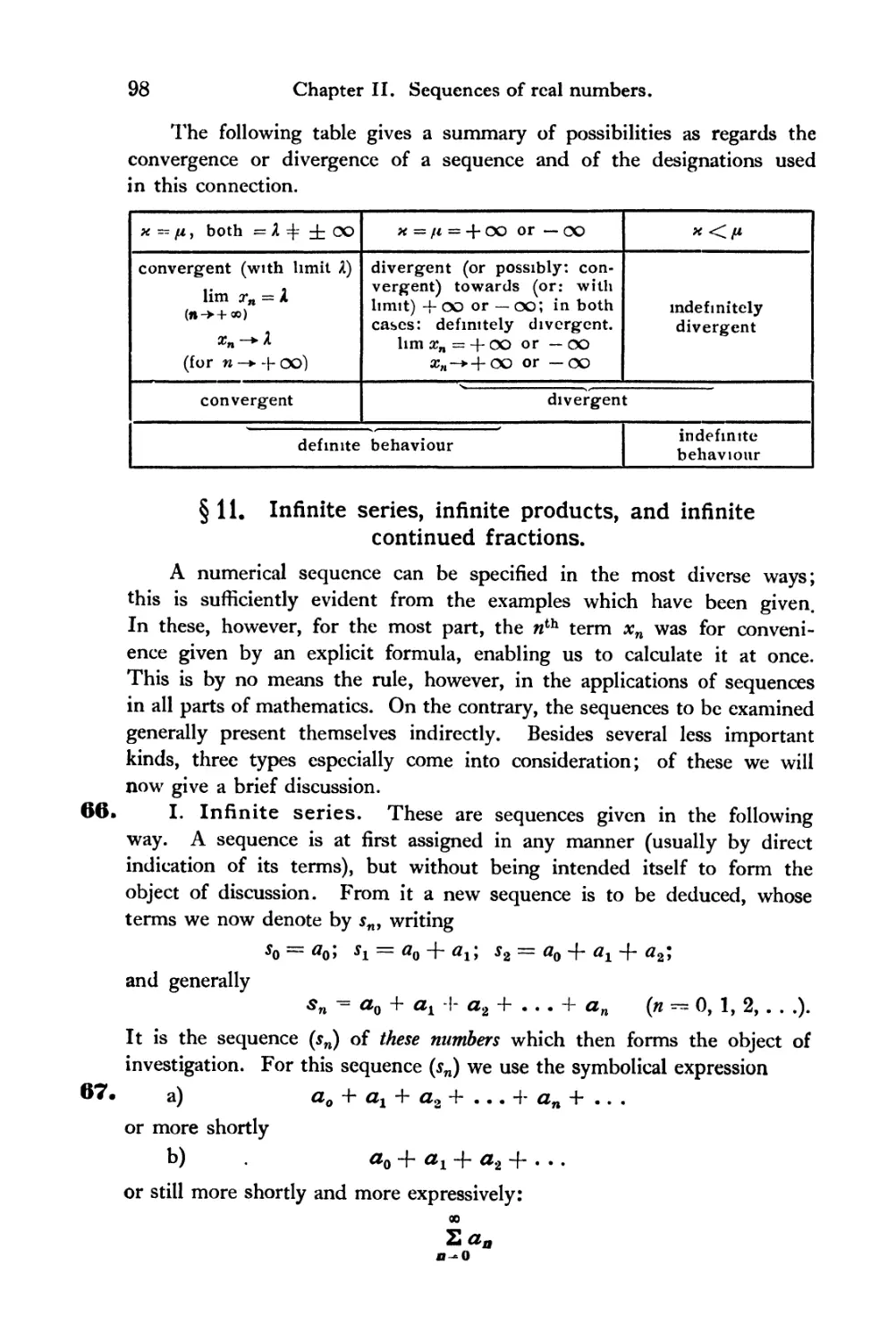
§11. Infinite series, infinite products, and infinite continued fractions . 98
Exercises on Chapter II (9—33) . . . . 106
Part II.
Foundations of the theory of infinite series.
/ Chapter 111.
* Series of positive terms.
§12. The first principal criterion and the two comparison tests .... 110
§ 13. The root test and the ratio test 116
§ 14 Series of positive, monotone decreasing terms 120
Exercises on Chapter III (34—44) 125
** (CJ51)
X
Contents.
Chapter IV. Page
Series of arbitrary terms.
§ 15. The second principal criterion and the algebra of convergent series 126
§ 16. Absolute convergence. Derangement of series 136
§ 17. Multiplication of infinite series 146
Exercises on Chapter IV (45—03) 149
/Chapter V.
Power series.
§ 18. The radius of convergence 151
§19. Functions of a real variable . . 158
§ 20. Principal piopertics of functions leprcsented by power series . . . 171
§ 21. The algebra of power series 179
Exercises on Chapter V (64 -73) 188
Chapter VI
The expansions of the so-called elementary functions.
§ 22. The rational functions 189
§ 23. The exponential function 191
§ 24. The trig-onometrical functions 198
§ 25. The binomial series 208
§ 26. The logarithmic series 211
§ 27. The cyclometrical functions 213
Exercises on Chapter VI (74 -84) 215
Chapter VII.
Infinite products.
§ 28. Products with positive terms 218
§ 29. Products with arbitrary terms. Absolute convcigcntc ... . 221
§ 30. Connection between series and products. Conditional and unconditional
convergence . 226
Exercises on Chapter VII (85—99; 228
Chapter VIII.
1_ Closed and numerical expressions for the sums of series.
§ 31. Statement of the problem 230
§ 32. Evaluation of the sum of a series by means of a closed expression 232
§ 33. Transformation of series 240
§ 34. Numerical evaluations 247
§ 35. Applications of the translorniation of series to numerical evaluations 260
Exercises on Chapter VIIT (100—132) 267
Contents.
Part III
Development of the theory.
Chapter IX.
Series of positive terms.
§ 36. Detailed study of the two comparison tests . 274
§ 37. The logarithmic scales . . 278
§ 38. Special comparison tests of the second kind 284
§ 39. Theorems of Abel, Dini, and Prinjsheim, and their application to a
fresh deduction of the logarithmic scale of comparison tests . . . 290
§ 40. Series of monotonely diminishing positive terms 294
§ 41. General remarks on the theory of the convergence and divergence
of series of positive terms 298
§ 42. Systematization of the general theory of convergence 305
Exercises on Chapter IX (138—141) 311
Chapter X.
Series of arbitrary terms.
§ 43. Tests of convergence for series ot arbitrary terms 312
§ 44. Rearrangement of conditionally convergent series 318
§ 45. Multiplication of conditionally convergent series 320
Exercises on Chapter X (142—153) 324
j Chapter XI.
Series of variable terms (Sequences of functions).
§ 46. Uniform convergence 326
§ 47. Passage to the limit term by term 338
§ 48 Tests of uniform convergence 344
§ 49. Fourier scries 350
A. Euler's formulae 350
B. Dirichlet's integral 356
C. Conditions of convergence 364
§ 50. Applications of the theory of Fourier series 372
§ 51. Products with variable terms 380
Exercises on Chapter XI (154—173; 385
Chapter XII.
Series of complex terms.
§ 52. Complex numbers and sequences 388
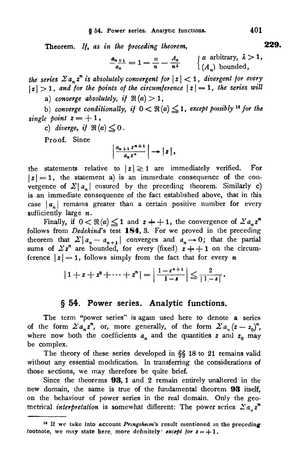
§ 53. Series of complex terms 396
§ 54. Power series. Analytic functions 401
XII Contents.
Page.
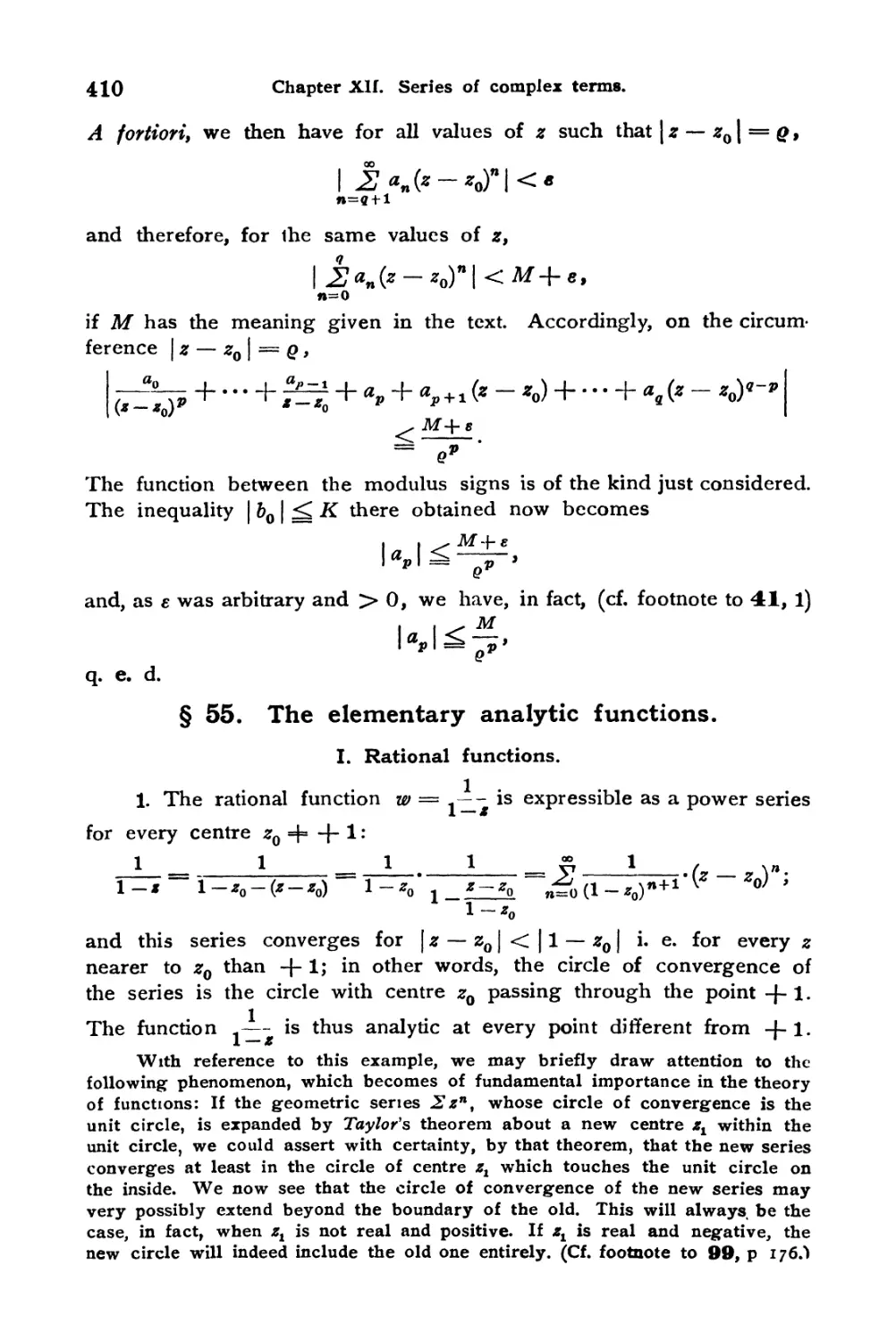
§ 55. The elementary analytic functions 410
I. Rational functions 410
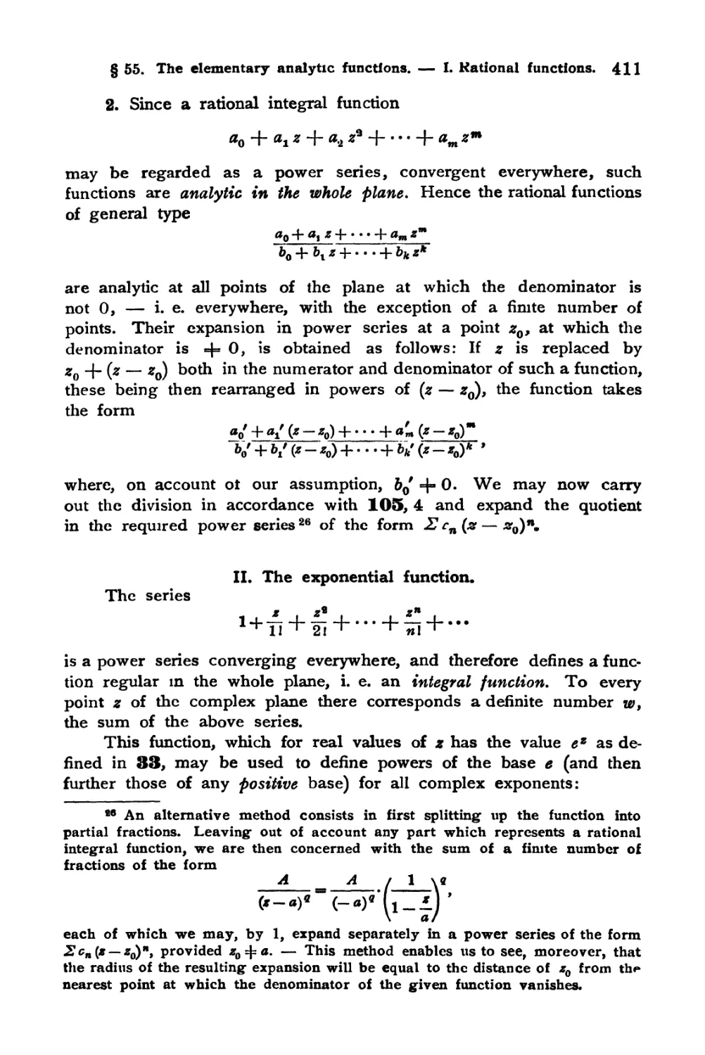
II. The exponential function 411
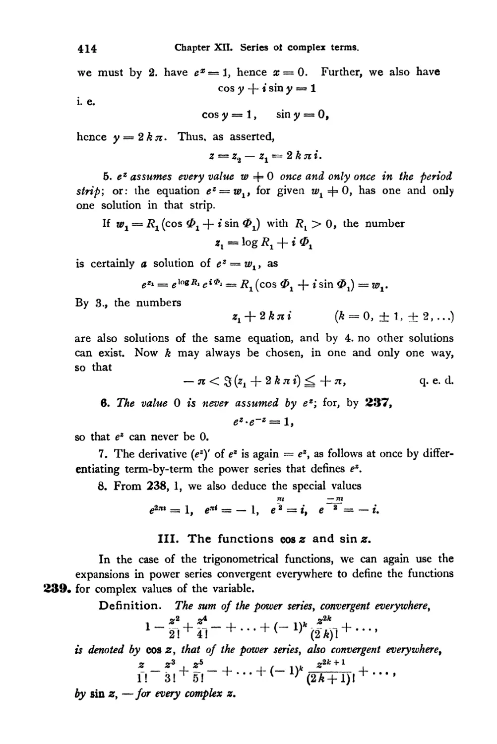
III. The functions cos z and sin z 414
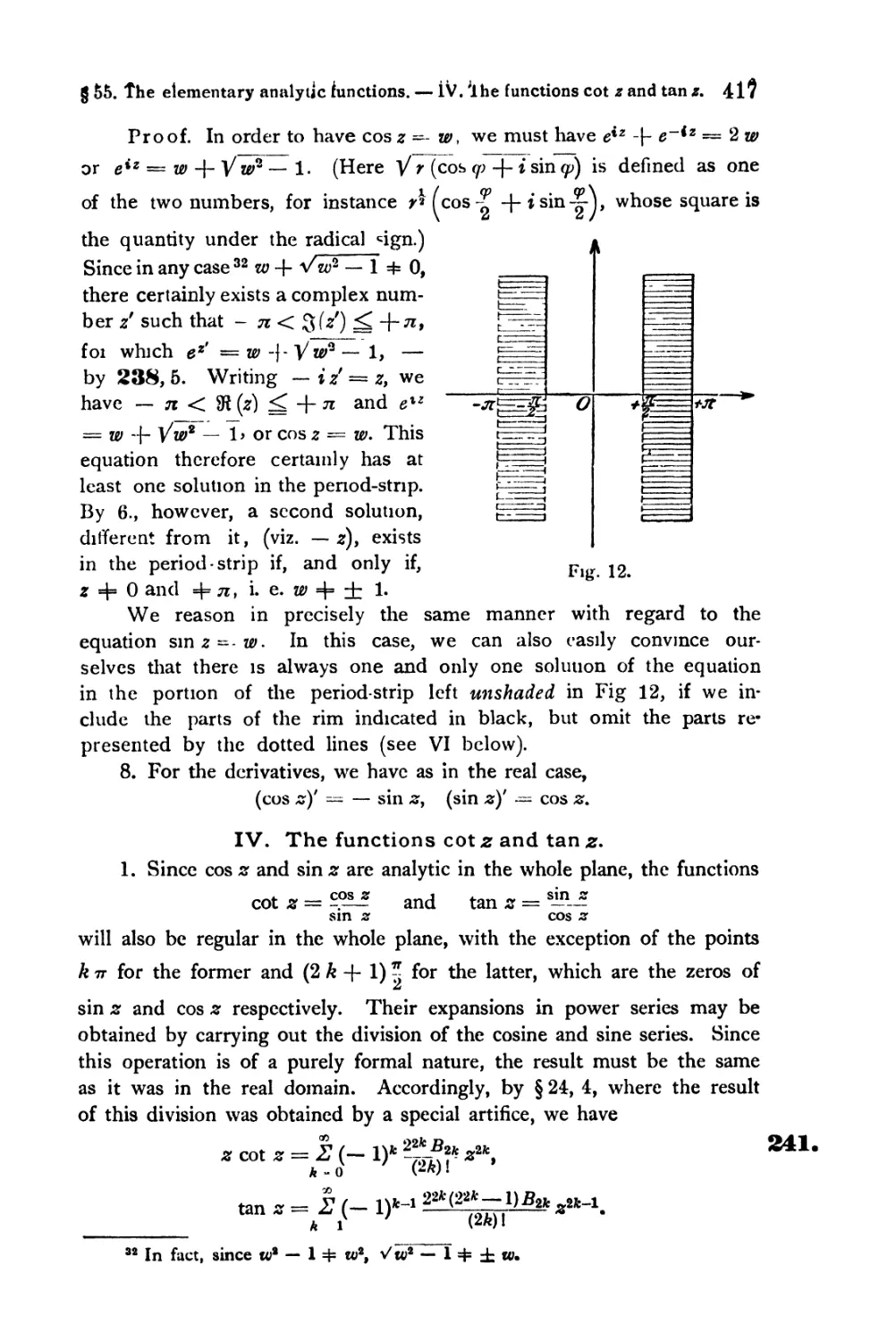
IV. The functions cot z and ta.n z 417
V. The logarithmic series 419
VI. The inverse sine series 421
VII. The inverse tangent series 422
VIII. The binomial series 423
§ 56. Series of variable terms. Uniform convergence. Weiersirass'
theorem on double series 428
§ 57. Products with complex terms 434
§ 58. Special classes of series of analytic functions 441
A. Dirichlet's series 441
B. Faculty series 446
C. Lambert's series 448
Exercises on Chapter XII (174—199) 452
/ Chapter XIII.
Divergent series.
§ 59. General remarks on divergent series and the processes of limitation 457
§ 60. The C- and H- processes 478
§ 61. Application of Cx- summation to the theory of Fourier series . . . 492
§ 62. The A- process 498
§ 63. The £- process 507
Exercises on Chapter XIII (200—216) 516
Chapter XIV.
Hauler's summation formula and asymptotic expansions.
§64. Euler's summation formula 518
A. The summation formula 518
B. Applications 525
C. The evaluation of remiinders 531
§ 65. Asymptotic scries 535
§ 66. Special cases of asymptotic expansions 543
A. Examples of the expansion problem 543
B. Examples of the summation problem 548
Exercises on Chapter XIV (217-225) 553
Bibliography 556
Name and subject index . 557
Introduction.
The foundation on which the structure of higher analysis rests is
the theory of real numbers. Any strict treatment of the foundations of
the differential and integral calculus and of related subjects must in-
inevitably start from there; and the same is true even for e. g. the cal-
calculation of roots and logarithms. The theory of real numbers first creates
the material on which Arithmetic and Analysis can subsequently build,
and with which they deal almost exclusively.
The necessity for this has not always been realized. The great
creators of the infinitesimal calculus —• Leibniz and Newton l — and
the no less famous men who developed it, of whom Eider 2 is the chief,
were too intoxicated by the mighty stream of learning springing from
the newly-discovered sources to feel obliged to criticize fundamentals.
To them the results of the new methods were sufficient evidence for
the security of their foundations. It was only when the stream began
to ebb that critical analysis ventured to examine the fundamental con-
conceptions. About the end of the 18th century such efforts became stronger
and stronger, chiefly owing to the powerful influence of Gauss 3. Nearly
a century had to pass, however, before the most essential matters could
be considered thoroughly cleared up.
Nowadays rigour in connection with the underlying number concept
is the most important requirement in the treatment of any mathematical
subject. Ever since the later decades of the past century the last word
on the matter has been uttered, so to speak, — by Weierstrass4 in the
sixties, and by Cantor 5 and Dedekind 6 in 1872. No lecture or treatise
1 Gottfried Wilhelm Leibniz, born in Leipzig in 1646, died in Hanover in
1716. Isaac Nezvton, born at Woolsthorpe in 1642, died in London in 1727. Each
discovered the foundations of the infinitesimal calculus independently of the other.
2 Leonhard Elder% born in Basle in 1707, died in St. Petersburg in 1783.
3 Karl Friedrich Gauss, born at Brunswick in 1777, died at Gottingen in 1853.
4 Karl Weierstrass, born at Ostenfelde in 1815, died in Berlin in 1897. The
first rigorous account of the theory of real numbers which Weierstrass had expounded
in his lectures since 1860 was given by G. Mittag-Leffler, one of his pupils, in his
essay: Die Zahl, Einleitung zur Theone der analytischen Funktionen, The Tohoku
Mathematical Journal, Vol. 17, pp. 157—209. 1920.
5 Georg Cantor, born in St. Petersburg in 1845, died at Halle in 1918: cf.
Mathem. Annalen, Vol. 5, p. 123. 1872.
8 Richard Dedekind, born at Brunswick in 1831, died there in 1916: cf. his
book: Stetigkeit und irrationaJe Zahlen, Brunswick 1872.
1
2 Introduction.
dealing with the fundamental parts of higher analysis can claim validity
unless it takes the refined concept of the real number as its starting-
point.
Hence the theory of real numbers has been stated so often and
in so many different ways since that time that it might seem superfluous
to give another very detailed exposition 7: for in this book (at least in
the later chapters) we wish to address ourselves only to those already
acquainted with the elements of the differential and integral calculus.
Yet it would scarcely suffice merely to point to accounts given elsewhere.
For a theory of infinite series, as will be sufficiently clear from later
developments, would be up in the clouds throughout, if it were not
firmly based on the system of real numbers, the only possible foundation.
On account of this, and in order to leave not the slightest uncertainty
as to the hypotheses on which we sh ill build, we shall discuss in the
following pages those idsas and data from the theory of real numbers
which we shall need further on. We have no intention, however, of con-
constructing a statement of the theory compressed into smaller space but
otherwise complete. We merely wish to make the main ideas, the most
important questions, and the answers to them, as clear and prominent
as possible. So far as the latter are concerned, our treatment throughout
will certainly be detailed and without omissions; it is only in the cases
of details of subsidiary importance, and of questions as to the complete-
completeness and uniqueness of the system of real numbers which lie outside the
plan of this book, that we shall content ourselves with shorter indications.
7 An account which is easy to follow and which includes all the essentials
is given by H. v. Mangoldt> Einfuhrung in die hohere Mathematik, Vol. I, 8th edition
(by K. Knopp), Leipzig 1944. — The treatment of G. Koivaiezvski, Grundziige
der Differential- und Integralrechnung, 6th edition, Leipzig 1929, is accurate and
concise. — A rigorous construction of the system of real numbers, which goes into
the minutest details, is to be found in A. Loewyt Lehrbuch dcr Algebra, Part I,
Leipzig 1915, in A. Pnngsheim, Vorlesungen uber Zahlen- und Funktionenlehre,
Vol. I, Part I, 2nd edition, Leipzig 1923 (cf. also the review of the latter work by
H. Hahn, Gott. gel. Anzeigen 1919, pp. 321—47), and in a book by E. Landau
exclusively devoted to this purpose, Grundlagen der Analysis (Das Rechnen mit
ganzen, rationalen, irrationalen, komplexen Zahlen), Leipzig 1930. A critical account
of the whole problem is to be found in the article by F. Bachmann, Aufbau des
Zahlensystems, in the Enzyklopadie d. math. Wissensch., Vol. I, 2ni1 edition, Part I,
article 3, Leipzig and Berlin 1938.
Part I.
Real numbers and sequences.
Chapter I.
Principles of the theory of real numbers.
§ 1. The system of rational numbers and its gaps.
What do we mean by saying that a particular number is "known"
or "given" or may be "calculated"? What does one mean by saying
that he knows the value of ^2 or n, or that he can calculate V5?
A question like this is easier to ask than to answer. Were I to say
that V2 = 1-414, I should obviously be wrong, since, on multi-
multiplying out, 1-414 X 1-414 does not give 2. If I assert, with greater
caution, that V2 = 1-4142135 and so on, even that is no tenable
answer, and indeed in the first instance it is entirely meaningless. The
question is, after all, how we are to go on, and this, without further
indication, we cannot tell. Nor is the position improved by carrying
the decimal further, even to hundreds of places. In this sense it
may well be said that no one has ever beheld the whole of V2, —
not held it completely in his own hands, so to speak—whilst a
statement that 1/9 = 3 or that 35 -f- 7 = 5 has a finished and thorough-
thoroughly satisfactory appearance. The position is no better as regards
the number n, or a logarithm or sine or cosine from the tables.
Yet we feel certain that V2 and n and log 5 really do have quite definite
values, and even that we actually know these values. But a clear
notion of what these impressions exactly amount to or imply we do
not as yet possess. Let us endeavour to form such an idea.
Having raised doubts as to the justification for such statements
as "I know Y 2", we must, to be consistent, proceed to examine
how far one is justified even in asserting that he knows the number
— ~ or is given (for some specific calculation) the number ~. Nay
more, the significance of such statements as "I know the number 97"
or "for such and such a calculation I am given a = 2 and b = 5" would
4 Chapter I. Principles of the theory of real numbers.
require scrutiny. We should have to enquire into the whole significance
or concept of the natural numbers 1, 2, 3, ...
This last question, however, strikes us at once as distinctly trans-
transgressing the bounds of Mathematics and as belonging to an order of
ideas quite apart from that which we propose to develop here.
No science rests entirely within itself: each borrows the strength
of its ultimate foundations from strata above or below it, such as experi-
experience, or theory of knowledge, or logic, or metaphysics, . . . Every science
must accept something as simply given, and on that it may proceed to
build. In this sense neither mathematics nor any other science starts
without assumptions. The only question which has to be settled by
a criticism of the foundation and logical structure of any science is what
shall be assumed as in this sense "given"; or better, what minimum of
initial assumptions will suffice, to serve as a basis for the subsequent
development of all the rest.
For the problem we are dealing with, that of constructing the system
of real numbers, these preliminary investigations are tedious and trouble-
troublesome, and have actually, it must be confessed, not yet reached any entirely
satisfactory conclusion at all. A discussion adequate to the present
position of the subject would consequently take us far beyond the limits
of the work we are contemplating. Instead, therefore, of shouldering
an obligation to assume as basis only a minimum of hypotheses, we
propose to regard at once as known (or "given", or "secured") a group
of data whose deducibility from a smaller body of assumptions is familiar
to everyone — namely, the system of rational numbers, i. e. of numbers
integral and fractional, positive and negative, including zero. Speaking
broadly, it is a matter of common knowledge how this system may be
constructed, if — as a smaller body of assumptions — only the ordered
sequence of natural numbers 1, 2, 3, . . . , and their combinations by
addition and multiplication, are regarded as "given". For everyone knows
— and we merely indicate it in passing — how fractional numbers arise
from the need of inverting the process of multiplication, — negative
numbers and zero from that of inverting the process of addition *.
The totality, or aggregate, of numbers thus obtained is called the
system (or set) of rational numbers. Each of these can be completely and
literally "given" or "written down91 or "made known" with the help of at
most two natural numbers, a dividing bar and possibly a minus sign.
For brevity, we represent them by small italic characters; a, &,...,
x, y, . . . The following are the essential properties of this system:
1 See the works of Loewy, Pringsheim, and Landau mentioned in the Intro-
Introduction; also O. Holder, Die Anthmetik in stranger Begriindung, 2nd edition, Berlin
liJi); and O. Stolz and J. A. Gmeiner, Theoretische Arithmetik, 3Pl! edition, Leipzig
1911.
§ 1. The system of rational numbers and its gaps. 5
1. Rational numbers form an ordered aggregate; meaning that
between any two, say a and b, one and only one of the three relations
a < b, a = b9 a > b
necessarily holds2; and these relations of "order" between rational
numbers are subject to a set of quite simple laws, which we assume known,
the only essential ones for our purposes being the
Fundamental Laws of Order.
1. Invariably 3 a — a.
2. a — b always implies b -- a.
3. a = by b — c implies a — c.
4. a ^ b, b < c, — or a < b, b < c, — implies 4 a < c.
2. Any two rational numbers may be combined in four distinct
ways, referred to respectively as the four processes (or basic operations)
of Addition, Subtraction, Multiplication, and Division. These operations
can always be carried out to one definite result, with the single exception
of division by 0, which is undefined and should be regarded as an entirely
impossible or meaningless process; the four processes also obey a number
of simple laws, the so-called Fundamental Laws of Arithmetic, and further
rules deducible therefrom.
These too we shall regard as known, and state, concisely, those
Fundamental Laws or Axioms of Arithmetic from which all the others may
be inferred, by purely formal rules (i. e. by the laws of pure logic).
I. Addition. 1. Every pair of numbers a and b has invariably associ-
associated with it a third, cy called their sum and denoted by a -\- b.
2. a = a!, b — b' always implv a \ b - af + b\
3. Invariably, a -j- b = b -f- a (Commutative Law).
4. Invariably, (a + b) + c = a + (b + c) (Associative Law).
5. a < b always implies a + c < b + c (Law of Monotony).
II. Subtraction.
To every pair of numbers a and b there corresponds a third number
Cy such that a + c =■ b.
9 a > b and b < a are merely two different expressions of the same relation.
Strictly speaking, the one symbol "<" would therefore suffice.
3 With regard to this seemingly trivial "law" cf. footnote 11, p. 9, remark 1, p. 28,
and footnote 24, p. 29.
4 To express that one of the relations of order: a < b, a — 6, or a > bt does
not hold, we write, respectively, a^_b ("greater than or equal to", "at least equal
to", "not less than"), a -t= b ("unequal to", "different from") or a *- b. Kach of
these statements (negations) definitely excludes one of the three relations and leaves
undecided which of the other two holds good.
6 Chapter I. Principles of the theory of real numbers.
III. Multiplication.
1. To every pair of numbers a and b there corresponds a third
number c, called their product and denoted by a b.
2. a — a', b — bf always implies ab = a b'.
3. In all cases ab = ba (Commutative Law).
4.. In all cases (ab) c =-- a(b c) (Associative Law).
5. In all cases (a -f- b) c — a c + b c (Distributive Law).
6. a < b implies, provided c is positive, a c <b c (Law of Mono-
Monotony).
IV. Division.
To every pair of numbers a and b of which the first is not 0 there
corresponds a third number c, such that a c = b.
As already remarked, all the known rules of arithmetic, — and
hence ultimately all mathematical results, — are deduced from these
few laws, with the help of the laws of pure logic alone. Among these
laws, one is distinguished by its primarily mathematical character, namely
the
V. Law of Induction, which may be reckoned among the fundamental
laws of arithmetic and is normally stated as follows:
If a set s3Jf of natural numbers includes the number 1, and if, every
time a certain natural number n and all those less than n can be taken to
belong to the aggregate, the number (n \- 1) miy be inferred also to belong
to it, then $)J includes all the natural numbers.
This law of induction itself follows quite easily from the following
theorem, which appears even more obvious and is therefore normally
called the fundamental law of the natural numbers :
Law of the Natural Numbers. In every set of natural numbers that
is not "empty" there is always a number less than all the rest.
For if, according to the hypotheses of the Induction Law, we con-
consider the set 9i of natural numbers not belonging to S1V, this set W must
be "empty", that is, SSI must contain all the natural numbers. For other-
otherwise, by the law of the natural numbers, M would include a number less
than all the rest. This least number would exceed 1, for it was assumed
that 1 belongs to S1)J; hence it could be denoted by n + 1. Then n would
belong to 9)i, but (n + 1) would not, which contradicts the hypotheses
in the law of induction.5
In applications it is usually an advantage to be able to make state-
statements not merely about the natural numbers but about any whole numbers.
6 The following rather more general form of the law of induction can be
deduced in exactly the same way from the fundamental law of the natural numbers.
If set $)l of natural numbers includes the number 1, and if the number (n -|- 1)
can be proved to belong to the aggregate provided the number n does, then tyl con-
contains all the natural numbers.
§ 1. The system of rational numbers and its gaps. 7
The laws then take the following forms, obviously equivalent to those
above:
Law of Induction. If a statement involves a natural number n (e. g.
"if n ^ 10, then 2n > w3", or the like) and if
a) this statement is correct for n = p,
and
b) its correctness for n = p, p -{- 1, . . . , k (where k is any natural
number >; p) always implies its correctness for n = k -f- 1, then the
statement is correct for every natural number ^ p.
Law of Integers. In every set of integers all ^ p that is not "empty",
there is always a number less than all the rest.6
We will lastly mention a theorem susceptible, in the domain of
rational numbers, of immediate proof, although it becomes axiomatic
in character very soon after this domain is left; namely the
VI. Theorem of Eudoxus.
If a and b are any two positive rational numbers, then a natural
number n always exists 7 such that nb > a.
The four ways of combining two rational numbers give in every
case as the result another rational number. In this sense the system
of rational numbers forms a closed aggregate {naturlicher Rationalitats-
bereich or number corpus). This property of forming a closed system with
respect to the four rules is obviously not possessed by the aggregate of
all natural numbers, or of all positive and negative integers. These are,
so to speak, too sparsely sown to meet all the demands which the four
rules make upon them.
This closed aggregate of all rational numbers and the laws zvhich hold
in it, are then all that we regard as given, knozvn, secured.
As that type of argument which makes use of inequalities and absolute values 3.
may he a little unfamiliar to some, its most important rules may be set down here,
briefly and without proof:
I. Inequalities. Here all follows from the laws of order and monotony.
In particular
1. The statements in the laws of monotony are reversible; e. g. a -f- c
< b -|- c always implies a < b; and so does a c < b r, provided c > 0.
2. a < b, c < d always implies a -\- c < b -\- d.
3. a < bt c < d implies, provided b and c are positive, a c < b d.
4. a < b always implies — b < —a,
and also, provided a is positive, , < -.
0 To reduce these forms of the laws to the previous ones, we need only con-
consider the natural numbers m such that, in the one case, the statement in question
is correct for n — (/> — 1) -f m, or, in the other, that (p — 1) -+• tn belongs to the
non-"empty" set under consideration.
7 This theorem is usually, but incorrectly, ascribed to Archimedes; it is already
to be found in Euclid, Elements, Book V, Def. 4.
8 Chapter I. Principles of the theory of real numbers.
Also these theorems, as well as the laws of order and monotony, hold (with
appropriate modifications) when the signs "<", "-•", "_/" and =" are sub-
substituted for "<", provided we maintain the assumptions that c, ft and a are posi-
positive, in 1, 3, and 4 respectively.
II. Absolute values. Definition: By |a|, the absolute value (or modulus)
of a, is meant that one of the two numbers -\-a and — a which is positive, sup-
supposing a 4= 0; and the number 0, if a — 0. (Hence | 0 | —- 0 and if a 4= 0, | a \ > 0.)
The following theorems hold, amongst others:
1. \a\ --- | - a\. 2. \ab\^\a\-\b\.
3.
1
a
1
ft
a
— I , provided a =# 0.
4. | a -f 6 | :_^ | « | + | 6 |; | a + 6 | ^ I « I - I ft |, and indeed | a +
5. The two relations | « | < r and — r < a < r are exactly equivalent;
similarly for | x — a | < r and a — r <. x < a -\- r.
(). \ a — b\ is the distance between the points a and by with the represen-
representation of numbers on a straight line described immediately below.
Proof of the first relation in 4: ± a '_£ \ a |, ± b ^ | b |, so that by 3, I, 2,
H ft) g | a | + | ft |, and hence | a -| ft | ^ | a | + | ft
We also assume it to be known how the relations of magnitude
between rational numbers may be illustrated graphically by relations
of positions between points on a straight line. On a straight line or
number-axis, any two distinct points arc marked, one O, the origin @)
and one U> the unit point A). The point P which is to represent a number
a = P (q > 0, p ^ 0, both integers) is obtained by marking off on the
axis, | p | times in succession, beginning at O, the #th part of the dis-
distance O U (immediately constructed by elementary geometry) either in
the direction O U, if p > 0, or if p is negative, in the opposite direction.
This point8 we call for brevity the point a, and the totality of points
corresponding in this way to all rational numbers we shall refer
to as the rational points of the axis. — The straight line is usually
thought of as drawn from left to right and U chosen to the right of O.
In this case, the words positive and negative obviously become equiva-
equivalents of the phrases: to the right of O and to the left of O, respectively;
and, more generally, a < b signifies that a lies to the left of b, b to the
right of a. This mode of expression may often assist us in illustrating
abstract relations between numbers.
8 The position of this point is independent of the particular representation
of the number at i. e. if a = p''Jq' is another representation with q' *> 0 and p' ^ 0
both integers, and if the construction is performed with q\ p' in place of qy />, the
same point P is obtained.
§ 1. The system of rational numbers and its gaps. 9
This completes the sketch of what we propose to take as the
previously secured foundation of our subject. We shall now regard
the description of these foundations as characterizing the concept of
number; in other words, we shall call any system of conceptually well-
distinguished objects (elements, symbols) a number system, and its
elements numbers, if — to put it quite briefly for the moment — we
can operate with them in essentially the same ways as we do with rational
numbers.
We proceed to give this somewhat inaccurate statement a precise
formulation.
We consider a system S of well-distinguished objects, which we 4,
denote by a, ft . . . . S will be called a number system and its elements
a, ft . . . will be called numbers if, besides being capable of definition
exclusively by means of rational numbers (i. c. ultimately by means of
natural numbers alone) 9, these symbols a, ft . . . satisfy the following four
conditions:
1. Between any two elements a and j8 of S one and only one of the
three relations 10
a < £, a = ft a >
necessarily holds (this is expressed briefly by saying that S is an ordered
system) and these relations of order between the elements of S are subject
to the same fundamental laws 1 as their analogues in the system of rational
numbers u.
2. Four distinct methods of combining any two elements of S are
defined, called Addition, Subtraction, Multiplication and Division. With
a single exception, to be mentioned immediately C.), these processes
can always be carried out to one definite result, and obey the same Fun-
Fundamental Laws 2, I—IV, as their analogues in the system of the rational
9 We shall come across actual examples in § 3 and § 5; for the moment, we
n.ay think of decimal fractions, or similar symbols constructed from rational numbers.
See also footnote K>, p. 12.
10 Cf. also footnotes 2 and 4.
11 As to what we may call the practical meaning of these relations, nothing
is implied; "<" may as usual stand for "less than", but it may equally well mean
'•before", "to the left of", "higher than", "lower than", "subsequent to", in fact
may express any relation of order (including "greater than"). This meaning merely
has to be defined without ambiguity and kept consistent. Similarly, "equality"
need not imply identity. Thus, for example, within the system of symbols of the
form p/q} where/), q are integers and q 4= 0, the symbols 3/4, 0/8, —1)/—12 are
generally said to be "equal"; that is, for certain purposes (calculating, measuring,
and so on) we define equality within our system of symbols in such a way that 3/4 -=s
6/8-= -9/ —12, although 3/4, tf/8, -9/-12 are in the first instance different
elements of that system (see also 14, note 1).
10 Chapter I. Principles of the theory of real numbers.
numbers 12. (The "zero" of the system, which must be known in order
that the elements can be divided into positive and negative, is to be defined
as explained in footnote 14 below.)
3. With every rational number we can associate an element of S
(and all others ''equal*' to it) in such a manner that, if a and b denote
rational numbers, a, j8 their associates from S:
a) the relation 1. holding between a and /? is of the same form as
that holding between a and b.
b) the element resulting from a combination of a and )8 (i. e. a + j8,
a — /?, a • j8, or a -f- j8) has for its associated rational number the result
of the similar combination of a and b (i. e. a -f- Z», a — Z», a • b, or a -f- b
respectively).
[This is also expressed, more shortly, by saying that the system S
contains a sub-system Sf similar and isowiorfihous to the system
of rational numbers. Such a sub-system is in fact constituted by those
elements of S which we have associated with rational numbers 13.]
In such a correspondence, an element of S associated with the rational
number zero, and all elements equal to it, may be shortly referred to as
the "zero" of the system of elements. The exception mentioned in 2.
then relates to division by zero 14.
12 With reference to these four processes it should be noted, as in the case
of the symbols < and —-, that no practical interpretation is implied. — We also
draw attention to the fact that subtraction is already completely defined in terms
of addition, and division in terms of multiplication, so that, properly speaking,
only two modes of combining elements need be assumed known.
13 Two ordered systems are similar if it is possible to associate each element
of the one with an element of the other in such a way that the same one of the
relations 4, 1 as holds between two elements of the one system also holds between
the two associated elements of the other, they are iso'mor'phous relatively to the
possible modes of combining their elements, if the element resulting from a com-
combination of two elements of the one system is associated with that resulting from
the similar combination of the two associated elements of the other system.
14 The third of the stipulations by means of which we here characterise the
concept of number is fulfilled, moreover, as a consequence of the first and second.
For our purposes, this fact is not essential; but as it is significant from a svstematic
point of view, we briefly indicate its proof as follows- By 4, 2, there is an element
£ for which a -f- £ -= a. From the fundamental laws 2, 1, it then quite easily follow^
tha one and the same element £ of S satisfies a -I- £ - a, for every a. This element
£, with all elements equal to it, is called the neutral element relatively to the process
of addition, or for brevity the "zero" in S. If a is different from this "zero", there
is, further, an element e for which a € — a; and it again appears thit this element
is the same as that satisfying rt e -a for any other a in S. This c, with all elements
equal to it, is called the neutral element relatively to the process of multiplication,
or, briefly, the "unit" in S. The elements of S produced bv repeated addition or
subtraction of this "unit", and any others equal to them, are then called "integers"
of S. All further elements of S (and all equal to them) which result fiom these
by the process of division then form the sub-system S' of S in question; that it
is similar and homorphous to the system of all rational numbers is in fact easily
deduced from 4, I and 4, 2. — Thus, as asserted, our concept of number is already
determined by the requirements of 4, 1, 2 and 4.
§ 1. The system ot rational numbers and its gaps. 11
4. For any two elements a and j8 of S both standing in the relation
">" to the "zero" of the system, there exists a natural number n for
which n j8 > a. Here n j3 denotes the sum j8 +/}+••• -|- ]8 containing
the element j8 n times. (Postulate of Eudoxus; cf. 2, VI.)
To this abstract characterisation of the concept of number we
will append the following remark l5: If the system S contains no other
elements than those corresponding to rational numbers as specified
in 3, then our system does not differ in any essential feature from the
system of rational numbers, but only in the (purely external) designation
of the elements by symbols, or in the (purely practical) interpretation
which we give to these symbols; differences almost as irrelevant,
at bottom, as those which occur when we write figures at one time in
Arabic characters, at another, in Roman or Chinese, or take them to
denote now temperature, now velocity or electric charge. Disregarding
external characteristics of notation and practical interpretation, we
should thus be perfectly justified in considering the system S as identical
with the system of rational numbers and in this sense we may put a = a,
b -"= p, . . .
If, however, the system S contains other elements besides the above
mentioned, then we shall say that S includes the system of rational
numbers, and is an extension of it. Whether a system of this more com-
comprehensive kind exists at all, remains for the moment an open question;
15 We have defined the concept of number by a set of properties characterising
it. A critical construction of the foundations of arithmetic, which is quite out
of the question within the limits of this volume, would have to comprise a strict
investigation as to the extent to which these properties are independent of one
another, i. e. whether any one of them can or cannot be deduced from the rest as
a provable fact. Further, »"t would have to be sh.un that none of these fundamental
stipulations is in contradiction with any other — and other matters too would
require consideration. These investigations are tedious and have not yet reached a
final conclusion.
In the treatment by E. Landau mentioned on p. 2, footnote 7, it is proved with
absolute rigour that the fundamental laws of arithmetic which we have set up
can all be deduced from the following 5 axioms relating to the natural numbers:
Axiom 1: 1 is a natural number.
Axiom 2: For every natural number n there is just one other number
that is called the successor of w. (I^et it be denoted by n'.)
Axiom 3: We have always ri 4= 1.
Axiom 4: From mf ~ n\ it follows that m = n.
Axiom 5: The induction law V is valid (in its first form).
These 5 axioms, first formulated as here by G. Peano, but in substance set up
by R. Dedekindy assume that the natural numbers as a whole are regarded as given,
that a relation of equality (and hence also inequality) is defined between them,
and that this equality satisfies the relations 1, 1, 2, 3 (which belong to pure
logic).
12 Chapter I. Principles of the theory of real numbers.
but an example will come before our notice presently in the system of
real numbers 16.
Having thus agreed as to the amount of preliminary assumption
we require, we may now drop all argument on the subject, and again
raise the question: What do we mean by saying that we know the number
V2 or it?
It must in the first instance be termed altogether paradoxical that
a number having its square equal to 2 does not exist in the system so
far constructed17, — or, in geometrical language, that the point A of
the number-axis, whose distance from O equals the diagonal of the
square of side O Ur, coincides with none of the "rational points". For
the rational numbers are dense, i. e. between any two of them (which
are distinct) we can point out as many more as we please (since, if a *^
the n rational numbers given by a + v - , for v = 1, 2, ...,«, evi-
n -\- \
dently all lie between a and b and are distinct from these and from one
another); but they are not, as we might say, dense enough to symbolise
all conceivable points. Rather, as the aggregate of all integers proved
too scanty to meet the requirements of the four processes of arithmetic,
16 The mode of denning the number-concept given in 4 is of course not
the only possible one. Frequently the designation of number is still ascribed to
objects which fail to satisfy some one or other of the requirements there laid down.
Thus for instance we may relinquish the condition that the objects under con-
consideration should be constructively developed from rational numbers, regarding
any entities (for instance points, or distances, or such like) as numbers, provided
only they satisfy the conditions 4, 1—4, or, in short, are similar and isomorphous
to the system we have just set up. — This conception of the notion of number,
in accordance with which all isomoiphous systems must be regarded as in the ab-
abstract sense identical, is perfectly justified from a mathematical point of view, but
objections necessarily arise in connection with the theory of knowledge. — We
shall encounter another modification of the number-concept when we come to
deal with complex numbers.
17 Proof: There is certainly no natural number of square equal to 2, as
I2 -— 1 and all other integers have their squares ^ 4. Thus V2 could only be a
(positive) fraction , where q may be taken ^ 2 and prime to p (i. e. the fraction
is in its lowest terms). But if - is in its lowest terms, so is ( - ) — , which there-
fore cannot reduce to the whole number 2. In a slightly different form: For any
two natural numbers p and q without common factor, we have necessarily p2 4- 2 q2.
For since two integers without common factors cannot both be even, either p is
odd, or else p is even and q odd. In the first case p2 is again odd, hence cannot
equal an even integer 2 q2. In the second case p* — B p'J is divisible by 4, but 2 q2
is not, since it is double an odd number. So p* 4= 2 r/2 again. This Pythagoras is
said to have already known (cf. M. Cantor, Gesch. d. Mathem., Vol. 1, 2nd ed., pp.
142 and 169. 1894).
§ 1. The system of rational numbers and its gaps. 13
so also the aggregate of all rational numbers contains too many gaps 18
to satisfy the more exacting demands of root extraction. One feels,
nevertheless, that a perfectly definite numerical value belongs to the point
A and therefore to the symbol V2. What are the tangible facts which
underlie this feeling?
Obviously, in the first instance, this: We do, it is true, know
perfectly well that the values 1-4 or 1*41 or 1-414 etc. for V2 are in-
inaccurate, in fact that these (rational) numbers have squares < 2, i. e.
are too small. But we also know that the values 1-5 or 1-42 or
1-415 etc. are in the same sense too large; that the value which we
are attempting to reach would have therefore to lie between the corres-
corresponding too large and too small values. We thus reach the definite
conviction that the value of n/2 is within our grasp, although the given
values are all incorrect. The root of this conviction can only lie in
the fact that we have at our command a process, by which the above
values may be continued as far as we please; we can, that is, form
pairs of decimal fractions, with 1, 2, 3, ... places of decimals, one frac-
fraction of each pair being too large, and the other too small, and
the two differing only by one unit in the last decimal place, i. e. by (y1^O1,
if n is the number of decimal places. As this difference may be made
as small as we ftlease, by sufficiently increasing the number n of given
decimal places, we are taught through the above process to enclose
the value which we are in search of between two numbers as near
as we please to one another. By a metaphor, somewhat bold at the
present stage, we say that through this process V2 itself is "given", —
in virtue of it, V2 is "known", -- by it, V2 may be "calculated", and
so on.
We have precisely the same situation with regard to any other value
which cannot actually be denoted by a rational number, as for instance
7T, log 2, sin 10° etc. If we say, these numbers arc known, nothing more
is implied than that we know some process (in most cases an extremely
laborious one) by which, as detailed in the case of V2, the desired value
may be imprisoned, hemmed in, within a narrower and narrower space
between rational numbers, — and this space ultimately narrowed down
as much as we please.
For the purpose of a somewhat more general and more accurate
18 This is the paradox, scarcely capable of any direct illustration, that a set
of points, dense in the sense just explained, mav already be marked on the number
axis, and yet not comprise all the points of the straight line. The situation may
be described thus: Integers form a first rough partition into compartments; rational
numbers fill these compartments as with a fine sand, which on minute inspection
inevitably still discloses gaps. To fill these will be our next problem.
14 Chapter I. Principles of the theory of real numbers.
statement of these matters, we insert a discussion of sequences of rational
numbers, provisional in character, but nevertheless of fundamental im-
importance for all that comes after.
§ 2. Sequences of rational numbers1.
In the process indicated above for calculating V2, successive well-
defined rational numbers were constructed; their expression in decimal
form was material in the description; from this form we now propose
to free it, and start with the following
5. Definition. If by means of any suitable process of construction, we
can form successively a first, a second, a third, . . . (rational) number and
if to every positive integer n one and only one well-defined (rational) number
xn thus corresponds, then the numbers
^1> ^2> ^3> • • • > ^m • • •
(in this order, corresponding to the natural order of the integers 1, 2, 3, ...
«,...) are said to form a sequence. We denote it for brevity by (xn)
or (#i, #2> • • •/•
©• Examples.
1. xn — - ; l. e. the sequence I - ], or 1, -,-,...,-,...
n \n/ 2 3 n
2. xn — 2n; i. e. the sequence 2, 4, 8, 16, ...
3. xn — an; i. e. the sequence a, a2, a3, . . . , where a is a given number.
- 4. xn — J {1 — ( — l)n}; i. e. the sequence 1, 0, 1, 0, 1, 0, ...
6. xn — the decimal fraction for V 2, terminated at the wth digit.
' l)n— 1 111
6. xn — s— ' ; i. e. the sequence 1, — ^, -f- _,—-_,...
ft 2i A 4
7. Let Xi = 1, #2 = 1, #3 = #, -f- x* = 2 and, generally, for w > 3, let
xn ~ ^n-i "T" *vn-2« We thus obtain the sequence 1, 1, 2, 3, 5, 8, 13, 21, . . ., ubually
called Fibonacci*s sequence.
8 12—2 3 1 ^
o. i, *> g' ' 2' * 3' ' 3' ' - *
Q 2 3 4 5 n+1
J o 4 72
j 1 2 3 4 w - 1
' 2f 3'4f 6f ""• "w~f ' ##
11. xn — the Hth prime number 2; i. e. the sequence 2, 3, 5, 7, 11, 13, ... \
12. The sequence 1, 1, _, _f, _L_, ..., m which #n = ^1 -f ^ + . . . + ~
1 In this section all literal symbols will continue to stand for rational numbers
only.
2 Euclid proved that there is an infinity of primes. If plt />2, . . . , pk are any
prime numbers, then the integer m — (p\p2 . . . pt) + 1 is either a prime different
from />!, />2,... , pk, or else a product of such primes. Hence no finite set of prime
numbers can include all primes.
§ 2. Sequences of rational numbers. 15
Remarks.
1. The law of formation may be quite arbitrary; it need not, in particular,
be embodied in any explicit formula enabling us to obtain xn, for a given w, by
direct calculation. In examples 6, 5, 7 and 11, clearly no such formula can be im-
immediately written down. If the terms of the sequence are individually given, neither
the law of formation (cf. 6, 5 and 12) nor any other kind of regularity (cf. 6, 11)
among the successive numbers is necessarily apparent.
2. It is sometimes advantageous to start the sequence with a th" term x0,
or even with a (—l)th or ( — 2)th term, x__lt #_2. Occasionally, it pays better to start
indexing with 2 or 3. The only essential is that there should be an integer m ^ 0
such that xn is defined for every n ^ m. The term xm is then called the initial term
of the sequence. We will however, even then, continue to designate as the nth term
that which bears the index n. In § 6, 2, 3 and 4, for instance, we can without further
difficulties take a 0th term or even (—I) or ( — 2)th to head the sequence. The "first
term" of a sequence is then not necessarily the term with which the sequence begins.
The notation will be preferably (x0, xlt . . .) or (x_lf x0,.. .), etc., as the case may be,
unless it is either quite clear or irrelevant where our enumeration begins, and the
abbreviated notation (xn) can be adopted.
3. A sequence is frequently characterised as infinite. The epithet is then
merely intended to emphasize the fact that every term is succeeded by other terms.
It is also said that there is an infinite number of terms. More generally, there is
said to be a finite number or an infinite number of things under consideration accord-
according as the number of these things can be indicated by a definite integral number
or not. And we may remark here that the word infinite, when otherwise used in
the sequel, will have a symbolic significance only, intended as a concise expression
of some perfectly definite (and usually quite simple) circumstance.
4. If all the terms of a sequence have one and the same value ct the sequence
is said to be identically equal to r, and in symbols (xn) ~ c. More generally, we shall
write (xn) == (xn') if the two sequences (xn) and (.vn') agree term for term, i. e. for
every index in question xn = xn'.
5. It is often helpful and convenient to represent a sequence graphically
by marking off its terms on the number-axis, or to think of them as so marked.
We thus obtain a sequence of points. But in doing this it should be borne in mind
that, in a sequence, one and the same number may occur repeatedly, even "in-
"infinitely often" (cf. 6, 4); the corresponding point has then to be counted (i. e. con-
considered as a term of the sequence of points) repeatedly, or infinitely often, as the
case may be.
0. A graphical representation of a different kind is obtained by marking,
with respect to a pair of rectangular coordinate axes, the points whose coordinates
are (w, xn) for n — 1, 2, 3, . . . and joining consecutive points by straight segments.
The broken line so constructed gives a picture (diagram, or graph) of the sequence.
To consider from the most diverse points of view the sequences hereby
introduced, and the real sequences that will shortly be defined, will be the
main object of the following chapters. We shall be interested more par-
particularly in properties which hold, or are stipulated to hold, for all the
terms of the sequence, or at least for all terms beyond (or following) some
definite term 3. With reference to this last restriction, it may sometimes
8 E. g. all the terms of the sequence 6, 9 are > 1. Or, all the terms of the
sequence 6, 2 after the 0th are > 100 (or more shortly: for n > 6, xn > 100).
16 Chapter I. Principles of the theory of real numbers.
be said that particular considerations in hand are valid "a finite number
of terms being disregarded", or only concern the ultimate behaviour of
the sequence. Our first examples of considerations of the kind referred
to are afforded by the following definitions:
Definitions. I. A sequence is said to be bounded*, if there is a
positive number K such that each term xn of the sequence satisfies the
inequality
I I ^-» Tr
or
The number K is then called a bound of the sequence.
Remarks and Examples.
1. In definition 8, it is a matter of practical indifference whether we write
or "</C". For if | xn | ^ K holds always (i. e. for every n in question),
then we can also find a constant K' such that | xn \ < K' holds always; indeed,
clearly any K' > K will serve the purpose. Conversely, if | xn \ < K always, then
a fortiori \ xn\ ^ K. When the exact magnitude of the bound comes in of course
the distinction may be essential.
2. If & is a bound of (xn)> then so is any larger number K'.
3. The sequences 6, 1, 4, 5, 0, 9, 10 are evidently bounded; so is 6, 3, pro-
provided | a | 5* 1. The sequences 6, 2, 7, 8, 11 are certainly not so. Whether 6, 3
for every \a\ >1, or 6, 12, is bounded or not, i> not immediately obvious.
4. If all we know is the existence of a constant Ku such that xn < Ku for
every w, then the sequence is said to be bounded on the right (or above) and Kx is
called a bound above (or a right hand bound) of the sequence.
If there is a constant K2 such that xn > K2 always, then (xn) is said to be
bounded on the left (or below) and K2 is called a bound belozv (or a left hand bound)
of the sequence.
Here Kx and K2 need not be positive.
5. Supposing a given sequence is bounded on the right, it may still happen
that among its numbers none is the greatest. For instance, 6, 10 is bounded on
the right, yet every term of this sequence is exceeded by all that follow it, and none
can be the greatest6. Similarly, a sequence bounded on the left need contain no
least term; cf. 6, 1 and 0. — (With this fact, which will appear at first sight para-
paradoxical, the beginner should make himself thoroughly familiar.)
Among a finite number of values there is of course always both a greatest and
a least, i. e. a value not exceeded by any of the others, and one which none of the
others falls below. (There may, however, be several equal to this greatest or least
value.)
E. The property of boundedness of a sequence xn (though not the actual value
of one of the bounds) is a property of the tail-end of the sequence; it is unaffected
by any alteration to an isolated term of the sequence. (Proof?)
4 This nomenclature appears to have been introduced by C. Jordan^ Cours
d'analyse, Vol. 1, p. 22. Paris 1893.
6 The beginner should guard against modes of expression such as these,
which may often be heard: "for n infinitely large, xn = 1"; is the greatest
number of the sequence". Anything of this sort is sheer nonsense (cf. on this point
7, 3). For the terms of the sequence are 0, £, J, j, . . . and none of these is ---= 1, on
the contrary all of them are < 1. And there is no such thing as an "infinitely large w".
§ 2. Sequences of rational numbers. 17
II. A sequence is said to be monotone ascending or increasing 9.
if, for every value of n,
it is said to be monotone descending or decreasing if, for every n>
xn ^ xn+v
Both kinds will also be referred to as monotone sequences.
Remarks and Examples.
1. A sequence need not of course be either monotone increasing, or mono-
monotone decreasing; cf. 6, 4, 6, 8. Monotone sequences are, however, extremely com-
common, and usually easier to deal with than those which are not monotone. That
is why it is convenient to give them a distinguishing name.
2. Instead of "ascending" we should more strictly say "non-descending",
and instead of "descending", "non-ascending". This, however, is not customary.
If in any special instance the sign of equality is excluded, so that xn < xni x or
xn > xn] j, as the case may be, for every n, then the sequence is said to be strictly
monotone (increasing or decreasing).
3. The sequences 6, 2, 5, 7, 10, 11, 12 and 6, 1, 9 are monotone; the first-
named ascending, the others descending. 6, 3 is monotone descending, if 0 ^ a ^ 1,
but monotone ascending if a " * 1; for a < 0, it is not monotone.
4. The designation of "monotone" is due to C. Neumann (Ober die nach
Kteis-, Kugel- und Zylinderfunktionen fortschreitenden Entwickelungen, pp. 20,
27. Leipzig 1881).
We now come to a definition to which the reader should pay
the greatest attention, sparing no effort to make himself master of its
meaning and all that it implies.
III. A sequence will be called a null sequence if it possesses the fol- 10
lowing property: given any arbitrary positive (rational) number e, the in-
inequality
is satisfied by all the terms, with at most a finite number 6 of exceptions. In
other words: an arbitrary positive number e being chosen, it is always possible
to designate a term xm of the sequence, beyond which the terms are less than
e in absolute value. Or a number n0 can ahvays be found, such that
\xn\ < € for every n > «0.
Remarks and Examples.
1. If, in a given sequence, these conditions are fulfilled for a particular c,
they will certainly be fulfilled for every greater e (cf. 8, 1), but not necessarily for
any smaller e. (In 6, 10, for instance, the conditions are fulfilled for e = 1 and there-
therefore for every larger e, if we put n0 =0; for e - } it is not possible to satisfy them.)
In the case of a null sequence, the conditions have to be fulfilled for every positive
8 Cf. 7, 3.
18 Chapter I. Principles of the theory of real numbers.
c, and in particular, therefore, for every very small e > 0. On this account, it is
usual to formulate the definition somewhat more emphatically as follows: (xn)
is a null sequence if, to every e > 0, however small, there corresponds a number
n0 such that
xn | < c for every n > n0.
Here n0 need not be an integer.
2. The sequence 6, 1 is clearly a null sequence; for
| xn | < e, provided n > -,
whatever be the value of €. It is thus sufficient to put n0 — .
3. The place in a given sequence beyond which the terms remain numeri-
numerically < e, will naturally depend in general on the magnitude of c; speaking broadly,
it will lie further and further to the right (i. e. w0 will be larger and larger), the
smaller the given e is (cf. 2). This dependence of the number n0 on c is often
emphasised by saying explicitly: "To each given c corresponds a number n0 — nQ (t)
such that ..."
4. The positive number below which | xn | is to he from some stage onwards
need not always be denoted by c. Any positive number, however designated, may
serve- In the sequel, where c, cc, /£,..., denoting any given positive numbers, we
may often use instead ^, -, ^, e2, a €, €a, etc.
5. The sign of xn plays no part here, since | ~xn | = | xn |. Accordingly
6, C is also a null sequence.
6. In a null sequence, no term need be equal to zero. But all terms, whose
index is very large, must be very small. For if I choose e = 10"~6, say, then for ever\
n > a certain nOi [ xn | must be < 10 ~'5. Similarly for e - - 10~10 and for any other €.
7. The sequence (a11) specified in 6, 3 ts also a null sequence provided \ a\ < 1.
Proof. If a — 0, the assertion is trivial, since then, for every € > 0, | xn \ < c
for every n. If 0 < | a \ < 1, then (by 3, 1, 4) ,---,> 1. If therefore we put
,—? = 1 -f />, then p > 0.
But in that case, for every « ^ 2, we have
(a)
For when n = 2, we have A -f- pJ -= 1 + 2p -\ p2 > 1 + 2/>; the stated relation
therefore holds in that case. If, for n — k ^ 2,
A +/>)* > 1 + kp,
then by 2, III, 6
therefore our relation, assumed true for n — k, is true for n — k -f- 1. By 2, V
it therefore holds 7 for every n ^ 2.
7 The proof shows moreover that (a) is valid for n ^ 2 provided only 1 4- />
> 0, i. e. p > — 1, but 4=0. For p -- 0 and for n — 1, (a) becomes an equality.
For p > 0, the validity of (a) follows immediately from the expansion of the left-
hand side by the binomial theorem. — The relation (a) is called Bernoulli's Inequality
(James Bernoulli, Propositiones arithmeticae de seriebus, 1689, Prop. 4).
§ 2. Sequences of rational numbers. 19
Accordingly, we now have
.n I _ I „ \n _ . }
so that, however small e > 0 may be, we have
xn | — | an | < e for every n >
P €
8. In particular, besides the sequence ( ) mentioned in 2., ( -), f - V
1 //4\"\ , . „ W \2n/ \3fi/
» [f?j j, etc., are also null sequences.
9. A similar remark to that of 8, 1 may be appended to Definition 10: no
essential modification is produced by reading "^ t" for "< *" there. In fact,
if, for every n > nOt \ xn\ < c, then a fortiori \ xn\ < e; conversely, if, given any
e, n0 can be so determined that | xn | i> e for every w > w3, then choosing any posi-
positive number et < € there is certainly an w, such that | xn | ^ el9 for every ?i > nx*
and consequently
xn | < € for every n > «x;
the conditions in their original form are thus also fulfilled. — Precisely analogous
considerations show that in Definition 10 " > w0" and " ^t n0" are practically inter-
interchangeable alternatives.
In any individual case, however, the distinction must of course be taken into
account.
10. Although in a sequence every term stands entirely by itself, with a definite
fixed value, and is not necessarily in any particular relation with the preceding
or following terms, yet it is quite customary to ascribe "to the terms xn"t or "to
the general term" any peculiarities in the sequence which may be observed on
running through it. We might say, for instance, in 6, 1 the terms diminish; in
6, 2 the terms increase; in 6, 4 or 6, 6 the terms oscillate; in 6, 11 the general
term cannot be expressed by a formula, and so on. — In this sense, the character-
characteristic behaviour of a null sequence may be described by saying that the terms become
arbitrarily small\ or infinitely small 8; by which neither more nor less is meant than
is contained in Definition 9 10, viz. that for every e > 0 however small the terms
are ultimately (i. e. for all indices n > a suitable «0; or from and after, or beyond,
a certain wu) numericallv less than e.
11. A null sequence is ipso facto bounded. For if we choose c — I, then there
must be an integer w, such that, for every n > Jij, | xn \ < 1. Among the finite
number of values | .Vi |, | x2 |, . . . , \ xni |, however, one (cf. 8, 5) is greatest, — M
say. Then for K — M -f 1, obviously | .vw | is ahvays < K.
12. To prove that a given sequence is a null sequence, it is indispensable
to show that for a prescribed e > 0, the corresponding w0 can actually be proved
to exist (for instance, as in the examples that follow, by actually designating such
a number). Conversely, if a sequence (.-vn) is assumed to be a null sequence, it is
thereby assumed that, for every e, the corresponding n0 may really be regarded as
existent. On the other hand, the student should make sure that he understands
clearly what is meant by a sequence not being a null sequence. The meaning is
this: it is not true that, for every positive number c, beyond a certain point | xn\
8 This mode of expression is due to A. L. Cauchy (Analyse algebrique, pp. 4
and 20).
9 There need of course be no question here of the sequence being monotone.
Also, in any case, some | xn \ *s of index 5* n0 may already be < c.
20 Chapter I. Principles of the theory of real numbers.
is always < e; there exists a special positive number e,,, such that | xn | is not, beyond
*iny // , a/ways < c0; after every //„ there is a larger index n (and therefore an in-
infinite number of such indices) for which | vn I ^ co«
13. Finally we may indicate a means of interpreting geometrically the special
character of a null sequence.
Using the graphical representation 7, 5, the sequence is a nuii sequence if
its terms ultimately (for n > nn) all belong to the intervali0 — e ... + €. Let
us call such an interval for brevity an ^-neighbourhood of the origin; then we may
state (xn) is a null sequence if every c-neighbourhood of the origin (however small)
contains all but a finite number, at most, of the terms of the sequence.
Similarly, using the graphical representation 7, 6, we can state: (.vn) is a
null sequence if every e-stnp (however narrow) about the a\is of absct^ae contains
the entire graph, with the exception, at most, of a finite initial portion, the e-strip
being limited by parallels to the axis of abscissae through the two points @, ± e).
14. The concept of a null sequence, the "arbitrarily small given positive
number c", to which we shall from now on have continually and indispensably to
appeal, and which may thus be said to form a main support for the whole super-
superstructure of analysis, appears to have been first used in 1055 by J. Walhs (v. Opera
I., p. 3S2/3). Substantially, however, it is already to be found in Euclid, Elements V.
We are already in a better position to comprehend what is involved
in the idea, discussed above, of a meaning for V2 or it or log 5. — In
forming on the one hand (we keep to the instance of V2) the numbers
*1=l-4; #2= Ml; *3= 1-414; *4 =■= 1-4142; ...
on the other, the numbers
yx = 1-5; y2 - 1-42; y.6 =-= 1-415; yA = 1-4143; . . •
we are obviously constructing two sequences of (rational) numbers (xn)
and (yn) according to a perfectly definite (though possibly very laborious)
method of procedure. These two sequences are both monotone, (xn)
increasing, (yn) decreasing. Furthermore xn is <Lyn for every //, but the
differences, i. c. the numbers
form, by 10, 8, a null sequence, since dn ~ — n. These are clearly the
facts which convince us that we "know" V2, and can "calculate" it,
and so on, although — as we said before — no one has yet had the
value V2 completely within his view, so to speak. — If we refer
again to the more suggestive representation on the number-axis, then,
obviously (cf. fig. 1, p. 25): the points xx and yx determine an interval
10 The word interval denotes a portion of the number-axis between a definite
pair of its points. According as we reckon these points themselves as belonging
to the interval or not, this is termed closed or open. Unless otherwise stated, the
interval will always in the sequel be regarded as closed. (For 10, 13 this is immaterial,
by 10, 9.) Supposing a to be the left end point, b the right end point, of an interval,
we call this for brevitv the interval a ... b.
§ 2. Sequences of rational numbers. 21
fx of length dt; the points x2 and y2, similarly, an interval /2 of length
d2. Since
the second interval lies wholly within the first. Similarly, the points x3
and v3 determine an interval of length d3, completely within /2, and
generally, the points xn and yn determine an interval fn completely
inside Jn-v The lengths of these intervals form a null sequence; the
intervals themselves shrink up, — one surmises, — about a definite
number, — contract to a quite definite point.
It only remains to examine how near this surmise is to truth. With
this purpose in view, we state, more generally, the following:
Definition. To express the fact that a monotone ascending sequence 11
(xn) and a monotone descending sequence (vn) are given% whose terms for
every n satisfy the condition
and for which the differences
dn = yn xn
form a null sequence, — we say for brevity that we are given a nest of
intervals (Intervallschachtelung)*. The nth interval stretches
from xn to yn and has length dn. The nest itself will be denoted by (/„) or
The conjecture which we made above now finds its first confirma-
confirmation in the following:
Theorem j\ There is at most one {rational) point s belonging to all 12
the intervals of a given nest, that is to say satisfying, for every n, the in-
inequality
Proof: If there were, besides s, another number s' differing from
it, and also satisfying the inequality
f^ yn
for every ny then, for every n, besides
s 5
• A set or series of similar objects is said to form a nest or to be nested (inein-
ander geschachtelt) when each smaller one is enclosed or fits into that which is next
in size to it. The word nest is here used with the additional (ideal) characteristic
implied, that the sizes diminish to zero. When this is not implied, we shall use the
more explicit phrase that each is contained in the preceding (or we might say that
they are nested).
f We note here for future reference that this theorem continues to hold un-
unaltered when the numbers which occur are arbitrary real numbers.
2 (GOl)
22 Chapter I. Principles of the theory of real numbers.
we should also have (v. 3, I, 4)
by 3, I, 2 and 3, II, 5, the inequalities
s — s' < dn% or \ s — s' < dn%
would therefore hold for every n. Choosing € = \ s — sr |, dn would never
(a fortiori not for every n beyond a certain w0) be < €. This contradicts
the hypothesis that (dn) is a null sequence. The assumption that two
distinct points belong to all the intervals is therefore inadmissible11.
Q. E. D.
Remarks and Examples.
1. Let xn « n~-±t yn - *-±J; that is to say,/,, - ^-^L1 . . .n +-1, <fn - 2
« If W W W
We can at once verify that we actually have a nest of intervals here, since
2
xn < xn+\ < Vn+i < >Vi f°r every w, and since, for every n > , we have dn < e,
however e > 0 be chosen.
W ■ ■ 1 'Wf —4— 1
The number s = 1 here belongs to all the /n's, since — < 1 < - -
n n
for every n. No number other than 1 can belong therefore to all the intervals.
2. Let fn be defined as follows 12: /Q is the interval 0 ... 1; /x the left half
°f/oJ .A the right half ofy^ /3 the left half of/2; and so on. These intervals are
obviously each contained in the preceding; and sinceJn has length dn - and
these numbers form a null sequence, we have a nest of intervals. A little considera-
consideration shows that the sequence of the xn's consists of the numbers
1 1 i 1 _ 3 1,1,121
' V I 16 T6' 4 + F6 "*" 04 6^' ' ' '
each taken twice running; and that the sequence of yn's begins with 1 and con-
continues with
1 ~~ 2 = 2y "" 2 "" 8 ^ 8' ~ 2 ~ 8 ~ 32 ^ 32* " " *
each taken twice running. Now
+ + +
l 1 1 /. . 2
A+
11 From a graphical point of view, what the proof indicates is that if s and
s' belong to all the intervals, then each interval has a length at least equal to the
distance | s — s' \ between s and s' (v. 3, II, 0); these lengths cannot, therefore,
form a null sequence.
12 Here we let the index start from 0 (cf. 7, 2).
13 For any two numbers a and b, and every positive integer kt the formula
ak - bk = (a - b)(ak~l + ak~* b + . . . + a bk~2 + b*^1)
is known to hold. Whence, more particularly, for a 4= 1, the formulae
= -.—ak and a + a* + ... + ak =\ ~ a& . a.
1 — a 1 — a
§ 3. Irrational numbers. 23
Hence, for every nt xn < J < yn\ thus s — J is the single number which belongs
to all the intervals. Here, therefore, (/n) "defines" or "determines" the number i,
or (yn) shrinks up to the number J.
3. vf we are given a nest of intervals (/n), and a number s has been recog-
recognised as belonging to all the /n's, then by our theorem, s is quite uniquely deter-
determined by (/n). We therefore say, more pointedly, that the nest (/n) "defines** or
"encloses** the number s. We also say that s is the innermost point of all the intervals.
4. If s is any given rational number and we put, for n — 1, 2, . . . , xn —- s —
1 n
and yn — s + ~, then (xn \ yn) is evidently a nest of intervals determining the number
s itself. But this is also the case if we put, for every n, xn — s and yn — s. — Mani-
Manifestly, we can, in the most various ways, form nests of intervals defining a given
number.
This theorem, however, only confirms what we may regard as one
half of our previously described impression; namely, that if a number
s belongs to all the intervals of a nest, then there is none other besides
with this property, — s is uniquely determined by the nest.
The other half of our impression, namely, that there must also
always be a (rational) number belonging to all the intervals of a nest,
is erroneouSy and it is precisely this fact which will become our induce-
inducement for extending the system of rational numbers.
This the following example shows. As on p. 20, let xx — 14; x.> --- 1-41; . . .;
Vi ~ 1 5\ yz = 1*42; . . . Then there is no rational number st for which xn ll a ^ yn
for every n. In fact, if we put
~ xn » yn ~ ^
then the intervals /n' — xn' . . . yn' also form a nest11. But xn' = #n2 < 2 for all nt
and yn' -- vn2 > 2 for all n (because this was how xn and yn were chosen), i. e.
xn' < 2 < yn'. On the other hand, if xn ^ s y_ yn we should have, by squaring
(as we may, by 3, 1, 3), xn' 5> s2 ^ ynf for all ;/. By our theorem 12 this would in-
involve s2 = 2, which is however impossible, by the proof given in footnote 17 on
p. 12. Here, therefore, there is certainly no (rational) number belonging to all the
intervals.
In the following paragraphs, we will investigate what, in a case such
as this, should be done.
§ 3. Irrational numbers.
We must come to terms with the fact that there is no rational
number whose square is 2, that the system of rational numbers is too
defective, too incomplete, too full of gaps, to furnish a solution for the
14 For it follows from xn ^ xn¥x < yn+i ^ yn — since all the numbers are
positive, so that squaring (cf. 3, I, 3) is allowed — that xn' ^ v'n+i < y'nhl ^ yn'\
further yn' — xH' -- (yn + xn)(yn — xn); therefore, since .vr} and yn are certainly
2 for every w, yn' — xn' < --^ i. e. < s, provided 1()n < £; and this, by 10, 8,
is certainly the case for every n > a certain w0.
24 Chapter I. Principles of the theory of real numbers.
equation x2 = 2. Indeed, this is only one of many equations for whose
solution the material of the system of rational numbers proves insufficient.
Almost all the numerical values which we are in the habit of denoting
by \/ny log n, sin a, tan a and so on, are non-existent in the system of
rational numbers and can no more be immediately "obtained", or "deter-
"determined", or be "stated in figures", than can V2, The material is too coarse
for such finer purposes.
The considerations brought forward in the preceding paragraphs
point to means foi providing ourselves with more suitable material.
We saw, on the one hand, that, behind the conviction that we do
know V2, there lay no more, substantially, than the fact that we possess
a method by which a perfectly definite nest of intervals may be
obtained; for its construction, the solution of the equation x2 — 2 of
course gave the occasion lr\ We saw, on the other hand, that if a
nest (/n) encloses any number s capable of specification at all (this still
implying that it is a rational number) then this number s is quite uniquely
defined by the nest (/n), - so unambiguously, indeed, that it is entirely
indifferent, whether I give (write down, indicate) the number directly,
or give, instead, the nest (/n) — with the tacit addition that, by the latter,
I mean precisely the number s which it uniquely encloses or defines. In
this sense, the two data (the two symbols) are equivalent, and may
to a certain extent be considered equal16, so that we may write in-
indeed:
(/n) = s or (xn | yn) = s.
15 The kernel of this procedure is in fact as follows: We ascertain that
I2 < 2, 22 > 2, and accordingly put x{) — 1, y0 ~ 2. We then divide the interval
k
Jo ~ %o • • • 3>o into 10 equal parts, and taking the points of division, 1 + ,„, for
k -=■ 0, 1, 2, . . . , 9, 10, determine by trial whether their squares are > 2 or < 2.
We find that the squares corresponding to k — 0, 1, 2, 3, 4 are too small, those
corresponding to k = 5, 0, . . . , 10 too large, and accordingly we put xx = 1-4 and
yt = 1-5. Next, we divide the interval /x — xx . . . Vi into 10 equal parts, and go
through a similar test with regard to the new points of division — and so on. The
known process for extracting the square root of 2 is intended mainly to make the
successive trials as mechanical as possible. — The corresponding treatment of,
for instance, the equation 10* = 2 (i. e. determination of the common logarithm
of 2) involves the following nest of intervals: Since 10° < 2, 10l > 2, we here pu:
xq — Of yo = * and divide JQ = #0 . . . y0 into 10 equal parts. For the points of
k
division, ,ft, we next test whether 10*'10 < 2 or > 2, that is to say, whether 10&
< 210 or > 210. As a result of this trial, we shall have to put xx ~ 0-3, y± — 0-4.
The interval Jx = #i . . . Vi is again divided into 10 equal parts, the same pro-
3 k
cedure instituted for the points of division ,- 4- .— and, in consequence, x2 put
equal to 0 30 and y2 to 0 31 — and so on. — This obvious procedure is of course
much too laborious for practical calculations.
16 The justification for this is provided by Theorems 14 to 19.
§ 3. Irrational numbers.
25
Consequently, we will not say merely: "the nest (,/n) defines the number
s" but rather "(*/n) *s °nly another symbol for the number s", or in fine,
"(/n) is tnc number s" — exactly as we are used to look upon the decimal
fraction 0-333 ... as merely another symbol for the number £, or as being
precisely the number £ itself.
It now becomes extremely natural to introduce tentatively an
analogous mode of expression with regard to those nests of intervals
which contain no rational number. Thus if xny yn denote the numbers
constructed previously in connection with the equation x2 = 2, one
might — seeing that in the system of rational numbers there is not
a single one whose square =2 — decide to say that this nest (xn \ yn)
determines the "true" "value of V2 " though one incapable of being
symbolised by means of rational numbers, — that it encloses this
vo
■J3
f— t
■•//■
Jn
Fig. 1.
value unambiguously — in fine, "it is a newly created symbol for this
number", or, for brevity, "it is the number itself". And similarly in every
other case. If (/n) — (xn\yn) is any nest of intervals and no rational
number s belongs to all its intervals, we might finally resolve to say that
this nest encloses a perfectly definite value, — though one incapable of
being directly symbolised by means of rational numbers, — it deter-
determines a perfectly definite number, — though one unfortunately non-
nonexistent in the system of rational numbers, — it is a newly created symbol
for this number, or briefly: is the number itself; and this number, in
contradistinction to the rational numbers, would then have to be called
an irrational number.
Here certainly the question arises: Can this be done without
further justification ? Is it allowable ? May we, without more ado,
designate these new symbols, the nests (xn \ yn)9 as numbers ? The fol-
following considerations are intended to show that to this course there is
no obstacle whatever.
In the first instance, a simple graphical illustration of these facts
on the number-axis (see fig. 1) gives every appearance of justification to
our resolution. If, by any construction, we have marked a point P on
the number-axis (e. g. by marking off to the right of O the length
26 Chapter I. Principles of the theory of real numbers.
of the diagonal of a square of side O U) then we can in any number
of ways define a nest of intervals enclosing the point P. We may
do so in this way, for instance. First of all we imagine all integers
^ 0 marked on the axis. Of these, there will be exactly one, say p,
such that our point P lies in the stretch from p inclusive to (p + 1)
exclusive. Accordingly we put x0 — p, y0 = p -f- 1, and divide the
interval f0 = x0 . . . y0 into 10 equal parts 17. The points of division
k
are p -f- - (with k = 0, 1, 2, . . . , 10), and among them, there will again
be exactly one, say p + - x, such that P lies between xx — p -\- t
inclusive and yx = p + 1y!T— exclusive. The interval Jx = #x . . . jy5
is again divided into 10 equal parts, and so on. If we imagine this process
continued indefinitely, we obtain a perfectly definite nest (/n) all of whose
intervals Jn contain the point P. No other point Pr besides P can lie in all
the intervals Jn. For, if that were so, all the intervals would have to con-
contain the whole stretch PPr, which is impossible, as the lengths of the
intervals (jn has length J form a null sequence.
For every arbitrarily given point P on the number-axis (rational or
not) there are thus nests of intervals — obviously, indeed, any number
of such nests — which contain that point and no other. And in the
present instance, — i. e. in the graphical representation on the number-
axis — the converse appears most plausible; if we consider any nest
of intervals, there seems to be always one point (and by the reasoning
above, only this one) belonging to all its intervals, which is thus deter-
determined by it. We believe, at any rate, that we may infer this directly from
our conception of the continuity, or gaplessness, of the straight line 18.
Thus in this geometrical representation we should have complete
reciprocity: every point can be enclosed in a suitable nest of intervals
and every such nest invariably encloses one and only one point.
This gives us a high degree of confidence in the adequacy of our
resolve to consider nests of intervals as numbers, — which we now for-
formulate more precisely as follows:
13. Definition. We will say of every nest of intervals (/n) or (xn \yn),
that it defines or, for brevity, it is, a determinate number. To represent
17 Instead of 10 we may of course take any other integer ^ 2. For furthei
detail, see § 5.
18 The proposition, by which the "continuity of the straight line" is expressly
postulated — for a proof cannot be here expected, since it is essentially a description
of the form of our concept of the straight line which is involved — is called the
Cantor-Dedekind axiom.
§ 3. Irrational numbers. 27
it> we use the symbol denoting the nest of intervals itself, and only as an ab-
abbreviation replace this by a small Greek letter, writing in this sense 19, e. gm
Un) or (xn\yn) - a.
Now, in spite of all we have said, this cannot but seem a very arbi-
arbitrary step, — the question has to be repeated most insistently: will it
pass without further justification? These purely ideal objects which we
have just defined — these nests of intervals (or else that still extremely
questionable 'something' which such a nest encloses or determines) — can
we speak of these as numbers? Are they after all numbers in the same
sense as the rational numbers, — more precisely, in the sense in which
the number concept was defined by our conditions 4?
The answer can only consist in deciding, whether the totality or
aggregate of all conceivable nests of intervals, or of the symbols (Jn) or
(xn | yn) or a introduced to denote them, forms a system of objects satis-
satisfying these conditions 420; a system therefore — to recapitulate these
conditions briefly — whose elements are derived from the rational numbers,
and 1. are capable of being ordered; 2. are capable of being combined
by the four processes (rules), obeying at the same time the fundamental
laws 1 and 2, I—IV; 3. contain a sub-system similar and isomorphous
to the system of rational numbers; and 4. satisfy the Postulate of Eud-
oxus.
If and only if the decision turns out to be favourable, all will be
well; our new symbols will then have vindicated their numerical char-
character, and we shall have established that they are numbers, whose
totality we shall then designate as the system or set of real numbers.
Now the decision in question does not present the slightest diffi-
difficulty, and we may accordingly be brief in expounding the details:
Nests of intervals — or our new symbols (xn \ yn) — are certainly
constructed by means of rational number-symbols alone; we have there-
therefore only to settle the points 4, 1—4. For this, we shall go to work in
the following way: Certain of the nests of intervals define a rational
number21, something, therefore, for which both meaning and mode of
combination have been previously established. We consider two such
rational-valued nests, say (xn \ yn) — s and (xn' \ yn') = s'. With the two
rational number-symbols s and s'y we can immediately distinguish whether
the first s is <, = or > the second sr; and we can combine the two by
the four processes of arithmetic. Essentially, what we have to do is to
endeavour directly to recognise the former fact, and to carry out the latter
processes, on the two nests of intervals themselves by which s and s' were
19 <7 is an abbreviated notation for the nest of intervals ( /n) or (xn | ya).
20 The reader should here read these conditions through again.
81 We will describe such nests for brevity as rational-valued.
28 Chapter 1. Principles of the theory of real numbers.
given, and finally to extend the result to the aggregate of all nests of intervals.
Each provable proposition {A) relating to rational-valued nests will ac-
accordingly give rise to a corresponding definition (B). We begin by setting
down concisely side by side these pairs of propositions (A) and
definitions (B) 22.
14. Equality: A. Theorem. If(xn \yn) = s and (xnf \ yn') = s' are two
rational-valued nests of intervals, then s = s' holds ify and only if
besides
xn ^ yn and xn' ^ yn\
we have 23
for every n.
On this theorem we now base the following:
B. Definition. Two arbitrary nests of intervals a = (xn \ yn) and
a -= (xnf | yn') are said to be equal if and only if
for every «.
Remarks and Examples.
1. The numbers xn and xn' on the one hand, yn and yn' on the other, need
of course have nothing whatever to do with one another. This is no more sur-
surprising than that rational numbers so entirely different in appearance as £, \\>
and 0 375 should be referred to as "equal". Equality is indeed something which
22 The import of proposition and definition should in each case be interpreted
in relation to the number-axis.
23 Into the very simple proofs of the propositions 14 to 19 we do not propose
to enter, for the general reasons explained on p. 2. They will not present the
slightest difficulty to the reader, once he has mastered the contents of Chapter II,
whereas at this stage they would appear to him strange; moreover they will serve
as exercises in that chapter. Merely as a specimen and example for the solution
of those problems, we will here prove Theorem 14:
a) If s — s'y then we have both xn ^ s ^ yn and xn' ^ s 5^ yn\ whence at
once, xn 5^ ynf and xn' 5^ yn for every n.
b) If conversely xn 5j yn' for every w, then s ^ sf must hold. For if we had
s > s\ i. e. s — s' > 0, then, since (yn — xn) is a null sequence, we could so choose
the index />, that
yp — xp<s — s' or xp — s' > yp — s.
As however s is certainly 5^ ypt this would imply xp — s' > 0. We could therefore
choose a further index r for which
3V %r <C Xp s •
Since xr' ^ s', this would imply y/ < xv. Choosing an integer m exceed-
exceeding both p and r, we could deduce, in view of the respective ascending and descend-
descending monotony of our sequences of numbers, that a fortiori ym' < xm> — which con-
contradicts the hypothesis that xn ^ yn' for every n. Thus s ^ s' is ensured.
By interchanging throughout the above proof the accented and non-accented
letters, we deduce in the same manner that if xn' <^ yn for every n> then s' ?5 s
— If then we have both xn' ^ yn and xn 5? yn' holding for every ny then s =■= s
necessarily follows. Q. E. D.
§ 3. Irrational numbers. 29
is not fixed a priori, but needs to be established by some form of definition, and
it i> perfectly compatible with marked dissimilarity in a purely external aspect.
2. The two nests ( ., .> ) and 12, 2 are equal in accordance with
\ A ft o H /
our present definition
3. By 14, we may write e. g. (s — s -\- j = s --■= (s | s), the latter symbol
denoting a nest all of whose intervals ha\e both their left and their right endpoints
-- s. In particular, ( — -| J -- @ | 0) = 0.
4. It still remains to establish — but the proof is so simple that we will not
go into it further — that (cf. Footnote 2.'{), in consequence of our definition, we
have a) a — a (Footnote 24), b) a ~ a' always implies a' = a, and c) a — a', a' — a"
involve a = a".
Inequality: A. Theorem. If (xn | yn) = 5 a//*/ (#,/ | yn') — $' are 15
two rational-valued nests, then we have s < s\ tf and only if
xn p^ y,! for every n, but not xn' ^ ynfur every ny
xm for lcast one m'
B. Definition. Given any two fiests of intervals a = (xn \ yn) and
a — (xn' | yn'), then we shall say a < a', //
xn ^' yn' for every //, but not xnf ^ ynfor every «,
i. e. for at least one m, ym -- xm'.
Remarks and Examples.
1. It is clear that by 14 and 15 the totality of all conceivable nests is ordered.
For if a and a' are any two of them, cither there is equality, a — a\ or, for at least
one p, we have yp <* .v^', implying a < a', or finally, for at least one r, yr' < .v;>
implying a' < a. The last two cases cannot occur simultaneously, since, for m
greater than r and />, we should then have, a fortiori t v?n' < v7/,', which is impossible.
Thus between a ard a' one and only one of the three relations
a < a', a — a', a' < a
always holds, and the totality of these new symbols is thus ordered by 14 and 15.
2. Here again it would have to be established in all detail that the laws of
order 1 continue to hold good with the adopted definitions of equality and in-
inequality. Taking as model the proof in the footnote to Theorem 14, this presents
so few essential difficulties that we will not enter into it further: The lazv* of order
dot effectually, all remain valid.
3. In consequence of 14 and 15 we now have, therefore, for every n
What does this mean? It means that each of the rational numbers xn is, in ac
cordance with 14 and 15, not greater than the nest a — (xn \ yn). Or: if we con-
24 Here it may be clearly recognised that this "law" is by no means trivial:
it has indeed to be proved that with the given definition of equality every nest of
intervals is effectually "equal" to itself, that is to say that the conditions of that
definition are fulfilled, when the same nest is taken for both of the nests of intervals
which we are comparing.
30 Chapter I. Principles of the theory of real numbers.
sider any particular one of the numbers xn, say xpt and denote it for brevity by xf
then we may write (see 14, Rem. 3)
x + nJ or -- (x | x)
(v;) -) x - (* - -
and our statement takes the form
(x | x) < (vn I yn).
We may prove it as follows. If it were not true, then for at least one r,
yr < xt i. e. yr < a^,
and so a fortiori, if m is greater than r and />,
ym < xmy
which certainly cannot be the case. In the same way we see that a < yn. Accord-
Accordingly y a is to be regarded as lyinq beiiveen xn and yn for each ;/, in other words, as con-
contained within the interval Jn.
The fact that no other number or', besides a, can possess the same property
is now easily proved. If in fact there were a second nest of intervals a' -- (v,/ | yn')
such that for every definite index /> we also had xp ^ a' jC yp, then the left hand
inequality means, more precisely (cf 3), that (v^ | xp) r^ (vn' | yn') and so, by 14
and 15, xp ^ y^ for every n. Since this must hold in particular for n />, we
deduce xp SI yp for every />, which signifies, by 14 and 15, that a < a'. In the
same manner the right hand inequality is seen to imply that a' jj <*• Thus neces-
necessarily a — o't which was what we set out to prove.
4. By 15, a is > 0, i. e. "positive", if and only if (xn | yH) > @ | 0), that is
to say, if for some suitable index pt xp > 0. But in this case, as the xH*& increase
with n, we have a fortiori xn ^ 0 for every n > p. We may therefore say: a —
(\n | yn) is positive if, and only if, all the endpoints .vw> yn are positive from and
after a definite index. — The exact analogue holds of course for a < 0.
5. If a > 0, and, for every n *r />, xn > 0, let us form a new nest (xn' \ yn')
= a* by putting xx' — x'2 ~ . . . ~ *'v-\ all equal to xpi but every other xn' and
yn' equal to the corresponding xn and yn. By 14, obviously a — o'\ and we may
say: If a is positive, then there are always nests of intervals equal to it, for which
all the endpoints of intervals are positive. The exact analogue holds for a < 0.
So far then, in respect of the possibility of ordering them, our nests
of intervals may be said to vindicate their character as numbers com-
completely. It is no more difficult to establish a similar conclusion with regard
to the possibilities of combining them.
£6. Addition: A. Theorem 2r\ If (xn\y n) and (xn'\ynf) are any two nests
of intervals, then (xn + xn\ yn -f- yn') w also one, and if the former are both
rational-valued and respectively = s and = s\ then the latter is also rational-
valued, and determines the number s + s'.
B. Definition. If (xn \ yn) — a and (xnf \ yn') — a are any two nests
of intervals and a" denotes the nest (xn + xn', yn + ynr) deduced from them,
then we write
a" =
and a" is called the sum of o and or'.
18 With regard to the proof, cf. footnote 23.
§ 3. Irrational numbers. 31
Subtraction: A. Theorem. If (xn \yn) is a nest of intervals, then so V7*
is (— yn | — xn); and if the former is rational-valued — s, then the latter
is also rational-valued, and determines the number — s.
B. Definition. If cr — (xn\ yn) is any nest of intervals and a de-
denote the nest of intervals (— yn | — xn), we write
a = — a
and say af is the o<p<posite of a. — By the difference of two nests of inter-
intervals we then mean the sum of the first and of the opposite of the second.
Multiplication: A. Theorem. If(xn\yn)and(xn'\ynr)areanytwo 18.
positive nests of intervals, — replaced, if necessary, (in accordance with
15, 5) by two nests of intervals equal to them, for which all the endpoints
of intervals are positive (or at least non-negative), — then (xnxn* \ynyn')
is also a nest of intervals; and if the former are rational-valued and respec-
respectively — s and — s', then the latter is also rational-valued, and determines the
number s s ,
B. Definition. If (xn \ yn) — a and (xn' \ yn') = a are any two
positive nests of intervals for which all the endpoints of intervals are positive
— which is no restriction, by 15, 5 — and a" denote the nest (xnxnf \ynyn')
derived from them, then we write
a" = a • a'
and call a" the product of a and vr.
The slight modifications which have to be made in this definition if
one or both of a and a are negative or zero, we leave to the reader, and
henceforth consider the product of any two nests of intervals as defined.
Division: A. Theorem. // (xn \ yn) is any positive nest of intervals 19.
for which all endpoints of intervals are positive, (cf 15, 5) then so is f— — J;
yn n
and if the former is rational-valued, and = sy the latter is also rational-
valued, and determines the number -.
s
B. Definition. If (xn\ yn) = a is any positive nest of intervals for
which all endpoints are positive, and <j denote the nest (- —), then we
\yn xn/
write
and say a is the reciprocal of a, — By the quotient of a first by a second
positive nest of intervals we then mean the product of the first by the reciprocal
of the second.
The slight modifications necessary in this definition, if a (in the one
case) or the second of the two nests of intervals (in the other) is negative,
32 Chapter I. Principles of the theory of real numbers.
we may again leave to the reader, and henceforth consider the quotient
of any two nests of intervals of which the second is different from 0, as
defined. — If (xn \ yn) — cr = 0, then the above method fails to produce
a "reciprocal" nest: division by 0 is here also impossible.
The result of the preceding considerations is thus as follows: By
definitions 14 to 19, the system of all nests of intervals is ordered in the
sense of 4, 1, and admits of having its elements combined by the four
processes in the sense of 4, 2. In consequence of the theorems 14 to 19,
as stated in each case, this system possesses further, in the aggregate of
all rational-valued nests, a sub-system, similar and isomorphous to the
system of rational numbers, in the sense of 4, 3. It remains to show that
the system also fulfils the Postulate of Eudoxus. But if (xn \ yn) = a and
(xn I yn) ~ a' are any two positive nests for which all endpoints of in-
intervals are positive (cf. 15, 5), let xm and ym' be a definite pair of these
endpoints; the theorem of Eudoxus ensures the existence of an integer
p, for which p xm > ym\ and the nest p cr, or (p xn \ p yn), in accordance
with 15, is then effectually > o .
The next step should be to establish in all detail (cf. 14, 4 and 15,
2) that the four processes defined in 16 to 19 for nests of intervals obey
the fundamental laws 2. This again offers not the slightest difficulty and
we will accordingly spare ourselves the trouble of setting it forth 26. The
Fundamental Laws of Arithmetic, and thereby the entire body of rules valid
in calculations with rational numbers, effectually retain their validity in the
new system.
By this, our nests of intervals have finally proved themselves in
every respect to be numbers in the sense of 4: The system of all
nests of intervals is a number-system, the nests themselves are numbers 27.
26 As regards addition, for instance, it should be shown that:
a) Addition can always be carried out. (This follows at once from the defini-
definition.)
b) The result is unique; i. e. cr — a', r = r' (in the sense of 14) imply
a -|- t — </ }- t', — if the sums are formed in accordance with 16 and the test
for equality carried out in accordance with 14. In the corresponding sense, it should
be shown further that
c) a -f- t = t + a always.
d) (q + a) + t = Q -{- (ct + t) always.
e) a < <j' implies a -j- t < a' + r always. —
And similarly for the other three processes of combination.
27 Whether, as above, we regard nests of intervals as themselves numbers,
or imagine some hypothetical entity introduced, which belongs to all the intervals
Jn (cf. 15, 3) and thus appears to be in a special sense the number enclosed by
the nest of intervals and, consequently, the common element in all equal nests —
this at bottom is a pure matter of taste and makes no essential difference. — The
equality a -. (xn \ yn) we may, at any rate, from now on, (cf. 13, footnote 19) read
indifferently either as "a is an abbreviated notation for the nest of intervals (xn \ ynY\
or as "a is the number defined by the nest of intervals (xn \ ynY*.
§ 4. Completeness and uniqueness of the system of real numbers. 33
This system we shall henceforth designate as the system of real numbers.
It is an extension of the system of rational numbers, — in the sense in
which the expression was used on p. 11, — since there are not only rational-
valued nests but also others besides.
This system of real numbers is in one-one correspondence with
the whole aggregate of points of the number-axis. For, on the strength
of the considerations set forth on pp. 24, 25, we can immediately assert
that to every nest of intervals a corresponds one and only one point,
namely that common to all the intervals /n, which on account of the Cantor-
Dedekind axiom is considered in each case as existing. Also two nests of
intervals a and a' have, corresponding to them, one and the same point,
if and only if they are equal, in the sense of 14. To each number a (that
is to say, to all nests of intervals equal to each other) corresponds exactly
one point, and to each point exactly one number. The point corresponding
in this manner to a particular number is called its image (or representative)
point, and we may now assert that the system of real numbers can be uniquely
and reversibly represented by the points of a straight line.
§ 4. Completeness and uniqueness of the system of real
numbers.
Two last doubts remain to be dispelled 28: Our starting point in
§ 3 was the fact that the system of rational numbers, by reason of its
"gaps", could not satisfy all demands which would appear in the course
of the elementary processes of calculation. Our newly created number-
system — the system Z as we will call it for brevity — is in this respect
certainly more efficient. E. g. it contains 29 a number a for which a2 — 2.
Yet the possibility is not excluded that the new system may still show
gaps like the old, or that in some other way it may be susceptible of still
further extension.
Accordingly, we raise the following question: Is it conceivable that
a system Z, recognizable as a number-system in the sense of 4, and con-
containing all the elements of the system Z, should also contain additional
elements distinct from these? ^
28 Cf. the closing words of the Introduction (p. 2).
29 For if a = (xn | yn) denote the nest of intervals constructed on p. 20
in connection with the equation x2 — 2, then by 18 we have aa — (xn2 | yn2). Since,
however, *n2 < 2 and yn2 > 2, it follows that a2 = 2. Q. E. D.
80 I. e. Z would have to represent an extension of Z in the same sense as Z
itself represents an extension of the system of rational numbers.
34 Chapter I. Principles of the theory of real numbers.
It is not difficult to see that this cannot be so, so that we have in
fact the following theorem:
20. Theorem of completeness. The system Z of all real numbers is in-
incapable of further extension compatible with the conditions 4.
Proof: Let Z be a system which satisfies the conditions 4 and
contains all the elements of /. If a denote an arbitrary element of Z,
then 4, 4 — in which we choose for /? the number 1, contained in Z,
and also, therefore, in Z — shows that there exists an integer p > a,
and similarly another p' > — a. For these 3l we have — p' < a < p.
Considering successively the (finite number of) integers between — p'
and p, starting with - />', we know that we must come to a last one which
is still ^ a. If this be called g, then
g^ a <g+ 1.
By applying to this interval g . . . g + 1 the method, already re-
repeatedly used, of subdivision into ten parts, a perfectly definite nest of
intervals (xn | yn) is obtained. And a repetition word for word of the
proof in 15, 3 shows that the number thus defined can neither be > nor
< a. Every element of Z is therefore equal to a real number, so that Z
can contain no elements other than real numbers.
A final objection might be this: We have succeeded in forming the
system Z in a comparatively natural, but after all an arbitrary, manner.
Other measures, obviously, might be adopted for filling up the gaps in
the system of rational numbers. (In the very next section we shall come
across other, equally ready means to this end.) It is conceivable that
a different method would lead to other numbers, i. e. to number-systems
differing, in more or less essential particulars, from the one constructed
by us. — The question thus indicated may be given a precise formulation
as follows:
Let us suppose that we have somehow, starting with the system
of rational numbers, succeeded in constructing a system <5 of elements
which, besides still satisfying the conditions 4, — as is the case with our
system Z, — and therefore deserving the name of a number-system, also
fulfils a further requirement, usually referred to as the Postulate of
completeness, on account of the theorem proved above. — On the
strength of 4, 3, ^ contains elements, corresponding to the rational numbers.
Let (xn | yn) be any nest and let \n and \)n be the elements of § associated
with xrli yn in accordance with 4, 3; the stipulation then runs thus: §
shall always contain at least one element * satisfying, for every n, the con-
conditions Xn ^ CS ^ t)n.
In exact form, our problem is now: Can such a system <5 differ in
At this point, the Postulate of Eudoxus gains its axiomatic significance.
§ 4. Completeness and uniqueness of the system of real numbers. 35
any essential particulars from the system Z of real numbers, or must the
two systems be regarded as substantially identical, in the perfectly definite
sense that they can be brought into relation as similar and isomorphous
to one another?
The theorem stated below, by solving this problem in the sense
which we should anticipate, closes the construction of the system of real
numbers.
Theorem ofUniqueness. Every such system §) is necessarily similar 21.
and isomorphous to the system Z of real numbers as constructed by us. Essen-
Essentially, only one such system therefore exists.
Proof. By 4, 3, § contains a sub-system §', which is similar and
isomorphous to the system of rational numbers contained in Z, and whose
elements may therefore be called, for short, the rational elements of ^«
If a = (xn | yn) is any real number, 5 rnust, according to our new stipula-
stipulation, contain an element *?, which for every n satisfies the conditions
\n ?? * ^ Un> if *» and \)n are tnc elements of J5 corresponding to the
rational numbers xn and yn.
Also, these conditions define $ uniquely. For if a second element
/, simultaneously with *, satisfied the conditions \w ^ * <* \>w for every
«, then it would follow, word for word as in the proof of 12, that for
every n
\)n — In ^ | « — *
i. e. ^ the non-negative one of the two elements g — $' and $' — «.
Let r stand for an arbitrary positive rational number, and i for the cor-
corresponding element in £> (therefore in 5'); then, on account of the similarity
and isomorphism of £>' with the system of rational numbers, we must
have, simultaneously with yp — xP < r, the relation \)p — xv < v holding
for a suitable index p. For every such r therefore
« — *' I < r.
If therefore rj denotes one particular such i and if rw, n = 1, 2, . . . ,
denotes the clement (certainly present in £>', by 4, 2) which, when repeated
n times, yields the sum vl9 we see, after writing down the above inequality
for r = vn and adding it to itself n times, that for every n — 1, 2, . . . ,
n -1 d —
must also hold. Since, however, § satisfies the postulate 4, 4, it follows
that a = $'.
If we proceed to associate this uniquely defined clement $ and
the real number <r, it becomes clear that 5 contains a sub-system 5*>
similar and isomorphous to the system Z of all real numbers. That
such a system 5* is not susceptible of further extension compatible
36 Chapter I. Principles of the theory of real numbers.
with the conditions 4, but must be identical with cij), was the import
of the previously established theorem of completeness. Thereby, it is
proved that 5 and '/* arc similar and isomorphous to one another,
and therefore may be regarded, in all essentials, as identical: Our system
Z of all real numbers is in all essentials the only one possible satisfying both
the conditions 4 and the postulate of completeness.
After these somewhat abstract considerations, the main result of our
whole investigation may be summarised as follows:
Besides the rational numbers with which we are familiar, there exist
others, the so-called irrational numbers. Each of them may be enclosed
(determined, given, . . .) by a suitable nest of intervals and this indeed
in many ways. These irrational numbers fit in consistently with the
rational numbers, in such a manner that the conditions stated in 4 are
fulfilled by the joint system of all rational and irrational numbers, with
which, to be brief, all calculations may be effected, formally, exactly as
with the rational numbers alone, but with greater success.
This wider system is moreover incapable of any further extension
compatible with conditions 4, and is in all essentials the only system of
symbols which satisfies these conditions 4 and also the postulate of com-
completeness.
We call it the system of real numbers.
It is with the elements of this system, with the real numbers, that
we work (at first exclusively) in the sequel. We consider a particular
real number as given (known, determined, defined, calculable, . . .) if
either it is a rational number and so can be literally written down with
the help of integers — inserting if need be a fractional bar or a minus
sign — or (and this holds in any case) we are given 32 a nest of intervals
defining the number.
We shall very soon see, however, that many other ways and means,
besides the nests of intervals, exist, for defining a real number. In pro-
proportion as such ways become known to us, we shall widen the above-
mentioned conditions, under which we consider a number as given.
32 I. e. by the complete explicit specification of the (rational) endpoints
the manner just described*
§ 5. Radix fractions and the Dedekind section. 37
§ 5. Radix fractions and the Dedekind section.
A few of the methods for defining real numbers may be mentioned
at once, as particularly important from the points of view of both theory
and practice.
In the first place, a nest of intervals need not always be given in
the form (xn \ yn) considered by us; it may often be written in a more
convenient form. Thus, as we have already seen, a decimal fraction,
e.g. 1-41421 . . . , may be immediately interpreted as a nest of intervals,
with the assumptions
xx = 1-4; x2 — 1*11 ; #3 = 1*414; . . . ,
and, generally, xn equal to the decimal fraction broken off after the
nth digit; yn being derived from xn by raising the last digit by one,
i-e. yn - - xn -f- 1(Tn- Practically, we may thus say that decimal fractions
represent a peculiarly clear and convenient specification of nests of
intervals 33.
It is obviously quite an unessential part that the base or radix 10
of the ordinary scale of notation plays in this connection. If g is any
integer 1: 2, we have the exact analogue for fractions in a scale of
radix g or radix fractions with base g. To begin with, given a real
number <r, an integer p (>, =, or < 0) is uniquely defined by the
condition
<a <p
The interval yo between p and p -f- 1 is next divided into g equal
parts, and each of these parts considered — both here and similarly
in the following steps — as including its left endpoint, but not its
right one. Then a belongs to one, and to one only, of these parts,
i. e. among the numbers 0, 1, 2, . . . , g — I there is one and
only one — which we shall call for brevity a "digit" and denote by
zx — for which
33 The drawback to it is that we can seldom perceive the Ijiw of succession
of the digits, i. e the law of formation of the xn*s and >'n's«
38 Chapter I. Principles of the theory of real numbers.
The interval Jx thus defined we proceed to divide again into g equal parts,
and a will, as before, belong to one, and to one only, of these parts, i.e.
a definite "digit" z2 w^ be found for which
+ l <p + -l + ~2~-~.
g g 8 JT
The interval /2 thus defined we proceed to divide again into g equal parts,
and so on. The nest of intervals (/„) = (xn \yn) determined by this pro-
process, for which
t> -I- *l 4- ~2 -4- 4- z-n^ -4- Zfl
^ g S 8n~1 Sn
~2 i i ~n-i i Zjn *r_
2 i • • • \ a-n-l i «n
(« - 1, 2, 3, . . .)
clearly defines the number a, so that M a = (jcw | jyn). But on the analogy
of decimal fractions we may now write
a - j> 1 Q-zx.
— where of course the base g of the radix fraction must be known from
the context.
We have therefore the
22. Theorem 1. Every real number can be represented in one and essen-
essentially only one 33 way by a radix fraction in the scale of base g.
We mention the following theorem relating further to this represen-
representation, but shall make no use of it in the sequel:
Theorem 2. The radix fraction for a real number a — whatever be
31 That we have a nest of intervals is immediately obvious, since xn_l <
xn <" yn ^ yn-\ throughout, and yn — xn — -n forms a null sequence, by 10, 7.
r> The slight alteration in our method, required if all the intervals are con-
considered as including their right and not their left endpoints, the reader will doubtless
be able to carry out for himself. The two results differ if, and only if, the given
number a is rational, and can be written as a fraction having, as denominator, a
power of gy so that the point a is an endpoint of one of our intervals. — Actually
the two nests of intervals
p -f 0*^! s2. .. zr_x {zr — 1) (g — 1) (g — 1) ... and p -|- Os^ z2. . . sr__l zr 0 0 . .. ,
where the digit zr is supposed ^ I, are equal by 14. In every other case, two radix
fractions which are not identical are unequal, by 14. — The reader will easily prove
for himself that, except in this case, the representation of any real number a as
a radix fraction with base g is absolutely unique.
§ 5. Radix fractions and the Dedekind section. 39
the chosen radix g^2 — will prove periodic (or recurring) if and only if
o- is rational™.
A particularly advantageous choice to make is often g — 2; the pro-
process for expressing the number a is then called briefly the method of
bisection and the resulting radix fraction, whose digits can in that case
only be 0 or 1, is called a binary fraction. The method, in a somewhat
more general light, is this: we start from a definite interval /0 and, in
accordance with some particular rule or point of view, definitely select
one of its two halves, calling it^; we then again make a definite choice
of one of the two halves of /1? calling it /2; and so on. By so doing, we
specify, in every case, a well-defined real number, determined with ab-
absolute uniqueness by the method which regulates at each stage the choice
between the two half-intervals 37.
In radix fractions, just as in decimal fractions, we accordingly see
a peculiarly clear and convenient mode of specifying nests of intervals.
They shall accordingly in future be admitted for the definition of real
numbers on the same footing as decimal fractions.
The distinction lies somewhat deeper between nests of intervals and
the following method of definition of real numbers.
We suppose given, in any particular way ;J8, two classes of numbers
A and B, subject to the following three conditions:
1) Each of the two classes contains at least one number.
2) Every number of the class A is ^ every number of the class B.
3) If an arbitrary positive (small) number e is prescribed, then two
numbers can be so chosen from the two classes, — a', say, from A and
b\ say, from B, — that 39
b' — a' <. €.
— Then the following theorem, holds:
SG Here for simplicity we regard terminating radix fractions as periodic with
period 0. — That every rational number can be represented by a recurring decimal
fraction was proved by J. Walks, De Algebra tractatus, p. 3<>4, 1GJK. That conversely
every irrational number can always, and in one way only, be represented as a non-
nonrecurring decimal fraction was first proved generally by O. Stofe (Allgemeine Anth-
metik I, p. 119, 1885).
37 An example was given in 12, 2.
38 E. g. A contains all rational numbers whose cube is < 5, B all rational
numbers whose cube is > 5.
3fl We say for short: the numbers of the two classes approach arbitrarily
near to one another. In the example of the preceding footnote, we see at once that
conditions 1) and 2) are satisfied; that 3) is also satisfied we recognise from the
possibility of calculating (by the method of partition into tenth parts, for instance)
two decimal fractions xn and yn with n places of decimals, differing only by a unit
in the last place, and such that xn3 < 5, vn3 > 5; n being so chosen that inn < €.
40 Chapter I. Principles of the theory of real numbers.
Theorem 3. There exists one and only one real number a such that
for every number a in A and every number b in B the relation
af^L a ^ b
is always true.
Proof. It is again obvious that no two different numbers a, a1
with this property can exist. For putting \a — a' | — e, we should have
€ >■ 0, yet b — a ^ e for every pair of elements a and b from A and B
respectively, contrary to condition 3.
There exists then at most one such number a. We find it in the
following way: By hypothesis, there is at least one number ax in A and
one number b± in B. If a± = bl9 then the common value is manifestly
the number a which we arc in search of. If a± 4= bl9 and therefore by
2), ax < bv then we choose two rational numbers x1 f^ av and y± ^ b±
and apply the method of bisection to the interval Jx which they deter-
determine; we denote the left or right half by /2, according as the left half
(endpoints included) does or does not still contain a point of the class B. By
the same rule we next select one of the halves of /2, calling it /3, and
so on.
The intervals /lf /2, . . . , ./n, . ♦ . , being obtained by the method of
bisection, necessarily form a nest
( /n) = (xn | yn) = a.
From their mode of formation, they possess moreover the property that
no number of B can lie to the left of any of their left endpoints, and no
number of A to the right of their right endpoints.
But from this it follows at once that the number a enclosed by them
is the number required by theorem 3. In fact, if, contrary to the assertion
in that theorem, a particular number a of A were > <r, so that a — a > 0,
then we could choose from the succession of intervals Jn a particular one,
say Jv -- xv . . . ypy with length < a — a. Since xv ^ a <] yp, this would
imply
^S V — **> < ^ — <*> i. e. y9 < a,
whereas, actually, no point of A lies to the right of the right endpoint
yv of Jv. If on the other hand, in any instance, b < cr, it would similarly
follow that for a suitable index q, b < xq, whereas actually no point of
B lies to the left of the left endpoint of an interval JQ. Hence we must in-
invariably have a <^ a <: b. Q. E. D.
As a special corollary, we have the following theorem, which sup-
supplements Theorem 12, forming an extension of it to the case when the
numbers there occurring are arbitrary real numbers. In the formulation,
we anticipate the obvious definitions 23 — 25 of next paragraph.
§ 5. Radix fractions and the Dedekind section. 41
Theorem 4. If (xn) is a monotone ascending\ and (yn) a monotone des-
descending, sequence of (any) real numbers; //, further, xn <i yn for every n,
and the differences yn — xn — dn form a null sequence; then there is invariably
one and only one real number a, such that for every n
We then say, as before (cf. Definition 11), that the two given sequences define
a nest of intervals (xn | yn) and that a is the number which it (uniquely) deter-
determines.
Proof. If with all the left endpoints xn we constitute a class A,
and with all the right endpoints yn a class B, of real numbers, these clearly
satisfy conditions 1) to 3) of Theorem 3, from which the correctness of
the above statement at once follows.
Remarks and Examples.
1. Instead of 3), it is often more convenient to stipulate that e.g. every
rational number should belong either to A or to B (as was the case in the
example of last footnote). In fact, in that case, since rational numbers are
dense on the number axis, the requirement 3) is fulfilled of itself. To see this,
we have only to imagine the whole number-axis subdi\ided into equal portions of
length < e/2. Now consider any one of the portions containing an element from
A, and, to the right of it, take another portion containing an element from B, together
with these two portions, take the finite number of portions, if any, between them.
One of these considered portions must be the first of them to contain an element
b from B. Either this particular portion, or the preceding one, will contain an element
a from Ay and we have b — a < e.
2. It is often still more convenient to divide all real numbers into two classes
A and B. In that case of course 3) is, a fortion, also satisfied of itself.
3. If the two classes A and B are given in one of the last-mentioned ways,
then we say that a JDedekind section is made in the domain of either rational or
real numbers, as the case may be 10. The somewhat more general specification of
two classes l! involved in our theorem 3 will also for brevity be termed a section
and denoted by (A \ B). Our theorem 3 can then be stated briefly in the form:
A section (A | B) invariably defines a determinate real number. And its proof consists
simply in pointing out that the specification of a section carries with it the speci-
specification of a nest of intervals, which furnishes a number a with the properties required.
4. Seeing then that every section immediately provides a definite nest of
intervals, we shall henceforth regard sections as permissible means of defining
(determining, specifying, . . .) real numbers; also, we now write, if the section
(A | B) defines the number ct,
(A\B) a.
40 Cf. p. 1, footnote 0.
41 This was given in the above form by A. Cafrelli, Giornale di Matematici,
Vol. 35, p. 209, 1897.
42 Chapter I. Principles of the theory of real numbers.
5. The converse is of course equally true and even more easily proved. Given
a nest (xn | vw) = cr, we can consider all left endpoints xn as forming a class A,
and right endpoints a class Bf and these two classes evidently furnish a section, which
defines the same number a as the nest itself. — A nest can accordingly be regarded
as a particular kind of section.
it. By our last remark, the method of sections (for the definition of real
numbers) is superior in generality to that of nests. It is also quite as convenient
from the intuitional point of \ lew. For if we take, say, the section (A | B) in the
somewhat more special form, mentioned in 2, of a section in the domain of real
numbers, then what our theorem implies is this. If we imagine all points of the
number-axis separated into two classes A and B, thinking e. g. of points of the
one class as marked black and those of the other as white; and if, when this is
done, (I) there is at least one point of each kind, B) every black point lies to the
left of every white point, and C) every point on the number-axis is effectually
coloured either black or white, then the two classes must come into contact at a
perfectly definite place, and to the left of this place all is black, to the right of it all
is white.
7. We must take care, however, not to accept the illustration just given as
a proof. Had we not already with the help of nests of intervals invented the class
of real numbers, our theorem could not be proved at all — any more than it could
be proved that e\ery nest defines a number. We simply agreed — and were amply
justified by the result — to regard e\ ery nest as a number. In exactly the same
way we can agree — and this is actually the course followed by JR. Dedektnd42
in his construction of the system of real numbers — to regard every section in the
domain of rational numbers as a "real number", and we should then, exactly as
in our investigations in § 3, only have to examine whether this is permissible; i. e.
we should have to make sure whether the totality of all such sections (A \ B) forms
a number system in the sense of conditions 4 — which is not more difficult than
the analogous investigations carried out in § 3.
Henceforward — and for the present exclusively — real numbers
form our working material. We may even, if we please, drop the word
"real": For the present, "number" shall invariably mean a real number.
Exercises on Chapter I.
1. From the fundamental laws 1 and 2 deduce the most important of the
further arithmetical rules, e. g. (a) the product of two negative numbers is positive;
(b) a .+ c < b + c invariably implies a < b\ (c) for every a we have a • 0 — 0;
etc.
2. When in 3, II, 4 are the signs of equality correct?
3. Express the following numbers as binary and as ternary fractions (i.e.
in scales of notation of which the bases are respectively 2 and 3):
1 3 1 1 10
2' 8* 3' V 17'
find the first few figures of the binary and ternary fractions for V2, V3, rr and e.
42 Stetigkeit und irrationale Zahlen, Brunswick 1872,
§ 6. Arbitrary sequences and arbitrary null sequences. 43
an ._ an
4. In the sequence 6, 7 prove xn — ' , where a and ft are the roots
of the quadratic equation x2 ~ x + 1. (Hint: the sequences (an) and (/3n) have
the same law of formation as the sequence 6, 7.)
5. Form the sequence (vn) of numbers given, for n \z. 1, by the formula
.vnfl ---= axn-\ b \n_u
where a and h are given positive numbers and the initial terms xlu xx 0, 1 ; 1,0;
-- 1, a; — 1, j3; or are arbitrary. (Here a and /? denote respectively the positive
and the negative root of the equation x2 — a x -}- b ) In each of the four cases
give an explicit formula for xn.
6. If /0, /j, /2, . . . is a sequence of nested intervals (i.e. each contained
in the preceding) about whose lengths nothing further is known, then there is at
least one point which belongs to all the /TO's.
7. A real number a is irrational, if we can find an ascending sequence of
integers (<yw), such that qna is not an integer for any «, but if, ^hen pn stands for
the integer nearest to qnay ((jncr — pn) is a null sequence.
8. Prove that (vn | yn) is a nest m each of the following examples:
1« -| 2* -f-... ! (/i-IJ l*-|-2a+ . . ! tr , . 9 .
a) xn ~ ^ , yn --= , , (h = 1. 2, . . .);
b) 0 < x1 < v, And for every n "~~~ J, vnui — v/vnrB, rM *.i - V (\\. -f- r«):
c) 0 < \, -- v, ,, „ „ „ , ywM - J (v7i -f yn), 3-w+l — ^'YM4I yn;
d) 0 < ac, < >'i „ „ „ „ yynU - \(\n ! rn). xn\-i '- K>xn 3'mu;
W v ^ iV I ^ y 1 >» »» t> »• » xn+l V7i^v/i' -Wi-rl " 2 ^nrl ' y 71/ »
'/ v -^ •*■! "• >1 »» »» m »» i _»/ii-I ~ /i-'Tl* /I rl 2 V vw • »l«|
g) 0 < Y, <3't „ „ „ „ ,.VnM \ (Xn f-.Vw), Vm4., --" \" 3w.
Evaluate the numbers defined in examples (a) and (g). (Cf. problems 91
and 92.)
Chapter II.
Sequences of real numbers.
§ 6. Arbitrary sequences and arbitrary null sequences.
We now resume our considerations of § 2, — and generalise them
by allowing all the numbers which there occur to be arbitrary real numbers.
Since, with these, we may operate precisely as with rational numbers,
both the definitions and the theorems of § 2 will, in all essentials, remain
unchanged. We may accordingly be brief.
44 Chapter II. Sequences of real numbers.
23. ° Definition1. If to each positive integer 1, 2, 3,..., corresponds
a definite real number xni then the numbers
are said to form a sequence.
Examples 6, 1—12, may, of course, also serve here. Similarly, the Remarks
7, 1—0 retain full validity. We give a few more examples, in which it is not im-
immediately apparent whether the numbers in question are rational or not.
Examples.
1. Let a — 0,:](I0 . . . , i. e. equal to the decimal fraction whose first few
digits were obtained in a footnote (p. 24) from the equation 10*- — 2; and put
xn — an for n - 1, 2, .*}, . . .
2. With the same meaning for a. let xn = , .
71 a + n
3. Apply the method of .successive bisection to the interval /0 — 0 . . . 1,
taking first the left half, then twice running the right half, then for the next three
steps again the left half, then four times running the right half, and so on. Denote
the number2 so defined by 6 (whit is its value, approximitely5), and put foi xny
successively,
-\- by by -|- ,, ,, + o", o", -\- ,2, — ,.„ j b , . . .
4. With the same meaning for b, put for xn, successively,
l - by l + by 1 - b\ 1 | b\ 1 ~ b\ 1 + b\ . . .
5. WTith the same meaning for a and 6, let xv bj the middle point of the stretch
between them, l. e. xl — J (a f b); x2 the middle point between #i and b, jc3,
that between x± and a, x4y that between #, and b\ — i. e. generally, *yw+1, the middle
point between xn and either «, or b, according as n is even or odd.
Definitions: °1. A sequence (xn) is said to be bounded if a constant
K exists, such that the inequality
is satisfied for every n.
2. A sequence (xn) is said to be monotone increasing if xn 5^ xn+i for
every n\ monotone decreasing, if xn^i xn+1 for every n.
All remarks made in 8 and 9 retain their full validity.
1 For the meaning of the mark ° cf. the preface, as also later the beginning
of § 52.
2 Written as a binary fraction, b -= 0 01100011110 ...
§ 6. Arbitrary sequences and arbitrary rnajl sequences. 45
Examples.
1. The sequences 23, 1, 2, 4 and 5 are evidently bounded. Sequence 3 is
not bounded, and in fact neither on the left nor on the right; for we certainly have
0 < ft < - and therefore ^ > 2m > mt and accordingly — , - < — m. Terms
of the sequence may therefore always be found, which are > K or < — Kt how-
however large the constant K is chosen. — For 5, the boundedness follows from the
fact that all the terms lie between a and b.
2. The sequences 23, 1 and 2 are monotone decreasing: the others are not
monotone.
The definition 10 of a null sequence and the appended remarks —•
which the student should read through again carefully — also remain
unchanged.
° Definition. A sequence (xn) shall be termed a null sequence if, 25.
subsequently to the choice of an arbitrary positive numbers, a number n0 = n0 (e)
may always be assigned, such that the inequality 3
is fulfilled for every n > n0.
Examples.
1. The sequence 23, 1 is a null sequence, for the proof 10, 7 is valid for any
real ay for which \ a\ < 1.
2. 23, 2 is also a null sequence, for here | xn | < , therefore < e, provided
n > .
e
For null sequences — these will later on play a dominating part —
a number of quite simple theorems, which will be continually applied in
the sequel, will also be proved here. The following two, in the first place,
are obvious enough:
° Theorem 1. If (xn) is a null sequence and the terms of the sequence 26.
(xn ')> for every n beyond a certain value mf satisfy the condition \ xn' | ^ | xn \9
or, more generally, the condition
\xn'\^K-\xn\,
in which K is an arbitrary (fixed) positive number, — then xn' is also a null
sequence. (Comparison test.)
3 Given any positive real number e, a positive rational number e' < e can be
designated; in fact, by the fundamental law 2, VI, we can find a natural number
n > , and e' -- satisfies the requirements. From this it follows that, for rational
sequences, the above definition is equivalent to the definition 10, in spite of the.
fact that only rational e were allowed there.
46 Chapter II. Sequences of real numbers.
Proof. If the condition | xn' | ^ K • | xn | is satisfied for n > m
and e > 0 is given, then by the assumptions we can assign ?i0 > w, so
that for every n > n0, \ xn | < . Since for these values of n we then
A.
also have | xn' | < £, (xnf) is therefore a null sequence.
The following theorem is only a special case of the preceding:
° Theorem 2. If (xn) is a null sequence, and (an) any bounded sequence,
then the numbers
xn — an xn
also form a null sequence.
On account of this theorem we say for short: A null sequence "may'
be multiplied by a bounded factor.
Examples.
1. If (xn) is a null sequence,
10 *„ j£, 10*3. *Q,
is also a null sequence.
2. If (.vn) is a null sequence, so is (| xn |).
3. A sequence, all of whose terms have the same value, say c, is certainly
bounded. If (xn) is a null sequence, (c xn) is therefore also a null sequence. In
particular, f-J, {c an) for | a \ < 1, etc. are null sequences.
The next propositions are less obvious:
° Theorem 1. If (xn) is a null sequence, then every sub-sequence (xnf)
of (xn) is a null sequence 4.
Proof. If, for every n > w0, | xn \ < s, then we have, ipso facto,
for any such n,
since kn is certainly > n0, when n is.
° Theorem 2. Let an arbitrary sequence (xn) be separated into two
subsequences (xnf) and (xn"), — so that, therefore, every term of (xn) belongs
to one and only one of these subsequences. If (xnr) and (#„") are both null
sequences, then so is (xn) itself.
* If ki < k2 < £3 < ... < kn < ... is any sequence of positive integers, then
the numbers
xn ^ xkn (n = !> 2, 3, . . .
are said to form a sub-sequence of the given sequence.
§ 6. Arbitrary sequences and arbitrary null sequences. 47
Proof. If a number e > 0 be chosen, then by hypothesis a num-
number ri exists, such that for every n > ri, |#n'| < e, and also a num-
number n", such that for every n > n", \xn"\<£- The terms xn' with
index <I w' and the terms x" with index <J w", have definite places,
i.e. definite indices, in the original sequence (xj. If n0 is the higher
of these indices, then for every n > no> obviously \xn\ < e, q. e. d.
° Theorem 3. // (xn) is a null sequence and (xn') an arbitrary
rearrangement* of it, then (xn') is also a null sequence.
Proof. For every n > nQ, | xn | <C e. Among the indices belong-
belonging to the finite number of places which the terms x±, x2, . . ., xn
occupy in the sequence (xn')} let n' be the largest. Then obviously,
for every n > n, |#n'| < si hence (xnf) is also a null sequence.
° Theorem 4. // (xn) is a null sequence and (xn') is obtained from
it by any finite number of alterations*, then (xnf) is also a null se-
sequence 7.
The proof follows immediately from the fact, that for a suitable
integer />^0, from some n onwards we must have xn' = xn+ . For
if every xn for n ^> n1 has remained unchanged, and #,?1 has received
the index nf in the sequence (xn'), then in point of fact for every
n > ri
Xn
if we put p = nx — n'.
Theorem 5. // (xn') and (xn") are two null sequences and if the
sequence (#n) is so related to them that from a certain m onwards
Xn
then (xn) is also a null sequence.
Proof Having chosen e > 0, we can chose n0 > m so that, for
every n > n0, — e < xn' and xn" < + e. For these ris we then have,
ipso facto, — e < xn < + ey that is | xn \ < e; q. e. d.
6 If kly k2> . . . , kn, ... is a sequence of positive integers such that every in-
integer occurs once and only once in the sequence, then the sequence formed by
is said to be a rearrangement of the given sequence.
6 We will describe this concept as follows: If we alter any sequence, by
omitting, or inserting, or changing, a finite number of terms (or by doing all three
things at once), and then renumber the altered sequence, without changing the
order of the terms left untouched, so as to exhibit it as a sequence Cvn'), then we
shall say, (xn') is obtained or has resulted from (xn) by a finite number of alterations.
7 It is precisely because of this theorem that one may say of a sequence that
the property of being a null sequence concerns only the ultimate behaviour of its terms
(cf. p. 16).
48 Chapter 11. Sequences ot real numbers.
Calculations with null sequences, finally, are founded on the
following theorems:
28. ° Theorem 1. // (xn) and (xn') are two null sequences, then
i. e. the sequence whose terms are the numbers yn = xn + xn', is also
a null sequence. — Briefly. Two null sequences "may" be added term
by term.
Proof. Ife>0 has been chosen arbitrarily, then by hypothesis
(cf. 10, 4 and 12) a number n1 and a number «2 exist such that for every
n> nl9 | xn | < I, and for every n > w2, | xn' \ < . If nQ is a number
2 2i
nx and ^ w2, then for n > nQ
*„' | ^
(yn) is therefore a null sequence 8.
Since, by 26, 3 (or 10, 5), (— a/) is a null sequence if (xn') is,
(ynf) == (xn ~ ajn') is then by the above also a null sequence, i. e. we
have the theorem-
° Theorem 2. // (xn) and (xnf) are null sequences, then so is
(yn') == (xn — xn'). Or briefly: null sequences "may" be subtracted term
by terw
Remarks.
1. Since we may add two null sequences term by term, we may also do
so with three or any definite number of null sequences. For supposing this prov-
proved for (p — 1) null sequences (a,/), {xn"), ..., (%np ~l)) > *• e. supposing the
sequence
to be already recognised as a null sequence, Theorem 1 ensures that the
sequence (xn), for which
Is also a null sequence. The theorem thus holds for every fixed number of null
sequences.
2. That two null sequences "may" also be multiplied term by term, is
immediately clear from 26, 1, since null sequences, by 10, 11, are necessarily
bounded.
3. Term by term division, on the contrary, is in general not allowed, as
is already obvious, for instance, from the fact that when a^» =J= ^» ~^ *s con*
11 x
stantly = 1. If we take xn •= —, a?^ = —^ , then the ratios -^ do not even pro
vide a bounded sequence.
8 For the last inequality 3, II, 4 is used.
§ 7. Powers, roots and logarithms. Special null sequences. 49
4. In the case of other sequences (xn) also, little can be said in the first
instance about the sequence (— I of the reciprocal values. The following is
\xn/
an obvious, but often useful theorem:
oTheorem 3. // the sequence (\ xn |) of absolute values of the terms of (xn\
have a positive lower bound, — %ft therefore, a number y >• 0 exists, such that for
every n,
\y,
then the sequence (—) of reciprocal values is bounded.
In fact, from | xn \ "> y > 0 it at once follows that for K = — we have
xn
for every n.
In order to increase the scope both of the application of our con-
concepts and of the construction and solution of examples, we insert p.
paragraph on powers, roots, logarithms and circular functions.
§ 7. Powers, roots and logarithms. Special null sequences.
As, in the discussion of the system of real numbers, it was not
our intention to give an exhaustive treatment of all details, but lather
to put fundamental ideas alone in a clear light, assuming as known,
thereafter, the body of arithmetical rules and concepts, with which
after all everyone is thoroughly conversant, so here, in the discussion
of powers, roots and logarithms, we will restrict ourselves to an exact
elucidation of the basic facts, and then assume known the details of their
application.
I. Powers with integral exponents.
If x is an arbitrary number, we know that the symbol xk for positive
integral exponents k ^ 2 is defined as the product of k factors, all equal
to x. Here we have therefore only another notation for something we know
already. By x1 we mean the number x itself, and if x =}= 0, it is convenient
to agree, besides, that
x° represents the number 1, x~h the number —^ (k =1, 2, 3, ...j,
so that xp is defined for every integral />^0. For these powers*
with integral exponents, we merely emphasize the following facts:
1. For arbitrary integral exponents p and q ($0) the three 29,
fundamental rules hold:
is a power of base x and exponent p. This continental use of the
word power cannot be here dispensed with, in spite of the slight ambiguity
resulting from by far the most frequent use of the word in English to designate
the exponent. This sense should be entirely discarded from the reader's mind,
notably for § 35, 2 a and others. (Tr.)
50 Chapter TI. Sequences of real numbers.
from which all further rules may be deduced, which regulate calcu-
calculations with powers0.
2. Since, in a power with integral exponent, merely a repeated
multiplication or division is involved, its calculation has of course to
be effected by 18 and 19. If therefore x is positive and defined
for instance by the nest (xn \ yn), with all its endpoints ^> 0 fcf. 15, 5),
then we have simultaneously with
-(xn\yn)> x* = (xl\yl) at once>
for all positive integral exponents: and similarly — with appropriate
restrictions — for x <^ 0 or k ^ o.
3. For a positive x we have furthermore
^;fc according as ^
as we at once deduce from x^l, if we multiply (v. 3, I, 3) by xk. —
And quite as simply we find:
If xx> x2 and the integral exponent k are positive, then
x*Sx* according as #!$#3.
4. For positive integral exponents n and arbitrary a and b we
have the formula
b)n = an (i) g)
a h
where iz\, for 1 ^ik <Zn, has the meaning
(n\ ___ n (n - 1) (« - 2). .. (n — * + 1)
W "~ 1 • 2~~^
o • • •
and TqJ will be put=l. (Binomial Theorem.)
II. Roots.
If a be any positive real number, and k a positive integer, then
shall denote a number whose &thpower=a. What interests us here
is solely the existence question: Is there such a number, and to what
extent is it determined by the problem thus set?
This is dealt with in the
9 In this, the value 0 for the base x or y is only admissible if the cor
responding exponent is positive.
§ 7. Powers, roots and logarithms. Special null sequences. 51
Theorem. There is, invariably, one and only one positive number f 30.
satisfying the equation ft (
s = a [a
k -
k -
We write § = ya and call f the kth root of a.
Proof. One such number may immediately be determined by a
nest of intervals, and its existence thereby established We use the
decimal-section method. Since 0* = 0 < at but, p denoting any positive
integer > a, pli^.p> a> — there is one and only one integer g ^> 0
for which10 k
k
I he interval Jo determined by g and (g-\- 1) we divide into 10 equal
parts and obtain, in the manner now repeatedly worked out, a defi-
definite one of the digits 0, 1, 2, ..., 9, — which we may denote, say, by zv
— and for which
and so on, and so on. We therefore obtain a nest of intervals
(/) = (xn | y ) whose endpoints have definite values of the form
» 1i lJ 1T I5 = 1.2,8,...)
and
0«_i r 10«
+ \ 4
If f = (aj^ | yj be ihe number thereby determined, then since here all
endpoints of intervals are ^0, it at once follows by 29, 2 that
But, by construction, xh <^a ^.yk for every w, hence, by § 5, Theorem 4,
we must have
* =
That this number f is, moreover, the only positive solution of the
problem, follows directly from 29, 3, since it was mere pointed out
that for a positive fx ={=£> necessarily f* 4s £*> * e- +#•
If fe is an even number, then — f is also a solution of the
problem. We shall not, however, take this into account in the follow-
following pages, but interpret the &th root of a positive number a as
meaning only the positive number f, completely and uniquely detet-
mined by 30. — For a = 0, we may also put \ a = 019
10 g is the last of the numbers 0, 1, 2, ...,/> whose &th power is <«.
11 In accordance with this we have, for instance, y/x* not always =#,
but always = | x \.
12 For negative a's we will not define y a at all; we can, however, if
% £
k is odd, write y a = — V Ia' •
52 Chapter II. Sequences of real numbers.
We will not enter further into the rules for calculations with roots,
but consider them as familiar to every one, and will only prove the
following simple theorems:
29, 3 gives at once the
ill. Theorem 1. If a > 0 and ax > 0, then Va ^ Val, according as
a $ flj. — Further we have the
(n~\
Theorem 2. If a> 0, then \V a) is a monotone sequence; and
we have, more precisely,
3
a > \(a > Va > -•- > 1, if a >1,
but
,- 3/—
a<\la<Va<'"<lt if a < 1.
(For a = 1, the sequence is of course = 1.)
Proof By 29, 3, a>\ involves «»-M > an >1, and thereiore
by the preceding theorem, taking n(n-\-l)th roots,
Va > Va>l.
Since for a<l all the irequality signs are reversed, this proves the
whole statement. — Hence finally we deduce the
Theorem 3. If a > 0, then the numbers
n, —
form a null sequence (monotone by the preceding theorem).
Proof. For a = l, the assertion is trivial, as then xn = 0. If
n.— n —
a > 1, and therefore \ a > 1, i. e. xn =y a — 1 > 0, then we reason
n —
as follows: By the inequality of Bernoulli (v. 10, 7), V« = 1 -j-a;
gives .„
a = A + xj >l + nxn>nxn.
Consequently xn= \xn\ < —, therefore (xj, by 26, 1 or 2, is a null
sequence.
If 0<fl<l, then — >1, and so, by the le^ult obtained,
*
is a null sequence. If we multiply this term by term by the factors
n.—
factors
n -~
— which certainly form a bounded sequence, as a <I V 0 < 1, — then
it at once follows, by 26, 2, that
^1 — VaJ, and therefore also
is a null sequence, — q. e. d.
§7. Powers, roots and logarithms. Special null sequences. 53
III. Powers with rational exponents.
We again regard as substantially known, in what manner one may
pass from roots with integral exponents to powers with any rational
exponent: By a9, with integral P~0, q > 0, we mean, for any post*
tive a, the positive number uniquely defined by
)
If p > 0, then a may also be = 0; aq must then be taken to have
the value 0.
With these definitions, the three fundamental rules 29, 1, i. e. the
formulae
ar ar' = ar+r'; ar br = (a b)r; (ar)r> = arr'
remain unaltered, for any rational exponents, and therefore calculations
with these powers are formally the same as when the exponents are
integers.
These formulae contain, at the same time, all the rules for working
with roots, since every root may now be written as a power with a
rational exponent. — Of the less known results we may prove, as
they are particularly important for the sequel, these theorems:
Theorem 1. When a > 1, — then ar > 1, if, and only if, r > 0. 32.
Similarly, when a < 1 (but positive), then ar is < 1 if, and only if,
r > 0.
Proof. By 31, 2, a and ya are either both greater or both less
/ q \p
than 1; by 29 the same is true of a and \Va) = aT if and only if
p> 0.
Theorem la. // the rational number r > 0, and both bases are
positive, then aT~a1T, according as a = ax.
The proof is at once obtained from 31, 1 and 29, 3.
Theorem 2. If a > 0, and the rational number r lies between the
rational numbers r' and r", then ar also always lies between ar' and
ar"xs, and conversely, — whether a be <, =or>l, and r' <,
== or > r".
Proof. If, firstly, a > 1 and r' < r"y then
r"
ar = ar> • ar~r' = -Arr
ar 5
18 The term "between" may be taken, as we please, either to include
or exclude equality on both sides, — excepting when a = 1, and therefore all
the powers ar also = 1.
3 (O51)
54 Chapter II. Sequences of real numbers.
By Theorem 1, this already proves the validity of our statement for this
case, and in the other possible cases the proof is quite as easy. — From
this proof we deduce, indeed, more precisely, the
Theorem 2 a. // a > 1, then to the larger (rationatj exponent also
corresponds the larger value of the power. If a < 1 (but positive)
then the larger exponent gives the smaller power. — In particular:
If the (positive) base a=%=l, then different exponents give different
powers. — Hence we deduce, further,
Theorem 3. // (rn) is any (rational) null sequence, then the
numbers
xn=ar»-l, (a>0)
also form a null sequence. If (rn) is monotone, then so is (#n).
Proof. By 81, 3, \y a — l) and (y lj are null sequences.
If therefore e > 0 be given, we can so choose nx and n% that
I III
for n > n19 \Va — 1
and for n > n.i9 \ 1
i
If m is an integer larger than both nl and n2, then the numbers
\am — 1/ and \a m — 1/ both lie between — e and -\- e, i. e
am and a m lie between 1 — e and 1 + * •
By Theorem 2, ar then lies between the same bounds, if r lies be-
1
—
m ' m
that for every n > nQy
1 1 . .1
tween — — and ~\- ~. By hypothesis we can, however, so choose n0,
r < — or < r < -] ;
for n > n0, a n is therefore between 1—e and l-|-e. Hence, for
these n's,
r 1 | <! e
proving that (ar — 1) is a null sequence. — That it is monotone, if
(r ) is, follows immediately from Theorem 2 a.
These theorems form the basis for the definition of
IV. Powers with arbitrary real exponents.
For this we first state the
38. Theorem. // (^n|^n) is any nest of intervals (with rational end-
points) and a is positive, then
for a ^ 1, a = (a*n \ aVn)
and for a<?sl, o = (aVfi
§7. Powers, roots and logarithms. Special null sequences. 55
is also a nest of intervals. And if (xn\yj is rational valued and = r,
then a = aT.
Proof. That in either case the left endpoints form a monotone
ascending sequence, the right endpoints a monotone descending se-
sequence, follows at once from 32, 2 a. By the same theorem, aXn <^ aVn
in the one case (a J> 1) and aVn <£ a*n in the other (a <^ 1), for every n.
Finally, that in both cases the lengths of the intervals form a null
sequence, follows, with the aid of 26, from
for here the first factor, by 32, 3, is a null sequence, because (yn — xn)
is by hypothesis a null sequence with rational terms; and the second
factor is bounded, because for every n
aVl
in the one case [a 2> 1),
in the other (a <J 1).
Now if {xn\yn) = ry then r lies between xn and yn, for every n,
and so by 32, 2, ar lies between a*n and aVn, for every n; hence by
§5, Theorem 4, necessarily o — ar.
In consequence of this theorem, we may agree to the following
Definition 14. If a > 0, and q = (xn I yn) is an arbitrary real
number, then:
aVn) it a
ae = <r, i. e.
if
This definition can of course only be regarded as appropriate,
if the concept of a general power thereby determined obeys substan-
substantially the same laws as the type of power so far considered, that
with rational exponents. That this is so, in the fullest sense, is shewn
by the following considerations.
1. For rational exponents, the new definition gives the same result 34,
as the old.
2. If q — (/, then 15 aP — a?.
14 This combination 33 of theorem and definition is, from the point
of view of method, of exactly the same kind as those set forth in 14—19:
What is demonstrable in the case of rational exponents is raised, in the
case of arbitrary exponents, to the rank of a definition, — whose appropriate-
appropriateness has then to be verified.
16 This assertion, formally rather trivial in appearance, when put some-
somewhat more explicitly, runs thus: If (xn \ yn) = q and (#,/ | y/) = (>' are two nests
of intervals, which may be regarded as equal in the sense of 14, then so are
those nests of intervals equal (again in the sense of 14), which by Definition 33
give the powers aQ and aQ>. ~ <
56 Chapter II. Sequences of real numbers.
3. For two arbitrary real numbers q and q', and positive a and b,
the three fundamental rules
hold, so that with the general powers now introduced we may cal-
calculate formally in precisely the same way as with the special types
hitherto used.
Into the extremely simple proofs of these facts we will, as
emphasized on p. 49, not enter further16; we will also, so far as
concerns the extension of theorems 32, 1 — 3 to general powers, now
immediately possible, content ourselves with the statement and a few
indications of the proof. We have therefore the theorems, generalized
from 82, 1—3:
85. Theorem 1. When a > 1, we have a^ > 1 if, and only if, q > 0.
Similarly, when a < 1, (but positive), we have a£ < 1 if, and only
if, Q>0.
For by 32, 1, we have e. g. for a > 1, a*» > 1 if, and only if,
xn>0.
Theorem la. // the real number q is > 0, and both bases are
positive, then aQ ^ a£, according as a ^ a±.
Proof by 32, la and 15.
Theorem 2. // a > 0 and q is between q' and q", then a& is al-
always between a& and a^". — The proof is precisely the same as
32, 2. It yields, more exactly, the
Theorem 2a. // a > 1, then to the larger exponent corresponds
the larger value of the power', if a < 1 (but positive), then the larger
exponent gives the smaller power. In particular: If a + 1, then different
exponents give different powers. — And from this theorem, exactly as
in 32, 3, follows the final
16 As a model we may sketch the proof of the first of the three fundamental
rules: If Q = {xn\yn) and q' = («„' |y,/)> then by 16, QJtQt = {xn-\-xnr\yn-\-ynf)
and therefore — we assume a > 1 —:
a* =
Since all endpoints (as powers with rational exponents) are positive, we
have, by 18,
Since, however, for rational exponents, the first of the three fundamental rules
has already been seen to hold, this last nest of intervals is not only equal, in
the sense of 14, to that defining ae+e , but even coincides with it term
by term.
§ 7. Powers, roots and logarithms. Special null sequences. 57
Theorem 3. // (pn) is any null sequence, then the numbers
xn = ae*-l (a>0)
form a null sequence. If (@n) is monotone, then so is
As a special application, we may mention the
Theorem 4. // (#J is a null sequence with all its terms positive,
then for every positive a,
is also the term of a null sequence. — Thus I— j for every a > 0 is a
null sequence.
Proof. If e > 0 be given arbitrarily, ea is also a positive number. By
hypothesis, we can choose n0 so that, for every n > n0 (cf. 10, 1 and 12),
Xn ! = Xn
For n > nQ, by 35, la, we then also have, however,
/v. a —
Xn —
Xn'\<*
which at once proves the whole statement.
The above theorems comprise the main principles used in cal-
calculations with generalized powers.
V. Logarithms.
The foundation for the definition of logarithms lies in the
Theorem. // a > 0 and b > 1 are two real, and in all further 36.
respects quite arbitrary numbers, then one and only one real number
always exists, for which
Proof. That at most one such number can exist, already follows
from 35, 2 a, because the base b with different exponents cannot give
the same value a. That such a number does exist, we show con-
constructively, by assigning a nest of intervals which determines it, —
thus for instance by the method of decimal sections: Since b > 1,
(b"n) = (t-J is a null sequence, by 10, 7, and there exists, conse-
consequently, since a and — are positive, natural numbers p and q for which
b~v<a and b"9<— or bq > a.
a
If, now, we consider the various integers between — p and -\- q m
succession, as exponents of b, there must be one, and can be only
one — call it g — for which
a, but ^
58 Chapter II. Sequences of real numbers.
The interval JQ «=- g ... (g -f- 1) thereby determined we divide into 10
equal parts and obtain, just as on p. 51, a "digit" z±, for which
g+a, but g + "~
By repetition of the process of subdivision we find a perfectly definite
nest of intervals
wlth , z
^ S~\ 10 ' '•• "T" 0*-1 ■" 10""'
for which
bVn
for every n, — for which, therefore, m accordance with 83,
This theorem justifies us in the following
Definition. // a > 0 and b > 1 fln? arbitrarily given, then the real
number £, uniquely determined by
is called the logarithm of a to the base b; and, symbolically;
(g is also called the characteristic, and the set of the digits z±, z», 2a ...
the mantissa, of the logarithm.)
We speak of a system of logarithms, when the base b is assum-
assumed fixed once for all and the logarithms of all possible numbers are
taken to this base b. The suffix b in log& is then usually omitted
as superfluous. Very soon a particular real number, usually denoted
by e, appears quite naturally as the most convenient for all theo-
theoretical considerations; the system of logarithms built up on this
base is usually called the system of natural logarithms. For practical
purposes, however, the base 10 is, as we know, the most convenient;
logarithms to this base are called common or Briggs' logarithms. These
are the logarithms found in all the ordinary tables17.
The rules for working with logarithms we assume, as we did
with powers, to be already known, and content ourselves with a mere
mention of the most important of them. If the base b 7> 1 is arbitrary,
17 As a matter of course, a system of logarithms may also be built up on a
positive base less than 1. This, however, is not usual. The first logarithms cal-
calculated by Napier in 1014 were, however, built up on a base b < 1, which presents
some small advantages, particularly for logarithms of trigonometrical functions.
Neither Napier nor Briggs, however, really used any base. The idea of logarithms
as the inverse of powers only developed in the course of the 18^ century.
§ 7. Powers, roots and logarithms. Special null sequences. 59
but assumed fixed in what follows, and if a, a', a"... denote any
positive numbers, then
1. log {a! a") = log a' + log a". 37m
2. log 1=0; log —- = — log a; log 6 = 1.
3. logaQ = Qloga (q arbitrary, real).
4. log aSlog a', according as aSa'; in particular,
5. loga^O, according as a^l.
6. If b and bx are two different bases (> l), and £ and £x the
logarithms of the same number a to these two bases, i. e.
then
as follows at once from (a=)b^ = bj1, by taking logarithms on both
sides to the base b and taking account of 37, 2 and 3
7. (,- ), n = 2, 3, 4, ... is a null sequence. In fact , < e,
Vlogw/ x logn '
1 A
provided log n > —, that is, n> be .
VI. Circular functions.
To introduce the so-called circular functions (the sine of a given
angle18, with the cosine, tangent, cotangent etc.) in an equally strict
manner, i e. avoiding on principle all reference to geometrical in-
intuition as element of proof and founding solely on the concept ot
the real number, is at this stage not yet possible. This question will
be resumed later (§ 24). In spite of this, we will unhesitatingly enlist
them to enrich our applications and enliven our examples (but of
course never to prove general propositions), in so far as their know-
knowledge may be presupposed from elementary work.
Thus e. g. the following two simple facts can at once be ascertained: 37tt
1. If a,, aa, ..., <*„, ... are any angles (that is to say, any numbers), then
(sin ccn) and (cos «„)
are bounded sequences; and
18 Angles will in general be measured in radians If in a circle of radius
unity we imagine the radius to turn from a definite initial position, then we
measure the angle of turning by the length of the path which the extremity
of the moving- radius has traversed — taking it as positive when the sense of
turning is counterclockwise, otherwise as negative. An angle is accordingly a
pure number; a straight angle has the measure -\-n or — 7t> a right angle the
measure -f--~- or —-o-. To every definitely placed angle there belongs an
a u
infinite number of measures which, however, differ from one another only by
integral multiples of 2jit i. e. by whole turns. The measure 1 belongs to the
angle, the arc corresponding to which is equal to the radius, and which there-
fere in degrees is 57°17'44"-8 nearly.
Chapter II. Sequences of real numbers.
2. the sequences
(SJ^A and
}
(
n } \ n
are (by 26) null sequences, for their terms are derived from those of the
null sequence (—) by multiplication by bounded factors.
VII. Special null sequences.
As a further application of the concepts now defined, we will
examine a number of special sequences:
33. °1. // \a\ < 1, then besides (dn) even (nan) is a null sequence.
Proof. Our reasoning is analogous to that of 10, 719: For
a = 0, the assertion is trivial; for 0<|a|<l, we may write,
with g > 0,
and therefore \an\ = , -v- -.—. — .
i+e'
Since here in the denominator each term of the sum is positive, we
have for every n > 1,
1 1 «2
| an | < -,—r—, therefore | n an | < ,—-
Thus we have
i. e. for every
a < e, as soon as 7 ^—5 <
' (W — 1 j Q*
The result thus proved is very remarkable: it asserts, in fact,
that for a large n the fraction -pr-—^ is very small, and its denominator
C1 + Q)
therefore very much greater than its numerator. This denominator is
however constant (= l) for o = 0, and when q is very small (and
positive), it only increases very slowly with n. Nevertheless, our result
shows that provided only n be taken sufficiently large, the deno-
denominator is very much larger than the numerator20. The point «0, from
which |nan \ = ;rr~yJ ^es ^e^ow a given £ — we found n0 = 1 + —g —
does indeed lie very far to the right, not only when e, but also when
q = p — 1, is very small (i. e. | a \ very near to l). Substantially this
19 Except that a and q need no longer be rational.
§ 7. Powers, roots and logarithms. Special null sequences. 61
and only this is true: However | a | < 1 and s > 0 may be given, we
have always, from a readily assignable point onwards, | n an | < s.
From this result many others may be deduced, e. g. the still more
paradoxical fact:
° 2. If \ a\ < 1 and a real and arbitrary, then {n% an) is also a null
sequence.
Proof. If a ^ 0, then this is evident from 10, 7, because of 26,
2; if a > 0, write | a | a = alt so that by 35, la, the positive number
ax is also < 1. By the preceding result, (n a^1) is a null sequence. By
35, 4
[Y* i.e. wa | a |n or \n*an
therefore, finally, (by 10, 5), n* an itself is also the term of a null sequence 21.
&^ J is a null sequence 22, to whatever base b > 1
the logarithms are taken.
Proof. Since b > 1, a > 0, we have (by 35, la), ba > 1. There-
Therefore (/,-xn) is a null sequence, by 1. Given z > 0, we have consequently
from a certain point onwards, — say for every n~> m —
(b')n
But, in any case,
71 < e'
if g denote the characteristic of log n (so that g^ log n <g f- 1). If,
therefore, we take n > bv\ log w, and a fortiori g + 1, is > m. Hence the
last value above, with our choice of w, is
f = e, i. e. -°^ w < e for every n > ?iQ = bm.
ba n(J
1 n
20 Writing as above | a \ = .-——, | w an | — t_— —i^, we may also say:
A -f- g)n becomes — for a positive Q — more pronouncedly lar%ey or, also more pro-
pronouncedly infinite, than n itself, — by which we again (cf. 7, 3) mean nothing more
and nothing less than that our sequence is precisely a null sequence. — For future
reference we remark here that the results proved in 1 and 2 are also valid for a
complex a, provided only \a\ < 1.
21 With the same change of notation as above, we may say here: "A + g)n
becomes more pronouncedly infinite than every (fixed) power however large of n
itself".
28 Or, in words, "log n becomes less pronouncedly large than every power, how-
however small (but determinate and positive), of n itself".
3* (c 51)
Chapter IT. Sequences of real numbers.
4. If a and p are arbitrary positive numbers, then
y1 )
/
is a null sequence —, however large cc and however small /? may be23.
Proof. By 3., ( J^.-j is a null sequence, because — > 0; by
33, 4, therefore, so is the given sequence.
5. (aJn)=(V« — l) is a null sequence. (This result is also very
remarkable. For when n is large, we have a large number under
the V ; the exponent of the V is, it is true, also large; but it is
not at all evident a priori which of the two — radicand or exponent —
will, so to speak, prove the stronger.)
n
Proof. For n > 1, we certainly have Vw > 1, therefore
n
xn = Vn — 1 certainly ;> 0. Hence in
n =
all the terms of the sum are positive. Consequently we have, in
particular,
. (n
n> \2
or24
•
11 m ~ I — n n
n - _
Hence
n
n
V
so that (xn) = Vn — 1 is in fact by 26, 1 and 35, 4 a null sequence.
6. // (xn) is a null sequence whose terms are all > — 1* then for
every (fixed) integer k, the numbers
fc
also form a null sequence
25
•3 "Every power of log n, however large, (but fixed) becomes less
pronouncedly large than every power of n itself, however small (but fixed).
94 The substitution, when n > 1, of the value n —^- for (n — 1) which
u
it cannot exceed, is an artifice often useful m simplifying1 calculations.
25 By the assumption that all a?n's >» — 1, we merely wish to ensure that
the numbers xnr are defined for every n. From a definite point onwards
this is automatically the case, since (xn) is assumed to be a null sequence and
therefore from some point certainly | xn \ <[ 1, and hence xn > — 1.
§ 7. Powers, roots and logarithms. Special null sequences. 63
Proof. From the formulae set forth on p. 22, Footnote 13, where
k .
we put a = V\ \~ xn and 6 = 1, it follows that
2fl
/
X =
n fk \l~\ (l U -2
therefore, since the terms in the denominator are all positive and
the last is 1,
whence, by 26, the statement at once follows.
7. // (xn) is a null sequence of the same kind as in 6., then
the numbers
Vn = log A + XH)
also form a null sequence.
Proof. If b > 1 is the base to which the logarithms are taken, and
e > 0 is given, we write
so that we have £j —- b* • s2 > e2 > 0. We then choose n0 so large, that
for every n > nOf \ xn \ < s2. For those w's we have, a fortiori,
— sa *r xn < Sj, i. e.
therefore (by 35, 2 or 37, 4)
\yn\ =
with which the statement is proved.
8. // (xn) is again a mill sequence of the same kind as in 6.,
then the numbers
also form a null sequence, if q denote any real number.
Proof. By 7. and 26, 3, the numbers
form a null sequence. By 35, 3 and 37, 3 the same is true of the numbers
*--l = *n, q.e.d.
w \ye assume k >; 2, since for k = 1 the assertion is trivial.
64 Chapter II. Sequences of real numbers.
§ 8. Convergent sequences.
Definitions.
So far, when considering the behaviour of a given sequence, we have
been chiefly concerned to discover whether it was a null sequence or not.
By extending this point of view somewhat, in a manner which readily
suggests itself, we reach the most important concept of all with which
we shall have to deal, namely, that of the convergence of a sequence.
We have already (cf. 10, 10) described the property which a sequence
(xn) may have, of being a null sequence, by saying that its members
become small, become arbitrarily small, with increasing n. We may also
say: Its terms, as n increases, approach the value 0, — without, in general,
ever reaching it, it is true; but they approach arbitrarily near to this
value in the sense that the values of its terms (that is to say, their differences
from 0) sink below every number e (> 0), however small. If we substitute
for the value 0 in this conception any other real number £, we shall be
concerned with a sequence (xn) for which the differences of the various
terms from the definite number £ — that is to say, by 3, II, G, the values
I xn — £ | > — sink, with increasing «, below every number £ > 0, how-
however small.
We state the matter more precisely in the following:
39. °Definition. If (xn) is a given sequencey and if it is related to a
definite number £ in such a way that
(*» ~ £)
forms a null sequence \ then we say that the sequence (xn) converges
to £, or that it is convergent. The number £ is called the limiting value
or limit of this sequence; the sequence is also said to converge to %, and
we say that its terms approach the {limiting) value £, tend to £, have the
limit £. This fact is expressed by the symbols
xn~^\ or I*111 Xn — ?•
To make it plainer that the approach to £ is effected by taking the index n
larger and larger, we also frequently write 2
for n -> oo or lim xn =
Including the definition of a null sequence in the new definition,
we may also say:
xn -> £ for n -> oo (or lim xn = £) if for every chosen s > 0, we can
n—>x>
always assign a number n0 = n0 (e), so that for every n > nQi we have
xn — I
1 Or (i — xn) or | xn — ( |; by 10, 5 the result is exactly the same.
2 Read: "xn (tends) towards £ for n tending to infinity" in the one case, and
"Limit xn for n tending to infinity equals (" in the other. In view of the definitions
40, 2 and 3, it would be more correct to write here "n -► + oo"; but for simplicity
the + sign is usually omitted.
§ 8, Convergent sequences. t>5
Remarks and Examples.
1. Instead of saying "(xn) is a null sequence", we may now, more shortly,
write "xn -> 0". Null sequences are convergent sequences with the special limiting
value 0.
2. Substantially, all remarks made in 10 therefore hold here, since we are
concerned only with a very obvious generalisation of the concept of a null sequence.
3. By 31, 3 and 38, 5, we have for a > 0
y/a -r 1 and y/n -> 1.
4. If (xn | yn) -^ a, then xn -> a and yn -> a. For both
I xn — a | and also | yn — a | are <Z\yn — xn | ,
so that both, by 26, ], form null sequences together with (yn — xn).
5. tor .vn = 1 — — - , that is, for the sequence 2, - - -, , . . . , xn -v 1,
n z o 4 o o
for I xn — 1 I — forms a null sequence,
in i n
6. In geometrical language, xn -> f means that all terms with sufficiently
large indices he in the neighbourhood of the fixed point (. Or more precisely (cf.
10, 13), in every e-neighbourhood of f, the whole of the terms, zvtth at most a finite
number of exceptions, are to be found 3. — In applying the mode of representation
of 7, 6, we draw parallels to the axis of abscissae, through the two points @, fie)
and may say: xn - > (y if the whole graph of the sequence (.vn), with the exception
of a finite initial portion, lies in every e-strip (however narrow).
7. The lax mode of expression: "for n — oo , xn = f" instead of xn -> f,
should be most emphatically rejected. — For an integer n = oo does not exist and
xn need never be — f. We are concerned merely with a process of approximation,
sufficiently clear from all that precedes, which there is no ground whatever for
imagining completed in any form. (In older text books and writings we frequently
find, however, the symbolical mode of writing: "lim xn — f>J, to which, since it
is after all meant only symbolically, no objection can be taken, — excepting that
it is clumsy, and that writing "w — oo" must necessarily create some confusion
regarding the concept of the infinite in mathematics.
8. If xn -»• £, then the isolated terms of the sequence (xn) are also called
approximations to £, and the difference £ — xn is called the error corresponding to
the approximation .vw.
9. The name "convergent" appears to have been first used by J. Gregory
(Vera circuit et hyperbolae quadratura, Padua 16C7), and "divergent" D0) by Bernoulli
(Letter to Leibniz of 7. 4. 1713). It was through the publications of A. L. Cauchy
(see p. 72, footnote 18) that a limiting value came to be denoted generally by the
prefixed symbol "lim". The arrow sign (->), which is so particularly appropriate,
came into common use after 1906, through the works of G. H. Hardyy who himself
referred it back to J. G. Leatham A905).
To the definition of convergence we at once append that of diver-
divergence:
° Definition 1. Every sequence which is not convergent in the sense 40.
of 39 is called divergent.
8 Frequently this is expressed more briefly: In every e-neighbourhood of
"almost all" terms of the sequence are situated. The expression "almost all"
has, however, other meanings, e. g. in the Theory of Sets of Points.
Chapter 11. Sequences of real numbers.
With this definition, the sequences tt, 2, 4, 7, 8, 11 are certainly
divergent.
Among divergent sequences, one type is distinguished by its
particularly simple and transparent behaviour, e. g. the sequences (n2),
(n), (an) for a > 1, (logn), and others. Their common property is
evidently that the terms increase with increasing n beyond every bound,
however high. For this reason, we may also say that they tend to -| oo,
or that they (or their terms) become infinitely large. This we put
more precisely in the following
Definition 2. // the sequence (xn) has the property that, given an
arbitrary (large) positive number G, another number nQ can always be
assigned such that for every n > n0
xn ^- G,
then 4 we shall say that (xn) diverges to |- oo, tends to + <*>, or is definitely
divergent 5 with the limit + oo ; and we then write
xn -> -f- oo (for n ~~> oo) or Urn xn = -f- oo or lint xn — + oo.
«
We are merely interchanging right and left by defining further:
Definition 3. // the sequence (xn) has the property that, given an
arbitrary negative number — G (large in absolute value), another number
nQ can always be assigned such that for every n > nQ
xn<-G,
then we shall say that (xn) diverges to — oo, tends to — oo or is definitely
divergent5 with the limit — oo, and we write
xn-> — oo (for n -> oo) or Urn xn = —■ oo or Urn xn -= — oo.
n—>on
Remarks and Examples
1 The sequences (n), (m2), (nn) for a > 0, Qogri), (log n)n for cc>0,
tend to H-OC; those whose terms have these values with the negative sign
tend to — OO.
2. In general* If xn—> -f- <X), then ornf = — xn -> — OO, and conversely. —
It is therefore sufficient, substantially, to consider divergence to + co in what
follows.
3. In geometrical language, xn —+ + OO means, of course, that however a
point G (very far to the right) may be chosen, all points xn, except at most a
linite number of them, remain beyond it on the right. — With the mode of
4 Notice that here not merely the absolute values \xn\t but the numbers xn
themselves, are required to be >» G.
6 It is sometimes even said, — with apparent distortion of facts, — that
the sequence converges to -f-OO. The reason for this is that the behaviour
described in Definition 2 resembles in many respects that of convergence C9).
We will not, however, subscribe to this mode of expression, although a mis-
misunderstanding would never have to be feared. — Similarly for — OO.
§ 8. Convergtiit sequences. 67
representation in 7, 6, it means that* however far above the axis of abscissae
we may have drawn the parallel to it, the whole graph of the sequence (xn) —
excepting a finite initial portion, lies still further above it.
4. The divergence to i CX) need not be monotone; thus for instance the
sequence 1, 21, 2, 22 3, 23, 4, 24, ..., k, 2", ... also diverges to + oo.
5. The succession 1, —2, +3, —4, ..., (—l)w~1»>... does not diverge
to -f-OO or to — OO. — This leads us to the further
Definition 4. A sequence (xu), which either converges in the sense
of definition 39, or diverges definitely in the sense of the defini-
definitions 40, 2 and 3, will be said to behave definitely (for n—►oo).
All other sequences, which therefore neither converge, nor diverge defini-
definitely, will be called indefinitely divergent or, for short, indefinite®.
Remarks and Examples.
1. The sequences [(—I)"], [(-2)"], (an) for a< — 1, and likewise the se-
sequences 0, 1, 0, 2, 0, 3, 0, 4, ... and 0,-1, 0, — 2, 0, — 3, ..., as also the se-
sequences 6, 4, 8 are obviously indefinitely divergent.
2. On the contrary, the sequence (|«n|) for arbitrary a, and, in spite of
all irregularities in detail, the sequences Cn-f(— 2)n), (n-f- (— l)n log n),
(n* ■{-(— \)nn), show definite behaviour.
3. The geometrical interpretation of indefinite behaviour follows imme-
immediately from the fact that there is neither convergence (v. 39, 6) nor definite
divergence (v. 40, 3, rein 3).
4. Both from xn—*-|-oo and from xn—► — oo it follows, provided every
term 4= 0 7, that — -+ 0; for | xn | > G = — evidently implies
xn
<». — On
the other hand, xn —>► 0 in no way involves definite behaviour of (- —).
\jcj
Example: For xn — , we have #M->0, but (— 1 indefinitely diver-
n \ xnJ
gent. — We have however, as is easily proved, the
Theorem: If (xn) is a null sequence whose terms all have the same sign,
then the sequence (— J is definitely divergent; — and of course to -f-oo or
— CO, according as the xn's are all positive or all negative.
9 We have therefore to consider three typical modes of behaviour of a
equence, namely: a) Convergence to a number f, in accordance with 39;
>) divergence to i OO, in accordance with 40, 2 and 3; c) neither of the
wo. — Since the behaviour b) shows some analogy with a) and some with c),
nodes of expressions in use for it vary. Usually, it is true, b) is reckoned as
livergence (the mode of expression mentioned in the last footnote cannot
>e consistently maintained) but "limiting values" -J-(X) and — oo are at the
;ame time spoken of. — We therefore speak, in the cases a) and b), of a de-
inite, in the case c) of an indefinite, behaviour; in case a), and only in
his case, we speak of convergence, in the cases b) and c) of divergence. —
Instead of "definitely and indefinitely divergent", the words "properly and im-
improperly divergent" are also used Since, however, as remarked, definite di-
divergence still shows many analogies to convergence and a limit is still spoken
of in this case, it does not seem advisable to designate this case precisely as
that of proper divergence.
7 From some place onwards this is certainly the case
E3 Chapter II. Sequences ot real numbers.
To facilitate the understanding of certain cases which frequently
occur, we finally introduce the following further mode of expression:
° Definition 5. If two sequences (xn) and (yn), not necessarily con-
convergent, are so related to one another that the quotient
yn
tends, for w—*-j-oo, to a definite finite limit different from
zero*, then we shall say that the two sequences are asymptotically
proportional and write briefly
If in particular this limit is 1, then we say that the two sequences are
asymptotically equal and write, more expressively
x p*4. v
n • n
Thus for instance
V -H £^ n * lo£ E n9 + 23) ~ log n, \'n + 1 — yfn <-v
1 -f- 2 H |- w ~ «'2, 1* + 22 H |-na/vjit3.
These designations are due substantially to P. du Bois-Reymond (Annali
di matematica pura ed appl. B) IV, p. 338, 1870/71).
To these definitions we now attach a series of simple, but quite
fundamental
Theorems on convergent sequences.
41. °Theorem 1. A convergent sequence determines its limit quite
uniquely9.
Proof. If a^—*!, and simultaneously xn-—►!', then (xn — f) and
(xn — I') are null sequences. By 28, 2,
is then also a null sequence, i. e. £ = £', q. e. d.
10
8 xn and yn must then necessarily be =}= 0 /n?m some place onwards. This
is not required for every n in the above definition.
9 A convergent sequence therefore defines (determines, gives . . .) its
limit quite as uniquely as any nesl of intervals or Dedekmd section defines the
number to which it corresponds. Thus from this point we may consider a real
number as given if we know a sequence converging to it. And as formerly we
said for brevity that a nest of intervals (a;,, I yn) or a Dedekind section (A \ B)
or a radix fraction is a real number, so we may now with equal right say that
a sequence (xn) converging to f is the real number f, or symbolically: (jcn) = f.
For further details of this conception, which was used by G. Cantor to construct
his theory of real numbers, see pp. 79 and 95.
10 The last step in our reasoning, by which the reader may at first sight
be taken aback, amounts simply to this: If with respect to a definite numerical
value a we know that, for every e>0, we always have | a \ < e, then we
8. Convergent sequences.
° Theorem 2. A convergent sequence (xn) is invariably bounded. And
if | xn | ^ K9 then for the limit £ we have n | £ | 5g K.
Proof. If xn -> £, then we can, given e > 0, assign a number m,
such that for every n > m
If therefore 1^ is a number greater than the m values | xx |, | x2 |, . . . 5
| #w |, and greater than | £ | + e, then obviously
<
for every w. Now let K be any bound of the numbers | xn |. If we had
| £ | > K, then | £ | — K > 0 and therefore, from some place onwards
in the sequence,
\
and therefore | xn | > AT, which is contrary to the meaning of K,
° Theorem 2a. #n -> £ implies \ xn \ —> \ £ |.
Proof. We have (v. 3, II, 4)
therefore (| xn | — | f | ) is by 26, 2 a null sequence when (xn — £) is.
° Theorem 3. If a convergent sequence (xn) has all its terms different
from zero, and if its limit £ is also=\=0> then the sequence (—J is bounded;
or in other words, a number y > 0 exists, such that | xn | ^ y > 0 for every
n; the numbers \ xn \ possess a positive lower bound.
Proof. By hypothesis, i | f | = e > 0, and there exists an integer
m9 such that for every n > my \ xn — £ | < e and therefore | xn \ > \ \ £ \ 12.
If the smallest of the (m + 1) positive numbers | xx |, | x2 |, . . . , \ xm\
and i | ^ | be denoted by y, then y > 0, and for every «, | xn \ ^ y,
1
kw
-^ K — -, q. e. d.
If, given a sequence (arn) converging to £, we apply to the null se-
sequence (xn — £) the theorems 27, 1 to 5, then we immediately obtain
the theorems:
necessarily have a — 0. For 0 is the only number whose absolute value is less than
every positive c. (In fact | 0 | < c is true for every e > 0. But if a 4= 0, so that
I a I > 0, then | a | is certainly not less than the positive number e == J | a |.) Simi-
Similarly, if we know of a definite numerical value a that, for every e > 0, we always
have a ^ K + e, then we must have further a g K. The method of reasoning
involved here: "If for every e > 0, we always have | a | < e, then necessarily a — 0"
is precisely the same as was constantly applied by the Greek mathematicians (cf.
Euclid, Elements X) and later called the method of exhaustion
11 Here the sign of equality in "| f | ^ K" must not be omitted, even when,
for every n9 \ xn\ < K.
12 For n > m, all the #n's are therefore necessarily 4= 0.
70 Chapter II. Sequences of real numbers.
° Theorem 4. // (xnf) is a sub-sequence of (#n), then
xn—>£ implies xn'—>£.
° Theorem 5. // the sequence (#n) can be divided into two sub-
sequences1'* of which each converges to f, then (a?fl) itself converges to £.
°Theorem 6. // (xnf) is an arbitrary rearrangement of xn$ then
xn —► £ implies xn' —> f .
° Theorem 7. // xn —> f and (#w') results from (xn) by a finite
number of alterations, then xn'—>|.
°Theorem 8. // #M'—>f and xn"-+g, and if the sequence (x^ is
so related to the sequences (xn') and [xn") that from some place onwards,
(i. e. for every n^tm, say,)
then xn—► £.
Calculations with convergent sequences are based on the following
four theorems:
° Theorem 9. xn —> f and yn —+ rj always implies {xn + yn) ~> f + V >
and the corresponding statement holds for term by term addition of any
fixed number — say p — of convergent sequences.
Proof. If (xn — f) and {yn — rj) are null sequences, then so, by
28, 1, is ((xn + yn) — (f + 17)). In the same way, 28, 2 gives the
° Theorem 9 a. xn—*-g and yn~*-rjt always implies {xn — yn)—>f — f].
° Theorem 10. xn —> | and yn ~-+ ?;, always implies xn yn —> f ^,
«wi //*£ corresponding statement holds for term by term multiplication
of any fixed number — say p — of convergent sequences.
In particular: xn—♦£ implies cxn—+cl;> whatever number p
denote.
Proof. We have
and since here on the right hand side two null sequences are multi-
multiplied term by term by bounded factors and then added, the whole
expression is itself the term of a null sequence, q. e. d.
°Theorem 11. #n—*! and yn—*i] always implies, if every a?n
and also £ 4= 0,
Proof. We have
18 Or three, or any definite number.
§8. Convergent sequences. 71
Here the numerator, for the same reasons as above, represents a null
sequence, and the factors -— are, by theorem 3, bounded. Therefore
the whole expression is again the term of a null sequence. — Only
a particular case of this is the
° Theorem 11a14. xn - > £ always implies, if every xn and also £ are
These fundamental theorems 8—11 lead, by repealed application,
to the following more comprehensive
° Theorem 12. Let R = R {x{l\ x{2), zC\ . . ., z<*») denote an ex-
expression built up, by a finite number of additionsy subtractions, multi-
multiplications, and divisions, from the letters x{1), xB\ ..., x^, and arbitrary
numerical coefficients1*; and let
be p given sequences, converging respectively to £A), fC),..., £<p>. Then
the sequence of the numbers
provided neither in the evaluation of the terms Rn, nor in that of the
number R(£A), |B), . . ., l(p)), division by 0 is anywhere required.
These theorems give us all that is required for the formal mani-
manipulation of convergent sequences: We give a few more
Examples.
1. #„->£ implies, if a>0, invariably,
a*n
For
fs a null sequence by 35, 3
2. xn~*-$ implies, if every xn and also £ are >*0, that
log orn -► log11.
Proof. We have
log #M - log f = log -- = los A -f -n
r —f
which by 38, 7 is a null sequence, since xn > 0 implies ~—— > — 1.
9
14 In theorems 3, 11 and lla, it is sufficient to postulate that the limit of
the denominators is 4= 0, for then the denominators are, from some index m on-
onwards, necessarily 4= 0, and only "a finite number of alterations" need be made,
or the new sequence need only be considered for n > m, to ensure this being the
case for all.
18 More shortly: a rational function of the/) variables .\;(I), vw», . . . , x(p) with
arbitrary numerical coefficients.
72 Chapter II. Sequences of real numbers.
3. Under the same hypotheses as in 2., we also have, for arbitrary real
Proof. We have
which by 38, 8 is a null sequence16, since -*-j-* > — 1 and tends to 0 as n ~> oo.
(This is to a certain extent further completed by 35, 4.)
Cauchy's theorem of limits and its generalisations.
There is a group of theorems on limits17 essentially more pro-
profound than the above, and of great significance for later work, which
originated in their simplest form with Cauchy18 and have in recent
times been extended in different directions We have first the simple
43. °Theorem 1. // (#0, x19 ...) is a null sequence, then the arith-
arithmetic means
„ 9 x0 " xi -f- • • • ~h %n n 1 9
xn ~ JTfl 9 n — U, 1, Jf ...,
also form a null sequence.
Proof. If e is given > 0, then m can be so chosen, that for
every n > m we have | xn | < -~-. For these n's, we then have
n + l ' 2 n + 1"
Since the numerator of the first fraction on the right hand side now
contains a fixed number, we can further determine n0, so that for
n > n0 that fraction remains < -^-. But then, for every n > n0, we
have | #n' | < €, — and our theorem is proved. — Somewhat more
general, but nevertheless an immediate corollary of this, is the
°Theorem 2. // a?n—♦£, then so do the arithmetic means
ltt Examples 1. to 3. mean — in the language of the theory of functions —
that the function ax is continuous at every point, the functions log* and xe
at every positive point.
17 The reader may defer the study of these theorems until, in the later
chapters, they come into use.
18 Augustin Louis Cauchy, born 1789 in Paris, died 1857 in Sceaux. In
his work Analyse algibnque, Paris 1821 (German edition, Berlin 1885, Julius
Springer) the foundations of higher analysis are for the first time developed
with full rigour, and among them the theory of infinite series. In what follows
we shall frequently have to refer to it; the above theorem 2 may be found on
p. 59 of that treatise.
§ 8. Convergent sequences. 73
Proof. By theorem 1,
is a null sequence when (xn — £) is, q. e d.
From this theorem, the corresponding one for geometric means
now follows quite easily.
Theorem 3. Let the sequence (y±f y3, .. .)—*??, an^ ^ave a^ ^5
members and its limit r\ positive. Then also the sequence of geo-
geometric means
n
Proof. From yn—+f], since all the numbers are positive, we
deduce, by 42, 2, that
By theorem 2, it follows that
iyt...yH = log yn'_^ log
By 42, 1, this at once proves the truth of our statement
Examples.
2 ^ 1
1. ►(). because ►()
n n
2. V«=|/l-1-2---Hi-1->l. because —-j ^ 1.
— 3 _ n_
+ y2-HV3 + ... +VW n-
8. ► 1, because y w-► 1.
( 1 \"
4. Because A -^ J -•• « (v. 46a in the next §), we have by theorem 3,
tJ U; vtj vnrJ k ^ v= also
or, therefore,
1 n |
n * e *
n
a relation which may also be noted in the form ""y/w!^—"
74 Chapter II. Sequences of real numbers.
Essentially more far-reaching, and yet as easily proved, is the
following generalisation of Cauchy's theorems 1 and 2, due to
Q. Toeplitz19:
°Theorem 4. Let (z0> xx, ...) be a null sequence and suppose
the coefficients a/lv of the system
(A)
an0 «»1 an2 ' • • «„„
satisfy the two conditions:
(a) Every column contains a null sequence, i. e. for fixed p^t.0
—>0 when n
(b) There exists a constant K, such that the sum of the absolute
values of the terms in any one row, i. e.y for every n, the sum
ano
+ I ani H H I ann I remains < K.
— Then the sequence formed by the numbers
Xn = an0X0 + anlXl + *n2X2 H 1" annXn
is also a null sequence.
Proof. If e is given >• 0, determine m s.o that for every n
Ihen for those w's,
\Xn\< l^nO^oH \-anmXJ+Y'
By the hypothesis (a), we may now (as m is fixed) choose n0 > m,
so that for every n > n{), we have | anQ xQ -| \- anm xm \ < y. Since
for these w's | xnf | is then < e, our theorem is proved.
In applications it is useful to have the following
°Complement. If, for the coefficients axiy are substituted other
numbers alx = aKx '^xi, obtained from the numbers aHx by multiplication
19 Canchy's Theorem 1 has been generalised in several ways, in particular
by J. L. W. V. Jensen (Om en Satning af Cauchy, Tidsknft for Mathematik, E)
Vol. 2, pp. 81—84. 1884) and O. Stolz (t)ber eine Verallgemeinerung eines Satzes
von Cauchy, Mathemat. Annalen, Vol. 33, p. 237. 1889). The above formulation,
due to O. Toeplitz (Uber lineare Mittelbildungen, Prace matematycznofizyczne,
Vol. 22, p. 113—119. 1911), is in a certain sense a final generalisation, for this reason
that it shows A. c.) the conditions, recognised in Theorem 5 as sufficient, to be
also necessary, for vn - - f to imply xn' ^ i in all cases (cf. 221, and the work of /.
Sthur: Cber lineare Transformationen in derTheorie der unendlichen Re ihen, Jour,
f.d. reine u. angew. Math., Vol. 151, pp. 79—111. 1920).
§ 8. Convergent sequences. 75
by factors a^x — all in absolute value less than a fixed constant a, —
then the numbers
'
also form a null sequence.
Proof The a^s also satisfy the conditions (a) and (b) of
theorem 4; for, if p is fixed, a'nv—+0 by 26, 1, and the sums
I | + Ki H l-\ann\ remain < I<! ==.- aK.
From Theorem 4 we may now deduce the •tib**^
0 Theorem 5. // xn—>f, and the coefficients afiV satisfy, besides
the conditions (a) and (b) of Theorem 4, the further condition
*Mn = An — ^
a/so £/&£ sequence formed by the numbers
l
Proof. We now have
whence our statement at once follows, in consequence of condition (c),
by theorem 4.
Before giving examples and applications of these important theorems,
we may prove the following further generalisation, which points in a
new direction.
0Theorem 6. If the coefficients afiV of the system (A) satisfy,
besides the conditions (a), (b) and (c) mentioned in Theorems 4 and 5,
the further condition, that
(d) the numbers in each of the "diagonals" of A form a null
sequence, i.e. for fixed p, ann-p—*0 when w—>-f-oo,
then it follows from #n~*£ and yn—+rj that the numbers
ann Xn
Proof. Since
xvyn_v = (x
we have
n n
v=0
10 In the applications, we shall generally have An = 1.
11 For positive a^y, this theorem may be found in a paper by the author
"Uber Summen der Form aobH -\-ax 6n-1 + . •. -\-aH b0" (Rend, del circolo mat.
di Palermo, Vol. 32, p. 95-110. 1911).
76 Chapter II. Sequences of real numbers.
Here the first sum tends to zero, by Theorem 4 and its complement,
for (xv — |) is a null sequence and the factors yn_y are bounded.
And if the second sum be written in the form
n n
f' J? ann-v yv = f * £ an v V*
we see, by theorem 5, that this, and thereby also zn, tends —►f^;
for the numbers a'nv= ann-v satisfy, in consequence of (d), precisely
the condition (a) there stipulated.
44* Remarks, applications and examples.
1. Theorem 1 is a particular case of Theorem 4; we need only put, in
the latter,
««0= ani = • • • = <*>nn = ^~T~j~ > (n = 0, 1, 2, . . .)
Theorem 2 is derived in the same way from Theorem 5. The conditions
(a), (b), (c) are fulfilled.
2. If a0, alt ... are any positive numbers, for which the sums
0 + 00 ,
it follows 22 from xn -> f that
n
0 + <*1 ^1 H +«nXn -
j aiso
«o + «i + • • • +
In fact, we need only put, in theorem 5,
CCy
f n = 0, 1, 2, . . .
\ v = 0, 1,. . . , ti
to see that the statement is correct. The conditions (a), (b), (c) are fulfilled.
— For <*„ = ], we again obtain Theorem 2.
2 a. The theorem of no-2. remains true for f = -foo or { = — go. The
same remark holds for the g-eneral theorem 5, provided all the a^'s are >0
there. For if xn—►-f-oo and, as in the proof of Theorem 4, m be so chosen,
given G>0, that for every n >- m we have #n;>G-J-l, then for those w's
we have
(G 4-1) Ksi-t-i + • • • + ann) — an0\x0\ — ... —anm\xm
In consequence of the conditions (a) and (c) in Theorems 4 and 5, we may
therefore so choose n0 that for every n>n0 we have xH'>G. Hence
xn' -► -f- oo.
u 3. Instead of assuming the aM's positive and an -> + oo, it suffices [by (b)]
to require onlv that |a0|-h|a1|-f... + |an|~>+oo, with the proviso, however,
that a constant K exists, such that 23 for every n
ao I + I ai
(For positive ant K=l gives all that is here required.)
2i O. Stolz, loc. cit. — Of course it also suffices, that the aH*s be from
some point onwards ^0, provided only an—► + oo. The xH"s must then be con-
considered from that point onwards, after which an is > 0.
88 Jensent loc. cit. — If ccm is the first of the a's to be =j= 0, then the a^'s
are defined only for n>wt.
§ 8. Convergent sequences. 77
4. If in 2. or 3 we put, for brevity, ccnxn = yni then we obtain:
+•■■+*.
provided
ccn
and provided the an*s satisfy the conditions given in 2. or 3.
5. If we write farther y0 +yx -f- ... + yn = ^n> and cc0 -f ^ -f ... + a* = An»
then the last result takes the form:
£ provided ?•=!*=*-
and provided the numbers an = An — An_t (n > 1, a0 = ^40) satisfy the conditions
given in 2. or 3.
6. Thus we have, for instance, by 5.:
.. 1 -f 2+ ... +n n n 1
hm c = lim -— —— = lim s - = —
n* n* — (n — 1J 2 n — 1 2
Similarly we have
1« _|_22+ . .. -f-n2 n2 1
lim = lim ; -r-~ = —-,
n3 n9 — {n — IK 3
and generally
liin 2—' - ■ "- . - = lim
lim
if p denotes a positive integer.
7. Similarly we find, if we anticipate the proof in 46 a of the convergence
of the sequence of numbers (l~\ ] ?
log 1 -f- log 2 -{-•••+ log n log n I
nlogn lognn
8. The numbers
1 (n\ ( n = 0, 1, 2, ...
VJ 1
fulfil the conditions (a), (b) and (c) of the theorems 4 and 5; for if p be fixed,
%np—+ 0, seeing that it is
= ^ (JJ) . ^d therefore < jj (v. 38. 2)
while
foi every n. Therefore xn—»-f always implies
2M
78 Chapter II. Sequences of real numbers.
9. The same specialisations as were given in 1., 2., 3. and 8. for theorem 5
may of course also be applied to theorem 6. We merely mention the two
following theorems:
(a) From #* —► £ and yn-+*} it always follows that
xoyn + x, yn_x + -r2 y,,_2+ - - - -f- ar» y0 fr
n-f 1
(b) If (#„) and (y/t) are two null sequences, the second of which fulfils
the extra condition that for every n
remains less than a fixed number K} then the numbers
form a null sequence. (For the proof we put anv = yn-v in theorem 4.)
10. The reader will have noticed that it is m no wise essential that the
rows of the system (A) of theorem 4 should break off exactly at the nih term.
On the contrary, these i ows may contain any number of terms. Indeed, after
we have mastered the first principles of the theory of infinite series, we shall
see that these rows may contain even an infinity of terms (anOi atll1 . .., anVi ...),
provided only the other conditions imposed on the system be fulfilled. The
theorem hereby indicated will be formulated and proved in 221.
§ 9. The two main criteria.
We are now sufficiently prepared to attack the actual problems of
convergence. There are two mam points of view from which we
propose, in what follows, to examine the sequences which come before
us. We have above all to consider the
Problem A. Is a given sequence (xn) convergent, or definitely
or indefinitely divergent? (Briefly: How does the sequence behave
with respect to convergence?) — And if a sequence has pioved to
be convergent, so that the existence of a limiting value is ensured,
we have further to consider the
Problem B. To what limit $ does the sequence (xn), recognized
to be convergent, tend?
A few examples may make the significance of these problems
clearer: If for instance we are given the sequences
nn
log n
examination of their construction shows that there are always two (oi
more) forces which here, so to speak, oppose one another and thereby
call forth the variation of the terms. One force tends to increase,
§9. The two main criteria. 79
the other to diminish them, and it is not clear at a glance which of
the two will get the upper hand or in what degree this will happen.
Every means which enables us to decide the question of convergence
or divergence of a given sequence, we call a criterion of convergence
or of divergence; these serve, therefore, to solve the problem A.
The problem B is in general much more difficult. In fact, we
might almost say that it is insoluble, — or else is trivial. The latter,
because a convergent sequence (xn\ by theorem 41, 1, entirely deter-
determines its limit f, which may therefore be regarded as "given" by the
sequence itself (cf. footnote to 41, 1). On account, however, of the
boundless complexity and multiplicity of form which sequences showy
this conclusion does not seem very satisfactory. We shall wish, rather,
not to consider the limit f as "known", until we have before us a
Dedekind section, or still better a nest of intervals, for instance a radix
fraction, in particular a decimal fraction. These latter especially are the
methods of representing a real number with which we have always been
most familiar. If we regard the problem in this light, we may call
it the question of numerical calculation of the limit1.
This question, one of great practical significance, is usually in
theoretical considerations of very second-rate importance, for from a
theoretical point of view, all modes of representation for a real number
(nests, sections, sequences, . . .) are precisely equivalent. If we observe
further, that the representation of a real number by a sequence may
be considered as the most general mode of representation, our problem B
may be stated in the following form.
Problem B'. Two convergent sequences (xn) and (x£) are given, —
how may we determine whether or not both define the same limit, or
whether or not the two limits stand in a simple relation to one another?
A few examples will serve to illustrate the kind of question referred to:
45.
Both sequences are quite easily (v. 46a and 111) seen to be convergent.
But it is not so apparent that if f denotes the limit of the first sequence, that
of the second is = fx.
2. Given the sequence
I. ? L ll 4L
1 ' ~2> 5 > ~12~' 29 ' '"
in which the numerator of each fraction is formed by adding twice the nume-
numerator of the last fraction preceding to the numerator of the last fraction but
one (e. g. 41 = 2-17 + 7), and similarly for the denominators. — The question of
1 Numerical calculation of a real number = representation of that num-
number by a decimal fraction. For further details, see chapter VIII.
80 Chapter II. Sequences of real numbers.
convergence again gives no trouble, nor does the numerical evaluation of the
limit, — but how are we to recognise that this limit = ]/~2 ?
8. Let / 11 1 (-l)»->\
X= ^l + + + )
and let xh be the perimeter of the regular polygon with n sides inscribed in
the circle of radius 1. Here also both sequences are easily seen to be con-
convergent. If f and f are their limits, — how does one see that here J' = 8»£?
These examples make it seem sufficiently probable, that Problem B
or B' is considerably harder to attack than Problem A. We therefore
confine our attention in the first instance entirely to the latter, and to
begin with make ourselves acquainted with two criteria, from which
all others may be deduced.
First main criterion (for monotone sequences).
46. A monotone bounded sequence is invariably convergent; a mono-
monotone sequence which is not bounded is always definitely divergent
(Or, therefore: A monotone sequence always behaves definitely, and
is then and only then convergent, when it is bounded, and then and
only then divergent, when it is not bounded. In the latter case the diver-
divergence is towards -{- oo or — oo according as the monotone sequence is
ascending or descending.)
Proof, a) Let the sequence (xn) be monotone ascending and not
bounded. Since it is then (because xn^x1) certainly bounded on
the left, it cannot be bounded on the right; given any arbitrary (large)
positive number G, there is then always an index n0, for which
But then, since the-sequence is monotone increasing, we have for
every n > n0, a fortiori, xn > G, and so, by Definition 40, 2, actually
a;n—*- + oo. Interchanging right and left, we see in the same way
that a monotone descending sequence which is not bounded must
diverge to — oo. Thus the second part of the proposition is also proved,
b) Now let (xn) be a monotone ascending, but bounded sequence.
There is then a number K, such that | xn | <^ K for every n, so that
for every n. The interval J± = xx . . . K therefore contains all the terms
of (xn); to this interval we apply the method of successive bisection:
We denote the right or the left half of J± by /9, according as the
right half does or does not still contain points of (#w). From /3 we
select one half by the same rule, and call this /3; and so on. The
intervals of the nest so constructed have the property3, that no point
• The reader should illustrate the circumstances on the number-axis.
§ 9. The two main criteria. 81
of the sequence lies to the right of them, but at least one lies inside
each of them. Or in other words: the points of the sequence (while
monotonely progressing towards the right) penetrate into each interval,
but do not emerge from it again; in each of these intervals, therefore,
all points from a certain index onwards come to lie. We may there-
therefore, if we suppose the numbers nL, w,3, . . . properly chosen, say that:
In Jk lie all xn's with n > nk, but to the right of Jk lie no
more xn s.
If f is now the number determined by the nest (/M), it can at
once be shewn that #n--*£. For if e is given > 0, choose the index p
so that the length of / is less than e. For n > npi all the xn's lie,
together with £, in / , so that for these ns we must have
(xn — |) is therefore a null sequence, and xn —*- f, q. e. d.
By a suitable interchange of right and left, we see that monotone
descending bounded sequences must also be convergent. Thus every
part of the theorem is proved.
Remarks and Examples.
1. We first draw attention again to the fact that (cf. 41, 1) even when
<! K, we may have for the limiting- value £ the equality | £ | = K.
2. Let
As
the sequence is monotone increasing, and as a?n<^n- 7<^li it is also bound-
n -{- 1
ed. It is therefore convergent. Of its limit f we know no more, so far, than that
xn < £ < 1
37
for every n, which e. g. for w = 3 becomes -n7?~C£^l* Whether it has a ra-
bU
tional value, or whether £ bears a close relation to a number appearing in any other
connection — in short: an answer to problem B — cannot here be perceived at
once. Later on we shall see that £ is equal to t\ e natural logarithm of 2. I. e. the
logarithm of 2 whose base is the number e introduced in 46a below.
3. Let a?n=(l-f7r--f-^--f-«-«H—), so that the sequence (xn) is monotone
\ co n/
increasing (cf. 6, 12). Is it bounded or not? — If G is given arbitrarily ;> 0,
chose w>2G; then for n>2OT
~1
The sequence is therefore not bounded and consequently diverges —► + OO
82 Chapter II. Sequences of real numbers.
4. If a = (xn | yn) is an arbitrary nest of intervals, the left and right end-
points of the intervals respectively form two monotone, bounded and therefore
convergent sequences. We then have
Km xH — Inn r« = (xn I yn) — a.
16a. As a particularly important example, we will consider the twc
sequences whose terms are __- . ,^\ ^v*\ i^aa^ «*;
' 1 \n
and
' V" " V
V
We have no means of perceiving immediately (cf. the general remark
on p. 78) how the sequences behave as n increases.
We proceed to show first that the second sequence is monotone
descending, that is to say that for n I> 2
—T)
This inequality is in fact equivalent 3 to
or to
(_Jl )•>! + !, i.e. to
But the truth of //w's inequality is evident, since, by Bernoulli's in-
inequality 10, 7 we have, for a > — 1, a -\= 0 and every n > 1,
or in particular
) > 1 + > X + X +
V1
As, moreover, yn > 1 for every n, the sequence (yj is monotone des-
descending and bounded, and therefore convergent Its limit will ofter
occur later on; it is, since Eulers time, denoted by the special4 letter e.
As regards this number, we can only deduce for the present that
which for e. g. n = 5 becomes
66
1 £ e < ya < 3 .
3 That is to say, each inequality follows from all the others.
4 Eider uses this letter to designate the above limit in a letter to Goldbach
(•25. Nov. 17.'U) and in 173G in his work: Mechanica sive motus scientia analytice
exposjta, II, p. 251.
§ 9. The two main criteria. 83
The first of our two sequences, on the contrary, is monotone ascending.
In fact, xn_x < xn here means 5
A \«--i
l + r--i)
(i + J rr < ( J
i. e. 1 — < ( ) = A — J .
n \ n2 / \ ;zv
But, again by 10, 7, we have actually for every n > 1,
n1 n
The sequence (xn) is therefore monotone increasing.
As, in any case,
(
n / 1 \ n+l
A )
we have, for every w, jcn <r jy2, i. e. (xn) is also bounded and hence con
vergent. As, finally, the numbers
are all positive and (by 26, 1) form a null sequence, we conclude at once
that (xn) has the same limit as (yn). Thus
lim #n = lim yn = ^.
And for this number £ we have furthermore, as has appeared in the proof, in
•((•+hr
a nest of intervals defining it. (It provides, for instance taking n — 3,
the inequality of < e < 2H5l~; we shall however become acquainted later
on (§ 23) with other sequences converging to e, which are more convenient
for numerical calculation.)
This is the number e that (cf. p. 58) forms the base of the natural
logarithms. We shall accordingly agree to use the symbol log to mean
this natural logarithm to the base e> unless the contrary is expressly stated.
The fruitfulness of the first main criterion is due above all to the
fact that it allows us to deduce the convergence of a sequence of
numbers from very few hypotheses, and these such as are usually very
easy to verify — namely, from monotony and boundedness alone. On
the other hand, however, it still relates only to a special, even though
particularly frequent and important kind of sequence, and therefore
5 Cf. footnote 3.
84 Chapter II. Sequences ot real numbers.
appears theoretically insufficient. We shall therefore ask for a criterion
which enables us to decide quite generally as to the convergence or
divergence of any sequence. This is accomplished by the following
47. °Second main criterion Ast form).
An arbitrary sequence (xn) is convergent if and only if, given
e > 0, a number no — no(e) can always be assigned, such that for any
two indices n and nf both greater than n0, ws have in every case
\xn — xn>\<e. —
We first give a few
Explanations and Examples.
1. The remarks 10, 1, 3, 4 and 9 are also substantially applicable here;
and the reader is recommended to read them through once more in this con-
connection.
2. The criterion states — to put it in intuitive language: all a;n's with
very high indices must he very close tog-ether.
3. Let ffo = O, 0^ = 1, and let every term after these be the arithmetic
mean between the two terms which precede it, i. e. for n ^ 2
xn — l "i xn — 9
Xm —
2
so that x2 = £, xs — -J, xA = jjr, . ... In this evidently not monotone sequence it
is clear, on the one hand, that the differences between consecutive terms form
a null sequence; for it may be verified quite easily by induction that0
and so tends to 0. On the other hand, between these two consecutive numbers
all the following ones he. If therefore, after e has been assigned ^>0, we
choose p so large that — < s1 we have
xn xn
provided only n and n' are ^>p. By the 2nd main criterion the sequence (xn)
is therefore convergent. The limit f also happens to be easily obtainable. A little
reflection in fact leads to the surmise that f = £. In point of fact, the formula
2 2 (-
*n~ * 2*
can immediately be proved by induction and shows that xn — £ is actually a
null sequence.
Before trying to fathom the meaning of the 2 nd main criterion
further, we proceed to give its
Proof, a) That the condition of the theorem — let us call it for
brevity its e condition — is necessary, i. e. that it is always fulfilled
This is true for n = 0 and 1. From
u
it follows that if proved for every n<kf it is true for n — k-\-l.
§ 9. The two mam criteria. 85
if (xn) is convergent, is seen thus: If «•„—►?, then (xn - £) is a null
sequence; given e > 0, we can so choose n0 that for every n > n0,
I x — |l is < -- . If besides «, we also have n > n0, then I xn> —
is also <; —, and so
8 . 8
which proves this part of the theorem.
b) That the e-condition is also sufficient is not so easy to see
We again prove it constructively, by deducing from the sequence (xn)
a nest of intervals (/J and then showing that the number determined
thereby is the limit of the sequence. This is done as follows:
Any e 7> 0 being chosen, | xn — xn> | must always be < e provided
only the indices n and n both exceed some sufficiently large value.
If we suppose the one fixed and denote it by p, then we may also
say: Given any a > 0, we can always assign an index p (actually, as
far to the right as we please) so that for every n > p
If we choose successively e — —>-, ~j t ..., ^, ... then we get:
1) There is an index pi such that
for every n > px, we have | xn — xPi \ < —.
2) There is an index pht, which we may assume >• p%t such that
for every n > />.2, we have | xn — xPi \ < - -,
and so on. A £th step of this kind gives:
k^ There is an index pk, which we may assume "> pk-19 such that
for every n > pk, we have | xn — xp^ \ < ^ •
Accordingly we form the intervals Jk:
1. The interval xPl — | . . . xPl -f- | call /1; it contains all the xn's
for n^>p1, in particular, therefore, the point xp^. It therefore contains
in whole or part the interval xPri —\ . . . xPi-\- J, in which all x^s
with n >> p2 nV. As these points also lie in Jx, they lie in the common
part of the two intervals. This common part we denote
2) by J2 and may state: J2 lies in J± and contains all points x
with w>^2. If in this result we replace p± and p2 by Pk^1 and pk>
and denote therefore
k) by Jk the portion of the interval xp — ^ . . . xp + ^ which
lies in /fc-1, we may then state: Jk lies in /&-1 and contains all
points a;n with n > pk.
4 (G51)
86 Chapter II. Sequences of real numbers.
But (Jk) is then a nest of intervals; for each interval lies in the
preceding and the length of Jk is ^ ~.
Now if £ is the number thus determined, we assert, finally, that
In fact, if an arbitrary e > 0 be now given, we choose an index r so
2
large that — < e. We then have
for every n > pr, | xn — 11 is" < e,
since f, together with all xn's for w > £r, lies in Jr and the length
of / is <.e. This proves all that was required7.
Further examples and remarks.
48. 1. The sequence 45, 3 can easily now be seen to be convergent For
we have here, if n'^>n\
A 1 (_l)n'-n-l\
If inside the bracket, we take the successive terms in pairs, we see (cf. later
81 c, 3) that the value of the bracket is positive, so that
1 1
It we now let the first term stand by itself and t ike the following* terms in
pairs, we see further that
1
Therefore \xn'— xn\ is •<«, provided n and n' are both ^>—-. The sequence
S
is therefore convergent.
2. If xn= (l+7f + ««' -i—), we have already seen in 46, 3 that (xn) is
not convergent. With the aid of the 2nd main criterion, this is dcducible fiom
the fact that here the s- condition is not satisfied for s <C -x- • For however n0
may be chosen, we have for n"p- n0 and «' = 2« (also therefore >■ n0)
not therefore <«. The sequence is therefore divergent, and in fact definitely
divergent, since it is evidently monotone ascending.
3. The previous example shows at the same time that the contrary of the
fulfilment of the e- condition is the following (cf. also 10, 12): Not for every
choice of e >> 0 can n0 be so assigned that the s-condition is then fulfilled;
there exists on the contrary (at least) one particular number e0 > 0 such that,
7 We shall become acquainted with other proofs of this fundamental cri-
criterion. The proof given above leads immediately to the definition of the limit
by the aid of a nest of intervals. — A critical account of earlier proofs of the
criterion may be found in A. Pnngsheim (Sitzungsber. d. Akad. MUnchen, Vol. 27,
p. 303. 1897).
§ 9. The two main criteria. 87
above every number not however large (therefore infinitely often) two positive in-
integers n and W may be found for which
4. The 2nd main criterion is now usually, after P. dn Bois Reymond (Allge-
meine Funktionentheorie, Tubingen 1882), called the general principle of conver-
convergence. In substance, it originated with B. Bolzano A817, cf. O. Stolz) Mathem.
Ann. Vol. 18, p. 259, 1881) but was first made a starting point, as an expressly
formulated principle, by A. L. Cauchy (Analyse algebrique, p. 125).
Our main criterion may also be given somewhat different forms,
which are sometimes more convenient in applications. We suppose
the notation for the numbers n and n' so chosen that n' > n, and
therefore we may wnte n' — n -f- k, where k is again a positive integer.
We then formulate thus the
° Second main criterion (Form la). 49.
The necessary and sufficient condition for the convergence of the
sequence (xn) is that, given any e > 0, a number n0 = no(e) can always
be assigned so that for every n > n0 and every k^>_\ we always have
From this statement of the criterion we can draw further con-
conclusions. If we suppose quite arbitrary natural numbers kt, k2,...,kn,...
chosen, then we must have, in view of the above, for every n > n0
But this implies that the sequence of differences
forms a null sequence. ■— In order to make ourselves more readily
understood, we will call the sequence (dn) for short a difference-sequence
of (x ). In it, d is therefore the difference between a; and some de-
finite later term. Our criterion may then be formulated thus:
0 Second main criterion Bnd form).
The sequence (xn) is convergent if and only if every one of its
difference-sequences is a null sequence.
Proof. The necessity of this condition we have just proved; we
have still to show that it is sufficient. We accordingly assume that
every difference-sequence tends to 0, and have to show that (x ) con-
converges. But if (xj were divergent, there would, by 48, 3, exist a par-
particular number e0 such that above every number n0, however large,
two numbers n and n' = n -f- k would always he, for which the
difference
111 + * -^n I WaS
88 Chapter II. Sequences of real numbers.
Since this must be the case infinitely often, \here would — in contradic-
contradiction to the hypothesis — exist difference-sequences 8 which did not tend
to 0; (xn) must therefore converge, q. e. d.
Remark. If (xn) is convergent, and we choose a particular difference-sequence
(dti), we therefore certainly have dn -> 0. But it should be expressly emphasized
that from dn -> 0 alone the convergence of (xn) need not follow. On the contrary,
for this, it is only sufficient that every arbitrary difference-sequence (not merely
a particular one) should prove to be a null sequence.
If for instance the sequence A, 0, 1, 0, ],...) is considered, every difference-
sequence for which all knys (from some point onwards) are even numbers is a null
sequence. Nevertheless the sequence in question is not convergent. Similarly in
the divergent sequence (.vOT) with xn ™ 1 -f- i + • • • + evety difference-sequence
for which the indices kn are bounded forms a null sequence.
Extending somewhat further the last obtained formulation of the
criterion, we may finally formulate it thus:
51. ° Second main criterion Crd form).
If vv i'2» .•.,"«,••• is any sequence of positive integers 9 which
diverges to -|- go, and kl9 k2t . . ., kny . . . are any positive integers (with-
(without any restriction), and if we again call the sequence of differences
"n = X'n+hi ~" Xln
for short a difference-sequence of (#„), then for the convergence of (xn)
it is again necessary and sufficient that (dn) is in every case a null sequence.
Proof. That this condition is sufficient is obvious from the pre-
preceding form of the criterion, since (dri) must, in the present case also,
always be a null sequence when vn is chosen = n. And that it is necessary
may at once be seen. For if e is chosen > 0, there certainly exists, if
(xn) is convergent (v. Form la), a number m, such that for every n > m
and every k^ 1, we have
I Xn+lc xn
As vn diverges -> -|- go, there must be a number n0 such that
for n > /z0, we have always vn > m.
But then, by the preceding, we have, for n > «0, always
i. e. (dn) is a null sequence, q. e. d.
8 For if we denote by nu n2, niy . . . the infinite number of values of n for
which that inequality (each time with a suitable choice of k) is assumed to be poss-
possible, a difference-sequence would exist whose nfht w2th» n3th> • • • terms were all in
absolute value > s0 ^ 0. This could not then be a null sequence.
%d Equal or unequal, monotone or not monotone.
§ 10. Limiting points and upper and lower limits. 89
§ 10. Limiting points and upper and lower limits.
The concept of the convergence of a sequence of numbers as
defined in the two preceding paragraphs admits of another, some-
somewhat more general mode of treatment, by which we shall at the same
time become acquainted with some other concepts, of the utmost
importance for all that comes after.
In #9, 6, we have already illustrated the fact of a given sequence
(xn) being convergent by saying that every e- neighbourhood (however
small) of f must contain all the terms of the sequence — with the possible
exception of a finite number at most. — There is therefore in eveiy
neighbourhood of £, however small, certainly an infinite number of
terms of the sequence. For this reason, f may be called a limiting
point or point of accumulation of the given sequence. Such points
may, as we shall at once see, occur also in the case of divergent
sequences, and we define therefore quite generally:
°Definition. A number f shall be called a limiting point* of
a given sequence (xn) if every neighbourhood of f, however small, contains
an infinite number of the terms of the sequence; or, therefore, if, for
any chosen e > 0, there is always an infinite number of indices n
for which
Remarks and examples.
1. The distinction between this definition and the definition of limit given 53.
in 5J9 lies, as already indicated, in the fact that here | cn — £ | <^f needs to be ful-
fulfilled not for every n after a certain point, but only for any infinite number
of w's, and therefore in particular for at least one n beyond every nd. On the
other hand, in aceoidance with «J9, the limit £ of a conveigent sequence (xn)
is always a limiting point of the sequence.
2. The sequence 6, 1 has the limiting; point 0; 6, 4, the limiting points
0 and 1. (Every number which occurs an infinite number of times in a
sequence (xH) is ipio facto a limiting point.) 6, 2, 7 and 11 have no limiting
point; 6, 9 and 10 have the limiting point 1.
3. We now form an example of more than illustrative significance: If p
is an integer > 2, there is obviously only a finite number of positive fractions
for which the sum of numerator and denominator =/>, namely the fractions
—i—> t~ > •••» — ~r • ^ these we suppose left out all those which are not
1 2 p — 1
in their lowest terms, and now consider in succession all the fractions thus
formed for p = 2, 3, 4, .. . . This gives the sequence, beginning with
which contains all positive rational numbers. If after each of these numbers
we insert the same number with sign changed and start with 0 as first term,
we have in the sequence
* German: J£iiitfnnff8tvert9 Hdufungspunkt or Hdufungsstelle. (Tr.)
90 Chapter II. Sequences ot real numbers.
(b) 0, 1, -1, 2, -2, 2, --2-f 3, -3, -3-, - 3, 4, -4,
3 3 2 2 1
"' ""' "' - 3' T1 •"
thus formed obviously a// rational numbers occurring, each exactly once.
For this remarkable sequence every real number is a limiting point; for
every neighbourhood of every real number contains an infinity of rational
numbers (cf. p. 12).
4. We shall frequently make use of the principle of arrangement in order
applied in this example We therefore formulate it somewhat more generally:
Suppose that for every k of the series k = 0, 1, 2, ... a sequence
(k) (k) ~.(k) (h — ft 1 9
is given. Wi? can then, in many different ways, form a sequence (xn) which con-
contains every term of each of these sequences and contains tt exactly once.
The proof consists simply in assigning a sequence (xn) which fulfils what
is required. For this purpose we write the given sequences in rows one be-
below the other:
.@) ^@) r@) ^ ^ ^ x@)
0 » xl » ~2 » * * *» *"n
The "diagonal" of this system which joins the element x]?' to the element x
Mr
then contains all elements x™ for which h + n = p, and no others. They are
p 4- 1 in number. These terms we write down in succession, taking p — 0, 1, 2, .. .,
and describe each of the diagonals say from bottom to top. Thus we obtain
the sequence
s@\ x{1) x{0) xi2) x{1), xP], zC), x{2),
which evidently fulfils the requirements. (Arrangement by diagonals*).
Another arrangement frequently used is that "by squares". Here we
first write the elements x^\ £JP\ •••, adp* of the pth row, then the elements
standing vertically above x^ in the above system: a;^"*, ..., ad0). These
groups of 2p-\-1 terms are then written down in succession for p = 0, 1, 2, ...,
and this gives, beginning with
3.@) 3.A) 3.A) 3.@) B) B) B) A) @) (8)
•^0 » 0 » 1 » 1 ' *o ' 1 ' 2 » 2 ' 2 > 0 »
the arrangement by squares**.
If some or all of the rows in the above system consist of only a finite
number of terms, or if the system consists of only a finite number of rows,
then the arrangements described above undergo slight and immediately ob
vious modifications.
* German: Anordnung nach Schrdglinien. (Tr.)
*♦ German: Anordnung nach Qitadraten. (Tr.)
§ 10. Limiting points and upper and lower limits. 91
5. An example similar to 3. is the following: For every p^.2 there arc
exactly £ —1 numbers of the form —H for which the sum of the positive
km
integers k and m is equal to p. If we suppose these written down in succession,
for p = 2, 3, 4, ..., we obtain the sequence
3 3 4 4 j> J> ^
f 2 ' 2' f ' 3 ' 4 ' 6 ' G ' "" "
We find that this sequence has the limiting points 0, 1, --, —, — , ...
U *J 4
and no others.
6. As in the case of the limit of a convergent sequence, the limiting
points of an arbitrary sequence may very well not belong to the sequence
itself. Thus in 3. the irrational numbers, and in 5. the value 0, certainly do
not belong to the sequence concerned. On the other hand, in both cases the
value -J, for instance, is both a limiting point and a term of the sequence.
We proceed to give a theorem which is fundamental for our
purpose, due originally to B. Bolzano10, though its significance was first
fully recognised by K. Weierstrass u.
°Theorem. Every bounded sequence possesses at least one limit- 54,
ing point.
Proof. We again determine the number in question by a suitable
nest of intervals. By hypothesis there exists an interval /0 which
contains all the terms of the given sequence (xn) To this interval
we apply the method of successive bisection and designate as J± its
left or right half according as the left half contains an infinite
number of the terms of the sequence or not. By the same rule we
designate a definite half of Jx as /a, and so on. Then the intervals
of the nest (/J so formed all have the property that an infinite
number of terms is contained in each, whilst to the left of their left
endpoint there is always at most a finite number of points of the
sequence. The point f thus defined is obviously a limiting point;
for if e > 0 is given arbitrarily, choose from the succession of inter-
intervals Jn one, say / , whose length is < e. The terms of (xn), in
number infinite, which belong to the interval / then lie ipso facto
in the e-neighbourhood of f, — which proves all that we require.
The similarity of the definitions of limiting point and limit (or
limiting value) in spite of the difference emphasized in 53, 1 ("every
limit is also a limiting point, but not conversely") naturally creates
a certain relationship between them. This is elucidated by the
following
10 Rein analytischer Beweis des Lehrsatzes, dafi zwischen je zwey Werthen,
die em entgegengesetztes Resultat gewllhren, wenigstens eine reelle Wurzel
der Gleichung liege, Prag 1817.
11 In Ins lectures.
92 Chapter II. Sequences of real numbers.
55. ° Theorem. Every limiting point £ of a sequence (#w) may be r&
garded as the limit of a suitable subsequence of (#n).
Proof. Since for every e > 0, we have, for an infinite number
of indices, \xn — £| < e, we have, in particular, for a suitable n = kx,
| xkl —- £ | < 1; for a suitable n = k2 > kx, we have similarly | xk% — f | < |,
and in geneial, for a suitable n = kv > &„_!
(v = 2, 3, .. .)•
For the subsequence (xn') == (x^J thus picked out, we have a?n'—►£,
as (x^n — |), by 26, 2, forms a null sequence.
The proof of the theorem of Bolzano-Weierstrass gives occasion
for a further most important remark: The intervals Jn of the nest
there constructed not only had the property that within them lay an
infinite number of terms of the sequence (xn), but as we noticed,
they had the further property that to the left of the left endpoint of
any definite one of the intervals there lay always a finite number
only of the terms of the sequence. From this, however, it follows
at once that no further limiting point can lie to the left of the limiting
point f already determined. For if we choose any real number £' < £,
we have e = £(f —- f) < 0; choosing an interval J of length < e, we
have the whole of the e-neighbourhood of the point f lying to the
left of the left endpoint of / and therefore containing only a finite
number of terms of the sequence. Therefore no point f to the left
of | can be a limiting point of the sequence (xn), and we have the
56, % Theorem. Every bounded sequence has a well-defined least limit-
* ing point (i. e. one farthest to the left).
If we interchange right and left in these considerations, we obtain 12
quite similarly the
57, Theorem. Every bounded sequence has a well-defined greatest limiting
point13 (i. e. one farthest to the right).
These two special limiting points we will designate by a special
name.
58, Definition. The least limiting point of a (bounded) sequence will
be called* its lower limit or limes inferior. Denoting it by x,
we write
lim xn -= x or lim inf xn = x
n->oo
12 Or by reflection at the origin.
13 These theorems are again obvious except in the case in which the sequence
(xn) has an infinite number of limiting points, like e. g. the sequence 53, 5. For
among a finite number of values there must always be both a greatest and a least.
* The German text has "untere Ilaufungsgrenze, unterer Limes, Limes inferior*9,
(Tr.)
§ 10. Limiting* points and upper and lower limits. 93
(possibly omitting the subscript n—**cd). If ju is the greatest li-
limiting point of the sequence, we write
lim xn = jul or lim sup xH = fi
and call fi* the upper Ihnit or limes superior of the sequence
We have necessarily always x^ju.
Since every e-neighbourhood of the point x contains an infinite
number of terms of the sequence (xj, and since on the other hand
only a finite number of terms of the sequence can lie to the left of
the left endpoint of any such neighbourhood, x (or similarly ft) is also
characterised by the following conditions:
Theorem. The number x (or p) is the lower (or upper) limit of 59«
the sequence (xn) if and only if, given an arbitrary e > 0, we have
still for an infinite number of n's,
xn < x + e (or > /u — e),
but for at most a finite number u of n*sy
xn < y. — e (or > /x + s).
Before we give a few examples and explanations of this theorem,
let us complete our definitions for the case of unbounded sequences.
Definitions. 1. If a sequence is unbounded on the left, then we 60.
will say that — co is a limiting point of the sequence; • and if it is
unbounded on the right, we will say that -f- oo is a limiting point
of the sequence. In these cases, however large we choose the number
G > 0, the sequence has an infinity of terms 15 below — G or above -j- G.
2. If therefore the sequence (xn) is unbounded on the left, then — oo
is the least limiting point, so that we have to write
x = lim xn = — co.
n->-t-oo
Similarly we have to write
ju =^ lim xn = + oo
if the sequence is unbounded on the right. In these cases, nowever
large we choose the number G > 0, we have, for an infinity of indices,
# The German text has "obere Hdufungsgrenze, oberen Limes, Limes superior".
(Tr.)
14 Or: There is an index n0 from and after which we never have xn < x — e
( ^ /* + e) but beyond every index w, there is always another n for which xn < x + e
(> /« - e).
15 Here therefore — and similarly in the following definitions — the portion
of the straight line to the right of -j- G plays the part of an s-neighbourhood of
+ 00, the portion to the left of — G that of an s-neighbourhood of — oo.
Atk
94
Chapter II. Sequences of real numbers.
3. If, finally, the sequence is bounded on the left, but not on the
right and (besides + ooj has no other limiting point, then -f- oo is
not only its greatest, but at the same time its least limiting point, and
we shall therefore equate the lower limit also to -f-cx>:
x = lim xn = +00;
and correspondingly we shall have to equate the upper limit to — 00.
yu = lim x_ = — 00
n
if the sequence is bounded on the right, but not on the left, and (besides — oo)
has no other limiting point. The former (latter) case occurs if and only
if, given any G > 0, the inequality
xn>G (*n < — G)
holds for an infinite number of n's, but the inequality
xn<G (xn>~ G)
for at most a finite number of n's, that is to say therefore when xn -> +- go
(-co), Cf. 63, Theorem 2.
Examples and explanations.
©1. 1. In consequence of the preceding definitions, every sequence of numbers
now of itself defines, absolutely uniquely, two determinate symbols x and ^m,
(which may now, it is true, stand for -f 00 or —00, and which bear the re-
relation x gjit to one another 16. And the following examples show that v. and ft
may actually assume all finite or infinite values compatible with the in
equality x
In f£
1. (n) =5 1,2, 3,4,
2. (afn'-^si
3. a, b, a, by a, b, .
5. ((-i)».») = -
6. (a ««-"")-«
7. (_«)^_l, _
ict,
(X
• •
* +
• •
a-
1,
I —
■2,
to
•
1,
-1,
+
1,
—
r the sequence
h > x , ...)
a -f 2, a + - -, a -f 4, ...
(«<6)
«+-g.a I.«+-!-.•••
2, -3, +4, ...
a —2, a——, a —4,...
0, ...
we ]
* =
+ 00
a
a
a
— GO
— 00
— 00
iave
/' =
+ 00
+ 00
b
a
+ 00
a
2. The reader should note particularly that it is not contradictory to
theorem 59 that an infinite number of terms of the sequence should he to the
left of x or to the right of ^u. Thus for instance we have, for the sequence
t *• e- for the sequence -2, +y, -y, +-^-, - — , ... evidently
)
16 We say of every real number that it is < + oo and >> — 00, and for
this reason we occasionally designate it expressly as ''finite".
§ 10. Limiting points and upper and lower limits. 95
k = —1, p = 4-11 and both to the left of k and to the right of fj, lies an
infinite number of terms of the sequence (and between x and fi lies no term of
the sequence I). It is therefore not at all necessary that there should be only a
finite number of terms of the sequence outside the interval x ...fi. Theorem
59 only asserts in fact that at most a finite number of terms of the sequence
can lie to the left of x — s or to the right of n-\-e.
3. "A finite number of alterations" has no effect on the limiting points
of a sequence — none, in particular, on its upper and lower limits. These
therefore represent an ultimate property of the sequence.
4. Since a sequence (xn) determines both the numbers k and ft with
complete uniqueness, and since their value, in connection with our definition, was
also enclosed by a well defined nest of intervals, we have herein a new legi-
legitimate means of defining (determining, giving) real numbers: a real number
shall henceforth also be regarded as "given", if it is the upper or lower limit of a
given sequence. This means of determining real numbers is evidently still more
general than the one mentioned in 41, 1 since now the sequence utilised need
not even be convergent, or be subject to any restriction whatever17.
As may be seen, in the light of 55, we have also the following
Theorem. The upper limit ft of the sequence (icn), jn = lim xn, is 62.
also, in the case jli =j= ± oo, characterised by the two following conditions:
a) the limit f of every convergent sub-sequence (xnf) of (ffj is
invariably ^ ju; but there exists
b) at hast one such sub-sequence, whose limit is equal to fi; —
and correspondingly for the lower limit.
A concept related to that of the upper and lower limits, though
one which must be sharply distinguished from it, is the concept of
upper and lower bounds of a sequence (#M), which is derived from
the following consideration: If no term of the sequence lies to the
right of ju = limxn, so that for every n, #„ ^/*> then /i is a bound
above (8, 4) of the sequence, — but one which cannot be replaced
by any smaller one; fi is therefore in this case the least bound above.
But such a least bound also exists if there is a term of the sequence
> fi. For if for instance x is > fi> then by 59 there is certainly
only a finite number of terms in the sequence which are ^> x , and
among these there is necessarily (8, 5) a largest one, say x . We
then have, for every n, xn <^ x , i. e. x is a bound above of the se-
sequence, — but again one, which cannot be replaced by any smaller
one. Every sequence bounded on the right therefore possesses a definite
least bound above. Since, in the same way, every sequence bounded
17 Whereas therefore a nest of intervals (with rational endpoints) was at
first to count as the only means of defining a real number, we have now
deduced quite a series of other means which we now admit as equally legi-
legitimate: Radix fractions, Dedckind sections, nests of intervals with arbitrary
real endpoints, convergent sequences, upper and lower limits of a sequence In
all these cases, however, we saw how at once to assign a nest oi intervals
(with rational endpoints) which encloses the given number.
96 Chapter II. Sequences of real numbers.
on the left must have a definite greatest bound below, we are justified
in the following
Definition. We define as the upper bound * of a sequence bounded
on the right the least of its bounds above [invariably determinate by our pre-
preliminary remarks), and similarly as the lower bound * of a sequence
bounded on the left the greatest of its bounds below. A sequence unbounded
on the right is said to possess the upper bound + <*>> one unbounded on the
left, to possess the lower bound — oo.
The concepts of upper and lower limits are due to A. L. Cauchy (Analyse
alg<5bnque, p. 132. Paris 1821) but were first made generally known by P. du Bots-
Reymond (Allgemeine Funktionentheorie, Tubingen 1882). Both nomenclature
and notation have remained variable up to the present day. The particularly con-
convenient notation lim and lim used in the text was introduced by A. Pnngsheim
(Sitzungsber. d. Akad. zu Munchen, vol. 28, p. 62. 1898), to whom the designations
of upper and lower limits are also due **.
It should be expressly pointed out again that the upper (and similarly the
lower) bound is not necessarily determined by the tail-end of the sequence. Thus
the upper bound of the sequence f - J is 1, and is obviously altered if the first term of
the sequence is altered.
The previous investigations of this paragraph were carried out quite
independently of the considerations on convergence of §§ 8 and 9, and
give us, for this very reason, a new means of attacking the problem of
convergence A of § 9. It may be shewn that the knowledge of the lower
and upper limits x and fi of a sequence — the knowledge, therefore, of
two numbers whose existence is a priori ensured — entirely suffices to
decide whether or how the sequence converges or diverges. We have
in fact the theorems
63. Theorem 1. The sequence (xn) is convergent if and only if its lower and
upper limits x and /a are equal and finite. If Ms the common value (different,
therefore, from + oo or — oo) of x and /x, then xn -> A.
Proof, a) Let x = /x and their common value =- A. Then, by 59,
given s, there is at most a finite number of w's for which
fC — £ = A — £.
* German: Obere, untere Grenze (frontier). The word "frontier" is not usual
in English writings, though sometimes found in French. The distinction between
any bounds and the narrowest bounds is emphasized chiefly by the article the in the
latter case; the upper bound and the lower bound always denoting the latter. For
fear of ambiguity, however, the word "bound" in the general sense is avoided as
much as possible in English text-books. (Tr.)
** We have omitted reference here to the untranslated term "Haufungsgrenze"
of the German text: "Die lm Texte benutzte ausfuhrlichere Bezeichnung Hdufungs-
greiize soil nur den Unterschied zu der soeben definierten unteren und oberen
Grenze starker betonen". (Tr.)
§ 10. Limiting points and upper and lower limits. 97
and similarly at most a finite number of «'s for which
Xn ^> {JL + £ = A + £.
For every n ^ some w0, we therefore have
A — e < xn < A + e, or | #n — A | < £,
i. e. the sequence is convergent and A is its limit.
b) If, conversely, lim xn — A, then, given s > 0, we have, for every
n > n0 (s), A — £ < #n < A + £• Therefore the inequality
xn < A + s (> A — e)
is satisfied for an infinite number of w's, but the inequality
xn < A — £ (> A + £)
for at most a finite number of w's. The former inequalities (with <) imply
y. = A, the latter /x — A. This proves all that we required.
Theorem 2. The sequence (xn) is definitely divergent if, and only if,
its upper and lower limits are equal, but have the common value 18 + oo or
— oo. In the former case it diverges to + oo, in the latter to — oo.
Proof, a) If x = fji — + oo (or — oo), then this signifies, by
60, 2 and 3, that, given G > 0, we have from and after a certain n0
xn> + G (<-G);
we therefore then have lim xn = + oo (— oo).
b) If, conversely, lim xn — + oo, then, given G > 0, we have for
every n after a certain n0, xn > -f G; therefore
the inequality xn < + G is satisfied for at most a finite number of
n's, whereas
the inequality xn > + G is satisfied for an infinite number of w's.
But this implies, by 60, that x — + oo and ipso facto also /u- = -f- oo.
Therefore x — /x = + oo. And in precisely the same way we show that
if lim xn = — oo, then x = /x = — oo.
From these two theorems we at once deduce further:
Theorem 3. The sequence (xn) is indefinitely divergent if and only if
its upper and lower limits are distinct.
The content of these three theorems provides us with the following
Third main criterion for the convergence or divergence of a sequence: 64«
The sequence (xn) behaves definitely or indefinitely, according as its
upper and lower limits are equal or distinct. In the case of definite behaviour,
it is convergent or divergent, according as the common value of the upper
and lower limits is finite or infinite.
18 In occasionally speaking of the symbols -f- oo and — oo (which are cer-
certainly not numbers) as "values", we make use of a mere verbal licence, to which
no importance should be attached.
98
Chapter II. Sequences of real numbers.
The following table gives a summary of possibilities as regards the
convergence or divergence of a sequence and of the designations used
in this connection.
* == fly both = A 4- ± OO
convergent (with limit A)
lim rn = I
(n->+«)
xn-+X
(for n -> -H 00)
convergent
* = /* = -f OO or — 00
divergent (or possibly: con-
convergent) towards (or: with
limit) + OO or — 00; in both
cases: definitely divergent.
lim xn = + OO or — OO
x«->4-oo or — 00
x O
indefinitely
divergent
divergent
definite behaviour
indefinite
behaviour
§ 11. Infinite series, infinite products, and infinite
continued fractions.
A numerical sequence can be specified in the most diverse ways;
this is sufficiently evident from the examples which have been given.
In these, however, for the most part, the nth term xn was for conveni-
convenience given by an explicit formula, enabling us to calculate it at once.
This is by no means the rule, however, in the applications of sequences
in all parts of mathematics. On the contrary, the sequences to be examined
generally present themselves indirectly. Besides several less important
kinds, three types especially come into consideration; of these we will
now give a brief discussion.
66. I. Infinite series. These are sequences given in the following
way. A sequence is at first assigned in any manner (usually by direct
indication of its terms), but without being intended itself to form the
object of discussion. From it a new sequence is to be deduced, whose
terms we now denote by sn, writing
and generally
$n "= #0 + al "I- «* + • • • + CLn (n = 0, 1, 2, . . .).
It is the sequence (sn) of these numbers which then forms the object of
investigation. For this sequence (sn) we use the symbolical expression
a) a0 + ax + a2 4- ... 4- an + .. .
or more shortly
b)
a
a
a2
or still more shortly and more expressively:
00
D-0
§ 11. Infinite series, infinite products, and infinite continued fractions. 99
and this new symbol we call an infinite series \ the numbers sn are
called the partial sums or sections * of the series. — We may therefore
state the
0 Definition. An infinite series is a symbol of the form 68.
Zan or ao-\~ ax^\- a2
n-U
or
a0 + <*1 + «2 + • • • f an
by which is meant the sequence (sn) of the partial sums
sn — <*o + *i+ -.. + <*n (» = 0, 1, 2, . . .).
\
Remarks and Examples.
1. The symbols
00 CO 00
an + 2 an\ an \ at -\ 2 on\ au -{■ aL -\ .. . -f am -\- 2 an
w 1 n — 1 n m \-1
re
shall be entirely equivalent to 2 an. The index n is called the index of summation.
Of course any other letter may take its place
00 CO
2av\ a0 -f ax + «2 + 2a,; etc.
The numbers an are the tenm of the series. They need not be indexed from 0 on-
onwards. Thus the symbol
2 a^ denotes the sequence (alt ax -f o2> ai + a2 + «3,...)
and more generally,
00
Zak
denotes the sequence of numbers spt .?^+i, ^+2, . . . given by
sn = av + a»+i + • • • + an for n ^ pyp -I- 1,
Here p may be any integer ^? 0. Finally we also write quite shortly
2av
when there is no ambiguity as to the values which the index of summation has to
assume, — or when this is a matter of indifference.
2. For n = 0, 1, 2, . . . let an be
b)
e) ^ ^r 9 = (- X)WJ 8) = (- !)nB« + 1);
= a real n^ber 4= 0, - 1, - 2,
# German: Teilsummen oder Abschnitte.
100 Chapter II.' Sequences of real numbers*
We are then concerned with the infinite series
CO
a) 2
1
2"~~
1
1
oo
c) 1 + 1 -f 1 + • • •; d) 0 + 1 + 2 -f- 3
;
*)
J»11
And we have in these simply a new — and as will be seen, very con
venient — symbol for the sequences (s0, s1, 5a. ...) for which sn is
a\ - 14- -1 + JL j l JL = 2 - — ; "
b) = y~ + +
= n 4-1; d) =
e) =l-I + -l-4....4-tl^ (Cf. 45,3 and 48,1);
f) = J [l - (-1)"+1] (see footnote 19);
g) =(-l)n(«+ 1);
h) ^
+ (a 4- 1) (a +
= /I 1 \ . /_! 1 \ . , / 1 1 \
\a a 4- 1/ \a + 1 a + 2/ TlllT U + jij a + n 4- 1/
a a 4- n + 1"
3. We emphasise above all that the new symbols have no significance in them-
selves. Addition, it is true, is a well-defined operation, always possible, with regard
to two or any particular number of values, in one and only one way. The partial
sums sn therefore, however the terms an may be given, have under all circumstances
00
definite values. But the symbol Z an has in itself no meaning whatever, — not
n = 0
even in a case as transparent, seemingly, as 2 a; for the addition of an infinite number
of terms is something quite undefined, something perfectly meaningless. It must
be considered substantially as a convention that we are to take the new symbol
to mean the sequence of its partial sums.
Equal to 1 or 0, according as n is even or odd.
§11. Infinite series, infinite products, and infinite continued fractions. 101
4. The reader should take particular care to distinguish a series from a se-
sequence 20: A series is a new symbol for a sequence deduciblc by a definite rule from it.
5. The symbol with the sign of summation "JLT" can of course only be used
when the terms of the series are formed by an explicitly assigned law, or when a
particular notation is available for them. If for instance the numbers
11111 1 1
v v 5' r ir i:r ir
or the numbers
1111 1 11
3' V 8' 15' 24' 2<>' 31' " ' *
are to be the terms of a series, we shall have to use the explicit symbols
1111 1,1,
2 + 3 + 5 "'" 7 '" 11 + 13 + ' ' '
and
3 ' 7 ' 8 ' 15 ' 24 '
and write down as many terms «is necessary, till we may assume that the reader
has recognised the law of formation. For the first of these two series, this may
be expected after the term Js: the terms are the reciprocals of the successive prime
numbers. In the second example it will not be known even after the term ,1,- how
to proceed: the denominators of the terms are meant to be the integers of the form
Pq - 1 (P,q=- 2, 3, 4, . . .)
in order of magnitude.
We now adopt the further convention that all expressions used to
describe the behaviour, in respect of convergence, of a sequence are to
be carried over from the sequence (sn) to the infinite scries Ean itself.
Thereby we obtain in particular the following
Definition. An infinite series E an is said to be convergent, definitely 69-
divergent or indefinitely divergent, according as the sequence of its partial
sums shows the behaviour indicated by those names. If in the case of con*
vergence, sn -> s, then zee say that s is the value or the sum of the convergent
infinite series and we write for brevity
'v
2 a,
v -0
so that 2J av denotes not only the sequence (sri) of the partial sums, as laid down
in the preceding definition, but also the limit lim sny when this exists 2i. In
the case of definite divergence of (sn), toe also say that the series is definitely
divergent and that it diverges to + oo or — oo according as sn -> -f- oo
or -> — oo. If finally, in the case of indefinite divergence of (sn), x and fi
are the lower and upper limits of the sequence, then we also say that the series
is indefinitely divergent and oscillates between the {lower and upper) limits
x and p.
20 The additional epithet of "infinite" may be omitted when obvious.
21 Exactly as we may now, in accordance with the footnote 9 to 41, 1, write
102 Chapter II. Sequences ot real numbers.
Remarks and examples.
1. It is at once obvious that the series 68, 2a, b and h converge and have
for sums -f- 2, 1 and — respectively; 2c and d are definitely divergent towards
-f- oo; 2 e is convergent and has for sum the number s defined by the nest2a
-i I s2ic); 2 ft finally, oscillates between 0 and 1, and 2g between — oo and
2. As regards the term sum the reader must be expressly cautioned about
a possible misunderstanding: The number 5 is not a sum in any sense previously
in use, bul only the limit of an infinite sequence of sums; the equation
2J an = s or aQ + a^ + an -\ = s
is therefore neither more nor less than another way of writing
lim sn = s or sn—*-s.
It would therefore seem more appropriate to speak not of the sum but of the
limit or value of the series. However the term "sum" has remained in use
from the time when infinite series first appeared in mathematical science and
when no one had a clear notion of the underlying limiting processes or,
generally, of the "infinite" at all.
3. The number 5 is therefore no sum, but is only so named, for the sake
of brevity. In particular, calculations involving series will in no wise obey
all the rules for calculating with sums. Thus for instance in an (actual) sum
we may introduce or omit brackets in any manner, so that for instance,
1 _ 1 + 1 _ 1 = (i _ i) + (i _ i) = 1 _ (i _ i) _ 1 = 0.
But on the contrary
n=o
is not the same thing as
or as
1 — A — 1) — A — 1) — A — 1) ==1-0-0-0 .
Nevertheless, calculations involving series will 'have many analogies with those
involving (actual) sums. The existence of such an analogy has, however, m
every particular case to be first established.
4. It is also, perhaps, not superfluous to remark that it is really quite
00
1
paradoxical that an infinite series, say J*]^, should possess anything at all
— -\— + ?2^zriJk' so that V^ 5° <Sft ^ ""; similarly from 5a*
= 1 — f— —) — ... — (— — pr-r -) we deduce that so>s9 >s4 >» •••. Finally
S2k~s2k-i s="^o~rTly ** e* P0Slt^ve and tending to 0. By 46, 4 and 41, 5,
we have s»~>(s2ft_1 | s2k). Cf. 81c, 3 and 82, 5 where these considerations
are generalised.
§ 11. Infinite series, infinite products, and infinite continued fractions. 103
capable of being called its sum. Let us interpret it in fourth-form fashion by
shillings and pence: I give some one first 1 s., then 1/g s., then */4 s., then 1/8 s., and
so on. If now I never come to an end with these gifts, the question arises, whether
the fortune of the recipient must thereby necessarily increase beyond all
bounds, or not. At first one has the feeling that the former must occur; for
if I continue constantly adding something, the sum must — it seems — ulti-
ultimately exceed every value. In the case under consideration this is not so,
since for every n
*„ = 1 + -2 + 4 + . .. + 27,- =- 2 — 2» remains < 2
The total gift therefore never reaches even the amount of 2 s. And if we now, in
spite of this, say that 2! 9n is equal to 2, then we are really only using an abbreviated
expression for the fact that the sequence of partial sums tends to the limit 2. — Cf.
the well-known paradox of Achilles and the tortoise (Zenon's paradox).
5. In the case of definite divergence we can also, in an extended sense, speak
of a sum of the series, which then has the "value" +oo or —go. Thus for instance
the series
y l =- l l + l l j
jfi 2 3 4
is definitely divergent, and has the "sum" -r-QQ, because by 46, .3 its partial23 sums
-* + oo. We write for short
GO 1
n=l n
which is only another mode of writing for
l+ + +
6. In the case of an indefinitely divergent series however, the word
"sum" loses all significance. If in this case lim sn — x and lim sn ~ p (>«),
then we said, in the above, that the series oscillates between y. and //. But it
must be carefully noted (cf. 61, 2), that this refers only to a description of the
ultimate behaviour of the series. In fact the partial suras sn need not lie between
x and (i. Thus, for instance, if a0 = 2, and for w
we can at once verify that
£4? (n = 0, 1, 2, ...
£4?
n -j- i
and therefore lim sn = — 1, lim sn = -f-1. But all the terms of the sequence (sn)
2a If therefore the payments discussed in 4. have the values 1 s., l/« s*>
*/8 s., 1/4s.,... the fortune of the recipient now does increase beyond all
bounds. It is not at first at all obvious to what it is due that in the case 4, the
sum does not exceed a modest amount, whereas in the present case it exceeds
every bound. The divergence of this series was discovered by ]ohnm££vwullL
and published by James Bernoulli in 1689; but seems to have been already known
to Leibniz in 1673, *
104
Chapter II. Sequences of real numbers.
lie outside the interval — 1 . . . + 1, alternately on the left and on the right, so that
an infinite number of terms of the sequence lies on both sides of the interval.
7. As we emphasized above that a series S an represents merely the sequence
(*„) of its partial sums, — and therefore is merely another mode of symbolising a
sequence, so we may easily convince ourselves that conversely every sequence
(*o> xu • • ♦) may be written as a series. We need only write
a0 — Xo, *i = *i - *o, «s = *s — *i, . . . , an = xn - xn_lt ... (n ^ 1).
30 00
For then the series 2J <*n =: xo + E (** — xk_^ has for partial sums s0 = x0t s± = x0
-f (xi — x0) = xl and generally for n ^ 1
*n = *o + (xi - x0) + (x, - Xl) + .. . -f (*n-i - *„_,) -f (*„ - *„_i) = *„,
so that the above written series does actually stand for the sequence (*„). The
new symbol of the infinite series is therefore neither more special nor more general
than that of the infinite sequence. Its significance resides principally in the fact
that the emphasis is on the difference an = *n — sn_1 of each term of the sequence
($„) from the preceding, rather than on these terms themselves.
The convention laid down in 68, 1, by which for instance
00 00
Zdji and a0 + ax -f ... + am + Z <*n
are to mean the same thing, now becomes the theorem (cf. 70 and 82, 4) that the
two series involved converge and diverge together, and that, when convergent,
the two expressions have the same value.
8. With regard to the History of Infinite Series, an excellent account is given
in a little book by R. Reiff (Tubingen 1889). Here it may suffice to mention the
following facts: The first example of an infinite series is usually ascribed to
Archimedes (Opera, ed. J. L. Heiberg, Vol. 2, pp. 310 seqq., Leipzig 1913). He, however,
1 1 4
merely shows that 1 -f* i + • • • "+" 7n remains less than r, whatever value n may
have, and that the difference between the two values is r • -rz, and consequently
less than a given positive number, provided n be taken sufficiently large. He therefore
oo i
proves — in our phraseology — that the series 2J jn *s convergent, and shows that
4
its sum equals ^. A more general use of infinite series does not, however, begin
till the second half of the 17th Century, when N. Mercator and W. Brouncker, in
1668, while engaged on the quadrature of the hyperbola, discovered the logarithmic
series 120, and when /. Newton, in 1669, in his work De analyst per aequationes
numero terminorum infinitas placed their use on a firmer basis. In the 18th Century
the consideration of principles was, it is true, entirely neglected, but the practice
of series, on the other hand, was developed, above all by Euler, in a magnificent
manner. In the 19th Century, finally, the theory was established by A. L. Cauchy
(Analyse alglbrique, Paris 1821) in an irreproachable manner, except for the want
of clearness which then still attached to the concept of number as such. (For further
historical remarks, see Introduction to § 59.)
II. Infinite products. Here we are concerned with products of
the form
00
«1-«s-«3...«ll... or H un;
n-l
§ 11. Infinite series, infinite products, and infinite continued fractions. 105
they must be taken, in a precisely similar manner to the infinite series just
considered, 6imply as a new symbolic form for the well-defined sequence
of the partial products
Pi = «i; P2~"U\'U2\ • • • i Pn = «i • U2 . . . Un\ ....
However we shall later, with reference to the exceptional part played by
the number 0 in multiplication, have to make a few special conventions
in this connection.
1. If for instance we have, for every n ^r 1. un - -, - ox, then the infinite
product
f fn + 1J 22 32 42 52 (w I- 1J
11 --, .... or -
1 3 2-4 3 5 4-0 * * * n(n |- 2)
represents the sequence of numbers
Pi — .ji Pi ^ > Pt — r} * • • •> Pn ~ «_!_»> I ....
2. The additions and remarks just made in I retain mutatis mutandis their
significance here. All further details will be considered later (Chapter VII).
III. Infinite continued_fractipns. Here the sequence (xn) under examination
is formed by means of two other sequences (au aA . . .) and F0, bl9 . . ), by writing:
x0 -
bi u 1 t . rt
and so on, trw, in the general case, being deduced from xn__x by substituting for
the last denominator bn_x of xn_x the value bn_x -f- » ", and proceeding thus ad
wfimtum. For the "infinite continued fraction" so formed the notation
6«> + I A1 ' + I A2 ' + * * * + I ^ ' I" ' * •
\°\ \b* \bn
is fairly usual. The most natural notation for it would be
CO
b I- Tf~n
?1 — 1
Here also a few special conventions have to be made, to take the fact into account
that in division the number 0 again plays an exceptional part. The subject of con-
continued fractions we shall not, however, enter into in this treatise 24.
Of the three modes of assigning a sequence discussed above,
that by infinite series is by far the most important for all applications
in higher mathematics. We shall therefore have to deal mainly with
these. — Since series merely represent sequences, the introductory
developments of § 9 provide us with the points of view from which
a given series will have to be investigated: Together with the
problem A which concerns the convergence or divergence of a given
series, we have again the harder problem By which relates to the sum
of a series already seen to be convergent. And for exactly the same
24 A complete account of their theory and applications is given by O. Perron,
Die Lehre von den Kettenbruchen, 2nd Edition, Leipzig 1929.
106 Chapter II. Sequences of real numbers.
reasons as we there explained, the second problem will generally
present itself in the form: A series 2an is known to be convergent;
does its sum coincide with that of any other series or with the limit
of any other sequence, or does it stand in any assignable relation tb
such another sum or limit?25
Since the problem A is the easier and since — in contradistinction
to problem B — it admits of a methodical solution, we will proceed
in the first place to give our attention to this in detail.
Exercises on Chapter II26.
9. Prove Theorems 15 to 19 of Chapter I by the method indicated in
the footnote to 14.
10. Prove in all details that the ordered arrangement, defined by 14
and 15, of the system of all nests of intervals, obeys each of the theorems of
order 1. (For this cf. 14, 4 and 15, 2.)
11. Carry out the details of the proof required on p. 32; i. e. prove that
the four modes of combining nests of intervals, defined by 16 to 19, obey
all the fundamental laws 2.
. For fixed ^, with 2 < 1,
13* For arbitrary positive a and /?,
(log: log n)a
(log n)fi
Vs" *
14. Which of the two numbers (--) and f^2 J2 is the larger?
11 1
25 Thus e.g. the series l-fl + rti+oT+***H—r+*" wl11 easily be
shown to converge. How do we see that its sum coincides with the number *
( 1 \n
given by the sequence \\-\ ) ? Similarly we may very soon convince our-
selves of the convergence of the two series
1+T+y+'"+n^+"- and 1--w+t~t+—•
g
But how do we discover that if s and s* are their sums, s = -q-s'2 and 4s'= ^
o
(i. e. equal to the limit in a third limiting process, which occurs in relation to
the circle; cf pp. 200 and 214)?
20 In several of the following exercises, a few of the simplest results
with regard to logarithms, and the numbers € and jit are Assumed known,
although they are only deduced later on in the text.
Exercises on Chapter 11. 107
15. Prove the following limiting relations:
l;
1 *
Note that in examples a) to d) a term 6y term passage to the limit gives
a wrong result, whereas in e) it gives a correct result
16. Let a be >*0, xx^>0 and the sequence (xlt xqt ...) defined by the
convention that for n 2> 2
•)
1+*.-,
Shew that in case a) the sequence tends monotonely to the positive root of
a*^ — x~ a = 0; that in case b) it tends to that of x2-^-x — a = 0, but with xn
lying alternately to the left and to the right of the limit
17. Investigate the convergence or divergence of the following sequences*
a) xQi x± arbitrary; for every n>2, xn = \(xn-x +xn-2);
b) x0, xXJ .. ., xp_x arbitrary; for every n > p
lalf afl, ..., ap given constants, e. g. all equal to —-);
c) a, #, positive; for every »>2, xH =
2.r _ x _
d) a?0, a?! arbitrary; for every n^2t xn =—~-~* "—*-
18. If in Ex. 17, c we put, in particular, #0 = 1, xx = 2, then the limit of
8
the sequence is = "y/ 4 .
19. Let al9 a8, ..., ap be arbitrary given positive quantities and let us
write, for n = 1, 2, • •.
n
and
108 Chapter IT Sequences of real numbers.
Show that xtt always increases monotonely and if one, say al9 of the given
numbers is greater than all the others, then xH —► at as limit.
(Hint: First show that
5, <
— s,
20. Somewhat similarly to last Ex., write
n . n __ ny
i + v a« h— + y<iP
—— p — = sn' and
and show that xnf decreases monotonely and -+yal a., ... ap.
21. Divide the interval a ... & @ < a < fc) into m equal parts; let xQ — ai
xlf x9, ..., xn = b denote the points of division. Show that the geometric mean
l b
V Ao vi v_>... xn -> ^ ^a j - exp ^-_ ^ J log x dxj
and the harmonic mean -{ * 1 ->
- -|- -|- ... h -
2. Show that in the case of the general sequence of Ex 5
JJ. Set x>^0 and let the sequence (rn) be defined by
^ X j Xa —= 3* j 3Jg = 3/ . • • j 3>n = ^IJ
For what values of x is the sequence convergent? (Answer: If and only if
e
24. Let lim xn = x} hm xn= fi, lim :rn' = ^', lim a;,/ = //. What may be
said of the position of the limits for the sequences
rn
Discuss all possible cases.
25. Let (an) be bounded and (with the possible exception of a few initial
terms) let us put
n
Then (an) and (/?n) have the same upper and lower limits. The same holds
if we put
\ n m log w/ n nlogti
26. Does Theorem 43, 3 still hold if 9=0 or = + 00?
27. If the sequences (xn) and (yn) given in 43, 2 and 3 are monotone,
then so are the sequences (xnf) and (yn') mentioned there.
Exercises on Chapter II. 109
28. If the sequence l-j^J is monotone and &n>»0, then the sequence
having nth term
VfA +
is also monotone.
L We have
lim -- = li
provided the limit on the right exists and (a*) and (bn) are null sequences,
with (bn) monoton<\
30. For positive, monotone cn's,
implies
provided ( nJ is bounded and Cn ~> -f oo . (Here Cn = c0 -f ct -f- ... -f cn.)
31. If fen > 0, and b0 + 6X H -f &n = J5n-> + cxd , and xn -► + oo , then
W (vn+i ~
implies
32. For every sequence (a?n), we invariably have
lim xn < lim -^-i—?_!— !—5 < ilnl ^ #
— — w ~|-1
(Cf. Theorem 161.)
33. Show that if the coefficients a^ t of the Theorem of Toeplitz 43, 5
are positive, then for every sequence (xn) the relation
lim xn < lim a?Mf < hm a?n
holds, where a;/ = a/4 0 jr0 -j- anx a;x -f • • • -f an „ ^.
Part II.
Foundations of the theory
of infinite series.
Chapter III.
Series of positive terms.
§ 12. The first principal criterion and the two
comparison tests.
In this chapter we shall be concerned exclusively with series, all of
whose terms arc positive or at least non-negative numbers. If 2 an is
such a series, which we shall designate for brevity as a series of positive
termSy then, since an ___ 0, we have
sn == sn-l \ an ~ sn~l>
so that the sequence (sn) of partial sums is a monotone increasing sequence.
Its behaviour is therefore particularly simple, since it is then determined
by the first main criterion 46. This at once provides the following simple
Jd fundamental
First principal criterion. A series with positive terms either con-
converges or else diverges to + <x>. And it is convergent if, and only if its partial
sums are bounded1.
Before indicating the first applications of this fundamental theorem,
we may facilitate its use by the following additional propositions:
Theorem 1. If p is any positive integery then the two series
TO TO
S an and £ an
converge and diverge together 2, and when both series converge,
00 QC
S an = a0 + <*! + ... + tfp-! -\- S an.
1 Only boundedness on the right (boundedness above) comes into question,
since an increasing sequence is invariably bounded on the left.
2 More shortly: We "may" omit an arbitrary initial portion. — For this
reason, it is often unnecessary to indicate the limits of summation (between which
the index n is made to vary).
110
§ 12. The first principal criterion and the two comparison tests. Ill
Proof. If sn (n — 0, 1, . . .) are the partial sums of the first series,
and sn' (n ~ p, p + 1, . . .) those of the second, then, for « ^ p,
sn = tfo + ax + • • * + <*p-i + sn\
whence, for «->oo, both statements follow, — even without requiring
the terms an to be non-negative.
Theorem 2. If Zcnis a convergent series with positive terms, then so
is S yncn> if the factors yn are any positive, but bounded, numbers *.
Proof. If the partial sums of £cn remain constantly <C K and
the factors yn<Cy, then the partial sums of 2yncn obviously remain
always < y K, which, by the fundamental criterion, proves the theorem.
Theorem 3. // 2dn is a divergent series with positive terms, then
so is 2dndn, if the factors dn are any numbers with a positive
lower bound <5.
Proof. If G > 0 be arbitrarily chosen, then by hypothesis the
partial sums of 2 dn, from a suitable index onwards, are all > G'.d.
From the same index onwards, the partial sums of 26 d are then
> G. Thus J£dndn is divergent.
Both theorems are substantially contained in the following
Theorem 4. // the factors an satisfy the inequalities
then the two series with positive terms 2an and 2anan converge and
diverge together. Or otherwise expressed. Two scries with positive terms
2! a and 2an' converge and diverge together if two positive numbers
a' and a" can be\assigned for which, constantly, (or at least irom some
n onwardsL
an
in particular therefore if anf ~ an or, a fortiori, if an' ^z an (v. 40, 5).
Examples and Remarks. 71.
1. If K is a bound above for the paitial sums of the series 2an with
positive terms, then the sum s of this series is <j K (v. 46, 1).
2. The geometric series. Given a]>0, and the so-called geometric series
w=0
we have, if a>. 1, then sn > n and so (sn) is certainly not bounded; the series
8 We shall in future usually denote by cn the terms of a series assumed
convergent, and by dn those of a series assumed divergent.
4 Since, in this formulation of the hypotheses, division by an occurs, the
assumption is of course implied that an > 0 and never =0. — Corresponding
restrictions should be observed in the more frequent cases in the sequel.
112 Chapter III. Series of positive terms,
is therefore in that case divergent. But if a << 1, then
1 _a +
sH = 1 -f a -f a- + • • • -f an = —^ , (cf. p. 22, footnote 13)
and therefore we have, for every n,
1
Sn<
so that the series is then convergent. Since further
1
1-a
1-a
forms a null sequence, by 10, 7 and 26, 1, we at the same time obtain — thi9
is rarely the case — a simple expression for the sum of the series:
1 — a '
3. The series JJ -__==_ + — + x-r+• • • has the partial sums
__ . Yl \Yl -\- X.) 1 • O &• O 0*4:
These are constantly <[ 1, the scries is therefore convergent. As it happens,
we can see at once that sn —► 1, so that s = 1.
/
e
/ °° 1 1 1
/ 4 Hi i 57 1 + + H
1 1 1
4. Harmonic series, 57 —==1 +77 + - • H 1- - - - is divergent, for,
— • —-~ ~ 1 n c, n
as we saw in 46, 3, its partial sums
diverge 5 to + oo. But the series
!? i ,,1,1.1
is convergent. For its nth partial sum is
+12^2
+ \ 2/ + \2 3/^ ^U-l n) n'
and therefore jw is constantly < 2, so that the given series is convergent. — The
sum s is not so readily obtainable in this case; we have however at any rate s < 2,
indeed certainly s < . We shall find later (see 136, 156, 189 and 210) that s = ~. —
A series of the form £ —- is called an harmonic series.
na
00 1 11
5. The series £ —: = l+l+o7 + 5i + -.. has the partial sums s0 = lf
= 2, and for n ^ 2,
6 Cf. footnote 2H, p. 103.
12. The first principal criterion and the two comparison tests. 113
, -24-* 4- * 4- J--1
2 ' 2-3 ' •"• ' 2-3.../T
Replacing each factor in the denominators by the least, namely 2, we deduce that
^ Q 1 1 ___J
^n - - + 2 + 2 - + '' * + 2 • 2 . . . 2
= o -4- 1 -I- * 4- -4- -L „ s - L ^ Q
The series is therefore convergent, with sum ^ 3. We shall see later that this sum
. - j \\n '
coincides with the limit e of the numbers f 1 + ) .
_.— -« \ nj
6. As we remarked above that every series with positive terms represents
a monotone increasing sequence, so we see, conversely, that every monotone in-
increasing sequence (xOf xlf . . .) may be expressed as a series with positive terms,
provided x0 is positive. We need only write
do == xot fli = #i xOi . . . , an — xn xn-i> • • • 5
for, actually,
sn ~ xo ~\~ \xi *o) "f" • • • ~f* \xn xn~l) — xn
and all the an*s are T- 0.
From our fundamental theorem we shall in due course deduce criteria
which arc more special, but are also easier to manipulate. This we shall
be enabled to do chiefly by the instrumentality of the two following "com-
"comparison tests" *:
Comparison test o£_the l^kind. 72,
Let Ecn and 2J dn be tzvo series with positive terms, already known to
he the first convergent, the second divergent. If the terms of a given series
am also with positive terms, satisfy, for every n > a certain my
a) the condition
then the series 2 an is also convergent. — Ify however, for every n > a cer-
certain my
b) we have constantly
>n
then the series E an must also diverge 6.
Proof. By 70, 1, it suffices to establish the convergence or di-
r/5
vergence of E an. In case a) the convergence of this series results
oo
at once, by 70, 2, from that of 27 cny because by hypothesis we may,
* German: Vergleichskriterien. (Tr.)
a Gauss used this criterion in 1812 (v. Werke III, p. 140). It was not, how-
however, formulated explicitly, nor was the following test of the 2nd kind, before Cattchy,
Analyse alge*brique (Pans 1821).
Chapter III. Series of positive terms.
for every n > m, write an= yncn, with yn^l> In case b) the di-
co
vergence results similarly7 from that of J£ dn, because here we may
n=m+l
write a = <3 dn, with <$> 1.
73. Comparison test of the 2nd hind.
Let 2 cn and 2 dn again denote respectively a convergent and a
divergent series of positive terms. If the terms of a given series £a% of
positive terms satisfy, for every n^> a certain m,
a) the conditions
\an+l
then the series 2<an is also convergent. If, however, for every n
a certain my we have
b) constantly
(&>*■* ~"^ (*>*.*.
n
V
then 2an must also diverge.
Proof. In case a), we have for every n
an
Gn +1 cn
The sequence of the ratio yn == -^ is, from a certain point on-
onwards, monotone descending, and consequently, since all its terms are
positive, it is necessarily bounded Theorem 70, 2 now establishes the
convergence. In case b) we have, analogously, f--^±i ]> ~, so that the
ratios dn = -~ increase monotonely from a point onwards. But as they
are constantly positive, they then have a positive lower bound. Theo-
Theorem 70, 3 now proves the divergence.
These comparison tests or criteria can of course only be useful
to us if we are already acquainted with a large number of convergent
and dhergent series with positive terms. We shall therefore have to
lay in as large a stock as possible, so to speak, of series whose con-
convergence or divergence is known. For this purpose the following
examples may form a nucleus:
7 Or else — almost more concisely —•: In case a) every bound above
of the partial sums of 2cn is also one for the partial sums of San\ and in
case b), the partial sums of 2'an must ultimately exceed every bound, since
those of 2dn do so.
§ 12. The first principal criterion and the two comparison tests. 115
Examples.
1. S was seen to be divergent, U ., convergent. By the first comparison 74.
test, the so-called harmonic series
n-\
n
n*
is therefore certainly divergent for a *% 1, convergent for a ^ 2. It is, however,
only known in the case a ---= even integer how its sum may be related to numbers
occurring in other connections; for instance we shall see later on that for a — 4
the sum is ^.
2. By the preceding, the convergence or divergence of £ - only remains
H1*
questionable in case 1 < a < 2. We may prove as follows that the series converges
for every a » 1: To obtain a bound above for any partial sum sn of the series,
choose k so large that 2fc > n. Then
* + (L>* + 3a) + Dx + 5 / *" Oa f >) + • • • + \BL-iy + '- + (^ „ 1}a) •
Sn ^ *i*-
Here we group in one parenthesis those terms whose indices run from a power
of 2 (inclusive) to the next power of 2 (exclusive). Replace, in each pair of paren-
parentheses, every separate term by the first; this involves an increase ot value and we
have therefore
2 4 2k~l
*n ^ l + 2~*+ 4«+••• +
If we now write for brevity ijt^ ~ ^, — a positive number certainly < 1, since
1 h h
a > 1
then we have
\~_
and since this holds for every w, the partial sums of our series are bounded, and
the series itself is convergent, q. e. d. (Cf. 77.)
All harmonic series E 'for a ^ 1 are divergent, and for a > 1, convergent.
In these, with the geometric series, we have already quite a useful stock of com-
comparison series.
3. Series of the type
where a and b are given positive numbers, also diverge for a < 1, converge for
a > 1. For since
*
a
1
1
1
and 70. 4 Droves the truth of our statement.
116 Chapter III. Series of positive terms.
Accordingly the series
11
1 + + +
in particular, are convergent for a > 1, divergent for a 5^ 1.
4. If 2 cn is a convergent series with positive terms, and we deduce from
n -o
it a new series Ecn' by omitting any (possibly an infinite number) of its terms, or
by inserting in any way terms with the value 0, thus "diluting" the series, then the
resulting "sub-series" 2cnf is also convergent. For every number which is a bound
above for the partial sums of 2cn is then also a bound above for those of the new
series.
In accordance with this, the series 2 -<& where p runs through all prime in-
integral values, l. e. the series
I , 1 , 1 , 1 , J_,
2<x • ■" 30c 1 La, "T" 70c \\<x T • • •
is certainly convergent for a > 1. (On the other hand, of course, we cannot
conclude without further examination that it diverges for a < 1!)
5. Since 2 an is already recognised as convergent for 0 < a -< 1, we infer
in particular the convergence of
00 1 1 1 1
00
If zlt z2i ..., znt ... denote any "digits", i. e. if each of them be one of the
numbers 0, 1, 2, ..., 9, and if z0 is any integer pO, then, by 70, 2, the series
^LJ inn
is also convergent. — Thus we see that an infinite decimal fraction may also
be regarded as an infinite series. In tkis sense we may say that every infinite
decimal fraction is convergent and therefore represents a definite real number. —
In this form of series we also have, according to our customary order of ideas,
an immediate conception of the value of its sum.
§ 13. The root test and the ratio test.
We prepare the way for a more systematic use of these two
comparison tests, by the two following theorems. If we take as com-
comparison series, to begin with, the geometric series 2an, with 0<a<l,
then we immediately obtain the
75. Theorem 1. //, given a series 2 an of positive terms, we have,
from some place onwards in the series, an <^ tfn with 0 < a < 1, i. e.
§ 13. The root test and the ratio test. \ ] 7
then the series is convergent. If however, from some place onwards*
then the series is divergent. (Cauchy's root test8.)
n
Supplementary note. For divergence it clearly suffices that y an >: 1
should be known to hold for infinitely many distinct values of n. For we then
also have, for those values of n} an ^ 1; and a particular partial sum sm will
consequently exceed a given (positive integral) number Gt if m is chosen so
large that the inequality an">l occurs at least G times while 0<w< m. The
sequence (sn) is therefore certainly not bounded.
The second comparison test gives immediately:
Theorem 2. //, from some place onwards in the series, an > 0, and
n
then the series 2.'an is convergent. If however, from some place
onwards.
then the series 2!an is divergent. (Cauchy's ratio test9.)
Remarks and Examples. 70.
n
1. In both these theorems, it is essential for convergence that "\/an and
-M+1 respectively should be ultimately lens than a fixed proper fraction a. It
does not at all suffice for convergence that we should have
L, or
1
for every n. An example presents itself at once in the harmonic series 2j —
n
for which we certainly always have
1 1 1
and also
n +1 n n +
though the series diverges. It is quite essential that the root and ratio should
not approach arbitrarily near to 1.
2. If one of the sequences ( ya^j or f -*-t!J is convergent, say with limit a,
then theorems 1 and 2 show that the series 27 an is convergent if a
8 Analyse alg£brique, p. 132 seqq.
9 Analyse alggbrique, p. 134 seqq.
« K-l \
118 Chapter III. Series of positive terms.
n . 1 - a
divergent if a > 1. For suppose y an —► cc <C 1, for instance; then e = —-— >* 0
and m may be determined so that, for every n>*w, we have
n/
And since this value o is -< 1, theorem 1 proves the convergence. If on the
contrary a > 1, then e' = —-—;> 0, and w' may be so determined that, for
every n >» mft we have
n— , 1+«
And since this value a is > 1, theorem 1 proves the divergence. — The proof
in the case of the ratio is quite analogous.
If a=l, these two theorems prove nothing.
3. The reasoning just applied in 2. is obviously also legitimate when
lim i/an or lim -^1 is < \f in the one case, and lim ^an or lim -£±i is >. 1,
a — a
an — an
in the other. If one of these upper or lower limits is =1, or the upper limit
> 1, the lower < 1, then we can infer almost nothing as to the convergence or diver-
divergence of 2J an. The supplementary note to 75, 1, however, shows that, in the root
test, it is sufficient for divergence 10 that hm \ an > 1.
4. The remarks just made in 2. and 3. are so obvious that, in similar
cases in future, we shall not specially mention them.
5. The root and ratio tests are by far the most important tests used in
practice. For most of the series which occur in applications, the question of
convergence or divergence can be solved by their means. We append a few
examples, in which x, for the present, represents a positive number.
a) Snaxn (a arbitrary).
Here we have
-5X1 = 1—I—j x
an \ n J
as = 1 -\ *>1 and is permanently positive (v. 38, 8). The series is
ti n
therefore — and this without reference to the value of a — convergent if
a? < 1, divergent if a; > 1. For x = 1 our two tests are inconclusive; however
we then get the harmonic series, with which we are already acquainted.
b) £ (n + P) xn = J; (- 1)« (~ P ~ l) xn (p an integer' > 1).
n=0 \ n J n=0 \ n J
Here we have
p\
an
10 Thereby the criterion obtains* a disjunctive form. San is convergent
— n —
or divergent according: as lim yan is <1 or >• 1. (Further details in §§ 36
and 42.)
§ 13. The root test and the ratio test. 119
Hence this series too is convergent for x < 1, divergent for x > 1, whatever be
the value of p. For x = 1 and p ^ 0 it obviously diverges, since then n-1 ^ 1 for
a
an
every n. In the case of convergence we shall later on find for its sum the value
/ 1 \pH
l-x
n
Here we have for every x > 0
the series is therefore convergent for every x ^ 0. For the sum we shall
later on find the value ex.
d) y. — is converefcnt for a;>0, as I/—-= —>0.
e) 57 , x is convergent u, as again V an -> 0.
7 -^ ^logn)*1
5 convergent, because an < ^ ;
nn
, 1-2...W.2, rt
convergent, because an = < —z for every n > 2;
divergent, because an ^> ;
V —-._ - convergent, because an << —
* \'n(l+n*) . J
g) Z!,,- xp (/> fixed > 0), is divergent, since by 38, 4 from some n on-
onwards (log n)p < n.
1
tj y^-n is convergent, as we may at once recognize by writing the
generic term in the form
1
log n*
11 In this series, summation may only begin with n = 2, since log 1 — 0.
Such and similar obvious restrictions we shall in future not always expressly men-
mention; it suffices, for the question of convergence or divergence, that the indicated
terms of the series, from some place onwards, have determinate values. — In all
that follows, as already agreed on p. 83, the sign "log" will always stand for the
natural logarithm, i. e. that to the base e D6 a).
120 Chapter III. Series of positive terms
On the other hand
y * == V e ~"*l0B l0*<|I
(logtt)loglo*n ^
is divergent, because by 38,4 and Ex. 13, (log log n)a <; log n from some n
onwards, so that the generic term of the series is > —.
1 n
§ 14. Series of positive, monotone decreasing terms.
Before passing from these quite elementary considerations, we
will mention a particularly simple class of series of positive terms,
namely those series whose terms an, at least from some place
onwards, form a monotone sequence. To this class belong nearly all
the series given as examples above and also the majority of those
which occur in applications. For such series we have the following:
77. Cauchy's theorem of convergence12. // X an *s a series whose
terms form a positive monotone decreasing sequence (an), then it con-
converges and diverges with
2fca9k ss ax + 2a3 + 4a4 + Sag -\
Preliminary remark. What is particularly remarkable in this theorem
is that it shows that a small proportion of all the terms of the series suffices
to determine the convergence or divergence of the whole series. For this
reason it is also called the condensation theorem.
It shows that the harmonic series yj —, for instance, is certainly diver-
gent, for it converges and diverges with the series
1
which is unmistakably divergent. And speaking generally, the series — is
na
inferred to converge and diverge with the series
but this is a geometric series and therefore converges or diverges according
as a>l or a fg 1.
These examples also show us that the convergence or divergence of
22 aok is often more easily ascertained than that of the series 2 an itself;
it is just in this that the value of the theorem lies.
Proof. We denote the partial sums of the given series by stt,
those of the new series by tk. Then we have (cf. 74, 2)
12 Analyse algebrique, p. 135.
§ 14. Series of positive, monotone decreasing terms. 121
a) for n < 2k
$n ^ a± + (a9 + a3) H f- (a& H f-
f- 2* fl9fc == *fc,
i. e.
b) for n > 2k
•
i. e.
Inequality a) shows that the sequence (sj is bounded if the sequence
is bounded; inequality b), conversely, that if (sn) is bounded, so is (tk).
The two sequences are therefore either both bounded or both un-
unbounded, and therefore the two series under consideration either both
converge or both diverge, q. e. d.
Before given further examples illustrating this theorem, we may
extend it somewhat13; for it is immediately evident that the number 2
plays no essential part in the theorem. In fact we have, more
generally, the
Theorem. // 2an is again a series whose terms form a positive 78,
monotone decreasing sequence (an), and if (g0, gx, ...) is any monotone
increasing sequence of integers, then the two series
QO QO
n=o
an and 2 (gk+1 - ft) a
*o
are either both convergent or both divergent, provided gh, for every
k > 0, fulfils the conditions
gk > gfc_, ^ 0 and gk+x -g^M- (gk - gM
in the second of which M stands for a positive constant11.
Proof. Exactly as before we have
a) for n < gh9 — denoting by A the sum of the terms possibly
preceding a9o (or otherwise 0), —
i. e.
18 Schlomilch, O.: Zeitschr. f. Math. u. Phys., Vol. 18, p. 425. 1873.
14 The second condition signifies that the gaps in the sequence (&), re-
relatively to the sequence of all positive integers, must not increase at too
great a rate.
122 Chapter III. Series of positive terms,
b) for n > gk
And from the two inequalities the statements in question follow in
the same way as before.
79* Remarks.
1. It suffices of course that the conditions in either theorem be fulfilled
from and after a definite place in the series. Therefore we may, in the extended
theorem, suppose, as a particular case,
^ = 3*, =4*, ..., or =
where g is any real number > 1 and [gH] the largest integer not greater
than g*. We also satisfy the requirements of this theorem by taking
Kit — ** i -~ ** * -~ /* • • • • •
00
With gk=zk* we obtain, for instance, the theorem that the series 2J am — if
{an) is a positive monotone decreasing sequence, — converges and diverges with
We may also replace this last series, according to 70, 4, by the series
2] k ah% == ax + 2a4 + 3<*9 -| .
oo 1
2. A1 —; is divergent^ — although its terms are materially less than
those of the harmonic series; for according to our theorem, this series con*
verges and diverges with
2 °° 1
oo
and is therefore, by 70, 2, like the harmonic series, divergent. The divergence
of this series and of those considered in the next examples was first discovered
by N. H. Abel1* (v. CEuvres II, p. 200).
3. y. —-< ; : is also still divergent, although its terms are again
wTr3 wlog n-log logn &
considerably less than those of the Abel's series just considered. For by
Cauchy's theorem it converges and diverges with
CO Ofc 00
=2 2*.log 2* • Iog(log2*) *=2 * Iog2.log(klog2)'
16 Niels Henrik Abel, born Aug. 5 th, 1802, at Findoe near Stavanger (Nor*
way), died April 6 th, 1829, at the Froland ironworks, near Arendal.
§ 14. Series of positive, monotone decreasing terms. 123
and this, since log 2 «< 1, has larger terms than Abel's series 57 r-= discussed
k log k
above, and must therefore diverge.
4. Thus we may continue as long as we please. To abbreviate, let us
denote by logr x the yPle repeated or iterated logarithm of a positive number x,
so that
logr x = log (log,..! x) .
We may also take log_1x to denote the value ex.
These iterated logarithms only have a meaning if x is sufficiently large;
thus logic only for a?>0, log2 x only for x >• 1, log3 x only for x>e, and
so on; and we shall only place them in the denominators of the terms of our
series if they are positive, i. e. log x only for x> 1, loga x only for x>e,
log3x only for x>ee, and so on. If therefore we wish to consider the series
V _ , fp integer > 1),
~ nlogn-log2 n . .. log^ n vr — "
then the summation must only begin with a suitably large index, — whose
exact value, however, (by 70, 1), does not matter. Since the logarithms increase
monotonely with n, and the terms therefore decrease monotonely, the series,
by Cauchy's theorem, converges and diverges with *
log 2*. logt2*...lofir,2*
and this, since 2 <C e, must certainly diverge, if
I
V
~ k log k . . . l0gp^ k
diverges. Since the divergence of the latter series was proved for p = 1 (and
/? = 2), it follows by Mathematical Induction B, V) that it diverges for
every p > 1.
5. The series above considered, however, become convergent if we raise
the last factor in the denominator to a power >> 1. That J£— converges for
a
na
a y> 1, we already know. If we assume proved for a particular (integer) p > 1,
that the series16
(*) E " (« > *)
k kAogh ... logkQogh)"
is convergent, it follows just as before that the series
— 7T <«>*)
n n • log n ... log^j n • (logp n)
is also convergent. For this, by the extended Cauchy's theorem 78, converges
and diverges with the series — we choose g^ = 3 —
3*+1-3*
3*log3*...(logp3*)a*
16 For /> = 1, this reduces to the series 5? —.
ka
124 Chapter III. Series of positive terms
As 3>«, this series has its terms less than those of the series (*) (assumed
convergent), if the terms of the latter are multiplied by 2 (which by 70, 2
leaves the convergence undisturbed).
The series brought forward in the two last examples will later on render
us most valuable services as comparison series.
We will prove one more remarkable theorem on series of positive
monotone decreasing terms, although it anticipates to a certain extent
the general considerations on convergence of the following chapter
(v. 825, Theorem 1).
80. %« Theorem. If the series 2 an of positive monotone decreasing terms
is to converge, then we must have not only an—>0, but17
nan-+0.
Proof. By hypothesis, the sequence of partial sums a0
-[- an = sn is convergent. Having chosen e > 0, we can therefore so
choose m that for every v >• m and every X I> 1 we have
| v+a — s
i. e.
If we now choose n> 2m, then, taking v = [\n\, the largest integer
not greater than \n, we have v^tm and therefore
-\ h an < y'»
a fortiori, therefore,
(n-v)an<~
and
Therefore nan—*0, q. e. d.
Remark. We must expressly emphasize the fact that the condition
n an —*- 0 is only a necessary, not a sufficient one for the convergence of our
present type of series, i. e. if n an does not tend to 0, then the series in question
is certainly divergent18, while n an —► 0 does not necessarily imply anything
as to the possible convergence of the series. In point of fact, the Abel's series
diverges, although it has monotone decreasing terms and
og n
—
n log n
nan = - ►O.
log n
w Olivier, L.: Journ. f d. reine u. angew. Math., Vol. 2, p. 34. 1827.
18 Accordingly, the harmonic series 57 —, for instance, must diverge
because it has monotone decreasing terms, but n> - does not tend to 0.
n
Exercises on Chapter 111. 125
Exercises on Chapter III.
34. Investigate the behaviour (convergence or divergence) of a series
an9 for which an, from some index onwards, has the following values:
(wl)« ^ 2nn\ ^ 3» nl
n tfl
(•:■).
,'n + 1 - y/n _ 1 1 y^ logn ^ log log n
a ° ' a
1 ' >
35* If 2dn diverges, so also does 2; ---•-. What is the behaviour of
36. Under the same assumption that Zdn diverges and ^n>-0, what is
the behaviour of the series YJ n ?
37. Suppose />n -> + °° • What is the behaviour of the series
V V 1
jLj ^ n >
^ ixjKn y, log lOgtl
Vn Yn
38. Suppose pn —► -f- a> , but with
What must be the upper and lower limits of the sequence (£„) so that
converge or so that it diverge?
39. For every n > 1,
40. The sequence of numbers
L1^
is monotone descending.
41. If 2an has positive terms and is convergent, then 2\anan+1 is also
convergent. Show by an example that the converse of this theorem is not
true in general, and prove that it does nevertheless hold when (an) is monotone.
Va,
42. If S an converges, and an ^ 0, then 27 B also converces. and also indeed
n
the series Z ^~T6, for every 8 > 0.
(O51)
126 Chapter IV. Series of arbitrary terms.
43. Every positive real number xx is, in one and only one way, ex-
expressible in the form
where an is a non-negative integer with an S n — 1 for n > 1, subject to the con-
condition of not being — n — 1 for every n after a definite n0. If xl is rational, and only
then, the series terminates.
44. If 0 < x <_ 1, then there is one and only one sequence of positive
integers (kv), with
K *i < *2 < *3 < • • • •
for which
1 . ! _L. -1. 1 ,
l l •* l i . • • f*fi
x is rational if, and only if, the ky's are all equal after some index vr
Chapter IV.
Series of arbitrary terms.
§ 15. The second principal criterion and the algebra of
convergent series.
An infinite series J£ an, — whose terms are now no longer assumed
subjected to any restriction, but may be arbitrary real numbers, —
was, we agreed, to be considered as essentially a new symbol for
the sequence (sn) of its partial sums
sn = ao + ai H Van (« = 0, 1, 2 , ...)
and we proposed to transfer immediately to the series itself the de-
designations introduced to characterise the convergence or divergence
of (sn). The case of convergence again occupies our main attention.
The second main criterion D7-—51), expressing the necessary and
sufficient condition for convergence, at once provides the following
81. °Fundamental theorem (First form). The necessary and sufficient
condition for the convergence of the series 2an *s that, having chosen
any e > 0, we can assign a number n0 = n0 (e) such that for every
n > n{) and every k _> 1, we have
— 8n
that is to say, in the present case, that
§ 15. The second principal criterion and the algebra of convergent scries. 127
Starting with the second form of the main criterion, we also ob-
obtain for the present fundamental theorem the following
°Second form. The series 2j an converges if, and only if, given 81a.
a perfectly arbitrary sequence (kn) of positive integers, — the sequence
of numbers
invariably proves to be a null sequence1. And as before we can
extend this somewhat to the
°Third form. The series J£ an converges if, and only if, given 81 h
two perfectly arbitrary sequences {vu) and (kn) of positive integers, of %
which the first, at least, tends to + oo, — the sequence of numbers
invariably proves to be a null sequence.
Remarks.
1. A series represents essentially a new symbolic expression for se-
sequences of numbers, and in particular, as we remarked, not only every series
represents a sequence, but every sequence is also expressible as a series; all
remarks and examples given on p. 84 have their parallels here.
2. The contents of the fundamental theorem may bo formulated as follows:
Given s ^> 0 , every portion of the series, however long, provided only its initial
index be sufficiently large, must have a sum whose absolute value is <Ce.
Or: Given f>> 0, we must be able to assign an index m so that for n > m the
addition, to sn, of an arbitrary number of terms immediately consecutive to an can
only alter this partial sum by less than e.
3. Our present theorems and remarks of course also hold for series of
positive terms This the reader should verify in each separate case.
A finite part of the series, such as
we may for brevity call a pot lion of the series, denoting it by Tv if it
begins immediately after the vth term. When required, we may further ex-
explicitly indicate the number of terms in the portion by denoting this by
TVtx. If we arc considering an arbitrary sequence of such portions
whose initial index —■* -f- oo, we shall refer to it for short as a "se-
"sequence of portions" of the given series. The second and third form
of the fundamental theorem may then also be expressed thus:
°4th form. The series J2an converges if, and only if, every
"sequence of portions" of the series is a null sequence.
1 It is substantially in this form that N. II. Abel establishes the criterion
in his fundamental memoir on the Binomial series (Journ f. die reine u. angew.
Math., Vol. 1, p. 311. 1826).
128 Chapter IV. Series of arbitrary terms.
Remarks and examples.
1. 2an is thus divergent if, and only if at least one sequence of portions
can be assigned which is not a null sequence. For the harmonic series
—, for instance, we have
n
The sequence (Tn) is therefore certainly not a null sequence, and therefore
— is divergent.
n
I
2. For 57—^ we have
"• * "•
therefore Tv <C —, so that 7V—>0, when v—►-f CX). The series therefore
converges.
3. For the sequence
f_ iy»-i 1 1 1 1
n—a
we have
Whether A is even or odd, the expression in brackets is certainly positive and
. For if we take together, in pairs, each positive term and the follow-
n -j- 1
ing negative term, the sum of the two U in each case positive. If k is even
all terms are exhausted in this manner, if k is uneven a positive term remains,
so that in either case the complete expression is seen to be positive. If, on
the other hand, we write it in the form
JL_(LL. U-f-L LJ\-...
n-f-l Vn + 2 w-f-3/ Vn + 4 n + 5/
all the terms are now exhausted when k is odd and a negative term remains
over if k is even, so that in both cases only subtractions from ■ occur,
w+1 f
and thus the expression is < . As we now have
n -f~ 1
= | T
nth
n+1
this involves
r» —o,
and our series converges. — We shall see later (cf. 120) that its sum coincides
with the limit of the sequence 46, 2 and has the value log 2.
§ 15. The second principal criterion and the algebra of convergent series. 129
To these four separate forms of the second fundamental criterion we
may at once attach the following simple but important considerations:
Since in the second form, by putting kn = l, we obtain
0n + 1—►O, we have also (by 27, 4), an—+0, i. e. we have the
° Theorem 1. In a convergent series, the terms an necessarily form 82,
a null sequence: an -> 0.
That this condition is not sufficient for convergence, we know
already, from the example of the harmonic series.
If, on the other hand, we already know that J£ an converges,
CO
then so does the series an + t-{- an + 2-{- an+3-{-•••= J>] av, whose
r-n + l
sum is usually, as the so called remainder of the series J>] a ,
denoted by rn (so that sn-\- rn = s = the sum of the complete
series). Now we may, in the inequality
valid for n > n0 and every k ^> 1, allow k to increase beyond all bounds
and so obtain, for every n > n0, rn^e. Thus we have the
QO
°Theorem 2\ The remainders rn==^Jav of a convergent series
r=n+l
an = s , — i. e. the numbers
n=0
always form a null sequence.
In 80, we saw further that if the terms of a convergent series
y a (of positive terms) are monotone decreasing, then, over and
above the theorem just proved, the condition n an —► 0 must hold.
That this need no longer be the case in scries of arbitrary terms is
already shewn by the series given in 81 C, 3. We can, however, show
that we must have
«i + 2 a2 -\ \-nan
► U
n
i. e. that the terms of the sequence (n an) are small on the average.
In fact we have 2 the more general
CO
°Theorem 3. // 2 an is a convergent series of arbitrary terms
w=o
and if (p0, p±, ...) denotes an arbitrary monotone increasing se*
quence of positive numbers tending to + oo, then the ratio
2 L. Kronecker, Comptes rendus de l'Ac. de Paris, Vol. 103, p. 980. 1886.
— Moreover, this condition is not only necessaryi but also, in a quite determinate
sense, sufficient, for the convergence of the series 27 an (cf. Ex. 58 a).
130 Chapter IV. Series of arbitrary terms.
Proof. By 44, 2, 5M—►s implies
o Pi *0 +
Since---—► () and sM—+s, we must therefore have
Pn n
(Pi - Po) SQ+(Pt Pl)Sl-l h (/>» Pn-y) Sn-t ^ n
But this is precisely the relation we had to prove, as may be seen
at once by reducing to the common denominator pn and grouping in
succession the terms which contain po, px , ..., pn respectively3.
As regards any condition for convergence whatsoever, we have
to repeat expressly that the stipulations made therem always concern
— or only need concern — those terms of the series which follow
on some determinate one, whose index may moreover be replaced
by any larger index. In deciding whether a series is or is not con-
convergent, the beginning of the series, — as it is usually put for brev-
brevity, — does not come into account. This we express more exactly
in the following
00
°Theorem 4. // we deduce^ from a given series ^Jan, a new
00
series ^J an'by omitting a finite number of terms, prefixing a finite
n=0
number of terms, or altering a finite number of terms (or doing
all three things at once) and now designating afresh the terms of the
series so produced by a0', at'9 .. .,4 then either both series converge
or both diverge.
Proof. The hypotheses imply that a definite integer q — 0 exists
such that from some place onwards, say for every n > m, we have
Every portion of the one series is therefore also a portion of
the other, provided only its initial index be > m -f- | q \ . The fun-
fundamental theorem 81 & immediately proves the correctness of our
statement.
8 Instead of the positive pn we may (cf. 44, 3 and 5) take any se-
sequence (pn), for which, on the one hand, | pn \ -* + oo and, on the other, a
constant K is assignable for which
-£n-i \<K\Pn\
for every n.
4 I.e. in short: "... by making: a finite number of alterations B7, 4) in
the sequence (an) of the terms of the scries ..."
15. The second principal criterion and the algebra of convergent series. 131
Remark.
It should be expressly noted that for series of arbitrary terms, compari-
comparison tests of every kind become entirely powerless. In particular, of two series
2an and 2anf whose terms are asymptotically equal (an ~ a,/), the one may
( D
quite well converge and the other diverge. Take for instance an = --- —
n
and aH' = an +
n logn '
Finally we prove the following criterion of convergence, which
appears almost unique in consequence of its particularly elementary
character, and relates to the so-called alternating series, i. e. to series
whose terms have alternately positive and negative signs:
Theorem 5. [Leibniz's rule 5.] An alternating series, for which
the absolute values of the terms form a monotone null sequence,
is invariably convergent.
The proof proceeds on quite similar lines to that of 81C, 3.
For if £ an is ^c given alternating series, then au has cither the
sign (—l)n, for every n, or the sign (—l)w+1, for every n. If we
write, therefore, | an\ = <xn, we have
As the u's are monotone decreasing, we may convince ourselves
precisely as in the example referred to, that the value of the square
bracket is always positive, but less than its first term ccn + 1. Thus
I Tn I = I Tn.l< I < «« + !>
which, since ccn forms a null sequence by hypothesis, involves Tn —► 0
and therefore convergence of J£ an, by 81c.
The algebra of convergent series.
Already in 69, 2, 3, it has been emphasized that the term "sum",
to designate the limit of the sequence of partial sums of a series,
is misleading in so far as it arouses a belief that an infinite series
may be operated on by the same rules as an (actual) sum of a definite
number of terms, e. g. of the form (a + b + o + d), say. This is not
the case, however, and the presumption is therefore fundamentally
erroneous, although some of the rules in question do actually remain
valid for infinite series. The principal laws in the algebra of (actual)
sums are (according to 2, I and III) the associative, distributive and
commutative laws. The following theorems are intended to show how
far these laws remain true for infinite series.
6 Letters to /. Hermann of 26. VI. 1705 and to John Bernoulli of 10.1.1714.
132 Chapter IV. Series of arbitrary terms.
83. ° Theorem 1. The associative law holds for convergent infinite series
unrestrictedly in the following sense only:
implies
f7 ri »r-2> • • • denote &ny increasing sequence of different integers and
the sum of the terms enclosed in each bracket is considered as one
term of a new series
..,
where, therefore, for k = 0, 1, 2,
^fe= Sc+i + St+s H 1" *S+1
(y0 = -" !)• The converse is however not always true.
Proof. The succession of partial sums SK of £Ak is ob-
obviously the sub-sequence sVl, s,.a, ..., sv , ... of the sequence of partial
sums sn of 2"aw. By 41, 4, 5W therefore tends to the same limit as sn.
Remarks and examples.
oo
/__ y\n -1 I j 1
1. The convergence of 57 ^ = 1 — - - -f - therefore im-
n=l n 2 J 4
plies that of
and also, similarly, of
2-3 4-5 6-7
and all three series have the same sum. If we denote this by s, the second
117
series shows that in any case, s > "T~o ~t~ oT ~ To » anc* tne tn*r^>
1 • U O»4 16
S<1-2.-3 = 12- ThuS
10
2. That we may introduce brackets, but may not without consideration omit
brackets occurring in a series, the following simple example shows: The series
0 -f 0 -+- 0 + ... is certainly convergent and has the sum 0. If we substitute every-
everywhere A — 1) for 0, we obtain the correct equality
A - 1) + A - 1) + ... = £(l - 1) = 0.
But by omitting the brackets we obtain the divergent series
1 — 1 + 1 — 1H ,
§ 15. The second principal criterion and the algebra of convergent series. 133
which therefore may not be put "= 0". For we should then by again grouping
the terms, though in a slightly different way, obtain
1 - A — 1) - A - 1) - ... = 1 - 0 - 0 - 0 . . .,
which again converges and has the sum 1. We should therefore finally deduce that
0 = 1!! «.
We proceed at once to complete Theorem 1 by the following
° Theorem 2. If the terms of a convergent infinite series 2 Ak are
*=o
themselves actual sums {say, as above, Ak = ai,k+1 + . . . + avk+1\ ^ — 0,
1, . . . ; v0 — — 1), then we "may" omit the brackets enclosing these if9
00
and only if, the new series 2 an thus obtained also converges.
In fact in that case, by the preceding theorem, S an — 2 Ak9 while in
the case of divergence of E an> this equality would become meaningless.
A usually sufficient indication as to whether the new series converges
is provided by the following
° Supplementary theorem. The new series 2an deduced from E Ak
in accordance with the preceding theorem is certainly convergent if the quantities
form a null sequence 7.
Proof. If e be given > 0, choose mx so large that, for every k > ml9
we have
and choose m2 so large that, for every k > m2J we have Ak < |. If m
is larger than both these numbers mx and m2, then we have, for every
6 In former times —»before the strict foundation of the algebra of infinite
series (v. Introduction) — mathematicians found themselves fairly at a loss when
confronted with paradoxes such as this. And even though the better mathematicians
instinctively avoided arguments such as the above, the lesser brains had all the
more opportunity of indulging in the boldest speculations. — Thus e. g. Guido
Grandi (according to R. Reiff, v. 69, 8) believed that in the above erroneous train
of argument which turns 0 into 1, he had obtained a mathematical proof of the
possibility of the creation of the world from nothing!
7 As Ak -* 0, this is of itself the case if the terms which constitute Ak have
one and the same sign — in particular, therefore, if by omission of the brackets
we obtain a series of positive terms. Furthermore, this is always the case if the terms
an form a null sequence and if the number vk±1 — vk of terms grouped together in
Ak forms a bounded sequence for k — 0, 1, 2, . . . (An example is afforded by the
series 2{an -f- bn) in the next Theorem 3.)
134
Chapter IV. Series of arbitrary terms.
For to each such n corresponds a perfectly definite number k, for
which
and this number k must be ^> m. In that case, however,
n — Sk-1 \£Ak
And since
sn ~
we then have, effectually,
— 5
QO
e. jj an = 5, q. e. d.
n=0
Example.
is convergent; for ^ is positive, and, for every k^> 1, is
Since similarly, for every
') is a null sequence. Therefore the series
is also convergent. — Its sum — call it S — is certainly >> AL + A
2
the series in its first form had only positive terms.
1 o
as
° Theorem 3. Convergent series may be added term by term. More
precisely,
QO
CO
n—o
s and J£bn = t
imply both
QO
n=o
— without brackets/ —
a* H =
§ 15. The second principal criterion and the algebra of convergent series. 135
Proof. If sn and tn are the partial sums of the first two
series, then (sn -f- tn) are those of the third. By 41, 9, it therefore
follows at once that (sn -f- tn)—*> s -f- t. That the brackets may be
omitted, in the series thereby proved convergent, follows from the
supplementary theorem of Theorem 2, since (|«n|) and (|fcn|) and
therefore also (|#n| + |&n|) are null sequences.
° Theorem 4. Convergent series may in the same sense be sub-
subtracted term by term. The proof is identical.
°Theorem 5. Convergent series may be multiplied by a constant,
that is to say, from 2an — s it follows, if c is an arbitrary number, that
Proof. The partial sums of the new series are csn, if those
of the old are sn. Theorem 41, 10 at once proves the statement. —
This theorem, to some extent, provides the extension to infinite series
of the distributive law.
Remarks and Examples.
1. These simple theorems are all the more important, as they not only allow
us to deduce the convergence of the new series from the convergence of known series,
but also set up a relation between its sum and that of the known series. They form
therefore the foundation for actual calculation in terms of infinite series.
2. The series JJ was convergent. Let s denote its sum. By
— 1 and y — \~~
i nt i 1 \tc n — O *± ft — & *fc R — 1 4 /?/
theorem 1, the series
00
2
mm i i'i A
are then also convergent with the sum s. Multiply the first by £, in accor-
accordance with Theorem 5, — this giving
— and add this term by term to the second; we obtain
jtlUA-3 + 4A-l 2A/~2 '
or more precisely: we obtain the convergence of the series on the left hand side
and the value ot its sum, — the latter expressed in terms of the sum of the
series from which we started. The convergence was also proved directly in
connection with theorem 2; the present considerations have led however appre-
appreciably further, since they afford a definite statement as to the sum of the series.
Before we examine the validity of the commutative and distributive
laws and investigate, in relation to the latter, the possibility of forming
the product of two series, we still require an important preliminary.
136 Chapter IV. Series ol arbitrary terms.
§ 16. Absolute convergence. Derangement of series.
The series 1—-1 + | — 7 + • • • proved (81 c, 3) to be convergent.
But if we replace each term by its absolute value, the series becomes
the divergent harmonic series 1 +1 + § + •••• In all that follows, it
will usually make a very material difference whether a convergent
series 2 an remains convergent or becomes divergent, when all its
terms are replaced by their absolute values. Here we have, to begin
with, the
85. o Theorem. A series 2an is certainly convergent if the series (of
positive terms) 2\an\ converges*. And if 2an~s, 2\an\ = S then
\
Proof. Since
the left hand side is here certainly < e if the right hand side is,
whence by the fundamental theorem 81 our first statement at once
follows. Since further
we have also, by 41, 2, | s | <^ 5.
By this theorem, all convergent series are divided into two classes
and 2an belongs to the one or the other according as -£|tfM| is or
is not also convergent. We define
86. ° Definition. If a convergent series San is such that Z\ an \ also
converges, then the first series will be called absolutely convergent, and other-
otherwise non-absolutely convergent9.
Examples.
The series
1) oo
rf
00
n-0 \
are absolutely convergent. — Every convergent series of positive terms is of course
absolutely convergent.
The very great significance of the concept of absolute convergence
will first appear in this: the convergence of absolutely convergent series
is much more easy to recognise than that of non-absolutely convergent
series, — usually, in fact, by comparison with series of positive terms,
8 Cauchy, Analyse alge*brique, p. 142. (The proof is inadequate.) — On
the other hand, the example just given showed that the convergence of 2an
need not involve that of 21 an \.
9 A series is thus "non-absolutely convergent" if it converges, but
not absolutely. The designation "non-absolutely convergent" applies therefore
to convergent series only.
§ 16. Absolute convergence. Derangement of series. 137
so that the simple and far-reaching theorems of the preceding chapter
become available for the purpose. But this significance will imme-
immediately become further visible in that we may operate on absolutely
convergent series, on the whole, precisely as we operate on (actual) sums
of a definite number of terms, whereas in the case of non-absolutely
convergent series this is in general no longer the case. — The following
theorems will show this in detail.
° Theorem 1. // 2cn is a convergent series of positive terms and 87,
if the terms of-a given series 2an, for every n > m, satisfy the condition
a.
n
or the condition
C
n
then 2an is {absolutely) convergent.10
Proof. By the 1st and 2nd comparison tests, 72 and 73, respec-
respectively, £ | an | is in either case convergentn, and so therefore, by 85,
is 2 an.
In consequence of this simple theorem the complete store of con-
convergence tests relating to series of positive terms becomes available
for series of arbitrary terms. We infer at once from it the following
°Theorem 2. // 2an is an absolutely convergent series and if
the factors an form a bounded sequence, then the series
is also (absolutely) convergent.
Proof. Since (|#n|) is a bounded sequence simultaneously with
(#n), it follows from 70,2 that Z\ an |-1 an | = J£| tfw«w| is convergent
simultaneously with 2 \ an \.
Examples.
1. If 2cn is any convergent series of positive terms and if the c^, 's are
bounded, then 2 ctncn is also convergent, for then 2 cn is also absolutely con-
convergent. We may thus, for instance, instead of joining the terms cQ1 clt c2i...
with the invariable sign +, replace this by quite arbitrary -J-.and — signs, —
in every case we get a convergent series; for the factors ± 1 certainly form
a bounded sequence. Thus for instance the series
are all convergent, where [*], as usual, stands for the largest integer not
greater than z.
10 In the second condition, it is tacitly assumed that, for every
an 4= 0 and cn 4= 0.
11 The corresponding criteria of divergence,
"K I ><*„", and
n
AH
dH+1
are of course abolished, since the divergence of 2\ an |, not necessarily of 2an,
is all that follows. Cf. Footnote 8.
138 Chapter IV. Series of arbitrary terms.
2. If 2an is absolutely convergent, then the series obtained from it by
an arbitrary alteration in the signs of its terms, is invariably an absolutely
convergent series.
We shall now — returning thereby to the questions put aside at
the end of last section (§ 15), — show that for absolutely convergent series
the fundamental laws of the algebra of (actual) sums are in all essen-
essentials maintained, but that for non-absolutely convergent series this is
no longer the case.
Thus the commutative law "a-\-b = 6 + a" does not in general
hold for infinite series. The meaning of this statement is as follows:
If (yo> ri* ra> • ••) is any rearrangement B7,3) of the sequence @,1,
2, ...) then the series
» 2 <*v 0- e- with «n' = av for * = 0, 1, 2,...)
n=0 n=0 w w
QO
will be said, for brevity, to result from the given series J£ an by
n=0
rearrangement or derangement of the latter. The value of (actual)
sums ot a definite number of terms remains unaltered, however the
terms may be rearranged (permuted). For infinite series this is no
longer the case12. This is shown already by the two series considered
as examples in 81 c, 3 and 83 Theorems 1 and 2, namely
1-1 + 1-5+ ^d 1 + 5-2 + 1 + I-I+ +
which are evidently rearrangements of one another, but have different
sums. The sum of the first was in fact s < j§, while that of the second
was s'>y|; an<* indeed the considerations of 84, 2 showed more
precisely that s' = | s.
This circumstance of course enforces the greatest care in working
with infinite series, since we must — to put it shortly — take account
of the oider of the terms13. It is therefore all the more valuable to
know in which cases we may not need to be so careful, and for this
we have the
88. ° Theorem 1. For absolutely convergent series, the commutative law
holds unrestrictedly1*.
Proof. Let S an be any absolutely convergent series (i. e. Z \ an \
is convergent as well), and let Z an' = Z av be a derangement of Z an.
M Thib was first remarked by Cauchy (Resume's analytiques, Turin 1833).
18 As 2an merely represents the sequence (sM), and a rearrangement of
Zan produces a series 2an' with entirely different partial sums s/, — these
not merely forming a rearrangement of (sn), but representing entirely diffe-
different numbers!! — it seems a priori most improbable that such a derangement
will be without effect on the behaviour of the series.
" Lejeune-Dmchlet, G.: Abh. Akad Berlin 1837, p. 48 (Werke I, p. 319).
Here we also find the example given in the text, of the alteration in the sum
of the series by derangement.
§ 16. Absolute convergence. Derangement of series. 139
Then every bound for the partial sums of E \ an | is clearly also a bound
for the partial sums of E\ anf |. So E an' is absolutely convergent with
E an. Let sn denote the partial sums of E an, and sn' those of E an'. Then
if e is arbitrarily given > 0, we may first choose m, in accordance with
81, so large, that for every k ^ 1 <
I + | am+2 | + • • • + | &m+k
and now choose n0 so large that the numbers v0, vv v2, . . . , vn comprise 15
at least all the numbers 0, 1, 2, . . . , m. Then the terms a0, ax, a2, . . . ,
am evidently cancel in the difference sn' — sn, for every n > n0, and only
terms of index > m remain, — that is, only (a finite number of the) terms
flwfl, flmf2> • • • Since, however, the sum of the absolute values of any
number of these terms is always < e, we have, for every n > nQ,
I hi — sn\ < e,
and therefore (sn' — sn) is a' null sequence. But this implies that
sn = sn + (*n — sn) ^as trie same limit as sny i. e. E an' is convergent
and has the same sum as E an, q. e. d.
This property of absolutely convergent series is so essential that it
deserves a special designation:
° Definition. A convergent infinite series which obeys the commutation 89.
law without any restriction, — i. e. remains convergent, with unaltered sum,
under every rearrangement, — shall be called unconditionally conver-
convergent. A convergent series, on the other hand, whose behaviour as to con-
vergence can be altered by rearrangement, for which therefore the order of
the terms must be taken into account, shall be called conditionally con-
convergent.
The theorem proved just above can now be expressed as follows:
"Every absolutely convergent series is unconditionally convergent.71 —
The converse of this theorem also holds, namely
° Theorem 2. Every non-absolutely convergent series is only condi-
conditionally convergent16. In other words, the validity of the equality
2 att = s
in the case of a non-absolutely convergent series E an depends essentially
on the order of the terms of the series on the left, and may therefore, by
a suitable rearrangement, be disturbed.
16 That such a number nQ exists follows from the very definition of derange-
derangement.
16 Cf. Fundamental theorem of § 44.
140 Chapter IV. Series of arbitrary terms.
Proof. It obviously suffices to prove that, by a suitable rearrange-
rearrangement, we can deduce from E an a divergent series Ean'. This we may
do as follows: The terms of the series Ean which are ^ 0, we denote,
in the order in which they occur in E an, by pv p2, />3, . . . ; those which
are < 0 we denote similarly by — ql9 — q2, — q3, . . . Then Epn and
E qn are series of positive terms. Of these, one at least must diverge. For
if both were convergent, with sums P and Q say, then we should obviously
have, for each n>
hence Ean would, by 70, be absolutely convergent, in contradiction with
our assumption17. If for instance Epn diverges, then we consider a series
of the form
Pi 4" P2 4" • • • 4" Pmx ?1 4" Pmi+l 4" Pmi+2 4" • • • 4" Pm2 #2 + Pm2+1 4" • • • >
in which, therefore, we have alternately a group of positive terms fol-
followed by a single negative term. This series is clearly a rearrangement
of the given series E an and will, as such, be denoted by E an'. Now since
the series Epn was assumed to diverge, and its partial sums are therefore
unbounded, we can, in the above, first choose m1 so large that px + p2
• • • + Pmi > 1 + ?i, then m2 > m1 so large that
P1+P2 -!-••• 4-Am + • • • +Prm > 2 4- ?i 4-
and, generally, mv > mv_x so large that
Pi + P% 4" • • • 4- Pmv > v + qx + q2
(y = 3, 4, ...). But E an' is then clearly divergent; for each of those partial
sums of this series whose last term is a negative term — qv of E any is by
the above > v (v = 1, 2, . . .). And since v may stand for every positive
integer, the partial sums of E an' are certainly not bounded, and E an'
itself is divergent, q. e. d.18.
If E qn is divergent, we need only interchange Epn and E qn suitably
in the above to reach the same conclusion.
17 It is not difficult to see that actually both the series £pn and £qn must
diverge (cf. § 44); but this is for the moment superfluous.
18 Ean' clearly diverges to + 00.
§ 16. Absolute convergence. Derangement of series.
141
Example.
-in " + 2 3 + 4 5 f
convergent. Since (ci[. 46, 3), for A — 1, 2,
y i i i
was seen to be non-absolutely
we have, for v — 1, 2, . . . ,
If therefore we apply to the series 2 — - the procedure described above, \
n
need only put m ~ 2 s", to deduce from it by rearrangement the divergent series
For the partial sums of this series terminating with the vth negative term is greater
than 2 v minus v proper fractions, — i. e. certainly > v.
Theorem 88, 1 on the derangement of absolutely convergent series
may still be considerably extended. For the purpose, we first prove the
following simple
° Theorem 3. If £ an is absolutely convergent, then every "sub-series"
S a\ —for which the indices Aw denote\ therefore, any monotone increasing
sequence of different positive integers, — is again convergent and in fact again
absolutely convergent.
Proof. By 74, 4, 2 \ a\n \ converges with U (an). By 85, the state-
statement at once follows.
We may now extend the rearrangement theorem 88, 1 in the fol-
following manner. We begin by picking out a first sub-series 2 a\n of the
given absolutely convergent series S an, and arranging this first sub-series
in any order, denote it by
be the sum of this series, certainly existing, by the preceding theorem,
and independent of the chosen arrangement by 88, 1 19. We may also
allow this and the following sub-series to consist of only a finite number
of terms, — i. e. not to be an infinite scries at all. From the remaining
19 The letter z is intended as a reference to the rows of the following doubly
infinite array.
142 Chapter IV. Series of arbitrary terms.
terms — as far as is possible — we again pick out a (finite or infinite)
sub-series, and denote it, arranged in any order, by
its sum by #A); from the remaining terms we again pick out a sub-series,
and so on. In this manner, we obtain, in general, an infinite series of finite
or (absolutely) convergent infinite series:
~
If the process was such as to give each non-zero term 20 of the series £ an
2l place in one (and only one) of these sub-series, then the series
or, that is to say, the series
may in a further extended sense be called a rearrangement of the given
series 21. For this again we have, corresponding to theorem 88, 1:
0 Theorem 4. An absolutely convergent series "may" also in the ex-
extended sense be rearranged. More precisely: The series
*<°> + *<*> + s<2> + ...
is again {absolutely) convergent^ and its sum is equal to that of
Proof. If e > 0 be given, first determine m so that, for every k ^ 1,
the remainder | am+11 + | am+2 | + .. . < e, and then choose n0 so that
in the first n0 + 1 sub-series 2J an^v\ v = 0, 1, . . . , «0, the terms aOt au a2,
. . . , am of the given series certainly appear. If n > n0 and > tw, then
the series
sn
20 The introduction or omission of zero terms in 27 an or in the partial sums
is obviously without influence on the present considerations.
21 Put into the first sub-series, besides a0 and au all those terms an> for in-
instance, in any order, whose indices n are divisible by 2; into the next all those of
the remaining terms whose indices are divisible by 3; into the next again all re-
remaining terms whose indices are divisible by 5; and so on, using the prime numbers
7, 11, 13 ... as divisors.
§ 16. Absolute convergence. Derangement of series. 143
contains only terms ± an whose indices are > m. Hence, by the choice
of m, the absolute value of this difference is < e, and tends therefore,
with increasing n, to zero, so that
Iim (*W> + *fl> + . . . + *M) = Hm sn = s = E an.
Moreover, the convergence of 2 z<& which is thus established is also
absolute, since for each n we have obviously
= £| a
The converse of this theorem is, of course, even less valid than
that of theorem 83, 1, without further consideration. Given, for k -- 0,
1,2,..., the convergent series
*(*> = 2anl*\
if the aggregate of terms anW be arranged in any way as a sequence (cf.
OC
53, 4), then 2an need not at all converge, — even should 2 zW be con-
vergent. To show this is possible we have only to take, for each of the
series z^k\ the series 1 — 1 -|- 0 -f- 0 + 0 + . . . . And even if E an con-
converges, the sum need not be equal to that of 2 z^k\
A general discussion of the question under what circumstances this
converse of our theorem does hold, belongs to the theory of double series.
However, we may even here prove the following case, which is a par-
particularly important one for applications:
° Main rearrangement theorem 22. We suppose given an infinite 90.
number of convergent series
(A)
*(o> = ao(O) + fll@) + ... + fln<o>
and assume that these series are not only absolutely convergent, but satisfy
the stricter condition that, if we write
00
21 «»w I = £<*> (* = 0, 1, 2, . . . , fixed),
the series ^
22 Also called Cauchy*s Double Series Theorem,
144 Chapter IV. Series of arbitrary terms.
is convergent. Then the terms standing vertically one below the other also
form (absolutely) convergent series; and if we write 23
E an(*> = sW (n = 0, 1, 2, . . . , fixed),
then Es&) is again absolutely convergent and we have
fl=0 Jfc-0
in other words, the two series formed by the sums of the rows and by the sums
of the columns, respectively, are both absolutely convergent and have the same
sum.
The proof is extremely simple: Suppose all the terms in (A) arranged
anyhow (in accordance with 53, 4) in a simple sequence, and denoted,
as terms of this sequence, by a0, al9 a2, . . . . Then £ an is absolutely con-
convergent. For every partial sum of E \ an | 9 for instance
must still be ^ a, since by choosing k so large that the terms a0, al9 a2,
. . . , am all occur in the k first rows of (A), we certainly have
i. e. 5^ o-. A different arrangement of the terms anW in (A) as a simple
sequence ao'9 ax\ a29 . . . would produce a series E an' which would be
a mere rearrangement of E an, and therefore again absolutely convergent,
with the same sum. Let this invariable sum be denoted by s.
Now both EzW and also EsW are rearrangements of E an = s9
in the extended sense of theorem 4, just proved. Therefore these two
series are both absolutely convergent and have the same sum s, q. e. d.
This rearrangement theorem may be expressed in somewhat more
general form as follows:
° Supplementary theorem. If M is a countable set of numbers
and there exists a constant K such that the sum of the absolute values
of any finite number of the elements of M remains invariably < K9
23 Here the letter s is intended as a reference to the columns of (A).
§ 16. Absolute convergence. Derangement of series.
145
then we can assert the absolute convergence — with the invariable
sum s — of every series 2 Ak whose terms Ah represent sums of a
finite or infinite number of elements of M {provided each element
of M occurs in one and only one of the terms A1(). And this remains
true if we allow a repetition of the elements of M, provided each ele-
element occurs exactly the same number of times in all the Ak's taken
together, as in M itself24.
Examples of these important theorems will occur at several crucial
points in what follows. Here we may give one or two obvious applications:
1. Let 2an=s be an absolutely convergent series and put
«o + 2a1 + 4aa + ... + 2nal,
2 n
tt = 0, 1,2,...)
Then we also have 2an' = s, The proof results immediately, by the previous
rearrangement theorem, from the consideration of the array
0
0+2^+2^+2^
= 0+0 +4^+4-?
2. Similarly, from
the array
-- (v. 68, 2h), and
P
- _
0
1-2
f
o
_f
2.3
a
3-4
"
a= 0 + 0 +3
a
2
3 4
we deduce the equality, valid for any absolutely convergent series 2an\
fl
2-3
3 4
8. The preceding rearrangement theorem evidently holds whenever every
an{Ki is > 0 and at least one of the two series 2z^ and 2s(n) converges;
it holds further whenever it is possible to construct a second array (A') similar
to (A), whose terms are positive and > the absolute values of the corresponding
terms in (A), and such that, in (A'), either the sums of the rows or the sums
of the columns form convergent series.
24 An infinite number of repetitions of a term different from zero is ex-
excluded from the outset, since otherwise the constant K of the theorem would
certainly not exist. And the number 0 can produce no disturbance.
146 Chapter IV. Series of arbitrary terms.
§ 17. Multiplication of infinite series.
We finally enquire to what extent the distributive law "a (b -f- c)
= a b -f- a c" holds for infinite series. That a convergent infinite series
2an may be multiplied term by term by a constant, we have already
seen in 83, 5. In the simplest form
the distributive law is therefore valid for all convergent series. In the
case of actual sums, it at once follows further, from the distributive
law, that (a-\-b){c-\-d) — ac-\-ad -\-bc-\-b d, and more generally, that
(«0+«H f" ai) (b0 + bl H h U = a0 b0 + a0 h H
or in short, that
A=0
where the notation on the right is intended to convey that the indices
X and ju assume, independently of one another, all the integral values
from 0 to I and 0 to m respectively, and that all (I + 1) {m + l) such
products axbM are to be added, in any order we please.
Does this result continue to hold for infinite series? If l£an = s
and 2bn~t are two given convergent infinite series of sum sand/,
is it possible to multiply out in the product
in any similar way, and in what sense is this possible? More precisely:
Let the products
/J = 0,l,2, ...\
Vii — 0 1 9 J
be denoted, in any order we choose 25, by pQ, ply p2, . • . ; is the series
Epn convergent, and if convergent, does it have the sum s • t ? — Here
again absolutely convergent series behave like actual sums. In fact we
have the
91. ° Theorem 26. If the series E an = s and Ebn= t are absolutely
convergent, then the series Epn also co?iverges absolutely and has the
sum s • /.
25 We suppose, for this, that the products a\ bM are written down exactly in
the same way as an(t) or a^ for 53, 4 and 90, to form a doubly infinite array (A).
We can then suppose in particular the arrangement by diagonals or the arrangement
by squares carried out for these products.
26 Cauchy: Analyse alglbrique, p. 147.
§ 17. Multiplication of infinite series. 147
Proof. 1. Let n be a definite integer > 0 and let m be the
largest of the indices X and jll of the products ax bft which have been
denoted by pQ, p±>..., pn. Evidently
m
i.e. < a • r, if <; and x denote the sums of the series 2 | a^ | and 21 fy, |.
The partial sums of ^|£w| are therefore bounded and 2pn is ab-
absolutely convergent.
2. The absolute convergence of 2pn having been proved, we need
only determine its sum — call it S — for a special arrangement
of the products ax bM, for instance the arrangement "by squares". For
this we have, however, obviously,
> (ao + «i)Fo + bi) = Po + P1+P2+ Pb
and in general
K H hO(*oH h 6J = ^0 H h An+i)»-i»
an equality which, by 41,10 and 4, becomes, when w—*>oo,
which was the relation to be proved.
Remarks and Examples.
1. As remarked, for the validity of the relation 2pn = s»t under the hypo-
hypotheses made, it is perfectly indifferent in what manner the products a«b are
A ft
enumerated, that is to say arranged in order as a simple sequence (pn). The
arrangement by diagonals is particularly important in applications, and leads,
if the products in each diagonal are grouped together (83, 1), to the following
relation:
co ao
2an'2K = <*Q fy) + (aQ bl + al &o) + (a0 b-2 + ai &i + ai &o) + * * *
n=0 n=0
CO
2 cn
writing for brevity a0 bn + ax bn _x + a2 bn^2 + • • • + <*n b0 == cn. The validity of
this relation is therefore secured when both series on the left converge ab-
absolutely.
We are also led to this form or arrangement of the "product series",
sometimes called Cauchy's product of the two given series27, by the conside-
consideration of products of rational integral functions and those of power series, which
latter will be discussed in the following chapter: If in fact, we form the pro-
product of two rational integral functions (polynomials)
«o + ai* + aia*i + * •• + ***' an(^ bQ-\-btx-\-bvX* + • • "\-bmxm
27 Cauchy loc. cit. examines the product series in this special form only.
148 Chapter IV. Series of arbitrary terms.
and arrange the result again in order of increasing powers of x, then the first
terms are
ao bo + (ao bi + ai bo) x + (ao b* + ai bi + aa 6o) x* H »
so that we have the numbers cOt clt c2, • • •, above introduced, appearing as
coefficients. It is precisely due to this connection that Cauchy*s product of two
series occurs particularly often.
2. Since 2xn is convergent for |a:|<l, we have for such an x
A \2 oo ao <x>
1 x/ n=o n=o n—0
3. The series 57—j, cf. 76, 5c and 85, is absolutely convergent for
every real number x. If therefore xx and xq are any two real numbers, we
may form the product of
It
according to CawcAy's rule. We get
» n rrrrn~v 1 n
X X
—: >, —T-. rz Xx X* = :
Therefore we have — for arbitrary xl and x% — putting xx -f- x% = x9:
ce
By our theorem, we have now established that the distributive
law may at any rate be extended without change to infinite series,
— and this, moreover, with an arbitrary arrangement of the products
ax bh —, if both the two given series are absolutely convergent. It is
conceivable that this restricting assumption is unnecessarily strict. On
the other hand, the following example, given already by Cauchy28
for the purpose, shows that some restriction is necessary, or the theorem
no longer holds: Let
aQ = b0 = 0 and an = bn = ^z^— f°r n > 1,
so that 2an and £bn are convergent in accordance with Leibnitz's
rule 82, 5. Then c0 = cx = 0, and for n ^ 2,
1 1 _L ... _L
T" I <7v" i 7Z I I
"„
}/2}/n-2
Replacing each root in the denominators by the largest, Vn — 1,
it follows that, for n ^ 2,
and therefore the product series Zcn *= Z (aQ bn + ax bn_t + • • • + an b0)
" Analyse alggbrique, p. 149.
Exercises on Chapter IV. 149
is certainly divergent in accordance with 82, 1. This is therefore a
fortiori the case when we omit the brackets.
Nevertheless, the question remains open, whether we may not
be able, under less stringent conditions than that of absolute conver-
convergence of both the series 2 an and 2 bn, to prove the convergence of
the product series 2 pn — at least for some special arrangement of
the terms axb^, for instance as in the series 2 cn above. To this
question we shall return in § 45.
Exercises on Chapter IV,
45. Examine the convergence or divergence of the series J£(— l)nan,
for which an, from some n onwards, has one of the following values:
a + w' an+b' Jn* log n' log log n' * ' i~^ n '
v yn v
46. What alterations have to be made in the answers to Kx. 34, when
the behaviour of J£ (—l)n an is required?
47. Let
-f-1 for 22* <w<22*+1,
Then the series
CO
converges. What is the behaviour of 5* ~?
» 2 n -f-1
48. Jj^ (— I)"-—f v is convergent and has the sum 1.
40. Let the partial sums of the series 1 —— -f — -\ ... be
£j o 4
denoted by sn, and its sum by s, and put --J—370+ • • • +9—= ^n- Show
that, for every n,
so that lim xn= 2j = s (= log 2).
fli—1 ^*
50. Let s(= log 2) denote as above the sum of the series 1 —i> +~o h • • •
2 3
Prove the following relations:
111.11111 1 11
e)
150 Chapter IV. Series of arbitrary terms.
51* With reference to the last two questions, show generally that the
series remains convergent when we alternately write throughout p positive terms
1 p
and q negative ones, and that the sum is then = log2 +~ log—.
J q
52. The harmonic series l4-~-f--.j--.-f ... remains divergent, when the
z o 4
signs are so changed that we have throughout alternately p positive terms
and q negative ones, with p =J= q. If p = q the resulting series is convergent.
00 / iy*-i
53* Consider the rearrangements of the series Jsj =— exactly corre-
n=i V
sponding to those of the series 57- in Ex. 50 and 61. When is the
resulting series convergent and when is it not? When is the sum expressible
in terms of the sum of the given series?
54. Consider, with the series J^ * t^ie same alterations in signs as in
\n
Ex. 52, for the series 57—. When is a convergent series obtained?
55. For which values of a do the following two series converge;
+ +
2a 3 4a 5 6a
3a 2a 5a 7a 4a
56. The sum of the series 1 1 1— ••• lies between - and 1,
2° 3a 4a 2
for every a >■ 0.
57. Given
,?.»« sl 6
show that
3
11s ^132 8 '
- 1 1,1.1 1 1 , , 4
2a 4*^58^7* 8a 103^r 9
(With the latter equality cf. Ex. 50 c.)
58. Tn every (conditionally) convergent series the terms can be grouped
together in such a manner that the new series converges absolutely.
58a. The following complement to Kroneckev's theorem 82, 3 holds good:
If a series 2an is so constituted that for every positive monotone sequence (pn)
tending to -f- °°» ^e quotients
Po ao -f Pi ai + • * • + Pn <**
Pn
tend to 0, then 2an is convergent. — In this sense, therefore, Kronecker's condition
is necessary and sufficient for the convergence.
§ 18. The radius of convergence. 151
59. If from a given series 2an, with the partial sums sn% we deduce,
by association of terms, a new series 2 A^ with the partial sums S&, then
the inequalities
lim sn ^ lim Sk ^ lim Sk ^ lim sn
invariably hold good, whether 2 an converges or not.
60. If 2an, with the partial sums sn, diverges indefinitely, and s' is a
value of accumulation E2) of the sequence (sn), then we can always deduce
from 2aA} by association of terms, a series 2 Ah converging to sr as sum.
61. If 2an, with the partial sums sni diverges indefinitely, and an—*0,
then every point of the stretch between the upper and lower limits of sH is a
point of accumulation of this sequence.
62. If every sub-series of 2an converges, then the series itself is absolutely
convergent
63. Cauchy's product of the two definitely divergent series
-§-(§)•-©■-•
and
•+('+i)+5("+;)+§r(»+j)+
•••
is
that of the two series 3 + 273n and — 2 + 27 2n is — 6 + 0 + 0+0
H" 1 rt-=l
In both cases it is absolutely convergent. How can this paradox be explained?
Chapter V.
Power series.
§ 18. The radius of convergence.
The terms of the series which we have examined so far were,
for the most part, determinate numbers. In such cases the series
may be more particularly characterised as having constant terms. This
however was not everywhere the case. In the geometric series J£an,
for instance, the terms only become determinate when the value of a
is assigned. Our investigation of the behaviour of this series did not,
consequently, terminate with a mere statement of convergence or
divergence, — the result was: 2an converges if\a\ < 1, but diverges
if | a | £> 1. The solution of the question of convergence or divergence
thus depends, as do the terms of the series themselves, on the value
of a quantity left undetermined — a variable. Series which have their
terms, — and accordingly their convergence or divergence, — depending
on a variable quantity (such a quantity will usually be denoted by x
152 Chapter V. Power scries.
and we shall speak of series of variable terms1) will be investigated
later in more detail. For the moment we propose only to consider
series of the above type whose generic term, instead of being a
number an, has the form
anxn,
i. e. we shall consider series of the form 2
00
ao + a±x + a.2x2-\ f- anxn -] = * 2J *n^W-
n —0
Such series are called power series (in x), and the numbers an are
their coefficients. For such power series, we arc thus not concerned
simply with the alternatives "convergent" or "divergent", but with the
more precise question: For what values of x is the series convergent,
and for what values divergent?
92* Simple examples have already come before us:
1. The geometric series 2 xn is convergent for |aj|<l, divergent for
| x | ^ 1. For | x | <C 1, indeed, we have absolute convergence.
xn
2. J£—; is (absolutely) convergent for every real x; likewise the series
2k oo , ~
and ^A}
X
ft
n
x
n
n
8. JPj—, because — ^|^|wi is absolutely convergent for | x \ < 1.
n
For | x | >> 1, the series is divergent, because in that case (by 38, 1 and 40),
-* + oo. For x = 1 it reduces to the divergent harmonic series, and for
x = — 1, to a series convergent by 82, Theorem 5.
oo OC**
4. J£ ~~2~~o7i *s (absolutely) convergent for |a;|<2, but divergent for
CD
5. X V>nxn is convergent for x = 0; but for every value of x =\-- 0 it is
divergent, for ifaj^O, | « a; | —► + oo and a fortiori \ nn xn \ —► -foo , so that
(by 82, Theorem 1) there can be no question of the series converging.
For x = 0, obviously every power series 2!anxn is convergent,
whatever be the values of the coefficients an. The general case is
evidently that in which the power series converges for some values
of x, and diverges for others, while, in special instances, the two
extreme cases may occur, in which the series converges for every x
(Example 2), or for none =|= 0 (Example 5).
1 The harmonic series J£ — is also of this type: it converges for a?>- 1,
diverges for x < 1.
• We here write, for convenience, x° = 1, even when £ = 0.
§ 18. The radius of convergence. 153
In the first of these special cases we say that the power series
is everywhere convergent, in the second — leaving out of account the
self-evident point of convergence x = 0 — we say that it is nowhere
convergent. In general, the totality of points x for which the given
series 2anxn converges is called its region of convergence.
In 2. this consists therefore of the whole axis of x, in 5. of the
single point 0; in the other examples, it consists of a stretch bisected
at the origin, — sometimes with, sometimes without one or both of
its endpoints.
In this we may see already the behaviour of the series in the
most general case, for we have the
°Fundamental theorem. If 2anxn is any power series which 93.
does not merely converge everywhere or nowhere, then a definite positive
number r exists such that 2anxn converges for every \ x | < r {indeed
absolutely), but diverges for every \ x | > r. The number r is called the
radius of convergence, or for short the radius, and the stretch
— r ... + r the interval of convergence, of the given power series 3.
— Fig. 2 schematizes the typical situation established by this theorem.
* conv.
-r O +r dur.
Fig 2.
The proof is based on the following two theorems.
°Theorem 1. If a given power series 2anxn converges for x = x0
(x0 4= 0), or even if the sequence (an xon) of its terms is only bounded
there, then Z anxn is absolutely convergent for every x = xx nearer
to the origin than xQ9 i. e. with \xx | < \x0 j.
Proof. If | anxQn\ < Ky say, then
xo
where # = the proper fraction —±. By. 87, 1 the result stated follows
xo
immediately.
* °Theorem 2. If the given power series 2anxn diverges for x = x0
then it diverges a fortiori for every x = x1 further from the origin
than x0, i. e. with \ x1 \ > | x01.
3 In the two extreme cases we may also say that the radius of conver-
convergence of the series is r = 0 or ris-f-oo, respectively.
154 Chapter V. Power series.
Proof. If the series were convergent for xx> then by theorem 1
it would have to converge for the point xQ> nearer 0 than x19 —
which contradicts the hypothesis.
Proof of the fundamental theorem. By hypothesis, there
exists at least one point of divergence, and one point of convergence
4= 0. We can therefore choose a positive number x0 nearer 0 than
the point of convergence and a positive number y0 further from 0
than the point of divergence. By theorems 1 and 2, the series 2 anxn
is convergent for x = x0, divergent for a; = y0, and therefore we
certainly have x0 < yQ. To the interval Jo = x0 ... y0, we apply the
method of successive bisection: we denote by J± the left or the right
half of Jx according as 2 anxn diverges or converges at the middle
point of /0. By the same rule, we designate a particular half of Jx
by /QJ and so on. The intervals of this nest (/n) all have the property
that 2anxn converges at their left end point (say xn) but diverges at
their right end point (say yn). The number r (necessarily positive),
which this nest determines, is the number required for the theorem.
In fact, if x — x9 is any real number for which | x91 < r (equality
excluded), then we have | x' \ < xk, for a sufficiently large k, i. e. such
that the length of Jk is less than r — | x9 |. By theorem 1, a/ is a
point of convergence at the same time as xk is; and indeed at x9 we
have absolute convergence. If, on the contrary, x" is a number for
which | x" | > r, then | x" | > ym, provided m is large enough for the
length of Jm to be less than | x" | — r. By theorem 2, x" is then a
point of divergence at the same time as ym is. This proves all that
was desired.
This proof, which appeals to the mind by its extreme simplicity,
is yet not entirely satisfying, in that it merely establishes the existence
of the radius of convergence without supplying any information as to
its magnitude. We will therefore prove the fundamental theorem by
an alternative method, this time obtaining the magnitude of the
radius itself. For this purpose, we proceed — quite independently
of our previous theorem, — to prove the moie precise
14. °Theorem4: // the power series 2 anxn is given and fi denotes
the upper limit of the {positive) sequence of numbers
n
i. e.
4 Cauchy: Analyse alg£brique p. 151. — This beautiful theorem remained
for the time entirely unnoticed, till /. Hadamard (J. de math, pures et appl., D)
Vol. 8, p. 107. 1892) rediscovered it and made use of it in important appli
cations.
§ 18. The radius of convergence. 155
then
a) if [X = 0, the power series is everywhere convergent;
b) if /a — + oo, the power series is nowhere convergent;
c) // 0 < fi < + oo, the power series
converges absolutely for every |#|<—>
6w£ diverges for every | a;' "
T^ms — w*7A ^ft^ suitable interpretation,
\imV\an\
is the radius of convergence of the given power series*.
Proof. If in case a) x0 is an arbitrary real number «f* 0, then
> 0 and therefore by 59,
*0
for every n > m. By 87, 1, this shows that 2 anx0H converges ab-
absolutely, — which proves a).
If conversely 2 an xn converges for x = x1 4s 0, then the sequence
(anxln) and, a fortiori, the sequence \V| ^n^i'* |A are bounded. If
>for every w*then ^1 flnI < T^n ^ -^^for every
i. e. \V | an j is a bounded sequence. In case b), in which the sequence
is assumed unbounded above, the series therefore cannot converge for
any x =4= 0.
Finally, in case c), if x' is any number for which | a/1 < —,
then choose a positive q for which |x'| < q < —, and so — > ^u. By
the definition of fi, we must have, for every n > some n0,
V| an | < — and consequently y\ anxfn\ < — < 1.
By 75,1, 2an^n is therefore (absolutely) convergent.
5) For convenience of exposition, we here exceptionally write — = -|- oo t
= 0. — Furthermore it should be noticed that is not for instance
- cc\ —_ ft
lV
1
the same as lim , — as the student should verify by means of obvious
VKT
examples. (Cf. Ex. 24.)
156 Chapter V. Power series.
On the other hand, if | x" | > —, so that
x"
ju, then we must
have, for an infinite number of w's (again and again; v. 59)
verge6.
By 82, Theorem 1, therefcre the series certainly cannot con-
con6.
Thus the theorem is proved in all its parts.
Remarks and Examples.
1. Since the three parts a), b), c) of the preceding theorem are mutually
exclusive, it follows that the conditions are not merely sufficient, but also
necessary for the corresponding behaviour of £anxn.
n.
2. In particular, we have y | an \ -> 0 for any power series everywhere
convergent. For by the remark above, ^ = 0, and since we are concerned
with a sequence of positive numbers, these certainly have their lower limit
x>.ti. Since on the other hand x must be <I fi, we must have «=^, = 0.
By 63 the sequence \y \ an | ) is therefore convergent with limit 0
Thus for instance
n/"i
0, or
xn
n'
because J£ — converges everywhere. (Cf. 43, Example 4.)
3. Theorems 93 and 94 give us no information as to the behaviour of
the series for x = -f r and for x = — r; this differs from case to case: JV? xn,
X^
, 5] —~r all have the radius 1 . The first converges neither at 1 nor at
, 5] r
— 1 , the second only at one of the two, the third at both.
4 Further examples of power series will occur continually in the course of
the next paragraphs, so that we need not indicate any particular examples here.
We saw that the convergence of a power series in the interior of
the interval of convergence is, indeed, absolute convergence. We
proceed to show further that the convergence is so pronounced as to
be undisturbed by the introduction of decidedly large factors. We have
in fact the
oo
95. °Theorem. // £anxn has the radius of convergence r, then the
w=o
00 CO
power series ^Jnanxn, or what is the same thing, J>J(t
n=o n=o
has precisely the same radius.
• Case c) may be dealt with somewhat more concisely: If
lim~Vi an | = Mf then lim \f\ ^T*>rl - lim y/V<£\ * I * I =» /* • I * I
(for what reason?). By 76, 3 the series is therefore absolutely convergent for
li - | x | < 1, and certainly divergent for /x • | x \ > 1, q. e. d.
§ 18. The radius of convergence. 157
Proof. This theorem may be immediately inferred from Theo-
Theorem 04. For if we write nan = ant, then
n n.— n.—
V I «„' I = Van-Yn.
Since (by 38, 5), y^~>l, it follows at once from Theorem 62 that
the sequences yty \ a ' \f and \ty I a \J have the same upper limits. For
if we pick out the same sub-sequences from both, as corresponding
terms only differ by the factor "p^, which—>-f-1, these sub-sequences
either both diverge or both converge to the same limit7.
Examples.
1. By repeated application of the theorem, we deduce that the series
Hnanxn-11 2n(n—l)anxn-29..., 2n(n- 1) ... {n — k -f l)anx*-*
or, what is exactly the same thing1, the series
all have the same radius as 22anxnt whatever positive integer be chosen
for k.
2. The same of course is true of the series
(n + 1) (n + 2) ... (n + k)
Thus far we have only considered power series of the form
£anxn. These considerations are scarcely altered, if we take the more
general type
n=0
Putting x — xQ ==• a^, we see that these series converge absolutely foi
I x' I = I * — xo I < r >
but diverge for | x — x0 | > t, if r again denotes the number deter-
determined by Theorem 94. The region of convergence of this series
— except in the extreme cases, in which it converges only for
x = x0, or for every x, — is therefore a stretch bisected by the
point #0, sometimes with, sometimes without one or both of its end-
points. Except for this displacement of the interval of convergence,
all our considerations remain valid. The point x0 will for brevity be
called the centre of the series. If x0 = 0, we have the previous form
of the series again.
7 Alternative proof. By 76, 5a or 91, 2, the series Jn^" is
convergent for every | & | < 1. If | x0 | < r, and g is so chosen that
I xo I < £ < r» tnen 2anQn converges, (an ^n) is therefore bounded, say
an^w|<JfiC. We infer that | n an V I < — "n
1 , proves the convergence.
, which, since
158 Chapter V. Power series.
In the interval of convergence, the power series 2 an(x — xo)n
has a definite sum s, for each x, and usually of course a different sum
for a different x. In order to express this dependence on x, we
write
San(x — xo)n = s (x)
and say that the power series defines, in its interval of convergence, a
function of x.
The foundations of the theory of real functions, that is to say the
foundations of the differential and integral calculus, we assume, as remarked
in the Introduction, to be already known to the reader in all that is essential.
It is only to avoid any possible uncertainty as to the extent of the facts
required from these domains, that we shall rapidly indicate, in the fol-
following section, all the definitions and theorems which we shall need,
without going into more exact elucidations or proofs.
§ 19, Functions of a real variable.
Definition 1 (Function). If to each value x of an interval of the
x-axis, by any prescribed rule, a definite value y is made to correspond,
then we say that y is a function ofx defined in that interval and write,
for short,
y =
where "/" symbolises the prescribed rule in virtue of which each x has
corresponding to it the relevant value of y.
The interval, which may be closed or open on one or both sides,
bounded or unbounded, is called the interval of definition of f(x).
Definition 2 (Boundedness). If there exists a constant K± such
that for every x of the interval of definition we have
then the function f(x) is said to be bounded on the left (or below) in the
interval, and Kx is a bound below (or left hand bound) of/(#). If there exists
a constant K2 such that for every x of the interval of definition/(#) ^ K2,
then / (x) is said to be bounded on the right (or above) and K2 is a bound
above (or right hand bound) of f(x). A function bounded on both sides is
said simply to be bounded. There then exists a constant K such that for
every x of the interval of definition, we have
§ 19. Functions of a real variable. 159
Definition 3 (Upper and lower bound, oscillation). There is
always a least one among all the bounds above of a bounded function, and
always a greatest among all its bounds below8. The former we call the
upper bound, the latter the lower bound, and their difference the oscillation
of the function /(x) in its interval of definition. Corresponding desig-
designations are defined for a sub-interval d ... V of the interval of definition.
Definition 4 (Limit of a function). If £ is a point of the interval
of definition of a function /(#), or one of the endpoints of that interval,
then the notation
li/() = c
or
f(x) —> c for x
means that
a) for every sequence of numbers xn of the interval of definition which
converges to £, but with all its terms different from £, the sequence of the
corresponding values
A1=1,2,3,...)
of the function converges to c; or
b) an arbitrary positive number e being chosen, another positive
number 8 -= S (e) can always be assigned, such that for all values of x in
the interval of definition with
I x — £ I < S but x 4= £.
we have 9
The two forms of definition a) and b) mean precisely the same thing.
Definition 5 (Right hand and left hand limits). If, in the case
of definition 4, it is stipulated besides that all points xn or x taken into
account lie to the right of £ (which must not of course be the right hand
endpoint of the interval of definition of / (#)), then we speak of a right
hand limit (or limit on the right) and write
/() = c\
similarly we write
li/() c,
and speak of a left hand limit (or limit on the left), if f is not the left hand
endpoint of the interval of definition of /(#), and if points xn or x to the
left of £ are alone taken into account.
8 Cf. 8, 2, and also 62.
9 The older notation lim/(#) for \imf(x) should be absolutely discarded since
x=£ x—K
the whole point is that x is to remain #= £.
160 Chapter V. Power series.
Definition 5a (Further types of limits). Besides the three types
of limit already defined, the following may also occur10:
]imf(x) = '
or >c,+oo, — oo
with one of the five supplementary indications ("motions of x")
for x—*f, —► £+(), —*? —0, —* + oo, —► — oo.
With reference to 2 and 3 there will be no difficulty in formulating
precisely the definitions — in the form a) or b) — which correspond
to the definitions just discussed.
Since, as remarked, ue assume these matters to be familiar to the
reader, in all essentials, we suppress all elucidations of detail and examples,
and only emphasize that the value c to which a function tends, for instance
for x-+£ , need bear no relation whatever to the value of the function at £.
Only for this we will give an example: let f(x) be defined for every x by
putting f(x) = 0 if x is an irrational number, but f(x) =— if a: is a rational
number which in its lowest terms is of the form -— (q >> 0). Thus e. g. f (p
Here we have for every
lim
For if s is an arbitrary positive number and tn is so large that —■ << e , then
m
there are not more than a finite number of rational points whose (least posi-
positive) denominator is < m . These we imagine marked in the interval £— 1
. ..f+1. As there are only a finite number of them, we can find one nearest
of all to £ ; (if f itself is one of these points we of course should not take it
into account here). Let d denote its (positive) distance from f. Then every xt
for which
is either irrational, or a rational number whose least positive denominator q
is > m . In the one case, f(x) = Q: in the other, = — <? — O. Therefore we
' i \ / » q m
have, for every a:inO<C|#—
\f(x)-O\<,
i. e., as asserted,
limf(x) = 0.
If therefore f is in particular a rational number, then this limit differs decidedly
from the value f(g) itself.
Calculations with limits are rendered possible by the following
theorem:
10 In the first of these three cases we say that f(x) tends or converges
to c; in the second and third cases: f(x) tends or diverges (definitely) to -f- OO
or — oo; and in all three, we speak of a definite behaviour or also of a limit
in the zvider sense. If f(x) shows none of these three modes of behaviour, then we
say that / (x) diverges indefinitely for the motion of x under consideration.
§ 19. Functions of a real variable. 161
Theorem 1. If fx (x), f%{x), ... f (x) arc given functions (p some
determinate positive integer), each of which, for one and the same
motion of x of the types mentioned in Definition 5 a, tends to a finite
limit, say £ (x) —* c±, ..., fp (x) -> cp, then
a) the function
f{x) = [/i {x) + f%(x) + ... + fp(x)]-+ cx + Ca -I- ..
b) the function
c) in particular, therefore, the function a f± {x) —> acx, (a = arbitrary
real number) and the function f± (x) — /"g (x) —*-c1 — c9 ;
d) the function ^-t-x —♦ —, provided cx 4= 0.
Theorem 2. If hm /^ (a;) = c D= ± °°) > tnen /* (*) is bounded in a
neighbourhood of f, i. e. two positive numbers d and 2£ exist
such that
\f(x)\<K,
and corresponding statements hold in the case of a (finite) limf(x)
for x—► f + 0, f — 0, +°o> —oo.
Definition 6 (Continuity at a point). If f is a point of the interval
of definition of f (x), then /"(a:) is said to be continuous at § if
exists and coincides with the value f(£) of the function at
limf (x) = /■(£).
If we include the definition of lim in this new definition, we may
also state:
Definition 6 a. f(x) is said to be continuous at a point £, if for
every sequence of xu's of the interval of definition, which tends to f,
the corresponding values of the function
y« =/(*„)->/(£).
Definition 6b. f(x) is said to be continuous at £, if, having chosen
an arbitrary e > 0, we can always assign S = S (e) > 0, such that for
every x of the interval of definition with
l* — fl<s we have \f(x) — /(£) | <e
Definition 7 (Right hand and left hand continuity), f (x) is
said to be continuous on the right (right-handedly) or on the left (left-hand-
edly) if lim/(#) exists at least for#->f + Oor x -> f — 0 respectively,
and coincides with /(£).
Corresponding to Theorem 1 we have here the
Theorem 3. If fx(x), /2(#), . . . 9fp (x) are given functions (p a
162 Chapter V. Power series.
particular positive integer), all continuous at £, then the functions
(*)+/, (*) + ...+ /„(*),
c) afx (x) (a = an arbitrary real number), fx (x) —/2 (#), and
d) if A (£) 4=0, also *
are all continuous at £. Corresponding statements hold, when only right
hand or only left hand continuity is assumed.
By repeated application of this theorem to the function f(x) ~ x,
certainly continuous everywhere (since for x -> £ we have precisely x -> £),
we at once deduce:
All rational functions are continuous everywhere, with the exception
of (at most a finite number of) points where the denominator ■= 0. In
particular: Rational integral functions are continuous everywhere.
Similarly, the limiting relations 42, 1—3, showed that: ax, (a > 0) is
continuous for every real x; log x is continuous for every x > 0; xx (a ~
arbitrary real number) is continuous for every x > 0.
Definition 8 (Continuity in an interval). If a function is con-
continuous at every individual point of an interval /, then we say that it is
continuous in this interval. Continuity at an endpoint of the interval is
here taken to be continuity "inwards", i. e. right handed continuity at
the left hand endpoint, and left handed continuity at the right hand end-
point. These endpoints of J may or may not, according to the circum-
circumstances, be reckoned as in the interval. Functions which are continuous
in a closed interval give rise to a series of important theorems, of which
we may mention the following:
Theorem 4. If f(x) is continuous in the closed interval a ^ x ^ b
and if f(a) > 0, but/(b) < 0, then there exists, between a and bt at least
one point f for which / (£) = 0.
Theorem 4a. If f(x) is continuous in the closed interval a^* x ^ b
and rj is any real number between f(a) and/(b), then there exists, between
a and b, at least one point £ for which/(£) = rj. Or: The equation/^) — -q
has at least one solution in that interval.
Theorem 5. If f(x) is continuous in the closed interval a ^ x 5^ bt
then, having chosen any e > 0, we can always assign some number S > 0
so that, if x' and x" are any two points of the interval in question whose
distance | x" — x' \ is < 8, the difference of the corresponding values of
the function, | f(x") — /(#') | , is < e. (The property, established by this
theorem, of a function continuous in a closed interval is called uniform
continuity of the function in the interval.)
Definition 9 (Monotony). A function defined in the interval
a ... b is said to be monotone increasing or decreasing in the interval, if for
every pair of points xx and x2 of that interval, with xx < x2i we in-
§ 19. Functions of a real variable. 163
variably have f (xx) <£ f(?9) in the one case, or invariably f(x^) ^>
in the other. We also speak of strictly increasing and strictly de-
decreasing functions, when the equality signs, in the inequalities between
the values of the function just written down, are excluded.
Theorem 6. The point f, certainly existing under the hypotheses
of Theorems 4 and 4a, is necessarily unique of its kind if the func-
function f(x) under consideration is strictly monotone in the interval a... b.
Thus in that case, to each r] between f(a) and f(b) corresponds one
and only one £ for which /■(£) = 17. We say in this case: The inverse
function of y = f(x) is everywhere existent and one-valued {or y = f(x)
is reversible) in the interval.
Definition 10 (Differentiability). A function f(x) defined at a
point £ and in a certain neighbourhood of f is said to be differentiable
at $ if the limit
exists. Its value is called the (unique derivative or) differential coefficient
of f{x) at £ and is denoted by /"'(£). If the limit in question only
exists on the left or on the right (that is, only for x—► £ + 0 or
x—► £— 0 respectively), then we speak of right hand or left hand
differentiability, differential coefficient, etc.
If a function is differentiate at each individual point of an inter-
interval /, then we say for brevity that the function is differ entiable in
this interval.
The rules for differentiation of a sum or product of a particular (fixed)
number of functions, of a difference or quotient of two functions, of functions
of a function, as also the rules for differentiation of the elementary functions
and of their combinations, we regard as known to the reader.
All means necessary to their construction have been developed in the
above, if we anticipate a knowledge of the limit defined in 112 and there
determined in a perfectly direct manner. If, for instance, it is inquired whether
ax(a^> 0 and 4= 1) is differentiate, and, if so, what is its differential coefficient,
at the point f, then, following Defs. 10 and 4, we have to choose a null se-
sequence (#„) with terms all =f= 0 and to examine the sequence of numbers
„
n n
If we write yn for the numerator in the last fraction, then by 35, 3 we know
that (y,t) is also a null sequence, and indeed one for which none of the terms
is equal to 0. Xn may then be written in the form
5 yn'\oza J
" log(l+yn)'
But since, as remarked, yn is a null sequence, we have by
Since the same then holds for the reciprocal values, by 41, lla, we deduce
A'n~>as-loga. The function ax is thus differentiate for every x and has the
differential coefficient av-\oga.
164 Chapter V. Power series.
In the same way, as regards differentiability and differential coefficient
of log a; for f l>0, we deduce, by consideration of
^ f
that the differential coefficient exists here and =- —-.
Of the properties of differentiable functions we shall for the pre-
present require scarcely more than is contained in the following simple
theorems:
Theorem 7. If a function f(x) is differentiable in an interval ]
and its differential coefficient is there constantly equal to 0, then f(x)
is constant in /, that is to say is =f(xQ), where xQ is any point of/.
If two functions fx (z) and f2 (x) are differentiable in / and their
differential coefficients constantly coincide there, then the difference of
the two functions is constant in /, therefore we have
/a (*) = ft (*) + c = fx (x) + ft (x0) - fx (*0)]
where x0 is any point of /.
Theorem 8. (First mean value theorem of the differential calculus!)
If f(x) is continuous in the closed interval a <^ x <^ b and differentiable
in at least the open interval a < x < 6, then there is, in the latter
interval, at least one point f for which
a
(In words: The finite difference quotient relative to the endpoints of the
intervals is equal to the differential coefficient at a suitable interior point.)
Theorem 9. lif(x) is differentiable at £ and/' (£) is > 0 (< 0) then
f(x) "increases" ("decreases") at £, i. e. the difference
st \ xtr\ u [ ^e same ) . u \ t
f(x)—fUi) has {,, . A sign as (to) (x —
J v ' J Vb/ |(the opposite)] & \ / \
provided | x — ^ | be less than a suitable number S.
Theorem 10. If f(x) is differentiable at an interior point £ of its
interval of definition, then unless /' (£) = 0 the functional value
cannot be ^ every other functional value f(x) in a neighbourhood of
of the form | x — £ | < 8, i. e. £ cannot be a (relative) maximum point.
Similarly the condition /' (£) — 0 is necessary for f to be a (relative)
minimum point, i. e. such that/(£) is not greater than any other functional
value f(x)y as long as x remains in a suitable neighbourhood of £.
Definition 11 (Differential coefficients of higher orders. If
f(x) is differentiable in /, then (in accordance with Def. 1) /' (x) is again
a function defined in J#. If this function is again differentiable in J%
* and called the derived function of f(x).
§ 19. Functions of a real variable. 165
then its differential coefficient is called the second differential coefficient
of f(x) and is denoted by f"(x). Correspondingly, we obtain the third
and, generally, the kih differential coefficient of f(x), which is denoted
by f^fa). For the existence of the kth differential coefficient at f it
is thus (v. Def. 10) necessary that the (k — l)tb differential coefficient
should exist both atf and at all points of a certain neighbourhood of £. —
The Ith differential coefficient of fm(x) is /*<*+*>(*), k ^ 0, I ^ 0. (As
0th differential coefficient of f(x) we then take the function itself)
Of the integral calculus we shall, in the sequel, require only the
simplest concepts and theorems, except in the two paragraphs on Fourier
series, where rather deeper material has to be brought in.
Definition 12 (Indefinite integral). If a function f(x) is given in
an interval a ... b and if a differentiate function F (x) can be found
such that, for all points of the interval in question, F' (x) = f(x), then
we say that F(x) is an indefinite integral of f(x) in that interval. (Be-
(Besides F(x), the functions F(x) -j- c are then also indefinite integrals
of /*(#), if c denotes any real number. Besides these, however, there
are no others). We write
In the simplest cases, indefinite integrals are obtained by inverting1 the
elementary formulae of the differential calculus E. g. from (sin a x)f = a cos ax
Jsin cc x
cosaxdx — , and so on These elementary rules we
a
assume known Special integrals of this kind, excepting- the very simplest, are
little used in the sequel; we mention
J
s\
dx 1 1 ,1 2 x —
_ ^-™ _ X ^C9 V I *^y /• K V •** "I *w f j , |M" Lc*lX _ _^
H^ d b ^3
icr v/ f a;2 + a; \/2" +1 v 2" r w /o ,m
• i^.^. ■ » • i * r*n«-i^Y'2 1 j -T" tan"
sin .c
Though in indefinite integrals, we find no more than a new mode
of writing for formulae of the differential calculus, the definite integral
introduces an essentially new concept.
Definition 13 (Definite integral). A function defined in a closed
interval a ... b and there bounded is said to be integrable over this
interval if it fulfils the following condition:
Divide the interval a ... b in any manner into n equal or un-
unequal parts (n ^> 1, a positive integer), and denote by xl9 x%i, ... , xn_x
the points of division between a = x0 and b = xn. Next in each of
these n parts (in which both endpoints may be reckoned) choose any
166 Chapter V. Power series.
point, and denote the chosen points in corresponding order by £l9 f 2» • • •
. Then form the sum11
Let such sums Sn be evaluated for each n = 1, 2, 3, ... independently
(that is to say, at each stage xv and £v may be chosen afresh). But, at the
same time, lni the length of the longest of the n parts into which the
interval is divided when forming Sn, shall tend to 0 12.
If the sequence of numbers Sv S2, . . . , in whatever way they may have
been formed, invariably proves to be convergent and always gives the same 13
limit S, then f (x) will be called integrable in Riemann's sense and the limit
S will be called the definite integral of f(x) over a . . . b, and written
b
jf(x)dx.
a
x is called the variable of integration and may of course be replaced by
any other letter. — Instead of/(£»,) we may also take, to form Sn, the
lower bound olv or the upper bound f$v of all the functional values 14 in the
interval #,._, < x< xv.
Theorem 11 (Riemanris test of integrability). The necessary and suffi-
sufficient condition for a function f(x), defined in the closed interval a . . . b
and there bounded, to be integrable over a ... b, is as follows: Given
e > 0, a choice of n and of the points xly x2, . • . , xn_1 must be possible,
for which
n
iv arv
if iv = | xv — xv_x | is the length of the vih part of a . . . b and av the
oscillation of f(x) in this sub-interval.
This criterion may also be expressed as follows, assuming the notation
chosen so that a < b: After choosing e, we must be able to assign two
"step-functions" (functions constant in stretches) such that in a ^ x 5^ b
we have always
g (*) ^/(*) ^ G (x)
11 If f (x) > 0, a > b> and we consider a plane portion S bounded on the
one side by the axis of abscissae, on the other by the verticals through a and b and
by the curve y = / (#), then Sn is an approximate value of the area of S. This
however only provides a satisfactory representation ify=f (x) is a curve in the
intuitive sense.
12 We may then also say that the subdivisions, with increasing n, become
indefinitely closer.
13 It is easily shewn that if the sequence (Sn) is invariably convergent it also
ipso facto always gives the same limit.
14 In these cases Sn gives the area of a ("step-") polygon inscribed or circum-
circumscribed to the plane portion S.
§ 19. Functions of a real variable. 167
b
as well as 15 / (G (x) — g (x)) d x < e.
a
It suffices in fact to put, in xv_x 5g x ^ xvy
g (x) -= <*„, G (x) = pv, v = 1, 2, . . . , w,
together with £ (ft) = an, G F) - £n.
From this criterion, the following particular theorems are deduced:
Theorem 12. Every function monotone in « 5^ # 5^ ft, and also every
function continuous in a 5j x 5^ ft, is integrable over a ... ft.
Theorem 13. The function/(#) is integrable over «... ft, if, in «... ft,
it is bounded and has only a finite number of discontinuities.
Riemanrfs test of integrability may also be given the following form:
Theorem 14. The function f(x) is integrable over «... ft if, and
only if, it is bounded there and if, two arbitrary positive numbers S and z
being assigned, the subdivision of «... ft into n sub-intervals described
in theorem 11 can be so carried out that the sub-intervals iv in which the
oscillation of f(x) exceeds 8 add up to a total length less than s.
Theorem 15. The function/(*) is certainly not integrable over «... ft
if it is discontinuous at every point of that interval.
Theorem 16. If f(x) is integrable over «... ft, then/(,v) is also in-
integrable over every sub-interval a' ... ft' of «... ft.
Theorem 17. If the function/(jc) is integrable over «... ft, then
every other function fx (x) is integrable over «... ft, and has the same
integral, which results from/(.v) by an arbitrary change in a. finite number
of its values.
Theorem 18. If f(x) and f1 (x) are two functions integrable over
«... ft, then they have the same integral provided that they coincide at
least at all points of a set everywhere dense in «... ft (e. g. all rational
points).
For calculations with integrals we have the following simple theorems,
where f(x) denotes a function integrable over the interval «... ft.
a b
Theorem 19. We have \f(x)dx — — jf(x)dx and if al9 a2, «3
b a
are three arbitrary points of the interval «... ft,
?/(*) dx + ff(x)dx + "if{x)dx = 0.
Theorem 20. If/Ov) and^ (x) are two functions integrable over «... ft,
(« < ft), and if in «... ft we have constantly f(x)^g (x), then we also
have b b
]f{x)dx<L]g{x)dx.
*6 It is immediately obvious from the first form of the criterion that a step-
function such as G (.v) — g (x) is integrable.
168 Chapter V. Power series.
■
Theorem 20a. \f(x) \ is integrable with/(#) and we have, if a < b,
a a
a a
Theorem 21. {First mean value theorem of the integral
calculus.) We have b
— a)
if jjl is a suitable number between the lower bound a and the upper bound
j8 of f(x) in a . . . b (a 5j \l ^ j8). In particular we have
\\f{x)dx\^K'(b-a)
a
if K denotes a bound above of | / (x) \ in a ... b.
Theorem 22. If the functions fx (#),/2 (#),.. . ,/j, (x) are all integrable
over a . . . b (p = y^ce*/ positive integer), then so are their sum and their
product and for the integral of the sum we have the formula
-.. +fv (*))dx = JA (x)dx+... + $U (*)dx;
a a
i. e. the sum of a fixed number of functions may be integrated term by term.
Theorem 22a. If f(x) is integrable over a . . . b and if the lower
bound of | / (x) \ in a . . . b is > 0, then j- is also integrable over a . . . b.
Theorem 23. Iff(x) is integrable over a . . . b, then the function
(*) = //« d t
a
is continuous in the interval a . . . b and is also differentiable at every point
of the interval, where f(x) itself is continuous. If x0 is such a point, then
^'(*o)=/(*b) thcre-
Theorem 24 (Fundamental theorem of the differential
and integral calculus). \i f(x) is integrable over a ... b, and \if(x)
has an indefinite integral -F (*) in that interval, then
b
lf(x)dx^F(b)-F(a).
a
Theorem 25 (Change of the variable of integration). If
f(x) is integrable over a . . . b and # = 9 (*) is a function differentiate in
<x . . . P, with 9 (a) = a and 9 (j8) = b, if further, when 2 varies from a to
/?, 9 (t) varies monotonely (in the stricter sense) from 0 to b, and if 9' (t),
the differential coefficient of 9 (*), is integrable 16 over a . . . /J, then
* =//(?(«))■ ?'
a
10 The derivative of a differentiable function need not be integrable. Examples
of this fact are, however, not very easily constructed (cf. e. g. H. Lebesgue, Lecons
sur l'integration, 2nd Edition, Paris 1928, pp. 93—94).
§ 19. Functions of a real variable. 169
Theorem 26 {Integration by parts). Iff(x) is integrable over
a . . . b and F (x) is the indefinite integral of f(x)y if further g (x) is a
function, diffcrentiable in a . . . b9 whose differential coefficient is inte-
integrable over a . . . b, then 17
!/(*)g(x)dx=[F(x) ■ g (*)].» - }F(*) • / (*) rf*.
The following penetrates considerably further than all the above
simple theorems:
Theorem 27 (Second vnean value theorem of the inte-
integral calculus). If / (x) and 9 (x) are integrable over a ... b and 9 (x)
is monotone in that interval, then a number £, with a t^ £ t£ b, can be so
chosen that
J 9 (*) 'f(x)dx -= 9 («) ]f(x)dx + 9 F) ff(x)dx.
a a $
Here 9 (a) may also be replaced by the limit, certainly existing under the
hypotheses, 9a = lim 9 (x), and similarly 9 (b) by cpb — lim 9 (#); but in
this case a different value may have to be chosen for £.
We mention only the following of the applications of the concept of
integral above considered:
Theorem 28 (Area). Iff(x) is integrable over a . . . b, (a < b) and,
let us suppose, always positive in the interval18, then the portion of plane
surface bounded by the axis of abscissae, the ordinates through a and b9
and the curve y — f{x) — or more precisely, the set of points (.v, y) for
which a ^ x ^ b, and at the same time, for each such x, 0 ;< y t£
b
— has a measurable area and its measure is jf(x) d x.
a
Theorem 29 (Length). If x = 9 (/) and y = ip (t) are two functions
differentiate in a ^ t ^ /?, and if 9' (t) and </'' @ themselves are con-
continuous in a ... j3, then the path traced out by the point x — 9 (t)y y = i/j (t)
in the plane of a rectangular coordinate system O x, O y, when / describes
the interval from a to /3, has a measurable length and this is given by the
integral
Finally we may say a few words on the subject of so-called improper
integrals.
17 Here [h (*)]* denotes the difference h (b) — h (a).
is — which may always be arranged by the addition of a suitable constant.
170 Chapter V. Power series.
Definition 14. If /(/) is defined for t^a and is integrable over
a ^ t ^ x, for every x, so that the function
a
is also defined for every x ^ a> then, if lim F (x) exists and = c> we say
that the improper integral *->+«>
a
converges and has the value c.
Theorem 30. If/(/) is constantly ^0 or constantly 5^ 0 for every
00
t^a9 then \f{t) d t converges if and only if the function F (x) of Def. 14
a
is bounded for x > a. If /(/) is capable of both signs for t^. a, then the
same integral converges if, and only if, given an arbitrary e ;> 0, x0 > a
can be so determined that
for every x' and #" both > #0.
And quite analogously:
Definition 15. If f(x) is defined, but not bounded, in the interval
a < / ^ b, open on the left, and is integrable, for every x of a < x < b9
over the interval x ^ t ^ bt so that the function
X
is defined for each of these xys> then, if lim F (x) exists and = c, we say
x—ra + 0
that the improper integral (improper at a)
is convergent and has the value c.
Exactly analogous conventions are made for an interval open on the
right. The case of an interval open on both sides is reduced to the two pre-
preceding cases by dividing it at an interior point into two half-open intervals,
and then taking theorem 19 as a definition.
Theorem 31. If in the case of Def. 15, we further havc/(/) Sg 0 every-
everywhere or ^ 0 everywhere, then the improper integral in question exists
if, and only if, F (x) remains bounded in a < x ^ b. If /(/) assumes both
signs, then the integral exists if, and only if, given e > 0, we can choose
8 > 0 so that
for every x' and x" both between a (excl.) and a + 8.
§ 20. Principal properties of functions represented by power series. 171
§ 20. Principal properties of functions represented by
power series.
We interrupted our discussion of power series at the observation,
terminating § 18, that the sum of a power series, in the interior of
its interval of convergence, defines a function, which we will now
denote by f(x):
f(x) ■= j}an(z - xo)n, \x - x0 I < r.
We resume it at that point, and agree in this connection, unless
special remark to the contrary is made, to leave the interval of con-
convergence open at both ends, even should the power series converge at
one or both of the endpoints.
Now if, as is the case here, an infinite series defines a function
in a certain interval, then the most important problem is, in general,
to deduce from the series the principal properties of the function re-
represented by it — interpreting these for instance in the sense of the
summary of the preceding section.
In the case of power series, this presents no great difficulty. We
shall see, on the whole, that a function represented by a power series
possesses all the properties which we may consider particularly im-
important and that the algebra of power series assumes a peculiarly
simple form. For this reason, power series play a prominent part,
and it is precisely on this account that their discussion belongs to the
elements of the theory of infinite series.
In these investigations, we may, without thereby restricting the
scope of the results, assume x0 = 0, i. e. assume the series to be of
the simplified form 2anxn. Its radius of convergence is of course
assumed positive (> 0), but may be -f- oo, i. e. the series may be
everywhere convergent. — We then have, first, the
° Theorem. The function f(x) defined, in its interval of convey- 96
CO
gence, by the power series J>jan{x — x(f)n, is continuous at x = x0;
that is to say, we have
lim f{x) = lim J an (x - xj = a0 = f{x0).
o n=0
Proof. If 0 < q < r, then by 83, 5,
0O QO
2J | an | Qn~l converges with J£I an I
l 0
n=l
If we write K(> 0) for the sum of the former, then we have, for
every |s —zo|<££,
l H( )iX( )-1! ^ I* ~
172 Chapter V. Power series.
If therefore e >• 0 is arbitrarily given and if d > 0 is less than both
g and -—, then we have, for every | x — x0 | < d,
which by § 19, Def 6 b, proves all that was required.
From this theorem, we immediately deduce the extremely far-
reaching and very frequently applied:
97. ° Identity Theorem for power series. // the two power series
jjanxn and
have the same sum in an interval \ x | < q in which both of them converge 19,
then the two series are entirely identical, that is to say, for every n = 0, 1, 2,
... , we then have
an = t>n.
Proof From
(a) a0 + ay x + a2 x2 -\ = b0 + b1 x -
it follows, by the preceding theorem, letting x—>0 on both sides of
the equation, that
a0 = b0.
Leaving out these terms and dividing by x, we infer that for 0 < | x | < q
(b) ax + a2 x + a3 x1 -| = \ + 62 x + b3 a:2 -\ ,
an equation from which we deduce, in exactly the same way20, that
+ \\ X H = ft2 + 63 X
Proceeding in this manner, we infer successively (more precisely: by
complete induction) that for every n the statement is fulfilled.
Examples and illustrations.
1. This identity theorem will often appear both in the theory and in
the applications. We may also interpret it thus: if a function can be re-
represented by a power series in the neighbourhood of the origin, then this is
only possible in one way. In this form, the theorem may also be called the
theorem of uniqueness It of course holds, in the corresponding statement, for
the general power series 2an(x — x0)n.
2. Since the assertion in the theorem culminates in the fact that the
corresponding coefficients on both sides of the equation (a) are equal, we may
also speak, when applying the theorem, of the method of equating coefficients.
19 Or even for every x = xv of a null sequence (xv) whose terms are all 4= 0.
— In the proof we have then to carry out the limiting processes in accordance with
§ 19, Def. 4a.
20 For x = 0, equation (b) is not in the first instance secured, since it was
established by means of division by x. But for the limiting process x -> 0 this is
quite immaterial (cf. § 19, Def. 4).
§ 20. Principal properties of functions represented by power series. 173
3. A simple example of this form of application is the following: We
certainly have, for every x,
or
v=
- V Bk\
If we multiply out on the left, by 91, Rem. 1, and equate the coefficients on
both sides, then we obtain, for instance, by equating- the coefficients of xh:
a relation between the binomial coefficients which would not have been so
easy to prove by other methods.
4. If f(x) is defined for | x | < r and we have, for all such aj's,
then f(x) is called an even function. If it is representable by a power series,
then we at once obtain by equating1 coefficients,
so that in the power series of f(x), only even powers of x can have coefficients
different from 0.
5. If on the other hand, f(—x) = —f(x), then the function is said to be
odd. Its expansion in power series can then only contain odd powers of x. In
particular, f@) = 0.
We now proceed one step further and prove a number of theorems
which must be regarded as in every respect the most important in
the theory of infinite series:
° Theorem 1. // « 98,
JX(*-*oJ"
n=0
is a power series with (positive) radius r, then the function f(x) thereby
represented, for \ x — xQ | < r, may also be expanded in a power series
with any other point xx of the interval of convergence as centre; we
have, in fact, *>
m=2 h (* - *,*
where *=o
n
and the radius r of this new series is at least equal to the positive
number r — | xx — xQ \.
Proof. If xx lies in the interval of convergence of the series, so
that | xt — x01 < r, then
L e. »=°
(a) f(x) =ft| an [fa - xo)» + (») fa - *„)»-! (* - xt
174 Chapter V. Power series.
and all that we have to show is that we may here group together
all terms with the same power of (x — xt), i. e. that the main re-
rearrangement theorem 90 may be applied. If, however, to test its
validity, we replace, in the latter series, every term by its absolute
value, then we obtain'the series
n=0
and this is certainly still convergent, if
K - xo I + I * - xi I < ' > or I * - xi I < r — I xi — xo I •
If therefore x is nearer to xx than either of the endpoints of the
original interval of convergence, then the projected rearrangement is
allowed, and we obtain for f{x), as asserted, a representation of
the form
f(x) =Jjble(x-xJ1' (I x - xx I < r - K - x0 |).
If we proceed in detail to group the terms containing (a; — xt)k to-
together, by writing the terms of the series (a) in successive rows one
below the other, then the &th column gives
= (J) a* + (* J 2) «*+i fo -xo) + ... =£o (" + k)an+K(Xl - xo)»,
which completes the required proof21.
From this theorem we deduce the most diverse consequences. First
we have the
° Theorem 2. A function represented by a power series
n=0
is continuous at every point xx interior to the interval of convergence.
Proof. By the preceding theorem, we may write, for a certain
neighbourhood of xx,
r
n—0
with
h n{lo) {l)
rt=0
For #—*#!, the second of the representations of f(x), by 96, at once
gives the required relation (v. § 19, Def. 6):
lim/•(*) = /•(*,).
° Theorem 3. A function represented by a power series
o
n=o
is differentiate at every interior point x± of the' interval of convergence
21 We thus have, quite incidentally, a fresh proof of the convergence,
already established in 95, of the different series obtained for the coefficients bu.
§ 20. Principal properties of functions represented by power series. 175
v. § 19, Def. 10) and its differential coefficient at that point, f (xx),
may be obtained by means of term-by-term differentiation, i. e. we have
T \ri) — Zjnan \ri — *o/ — ^j\r v L) an+i \ri o/ *
CO
Proof. Since f(x) = 2Jbn(% — %i)n, we have for every x suf-
ficiently near xxi
n=o
whence for x —>#1, by 96, taking into account the meaning of bv
we at once deduce the required result: f (x^ = bx = ^nan{xl — ^o)*".
Theorem 4. A function represented by a power series,
n
has, at every interior point xx of its interval of convergence, differential
coefficients of every order and we have
f <*>(*,) = *;&„ = 2{n + l)(n + 2)...(n+k)an+lc(xt - *„)-.
n=o
Proof. P^or every x of the interval of convergence we have, as
we have just shown,
ti=o
f'(x) is thus again a function represented by a power series, — and
in fact by one which, in accordance with 95, has the same interval
of convergence as the original series. Hence the same result may be
again applied to f (x), giving
f>(x) = in(n + l)an+1 {x ~ zo)--i = ^(n + 1)(n + 2) an+« (x - xQ)\
By a repetition of this simple process, we obtain for every k,
J2) ...(„+ k)(an+k(x - xo)\ -
valid for every x of the original interval of convergence. Putting in
particular x = xx, we therefore at once deduce the required statement.
If we substitute, for the coefficients bk in the expansion of theorem 1,
the values -j-\f{k)(xi) now obtained, then we finally infer from all the
above the so-called
°Taylor series22. If for \x — x^\ < r, we have 99.
n=o
and if xt is an interior point of the interval of convergence, then we
33 Brook Taylor: Methodus incrementorum directa et in versa, London 1715.
— Cf. A. Pnngsheitn, Gcschichte dcs Taylorschen Lehrsatzes, Bibl. math. C)
Vol. 1, p. 433. 1900.
176 Chapter V. Power series.
have, for every x for which 23 | x — xt\ < r1 -— r — | xt — xo\9
f(x) =/(*t) + ^f^ (x - X
• • • H »f (^ -^1) i~ • • • •
With Theorem 3 for the differentiation of our series, we couple the cor-
corresponding theorem for integration. Since a function represented by a
power series is continuous in the interior of its interval of convergence,
it is also, by § 19, Theorem 12, integrable over every interval contained,
together with its endpoints, in the interior of this interval of convergence.
For this we have the
o
00
Theorem 5. The integral of the (continuous) function f (x) represented
by U an(x — xo)n in the interval of convergence\ may be obtained by means
n-=0
of term by term integration, with the formula
provided xx and x2 are both interior to the interval of convergence.
Proof. By 95, 2, the power series
00
has the same interval of convergence as the given series
f(x) = 2_<*n (* ~ *o)n-
By 98, 3, the first series is an indefinite integral of the second. Ilencc by
§ 19, Theorem 24, the statement follows at once.
These theorems on power series we may complete in a special
direction by the following important addition: Theorem 2 on the
continuity of the function represented by a power series was, as we
may again expressly observe, only valid for the open interval of con-
convergence. Thus, for instance, in the case of the geometric series 2 xn9
23 The number r1 — r — | xL — x0 | of the text need not be the exact radius
of convergence of the new series. On the contrary, the latter may prove considerably
larger. Thus for/(#) = 2 xn — -= ■ and xt = — - we obtain, by an easy cal-
culation, _ £ /2\*+l / . 1\*
/ \x) ~
1 3
and the radius of this series is not — r — | jcx — jc0 | ~ k, but is = ^.
§ 20. Principal properties of functions represented by power series. 177
of sum -z , we can deduce from our considerations neither its con-
1—x'
tinuity at the point x =—1, nor its discontinuity at x—-\-lt by
immediate inspection of the series. Even if the power series con-
(xn
as here 57— for
x = — 1J, we should not be able to conclude this fact directly. That
however, in this last particular case, the presumption is, at least to
some extent, justified, we learn from the following:
oo
Abel's limit theorem24. Let the power series f (x) = y, anxn 100,
have radius of convergence r and still converge for x = -f~ r •
77,.™, »
lim/(ac) ^15/5 «w^ = £anrn.
ac->»—0 n = 0
00
Or in other words: If ^a xn still converges for x=-{-r, then
the function f (x) defined by the series in — r < x <^ -j- r, is also
continuous on the left at the endpoint x = -{- r.
Proof. There is no restriction23 in assuming r = + 1. For
if Sanxn has radius r, then the series 2 an' xn, in which an' = anrn,
obviously has radius 1; and the latter scries is convergent at -f-1 or
— 1, if, and only if, the former was at -J~ r or — r respectively.
We therefore in future assume r = -f- 1. Our hypothesis is,
therefore, that f(x) = 2anxn has radius 1 and that 2an = s con-
converges; and our statement is that
lim f (x) = s, i.e. — JE an.
Now by 01 (v. also later, 102), we have for \x\ < 1,
1 00 00 00 00
if by sn we denote the partial sum of Zan. Consequently f{x)
= A — x) 2snxn and since 1 = A — xJxn, we therefore deduce, for
x\< l/
CO CO
(a) s - f(x) ~{l-x)£(s- sn) xn = A - *JJrnx«.
n=o n=o
24 Journal f. d. reine u. ang-ew. Math. Vol 1, p. 311. 1826. cf. 233 and
§ 62. — The theorem had already been stated and used by Gauss (Disquis.
generates circa seriem ..., 1812; Wcrke III, p 143) and in fact precisely in
the form proved further on, that rn -> 0 involves A — x) 2? rn xn -> 0 if x —► 1
from the left (v. eq. (a)). The proof given by Gauss loc. cit. is however in-
incorrect, as he interchanged the two limiting processes which come under con-
consideration for this theorem, without at all testing whether he was justified in
so doing
26 This remark holds in general for all discussions of (not everywhere
convergent) power series of positive radius r.
178 Chapter V. Power series.
Here we have written s — sn = rni the "remainder" of the series;
these remainders, by 82, Theorem 2, form a null sequence.
If now e > 0 is arbitrarily given, then we first choose m so large that,
for every n > m, we have | rn \ < . We then have, for 0 ^ x < 1,
m g oo
S ~~~ j \X) I ^a I A — X) 2mi r^ X I ~t~ ~^r ^ 1 — X) ' 2mi X ,
w-0 ^ n-
hence, if p denotes a positive number greater than | r0 | + | rx | + . .
rm\y this is
If we now write 8 = the smaller of the two numbers 1 and ^- then we
have, for 1 - 8 < * < 1, pt
\'-f (*)[<{+ 2 = e'
which, by § 19, Def. 5, proves the required statement "f{x) -> s for x -> 1
-0".
We have of course, quite similarly, Abel's limit theorem for the left
endpoint of the interval of convergence:
X
If E anxn still converge for x = — r, then
CO
limf(x) exists and = U (— 1)M an rn.
— r + 0 w-0
The continuity theorem 98, 2 and Abel's theorem 100 together assert
that
101. lim B an xn) =
if the series on the right converges and x tends to f from the side on which lies
the origin.
If the series Ean£n diverges, we cannot assert anything, without
further assumptions, as to the behaviour of E an xn when x -> £. We
have however in this connection the following somewhat more definite:
Theorem If Ean is a divergent series of positive terms, and Eanxn
has radius 1, then
go
f(x) = E anxn->+ oo
0
when x tends towards + 1 from the origin.
Proof. A divergent series of positive terms can only diverge to
+ oo . If therefore G > 0 is arbitrarily given, we can choose m so large
that a0 + aY + ... + am > G + 1, and then by § 19, Theorem 3, choose
8 < 1 so small that for every 1 > x > 1 — 8, we continue to have
ax x + ... + am xm > G.
§ 21. The algebra of power series. 179
But then we have, a fortiori^
/(*)= Z anx">Gy
n 0
which is all that required proof.
Remarks and examples for the theorems of the present paragraph
will be given in detail in the next chapter.
§ 21. The algebra of power series.
Before we make use of the far-reaching theorems of the preceding
section (§ 20), which lead to the very centre of the wide field of application
of the theory of infinite series, we will enter into a few questions whose
solution should facilitate our operations on power series.
That powTer series, as long as they converge, may be added and sub-
subtracted term by term already follows from 83, 3 and 4. That we may
immediately multiply out term by term, in the product of two power
series, provided we remain in the interior of the intervals of convergence,
follows at once from 91, since power series always converge absolutely
in the interior of their intervals of convergence. We therefore have, with
Zanxn ± Zbn xn ^Z(an± bn) xn
00 00 CO
also Z an xn- Z bnxn = Z (aQ bn + a1 b^ + ... + an b0) xn,
w 0 n - 0 n -0
provided x is interior to the intervals of convergence of both series 26.
The formulae 91, Rcm. 2 and 3 were themselves a first application
of this theorem. If the second series is, in particular, the geometric series,
then we find
oo qo on
Z anxn- Z xn = Z sn x\
n -0 « = 0 w---0
1 TO CO
i.e. - - Z anxn = Z sn xn
1 — X n -o w_-0
qo oo
or Z anxn = A - x) Z sn xn,
where sn = aQ -\- aY -\- ... -)- an> anc^ | ^ | < 1 and also less than the
radius of Z an xn.
We infer in as simple a manner that every series may be multiplied
— and in fact, arbitrarily often — by itself. Thus
Z an xn) = Z (a0 an + ax aH^ + ... + an a0) xn ;
and generally, for every positive integral exponent k>
(
Zan xn)k = Z anw xn
j-0 / M--0
20 Here we see the particular importance of Cauchy's product (v. 91, 1).
180 Chapter V. Power series
where the coefficients an are constructed from the coefficients an in a
perfectly determinate manner — even though not an extremely obvious
one27 for larger &'s. And these series are all absolutely convergent,
so long as 2anxn itself is.
This result makes it seem probable that we "may" also divide
by power series, — that for instance we may also write
+ ci x + ca x<* H—'
and that the coefficients cn may again be constructed in a perfectly
determinate manner from the coefficients an. For we may first,
writing - = an', for n = 1, 2, 3, ..., replace the left hand ratio by
1 1
aQ ' 1 - (axf x + a./ x* -f • • •)
and then by
ao
which must actually result in a power series of the form 2cnxn, if
the powers are expanded by 103 and like powers of x then grouped
together.
Our justification for writing the above may at once be tested
from a somewhat more general point of view:
We suppose given a power series 2anxn (in the above, the
00
series J£ an' %n), whose sum we denote by f(x) or more shortly by y.
We further suppose given a power series in y, for instance
g (y) = 2 bn yn (in the above, the geometric series 2 yn) and in this
we substitute for y the former power series:
+ h K + aix + •••) +b* Oo + aix + - - ')* H
Under what conditions do we, by expanding all the powers, in
accordance with 103, and grouping like powers of x together, ob-
obtain a new power series c0 + cx x -f- ca x2 + • • • which converges and
has for sum the value of the function of a function g(f(x))? We
assert the
104. °Theorem. This certainly holds for every x for which 5]
converges and has a sum less than the radius of 2bnyn.
CD
n
n=0
27 Recurrence formulae for the evoluation of d® are to be found in
w
/. W. L Glaisker, Note on Sylvester's paper: Development of an idea of Eisen
stein (Quarterly Journal, Vol. 14, p. 79—84. 1875), where further references to
the bibliography may also be obtained. See also B. Hanstedy Tidbkrift for
Mathematik, D) Vol. 5, pp. 12—16, 1881.
§ 21. The algebra of power series.
181
Proof. We have obviously here a case of the main rearrangement
theorem 90, and we have only to verify that the hypotheses of that
theorem are fulfilled. If we first write
adopted
forming the powers by 103, and also suppose this notation
for k — 0 and k = 1, then we have, in
i ~ i i @) ~n i \
X -J- . . . -J- #0 x -J- • •')
(A)
K =
y =
*
}
hv'
the series z^ occurring in the theorem 90. If we now take, instead
of y = 2an xn, the series rj = 21 an xn |, and, writing | x | = £, form,
quite similarly,
,@)
(A')
then all the numbers in this array (A'j are ^ 0 and since furthermore
£\bk\r]k was assumed to converge, the main rearrangement theorem
is applicable to (A'), But obviously every number of the array A is
in absolute value ^ the corresponding number in (A'); hence our
theorem is a fortiori applicable to (A) (cf. 90, Rem. 3). In particular,
therefore, the coefficients standing vertically one below the other in
(A) always form (absolutely) convergent series
GO
yjbk an{k) = cn (for every definite n = 0, 1, 2, ...)
Ar=O
and the power scries formed with these numbers as coefficients, i. e.
W-0
is again, for the considered values of x, (absolutely) convergent and
has the same sum as 2 b vn. We therefore have, as asserted.
g (f (*)) =
with the indicated meaning of cM.
Remarks and Examples. 105.
1. If the "outer" series g(y) = 2bitxk converges everywhere, then our
theorem evidently holds for every x for which 2anxn converges absolutely.
88 We have therefore to write a
the latter for n = 0, 1, 2,....
{0) = a^ =
= 1, a{0) = a^ =
0 , and
<oM)
182 Chapter V. Power series.
If both series converge everywhere, then the theorem holds without restriction
for every x.
2. If a0 = 0 and both series have a positive radius, then the theorem
ceitainly holds for every "sufficiently" small xy that is to say, there is then
certainly a positive number g, such that the theorem holds for every | x | << q .
For if y = a± x + aa x* -f- • • •, then tj = \ ax | • | x \ -f- \ al \ • \ x2 | + • • •; and since for
x—► 0, we now also, by 96, have tj ~> 0, rj is certainly less than the radius
of 2bkyk for all x whose absolute value is less than a suitable number q.
yn
3. In the series 5]—: , we "may" for instance substitute y = 2xn for
^"^ til
xn
x I <C 1 , or y — J>J— for every nt and then rearrange in powers of x.
*■ •
4. To write, as we did above:
1
; — = CQ -f C± X + Cq JT9 -f . . •
x\ax2{ ° * a
is, we now see, certainly allowed if a0 ={= 0 and further x is in absolute value
so small that
ar
a
o
which by Rem. 2 is certainly the case for every | x \ <; q with a suitable
choice of g . We may therefore say: We "may" divide by a power series of
positive radius if its constant term is =(= 0 an^ provided we restrict ourselves to
sufficiently small29 values of x.
To determine the coefficients cn by the general method used to prove
their existence, would, — even for the first few indices, — be an extremely
laborious process. But once we have established the possibility of the expansion
— which is at the same time necessarily unique by 97, — we may determine
the cn's more rapidly by remarking that
2anxn-2cnxn == 1,
so that we have successively
co =
a0 cx + ax c0 = 0
x -f <*2 c0 = 0
ao C3 + flici + a2 ci + «3 co =
From these relations, since a0 =4= 0, the successive coefficients cQt cu c2t . . . may be
uniquely determined, the simplest method being with the aid of determinants, by
Cramer's Rule, which immediately yields a closed expression 30 for cn in terms of
5. As a particularly important example for many subsequent investigations
we may set the following question 31:
Expand ^ or
27 + 37
*'
29 How small x has to be, is usually immaterial. But what is essential, is that
some positive radius g exists, such that the relation holds for every \ x\ < 2.
— The determination, of the precise region of validity requires deeper methods of
function theory.
80 Explicit formulae for the coefficients of the expansion, in the case of the
quotient of two power series, may be found e. g. in J, Hagen, On division of series,
Americ. Journ. of Math., Vol. 5, p. 236, 1883.
*l Euler: Institutions calc. diff., Vol. 2, § 122. 1755.
§ 21. The algebra ot power series. 183
in powers of x. Here the determination of the new coefficients becomes
c
peculiarly elegant if we denote them, not by cn, but by —r, or as we shall
do, for historic reasons, by ~. Then the above equation is
and the equations for determining Bn are, in succession,
and, in general, for n = 2, 3, ...,
l*o,l B. 1 B 1 »„_,
n\ O'^(n-l)! l!^(n-2)l 2!^ ^ 11 (w -1I
If we multiply by n\t we may write this more concisely:
(o)*+(?)M*)B'+"-+(«-iK'-°-
Now if we here had Bv in place of BVy for each vy then we could write instead
=:O; 106,
and the recurring formula under consideration also may bo borne in mind under
this convenient form, as a symbolic equation, i. e. one which is not intended to
be interpreted literally, but only becomes valid with a particular convention, —
here the convention that after expanding the wtb power of the binomial (#+1),
we replace each Bv by Bv. Our formula now yields, for n = 2, 3, 4, 5,...
successively, the equations
2/^ + 1=0,
3 B3 + 3 Bx + 1 == 0 ,
45,-f 62?2
from which we deduce
and then
and
a* ~ 42 f 8 ~ 30 f 10 " 66 f ia ~ 2730 ' u " 6 '
These are called Bernoulli's numbers and will be mentioned repeatedly
later on (§ 24,4; § 32,4; § 55, IV; §64). For the moment, we are able to infer
only that the numbers Bn are definite rational numbers. They do not, however,
conform to any apparent or superficial law, and have formed the subject of
many elaborate discussions88.
32 Bernoulli's numbers are frequently indexed somewhat differently, BQt
Blt B3 B6,B71... being omitted and (—l)*"^ written instead of B2k, for
A = 1,2, ... A table of the numbers 2?ai£4, ..., to £m may be found in
/. C. Adams, Journ. f. d. leine u. angcw. Math., Vol. 85, 1878 We may mention
in passing that Bvi0 has* for numerator a number with 113 digits, and for de-
denominator the number 2 358 255 930; while B123 has the denominator 6 and,
184 Chapter V. Power series.
Finally we will prove one more general theorem on power series:
CO
Given the power series y = U an(x — xo)n, convergent for | x — x01 < r,
we have, for every x in the neighbourhood of x0, a determinate corre-
corresponding value of y, in particular for x — x0 the value y = a0, which we
will accordingly denote by y0. Then we have
y — y0 = «i (x — xo) + a2 (x — *oJ + • • • •
Because of the continuity of the function, to every x near x0 also corre-
corresponds a value of y near y0. We would now enquire whether or how far
every value of y near yQ is obtained and whether it is obtained once only. If
the latter was the case, not merely y would be determined by x, but con-
conversely x would be determined by y, and therefore x would be a function
of y. The given function y—f(x) would, as we say for brevity, be
reversible in the neighbourhood of x0 (cf. § 19, Theorem 6). The
question of reversibility is dealt with by:
107. ° Reversion theorem for power series. Given the expansion
y~yQ^a1(x — x0) + a2 (x — x0J + ...,
convergent for \ x — x0 | < r, the function y =f(x) thereby determined is
reversible in the neighbourhood of xOf under the sole hypothesis that a± =j= 0;
i. e. there then exists one and only one function x — 9 (y) which is expressible
by a power seriest convergent in a certain neighbourhood of yOi of the form
x-xo = b1(y- y0) + b2 (y - yof +...
and for which, in that neighbourhood, we have (in the sense of 104)
Moreover bx = I : av
Proof. As we have already done more than once, we assume in
the proof that x0 and y0 are =0, — which implies no restriction 33. But
we will then further assume that ax = 1, so that the expansion
(a) y = x + a2 x2 + a3 X* + . . .
is the one to be reversed. That too implies no restriction, for since ax 4= 0,
by hypothesis, we can write a1 x + a2 x2 + ... in the form
in the numerator, a number with 107 digits. The numbers B3y BAt . . . , to B62
had previously been calculated by Ohm, ibid., Vol. 20, p. Ill, 1840. — The
numbers Bv first occur in James Bernoullit Ars conjectandi, 1713, p. 96. — A com-
comprehensive account is given by L. Saalschutz, "Vorlesungen uber die Bernoullisehen
Zahlen", Berlin (J. Springer) 1893, and by N. E. Norlund, "Vorlesungen uber
Differenzenrechnung", Berlin (J. Springer) 1924. New investigations, which chiefly
concern the arithmetical part of the theory, are given by G. Frobenins, Sitzgsber.
d. Berl. Ak., 1910, p. 809—847.
ss Or: we write for brevity x — xQ = x' and y — yQ =■ y' and then, for sim-
simplicity's sake, omit the accents.
§ 21. The algebra of power series. 185
If we write for brevity ax x = x9 and, for n ^> 2,
—n == an >
and subsequently, for simplicity's sake, omit the accents, then we
obtain precisely the above form of expansion. It suffices therefore to
consider this. But we can then show that a power series, convergent
in a certain interval, of the form
exists which represents the inverse function of the former, so that
is identically = y, if this series is arranged in powers of y, in accor-
accordance with 104, — i. e. all the coefficients must be = 0 except that
of y1, which is = 1.
Since we have written, for brevity, x instead of ax x, we see that
the series on the right hand side of (b) has still to be divided by a±
to represent the inverse of the series a± x -f- a^x2 -j- •• •, where ax has
no specialised value. In this general case we shall therefore have
bt= — as coefficient of y1.
If we assume, provisionally, that the statement (b) is correct,
then the coefficients bv are quite uniquely determined by the condition
that the coefficients of y2, y:i, ... in (c) after the rearrangement, have
all to be =0. In fact, this stipulation gives the equations
0« = 0
(d)
36, «3 +a4 =0
from which, as is immediately evident, the coefficients bv may be
determined in succession, without any ambiguity. Thus we obtain, the
values
K = — a<
'2 — "a
2&3) a3 — 369 a3 — a4
but the calculation soon becomes too complicated to convey any clear
idea of the whole. Nevertheless, the equations we have written down
show that if there exists at all an inverse function of y = f(x),
capable of expansion in form of a power series, then there exists
only one.
Now the calculation just indicated shows that whatever may have
been the original given series (a), we can invariably obtain perfectly
186 Chapter V. Power series.
determinate values b9, so that we can invariably construct a powei
series y -\- 63 y2 -J— • which at least formally satisfies the conditions
of the problem, the series (c) becoming identically = y. It only
remains to be seen whether the power series has a positive radius
of convergence. If that can be proved, then the reversion is completely
carried out.
The required verification may, as Cauchy first showed, actually
be attained, in the general case, as follows: Choose any positive
numbers a for which we have
n
av
and 2, ccyxv has a positive radius of convergence. Proceeding in the
above manner, for the series:
y = x — cc2 x1 — cc3
whose inverse is, then, say,
we obtain, for the coefficients f$v, the equations
8 A <*
in which all the terms are now positive. Thus for every r.
If, therefore, it is possible so to choose the av that the series 2 ft yv
has a positive radius of convergence, it would follow that 2 b yv also
had a positive radius and our proof would be complete.
We choose the ccjs as follows: There is certainly a positive
number g, for which the original series x -f- a2 x2 -)- • • • converges
absolutely. A positive number K must, however, then exist (by 82,
Theorem 1 and 10, 11) such that we have, for every v = 2, 3, ...,
or
We then choose, for v — 2, 3, ...,
_ K
so that we are concerned with reversing the series, convergent for
* [ x x* \ Kx2
Q1 \ Q Q* J
Q1 \ Q Q
But this function is immediately reversible. For we may at once see
by differentiation — we are dealing, in fact, with a simple hyperbola,
of which the student should draw a graph for himself —, that in
§ 21. The algebra of power series. 187
the function increases monotonely (in the stricter sense) from — oo
to the value
and therefore possesses, for y < ylt a uniquely determined inverse
whose values arc << x±. For this, since
l or (K + q)z'2 - q (q + y)x
we have, uniquely,
Further
y9 - 2BK + g)y +e9 s (y - Vi){y -
if we write for brevity, with the above defined value of y%9
and both yx and y2 are >> 0, since the second is and the two have
product = q2. But
q V yj \ yj J
In the following chapter we shall see that, for |j?|«<1, the power
A — 2)$ can actually be expanded in a power series — beginning
with 1 — -« + •••• Assuming this result, it follows immediately that
Li
x also may be expanded in a power series, convergent at least for
['+?-(>-£+■••)(>-£+••■)]
= y + ^ y* H— •
By our first remarks the proof is hereby entirely completed.
The actual construction of the series
y + h y9 H—
from the series
a; + a3 a9 -]
here also involves in general considerable difficulties and necessitates
the use of special artifices in each particular case34. Examples of
this will occur in §§ 26, 27.
We only note further, a fact which will be of use later on, — that
if (b) is the inverse of (a), then the inverse of the series
(b!) y = x — a2 x2 + as 7? 1
where the signs are alternated, is obtained from (b) by similarly
alternating the signs, i. e.
(V)* =
34 The general values of the coefficients of expansion bH are worked out
as far as 613 by C E. van Orstrand, Reversion of power series, Philos. Magazine F),
Vol. 19, p. 366, 1910.
188 Chapter V. Power series.
This is at once evident, if we first actually expand the powers of
in (c), obtaining, say,
(c) {y + b2y* + ...) + «2 (y2 + *3B) J3 + • • •)
Under the new assumption, the same process, since the product of two
series with alternating coefficients is again a series with alternating co-
coefficients, gives
(O (y - t>*y2 + ...)-««(y2 - 6
And from this we immediately infer that on equating to zero the coeffi-
coefficients of y2, jy3, . . . , we must obtain the identical equations (d), thus de-
deducing for bv precisely the same values as before.
The exact analogue holds good when the two power series contain,
from the first, only odd powers of x. Thus, if the inverse series of
y = x + #3 x3 -f- a5 tf5 4-
is x = y + b3y* + b5yr° -f . . . ,
then the inverse series of
— X GL>£ X j GLz.
is necessarily x = y — b.3y3 -{- b5y5 —
Exercises on Chapter V.
64. Determine the radius of convergence of the power series S an x11, when
an has, from some point onwards, the values given in Ex. 34 or 45.
65. Determine the radii of the power series
x
nn
66. Denoting by y. and fi the lower and upper limits of
an+i
, the radius
r of the power series Zanxn invariably satisfies the relation x ^ r ^ fi. In par-
particular: If lim n— exists, it has for value the radius of 2 anxn.
I an+\
67. Sanxn has radius r, S an' xn radius r'. What may be said of the radius
of the power series
y (a 4- a '} xn y a a ' xn ya<n xn ?
67 a. What is the radius of £ an x11 if 0 < lim | an \ < + oo?
00
68. The power series 2 — t n xny where en has the same value as in Ex. 47,
converges at both ends of the interval of convergence, but in either case only con-
conditionally.
69. Prove, with reference to 97, example 3, that
§ 22. The rational functions. 189
70. As a complement to AbeVs theorem 100, it may be shewn that in every
case in which E an xn has a radius r ^ 1, we have
00
(oo v
E an xn \ 5* hm sn
n — flo + «i -f . - - + «n).
71. The converse of AbeVs theorem 100, not in general true, holds, however,
if the coefficients an are ^ 0; if therefore, in that case,
lim £ an xn
0
exists, then E an rn converges and its sum is equal to that limit.
72. Let E an xn -- / (x) and E bnxn - g (x),
both series converging for | x \ < g. We then have (for what values of x
E bnf{xn)=S ang(xn).
(By specialising the coefficients many interesting identities may be obtained. Write
e. g. bn = 1, (-l)^1, —, etc.)
73. What are the first terms of the series, obtained by division, for
1 "" 2! + 4! " + ' • • l+'2 + 3+ '"
(Further exercises on power series will be found in the following Chapter.)
Chapter VI.
The expansions of the so-called elementary functions.
The theorems of the two preceding sections (§§ 20, 21) afford us the
means of mastering completely a large number of series. We proceed to
explain this in the most important cases.
A certain — not very large — number of power series, or functions
represented thereby, have a considerable bearing on the whole of Analysis
and are therefore frequently referred to as the elementary functions.
These will occupy us first of all.
§ 22. The rational functions.
From the geometric series
l + x + ^ + ...= Exn= .---, | x I < 1,
7l=-0 L X
which forms the groundwork for many of the following special investi-
investigations, we deduce, by repeated differentiation, in accordance with 98, 4:
("^ ) *» = A-
and generally, for any positive p:
(G51)
190 Chapter VI. The expansions of the so-called elementary functions.
If we multiply this equation once more, in accordance with 91, by
S]xn = ^ , we obtain, by 91 and 108:
** 1 —x J
\p)^\ p )^ \ * L
By comparing coefficients (in accordance with 97), we deduce from
this that
GO **n\ * *r% i ■ % r*n i nn~\ ^™" *nn ■ *n ■ ■ \ ^»
2
n=0
X
which may of course be proved quite easily directly (by induction).
If we do this, we may also deduce the equality 108 by repeated mul-
multiplication of ^xn = r^— with itself, by 103.
l -— x
Since we have
we obtain from 108, if we there write — x for x and — k for p
the formula
109.
valid for |x| < 1 and negative integral k. This formula is evidently
an extension of the binomial theorem B9, 4) to negative integral
exponents; for this theorem may for positive integral k (or for k = 0),
also be written in the form 109, as the terms of the series for n > k
are in that case all =0.
Formulae such as those we have just deduced have — as we may observe
immediately, and once for all — a two-fold meaning; if we read them from
left to right, they give the expansion or representation of a function by a
power series; if we read them from right to left, they give us a closed ex-
expression for the sum of an infinite series. According to circumstances, the one
interpretation or the other may occupy the foremost place in our attention.
By means of these simple formulae we may often succeed in
expanding, in a power scries, an arbitrary given rational function
o
namely whenever f(x) may be split up into partial fractions, i. e. ex-
expressed as a sum of fractions of the form
A
Every separate fraction of this kind, and therefore the given func-
function also, can be expanded in a power series by 108. And in fact
this expansion can be carried out for the neighbourhood of every point
x0 distinct from a. We only have to write
x-a
§ 23. The exponential function. 191
and then expand the last fraction by 108. By this means we sec,
at the same time, that the expansion will converge for | x — x0 | < | a — x0 \
and only for these values of x.
This method, however, only assumes fundamental importance when
we come to use complex numbers.
00
Examples. 110.
1
1
3. iH
H- (
§ 23. The exponential function.
1. Besides the geometric series, the so called exponential series
y 5_ = i 4. x 4- -- - 4- - 4 \~—4
plays a specially fundamental part in the sequel. We proceed now
to examine in more detail the function which it represents. This
so-called exponential function we denote provisionally by E(x). As
the seiies converges everywhere by 92,2, E (x) is certainly, by 98,
defined, continuous and differentiable any number of times, for every x.
For its derived function, we at once find
so that for all derived functions of higher order we must also have
We shall attempt to deduce all further properties from the series
itself. We have already shown in 91, 3 that if x1 and x2 are any two
real numbers, we have in all cases
(a) £(xi + oc*) = E{xx)*Il(Xi) .
This fundamental formula is referred to briefly as the addition theorem
for the exponential function1. It gives further
and by repetition of this process, we find that for any number of real
numbers x13 #3, ..., xk,
(b) E(x1+x%-\ 1- xk) = E (xJ-E (a?3)... E(xk).
1 Alternative proof. The Taylor's series 99 for E(x) is
valid for all values of x and xl. If we observe that E^(xt) = E(xt)t then it
at once follows, replacing x by x1-\-x2) that
q. e. d.
192 Chapter VI. The expansions of the so-called elementary functions.
If we here write x = 1 for each v, we deduce in particular that
holds for every positive integer k. Since E @) = 1, it also holds for
i = 0. If we now write, in (b), xv = ~ for each y, denoting by m
a second integer ^ 0, then it follows that
or, — since E(m) = [E (l)]m, — that
If we write for brevity E(l) = E, we have thus shewn that the
equation
(c) E(x) = Ex
holds for every rational x^>0.
If £ is any positive irrational number, then we can in any
number of ways form a sequence (xn), of positive rational terms, con-
converging to f. For each n, we have, by the above,
When w--* + oo> the left hand side, by 98,2, tends to£(f), and the
right hand side, by 42, 1, to E , so that we obtain
Thus equation (c) is proved for every real x ^> 0.
But, finally, (a) gives
- x)-E (x) = E(x-x) =
whence we first conclude that E (x) = 0 cannot hold 2 for any real x
and that for x ^ 0
E(x) Ex
But this implies that equation (c) is also valid for every negative
real x.
We have thus proved that the equation holds for every real X;
and at the same time the function E(x) has justified its designation
of exponential function; E (x) is the Xth power of a fixed base,
namely of
fl This may of course, for x > 0, be deduced immediately from the series,
by inspection, since this is a series of positive terms whose term of rank
0 is = 1.
§ 23. The exponential function.
193
2. It will next be required to obtain some further information
about this base. We shall show that it is identical with the number e
already met in 46 a, so that3
n
7
The proof may be made somewhat more comprehensive, by at
once establishing the following theorem, and thus completing the investi-
investigation of 46, a:
o Theorem. For every real x, 111
Jim A -| ) exists and is equal to the sum 4 of the series E -,.
n->x n/ ' v oi>!
Proof. We write for brevity
T
W
T\
-) = xn and
j n
It then suffices to prove that (s — xn) —*• 0. Now if, — given, first, a
definite value for x, — e is chosen > 0, we can assume p so large
that the remainder
x
Further, for w > 2,
H <
2 '
V nj \ nj \ n J
a series which terminates of itself at the nth term. The term in xk,
£ = 0,1,..., evidently has a coefficient I> 0, but not greater than
the coefficient 1/ftl of the corresponding term of the exponential series.
The same is also true, therefore, of the difference of the former and
the latter term. Accordingly we have, for n > p — from the manner in
which p was chosen 5 —
Is -*.
=^ 2!
— A j
a; I9 +
pi
n
Every individual term of the (p — 1) first terms on the right hand side
8 We have here, therefore, a significant example of problem B. Cf. intro-
introduction to § 9.
* First proved — if not in an entirely irreproachable manner — by Euler,
Introductio in analysin infinitorum, Lausanne 1748, p. 86. — The exponential
series and its sum ex were already known to Newton A669) and Leibniz A676).
6 We assume p>2 from the first.
194 Chapter VT. The expansions of the so-called elementary functions.
is now obviously the nth term of a null sequence6; hence their sum —
for p is a fixed number — also tends to 0, and we may choose
n0 > p so large that this sum remains < -^- for every n > ni}. But
we then have, for every w>w0,
\s-xn\<e,
which proves our statement7. — For 35=1, we deduce in particular
(
and more generally, for every real x,
r-0 Vl
The new representation thus obtained for the number e9 by the
exponential series, is a very much more convenient one for the further
discussion of this number. In the first place, we can, by this means,
easily obtain a good approximation to e. For, since all the terms of the
series are positive, we evidently have, for every n,
^ ^ i 1 , 1 . 1
S^^ ft ^^ O I I I _________^__
w n ' (w + l)I • in -j- 1) I (w -f-1) ' (w+lj*(w+l)
or
_____ n + 1
(w-fDi* «
i. e.
1
8 We have ^1--1^1, (\-l\—. l, ..., ^1 _^LziW i^nd so their
product (by 41, 10), also -► 1, or 11 - (l J ... A — ^~ j I -► 0; so, as x
and p are fixed numbers, the product of this last expression by —-|a:
P *
also -> 0; and similarly for the other terms. — We can also infer the result
directly from 41, 12
7 The artifice here adopted is not one imagined ad hoc) but one which
is frequently used: The terms of a sequence are represented as a sum
xn = x0{n) + x^n* + • * * + #in\ where the terms summed not only depend in-
Kn
dividually on n, but also increase in number with n: kn —► 00. If we know
how each individual term behaves for n—>oo, as for instance, that xjin) for
fixed v tends to £v, then we may often attain our end by separating" out a fixed
number of terms, say xjn) -j- xt(n) -f • • • + xp^n) with fixed p] this tends, when
, to lo + fiH hf/,. by 41,9. The remaining terms, xlPh-] h xLn)
we then endeavour to estimate in the bulk directly, by finding bounds above
and below for them, which often presents no difficulties, provided p was
suitably chosen.
§ 23. The exponential function. 195
where sn denotes a partial sum of the new series for e. If we cal-
calculate these simple values e. g. for n = 9 (v. p. 251) then we find
2 . 718 281< e < 2 • 718 282,
which already gives us a good idea of the value 8 of the number e.
— From the formula (a) we may, however, draw further important
infciences. A number is not completely before us unless it is rational
and is written in the form —. Is e perhaps a rational number? The
inequalities (a) show quite easily that this is unfortunately not the case.
For if we had e — —, then for n — q, formula (aj would give:
where sq = 2 -f- 97 + ••• -f—• • K we multiply this inequality by ql,
q = 2 f 97 + ••• -f—• •
then q! s is an integer, which we will denote for the moment by g,
and it follows that
But this is impossible; for between the two consecutive integers g and
g -\- 1 there cannot be another integer p-(q — 1I distinct from either:
e is an irrational number.
3. The above investigations give us all the information, with regard
/ x \n
to the limit of A -| ) , which we, in the first instance, require; the
two problems A and B (§ 9) are both satisfactorily solved. In spite
of this, we propose, in view of the fundamental importance of these
matters, to determine the same limit again and in a different way, —
entirely independent of the preceding.
/ 1 \n
We use only the fact, previously established, that A -| ) —> e.
This we will first extend by showing that
N yn
also, when (yj is any sequence of positive numbers tending to + °c-
When yn = a positive integer, for every n, this is an immediate con-
consequence of the previous result9.
8 The number e nas been calculated to 346 places of decimals by
/. M. Boormann (Math, magazine, Vol. 1, No. 12, p. 204, 1884).
9 For if e is given >> 0, and n0 is determined, by 46 a, so that
1\*
(l-f-1-
V «
remains < e for every m>>m0> then we shall also have
s for every n^>nlt provided nx is so chosen that for every
n y> nx we have yn ;> *»0.
196 Chapter VI. The expansions of the so-called elementary functions.
If the numbers yn are not integers, there will still be for each n
one (and only one) integer kn such that
and the sequence of these integers kn must evidently also tend to -|- oo.
Now, however, if kn ^ 1,
And since the numbers k are integers, the sequence
and the sequence
both tend to e, by our first remark. Hence, by 41, 8, we also have
We may next show that when yn'—> — oo, we also have
or, otherwise, that when y —> -f~ oo, we have
All the numbers yn' must, however, be assumed < — 1, i. e.
yn > 1, so that the base of the power does not reduce to 0 or a
negative value; this can always be brought about by "a finite number
of alterations". Since
and since, with yn, yn — 1 also —► -|~ °°> ^e statement to be proved
is an immediate consequence of the preceding one.
Writing — = zn, we may couple the two results thus:
provided (*n) is any null sequence with only positive or only negative
terms, — the terms in the latter case being all > — 1. From this
we finally obtain the theorem, including all the above results:
112. Theorem: // (xn) is an arbitrary null sequence whose terms are
different from 0 and > — 1 from the first10, then u
l
(a) lim A + xn) Xn = e.
n->oo
10 The latter may always be effected by "a finite number of alterations'
(cf. 38, 6).
11 Cauchy: Re'sume' des lecons sur le calcul infinit., Paris 1823, p. 81.
§ 23. The exponential function. 197
Proof. Since all the xn's =J= 0, the sequence (xn) may be divided
into two sub-sequences, one with only positive and one with only ne-
negative terms. Since, for both sub-sequences, the limit in question, as
we have proved, exists12 and = e, it follows by 41, 5 that the given sequence
also converges, with limit e.
By 42, 2, the result thus obtained may also be expressed in the
form
(b) log, (! + *„) ^
xn
which will frequently be used.
By § 19, Def. 4, the result also signifies that, invariably:
From these results, it again follows, — quite independently, as
we announced, of our investigations of 1. and 2. —, that
+5)'
ex;
for (—J is certainly a null sequence18, so that we have, by the pre-
preceding theorem,
n
-1 —+e and therefore (l-l— —+e*t —■
nJ \ • nJ *
which was what we required14.
4. If a > 0, and x is an arbitrary real number, then, denoting by log
the natural logarithm (v. p. 211),
1! Z\ 3!
is an expansion in power series of an arbitrary power. We deduce the
limiting relation 15
a* ~ !.-> log a for *->0, a> 0. US
x
12 If one of the two sub-series breaks off after a finite number of terms,
then we can, by a finite number of alterations, leave it out of account.
18 We consider this null sequence for n > | x | only, so that we may al-
ways have — > — 1.
n
14 Combining this with the result deduced in 2., that the above limit has
the same value as the sum of the exponential series, we have a second proof
of the fact that the sum of the exponential series is =**.
16 Direct proof: If the xn's form a null sequence, then by 35, 3, so
do the numbers yn — aXn — 1; and consequently, by 112(b),
aXn—\ yn*\og a log"a
->—-— = loga.
198 Chapter VI. The expansions of the so-called elementary functions.
This formula provides us with a first means of calculating loga-
logarithms, which is already to a certain extent practicable. For it gives,
e. g. (cf. § 9, p. 78)
n
log a = lim n Q/a —
2*
k->co
As roots whose exponent is a power of 2 can be calculated directly
by repeated taking of square roots, we have in this a means (though
still a primitive one) for the evaluation of logarithms.
5. We have already noted that e° is everywhere continuous and
differentiable up to any order, — with ex = (e*)' = (ex)" ==•••. It also
shares with the general power ax, of base a > 1, the property of
being everywhere positive and monotone increasing with x.
More noteworthy than these are the properties expressed by a
scries of simple inequalities, of which we shall make use repeatedly
in the sequel, and which are mostly obtained by comparison of the
exponential with the geometric series. The proofs we will leave to
the reader.
114. a) For every 16 x, e* > ] -f x9
for x<l, e* <
y) for x > — 1, y-^ < 1 — c~x < x,
S) for x < + 1, x < ex — 1< Yzr^y
x
e) for x > — 1, l-\-x> e1**,
= 0,1,2,...),
tj) for x > 0 and y > 0, e" > [1 + -) >
O) for every x^=0y \ex — l| < e\*\ — 1< | x
§ 24. The trigonometrical functions.
We are now in a position to introduce the circular functions
rigorously, i. e. employing purely arithmetical methods. For this pur-
purpose, we consider the series, everywhere convergent by 92, 2:
== 1 — — 4- fL I l
16 Only for x = 0 do these and the following inequalities reduce to equa-
equalities. — The reader should illustrate the meaning of the inequalities on th6
relative curves.
§ 24. The trigonometrical functions. 199
X . X
+
a n A /~3 «i5 , ^. 2
€*11U" X X J ^
Each of these series represents a function everywhere continuous and
differentiable any number of times in succession. The properties of
these functions will be established, taking as starting point their ex-
expansions in scries form, and it will be seen finally that they coincide
with the functions cos a; and sin a; with which we are familiar from
elementary studies.
1. We first find, by 98, 3, that their derived functions have the
following values:
C/ ^
St /**
— relations valid for every x (which symbol is for brevity omitted).
Since, here, the 4th derived functions are seen to coincide with the
original functions, the same series of values repeats itself, in the same
order, from that point onwards in the succession of differentiations.
Further, we see at once that C (x) is an even, and S(x) an odd,
function: C(- *) = C(*), 5(- x) = - S(*).
These functions also, like the exponential function, satisfy simple ad
dition theorems, by means of which they can then be further examined.
They are most easily obtained by Taylor's expansion (cf. p. 191, foot-
footnote l). This gives, for any two values xx and x2, — since the two
series converge everywhere (absolutely), —
and as this series converges absolutely, we may, by 89, 4, rearrange
it in any order we please, in particular we may group together all
those terms for which the derived functions which they contain have
the same value. This gives
= C(xt) [l - £ + & -
(a) C (xx + ar9) = C (xt )C(x,)~S (*J 5 (»,);
and we find 17 quite similarly
(b)S {xt + x,) = S (xt) C (*,) + C (xj S (*,).
17 Second proof. By multiplying out and rearranging in series form,
we obtain from
C(x1)C (x2) - S (xt) S (x2)
the series C (xt -f- x^), — as in 91^ 3 for the exponential series.
Third proof. The derived function of f(x) =
[C (Xl + x)-C (as^ C (*) + S fo) S (s)]a + [S to + x) - S (x,) C (x) - C to) S (*)]*
is, as may at once be seen, =0. Consequently (by § 19, theorem 7), f(x) = f@) = 0.
Hence each of the square brackets must be separately =0, which at once gives
both the addition theorems.
200 Chapter VI. The expansions of the so-called elementary functions.
From these theorems, — whose form coincides with that of the
addition theorems, with which we are already acquainted from an ele-
elementary standpoint, for the functions cos and sin, — it easily follows
that our functions C and S also satisfy all the other so called purely
goniometrical formulae. We note, in particular:
From (a), writing a?a = — x±, we deduce that, for every x9
(c) C3 (x) + S9 (as) = 1;
from (a) and (b), replacing both xt and *9 by x:
= C*(x)-S*(x)
SBx)=2C(x)S(x).
2. It is a little more troublesome to infer the properties of
periodicity directly from the series. This may be done as follows:
We have
C @) = 1 > 0.
On the other hand, CB) < 0; for
where the expressions in brackets are all positive, —since for n^.2,
n! (n + 2)!> '
and therefore CB) < 1 — -^ + gj = — ir> '• e- certainly negative. By
3
§ 19, Theorem 4, the function C (x) therefore vanishes at least once
between 0 and 2. Since further, as may be again easily verified,
is positive for all values of x between 0 and 2, and therefore
C*(x)= — S(x) constantly negative there, — it follows that C (x) is
(strictly) monotone decreasing in this interval and can only vanish at
one single point f in that interval. The least positive zero of C(x),
i. e. f, is accordingly a well-defined real number. We shall imme-
immediately see that it is equal to a quarter of the perimeter of a circle
of radius 1 and we accordingly at once denote it18 by :
2 \2/
From (c), it then follows that 52f~J = l, i. e. since S (x) was seen
to be positive between 0 and 2, that
18 The situation is thus that n is to stand for the moment as a mere ab-
abbreviation for 2£; only subsequently shall we show that this number n has
the familiar meaning for the circle.
§ 24. The trigonometrical functions.
201
The formulae (d) show further that
C(*)— — 1, S(n) =
and by a second application, that
CBn) = l, SBn) = 0.
It then finally follows from the addition theorems that, for every z,
C(n — x) = — C (x)9
= - S(x)9
S(tz — x) = S(x),
Our two functions thus possess 19 the period 2 it.
3. It therefore only remains to show that the number n9 intro-
introduced by us in a purely arithmetical way, has the familiar geometrical
significance for the circle. Thereby we shall have also established the
complete identity of our functions C (x) and S(x) with the functions
cos a; and sin # respectively.
Let a point P (fig. 3) of the plane of a rectangular coordinate
system OXY, be assumed to move in such a manner that, at the
time t9 its two coordinates are given by
x = C(t) and y = S(t);
then its distance | O P | = Yx2 -f- y* from the origin of coordinates is
constantly = 1, by (c). The point P therefore moves along the peri-
perimeter of a circle of radius 1 and centre O.
If, in particular, t increases from 0 to 2 jr,
then the point P starts from the point A of
the positive a?-axis and describes the peri-
perimeter of the circle exactly once, in the mathe-
mathematically positive (i. e. anticlockwise) sense.
In fact, as / increases from 0 to n, x = C (t)
decreases, as is now evident, from -|~ 1
to — 1, monotonely, and the abscissa of P
thus assumes each of the values between -f- 1
and — 1, exactly once. At the same time,
S(t) remains constantly positive; this therefore implies that P describes
the upper half of the circle from A to B steadily, and passes through
19 2 n is also a so-called primitive period of our functions, i. e. a period,
no (proper) fraction of which is itself a period. For the formulae (e) show that
-£■ = n is certainly not a period. And a fraction —, with m>>2, cannot be
Fig. 3.
m
— J = S@) = 0, which is impossible since S(x) was
seen to be positive between 0 and 2 and in fact, as S (jt — x) = 5 (x), is positive
2tt
between 0 and jr. Similarly for C (x), — (m > 1) cannot be a period.
202 Chapter VI. The expansions of the so-called elementary functions.
each of its points exactly once. The formulae (e) then show further
that when t increases from n to 2 n, the lower semi-circle is described
in exactly the same way from B to A. These considerations provide
us first with the
Theorem. // x and y are any two real numbers for which x*-{-y2~l,
then there exists one and only one number t between 0 {inch) and 2n
(excl.)9 for which, simultaneously,
C(t) = x and S (t) = y .
If we next require the length of the path described by P when
t has increased from 0 to a value tQy the formula of § 19, Theorem 29
gives at once, for this, the value
f f
0 0
In particular, the complete perimeter of the circle is
= / V~C9 + Sdt = J dt = 2 n •
0 0
The connection which we had in view between our original conside-
considerations and the geometry of the circle, is thus completely established:
C (t), as abscissa of the point P for which the arc A P = t, coincides
with the cosine of that arc, or of the corresponding angle at the centre,
and 5 (t), as ordinate of P, coincides with the sine of that angle. From
now on we may therefore write cos t for C{i) and smt for S(t). —
Our mode of treatment differs from the elementary one chiefly in that
the latter introduces the two functions from geometrical considerations,
making use naively, as we might say, of measurements of length, angle,
arc and area, and from this the expansion of the functions in power
series is only reached as the ultimate result. We, on the contrary,
started from these series, examined the functions defined by them, and
finally established — using a concept of length elucidated by the in-
integral calculus — the familiar interpretation in terms of the circle.
4. The functions cota; and tan a; are defined as usual by the ratios
cos x sin x
cotsc = —;— , tan x —
sin x
sin x cos x
as functions, they therefore represent nothing essentially new.
The expansions in power series for these functions are however
not so simple. A few of the coefficients of the expansions could of
course easily be obtained by the process of division described in 105, 4.
But this gives us no insight into any relationships. We proceed as
follows: In 105, 5, we became acquainted with the expansion20
20 The expression on the left hand side is defined in a neighbourhood of
0 exclusive of this point; the right hand side is also defined in such a neigh-
neighbourhood, but inclusive of 0, and moreover is continuous for a; = 0. In such case
we usually make no special mention of the fact that we define the left hand
side for x = 0 by the value of the right hand side at the point.
§ 24. The trigonometrical functions. 203
where the Bernoulli's numbers 2?v are, it is true, not explicitly known,
but still are easily obtainable by the very lucid recurrence formula 106.
These numbers we may, and accordingly will, in future, regard as
entirely known21. We have therefore, — for every "sufficiently" small x
(cf. 105, 2, 4) —
2"" T 2!
The function on the left hand side is however equal to
2 +e 2
x / 2 , \ a g*-f- 1 x e* +e
and from this we see that it is an even function. Bernoulli's numbers 2?3,
B59 B7 are therefore, by 97, 4, all = 0, as already seen in 106, and we
x ^ . X
have, using the exponential series for e%l and writing for brevity — z:
•+IT + 5T
If on the left hand side, we had the signs -f- and — occurring alter-
alternately, both in the numerator and denominator, we should have pre-
precisely the function z cot z. Dividing out on the left hand side by the
factor z, so that only even powers of z occur, may we then deduce
straight away that the relation
zl_L j
1
3!
obtained from our equality by alternating the signs throughout, is also
valid? Clearly we may. For if, to take the general case, we have for
every sufficiently small z:
1 -f a2 z2 -f a4 z* -\ „ , 4
T+b.* + bt* + ... = X + c*z + c*z + •••'
the same relation holds good when the + signs throughout are re-
replaced by alternate -f- and — signs. In either case, in fact, the coeffi-
coefficients c»v are obtained, according to 105, 4, from the equations:
4
C2 + b9 = a2%> C
fl As appears from the definition, they are certainly all rational.
204 Chapter VI. The expansions of the so-called elementary functions.
We therefore, as presumed, — now writing x for z, — have the
formula 22:
115. « cot a; = 1 ^a,8 + _V_ + ...+ (_1)*__^
11 o 1 i " rt •*■ S
3* 45* 945* 4725*
The expansion for tan x is now most simply obtained by means
of the addition theorem
rt irt cos2 a; — sin2#
2 cot 2 x = =— =■= cot x — tana;,
cos a;-sin a;
from which we deduce
tan x = cot x — 2 cot 2 a;
and therefore *•
116. (a) tanx = Z(— I)* ,„,,/ ** ac™-*
k=l \r
From the two expansions, with the help of the formula
x 1
cot x + tan -pr = -7—
1 2 sin a;
we obtain further
J7(_ I)*-'
J7( I) aJ
since fc^ov ' B A)!
==1+ 6"* +360* +15126* "•
(An expansion for 1/cos re will be found on p. 239.) — These ex-
expansions, at the present point, are still unsatisfactory, as their interval
of validity cannot be assigned; we only know that the series have a
positive radius of convergence, not, however, what its value is.
5. From another quite different starting point, Euler obtained an
interesting expansion for the cotangent which we proceed to deduce,
especially as it is of great importance for many problems in series34.
At the same time, it will give us the radius of convergence of the
series 115 and 116 (v. 241).
22 This and the following expansions are almost all due to Euler and are
found in the 9th and 10th chapters of his Introductio in analysm mfimtorum,
Lausanne 1748.
28 We shall afterwards see that B2k has the sign (—I)*" (v. 136), so
that the expansion of arcotar, after the initial term 1, has only negative coeffi-
coefficients, those of tana? and —;— only positive coefficients.
* sin a; r
24 The following considerable simplification of Euler's method for obtaining
the expansion is due to Schrdter (Ableitung der Partialbruch- und Produkt-
entwicklungen ttir die trigonometrischen Funktionen. Zeitschrift ftlr Math. u.
Phys., Vol. 13, p. 254. 1868).
§ Z4. me trigonometrical tunctions. o(M
We have, as was just shewn,
\ ( y y\
cot v = y lcot -2- -tan t;
or
a formula in which we may, on the right, take either of the signs
Let x be an arbitrary real number distinct from 0, ± 1, ±2, ...,
whose value will remain fixed in what follows. Then
7i # cot
nx f nx . .»(a; + l)|
?r a; = - -1 cot -^- -f- cot y >
and applying the formula (*) once more to both functions on the right
hand side, taking for the first the -f- and for the second, the — sign,
we obtain
rcx cot7rx = -j-{cot -4- + Lcot - -4T— + cot 4 ;J + cot
A third similar step gives, for nxcotjzx, the value
71X
, n(x+V) , n(x + 2) .
+ cot -A-8-L-i + cot —-g1-^ + cot
7l(X-)-4:)
+ cot
since here each pair of terms which occupy symmetrical positions
relatively to the centre (#) of the aggregate in the curly brackets give,
except for a factor \, a term of the preceding aggregate, in accordance
with the formula (*). If we proceed thus through n stages, we obtain
for n > 1
(f) nXcotjTX = w cot2^ + 2 [COt 2- + COt 2^^J"" tan 2M
Now by 115,
lim z cot z = 1
2->0
and hence for each a =f= 0
v 1 . a 1
lim -cot -- = ;
if in the above expression we let w—*oo and, at first tentatively, carry
out the limiting process for each term separately, we obtain the ex-
expansion
)
x — vJ ' r±^ a;9 — va
We proceed to show that this in general faulty mode of passage to the
limit has, however, led in this case to a right result.
We first note that the series converges absolutely for every
x Az ± 1> ±2, ..., by 70, 4, since the absolute values of its terms
206 Chapter VT. The expansions of the so-called elementary fnnctfons.
are asymptotically equal to those of the series JJ-j. Now choose an
arbitrary integer k > 6 | x |, to be kept provisionally fixed. If n is so
large that the number 2n~1 — 1, which we will denote for short by mf
is "> k, we then split up the expression (f) for tzx cot x, as follows35:
n
jix[ .nx . Jtx . Ar -.1 . jix { ™ r -l
x cot nx = cot - — tan _+ J£ [■••]} + _. { J£ [...].
(In the square brackets we have of course to insert the same expression
as occurs in (f).) The two parts of this expression we denote by
A and B . Since A consists of a finite number of terms, the passage
to the limit term by term is certainly allowed there, by 41, 9, and
we have
Also Bn is precisely nx cotnx — An, hence lim Bn certainly exists.
Let rk denote its value, depending as it docs upon the chosen value k;
thus
r *
■ 11 + 2 a*
lim Bn = rk = n x cot n x
r=l
Bounds above for the numbers Bn, for their limit rk and so finally for
the difference on the right hand side, may now quite easily be esti-
estimated :
We have
. z i t\ I . / i\ — 2 cot a
cot (a + b) + cot (a — b) = -. -.-.-
v i / i \ / sin2 6
sin2 a
— 1
and hence
cot
cot
2 COt
si/?
sin
2
a;
writing for the moment -^ = cc and — = ^, for short.
As 2n > ft > 6 I x I, we certainly have
7CX
27|~
< 1 and so 26
sm«
3!
Since, further, 0 < /# < ^- < 2, we have
27
3 *
•» Cf. Footnote 7, p. 194.
M For the sake of later applications we make these estimates in the above
rough form.
87 Cf. p. 200.
§ 24. The trigonometrical functions.
207
Hence
sin ft
sin a
the latter, because v > ft > 6 | x |. It therefore follows that (for v > k)
JtX
cot
Jt
71
cot
,2
and hence
B J<
n
IT T IT T
2^ COt 2-
36 a?
72 z2
-1
The factor outside the sign of summation is — quite roughly estimated
— certainly < 3; for
n x
was < 1, and for \z < 1 we have
| 5T COt 5T
Accordingly,
B
4.
2!
<3
3! 5!
m
.
1
00
1
But this is a number quite independent of w, so that we may also
write
lim B I =
But the bound above which we have thus obtained for rk is equal
to the remainder, after the kih term, of a convergent series 28. Hence
rk -~> 0 as k -> -f- oo. If we refer back to the meaning of rk, we see that
this implies
lim f 77 x cot 7T x - (~1 + 2 *2 Z1 , ] ,1} - 0,
or, as asserted,
QC
a: cot n a: - 1 + 2 *2 E 2_ ,
— a formula which is thus proved valid for every .v 4^ 0, +1, + 2, . .. .
6. We shall in the next chapter but one make important applications
(p. 236 seqq.) of this most remarkable expansion in partial fractions, as it is
called, of the function cot. We can of course easily deduce many further
such expressions from it; we make note of the following:
117
28
The convergence is obtained just as simply as, previously, that of the series
X
s a*
208 Chapter VI. The expansions of the so-called elementary functions.
The formula
n cot -^ 2 n cot jix = jz tan -^-
first of all gives 29
—
The formula
cot z 4- tan -*- = -—
1 2 sin z
then gives further, for x =j= 0, ± 1, ±2, ..
ar
Finally if we here replace x by \ — #, we deduce
_£ =_L_4.f_J 2-\-(—2 2-)\
cosnx \-2x~ \\+2x S-2xJ \3 + 2a; 5-2;xJ l
By 83, 2, Supplementary theorem, the brackets may heie be
omitted. But if we then take the terms together again in pairs, starting
from the beginning, we obtain, — provided x =f= ± |> ± 5> ± S, • •••
n - 1 3,5 ,
COS7TA: (-1J _ X* (|J _ ^2 ^ (|J _ ^.2 ^ '*
With these expansions in partial fractions for the functions cot, tan,
-7- and —, we will terminate our discussion of the trigonometrical
sin cos
functions.
§ 25. The binomial series.
We have already, in § 22, seen that the binomial theorem for
positive integral exponents, if written in the form
remains unaltered in the case3a of a negative integral £. But we have
then to stipulate | x \ < 1. We will now show that with this restriction
99 The formula first follows only for x =)= 0, ±1, ±2, ... but can then
be verified without any difficulty for x = Qt ±2, ±4, .... (The series has
the sum 0, as is most easily seen from the second expression, for an even
integral x.)
•° In the former case the series is infinite only in form, in the latter it
is actually so.
§ 25. The binomial series. 209
the theorem holds 31 even for any real exponent a, i. e.
a any real number.
As in the preceding cases, we will start from the series and shew
that it represents the function in question
The convergence of the series for [ x \ < 1 may be at once established;
for the absolute value of the ratio of the (n -f- l)th to the nth term is
— n
and therefore —> | x
n — l
which by 76, 2 proves that the exact radius of convergence of the
binomial series is 1. It is not quite so easy to see that its sum is
equal to the — of course positive — value of A -|- x)a* If we denote
provisionally by fa (x) the function represented by the series for | x | < 1,
the proof may be carried out as follows.
Since 57 ( a }xn converges absolutely for I x I < 1, whatever may be
\ti j ' '
the value of a, it follows, by 91, Rem. 1, that for any a and 0, and
every \x\ < 1, we have
Now
xn.
as may quite easily be verified e. g. by induction33. Hence — for
81 The symbol f a \ is defined for an arbitrary real a and integral n j> 0
»/ 1- 2- ... n
by the two conventions
and for every real a and every n > 1, it satisfies the relation, which may at
once be verified by calculation.
CUMtOO
14 For thLs, give the statement, by multiplying by »l, the form
(l) (a + /?- 1) .. . (a +/?- n +
Then multiply each of the (w -f 1) terms on the left hand side first by the corres-
corresponding term of
a, (a- 1), . .., (a-£), ..., (a —«),
then by the corresponding term of
(fi-n), @-H+ 1), ..., (/?-n + *)f ..., f
and add, so that in all we multiply by (ct-\- ft — n)] grouping together the similar
terms on the left, we obtain precisely the asserted equality, where n is replaced
by n-f-1. — The above formula is usually called the addition theorem for the
binomial coefficients.
210 Chapter VI. The expansions of the so-called elementary functions,
fixed | a; | < 1, — we have, for any a and /?,
By precisely the same method as we used to deduce from the adcjitiWi
theorem of the exponential function, — E(x1)'E(xt2) = E{x± + #a)^t^
that for every real x we had (E (x) = (E A)/*, — so we could heT
conclude that for every a,
fa =
if we knew here also that fa was for every real a (with fixed x) a
continuous function of a. As f1=l-{-x, the equality
fa = (i + xy
would then be established generally for the stated values of x.
The proof of the continuity results quite simply from the main
rearrangement theorem 90: If we write the series for fa in the more
explicit form
and then replace each term by its absolute value, we obtain the series
n
also convergent for | x \ < 1 by the ratio test. We may accordingly
rearrange the above series (a) in powers of a, obtaining
(b) /•„-!(£ £ £ )
i. e. certainly a power series in a. Since this — still for fixed x in
x | < 1 — converges, by the manner in which it was obtained, for
every cc, we have an everywhere convergent power series in a, hence
certainly a continuous function of a.
This completes the proof33 of the validity of the expansion 119 and
at the same time fills the gap left in the proof of the reversion theorem
§21.
83 An alternative proof, perhaps still easier than the above, but using- the
differential calculus, is as follows: From fa(x) = J>] )xn it follows that
n=0 vw/
) i
Since however (n +1) ( " ^ = cc (" ~ ) , it follows further that
But
n—0
QO
n=l
n
§ 26. The logarithmic series. 211
The binomial series provides, like the exponential series, an expansion
of the general power aP: Choose a (positive) number c for which, on the
one hand, c$ may be regarded as known, and on the other, 0 < ~ < 2.
Then we may write = 1 + x with | x | < 1 and so obtain, as the required
expansion,
= ci - A + *)' = * [l + (f)x h (|) «• + ...].
a?
Thus e. g.
V-7
— 5
- * V*
50/
50
is a convenient expansion of V2.
The discovery of the binomial series by Newton M forms one of the
landmarks in the development of mathematical science. Later Abel35
made this series the subject of researches which represent a perhaps equally
important landmark in the development of the theory of series (cf. below
170, 1 and 247).
§ 26, The logarithmic series.
As already observed on pp. 58 and 83, in theoretical investigations
it is convenient to employ exclusively the so-called natural logarithms,
that is to say, those with the base e. hi the sequel, log x shall therefore
always stand for loge x (x > 0).
If y = log x9 then x = ev or
y* , yT
X —
By the theorem for the reversion of power series A07), y = log x is there-
thus, for every | x \ < 1, we have the equation
A + *)/„' (*) - «/a (*) = 0.
Since A + x)* > 0, this shows that the quotient
has everywhere the differential coefficient 0, i. e. is identically equal to one and the
same constant. For x = 0 the value is at once calculated and — + 1; thus the
assertion f<x (x) — A + a?)a is proved afresh.
34 Letter to Oldenburg, 13 June 1676. — Newton at that time possessed no
proof of the formula; the first proof was found in 1774 by Eider.
86 J. f. d. reine u. angew. Math., Vol. 1, p. 311, 1826.
212 Chapter VI. The expansions of the so-called elementary functions.
fore expansible in powers of (x - 1) for all values of x sufficiently near
to + 1, ory = log A -f- x) in powers of x, for every sufficiently small | x |:
y = log A + x) = x + b2 x2 + 63 x* + . . . .
The coefficients bn may actually be evaluated by the process indicated,
provided the working is skilfully set out 36. But it is advisable to seek more
convenient methods: For this purpose, the developments of the preceding
section suffice. For | x | < 1 and arbitrary a, the function /a — /a (x\
there examined is
= A + xy = *»iog(i+x).
Using, for the left hand side, the expression (b) of the former paragraph
and for the right hand side, the exponential series, we obtain the two
power series everywhere convergent:
f - + + (r *j *" ]
+ f + ... + j *" + . . .] a
By the identity theorem for power series 97, the coefficients of corre-
corresponding powers of a must here coincide. Thus, in particular 37, — and
for every \x\ < 1 —
120- (a) log A + x) = x - f + f - + ... 4 (-^P *»+...
Thus we have obtained the desired expansion, which, we also see a pos-
posteriori, cannot hold for | x | > 1. If we replace in this logarithmic series,
as it is called, x by — x and change the signs on both sides of the equality,
we obtain, — equally for every \x\ < 1, —
X x*1 x? xn
(b) \0gr^ = X+ j+j + ...+ -
By addition we deduce, — again for every | x | < ], —
1 4- X F X^ X**
(c) logj—^2L* + '3'-|-
There are of course various other ways of obtaining these expansions;
but they either do not follow so immediately from the definition of the
log as inverse function of the exponential function, or make more extensive
use of the differential and integral calculus 38.
36 Herm. Schmidt, Jahresber. d. Deutsch. Math. Ver., Vol. 48, p. 56. 1938.
87 Cf. the historical remarks in 69, 8.
88 We may indicate the following two ways:
1. We know from the reversion theorem that we may write
log (I + x) = x + &2 xa + 63 x3 + ... ;
it follows from Taylor's series 99 that
, __ 1
1 /</* log A + x)
§ 27. The cyclometrical functions. 213
Our mode of obtaining the logarithmic series — also the two
modes mentioned in the footnote — do not enable us to determine
whether the representation remains valid for x = -f- 1 or x = — 1.
Since however 120a reduces, for x = + 1* to tne convergent series
(v. 81 c, 3)
1 1 J
the value of this series, by Abel's theorem of limits, is
= lim log A + X) = log 2 .
x->\ — 0
Our representation (a) there remains valid for x = + 1; but for x -= —
it certainly no longer holds, as the series is then divergent.
§ 27. The cyclometrical functions.
Since the trigonometrical functions sin and tan are expansible in
power series in which the first power of the variable has the coeffi-
coefficient 1, different from 0, this is also true of their inverses, the so-
called cyclometrical functions sin and tan". We have therefore to
write, for every sufficiently small \x\,
y = sin" x x = x -f- b3 xz + &5 x* -f- • • •
y = tan a; = x + 63' a;3 -f br>' x* H
where we have left out the even powers at once, since our functions are
odd. Here too it would be tedious to seek to evaluate the coefficients
b and bf by the general process of 107. We again choose more con-
convenient methods: The series for tan-1a; is the inverse of
y y
, N siny y 31^ 5! ^
(a) x = tan y = = 7 ,
w ' cosy - y\ yA ,
1-2T+4" + "-
or of the series obtained by 105, 4 after carrying out the process of
division in the last quotient. If here all the signs, in numerator and
denominator, were -J-, then we should be concerned with reversing
the function
ax i-i-x
Integrating, it follows at ence, by 09, theorem 5, — since log 1=0, — that
k=Q *=1
The method in the text is so far simpler that it proceeds entirely without
the use of the differential and integral calculus.
8 (O51)
214 Chapter VI. The expansions of the so-called elementary functions.
But the inverse of this function is, as we immediately find,
By the general remark at the end of § 21, the reverse series of the series
for x = tdny actually before us is obtained from the series last written
down by alternating the signs 39 again, i. e.
121. tan-1 x — x — ~
If therefore this power series, which obviously has the radius of conver-
convergence 1, is substituted for y in the quotient on the right of (a), and this
is then rearranged, as is certainly allowed, — we obtain the terminating
power series x. Hence its sum for an arbitrary given | x | < 1 is a solution
of tan y = x, and is precisely the so-called principal value of the function
tan x hereby defined, i. e. the value which is = 0 for x — 0 and then
varies continuously with x. Hence for — 1 < x < + 1, it satisfies the
condition
TX , TX
4 < +
and is defined, in the interior of this interval, without any ambiguity.
For | x | > 1 the expansion obtained is certainly no longer valid;
but Abel's theorem of limits shews that it does still hold for x — ± 1.
For the series remains convergent at both endpoints of the interval of
convergence and tan x is continuous at both these points. We have
therefore in particular the series, peculiarly remarkable for clearness and
simplicity: _
giving at the same time a first means of determining -n of some practical
value. This beautiful equation is usually named after Leibniz40; it may
be said to reduce the treatment of the number tt to pure arithmetic. It
is as if, by this expansion, the veil which hung over that strange number
had been drawn aside.
89 A different method is the following: We have
d tan x 1 1 1 , 9 . . ,
__ _________ — _________________ r— ——: I — V" I V' — -I—
d x d tany 1 -+• tan2 y 1 + xl
dy
the latter for | x \ < 1. As tan"*1 0 = 0, it follows by 99, theorem 5, that for | ^: | < 1,
__i x^ x .
tan 1 x — x — «- + -=■ h . .. .
o 5
A method corresponding to that given first in the preceding footnote is some-
somewhat more troublesome here, as the differential coefficients of higher order of tan x
— even at the single point 0 — are not easy to find directly. — The expansion of
tan x was found in 1671 by J. Gregory, but did not become known till 1712.
40 He probably discovered it in 1673 from geometrical considerations and
without reference to the inverse tan-series.
Exercises on Chapter VI. 215
For the deduction of a series for sin" a;, the method which we
have just used for tan" a; is not available. The process indicated
in the last footnote, however, provides the desired series: We have
for | x | < 1
l-o;2
djc
\ dy )
the positive sign being given to the radical since the derived function
of sin a; is constantly positive in the interval — 1...-J-1. From
it at once follows, however, by 99, theorem 5, as sin~10 = 0, that
for | x | < 1
sin""l X = X + -5- -T-
This power series also has radius 1, and on quite similar grounds to
the above we conclude that for | x | < 1 its sum is the principal value
of sin a;, i. e. that uniquely determined solution y of the equation
sin y = x which lies between — — and + tt •
For x=±\9 the equality is not yet secured. By Abel's theorem
of limits it will hold there if, and only if, the series converges there.
As we have a mere change of sign in passing from -|- x to — x, this
only needs testing for the point -f~ 1 • There we have a series of po-
positive tcims and it suffices to show that its partial sums are bounded.
Now for 0 < x < 1, if we denote by sn(x) the partial sums of 123,
sn (x) < sin" a x < sin1 = ^.
And as this holds (with fixed n) for every positive x •< 1, we also have
lim sn (x) = sn A) £ |;
1 *
and as this holds for every n, we have proved what we required. Thus
it , . 1 1 . 1-3 1 . 1-3.5 1 ,
2 ~2 3~2-4 5 ~ 2.4-6 7 '
§§ 22 to 27 have thus put us in possession of all the power series
which are most important for applications.
Exercises on Chapter VI.
74. Show that the expansions in power scries of the following functions
huve the form indicated in each case:
CO £ ^j
a) e*s'mx= y —-xn with sH = J2n-sinn — , i.e. $u = 0 ,
n=on! 4
9**11 c —
6 » 54ft + 3~
11 1
with ^1 + - + - + ... + -^ — .
216 Chapter VI. The expansions of the so-called elementary functions.
1 _t 1-fst £ a;4A+2 . 11 1
4 1 — x j^0 4^ + 2 3 5 4&-J-1*
d) or
with hn - 1 -f 7,
ir ila °°//_
) 77 lo£* = ^J ~—-xn, with the same meaning of hn as in d).
& L 1 — a; I „ _ o w
75. Show that the expansions in power series of the following1 functions
begin with the terms indicated:
x x x2
1
log
1-a;
1 29
c) tan (sin x) - sin (tan jr) = ~ a7 + —g cr° H
ar 11 p 7 , , 2447 . 959 .
76. Deduce, with reference to 105, 5, 115 and 116, the expansions in
power series of the following functions
a) log cos x; b) log
x
tan x x
* x * * sin x'
r3 1
e)T-4^; o
1 — cos x ' cos a; *
x
log
o • l
2 sin —
i)
cosa;— sina?
vi-
77. Show that, for a 4= 0, — 2, — 4, . . .
1 ri 1 * 1-3 *■ 1
—L. ————— -I- • -f- * * * I z=Z
a 2a + 2T2-4 a + 4^ J
c2 -f • • • .
/2n+ l\n
78. We have [^ ; ) —+e. Is the sequence monotone? Increasing or
\2n-l/ °
decreasing? What, in this respect, is the behaviour of the sequences
79. From xn —> f it invariably follows that
Exercises on Chapter VI. 217
and also, if xn and £ are positive, that
x a
80. If (xn) is an arbitrary real sequence, for which —-—►O, and we write
n
(x \n
1 -1 =yn9 then, in every
case,
81. Prove the inequalities of 114.
. Express the sums of the following series by closed expressions in
terms of the elementary functions:
1 x x2 x9
(IHnt: If f(x) be the required function, then obviously
whence f(x) may be determined. Similarly in the following examples.)
x9
xh x1 x9
1 . x . x*
1.2.3^2-3 4^3 4
x9 xT> x7
83. Obtain the sums of the following series as particular values of ele-
elementary functions:
11l U ... = 1 ;
b) ^2+2T4 + 2 4:6 + 2nr6T
2 68.KM2~144" 2 v ;
2 '240*2 4-6.8 10 ' 2 4 6-8-10.12-14 ' 2
1 1-3 1-3 5-7 1 3-5-7 9 H_ _l/
' 72 2 4 G + 2.4-6 8 10~2 4-6 8~l6-12.T4" \ .^
84. Deduce from the expansion in partial fractions 117scq. the following
expressions for n\
x a= ex. • tan — • 11 — 1- ———— — ————- -4- —— — A- • •«! .
a L or — 1 or + 1 2or—1 2a4-l J
-fl 2a—1 2cjf+
1
where a 4= 0, ±1, ± }, zL J, ... Substitute in particular a - 3, 4, 6.
7T = a • Sin - • 1 H : t—r - x + - -- -~r +
L a— la+12a— 12aHl
218 Chapter VII. Infinite products.
Chapter VII.
Infinite products.
§ 28. Products with positive terms.
An infinite product
un
is, by § 11, II, to be taken merely as representing a new symbol for the
sequence of the partial products
Accordingly such an infinite product should be called convergent, with
value U9 X
if the sequence of the partial products tends to the number U as limit.
But this is particularly inconvenient, owing to the fact that then every
product would have to be called convergent for which a single factor was
= 0. For if um were 0, then the sequence of partial products also would
tend to U — 0, since its terms would all be equal to 0 for « ^ m. Simi-
Similarly every product would be convergent — again with the value 0 — for
which from some m onwards
In order to exclude these trivial cases, we do not describe the behaviour
of an infinite product by that of the sequence of its partial products,
but adopt the following more suitable definition, which takes into
account the peculiar part played by the number 0 in multiplication:
125. o Definition. The infinite product
CO
will be called convergent (in the stricter sense) if from some point
onwards — say for every n > m — no factor vanishes, and if the
partial products, beginning immediately beyond this point
P (
tend, as n increases, to a limit, finite and different from 0.
// this be = Umy then the number
ymm
obviously independent of mt is regarded as the value of the product1.
1 Infinite products are first found in F. Vieta (Opera, Leyden 1646, p. 400)
who gives the product
§ 28. Products with positive terms. 219
We then have first, as for finite products, the
o Theorem 1. A convergent infinite -product has the value 0 if,
and only if, one of its factors is = 0.
As further pn^x-^Um with pn—+Umy and as Um is =4= 0, we
have (by 41,11)
and we have the
o Theorem 2. The sequence of the factors in a convergent infinite
product always tends —>1.
On this account, it will be more convenient to denote the factors
by un = 1 + an> so *kat me Pr°ducts considered have the form
// (!+«„)■
n=l
For these, the condition an—>0 is then a necessary condition for con-
convergence. The numbers an — as the most essential parts of the factors —
will be called the terms of the product. If they are all ^> 0, then
as in the case of infinite series, we speak of products with positive
terms. We will first concern ourselves with these.
The question of convergence is entirely answered here by the
Theorem 3. A product U A -f- an) with positive terms an is
convergent if, and only if, the series J>} an converges.
Proof. The partial products pn = A -J- ax)... A + an), since
an ^ 0» increase monotonely; hence the First main criterion D6) is
available and we only have to show that the partial products p are
bounded if, and only if, the partial sums sn = ax + a> -| -f- an are
bounded. Now by 114 a, 1 -f- av <^ ea* and so for each n
n
on the other hand
an) = x + ai + rt2 H hfln + «i^-| > s
n
the latter because in the product, after expansion, we have, besides the
terms of sn, many others, but all non-negative ones, occurring.
Thus for each n
*n<Pn'
(cf Ex.89) and in /. Walhs (Opera I, Oxford 1695, p. 468) who in 1656 gives
the product
*-ii 1 1 1 i
"" 1 ' 3 ' 3 ' 5 ' 5 ' 7 '"
But infinite products first secured a footing in mathematics through Euler, who
established a numher of important expansions in infinite product form. The first
criteria of convergence are due to Cauchy.
220 Chapter VII. Infinite products.
The former inequality shows that pn remains bounded when sn does,
the latter, conversely, that sn remains bounded when pn does, — which
proves the statement.9
Examples.
1. As we are already acquainted with a number of examples of con-
convergent series 2an with positive terms, we may obtain, by theorem 3, as many
examples of convergent products 7Z"(l-fan). We may mention:
7J A-| J is convergent for a>l, divergent for a<Jl.— The latter
is more easily recognised here than in the corresponding series3, for
2. 77A -fxn) is convergent for 0<a;<^l; similarly 77A-fa;8").
J--L \ M(n+l)/"~~ -f£ n(n+l) 3
\ (+l)/ f£
With theorem 3 we may at once couple the following very
similar
Theorem 4. //, for every n, an ^ 0, then the product 77A — an)
also is convergent if, and only if, J£an converges.
Proof. If an does not tend to 0, both the series and the pro-
product certainly diverge. But if an —► 0, then from some point onwards,
say for every n > m, we have an < \, or 1 — an > \. We consider
the series and product from this point onwards only.
Now if the product converges, then the monotone decreasing
sequence of its partial products pn = A — «7W + 1)«- • A — an) tends to
a positive (> 0) number Um, and, for every n > m,
(i-«M+i)---(i-«J
Since, for 0 < ar < 1, we always have
(as is at once seen by multiplying up), we certainly have
tn
2 In the first part of the proof of this elementary theorem, we use the
transcendental exponential function. We can avoid this as follows: If 2Jan — s
converges, choose m so that for every n >> m
am
As, obviously, for these w's, we now have
) («• + i H h Os H
we certainly have, for all n's,
hence (pn) is bounded.
8 In this we have therefore, on account of theorem 3, a new proof of the
divergence of 57 —.
§29. Products with arbitrary terms. Absolute convergence. 221
Accordingly the convergence of the product 77A -f- an), and hence of
the series 2 an, results from that of 77A — an). — If, conversely,
E an converges, then so does S 2 any and consequently by Theorem 3 the
product 77 A + 2 an) also does. Hence, with a suitable choice of A', the
products A + 2 am+1) ... A + 2 an) remain < K. If we now use the fact
that, for 0 ^ av fg £,
1
— av >k
— as may again be seen by multiplying up — we infer
and the partial products on the left hand side, as they form a mono-
monotone decreasing sequence, therefore tend to a positive limit: i. e. the
product 77A — #w) is convergent.
Remarks and Examples. Iq«
!• // A — —) *s convergent for a > 1, divergent for a <I 1.
2. If an < 1 and if San diverges, then II (I — an) is not convergent, with
our definition. As however the partial products pn decrease monotonely and remain
> 0, they have a limit, but one which is necessarily = 0. We say that the product
diverges to 0. The exceptional part played by the number 0 thus involves us in
some slight incongruity of expression. A product is called divergent whose partial
products form a decidedly convergent sequence, namely a null sequence, (pn). The
addition "in the stricter sense" to the word "convergent" in Def. 125 is intended
to serve as a reminder of this fact.
00
3. That e. g. II M J diverges to 0 is again very easily seen from
n=2
pn~\^YA TJ'"\ 1";-T'T'7""~V-~ n~~"u"
§ 29. Products with arbitrary terms,4
Absolute convergence.
Jf the terms an of a product have arbitrary signs, then the following
theorem — corresponding to the second principal criterion 81 for
series — holds:
o Theorem 5. The infinite product 77A+ an) converges if, and
4 A tull and systematic account of the theory of convergence of infinite
products may be found in A. Pringsheim: t)ber die Konvergenz unendlicher
Produkte, Math. Annalen, Vol.33, p. 119—154, 1889.
It* men
222
Chapter VII. Infinite products.
only if, given e > 0, we can determine5 n0 so that for every n > n0
and every k ^> 1,
[A + "n + lX1 + «« + *)•• • (! + *» + ») -!]<«■
Proof, a) If the product converges, then from some point on-
onwards, say for every n > m, we have an =j= — 1> and the partial
products
Pn = C1 + «» + l) • • • A + O> (* >
tend to a limit ={= 0. Hence there exists (v. 41, 3) a positive number
such that, for every n > m, |/>n | ^ /? > 0. By the second principal
criterion 49 we may now, given e > 0, determine w0 so that for
every n > n0 and every k ^ 1,
But then, for the same w and k,
whic
Pn-\ ft
-1
i is precisely what we asserted.
b) Conversely, if the e- condition of the theorem is fulfilled, first
choose e = |, and determine m so that, for every n > w,
For these n's we then have
h<\Pn\<h
showing that, for every n > m, we must have 1 -|- an4=0; and further,
that if pn tends to a limit at all, this certainly cannot be 0. But
we may now, given e > 0, choose the number n0 so that for every
n > n0 and every k ^> 1,
8
~2
ft.
— 1
or
8
< fc, •«-<«•
And this shows that pn really has a unique limit. Thus the conver-
convergence of the product is established.
As in the case of infinite series, so similarly in that of infinite
products, those are the most easily dealt with which converge "abso-
"absolutely". By this we do not mean products ITun for which 1I\ un |
also converges, — such a definition would be valueless, since then
every convergent product would also be absolutely convergent, — but
we define, on the contrary, as follows:
127• o Definition. The product i7(l + an) is said to be absolutely con-
convergent if the product II(l-\-\an\) converges.
6 Or — v. 81, 2nd form — if invariably
or — v. 81, 3rd form — if invariably
[A
§ 29. Products with arbitrary terms. Absolute convergence. 223
This definition only gains significance through the theorem:
o Theorem 6. The convergence of 77A-f-| aw | ) involves that of
JZ A + «J.
Proof. We have invariably
as is at once verified by multiplying out. If therefore the necessary
and sufficient condition for the convergence of Theorem 5 is satisfied
by 77A -|- | an |), it is ipso facto satisfied by 77A + O> <1-e-d.
In consequence of Theorem 3, we may therefore at once state
o Theorem 7. A product 77A -f- an) is absolutely convergent if,
and only if, J£an converges absolutely.
As we have an already sufficiently developed theory for the
determination of the absolute convergence of a series, Theorem 7 solves
the problem of convergence in a satisfactory manner for absolutely
convergent products. In all other cases, the following theorem reduces
the problem cf convergence of products completely to the correspond-
corresponding one for series:
Theorem 8. The product 77A + an) converges if, and only if
the series
3t
commencing with a suitable index*, converges. And the convergence of
the product is absolute if, and only if, that of the series is so.
Furthermore, if L is the sum of the series, then
m+o=a + «,)••• a+« j • «*•
n=L
Proof, a) If 77A -f- an) converges, then an—>0 and hence from
some point onwards, say for every n > m, we have | an | < 1. Since,
further, the partial products
tend to a limit Um 4= 0 (hence positive), we have by D2, 2),
pHgm
But logpn is the partial sum, ending with the nth term, of the series
in question. This, therefore, converges to the sum L = log Um.
As Um = eL, we thus have
7/A + «J = A + «,) • • • A + O • cz-
b) If, conversely, the series is known to converge, and to have
the sum L, then we have precisely log£rt—->L, and consequently
(by 42, 1)
This completes the proof of the first part of the theorem, since eL=\=Q.
e It suffices to choose m so that for every n ;> m we have | an | <C 1.
224 Chapter VH. Infinite products.
To deduce, finally, that the series and product are, in every
possible case, either both or neither absolutely convergent, we use with
theorem 7 and 70, 4, the fact that A12, b), when an ->0
log A + an)
an
(Here any terms an which = 0 may be simply omitted from con-
consideration.)
Although we have thus completely reduced the problem of the
convergence of infinite products to that of infinite series, yet the
result cannot entirely satisfy us, because of the difficulties usually
involved in the practical determination of the convergence of a series
of the form J^log A -f- aj. The want here felt may, at least partially,
be supplied by the following
° Theorem 9. The series (starting with a suitable initial index)
if log A -|- an) and with it the product 77A -|- an), is certainly convergent,
if 2an converges and if 2a* is absolutely convergent1.
Proof. We choose m so that for every n > m, we have I a I < L
and consider 77A + an) and -S'log A -|- aj, starting with the (m -f- l)lh
terms. If we write
or
then the numbers &n so determined certainly form a bounded sequence,
for8, as tfn->0, \>n —.> — J. If therefore 2?an and J?|<?n|2 are con-
convergent, Jnog(l 4- an), and hence also 77A ~\-an), is convergent.
This simple theorem leads easily to the following further theorem
°Theorem 10. // 2an* is absolutely convergent, and \an\ is <1
for evety n~> m, then the partial products
n n
pn= JT A + «,) and the partial sums sn = 2J %> (w > m),
are so related that pn /-x^ e*n
i. e. the ratio of the two sides of this relation tends to a definite limit,
finite and =%= 0, — whether or no 2an converges.
7 2!an2, if convergent at all, is certainly absolutely convergent. We adopt
the above wording so that the theorem may remain true for complex an*s,
for which an2 is not necessarily ;> 0 (cf. § 57).
8 For 0 < | x | <C 1 we have in fact
10* A+*)=* + ** [--L + JL _ _?! + j
or
log(l + x) — x 1 x
_ __ _
x2 " " ~2~+ 3 h""
And those terms which are possibly = 0 may be again simply neglected, as
they have no influence on the question under consideration.
§ 29. Products with arbitrary terms. Absolute convergence. 225
Proof. If we adopt the notation of the preceding proof, then, as
log A + an) = an -\- $n'(in> we kave 'or every n > m
n
A -}- am+i) • • • A ~r an) ~ 11 & v v v = e v • e ,
v=m+l
if the sums in the last two exponents are taken also from v = m -f- 1
to v = n.
And as Jf#ntfn9, the #w's being bounded, converges absolutely
when 2an2 does so, we can, from the above equation, at once infer
the result stated. — This theorem also provides the following, often
useful
Supplementary theorem. If <2an* converges absolutely, then
and II(l-\- an) converge and diverge together.
Remarks and examples.
1. The conditions of Theorem 9 are only sufficient] the product 77A+ an)
may converge, without 2an converging. But in that case, by Theorem 10,
an I9 must also diverge.
2. If we apply theorem 10 to the (divergent) product H\l H j , then it
n=iv w
follows that
e n r\r h
if hn denotes the n^ partial sum of the harmonic series An = 1 -f- -— -j- . .. -j ..
2 n
A
Accordingly the limits lim —c and lim [hn — log n] = log c — C exist, the
latter because c =f= 0, hence > 0. The number C defined by the second limit is
called Euler's or Mascherom's constant. Its numerical value is C = 0-577 215 6649 ...
(cf. Ex. 86 a, 176, 1 and § 64, B, 4). The latter result gives us further valuable
information as to the degree of divergence of the harmonic series, as it gives
Further the estimates of bounds above made for the proof of Theorem 3 show,
even more precisely, if we there put ay = —, that
y
ehn > ehn-l ;> n or hn > hnl > log n
so that Eulev s constant cannot be negative.
» / (_ l)"-1^
3- J/U + ) *s convergent. Its value may, as it happens, be
found at once by forming the partial products, and is = 1.
4. JJ [I-\ ) diverges for x 4= 0. However, theorem 10 shows that
n=iV w '
n=i
• / av Jt + l + ... + l)
]l A -\ J /^/ e V 2 n', or — what is the same thing by 2,
n*.
i. e. (v. 40, def. 5) the ratio
226 Chapter VII. Infinite products.
has, for every (fixed) x, when n—*(X>, a determinate (finite) limit which is also
different from 0 if a is taken =)= — 1, —2, ... (cf. below, 219, 4).
5. II A— -J is absolutely convergent for every x,
n=lV nl
n=2 * " ' u
§ 30. Connection between series and products.
Conditional and unconditional convergence.
We have more than once observed that an infinite series Han is
merely another symbol for the sequence (sM) of its partial sums. Apart
from the fact that we have to take into account the exceptional part
played by the value 0 in multiplication, the corresponding remark holds
good for infinite products. It follows that, with this reservation, every
series may be written as a product and every product as a series.
As regards detail, this has to be done as follows:
00
129. 1. If ZT(l""f~<0 *S Slven> ^en this product, if we write
7/A
l
represents essentially the sequence (/>n). This sequence, on the other
hand, is represented by the series
This and the given product have the same meaning — if the product
converges in accordance with our definition. But the series may also
have a meaning without this being the case for the product (e. g. if
the factor (l -f- #5) is = 0 and all other factors are =2).
00
2. If conversely the scries J£ an is given, then it represents the
l
n=l
n
00 s
sequence for which sw = 2Jav- Tlris is also what is meant by the
product
'1 + «. ),
— provided it has a meaning at all. And for this obviously all that
we require is that each sn =J= 0. In general the convergence of the product
implies the convergence of the series, and conversely. In the case, however,
of sn -> 0, although we call the series convergent with sum 0, we say that
the product diverges to 0. ^ x
Thus e. g. the symbols E %n and i • // (l + 2^2)'
00 1 1 00 / 1 v
or 2J
have precisely the same meaning.
30. Connection between series and products. 227
It is, however, only in rare cases that a passage such as this
from the one symbol to the other will be advantageous for actual
investigations. The connection between series and products which is
theoretically conclusive was, moreover, established by Theorem 8 alone,
— or by Theorem 7, if we are concerned with the mere question of
absolute convergence. In order to show the bearing of these theorems
on general questions, we may prove — as analogue of Theorem 88,1,
and 89, 2, — the following:
° Theorem 11. An infinite product 11A -f- an) is unconditionally 130
convergent — i. e. remains convergent, with value unaltered, however
its factors be rearranged (v. 2,7, 3) — if, and only if, it converges
absolutely9.
Proof. We suppose given a convergent infinite product 77A -f- an).
The terms a, certainly finite in number, for which a 2> h, we re-
place by 0. In so doing, we only make a "finite number of alterations"
and we ensure \an\ < \ for every n. The number m in the proof of
theorem 8 may then be taken ~= 0. We first prove the theorem for
the altered product.
Now, with the present values of an,
and
are convergent together, and their values U and L stand in the relation
U = eL to one another. It follows that a rearrangem ent of the factors
of the product leaves this convergent, with the same value U, if and
only if the corresponding rearrangement of the terms of the series also
leaves this convergent, with the same sum. But this, for a series, is
the case if, and only if, it converges absolutely. By theorem 8 the same
therefore holds for the product
Now if, before the rearrangement, we have made a finite number
of alterations, and then after the rearrangement make them again in
the opposite sense, this can have no influence on the present question.
The theorem is therefore true for all products
Additional remark. Using the theorem of Riemann proved later
A87) we can of course say, more precisely: If the product is not
absolutely convergent and has no factor = 0, then we can by suitable
rearrangement of its factors, always arrange that the sequence of its
partial products has prescribed lower and upper limits x and /x, provided
they have the same sign as the value of the given product10. Here
x and /x may also be 0 or ± oo.
9 Dim, U.: Sui prodotti infiniti, Annali di Matem., B) Vol. 2, pp.28—38. 1868.
10 For a convergent infinite product has certainly only a finite number
of negative factors; and their number is not altered by the rearrangement.
228 Chapter VII. Infinite products.
Exercises on Chapter VII.
85. Prove that the following products converge and have the values indi-
indicated:
* n3 — 1 2 °° / /1\2"
ii ( ()
4
:) 11 K1 + (,,2 ._ 1) („ +
»1 **
c; 11 i * -T- (w2 ._ j) („ + !J1 - 3.
n - 2 x '
85a. By 128, 2 the sequences
l and y« = J + } + +
have positive terms for n > 1. Show that (xn \ yn) is a nest of intervals. The value
so defined is Euler's constant.
86. Determine the behaviour of the following products:
a
V2/ \ V5/ \ V7/ \ V4/ \ V9
-
rl 0 ('" ,^n
r ^ i X l
tor a =f= 1, g, qi • • •
87. Show that 7/cos #w converges if 271 5cn |a converges.
88. The product in Ex. 86 d has, for positive integral values of a, the
value
Hint: The partial product with last factor ( 1 — 5-^—3^: ) is = // A J .
89. Prove, with reference to Ex. 87, that cos y • cos =■ • cos^- ... = -.
4 O 16 7T
(We recognise Vieta's product mentioned in footnote 1, p. 218.)
90. Show, more generally, that for every x
x x x x sin x
cos h . cos . • cos _ • cos ,>... . = - —.
2 4 8 16 x
, x , x . x , x sinh x
cosh jl - cosh -. • cosh r • cosh tt; • • • •
2 4 8 16 x
0 j cg g
in which latter formula cosh x =■ — o - , sinh x = denote the hyperbolic
cosine and sine of x.
91. With the help of Ex. 90, show that the number defined by the nest of
intervals in Ex. 8 c is = ~^— yu where ^ is defined as the acute angle for which
cos S- = —. Similarly the number defined by Ex. 8 d is =* —— xlt if ^ is defined
y\ ^
by cosh ^ = Vl.
xx
Exercises on Chapter VII. 229
02. In a similar way, show that the numbers defined in Ex. 8e and 8f
have the values:
e) Siy», with cosh* 0 = £-,
.. sin 2 # . . _ n x,
0 2 0 yi wlth cos* * =
03. We have
What can you deduce for the series and product of which we here have the
initial portions?
04. With the help of theorem 10 of § 29, show that
1-3 5...Bn- 1)
2-4-6...~2~n
05. Similarly, show that, for 0<a;<)',
*(*+l)(* + 2)...(* + «)
+1) (y +2) • • •
06. Similarly, show that if a and b are positive, and An and G,, are
respectively the arithmetic and geometric means, of the n quantities
a, a-\-b, a-\-2bt ..., a-\-{n —
(n = 2,3,4,...) then
07. What can be deduced, from the convergence of 77A-J-an) and
II{\ + bn) , as to that of
1 _1_ rw
and
(Cf. 83, 3 and 4.)
OS. Given (un) monotone decreasing and —»• 1, is
1 1
always convergent? (Cf. 82, theorem t5.)
00. To complete §29, theorem 9, prove that 77A -\-an) certainly con-
converges if the two series
and 2
converge. — How may this be generalized? — On the other hand, show, by
the example of the product
where we assume \ < a < J , that 77A -\-an) may converge even when 2an
and 2*flM2 both diverge.
230 Chapter VIM. Closed and numerical expressions for the sums of series.
Chapter VIII.
Closed and numerical expressions for the sums
of series.
§ 31. Statement of the problem.
In Chapters III and IV, we were concerned mainly with our
problem A, the question of the convergence of series, and it was not
till the last few chapters that we considered also the sum of the
series. This latter point of view we shall now place in the fore-
foreground. It is necessary, however, in order to supplement our deve-
developments of pp. 78-79 and 105, that we should make it quite clear once
more what is the significance of the questions which arise in this
connection. If, for instance, we have proved the relation 122:
"'
4 3*5 7
we may interpret it in two ways. On the one hand, the equation indi-
indicates that the sum of the series on the right has the value ~, one
quarter of the value of a number1 which we meet with in many other
connections and to which approximations are well-known. In this
sense, it may be claimed that we have specified the sum of the series
written down above. But such a statement can only hold in a very
relative sense; for it is not possible to give a complete specification
of the number n, otherwise than by a nest of intervals or some
equivalent symbol, and such a symbol is precisely furnished by the
series; i. e. the expression on the right, in the above equation. We
are therefore equally justified in claiming the exact opposite, namely
that the equation provides an (extremely simple) expression for the
number n in series form, — that is to say, by means of a conver-
convergent sequence of numbers, — which happens indeed in our case to
have a peculiarly straightforward and convenient form and may also
F9, 1) be immediately expressed as a nest of intervals9.
The circumstances are entirely altered when we come to the
equation (cf. 68, 2 b):
1 In former times, when these matters were all interpreted rather geo-
geometrically, -j- was always thought of as the ratio of the area of a circle to
that of the circumscribed square.
* Namely:
-j- = E2*! s2*+i)>
where
§ 31. Statement of the problem. 231
Here we are perfectly satisfied with the statement that the sum
of the series is =1, precisely because the number 1 (and similarly
every rational number) can be fully and literally assigned. In such
cases, we have a perfect right to assert that we have a closed
expression for the sum of the series. But in all other cases, where
the sum of the series is not a rational number, or at any rate not
known to be one3, we cannot strictly speak of evaluating the sum of
the series by means of a closed expression. On the contrary, the
series ought then to be regarded as a (more or less imperfect) means
of representing or approximating to its sum. By proceeding to express
these approximations (usually in the form of decimal fractions) and
estimating the errors involved, we form what is called a numerical
evaluation of the sum.
Lastly, as above in the case of the series for —, we may have
ascertained merely that the given series has for sum a number related
in some simple (or at any rate specifiable) manner to a number which
we meet with in other connections; as e. g. it follows from 122 and
124 that
1 1
In that case, we should still welcome the information so obtained,
since it establishes a connection between results where formerly we
saw none. It is usual, in such cases, still to say — though in an
extended sense — that we have evaluated the sum by means of a
closed expression; in fact, the number concerned is then regarded as
"known" through those other connections, and we simply express the
sum of the series "by means of a closed expression*' involving this
number. Here the student must, however, guard against self-delusion.
If it has been ascertained, for instance (v. p. 211) that the sum of the
series
50 "■" 2- +
4
2 ' 50 ■ 2-4 ' 50* + 24S 503
5 /~~
has the value -=-y2, it is still only in a very relative sense "deter-
"determined in the form of a closed expression". The number V2 is not
per se any better known than the sum of any arbitrary convergent
series. It is only because V2 occurs in so many hundreds of other
connections and has, for practical purposes, been so often evaluated
numerically, that we are in the habit of considering its value as almost
as perfectly "known" as any literally specified rational number. If
3 For instance, if we have determined the sum of a series to be equal to Euler's
constant, we do not know to this day whether we are confronted with a rational number
or not.
232 Chapter VIII. Closed and numerical expressions for the sums of series.
instead of the above scries, we consider, for instance, the following
binomial series:
1 24 4 24* , 4 9 24s
1
' ' "J
5 1000 5-10 10002 » 5-10 15 1000s
and its sum has been ascertained to be equal to y 100, we shall
be less inclined to regard the sum as fully determined thereby; on
the contrary, we shall prefer to accept the series as a most useful
means of evaluating y 100 to a degree of approximation not so easily
attainable by other means. In other words, — with the exception of
those few cases in which the sum of a series can be specified as a
definite rational number, — when we consider equalities of the form
"s = -2?a ", the emphasis will be laid sometimes on the right hand
side and sometimes on the left, according to the circumstances of the
case. If s may be considered as known through other connections,
we shall still (though in an extended sensfc) say that the sum of the
series has been evaluated in the foim of a closed expression. If this
is not the case, we shall say that the series is a means of evaluating
the number s (of which it provides the definition). (Obviously both
points of view may be taken with regard to the same equality.) In
the former of the two cases, we shall, so to speak, have achieved our
object, since the problem B (v. p. 105) also is then solved to our satis-
satisfaction. In the latter case, however, a new task now begins, that of
actually expressing the approximations, provided by the series itself,
to its sum, in a convenient and simple form (e. g. in decimal fraction
form, as the most desirable for our purposes), and of estimating the
errors involved in these approximations.
§ 32. Evaluation of the sum of a series by means
of a closed expression.
1. Direct evaluation. It is obvious that we may without difficulty
construct series with any assigned sum. If s be the assigned sum,
construct, by any one of the many processes at our disposal, a sequence
(sn) cc>nverging to s, and consider the series
Since its nth partial sum is precisely = sn, this series is convergent
and has the sum s. This simple procedure affords an inexhaustible
means of constructing series capable of summation in the form of a
closed expression; e.g.we need only assume one of the numerous null
sequences (#n) known to us, and write sn = s — xn, n — 0, 1, 2, ....
Examples of series of sum 1.
1 \ . 111.
§ 32. Evaluation of the sum of a series by means of a closed expression. 233
/ i\«\ 3 5 7 9
/ 1 \3 °° 2 n-f 1
A \
7
7
n=l
/ 1 \
6. Ws L
7. If we multiply the terms of one of these series by s, we obtain a
convergent series of sum s.
It is not superfluous to be able to construct such examples, as we shall
see that the power to provide series with known sum is an advantage in
the discussion of further series.
The converse of the principle just treated is expressed by the
° Theorem. Given a series 5} an, whose terms an are expressible 131.
in the form an = xn — xn + x, where xn is the term of a convergent
sequence of known limit f, the sum of the series can be specified, for
we have ^
n=0
Proof. We may write
Since a; —►<?, the statement follows.
Examples.
1. If a be any real number =(=0,-1,-2,..., then (v. 68, 2b):
00 1 1 fill
2? r-; rr = — , as here an = .
w=(, («+«) (a +»+ 1) a* n la-\-n a + n + lJ
2. Similarly
% 1 1
n^ (« + n)(a + n+
as here
1
"
1
L(a + n)(a + n+l)
1 1
(a + n + 1) (a + n + 2)J
3. Generally, if p denotes any positive integer,
od 1 l
>7
4. Putting a = ^, we thus obtain, for instance, from 2.:
1.4-7^4 7.10^7.10 13" 24'
5. Putting a = 1 in 3. we obtain
p-pl
or -1
234 Chapter VIII. Closed and numerical expressions for the sums of series.
The following is a somewhat more general theorem.
133. ° Theorem. // the term an of a given series 2an is expressible
in the form xn — xn+ , where xn is the term of a convergent sequence
of known limit f, and q denotes a fixed integer > 0, then
2 *n = xo + xi H h *g -1 - ? £ •
n=o
Proof. We have, for n > q,
Sn = (*0 - *,) + (Xl - ^g + l) H h (*«-l ~ *9«-l) + (Xq ~ X2
Xl
Since xv—+!; (by 41, 9), the statement at once follows.
Examples.
00 1 1/11 1
I yi ^ _ A [ i i j x
' n^0 (« + ^)(« + w + g) " q U ta + lt"lt« + ?-
since here we have
d —
q \a+n a + n + q,
In particular, writing a = \ ,
2 For a = l and ^ = 2 we have accordingly:
1,1,1, 3
J L . . . •
1-3^2.4^3- 5^ "'
and for a — \, q = 3:
J_ J_ 1_ 23
+ + + 90*
3. Somewhat more generally, if A, as well as q, denotes a fixed integer ;>0:
00 1
y - =
1 Q l
A 5
4. Thus for a = }, q = 2, A = 2 we find
1 -±- X _ -L. !_J. _ii
' "> 420'
The artifices here employed may be extended to obtain, finally,
the following considerably further reaching
134. ° Theorem. If the terms of a series 2 an are expressible, for
every n, in the form
an = Cl Xn + X + C2 ^n + 2 H V CkXn+k (k Constant, ^ 2)
where (xn) denotes a convergent sequence of known limit £, and the
coefficients ex satisfy the condition
ci + ca H h h = Of
§ 32. Evaluation of the sum of a series by means of a closed expression. 235
then 2an is convergent and has for sum-
an = cxxx + (cx
The proof is at once obtained by writing the expressions for
a19 a2, ..., am, one below the other so that terms involving xv occupy
the same vertical. Carrying out the addition in columns, — which of
course is allowed even without reference to the main rearrangement
theorem — we find, for m > k, taking into account the condition ful-
fulfilled by the coefficients cA,
n=0 x=l
which is again the sum of a finite number of terms. Letting m —+ oo,
we at once obtain the required relation.
Examples.
1 Putting xn = —5 =-, k = 2, cx= — 1, c2 = 4-l, we obtain
ti -f- 1
7 2» fl
oo
13
+ n+l -1+H + 4J 84'
These examples may of course easily be multiplied to any extent desired.
2 Application to the elementary functions. The above few theo-
theorems have, speaking generally, made us familiar with all types of series
which may, without requiring any more refined artifices, be summed
in the form of a closed expression.
By far the most frequent series, in all applications, are those ob-
obtained by substituting particular values for x in series expansions of
elementary functions and in series derived from these by every species
of transformation or combination, or other known processes of deduction.
Examples, obtained in this manner, of summation by closed expres-
expressions are innumerable. We must content ourselves with referring the
reader to the particularly ample selection of examples at the end of
this chapter, in the working out of which the student will rapidly be-
become familiar with all the main artifices used in this connection. The
developments in this and the following section will afford further
guidance in this part of the subject Let us merely observe quite
generally, for the moment, that it is often possible to deal with a given
series by splitting it up into two or more parts, each of which again
represents a convergent series; or else by adding to or subtracting
from 2 an, term by term, a second series of known sum. In particular,
if an is a rational function of n its expansion in partial fractions will
frequently be a considerable help.
236 Chapter VIII. Closed and numerical expressions for the sums of series.
3. Application of Abel's theorem of limits. A further means of
evaluating the sum of a series, — one of great theoretical importance,
differing from that just indicated in the principle it involves, though
in most cases intimately connected with it in virtue of 101, — con-
consists in applying Abel's theorem of limits. Given a convergent se-
series 2an, the power series f(x) = 2anxn converges at least for
— 1< x <£ +1, and hence, by 101,
2 an = hm f(x).
If we suppose that the function f(x) which the power scries represents
is so far known, that the latter limit can be evaluated, the summation
of the series is achieved. The developments of Chapter VI offer a
wide basis for this mode of procedure, and in fact AbeVs theorem has
already been used there more than once in the sense now explained.
We shall give here only a few relatively obvious examples, with
a reference to the exercises at the end of this chapter.
135. Examples. We are already acquainted with the series:
QO / IN/I QO jj.211+1
We have the further example
3
J
The series inside the bracket has for derived series
1 + x*
and therefore represents the function (v. § 19, Def. 12)
J
tan-
X2-X+l
r
0
Accordingly, the sum ot the given series is = — log- 2 -f-
3
4. Similarly we find (v. § 19, Def. 12)
For further series constructed on the same lines, the formulae of course become
more and more complicated.
4. Application of the main rearrangement theorem. Equally great
theoretical and practical significance attaches, in our present problem,
to the application of the main rearrangement theorem. This application
we proceed at once to illustrate by one of the most important cases;
additional examples will again be furnished by the exercises.
In 115 and 117, we obtained two entirely distinct expansions
of the function a: cot a;, both valid at least for every sufficiently small \x\.
§ 32. Evaluation of the sum of a series by means of a closed expression. 237
If, in the first of these, we replace x by nx, we obtain, certainly for
every sufficiently small | x |,
00
Each term of the series on the right may obviously be expanded in
powers of x:
~kt~—x* — ~~~ 2j % yj^j • (& = 1, 2, ... fixed)
These are the series 2(k) of the main rearrangement theorem;
since the series f(fc) of that theorem in our case only differ in sign
from the series 2(fc) themselves, the conditions of that theorem are all
fulfilled, and we may sum in columns. The coefficient of x2? on the
right then becomes
™ - 2 j? ~ (P fixed)
and since, by 97, it has to coincide with that on the left, we obtain
the important result (once more denoting the index of summation
by n)
B fp
This gives us the sum of the series
14- X -I- 1
in the form of a closed expression, since the number n and the (ra-
(rational) Bernoulli's numbers may be regarded as known4.
In particular,
4 Quite incidentally, formula 136 shows that Bernoulli's numbers B2n are
of alternating signs and that (— II1" B2n is positive; further, that they increase
oo
with extreme rapidity as n increases; for since the value of J£ ^7^ lies between 1
and 2, whatever be the value of w, we necessarily have
1}
whence it follows that
*g » + a
-j-OO. Finally, as the above transformation
holds for |aj|<l, it also follows that the series 115 converges absolutely at
least for | x | <C n • But for | x | >• % it certainly cannot converge absolutely,
for then cot as would be continuous for x = n> by 98, 2, which we know is not
the case; thus the series 115 has exactly the radius jt. It follows from this
that 116 a has the radius o , 116 b the radius n.
238 Chapter VIII. Closed and numerical expressions for the sums of series.
It is not superfluous to try to realise all that was needed to obtain
even the first of these elegant formulae 5. This will be seen to involve
much of our investigations up to this point.
The above provides us with the sum of every harmonic series with
an even integral exponent; we know nothing yet of the sum of a harmonic
series with odd exponent (> 1); that is to say, we have not succeeded
as yet in finding any obvious relations that might result in connecting
such a sum (e. g. ^13) with any numbers occurring elsewhere. (There
is of course no obstacle to our evaluating the sum of any harmonic series
numerically, to any degree of approximation8; v. §35). On the other
hand, our results readily yield the following further formulae: We have
00 1 00 1 CO 1
y _ = v l y .-
ti8' tiBl)a» \ti B *•
1 °° 1
The latter series is precisely the same thing as —— V - o . Subtract-
ing this from both sides, we obtain
S I . =
(,tiBn-l)s"
or
For /> = 1|2,3,..., the sums are in particular
Jt2 JT* JTg
8 ' 96' 960'
1 °° 1
If we again subtract the same series - J>] —^-, we obtain
138. 1-^ + ^^ ii
6 James and John Bernoulli did their utmost to sum the series
1 j j 1J
The former of the two did not live to see the solution of the problem, which
was found by Euler in 1736. John Bernoulli, to whom it became known soon
after, wrote in this connection (Werke, Vol. 4, p. 22): Atque ita satisfactum est
ardenti desidcrio Fratris mei, qui agnoscens summae huius pervestigationem
difficihoretn quam quis putavent, ingenue fassus est omnem suam industriam fuisse
elusam ... Utinam Frater superstes esset» A second proof, of a quite different
kind, will be found in 156, a third in 189, and a fourth in 210.
6 T. /. Sheltjes (Tables des valeurs des sommes Sk — JT — , Acta mathe-
n
matica, Vol. 10, p. 299, 1887) evaluated the sums of these series, up to the ex-
exponent 70, to 32 places of decimals.
§ 32. Evaluation of the sum of a series by means ot a closed expression. 239
In particular, fur p =--- 1, 2, 3, ... the sums are
J_ 2 7 4
\2n ' 720W '
31
a
30240
'""
Here again, however, we know nothing of the corresponding series
with odd exponents. — The last two results might of course also have
been obtained by starting with the expansions in partial fractions of
the functions tan or -r-, and reasoning as above for that of the func-
sin °
sin
tion cot. We may deduce further results by treating the expansion
in partial fractions, given in 118, of the function -—, i.e.
71X
4 cos - -
1" - X3
^ B
The vth term is here expressible by the power series
after rearranging, the coefficient of x2* thus becomes:
1
A
00
Let us denote these sums provisionally by ao +1; then
4 cos
or
COS*
'l + (~)S + -5 gL +
On the other hand, this power series may be obtained by direct division
and its coefficients — just like Bernoulli's numbers in 105, 5 —
by simple recurring formulae. We usually write
zn
so that
This gives EQ = 1, and, for every n ^ 1, recurring formulae7 which
may be written as follows (after multiplication by Bn)\):
J J^ +
J J^n — 2 + \ 4 j-Efin —4+'"+-Eo=0,
139.
7 The numbers determined by these formulae (which are moreover rattonal
integral numbers) are usually referred to as Euler's numbers. The numbers Ev up
to v * 30 have been calculated by W. Scherk, Mathem. Abh., Berlin 1825.
240 Chapter VIII. Closed and numerical expressions for the sums of series,
or in the shorter symbolical form (cf. 106):
now holding for every k I> 1.
We deduce without difficulty:
and
In terms of these numbers, which we are perfectly justified in con
sidering as known, we have, finally,
E 4 2^ ^
i. e.
In particular, for /> = 0,l,2,3,..., this gives the values
J L 3 A s
for the sums of the corresponding series.
§ 33. Transformation of series.
In the preceding section (§ 32), we became acquainted with the most
important types of series which can be summed by means of a closed
expression — either in the stricter or in the wider sense of the term.
In the evaluations last made, which are really of a profound nature,
the main rearrangement theorem played an essential part; indeed, in
virtue of this theorem, the original series was changed, so to speak,
into a completely different series which then yielded further informa-
information. We were therefore principally concerned with a special trans-
transformation of series*. Such transformations are frequently of the greatest
use, and indeed even more so in the numerical calculations which
form the subject of the following two sections, than in the determina-
determination of closed expressions for the sums of series. To these trans-
transformations we will now turn our attention, and we start at once with
a more general conception of the transformation deduced from the
main rearrangement theorem and repeatedly applied to advantage
already in the preceding section.
8 Such transformations were first indicated by /. Stirling (Methodus diffe-
rentialis, London 1730); they are based, in his case, on similar lines to the
above, excepting that he fails to verify the fulfilment of the conditions under
which the processes are valid.
§ 33 Transformation of series. 241
00
Given a convergent series J>]z{k), let each of its terms be
expressed, in any manner, (e. g. by § 32, p. 232) as the sum of an
infinite series:
(A)
= a (fc) -I- a w -4- a kK} A \- a
We shall assume further that the vertical columns in this array them-
themselves constitute convergent scries, and denote their sums by
no
s@), sA),..., s(n),.... Under what conditions may the series
«t=n
formed by these numbers be expected to converge, with
k=0 n-0
If this equality is justified, we have certainly effected a trans-
transformation of the given series. The main rearrangement theorem im-
immediately gives the
° Theorem. If the horizontal rows of the array (A) all constitute 141.
oo
absolutely convergent series and — denoting by £(fc) the sum, ^V/1 aw(fc) |, of
n=0
the absolute values of the terms in one row —, if the series ^£(fc) is
convergent, the series £ s^ also converges and =Jt?2(fe).
It is this theorem that we have applied in the preceding para-
paragraph. The question arises whether its requirements are not un-
unnecessarily stringent, whether the transformation is not allowed under
very much wider conditions.
A. In this direction, an extremely far-reaching theorem was proved
by A. Markoff9. He assumes first only that the series constituted by the
vertical columns of the array (A) converge, as well as the original series
and the series constituted by the horizontal rows of the array. The
00 QO
numbers s(n) have thus determinate values. Since £ * and J>} a
QO
QO
converge, so does J£B(fc) — a0(fc)); and also, similarly, for any fixed m,
1=0
the series
00
2 [z — #0 ~ ai — *** — tfm-i) (w fixed).
0 Mtfmoire sur la transformation de series (M^m. de TAcad. Imp. de
St. Petersburg-, G) Vol. 37. 1891). Cf. a note by the author, "Einige Bemer-
kungen zur Kummerschen und Markoffschen Reihentransformation", Sitzungs-
berichte der Berl. Math. Ges., Vol. 19. pp. 4—17, 1919.
242 Chapter VIII. Closed and numerical expressions for the sums of series.
The terms of this series are, however, precisely the remainders, each
with the initial10 index m, of the series constituted by the individual rows
of the array. If, for brevity, we denote these remainders by /k\ so that
= S a{® (k and m fixed),
the series
=m
Z r(h2 =- Rm (m fixed)
0
k-0
is convergent. The further assumption is then made that
Rn, -> 0 when m -> oo.
It may be shown that under these hypotheses UsW converges and =
The theorem obtained will thus be as follows:
142, ° Marhoff's transformation of series. Let a convergent series
00
be given with each of its terms itself expressed as a convergent series:
QO
Le^ ^A^ individual columns U anW of the array (A) so formed represent
convergent series with sum s("\ n = 0, 1, 2, . . . , so that the remainders
(m^O)
of the series in the horizontal rozvs also constitute a convergent series
QO
m n
oo
rw = R
m
■**- '«i nxed).
In order that the sums by vertical columns should form a convergent serie*
2s("\ it is necessary and sufficient that lim/£m = R should exist; and in
order that the relation
2 s<fl> = 2 *<»
n-0 k=Q
should hold as well, it is necessary and sufficient that this limit R should be 0.
The proof is almost trivial, for we have
(a) sM + *d> + . . . + 5<»> = RQ - Rn+19
whence the first statement is immediate. Since it follows that
E * <»> = R0- R,
n=0
°° (k) ^
and since Ro is simply S r\ = S z&\ the second statement now follows
also. *-° *=0
10 Here we of course take m — 0 to give the whole series, i. e. zlk) itself.
§ 33. Transformation of series. 243
B. The superiority of Markqff'& transformation over Theorem 141
consists, of course, in the absence of any mention of absolute conver-
convergence, only convergence pure and simple being required throughout. Its
applications are numerous and fruitful: those bearing on numerical evalua-
evaluations will be considered in §35, and we shall only indicate in this place one
of the prettiest of its applications, which consists in obtaining a trans-
transformation given by Euler u — of course, in his case, without any con-
considerations of convergence.
It is advantageous here to use the notation of the calculus of finite
differences, and this we will accordingly first elucidate in brief. Given
any sequence (x09 xly x2, . . .), the numbers
are called the first differe?ices of (xn) and are denoted by
LA Xqj LA X-^j . * . , LA Xfoy ...
The differences of the first order of (A xn), i. e. the numbers A xk — A
k — 0, 1, 2, . . . , are called the second differences of (xn), denoted by
In general, we write for n ^ 1
A A ft = 0, ] , 2, . . .
and this formula may also be taken to comprise the case n — 0 if we in-
interpret A0 xk as being the number xh itself. It is convenient to imagine the
numbers xk and An xk arranged in rows so as to form the following tri-
triangular array, in which each difference occupies the place in its own row
immediately below the space, in the row above, between the two terms
whose difference it is:
0 i 2 3
A #0, A xl9 A x2, A #
{A)
0'
•••••
The difference An xk may be expressed in terms of the given numbers
xk directly. In fact
A2 xk = A xk — A xk+1 = (xk — ^fc+1) — (xk+1 — xk+2)
= xk—2 xk+1
and similarly
/I Xk = Xk 3 X1x + 1 -f- 3 Xk
11 Institutiones calculi differentiahs, 1755, p. 281.
244 Chapter VIII. Closed and numerical expressions for the sums of series.
143. the formula
for fixed &, is thus established in the cases n = 1, 2, 3. By induction, its
validity for every n follows. For, supposing 143 proved for a particular
positive integer «, we have for n + 1:
= A* xk - A*x
= ^A: V1 y Xk+1 "'" \2/ *fc+2 h • • • +
- (J) **f l + (j) **+2 - + .-.+ (-1)" (w " j
whence by addition, since fwj + ( * J = fw )> we ^ave tne formula
143 for n + 1 instead of «. This proves all that is required.
Making use of the above simple facts and notation, we may now state
the following theorem:
144. ° Euler's transformation of series. Given an arbitrary con-
convergent series 12
2 (—If ak ==- a0 — ax + a2 —
we invariably have:
00 °° An a.
A 0 n-0
i. e. the series on the right also converges and has the same sum as the given
series 13.
12 The series need not be an alternating series, i. e. the numbers an need not
all be positive. There are however small, though by no means essential, advan-
advantages in writing the series in alternating form as above, when effecting the trans-
transformation.
13 This general transformation is due to Euler (Inst. calc. diff., pp. 281 seq.,
1755). The particular transformation given below in example 2 is to be found
already in a letter to Leibniz dated 2. 8. 1704, from/. Bernoulli, who attributed the
discovery to N. Fatzius. (Cf. also /. Hermann, letter to Leibniz of 21. 1. 1705.)
An early investigation of a more searching kind, using remainder terms, was under-
undertaken by /. V. Poncelety Journ. f. d. reine u. angew. Math., Vol. 13, pp. 1 seq., 1835.
The proof that the transformation is always valid, provided only the series Z( — \)k ak
is assumed also convergent, was first given by L. D. Ames (Annals of Math., B)
Vol. 3, p. 185. 1901). Cf. also E. Jacobsthal (Mathem. Zeitschr., Vol. 6, p. 100.
1920) and the note bearing on that by the author (ibid. p. 118).
§ 33. Transformation of series. 245
Proof. In the array (A) of p. 211, we substitute for anik):
(b) an™ = ( -1)' [i J« ak - -2nV. A*» aJ.
By 131, if we now sum for every «, keeping h fixed (i. e. form the sum
of the klh horizontal row), we obtain
*<*■> = S anlk) = ( l)fc A J° flfc — (-1)* a* (* fixed).
0
w=0
For
lim 4" «-*lim (o)t (l
2rt 2n
2rt ^
n—^"QO ** n—>ao
is equal to zero by 44, 8, because ak9 — ah±u akvi* • • • certainly form
a null sequence. Accordingly (b) gives an expression for the individual
terms of the given series S(—II ak in infinite series. Forming the sum
of the nih column, we obtain the series
n fixed);
the generic term of this series, as An+1 ak — An ak — An ak+1, can be written
in the form
An<
so that the series under consideration may again be summed directly, by
131. We obtain
X! n (*J = - - \An an — lim (—l^fc An aA (n fixed'i
Ami C*yj sytl-l-X L 0 Hill ^ ±J imi ^Jcj \'* ILAX^KXI,
Since, however, the numbers aL form a null sequence, so do the first differ-
differences and the «th differences generally, for any fixed n. The vertical
columns are thus seen to constitute convergent series of sums
The validity of Euler's transformation will accordingly be established when
we have shown th
to have the values
we have shown that Rm -> 0. Now the horizontal remainders are seen
(G51)
246 Chapter VIII. Closed and numerical expressions for the sums ol series.
— following precisely the bame line of argument as was used above
for the entire horizontal rows. Thus
R = — 2J(- l)kA™ak (fixed m).
If we write for brevity
this series for Rm may be thought of as obtained by term-by-term
addition from the (m -f- 1) series:
Hence
r (m)r (m)r (m)r
therefore, as rm is the term of a null sequence, so is Rm, by 44, 8.
This proves the validity of Enter s transformation with full generality.
Examples.
1. Take
s = l — -\ 1— •••■
The triangular array (A) takes the form
ill1!
It 2> 3» 4» 5
1111
1-2' 2.3' 3 4' 4-5' '
12 1-2 12
1.2"B' 2T3.4' 3 4 5' ' "
72^3^4' 2-3.45' ' *'
The general expression of the n difference is found to be
n\
so that in particular
An a _ ,
J a°-
This is easily verified by induction. Accordingly we have
{ « 1 i.i.i... 1.11
The significance of this transformation e. g. for purposes of numerical calcu-
calculation (§ 34) is at once apparent.
2. With equal facility, we may deduce
2» JLj-JL JLj — JLTt4-i-i-li?-i-Iiii54- 1
Jn what cases this transformation is particularly advantageous for pur-
purposes of numerical calculation will be seen in the following section.
§ 34. Numerical evaluations. 247
C. ° Rummer's transformation of series. Another very obvious
transformation consists simply in subtracting from a given series one
whose sum is capable of representation by means of a known closed
expression and which at the same time has terms as similar in con-
construction as possible to those of the given scries. By this means,
subtracting for instance fiom s = 2,'-t2 the known series (v. 68,2b)
we deduce the transformation
CO I CO
s== y . ==14- y
The advantage of this transformation for numerical purposes is at
once clear.
Simple and obvious as this transformation is, it yet forms what
is really the kernel of Hummer's transformation of series1*', the only
difference being that a particular emphasis is now laid on a suitable
choice of the series to be subtracted. This choice is regulated as
follows: Let 2!an = s be the given series (of course, by hypothesis,
convergent). Let £cn = C be a convergent scries of known sum C.
Let us suppose that the terms of the two series are asymptotically
proportional, say
lim ""--^y
In that case
0 \
and the new series occuring on the right may be regarded as a trans-
transformation of the given series. The advantage of this transformation
lies mainly in the fact that the new series has terms less in absolute
value than those of the given series, as in fact A — y—)—>0. Con-
Consequently its field of application belongs for the most part to the do
main of numerical calculations and examples illustrating it will be
found in the following paragraph.
§ 34. Numerical evaluations.
1. General considerations. As repeatedly explained already, it
is only on very rare occasions that a closed expression, properly so-
called, exists for the sum of a series. In the general case, the real
11 Kummer. E. E.: Journ. f. d. reine u. angew. Math., Vol. 16, p. 206. 1837-
Cf. also Leclert and Catalan, Memoires couronnls et de savants etrangers de l'Ac.
Belgique, Vol. 33, 1865—67, and the note by the author mentioned in footnote 9.
248 Chapter VTII. Closed and numerical expressions for the sums of series.
number to which a given convergent series, or the sequence of num-
numbers for which it stands, converges, is, so to speak, first defined (given,
determined, ...) by the series itself, in the only sense in which a number
can be given, according to the discussion of Chapters I and II15. In
this sense, we may boldly affirm that the convergent series is the
number to which its partial sums converge. But for most practical
purposes we gain very little by this assertion. In practice, we usually
require to know something more precise about the magnitude of the
number and to compare different numbers among themselves, etc. For
this purpose, we require to be able to reduce all numbers, defined
by any kind of limiting process, to one and the same typical form.
The form of a decimal fraction is that most familiar to us to-day, and
the expression, in this form, of numbers represented by series accor-
accordingly interests us first and foremost10. The student should, however,
get it quite clear in his own mind that by obtaining such an expres-
expression we have merely, at bottom, substituted for the definition of a
number by a given limiting process, a representation by means of
another limiting process. The advantages of the latter, namely of the
decimal form, are mainly that numbers so represented are easily com-
compared with one another and that the error involved in terminating an
infinite decimal at any given place is easily evaluated. Opposed to
this there are, however, considerable disadvantages: the complete ob-
obscurity of the mode of succession of the digits in by far the greater
number of cases and the consequent labour involved in their succes-
successive evaluation.
The se advantages and disadvantages may be conveniently illustrated
by the two following examples:
^=^1 — 1+4 — I -I = 0-785398 . . .
H = 0-693147...
By the series, distinct laws of formation are given; but they afford us
no means of recognizing which of the two numbers is the larger of
the two, for instance, or what is its excess over the smaller number.
The decimal fractions, on the other hand, exhibit no such laws, but
give us a direct sense of the relative and absolute magnitudes of
both numbers.
15 Indeed an infinite series — our previous considerations give ample
confirmation of the fact — is one of the most useful modes of so defining1 a
number, one of the most significant both for theoretical and practical purposes.
ld And only in special cases the expression in ordinary fractional form.
The reason is always that of convenience of comparison; which, of \\ or J$,
is the larger, we cannot say at once, whereas the answer to the same question
for 0 647 and 0*641 requires no calculation whatever.
§ 34. Numerical evaluations. 249
We shall therefore henceforth reserve the term numerical eva-
evaluation for the expression of a number in decimal form.
As no infinite decimal fraction can be specified in toto, it will
be necessary to break it off after a definite number of digits. We
have still a few words to say as to the significance of this process
of breaking off decimal fractions. If it be desired, for instance, to
indicate the number g by a two-digit decimal fraction, we may with
equal justification write 2*71 and 2*72, — the former, because the two
first decimals are actually 7 and 1, — the latter, because it appears
to involve a lesser error. We shall therefore make the following con-
convention: when the n specified digits after the decimal point are the
actual first n digits of the complete infinite decimal which expresses
a given number, we shall insert a few dots after the wth digit, writing
for instance g = 2*71...; when, however, the number is indicated by
the nearest possible decimal fraction of n digits, we insert no dots
after the nih digit, but write 17 e. g. e & 2-72, in the latter case the nth digit
written down is thus the nth digit of the actual infinite fraction raised or
not by unity according as the succeeding part of the infinite fraction re-
represents more or less than one half of a unit in the nih decimal place.
In point of fact, cither specification has the effect of assigning an
interval of length l/10n containing the required number. In the one
case, the left hand endpoint is indicated, in the other, the centre of the
interval. The margin, for the actual value, is the same in both cases.
On the other hand, the error attaching to the indicated value, relatively
to the true value of the number considered, is in the former case only
known to be 2> 0 and <S I/10n, in the latter to have modulus 5^ i/10n.
We may therefore describe the first indication as theoretically the
clearer, and the second as practically the more useful. The diffi-
difficulty of actual determination of the digits is also in all essential par-
particulars the same in both cases. For in either, it may become ne-
necessary, when a specially unfavourable case is considered, to diminish
the error of calculation to very appreciably less than l/10w before
the nth digit can be properly determined. If we are, for instance,
concerned with a number a = 5*279 999 993 26 ..., — to determine
whether a = 5*27... or 5*28... (retaining two decimals), we have
to diminish the error to less than a unit in the 8th decimal place. On the
other hand, if we are concerned with a number /? = 2*385000002 6 ...,
the choice between /??=^2*38 and 239 would be influenced by an
uncertainty of one unit in the 8th decimal place18.
17 In 0 = 2*71..., the sign of equality may be justified as representing"
a limiting relation.
18 The probability of such cases occurring is of course extremely small.
By mentioning them, we have merely wished to draw attention to the signi-
significance of these facts. In Kx. 131, however, a particularly crude case is indicated.
250 Chapter VIII. Closed and numerical expressions for the sums of series.
2. Evaluation of errors and remainders. When given a conver-
convergent series £an=s, we shall of course assume that the individual
terms of the series are "known", i. e. that their expressions in decimal
form canv easily be obtained to any number of digits. By addition,
every partial sum sn may accordingly also be evaluated. The question 19
remains: what is the magnitude of the error attaching to a given sn?
Here the word error designates the (positive or negative) number which
has to be added to sw to obtain the required value s. Since this error
is s — sn, i. e. is equal to the remainder of the series, starting im-
immediately after the nth term, we will denote it by rn, and the process
of determining this error will also be designated by the term evaluation
of remainders.
In practical problems, evaluations of remainders almost invariably
reduce to one of the two following types:
A. Remainders of absolutely convergent series. If s — 2an con-
converges absolutely, determine a scries 2J an' of positive terms, capable
of summation in a convenient closed expression, and with terms not
less than the absolute values of the corresponding terms of the given
series (though also exceeding these by as little as possible). Obviously
r
n
H
and the number rn', which is assumed known, thus provides a means
of estimating the magnitude of the remainder rn, i. e. | rn | <[ rn', and
this all the more closely the less a ' exceeds a I.
A particularly frequent case is that in which, for some fixed m,
and every k ^ 1:
a" with 0
in that case, ot course,
i CL
and in particular, if 0 < a <I \\
r
VI
a
m
The absolute value of the remainder is in this case not greater than
that of the term last calculated.
B. Remainders of alternating series. Given a series of the form
s = 2(— i)nan> and supposing that the (positive) numbers an form
a monotone (decreasing) null sequence, we have (cf. 82, Theorem 5):
19 Or in more practical form: Up to what order of decimal does sn coin-
coincide with the required value 5?
80 In forming these estimates, it should be noticed that they give no in-
indications as to the sign of the remainder rn, only as to its absolute value.
§ 34. Numerical evaluations. 251
Hence we may assert that the error rn has the same sign as the first
neglected term, but has a smaller absolute value.
When neither of these two modes of procedure is applicable, the
evaluation of remainders is usually more troublesome, and it becomes
necessary to adopt special artifices in each particular case. We shall,
then, designate the series considered as rapidly or slowly convergent,
according as rn does or does not fall within the desired limit of error
for moderate values 21 of n.
A few further fundamental remarks may be elucidated by the
3. Evaluation of the number e. We found
^11^21 r 3!^ ^ n! ^
Already, on p. 194, we have mentioned that the (positive) remainder rn
was less than the nih part of the term immediately before, so that
s.. —\~ ~. •
In effecting the numerical calculations, we have now to take into ac-
account the following fact: When we express the individual terms of the
series in decimal form, we have even at that point to break off the
decimals at some particular digit, and we therefore incur a certain
error. Unless n remains comparatively small, these errors may accu-
accumulate to such an extent that the whole calculation is in danger of
becoming illusory. The mode of procedure is then as follows: Sup-
Supposing that we are retaining 9 digits, we write22
a0 + ax -|- a2 = % = 2-500000000
aA ~ = 0 166 666 667"
a4 =--0-.41 666667-"
a, =0-.. 8 333 333+
aa =-0-.. 1388889""
a1 —0... 198413"
a8 =-0-.. .24802-
a9 =- 0- 2 756"
al0 =0* 276~
alt ()• 25+
a19 =-0-
Here the small -}- and — signs are intended to indicate whether the
error in the term in question is positive or negative. In either case
it is in absolute value less than one half of a unit in the last decimal
place. By addition, we obtain the number
2-718281830.
21 A more precise definition of rapid convergence will be given in § 37.
82 an is deduced from an^l by simple division by n.
252 Chapter VIII. Closed and numerical expressions tor the sums of series.
But s13 itself may possibly (namely if all positive errors are nearly 0
and all negative ones nearly }2 of a unit in the last decimal place)
fall short of the number required by as much as | of a unit in the
last decimal place; or it may, on the other hand, be as much as |j of
a unit in excess, since there are 7 negative and 3 positive errors.
Taking also into account the remainder, we can only deduce with
certainty, since sn < e = sn + rn, that
2-718281826 < e < 2718281832 .
Our calculation thus secures only the first seven true decimals, while
the approximate value23 is obtained with eight digits: e f& 2-71828183.
In practice it will generally suffice to proceed a few decimal places
further B or 3 at most) with the evaluation of the terms than it is desired to
proceed for the sum. The number n of terms taken into account will be chosen
so large that the remainder rn contributes at most one unit in the last decimal
place considered. The error in the individual terms will then, in general, have
no appreciable effect. But to obtain perfect security for the resulting' digits,
it is necessary to proceed as described above. For we may retain a large
number of digits beyond the desired number in calculating the individual terms,
— yet as an error attaches to each of the decimals broken off and these errors
accumulate, they may, in particularly unfavourable cases (cf. the example oi?
p. 249), influence some of the much earlier digits
4. Evaluation of the number jr. The chief means placed at
our disposal, up to the present, for the evaluation of the number tt,
are the series expansions of the functions tan and sin; of these,
the former has the preference, owing to its simple mode of formation.
From this series, we deduced the expansion
1 1 1
1
which for numerical purposes is practically valueless. In fact, by
p. 250, we can say no more on inspection about the remainder r in
this expansion, than that it has the sign (— l)w+1 and is in absolute
value < s——. In order to secure 6 decimals, we should therefore
fiM + O
be obliged to take n > 10fl, but an evaluation of a million terms is,
for practical purposes, quite impossible. The rapidity of the conver-
convergence may be increased very materially by Eulers transformation
144, 2. In the next paragraph, we shall discuss the utility of such
transformations for purposes of numerical calculation. Our present
object is to deduce more convenient series expressions for n directly
from the tan series itself.
_ 1 n
The series expansion for tan —— = — is already of appreciable
yj 3 6
use: this gives
Cf. p. 249.
§ 34. Numerical evaluations. 253
The iollowing mode of procedure, however, provides considerably more
convenient series94.
The number
♦ -i 1 * 1
a = tan y = Y ~ 3.5* + 5 5» ~ T-5
is easily calculated from the series itself (see below). For this value
of a, tan a = \, and so
,. 2 tan a 5
tan 2 a = , ;— =■ = TTi
1 - tan2 a
and
120
tan 4 a —
119*
Consequently 4 a exceeds - - by only a small amount. Writing
4 '
we have
a tan 4«- tan \ jz 1
ran p - — - - - — r* •-><-» •
r 1 -f tan 4 a tan -J n 239
Hence /? can very easily be evaluated from the series
The two numbers a and fi give us
If it be desired to obtain the first seven true decimals of jt, we may
endeavour to attain this end by taking-, say, 9 decimals for each of the terms
and for the remainder'26 — a scanty enough margin, for the errors incurred
on the numbers a and ft have ultimately to be multiplied by 16 and 4 respec-
respectively Denoting- the first series by a1 — at}-|-a5 [-•••> lne second by
a/ —a8'4-a6'—I , and the corresponding- partial sums by s and sy', the
calculation proceeds as follows:
ai =-- 0 200000000
a,-- 0 000004000
«,, o- r>7 -
aL I- a, + 09 - 0 200 004 057-
03 = 0 002 606 007-
a7 —- 0 000001829-
an - 0-
2-
fl, I- a7 + an — 0 002 008 498
Hence, as the errors change signs in a subtraction,
Sll = 0-197395559+ + + -
and
0 < rLl < 10 10
Accordingly
3 158328930 < 10 a < 3158328970,
24J. Machin (in W.Jones: Synopsis, London 1700).
26 The result alone can show whether this suffices. In fact we do not know
a priori whether we are not in the presence of one of the particularly unfavourable
cases described on p. 249.
9* (g51)
254 Chapter VIIT. Closed and numerical expressions for the sums of series.
for after multiplying by 16 we have to subtract ^=8 units of the 9th deci-
decimal place, or add ^— = 24 of these units, to obtain bounds on either side
for 16SJ,. Since
0<16r11<2.10-9>
we have finally to add 2 units to the bound above, to obtain the correspond-
corresponding bounds of 16 a. Further
a/ = 0 004184100 +
fl/-*/-■= 0 004184 076*
hence
- 0 016736307 < - 4 ft < - 0-016736302.
Combining the two results, we get
3-141592629 < n < 3141592668 .
This brief calculation thus really gives us the seven first true decimals of jz:
jt = 3-1415926 ..
(The same procedure would only have secured six decimals for the approxi-
approximate value; cf. calculation of e, where circumstances, in this respect, were
the exact reverse)
The scries here utilized for the calculation of n are among the most
convenient; by their means, a very much greater number of decimals may
also be secured28 with relatively small trouble, and we are therefore fully
justified in regarding n henceforth as one of the ''known" numbers.
147. 5. Calculation of logarithms. The starting point for the cal-
calculation of logarithms resides in the series
+
This series converges with considerable rapidity for #==*, and at
once gives
Denoting by a0, aif..., the terms of the series inside the square
bracket, we have
1
and
0 < r., <
1
n — Bn-f
1 + T + "9* +
or
26 The number it has been evaluated to 810 places of decimals (Mathematical
Gazette, Feb. 1948, p. 37).
§ 34 Numerical evaluations. 255
Our calculations then proceed as follows, if we again take 9 decimals
for each of the terms an-
ao = 0 333333333+
a^ 0 012345679+
a,-0 000823045+
*~=--0-...065321+
a4r= ()•... 00.-) 645+
a,----0- 513+
ao-0- 048+
tf7 = 0- 005-
[r, <0- 001]
0 346573589
Whence it follows, taking1 into account the remainder and the small -f- and
— signs:
log 2 = 0-6931471... or log 2 ^ 0-693147 2
with seven decimals secured27.
Once log 2 is evaluated, the calculation of the logarithms of all
other numbers involves very little further trouble. In fact, our seiies
gives, for s
log (p + 1) = log p + 2 f—? 1 . A ! r A 1;
therefore if log p is known (p = 2, 3, ...), we obtain the value of
log (p -\- l), by the above formula. Moreover, since » . , -, = —, —,...,
the expression involves a series converging very rapidly. In fact
(cf. above, case p = 1)
1l
148.
a"
1 B p -F
so that the remainder is already very small for quite moderate values
of n. The rapidity of convergence of course increases when p is
given somewhat larger values, l. e. as soon as the first few logarithms
have been successfully determined. It is useful to observe that by
37,1, only logarithms of prime numbers 2, 3, 5, 7, 11, 13,... need be
evaluated; those of all other numbers follow by mere combination.
Now supposing that we have effected the calculations for the
logarithms of the first four prime numbers, 2, 3, 5, 7, the labour in.
volved in calculating the logarithms of further primes is small. Thus,
for instance, taking p = 10, we have
log 11 = log 2 + log 5 + 2 L\ + o-oT, + -5-^5 + • • •]
with P
11-40'
27 The series 1 — J+J- — }+••• for log- 2 is of course inappropriate for
the evaluation of this number; even its Eider's transformation effected in 144,1
is less convenient than the series utilized above.
256 Chapter VIII. Closed and numerical expressions for the sums of series
Thus already for n = 3,
0 r ! L11
7217 11-40 ^ 20"-2-11.7 ^ 10".2!>-7 ^ 10ia
ensuring a degree of approximation sufficient even for the most refined
scientific needs.
It would accordingly appear desirable to possess somewhat more con-
convenient methods of calculation for log 2, log 3, log" 5, and also, at any rate,
log 7. Diverse artifices may be applied for the purpose, all of which consist
k
mainly in finding rational numbers —, as near as possible to 1, whose
wt
numerators and denominators are products of powers of these first four primes.
If q of these primes have been utilized, q fractions will be needed to deduce
the logarithms of those q primes from those of the fractions. For actually
effecting these calculations, it is convenient to follow the method indicated
10 25 81
by Adams2*: Evaluate the logarithms of - , or, ttx by means, not of the series
120, c just employed, but of the original series 120, a and b, which here give
l A1I
A i =
V 10/ 10
- 4-
25 , /, 4 \ 4 1 16 , 1 64
— = - - loc I 1 — — = 1—• 1—•
24 *\ 100/ 100^2 100^3 100
81 / 1 \ 1 1 1
11 + J +
Owing to the occurrence, in the denominator, of powers of 10, the calculation
here becomes extremely simple With the aid of these logarithms, we then
obtain, as may be verified immediately:
10 2S 81
Iog2= 7 log y - 2 log |j + 3 log ~
log 3 = 11 loK — - 3 log g + 5 log
ff we proceed further to evaluate, as we may with equal facility,39
i 126_. /■, , 8 \ 8 1 83 , 1 88
°s 125~ e\ + vm) ~ io«~TW + TvF~ + "''
we also obtain
10 ., 25 O1 81 , 126
41 + 81H
41og
28 Proc. of the Royal Society, Vol. 27, p. 88, 1878.
29 The facility with which this calculation is effected may be seen by
126
the following, which in 5 simple lines provides log ^^ with 10 decimals
secured:
4-0-008000000000
— 0 ...032000000
+ 0- 170667-
-0- 001024
+ 0- 007-
log |^j = 0007 968169 6..,
§ 34. Numerical evaluations. 257
We have thus, for the actual calculation of natural logarithms, a method which
is convenient and easily applicable in practice. Into further details of the com-
computation of logarithmic tables we cannot enter in this place.
Having obtained log 2 and log 5, we have also the value of log 10;
and hence, in
M= t-^va = 0-434 294 48190 ..,
log 10
the "modulus" of Briggs' system of logarithms to the base 10, or
factor by which the natural logarithm of a number must be multi-
multiplied to give the Briggian logarithm30.
6. Calculation of roots. Once logarithms have been mastered
no great practical importance attaches to the problem of obtaining
simple methods of calculation for the roots of natural numbers. We
shall therefore be quite brief m the following explanations. The ra-
rapidity of convergence of the binomial series
xn
increases as | x | diminishes. Now the calculation of a power yq = q*
1
can always be reduced to that of a power of the form (l-f-#)p> with
some small value of I a
A few examples may serve to illustrate the above. On p. 211, we gave 149,
/— 7 / 1 \~^
for y2 the series expansion of fA~"F7t) •
, 1 1 1-3 1 . 1.3-5 1
Since (— 1)" ( a J is constantly positive and forms a monotone decreasing se-
sequence, the remainder rn may be estimated by means of the inequality
/I . 1 . \ aM
showing that, even for small values of w, a considerable degree of approxi-
approximation is attained*11. The method is even more effective if we write
— v —l
v'^ = 70 V1 + 98Oo) ' °r ^ = 100 V ~ 20000/ '
30 We may remark in passing that we have certainly found ample justi-
justification, by this time, for what seemed at first the rather arbitrary designation
of the logarithms with the remarkable base e as the "natural" logarithms.
31 How simply the calculation proceeds is shewn by the following details:
a0-!-«! = 1010 0
a2 = 0-... 15 0
aa = 0- 25 0
hence — indeed without any error! —
s6= 1-0101525445375
4375.0 ^=14142135623...,
a6 = 0- 7875
by which the first 10 decimals are thus already seemed.
258 Chapter VIII. Closed and numerical expressions lor the sums of series.
or other similar expressions, obtained by taking- any rough approximation a
to V^M^n m *ke nrst case, 1-41 in the second), and putting
Since aq is chosen to be very near 2, the quantity under the y[~ is of the form
1 -\-x, with small \x\. — Similarly, if we are already aware that ^3 = 1*732...,
we have only to write
176
~~ 3000000.
to obtain, with the greatest ease, an expansion of y/3 to 50 or more places oi
decimals.
We may, without further explanation, indicate the examples:
10/. 1 \* ^ 18/. 1
5 /. . 3\! s,- 10/. 29
150. 7. Calculation of trigonometrical functions. The series expansions
of sin a; and cos a; converge with even greater rapidity than the ex-
exponential series, since only the even or only the odd powers occur
in them, and these have, moreover, alternating signs. Accordingly, no
special artifices are required; for angles of no excessive magnitude,
the series furnish all that can possibly be desired.
To determine, for instance, sin 1°, we have first to express 1° in
circular measure. We have 1° == r^r = 0017 453 292 ..., i. e. ccr-
tainly < =- -. Denoting this quantity by a,
a 3 a J
Sill JL - -"■ CC ~~~ "Tj"". j V i ~~~ j • • • ;rzr Clr* d-t j &■) ""—~ I • ' * f
and the error rn may at once be estimated (p. 250, B) by
which last expression is already less than y-10"5 for n = 2.
Circumstances are similar in the case of cos 1°; this quantity may
also, however, since sin21° < oFnn> be obtained easily from the relation
O\)\)
cos 1° = A - sin2 I0)*
by means of the binomial series: — tan x and cot x are then obtained
by division, or from their expansions 116 and 115, whose conver-
convergence is still quite sufficiently rapid when |a;| is small.
These latter series also lead to useful expansions for the log-
logarithms of sin a; and cosjc, — which for practical purposes are of
■g 34. Numerical evaluations. 259
greater importance than the values of sin a; and cos a; themselves. We
have32 (cf. §19, Dcf. 12)
X
log sin x — log x -\- log —- = log x -\-\ cot x \dx
X J L xJ
2k
and similarly from 116
/"» O2WO2A
tansrfs = JE(-l)* —o w
o
log tan a; and log cot a; may be obtained from these by simple addition.
As regards the convergence of these series, we can only state in the
first instance that they certainly do converge for all sufficiently small
values of \x\. However, the remarks of p. 237, footnote 4, show further
that the series in 151 has the radius jt, that in 152 the radius ^.
Further details in the computation of trigonometrical tables will
not be entered into here, as they do not concern the theory of in-
infinite series.
8. More accurate evaluation of remainders. In the cases pre-
previously considcied, the sum of a given series was invariably deduced
by evaluating suitable partial sums and estimating the error involved
in the corresponding remainder. It is obvious that this method is im-
impracticable unless the convergence of the series is relatively rapid. If
it be desired to evaluate, with some degree of approximation, for
instance
2. 1
this direct method is pretty hopeless33. Even if we are very cautious
in the margin we allow, we can only deduce, as an upper estimate
of the remainder
2 '
32 The function in the square bracket has to be understood to stand for
the series 115 after division by x and subtraction of the foremost term —.
x
The function is therefore defined and continuous also for a? = 0.
33 As we happen to know that the sum is —-, its evaluation indirectly
by means of the value of n is of course quite simple. But for the moment we
are assuming- that we know as little about this sum as e. g. about the sum
260 Chapter VIII. Closed and numerical expressions tor the sums of series.
the inequality
1 , 1 . JL_.
1) ' (n+l)(n
according to this, it would become necessary to calculate a million
terms, in order to secure 6 places of decimals. This of course is out
of the question.
This state of things may frequently be improved to some extent,
if it is possible to supplement the upper estimate of the remainder rn
by a lower estimate, i. e. to deduce an inequality for rn of opposite sense
to the above in our case. In our example, the same principle as that
already used gives
i • i , _j_.
we are thus able to assert that our sum s satisfies the conditions
for every n. To secure 6 decimals, we may accordingly need only
1000 terms. This is still too large a number for practical purposes.
But in special examples this method of upper and lower estimates
of the remainder (cf. Ex. 131) may lead to a satisfactory result.
These cases are, however, so rare, that they do not come into
account for practical purposes. Greater importance attaches to methods
for transformation of slowly convergent into rapidly convergent series,
because they admit of a far wider range of applications. To these
methods we proceed to give our attention.
§ 35. Applications of the transformation of series
to numerical evaluations.
In cases of slow convergence, one naturally attempts to change
the given series into one with a more rapid convergence, by means
of some suitable modification. We proceed to examine in this light
the transformations discussed in § 33, so as to see how far they will
be of use to us here.
A. Kmnmev's transformation. For this transformation it is im-
immediately obvious whether and to what extent an increase in the ra-
rapidity of the convergence can be obtained by it. In fact, using the
notation of 145, we have
00 00
n=0 n=
as A —y-n)—*0, the terms of the new series (from some index on-
onwards ) are less than those of the given series. The method will ac-
§ 35. Applications of the transformation of series to numerical evaluations. 261
cordingly be all the more effective the smaller the factors A — y —)
are, from the first: or in other words, the nearer the terms of £c
are to those of 2an.
Examples. 153
1. We found on p. 247 that Y. — = 1 + X1-^ rx- . The terms of the
^ ni ^ «2 (n -|- 1)
new series are asymptotically equal to those of the series
oo i l^/l 1 \ 1
£ «(» + !)(»+ 2) = T ^ U(«+l) " (n+l)(» + 2)j = ;
thus here C = — and y = l, and so
00 1 1 °° 1
„■?!* = 1 +^ +
Proceeding1 in this manner, we obtain, at the pth stage:
00 1 11 1 QO 1
n'
The latter series, even for moderate values of />, shows an appreciably rapid
convergence.
2. Consider the somewhat more general scries
v/a arbitrarv o
Here we take
)(l)l, n = 0, 1, 2
and we try to determine y (independent of n) so that cn is as near an as
possible34. Here we have C — ya0 and a simple calculation gives y = x .
2 p — 1
Hence we obtain
The expression in the large bracket is
Since, by simplification, the terms in n8 and na must disappear of themselves,
this gives
) B -1-y) (a +
If we now choose y so that the terms in n also disappear, i. e. take y = a-\—^-p— 1»
then the expression in the large bracket above now becomes
-l) (n + a
34 The choice of a number cn of the form xn — xn \-\ will, by 131, always
prove most convenient, as in that case C at any rate may be specified at
once and the choice still be so arranged that the cn's are near to the an's.
262 Chapter VlJl. Closed and numerical expressions tor the sums of series.
and accordingly
GO
2
1
The transformation thus has the effect of introducing an additional quadiatic
factor in the denominator. — Particular cases:
a) a = 1.
oo
CO
>7
Write for brevity
00
^ Oh-1)J• •
the result then takes the form
* 2B^-1).I9.2a.../»a ' S
This formula enables us easily to obtain very rapidly convergent series for
s-S - V1
fP
1
b) Similarly, for a = -,y :
00
1
n=0
154.
This formula similarly leads to rapidly convergent series for
For further examples, see Exercises 127 seq.
B. Eider's transformation.
Euler's transformation 144 need not by any means involve an
increase in the rapidity of convergence35 of the series to which it is
applied.
For instance the transformation of £ (-=-) gives the series
1 * / 3 \n
o J? (-T-) , which evidently has a less rapid convergence. But even
85 The explicit definition of what we mean by more or less rapid con-
convergence will be given in § 37: 2an' is said to be more or less rapidly con-
convergent than 2 an1 according as
or
OO.
§ 35. Applications of the transformation of series to numerical evaluations. 263
in the case of alternating series, the effect need not be an increased
rapidity of convergence; indeed the following tliree examples show
that all conceivable cases may actually occur here:
00 1 1 °° 1
1. 21 (— l)n o^ gives a more rapidly convergent series, - 2J _..
n=0 d * n=0 4
00 1
2. y, (— l)n -^ „ „ series with the same rapidity of conver-
1 oo l
gence, -^- >
1
00 1 1 °? /3\n
3. 2J(—l)n-in » » ^ss rapidly convergent series, - - £ (j-J •
n=0 * * n=0 w
We shall now show, however, that such an increase in the rapi-
rapidity of the convergence does result, in the case of those alternating
series Z{— l)n an, an > 0, whose terms, though not showing rapidity
of convergence, still tend to zero in a particular regular manner, which
we proceed to describe. These are the only types of alternating series
of any practical importance.
The hypothesis required will be that not only the numbers an
form a monotone decreasing sequence, i. e. have positive first diffe-
differences A an, but that the same is true of all differences of every order.
A (positive) sequence a0, a]ya2, ... is said to have p-fold monotony36
if its first, second,..., pth differences are all positive, and it is said
to be fully monotone if all the differences A*an, (k, n = 0, 1, 2, ...)
are positive. With these designations, the theorem referred to is:
Theorem 1. // j£](—l)nan is an alternating series for which 15S
n=0
the (positive) numbers ao,alf... form a fully monotone null se
quence, while, from the first, -n ] x ^ a > o (for every nK7, then the
an
transformed series 27-—£Zlnfl0 converges more rapidly than the given
i
M+1
series.
The proof is very simple. As "n+1 ^ a, we have an ^ «0 • an.
Further, for the remainder rn of the given series we have
/ 1 \W+1 y /tt /7 _L __ A /7 _l A fj A. A n
\ x) ' n — unt-l an+2 i • • • — " an+l ^T *-* un-\ 3 \ *"■ an+5
hence, since (A av) is itself a monotone null sequence,
i -> 1 /a , a . a , \ 1 ^ 1
38 Cf. Memoir of E. Jacobsthai referred to in 144.
37 This assumption is the precise formulation of the expression used above,
that the given series should not converge particularly rapidly. The series will in
/i\ n
fact, as the example shows more distinctly, converge less rapidly ^f
Cf. further the work by F. V. Poncelet quoted in footnote 13.
264 Chapter VIIT. Closed and numerical expressions for the sums of series.
On the other hand, as An a0 — An ' ] a0 = An ax ^> 0, the numerators
of the transformed series also form a monotone null sequence, and
in particular are all <^ a0. Consequently the remainders r ' of the
transformed series, — which, moreover, is a series of positive terms, —
satisfy
y r = v _L_ . . . <T -— I I -I L • • • I = — .
rn 2n + - ^ — 2n + 2\ ^ 2 ^ 4 ' / 2" + 1
Consequently, we have
= a \2 a) >
r '
which proves our statement completely. Further, we sec that the
larger a is, the greater will be the increase in the rapidity of con-
r '
vergence, i. e. the more rapidly will —-—►O. In particular, we may
transform into series which converge with practically the same rapid-
n
/ 1 \
ity as JSI-K-) , all alternating series for which the ratio of two con-
consecutive terms tends to 1 in absolute value; such series have usually
a slow convergence.
Examples. The two most striking- examples of Euler's transformation,
that of 2j ~z anc* 2 S ~T > were anticipated in 144. For further appli-
n -4- 1 u n -4- 1
cations it is essential to know which null sequences are fully monotone. We
may prove, in this connection, by repeated application of the first mean
value theorem of the differential calculus (§ 19, Theorem 8), the following
theorem:
Theorem 2. A (positive) sequence aOi alt ... is fully monotone decreasing if
a function f (x) exists, defined for x ^ 0, and possessing differential coefficients of
all orders for #]>0, for which f(n) = an while the k*>h derived function has the
constant sign (— 1)*, (k — 0, 1, 2, —).
Accordingly the numbers
, (P>, >);
(n + P) !o^ (n + P)
for instance, form fully monotone decreasing sequences; and from these many
further sequences of this kind may be deduced, by means of the
Theorem 3. // the numbers a0, aL, ... and bot blt ... constitute fully mono-
monotone decreasing sequences, the same is true of the products a0 b01 aLblt a^b^t ...
Proof. The following formula holds, and is easily verified by induction
relatively to the index k:
It shows that, as required, all the differences of (aH bn) are positive, if those
of (an) and (bn) are so.
The following may be sketched as a particular numerical example:
The series
00 111
§ 35. Applications of the transformation of series to numerical evaluations. 265
has extraordinarily slow convergence; in fact, it converges with practically as small
a rapidity as Abel's series 2 1 \n (lognJ. Yet by means ot Euler's transformation,
its sum may be calculated with relative ease. If we use only the first seven
terms [to — inclusive], we can deduce the first seven terms of the trans-
\ log 16 /'
formed series. If we use logarithms to seven places of decimals, we find,
with 6 decimals secured, the value 0 221 840... for the sum of the series88.
C. MarJcoff's transformation.
As the choice of the array (A), p. 241, from which Markoff's
transformation was deduced, is largely arbitrary, it is not surprising
that we should be unable to formulate general theorems as to the
effect of the transformation on the rapidity of the convergence. We
shall therefore have to be content with laying down somewhat wider
directing lines for its effective use, and with illustrating this by a few
examples:
Denoting as before by 2z*® the given series (assumed convergent),
we choose the terms of the 0th column in our array (A) to be as
near as possible to those of the given series, and at the same time
to possess a sum s@) which we can indicate by a convenient closed
expression; this is analogous to the condition of Rummers trans-
transformation. The series 2{z^ — ^o^) now certamly converges more
rapidly than 2zAc); proceed with this new series in the same way, for
the choice of the next column in our array, and so on. The effect
of the transformation will be similar to that of an indefinitely repeated
Rummers transformation, — the possibility of which was already indi-
indicated in the examples 153, 2a (cf. Ex. 130).
As an example, we may take the series J^ ~, which is practically useless 156.
for the direct evaluation of its sum —. Here we think of the 0th row and
o
column as consisting- entirely of noughts, which we do not write down The
choice of the scries J>j — — for the first column^ which was already used
on p. 247, then appears obvious enough. This gives
As second column, we shall then, as in 153,1, choose the series
and so on. The kth row of the array thus takes the form
1 0!1J21«fl .
k* ~ k(k + 1) *~ k(k + I) (k + 2) ~*~ k {k + 1) (k + 2) (k + 3) + • • •
The further calculations are, however, simplified by breaking off this series at
the (k — l)th term and adding as kih term the missing remainder rhf after
38 This example is taken from the work of A. A. Markqff: "Differenzen-
rechnung", Leipzig, p. 184. 1890.
266 Chapter VTIT. Closed and numerical expressions loi the sums of series.
which the series is regarded as consisting entirely of noughts. The kih row
now has the form:
Subtracting the terms of the right hand side from the left in succession,
we easily find
** AT
1) ... B * — 1) *
In our case, the process of splitting up the series ^J --^ into an array of the
form (A) of p. 241 thus gives:
1 = 1
1 _ JM 11
2~J~ 2 3 + 29 3
1 0! _J! 2!
"T o a e "T
3'2 3 4 ' 34-5 ' 32-4-5
k\k -fl)+^(H 1) (*+) hA(Hl)"B/Jl)
Since all the terms of this array are ^> 0, the main rearrangement
a2
theorem 90 itself shows that we may sum in columns and must obtain -— as
6
ultimate result. Now in the nth column we have the series
U ! + V
0T+2) - .VB »T
By 132,3 for a = w-f-l and p~n, the series in the square brackets has
the sum 1
n (n -f 1) . .. 2 n '
Hence the nth column has for sum
«»)
- Cn — 1}! I
y } Ln2(n+l)...Bn
I
(n+l)...Bn- 1) ^ n (n+1) . .. 2
o (n-l)l ^ (n-l)l*
(+l)B)
Bn!) '
Therefore we have
(n-l)t3
3
This formula is significant not only for numerical purposes, in view oi
the appreciable increase in the rapidity of the convergence, but almost more
so because it provides a new means of obtaining the closed expression for the
sum of the series J>} —, which we only succeeded in determining indirectly
by using the expansion in partial fractions as well as the series expansion of
the function cot. In fact we can easily establish directly (cf. Ex. 123), that
123 implies the expansion, for | x \ < 1:
2
Exercises on Chapter Vill. 267
Putting x — ■£, we at once deduce39
00 1 °° (n—\\2
A further application of fundamental importance of Markoff's transforma-
transformation we have already come across (v. 144) in Euler's transformation, which
was indeed deduced from Markoff's.
For further applications of Markoff's transformation we must refer to the
accounts of Marhoff himself (v. p. 2G5, footnote 38) and of E. Fabry (The'orie des
series a termes constants, Paris 1910). Their success depends for the most
part on special artifices, but they are sometimes surprisingly effective. Nu-
Numerous examples will be found, completely worked out, in the writings re-
referred to.
Exercises on Chapter VIII.
I. Direct formation of the sequence of partial sums.
100. .,-±_ + I^i + I^l + I^5+...-i4. for
ra
' l-x* 1 1-
for I x i <C 1.
\ — X 'I ■
co
a
101. 57 7,— rrr~r ~\ T<-> \ is» for an positive, invariably conver-
gent When does the series still continue to converge for arbitrary ant and
what is its sum?
108. a) JA^
[hint: tan-1 --tan - = tan~1-— J.
\ n — 1 n-f-1 n"J
») 2 tan"t^A
108. a) Ji?
J B as +
.. 1 . * a: Ca: +1) 1
a (a + 1)(«+ 2)
6 F+1) F+ 2) '
6 ' 6 F -4- lj 6 F+1) F+ 2)
if 6>a + l> 1
2 4. l If
1
every Ay 2>0 and^~- is divergent.
39 Cf. a note by /. Schur and the author: "Uber die Herleitung der Glei-
,-^. 1 n2
Chung J?-« =-£-", Archiv der Mathematik und Physik, Ser. 3, Vol. 27,
p 174. 1918.
268 Chapter VIII. Closed and numerical expressions for the sums of series.
105. a) J; ^. tan giL-. = 1;
~ 1 x 1
b) ^ oTi tan oU "" "T "~
(hint: cot y — tan y = 2 cot 2 y).
00
106' In £( + H + H + l+))-< + P + ny let
denote fixed given natural numbers, all different, and a =j= 0, — 1, — 2, ... any
real number, while g (x) denotes an integral rational function (polynomial) of
degree <k — 2. We assume the expansion in partial fractions:
g(x-a) ct ck
H r
+ Pk
The given series then has the sum
* n i in
v^i La a-fl cc + pr — 1J
^
_i + +...=i^-^v
1.2.6-7 3-4 8-9^5-6 10-11 ^ 60 \ 60)%
L ! 1 JLl
1.2.4.5^3.4 6-7^5-6-8-9^ 36
18 38 , 58
= 0 :
1 11
1 1— . = loo- 2 — -- •
2-D-24-fl)^ 3.D ^4 { 1) ^ * 2'
II. Determination of closed expressions by means of the expansions
of elementary functions.
108. a) 1 - J-s- - Jp + ^ ^
1 1,1-31, 1-3-5 1
.v 1,1,1, 1 , 1 , jr
a) —I -J 1 — )-••• = — col
x x — y x-{-y x — 2y x + 1y y y
gives for y = 7 and # = 1, 2, 3:
Exercises on Chapter VJI1. 269
109. a) lTJ-8- + 3-J_ + 5 J_- + ... = log 2 -1
L _!
y _i__=
•AD»a-1>9
y =
AD»a-1>9 16
— 1 v '
V 1
5 ' 7 11 ' 13 17 '
,1-2 1-2-3 12 3-4 n
110. a) - -- -f- - 4- T-o-ir-7- H = tt ;
; 2-3^3 4-5^4.5-6 7
1.2
2-3 4 + 3-4.5.6 + 4.5-6V7.8l 18 2
. IE we write ^ (-il-I. r,, then
^-4-16' i«-F4*~2lS"
00
n
. If we write J£ —- = gp et (p = 1, 2, ...), then the numbers gp are
n=l w l
integers obtainable by the symbolical formula gp+1 = A +g)p. We have gx = 1
£« = 2, g8 = 5t ... .
113. -I 1 1 z l 1—...
x x+y x+2y x+3y
may be summed in the form of a closed expression by means of elementary
functions when x\y is a rational number. Special cases are:
8
270 Chapter VIII. Closed and numerical expressions lor the sums of series.
oo
114. Writing J>] - = L (#), (| x | < 1), we have, if (xH) denotes
w=i l~x
Fibonacci's sequence 6, 7,
OO 1 OO
And if we write V — = s, and V _^ 1 — 5' we have — — v/ 5 .
1 ■« •v.l 7- *J
III. Exercises on Enler's transformation.
115. We have (for what values of
<*> (— "H* °° 1 k '
.=0*
,=
« + 1 Vl -h W
c) ^ (M +~i)THr2)":~"(,M:7Tij= pik^0 2*"+"*(/»+ a+TJ"
116. If we put
00
n=0 "* n=0
we have bn = A" a0. In particular, therefore,
)( + j 2fl.2T
n / 1
( J
117. Quite special cases are:
a
2-4... Bw)
118. If Jna0 = &n, then Jn60 = an. What accordingly are the inverse
equations to those of the preceding exercise?
119. If (an) be a null sequence with (p + l)-fold decreasing monotony (p ^ 1),
the sum s of the series 2J (—l)n<*» satisfies the inequalities
n 0
2*1
Use this to prove the equality
1 * . x9 . 1 1
Exercises on Chapter VIII.
271
120. If Sh and Sn denote the paitial sums of both the series in 144,
we have
Use this relation to prove the validity of Euler's transformation.
121. The following* relations hold, if the summation on either side is
taken to start with the index 0 and the difference-symbols A operate on the
coefficients on the left, ajn a1 &, a>k + i respectively:
a) 27 (— l)'l«*s* = (l -y)ZAnaQ.yn with A + x) A - y) = 1;
'1<V}'2n with
27(-
c) 27(- 1) *««*+i z2/f + 1 = V1 ~y2 £Ana0.y»n +1 with A + x2) A -- y2) = 1.
122. Thus e. g.
tan x =
x
2
3
9
^3 5U
Putting- x = £ -, -—, -=-, , j-, „„, .... this provides peculiarly convenient
2 371179
series for jt, as for instance
n .1 .14
1 +
3 V10,
3
10
3
-~ = 2 tan - - + tan — - = 5 tan" - -f- 2 tan-1 ^— , and others.
4 «5 i i / J
12$. The preceding scries for tan x may also be put m the form
„ 2-4 .
' + n-vy-H •
J 5
^ 2
:=-_ = y + -«
1 — yz 3
Hence deduce the expansion
oo
n-l
IV. Other transformations of series.
124. Writing1
oo
n :3
,P
Spi we have
a) S,
9
b)S
3
a
c) 52 - S8
S4 -
4 '
1
1
1
1
h) -J- 5d - -J 5a + = 1 o g 2 + C - 1,
where C denotes Euler's constant, defined in 128,2 and Ex. 85 a.
272 Chapter VIII. Closed and numerical expressions for the sums of series.
125. With the same meaning for Sp as in the preceding exercise, writing
{_—— —--) = bk and hm r=*»
we have
b2 59 -f 63 5j H = 1 — log A.
(The existence of the limit X results from the convergence of the series. We
have X =
126.
, » i r i ti 11
^ « /'■« . i- i \ //-l-mN Ix II o;+121x4-2
1
128. With reference to § 35 A, establish the relation between
1 00 1
00
n^Ti (w + «)8(n + a+ lj3 . (n + « + £ - 1)» an ^ («+«-1)»TT. (n + a
and, by giving" special values to a and />, prove the following transformations:
±
n^2 n^ 8 + 2-3* 3 n^x {n + 1)» (n + 2)« (n
^ 133 3
8 f 2«.33 ' 5 ^ m* (n -f l)a (w + 2K (n + 3K (n + 4)« '
. « 1 _83 _ 2-3
m3 (w + XK " 63ci 35
Evaluate the sum of the first series to 6 places of decimals.
129. Prove similarly the transformations:
. V J _ 1. _ V 28tt(nH) +24
^tifi^B ^ 12n«(n+lN
4
Evaluate the sums of the series a) and b) to 6 places of decimals.
Exercises on Chapter VIII. 273
130. a) Denoting by Tv the sum of the series c) in the preceding exercise,
we obtain relations between Tt and T.lk+U T£ and T2jL-\-2' What are these
relations? Is the process k—> QO allowed in them? What is the transformation
thus obtained? Is it possible to deduce it directly as a Markoff transformation?
b) We have
n—1 1 1 oo ( 1\n-l O I
2 ' 2 £x n(n+l) 4 4 9
Give the form now taken by the transformations of the series for log 2
which were indicated in a).
c) Carry out the same process with the series 122 for — .
4
131, The sum of the series J£7—; y. r^, where n starts from
^nlogn log2 n (log3 nJ
the first integer satisfying loga n >- 1, evaluated to 8 decimal places, is exactly
^ 1*00000000. — How may we determine whether the actual decimal expan-
expansion begins with 0 •.. . or with 1 •. ..? — The solution of this problem requires
it>e\
a knowledge of the numerical value of e'rt'= eKe' to one decimal place at least:
this is e"' = 3814 279-1 ... It suffices, however, to know that e!" — [>'"] ^ 01
(Cf. remarks on p. 249.)
132. Arrange in order of magnitude all natural numbers of the form pq .
(Pi 9 positive integers ^2) and denote the nth of the numbers so arranged
by pn1 so that
(Pi> P%i • • •) = D> 8, 9» 16, 25, 27, 32, ...).
We then have
oo 1
V - — 1
71=1
(Cf. 68, 5.)
Part III.
Development of the theory.
Chapter IX.
Series of positive terms.
§ 36. Detailed study of the two comparison tests.
In the preceding chapters we contented ourselves with setting
forth the fundamental facts of the theory of infinite series. Henceforth
we shall aim somewhat further, and endeavour to penetrate deeper
into the theory and proceed to give more extensive applications. For
this purpose we first resume the considerations stated from a quite
elementary standpoint in Chapters III and IV. We begin by examin-
examining in greater detail the two comparison tests of the first and second
kinds GS and 73), which were deduced immediately from the first
main criterion G0), for the convergence or divergence of series of
positive terms. These, and all related criteria, will in the sequel be
expressed more concisely by using the notation 2cn and 2dn to de-
denote any series of positive terms known a priori to be convergent
and divergent respectively, whereas 2an shall denote a scries —
also, in the present chapter, of positive terms only — whose con-
convergence or divergence is being examined. The criterion 72 can then
be written in the simple form
157. (I) an<^cn : <B, an7>dn : 3).
This indicates that, if the terms of the series under consideration
satisfy the first inequality from and after a certain n, then the series
will converge; if, on the other hand, they satisfy the second inequality,
from and after a certain n, then it must diverge.
The criterion 73 becomes in the same abbreviated notation
an un
Before proceeding we may make a few remarks in this connexion.
But let us first insist once more on one point: Neither these nor any
274
§ 36. Detailed study of the two comparison tests. 275
of the analogous criteria to be established below will necessarily solve
the question of convergence or divergence of any particular given
series. They represent sufficient conditions only and may therefore
very well fail in special cases. Their success will depend on the
choice of the comparison series 2cn and 2dn (see below). The fol-
following pages will accordingly be devoted to establishing tests, as
numerous and as efficacious as possible, so as to increase the pro-
probability of actually solving the problem in given special cases.
Remarks on the first comparison test A57). 159<
1. Since for every positive number g the series 2gcn and 2 g dn
necessarily converge and diverge respectively with 2cn and 2 dn, the
first of our criteria may also be expressed in the form:
"n>g(>0)
d
n
or, even more forcibly, in the form
hm-* < + oo : S, lim ^ > 0 : S.
2. Accordingly we must always have:
"^ = +co, ^
cn
or, otherwise expressed:
lim -* -= -|-oo is a necessary condition for the divergence of 2?a ,
lim n — 0 » » necessary n » n convergence » 2 an.
3. Here, as in all that follows, it is not necessary that actual
unique limits should exist. This may be inferred, to take the question
quite generally, from the fact that the convergence or divergence of
a series of positive terms remains unaltered when the series is sub-
subjected to an arbitrary rearrangement (v. 88). The latter can in every
case be so chosen that the above limits do not exist. For instance
2cn can be taken to be 1 + J- + j +'J + • • •> and 2 an to be the series
obtained from the former by interchanging the terms in each successive
pair; the ratio — certainly tends to no unique limit; in fact, it has
cn
distinct upper and lower limits 2 and |. Similarly, let 2 dn be chosen
to be the series l+i + H~H|~H***> anc* let 2an be the series
a T 2
276 Chapter IX. Series of positive terms.
deduced from the former by rearrangement, (in this series every two
odd denominators are followed by one even one). Here ~ has the
two distinct upper and lower limits | and |. In a similar manner we
may convince ourselves by examples in the other cases that an actual
unique limit need not exist. //, however, such an unique limit does
exist, it necessarily satisfies the conditions indicated for lim and lim,
since it is then equal to both.
4. In particular: No condition of the form -j- —► 0 is necessary
for the convergence of 2 a — unless all the terms of the divergent
series 2 dn remain greater than a fixed positive d. For, even if we
only have hm dn = 0, by choosing
K < K < - - - < K < • • • •
so that
1
dK < ^
and writing ak ~ dk , an = 0 or = the corresponding term cn of any
convergent series cn for every other n, we evidently obtain a convergent
series an, but it is equally evident that ~ does not —*0.
160. Remarks on the second comparison test A58).
1. The validity of the comparison test II may now be established
more concisely as follows:
In the case marked (G), we have, from and after a definite n,
- " + 1, i. e. (-—) is a monotone descending sequence, whose limit
y is defined and ^ 0. In particular lim — = y < + oo, and, by 159,1,
cn
2 a is convergent. In the case marked (©), (-=*) is monotone ascend-
ing from and after a particular n, and accordingly also tends to a
definite limit > 0, or to -|-oo. In either case the condition lim -" > 0
of 159,1 is fulfilled and this shows that 2an is divergent.
2. The comparison test II thus appears as an almost immediate
corollary to the comparison test I. If the convergence or divergence
of a series 2 an can be inferred by comparison with a (definitely
chosen) series 2cn or 2dn in accordance with 158, then this may
also be inferred by means of 157 (or 159, 1), but not conversely,
i. e. if I is decisive, II need not be so.
Examples of this have already occurred in the pairs of series of
159, 3. For the first pair we have lim—= 2, while -~±i alter-
n
§ 36. Detailed study of the two comparison tests. 277
nately — 2 and -— —, i. e. it is sometimes greater, sometimes less than the
corresponding ratio -^ii, since this constantly = -^. The second
pair of series represents an equally simple case.
3. This relation between the two types of comparison tests be-
becomes particularly interesting when we come to deal with the two tests
to which we were led in § 13 as immediate applications of the first
and second comparison tests. These were the root and ratio tests,
inferred from I and II by the use of the geometric scries as com
parison series, and they may be stated thus: —
(p
a« + l
< * < 1 : e
a« L>1 : ®.
Our remark 2. shows that the ratio test may very well fail when the
root test applies (the series 2an given there are obvious examples of
this). On the other hand our remark 1. shows that the root test must
necessarily work, if the ratio test does so. This relation between the
two comparison tests is expressed in more significant form by the
following theorem, which may be regarded as an extension of 43, 3.
Theorem. // x±, x,2, ... are arbitrary positive terms, we always 161.
have 1
~^±1 <£ lim Vxn ^ lim yxn ^ lim
Proof. The inner inequality is obvious2, and the two outer in-
inequalities are so closely similar that we may be content with proving
one of them. Let us choose the right hand inequality and put
n
so that the statement reduces to "/* ^/*'". Now if pi = + oo, there
is noihing to prove. But, if pi < + oo, we may, given e > 0, assign
an integer p, such that, for every v^p, we always have
Xy _J_ f _ § , 8
1 This theorem is of the same character as 43, 3. In fact, writing
XXX
* ''' *or tne ratios y, —, -—, ..., we are concerned with a com-
1 2
n
parison of the upper and lower limits of yn and of yn' = y yx y2 ... yn .
8 For this reason, it is usual to write more shortly:
lim n + 1< limvsc < lim * + 1.
implying that in the centre, either lim or lim may be considered indifferently.
Such an abbreviated notation will frequently be used by us in the sequel.
10 (G51)
278 Chapter IX. Series of positive terms.
This inequality may be supposed written down for every v ~ f>,
/> + *>•••> n — *> anc* we then multiply all these inequalities together,
deducing, for n > />,
Let us, for brevity, denote the constant number #*,* (/^ + t>) by
then, for n > />> we always have
But VA^—> 1, and hence (/* +—JVM—>ia +-H-. We can therefore
so choose no>p that, for every n > w0, we have (// + 4) v^4 < jll' + 6.
We then have a fortiori, for every n > w0,
and hence also fi <^ // -f- £> or> as asserted, since e is arbitrary, /i <[ /e'.
(Cf. p. 68, footnote 10.) Moreover we can show by simple examples
that the sign of equality need not hold in any of the three inequalities
of 161, which is now completely established.
4. The preceding theorem shows in particular that, if lim—~±±
n —
exists, lim \xn must also exist and have the same \alue. Hence in
particular: If the ratio test works in the form given in 76, 2, then so
will the root test, necessarily, (but not the converse!). To sum up: —
The ratio test is theoretically less powerful than the root test. (Never-
(Nevertheless it may frequently be preferred, as being easier of application.)
5. In this place we have also to refer to the remarks 75, 1
and 76, 3.
§ 37. The logarithmic scales.
We have already observed that such criteria as those just dis-
discussed only provide sufficient conditions and may accordingly fail Li
particular cases. Their efficiency will depend on the nature of the
chosen comparison series 2cn and 2dn; in general terms we may
say that a G-test will present a better prospect of success the greater
the magnitude of the cn*s, a 3)-test, on the contrary, the smaller the
magnitude of the dn's. In order to express these circumstances more
precisely, we proceed first to define the concept of the rapidity of
convergence: A convergent series wilt be said to converge more or
less rapidly according as its partial sums approach more or less ra-
rapidly to the sum of the series; and a divergent series will be said to
diverge more or less rapidly in proportion to the rapidity with which
its partial sums increase. More precisely:
§ 37. The logarithmic scales. 279
Definition 1. Given two convergent series Hcn = s and £cn' =■= s ' 162.
of positive terms, whose partial sums are denoted by sn and sn', the
corresponding remainders by s — sw = rn, s'— sn' = rn'9 we say that
the second converges more or less rapidly (or better or less well)
than the first, according as
or lim -"' = 4- oo.
rn 'n
If the limit of this ratio exists and has a finite positive value, or
if it be known merely that its lower limit > 0 and its upper limit
< -f-oo, then the convergence of the two series will be said to be
of the same kind. In any other case a comparison of the rapidity of
convergence of the two series is impracticable3.
Definition 2. // 2 dn andZd^ are two divergent series of posi-
positive terms, whose partial sums are denoted by sn and sn' respectively,
the second is said to diverge more or less rapidly (or more or less
markedly) than the first according as
s ' s '
lim — == + co ot lim - = 0.
If the upper and lower limits of this ratio are finite and positive,
then the divergence of both series will be said to be of the same kind.
In any other case we shall not compare the two series in respect of
rapidity of divergence4.
The two following theorems show that the rapidity of the con-
>ergence or divergence of two series may frequently be recognised
from the terms themselves (without reference to partial sums or re-
remainders):
Theorem 1. // — —►0(+oo), then 2!cn' converges more (less)
rapidly than 2
Y —— Y
8 In the case lim - - = 0 (> 0) and lim — < -f <x> (= + OO), we might also
speak of the series 2cn' as "no less" ("no more") rapidly convergent than the
series 2cn\ this however presents no particular advantages In the case of the
lower limit being 0 and the upper limit +OO, the rapidity of the conver-
convergence of the two series is totally incommensurable. A similar remark holds
for divergence. (The student should illustrate by examples the fact that all
the cases mentioned can really occur.) — These definitions may be directly
transferred to the case of series of arbitrary terms, replacing Yn and rm' by
their absolute values.
4 The properties referred to in these definitions are obviously transitive,
i. e. if a first given scries converges more rapidly than a second, and this
again more rapidly than a third, the first series will also converge more ra-
rapidly than the third.
280 Chapter IX. Series of positive terms.
Proof. In the first case, given e, we choose n0 so that for every
n > nQ we have c ' < e cn. We then also have
rJL
< e €9
Consequently this ratio tends to 0. The second case reduces to the
first by interchanging the two series (cf. the theorem of 40,4, Rem. 4).
This proves all that was required.
d '
Theorem 2. // -,-—►0(-f-o°)> then 2dn' diverges less (more)
dn
rapidly than 2dn.
d '
Proof. By 44,4 it follows immediately from --?-—*0 that
di + d2 H + dn s
_> 0
This proves the statement.
163* Simple examples. 1. The series
^ 2' ^3> ^2> ^3" ^' ^
are such that each converges more rapidly than the preceding1. In fact we
have e. g. for n > 3:
w! ' 3""n!"~\i-2.3j.4"...n<2 "U/ '
which tends to 0. Similarly -> 0 (by 38,4); the other cases are even
simpler.
2. The series
A7 S
are such that each diverges less rapidly than the preceding.
Besides the above simple examples, the most important cases of
series with rapidity of convergence forming a graduated scale are
afforded by the series which we came across in § 14. As we saw in
that paragraph, the series
51 7 ^ ^ _
na "^n(logn)a *~* wlogw(log2 w)a ' ""' wlog w . .. log._t w«(log n)a
converge for a > 1 and diverge for a <^ 1. Our theorems 1 and 2 now
show more precisely that when p is fixed each of these series will
converge or diverge less and less rapidly as the exponent a approaches
unity (remaining > 1 in the first case and <^ 1 in the second). Simi-
Similarly each of these series will converge or diverge less and less ra-
§ 37. The logarithmic scales. 281
pidly, as p increases, whatever positive5 value may be given to the ex-
exponent a (> 1 in the first case, <^ 1 in the second).
The second alone of these statements perhaps requires some justi-
justification. Divide the generic term of the (p -\~ l)th series with the ex-
exponent c! by the corresponding term of the />th series taken with the
exponent a. We obtain
a'#
\ogpn-{logp+1n)
In the case of divergent series, a and of are positive and ^1; the
ratio therefore tends to 0, q e. d. In the case of convergence, i. e. a
and a' both > 1, the ratio tends to -f- oo; in fact, — by reasoning
analogous to that of 38, 4, — we have the auxiliary theorem that
the numbers
form a null sequence, /? = a — 1 denoting any positive exponent and
p any positive integer. This proves all that was required.
The gradation m the rapidity of the convergence and divergence
of these series enables us to deduce complete scales of convergence
and divergence tests by introducing these series as comparison series
in the tests I and II (p. 274). We first immediately obtain the fol-
following form of the criteria:
(I) \ : With
a^}nl°SnAogn(\o?pn)a l«^l : ©
164.
( ' an ^ | »-|-1' log (n +1) " " lojg> -1 (n + 1)' \\ogp ^n + \)J
with
These criteria will be referred to briefly as the logarithmic tests
of the first and second kinds — also in the case p = 0. Their effi-
efficiency may be increased by the choice of p, and, for fixed p, by the
choice of a, in accordance with our previous remarks6.
b For a = — /?<;0, each series of course diverges more rapidly than the
it
preceding one with the exponent replaced by 1; thus e. g. JJ — -— , with
/?^>0, diverges more rapidly than 57—.
n
6 The convergence and divergence of series of the above type was known
to N. H. Abel in 1827, but was not published by him (CEuvres II, p. 200).
A. de Morgan (The differential and integral calculus, London 1842) was the first
282 Chapter IX. Series of positive terms.
For practical purposes it is advantageous to give other forms of these criteria.
Such transformations are given below with a few remarks appended, but without
completely carrying out the necessary calculations.
Transformation of the logarithmic tests of the 1st kind.
1. When a and b are positive, the two inequalities a %b and log a 5C log b
are equivalent; after a slight alteration the inequalities 164, I accordingly become:
logfln -f logtt + logjft I- ... + logvn i <; - p < 0 : <o
( } log« \^0 : 2).
2. Denoting for a moment by An the expression on the left of (I'), we have,
in
(I") hm An < 0 : <2, Hm An > 0 : £>,
a test of practically the same effect. The parts relating to convergence are indeed
completely equivalent in (I') and (I"); that relating to divergence is not quite
so powerful in A") as in (I'), since it is required in (I") that An should remain,
from some value of n onwards, not merely = 0 but greater than a fixed positive
number 7.
3. If we use the somewhat more explicit notation An = An , and consider
both A(*} and A!** \ we obviously have
— 1 t I
n Iog7>1 n
And since, by 38, 4,.—- - - = -,—y~ r tends as n increases to + cc , this simple
'logrt Iog(logw) H
transformation leads to the following result: If for a particular p one of the limits
of An — A™ is different from zero, it is necessarily oo for the following p, in fact
+ oo or — go according as the preceding p was positive or negative. More pre-
precisely, if we denote by \iv and xp the upper and the lower limits of An — A£, for
every pt then if we have, for any particular p,
xp^f*P< 0, we have xp+1 -= ^+1 = — oo,
and if
/*„ ^ v-j, > 0, we have np+l = xp+l = + oo.
If, however,
xv < 0, pp > 0, we have Kp+1 = — oo, f*P+1 == + oo.
The scales of reference (I) thus lead to the solution of the question of conver-
convergence or divergence if, and only if, for a particular />, the values xp and fip
have the same sign. If the sign is negative, the series converges; if positive, it
to use these series for the construction of criteria. Essentially, these criteria are
consequences of 164, I and II; numerous transformations of them were subse-
subsequently published as special criteria, e. g. by/. Bertrand (J. de math, pures et appl.,
A) Vol. 7, p. 35. 1842), O. Bonnet (ibid., A) Vol. 8, p. 78. 1843), U. Dint (Giornale
di matematiche, Vol. 6, p. 166. 1868).
7 It would clearly, however, be wrong to write the last 25-test in the form
Hm An ^ 0, since the lower limit may very well be 0 without a single term being
positive.
§ 37. The logarithmic scales. 283
diverges; if the two numbers have opposite signs for some value of p, then for
all higher />'s we have
l.m AT - - « , lim A™ = + oo
and the scale therefore is not decisive. Similarly it fails when both numbers are
zero for every p.
Transformation of the logarithmic tests of the 2nd kind. 166.
1. The following Lemmas are easily proved:
Lemma 1. For every integer p ^ 0,/or every real on. and every sufficiently large
w, an equality of the form
a *n
n ) n log n . . . logp n n'z
holds, where (§n) is bounded 8. The index n is here assumed to start with a value from
and after which all the denominators are defined and positive.
We immediatelv infer that, for every integer p ^ 0, for every real a and every
sufficiently large n,
n logw "* log^^n \ \ogpn
-i > * l
n wlogw n log n ... logf,_1w w logn ... logp n n2
where (»/„) is again certainly bounded9.
Lemma 2. Let 2 an and 2 anf be two series of positive terms; tf the series J.67«
whose n** term is
is absolutely convergent, the two given series are either both convergent or both
divergent.
In fact, we have yv^> —1 for every v\ taking1, then, any positive in-
integer m, writing down the relations
for r = m, m + 1, ..., w — 1, and multiplying" them together, we at once de-
deduce that the ratio a,/ \an for w> m lies between two fixed positive numbers. —
8 An equality of the above form of course holds under any circumstances.
In fact we can consider the numbers #„ as defined precisely by the equation:
\ _ * fl°*r (» "
n log n ... \ogp n \ \ogp n / J
The emphasis lies on the statement that @n) is bounded. — The proof is ob-
obtained inductively, with the help of the two remarks that if (#„') and (V) are
defined, for every sufficiently large w,
and
nyn n*
they are necessarily bounded, provided (x,t) is a null sequence and the num-
numbers yn are in absolute value |> 1, say.
0 The interpretation in the case p — 0 is immediately obvious.
284 Chapter IX. Series of positive terms.
The conditions of the Lemma are fulfilled, in particular, when the ratios -'—
'—
and —j- lie between fixed positive bounds and the series
an
converges.
2. In accordance with the above we may express the logarithmic test of
the second kind e. g. in the following form10:
1 1 «'
an 2^J n nlogn ft log/*... logp_1 n nU)gn...\ogpn
or, after a simple transformation,
169. I —!izhl— 1 _j 1 1 . *nlog71 ...log ft
L aH ft ' ■ nlogn...logr|lnj ° &i'
<-/5<0 : e
or, finally, denoting the expression on the left hand side for brevity by Bnt
and slightly restricting the scope of the ©-test (cf. 165,2),
lim 7? ^ rt • <? lirn 7? >> n • ^
{>
Remarks analogous to those of 165, 2 hold here.
3. The developments of 165, 3 also remain valid, with quite unessential
alterations. For, if we use the more explicit notation Bn — B^v\ we have ob-
obviously
And, as log^ + x n -► 4- OO, we may reason with this relation in precisely the
same manner as with its analogue in 165, 3. It is unnecessary to develop this
in detail.
4. Still more generally, we may at once prove that a series of the form
V I
«(a~1)n.wa° (log nf1 (log3 n)a» .. . (log7 n)a*
converges »'/» &nd °^y *7» the first of the exponents a, a0, at, . . ., aq which
differs from 1 is > 1. The values of the subsequent exponents have no further
influence. — When the comparison scries is put into this form, Raabes test
(§ 38) and Cauchy's ratio test appear naturally as the 0th and the (—l)th terms
of the logarithmic scale.
§ 38. Special comparison tests of the second kind.
The logarithmic tests deduced in the preceding article are un-
undoubtedly of greater theoretical than practical interest. They afford in-
indeed a more profound insight into the systematic theory of the con-
convergence of series of positive terms, but are of little use in actually
testing the convergence of such series as occur in applications of the
10 Here we make the nth term of the investigated series 2'an correspond
to the (w-l)th term of the comparison series, which, by 82, theorem 4, is
allowable.
§ 38. Special comparison tests of the second kind. 285
theory. (For this reason we have only sketched the considerations
relating to them.) For practical purposes the first two or three terms,
at most, of the logarithmic scales may be turned to account; from
these we proceed to deduce by specialization a number of simpler
tests, which were discovered at various times, rather by chance, and
each proved in its own way, but which may now be arranged in
closer connexion with one another.
For p = 0 the logarithmic scale provides a criterion already estab-
established by /. L. Raabe11. We deduce it from 169, first in the form
a,
a
l + TT
n
n
p
^0
or, as we may now write more advantageously,
«n
>—1 : s>.
170,
The tfery elementary nature and great practical utility of this cri-
criterion makes it worth while to give a direct proof of its validity: the
@-condition means that, for every sufficiently large n,
where fi = a — 1 > 0. Hence
(n - 1) an - n an + l^ p an> 0
and therefore n«n+1 is the term of a monotone descending sequence,
for a sufficiently large n. Since it is constantly positive, it tends to
a limit y ^ 0. The series 2cn with cn = (n — l)an — nan + \ tnere*
fore converges, by 131. Since an ^ ~acn> l^e convergence of
San immediately follows. — Similarly, if the ©-condition is fulfilled,
we have
Accordingly nan + 1 is the term of a monotone increasing sequence
and therefore remains greater than a fixed positive number y. As
«n + 1 > —» y>0, the divergence follows immediately.
If the expression on the left in 170 tends, when n —► + o°> t0
a limit I, it follows from the reasoning already repeatedly applied
(v. 76, 2) that / < — 1 involves the convergence of -Tan> and I > — 1,
its divergence, while / = — 1 leads to no immediate conclusion.
11 Zeitschr. f. Phys. u. Math, von Baumgarten u. Kttinghausen, Vol. 10,
p. 63, 1832. Cf. Duhamel, J. M. C: Journ. de math, pures et appl., A) Vol. 4,
p. 214, 1839.
10* (a 31)
286 Chapter IX. Series of positive terms.
Examples.
1. In § 25 we examined the binomial series and were unable to decide
there whether the series converged or not at the endpoints of the interval of
convergence, that is, whether for given real a's the series
2 («) and £ (- 1)" 0
n=0 v ' n=0 v 7
were, or were not, convergent. We are now able to decide this question.
For the second series we have
=
aH ~ w + 1 ~ w-f-1
Since this ratio is positive from a certain stage on, it follows that the terms
then maintain one sign; this we may assume to be the sign +, since changing the
signs of all the terms does not, of course, affect the argument. Further, ac-
according to this.
from which we at once deduce, by Raabe's test, that the second of our series
converges for a>0, and diverges for a«<0. For a — 0, the series reduces
to its initial term 1.
For the first series we have
and, since this value becomes negative from some stage on, the terms of the
seafcs have an alternating sign from that stage on. If now we supple a-f-l<0,
^Bhf h
eafcs ha
we ^Before have
* |^| a i
wbenff we inipr'that ultimately the terms an are non-decreasing. The series
must thercfore^diverge. If however we suppose a-\~ 1 > Q, we have ultimately,
say for every n |> m,
<*n
and the terms ultimately decrease in absolute value. By Leibniz's criterion for
series with alternately positive and negative terms, our series must therefore
converge, provided we can show that I \—+0. If we write • down the rela-
relations (a) for w, w-fl, ...,n- 1 and multiply them all together, we deduce
for every n ;> m
if (l-
Since, however, the product JJ fl j, by 126, 2, 3, diverges to 0, an must
/cc\
also —►O, and theref6re J£ I J must converge. Summing up, we therefore
have the following results relating to the binomial series:
The series JS] \ ) x" converges ift and only */, either \x\ <i\, or x = — 1
§ 38. Special comparison tests of the second kind. 287
and a > 012, or x = -f-1 and a > — 1. The sum of the series is then by Abel's theorem
of limits always A -f #)a« If a ts an integer and is non-negative, then the series is finite
and hence converges for each x. In all other cases the series is divergent. (An appreciable
addition to this theorem is provided by 247.)
2. The following criterion does not differ essentially from that of Raabe;
it is due to O. Schlomilch:
7 , / «••" r# *— —_ 1 • fa
In fact, in the case ($), we have, by 114, n+l !> e « > 1 — ,
an ~ n%
from which the divergence follows by Raabe's test. In case F) we have,
ultimately,
a
— — /
an = = n '
if a]>a']>l. By 170, this involves convergence.
If, in the logarithmic scale, we choose /> = 1, we obtain a cri-
criterion of the second kind which, omitting the limiting case a — 1, '
we mav write
f«n^«>i : e
With { 171.
1^ ©
= l;
«» n nlogn
A ii>£c£ £yoo/ of the validity of this criterion can be given as
follows As in the proof of Raabes test we first put the criterion in
the following form:
^ P an With P
// wos^ ^/t^ <2" condition is fulfilled, since, as we may immediately
verify by 114, a, *
(w — 1)log(n — 1) > — 1 + (n — 1)
we have a fortiori
(n — l)log(n —l)-«n — wlogw-^w + 1
Accordingly wlogwaM + 1 is the term of a monotone descending se-
sequence and accordingly tends to a limit y^O. By 131, the series
whose nth term is
must converge. As <zn ^-gCn> the same is true of 2'an.
1 //, on the other hand, the S>- condition is fulfilled, we have
For n—*-\-oof however, the expression in square brackets —♦ —
12 For a = 0, see above
288 Chapter IX. Series ol positive terms.
(by 112, b), and is therefore negative for every sufficiently large n
Hence for those w's the expression n\ogffan + 1 increases monotonely
and consequently remains greater than a certain positive number y
^s an + i^"\ —> Y>09 it follows that 2an must diverge.
Here again we may observe, as repeatedly in previous instances,
that, if an tends to a limit Z, then / > 1 involves convergence, and
/ < 1 involves divergence, while, from / = 1, nothing can be directly
inferred.
Even this, the first properly logarithmic criterion of the scale, will
rarely be actually applied in practice. In fact, the series which are
amenable to this test, and not already to a simpler one (Raabe's test,
or the ratio test), occur exceedingly seldom; and as their convergence
is no more rapid than that of £ > (a > l), these series are
n (log n)a
useless for numerical calculation.
It enables us, however, to deduce easily one or two other cri-
criteria. We will above all mention
a
172. Gauss's Test18: // the ratio ■ *- can be expressed in the form
<*n
where X > 1, and {&n) is bounded1*, then 2 an converges when a
and diverges when «5^1.
The proof is immediate: when a^l, Raabes test itself proves
the validity of the assertion. For a = 1, we write
f»j-i _ 1 __ _!_ __ 1 ZiVlogttN .
an n nlogn\ w*-l )'
and as now the factor in brackets tends to zero since (A — 1) > 0,
the series certainly diverges, by 171.
Gauss expressed this criterion in somewhat more special form as
follows: "// the ratio -w + 1 can be expressed in the form
a,
{kanm ger^
then 2an will converge when b1 — b^ < — 1 and diverge when bx
— l." — The proof is obvious from the preceding.
18 Werke, Vol. 3, p. 140. — This criterion was established by Gauss
in 1812.
u Cf. footnote 8, p. 283.
§ 38. Special comparison tests of the second kind. 289
Examples.
1. Gauss established this test in order to determine the convergence of
the so called ?iy per geometric series
2)
1-2 ,,(,,4-1) •* "^ i.2. y (j, 4. i) (y + 2)
*
n — yj 1*2 ... tt J
where a, ft, y are any real numbers l5 different from 0, — 1, — 2, ... . Here
which shows in the first instance that the series converges (absolutely) for
j x | << 1, and diverges for | x | > 1. Accordingly it only remains to examine
the values x = 1 and x = — 1. This is analogous to the case of the binomial
series, to which, of course, the present one reduces when we choose /? = y (= 1)
and replace a and x by — a and —a:.
For x = 1, we have
This shows that for every sufficiently large n, the terms of the series have
one and the same sign, which may be assumed positive. Gauss's test now shows
that the series converges for a-f-/? — y — 1<—1, i.e. for a~t-p<Cy, but di-
diverges for a -\- 0 > y
For x = — 1, the series has, from some stage on, alternately positive and
negative terms, since —!L±I—*> — 1, i. e. is ultimately negative. The relation18
ft.
-y— 1 , #,
Inn
with word for word the same reasoning as was employed in 170, 1 for the
binomial series, now shows that the hypergeometric series will
diverge when a 4- 0 — y >• 1
converge when a -f- /? — y <C 1 •
We have only to verify further that it also diverges when a -\- P — y — 1,
as this does not follow from precisely the same reasoning as before. If for
every n ^> p ^> 1 we have
= _ (l + ^A with I &n I < & for every n,
then, assuming p chosen so large that
*l>KlA-£)A-7pTOT)-"A-Hnr
Since on the right hand side we have the product of the first (n — p) factors of
a convergent infinite product of positive factors, it follows that \an\t for all
these values of n, remains greater than a certain positive number. The series
can therefore only diverge.
15 For these values, the series would terminate or become meaningless.
For n = 0, the general term of the series should be equated to 1.
16 As before, (&M) denotes a bounded sequence of numbers.
290 Chapter IX. Series of positive terms.
2. Raabc's 6-test fails if the numbers an in the expression
a" +l 1 a"
aH n
though constantly > 1, have the value 1 for lower limit. In that case, writing
a» = 1 + An the condition
lim n fin = -f OO
is a necessary condition for the convergence of 2an. In f.ict, if n fin were hounded,
we should have
an n n
9
17
and 2an would be divergent by Gauss's test
§ 39. Theorems of Abel, Dint and JPringsheim and their
application to a fresh deduction of the logarithmic scale
of comparison tests.
Our previous manner of deducing the logarithmic tests invests
these, the most general criteria yet obtained, with something of a for-
fortuitous character. In fact everything turned on the use, as comparison
series, of AbeVs series, which were obtained themselves only as chance
applications of Canchys condensation test. This character of fortuitous-
fortuitousness disappears to some extent if we approach the subject from a
different direction, involving a greater degree of inevitablencss. Our
starting point for this is the following
Theorem of Abel and Dint18: If 21 dn is an arbitrary divergent
n-l
series of positive terms, and Dn == dt -j- ia -f- • • • -f- dn denotes its partial
sums, the series
* * dn f converges when a > 1
n=i n=i D£ I diverges when a <^ 1.
Proof. In the case a = 1,
d/L±J I
L nAk > +1 + ft
l
D
n+k
As D —► -f" oo by hypothesis, we can therefore choose k = kn, for
each n, so that
^<^, i. e. 0W + 1 + H\>
17 Cahen, E.\ Nouv. Annales de Math., C) Vol. 5, p. 535.
" N. H. Abel (J. f. d. reine u. angew. Math, Vol. 3, p. 81. 1828) only
proved the divergence of 5; ~ ; U. Dini (Sulle serie a termini positivi, An-
nali Univ. Toscana Vol. 9. 1867) established the theorem in the above com-
complete form. It was not till 1881 that writings of Abel were discovered (CEuvres II,
p. 197) which also contain the part relative to convergence of the theorem
given above.
§ 39. Theorems of Abel, Dini and Pringsheim. 291
by 81,2, the series 2an must accordingly diverge when a = l, and
a fortiori when «<[1.
The proof of its convergence in the case a > 1 is slightly more
troublesome. We may at the same time prove the following extension,
clue to Pringsheim19.
Theorem of JPringsIieim: The series 174,
y dn__ _ y
where dn and Dn have the same meaning as before, converges for
every q > 0.
Proof. Choose a natural number p such that ^r<(>- It then
suffices to prove the convergence of the above series when the ex-
exponent q is replaced by x = —■. Since, further, the series
00 / 1
y.
converges, by 131, since Dn_l <^ Dn~+ + °°> anc^ since its terms are
all positive, it would also suffice to establish the inequality
n
that is to say, to prove that
V A.
for every a; such that 0 < a; ^ 1. But this is obvious at once, from
A _ xp) = A - x) A + a: H h «P~1) •
Therefore the theorem is established.
Additions and Examples. 175.
1. In the theorem of Abel-Dinit we may of course replace the quantities
Dn by any other quantities Dn' asymptotically equal to them, or for which the
D'
ratio —- lies between two fixed positive numbers, for every n (at least from
some stage on). By 70,4 the convergence or divergence of the series 2an
cannot be affected by this change.
2. By the theorem of Abel-Dint,
A
diverges with 2dH. We may enquire what is the relation as to magnitude
between the partial sums of the two series. Here we have the following elegant
» Math. Annalen, Vol. 35, p. 329. 1890.
292 Chapter IX. Series of positive terms.
Theorem90. // -~ -+ 0, we have 21
The new partial sums thus increase essentially like the logarithms of the old ones.
Proof. It Xn=~-+0, we have, by 112, b,
log log
1 - xn * Dn-x
The undefined number Do we here assume = 1, also replacing- the above ratio
by 1 for all indices n for which xn = 0. By the theorem of limits 44,4, since
log Dn —> + OO, we then have
dJL l.
3
log Dx + log — + ••• + log w—
This proves the theorem.
Further, it is at once clear that in the statement of this theorem, the
numbers Dn may on both sides be replaced by others Dnf asymptotically equal
to them.
3. These remarks now enable us to elaborate in the simplest manner the
considerations indicated at the beginning of this section:
00
a) The series 22dn, with dn = l} i. e. Dn = n, must be considered as the
n=l
simplest of all divergent series, for the natural numbers Dn = n form the proto-
prototype of divergence to -f-OO. The theorem of Abel-Dim then shows at once that
the harmonic series
^ 1 ( converges for a >* 1
»=i wa \ diverges for a <J 1 ,
and the theorem in 2. shows further that in the latter case we have for a = 1,
2 + 3 H h n
(cf. 128,2).
b) Now choosing for 2 dn, in the theorem of Abel-Dini, the series 5? -
^ n
newly recognised to be divergent by a), and replacing, as we may by Land 2.,
Dn by Dnf = \ognt we conclude that
J I (co
»=2 n (log n)a \ dr
converges when a
diverges when a <J 1 .
The theorem in 2. shows further that
1.1. 1
2 log 2 3 log 3 nlogn
80 v. Osdyo, £.: Nouv. Annales de Math., C) Vol. 9, p. 353. 1890.
21 This condition is certainly satisfied if the numbers dn remain bounded, —
hence in all the series which will occur in the sequel.
§ 39. Theorems of Abel. Dini and Pringsheim. 293
c) By repetition of this exiremely simple method of inference, we obtain
afresh, and quite independently of our previous results*
Starting from a suitably large index (ep 4- 1), the series2Z
1 ( converges when a >» 1 ,
n log n . .. logp_1 n (log^ n)a \ diverges when a < 1,
whatever value is given to the positive integer p. The partial sums of the series
for a = 1 satisfy the asymptotic relation
■"*"^'. 4 v loc v .. . loc-, « v* lofi"- v ~
V=« +1 » **•/> —1 &p
p
4. A theorem analogous to 173, but starting from a convergent series,
is the following:
Theorem of Dini29. If Scn is a convergent series of positive terms* and
rn_t = cn -\- cn + 1 + • • • denotes its remainder after the (n—\,xh term, then
\r\ cn xr\ cn { converges when a <C 1 ,
rn-i (c» ■*-r» 1-1 "I ) I diverges when a>l.
Proof. The divergent case is again quite eavSily dealt with, since,
for a = 1,
and for eveiy (fixed) n, this value may be made ;> —- by a suitable choice
of k, as r^—+0. By 81,2 the series must therefore then diverge. For cc
this will a fortiori also be the case, since rH is <C 1 for every sufficiently
large n.
If, however, a< 1, we may choose a positive integer p so that a< 1 ,
P
and it now suffices — again because rn < 1 for w >» nx — to establish the con-
convergence of the series
where x = — .
Now rn tends monotonely to 0 and consequently 2J (r*_i —r*) >s cer-
certainly convergent with positive terms. It therefore suffices to show that
that is to say r
But the latter relation is evident, since 0 <; y < 1.
22 If we wiite c =cf, e* = e", ..., e* = e(I'+1), ... and denote by
the largest integer contained in (<) e^, we may say that the factors in the
denominators of the terms of our series are all ;> 1, if n be taken to start
from the value (^+1).
8>l v. footnote 18, p. 290.
294 Chapter IX. Series of positive terms.
§ 40. Series of monotonely diminishing positive terms.
Our previous investigations concerned for the most part scries of
quite arbitrary positive terms. The comparison series used for the con-
construction of our criteria, however, were almost always of a much simpler
nature; in particular, their terms decreased monotonely. It is clear that
for such series simpler laws altogether will become valid and perhaps
also simpler tests of convergence may be constructed.
We have already shown in 80 that if in a convergent series E cn the
terms diminish monotonely to zero, we have necessarily n cn ~> 0, a fact
which need not occur in the case of other convergent series (even with
positive terms only). Again, Cauchy's condensation test 77 belongs to
the series we are considering.
We propose to institute one or two further investigations of this
kind and, in the first instance, to deduce for such series a few very
simple and at the same time very far reaching criteria. Their con-
convergence, as we shall see, is often very much more easily determined
than that of more general types of series.
CO
176. 1- The integral test'24. Let 2an be a given series of monotonely
n=l
diminishing terms. If there exist a function f(x), positive and monotone
decreasing for x ^ 1, for which
f(n) = an for every n,
then 2an converges if, and only if, the numbers
n
1
are bounded**.
Proof. Since, for (k — 1) <[ t <£ k, we have f(t) ^> ak, and
for k <L t<* k + 1, f(t) <>ak, (k an integer 2> 2), it follows (by § 19,
Theorem 20), that
/ f(t)dt (* = 2, 3, ...).
* k-X
Assuming these inequalities written down for t = 2,3,..,,» and
added, we obtain
n+l n
J f(t)dt£a, + as + :. + aH = sn-al< / f{t)dt.
94 Cauchy: Exerciccs mathem , Voi 2 p 221. Paris 1827.
25 By 70, 4 it is of course sufficient that /'(») should be asymptotically
proportional to the terms an, or that f'(n) = ccnan with a positive lower limit
for ccn. — Instead of requiring* that /„ should remain bounded, we can of
GO
course also require that J f(t) dt should converge. The two conditions (by
l
19, Def. 14) are exactly equivalent.
§ 40. Series of monotonely diminishing positive terms. 295
From the right hand inequality it follows, as the integrals Jn are
bounded, that so are the partial sums of the series; from the left
hand inequality the converse is inferred. This, by 70, proves all that
was required.
Supplement. The differences (sn —yw) at the same time form a monotone
decreasing sequence with limit between 0 and ax. — In fact, we have
nfi
(§ j \ (§ j \ === I f (t) dt a ^ 0 *
n
whence the statement follows, since ax ^ sn — Jn ^> at — J, I> 0. —
The limit in question is therefore certainly positive, if f[t) is strictly
monotone decreasing.
Examples and Illustrations.
1. This test not only enables us to determine the convergence of numerous
series, but is also frequently a means of conveniently estimating the rapidity
of their convergence or divergence. Thus e. g. we can see at once that for
a >* 1 the series
n
i
since Jn
l
Cdt 1 fi l \ ^ l
I — = 1 — ] <
must converge, whereas
n
00 1 C dt
2J—> where /„ = —- = log n
n=l n J l
OO
l
must diverge. But we learn further that, for a>l,
J ta » = n + i va J ta'
n
and therefore
ir Yn
For a = 2, this evaluation was already established on p. 260. In the same way
the supplement to 170 gives a fresh proof of the fact that the difference
1 + y H h ~ ~ l°g **
is the term of a monotone descending sequence tending to a positive limit
between 0 and 1. This was Euler's constant mentioned in 128, 2.
Similarly, the supplement also shows that when 0 < a <C 1 > the difference
n
2 a et I id
n J t
l
is the term of a monotone descending sequence with a positive limit less than 1.
Therefore, in particular (cf. 44, 6), for 0 <; a «< 1:
1 1 l «!-*«
J -X— —J— ■ ~*— . • • -J— ——.
2(X ey (X o,
and it is easily seen that this relation holds equally when a < 0.
296 Chapter IX. Series of positive terms.
2. More generally, from
v«-T' if«=H»
J
dt
a-1 Uogr 0
/io(r/...ioR,_1«.(io8r, , ,__ t lfB = 1
we can immediately deduce, by the same method, the known conditions ot
convergence and divergence of Abels series. We have now three totally
distinct methods of obtaining these. The supplement to 176 again affords us
good evaluations of the remainders in the case of convergence, and of the
partial sums in the case of divergence.
3. If f(x) be positive for every sufficiently large x, and possesses, for
those x's, a differential coefficient equal to a monotone decreasing (also posi-
positive) function with the limit 0 at infinity, the ratio f'(%)lf(x) is also mono-
tone decreasing. Since
J
it follows that the integrals
x x
(rut" .«- jrf§
are either both bounded or both unbounded. Hence we conclude that the series
and
will either both converge or both diverge. In the case of divergence, when
necessarily f\n)—► -j-OO, we have
V _Z—\J— convergent when a > 1 •
In fact, here
f{t) = i_
J
whence the validity of the statement can be directly inferred. — These theorems
are closely connected with the theorem of Abel-Dim.
2. A test of practically the same scope, and independent of the
integral calculus in its wording, is
Ermakoff'8 test29.
177. Jf f(x) is related to a given series 2 an of positive, monotonely
diminishing terms, in the manner described in the integral test, and
also satisfies the conditions there laid down, then
] %t 1W U 1 J
diverges]
for every sufficiently large x.
Proof. If we suppose the first of these inequalities satisfied for
x^xQ, we have for these #'s
ex x x
f(t) dt = 5 e'f(e<) dt£#f f(t) dt.
€ZO Xq Xq
26 Bulletin des sciences mathcSm., A) Vol. 2, p. 250. 1871.
§ 40. Scries of monotonely diminishing positive terms. 297
Consequently
€X X
f{t)dt^0{5 f{*)dl-
Xq
ex
-J f{t)dt]
Xo X
^# / f{t)dt.
x.
Thus the integral on the left, and hence also / f(t)dt, is, for every
#0, less than a certain fixed number. The series 2 an must there-
therefore converge, by the integral test.
If, on the other hand, we assume the second inequality satisfied
for x > xx, we have, for these x's,
ex r x
A comparison of the first and third integrals shows further that
ex
$
X Xx
On the right hand side of this inequality, we have a fixed quantity
y > 0, and the inequality expresses the fact that for every w(>ar1)
we can assign kn so that (with the same meaning for Jn as in 176)
n
By 46 and 50, the numbers Jn cannot be bounded and 2an therefore
cannot converge *7.
Remarks.
1. Ermahoff's test bears a certain resemblance to Cauchy's condensation
test It contains, in particular, like the latter, the complete logarithmic com-
comparison scale, to which we have thus a fourth mode of approach. In fact, the
behaviour of the series
nlogn ..\og;p_1n(\ogj>n)
is determined by that of the ratic
a
a? It is not difficult to carry out the proof without introducing integrals,
but it makes it rather more clumsy.
298 Chapter IX. Series of positive terras.
As this ratio tends to zero, when a > 1, but —► -f-OO, when a < 1 , Ermakoff's
test therefore provides the known conditions for convergence and divergence
of these series, as asserted28.
2. We may of course make use of other functions instead of ex. If q> (x)
is any monotone increasing" positive function, everywhere differentiate, for
which q? (x) >> x always, the series 2an will converge or diverge according as
we have
y'(x) f (v
for all sufficiently large xs
With Ermakoff's test and Cauchy's integral test, we have command oveT
the most important tests for our present series.
§ 41. General remarks on the theory of the convergence
and divergence of series of positive terms.
Practically the whole of the 19th century was required to estab-
establish the convergence tests set forth in the preceding sections and to
elucidate their meaning. It was not till the end of that century, and in
particular by Pringsheitns investigations, that the fundamental questions
were brought to a satisfactory conclusion. By these researches,
which covered an extiemely extensive field, a series of questions were
also solved, which were only timidly approached before his time,
although now they appear to us so simple and transparent that it
seems almost inconceivable that they should have ever presented any
difficulty20, still more so, that they should have been answered in a com-
completely erroneous manner. How great a distance had to be traversed
before this point could be reached is clear if we reflect that Eider
never troubled himself at all about questions of convergence; when a
series occurred, he would attribute to it, without any hesitation, the
value of the expression which gave rise to the series80. Lagrange in
177031 was still of the opinion that a series represents a definite
value, provided only that its terms decrease to 032. To refute the latter
28 This also holds for £ = (), if we interpret log^1 x to mean e*.
29 As a curiosity, we may mention that, as late as 1885 and 1889, several
memoirs were published with the object of demonstrating the existence of con-
vergent series Scn for which --— did not tend to a limit! (Cf. 150, 3.)
c
cn
80 Thus in all seriousness he deduced from = 1 -f x -j- x2 -f- • • •, that
1 — x
and
i=l-2-f-2a-23-f. .
Cf the first few paragraphs of § 59.
81 V. CEuvres, Vol. 3, p. 61.
ia In this, however, some traces of a sense for convergence may be seen,
§ 41. General remarks on series ot positive terms. 299
assumption expressly by referring to the fact (at that time already
well known) of the divergence of £ —, appears to us at present
superfluous, and many other presumptions and attempts at proof cur-
current in previous times are in the same case. Their interest is there-
therefore for the most part historical. A few of the questions raised, how-
however, whether answeied in the affirmative or negative, remain of
sufficient interest for us to give a rapid account of them. A con-
considerable proportion of these are indeed of a type to which anyone
who occupies himself much with series is naturally led.
The source of all the questions which we propose to discuss
resides in the inadequacy of the ciiteria. Those which are necessary
and sufficient for convergence (the main criterion 81) are of so general
a nature, that in particular cases the convergence can only rarely be ascer-
ascertained by their means. All our remaining tests (comparison tests or trans-
transformations of comparison tests) were sufficient criteria only, and they only
enabled us to recognise as convergent series which converge at least
as rapidly as the comparison series employed. The question at once
arises:
1. Does a series exist which converges less rapidly than any other/ 178,
This question is already answered, in the negative, by the theorem
175, 4. In fact, when Zcn converges, so docs J£cn' = £ ~r~~» though,
rn-l
obviously, less rapidly than 2cn, as cn:cn' = r£_t ■—•» 0.
The question is answered almost more simply by / Hadamard2*;
who takes the series 2!cn' == 2\Vrn_± — Vrn). Since cn — rn_1 — rn,
the ratio cn:cn' = VVn_j + Vrn —► 0. The accented series conver-
converges less rapidly than the unaccented series.
The next question is equally easy to solve:
2. Does a series exist which diverges less rapidly than any other?
Here again, the theorem of Abel-Dini 173 shows us that when 2dn
diverges, so does ^dnf = ^J~9 and hence the answer has to be in
the negative. In fact as dn : dn' = Dn —♦ -|- oo, the theorem provides,
for each given divergent series, another whose divergence is not so
rapid.
These circumstances, together with our preliminary remarks,
show that
3. No comparison test can be effective with all series.
Closely connected with this, we have the following question, raised*
and also answered, by AbelSi:
«a Acta mathematica, Vol. 18, p. 319. 1894.
84 J. f. d. reine u. angew. Math.. Vol. 3, p. 80. 1828
300 Chapter IX. Series of positive terms.
4. Can we find positive numbers pn, such that, simultaneously,
a) P* an ~+ 0 1 a - - * j'i- j i convergence \
*f rn n \ are sufftc%ent conditions for s T. ?
b) pn an I> a > 0 J I divergence J
0/ tftttfry possible series of positive terms?
It again follows from the theorem of Abel-Dint that this is not
the case. In fact, if we put an = --, a > 0, the series 2 an necessar-
r n
ily diverges, and hence so does £an'^2s~> where sn = aL +••• + #n-
But, for the latter, pn an' = — —*0 .
The object of the comparison tests was, to some extent, the con-
construction of the widest possible conditions sufficient for the determination
of the convergence or divergence of a series. Conversely, it might be
required to construct the narrowest possible conditions necessary for
the convergence or divergence of a series. The only information we
have so far gathered on this subject is that an —+ 0 is necessary for
convergence. It will at once occur to us to ask:
5. Must the terms an of a convergent series tend to zero with
any particular rapidity? It was shown by PringsheimA7i that this is
not the case. However slowly the numbers pn may tend to -\- 00, we
can invariably construct conveigent series 2cn for which
Indeed every convergent series £cn', by a suitable rearrangement, will
produce a series 2cn to support this statement86.
Proof. We assume given the numbers pn, increasing to -f- oo,
and the convergent scries 2cn'. Let us choose the indices n1,n2,...f
n , ... odd and such that
and let us write cn = cjr_i, filling in the remaining cn's with the terms
c/, c/, ... in their original order. The series 2cn is obviously a re-
rearrangement of £cn'. But
Pn Cn>V
whenever n becomes equal to one of the indices n9. Accordingly, as
asserted,
The underlying fact in this connection is simply that the behaviour
ot a sequence of the form (pn cM) bears no essential relation to that of
•» Math. Annalen, Vol. 35, p 344. 1890
86 Cf. Theorem 82, 3, which takes into account a sort of decrease on
the average of the terms aH.
§ 41. General remarks on series of positive terms. 301
the series 2cn — i. e. with the sequence of partial sums of this
series, — since the latter, though not the former, may be funda-
fundamentally altered by a rearrangement of its terms.
6. Similarly, no condition of the form lim pndn> 0 is necessary
for the divergence of 2dn, however rapidly the positive numbers pn
may increase to -f-co37. On the contrary, every divergent series 2dn',
provided its terms tend to 0, becomes, on being suitably rearranged,
a series 2 dn (still divergent, of course) for which \impndn = 0. —
The proof is easily deduced on the same lines as the preceding.
The following question goes somewhat further:
7. Does a scale of comparison tests exist which is sufficient for
all cases? More precisely: Given a number of convergent series
v r d) v r B) v - <*)
each of which converges less rapidly than the preceding, with e. g.
co, for fixed k.
logarithmic scale affords an example of such series.) Is it pos-
possible to construct a series converging less rapidly than any of the given
series? The answer is in the affirmative38. The actual construction
of such a series is indeed not difficult. With a suitable choice of the
indices n13 w3, ..., nky..., the series
^ \X) | \-*-/ I I \-*■/ I \^ * f I \&) \ \**) f
/Q\ / 4 \
+ C«»* -\- Cm _li -4- • • *
is itself of the kind required. We need only choose these indices so
large that if we denote by rn^ the remainder, after the nth term, of
the series 2 c^k\
for every n I> n1, we have rnC2) < -^- with cnB) > 2 c (l)
The series ^ cn is certainly convergent, for each successive portion of
it belonging to one of the series 2 cn^k) is certainly less than the
87 Pnngsheim, loc. cit. p. 357
18 For the logarithmic scale, this was shewn by P. du Bois-Reymond (J. f.
3. reine u. an#ew. Math., Vol. 76, p. 88. 1873). The above extended solution
is due to /. Iladamard (Acta math., Vol. 18, p. 325. 1894).
302 Chapter IX. Series of positive terms.
remainder of this series, starting with the same initial term, i. e
~ (k = 2, 3, ...). On the other hand, for every fixed k,
in fact for n > n (q > k) we have obviously —^- > 2q~k. This proves
all that was required. — In particular, there are series converging
more slowly than all the series of our logarithmic scale39.
8. We may show, quite as simply, that, given a number of di-
divergent series 2dn^h\ k = 1, 2, ..., each diverging less rapidly than
the preceding, with, specifically, d^+1) -{- dn^ —»-0, say, there are always
divergent series H dn diverging less rapidly than every one of the
series 2 d^h) -
All the above remarks bring us near to the question whether and
to what extent the terms of convergent series are fundamentally distm
guishable from those of divergent series. In consequence of 7. and 8., we
shall no longer be surprised at the observation of Stieltjes:
9. Denoting by (e1, e3, ...) an arbitrary monotone descending se-
sequence with limit 0, a convergent series <2cn and a divergent series
2dn can always be specified, such that cn = £ndn. — In fact, if en— *>0
monotonely, pn = ► -f- oo monotonely. The series
whose partial sums are the numbers pn, is therefore divergent. By
the theorem of Abel-Dini, the series
00 GO Jj __ Jy
^Lj un —
«=1
is also divergent. But the series J£cn s= 2endn =^ J£ (- ) is
convergent by 131. —
The following remark is only a re-statement in other words of
the above:
10. However slowly pn—*+ao, there is a convergent series -2cn
and a divergent series 2dn for which dn = pncn.
In this respect, the two remarks due to Pringsheim, given in 5.
and 6., may be formulated even more forcibly as follows:
89 The missing- initial terms of these series may be assumed to be each
replaced by unity.
§ 41. General remarks on series ot positive terms. 303
1J. However rapidly 2cn may converge, there are always divergent
series, — indeed divergent series with monotonely diminishing
terms of limit 0, — for which
Thus 2 dn must have an infinite number of terms essentially smaller
than the corresponding terms of 2cn. Conversely:
However rapidly 2dn may diverge, provided only <2n—*0, there
are always convergent series 2"cn for which lim~ = -(-co.
We have only to prove the former statement. Here a scries J£dn
of the form
00 111
ft i g* I £* ^^^m m m m I y* _ !__ __ /* I ^^^ f* l m m m I _„_ /*
VV -**-^» ^^4 ^^ I" •. ^^|^ I W^ 1 W4M I w<M ■ www | W4B
T— —I— r^ —4— • • • —I— C~. —T— C— ~T— • ♦ •
o o o * t °
is of the required kind, if the increasing sequence of indices w1, w3, ...
be chosen suitably and the successive groups of equal terms contain
respectively nx, (n.t — wx), (ns — wa), ... terms. In fact, in order that
this scries may diverge, it is sufficient to choose the number of terms in
each group so large that their sum > 1, and in order that the se-
sequence of terms in the series be monotone, it is sufficient to choose
nk > nk^1 so large that cn < cn (k = 1, 2, ...; n0 = 1) as is always
possible, since cn—*►(). As the ratio — has the value - for n =nk,
it follows that hm — = 0, as required.
In the preceding remarks we have considered only convergence
or divergence per se. It might be hoped that wi:h narrower require-
requirements, e. g. that the terms of the series should diminish monotonely,
a correspondingly greater amount of information could be obtained.
Thus, as we have seen, for a convergent series 2cn whose terms
diminish monotonely, we have n cn—*0. Can more than this be asserted?
The answer is in the negative (cf. Rem. 5):
12. However slowly the positive numbers pn may increase to + oo,
there are always convergent series of monotonely diminishing terms
for which
nj) c
t n n
not only does not tend to 0, but has +oo for upper limit40.
40 Pnngsheim, loc. cit. In particular it was much discussed whether for
convergent series of positive terms* diminishing- monotonrly, ihe expression
n\ogn-cn must —►O; the opinion was held by many, as late as I860, that
n\o\rn>cn—*-0 was necessary for convergence.
304 Chapter IX. Series of positive terms.
The proof is again quite easy. Choose indices n± < wa < ...
such that
and write
1
Cl = C9
_ _ _ 1
1
— t
The groups of terms here indicated contribute successively less than
-, —,...,—, ... to the sum of the series JEc^, so that this seiies
2 2* 2V w
will converge. On the other hand, for each n = n9 we have
so that, as was required,
lim w/>n-cn= +oo.
13. These remarks may easily be multiplied and extended in all
possible directions. They make it clear that it is quite useless to
attempt to introduce anything of the nature of a boundary between
convergent and divergent series, as was suggested by P. du Bois-
Reymond. The notion involved is of course vague at the outset. But
in whatever manner we may choose to render it precise, it will never
correspond to the actual circumstances. We may illustrate this on the
following lines, which obviously suggest themselves41.
a) As long as the terms of the series J?cnand 2 dn aie subjected
to no restriction (excepting that of being Z> 0), the ratio -y. \s capable
of assuming all possible values, as besides the inevitable relation
lim ~ = 0 we may also have lim-^ = +<X)»
The polygonal graphs by which the two sequences (cn) and (dn) may be
represented, in accordance with 7, 6, can therefore intersect at an in-
indefinite number of points (which may grow more and more numerous,
to an arbitrary extent).
41 A detailed and careful discussion of all the questions belonging to the sub-
subject will be found in Pringsheim's work mentioned on p. 2, and also in his writings
in the Math. Ann. Vol. 35 and in the Munch. Ber. Vol. 26 A890) and 27 A81O),
to which we have repeatedly referred.
§ 42. Systematization of the general theory of convergence. 305
b) By our remark 11, this remains true when the two sequences
(cn) and (dn) are both monotone, in which case the graphs above referred
to are both monotone descending polygonal lines. It is therefore certainly
not possible to draw a line stretching to the right, with the property that
every sequence of type (cn) has a graph, no part of which lies above the line
in question, and every sequence of type (dn) a graph, no part of which lies
below this line, — even if the two graphs are monotone and are considered
only from some point situated at a sufficiently great distance to the right.
14. Notes 11 and 12 suggest the question whether the statements
there made remain unaltered if the terms of the constructed series 2 cn
and 2J dn are not merely simply monotone as above, but fully monotone
in the sense of p. 263. This question has been answered in the affirmative
by H. Hahn 42.
§ 42. Systematization of the general theory of convergence.
The element of chance inherent in the theory of convergence as
developed so far gave rise to various attempts to systematize the criteria
from more general points of view. The first extensive attempts of this
kind were made by P. du Bois-Reymond43, but were by no means brought
to a conclusion by him. A. Pringsheim44 has been the first to accomplish
this, in a manner satisfactory both from a theoretical and a practical stand-
standpoint. We propose to give a short account of the leading features of the
developments due to him 45.
All the criteria set forth in these chapters have been comparison tests,
and their common source is to be found in the two comparison tests of
the first and second kinds, 157 and 158. The former, namely
is undoubtedly the simplest and most natural test imaginable; not so
that of the second kind, given originally in the form
42 //. Hahn, Uber Reihen mit monoton abnehmenden Ghedern, Monatsheft
f. Math. u. Physik, Vol. 33, pp. 121—134, 1923.
43 J. f. d. reine u. angew. Math. Vol. 76, p. 61. 1873.
44 Math. Ann. Vol. 35, pp. 297—394. 1890.
45 We have all the more reason for dispensing with details in this connexion,
seeing Pringsheim's researches have been developed by the author himself in a
very complete, detailed, and readily accessible form.
306 Chapter IX. Series of positive terms.
In considering the ratio of two successive terms of a series we are
already going beyond what is directly provided by the series itself-
We might therefore in the first instance endeavour to construct further
types of tests by means of other combinations of two or more terms
of the series. This procedure has, however, not yielded any criterion
of interest in the study of general types of series.
If we restrict our consideration to the ratio of two terms, it is
still possible to assign a number of other forms to the criterion of the
second kind; e. g. the inequalities may be multiplied by the positive
factors an or cn without altering their significance. We shall return to
this point later. Except for these relatively unimportant transformations,
however, we must regard (I) and (II) as the fundamental forms of all
criteria of convergence and divergence46. All conceivable special com-
comparison tests will be obtained by introducing in A) and (II) all conceiv-
conceivable convergent and divergent series, and, if necessary, carrying out
transformations of the kind just indicated.
The task of systematizing the general theory of convergence will
accordingly involve above all that of providing a general survey of all
conceivable convergent and divergent series.
This problem of course cannot be solved in a literal sense, since
the behaviour of every series would be determined thereby. We can
only endeavour to reduce it to factors in themselves easier to survey
and therefore not appearing so urgently to require further treatment.
Pringsheitn shows — and this is essentially the starting point of his
investigations — that a systematization of the general theory of convergence
can be fully carried out when we assume as given the totality of all
monotone sequences of (positive) numbers increasing to + oo.
Such a sequence will be denoted by (/>n); thus
°< Po ^LPi I^LPi ^" and />n-*
In principle, the problem is solved by the two following simple
remarks:
a) Every divergent series 2 dn is expressible in the form
+ (Pi— Po) H h (Pn— Pn-l)
nsO
(each in one and only one way) in terms of a suitable sequence of
type (pn). Also, every series of this form is divergent.
46 Thus — since (as seen in 160, 1,2) (II) is a consequence of (I) —• it
is ultimately from A) that all the rest follows.
§ 42 Systematization of the general tneory of convergence. 307
b) Every convergent series47 2£cn is expressible in the form
c
(each in one and only one way) in terms of a suitable sequence of
type (£M). AlsOy every series of this form is convergent®.
In fact, when these statements have been established, we have
only to substitute, in the two comparison tests (I) and (II),
respectively for cn and dn, to obtain in principle all conceivable tests
of the first and second kinds: All particular criteria must necessarily
follow by more or less obvious transformation from the tests so ob-
obtained; for this very reason, the former can never present anything
fundamentally new. They become of considerable importance, how-
however, in that they give deeper insight into the connexion between the
various criteria and state the latter in a coherent form, and also apply
them in practice. Herein lies the chief value of the whole method. It
would accordingly be well worth our while to describe the details of
the construction of special criteria exactly; but for the reasons given,
we shall abide by our plan of giving only a brief account.
1. The typical forms a) and b) must be regarded as undoubtedly 180.
the simplest imaginable forms for convergent and divergent series.
But we can obviously replace them by many other forms, thereby
altering the outward form of the criteria in various ways. For instance,
by the theorem of Abel-Dini 173,
n-x- and £
^ and £
Pn Pn—1
diverge with Z{pn — />n-i)> while at the same time, by Pringsheim's
theorem 174,
» — - — - dim •*. r—
P»'PQ P1*6
converge for q > 0. With a few restrictions of little importance, all
divergent and convergent series are also expressible in one of these
new forms.
2. Since the only condition to be satisfied by the numbers p ,
in the typical forms of divergent and convergent series which we are
** Unless the terms are all 0 from some stage on.
48 The pi oofs of these two statements are so easy that we need not go into
them further.
308 Chapter IX. Series of positive terms.
considering, is that they are to increase monotonely to f- oo, we may of
course write \ogpnt log2pn, ... or generally F (pn) instead of pnt where
F (x) denotes any function defined for x > 0 and increasing monotonely
(in the strict sense) to +00 with x. This again leads to criteria which,
though not essentially new, are formally so when the pnys are specially
chosen. It is easy to verify that the first named types of series diverge
or converge more and more slowly, as />„-> + 00 more and more slowly;
by replacing pn successively e. g. by \ogpn, Iog2/>n> . . . , we therefore
obtain a means of constructing scales of criteria 4a. The case pn= n
naturally calls for consideration on account of its peculiar simplicity; the
development of the ideas indicated above for this particular case forms
the main contents of §§ 37 and 38.
3. A further advantage of this method is due to the fact that one and
the same sequence (pn) will serve to represent both a divergent and a con-
convergent series. The criteria therefore naturally occur in pairs. E. g. every
comparison test of the first kind may be deduced from the pair of tests:
PnPn-l
A. ~ A.-1
—1
and similarly for other typical forms of series.
4. The right hand sides can be combined to form a single disjunctive
criterion^ if we introduce a modification, arbitrary in character in so far as
it is not necessarily suggested by the general trend of ideas, but otherwise
of a simple nature. We see at once, for instance, that the series
Pn Pn—1 rtrij x^Pn Pn-
-and Z - ^—
a
and Z -
i
converge when a > 1 and diverge when a ^ ]. For the first of these series
the proof has just been given; and the second has all its terms less than
the first if a > 1, while if a = 1, and hence for all a ^ 1, it is immediately
seen to be divergent. The pair of criteria set up in 3. may accordingly
be replaced by the following disjunctive criterion:
n
49 The usual passage from pn direct to log pn9 log2 Pn* • . . , is again quite an
arbitrary step, of course. Theorems 77 and 175, 2 render the step natural, however.
Between e. g. pn and logpn, we could easily introduce intermediary stages, for
instance e lo*^n^ wnich increases less rapidly than pn, — in fact less rapidly than
any fixed positive power of pn, however small its exponent, — yet more rapidly
than every fixed positive power of log/>n> however large its exponent.
§ 42. Systematization of the general theory of convergence. 309
and, in all essentials50, also by:
wltn {
It is remarkable that in the criteria of convergence arising through
these transformations, the assumption pn—► -f~ °° ls no longer necessary
at all. It is sufficient that (pn) should be monotone. In fact, it (pn) is boun-
P ~ P -i
ded, the convergence of 2{pn — pn-^), and hence that of £—n — and
P
f--^—n~~l- for arbitrary a > 0, follows from that of (pn), as (p~a)
and (a~p») are also bounded sequences. These convergence tests 51 thus
possess a special degree of generality, similar to that of Rummers**1 cri-
criterion of the second kind, mentioned below in 7.
5. From this disjunctive criterion — as indeed in general from any
criterion — others may again be deduced by various transformations,
though the criteria so obtained can be new only in form. For these
transformations we can of course lay down no general rule; new ways
may always be found by skill and intuition. This is the reason for
the great number of criteria which ultimately remain outside the scope
of any given systematization.
It is obvious that every inequality may be multiplied by arbitrary
positive factors without altering its meaning; similarly we may form
the same function F(x) of either meinber, provided F(x) be monotone
increasing (in the stricter sense), — in particular we may take log-
logarithms, roots, etc. of cither side. E. g. the last disjunctive criterion
may therefore be put into the form
Pn I < 0 : S)
or
P« / 1 " ( 4< A 1 . @
We see at a glance that by this means we obtain a general frame-
framework for the criteria of the preceding sections which were set up by
assuming pn === n or == log n.
50 The equivalence is not complete, i. e. with the same sequence (pn) as basis,
the new criterion is not so effective as the old one; in fact, the divergence of
5? —— , for instance, may be inferred from the old criterion, but not
^ Pn
from the new one
61 Pnngsheim: Math. Ann , Vol. 35, p. 342. 1890
52 Journ. f. d. reine u. angew. Math., Vol. 13, p. 78. 1835
11 (o5l)
310 Chapter IX. Series of positive terms.
6. Substantially the same remarks remain valid,, when we sub-
stitute ——£2=L for c and i> — i>n-t for d in the fundamental cri-
Vn Vn—\
terion of the second kind (II), or perform any of the other typical
substitutions for cn and dn there. In this way we obtain the most general
form of the criteria of the second kind.
7. We may observe (cf. Rem. 4.) that here again, after carrying
out a simple transformation, we may so frame the convergence test
that it combines with the divergence test to form a single disjunctive
criterion. The convergence test requires in the first instance that, for
every sufficiently large w,
or
cn *n Cn an
If here we replace cn by ~— -—-, the former inequality reduces to
n + 1—Pn Pn'Pn-l
Pn + l'Pn Pn — Pn-1 an
as pn cancels out, the typical terms of a divergent series automatically
appear, so that the convergence test reduces to
= - : e
or
Finally, if we take into account the fact that 2q dn (g > 0) diverges
with 2d , the criterion takes the form:
n an
Now the original criterion is certainly satisfied by the assumption
It thus appears that in this form — slightly less general than the
original form — of the convergence test, it is absolutely indifferent
whether a convergent series or a divergent series is introduced as comparison
series. Hence, still more generally, the cn's and dn's in the above forms
of the criterion may be replaced by any (positive) numbers bn; thus
we may write:
• <D
n
Exercises on Chapter IX. 311
This extremely general criterion is due to E. Ktimmer63.
On the other hand,
an <'n+l I <£ 0
represents a disjunctive criterion of the second kind which immediately
follows, as the part relative to divergence is merely a slight trans-
transformation of (II)
All further details will be found in the papers and treatise by
A. Pringsheim. The sequences of ideas sketched above can of course
lead only to criteria having the nature of comparison tests of the first
or second kinds, though all criteria of this character may be developed
thereby. The integral test 176 and Ermakoff's test 177 of course
could not occur in the considerations of this section, as they do not
possess the character in question.
Exercises on Chapter IX.
133. Prove in the case of each of the following series that the given
indications of convergence or divergence are correct:
, 1-8...0H-1) 1 . „.
2-4...Bn) 2«+ 1
**) *, I , * "~ *Ofi; I . C> .
' ^ \ n log n logg n log2 w /
>0
[y>x
\x>y
for * - >o
68 It was given by Kummer as early as 1835 (Journ. f. d. reine u. angew.
Math , Vol. 13, p. 172) though with a restrictive condition which was first re-
recognized as superfluous by U. Dim in 1867. Later it was rediscovered several
times and gave rise, as late as 1888, to v.olent contentions on questions of
priority. O. Stolz (Vorlesungen liber allgem. Arithmelik, Vol. 1, p. 259) was the
first to give the following extremely simple proof, by means of which the
criterion was first rendered fully intelligible:
Direct proof: The criterion is that from some stage on
It follows in particular that the products anbn diminish monotonely and
therefore tend to a definite limit y>0. By 131, J£ — {anbn — an + ibn+i) is
thus a convergent series of positive terms And as its terms are not less than
the corresponding terms of 2an) this series is also convergent.
312 Chapter X. Series of arbitrary terms.
134. For every fixed p, the expression
* 1
71og v .. .
has a definite limit Cp when n —> + oo, if the summation commences with
the first integer for which logpn^> 1.
135. For every fixed q in 0 << g < 1, the expression
n
V
1
A-e
has a definite limit y when n—*-f OO.
136. If #„-*?> !t follows that
+ •••+ -3rS
pp'n + q
where p, p\ and q denote given natural numbers.
137. If 2dn is divergent, with dn —> 0 t and if the Dn's are its partial suras
we have
n 2
> •? 7"^ ^^^^ ——— 7"^
r=l
138. If Zan has monotonely diminishing terms, it is certainly divergent
when p-avn — an >: 0 for a fixed p and every sufficiently large n.
139. H 0 < dB < 1 for every n, the two series
2dn+\ [A-
are convergent, for every ^
140. Give a direct proof, without the use of Ermakoff's test and without
the Help of the integral calculus, of the criterion
lim 1>2
for series of monotonely diminishing terms
141. If the convergence of a series 2an follows from one of the criteria
of the logarithmic scale 164, II, then, as »-> + oo,
[n logw logaw ... logfcn].art -> 0
and diminishes monotonely from a certain stage on, whatever the value of the
positive integer k may be.
Chapter X.
Series of arbitrary terms.
§ 43. Tests of convergence for series of arbitrary terms.
With series of positive terms, the study of convergence and
divergence was capable of systematization to some extent; in the
case of series of arbitrary terms, all attempts of this kind have
to be abandoned. The reason lies not so much in insufficient de-
8 43. Tests of convergence tor series ot arbitrary terms. 313
velopment of the theory, as in the essence of the matter itself.
A series of arbitrary terms may- converge, without converging abso-
absolutely1. Indeed this is practically the only case which will interest us
here, as the question of absolute convergence reduces, by 85, to the
study of a series of positive terms. We therefore need only consider
the case in which either the series is actually not absolutely conver-
convergent or its absolute convergence cannot be demonstrated by any of
the previously acquired means. If a series is conditionally conver-
convergent, however, this convergence is dependent on the mode of succession
of the terms as well as on their individual values; any comparison test
which we might set up would therefoie have to concern the series
as a whole, and not merely its terms individually, as before. This
ultimately means that each series has to be examined by itself and
we cannot obtain a general method of approach valid for them all.
Accordingly we have to be content to establish criteria with a
more restricted field of validity. The chief instrument for the purpose
is the formula known as
°Abel's partial summation9. // aQ, alf ... and bo,b19... denote 182
arbitrary numbers, and we write
an = An
then for every n ^> 0 and every k^.
Proof. We have
Vavbv - (Ap - A9_t) bv = A9(b9 - by+1) - A9_t bv + A
v
by summation from r = n -\~ 1 to v ~ n -f- k, the statement at once
follows3.
° Supplements. 1. The formula continues to hold when n— — 1,183,
if we put A _ x = 0.
1 The case in which the series may be transformed into one with posi-
positive terms only, by means of a "finite number of alterations" (v. 82,4) or by
a change of sign of all its terms, of course requires no special treatment.
2 Journ f. d. reine u. angew. Math Vol. 1, p. 314. 1826.
1 It is sometimes more convenient to write the formula in the form
n + k
=n M >- n f1
314 Chapter X. Series of arbitrary terms.
2. If c denotes an arbitrary constant, and AJ = Av -f- c, we have also:
n+k n+k
E avbv — E AJ (bv — bl>+1) — A^ bn+1 + A'n+k. bn+k+1
v—n+l " M+l
— for av = Av — A,,__1 = AJ — Av_v
Accordingly, in Abel's partial summation we "may" increase or
diminish all the AJs by any constant amount. This is equivalent to alter-
altering aQ.
AbeVs partial summation enables us to deduce a number of tests of
convergence for series of the form E av bv almost immediately 4. In the
first place, it provides the following general
184. ° Theorem. The series Eavbv certainly converges\ if
1) the series E Av (bv — bv+1) converges^ and
2) lim AP • bp+1 exists.
Proof. Abel's partial summation gives for n = — 1:
k
E av bv = E Av (bv — bv+1) + Ak bk+l>
for every ft^O; making /i~> + oo, the statement follows, in view of
the two hypotheses. — The relation just written down shows further that
where E avbv~ s, E Av (bv — bu+1) = s\ lim Av Jj,+1 = /.
In particular, s = s' if, and only if, / = 0.
The theorem does not solve the question as to the convergence of the
series Eaubv, since it merely reduces it to two new questions; but these
are in many cases simpler to treat. The result is in any case a far-reaching
one, and it enables us immediately to deduce the following more special
criteria, which are comparatively easy to apply.
° 1. Abel's test6. Eavbv is convergent if Eav converges and (bn)
is monotone 6 and bounded7.
4 We can of course reduce any series to this form, as any number can be
expressed as the product of two other numbers. Success in applying the above
theorem will depend on the skill with which the terms are so split up.
5 loc. cit. — Abel's test provides a sufficient condition to be satisfied by Fn),
in order that the convergence of 27 an may involve that of Zanbn. J. Hadamard
(Acta math., Vol. 27, p. 177. 1903) gives necessary and sufficient conditions; cf.
E. B. Elliot (Quarterly Journ., Vol. 37, p. 222. 190E), who gives various refinements.
6 In anticipation of the extension to complex numbers (v. p. 397) it may be em-
emphasized already that a sequence of numbers assumed to be monotone is necessarily
real.
7 In other words: A convergent series "may" be multiplied^ term by termt by
factors forming a bounded and monotone sequence. — Theorem 184 and the criteria
deduced from it all deal with the question: By what factors may the terms of a
convergent series be multplied so that a convergent series results? And by what
factors must the terms of a divergent series be multiplied, so that the resulting series
may be convergent?
§ 43. Tests of convergence for series of arbitrary terms. 315
Proof. By hypothesis (An) and (bn)y (v. 46), and hence also (An bn+l),
are convergent. On the other hand, by 131, the series E{bv — bv+1) is
convergent, and indeed absolutely convergent, as its terms all have the
same sign, in consequence of the monotony of (#n). It follows, by 87,
2, that the series E Av (bt, — b^+1) is also convergent, since a convergent
sequence is certainly bounded. The two conditions of theorem 184 are
accordingly fulfilled and Eav bv is convergent.
° 2. Dirichlet's test8. Eavbv is convergent if Eav has bounded
partial sums and (bn) is a monotone null sequence.
Proof. By the same reasoning as above, EAv(bv~ bv+1) is con-
convergent. Further, as (An) is bounded, (An bn+1) is a null sequence if (bn)
is, i. e. it is certainly convergent. The two conditions of 184 are again
fulfilled.
° 3. Tests of du Bois-Reywiond9 and Dedekind10
a) Eavbv is convergent if E(bv — bv+1) converges absolutely and Eav
converges, at least conditionally.
Proof. By 87, 2, E Atr (bv — b^+1) also converges, as (An) is cer-
certainly bounded. Since further
(*o - *i) + (*!-*«) + ... + (*.-i - K) = K-
tends to a limit when n -> + <x>, so does bn itself; lim An exists by hypo-
hypothesis, and the existence of lim An bn+1 follows.
b) E avbv is convergent if E {bv — 6,+1) converges absolutely and E av
has bounded partial sums, provided bn -> 0.
Proof. E Av[bv — by+1) is again convergent and An bn+l -> 0.
Examples and Applications. 1SS
1. The convergence of 2 an involves, by Abel's test, that of E n,
log/i logyn n n " \ nj
2. Z{— \)n has bounded partial sums. Hence if Fn) is a monotone null
sequence,
8 Vorlesungen uber Zahlentheorie, 1st edition, Brunswick 1863, § 101.
9 Antnttsprogramm d. Univ. Freiburg, 1871. — The designation above
adopted for the three tests is rather a conventional one, as all three are substantially
due to Abel. For the history of these criteria cf. A. Prtngsheim, Math. Ann., Vol.
25, p. 423. 1S85.
10 § 143 of the work referred to in footnote 8.
316 Chapter X. Series ot aroitrary terms.
converges by DinchUVs test. This is a fresh proof of Leibniz's criterion for
series with alternately positive and negative terms (82,5).
3. Given positive integers k0, klt k2t ... such that 2 (— \)kn has bounded
partial sums — for this the excess of the number of even integers over that
of odd integers among the n first exponents klt k21 ..., kn has to remain bounded
as n —> + OO — the series
converges, if (bn) denotes any null sequence.
4. If 2an is convergent, the power series 2 anxn is convergent for
0<a;<4-l, since the factors xn form a monotone and bounded sequence.
If 2 an merely has bounded partial sums, the power series at any rate con-
converges for every x such that 0 <j x <C 1, since xn then tends to 0 monotonely.
5. The series 2"sinnz and 2?cos/ta; have bounded partial sums, the first
for every (fixed) real x and the second for every (fixed) real x not a multiple
of 2ji. This follows from the following elementary but important formula,
valid ll for every x 4= 2 k -n:
sin w —sin foc + (n+l)~ J
sin (cc + x) + sin (a + 2 x) -\ \- sin (a -f n x) = .
on
The proof of the formula is given in 201. For a = 0, we get
sin n -—• sin (w -f-1) —
sin x + sin 2 x + • • • -J- sin nx — , (x =j= 2 k tz)
sin 2"
and for a = ^-,
a; a;
sin w — • cos (« + 1) --
cos a; + cos 2 a; -f- • • • + cos nx = , (x -\- 2 k n).
From this the boundedness of the partial sums can be inferred at once.
Thus if 2(bn — fcn+i) converges absolutely and bn—+Q, we conclude from
the criterion 3b that
2bn sin n x converges for every x}
2bn cos n x converges for every x =f- 2 k ut.
In particular 12, this is the case when bn diminishes monotonely to 0.
6. If the 6n's are positive, and if we may write
bJL±l - 1 _ if __ ft"
6 i
where S^> o and (fin) is bounded, then Z(— l)n bn converges if, and only if, a > 0. In
fact, %f cc y> 0, it follows from these hypotheses that ",+1<C 1 from some stage on,
i. e. (bn) decreases monotonely, and the convergence of the series in question is
therefore secured by 2., if we can show that bn —► 0. The proof of this is
similar to that of the parallel fact in 170, 1: Jf 0 <; a' < a, we have for every
sufficiently large v, say v >: m,
11 For x=2k7t, the sum has obviously the value n sin a, for a// w's.
19 Mabnsthi, C. /.: Nova acta Upsaliensis B), Vol. 12, p. 255. 1844.
§ 43. Tests of convergence for series of arbitrary terms. 317
Writing down this inequality for v = mf m-f-1, .... n — \ and multiplying
together, we obtain
n-l / a'\
bn<bm-n (i--).
From the divergence of the harmonic series, it follows as in 170,1 that bn—►O.
In the case a «< 0, bn must for similar reasons increase monotonely from
some stage on, so that 2{—\)nbn certainly cannot converge. Finally, when
cc = 0, we deduce in precisely the same way as on p. 289, that bn cannot tend to 0
and the scries therefore cannot converge.
an
7. If a series of the form 2j ~~# — such series are known as Dirichlet
series; we shall investigate them in more detail later on (§ 58, A) — is con-
convergent for a particular value of x, say x = x0, it also converges for every
x"P*x0, for [ ) is a monotone null sequence. This simple application of
\nx~x°J
Abel's test, by reasoning quite similar to that employed for power series (93),
leads to the theorem: Every series of the form Jy ~ possesses a definite abscissa
of convergence X with the property that the series converges whenever x > X and
diverges whenever x<^X. (For further details, v. §58, A.)
General Remarks. 186.
1. We have already mentioned the fact that the magnitude of the indiv-
individual term in an arbitrary scries is not conclusive with regard to convergence.
In particular, two series 2 an and 2bn, whose terms are asymptotically equal,
i. e. such that n- —* 1, need not exhibit the same behaviour as regards con-
K
vergence (cf. 70, 4).
Thus e. g. for
d = 1 — and bn =
w n log n
we have
n
log n
But 2bH is convergent and 2 an divergent, since 2(an — bn) diverges by 79,2.
2. // the series ~ an t? non-absolutely convergent, (cf. p. 136, footnote 9), its
positive and ite negative terms, taken separately, form two divergent series. More
precisely, let pn = an when an ^.- 0, and = 0 when an < 0, and similarly let qn = — an
when an < 0, and =0 when aw^>0.18 The two series 2pn and 2 qn are scries
of positive terms, the first containing only the positive terms of 2 an and the
second only the absolute values of the negative terms of 2any in either case
with the places unchanged, while their other terms are all 0. Both these series
are divergent. In fact, as every partial sum of 2 an is the difference of two
suitable partial sums of 2pn and 2qn9 it follows at once that if 2pn and 2qn
were both convergent, so would 2 \ an \ be (by 70), contrary to hypothesis;
and if the one were convergent, the other divergent, the partial sums of 2an
Thus t -U±\+-a» a -|g
i nus pn — , qn — g
• (Q51)
318 Chapter X. Series of arbitrary terms.
would tend to -— oo or + 00 (according as 2 pn 01 2 qn is assumed convergent),
which is again contrary to hypothesis.
3. By the preceding remark, a conditionally convergent series, or rather
the sequence formed by its partial sums, is exhibited as the difference of two
monotone increasing sequences of numbers tending to infinity14. As regards
the rapidity with which these increase, we may easily establish the following
Theorem. The partial sums of X pn and 2 qn are asymptotically equal.
In fact, we have
Pi + fta -1 f- P"__i = gi + aa H r- an .
01 + ft H 1" <ln ft + ft + • ' • + <ln '
since the numerator in the latter ratio remains bounded, while the denominator
increases to +00 with nt this ratio tends to 0, which proves the result.
4. The relative frequency of positive and negative terms in a conditionally
convergent series San for which \an\ diminishes monotonely is subject to the
following elegant theorem, due to E. Cesaroxu\ The limit, if it exists, of the
p
ratio - w of Pn, the number 0/ positive terms, to Qn, the number of negative terms avi
Sin
for v<w, is necessarily 1
§ 44. Rearrangement of conditionally convergent series.
The fundamental distinction between absolutely and non-absolutely
convergent series has already been made clear in 89, 2. This is, that
the behaviour of non-absolutely convergent series depends essentially
on the order of the terms in the series, so that for these series the
commutative law of addition no longer holds. The proof consisted in
showing that a non-absolutely convergent series could, by a mere re-
rearrangement in the order of its terms, be transformed into a divergent
series. This result may now be considerably elaborated. In fact it
may be shewn that by a suitable rearrangement any prescribed behav-
behaviour, as regards convergence or divergence, may be induced. The
theorem which we obtain is
187. Riemann's rearrangement theorem. // 2an is a conditionally
convergent series, we may, by a suitable rearrangement (v. 27, 3), de-
deduce a series £an' with any one of the following properties:
14 It is best to avoid, as being far too superficial in character, the mode
of expression which may be found in some writings: "the sum of a condition-
conditionally convergent series is given in the form 00 —OO."
16 Rom. Ace. Lincei Rend. D), Vol. 4, p. 133 1888. — Cf. a Note by
G. H. Hardy, Messenger of Math. B), Vol. 41, p. 17. 1911, and one by H. Rade
tnacher, Math. Zeitschr., Vol 11, pp. 276—288. 1921.
§ 44. Rearrangement of conditionally convergent series. 319
a) to converge to an arbitrary 16 prescribed sum sf;
b) to diverge to -f- oo or to — oo;
c) to exhibit as upper and lower limits of its partial sums two
arbitrary numbers [i and x, with ju^>.x.
Proof. It suffices to prove c), since a) and b) are particular cases
of c), the former for x = fi = sf and the latter for « = iu=r-(-oo or
= — oo.
To prove c), let (hJ be any sequence tending to x and (^n) any
sequence tending to ju, with jun > xn and 17 /zx > 0.
Let us denote by px, p.2, ... the terms in 2an = a1 -\- a9 -\
which are ^ 0, in the order in which they occur, and by q±) q2, ...
the absolute values of those which are < 0, again in their proper
order, thus slightly modifying the definition in 186, 2. The series
21p and £qn only differ from those in 186, 2 by the absence of a
number of zero terms, and are accordingly both divergent, with posi-
positive terms which tend to 0. We proceed to show that a series of
the type
Pi + Pq h Pmx — ?i — ft £*i + Pmx + 1 H h Pm2
Pm2+1
will satisfy all the requirements. Such a series is clearly a re-
rearrangement of the given series, and is indeed one which leaves un-
unaltered the order of the positive terms relatively to one another and
that of the negative terms relatively to one another.
Let us choose the indices m1 <C m3 -„..., k± <. k2 <C ..., in the
above series, so that:
1) the partial sum whose last term is pMl has a value > //x,
while that ending one term earlier is ^ ju1;
2) the partial sum whose last term is — qkj has a value < xx,
while that ending one term earlier is ^> xt;
3) the partial sum whose last term is pm3 has a value
while that ending one term earlier is
16 Riemann.B.i Abh. d. Ges. d. Wiss. z. Gottingcn, Vol. 13, p. 97. 1866—68.
The statements b) and c) are obvious supplementary propositions.
17 This is clearly possible in any number of ways. In fact, if x = /* with
a finite value s', say, take xn = sf and fin = s'H , — taking px even larger,
w ft
if necessary. If x = ju, = + oo (— oo), take xn = n (— n) and //„ = xn + 2. If,
finally, *<fi, take any (*n) and (fi;l) tending to * and p; from some stage
on, Xn^Cftn* an<* ^y a finite number of alterations, we can arrange that this
may be the case from the beginning, and also that ^ >> 0.
320 Chapter X. Series of arbitrary terms.
4) the partial sum whose last term is — qkl has a value < x2, while
that ending one term earlier is ^ x2;
and so on.
This can always be arranged; for by taking a sufficient number of
positive terms, the partial sum may be made as large as we please, and
by allowing a sufficient number of negative ones to follow, the partial
sum may again be depressed below any assigned value. On the other
hand, at least one term must be taken at each stage, since xn < /xn; so
every term of the original series really does occur in the new series.
Let £an' denote the definite rearrangement of San so obtained;
the partial sums of 2 an' have the prescribed upper and lower limits. In
fact, if for brevity we denote by rlf r2, . . . , the partial sums whose last
terms are />Wl, />m2, . . . and by al9 <r2, . . . , those whose last terms arc
we have
and | r,, — [iv
Since pn ->■ 0 and qn —> 0, it follows that av -> x and rv -> /x, so
that x and fi certainly represent values of accumulation of the partial
sums of 27 an. Now a partial sum sn' of 27 an', which is neither a av nor
a r,,, has necessarily a value between those of two successive partial sums
of this special type; hence snf can have no value of accumulation outside
the interval x . . . /*, (or different from the common value of x and fx if
these coincide). In other words, fx and x are themselves the upper and
the lower limit of the partial sums, q. e. d.
Various researches of an analogous nature were started in different directions
as a consequence of this theorem. M. Ohm l8 and O. Schlonnlch 19 investigated
the effect of rearrangement on the special series 1 — *> + ~" t"T" — . . . , in par-
4 0*1
ticular the case in which p positive terms are followed by q negative terms throughout
(cf. Exercise 148). A. Pringsheim 20 was the first, however, to aim at general results
for the case in which the relative frequency of the positive and negative terms in
a conditionally convergent series is modified according to definite prescribed rules.
E. Borel 2l investigated the opposite problem, as to what rearrangements in a con-
conditionally convergent series do not alter its sum. Later, W. Sierpinski22 showed
that if 2J an — s converges conditionally and s' < s, the series can be made to have
the sum s' by rearranging only the positive terms in the series, leaving all the negative
terms with unaltered place and order, while similarly it can be made to have any
sum s" > s by rearranging only the negative terms. (The proof is not so simple.)
§ 45. Multiplication of conditionally convergent series.
We showed in the preceding section, thus completing the con-
considerations of 89, 2, that the commutative law of addition no longer
holds for series which converge only conditionally. We have also seen
18 Antrittsprogramm, Berlin, 1839. 19 Zeitschr. f. Math. u. Phys., Vol. 18, p.
520. 1873. 20 Math. Ann., Vol. 22, p. 455. 1883. 21 Bulletin des sciences mathEm.
B), Vol. 14, p. 97. 1890. 22 Bull, internat. Ac. Sciences Cracovie, p. 149. 1911.
§ 45. Multiplication of conditionally convergent series. 321
already (end of § 17), in an example due to Cauchy, that the dis-
distributive law does not in general subsist, so that the product of two
such series 2 a and 2bn may no longer be formed according to the
elementary rules. The question remained unsolved, however, whether
the product series 2cn (with cn = a0 bn -f- ax &n-1 -\ (- an b0) might
not continue to converge under less stringent conditions for 2an = A
and 2bn = B, and to have the sum AB. In § 17, it was required
that both 2an and 2bn should converge absolutely.
In this connection, we have first the
° Theorem of Mertens 23. If at least one of the two convergent series 188.
2 an = A and 2bn=B converges absolutely, 2 cn converges and = A • B.
Proof. We have only to show that, with increasing «, the partial
sums
= c0 + cl
K *i + «i ^o) + • ■ • + {Oq K + at bn_1 + . . . + an b0)
tend to A • B as limit. We may assume that 2 an is, of the two series, the
one that converges absolutely. If we denote by An the partial sums of
2 an, by Bn those of 2 bm we have
Cn = «o ' Bn + «i Bn-X ~\ h«n50'
or, if we put Bn == B + fin,
= 4n.B + («0-/?n + ai/»„_,+... -J- a
Since ^4 -B—►yl-B, it only remains to show lhat when 2a is
absolutely convergent and /? —^0, the expressions
<*>n = an " A) + ^«-l AH 1" % fin
form a null sequence. But this is an immediate consequence of 44, 9b;
we have only to put xn = fin and yn = an there. Thus the theorem
is proved.
Finally, we shall answer the question whether the product series
2cny if convergent, necessarily has the sum A-B.
The answer is in the affirmative, as the following theorem shows:
°Theorem of Abel**. If the three series 2an, 2bn and 189.
2cn = 2(aQbn -f- ••• -f- anb0) are convergent, and A, B, and C are
their sums, we have A-B = C.
1. Proof. The theorem follows immediately from Abel's limit
theorem A00) and was first proved by Abel in this way. If we
write
98 J. f. d. reine u. angew. Math., Vol. 79, p 182. 1875. — An extension was
given by T. J. Stieltjes (Nouv. Annales C), Vol.6, p. 210. 1887).
94 J. f. d. reine u. angew. Math., Vol. 1, p. 318. 1826.
322 Chapter X. Series of arbitrary terms.
these three power series (cf. 185,4) certainly converge absolutely for
0 <^ x < 1, and for these values of x, the relation
holds. The assumed convergence of 2an, 2bn and 2, cn implies, by
AbeVs limit theorem 100, that each of the three functions tends to a
limit when x—►-f-1 from the left; and
Since the relation (a) holds for all the values of x concerned, it follows
(by § 19, Theorem l) that it must hold in the limit:
— We may also dispense with the use of functions and adopt the
following
2. Proof due to Cesdro**. It was shown above that
v~l
From this it follows that
4- C A • -+- C =A B A-A B A V-A B
Dividing both sides of this equality by n -f-1 and letting w—*
we obtain C as limit on the left hand side (by 43,2) and A-B as
limit on the right (by 44,9a). Hence A-B = C, q. e. d.
In consequence of this interesting theorem, with which we shall
again be concerned later on, any further elaboration of the question
of multiplication of series has only to deal with the problem whether
the series 2. cn converges. Into these investigations we do not, however,
propose to enter36.
Examples and Applications.
1. It follows from -— = V £ ~ == 1 — - -f h • • -, by the pre-
4 nTT0 ^ n -f- 1 6 f> 7
ceding theorem, that
3E* °* / 1 1
provided the series thus obtained converges.
26 Bull, des sciences math. B), Vol. 14, p. 114. 1890.
26 Theorems of the kind in question have been proved by A. Pringsheim
(Math. Ann., Vol.21, p. 340. 1883), and in connection with the latter's work, by
A. Voss (ibid. Vol. 24, p. 42. 1884) and F. Cajori (Bull, of the Americ. Math. Soc,
Vol. 8, p. 231. 1901-2 and Vol. 9, p. 188. 1902-3). — Cf. also § 66 of A. Prings
heim's treatise, Vorlesungen Uber Zahlen- und Funktionenlehre (Leipzig- 1916),
to which we have already referred more than once. G. H. Hardy (Proc. Lon-
London Math. Soc. B), vol. 6, p. 410, 1908) has proved a particularly elegant example
of a related group of much more fundamental theorems.
§ 45. Multiplication of conditionally convergent series. 323
Now
* = 1 / 1 1 \
B p + 1) B n + 1 - 2 p) 2(n+l) \2 p + 1 ^ 2 n - 2 £ + 1 / '
so that the generic terra of the new series has the value
Since ^——v tends tnonotoncly to zero, so docs its arithmetic mean
2 n + 1
n -f-1 \ 3 2 n + 1/
and the new series therefore does converge by Leibniz's test 82,5 We thus
have
2. In a precisely similar manner, we deduce (v. 120), by squaring the
series log 2=1 — - -f h . ..,
(b)
3. The result obtained in 1. provides a fresh mode of approach to the
~ 1 7t2
equation J[; 7, * = ~£~ > which has occupied us repeatedly before now (v. 136
and 156) To see this, we first prove the following
Theorem. Let (a0, al9 a2t ...) be a monotone sequence of positive numbers,
for which 2! an2 is convergent. Then the series
00 00
21 (— 1)**,* = *; 2 yj anan+p = S,, £=1,2,...,
n—0 n=0
3.
a/so converge, with
(c)
Proof. Since ^^n2 converges, aH-+0; accordingly the series 1 con-
converges by Leibniz's test. As aH an+p < aMs for every p^>l, and 2"an2 converges,
the series 2 are also convergent for £>1. Further, as an + ;> + 1 < «n + p» we
have Sp + 1<6p. The series 3 will accordingly converge if ^-^0. Now
given s>0, we can choose m so that a^ fl + a^+2 + "" * ^"o"' ^or evcry suffi-
sufficiently large p} we shall then have
f- am ap + rn + -~- < «p (a0 + aA H 4- am) -f -|- < #.
Hence 5^ —♦ 0 and the series 3 also converges. Let us now form the array
"o3 — ao ai + ao a2 — ao ai H • •
— at a0 -I- a/2 - a, «> + ax a, — 4- • • •
+ «a ao — ai ai ■ a.' - a2 H H ' •
~ «a «D 4- «j «A — «a a2 + a3" — H
324 Chapter X. Series of arbitrary terms.
and let Sn denote the sum of the products ^ a^a^ for which X and fi are < n.
These obviously fill up a square in the upper left hand corner of the array, and
On the other hand, the sum of all the (primary) diagonals which contain at
least one product ax a^ belonging* to that square, is clearly
Hence, to obtain (cj, it now suffices to prove that Tn — Sn~>0. By writing
out the above array in a more detailed fashion, we see, moreover, that
- l)n (Tn - SH) = 2 [a3 aH+l+ a2 an + 2-\ ] - 2 [a2 an hl -f- a3 aH+9 + • •
+ 2 [a3 an + i 4- a4 an ,. « -\ ] — |
This we write for brevity
= at _«, + a, - + ... + (- l)«-i «„ + (- 1)"
and as a, j> r^ > • • • > aM ^ 0, we have (cf. 81 c, 3)
\T«- 5W | < ai-h/?„ < ^-f/?„ ;
thus, as was asserted, Tn —SM->0 and therefore 2fana — s3 — 2 A.
4. If, in 3., we now take an = - -, the hypotheses are obviously all
fulfilled, and we have
1 n* . ,
But in this case, we have, by 133,1,
00 1 1/1
2^1 3
for every p^l, and hence
X 712
By the equality (a) proved in 1., the right hand side = -6-. By the method
o
used to deduce 137 from 136, the equality J£J - - = -^ follows at once
The fresh proof thus obtained for this relation may be regarded as the
most elementary of all known proofs, since it borrows nothing from the theory
of functions except the Leibniz series 122. The main idea of the proof goes
back to Nicolaus Bernoulli21.
Exercises on Chapter X.
142. Determine the behaviour of the following series:
n
87 Comment. Ac. Imp scient. Petropolitanae, Vol. X, p. 19. 1738.
Exercises on Chapter X. 325
e) 27(-J ^
g) 2 sin (n2x), h) 2 sin (w! n x),
x + logn ' * ^ n >
1) z 1+T.H— • H ) i m) 2 an sin w x cos2 was.
7 ^ \ 2 n J n '
In the last series, (ccn) is a monotone null sequence. The series g) does not converge
unless x—-kji\ the series h) converges for all rational values of x, also e. g. for
2 &
r = ^, =Bk-\-l)e, =—, = sin 1, = cos 1, and for
X 24! 5!+ 2" 6! 7!+28i "*"'"
and many other special values of x. Indicate values of x for which it cer-
certainly d Merges.
00 T 1 1 1 "I
for <i;cyy a;>• 0.
144. If (nan) and 2" w (an — an +1) converge, the series 2*an also con-
converges.
145. a) If 2an and 2\bn — bn + 1\ both converge, or b), if 2an has bounded
partial sums, 2'| /»n — &w + i | converges and 6n—»-0, then for every integer
/>s>l the series Zanbnp is convergent.
146. The conditions of the test 184, 3 are in a certain sense necessary,
as well as sufficient, for the convergence of 2Lanbn: If it be required that for
a given (&„), 2£anbn always converges with 2"an, the necessary and sufficient
condition is that 2Z\bn — bn + x\ should converge. — Show also that it makes
little difference in this connection whether we require that 2"|&n —&n + 1 | con-
converges or merely that (bn) is monotone.
147* If 2an converges, and if pn increases monotonely to +oo in such
a way that 2pn~x is divergent, we have
Tim ftgi + fog« + '" + fag» / ^ ° '
n \ <0.
148. Let an tend to 0 monotonely, and assume that lim n an exists. If
00
we write j? (— l)naM = s, and now rearrange this series (cf. Ex. 51) so as to
n=o
have alternately p positive and q negative terms:
the sum s' of the new series satisfies the relation
1 p
s' = s + -- hm (n an)-log IL%
149. A necessary and sufficient condition for the convergence of the
product series
2 cn ss 2 (a0 bn + aL bn_x + ... + an 6U)
of two convergent series 2an> 2bn, is that the numbers
n
should form a null sequence.
326 Chapter XI. Series of variable terms.
150. If (a») and (bn) are monotone sequences wilh limit 0, the Cauchy's
product series of 2(—\)nan and 2(— l)n bn is convergent if, and only if, the
numbers an = an (bQ -f- bx H \- bH) and xn = bn {a0 -f a± -\ j- an) also form a
null sequence.
151. The two series J£ ^~ ^" and JTj±^J-t «>0, /?>0, may be
multiplied together by Cattchy's rule if, and only if, cc-\-f}>l.
152* If (an) and (bn) are monotone null sequences, Cauchy's product of
the series 2{—\)nan and 2(—l)nbn certainly converges if 2anbn converges.
A necessary and sufficient condition for the convergence of the product series
is that ~ (anbnI+e should converge for every g>>0.
153. If, for every sufficiently large nt we can write
an = Ma°.(logwy*' • (log2 n)a* • • • (logr n)*',
bn = w^-tlogn/' • (log3 w^2 • • • (log, nfs ,
and if 2bn converges, we have, provided an is not equal to bn for every nt
(a0 b n + ax bn _, H -f* an b0) ^l an - ( 2 bv\ .
Chapter XI.
Series of variable terms (Sequences of functions).
§ 46. Uniform convergence.
Thus far, we have almost exclusively taken into consideration
series whose terms were given (constant) numbers. It was only in
particularly simple cases that the value of the terms depended on the
choice of a definite quantity, or variable. Such was the case e. g. when
we were considering the geometric series 2* an or the harmonic series
y1 —; their behaviour was dependent on the choice of a or of a. A more
^ na
general example is that of the power series 2anxn, where the number
x had to be given, before we could attack the problem of its con-
convergence or divergence. This type of case will now be generalized in
the following obvious way: we shall consider series whose terms depend
in any manner on a variable xy i. e. are junctions of this variable.
We accordingly denote these terms by fn(x) and consider series of
the form 2fn(z).
A function of x, in the general case, is defined only for certain
values of x (v. § 19, Def. 1); for our purposes, it will be sufficient to
assume that the functions fn(x) are defined in one or more (open or
closed) intervals For the given series to have a meaning for any value
§ 46. Uniform convergence. 327
of x at all, we have to require that at least one point x belongs to
the intervals of definition of all the functions fn(x). We shall, however,
at once lay down the condition that there exists at least one interval,
in which all the functions fn(x) are simultaneously defined. For every
particular x in this interval, the terms of the series 2fn(x) are in
any case all determinate numbers, and the question of its convergence
can be raised. We shall now assume further that an interval /
(possibly smaller than the former) exists, for every point of which the
series 2Jfn (x) *s found to converge.
° Definition*. An interval ] will be called an interval of conver* 190,
gence of the series 2 fn(x) if, at every one of its points {including one,
both, or neither of its endpoints), all the functions fn(x) are defined
and the series converges.
Examples and Illustrations.
1. For the geometric series 2 xn, the interval — 1 < a; < -f-1 is an interval
of convergence, and no larger interval of convergence exists outside it.
2. A power series ~ an (x — x0)n, —provided it converges at one point at
least, other than xOi — always possesses an interval of convergence of the form
(x0 — r). .. (xoi-r), inclusive or exclusive of one or both endpoints. When r is
properly chosen, no further interval of convergence exists outside that one.
3. The harmonic series JjJ has as interval of convergence the Semi-
Semiaxis x > 1, with no further interval of convergence outside it.
4. As a series is no more than a symbolic expression for a certain se-
sequence of numbers, so the series 2fn(x) represents no more than a different
symbolic form for a sequence of functions, namely that of its partial sums
= fQ(x) + A (s)-f • • - + fn(z).
In principle, it is therefore immaterial whether the terms of the series or its partial
sums are assigned, as each set determines tlu other uniquely. Thus, in principle, it
also does not matter whether we speak of infinite series of variable terms or
of sequences of functions. We shall accordingly state our definitions and
theorems only for the case of series and leave it to the student to formulate them for
the case of sequences of functions9.
5. For the series
1 For the case of complex numbers and functions, we have here to substitute
throughout the word region for the word interval and boundary points of the region
for endpoints of the interval. With this modification, the sign o has the same sig-
significance in this chapter as previously.
2 Occasionally, however, the definitions and theorems will also be applied
to sequences of functions.
328 Chapter XI. Series of variable terms.
we have
c
The series converges for every real x. Clearly, indeed, we have
a) sn (x) —* 0, if | x j < 1,
b) sn (as) -> 1, if | x | > 1, and
c) sn(x)-+2> li \x\ = X*
6. On the other hand,
sn (x) = B sin x) n
defines a series with an infinity of separate intervals of convergence; foi
lim sn (x) obviously exists if, and only if, — -^ < sin x <£ 75-, i. e. if
£1 d
It ^. 71 5 It ^ 1 Jt
—6<x<- or _£*<_-
or if a; lies in an interval deduced from these by a displacement through an
integral multiple of 2 it. The sum of the seties = 0 throughout the interior
of the interval and =1 at the included endpoint.
_ ™. . si° 2x sin 3 x , . ^^^ „ ,
7. Ihe series sin x -\ ^ 1 h • • • converges, by 185, 5. for every
, cos 2 a; , cos 3 a: , £
real x\ the series cosa;H -^ 1 Q h • • • converges for every real
a: =f= 2 ^w.
If a given series of the form 2! fn (x) is convergent in a deter-
determinate interval /, there corresponds to every point of / a perfectly
definite value of the sum of the series. This sum accordingly (§ 19,
Def. l) is itself a function of x, which is defined or represented by
the series. When the latter function is the chief centre of interest, it
is also said to be expanded in the series in question* In this sense,
we write
In the case of power series and of the functions they represent
(v. Chapters V and VI), these ideas are already familiar to us.
The most important question to be solved, when a series of variable
terms is given, will usually be whether, and to what extent, properties
belonging to all the functions fn(x), i. e. to the terms of the given
series, are transferred to its sum.
Even the simple examples given above show that this need not
be the case for any of the properties which are of particular interest
in the case of functions. The geometric series shows that all the func-
functions fn(x) may be bounded, without F(x) being so; the power series
for sin a;, x > 0, shows that every fn(x) may be monotone, without
F(x) being so; example 5 shows that every fn(x) may be continuous,
§ 46. Uniform convergence. 329
without F(x) being so, and the same example illustrates the corres-
corresponding fact for differentiability. It is easy to construct an example
showing that the property of integrability may also disappear.
For instance, let
{ = 1 for every rational x expressible as a fraction with denominator
(positive and) <j n,
= 0 for every other x.
Then sn(x), for each n, — and consequently fn(x), for each n9 — is inte-
grable over any bounded interval, as it has only a finite number of discon-
discontinuities in such an interval (cf. §19, theorem 13) Also lim sn (x) = F{x) exists
P
for every x. In fact, if x is rational, say = — (#>0, p and q prime to one
another), we have, for every «>^, sn (x) = 1 and hence F(a;)=l. If, on
the other hand, x is irrational, sn (x) = 0 for every n and so F(x) = Q. Thus
2l fn (x) = lim sn (a;) defines the function
= 1 for a rational x.
F(x)
v ' * =0 for an irrational x.
This function is not integrable, for it is discontinuous3 for every x.
Even by these few examples, we are led to see that a quite
new category of problems arises with the consideration of series of
variable terms. We have to investigate under what supplementary con-
conditions this or the other property of the terms fn{x) is transferred to
the sum F(x). It is clear from the examples cited that the mere fact of
convergence does not secure this, — the cause must reside in the
mode of convergence. A concept of the greatest importance in this
respect is that known as uniform convergence of a series 2 fn (x) in one
of its intervals of convergence or in part of such an interval.
This idea is easy to explain, but its underlying nature is not so
readily grasped. We shall therefore first illustrate the matter somewhat
intuitively, before proceeding to the abstract formulation:
Let 2 fn(%) converge, and have for sum F(x)9 in an interval/,
we shall speak of the graph of the function y = sn (x) = f0 (x) -)-... -f fn (x) as
being the n^ curve of approximation and of the graph of the function y = F(x)
3 We may modify this definition a little by taking sn (x) = 1 for all rational
x's whose denominators are factors of »', and =0 elsewhere; the rational x's
in question comprise, for each w, a definite number of other values besides
the integers ^n used above. We then obtain as lim sn(a;) the same function
F(x) as above. In this case, however, both sn (x) and F(x) may be represent-
represented in terms of a closed expression, by the usual means; in fact, we have
sn (x) = lim (cos9wl 7tx)k9 and therefore
F(x) — lim [ lim (cos2n! jtx)k].
n->oo &->»
This curious example of a function, discontinuous everywhere, yet obtainable
by a repeated passage to the limit from continuous functions, is due to
Dirichlet.
330 Chapter XI. Series of variable terms.
oo
as the limiting curve. The fact of the convergence of J£ fn(x) to F (x) in J
then appears to imply that for increasing ny the curves of approximation lie
closer and closer to the limiting curve. This, however, is only a very imper-
imperfect description of what actually occurs. In fact, the convergence in / implies
only, in the first instance, that at each individual point there is convergence;
all we can say, to begin with, is therefore that when any definite abscissa x
is singled out (and kept fixed) the corresponding ordinates of the curves oi
approximation approach, as n increases, the ordinate of the limiting curve for
the same abscissa. There is no reason why the curve y = sn (x), as a whole,
should lie closer and closer to the limiting curve. This statement sounds rather
paradoxical, but an example will immediately make it clear.
The series whose partial sums for n = l, 2, ... have the values
nx
certainly converges in the interval l<a:<2. In fact, in that interval,
n x
n*x
1_
n
0 < stt (x) <
The limiting curve is therefore the stretch 1 < x < 2 on the axis of x. The n**
curve of approximation lies above this stretch and, by the above inequality, at a
distance of less than — from the limiting curve, throughout the whole of the
n
interval l<a?<2. For large n's, the distance all along the curve is therefore
very small.
In this case, therefore, matters are much as we should expect; the position is
entirely altered if we consider the same series in the interval 0 < x < 1. We
still have lim sn (x) = 0 at every point of this interval4, so that the limiting
curve is the corresponding poition of the x- axis. But in this case the
ntt approximation curve no longer lies close to the limiting curve through-
throughout the interval, for any n (however large). For x = —, we have always
sn (#) = — , so that, for every n, the approximation curve in the interval from
0 to 1 has a hump of height — !! The graph of the curve y = s4 (x) has the
following appearance:
4 In fact, for x
Fig. 4.
0 we have 0<5a (x) <C — as before, i. e. «< « for
nx
every n >• ; for x = 0, sn(x) =0 even permanently.
£ X
§ 46. Uniform convergence. 331
The curve y = s^ipc), however, corresponds more nearly to the following graph:
Fig. 5.
For larg-er n's, the hump in question — without diminishing in height — be-
becomes compressed nearer and nearer to the ordinate-axis. The approximation
curve springs more and more steeply upwards 5 from the origin to the height --,
which it attains for x = — only to drop down again almost as rapidly to
n
within a very small distance of the a;-axis.
The beginner, to whom this phenomenon will appear very odd, should
take care to get it quite clear in his mind that the ordinates of the approxima-
approximation curves do nevertheless, for every fixed xt ultimately shrink up to the point
on the #-axis, so that we do have, for every fixed x, limsM(a;) = 0. If x is
given a fixed value (however small), the disturbing hump of the curve y=sn(x)
will ultimately, i. e. for sufficiently large w's, be situated entirely to the left of
the ordinate through x (though still to the right of the y-axis) and on this
ordinate the curve will again have already dropped very close to the a;-axis*.
Therefore the convergence of our series will be called uniform in the
interval 1 <C x < 2 , but not in the interval 0 < x < 1.
We now proceed to the abstract formulation: Suppose 2fn{x)
possesses an interval of convergence /; it is convergent for every indiv-
individual point of /, for instance at x = x0; this means that if we write
F(x) = sn(x) + rn(x) anc* assume e>0 arbitrarily given, there is a
number nQ such that, for every n > n0,
Of course the number n0, as was already emphasized (v. 10, rem. 3), de-
depends on the choice of e. But nQ now depends on the choice of xQ also.
In fact for some points of / the series will in general converge more
6 At the origin, its slope is sn'@) ~ n.
e If we take, say, x = jqaq and n = J 000 000, the abscissa of the highest
point of the hump is JqqOOqq» and at our Point * the curve has alreaJy dropped
1000*
to a height < v-,
332 Chapter XI. Series of variable terms.
rapidly than for others7. By analogy with 10, 3, we shall therefore
write n0 = no(e,xo); or more simply, dispensing with the index 0 and
with the special emphasis on the dependence on e, we shall say:
Given e > 0 and given x in the interval /, a number n (x) can always
be assigned, such that for every n > n(x),
\rn{x)\<e.
If we now assume n (x) — still for the definite given e — chosen,
say as an integer, as small as possible, its value is then uniquely
defined by the value of x; as such it represents a function oi x. In a
certain sense, its value may be considered as a measure of the rapid-
rapidity of convergence of the series at the point x. We now define as
follows:
191. °Definition of uniform convergence (l8t form). The series 2fn(%)
convergent in the interval J, is said to he uniformly convergent in the
sub interval Jr of /, if the function n(x) defined above is hounded in /',
for each value8 of e. — Supposing we then have n(x) < N in / —
this N will of course depend on the choice of c, like the numbers
n(x) themselves — we may also say:
°2nd (principal) form of the definition. A series 2fn(x), con-
vergent in the interval /, is said to he uniformly convergent in a
sub-interval J' of J, if, given e, a single number N = N(e) can be
assigned independently of x, such that
\rn(x)\<£,
not only (as formerly) for every n > N9 hut also for every x in J'.
We also say that the remainders rn (x) tend uniformly to 0 in J'.
Illustrations and Examples.
1. Uniformity of convergence invariably concerns a whole interval, nevei
an isolated point9.
2. A series 2 fn (x) convergent in an interval / does not necessarily con-
converge uniformly in any sub-interval of /.
3. If the power series 2an(x — x0)n has the positive radius r and if
0 <g <£.*i tne series is uniformly convergent in the closed sub-interval /' of
7 The student should compare, for instance, the rapidity of convergence
of the geometric series 2xn (i. e. the rapidity with which the remainder diminishes
1 99
as n increases) for the values x = r-^r and * = Tjwv-
8 If, that is to say, the above-mentioned measure of the rapidity of con-
convergence evinces no unduly great irregularities in the interval /'. — In par-
particular cases /' may of course consist of the complete interval /.
• More generally, it may have reference to sets of points more than finite
in number.
§ 46. Uniform convergence. 333
its interval of convergence, defined by — £<jx — x0 <^ + Q- In fact, as the point
x~ xo-\-q lies in the interior of the interval of convergence of the power series,
the latter is absolutely convergent at that point. But if 2ZanQn converges
absolutely, we can, given c>-0, choose N~N(e) so that for every n >> N
Also, since \x — xo\<q for every x in /', we have
Thus for ny>Nt we certainly have |yn(#)|<C£> whatever the position of a; in
/' may be.
The result we have obtained is as follows
oTheorem. A power series 2Zan(x — x0)n of positive radius r converges unt-
formly in every sub-interval of the form \ x — x0 | < q < r of its interval of con-
convergence.
4. The above example enables us to make ourselves understood, if we
formulate the definition of uniform convergence a little more loosely, as follows:
22 fn (x) is said to be uniformly convergent in J', if it is possible to make a
statement about the value of the remainder, %n the form "J rn (x) | < e'\ valid for
all positions of x simultaneously.
rg$ sin n x
5. The series 2 5— ls uniformly convergent for every value of x\
n
2 5
=l n
for, whatever the position of x may be,
whence the rest may be inferred by 4.
(). The geometric series is not uniformly convergent in the whole interval
of convergence — 1 < x < -|- 1. For
rn (x) - *«+1 + *«+* + ...= * — ;
however large N may be chosen, we can always find an rn (x) with n > AT and
0 < x < 1, for which e. g. rn (x) > 1.
If, for instance, we choose any fixed n > N, then as x -> 1 — 0 we have
xn+1
+
Hence rn (x) > 1 for all x in a definite interval of the form x0 < x < 1.
7. The above clears up the meaning of the statement: Sfn (x) is not uni-
uniformly convergent in a portion J' of its interval of convergence. A special value
of e, say the value £0 > 0, exists, such that an index n greater than any assigned
N may be found, so that the inequality | rn (x) | < e0 is not satisfied for some suit-
suitably chosen x in J'.
8. With reference to the curves of approximation y = sn (x), our definition
clearly implies that, with increasing n, the curve should lie arbitrarily close to the
limiting curve throughout the portion which lies above J'. If, for any given e > 0,
we draw the two curves y = F (x) ± e, the approximation curves y = sn (x) will
ultimately, for every sufficiently large w, come to he entirely within the strip bounded
by the two curves.
334 Chapter XI. Series of variable terms.
9. The distinction between uniform and non-uniform convergence, and the
great significance of the former in the theory of infinite series, were first re-
recognized (almost simultaneously) by Ph. L. v. Seidel (A.bh. d. Mimch. Akad.,
p. 383, 1848) and by G. G. Stokes (Transactions of the Cambridge Phil. Soc,
Vol. 8, p. 533. 1848). It appears, however, from a paper by K. Weierstrass, un-
published till 1894 (Werke, Vol. 1, p. 67), that the latter must have drawn the
distinction as early as 1841. The concept of uniform convergence did not
become common property till much later, chiefly through the lectures of
Weierstrass.
Other forms of the definition of uniform convergence.
°3rd form. 2fn(x) is said to be uniformly convergent in Jr tf,
in whatever way we may choose the sequence10 (xn) in the interval J\
the corresponding remainders
rn
invariably form a null sequence11 m
We can verify as follows that this definition is equivalent to the
preceding:
a) Suppose that the conditions of the 2 nd form of the definition are
fulfilled. Then, given e, we can always determine N so that | rn(x) \ <. e
for every n > N and every x in /'; in particular
I rn(xn) I < € f°r everY n > N;
hence rn(xn)-+O.
b) Suppose, conversely, that the conditions of the 3 rd form are ful-
fulfilled. Thus for every (xn) belonging to /', rn (xn)—*- 0 . The conditions
of the 2 nd form must then be satisfied also. In fact, if this were not
the case, — if a number 2V = N(e) with the properties formulated there
did not exist for every e > 0, — this would imply that for some
special e, say e = e0, no number N had these properties; above any
number N, however large, there would be at least one other index n such
that, for some suitable point x = xn in /', | rn (xn) \ ^ e0. Let nx be an
index such that | rn (xn ) \ ^ s0. Above nx there would be another index
n2, such that \rn (xn ) \ ^ £0 for a suitable corresponding point xn^ and
so on. We can choose (xn) in/' so that the points xn^ x^ . . . belong to
(xn), in which case
10 The sequence need not converge, but may occupy any position in./'.
11 Should each of the functions | rn (x) \ attain a maximum in J\ we may
choose xn in particular so that | rn (xn) | = Max | rn (x) \; our definition thus takes
the special form: Efn(x) is said to be uniformly convergent in /' if the maxima
Max | rn (x) \ in/' form a null sequence.
If the function | rn (x) \ does not attain a maximum in J't it has, however, a
definite upper bound /xw. We may also formulate the definition in the general form:
° Form 3 a. 27/n (x) is said to be uniformly convergent in J' if p.n -> 0. (Proof?)
§ 46. Uniform convergence. 335
will certainly not form a null sequence, contrary to hypothesis. Our assump-
assumption that the conditions of the 2nd form could not be fulfilled is inadmissible;
the 3rd form of the definition is completely equivalent to the 2nd.
In the previous forms of the definition, it was always the remainder
of the series which we estimated, the series being already assumed to con-
converge. By using portions of the series instead of infinite remainders (v. 81)
the definition of uniform convergence may be stated so as to include that
of convergence. We obtain the following definition:
° 4th form. A series Efn (x) is said to be uniformly convergent in the
interval /' if given s > 0, we can assign a number N = N (e) depending
only on e, and independent of x> such that
l/W+l (*) +/n+2 (*) + ... +fn+k (X) | < €
for every n > N, every & 2?; 1 and every x in J\ For if the conditions of
this definition are satisfied, then it follows firstly (by 81) that Efn (x)
converges for each fixed x vaj'. In the inequality, we may make k tend
to qo, and we find that | rn (x) | <^ e for each x in /'. Conversely, if
| rn (x) | ^ s for all n > N and all x in /', then for all these w, all k ^> 1,
and all x in /', we have
l/n+i (*) + ... +fn+k (*) I = I rn (x) - rn+k (x) | ^ 2 €.
This shows, however, that if the series Efn (x) satisfies the conditions of
the 4th form, it also satisfies those of the 2nd form, and conversely. — We
may finally express this definition in the following form (cf. 81a):
0 5th form. A series Efn (x) is said to be uniformly convergent in the
interval J' if when positive integers kl9 k2i /f3, . . . and points xv x29 #a, . . .
of f are chosen arbitrarily, the quantities
L/nfl \xn) +./n+2 \xn) ~\~ • • • ~\~fn\-l;n \xn) J
invariably form a null sequence 12.
Further Examples and Illustrations.
1. The student should examine afresh the behaviour of the series Zfn (x), with 192<
n x
a) in the interval 1 ^ x ^ 2,
b) in the interval 0 ^ x 5^ 1 (cf. the considerations on pp. 330—1).
2. For the series
1 + (x - 1) + (x2 - x) 4- ... + (xn - xn~l) +.
12 By 51, we might even write [/en+i C*n) + . . . +/^n+fcn (*n)] for the above,
where the vn's are any integers tending to -f <». Exactly as in 81, we may speak
of a sequence of portions, except that here we may substitute a different value of x
in each portion. The statement we then obtain is: A series 2fn(x) is said to be
uniformly convergent in J' if every sequence of portions of the series forms a null
sequence. Similarly: A sequence of functions sn (x) is said to be uniformly conver-
convergent inj' if every difference-sequence is a null sequence.
336
Chapter XI. Series of variable terms.
we have obviously sn(x) = xn. The series accordingly converges in the inter
val /: — 1 < x < ■+-1, in particular in the sub-interval /': 0 <^ x < 1. Here
= l for x-
"
The convergence in this interval is not uniform. It is not so even in /
0<af<l; for here rn (x) = F (x) — sn (x) = — xn. We have only to choose in /"
(hence in /') the sequence of points
1
)
( 1 \n 1
to have rn (xn) = — ( 1 ] —► , so that the series cannot converge uni-
fornily13. — This may be made clear geometrically by examining the position
of successive curves of approximation, as illustrated by the accompanying
figure:
For large values of n, the curve y — sn (x)
remains, almost throughout the whole interval
quite close to the rc-axis, which represents the
limiting curve. Just before the ordinate jc = -+-1,
it rises abruptly until it reaches its terminal
point A, 1). However large a value may be
assumed for n, the curve y = sn(x) will never
remain close to the limiting curve throughout
the entire l* interval J" (or/).
3. In the preceding example, we could
almost expect a priori that the convergence
would not be uniform, as F(x) itself has a
"jump" of height 1 at the endpoint of the interval.
The case was different with the example treated
on p. 330. An example similar to the latter, but even more striking, is the
following: Consider the series for which
O
Fig. 6.
sn (x) =
(n = 1, 2, ...) .
For x = 0, we have sn @) = 0, for every w; for x =)= 0 , the number e~^x is
positive and less than 1, so that (by 38,1) sn(x)—>0. Our series is therefore
convergent for every x and its sum is F(a;) = 0, i. e. the limiting curve coin-
coincides with the x-axis. The convergence is not in the least uniform, however,
if we consider an interval containing the origin. Thus, for xn = —z=r ,
^ n
n
which certainly does not —*• 0. The approximation curves have a similar
13 For Xn= [l — -JJ5-) , we even have rn (xn)-► 1.
14 In spite of this, it is easy to see that for every fixed x (in 0 < % <C 1)
the values sn (x) diminish to 0 as n increases, so that the abrupt rise to the
height 1 occurs to the right of x, however near x may be taken to + 1> provid-
provided only that n is chosen sufficiently large.
§ 46. Uniform convergence. 337
appearance to those in Figs. 4 and 5, with this modification, that the height of
the hump now increases indefinitely with n; this is because15
4. We i lust emphasize particularly that uniform convergence does not
require each of the functions fn (x) to be individually bounded. The series
_ . _L_ 1 ~\- x + x2 + • • •, for instance, is uniformly convergent in 0 << X < -~-, with
x ' «
the sum y, x> since the remainders have the value
x A — x)
\rn(x)\ =
l-x
The first term of this series (as also the limiting function) is not bounded in
the interval in question. (Cf., however, theorem 4. below.)
With a view to calculation with uniformly convergent series, it
is convenient to formulate the following theorems specially, although
the proofs are so simple that we may leave them to the reader:
°Theorem 1. // the p series 2fnl(x), 2fn2(x), . . ., 2fnp(x) are,
simultaneously, uniformly convergent in the same interval J, (p is a
definite whole number), the series 2fn(x) for which
is also uniformly convergent in that interval, if cx, c2, . . ., c denote
any constants. (I. e.: Uniformly convergent series may be multiplied
by constant factors and then added term by term!)
° Theorem 2. // 2fn(z) is uniformly convergent in J, so is the
series 2g(x)fn(x), where g(x) denotes any function defined and bounded
in the interval J. (L e.: A uniformly convergent series may be multi-
multiplied term by term by a bounded function.)
°Theorem 3. // not merely J£fn(x), but 2J\fn(x)\ is uniformly
convergent in J, then so is the series 2gn(x) fn(x), provided that when m
is suitably chosen, the functions gm+i(x), gm+2(%)> •••> are uniformly
bounded in J, — i. e. provided we can find an integer m >• 0 and a
number G > 0 such that j gn (x) | < G for every x in J and every n > m.
(I. e.: A series which still converges uniformly when its terms are taken
in absolute value may be multiplied term by term by any functions
all but a finite number of which, at most, are uniformly bounded
in /.)
15 The point for which x — —p= is actually the maximum point of the curve
yn
y — sn (x), as may be inferred from s'n = (n — n2 x2) e~ hnx* — Q .
338 Chapter XI. Series of variable terms.
0 Theorem 4. If Efn (x) converges uniformly in J> then for a suitable
m the functions fm+1 (x), fm+2 (#), . . . are uniformly bounded in J and con-
converge uniformly to 0.
° Theorem 5. If the functions gn (x) converge uniformly to 0 in/, so
do the functions yn (x) gn (x), where the functions yn (x) are any functions
defined in J and — with the possible exception of a finite number of them —
uniformly bounded in J.
We may give as a model the proofs of Theorems 3 and 4:
Proof of Theorem 3. By hypothesis, given s > 0, we can de-
determine «0 > m so that for every n > n0 and every x in /,
For the same w's and x's we then have
\gn + lfn+l + • • .| 2 \gn+l | • |/« + l| + •••
This proves all that was required.
Proof of Theorem 4. By hypothesis, there exists an m such that,
for every nT^m and every x in /, | rn {x) \ < \. Hence for n> m and
every x in /,
\fn(x)\ =\rn-1{x)-rn{x)\ ^Ir^il +\rn\ < 1,
which proves the first part of the theorem. If we now choose n0 > m so
that for every n ^ nQ and every x in /, | rn (x) \ < i s, (s being previously
assigned) the second part follows in quite a similar way.
§ 47. Passage to the limit term by term.
Whereas we saw on pp. 328—9 that the fundamental properties of
the functions fn (x) do not in general hold for the function F (x) repre-
represented by 2fn (x), we shall now show that, roughly speaking, this will
be the case when the series is uniformly convergent16.
We first give the following simple theorem, which becomes particularly
important in applications:
193. ° Theorem 1. If the series 2fn (x) is uniformly convergent in an
interval and if its terms fn (x) are continuous at a point xa of this interval, the
function F (x) represented by the series is also continuous at this point17.
16 We may, however, mention at once that uniform convergence still only
represents a sufficient condition in the following theorems and is not in general
necessary,
17 If x0 is an endpoint of the interval J> only one-sided continuity can of course
be asserted at #0 for F(x), but of course only the corresponding one-sided con-
continuity need be assumed at xQ for fn (x).
§ 47. Passage to the limit term by term. 339
Proof. Given s > 0, we have (in accordance with § 19, Def. 6b)
to show that a number d — d (e) > 0 exists such that
| F (x) — F (#0) | < s for every x with | :c — x0 | < 8
in the interval. Now we may write
F(x) - F(x0) = sn (x) - sn (a0) + rn (x) - rn (x0).
By the assumed fact of uniform convergence, we can choose w = w so
large that, for every x in the interval, | rm (x) \ < -«-. Then
\F(x) - F(x0)| £ |sm(*) - sm(x0)\ +|«.
The integer m being thus determined, sm(x) is the sum of a fixed
number of functions continuous at xQ, and is therefore (by § 19, Theorem 3)
itself continuous at x0. We can accordingly choose d so small that
for every x in the interval for which \x—- xo\ < d, we have
For the same x's we then have
\F(x)-F(xJ\<e,
which establishes the continuity of F(x) at x0.
° Corollary. If Sfn{x) = F(x) is uniformly convergent in an interval,
and if the functions fn (x\ are all continuous throughout the interval,
then so is F(x). '
In connection with example 3 of 191, 2, we have in the above a fresh
proof of the continuity of the function represented by a power series in its in-
interval of convergence.
If we use the lim-definition of continuity (v. § 19, Def. 6) instead
of the e-definition, the statement of the theorem may be put into the
form :
OC CD
lim (Zfn (X)) == J£ (Hm/B (ac)).
se->aro w=0 n=0
In this form it appears as a special case of the following much more
elaborate theorem:
00
°Theorem 2. We assume that the series F(x) = J>]fn(x) is uni- 194,
n=o
formly convergent in the open interval18 x0 ... xx and that the limit,
when x approaches x0 from the interior of the interval19,
lim fn (x) = an
18 xQ may be > or •< #,. Whether the series remains convergent at x0,
and indeed whether the functions fn (x) are defined there at all, is immaterial
for the present theorem.
19 We are therefore concerned here, as also in the two subsequent state-
statements, with a one-sided limit.
340 Chapter XI. Series of variable terms.
exists. The series 2Jan ^en C(>nverges and Mm F(x), when x—+x0 in
n—o
the above manner, exists. Moreover, if we write JSan = A, we have
lim F(x) «= A,
or, otherwise,
qc at
lim B7» (*)) — Klim/. @5)).
n=0 n=0 jt~>x0
(The latter form is expressed shortly by saying: In the case of uni-
uniform convergence, we may proceed to the limit term by term.)
Proof. Given e > 0, first choose nx, (v. 4th form of the defini-
definition 191) so that for every n 7> nx, every k I> 1 and every x in our
interval,
Let us for the moment keep n and k fixed, and make x—+xQ. By
§ 19, Theorem la, it follows that
And this is true for every n > nt and every k ^ 1. Hence 2an is
convergent. Let us denote the partial sums of this series by An and
its sum by A. It is easy to see now that F(x)—> A. If, for a given e9
n0 is determined so that, for every n y> n0, we not only have
)\<Y> but alsO
then, for a (fixed)
- ^ J ~ (A ~ Am)+rm(x)\£\sm(x) -AJ+ -5- + -J-.
As x—+xQ involves sTO(#)—*• Am> we can determine 5 so that
I Sm \X) ~ Am I < -g-
for every x belonging to the interval, such that 0 < | x — xQ \ < d
For these x's, we then also have
which proves all that we required.
If (xn) is chosen arbitrarily in the interval of uniform convergence, it
follows from
F (xn) = sn (xn) + rn (xn)
and rn(xn)—+0 (v. 191, 3rd form) that the sequences F(xn) and sn(xn) will in-
invariably exhibit the same behaviour as regards convergence or divergence, and
that if they converge, the limits will coincide. We may contrast this with the case
§ 47. Passage to the limit term by term
of the series, already seen to be non-uniformly convergent, whose partial sums
/ \ nx rrt
are sn (x) = ■=—r—t~t, . If here we
1
xn ~ » we nave
~ °» *• e-
con"
vergent with the limit 0, whereas sn (xn) — J, i. e. it also converges, but with the
limit \. The two sequences do not have the same behaviour.
Theorem 3. The series F(x) = Efn (x) is assumed uniformly con- 195.
vergent in the interval/, and all the functions fn(x) are supposed integrable
over the closed sub-interval J': a ^ x ^ b> so that F (x) is also continuous
in that sub-interval. Then F (x) is also integrable over J' and the integral of
F (x) over the interval J' may then be obtained by term-by-term integration, i. e.
b b b
fF(x)dx or f [ S /„ (*) 1 dx = £ [ //n (x) dx\
a a a
(More precisely: The series on the right hand side is also convergent and
has for its sum the required integral of F (x).
Proof. Given s > 0, we determine m so large that for every n > m
and every x in «... b,
Since sm (x) is the sum of a finite number of integrable functions, it is
itself integrable over /'. By §19, theorem 11, we can therefore divide
the interval J' into p parts ilt i2y . . . , iv such that, if av denotes the oscil-
oscillation of sm (x) in iV, we have
Now the oscillation of rm (x) is certainly < 2 ?7 1:~S» ky the manner in
which m was determined. Also the oscillation of the sum of two functions
is never greater than the sum of the oscillations of the two functions. So
for the same subdivision ilt i2, ...,/„ of the interval a . . . b, we have
where ov denotes the oscillation of F (x) in iv. Thus (again bv § 19, theorem
11) F(x) also is integrable overy. Furthermore, as F = sn + rn, we have,
for every n^.m,
o o o
j F(x)dx —- I sn(x)dx = I rn (x) d x
— the latter by § 19, theorem 21. Now sn (x) is the sum of a finite number
of functions; applying § 19, theorem 22, we therefore at once obtain
b b
F(x)dx- Z ffv(x)dx
12
a
@61)
342 Chapter XI. Series of variable terms.
b
This, however, implies the convergence of 2J fv(x)dx and the iden-
a
tity of its sum with the corresponding integral of F(x).
Matters are not so simple in the case of term-by-term differen-
differentiation.
In 190, 7, we saw, for instance, that the series
sin n x
converges for every x, and so represents a function F(x) defined for every
real x> The terms of this series are, without exception, continuous and dilfer-
cntiable functions. If we differentiate term by term, we obtain the series
00
cos n x ,
which is divergent20 for every x. -— Even if a series converges uniformly
for every xt as for instance the series
00 sin n x
n*
(cf. Kxample 5,191, 2), the position is no better, since on differentiating term
by term we obtain
CO
V
00 cos n x
n=l w
a series which diverges e. g. for se = O.
The theorem on term-by-term differentiation must accordingly be
of a different stamp. It runs as follows:
CO
196. Theorem 4. Given21 a series E fn (x) whose terms are differen-
tiable in the interval J= a ... b, (a <b)i if the series
n=o
deduced from it by differentiating term by term, converges uniformly
in J, then so does the given series, provided it converges at least at
one point of J. Further, if F(x) and cp(x) are the functions represented
by thejwo series, F(x) is differentiable, and we have
In other words, with the given hypotheses, the series may be differ-
differentiated term by term.
20 The formulae established on p. 357 give, for every x ={= 2 k n%
l sin^n + ^J*
■jr--f cos x-f cos'2 £ + ••• + cos w*=
jrf cos xf cos2 £ + + cos w*•
2sin|
21 As regards the convergence of the series, no assumption is made in
the first instance.
§ 47. Passage to the limit term by term. 343
Proof, a) Let c denote a point of / (existent by hypothesis) for
which 2 fn (c) converges. By the first mean value theorem of the
differential calculus (§ 19, theorem 8)
n-\- k n\-k
2 (f, (*) - U W) = (* -c) • 2 V
where f denotes a suitable point between x and c. Given e > 0, we
can, by hypothesis, choose n0 so that for every n > n0> every & ^> 1,
and every x in y,
n < &
^J Ty
v=n hi
Under the same conditions, we therefore have
n + fc
2
v—n i-l
This shows that 2(fn(x) — fn(c))> and hence 2fn(x) itself, is uniformly
convergent in the whole interval / and accordingly represents a de-
definite function F(x) in that interval.
b) Now let xQ be a special point of / and write
fv (%o A~h) — fv (x0)
=
These functions are defined for every h^O for which a?0 -f- A belongs
to /. As above, we may write
n+k n+k
2 &,(*) = 2 /;'(*« + **) (o<0<
l l
CO
and we find, as in a), that
2 gn
n=0
converges uniformly for all these values of /t. This series represents
the function
h
By theorem 2, we may let /t—>0 term by term, and we conclude that
Ff (#0) exists, with
co oo
' {x0) = 2 (lim gn (*)) = % fn' (x0).
n=o h->0 n=0
This signifies that F'(x0) = cp{xQ)9 as asserted.
Examples and Remarks.
1. If 2an (x — xo)n has the radius f>0 and if 0 < q < r, the series
2nan(x — a^)** converges uniformly for every | a; — x0 \ < ^. By theorem 4, the
given power series accordingly represents a function which is differentiable for
every |# —#0|«£* ^or anv particular x, with \x — xo\<lr, which we may
choose to consider, we can determine q <; r so that | x — x0 \ <C q <C r. The
344 Chapter XI. Series of variable terms.
function represented by 2an(x-~x0)n therefore remains differentiable at every
point of the open interval | x — x0 | <C *•
00 sin n x
2. The function represented by ^J — is differentiable for every x
and its derived function is Jj cosn* ^Cf Example 5j jg^ 2.)
n = l n
3. The condition of uniform convergence is certainly sufficient in all
four theorems. But it remains questionable whether it is also necessary.
a) In the case of the continuity-theorem 1 or its corollary, this is cert-
certainly not so. The series considered in 192, 2 and 4 have everywhere-con-
everywhere-continuous terms and represent everywhere-continuous functions themselves. Yet
their convergence was not uniform. The framing of necessary and sufficient
conditions is not exactly easy. S. ArzelA (Rendiconti Accad. Bologna, A), Vol. 19,
p. 85. 1883) was the first to do so in a satisfactory manner. A simplified
proof of the main theorem enunciated by him will be found in G. Vwanti
(Rendiconti del circ. matem. di Palermo, Vol. 30, p 83. 1910). In the case in
which the functions fn (x) are positive, it has been shown by U. Dim that uni-
uniform convergence is also necessary for the continuity of F(x). Cf. Ex. 158.
b) The fact that in theorem 195 on term-by-term integration uniform
convergence is again not a necessary condition may also be verified by various
examples. Taking the series Jjj fn (x) discussed on pp. 330-1, whose partial
sums are
and whose sum is F(x)~Q, we see at once that
n 1
J£ J U (x
v = l 0
1
11 « '*• — 1 C If \ n
' 1 %J¥ JU —■ 1 v«> Im/I M
/ J *• \ /
0
1
-# ~> 0 = J F (x) dx .
0
Thus term-by-tcrm integration leads to the correct result. In the case of the
l
series 192,3, however, in which we also have J F(x) dx = Q9 term-by-term
o
integration gives, on the contrary,
n 1 1 -in
2J f fp(*)dz = J sn(z) dz =* 1 - e * -*1.
v=ob o
In this case, therefore, term-by-term integration is not allowed.
§ 48. Tests of uniform convergence.
Now that we are acquainted with the meaning of the concept
of uniform convergence, we shall naturally inquire how we can de-
determine whether a given series does or does not converge uniformly
in the whole or a part of its interval of convergence. However
difficult it may be — and we know it often is so — to determine
the mere convergence of a given series, the difficulties will of course
be considerably enhanced when the question of uniform convergence
§ 48. Tests of uniform convergence. 345
is approached. The test which is the most important for applications, be-
because it is the easiest to handle, is the following:
° Weierstrass9 test. If each of the functions fn(%) is defined and 197'.
bounded in the interval J, — say
throughout J — and if the series £yn (of positive terms) converges, the
series 2fn{%) converges uniformly in J.
Proof. If the sequence (#w) is chosen arbitrarily in /, we have
1/ W+UWH\f(X)\^y +r \h
By 81, 2, the right hand side —>0 when n—*oo; hence so does
the left. By 191, 5th form, 2 fn(x) is therefore uniformly conver-
convergent in /.
Examples.
1. In the example 191, 3 we have already made use of the substance of
Weierstrass1 test.
2. The harmonic series J} — > which converges for#>l, is uniformly
convergent on the semi-axis a;>l + 5, where <5 is any positive number. In
fact, for such s's,
n
*
where 2yn converges. This proves the statement.
The function represented by the harmonic series — known as Riemanris
£-function and denoted by £ (x) — is therefore certainly continuous for every 2a
x > 1.
3. Differentiating the harmonic series term by term, we deduce the series
This again is uniformly convergent ina;^>l-|-<5>l. In fact, for every suffi-
6/2
log" 71
ciently large n, —r^r<l (by 38,4); for these n*s and for every #>
n1
we then have
log-w
Alt X
Riemann's ^-function is accordingly differentiable for every x > 1, and its derivative
is represented by the series (*).
4. If E an converges absolutely, the series
Z an cos n x and S an sin n x
are uniformly convergent for every x, since e. g. | an cos n x \ ^ an = yn. These
series accordingly define functions continuous everywhere.
In spite of its great practical importance, Weierstrass* test will
necessarily be applicable only to a restricted class of series, since it
22 In fact, if we consider a special x > 1, we can always assume 8 > 0 chosen
so that x > 1 -f- S.
346 Chapter XI. Series of variable terms.
requires in particular that the scries investigated should converge
absolutely. When this is not the case, we have to make use of more
delicate tests, which we construct by analogy with those of § 43. The
most powerful means for the purpose is again AbeVs partial summation
formula. On lines quite similar to those already followed, we first ob-
obtain from it the
198. °Theorem. A series of the form £ an ix)' K (x) certainly converges
uniformly in the interval J, if, in J,
00
1) J£Ay-(bp — by+:i) is uniformly convergent (as a series) and
v=0
2) (An*bn + 1) is uniformly convergent (as a sequenceJ*.
Here the functions An = An(x) denote the partial sums of 2 an(x).
Proof. As formerly — we have merely to interpret the quant-
quantities av, bv and Av as no longer numbers, but functions of x — we
first have
n + k n+ft
v-n-t-1 r=n+l
Letting x and k vary in any manner with n, we have on the left 2
sequence of portions
of the series 2 av bv, and on the right the corresponding one relative
to the series 2Av(bv — K+i)> anc* a difference-sequence of the sequence
(/4n«&n+1). Since by hypothesis the latter sequences always tend to 0
(v. 191, 5th form), it follows that so does the sequence on the left.
This (again by 191, 5), proves the statement.
Exactly as in § 43, the above theorem, which is still very general
in character, leads to the following more special, but more easily man-
manageable tests 24:
°1. AbeVs test. 2 av(x)• bv(x) is uniformly convergent in J,
if 2av(x) converges uniformly in /, if furthert for every fixed value
of x, the numbers bn (x) form a real monotone sequence2B and if for
23 ant bnt An are now always functions of x defined in the interval /; only
for brevity we often leave the variable x unmentioned. — For the notion of the
uniform convergence of a sequence of functions cf. 190, 4.
24 For simplicity's sake, we name these criteria after the corresponding ones
for constant terms. — Cf. p. 315, footnote 8.
25 Cf. footnote to 184, I.
§ 48. Tests of uniform convergence. 347
every n and every x in J, the functions bn(x) are less in absolute
value than one and the same number28 K.
Proof. Let us denote by ccn(x) the remainder corresponding to
QO
the partial sum An(x); i.e. J>j av(x) = An(x) + un(x)m *n the formula
n=o
of Abel's partial summation, we may (by the supplement 183) sub-
substitute — ccy for Av, and we obtain
n\-k n + k
v—n\-l
it therefore again suffices to show that both JE av(bv—
(#M&W + 1) converge uniformly in/. However, the^n(a?/s, as remainders
of a uniformly convergent series, tend uniformly to 0 and the bv(x)'s
remain < K in absolute value for every x in /; it follows that (an'bn + 1
also converges uniformly to 0 in /. On the other hand, if we con
sider the portions
v—n
we can easily show that these tend uniformly to 0 in /, — thereby
completing the proof of the uniform convergence in / of the series
under discussion. In fact, if av denotes the upper bound of av (x) in /,
«v—*0 (v. form 3 a). Thus if en is the largest of the numbers aw + 1,
«-joi.«-t this « also —*0 and
\TJ< en- Z\K - br+1 \£fn-\bn + 1 - bn + k + 1\£ 2KeH
v=n+l
involves the fact that Tn —► 0 uniformly in /.
°2. DirichleVs test. ]£ an (x)-bn (x) is uniformly convergent in /,
o
n-o
if the partial sums of the series 2 an (x) are uniformly bounded26 in J
and if the functions bn (x) converge uniformly to 0 in J, the conver-
convergence being monotone for every fixed x.
Proof. The hypotheses and 192, 5 immediately involve the
uniform convergence (again to 0) of (An'bn + 1). If, further, K' denotes
!ft The bn (x)*s form, for a fixed xy a sequence of numbers b0 (x), bx (x)t ...;
for a fixed n, however, bn(x) is a function of x> defined in /. The above as-
assumption may, then, be expressed as follows: All the sequences, for the various
values of x, shall be uniformly bounded with regard to all these values of x\
in other words, each one is bounded and there is a number K which is
simultaneously a bound above for them all. Or again: All the functions defined
in / for the various values of n shall be uniformly bounded with regard to
all these values of w; i. e. each function is bounded, and a number J\ exists
which simultaneously exceeds them all in absolute value.
348 Chapter XI. Series of variable terms.
a number greater than all the |^n(#))'s for every x, we have
n + k
£K'> U\K-bv+l\£K'.\bn+1c+1-bn+1)
n + k
In whatever way x and k may depend on «, the right hand side will
tend to 0 by the hypotheses, hence also the left. This proves the uni-
uniform convergence in / of the series under consideration.
The monotony of the convergence of bn(x) for fixed x has only
been used in each of these tests to enable us to obtain convenient
upper estimations of the portions 2\br — bv + 1 |. By slightly modifying
the hypotheses with the same end in view, we obtain
°3. Two tests of du Bois-Reymond and JDedeMnd.
a) The series 2 av(x)-bv(x) is uniformly convergent in /, if both
2 av and 2 \ bv — 6v+i | converge uniformly in f and if, at the same
time, the functions bn(x) are uniformly bounded in /.
Proof. We use the transformation
n+k n+k
av'K= — U <V(&y— &„ + !) — ("n+lc'bn + ic+l ~ "n'K
As the remainders ccv(x) now converge uniformly to 0, we have, for
every v > m, say, and every x in /, |#y(a;)|<l. Hence for every
n ]> m,
n+k
n+l
n\-k
r=n + l
the expression on the right — even if x and k are made to depend
on n, in any manner — now tends to 0 as n increases, hence so
does the expression on the left. That ccn • bn f x tends uniformly to 0
m / follows, by 192, 5, from the fact that ccn (x) does and that the
bn (a?)'s are uniformly bounded in /.
b) The series 2 av (x) • bv (x) is uniformly convergent in / if the
series S\bv — bv+x \ converges uniformly in /, and the series 2av has uni-
uniformly bounded partial sums, provided the functions bn (x) -> 0 uniformly
in y.
Proof. From the hypotheses, it again follows at once that An bn hl
converges uniformly (to 0) in /. Further, if K! once more denotes a
number greater than all the |^n(s)|fs for every x9
n+k
n+k
v—n + 1
whence, on account of our present hypotheses, the uniform conver-
convergence in / of the series 2 Av(bp — bp + 1) may at once be inferred
g 48. Tests of uniform convergence. 349
Examples and Illustrations.
1. Tn applications, one or other of the two functions an (x) and bn (x) 199,
will often reduce to a constant, for every w; it will usually be the former.
Now a series of constant terms ~ av must, if it converges, of couisc be re-
regarded as uniformly convergent in every interval; for, its terms being independent
of #, so are its portions, and any upper estimation valid for the latter is
valid ipso facto for every x. Similarly the partial sums of a series of constant
terms Zavt if bounded, must be accounted uniformly bounded in ever}' interval
2. Let (fln) be a sequence of numbers with 2 an convergent, and let
bn (x) = xn. The series 2anxn is uniformly convergent in 0 < x < 1, for the
conditions of Abel\ test are fulfilled in this interval. In fact, 2?anf as re-
remarked in 1., is uniformly convergent; fuither, for every fixed x in the inter-
interval, {xn) is monotone and | £n | <C 1. — By the theorem 194 on term-by-term
passage to the limit, we may therefore conclude that
lim Ban x") = 2 (lim an xn), i. e.
l
= 2 an.
n
This gives a fresh proof of Abel's limit theorem 100.
3. The functions bn (x) ~ ■—• also form a sequence bounded uniformly
nc
in / (namely, again <j 1), and monotone for every fixed x. Hence, as above,
we deduce that
if 2 an denotes a convergent series of constant terms. (Abel's limit theorem
or Dinchlet series.)
4. Let an (x) = cos n x or =sin»a;, and bn(x)~— -, a>-0. The series
nn
PS. » cos n x f°, sinnau
n=l n-l na w-i na
then satisfy the conditions of Dirichlet's test in every interval of the form 27 5 5^
# 5^ 2 7r — 8, where 8 denotes a positive number < it.
In fact, by 185,5, the partial sums of 2an (x) are uniformly bounded
in the interval (we may take K = —\ and bn (x) tends monotonely to 0,
— uniformly, because bn does not depend on a;. If (bn) denotes any monotone
null sequence, it follows for the same reason that
2 bn cos n x and 2 bn sin n x
n
are uniformly convergent in the same intervals (cf. 185, 5). — All these series
accordingly represent functions which are defined and continuous28 for every
87 Or in intervals obtained from the above by displacement through
an integral multiple of 2#.
28 Every fixed x =|= 2 k n may indeed be regarded as belonging to an inter-
interval of the above form, if 3 is suitably chosen (cf. p. 343, example 1, and p. 345,
footnote).
12# (G51)
350 Chapter XI. Series of variable terms.
x 4= 2 k ir. Whether the continuity subsists at the excluded points x — 2 k n we
cannot at once determine, — not even in the case of the series 27 bn sin n x, although
it certainly converges at these points (cf. 216, 4).
§ 49. Fourier series.
A. Euler's formulae.
Among the fields to which we may apply the considerations developed
in the preceding sections, one of the most important, and also one of the
most interesting in itself, is provided by the theory of Fourier series, and
more generally by that of trigonometrical series, into which we now pro-
propose to enter29.
By a trigonometrical series is meant any series of the form
1 °°
~ aQ + 2 (an cos n x -f- bn sin n x)y
* i
with constant 30 an and bn. If such a series converges in an interval of
the form c^x<c-\-2tt, it converges, in consequence of the periodicity
of the trigonometrical functions, for every real x, and accordingly represents
a function defined for all values of x and periodic with the period 2 n. We
have already come across trigonometrical series convergent everywhere,
for instance, the series, occurring a few lines back,
sin n x ^ n ?» cos n x
a > 0; 2J
S sin n x ^ n ?» cos n x ^ i
27- a—, a > 0; 2J—-—, a > 1; etc.
w = l '* n = l *
We have never been in a position, so far, to determine the sum of any
of these series for all values of x. It will appear very soon, however, that
trigonometrical series are capable of representing the most curious types
of functions — such as one would not have ventured to call functions
at all in Euler's time, as they may exhibit discontinuities and irregularities
of the most complicated description, so that they seem rather to represent
a patchwork of several functions than to form one individual function.
29 More or less detailed and extensive accounts of the theory are to be found
in most of the larger text books on the differential calculus (in particular, that
referred to on p. 2, by H. v. Mangoldt and K. Knopp, Vol. 3, 8th ed., Part 8, 1944).
For separate accounts, we may refer to H. Lebesgue, Lecons sur les series tngono-
me'triques, Paris 1906, and to the particularly elementary Introduction to the
theory of Fourier's series, by M. Bdcher, Annals of Math. B), Vol. 7, pp. 81—152.
1906. A particularly detailed account of the theory is given by E. W. Hobson, The
theory of functions of a real variable and the theory of Fourier series, Cambridge,
2ud ed., Vol. 1, 1921, and Vol. 2, 1926. The comprehensive works of L. Tonelli,
Sene trigonometnche, Bologna 1928, and A. Zygmund, Trigonometrical series,
Warsaw 1935, are quite modern treatments; the little volume by W. Rogosinski,
Fouriersche Reihen, Sammlung Goschen 1930, is particularly attractive and con-
contains a wealth of matter.
80 It is only for reasons of convenience that — a0 is written instead of a0.
§ 49. Fourier series. — A. Euler's formulae.
351
Thus we shall see later on (v. 210 a) that e. g.
= 0 for x = kn, (k = 0, ± 1, ± 2, ...), but
sin n x
the function represented by this series thus has a graph of the following type:
Fig. 7.
Similarly, we shall see (v. 209) that
/ = 0 for n = k 7t, but
sin B n -f- 1) a;
n=0
for 2 k 7i < x < B k -f-1) w, and
71
= -_ for
i)*;
thus the function represented by the series has a graph of the type:
A
-2JZ
o
Jt
2jz
Fig. 8.
In either case, the graph of the function consists of separated stretches
(unclosed at either end) and of isolated points.
However, the circumstance that simple trigonometrical series such
as the above are capable of representing functions which are them-
themselves altogether discontinuous and "pieced together", is precisely what
was chiefly responsible for the thorough revision to which the concept
of function, and thence the whole foundation of analysis, came to be
subjected at the beginning of the 19th century. We shall see that
trigonometrical series are capable of representing most of the so-called
"arbitrary functions1'31; in this respect, they constitute a far more
powerful instrument in higher analysis than power series.
81 Of course the concept of an "arbitrary function" is not sharply defined.
The term usually denotes a function which cannot be assigned by means of
a single closed, formula (i. e. one avoiding the use of limiting processes) in terras
352 Chapter XI. Series of variable terms.
We will mention only incidentally that the range of this instru-
instrument is by no means restricted to pure mathematics Quite the con-
contrary: such scries were first obtained in theoretical physics, in the
course of investigations on periodic motion, i. e. chiefly in acoustics,
optics, electrodynamics, and the theory of heat; Fourier, in his
ThSorie de la chaleur A822) instituted the first more thorough study
of certain trigonometrical series, — although he did not discover any
of the fundamental results of their theory.
What functions can be represented by trigonometrical series and by
what means can we obtain the representation of a given function, sup-
supposing this to be feasible?
In order to lead up to a solution of this question, let us first
assume that we have been able to represent a particular function f(x)
by a trigonometrical series convergent everywhere:
f(x) = T ao + J? («„ cos n x + bn sin n x).
On account of the periodicity of the sine and cosine functions,
f(x) is then necessarily periodic with the period 2 n, and it is suffi-
sufficient, therefore, to consider any interval of length 2tz. We choose this
interval, for all that follows, to be 0 <£ x <[ 2 n, — where one of the end-
points in ay, moreover, be omitted.
The function f(x) is then represented in this interval by a con-
convergent series of continuous functions. We know that f(x) may none
the less be discontinuous, although it also will be continuous if the
series in question converges uniformly in the interval For the moment,
we will assume this to be the case.
With these hypotheses, we obtain a relationship between f(x) and
the coefficients an and bn which was conjectured by Euler:
of the so-called elementary functions alone, — i. e. in particular, it denotes a
function which is apparently built up from separate portions of simple func-
functions of this type, like the functions given as examples in the text, or the
following, defined for every real x:
f(x)^k t | in *<*<* + !
{0 for irrational x
x for rational x,
etc. Cf., however, the "arbitrary" function expressed by means of limiting
processes on p 329, footnote. Not until it was found that even a perfectly
"arbitrary" function such as these could be represented by a single (relatively
simple) expression, as for instance by our trigonometrical series or by other
limiting processes, — did any necessity arise for regarding it as being actually
one function, instead of a mere patchwork of several functions.
§ 49. Fourier series. — A. Euler's formulae.
853
Theorem 1. The series
200.
n=l
is assumed uniformly convergent32 in the interval
the sum f[x). Then for n = 0,1, 2,..., we have
an=— f(x)cosnxdx9 6W = —-
ft j ft j
0
with
(Euler or Euler-Fourier formulaeK3.
Proof. As is known by elementary considerations, the following
formulae 34 hold for every integral p and q (^> 0):
= 0 for p 4s q
— ?r for p = q > 0
= 2 ji for/> = 0 = O
b) / cos px- sin qxdx = 0
= 0 for p =j= £ and p = q= 0
— 7t (or p = q> 0.
a\ J cos px-cos qxdx
o
2k
c) J sin px • sin qxdx
Let us multiply the series for f(x), which is uniformly convergent
in 0 ^x <^2n, by cospx; by 192,2 the uniformity of the conver
gence is not destroyed, and after performing the multiplication we
may accordingly (v. 195) integrate term by term from 0 to 2n.
We immediately obtain:
O mm
J f(x) cospx dx
== "o" ao I COSPX dx for p = 0
2n
— a J cospX'Cospxdx for p>09
o
32 In consequence of the periodicity of cos 2 and sin a;, it is then, tpso
facto, uniformly convergent for every x.
88 This designation is a purely conventional one; historical remarks are
given by H. Lebesgue, loc cit., p. 23; A. Sachse, Versuch einer Geschichte der
trigonometrischen Reihen, Inaugf.-Diss., Gottingen 1879; P. du Bois-Reymond, in
his answer to the last-named paper; as well as very extensively by H. Burk-
hardt, Trigonometrische Reihen und Integrate bis etwa 1850 (Enzyklop. d. math.
Wiss., Vol. II, 1, Parts 7 and 8, 1914—15).
84 We have only to transform the product of the two functions in the
integrand into a sum in accordance with the known addition theorems,
f e. g. cospx-cos qx = -^-[cos(P —q)x + cos(p + q) x]\9 in order to be able to
integrate straight away.
354 Chapter XI. Series of variable terms,
i. e in either case
C 3%
ap = — f(x) cos pxdx;
o
for the remaining terms give, on integration, the value 0. In the same
way, multiplying the assumed expansion of f(x) by sin^a; and then
integrating, we at once deduce the second of Eiders formulae
2jt
bp = — f(x) sin pxdx.
o
The value of this theorem is diminished by the number of
assumptions required to carry out the proof. Also, it gives no indi-
indication how to determine whether a given function can be expanded in
a trigonometrical series at all, or, if it can, what the values of the
coefficients will be.
However, the theorem suggests the following mode of procedure:
Let f(x) be an arbitrary function defined in the interval 0 < x <^ 2 ji,
and integrable in Riemanns sense in the interval. In that case the
integrals in Ruler's formulae certainly have a meaning, by § 19,
theorem 22, and give definite values for an and &n. We therefore
note that these numbers, exist, on the single hypothesis that f(x) is
integrable. The numbers -=- a0, at, a2, ... and &1,6J,... thus defined
by Euler's formulae will be called the Fourier constants or Fourier
coefficients of the function f(x). The series
(fln COS nX + bn
* n=l
may now be written down, although this implies nothing as regards
its possible convergence. This series will be called (without reference
to its behaviour or to the value of its sum, if existent) the Fourier
series generated fty, or belonging to, f(pc)9 and this is expressed
symbolically by
1 **>
a + 2J (ancosnoc-\-bn&mnx).
l
This formula accordingly implies no more than that certain constants
an, bn, have been deduced from f(x) (assumed only to be integrable)
by means of Eulers formulae, and that then the above series has been
written down35.
3i The symbol "/-v/1 has of course no connection here with the symbol
introduced in 40, Definition 5, for ifasymptotically proportional". There is no
fear of confusion.
§ 49. Fourier series. — A. Euler's formulae. 355
From theorem 1. and the manner in which this series was derived,
we have, it is true, some justification for the hope that the series may
converge and have f{x) for its sum.
Unfortunately, this is not the case in general. (Examples will be
met with very shortly.) On the contrary, the series may not converge
in the whole interval, nor even at any single point; and if it does so,
the sum is not necessarily f(x). It is impossible to say off-hand
when the one or the other case may occur; it is this circumstance which
prevents the theory of Fourier series from being entirely a simple subject,
but which, on the other hand, renders it extraordinarily fascinating;
for here entirely new problems arise, and we are faced with a funda-
fundamental property of functions which appears to be essentially new in
character: the property of producing a Fourier series whose sum is
equal to the function itself. The next task is then to elucidate the
connection between this new property and the old ones, — viz. con-
continuity, monotony, differentiability, integrability, and so on. More con-
concretely stated, the problems which arise are therefore as follows:
1. Is the Fourier series of a given {integrable) function f(x) con-
convergent for some or all values of x in 0 <^ x <T 2 n ?
2. // it converges, does the Fourier series of f(x) have for its
sum the value of the generating function ?
3. // the Fourier series converges at all points of the interval
a<^#<^/3, is the convergence uniform in this interval?
As it is conceivable that a trigonometrical expansion of f(x) might
be obtained by other means than that of Rulers formulae, we may
also raise the further question at once:
4. Is it possible for a function which is capable of expansion in
a trigonometrical series to possess several such expansions, — in par-
particular, can it possess another trigonometrical expansion besides the
possible Fourier expansion provided by Euler's formulae?
It is not very easy to find answers to all these questions; in
fact no complete answer to any of them is known at the present day.
It would take us too far to treat all four questions in accordance with
modern knowledge. We shall turn our attention chiefly to the first
two; the third we shall touch on only incidentally, and we shall leave
the last almost entirely out of account36.
36 It should be noted, however, that the fourth question is answered under
extremely general hypotheses by the fact that two trigonometrical series which
converge in 0 ^ x ^S 2 it cannot represent the same function in that interval
without being entirely identical. And if/(*), the function represented, is integrable
over 0 . . . 2 7r, its Fourier coefficients are equal to the coefficients of the trigono-
trigonometrical expansion; cf. G. Cantor (J. f. d. reine u. angew. Math., Vol. 72, p. 139.
1870) and P. du BoU-Reymond (Munch. Abh., Vol. 12, Section I, p. 117. 1870).
356 Chapter XI. Series of variable terms.
With the designations introduced above, the content of Theorem 1
may be expressed as follows:
Theorem la. If a trigonometrical series converges uniformly in
0 ^ x ^ 2 77 (i. e. for all x), it is the Fourier series of the function repre-
represented by it, and this function 37 admits of no other representation by a trigono-
trigonometrical series converging uniformly in 0 ^ x ^ 2 tt.
The fact that the Fourier scries of an integrable function does not neces-
necessarily converge will be seen further on; that even when it does converge, it need
not have / (x) for its sum, is obvious from the fact that two different functions f± (x)
and f2 (x) may very well have identically the same Fourier constants; in fact two
integrable functions have the same integral (and therefore the same Fourier con-
constants; i. c. the same Fourier series), if they coincide, for instance, for all rational
values of x, without coinciding everywhere (v. § 19, theorem 18). The fact that
in an interval of convergence the series need not converge uniformly is shown by
sin tt x
the example already used above; for the series 2J converges everywhere
(v. 185, 5), and if the convergence were uniform, say in the interval — 8 <^ x ^ 8,
8 0, it would have to represent a continuous function in that interval, by 193.
This is not the case, however, as we mentioned before on p. 351 and will prove
later on p. 375.
These few remarks suffice to show that the questions formulated
above are not uf a simple nature. In answering them, we shall follow
the line adopted by G. Lejeune-Dirichlett who took the first notable step
towards a solution of the above questions, in his paper Sur la convergence
des series trigonometriques 38.
B. Dirichlet's integral.
We proceed to attack the first of the proposed problems, namely,
the question of convergence:
If the Fourier series o- a0 + 2 (an cos n x + bn sin n x) generated by
a given integrable function /(#), — i. e. with coefficients given in terms
of / (x) by Euler*s formulae, — is to converge at the point x = x0, its
partial sums
n
1
sn (*o) = -o *o + % (av cos v x0 + bv sin v x0)
must tend to a limit when n ->■ + oo. It is often possible to determine
whether or no this is the case, by expressing sn (x0) in the form of a definite
integral as follows:
87 This function is then (by 193, Corollary) everywhere continuous.
88 Journ. f. d. reinc u. angew. Math., Vol. 4, p. 157. 1829.
§ 49. Fourier series. — B. Dinchlet's integral. 357
For v ^ 1, the function av cos v xQ + bv sin v x0 is represented by 39
2.-t
•2 n
o
Thus
cos vtdt
cosa>a;0 -f-
sin v t dt
sin v x,
= 1 I f(t)'cos v (* — xo) df-
0
Sin* \ ——
{)
0
~ I f (t)-cos n(t — xo)dt
0
dt.
o
We now take the important step of replacing the sum of the (n -f-1) terms
in brackets by a single closed expression. We have indeed40 for every
z 4= 2 k7i, for every a and all positive integral w's,
cos
(os (« + 2 2)
+ cos (« +
201.
sin (« + 5^T+7 -J) - sin (« + -J)
2 sin-
2 /
n m —-cos f «
Z \
—I
sinT
39 In order to distinguish the parameter of integration from the fixed
point x0} we henceforth denote the former by t.
40 Proof. If the expression on the left is denoted by COT, we have
2 sin —. Cm =
m
m
sin
a+ o-) + sin ( a -f- 2 m + 1 — )
= 2 sin m-^-. cos f a-f-m + I ~J .
Moreover the above formula continues to hold for 2 = 2Ajt, provided we attrib-
attribute to the ratio on the right hand side the limiting* value for z—*2kjt,
i. e. the value tn cos a.
358 Chapter XI. Series of variable terms.
from which many analogous formulae may be deduced as particular
cases41. Taking a = 0, z = t — xQ> m = n, we obtain
2 + cos (' — *o) H 1" cos n (* ""
x B + l)^l^P. sin
Accordingly42,
1 * — x0 t — x0
2 sin -—- — 2 sin — ~
4 ^
2
-£ I
t — X»
8faB«+I)— =!■
o sm
Finally, we may transform this expression somewhat The function
f(x) need only be defined in the interval 0 <£ x <^ 2 tt and integrable
over this interval. The latter property remains unaltered if we merely
modify the value of fB7r) (cf. § 19, theorem 17). We will equate it
to f@) and define f(x) further, for every x such that
^^( ) ( 1, ± 2,
by:
f(x) = f(x — 2
41 For subsequent use, we mention the following:
- - + <* substituted for a gives:
sin m • sin f a -J- m -\- 1 g-)
sin (a -f -ar) -f sin (a -f- 2-?) + * * * -f s (a + w ^ =
sin m cosw-f-1—-
2. cf = 0 gives: cosz-f- cos2*-f-» • .+ cos mz — —
sinT
sin m - • sin m + 1 —
3. a = -g- gives: sin z-+- sin 2 j -J- • • • -f sin mz =
4. z = 2x, a = y —a;, give:
/•\i /,o\, . /. o 7 % sin ma;-cos (y-f ma;)
cos (y + x) + cos (y + 3 #) H h cos (y + 2 in — 1 • a;) = r— J ;
si n x
b 2 + i
'-+y — x, give:
sin (y + a?) + sin (y + 3 a;) H + sin (y + 2 w — 1 . x) =
sin tn a; • sin (y-f-ma;)
:
sin a?
42 For ^ = a;u, as we observed once before, we should attribute to the
sine-ratio the limiting value for t—+x0, here Bw-f 1).
§ 49. Fourier series. — B. Dirichlet's integral. 359
Our function f(x) is now defined for all real values of x and we have
arranged for it to be periodic with period 2n. Now for any function
(p (x) periodic with period 2jr, we have (by § 19, theorem 19), what-
whatever the values of c and c' may be,
+ fi fi+
/ (p(t)dt = j (p(t)dt = J <p(c' + t)dt and / cp(t)dt = J cp(t)dt.
0 S
/ () )
0 c 0 a
As the integrand in (a) is now a function of this type, we have
sin B »+
o sin
If we split up this integral into the pans relative to the intervals
0 to n and n to 2n, substituting —/for / in the second, the latter
becomes
2
f sinB»+l)-g-
/•K-0 ; dt>
sin
2
i. e. by the above remark with regard to J <p(t)dt .
a
i2+l)
and we accordingly obtain
71
2 . «
o sm y
Substituting 2 / for ^, we are ultimately led to the formula
n
2 f /(»„ 4-2«)+ /•(:*•„ — 2«) sinBn+l)«
J
u
This is Dirichlet's integral43, by which the partial sums of the Fourier
series generated by f(x) may be expressed. We may therefore state,
as our first important result, the theorem:
Theorem 2. In order that the Fourier series generated by a {unc-
{unction f(%)> integrable (hence bounded) and periodic with period 2jz, may
43 We designate as. DmchleVs integrals all integrals of either of the
two forms
a a
/
sin kt f sin kt
*1 or J?@——dt.
n
360 Chapter XL Series of variable terms.
converge at a point x0, it is necessary and sufficient that Dirichlet'&
integral
sinBw-j-l)* ,.
i—;— dt
% J z sin t
u
should tend to a (finite) limit as n —► + co. This limit is then the
sum of the Fourier series at the point xQ.
Let us denote this sum by s(xQ). The second question (p. 355),
concerning the sum of the Fourier series, when convergent, may be
included in our present considerations and our result may be put in a
form still more advantageous in the sequel, by expressing the quantity
s(x0) in the form of a Dirichlet integral also. As
j sinB»+l)~
-^ -f- cos t -f- cos 21 -\ -f- cos n t = ,
2 sin 2-
we have
IrrsinBw-f 1) —
2 Sin
J 2 Sin rr
0 2
or, effecting the same transformations as before with the general
integral,
71
(b) w J sin
o
Multiplying this equation44 by 5 (*0), we finally obtain, by subtraction from
202,
TT
'n W - * W = J
0
Our preceding theorem may now be expressed as follows:
Theorem 2 a. /« an&r //w/ /Ae Fourier series generated by a function
f(x), integrable and periodic with period 2tt, should converge to the sum
s (#0) at the point x0, it is necessary and sufficient that, as n-> + OO , Dirichlet*s
integral
ir
2 f , . sin B « + 1) *
- / <p (t; x0) — . 7 ;—
w J r N u/ sin £
o
44 This equation may also be obtained from 202, by substituting f(x) s 1;
this gives a0 = 2 and, for every w 7-: 1, an - bn - 0, i. e. sn (#„) == 1 for every n
and every xQ.
§ 49. Fourier series. — 13. Dinchlet's integral. 361
should tend to 0, where for brevity we have put
rf(x-\-2t)+f(x-2t) t N"l . N
L 2 --*(*)]=?(';*)•
Although this theorem by no means solves questions 1 and 2 in such
a manner that the answer in given concrete cases lies ready to hand, yet
it furnishes an entirely new method of attack for their solution. Indeed
the same may be said with regard to the third of the questions proposed
on p. 355, for theorem 2a may at once be modified to the following:
Theorem 3. On the assumption that the partial sums sn (x) converge
to s (x) at every point of the interval ol 5£ x 5^ ft, they will converge uniformly
to this limit in the interval, if, and only if, the integral, depending on xt
J sin t
u
tends uniformly to 0 as n-> + oo in a ^ x ^ ft, that is to say if, given
e > 0, we cap assign N = N (e) so that this integral is less than z in absolute
value for every n> N and every x in a ^ x fg ft*
J3efore we make use of theorem 2 to construct immediate tests of
convergence for Fourier series, we proceed first to transform and simplify
this theorem in various ways. For this purpose, we begin by proving the
following theorems, which apparently lead us rather off the track, but
also claim considerable interest in themselves.
Theorem 4. If f(x) is integrable over 0 ... 2 n, and if (an) and (bn)
are its Fourier constants^ then 2 (an2 -j- bn2) converges.
Proof. The integral
27t
J [/@ — 2K cos v l I- Ksm vf\2dt
0
is ^ 0, as its integrand is never negative. On the other hand, it is
J [f(t)]2 dt — 2 2[av lf{t) cos v td t] — 2 2 [bv $f{t) sin v td t]
0 0 0
J [27 {av cos v t + bv sin v t)]2 d t
o
= J t/@]2 dt - 2 tt 27fl* - 2 tt 27ftJ + tt Z *; + ir S 6;
0
2.71
= J [/(OP d t - n Z (a« + b%
0
where each summation is extended from v = 1 to v = n. Since this
expression is non-negative, we have
v=i
362 Chapter XI. Series ot variable terms.
Thus the partial sums of the series (of positive terms) in question are
bounded and the series is convergent, as asserted.
The above contains in particular
Theorem 5. The Fourier constants (#n) and Fn) of an integrable
function form a null sequence.
From this, we may deduce quite simply the further
Theorem 6. // yj(t) is integrable in the interval a<^t^b, then
h
An = / xp (£) cos n t tit —► 0,
a
b
Bn = / tf> (t) sinnt dt -> 0.
Proof. If a and b both belong to one and the same interval of
the form 2 k n <I t <> 2 (k + 1) n , we define f{t) = y> @ in a<Lt<^b
and f{t) = 0 at the remaining points of the first-named interval, for every
other real t, f(t) is defined so as to be periodic with the period 2jz. Then
b 2ji
An = J %p(t) cos ntdt = J f{t) cos ntdt = n an
a o
and similarly Bn = nbni where an and bn denote the Fourier constants
of the function f(i). By theorem 5, An and Bn therefore —►O. If a
and b do not fulfil the above condition, we can split up the interval
a <Lt ^b into a finite number of portions, each of which satisfies the
condition. An and Bn then appear as the sum of a (fixed) finite number
of terms, each of which tends to 0 as n—►oo. Hence A and B do
the same 45.
This important theorem will enable us to simplify the problem of
the convergence of Dirichlet's integral46.
Supposing d chosen arbitrarily with 0 < fi <~i/> l^e function
4- &(*,+ 2 0 + fix, - 2 0] - « (*„)
2
^ v ' sin * sin t
4& This important theorem appears intuitively plausible if we imagine the
curve y — \p {t) cos nt to be drawn for large values of n: We isolate a small interval
a . .. /? in which \p (t) has an almost negligible oscillation (is practically con-
constant) and proceed to choose n so large that the number of oscillations of
cosnl is fairly large in the interval; in that case, the arc of the curve
y = tp (t) cos nt corresponding to a,., ft will enclose positive and negative
areas in approximately equal numbers and of approximately the same size,
so that the integral is almost 0.
46 Of course theorem 6 may be proved quite directly, without first proving
theorem 4. The latter is, however, an equally important theorem in the theory,
even though, as it happens, we shall not need it again in the sequel.
§ 49. Fourier series. — B. Dirichlet's integral. 368
is integrable in d <^ t <^ -§■. Hence, for fixed d,
n
T
c) / y @ sin B n + 1) t- d t -► 0,
The Dirichlet integral of theorem 2a will therefore tend to 0 as
limit as n —>oo, if, and only if — for a fixed, but in itself arbitrary,
value of d > 0 — the new integral
2 f , NsinB
?{J rv' 0/ s
sin
0
tends to 0 as n increases. Now the latter integral only involves the
values of f(xQ ±2t) in 0<£t<Ld, I e. of f(x) in x0- 2 E £x£x0 + 2d.
Since <5 > 0 may be assumed arbitrarily small, this remarkable result
contains at the same time the following
Theorem 7. (Itiemann's theorem.47) The behaviour of /A^ 204.
Fourier series of f(x) at the point xQ depends only on the values of
f(x) in the neighbourhood of xQ. This neighbourhood may be as-
assumed as small as we please
In order to illustrate this peculiar theorem, we may mention the
following consequence of it: Consider all possible functions f(x) (inte-
(integrable in 0 ... 2 ti) which coincide at a point xQ of the interval 0... 2 n
and in some neighbourhood of this point, however small, possibly
varying with the particular function. Then the Fourier series of all
these functions — however much they may differ outside the neigh-
neighbourhood in question — must, at x0 ilself, either all converge or all
diverge, and in the former case they have the same sum s (xQ) (which
may or may not be equal to f(x0)).
After inserting these remarks, we proceed to re-formulate the
criterion obtained above, which we may henceforth substitute for
theorem 2:
Theorem 8. The necessary and sufficient condition for the Fourier
series of f(x) to converge at x0 to the sum s(xQ), is that for an ar-
it
bitrarily chosen positive d < ^, Dirichlet's integral
s
0
should tend to 0 as n increases*8.
47 tJber die Darstellbarkeit einer Funktion durch cine trigonometrische
Reihe, Hab.-Schrift, Gottingen 1854 (Werke, 2nd ed. p. 227).
48 As regards uniformity of convergence, we can assert nothing straight
away, since we are ignorant as to whether the integral (c) above considered,
which tends to 0 as n increases, for every fixed x0, will do so uniformly for
every a; of a specified interval on the x- axis. Actually this is the case, but we
do not propose to enter into the question further.
364 Chapter Xf. Series of variable terras.
There is no difficulty in showing that the denominator sin t in
the last integrand may be replaced by t. In fact the difference be-
between the original integral and the one so obtained, i. e. the integral
0
automatically tends to 0 as n increases, by theorem 6, — because
__ is continuous and bounded49, and hence intcgrable, in 0 < t < 6.
sin/ t ' ° —
Thus we may finally state:
205* Theorem 9. The necessary and sufficient condition for the Fourier
series of a function f(x), periodic with the period 2 n and integrable over
0... 2 71, to converge to s(xQ) at the point xQ, is that for an arbitrarily
chosen positive <5(<"o)> the sequence of the values of the integral
If
0
forms a nw/Z sequence. Here <p (t\ xQ) has the same meaning as in
theorem 2 a. In another form, the condition is that, given e > 0, we
can assign d < « ani iV > 0, so /^«/50 /or wery n > N,
u
1 f f/. \SinBn+l)/
C. Conditions of convergence.
Our preliminary investigations have prospered so far that the
first two questions of p. 355 may now be attacked directly. By the
above, these are completely reduced to the following problem:
Given a function <p(t), integrable in 0<Lt^d, what further
conditions must this function fulfil in order that the integrals*1
sin ^ /
0
1
4J
In fact, ——- — — s= --—:—-- = in the interval, and thus itself
7 sin / / t»sw t 1 h* • •
tends to 0 as *->0.
60 The student should make it quite clear to himself that the second for-
formulation is actually equivalent to the first, although <5 need only be determined
after the value of e has been chosen.
sin k t
61 For f = 0, we attribute to —-— in the integrand the value A,
§ 49. Fourier series. — C. Conditions of convergence. 365
should tend to a limit as k increases, and what, in that case, is the
value of this limit?52
Since in this integral, d has a fixed but arbitrarily small value,
the answer to this question depends only — cf. Riemann's theorem 7 —
on the behaviour of q)(t) immediately to the right of 0, say in an
interval of the form 0 < t < d1 (<I d). We may accordingly inquire
also: What properties must q>(f) possess immediately to the right
of 0, in order that the limit in question may exist?
A large number of sufficient conditions for this have been found,
of which we shall only explain two, the great generality of which
renders them sufficient for most purposes. The first of these was
established by Dirichlet in the above-named paper (v. p. 356) and was
the first exact condition of convergence in the theory of Fourier series,
in winch Dirichlet's work is altogether fundamental. The second is
due to U. Dini and was discovered in 1880.
1. Dirichlet's rule. // cp(t) is monotone to the right of 0, —206
t. e. in an interval of the form 0 < t < dx (^ 6) — then the limit in
question exists, and we have
lim
V
lim \ {y
t
o
where (pQ denotes the {right hand) limiting value lim <p(t)f which cer-
certainly exists with the assumptions made™. *->+o
Proof. 1) In the first place,
i* i sin i
hm zL : £t —
b o
The existence of this limit, i. e. the convergence of the improper in-
integral, follows simply from the fact that, given e > 0, and any two
values x1 and x" both > —, we have (by § 19, theorem 26)
r" ti x"
Jsin t , r cos n*" Ccost
x' x'
hence
X" X"
sint
x'
dt
52 There is no simplification in observing that it would suffice tor k to
tend to + oo through odd integral values.
63 In fact, as q> (t) is integrable, it is certainly bounded, and by hypothesis
it is monotone in 0 < / < <V — Furthermore <p0 need not =97@).
366
Chapter XI. Series of variable terms.
Now, as we saw on p. 360, equation (b), the integrals
n
2
Jsin B n + 1) t
sin*
0
jt
for w — 0, 1, 2,..., are all = tt • Therefore we also have i
On the other hand, the numbers
n
(cf. the developments on p. 364) form a null sequence, by theoiem 6
Accordingly we also have
n
*n = ^n — K = J i ^^ -
71
Since, however (v. § 19, theorem 25),
~
a
f " =
n
0
this implies that the above-named limit has the value ^-.
2) By 1), a constant iiC' exists such that
X
J
0
sin
for every a;^0, and therefore a constant K(=2K') exists such that
b
sin/
b
J
for every a, 6 such that 0 <^ « ^ 6.
3) Suppose £ given > 0 and choose a positive 8' ^S19 so that
Writing
sin ft t
0
we then have Jk — Jk' tending to 0 as k —► + °°> ^y theorem 6, and we
§ 49. Fourier series. — C. Conditions of convergence. 307
can accordingly choose kf so large that \ Jk — Jk' | < -g- for every k > k'.
Further,
(a\ t 2 fr f*\ -\ sinktj* i 2 f sin ft t t//_i 7"'
(d) 7fc = ~J WHO — 9>oJ ~dt + H<p^J —j-dt — Jk +Jk .
0 0
For the second of these two quantities, we have
d
and we may accordingly choose kn > k' so large that
for every k > Ao. For Jh", the first of the two quantities on the right
of (d), we use the second mean value theorem of the integral calculus
§ 19, theorem 27), which gives, for a suitable non-negative <$" <^ d',
3'
sin ft/ , 2 r /s,v -• (sin ft t
dt [{d) y\dt.
n It \ / 7 OJ j j
0
C sin /
The latter integral = I —— dt and therefore remains < K in absol-
f sin t
.6"
ute value, by 2). Accordingly
"
Combining the three results of this paragraph, by means of
Jk === Uk ~ /k ) + Jk "f" A »
we see that, given € > 0, we can choose &0 so that, for every k > k0,
Thereby the statement is completely established.
2. Dint's rule. // lim 99 (t) = q90 exists, and if for every positive
x <C d, the integrals
/
remain less than a fixed positive number5*, then lim/ft exists and
5* More shortly: If the integral I ^^ Z^dt, which is improper at 0,
0
has a meaning'.
368
Chapter XI. Series ot variable terms.
Proof. When x decreases to 0, the above integral increases mono-
tonely but remains bounded; it therefore tends to a definite limit as
t—>0, which we denote for brevity by
J
u
Given e > 0, we may choose a positive d' < d so small that
J
t
Writing, as in the previous proof,
s
u
the difference (/ft — Jk') tends to 0, by theorem 6, and we may choose
k' so large that | Jh — Jk'\ < -^ for every k > k'. Further, as we saw
before, with a suitable choice of k0 > k' we also have
//" -
for every k > k0. Finally,
2 Csmkt ,.
<Po
<i
0
0 0
i. e. when <5' is suitably chosen, | ]h" | also remains <: -^. Thus, pre-
precisely as before., we conclude that, for every k > kQ,
which proves the validity of Dims rule.
We may easily deduce from it the two following conditions.
3. MpschUz's rule. // two positive numbers A and a exist,
such that55
for every t in 0 < t ^ d, then Jk —> <p0 .
Proof.
66 The "Lipschitz-condition",
that lim <p (/) = <pQ exists.
I <P W ~" *Po I < ^ • ^a as
, itselt implies
§ 49. Fourier series. — C. Conditions of convergence. 369
so that for every positive r <. b the former integral remains less than
a fixed number and in consequence of Dint's rule Jk-—>(p0, as required.
4th rule. // <p'@) exists** and therefore lim <p(t) = <p0 = q?@)
exists, then Jk—+<p0- <->+o
Proof. The existence of
lim y
implies the boundedness of this ratio in an interval of the form
0 < t < E2, i. e. the fulfilment of a Lipschitz-condition with a = l.
Hence Jk—*~<pQ> as asserted.
The following corollary to these conditions is immediately ob-
obtained *
Corollary. If (p(t) can be split tip into the sum of two or more
functions, each of which satisfies the conditions of one of the four rules
above, then lim cp (t) = (p0 again exists^ and the Dirichlet integrals Jk
of the function <p(t) tend to q>0.
The above rules may at once be transferred to the Fourier series
of an integrablc function f(x), which we assume from the first to be
given in 0 <I x < 2 n and to be extended to all other real values of x
by the equation
In order thai the Fourier scries generated by f (x) should converge
to a sum s(#0) at the point xQ, the integrals
0
must, by theorem 9 (£05), form a null sequence, where, as before,
V (*i O = \ if(xo + 20+ f (*o - 2 <)] - «(*o) •
This form of the criterion shows, over and above Riemanns theorem
204, that neither the behaviour of f(x) immediately to the right of a?0,
nor that immediately to the left of a:0, have in themselves any influence
whatever on the behaviour of the Fourier series of f(x) at xQ. What
is important is that the behaviour of f(x) to the right of x0 should
stand in a certain relation to that on the left of x0, namely, such that
the function
= y (t; x0) = I [f(x0 + 2t)-\- f(x0 -2t)]-s (x0)
56 It suffices that cp' @) should exist as the riqht hand differential coefficient (v.
§ 19, Def. 10), as in fact the possible values of 9 (t) for t '^> 0 do not come into account.
370 Chapter XI. Series ot variable terms.
should possess the necessary and sufficient properties57 for the existence
of the limit of Dirichlet's integrals Jk B06) relative to q)(t).
It is not known what these properties are. The four conditions
given above for the convergence of Dirichlet's integrals furnish us,
however, with the same number of sufficient conditions for the con-
convergence, at a special point xQ, of the Fourier series of a function f(x).
Each of these conditions requires, in the first instance, that the function
<p (t) = <p (t; x0) = i [f(x0 + 20 + /•(*„ ~ 2 <)] - s
should tend to a limit <p0. A common assumption for all the rules
which we are about to set up is accordingly the following: The limit
(g) lim \ [f(x0 + 2t)- f(x0 - 2 tj]
must exist. The value of this limit, by theorem 2, will then also be
the sum of the Fourier series of f(x) at xQ, if the latter converges.
This convergence is ensured if the function
<p (t) = <p {t; x0) -1 [f{x0 + 21) + f(x0 - 21)} - s (x0),
considered as a function of t, fulfils one of the four conditions given
above. At the same time, the value <p0 in those conditions must, by
theorem 2a, be 0. We accordingly assume that the two following
conditions are satisfied:
207. 1st assumption. The function f(x) is defined and integrable (hence
bounded) in the interval 0 ^ x < 2 n and its definition is extended to all
real values of x by means of the relation
( Ar = ± 1, ±2,...
2nJ assumption. The limit
lim i [f(x0 + 2 t) + f(x0- 2 t)],
0^
where x0 denotes an arbitrary real number, but is kept fixed throughout, exists 58,
and its value is denoted by s (x0), so that the function
? (t) - 9 (t\ *0) = \ U (*o + 2 t) + f (x0 - 2 t)] - s (x0)
has a right hand limit lim cp (t) = 0.
o
With these joint assumptions, we have the following four criteria
for the convergence of the Fourier series of f{x) at the point x0:
67 Define e. g. f(x) as entirely arbitrary to the right of x0 (but integrable in
an interval of the form xQ < x < x0 -f- 8) and, in xQ — 8 < x < xOi let f(x) =
1 — /B ar0 — x) say. The Fourier series of/(#) at :v0 is convergent with the sum „■
(Proof, for instance, by means of DtrichleVs rule 208, 1 below.)
68 The two-sided limit then necessarily also exists.
§ 49. Fourier series. — C. Conditions of convergence. 371
1. IHrichleVs rule. // q?(t) is monotone in an interval of the 208*
form 0 < t < d19 the Fourier series of f(x) converges at x0 and its sum59
is equal to s(xQ).
2. DinVs rule. // for a fixed {otherwise arbitrary) positive num-
number d the integrals
dt
remain less than a fixed number for every x such that 0 < % < d, the
Fourier series of f(x) converges at xQ and its sum is s(xQ).
3. Lip8chitz'$ rule. The same is true, if instead of requiring
that the integrals should be bounded, we stipulate that two positive
numbers A and a should exist, such that, for every t such that 0 < t < d,
\<p(t)\<A-ta.
4th rule. The same is true, if instead of the Lipschitz-condition
we require that <p(t) should possess a right hand differential coeffi-
coefficient at 0.
The application of these rules is made considerably easier by the
following corollaries:
Corollary 1. The function f(x) also fulfils the assumptions 1 and 2
and its Fourier series converges at xQ to the sum s(#0), if f(x) can
be split up into the sum of two or any fixed number of functions,
each of which satisfies these two joint assumptions (for a suitable s)
and in some neighbourhood of xQ fulfils the conditions of one of
the above rules.
Corollary 2. Similarly, it suffices to stipulate in place of assump-
assumption 2 that each of the two (one-sided) limits
lim f(x0 + 2t) = f(x0 + 0) and lim f(xQ -20 = f(x0 - 0)
should exist, and that the two functions
Vx @ = /"(*<> + 2 0 - f(xo + 0) and Vt (<) = f(x0 -2t)~ f(xQ - 0)
should each, individually, satisfy the conditions of one of the four rules.
The Fourier series of f(x) is then convergent at x0 and has the sum
One or two special cases, which, however, are of particular im-
importance in applications, may be mentioned in the following further
corollaries:
69 In case it converges at a^, the Fourier series of a function f(x) satis-
satisfying the assumptions 207 accordingly has the sum f(x0) if, and only if, the
limit s(a?0), whose existence is stipulated in the second assumption, =f(x0).
Similarly in the case of the following rules.
372 Chapter XJ. Series of variable terms.
Corollary 3. If f(x) satisfies the first assumption and is monotone
both to the right and to the left of x0, the limits mentioned in the
preceding corollary exist, and the Fourier series of f(x) converges at x0
to the sum s(x0) = y [f\x0 + 0) -f- f(x0 — 0)]. — Hence, still more
particularly:
Corollary 4. The Fourier series of a function f(x) which satisfies the
first assumption will converge at the point x0 and its sum will be the
value f(x) of the function at that point, if f(x) is continuous at x0 and
monotone on either side of xQ.
Corollary 5. If f(x) satisfies the first assumption, and the two
limits f(xQ dt 0) exist; if, further, both the (one-sided) limits
and
h->+o n
exist; then the Fourier series of f(x) will converge at x0 and will
have the sum s (x0) = ~- [f(x0 + 0) + f(x0 — 0)].
Corollary 6. The Fourier series of a function f(x) which satisfies the
first assumption will converge, and will have as its sum the value of the
function, at any point xQ at which f(x) is differentiate.
§ 50. Applications of the theory of Fourier series.
As we see from the rules of convergence developed above,
extremely general classes of functions are represented by their Fourier
series. This we propose to illustrate by a number of examples.
The function f(x) to be expanded must always be given in the
interval 0 <^ x < 2 n and must possess the period 2 n: f(x ±2jz)=^ f(x).
The corresponding Fourier series is then, in general, obtained in the
form
1
x n C0S
n--\ X
In particular cases, the sine- or cosine-terms may be absent. In fact,
if f{x) is an even function,
-*) = fB *-*) = /■(*)>
(the graph of f(x) is symmetrical with respect to the straight lines
x = k 7i, (k = 0, ± 1, ± 2, ...), and therefore
2n n 2 7i
n-bn = j f(x)s'mnxdx = J + / = 0,
0 0 n
as is evident if we replace x by 2 tt — x in the second of these two
partial integrals. The Fourier series of f(x) thus reduces to a pure
§ 50. Applications of the theory of Fourier series. 373
cosine-series. If, on the other hand, f(x) is an odd function,
(the graph of f(x) is symmetrical with respect to the points x —
= 0, ±1, ± 2, ...), and therefore
2tz
7i-an = f f(x)co$>nx dx = 0,
o
as is equally evident. Thus here the Fourier series of f(x) reduces
to a pure sine series.
There are accordingly three different ways in which an arbitrary
given function F(x)y which is defined and integrablc in a <^ x ^ b,
may be prepared for the generation of a Fourier series.
l£t method. If b — a ^ 2 n, a portion of length 2 n is cut out of
the interval (a,b), say a <^x < a -f- 2 n, and the origin is transferred
to the point a; we thus obtain a function f(x) defined in 0 <^ x < 2 n
It is then defined for the whole #-axis 60 by means of the condition of
periodicity f(x J~ 2 it) =f(x). If b — a < 2 tt, define f(x) to be con-
constant ~ F(b) in b^x<Za-\-27r and proceed as before 61.
2nd method. Precisely as above, define a function / (x) in 0 <^ x 5^ 77
(not 2 77-) by means of F (x), put / (x) — / B 77 — #) in tt 5^ # <g 2 tt, and
then define/(jc) for all further jc's by the condition of periodicity.
3rd method. Define/(^) as above for 0 < x < tt, put/@) —fGr) =
0, but put f(x)~ —/B 7T — a?) in tt < # < 2 tt; then again define f(x)
for all further x's by the condition of periodicity.
The three functions which aie obtained by these methods from
a given function F(x), and which are now suitable for the generation
of a Fourier series, we shall distinguish as fl{x)i f2(x), fs(x). Whereas
A (x) W1^ certainly give a pure cosine scries and /!, (x) a pure sine-
series, f± (x) will lead, as a rule, to a Fourier series of the general
form (unless, in fact, f± (x) is itself already an odd or an even function).
Since our rules of convergence enable us to recognize the con-
convergence only at points xQ for which
lim -I [f(x0 + 2t) + f(x0 - 2 t)]
exists, it will be advisable to modify our functions further at the
60 If b — a > 2 7T, a portion of the curve y = F (x) is left out of the repre-
representation altogether. If we wish to avoid this, we need only alter the unit of measure-
measurement on the je-axis so that the interval of definition of F (x) has the length 2 n;
i. e. we substitute a + - »—- x for x.
61 Or else give the interval of definition of F (x) the exact length 2 n by modi-
modifying the unit of measurement on the jc-axis.
13 (G51)
374
Chapter XI. Series of variable terms.
junctions 2 k -n by writing
/@) = /B * tt) -- lim i [/(*) -I- /B ir - *)]
whenever this limit exists. (This is certainly the case for fa (x)y and
provides the condition /3 @) = /3 B k n) = 0.) If this limit does
not exist, the functional value fBkir) does not come into account,
as with our resources we cannot discover whether the Fourier series con-
converges there or not. — For corresponding reasons we have already put
= 0 above.
209.
We now go on to concrete examples.
1. Example. F(x) = a=f=O. Here
ft (x) = f2 (x) = a, while we have to put
0 for x = 0 and x = n,
a „ 0 < x < n,
— a ,, n <x <.2tz.
t, H -
Dirichlefs conditions are evidently fulfilled at every point (inclusive of
the junctions), for each of the three functions. The expansions obtained
must accordingly converge everywhere and must represent the functions
themselves. For ft(x) and f2(x), however, they are trivial, as they
reduce to the constant term — ao = a. For fs(x), however, we obtain:
2 71
2n
K-±
nx
J
0
dx = — sin nxdx \smnxdx = — \ s
nj nj nj
sm nxdx
i. e.
0 for even values of «,
— for odd values of n.
njt
The expansion accordingly is
4flT •
sin 3 £ , sin 5 x
or
sin 3 x . sin A X
0
yinO<0C<
at 0 and at
T in jz < X < 2jz.
This establishes the second of the examples given on p. 351, and
provides the sum of this curious series, of whose convergence we were
§ 50. Applications of the theory of Fourier series.
375
already aware (v. 185,5N2. For x = ^r, —, ^, we obtain special
u O <J
series, with the first of which we are familiar in an entirely different
connection (v. 122):
1 __ 1_ j __ n
5"
14 -
1
1 _.!. + .i
7 11 ' 13
1 1
- i+-
2. Example. F(x) ---■ ax, (a 4= 0). Here
J ax in 0 <x <2n,
1 ^ ' ~ \ a n at 0 and at 2 n,
ax in 0 <x <7iy
h H ===-q-»
271
a B n — x) in 71 ^ a? ^ 2
ax in 0 < # < ^r,
0 at 0 and at 71,
— x) in
After an easy calculation, the expansion of fx{x) gives:
sin 2 x . sin Ha? . sin4oc
:, 1 5 1
3
4
71 — X
210,
in 0 < X < 2
0 at 0 and at 2jt,
which establishes the first of the examples of p. 351. Similarly, the
expansion of f%{x) gives
1X . sin 2 x* . sinSac sin 4 a;
(b) smoc 5 H
2
3
in 0 ^ x < Jt9
0
31
■77 x — Jt in
< x < 2 n: m.
Or, more shortly,
| in — 77" < X < 77",
0 at ±tt.
62 This and the following examples are already found, for the most part, in
Ruler's writings. Many others have been given by Fourier, Legendre, Cauchy, Frullani,
Dirichlet and others. They are collected together, in a convenient form for refer-
reference, in H. Rurkhardt, Trigonometrische Reihen und Integrate bis etwa 1850,
Enzyklopadie d. math. Wiss., Vol. II A, pp. 902—920.
376 Chapter XI. Series of variable terms.
The function f2 (x), however, provides the expansion:
cos x , cos 3 a; . cos 5 x ,
+ ~V~ + ~~V~ + * * •
4
-?2. in
The first of these expansions gives for x = - the known series for ^; the
2 4
third, for * — 0, gives the series, also previously known to us A37),
111 —2
1 + 3i + 52 + 72 + • • • = ~g"'
from which we may immediately deduce the relation
i+i+i+i+...-f
previously established A36, 156 and 189) in an entirely different way83.
— On comparing the two results, we obtain the remarkable fact that in
0 < x ^ 77 the function x is capable of the two Fourier expansions
Fsin x . sin 2 x , sin 3x , t
I -r + —g- + —3- + • • -J and
4 jcos ^ , cos 3 x , cos o * 1 I
- [_-!?- i 32 I 52 r ' * -J •
•n 4 jcos ^ , cos 3 x , cos
2 [ i I
With a view to penetrating still further into the significance of these
results, it is well to sketch the graphs of the function f(x) and a few of
the corresponding curves of approximation. This we must leave to the
reader, and we shall only draw attention to the following phenomenon:
The convergence of the series 210 c is uniform for all #*s; not so
that of the scries 210 a and b, since their sums are discontinuous, the
63 A fifth proof, quite different again, is as follows: The expansion 123 is
uniformly convergent in 0 ^ x ^ 1, by the stipulations made in 123, together
with 199, 2. Putting x = sin t, we see that the expansion
n1Ll 1} \ n J 2 n + 1
71
is uniformly convergent in 0 2> t ^ ^ and may therefore be integrated term-by
term over that interval. Now
this is shewn by a recurrence process, or by writing cos t = z and using Example
117 b. Hence at once
7T*
This method was essentially given by Euler, (Cf. the note referred to in the foot-
footnote 38 to 156.)
h (x) =
§ 50. Applications of the theory of Fourier series. 377
first at 0, the second at 77. In the former case, the approximation curves
lie close to the zigzag line representing the limiting curve along the
whole of its length, whilst in (a) and (b) the corresponding state of affairs
does not and cannot occur (cf. 216, 4).
3. Example. F (x) = cos a x (a arbitrary 64, but =4= 0, ± 1* rb 2, . . .).
a) We first form the function f2 (x), and accordingly define
cos olx in 0 < x < 7T
cos a B 7T — x) in 7T ^ x ^ 2 ir\
thus f2 (x) is a function continuous everywhere, which by Dirichlefs rule
will also generate a Fourier series continuous everywhere, which represents
the function, and is necessarily a pure cosine-series. Here we have
77 an — 2 J cos a # cos nx dx — J [cos (a + «) x + cos (a — n) x] d x;
0 0
hence, as a was assumed not to be an integer,
2 a sin aw
77 tfn = (—
Therefore the function /2 (x) in 0 5^ x fS 2 77, or in other words the function
cos olx in — 77 ^ # ^ + 77, is represented by the series:
Wd Uw iw ~~~ __ I > 1 <> vw3 iw r^ , £*-> l/UD K* »^ r • • • I « ^ I ^^
For x — 7T> we obtain from this the expansion 117, previously deduced
from entirely different sources:
cos a. it ^ 1 . 2 a . 2 a
= 77 cot a 77 = - + -= r: + -a —ni
sin a it a a — 1 a2 — 22
We thus enter the sphere of the developments of § 24. Of course the
other series expansions there deduced may also be obtained directly from
our new source. Thus 212 gives for x = 0
7T1 2ai2a2a
sin a 7T a a2^l2 + a2- 22
Subtracting the cotangent expansion obtained just before, we further obtain
1 — cos a it octt 4a 4a 4a
17 ~~8in~a~ ~ w " "" "" a3 ^l "" a2 - 32 "" a2~^52 *
and so on.
b) If we now similarly construct an odd function /3 (x) from F (x) =»
cos a xy we have
cos olx in 0 < # < 77,
/a(*)
0 at 0 and at 77,
— cos a B 77 — x) in 77 < x < 2 77.
84 Because otherwise the cosine-expansion would become trivial.
378 Chapter XI. Series of variable terms.
Here a may also assume integral values without reducing the result to
a trivial one. The coefficients bn are obtained from integrals whose value
is easily worked out, and they lead to the following expansions, valid in
0 <x <tt:
213. a) for a #= 0, ± 1, ± 2, . ..
1 + cos out P 2 . , 6 . n , 10 «ki
cos a x ~~ ?2 - -* sin x -\~ =2 2 sin 3 x + ?2 — -2 sin 5 x + • • •
tt L* — a- ' 32 — a2 5* — a2 J
i 1 — cos a 7T F 4 . o , 8 .. , ~|
H o, j,sm 2 x + t, „ sin 4 # + • • • ;
rr \_zz — a2 ' 43 — aa J
j8) for a — ± p = integer
- [p —p sin * + 32 ~p2 sin 3 ^ -( J, if p is
4 r 9 ^ 1
* I22 2r^sin2* + 42~^sin/ttrH I*if^ i
cos p x = -
From all the above series, innumerable numerical series may be
deduced by taking particular values of x and a.
4. The treatment of F (x) — sin a x leads to quite similar expansions.
5. If the function F (x) = — log B sin ^ J is arranged for the genera-
generation of a pure cosine series, we obtain the expansion, valid in 0 < x < tt,
**i * . cos2x , cos3x , 1 /« • <* \
214. cos ^ H g— -1 g h . . . = — log ^2 sm 2 y
It has, however, to be shewn by a special investigation that the result
holds in spite of the fact that the function is unbounded in the neigh-
neighbourhood of the points 0 and 2 tt, and therefore is not (properly) intc-
grable. (Cf. § 55, V below, where this will follow quite simply in another
way.)
6. Example. F (x) = eyx + e~~aX, a 4= 0, is to be expanded in a
cosine series. We have therefore to take
in 0 5^ x ^ 77
in tt <, x < 2 7T.
After working out the extremely easy integrals giving the coefficients an,
we obtain
215. 2 e«» - «- = COS * +
which is valid in —- tt ^ x f£ + tt. If we substitute e. g. x = ?r and write
f for 2 a tt for simplicity, we are led, after a few simple transformations,
to the relation, — valid for every / 4= 0 —
J. r — — A -I — 9 y
* i — #»~* ~" * ~" 2
§ 50. Applications of the theory of Fourier series.
379
i. e. to an "expansion in partial fractions'1 of this remarkable function;
its expansion in power series we can at once deduce from § 24, 4, where
the function '**t~zr\ was considered, — for our function reduces to
the latter by multiplying by t2 and adding 1.
Various remarks.
The very fact that trigonometrical series are capable of representing extremely
general types of functions renders the question as to the limits of this capacity
doubly interesting. As was already remarked, necessary and sufficient conditions
for a function to be representable by its Fourier series are not known. On the con-
contrary, we find ourselves obliged to consider this as a fundamental property of functions,
new of its kind, for all attempts to build it up directly by means of the other fun-
fundamental properties (continuity, differentiability, integrability, etc.) have so far
failed. We must deny ourselves the satisfaction of supporting this statement in
all details by working out relevant examples, but we should nevertheless like to
put forward a few of the facts in this connection.
1. One of the conjectures which will naturally be made at first sight is that
all continuous functions are representable by their Fourier series. This is not the
case, as du Bois-Reymond was the first to show by an example (Gott. Nachr. 1873,
p. 571) «.
2
i i
O J12J
9 1O
8J19JI
3 10
Fiff. 9.
2. On the other hand, to assume the function differentiable as well as con-
continuous is more than is necessary, as is shown by Weierstrass* 66 example of a uni-
uniformly convergent trigonometrical series, viz.
00 / 3 \
Ean cos (bn it x) ( 0 < a < 1, b a positive integer, ab > 1 + o *0,
which accordingly is the Fourier series of its sum (v. 200, 1 a), but which represents
a function that is continuous but nowhere differentiable.
65 We now have simpler examples than that mentioned above. E. g. L. Fejer
has given a very clear and beautiful example (J. f. d. reine u. angew. Math., Vol.
137, p. 1. 1909).
66 Abhandlungen zur Kunktionenlehre, Werke, Vol. 2, p. 223. (First published
1875.)
380 Chapter XI. Series of variable terms.
3. Whether continuous functions exist whose Fourier series are everywhere
divergent is not at present known.
4. A specially remarkable phenomenon is that known as Gibbs* phenomenon 67,
which was first discovered (by J. W. Gibbs) in connection with the series 210a:
The curves of approximation y ~ sn (x) overshoot the mark, so to speak, in the
neighbourhood of x = 0. More precisely, let us denote by (n the abscissa of the
greatest maximum fla of y = sn (x) between 0 and -n and let rjn be the corresponding
ordmate. Then £n -> 0; but v\n does not -> <r, as we should expect, but tends to a
value f> equal to o A 17808 . . .). Thus it appears that the limiting configuration to
which the curves y — sn (x) approximate contains, besides the graph of the function
210 a (p. 351, fig. 7), a stretch of the j-axis, between the ordinates ± g> whose
2
length exceeds the "jump" of the function by nearly r. In fig. 9, the nth approxi-
approximation curve is drawn for n = 9 in the interval 0 . . . w, and for n = 44 the initial
portion is given.
§ 51. Products with variable terms.
Given a product of the form
2/A +/„ (*)),
1
whose terms are functions of xy we shall define (in complete analogy with
the theory of series) as an interval of convergence of the product, an interval
J at every point of which all the functions fn (x) are defined and the product
itself is convergent.
Thus e. g. the products
are convergent for every real xt and the same is true of any product of the form
7/A + anx), if 2 an is either absolutely convergent (v. 127, theorem 7) or a con-
conditionally convergent series for which 2J an2 converges absolutely A27, theorem 9).
For every x in yi the product then has a specific value and therefore
defines a determinate function F(x) in J. We again say: the product
represents the function F (x) in /, or: F(x) is expanded in the given product
in J. The main question is as before: how far do the fundamental pro-
properties {of continuity, differentiability, etc.) belonging to the terms fn (x)
still hold for the function F (x) represented by the product ? Here again the
67 J. W. Gibbs, Nature, Vol. 59 (London 1898-99), p. 606. — Cf. also T. II.
Gronwall, Ober die Gibbssche Erscheinung, Math. Annalen, Vol. 72, p. 228, 1912.
68 The maxima in the interval occur at x = —;—7, —- ,, - - ,,..., the
first being the greatest maximum. The minima occur at x = - , —,.. . •
0 n n
§ 51. Products with variable terms. .'381
answer will be that this is the ease in the widest measure, as long as the
products considered are uniformly convergent.
What the definition of uniform convergence of a product is to be
is almost obvious if we refer to the corresponding definition for series,
since in either case we are essentially concerned with sequences of functions
(cf. 190, 4). However, we shall set down the definition corresponding
to the 4th form A91, 4) for series:
° Definition69. The product II A +fn(x)) is said to be uniformly 217
convergent in an interval /, if> given z > 0, a single number N = N (s)
depending only on e, not on x, can be chosen so that
I A + A+i (*)) A -I-At. (*)) • • • (I + A+i (*)) - 1 | < e
for every n > N, every k >l and every70 x in /.
It is not difficult to show that with tins definition as basis the theorems
of § 47 hold substantially for infinite products 71. We will, however, leave
the details to the student, while we prove a few theorems which are less
far-reaching, but which will amply suffice for all our applications, and
which have the advantage of providing us at the same time with criteria
for the uniformity of the convergence of a product. We first have
° Theorem 1. The product II(I +fn(x)) converges uniformly in /218,
and represents a continuous function in that interval, if the functions fn (x)
are all continuous in / and the series £ \ fn (x) \ converges uniformly in J.
Proof. If 271 fn(x) | converges in /, so does the product //(I \-fn(x))f
by 127, theorem 7; indeed, it converges absolutely. Let F (x) denote the
function it represents. Let us choose m so large that
I Ah-i (*) I + I An i (*) I + • • • + I Ah* (*) I < 1
for every x in J and every k*zl; this is possible, by hypothesis.
Consider the product
i + /„ (*)),
n=w+l
69 The symbol o in this section again holds only with the same restrictions as
in §§ 46—48; cf. p. 327, footnote 1.
70 This definition includes that of convergence. If the latter be assumed,
we may speak of the "remainder" rn (x) — A +/M+i (x)) A I fn+2 (x)) . . . and
define uniform convergence as follows: // A -h fn (x)) is said to converge uniformly
in/, if for every (xn) in/, however chosen, rn (x) -> 1.
m oo
" Writing // A +/„ (*)) = Pm (x) and // A +/„ (*)) - Fm (*), we may
quite easily deduce e. g. the continuity of F (x) at x0 from that of the functions
fv (x) there, by means of the relation
F (x) - F (*0) - Pm (x) - Fm (x) - Pm (x0) - Fm (*„)
= [Pm (*) - Pm (*0)] Fm (x) + [Fm (x) - Fm («b)] Pm (x0).
13* (O51)
382 Chapter XI. Series of variable terms.
and denote its partial products by pn (x), n > m. Let Fm (x) be the function
represented by this product. We have (cf. 190, 4)
F<ni ^ Pm+l + (Pm+2 ~~ Pm-\ l) + • • • + (Pn — Pn-l) + - • •
= Pm+l + Pm\ 1 'fm+2 + Pmj 2 ' fm+3 + • • • + Pn-l '/« + •••»
l. e. Fm (x) is also expressible by an infinite series — as is indeed evident
from §30. Now (by 192, theorem 3) this series converges uniformly in J.
In fact, for every n > m, we have
and
n
is uniformly convergent in /, by hypothesis. Accordingly the sequence
of its partial sums, i. e. the sequence of functions pn (x), tends uniformly
CO
to Fm in/, so that the product // A +/„ (#)) is seen to converge uniformly
n - m + I
in /, and this property is not affected when we prefix the first m factors.
By 193, Fm (x) is necessarily continuous in /, since the terms of the
series which represents it are all continuous in that interval. The same
is then true of the function
F (x) = A + A (*)) . .. A + fm (x)) Fm (x), q. e. d.
A similar proof holds for
° Theorem 2. // the functions fn (x) are all differentiable in J and
if not only E \ fn (x) |, but U | fn' (x) \ converges uniformly in /, then F (x)
is also differentiable in /. Moreover its differential coefficient at every point
of J where F (x) =|= 0 is given by 72
F' (x) S
Proof. The proof may be put in a form analogous to that of the
previous theorem; however, in order to make other methods of attack
familiar, we will conduct the proof by means of the logarithmic function,
as follows. Let us choose m so large that
I fm+l (x) I ~f" I fm+2 W I + • • • < 2
72 If g (x) is difTerentiabte at a special point x and g (x) #= 0 there, the ratio
S / v- is called the logarithmic differential coefficient of g (x), because it is .— log \ g (x) \.
g(x) ax
For g (x) — gl (x) • g2 (x). . . gk (x), we have, as is well known,
' W , g*J?) , , Ski*)
gk(x) •
provided that the functions #A (x) are all differentiable at the point x in question.
§ 51. Products with variable terms. 383
for every x in /, so that, in particular, for every n > m9
I/• (*)!<£•
By 127, theorem 8, the series
% log A + /. (*))
1
is then absolutely convergent in /. The series obtained from it by differen-
differentiating term by term,
is indeed also uniformly (and absolutely) convergent in J. For since
| fn (x) | < -z for every n > tnf | 1 + fn (x) | > ^ and therefore
i~T7~T~S < 2, so that the uniform convergence of the last series follows
* ~\~ Jn \x)
from that of £\fn' (x) |. Accordingly (by 196)
if, as before, we put
GO
V * J ** \ Xx Trp*
i. e.
27 log(l+/,(*)) = log Fm(»).
Since finally
F (x) = A + /, (*))... A + /«(*)) • ^m (*),
and the last factor on the right has been seen to be differentiable in /,
F (x) itself is differentiablc in /. If, further, F (x) 4= 0, the last relation
leads at once to the required result, by the rule of differentiation men-
mentioned in the preceding footnote.
Applications.
• 1. The product 219,
Fm(x) - // A -^) (m > 0)
X1
is uniformly convergent in every bounded interval, since, with fn (x) = — 2»
!/.(*) I-27
n2
n
2
is evidently a uniformly convergent series in that interval. The product accordingly
defines a function Fm (x) continuous everywhere, which, in particular, is never
zero in | x \ < m + 1. This function is also differentiable, for 2 \fn' (x) | = 2 | x | E—%
384 Chapter XT. Series of variable terms.
is uniformly convergent in every bounded interval. Hence for | x | <«+
,'(*)! , S 2*
z1
By 117, this however implies
1 _ £ 2x Gm'(x)
COt 77 .V — „ ,
jc w==ri x" — w
where Gm (x) denotes the function
sin 77 x
m
interpreting this expression as equal, for a: = 0, ± 1, . . . , ih w, to its limit (obvi-
(obviously existent and + 0) as x tends to these values. (The corresponding conven-
convention is made for the middle term in the relation immediately preceding.) If however
two functions F (x) and G(x) have their logarithmic derivatives equal in an interval,
in which the two functions never vanish, it follows that they can only differ by a
constant factor D= 0). Hence, in | x \ < m + 1,
00
sin 77-
x = c-x- ft I I - )9
where c is a suitable constant. To determine its value, we need only divide the
last relation by x and let x -> 0. The left hand side then -> 77, while the right hand
side -> c, because the product is continuous at x = 0. Accordingly c — 77 and we
have, first for | x \ < m -f- 1, but hence, as m was arbitrary, for all xt
sin t x = 71 a: • // A — X-A.
This product, and those discussed below in 2 and ±t as well as the remarkable product
257, 9, and many other fundamental expansions in products, are due to Eider.
2. For cos 77 x we now find, without further calculation,
sin 2 77 x ^l 9 l
COS 7C X =- o-- =
2 sin 77 -c rt
3. The sine-product for special values of x leads to important numerical
product expansions. E. g. for x = x,
E
— -> 1, we may clearly omit the brackets, and we accordingly write
2 71
77 _ 2-2-4 • 4 • 6 -_6 • 8 • 8 . . .
2 ~~ l^S^S"^- 5~7~7 • 9T7.
(Wallis* Product)™.
Since it follows from this that
()(()
or
2 4 6 2k 1
135 2k - \ Vk
78 Arithmetica infinitorum, Oxford 1656. (Cf. pp. 218—9, footnote 1.)
Exercises on Chapter XI. 385
we obtain at the same tune the remarkable asymptotic relation
_ 1 /2>A _ 1)n(-k)~
2*n\nJ~k ; \ n )=
1.3.5. ..Bn-
2.4.6.. .2n
for the ratio of the middle coefficient in the binomial expansion of the B »)th
power to the sum 22w of all the coefficients of this expansion or for the co-
coefficient of xn in the expansion of
04. The sequence of functions
.fe±l ^ ,.vJ1 + )A + |)...(n.),
n\nx nl \ l/\ 2/ \ nj
(v. 128 4) cannot be immediately replaced by n product of the form 77A-f /*„(#)),
as 77A -|—) diverges for x 4= 0. However, this divergence is of such a
kind that
By 128, 2 and 42, 3, this implies that
tends, as n—*oo, to a specific limit, finite and =}= 0; — the latter, of course,
only if x -\- 0, — 1, — 2, . . . . Accordingly
lim —V
is a definite number for every x 4= 0, —1, —2, .... The function of x so de-
defined is called the Gamma-function {T-function). It was introduced into
analysis by Euler (see above) and, next to the elementary functions, is one of
the most important in analysis. Further investigation of its properties lies out-
outside the scope of this book. (Cf., however, pp. 439—440 and p. 530.)
Exercises on Chapter XI.
I. Arbitrary series of variable terms.
154. Let (nx) denote the difference between nx and the integer nearest
to x, or the value -f- --, if nx lies exactly in the middle of the interval between
two consecutive integers. The series Jj] ~ir~ *s lim?formly convergent for all
x*3. The function represented by it, however, is discontinuous for x = —cp%
2 q
(pt q integers), while it is continuous for all other rational values of x and
for all irrational values of x.
155. ff an-+0,
( sin nx\*
converges uniformly for all x's Does this remain true for an » 1 ?
X2fl
386 Exercises on Chapter XL
156. The products
c) ft (l + sin« -J) , d) 77 (l+(-!)" sin-J),
converge uniformly in every bounded interval.
157* The series whose partial sums have the values sn(x) = OJ|
converges for every x. Is this convergence uniform in every interval? Draw
the curves of approximation.
158* A series ~ fn (x) of continuous positive functions certainly converges
uniformly if it represents a continuous function F(x). (Cf. p. 344, Rem. 3.)
x
159. Does 57—— — converge uniformly in every interval? Is the
^ n(l + nx2)
function it represents continuous?
160* In the proof of 111, a situation of the following kind occurred:
An expression of the form
F(n) = ao(n) + ai(n)-\ r- «fc (»H h aPn (n)
is considered, in which, for every fixed k, the term ak(n) tcnJs to a limit cck
as n increases. At the same time, the number of terms increases, pn —*■ oo.
May we infer that
lim F in) = 2 cck ,
provided the series on the right converges? Show that this is certainly per-
permissible if, for every k and every n,
\ak(n)\ remains < yk and 2>fc
converges. — Formulate the corresponding theorem for infinite products. —
(Cf. Exercise 15, where such term-by term passages to the limit were not
allowed.")
161. The two series
x* xs
x3 x* x*
are both convergent for 0 < x < 1 and have the same sum - log 2 for x = + 1.
What is their behaviour when x—► 1 — 0? — Examine the two series, con*
vergent for x ^ 1,
JLl ! 2_
7*p 8 ^
for x—♦•-f-1 + 0.
oo
162* The series ^/ ^ , — ■=— converges in 0 < x < 1 What
n=l L w 2n —1 2nJ — ==
is its sum? Is its convergence uniform?
Kxercises on Chapter XI. 387
163. Show that, for x -> 1 + 0 ,
=1
a) lim (x— 1)
b) lim f" V -i- - —^ 1 = C (v. 176, 1)
164. Show that, for x-+l— 0,
as"
b) d-
ft x
165. The scries whose partial sums have the values sn (x) = s-
may wo/ be integrated term by term over an interval with endpoint 0. Draw
the curves of approximation.
II. Fourier series.
166. May we deduce from the series 210 a, by integration term by term:
« &in2?t«a: / 2 1
cos2jrn» / 1 2 ., 1 1
In which intervals are these relations valid? (Cf. 297.)
167. In the same way, deduce from 210 c the relations
* sinBn — 1) x _ nx
a) 2j I2~n^l)* ~-~8r{jl~X)'
* cos B w -- 1) x 3i f n \ , _ rt rt av
b) ^ -(.; —!,-/-- = 4g (T-«) (»• + 2*«-2»•).
What would be the results of further integrations? In which intervals are these
expansions valid?
168. From 209, 210, and the relations in the two preceding- exercises,
deduce the following further expansions and determine their exact intervals
of validity:
cos 3 x cos hx t , 7i
a) cos a; 1 g V • • • = ±-^,
cos 3 a; , cos 5 a; n f jt2 \
b) cos *_ ___ + _5g + ... = _ ^ j
v . sin 3x , sin 5x , nxfn* x*\
C) sm*~-34 +-gi + ... = _^___j, etc.
169. From 215, deduce further expansions by substituting n — x for x
or by differentiating term by term. Is the latter operation allowed? What are
the new series so obtained?
388 Chapter XII. Series ot complex terms.
170» What are the sine-series and the cosine-series for eax^ What is
the complete Fourier expansion of e*mx7 Show that the latter is of the form
— a0 H- 6j sin x — a1 cos 2 x — &3 sin 3 x -\- a4 cos 4 x -f- bb sin 5 x h 4- • • •
where av and bv are positive.
171. If x and y are positive and <<w,
fl sin n x cos n y
n=l
71
2~
n
4 "
X
' 2"'
X>V'
X
172* Determine the values of the integrals
T 7T
Jsin a; _ , | sin a;
dee and I
x J x
o o
(The former = 1 37498..., the latter = 1-8519... .)
173. For every x and every w,
sin 2a; sin was
sin x H jz 1h
f sin a:
2 ' ' n
o
where the bound on the right hand side cannot be diminished (cf. the preceding
exercise).
(Further exercises on special Fourier series will be given in the next
chapter.)
Chapter XII.
Series of complex terms.
§ 52. Complex numbers and sequences.
After we have discussed in detail, as in Chapter I, the modes of
formation of all the concepts essential for building up the system of
real numbers, no new difficulties are raised by the introduction of further
types of numbers Since the (ordinary) complex numbers and their
algebra are known to the reader, we may accordingly be content
with briefly mentioning one or two main points here.
1- I* was snown m § 4 that the system of real numbers is in-
incapable of any further extension, and is, moreover, the only system
of symbols satisfying the conditions which we laid down for a number
system. Yet the system of complex numbers is a system of hymbols
to which the name of number system is applied. This apparent contra-
§ 52. Complex numbers and sequences. 389
diction is easily removed. For our definition of the number concept
was in a certain sense an arbitrary one, as we emphasized on p. 12,
footnote 16: A series of properties which appealed to us essential in the
case of rational numbers was raised to the rank of characteristic pro-
properties of numbers in general, and the result justified our doing this,
in so far as we were able actually to construct a system — in all essen
tials, a single one, — which possessed all these properties.
If we desire to attribute to other systems the character of a system
of numbers, we must therefore of necessity diminish the list of char-
characteristic properties which we set up in 4, 1—4. The question arises
which of these properties may be dispensed with first of all; i. e. which
of them may be missing from a system of symbols without its becoming
impossible to legard the latter as a number system.
2 Among the properties 4 of a system of symbols, the first with
which we may dispense, without fear of the system losing the character
of a number system entirely, are the laws of order and monotony.
These are based, by 4, 1, on the fact that of two different numbers
of the system, the one can always be called less than the other, and
the latter greater than the former. If we drop this distinction and in
4 replace both the symbols < and > by 4=» i* appears that the
modified conditions 4 are satisfied by another more general system
of symbols, namely the system of ordinary complex numbers, but thai
no other system substantially different from the latter can satisfy them
3. Accordingly, the system of (ordinary) complex numbers is a
system of symbols — which, as is known, may be assumed to be of the
form x + yi, where; x and y are real numbers, and i is a symbol whose
manipulation is regulated by the single condition i9 = — 1, — for
which the fundamental laws of arithmetic 2 remain valid without ex-
exception, provided the symbols < and >> are suitably replaced throughout
by =4=. In short: Except for the last-named restriction, we may work
formally with complex numbers exactly as with real numbers.
4. In a known manner (cf. p. 8), complex numbers may be
brought into A, 1) correspondence with the points of a plane and may
thus be represented by these: with the complex number x --j- yi we
associate the point (xs y) of an x y- plane. Every calculation may then
be interpreted geometrically. Instead of representing the number x -{- yi
by the point (x, y), it is often more convenient to represent it by a
directed line (vector) coincident in magnitude and direction with the
line from @, 0) to (x, y).
5. Complex numbers will be denoted in the sequel by a single
letter: z, £, a, b, ...; and unless the contrary is expressly mentioned
or follows without ambiguity from the context, such letters will in-
invariably denote complex numbers.
390 Chapter XII. Series of complex terms.
6. By the absolute value (or modulus) | z | of the complex numbei
x-\-yi, is meant the non-negative real value Vx2 + y2; by its amplitude
(am z, z+Oj, we mean the angle w for which both cos m ~-.—j- and
y
sin cp = -j—p. When we calculate with absolute values, the rules 3, II,
1—4 hold unchanged, while 5. loses all meaning.
Since we may accordingly operate, broadly speaking, in precisely
the same ways with complex as with real numbers, by far the greater
part of our previous investigations may be carried out in an entirely
analogous manner in the realm of complex numbers, or transferred
to the latter, as the case may be. The only considerations which will
have to be omitted or suitably modified are those in which the numbers
themselves (not merely their absolute values) are connected by the
symbol < or ;>.
In order to avoid repetitions, which this parallel course would
otherwise involve, we have prefixed the sign ° to all definitions and
theorems, from Chapter II onwards, which remain valid word for word
when arbitrary real numbers are replaced by complex numbers, (this
validity extending equally to the proofs, with a few small alterations
which will be explained immediately). We need only glance rapidly over
the whole of our preceding developments and indicate at each place
what modification is required when we transfer them to the realm of
complex numbers. A few words will also be said on the subject of
the somewhat different geometrical representation.
Definition 23 remains unaltered A sequence of numbers will now
be represented by a sequence of points (each counted once or more
than once) in the plane. If it is bounded B4, 1), none of its points
He outside a ciicle of (suitably chosen) radius K with origin at 0.
Definition 25, that of a null sequence, and the theorems 26,
27, and 28 relating to such null sequences remain entirely unaltered.
The sequences (zn) with
n9
are examples of null sequences whose terms are not all real. The student
should form an exact idea of the position of the corresponding sets of points
and prove that the sequences are actually null sequences.
The definitions in § 7 of roots, of powers in the general sense, and
of logarithms were essentially based on the laws of order for real
numbers. They cannot, therefore, be transferred to the realm of
complex numbers in that form (cf. § 55 below).
The fundamental notions of the convergence and divergence of
a sequence of numbers C9 and 40, l) still remain unaltered,
§ 52. Complex numbers and sequences.
391
although the representation of zn -> £ now becomes the following l: If
a circle of arbitrary (positive) radius e is described about the point £ as
centre, we can always assign a (positive) number n0 such that all terms
of the sequence (zn) with index n > n0 lie within the given circle. The
remark 39, 6 Ast half) therefore holds word for word, provided we in-
interpret the z-neighbourhood of a complex number £ as being the circle mentioned
above.
In setting up the definitions 40,2,3, the symbols < and >
played an essential part; they cannot, therefore, be retained unaltered.
And although it would not be difficult to transfer their main content
to the complex realm, we will drop them entirely, and accordingly
in the complex realm we shall call every non-convergent sequence
divergent3.
Theorems 41, 1 to 12, and the important group of theorems 43,
with the exception of theorem 3, remain word for word the same,
together with all the proofs.
The most important of these theorems were the Cauchy-Toeplitz
limit-theorems 43, 4 and 5, and since we have in the meantime gained
complete familiarity with infinite series, we shall formulate them once
more in this place, with the extension indicated in 44,10, and for
complex numbers.
Theorem 1. The coefficients of the matrix 221 •
(A)
a
20>
i , • • •, M(
in>
are assumed to satisfy the two conditions:
(a) the terms in each column form a null sequence, i. e. for every
fixed n ^ 0,
a
kn
0 as k—>oo.
1 For complex numbers and sequences, we preferably use in the sequel
the letters z, £, Z, ....
2 We might say, in the case | *n I-*"-!-OO > tnat (zn) is definitely
divergent with the limit OO, or tends or diverges (or even converges) to oo.
That would be quite a consistent definition, such as is indeed constantly made
in the theory of functions. However, it evidently involves a small inconsist-
inconsistency relative to the use of the terms in the real domain, that e. g. the sequence
of numbers (—l)nw should be called definitely or indefinitely convergent,
according as it is considered in the complex or in the real domain. And even
though, with a little attention, this may not give us any trouble, we prefer
to avoid the definition here.
392 Chapter XII. Series of complex terms.
(b) there exists a constant K such that the sum of the absolute
values of any number of terms in any one row remains less than Kt
i. e.f for every fixed & ^> 0, and any n:
«*•
Under these conditions, when (z0, zlt...) is any null sequence, the
numbers
00
= ak0 Z0 + akl Zl H = ^ Ukn Zn
n=o
also form a null sequence9.
Theorem 2. The coefficients akn of the matrix (A), besides satis-
satisfying the two conditions (a) and (b), are assumed to satisfy the further
condition 3
or>
(c) H akn == Ak -> 1 as k -> oo.
In this case, if zn —*- £, we have also
CO
(For applications of this theorem, see more especially 233, as well
as §§ 60, 62 and 63.)
Unfortunately, we lose the first of the two main criteria of § 9,
which was the more useful of the two. Moreover, the proof of the
second main criterion cannot be transferred to the case of complex
numbers, as it makes use of theorems of order throughout. In spite
of this, we shall at once see that the second main criterion itself —
in all its forms — remains valid for complex numbers. The proof
may be conducted in two different ways: either we reduce the new
(complex) theorem to the old (real) one, or we construct fresh founda-
foundations for the proof of the new theorem, by extending the develop-
developments of § 10 to complex numbers. Both ways are equally simple
and may be indicated briefly:
1. The reduction of complex sequences to real sequences is most
easily accomplished by splitting up the terms into their real and
imaginary parts. If we write zn = xn -\- iyn and f = f -|- irj, we have
the following theorem, which completely reduces the question of the
convergence or divergence of complex sequences to the corresponding
real problem:
Theorem 1. The sequence (zn) = (xn + iyn) converges to £ = £ -f- i r\
if, and only if, the real parts xn converge to $ and the imaginary parts
yn converge to rj.
3 In consequence of (b), Ak — 2akn is absolutely convergent and there-
therefore, as the zn's are bounded, by 41, Theorem 2, the series 2 akn zn = zk' is also
absolutely convergent. n
§ 52. Complex numbers and sequences. 393
Proof, a) If a?n—► £ and yn—>rj, (xn — f) and (yn — rj) are null
sequences. By 26,1, the same is true of i (yn — rj) and, by 28,1, of
(xn - f) + »(y« - v)> *•e- of (*» - 0-
b) If zn—► £, |£w— f | is a null sequence; since4
\xn — f | <I | 2n — £ | and
: — f) and (y — ?;) are also null sequences, by 26, 2, i. e. we have
both
and
The theorem is established.
The theorem at which we are aiming follows immediately:
Theorem 2. For the convergence of a complex sequence Bn), the
conditions of the second main criterion 47 are again necessary and
sufficient, — namely, that, for every choice of e > 0, we should be able
to assign n0 so that
for every n > nQ and every n' > nQ.
Proof, a) If Bn) converges, so do (xn) and (yn) by the preceding
theorem As these are real sequences, we may apply 47, and,
given e > 0, we may choose nx and w3 so that
every n
and
I ynr — yw | < -o- ^or every w > w9 and every nf > ?ta.
Taking nQ greater than nx and na, we have accordingly, for every w > w0
and every nf > w0,
J i J
2*2
The conditions of our theorem are therefore necessary.
b) If, conversely, (zn) fulfils the conditions of the theorem, —
i. e. given e > 0, we can determine nQ so that | zn> — zn \ < e, provided
only that n and w' are both > n0, — we have also, for the same n
and n1 (by our last footnote)
and
* We have in general
since
i.e.
394 Chapter XII. Series of complex terms.
By 47, this implies that (#n) and (yn) are convergent, so that (zn) must
also converge, by the preceding theorem; the conditions of our theorem
are therefore also sufficient.
2. Direct treatment of complex sequences. In the treatment of real
sequences, nests of intervals constituted our most frequent resource.
In the complex domain, nests of squares will render us the same
services:
223. Definition. Let Qo, Q±, Q2, ... denote squares, whose sides will
for simplicity be assumed parallel to the coordinate-axes. If each square
is entirely contained in the preceding and if the lengths l0, ll9... of
the sides form a null sequence, we shall say that the squares form
a nest.
For nests of squares, we have the
Theorem. There exists one and only one point belonging to all the
squares of a given nest of squares. {Principle of the innermost
point.)
Proof. Let the left hand bottom corner of Qn be denoted by
an-\-ia'n and the right hand upper corner by bn-\-ibn> A point
z = x-\-iy belongs to the square Qn if, and only if5,
and aw' <; y <: b'n .
Now, in consequence of our hypotheses, the intervals Jn = an... bn on
the a;-axis, and similarly the intervals /w'= a^i...bni on the y-axis,
form a nest of intervals. There is therefore exactly one point f on
the #-axis and exactly one point irj on the y-axis belonging to all the
intervals of the corresponding nest. But this means that there is also
exactly one point f = f -\-iri, belonging to all the squares Qn.
We are now in a position to transfer definition 52 and theorem 54
to the complex domain:
224. Definition. If (sn) is an arbitrary sequence, £ is said to be a
limiting point or point of accumulation of the sequence if, given an
arbitrary e > 0, the relation
is satisfied for an infinity of values of n (in particular, for at least
one n > any given n0).
225. Theorem. Every bounded sequence possesses at least one limiting
point. (Bolzano- Weierstrass Theorem.)
Proof. Suppose |2M|<2£ and draw the square QQ whose sides
lie on the parallels to the axes through ± K and -j^iK. All the zn's
5 This statement at the same time expresses, in pure arithmetical lang-
language, the relations of magnitude framed in geometrical form in the theorem
and definition 22$.
§ 52. Complex numbers and sequences. 395
are contained in it, i. e. certainly an infinity of zn's. Qo is divided by
the cooi dinate axes into four equal squares One at least of the four
must contain an infinity of zn's. (In fact, if there were only a
finite number in each, there would also be only a finite number
in Qo, which is not the case) Let Qt denote the first quarter'1
which has this property. This we again proceed to divide into four equal
squares, denoting by Q>2 the first quarter which contains an infinity of
points zn, and so on. The sequence Qo, Qx, Q2, ... forms a nest of
squares, since each Qn lies within the preceding and the lengths of the
sides form a null sequence, namely Bi£« -J. Let f denote the
innermost point of this nest7; £ is a point of accumulation of (zw).
For if e is given > 0 and m is chosen so that the side of Qm is less
than -=-, the whole of the square Qm lies within the e- neighbourhood
of £, and, with it, an infinite number of points zn also lie in this
neighbourhood. Therefore f is a point of accumulation of (zn), and
the existence of such a point is established.
The validity of the second main criterion for the complex domain,
— i. e. of the theorem 223,2, formulated above — may now be
established once more, but without any appeal to the "real" theorems,
on the same lines as in 47.
Proof, a) If zn —► £, i.e. (zn — £) is a null sequence, we can
determine n0 so that
zn — f I < Y and I z» — 11 < 2
provided only that n and ri are simultaneously > n0 [see part a) of
the proof of 47]. For these n's and n"s, we therefore also have
I *„ - zn' | ^ | < - £ | + | zn - £ I < e.
The condition is accordingly necessary.
b) If, conversely, the e-condition is fulfilled, (zM)is certainly bounded.
In fact, if m > nQ and w > w,
Zn Zm I < 6>
i. e. every * with n > m lies in the circle of radius e round z .
ft m
Taking K to be larger than all the m numbers 1^1, |
<Zm-l\> ll \
6 We regard the four quarters as numbered in the order in which the
four quadrants of the xy-plane are habitually taken.
7 The process of obtaining this point corresponds exactly to the method
of successive bisection so often applied in the real domain.
396 Chapter XIT. Series of complex terms!
By our preceding theorem, it follows that (zn) tas at least one
limiting point £. Supposing there exists a second limiting poia*
C 4" £y choose /
which is positive. By 224, the definition of limiting point, we can
choose n0 as large as we please and yet have an n > nQ for which
| zn — £ | < e and also an ri > n0 for which \zn» — t' | < e. Thus
above any number nQ> however large, there, exist a pair of indices n
and ri for which 8
This contradicts our hypothesis. Accordingly f must be the unique
limiting point, and outside the circle of radius e round f there is
only a finite number of points zn. If n0 is suitably chosen, we there-
therefore have \zn— £|<e for every n > n0, and consequently zn—►£•
The condition of the theorem is therefore sufficient also °.
§ 53. Series of complex terms.
As a series 2 an of complex terms must obviously be interpreted
as the sequence of its partial sums, the basis for the extension of
our theory of infinite series has already been provided by the above.
Corresponding to 222,1, we have first the
2126. Theorem. A series 2 an of complex terms is convergent if, and
only if, the series 2 SR (an) of the real parts of its terms and the series
2 3 (a J of their imaginary parts converge separately. Further, if these
two series have the sums s' and s" respectively, the sum of 2 an is
In accordance with 222,2 the second principal criterion (81) for
the convergence of infinite series remains unaltered in all its forms,
and, at the same time, the theorems 83 deduced from it, on the algebra
of convergent series, also retain their full validity.
Since, in the same way, theorem 85 also remains unchanged,
we shall, as before, distinguish between absolute and non-absolute con
vergence of series of complex terms (Def. 86).
hence
9 Hence we may also say: (zn) converges if, and only if, it is bounded
and possesses only one point of accumulation. This is then at the same time
the limit of the sequence.
§ 53. Series of complex terms. 397
Here again we have the
Theorem. The series 2 an of complex terms is absolutely con-227.
vergent if, and only if, both the series 2$i(an) and 2%(an) are ab-
absolutely convergent.
The proof results simply from the fact that every complex number
z = x -f- i y satisfies the inequalities (cf. p. 393, footnote 4)
In consequence of this simple theorem, it is at once clear that,
with series of complex terms as with real series, the order of the terms
is immaterial if the series converges absolutely (Theorem 88,1).
If, however, 2an is not absolutely convergent, either <Z'9t(afl) or
^300 must t>e conditionally convergent. By a suitable rearrangement
of the terms, the convergence of the series 2an may therefore be des-
destroyed in any case, as in the proof of theorem 89, 2, that is: In the
case of series of complex terms also, the convergence, when it is not
absolute, depends essentially on the order of succession of the terms.
(Regarding the extension to series of complex terms of Riemann's
rearrangement theorem § 44, cf. the remarks on the following page.)
The next theorems, 89, 3 and 4, as also the main rearrangement
theorem 90, which relate to absolutely convergent series, still remain
valid, without modification or addition, for series of complex terms.
Since the determination of the absolute convergence of a series
is a question relating to series of positive terms, the whole theory of
series of positive terms is again enlisted for the study of series of
complex terms: Everything that was proved for absolutely convergent
series of real terms may be utilized for absolutely convergent series
of complex terms
If we omit power series from consideration for the present, we
observe, on looking over the later sections of Part II (§§ 18—27), that
the developments of Chapter X are the first for which there is any
question of transference to series of complex terms.
Abel's partial summation 182, being of a purely formal nature,
and its corollary 183, of course hold also for complex numbers, and
so does the convergence-test 184 which was based directly on them.
The special forms of this test may also all be retained, provided we
keep to the convention agreed on in 220, 5, in accordance with which
all sequences assumed to be monotone are real. In the case of du Bois-
Reymond's and Dedekifid's tests, even this precaution becomes unnecessary:
they hold word for word and without any restriction for arbitrary series
of the form E an bni with complex an and bn.
Riemanris rearrangement theorem (§ 44) is, on the contrary, essen-
398 Chapter XII. Series of complex terms.
tially a "real" theorem. In fact, if a series 2an of complex terms is
not absolutely convergent, so is one at least of the two series 2fH(an)
and 2%(a^), by 227. By a suitable rearrangement, we can therefore,
in accordance with Riemanns theorem, produce in one of these two
series a prescribed type of convergence or divergence. But the other
one of the two series will be rearranged in precisely the same manner,
and there is no immediate means of foreseeing what the effect of the
rearrangement on this series or on 2 an itself will be. — It has recently
been shown, however, that if 2an is not absolutely convergent, it may
be transformed by a suitable rearrangement into a series, again con-
convergent, whose sum may be prescribed to have either any value in
the whole complex plane or any value on a particular straight line in
this plane, according to the circumstances of the case l0.
The theorems 188 and 189 of Met tens and Abel on multi-
multiplication of series (§45) again remain valid word for word, together
with the proofs. For the second of these theorems we must, it is true,
rely on the second proof (Cesaro's) alone, as we have provisionally
skipped the consideration of power series (cf. later 232).
At this point we are in possession of the whole machinery
required for the mastery of series of complex terms and we can at
once proceed to the most important of its applications.
Before doing so, however, we shall first deduce the following
extremely far-reaching criterion.
00
228. Weierstrass' criterion u. A series J? an of complex terms, for which
n=0
an n n'>
with Anbounded, — where a is complex and arbitrary, and12 A>1, —
10 We thus have the following very elegant theorem, which in a certain sense
completes the solution of the rearrangement problem: The "range of summation"
of a series San of complex terms — i. e. the set of values which may be obtained
as sums of convergent rearrangements of 2an — is either a definite point, or a
definite straight line, or the entire plane. Other cases cannot occur. A proof is
given by P. L&oy (Nouv. Annales D), Vol. 5, p. 506, 1905), but an unexception-
unexceptionable statement of the proof is not found earlier than in E. Steinits (Bedmgt kon-
vergente Reihen und konvexe Systeme, J. f. d. reine u. angew. Math., Vol. 143,
1913; Vol. 144, 1914; Vol. 146, 1915).
For the (more restricted) result that every conditionally convergent series
San ~ s can be rearranged to give another convergent series Ean' ■■ s' with s' 4= s,
W. Threlfall has given a fairly short proof (Bedingt konvergente Reihen, Math.
Zschr., Vol. 24, p. 212, 1926).
11 J. f. d. reine u. angew. Math., Vol. 51, p. 29, 1856; Werke I, p. 185.
12 An equality of this kind may of course always be assumed; we need only
write An = «A A n~ ) as a definition. What is essential in the condition
is here, as previously (cf. footnote to 166), that when a and A are suitably chosen
the An's should be bounded. — It is substantially the same thing to assume that
+ Bnln* WJtn A > 1 and Bn bounded*
§ 53. Series of complex terms.
399
is absolutely convergent if, and only if, SR (a) > 1. For 9t (a) <£ 0 the
series is invariably divergent. If 0<8ft(a)<*l, both the series
n=o
n=o
are convergent**.
Proof. 1. Let a = ft-\~iy and let us first assume /S = fR(cc
In that case, if | An | < K, say, we write, as is permissible,
1 —
n
and it follows at once that, if {$' is any number such that 1 < ft'
1 —
n
for every sufficiently large w. By Raabe's test, the series
therefore convergent.
2. Now suppose $H (a) = ft ^ 1. In that case, since
is
a.
n
for sufficiently large values of n, it follows from Gawss's test 172 that
2"|«n| is divergent.
3 a. If, on the other hand, 9ft (a) — p < 0, our last inequality shows that
then
Therefore
3b. If
must now diverge.
i. e.
a,
= 1 — 1L _
n n*
it is easy to verify that we then have
a
where Xf > 1 and is the smaller of the two numbers 2 and >l, and
them's are again bounded. Accordingly, if c denotes a suitable constant,
a,
"n
13 As regards the series E an itself, it was shown by Weierstrass, I.e., that this is
also divergent whenever *Jl (a) fS 1. The proof is somewhat troublesome. — A
further more exact investigation of the series 27 an itself in the case 0 5C 0? (a) ^ 1
is given by A. Pringsheim (Archiv d. Math, und Phys. C), Vol. 4, pp. 1—19, in
particular pp. 13—17. 1902), J. A. Gmeiner, Monatshefte f. Math. u. Phys., Vol.
19, pp. 149—1G3. 1908.
400
Chapter XII. Series of complex terms.
for every n ^> w, say. It follows by multiplication that
Hence | an | > Cw-1 am |, for every n > m, and #w cannot tend to 0,
so that 2 an again diverges (cf. 170, 1).
4. If, finally, fR(cc) = /? > 0, we have to show that both the
series
a
n+1
and
are convergent. Now as in 1. we have, for every sufficiently large n,
with
n
so that | an | diminishes monotonely from some stage on, and there
fore tends to a definite limit ^> 0. Accordingly,
a) the series 2(\a I — |««4.il) is convergent, by 131, and has,
moreover, all its terms positive for sufficiently large ns. Now
1 —
I
a*
+
n
since the fraction on the right hand side tends to the positive limit
r
when n—*--}-<x), that on the left is, for every sufficiently large n, less
than a suitable constant A. By 70, 2, this means that 2\an —«fI + 1|
converges with J?(| an\ — | fln+i I)' — ^e can snow more precisely, how-
however, that
b) an—+0. For it again follows, by multiplication, from
that
(n ^ m)
a
n
a
m
m) \
The right hand side (by 126,2) tends to 0 as «
(cf. 170, l) we must have «M—>0. Now the series
hence
is a sub series of £(an—an+i)
therefore converges absolutely,
by a); also, since | «n| -|- | an + 1 \ —*0 with an, we may omit the
brackets, by 83, supplement to theorem 2. This proves the con-
convergence of 2(—l)nan.
This theorem enables us to deduce easily the following further
theorem, which will be of use to us shortly:
§ 54. Power series. Analytic functions. 401
Theorem. //, as in the preceding theorem, 229.
_?»±i. = i _ _?l _ A Ia arbitrarv> ^ > 1>
an "" w n* I DJ bounded,
smVs 2anzn is absolutely convergent for \z\ < 1, divergent for every
\z\ > 1, fl»d /or £&£ points of the circumference \ z | = 1, tf/&0 sm'tfs 10*7/
a) converge absolutely, if 9t (a) > 1,
b) converge conditionally, if O< 3t(a)<^l, except possibly u for the
single point z = + 1,
c) diverge, if $1 (a) ^ 0.
Proof. Since
the statements relative to \z\~Zl\ are immediately verified. For
I z | = 1, the statement a) is an immediate consequence of the con-
convergence of <£|fln| ensured by the preceding theorem. Similarly c)
is an immediate consequence of the fact established above, that in this
case | an | remains greater than a certain positive number for every
sufficiently large w.
Finally, if 0 < $l(a) <^ 1 and z 4s + 1> tne convergence of 2anzn
follows from Dedekind's test 184, 3. For we proved in the preceding
theorem that 2\an — an + 1\ converges and an—>0; that the partial
sums of 2zn are bounded, for every (fixed) ^=^+1 on the circum-
circumference \z\ = 1, follows simply from the fact that for every n
<
l-z
§ 54. Power series. Analytic functions.
The term "power series" is again used here to denote a series
of the form 2anzn, or, more generally, of the form 2au{z — z^)n,
where now both the coefficients an and the quantities z and z0 may
be complex.
The theory of these series developed in §§ 18 to 21 remains valid
without any essential modification. In transferring the considerations of
those sections, we may therefore be quite brief.
Since the theorems 93, 1 and 2 remain entirely unaltered in the
new domain, the same is true of the fundamental theorem 93 itself,
on the behaviour of power series in the real domain. Only the geo-
geometrical interpretation is somewhat different: The power scries £anzn
14 If we take into account Pringsheim's result mentioned in the preceding*
footnote, we may state here, more definitely except for z = -|-l.
402 Chapter XII. Series of complex terms.
converges — indeed absolutely — for every z interior to the circle of
radius r round the origin 0, while it diverges for all points outside
that circle. This circle is called the circle of convergence of the power
series — and the name radius applied to the number r thus becomes,
for the first time, completely intelligible. Its magnitude is given as before
by the Cauchy-Hadamard theorem 94.
Regarding convergence on the circumference of the circle of con-
convergence, we can no more give a general verdict than we could re-
regarding the behaviour at the endpoints of the interval of convergence
in the case of real power series. (The examples which follow immedia-
immediately will show that this behaviour may be of the most diverse nature.)
The remaining theorems of § 18 also retain their validity unaltered.
230. Examples.
1. 2zn\ r=l. In the interior of the unit circle, the series is convergent,
with the sum - . On the boundary, i. e. for | z | = 1, it is everywhere di-
x ~~ Z
vergenty as zn does not —► 0 there.
zn
2. J?—5-; f= 1. This series15 remains (absolutely) convergent at all
the boundary points I z I = 1.
zn
8. 5? —; r=l. The series is certainly not convergent for all the
^"^ it
boundary points, for z = l gives the divergent series £—. However, it is also
not divergent for all these points, since z = — 1 gives a convergent series. In
fact, theorem 229 of the preceding section shows, more precisely, that the
series must converge conditionally at all points of the circumference |*| = 1
different from +1; for we have here
an n — 1 1
an_x n n
The same result may also be deduced directly from Dinchlefs test 184, 2, since
Zzn has bounded partial sums for z 4= + 1 an(* I z \ — 1 (c*- tne last formula of
1
the preceding section) and — tends monotonely to 0. As V
the convergence can, however, only be conditional16.
zn
n
1
n
z*n
4. 5? ——; r = 1. This series diverges at the four boundary points
^^ 4 w
and ±1, and converges conditionally at every other point of the boundary.
16 If 2anzn has real coefficients (as in most of the subsequent examples)
this power series of course has the same radius as the real power series 2an xn.
18 These facts regarding convergence may also be deduced from 185, 5,
by splitting up the series into its real and imaginary parts. Conversely, how-
however, the above mode of reasoning provides a new proof of the convergence
of these two real series.
§ 54. Power series. Analytic functions. 403
zn
zn
5. For y —, r = + OO. For 2n\zn9 r=0; thus this series converges
nowhere but at £=0.
ao g2k oo
6. The series ^(-Vf—— and £(-1)* are everywhere
convergent.
7. A power series of the general form 2an(z — z0)n converges absolutely
at all interior points of the circle of radius r round z0} and diverges outside
this circle, where r denotes the radius of 2anzn.
Before proceeding to examine the properties of power series in
more detail, we may insert one or two remarks on
Functions of a complex variable.
If to every point z within a circle $ (or more generally, a
domain17 ®) a value w is made to correspond in any particular manner,
we say that a function w = f(z) of the complex variable z is given in
this circle {or domain). The correspondence may be brought about in
a great number of ways (cf. the corresponding remark on the concept
of a real function, § 19, Def. l); in all that follows, however, the func-
functional value will almost always be capable of expression by an explicit
formula in terms of z, or else will be the sum of a convergent series
whose terms are explicitly given. Numerous examples will occur very
shortly; for the moment we may think of the value w, for instance,
which at each point z within the circle of convergence of a given
power series represents the sum of the series at that point.
The concepts of the limit, the continuity, and the differentiability of a
function are those which chiefly interest us in this connection, and their
definitions, in substance, follow precisely the same lines as in the real
domain :
1. Definition of limit. If the function w=f(z) is defined18 for 281
every z in a neighbourhood of the fixed point £, we say that
iim f(z) = ct)
or
f(z)—+co for Z—+C,
17 A strict definition of the word "domain" is not needed here. In the
sequel, we shall always be concerned with the interior of plane areas bounded
by a finite number of straight lines or arcs of circles, in particular with circles
and half-planes
18 f{z) need not be defined at the point f itself, but only for all zys which
satisfy the condition 0 < | z — £ \ < q . The S of the above definition must then
of course be assumed
404 Chapter XII. Series of complex terms.
if, given an arbitrary e > 0, we can assign d — d (e) > 0 so that
f(z) - CO I < €
for every z satisfying the condition 0 < | 2 — £(<<<$; or — which comes
to exactly the same thing19 — if for every sequence (zn) converging
to £, whose terms lie in the given neighbourhood of £ and do not
coincide with £, the corresponding functional values wn = f(zn) con-
converge to co.
If we consider the values of f (z), not at all the points of a neigh-
neighbourhood of £, but only at those which lie, for instance, on a parti-
particular arc of a curve ending at £, or in an angle with its vertex at £,
or, more generally, which belong to a set of points M, for which £
is a point of accumulation, — we say that lim f(z) = co or f(z) —► co
as Z—+-C along that arc, or within that angle, or in that set M> if the
above conditions are fulfilled, at least for all points z of the set M which
come into consideration in the process.
2. Definition of continuity. If the function w == f(z) is defined
in a neighbourhood of £ and at £ itself, we say that f(z) is continuous
at the point £, if
lim f(z)
exists and is equal to the value of the function at f, i. e. if f(z)--+ /"(£)•
We may also define the continuity of f{z) at f when z is restricted to an
arc of a curve containing the point f, or an angle with its vertex at f,
or any other set of points M that contains I and of which £ is a limiting
point; the definitions are obvious from 1.
3. Definition of differentiability. If the function w = f(z) is de-
defined in a neighbourhood of f and at f itself, f{z) is said to be differ-
entiable at £, if the limit
lim
exists in accordance with 1. Its value is called the differential coeffi-
coefficient of f(z) at £ and is denoted by /*(£). (Here again the mode of
variation of z may be subjected to restrictions.)
We must be content with these few definitions concerning the
general functions of a complex variable. The study of these functions
in detail constitutes the object of the so-called theory of functions, one
of the most extensive domains of modern mathematics, into which we
of course cannot enter further in this place30.
19 Same proof as in the real domain.
80 A rapid view of the most important fundamental facts of the theory
of functions may be obtained from two short tracts by the author: Funktionen-
§ 54. Power series. Analytic functions. 405
The above explanations arc abundantly sufficient to enable us to
transfer the most important of the developments of §§ 20 and 21 to
power series with complex terms.
In fact, those developments remain valid without exception for
our present case, if we suitably change the words "interval of conver-
convergence' to "circle of convergence" throughout. Theorem 5 (99) is the
only one to which we can form no analogue, since the concept of
integral has not been introduced for functions of a complex argument.
All this is so simple that the reader will have no trouble, on looking
through these two sections again, to interpret them as if they had been
intended from the first to relate to power series with complex terms.
At the most, a few remarks may be necessary in connection with
AbeVs limit theorem 100 and theorem 107 on the reversion of
a power series. In the case of the latter, the convergence of the series
y ~\~ fiv y<2 4" • * * > and hence of the series y -f- 63 y2 -f- • • •, which satis-
satisfied the conditions of the theorem, were only proved for real values of y.
This is clearly sufficient, however, as we have thereby proved that this power
series has a positive radius of convergence, which is all that is required.
As regards AbeVs limit theorem, we may even — corresponding
to the greater degree of freedom of the variable point z — prove more
than before, and for this reason we will go into the matter once more:
Let us suppose 2 an zn to be a given power series, not everywhere
convergent, but with a positive radius of convergence. We first observe
that, exactly as before, we may assume this radius = 1 without intro
ducing any substantial restriction On the circumference of the circle
of convergence, | z | = 1, we assume that at least one point z0 exists
at which the series continues to converge. Here again we may assume
that z0 is the special point -(-1. In fact, if z0 4= + 1> we need only put
9.
un
the series 2an'zn also has the radius 1 and converges at the point -)- 1.
The proof on^inally given, where everything may now be
interpreted as "complex", then establishes the
Theorem. // the power series 2 an zn has the radius 1 and remains 232.
convergent at the point -f-1 of the unit circle, and if 2an = st then
we also have
lim B anzn
l
if z approaches the point + 1 along the positive real axis from the
origin 21 0.
theorie, I. Teil, Grundlagen der allgemeinen Theorie, 4th ed., Leipzig 1930; II.
Teil, Anwendungen und Weiterfiihrung der allgemeinen Theorie, 4th ed., Leipzig
1931 (Sammlung Goschen, Nos. 668 and 703).
21 We are therefore dealing with a limit of the kind mentioned above in
231, 1.
14 (C51)
406
Chapter XII. Series of complex terms.
233. We can now easily prove more than this:
Extension of AbeVs theorem. With the conditions of the preceding
theorem, the relation
lim {2 an zn) = s
remains true if the mode of approach of z to -f-1 is restricted only
by the condition that z should remain within the unit circle and in
the angle between two arbi-
arbitrary (fixed) rays which pene-
penetrate into the interior of the
unit circle, starting from the
point +1 (see Fig. 10).
The proof will be con-
conducted quite independently of
previous considerations, so that
we shall thus obtain a third
proof of Abel's theorem.
Fig. 10.
We have to show that
Zqj z~ , .. ., Zi. , • «.
any sequence of points of
limit -f~ 1 in the described
portion of the unit circle
f(h)
if, as before, we write 2anzn — f(z). In Toeplitz theorem 221,2,
choose for ahn the value
a
kn
= A- **)•*!
and apply the theorem to the sequence of partial sums
which, by hypothesis, converges to s. It follows immediately that
2 A - *,) • x* ■ sn = A - xk) ■ 1 sn zkn = 1 an zk" = /•(*„)
n=0 n-0 n=0
also tends to s as k increases. This proves the statement, provided
we can show that the chosen numbers akn satisfy the conditions (a),
(b) and (c) of 221. Now (a) is clearly fulfilled, as zk-+l, and the
sum of the kth row is now Ak = (l — zk) £zkn = 1, so that (c) is
fulfilled. Finally (b) requires the existence of a constant K such that
for all points z = zk + +1 m t^ie angle (or any sector-shaped portion
of it with its vertex at +1). It only remains, therefore, to establish
§ 54. Power series. Analytic functions. 407
the existence of such a constant. This reduces (v. Fig. 10) to proving
the following statement: If z = l — Q (cos cp + i sin <p) with \ cp | ^ <p0 < J
and 0 < q ^ q0 < 2 cos <p0, a constant A = A (<pQ, qq) exists, depending
only on cpQ and q0, such that
1-1*1
for every z of the type described. In the proof of this statement, it is
sufficient to assume £0 = cos<p0, and in that case we may at once
2
show that A = is a constant of the desired kind. In fact, the
cos 9?
statement then runs:
y - 2 q cos <p + pa — cos <Po
or
-
cos <p0 + - £* cos2
for 0 < Q^ cos9?0 and | <p | ^ <7V By replacing cp by <p0 and £2 by
£cos<p0 on the left hand side, the latter is increased; therefore it cer-
certainly suffices to show that
— e cos cp0 ^ — e cos <p0 -f ^ e2 cos2 <p0,
-— which is obviously true. — This extension of Abel's theorem to "com-
"complex modes of approach" or "approach within an angle" is due to
O. Stolz 22.
This completes the extension to the case of complex numbers of all the
theorems of §§ 20 and 21 — with the single exception of the theorem on inte-
integration, which we have not defined in the present connection. In particular,
it is thereby established that a power series in the interior of its circle of
convergence defines a function of a complex variable, which is continuous
and differentiable — the latter "term by term" and as often as we please
— in that domain, and accordingly possesses the two properties which
above all others are required, in the case of a function, for all purposes
of practical application. For this reason, and on account of their great
importance in further developments of the theory, a special name has
been reserved for functions representable in the neighbourhood of a point
22 Zeitschrift f. Math. u. Phys., Vol. 20, p. 369, 1875. In recent years the
question of the converse of Abel's theorem has been the object of numerous investi-
investigations, — i. e. the question, under what (minimum of) assumptions relating to
the coefficients an> the existence of the limit of j (z) as z -> 1 (within the angle)
entails the convergence of 2 an. An exhaustive survey of the present state of research
in this respect is given in papers by G. H. Hardy and J. E. Littlewood, Abel's theorem
and its converse, Proc. Lond. Math. Soc. B), I. Vol. 18, pp. 205—235, 1920; II.
Vol. 22, pp. 254—269, 1923; III. Vol. 25, pp. 219—23G, 1926. —Cf. also theorems
278 and 287.
408 Chapter XII. Series of complex terms.
zQ by a power series E an(z — zo)n. They are said to be analytic or regular
at z0. By 99, such a function is then analytic at every other interior point
of the circle of convergence; it is therefore said simply to be analytic or
regular in this circle 23. In particular, a series everywhere convergent re-
represents a function regular in the whole plane, which is therefore shortly
called an integral function.
All the theorems which we have proved about functions expressed
by power series are theorems about analytic functions. Only the two fol-
following, which are of special importance in the sequel, need be expressly
formulated again.
234. 1- U tw° functions are analytic in one and the same circle, then so are
(by §21) their sum, their difference, and their product.
For the quotient the corresponding statement is primarily true (by
105, 4) only if the function in the denominator is not zero at the centre
of the circle, and provided, if necessary, that this circle is replaced by a
smaller one.
2. If two functions, analytic in one and the same circle, coincide in a
neighbourhood, however small, of its centre (or indeed at all points of a set
having this centre as point of accumulation), the two functions are completely
identical in the circle (Identity theorem for power series 97).
Besides stating these two theorems, which are new only in form,
we shall prove the following important theorem, which gives us some
information on the connection between the moduli of the coefficients of
a power series and the modulus of the function it represents:
00
235. Theorem. If f(z) = 2J an (z — zQ)n converges for \ z — z0 \ < r, then
o
\ap\^Mp (p = 0, 1, 2, . . .),
ifO<Q<r and M — M(q) is a number which \ f(z) \ never exceeds along
the circumference \ z — z0 | = q. (Cauchyys inequality.)
Proof24. We first choose a complex number 77, of modulus = 1,
for which however rf1 4= 1 for any integral 25 exponent q ^ 0. Now we
consider the function
g (z) = a • (z - zQ)k
28 A function is accordingly said to be "analytic" or "regular" in a circle M
when it can be represented by a power series which converges in this circle.
24 The following very elegant proof is due to Weterstrass (Werke II, p. 224)
and dates as far back as 1841. Cauchy (Meinoire lithogr., Turin 1831) proved the
formula indirectly by means of his expression for / (z) in the form of an integral.
The existence of a constant M that | f(z) | never exceeds on | 2 — z0 | — 2 is practically
obvious, of course, since M ■- 2 \ an \ Qn clearly has this property. This M is obviously
also such that | an | Qn ^ M. But the above theorem states that every M that \f(x) \
never exceeds has the property that | an | 2n is always 5^ M.
25 Such numbers 17 of course exist, for if t\ — cos (a v) + 1 sin (a tt), then
17G = cos (q a n) + i sin {q a n); this is never 1 if a is chosen irrational.
§ 54. Power series. Analytic functions.
409
for a specific integral value of the exponent k g 0 and an arbitrary
constant coefficient a. If we denote by g0, gx, g3, ... the values of
this function for z = z0 + Q-f]v, v = 0,1,2,..., we have for w ^
J
hence
+ gn-l\ <^
\ = n
fc
The expression on the right hand side contains only constants, besides
the denominator n; it therefore follows that the arithmetic mean
0
n
as n increases. In the case k = 0, we should be concerned with the
identically constant function g(z) == a, for which
n
since the ratio is equal to a for every n, in this case. If we consider
the rather more general function
«(*)
I
where Z and m are fixed integers
metic mean
£o + 8i H— • 4- ^n-
0, and now form the arith-
arithn
(where, as before, gv = g(z0 -\- q rjv), v = 0, 1, ...), this clearly —>b0,
by the two cases just treated. If, further, it is known that the function g{z),
for every z of the circumference \z — zQ \ = q, is never greater than a
certain constant K, we have also
and therefore also
n
n
With these preliminary remarks, the proof of the theorem is now
quite simple: Let p be a specific integer ^> 0. As
verges, given e > 0, we can determine q > p so that
an | on con
410 Chapter XII. Series of complex terms.
A fortiori, we then have for all values of z such that \z — z0 | = Q,
I J?««(*-*o)"l<«
and therefore, for the same values of z,
if M has the meaning given in the text. Accordingly, on the circum-
circumference \z — ZQ\ = Q ,
'
The function between the modulus signs is of the kind just considered.
The inequality | b0 | <^ K there obtained now becomes
M+8
and, as e was arbitrary and > 0, we have, in fact, (cf. footnote to 41, l)
M
q. e. d.
§ 55. The elementary analytic functions.
I. Rational functions.
1. The rational function w = -— is expressible as a power series
for every centre zQ + + 1 •'
o,
and this series converges for [ z — zQ | < 11 — z0 \ i. e. for every z
nearer to z0 than + 1; in other words, the circle of convergence of
the series is the circle with centre z0 passing through the point + 1.
The function 1— is thus analytic at every point different from +1.
With reference to this example, we may briefly draw attention to the
following phenomenon, which becomes of fundamental importance in the theory
of functions: If the geometric series 2zn% whose circle of convergence is the
unit circle, is expanded by Taylor's theorem about a new centre zt within the
unit circle, we could assert with certainty, by that theorem, that the new series
converges at least in the circle of centre zx which touches the unit circle on
the inside. We now see that the circle of convergence of the new series may
very possibly extend beyond the boundary of the old. This will always be the
case, in fact, when z1 is not real and positive. If z± is real and negative, the
new circle will indeed include the old one entirely. (Cf. footnote to 99, p
§ 55. The elementary analytic functions. — I. Kational functions. 411
2. Since a rational integral function
aiz
may be regarded as a power series, convergent everywhere, such
functions are analytic in the whole plane. Hence the rational functions
of general type
are analytic at all points of the plane at which the denominator is
not 0, — i. e. everywhere, with the exception of a finite number of
points. Their expansion in power scries at a point z0, at which the
denominator is ^ 0, is obtained as follows: If z is replaced by
Zq _|_ (z — z0) both in the numerator and denominator of such a function,
these being then rearranged in powers of (z — z0), the function takes
the form
where, on account ot our assumption, &0' 4s 0. We may now carry
out the division in accordance with 105, 4 and expand the quotient
in the required power series26 of the form Scn{s — #
II. The exponential function.
The series
1J-— -4- — -4- -L-OljL.
is a power series converging everywhere, and therefore defines a func-
function regular in the whole plane, i. e. an integral function. To every
point z of the complex plane there corresponds a definite number w,
the sum of the above series.
This function, which for real values of z has the value ez as de-
defined in 33, may be used to define powers of the base e (and then
further those of any positive base) for all complex exponents:
29 An alternative method consists in first splitting up the function into
partial fractions. Leaving out of account any part which represents a rational
integral function, we are then concerned with the sum of a finite number of
fractions of the form
A A
each of which we may, by 1, expand separately in a power series of the form
2cn(* — *o)n> Provided zo^a. — This method enables us to see, moreover, that
the radius of the resulting expansion will be equal to the distance of z0 from the
nearest point at which the denominator of the given function vanishes.
412 Chapter XII. Series ot complex terms.
236. Definition. For all real or complex exponents, the meaning to be
attributed to the power ez is defined, without ambiguity, by the
relation
*0 KM — KM **
And if p is any positive number, pz shall denote the value determined,
without ambiguity, by the formula
where log/) is the (real) natural logarithm of p as defined21 in 36.
(For a non-positive base b, the power bz can no longer be uniquely
defined; cf., however, 244.)
As there was no meaning attached per se to the idea of powers
with complex exponents, we may interpret ihcm in any manner we please.
Reasons of suitability and convenience can alone determine the choice
of a particular interpretation. That the definition just given is a th >r-
oughly suitable one, results from formula 91, example 3 (leaving
out of account the obvious requirement that the new definition must
coincide with the old one for real values of the exponent28); this formula
was proved by means of a multiplication of series, the validity of which
holds equally for real and complex variable*?, and the formula must
accordingly also hold for any complex exponent; it is
whence also
This important fundamental law for the algebra of powers therefore
certainly remains true. At the same time it provides us with the key
to the further study of the function ez.
238. 1. Calculation of ez. For real y's, we have
n=o ni A:=o \*R>X Jfc=
= cos y -\- i sin y.
27 It may be noted how far removed this definition is from the elementary
definition l<xk is the product of k factors all equal to x". — At first sight, there is
no knowing- what value belongs e. g. to 2*; yet this value is in any case uni-
uniquely determined by the above definition.
28 By 234,2, there can exist no other function than the function ez just
defined which is regular in the neighbourhood of the origin and coincides on
the real axis z = x with the function ex defined by 33. For this reason we
may indeed say that every definition of ez differing from the above would
necessarily be unsuitable,
§ 55. The elementary analytic functions. — II. The exponential function. 413
Hence it follows that, for z =•= x ~\- iys
e* = ex* iv -= ex eiv = er (cos y -f- iisi
By means of this iormula20 the value of ez may easily be determined
for all complex z's.
This formula enables us, besides, to obtain in a convenient and
complete manner an idea of the values which the function ez assumes
at the various points of the complex plane (in short, of its stock of
values). We note the following facts.
2. We have \ez\ = e™w = ex. In fact
= | cos y ~\-i sin y | -= Vcos9 y -f- sin2 y = 1,
hence | ez | = | ex | • | eiy \ = ex, because ex > 0 and the second factor
= 1. Similarly,
also from the formula 238,1 just used.
3. ez has the periods 2kni, that is to say, for all values of z,
£* = ez+**%^ ezi-2kn%f (k^O, integral).
For if we increase z by 2 n i its imaginary part y increases by 2nt
while its real part remains unaltered, and by 1. and § 24, 2, this leaves
the value of the function unchanged. Every value which ez is able
to assume accordingly occurs in the
strip — n < 3 (z) = y <I n, or in any A
strip which may be obtained from it
by a parallel translation. Every such
strip is called a period-strip; Fig. 11
represents the first-named of these strips.
4. ez has no other period, — in- O
deed, more precisely: if between two
special numbers zx and z% we have
the relation
ezi = e2*,
this necessarily implies that
*3 === z
-JZl
For we first infer that ez*~z* = 1, then we note that if
ez _ ex+iv = ^* (cos y + i sin y) = 1,
30 Euler: Intr. in Analysin inf. Vol. T, § 138. 1748.
14* CO 51)
414 Chapter XII. Series ot complex terms.
we must by 2. have ex=l, hence x — 0. Further, we also have
cos y -f- i sin y — 1
i. e.
cos y = 1, sin y = 0,
hence y = 2 & n. Thus, as asserted,
z = z2 — jar1 = 2 k ni.
&. ez assumes every value w 4= 0 owc^ ani on/y owce in tt« period
strip; or: the equation ez — wx, for given le^ =f* 0, has one and only
one solution in that strip.
If wx = Rx (cos 0X + i sin 0J with jRt > 0, the number
*j = log Rx + f 0X
is certainly a solution of es = wx, as
^zx = ^logi?, ^i^ ^ ^(cos 0X + /sin *J = wx.
By 3., the numbers
z1 + 2kni (k = 0, ± 1, ± 2, ...)
are also solutions of the same equation, and by 4. no other solutions
can exist. Now k may always be chosen, in one and only one way,
so that
— ^i < 3 (zx + 2 k 7i i) <£ + n, q. e. d.
6. The value 0 is never assumed by ez; for, by 237,
so that ez can never be 0.
7. The derivative (ez)' of ez is again — ea, as follows at once by differ
entiating term-by-term the power series that defines ez.
8. From 238, 1, we also deduce the special values
m
III. The functions cos z and sin z.
In the case of the trigonometrical functions, we can again use the
expansions in power series convergent everywhere to define the functions
239* for complex values of the variable.
Definition. The sum of the power series, convergent everywhere,
«y2fc
2r 4i ^---^^ ^ B*yr •■■•
f5 denoted by cos 2r, //r^/ o/ //r^ power series, also convergent everywhere,
1! 3
sin a, —/or every complex z.
*" *
§ 55. The elementary analytic functions. — III. The functions cos z and sin z. 415
For real z = x, this certainly gives us the former functions cos x
and sin x. We have only to verify, as before, whether these defini-
definitions are suitable ones, in the sense that the functions defined, — which
are analytic in the whole plane, i.e. integral functions, — possess the
same fundamental properties as the real functions 30 cos x and sin x.
That this is again the case, to the fullest extent, is shown by the
following statement of their main properties:
1. For every complex z, we have the formulae 240.
cos # + i s*n # — e<% cos z — * iz
whence further
etzte-t» m
= -~ , SHI 2
(Eider's formulae)*
The proof follows immediately by replacing the functions on both
sides by the power series which define them.
2. The addition theorems remain valid for complex values of z:
cos (zx -f- Zq) = cos zx cos z,t — sin z1 sin z2>
sin {zy + z2) = cos zx sin z2 + sm*x cos Z2>
This follows from 1., since by 237
and the latter involves
cos (z, + z9) + i sin (zt + z9)
= (cos zx + i sin z±) (cos z% + i sin z.2)
= (cos z1 cos z2 — sin zx sin z^j + * (cos zx sin z» -f- sm ^, cos ^2) •
Substituting — zx and — *3 for zx and ^, and taking into account the
fact that cos z is an even, sinz an odd function, we obtain a similar
formula, which differs from the last only in that i appears to be changed
to — i on either side. Addition and subtraction of the two relations
give us the required addition formulae.
3. The fact that the addition theorems for our two integral func-
functions are formally the same as those for the functions cos a; and sinx
of the real variable x, not only sufficiently justifies our designating
these functions by cosz and sinz, but shows, at the same time, that
the entire formal machinery of the so-called goniometry, since it is
evolved from the addition theorems, remains unaltered. In particular,
*> Here again a remark analogous to that on p. 412, footnote 28, may
be made.
416 Chapter XII. Series ot complex terms.
we have the formulae
cos3z + sin2z = 1, cos 2 z = cos9z — sin0 z,
sin 2 z = 2 sin z cos 2, etc.
valid without change for every complex z.
4. The period-properties of the functions are also retained \n the
complex domain. For it follows from the addition theorems that
cos (z + 2 71) = cos z• cos 2 n — sin z • sin 2 n = cos 2,
sin B -f- 2 jt) = cos z • sin 2 jz + sin 2: • cos 2 n = sin 2.
5. The functions cos 2 <zw^ sin z possess no other zeros in the com-
complex domain besides those already known in the rea1 domain*1. In fact,
cos z = 0 necessarily involves, by 1., eiz = — e~iz or
i. e.
By 238,4, this can only occur when
2iz — 7ii = 2 kni or z = B A; + 1) 2-.
Similarly, sins = 0 implies #iz ~ <?"**, or e2** = 1, 1. c. 2 iz = 2 k ni,
or z — kn, q. e. d.
6. The relation cos z± = cos z2 is satisfied if, and only if,
z2 = ^ zl -\- 2 k n, — i. e. under the same condition as in the real
domain. Similarly sin z1 = sin z^ if, and only if, z3 == zx -f- 2 k n or
z2 = n — zx + 2 k 71. It follows in fact from
cos zx — cos z2 = — 2 sin ^-^ ^2 sin — ~~~*- = 0,
by 5., that either -L-n—fl or -J-o-2- must = ^ jt; similarly it follows from
sin 2^ — smz2 = 2 cos 1 2 sin -^-g-- = 0,
by 5., that either -t=A = « ^ or -1-J-^- = B A + 1) y .
7. 77i£ functions cosz and sin2 assume every complex value w
in the period-strip, i. e. in the strip — n < di (z) ^ + 71, the equations
cos z = te» and sin z = ze/ have indeed exactly fte>o solutions in that strip,
if w
81 Or in other words: The sum of the power series 1— - J .. = 0 if,
and only if, z has one of the values B^ + 1)-^, k = 0, ± 1, ±2, ...; and
.similarly for the sine series.
55. The elementary analytic functions. — iV. ;lhe functions cot z and tan z.
Proof. In order to have cos z — - w, we must have eiz -\- e~iz = 2 w
or eiz — w -f- V w2 — 1. (Here V r (cos r/; -f" * sm <p) 1S defined as one
of the two numbers, for instance y^lcos^ -|- * sin -—-J, whose square is
the quantity under the radical cign.) *
Since in any case 32 w + Vni^-l =t= 0,
there certainly exists a complex num-
number z' such that - n < 3f/) ^ -\-nf
foi which ez' = w -f- Vze^2 — 1, —
by 238, 5. Writing — *Y = z, we
have — n < 9ft (z) ^ + ji and e12
= ze^ -f- Vw* — If or cos z = w. This
equation therefore certainly has at
least one solution in the penod-stnp.
By 6., however, a second solution,
different from it, (viz. — z), exists
in the period strip if, and only if,
:4s 0 and =f= nt i. e. w + ± 1-
i
»-■
f-Jt
12.
We reason in precisely the same manner with regard to the
equation sin z ~-w. In this case, we can also easily convince our-
ourselves that there is always one and only one solution of the equation
in the portion of the period-strip left unshaded in Fig 12, if we in-
include the parts of the rim indicated in black, but omit the parts re-
represented by the dotted lines (see VI below).
8. For the derivatives, we have as in the real case,
(cos z)' — — sin zy (sin z)' ~ cos z.
IV. The functions cot z and tan z.
1. Since cos z and sins are analytic in the whole plane, the functions
cot z = ^^? and
sm ar
tan 2: = ---
cos z
will also be regular in the whole plane, with the exception of the points
k it for the former and B k + 1) % for the latter, which are the zeros of
sin z and cos z respectively. Their expansions in power series may be
obtained by carrying out the division of the cosine and sine series. Since
this operation is of a purely formal nature, the result must be the same
as it was in the real domain. Accordingly, by § 24, 4, where the result
of this division was obtained by a special artifice, we have
ao
z cot
z = S (- 1)* 5&
h - 0 ('"> •
241,
CO
tan -
S (-
32
In fact, since w2 - 1 + w2, Vw2 — 1 4=
w.
418 Chapter XII. Series oi complex terms.
On account of 94 and 136, we are now also in a position to de
termine the exact radius of convergence of these series. The absolute
value of the coefficient of z2k in the first series, by 136, is
B*)
Its Bft)th root is
2k
if s9fc denotes the sum ^—j^. The latter lies between 1 and 2 for
'2* — n
every ft = 1, 2, ... (for it is -"- when ft = 1, and is less than this for
every other ft, but > 1); therefore
B h) \ n*
and the radius of the cot-series = n, by 94. Similarly that of the
tan-series is found to be - .
2. cot z and tan 2 have the period n. For cos 2 and sin z both
change in sign alone when z is increased by n. Here again we may
show, more precisely, that
cot zx = cot z.2 and tan zx = tan z2
involve
z2 = zx + ft 71 (ft = 0, dr
In fact, it follows from
cos z. cos z9 sin (z9 —
sin zl sin z2 sin zy • sin z2
that in the case of the first equation sin (z2 — zx) = 0, i. e. z^ — z± = ft tt.
Similarly in the case of the second.
3. In the "period-strip1*, i. e. in the strip — ^ < 91 (z) <£ + ~o"'
cot 2 aw^ tan 2: assume every complex value w =f= ± » /ms/ owc^; ^
values w=zk.i are never assumed. To see this, write e2iz = £. The
equation cot z = w then becomes
i±±-±=w or C = ^±l.
For each w + ± i, f is a definite complex number 4s 0 an<^ (by
II, 5) there accordingly exists a / such that — n <. $5 (/) <J jr,
for which ez' == f. For 2 = —*"~?r> we then have
* —' * - * and cot* = o>,
i. e. z is a solution of the latter equation in the prescribed strip.
By 2. there can be no other solution in this strip. The impossibility
§ 55. The elementary analytic functions. — V. Ihe logarithmic series. 419
of a solution for cots = ^fc f results from the fact that these equations
both involve
cot2* + 1 = 0
which cannot be satisfied by any value of z, as cos9z + sin9z =1. —
For tan 2 the procedure is quite similar.
4. TTie expansion in partial fractions deduced in § 24, 5 for the
cotangent in the real domain remains valid in the same form for every
complex z different from 0, ± 1, ± 2, ... (and similarly for the ex-
expansions of tans, —— etc.). Indeed the complete reasoning given
there may be interpreted in the "complex" sense, without altering a
single word33. In particular, for every z satisfying the above con-
condition,
\± 1} 2 z2 i
» n
Now
e2in2+\
71 Z COt 71 Z = l7t Z : = I 71 Z
^xnz o—\nz
it follows, if we substitute z for 2inzy that
hence we obtain the expansion
oo
valid for every complex z =4= 2 kni (&^0, integer). This is the ex-
extension to the complex variable z of the remarkable expansion in partial
fractions obtained on p. 378, and it exhibits the true connection
between this expansion and that of cots, which previously seemed
rather fortuitous.
V. The logarithmic series.
In § 25, we saw that the series
represents for every | x | < 1 the inverse function of the exponential
function ev— 1; i. e. substituting for y in
! ' 3!
4
2! ' 3!
33 It was precisely for this purpose that at the time we framed some of our
estimates in a form somewhat different from that required for the real domain
(e. g. those on pp. 206—207 to which footnote 26 refers).
420 Chapter XII. Series of complex terms.
the above series and rearranging (as is certainly allowed) in powers of
x, we reduce the new series simply to x. This fact — because it is purely
formal in character — necessarily remains when complex quantities are
considered. Hence, for every \ z\ < 1,
e™ — 1 = z or ew = 1 + z,
if w denotes the sum of the series
(L) w =
n
We now adopt for the complex domain the
242. Definition. A number a is said to be a natural logarithm of c, in
symbols,
a =- log c,
if ea = c.
In accordance with II, 5, we may then assert that every complex
number c 4= 0 possesses one, and only one, logarithm whose imaginary
part lies between — it exclusive and + 77 inclusive (to the number 0,
however, by II, 6, no logarithm can be assigned at all). This uniquely
defined value will be more especially referred to as the principal value
of the natural logarithm of c. Besides this value, there is an infinity of
other logarithms of cy since with ea = c we have also ea + 2k7lt = c\ thus
if a is the principal value of the logarithm of c> the numbers
a + 2 k 7T i (k ^ 0, integer)
must also be called logarithms of c. These values of the logarithm (for
k 4= 0) are called its subsidiary values M. By 238, 4 there can be no further
logarithms of c. We have, for each of its values,
0* (log c) = log I c I , 3 (log <;) = am c,
if in the first of these relations log | c \ denotes the (single-valued) real
logarithm of the positive number | c \, and the second is interpreted as
meaning that, taken as a whole, all the values of the one side are equal to
all the values of the other.
With these definitions, we may assert in any case that the above series
(L) provides a logarithm of A + z). But we may at once prove more,
namely the
243* Theorem. The logarithmic series (L) gives, at each point of the unit
circle (including its rim, with the exception of the point —1), the principal
value of log A + z).
84 If c is real and positive, the principal value of log c coincides with the (real)
natural logarithm as formerly defined C6, Def.).
§ 55. The elementary analytic functions — VI. The inverse sine series. 421
Proof. That the series converges for each z 4= — 1 for which
| z | 5g 1 was shown in 230, 3. (We have only to put — z for z there.)
For this z, am(l -|- z) has precisely that value iff for which
77
Hence we have, for the imaginary part of the sum w of the series (L),
C ) 3 (to) = 3 (log A + *)) = i/j + 2 A i,
with integral £. Now w is a continuous function of z in | # | < 1, and
assumes the value 1 for z — 0. Hence 3 (w) too is a continuous function
in \ z\ < 1. Therefore, in the equation (^), k must have the same value
for all these z. But for z — 0 we have clearly to take & = 0; hence this
is its value in the whole of | z | < 1. Finally we learn from the application
of Abel's limit theorem that the sum of our series is still equal to the prin-
principal value of log A -f z) at the points z =|= — 1 for which | z \ = 1.
VI. The inverse sine series.
We saw in III, 7 that the equation sin w = z, for a given complex
~ r*= dz A» has exactly tzvo solutions, — for z - =[: 1 exactly one, — in
the strip — rr < 91 (rr) ^ + ?r. The two solutions (by III, 6) are sym-
symmetrical, either with respect to + ^ or — s", accordingly, we may assert
more precisely that the equation sin w — z, for an arbitrary given z (in-
(inclusive of i 1)> nas 0//£ an(l only one solution in the strip
- | ^ SB
if the lower portions of its rim, from the real axis downwards, arc omitted
(cf. Fig. 12, where the parts of the rim not counted with the strip are
drawn in dotted lines, and the others are marked by a continuous black
line). This value of the solution of the equation sin zv = zy which is thus
uniquely defined for every complex z, is called the principal value of the
function
zv — sin1 z.
All the remaining values are contained, by III, 0, in the two formulae
sin z -\- 2 k 7T,
7T — sin z + 2 k 77-,
and may be called subsidiary values of the function.
422 Chapter XII. Series of complex terms.
For real values of x such that \x\ <£l, the series 123,
1a;8, 1-3 x*
represents the inverse series of the sine power series
Z
v _ 2L
y 3! ^ 5!
Exactly the same considerations as in V. for the case of the log-
logarithmic series now show that, for complex values of z such that \z\ <^ 1,
the series
is the inverse series of the sine power series w ~ 1 * * * • It
therefore gives at any rate one of the values of sin,?. That this
actually is the principal value, may be seen from the fact that, for
1*1 ^ *> z
= sin \z\ <^ sin1 = -^r»
a condition which the principal value alone fulfils.
VII. The inverse tangent series.
The equation tanz0 = z, as we know from IV, 3, has for every given
it * onc anc^ only one solution in the strip ^- <C 9fl (w) <! -4- -^-.
This is called the principal value of the function
the other values of which (by IV, 2) are then obtained from the formula
tan" z + k n. The equations tan z = ± i have no solutions whatever.
Almost word for word the same considerations as above again
show that, for | z \ <T 1, the series
(A) M, = 2_jJ-l
gives one of the solutions of tan w — z. To show that this is actually
the principal value of tan"^, we have to show that the real part of
the sum of the series lies between ^- (exclusive) and -|- -x- (inclusive).
This remains true for every z 4= ± » on |z \ t== 1> as we^ as *or | ^ | < 1,
and is proved as follows:
The sum w of the series (A), as may be seen by substituting the
log-series, is
w=4t log ^+* *) -~ 4t log ^""l
§ 55. The elementary analytic functions. — VIII. The binomial series. 423
for every \z | <[ 1, z 4s i i» where principal values are taken for both
logarithms. Accordingly,
^iga + ^
d |
by 243, both terms of the difference lie between -v- and -|- -j-,
hence ffi (w) lies between ~ and -f- -^, the two extreme values
being excluded in either case. Thus the series (A) certainly represents
the principal value of tan;?, provided |*| <C 1 and z 4s ± i> <!• e- d.
VIII. The binomial series.
To complete our present treatment of the special power series in-
investigated in the real domain, we have only to consider the bino
mial series
in the case where the quantities occurring there — i. e. the exponent a
as well as the variable x — assume complex values. We start with the
Definition. The name of principal value of the power ba, where 244
a and b denote any complex numbers, with b =\=0 as the only condi-
condition, is given to the number uniquely defined by the formula
t a alogb
o — e
when log b is given its principal value. — By choosing other values of
log 6, we obtain further \alues of the power, which may be called its
subsidiary values. All these values are contained in the formula
0 = e y
each value being represented exactly once, if log b is given its prin-
principal value and k takes all integral values ^
Remarks and Examples.
1. A power ba accordingly has an infinite number of values in general,
but possesses one and only one principal value.
2. The symbol **, for instance, denotes the infinity of numbers (all real
numbers, moreover)
, A-0, ±1. ±2, .. )
n
of which e 2 is the principal value of the power ♦*.
3. The only case in which a power ba will not have an infinite number
of values is that in which
= 0,±l,±2, ...
424 Chapter XII. Series of complex terms.
gives only a finite number of values; this will occur if, and only if, h*a
assumes, for k = 0, ±1, ±2, ..., only a finite number of essentially different
values. Hero I wo numbers <\rv described (just for the moment) .is essentially
different if, and only if, they do not differ merely by a (real) integer. i\ow
this is the case if, and only if, a is a real rational number, as may be seen
at once; and the number of "essentially different" values which may in this
case be assumed by k>a is given by the smallest positive denominator with
which a may be written in fractional form.
l
4. Tt follows that bm =y&, where m is a positive integer, has exactly
m different values, one of which is quite definitely distinguished as the prin-
principal value.
.">. Tae number of different values of ba will reduce to one, by 3. and 4., if,
and only if, a is a rational number of denominator 1, i. e. a real integer. For all
real integral exponents (but for these alone), the power thus remains now as before
a single-valued symbol.
6. If b is positive and a real, the value formerly defined (v. 33) as the
power ba is now the principal value of this power.
7. Similarly, the values defined in 230 for ez and pz, (£>0), arc now,
more precisely, the principal values of these powers In themselves, these sym-
symbols would represent, for complex values of z, an infinity of valius, in ac-
accordance with our last definition. Nevertheless, we shall Keep m future to the
convention that ez, and generally pz for any positive p, shall represent the value
defined by 236. i e the principal value only
8. The following theorems will show that it is consistent to define ba also
for b = 0 when 9l(a)>»0. The value attributed to the power in that cast* is 0
(uniquely).
After making these preliminary preparations, we proceed to prove
the following far-reaching
Theorem35. For any complex exponent a and any complex z in
z | < 1, the binomial series
)Z Sl
converges and has for sum the principal value of the power
Proof The convergence follows word for word as in the case
of real zs and as (v pp 200 -210), so that we ha\r only to prove the
statement as to the sum of the series. Now for real x's such that \x\ < 1,
and real «'s, we may substitute
« 2 -(~V-*- x" - « l0S C1 + *)
35
-Uul I. f d reme 11 an^r-w Math, V 1, p. 311 1826.
§ 55. The elementary analytic functions. — VIII. The binomial series. 425
for y in the exponential series ev = l-\-y-{-J~-{-"' and so obtain,
after learranging in powers of x fallowed by 104), the power series
for 0«iogu + a-) ==(l -f ar)«, i. e. the binomial series ^j(^)xn. Let us
proceed m this manner, purely formally in the first instance, assuming a
complex and writing z for x\ i. e. we substitute
and rearrange in powers of z. We necessarily obtain — without refer-
reference as yet to any question of convergence — the series
whose sum would therefore be proved to be ealo&{1+z) = (l -f- z)a (where
the principal value is taken for the logarithm and hence for the power
also), if we could show that the rearrangement carried out was per-
permissible. Now by 104 this is certainly so; in fact the exponential
series converges everywhere and the scries a ^J -— zn remains
w
convergent for | z \ <C 1 when a and all the terms of the senes are
replaced by their absolute values. This proves the theorem in its full
extent.
If we split up A + z)a into its real and imaginary parts, we obtain
a formula due to Abel, which is complicated in appearance, but which
for that very reason shows how far-reac hing a result is contained in
the preceding theorem, and from which we also obtain a means for
evaluating the power A -f- *)*• Writing z = r (cos cp -f- * sin (p) and
a = /3 + iy, 0 < r < 1, <p> fi> y all real, and writing
1 + z = R (cos 0 + i sin 0),
we have
R = Vl + 2 r cos <p + r'2, 0 = principal value 36 of tan -J
^ COS
With these values of R and 0, we thus obtain
= R fi. e-r0- [cos @0 + ylogR) + isin(p& + ylog R)].
For the case |z|<l, theorem 245 and the remark just made
completely answer the question as to the sum of the binomial series.
We have now only to consider the points of the circumference |z| = l.
From Abel's theorem, together with the continuity of the principal value
of log A -f- z) for every z =%= -- 1 in | z \ <^ 1 and the continuity of the
exponential function, we at once deduce the
86 0 has accordingly to be chosen between -f- — and
426 Chapter XII. Series of complex terms.
246. Theorem. At every point of the rim |*| = 1 of the unit circle,
at which the binomial series continues to converge, except possibly for
z = — 1, its sum remains now as previously the principal value of
The determination whether, and for what values of a and z, the
binomial series continues to converge on the rim of the unit circle
presents no difficulties after the preparations made in this respect (and
chiefly for this purpose) in § 53. The theorem we have is the following,
which sums up the entire question once more:
247. Theorem. The binomial series 2j\ k" reduces, for real integ-
n=o ^ w '
ral values of a^O, to a finite sumy and has then the (ipso facto
unique) value (l-f-*)°; in particular for a — 0 it has the value 1 (also
when z = — 1). If a does not have one of these values, the series con-
converges absolutely for \ z | < 1 and diverges for | z | > 1, while it exhibits
the following behaviour on the circumference \z\ = 1:
a) if 9t (a) > 0, it converges absolutely at all points on the circum-
circumference;
b) if 9ft (a) ^—1, it diverges at all these points)
c) if —1< SR(a) ^ 0, it diverges at z — — 1 and converges con-
conditionally at every other point of the circumference.
The sum of the series when it converges is invariably the principal
value of (l -\- z)a', in particulary its value is 0 in the case z = — 1.
Proof. Writing (— l)n \"\ = an + 1, we have
I a \
U-l/
=
an I a \ n n '
hence theorem 229 may be applied, and the validity of a), b) and c)
follows immediately. Only the case of the point z = — 1, i. e. the con-
convergence of the series
requires special investigation. Now
(nu)
>- G)+0 - (I) -<>-<•>('-1) -
§ 55. The elementary analytic functions. — IV. The binomial series. 427
and in general, as may at once be verified by induction:
the partial sums of our series are equal to the paitial products, with
the same index n, of the product /Til 1. The behaviour of this
product is immediately evident. In fact
1. If <K(a) = ^>0, choose /?' such that 0</2'<^; for every
sufficiently large n, say w
hence
a
n
n
)(i)(i
I)(i
By 120, 2, it foJows at once that the partial products, and hence the
partial sums of our series, tend to 0. The series therejore converges37
to the sum 0.
2. If, however, R(cc) = — ft < 0, we have
a
n
n
whence it again follows by multiplication that
and hence that the left hand side tends to oo. The series therefore
diverges in this case.
3. If, finally, 9? («) — 0, a = — i y, say, with y ^ 0, the wth partial
sum of our series is
( )
The fact that this value tends to no limit as n —► + oo may be proved
most speedily in the present connection as follows: On account of the ab-
—J , we have, by § 29, theorem 10.
Letting w—^ + oo, the right hand side evidently tends to no limit; on
the contrary, the points which it represents for successive values of n
circulate incessantly round the circumference of the unit circle in a
constant sense, the interval between successive points becoming smaller
37 The mere convergence of S(— l)n ( ) follows already from 22S and
we see that the convergence is absolute when 9ft (a) >0. It is the fact of the
sum being* 0 which requires the artifice employed above for its detection.
428 Chapter XII. Series of complex terms.
and smaller at each turn. In view of the asymptotic relationship,
the same is therefore true of the left hand side. Hence our series
J£(—l)w( J also diverges when 3{(a) = 0. Thus theorem 247 is
established in all its parts, the behaviour of the binomial series is de-
determined for every value of z and of a, and its sum for all points
of convergence is given by means of a "closed expression".
§ 56. Series of variable terms. Uniform convergence.
Weierstrass' theorem on double series.
The fundamental remarks on series of variable terms
are substantially the same for the complex as for the real domain
(v. § 46); but instead of the common interval of definition we must
now assume a common region of definition, which for simplicity —
this is also quite sufficient for most purposes — we shall suppose to
be a circle (cf. p. 403, footnote 17). We accordingly assume that
1. A circle \z — z0 \ < r exists, in which the functions fn(z) are
all defined.
2. For every individual z in the circle \z — zQ | < r, the series
n=0
is convergent.
The series H fn(z) then has, for every z in the circle, a definite
sum, whose value therefore defines a function of z (in the sense of
the definition on p. 403). We accordingly write
»=o
The same problems as those discussed in §§ 46 and 47 for the
case of real variables anse in connection with the functions represented
by complex series of variable terms. In the real domain, however,
it is of the greatest importance, both for the theory and its appli-
applications, to make use of the concept of function in its most general
form, while in the complex domain this has not been found profitable.
The usual restriction, which is sufficiently wide for all ordinary pur-
purposes, is to consider analytic functions only. We therefore assume
further that
3. The functions fn (z) are all analytic in the circle \z — zn | < r,
t. e. expressible by power series with z0 as centre and radius not less
than a fixed number r.
56. Series of variable terms. 429
We then speak for brevity of series of analytic functions**;
the chief problem concerning such a series is the following: Is the
function F(z) which it represents analytic in the circle \z — zo\ < r,
or not? Precisely as in the real domain, it may be shown by examples
that without further assumptions this need not be the case. On the
other hand, the desired behaviour of F(z) may be ensured by stipul-
stipulating (cf. § 47, first paragraph) that the series converges uniformly.
The definition for this is almost word for word a repetition of 191:
Definition Bnd form39). A series 2 fn (z), all of whose terms are 248.
defined in the circle \ z — zQ | < r or in the circle \ z — z0 | <^ r, and
which converges in this circle, is said to converge uniformly in this
circle if, for every e > 0, it is possible to choose a single number
N > 0 {independent, therefore, of z) such that
for every n > N and every z in the circle considered.
Remarks.
1. Uniformity of convergence is here considered relative to all the points of
an open or closed circle*0. Of course other types of region or indeed arcs
of curves or any other set W of points, not merely finite in number^ may be
taken as a basis for the definition. The definition remains the same in sub-
substance. — Tn applications, we shall usually be concerned with the case in
which the terms fn(z) are defined, and the series ~fn(z) converges, at every
point interior to a circle \z — zo\<C r (or a domain (\J), but the convergence
is uniform only in a smaller circle \z — zo\ < q, \Uicre q < r, (or in a smaller sub-
domain ©j, which, together with its boundary, belongs to the interior of ($})
2 If the power series lman(z — z0)n has the radius r, and 0<iQ<Cr, the series
is uniformly convergent in the (closed) circle \z — zo\<^q. Proof word for
word as on p. 333.
3. If r is the exact radius of convergence of 2 an (z — z0)n, the conver-
convergence is not necessarily uniform in the circle | z — zQ | < t. Example the geo-
geometric series, proof on p 333.
4. Exactly as befoie, we may verify that our definition is completely
equivalent to the following:
88 Here ugain we may remark (cf. 190, 4) that there is no substantial
difference between the treatment of series of variable terms and that of sequences
of functions A series 2fn(z) is equivalent to the sequence of its partial sums
s0 (*), sx (*),..., — and a sequence of functions sn (z) is equivalent to the series
s0 {z)-\- (s, iz) - so(z)) -J- .... For simplicity, we shall hereafter formulate all
definitions and theorems for series alone; the student will easily be able to
enunciate them for sequences.
89 This definition corresponds to the former 2Dd form. The 1st form 191
may here be omitted, as it did not appear essential for the application of
the concept of uniform convergence, but only for its introduction.
43 The set of points of a circle (or, for short, the cucle itself) is said to
be closed or open according as the points of the circumference are regarded
as included in the set or not.
430 Chapter XII. Series of complex terms.
3rd form. 2 fn (z) is said to be uniformly convergent in | z — z0 | < q (or in
the set 9ft), %f% for every choice of points zn belonging to this circle (or set), the
corresponding remainders rn (zn) always form a null sequence.
The 4 th and 5th forms of the definition (p. 335) also remain entirely un
altered and we may dispense with a special statement of them here.
On the other hand, it is impossible to give as impressive a geometrical
representation of uniform and non-uniform convergence of a series as in the
real domain.
We are now in a position to formulate and prove the theorem
announced.
249. WHerstrass* theorem on double series41. We suppose given a
series
each of whose terms fk (z) is analytic at least for \z — zQ | < r, so that
the expansions42
fx to = «oA) + «iA) (* - *o) + • • • + «»A) (* - *<>)" +
all exist and converge at least for \ z — z0 \ <y. Further, we assume
that the series 2fk(z) converges uniformly in the circle \z — zQ\ <£ q,
for every q < r, so that the series converges, in particular, everywhere
within the circle \z — zo\ <.r, and represents a definite function F(z)
there. It may then be shown that.
1. The coefficients in a vertical column form a convergent series:
(fixed n, =0,1,2,...).
00
2. 2,An(z — zQ)n converges for \z — zQ | < r.
n=0
3. For | z — z01 < r, the function
CO
%s again analytic, with
00
n--=0
" Werke, Vol. 1, p. 70. The proof dates from the year 1841.
42 The upper index, in the coefficient an(A), indicates the place occupied
in the given series by the corresponding function, while the lower index relatec
to the position, in the expansion of this function, of the term to which th« zo
-tt'.-l
§ 56. Series of variable terms. 431
4. For | z — z0 | < r and for every (fixed) v — 1, 2, . . . ,
& (z) = 2 /,/"> (z)
k-o
L e. the successive derived functions of F (z) may be obtained by term-by-term
differentiation of the given series, and each of the new series converges uniformly
in every circle \ z — z0 \ ^ £, with e < r.
Remarks.
1. If we direct our attention primarily to expansions in power series, the
theorem simply states that with the assumptions detailed above, an infinite number
of power series "may" be added term by term. If on the other hand we look rather
at the analytic character of the various functions, we have the following
Theorem. If each of the functions fk (z) is regular for \ z — z0 \ < r and the
series 2fk (z) converges uniformly in \z — zo\ 5* g, for every Q < r, then this series
represents an analytic function F (js), regular in the circle \ z — z0 \ < r. The succes-
successive derived functions F(v) (z) of F (z)t for every v ^ 1, are represented, in that circle■,
by the series Sfk(v) (#), obtained from Sfk (z) by differentiating term by term, v times
in succession. Each of these series converges uniformly in every circle \ z — zo\ 5^ g,
with Q < r.
2. The assumption that Eflc (z) converges in | z — zQ \ 5^ Q for every g < r
is satisfied, for instance, by every power series 2J clc (z — zo)k with radius of con-
vergence r. It is also satisfied e. g. by the series JT ^ for r = 1; cf. § 58, C.
3. The first of our four statements shows that the present theorem cannot
be proved simply as an application of Markoff's transformation of series; for the
latter assumes the convergence of the columns, — here this is deduced from the
other hypotheses.
Proof. 1. Let an index m, a positive q < r and an e > 0 be chosen
to be kept fixed throughout. By hypothesis, we can determine a kQ such
that, throughout \z — z0 \ ^ q,
for every k such that k! > k > kQ, if we write
sk == sk \z) ==: /o C*) " • • • "f* fk {%)•
Now the function sk> (z) — sk (z) is a definite power series, whose mth
coefficient is
By Cauchy*s inequality 235, we therefore have
Hence the series
U) 0(O) 4- a0) 4- h a
»(*) _l ... = y
is convergent, by 81. Let Am be its sum. As m could be chosen arbitrarily,
the first of our statements is thus established.
432 Chapter XII. Series of complex terms.
2. Now let M' be the maximum 43 of | sko M (z) | along the circum-
circumference | z - z0 I ^ V' We have then for every k > k0 on the same cir-
circumference
| sk (z) I ^ I **„+ j (*) | + | sk (z) - Wl (z) | ^ M' + z' = M.
Again, using Cauchy's inequality, we obtain, for every n —-- 0, 1, 2, . . . ,
whatever the value of k. Hence
^ M
and 2 An (z — zo)n therefore converges for \ z — zo\ < q. Since the only
restriction on q was that it should be < r, the series must even converge
for | z — z0 | < r. (In fact, if z is any determinate point satisfying the
inequality \z — z0 \ <L r, it is always possible to assume q to be chosen
so that \ z — zo\ < q < r.) Let us for the moment denote by i*\ (z) the
function represented by the series £ An(z — #o)n'> it is thus, by its defini-
definition, an analytic function in \ z — zo\ <.r.
3. We have now to show that Fx (z) = F (z), so that F (z) is itself
an analytic function regular in | z — z0 \ < r. For this purpose, we choose,
as in the first part of our proof, a positive #' < r, a positive g in (/ < f> < r,
and an z > 0, fixed. We can determine k0 so that, for all z in | z — z0 \
for every k such that kf > k > k0. By Cauchy's inequality, it follows as
before that, for k' > k > k0 and for every n ^ 0,
Making ^' -> + °o, we infer that, for every k > kQ and every n ^ 0,
. - K@) g
Now the expression between the modulus signs is the nth coefficient in
k
the expansion of Fx (z) — Zfv (z) in powers of (z — z0). Hence we have,
for | z — zQ | < g:
I fl
L
The right hand side is, for | z — ^0 I = s'»
43 I ^*0+i W I >s a continuous function of am z — 9 along the circumference in
question and (9 being real) attains a definite maximum on this circumference.
§ 56. Series of variable terms. 433
Thus, when e > 0 and q' < q <T r have been chosen arbitrarily, we
can determine k0 so that
for every k > Ao and every | 2 — 20 | <^ (/. This implies, however, that for
these values of z
CO
V f (y\ \ f»
r=0
The numbers q' and g were subjected to no restriction other than
0 < gf < £ < ?; hence (as above) it follows that the equation holds
for every z interior to the circle \z — zo\ < r.
4. We write
fo (*) ■= <0) + 2 «/> (*--*„) + 3 «3@> (* - *0)9 + • • •
i' (*) - «iA) + 2 «9A) (* - *0) + 3 «3A> (* - zof + • • •
2 ilfl (* - r0) + 3A3 (z - z
where the sum of the coefficients in any one column converges to the
value written immediately below them. Just as in 3. (we have only
to begin our evaluations with e' = (Q —^ j • e) we deduce that for
z — z0 \ ^ q' < q < r and every k > /e0,
)i^'()|'[l2|' 3e? ] ' ^ = e.
QO
Hence for those values of #, Ff (z) ~ 2 fk'(z). Indeed, by the same
k -o"
reasoning as before, this series converges uniformly in | z — z0 \ < r, for
every q < r. If we write down the corresponding system of series for the
vih derived functions, we obtain, in the same manner:
> (*) = J£fhM (z) (v = 1, 2, . . . , fixed)
k u
for every \z — zQ\<.r\ i.e. the scries Ufk^(z) obtained by differ-
differentiating term by term, v times in succession, converges in the whole circle
\z — #0 | < r (and converges uniformly in every circle \ z — #0 | ^ q < r)
and gives the vih derived function of F (z) there.
Remarks.
1. A few examples of particular importance will be discussed in detail in
the next section but one.
2. The fact of assuming the convergence uniform in a circular domain is
immaterial for the most essential part of the theorem: If G is a domain of arbitrary
shape 44 and if every point z0 of the domain is the centre of a circle | z — z0 | ^ g
(for some (?) which belongs entirely to the domain, is such that each term of the series
2fk (z) is analytic there, and is a circle of uniform convergence of the given series,
then this series also represents a function F (z) analytic in the domain in question,
whose derived functions may be obtained by differentiation term by term. — Examples
of this will also be given in § 58.
44 Cf. p. 403, footnote 17.
434 Chapter Xll. Series of complex terms.
§ 57. Products with complex terms.
The developments of Chapter VII were conducted in such a way
that all definitions and theorems relating to products with "arbitrary"
terms hold without alteration when we admit complex values for the
factors. In particular the definition of convergence 125 and the theo-
theorems 1, 2 and 5 connected with it, as well as the proofs of the latter,
remain entirely unchanged. There is also nothing to modify in 127, the
definition of absolute convergence, and the related theorems 6 and 7.
On the other hand, some doubt might arise as to the literal trans-
transference of theorem 8 to the complex domain. Here again, however,
everything may be interpreted as "complex", provided we agree to
take log A + aJ to mean the principal value of the logarithm, for every
sufficiently large n. The reasoning requires care, and we shall therefore
carry out the proof in full:
250. Theorem. The product 11A + an) converges if, and only if, the
series, starting with a suitable index m,
tvtiosc terms are the principal values of log A + an), converges. If Lm is
the sum of this series, we have, moreover,
7/A + an) = A + ax) A + a2)... A + am) • e'-.
Proof, a) The conditions are sufficient For if the series
l°g(l + O> w*tn tne principal values of the logarithms, is con-
n-m+1
vergent, its partial sums sn, (n > m), tend to a definite limit L, and
consequently, since the exponential function is continous at every
point,
i. e. it certainly tends to a value 4s 0- Hence the product is con-
convergent in accordance with the definition 125 and has the value
stated.
b) TTie conditions are necessary. For, if the product converges,
given a positive e, which we may assume < 1, we can determine n0
so that
(a) | A -f *n+1)(l + an+2)...
for every n ^> nQ and every fcj>l. We then have, in particular,
I an | < y < -g- for every n > n0, and the inequality | an \ < -„- is thus
certainly fulfilled for every n greater than a certain index m. We may
now show further that for the same values of n and h fusinc the
§ 57. Products with complex terms. 435
principal values of the logarithms) 45
(b)
log A + a,)
v n-r 1
and therefore the series 2 log A + an) is convergent. In fact, as | av \ < ^
for every v > nOf we also have 46, for these values of v,
(c) I log A + a.) I < e,
and likewise, by (a),
I 1°8 [A ~f~ an+l) •••(! + fln+7c)] I < e
for every w ^ n0 and every & 25 1. Accordingly, for some suitable integer 47
q9 we certainly have
I log A + an+1) + log A + an^2) + ... + log A + an+k) + 2q7ri\ < s,
and it only remains to show that q may in every case be taken = 0. Now
if we take any particular n ^ nQf this is certainly true for k = 1, by (c).
It follows that it is true for k = 2. For in the expression
log A + an+1) + log A + an+2) + 2q7ri
the modulus of either of the two first terms < e, by (c), and by (d) the
modulus of the whole expression has to be < e; as e <C 1, q cannot, there-
therefore, be an integer different from 0. For corresponding reasons, it also
follows that for k = 3 the integer q must be 0, and this is then easily seen
by induction to be true for every k. This establishes the theorem.
The part of theorem 127, 8 relating to absolute convergence may
also be immediately transferred to the complex domain, — viz.
no 00
the series 2 log A + an) and the product JJ A + an)
n = m + 1 w - m i 1
are simultaneously absolutely or non-absolutely convergent, in every case.
Similarly the theorems 9—11 of §§29 and 30 remain valid. In fact, it
remains true for complex an9s of modulus < - that in
log A + an) = an + §n a*
45 The logarithms are always taken to have their principal values in what
follows.
46 In fact, for I ar I < g,
I log A + *) 1 <: 1 z 1 + L*'+ ... g 1 * 1 + ! z 1 ■ + ... = yl*'^| < 21 z 1.
47 For the principal value of the logarithm of a product is not necessarily
the sum of the principal values of the logarithms of the factors, but may differ from
*
IT I
this sum by a multiple of 2 n 1. Thus e. g. log i = -, but
log (f -i'i'i) = log 1=0,
if we take principal values throughout.
436 Chapter Xll. Series of complex terms,
the quantities {hn are bounded, — since when \z\< 4>
JJ
log(l +*) = * + [{ + J-J }
while the expression in square brackets clearly has iis modulus < 1
for those z's.
Finally, the remarks on the general connection between series
and products also hold without alteration, since they were purely formal
in character.
251* Examples.
1 H ) is divergent. For 2 \ an |2 = J>} —s is convergent, so that
by § 29, theorem 10, the partial products
the right hand expression represents, for successive values of «, points on the
circumference of the unit circle, which circulate incessantly round this circum-
circumference at shorter and shorter intervals. pn therefore tends to no limiting
value. (Cf. pp. 427—8.)
00 n (n 4-1} + A 4- i)
2. 7/ —7——J~-t^-L-( =— 1. In fact, the nth partial product is at once
tfn(n+l) + (l-0
. l + (n+l)» ...
seen to be ; ~— , which -► — 1.
1 — (w-f 1) i
00
< 1
3. For I z I < 1, 1/A+ *s") = •; . In fact the absolute) convergence
n=o !-*
of this product is obvious by 127, 7 and its nth partial product multiplied by
A - z) is
s
which tends to 1.
The consideration of products whose terms are functions of a
complex variable, m
n=l
— like that of series of variable terms in the preceding section, —
will be restricted to the simplest, but also the most important case,
in which the functions fn{z) are all analytic in one and the same circle
| z — Zq | <; y (i. e. possess an expansion in power series com crgent in
that circle) and in which the product also converges everywhere in
the circle. The product then represents a definite function F(z) in
the circle, which is said, conversely, to be expanded in the given
bvoduct.
We next enquire under what convenient conditions the function
F(z) represented by ihe product is also analytic in the circle
|z — zQ\<Cr. For the great majority of applications, the following
theorem is sufficient:
§ 57. Products with complex terms. 437
Theorem. If the functions fx (z), /2 (z)y... , fu (#),.. . are all analytic 252.
at least in the (fixed) circle | z — xr0 | < r; if, further, the series
|
cotwerges uniformly in the smaller circle \ z — z0 | ^ g, /or e?;<?ry positive
g < r; //zew the product //(I +/n (#)) converges everywhere in \ z — ~0 | < r
a/w/ represents a function F (z) which is itself analytic in that circle.
The proof follows the same line of argument as that of the
continuity theorem 218, 1 almost word for word. To establish the con-
convergence and analytic character of the product at a particular point zx
in the circle | z — z0 | < r, we choose a g < r and prove the two facts
first for every z of the circle | z — z0 | < g. The series £ \ fn (z) \ converges
uniformly in the whole of | z — #0 | ^ g, so that the product //(I +/n
certainly converges there (indeed absolutely). Choose m so large that
i/m+i (*) i +1/*1+3 (*) i + • • • +1/« (*) i < i
for every n > m and every | z — zQ \ ^ g; then for all these »'s and z%
It follows precisely as on p. 382 that the series
Pm\-1 ~1~ \Pm+2 Pm+l) + • • • + (Pn Pn-\)
converges uniformly in | z — zQ \ ^ g. As all the terms of this series are
analytic in | z — z0 \ < r, the scries itself, by 249, therefore represents
a function Fm (z) analytic in | -cr — xr0 | < g. Hence
F (z) =-.11A+ /„ (*)) = A + A (*)) •. • A + /„, (*)) • Fm (z)
is also an analytic function, regular in that circle.
From the above considerations, we may deduce two further theorems,
which provide an analogue to Weierstrass* theorem on double series:
Theorem 1. With the assumptions of the preceding theorem, the ex-25%
pansion in power series of F (z) may be obtained by expanding the product
term by term. More precisely, we know that the (finite) product
P»(*) =//(l+/,(*))
may be expanded in a power series of centre zQ which converges for
\ z — zQ\ < r, since this is the case with each of the functions fi,f& . . . •
15 (G51)
438 Chapter XII. Series of complex terms.
Let the expansion be
Pk{z) = A? + Af{z - z0) + A?\z - z0)* + • • • + Ali\* - zo)»
Then for each {fixed) n = 0, 1, 2, ..., the limit
lim A£' = A^
exists, and
oo
r (z\\ _ y a (z __
00 00
A;=l
Proof. By § 46, theorem 2, the uniform convergence, in
z — z0 | <^ q, of the series
used in the preceding proof, implies the uniform convergence in the
same circle of the series48
L* \ J §A •— 1
Applying Weierstrass* theorem on double series to this series, we
obtain precisely the theorem stated.
Finally we prove a theorem about the derived function of F(z),
quite similar to 218,2:
Theorem 2. For every z in \z — z0 \ < r for which
we have
*. e. the series on the right hand side converges for all these values
of z and gives the ratio on the left hand side, the logarithmic dif*
ferential coefficient of F(z).
Proof. We saw that the expansion
F(z) = J\(«) + (P3 (z) - Pt (*)) + • • •
was uniformly convergent in \z — za\^Q<*- By 249,
F'(z) = Pi (z) + {Pi («) - Pi (z)) + • • -,
which implies that
at every point in the circle. If at a particular point F(eL*0, we
have Pn (z) =4= 0 for each n, and hence by 41, 11,
48 For the remainders of the latter scries only differ from those of
the former in that they contain the common factor Pm (z), which is a con-
continuous function for every z in the circle \z — £0 I 5S £t anc* hence is bounded
in this closed circle.
§ 57. Products with complex terms. 439
Since, however, *V (*) _ A U (*)
this is precisely what our theorem asserts.
Examples.
1. If Zan is any absolutely convergent series of constant terms, the product 254.
77A +«n *)
represents a function regular in the whole plane, by 252. By 253, its ex-
expansion, iii power series, which is convergent everywhere, is
with
00 00 00
A= 1 *^ "l^»'^x
00
Here the indices A,, X2, ., ., Ai( independently take for their values all the natural
numbers, subject only to the condition Xx «<^3 < • • • <^ft* Tne existence of
the sums Al} A2i ... is secured by theorem 253 itself; it is also easy to verify
that they are independent of the order of the terms. — It was by applying
this theorem that Euler *9 and later C. G. J. Jacobi 60 were led to an abundance
of most remarkable formulae.
2. We have
7ZZ = 71Z. ft (l— —)
n=i \ n 2 / *
where the product on the right hand side converges in the whole plane The
proof is word for word the same as that given in 219,1 for a real variable.
3. Taking z = i in the above sine product, we obtain
en
or
(Cf. however the extremely easy evaluation of Jf A ^j in 128, 6).
4. The sequence of functions
&,(*) = — ' /v ' '; ^^, n=l,a
converges for every z in the whole plane. — In fact
by 127, theorem 10,
49 Introductio in analysin inf. Vol. 1, Chap. 15. 1748.
60 Fundamenta nova, Kdnigsberg 1829.
440
Chapter XII. Series ot complex terms.
also, by 128, 2, the numbers yn = M-f- - - -j- ... -| j — log n tend, as n
to Euler's constant C, so that the right hand expression, — which is
when divided by nzt tends to a definite limit as n—*4-ao. This proves the
statement. — Further, the limit, K(z) say, becomes 0 only for z — 0, — 1,
- 2, .... Excluding these values, we have, for all other values of «?,
nln*1
~K{z)
.
-
This function of a complex variable-? (restricted only to be ={= 0, ~1, — 2, ...)
is the so-called Gamma-function T(z) which we have already defined on
p. 385 for real values of the argument.
We proceed to show that K(z) is analytic in the whole plane (l. e. an
integral function). For this, it suffices to show that the series
K W = #1W + tea w - ft toH h (gn to - ft,-i to) H
converges uniformly in every circle | z | < q . Now
& W - *»-
[(
i
also a constant A exists B1 such that | gv (z) \ < A for every v -= 1, 2, 3, ... and
every \ z\ ^ Q, and further, we may write (see p. 283 and p. 442, footnote 54)
\ n) n
where |#nW| remains less than some constant B for every n = 2, 3, ... and
51 Let | z | < q and n >> w > 2 ^ . Then
where log
—
v
As
v
z
v
<< — (cf. p.435) we have
|a
t>2--:r
a
and the last factor in the preceding expression therefore remains << e b = As,
for every |'|^^ and every w^-m. Similarly the last factor but one (see p. 295),
also remains less than a fixed number A2. As the remaining factor is also
always less than a fixed number Ax for every \z\ < g, it follows that
I 8n (z) | ^ AX*A%*AZ for all these values of z and every n >> w . On the other
hand, the first m functions | ft (*; |, | g.2 (z) \, ..., \ gm(z) \ a^so remain bounded
for every | z | < g>; the existence of the number A as asserted in the text is
thus established.
If z is restricted to lie in a circle ®, in the interior and on the boundar}"
ot which ^=^0, —1, — 2 , ... and | z \ <j q > then for every n >> m
From this we infer in exactly the same way that a constant A1 exists such
1
that I -—,-r I < A' in ®, Cor every n = 1, 2, ....
§58. Special classes ot series of analytic functions. — A. Dirichlet's series. 441
every |*|*2(>. Thus for all these z's and w's,
\Sn(*)-gn-l(z)\<A
n
where C is a suitable constant By 197, it follows that the series for K(z)
converges uniformly in the circle |*|<p, — indeed the series of absolute
values -|ga(:)-gw-iD| does so» — and> by 249, K{z) is analytic in the
whole plane
§ 58. Special classes of series of analytic functions.
A. Dirichlet's series.
A Dirichlet series is a scries of the form52
Here the terms — as exponential functions — are analytic in the
whole plane. The chief question will therefore be to determine whether
and where the series converges and, in particular, whether and where
it converges uniformly. We have
Theorem 1. To every Dirichlet series there corresponds a real 255,
number X — known as the abscissa of convergence of the series —
such that the series converges when ?fi (z) > I and diverges when ?fl (z) < I.
The number X may also be — oo or -f- oo; in the former case
the series converges everywhere, in the latter nowhere. Further, if
jl =4= —J— oo and A'>A, the series is uniformly convergent in every
circle of the half-plane $ft (z) ^> /' and accordingly the series, by Weier-
strass* theorem 249, represents a function analytic and regular in every sucn
circle and hence in the half-plane 53 SM (z) > A.
The proof follows a line of argument similar to that used in the
case of power series (cf. 93) We first show that if the series ron*
verges at a point zQ, it converges at every othei point z for winch
(z) > 9t (*0). As however
n2 ~ nz° nz~z°
it suffices, by 184, 3 a, to show that the series
1 1
ao
n-i
oo
o+n
hl More g-enerally, a sories is called a Dirichlet series when it is of the
form J£ ~-'n~ or of the form ^Jane~ > where the pn's are positive numbers
Pn
and the Xn's any real numbers increasing monotonely to -foo.
63 The existence of the half-plane of convergence was proved by /. L. W. V.
Jensen (Tidskrift for Mathematik E), Vol. 2, p. 63. 1884); the uniformity of the
convergence and thereby the analytic character of the function represented
were pointed out by E. Cohen (Annales fie. Norm. sup. C), Vol. 11, p. 75. 1894;
4 12 Chapter XII. Series of complex terms,
is convergent. Writing (for a fixed exponent (z — z0))
n) ' n
the numbers 0-n -> (# — #o)> as 1S at °nce seen 54; they are therefore cer-
certainly bounded, | &n | < A, say. The nth term of the above series is therefore
and the series is accordingly convergent when 91 (z — 20)>0.
As a corollary, we have the statement: If a Dirichlet series is
divergent at a point z = zlt it is divergent at every other point whose
real part is less than that of z1. Supposing that a given Dirichlet
series does not converge everywhere or nowhere, the existence of the
limiting abscissa X is inferred (as in 93) as follows: Let z' be a
point of divergence and z" a point of convergence of the series, and
choose xo<SR(z') and yo>9i(z"), — both real. For z = x0 the
series will diverge, for z = yQ it will converge. Now apply the method
of successive bisection, word for word as in 93, to the interval
Jo = x0 ... y0 on the real axis. The value X so obtained will be the
required abscissa.
Now suppose X9 > X (for X = — oo, X' may therefore be any real
number); if z is restricted to lie in a domain G in which SR^^Ji'
and |^| ^R, — so that in general G will take the shape of a seg-
segment of a circle, — our series is uniformly convergent in that domain.
To show this, let us choose a point z0 for which X< ?fi(zo)<Xf; as
before, we write
n nQ n
54 More generally, we may at once observe that if |*| <s~~- and \w\ </?,
and if we write, taking the principal value,
the factor •&, which depends on z and w, remains less than a fixed constant
for all the values allowed for z and w. — Proof:
with iy= +
For every | z \ < -^ , we therefore have | tj \ < 1; hence in
the expression in square brackets, which was denoted by #, satisfies the in-
inequality
This is at once obvious if we replace all the quantities in the brackets by theii
§ 58. Special classes of series of analytic functions. — A. Dirichlet's series. 443
JJ —— is a convergent series of constant terms; by 198, 3 a it there-
nz°
fore suffices to show that
CO
2
n==l
n
Z — Zq
converges uniformly in the domain in question and that the factors
are uniformly bounded in G. Now, writing X— 91 (z ) = <5 (> 0),
1
n'
n
<5
— 1
Using the evaluation given in the preceding footnote (or else directly, by
(j vZ—z0 (z-z0) logfn—j
1-^ J == e n in powers of (z — z0)) we now
see that a constant A certainly exists such that the difference within
the modulus signs on the right hand side of the above inequality is
in absolute value
A
n
for every z in our domain and every n = 1, 2, 3, .... The whole
expression on the right is thus
A
n
On the other hand, since
n
Z—Zq
1
the factors
1
are
n
n'
nz
•
1
nz-z0
uniformly bounded in G. By 198, 3 a, this proves that ihe Dirichlet
series is uniformly convergent in the domain stated, and hence, in
particular, that every Dirichlet series represents a function which is
analytic in the interior of the region of convergence of the series (the
half-plane 9i (z) >X).
From
2
it follows at once that if a Dirichlet series converges absolutely at a
point zQS it does so at any point z for which 91 (z) > SK B0), and if it
does not converge absolutely at z0> then it cannot do so at any point
z for which 9ft (z) < di (z0). Just as before we obtain
Theorem 2. There exists a definite real number I {which may
also be +oo or —oo) such that the Dirichlet series converges ab*
solutely for $l(z)>l, but not for di(z)<l.
Of course we have X<Ll\ over and above this, the relative posi-
positions of the two straight lines 9{ (z) = k and 91 (z) = / is subject to the
following
444 Chapter XII. Series of complex terms.
Theorem 3. We have in every case I — A<^1.
Proof. If 21 — is convergent and 3t (*) > 3t (*0) +1, then
a
21 ~ *s absolutely convergent, for
nz
a
n
a
n
n'
n
with
?fi (z — zQ) > 1. This proves the statement at once.
Remarks and Examples.
250. 1. If a Dirichlet series is not merely everywhere or nowhere convergent the
situation will in general be as follows, the half-plane $1 (z) < A of divergence of
the scries is followed by a strip A < $ft (z) < I of conditional convergence of the series;
the breadth of this strip is in any case at most 1, and in the remaining half-plane
$ft (s) > /, the series converges absolutely.
2. It may be shown by easy examples that the difference / — A may assume
any value between 0 and 1 (both inclusive), and that the behaviour on the bounding
lines 91 (z) = A and SJH (z) = / may vary in different cases.
1 2n
3. The two series 27s«'~, arid 2 , provide simple examples of Dirichlet
2n • nz nz
4. 2] ~~z has the abscissa of convergence A = 1; thus it represents an analytic
, 2 ,
• nz nz
series which converge everywheie and nowhere.
\
n*
function, regular in the half-plane SM (z) > 1. It is known as Riemann\ ^-function
(v. 197, 2, 3) and is used in the analytical theory of numbers, on account of its
connection with the distribution of prime numbers (see below, Rem. 9M5.
5. Just as the radius of a power series can be deduced directly from its co-
coefficients (theorem 94), so we may infer from the coefficients of a given Dirichlet
series what positions the two limiting straight lines occupy. We have the following
Theorem. The abscissa of convergence A of the Dirichlet series 2J nz is invariably
given by the formula
j I
A = lim log au+l -f tf
where x increases continuously and
[e W] = u, [**] - t;.
Substituting an for an in this formula, we obtain /, the limiting abscissa of absolute
convergence 56.
0. A concise account of the most important results m the theory of Dinchlet's
series may be found in G. H. Hardy and M. Riesz, Theory of Dirichlet's series,
Cambridge 1915.
55 A detailed investigation of this remarkable function (as well as of arbitrary
Dirichlet series) is given by E. Landau, Handbuch der Lehre von der Verteilung der
Primzahlen, Leipzig 1909, 2 Vols., in E. Landau, Vorlesungen uber Zahlentheorie,
Leipzig 1927, 3 Vols., and in E. C. Titchmarsh, The Zeta-Function of Riemann, Cam-
Cambridge 1930.
5e As regards the proof, we must refer to a note by the author: "Ober die
Abszisse der Grenzgeraden emer Dinchletschen Rcihe" in the Sitzungsberichte der
Berliner Mathematischen Gesellschaft (Vol. X, p. 2, 1910).
§ 58. Special classes of series of analytic functions. — A. Dirichlet's series. 445
7. By repeated term-by-term differentiation of a Dirichlet series F(z) ~ 2 %
we obtain the Dirichlet series n
% (fixedK).
n -1 n
As an immediate consequence of Weierstrass' theorem on double scries, these neces-
necessarily cannot have a larger abscissa of convergence than the original series, and,
owing to the additiopal factors log" n, they can obviously not have a smaller one
either. They represent, in the interior of the half-plane of convergence, the derived
functions F^ (z).
8. By 255, the function represented by a Dinchlct series can be expanded
in a power series about any point interior to the half-plane of convergence as
centre. The expansion itself is provided by Weierstrass' theorem on double
series. If, for instance, it is required to expand the function £ (z) =
about *0 = 4-2 as centre, we have for k = 2, 3, ...
ao
hjrihzlJ i i ( U f? () (*
R* k k k k n=() 7t"
and this continues to hold for k — 1 provided we interpret (log l)° as having
the value 1. Hence for w J> 0
which gives the desncd expansion
n=0
Jfc=l
9. For M (z) > 1, 257,
oo j 1
series Yj — and the product
(where p takes for its values all the prime numbers 2, 3, 5, 7, . . in succession)
have everywhere the same value, and accordingly both represent the Riemann £- func-
function £"(*)• (Euler, 1737; v. Introd. in analysin, p. 22.5)
Proof. Let 2 be a definite point such that 5H (z) = 1 -f-<$ > 1. By our
remark 4 and 127, 7, the series and product certainly converge absolutely at
this point. We have only to prove that they have the same value. Now
p* p
multiplying these expansions together, for all prime numbers /> < AT, — wh
AT denotes an integer kept fixed for the moment, — the (finite) product
btid i
whore
g p , () p so
obtained is
1 # 1 GO I
l JL_ y" _
n=JVT+l nz
where the accent on the 2 indicates that only some, and not all, of the terms
of the series written down are taken. Here we have made use of the elemen-
elementary proposition that every natural number > 2 can be expressed in one and
only one way as a product of powers of distinct primes (provided only positive
(G5L)
446 Chapter XII. Series ot complex terms.
integral exponents are allowed and the order of succession of the factors is
left out of account). Accordingly
N
1
oo
S 2
p<N I-P ~ n=i *>*
On the right hand side we have the remainder of a convergent series, which
tends to 0 when AT —*- + co. This proves the equality of the values of the
infinite product and of the infinite series, as was required.
10. By 257, we have for $R (z) > 1
v v P n— 1 "
where
p A) = 1, p B) = - 1, p C) = - 1, p D) = 0, p E) - - 1, p F) = + 1, . . .
and generally p (w) — 0, + 1, or — 1 according as n is divisible by the square of
a prime number, or is a product of an even number of primes, all different, or of
an odd number of primes, all different. The product-expansion of the ^-function
also shows that for {ft (z) > 1, we always have £ (z) 4= 0. The curious coefficients
p (w) are known as Mobius* coefficients. There is no superficial regularity m the
mode of succession of the values 0, +1, — 1 among the numbers p («).
1
11. Since J (z) = 5?— converges absolutely for 9i(*)>'lf we may form
nz
the square (f(s)J by multiplying the series by itself term by term and re-
rearranging in order of increasing denominators (as is allowed by 91). We thus
obtain
00 _
ln
where rn denotes the number of divisors of n. — These examples may suffice
to explain the importance of the £-function in problems in the theory of
numbers.
B. Faculty series.
A faculty series (of the first kind) is a scries of the form
t
which of course has a meaning only if z =f= 0, — 1, — 2,... . The
questions of convergence, elucidated in the first instance by Jensen,
are completely solved by the following
258. Theorem of r,<ti>daubl. The faculty series (F) converges — with
the exclusion of the points 0, — 1, — 2, ... — wherever the "asso-
"associated" Dirichlet series ^
z
n=l w
converges, and conversely the latter converges wherever the series (F) con-
converges. The convergence is uniform in a circle for either series, when it
is so for the other, provided the circle contains none of the points
0, — 1, — 2, ... either in its interior or on its boundary.
•J Uber die Grundlagen der Theorie der Fakultatenreihen. MUnch. Ber
Vol. 36, pp. 151—218. 1906.
§58. Special classes of series of analytic functions. — B. Faculty series. 447
Proof. 1. We first show that the convergence of the Dirichlet
series at any particular point =4=0, —1, —2,... involves that of
the faculty series at the same point. As
nl a
n
a
n
if gn(z) has the same significance as in 254, example 4, it is sufficient,
by 184, 3 a, to show that the series
1 1
GO
2
n=l
gn (*) gn + 1 (*)
ft
ft
is convenient. Now
1
0
tends to a finite limit as n increases, namely
to the value .T(z); hence, in particular, this factor remains bounded iox
all values of n {z being fixed). Hence it suffices to establish the con*
vergence of the series
But this has been done already in 254, example 4.
• 2. The fact that the convergence of the faculty series at any
point invoh es that of the Dirichlet series follows in precisely the same
manner, as again, by 184, 3 a, everything turns on the convergence of
3. Now let ff be a circle in which the Dirichlet series converges
absolutely and which contains none of the points 0, — 1, — 2, . . .,
either as interior or boundary points. We have to show that the
faculty scries also converges uniformly in that circle. By 198,3 a,
this again reduces to proving that
GO
n-1
is uniformly convergent in $ and that the functions 1 I gn (z) remain
uniformly bounded in ©. The uniform convergence of
n=l
was already established in 254, 4. Also it was shown on p. 440,
footnote 51, that there exists a constant A' such that
1
for every z in © and every n. This is all that is required. (Cf. § 4(j,
theorem 3.)
4. The converse, that the Dirichlet series converges uniformly in
every circle in which the faculty series does so, follows at once by
198, 3 a from the uniform convergence of the series 2\ gn + 1 (z) — gn (z) |
and the uniform boundedness of the functions gn (z) in the circle, both
of which were established in 254, 4.
448 Chapter XII. Series of complex terms.
Examples.
1. The faculty series
00 1 n\
<£j on + i;
converges at every point of the plane =£0, —1, .... For the Dirichlet series
is evidently convergent everywhere.
As
.111 1
x x se+1 x(x-\-Y)'
!2i a*1 kl
x x(x+l)(x + 2)' '"' x
the given faculty series results simply, by Euler's transformation 144, from
the series
2. It is also easily seen (cf. pp. 265—6) that for $R (z) > 0
1 0' . 1J
. . (nl)l .
23 -g:(-g:+lJrBr+l)(z+2) r f (*+ 1) (^+«)
i. e.
*2 itiw
To show this, we have only to subtract the terms of the right hand side sue
cessively from the left hand side. After the nih subtraction we have
n\ 1 n\nz
z*(z+l)(z+2). ..(z+n) z-nz z(z+l).. . (z + n)'
and this, by 254, example 4, tends to 0 when n—*oo, provided ff
(Stirling Methodus differential, London 1730, p. 6 seqq.)
C. Lambert's series.
A Lambert series is a series of the form 58
n 1 l z
If we again inquire what is the precise region of convergence of the
series, it must first be noted that for every z for which zn — 1 can
be equal to zero, an infinite number of the terms of the series be-
become meaningless. For this reason, the circumference of the unit circle
will be entirely excluded from consideration59 while we discuss the
68 A more extensive treatment of this type of series is to be found in a paper
by the author: Cber Lambertsche Reihen. Journ. f. d. reine u. angew. Mathem.,
Vol. 142, pp. 283—315. 1913.
59 This does not imply that this series may not converge at some points zx
of this circumference, for which ztn 4= + 1 for every n^l. This may actually
happen; but we will not consider the case here.
§ 58 Special classes of series of analytic functions. — C. Lambert's series. 449
question of convergence of these series, and the points inside and
outside the circle will be examined separately. We have the following
theorem, which completely solves the question of convergence in
this respect:
Theorem. // 2an converges, the Lambert series converges for every z 259.
whose modulus is 4s !• ^f^an *s n°t convergent, the Lambert series
converges at precisely the same points as the "associated" power
series 2anzn — provided \ z | + 1 as before.
Further, the convergence is uniform in every circle S which lies
completely (circumference included) within one of the regions of convergence
of the series and contains no point of modulus 1.
Proof. 1. Suppose 2an divergent The radius r of 2anzn is
in that case necessarily <^ 1 and we have to show first that the Lambert
series and the associated power series converge and diverge together
for every \z\ < 1, and that the Lambert series diverges for \z\ > 1.
Now 27««"-27«
and
Accordingly, it suffices, by 184, 3 a, to establish the convergence of
the two series
and
1 1
— zn I I ^ I A — zn)(\ — zn +
for |«|<1. The first of these facts is obvious, however, while the
second follows from the remark that for | z \ <. 1, we have 11 — zn\ > ~9
for all sufficiently large w's.
On the other hand, if the Lambert scries converged at a point zv
where | zQ | > 1, the power series
zn
would converge for z = z0, and by 93, theorem 1, would have also
to converge for z — -f- 1. Hence the series
2 a
T7 n == 2j an
would also have to converge, which is contrary to hypothesis.
Finally, the fact that the Lambert series converges uniformly in
| z | <I Q < r may at once be inferred from the corresponding fact in
the case of the power series 2J\anzn\, by §46,2, — in virtue of the
inequality
a
n 1 _ xn
a z
450 Chapter XII. Series of complex terms.
The case where 2. an diverges is thus completely dealt with.
2. Now suppose 2! an convergent, so that 2! anzn has a radius
r^. 1. The Lambert series is certainly convergent for every | z \ < 1 and
indeed uniformly so for all values of z such that | z | <^ (> < 1.
For | z | ^> q' > 1, we have
a = Va — Va. V}
and as
1
<£ — < 1, this reduces the later assertions to the pre-
preceding ones, and the theorem is therefore established in all its parts.
By the above, a very simple connection exists, in the case where
2f an is com ergent, between the sum of the series at a point z
outside the unit circle and the same sum at the point — inside it.
Accordingly it will suffice if we consider only thdt region of
convergence of the series which lies inside the unit circle. This is
either the circle | z | < r or the unit circle | z | < 1 itself, according as
the radius r of the series 2! anzn is < 1 or ^ 1. Let rt denote the
radius of this perfectly definite region of convergence.
The terms of a Lambert series are analytic functions regular in
| jgr | < ra, and for e\ery positive Q<£r19 the series is uniformly con-
convergent in | z | <Lq: hence we may apply Weierstrass' theorem on double
series to obtain the expansion in power series of the function re-
represented by a Lambert series in | z | < r±. We have
z , 3 , 8 , 4 , 5 , fl , 7 ,
^ o i ^ i ft i
and we may add all these series together term by term. In the
row, a given power zn will occur if, and only if, n is a multiple of k,
or k a divisor of n. Therefore An, the coefficient of zn in the result-
resulting series, will be equal to the sum of those coefficients av whose
suffix v is a divisor of n (including 1 or w). This we write sym-
symbolically 60
dm
and we then have, for | z \ < rx,
00 g/l CO
n=l L z n=l
60
In words: the sum of all ad's for which d is a divisor of n.
§ 58. Special classes of series of analytic functions — C. Lambert's series. 451
Examples. 200.
1. an = 1. Here An is equal to the number of divisors of n> which (as in 257,
example 11) we denote by rn\ then
co n
2
- z + 2z* + 2 s3 + 3** + 2*5 + 4s« + 2z7 -f 4*8 -f . .. .
In this curious power series, the terms zn whose exponents are prime numbers are
distinguished by the coefficient 2. It was due to the misleadingly close connection
between this special Lambert series and the problem of primes that this series (as
a rule called simply the Lambert series) 61 played a considerable part in the earlier
attempts to deal with this problem. But nothing of importance was obtained in
this manner for some time. Only quite recently N. Wiener62 succeeded by this means
in proving the famous prime number theorem.
2. an = n. Here An is equal to the sum of all the divisors of n, which we
will denote by rn'. Thus for | z \ < 1
2 n r ~"¥ = % Tn ~* = ~ + 3 ss H- 4 2» + 7 z* + 6 z5 -f 12 *• + ... .
3. The relation An — 2J<*d ls uniquely reversible, i. e. for given Anyst the
din
coefficients an can be determined in one and only one way so as to satisfy the relation.
We then have in fact
an = EP
din
where /i (k) denotes the Mobws coefficients defined in 257, example 10, whose
values are 0, -+■ 1 and — 1. In consequence of this fact, not only can a Lambert
scries always be expanded in a power series, but conversely every power series
may be expressed as a Lambert scries, provided it vanishes for z == 0, i. e, Ao ~~ 0.
But it should be observed that a relation of the form
z — 2j an Y~7"~
need not remain true for | z \ > 1, even when both series converge there,
4. For instance, if Al — 1 and every other An = 0,
and we have the curious identity
6. Similarly, we find the representation, valid for | z \ < 1,
Si ^n
where 9 (n) denotes the number of integers less than n and prime to n, — a number
introduced by Eider.
00
6. Writing S an - ~-—n ~f(z) and E anzn — g (z), and grouping the terms
n 1 L ~ z « 1
by diagonals in the double expansion of the Lambert series on p. 450 (which is
allowed), we obtain
m
81 Lambert, JH. Anlage zur Architektonik, Vol. 2, p. 507. Riga 1771.
62 Wiener, N., a new method in Taubenan theorems, J. Math. Massachusetts,
Vol. 7, pp. 101—184, 1928, and Taubenan theorems, Ann. of Math. B), Vol. 33,
pp. I—100, 1932,
452 Chapter XII. Series of complex terms.
obtain in this way, successively, the following remarkable identities, valid for
* | < 1, in which the summations are taken from n — 1 to oo:
~n
,n zi
W *-J \ mj "i _n ~~ *-* /i i _n
a; ^ « 1 - z"
e) 2
2/ a , OT --2/ i ^n (I «I <
1 — at *»
etc.
8. In the two identities d) and e) we have on the right hand side a series
of logarithms (for which of course we take the principal values); thus simple con-
connections can be established between certain Lambert series and infinite products.
E. g. from the two identities in question:
II (I - a") --- e", with ">~-
II A h «") = e«>, with « - Zl , „„ •
9. As an interesting numerical example we may mention the following: Taking
un -- 0, ut 1, and for every n > 1, un — wn_i -f- wn_2, we obtain Fibonacci's
sequence (cf. 6, 7)
0, 1, 1, 2, 3, 5, 8, 13, 21, 34, 55
We then have
- V'5\ r A - 3
where L (x) denotes the sum of the Lambert series °3 2 , M . The proof is based
on the fact, which is easily established, that
R\
t\ 1 n
" ~ ^^i *■ * ~* % . . .
where a and /3 are the roots of the quadratic equation x2 — x — 1 = 0. (Cf. Ex. 114.)
Exercises on Chapter XII64.
174. Suppose zn -> £ and bn -> b 4= 0. Under what conditions may W3 infer
that bnzn ~> b*?
175. Suppose zn -> X) (i. e. | arn | -> + oo). Under what conditions may
we then infer that
a) (l + ~)*n-
b) zn • (sr1/^ — 1) -> log ar?
es Landau, E.: Bull, de la Soc. math, de France, Vol. 27, p. 298. 1899.
64 In these exercises, wherever the contrary does not follow clearly from the
context, all numbers are to be regarded as complex.
Exercises on Chapter XII. 453
176. The principal value of zx remains, for all values of x, less in absolute
value than some fixed bound.
177. If zn - 2f(- IV (*),
v 0 \v/
v
either zn -> 0 or -> 0, according as 9R (z) > 0 or < 0. What is the behaviour
zn
of (zn) when $1 (z) -= 0 ?
178. Let a, A, c, <i be four constants for which a d — b c 4= 0 and let z0 be
arbitrary. Investigate the sequence of numbers (zOt zlt z2, • • •) given by the re-
recurrence formula
« = 0, 1,2,...).
n
What are the necessary and sufficient conditions that (zn) or ( ) should converge?
And if neither of the two converges, under what conditions can zv become — z0
again for some index />? When are all the zn's identically equal?
179. Let a be given 4= 0 and z0 chosen arbitrarily, and write for each n ^ 0
= l (z + a \
(zn) converges if, and only if, z0 does not lie on the perpendicular to the straight
line joining the two values of yo through its middle point. If this condition is
fulfilled, (zn) converges to the value of \/a nearest to zQ. What is the behaviour of
(zn) when z0 lies on the perpendicular in question?
180. The series 2J- rx - does not converge for any real y: the series 2j~t£~~ ~% »
-lH-4" ° - nl+tv log n
on the other hand, does converge for every real y 4= 0.
180 a. The refinement of Weierstrass*& theorem 228 that was mentioned in
footnote 13, p. 399, may be proved as follows in connection with the foregoing
example: From the assumptions, it follows, firstly, that we may write
> 2)
+
a,n
where the #n's are bounded; hence, secondly, that we may write
(C \~x
1 + —K. ~ 1 satisfy the as-
assumptions of the test 184, 3. If Ean were to converge, then Zanbn — E - would
also have to converge, contrary to the preceding example and theorem 255.
181. For a fixed value of z and a suitable determination of the logarithm,
does
tend to a limit as n ->
182. For every fixed z with 0 < SR (z) < 1,
exists (cf. Ex. 135).
183. The function A — z) • sin [log z ) may be expanded in a power
\ 1 — z/
series E an zn for | z | < 1, if we take the principal value for the logarithm. Show
Jhat this serjies stjjl converges absolutely for J s J ■== 1.
454 Chapter XII. Series ot complex terms.
184. If z tends to +1 from within the unit circle, and "within the
angle", we have
a) l-f*°\lfi\
C) Lr_^+^ + 2P2+^
d) (I - z)V+1 [z+ 2*> z* + 3P z>
2 aKz" aH
e) vfc~^ "* hm 6" '
— °nz °n
provided the right hand limit exists, bn is positive for each w, and 2bn is
divergent.
185. Investigate the behaviour of the following power series on the
circumference of the unit circle:
d) 2;
e) 57——-—zni where en has the same meaning as in Ex. 47.
186. If 2 anzn converges for | z [ << 1 and its sum is numerically
for all such values of z, then ^|«n|9 converges and its sum is < 1.
187. The power series
c) ^^ ^
8)'
if) 27
all have the unit circle as circle of convergence. On the circumference, they
also converge in general, i. e. with the possible exception of isoLited points.
Try to express their sums by means of closed expressions involving elementary
functions; separate the real and imaginary parts by writing z = r(cos x-\-i sin x),
and write down the trigonometrical expansions so obtained for y<l and for
r=l separately. For which values of x do they converge? What are their
sums? Are they the Fourier series of their sums?
188. What are the sums of the following series:
^ 2™»*™»y., b)
2
n ' *-> n
sin n#sin ny
n
and of the three further series obtained by giving the terms of the above series
the sign (-
tixercises on Chapter XII. 455
189. Proceeding with the geometric series JS zn as in Ex. 187f but leaving
r <; 1, we obtain the expressions
« 1 — r cos x
a) V rn cosnx = -, o ■—, ;
7 ^ 1 — 2rcosx-\-r2
n—Q '
n—
b) V rn sin na; =
s —^.
1 — 2 r cos a; + r1
Deduce from them the further expansions
C) 2j 7n T7T = C0S 2 * »
y n-fri B cos as)"
~ sinwa; .
d) ^7 ,« ---sin 2 a
n^i B cos*)"
and indicate the exact intervals of validity.
190. In Exercise 187 a the following expansion will have been obtained,
among others.
2] sin n x — tan - x I.
w x n \ 1 — r cos x I
Deduce from it the expansions
J (— 1)" Ml vn sinn X- sinna; = tan-^y-f- cot x) — f -=- —x\ f
cos" xsm nx it
b) ^wT
and determine the exact intervals of validity.
191. Determine the exact regions of convergence of the following series
[1 1 Z *n*~1-l
t l _!_ 4. JL. j u * I
where (pn) is real and increases monotonely to -|-oo
192. Establish the relations
— >: z
——— •
-zn '
zn
where the summation begins with n = l.
45G Chapter XII. Series of complex term9.
193. Corresponding to Landau's theorem B58) we have the following: The
Dirichlet series J] (— l)n~1 n and the so-called binomial coefficient series 2Jan( )
are convergent and divergent together, the points z = 1, 2, 3, . . . being disregarded.
194. For which values of z does the equation
f (- i)n (*) = o
hold good?
195. Determine the exact regions of convergence of the following in
finite products:
«0
0
196. Determine, by means of the sine product, the values of the products
for real values of a;. The second of these has the value
j
* V 2) ~ cos (* *
Does this continue to hold for complex values of x7
197. The values of the products 195, i) and k), can be determined in the
form of a closed expression by means of the F- function.
198. For 111< 1 ,
199* By means of the sine product and the expansion of the cotangent
in partial tractions, the following series and product may be evaluated in the
+ 00
form of closed expressions; x and y are real, and the symbol Jg f(n) indicates
n= —oo
+ 0O + CO
the sum of the two series 2 f(n) and 2 f(~k)i and similarly for the
product:
+ QO J +O0 J
*)•+?•'
"?
„=?„
§ 59. General remarks on divergent sequences. 457
Chapter XIII.
Divergent series.
§ 59. General remarks on divergent sequences and the
processes of limitation.
The conception of the nature of infinite sequences which we have
set forth in all the preceding pages, and especially in §§ 8—11, is of
compaiativcly recent date; for a strict and irreproachable construction
of the theory could not be attempted until the concept of the real
number had been made clear. But even if this concept and any one
general convergence test for sequences of numbers, say our second main
criterion, were recognized without proof as practically axiomatic, it
nevertheless remains true that the theory of the convergence of infinite
sequences, and of infinite series in particular, is far more recent than
the extensive use of these sequences and series, and the discovery of
the most elegant results of the subject, e. g. by Euler and his con-
contemporaries, or even earlier, by Leibniz, Newton and their contem
poraries. To these mathematician?, infinite series appeared in a very
natural way as the result of calculation, and forced themselves into
notice, so to speak : e. g. the geometric series 1 -j- # -f- x* -f- • • • oc-
occurred as the non-terminating result of the division l/(l — x); Taylor's
series, and with it almost all the series of Chapter VI, resulted from
the principle of equating coefficients or from geometrical considerations.
It was in a similar manner that infinite products, continued fractions
and all other approximation processes occurred. In our exposition,
the symbol for infinite sequences was created and then worked with;
it was not so originally, these sequences were there, and the question
was, what could be done with them.
On this account, problems of convergence in the modern sense
were at first remote from the minds of these mathematicians1. Thus
it is not to be wondered at that Euler, for instance, uses the geometric
series
1 -\- x -\- x* +
l-x
even tor x = — 1 or cc = — 2, so that he unhesitatingly writes2
1 Cf. the remarks at the beginning of § 41.
a This relation is used by James Bernoulli (Posit, arithm., Part 8, Basle 1696)
and is referred to by him as a "paradoxon non inelegans". For details of the
violent dispute which arose in this connection, see the work of J?. Reiff men-
mentioned in 69,8.
458 Chapter XIII. Divergent series.
or 1 - 2 + 22 - 2J + - . •. = I ;
A \2
-J = 1 + 2 # + 3 #2 + . . . he deduces the relation
1-2 + 3-4+-...= *;
and a great deal more. It is true that most mathematicians of those times
held themselves aloof from such results in instinctive mistrust, and recog-
recognized only those which are true in the present-day sense 3. But they had
no clear insight into the reasons why one type of result should be admitted,
and not the other.
Here we have no space to enter into the very instructive discussions
on this point among the mathematicians of the 17th and 18th centuries 4.
We must be content with stating, e. g. as regards infinite series, that Euler
always let these stand when they occurred naturally by expanding an
analytical expression which itself possessed a definite value 5. This value
was then in every case regarded as the sum of the series.
It is clear that this convention has no precise basis. Even though,
for instance, the series 1 — 1 + 1 — 1~| ... results in a very simple
manner from the division 1/A — x) for x = — 1 (see above), and there-
therefore should be equated to ~> there is no reason why the same series should
not result from quite different analytical expressions and why, in view
of these other methods of deducing it, it should not be given a different
value. The above series may actually be obtained, for x = 0, from the
function f(x) represented for every x > 0 by the Dirichlet series
f(x)- s ir-JI-1- i ! !!
+
2* + 3* 4*
1 _L X I — X2
or from ^—r-—t—t = 1 ~—3 = 1 — #2 + tf3 — x° + x6 — x8 -\ ...
* ~f~ X "Is X IX
putting x = 1. In view of this latter method of deduction, we should have
2
to take 1 — 1 + .. . = ot and in the case of the former there is no im-
immediate evidence what value/@) may have; it need not at any rate be -\— .
2
3 Thus d'Alembert says (Opusc. Mathem., Vol. 5, 1768, 35; M&noire, p. 183):
"Pour moi, j*avoue que tous les raisonnements et les calculs fond^s sur des series
qui ne sont pas convergentes ou qu'on peut supposer ne pas P£tre, me paraitront
toujours tr&s suspects'*.
4 For details, see R. Reiff, loc. cit.
5 In a letter to Goldbach G. VIII. 1745) he definitely says: ". . . so habe ich
diese neue Definition der Summe einer jeglichen seriei gegeben: Summa cujusque
seriei est valor expressions illius finitae, ex cujus evolutione ilia series oritur".
§ 59. General remarks on divergent sequences. 459
Eulers principle is therefore insecure in any case, and it was
only Eulers unusual instinct for what is mathematically correct which
in general saved him from false conclusions in spite of the copious
use which he made of divergent series of lhis type6. Cauchy and
Abel were the first to make the concept of convergence clear, and to
renounce the use of any non-convergent series; Caachy in his Analyse
algebrique A821), and Abel in his paper on the binomial series A826),
which is expressly based on Cauchys treatise. At first both hesitated to
take this decisive step7, but finally resolved to do so, as it seemed
unavoidable if their reasoning were to be made strict and free from gaps.
We are now in a position to survey the problem from above, as it
were; and the matter at once becomes clear when we remember that
the symbol for an infinite sequence of numbers — in whatever form it
is given, sequence, series, product or otherwise — has, and can have,
no meaning whatever in itself, but that a meaning was only assigned
to it by us, by an arbitrary convention. This convention consisted
firstly in allowing only convergent sequences, i. e. sequences whose
terms approached a definite and unique number in an absolutely de-
definite sense; secondly, it consisted in associating this number with the
infinite sequence, as its value, or in regarding the sequence as no
more than another symbol (cf 41, 1) for the number. However ob-
obvious and natural this definition may be, and however closely it may
be connected with the way in which sequences occur (e. g. as suc-
successive approximations to a result which cannot be obtained directly),
a definition of this kind must nevertheless in all circumstances be con-
considered as an arbitrary one, and it might even be replaced by quite
different definitions. Suitability and success are the only factors which
can determine whether one or the other definition is to be preferred;
in the nature of the thing itself, that is to say, in the symbol (s ) of
an infinite sequence 8, there is nothing which necessitates any preference.
We are therefore quite justified in asking whether the compli-
complication which our theory exhibits (in parts at least) may not be due
G Cf. on the other hand p. 133, footnote 6.
7 So far as Cauchy is concerned, cf. the preface to his Analyse algebrique,
in which, among other things, he says: "Je me suis vu force d'admetlre plusieurs
propositions qui paraitront peut-etre un peu dures, par exemple qu'une serie diver-
gente n'a pas de somme". As regards Abel, cf. his letter to Holmboe A6. I. 1826)^
in which he says: "Les series divergentes sont, en general, quelque chose de bien
fatal, et e'est une honte qu'on ose y fonder aucune demonstration*'.—As already
mentioned (p. 458, footnote 3), J. d'Alembert had expressed himself in a similar
sense as early as 17G8.
8 (sn) may be assumed to be any given sequence of numbers, in particular,
therefore, the partial sums of an infinite series 27 an or the partial products of an
infinite product. We use the letter st with its reminder of the word "sum", because
infinite series are by far the most important means of defining sequences.
460 Chapter XIII. Divergent series.
to our interpretation of the symbol (sn), as the limit of the sequence,
assumed convergent, being an unfavourable one, — however obvious
and ready-to-hand it may appear. Other conventions might be drawn
up in all sorts of ways, among which more suitable ones might per-
• haps be found. From this point of view, the general problem which
presents itself is as follows: A particular sequence (sn) is defined in
some way, either by direct indication of the terms, or by a series or
product, or otherwise. Is it possible to associate a "value" s with it,
in a reasonable way?
"In a reasonable way" might perhaps be taken to mean that the
number s is obtained by a process closely connected with the previous
concept of convergence, that is to say, with the formation of lim sM — s.
This has been found so extraordinarily efficacious in all the preceding
that we will not depart from it to any considerable extent without
good reasons.
"In a reasonable way*9 might also, on the other hand, be inter-
interpreted as meaning that the sequence (sn) is to have such a value 5
associated with it that wherever this sequence may occur as the final
result of a calculation, this final result shall always, or at least usually,
be put equal to s.
Let us first illustrate these general statements by an example.
The series
i. e. the geometric series Zxn for x = — 1, or the sequence
=1, °> h °> It 0, ...,
has so far been rejected as divergent, because its terms sn do not
approach a single definite number. On the contrary, they oscillate
unceasingly between 1 and 0. This very fact, however, suggests the
idea of forming the arithmetic means
sn = ^qn (tt — 0, 1> 2, ...).
Since sn = ~ [1 + (— l)n], we find that
S" 2 (n + 1) 2 + 4 (w + 1) '
so that sn' (in the former sense) approaches the value -jr
By this very obvious process of taking the arithmetic mean, we
have accordingly managed, in a perfectly accurate way, to give a
meaning to Euler's paradoxical equation 1 — 1 -f-1 [-... = ■-., to
§ 59. General remarks on divergent sequences. 461
associate with the series on the left hand side the number ^ as its
"value", or to obtain this number from the series. Whether we can
always equate the final result of a calculation to — whenever it ap-
Ci
pears in the foim J£*(— l)n, cannot of course be determined off-hund.
In the case of the expansion ^ = 2xn for x = — 1, it is certainly
so; in the case of ^J- ~— for x = 0, it is equally true, as may
be shown by fairly simple means (cf. Exercise 200); — and a great
deal more evidence can be adduced to show that the association of
the sequence 1, 0, 1, 0, 1, ... with the value — obtained in the manner
described above is "reasonable"9.
We might therefore, as an experiment, make the following de-
definition. If, and only if, the numbers
c ' — Vtii + ... + *„ /„ _ n i 9 \
*n — i | \n — u> Lt *9 • • •/
tend to a limit s in the previous sense, the sequence (sM), or series
£an, will be said to "converge" to the "limit", or "sum", s.
The suitability of this new definition has already been demon-
demonstrated in connection with the series 2{— l)n, which now becomes
convergent "in the new sense", with the sum -~ > — which seems
thoroughly reasonable. Two further remarks will illustrate the ad-
advantages of this new definition:
1. Every sequence (sn), convergent in the former sense and of
limit s, is so constituted, in virtue of Cauchys theorem 43, 2, that
it would also have to be called convergent "in the new sense", with
the same limit s. The new definition would therefore enable us to
accomplish at least all that we could do with the former, while the
example of the series J£(— l)n shows that the new definition is more
far-reaching than the old one.
2. If two series, convergent in the old sense, £an = A and
2!bn = B, are multiplied together by Cauchys rule, giving the series
2Jcn s= 2(aobn + a1bn_1 -\ f- anb0), we know that this series is
not necessarily convergent (in the old sense). And the question when
2 c does converge presents very considerable difficulties and has not
been satisfactorily cleared up so far. The second proof of theorem 189,
1 -4- x
9 From the series (see above) for also we can accordingly de-
1 4- x + x%
2
duce the value ~ for x — 1. We have only to observe that the series, written
o
somewhat more carefully, is 1 4- Q*x — x1 -f- as8 4- O'X1 — #5 + H •••» and is
therefore l + 0-l + l-r-O-l-H for x =
462 Chapter XIII. Divergent series,
however, shows that in every case
fi) 4- fi + * * * + Cn j Afi
n-f-1
if Cn denotes the nth partial sum of 2cn. The meaning of this is
that 2Jcn always converges in the new sense, with the sum A B. Here
the advantage of the new convention is obvious: A situation which,
owing to the insuperable difficulties involved, it was impossible to
ciear up as long as we kept to the old concept of convergence, may
be dealt with exhaustively in a very simple way, by introducing a
slightly more general concept of convergence.
We shall very soon become acquainted with other investigations
of this kind (see § 61 in particular); first of all, however, we shall
make some definitions relating to several fundamental matters:
Besides the formation of the arithmetic mean, we shall become
acquainted with quite a number of other processes, which may with
success be substituted for the former concept of convergence, for the
purpose of associating a number s with a sequence of numbers (s ).
These processes have to be distinguished from one another by suitable
designations. In so doing it is advisable to proceed as follows: The
former concept of convergence was so natural, and has stood the test
so well, that it ought to have a special name reserved for it. Accor-
Accordingly, the expression: "convergence of an infinite sequence (scries,
product, . . .)" shall continue to mean exactly what it did before. If
by means of new rules, as, for instance, by the formation of the arithmetic
mean described above, a number s is associated with a sequence (sn),
we shall say that the sequence (sn) is limitable* by that process, and
that the corresponding series 2an is summable by the process, and
we shall call s the value of either (or in the case of the series, its
sum also).
When, however, as will occur directly, we are making use of
several processes of this kind, we distinguish these by attached initials
Ay By ..., V, ..., and speak for instance of a V-process10. We shall say
that the sequence (sn) is limitable V, and that the series 2an is summ
able V; and the number 5 will be referred to as the F-limit of the
sequence or F-sum of the series; symbolically
F-lim sn = 5, V-2an = s .
When there is no fear of misunderstanding, we may also express the
* German: hmtherbar.
10 In the case of the concept of integrdbility the situation is somewhat
similar and it was prob.tbly in this connection that the above type of notation
was first introduced. 'Ihus we say a function is integrable It or integrable L
according as we are referring* to integrability in RiemanWs or in Lebesgue's
sense.
§ 50. General remarks on divergent sequences. 463
former of the two statements by the symbolism
V (sn)->s,
which more precisely implies that the new sequence deduced from (sn) by
the K-process converges to s.
When, as will usually be the case in what follows, the process admits
of a &-fold iteration, or can be graded into different orders, we attach a
suffix and speak of a V^-limitation process, a V ^-summation process, etc.
In the construction and choice of such processes we shall of course 263.
not proceed quite arbitrarily, but we shall rather let ourselves be guided
by questions of suitability. We must give the first place to the fundamental
stipulation to be made in this connection, namely that the new definition
must not contradict the old one. We accordingly stipulate that any F-
proccss which may be introduced must satisfy the following permanence
condition:
I. Every sequence (sn) convergent in the former sense, with the limit s9
must be limitable V with the value s. Or in other words, lim sn = s must
in every case imply u V-lim sn = s.
In order that the introduction of a process of this kind may not
be superfluous, we further stipulate that the following extension con-
condition is to hold:
II. At least one sequence (sn), which diverges in the former sense,
must be limitable by the new process.
Let us call the totality of sequences which are limitabie by a
particular process the range of action of this process. The condition II
implies that only those processes will be allowed which possess a
wider range of action than the ordinary process of convergence. It
is precisely the limitation of formerly divergent sequences and the
summation of formerly divergent series which will naturally claim the
greater part of our attention now.
Finally, if several processes are employed together, say a V-process
and a W-process simultaneously, we should be in danger of hopeless
confusion if we did not also stipulate that the following compatibility
condition should be fulfilled:
III. If one and the same sequence (sn) is limitable by two different
Processes, simultaneously applied, then it must have the same value
by both processes. In other words, we must in every case have
V-hmsn = W'limsn, if both these values exist.
11 We might also be satisfied if some convergent sequences at least are
limitable with unaltered value by the process considered. This is the case e. g
with the Ep- process discussed further on, provided the sutfix p is complex
464 Chapter X11I. Divergent series.
We shall only consider processes which satisfy these three con
ditions. Besides these, however, we require some indication whether
the association of a value s with the sequence (sn) effected by a parti-
particular V- process is a reasonable one in the sense explained above
(p. 460). Here widely-varying conditions may be laid down, and the
processes which are in current use are of very varied degrees of ef-
efficiency in this respect. In the first instance we should no doubt require
that the elementary rules of the algebra of convergent sequences (v. § 8)
should as far as possible be maintained, i. e. the rules for term-by-term
addition and subtraction of two sequences, term-by-term addition of a
constant, and term-by-term multiplication by a constant, and the effect of
a finite number of alterations B7, 4), etc. Next we might perhaps
require that if, say, a divergent series 2an has associated with it the
value s, and if this series is deduced, e. g. from a power series
/*(#) =J!cnxn by substituting a special value xL for x, then the number s
should bear an appropriate relation to f(x^) or to \imf(x) for x —*-a51;
and similarly for other types of series {Dirichlet series, Fourier series etc.).
In short, we should require that wherever this series appears as the final
result of a calculation, the result should be s. The greater the
number of conditions similar to the above which are satisfied by a
264. particular process — let us call them the conditions F, without taking
pains to formulate them with absolute precision — and at the same
time, the greater the range of action of the process, the greater will
be its usefulness and value from our point of view.
We proceed to indicate a few of these processes of limitation
which have proved their worth in some way or another.
265. \s 1. The Cr, H^, or Af-process 12. As described above, 262, we
form the arithmetic means of the terms of a sequence (sn):
* ~ ' ' ''"'
which we will denote by cnf, hn\ or tnn. If these tend to a limit s in
the older sense, when n -> oo, we say that (sn) is limit able Cx or
limitable Hx or limitable M with the value s and we write
Af-lim sn = s or M (sn) -> sf
or use the letters Ct or Hx instead of M. The series E an with the partial
sums sn will be called summable Cx or suntmable Hx or
sumtnable M, and s will be called its Cj-, H^ or M-sum.
The sequence of units 1, 1, 1, ... may be considered to be the
simplest convergent sequence we can conceive. The process described
above consists in comparing, on the average, the terms sn of the sequence
11 The choice of the letters C and H is explained in the two next sub-sections.
§ 59 General remarks on divergent sequences. 465
under consideration with those of the sequence of units:
f _
~" n*» ■""H"r-i-.., + r*
This "averaged" comparison of (sn) with the unit sequence will be met
with again in the case of ihe following processes.
The usefulness of this process has already been illustrated above
by several examples. We have also seen that it satisfies the two con-
conditions 263, I and II, and 111 does not come under consideration at
the moment. In §§ 60 and 61 it will further be seen that the con-
conditions F B64) are also in wide measure fulfilled.
2. Holder's process, or the Hp - process13. If with a given
sequence (sn), we proceed from the arithmetic means hn' just formed
to their mean
K — -£■+! (w —u,
and if the sequence (hn") has a limit in the ordinary sense, lim hn" = $9
we say that14 the sequence sn is limitable Jf2 with the value s.
By 43, 2, every sequence which is limitable i/a (and therefore
also every convergent sequence), is also limitable Hq> with the same
value. The new process therefore satisfies the conditions 263, I, II and
III; moreover, its range is wider than that of the ^-process, for
the series
for instance, is summable H2 with the sum .-, but not summable
Hx nor convergent. In fact, we have here
n)^- 1, -1, 2, - 2, 3, -3, ...
and
o ~ o 3 o
These sequences are not convergent. On the other hand, the numbers
hn"—-*-r-» as *s easu"v calculated. This is precisely the value which
one would expect from
A \2 °°
1 x/ n=0
n=0
for x = — 1.
13 Holder, O.: Grenzwerte von Reihen an der Konvergfenzgrenze. Math.
Ann., Vol. 20, pp. 535—-549. 1882. Here arithmetic means of the kind described
are for the first time introduced for a special purpose.
14 The rest of the notation is formed in the same way, //a-lim sn = s,
H%-2!an = s1 //3(sn)—►s, etc. but hereafter we shall not mention it specially.
466 Chapter XIII. Divergent series.
If the numbers hn" do not tend to a unique limit, we proceed to
take their mean
h '" no •">" ni ~r • • • nn /„ 0 19 \
n ~ w"+~l * ~ ' » * *' "'
or, in general, for 15 p ^ 2, the mean
between the numbers hnp~1^ obtained at the previous stage; if these new
numbers h^' -> st for some definite />, we say that the sequence {sn) is
limitable Hv with the value s.
It is easy to form sequences which are limitable H9 for any particular
given p, but for no smaller value of p than this 16. This, together with
43, 2, shows that the ^-processes not only satisfy the conditions 263,
I—III, but that their range of action is wider for each fixed p ^ 2 than
for all smaller values of p. As regards the conditions F, we must again
••cfer to §§ 60 and 61.
3. Cesaro's process, or the C^-process17. We first write
n =-S^\ and also, for each k ^ 1,
Sj*-1)+S1w-1> + ... + S«-1) = SBw, (« = 0,1,2,...)
and we now examine the sequence of numbers 18
ft*)
for each fixed k. If, for some value of k9 <r * -> 5, we say that the sequence
(sn) is limitable Ck with the value s.
In the case of the //-process, we cannot obtain simple formulae giving
h ^ directly in terms of snt for larger values of/>. In the case of the C-process,
this is easily done, for we have
<n -V k - 1\ _ , (n + k - 2\ . (k-l\
\ /v X / \rC J./
n>
15 Or indeed for p ^ 1, provided we agree to put h^ = sn and take the Ho-
process to be ordinary convergence, as we shall do here and in all analogous cases
in future.
16 Write, for instance, {h{*^) — *» 0, 1,0, 1, ... and work backwards to the
values of sn. Other examples will be found in the following sections.
17 Cesdro, E.: Sur la multiplication des series. Bull, des sciences math. B),
Vol. 14, pp. 114—120. 1890.
18 The denominators of the right hand side are exactly the values of S™
obtained by starting with the sequence (sn) = 1, 1, 1, . . . , i. e. they indicate how
many of the partial sums St, are comprised in S™. Thus the C^-process again in-
involves an "averaged" comparison between a given sequence (sn) and the unit
sequence.
§ 59. General remarks on divergent sequences. 467
or if we wish to go back to the series ~«n, with the partial sums sn,
This may be proved quite easily by induction, or by noticing that,
by 102,
2 S^ x» = A - x) £ S{nk) xn,
n=0 n=o
so that for every integral k ^> 0
X1 = n .k 2! snX — 2aX
n 7j I&TT
n=o ^ x' n^=o A —«) n=o
whence, by 108, the truth of the statement follows19.
In the following sections we shall enter in detail into this process
also, which becomes identical with the preceding one (hnf == cn') for
^ 4. Abel's process, or the A -process. Given a series 2an with
the partial sums sn, we consider the power series
If its ladius is I>1, and if (for real values of x) the limit
lim 2%anxn = lim A — x) 2snxn = s
0 l0
exists, we say that the series 2Jan is20 surntnable A, and (hat tli$
sequence [sn) is limit able A, with the value s; in symbols:
A-2an = s, A-hmsn = s.
In consequence of Abel's theorem 100, this process also fulfils
the permanence condition I, and simple examples show that it fulfils
the "extension condition" II; for instance, in the case of the series
(—l)w already used, the limit for x—+1 — 0
exists. Thus Euler's paiadoxical equation (p. 457) is again justified
19 In view of these last formulae, it is fairly natural to allow non-integral values
> — 1 for the suffix k also. Such limitation processes of non-integral order were
first consistently introduced and investigated by the author (Grenzwerte von Reihen
bei der Annaherung an die Konvergenzgrenze, Inaug.-Diss., Berlin 1907). We
shall however not enter into this question, either here in the case of the C-process,
or later vh that of the other processes considered.
20 If the product A — x) 2 snxn is written in the form
we see that it is again an "averaged** comparison of the given sequence with the
unit sequence which is involved, though in a somewhat different manner.
468 Chapter XIII. Divergent series.
by this process. If we now use the more precise form
=-J or
we thus indicate two perfectly definite processes by which the value
- may be obtained from the series 2{—l)w.
5. Ettler's process, or the I£-process. We saw in 144 that if
the first of the two series
qo co A k n
J?(-l)X and 2>*S
n=0 &--0 *
converges, then so does the second, and to the same sum. Simple
examples show, however, that the second series may quite well con-
converge without the first one doing so:
1. If an =5 1, then a0 = 1 and Akao — O for &I>1. Accordingly,
the two series are
1 — 1 + 1 — 1-| and i--|-O + O + OH
the second of which converges to the sum - -.
2. If, for w = 0, 1, 2, ...,
an = 1, 2, 3, 4, ...»
then
A ttn = 1, 1 > 1 r 1 y • • • f
and for k ^ 2
Akan= 0, 0, 0, 0,
Accordingly, the two series are
1—2 + 3 — 4-1 and — — -*- + 0 + 0 -( ,
the second of which converges to the sum -j-.
3. Similarly for an = (n +1K we find Jao = - 7, /J2«0=12,
%aQ= — 6, and, for &>3, zlfe«0=0. The two series are thus
1 7 12 6
1 - 8 + 27 - 64 H and y - -L + _ - ^ + 0 + 0 + ...,
the second of which converges to the sum 5-.
o
4. For an= 2n, Aka0~(—1)*. Thus the two series are:
1-2+4-8H and i- - -J- + i- ~ -I H ,
the second of which converges to the sum „, i. e. the sum which we should
expect for x = — 2 from j-— = i7 A?n.
5. For an=(— l)nzn> Aka0 = (l + z)k. The two series are therefore
00 °° (l+z)k
n=0
the second of which converges to the sum ^ , provided |j?+ l( < 2.
§ 59. General remarks on divergent sequences. 469
If we start with any scries 2an, without alternately -f- and —
signs, the series
<-Mil)"'+(")''+■■■+(>')
will be an Eiders transformation of the given series, which we ma>
also obtain as follows: The series 2an results from the power series
2anxn+1 for x = l, hence from
2 a- ir^J
for y = o . Expanding the latter in powers of y, before substituting
y = ---, we obtain Eulers transformation. In fact
00 °° / v \k+l » °° fk 4- X\
V n vk+l — V n f y \ V n V f 1 i
In order to adapt this process for use with any sequence (sw) we write,
deviating somewhat from the usual notation,
«M -l = sn for w ^ 2' and 5o = ° >
and also
*n'-Mi'H 1-^-1 = 5/ for w^l, and so'=0.
It is now easy to verify that21 for cvvry n Ji 0
We accordingly make the following definition: A sequence (sw) is said
to be limitable JZ\ with the value 5, if the sequence (sn') just de-
defined tends 22 to s. If, without testing the convergence of (sn'), we write
21 From 2anxn+1 =2an'By)n+1 it follows, by multiplication by
n
Hence
n=o ! yH=o \i—y/ A = 0A==0^ ^ y
whence the relation may at once be inferred.
82 Here also the denominator 2n is obtained from the numerator
by replacing each of the sn*s by 1. Thus we are again concerned with an
"averaged" comparison, of a definite kind, between the sequence (sn) and the
unit sequence.
470 Chapter XIII. Divergent series.
and in general, for t ^ 1,
[U ( C)];
we shall similarly say that the sequence (sw) is limitable Er and
regard s as its Er-limit, if, for a particular r, s^ —>s.
Our former theorem 144 (see also 44, 8) then shows in any
case that this E- process satisfies the permanence condition I, and the
examples given there show that the condition II is also satisfied. This
process will be examined further in § 63.
6. JRiesz's process, or the liXu-process23. For making the
principle of averaged comparison of the sequence E ) with the unit
sequence more powerful, — a principle which, as we saw, lies at the
basis of all the former limitation processes, — a fairly obvious pro
cedure consists in attributing arbitrary weights to the various terms 5 .
If fiOt fil9 fi2, . . . denote any sequence of positive numbers, then
i + • • • f"
A*o + Mi + . . . +
is a generalized mean of this kind. In the special case of /xn = - t,
we speak of a logarithmic mean.
As with the //-, C-, or ^-processes, this generalized method of form-
forming the mean may of course be repeated, writing, for instance, as in the
C-process,
vi0) = sn and A@)=lf
and then, for k 2g 1,
(k) (*-i) . (k-i)
and
n
and then proceeding to investigate, for fixed k ^ 1, the ratio
for « -> + oo. If these tend to a limit s, we might say that (sn) was
limitable24 J?/yfc with the value s. This definition, however, is not
in use. The process in question has reached its great importance only
by being transformed into a form more readily amenable to analysis, as
23 Riesz, M.: Sur les series de Dirichlet et les series entieres. Comptes rendus
Vol. 149, pp. 909—912. J909.
24 Here we add a suffix /* to Rkt the notation of the process, as a reference to
the sequence (/xn) used in the formation of the mean. For /in = 1, this process
reduces exactly to the CA-process.
§ 59. General remarks on divergent sequences. 471
follows: A (complex) function s (t) of the real variable / ^ 0 is defined by
5 (*) = sv in \£\ < t ^ Aj1} (v = 0, 1, 2, .. . ; \Bi = 0)
with 5@) = 0; then
n
sn =
0
and it is natural to substitute repeated integration for the repeated sum-
summation used in the formation of the numbers cr^k) and X^\ A A-ple in-
integration 25 gives
J dh-y J ■'' J S W dt = (*^T)< J s W • (m - tf'1 dt
0 0
0 0 0 0
instead of an(fc). Similarly, instead of the numbers An(fc), we have to
take the values which we obtain by putting sn = 1 m the integrals
just written down, i. e.
CO
We should then have to deal with the limit (for fixed ft)
t js (t) (co -
lim
«0->+ <
0
If this limit exists and = 5, the sequence (sw) will be called limitable
lixu with the value s.
Here we cannot enter into a more detailed examination of the
question whether the two definitions given for the RXk- process are
really exactly equivalent, or into the elegant and far-reaching appli-
applications of the process in the theory of Dirichlefs series. (For refer-
references to the literature, see 266.)
7. KoreVs process, or the /J-process. We have just seen how
Riesz* process tends to increase the efficiency of the H- or C-pro-
C-processes, by substituting for the method of averaged comparison be-
between the sequence (sn) and the unit sequence a more general form
of this procedure. The range of Abel's process may be enlarged in
a similar way by making use of other series instead of the geometric
series there used for purposes of comparison. Taking the exponential
series as a particular case, and accordingly considering the quotient
of the two series
n=0 n! n^o
25 The equality of the two sides is easily proved by induction, using inte-
integration by parts.
£72 Chapter XIII. Divergent series,
that is to say, the product
n=0
for x—♦ + oo, we obtain the process introduced by E. Borel2*. In
accordance with it we make the following definition: A sequence (sw)
xn
such that the power series £sn— converges everywhere and the
function F(x) just defined tends to a unique limit s as x—*-{-oo,
will be called Hmitable B with the value s.
In order to illustrate the process to some extent, let us first take
2an see 2{— l)n once more; then sn = 1 or 0, according as n is even
or odd. Accordingly
and we have to deal with the limit
hm e (y ,
which is evidently -^ . Thus 2T(—l)n is summable B with the
sum-jr. More generally, taking 2an = Hz11, we have, provided only
that z + + 1,
5"~ \-z
and
F(x) = e-2$n} = ^
v J *-* n nl 1 — z \—z
which —►- when x—►-f-°°> provided 9ft(z)«< 1. Thus the geometric
x —~ z
x z
series 2 zn is summable B with the sum =—- throughout the half-
plane 27 5ft (z) < 1.
This process also satisfies the permanence condition; for we have
If sn —* s in the ordinary sense, we can for any given e choose m so
28 Sur la sommation des series divergentes, Comptes rendus, Vol 121, p. 1125.
1895, — and in many Notes in connection with it. A connected account is given
in his Lecons sur les series divergentes, 2nd ed., Paris 1928.
27 By the C-processes, as shewn in 268, 8, the geometric series is summable,
beyond \z\ < 1, only for the boundary points of the unit circle, + 1 excepted;
by Euler's process it is summable throughout the circle | z -f- 1 | < 2, which en-
encloses the unit circle, with a wide margin; by BoreVs process it is summable in the
whole half-plane 9ft (z) < 1, — the value in this and the preceding cases being every-
everywhere ,
i — Z
§ 59. General remarks on divergent sequences. 473
large that | sn — s | < \z for every n > m. The expression on the right
hand side is then in absolute value
ss e *. z# $n — s \ . , ^ e . Z/ j ^n — i
for positive x's. Now the product of erx and a polynomial of the mth
degree tends to 0 when x ~> + oo; we can therefore choose £ so large
that this product is < £s for every x > £. For these #'s the whole ex-
expression is then < s in absolute value, and our statement is established.
8. The 2?r-process. The range of the process just described is, in
a certain sense, extended by substituting other series for 27 -,, in the first
instance 27 >--y(, say, where r is some fixed integer > 1. We accordingly
say that a sequence (sn) is limit able BT with the value s if the quotient
of the two functions
00 xrn S x™ S xrn
7;^ (r
n 0 \rn>' n-Q\r
tends to the limit s when x -> -f- qo . (We must, of course, assume again
here that the first-named series is everywhere convergent.) Thus the
fi-process, for instance, is quite useless for the sequence sn = (— l)n n!,
since here 2 sn -^ = S (— l)n xn does not converge for every x; whereas
mm •
xrn
the series 27 sn ( —r, already converges everywhere 28 when we take r — 2.
9. -Le /?cj;'s process. We have usually interpreted the limitation
processes by saying that by means of them we carry out an "averaged"
comparison between the given sequence (sn) and the unit sequence 1, 1,
1, ... We may look at the matter in a slightly different way. If the numbers
sn are the partial sums of the series 27 an> we have to examine, for instance
in the Cx-process, the limit of
$0 ~T~ *1 • • • •
Here the terms of the series appear multiplied by variable factors which
reduce the given series to a finite sum, or at any rate to a series convergent
in the old sense. By means of these factors, the influence of distant terms
is destroyed or diminished; yet as n increases all the factors tend to 1
and thus ultimately involve all the terms to their full extent. The situation
is similar in the case of Abel's process, where we were concerned with
the limit of Uanxn for x -> 1 —0; here the effect described above is
88 This does not mean that the 2?r-process (r > 1) is more favourable than
the B-process for every sequence (sn). On the contrary, there are sequences that
are hmitable B but not limitable B%.
474 Chapter XIII. Divergent series.
brought about by the factors xn, which, however, increase to 1 as x -> 1 — 0.
This principle appears most clearly as the basis of the following process 29:
The series
n=0
un
is assumed convergent for 0 ^ x < 1. If the function which it defines
in that interval tends to a limit s as x—>l — 0, the series San may
be called summable R to the value s.
This method is not so easily dealt with analytically, and for this
reason it is of smaller importance.
10. The most general form of the limitation processes. It will
have been noticed that all the processes so far described belong es-
essentially to two types:
1. In the case of the first type, from a sequence (sn), with the
help of a matrix (cf. Toeplitz theorem 221)
a new sequence of numbers
Sk=^uoso + akisi-\ Mft«5nH > (ft = 0,1, 2,...)
is formed by combination of the sequence s0, s1J..., sn, ... with the
successive rows akQf akl, ..., aknJ ... , — the assumption being, of
course, that the series on the right hand side represents a definite
value, 1. e. is convergent (in the old sense) 30. The sequence sQ'f s^, . . . ,
sk\ . . . will be called for short the T-transformation 31 of the sequence
(sn) and its nth term, when there is no fear of ambiguity, will be denoted
by T(sn). If the accented sequence (sk) is convergent with the
limit sf the given sequence is said to be limit able T with the value s. In
symbols:
T- lim sn = s or T (sn) —* s .
29 Le Roy: Sur les series divergentes, Annalcs de la Fac. des sciences
de Toulouse B), Vol. 2, p. 317. 1900.
*° If each row of the matrix T contains only a finite number of terms,
this condition is automatically fulfilled. This is the case with the processes
1, 2, 3 and 5.
31 The series 2!aif, of which the sk*s are the partial sums, may similarly
be called the T-transformation of the series 2 an with the sn's as its partial
sums. Thus e. g. the series
2 \-nan
is the Cx-transformation of the series 2an. In this sense, all T-processes
give more or less remarkable transformations of series, which may very often
he of use in numerical calculations. (This is particularly the case with the
is-process). The transformation of the series may equally, of course, be re-
regarded as the primary process and the transformation of the sequence of partial
sums may be deduced from it. Indeed it was in this way that we were led
to the E- process.
§ 59. General remarks on divergent sequences. 475
It is at once clear that the processes 1, 2, 3, 5, and the first one
described in 6 belong to this type. They differ only in the choice of the
matrix T. Theorem 221, 2 also immediately tells us with what matrices
we are certain to obtain limitation processes satisfying the permanence
condition 32.
2. In the case of the second type, we deduce from a sequence (sn),
by combining it with a sequence of functions
(9n) = ?o (*). 9i (*)> - - • > ?n
the function
F (x) = 90 (x) so + <?1(x)s1 + ... + cpn
where we assume, say, that each of the functions <pn (x) is defined for every
x > x0 and that the series 2 cpn (x) sn converges for each of these values
of x. In that case F (x) is also defined for every x > xQy and we may in-
investigate the existence of the limit lim F (x). If the limit exists and = $,
the sequence (sn) will be called 33 limit able cp with the value s.
By analogy with 221, 2, we shall at once be able to assign conditions
under which a process of this type will satisfy the permanence condition.
This will certainly be the case if a) for every fixed n9
lim <pn (x) -— 0,
if b) a constant K exists such that
for every x > x0 and all n's, and if c) for x -> +
lim {E 9n (*)} = 1.
It will be noticed that these conditions correspond exactly to the assump-
assumptions 34 a), b) and c) of theorem 221, 2. The proof, which is quite analogous
to that of this theorem, may therefore be left to the reader.
Borel's process evidently belongs to this type, with cpn (x) = e"x • —.
The same may be said of Abel's process, if the interval 0 . . . + oo
32 The importance of theorem 221, 2 lies chiefly in the fact that the con-
conditions a), b) and c) of the theorem are not merely sufficient, but actually necessary
for its general validity. We cannot enter into the question (v. p. 74, footnote 19),
but we may observe that in consequence of this fact, the T-processes whose matrix
satisfies the conditions mentioned are the only ones which fulfil the permanence
condition.
33 In all essentials this is the scheme by means of which O. Perron (Beitrage
zur Theorie der divergenten Reihen, Math. Zschr. Vol. G, pp. 28G—310. 1920)
classifies all the summation processes.
34 Like these they are not only sufficient, but also necessary for the general
validity of the theorem. Further details in H. Raff, Lineare Transformationen bes-
chrankter integrierbarer Funktionen. Math, Zeitschr. Vol. 41, pp. 605—629. 1936.
476 Chapter XIII. Divergent series.
is projected into the interval 0 ... 1 which is used in the latter, that
is, if the series A — x) 2 sn xn is replaced by the series
and the latter is examined for x—+-{-oo. — In an equally simple
manner, it may be seen that Le Roy's process belongs to this type.
The second type of limitation process contains the first as a par-
particular case, obtained when x assumes integral values ^ 0 only
(SPnfo) — akn)- ^e merely use a continuous parameter in the one case,
and a discontinuous one in the other. Conversely, in view of § 19,
def. 4 a, the continuous passage to the limit may be replaced by a
discontinuous one, and hence the ^-processes may be exhibited as
a sub-class of the T- processes. These remarks, however, are of little
use: in further methods of investigation the two types of process
nevertheless remain essentially different.
It is not our intention to investigate all the processes which come
under these two headings from the general points of view indicated
above. Let us make only the following remarks. We have already
pointed out what conditions the mati ix I or sequence of functions (cpn)
must fulfil, in order that the limitation process based on it may satisfy
the permanence condition 263, I. Whether the conditions 263, II
and III are alco fulfi led, will depend on fuither hypotheses regarding
the matrix T or sequence (9°,,); this question is accordingly be t left
to a separate investigation in each case. The question as to the ex-
extent to which the conditions F B64) are fulfilled, cannot be attacked
in a general way either, but must be specially examined for each
process. One important property alone is common to all the T-
and 9?-processes, namely their linear character: If two sequences (sn)
and (tn) are limitable in accordance with one and the same process,
the first with the value s, and the second with the value t, then the
sequence (asn-\-btn), whatever the constants a and b may be, is also
limitable by the same process, with the value as-\-bt. The proof
follows immediately from the way in which the process is constructed.
Owing to this theorem, all the simplest rules of the algebra of con-
convergent sequences (term-by-term addition of a constant, term-by-term
multiplication by a constant, term-by term addition or subtraction of
two sequences) remain formally unaltered. On the otrK-r hand, we must
expressly emphasize the fact that the theorem on the influence of a
finite number of alterations D2, 7) doe> not necessarily remain valid35.
35 For this, the following simple example relating to the S-process was first
given by G. H. Hardy: Let sn be defined by the expansion
sin(e*) = £ sn .
n -0 nl
§ince e~x • sin (e?) -> 0 as x -> + 00? the sequences s0, slt sp . . f is limitable
§ 59. General remarks on divergent sequences. 477
If we wished to give a general and fairly complete survey of the
present state of the theory of divergent series, we should now be
obliged to enter into a more detailed investigation of the processes which
we have described. To begin with, we should have to deal with the
questions whether, and to what extent, the individual processes do
actually satisfy the stipulations 2G3, II, III and 264; we should have
to obtain necessary and sufficient conditions for a series to be summable
by a particular process; we should have to find the relations between
the ways in which the various processes act, and go further into the
questions indicated in No. 10, etc. Owing to lack of space it is of
course out of the question to investigate all this in detail. We must be
content with examining a few of the processes more particulary; —
we choose the H-, C-, A-, and E-processes. At the same time we
will so arrange the choice of subjects that zs far as possible all
questions and all methods of proof which play a part in the com-
complete theory may at least be indicated.
For the rest we must refer to the original papers, of which we may men-
tion the following, in addition to those mentioned in the footnotes of this
section and of the following sections:
1. The following- give a general survey of the group of problems:
Borel, E.: Lecons sur les sdnes divergentes, 2ld ed., Pans J928.
Bromwich, T. J. PA.- An introduction to the theory of infinite series.
London 1908: 2Ild ed. 102f5.
Hardy, G. H.f and S. Chapman A general view of the theory of suramable
series. Quarterly Journal Vol. 42, p. 181. 1911.
Chapman, S.: On the general theory of summability, with applications to
Fourier's and other series. Ibid., Vol. 43, p. 1 1911.
Carmichael, R. D.: General aspects of the theory of summable series.
Bull, of the American Math. Soc. Vol. 25, pp. 97—131. 1919.
Knopp, K.'. Neuere Untersuchungen in dcr Theorie dor divergenten Reihen.
Jahresber. d. Deutschen Math.-Ver. Vol. 32. pp. 43—67. 1923.
2. A more detailed account of the Rx,u-process, which is not specially
considered in the following sections, is given by
Hardy, G. H, and M. Riesz. The general theory of Dirichlet's series-
Cambridge 1915.
The B- process is dealt with in the books by Borel and Bromwtch
mentioned under 1., and also in more detail by
Hardy, G. H.: The application to Dinchlet's series of Borel's exponential
method of summation. Proceedings of the Lond. Math. Soc. B) Vol. 8, pp. 301
to 320. 1909.
w.th the value 0. By differentiation of the relation above, we obtain
n=0 -
this shows, since cos («*) tends to no limit when x —* + OO, that the sequence
fn 5«» sa> • • • IS not limitable B at all!
478 Chapter XIII. Divergent series.
Hardyt G. //., and /. E. I.ittlewood: The relations between Borel's and
Cesaro's methods of summation. Ibid., B) Vol. 11, pp. 1—16. 1913.
Hardy, G. //., and /. E. Littlewood: Contributions to the arithmetic theory
of series. Ibid., B) Vol. 11, pp. 411—478. 1913.
Hardy, G. H., and /. E. Littlewood: Theorems concerning the summabilitjr
of series by Borel's exponential method. Rend, del Circolo Mat. di Palermo
Vol. 41, pp. 36—53. 1916.
Doetsch, G.: Mine neue Verallgemeinerung* der Borelschen Summabilita'ts-
theorie. Jnaug.-Diss., Gottingen 1920.
3. Apart from the books mentioned under 1., a full account of the theory
of divergent series is to be found in
Bieberbach, L.: Neuere Untersuchungen ttbcr Funktionen von komplexen
Variablen. Enzyklop. d. math. Wissensch. Vol. II, PartC, No. 4. 1921.
4. Finally, the general question of the classification of limitation processes
is dealt with in the following papers:
Perron, O.: Beitrag zur Theorie der divergenten Reihen. Math. Zeitschr.
Vol. 6, pp. 286—310. 1920.
Hausdorff, F.: Summationsmethoden und Momentenfolgen I und II. Math.
Zeitschr. Vol. 9, p. 74 seqq- and p. 280 seqq. 1920.
Knopp, K.: Zur Theorie der Limitierungsverfahrcn. Math. Zeitschr. Vol. 31;
communication pp. 97—127, 2nd communication pp. 270—305. 1929.
§ 60 The C- and //"-processes.
Of all the summation processes briefly sketched in the preceding
section, the C- and /^-processes — and especially the process of limitation
by arithmetic means of the first order, which is the same in both — are
distinguished by their great simplicity; they have, moreover, proved of
great importance in the most diverse applications. We shall accordingly
first examine these processes in somewhat greater detail.
267. In the case of the if-process, Cauchy*% theorem 43, 2 shows that,
for p ^ 1, h^~l) -> s implies 3e h^ -> s, so that the range of the //^-process
contains that of the //3)_1-process. The corresponding fact holds in the
case of the C-process:
Theorem 1. If a sequence is limitable Cfc-1 with the value s, (k ^ 1),
it is also limitable Ck with the same value. In symbols: From c^ ->• s9
it follows that c^ -> s. (Permanence theorem for the C-process.)
36 Cf. p. 466, footnote 15. By the Oth degree of a transformation, higher
degrees of which are introduced, we mean the original sequence.
§ 60. The C- and //-processes. 479
Proof. By definition (v. 265,3)
n 0 "•" *" * ' n
whence by 44, 2 the statement immediately follows.
Accordingly, to every sequence which is limitable C , for some
suitable suffix p, there corresponds a definite integer k such that the
sequence is limitable Ck but is not limitable Ck-1. (If the sequence
is convergent from the first, we of course take k = 0.) We then say
that the sequence is exactly limitable Cft.
Examples of the C^-limitation Process87. 268.
oo 1
1. 2 (—1)* is summable Ct with the value --. Proof above, 262.
'n + h\ ._ ^ u,_ „ _ __ _, 1
2. J£ (— l)n( ) is exactly summable Cft+i, to the value s = k,
n=o \ « / -2
In fact, for aw = (-1)" (n"^*V we have by 265,3
(f)
Accordingly
5^*) = f j or = 0, according as w = 2j> or =
Hence both for n = 2v and for w = 2v + 1,
4 f \ 4 4^
whence the statement follows immediately.
3. The series 2(- l)n (n+ 1)*= 1 - 2*+ 3*-4*-f , summable Ct to
the value -3- for k — 0, by Example 1., is for each £> 1 exactly summable Ck + 1
2*+1—1
to the sum s = —-—-—^Jfc+ii if Bv denotes the yth of Bernoulli's numbers.
k +1
The fact of the summability indeed follows directly from Example 2. For the
moment denoting the series there summed by 2*, we at once see, from the
linear character of our process (v. p. 476), that the series, obtained from
37 As a result of the equivalence theorem established immediately below
these examples he'd unaltered for the f?*-limitation processes. On account
of the explicit foi mulae for S®* and c£\ given in 265,3, to which there is
no analogue in the H-process, the C-process is usually Dreferred.
480 Chapter XIII. Divergent series,
by term-by-term addition, of the form
Cq ^/0 ~i ^1 JLJ\ i~ • • • |~ Cfc ^/fr
is exactly summable Cfc+1 if cOt cx ck denote any constants, with ck =♦= 0. Now
the cv may obviously be chosen so that we obtain precisely the series 2 (— l)n (w + l)fc«
The value s is most easily obtained by A - summation; see 288, 1.
4. The series 9 -\~ cos x + cos 2 x + . . . + cos a jc -f- - - • us summable Cj to
the sum 0, provided x 4= 2 & tt.
Proof. By 201,
sin (n -f o ) *
5ti = o "J" cos * + cos 2 jc + . . . 4- cos w a: == »
2 sin 2
for each w = 0, 1, 2, . . . ; hence
x ina(w 4-1)*
+ sin3 + . . . + sin
x sina(w
inBw -f- 1I =
2/ 2 sm
and consequently
$0 4* S i 4" • • • ~t~ $n ' ^—- * -I
2 sin- 2
For a fixed jc =+= 2 & tt, the expression on the right tends to 0 as n increases, which
proves what was stated. — This is our first example of a summable series with
variable terms. The function represented by its "sum" ^ 0 m every interval not
containing any of the points 2 k it. At the excluded points, the series is definitely
divergent to + oo !
5. The series sin x + sin 2 x 4- sin 3 x -f . . . is obviously convergent with
the sum 0, for x = k n. For x 4= k tr it is no longer convergent, but it is summable
1 x
Cj, and it then38 has the " sum " ~2 cot 2 .
Proof. From the relation
j x cos B n + 1) *
sn = sin jc + • • • + sin n x — o cot o »
2 sin 2
the statement follows as in 4.
6. cos x -\- cos 3 x -f cos 5 x + . . . is summable C\ to the sum 0, for x =f= k n.
7. sin jc -f- sin 3 x -f- sin 5 x -f • • • is also summable C^ to the sum tt -. - »
* _i_ u 2 sin .v
for x =t= « TT.
8. 1 -J-ar-f-^r2-}-... is summable Cx on the circumference | jst | = 1, ex-
excepting only for z = + 1, and the sum is .- —. (Examples 4 and 5 result from
this by separating real and imaginary parts.) Here, in fact,
*» - 1 1 «• SO mat
» - 1 - * 1 - «• SO mat /i + 1 - 1 -* n + 1 A - z
whence the statement can be inferred at a glance.
38 The graph of this function thus exhibits *'infinitely great jumps" at the
points 2 k it.
§ 60. The C- and ^-processes. 481
9. The series t\ ^\a- - 2 ( , . ) zn remains summable Cfc to the
o
sum 7z v-f on the circumference \z\ = 1, provided only z 4= + 1. For the
A s)fc
}
corresponding quantities £n } are, by 265, 3, the coefficients of xn in the expansion of
J! a
_J !_ =
- x)k+1 A - x z)k
(the right hand side being the expansion m partial fractions of the left hand side).
All the partial fractions after the one written down contain in the denominator
the kth power of A — x) or A — x z) at most. Hence, multiplying by A — x)k+1
and letting x -> 1, we at once obtain a = r-. rr.. Accordingly
c
where it is sufficient to know that the supplementary terms within the square bracket
involve binomial coefficients of the order nk~l with respect to n at most. Therefore,
as n -* -f- oo,
--" ^ X >> a e d
k )
Since the //-process outwardly seems to bear a certain relationship
to the C-process, it is natural to ask whether their effects are distinguish-
distinguishable or not. We shall see that the two ranges of action coincide completely.
Indeed we have the following theorem, due to the author 39 and to W.
Schnee40:
Theorem 2. If a sequence (sn) is, for some particular k, limit able41 Hh
to the value st it is also summable Ck to the same value s and conversely. In 269.
symbols:
h. -> s always involves c^ -> s>
and conversely. (Equivalence theorem for the C- and H-processes.)
Many proofs have been given for this theorem 42, among which that
of Schur 43 is probably the clearest and best adapted to the nature of the
39 Cf. the paper cited on p. 467, footnote 19.
40 Schnee, W.: Die Identitat des Cwaroschen und Hdlderschen Grenzwertes.
Math. Ann. Vol. 07, pp. 110—125. 1909.
41 Since for k — 1 the theorem is trivial, we may assume k ^ 2 in the sequel.
42 A detailed bibliography, for this theorem and its numerous proofs, may
be found m the author's papers: I. Zur Theorie der C- und H-Summierbarkeit.
Math. Zeitschr. Vol. 19, pp. 97—113. 1923; II. Uber eine klasse konvergenz-
erhaltender Integraltransformationen und den Aquivalenzsatz der C- und H-Ver-
fahren, ibid. Vol. 47, pp. 229—264. 1941; III. Uber eine Erweiterung des Aquiva-
lenzsatzes der C- und H-Verfahren und eine Klasse regular wachsender Funktionen,
ibid. Vol. 49, pp. 219—255. 1943.
43 Schur\ I.: (Jber die Aquivalenz der Cesdroschen und Hdlderschen Mittel-
werte. Math. Ann. Vol. 74, pp. 447—458. 1913. Also: Einige Bemerkungen zur
Theorie der unendhchen Reihen, Sitzber. d. Berl. Math. Ges., Vol. 29, pp. 3—13.
1929.
482 Chapter XIII. Divergent series.
problem. Combined with a skilful artifice of A. F. Andersen 44, the proof
becomes particularly simple.
We next show that the equivalence theorem is contained in the fol-
following theorem, simpler in appearance:
270. Theorem 2a. If (zn)9 for k^\9 is limitable C1c with the value £, the
sequence 270 of the arithmetic means zn' = -°——* - --- * ~n is limit-
able Ck_x with the value £, and conversely.
By this theorem, each of the k relations
is in fact a consequence of any of the others; in particular, the first is a
consequence of the last. But that is what the equivalence theorem states.
It suffices, therefore, to prove Theorem 2 a. But this follows immedi-
immediately from the two relations connecting the C/w- and Cfc_ ^transformations
of the sequence (zn) with those of the sequence (zn')9 viz.
(I) Ck (zn) = h Ck_x (*„') - (*-l) C* (O,
{sx) +■■■ +
For if, in the ^rrf place, we have Ck_t (znf) -> ^, then, by Theorem 1, we
have also Ck (znf) -> ^. Hence by (I),
If, in the second place, Cfc (zn) -> ^, then, by 43, 2, so do the arithmetic
means
Ck(z0) + C
and, with equal ease, (II) provides that45
Accordingly all reduces to verifying the two relations (I) and (II),
and this may be done for instance as follows:
44 Andersen, A. F.: Bemerkung zum Beweis des Herrn Knopp fiir die Aqui-
valenz der Cesdro- und 2/d/tfer-summabilitflt. Math. Zeitschr. Vol. 28, pp. 356—359.
1928.
45 If M denotes the operation of taking the arithmetic mean of a sequence,
the above relations (I) and (II) may be written in the short and comprehensive form
(I) Ch = k C^.! M - (k - 1) CkMt
(II) Cfc - * Cw Jlf - (* - 1) AT CA.
Each of these follows from the other if it is known that the C&-transformation and
the process of taking the arithmetic mean are two commutable operations.
§ 60. The C- and //-processes. 483
In 265, 3, the iterated sums S^ were formed, to define the
transformation of a sequence (sn). Let us denote these sums more precisely
by S^ (s), and use the corresponding symbols when starting with other
sequences. The identity
n-0 I1 y> n 0
(i - y?" n0
then implies
• -o +•••+( ^ _ 2 J (^ + 1) ^ + • • .
+ (I I J) (» + 1) *-'.
Here write v + 1 = (« + /e) — (n -\- k — 1 — v)>
and observe that
It then follows further that
Dividing by fw , J, we deduce at once the relation (I).
On the other hand, by the definition of the quantities Sn , we have
Substituting in (#), we get
f (a) - (* -J-
and hence, dividing by f ^ )>
1) C (') - n
Substituting in turn 0, 1, . . . , n for n in this relation, and adding, we
obtain finally
i) + ■ ■ ■ + Ck (zn
n -f- 1
Put into words, this relation signifies that the arithmetic mean of the
transformations of a sequence is equal to the (^-transformation of its
arithmetic means, or, as we say for short, the C^-transformation and the
process of forming the arithmetic mean are two commutable operations 46.
*6 Cf. preceding footnote 45.
484 Chapter XTII. Divergent series.
Now if we substitute for Ck (znf) in (I) ti*e expression just found, we
obtain (II) at once. This completes the proof of the Equivalence Theorem.
After thus establishing the equivalence of the C-process and the
//-process, we need only consider one of them. As the C-process is easier
to work with analytically, on account of the explicit formulae 265, 3 for
the S^ )js, it is usual to give the preference to it.
We next inquire how far its range of action extends, i. e. what are
the necessary conditions to be satisfied by a sequence in order that it may
be limitable Ck. Using the notation, which was introduced by Landau
and has been generally adopted, xn -— O (wa), a real, to indicate that the
sequence (Jfij is bounded, and xn = o («a) to indicate that (x*\ is a null
sequence*7, we have the following theorem, which may be interpreted by
saying that sequences whose terms increase too rapidly are excluded from
CA-limitation altogether:
271. i Theorem 3. If E ani with partial sums sni is summable Cki then
an~ o (nk) and sn = o (nk).
Proof. For k = 0, the statement is a consequence of Theorem 82,
1, which we are generalizing. For k ;> ], with the notation of 265, 3,
the sequence of numbers
(*-D
k\ /n-f- k
k
(n + k\ /n
\ k ) \
is convergent. Since (n ~~ ) ^ (n "t V the sequence
is convergent, with the same limit. The difference of the two quotients,
viz. S*/(flt*I therefore forms a nul1 sequence. As (n + k\ ~ n
this implies that Sn(*~1} = o (nk). It follows that
h
5 5j 0 {n) + 0 (wfc) = 0
and similarly48
) = o
47 The first statement thus implies that the quantities | xn | are of at most
the same order as const. • «a, the second that they are of smaller order than wa, in
the way in which they increase to +oo.
48 The reader will be able to work out quite easily for himself the very simple
rules for calculations with the order symbols O and o which are used here and in
the sequel.
§ 60. The C- and //-processes. 485
The intermediary result S^'^ = o (nk) just obtained in the proof may
be interpreted as an even more significant generalization of the theorem
in question. In fact, it means that
/n-\-k-l\
("V)
We accordingly have the following elegant analogue of 82, 1:
Theorem 4. In a series Eanf summable C\f we necessarily have 272.
an — 0.
Moreover, even Kronecker's theorem 82, 3 has its exact analogue,
though we shall confine ourselves to the case pn = n:
Theorem 5. In a series E anf summable Ck, we necessarily have 273.
K \ n + 1 /
In fact, it follows from the corollary to 270 that C\ (sn) -> s involves
(v I s -\ -4- s \
° 1 'JTY n) ""* s> anc^ therefore by the permanence theorem
Ck (-0 ^ h^-~±-n\ -> s. Subtracting this from Ck (sr) -> sy we at once
obtain the statement
n + I / h \ n
By means of these simple theorems, the range of action of the Ck-
process is staked off on the outside, as we might say, for the theorems inform
us how far at tnost the range may extend into the domain of divergent
scries. Where this range properly begins is a much more delicate question.
By this we mean the following: Every series convergent in the usual sense
to the value s is also summable Ck (for every k > 0) to the same value s.
Where is the boundary line, in the aggregate of all series which are summable
Cfc, between convergent and divergent series? On this point we have the
following simple theorem, relating solely to the C\-process:
Theorem 6. If the series 2 an is C\-summablc to sum s, and if 274
— ——:————-^ n°n -> 0, then E an is in fact convergent with sum
For (v. supra)
iili 4- • • • 4- sn
n « -h 1 ~~ n 4- 1 " m
whence the proof of the statement is immediate 49. The last expression
49 With reference to 262, 1 (or 43, Theorem 2), and to 82, Theorem .'I, we may
express the theorem as follows: A series 27«n converges if, and only if, it is Cy-
summable with Sn -► 0.
486 Chapter XIII. Divergent series.
tends, in particular, to 0 if an = o (—J. A much deeper result is the fact
that an = O (—) suffices, i. e.
Theorem 6a. If a series S an is summable Ck and if its terms an satisfy
the condition
then E an is convergent. (O-Ck -> K-theoremM0.
A proof of this theorem may be dispensed with here, since it will
follow as a simple corollary of Littlewood's theorem 287. The direct proof
would not be essentially easier than the proof of that theorem.
00 00 -I
Application. The series S an = 2 l+ t, a ^ 0, is not convergent,
as it is easy to verify, by an argument modelled on the proof on p. 442, footnote
54, that for n = 1, 2, . . .,
*" 1 1
t a
(n + 1)**
n
2
with (^w) bounded. Further, for this series (n an) is bounded, hence the series cannot
be summable C/c to any order.
Closely connected with the preceding, we have the following theorem,
where for simplicity we shall confine ourselves to summation of the first
order.
275. Theorem 7. A necessary and sufficient condition for a series Eany with
partial sums sn, to be summable C1 to the sum s, is that the series
av
60 Hardy, G. II.: Theorems relating to the convergence and summability
of slowly oscillating series. Proc. Lond. Math. Soc. B) Vol. 8, pp. 301—320. 1909.
Cf. also the author's work I. quoted on p. 481, tootnote 42. — The theorem deduces
convergence (K) from C-summabihty. We accordingly call it a C -> K theorem for
short, and more precisely an O-C -> K theorem, since an O (that is, the bounded-
ness of a certain sequence) is employed in the determining hypothesis. A theorem
of this kind was first proved by A. Tauber, — in his case, for the A -process (v.
286); for this reason, Hardy gives the name of "Tauberian theorems" to all theorems
in which ordinary convergence is deduced from some type of summability. We
shall call them converse theorems or, more precisely, limitizing converse or averaging
converse theorems,.
§ GO The C- and H-processes. 487
should be convergent and that for its remainder
Qn — ~; I o i ZTTTq "T • • {H = U, 1, z, . . .)
£fo relation
holds 5l.
If crn denotes the partial sums of the series (A), and a its sum, then
(B) asserts that
(B') S - sn - (n + 1) (a - an) -> 0,
i. e. that the error (s — sn) is n times as large as the error (o- — crn), except
for a difference that decreases to 0 with n.
Proof. I. If E anis summable Clt we have by 183, since av—sv—sv~u
^L^-fl n + 2 ' v^,X(v-h l)(v + 2) ' w + p + 2'
and, since ^ — 6V — *^v-i> on again applying Abel's partial summation
this becomes
w+ 2 (w + 2)(«+ 3)
^ vnM (>> + !) (v"+ 2> (^ + 3) w + /> + 2 (« + /> + 2) («"+ /> + 3)'
As « -> + qo, all five terms of the right hand side tend to 0, whatever
the value of/>, for by the assumed Cj-summability and theorem 3, sn — o (n)
and Sn' — O («). Hence (A) holds. At the same time, keeping n fixed
and letting p -> + go, we obtain
2) e» = - :¥■»- + 2 (n
This tends to s. by 221, because ,n . ~> s. Hence (B) also holds,
since gn -> 0. Thus (A) and (B) are necessary.
II. Suppose conversely the conditions (A) and (B) hold good. Then,
if we write Tn for the expressions on the left in (B), we have
Tn+i ~ Tn = an+1 + (n + 2) en+1 — (/i + 1) en
= en + *«+l + (» + 2) (en+1 — Qn)
and hence
Tn = sn + (n + 1) (tw+1 — Tn).
61 Knopp, K.: "Ober die Oszillationen einfach unbestimmter Reihen, Sit-
zungsber. Uerl. Math. Ges., Vol. XVI, pp. 45—50. 1917.
Hardy, G. H.: A theorem concerning summable series. Proc. Cambridge
Phil. Soc. Vol. 20, pp. 304—307. 1921.
Another proof is Riven in the author's work I. quoted in footnote 42, and
another again in G. Lyra. Uber einen Satz zur Theorie der C-summierbaren Reihen.
Math. Zeitschr. Vol. 45, pp. 559—572. 1939. This latter work has furnished the
above proof of the sufficiency of (A) and (B) for the Cl-summabihty of £ an.
488 Chapter XIII. Divergent series.
Consequently
Tn+1 n Tn]
and therefore
*o + $i + . . . Hr_*n __ o To + Ti + • • • + Tn _
n +1 " n-fl
But owing to Tn -> $, it follows from this that the sequence (sn) is limitable
C\ to the \ alue sy as required 52.
We shall content ourselves with these general theorems on C-sum-
mability 53 and we shall now proceed to a few applications.
Among the introductory remarks (pp. 461—162), it was pointed out
that the problem of multiplication of infinite series, which remained very
difficult and obscure as long as the old concept of convergence was scrupu-
scrupulously adhered to, may be completely solved in an extremely simple manner
when the concept of summability is admitted. For the second proof of
Abel's theorem (p. 322) provides the
270. Theorem 8. Cauchy's product E cn ^ 2(a0 bn -|- ax bn_1 + ...~\- an b0)
of two convergent series Ean = A and Ebn — B is always summable C2
to the value C = A • B.
Over and above this, we now have the following more general
277. Theorem 9. // Ean is summable Ca to the value A and Ebn is sum-
summable Cp to the value B, then their Cauchy product
Ecn - E(a0 bn + ax bn_x + ... + anb0)
is certainly summable C\, to the value C — A • B> where y ~ cc + P + 1.
Proof. Let us denote by A^\ B(£\ C^ the quantities which in
the case of our three series correspond to the S s of the general C-process
as described in 265, 3. For | x \ < 1, since
Ean xn • Ebn xn = Ecn xn9
we have54
l -, l « l -.
y n vn . y h vn y r v*»
Hence, by 265, 3,
62 The theorem may be established similarly for summabihty C%; cf. the
paper quoted in footnote 42, p. 481.
63 A very complete account of the theory is given by Andersen, A. F.: Studier
over Cesaro's Summabihtetsmetode, Kopenhagen 1921, and E. Kogbetliants, Som-
mation des series et int^rales divergentes par des moyennes arithm^tique3 et
typiques, Memorial des Sciences math., Fasc. 51, Paris 1931.
54 Since an — o (wa), bn — o (n^)t the power series employed are absolutely
convergent for | x \ < 1.
§ 60. The C- and H-processes. 489
But from this the statement required follows immediately, by Theorem
43, 6. We need only write
' + a\ /n - v ■+- ]8\
a -
\^// \ n ) \ n )
in that theorem, so that
c(v)
/i w
By the h)rpotheses made, we have *n > J, _yn -> /?, and the «„,. clearly
satisfy the four requirements of the theorem. Hence the last expression
tends to A B as n -> -\- go.
Examples and Remarks.
1. If the series E'(— l)n is multiplied by itself (& — 1) times in succession,
we obtain the series
- 1)! T)
The original scries (k == 1) being summable Cx by 262, its square is (certainly)
summable C3, its cube summable C5, etc. However, by 268, 2, we know that the
kth of these series is (exactly) summable CJc.
2. These examples show that the order of summabihty of the product-series
given by theorem 0 is not necessarily the exact order, and that in special cases it
may actually be too high. This is not surprising, inasmuch as we already know
that the product of two convergent series (k — 0) may still be convergent. The
determination of the exact order of summabihty of the product series requires a
special investigation in each case.
In conclusion, we will investigate one more theorem which may be
materially extended by introducing summabihty in place of convergence,
— namely Abel's limit theorem 100 and its generalization 233:
Theorem 10. If the power series f(x) = 2an zn is of radius 1 and is 278.
summable Ck to the value s at the point + 1 of the circumference of the unit
circle, then
/(a) = (£«,,*»)-**,
for every mode of approach of z to + 1, in which z remains zvithin an angle
of vertex + It bounded by two fixed chords of the unit circle (v. Fig. 10,
p. 406).
Proof. As in the proof of 233, we choose any particular sequence
of points (s:0, zl9 . . . , zKi . . .) within the unit circle and the angle, and
tending to + 1 as limit. We have to show that/(#A) -> $, Apply Toepfitz9
490 Chapter XIII. Divergent series.
theorem 221 to the sequence55 <rn = S{®/ (n + k\ which by hypothesis
converges to s, using for the matrix (aXn)
(n 4- k\
) A z )k+1. z^.
We deduce at once that the transformed sequence also tends to s:
Since S S^ zn = /i _ ^Tl/Wt tn*s *s exactly what our statement im-
implied. For this proof to be correct, we have, however, still to verify that
the chosen matrix (#Aw) satisfies the conditions (a), (b) and (c) of the
theorems 221. Since zK~.> 1, this is obvious for (a); and, since
00 00
fc+i Y (n
(c) is also fulfilled. The condition (b) requires the existence of a constant
K such that
n
for every A. By the considerations on p. 40G, this is obviously the case
with K! — Kk+19 if K has the meaning there laid down.
For k — 0, this is exactly the proof of AbeVs theorem as carried out
on pp. 406—407, in the generalized form of Stolz. For k — 1, we obtain
an extension of this theorem, first indicated by G. Frobenius 56, and for
k = 2, 3, . . . we obtain further degrees of generalization, due in sub-
substance to O. Holder57 — taking Hk- instead of C/c-summability and
approaching along the radius instead of within the angle only — and first
expressed in the form proved above (though with entirely different proofs)
by E. Lasher 58 and A. Pringsheim 59.
By this theorem 10, we have, in particular, lim B an xn) = s> for
real x's increasing to + 1, and accordingly we can express the essential
content of the theorem in the following short form, which is more in
keeping with the context:
279. Theorem 11. The Ck-summability of a series E an to a value s always
involves its A-summability to the same value.
65 k is now the fixed order of the assumed summability.
56 Journ. f. d. reme u. angew. Math. Vol. 89, p. 262. 1880.
57 Cf. the paper cited on p. 405, footnote 13.
68 Phil. Trans. Roy. Soc, Series (A), Vol. 196, p, 431, London 1901.
69 Acta mathematica VoU 28, p, 1, 1904,
§ 60. The C- and H-processes. 491
With the exception of the Cj-summation of Fourier series, which
will be considered more fully in the following section, further applications
of the GVprocess of summation mostly penetrate too deeply into the
theory of functions to permit us to discuss them in any detail. We should,
however, like to give some account, without detailed proofs, of an appli-
application which has led to specially elegant results. This is the application
of C/c-summation to the theory of Dirichlet series.
The Dirichlet series
n 1 "
is 60 convergent for every z for which M (z) > 0, divergent for every other
z. At the point 0, however, where it reduces to the series 27( — I)",
n 1
it is summable C\ to the sum '> at tnc point — 1, where it reduces to
27 (— I)" w, it is (cf. p. 465) summable C2 to the sum • and the in-
indications given in 268, 3 show that for z — — (k — 1) the series is sum-
mablc Ck to the sum w , Bk, for every integral value of k 1= 2.
This property of being summable CA, for a suitable k, outside its
region of convergence dl (z) > 0, is not restricted to the points mentioned;
it can be shown by relatively simple means that our series is summable
Ck for every z with SR (z) > — k. Moreover the order of summability
is exactly k throughout the strip
z)^-(k- 1).
Thus in addition to the boundary of convergence, we have boundaries
of summability of successive orders, the domain in which the series is
certainly summable to order k being, in fact, the half-plane
%(#)>-* (* = 0, 1, 2, . . .)•
Whereas formerly it was only with each point of the right hand half-
plane JR (z) > 0 that we could associate a "sum" of the series 27 -z;- -f
we now associate such a sum with every point of the entire plane, thus
defining a function of z in the whole plane. In a way quite analogous to
that used for points within the domain of convergence of Dirichlet's series,
further investigations now show that these functional values also repre-
(O \ ^ 1
1 — )"£(#)» where £ (z) — 27 <. is Riemanrf* £-function. (Cf.
256, 4, 9, 10 and 11.)
492 Chapter XIII. Divergent series.
sent an analytic function in the domain of summability — i. e. in the
whole plane. Our series therefore defines an integral function61.
Quite analogous properties of summability belong in general to
every Dirichlet series fi2
n-1 «"
Besides the boundary of convergence di (z) = A, — or Aq, as we shall
now prefer to write, since convergence coincides with C0-summability,
— we have the boundaries 9i (z) = Xk for Cfc-summability, k —= 1, 2, . . . .
They are defined by the condition that the series is certainly summable
to the kih order for 31 (~) > \k, but no longer so for 9? (z) < AA. We of
course have Ao ^ Ax ^ A2 ^ . . . , and the numbers Ak therefore tend
cither to — oo or to a definite finite limit. Denoting this in cither case
by A, the given Dirichlet series is summable Ck for every z with $R (z) > A9
where k is suitably chosen, and its sum defines an analytic function which
is regular in this domain. If A is finite y the straight line 8t (z) = A
is called the boundary of summability of the series.
For the investigation of the more general Dirichlet series, (v. p. 4.41,
footnote 52)
2 an £~A»S,
it has been found more convenient to use Riesz* /^-summation. Cf.
the tract by Hardy and Riesz mentioned in 266, 2.
§ 61. Application of ^-summation to the theory
of Fourier series.
The processes described above possess the obvious advantage of
all summation processes, namely, that many infinite series which pre-
previously had to be rejected as meaningless are henceforth given a useful
meaning, with the result that the field of application of the theory of
infinite series is considerably enlarged. Apart from this, the extremely
satisfactory nature of these processes from a theoretical point of view
lies in the fact that many obscure and confusing situations suddenly be-
become very simple when these processes are introduced. The first example
of this was afforded by the problem of the multiplication of infinite series
(see p. 461-2, also p. 488). But the application of C^-summation which
61 From this it follows fairly simply that for Riemann's ^-function the differ-
difference £ (z) — . is an integral function, — an important result.
z — i
62 Bohr, H.: Ober die Summabilitat Dirichletscher Reihen, Gott. Nachr.
1909, p. 247, and: Bidrag til de Dinchletske Rakkers Theon, Dissert., Kopenhagen
1910.
§ 61. Application of Cx-summation to the theory of Fourier series. 493
is, perhaps, the most elegant in this respect, as well as the most important
in practice, is the application to the theory of Fourier series, due to L.
Fejir 63. As we have seen (pp. 369—370), the question of the necessary
and sufficient conditions under which the Fourier series of an integrable
function converges and represents the given function is one which pre-
presents very great difficulties. In particular, it is not known e. g. what type
of necessary and sufficient conditions a function continuous at a point
x0 must satisfy at that point in order that its Fourier series may converge
there and represent the functional value in question. In § 49, C, we became
acquainted with various criteria for this; but all of these were sufficient
conditions only. It was for a long time supposed that every function f(x)
which is continuous at x0 possesses a Fourier series which converges at
that point and has the sum / (x0) there. An example given by du Bois-
Reymond (see 216, 1) was the first to discredit this supposition. The
Fourier series of a function which is continuous at xQ may actually diverge
at that point.
The question becomes still more difficult, if we require only — as
the minimum of hypotheses regarding / (x)— that the (integrable) func-
function f{x) should be such that the limit
lim \ [f(x0 + 2t)+f(xo-2 t)] = s (x0)
o
exists. What are the necessary and sufficient conditions which must be ful-
fulfilled by f(x) in order that its Fourier series may converge at x0 and have
the sum s (x0) ?
As was pointed out, this question is not yet solved by any means.
Nevertheless, this obscure and confusing situation is cleared up very
satisfactorily when the consideration of the summability of Fourier series
— C^-summability is quite sufficient — is substituted for that of their
convergence. In fact we have the following elegant
Theorem of Fejer. If a function f(x)y which is integrable in 280.
0 ^ x fg 2 77 and periodic with period 2 tt, is such that the limit
lim \ [f(x0 + 2 /) + f(x0 - 2 *)] = * (*0)
exists 9 then its Fourier series is always summable Cx at this point, to the
value s (x0).
Proof. Let
1 °°
~ aQ + E (an cos n xo-\- hn sin n #0
1
w-l
63 Fejir, L.: Untersuchungen uber die /♦Ywricrschen Reihen. Math. Ann.
Vol. 58, p. 51. 1904,
494 Chapter XIII. Divergent series.
be the Fourier series of f{x) at the point x0; we know, from pp. 356-
359, that the nth partial sum may be expressed by
n
2
0
{n = 0, 1, .. .)•
Consequently, for n = 1, 2, . . •,
^1 ~r* • • • i ^n— 1
n
0
Now by 201, 5, we have, for t 4= kn,
sin t + sin 3 t + .. . + sin Bn —l)t = —n--, -,
1 i i \ / sin f >
and this continues to hold for t = k tt, if we take the right hand side to be
in this case the limit of the ratio for t -> k it, which is evidently 0. Hence M
— ^0 ~f ^1 T • • ■ T sn-l
0
As contrasted with Dirichlefs integral, the critical factor ^n-?— occurs
° sin t
to the second power in the above integral — which is called Fejfr's
integral for short — and therefore the latter can never change sign; to
this and to the fact that the whole is multiplied by - the success of the
subsequent part of the proof is due. If then the limit
lim -
exists, Fejfr's theorem simply states that orn ->■ s.
We observe that
n
2
//Sin«f\» . 7T
\ sin t / 2*
o
since •*» the integrand is
y, sin B v — 1) t
.,« sin t
64 Here the arithmetic mean of the numbers sn is denoted by an = an (x)
instead of by sn' — sn' (x), to avoid confusion with the notation for differentiation.
65 The value of the integral may also be inferred directly from Fejer's integral
itself, forf(x) = 1, for which aQ = 2 and the remaining Fourier constants = 0f
§ 61. Application of Ci-summation to the theory of Fourier series. 495
and each term of this, when integrated from 0 to ^, contributes the value
2
*, — since
vl)j = ! + 2 cos 2 < + 2 cos 4 < H + 2 cos 2 (v - 1) *.
in t ' x '
sin t
Hence we may write
n
2
2 f /sin»A2,
n irj \ suit /
0
and therefore
n
2
-s^2 f r/fa
n_i nnJL
L J \ sin*
0
By hypothesis, the expression in square brackets tends to 0 when t -> + 0.
In order to prove that an_x or <rn -> s, it is therefore sufficient to show that
If cp (t) is integrable in 0 . . .? and 281 (
lim 9 (t) = 0,
then
n
/
0
increases.
Now this follows from a very simple train of inequalities. As 9 (t) -> 0,
we can determine 8 < ^ , for a given e > 0, so that | 9 (t) | < | for every
t such that 0 < t^ 8. Then
a a
2 /• ,v /sin«A2. e 2 T/sinwA
nir J T K ' \ smt / 2 n it J \ sin t /
0 0
since the last integral has a positive integrand, and therefore remains
less than the integral of the same function over the whole range 0 to -.
On the other hand, a constant M exists such that | 9 (t) \ remains < M
throughout 0 < t < |7r. Consequently
n
9
2 f ,A /sin«
sin«A2 . I 2M w 1
\/ \ nir 2 sin10
E
On the right hand side, everything but n is fixed, and we can therefore
496 Chapter XIII. Divergent series.
choose n0 so large that this expression becomes < £e for every n > n0.
We then have
| Tn_! — s | < e
for these n's; hence <rn->s. Thus FejeVs theorem is completely estab-
established 66.
282. Corollary 1. If f(x) is continuous in the interval 0 fg x ^ 2 tt,
and if further /@) =/Btt), /#?/* /&? Fourier series of f(x) is summahle Cx to
the sumf{x),for every x. For the hypotheses of Fcjdr's theorem are now cer-
certainly fulfilled for every x, and s (x) = f{x) everywhere. We assume, as usual,
that the function f(x) is defined in the intervals 2ktT <^ x <L 2(&-f \)tt, for
k= + 1, + 2,..., by means of the periodicity condition,/(#) =f(x — 2ki7).
We now further state:
Corollary 2. With the conditions of the preceding corollary, the Cx-
summability9 which has been established for all xys> is, moreover, uniform
for all x's, i. e. the sequence of functions an (x) tends uniformly to f (x) for
all xys. In other words: Given e > 0, we can determine one number N
such that for every n > N, irrespective of the position of x, we have 67
Proof. We have only to show that the inequalities in the proof
of the theorem can be arranged so as to hold for every x. Now
? @ = 9 (t, x) = I [f(x + 2 0 -/(*)] + I [/(* - 2 t) -f(x)];
since f(x) is periodic and is continuous everywhere, it is uniformly con-
continuous for all xfs (cf. § 19, theorem 5), and, given e, we can choose one
8 > 0 such that
for every \ t\ < 8, and every x. This implies that for all these f'
irrespective of x; hence, as before,
6
2 f /.x /Sinn A*,.
- / <p(t) I . --) dt
nir J T v ' \ sin t )
0
Further, since f(x) is periodic and is continuous everywhere, it is bounded,
say \f(x) | < K for every x. It follows at once that for all tfs and all xfs$
66 Note in passing that the curves of approximation y — an (x) do not exhibit
Gibbs* phenomenon (v. 216, 4). (FejYr, L.: Math. Annalen, Vol. 64, p. 273. 1907.)
87 The corresponding statement holds, moreover, in the case of the general
theorem of Feje'r for every closed interval entirely contained, together with its end*
nnint in an nnpn interval in whirh /^v^ ic
§ 61. Application of Ci-summation to the theory of Fourier series. 497
and hence, as before,
n
2
1 2K
n sin2 8"
2 r ,. /sin w A
nnJTK/ \ sin * )
o
Now we can actually determine one number N such that the last ex-
expression remains < \z for every n ^ N. For these «'s we therefore have
| <rn_1 — s\ < e, so that, as asserted, we can associate with every given s
orte number N such that
KM-/Ml <e
for every n > N, irrespective of the position of x.
As an easy application, the following important theorem results from
the above theorems:
Weierstrass's Approximation. If F (x) is a function continuous282a.
in the closed interval a ^ x 5^ b> and if e > 0 is arbitrarily assigned, then
there is always a polynomial P (x) with the property that, in a ^ x fS 6,
\F(x)-P(x)\<t.
Proof. Put F (a + b-^ x\ =/(*). Then / (x) is denned and
continuous in 0 <^ x ^ tt. In tt ^ ^ <^ 2tt, write as in §50, 2nd method.
f(x) =f(?7T — x)- Define f(x) for all other * by the periodicity con-
condition f(x \- 2n) ~f(x). Then/(^) is everywhere continuous. Now,
for this f(x)> let crn (x) have the meaning laid down in the statement of
the preceding theorem. An index m may then be found such that
\f(x)-*m(x)\<l
for all x. This <rm (x) is the sum of a finite number of expressions of the
form acosp x-\-bsinq x; hence it can be expanded in a power series
convergent everywhere, by means of the power series of § 24. Let
denote this expansion. Since it converges uniformly in 0 ^ x 5^ ^» we
can determine a finite k so that the polynomial
cQ + cx x + ... + ck xk = p (x)
satisfies the inequality | <rm (x) — p (x) \ < 2
throughout 0 ^ x ^ n. Hence it satisfies
\f(x)-p(x)\<z.
Putting finally /> (J^| n) = P (*),
we see that P(«) is a polynomial of the required kind, since, throughout
a ^ x ^ b,
\F(x)-P(x)
498 Chapter XIII. Divergent series.
§ 62. The -^-process.
The last theorem of § 60 has already shown that the range of action
of the ^4-process embraces that of all the Cfc-processes. In this respect
it is superior to the C- and //-processes. Also, it is not difficult to give
examples of series which are summable A but not summable Ck to any
order k> however large. We need only consider 2 an xn9 the expansion
in power series of
at the point x = —- 1. Since obviously \imf(x) exists for x -> — 1 + 0
and = Ve, the series 2 {— l)n an is summable A to the value Ve. If,
however, it were summable C&, for some specific ky by 271 we should
require to have an = o («*). Now a particular coefficient an is obtained
by adding together the coefficients of xn in the expansions of the indi-
individual terms of the series, which is uniformly convergent for | x | <^ g < 1:
T-~x +
(v. 249). As all the coefficients in these expansions are positive, an is
certainly greater than the coefficient of xn in the expansion of a single
term. Picking out the (k + 2)th term, we see that
1_ in + k + l\
an>(k + 2)\\ k+1 )
For a fixed k, ajnk therefore cannot tend to 0; on the contrary, it tends
to +oo.
Although the ^4-process is thus more powerful than all the C^-processes
taken together, it is, nevertheless, restricted by the very simple stipulation
that in order that it may be applicable to a series E ani the series 2 an xn
and 2snxn must converge for \x\ < 1:
283. Theorem 1. If the series 2 aw with partial sums sn, is summable A,
ecessarily have
lim <y | an I[ g 1 and lim \/
or, what comes to exactly the same thing,
an=O((l + e)«) and sn = O (A
for every s > 0, however small.
In this we have a companion to theorem 3 of §60; but theorems
4 and 5 of that section also have literal analogues in this connection:
284. Theorem 2. In a series 2 an9 which is summable At we necessarily have
an = 0 and indeed A-hm y «"hPT—~ / " ^#
§ 62. The ^-process. 499
Proof. The first of these two relations indicates that A — x) E an xn
must tend to 0 as x -> 1 — 0. This is almost obvious, since by hypothesis
E anxn -> s. The truth of the second statement follows, on the same
lines as the proof of 273, from the two relations
(l-x)-Esnx»->s and A - x) • E °° + \\'[' ±J-n xn->s
by subtraction; the first of these is nothing more than an explicit form
of the hypothesis that Ean is summable A, while the second is quite
easily deduced from it. In fact, from A — x)Esnxn->st we first infer
that
A - xf E (s0 + Sl + ... + sn) xn -> s,
by 102. That the second of the relations (*) follows from this, is a special
case of the following simple theorem:
Auxiliary theorem. //, for x-> 1 — 0, a function f(x\ which is 285.
integrable in 0 ^ x fg 1, satisfies the limiting relation
then, for x -> 1 — 0, we also have
A - x) //(*) d t = A - x) F(x) -> s.
0
The proof follows immediately from the rule known as l'Hospital's,
by which
F'{x)
lim ^rrT = lim
provided the right hand side exists and G (x) is positive and tends to
+ oo as x-> 1 — 0. The direct proof is as follows 68:
Put A — xJf(x) = s + e (*)• ^ne Unction g (x) tends to 0 as
x -> + 1 — 0, and so for any given e > 0, we can assign an x1 in 0 < xx < 1,
such that | g (x) \ remains < 2 for x1 < x < 1. We then have, for these
values of x,
-x)F(x)-,\ <(l -x)' \s\
0
From this the statement follows in the usual way.
By these theorems 1 and 2 we have to some extent fixed outer limits
to the range of action of the -4-process. As before (cf. the developments
88 The proof is on quite similar lines to that in 43, 1 and 2. — The meaning
of the assertion under consideration, that the first of the relations (*) implies the
second, may also be stated thus:
^4-lim sn = s implies A C^lim sn = s.
For in the case of the second relation we are concerned with the successive appli-
application first of the d-orocess. and then of the ^4-orocess. for the limitation of (s~)<
500 Chapter XIII. Divergent series.
on p. 485 -0), th'j question as to the point, beyond the region of series which
actually converge, at which its action begins is a much more delicate one.
In this connection we have the following theorem due to A. Tauberm:
286. Theorem 3. A series £ an, which is summable At and for which nan-+Qy
i. e. for which
is convergent in the usual sense. (o-A - > K-theorem.)
Proof. If we are given e > 0, we can choose nQ > 0 so that for
every n > ;/0
a) | ««„ | < |. b) li^!-2KI + --- + "l«nl < «,
c) |()|
(Here a) and c) can be satisfied by hypothesis, and b) by referring to
43, 2.) For these n's and for every positive x < 1, we then have
sn — s=f(x) — s+ 2av(l — xv) — 2 avxv.
v -1 v n\-l
If we now observe that in the first of the sums
A _ xv) = A — x) A + x + . .. + X*-1) <; v A — x)y
and in the second av I = " < ir- , it follows that
• v on
n
sn—s
-X)
for every positive x < 1. Choosing, in particular, # = 1 — , we obtain,
by a), b) and c),
for every n > nQ. Hence sn -> ^, q. e. d.
In this proof, if we interpret e as being, not an arbitrary prescribed
positive number, but a suitably chosen (sufficiently large) one, then we
may infer the following corollary:
Corollary. A series 2 ani summable A, with (nan) bounded, i. e. one
for which
- - o ©•
has bounded partial sums.
On account of the great similarity between this theorem and theorem
6 of § 60, it appears likely that an O-A -> K-theorem also holds, i. e. one
69 Tauber, A.: Ein Satz aus der Theorie der unendlichen Reihen, Monats
hefte f. Math. u. Phys., Vol. 8, pp. 273—277. 1897. Cf. p. 486, footnote 50.
§62. The ^-process. 501
which deduces the convergence of 2 an from its ^4-summability, by as-
assuming, as regards the anys, merely the fact that they are O (-). This
theorem is actually true. It goes very much deeper, however, and was
proved for the first time in 1910, by J. E. Littlewood70 :
1 Theorem 4- A series 2 an, which is summable A> and whose terms 287.
satisfy the relation
G
— i. e. for which (n an) is bounded, — is convergent in the ordinary sense.
(O-A -> K-theorem.)
Before going on to the proof, we may mention that this theorem
contains, as a corollary, Theorem 6 of § 60, as already stated there. For
if a series is summable Ck, then by Theorem 11, § 60, it is also summable
A. Every series, therefore, that satisfies the assumptions of Theorem 6,
§ 60, also satisfies those of Littlewood's theorem just stated, and is therefore
convergent.
Previously known proofs of Littlewood's theorem were very com-
complicated, in spite of the number of researches devoted to it71, till in 1930
J. Karamata n found a surprisingly simple proof. We shall preface his
argument with the following obvious lemma:
Lemma. Let g and e be arbitrary real numbers, and let f(t) denote the
following function 73, defined and integrable (in the Riemann sense) over the
interval 0 ^ / ^ 1 (v. Fig. 13):
0 in 0 <L t < erQ+e\
- in P-Q-+3) <l t <* p~l
111 C N -—S» *• ^>^ C f
\0 in e-1 ^ t<: 1.
Then there exist two polynomials p (t) and P (t) for which
(a) p(t)^f(t)^P(t) in 0^
(b) }(P(t)-p(t))dt<*.
o
70 The converse of Abel's theorem on power series: Proc. Lond. Math.
Soc. B) Vol. 9, pp. 434—448. 1911.
71 Besides the paper just mentioned, cf. E. Landau, Darstellung u. Begrun-
dung einiger neuerer Ergebnisse d. Funktionentheorie. 1st ed. pp. 45—46. 1916;
2»* ed. pp. 57—62. 1929.
72 Karamata, /., l)ber die Hardy-Littlewoodsche Umkehrung des ;4te/schen
Stetigkeitssatzes. Math. Zeitschr. Vol. 32, pp. 319—-320. 1930.
73 The theorem holds unaltered for every function integrable in the sense of
Riemann.
502
Chapter XIII. Divergent series.
Proof. Let O A A'B'BE (cf. the rough diagram, Fig. 13) be the graph
of the function /(*)> so that A and A' have the abscissa e -d'e), while that
of B and B' is e*1. Now choose a positive 8 less than the abscissa of A>
less than half the difference between the abscissae of A and B> and further-
furthermore
On the graph, mark the points Alt A2 with the abscissae e-O+e) -j- 8t and
the points Bl9 B2 with the abscissae * x i S. Then the lines OAA2BXBE
Fig. 13.
and OA^A'B'B^E (with ^Bj and A'B' taken along the curve * , the other
portions being straight) are the graphs of two continuous functions g (t)
and G (t) respectively, for which, obviously,
(a')
(b')
g (t) <
in 0 <£ t< 1,
i
f(G (t) - g (I)) </ * < J.
0
By Weierstrass's approximation B82 a), there exists a polynomial p (t)
that differs by less than - from the continuous function g (t) — - in the
interval 0 < t < 1:
g(t)
4
in
Similarly there exists a polynomial P (t) that differs by less than c from
| there:
s
4
These polynomials clearly satisfy the conditions (a) and (b) of the lemma.
§ 62. The ^-process. 503
Proof of Littlewood's theorem.
I. By the corollary to theorem 3, the sequence (sn), under present
hypotheses, is certainly bounded.
In proceeding with the proof, it will be no restriction to assume the
terms of the series 2 an to be real. For, once the theorem is proved for real
series, it can be inferred immediately for series of complex terms by split-
splitting these up into their real and imaginary parts.
II. Let q be given > 0, and put [A + g) n] — k (n) = k. Let sn denote
as usual the partial sums of S ani andt for n > -, write 74
Max | sv — sn | = fxn
and
lim fin B) = /x B).
n-> I »
Then jx (g) -> 0 as g -> 0.
Indeed, for n <C v ^ k> we have
Sv Sn I "= I an VY ~\~ an+2 1 • • • I av
^(k — n) Max (I an+1 \ , | an+21 , . . , | ak
If I ar I be this maximum, it follows further that
I sv — sn I < -~ • r I ar I ^ 2 ' r I ar I-
Now, (// an) being assumed bounded, there exists a constant /£ such that
n I tfn i < K ^or a^ ;/> anc^ so
Mn (e) = Max \sv—sn\<ZeK.
Thus /x (e)
whence the statement follows.
III. Suppose the sequence (sn) is
(i) bounded on one side, say sn^. — M> (A/^g 0);
(ii) limitable A, say A — x) 2 sv xv -> s, for x -> 1 — 0.
v-o
74 The symbol Max (tlf t2t . . . , tp), or Max fr A ^ » ^ />), denotes the largest
of the numbers tu t2i . . . , tp (assumed real).
504 Chapter XIII. Divergent series.
Then 75 if f(t) denotes the function defined in the lemma,
eo 1
(*) A — x) Zsvf(xv) - xv -> s //(*) dt, i. e. = g 5.
V-0 0
For, by 2, we have, for every integer k ^ 0,
A — x**1) I! sv • (a**1)" -> s,
as jc -> 1 — 0, so
Now if 0 (#) = £0 + *i * + • • • + ^<z xQ ^s anY polynomial, it follows at
once that
(**) A - *) E Sv Q (**) *>-* s (*• + | + ... + -V ) = , . } Q @ rf<.
Now let € denote any positive number. Then a pair of polynomials
/>(/), P (*) can be assigned, by the lemma, so that
(a) p(t)^f(t)^P(t) in 0^*^l,
(b) ){P(t)-p{t))dt<z.
o
First assume M = 0, so that sv 2^ 0 for all v; then
A — x) Zsvp (xv) • x? ^ A — x) Zsvf(xv) -xv^(l — x)
For * -> 1 — 0, it follows by (**), that
5 • fp(t)dt^ lim A — *) Z svf(xv) -xv^s jP(t)d U
By (a) and (b), the integrals on the left and on the right differ from each
i
other and from J f(t) d t by less than e. Hence
o
CO
-x)Zsvf(x»)-tf>-s jf(t)dt
v-0 0
s • e.
Since e > 0 was arbitrary, it follows that the statement (*) is true for
non-negative sn.
75 This is J. Karamata's Main Theorem. Both theorem and proof apply un-
unaltered to any function integrable in the Riemann sense over 0 ^ t ^ 1, — except
1
for the special value p s of the integral \f(t)dt in our case.
0
§ 62. The ^-process. 505
If however M > 0, apply the theorem as so far proved to the two
sequences tn = sn + M and un = M instead of to sn. Subtracting the
results, we get (*) in its full generality.
IV. In III (*), put x = e~~n on the left hand side, and refer back to the
definition of /(/) in the lemma; writing as before [A + S) n] ~^ (n) — K
we infer that as n -> -f- oof
_i k
A — e *) S sv-> qs.
l
Since n A — e~n) -> 1 and - -n -> g,
j k
we have then . — E sv -> s.
1 k
Writing, therefore, ^_i n S sv — s = Sn>
v~n\ 1
we have 8n -> 0, and
/J A« \ * f ••
Hence
9 — sw < Max I sv — sn I + I Sn I = an (p)
Making n -> + °° > we deduce
lim
and as this holds for every g > 0, it follows by II that, for g -> -f 0,
lim | s — sn | — 0,
i. e. sn -> $m
This completes the proof.
506 Chapter XIII. Divergent series.
28S* Examples and Applications.
1. Every series which is summable C is also summable A, to the same value.
This often enables us to determine the values of series which are summable C
Thus in 268, 3 we saw that the series Z (— l)n (n -f l)k are summable Ck+l; by
means of the ^4-summation process we can now obtain the values of these series,
which occur conveniently as the kih derivatives of the geometric series <£(— l)n xnt
when the exponential function is inserted by substituting x — e~*. In this way we
obtain the series
e-t _ e-2t + e-zt _ + # # m f
convergent for t > 0. The sum of this series is
<r*1 e* - 1 ^+J- 2 12
1
f c« - 1 / e2* - 1'
For a sufficiently small t > 0, these last fractions may be expanded in power series
by 105, 5; the first terms of the two expansions cancel each other and we obtain
e-t _ e-2t + _
on+i
n,0 (« -r-
Differentiating k times in succession with respect to tt we further obtain
e^ - 2ke~2t + - .. . + (- l)n (n +
— 1
Now, letting t diminish and -> + 0, we at once obtain on the right hand side 76
Putting e~* = x on the left hand side, we see that we are dealing with a power series
of radius 1; when / decreases to 0, x increases to + 1. The value just obtained is
therefore by definition the ^4-sum of the series
1 _ 2* + 3* - + ... +
for integral & p^ 0. And as this series was seen to be summable Cfc+1 in 268, 3,
we have thus obtained its CA+1-sum also, by 279.
2. If the function represented by a power series Z cn zn of radius r is regular
at a point zx of the circumference of the unit circle, lim / (x zx) for positive in-
increasing x -> + 1 certainly exists and =/(s>i). At every such point the series
Zan = Scns^ is therefore summable A and its ^4-sum is the functional value
ro For k > 0, the sign (— I)**1 may simply be omitted, by footnote 4, p. 237
§ 63. The E-process. 507
3. Combining the preceding remark with theorem 4, we get the statement:
If f(x) = Ecnzn converges for | s | < 1 and (n cn) is bounded, then the scries
continues to converge (in the ordinary sense) at every point zlt on the circumference
of the unit circle, at which f(z) is regular.
4. Cauchy's product 2 cn — 2 (a0 bn -| . + an bQ) of two series 2 an and
2bnt which are summable A to the values A and J5, is also summable A,
to the value C = AB, as an immediate consequence of the definition of ^-sum-
mability.
oo
5. With regard to the series JJ—TmT*' a-^.®> we have already seen
n—1
in 274 that these do not converge, and that they are not summable C* to any
order k. By Littlewood's theorem 4, we may now add that they cannot be
summable A either.
§ 63. The JE7-process.77
The ZTj-process was introduced on the strength of Enter's trans-
transformation of series A44). Starting from any series 2an (not having
alternately -|- and — signs), we should have to write
2^ [(o) ao + (l) ai + ' * * + (I) a«] = <
and we should have to consider £an' as the Ex - transformation of
Z an. We had agreed to depart from the usual notation so far as to write 78
s0 = 0 and sH = a0 + ax + . . . -\- an_x for // > 0, — and similarly for
the accented series. Then (v. 265, 5)
•.' - F [ffl '» + (") '.+•-'■ 0 SJ
is the Ex - transfoi mation of the sequence (sn). Applying this again,
we obtain for the Zfa-transformation, after an easy calculation,
O with «B" = ^MKK««0 (g1 QJ
the partial sums of which are now
< + < + "■ + <-* = s»"
7» A detailed investigation of this process is to be found in two papers
by the author, tlber das Eulersche Summierungsverfahren (I: Mathemat. Zeitschr.
Vol. 15, pp. 226—253. 1922; II: ibid., Vol. 18, pp. 125—156. 1923). Complete
proofs of all the theorems mentioned in this section are given there.
78 It may be verified without much difficulty that in the case of the Ex-
process "a finite number of alterations" is allowed, as in the case of con-
convergent series. (A proof, into which we shall not enter here, is given in
the first of the two papers mentioned in the preceding footnote.) Conse-
Consequently the shifting of indices has no effect on the result of the limitation
process.
508 Chapter XIII. Divergent series.
For the /^-transformation we obtain in the same way the series
n
with terms
1)- a0 + (*) B» - l)»-i a1+... + Q an]
and partial sums 79 (n > 0)
a'.'lt-&»
The examples given in 265, 5 have already illustrated the action
of the isx-process; the last of them shows that the range of the
Zfj- process is considerably wider than those of the C- and //-processes.
By analogy with that example, we may form the E -transformation of
the geometric series JEzny and we shall obtain
GO
2
n=0
n
This series converges80, — to the sum - , — if, and only if,
l — z
| z -f- Bp — 1) | < 2p, i. e. \i z lies within the circle of radius 2p round
the point — BP — 1). Evidently every point in the half-plane 9ft(z) < 1
can be made to lie inside such a circle, by taking the exponent p
sufficiently large. We may accordingly say: The geometric series 2zn
is summable E to a suitable order p for each point z interior to the
1
half-plane 9ft(z)<l. The sum is in every case «—> i. e. it is the
analytical extension of the function defined by the series in the unit
circle.
The case of any power series is quite similar, but in order to carry out
the proofs we require assistance from the more difficult parts of function theory.
We shall therefore content ourselves with indicating the most tangible results81:
The power series 2cnzn is assumed to have a finite positive radius of
convergence, and the function which it represents in its circle of convergence
is denoted by f(z). This function we suppose analytically extended along every
ray am z — q> = const, until we reach the first singular point of f(z) on this
ray, which we shall denote by £,p. (If there is no singular point at all on the
ray, it may be left entirely out of account.) For a particular integer p ^> 0
we now describe the circle
<2",
which corresponds to the one occurring in the case of the geometric series,
and which we shall denote by Krp. The points common to all the circles K<p
70 The formula of this transformation suggests that, for the order pt the
restriction to integers I> 0 might be removed. Here, however, we shall not
enter into the question of these non-integral orders. Cf. p. 467, footnote 18,
80 This series is then, moreover, absolutely convergent.
81 As regards the proof, see p. 507, footnote 77.
§ 63. The E-process. 509
will, in the simplest cases (i. e. when there are only a small number of singular
points), make up a curvilinear polygon whoso boundary consists of arcs of
the different circles, and »n every case they will foim a definite set of points
which we denote by (&p. We then have the
Theorem. For each fixed p, 2cnzn is summable Ep at every interior point o/289t
(SJ« and the Ep~ transformation of Scnzn is indeed absolutely convergent at that
point. The numerical values thus associated with every interior point of &p form
the analytical extension of the element 2cnzn into the interior of Qfrp. Outside &p9
the Ep-transformation of Scnzn is divergent.
After noting these examples, we now return to the general question,
within what bounds the range of action of the E-process lies; in this
as in further investigations, we shall restrict ourselves to the first order,
i. e. to the Z^-process. The cases of E- summation of higher orders
are, however, quite analogous.
Since Zfj-summability of a series 2an means, by definition, the
convergence of its E^ - transformation
^. [© «o
the general term of the latter must necessarily tend to 0:
which we may now write, for short,
E1-)im an = 0.
In this form, we again have an exact analogue to 82, 1 and 272
or 284. Kroneckers theorem 82, 3 also has its analogue here. For
if (sn) is a sequence which is limitable Ex with the value s, its E.-
transformations Ex (sn) = sn' —► s. The arithmetic means
n+1
of the latter therefore also tend to s; we may denote them for short by
C1£1(sn), since they are obtained by applying in succession first the
Ex-transformation and then the Cx-transformation. Now it is easy to
show by direct calculation — we prefer to leave this to the reader —,
th'at we obtain exactly the same result if we apply the C1- transfor-
transformation first, and then the /^-transformation, i. e. if we form the
sequence E, Cx (sn) = Ex (*» + *■+ - + M. We have Cj ^ (sj s ElC,(»J;
the two transformations are completely identical . Thus we also
82 By calculation, the identity to be proved is at once reduced to the
relation
for 0<n<j£, which is easily seen to be true. — On account of the property
in question, the Ex- and Crtransformations are said to be cotnmutable. The
corresponding property holds good for Ep- and Cq- transformations of any
order; in every case, EP Cq (sn) = Cq Ev (sn). Cf. p. 482, footnote 45, and p. 4S3.
17* (a 51)
510 Chapter XIII Divergent series,
have
M n
and subtracting this from
El (Sn) ~* ^ ,
we obtain, exactly as on p. 485, the relation stated, namely
x-)im n—x =
as a necessary condition for the E1 - summability of the series 2a .
To determine further what the condition Zs^-lim a = 0 implies as
regards the order of magnitude of the terms a , we deduce from
' l [fn\ i i fn\ 1
"n = g.+1 LU; U0 + '" + [n) Un\
the expression for the #M's in terms of the an"s:
whence, as an'—+0, it at once follows, by 43, 5, that
J=-*0 or a,, = oCn).
If we carry out the corresponding calculation ior sn and sn', we simi-
similarly find that sM = oCn). Summing up, we therefore have
290. Theorem 1. The four conditions
E1-hman=^0i E1-hm-i =—f ^-^ = 0,
an = oCn) and sn = oCn)
are necessary in order that the series 2an, with partial sums snt
may be summable E{.
A comparison of this theorem with the theorems 271 and 283
and the examples for 265, 5 shows that the range of the /s'j-process is
considerably more extensive than those of the C- and A -processes; the
7i\-process is a good deal more powerful than these. The question, how-
however, which in the case of the C- and v4-processes led to the theorems
274 and 287, here reveals what may be described as a loss of sensitiveness
in the /^-summation process, as compared with the C- and ^4-processes.
We in fact have
291. Theorem 2. // the series 2a)%J with partial sums sn, is sum-
mable Ex to the value s, so that the numbers
and if, besides this, we have
then the series Zan is convergent with the sum s • (p-Ex —* K-theorem).
§ 63. The ^-process. 511
Proof. We form the difference
/ __ _ 1 £? /4w
4n S2n — W\n *■* \
v=0 x
$v ^2nh
and we split up the expression on the right hand side into three parts:
7\ + T2 + T3. 1\ is to denote the part from v = 0 to ^ - », jT« the
part from v — 3 n to v — 4 w, and 7^ the remaining part in the middle.
In virtue of A3) there certainly exists — roughly estimated — a constant
Kx such that | sn | 5> Kx Vn. Hence there also exists a constant K such
that
| sv - s2n | < K
for every //, provided 0 ^ i/ ^ 4 k. Hence | Tx \ and j T.3 \ are both
o ( J.
Now for every integer /e > 1, we have 83
and accordingly 84
Therefore 7\ and 7\j both tend to 0 as n increases.
In T.,y i. c. for n <C v < 3 w, we have, by (B),
if ew denotes the largest of the values | a^+1 \ \Jn + 1, | an+2 | \/w + 2, . ..;
en must tend to 0 as n increases. Therefore
r2 I ^7- ,n.v ^J 2» - y\ ( J <sm~viv\ B» - v) ( J.
This last sum is however easily seen to have the value w f WJ; it suffices
to separate 2 n — v into 2 n and — i/. Thus
88 This somewhat rough estimation for k\ which, however, is often useful,
is most simply obtained by multiplying together all the inequalities
(see 46 a) for v • 1,2 k — 1.
D n\ D n) \
) — - , /o . , and use in the numerator the upper estimate
n / n! C ti)! rr
for k\ in the denominator the lower estimate.
512 Chapter XIII. Divergent series.
Thus, as «n—*0, we have, by 219, 3,
Summing up, we therefore have
Now by hypothesis s^ —►s, hence s^n—*s also; and further, since
ay-+0 by (B), it finally follows that
q. e. d.85.
In conclusion, we shall also consider the question of the £-sumnia-
bility of the product of two series which are summable El9 as well
as that of the relation of the range of action of the E-process to that
of the C-process.
As regards the multiplication problem, we have two theorems,
which are the exact analogues of Mertens' theorem 188 and Abel's
theorem 189. We confine ourselves to the development of the former
and we therefore proceed to prove
292* Theorem 3. Let the two series 2an and Sbn be assumed to be
summable Ev i. e. let their E\-transformations, which we shall denote by
J£an' and 2bn', be convergent. If one at least of the two latter series
converges absolutely, then Cauchy's product
Cn = 2 (a0 K + ai K -1 ~\ h «n K)
is also summable Exy and between A, B, and C, the Ex-sums of the
three series, we have the relation A-B =
Proof. By 265,5, for x = -— - and for all sufficiently small
values of x (v. theorem 1), we have
On the other hand
Thus we have the identity
B y)-2>0' v + <Ci + • • • + < K) B y)n+1 = r=
84 The theorems 274 and 287 suggest that an O-£-> K-theorem may
also hold here, i. e. one which enables us to infer the convergence of 2an
from its i^-sumniability, provided that an = O I —=). This is actually the
case, but the proof is so much more difficult than the above that we must
omit it here. (Cf. the second of the papers referred to on p. 507, footnote 77.)
§ 63. The E- process. 513
whence, besides c0' = 2 aQ' 60', we obtain the general formula for n JJ> 1:
< = 2 («„' V + < C + ••• + «„' V) --K'£-1 -ly • • + «»-i V) •
Since by hypothesis owe at least of the two series 2an' and -£6n' is
absolutely convergent, Cauchy's product, 2£(ao'bn' -\ h^n'V)' °*
these two series is convergent and = A-B, by 188 From the last-
obtained expression for cn't the convergence of 2! cn' follows at once,
and for its sum C we obtain
q. e. d.86
Finally, we shall examine the question of the relation between
the C- and E -processes. It is very easy to show, in the first in-
instance, that the processes fulfil the compatibility condition 263, III;
\. e. that we have
Theorem 4. If a series is summable Cx and also summable Elt
two processes give it the same value.
Proof. If (c ') is the Cx-transformation and (srt') the Zs^-trans-
'formation of (sM), both these sequences are convergent, by hypothesis:
say cn'—>c', sn'—*-s'. Since both processes satisfy the permanence
'Condition, the Cx-transformation of (sn') also converges to s':
and the Ex -transformation of (cw') converges to c'\
With the abbreviated notation, these two relations are
Ci Ei (sn) "* s' and Ei Ci (SJ -* c' •
But, as was pointed out on p. 509, these two sequences are identical,
so that s' must be equal to c', q. e. d.
We have already seen (p. 508), from the example of the geometric
series 2zn, that the E1- process is considerably more powerful than
the Q-process. In fact, we cannot sum the geometric series by the
latter anywhere outside the unit circle, while the Ex-process enables
us to sum it at every point of the circle | z + 11 < 2. But this must
not be interpreted to mean that the range of action of the Zfj-process
completely includes that of the Cx-process, much less those of all
Ck-processes. On the contrary, it is easy to give an instance of a se-
86 The form of this proof suggests that in certain cases it will be con-
convenient to introduce the concept of absolute summability: A series 2an will be
said to be absolutely summable Ex if 2an'% its E1-transformation, converges
absolutely.
514 Chapter XIII. Divergent series.
quence (sn) which is limitable Cx, but not limitable Ex. The sequence
(sJ = O, 1, 0, 0, 2, 0, 0, 0, 0, 3, 0, ...
is of this type, where sv% = v and every other sn = 0 (i. e. for every
index n which is not a perfect square).
This sequence is limitable Cx with the value -^. For the largest
values of the arithmetic means ° ' ' *-l^_J? are obviously attained
n-\-1
for n = v<1 and the least for n = v2 — 1. The latter = ^-~~t-^, the former
, both of which —* -^; i e. C2 (sn) —> fv.
If the same sequence were also limitable Ex we should therefore
require to have ^(SjJ—* «■: but, for n = v1, the B »)th term of the
Ex- transformation is
9*" \0ySo"^"###*VwJSn~^###'v2wJS2n ~ oT-r" V n J l'
The expression on the right hand side tends to —^_ by 219 3, so
that for all sufficiently large n's the terms remain > ^- > --; and ZTj (s(j
cannot —► -^ . The sequence (sj is therefore no^ limitable Ex. We may
accordingly state:
294. Theorem 5. 0/ /fo ^o ranges, ^/^^ o/ ^^ Cx-process ani that
of the E\-process, neither contains the other entirely. There are series
which can be summed by the Cx-processt but not by the Et- process,
and conversely 87.
This circumstance raises the further question: which series, sunnn-
able Cj, can be summed by the Ex- process? Little is as yet known on
this subject, and we shall content ourselves with mentioning the foLow-
ing theorem:
295* Theorem 6. // 2an is summable Clf with
then 2an is also summable Ex> (o-Ct—* Ex- theorem88.)
87 The statement remains the same when higher orders of both processes
are considered.
88 The corresponding O-theorem does not hold, as has already been shown
by the example on theorem 5, where the arithmetic mean is actually O + O (— . )„
§ 63. The E-process.
Proof. Writing sn — s = an, the sequence (an) is limitable Cx with
the value 0. Put
ao + <*i 4- • • • + an /.
W + 1 n '
by the hypotheses, we then have not only an' —>0, but also Vnon'—>0.
Now we have the following general inequality, due to Abel: If
°o> °i> "*> °n are any numbers, aj == — Hzi " > (v ^ 0, 1, ..., w),
the corresponding arithmetic means; if, further, r is a number greater
than all the (w +1) quantities \ov'\, for i> = 0, 1, ..., n, and rk a
number greater than all the quantities la'I, for k<^v <n; then, given
any set of (n -f- l) positive numbers a0, c^t, ..., «n, which increase
monotonely to the term am and decrease monotonely from that term
on, we have the following inequality 89, if 0 < p ^ m <T n:
li i
Applying this, for a fixed n > 8, to the numbers av, oj intro-
introduced above, and taking ccy= ( ), i> = 0, 1, 2,...,«, we can choose
for p the greatest integer <^-^-, i-e. p == -- , and we may similarly
take m — \-~ . We then obtain
1 \(n\ JL-[n\ -I \-(n\ ]< -J l-afM -|_ ?i* fW^
<j L \ U / \ X / \M/ ™_ ' £ \P / ci \ ^W /
This inequality will hold a fortiori if we assume x to be greater than
all the quantities | oj | and ru greater than all the quantities | oj
with r ^> ^. Now, by 219, 3, the greatest term f ) of the values
() satisfies the limiting relation -^ (n ) -> —=, so that ^~ (n ) is cer-
tainly < 1 from some stage on. Since from some stage on we have also
3 Vp, it follows that, for all sufficiently large n,
80
In fact, av = {y + 1) a^ — v a^! and therefore, taking an+i — 0,
ov - E (^ "I" 1) aj (a». - al(+1) =- 27 + i7 + 27 .
Noting that (a^ — av+1) is negative in the first and second sums and positive in
the third, it follows that
ii
I 27 a,>av | *X t p <xp -f- Tjl m am f- tw (m am -f am + aw+1 -f . . . -f «n),
whence the above relation follows directly.
516 Chapter XIII. Divergent series.
Since tpVp was to tend to 0, since, further, p and m tend to + °°
as n does, and at the same time -t£t ( ) —♦ 0. it follows that when
2n \pj
n
i. e.
El (Sn) — 5 >
q. e. d.
Exercises on Chapter XIII.
200. With the help of example 119 (p. 270), prove the fact mentioned
on p. 461, namely that
What summation process related to the /J-process might be deduced from
this? Define it and indicate some of its properties.
201* Is the condition
Ck - Um ('■ + 2y+14"-) = 0,
given in 273, substantially equivalent
a) to Ck+1- lim (n an) = 0, b) to Ck - l.m (?1±^< + ''' + n "") = 0 ?
202. With reference to the relations (*) in the proof of 284, show that
in general A lim sn — s always involves A C^-lim sn — 5, i c.
A — x) 2 snxn -♦ s always involves A — x) J£ — --— xn —► s,
(for x-+ 1 — 0).
203. Show similarly that B- lim sn = s always involves B Ck-lim sn = 0, i.e.
-—x vi » j^ -
nti^n + ftN' n!
for »•-♦ -f 00.
204* Are the conclusions mentioned in 202 and 203 reversible, e. g.
does the relation A — x) 2j i xn-+-s imply, conversely, that
A—
205. The series JJ (nt" * ") <?» is summable Cfe for |*|=1,
n=0 ^ A~1 /
Put z = cos 97 4-* sin 97, separate the real and imaginary parts and write down the
trigonometrical series summed in this way, as well as their respective values.
2 cos x + 3 cos 2 x + 4 cos 3 a; 4- • • • = -^
4 sin9 -—
-cosa;4-2 cos2a:-f 3 cos3a;+«« •= , eta
4. n X
sin9 - -
206. If (an) is a positive monotone null sequence, and if we put
the series
aO + ai
is summable Cx to the sum s = -ir^'(— l)n an.
207. If we write 1 + -q- +-£-+••• H = ^n> it follows from the preceding
exercise that the C^sum
hx - h2 + \ - A4 H = 2 log 2,
and similarly that the Cj-sura
1 jt
log 2 — log 3 + log 4 - H = log y.
SOS. If 2,'an is convergent or summable Cx with the sum s, the follow-
following series is always convergent with the sum s:
00
q -+" - • ~> :—^ — S .
209. If Zan is known to be summable Cx and 2"w \an |9 is convergent,
then 2l alt is itself convergent.
210. Prove the following extensions of Frobenius* theorem (p. 490): If £an
is summable Cx to the sum s, then for z—* + l (within the angle) n=1
2 an^n ""*" $ and £ an&n —> s
n=i n=o
and in general, for every fixed integer p "> 1,
n=0
But £aHznl does not necessarily tend to s, as may be shown by the example
n=0
for real x—► 1 — 0. (Hint: The maximum of t-~tni and the value of / for
which it is attained, both -> + 1 from the left as n increases.)
211. For every real series E an% for which Zanxn converges in 0 ^ x < 1,
we have
Iim ^±-51 J"'"+*" ^ lim A - x) E sn
(Cf. Theorem 161.)
212. With reference to FejSr's theorem, show that the arithmetic means
an (as) considered there do not exhibit Gibbs' phenomenon. (Cf. p. 496, footnote 66.)
213. The product of two series which are summable Ex is invariably
summable Ex Cx
214. If 2an is summable El9 then 2anxn is also summable Ex for
0 < x < 1 and
lim E1-Zanxn = EX-Zan.
215. Give a general proof of thecommutability of the Ep- and C^-processes.
216. Deduce the o-Ep -> K-theorem (what is its statement?) by induction
from the o-E^-* /s% theorem.
518 Chapter XIV. Euler's summation formula and asymptotic expansions.
Chapter XIV.
Euler's summation formula and asymptotic
expansions.
§ 64. Euler's summation formula.
A. The summation formula.
The range of action of all the summation processes with which we
became acquainted in the last chapter was limited. It is only when the
terms an of E ani the divergent series under consideration, do not increase
too rapidly as n increases that we can sum the series. Thus in the case
of the .©-process, it is necessary that 2 -nf xn should be convergent every-
everywhere, i. e. that */-—- or -vi^l should tend to zero. Hence the
\ n\ n
^-process cannot be used e. g. for the series
Series like this one, and even more rapidly divergent series, occurred,
however, in early investigations of the most varied kind. In order to deal
conclusively with them by the methods used hitherto, we should have to
introduce still more powerful processes, such as the 2?r-process. How-
However, no essential results have been obtained in this way.
At a fairly early stage in the development of the subject other methods
were indicated, which in certain cases lead more conveniently to results
useful both in theory and in practice. In the case of the numerical evalua-
evaluation of the sum of an alternating series S (— l)n ant in which the an's
constitute a positive monotone null sequence, we observed (see pp. 250
and 251) that the remainder rn always has the same sign as the first term
neglected, and, moreover, that it is less than this term in absolute value.
Thus in the calculation of the partial sums we need only continue until
the terms have decreased down to the required degree of accuracy. A
somewhat similar state of affairs exists in the case of the series
r- = 1 - x + |- - + ... + (- 1)» ?-, + ...,*> 0,
§ 64. Euler's summation formula. — A. The summation formula. 519
xn
since the terms -f likewise decrease monotonely when n 2> x. We can
therefore write
(
for every n > x> where & stands for a value between 0 and 1, depending
on x and «, but is otherwise undetermined. It is impossible in practice,
however, actually to calculate e~x from this formula when x is large, for
JO 3000
e. g. when x — 1000, the thousandth term is equal to -jqqq-j- As 10001
is a number with 2568 digits (for the calculation see below, p. 529), the
term under consideration is greater than 10431, so that the evaluation of
the sum of the scries cannot be carried out in practice. From the theoretical
point of view, on the other hand, the series fulfils all requirements, since
its terms, which (for large values of x) at first increase very rapidly, never-
nevertheless end by decreasing to zero, and that for every value of x. Hence
any degree of accuracy whatever can be obtained in theory.
The circumstances are exactly the reverse, if we know that the value
of a function f(x) is represented by the formula
= 1 - ~ + ^ - + -.. + (- 1)" "I
0 < * < 1,
for every n. The series E (— l)n ~-^y whose partial sums appear in this
formula, diverges for every x: but in contrast to nearly all the divergent
series met with in the last chapter', the terms of the series (for large values
of x) at first decrease very rapidly — the series at first behaves like a con-
convergent one — and it is only later on that they increase rapidly and without
limit. Hence we can calculate e. g. /A000) to about ten decimal places
with great case; we have only to find an n for which ^Q^n+r < o
As this is true even for n — 3, the value sought is given by
A . 2 _A
•" 10« 10»
103
to the desired degree of accuracy. Thus it happens here that an expansion
in powers, which takes the form of an infinite series which is divergent
everywhere and very rapidly so, nevertheless yields useful numerical
results, because it appears along with its remainder. We are not in a position,
however, — not even in theory — to obtain any degree of accuracy what-
520 Chapter XIV. Euler's summation formula and asymptotic expansions.
ever in the evaluation of f(x), since f(x) is given by its expansion only
with an error of the order of one of the terms of the series. The degree
of accuracy therefore cannot be lowered below the value of the least term
of the series. (A least term certainly exists, seeing that the terms finally
increase.) As the example shows, however, in suitable circumstances all
practical requirements may be satisfied.
Series of the type described were produced for the first time by Euler's
summation formula L, which we shall now consider more closely.
If the terms aQy al9 . . . , an, . . . of a series 2 are the values of a func-
function f(x) for x = 0, 1, . . . , w, . . . , we have already proved by the in-
integral test A76) that in certain circumstances there is a relation between
the partial sums sn = a0 + #i + ... + #n an(i tne integrals
n
Euler's summation formula throws further light on this relation. If f(x)
possesses a continuous differential coefficient in 0 ^ x <I w, then, fo r
v = 0, 1, . . . , n — 1,
I (x-v- J)/' (*) dx = [(* - v - \)f{x)\ - J /(*) dx.
V V
Now, for each of the values vy we can put v = [x] in the integrand on the
left, at least for v ^ x < v + 1. Since, however, by §19, theorem 17,
the one value x = v -j- 1 does not matter, we get
v+l v+l
2JJ \**7 u *•
(To simplify the writing, we denote by /„ and f^ respectively the values
of / (x) and of its derivative /(** (x) for integral values x = v.) Adding
these relations for the relevant values of v> and adjoining the term \ (f0 -f- /n),
we finally obtain the formula
1 With regard to the summation formula cf. footnote 3, p. 521. —The pheno-
phenomenon described above was first noticed by Euler (Commentarii Acad. sc. Imp.
Petropolitanae, Vol. 11 (year 1739), p. 116, 1750); A. M. Legendre gave the name
of semi-convergent series to series which exhibit this phenomenon. This name has
survived to the present time, especially in astronomical literature, but nowadays
it is being superseded by the term "asymptotic series", which was introduced by
H, Poincare on account of another property of such series.
8 In the subsequent remarks all the quantities are to be real.
§ 64. Euler's summation formula. — A. The summation formula. 521
n n
0 0
This in fact is Euler's summation formula in its simplest form 3. It gives
a closed expression for the difference between the sum f0 + fx +...+/»
n
and the corresponding integral ff(x)dx.
o
We shall denote the function which appears in the last integrand
This is essentially the same function as the one which we met with
in one of the first examples of Fourier expansions (see pp. 351, 375).
It is periodic, with period 1, and for every non-integral value of
x we have
2 sin2njtx
A simple example to begin with will illustrate the importance of this
formula. If f(x) — , we obtain, by replacing1 n by n — 1,
1 -[- x
n
n-1
We may substitute the latter integral for 1 v~~ dx, since Pt (a? -f-1) = Pt (x).
o
As Px (x) is bounded in x > 1, the integral obviously converges when n—►OO,
and we find thai
OO
- + ... + 1 -logn^C =i- f'AWi,.
2 ^ ^n sy 2 J a?9
8 The formula, in its general form 298, originated with Euler, who men-
mentioned it in passing in the Commentarii Acad. Petrop., Vol. 6 (years 1732—3,
published 1738) and illustrated it by a few examples. In Vol. 8 (year 1736,
published 1741) he gives a proof of the formula. C. Maclaurin uses the formula
in several places in A Treatise of Fluxions (Edinburgh 1742), and seems to
have discovered it independently. The formula became well-known, especially
through Eukr's Institutiones calculi differ en tialis, in the fifth chapter of which
it is proved and illustrated by examples. For long it was known as Maclaunn's
formula, or the Euler-Maclaurin formula; it is only recently that Euler's un-
undoubted priority has been established.
The remainder — which is most essential — was first added by 5. D. Poisson
(v. Me'moires Acad. scienc. Inst. France, Vol. 6, year 1823, published 1827). The
particularly simple proof given in the text is due to W. Wirtinger (Acta mathe*
matica, Vol. 26, p. 255, 1902).
An up-to-date, detailed, and expanded treatment is to be found in N.E. Ndr»
lund's Differenzenrechnung, Berlin 1924, especially in chapters II—V.
Chapter XIV. Euler's summation formula and asymptotic expansions.
We already know that this limit exists, from 128, 2. Now we have a new
proof of this fact, and In addition we have an expression in the form of an
integral for Euler's constant C, by means of which we can evaluate the con-
constant numerically.
From the formula 296, i. e.
n n
(*) /o I-A + • • • + /« = //(*) dx + I (/„+/„) H- / I\ (x)f (x) dx,
0 0
integration by parts leads to more advantageous representations. In
order to be in a position to carry it out, we must first assume that/(x)
has continuous derivatives of all the orders which occur in what follows;
then we have to select an indefinite integral of P1 (x)9 and an integral of
the latter, and so on. By suitable choice of the constants of integration
the further calculations are greatly simplified. We shall follow Wirtinger 4
and set
*" 2 cos 2 n ji x
Then P3' (x) = P1 (x), for every non-integral value of x, and Po @)
= _^_ j^ — s^ Moreover, P«(#) is continuous throughout, and
has the period 1. We now proceed to set
whence we have Ps'(x) = P2 (x) for every value of x, P3 @) — 0,
and in general
JP2x(«3C)===(—1) Jt ~
^ ^ ' i — i °° 2 sin 2 n jz
Then, for A = 1,2,..., all these functions are throughout continuous
and continuously differentiable, and have the period 1; and we have
n=l
for ^, A = 1, 2, ... (cf. 136). As is immediately obvious from the proof,
in the interval 0 5^ x ^ 1 and for k ^ 2, the functions Pfc (#) are rational
integral functions. Besides the fact that Px (x) = x — 2 in 0 < .r < 1,
4 Cf. the last footnote.
§ 64. Euler's summation formula. — A. The summation formula. 523
we have, in 0 fj x ^ 1,
— — — 4- ?*■ — -L ^L
12 ~~ 21 ' if 1! "*" 21 '
a;3 #« , a; a;3 , 2?x a;2 . #2 a?
ji * Ia
6 4 ^ 12 81 n 11 21 ^ 21 11 '
-- - U — -— = — U —i- -- U —^ — U ■—t
24 12 r 24 720 41 "*" l! 3' " 2! 2i "t" 41
Hence in general, as may immediately be established by induction,
1! (A-l)I ^ 2! (*-
-1) «*-»(*)+(I)
or
1
if we employ the symbolic notation already used in 105. These are
the so-called Bernoulli's polynomials51 which play an important part in
many investigations6. We shall meet with some of their important
properties directly.
First of all, however, we shall improve the formula (*) by means
of these polynomials. Integration by parts gives
fPt(x)f'(x)dx=[P,f%-fP,f"dx
0 0
fl
=fi (/■„' - fo) - [p* n:+J
'" * *
n
o
fi They first occur in James Bernoulli, Ars conjectandi, Basle 1713. -•
There the polynomials appear as the result of the special summation problem
which will be dealt with later in B, 1.
6 Many writers call the polynomial q> (x) = (x+ B)* — Bk the &th Bernoulli
polynomial; others, again, give this name to the polynomial
These differences are unimportant.
524 Chapter XIV. Euler's summation formula and asymptotic expansions,
and, generally,
n n
Pu+1f<*»» dx
0 0
f Pn-if>M> dx = (f J-, (/n(^-D -/,<•*-«) + f
for A ^> 1. Hence, for every £ S; 0, provided only that the derivatives
of f(x) involved exist and are continuous, we can write:
n
+|f (/„' -/,') + ff (/„'" -/,-")+
where we put
JP«+i (*)/B*+1> (at) dx
0
for short. This is Euler's summation formula.
Remarks.
1* Since in the last integration by parts, namely
0
the integrated part vanishes, on account of the fact that P>ikv\{n) *= P&+i@) *- 0,
we may also write
0
for the remainder term in the summation formula.
2. If we put F(a + xh) =» / (^), the formula takes the somewhat more general
form, in which
F {a) + F(a + h) + ... + F(a + «
forms the left hand side. The formula may therefore be used for the summation
of any equidistant values of a function.
3. With suitable provisos, it is permissible t6 let n -> oo in the summation
formula. According as Sfn converges or diverges, we then obtain an expression
for the sum of the series or for the growth of its partial sums. The statement is.
different (on the right hand side) for every value of k.
§ 64. Euler's summation formula. — B. Applications. 525
4. If we let k -> oo, Rk may tend to 0. We should then have an infinite series
on the right hand side, into which the sum on the left hand side is transformed.
This case actually occurs very seldom, however, since, as we are aware (v. p. 237,
footnote), Bernoulli's numbers increase very rapidly. The series
will turn out divergent for almost all the functions / (x) which occur in applications,
no matter what n may be. Thus the formula suggests a summation process jor a
certain type of divergent series. Cf. however the example B. 3 below.
5. Provided that the differences (/ f\ ) have the same sign, the
series just discussed is an alternating series, since the signs of the numbers B2\
are alternating. We shall see that, in spite of the divergence, the above-mentioned
evaluation of the remainder of the alternating series remains valid. (Cf. the intro-
introductory remarks to this section.)
6. The formula will be useful only in the cases where, for a suitable value of
ky RJc is small enough to give the desired degree of accuracy. At first sight, we have
only the inequality
2 °° 1
^ B w)* fpx nk
at our disposal for the estimation of Rk, for k ^ 2: but, as we see subsequently,
the inequality also holds for k — 1, and by 136 it can be put in the more precise
form | Pk (x) | ^ - *- for even values of k.
B. Applications.
1. It is obvious that the most favourable results are obtained when 299.
the higher derivatives of f(x) are very small, and especially when they
vanish. We therefore first choose / (x) = xp> where p is an integer ^ 1,
and we have
n
P + 2* + 3* + ... + n* =fx* d x + \ n* + ** p n*-i + ... .
o
Here the series on the right hand side is to be broken off at the last positive
power of «, for (/^ —/j^) vanishes not only when /(/f) (x) = 0, but also
(by 297 b) when pk* (x) is identically equal to a non-vanishing constant.
Thus by transferring np to the right hand side we have
+ 2» +...
526 Chapter XIV. Euler's summation formula and asymptotic expansions.
or — since there is no constant term appearing inside the brackets
on the right hand side —
2. The sums dealt with above can be obtained in quite a differ-
different way. If we imagine that each term of the sum
2t
tp
i
tp
is expanded in powers of t, the coefficient of —r is obviously
pi
On the other hand, if we use symbolic notation (cf. 105,5), the first
sum is equal to
Hence we immediately obtain the expression
p+1
tp
for the coefficient of —,.
pi
3. If we put f(x) = eax, » = 1, we obtain
v=l
or
o" I
o
Since we can immediately prove, by 208,6, that the remainder tends
to zero in this case, provided only that \a\ < 2n, we have, for these
values of a,
which is the expansion stated in 105.
Similarly, by putting f(x) — cos a x, n = l, we obtain the expan
sion 115 for -^
§ 64. Euler's summation formula. — B. Applications. 627
4. If we put f(x) = YT~3 we ^ave» ^y replacing n by (n — 1),
n
n
Since here we may let m—>oo, just as on p. 521 above, we obtain the
following refined expression for Euler*s constant:
2
/Jo*
... -1 — B 7c
» 2/c ^^
In this case the remainder certainly does not decrease to 0 as A in-
increases; and the series 2,-^ diverges rapidly, — so rapidly that even
the corresponding power series ^JW^»2* diverges everywhere; for,
by 136,
Nevertheless, we can evaluate C very accurately by means of the above
expression (cf. Rem.6). If we take e. g. & = 3, we have, in the first
instance,
2^12 120 ^252 ' J a;8 *
If we take only the part of the integral from x = 1 to a; = 4, the
absolute value of the error is
4
Hence
4
C==252O~IJ "V^ + i^' Where
J
l
The required evaluation of the integral is also given by the first
formula written down, for n = 4, namely
1459 1_
2520 24 "■" 12-49 120-4* ^ 252-4« '
528 Chapter XIV. Euler's summation formula and asymptotic expansions.
Hence
0-5772146 < C < 0-5772168.
In this way we can easily obtain C with much greater accuracy than
before, and theoretically to any degree of accuracy whatever. The reason
for this favourable state of affairs lies solely in the fact that we may regard
the logarithms as known.
5. We now put f(x) = log(l + %) and proceed just as we did in
the previous examples on pp. 525—7. If we again substitute (n — 1) for
/z, we first of all obtain, from 298 with k = 0,
n n
C 1 C P (x)
log 1 + log 2 + • • • + log n = / log x dx + ~ log n + / -1-^ dx
l l
or
n
log n\ = (» + 1) log n - (n - 1) +/-^ dx.
i
Integrating by parts, we have
which shows that the integral converges as n -> oo. Hence we can put
(*) log n! = (n + 2) log n — n + yn,
and we know that
lim yn = y
n—>oo
exists. Its value is obtained as follows: by (#) we have
2 log B • 4 ... 2 n) = 2 n log 2 + 2 log n\
= 2 /* log 2 + B h + 1) log n — 2 n + 2 ya
= B rc + 1) log 2 /* — 2 n — log 2 + 2 yn
and
log B n + 1)! = B n + I) log Bn + I) - Bn + 1) + y2n+1.
By subtraction
+ 1 -log 2+ 2yn — y2n+1.
§ 64. Euler's summation formula. — B. Applications.
529
If we now transfer the term ^- log B n + 1) to the left hand side and
let w—*oo, we know, from Wallis* product B19, 3), that
so that
y =
Hence, finally, we have
(**) logw! = (n + -^-)log» — n -flog
n
If we multiply by M, the modulus of the Bnggian logarithms (pp. 256—7).
and denote the latter logarithms by Log, we have
00
Log n ! = (n + *-) Log n-n M+ Log y/~2^ - M I El&l dx.
n
TJiis gives, e. g. for n = 1000,
Log 1000! = 3001-5 - 434-29448 ... + 0-39908 ... -
\(*)
dx.
Since
J
1000
09
M
1000
J x
±LJ\
it follows that
00
-f
1000
1000
M 4 M 1 _
1000 "I" B w)a " 1000 < 10000
Log 10001 = 2567-6046...
with an error << 10~ * in absolute value, so that 1000! is a number with 2568
digits, which begins with the figures 402 ....
Just as in the previous example, we can now improve our result (**)
considerably by means of integration by parts. Since
n
n
after 2 k steps we obtain
or
(a?)
n
As here the remainder (for fixed k) is less than a certain constant
divided by n2k, we can also write the result in the form
^(^y V 2 jtn
—■■■ •—■ a^- . . « -^»
1-2 n
530 Chapter XIV. Euler's summation formula and asymptotic expansions.
in which the An*s always (i. e. for every fixed k) form a bounded sequence.
The result in either form is usually known as Stirling's formula 7.
6. If we take the somewhat more general form f(x) = log (y -j- x),
where y > 0, Euler's formula for k = 0 gives, to begin with,
logy + log (y + 1) + ... + log (y + n) = (y + n) log (y + n) — n
n
0
Hence we can obtain a corresponding expression for the gamma-function
(v. p. 385 and pp. 439—40) as follows: subtract this equation from the
equation (*•) in the last example, add log nv to both sides, and we obtain
v + n
n
n oo
+ log V^^ - f ZW dx-f P*& dx.
G J y + x J x
o *
If n ->- qo , this relation becomes
log r (y) = (y -1) logy - j> + log V2 w - |y_
0
By integrating this expression by parts 2 k times (or by at once using
Euler's formula for any value of k), we deduce the following generalized
Stirling's formula 8:
log F (y) = ( y — tt) logy —y -f- log V2 tz
""*" 1 • 2 y
Jj j
1 • 2 y ^ 3 4 y* ^ "" " ^ B& - 1)
o
7. We now put f(x) = n , v^, where x > 0 and 5 is arbitrary.
I* j x)
As we have already dealt with the cases s=l, — 1, — 2, ..., and the
case 5 = 0 is trivial, we shall consider s as being different from any of
these values. If we again replace n by (n — 1), Euler's formula now gives
1 J. Stirling, Methodus differentialis, London 1730, p. 135. But the fact
that the constant y is log V~2 v was not discovered till later.
8 Stirling (loc. cit.) gives the formula for the sum
log x + log (x + a) + log (x + 2 a) + . .. -f- log (x + n a).
§ 64. Euler's summation formula. — C. The evaluation of remainders. 531
n
If * > 1 we can let n -> oo, and we obtain the following remarkable ex-
expression for Riemann's ^-function (cf. pp. 345, 444—6, and 491-2):
— 1 ■ 2
ao
Since the right hand side has a meaning for $ > — 2 &, s =f= 1, and since
& can take any positive integral value whatever, we immediately infer
from the above — the details of the proof belong to the theory of com-
complex functions — that
is an integral transcendental function (cf. p. 492, footnote 61). Further
this expression gives the values
and for s = — p (p a positive integer), if we suppose that 2 k > pi
Here the series terminates of itself, and we can write
where the last step follows from the fact (v. 106) that
A + B)»+l — B*+1 = 0.
C. The evaluation of remainders.
The evaluation of the remainder in Euler's formula, which for prac-
practical purposes is particularly important, we have avoided hitherto. Now,
however, the question becomes imperative whether we cannot formulate
some general statement as to the magnitude of the remainder in Euler's
532 Chapter XIV. Euler's summation tormula and asymptotic expansions.
summation formula. It may be shown that, very generally, the remainder
is of the same sign ast but smaller in absolute value than, the first term neglected,
— i. e. the term which would appear in the summation formula, if we
replaced k by k + 1. This will, moreover, always be the case if f(x) has
a constant sign for x > 0 and if f(x) and all its derivatives tend monotonely
to 0 as x tends to -f- oo.
In order to prove this, we must examine the graph of the function
y = Pk (x)> k ^ 2, in the interval 0 5^ x ^ 1, somewhat more closely.
We assert that the graph is of the type represented in Fig. 14; 1, 2, 3, 4,
according as k leaves the remainder 1, 2, 3, or 0, when divided by
7*
Fig. 14.
More precisely, we assert that the functions with odd suffixes have exactly
three zeros of the first order at 0, £, 1, but those with even suffixes exactly
two zeros of the first order within the interval, and, moreover, that the
functions have the signs shown in the graphs. More shortly: P±\ (x)
is of the type of the curve (— I)* cos 2 tt x and P2A+1 (x) is of the type
of the curve (— I)* sin 2 tt x.
These statements are proved directly for the suffixes 2, 3, 4, by using
the methods which follow, or they can be deduced from the explicit for-
formulae on p. 522. We may therefore assume that the assertions are
proved up to P^\ (x)f A ^ 2, inclusive. It is immediately obvious, by
297, that P^Xii (x) vanishes for x = 0, £, 1, and also that
so that P2A+1 (#) is symmetrical with respect to the point x = ~, y = 0.
Thus if P2A+1 (x) has another zero, it must have two more at least, i. e.
five in all, and P&\(x) must have at least four zeros by Rolle's theorem
(§ 19, theorem 8), which is contrary to hypothesis. The sign of P2A+1 (x)
in 0 < x < g is the same as that of P2A+1 @) — P2A @), that is, the same
as that of 2J2a> i. e. the sign is given by (— 1)A~X.
§ 64. Euler's summation formula. — C. The evaluation of remainders. 533
Since P2A+12 (*) = P2A41 (*)> ^\ 1 2 (^) has only one stationary value
in 0 < x <: 1, namely at x - t>. Its value P%\v 2 (o) must have the opposite
sign to P^a+2@), for otherwise P2\v%{x) would have a constant sign in
0 5^ x 5^ 1, and consequently we should have
J ^2A4 2 (*) </* = [Aa.3 (*)] J #= 0,
0
which is certainly not the case, because of the periodicity of our functions.
Finally, since Pj>a+2@) has the same sign as U2A+2, i« e. the sign (—
all our assertions are now established 9. Since
P2A A - X) = P2A
P2A M is symmetrical with respect to the line x = t).
Now, if /1 (^) is a positive and monotone decreasing function for x ^ 0,
J P2A+1 (#) h{x)dx (p an integer ^ 0),
p
obviously has the sign of P2A+1 (x) in 0 < x <. 2, i. e. the sign (— I)*.
For, on account of the symmetry of the graph of P2A«-i C*0 and the fact
that h (x) decreases, we have
P+h P+l
P P+h
Hence
n
0
also has the sign of (— I)*, so that, in particular, the signs are alter-
alternating, if A = 0, 1, 2, ... . The exact opposite signs occur, of course,
when h (x) is always less than 0 and increasing.
Now if we assume that/(#) is defined for #^0, and, together with
all its derivatives, tends monotonely to 0 as x -> oo, each of these deriva-
derivatives is of constant sign10, and yB*+i) (x) has the same sign as/<2*+3> (x).
The remainder in Euler's summation formula is given by
9 The fact that only zeros of the first order come under consideration follows
immediately from the relation
K+i <*> = pfe (*)•
10 The possibility that one of these derivatives is always = 0 from some point
onwards is to be included here.
18 @51)
534 Chapter XIV. Euler's summation formula and asymptotic expansions.
Hence Rk and Rh + x have opposite signs, and therefore Rk and (Rk ~ Rk+1)
have the same sign, and we have, moreover,
I Rk I ^21 Rk — Rk+i I •
Now, by Euler's summation formula,
Rk = (/. +/i +•••+/„)- //(*) dx-...-
whence it follows that
-f 2)! W/i /o
But this is the "first term neglected", so that its sign also is the same as
the sign of Rk, whereas its absolute value exceeds the absolute value of
Rky q. e. d.
Thus we have the
300, Theorem: Iff(x) is defined for x^.0, and, together with all its deriva-
derivatives, tends tnonotonely to 0 as x -> oo, Euler's summation formula may be
stated in the simplified form
n
/• +/i + ..•+/.= //(*) dx + \ (/„ +/0) + f * (/.' -/„')
0
i B*k_ /fB* -1) _ fB^ !)\ i a BM\2 ( AM+l) __ fBA» IK
* # # * B k) \^J" J 0 / ^ ^ B ^ + 2) I KJ» JO /»
B k) \^J" J 0 / ^ ^ B ^ + 2)
0 < J> < 1.
Thus in this form the series (divergent in general), of which the
first few terms appear on the right hand side, effectively possesses the
characteristic property of alternating series (mentioned on p. 518) which
is particularly convenient for numerical calculations.
Remarks and Examples.
1. As Cauchy remarks, the characteristic property of alternating series just
mentioned is exhibited by the geometrical series
1 1 t t2
~ - .2 + Ts -+..., C> 0, t> 0,
c + t c c2 c
not only when it converges, but for arbitrary (positive) c and U For, if we write
it with the remainder, i. e. in the form
1 1 t tn £n+1 1
FVt= c ~~ ? + • • •+ (~ 1)n c»+i+ (~ 1)n+1 c«+* * r tf
c
it is true without exception. For any (positive) c and t, the value of the left hand
side is represented by the nih partial sum, except for an error which has the sign
of the first term neglected* but is less than this term in absolute value.
If we carry out this process with the fractions
2 / 1 t2 t* \
4 va 7T* -fT2 = 2 \B v ttJ ~ B v n)* + + )
§ 65. Asymptotic series. 535
and add, we see that the value of
f 2 = / J 1 + h ^
for every f > 0 is also equal to the sum
4 / _ /
2! + 4T +"• + B*)!
where all that is known about ^ is that it lies in the interval 0 ... 1.
If we now multiply by e~xt and integrate from 0 to + oo, it follows, since
cr oo
0 0
that
oo
0
2. By B.tt the function
log r (x) — \(x — ^\ \ogx — x + log V2 tt|
also can be equated to the expression found in 1, for the remainder term used in
B. tJ may be replaced by the one just written down, by 300. But wj may not conclude
from this, without further examination, that
00
0
(cf. 301, 4). We have indeed proved that both sides agree very closely for large
values of x; but we may not conclude from the previous considerations that they
are actually equal for any value of x. (In fact, however, the equation written above
is true.)
3. Just as before, we can also briefly evaluate the remainder in the examples
4, 5, 6, 7 of section B., from the fact that the remainder has the same sign as, but
is smaller in absolute value than, the "first term neglected'*. For it is immediately
obvious that the functions / (x) used in these examples satisfy the hypotheses of the
theorem 300.
§ 65. Asymptotic series.
We now return to the introductory remarks of § 64, A. The series
which we obtain from Euler's summation formula in examples 4—7,
by continuing the expansion to infinity instead of writing down the
remainder, are divergent. In the cases when they are power series in
- or -, we can say, more precisely, that they are power series which
x ti
diverge everywhere. In spite of this, they can be employed in
practice, since examination of the remainder shows that the error
corresponding to a particular partial sum is smaller in absolute value
536 Chapter XIV. Euler's summation formula and asymptotic expansions.
than, and of the same sign as, the first term neglected. Now at first
these terms decrease, and become even very small for large values of
the variable; it is only later on that they increase to a high value. Hence
the series can be used for numerical calculations in spite of its di-
divergence; with limited accuracy, to be sure, but with an accuracy
which is often close enough to be sufficient for the most refined practical
purposes (in Astronomy in particularI1. Moreover, the larger the variable
is, the more readily does the series yield the results just mentioned.
More precisely: if (as in B, 5 and 6) the expansion obtained from
Euler's summation formula is of the form
not only do we have
f(«) -(«(*)+«0+S+-+3)-*°
as X—*oo, for every fixed k, but even
A general investigation of this property of the expansions was
lade almost simultaneously by Th. J. Stieltjes12 and H. Poincard13.
olio wing the older usage, Stieltjes calls our series semi-convergent,
term which emphasizes the fact that so far as numerical purposes
re concerned they behave almost like convergent series. Poincare,
n the other hand, speaks of asymptotic series, thus putting the last-
lentioned property, which can be accurately defined, in the foreground.
Tie older term has not held its ground, although it is often used,
specially in astronomical literature. The reason is that it clashes with
le terminology which is customary, particularly in France, whereby
ur conditionally convergent series are called semi-convergent. We
hall therefore adopt Poincar£s term, and we proceed to set up the
jllowing exact
u Euler, who makes no mention of remainders whatever, frankly regards
le left hand side of 298 as the sum of the divergent series on the right hand
1 75 B
side. Thus he writes C = -^-f--^ + -~+«*- without hesitation, on account of
299,4. This interpretation is not valid, however, even from the general view-
viewpoint of § 59, for the investigations of § 64 have provided no process by which
the sum in question may be obtained from the partial sums of thq series by a
convergent process, as was always the case in Chap. XIII*
12 Stieltjes, Th. /. Recherches sur quelques series semi-convergentes, An-
nales de I'Ec. Norm. Sup. C;, Vol. 3, pp. 201—258. 1886.
» PoincarS, H.: Sur les integrates irregulieres des Equations lin^aires,
Acta mathematica, Vol. 8, pp. 295—344. 1886.
§ 65. Asymptotic series. 537
a. . a<
Definition. A series of the form a0 -f- — ■+• -J H (which need 301,
X X
not converge for any value of x) is called an asymptotic representation
(or expansion) of a function F(x) which is defined for every suffi-
sufficiently large positive value of x, if, for every (fixed) n = 0, 1, 2,...,
as x—~ -\- oo: and we shall write symbolically
Remarks and Examples.
1. Here the coefficients an are not bound to satisfy any conditions, since
the series SI—- need not converge. They may be complex, in fact, if F(x)
x
is a complex function of the real variable x. The variable may also be com-
complex, in which case x must approach infinity along1 a fixed radius am x --- con-
constant; for the asymptotic expansion may be different for each radius. In what
follows we shall set these generalizations aside and henceforward suppose alJ
the quantities to be real
On the other hand, it frequently happens that the function F(x) is defined
for integral values of the variable only; e. g.
1* + 2* + ... + x*>, 1 -j- I + .. . + -.
In such cases we shall usually denote the variable by k,v,nt... Then F(x) simply
represents a sequence, the terms of which are asymptotically expressed as functions
of the integral variables.
2. If the series J^-" does converge for a5>i?, and represents the func-
x
tion F(x)y the series is obviously an asymptotic representation of F(x) in this
case also. Thus .examples of asymptotic representation can be obtained from
any convergent power series.
3. The question whether a function F(x) possesses an asymptotic re-
representation, and what the values of the coefficients are, is immediately settled
in theory by the fact that the successive limiting values (for x-+-\-OQ)
F(x)-+aoi
must exist. In fact, however, the decision can seldom be made in this way,
but these simple considerations show that any function can have only one
asymptotic expansion.
4. On the other hand, for f(x) = e~*, &>0, all the an's are zero, since
538 Chapter XIV. Euler's summation formula and asymptotic expansions.
for every integral k^O, when x —► OO. Thus
0 0
+
a result which shows that different functions may have the same asymptotic
expansion. Thus, if F(x) has an asymptotic representation, e. g.
+ ae~bx (b > 0) , ...,
have the same asymptotic representation.
It was for this reason that we could not inter that the two functions
mentioned in 300,2 were identical.
5. Geometrically speaking, the curves
y = ao+^ + --- + ^ and y = F(x)
x x
have contact of at least the n** order at infinity; and the contact becomes
closer as n increases.
6. For applications it is advantageous to use the notation
F(x)~f(x) + g(*) (ao+ 2* + *f + ...),
where f(x) and g (x) are any two functions which are defined for sufficiently large
values of x, and such that, further, g (x) never vanishes. This notation is intended
essentially to express that
F(x)-f(x)^a +«i + £i +
g (x) ~ ° x x2
Some of the examples worked out in § 64, B may be regarded as giving the asymptotic
expansions, in this sense, of the functions involved, for we may now write
b) log n! ~ (n + i) log n - n + log \/^ + ~l • £ +
c) log(r(«))~ (* - i) log* - *
!- 1.
n* **J'
+ [()(
^ n'12 2 \ljn 4 \ 3
In the last formula we must have i# 1; for i = 1 it becomes the expansion in a).
§ 65. Asymptotic series. 539
Calculations with asymptotic series.
In many respects we can make calculations with asymptotic series
just as we do with convergent series.
It is immediately obvious that from
and
there results the expansion
where a and /? are any constants.
It is almost as easy to see that the product of the functions also
possesses an asymptotic expansion, and that
F (a?) G (a?) ~ c0 + J + ^ + ...
if, as in the case of convergent series,
is set equal to cn. For, by hypothesis, we may write (for fixed n),
Xn~K ' X
a; ' %* ' ' a;w-A ' x
if by g = e (x) and tj — r)(x) we denote functions which tend to 0 as
x—>-[-oo. But in this case we have
I ai (fen + ^) + ^ &n -1 H h (g,» + g) &t , ,
and this obviously tends to 0 as x—>-f"°°«
Repeated application of this simple result gives
Theorem 1. If each of the functions F1(x), F2(x)f ..., Fp(a;)80
possesses an asymptotic representation, and if g(zt, z2,..., s ) ts a />o/y-
nomial, or — if we anticipate what immediately follows — any rational
function whatever, of the variables zlt zi9 ..., zp, then the function
= g(F1(x),F2(z),...,Fp(x))
540 Chapter XIV. Euler's summation formula and asymptotic expansions.
also possesses an asymptotic representation; and this is calculated exactly
as if all the expansions were convergent series^ provided only that the denom-
denominator of the rational function does not vanish when the constant terms of
the asymptotic expansions are substituted for zlt #2, . . . , zp.
Further, the following theorem also holds:
Theorem 2. If g (z) = a0 -f- ax z -f . . . + an zn + ... is a power series
with positive radius r> if F (x) possesses the asymptotic representation
and if \ ao\ < r, the function of a function
x) = g (F (*))
— which is obviously defined for every sufficiently large x, since F (x) ->• oQ
as x -> -f- °° > and since | a0 | < r — also possesses an asymptotic repre-
representation, and this is again calculated exactly as if 2 -^ were convergent.
x
Proof. In order to calculate the coefficients of the expansion of
<p (x)t when 2(JJ converges for x > R, say, we have to set F (x) = aQ + /,
and — assuming only that \ ao\ < r — we obtain, in the first instance,
g (F) =- g K + /) = A> + A /+... + pkf + ...,
where we put
(* = 0. 1, 2, .
for short. This expansion (#) converges whenever \f(x) \ < r •— | aQ |,
which is certainly the case for every sufficiently large value of x, whether
2 JJ converges or not, since in fact/fa)->0 as x -> oo. In accordance
with the part of theorem 1 which has already been proved, from
we deduce the asymptotic expansion
5^
for every k = 1, 2, 3, . .. . Here the quantities a^ have quite definite
values, obtainable by the product rule for asymptotic expansions (i. e.
as for convergent series). We must now substitute these expansions (*#)
in (#) and arrange the result formally (i. e. again just as if the series (##)
§ 05. Asymptotic series. 541
were convergent) in powers of • Thus we obtain an expansion of the
form
where the coefficients are given by
A\ = ^i «it A = 02 «s + 02 <*2B)> • • • .
^ 01 flw + 02 «nB) + • • • + A. «n(W), .-..
It remains to show that 27 —~ is an asymptotic expansion of 0 (x), that
is, that the expression
(*) - (Ao + ^ + AJ + -. • + AJj] •*•
tends to 0 for fixed « as jc -> oo.
Now if £! = z1 (x)y So = e2 (*)> • • • denote certain functions which
tend to 0 as #->ao, it follows from (*) and (•*) that
Hence, since /n+1 may be put equal to z-n^,
and our assertion follows at a glance, for the expression in the last square
bracket tends to 0W+1 as #-> + oo, and the (finitely numerous) £v's tend
to 0.
Taking g (z) = — -— and replacing F (x) by F (x) — a0> it follows
as a particular case, provided only that a0 ={= 0, that
a
Hence we "may** divide by asymptotic expansions with non-vanishing
constant terms; this completes the proof of theorem 1.
Taking g (z) = ez, we obtain, without any restrictions.
In particular, we may write, by 299, 5,
fn\n ["- 1 1 139 1
111 ~W V27rWL ' I2«"r" 288 S«"" 51840 S* ' # * ' J *
Term^by-term integration and diflFerentiation are also valid with
suitable provisos. We have
18« (a 51)
542 Chapter XIV. Euler's summation formula and asymptotic expansions.
Theorem 3. If F (x) ~ a0 + --l + ^J + ... and if F (x) is continuous
for x ;> xQt then
00
If F (x) has a continuous derivative, and if Fr (x) is known to ^possess
an asymptotic expansion, then this expansion may be obtained by
differentiating term-by-term9 i. e.
Proof. Since t2 (F (t) — a0 — a*j -> a2 as t -> + <x>, the integral
which defines the function Wipe) always exists for x ^> xQ. Further, we may
set F(t) - a0 - ^ - ... - atZi = ^g (n^ 1, fixed), where e (t) -> 0 as
t-> 4-00. Hence
00
Now if e (x) denotes the maximum value of | e(/)| in JCf^/<+oo, then
c (x)
e (x) -> 0 also as # increases; and since the last integral ^ n xnf after
multiplication by xn it likewise tends to 0.
Now if the derivative F' (x), which is continuous for x ^> .r0,
possesses an asymptotic expansion
we have
« a a?
- Jf'@ <» + C, = J(&0 + ^) ^< + J(F'(O - 60 - y) ^< -I- C,
iFo a^o #o
= 6oa; + \ logo; + C9 - f(F'(t) -bo-b-±)dt,
T
where C±, C2 are constants. By what we have just proved, and be-
because a function defines its asymptotic expansion uniquely, it follows
that b0 = 6j = 0 and that &n = — (n — l) an_1 for w ^ 2.
The expansion
exemplifies the fact that F' (#) need not possess an asymptotic ex
pansion, even when F(x) does.
§ 66. Special cases of asymptotic expansions. 543
Theorems 1—3 lay the foundation for Poincari's very fruitful
applications of asymptotic series to the solution of differential equations14.
A detailed account lies outside the plan of this book, however, and
we must content ourselves by giving an example of this application
of asymptotic series in the following section.
§ 66. Special cases of asymptotic expansions.
The use of asymptotic expansions raises two main questions:
first there is the question whether the function under consideration
possesses an asymptotic expansion at all, and how it is to be found
in a given case (the expansion problem); on the other hand, there is
the question how the function, or rather, a function, is to be found,
which is represented by a given asymptotic expansion (the summation
problem). In the case of both questions, the answers available in the
present state of knowledge are not completely satisfactory as yet, for
although they are very numerous and in part of remarkably wide
range, they are somewhat isolated and lack methodical and funda-
fundamental connections. This section will therefore consist rather of a
collection of representative examples than of a satisfactory solution of
the two problems.
A. Examples of the expansion problem.
1. From the theoretical point of view, the expansion of given 303 •
functions was thoroughly dealt with in the note 301, 3; but it is only
seldom that the required determinations of limits can all be carried
out. The method also fails if lim F (x) does not exist, i. e. if only an
asymptotic expansion in the more general sense mentioned in 301, 6
can be considered. It is only when f(x) and g(x), the functions in-
involved, have been found that we can proceed as in 301, 3.
2. We have learned that asymptotic series very frequently arise
from Euler's summation formula: but there it is not so much a
case of expanding given functions as that by special choice of the
function f(x) in the summation formula we are often led to valuable
expansions.
3. As we have already emphasized, hitherto perhaps the most
important application of asymptotic expansions is Poincari's use of
them in the theory of differential equations14. The simple fundamental
14 A very clear account of the contents of PomcarS's paper, including alJ
the essential points, is given by E. Borel in his "Lecons sur les series diver
gentes" (v.
544 Chapter XIV. Euler's summation formula and asymptotic expansions.
idea is this: suppose we know that a function y = F{x) satisfies a
differential equation of the «th order
where 0 denotes a rational function of the variables involved. Now
if we know that y = F(x) and its first n derivatives all possess asymptotic
representations, the expansions for y', y",..., y(n) follow, by 302
Theorem 3, from the first one,
If we substitute these expansions in the differential equation, in accord
ance with 302, Theorem 1, we must obtain an expansion which stands
for 0, all the coefficients of which must therefore vanish. From
the equations obtained in this way, together with the initial condi-
conditions, the coefficients and hence the expression for F (x) are in general
found.
Thus e. g. the function
00
which is defined for x > 0, has for its derivative
00
.-*
x
that is, it satisfies the differential equation
y' - y + -j =
for x > 0. It may be proved directly — but we cannot give the details
here — that this equation has only one solution y such that y and y'
exist for x > x0 I> 0 and have an asymptotic representation. If we
accordingly set
1
so that
2 CL
we have the equations
aQ=0, ^ = 1
whence it follows that
=== ~~ nan>
We therefore find that
\ / x x2 ' xa x4 ■
§ 66. Special cases of asymptotic expansions. 645
4. The function in the previous example can be asymptotically
expanded by another method, which is frequently applicable. If we
put t = u -\-x, we have
00
Je-u
: dtt.
u + x
o
Here, by Cauchy's observation (v. 300, l), we can put
x
for all positive values of x and u. It follows that
4 II ( l)w^ 4- (—
x x*
0 < ^ < 1 •
Thus we have again found the expansion in the last example 15.
5. If f{u) is a function which is defined for m^O and is positive
there, and if the integrals
CO
exist for every integral n 7> 1, we similarly obtain the asymptotic expan-
expansion
for the function
00
o
Moreover, the partial sums of this series represent F(x), except for an
error which is less in absolute value than the first term neglected and is
of the same sign as the latter. Expansions of this kind have been investi-
investigated especially by Th. J. Stieltjes 16. (For further particulars, see below,
B, p. 549.)
18 The function e~* F (x) = f e^Jf which becomes - f f-^L with the
J t J log©
x o
transformation e~l — v, is known as the Logarithmic-integral function of y — e~a.
16 Stieltjes, Th. J.: Recherches sur les fractions continues, Annales de la
Fac. des Sciences de Toulouse, Vols. 8 and 9, 1894 and 1895.
546 Chapter XIV. Euler's summation formula and asymptotic expansions.
6. Certain methods requiring the more advanced resources of the
theory of functions date back to Laplace, but have recently been ex-
extended by E. W. Barnes17', H. Burkhardt18, 0. Perron19, and G. Faber20.
We cannot go into details, but must content ourselves with the following
remarks. Barnes gives the asymptotic expansions of many integral
functions, e.g. 2j ■ a^> (# 4= 0, — 1, — 2, ...), and similar func-
functions. Besides the expansions we have met with, O. Perron obtains as
examples the asymptotic expansion in terms of n of certain integrals which
occur in the theory of Keplerian motion, such as
Jen{t-esint)i
-i dt, io < e < 1, n an integer),
1 — E COS* x '
— n
C («) =_^
From our point of view it is noteworthy that in these examples the
terms of the expansion do not proceed by integral powers of —, but by
fractional powers. Thus the expansion of C (n) is of the form
C(n) ■
n'■ n'3 n/3 n
This suggests another extension of the definition 301, 6, which, however,
we shall not discuss.
Numerous additional examples of asymptotic expansions of this
kind, in particular those of trigonometrical integrals occurring in physical
and astronomical investigations, are to be found in the article by H. Burk-
hardt: "Ober trigonometrische Reihen und Integrate", in the Enzyklo-
padie der mathematischen Wissenschaften, Vol. II, 1, pp. 815—1354.
7. An expansion, which was first given by L. Fejer21, and was
subsequently treated in detail by 0. Perron22, is of a more specialized
nature; its object is to deduce an asymptotic representation for the
X
a
coefficients of the expansion in power series of e 1~x, or, more gener-
17 Barnes, E. W.: The Asymptotic Expansions of Integral Functions defined
by Taylor's Series, Phil. Trans Roy. Soc, A, 206, pp. 249—297. 1906.
18 Burkhardt, H.\ Ober Funktionen grofier Zahlen, Sitzungsber. d. Bayr.
Akad. d. Wissensch., pp. 1—11. 1914.
19 Perron, O.: Ober die naherungsweise Berechnung von Funktionen grofier
Zahlen, Sitzungsber. d. Bayr. Akad. d. Wissensch., pp. 191—219. 1917.
20 Faber, G.: Abschatzung von Funktionen grofier Zahlen, Sitzungsber.
d. Bayr. Akad. d. Wissensch., pp. 285—304. 1922.
21 Fej&r, L.: in a paper in Hungarian. 1909.
22 Perron* O.: t)ber das infinitare Verhalten dcr Koeffizienten einer ge-
wissen Potenzreihe, Archiv d. Math. u. Phys. C), Vol. 22, pp. 329—340. 1914.
§ 06. Special cases of asymptotic expansions. 547
ally, of <?a/tt-*)p, where q > 0 and a > 0. We at once find that
<x x
e !-« = 2 I (a * )
where the coefficients cn have the values
f (n - 1\ a"
cn = 2/ ( !) -; •
For these Perron showed in a later work 23 that they have an asymptotic
expansion of the form 24
8. Finally, we draw attention to the fact that the asymptotic repre-
representation of certain functions forms the subject of many profound in-
investigations in the analytical theory of numbers. In fact, our examples
301, 6, a, b, and d, belong to this class, for the functions expanded have
a meaning only for integral values of the variable in the first instance.
Just to indicate the nature of such expansions, we give a few more examples,
without proof:
a) If r (n) denotes the number of divisors of «,
B C-
where C is Euhr*s constant25. Regarding the next term26, practically
all that is known is that it is lower in degree than n~* but not lower than
b) If a (n) denotes the sum of the divisors of «,
a A) + a B) + • • • + or (») _ V ^ + . . . .
n 12
23 perroftt o.: tJbcr das Verhalten einer ausgearteten hypergeometrischen
Reihe bei unbegrenzten Wachstum eines Parameters. J. reine u. angew. Math.
Vol. 151, pp. 63—78. 1921.
24 An elementary proof of the far less complete result
log cnr^2 Vcan
is given by K. Knopp and /. Schur: Elementarer Beweis einiger asymptotischer
Formeln der additiven Zahlentheone, Math. Zeitschr., Vol. 24, p. 559. 1925.
26 Lei'eune-Dirichlet, P. G.: t)ber die Bestimmung der mittleren Werte in
der Zahlentheorie A849), Werke, Vol. II, pp. 49—66.
20 Hardy, G. H.: On Dinchlet's Divisor Problem, Proc. Lond. Math. Soc.
B), 15, pp. 1—15. 1915.
648 Chapter XIV. Euler's summation formula and asymptotic expansions.
c) If 9 (») denotes the number of numbers less than n and prime
to it,
9(l) + yB) + --- + 9(ii)^3 ■ ... .
d) If 77 (n) denotes the number of primes not greater than »,
In all these and in many similar cases, it is not known whether a
complete asymptotic expansion exists. Hence the relation which we have
written down only means that the difference of the right and left hand
sides is of smaller order, as regards w, than the last term on the right hand
side.
e) If p (ri) denotes the number of different ways in which n may be
partitioned into a sum of (equal or unequal) positive integers 27,
In this particularly difficult case G. H. Hardy and S. Ramanujan 28 suc-
succeeded by means of very profound investigations in continuing the
expansion to terms of the order -- .
V n
B. Examples of the summation problem.
3Q4. Here we have to deal with the converse question, that of finding a
function F(x) whose asymptotic expansion
is an assigned, everywhere divergent series 2\ The answers "to this ques-
question are still more isolated and lacking in generality than those of the previous
division.
When the function F (x) is found, it has some claim to be regarded
as the "sum** of the divergent series E — in the sense of § 59, since it
becomes more and more closely related to the partial sums of the series
as their index increases. This is the case only to a very limited extent,
however, since, as we have already emphasized, the function F(x) is not
17E. g. />D) = 5, since 4 admits of the five partitions: 4, 3 + 1, 2 -f 2,
2 + 1-f 1, and 1 + 1 + 1 + 1.
28Hardy, G. H.t and S. Ramanujan: Asymptotic Formulae in Combinatory
Analysis, Proc. Lond. Math. Soc. B), Vol. 17, pp. 75—115. 1917. See also
Rademacher, H.: A Convergent Series for the Partition Function. Proc. Nat.
Acad. Sci. U.S.A., Vol. 23, pp. 78—84. 1937.
29 When the series converges, the required function is defined by the series
itself.
§ 66. Special cases of asymptotic expansions. 549
defined uniquely by the series. Thus the question how far F(x) behaves
like the "sum" of the series can only be investigated in each particular
case a posteriori.
1. The most important advance in this direction was made by Stieltjes 30.
We saw above (v. A, 5), that a function given in the form
X + U
0
tin.
possesses the asymptotic expansion 27 --HJ in which
CO
C) (- I)"'1 an = //(«) «»-i d u, (n = 1, 2, 3, . . .)•
0
Conversely, if we are given the expansion 27 a~y with coefficients aly a2,
y
a3y . . . , and if we can discover a positive function /(«) defined in u > 0,
for which the integral in (*) has the given values al9 — a2i fl3, . . . , for
n = 1, 2, 3, . . . , then the function
F(x) = f-l® du
J X + U
0
will be a solution of the given summation problem, by A. 5. The problem
of finding, given an9 a function f(u) which satisfies the set of equations (•)
is now called Stieltjes* problem of moments. Stieltjes gives the necessary
and sufficient conditions for it to be capable of solution, and, in particular,
for the existence of just one solution, with very general assumptions. In
particular, if/(w), and hence F (x)> is uniquely determined by the problem
of moments — such a series S - is called a Stieltjes series for short — we
xn J
are more justified in claiming F (x) as a sum of the divergent series 27 ---, for
X**
instance as its S-sum.
Lack of space prevents us from entering into closer details of these
very comprehensive investigations. An account which includes every-
everything essential is given by E. Borel in his "Lecons sur les series divergentes",
which we have repeatedly referred to. As an example, suppose we are given
the series
x
80 Loc. cit. (footnotes 12, 16), and also in his memoir, Sur la reduction en
fraction continue d'une s£ne proc£dant suivant ies puissances descendantes d'une
variable, Annales de la Fac, Scienc, Toulouse Vol. 3, H. 1—17. 1889,
550 Chapter XIV. Euler's summation formula and asymptotic expansions.
The statement of the problem of moments is
n = 1, 2, .
0
which obviously possesses the solution /(«) = e~u. In this case we can
prove without difficulty that the above is the only solution. Hence in
QO
F(x)=f e~2 du
o
we have not only found a function whose asymptotic expansion is the
given series, but, in the sense of § 59, we can regard F (x) as the S-sum 3l
of the (everywhere) divergent series (f).
2. The appeal to the theory of differential equations is just as useful
in the summation problem as in the expansion problem (v. A, 3). Fre-
Frequently we can write down the differential equation which is formally
satisfied by a given series and among the solutions there may be a function
whose asymptotic expansion is the original series. As a rule, however,
matters are not as described above, nor as in A. 3, but the differential
equation itself is the primary problem. It is only when this equation can
be solved formally by means of an asymptotic series, as was indicated
in A, 3, and provided we succeed in summing the scries directly that we
can hope to obtain a solution of the differential equation in this way. Other-
Otherwise we must try to deduce the properties of the solution from the asymp-
asymptotic expansion. Poincard's researches32, which were extended later,
especially by A. Kneser and J. Horn 33, deal with this problem, which lies
outside the scope of this book.
3. In Stieltjes' process the coefficients an were recovered, so to speak,
00 a
from the given series S ~, by replacing an by
_ i X
00
n~l f (U) un-l d U
0
81 Thus for x = 1 we obtain the value
QO
-A
0
oo
fe-u ^J* ^ = 0-596347 . ..
CO
for the *9-sum of the divergent series £ (— l)n n\ This series had already been
studied by Euler (who obtained the same value for its sum), Lacroix, and Laguerre.
Laguerre's work formed the starting-point of Stieltjes' investigations.
82 Poincare, loc, ciU (footnote 13).
83 A comprehensive account is given by J, Horn: Gewohnliche Differential-
gleichungen, 2nd ed.# Leipzig 1927.
§ 66. Special cases of asymptotic expansions. 551
and hence the series by
u
In place of the series 2 xn there now appears the very simple geometrical
series, multiplied through by the factor/(w). The solution of the problem
of moments is necessary in order to determine /(«), and this is usually
not easy. We can, however, make the process more elastic by putting
(
and choosing the factors cn firstly so that the problem of moments
00
cn =
0
is soluble, and secondly so that the power series
cn \xj
represents a known function. Thus we can for instance link up in this
way with BoreVs summation process, by putting cn — n!. If the function
cn \xj n\ \xj , \x
can be regarded as known, then
0
is a solution of the given summation problem M. Here we cannot discuss
the details of the assumptions under which this method leads to the desired
34 The connection with BoreVs summation process can be established as
follows. The function
which was introduced in § 59, 7 for the definition of Borel's process, has for its
derivative
y = J
00 an
Thus if we set 27 r tn = 0 (t), as in the text above, we have y' = e~x 0' (x), so that
n«Q nl
x
y = ao + je-* &' @ d U
o
Hence if the 5-sum of S an exists, it is given by
o
— an expression which, with suitable assumptions, can be transformed into J e~*0 (t) dt
0
by integration by parts. This corresponds precisely to the value of F A) deduced
in the text.
552 Chapter XIV. Euler's summation formula and asymptotic expansions.
result. We shall conclude with a few examples of this method of sum-
summation: in these, of course, the question whether the function found is
really represented by the series must remain unsettled, since we have not
proved any general theorems. It can, however, easily be verified a posteriori.
a) For the series
1 1\ 21 3!
x x2 + a?3 4 *
which we have already discussed in 1, we have
an = (- I)* (n - 1)!, so that 0 g) = log (l + "),
and accordingly
ao
0
By integration by parts, it is easily shown that the function is identical
with that discussed in 1.
b) If we are given the asymptotic series
1 . lj_S _t_ / ly, 1-3-5...Bk - 1)
2 • x ~*~ 2a • x2 ~T~ ° ' ' r \ *■) 2"-x" ■ * * *
-i
we have 0 g) = (l + ^) , so that
00 00
// *y — Q Z'3' V A? I /*~ « /
—. C* t* —— £i 1* V Jit i ts I* t <
0 \*
This provides, further, the asymptotic expansion
00
G
= *0
for what is known as Gauss's error-function, which is of special importance
in the calculus of probabilities.
c) If we are given the somewhat more general series
1 - <*-~ + «(«+ 1)^2 - + ... + (-l)« a(a+l)" -(a i n - \
with a > 0, we have 0 g) = ^1 + -V", so that
x« f, e" - du = - x« e* fer**f
J (u + x)* a J
Exercises on Chapter XIV. 553
d) For the series
* Zl _1_ Hi L.
X X3 X& '
we have 0 f-J = tan f-\ so that
F(x) =fe-» tan- g) rf« - xfjfa du.
0 0
If this is regarded as the S-sum of the given divergent series, we obtain
e. g. the value
s = /fqrji <** = °'6214 • • •
0
for the sum of the series
1 - 21 + 4!—6! + —
Exercises on Chapter XIV.
217. Generalize this result and prove the following statements:
lt ex+ l ~ l + i|*+ 2! * + '•• +
symbolically, we have, in the first instance,
A + 2fl)n+1 - BB)n+1 _
w w + 1 » + l
and
(C + l)n + Cn = 0 for n ^ 1,
so that
Co — *» ^i === o* a == ' 3 = 4* * == » ^s ~ — o» • • • •
Using these numbers, we have (again symbolically)
IP- 2P + 3P h ... + (— l)n «p = I {(- I)'1 (C + 1 + *)* - CP}.
218. Generalize the result of Exercise 217 and deduce a formula for the sum
/(I) -/B) +/C) - + ... + (- lJ-i/W,
where / (x) denotes a polynomial.
219. Following 296 and 298, deduce a formula for
220. a) Following 299, 3, and using Euler's summation formula, derive the
power series expansion for -—.
sin x
b) In Euler3s summation formula, put
f(x) — x log x, x2 log x, x* log a, x (log a?J,.. .
and investigate the relations so obtained. (Cf. Exercise 224.)
554 Chapter XIV. Euler's summation formula and asymptotic expansions.
221. Ruler's summation formula 298 can of course be used equally well
for the evaluation of integrals as for the evaluation of sums. Show in this way that
4
^'- 2 dt = 0-620 . . .
b
(v. Ex. 223 below).
222. a) The sum 1 + -o + -«- + • • • H nas *ne value
** «J 71
7-485 470. . . for n ~ 1000,
and the value 14-392 726 . . . for n = 1000000.
Prove this, first assuming that C is known, and then without assuming a knowledge
of C.
b) Prove that n! has the value
10466 573 2-8242...
for 7i -— 105, and the value
105565708 g 2639. . .
for n = 10«.
c) Prove that F (x + s") has the value
102566. 1-2723.. .
for x — 103, and the value
105 665 705. 8 2639...
for x = 10fl.
d) Without assuming a knowledge of the value of n2f evaluate
TV»2 ~T" * •* a l" . • • ~T" n IOr ft =
and find the limit of this sum as n -> 00. (We obtain 0-104 166 83 ..., 0-105 166 33 ...).
e) Using d), show that
^ = 1-64493406.. . .
o
f) Show that
E -\ = 1-20205690...,
and that
oo 1
S ~ = 2-61237... .
g) Prove that 1 -f —-^ + " /w + .. . + ~ /-- has the value
1998-54014...
for n - 108.
223. Taking § 66, B. 3 d as a model, find the S-sum of the following series,
for fixed p = 1, 2, 3, . . . :
a) E(- ir(pn)\, b) E(- l)n(pn+l)\, ...,
w=0 n 0
c) E(~ l)n{pn+p- 1)!, d) E (~
n-0 n0\n
(Cf. Ext 221.)
Exercises on Chapter XIV. 555
224. Prove the following relationships, stated by Glaishen
n% n 1 la
where A has the following value:
l\ )] = 1*2824271---.
GO J
where C is Euler's constant and sk denotes the sum 27 /o~ ^ i\i* (^^- Exercise
220, b.) «_o(^ + l)
225. For the function
A\
obtain the asymptotic expansion
2 n i
and prove that the coefficient an has the value - Bn for n ^ 2*
556 Bibliography.
Bibliography.
(This includes some fundamental papers, comprehensive accounts, and
textbooks.)
1. Newton, /.* De analysi per aequationes numero terminorum infinitas. Lon-
London 1711 (written in 1669).
2. Wallis, John: Treatise of algebra both historical and practical, with some
additional treatises. London 1685.
3. Bernoulli, James: Propositiones arithmeticae de seriebus infinitis earumque
summa finita, with four additions. Basle 1689—1704.
4. Euler, L.: Introductio in analysin infinitorum. Lausanne 1748.
5. Euler, L.: Institutiones calculi differentialis cum ejus usu in analysi infini-
infinitorum ac doctrina serierum. Berlin 1755.
6. Euler, L.: Institutiones calculi integralis. St. Petersburg 1768—69.
7 Gauss, K. F.: Disquisitiones generales circa seriem infinitam
GSttingen 1812
8. Cauchy, A. L.: Cours d'analyse de l'£cole polytechnique. Part I. Analyse
algSbrique. Paris 1821.
9. Abel, N. H.: Untersuchungen liber die Reihe 1 + ^ x + W \ JT ** H •
1 1* 2»
Journal fUr die reine und angewandte Mathematik, Vol. 1, pp. 311
to 339. 1826.
10. du Bois-Reymond, P.: Eine neue Theorie der Konvergenz und Divergenz
von Reihen mit positiven Gliedern. Journal flir die rcine und ange-
angewandte Mathematik, Vol. 76, pp 61—91. 1873.
11. Pringsheim, A,: Allgemeine Theorie der Divergenz und Konvergenz von
Reihen mit positiven Gliedern. Mathcmatische Annalen, Vol. 35,
pp. 297—394. 1890.
12. Pringsheim, A,: Irrationalzahlen und Konvergenz unendlicher Prozesse.
Enzyklopadie der mathematischen Wissenschaften, Vol. I, 1, 3
Leipzig 1899.
13. Borel, J§.: Lecons sur les series a termes positifs. Paris 1902.
14. Runge, C: Theorie und Praxis der Reihen. Leipzig 1904.
15. Stolz, O., and A. Gmeiner: Einleitung in die Funktionentheorie. Leipzig 1905
16. Pringsheim^ A. and /. Molk: Algorithmes illimit£s de nombres re"els. En-
cyclope'die des Sciences Mathe'matiques, Vol. I, 1, 4. Leipzig 1907.
17. Bromwich, T. /. I*A.: An introduction to the theory of infinite series
London 1908: 2nd ed. 1926.
18. Pringsheim, A, and G. Faber: Algebraische Analysis. Enzyklopddie der
mathematischen Wissenschaften, Vol. II, C. 1. Leipzig 1909.
19. Fabry, 2?.: Theorie des series a termes constants. Paris 1910.
20. Pringsheim, A., G. Faber, and J. Molk: Analyse alg£brique, Encyclopedic
des Sciences Mathdmatiques, Vol. II, 2, 7. Leipzig 1911.
21. Stolz, O., and A. Gmeiner: Theoretische Arithmetik, Vol. II. 2nd edition.
Leipzig 1915.
22. Pringsheim, A.: Vorlesungen uber Zahlen- und Funktionenlehre, Vol. I, 2
and 3. Leipzig, 1916 and 1921. 2nd (unaltered) ed. 1923.
Name and Subject Index .
The references are to pages .
Abel , N IL , 122 , 127 , 211 , 281 , 290
seq . , 299 , 313 , 314 , 321 , 424 seqq . ,
459 , 467 , 556 .
Abel -Dim theorem , 290 .
Abel's convergence test , 314 .
— limit theorem , 177 , 349 .
— partial summation , 313 , 397 .
— series , 122 , 281 , 292 .
— theorem , extension of , 406 .
Abscissa of convergence , 441 .
Absolute convergence of series , 136
seqq . , 396 .
— of products , 222 .
Absolute value , 7 , 390 .
Adams , J . C , 183 , 256 .
Addition , 5 , 30 , 32 .
— term by term , 48 , 70 , 134 .
Addition theorem for the exponential
function , 191 .
— for the binomial coefficients , 209 .
— for the trigonometrical functions ,
199 , 415 .
Aggregate , closed , 7 .
— ordered , 5 .
d'Alembert , J . , 458 , 459 .
" Almost all " , 65 .
Alterations , finite number of , for
sequences , 47 , 70 , 95 .
— for series , 130 , 476 .
Alternating series , 131 , 250 , 263 seq . ,
316 , 518 .
Ames , L . £> . , 244 .
Amplitude , 390 .
Analytic functions , 401 seqq .
— series of , 429 .
Andersen , A . F . , 488 .
Approach within an angle , 404 .
Approximation , 65 , 231 .
Archimedes , 7 , 104 .
Area , 169 .
Arithmetic , fundamental laws of , 5 .
— means , 72 , 460 .
Arrangement by squares , by diagonals ,
90 .
Arzeld , S . , 344 .
Associative law , 5 , 6 .
— for series , 132 .
Asymptotically equal , 68 .
— proportional , 68 , 247 .
Asymptotic series (expansion ,
representation) , 518 seq . , 535 seqq .
Averaged comparison , 464 -66 .
Axiom , Cantor -Dedekind , 26 , 33 .
Axioms of arithmetic , 5 .
Bachmann , F . , 2 .
Barnes , E . W . , 546 .
Bernoulli , James and John , 18 , 65 , 184 ,
238 , 244 , 457 , 523 seq . , 556 .
Bernoulli's inequality , 18 .
Bernoulli , Nicolaus , 324 .
Bernoulli's numbers , 183 , 203 -4 , 237 ,
479 .
— polynomials , 523 , 534 seqq .
Bertrand , J . , 282 .
Bieberbach , L . , 478 .
Binary fraction , 39 .
Binomial series , 127 , 190 , 208 -11 , 423 -8 .
— theorem , 50 , 190 .
Bdcher , M . , 350 .
Bohr , H . , 492 .
du Bois -Reymond , P . , 68 , 87 , 96 , 301 ,
304 , 305 , 353 , 355 , 379 , 556 .
du Bois -Reymond's test , 315 , 348 .
Bolzano , B„ 87 , 91 , 394 .
Bolzano -Weierstrass theorem , 91 , 394 .
Bonnet , O . , 282 .
Boormann , J . M . , 195 .
Borel , E . , 320 , 471 seqq . , 477 , 543 , 549 ,
551 , 556 .
Bound , 16 , 158 .
— upper , lower , 96 , 159 .
Bounded functions , 158 .
— sequences , 16 , 44 , 80 .
Breaking off decimals , 249 .
Briggs , H . , 58 , 257 .
Bromwich , FA . , 477 , 556 .
Brouncker , W . , 104 .
Burkhardt , H . , 353 , 375 , 546 .
Cahen , E„ 290 , 441 .
Cajori , F . , 322 .
Cantor , G . , 1 , 26 , 33 , 68 , 355 .
Cantor , M . , 12 .
557
558
Index .
Cantor -Dedekind axiom , 26 , 33 .
Carmichael , R . £> . , 477 .
Catalan , E . t 247 .
Cauchy , A . L . , 19 , 72 , 87 , 96 , 104 , 113 ,
117 , 136 , 138 , 146 , 147 , 148 , 154 ,
186 , 196 , 219 , 294 , 408 , 459 , 534 ,
545 , 556 .
Cauchy*s convergence theorem , 120 .
— double series theorem , 143 .
— inequality , 408 .
— limit theorem , 72 .
— product , 147 , 179 , 488 , 512 .
Cauchy -Toephtz limit theorem , 74 , 391 .
Centre of a power series , 157 .
Cesdro , E . } 292 , 318 , 322 , 466 .
Chapman , S . t 477 .
Characteristic of a logarithm , 58 .
Circle of convergence , 402 .
Circular functions , 59: see also
Trigonometrical functions .
Closed aggregate , 7 .
— expressions for sums of series , 232
to 240 .
— interval , 20 , 162 .
Commutative law , 5 , 6 .
— for products , 227 .
— for series , 138 .
Comparison tests of the first and second
kinds , 113 seq . , 274 seq .
Completeness of the system of real
numbers , 34 .
Complex numbers: see Numbers .
Condensation test , Cauchy's , 120 , 297 .
Conditionally convergent , 139 , 226 seq .
Conditions Ft 464 .
Continued fractions , 105 .
Continuity , 161 -2 , 171 , 174 , 404 .
— of power series , 174 , 177 .
— of the straight line , 26 .
— uniform , 162 .
Convergence , 64 , 78 seq .
— absolute , 136 seq . , 222 , 396 seq . , 435 .
— conditional , unconditional , 139 , 227 .
— of products , 218 , 222 .
— of series , 101 .
— uniform , 326 seq . , 381 , 428 seq .
Convergence , abscissa of , 441 .
— circle of , 402 .
— criteria of: see Convergence tests ,
also Main criterion .
— general remarks on theory of , 298 to
305 .
— half -plane of , 441 .
— interval of , 153 , 327 .
— radius of , 151 seqq .
— rapidity of , 251 , 262 , 279 , 332 .
— region of , 153 .
Convergence , systematization of theory
of , 305 to 311 .
— tests for Fourier series , 361 , 364 -72 .
— for sequences , 78 - 88 .
— for series , 110 -20 , 124 , 282 -90 .
— for series of complex terms , 396 - 401 .
— for series of monotonely diminishing
terms , 120 -4 , 294 -6 .
— for series of positive terms , 116 , 117 .
— for uniform convergences , 332 -8 .
Convergent sequences: see Sequences .
Cosine , 199 seq . , 384 , 414 seq .
Cotangent , 202 seq . , 417 seq .
Curves of approximation , 329 , 330 .
Decimal fractions , 116: see Radix
fractions .
— section , 24 , 51 .
Dedekind , R . t 1 , 26 , 33 , 41 .
— section , 41 .
Dedekind*s test , 315 , 348 .
Dense , 12 .
Diagonals , arrangement by , 90 .
Difference , 31 , 243 .
Difference -sequence , 87 .
Differentiability , 163 .
— of a power series , 174 -5 .
— right hand , left hand , 163 .
Differentiation , 163 -4 .
— logarithmic , 382 .
— term by term , 175 , 342 .
Dint , U . t 227 , 282 , 290 , 293 , 311 ,
344 .
Dint's rule , 367 -8 , 371 .
Dirichlet , G . Lejeune - , 138 , 329 , 347 ,
356 , 375 , 547 .
Dirichlet's integral , 356 seq . , 359 .
— rule , 365 , 371 .
Dirichlet series , 317 , 441 seq .
Dirichlet's test , 315 , 347 .
Disjunctive criterion , 118 , 308 , 309 .
Distributive law , 6 , 135 , 146 seq .
Divergence , 65 , 101 , 160 , 391 .
— definite , 66 , 101 , 160 , 391 .
— indefinite , 67 , 101 , 160 .
— proper , 67 .
Divergent sequences , 457 seqq .
— series , 457 seqq .
Division , 6 , 32 .
— of power series , 180 seqq .
— term by term , 48 , 71 .
Divisors , number of , 446 , 451 , 547 .
— sum of , 451 , 547 .
Doetsch , G . , 478 .
Double series , theorem on , 430 .
— analogue for products , 437 -8 .
Duhamel , J . M . C , 285 .
Index .
559
e , 82 , 194 -8 .
— calculation of , 251 .
Eisenstein , G . , 180 .
Elliot , E . B„ 314 .
e -neighbourhood , 20 .
Equality , 28 .
Equivalence theorem of Knopp and
Schnee , 481 .
Ermakoff's test , 296 seqq . , 311 .
Error , (55 .
— evaluation of: see Evaluation of
remainders .
Euclid , 7 , 14 , 20 , 09 .
Eudoxus , postulate of , 11 , 27 , 34 .
— theorem of , 7 .
Euler , L„ 1 , 82 , 104 , 182 , 193 , 204 ,
211 , 228 , 238 , 243 , 244 , 262 , 353 ,
375 , 384 , 385 , 413 , 415 , 439 , 445 ,
457 seqq . , 468 seq . , 507 , 518 , 535 -6 ,
556 .
Eider's constant , 225 , 228 , 271 , 522 ,
527 seq . , 536 , 538 , 547 , 555 .
— 9 -function , 451 , 548 .
— formulae , 353 , 415 , 518 , 536 .
— numbers , 239 .
— transformation of series , 244 -6 ,
262 -5 , 469 , 507 .
Evaluation , numerical , 247 -60 .
— of e , 251 .
— of logarithms , 198 , 254 -7 .
— of 7U , 252 -4 .
— of remainders , 250 , 525 , 531 -5 .
more accurate , 259 .
— of roots , 257 -8 .
— of trigonometrical functions , 258 -9 .
Even functions , 173 .
Everywhere convergent , 153 .
Exhaustion , method of , 69 .
Expansion of elementary functions in
partial fractions , 205 -8 , 239 , 377
seqq . , 419 .
— of infinite products , 437 .
— problem for asymptotic series , 543
seqq .
Exponential function and series , 148 ,
191 -8 , 411 -4 .
Expressions for real numbers , 230 .
— for sums of series , 230 -73 .
— for sums of series , closed , 232 -40 .
Extension , 11 , 34 .
Faber , G . , 546 , 556 .
Fabry , E . t 267 , 556 .
Faculty series , 446 seq .
Fatzius , N . , 244 .
Fejer , L . , 493 , 496 , 546 .
Fejer's integral , 494 .
Feje'r's theorem , 493 .
Fibonacci's sequence , 14 , 270 , 452 .
Finite number , 15 , 16 .
of alterations: see Alterations .
Fourier , J . P . , 352 , 375 .
— coefficients , constants , 354 , 361 , 362 .
— series , 350 seqq . , 492 seqq .
— Riemann's theorem on , 363 .
Frobenius , G . , 184 , 490 .
Frullani , 375 .
Fully monotone , 263 , 264 , 305 .
Function , 158 , 403 .
— interval of definition , limit ,
oscillation , upper and lower boundb ot ,
158 -9 .
Functions , analytic , 401 seq .
— arbitrary , 351 -2 .
— cyclometrical , 213 -5 , 421 seq .
— elementary , 189 seq .
— elementary analytic , 410 seq .
— even , odd , 173 .
— integral , 408 , 411 .
— of a complex variable , 403 seq .
— of a real variable , 158 seq .
— rational , 189 seq . , 410 seq .
— regular , 408 .
— sequences of , 326 seq . , 429 .
— trigonometrical , 198 seq . , 258 , 414
seq .
Fundamental law of natural numbers ,
6 -7 .
— of integers , 7 .
— laws of arithmetic , 5 , 32 .
—■ of order , 5 , 29 .
Gamma -function , 225 -6 , 385 , 440 ,
530 .
Gaps in the system of rational numbers ,
3 seqq .
Gauss , K . F . , 1 , 113 , 177 , 288 , 289 , 552 ,
556 .
Geometric series: see Series .
Gibbs' phenomenon , 380 , 496 .
Glaisher , J . W . L . , 180 , 555 .
Gmeiner , J . A , , 399 , 556 .
Goldbach , 458 .
Goniometry , 415 .
Grandi , G . , 133 .
Graphical representation , 8 , 15 , 20 , 390
seq .
Gregory , J , , 65 , 214 .
Gronwall , T . H . 380 .
Hadamard , J . , 154 , 299 , 301 , 314 .
Hagen , J . , 182 .
Hahn , H„ 2 , 305 .
Half -plane of convergence , 441 .
560
Index .
Hanstedt , B . , 180 .
Hardy , G . H . , 318 , 322 , 407 , 444 , 477
seq . , 486 , 487 , 547 , 548 .
Harmonic series: see Series .
Hausdorff , F . , 478 .
Hermann , J . , 131 .
History of infinite series , 104 .
Hobson , E . W . , 350 .
Holder , O . , 465 , 490 .
Holmboe , 459 .
Horn , J . , 550 .
Hypergeometric series , 289 .
Identically equal , 15 .
Identity theorem for power series , 172 .
Improper integral: see Integral .
Induction , law of , 6 .
Inequalities , 7 .
Inequality of nests , 29 .
Infinite number , 15 .
— series: see Series .
Infinitely small , 19 .
Innermost point , 23 , 394 .
Integrabihty in Riemann's sense , 166 .
Integral , 165 seq .
— improper , 169 -70 .
— logarithmic , 545 .
Integral test , 294 .
Integration by parts , 169 .
— term by term , 176 , 341 .
Interval , 20 .
— of convergence , 153 , 327 .
— of definition , 158 .
Intervals , nest of , 21 , 394 .
Inverse -sine function , 215 , 421 seq .
Inverse -tangent function , 214 , 422 seq .
Isomorphous , 10 .
Jacobi , C . G . J . , 439 .
Jacobsthal , E . , 244 , 263 .
Jensen , J . L . W . V . , 74 , 76 , 441 .
Jones , W . , 253 .
Jordan , C , 16 .
Karamata , J . , 501 , 504 .
Keplerian motion , 546 .
Kneser , A . , 550 .
Knopp , K„ 2 , 75 , 241 , 244 , 247 , 267 ,
350 , 404 , 448 , 467 , 477 , 481 , 487 , 507 ,
547 .
Kogbetliantz , E . , 488 .
Kowalewskiy G . , 2 .
Kronecker , L . t theorem of , 129 , 485 .
— complement to theorem of , 150 .
Kummer , E . E . , 241 , 247 , 260 , 311 .
Kummer's transformation of series . 247 ,
260 .
Lacroix , S . F . , 550 .
Lagrange , J . L . , 298 .
Laguerre , E . , 550 .
Lambert , J . H . , 448 , 451 .
— series , 448 seq .
Landau , E . , 2 , 4 , 11 , 444 , 446 , 452 , 484 .
Laplace , P . S . , 546 .
Lasker , E . , 490 .
Law of formation , 15 , 37 .
— of induction , 6 .
— of monotony , 6 .
Laws of arithmetic , 5 , 32 .
— of order , 5 , 29 .
Lebesgue , H . , 168 , 350 , 353 .
Leclert , 247 .
Left hand continuity , 161 .
— differentiability , 163 .
— limit , 159 .
Legendre , A . M . , 375 , 520 .
Leibniz , G . W . , 1 , 103 , 131 , 193 , 244 , 457 .
— equation of , 214 .
— rule of , 131 , 316 .
Length , 169 .
Le Roy , E . , 473 .
Levy , P . , 398 .
Limit , 64 , 462 .
— on the left , right , 159 .
— upper , lower , 92 -3 .
Limit of a function , 159 , 403 -4 .
— of a sequence , 64 .
— of a series , 101 .
Limitable , 462 .
Limitation processes , 463 -77 .
— general form of , 474 .
Limiting curve , 330 .
Limiting point of a sequence , 89 , 394 .
— greatest , least , 92 -3 .
Limit theorems: see Abel , Cauchy , Toe -
plitz .
Lipschitz , R . , 368 , 371 .
Littlewood , J , E . , 407 , 478 , 501 .
Loezvy , A . , 2 , 4 .
Logarithmic differentiation , 382 .
— scales , 278 seqq .
— series , 211 seq . , 419 seq .
— tests , 281 -4 .
Logarithms , 57 -9 , 211 seq . , 420 .
— calculation of , 24 , 198 , 254 -7 .
Lyra , G . , 487 .
Machin , J . , 253 .
Maclaurin , C , 521 .
Main criterion of convergence , first ,
for sequences , 80 .
— for series , 110 .
— second , for sequences , 84 , 87 , 393
395 .
Index .
561
Main criterion of convergence , second ,
for series , 126 -7 .
— third , for sequences , 97 .
Malmsten , C . J . , 316 .
Mangoldt , H . v . , 2 , 350 .
Mantissa , 58 .
Markoff , A . , 241 , 242 , 265 .
Markoff's transformation of series , 242
to 244 , 265 seq .
MascheronVs constant: see Euler's
constant .
Mean value theorem of the differential
calculus , first , 164 .
— of the integral calculus , first , 168 .
— second , 169 .
Measurable , 169 .
Mercator , N . , 104 .
Mertens , F . , 321 , 398 .
Method of bisection , 39 .
Mittag -Leffler , G . , 1 .
Mobius' coefficients , 446 , 451 .
Modulus , 8 , 390 .
Molk , J . , 556 .
Moments , Stieltjes' problem of , 549 .
Monotone , 17 , 44 , 162 -3 .
— fully , 263 -4 , 305 .
Monotony , p -fold , 263 -4 .
— law of , 5 , 6 .
de Morgan , A , 281 .
Motions of x , 160 .
Multiplication , 6 , 31 , 50 .
— of infinite series , 146 seq . , 320 seq .
— of power series , 179 .
— term by term , 70 , 135 .
Napier , J . , 58 .
Natural numbers: see Numbers .
Nest of intervals , 21 , 394 .
— of squares , 394 .
Neumann , C , 17 .
Newton , I . , 1 , 104 , 193 , 211 , 457 ,
556 .
Non -absolutely convergent , 136 , 396 -7 ,
435 .
Norland , N . E . t 521 .
Null sequences , 17 , 45 seq . , 60 -3 , 72 ,
74 .
Number axis , 8 .
— concept , 9 .
— corpus , 7 .
Number system , 9 .
— extension of , 11 , 34 .
Numbers: see also Bernoulli's numbers ,
Euler's numbers .
— complex , 388 seq .
— irrational , 23 seq .
— natural , 4 .
Numbers , prime , 14 , 445 seq . , 451 , 548 .
— rational" , 3 seqq .
— real , 33 seqq .
Numerical evaluations , 79 , 232 -73 ,
especially 247 -60 .
Odd functions , 173 .
Ohm , M„ 184 , 320 .
Oldenburg , 211 .
Olivier , L . , 124 .
Open , 20 .
Ordered , 5 , 29 .
Ordered aggregate , 5 .
Orstrand , C . E . van , 187 .
Oscillating series , 101 -3 .
Oscillation , 159 .
Pair of tests , 308 .
Partial fractions , expansion of
elementary functions in , 205 -8 , 239 , 377
seqq . , 419 .
Partial products , 105 , 224 .
Partial summation , Abel's , 313 , 397 .
Partial sums , 99 , 224 .
Partitions , number of , 548 .
Passage to the limit term by term ,
338 seqq . : see also Addition ,
Subtraction , Multiplication , Division ,
Differentiation , Integration .
Peano , G . , 11 .
Period strip , 413 seq . , 416 -8 .
Periodic functions , 200 , 413 seq .
Permanence condition , 463 .
Perron , O . , 105 , 475 , 478 , 546 .
TV , 200 , 230 .
— evaluation of , 252 -4 .
— series for , 214 , 215 .
Poincare' , H . , 520 , 536 , 543 , 550 .
Poisson , S . £> . , 521 .
Poncelet , y . V . , 244 .
Portion of a series , 127 .
Postulate of completeness , 34 .
Postulate of Eudoxus , 11 , 27 , 34 .
Power series , 151 seqq . , 171 seqq . ,
401 seqq .
Powers , 49 - 50 , 53 seq . , 423 .
Prime numbers , 14 , 445 seq . , 451 , 548 .
Primitive period , 201 .
Principal criterion: see Main criterion .
Principal value , 420 , 421 -6 .
Pringsheim , A . , 2 , 4 , 86 , 96 , 175 , 221 ,
291 , 298 , 300 , 301 , 309 , 320 , 399 ,
490 , 556 .
Problem of moments , 559 seq .
Problems A and B , 78 , 105 , 230 seqq .
Products , 31 .
— infinite , 104 , 218 -29 .
562
Index .
Products with arbitrary terms , 221 seq .
— with complex terms , 434 seq .
— with positive terms , 218 seq .
— with variable terms , 380 seq . , 436 seq .
Pythagoras , 12 .
Quotient , 31 .
— of power series , 182 .
RaabetJ . Z , . , 285 .
Rademacher , H . t 318 , 548 .
Radian , 59 .
Radius of convergence , 151 .
Radix fractions , 37 seq .
— breaking off , 249 .
— recurring , 39 .
Raff , H . t 475 .
Ramunujan , S . t 548 .
Range of action , 463 .
— of summation , 398 .
Rapidity of convergence: see
Convergence .
Ratio test , 116 -7 , 277 .
Rational functions , 189 seq . , 410 seq .
— numbers: see Numbers .
Rational -valued nests , 28 .
Real numbers: see Numbers .
Rearrangement , 47 , 138 .
— in extended sense , 142 .
— of products , 227 .
— of sequences , 47 , 70 .
— of series , 136 seqq . , 318 seqq . , 398 .
— theorem , main , 143 , 181 .
application of , 236 -40 .
— Riemann*s , 318 seq .
Reciprocal , 31 .
Regular functions , 408 .
Reiff , R . t 104 , 133 , 457 seq .
Remainders , evaluation of , 250 , 259 ,
526 , 531 -5 .
Representation of real numbers on a
straight line , 33 .
Representative point , 33 .
Reversible functions , 163 , 184 .
Reversion theorem for power series ,
184 , 405 .
Riemann , B . , 166 , 318 , 319 , 363 .
Riemann1s rearrangement theorem , 318
to 320 .
Riemann*s theorem on Fourier series ,
363 .
Riemann's ^ -function , 345 , 444 -6 , 491 -2 ,
531 , 538 .
Riesz , M . t 444 , 477 .
Right hand continuity , 161 .
— differentiability , 163 .
— limit , 159 ,
Rogosinski , W . t 350 .
Roots , 50 seqq .
— calculation of , 257 -8 .
Root test , 116 -7 .
Runge , C , 556 .
Saalschutz , L . , 184 .
Sachse , A . , 353 .
Scales , logarithmic , 278 seqq .
Scherk , W . t 239 .
Schlomilch , O . , 121 , 287 , 320 .
Schmidt , Herm . , 212 .
Schnee , IT . , 481 .
Schroter , H . , 204 .
Schur , / . , 267 , 481 , 547 .
Section , 40 , 99 .
Seidel , Ph . L . v . , 334 .
Semi -convergent , 520 , 536 .
Sequences , 14 , 43 seqq .
— bounded , 16 .
— complex , 388 seqq .
— convergent , 64 - 78 .
— divergent , 65 .
— infinite , 15 .
— null , 17 seqq . , 45 seq . , 60 -3 , 72 , 74 .
— of functions , 327 seqq . , 429 .
— of points , 15 .
— of portions , 127 .
— rational , 14 .
— real , 15 , 43 seq .
Series , alternating , 131 , 250 , 263 seqM
316 , 518 .
— asymptotic , 535 seqq .
— binomial , 127 , 190 , 208 seqq . , 423
seqq .
— Dirichlety 317 , 441 seqq .
— divergent , 457 seqq .
— exponential , 148 , 191 , 411 .
— faculty , 446 seq .
— for trigonometrical functions , 19?
seq . , 414 seq .
— Fourier , 350 seqq . , 492 seqq .
— geometric , 111 , 179 , 189 , 472 , 508 .
— harmonic , 81 , 112 , 115 -7 , 150 , 237 ,
238 .
— hypergeometric , 289 .
— infinite , 98 seqq .
— infinite sequence of , 142 .
— Lambert , 448 seq .
— logarithmic , 211 seq . , 419 seq .
— of analytic functions , 428 .
— of arbitrary terms , 126 seqq . , 312
seqq .
— of complex terms , 388 seqq .
— of positive terms , 110 seqq . , 274 seqq .
— of positive , monotone decreasing
terms , 120 seqq . , 294 seq .
Index .
563
Scries of variable terms , 152 seq . , 326 I
seq . , 428 seq .
— transformation of , 240 seqq . , 200
seqq .
— trigonometrical , 350 seq .
Sierpinski , W . , 320 .
Similar systems of numbers , 10 .
Sine , 199 seq . , 384 , 414 seq .
Sine product , 384 .
Squares , arrangement by , 90 .
Stetnitz , E . , 398 .
Stieltjes , Th . J . , 238 , 302 , 321 , 530 , 545 ,
549 seqq . , 554 .
Stieltjes* moment problem , 549 .
— series , 549 .
Stirling , J . , 240 , 448 , 530 .
Stirling's formula , 529 seq . , 538 , 541 .
Stokes , G . G . , 334 .
Stolz , O . , 4 , 39 , 76 , 87 , 311 , 407 , 556 .
Strips of conditional convergence , 444 .
Sub -sequences , 46 , 92 .
Sub -series , 116 , 141 .
Subsidiary value , 421 .
Subtraction , 5 , 31 .
— term by term , 48 , 71 , 135 .
Sum , 30 .
— of divisors , 451 .
— of a series , 101 seq , , 462 .
Summability , boundary of , 492 .
Summable , 462 .
— absolutely , 513 .
— uniformly , 496 .
Summation by arithmetic means , 460
seqq .
— of Dirichlet series , 464 , 491 .
— of Fourier series , 464 , 492 seqq .
Summation formula , Eider's , 518 seqq .
Summation , index of , 99 .
— range of , 398 .
Summation problem for asymptotic
series , 543 , 548 seqq .
Summation processes , 464 -76 .
— commutability of , 509 .
Sums of columns , of rows , 144 .
Sylvester , J . J . , 180 .
Symbolic equations , 183 , 523 , 526 .
Tangent , 202 seq . , 417 seq .
Tauber , A . , 486 , 500 .
Tauberian theorems , 486 , 500 .
Taylor , B . , 175 .
Taylor's series , 175 -6 .
Term by term passage to the limit:
see Passage .
Terms of a product , 219 .
— of a series , 99 . )
Tests of convergence: see Convergence
tests .
Theory of convergence , general
remarks on , 298 - 305 .
— systematization of , 305 -11 .
Titchmarsh , E . C , 444 .
Toeplitz , O . , 74 , 474 , 489 -90 .
Toeplitz* limit theorem , 74 , 391 .
Tonelli , L . , 350 .
Transformation of series , 240 seqq . ,
260 seq .
Trigonometrical functions , 198 - 208 ,
414 -9 .
— calculation of , 258 -9 .
Trigonometrical series , 350 seq .
Ultimate behaviour of a sequence , 16 ,
47 , 95 , 103 .
Unconditionally convergent , 139 , 226 .
Uniform continuity , 162 .
— convergence of products , 381 .
of series , 326 seq . , 428 seq .
of Dirichlet series , 442 .
of faculty series , 446 -7 .
of Fourier series , 355 -6 .
of Lambert series , 449 .
of power series , 332 seqq .
— convergence , tests of , 344 seq . , 381 .
— summability , 496 .
Uniformly bounded , 337 .
Uniqueness of the system of real
numbers , 33 seqq .
Uniqueness , theorem of , 35 , 172 .
Unit , 10 .
Unit circle , 402 .
Value of a series , 101 , 460 .
Vteta , F . , 218 .
Vivanti , G . , 344 .
Voss , A . , 322 .
Wallis , J . , 20 , 39 , 219 , 556 .
Wallis' product , 384 , 529 .
Weierstrass , K . , 1 , 91 , 334 , 345 , 379 ,
394 , 398 , 408 , 430 .
Weierstrass' approximation , 497 .
— test for complex series , 398 seq .
— test of uniform convergence , 345 .
— theorem on double scries , 430 seqq .
Wiener , N . , 451 .
Wirtinger , W . , 521 seq .
Zero , 10 .
£ - function , Riemann's , 345 , 444 -6 ,
491 -2 , 531 , 538 .
Zygmund , A . , 350 .