/


Автор: Keith O.G. Labahn G.
Теги: mathematics algebra informatics mathematical physics computer science kluwer academic computer algebra
ISBN: 0-7923-9259-0
Год: 1992


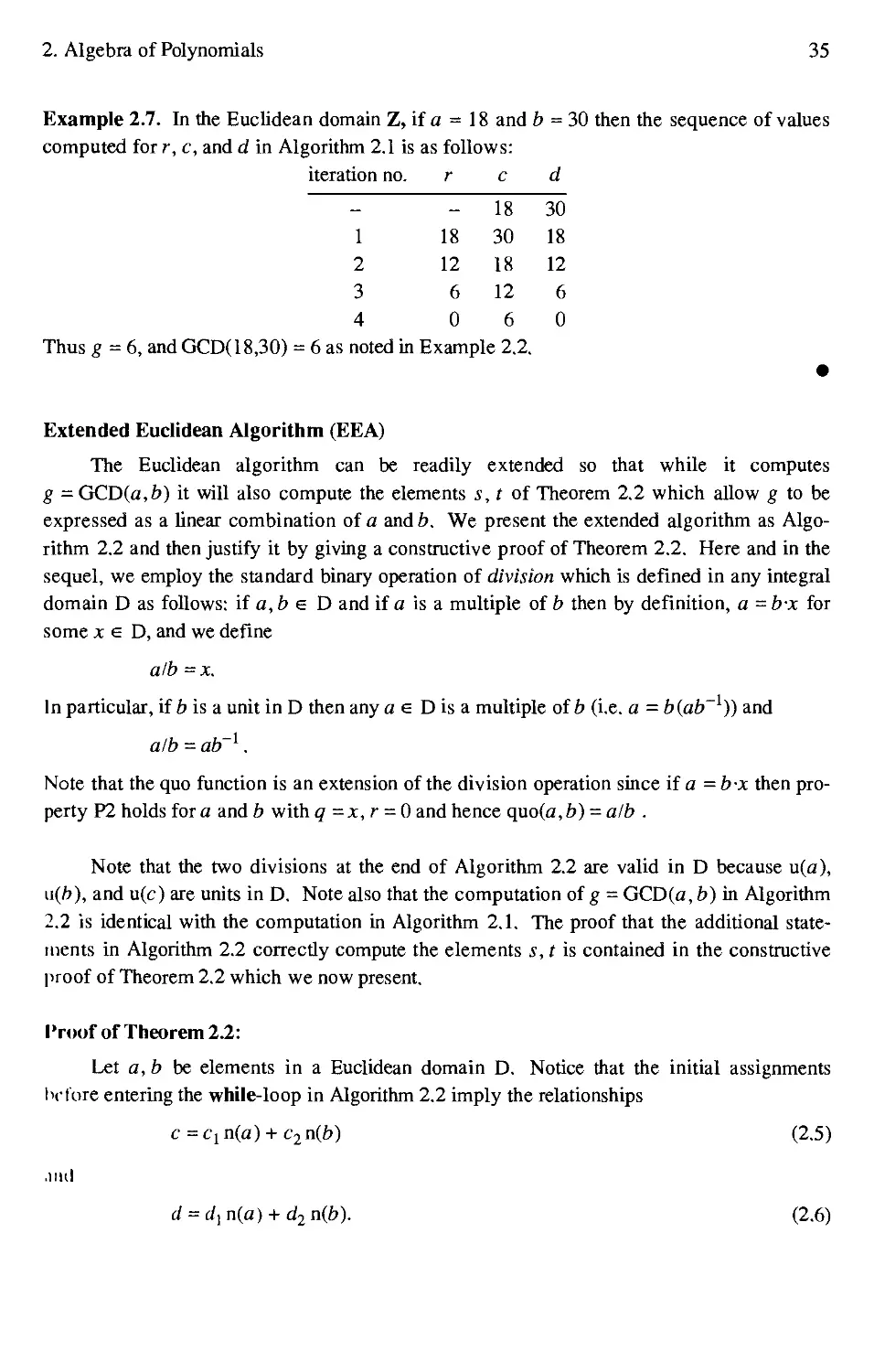
Текст
Algorithms for
Computer Algebra
K.O. Geddes
University of Waterloo
S.R. Czapor
Laurentian University
G. Labahn
University of Waterloo
Kluwer Academic Publishers
Boston/Dordrecht/London
Distributors for North America:
Kluwer Academic Publishers
101 Philip Drive
Assinippi Park
Norwell, Massachusetts 02061 USA
Distributors for all other countries:
Kluwer Academic Publishers Group
Distribution Centre
Post Office Box 322
3300 AH Dordrecht, THE NETHERLANDS
Library of Congress Cataloging-in-Publication Data
Geddes, K.O. (Keith O.), 1947-
Algorithms for computer algebra / K.O. Geddes, S.R. Czapor, G.
Labahn.
p. cm.
Includes bibliographical references and index.
ISBN 0-7923-9259-0 (alk. paper)
1. Algebra—Data processing. 2. Algorithms. I. Czapor, S.R.
(Stephen R.), 1957- . II. Labahn, G. (George), 1951- .
III. Title.
QA155.7.E4G43 1992
512'.00285-dc20 92-25697
CIP
Copyright © 1992 by Kluwer Academic Publishers
All rights reserved. No part of this publication may be reproduced, stored in a retrieval
system or transmitted in any form or by any means, mechanical, photo-copy ing, recording,
or otherwise, without the prior written permission of the publisher, Kluwer Academic
l'uhlishcrs, 101 Philip Drive, Assinippi Park, Norwell,Massachusetts (COM.
I't mlt'd on at id-free paper.
l'niiiril ill llit- United States of America
Dedication
For their support in numerous ways, this book is dedicated to
Debbie, Kim, Kathryn, and Kirsten
Alexandra, Merle, Serge, and Margaret
Laura, Claudia, Jeffrey, and Philip
CONTENTS
Preface xv
Chapter 1 Introduction to Computer Algebra
1.1 Introduction 1
1.2 Symbolic versus Numeric Computation 2
1.3 A Brief Historical Sketch 4
1.4 An Example of a Computer Algebra System: MAPLE 11
Exercises 20
Chapter 2 Algebra of Polynomials, Rational Functions, and Power Series
2.1 Introduction 23
2.2 Rings and Fields 23
2.3 Divisibility and Factorization in Integral Domains 26
2.4 The Euclidean Algorithm 32
2.5 Univariate Polynomial Domains 38
2.6 Multivariate Polynomial Domains 46
2.7 The Primitive Euclidean Algorithm 52
2.8 Quotient Fields and Rational Functions 60
2.9 Power Series and Extended Power Series 63
2.10 Relationships among Domains 70
Exercises 73
( hapter 3 Normal Forms and Algebraic Representations
3.1 Introduction 79
.1.2 Levels of Abstraction 79
3.3 Normal Form and Canonical Form 80
.1.4 Normal Forms for Polynomials 84
.1.5 Normal Forms for Rational Functions and Power Series 88
.1.6 Data Structures for Multiprecision Integers and Rational Numbers 93
.1.7 Data Structures for Polynomials, Rational Functions,
and Power Series 96
Exercises 105
viii Algorithms fur ('mnpmcr Algebra
Chapter 4 Arithmetic of Polynomials, Rational Functions, and Power Series
4.1 Introduction Ill
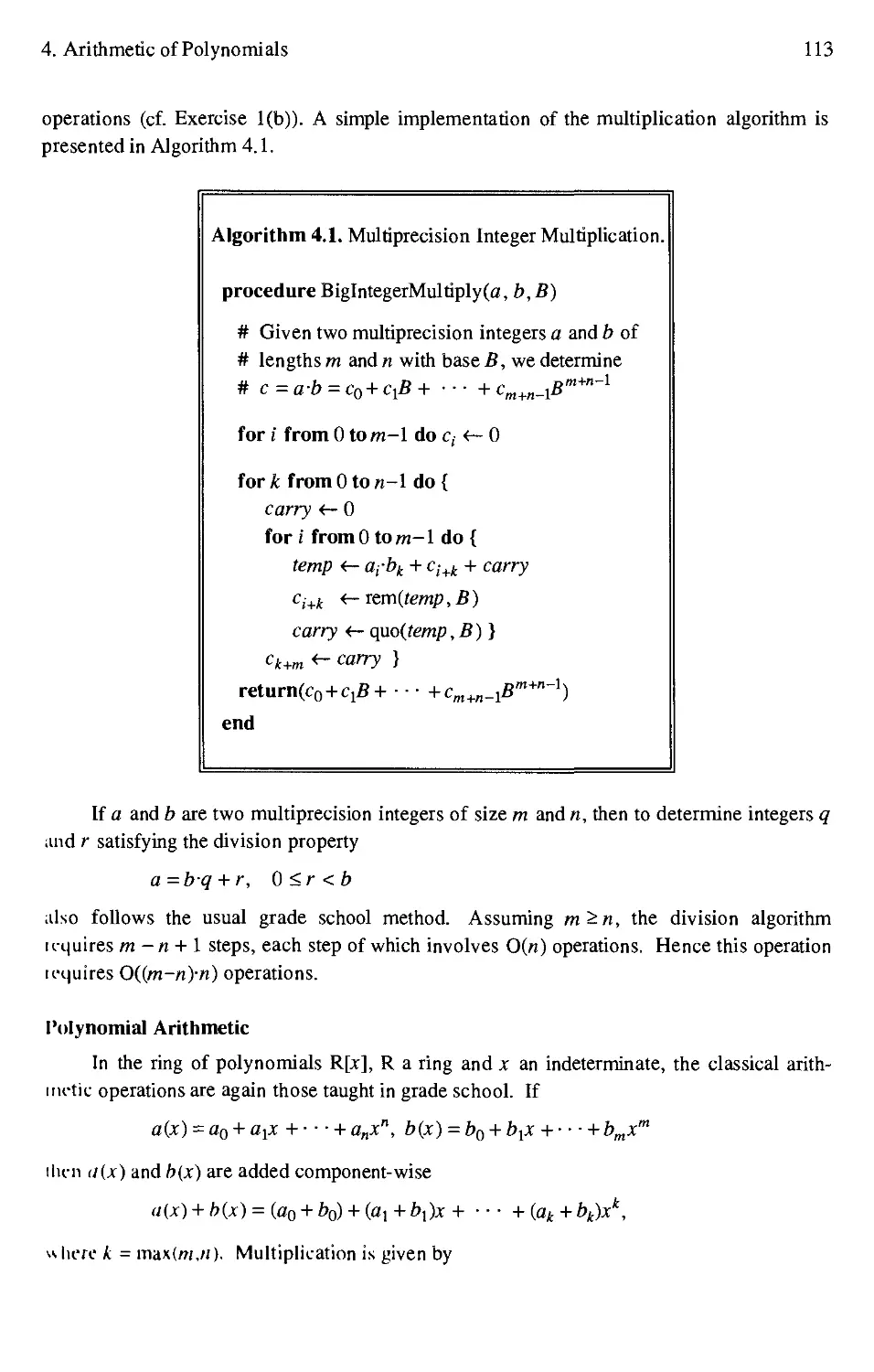
4.2 Basic Arithmetic Algorithms 112
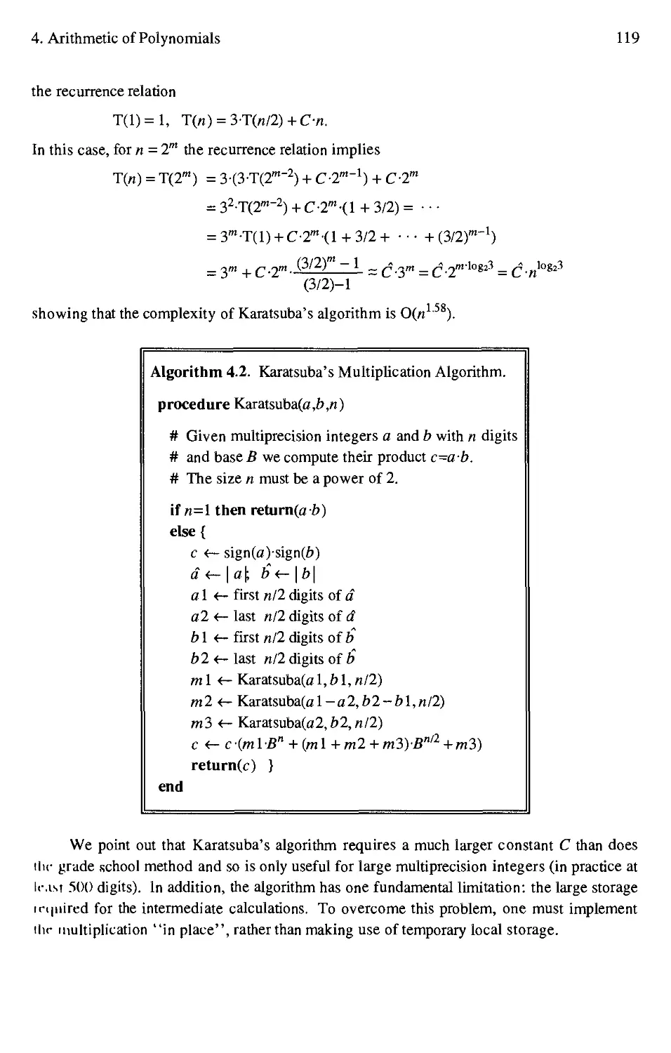
4.3 Fast Arithmetic Algorithms: Karatsuba's Algorithm 118
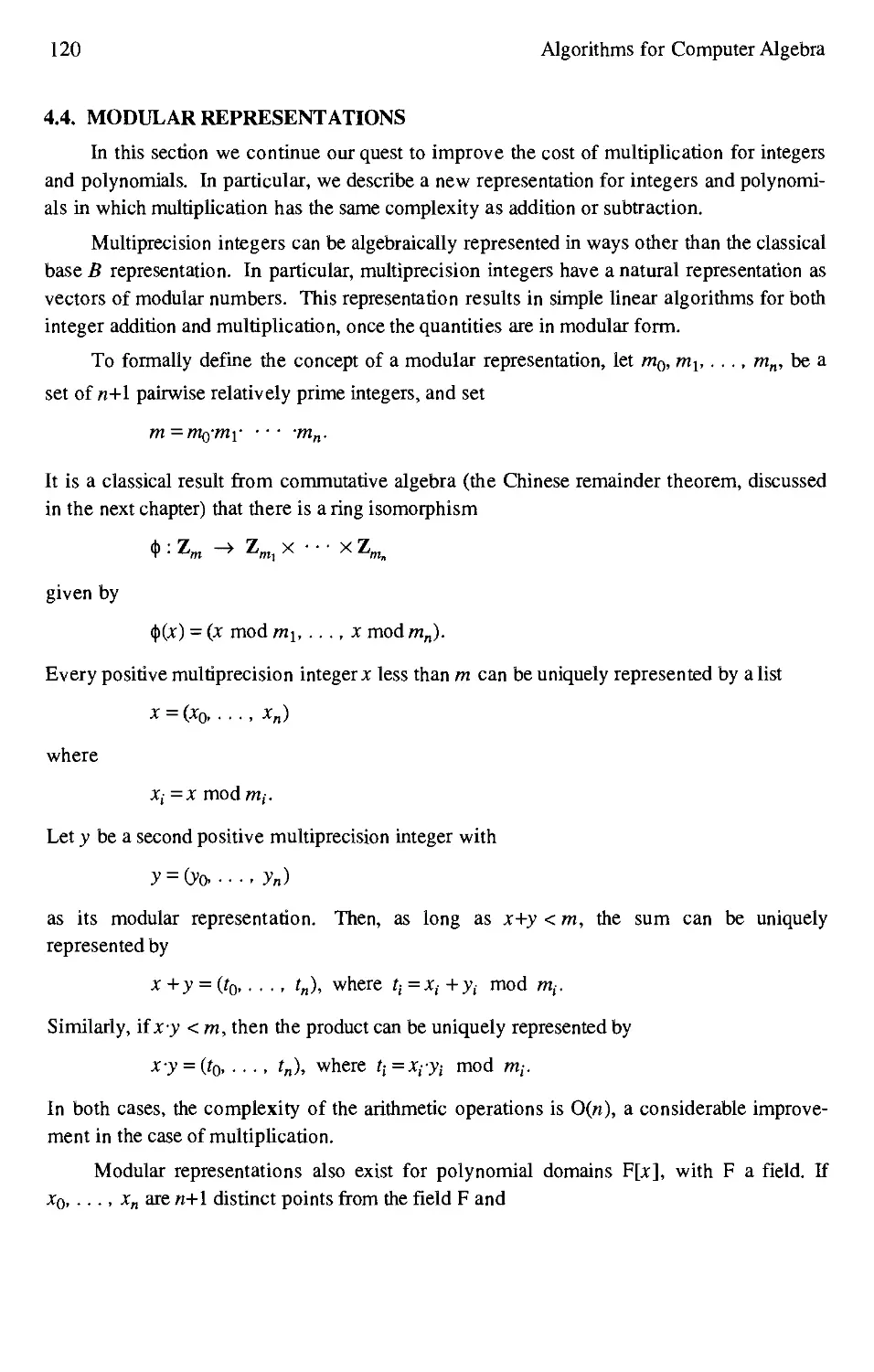
4.4 Modular Representations 120
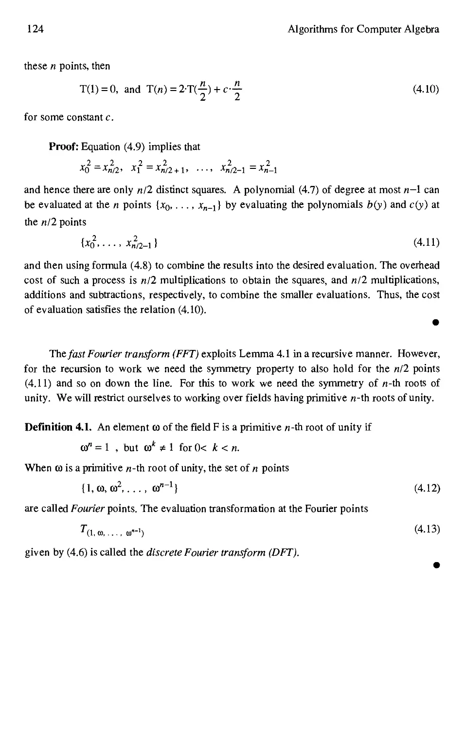
4.5 The Fast Fourier Transform 123
4.6 The Inverse Fourier Transform 128
4.7 Fast Polynomial Multiplication 132
4.8 Computing Primitive N-th Roots of Unity 133
4.9 Newton's Iteration for Power Series Division 136
Exercises 145
Chapter 5 Homomorphisms and Chinese Remainder Algorithms
5.1 Introduction 151
5.2 Intermediate Expression Swell: An Example 151
5.3 Ring Morphisms 153
5.4 Characterization of Morphisms 160
5.5 Homomorphic Images 167
5.6 The Integer Chinese Remainder Algorithm 174
5.7 The Polynomial Interpolation Algorithm 183
5.8 Further Discussion of the Two Algorithms 189
Exercises 196
Chapter 6 Newton's Iteration and the Hensel Construction
6.1 Introduction 205
6.2 P-adic and Ideal-adic Representations 205
6.3 Newton's Iteration for F(u)=0 214
6.4 Hensel's Lemma 226
6.5 The Univariate Hensel Lifting Algorithm 232
6.6 Special Techniques for the Non-monic Case 240
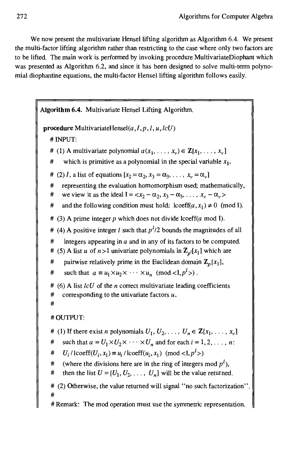
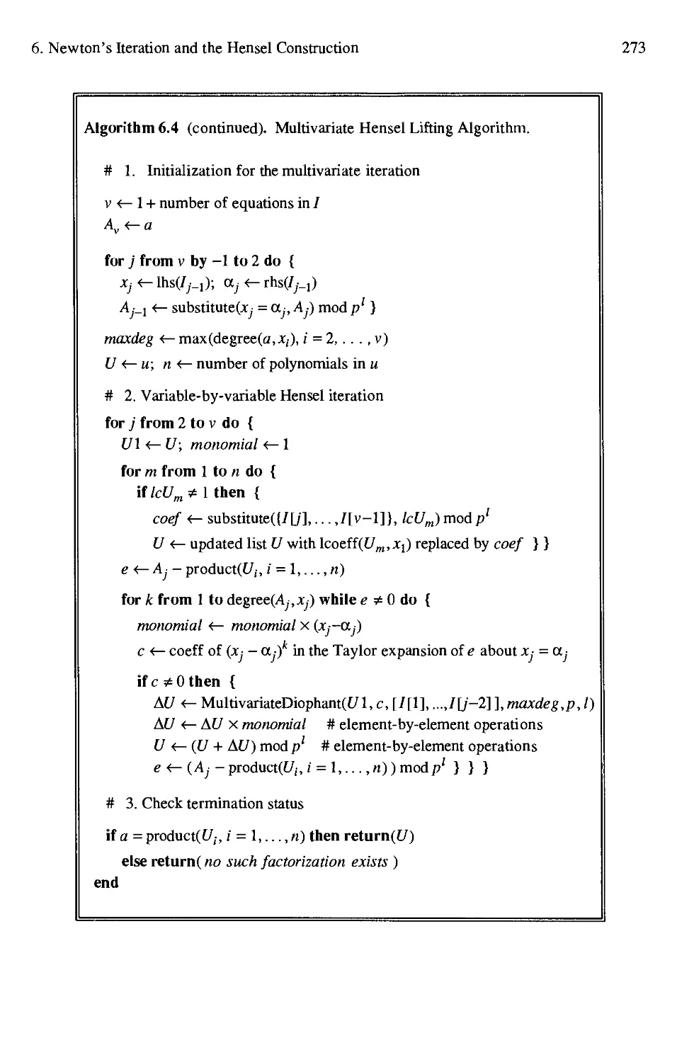
6.7 The Multivariate Generalization of Hensel's Lemma 250
6.8 The Multivariate Hensel Lifting Algorithm 260
Exercises 274
Chapter 7 Polynomial GCD Computation
7.1 Introduction 279
7.2 Polynomial Remainder Sequences 280
7.3 The Sylvester Matrix and Subresultants 285
7.4 The Modular GCD Algorithm 300
7.5 The Sparse Modular GCD Algorithm 311
7.6 GCD's using Hensel Lifting: The EZ-GCD Algorithm 314
7.7 A Heuristic Polynomial GCD Algorithm 320
Exercises 331
Contents ix
Chapter 8 Polynomial Factorization
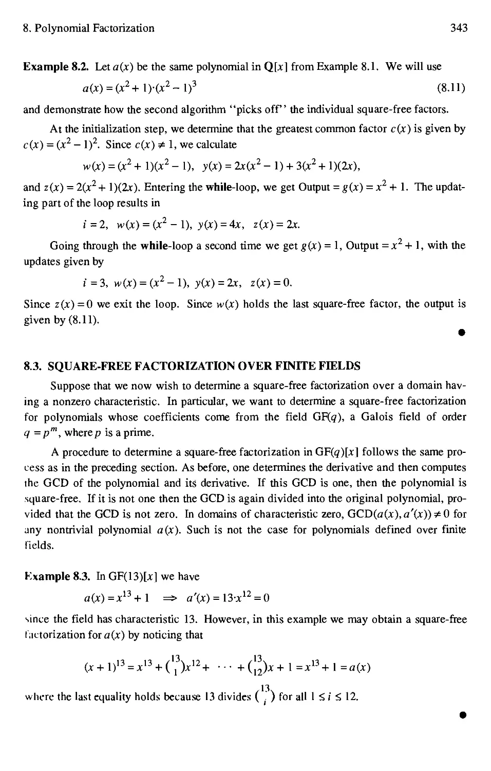
8.1 Introduction 337
8.2 Square-Free Factorization 337
8.3 Square-Free Factorization Over Finite Fields 343
8.4 Berlekamp's Factorization Algorithm 347
8.5 The Big Prime Berlekamp Algorithm 359
8.6 Distinct Degree Factorization 368
8.7 Factoring Polynomials over the Rationals 374
8.8 Factoring Polynomials over Algebraic Number Fields 378
Exercises 384
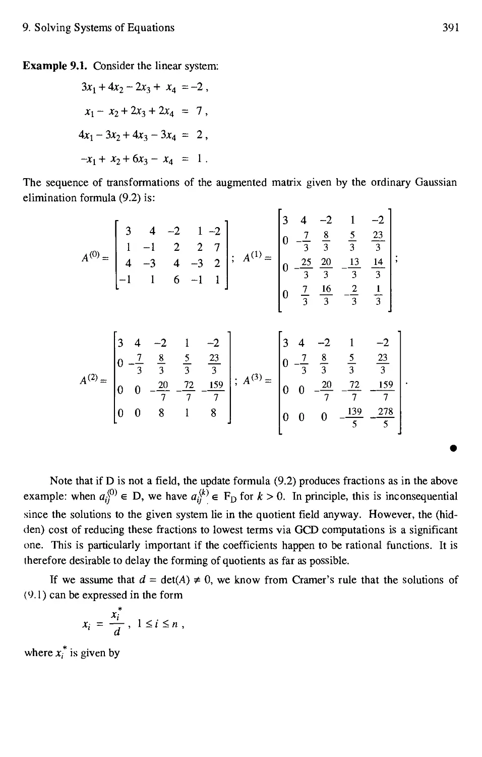
C hapter 9 Solving Systems of Equations
9.1 Introduction 389
9.2 Linear Equations and Gaussian Elimination 390
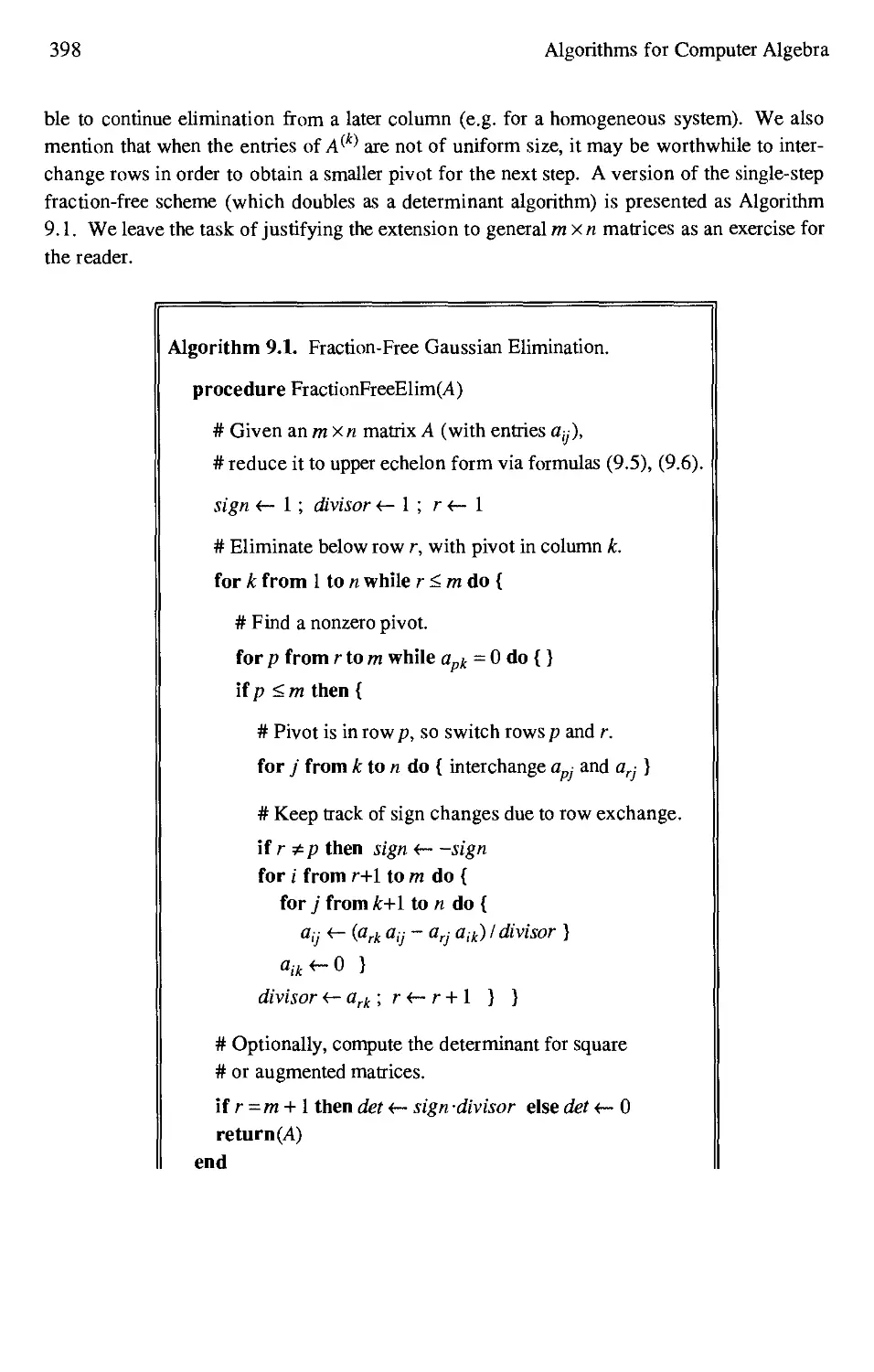
9.3 Fraction-Free Gaussian Elimination 393
9.4 Alternative Methods for Solving Linear Equations 399
9.5 Nonlinear Equations and Resultants 405
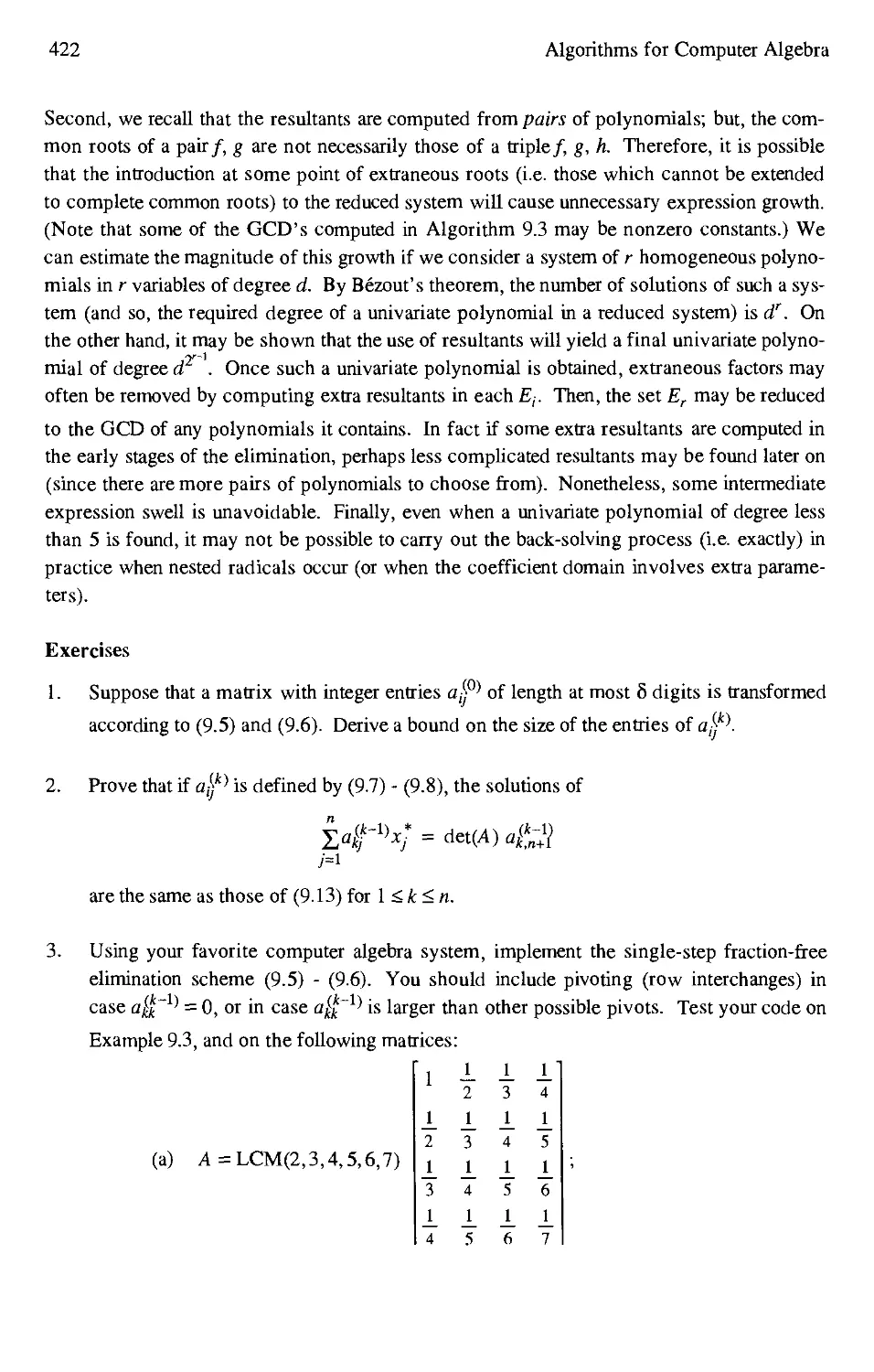
Exercises 422
( hapter 10 Grobner Bases for Polynomial Ideals
10.1 Introduction 429
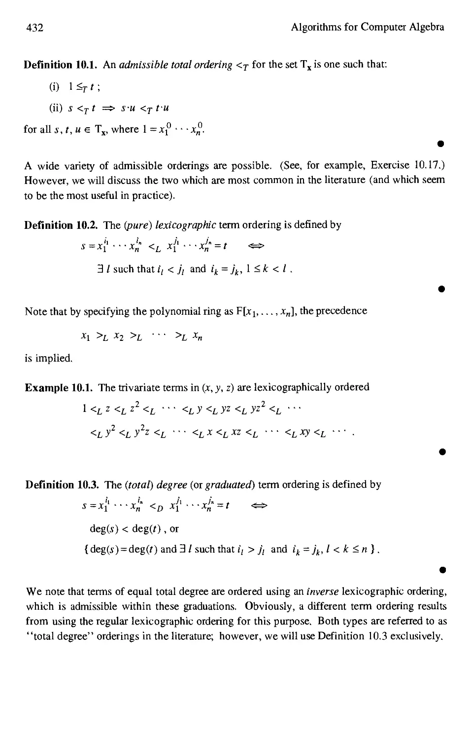
10.2 Term Orderings and Reduction 431
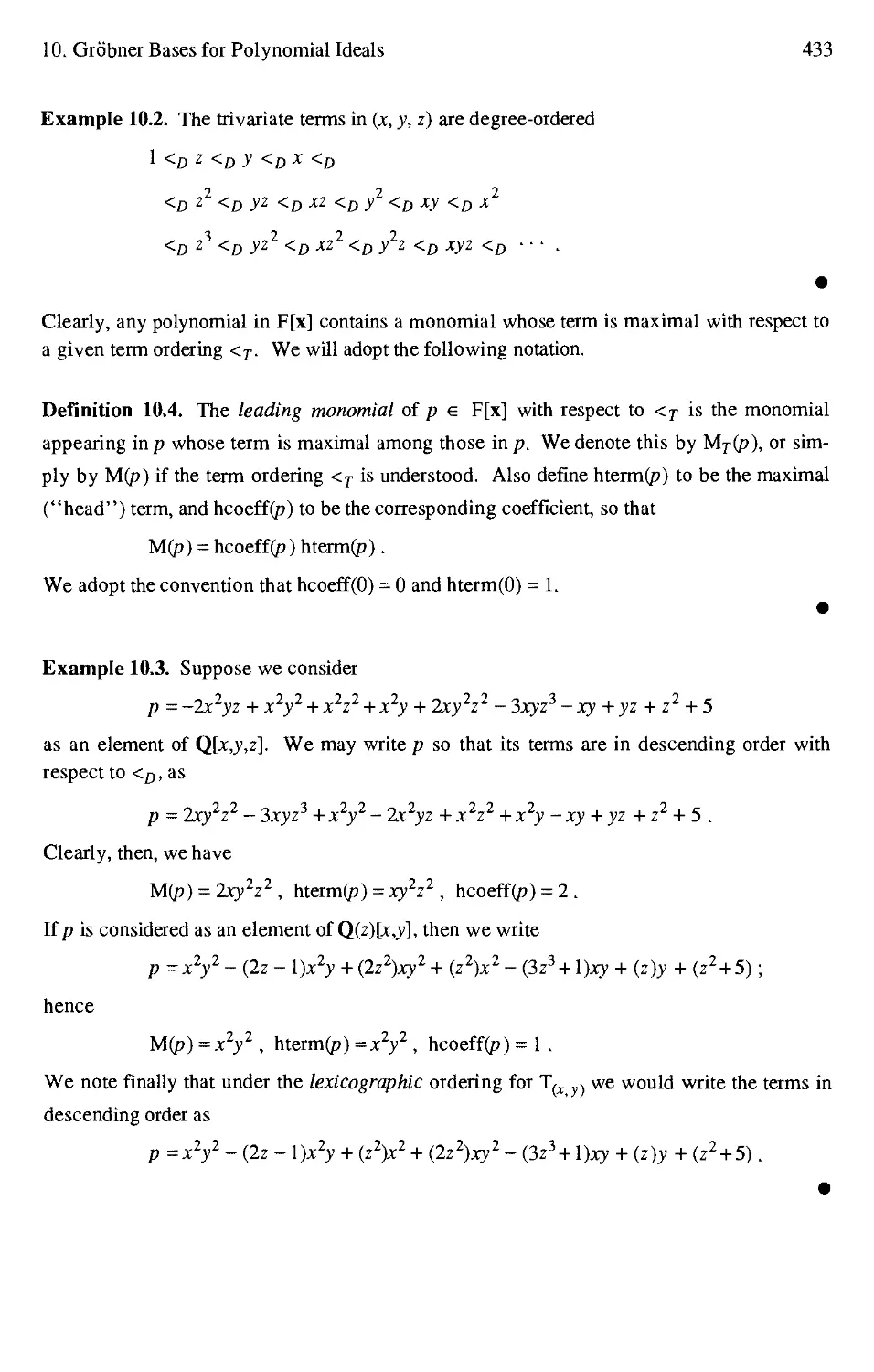
10.3 Grobner Bases and Buchberger's Algorithm 439
10.4 Improving Buchberger's Algorithm 447
10.5 Applications of Grobner Bases 451
10.6 Additional Applications 462
Exercises 466
( hapter 11 Integration of Rational Functions
11.1 Introduction 473
11.2 Basic Concepts of Differential Algebra 474
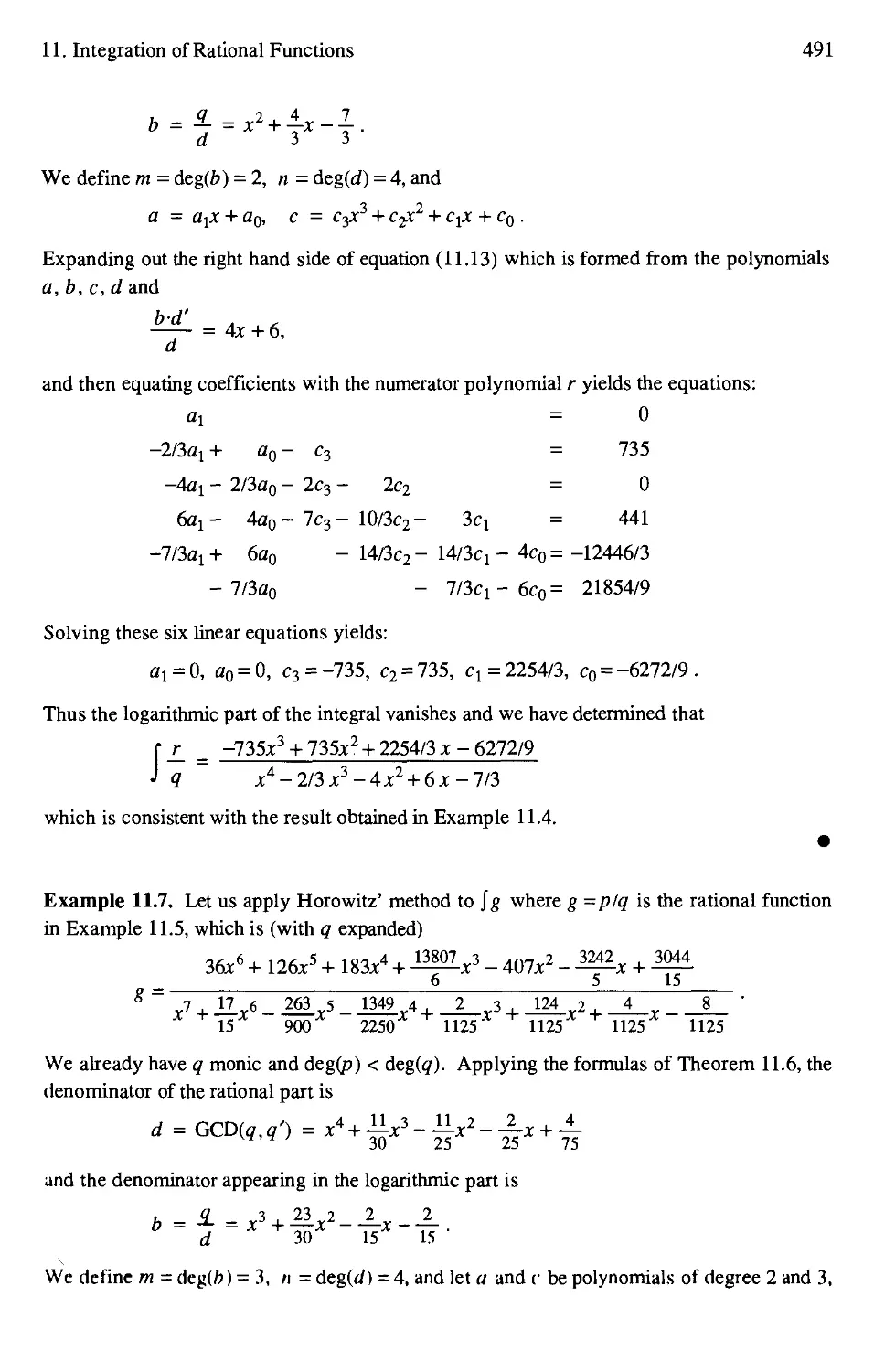
11.3 Rational Part of the Integral: Hermite's Method 482
11.4 Rational Part of the Integral: Horowitz' Method 488
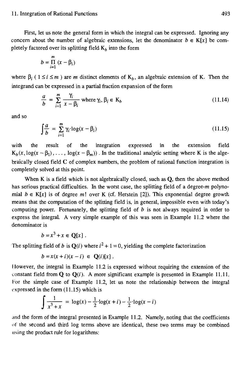
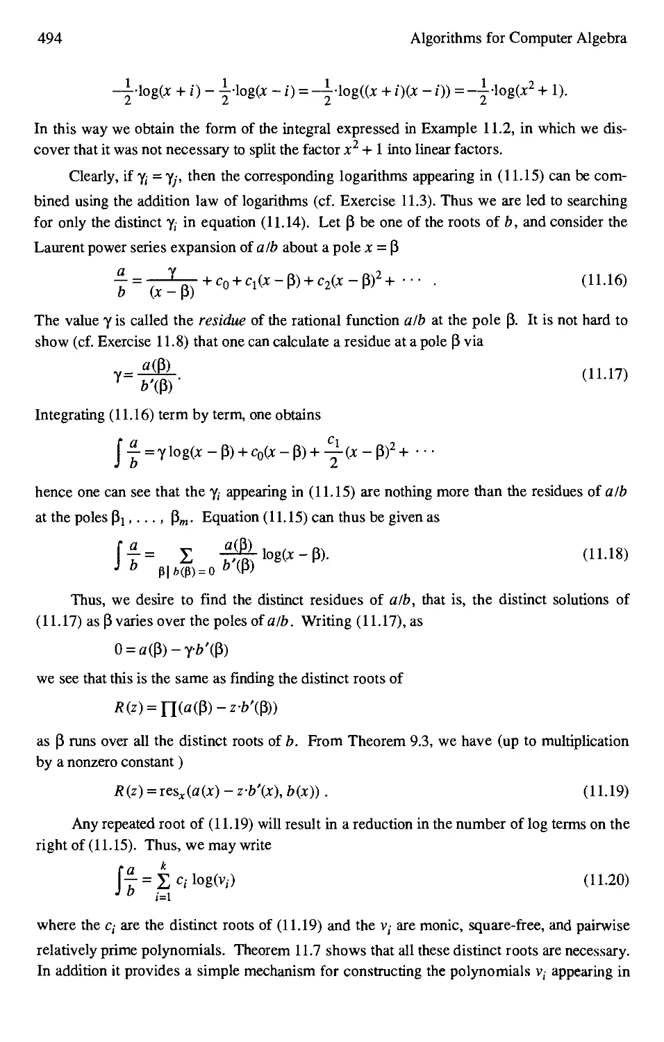
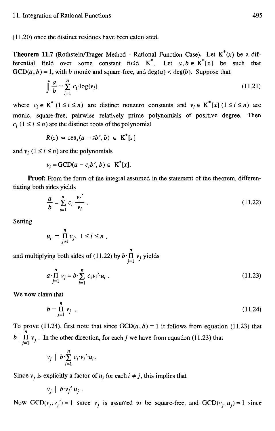
11.5 Logarithmic Part of the Integral 492
Exercises 508
x Algorithms tin ('umpiiit-i
Chapter 12 The Risch Integration Algorithm
12.1 Introduction 511
12.2 Elementary Functions .512
12.3 Differentiation of Elementary Functions 519
12.4 Liouville's Principle .523
12.5 The Risch Algorithm for Transcendental Elementary Functions 529
12.6 The Risch Algorithm for Logarithmic Extensions 5.10
12.7 The Risch Algorithm for Exponential Extensions 547
12.8 Integration of Algebraic Functions 561
Exercises 569
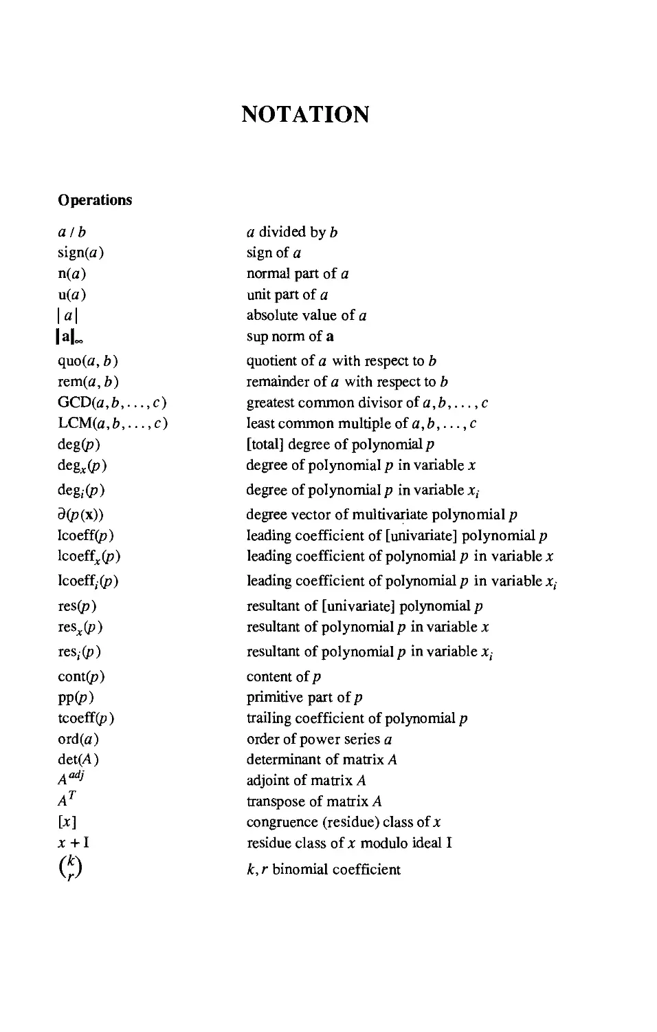
Notation 575
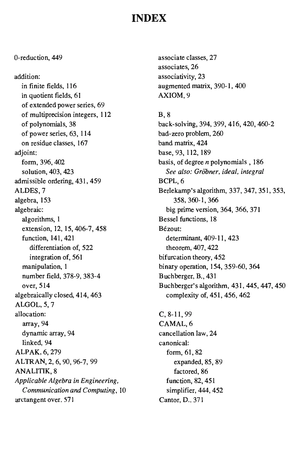
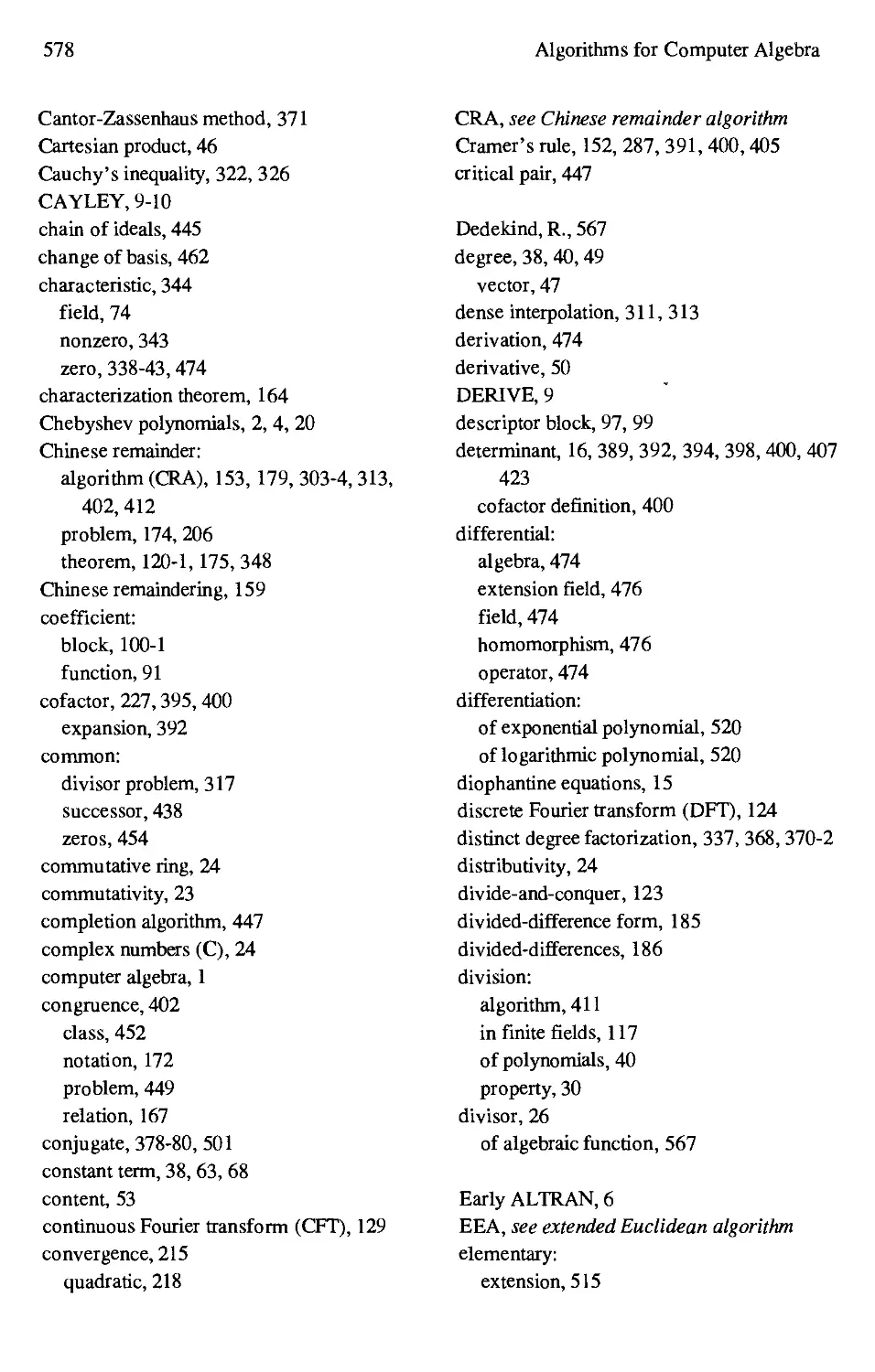
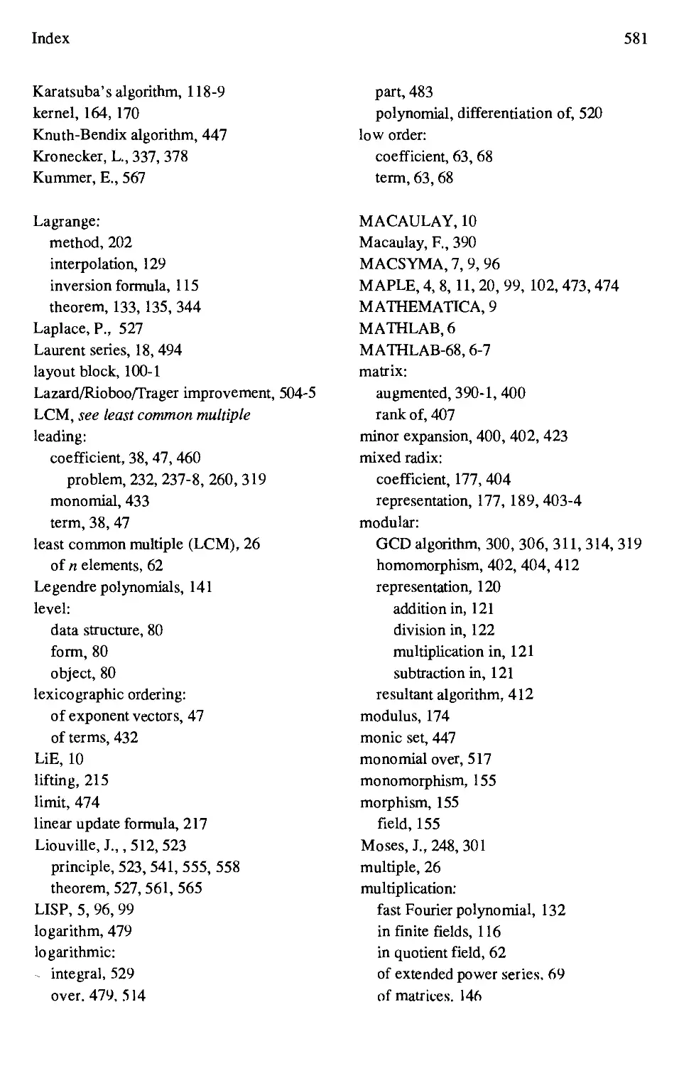
Index 577
LIST OF ALGORITHMS
2.1 Euclidean Algorithm 34
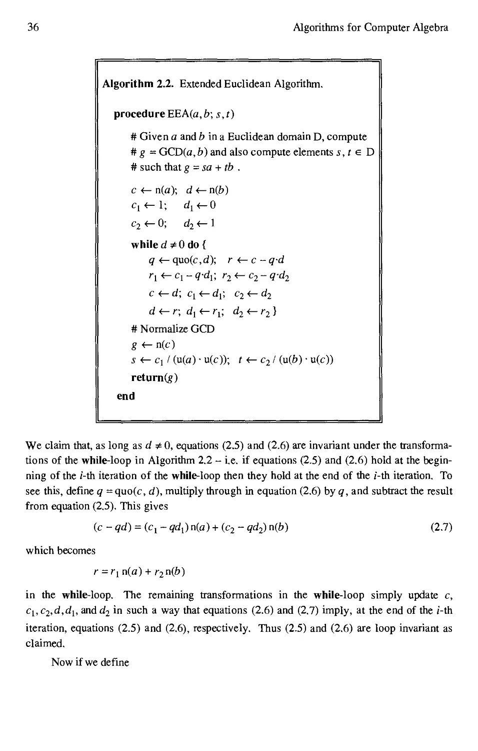
2.2 Extended Euclidean Algorithm 36
2.3 Primitive Euclidean Algorithm 57
4.1 Multiprecision Integer Multiplication 113
4.2 Karatsuba's Multiplication Algorithm 119
4.3 Polynomial Trial Division Algorithm 122
4.4 Fast Fourier Transform (FFT) 128
4.5 Fast Fourier Polynomial Multiplication 132
4.6 Newton's Method for Power Series Inversion 140
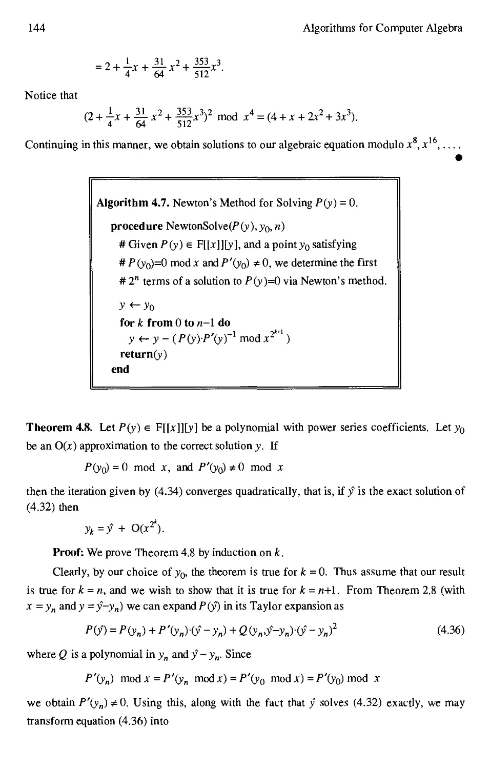
4.7 Newton's Method for Solving P(y) = 0 144
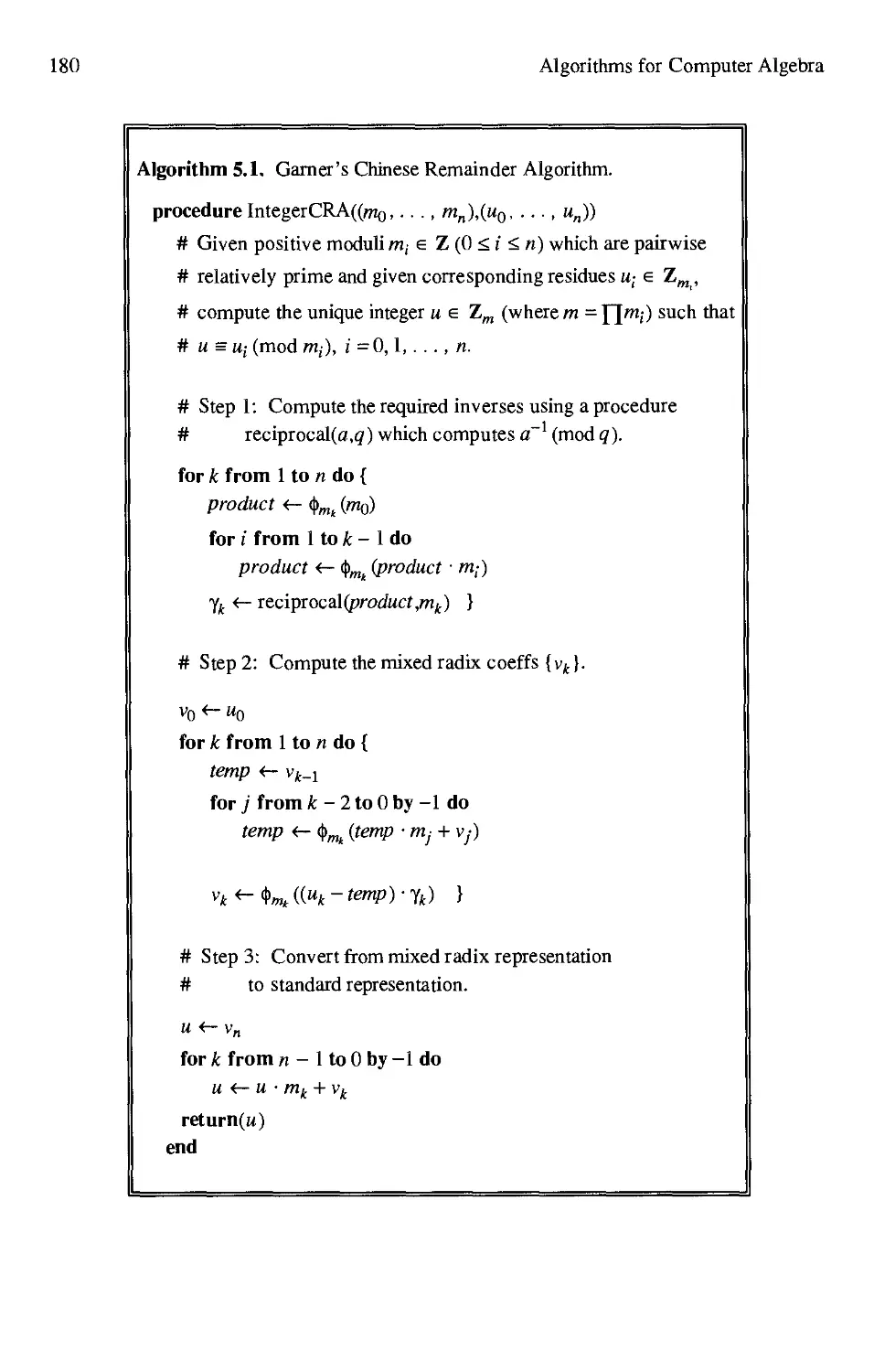
5.1 Garner's Chinese Remainder Algorithm 180
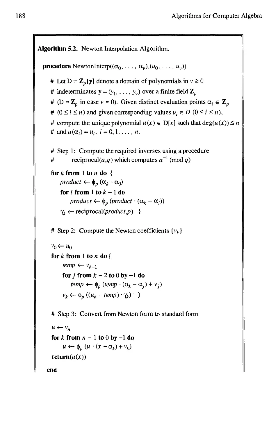
5.2 Newton Interpolation Algorithm 188
6.1 Univariate Hensel Lifting Algorithm 233
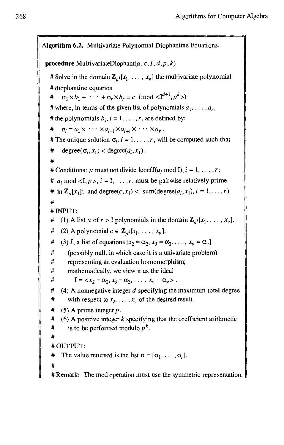
6.2 Multivariate Polynomial Diophantine Equations 268
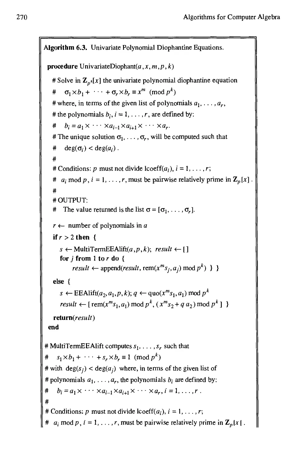
6.3 Univariate Polynomial Diophantine Equations 270
6.4 Multivariate Hensel Lifting Algorithm 272
7.1 Modular GCD Algorithm 307
7.2 Multivariate GCD Reduction Algorithm 309
7.3 The Extended Zassenhaus GCD Algorithm 316
7.4 GCD Heuristic Algorithm 330
8.1 Square-Free Factorization 340
8.2 Yun's Square-Free Factorization 342
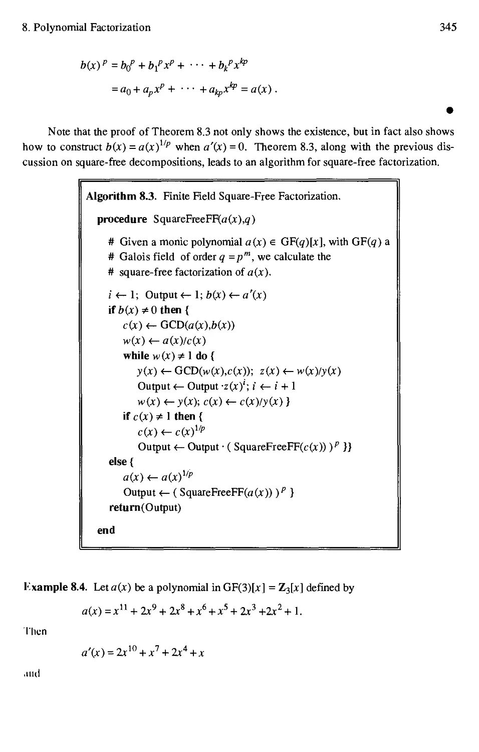
8.3 Finite Field Square-Free Factorization 345
8.4 Berlekamp's Factoring Algorithm 352
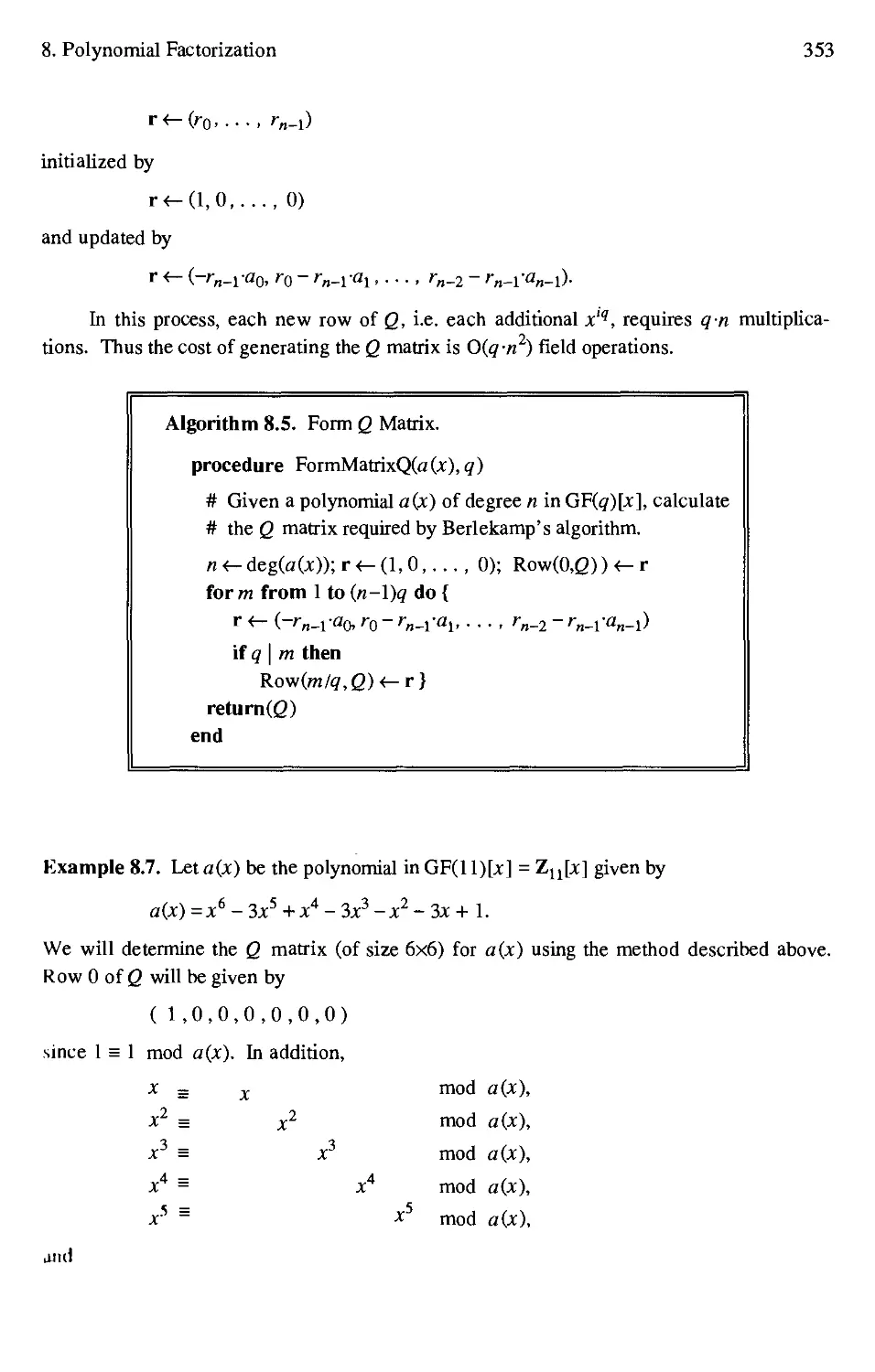
8.5 Form Q Matrix 353
8.6 Null Space Basis Algorithm 356
8.7 Big Prime Berlekamp Factoring Algorithm 367
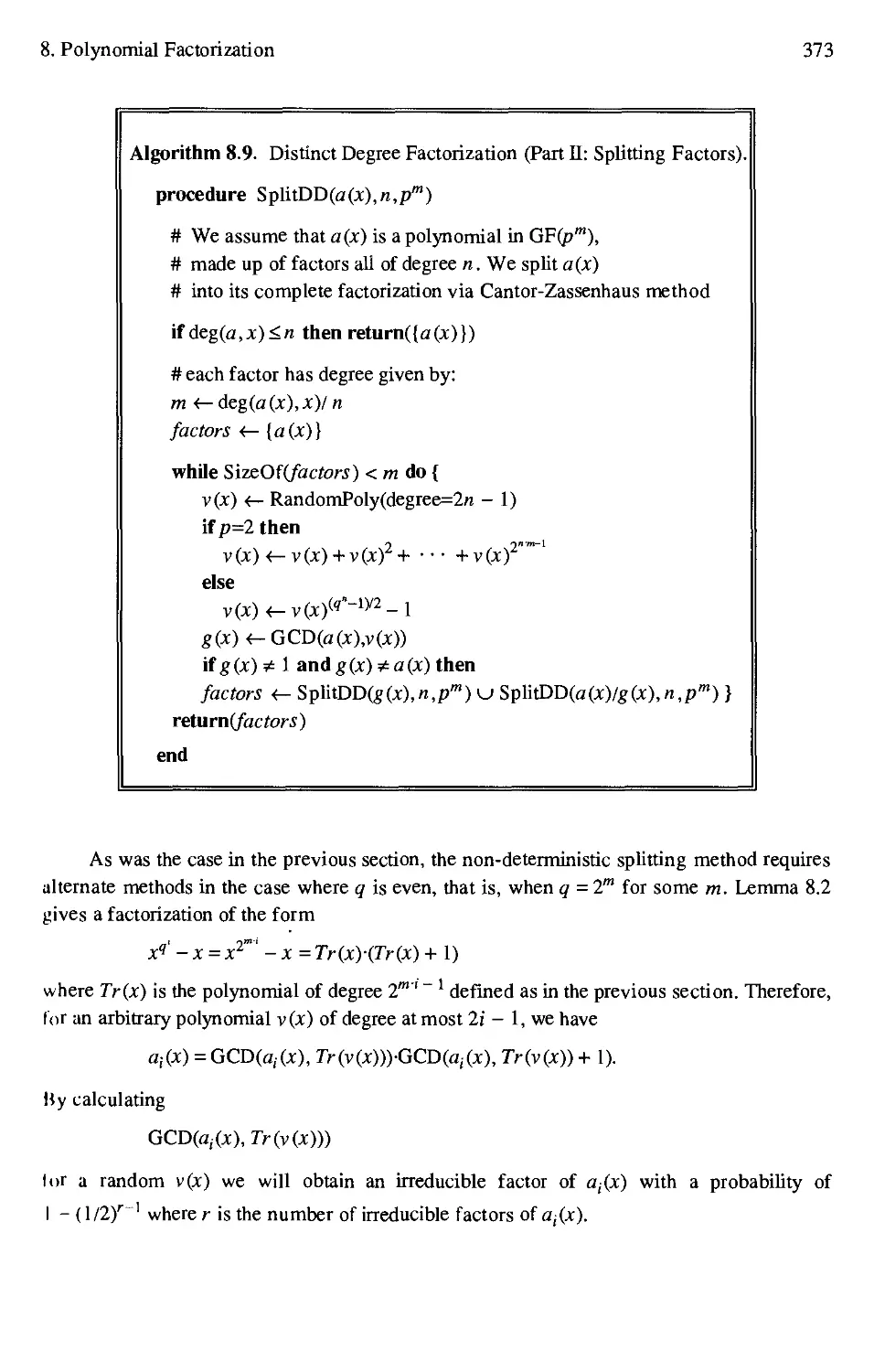
8.8 Distinct Degree Factorization (Partial) 371
8.9 Distinct Degree Factorization (Splitting) 373
8.10 Factorization over Algebraic Number Fields 383
xii Algorithms for Computci Algebra
9.1 Fraction-Free Gaussian Elimination. .W8
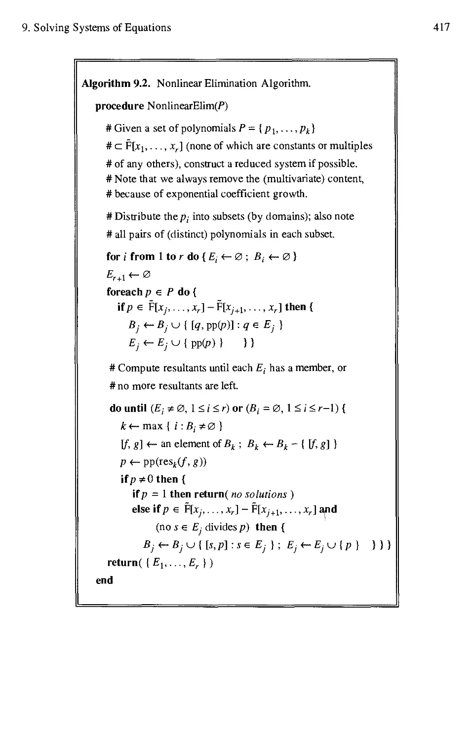
9.2 Nonlinear Elimination Algorithm 417
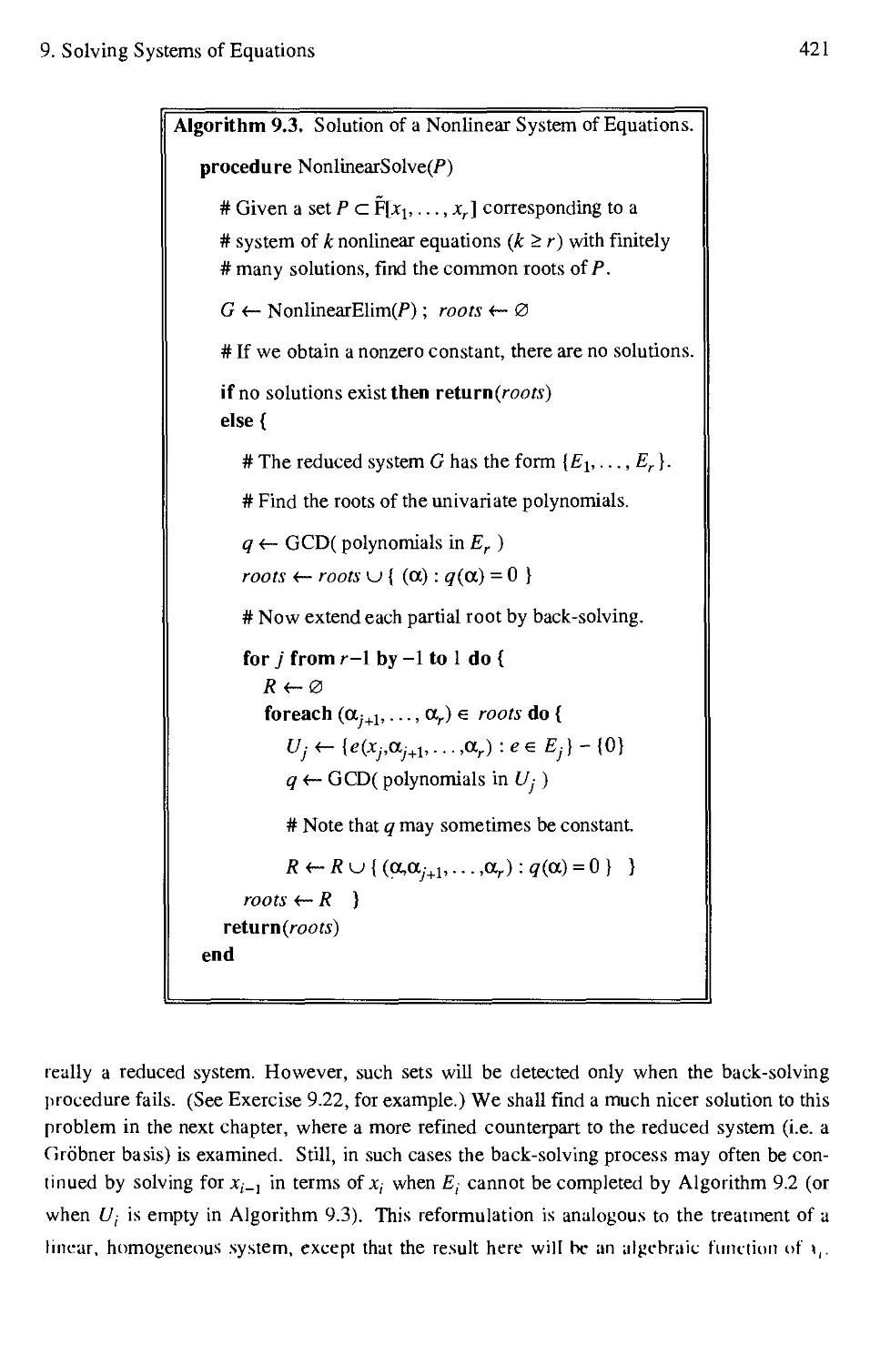
9.3 Solution of a Nonlinear System of Equations 421
10.1 Full Reduction Algorithm 43ft
10.2 Buchberger's Algorithm for Grobner Bases 44o
10.3 Construction of a Reduced Ideal Basis 448
10.4 Improved Construction of Reduced Grobner Basis 450
10.5 Solution of System for One Variable 457
10.6 Complete Solution of System 458
10.7 Solution using Lexicographic Grobner Basis 461
11.1 Hermite's Method for Rational Functions 485
11.2 Horowitz' Reduction for Rational Functions 490
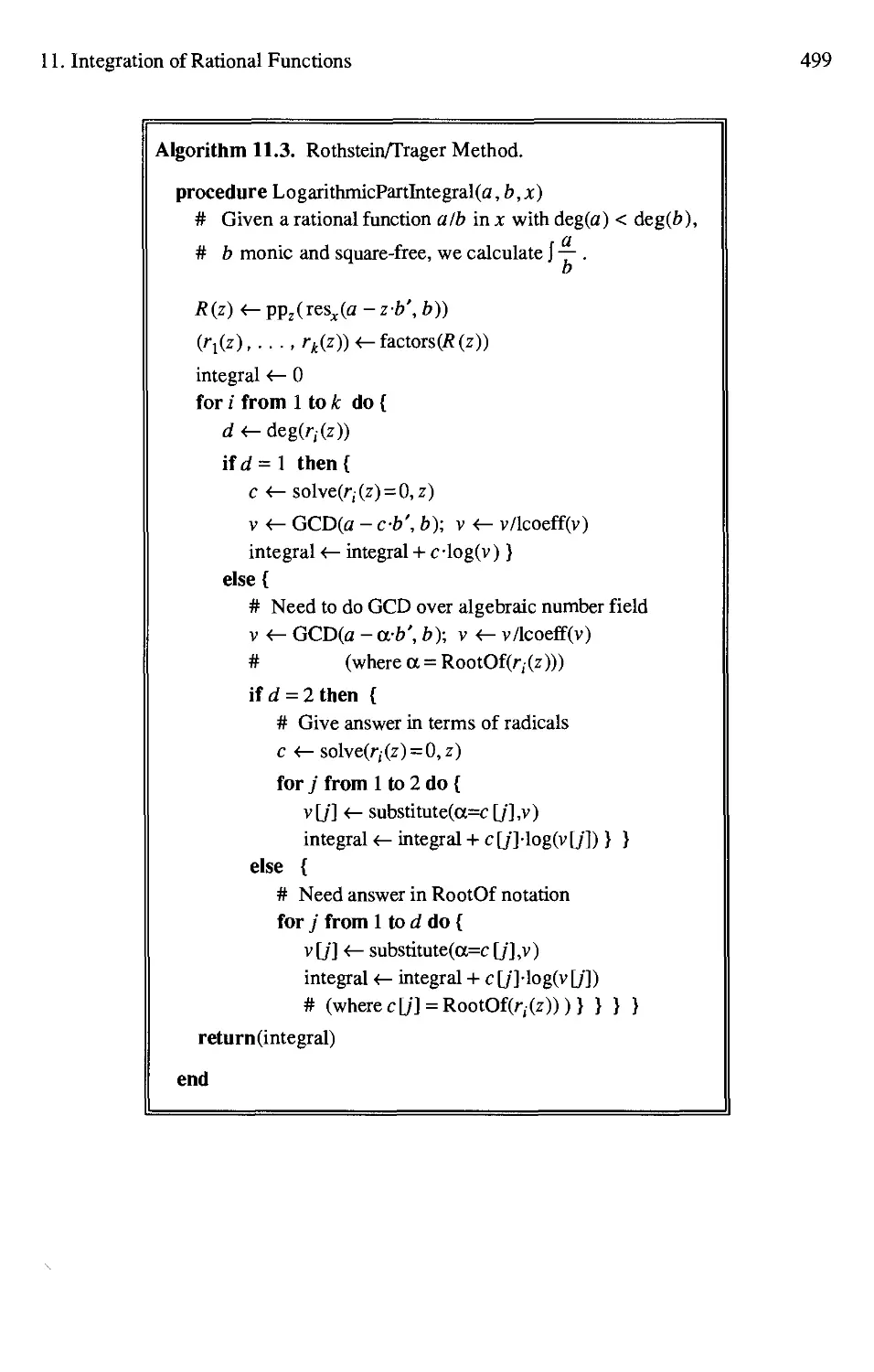
11.3 Rothstein/Trager Method 499
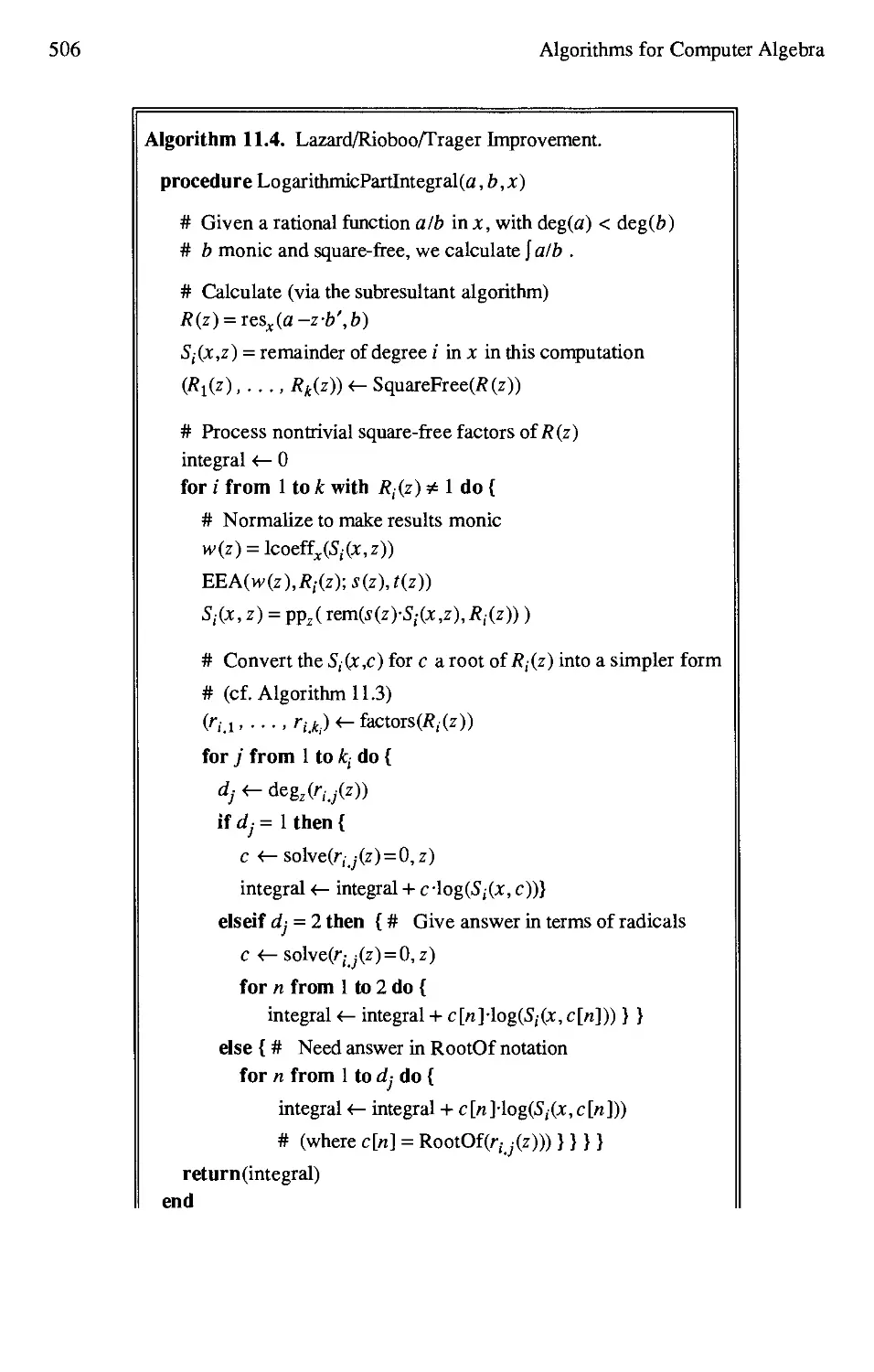
11.4 Lazard/Rioboo/Trager Improvement 506
LIST OF FIGURES
1.1 FORTRAN program involving Chebyshev polynomials 3
1.2 ALTRAN program involving Chebyshev polynomials 3
1.3 Output from ALTRAN program in Figure 1.2 4
1.4 MAPLE session involving Chebyshev polynomials 5
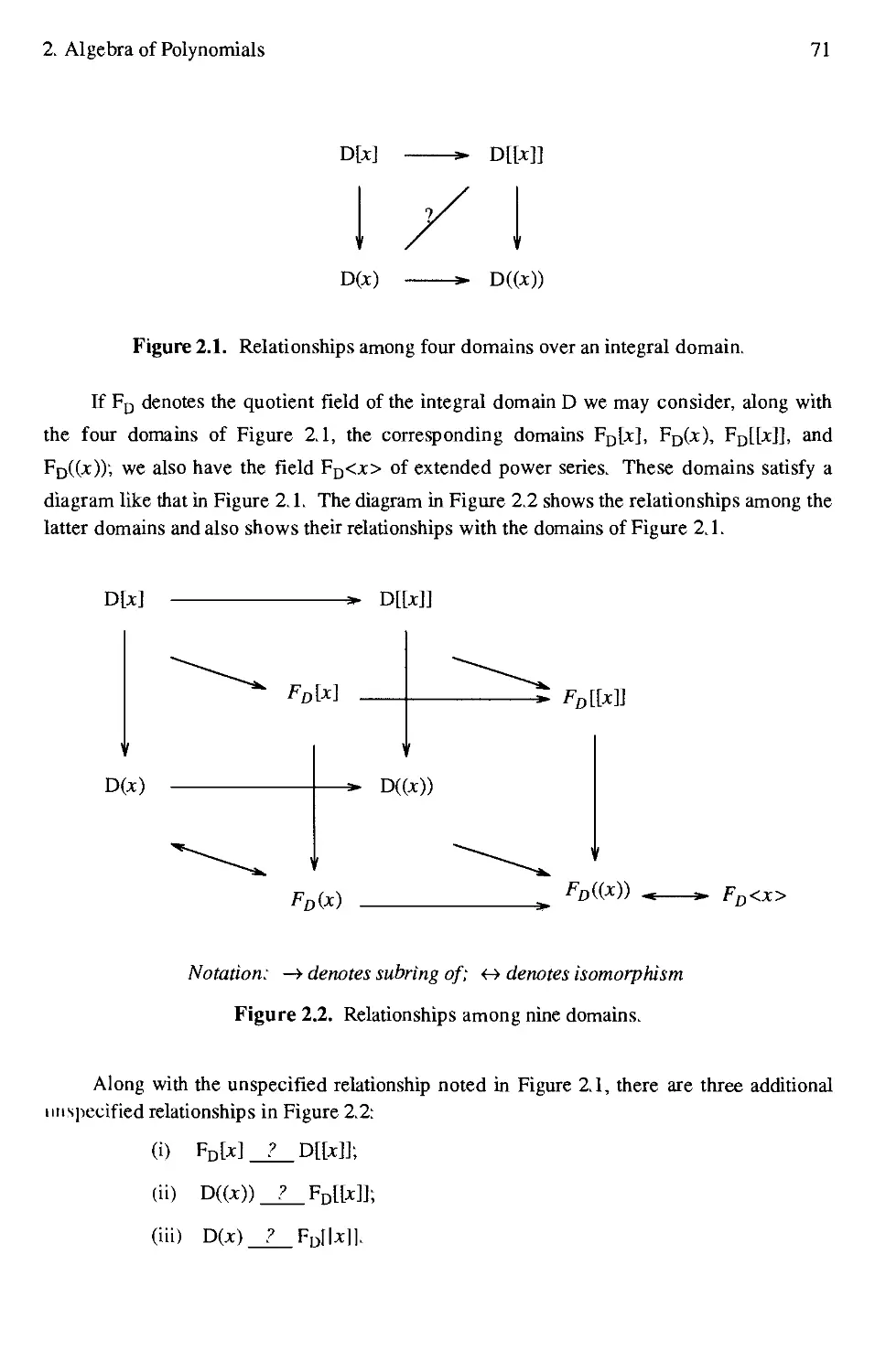
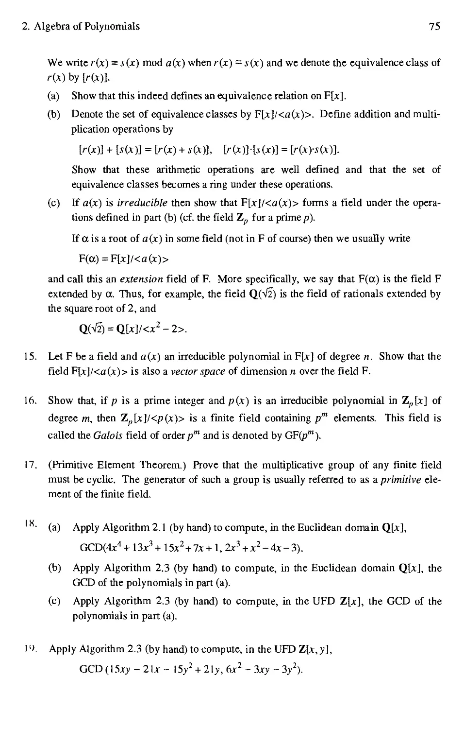
2.1 Relationships among four domains over an integral domain 71
2.2 Relationships among nine domains 71
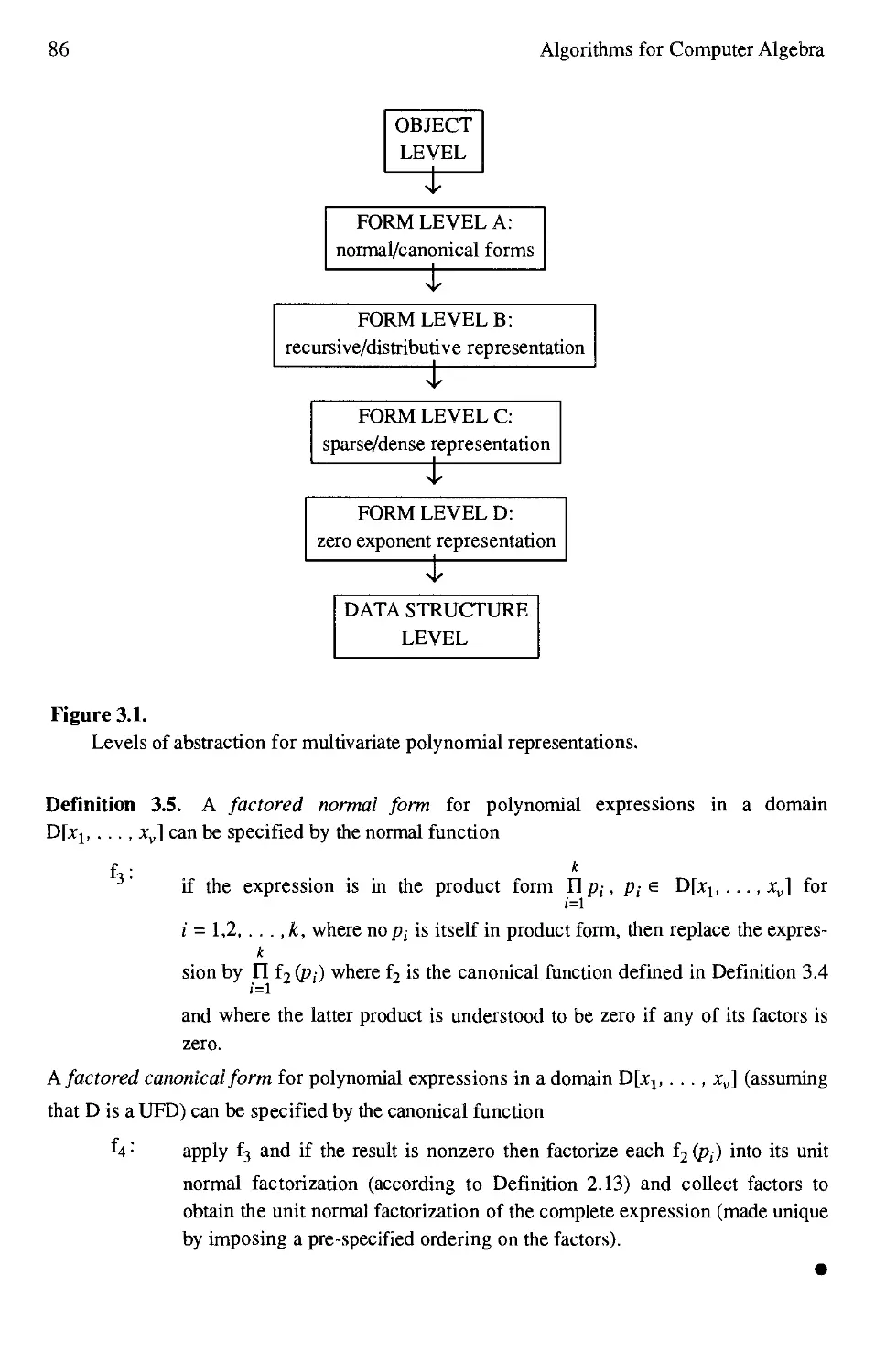
3.1 Levels of abstraction for multivariate polynomial representations 86
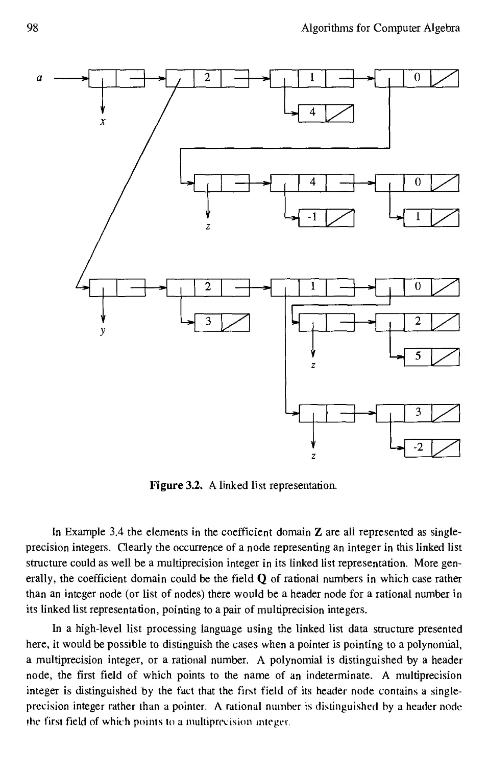
3.2 A linked list representation 98
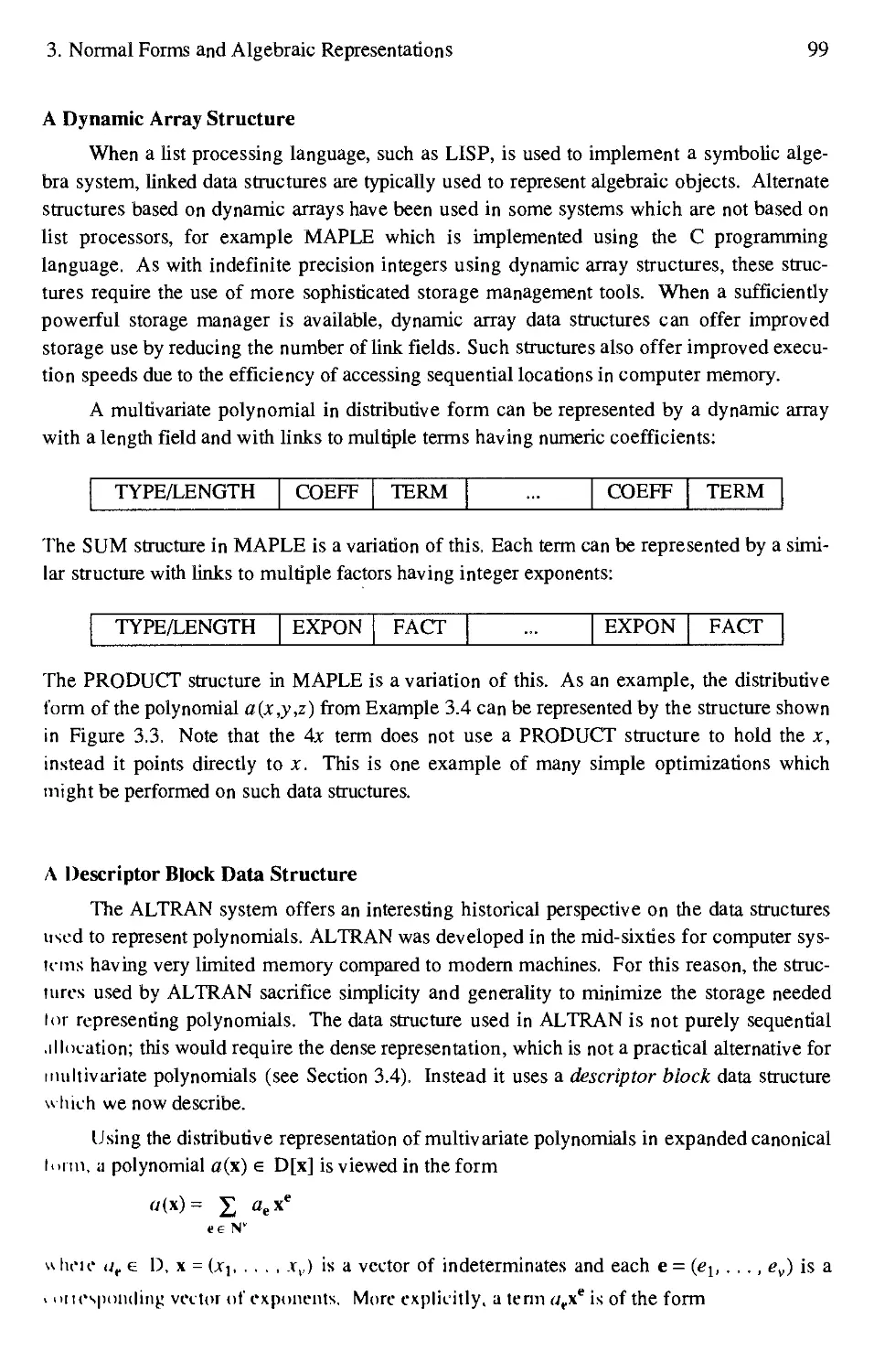
3.3 A dynamic array representation 100
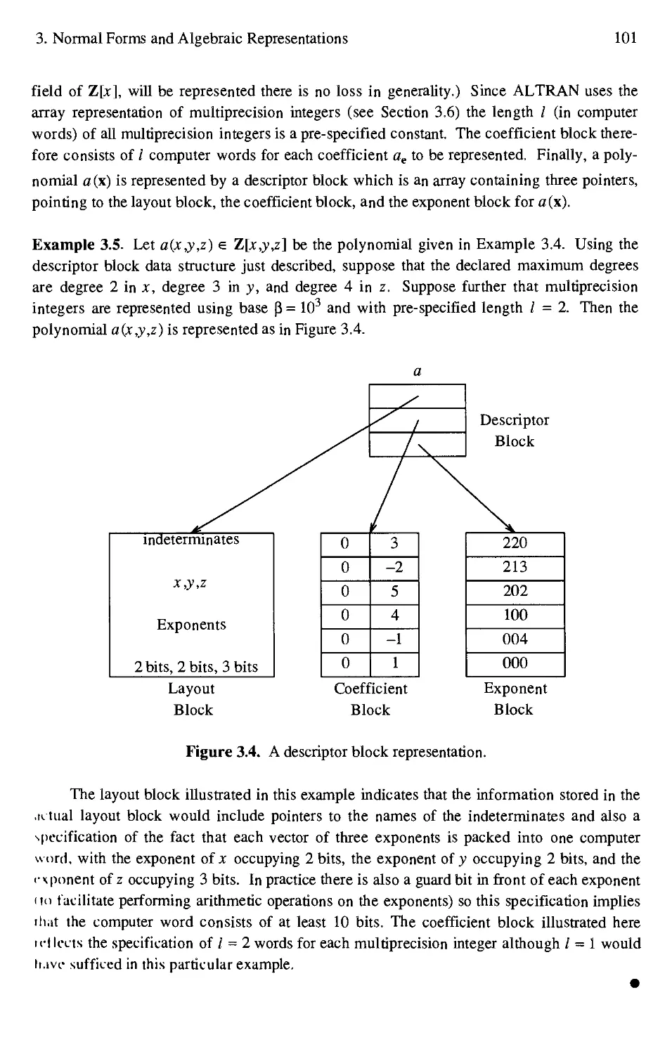
3.4 A descriptor block representation 101
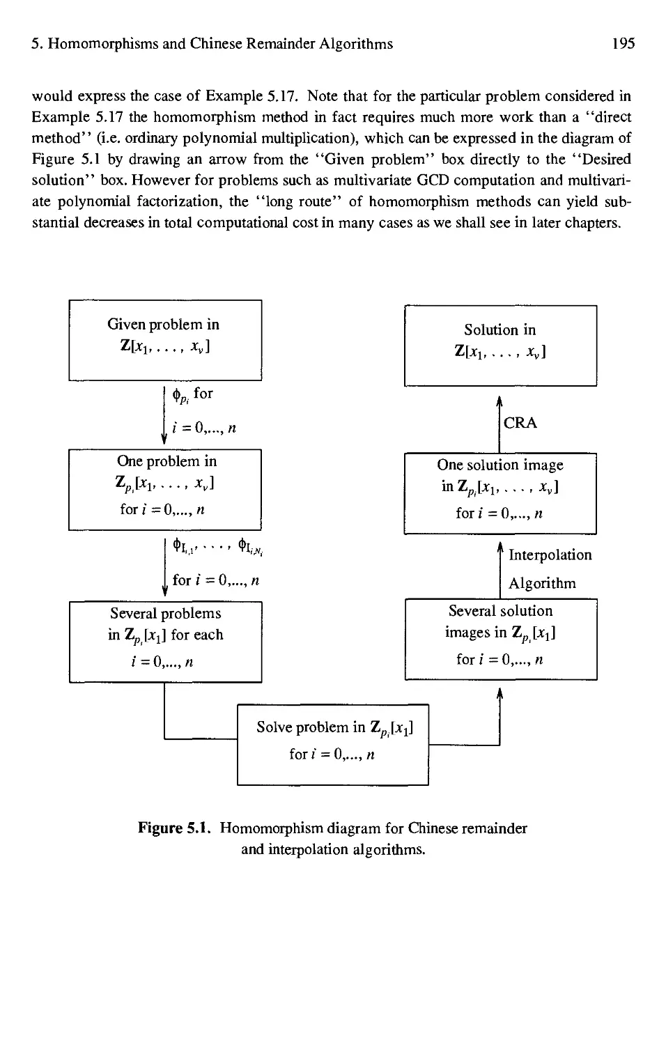
5.1 Homomorphism diagram for Chinese remainder and interpolation algorithms 195
6.1 Homomorphism diagram forp-adic and ideal-adic Newton's iterations 226
6.2 Homomorphism diagram for univariate and multivariate Hensel constructions ....251
LIST OF TABLES
1.1 The first five Chebyshev polynomials 2
2.1 Definitions of algebraic structures 25
2.2 Addition and multiplication tables for Z5 25
2.3 Hierarchy of domains 31
PREFACE
The field of computer algebra has gained widespread attention in recent years because
of the increasing use of computer algebra systems in the scientific community. These sys-
systems, the best known of which are DERIVE, MACSYMA, MAPLE, MATHEMATICA,
REDUCE, and SCRATCHPAD, differ markedly from programs that exist to perform only
numerical scientific computations. Unlike the latter programs, computer algebra systems can
manipulate symbolic mathematical objects in addition to numeric quantities. The operations
that can be performed on these symbolic objects include most of the algebraic operations that
one encounters in high school and university mathematics courses. The ability to perform
calculations with symbolic objects opens up a vast array of applications for these systems.
Polynomials, trigonometric functions, and other mathematical functions can be manipulated
by these programs. Differentiation and integration can be performed for a wide class of func-
functions. Polynomials can be factored, greatest common divisors can be determined, differential
and recurrence equations can be solved. Indeed any mathematical operation that allows for
an algebraic construction can, in principle, be performed in a computer algebra system.
The main advantage of a computer algebra system is its ability to handle large algebraic
computations. As such, however, one cannot necessarily use the classical algorithms which
appear in mathematics textbooks. Computing the greatest common divisor of two polynomi-
polynomials having rational number coefficients can be accomplished by the classical Euclidean algo-
algorithm. However, if one tries to use this algorithm on polynomials of even a moderate size
one quickly realizes that the intermediate polynomials have coefficients which grow
exponentially in size if one omits reducing the rationals to minimum denominators. An algo-
algorithm that exhibits exponential growth in the size of the intermediate expressions quickly
becomes impractical as the problem size is increased. Unfortunately, such algorithms
include a large number of familiar approaches such as the Euclidean algorithm. Programs
written for purely numerical computation do not suffer from this difficulty since the numer-
numerics are all of a fixed size.
The use of exact arithmetic in computer algebra systems adds a second area of com-
complexity to the algorithms. Algorithms designed for numerical computation have their com-
complexity judged by a simple count of the number of arithmetic steps required. In these sys-
systems every arithmetic operation costs approximately the same. However, this is not true
when exact arithmetic is used as can easily be seen by timing the addition of two rational
numbers having 5 digit components and comparing it to the addition of two rational numbers
having 5000 digit components.
xvi Algorithms for Computer Algebra
The motivation for this book is twofold. On the one hand there is a definite need for a
textbook to teach college and university students, as well as researchers new to the field,
some basic information about computer algebra systems and the mathematical algorithms
employed by them. At present, most information on algorithms for computer algebra can
only be found by searching a wide range of research papers and Ph.D. theses. Some of this
material is relatively easy to read, some is difficult; examples are scarce and descriptions of
implementations are sometimes incomplete. This book hopes to fill this void.
The second reason for undertaking the writing of this book revolves around our interest
in computer algebra system implementation. The authors are involved in the design and
implementation of the MAPLE computer algebra system. The implementation of efficient
algorithms requires a deep understanding of the mathematical basis of the algorithms. As
mentioned previously, the efficiency of computer algebra algorithms is difficult to analyze
mathematically. It is often necessary to implement a number of algorithms each with the
same goal. Often two algorithms are each more efficient than the other depending on the
type of input one encounters (e.g. sparse or dense polynomials). We found that gaining an
in-depth understanding of the various algorithms was best accomplished by writing detailed
descriptions of the underlying mathematics. Hence this book was a fairly natural step.
Major parts of this book have been used during the past decade in a computer algebra
course at the University of Waterloo. The course is presented as an introduction to computer
algebra for senior undergraduate and graduate students interested in the topic. The
mathematical background assumed for this book is a level of mathematical maturity which
would normally be achieved by at least two years of college or university mathematics
courses. Specific course prerequisites would be first-year calculus, an introduction to linear
algebra, and an introduction to computer science. Students normally have had some prior
exposure to abstract algebra, but about one-quarter of the students we have taught had no
prior knowledge of ring or field theory. This does not present a major obstacle, however,
since the main algebraic objects encountered are polynomials and power series and students
are usually quite comfortable with these. Ideals, which are first encountered in Chapter 5,
provide the main challenge for these students. In other words, a course based on this book
can be used to introduce students to ring and field theory rather than making these topics a
prerequisite.
The breadth of topics covered in this book can be outlined as follows. Chapter 1
presents an introduction to computer algebra systems, including a brief historical sketch.
Chapters 2 through 12 can be categorized into four parts;
I. Basic Algebra, Representation Issues, and Arithmetic Algorithms (Chapters 2, 3, 4):
The fundamental concepts from the algebra of rings and fields are presented in Chapter
2, with particular reference to polynomials, rational functions, and power series.
Chapter 3 presents the concepts of normal and canonical forms, and discusses data
structure representations for algebraic objects in computer algebra systems. Chapter 4
presents some algorithms for performing arithmetic on polynomials and power series.
Preface xvii
II. Homomorphisms and Lifting Algorithms (Chapters 5, 6): The next two chapters intro-
introduce the concept of a homomorphism as a mapping from a given domain to a simpler
domain, and consider the inverse process of lifting one or more solutions in the image
domain to the desired solution in the original domain. Two fundamental lifting
processes are presented in detail: the Chinese remainder algorithm and the Hensel lift-
lifting algorithm.
in. Advanced Computations in Polynomial Domains (Chapters 7, 8, 9, 10): Building on
the fundamental polynomial manipulation algorithms of the preceding chapters,
Chapter 7 discusses various algorithms for polynomial GCD computation and Chapter
8 discusses polynomial factorization algorithms. Algorithms for solving linear systems
of equations with coefficients from integer or polynomial domains are discussed in
Chapter 9, followed by a consideration of the problem of solving systems of simultane-
simultaneous polynomial equations. The latter problem leads to the topic of Grobner bases for
polynomial ideals, which is the topic of Chapter 10.
IV. Indefinite Integration (Chapters 11 and 12): The topic of the final two chapters is the
indefinite integration problem of calculus. It would seem at first glance that this topic
digresses from the primary emphasis on algorithms for polynomial computations in
previous chapters. On the contrary, the Risen integration algorithm relies almost
exclusively on algorithms for performing operations on multivariate polynomials.
Indeed, these chapters serve as a focal point for most of the book in the sense that the
development of the Risch integration algorithm relies on algorithms from each of the
preceding chapters with the major exception of Chapter 10 (Grobner Bases). Chapter
11 introduces some concepts from differential algebra and develops algorithms for
integrating rational functions. Chapter 12 presents an in-depth treatment of the Liou-
ville theory and the Risch algorithm for integrating transcendental elementary func-
functions, followed by an overview of the case of integrating algebraic functions.
As is usually the case, the number of topics which could be covered in a book such as
this is greater than what has been covered here. Some topics have been omitted because
there is already a large body of literature on the topic. Prime factorization of integers and
other integer arithmetic operations such as integer greatest common divisor fall in this
category. Other topics which are of significant interest have not been included simply
hecause one can only cover so much territory in a single book. Thus the major topics of dif-
lerential equations, advanced linear algebra (e.g. Smith and Hermite normal forms), and sim-
simplification of radical expressions are examples of topics that are not covered in this book.
The topic of indefinite integration over algebraic (or mixed algebraic and transcendental)
extensions is only briefly summarized. An in-depth treatment of this subject would require a
substantial introduction to the field of algebraic geometry. Indeed a complete account of the
integration problem including algebraic functions and the requisite computational algebraic
geometry background would constitute a substantial book by itself.
xviii Algorithms for Computer Algebra
The diagram below shows how the various chapters in this book relate to each other.
The dependency relationships do not imply that earlier chapters are absolute prerequisites for
later chapters; for example, although Chapters 11 and 12 (Integration) have the strongest
trail of precedent chapters in the diagram, it is entirely feasible to study these two chapters
without the preceding chapters if one wishes simply to assume "it is known that" one can
perform various computations such as polynomial GCD's, polynomial factorizations, and the
solution of equations.
The paths through this diagram indicate some logical choices for sequences of chapters to be
covered in a course where time constraints dictate that some chapters must be omitted. For
example, a one-semester course might be based on material from one of the following two
sets of chapters.
Course A: ch 2, 3, 4, 5, 6, 9, 10
(Algebraic algorithms including Grobner bases)
Course B: ch 2, 5, 6, 7, 8, 11, 12
(Algebraic algorithms including the integration problem)
Acknowledgements
As with any significant project, there are a number of people who require special
thanks. In particular, we would like to express our thanks to Manuel Bronstein, Stan Cabay,
David Clark, Bruce Char, Greg Fee, Gaston Gonnet, Dominik Gruntz, Michael Monagan,
and Bruno Salvy for reading earlier drafts of these chapters and making comments and
suggestions. Needless to say, any errors of omission or commission which may remain are
entirely the responsibility of the authors. Acknowledgement is due also to Richard Fateman,
University of California at Berkeley, and to Jacques Calmet, Universite de Grenoble (now at
Universitaet Karlsruhe) for hosting Keith Geddes on sabbatical leaves in 1980 and 1986/87,
respectively, during which several of the chapters were written.
Special mention is due to Robert (Bob) Moenck who, together with one of us (Keith
Geddes), first conceived of this book more than a decade ago. While Bob's career went in a
different direction before the project proceeded very far, his early influence on the project
was significant.
CHAPTER 1
INTRODUCTION TO COMPUTER ALGEBRA
1.1. INTRODUCTION
The desire to use a computer to perform a mathematical computation symbolically
arises naturally whenever a long and tedious sequence of manipulations is required. We have
all had the experience of working out a result which required page after page of algebraic
manipulation and hours (perhaps days) of our time. This computation might have been to
solve a linear system of equations exactly where an approximate numerical solution would
not have been appropriate. Or it might have been to work out the indefinite integral of a
fairly complicated function for which it was hoped that some transformation would put the
integral into one of the forms appearing in a table of integrals. In the latter case, we might
have stumbled upon an appropriate transformation or we might have eventually given up
without knowing whether or not the integral could be expressed in terms of elementary func-
functions. Or it might have been any one of numerous other problems requiring symbolic mani-
manipulation.
The idea of using computers for non-numerical computations is relatively old but the
use of computers for the specific types of symbolic mathematical computations mentioned
above is a fairly recent development. Some of the non-numerical computations which we do
not deal with here include such processes as compilation of programming languages, word
processing, logic programming, or artificial intelligence in its broadest sense. Rather, we are
amcemed here with the use of computers for specific mathematical computations which are
i" be performed symbolically. This subject area is referred to by various names including
algebraic manipulation, symbolic computation, algebraic algorithms, and computer algebra,
in name a few.
Algorithms for Computer Algebra
1.2. SYMBOLIC VERSUS NUMERIC COMPUTATION
It is perhaps useful to consider an example illustrating the contrast between numeric
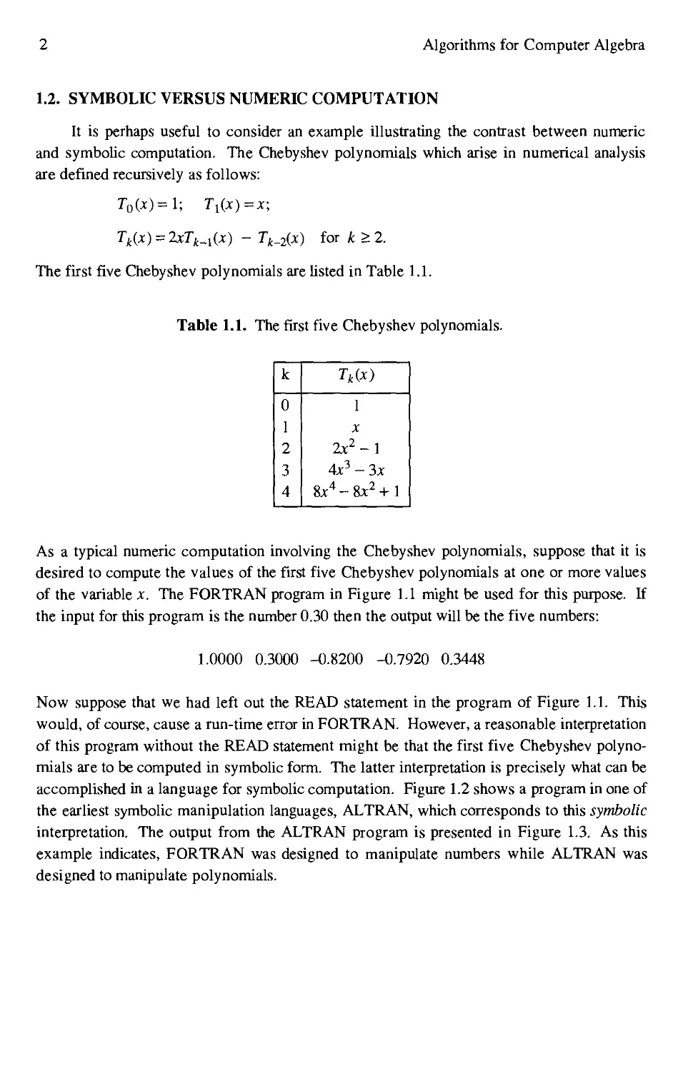
and symbolic computation. The Chebyshev polynomials which arise in numerical analysis
are defined recursively as follows:
T0(x)=l;
Tk(x) = 2xTk_l(x) - Tk_2(x) for k > 2.
The first five Chebyshev polynomials are listed in Table 1.1.
Table 1.1. The first five Chebyshev polynomials.
k
0
1
2
3
4
Tk(x)
1
X
2x2-\
4x3 - 3x
8x4-8x2+l
As a typical numeric computation involving the Chebyshev polynomials, suppose that it is
desired to compute the values of the first five Chebyshev polynomials at one or more values
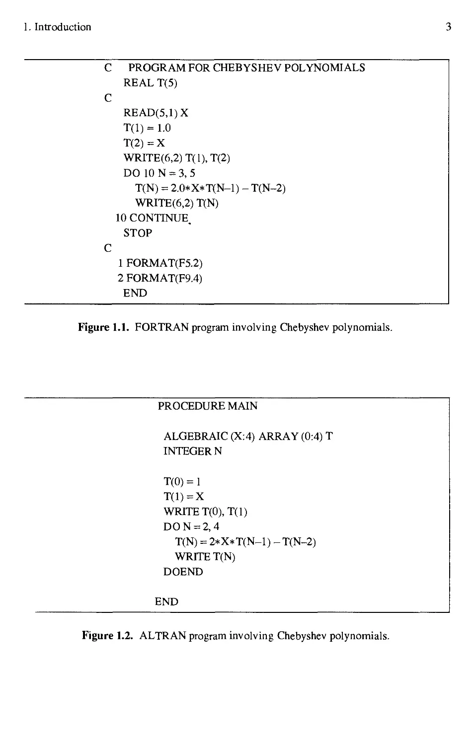
of the variable x. The FORTRAN program in Figure 1.1 might be used for this purpose. If
the input for this program is the number 0.30 then the output will be the five numbers:
1.0000 0.3000 -0.8200 -0.7920 0.3448
Now suppose that we had left out the READ statement in the program of Figure 1.1. This
would, of course, cause a run-time error in FORTRAN. However, a reasonable interpretation
of this program without the READ statement might be that the first five Chebyshev polyno-
polynomials are to be computed in symbolic form. The latter interpretation is precisely what can be
accomplished in a language for symbolic computation. Figure 1.2 shows a program in one of
the earliest symbolic manipulation languages, ALTRAN, which corresponds to this symbolic
interpretation. The output from the ALTRAN program is presented in Figure 1.3. As this
example indicates, FORTRAN was designed to manipulate numbers while ALTRAN was
designed to manipulate polynomials.
1. Introduction
C PROGRAM FOR CHEBYSHEV POLYNOMIALS
REAL TE)
C
READE,1)X
T(l) = 1.0
TB) = X
WRITEF,2)TA),TB)
DO ION = 3, 5
T(N) = 2.0*X*T(N-l) - T(N-2)
WRITEF,2) T(N)
10 CONTINUE.
STOP
C
1 FORMAT(F5.2)
2 FORMAT(F9.4)
END
Figure 1.1. FORTRAN program involving Chebyshev polynomials.
PROCEDURE MAIN
ALGEBRAIC (X:4) ARRAY @:4) T
INTEGER N
T@) = 1
TA)=X
WRITE T@),T(l)
DON = 2,4
T(N) = 2*X*T(N-1) - T(N-2)
WRITE T(N)
DOEND
END
Figure 1.2. ALTRAN program involving Chebyshev polynomials.
Algorithms for Computer Algebra
#T@)
1
#TA)
X
#TB)
2*X**2-1
#1X3)
X* D*X**2-3)
#TD)
8*X**4-8*X**2
Figure 1.3. Output from ALTRAN program in Figure 1.2.
ALTRAN can be thought of as a variant of FORTRAN with the addition of an extra
declaration, the "algebraic" type declaration. Even its name, ALTRAN, is derived from
ALgebraic TRANslator, following the naming convention of FORTRAN (derived from
FORmula TRANslator). Also, again following the spirit of FORTRAN, ALTRAN was
designed for a batch processing mode. Later, with the advent of the hand-held numeric cal-
calculator in the mid-sixties, computer algebra systems began to be designed for interactive use,
as a type of symbolic calculator. Since the early seventies, nearly all modern computer alge-
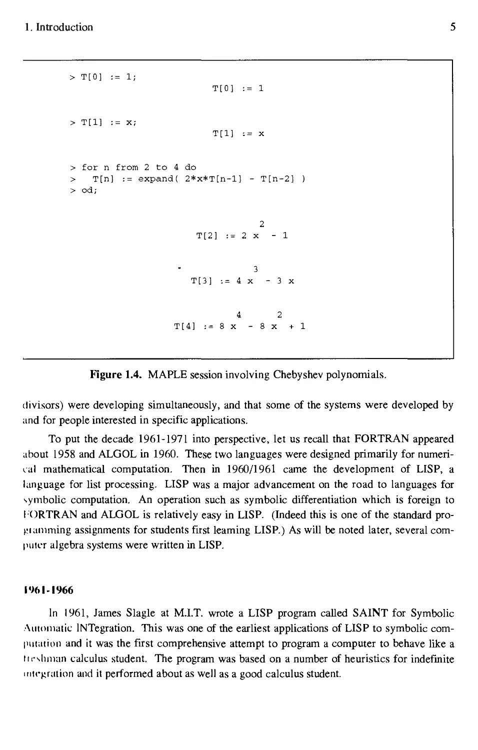
algebra systems have been designed for interactive use. In Figure 1.4 we present an example of
this approach, showing an interactive session run in one of the modern systems, MAPLE, for
performing the same computation with Chebyshev polynomials. We will return to the capa-
capabilities and usage of a modern computer algebra system in a later section.
1.3. A BRIEF HISTORICAL SKETCH
The development of systems for symbolic mathematical computation first became an
active area of research and implementation during the decade 1961-1971. During this
decade, the field progressed from birth through adolescence to at least some level of matu-
maturity. Of course, the process of maturing is a continuing process and the field of symbolic
computation is now a recognized area of research and teaching in computer science and
mathematics.
There are three recognizable, yet interdependent, forces in the development of this field.
We may classify them under the headings systems, algorithms, and applications. By systems
we mean the development of programming languages and the associated software for sym-
symbolic manipulation. Algorithms refers to the development of efficient mathematical algo-
algorithms for the manipulation of polynomials, rational functions, and more general classes of
functions. The range of applications of symbolic computation is very broad and has pro-
provided the impetus for the development of systems and algorithms. In this section, the
appearance of various programming languages (or systems) will be used as milestones in
luirtly tracing the history of symbolic mathematical compulation. It should be remembered
tli.it uncial advances in mathematical algorithms (e.g. the compulation of greatest common
1. Introduction
> T[0] :
> for n
> T[n]
> od;
= 1;
= x;
from
T[0] :
2 to 4 do
expand! 2*x*T[n-l]
T[2] := 2
T[3] := 4
4
T[4] := 8 x
= 1
= X
- T[n-2] )
2
x - 1
3
x - 3 x
2
- 8 x +1
Figure 1.4. MAPLE session involving Chebyshev polynomials.
divisors) were developing simultaneously, and that some of the systems were developed by
and for people interested in specific applications.
To put the decade 1961-1971 into perspective, let us recall that FORTRAN appeared
about 1958 and ALGOL in 1960. These two languages were designed primarily for numeri-
numerical mathematical computation. Then in 1960/1961 came the development of LISP, a
language for list processing. LISP was a major advancement on the road to languages for
symbolic computation. An operation such as symbolic differentiation which is foreign to
I-'ORTRAN and ALGOL is relatively easy in LISP. (Indeed this is one of the standard pro-
i;ianiming assignments for students fust leaming LISP.) As will be noted later, several com-
iniicr algebra systems were written in LISP.
l«N1-1966
In 1961, James Slagle at M.I.T. wrote a LISP program called SAINT for Symbolic
Automatic INTegration. This was one of the earliest applications of LISP to symbolic com-
computation and it was the first comprehensive attempt to program a computer to behave like a
ti<-slim;in calculus student. The program was based on a number of heuristics for indefinite
integration and it performed about as well as a good calculus student.
6 Algorithms for Computer Algebra
One of the first systems for symbolic computation was FORMAC, developed by Jean
Sammet, Robert Tobey, and others at IBM during the period 1962-1964. It was a FOR-
FORTRAN preprocessor (a PL/I version appeared later) and it was designed for the manipulation
of elementary functions including, of course, polynomials and rational functions. Another
early system was ALPAK, a collection of FORTRAN-callable subroutines written in assem-
assembly language for the manipulation of polynomials and rational functions. It was designed by
William S. Brown and others at Bell Laboratories and was generally available about 1964. A
language now referred to as Early ALTRAN was designed at Bell Laboratories during the
period 1964-1966. It used ALPAK as its package of computational procedures.
There were two other significant systems for symbolic computation developed during
this period. George Collins at IBM and the University of Wisconsin (Madison) developed
PM, a system for polynomial manipulation, an early version of which was operational in
1961 with improvements added to the system through 1966. The year 1965 marked the first
appearance of MATHLAB, a LISP-based system for the manipulation of polynomials and
rational functions, developed by Carl Engelman at M.I.T. It was the first interactive system
designed to be used as a symbolic calculator. Included among its many firsts was the use of
two-dimensional output to represent its mathematical output.
The work of this period culminated in the first ACM Symposium on Symbolic and
Algebraic Manipulation held in March 1966 in Washington, D.C. That conference was sum-
summarized in the August 1966 issue of the Communications of the ACM [1].
1966-1971
In 1966/1967, Joel Moses at M.I.T. wrote a LISP program called SIN (for Symbolic
INtegrator). Unlike the earlier SAINT program, SIN was algorithmic in approach and it was
also much more efficient. In 1968, Tony Hearn at Stanford University developed REDUCE,
an interactive LISP-based system for physics calculations. One of its principal design goals
was portability over a wide range of platforms, and as such only a limited subset of LISP was
actually used. The year 1968 also marked the appearance of Engelman's MATHLAB-68, an
improved version of the earlier MATHLAB interactive system, and of the system known as
Symbolic Mathematical Laboratory developed by William Martin at M.I.T. in 1967. The
latter was a linking of several computers to do symbolic manipulation and to give good
graphically formatted output on a CRT terminal.
The latter part of the decade saw the development of several important general purpose
systems for symbolic computation. ALTRAN evolved from the earlier ALPAK and Early
ALTRAN as a language and system for the efficient manipulation of polynomials and
rational functions. George Collins developed SAC-1 (for Symbolic and Algebraic Calcula-
Calculations) as the successor of PM for the manipulation of polynomials and rational functions.
CAMAL (CAMbridge ALgebra system) was developed by David Barton, Steve Bourne, and
John Filch al ihe University of Cambridge. It was implemented in the BCPL language, and
was particularly geared lo compulations in celestial mechanics and general relativity.
kl;.Dt!('!•! was redesigned by lc>7() inio REDUCE 2, a general purpose system with special
1. Introduction 7
facilities for use in high-energy physics calculations. It was written in an ALGOL-like
dialect called RLISP, avoiding the cumbersome parenthesized notation of LISP, while at the
same time retaining its original design goal of being easily portable. SCRATCHPAD was
developed by J. Griesmer and Richard Jenks at IBM Research as an interactive LISP-based
system which incorporated significant portions of a number of previous systems and pro-
programs into its library, such as MATHLAB-68, REDUCE 2, Symbolic Mathematical Library,
and SIN. Finally, the MACSYMA system first appeared about 1971. Designed by Joel
Moses, William Martin, and others at M.I.T., MACSYMA was the most ambitious system of
the decade. Besides the standard capabilities for algebraic manipulation, it included facilities
to aid in such computations as limit calculations, symbolic integration, and the solution of
equations.
The decade from 1961 to 1971 concluded with the Second Symposium on Symbolic
and Algebraic Manipulation held in March 1971 in Los Angeles [4]. The proceedings of that
conference constitute a remarkably comprehensive account of the state of the art of symbolic
mathematical computation in 1971.
1971-1981
While all of the languages and systems of the sixties and seventies began as experi-
experiments, some of them were eventually put into "production use" by scientists, engineers, and
applied mathematicians outside of the original group of developers. REDUCE, because of
iis early emphasis on portability, became one of the most widely available systems of this
decade. As a result it was instrumental in bringing computer algebra to the attention of many
new users. MACSYMA continued its strong development, especially with regard to algo-
algorithm development. Indeed, many of the standard techniques (e.g. integration of elementary
functions, Hensel lifting, sparse modular algorithms) in use today either came from, or were
strongly influenced by, the research group at M.I.T. It was by far the most powerful of the
existing computer algebra systems.
SAC/ALDES by G. Collins and R. Loos was the follow-up to Collins' SAC-1. It was a
non-interactive system consisting of modules written in the ALDES (ALgebraic DEScrip-
iion) language, with a translator converting the results to ANSI FORTRAN. One of its most
notable distinctions was in being the only major system to completely and carefully docu-
document its algorithms. A fourth general purpose system which made a significant mark in the
I-iic 1970's was muMATH. Developed by David Stoutemyer and Albert Rich at the Univer-
University of Hawaii, it was written in a small subset of LISP and came with its own programming
language, muSIMP. It was the first comprehensive computer algebra system which could
.«. tually run on the IBM family of PC computers. By being available on such small and
widely accessible personal computers, muMATH opened up the possibility of widespread
use of computer algebra systems for both research and teaching.
In addition to the systems mentioned above, a number of special purpose systems also
(•(•in-rated some interest during the 1970's. Examples of these include: SHEEP, a system for
iriisui component manipulation designed by Inge Frick and others at the University of
8 Algorithms for Computer Algebra
Stockholm; TRIGMAN, specially designed for computation of Poisson series and written in
FORTRAN by W. H. Jeffreys at University of Texas (Austin); and SCHOONSCH1P by M.
Veltman of the Netherlands for computations in high-energy physics. Although the systems
already mentioned have all been developed in North America and Europe, there were also a
number of symbolic manipulation programs written in the U.S.S.R. One of these is ANALI-
TIK, a system implemented in hardware by V. M. Glushkov and others at the Institute of
Cybernetics, Kiev.
1981-1991
Due to the significant computer resource requirements of the major computer algebra
systems, their widespread use remained (with the exception of muMATH) limited to
researchers having access to considerable computing resources. With the introduction of
microprocessor-based workstations, the possibility of relatively powerful desk-top computers
became a reality. The introduction of a large number of different computing environments,
coupled with the often nomadic life of researchers (at least in terms of workplace locations)
caused a renewed emphasis on portability for the computer algebra systems of the 1980's.
More efficiency (particularly memory space efficiency) was needed in order to run on the
workstations that were becoming available at this time, or equivalently, to service significant
numbers of users on the time-sharing environments of the day. This resulted in a movement
towards the development of computer algebra systems based on newer "systems implemen-
implementation" languages such as C, which allowed developers more flexibility to control the use of
computer resources. The decade also marked a growth in the commercialization of computer
algebra systems. This had both positive and negative effects on the field in general. On the
negative side, users not only had to pay for these systems but also they were subjected to
unrealistic claims as to what constituted the state of the art of these systems. However, on
the positive side, commercialization brought about a marked increase in the usability of com-
computer algebra systems, from major advances in user interfaces to improvements to their range
of functionality in such areas as graphics and document preparation.
The beginning of the decade marked the origin of MAPLE. Initiated by Gaston Gonnet
and Keith Geddes at the University of Waterloo, its primary motivation was to provide user
accessibility to computer algebra. MAPLE was designed with a modular structure: a small
compiled kernel of modest power, implemented completely in the systems implementation
language C (originally B, another language in the "BCPL family") and a large mathematical
library of routines written in the user-level MAPLE language to be interpreted by the kernel.
Besides the command interpreter, the kernel also contained facilities such as integer and
rational arithmetic, simple polynomial manipulation, and an efficient memory management
system. The small size of the kernel allowed it to be implemented on a number of smaller
platforms and allowed multiple users to access it on time-sharing systems. Its large
mathematical library, on the other hand, allowed it to be powerful enough to meet the
mathematical requirements of researchers.
Another system written in C was SMP (Symbolic Manipulation Program) by Stephen
Wnltium at Cultech. It was portable over a wide range of machines and differed from
1. Introduction 9
existing systems by using a language interface that was rule-based. It took the point of view
that the rule-based approach was the most natural language for humans to interface with a
computer algebra program. This allowed it to present the user with a consistent, pattern-
directed language for program development.
The newest of the computer algebra systems during this decade were M ATHEMATICA
and DERIVE. MATHEMATICA is a second system written by Stephen Wolfram (and oth-
others). It is best known as the first system to popularize an integrated environment supporting
symbolics, numerics, and graphics. Indeed when MATHEMATICA first appeared in 1988,
its graphical capabilities B-D and 3-D plotting, including animation) far surpassed any of the
graphics available on existing systems. MATHEMATICA was also one of the first systems
to successfully illustrate the advantages of combining a computer algebra system with the
easy-to-use editing features on machines designed to use graphical user-interfaces (i.e. win-
window environments). Based on C, MATHEMATICA also comes with its own programming
language which closely follows the rule-based approach of its predecessor, SMP.
DERIVE, written by David Stoutemyer and Albert Rich, is the follow-up to the suc-
successful muMATH system for personal computers. While lacking the wide range of symbolic
capabilities of some other systems, DERIVE has an impressive range of applications consid-
considering the limitations of the 16-bit PC machines for which it was designed. It has a friendly
user interface, with such added features as two-dimensional input editing of mathematical
expressions and 3-D plotting facilities. It was designed to be used as an interactive system
and not as a programming environment.
Along with the development of newer systems, there were also a number of changes to
existing computer algebra systems. REDUCE 3 appeared in 1983, this time with a number of
new packages added by outside developers. MACSYMA bifurcated into two versions,
DOE-MACSYMA and one distributed by SYMBOLICS, a private company best known for
ils LISP machines. Both versions continued to develop, albeit in different directions, during
this decade. AXIOM, (known originally as SCRATCHPAD II) was developed during this
decade by Richard Jenks, Barry Trager, Stephen Watt and others at the IBM Thomas J. Wat-
Watson Research Center. A successor to the first SCRATCHPAD language, it is the only
"strongly typed" computer algebra system. Whereas other computer algebra systems
develop algorithms for a specific collection of algebraic domains (such as, say, the field of
rational numbers or the domain of polynomials over the integers), AXIOM allows users to
write algorithms over general fields or domains.
As was the case in the previous decade, the eighties also found a number of specialized
systems becoming available for general use. Probably the largest and most notable of these
is the system CAYLEY, developed by John Cannon and others at the University of Sydney,
Australia. CAYLEY can be thought of as a "MACSYMA for group theorists." It runs in
l.iigf computing environments and provides a wide range of powerful commands for prob-
problems in computational group theory. An important feature of CAYLEY is a design geared to
answering questions not only about individual elements of an algebraic structure, but more
importantly, questions about the structure as a whole. Thus, while one could use a system
mkIi as MACSYMA or MAPLE lo decide if an element in a given domain (such as a
10 Algorithms for Computer Algebra
polynomial domain) has a given property (such as irreducibility), CAYLEY can be used to
determine if a group structure is finite or infinite, or to list all the elements in the center of
the structure (i.e. all elements which commute with all the elements of the structure).
Another system developed in this decade and designed to solve problems in computa-
computational group theory is GAP (Group Algorithms and Programming) developed by J. Neubiiser
and others at the University of Aachen, Germany. If CAYLEY can be considered to be the
"MACSYMA of group theory," then GAP can be viewed as the "MAPLE of group
theory." GAP follows the general design of MAPLE in implementing a small compiled ker-
kernel (in C) and a large group theory mathematical library written in its own programming
language.
Examples of some other special purpose systems which appeared during this decade
include FORM by J. Vermaseren, for high energy physics calculations, LiE, by A.M. Cohen
for Lie Algebra calculations, MACAULAY, by Michael Stillman, a system specially built
for computations in Algebraic Geometry and Commutative Algebra, and PARI by H. Cohen
in France, a system oriented mainly for number theory calculations. As with most of the new
systems of the eighties, these last two are also written in C for portability and efficiency.
Research Information about Computer Algebra
Research in computer algebra is a relatively young discipline, and the research litera-
literature is scattered throughout various journals devoted to mathematical computation. How-
However, its state has advanced to the point where there are two research journals primarily
devoted to this subject area: the Journal of Symbolic Computation published by Academic
Press and Applicable Algebra in Engineering, Communication and Computing published by
Springer-Verlag. Other than these two journals, the primary source of recent research
advances and trends is a number of conference proceedings. Until recently, there was a
sequence of North American conferences and a sequence of European conferences. The
North American conferences, primarily organized by ACM SIGSAM (the ACM Special
Interest Group on Symbolic and Algebraic Manipulation), include SYMSAM '66 (Washing-
(Washington, D.C.), SYMSAM '71 (Los Angeles), SYMSAC '76 (Yorktown Heights), SYMSAC '81
(Snowbird), and SYMSAC '86 (Waterloo). The European conferences, organized by SAME
(Symbolic and Algebraic Manipulation in Europe) and ACM SIGSAM, include the follow-
following whose proceedings have appeared in the Springer-Verlag series Lecture Notes in Com-
Computer Science: EUROSAM '79 (Marseilles), EUROCAM '82 (Marseilles), EUROCAL '83
(London), EUROSAM '84 (Cambridge), EUROCAL '85 (Linz), and EUROCAL '87
(Leipzig). Starting in 1988, the two streams of conferences have been merged and they are
now organized under the name ISSAC (International Symposium on Symbolic and Algebraic
Computation), including ISSAC '88 (Rome), ISSAC '89 (Portland, Oregon), ISSAC '90
(Tokyo), ISSAC '91 (Bonn) and ISSAC '92 (Berkeley).
1. Introduction 11
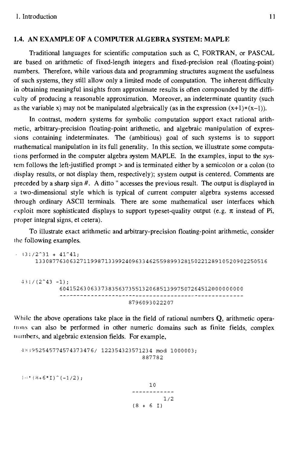
1.4. AN EXAMPLE OF A COMPUTER ALGEBRA SYSTEM: MAPLE
Traditional languages for scientific computation such as C, FORTRAN, or PASCAL
are based on arithmetic of fixed-length integers and fixed-precision real (floating-point)
numbers. Therefore, while various data and programming structures augment the usefulness
of such systems, they still allow only a limited mode of computation. The inherent difficulty
in obtaining meaningful insights from approximate results is often compounded by the diffi-
difficulty of producing a reasonable approximation. Moreover, an indeterminate quantity (such
as the variable x) may not be manipulated algebraically (as in the expression (x+l)*(x-l)).
In contrast, modern systems for symbolic computation support exact rational arith-
arithmetic, arbitrary-precision floating-point arithmetic, and algebraic manipulation of expres-
expressions containing indeterminates. The (ambitious) goal of such systems is to support
mathematical manipulation in its full generality. In this section, we illustrate some computa-
lions performed in the computer algebra system MAPLE. In the examples, input to the sys-
system follows the left-justified prompt > and is terminated either by a semicolon or a colon (to
display results, or not display them, respectively); system output is centered. Comments are
preceded by a sharp sign #. A ditto " accesses the previous result. The output is displayed in
a two-dimensional style which is typical of current computer algebra systems accessed
ihrough ordinary ASCII terminals. There are some mathematical user interfaces which
exploit more sophisticated displays to support typeset-quality output (e.g. n instead of Pi,
proper integral signs, et cetera).
To illustrate exact arithmetic and arbitrary-precision floating-point arithmetic, consider
i he following examples.
■ !3!/2~31 + 41-41;
13 3 0877 53 0 53 2711998713 3 992409 53 3 4 52 5 59 8993 2815022128910 5209 02250515
■13 !/B~43 -1) ;
504152 53 0 533 73 83 55373 5513 20 58513 997507254512000 0 0 000 0
8795093022207
While the above operations take place in the field of rational numbers Q, arithmetic opera-
operations can also be performed in other numeric domains such as finite fields, complex
numbers, and algebraic extension fields. For example,
■1H (952545774574373475/ 12235432357123 4 mod 1000003;
887782
1>'(H+6*I)~(-1/2);
10
1/2
(8+5 1)
12 Algorithms for Computer Algebra
> evalc( " ) ;
3-1
In the last calculation, the command ' 'evalc'' is used to place the result in standard complex
number form, where "I" denotes the square root of -1. A similar approach is used by
MAPLE when operating in domains such as algebraic extensions and Galois fields.
Computer algebra systems also allow for the use of other common mathematical con-
constants and functions. Such expressions can be reduced to simplified forms.
> sqrtA5523/3 - 98/2);
1/2
124/3 3
a-.= sin(Pi/3) * expB + lnC3));
1/2
a := 1/2 3 expB + lnC3))
> simplify(a);
1/2
33/2 3 expB)
> evalf(a);
211.1706396
In the above, the command "evalf" (evaluate in floating-point mode) provides a decimal
expansion of the real value. The decimal expansion is computed to 10 digits by default, but
the precision can be controlled by the user either by re-setting a system variable (the global
variable "Digits") or by passing an additional parameter to the evaluation function as in
> evalf(a, 60) ;
211.17 0 63 9 62 4855418173 45701694995293 53197 6323 845853 5271731859
Also among the numerical capabilities of computer algebra systems are a wide variety
of arithmetic operations over the integers, such as factorization, primality testing, finding
nearest prime numbers, and greatest common divisor (GCD) calculations.
> n.-= 19380287199092196525608598055990942841820;
n := 19380287199092196525608598055990942841820
> isprime(n);
false
> ifactor(n);
2 2 3 4 2
B) C) E) A9) A01) A2282045523619)
1. Introduction 13
> nextprime(n) ;
1938 028719909219 6525 60 8 598 0559909428420 43
> igcdA5990335972848346968323925788771404985, 15163659044370489780);
1263638253697540815
It should be apparent that in the previous examples each numerical expression is
evaluated using the appropriate rules of algebra for the given number system. Notice that the
arithmetic of rational numbers requires integer GCD computations because every result is
automatically simplified by removing common factors from numerator and denominator. It
should also be clear that such manipulations may require much more computer time (and
memory space) than the corresponding numerical arithmetic in, say, FORTRAN. Hence, the
efficiency of the algorithms which perform such tasks in computer algebra systems is a
major concern.
Computer algebra systems can also perform standard arithmetic operations over
domains requiring the use of symbolic variables. Examples of such algebraic structures
include polynomial and power series domains along with their quotient fields. Typical exam-
examples of algebraic operations include expansion ("expand"), long division ("quo'Y'rem"),
normalization of rational functions ("normal"), and GCD calculation ("gcd").
> a := (x + y)~12 - (x - y)~12;
12 12
a := (x + y) - (x - y)
expand(a) ;
11 39 57 75 93 11
24 y x + 440 y x + 1584 y x + 1584 y x + 440 y x + 24 y x
quo( x~3*y-x~3*z+2*x~2*y~2-2*x~2*z~2+x*y~3+ x*y~2*z-x*z~3, x+y + z, x) ;
2 2 2 2
(y-z)x +(y -z)x+z y
<jcd( x~3*y-x~3*z+2*x~2*y~2-2*x~2*z~2+x*y~3+ x*y*z-x*z~3, x+y + z );
1
I. := (x - y~4)/(x~3 + y~3) - (x + y~5)/(x~4 - y~4);
4 4 5 5
x - y x + y
b != .
3 3 4 4
x + y x - y
14 Algorithms for Computer Algebra
> normal (b) ;
3 3
x y
3 2 2 3 2 2
(x -x y + xy -y) (x -xy + y)
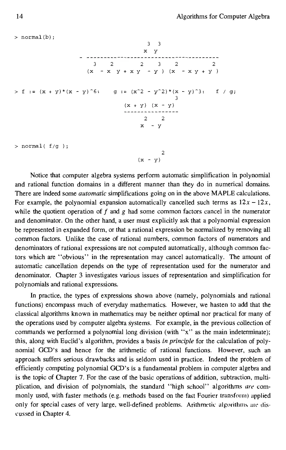
> f := (x + y)*(x - y)~6: g := (x~2 - y~2)*(x - y)~3: f / g;
3
(x + y) (x - y)
2 2
k - y
> normal( f/g );
2
(x - y)
Notice that computer algebra systems perform automatic simplification in polynomial
and rational function domains in a different manner than they do in numerical domains.
There are indeed some automatic simplifications going on in the above MAPLE calculations.
For example, the polynomial expansion automatically cancelled such terms as 12x - 12x,
while the quotient operation of / and g had some common factors cancel in the numerator
and denominator. On the other hand, a user must explicitly ask that a polynomial expression
be represented in expanded form, or that a rational expression be normalized by removing all
common factors. Unlike the case of rational numbers, common factors of numerators and
denominators of rational expressions are not computed automatically, although common fac-
factors which are "obvious" in the representation may cancel automatically. The amount of
automatic cancellation depends on the type of representation used for the numerator and
denominator. Chapter 3 investigates various issues of representation and simplification for
polynomials and rational expressions.
In practice, the types of expressions shown above (namely, polynomials and rational
functions) encompass much of everyday mathematics. However, we hasten to add that the
classical algorithms known in mathematics may be neither optimal nor practical for many of
the operations used by computer algebra systems. For example, in the previous collection of
commands we performed a polynomial long division (with "x" as the main indeterminate);
this, along with Euclid's algorithm, provides a basis in principle for the calculation of poly-
polynomial GCD's and hence for the arithmetic of rational functions. However, such an
approach suffers serious drawbacks and is seldom used in practice. Indeed the problem of
efficiently computing polynomial GCD's is a fundamental problem in computer algebra and
is the topic of Chapter 7. For the case of the basic operations of addition, subtraction, multi-
multiplication, and division of polynomials, the standard "high school" algorithms are com-
commonly used, with faster methods (e.g. methods based on the fast Fourier transform) applied
only for special cases of very large, well-defined problems. Arithmetic algorithms arc dis-
discussed in Chapter 4.
1. Introduction 15
A fundamental operation in all computer algebra systems is the ability to factor polyno-
polynomials (both univariate and multivariate) defined over various coefficient domains. Thus, for
example, we have
> factor(x~6 - x~5 + x~2 + 1);
6 5 2
X - X + X +1
> factorE*x~4 - 4*x~3 - 48*x~2 + 44*x + 3);
2
(x - 1) (x - 3) E x + 16 x + 1)
> Factor(x~6 - x + x + 1) mod 13 ;
3 2 - 3 2
(x + 10 x + 8 x + 11) (x + 2 x + 11 x + 6)
FactorE*x~4 - 4*x~3 - 48*x~2 + 44*x + 3) mod 13 ;
2
5 (x + 12) (x + 10) (x + 11 x + 8)
factor(x~12 - y~12) ;
2 2 2 2224224
(x-y)(x +xy+y)(x+y)(y -xy+x)(x +y)(x -x y + y )
alias ( a = RootOf( x~4 - 2 ) ):
factor( x~12 - 2*x~8 + 4*x~4 - 8 , a );
4 2 4 2 2 2
(x - 2 x + 2) (x + 2 x + 2) (x - a) (x + a) (x + a )
• Factor! x~6 - 2*x~4 + 4*x~2 - 8 , a ) mod 5;
2 2
(x + 4) (x + 2) (x + 1) (x + a ) (x + 4 a ) (x + 3)
In the previous examples, the first two factorizations are computed in the domain Z[x],
ihe next two in the domain Z13[x], and the fifth in Z[x,y]. The sixth example asks for a fac-
iiii ization of a polynomial over QB1/4), an algebraic extension of Q. The last example is a
t;iclorization of a polynomial over the coefficient domain Z5B1/4), a Galois field of order
''25. The command "alias" in the above examples is used to keep the expressions readable
(It'll ing "a" denote a fourth root of 2).
While polynomial factorization is a computationally intensive operation for these sys-
irms, il is interesting to note that the basic tools require little more than polynomial GCD
i .ik illations, some matrix algebra over finite fields, and finding solutions of simple diophan-
inif equations. Algorithms for polynomial factorization are discussed in Chapter 8 (with prel-
preliminaries in Chapter 6).
16 Algorithms for Computer Algebra
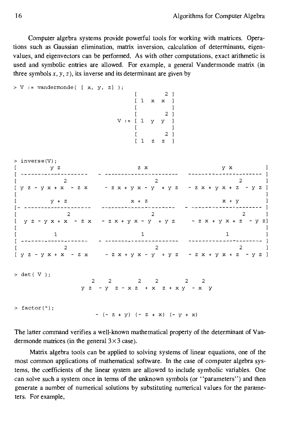
Computer algebra systems provide powerful tools for working with matrices. Opera-
Operations such as Gaussian elimination, matrix inversion, calculation of determinants, eigen-
eigenvalues, and eigenvectors can be performed. As with other computations, exact arithmetic is
used and symbolic entries are allowed. For example, a general Vandermonde matrix (in
three symbols x, y, z), its inverse and its determinant are given by
> V := vandermonde ( [ x, y, z] );
[
[
[
V := [
[
[
1
1
1
X
y
z
2 ]
X
2
y
2
z
> inverse (V) ;
[ y z
[2 2 2 ]
[yz-yx + x -zx -zx + yx-y +yz -zx + yx+z -yz]
[ ]
[ y+z x+z x + y ]
[ ]
[2 2 2 ]
[ yz-yx + x -zx -zx + yx-y +yz -zx + yx+z -yz]
[2 2 2
[yz-yx + x -zx -zx + yx-y +yz -zx + yx + z -yz
> det( V );
2 2 2 2 2 2
yz -y z-xz +x z + xy -x y
> factor(");
- (- z + y) (- z + x) (- y + x)
The latter command verifies a well-known mathematical property of the determinant of Van-
Vandermonde matrices (in the general 3x3 case).
Matrix algebra tools can be applied to solving systems of linear equations, one of the
most common applications of mathematical software. In the case of computer algebra sys-
systems, the coefficients of the linear system are allowed to include symbolic variables. One
can solve such a system once in terms of the unknown symbols (or "parameters") and then
generate a number of numerical solutions by substituting numerical values for the parame-
parameters. For example,
1. Introduction 17
> equationl := ( 1 - eps)*x +2*y-4*z-l=0:
> equation2 := C/2 - eps)*x +3*y-5*z-2=0:
> equation3 := E/2 + eps)*x + 5*y - 7*z -3=0:
solutions := solve ( {equationl, equation2, equation3}, {x, y, z} );
1 1+7 eps
solutions := {x = , z = 3/4, y = 1/4 }
2 eps eps
> subs( eps=10~(-20), solutions ) ;
{z = 3/4, x = -50000000000000000050, y = 100000000000000000007/4}
where the last command substitutes the value eps = 1(T20 into the solution of the linear sys-
system. For numerical computation, the parameters must be given numerical values prior to
solving the system, and the process must be repeated for any other parameter values of
interest. The results generated from numerical computation are also subject to round-off
error since exact arithmetic is not used. Indeed, the above example would cause difficulties
for numerical techniques using standard-precision arithmetic. Of course, using exact arith-
arithmetic and allowing symbolic parameters requires specialized algorithms to achieve time and
memory space efficiency. Chapter 9 discusses algorithms for solving equations.
Solving a linear system typically involves "eliminating" unknowns from equations to
obtain a simplified system, usually a triangularized system which is then easy to solve. It is
less well known that a similar approach is also available for systems of nonlinear polynomial
equations. Chapters 9 and 10 provide an introduction to classical and modern techniques for
solving systems of polynomial equations.
As an example of solving a nonlinear system of equations, consider the problem of
(hiding the critical points of a bivariate function:
I := x *y*(l - x - y):
<iuationl := diff( f, x ); equation2 *.- diff( f, y ) ;
3 2 2
equationl :=2xy(l-x-y) -3x y(l-x-y)
2 3 2 2
equation2 := x A-x-y) -3x y(l-x-y)
i<>lve( (equationl, equation2}, {x,y} ) ;
(x = 0, y = y}, {y = 0, x = 1}, {y = 1/6, x = 1/3}, {y = y, x = 1 - y}
which gives two critical points along with two lines of singularity. One could then obtain
mmr information about the types of singularities of this function by using MAPLE to calcu-
l.iir the Hessian of the function at all the critical points, or more simply by plotting a 3-D
(•i.i|ih of ihe function.
18 Algorithms for Computer Algebra
One of the most useful features of computer algebra systems is their ability to solve
problems from calculus. Operations such as computing limits, differentiation of functions,
calculation of power series, definite and indefinite integration, and solving differential equa-
equations can be performed. We have already illustrated the use of MAPLE for calculus when we
determined the critical points of a function. Some additional examples are
> limit ( tan(x) / x , x=0 );
> diff ( ln(sec(x)), x );
tan(x)
> series! tan( sinh(x) ) - sinh( tan(x) ), x=0, 15 );
7 13 9 1451 11 6043 13 15
1/90 x + x + x + x + O(x )
756 75600 332640
> series! BesselJ@,x)/Besselj(l,x) , x, 12 );
-1 3 5 7 13 9 10
2 x - 1/4 x - 1/96 x - 1/1536 x - 1/23040 x x + O(x )
4423680
where the last example gives the Laurent series for the ratio of the two Bessel functions of
the first kind, J0(x) and Ji(x).
The ability to differentiate, take limits, or calculate Taylor (or Laurent) series as above
does not surprise new users of computer algebra systems. These are mainly algebraic opera-
operations done easily by hand for simple cases. The role of the computer algebra system is to
reduce the drudgery (and to eliminate the calculation errors!) of a straightforward, easy to
understand, yet long calculation. The same cannot be said for solving the indefinite integra-
integration problem of calculus. Integration typically is not viewed as an algorithmic process, but
rather as a collection of tricks which can only solve a limited number of integration prob-
problems. As such, the ability of computer algebra systems to calculate indefinite integrals is very
impressive for most users. These systems do indeed begin their integration procedures by
trying some heuristics of the type learned in traditional calculus courses. Indeed, until the
late sixties this was the only approach available to computer algebra systems. However, in
1969 Robert Risch presented a decision procedure for the indefinite integration of a large
class of functions known as the elementary functions. This class of functions includes the
typical functions considered in calculus courses, such as the exponential, logarithm, tri-
trigonometric, inverse trigonometric, hyperbolic, and algebraic functions. (Additional research
contributions in succeeding years have led to effective algorithms for integration in most
cases, although the case of general algebraic functions can require a very large amount of
computation.) The Risch algorithm either determines a closed formula expressing the
integral as an elementary function, or else it proves that it is impossible to express the
integral as an elementary function. Some examples of integration follow.
1. Introduction 19
int( (C*x~2 - 7*x + 15)*exp(x) + 3*x~2 - 14)/(x - exp(x))~2, x ) ;
2
3 x - x + 14
x - exp(x)
> int( C*x~3 - x + 14)/(x + 4*x - 4), x );
2 2 1/2 1/2
3/2 x - 12 x + 59/2 ln(x + 4 x - 4) + 38 2 arctanh(l/8 B x + 4) 2 )
> int( x*exp( x ), x );
I 3
I x exp(x ) dx
I
In the latter case, the output indicates that no dosed form for the integral exists (as an ele-
elementary function). Chapters 11 and 12 develop algorithms for the integration problem.
Computer algebra systems are also useful for solving differential, or systems of dif-
differential, equations. There are a large number of techniques for solving differential equations
which are entirely algebraic in nature, with the methods usually reducing to the computation
of integrals (the simplest form of differential equations). Unlike the case of indefinite
integration, there is no known complete decision procedure for solving differential equations.
For differential equations where a closed form solution cannot be determined, often one can
compute an approximate solution; for example, a series solution or a purely numerical solu-
tion. As an example, consider the following differential equation with initial conditions.
■ diff_eqn := diff(y(x), x$2) + t*diff(y(x), x) - 2*t~2*y(x) = 0;
/ 2 \
Id I / d \ 2
diff_eqn := I y(x)| + t I y(x)l - 2 t y(x) = 0
12 I \ dx /
\ dx /
init_conds := y@) = t, D(y)@) = 2*t~2;
2
init_conds := y@) = t, D(y)@) = 2 t
.l:n>lve( (diff_eqn, init_conds}, y(x));
y(x) = 4/3 t exp(t x) - 1/3 t exp(- 2 t x)
Designers of computer algebra systems cannot anticipate the needs of all users. There-
li'ic it is important that systems include a facility for programming new functionality, so that
individual users can expand the usefulness of the system in directions that they find neces-
■..uy it interesting. Trie programming languages found in computer algebra systems typi-
> .illy provide a rich set of data structures and programming constructs which allow users to
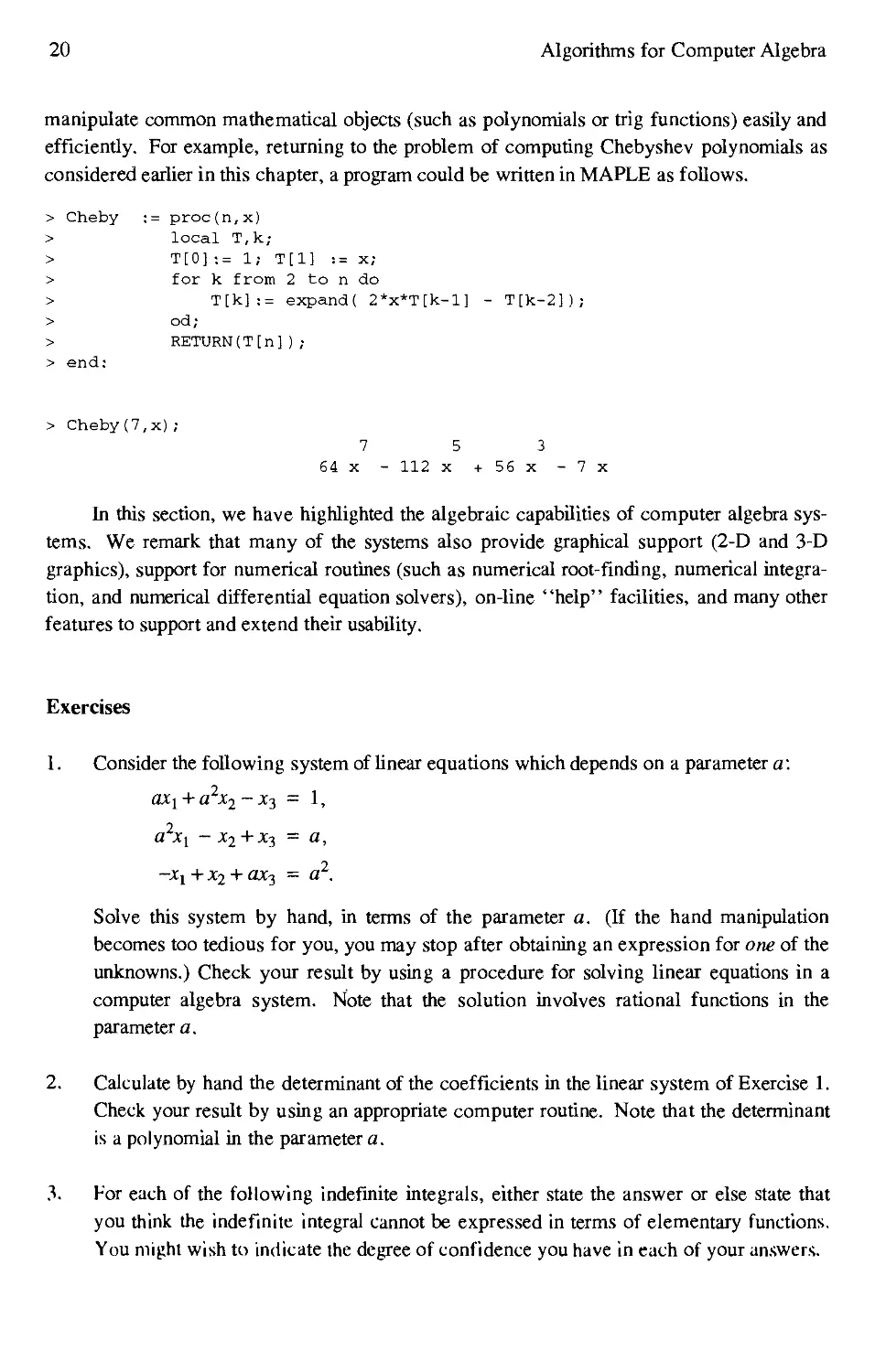
20 Algorithms for Computer Algebra
manipulate common mathematical objects (such as polynomials or trig functions) easily and
efficiently. For example, returning to the problem of computing Chebyshev polynomials as
considered earlier in this chapter, a program could be written in MAPLE as follows.
> Cheby := proc(n,x)
> local T,k;
> T[0]:= 1; T[l] := x;
> for k from 2 to n do
> T[k]:= expand( 2*x*T[k-l] - T[k-2]);
> od;
> RETURN(T[n]);
> end:
> ChebyG,x);
7 5 3
64 x - 112 x + 56 x - 7 x
In this section, we have highlighted the algebraic capabilities of computer algebra sys-
systems. We remark that many of the systems also provide graphical support B-D and 3-D
graphics), support for numerical routines (such as numerical root-finding, numerical integra-
integration, and numerical differential equation solvers), on-line "help" facilities, and many other
features to support and extend their usability.
Exercises
1. Consider the following system of linear equations which depends on a parameter a:
axl + a2x2- Xj = 1,
-xl +x2 + ax3 - a2.
Solve this system by hand, in terms of the parameter a. (If the hand manipulation
becomes too tedious for you, you may stop after obtaining an expression for one of the
unknowns.) Check your result by using a procedure for solving linear equations in a
computer algebra system. Note that the solution involves rational functions in the
parameter a.
2. Calculate by hand the determinant of the coefficients in the linear system of Exercise 1.
Check your result by using an appropriate computer routine. Note that the determinant
is a polynomial in the parameter a.
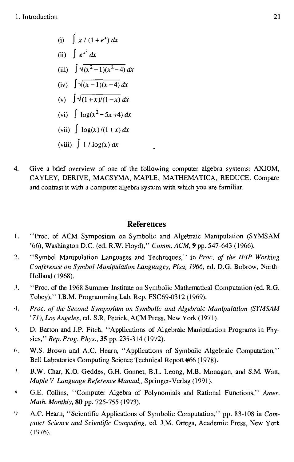
3. For each of the following indefinite integrals, either state the answer or else state that
you think the indefinite integral cannot be expressed in terms of elementary functions.
You might wish to indicate the degree of confidence you have in each of your answers.
1. Introduction 21
(i) \xl{\+ex)dx
(ii) J ex* dx
(iii) J V(x2-l)(x2-4) fltc
(iv) JV(jt-l)(jt-4)dr
(v) JV
(vi) J Iog(x2-5x+4)fltt
(vii) J log(x)/(l+x)flbc
(viii) J 1 / log(x) dx
4. Give a brief overview of one of the following computer algebra systems: AXIOM,
CAYLEY, DERIVE, MACSYMA, MAPLE, MATHEMATICA, REDUCE. Compare
and contrast it with a computer algebra system with which you are familiar.
References
1. "Proc. of ACM Symposium on Symbolic and Algebraic Manipulation (SYMSAM
'66), Washington D.C. (ed. R.W. Floyd)," Comm. ACM, 9 pp. 547-643 A966).
2. "Symbol Manipulation Languages and Techniques," in Proc. of the IFIP Working
Conference on Symbol Manipulation Languages, Pisa, 1966, ed. D.G. Bobrow, North-
Holland A968).
.1. "Proc. of the 1968 Summer Institute on Symbolic Mathematical Computation (ed. R.G.
Tobey)," I.B.M. Programming Lab. Rep. FSC69-0312 A969).
•I. Proc. of the Second Symposium on Symbolic and Algebraic Manipulation (SYMSAM
'71), Los Angeles, ed. S.R. Petrick, ACM Press, New York A971).
*>. D. Barton and J.P. Fitch, "Applications of Algebraic Manipulation Programs in Phy-
Physics," Rep. Prog. Phys., 35 pp. 235-314 A972).
'i. W.S. Brown and A.C. Hearn, "Applications of Symbolic Algebraic Computation,"
Bell Labratories Computing Science Technical Report #66 A978).
/. B.W. Char, K.O. Geddes, G.H. Gonnet, B.L. Leong, M.B. Monagan, and S.M. Watt,
Maple V Language Reference Manual,, Springer-Verlag A991).
N G.E. Collins, "Computer Algebra of Polynomials and Rational Functions," Amer.
Math. Monthly, 80 pp. 725-755 A973).
'' A.C. Hearn, "Scientific Applications of Symbolic Computation," pp. 83-108 in Com-
Computer Science and Scientific Computing, ed. J.M. Ortega, Academic Press, New York
22 Algorithms for Computer Algebra
10. A.D. Hall Jr., "The Altran System for Rational Function Manipulation - A Survey,"
Comm.ACM, 14 pp. 517-521 A971).
11. J. Moses, "Algebraic Simplification: A Guide for the Perplexed," Comm. ACM, 14 pp.
527-537 A971).
12. J. Moses, "Algebraic Structures and their Algorithms," pp. 301-319 in Algorithms and
Complexity, ed. J.F. Traub, Academic Press, New York A976).
CHAPTER 2
ALGEBRA OF POLYNOMIALS,
RATIONAL FUNCTIONS,
AND POWER SERIES
2.1. INTRODUCTION
In this chapter we present some basic concepts from algebra which are of central impor-
importance in the development of algorithms and systems for symbolic mathematical computation.
The main issues distinguishing various computer algebra systems arise out of the choice of
algebraic structures to be manipulated and the choice of representations for the given alge-
algebraic structures.
2.2. RINGS AND FIELDS
A group (G; o) is a nonempty set G, closed under a binary operation o satisfying the
axioms:
Al: a o(b oc) = (a ob)oc for all a, b, c e G (Associativity)
A2: There is an element e e G such that
e oa = a oe =a for all a e G (Identity).
A3: For all oeG, there is an element a~l 6 G such that
a oa = a oa = e (Inverses).
An abelian group (or, commutative group) is a group in which the binary operation o satisfies
ihe additional axiom:
A4: aob=boa foralla,foeG (Commutativity).
A ring (R; +, •) is a nonempty set R closed under two binary operations + and • such
iluii (R; +) is an abelian group (i.e. axioms A1-A4 hold with respect to +), • is associative and
tus ;ui identity (i.e. axioms A1-A2 hold with respect to •). and which satisfies the additional
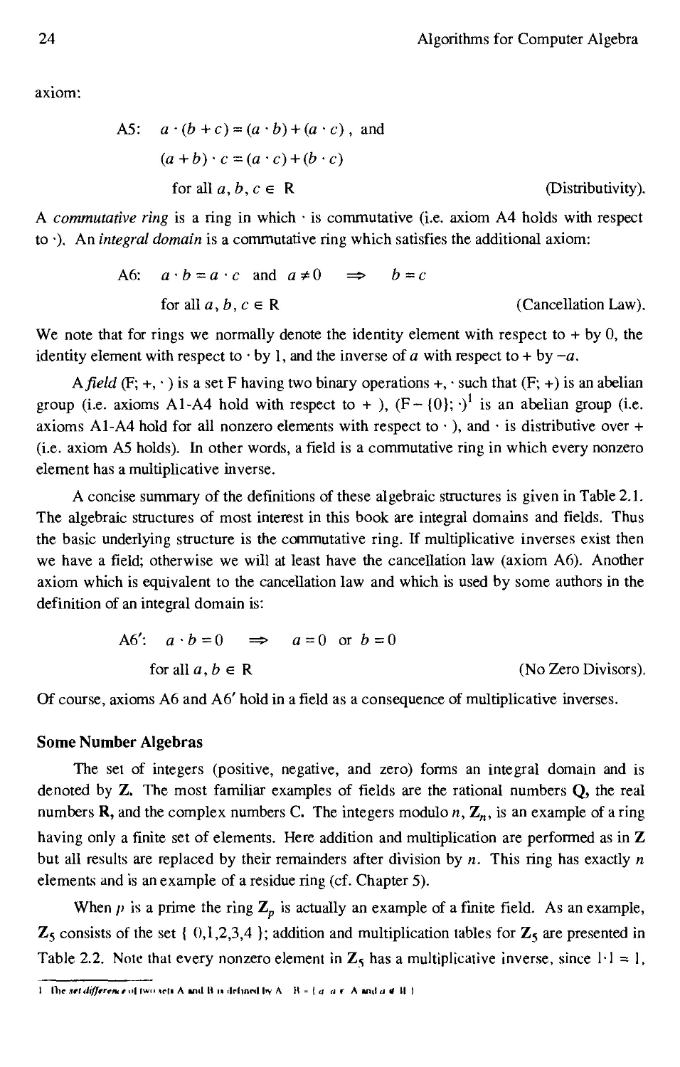
24 Algorithms for Computer Algebra
axiom:
A5: a ■ (b + c) = (a • b) + (a • c), and
(a+b) ■ c-(a -c) + (b • c)
for all a, b, c e R (Distributivity).
A commutative ring is a ring in which ■ is commutative (i.e. axiom A4 holds with respect
to •). An integral domain is a commutative ring which satisfies the additional axiom:
A6: a ■ b -a • c and a *0 =s- b = c
for all a, b, c e R (Cancellation Law).
We note that for rings we normally denote the identity element with respect to + by 0, the
identity element with respect to • by 1, and the inverse of a with respect to + by -a.
Afield (F; +, •) is a set F having two binary operations +, • such that (F; +) is an abelian
group (i.e. axioms A1-A4 hold with respect to + ), (F- {0}; •) is an abelian group (i.e.
axioms A1-A4 hold for all nonzero elements with respect to • ), and • is distributive over +
(i.e. axiom A5 holds). In other words, a field is a commutative ring in which every nonzero
element has a multiplicative inverse.
A concise summary of the definitions of these algebraic structures is given in Table 2.1.
The algebraic structures of most interest in this book are integral domains and fields. Thus
the basic underlying structure is the commutative ring. If multiplicative inverses exist then
we have a field; otherwise we will at least have the cancellation law (axiom A6). Another
axiom which is equivalent to the cancellation law and which is used by some authors in the
definition of an integral domain is:
A6': a-b=0 =£■ a=0 or b=0
for all a, b e R (No Zero Divisors).
Of course, axioms A6 and A6' hold in a field as a consequence of multiplicative inverses.
Some Number Algebras
The sei of integers (positive, negative, and zero) forms an integral domain and is
denoted by Z. The most familiar examples of fields are the rational numbers Q, the real
numbers R, and the complex numbers C. The integers modulo n, Zn, is an example of a ring
having only a finite set of elements. Here addition and multiplication are performed as in Z
but all results are replaced by their remainders after division by n. This ring has exactly n
elements and is an example of a residue ring (cf. Chapter 5).
When /; is a prime the ring Zp is actually an example of a finite field. As an example,
Z5 consists of the set { 0,1,2,3,4 }; addition and multiplication tables for Z5 are presented in
Table 2.2. Note that every nonzero element in Zs has a multiplicative inverse, since 1-1 = 1,
1 lltr jet different e u| lw>> td» A Mill It u >lrftiml by A H = I it it r A ant! 11 tf II ]
2. Algebra of Polynomials
25
Table 2.1. Definitions of algebraic structures.
Structure
Group
Abelian Group
Ring
Commutative Ring
Integral Domain
Field
Notation
(G;o)
(G;o)
(R; +, ■)
(R; +, ■)
(D; +, 0
(F; +, •)
Axioms
Al; A2; A3
Al; A2; A3; A4
Al; A2; A3; A4 w.r.t. +
Al; A2 w.r.t. •
A5
Al; A2; A3; A4 w.r.t. +
Al; A2; A4w.r.t. •
A5
Al; A2; A3;A4w.r.t. +
Al; A2; A4 w.r.t. •
A5; A6
Al; A2; A3; A4w.r.t. +
Al; A2; A3; A4for F-{0} w.r.t. •
A5
(Note: A6 holds as a consequence.)
2 3 = 1,3-2 = 1, and 4-4 =1. If we consider the integers modulo n, Zn, for some non-prime
inieger n, then some nonzero elements will not have multiplicalive inverses. Zn is, in gen-
general, a commutative ring but not even an integral domain. For example, in Z12 we have
2 6 = 0. For finite rings, the concepts of the cancellation law (or, no zero divisors) and the
existence of multiplicative inverses turn out to be equivalent; in other words, every finite
integral domain is a field (cf. Exercise 2.7).
Table 2.2. Addition and multiplication tables for Z5
+
0
1
2
3
4
0
0
1
2
3
4
1
1
2
3
4
0
2
2
3
4
0
1
3
3
4
0
1
2
4
4
0
1
2
3
0
1
2
3
4
0
0
0
0
0
0
1
0
1
2
3
4
2
0
2
4
1
3
3
0
3
1
4
2
4
0
4
3
2
1
26 Algorithms for Computer Algebra
2.3. DIVISIBILITY AND FACTORIZATION IN INTEGRAL DOMAINS
The concept of divisibility plays a central role in symbolic computation. Of course
division is always possible in a field. In an integral domain division is not possible, in gen-
general, but the concept of factorization into primes which is familiar for the integers Z can be
generalized to other integral domains. Throughout this section, D denotes an integral
domain. Here and in the sequel, we adopt the standard mathematical convention of omitting
the ■ symbol for multiplication.
Greatest Common Divisors
Definition 2.1. For a, b e D, a is called a divisor of b if b = ax for some jeD, and we say
that a divides b (notationally, a \ b). Correspondingly, b is called a multiple of a.
Definition 2.2. For a,b e D, an element c e D is called a greatest common divisor (GCD)
of a and b if c \ a and c \ b and c is a multiple of every other element which divides both a
andfr.
Definition 2.3. For a, b e D, an element c e D is called a least common multiple (LCM) of
a and b if a \ c and b \ c and c is a divisor of every other element which is a multiple of both
a andfo.
The most familiar application of GCD's is in reducing rational numbers (i.e. quotients
of integers) to "lowest terms". Another role of GCD's in symbolic computation is the
corresponding problem of reducing rational functions (i.e. quotients of polynomials) to
"lowest terms". The use of the phrase "a GCD" rather than "the GCD" is intentional. A
GCD of two elements a,b e D, when it exists, is not unique (but almost).
Definition 2.4. Two elements a, b e D are called associates if a \ b and b \ a.
Definition 2.5. An element u e D is called a unit (or invertible) if u has a multiplicative
inverse in D.
Example 2.1.
In the integral domain Z of integers, note the following facts,
(i) The units in Z are 1 and-1.
(ii) 6 is a GCD of 18 and 30.
(iii) ^6 is also a GCD of 18 and 30.
(iv) 6 and -6 are associates.
2. Algebra of Polynomials 27
It can be easily proved that in any integral domain D, two elements c and d are associ-
associates if and only if cu = d for some unit u. It is also easy to verify that if c is a GCD of
a and b then so is any associate d =cu, and conversely if c and d are GCD's of a and b then
c must be an associate of d. In the integral domains of interest in symbolic computation, it is
conventional to impose an additional condition on the GCD in order to make it unique. This
is accomplished by noting that the relation of associativity is an equivalence relation, which
therefore decomposes an integral domain into associate classes. (For example, the associate
classes in Z are {0}, {1, -1}, {2, -2}, ) For a particular integral domain, a criterion is
chosen to single out one element of each associate class as its canonical representative and
define it to be unit normal. In the integral domain Z we will define the nonnegative integers
to be unit normal. In any field F, every nonzero element is an associate of every other
nonzero element (in fact, every nonzero element is a unit). In this case we define the ele-
elements 0 and 1 to be unit normal.
Definition 2.6. In any integral domain D for which unit normal elements have been defined,
an element c is called the unit normal GCD of a, b e D, denoted c=GCD(a,b), if c is a
GCD of a and b and c is unit normal.
Clearly the unit normal GCD of two elements a,b e D is unique (once the unit normal
elements have been defined). For each integral domain D of interest in this book, unit nor-
normal elements will be appropriately defined and the following properties will always hold:
A) 0 is unit normal;
B) 1 is the unit normal element for the associate class of units;
C) if a, b e D are unit normal elements then their product ab is also a unit nor-
normal element in D.
In the sequel, whenever we refer to the GCD of a, b e D it is understood that we are refer-
iing lo the unique unit normal GCD.
1 xample 2.2. In the integral domain Z, GCDA8,30) = 6.
Definition 2.7. Let D be an integral domain in which unit normal elements have been
(let incd. The normal part of a e D, denoted n(a), is defined to be the unit normal representa-
ii vi- of the associate class containing a. The unit part of a e D (a *0), denoted u(a), is the
unique unit in D such that
a = u(a) n(a)
i 'It-iirly n@) = 0 and it is convenient to define u@) = 1.
28 Algorithms for Computer Algebra
Example 2.3. In the integral domain Z, n(a) = I a I and u(a) = sign(a) where the sign of an
integer is defined by
f ifa<0
sign(a)=
The LCM of two elements a,b e D, when it exists, can be made unique in a similar
manner. It can be verified that a LCM of a,b e D exists if and only if GCD(a,b) exists.
Moreover, GCD(a, b) is clearly a divisor of the product ab and it easy to verify that the ele-
element
ab
GCD(a,b)
is a LCM of a and b. We therefore define the unique unit normal LCM of a, b e D, denoted
LCM(a, b) by
Unique Factorization Domains
Definition 2.8. Anelementpe D-{0} is called aprime (or irreducible) if
(a) p is not a unit, and
(b) whenever p = ab either a or fo is a unit.
Definition 2.9. Two elements a,fo e Dare called relatively prime if GCD (a, &)=!.
Definition 2.10. An integral domain D is called a unique factorization domain (UFD) if for
all a e D - {0}, either a is a unit or else a can be expressed as a finite product of primes (i.e.
a = P1P2 '' ' Pn f°r some primes p,-, 1 ^ 1'^ n) such that this factorization into primes is
unique up to associates and reordering.
The last statement in Definition 2.10 means that if a =P\Pi ■' • pn and a = qfli '' Qm
are two prime factorizations of the same element a then n = m and there exists a reordering
of the qj's such that/?,- is an associate of qt for l<iSn.
It follows from Definition 2.8 that if p is a prime in an integral domain D then so is any
associate of p. If unit normal elements have been defined in D then we may restrict our atten-
attention to unit normal primes - i.e. primes which are unit normal. Clearly, every prime factori-
factorization can be put into the canonical form of the following definition.
2. Algebra of Polynomials 29
Definition 2.11. Let D be a UFD in which unit normal elements have been defined. Then
for a e D a prime factorization of the form
a=u(a)plp22 ---pn
is called a uni'f normal factorization if p; A < i < n) are unit normal primes,
et > 0 A < i < n), and p; * p ■ whenever i * j.
•
A basic property of primes in a UFD is that if p \ ab andp is a prime, then either p \ a
or p | b - i.e. p (or an associate of p) must appear as one of the factors in the prime factori-
factorization of a or of b. The integral domain Z of integers is the most familiar example of a UFD.
It turns out that the integral domains of primary interest in symbolic computation, the poly-
polynomial domains to be introduced in the following sections, are also UFD's. (In the case of
the polynomial domains, elements are usually referred to as irreducible rather than prime.)
Exercise 2.11 shows that not every integral domain is a UFD and Exercise 2.12 shows that
GCD's do not necessarily exist in an arbitrary integral domain. The following theorem
assures us of the existence of GCD's in a UFD. Here and in the sequel, we assume without
loss of generality that unit normal elements satisfying A) - C) have been defined for every
integral domain D.
Theorem 2.1. If D is a UFD and if a,b e D are not both zero then GCD(a, b) exists and is
unique.
Proof: The uniqueness has already been established. To show existence, first suppose
i hat a & 0 and b * 0 and let their unique unit normal factorizations be
a = u(a)pel>p?---pen» and b =u(b) q{lqf ■ ■ •<£ B.1)
where p,, q: are unit normal primes. Let r±, ... ,rt denote the distinct elements in the set
(/>, Pn>9i Qm )• Then the factorizations B.1) may be written in the form
a = u(a) TJ '■;' and b = u(b) TJ r,-
i=i 1=1
wuh some of the g,'s and /j,'s zero. Clearly the element
is ihc GCD of a and b. Finally, if one of a, b is zero assume without loss of generality that
i</(), b =0. If a has the unique unit normal factorization as given in B.1) then clearly the
clrment
itic (iC'D of« and/?.
30 Algorithms for Computer Algebra
Euclidean Domains
There is a special class of integral domains in which the divisibility properties are par-
particularly appealing. Unfortunately, most of the polynomial domains of interest to us will not
belong to this class. The concepts are nonetheless of central importance and where a polyno-
polynomial domain does not satisfy the "division property" discussed here we will be inventing a
corresponding "pseudo-division property" in order to achieve our purposes.
Definition 2.12. A Euclidean domain is an integral domain D with a valuation
v: D - {0} —> N, where N denotes the set of nonnegative integers, having the following pro-
properties:
PI: For alia,foe D - {0}, v(afo) > v(a);
P2: For all a, b e D with b * 0, there exist elements q, r e D such that a =bq + r where
either r = 0 or v(r) < \{b).
Example 2.4. The integers Z form a Euclidean domain with the valuation \{a) =\a\
•
Property P2 of Definition 2.12 is known as the division property and is a familiar pro-
property of the integers. In the case of a polynomial domain, the valuation of a polynomial will
be its degree. Note that the quotient q and the remainder r in P2 are not uniquely determined,
in general, if r * 0. For example, in the Euclidean domain Z if a = -8, fo = 3 then we have
-8 = C) (-2)-2 or -8 = C) (-3) + 1
so that both pairs q = -2, r = -2 and q = -3, r = 1 satisfy P2. There are two different con-
conventions which are adopted in various contexts to make the quotient and remainder unique in
Z. One convention is to choose the pair q, r such that either r = 0 or sign(r) = sign(a) (as in
the first case above). The other convention is to choose the pair q, r such that either r = 0 or
sign(r) = sign(fo) (as in the second case above). Fortunately, when we turn to polynomial
domains the quotient and remainder will be uniquely determined.
Any Euclidean domain is a unique factorization domain and therefore GCD's exist (and
are unique). Moreover, in a Euclidean domain the GCD can always be expressed in a special
convenient form as stated in the following theorem.
Theorem 2.2. Let D be a Euclidean domain and let a, b e D (not both zero). If g =
GCD(a,b) then there exist elements s,t e D such that
g = sa + tb.
Proof: A constructive proof of Theorem 2.2 is presented in the following section.
2. Algebra of Polynomials
31
Example 2.5. We stated in Example 2.2 that GCDA8,30) = 6. We have
30 where i =2 and t = -1.
Note that in the Euclidean domain Z the elements s and t of Theorem 2.2 are not uniquely
determined. Two other possible choices for s and t in this example are s = -3,
t = 2 and s = 7, t = -4 .
Hierarchy of Domains
In this section, we have introduced two new abstract structures intermediate to integral
domains and fields. Table 2.3 shows the hierarchy of these domains. It is indicated there
lhat a field F is a Euclidean domain, which can be seen by choosing the trivial valuation v(a)
= 1 for all a e F - {0}. (F is uninteresting as a Euclidean domain; for example, the
remainder on division is always zero.) It also follows that a field F is a unique factorization
domain. (F is a trivial UFD in which every nonzero element is a unit and therefore no ele-
element has a prime factorization — there are no primes in F.)
Table 2.3. Hierarchy of domains.
Commutative
Ring
\
Integral
Domain
Unique
Factorization
Domain
\
Euclidean
Domain
Field
Notation: Downward pointing arrows indicate that a former domain becomes a
latter domain if additional axioms are satisfied.
32 Algorithms for Computer Algebra
2.4. THE EUCLIDEAN ALGORITHM
From a computational point of view, we are interested not only in the existence of
g = GCD(a,b) and the existence of elements s, t satisfying Theorem 2.2 in any Euclidean
domain, but we are also interested in algorithms for computing these values. It might seem
at first glance that the proof of Theorem 2.1 is a constructive proof yielding an algorithm for
computing GCD(a, b) in any unique factorization domain. However the construction in that
proof is based on prime factorizations of a and b and it is computationally much more diffi-
difficult to determine a prime factorization than to compute GCD(a, b). A very effective algo-
algorithm for computing GCD(a,b) in any Euclidean domain will now be developed.
GCD's In Euclidean Domains
Theorem 2.3. Given a, b e D (b * 0) where D is a Euclidean domain, let q, r be a quotient
and remainder satisfying
a=bq + r with r = 0 or v(r) < \{b). B.2)
Then GCD{a,b) = GCD(b, r).
Proof: Suppose that g = GCD(b,r) and h = GCD{a,b). From B.2) we see that g | a
and therefore g is a common divisor of a and b. By definition of GCD, it follows that g\ h.
Rewriting equation B.1) as
r =a -bq
we see that h \ r and so is a common divisor of b and r. Again by the definition of GCD, it
follows that h\g. Thus g must be a greatest common divisor of a and b and hence an asso-
associate of h. Since g and h are both unit normal, we get that g = h.
In any integral domain D, it is useful to define
GCD@,0) = 0,
and obviously for any a, b e D:
It is also easy to show from the definitions that the following properties hold for any a,b e
D:
GCD(a, b) = GCD(n(a), n(b));
GCD(a,0) = n(a),
where n(a) denotes the normal part of a as defined in Definition 2.7.
In any Euclidean domain D, if a,b e D with b * 0 let q and r be a quotient and
remainder such that
2. Algebra of Polynomials 33
a =bq + r with r = 0 or v(r) < \{b)
and define the functions quo and rem by
rem(a, fr) = r.
(Note: The above functions are not well-defined, in general, because q and r are not
uniquely determined. For the Euclidean domain Z we may adopt either of the two conven-
conventions mentioned in the preceding section in order to make the above functions well-defined.
For the polynomial domains which will be of interest to us later we will see that q and r are
uniquely determined by the division property.) For a, b e D with b * 0 and v(a) £ v(fr), by a
remainder sequence for a and b we understand a sequence {rt} generated as follows:
ro=a, r{=b,
r(= rem(r,_2, /•,•_!>, i = 2, 3, 4,.... B3)
(The sequence is undefined beyond a point where r(=0 for some i.)
Theorem 2.4. Let D be a Euclidean domain with a, b e D and v(a) > \(b) > 0. Let {r,} be
a remainder sequence for a and b generated as in B.3). Then there is a finite index k > 1
such that rk+l = 0 and
GCD(a,b) = n(rt). B.4)
Proof: Consider the sequence of valuations {v(r,)} formed from the nonzero elements
nt the sequence {r,}. By definition, {v(r,)} is a strictly decreasing sequence of nonnegative
integers. Since the first element of this sequence is v(a), there can be at most v(a)+l ele-
elements in the sequence. Therefore it must happen that ^+1=0 for some k < \{b).
From Theorem 2.3 we have:
GCD(a, b) = GCD(r0, r{) = GCD(rb r2).
II /_>=0 then k = l and B.4) holds by definition. Otherwise, we have from repeated use of
1 'lit'orem 2.3:
GCD(a, b) = GCD(b, r£ = ■ ■ ■ = GCD(rk, rk+l) = n(rk).
v. tiich is the desired result.
I be Basic Algorithm
I-rom Theorem 2.4, the GCD of a, b e D (b * 0) is simply the normal part of the last
nnii/cro element of a remainder sequence {r, } generated as in B.3). If b = 0 then GCD(a,b)
r- nivcn by n(r;). Thus we have a complete specification of the Euclidean algorithm to com-
|mik" (K'D's in any Euclidean domain, and it is given formally as Algorithm 2.1. We have
■ hi ist'n lo lake the normal pans of ci and b initially in Algorithm 2.1 since this often
34
Algorithms for Computer Algebra
simplifies the computation. For an actual implementation of Algorithm 2.1 we need only
specify the functions rem(a,fr) and n(a). Note that Algorithm 2.1 can also be applied to
compute LCM(a, b) since if a and b are not both zero then
n(ab)
LCM(a,b) =
GCD(a,b)
It is conventional to define
LCM@,0) =0.
Example 2.6. In the Euclidean domain Z, the following function specifications are used for
Algorithm 2.1. For any a e Z, n(a) = | a\ as noted in Example 2.3. The rem function for
integers is defined as the remainder and is made unique by imposing one of the two conven-
conventions discussed in the preceding section. Note that since the while-loop in Algorithm 2.1 is
entered with nonnegative integers and since either of the two conventions for defining rem
will then produce a nonnegative remainder, the value of c on exit from the while-loop will be
nonnegative. Therefore when applying Algorithm 2.1 in the particular Euclidean domain Z
the final operation n(c) is unnecessary.
•
(Note: The essential ideas in Algorithm 2.1, as it applies to positive integers, date back to
Euclid, circa 300 B.C.)
Algorithm 2.1. Euclidean Algorithm.
procedure Euclid(a, b)
# Compute g = GCD(a, b), where a and b
# are from a Euclidean domain D.
c <— n(a); d <— n(b)
whiled^Odo {
r <— rem(c, d)
g <r- n(c)
return(g)
end
2. Algebra of Polynomials 35
Example 2.7. In the Euclidean domain Z, if a = 18 and b = 30 then the sequence of values
computed for r, c, and d in Algorithm 2.1 is as follows:
iteration no. r c d
-
1
2
3
4
-
18
12
6
0
18
30
18
12
6
30
18
12
6
0
Thus g = 6, and GCD( 18,30) = 6 as noted in Example 2.2.
•
Extended Euclidean Algorithm (EEA)
The Euclidean algorithm can be readily extended so that while it computes
g = GCD(a,b) it will also compute the elements s, t of Theorem 2.2 which allow g to be
expressed as a linear combination of a and b. We present the extended algorithm as Algo-
Algorithm 2.2 and then justify it by giving a constructive proof of Theorem 2.2. Here and in the
sequel, we employ the standard binary operation of division which is defined in any integral
domain D as follows: if a, b e D and if a is a multiple of b then by definition, a = b-x for
some x e D, and we define
alb = x.
In particular, if b is a unit in D then any a e D is a multiple of b (i.e. a = b{ab~1)) and
alb = ab^.
Note that the quo function is an extension of the division operation since if a = b-x then pro-
property P2 holds for a and b with q = x, r = 0 and hence quo(a, b) = alb .
Note that the two divisions at the end of Algorithm 2.2 are valid in D because u(a),
u(fr), and u(c) are units in D. Note also that the computation of g = GCD(a, b) in Algorithm
2.2 is identical with the computation in Algorithm 2.1. The proof that the additional state-
statements in Algorithm 2.2 correctly compute the elements s, t is contained in the constructive
proof of Theorem 2.2 which we now present.
I'roof of Theorem 2.2:
Let a, b be elements in a Euclidean domain D. Notice that the initial assignments
I'd ore entering the while-loop in Algorithm 2.2 imply the relationships
c = cl n(a) + c2 n{b) B.5)
.uul
d = dln{a) + d2n(b). B.6)
36
Algorithms for Computer Algebra
Algorithm 2.2. Extended Euclidean Algorithm.
procedure EEA(a,b\ s,t)
# Given a and b in a Euclidean domain D, compute
# g = GCD(a,b) and also compute elements s,t e D
# such that g = sa + tb .
c <— n(a); d <— n(fo)
c2 <— 0; d2 <— 1
while d * 0 do {
q <— quo(c,d); r <— c - q-d
<^c2- q-d2
c2 <— d2
d2<^ r2]
c <—d;
d <— r; j
# Normalize GCD
£ <- n(c)
s <- c{ I (u(a)
return^)
end
c2 /
u(c))
We claim that, as long as d * 0, equations B.5) and B.6) are invariant under the transforma-
transformations of the while-loop in Algorithm 2.2 - i.e. if equations B.5) and B.6) hold at the begin-
beginning of the /-th iteration of the while-loop then they hold at the end of the /-th iteration. To
see this, define q = quo(c, d), multiply through in equation B.6) by q, and subtract the result
from equation B.5). This gives
(c - qd) = (Cj - qd{) n(a) + (c2 - qd2) n(b)
B.7)
which becomes
r = rln{a) + r2n{b)
in the while-loop. The remaining transformations in the while-loop simply update c,
cu c2,d,d{, and d2 in such a way that equations B.6) and B.7) imply, at the end of the /-th
iteration, equations B.5) and B.6), respectively. Thus B.5) and B.6) are loop invariant as
claimed.
Now if we define
2. Algebra of Polynomials 37
c = n(a); d = n(b); q = 1; c2 = 0; d{ = 0; d2 = 1,
then equations B.5) and B.6) clearly hold. If d = 0 then fo = 0 and so
GCD(a,b) = n(a) = c
and
c = q n(a) + c2 n(b).
Otherwise, by Theorem 2.4, the transformations of the while-loop in Algorithm 2.2 may be
applied some finite number, jfc+1, times yielding, at the end of the (fc+l)-st iteration, elements
c and d satisfying
d=0 and GCD(a,b) = n(c).
But since B.5) is invariant, we also have elements cl,c2e D such that
c = Cj n(a) + c2 n(b).
To complete the proof recall that for all a e D, a = u(a) n(a) and u(a) is a unit (i.e. u(a) is
invertible). Thus we can divide through by u(c) in B.5), yielding
, . n(a) n(b)
u(c) " u(c)
Noting that n(a) = , n(b) = , we have from the previous five equations that, in all
u(a) u{b)
cases,
1 u(a) u(c) l u(b) u(c) "
Thus
GCD(a,b) = sa + tb
cl C2
;is required, with s = and t = .
u(a)u(c) u(ft)u(c)
l.xample 2.8. In the Euclidean domain Z if a = 18 and fo = 30 then the sequence of values
i(imputed for q,c,q, c2,d,du and d2 in Algorithm 2.2 is as follows.
iteration no. q c q c2 d dl d2
-
1
2
3
4
-
0
1
1
2
18
30
18
12
6
1
0
1
-1
2
0
1
0
1
-1
30
18
12
6
0
0
1
_j
2
-5
1
0
1
-1
3
Unix k = 6, .v = 2, and t = -1; i.e. GCDA8,30) = 6 = 2A8) - 1C0) as noted in Example 2.5.
38 Algorithms for Computer Algebra
2.5. UNIVARIATE POLYNOMIAL DOMAINS
For any commutative ring R, the notation R[x] denotes the set of all expressions of the
form
m k
a(x)= % akxK
k=o
with ake R @ < k < m), where m is a nonnegative integer. Thus, R[x] denotes the set of all
polynomials in the indeterminate x with coefficients lying in the ring R (or, more concisely,
the set of all univariate polynomials over R). The degree deg(a(x)) of a nonzero polynomial
a(x) is the largest integer n such that an * 0. The standard form of a polynomial a(x) is
%akxk with an*Q. B.8)
The exceptional case where ak=0 for all k is called the zero polynomial and its standard form
is 0. It is conventional to define deg(O) = -°o . For a polynomial a(x) in the standard form
B.8), anx" is called the leading term, an is called the leading coefficient (denoted function-
functionally by lcoeff(a(x))), and a0 is called the constant term. A polynomial with leading coeffi-
coefficient 1 is called a monic polynomial. A polynomial of degree 0 is called a constant polyno-
polynomial. If / denotes the smallest integer such that a, * 0 in B.8) then the term atxl is called the
trailing term and al is called the trailing coefficient (denoted functionally by tcoeff(a(x))).
Note that if a0 * 0 then the trailing term, trailing coefficient, and constant term are all identi-
identical.
The binary operations of addition and multiplication in the commutative ring R are
extended to polynomials in the set R[x] as follows. If
m v " v
a(x) = £ akxk and b(x) = £ bkxk
k=0 i=0
then polynomial addition is defined by
max(m,«)
c(x) = a(x) + b(x) = j ckx
k=O
where
k + bk for k <min (m,n)
ak forn < fc < m if m > n
bk for m < k i n if m < n .
Similarly, if a(x) and b{x) are as above then polynomial multiplication is defined by
2. Algebra of Polynomials 39
tn+n
tn+n
= a(x)b(x) = £ dkxk
k=0
where dk = £ a,fo;.
i+j=k
Algebraic Properties of R[x]
We now consider the properties of the algebraic structure Rfx] under the operations of
addition and multiplication defined above. Since addition and multiplication of polynomials
in Rfx] are defined in terms of addition and multiplication in the coefficient ring R, it is not
surprising that the properties of R[x] are dependent on the properties of R. The following
theorem summarizes a number of facts about univariate polynomial domains. The proofs are
straightforward but tedious and will be omitted.
Theorem 2.5.
(i) If R is a commutative ring then R[x] is also a commutative ring. The zero (additive
identity) in R[x] is the zero polynomial 0 and the (multiplicative) identity in R[x] is the
constant polynomial 1.
(ii) If D is an integral domain then Dfx] is also an integral domain. The units (invertibles)
in Dfx] are the constant polynomials a0 such that a0 is a unit in the coefficient domain
D.
(iii) If D is a unique factorization domain (UFD) then Dfx] is also a UFD. The primes
(irreducibles) in Dfx] are the polynomials which cannot be factored (apart from units
and associates) with respect to the coefficient domain D.
(iv) If D is a Euclidean domain then Dfx] is a UFD but not (necessarily) a Euclidean
domain.
(v) If F is a field then Ffx] is a Euclidean domain with the valuation
v(a(x)) = deg(a(x)).
Definition 2.13. In any polynomial domain Dfx] over an integral domain D, the polynomi-
.ils with unit normal leading coefficients are defined to be unit normal.
I winnple 2.9. In the polynomial domain Zfx] over the integers, the units are the constant
polynomials 1 and -1. The unit normal polynomials in Zfx] are 0 and all polynomials with
positive leading coefficients.
I' \iiiiiple 2.10. In the polynomial domain Qfx] over the field of rational numbers, the units
iic ;ill nonzero constant polynomials. The unit normal polynomials in Qfx] are all monic
I'xlyiioniials, and the 0 polynomial.
40 Algorithms for Computer Algebra
At this point let us note some properties which can be easily verified for the degree
function in a polynomial domain Dfx] over any integral domain D. For the degree of a sum
we have
deg(a(x) + bix)) < max{ deg(a(jt)), deg(&(*)) h
with equality holding if deg(a(x)) * deg(fr(x)). For the degree of a product we have
deg(a(x) b{x)) = deg(a(x)) + deg(Z>(x)). B.9)
For the degree of a quotient we have, assuming b(x) * 0,
j ifdeg(a(x))<degO>(x))
In particular note that if b{x) | a(x) then we have
deg(a(x)/fc(x)) = deg(a(x)) - deg(fc(x))
since when b(x) divides a(x) it follows that either a(x) = 0 or else deg(a(x)) > deg(fr(x)).
We note from Theorem 2.5 that the algebraic structure of a coefficient domain D is
inherited in full by the polynomial domain Dfx] if D is an integral domain or a UFD, but if D
is a Euclidean domain or a field then Dfx] does not inherit the Euclidean axioms or the field
axioms (see Example 2.12 and Example 2.13). However in the case of a field F, the polyno-
polynomial domain Ffx] becomes a Euclidean domain by choosing the valuation defined by the
degree function. Since by definition deg(a(x)) > 0 for any nonzero polynomial a(x), this
valuation is indeed a mapping from Ffx] - {0} into the nonnegative integers N as required by
Definition 2.12. Property PI of Definition 2.12 can be verified by using equation B.9) since
if a(x),b(x) e Ffx] - {0} then
deg(a(x)-fo(x)) = deg(a(x)) + deg(fo(x)) :> deg(a(x)).
Property P2 of Definition 2.12, the division property, is the familiar process of polynomial
long division which can be carried out as long as the coefficient domain is a field F. Unlike
the Euclidean domain Z, in the Euclidean domain Ffx] the quotient q and remainder r of pro-
property P2 are unique.
Example 2.11. In the Euclidean domain Qfx] of polynomials over the field Q of rational
numbers, let
a(x) = 3x3+x2 + x + 5, and b(x) = 5x2 - 3x + 1. B.10)
To find the quotient q{x) and remainder r(x) of the division property in Definition 2.12, we
perform polynomial long division:
2. Algebra of Polynomials 41
5x2 - 3x
3
3x3-
14
25
14 2
5X
x +
h
f"
5
5
14
25
52 111
25 X + 25
Thus a{x) - b(x) q{x) + r{x) where
3 14 , " 111
= —x + -r, and
Example 2.12. The polynomial domain Z[x] over the integers Z is an integral domain, in
fact a UFD (because Z is a UFD), but Z[x] is not a Euclidean domain with the "natural"
valuation v(a(x)) = deg(a(x)). For consider the polynomials a(x), b(x) given in B.10). Note
that a(x), b(x) e Z[x]. Property P2 is not satisfied by using the polynomials q(x), r{x) of
Example 2.11 because q(x), r(x) 4 Z[x]. If we assume the existence of polynomials q(x),
r(x) e Z[x] satisfying property P2 for the polynomials B.10), then since deg(r(x)) <
cleg(fo(x)) = 2 it is easy to argue that we must have
3x3 + x2 + x + 5 = Ex2 - 3x + 1) (qi x + q0 ) + (rl x + rQ )
t or some coefficients qv q0, ru r0 e Z. But this implies
3 = 59l B.11)
which is a contradiction since equation B.11) has no solution in Z. Thus property P2 does
not hold in the domain Z[x] for the polynomials B.10) and therefore Z[x] is not a Euclidean
domain.
•
Example 2.12 shows that the coefficient domain must be a field in order to carry out
polynomial long division because only in a field will equations of the form B.11) always
li.ive a solution. A more concise argument for Example 2.12 could have been obtained by
inning the uniqueness of q{x), r{x) in polynomial long division. The next example verifies
ili;it a polynomial domain F[x] over a field F is not itself a field.
l\;imple 2.13. In a polynomial domain F[x] over any field F, the polynomial x has no
inverse. For if it had an inverse, say q(x), then
42
Algorithms for Computer Algebra
deg(x) + deg(g(x)) = deg(l)
1 + deg(q(x)) = 0
x q(x) = 1
which is impossible. Therefore F[x] is not a field.
GCD Computation in F[x]
Since the univariate polynomial domain F[x] over a field F is a Euclidean domain, the
Euclidean algorithm (Algorithm 2.1) and the extended Euclidean algorithm (Algorithm 2.2)
can be used to compute GCD's in F[x]. For a nonzero polynomial a(x) e F[x] with leading
coefficient an, the normal part and unit part of a(x) satisfy:
a(x)
n(a(x)) = ■
u(a(x))=an.
Note that an * 0 is a unit in F[x] because it is a unit in F. As usual, n@) = 0 and u@) = 1.
For a(x), b{x) e F[x] with b{x) * 0, the quotient and remainder of property P2 are unique so
the quo and rem functions are well-defined and the remainder sequence {r,(x)} defined by
B.3) is unique.
Example 2.14. In the Euclidean domain Q[jt], let
a{x) = 48x3 - 84x2 + 42jc - 36, b{x) = -4x3 - 10x2 + 44x - 30. B.12)
The sequence of values computed for r{x), c{x), and d{x) in Algorithm 2.1 is as follows.
(Here a(x), b(x), r(x), c{x), and d(x) are denoted by a, b, r, c, and d, respectively, in Algo-
Algorithm 2.1. It is common practice to use the former notation, called "functional notation",
for polynomials but clearly the latter notation is also acceptable when the underlying domain
is understood.)
iteration no.
1
2
3
r(x)
535 1605
289X 578
c(x)
2,95
" 4
535 1605
289X 578
d(x)
17X2\95X 33
535 1605
289 578
1605,
2. Algebra of Polynomials 43
Example 2.15. In the Euclidean domain Q[x], if Algorithm 2.2 is applied to the polynomials
B.12) of Example 2.14 then three iterations of the while-loop are required as in Example
2.14. At the end of the third iteration we have
= fx-f; d(x) = 0
as before. We also have
4 71
Thus,
48
17
6420-
17
x +
3
214 '
71
2140
289
It is readily verified that
t(x)b(x)=x-j.
In the Euclidean domain F[x] of univariate polynomials over a field F, an important
.ipplication of the extended Euclidean algorithm in later chapters will be to solve the polyno-
polynomial diophantine equation
a{x) a(x) + t(jt) b(x) = c(x)
where a(x), b(x), c(x) e F[x] are given polynomials and o(x), X(x) e F[x] are to be deter-
determined (if possible). The following theorem gives sufficient conditions for the existence and
uniqueness of a solution to this polynomial diophantine equation and a constructive proof is
f. 1 ven. Note that an important special case of the theorem occurs when a(x) and b(x) are
1 datively prime in which case the given polynomial diophantine equation can be solved for
.my given right hand side c(x).
44 Algorithms for Computer Algebra
Theorem 2.6. Let F[x] be the Euclidean domain of univariate polynomials over a field F.
Let a(x), b(x) e F[x] be given nonzero polynomials and let g(x) = GCD(a(x), b(x)) e F[x].
Then for any given polynomial c(x) e F[x] such that g(x) \ c(x) there exist unique polynomi-
polynomials a(x), X(x) e F[x] such that
a(x) a{x) + X(x) b(x) = c(x) and B.13)
deg(a(x)) < deg(Z>(x)) - deg(g(x)). B.14)
Moreover, if deg(c(x)) < deg(a(x)) + deg(fr(x)) - deg(g(x)) thenx(x) satisfies
deg(x(x)) < deg(a (x)) - deg(g (x)). B.15)
Proof: Existence: The extended Euclidean algorithm can be applied to compute polyno-
polynomials s(x), t(x) e F[x] satisfying the equation
s(x)a(x) + t(x)b(x)=g(x).
Then since g(x) \ c(x) it is easily seen that
(s(x) c(x)/g(x)) a{x) + (t(x) c{x)lg{x)) b{x) = c(x). B.16)
We therefore have a solution of equation B.13), say o(x) = s(x) c(x)lg(x) and t(x) = t(x)
c{x)l g(x). However the degree constraint B.14) will not in general be satisfied by this solu-
solution so we will proceed to show how to reduce the degree. Writing B.16) in the form
a(x) (a(x)/g(x)) + x(x) (b(x)/g(x)) = c{x)lg{x\ B.17)
we apply Euclidean division of o(x) by (b(x) Ig (x)) yielding q(x), r(x) e F[x] such that
a(x) = (b(x)!g(x))q(x) + r(x) B.18)
where deg(r(x)) < deg(b(x)) - deg(g(x)). Now define a(x)=r(x) and note that B.14) is
satisfied. Also define X(x) = X(x) + q(x) {a{x)l g(x)). It is easily verified by using B.17) and
B.18) that
O(x) (a(x) I g(x)) + x{x) (b(x) I g{x)) = c{x)l g{x).
Equation B.13) follows immediately.
Uniqueness: Let O^x), Xj(x) e F[x] and O2(x), X2(x) e F[x] be two pairs of polynomials
satisfying B.13) and B.14). The two different solutions of B.13) can be written in the form
(*!(*) (a(x)!g(x)) + x^x) (b(x)/g(x)) = c(x)/g(x);
O2(x) (a (x) I g (x)) + X2(x) (b(x) lg{x)) = c{x)lg (x)
which yields on subtraction
O2(x)) (a(x)lg(x)) = -(Xi(x) - X2(x)) {b{x)lg{x)). B.19)
2. Algebra of Polynomials 45
Now since a (x) I g (x) and b (x) I g (x) are relatively prime it follows from equation B.19) that
(b(x) Ig(x)) | «»!(*) - O2(i)). B.20)
But from the degree constraint B.14) satisfied by Oi(x) and G2(x) it follows that
deg(O!(x) - o2(x)) < deg(b(x)/g(x)). B.21)
Now B.20) and B.21) together imply that a^x) - a2{x) = 0. It then follows from B.19) that
x{(x) - X2(x) = 0 since b(x)lg(x) * 0. Therefore a^x) = a2(x) and x{(x) = X2(x).
Final Degree Constraint: It remains to prove B.15). From B.13) we can write
x(x) = (c(x)-a(x)a(x))!b(x)
so that
deg(t(Jt)) = deg(c(x) - a{x) a{x)) - deg{b{x)). B.22)
Now if deg(c(x)) > deg(O(x) a{x)) then from B.22)
deg(t(Jt)) ^ deg(c(x)) - deg(fo(x)) < deg(a(x)) - deg(£(x))
as long as deg(c(x)) < deg(a(x)) + dcg{b(x)) - deg(g{x)) as stated. Otherwise if deg(c(x)) <
deg(o(x) a(x)) (in which case the stated degree bound for c{x) also holds because of B.14))
then from B.22)
deg(t(Jt)) = deg(o(x) a(x)) - deg(b(x)) < deg(a(x)) - deg(g(x))
where the last inequality follows from B.14). Thus B.15) is proved.
The result of Theorem 2.6 is related to the concept of partial fraction decompositions of
uitional functions. For example, if a(x) and b(x) are relatively prime, then Theorem 2.6
states that we can always find polynomials a(x) and x(x) satisfying
c(x) ^ x(x) + a(x)
a(x)-b(x) a(x) b(x)
with
deg(t(Jt)) < deg(a(x)), deg(o(x)) < deg{b{x)).
I leif the degree inequalities follow from Theorem 2.6 since the degree of the GCD of a(x)
.mil h{x) is 0 in this case. Equation B.23) is what one looks for when constructing a partial
lniction decomposition. Applications of Theorem 2.6 to the computation of partial fraction
i let (impositions will arise later in Chapter 6 and in Chapters 11 and 12.
46 Algorithms for Computer Algebra
2.6. MULTIVARIATE POLYNOMIAL DOMAINS
The polynomial domains of most interest in symbolic computation are multivariate
polynomials (i.e. polynomials in one or more indeterminates) over the integers Z, or over the
rationals Q, or over a finite field F. We will see later in Chapters 11 and 12 that much of
symbolic integration relies on computing efficiently in multivariate polynomial domains. In
the previous section on univariate polynomial domains we have noted that Q[x] and F[x] are
Euclidean domains so that the Euclidean algorithm can be used to perform the important
operation of computing GCD's. In the univariate polynomial domain Z[x] over the integers
it would be possible to compute GCD's (and other important computations) by embedding
Z[x] in the larger domain Q[x] so that the coefficient domain is a field. However, coefficient
arithmetic in Q is considerably more expensive than arithmetic in Z so that in practice we
prefer to develop GCD algorithms that are valid in the UFD Z[x]. More significantly, when
dealing with multivariate polynomials in two or more indeterminates it turns out that the
multivariate polynomial domain is a UFD but not a Euclidean domain even (/the coefficient
domain is a field. Hence further discussion of GCD computation in Z[x] will be postponed
to a later section after we have discussed multivariate polynomial domains, where the under-
underlying algebraic structure will be the UFD rather than the Euclidean domain.
Bivariate Polynomials
For any commutative ring R, the notation Rfx^] denotes the set of all expressions of
the form
;=0 ;=0
with a,- • e R for all relevant i,j, and where ml andm2 are nonnegative integers. Thus,
Rfxj^cJ denotes the set of bivariate polynomials over the ring R. For example, one polyno-
polynomial in the set Z[x,y] is the bivariate polynomial
a(x,y) = 5xV - x2y4 - 3x2y2 + 7xy2 + 2xy - 2x + 4/ + 5. B.25)
In order to generalize our notation to polynomials in v > 2 indeterminates, it is con-
convenient to introduce a vector notation for bivariate polynomials. Let x = (xlrx2) be the vector
of indeterminates and for each term oqx[ x{ in B.24) let e = (ei,e2) be the exponent vector
with ej = /, e2 = j. Note that the exponent vectors lie in the Cartesian product2 set N x N (or
N2) where N is the set of nonnegative integers. Then we may denote the set of all bivariate
polynomials over the ring R by the notation R[x] and we may define it to be the set of all
expressions of the form
2. The Cartesian product of n sets Ai.A2 An is defined by AiXA2x ■■• xAn = \{a^a2. .,«„): a, e A, |. If
A, = A2 = • • ■ = An = A then A x A x ■ • • x A ii alio deniKed by A"
2. Algebra of Polynomials 47
a(x) = £ aexe B.26)
e£ NxN
with ae e R, where it is understood that only a finite number of coefficients ae are nonzero.
Note that a particular term ae xe in B.26) is a shorthan
which is our vector representation of the term aex eix^ x£.
Note that a particular term ae xe in B.26) is a shorthand notation for a^a) (xux2>
Multivariate Polynomials
Let us now consider the general case of v ^ 1 indeterminates. For any commutative
ring R, the notation Rfxj,. .. , xv], or R[x] where x = (xl xv), denotes the set of all
expressions of the form
a(x) = £ aexe B.27)
with ae e R, where it is understood that only a finite number of coefficients ae are nonzero.
In other words, R[x] denotes the set of all multivariate polynomials over the ring R in the
indeterminates x. The exceptional case where there are no nonzero terms in B.27) is called
the zero polynomial and is denoted by 0.
Definition 2.14. The lexicographical ordering of exponent vectors e e Nv is defined as fol-
follows. Let d = (dj dv) and e = (e{ ev) be two exponent vectors in the set Nv. If
di = e, A < / < v) then d = e. Otherwise, let j be the smallest integer such that d;- * e-} and
define:
d < e if dj < e-j,
d > e if dj > ey
Kxample 2.16. The terms in the bivariate polynomial a(x,y) e Z[x,y] given in B.25) are
listed in lexicographically decreasing order of their exponent vectors.
•
Assuming that the terms in a nonzero multivariate polynomial a(x) have been arranged
in lexicographically decreasing order of their exponent vectors, the first term is called the
leading term, its coefficient is called the leading coefficient (denoted functionally by
k'oeff(a(x))), the last (nonzero) term is called the trailing term and its coefficient is called
the trailing coefficient (denoted functionally by tcoeff(a(x))). A multivariate polynomial
with leading coefficient 1 is called a monic polynomial. The degree vector 9(a(x)) of a mul-
liviiriate polynomial a(x) * 0 is the exponent vector of its leading term. The total degree
t\v$Uiexe) of a term in a multivariate polynomial a(x), where e = (el ev), is the value
X (-,. The total degree deg(a(x)) of a polynomial a(x)*0 is the maximum of the total
48 Algorithms for Computer Algebra
degrees of all of its nonzero terms. It is conventional to define deg(O) = —°° , while 9@) is
undefined. A polynomial with total degree 0 is called a constant polynomial.
A Recursive View of R[x]
It is convenient to define the operations of addition and multiplication on multivariate
polynomials in R[xj xv] in terms of the basic operations in a univariate polynomial
ring. This can be done by using a different, but equivalent, definition of the set
Rfxj, ..., jtv]. The new definition will be recursive. Let us first consider the case of bivari-
ate polynomials in the indeterminates jq and x2. Recalling that the set R[xJ of univariate
polynomials over a commutative ring R forms a commutative ring, we may use it as a coeffi-
coefficient ring and define a new univariate polynomial ring RfxJfxJ of polynomials in the
indeterminate xu with coefficients lying in the commutative ring RfxJ. By Theorem 2.5,
RfxJfxJ is a commutative ring with the operations of addition and multiplication defined in
the previous section in terms of the operations in the coefficient ring RfxJ. It is easy to see
that the set of expressions in Rfj^Hxj] is tne set °f all expressions of the form B.24) which
we have denoted by R[jti, Jtj. Therefore we identify
R[xhx2] = R[x2][x,] B.28)
and this identification serves to define the arithmetic operations on bivariate polynomials.
(Clearly, we should be able to identify Rfjq.jtJ as well with Rfxjfxj]- The operations of
addition and multiplication in RfxJfxJ are defined differently than the operations in
RfxjHxj] but it is straightforward to prove that the commutative rings Rfxjfxj] and RfxJfxJ
are ring isomorphic.3 Therefore we are justified in identifying all three of these rings.)
Turning now to multivariate polynomials in v > 2 indeterminates, a recursive definition
of R[x{ xv] is given by
xv] = R[x2 xjfx,].' B.29)
Applying B.29) recursively to R[x2 xv] leads to the identification
R[*i xv] = R[xv][xv_i] • • • [x,].
Thus from knowledge of the operations in R[xv] we define the operations in R[xv][xv_1], and
from R[xv][xv_!] to R[xv][xv_1][xv_2], etc. (Again, the order of singling out indeterminates as
in B.29) is not important algebraically since the rings obtained by different orderings of the
indeterminates can be shown to be isomorphic.) If the multivariate polynomial ring
R[xj xv] is viewed as in B.29) then we refer to x{ as the main variable and to
x2, .. ., xv as the auxiliary variables. In this case we consider a polynomial
3. Two rings Rj and R2 arc isomorphic if there is a mapping 0:Rj —> R2 which n litjectlve (l.c tmc lu one and oniu( aixl which
pit-serves all of the ring operations, l'or a precise tlefimtion \ee Chapter S
2. Algebra of Polynomials 49
a(x) e R[X[ xv] as a univariate polynomial in the main variable with coefficients lying
in the ring of polynomials in the auxiliary variables.
Example 2.17. The polynomial a(x,y) e Z[x j] given in B.25) may be viewed as a polyno-
polynomial in the ring Z[y][x]
a(x,y) = Ey2)x3 - (y4+3y2)x2 + Gy2+2y-2)x + D/+5).
Considered as a polynomial in the ring Z[x][)>] we have
a(x,y) = (-x2+4) / + Ex3-3x2+7x) y2 + Bjc) y + (-2*+5).
•
For a polynomial a(x) e R[xj xv] we sometimes refer to the degree ofa(x) in the
i-th variable, denoted deg,- (a(x)). This j-th degree is just the degree of a(x) when considered
as a univariate polynomial in the ring R[xj Jt,-_i, Jt,-+1 ^v][^,]-
Example 2.18. Let a(x,y) e Z[x j] be the bivariate polynomial given in B.25). The leading
term of a(x,y) is 5x3y2 and the leading coefficient is 5. The values of the various degree
functions are:
d(a(x,y)) =C,2); deg(a(x,y)) = 6;
x,y)) = 4.
Algebraic Properties of R[x]
The algebraic properties of a multivariate polynomial ring R[x], for various choices of
algebraic structure R, can be deduced immediately from the recursive view of R[x] and
Theorem 2.5. These properties are summarized in the following theorem whose proof is now
trivial.
Theorem 2.7.
(i) If R is a commutative ring then R[x] is also a commutative ring. The zero in R[x] is the
zero polynomial 0 and the identity in R[x] is the constant polynomial 1.
in) If D is an integral domain then Dfx] is also an integral domain. The units in Dfx] are
the constant polynomials a0 such that a0 is a unit in the coefficient domain D.
(m) lfDisaUFDthenD[x]isalsoaUFD.
(i v) If D is a Euclidean domain then Dfx] is UFD but not a Euclidean domain.
iv) If F is field then F[x] is a UFD but not a Euclidean domain if the number of indeter-
niinates is greater than one.
50 Algorithms for Computer Algebra
Definition 2.15. In any multivariate polynomial domain Dfx] over an integral domain D, the
polynomials with unit normal leading coefficients are defined to be unit normal.
At this point we note some of the properties of the various degree functions which have
been introduced for multivariate polynomials. It can be readily verified that the following
properties hold for nonzero polynomials in a domain Dfx] over any integral domain D:
3(a(x) + b(x)) < max{3(a(x)), 3(fc(x))};
3(a(x) b(x)) = 3(a(x)) + 3(ft(x));
deg;(a(x) + b(x)) < max{deg,-(a(x)), deg;(&(x))};
deg;(a(x) b(\)) = deg;(a(x)) + deg;
deg(a(x) + b(\)) < max{deg(a(x)),
deg(a(x) b{\)) = deg(a(x)) + deg(ft(x)). B.30)
The addition operation on degree vectors given above is the familiar operation of vector
addition (component-by-component addition) and the "order" operations < and max are
well-defined by the lexicographical ordering of exponent vectors defined in Definition 2.14.
The concept of the derivative of a polynomial can be defined algebraically. For a
univariate polynomial
a{x) = £ akxk e Dfx]
fc=o
(where D is an arbitrary integral domain) the derivative of a(x) is defined by
a'(x)=£ (Jt + l)at+1** e Dfx].
It is straightforward to show (using completely algebraic arguments) that the familiar proper-
properties of derivatives hold:
(i) if a(x) = b{x) + c(x) then a\x) = b'(x) + c\x)\
(ii) if a(x) = b(x) c(x) then a\x) = b(x) c\x) + b\x) c(x)\
(iii) if a(x) = b(c(x)) then a\x) = b\c(x)) c\x).
For a multivariate polynomial a{x\,..., xv) e Dfxj,..., xv] over an arbitrary integral
domain D the partial derivative of a(xl xv) with respect to x;, denoted ax(xl xv),
is simply the ordinary derivative of a(xl xv) when considered as a univariate polyno-
polynomial in the domain Dfxj,.. . , x,>_i,jcj+1, ... , xv] [x,]. In later chapters it will be necessary to
use the concept of a Taylor series expansion in the sense of the following Theorem 2.8 and
also the bivariate version as presented in Theorem 2.9.
2. Algebra of Polynomials 51
Theorem 2.8. Let a(x) e Dfx] be a univariate polynomial over an arbitrary integral domain
D. In the polynomial domain Dfx] [y] = Dfxj],
a(x+y) = a(x)+a'(x)y+b(x,y)y2 B.31)
for some polynomial b(x,y) e Dfxj].
Proof: First note that x + y is a polynomial in the domain Dfxj] and since a(x) e Dfx]
it follows that a(x + y) e Dfxj]. Now any bivariate polynomial in Dfxj], and in particular
a(x + y), may be expressed in the form:
a(x + y) = ao(x) + a^x) y + b{x,y) y2 B.32)
where ao(x), aj(x) e Dfx] and b(x,y) e Dfxj]. For we simply first write all terms indepen-
independent of y, then all terms in which y appears linearly, and finally notice that what remains
must have y2 as a factor. It remains to show that ao(x) = a(x) and that a^x) = a'(x).
Setting y = 0 in B.32) immediately yields ao(x) = a(x). Taking the partial derivative
with respect to y on both sides of equation B.32) yields
a\x + y) = a^x) + 2b(xj)y + by(x,y)y2.
Setting y = 0 then yields a^x) = a'(x) and hence equation B.31).
Theorem 2.9. Let a(x,y) e Dfxj] be a bivariate polynomial over an arbitrary integral
domain D. In the polynomial domain Dfxj] [u,v] = Dfx ,y,u,v],
a(x+u,y+v) =a{x,y) + ax(x,y)u + ay(x j)v + ^(^j.k.vJm2
+ b2(x,y,u,v)uv + fr3(xj,u,v)v2 B.33)
tor some polynomials ^(xj.u.v), b2(x,y,u,v), b3(x,y,u,v) e D[xj,u,v].
Proof: First consider the (univariate) polynomial
c(x) = a(x,y)e Dty][x].
Horn Theorem 2.8 we have
c(x + u) = c(x) + c'{x)u +d{x,u)u2
Inr some polynomial d(x,u) e Dfy] [x,u], or equivalently
a(x + u,y) = a(x,y) + ax(xj)u + e{x,y,u)u2 B.34)
Im some polynomial e(x,y,u) e D[xj,u]. Next consider the (univariate) polynomial
f(y) = a(x + u,y)e Dfx,u][y].
\ ppiying Theorem 2.8 to express f(y + v) we get
ci(x+u.y+v) = a(x+u,y) + a (x+u,y)v + g{x,y,u,v)v2 B.35)
■i some polynomial Kl\,y,u,v) e D\.\,y,u,v\. In B.35), if we express the polynomial
52 Algorithms for Computer Algebra
a(x + u,y) directly as given by B.34) and if we express the polynomial ay(x + u,y) also in
the form indicated by B.34), we get
a(x+u,y+v) = a(x,y) + ax(x,y)u + e(x,y,u)u2 + ay(x,y)v
+ ayx(x,y)uv + e(x,y,u)u2v + g(x,y,u,v)v2 B.36)
where ayx(xj) denotes the partial derivative with respect to x of the polynomial
ay(x, y) e D[jcj]. Equation B.36) can be put into the form of equation B.33).
We see from Theorem 2.7 that a domain Dfx] of multivariate polynomials forms a
unique factorization domain (UFD) (as long as the coefficient domain D is a UFD) but that
Dfx] forms no higher algebraic structure in the hierarchy of Table 2.3 even if D is a higher
algebraic structure (except in the case of univariate polynomials). Thus the UFD is the
abstract structure which forms the setting for multivariate polynomial manipulation. In the
next section we develop an algorithm for GCD computation in this new setting.
2.7. THE PRIMITIVE EUCLIDEAN ALGORITHM
The Euclidean algorithm of Section 2.3 cannot be used to compute GCD's in a mul-
multivariate polynomial domain Dfx] because Dfx] is not a Euclidean domain. However Dfx] is
a UFD (if D is a UFD) and we are assured by Theorem 2.1 that GCD's exist and are unique
in any UFD.
Example 2.19. In the UFD Z[x] let a(x), b(x) be the polynomials B.12) defined in Example
2.14. Thus
a(x) = 48x3 - 84x2 + 42jc - 36, b{x) = -4x3 - 10x2 + 44x - 30.
The unique unit normal factorizations of a(x) and b(x) in Zfx] are
a(x) = B)C)Bx-3)Dx2-x + 2y,
b{x) = (-1) B) Bx - 3) (x - 1) (x + 5)
where we note that u(a(x)) = 1 has not been explicitly written, and u(b(x)) = -1. Thus
GCD(a(jt), b(x)) = 2 Bx - 3) = Ax - 6.
Example 2.20. Let a(x), b(x) be the polynomials from the previous example, but this time
considered as polynomials in the Euclidean domain Qfx]. The unique unit normal factoriza-
factorizations of a(x) and b(x) in Qfx] are
2. Algebra of Polynomials 53
where we note that u(a(x)) = 48 and u(b(x)) = -4. Thus
GCD(a(x),Z>(x))=x-|.
as noted in Example 2.14.
As in the case of Euclidean domains, it is not practical to compute the GCD of a(x),
b(x) e Dfx] by determining the prime factorizations of a(x) and b(x) but rather we will see
that there is a GCD algorithm for the UFD Dfx] which is very similar to the Euclidean algo-
algorithm. The new algorithm will be developed for the univariate polynomial domain Dfx] over
a UFD D and then we will see that it applies immediately to the multivariate polynomial
domain Dfx] by the application of recursion.
Primitive Polynomials
We have noted in Section 2.4 that if elements in an integral domain are split into their
unit parts and normal parts then the GCD of two elements is simply the GCD of their normal
parts. It is convenient in a polynomial domain Dfx] to further split the normal part into a
part lying in the coefficient domain D and a purely polynomial part. For example, the unit
normal factorizations of a{x), b(x) e Zfx] in Example 2.19 consist of a unit followed by
integer factors followed by polynomial factors and similarly GCD(a(x),fr(x)) consists of
integer factors followed by polynomial factors.
Definition 2.16. Let D be an integral domain D. The GCD of n elements a^ an e D is
defined recursively for n > 2 by:
GCD(fll an) = GCD(GCD(ai an_{),an).
llie n > 2 elements a^ an e D are called relatively prime if
GCD(fll an) = l.
Definition 2.17. A nonzero polynomial a{x) in Dfx], D a UFD, is called primitive if it is a
unit normal polynomial and its coefficients are relatively prime. In particular, if a(x) has
i-\iictly one nonzero term then it is primitive if and only if it is monic.
Definition 2.18. In a polynomial domain Dfx] over a UFD D, the content of a nonzero poly-
iiuiiiiiil a(x), denoted cont(a(x)), is defined to be the (unique unit normal) GCD of the coeffi-
i irnts of a(x). Any nonzero polynomial a(x) e D[x] has a unique representation in the form
54 Algorithms for Computer Algebra
a(x) =u(a(x))- cont(a(x))- pp(a(x))
where pp(a(x)) is a primitive polynomial called the primitive part of a(x). It is convenient to
define cont@) = 0 and pp(O) = 0.
It is a classical result (known as Gauss' lemma) that the product of any two primitive
polynomials is itself primitive. It follows from the above definitions that the GCD of two
polynomials is the product of the GCD of their contents and the GCD of their primitive parts;
notationally,
GCD(a(x),b(x)) = GCD(cont(a(x)),cont(k(x)
B.37)
By definition, the computation of the GCD of the contents of a(x), b(x) e D(x) is a compu-
computation in the coefficient domain D. Assuming that we know how to compute GCD's in D, we
may restrict our attention to the computation of GCD's of primitive polynomials in D(x).
Example 2.21. For the polynomials a{x), b(x) e Zfx] considered in Example 2.19 we have:
cont(a(x)) = 6, pp(a(x)) = Sx3 - 14x2 + Ix - 6,
cont(b(x)) = 2, pp(fc(x)) = 2jc3 + 5x2 - 22jc + 15.
For the same polynomials considered as elements in the domain Q[x] as in Example 2.20 we
have:
cont(a(x)) = 1, pp(a(jt)) = x3 - jx2 + jx - j,
cont(b(x)) = 1, pp{b{x)) = x3 + -|x2 -Ux + y-
Pseudo-Division of Polynomials
The Euclidean algorithm is based on the computation of a sequence of remainders
which is defined in terms of the division property in a Euclidean domain. For a non-
Euclidean domain, Dfx], the division property does not hold. However there is a very simi-
similar pseudo-division property which holds in any polynomial domain Dfx], where D is a UFD.
This new property can be understood by considering the UFD Zfx] of univariate polynomials
over the integers.
Consider the polynomials a(x), b(x) given by equation B.12) in Example 2.11. As
polynomials in the Euclidean domain Qfx], we found in Example 2.11 that the division pro-
property holds in the form:
2. Algebra of Polynomials 55
Cx3 + x2 + x + 5) = Ex2 - 3x + 1) (}x + £) + (||x + -g-). B.38)
Note that the leading coefficient of fr(x) is 5 and that the only denominators appearing in the
coefficients of the quotient and remainder in B.38) are 5 and 52. Therefore in this example,
if we started with the polynomials d(x) and b(x) where
d(x) = 52a(x)
then we would have the following relationships among polynomials with integer coefficients:
52 Cx3 + x2 + x + 5) = Ex2 - 3x + 1) A5* + 14) + E2x + 111). B.39)
Equation B.39) is an instance of the pseudo-division property which holds in any polynomial
domain Dfx] over a UFD D, just as equation B.38) is an instance of the division property in
a Euclidean domain. The generalization of B.39) is obtained by close examination of the
process of polynomial long division in a domain Dfx]. If deg(a(x))=m, deg(fr(x)) = n,
m > n > 0 and if the leading coefficient of b(x) is P then viewing the division of a(x) by b(x)
as operations in the coefficient domain D we find that the only divisions are divisions by P
and such divisions occur m - n + 1 times. We thus have the following result.
Pseudo-Division Property (Property P3).
Let Dfx] be a polynomial domain over a UFD D. For all a(x), b(x) e Dfx] with
b(x) * 0 and deg(a(x)) S deg((fr(x)), there exist polynomials q(x), r(x) e D[x] such that
P3: P' a(x) = b(x) q(x) + r(x), deg(r(x)) < deg(b(x))
where P = lcoeff(b(x)) and / = deg(a(x)) - deg(b(x)) + 1 .
•
For given polynomials a(x), b(x) e Dfx] the polynomials q(x) and r(x) appearing in
in operty P3 are called, respectively, the pseudo-quotient and pseudo-remainder. Function-
Functionally, we use the notation pquo(a(x),fr(x)) and prem(a(x),fr(x)) for the pseudo-quotient and
liscudo-remainder, respectively, and we extend the definitions of these functions to the case
ik-g(a(x)) < deg(fr(x)) by defining in the latter case pquo(a(x),fr(x)) = 0 and
\ncm(a(x),b(x)) = a(x). (Note that these special definitions satisfy the relationship P3 with P
I rather than with P = lcoeff(fr(x)) .) Just as in the case of the division property (Property
I'2) for univariate polynomials over a field, the polynomials q(x), r(x) in property P3 are
unique. We may note that for given a(x), b(x) e Dfx], we obtain the pseudo-quotient q(x)
.mil pseudo-remainder r(x) of property P3 by performing ordinary polynomial long division
■ 'I |i' a(x) by b(x). In this process, all divisions will be exact in the coefficient domain D.
(;( 1) Computation in D[x]
The pseudo-division property leads directly to an algorithm for computing GCD's in
.my polynomial domain D[x] over a UFD D. As previously noted, we may restrict our atten-
inm to primitive polynomials in D[jc|.
56 Algorithms for Computer Algebra
Theorem 2.10. Let Dfx] be a polynomial domain over a UFD D. Given primitive polyno-
polynomials a(x), b(x)e Dfx] with b(x)*0 and deg(a(x)) > deg(b(x)), let q(x), r(x) be the
pseudo-quotient and pseudo-remainder satisfying property P3.
Then
GCD(a(x), b{x)) = GCD(Z>(x),pp(r(x))). B.40)
Proof: From property P3 we have
and applying to this equation the same argument as in the proof of Theorem 2.3 yields
GCD(P' a(x), b(x))=GCD(b(x), r(x)). B.41)
Applying B.37) to the left side of B.41) yields
GCD(ft a(x),b(x)) =GCD(P', 1) GCD(a(x),b(x))
= GCD{a(x),b{x))
where we have used the fact that a(x), b(x) are primitive polynomials. Similarly, applying
B.37) to the right side of B.41) yields
GCD(b(x),r(x)) = GCD(l,cont(r(x)))GCD(b(x),pp(r(x)))
= GCD(Z>(x),pp(r(x))).
The result follows.
•
It is obvious that for primitive polynomials a(x), b(x) we can define an iteration for
GCD computation in Dfx] based on equation B.40) and this iteration must terminate since
deg(r(x)) < deg(fr(x)) at each step. This result is the basis of Algorithm 2.3. In Algorithm
2.3 the sequence of remainders which is generated is such that the remainder computed in
each iteration is normalized to be primitive, so the algorithm is commonly referred to as the
primitive Euclidean algorithm. Algorithm 2.3 uses the prem function (in the sense of the
extended definition given above) and it also assumes the existence of an algorithm for GCD
computation in the coefficient domain D which would be used to compute contents, and
hence primitive parts, and also to compute the quantity y in that algorithm.
Example 2.22. In the UFD Zfx], let a(x), b(x) be the polynomials considered variously in
Examples 2.14-2.15 and Examples 2.19 - 2.21. Thus
a(x) = 48x3 - 84x2 + 42jc - 36, b(x) = -4x3 - 10x2 + 44x - 30.
The sequence of values computed for r(x), c(x), and d(x) in Algorithm 2.3 is as follows:
2. Algebra of Polynomials
57
Algorithm 2.3. Primitive Euclidean Algorithm.
procedure PrimitiveEuclidean(a {x),b(x))
# Given polynomials a(x), b(x) e Dfx]
# where D is a UFD, we compute
# g(x) = GCD(a(x),b(x)).
c(x) <- pp(a(x)); d(x)
whiled(x)*0 do {
pp(b{x))
d(x)<-pp(r(x))}
y<r-
return^ (x))
end
iteration
0
1
2
3
rix)
-
-68x2+19(k-132
4280x - 6420
0
c(x)
8*3-14*2 + 7*-6
2*3 + 5;t2-22* + 15
34x2-95x + 66
2jc-3
d(x)
2,3 + 5x2-22, + 15
34x2-95x + 66
2x-3
0
Then y= GCDF,2) = 2 and g(x) = 2Bjc - 3) = 4x - 6 as noted in Example 2.19.
Mullivariate GCD Computation
l"he primary significance of Algorithm 2.3 is that it may be applied to compute GCD's
hi ,i multivariate polynomial domain Dfx] over a UFD. Choosing jq as the main variable, we
identify D|xi xv] with the univariate polynomial domain D[^2 *v]W over tne
1 I I) O|x2 xv]. In order to apply Algorithm 2.3, we must be able to compute GCD's in
iIn- ■'LoiMficient domain" D[x2 xj - but this may be accomplished by recursively
.i|<|ilymg Algorithm 2.3, identifying D|jf2 xv] with D[x3 xJUJ, etc- Thus t^6
hi nisivi" view iif a multivariate polynomial domain leads naturally to a recursive algorithm
58
Algorithms for Computer Algebra
Example 2.23. In the UFD Z[x,y] let a(x,y) and b(x,y) be given by
a(x,y) = -30x3y + 9(k2y2 + 15x2 - 60xy + 45y2
b(x,y) = 100x2y - 140x2 - 250xy2 + 350xy - 150y3 + 210y2.
Choosing x as the main variable, we view a(x,y) and b{x,y) as elements in the domain
Z\y][x]:
a(x,y) = (-30y)x3 + (90y2+ 15)x2 - F0y)x + D5y2),
b(x,y) = (lOOy - 140)x2- B50y2 - 350y)x - A50y3 - 210y2).
The first step in Algorithm 2.3 requires that we remove the unit part and the content from
each polynomial; this requires a recursive application of Algorithm 2.3 to compute GCD's in
the domain Z[y]. We find:
u(a(x,y)) = ~l,
cont(a(x j)) = GCDC0y,-(90y2 + 15), 60y,-45y2) = 15;
pp(a(jtj)) =
- Fy2
Dy)x -
and
u(b(x,y))=l,
cont{b(x,y)) =GCDA00y - 140,-B50y2 - 350y),-A50y3 - 210y2))
= 50y-70.
pp(b(x,y)) = B)x2 - Ey)x - Cy2).
The sequence of values computed for r(x), c(x), and d(x) in Algorithm 2.3 is then as fol-
follows:
iteration
0
1
2
r(x)
By3+6y)x-F/+18y2)
0
c(x)
By)x3-Fy2+l)x2+Dy)x-Cy2)
2z2-Ey)x-Cy2)
x-Cy)
d(x)
2j:2-Ey)x-Cy2)
x-C3y)
0
Thus,
and
y=GCDA5,50y-70) = 5
> = 5(*-Cy)) = 5x-A5y);
2. Algebra of Polynomials
59
that is,
GCD(a(x,y),b(x,y)) = 5x-
The Euclidean Algorithm Revisited
Algorithm 2.3 is a generalization of Algorithm 2.1 and we may apply Algorithm 2.3 to
compute GCD's in a Euclidean domain F[x] over a field F. In this regard, note that the GCD
of any two elements (not both zero) in a field F is 1 since every nonzero element in a field is
a unit. In particular, cont(a(x)) = 1 for all nonzero a(x) e F[x] and hence
pp(a(x)) = n(a(x)) for all a(x) e F[jt].
Functionally, the operations pp() and n() when applied in a Euclidean domain F[x] both
specify that their argument is to be made monic. The prem function can be seen to be identi-
identical with the standard rem function when applied to primitive polynomials in F[x] since P = 1
in property P3 when b(x) is monic.
A comparison of Algorithm 2.3 with Algorithm 2.1 thus shows that when applied in a
polynomial domain F[x] over a field F, both algorithms perform the same computation
except that in Algorithm 2.3 the remainder is normalized, that is, made monic in each itera-
iteration. This additional normalization within each iteration serves to simplify the computation
somewhat and may be considered a useful improvement to Algorithm 2.1.
Example 2.24. In the Euclidean domain Q[jt], let a(x), b(x) be the polynomials of Example
2.14. The sequence of values computed for r(x), c(x), and d(x) in Algorithm 2.3 is as fol-
follows:
iteration
0
1
2
3
~fx2
535
289
r(x)
-
+ fX~
1605
X 578
0
33
4
x3~J
x3 + {
x2-
c(x)
'x2 + T
x2-lb
95
34AI
_3_
: +
33
17
2
4
d(x)
x3 + f2-llx + f
2 95 33
x --^jx + —
3
X 2
0
Theny= 1 andg(x)=x - — as computed by Algorithm 2.1 in Example 2.14.
60 Algorithms for Computer Algebra
2.8. QUOTIENT FIELDS AND RATIONAL FUNCTIONS
An important property of an integral domain is that it can be extended to a field in a
very simple manner. One reason for wanting a field is, for example, to be able to solve linear
equations - a process which requires division. The most familiar example of extending an
integral domain to a field is the process of constructing the field Q of rationals from the
integral domain Z of integers. This particular construction extends immediately to any
integral domain.
Quotient Fields
Let D be an integral domain and consider the set of quotients
S = {a/b: a e D, b e D-{0} }.
Keeping in mind the usual properties of field arithmetic, we define the following relation on
S:
alb ~ eld if and only if ad = be.
It is readily verified that the relation - is an equivalence relation on S and it therefore divides
S into equivalence classes [alb]. The set of equivalence classes is called a quotient set,
denoted by
S/~ = {[alb]: asD,i)sD-|0))
(read "S modulo the equivalence relation -"). In dealing with the quotient set S/~, any
member of an equivalence class may serve as its representative. Thus when we write alb we
really mean the equivalence class [alb] containing the particular quotient alb. The opera-
operations of addition and multiplication in the integral domain D are extended to the quotient set
S/~ as follows: if alb and eld are in S/~ (in the above sense) then
(alb) + (eld) = (ad + bc)lbd\ B.42)
(alb) (eld) = aclbd. B.43)
(It is straightforward to show that the operations of addition and multiplication on
equivalence classes in S/~ are well-defined by B.42) and B.43) in the sense that the sum or
product of equivalence classes is independent of the particular representatives used for the
equivalence classes.) The quotient set S/~ with the operations of addition and multiplication
defined by B.42) and B.43) is a field, called the quotient field (ox field of quotients) of the
integral domain D and denoted variously by Q(D) or FD.
The quotient field Q(D) contains (an isomorphic copy of) the integral domain D.
Specifically, the integral domain D is identified with the subset of Q(D) defined by
{a/1: a e D }
using the natural relationship a <-> a/1. Indeed the quotient field Q(D) is the smallest field
which contains the integral domain D. The zero in the field Q(D) is the quotient 0/1 and the
multiplicative identity is I/I. By convention, a quotient al\ e Q(D) with denominator 1 is
denoted by a: in particular, the zero and identity are denoted by 0 and 1.
2. Algebra of Polynomials 61
When dealing with an algebraic system whose constituent elements are equivalence
classes, it is fine in principle to note that any member of an equivalence class may serve as
its representative but in practice we need a canonical form for the equivalence classes so that
the representation is unique. Otherwise, a problem such as determining when two expres-
expressions are equal becomes very nontrivial. If GCD's exist in the integral domain D and if a
canonical form (i.e. unique representation) for elements of D has been determined, then a
common means of defining a canonical form for elements in the quotient field Q(D) is as fol-
follows: the representative alb of [alb] e Q(D) is canonical if
GCD(a,ft)=l, B.44)
b is unit normal in D, B.45)
a and b are canonical in D. B.46)
Any representative eld may be put in this canonical form by a straightforward computational
procedure: compute GCD(c,d) and divide it out of numerator and denominator, multiply
numerator and denominator by the inverse of the unit u(d), and put the resulting numerator
and denominator into their canonical forms as elements of D. It can be verified (see Exercise
2.20) that for each equivalence class in Q(D) there is one and only one representative satisfy-
satisfying B.44), B.45) and B.46).
Example 2.25. If D is the domain Z of integers then the quotient field Q(Z) is the field of
rational numbers, denoted by Q. A rational number (representative) alb is canonical if
a and b have no common factors and b is positive. The following rational numbers all
belong to the same equivalence class:
-2/4, 2/-4, 100/-200, -600/1200;
their canonical representative is -1/2.
Rational Functions
For a polynomial domain Dfx] over a UFD D, the quotient field Q(D[x]) is called the
field of rational functions (or rational expressions) over D in the indeterminates x, and is
i It-noted by D(x). Elements of D(x) are (equivalence classes of) quotients of the form.
a{\) I b{x) where a(x), b{x) e Dfx] with b{\) * 0.
The canonical form of a rational function (representative) a(x)/b(x) e D(x) depends on the
i .monical form chosen for multivariate polynomials in Dfx] (canonical forms for multivariate
polynomials are discussed in Chapter 3) but the definition of canonical forms for rational
I unctions will always include conditions B.44) and B.45) - namely, a(x) and b(x) have no
i ommon factors and the leading coefficient of b(x) is unit normal in the coefficient domain
I).
The operation of addition in a quotient field is a relatively complex operation. From
i.' 12) we see that to add two quotients requires three multiplications and one addition in the
inn Inlying integral domain. Additionally, a CiCD computation will be required to obtain the
62 Algorithms for Computer Algebra
canonical form of the sum. It is the latter operation which is the most expensive and its cost
is a dominating factor in many computations. For the field D(x) of rational functions, we try
to minimize the cost of GCD computation by intelligently choosing the representation for
rational functions (see Chapter 3) and by using an efficient GCD algorithm (see Chapter 7).
On the other hand, the operation of multiplication in a quotient field is less expensive than
addition. From B.43) we see that to multiply two quotients requires only two multiplica-
multiplications in the underlying integral domain, but more significantly, with an appropriate choice of
representation (namely, factored normal form as defined in Chapter 3) it is possible to greatly
reduce the amount of GCD computation required in performing the operation B.43) com-
compared with the operation B.42).
Two polynomial domains of interest in symbolic computation are the domains Z[x] and
Q[x]. Let us consider for a moment the corresponding fields of rational functions Z(x) and
Q(x). In the univariate case, a typical example of a rational function (representative) in Q(x)
is
a(x) I b{x) = (-^x2 - -2-x + \) I (}x2 + j). B.47)
But note that the equivalence class [a(x)/b(x)] also contains representatives with integer
coefficients. The simplest such representative is obtained by multiplying numerator and
denominator in B.47) by the least common multiple (LCM) of all coefficient denominators;
in this case:4
LCM A00,112,2,9,5) = 25200.
Thus another representative for the rational function B.47) in Q(x) is
aix) I b{x) = D284x2 - 675x + 12600) / (HOOOx2 + 20160) B.48)
which is also a rational function (representative) in the domain Z(x). The argument just
posed leads to a very general result which we will not prove more formally here; namely, if
D is any integral domain and if Fq denotes the quotient field of D, then the fields of rational
functions D(x) and FD(x) are isomorphic. More specifically, there is a natural one-to-one
correspondence between the equivalence classes in D(x) and the equivalence classes in
FD(x). The only difference between the two fields is that each equivalence class has many
more representatives in FD(x) than in D(x).
Example 2.26. In the field Q(x), a canonical form for the rational function B.47) satisfying
conditions B.44) and B.45) is obtained by making the denominator unit normal (i.e. monic):
4. The LCM of n elements a^, ... , an in an integral domain D is defined recursively for n > 2 by:
LCM(o, ,!!,,_,,a.) = LCM(LCM(u,, .. . , a^\aj.
2. Algebra of Polynomials 63
(since there are already no common factors). In the field Z(x), the same rational function has
B.48) as a canonical form since the denominator in B.48) is unit normal in Z[x] and there
are no common factors (including integer common factors).
2.9. POWER SERIES AND EXTENDED POWER SERIES
Ordinary Power Series
Whereas algebraists are interested in such objects as univariate polynomials
• • ■ + anx"
a more useful object for analysts occurs when we do not stop at anx", that is, when we have a
power series. The definition of univariate polynomials can be readily extended to a defini-
definition of univariate power series. For any commutative ring R, the notation R[[x]] denotes the
set of all expressions of the form
a(x) = £ akxk B.49)
with ak e R In other words, R[[x]] denotes the set of all power series in the indeterminate x
over the ring R. The order ord(a(x)) of a nonzero power series a(x) as in B.49) is the least
integer k such that ak * 0. The exceptional case where ak = 0 for all k is called the zero
power series and is denoted by 0. It is conventional to define ord(O) = ~. For a nonzero
power series a(x) as in B.49) with ord(a(x)) = /, the term atxl is called the low order term of
(/(»), al is called the low order coefficient, and a0 is called the constant term. A power series
in which ak = 0 for all k >1 is called a constant power series.
The binary operations of addition and multiplication in the commutative ring R are
extended to power series in the set R[[x]] as follows. If
a{x) = £ akxk and b(x) = X bkxk
ilien power series addition is defined by
c(x) = a(x) + b(x) = X ckxk B.50)
k=O
wIllTC
ck=ak + bk for all k > 0;
|inwiT series multiplication is defined by
64 Algorithms for Computer Algebra
d(x) = a(x)b(x)=^dkxk B.51)
where
dk = d(pk + • • • + akb0, for all k > 0.
Note that the set R[x] of univariate polynomials over R is the subset of R[[x]] consisting of
all power series with only a finite number of nonzero terms. Equations B.50) and B.51)
reduce to the definitions of polynomial addition and multiplication when a(x) and b(x) have
only a finite number of nonzero terms. Just as in the case of polynomials, the set R[[x]] of
power series inherits a ring structure from its coefficient ring R under the operations B.50)
and B.51). The following theorem states the basic results.
Theorem 2.11.
(i) If R is a commutative ring then R[[x]] is also a commutative ring. The zero in R[[x]] is
the zero power series 0 (= 0 + 0x + 0x2+ ■ ■ •) and the identity in R[[x]] is the constant
power series 1 (= 1 + Ox +0x2+ ■ ■ ■).
(ii) If D is an integral domain then D[[x]] is also an integral domain. The units (inverti-
bles) in D[[x]] are all power series whose constant term a0 is a unit in the coefficient
domain D.
(iii) If F is a field then F[[x]] is a Euclidean domain with the valuation
v(a(jt)) = ord(a(jt)). B.52)
•
It is instructive to note the following constructive proof of the second statement in part
(ii) of Theorem 2.11. If a(x)= X akxk is a unit in D[[x]] then there must exist a power
series b(x) = X bkxk such that a(x) b(x) = 1. By the definitions of power series multiplica-
multiplication, we must have
1 = d(pQ,
■■■ +anb0,
Thus, a0 is a unit in D with a0 l = b0. Conversely, if a0 is a unit in D then the above equa-
equations can be solved for the bk's as follows:
2. Algebra of Polynomials 65
b0 = ao"
bi = ~a
■■■ +anb0),
Thus we can construct b(x) such that a{x) b{x) = 1, which implies that a{x) is a unit in
Example 2.27. In the polynomial domain Z[x] the only units are 1 and —1. In the power
series domain Z[[x]], any power series with constant term 1 or -1 is a unit in Z[[x]]. For
example, the power series 1 - x is a unit in Z[[x]] with
A-jt)"^! +x+x2 + x3 +
Example 2.28. In any power series domain F[[x]] over a field F, every power series of order
0 is a unit in F[[x]]. For if a(x) e F[[x]] is of order 0 then its constant term a0 * 0 is a unit in
the coefficient field F.
The order function defined on power series has properties similar to the degree func-
functions defined on polynomials. It can be readily verified that the following properties hold for
power series in a domain D[[x]] over any integral domain D:
ord(a(x) + b(x)) > min{ord(a(x)), ord(b(x))}; B.53)
ord(a{x) b(x)) = ord(a(x)) + ord(b(x)). B.54)
Using B.54) we can verify that in a power series domain F[[x]] over a field F, B.52) is a
viilid valuation according to Definition 2.12. Since by definition ord(a(x))>0 for any
nonzero power series a(x), the valuation B.52) is indeed a mapping from F[[x]]-{0} into the
iioiiiiegative integers N as required by Definition 2.12. Property PI can be verified by using
i:.54) since if a(x), b(x) e F[[x]]-{0} then
ord(a(x) b(x)) = ord(a(jt)) + md(b(x)) > ord(a(x)).
In order to verify property P2 first note that for nonzero a(x), b(x) e F[[x]] either a(x) \ b(x)
01 /;(x) | a(x). To see this let ord(a(x)) = / and ord(fr(x)) = m so that
a(x)=x'd(x) and b{x)=xmb(x)
« Iiiti* (i(x) and b(x) are units in F[pc] |. Then if / > m we have
■ mil similarly if / < in then
66 Algorithms for Computer Algebra
b(x) la(x) = xm-' b(x) [d(x)Tl e F[[x]].
Therefore given a(x), b(x) e F[[x]] with b(x) * 0 we have
a{x) = b(x)q(x) + r{x)
where if ord(a(x)) > ord(b(x)) then q(x) = a(x)lb(x), r(x) = 0 while if oid(a(x)) < ord(b(x))
then q(x) = 0, r(x) = a(x). This verifies property P2 proving that F[[x]] is a Euclidean
domain if F is a field.
The Quotient Field D((x))
For a power series domain D[[x]] over an integral domain D, the quotient field
Q(D[[x]]) is called the field of power series rational functions over D and is denoted by
D((x)). Elements of D((x)) are (equivalence classes of) quotients of the form
a(x) Ib(x) where a(x), b(x) e D[[x]] with b(x) * 0.
Unlike ordinary (polynomial) rational functions, power series rational functions cannot in
general be put into a canonical form by removing "common factors" since the power series
domain D[[x]] is not a unique factorization domain. Indeed it is not even clear how to define
"unit normal" elements in the integral domain D[[x]]. Recall that in any integral domain
the relation of associativity is an equivalence relation and the idea of "unit normal" ele-
elements is to single out one element from each associate class as its canonical representative.
In D[[x]], two power series are in the same associate class if one can be obtained from the
other by multiplying it by a power series whose constant term is a unit in D.
Example 2.29. In the power series domain Z[[x]], the following power series all belong to
the same associate class:
a{x) = 2 + 2x+2x1 + ?>
b(x) = 2 + 4x + 6x2 + 9x3 + 13x4
c(x) = 2 + xi+x4+x5+x(' +
This can be seen by noting that
b(x) = a(x)(l+x+x2 + x3+x4+
and
It is not clear how to single out one of a(x), b(x), c(x), or some other associate of these, as
the unit normal element.
The Quotient Field F((x))
The case of a power series domain F[|x]| over a field F and its corresponding quotient
field F((x)) can be dealt with in a manner just like polynomials and ordinary (polynomial)
riitlomil functions. For if a(\) 6 !-((»)) is a non/.cro powi-r scries then «U) c;m be expressed
2. Algebra of Polynomials 67
in the form
a(x)=x'b(x)
where / = ord(a(x)) and
b{x) = a,+ al+l x + al+2x2 + ■ ■ ■.
Then at * 0 and hence b(x) is a unit power series in F[[jt]]. This leads us to the following
definition.
Definition 2.19. In any power series domain F[[x]] over a field F, the monomials x1 (/ > 0)
and the zero power series 0 are defined to be unit normal.
From the above definition we have the following "functional specifications" for the
normal part n(a(x)) and the unit part u(a(x)) of a nonzero power series a(x) e F[[x]]:
n(a(x))=xord(a(j:»; B.55)
u(a(x)) = a(x) /xord(a(j:». B.56)
(Note that the monomial x° is identified with the constant power series 1 and therefore the
unit normal element for the associate class of units is 1 as usual.) With this definition of unit
normal elements it becomes straightforward to define the GCD of any two power series a(x),
b(x) e F[[x]] (not both zero); namely,
GCD(a(jt), b{x)) = xmin|OTd<a(j:»' °««6M)). B.57)
To see that B.57) is valid, recall that we may restrict our attention to the unit normal GCD
which must be a monomial xl and clearly the "greatest" monomial which divides both a(x)
and b(x) is that given by formula B.57).
Canonical forms for elements of the quotient field F((x)) can now be defined to satisfy
conditions B.44) - B.46) just as in the case of ordinary (polynomial) rational functions.
Namely, if a representation for power series in the domain F[[x]] has been chosen then the
canonical form of a power series rational function (representative) a(x) I b(x) e F((x)) is
obtained by dividing out GCD(a(x),b(x)) and then making the denominator unit normal. It
follows that the canonical form of a power series rational function over a field F is always of
I lie form
d(x)/x" B.58)
where d{x) e F[[x]] and n > 0; moreover if n > 0 then ord(a(x)) = 0. Clearly the representa-
inm of canonical quotient B.58) is only trivially more complicated than the representation of
■i power series in the domain F[[x]], and similarly the arithmetic operations on canonical
quotients of the form B.58) are only slightly more complicated then the operations in the
Since the power series rational functions in a field F((x)) over any field F have the sim-
simple canonical representation B.58) while the elements in a field D((x)) over a general
mu'ural domain D have a much more complicated representation, we will always embed the
68 Algorithms for Computer Algebra
field D((x)) into the larger field FD((x)) for computational purposes (where FD denotes the
quotient field of the coefficient domain D). Thus we will never need to represent quotients
a(x) I b(x) where a(x) and b(x) are both power series. We have noted earlier that for ordi-
ordinary (polynomial) rational functions the fields D(x) and FD(x) are isomorphic. The follow-
following example indicates that for power series rational functions, the field D((x)) is a proper
subset of (i.e. not isomorphic to) the field FD((x)) when D is not a field.
Example 2.30. In the domain Q((x)) of power series rational functions over the field Q, let
a(x)/b(x) = A +x + jx2+jx3 + jx4 + ■■■)/(! -*)■
The power series rational function a(x)/b(x) has no representation with integer coefficients
because the denominators of the coefficients in the numerator power series grow without
bound. Thus the equivalence class [a(x)/b(x)] e Q((x)) has no corresponding equivalence
class in the field Z((x)). Note that the reduced form of a(x)/b{x) in the field Q((x)) is a
power series since A-x) is a unit in Q((x)); specifically, the reduced form is
a(x)/b(x) = 1 + 2x + \x1+^x> + ^-x4 + ■■■ .
2 o 12
Extended Power Series
We have seen that to represent the elements of a field F((x)) of power series rational
functions over a field F, we need only to represent expressions of the form
^ B.59)
where n is a nonnegative integer. One way to represent such expressions is in the form of
"extended power series" which we now define.
For any field F, the set ¥<x> of extended power series over F is defined to be the set of
all expressions of the form
a(x) = £ akxk B.60)
k=m
with ateF (k >m), where m e Z (i.e. m is any finite integer, positive, negative or zero).
As in the case of ordinary power series, we define the order ord(a(x)) of a nonzero extended
power series a(x) as in B.60) to be the least integer k such that ak * 0. Thus ord(a(x)) < 0
for many extended power series a(x) e F<x> but clearly the set F<x> also contains the set
F[[x]] of ordinary power series satisfying ord(a(x)) > 0. As with ordinary power series, the
zero extended power series is denoted by 0, ord@) = « by definition, and if a{x) is a nonzero
extended power series as in B.60) with ord(a(x)) = m then fin,* is the low order term, am is
the low order coefficient, and a0 is the constant term. An extended power series in which ak
= 0 for all k £ 1 and for all k <() is called a constant extended power series.
2. Algebra of Polynomials 69
Addition and multiplication of extended power series are defined exactly as for ordi-
ordinary power series as follows. If
a(x)= £ akxk and b(x)=^bkxk
k=m k=n
B.61)
then addition
c
where
c
is defined
(x) = a(x)
k = '
ak
k
by
+ b(x) =
bk fork
form
for n
£
k=mm(m.n)
>max(m
<k < n
<k <m
ckxk
,n)
if m
if m
<
>
n
n
Similarly, multiplication is defined by
d(x) = a(x) *>(*) = £ dtx* B.62)
<fc=m+n
where
dk= £ «;V
It is easy to verify that the order function defined on extended power series satisfies proper-
lies B.53) and B.54) for the order of a sum and product, just as for ordinary power series.
Under the operations B.61) and B.62), F<x> is a field with zero element the zero extended
power series 0 and with identity the constant extended power series 1.
Let us consider a constructive proof that every nonzero extended power series
«(.«■) e F<x> has an inverse in F<x>. Firstly, if ord(a(x)) = 0 then a(x) is a unit in the
power series domain F[[x]] and the inverse power series [a(x)]~l e F[[x]] may be considered
an element of F<x>. Then [a(x)]~l is the desired inverse in F<x> because power series
multiplication is defined the same in Foc> as in F[[x]]. More generally, if ord(a(x)) = m
i which may be positive, negative, or zero) then a(x) = xm b(x) where ord(fr(x)) = 0. Then it
is easily verified that the inverse of a(x) in F<x> is given by
[a{x)Tl=x-m[b(xTl.
Noli- in particular that
ord([a(x)]) = -ord(a(x)).
70 Algorithms for Computer Algebra
Example 2.31. In the field Q<x> let
a(x) = x +—x +-x +-x +—x + ■■■ .
The inverse of a(x) can be determined by noting that
a(x) = x2 A + —x + —x2 + —x3 + —-x4 + ■ ■ ■)
2 4 8 16
and
Thus,
As we have already implied, a power series rational function in the canonical form
B.59) may be represented as an extended power series. Specifically, we may identify the
quotient B.59) in the field F((x)) with the extended power series a(x) e F<x> defined by
a(x)= £ ak+nxk. B.63)
k=-n
Formally, it can be proved that the mapping between the fields F((x)) and F<x> defined by
identifying B.59) with B.63) is an isomorphism. Thus F<x> is not a new algebraic system
but rather it is simply a convenient representation for the quotient field F((x)).
2.10. RELATIONSHIPS AMONG DOMAINS
As we come to the close of this chapter it is appropriate to consider the relationships
which exist among the various extensions of polynomial domains which have been intro-
introduced.
Given an arbitrary integral domain D, we have introduced univariate domains of poly-
polynomials, rational functions, power series, and power series rational functions, denoted
respectively by Dfx], D(x), D[[x]], and D((x)). Several relationships among these four
domains are obvious; for example,
D[i]cD(i)cD((i)), and
The notation ScR used here denotes not only that S is a subset of R but moreover that S is a
subring5 of the ring R. The diagram in Figure 2.1 summarizes these simple relationships.
The only pair for which the relationship is unclear is the "diagonal" pair D(x) and D[[x]].
The relationship between rational functions and power series will be considered shortly.
^. If [R". +. x| is a ring then a subset S of R is a subring (more formally. |S: +. x] is a subnng) if S is closed under the nng operations
defined on R. (See Chapter 5.)
2. Algebra of Polynomials
71
D[M]
Figure 2.1. Relationships among four domains over an integral domain.
If FD denotes the quotient field of the integral domain D we may consider, along with
the four domains of Figure 2.1, the corresponding domains FD[x], FD(x), FD[[x]], and
FD((x)); we also have the field FD<x> of extended power series. These domains satisfy a
diagram like that in Figure 2.1. The diagram in Figure 2.2 shows the relationships among the
latter domains and also shows their relationships with the domains of Figure 2.1.
Dfx]
FD[x]
D(x)
FD<x>
Notation; —> denotes subring of: <-> denotes isomorphism
Figure 2.2. Relationships among nine domains.
Along with the unspecified relationship noted in Figure 2.1, there are three additional
unspecified relationships in Figure 2.2:
@ FDM
(ii) TVCr-n ?
(iii) D(x) ? Fn[|x]
72 Algorithms for Computer Algebra
In order to determine the relationship between a pair of domains A and B, we may con-
consider a larger domain C which contains both of them and pose the question: In the domain C,
what is the intersection of the subset A with the subset B? Thus for (i) - (iii) above we may
pose the question in the domain FD((x)). Relationship (i) is trivial and uninteresting; namely,
{FD[x]nD[[x]]}=D[x].
Relationship (ii) is a little more complicated; for example,
and
FD[x]c{D((x))nFD[[x]]}
but the intersection contains more than just D[[x]] uFD[x]. Since the domain D((x)) is
avoided for computational purposes (by embedding it in Fq((x))), relationship (ii) is not of
practical interest and will not be pursued further. (See Exercise 2.24.)
Relationship (iii) leads to an interesting pair of questions. In one direction, we are ask-
asking under what conditions a rational function a(x) lb(x) e D(x) can be expressed as a power
series c(x) e FD[[x]]. By putting a(x)/b(x) into the canonical form B.59) as an element in
Pd((x))> we see tnat a(x)/b(x) is a power series in FD[[x]] if and only if
ord(fr (x)) < ord(a(x)) - i.e. if and only if the rational function a(x) lb(x)e D(x) has a canon-
canonical representative with denominator of order 0. In the other direction, we are asking under
what conditions a power series c(x) e FD[[x]] can be expressed as a rational function
a(x)/b(x)e D(x). This question is of considerable practical interest because it is asking
when an infinite expression (a power series) can be represented by a finite expression (a
rational function). By examining the formula for the coefficients in the power series expan-
expansion of a rational function, we obtain the following answer. A power series c(x) = X ckx e
is equal in FD((x)) to a rational function a(x)lb(x) e D(x) if and only if the ck's ulti-
ultimately satisfy a finite linear recurrence; specifically, there must exist nonnegative integers
/, n and constants dh d2 dn e FD such that
ck = dl ck_x + d2 ck_2 + ■ ■ ■ + dn ck_n for all k > I. B.64)
More specifically, if the power series c(x) satisfies B.64) then in FD((x)),
c(x) = a(x) I A - dxx - d^c2 - ■ ■ ■ - dnx")
where deg(a(x)) <, L (Of course, the rational function can be normalized so that its coeffi-
coefficients lie in D since D(x) = FD(x).)
Let us finally return to the relationship marked by a question mark in Figure 2.1,
namely, the relationship between D(x) and D[[x]]. In view of the relationship between D(x)
and FD[[x]] stated above, the following statements are easily verified. A rational function
a(x) Ib{x) e D(jc) can be expressed as a power series c(x) e D||.t]] if and only if the rational
2. Algebra of Polynomials 73
function has a canonical representative in which the constant term of the denominator is a
unit in D. A power series c(x) = £ ckxk e D[[x]] can be expressed as a rational function
fc=0
a(x)/b(x) e D(x) if and only if the ck's ultimately satisfy a finite linear recurrence of the
form
d0ck + dxct_! + ■ ' ■ +dn ck_n =0 for allk > I, B.65)
for some nonnegative integers /, n and some constants do,d^ dn e D. Note that the
recurrence B.65) expressed over D is equivalent to the recurrence B.64) expressed over Fr>
Exercises
1. Let M denote the set of all 2 x 2 matrices
\a b
[cd
with entries a, b,c,d e R. Verify that the algebraic system [M; +, .], where + and
denote the standard operations of matrix addition and matrix multiplication, is a ring.
Give a counter-example to show that [M; +,.] is not a commutative ring.
2. Prove that in any commutative ring, axiom A6 (Cancellation Law) implies and is
implied by axiom A6' (No Zero Divisors).
). Form addition and multiplication tables for the commutative ring Z6. Show that Z6 is
not an integral domain by displaying counter-examples for axioms A6 and A6'. Show
that Z6 is not a field by explicitly displaying a counter-example for one of the field
axioms.
•I. Make a table of inverses for the field Z37. Hint: Determine the inverses of 2 and 3, and
then use the following law which holds in any field:
V Prove that in any integral domain D, elements c,d e D are associates if and only if
cu = d for some unit u.
'>. Prove that in any integral domain D, if p e D is a prime then so is any associate of p.
/ Prove that every finite integral domain is a field.
74 Algorithms for Computer Algebra
8. The characteristic of a field F is the smallest integer k such that k-f = 0 for all f e F. If
no such integer exists, then the field is said to have characteristic 0. Let F be a finite
field.
(a) Prove that F must have a prime characteristic.
(b) Ifp is the characteristic of F, prove that F is a vector space over the field Zp.
(c) If n is the dimension of F as a vector space over Zp, show that F must havep" ele-
elements.
9. The set G of Gaussian integers is the subset of the complex numbers C defined by
G={a + b^Fl: a,beZ)
(where we usually use the notation V^l = i). Verify that G, with the standard operations
of addition and multiplication of complex numbers, is an integral domain. Further, ver-
verify that G is a Euclidean domain with the valuation
v(a + b^Fi) = a2 + b2.
10. Let S be the subset of the complex numbers C defined by
S= {a + b^Fs : a,b e Z}
(where we may take V^5 = V5i). Verify that S, with the usual operations, is an integral
domain. Prove that the only units in S are 1 and -1.
11. In the integral domain S defined in Exercise 10, show that the element 21 has two dif-
different factorizations into primes. Hint: For one of the factorizations, let one of the
primes be 1 -2-FE. Why is this a prime?
12. In the integral domain S defined in Exercise 10, show that the elements 147 and
21 -42V^5 have no greatest common divisor. Hint: First show that 21 is a common
divisor and that 7-14 -^5 is a common divisor.
(a) Apply Algorithm 2.1 (by hand) to compute, in the Euclidean domain Z,
g = GCD C801,525).
(b) Apply Algorithm 2.2 (by hand) to compute g as in part (a) and thus determine
integers s and t such that
g = .s C801)+ f E25).
14. Let F be a field and a(x) a polynomial in F[x]. Define an equivalence relation on F[x]
by
r{x) = s(x) <=> a{x) | r(x) - s(x).
2. Algebra of Polynomials 75
We write r(x) = s(x) mod a(x) when r(x) = i(x) and we denote the equivalence class of
r{x) by [r(x)].
(a) Show that this indeed defines an equivalence relation on F[x].
(b) Denote the set of equivalence classes by F[x]/<a(x)>. Define addition and multi-
multiplication operations by
[/•(*)] + [s(x)] = [r(x) + s(x)], lr(x)]-[s(x)] = [r(x)-s(x)].
Show that these arithmetic operations are well defined and that the set of
equivalence classes becomes a ring under these operations.
(c) If a(x) is irreducible then show that F[x]/<a(x)> forms a field under the opera-
operations defined in part (b) (cf. the field Zp for a prime p).
If a is a root of a(x) in some field (not in F of course) then we usually write
and call this an extension field of F. More specifically, we say that F(a) is the field F
extended by a. Thus, for example, the field Q(^/5) is the field of rationals extended by
the square root of 2, and
Q(V2) = Q[x]/<x2 - 2>.
15. Let F be a field and a(x) an irreducible polynomial in F[x] of degree n. Show that the
field F[x]/<a(x)> is also a vector space of dimension n over the field F.
16. Show that, if p is a prime integer and p(x) is an irreducible polynomial in Zp[x] of
degree m, then Zp[x]/<p(x)> is a finite field containing pm elements. This field is
called the Galois field of order pm and is denoted by GF(pm).
17. (Primitive Element Theorem.) Prove that the multiplicative group of any finite field
must be cyclic. The generator of such a group is usually referred to as a primitive ele-
element of the finite field.
x- (a) Apply Algorithm 2.1 (by hand) to compute, in the Euclidean domain Q[x],
GCDDx4 + 13x3 + 15x2+7x + 1, 2r* + x2 - 4x - 3).
(b) Apply Algorithm 2.3 (by hand) to compute, in the Euclidean domain Q[x], the
GCD of the polynomials in part (a).
(c) Apply Algorithm 2.3 (by hand) to compute, in the UFD Z[x], the GCD of the
polynomials in part (a).
I'». Apply Algorithm 2.3 (by hand) to compute, in the UFD Z[x,y],
GCD(l5jry - 2Ijc - I5>>2 + 2\y, 6x2 - 3xy - 3y2).
76 Algorithms for Computer Algebra
20. Let F[x] be the univariate Euclidean domain of univariate polynomials over a field F.
Let ax(x),. .., ar(x) be r irreducible, pairwise relatively prime polynomials in F[x].
Define r polynomials vx(x),..., vr(x) by
r
v;(x) = II «;(*)■
Show that there must exist r unique polynomials O,(x) with deg(O;(x)) < deg(a,(x))
satisfying
ax(x)-vx(x) + ■ ■ ■ + ar(x)-vr(x) = 1.
21. In the quotient field Q(D) of any integral domain D in which GCD's exist, prove that
each equivalence class [a Ib] e Q(D) has one and only one representative a Ib satisfy-
satisfying properties B.44) - B.45) of Section 2.7.
22- (a) In the field Z(x) of rational functions over Z, let
a(x)/b(x) = A080x3 - 3204x2 + 1620x - 900)/(-264x2 + 348x + 780);
c(x)/d(x) = A0x2 - 10)/A65x2 + 360x + 195).
Put a(x)/b(x) and c(x)/d(x) into their canonical forms satisfying properties
B.44)-B.45) of Section 2.7.
(b) Let a(x)/b(x) and c(x)/d(x) be the rational functions defined in part (a). Calcu-
Calculate:
[a(x) I b(x)] + [c(x) ld(xj] and
[a(x)/b(x)][c(x)/d(x)]
and put the results into their canonical forms as elements of the field Z(x).
(c) What are the canonical forms of the two rational functions in part (a) as elements
of the field Q(x) ? What are the canonical forms of the sum and product of these
two rational functions as elements of Q(x)?
23. Determine the inverse in the power series domain Z[[x]] of the unit power series
a(x) = 1 +x + 2x2 + 3x3 + 5x4 + ■ ■ •
where ak = ak_x + at_2 (k>2). (Note: The sequence {ak) is the famous Fibonacci
sequence.)
2. Algebra of Polynomials 77
24- (a) In the field Q((x)) of power series rational functions over Q, let
a(x) 1 + x + x2 + x3 + x4 + ■ • •
b(x) ~ 2x4 + 2x5 + 4x6 + 6x7 + 10x8 +
where bk = bk_\ + bk_2 (k > 6). Put a{x) lb{x) into its canonical form satisfying
properties B.44)-B.45) of Section 2.7.
(b) Express a(x) lb{x) of part (a) as an extended power series in the field Q<x>.
25. Give a complete specification of the elements in the intersection of the domains D((x))
andFD[[x]], as subsets of FD((jt)).
26. Determine a rational function representation in Z(x) for the following power series in
c(x) = 1 + x + 2x2 + 3x3 + 4x4 + 5x5 +
Hint: Noting that ck = k does not lead directly to a finite linear recurrence of the form
B.65), but use the fact that k - 2{k - 1) - (k - 2).
References
1. G. Birkoff and S. MacLane, A Survey of Modern Algebra Crd ed.), Macmillian A965).
2. G. Birkoff and T.C. Bartee, Modern Applied Algebra, McGraw-Hill A970).
1. W.S. Brown, "On Euclid's Algorithm and the Computation of Polynomial Greatest
Divisors," J. ACM, 18 pp. 476-504 A971).
4. D.E. Knuth, The Art of Computer Programming, Volume 2: Seminumerical Algorithms
(second edition), Addison-Wesley A981).
5. J.D. Lipson, Elements of Algebra and Algebraic Computing, Addision-Wesley A981).
<>. B.L. vanderWaerden, Modern Algebra (Vols. I and II), Ungar A970).
CHAPTER 3
NORMAL FORMS
AND
ALGEBRAIC REPRESENTATIONS
3.1. INTRODUCTION
This chapter is concerned with the computer representation of the algebraic objects dis-
discussed in Chapter 2. The zero equivalence problem is introduced and the important concepts
of normal form and canonical form are defined. Various normal forms are presented for
polynomials, rational functions, and power series. Finally data structures are considered for
ihe representation of multiprecision integers, rational numbers, polynomials, rational func-
nons, and power series.
3.2. LEVELS OF ABSTRACTION
In Chapter 2 we discussed domains of polynomials, rational functions, and power series
in an abstract setting. That is to say, a polynomial (for example) was considered to be a basic
oliject in a domain Dfx] in the same sense that an integer is considered to be a basic object
when discussing the properties of the domain Z. The ring operations of + and ■ were con-
considered to be primitive operations on the objects in the domain under consideration. How-
However when we consider a computer implementation for representing and manipulating the
i ih]cct.s in these various domains, we find that there is a great difference in the complexity of
ilit- data structures required to represent a polynomial, rational function, or power series com-
compared with the representation of an integer. Also, at the machine level the complexity of the
algorithms defining the ring operations is very dependent on the actual objects being manipu-
manipulated.
While the point of view used in Chapter 2 is too abstract for purposes of understanding
issues such as the complexity of polynomial multiplication, the data structure level (where a
distinction is made, for example, between a linked list representation and an array representa-
iiiui) is too low-level for convenience. It is useful to consider an intermediate level of
80 Algorithms for Computer Algebra
abstraction between these two extremes. Three levels of abstraction will be identified as fol-
follows:
(i) The object level is the abstract level where the elements of a domain are considered to
be primitive objects.
(ii) The form level is the level of abstraction in which we are concerned with how an object
is represented in terms of some chosen "basic symbols", recognizing that a particular
object may have many different valid representations in terms of the chosen symbols.
For example, at this level we would distinguish between the following different
representations of the same bivariate polynomial in the domain Z[jtj]:
a(x,y)=12x2y-4xy+9x-3; C.1)
a(x,y) = Cx-l)Dxy + 3); C.2)
2 9)x-3. C.3)
(iii) The data structure level is where we are concerned with the organization of computer
memory used in representing an object in a particular form. For example, the polyno-
polynomial a(x,y) in the form C.1) could be represented by a linked list consisting of four
links (one for each term), or a{x,y) could be represented by an array of length six con-
containing the integers 12, 0, -4, 9, 0, -3 as the coefficients of a bivariate polynomial with
implied exponent vectors B, 1), B, 0), A, 1), A, 0), @, 1), @, 0) in that order, or a(x,y)
could be represented by some other data structure.
In a high-level computer language for symbolic computation the operations such as +
and • will be used as primitive operations in the spirit of the object level of abstraction.
However in succeeding chapters we will be discussing algorithms for various operations on
polynomials, rational functions, and power series and these algorithms will be described at
the form level of abstraction. The next three sections discuss in more detail the various
issues of form which arise. Then choices of data structures for each of the above classes of
objects will be considered.
3.3. NORMAL FORM AND CANONICAL FORM
The Problem of Simplification
When symbolic expressions are formed and manipulated, there soon arises the general
problem of simplification. For example, the manipulation of bivariate polynomials might
lead to the expression
A2*2y - Axy + 9x - 3) - Cx - 1) Dxy + 3). C.4)
Comparing with C.1) and C.2) it can be seen that the expression C.4) is the zero polynomial
as an object in the domain Z[x,y]. Clearly it would be a desirable property of a system for
polynomial manipulation to replace the expression C.4) by the expression 0 as .soon a.s it is
encountered. There are two important aspects to this problem:
3. Normal Forms and Algebraic Representations 81
(i) a large amount of computer resources (memory space and execution time) may be
wasted storing and manipulating unsimplified expressions (indeed a computation may
exhaust the allocated computer resources before completion because of the space and
time consumed by unsimplified expressions); and
(ii) from a human engineering point of view, we would like results to be expressed in their
simplest possible form.
The problem of algorithmically specifying the "simplest" form for a given expression
is a very difficult problem. For example, when manipulating polynomials from the domain
Z[xj] we could demand that all polynomials be fully expanded (with like terms combined
appropriately), in which case the expression C.4) would be represented as the zero polyno-
polynomial. However consider the expression
(x+yI000-y1000; C.5)
the expanded form of this polynomial will contain a thousand terms and from either the
human engineering point of view or computer resource considerations, expression C.5)
would be considered "simpler" as it stands than in expanded form. Similarly, the expres-
expression
xiooo_yiooo C6)
which is in expanded form is "simpler" than a corresponding factored form in which (x - y)
is factored out.
Zero Equivalence
The zero equivalence problem is the special case of the general simplification problem
in which we are concerned with recognizing when an expression is equivalent to zero. This
special case is singled out because it is a well-defined problem (whereas "simplification" is
not well-defined until an ordering is imposed on the expressions to indicate when one expres-
expression is to be considered simpler than another) and also because an algorithm for determining
zero equivalence is considered to be a sufficient "simplification" algorithm in some practi-
practical situations. However even this well-defined subproblem is a very difficult problem. For
example, when manipulating the more general functions to be considered later in this book
niie might encounter the expression
1^^ 1***1 C.7)
^) + sec(^))sinh(^), 1***1
2 2 l+cos(x)
which can be recognized as zero only after very nontrivial transformations. The zero
iijiavalence problem at this level of generality is known to be unsolvable by any algorithm in
a "sufficiently rich" class of expressions (cf. Richardson [9]). Fortunately though, the zero
equivalence problem can be solved in many classes of expressions of practical interest. In
I'.nticular the cases of polynomials, rational functions, and power series do not pose any seri-
"iis difficulties.
82 Algorithms for Computer Algebra
Transformation Functions
The simplification problem can be treated in a general way as follows. Consider a set E
of expressions and let - be an equivalence relation defined on E. Then - partitions E into
equivalence classes and the quotient set E/~ denotes the set of all equivalence classes. (This
terminology has already been introduced in Chapter 2 for the special case where E is the set
of quotients of elements from an integral domain.) The simplification problem can then be
treated by specifying a transformation f: E —> E such that for any expression a e E, the
transformed expression i(a) belongs to the same equivalence class as a in the quotient set
E/~. Ideally it would be desired that f(a) be "simpler" than a.
In stating the definitions and theorems in this section we will use the symbol = to
denote the relation "is identical to" at the form level of abstraction (i.e. identical as strings
of symbols). For example, the standard mathematical use of the symbol = denotes the rela-
relation ' 'is equal to" at the object level of abstraction so that
12jc2y - 4xy + 9x - 3 = Cx - \)Dxy + 3),
whereas the above relation is not true if = is replaced by =. In fact the relation = of
mathematical equality is precisely the equivalence relation - which we have in mind here.
(In future sections there will be no confusion in reverting to the more general use of = for
both = and - since the appropriate meaning will be clear from the context.)
Definition 3.1. Let E be a set of expressions and let - be an equivalence relation on E. A
normal function for [E; -] is a computable function f: E —> E which satisfies the following
properties:
(i) i(a) -a for all a e E;
(ii) a - 0 => f(a) = f@) for all a e E.
Definition 3.2. Let [E; -] be as above. A canonical function for [E; -] is a normal function
f: E —> E which satisfies the additional property:
(iii) a-b => i(a) = f(b) for all a,b e E.
Definition 3.3. If f is a normal function for [E; -] then an expression a e E is said to be a
normal form if f(a) = a. If f is a canonical function for [E; -] then an expression ae E is
said to be a canonical form if f(a) = a .
•
Example 3.1. Let E be the domain Z[x] of univariate polynomials over the integers. Con-
Consider the normal functions ft and f2 specified as follows:
fj: (i) multiply out all products of polynomials;
3. Normal Forms and Algebraic Representations 83
(ii) collect terms of the same degree.
f2: (i) multiply out all products of polynomials;
(ii) collect terms of the same degree;
(iii) rearrange the terms into descending order of their degrees.
Then f j is a normal function which is not a canonical function and f2 is a canonical function.
A normal form for polynomials in Z[x] corresponding to fj is
axxex + a^x + • ■ • + amxe" with e, * ej when i *■ j.
A canonical form for polynomials in Z[x] corresponding to f2 is
aiXe] + a-gn'1 + • • • + amxem with et < ej when i > j.
It is obvious that in a class E of expressions for which a normal function has been
defined, the zero equivalence problem is solved. However there is not a unique normal form
for all expressions in a particular equivalence class in E/~ unless the equivalence class con-
contains 0. A canonical form, in contrast, provides a unique representative for each equivalence
class in E/~, as the following theorem proves.
Theorem 3.1. If f is a canonical function for [E; -] then the following properties hold:
(i) f is idempotent (i.e. f f = f where denotes composition of functions);
(ii) f(a) s f(ft) if and only if a - ft;
(iii) in each equivalence class in E/~ there exists a unique canonical form.
Proof:
(i) f(a) ~ a for all a e E, by Definition 3.1 (i)
=s> f(f(a))sf(a) for all a s E, by Definition 3.2 (iii).
(ii) "if": This holds by Definition 3.2 (iii).
"only if": Let f(a) = fF). Then
a - f(a) = fF) ~ ft by Definition 3.1 (i)
=*> a-ft.
(iii) "Existence": Let a be any element of a particular equivalence class.
Define a =f(a). Then
= f(f(a))
s f(a), by idempotency
5A.
84 Algorithms for Computer Algebra
"Uniqueness": Suppose dx and d2 are two canonical forms in the same
equivalence class in E/~. Then
a! - d2
=s> f(a"i) = f(a2) by Definition 3.2 (iii)
=> a'j = a2 by definition of canonical form.
3.4. NORMAL FORMS FOR POLYNOMIALS
Multivariate Polynomial Representations
The problem of representing multivariate polynomials gives rise to several important
issues at the form level of abstraction. One such issue was briefly encountered in Chapter 2,
namely the choice between recursive representation and distributive representation. In the
recursive representation a polynomial a(xv . . ., xv) s D^,. .., xv] is represented as
deg,(a(x))
a(*i xv)= £ ai(x2,...,xv)x{
(i.e. as an element of the domain D[x2,.. ., xv] [x^]) where, recursively, the polynomial coef-
coefficients aj(x2,..., xv) are represented as elements of the domain D[x3, . . ., xv] [jcJ, and so
on so that ultimately the polynomial a(Xi xv) is viewed as an element of the domain
D[xv] [xv_i\ ■ ■ ■ [*[]. An example of a polynomial from the domain Z[x,y,z] expressed in the
recursive representation is:
a(x,y,z) = Cy2+(-2z3)y+5z2)x2 + Ax + ((-6z+l)y3+3y2+(z4+l)). C.8)
In the distributive representation a polynomial a (x) s D[x] is represented as
a(x)= X aexe
IE N"
where aee D. For example, the polynomial a(x,y,z)e Z[x,y,z] given in C.8) could be
expressed in the distributive representation as
a(x,y,z) = 3x2y2-2x2yz3+5x2z2+4x-6y3z+y3+3y2+z4+l. C.9)
Another representation issue which arises is the question of sparse versus dense
representation. In the sparse representation only the terms with nonzero coefficients are
represented while in the dense representation all terms which could possibly appear in a
polynomial of the specified degree are represented (whether or not some of these terms have
zero coefficients in a specific case). For example, a natural representation of univariate poly-
n
nomials £ a,*' s 1\x\ of specified maximum degree n using arrays is to store the («+l)-
<=o
array (a0 an); this is a dense representation since zero todiicicnis will be explicitly
3. Normal Forms and Algebraic Representations 85
stored. While it is quite possible to generalize this example to obtain a corresponding dense
representation for multivariate polynomials (e.g. by imposing the lexicographical ordering of
exponent vectors), such a representation is highly impractical. For if a particular computa-
computation involves the manipulation of polynomials in v indeterminates with maximum degree d
in each indeterminate then the number of coefficients which must be stored for each specific
polynomial is (d+l)v. It is not an uncommonly large problem to have, for example,
v = 5 and d = 15 in which case each polynomial requires the storage of over a million coeffi-
coefficients. In a practical problem with v = 5 and d = 15 most of the million coefficients will be
zero, since otherwise the computation being attempted is beyond the capacity of present-day
computers. (And who would be interested in looking at an expression containing one million
terms!) All of the major systems for symbolic computation therefore use the sparse represen-
representation for multivariate polynomials.
A similar choice must be made about storing zero exponents (i.e. whether or not to
store them). When we express polynomials such as C.8) and C.9) on the written page we do
not explicitly write those monomials which have zero exponents (just as we naturally use the
sparse representation of polynomials on the written page). However the penalty in memory
space for choosing to store zero exponents is not excessive while such a choice may result in
more efficient algorithms for manipulating polynomials. Some computer algebra systems
store zero exponents and others do not.
The polynomial representation issues discussed so far do not address the specification
of normal or canonical forms. While all of these issues can be considered at the form level
of abstraction, the three issues discussed above involve concepts that are closer to the data
structure level than the issue of normal/canonical forms. A hierarchy of the levels of abstrac-
i ion of these various representation issues is illustrated in Figure 3.1.
Definitions of Normal Forms
Definition 3.4. An expanded normal form for polynomial expressions in a domain
Dl-rp . . . , xv] can be specified by the normal function
fj: (i) multiply out all products of polynomials;
(ii) collect terms of the same degree.
An expanded canonical form for polynomial expressions in a domain DfXj, . . ., xv] can be
specified by the canonical function
f2: apply f1? then
(iii) rearrange the terms into descending order of their degrees.
86
Algorithms for Computer Algebra
OBJECT
LEVEL
FORM LEVEL A:
normal/canonical forms
FORM LEVEL B:
recursive/distributive representation
1
FORM LEVEL C:
sparse/dense representation
1
FORM LEVEL D:
zero exponent representation
1
DATA STRUCTURE
LEVEL
Figure 3.1.
Levels of abstraction for multivariate polynomial representations.
Definition 3.5. A factored normal form for polynomial expressions in a domain
D[Xi, . .., xv] can be specified by the normal function
f •
if the expression is in the product form lip;, p; s
<i
xv] for
i = 1,2, . . ., k, where no p; is itself in product form, then replace the expres-
k
sion by II f2 (p,) where f2 is the canonical function defined in Definition 3.4
i'=i
and where the latter product is understood to be zero if any of its factors is
zero.
A. factored canonical form for polynomial expressions in a domain T)[xx, . . . , xv] (assuming
that D is a UFD) can be specified by the canonical function
U '■ apply f3 and if the result is nonzero then factorize each f2 (p,) into its unit
normal factorization (according to Definition 2.13) and collect factors to
obtain the unit normal factorization of the complete expression (made unique
by imposing a pre-specified ordering on the factors).
3. Normal Forms and Algebraic Representations 87
In an implementation of the transformation functions fj and f2 of Definition 3.4, the
concept of "degree" means "exponent vector" if the distributive representation is used and
it means "univariate degree" applied to each successive level of recursion if the recursive
representation is used. Note also that in the specification of the transformation function f3 of
Definition 3.5, the canonical function f2 could be replaced by the normal function fj and f3
would still be a valid normal function. However the normal function f3 as specified is more
often used in practical systems. Finally note that the factors p; A < i<k) appearing in Defin-
Definition 3.5 are not necessarily distinct (i.e. there may be some repeated factors).
Example 3.2. The polynomial a(x,y,z) in C.8) is expressed in expanded canonical form
using the recursive representation for the domain Z[x,y,z]. The same polynomial is
expressed in C.9) in expanded canonical form using the distributive representation for the
domain Z[x,y,z].
Example 3.3. Let a(x,y) s Z[x,y] be the expression
a(x,y) = ((x2~xy +x) + (x2 + 3)(x -y + 1)) •
((y3 - 3y2 - 9y - 5) + x4 (y2 + 2y + 1)).
Using the distributive representation for writing polynomials, an expanded normal form
obtained by applying f[ of Definition 3.4 to a(x,y) might be (depending on the order in
which the multiplication algorithm produces the terms):
fi(a(x,y)) = 5x2y3 + 3x2y2 - I3x2y - l(k2 + 3x6y + 2x6- xyA + Ixy3
- 3xy2 - 3 Ley - x5y3 + 2x5y2 + lx5y - 2Qx + 4x5 + x3y3
- 3x3y2 - 9x3y - 5x3 + x1y2 + lx1y +x7- x2y4 -x6y3
- 3/ + I2y3 + 18y2 - 12y - 3xAy3 - 3x4y2 + 3x4y - 15 + 3x4.
The expanded canonical form obtained by applying f2 of Definition 3.4 to a(x,y) is
f2 (a(x,y)) = x1y2 + 2x7y +x7- x6y3 + 3x6y + 2x6-x5y3 + 2x5y2
+ lx5y + 4x5 - 3x4y3 - 3x4y2 + 3x4y + 3x4 + x3y3 - 3x3y2
- 9x3y - 5x3 -x2y4 + 5x2y3 + 3x2y2 - \3x2y - l(k2 - xy4
+ Ixy3 - 3;cy2 -3\xy-2Qx- 3y4 + I2y3 + 18y2 - I2y - 15.
Applying, respectively, f3 and f4 of Definition 3.5 to a(x ,y) yields the factored normal form
) = (x3 - x2y + 2x2 - xy + 4x - 3y + 3) •
(x4y2 + lx4y + x4 + y3 - 3y2 - 9y - 5)
88 Algorithms for Computer Algebra
and the factored canonical form
U(a(x,y)) = (x - y + 1) (x2 + x + 3) (x4 + y - 5) (y + IJ.
Some Practical Observations
The normal and canonical functions f1( f2, f3, and f4 of Definitions 3.4-3.5 are not all
practical functions to implement in a system for symbolic computation. Specifically the
canonical function f4 (factored canonical form) is rarely used in a practical system because
polynomial factorization is a relatively expensive operation (see Chapter 8). On the other
hand, one probably would not choose to implement the normal function f j since the canoni-
canonical function f2 requires little additional cost and yields a canonical (unique) form. One there-
therefore finds in several systems for symbolic computation a variation of the canonical function
f2 (expanded canonical form) and also a variation of the normal function f3 (factored normal
form), usually with some form of user control over which "simplification" function is to be
used for a given computation. It can be seen from Example 3.3 that the normal function f3
might sometimes be preferable to the canonical function f2 because it may leave the expres-
expression in a more compact form, thus saving space and also possibly saving execution time in
subsequent operations. On the other hand, the canonical function f2 would "simplify" the
expression
a(x,y) = (x-y)(x19 + xwy +xlly2 +x16y3 + x15/ + xuy5
+ x13y6 + xl2y7 + xny% + xmy9 + x9y10 + x*yn + x7yn
into the expression
f2(a(x,y)) =
while the normal function f3 would leave a(x,y) unchanged. Finally it should be noted that
both f2 and f3 would transform the expression C.5) into an expression containing a thousand
terms and therefore it is desirable to also have in a system a weaker "simplifying" function
which would not apply any transformation to an expression like C.5). The latter type of
transformation function would be neither a canonical function nor a normal function.
3.5. NORMAL FORMS FOR RATIONAL FUNCTIONS AND POWER SERIES
Rational Functions
Recall that a field D(xv . .., xv) of rational functions is simply the quotient field of a
polynomial domain D[xh . . . , xv]. The choice of normal forms for rational functions there-
therefore follows quite naturally from the polynomial forms that are chosen. The general concept
of a canonical form for elements in a quotient field was defined in Section 2.7 by conditions
3. Normal Forms and Algebraic Representations 89
B.44)-B.46), which becomes the following definition for the case of rational functions if we
choose the expanded canonical form of Definition 3.4 for the underlying polynomial domain.
(We will assume that D is a UFD so that GCD's exist.)
Definition 3.6. An expanded canonical form for rational expressions in a field
D(xv . . ., xv) can be specified by the canonical function
fs: (i) [form common denominator] put the expression into the form alb where
a, b s DfXj, . . ., xv] by performing the arithmetic operations according to
equations B.42)-B.43);
(ii) [satisfy condition B.44): remove GCD] compute g = GCD(a,b)e
D[xlt . . . , xv] (e.g. by using Algorithm 2.3) and replace the expression alb
by a'lb' where a = a'g and b = b'g;
(iii) [satisfy condition B.45): unit normalize] replace the expression a'lb' by
a"lb" where a" = a'Mb'))-1 and b" = b'-iuib'))'1;
(iv) [satisfy condition B.46): make polynomials canonical] replace the expres-
expression a"lb" by f2(a")lf2(b") where f2 is the canonical function of Definition
3.4.
•
It is not made explicit in the above definition of canonical function f5 whether or not
some normal or canonical function would be applied to the numerator and denominator poly-
polynomials (a and b) computed in step (i). It might seem that in order to apply Algorithm 2.3 in
step (ii) the polynomials a and b need to be in expanded canonical form, but as a practical
observation it should be noted that if instead a and b are put into factored normal form (for
example) then step (ii) can be carried out by applying Algorithm 2.3 separately to the various
I actors.
As in the case of polynomials, it can be useful to consider non-canonical normal forms
Ini rational functions (and indeed more general forms which are neither canonical nor nor-
normal). We will not set out formal definitions of normal forms for rational expressions but
several possible normal forms can be outlined as follows:
factored/factored: numerator and denominator both in factored normal form;
factored/expanded: numerator in factored normal form and denominator in expanded
canonical form;
t'xpandedlfactored: numerator in expanded canonical form and denominator in factored
normal form.
In ihis notation the expanded canonical form of Definition 3.6 would be denoted as
r\puiuli'(lk'xpanded. In the above we are assuming that conditions B.44) and B.45) are
•itistk-d but that condition B.46) is not necessarily satisfied. Noting that to satisfy condition
■.' II) (i.e. to remove the GCD of numerator and denominator) requires a (relatively expen-
.i\ei (i('D computation, it can be useful to consider four more normal forms for rational
90 Algorithms for Computer Algebra
functions obtained from the above four numerator/denominator combinations with the addi-
additional stipulation that condition B.44) is not necessarily satisfied.
Among these various normal forms one that has been found to be particularly useful for
the efficient manipulation of rational expressions is the expanded/factored normal form, with
condition B.44) satisfied by an efficient scheme for GCD computation which exploits the
presence of explicit factors whenever an arithmetic operation is performed. One of the origi-
original computer algebra systems, ALTRAN, used just such a choice as its the default mode,
with the other normal forms available by user specification. Finally noting that step (i) of
function f5 (Definition 3.6) is itself nontrivial, a weaker "simplifying" function normally
chooses to leave expressions in a less transformed state yielding neither a canonical nor a
normal form (until the user requests a "rational canonicalization").
Power Series: The TPS Representation
The representation of power series poses the problem of finding a finite representation
for an infinite expression. Obviously we cannot represent a power series in a form directly
analogous to the expanded canonical form for polynomials because there are an infinite
number of terms. One common solution to this problem is to use the truncated power series
(TPS) representation in which a power series
Z C.10)
i=0
is represented as
fdtx* C.11)
t=o
where / is a specified truncation degree. Thus only a finite number of terms are actually
represented and a TPS such as C.11) looks exactly like a polynomial. However a distinction
must be made between a polynomial of degree t and TPS with truncation degree t because
the results of arithmetic operations on the two types of objects are not identical. In order to
make this distinction it is convenient to use the following notation for the TPS representation
(with truncation degree t) of the power series C.10):
a(x)=J:akxk + O(x'+1), C.12)
t=o
where in general the expression O(xp) denotes an unspecified power series a(x) with
ord(a(x))>p.
The non-exact nature of the TPS representation of power series poses a problem when
we consider normal forms for power series. For if in Definition 3.1 we consider the set E of
expressions to be the set of all (infinite) power series then the transformation performed by
representing a power series in its TPS representation (with specified truncation degree t)
violates the first property of a normal function. Specifically, two power series which are not
equivalent will be transformed into the same TPS representation if they happen to have
identical coefficients through degree t. On the other hand, we can take a more practical point
3. Normal Forms and Algebraic Representations 91
of view and consider the set E, of all TPS expressions of the form C.12) with specified trun-
truncation degree /. Since we are only considering univariate power series domains with the most
general coefficient domain being a field of rational functions, it follows immediately that
C.12) is a normal form for the set E, if we choose a normal form for the coefficients and it is
a canonical form for the set E, if we choose a canonical form for the coefficients.
Power Series: Non-Truncated Representations
The TPS representation is not the only approach by which an infinite power series can
be finitely represented. There are representations which are both finite and exact. For exam-
example, the Taylor series expansion about the point x = 0 of the function ex might be written as
£ 7T** C-13)
which is an exact representation of the complete infinite series using only a finite number of
symbols. The form C.13) is a special instance of what we shall name the non-truncated
power series (NTPS) representation of a power series a(x) e D[[x]] which takes the general
form
fl(*)=£ffl(*)x*, C-14)
k=O
where ia(k) is a specified coefficient function (defined for all nonnegative integers k) which
computes the k-th coefficient. By representing the coefficient function fa(k), the infinite
power series a(x) is fully represented. The fact that only a finite number of coefficients
could ever be explicitly computed is in this way separated from the representation issue and,
unlike the TPS representation, there is no need to pre-specify the maximum number of coef-
I icients which may eventually be explicitly computed.
If a (x) is the power series C.13) then the coefficient function can be specified by
W-j^. C.15)
In a practical implementation of the NTPS representation it would be wise to store coeffi-
i u-nts that are explicitly computed so that they need not be re-computed when and if they are
iri|uired again later in a computation. Thus at a particular point in a computation if the first /
iDi-1'l'icients for a(x) have previously been explicitly computed and stored in a linear list
ii (<J(),al,. . ., a,_j) then the specification of the coefficient function should be changed
limn C.15) to
fa(k) :=if k < I then a[£] else -^- C.16)
%«. dm- a|£ | denotes an element access in the linear list a. Initially / = 0 in specification C.16)
mil in general / is the current length of a. It can also be seen that from the point of view of
. i>ni|uitutional efficiency it might be better to change specification C.16) to
92 Algorithms for Computer Algebra
fa(k) := if k = 0 then 1
ia(k ~ 1)
else if k < I then a[£] else ■ C.17)
k
ak-\
where the recurrence a^ = (for k > 0) will be used to compute successive coefficients.
The specification of the coefficient function can become even more complex than indi-
indicated above. For example if a(x) and b(x) are two power series with coefficient functions
ia(k) and ib(k) then the sum
can be specified by the coefficient function
fc0fc):=fo(*)+f6(Jfc) C.18)
and the product
= a(x)b(x)
can be specified by the coefficient function
W:= Ifa(Offc(£-O. C.19)
<=o
If fa(k) andffc(&) are explicit expressions ink then the coefficient function fc(k) in C.18) can
be expressed as an explicit expression in k but the coefficient function fj(k) in C.19) cannot
in general be simplified to an explicit expression in k.
The problem of specifying normal forms or canonical forms for the NTPS representa-
representation has not received any attention in the literature. A practical implementation of the NTPS
representation has been described by Norman [8], and is implemented in the SCRATCHPAD
system. The NTPS representation is seen to offer some advantages over the TPS representa-
representation. However the question of normal forms is left at the TPS level in the sense that the
objects ultimately seen by the user are TPS representations, and we have already seen that
TPS normal or canonical forms are readily obtained. While a true normal form for the NTPS
representation in its most general form is impossible (because such a normal form would
imply a solution to the zero equivalence problem for a very general class of expressions), it
would be of considerable practical interest to have a canonical form for some reasonable sub-
subset of all possible coefficient function specifications. (For example, see Exercises 3.7 and
3.8 for some special forms of coefficient function specifications which can arise.)
3. Normal Forms and Algebraic Representations 93
Extended Power Series
Recall that a field F<x> of extended power series over a coefficient field F can be iden-
identified with the quotient field F((x)) of a power series domain F[[x]]. It was shown in Section
2.9 that a canonical form for the quotient field F((x)) satisfying conditions B.44)-B.46) takes
the form
-2£i C.20)
x"
where a (x) s F[[je]] and n > 0. Thus normal and canonical forms for extended power series
are obtained directly from the forms chosen for representation of ordinary power series. The
representation of an extended power series can be viewed as the representation of an ordinary
power series plus an additional piece of information specifying the value of n in C.20).
3.6. DATA STRUCTURES FOR MULTIPRECISION INTEGERS AND RATIONAL
NUMBERS
We turn now to the data structure level of abstraction. Before discussing data structures
for polynomials in a domain D[x] or rational functions in a field D(x), it is necessary to
determine what data structures will be used for the representation of objects in the coefficient
domain D. We consider two possible choices for D: the integral domain Z of integers and
the field Q of rational numbers.
Multiprecision Integers
A typical digital computer has hardware facilities for storing and performing arithmetic
operations upon a basic data type which is usually called "integer" and which we shall call
single-precision integer. The range of values for a single-precision integer is limited by the
number of distinct encodings that can be made in the computer word, which is typically 8,
16, 32, 36, 48, or 64 bits in length. Thus the value of a signed single-precision integer cannot
exceed about 9 or 10 decimal digits in length for the middle-range word sizes listed above or
about 19 decimal digits for the largest word size listed above. These restricted representa-
representations of objects in the integral domain Z are not sufficient for the purposes of symbolic com-
inilation.
A more useful representation of integers can be obtained by imposing a data structure
on top of the basic data type of "single-precision integer". A multiprecision integer is a
linear list (do.di. • • • . d/-i) of single-precision integers and a sign, s, which can take on the
v.ilue plus or minus one. This represents the value
<=0
w lu-re the base C has been pre-specified. The sign is usually stored within the list
111, i di_ i), possibly as the sign of do or one or more of the other entries.
94
Algorithms for Computer Algebra
The base B could be, in principle, any positive integer greater than 1 such that B-l is a
single-precision integer, but for efficiency B would be chosen to be a large such integer.
Two common choices for B are (i) B such that B-l is the largest positive single-precision
integer (e.g. B = 231 if the (signed) word size is 32 bits), and (ii) B = lC where p is chosen as
large as possible such that B-1 is a single-precision integer (e.g. B = 109 if the word size is 32
bits). The length I of the linear list used to represent a multiprecision integer may be
dynamic (i.e. chosen appropriately for the particular integer being represented) or static (i.e.
a pre-specified fixed length), depending on whether the linear list is implemented using
linked allocation or using array (sequential) allocation.
Linked List Representation and Array Representation
One common method of implementing the linear list data structure for multiprecision
integers uses a linked list where each node in the linked list is of the form
DIGIT
LINK
The DIGIT field contains one base-B digit (a single-precision integer) and the LINK field
contains a pointer to the next node in the linked list (or an "end of list" pointer). Thus the
multiprecision integer d = (d0, dv ..., d[_{) with value
C.21)
<=o
is represented by the linked list
where the sign has been stored with dg. Note that the order in which the B-digits dt are
linked is in reverse order compared with the conventional way of writing numbers. For
example if B = 103 then the decimal number
N = 1234567890 C.22)
is represented by the linked list
N
567
234
1
This ordering corresponds to the natural way of writing the base-B expansion of a number as
in C.21) and, more significantly, it corresponds to the order in which the digits are accessed
when performing the operations of addition and multiplication on integers.
A second possible implementation for multiprecision integers is dynamic array alloca-
allocation. In this scheme a multi-precision integer is stored as a variable length array containing
the length of the integer in computer words, and the digits of the integer. In such a scheme,
the sign i is typically encoded in the header word along with the length /
3. Normal Forms and Algebraic Representations
95
si
d0
d,-i
4
890
567
234
1
For example if C = 10 then the number iV in C.22) would be represented as
N
A third possibility for implementing linear lists is to use fixed-length arrays. In this
scheme the length / of the allowable multiprecision integers is a pre-specified constant and
every multiprecision integer is allocated an array of length / (i.e. / sequential words in the
computer memory). Thus the multiprecision integer d in C.21) is represented by the array
where it should be noted that every multiprecision integer must be expressed using / C-digits
(by artificially introducing zeros for the high-order terms in C.21) if necessary). For exam-
example if C = 103 and / = 10 then integers not exceeding 30 decimal digits in length can be
represented and the particular decimal number N in C.22) is represented by the array
N
890
567
234
1
0
0
0
0
0
0
Advantages and Disadvantages
There are several factors affecting the choice of internal representation for integers.
l'lie main disadvantage of a fixed-length array representation is the requirement that the
length / be pre-specified. This leads to two significant disadvantages: (i) a decision must be
made as to the maximum length of integers that will be required (with a system failure occur-
i ing whenever this maximum is exceeded); and (ii) a considerable amount of memory space
is wasted storing high-order zero digits (with a corresponding waste in processor time
.ii cessing irrelevant zero digits). Linked list representation and dynamic array representation
I'Dth avoid these problems since irrelevant high-order zero digits are not represented and the
length of the list is limited only by the total storage pool available to the system.
On the other hand the use of linked lists also involves at least two disadvantages: (i) a
• "iisiderable amount of memory space is required for the pointers; and (ii) the processing
min.- required to access successive digits is significantly higher than for array accesses.
I liese two disadvantages would seem to be especially serious for this particular application
■I linked lists because the need for pointers could potentially double the amount of memory
nsrd by multiprecision integers and also because the digits of an integer will always be
.intcd and accessed in sequence. Dynamic array representation uses less storage and has fas-
u i imiccs.sing time for access to digits. However this method requires a sophisticated
■ idi.ijt management algorithm.
96 Algorithms for Computer Algebra
The advantage of indefinite-precision integers (i.e. multiprecision integers with dynam-
dynamically determined length /) makes the first two allocation schemes the only practical methods
for modern computer algebra systems. The LISP-based systems such as MACSYMA,
REDUCE, and SCRATCHPAD all use the multiprecision integers supported by the LISP
systems upon which they are built, which in most cases is linked list representation.
MAPLE, which is C-based, is an example of a system which uses dynamic array representa-
representation. The older system, ALTRAN, is an example of a system which used fixed-length arrays.
Rational Numbers
The field Q of rational numbers is the quotient field of the integral domain Z of
integers. A natural representation for rational numbers is therefore the pair (numerator,
denominator) where each of numerator and denominator is a multiprecision integer. The
basic data structure is a list of length two each element of which is itself a linear list. The
representation is made canonical by imposing conditions B.44) - B.45) of Section 2.8 (con-
(condition B.46) is automatic since the representation for multiprecision integers will be unique).
If multiprecision integers are represented by either linked allocation or array allocation,
a rational number can be represented by a node
LINK1
LINK2
where LINK1 is a pointer to the numerator multiprecision integer (either a linked list or an
array) and similarly LINK2 is a pointer to the denominator. In the case of array allocation
for multiprecision integers, it is also possible to represent a rational number by a two-
dimensional array (e.g. with / rows and 2 columns) since the length / of the numerator and
denominator is a fixed constant.
3.7. DATA STRUCTURES FOR POLYNOMIALS, RATIONAL FUNCTIONS, AND
POWER SERIES
Relationships between Form and Data Structure
The data structures used to represent multivariate polynomials in a particular system
influence (or conversely, are influenced by) some of the choices made at the form level of
abstraction. Referring to the hierarchy illustrated in Figure 3.1 of Section 3.4, the choice
made at form level A (normal/canonical forms) is independent of the basic data structure to
be used. At form level B the choice between the recursive representation and the distributive
representation is in practice closely related to the choice of basic data structure. The recur-
recursive representation is the common choice in systems using a linked list data structure while
the distributive representation is found in systems using an array data structure. (Note how-
however that these particular combinations of choice at form level B and the data structure level
are not the only possible combinations.) At form level C the sparse representation is the
choice in all of the major systems for reasons previously noted and this fact is reflected in the
details of the data structure. The choice at form level D regarding the representation of zero
exponents is more variable among systems.
3. Normal Forms and Algebraic Representations 97
In this section we describe three possible data structures for multivariate polynomials.
The first is a linked list data structure using the recursive, sparse representation. The second
is a dynamic array data structure using the distributive, sparse representation. The third struc-
structure is used in ALTRAN and is referred to as a descriptor block implementation. We
describe these data structures as they apply to multivariate polynomials in expanded canoni-
canonical form. Then we describe the additional structure which can be imposed on these basic data
structures to allow for the implementation of the factored normal form.
A Linked List Data Structure
Using the recursive representation of multivariate polynomials in expanded canonical
form, a polynomial domain D[xlt .. ., xv] is viewed as the domain D[x2, . . ., xv] [x^ and
this view is applied recursively to the "coefficient domain" D[x2, ■ ■ ■ , xv]. With this point
of view, a polynomial a(x±, . . . , xv) s D^, . . ., xv] is considered at the "highest level" to
be a univariate polynomial in X\ and it can be represented using a linked list where each node
in the linked list is of the form
COEF_LINK
EXPONENT
NEXT_LINK
Each such node represents one polynomial term a,;tj with a, s D[x2, . . . , xv], where the
EXPONENT field contains the value i (as a single-precision integer), the COEF_LINK field
contains a pointer to the coefficient a; of x[, and the NEXT_LINK field contains a pointer to
the next term in the polynomial (or an "end of list" pointer). This representation is applied
recursively. In order to know the name of the indeterminate being distinguished at each level
of this recursive representation, we can use a "header node"
INDET_LINK
FIRST LINK
where the INDET_LINK field contains a pointer to the name of the indeterminate and the
I:1RST_LINK field contains a pointer to the first term in the polynomial (at this specific level
nt recursion).
Kxample 3.4. Let a(x,y,z) s Z[x,y,z] be the polynomial
a(x,y,z) = 3x2y2 - 2x2yz3 + 5x2z2 + Ax - z4 + 1
Di. in recursive representation,
a(x,y,z) = Cy2 + (-2z3)y + 5z2)x2 + Ax + (-z4 + 1).
I Mng the linked list data structure just described, the recursive form of the polynomial
./(t .v,z) is represented as shown in Figure 3.2.
98
Algorithms for Computer Algebra
Figure 3.2. A linked list representation.
In Example 3.4 the elements in the coefficient domain Z are all represented as single-
precision integers. Qearly the occurrence of a node representing an integer in this linked list
structure could as well be a multiprecision integer in its linked list representation. More gen-
generally, the coefficient domain could be the field Q of rational numbers in which case rather
than an integer node (or list of nodes) there would be a header node for a rational number in
its linked list representation, pointing to a pair of multiprecision integers.
In a high-level list processing language using the linked list data structure presented
here, it would be possible to distinguish the cases when a pointer is pointing to a polynomial,
a multiprecision integer, or a rational number. A polynomial is distinguished by a header
node, the first field of which points to the name of an indeterminate. A multiprecision
integer is distinguished by the fact that the first field of its header node contains a single-
precision integer rather than a pointer. A rational number is distinguished by a header node
the first field of which points to a nuiltiprrcision i
3. Normal Forms and Algebraic Representations 99
A Dynamic Array Structure
When a list processing language, such as LISP, is used to implement a symbolic alge-
algebra system, linked data structures are typically used to represent algebraic objects. Alternate
structures based on dynamic arrays have been used in some systems which are not based on
list processors, for example MAPLE which is implemented using the C programming
language. As with indefinite precision integers using dynamic array structures, these struc-
structures require the use of more sophisticated storage management tools. When a sufficiently
powerful storage manager is available, dynamic array data structures can offer improved
storage use by reducing the number of link fields. Such structures also offer improved execu-
execution speeds due to the efficiency of accessing sequential locations in computer memory.
A multivariate polynomial in distributive form can be represented by a dynamic array
with a length field and with links to multiple terms having numeric coefficients:
| TYPE/LENGTH | CQEFF | TERM | ... | COEFF | TERM |
The SUM structure in MAPLE is a variation of this. Each term can be represented by a simi-
similar structure with links to multiple factors having integer exponents:
TYPE/LENGTH
EXPON
FACT |
EXPON | FACT
The PRODUCT structure in MAPLE is a variation of this. As an example, the distributive
form of the polynomial a(x,y,z) from Example 3.4 can be represented by the structure shown
in Figure 3.3. Note that the Ax term does not use a PRODUCT structure to hold the x,
instead it points directly to x. This is one example of many simple optimizations which
might be performed on such data structures.
A Descriptor Block Data Structure
The ALTRAN system offers an interesting historical perspective on the data structures
used to represent polynomials. ALTRAN was developed in the mid-sixties for computer sys-
systems having very limited memory compared to modern machines. For this reason, the struc-
structures used by ALTRAN sacrifice simplicity and generality to minimize the storage needed
lor representing polynomials. The data structure used in ALTRAN is not purely sequential
.illotation; this would require the dense representation, which is not a practical alternative for
multivariate polynomials (see Section 3.4). Instead it uses a descriptor block data structure
which we now describe.
Using the distributive representation of multivariate polynomials in expanded canonical
l.inn, a polynomial a(x) s D[x] isviewedin the form
a(\)= £ aexe
ieN"
wht-ie at e D, x = (x, xv) is a vector of indeterminates and each e = (elf . . ., ev) is a
vector of exponents. More explicitly, a term at\e is of the form
100
Algorithms for Computer Algebra
a —* +/12
-2
*/4
1
1
1
1
2 x 2 y
rrf
4 x -I
ri
*/2
1
1
4 z
*/6
1
1
1
1
1
1
*/4
1
1
1
1
2 ;t 1 y 3 z 2x2z
Figure 3.3. A dynamic array representation.
aeX^ Xj ' ' ' Xv .
With this point of view, the representation of a polynomial a(x) can be accomplished by stor-
storing three blocks of information: (i) a layout block which records the names of the indeter-
minates *i xv; (ii) a coefficient block which records the list of all nonzero coefficients
ae; and (iii) an exponent block which records the list of exponents vectors (ej ev), one
such v-vector corresponding to each coefficient ae in the coefficient block. The order of the
integers in the exponent vectors corresponds to the order of the indeterminates specified in
the layout block.
Each block of information is stored as an array (or more specifically in ALTRAN, a
block of sequential locations in a large array called the workspace). The use of sequential
allocation of storage imposes the requirement that the precise "width" of each block of
storage be pre-specified. Thus in the ALTRAN language each variable is associated with a
declared layout which specifies the names of all indeterminates which may appear in expres-
expressions assigned to the variable and the maximum degree to which each variable may appear.
The layout blocks are therefore specified by explicit declarations and the size of each
exponent block to be allocated is also known from the declarations. The system then
exploits the fact that the maximum size specified for each individual exponent e, in an
exponent vector e will generally be much smaller than the largest single-precision integer
and hence several exponents can be packed into one computer word. The layout block is
used to store detailed information about this packing of exponents into computer words.
The "width" of the coefficient block is determined by the range of values allowed for
the coefficient domain D. In ALTRAN only multiprecision integers are allowed as coeffi-
coefficients. (Thus the domain Q| < | is not represented in this system but since /.(<). the quotient
3. Normal Forms and Algebraic Representations
101
field of Z[x], will be represented there is no loss in generality.) Since ALTRAN uses the
array representation of multiprecision integers (see Section 3.6) the length / (in computer
words) of all multiprecision integers is a pre-specified constant. The coefficient block there-
therefore consists of / computer words for each coefficient ae to be represented. Finally, a poly-
polynomial a(x) is represented by a descriptor block which is an array containing three pointers,
pointing to the layout block, the coefficient block, and the exponent block for a(x).
Example 3.5. Let a(x,y,z) s Z[x,y,z] be the polynomial given in Example 3.4. Using the
descriptor block data structure just described, suppose that the declared maximum degrees
are degree 2 in x, degree 3 in y, and degree 4 in z. Suppose further that multiprecision
integers are represented using base C = 103 and with pre-specified length / = 2. Then the
polynomial a(x,y,z) is represented as in Figure 3.4.
mdeterminates
x,y,z
Exponents
2 bits, 2 bits, 3 bits
Layout
Block
0
0
0
0
0
0
3
-2
5
4
-1
1
Coefficient
Block
220
213
202
100
004
000
Exponent
Block
Descriptor
Block
Figure 3.4. A descriptor block representation.
The layout block illustrated in this example indicates that the information stored in the
.k tual layout block would include pointers to the names of the indeterminates and also a
specification of the fact that each vector of three exponents is packed into one computer
word, with the exponent of x occupying 2 bits, the exponent of y occupying 2 bits, and the
exponent of z occupying 3 bits. In practice there is also a guard bit in front of each exponent
no facilitate performing arithmetic operations on the exponents) so this specification implies
ihat the computer word consists of at least 10 bits. The coefficient block illustrated here
iftk'cis the specification of / = 2 words for each multiprecision integer although 1 = 1 would
li.ivo sufficed in this particular example.
102
Algorithms for Computer Algebra
Implementing Factored Normal Form
The three basic data structures of this section have been described as they apply to the
representation of multivariate polynomials in expanded canonical form. It is not difficult to
use any of these basic data structures for the representation of polynomials in a non-
canonical normal form or indeed in a non-normal form. The case of the factored normal
form will be briefly examined here.
A polynomial p in factored normal form as defined in Definition 3.5 of Section 3.4 can
be expressed as a product of factors
P=Ylf?
C-23)
where a,- A < i < k) is a positive integer, /,- A < i < k) is a polynomial in expanded canonical
form, and /, * /; for i * j. Using a linked list data structure, the polynomial p in the product
form C.23) can be represented by the linked list
h
ak
h
ft
where each factor /; A < i < k) is represented by a linked list as previously described for
polynomials in expanded canonical form. In a system using this scheme, all polynomials are
assumed to be in product form and if a is a single polynomial factor in expanded canonical
form then it is represented by
1
1
'—»- linked list for a as previously described
Thus we have simply introduced more structure on top of the original linked list data struc-
structure for representing multivariate polynomials.
A similar scheme can be used to represent the product form C.23) based on a dynamic
array data structure. The MAPLE system achieves this by allowing the pointers to factors in
the PRODUCT structure to refer to SUM structures. This allows the representation of arbi-
arbitrarily nested polynomial expressions.
The descriptor block data structure can also be modified to support factored normal
form. Indeed the ALTRAN system uses the factored normal form as its basic polynomial
form. Here the polynomial p in the product form C.23) is represented by & formal product
block which is an array containing one pointer to each factor/, A < / < k) and an additional
pointer to a corresponding array of the powers a, A <,i<k). Thus the representation of p is
3. Normal Forms and Algebraic Representations
103
► /l
► h
► fk
«2
ak
where each factor/; A < i < k) is represented by the descriptor block data structure as previ-
previously described for polynomials in expanded canonical form.
Rational Functions
A field D(;q xv) of rational functions has a natural representation as the quotient
field of a polynomial domain D[xv ..., xv]. In this point of view a rational function is
represented by a pair (numerator, denominator) where each of numerator and denominator is
a representation of a polynomial lying in the domain D[xv ..., xv]. Using either a linked
list data structure or a descriptor block data structure for polynomials, a rational function is
thus represented by a node
LINK1
LINK2
ot pointers to the numerator and denominator polynomials. As discussed in Section 3.5 a
rational function would usually be represented with numerator and denominator relatively
prime and with unit normal denominator. In addition, a system would provide one or more
(possibly independent) choices of normal forms for the numerator and for the denominator.
A slightly different representation for rational functions is obtained by a trivial general-
generalization of the formal product representation described for polynomials. In the formal product
11 we allow the powers a,- to be negative integers as well as positive integers then we
immediately have a data structure for representing rational functions. No change is required
in the data structures already described for formal product representation. This is the data
>mature used for rational functions in the MAPLE system. In this formal product represen-
i.mon, the numerator consists of all factors with positive powers and the denominator con-
msis ot all factors with negative powers.
104 Algorithms for Computer Algebra
Power Series
We are considering in this book univariate power series lying in a domain D[[x]] where
the coefficient domain D is one of the domains previously discussed (i.e. integers, rational
numbers, polynomials, or rational functions). A data structure for power series representa-
representation is therefore an extension of data structures previously discussed.
If the TPS representation of power series is used, the TPS
X akxk + O(x'+1)
has a natural representation as a linear list (oq, a\ a,). This linear list is easily imple-
implemented as either a linked list or an array of pointers to the coefficients ak in their appropriate
representation. Using linked list or dynamic arrays, the "sparse representation" would be
natural (i.e. with only nonzero terms stored). With fixed-length arrays, the "dense represen-
representation" would be used. In the dense representation, the truncation degree / is implicitly
specified by the fact that there are t+\ elements in the linear list, while in the sparse
representation the value of / must be stored as an additional piece of information.
The non-truncated representations of power series can be implemented using a similar
data structure. The power series
a(x) = £ ia{k)xk
k=0
can be represented as a linear list
where the number / of coefficients which have been explicitly computed may increase as a
computation proceeds. Again this linear list can be implemented using either a linked list or
an array of pointers, with all but the last element pointing to explicit representations of coef-
coefficients and with the last element pointing to a representation of the coefficient function
fa(k). We note that in general the representation of the coefficient function fa(Jc) will involve
expressions which are much more complicated than we have so far discussed.
Representations for extended power series are obtained by straightforward generaliza-
generalizations of the representations for ordinary power series. As noted at the end of Section 3.5, the
representation of an extended power series a{x) with coefficients lying in a field F can be
viewed as the representation of an ordinary power series plus an additional piece of informa-
information specifying the power of x by which the ordinary power series is to be "divided". Thus
if a particular data structure is chosen for ordinary power series, a data structure for extended
power series is obtained by allowing for the representation of one additional integer.
3. Normal Forms and Algebraic Representations 105
Exercises
1. For each of the following expressions try to find the simplest equivalent expression. As
a measure of "simplicity" one could count the number of characters used to write the
expression but a higher level measure such as the number of "terms" in the expression
would suffice.
(a) a(x,y) =
(Cv3-3y2 -9y - 5) +x*(y2 + 2y
1
(b) Hx,y) =
x9 +x%y +x7y2 +x6y3 +x5y4 +x4y5 +x3y6 +x2y1 +xy% +y9 '
(x -y)
(c) c(x,y) = —, where b(x,y) is defined in part (b);
b(x,y)
(d) d( - e* cosx + cosx s'* + ^ cos3* sin2x + cos5 x
x2-x2t2*
e~* cos* + cos* sin x + cos x
2. Determine whether or not each of the following expressions is equivalent to zero.
2x x -y
(a) a(x,y) = ——5 z~ + —; j , , , , -. r
3y\xl - yl) x3 + xy + x y + *y + xy + y
x +y x -y x2 + y2
3y\x2-xy+y2) 3y3(x2 + xy +y2) x6-y6
(b) b^=xi+x*y+xy~+yx2y. + xy* + ys ~lV^ ;
(c) c(x) = 16 sin (x) + 2 cos Bx) - 3 sinh (tan (yx));
(d) d(x) = 16 cos3 (x) cosh (—x) sinh (x) - 6 cos (x) sinh (-^-x)
L L
3 1
3 T* T* ->
-6 cos(x)sinh(—x)-cosCx)(e +e )(l-e ).
2
In this problem you will show that, in a certain sense, if the zero equivalence problem
can be solved for a given class of expressions then the general simplification problem
can also be solved. Let E be a class of expressions and let f be a normal function
defined on E. Suppose there is an algorithm A which will generate all of the syntacti-
syntactically valid expressions in the class E, in lexicographically increasing order. (That is,
Algorithm A generates all syntactically valid expressions containing / characters, for /
= 1, then / = 2, then / = 3, etc. and the expressions of a fixed length / are generated in
increasing order with respect to some encoding of the characters.)
106 Algorithms for Computer Algebra
(a) Define a simplification function g on E in terms of normal function f and
algorithm A such that g is a canonical function and moreover the canonical
form g(a) of any expression as E is the shortest expression equivalent to a.
(b) If E is a class of expressions obtained by performing the operations of addi-
addition and multiplication on the elements in a quotient field Q(D) of an integral
domain D then the usual canonical function (i.e. "form a common denomi-
denominator" and "reduce to lowest terms") is not a simplification in the sense of
the function g of part (a). Illustrate this fact for the field Q of rational
a\ a2 03
numbers by giving examples of expressions of the form — + — + —
£>i £>2 ^3
(where a,, ft, s Zand-7- is in lowest terms, for i = 1,2,3) such that the
"reduced form" of the expression requires more characters for its represen-
representation than the original expression.
4. Consider the four forms for rational functions discussed in Section 3.5:
factored/factored, factored/expanded, expanded/factored, expanded/expanded, with
numerator and denominator relatively prime in each case.
(a) Put each of the expressions a(x,y), b(x,y), and c(x,y) given in Exercise 1
into each of the above four forms. Similarly for the expressions a(x,y) and
b(x,y) given in Exercise 2.
(b) Which (if any) of these four forms is useful for performing ' 'simplification"
as requested in Exercise 1? For determining "zero-equivalence" as
requested in Exercise 2?
5. Consider the problem of computing the functions f(x,y) and g (x,y) defined by
,, . da db
f(x,y) = 3- 3- ,
dx dx
. . da db
8iX'y) = ^^
(where 3 denotes partial differentiation) where a and b are the rational functions
V + 13jc-7) Cx2 - ly2J
Ex2y2+lJ(x-yf(x+yJ
3y3
13x3y
Ex2y2+l)(x-y)(x+yf
Perform this computation on a computer algebra system available to you using several
different choices of normal (or non-normal) forms available in the system. Compare
the results obtained using the various choices of form in terms of (i) processor time
used, (ii) memory space required, and (iii) compactness (i.e. readability) of the output.
3. Normal Forms and Algebraic Representations 107
6. The TPS representation of a power series appears to be similar to a polynomial but
must be distinguished from a polynomial. Consider the two power series defined by
k=0
" lxk
(a) The TPS representations of a (x) and b(x) with truncation degree / = 3 are
/.
= 1 +x + \x2 + -^x3 + O(x4).
2 6
Let p(*) and q(x) be the corresponding polynomials defined by
p (x) = 1 - x + x2 - x3,
q(x) = l+x + —x2+-x3.
What should be the result of performing the TPS multiplication d{x)b\x)l
What is the result of performing the polynomial multiplication p(x) q{x)l
What is the correct power series product a(x)-b(x) expressed as a TPS with
truncation degree / = 6?
(b) Let d{x) and p(x) be as in part (a). The result of performing —— is the
p\x)
rational function ; . What is the result of performing the TPS
1 -x+xl-xi
division ? What is the correct power series reciprocal —-— ?
d(x) a(x)
Consider the problem of computing the power series solution of a linear ordinary dif-
differential equation with polynomial coefficients:
pv(x)yw+ ■■■ +p1(x)y'+p0(x)y = r(x)
where /?,(*), 0 < i < v, and r(x) are polynomials in x and where y denotes the unknown
function of x. Show that if this differential equation has apower series solution
k=0
then the power series coefficients can be expressed, for k > K for some K, as a finite
linear recurrence:
yk = «i(*)yt_i + u2(k)yk_2+ ■■■ + un(k)yk_n
where u,(k), 1 <. i <.n, are rational expressions in k. Thus an NTPS representation for
lhc solution v(v) is possible with the coefficient function fy(k) specified by a finite
108 Algorithms for Computer Algebra
linear recurrence (and with the first k coefficients specified explicitly).
o k
°- Show that a power series a(x)= £ akx has an NTPS representation in which the
coefficient function can be expressed, for k > K for some K, as a finite linear recurrence
with constant coefficients:
ak = «! at_! + «2 at_2 +•••+«„ at_n
if and only ifa(x) can be expressed as arational function of x. (See Section 2.10.)
9. Generalize the results of Exercise 7 and of Exercise 8 into statements about the NTPS
representation of extended power series rather than just ordinary power series.
10. Using a language in which linked list manipulation is convenient, implement algo-
algorithms for addition and multiplication of indefinite-precision integers (i.e. multipreci-
sion integers in linked list representation). Base your algorithms on the methods you
use to do integer arithmetic by hand.
11. Assuming that the algorithms of Exercise 10 are available, implement algorithms for
addition and multiplication of multivariate polynomials in expanded canonical form
with indefinite-precision integer coefficients. Use the linked list data structure
described in Section 3.7. Base your algorithms on the methods you use to do polyno-
polynomial arithmetic by hand.
12. Assuming that the algorithms of Exercise 10 and 11 are available, implement algo-
algorithms for addition and multiplication of multivariate rational functions in
expanded/expanded form (i.e. in the expanded canonical form of Definition 3.6) with
indefinite-precision integer coefficients. Use either of the linked list data structures for
rational functions described in Section 3.7. You will need a recursive implementation
of Algorithm 2.3 (or some other algorithm for GCD computation).
13. Assuming that the algorithms of Exercise 12 are available, implement algorithms for
addition and multiplication of univariate power series with coefficients which are mul-
multivariate rational functions. Use the TPS representation implemented as a linked list.
14. Choose a specific representation for extended power series and implement algorithms
for addition, multiplication, and division of extended power series with coefficients
which are multivariate rational functions. You will need to have available the algo-
algorithms of Exercise 12 and you may wish to have available the algorithms of Exercise
13.
3. Normal Forms and Algebraic Representations 109
References
1. W.S. Brown, "On Computing with Factored Rational Expressions," ACM SIGSAM
Bull., 8 pp. 26-34 A974).
2. B.F. Caviness, "On Canonical Forms and Simplification," /. ACM, 2 pp. 385-396
A970).
3. B.W. Char, K.O. Geddes, G.H. Gonnet, B.L. Leong, M.B. Monagan, and S.M. Watt,
Maple V Language Reference Manual,, Springer-Verlag A991).
4. A.C. Hearn, "Polynomial and Rational Function Representations," Tech. Report
UCP-29, Univ. of Utah A974).
5. E. Horowitz and S. Sahni, Fundamentals of Computer Algorithms, Computer Science
Press, Maryland A978).
6. A.D. Hall Jr., "The Altran System for Rational Function Manipulation - A Survey,"
Comm.ACM, 14 pp. 517-521 A971).
7. J. Moses, "Algebraic Simplification: A Guide for the Perplexed," Comm. ACM, 14 pp.
527-537 A971).
X. A.C. Norman, "Computing with Formal Power Series," ACM TOMS, 1 pp. 346-356
A975).
l). D. Richardson, "Some Unsolvable Problems Involving Elementary Functions of a Real
Variable,"/. Symbolic Logic, 33 pp. 511-520 A968).
CHAPTER 4
ARITHMETIC OF POLYNOMIALS,
RATIONAL FUNCTIONS,
AND POWER SERIES
4.1. INTRODUCTION
In Chapter 2 we introduced the basic algebraic domains which are of interest to com-
computer algebra. This was followed by the representation problem, that is, the problem of how
dements of these algebras are to be represented in a computer environment. Having
described the types of objects along with the various representation issues, there follows the
problem of implementing the various algebraic operations that define the algebras. In this
chapter we describe the arithmetic operations of addition, subtraction, multiplication, and
division for these domains. In particular, we describe these fundamental operations in the
i ing of integers modulo n, the ring of formal power series over a field, and the ring of poly-
polynomials over an integral domain along with their quotient fields. The latter includes the
domain of multiprecision integers and rational numbers.
In addition to the fundamental algorithms, we will also describe algorithms which
improve on the standard arithmetic algorithms. In particular, we describe fast algorithms for
multiplication of multiprecision integers (Karatsuba's algorithm), for polynomial multiplica-
iniii over certain fields (FFT) and for power series inversion (Newton's method). The
mil-rested reader should refer to Lipson [8] or Knuth[6] for additional algorithms in this area.
112 Algorithms for Computer Algebra
4.2. BASIC ARITHMETIC ALGORITHMS
Multiprecision Integers
As discussed in the previous chapter, we look at multiprecision integers as objects of
the form
where each a,- satisfies a, <B. Here B is the base of the multiprecision number system.
Choices for B vary from system to system. Clearly we wish that B < W where W is the larg-
largest integer to fit into a single computer word. Implementation considerations may dictate
that the base B be chosen so that it is less than one-half the computer word size. This is to
allow for all component arithmetic operations to be performed in a single computer word.
Still another consideration for choosing the base B is portability. A smaller choice of B
allows a wider range of architectures for which multiprecision arithmetic can be imple-
implemented without alteration.
Addition and subtraction are carried out in the same manner as one would with base 10
arithmetic. One adds (or subtracts) two integers component-wise starting on the left. The
only complication results from the need for a carry digit (either 0 or 1) as we proceed from
left to right. It is an easy exercise to see that the addition of two multiprecision integers with
m and n digits, respectively, has a complexity of 0(max(m,«)) operations (cf. Exercise l(a)).
If a and b are two multiprecision integers
+ ■■■ +am_]Bm-\
b1B+ ■■■ +bn_1Bn-1
of m and n digits, respectively, then their product c is a multiprecision integer having at
most m + n digits. Multiplication of two multiprecision integers can be done in the same
way that one multiplies two base 10 integers: for each i, multiply a by bi carrying digits for-
forward as necessary, and then add the accumulated partial products. However, this requires
that all the partial products be stored, a significant drawback when the number of digits is
very large. A slight modification to this algorithm, which accomplishes the calculation in
place can be achieved by simply performing one addition after each partial product. If we let
ft@) = 0 and for each integer 1 < k < n let
&(*> =bo+ ■■■ +bk_1Bk-1
then, including carries, we have
with c = a-b^"\ For each k, we have
a-b(M) = aibw + bkBk) = ab(k) + abkBk
and hence the first k digits of a/)(*+1) remain unaltered. From this it is easy to see that multi-
multiplication of two multiprecision integers having m and n digits, respectively, requires ()(///71)
4. Arithmetic of Polynomials
113
operations (cf. Exercise l(b)). A simple implementation of the multiplication algorithm is
presented in Algorithm 4.1.
nt+n-l
Algorithm 4.1. Multiprecision Integer Multiplication.
procedure BigIntegerMultiply(a, b,B)
# Given two multiprecision integers a and b of
# lengths m and n with base B, we determine
# c = ab = co + ClB + ■ ■ ■ + cm+n_fi
for i from 0 to m-\ do c, <— 0
for k from 0 to n-\ do {
carry <- 0
for i from0 tom-\ do {
temp <r- afbk + cl+k + carry
ci+k <~ rem(/emp, B)
carry <- quo(/emp, B) }
ct+m <- carry }
return(co + ClB+ ■ ■ • + cm+n^Bm+
end
If a and b are two multiprecision integers of size m and n, then to determine integers q
and r satisfying the division property
a=b-q + r, 0<r<b
also follows the usual grade school method. Assuming m^n, the division algorithm
[(.-quires m-n + 1 steps, each step of which involves O(n) operations. Hence this operation
[(.■quires O((m-n)-n) operations.
Polynomial Arithmetic
In the ring of polynomials K[x], R a ring and x an indeterminate, the classical arith-
arithmetic operations are again those taught in grade school. If
a(x) = a0 + axx + ■ ■ ■ + anxn, b(x) = bo + b1x +■■ -+bmxm
ihi-n d(x) and b(x) are added component-wise
«(jr) + b(x) = (a0 + b0) + (a, + bx)x + • • • + (ak + bk)xk,
w here A: = max(m,/z). Multiplication is given by
114 Algorithms for Computer Algebra
a(xyb(x) = h0 + h1x+ ■■■ hm+nxm+n
where
hi = a-,b0 + • • • + aobi.
As was the case with multiprecision arithmetic, these methods have complexity
O(max(m,«)) and O(m-n) ring operations, respectively. Similarly, when the coefficient
domain is a field so that the division property holds in the polynomial domain, the grade
school method determines the remainder and quotient with a complexity of O((m-n)-n) field
operations.
Power Series Arithmetic
Polynomial-type arithmetic is also the basis for arithmetic in the ring of truncated
power series over a field F. These truncated power series have their algebraic representation
as
for some fixed integer n, where a(x) is a polynomial of degree at most n. Arithmetic is
essentially mod xn+1 arithmetic. Power series are added and subtracted component-wise and
multiplied according to the Cauchy product rule
(a(x) + O(xn+1Mb(x) + O(xn+1)) = c(x) + O(xn+1)
where
c,- = ao-bi + ■ ■ ■ + at-b0, i = 0,..., n.
The quotient A(x)IB(x), of two power series is well-defined when the constant term,ft0, of
B(x) is a unit in the coefficient domain. If we denote the quotient by C{x), then its com-
components are determined by
It is easily seen that both the product and quotient require O(n2) operations.
Up to now, the arithmetic operations on power series are identical to those found with
polynomial arithmetic. However, power series domains allow for some additional arithmetic
operations. For example, one can ask for the square root of a polynomial a(x), that is, b(x)
such that b(xJ = a(x). However such a b(x) is usually a power series rather than a polyno-
polynomial. Thus it is more natural to embed a(x) into the domain of power series and ask to find
the square root in this domain. Indeed, this is a natural domain for a powering operation.
Another arithmetic operation important to power series domains is the operation of rever-
reversion. This is essentially the taking of inverse with respect to the composition operation.
Such an operation is not available in polynomial domains.
4. Arithmetic of Polynomials 115
Power series powering asks to calculate
B(x)=A(x)p D.1)
for a given power series A (x). Herep is some arbitrary real number. The arithmetic opera-
operations of taking reciprocals of power series (p=-l), square roots of power series (p=l/2) along
with the obvious operations such as squaring and cubing are all covered in this operation.
We will assume that the constant term Oq is the unit 1 (the powering operation can always be
reduced to this case; cf. Exercise 4.4) so that b0 will also be the unit 1. The other coefficients
can then be determined by the following procedure. Notice that taking derivatives on both
sides of D.1) gives
■■■ =p-A(xf-1-A'(x)
so
B\x)-A{x) = p-B{x)-A\x). D.2)
Equating the (i - l)-th coefficients in D.2) gives
b\di_i + 2ft2a,_2 + ■ ■ ■ + ib; = p\a\-bi_\ + 2a1-bi_1 + • • • + /-a,)
and so
ft; = (i-p-at + (O'-l)-p-l)ai-i&i + • • • + (p-(«-l))ai&,-_i) / »• D-3)
I \ample4.1. Let
a(x) = 1—x.
Then using the above recurrence we obtain
( 'nictitating B(x) using D.3) gives an algorithm that requires O(n2) operations to determine
i hi" first n terms.
Power series reversion can be stated as: given
t=x + a2x2 + ajx3+ ■ ■■ =a(x)e F[[x]]
I ind x in terms of t; that is, find
x=t + b2t2 + b3t3+ ■■■ =b(t)e F[[/]] with a(b(t)) = t.
I in- example, we have
.mil from this would like to calculate the power series for* = arcsin(f). The classical method
tor solving the reversion operation is to use the inversion formula of Lagrange. This formula
states that
116 Algorithms for Computer Algebra
where
1 + cPx + cpx2 + ■■■ = (tixT1 = A + a2x + a-iic1 + ■ ■ ■)"'
for / = 1, 2,3,.... Calculating the reversion of a power series using Lagrange's inversion
formula leads to a computation requiring approximately «3/6 multiplications to find the first
n terms. Here we assume that the powering method given previously in this section is used to
calculate the negative powers of tlx.
Example 4.2. If we use
t = i() ±i i5 OG)
then
hence the first few coefficients of arcsin(f) are given by
_n _ 1/2 _ 1 _n _ 3/8 _ 3
(where st = c/'+1)/(i+l)). Thus
arcsin(f) = t + -g-/3 + -^-/5 + • • • .
Integers mod n Arithmetic
The set Zn can be represented in either a positive or symmetric representation. For
example, the positive representation of Z7 is {0, 1, 2, 3, 4, 5, 6 } while its symmetric
representation is {-3, -2, -1, 0, 1, 2, 3}. The integer 19 mod 7 is represented by 5 in the
positive representation and -2 in the symmetric representation. The negative integer -8 mod
7 is 6 in the positive representation and -1 in the symmetric one. The modular representa-
representation of an integer is obtained by simple remainder operations in either form.
The operations of addition, subtraction and multiplication in Zn are straightforward,
regardless of the representation used. In each case the operation is performed on the
representatives considered as integers and the results reduced modulo n.
4. Arithmetic of Polynomials 117
When n = p, a prime, the set Z_ is a finite field, and hence it is possible to divide. The
operation of inverting a nonzero element in this case, involves the use of the extended
Euclidean algorithm (EEA) of Chapter 2. If an integer m is nonzero modulo the prime p,
then it must be relatively prime to p. The EEA finds integers 5 and / such that
s-m + t-p = l
so that
s-m = 1 (mod p).
Thus, the representative of 5 in Zp is the inverse of m. For example, the EEA applied to the
integers 14 and 17 produces the equation
11-14-9-17 = 1
giving 11 as the inverse of 14 in the field Z17. The complexity of the EEA is O(n2) bit
operations (cf. Exercise 4.2), hence the cost of division is the same as the cost of multiplica-
multiplication.
The last arithmetic operation of interest for integers mod p is the powering operation,
i.e. determining
ak mod p
tor an integer k. This is efficiently accomplished by repeated squaring. Thus, if we write the
integer k in binary as
[iog2*J
k= 2 br2\
;=o
where each bi is either a 0 or a 1, then ak is computed by
|log2* I
ak = n a • .
;=o
lor example, to calculate 711 in the field Z17 we first calculate
72=15, 74=152 = 4, 78 = 42=16
.ind then
7n = 7-72-78 = 7-15-16 =14.
1 ho total cost complexity of this operation is O(\og2k) multiplications (cf. Exercise 4.1(d)).
118
Algorithms for Computer Algebra
4.3. FAST ARITHMETIC ALGORITHMS: KARATSUBA'S ALGORITHM
In this section we describe an algorithm due to A. Karatsuba [5] which multiplies two
polynomials with a complexity that is less than that of the classical grade school method.
This algorithm, discovered in 1962 was the first algorithm to accomplish this multiplication
in under O(m ) operations. Similar techniques have been used to obtain algorithms to speed
up matrix multiplication (called Strassen's method — cf. Exercise 4.13 ).
We will describe Karatsuba's algorithm as a fast algorithm to multiply two multipreci-
sion integers of size n digits. The modification to fast multiplication of two polynomials of
degree n is straightforward and is left to the reader.
If the two integers x and y are of size n digits, with B the base, then x and y can be
represented as
x -
a
b
c
d
that is,
x=aBnl2
= c-B
nl2
Therefore the classical form of the product is
x-y=a-c-B" + (ad + bc)Bnl2 + bd. D.4)
One method of determining the complexity of the classical multiplication method is by
the use of recurrence relations. If T(n) denotes the cost of multiplying two multiprecision
integers of size n digits, then equation D.4) shows that multiplying two multiprecision
integers with n digits can be accomplished by four multiplications of integers having only
nl2 digits and one addition of two nl2 digit integers. Thus we have the recurrence relation
) = 4-T(«/2) + C-«
for some constant C. For n = 2m this implies
T(«)=TBm) = 4-D-TBm) + C-2'") + C-
= 42-TBm-2) + C-2m-(l + 2) =
= 4m-T(l) + C-2'"-
giving a simple proof that the complexity of the grade school method is O(m ) operations.
Karatsuba's method depends on noticing that the product of x and y may also be writ-
written as
xy = acB" + (ac +bd + (a-6)(d-c))Bn" + bd
D.5)
(this formula may be verified by simple algebra). Although D.5) appears far more compli-
complicated than D.4), one sees that using D.5) gives the product at a cost of four
;idAitions/subtractions but only three multiplications. Thus the cost function T(«) satisfies
4. Arithmetic of Polynomials
119
the recurrence relation
T(l) = 1, Tin) = 3-T(«/2) + C-n.
In this case, for n = 2m the recurrence relation implies
T(«) = TBm) = 3-C-TBm) + C-2m~x) + C-2m
= 32-TBm-2) + C-2m-(l + 3/2) =
= 3
~ C-3m =
15s)
showing that the complexity of Karatsuba's algorithm is O(n15s).
Algorithm 4.2. Karatsuba's Multiplication Algorithm.
procedure Karatsuba(a,6,«)
# Given multiprecision integers a and 6 with n digits
# and
# The
if«=l
else {
c <-
base B we compute their product c-ab.
size n must be a power of 2.
then return(a 6)
- sign(a)-signF)
a <— | at 6"<-|6|
al
a2
61
62
ml
ml
m3
<- first nil digits of a
<- last n/2 digits of d
<- first n/2 digits of b
<- last n/2 digits of 6
<- Karatsuba(a 1,61, nil)
<-Karatsuba(al-a2,62-61,«/2)
<- Karatsuba(a2,62,n/2)
return(c) }
end
We point out that Karatsuba's algorithm requires a much larger constant C than does
the grade school method and so is only useful for large multiprecision integers (in practice at
Iimm 500 digits). In addition, the algorithm has one fundamental limitation: the large storage
irqnired for the intermediate calculations. To overcome this problem, one must implement
ili<- multiplication "in place", rather than making use of temporary local storage.
120 Algorithms for Computer Algebra
4.4. MODULAR REPRESENTATIONS
In this section we continue our quest to improve the cost of multiplication for integers
and polynomials. In particular, we describe a new representation for integers and polynomi-
polynomials in which multiplication has the same complexity as addition or subtraction.
Multiprecision integers can be algebraically represented in ways other than the classical
base B representation. In particular, multiprecision integers have a natural representation as
vectors of modular numbers. This representation results in simple linear algorithms for both
integer addition and multiplication, once the quantities are in modular form.
To formally define the concept of a modular representation, let m0, mj mn, be a
set of n+l pairwise relatively prime integers, and set
m=mQ-m\ mn.
It is a classical result from commutative algebra (the Chinese remainder theorem, discussed
in the next chapter) that there is a ring isomorphism
given by
§(x) = (x mod mi x mod mn).
Every positive multiprecision integer* less than m can be uniquely represented by a list
x = (x0 xn)
where
Xj =x modm,.
Let y be a second positive multiprecision integer with
y = (yo yn)
as its modular representation. Then, as long as x+y < m, the sum can be uniquely
represented by
x +y = (t0 /„), where /; = xt + yt mod m,.
Similarly, if x-y < m, then the product can be uniquely represented by
xy = (t0 /„), where /; =*,-y; mod m;.
In both cases, the complexity of the arithmetic operations is O(n), a considerable improve-
improvement in the case of multiplication.
Modular representations also exist for polynomial domains F[*], with F a field. If
x0 xn are n+l distinct points from the field F and
4. Arithmetic of Polynomials 121
mt(x) = (x -xt), and m(x) =niQ(x) mn(x),
then the polynomial version of the Chinese remainder theorem (cf. Chapter 5) shows that
there is a ring isomorphism
<|>: F[x] I <m(x)> -> F[j[]/<m1(i)>x ••• xF[x]l<mn(x)>
given by
§(a(x) modm(jc)) = (a(x)modm1(jt) a(x)modmn(x)).
The mod operation for polynomials is the same as remainder on division, hence, for any
polynomial aix) of degree at most n + lwe have
a(x) mod m(x) = a(x), and a{x) mod m-l(x) = a(xi)
with each F[x]/<m,-(x)> identified with F. For polynomials of degree at most n, § can be
viewed as the evaluation isomorphism
4>(flCO) = (fl(xo) a(xn)).
Thus, rather than represent a polynomial in its coefficient representation
n
a(x) <- (a0 an) where a(x) = £a,-*'.
>=o
we can represent a(x) in its evaluation representation
a(x) <- (a0 dn) where a,- = a (*,-).
As was the case with multiprecision integers, the resulting modular representation
iillows both addition/subtraction and multiplication to be implemented with O(n) cost com-
complexity. For example, if aix) and b(x) are two polynomials each of degree at most (n+l)/2
i hen the modular representation of their product is given by
a(x)-b(x) <- (.do-bo dn-bn).
< 'lcarly, polynomial multiplication in the modular representation is accomplished with a
i uniplexity O(n), the same as the complexity of addition or subtraction.
Since multiplication is improved by one order of magnitude in a modular representa-
Moii, it is natural to ask whether it is also possible to improve division in this representation,
l'luis, let a(x) and b(x) be polynomials of degree m and n, respectively, with say m >n. Let
>n xm be n+\ points, each of which satisfies b(xt) #0. Then a(x) and b(x) will have
modular representations of
a(x) <- (do <U b(x) <r-(b0,..., bn)
\\Ihti- d, = (i(Xj) and bv = bix^. If bix) \ a(x) then their quotient, say c(x), will have amodu-
l.n i(.-presentation
122
Algorithms for Computer Algebra
c{x)<r-
x dnlbn).
However, unlike multiplication, division is not always possible. Indeed, one usually wishes
to determine if one polynomial divides a second and, if so, to obtain the quotient. In our
case, if the quotient r(x) does exist then we know that it must have degree m-n when
returned to its polynomial representation. Thus, we obtain an algorithm which in essence
performs trial divisions in F[x] by using only divisions in F.
Algorithm 4.3. Polynomial Trial Division Algorithm.
procedure TrialDivision(a {x),b{x ),m ,n)
# Given two polynomials a(x) and b(jc) with degrees m and n with
# m S n, determine ifb(x) divides into a{x) by trial division at the
# points x0,..., xm. If true then return the quotient c(x).
for i from 0 tom do q = a(^,)/ft(^,)
c{x) <- Polylnterp(c0 cm)
if deg(c(*)) = m-n then return( c(x))
else return( does not divide)
end
Hidden in all this is a significant drawback which limits the usefulness of multiplication
and division using modular representations. The O(n) cost for multiplication is the cost
given that the algebraic objects are already present in their modular representations. How-
However, in most practical applications one must convert to the modular representation, do the
necessary arithmetic in the modular domain and then convert the representation back. A
problem arises because the conversion process (in either direction) is generally higher than
the cost of classical methods of multiplication. Thus, as it is presented above, the use of
modular representation for reducing the complexity of multiplication is impractical. However
there are applications where one can convert the input values, do a significant amount of
work in the modular representation, and then convert the final result back to standard form.
4. Arithmetic of Polynomials 123
4.5. THE FAST FOURIER TRANSFORM (FFT)
The Forward Fourier Transform
In this section we will study the (forward) conversion process from a coefficient
representation of a polynomial to a modular representation in more detail. In all cases, the
constants come from a field F. We are given a set of n points xq> xn_i and wish to cal-
calculate a transformation of the type
T^ *„_,) (ao «n-i) = (do an_i) D.6)
where, for each i
By setting
■■■+an_1x"-1 D.7)
we see that this is the same as the problem of evaluating polynomials of degree at most n-\
at the points {x0 xn-i)-
In analyzing the conversion process in the polynomial case, note that the cost of the for-
forward transform is the cost of polynomial evaluation. The normal cost of evaluating a polyno-
polynomial of degree n-\ (using say Homer's method) at a single point is O(n) operations. Thus, in
general the forward transformation D.6) from a coefficient representation to a modular
representation requires O(n2) operations. Our goal is to reduce the cost of such a transforma-
transformation. We accomplish this by picking a special set of evaluation points combined with a spe-
special divide-and-conquer evaluation technique that can be applied at these special points.
Consider the problem of polynomial evaluation. If a(x) is given by D.7) with n even,
then one can rewrite a (x) in the form
a(x) = b(x2) + x-c(x2) D.8)
where
''1
) = ao+a2-y + ■■■ +an.2y'
.iikI
Notice that both b(y) and c (y) have degree at most one-half the degree of a (x).
I rinnia 4.1. Let {x0 xn_x} be a set of n points satisfying the symmetry condition
*(«/2H)' = -*> D-9)
11n i e ( 0, 1 nil— 11. If T(«) is the cost of evaluating a polynomial of degree «-l at
124 Algorithms for Computer Algebra
these n points, then
T(l) = 0, and T(«) = 2-T(-|) + c~ D.10)
for some constant c.
Proof: Equation D.9) implies that
V2_V2 ^.2_V2 V2 _V2
x0 ~xn/2' x\ ~xn/2+l' •••' xn/2-l ~ xn-\
and hence there are only nil distinct squares. A polynomial D.7) of degree at most n-\ can
be evaluated at the n points {x0 xn_i\ by evaluating the polynomials biy) and c(y) at
the nil points
fco *«2/2-i} D-11)
and then using formula D.8) to combine the results into the desired evaluation. The overhead
cost of such a process is nil multiplications to obtain the squares, and n/2 multiplications,
additions and subtractions, respectively, to combine the smaller evaluations. Thus, the cost
of evaluation satisfies the relation D.10).
•
The/as/ Fourier transform (FFT) exploits Lemma 4.1 in a recursive manner. However,
for the recursion to work we need the symmetry property to also hold for the n/2 points
D.11) and so on down the line. For this to work we need the symmetry of n-th roots of
unity. We will restrict ourselves to working over fields having primitive n-th roots of unity.
Definition 4.1. An element co of the field F is a primitive n-th root of unity if
co" = 1 , but co* * 1 for 0< k < n.
When co is a primitive n-th root of unity, the set of n points
{1, co, co2, co"} D.12)
are called Fourier points. The evaluation transformation at the Fourier points
T(ha „,-!) D.13)
given by D.6) is called the discrete Fourier transform (DFT).
4. Arithmetic of Polynomials
125
Example A3. Let F = C, the field of complex numbers, and let n = 8. Then
is a primitive 8-th root of unity, while
satisfies co8 = 1, but also co4 = 1 and hence is an 8-th root of unity which is not primitive.
Example 4.4. In Z17, 4 is a 4-th root of unity since 44 = 256 = 1 mod 17. It is also primitive
since
42=16, and 43=13.
The corresponding set of Fourier points are
{1,4,42,43} ={1,4,16,13}.
The associated DFT, TA4 16 13), is a linear transformation from the vector space (Z17L to
itself. Its matrix in the standard basis is given by
1111
1 4 16 13
1 16 1 16
1 13 16 4
D.14)
lemma 4.2. If co is a primitive n-th root of unity, then the n Fourier points satisfy the sym-
symmetry condition D.9).
Proof: Since co is a primitive n-th root of unity, we have
hence
= 0.
i hen
C0"/2=l,
mitradicting the assumption that co is a primitive n-th root of unity. Therefore
« hit h is equivalent to equation D.9) in the case of the Fourier points.
126 Algorithms for Computer Algebra
Lemma 4.3. Let co be a primitive n-th root of unity with n even. Then
(a) co2 is a primitive n/2-th root of unity and
(b) the nil squares
{1,w2,h;4 w"}
satisfy the symmetry condition D.9).
Proof: That co2 is an n/2-th root of unity follows from
fco2j"/2=co" = l.
To see that it is also primitive, suppose k < nil and
r«2/ = l.
Then
co2* = 1 with 2k < n
contradicting that co is a primitive n-th root of unity. Hence co2 is a primitive nil -th root of
unity. The second statement of Lemma 4.3 follows directly from Lemma 4.2.
•
Lemma 4.3 implies that when co is a primitive n-th root of unity, the set of Fourier
points generated by co provides a set of points that allow equation D.8) to be evaluated recur-
recursively.
Example 4.5. In Z41, 14 is a primitive 8-th root of unity. The corresponding set of Fourier
points is
{ 1,14,-9,-3,-1,-14,9,3}
which clearly satisfies D.9). Also, 142--9 is a primitive 4-th root of unity with the set of
Fourier points given by
{ 1,-9,-1,9}.
These points also clearly satisfy D.9). Finally, (-9J = -l is a primitive 2-nd root of unity
with the Fourier points given by
{1,-1}.
Again the symmetry condition D.9) holds.
Theorem 4.1. Let co be a primitive n-th root of unity. Then the DFT defined from the n
Fourier points can be calculated in O(wlog n) operations.
Proof: We will prove Theorem 4.1 when n = 2m for some integer m. Lemma 4.3
implies that the cost function T(«) satisfies the recursion
T(l) = 0, TB*) = 2-TB*~1) + c-2*~1 for k > 1.
Therefore the cost function simplifies to
4. Arithmetic of Polynomials 127
T(«) = TBm) = 2-TBm) + c-2'1
= 22-TBm-2) + c-2m-1-2
= 23-TBM) + c-2m-x-1 = ■■■ = 2m-T(l) + c-2m-x-m
= c-2m-1-m = c~-logn,
proving our result.
Example 4.6. Let a (x) be the polynomial
a polynomial in Z41[x]. Then a(x) is the same as
a(x) = b(y) + xc(y)
where y = x2 and
b(y) = 5yi + y + \, c(y) = y2 + 3y -4.
Thus, if we wish to evaluate a (x) at the 8 Fourier points
{ 1,14,-9,-3,-1,-14,9,3}
then this would be the same as evaluating b(y) and c(y) at the 4 Fourier points
{1,-9,-1,9 }.
Writing b(y) as
b(y) = d(z)+ye(z)
where z = y2 and
we see that evaluating b(y) at the 4 Fourier points is the same as evaluating d(z) and e(z) at
the two points
{1,-1 }•
A similar operation will be done when evaluating c(y) at the 4 Fourier points. As a result,
we obtain
) = -4,b(9) = 6.
In a similar manner we deduce that
c(l) = 0, f(-l) = -2, c(-9) = 9,c(9)=-19.
Thus we may now determine the components of the FFT of a(x). For example, we have
128
Algorithms for Computer Algebra
) = -10, and a(-3) = 6(9)-3-c(9) = -19.
Calculating the other 6 components gives
A <- FFT(8,14, a W) = G, -1, 8, -19, 7, -7, -18, -10).
Thus, as long as there exist n-th roots of unity in the coefficient field, we can transform
the coefficient domain to the modular domain in O(n-log n) operations, rather than the O(n2)
operations required before.
Algorithm 4.4. Fast Fourier Transform (FFT).
procedure FFT(iV, co, a (x))
# Given N, a power of 2, co a primitive iV-th root of
# unity and a(x) a polynomial of degree <N-1, we calculate
# the N components of the Fourier transform of a (x).
ifN=l
else {
a0
JV/2-1 . AT/2-1
Hx)<r- X a2i-x';c(x)<r- X
i=0 1=0
B <- FFT(N/2, co2, b(x)); C <- FFT(W/2, co2, c(x))
for i from 0 to Nil - 1 do {
return (G40,/I j AN_{))
end
4.6. THE INVERSE FOURIER TRANSFORM
Consider now the problem of transforming from the modular domain back to a coeffi-
coefficient domain. Thus, for a set of points {xq, . . . , xn_i} we are looking for
T -l
Since the matrix of the linear transformation T(Xr> x^ with respect to the standard basis is
the Vandermonde matrix
4. Arithmetic of Polynomials
129
V(Xq, .... Xn-{) =
lx0
-.n-1
the problem is the same as finding the inverse of this nxn matrix. Using Gaussian elimina-
elimination such an inverse can be determined in O(n ) operations.
However, the Vandermonde matrix is a highly structured matrix, and hence it comes as
no surprise that such a matrix can be inverted in less than O(n3) operations. Indeed, the prob-
problem of transforming from the modular domain to the coefficient domain is really a problem
of polynomial interpolation. That is, we are given a set of n points (q0, .. . , qn_{) and we
are looking for a polynomial a{x) of degree at most n-\ such that
di=a{xi)=qi, for i =0,1 «-l.
Thus, this problem can be solved using either Lagrange interpolation or Newton interpolation
(cf. Chapter 5) at the reduced cost of O(n2) operations, an improvement of one order of mag-
magnitude. However, as mentioned in Section 4.4, converting from a coefficient domain to a
modular domain to take advantage of the efficient multiplication in a modular domain, and
then converting back again, is only useful when both transforms can be done with less than
O(n2) operations. Hence we seek a faster inverse transform. Again primitive roots of unity
and the corresponding Fourier points provide the correct mechanism via the DFT.
We note that transforming problems from one domain to a second (simpler) domain and
then back again is a common technique in mathematics and its related disciplines. Indeed, a
standard technique in engineering, low level image processing, makes use of the Fourier
transform to convert from the time domain to the frequency domain and back again. The
advantage of such a transformation is that the frequency domain represents a more natural
environment for formulating and solving problems.
To solve the problem of inverting our DFT, consider what happens in the case of invert-
inverting the continuous Fourier transform used in engineering. The analytic Fourier transform of
a continuous function f(x) is defined by
= \f{x)-elni'sxdx.
elni'sx
D.15)
Notice that, if the function f(x) is defined by a discrete (i.e. finite) set of samples,
/'[). • •. /n-i> rather than a continuous sample, then the discrete version of D.15) becomes
F, = I/re2*''''*" = iW)* D.16)
where CO = e ". Since CO is' a primitive n-th root of unity over the complex numbers, the
discrete version of D.15) given by D.16) is precisely the forward DFT of the preceding sec-
section. I "his explains how our discrete I-'ourier transform gets its name. It will also help us in
130 Algorithms for Computer Algebra
inverting our transform.
In the continuous analytic case, the inverse Fourier transform problem is similar to the
Fourier transform problem. If F(s) given in D.15) is the Fourier transform of f(x), then the
inverse Fourier transform is given by
fix) = 4" \F{s)-e-2nisxds. D.17)
The discrete transform corresponding to D.17) is given by
fj = -njJFk-(e-2niJln)k = lM-£Fr(GT'y
n k=O k=O
where co = e2n'"" is a primitive n-th root of unity over the field of complex numbers.
Definition 4.2. The inverse discrete Fourier transform (IDFT) for a Fourier set of points
D.12) is
5A, a a>"-i)(?0- • • • ' In-l) = (<7o • • • . <7n-l)
where
k=O
and co is a primitive n-th root of unity.
Theorem 4.2. The DFT and the IDFT transform are inverses of each other.
Proof: Let 0 < p < n. Then
(toP)n = (coll)p = 1, and (coP)*l,
since co is a primitive n-th root of unity. Since
(xn -l) = (x- iy(x"-1 + x"-2+ ■■■ +x + l)
of must be a root of the second factor, that is
0 = (o/)" + (cop)"+ • • • + (coP) + 1. D.18)
By multiplying through by of ("\ it is also possible to see that equation D.18) is true for
—n < p < 0. Of course, when p =0 the right hand side of equation D.18) will be n rather
than 0.
The simple observations of the previous paragraph provide the tools necessary for a
proof of Theorem 4.2. Suppose that
7"(ijl0 m"-i)- (a0,.... an_j) = (a0,.... an_i)
that is,
4. Arithmetic of Polynomials
131
n-l
a, = £a;(co');, for i =0,1,.... n-l.
;=0
For any integer k we have
n-l . n-l n-l
« ■ I dt CO"*' = nx- £ £ fly co';-co-*'
(=0 (=0 ;=0
n
n-l n-l
;'=0 (=0
= «-Ia;(Xcou"*)(') = at
;=0 i=0
since the inside summation works out to 0 in the cases when j -k * 0, and n in the case
where j = k. Using Definition 4.2, we obtain
•V co cO'Wo. • • • . On-l) = («0. • • • ■ «n-l)
showing that 5A m ^-^ is the inverse of TA m m.-ij. This proves Theorem 4.2.
In terms of our matrix interpretation for the interpolation, Theorem 4.2 gives the
inverse of the Vandermonde matrix as
1,(D co") =/T1-
1 1
1 go
1
co"
co
-("-1J
Kxample 4.7. Let the field be Z17 with co = 4, a primitive 4-th root of unity. Then the
inverse transform 5A4 16 13-, is a linear transformation from (Z17L to itself having as its
matrix with respect to the standard basis
13 13 13 13
13 16 4 1
13 4 13 4
13 1 4 16
This is easily checked to be the inverse of the matrix D.14) of Example 4.4.
The significance of Theorem 4.2 is that both the forward and inverse transformations
.uc Fourier transforms. Thus' the transformation from coefficient domain to modular domain
is via the calculation of
1
1
1
1
1
13
16
4
1
16
1
16
1
4
16
4
—
132
Algorithms for Computer Algebra
ra,co co"->)'P - q
while the transformation from the modular domain to the coefficient domain is via the calcu-
calculation of
n
1 (l.of'
= P;
The complexity in either case is O(«-log«), which is faster than O(« ).
4.7. FAST POLYNOMIAL MULTIPLICATION
Let us now return to our original goal, that of multiplying two polynomials a(x) and
b(x). If our polynomials are of degree m and n, and our coefficient field F has a required
N-th root of unity where N is the first power of 2 greater than the sum of the two degrees,
then a fast multiplication algorithm is given by Algorithm 4.5.
Algorithm 4.5. Fast Fourier Polynomial Multiplication.
procedure FFT_Multiply(a (x),b(x), m, n)
# Given polynomials a(x) and b(x) of degree m and n
# calculate c(x) = a(x)-b(x) using FFT's.
N <- first power of 2 greater than m+n
co <— primitive iV-th root of unity
A <- FFT(iV,co,a(;<:))
B <r-FFT(N,a,b(x))
for i from 0 to AM do C, = At ■Bi
JV-l
C(X)<T- X Ci
i=0
return(c(jr))
end
The fast multiplication algorithm above has a complexity of O((m+n)-log (m+n)) com-
compared with O(m-n), the complexity of the classical method, a considerable improvement. Of
course, this does not take into consideration the constants of proportionality of each method.
In practice, depending on the method of recursion used, the fast method is better than the
classical method approximately when m + n> 600 (cf. Moenck [9]).
4. Arithmetic of Polynomials 133
Example 4.8. Multiply the two polynomials
in the field Z41. Use 14 as a primitive 8-th root of unity for this problem. From the previous
section we have
A <- FFT(8,14, a{x)) = A, 9, -19, -18, 3, 16,19, -3)
and
B <- FFT(8, 14,fc(*)) = E, 5,0, 14, -7, -6, -10, 16).
Multiplying these together gives
C <- E, 4, 0, -6, 20, -14, 15, -7)
which istheFFTof c(x) = a(x)-b(x). To obtain c(x) from C we do
c <- g^-FFT^, 3, -Ix1 + 15/ - 14x5 + 20x4 - 6x3 + 4x + 5)
= (-3, 17,20,-11,13,7,3,0);
hence the product is
c(x) = 3x6 + Ix5 + 13x4 - 1 Ix3 + 2Qx2 + 17jc - 3.
4.8. COMPUTING PRIMITIVE N-th ROOTS OF UNITY
When applying the FFT for polynomial multiplication over a given field F, we are
faced with the problem of finding a primitive n-th root of unity in F. When F is the field of
complex numbers there is no problem with determining a primitive n-th root of unity for a
given integer n. A simple example of such a primitive root is
= e2m/".
l-'or example,
is a primitive 12-th root of unity over the complex numbers. When dealing with other fields,
tor example, the finite fields Zp, the situation is not as simple. In this section we discuss the
pnictical problem of finding primitive n-th roots of unity for finite fields.
Theorem 4.3. The finite field Zp has a primitive n-th root of unity if and only if n divides
/'-I.
Proof: If co is a primitive n-th root of unity in Zp, then the set of Fourier points
{l,co co"}
lonns a (cyclic) subgroup of the multiplicative group of Zp. Since this multiplicative group
Ins />-1 elements while the subgroup has n elements, Lagrange's theorem from group theory
ut Hcrstein |4|) implies that n must divide/; - 1.
134 Algorithms for Computer Algebra
Conversely, we know from finite field theory that the multiplicative group of the field
Zp is a cyclic group (this is true in general for all finite fields of order pk for some integer k).
Let a be any generator of this multiplicative group, that is
Zp = { 1, a, a2 aP'2) with c^ = 1.
Let n be an integer which divides p - 1. If we set
(D = a(P-iyn) D19)
then
co" = aP'1 = 1;
so, co is an n-th root of unity. For 0 < k < n, we have the inequality (p-l)-kln < (p-1), so
ffl* = o<P-1)-**l. D.20)
Equation D.20) implies that co is a primitive n-th root of unity, completing our proof.
Example 4.9. In Z41 we have 8 | D1 — 1) so that there are primitive 8-th roots of unity in
Z41. Indeed, the element 14 is a primitive 8-th root of unity in Z41.
•
The problem we now face is that, although we may know when a primitive n-th root of
unity exists in Zp, we have no way of determining what that primitive n-th root might be.
One approach is to check each co in Zp and stop when there is one satisfying co" = 1 and
co* * 1 for k < n. This is a very costly procedure however (as could well be imagined). A
better approach would be to find the particular a that generates the multiplicative group and
then use equation D.19) to define co.
In our case, we are actually interested in primes p and integers n of the form n = 2r, for
which there is a primitive n-th root of unity in Zp. By Theorem 4.3, Zp has such a root if
and only if 2r divides p-1, that is, if and only if p is a prime of the form
p=2r-k+l
for some odd integer k. Such primes are called Fourier primes. In the case of Fourier
primes, the brute force method mentioned in the last paragraph does have some merit. This
is because there are a large number of primitive elements in Z_ in this case. To see how
many, we quote a fundamental result from analytic number theory.
Theorem 4.4. Let a and b be two relatively prime integers. Then the number of primes <, x
in the arithmetic progression
ak +b, A: = 1,2,...
4. Arithmetic of Polynomials 135
X
is approximately where <|)(a) is the Euler phi function (i.e. the number of integers
less than and relatively prime to a).
Since all odd integers less than 2r are relatively prime to 2r, and these account for approxi-
approximately half the total number of integers, we have <|)Br) = 2r-1. Theorem 4.4 then tells us that
there are approximately
x
Fourier primes less than a given integer*.
Example 4.10. Let x = 231, which represents the usual size required for single precision
integers in most computers. When r = 20 there are approximately
- = 130
logB31HB19)
primes of the form 2e-k + 1 with e > 20 in the interval 220 to 231. Any such Fourier prime
could be used to compute FFT's of size 220.
Even though we know that we can use brute force to find our primitive generators of
the multiplicative group of Z_ (and correspondingly our primitive roots of unity), we still
need a simple way to recognize that a given element is a primitive generator. For this we
have
Theorem 4.5. An element a is a generator of the multiplicative group of Zp iff
a(p-iy? ^ i mocj p
tor every prime factor, q, of the integer p - 1.
Proof: This is a simple consequence of Lagrange's theorem from group theory.
•
Theorem 4.5 allows for a probabilistic algorithm to determine a generating element of
Z,,. First factor p - 1. Note that this is tractable for p ~ 231, and besides this only needs to
be done a single time with the factors stored in a table in the program. Choose an integer a at
random from2,. .., p-\. Thenfor every prime factor q, of p-\, calculate
a i .
It this quantity is not 1, then it is a generating element.
l-'.xumple 4.11. Since 41 - 1 = 40 = 23-5, an element of Z41 is a generator of the multiplica-
multiplicative group if and only if it is not the identity when taken to either the 8-th or 20-th powers.
136 Algorithms for Computer Algebra
Choose a random element of Z41, say 15. Then, modulo 41 we have
158=18*1, and 1520 = -l*l;
hence 15 is a primitive 40-th root of unity.
•
How lucky do we need to be for this probabilistic procedure to work? From finite group
theory the number of primitive generators in Zp is just (|>(p>—1) and so the percentage of prim-
primitive elements will be §(p-l)l(p-l). Number theory tells us that this quantity is, on average,
3/7t2. Thus we would be expected on average to find a primitive generator with probability
= 0.3, i.e. a success rate of about one in every three attempts, an acceptable ratio.
4.9. NEWTON'S METHOD FOR POWER SERIES DIVISION
In the previous sections we presented an algorithm that (over certain coefficient fields)
multiplied two polynomials of degrees m and n, respectively, with an asymptotic complexity
of O((m+n)log(m+n)), rather than O(mn), the complexity of the classical polynomial mul-
multiplication. It is a natural question to ask whether the same speedup may be applied to divi-
division of two polynomials. That is, given two polynomials a(x) and b(x) is it possible to find
polynomials q(x) and r(x) such that
£ 77T with deg(r(x)) < deg(ft(x)) D.21)
b(x) b(x)
and such that the number of operations is less than the number of operations in the classical
method?
Let
a*(x)=xma(llx), b*(x)=xnb(llx) D.22)
where m and n are the degrees of a(x) and b(x), respectively. The a*(x) and b (x) defined
as in D.22) are called reciprocal polynomials of a(x) and b(x), respectively. They are the
same polynomials as a(x) and b(x), except with the coefficients in reversed order. Thus, for
example, if
a(x) = 3-x2 + 4x3
then
a*(x) =x3-C - (—J + 4(—K) = 3x3-x +4.
x x
Equation D.21) can be rewritten as
and hence to find the quotient q(x) in D.21) it is sufficient to find the first m-n+l terms of
the quotient power series defined by a*(x)lb*(x). This formulation of the problem can in
turn be stated as finding the first m-n+l terms of the power series for b*(*)"' and multiply-
multiplying the result by a (x). Thus to find a fast division algorithm, we look for a fast algorithm
4. Arithmetic of Polynomials 137
for calculating the truncated power series for llp(x), with p(x) a polynomial.
A fast technique for calculating the terms in a power series expansion is based on the
well known Newton's iteration scheme for solving a nonlinear equation
f(x)=0. D.23)
Newton's method assumes the existence of a point x0, "near" the correct answer. It then
approximates the graph of the function about this point by the tangent line to the graph at the
point (xo,f(xo)), that is
f{x) = T(x) = f(x0) + f'(xo)ix - x0).
Equation D.23) is therefore approximated by the linear equation
T(x) = 0. D.24)
The solution to equation D.24) is the point where the tangent line crosses the *-axis. This
point, x-y, becomes the next approximation to the root. Solving for xx in equation D.24) gives
D25)
The process is then repeated with xx representing the new point "near" the correct solution
of D.23). With a good initial point x0 and a suitably well-behaved function f(x), the itera-
iteration does indeed converge to the correct root of the nonlinear equation. Furthermore, at least
in the case where the solution is a simple root, the convergence is quadratic. Let ek be the
error at the fe-th step of Newton's iteration. Then quadratic convergence means that there
exists a constant C with
\en+1[<C\en\2
for all n. In the context of nonlinear equations this is roughly the statement that there is an
integer N such that the number of correct digits in the approximations doubles every N itera-
iterations. The fact that Newton's method converges quadratically in the case of a simple root
follows from considering the Taylor series expansion of / from which the linear term has
t>een cancelled by the choice of xn+\.
Newton's method for solving a nonlinear equation has been used previously to deter-
determine approximations to "reciprocals". In the early days of computers, division was often
not implemented in hardware. Rather Newton's method was used to find floating-point
representations of reciprocals of integers. For example, to find the floating-point representa-
representation of 1/7 is the same as finding the solution to the nonlinear equation
7 0
In this case, Newton's iteration formula simplifies to
138 Algorithms for Computer Algebra
• = 2-xn - 1-x2
which requires no division. If we use as our initial point xQ = Q.\, then the subsequent
approximations are
xx = 0.13, x2 = 0.1417, x3 = 0.14284777, xA = 0.1428571423,....
The last approximation is correct to 9 decimal places. Notice that from x^ to x2 there is 1
extra correct digit, from x2 to x3 there are 2 more correct digits, and from x3 to xA there are at
least 4 more correct digits. This provides a good example of quadratic convergence.
It is the fact that Newton's method is primarily an algebraic algorithm, rather than an
analytic algorithm, that enables us to use it to solve problems in algebraic computation.
However, to use such an algorithm, we must make clear the notions of convergence in the
domain of power series F[[je]].
Definition 4.3. A power series y(x) is an order n approximation of y(x) if
y(x)=y(x) + O(xn). D.26)
Thus y(x) is an order n approximation to y(x) if the two power series have the same
first n terms. A sequence of power series will then converge to a given power series if the
sequence approximates the power series to higher and higher terms. In this context, qua-
quadratic convergence will mean that there are twice as many terms that are correct than at a pre-
previous step as we iterate.
In a polynomial or power series domain F[x] or F[[x]], we can do "mod xk" arith-
arithmetic. A polynomial or power series modulo xk is just the remainder after dividing by the
polynomial xk. In this form equation D.26) becomes
y(x)=y(x) mod xn+\
providing an alternate description of an order n approximation.
Consider now the special case of finding the power series of the reciprocal of a polyno-
polynomial a(x) with a@) * 0. One can of course solve this directly as in Chapter 2 by
~l = do + d]X+d2x2+ ■ ■ ■
where a0 = — and
a0
a,- = doidi-i-ci! + ■■■ +do-ai) for i > 1.
Unfortunately, the cost of determining the first n terms of the reciprocal satisfies the
recurrence relation
T(l) = 0, and T(n) = T(n-l) + c-(m-I)
for some constant c. Solving this recurrence in the same way as earlier in the chapter gives
4. Arithmetic of Polynomials 139
T(n)=C-n2,
that is, the cost of determining the first n terms of the power series is O(n2).
Suppose that we use Newton's method instead, in a manner similar to the case of com-
computing the floating-point representation of 1/7. Finding the reciprocal power series is the
same as solving the equation
- = 0.
Newton's iteration scheme in this case will be stated as
yn+i=yn-{~7pr mod*2"'}. D.27)
The mod operation is there because we will be finding only the first 2"+1 terms of our
reciprocal power series per iteration. In this case, as was the case where we worked out 1/7,
Newton's iteration simplifies to
a(x) — \lyn „+! „+!
yn+\=yn y 1 " mod xT =yni2-yn-a(x)) mod x2" .
Since
/(-L) = a(x) - a0 = 0 mod x D.28)
a0
we can let
= J_
y° %
;md so obtain a starting value. Equation D.28) can be thought of as representing a solution
that has the first "decimal'' of the answer correct.
Kxample4.12. Let
a(x) = l-2x + 3x2 + x*-x5 + 2x6 +x7 + ■■■ s Z7[[x]].
Then, using the iteration scheme above gives the approximations
a(x)~x mod x = 1,
a{x)~l mod x2 = 1 + 2x,
l mod x4 = 1 + 2x + x2 + 3x3,
)~l mod*8= 1 + 2x +x2 + 3x3 + 2x4 + x5 + 2x6 + x7.
•\s More, it is easy to see the quadratic convergence to the reciprocal in this case in the con-
n\! of power series convergence.
140
Algorithms for Computer Algebra
Algorithm 4.6. Newton's Method for Power Series Inversion.
procedure FastNewtonInversion(a (*),«)
# Given a power series a(x) in x with a@) = a0 * 0,
# find the first 2" terms of the power series l/a(x).
y <-
for k from 0 to n-\ do
y <r~yB- ya(x)) mod x2
return^)
end
There are some observations that are useful when considering the cost of Newton's
method for finding reciprocals. Notice that
2-yk-a(x)=l+O(x2k)
which, combined with the knowledge thatyk is a polynomial of degree at most 2k, means that
the cost of determining yk+1, given that yk is known, is the same as the cost of multiplying
two polynomials of degree 2k. Thus, using Newton's method to invert a power series gives a
recurrence relation
TB*+1) = TB*) + c-MB*) D.29)
where MB*) is the cost of multiplying two polynomials of degree 2k.
Theorem 4.6. Let F be a field. If F supports fast Fourier multiplication then the cost of
finding the first n terms of the power series of the reciprocal of a polynomial is O(nlog n).
Otherwise the cost is O(n2).
Proof: Let n = 2m. From equation D.29) we obtain
TBm) =TBm) + c-2'"-(m-l) D.30)
since MBm) = 2mlog Bm~1) = 2m(m-l). We will show by induction that
TBm)<c-2m-m D.31)
for all m. This will prove Theorem 4.6.
Certainly D.31) holds for m = 0, hence we may assume that m > 0 and that the result is
true form-1. Since the result holds for m-l, equation D.30) implies
Thus equation D.31) holds for all m by the induction hypothesis.
4. Arithmetic of Polynomials 141
Returning to the initial query from the beginning of this section that motivated this
search, we have
Corollary 4.7. Let F be a field that supports fast Fourier multiplication. Let a(x) and b(x)
be two polynomials in F[x] of degrees m and n, respectively, with m>n. Then the quotient
and remainder of a(x)lb(x) can be calculated in O(nlog ri) operations when n - mil.
Proof: Corollary 4.7 follows directly from Theorem 4.6 and the discussion at the start
of this section.
Generalizing Newton's Method For Solving P(y) = 0
Just as Newton's method in the real setting is developed in a setting more general than
just finding floating-point approximations of reciprocals, we will formulate Newton's
method for power series as a general problem of solving algebraic equations involving power
series. To this end, recall that for a field F, the set F<x> denotes the field of extended power
series over F with indeterminate x. Then
Definition 4.4. An extended power series y(x) in F<x> is called an algebraic function over
the field F<x> if it satisfies a polynomial equation
P(y) = 0 D.32)
where P(y) is a polynomial iny with coefficients from the field F<x>.
Kxample 4.13. The Legendre polynomials
L0W = 1, Lj(O = t, L£t) = \t2-\, L3(t) = -p -■§*,...
have a generating function
G(tyx) = (\-2tx+x2Tm,
lhat is,
i'=0
I'o find all the Legendre polynomials is therefore the same problem as finding the power
series expansion in x of a function y satisfying
P(y) = (\ -2t-x+x2)y2-l=0.
Notice that P(y) is a polynomial in y with coefficients from the field F<x>. F in turn is Q(t),
ihc quotient field of Q[f], the ring of polynomials over the rationals with indeterminate t.
The solution, y(x), will also have coefficients which are not just rationals, but polynomials in
(^|r|. Thus y(x) is in Q|r|||x|| which in turn is a subset of Q(t)<x>. Here Q|>][[*]] is the
ilomain of power series in x with coefficients that are polynomials with rational coefficients,
142 Algorithms for Computer Algebra
while Q(t)<x> is the domain of extended power series in x having rational functions over Q
as the coefficients.
The notion of convergence in a power series domains has been presented in the previ-
previous section. To complete our generalization of Newton's iteration procedure to algebraic
functions over power series domains, we need to describe a starting point for the iteration
process. Thus, we must obtain an initial approximation y0. This initial approximation is
obtained by solving the simpler equation
P(y)=0 mod x. D.33)
At the k-th step of the iteration we wish to have the first 2k terms of the power series; hence
we need only calculate our iteration up to x2 . Therefore the power series generalization of
equation D.25) is given by
yn+\=yn
modr* . D.34)
P'(yn)
Example 4.14. Let us solve the first two steps of Newton's method as applied to the previ-
previous example. The initial value y^ is determined by solving the equation D.33), which in our
example is just the equation
y2 - 1 = 0.
One solution is given by yo = 1. hence
P(y6) = A - 2f •* + x2)-y% -1=0 mod x
and so is an order one approximation to the exact power series answer. This gives a starting
point for the iteration.
Equation D.34) with n = 0 and y0 = 1 is
= 1-
(-2tx+x2) , 2
— modjr
2{\-2tx+x2)
= 1 - f-tt + j(l -At2)-x2 + ■■■ mod x2) = 1 + tx.
Simple algebra verifies that P(y{) = 0 mod x2.
Equation D.34) with n = 1 and yx = 1 + tx is
4. Arithmetic of Polynomials 143
„ , , , (l-3t2)x2 + Bt-2t3)x3 + t2x4 , 4,
= A + tx) - (- - r-^ ;— mod*4)
2 - 2tx + (l-2t2)x2 + tx3
= A + tx) - ((}r2 - \)-x2 + (|f3 - \t)-x3 + ■■■ mod x4 )
\)x + (|f \
= 1 + tx + (|f2 - \)-x2 + (\t3 - \t)-x3.
Again, a simple check shows that Piy-^) = 0 mod xA.
Hence our approximations are
y mod x = 1,
y mod x2 = I + tx,
y mod x4 = 1 + tx + (|f2 - |)x2 + (j-t3 - \t)x3
which demonstrates the notion of quadratic convergence of our approximations.
Example 4.15. Newton's method gives a very good method for determining n-th roots of a
power series. For example, to calculate the square root of
a(x) = A+x + 2x2 + 3x3+ ■■■
means finding a power series y in x satisfying y2 = a(x), that is
P(y)=y2-a(x)=0.
Newton's iteration scheme becomes
D.35)
The initial point of the iteration process is the solution of
0 = P{y) mod x = y2 - 4
which in this case gives one solution as y0 = 2. To determine ylt we use equation D.35) to
obtain
4
Notice that B + j*J mod x2 = {A+x).
To determine y2 we calculate
144
Algorithms for Computer Algebra
Notice that
B + -x + -§^- x2 + ^rx
4 64 512
mod x4 = ( )
Continuing in this manner, we obtain solutions to our algebraic equation modulo xs, x16,
Algorithm 4.7. Newton's Method for Solving P(y) = 0.
procedure NewtonSolve(P(}>), y0, n)
# Given P (y) s F[[x] ] \y ], and a point y0 satisfying
# p(yo)=Q mod x and P'iyo) * 0, we determine the first
# 2" terms of a solution to P (y )=0 via Newton's method.
y <-%
for fe from 0 to n-1 do
y*-y- (P(y)-P'(y)'1 mod ^2" )
return^)
end
Theorem 4.8. Let P(y) s F[[jr]]|j] be a polynomial with power series coefficients. Let y0
be an O(x) approximation to the correct solution y. If
P(yo) = 0 mod x, and P'(y0) * 0 mod x
then the iteration given by D.34) converges quadratically, that is, if y is the exact solution of
D.32) then
yk=y + O(x2k).
Proof: We prove Theorem 4.8 by induction on k.
Clearly, by our choice of y0, the theorem is true for k = 0. Thus assume that our result
is true for k = n, and we wish to show that it is true for k = n+\. From Theorem 2.8 (with
x =yn and y = y-yn) we can expand P (y) in its Taylor expansion as
P^) = Piyn) + P'iyn)-iy-yn) + QiynJ-yn)-iy-ynf D.36)
where Q is a polynomial in yn and y - yn. Since
P'(yn) mod *=/>'(>>„ modx)=P'(}>o mod x) = P'(y0) mod x
we obtain P'(yn) * 0. Using this, along with the fact that y solves D.32) exactly, we may
transform equation D.36) into
4. Arithmetic of Polynomials
145
This in turn can be rewritten as
D-37)
By definition we have
:—- mod xz
P'(yn)
while our induction hypothesis gives
y=yn mod xr,
hence
(y - yn) = 0 mod x ,
and equation D.37) becomes
y =yn+i mod xr\
Since the result is true for k = n+l, Theorem 4.8 follows by induction.
Exercises
1. Determine recurrence relations for the cost of the following arithmetic operations. Then
determine the complexity of the operations in each case.
(a) The arithmetic operation of addition of two multiprecision integers of length m
andn.
(b) The arithmetic operation of multiplication of two multiprecision integers of length
m andn.
(c) The arithmetic operation of division with remainder of two polynomials of
degrees m and n.
(d) The arithmetic operation of binary powering in Zn.
1. Show that the extended Euclidean algorithm applied to two n-bit integers has a com-
complexity of O(n2). Show also that the worst case occurs when taking the GCD of two
consecutive Fibonacci numbers (cf. Chapter 2).
1 Modify the power series powering algorithm of this chapter to determine eaW for a
given power series satisfying u@) = 0.
146 Algorithms for Computer Algebra
4. Modify the power series powering operation B(x) =A(xf to allow for the case where
A@) = 0.
5. Determine a recurrence relation for the cost of power series powering. What is the com-
complexity of calculating the first n terms of the power series for A (x f when A @) = 1 ?
6. Apply the reversion algorithm of this chapter twice to see that the process does indeed
return to its original power series.
7. Apply the reversion algorithm to the polynomial a (x) = x - x3.
8. Determine a recurrence relation for the cost of reversion using Lagrange's inversion
formula and our power series powering algorithm. What is the complexity of calculat-
calculating the first n terms of the power series for this case?
9. Let a(x) and b(x) be the polynomials
a(x)=x4-2x2 + 3x-3, b(x)=x2 + 2x + 3
from the domain Zn[;t].
(a) Multiply the two polynomials by using the modular algorithm.
(b) Determine if b(x) divides a(x) by using the trial division algorithm.
(c) Repeat part (b) with b(x) = x2 + x + 3.
10. Develop a trial division algorithm for division of integers by performing divisions in Zp
for primes p.
11. What are the storage requirements of Karatsuba's algorithm for multiplying two mul-
tiprecision integers of length ri) How do the space requirements compare to those
required by the grade school method?
12. Develop a Karatsuba algorithm for the fast multiplication of two polynomials.
13. The following divide-and-conquer approach to matrix multiplication is due to V.
Strassen [13]. Note the similarity of ideas with Karatsuba's algorithm. To compute the
matrix product
;cn C12
C22
12
L«21 a22
P\\ bU
first compute the following products:
m1 = (an-a22)(b2\+b22)< m2 =
4. Arithmetic of Polynomials 147
m3 = (an-a21)(bn+b12), mA = (an+an)b22,
m5 = an{bn-b2i), m6 = a22(b21-bn),
m1 = {an+a22)bn.
Then compute the Cy by
cll = m\ + m2 ~ m4 + m6> C12 = m4 + m5>
C21 = m6 + m7> C22 = m2 ~ m3 + m5 ~ ml-
Analyze the performance of this algorithm. We mention in passing that Strassen's
algorithm was the first known method of multiplying two nxn matrices with a com-
complexity less than O(n3). The result was very surprising and has spawned numerous
similar approaches to reduce the complexity of matrix multiplication even further (cf.
Pan [10] or Coppersmith and Winograd [3]). The last named reference gives the lowest
known exponent B.375477) at the time of writing.
14. Let
a(x) = -x3 + 3x + 1, b(x) = 2xA-?>xi-2x2 + x + \
be polynomials from Z17[;t]. Determine the FFT of both a(x) and b(x). Use this to cal-
calculate the product of the two polynomials.
15. Let a (x) be a polynomial of degree 3"-l.
(a) Show that a(x) can be decomposed into
a(x) = b(x3) + x-c(x3) +x2-d(x3)
where b, c, and d are polynomials of degree at most 3" -1.
(b) Determine a symmetry condition similar to that found in Lemma 4.1 which will
allow a(x) to be evaluated at 3" points, by evaluating 3 polynomials at 3"
points.
(c) Show that if co is a primitive 3"-th root of unity in a field F, then the points
1, co co3 -1 satisfy the symmetry condition determined in part (b).
(d) What is the cost of evaluating a(x) at the 3" points given in part (c)?
(e) Use parts (a) to (d) develop a 3-ary FFT algorithm. Notice that a similar approach
can be used to develop a i-ary FFT algorithm for any positive integer b.
I (>. Use Newton's method to find the first 8 terms of the reciprocal of
2-x2+x3 + 4x4-5x5+x1+ ■■■ .
148
Algorithms for Computer Algebra
17. Calculate the first 8 terms of
3
using Newton's iteration on the equation
P(y) = (l-x)-y3-l=0.
18. Determine an algorithm to find thep-th root of a power series a(x) based on Newton's
method.
19. This question determines the cost of Newton's iteration
in the case where P (y) is an arbitrary polynomial over F[[x]] of degree m.
(a) For a polynomial P(y) and a point y, show that there are polynomials Q(y) and
R(y) such that
P(y) = (y-yy<2(y)+P(y),
GOO = Cv-y)^Cv)+/"(/).
(b) Using part (a), show that P(y) and P'(y) can be calculated with 2m - 1 multiplica-
multiplications.
(c) Show that Newton's iteration requires O(m-M(n)) operations to compute the first
n terms of the power series for a solution of P(y)=Q where M(n) is the cost of
multiplying two polynomials in F[[x]] of degree n.
(d) Deduce that if F is a field supporting the FFT, then Newton's method applied to
an algebraic equation of degree m requires O(m-n-log n) operations to determine
the first n terms of the power series expansion of the root.
20. Determine an algorithm for power series reversion using Newton's iteration procedure.
Use this algorithm to determine the first 8 terms of arctan(;t).
References
1. R.P. Brent and H.T. Kung, "Fast Algorithms for Composition and Reversion of Power
Series,'' pp. 217-225 in Algorithms and Complexity, ed. J.F. Traub, A976).
2. J.W. Cooley and J.W. Tuckey,' 'An Algorithm for the Machine Calculation of Complex
Fourier Series," Math. Comp., 19 pp. 297-301 A965).
3. D. Coppersmith and S. Winograd, "Matrix Multiplication via Arithmetic Progres-
Progressions," J. Symbolic Comp., 8C)A990).
4. I.N. Herstein, Topics in Algebra, Blaisdell A964).
4. Arithmetic of Polynomials 149
5. A. Karatsuba, "Multiplication of Multidigit Numbers on Automata," Soviet Physics -
Doklady, 7 pp. 595-596 A963).
6. D.E. Knuth, The Art of Computer Programming, Volume 2: Seminumerical Algorithms
(second edition), Addison-Wesley A981).
7. J.D. Lipson, "Newton's Method: A Great Algebraic Algorithm," pp. 260-270 inProc.
SYMSAC '76, ed. R.D. Jenks, ACM Press A976).
8. J.D. Lipson, Elements of Algebra and Algebraic Computing, Addision- Wesley A981).
9. R.T. Moenck, "Practical Fast Polynomial Multiplication," pp. 136-145 in Proc. SYM-
SYMSAC '76, ed. R.D. Jenks, ACM Press A976).
10. V. Pan, "Strassen's Algorithm is not Optimal," pp. 166-176 in Proc. of 19-th IEEE
Symp. on Foundations of Computer Science, A978).
11. J.M. Pollard, "The Fast Fourier Transform in a Finite Field," Math. Comp., 25 pp.
365-374 A971).
12. A. Schonhage and V. Strassen, "Schnelle Multiplikation Grosser Zahlen," Computing,
7 pp. 281-292A971).
13. V. Strassen, "Gaussian Elimination is not Optimal," Numerische Mathematik, 13 pp.
354-356 A969).
14. J.F. Traub and H.T. Kung, "All Algebraic Functions Can Be Computed Fast," J. ACM,
pp. 245-260 A978).
CHAPTER 5
HOMOMORPHISMS AND
CHINESE REMAINDER ALGORITHMS
5.1. INTRODUCTION
In the previous three chapters we have introduced the general mathematical framework
for computer algebra systems. In Chapter 2 we discussed the algebraic domains which we
will be working with. In Chapter 3 we concerned ourselves with the representations of these
algebraic domains in a computer environment. In Chapter 4 we discussed algorithms for per-
performing the basic arithmetic operations in these algebraic domains.
In this and subsequent chapters we will be concerned with various algorithms which are
fundamental for computer algebra systems. These include factorization algorithms, GCD
algorithms, and algorithms for solving equations. We will see that there are fundamental
differences between algorithms required for computer algebra systems versus those required
tor systems supporting only floating-point arithmetic. We must deal with the problem of
intermediate expression swell, where it is not uncommon for the coefficients involved in
intermediate steps to grow exponentially in size. In addition, we must concern ourselves
with the special properties of the computer environment in which we are working. Thus we
realize that computing with coefficients which are single-precision integers (that is, integers
which fit inside one computer word) is considerably more efficient than computing with mul-
tiprecision coefficients. At the same time, we realize that computer algebra systems require
exact rather than approximate answers. Thus having multiprecision coefficients in a solution
to a given problem will be the norm, rather than the exception.
5.2. INTERMEDIATE EXPRESSION SWELL: AN EXAMPLE
Consider the simple problem of solving a system of linear equations with integer coeffi-
coefficients, for example the system
22jc + 44y + 74z = 1,
15* + \4y - lOz =-2,
-25* - 2Xy + 2()z = 34.
152 Algorithms for Computer Algebra
If we wish to solve this system using only integer arithmetic, then a variation of Gaussian
elimination may be applied. Thus, to eliminate the x term from the second equation we sim-
simply multiply equation one by 15, equation two by 22 and take the difference. The system of
equations, without the x term in equations two and three, will then be
22* + 44y + 74z= 1,
-352y-1330z=-59,
484y + 2290z = 773.
Continuing in this manner until we isolate x, y and z gives the "reduced" system
1257315840* =7543895040,
-57150720? =314328960,
162360z= 243540,
which gives our solutions as
_ 7543895040 _ ,
X ~ 1257315840 ~ '
_ 314328960 _ -11
y -57150720 2 '
243540 3
162360 2 '
Notice the growth in the size of the coefficients. Indeed it is easy to see that if each
coefficient in a linear system having n equations and n unknowns requires co computer
words of storage, then each coefficient of the reduced linear system may well need 2"~1co
computer words of storage. That is, this method suffers from exponential growth in the size
of the coefficients. Notice that the same method may also be applied to linear systems hav-
having polynomials, rather than integers, as coefficients. We would then have both exponential
growth in the size of the numerical coefficients of the polynomials, and exponential growth
in the degrees of the polynomials themselves.
Although our method in the previous example may suffer from exponential growth, our
final answer will always be of reasonable size. For, by Cramer's rule we know that each
component of the solution to such a linear system is a ratio of two determinants, each of
which requires approximately n ■ co computer words. Thus the simplification found in the
final form of the answer is the norm rather than the exception.
Of course we can always solve the system by reverting to rational arithmetic, but this
also involves a hidden cost. Each rational arithmetic operation requires GCD computations,
which are expensive when compared to ordinary operations such as addition or multiplica-
multiplication. (While this may not be so apparent with linear systems having integer coefficients, one
only need consider linear systems having polynomial coefficients.) In Chapter 9 we will give
a fraction-free method that closely resembles the method just described, but which has a con-
considerable improvement in efficiency while still avoiding quotient field computation. We
remark that the problem of exponential intermediate coefficient growth is not unique to
5. Homomorphisms and Chinese Remainder Algorithms 153
linear systems. It appears in numerous other calculations, most notably in polynomial GCD
calculations (cf. Chapter 7).
In this chapter we describe one approach, commonly called the modular or multiple
homomorphism approach, to solving problems such as our previous example. This method
involves breaking down a problem posed in one algebraic domain into a similar problem in a
number of (much simpler) algebraic domains. Thus in our example, rather than solving our
system over Z we solve the linear system over Zp, for a number of primes p. These domains
are simpler in that they are fields, and so allow for the normal use of the Gaussian elimina-
elimination method. In addition, since the coefficient domains are finite fields, the coefficients that
arise during the solution are all of fixed size. Thus we avoid the problem of exponential
coefficient growth that plagues us in numerous applications. In some sense we may think of
ourselves as working in a number of fixed-precision domains.
Of course, we still must know how to piece together the solutions from these
"homomorphic images" of our original problem. This is the subject of the Chinese
remainder algorithm (in both integer and polynomial forms) which provides the central focus
of this chapter. Along the way we must also deal with such problems as determining which
domains are most suitable for our reductions, and deciding how many such homomorphic
reductions are needed to piece together a final solution.
5.3. RING MORPHISMS
In this section we introduce the concept of mapping an algebraic system onto a simpler
"model" of itself and, alternatively, the concept of embedding an algebraic system into a
larger algebraic system. A related concept is that of an isomorphism between two algebraic
systems which we have already encountered in Chapter 2. It is convenient to adopt the ter-
terminology of universal algebra when discussing these concepts.
Subalgebras
By an algebra (or algebraic system) we understand a set S together with a collection of
operations defined on S. Specifically for our purposes, by an algebra we shall mean any one
of the following types of rings:
commutative ring
integral domain
unique factorization domain (UFD)
Euclidean domain
field .
154 Algorithms for Computer Algebra
Thus the operations in the algebras we are considering are the binary operations of addition
and multiplication, the unary operation of negation, and the nullary operations of "select 0"
and "select I".6 In addition, if the algebra is a field then there is also the unary operation of
inversion which maps each element (except 0) onto its multiplicative inverse. When the col-
collection of operations is implied by context, we often refer to the algebra S when what we
mean is the algebra consisting of the set S together with the operations defined on S.
Definition 5.1. Let S be an algebra. A subset S' of the set S is called a subalgebra if S' is
closed under the operations defined on S.
We use the following terminology for subalgebras of the specific algebras listed above.
If S is a (commutative) ring then a subalgebra of S is called a subring. If S is an integral
domain, UFD, or a Euclidean domain then a subalgebra of S is called a subdomain. If S is a
field then a subalgebra of S is called a subfield. For any algebra S, it is clear that if a subset
S' is closed under all of the operations defined on S then all of the axioms which hold in S
are automatically inherited by the subalgebra S'. In particular, a subring of a commutative
ring is itself a commutative ring, a subdomain of an integral domain (UFD, Euclidean
domain) is itself an integral domain (UFD, Euclidean domain), and a subfield of a field is
itself a field.
Example 5.1. In Figure 2.2 of Chapter 2, if two domains S and R are related by the notation
S —> R then S is a subdomain of R. For example, D[x] and D[[x]] are subdomains of
FD((;t)). Also, D(x) and D((x)) are subfields of FD((;t)).
Morphisms
In discussing mappings between two rings R and R' we will adopt the convention of
using the same notation to denote the operations in R and in R' Thus + will denote addition
in R or in R', depending on context, multiplication in both R and R' will be denoted by juxta-
juxtaposition without any operator symbol, and 0 and 1 will denote (respectively) the additive and
multiplicative identities in R or R', depending on context. This convention is particularly
appropriate in the common situation where one of R, R' is a subring of the other.
6. A binary operation takes two operands and a unary operation takes one operand. Similarly, a nullary operation takei no operands
and is simply a selection function — in our case, the operations of selecting the additive identity 0 and the multiplicative identity 1.
5. Homomorphisms and Chinese Remainder Algorithms 155
Definition 5.2. Let R and R' be two rings. Then a mapping $: R —> R' is called a ring mor-
phism if
(i) <|>(a + b) = <|>(a) + <|>(&) for all a,b s R;
(ii) <|>(a&) = <|)(a) <|>(&) for all a,b s R;
(iii)
The general (universal algebra) concept of a morphism between two algebras is that of a
mapping which preserves all of the operations defined on the algebras. In Definition 5.2,
note that properties (i) - (iii) ensure that three of the ring operations are preserved but that no
mention has been made of the unary operation of negation and the nullary operation "select
0". This is because the two additional properties:
<|>@) = 0;
<|>(-a) = -(t>(a) for alia sR
are simple consequences of the ring axioms and properties (i) - (iii). Similarly, if R and R'
are fields with the additional unary operation of inversion then the ring morphism of Defini-
Definition 5.2 is in fact afield morphism because the additional property:
^af1) = [(Ka)r1 for all a s R-{0}
is a consequence of the field axioms and properties (i) - (iii). Therefore in the sequel when
we refer to a morphism it will be understood that we are referring to a ring morphism as
defined in Definition 5.2.
Morphisms are classified according to their properties as functions. If $ : R —> R' is a
morphism then it is called a monomorphism if the function $ is injective (i.e. one-to-one), an
I'frimorphism if the function $ is surjective (i.e. onto), and an isomorphism if the function $ is
hijective (i.e. one-to-one and onto). The classical term homomorphism in its most general
usage is simply a synonym for the more modern term "morphism" used in the context of
universal algebra. However in common usage the term "homomorphism" is most often
identified with an epimorphism and in particular if $ : R —> R' is an epimorphism then R' is
called a homomorphic image of R.
A monomorphism $ : R —> R' is called an embedding of R into R' since clearly the
mapping <|): R —> <|)(R) onto the image set
<|)(R) = {r'e R': <|>(r) = r for some rsR)
is an isomorphism - i.e. the ring R' contains R (more correctly, an isomorphic copy of R) as
,i subring. An epimorphism <|) : R —> R' is called a projection of R onto the homomorphic
image R'. In this terminology, it is clear that for any morphism <|) : R —> R' the image set
<t>(K) is a homomorphic image of R. An important property of morphisms is that a
limnomorphic image of a (commutative) ring is itself a (commutative) ring. However, a
liniiiomorphic image of an integral domain is not necessarily an integral domain (see Exam-
Example V4).
156 Algorithms for Computer Algebra
Example 5.2. Several instances of isomorphic algebras were encountered in Chapter 2. For
any commutative ring R, the polynomial domains R[*,y], R[*]|j], and R|j][^] are iso-
isomorphic; for example, the natural mapping
<|>: R[x,y] -+ R[x][v]
defined by
m n n m
j=0 ;=0 ;'=0 i=0
is an isomorphism. Similarly, for any integral domain D with quotient field FD the fields of
rational functions D(x) and FD(x) are isomorphic with a natural mapping between them.
Also, for any field F the fields F((x)) and F<x> are isomorphic with a natural mapping from
the canonical form of a power series rational function in F((;t)) onto an extended power
series in F«t>.
Example 5.3. Let D be an integral domain and let FD be its quotient field. The mapping
<|>: D -» FD
defined by
<|)(a) = [a/l] for alia sD
is a monomorphism. Thus $ is an embedding of D into FD and we call FD an extension of D
(the smallest extension of the integral domain D into a field).
Example 5.4. Let Z be the integers and let Zg be the set of integers modulo 6. Let
$: Z —> Zfi be the mapping defined by
<|)(a) = rem(a,6) for all a s Z
where the remainder function "rem" is as defined in Chapter 2. Then $ is an epimorphism
and thus $ is a projection of Z onto the homomorphic image Z6. Z6 is a commutative ring
because Z is a commutative ring. Z6 is not an integral domain (see Exercise 2.3) even
though Z is an integral domain.
Example 5.5. Let R and R' be commutative rings with R a subring of R'. Let K[x] be the
commutative ring of univariate polynomials over R and let
-> R'
be the mapping defined by
5. Homomorphisms and Chinese Remainder Algorithms 157
for some fixed element a e R' (i.e. the image of a(x) is obtained by evaluating a{x) at the
value x = a). Then $ is a morphism of rings.
Modular and Evaluation Homomorphisms
In the sequel the morphisms of interest to us will be projections of a ring R onto
(simpler) homomorphic images of R. In keeping with common usage we will use the term
"homomorphism" for such projections. We now consider two particular classes of
homomorphisms which have many practical applications in algorithms for symbolic compu-
computation.
The first homomorphism of interest is a generalization of the projection of the integers
considered in Example 5.4. Formally, a modular homomorphism
i xv] -» Zm[xh ...,xv]
is a homomorphism defined for a fixed integer m s Z by the rales:
§m{xi)=xi, for 1 mv;
<|>m(a) = rem(a,m), for all coefficients a s Z.
In other words, a modular homomorphism tym is a projection of Zfjq xv] onto
Zm[xv. .. , xv] obtained by simply replacing every coefficient of a polynomial
a(x) s Zf*!,..., xv] by its "modulo m" representation. Of course §m remains well-defined
in the case v = 0 in which case it is simply a projection of Z onto Zm.
Example 5.6. In Z[x,y] let a(x,y) and b{x,y) be the polynomials
a{x,y)=3x2y2-x2y + 5x2 + xy2-3xy; E.1)
b(x,y) = 2xy + 7x+y2-2. E.2)
The modular homomorphism $5 maps these two polynomials onto the following polynomials
in the domain
a(x,y)) = 3x2y2 + Ax^ +xy2+2xy;
,y)) = 2xy+2x+y2+3.
Similarly, the modular homomorphism fa maps E.1) - E.2) onto the following polynomials
in the domain Z7[jr,y]:
,y)) = 3x2y2+6x2y + 5x2 + xy2 + Axy\
158 Algorithms for Computer Algebra
The second homomorphism of interest is a special case of the ring morphism con-
considered in Example 5.5 applied in the context of a multivariate polynomial domain
D[xi xv]. In the notation of Example 5.5, we identify x with ^particular indeterminate
X; and we choose
R = R' = D[Xj *;-i.*>+i' ■■■,xv]
so that
K[x]=D[Xl,...,xv].
Formally, an evaluation homomorphism
<k-a : °[*i xv] -» D[Xl X;_hxM xv]
is a homomorphism defined for a particular indeterminate xt and a fixed element a s D such
that for any polynomial a{x^ xv) s D[;q xv],
i> xv)) = «(*i' ■■■• *;-i, a,xM,..., xv).
In other words, an evaluation homomorphism §x._a is a projection of D^, ..., xv] onto
D[x1 *j-i»*«+i xv] obtained by simply substituting the value as D for the i-th
indeterminate x-t. Thus the notation §Xra can be read "substitute a for x{". (The particular
choice of notation §Xra for an evaluation homomorphism is such that the subscript x,— a
corresponds to the subscript m in the notation §m for a modular homomorphism. The reason
for this correspondence of notation will become clear in a later section.)
Compositions of modular and evaluation homomorphisms will be used frequently in
later chapters for projecting the multivariate polynomial domain Zfjq xv] onto simpler
homomorphic images of itself. In most such applications a modular homomorphism §p,
where p is a positive prime integer, will be chosen to project Z[x1 xv] onto
Zp[x-i xv] where the coefficient domain Zp is now a field. A sequence of evaluation
homomorphisms (one for each indeterminate) can then be applied to project the multivariate
polynomial domain Zp\xx xv] onto a homomorphic image of the form Zp\x^\ (a
Euclidean domain) or, if desired, onto a homomorphic image of the form Zp (a field). It will
be seen in later chapters that for the problem of GCD computation in Z[xh ... , xv], and also
for the problem of polynomial factorization in Z[*i xv\ very efficient algorithms can
be obtained by projecting to homomorphic images of the form Zp\x-^\ where the ordinary
Euclidean algorithm applies. The following example considers the more elementary problem
of polynomial multiplication in which case projections onto fields Zp are appropriate.
5. Homomorphisms and Chinese Remainder Algorithms 159
Example 5.7. In the domain Z[x] let
a(x)=7x + 5 and b{x) = 2x-3.
Suppose we wish to determine the product polynomial
c(x)=a(x)b(x).
Rather than directly multiplying these polynomials in the domain Z[x] we could choose to
project Z[x] onto homomorphic images Zp and perform the (simpler) multiplications in the
fields Zp. For example, the composite homomorphism
^_o <|>5: Z[x] -+ Z5
maps a(x) and b{x) as follows:
fo <t>ar-0
a(x) -> 2x -> 0 ;
Thus the product in this particular homomorphic image Z5 is 0-2 = 0. Using standard
congruence notation for "mod p " arithmetic we represent this as follows:
c@) = 0(mod5).
Similarly, applying the composite homomorphism §x_i $$ yields:
a(x) -> 2x -> 2 ;
b(x) -^ 2x + 2 -> 4 .
This times the product in Z5 is 2 • 4 = 3. Thus,
Similarly, we find
cB)=4(mod5)
by applying the composite homomorphism tyx_2 §5. If in addition we apply the triple of com-
composite homomorphisms:
§x-o h > <I>jc—l fa ; ^-2 <l>7
each of which projects Z[x] onto Z7, we get
c@) = 6 (mod 7);
c(l) = 2(mod7);
cB) = 5 (mod 7).
The above process is only useful if we can 'invert' the homomorphisms to reconstruct
lhe polynomial c(x)s Z[x\, given information about the images of c{x) in fields Zp. The
inverse process involves the concepts of interpolation and Chinese remaindering which will
160 Algorithms for Computer Algebra
be discussed later in this chapter. Briefly, since we know that deg(cOO) = deg(a(;t)) +
deg(ftOO) = 2, the polynomial c(x) is completely specified by its values at 3 points. Using
the above information, we obtain by interpolation:
c(x) = 3x + 6 (mod 7).
Thus we know the images of c(x) in Z$[x] and in Z7[je]. Finally, we can determine
c{x) = c^x2 + c^x + coe Z[x]
by a process known as Chinese remaindering. For example, since we know that
c2 = 4(mod5) and c2s0(mod7)
we can determine that
c2=14(mod35)
(where 35 = 5 • 7). We eventually get:
2 Z[x].
5.4. CHARACTERIZATION OF MORPHISMS
Ideals
A ring morphism $ : R —> R' can be conveniently characterized in terms of its action on
particular subsets of R known as ideals.
Definition 5.3. Let R be a commutative ring. A nonempty subset I of R is called an ideal if
(i) a - b s I for all a, ft s I;
(ii) ore I for all a s I and for all r s R.
•
Two very special ideals in any commutative ring R are the subsets {0} and R since pro-
properties (i) and (ii) of Definition 5.3 are clearly satisfied by these two subsets. We call {0}
the zero ideal and R the universal ideal. By a proper ideal we mean any ideal I such that I *
{0} and I * R. Note that the subset {0} is not a subring of R according to Definition 5.1
since it is not closed under the nullary operation "select 1" defined on R (i.e. {0} does not
contain the multiplicative identity of R). This is a characteristic property of ideals which we
formulate as the following theorem.
Theorem 5.1. Every proper ideal I in a commutative ring R is closed under all of the ring
operations defined on R except that 1 is not closed under the nullary operation "select 1"
(i.e. 1 4 1).
5. Homomorphisms and Chinese Remainder Algorithms 161
Proof: It is easy to verify that property (i) of Definition 5.3 guarantees that I is closed
under the operations + (binary), - (unary), and "select 0" (nullary). (Indeed property (i) is
used precisely because it is sufficient to guarantee closure with respect to these three
"group" operations.) It is also trivial to see that property (ii) guarantees that I is closed
under multiplication. As for the nullary operation "select 1", if 1 s I then by property (ii)
re I for all r s R - i.e. I = R so that I is not a proper ideal.
The crucial property of an ideal I, apart from the closure properties of Theorem 5.1, is
the "extended closure" property (ii) of Definition 5.3 which guarantees that I is closed under
multiplication by any element of the ring R.
Example 5.8. In the integral domain Z of integers, the subset
= { mr:r = 0,+l,+2,...}
for some fixed integer me Z is an ideal called the ideal generated by m. For example, the
ideal <4> is the set
= {0,±4,±8,±12,...}.
Example 5.9. In the polynomial domain Q[x], the subset
={p(xya(x):a(x)eQ[x]}
for some fixed polynomial p(x) e Q[x] is an ideal called the ideal generated by p{x). For
example, the ideal <x - a> for some fixed as Q is the set of all polynomials over Q which
have x - a as a factor (i.e. polynomials a{x) such that a(a) = 0).
Example 5.10. In the bivariate polynomial domain Z[x,y], the subset
{pl{x,y)ax{x,y)+p1{x,y)a1{x,y)\ a1(x,y),a2(x,y) e Z[x,y]}
for some fixed polynomials P\{x,y), P2(x,y) 6 Z[x,y] is an ideal called the ideal generated by
p^ixy) andp2(x,y). We use the notation <Pi{x,y),p2(x,y)> for this ideal. For example, the
ideal <x,y> is the set of all bivariate polynomials over Z with constant term zero. Also note
that <y - a> for some fixed as Z is an ideal in Z[x,y] consisting of all bivariate polynomi-
polynomials over Z which have y - a as a factor (i.e. polynomials a(x,y) such that a(x,a) = 0). Simi-
Similarly <m> for some fixed integer me Z is an ideal in Z[x,y] consisting of all bivariate poly-
polynomials whose integer coefficients are multiples of m.
The fact that an ideal I in a commutative ring R is closed under addition and is closed
under multiplication by any element of R, implies that if I contains the n elements
I/, an then it must contain the set of all linear combinations of these elements, defined
162 Algorithms for Computer Algebra
by:
<a\ an> = {a1r1+ ■■■ +anrn : rt e R}.
On the other hand, it is easy to verify that for any given elements a\, . . ■ , an s R, the set
<a\, ..., an> of all linear combinations of these elements is an ideal in R. The ideal
< a1(..., an> is called the ideal with basis a^,..., an.
Definition 5.4. An ideal I in a commutative ring R is called an ideal with finite basis if I can
be expressed as the set < a1( . . ., an> of all linear combinations of a finite number n of ele-
elements ay,..., an s R.
Definition 5.5. An ideal I in a commutative ring R is called a principal ideal if I can be
expressed as the set < a > of all multiples of a single element a s R.
Domains with Special Ideals
Definition 5.6. An integral domain D is called a Noetherian integral domain if every ideal
in D is an ideal with finite basis.
Definition 5.7. An integral domain D is called a. principal ideal domain if every ideal in D is
a principal ideal.
It can be proved that every Euclidean domain is a principal ideal domain and therefore
the domains Z and Q[x] considered in Examples 5.8 and 5.9 are principal ideal domains.
The polynomial domain Z[x,y] considered in Example 5.10 is an example of an integral
domain that is not a principal ideal domain since it is not possible to generate the ideal
< x,y >, for example, by a single element. However it can be proved that if D is a Noeth-
Noetherian integral domain then so is the domain D[x], which implies by induction that Z[x,y] and
indeed any multivariate polynomial domain over Z or over a field is a Noetherian integral
domain.
In the hierarchy of domains given in Table 2.3 of Chapter 2, the principal ideal domain
lies between the unique factorization domain (UFD) and the Euclidean domain (i.e. every
Euclidean domain is a principal ideal domain and every principal ideal domain is a UFD).
However the multivariate polynomial domains considered in this book are Noetherian
integral domains but are not principal ideal domains. The abstract concept of a Noetherian
integral domain, unlike a principal ideal domain, is not simply a UF-'D which satisfies addi-
additional axioms. (For example, the integral domain
5. Homomorphisms and Chinese Remainder Algorithms 163
V=5 : a,b e Z}
considered in Exercises 2.10 and 2.11 is a Noetherian integral domain but is not a UFD.)
In the sequel we will require the concepts of the sum and product of two ideals and also
the concept of an integral power of an ideal. These concepts are defined in the following
definition in the context of an arbitrary Noetherian integral domain. Before proceeding to
the definition let us note the following generalization of our notation for specifying ideals in
a Noetherian integral domain D. If I and J are two ideals in D then by the notation <IJ> we
understand the ideal <ax an,bh ..., bm> where ah ..., an e D forms a basis for I
and where ft1(..., bm s D forms a basis for J (that is, I = < av . . ., an> and J =
<6i,..., bm>). The notation <I, b> or <b, I> where b s D and I is an ideal in D is simi-
similarly defined - i.e. <I, b> = <I, <b».
Definition 5.8. Let I and J be two ideals in a Noetherian integral domain D and suppose
I = < ai, ..., an>, J = < b\, . . ., bm> for elements a,- s D A <, i <, n), b}■, e D A <, j <, m).
(i) The sum of the ideals I and J in D is the ideal defined by <I, J> =
< av ..., an, bv . .., bm>. Note that the ideal <I, J> consists of all possible sums
a + b where a s I and b s J.
(ii) The product I • J of the ideals I and J in D is the ideal generated by all elements a, bj
such that a; is a basis element for I and bj is a basis element for J. Thus the product of I
and J can be expressed as
M = < axbx,..., axbm, a2bx,..., a2bm ,..., anbx,..., anbm >.
(iii) The i-th power of the ideal I in D (for i a positive integer) is defined recursively in
terms of products of ideals as follows:
1^1;
I* = I -1* fori £2.
The application of Definition 5.8 to the case of principal ideals should be noted in par-
particular. For the product of two principal ideals < a > and < b> in D it follows from Defini-
Definition 5.8 that
= <ab>.
Similarly for the !-th power of the ideal < a > in D we have
for;>l.
The sum of the ideals < a > and <b> in D is simply the ideal <a,b> which may not be a
principal ideal. However if D is a principal ideal domain then the sum <a,b> must be a
principal ideal. It can be proved that in any principal ideal domain,
164 Algorithms for Computer Algebra
(Note that since D is a principal ideal domain it is also a UFD and therefore the GCD exists
by Theorem 2.1.)
The Characterization Theorem
Definition 5.9. Let R and R' be commutative rings and let $: R —> R' be a morphism. The
kernel K of the morphism § is the set defined by:
K = <|)~1@) = {a:ae Rand<|)(a) = 0}.
Theorem 5.2. Let R and R' be commutative rings. The kernel K of a morphism <|): R —> R'
is an ideal in R.
Proof: The set K is not empty since <|>@) = 0. If a,b s K then
<|>(a - b) = <|)(a) - <|>(&) = 0 - 0 = 0
so that a-be K, proving property (i) of Definition 5.3. Similarly property (ii) holds
because if a s K and r s R then
so that ar s K.
There is a direct connection between the homomorphic images of a commutative ring R
and the set of ideals in R. Recall that every morphism $: R —> R' determines a
homomorphic image <|)(R) of the ring R. We see from Theorem 5.2 that to each morphism
$ : R —> R' there corresponds an ideal in R which is the kernel K of $. Conversely, we shall
see in the next section that to each ideal I in R there corresponds a homomorphic image R' of
R such that I is the kernel of the corresponding morphism $: R —> R'. We first prove that a
homomorphic image of R is completely determined (up to isomorphism) by the ideal of ele-
elements mapped onto zero.
Theorem 5.3 (Characterization Theorem). Let R be a commutative ring and let K be an
ideal in R. If (j)j: R —> R' and §2 '■ R ~> R" we tw0 morphisms both having kernel K then the
correspondence between the two homomorphic images (^(R) and (^(R) defined by
is an isomorphism.
Proof: Suppose §\ and §2 have kernel K. The correspondence mentioned above can be
formally specified as follows. For any element a s (^(R) the set of pre-images of a is the
set
5. Homomorphisms and Chinese Remainder Algorithms 165
We define the mapping
by
V|/ (a) = <b2(<bi\a)) for all a e ^(R) E.3)
where we claim first that the image under §2 of the set (^(a) is a single element in <|J(R).
To see this, note that if a, b s R are two elements in the set <|)f 1(a) then a - b s K (the ker-
kernel of §{) since
Hence,
<|J(a-ft) = <|>2(a)
(because K is also the kernel of <|J) yielding
Thus E.3) defines a valid mapping of <|>i(R) into <|J(R) and clearly V|/ specifies the correspon-
correspondence mentioned above. We may calculate E.3) by letting a s <|)f Ha) be any particular
pre-image of a and setting \|/ (a) = <|J(a).
We now claim that V|/ is an isomorphism. Properties (i) - (iii) of Definition 5.2 are satis-
satisfied by V|/ because they are satisfied by the morphisms (^ and <|J. To see this, for any
a, C s (^(R) let a s <|)f 1{a) and b s cfi{(p) be particular pre-images of a and C, respectively.
Then a particular pre-image of a + C s <|>i(R) is the element a + b s R since
= a + C;
similarly, aft s R is a particular pre-image of aC s (^(R). Thus,
V(a + C) = ^(^fHa + p)) = Ua+b) = 4>2(a) + W*) =
and
v|/(aP) = (frz^rHaP)) = Uab) = <|J(a) <|J(ft) =
verifying properties (i) and (ii). To verify property (iii), note that 1 s R is a particular pre-
image of 1 s <|>i(R) because <|>i(l) = 1 (i.e. (^ is a morphism) and therefore
(because <|J is a morphism). We have thus proved that V|/ is a morphism. It is easy to see that
166 Algorithms for Computer Algebra
the mapping V|/ is surjective since the mappings
fa: R -> fa(R) and fa :R -> fa{K)
are surjective. To see that V|/ is injective, let a, C s fa{K) have particular pre-images a,ft s R
(i.e. a = fa(a) and C = ^(ft)) and suppose that V|/ (a) = V|/ (C). Then we have
fa(fa~\a)) = H
=s> a -b s K (the kernel of <|J)
=> <|>i(a) = fa(b) (because K is the kernel of fa)
Hence the mapping V|/ is injective and V|/ defines an isomorphism between fa(K) and fa(K).
Corollary to Theorem 5.3.
Let $ : R —> R' be a morphism between commutative rings R and R'. If K denotes the
kernel of $ then:
(i) K = {0} if and only if <|) is injective (i.e. <|)(R) = R in the sense of isomor-
isomorphism);
(ii) K = R ifandonlyif<|)(R) = {0}.
Proof:
(i) If $ is injective then K = {0} because <|)@) = 0. In the other direction, sup-
suppose K = {0}. Then since the identity mapping <I>: R —> R is also a mor-
morphism with kernel {0}, we have from Theorem 5.3 that the mapping
<|): R —> <|)(R) is an isomorphism; i.e. <|) is injective.
(ii) By definition of the kernel K, if <|>(R) = {0} then K = R and if K = R then
<KR)={0}.
By Theorem 5.3, we can specify a homomorphic image of a commutative ring R by
simply specifying the ideal of elements which is mapped onto zero. The above corollary
specifies the two "degenerate" cases corresponding to the two choices of ideals which are
not proper ideals. By a proper homomorphic image of a commutative ring R we mean a
homomorphic image specified by a morphism <|) whose kernel is a proper ideal in R.
5. Homomorphisms and Chinese Remainder Algorithms 167
5.5. HOMOMORPHIC IMAGES
Quotient Rings
If R is a commutative ring and if I is any ideal in R, we now show how to construct a
homomorphic image <|)(R) such that I is the kernel of the morphism $. Note that if $: R —>
R' is to be a morphism with kernel I then we must have
<|)(a) = §(b) if and only if a - ft e I.
We therefore define the following congruence relation on R:
a s ft if and only if a - ft s I. E.4)
It is readily verified that the congruence relation s is an equivalence relation on R and it
therefore divides R into equivalence classes, called residue classes. For any element a s R,
it is easy to prove that every element in the set
a+l = {a + c:cel}
belongs to the same residue class with respect to the congruence relation s, that a s a + I,
and moreover that if ft is in the same residue class as a (i.e. if ft = a) then ft s a + I. Thus
the residue class containing a is precisely the set a + I.
The set of all residue classes with respect to the congruence relation = defined by E.4)
is called a quotient set, denoted by
R/I = {a+I: a s R}
(read "R modulo the ideal I"). Note that if a and ft are in the same residue class (i.e. if
a =b) then a + I and ft + I are two representatives for the same element in the quotient set
R/I. We define the operations of addition and multiplication on the quotient set R/I, in terms
of the operations defined on R, as follows:
(a+I) + (ft + I) = (a+ft) + I; E.5)
(a +1) (ft +1) = (aft) +1. E.6)
Using the fact that I is an ideal, it can be verified that the operations of addition and multipli-
multiplication on residue classes in R/I are well-defined by E.5) - E.6) in the sense that the defini-
definitions are independent of the particular representatives used for the residue classes. (Note that
the terminology being used here is very similar to the terminology used in Chapter 2 for
defining the quotient field of an integral domain.) The following theorem proves that the
quotient set R/I with the operations E.5) - E.6) is a commutative ring, and R/I is called the
quotient ring of R modulo the ideal I. Moreover, the theorem specifies a "natural"
homomorphism $: R —> R/I such that I is the kernel of $ and the quotient ring R/I is the
desired homomorphic image of R.
168 Algorithms for Computer Algebra
Theorem 5.4. Let R be a commutative ring and let I be an ideal in R. The quotient set R/I is
a commutative ring under the operations E.5) - E.6) and the mapping $ : R —> R/I defined
by
<|)(a) = a +1 for all a s R
is an epimorphism with kernel I.
Proof: First note that the residue classes 0 + I and 1 + I act as the zero and identity
(respectively) in R/I since from E.5) - E.6) we have:
(a +1) + @ +1) = a +1 for any a + I e R/I;
(a +1) A + I) = a + I for any a + I s R/I.
Now consider the mapping <|): R —> R/I defined by
<|)(a) = a +1 for all a s R.
It follows immediately from E.5) - E.6) that for any a, b s R,
<|)(a + b) = (a + b) +1 = (a +1) + (b +1) = <|>(a) + <K&)
and
ty(ab) = (ab) +1 = (a +1) (b +1)
Also,
by definition of $. Thus <|) is a morphism according to Definition 5.2. But $ is surjective by
the definition of R/I, so $ is an epimorphism. The fact that R/I is a homomorphic image of R
implies that R/I is a commutative ring. Finally, we can prove that the kernel of $ is precisely
I as follows:
and
=> a-OsI =j> a s
Example 5.11. In the integral domain Z of integers, we noted in Example 5.8 that <m> is
an ideal, for some fixed m s Z. Thus the quotient ring Zl<m> is a homomorphic image of
Z and < m> is the kernel of the natural homomorphism <|): Z —> Z/< m >. Assuming that m
is positive, the elements of Z/< m> are given by:
Z/<m> =
We usually denote Zl<m> by Zm (the ring of integers modulo m) and we may denote its
elements simply by {0,1, .. ., m-1}. The natural homomorphism is precisely the modular
homomorphism §m : Z —> Zm defined in Section 5.3.
5. Homomorphisms and Chinese Remainder Algorithms 169
Example 5.12. In the polynomial domain Q[x], we noted in Example 5.9 that <p(x)> is an
ideal for a fixed polynomial p(x) s Q[x]. Thus the quotient ring Q[x]l<p{x)> is a
homomorphic image of Q[x] and <p(x)> is the kernel of the natural homomorphism
<|>: Q[x] —> Q[x]l<p(x)>. Two polynomials a(x), b(x) s Q[x] are in the same residue class
if they have the same remainder after division by p(x). In particular if p(x) =x -a for some
constant a e Q then
- a> = {r + < x - a>: re Q}.
In this case we may identify Q[*]/< x - a> with Q and the natural homomorphism is pre-
precisely the evaluation homomorphism $x_a: Q[x] —> Q defined in Section 5.3. (See Exercise
5.14.)
Example 5.13. In the bivariate polynomial domain Z[x,y], we noted in Example 5.10 that
< m > is an ideal for some fixed integer m s Z. The quotient ring Z[x,y]l< m > can be iden-
identified with the ring Zm[x,y] and the natural homomorphism is precisely the modular
homomorphism §m : Z[x,y] —> Zm[x,y] defined in Section 5.3. We also noted in Example
5.10 that <y-a> is an ideal in Z[x,y], for some fixed a e Z. The quotient ring
Z[x,y]l<y -a> can be identified with the ring Z[x] (see Example 5.12) and the natural
homomorphism is the evaluation homomorphism §y_a: Z[x,y]-^Z[x] defined in Section
5.3. (See Exercise 5.15.)
Ideal Notation for Homomorphisms
The choice of notation used for the modular and evaluation homomorphisms defined in
Section 5.3 and used in the above examples can now be justified. In general if R is a com-
commutative ring then any ideal I in R determines a homomorphic image R/I and we use the
notation <|>i to denote the corresponding natural homomorphism from R to R/I. Thus if
\< - Z[x\ xv] and if 1= < m> for some fixed integer m s Z then §<m> (or simply §m)
ilcnotes the modular homomorphism which projects Z[xv ..., xv] onto the quotient ring
/[ v, xv]l<m> = Zm[x1 xv]. Similarly for the evaluation homomorphism we have
R = D[x1 xv] for some coefficient domain D (usually D will be a field Zp in practical
ipplications), and if I = <x-t— a> for some fixed a s D then <|)<^_a> (or simply <|)^._a)
ilcnotes the evaluation homomorphism which projects D^ xv] onto
D| 11 , xvV<xi-a> = D[x! x:_hxi+1 xv].
As we have noted previously, modular and evaluation homomorphisms will be used in
piactice to project the multivariate polynomial domain Z[x± xv] onto a Euclidean
iloinain Zp\xx\ or else onto a field Zp. For example the projection of a polynomial domain
I >| i, xv\ onto its coefficient domain D can be accomplished by a composite homomor-
plnsm of the form
170
Algorithms for Computer Algebra
where a,- s D, 1 < i < v. It is convenient to express such a composite homomorphism as a
single homomorphism fa^ but in order to do so we must specify the kernel I of the composite
homomorphism. The following theorem proves that under special conditions (which are
satisfied in the cases of interest here) the kernel of a composite homomorphism is simply the
sum of the individual kernels, where the "sum" of two ideals was defined in Definition 5.8.
Theorem 5.5. Let D[xh . .., xv] be a polynomial domain over a UFD D. Let fat-% be an
evaluation homomorphism defined on D[;q,. .., xv] with kernel <*;-{Xj> and let fa be
another homomorphism defined on D[xx xv] with kernel I. Suppose that the homomor-
homomorphism fa is independent of the homomorphism tyXl-a, in the sense that the composite map-
mappings <|)^_a $1 and fa ^-(x, are valid homomorphisms defined on D[x^ xv] and more-
moreover the composition of these two homomorphisms is commutative (i.e.
§x,-a,■ fo^i'K-a,)- Then the kernel of the composite homomorphism is the sum
< x; - a;, I> of the two kernels. Notationally,
Proof: We must prove that for any polynomial a s T)[xlt... , xv], ^.-o, fa(a) = 0 if
and only if a s < x,- — a,-, I>.
"if":
Suppose as <xt - a,-, I>. Then a =p +r for some polynomials p e <x;~ a,-> and
r s I. Hence
-a, fa W
= §x.-ai fa (p) because r s I
= fafa:l-al(p) bycommutativity
= 0 becausep s <xt- a,->.
"only if":
Suppose ^-a, $1 (a) =0 for a polynomial a s D[;q,..., xv]. Consider the polyno-
polynomial domain D^, ... , xv] as the univariate domain Cfjr,] over the coefficient domain
C = D[;t1 Xi_i,x!+1 xv]. Then since C[x;] is a UFD the pseudo-division property
holds and applying it to the polynomials a and (x; - a,), we can write
5. Homomorphisms and Chinese Remainder Algorithms 171
a = (*,• - a;) q + r E.7)
for some polynomials q,r e C[x;] with either r = 0 or deg,-(r) < deg,(;t; - a,-) = 1. (Note that
in applying the pseudo-division property to obtain E.7) we have used the fact that the lead-
leading coefficient of the "divisor" X; - a; is 1.) Hence a can be expressed as the sum E.7)
where the first term of the sum is clearly a member of the ideal < X; — a,- > and it remains
only to prove that r s I. We will then have the desired result that a e <xt — a,-, I>.
To prove that r s I, apply the composite homomorphism (^-o, §\ to equation E.7).
Then since by supposition <|)^._ai <h (a) = 0 we get
0 = ^,-a, yI ((*; -
- yI y*, -a, (r) bv commutativity
= <|)l(r) because either r = 0 or deg,-(r) = 0
(where in the last step we have used the fact that the evaluation homomorphism <|)^_a.
clearly acts as the identity mapping on any polynomial r which is independent of x{). But
$1 (r) = 0 implies that r s I.
From Theorem 5.5 we see that if (^-a, and tyx.-a. (J * i) are two distinct evaluation
homomorphisms defined on a polynomial domain D[xv ..., xv] (where D is a UFD) then
By repeated application of Theorem 5.5 we have the more general result that for any n dis-
distinct evaluation homomorphisms <|)^_ai ^,-a, defined on D[^, . .., xv], where
l'hus the notation <b-r „ r _„ ^ can be read "substitute a. for xi, 1 ^ ( <n" and we
rail this a multivariate evaluation homomorphism. (Note that the order in which the substitu-
iinns are performed is irrelevant.)
It also follows from Theorem 5.5 that if
Tp : Z[Xj xv] -» Zp\xx xv]
is ;i modular homomorphism (with p a prime integer) and if
y*,-<x, : Zp[*l *»] -» ZP[^l Xi-1'XM *v]
is .in evaluation homomorphism (with a,- s Z_) then
172 Algorithms for Computer Algebra
Again by repeated application of Theorem 5.5 we can generalize this result to show that
if I is the kernel of a multivariate evaluation homomorphism. In practical applications the
most commonly used homomorphisms will be of the form
where I = <x2-a2,. .. , xv-av> with a,- s Zp B < i <, v). For implementation purposes a
composite homomorphism §<iP> where p is a prime integer and I is the kernel of a mul-
multivariate evaluation homomorphism will be viewed as the composition of precisely two map-
mappings, namely a modular homomorphism
<|>p : Z[xh ...,*„]-» Zp[xh ...,xv]
followed by a multivariate evaluation homomorphism
tyV-ZplXi xv]^Zp[Xl xv]ll.
The notation <|)<] p> will be freely used for this pair of mappings but for computational effi-
efficiency it will be important that the order of application of the mappings is as specified above,
namely <|><Ip> = ft <|>p.
Congruence Arithmetic
It is useful to formally specify a congruence notation that is used when performing
arithmetic on residue classes in a homomorphic image R/I of a ring R. Recall that if I is an
ideal in a commutative ring R then the residue classes (i.e. equivalence classes) which form
the quotient ring R/I are determined by the congruence relation = defined on R by
a = b if and only if a - b s I.
We read this relation as "a is congruent to b modulo I" and we write
a = b (mod I).
In the particular case where I is a principal ideal < q > for some fixed element q s R, we
write (mod q) rather than (mod < q>). (This notation was already seen briefly in Example
5.7 for the particular case of ''modulo p'' arithmetic in the quotient ring Z / < p > = Zp.)
We will have occasion to solve certain equations involving the congruence relation =,
so let us note some useful properties of = in addition to the standard properties of an
equivalence relation. For any commutative ring R and I an ideal in R we have the following
relationships. For any a,ft,c,ds R, \ia=b (mod I) and c = d(mod I) then
a + c^b + d (mod I); E.8)
5. Homomorphisms and Chinese Remainder Algorithms 173
a-c=b-d (modi); E.9)
ac = bd (mod I). E.10)
For E.8) and E.9) it is easy to see that
(a±c)-(b±d) = (a-b)±(c-d)e I.
The proof of E.10) is only slightly less obvious, namely
ac-bd = c(a-b) + b(c-d)e I.
We will need another property which will allow us to solve a congruence equation of
the form
ax=b(mod I)
for x if a and b are given. Clearly if there is an element, say a, such that aa~x = 1 (mod I)
then by E.10) it follows that aa~xb = b (mod I) so that choosing x = a~xb yields a solution to
the given congruence equation. Since an element in an arbitrary commutative ring does not
necessarily have a multiplicative inverse, the property which will allow us to solve
congruence equations in the above sense will be less general than properties E.8) - E.10).
In order to obtain the desired property we will restrict attention to the case where the
ring R is a Euclidean domain D. As we noted in Section 5.4, every ideal I in a Euclidean
domain D is a principal ideal so I = <q> for some fixed element q e D. The following
theorem states a condition under which an element a e D has an inverse modulo < q>. The
proof of the theorem is constructive - i.e. it gives an algorithm for computing inverses
modulo < q >.
Theorem 5.6. Let < q > be an ideal in a Euclidean domain D and let a e D be relatively
prime to q (i.e. GCD(a,q) =1). Then there exists an element a e D such that
aa~l = 1 (mod q).
This is equivalent to saying that in the homomorphic image D/< q> the element §q{a) has a
multiplicative inverse.
Proof: Since D is a Euclidean domain we can apply the extended Euclidean algorithm
(Algorithm 2.2) to a,q e D yielding elements s,(eD such that
sa+tq = 1,
where we have used the fact that GCD(a,q) = 1. Then sa - 1 e <q>, or sa = 1 (modq).
Thus a'1 = s is the desired inverse.
To show the equivalence of the last statement in the theorem, first suppose that
nit ' = 1 (mod q). Then aa~x - 1 e < q>, so §q(aa~x - 1) = 0 which yields §q(a) ^(a) = 1
i.e. §q{a~ ) is the multiplicative inverse of §q{a) in D/< q>. In the other direction, sup-
suppose <Mr;) has a multiplicative inverse be Dl<q>. Then there is an element b e D such
174 Algorithms for Computer Algebra
that §q{b) = b~. We have §q{a)§q{b) = 1 which implies that §q{ab-\) = 0, or
aft - 1 s < q >, or ab = 1 (mod q),
Finally we are able to state the property of congruence relations that we have been seek-
seeking. For any Euclidean domain D and < q> the ideal generated by a fixed element q s D the
following property holds:
For any a,b s D with a relatively prime to q there is an element a s D which is the
inverse (mod q) of a and any element* s D such that
x = a~lb {mod q) E.11)
is a solution of the congruence equation
ax = b (mod q).
5.6. THE INTEGER CHINESE REMAINDER ALGORITHM
We now turn to the development of algorithms for inverting homomorphisms. The
basic tenet of these "inversion" algorithms is that under appropriate conditions an element a
in a ring R can be reconstructed if its images §\.{a), i = 1,2,... are known in an "appropriate
number" of homomorphic images R/I,- of R.
The Chinese Remainder Problem
Recall that for any fixed integer m s Z the modular homomorphism §m : Z —> Zm
which projects the ring Z of integers onto the finite ring Zm of "integers modulo m" is
specified by
<|)m(a) = rem(a,m) for alia s Z. E.12)
Using congruence notation, if a s Z and if <|)m(a) = a s Zm then we write
a =a(mod«).
The classical mathematical problem known as the Chinese remainder problem can be
stated as follows:
Given moduli mo,mi mn s Z and given corresponding residues M;sZm,
0 <, i <,n, find an integer u s Z such that
u = «,• (mod mi), 0 <, i <, n.
(This problem, in a less general form, was considered by the ancient Chinese and by the
ancient Greeks about 2000 years ago.) Note that an algorithm for solving the Chinese
remainder problem will be an algorithm for "inverting" the modular homomorphism, since
if we know the images (residues) «, = <|)m («) of an integer u, for several modular homomor-
homomorphisms <|)m, then such an algorithm will reconstruct the integer u. (More correctly, the latter
5. Homomorphisms and Chinese Remainder Algorithms 175
statement will be true once we have determined conditions such that there exists a unique
integer u which solves the problem.) The following theorem specifies conditions under
which there exists a unique solution to the Chinese remainder problem.
Theorem 5.7 (Chinese Remainder Theorem). Let m0, m1 mn s Z be integers which are
pairwise relatively prime - i.e.
GCD(m,, rrij) = 1 for i*j,
and let «; s Zm,i = 0,1 n be n + 1 specified residues. For any fixed integer a s Z
there exists a unique integer u s Z which satisfies the following conditions:
n
a <,u < a + m, where m = Ylm;> E.13)
u=u;(modmi), 0<,i<n. E.14)
Proof:
Uniqueness:
Let u,v s Z be two integers satisfying conditions E.13) and E.14). Then using the fact
that = is an equivalence relation, it follows from condition E.14) that
u = v (mod mi), for i = 0,1 n
=> u — v s < m,- >, for i = 0,1 n
n
=> u - v s <m> wherem = \\m{
;=o
where in the last step we have used the fact that since the moduli niQ, m1( . . . , mn are pair-
wise relatively prime, an integer which is a multiple of each m; must also be a multiple of the
product m. But from condition E.13) it follows that
| u - v | < m
and hence u — v = 0 since 0 is the only element of the ideal <m> which has absolute value
k-ss than m. Thus u = v.
I xistence:
Let u ran through the m distinct integer values in the range specified by condition
i V13) and consider the corresponding (n + l)-tuples (^(m),<!>«,(«)> • • •» <|V,,(«))> where §m.
is the modular homomorphism defined by E.12). By the uniqueness proof above, no two of
ilii-.se (n + l)-tuples can be identical and hence the (n + l)-tuples also take on m distinct
values. But since the finite ring Z^ contains precisely m,- elements there are exactly
n
rr\ - 11 m, distinct (n + l)-tuples (vq, vl vn) such that v,- s Zm. Hence each possible
in ♦ I (tuple occurs exactly once and therefore there must be one value of u in the given
176 Algorithms for Computer Algebra
range such that
It is important to note the sense in which the solution to the Chinese remainder problem
is unique. If we are given n + 1 residues u; s Zm @ < i < n) corresponding to n + 1 moduli
m, @ < f < n) (assumed to be pairwise relatively prime) then the Chinese remainder problem
has an infinite set of integer solutions, but by property E.13) of Theorem 5.7 (choosing
a = 0) we see that the solution is unique if we restrict it to the range 0 <, u < m. Thus we say
that the solution is unique modulo m. In other words, given u; s Zm @ < i <, n) the system
of congruences E.14) does not have a unique solution in the ring Z but it does have a unique
n
solution in the ring Zm, where m = Jim,.
Different choices of values for the arbitrary integer a in Theorem 5.7 correspond to dif-
different representations for the ring Zm. The choice a = 0 corresponds to the familiar positive
representation of Zm as
Zm = {0,l m-l}
(where we are assuming that m is positive). In practical applications all of the moduli
rtiQ, mi,. .. ,mn and m will be odd positive integers and another useful representation will be
the symmetric representation of Zm as
m v 2 ' ' ' 2 '
The choice of value for the integer a in Theorem 5.7 which corresponds to the symmetric
representation of Zm is clearly
m-l
Q~ 2 '
The proof given above for Theorem 5.7 is not a constructive proof since it would be
highly impractical to determine the solution u by simply trying each element of the ring Zm
when m is a large integer. We will now proceed to develop an efficient algorithm for solving
the Chinese remainder problem.
Garner's Algorithm
The algorithm which is generally used to solve the Chinese remainder problem is
named after H. L. Garner who developed a version of the algorithm in the late 1950's
(cf.[2]). Given positive moduli m,- s Z @ ^ ( <n) which are pairwise relatively prime and
given corresponding residues «; s Zm. @ < i ^n), we wish to compute the unique iieZ,
n
(where m = UmA which satisfies the system of congruences E.14). The key to Garner's
i=0
5. Homomorphisms and Chinese Remainder Algorithms 177
algorithm is to express the solution u s Zm in the mixed radix representation
n-\
u = vo+ v^wzq) + v2(moml) + • • • + vn{\\m;) E.15)
<=o
where vk s Zmj for k = 0,1, ..., n.
The mixed radix representation E.15) is not meaningful in the full generality stated
above since the addition and multiplication operations appearing in E.15) are to be per-
performed in the ring Zm but each mixed radix coefficient vk lies in a different ring Zmt. In
order to make E.15) meaningful, we will require that the rings Zmt @<k <,n) and Zm be
represented in one of the following two consistent representations:
(i) Each ring Zmt @ <, k <, n) and Zm is represented in its positive representa-
representation; or
(ii) Each ring Zmt @ <, k <, n) and Zm is represented in its symmetric representa-
representation (where we assume that each mk is odd).
Then the natural identification of elements in a ring Zmt with elements in the larger ring Zm
gives the desired interpretation of E.15). It can be proved that any u s Zm can be
represented in the form E.15) and if one of the consistent representations (i) or (ii) is used
then the coefficients vk @ <, k < n) are uniquely determined. It should be noted that in the
case when the positive consistent representation (i) is used, E.15) is a straightforward gen-
generalization of the familiar fact the any integer u in the range 0 <, u < C"+1 (i.e. u s Zp»+i), for
a positive integer C > 1, can be uniquely represented in the radix C representation:
M=V0+V1P+V2P2+ ••• +VnC"
where 0 <, vk < P (i.e. vk s Zp).
Kxample 5.14. Let m0 = 3, mj = 5, and m = m^/rii = 15. Using the positive consistent
representation, the integer u = 11 s Z^ has the unique mixed radix representation
with v0 = 2 s Z3 and vj = 3 s Z5. Using the symmetric consistent representation, the integer
11 =-4 e Zj5 has the unique mixed radix representation
-4 = vb + v"iC)
with v() = -1 s Z3 and vt = -1 s Z5. Note that u = 11 and u = -4 are simply two different
^presentations for the same element in Z15 but that the corresponding coefficients v\ and v\
.ire not simply two different representations for the same element in Z5.
178 Algorithms for Computer Algebra
Writing the solution u of the system of congruences E.14) in the mixed radix represen-
representation E.15), it is easy to determine formulas for the coefficients vt@5Hn) appearing in
E.15). It is obvious from E.15) that
u = v0 (mod m0)
and therefore the case i = 0 of the system of congruences E.14) will be satisfied if v0 is
chosen such that
v0="o(modm0). E.16)
In general for k > 1, if coefficients v0, v1(..., vk_i have been determined then noting from
E.15) that
k-1
u = vo + V](m0) + • • • + vk (EK) (mod mk\
<=o
we can satisfy the case ;' = k of the system of congruences E.14) by choosing vk such that
k-1
v0 + vx{m0) + ■■■ +vk (Ylmi) = uk (mod mk).
;=o
Using properties E.8) - E.11) to solve this congruence equation for vk we get for k > 1:
vk =
uk - [v0 +
k-2
<=0
i-1
i=0
-1
(modmt) E.17)
k-\
where the inverse appearing here is valid because II mt is relatively prime to mk. Finally we
<=o
note that once a consistent representation has been chosen, there is a unique integer vq s Z^
satisfying E.16) (namely v0 = «o s ^m,) md similarly for k = 1,2, .. . , n there is a unique
integer vk s Z^ satisfying E.17).
Implementation Details for Garner's Algorithm
Garner's algorithm is presented formally as Algorithm 5.1. Some details about the
implementation of this algorithm need further discussion. It is important to note that in the
usual applications of Garner's algorithm the moduli m,{Q<,i <,n) are single-precision
integers (typically, large single-precision integers) and therefore the residues «,- @<,i <,n)
are also single-precision integers. The integer u being computed will be a multiprecision
integer and indeed the list of residues (u0, Mj «„) can be viewed simply as a different
representation for the multiprecision integer u (see Chapter 4). Algorithm 5.1 is organized
so that in this typical situation operations on multiprecision integers are completely avoided
until the last step. In particular we use the notation <|)mj in Algorithm 5.1 in a manner that is
consistent with its mathematical meaning as a modular homomorphism but we give it the fol-
following more precise algorithmic specification:
5. Homomorphisms and Chinese Remainder Algorithms 179
§ ^expression) means "evaluate expression in the ring Zmt".
More specifically, it means that when expression is decomposed into a sequence of binary
operations, the intermediate result of each binary operation is to be reduced modulo mk
before proceeding with the evaluation of expression. In this way we are guaranteed that
every variable (except of course u) appearing in Algorithm 5.1 is a single-precision variable
and moreover that every operation appearing in step 1 and step 2 is an operation on single-
precision integers. (Note however that if a and b are single-precision integers then the
operation §mt(a -b), for example, is usually performed by an ordinary integer multiplication
a ■ b yielding a double-precision integer, say c, followed by an integer division operation to
compute rem(c,mk).)
For k = 1,2 n the integer vk satisfying E.17) is computed in step 2 of Algorithm
5.1 by evaluating the right hand side of E.17) in the ring Z^. The inverses appearing in
E.17):
k-\
yk = (n™;) (mod mk\ forjk = 1,2 n
<=o
are all computed in step 1. Note that a method for implementing the procedure
reciprocal^, (jr)
to compute a (mod q) for relatively prime a and q, is given in the proof of Theorem 5.6;
namely, apply the extended Euclidean algorithm (Algorithm 2.2) to a,q s Z yielding
integers 5 and t such that
sa + tq = 1
and then §q(s) = iem(s,q) is the desired inverse in the ring Zq. The computation of the
inverses {yk} was purposely separated from the rest of the computation in Algorithm 5.1
because {yk} depend only on the moduli {m,-}. For typical applications of Garner's algo-
r ithm in a system using the modular representation for multiprecision integers, the moduli
|/»,) would be fixed so that step 1 would be removed from Algorithm 5.1 and the inverses
I y*) would be given to the algorithm as precomputed constants. It is also worth noting that
itu-re are situations when both step 1 and step 3 would be removed from Algorithm 5.1. For
i\;imple, in the above-mentioned setting if it is desired to compare two multiprecision
integers a and ft represented in their modular representations then it is sufficient to compute
i heir (single-precision) mixed radix coefficients and compare them (cf. Knuth [3]).
Finally, step 3 needs some justification. We have stated that if consistent representa-
in>ns are used for Zmj @ < k <n) and Zm then the mixed radix representation E.15) for
i/ i Zm is unique. However we have not shown that if the operations in E.15) are performed
in the ring Z rather than in the ring Zm, we will still obtain the unique u s Zm as desired -
i iv in step 3 of Algorithm 5.1 there is no need to write the for-loop statement as
180
Algorithms for Computer Algebra
Algorithm 5.1. Garner's Chinese Remainder Algorithm.
procedure IntegerCRA((/no mn),(«0. • • •, «„))
# Given positive moduli m; s Z @ < i < n) which are pairwise
# relatively prime and given corresponding residues u; s Zm,
# compute the unique integer u s Zm (where m = Omi) such t
# « = «; (mod m,-), i = 0,1 n.
# Step 1: Compute the required inverses using a procedure
# reciprocal(a,(jr) which computes a (mod q).
for fe from 1 to n do {
producf <- <|)mt (/no)
for i from 1 to fe - 1 do
product <r- §mt (product ■ m{)
yk <- reciprocal^rodwrt.m^) }
# Step 2: Compute the mixed radix coeffs {vk}.
vo<-mo
for k from 1 to n do {
temp <— v,j_i
for j from fe - 2 to 0 by -1 do
temp <- ^ (te/np • m;- + vj)
# Step 3: Convert from mixed radix representation
# to standard representation.
u<-vn
for fe from n - 1 to 0 by -1 do
u <— « • mt + vk
return(u)
end
5. Homomorphisms and Chinese Remainder Algorithms 181
To justify this, note from E.15) that if | vk\ < (mk - l)/2 for k = 0,1 n (i.e. if the sym-
symmetric consistent representation is used) then
/nn-1 m-i-X mn-\ n-\
I I •• +—=—OP".-)
2. ;=0
1 (=0
proving that u lies in the correct range. Similarly if 0 <, vk ^mk — 1 for k = 0,1,. .., n (i.e. if
the positive consistent representation is used) then clearly u > 0 and, proceeding as above,
<=o
proving again that u lies in the correct range. Finally, step 3 performs the evaluation of
E.15) using the method of nested multiplication:
u = v0 + mo(v1 + mx{v2 + • • • + mn_2(vn_! + mn_i(vn)) •••))•
Kxample 5.15. Suppose that the single-precision integers on a particular computer are res-
restricted to the range -100 < a < 100 (i.e. two-digit integers). Consider as moduli the three
largest single-precision integers which are odd and pairwise relatively prime:
/no = 99; mi = 97; m2 = 95.
Then m =m(/n1m2 = 912285. Using the symmetric consistent representation, the range of
integers in Z912285 is -456142 <, u ^456142.
Now consider the problem of determining u given that:
u = 49 (mod 99);
u=-2l (mod 97);.
u = -30 (mod 95)
Applying Algorithm 5.1, we compute in step 1 the following inverses:
Yi = m1 (mod mi) = 99 (mod 97) = 2 (mod 97) = -48;
Y2 = (woWj) (mod m2) = 8 (mod 95) = 12.
< :irrying out the computation of step 2, we get the following mixed radix coefficients for u:
vo = 49; v,=-35; v2 = -28.
At this point we have the following mixed radix representation for u:
u = 49 - 35 (99) - 28 (99) (97).
182
Algorithms for Computer Algebra
Finally, carrying out the conversion of step 3 using "multiprecision" arithmetic we find
u =-272300.
Let us return to the example in the introduction of this chapter. We may look at our
linear system over the domains Zp, for various primes p. However, piecing together the
solutions using the CRA will give us integer values for x, y and z, which we know happens
infrequently. Rather, if we let
= det
1 44 74
2 14 -10
343 -28 20
22 1 74
15 -2 -10
-25 34 20
\ = det
22 44 1
15 14 -2
-25 -28 34
d =det
22 44 74
15 14 -10
-25 -28 20
then we know that X\, y\, Zj and d will be integers and that
However, for a given domain Zp we need not calculate these determinants. Rather we find
the modular solutions
*(modp), y(modp), z(modp), and d(modp),
via the usual efficient Gaussian elimination method, and use
xx = x-d (modp), yj^ydCmodp), zl sz-d (modp).
In this way we obtain modular representations for x± , yi, z\, and d. Using the integer
CRA gives integer representations for these four quantities, and hence rational number
answers forX\,y^, and z.
For example, working over Zq the system becomes
x + 2y - 3z = 1,
x - 3z = -2,
3x - z = -1.
Gaussian elimination gives
x=-l (mod 7), y = -2 (mod 7), z=-2 (mod 7) and d = -2 (mod 7).
Similarly, working over the domains Zllt Zj3, Z]7 and Z19 gives
5. Homomorphisms and Chinese Remainder Algorithms 183
^3-5 (mod 11), yx= 0 (mod 11), zx=-A (mod 11), d= 1 (mod 11),
xx 3-2 (mod 13), yj= 4 (mod 13), zj= 6 (mod 13), d= 4 (mod 13),
^s 5 (mod 17), y! = -6(mod 17), zx = -3 (mod 17), d = -2 (mod 17),
Xi= 9(modl9), yx = 6 (mod 19), zx= 7 (mod 19), d=-8(modl9).
Thus, for example the "modular representations" for xx and d are
xx = B, -5, -2, 5, 9) and d = (-2, 1, 4, -2, -8)
with respect to the moduli 7,11, 13, 17 and 19.
Using Garner's algorithm, we find that corresponding integer representations are then
*! =-44280 and d=-7380
giving
^44280 _,
^ = 6
Similarly, we obtain
40590 -11 , -11070 3
y = andZ = =
We will return to the topic of modular methods for solving linear systems in Chapter 9.
5.7. THE POLYNOMIAL INTERPOLATION ALGORITHM
We now consider the corresponding inversion process for evaluation homomorphisms.
Recall that we are primarily interested in homomorphisms §ip which project the multivariate
polynomial domain Z[xx xv] onto the Euclidean domain Z,p\xx\ (or perhaps onto the
field Zp). In the notation §<ip>, p denotes a prime integer, I denotes the kernel of a mul-
multivariate evaluation homomorphism, and <|><ijp> denotes the composite homomorphism §i$p
with domains of definition indicated by:
*v]-*Zp[*i *»] E-18)
and
^:Zp[Xl xv]-+Zp[Xl\ E.19)
(or the homomorphic image in E.19) could as well be Z_). The inversion process for
liomomorphisms of the form E.18) is the Chinese remainder algorithm of the preceding sec-
iron. (Note that Garner's Chinese remainder algorithm can be applied coefficient-by-
loefficient in the polynomial case, with the polynomials expressed in expanded canonical
lorm.) The inversion process for homomorphisms of the form E.19) is the problem of poly-
polynomial interpolation.
184 Algorithms for Computer Algebra
The Polynomial Interpolation Problem
The inversion of multivariate evaluation homomorphisms of the form E.19) will be
accomplished one indeterminate at a time, viewing (j); in the natural way as a composition of
univariate evaluation homomorphisms. Therefore it is sufficient to consider the inversion of
univariate evaluation homomorphisms of the form
k-o,. :D[x]->D
where D is (in general) a multivariate polynomial domain over a field Zp and where a,- e Zp.
It will be important computationally that a; lies in the field Zp.
The development of an algorithm for polynomial interpolation will directly parallel the
development of Garner's algorithm for the integer Chinese remainder problem. Indeed it
should become clear that the two processes are identical if one takes an appropriately abstract
(ring-theoretic) point of view. In particular, by paraphrasing the statement of the integer
Chinese remainder problem we get the following statement of the polynomial interpolation
problem:
Let D be a domain of polynomials (in zero or more indeterminates other than x) over a
coefficient field Zp. Given modulix — Oq,x — ctlf..., x — ocn where a,- e Zp, 0 < / < n,
and given corresponding residues ut e D, 0<f <n, find a polynomial u(x) e D[x]
such that
u(x) = M; (mod x - a,), 0 < i < n. E.20)
Note that in this case the congruences E.20) are usually stated in the following equivalent
form:
M;,0<; <n E.21)
and the elements a; e Zp @ < i < n) are usually called evaluation points or interpolation
points. As in the case of the integer Chinese remainder problem, in order to guarantee that a
solution exists we must impose the additional condition that the moduli [x — a,-} be pairwise
relatively prime. But clearly
GCDQt -ahx -a.j)=\ if and only if a,- * ay-
so the additional condition reduces to the rather obvious condition that the moduli {x - at}
must be distinct (i.e. the evaluation points {a,} must be distinct). Also as in the integer
Chinese remainder problem, the solution to the polynomial interpolation problem is only
n
unique modulo II (x - a,), which is to say that the solution is unique if we restrict it to be of
degree less than n+\.
The following theorem proves the above existence and uniqueness results in a more
general setting where the domain D is an arbitrary integral domain and the evaluation points
{a,} are arbitrary distinct points in D. However this theorem allows the solution m(.v) to lie
in Fd|j:| rather than in D|x|, where HD denotes the quotient field of the integral domain O.
5. Homomorphisms and Chinese Remainder Algorithms 185
We will then proceed to develop an efficient algorithm for solving the polynomial interpola-
interpolation problem and it will be obvious that in the particular setting presented above, the solution
u(x) will lie in D[x] because the only divisions required will be divisions in the coefficient
field Zp.
Theorem 5.8. Let D be an arbitrary integral domain, let a,- e D,; = 0,1 n be n+\ dis-
distinct elements in D, and let u, e D, / = 0,1, ..., n be n+\ specified values in D. There exists
a unique polynomial u(x) e Fofx] (where FD is the quotient field of D) which satisfies the
following conditions:
(i) deg(u(Jt))<n;
(ii) m(oC;) = M; 0 < i < n.
Proof: By condition (i) we may write u(x) in the form
u(x) = ao + d]X + • • • + anxn
where the coefficients a,- e FD @ <i <n) are to be determined. Condition (ii) then becomes
the following linear system of order (n+\):
Va = u
where V is the Vandermonde matrix with (;,y)-th entry a/ (/,/ = 0,1, ..., n),u is the vector
with ;-th entry m,-(/= 0,1, ...,«), and a is the vector of unknowns with ;-th entry
a, (i — 0,1, ...,«). From elementary linear algebra, this linear system can be solved in the
field FD and the solution is unique if det(V) * 0. Employing the classical formula for the
Vandermonde determinant:
det(V)= n («*-«;),
0<l<ifc<n
we see that det(V) * 0 because the elements oco, ax a,eD are distinct.
The Newton Interpolation Algorithm
The proof of Theorem 5.8 is a constructive proof since we can solve linear equations
over the quotient field of an integral domain (see Chapter 9). However the solution to the
interpolation problem can be computed by an algorithm requiring much less work than solv-
solving a system of linear equations (cf. Exercise 5.22). The algorithm we will develop for poly-
polynomial interpolation dates back to Newton in the 17th century. As with Garner's algorithm,
the key to the development is to express the solution u(x) e Fq[x] in the following mixed
i adix representation (sometimes called the Newton form or the divided-difference form):
186 Algorithms for Computer Algebra
n-l
u(x) = v0 + vt(x - ao) + v2(x - oto)(x - at) + • • • + vnn(* - a,-) E.22)
»=o
where the Newton coefficients vke FD @ < k < n) are to be determined. The justification for
this mixed radix representation is the fact from elementary linear algebra that any set of poly-
polynomials mk(x) e FD[x], k = 0,1, ..., n with &zg{mk{x)) =k forms a valid basis for polyno-
polynomials of degree n in x over the field F^; in this case we are choosing
mo(x) = 1, mk(x) = II (x - a;) for k = 1,2,..., «.
The Newton interpolation algorithm can be developed for the general setting of
Theorem 5.8 in which case the Newton coefficients {v*} in E.22) will be quotients of ele-
elements in D (called divided-differences ). However we will develop the algorithm for the case
of practical interest to us, namely the setting indicated in the preamble to E.20). In this case
no quotients of elements (polynomials) in D will arise since the only divisions which arise
will be divisions (i.e. multiplications by inverses) in the coefficient field Zp of the polyno-
polynomial domain D.
Writing the solution u(x) in the Newton form E.22) we apply the conditions E.21) to
obtain formulas for the Newton coefficients vk @ < k < n). It is obvious from E.22) that
= V0
and therefore the case ;=0 of the conditions E.21) will be satisfied if v0 is chosen to be
vo=Mo. E.23)
In general for k ^ 1, if the Newton coefficients vo,vi vk^ have been determined then
noting from E.22) that
k-\
u(ak) = v0 +
;=o
the case i=k of the conditions E.21) will be satisfied if vk is chosen such that
v0 + Vl(ak - a0) + • • • + vkY\(ak - a,) = uk.
;=o
Now since a; e Zp @ < / < n) we can compute in the field Zp the inverse of the nonzero ele-
ment Il(aJ(.-a;)e Zp, using once again the extended Euclidean algorithm since any
nonzero integer in Zp is relatively prime (in Z) to the prime integer p. Solving for vk, we get
forfc^l:
*-2
1M I
uk-[v0+ ■■■ + v^nta* - a,)] n(a* " a<-> • <5-24)
i=o J [,=0 J
It is important to note that uk and vk @ <, k <, n) will be, in general, multivariate polynomials
in a domain D with coefficients lying in a field Z/( and all coefficient arithmetic arising in
5. Homomorphisms and Chinese Remainder Algorithms 187
equation E.24) will be performed in the field Zp.
The Newton interpolation algorithm is presented formally as Algorithm 5.2. Comparing
with Algorithm 5.1 it can be seen that the two algorithms are statement-by-statement identi-
identical except for computational details. As with Garner's algorithm, the Newton interpolation
algorithm is divided into three steps. Step 1 again could be removed and precomputed if the
evaluation points {d;} are fixed, although in the multivariate case the computational cost of
step 1 will be insignificant compared with step 2 (because step 1 involves only operations on
integers in Zp while step 2 involves operations on polynomials in Zp [y]). The notation i)p
has an algorithmic specification as before:
^{expression) means "evaluate expression with all operations on integers being per-
performed modulo p ".
Note that in Algorithm 5.2 all coefficient arithmetic is to be performed modulo p (i.e. in the
field Zp).
Example 5.16. Let us determine the polynomial u(x,y) e Z91[x,y] of maximum degree 2 in
x and maximum degree 1 in y specified by the following values in the field Z97:
m@,0) = -21; u@,l) = -30;
mA,0) = 20; mA, 1) = 17;
uB,0) = -36; uB,l) = -31.
Let us first reconstruct the image of u(x,y) in Z91[x,y]/< x -0> (i.e. the case x = 0). In
the notation of Algorithm 5.2 we have D = Z97, oco = 0,01! = l,«o = -2l,u1 = -30, and we are
computing a polynomial u@,y) e Z^lj] (i.e. the indeterminate x in Algorithm 5.2 is y for
now). Step 1 is in this case trivial:
Yi = (at - do) (mod 97) = F1 (mod 97) = 1.
Step 2 computes the following Newton coefficients for u@,y):
vo=-21; Vi = -9;
and therefore in step 3 we find
M@,y) = - 21 - 9(y - 0) = -9y - 21.
Similarly, reconstructing the images of u{x,y) in Z91[x,y]l<x- 1> and Z91[x,y]/<x-2> we
lind
M(l,y) = -3y+20;
MB,y) = 5y-36.
Now for the multivariate step, we apply Algorithm 5.2 with D = Z91\y],
u,, = 0,a, = l,a2 = 2, ;<(, = h@,)>),m1 = u(\,y),u.2= uB,y), and we compute the polynomial
n(».v)e D|.v| = Zl>7|v|h |. Step I in this case computes the following inverses:
188 Algorithms for Computer Algebra
Algorithm 5.2. Newton Interpolation Algorithm.
procedure Newtonlnterp((oto,..., cxv),(m0 uv))
# Let D = Zp [y] denote a domain of polynomials in v > 0
# indeterminates y = (yr yv) over a finite field Zp
# (D = Zp in case v = 0). Given distinct evaluation points a,- e Zp
# @ < / < n) and given corresponding values u,< € £> @ < / £ n),
# compute the unique polynomial u(x) e Dfx] such that deg(u(x))<n
# and m@C;) = m,-, ;' = 0,1 n.
# Step 1: Compute therequrred inverses using a procedure
# reciprocal(a,<7) which computes a (mod q)
for fc from 1 to n do {
product <— <|>p (a^ - Oq)
for; from 1 to k - 1 do
product <- <|>p (product ■ (ak - a,))
y^ <— reciprocal(prodMCf ,p) }
# Step 2: Compute the Newton coefficients {v^}
vo<-«o
for k from 1 to n do {
temp <— vjt_1
for / from k - 2 to 0 by -1 do
temp <- <S)p (temp ■ (ak - a,) + vj)
# Step 3: Convert from Newton form to standard form
for k from « - 1 to 0 by -1 do
" *- <t»p (m • (Jt - at) + vt)
return(u(x))
end
5. Homomorphisms and Chinese Remainder Algorithms 189
Yi = (ax - ao) (mod 97) = F1 (mod 97) = 1;
y2 = [(a2 - ao)(a2 - "l)] (mod 97) = Tx (mod 97) = -48.
Step 2 computes the following Newton coefficients:
41;
Finally in step 3 we find
u(x,y) = {-9y - 21) + Fy + 41)(x - 0) + y(x - 0)(x - 1)
= x2y + 5xy + 4 be - 9y - 21
which is the desired polynomial in the domain X91[x,y].
5.8. FURTHER DISCUSSION OF THE TWO ALGORITHMS
Integer and Polynomial Representations
It is important in some circumstances to recognize that in each of Algorithms 5.1 and
5.2, three different representations arise for the same object. In the polynomial case (Algo-
(Algorithm 5.2), the polynomial u(x) e D[x] is initially represented uniquely by its n + 1 values
(residues) [Uq, uv ...,«„} corresponding to the n + l distinct evaluation points
(oto, <Xx,..., an}. At the end of step 2, the polynomial u(x) is represented uniquely in New-
Newton form by its n + 1 Newton coefficients {v0, Vj, .. ., vn] with respect to the basis polyno-
polynomials
n-l
1, (x - Oq), (x - ao)(* - ax) n (* - «»)•
;=o
In step 3 the Newton form of u(x) is converted to standard polynomial form, which can be
characterized as uniquely representing u(x) by its n + 1 coefficients {oq,a\, ..., an\ with
respect to the standard basis polynomials l,x,x2, . .., xn. Similarly in the integer Chinese
remainder case (Algorithm 5.1), the initial representation for the integer u is by its n + 1 resi-
residues [uo,uh ..., un\ with respect to the n + 1 moduli {niQ,mh ..., mn\. The second
representation is the mixed radix representation {v0,vh ..., vn] with respect to the mixed
radices
n-l
1, niQ, m0, mi , . . . , Ylmi-
>=0
Thi; final step converts the mixed radix representation to the more familiar radix P represen-
representation where the base P depends on the representation being used for multiprecision integers
(m:i- Chapter 3).
190 Algorithms for Computer Algebra
Residue representations of integers and of polynomials arise (by the application of
homomorphisms) because some operations are easier to perform in this representation. For
example, multiplication of integers or of polynomials is a simpler operation when residue
representations are used than when standard representations are used. The conversion
processes of Algorithms 5.1 and 5.2 are required not only because the human computer user
will generally want to see his answers presented in the more standard representations of
objects but also because some required operations cannot be performed directly on the resi-
residue representations. For example, the result of the comparison "Is u < v ?" where u and v
are integers cannot be determined directly from knowledge of the residue representations of
u and v, but as previously noted the result of such a comparison can be directly determined
by comparing the mixed radix coefficients of u and v. As another example, if a polynomial
u(x) is to be evaluated for arbitrary values of x then the residue representation of u(x) is not
appropriate, but u(x) can be evaluated in the Newton form as well as in standard polynomial
form. These two examples indicate circumstances where conversions from residue represen-
representations are required but where step 3 of the algorithms may be considered to be unnecessary
extra computations. However in the context of applying Algorithms 5.1 and 5.2 to the inver-
inversion of composite modular/evaluation homomorphisms on the polynomial domain
ZfXj,. .., xv] (which is the context of primary interest in this book), step 3 of the algorithms
will always be applied. The reason for this in the polynomial case (i.e. Algorithm 5.2) will
be explained shortly. In the integer case (i.e. Algorithm 5.1) the reason is simply that subse-
subsequent operations on the integer coefficients (whether output operations or arithmetic opera-
operations) will require the standard integer representation. For output this is a user requirement,
while for arithmetic operations there is no practical advantage in requiring a system to sup-
support arithmetic operations on integers in more than one representation. (Of course it is con-
conceivable to have a system in which the "standard" integer representation is not a radix P
representation but all of the present-day systems of interest to us use a radix P representation
for integers.)
Another issue which arises in the practical application of modular and evaluation
homomorphisms and their corresponding inversion algorithms is to determine the number of
moduli (evaluation points) needed to uniquely represent an unknown integer (polynomial).
In the polynomial case, the information needed is an upper bound D for the degree of the
result since then D+\ moduli (evaluation points) are sufficient to uniquely represent the
polynomial result. Similarly in the integer case, if an upper bound M for the magnitude of the
integer result is known then by choosing enough moduli {m;} such that
n
m = \\rrii > 2M,
;=o
we are guaranteed that the ring Zm is large enough to represent the integer result. In other
words, the result determined by Algorithm 5.1 lies in the ring Zm and this result will be the
same (when expressed in the symmetric representation) as the desired result in Z, since
5. Homomorphisms and Chinese Remainder Algorithms 191
i '-r- -*> "r
m — 1
with > M. Such polynomial degree bounds and integer magnitude bounds can usually
be calculated with little effort for practical problems, although it is quite common for easily-
calculated bounds to be very pessimistic (i.e. much larger than necessary). An alternate
computational approach is available in situations where it is easy to verify the correctness of
the result. This alternate approach is based on the observation that the mixed radix coeffi-
coefficients (or Newton coefficients) {vk} will be zero for k > K if the moduli m0, mlt ..., mK (or
x - oifrX - ah ..., x - aK) are sufficient to uniquely represent the result. The computation
therefore can be halted once vK+i = 0 for some K (on the assumption that vk = 0 for all
k > K) as long as the result is later verified to be correct
A Generalization of Garner's Algorithm
There is a slight generalization of Garner's Chinese remainder algorithm which is use-
useful in the applications of interest to us. Recall that we wish to invert composite homomor-
homomorphisms <t><i,;iPi> = tyiflpi where
i)p.: Z[xx xv] -> Zp.pt! Jtv], i = 0,1 ,n E.25)
is a sequence of modular homomorphisms for some chosen prime moduli Po>Pi> • • • > Pn> and
for each i there is a corresponding sequence of some N multivariate evaluation homomor-
homomorphisms
<|>Iv.: ZpJLXi,..., xv] ->Zp[Xl], j = 1,2,..., JV E.26)
with kernels of the form Iy = <x2- a2,y,..., xv - avij>. In this notation, for a fixed / the
evaluation points o^y,. .., av,y all lie in the field Zp and the number N of different kernels
l,j is determined by the degree of the solution in each indeterminate. Now suppose that Algo-
Algorithm 5.2 is applied (as in Example 5.16) to invert the evaluation homomorphisms E.26) and
suppose that the n + 1 polynomials which arise are u,(x) e Zp [xh ..., xv], for
i - 0,1, ..., n. If the polynomials u,(x) are all expressed in expanded canonical form then
Algorithm 5.1 can be applied coefficient-by-coefficient to reconstruct the coefficients of the
ilcsired solution u(x) e Z\xy, ..., xv] (i.e. to invert the modular homomorphisms E.25)).
The desired generalization of Garner's algorithm is obtained by simply noting that
Algorithm 5.1 can be applied directly to the polynomials u,(x) to reconstruct u(x), rather than
U-ing applied many times separately for each coefficient of the polynomial u(x). To see this,
suppose u(x) is the polynomial
M(x) = IXxee Z[x|
e
with images
192
Algorithms for Computer Algebra
m,-(x) = 2>e,;xe e Zp.[x], / = 0,1,..., n
e
where uei = typ.{ue). If Algorithm 5.1 is applied separately for each coefficient ue, it calcu-
calculates (in step 2) each integer ue in its mixed radix representation
n (k-l
«e=2>e,* \TlPj
where veke Zpk,0<k<n. But since the same mixed radices appear in the mixed radix
representations for each different coefficient ue, we may express the polynomial u(x) as fol-
follows:
m(x)=;
[k-l
,k \Upj
Hp
1=0
The latter expression for the polynomial u(x) is called a polynomial mixed radix representa-
n-\
tion with respect to the mixed radices l,Po>PoPi> • • • >
j
P
j=o
m(x) = vo(x) + v1(x)(p0) + v2(x)(p0p1) + • • • + vn(x)
its general form is
6,-1
r=o
where vk(x) e Zpj[x] for fc = 0,1, ...,«. It can be seen that step 2 of Algorithm 5.1 will
directly generate the polynomial u(x) in its polynomial mixed radix representation if we sim-
simply change the specification of Algorithm 5.1 to allow the residues to be polynomials
Mj(x) e Zp [x] @ <i <n). Note that step 3 of Algorithm 5.1 also remains valid to convert the
polynomial to its standard representation as a polynomial with integer coefficients. The vali-
validity of this generalized Garner's algorithm follows immediately from the fact that the opera-
operations of multiplying a polynomial by a constant and of adding two polynomials are by defini-
definition coefficient-by-coefficient operations. This generalization can be viewed simply as a
method for computing "in parallel" the separate Chinese remainder processes for each coef-
coefficient of the polynomial solution u(x).
The generalized Garner's algorithm is only valid if all of the polynomial residues
Mj(x), 0 <; <n are expressed in expanded canonical form for only then can we be assured
that the operations in the algorithm are the correct coefficient-by-coefficient operations.
Since the given polynomial residues u,(x) e Zp [x] will usually result from a previous inter-
interpolation step, it is worth noting in particular why the polynomials cannot be left in Newton
form. The reason is that the basis polynomials for the Newton form of one polynomial resi-
residue m,(x) e Zp [x] involve evaluation points lying in the field Z;) while ihe basis polynomials
for the Newton form of a different polynomial residue (^(x) e Z;, |x| involve evaluation
5. Homomorphisms and Chinese Remainder Algorithms 193
points lying in the different field Zp . There is in general no consistent interpretation of these
various polynomial residues as images of the solution u(x) unless each polynomial residue
m,(x) e Zp [x] is first converted to expanded canonical form in its own domain Zp [x]. The
basis polynomials for the expanded canonical form are independent of the evaluation points.
This explains why step 3 of Algorithm 5.2 is an essential step of the Newton interpolation
algorithm in the context of inverting composite modular/evaluation homomorphisms.
Example 5.17. Let us complete the details of the process of inverting the homomorphisms
used in Example 5.7 at the end of Section 5.3. The problem was to determine the product
polynomial
c(x) = a(x) b(x) = (Ix + 5)Bx - 3) e Z[x].
To determine the number of evaluation homomorphisms to use, note that deg(c(jc)) =
deg(a(x)) + deg(b(x)) = 2 so that three evaluation points will be sufficient. For a bound on
the magnitudes of the integers in the product c(x), it is easy to see that the product of two
linear polynomials a(x) and b (x) will have coefficients bounded in magnitude by
where| a\x and| b\^ are the magnitudes of the largest coefficients in a(x) and b(x) respec-
respectively. Thus M = 42 in this example so it will be sufficient to use moduli such that
n
m - Y\mi > 84.
>=0
In Example 5.7 it was seen that the three composite homomorphisms
•b-a.fo : Z[x] -> Z5 where o^ = 0, ax = 1, a2 = 2
yield the following images in the field Z5 (when converted to the symmetric representation):
c@)=0,c(l) = -2,cB) = -l.
Applying Algorithm 5.2 to this interpolation problem yields
c(x) = -x2-x e Z5[x].
Next the three composite homomorphisms
<t>x-a,(tO : Z[x] ->Z7 where 0^ = 0, ax = 1, a2=2
led to the following images in the field Z7:
c@)=-l;c(l)=2;cB)=-2.
Applying Algorithm 5.2 to this interpolation problem yields
c(x) = 3x- I e
Now since the moduli />() = 5 and pt = 7 do not satisfy PoP\ > 84, let us choose also Pi = 3.
Then />,,/>,/>2 = 105 > 84 so these moduli will be sufficient. The three composite
194 Algorithms for Computer Algebra
homomorphisms
(t)x-a,(tK: Z[x] -> Z3, where oto = 0, ax = I,a2 = -1
yield the following images in the field Z3:
c@)=0; c(l)=0; c(-l)=l.
Applying Algorithm 5.2 to this interpolation problem yields
c{x) = -x2 + xe Z3[x].
Now let us apply the generalized Garner's algorithm to invert the three modular
homomorphisms:
<S)Pi: Z[x] -> Zp[x], wherepo = 5,Px = 7,p2 = 3.
The given residues are
Uq(x) = -x2 - x; Ui{x) = 3x -1; u2(x) = -x2 + x.
The inverses computed in step 1 are:
Yi =Po (mod px) = S-^mod 7) = 3;
Yz = (PoPir^modpz) = (-lr^mod 3) = -1.
In step 2 the following polynomial mixed radix coefficients are computed:
vo(x) = -x2 - x; Vx(jc) = 3jc2 - 2x - 3; v2(x) = 0.
Finally in step 3 we find
u{x) = (-x2 -x) + {3x2 -2x- 3)E) + @)E)G)
= 14x2-llx-15e Z105[x].
Note that the last polynomial mixed radix coefficient v2(x) is zero which implies that the two
moduli Po = 5 and Px = 7 would have been sufficient for this problem. In other words, the
bound M = 42 on the magnitudes of the integer coefficients in the result is a large overesti-
overestimate. In any case, we are guaranteed that u(x) is the desired result - i.e.
c(x) = Ux2 - Ux - 15 e Z[x].
A Homomorphism Diagram
Finally in this chapter, Figure 5.1 presents a homomorphism diagram which is a con-
convenient way to visualize the computational "route" to the solution of a problem when
homomorphism methods are used. The particular homomorphism diagram expressed in Fig-
Figure 5.1 is for the case of applying composite modular/evaluation homomorphisms as in
E.25) - E.26) to project the multivariate polynomial domain Z|x, xv\ onto Euclidean
domains Z^Jx,]. Of course, the same diagram is valid if Z;, jvjl is replaced by Z;, which
5. Homomorphisms and Chinese Remainder Algorithms
195
would express the case of Example 5.17. Note that for the particular problem considered in
Example 5.17 the homomorphism method in fact requires much more work than a "direct
method" (i.e. ordinary polynomial multiplication), which can be expressed in the diagram of
Figure 5.1 by drawing an arrow from the "Given problem" box directly to the "Desired
solution" box. However for problems such as multivariate GCD computation and multivari-
multivariate polynomial factorization, the "long route" of homomorphism methods can yield sub-
substantial decreases in total computational cost in many cases as we shall see in later chapters.
; =0,..., n
One problem in
Zp,[*i xv]
for; =0,..., n
Several problems
in Zp [xx] for each
for i = 0,..., n
Solve problem in Zp [
for;" = 0,...,«
One solution image
in Zp.tJt! xv]
for i =0,..., n
Interpolation
Algorithm
Several solution
images in Zp [xj
for ; = 0,..., n
Figure 5.1. Homomorphism diagram for Chinese remainder
and interpolation algorithms.
196 Algorithms for Computer Algebra
Exercises
(a) Let R and R' be two rings and let ty : R —> R' be a ring morphism as defined by
Definition 5.2. Properties (i) - (iii) of Definition 5.2 guarantee that ty preserves
three of the ring operations. Using properties (i) - (iii) and the fact that R and R'
are rings, prove that the other two ring operations are also preserved - i.e. prove
that
(|)(-a) = -<|)(a) for all a e R.
(b) Suppose that the rings R and R' in part (a) are fields. Prove that the operation of
inversion is also preserved by any ring morphism ty : R —> R' - i.e. prove that
for alia e R- {0}.
(c) Suppose that the ring R is commutative. Prove that if R' is a homomorphic image
of R then R' is also commutative.
2- (a) In the integral domain Z, give a complete description of each of the following
ideals: < 3>, < -3>, < 4,6>, < 4,7>.
(b) In the polynomial domain Q[x] let a e Q be a fixed constant. The subset
1= [a(x): a(a) =0} is an ideal in Q[x] (see Example 5.9). Consider the subset
J = [a{x): a (a) = 1}. Prove or disprove that J is an ideal in Q[x].
3. In any integral domain D, prove that <a> = <ft>if and only if a and b are associates
inD.
4. In the bivariate polynomial domain X[x,y] consider the ideals I = <x,y > and J = <x>.
The subset relationships between I, J and Z[x,y] can be specified as follows:
JcIcZM.
The ideal I can be described as the set of all bivariate polynomials over Z with no con-
constant term and the ideal J can be described as the set of all polynomials in I which have
no constant term when expressed as univariate polynomials in x - i.e. when expressed
as elements of the domain Z[y][x].
(a) Express in the usual notation for ideals the following three ideals: the sum < I, J>,
the product I • J, and the power I2.
(b) Specify the subset relationships between <I, J>, I • J, and I2.
(c) Given a description (in the sense of the descriptions of I and J given above) of
each of the ideals <I, J>, I • J, and I2.
5. Let D be a Euclidean domain and let a,b e D be any two elements. Use Theorem 2.2
(i.e. the extended Euclidean algorithm) to prove that the ideal <a,b> generated by
these two elements is a principal ideal. More specifically, prove that
5. Homomorphisms and Chinese Remainder Algorithms 197
<a,b> = < g>
where g = GCD(a,b). (Remark: A proof that every Euclidean domain is a principal
ideal domain can be based on this result.)
"• (a) Let D be a principal ideal domain and let a,b e D be any two elements. Then the
ideal <a,b> generated by these two elements must be a principal ideal, say
<a,b> = < g>
for some element g e D. Prove that g is a greatest common divisor of a and b.
(b) Use the result of part (a) to prove that the extended Euclidean property of
Theorem 2.2 holds in any principal ideal domain.
7. Show that the domain Z[x] is not a principal ideal domain by exhibiting an ideal in
Z[x] which is not a principal ideal.
**• (a) Determine all of the ideals in Z5. Thus determine all of the homomorphic images
ofZ5.
(b) Prove that a field has no proper homomorphic images.
9- (a) Determine all of the ideals in Z6. Thus determine all of the homomorphic images
ofZ6.
(b) Determine all of the ideals in Zm, for every integer m. Thus determine all of the
homomorphic images of Zm.
' 0- (a) Prove that the only proper homomorphic images of the ring Z are rings of the
form Zm. (Hint: Z is a principal ideal domain.)
(b) Prove that the quotient ring Zp = Z/< p > of the ring Z is an integral domain if and
only if p is a prime integer. (Hint: A fundamental step in the proof is to deduce
that if p is a prime integer then
ab e <p> => a e <p> or b e <p>.)
(c) Prove that if p is a prime integer then the integral domain Xp of part (b) is in fact a
field. (Hint: Use Theorem 5.6.)
I I. Generalize Exercise 10 (a), (b), and (c) to the case where the Euclidean domain Z is
replaced by the Euclidean domain F[x] of univariate polynomials over a field F.
(a) In the integral domain Q[[x]] of power series over Q, describe the ideal <xe>
where e is a fixed positive integer.
(b) Consider the natural homomorphism
Describe the elements in the homomorphic image Q[[jc]]/<xe>. Describe a prac-
practical representation for the elements in this homomorphic image, (cf. Chapter 3.)
198 Algorithms for Computer Algebra
13. For extended power series in Q<x>, what is the ideal <xe> where e is a fixed integer?
Does Q<x> have a homomorphic image comparable to the case of ordinary power
series considered in the preceding problem?
14- (a) Let p(x) e Q[x] be a fixed polynomial and consider the quotient ring
Q[x]/<p(x)>. Prove that two polynomials a(x),b(x) e Q[x] lie in the same resi-
residue class in this quotient ring if and only if
rem(a(x),p(x)) = rem(b(x),p(x)).
Thus deduce a practical representation for the elements in the homomorphic
image Q[x]/<p{x)>.
(b) Let the polynomial p (x) in part (a) be the linear polynomial
p{x) -x - a for some fixed a e Q.
Prove that the evaluation homomorphism
4>,-a : QW -» Q
as defined in Section 5.3 can be defined equivalently by
§x_a(a(x)) = Km(a(x),x - a) for all a(x) e Q[x].
Thus deduce that the evaluation homomorphism (|)x_a is indeed the natural
homomorphism with kernel <x — a> which projects Q[x] onto the homomorphic
image Q[x]/< x - a>.
15. Generalize the preceding problem to the case of a multivariate polynomial domain
D[xh ... ,xv] over an arbitrary UFD D, as follows.
(a) Let p(Xj) e D[x,] be a monic univariate polynomial over D in the particular
indeterminate jc,- and consider the quotient ring Dpti,..., xv]/<p (*,-)>. Prove that
two polynomials a{x^ xv),f>(x1 xv) e DfXj,..., xv] lie in the same
residue class in this quotient ring if and only if
xj, ..., xv), p(*,■)) = prem^C^,..., xv), p(x;)),
where the prem operation is performed in the (univariate) polynomial domain
D[xj,..., X;_i,xI+1, ..., jcv][jc,-]. (Note that since p(Jt;) is assumed to be monic,
the operation of pseudo-division is in fact just ordinary polynomial division.)
Thus deduce a practical representation for the elements in the homomorphic
image D[xx xv]l<p(x{)>.
(b) Let the polynomial p (x,-) in part (a) be the linear polynomial
p(x{) = xt - a for some fixed a e D.
5. Homomorphisms and Chinese Remainder Algorithms 199
Prove that the evaluation homomorphism
<t>x,-a •" D[*i xv] -> D[xlf.... x,_i,x,+i, ...,xv]
as defined in Section 5.3 can be defined equivalently by
<|>;c-a(a(*i. • • •. *v)) = premCaCXi,..., xv),xt - a)
for all a{xh ... ,xv)e D[xx xv].
Thus deduce that the evaluation homomorphism tyx_a is indeed the natural
homomorphism with kernel <jt(- —a> which projects D[Xj, . .. , xv] onto the
homomorphic image D[xx xv]/<x,--a>.
"• (a) Describe a practical representation for the elements in the quotient ring
Q[x]/<x2+l>. (cf. Exercise 14(a).) Prove that this quotient ring is a field, (cf.
Exercise 11.)
(b) In part (a) suppose that the coefficient field Q is changed to R (the real numbers).
What is the field R[x]/<x2+l>?
(c) Is the quotient ring Z[x]/<x2+1> a field? Is it an integral domain? What is the
relationship between this quotient ring and the domain G of Gaussian integers
defined in Exercise 2.9?
(a) In the congruence notation defined in Section 5.5, what is the meaning of
a=b(modO)?
(b) In the integral domain Z, compute the inverse of 173 modulo 945 - i.e. solve the
following congruence equation forx e Z:
173* = 1 (mod 945).
Use the method given in the proof of Theorem 5.6.
(c) In the polynomial domain Q[x], solve the following congruence equation for u(x):
(x + \)(x + 2) u(x) = x (mod Jt(x - l)(x - 2)).
Be sure to reduce the solution modulo x(x - \)(x - 2).
■ (a) Suppose that the single-precision integers on a particular computer are restricted
to the range -100 < a < 100 (i.e. two-digit integers). Determine the ten largest
such single-precision integers which are odd and pairwise relatively prime. (Note
that Example 5.15 uses the three largest such integers.)
(b) What range of integers can be represented in a modular representation using as
moduli the ten integers determined in part (a)? In particular, how many decimal
digits long must an integer be in order that it not be representable?
200 Algorithms for Computer Algebra
9- (a) Using the positive consistent representation, express the integer u = 102156 in
mixed radix representation with respect to the moduli mo = 99,
(b) Repeat part (a) using the symmetric consistent representation.
20. Apply Algorithm 5.1 by hand to solve the following Chinese remainder problems for
the integer u:
(a) u = I(mod5); u = -3 (mod 7); u = -2 (mod 9).
(b) u = I(mod5); u = -2 (mod 7); u = -4 (mod 9).
21- (a) Step 2 of Algorithm 5.1 is based on formulas E.16) - E.17) with the computation
of the required inverses performed in step 1. Show that an alternate method to
compute the same mixed radix coefficient vk @<,k<n) can be based on formula
E.16) and the following rearrangement of formula E.17) for fc > 1:
vk S ( • - • ((«* ~ VcM)'1 " Vl)mf * ~ • • • ~ Vk-l)mk-l (mod mk)-
Note that the inverses appearing in this formula are inverses modulo m^.
(b) If step 2 of Algorithm 5.1 were based on the alternate formula of part (a), what set
of inverses would have to be computed in step 1? In particular, how many
inverses are now required?
(c) Compare the computational efficiency of Algorithm 5.1 with the alternate algo-
algorithm proposed above. Consider the case where the set (m;) of moduli is fixed
(i.e. the case where the computation of inverses in step 1 would be removed from
the algorithm and pre-computed) and also consider the case where no pre-
computation is possible.
(a) The proof of Theorem 5.8 outlines a method for solving the polynomial interpola-
interpolation problem by solving a system of linear equations. For the specific problem
described in the preamble of Algorithm 5.2 (in particular, D =Zp[y] and
a; e Zp, 0 < ; S n) the linear system of Theorem 5.8 can be solved by an algo-
algorithm based on the familiar Gaussian elimination method and the only divisions
required are divisions in the field Zp. In this case the solution u(x) will lie in the
domain D[jc] and not in the larger domain Fd[jc] of Theorem 5.8. Give an algo-
algorithmic description of such a method for solving the polynomial interpolation
problem.
(b) Compare the computational cost of the algorithm of part (a) with the cost of Algo-
Algorithm 5.2.
5. Homomorphisms and Chinese Remainder Algorithms 201
23. Use Algorithm 5.2 (by hand) to determine the polynomial u(x,y,z) e Z$[x,y,z] with
maximum degrees 2 in x, 1 in y, and 1 in z specified by the following values in the
field Z5:
m@,0,0) = 1; m@,0, 1) = 2;
m@, 1,0) =-1; m@, 1,1) = 0;
mA,0,0) = 0; mA,0, 1) = 2;
mA, 1,0) = 2; mA, 1,1) = -2;
mB,0,0) = 1; mB,0, 1) = 2;
mB, 1,0) = 0; mB, 1,1) = 0.
Express the result in expanded canonical form.
24. Consider the problem of inverting composite modular/evaluation homomorphisms of
the form
Suppose that the polynomial u(x) e Z[x] to be determined is known to be of degree 3
with coefficients not exceeding 17 in magnitude, and suppose that the following images
of u(x) have been determined.
Pi <*i <bx-a
5
5
5
5
7
7
7
7
0
1
2
-1
0
1
2
-1
1
1
2
0
0
-2
0
2
(a) Verify that the image of u(x) in Z5[x] is
uo(x) = 1 - 2x(x - 1) + 2x(x - l)(jt - 2) e
and that the image of u(x) in Z7[x] is
MiOc) = -2x + 2x(x - 1) + 3x(x - l)(x - 2) e Z7[x].
Note that these interpolating polynomials have been left in Newton (mixed radix)
form.
(b) To complete the inversion process, we must solve the following Chinese
remainder problem:
u(x) = uo(x) (mod 5);
u(x) = u^x) (mod 7).
202 Algorithms for Computer Algebra
Suppose that this Chinese remainder problem is solved by leaving the polynomials
uo(x) and Mj(x) of part (a) in Newton form, yielding the result in the Newton form
u(x) = co + qx + c2x(x - 1) + cjx(x - l)(x - 2).
Calculate the values of c0, q, c2, and c3 that would result.
(c) Determine the polynomial u(x) e Z[x] by solving the Chinese remainder problem
of part (b) after expressing the polynomials uo(x) and u^x) of part (a) in expanded
canonical form in their respective domains. Is the result the same as the result in
part (b)? Is there any relationship between the two results?
(d) In the problem considered above, the set of evaluation points is the same for each
modulus p0 = 5 andpj = 7. In many practical problems the set of evaluation points
will be different for different moduli. Does this affect the possibility of avoiding
the conversion from Newton form to expanded canonical form as contemplated in
part (b)?
25. There are other well-known techniques for solving the interpolating polynomial prob-
problem that differ from Newton's method. Some of these methods provide other construc-
constructive proofs of the Chinese remainder theorem. In particular consider the following
method.
(a) Let mo ,.. ., mk be pairwise relatively prime moduli. For each integer 0 <; < k
construct integers Af,- such that
f i mod m,-
' [ 0 mod nij if i * j .
(b) Using the integers from part (a) let
u = uo-Mo + ■ ■ ■ + uk-Mk.
Show that u satisfies the requirements of the integer Chinese remainder theorem
in the special case when a = 0. What do we do for other values of a?
(c) Use the above method to give a second solution for Example 5.15. Is there an
obvious drawback to this method compared to Newton's method?
(d) The corresponding technique for polynomial interpolation is called Lagrange's
method. Give the parallels to parts (a) and (b) in this case.
(e) Give a Lagrange construction in the case of the Chinese remainder theorem when
working over an arbitrary Euclidean domain.
5. Homomorphisms and Chinese Remainder Algorithms 203
References
1. W.S. Brown, "On Euclid's Algorithm and the Computation of Polynomial Greatest
Divisors," /. ACM, 18 pp. 476-504 A971).
2. H. Garner, "The Residue Number System," IRE Transactions, EC-8, pp. 140-147
A959).
3. D.E. Knuth, The Art of Computer Programming, Volume 2: Seminumerical Algorithms
(second edition), Addi son-Wesley A981).
4. M. Lauer, "Computing by Homomorphic Images," pp. 139-168 in Computer Algebra -
Symbolic and Algebraic Computation, ed. B. Buchberger, G.E. Collins and R. Loos,
Springer-Verlag A982).
5. J.D. Lipson, "Chinese Remainder and Interpolation Algorithms," pp. 372-391 in Proc.
SYMSAM '71, ed. S.R. Petrick, ACM Press A971).
6. J.D. Lipson, Elements of Algebra and Algebraic Computing, Addision-Wesley A981).
7. B.L. van der Waerden, Modern Algebra (Vols. I and II), Ungar A970).
CHAPTER 6
NEWTON'S ITERATION AND
THE HENSEL CONSTRUCTION
6.1. INTRODUCTION
In this chapter we continue our discussion of techniques for inverting modular and
evaluation homomorphisms defined on the domain Z[Xp ..., xv]. The particular methods
developed in this chapter are based on Newton's iteration for solving a polynomial equation.
Unlike the integer and polynomial Chinese remainder algorithms of the preceding chapter,
algorithms based on Newton's iteration generally require only one image of the solution in a
domain of the form Zp[Xi] from which to reconstruct the desired solution in the larger
domain Z[xj,..., xv]. A particularly important case of Newton's iteration to be discussed
here is the Hensel construction. It will be seen that multivariate polynomial computations
(such as GCD computation and factorization) can be performed much more efficiently (in
most cases) by methods based on the Hensel construction than by methods based on the
Chinese remainder algorithms of the preceding chapter.
6.2. P-ADIC AND IDEAL-ADIC REPRESENTATIONS
The reason for introducing homomorphism techniques is that a gain in efficiency can be
leulized for many practical problems by solving several image problems in simpler domains
(such as Zp [Xj] or Zp.) rather than directly solving a given problem in a more complicated
domain (such as Z[xj xv]) (cf. Figure 5.1). However the particular homomorphism
techniques discussed in Chapter 5 have the potentially serious drawback that the number of
image problems that have to be solved grows exponentially with the size of the solution
(where by the "size" of the solution we mean some measure that takes into account the mag-
magnitudes of the integer coefficients, the number of indeterminates, and the degree of the solu-
lKin in each indeterminate). This fact can be seen by referring to the homomorphism
ilugram of Figure 5.1 in which we see that the number of image problems that have to be
solved is (n+\ )/V, where n +1 is the number of moduli required for the residue representation
hi the integer coefficients that can appear in the solution and where N is the number of
206 Algorithms for Computer Algebra
multivariate evaluation homomorphisms required. Noting that if the degree of the solution in
each of v indeterminates is d then JV - (d+1)" (because d+1 evaluation points are required
for each of the v-1 indeterminates being eliminated), we see that the number of image prob-
problems is given by
which grows exponentially as the number of indeterminates increases.
There is a homomorphism technique of a rather different nature in which only one
image problem is constructed and solved and then this image solution is "lifted" to the solu-
solution in the original domain by solving some nonlinear equations associated with the problem.
Because this method requires the solution of nonlinear equations, it can only be used for
specific problems where such equations are solvable. The specific problems where it is
applicable, however, include such important areas as GCD calculations and polynomial fac-
factorization. In addition, nothing really comes for free and this new method can be viewed as
trading off a sharp decrease in the computational cost of solving image problems with a
sharp increase in the computational cost of "lifting" the image solution to the larger domain.
In other words, the new algorithm will be rather more complicated than the interpolation and
Chinese remainder algorithms which perform the corresponding "lifting" process in the
diagram of Figure 5.1. However this new approach has been found to be significantly more
efficient for many practical problems. (Actually the efficiency of the new approach lies
mainly in its ability to take advantage of sparseness in the polynomial solution, and as we
noted in Chapter 3 polynomials which arise in practical problems involving several indeter-
indeterminates will invariably be sparse.)
P-adic Representation and Approximation
Consider the problem of inverting the modular homomorphism §p : Z[x] —> Zp[x]. The
starting point in the development of the new algorithm is to consider yet another representa-
representation for integers and polynomials. Recall that, in applying Garner's algorithm to solve the
Chinese remainder problem, the integer solution u is developed (in step 2 of Algorithm 5.1)
in its mixed radix representation:
n-l
u=vo + v^/mq) + v2(/n0m1) + • • • + vn(Y[mi)
n
where m;@<i<n) are odd positive moduli such that nm,>2|M| and
i'=0
vk e Zmj @ < k < n). The new approach is based on developing an integer solution u in its
p-adic representation:
u=uo + u1p +u2p2+ ■■■ +unpn F.1)
where p is an odd positive prime integer, n is such that pn+l > 2| u \, and u, e Zp@SiS«).
As in the case of the mixed radix representation, the p-adic representation can be developed
using either the positive or the symmetric representation of Z.,. Obviously if the positive
representation is used then F.1) is simply the familiar radix /> representation of the
6. Newton's Iteration and the Hensel Construction 207
nonnegative integer u (and it is sufficient for n to be such thatp"+1 > u). However as we
have seen, the symmetric representation is more useful in practice because then the integer u
is allowed to be negative.
There is a simple procedure for developing the p-adic representation for a given integer
u. Firstly we see from equation F.1) that u = u0 (modp), so using the modular mapping
<|>p(a) = rem(a,p) we have
For the next p-adic coefficient uu note that u - u0 must be divisible by p and from equation
F.1) it follows that
M"
u + u
l
p
Hence as before, we have
u -u0
Continuing in this manner, we get
n-l
■■■ + u,j}n \
+M,_lP3
)p: ), i = l, ...,n F.3)
where the division by p' is guaranteed to be an exact integer division. In formula F.3) it is
important to note that the calculation is to be performed in the domain Z and then the modu-
modular mapping §p is applied (unlike the "algorithmic specification" of the typ notation previ-
previously used).
Example 6.1. Let u =-272300 be the integer which arose as the solution in Example 5.15
where a mixed radix representation of u was developed. Let us develop thep-adic represen-
representation of u choosing p to be the largest two-digit prime, namely p = 97. Thep-adic coeffi-
coefficients are
u -ua
—— ) = 6,
«2 = *pB) = 29-
If we try to compute another coefficient u3 we find that u - [uq + u^p + u^p2] = 0 so we are
finished. Thus thep-adic representation of u = -272300 whenp = 97 is:
-272300 = -21 + 6 (97) - 29 (97J.
208 Algorithms for Computer Algebra
As in the case of a mixed radix representation, the concept of a p-adic representation
can be readily extended to polynomials. Consider the polynomial
u{x) = Jjuexe e Z[x]
e
and let p and n be chosen such that pn+1 > 2 Mmax, where i^^ = max | ue \. If each integer
e
coefficient ue is expressed in its p-adic representation
n
ue = 5>e,iP' with ue,i S Zp
then the polynomial u(x) can be expressed as
e i=0 i=0 e
The latter expression for the polynomial u(x) is called a polynomial p-adic representation
and its general form is
u(x) - uo(x) + ut(x)p + M2(x)p2 + • • • + un(x)pn F.4)
where u,(x) e Zp[x] for / = 0,1,...,«. Formulas F.2) and F.3) remain valid when u and
M; @ <; < n) are polynomials.
Example 6.2. Let u(x) = 14x2 - 1 Ix - 15 e Z[x] be the polynomial which arose as the solu-
solution in Example 5.17 where a polynomial mixed radix representation of u(x) was developed.
Let us develop the polynomial p-adic representation of u{x) choosing p = 5. The polynomial
p-adic coefficients are:
Ul(x) = i)p ( ) = -2x2 - 2x + 2,
U2(X) = <S)p ( ) = X2 - 1.
If we try to compute another coefficient M3(x) we find that u(x) - [uo(x) + u1(x)p + u2(x)p2]
= 0 so we are finished. Thus the polynomial p -adic representation of the given polynomial
u(x) e Z[x] whenp = 5 is:
u(x) = (-x2 -x) + (-2x2 - 2x + 2) 5 + (x2 - 1) 52.
It is useful to introduce a concept of approximation which is associated with a polyno-
polynomial p-adic representation. Recall that the congruence relation
6. Newton's Iteration and the Hensel Construction 209
a(x) = b(x) (mod < q>)
defined on the domain Z[x] with respect to a principal ideal < q> in Z[x] has the meaning:
a(x)-b(x) e < q>
(i.e. a(x) - b{x) is a multiple of q). Using this congruence notation, it is readily seen that the
following relations hold for the polynomials appearing in the polynomial p -adic representa-
representation F.4):
u(x) = uo(x) (modp)
and more generally
u(x) = uo(x) + u^p + ■■■ + uk_1(x)pk~1 (mod/),
for 1 < k < n + 1. We thus have a finite sequence of approximations to the polynomial u(x) in
the sense of the following definition.
Definition 6.1. Leta(x)e Z[x] be a given polynomial. A polynomial b(x) e Z[x] is called
an order np-adic approximation to a(x) if
a(x) = b(x) (modp").
The error in approximating a(x) by b(x) is a(x) - b(x) e Z[x].
Note the similarity of Definition 6.1 with order n approximations of power series used in
Chapter 4.
Multivariate Taylor Series Representation
We now consider a generalization of the p-adic representation which will lead to a new
technique for inverting a multivariate evaluation homomorphism
<t>i:Zp[X! xv]-+Zp[Xl] F.5)
with kernel I = <x2-a2 xv-av> for some specified values a,- e Zp B</ < v). As
tiefore, the key to the development of the new algorithm is to choose an appropriate represen-
representation for the solution. In this case the "solution" is a multivariate polynomial
u = u(xl,..., xv) e Zp[Xj, . .. , xv] and the "fust term" of u is a univariate polynomial
i(A)e Zpfxj], where
uw = Uu'l F.6)
Note that
MA) = M(x,,a2,..., av).
Corresponding to the previous representation, suppose that we choose a representation
liu the solution li of the form
210 Algorithms for Computer Algebra
u = uA) + AmA) + AmB) + AwC) + ■ • ■ F.7)
with the first term given by F.6). In order to determine the remaining terms, consider the
"error" eA) = u - uS1^ and note that from F.6) we clearly have <|>i(eA)) = 0 whence
eA) e I. F.8)
Now any element of the ideal I can be expressed as a linear combination of the basis ele-
elements of I, so F.8) can be expressed as
eA) = 2 c,-(*,- - a,-), where c,- e Zp[jt, xv]. F.9)
i=2
For the first "correction term" Aw'1' in the representation F.7), we choose the linear terms
in the error expression F.9) defined by
i;uI-(Jc1)(xI--a,-) F.10)
i=2
where the coefficients m,-(jci) e Zp[Xi] are given by
ui{x1) = fa{ci), 2<i<v. F.11)
Note that AwA) e I. At this point we have the "approximation" to u
defined by F.6) and F.10). Consider the new error term
Applying F.9) and F.10) we have
»=2
Now
C; - M;^) e I, 2</<V
because from F.11) clearly (j»j(c,- - ufai)) = 0, which implies that
eB)el2. F.12)
In order to understand the statement F.12) (and similar statements in the sequel) let us
recall from Chapter 5 the definition of the /-th power of an ideal I with finite basis. Specifi-
Specifically, I is the ideal generated by all pairs of products of basis elements of I, I is the ideal
generated by all triples of products of basis elements of I, and so on. In our particular case
since the basis elements of I = < x2 - o^,..., xv - ocv > are linear terms, the basis elements
of I2 will be multivariate terms of total degree 2 and, in general, the basis elements of I' will
be multivariate terms of total degree i. As a clarification, consider the particular case where
v = 3 in which case we have
6. Newton's Iteration and the Hensel Construction 211
1 = <x2- a2,x3 -
12 = < {x2 - ocjJ, (x2 - a2) (x3 - a3), (x3 - ct3J>;
13 = < {x2 - a2K, (x2 - o^fix-i - 03), (x2 - a2) (x3 - a,J, (x3 - a3K>;
I'' = <{x2- a2Y,{x2- aif'1 (x3 - a3) (x3 -a$>.
The result F.12) should now be evident. Expressing e™ e I as a linear combination
of the basis elements of I2 yields
V V
e =11 c,7 (X,- - a,-) (Xj - a,), where c,y e Zp[jclf..., xv].
The next correction term in the representation F.7) is the term AmB) e I2 defined by
AuB) = £ £ M,y(*i) (Jt; - «,) (xy - ay) F.13)
;=2;=i
where the coefficients Uij(x{) e Zp[xj] are given by
My(*l) = WCy). 2<l<j<V.
We then have the "approximation" to u
defined by F.6), F.10), and F.13). Continuing in this manner, we can show that
e<3>el3
where eC) = u - uC) and we can proceed to define the next correction term AuC) e I3 in the
lorm
AmC) =Y,Y,J, uijk{x{) (x; - a;) {Xj - ay) {xk - ak)
i=2 j=i k=j
lor some coefficients Uyk{Xi) e Zp[Xi]. This process will eventually terminate because the
solution u is a polynomial. Specifically, if d denotes the total degree of u as an element of
the domain Zp[Xi][x2,.. ., xv] (i.e. as a polynomial in the indeterminates x2, ..., xv) then
with
wo will have e(rf+1) = u - M(rf+1) = 0 so that M(rf+1) is the desired polynomial. This must be so
Ix'tause each correction term Au(<:) e 1* is of total degree k (with respect to x2,. .., xv).
The representation F.7) which we have just developed for a polynomial
11 /((Vj v,,) e Zj,|.Vi \,.| is called the multivariate Taylor series representation
v\ ith respect to the ideal I ■ <i, - (l2 \,. - (», > and its general form is
212 Algorithms for Computer Algebra
V
u(xv ..., xv) = u{xhocj,..., Ov) + X ui(xD (xi - a,)
<=2
v v
+ XI "y(*i) (Jt; - «i) (Jt; - a;)
i=2;=i
V V V
+ III m,)*(*i) (Jc,- - a,) (Xj - Uj) (xk - ak)
1=2 ;=» <:=;
+ ••• . F.14)
The number of terms here will be finite with the last term containing d nested summations,
where d is the total degree of u(x1,..., xv) with respect to the indeterminates x2,..., xv.
Ideal-adic Representation and Approximation
The multivariate Taylor series representation F.14) for a polynomial u(x) e Zp[x] can
be viewed as a direct generalization of a polynomial p-adic representation. Recall that the
polynomial p-adic representation of a polynomial u — u(x) e Z[x] can be expressed in the
form
••• +Au{n)
where
mA) = m0(x) e
Au{k) = uk(\)pk e <p>k, for k = 1,2 , n.
Note here that Z[x]/<p> = Zp[x] and that <p>k = <pk>. We also have the property that
the coefficient uk(x) in the expression for Au^ as a multiple of the basis element of the ideal
in which it lies satisfies
uk(x)e
In thep-adic case, we may define a sequence of order k+\ p-adic approximations
uik+1)e Z[x]l<p>k+\ for£ = l,2 n
where
••• +Au<*>.
In defining the k-th element of this sequence, we have an approximation u^ e Z
and we define the new approximation u(*+1) e Z[x]/<p>*+1 by adding the term
Au^ e <p>k. The addition
U(M) = u(k) + Au(k)
is an addition in the larger domain Z[x] /<p > and is made valid by assuming the natural
embedding of the domain Z[x]/<p>* into the larger domain Z[x|/<p>*+1. Thus the suc-
successive p-adic approximations uA), uB), uP\ ... to u e Z|x| lie in a sequence of subdomains
of Zfx] of increasing size indicated by
6. Newton's Iteration and the Hensel Construction 213
Z[x]/<p> c Z[x]/<p>2 c Z[x]/<p>3 cz ■■■ cz Z[x].
Noting that a polynomial u e Z[x] has a finite polynomial p-adic representation, it is clear
that for some k = n the subdomain Z[x] l<p>n+1 will be large enough to contain the polyno-
polynomial u.
The multivariate Taylor series representation F.14) for a polynomial u = u (x) e Zp [x]
can be viewed in an abstractly equivalent manner with the ideal I taking the place of the ideal
< p > above. The polynomial u was developed in the form
where
u{1) = u(x1,a2 aje Zp[x]/I;
Au{k)e r\ for* = 1,2,..., d.
Here x = (xh ..., xv), I- <x2-a2 xv-av>, and note that Zp[x]/I = Zp[xi].
Corresponding to the p-adic case, we have the additional property that for each k the coeffi-
coefficients in the expression for Au1-^ as a linear combination of the basis elements of the ideal I*
all lie in the domain Zp [x] /1. (For example,
AUB) = £ £ UyUi) {X; - a,-) (Xj - O,)
i=2 j=i
with U;j(x{) e Zp[x]/I, 2<i<j < v.) It is therefore appropriate to speak of a sequence of
approximations (see Definition 6.2) to u defined by
u{k+1) e Zp [x] / \k+\ for k = 1,2 d
where
Again we must assume a natural embedding of domains and the sequence of approximations
i/",mB), uC),... to u e Zp[x] lie in the following sequence of subdomains of Zp[x] of
increasing size:
Zp[x]/I c Zp[x]/I2 c Zp[x]/I3 c ••• c Zp[x].
As in thep-adic case, since the multivariate Taylor series representation for u is finite there
is an index k = d such that the subdomain Zp[x] / \d+l is large enough to contain the polyno-
polynomial it.
In view of this close correspondence with the p-adic representation of a polynomial, the
multivariate Taylor series representation F.14) of a polynomial u(x) e Zp[x] is also called
ihe idi'al-adic representation of u(x) with respect to the ideal I = <X2-OC2, . . ., xv-ocv>.
I ho concept of approximation mentioned above is made precise by the following definition
v\ hich is1 an obvious abstraction of Definition 6.1.
214 Algorithms for Computer Algebra
Definition 6.2. Let D be a Noetherian integral domain and let I be an ideal in D. For a given
element a e D, the element ft e D is called an order n ideal-adic approximation to a with
respect to the ideal I if
a=b mod I".
The error in approximating a by b is the element a - b e I" .
Recalling that a = b mod I" means that a -b e I", it is clear from the development of
the ideal-adic representation (multivariate Taylor series representation) F.14) for
m(Xj, ..., xv) e Zp[Xj xv] that u^ is an order k ideal-adic approximation to
u (x1,..., xv) with respect to the ideal I = < x2 - oc2, • • • ■ xv ~ <*v>> where
uA) = u{xx, a2,..., av);
M(*+i) = u(k) + Au(k)^ for A: = 1,2 d;
with Am1-4' defined to be the term in F.14) of total degree k with respect to I (i.e. the term
represented by k nested summations). In connection with the concept of ideal-adic approxi-
approximation it is useful to note the following computational definition of the homomorphism (^
defined on the domain Zp[x], where I = <x2-oc2,..., xv-av>. Since
4>P:Zp[x]-»Zp[x]/r
denotes the homomorphism with kernel I", if the polynomial a(x) e Zp[x] is represented in
its ideal-adic representation with respect to the ideal I then <j)j» (a(x)) is precisely the order n
ideal-adic approximation to a(x) obtained by dropping all terms in the ideal-adic representa-
representation of a(x) which have total degree equal to or exceeding n (with respect to I).
6.3. NEWTON'S ITERATION FOR F(u) = 0
Linear p-adic Iteration
We wish to develop a method corresponding to the Chinese remainder algorithm for
inverting the modular homomorphism typ : Z[x] —> Zp [x]. In the new approach we assume
that we use only one prime p and that we know the image Uq(x) e Zp [x] of the desired solu-
solution u(x) e Z[x]. In the terminology of the preceding section, uo(x) is an order 1 (or first-
order) p-adic approximation to u(x) and it is also the first term in the polynomial p-adic
representation of u(x). We will develop a method to compute successively the order k
approximation
uo(x) + Mj(x)p + • • • + uk_i(\)pk~i e Z <[x],
for k = 1,2,...,«+ 1. Then the order n + 1 approximation which lies in the domain Z ,..|x|
is the desired solution u(x) e Z|x| (assuming that n was chosen large enough) This general
6. Newton's Iteration and the Hensel Construction 215
process is called lifting the image uo(x) e Zp[x] to the solution u(x) in the larger domain
Z[x].
The lifting process clearly requires more information about the solution u(x) than sim-
simply the single image Mq(x). We will assume that the additional information can be specified
in the form of one or more equations (usually nonlinear) which u(x) must satisfy. For now,
let us assume that the solution u = u(\) is known to satisfy
F(u) = 0 F.15)
where F(u) e Z[x] [u] - i.e. F(u) is some polynomial expression in u with coefficients lying
in the domain Z[x]. The basic idea of the new approach is to have an iterative method which
will improve the given first-order p-adic approximation Uq(\) into successively higher-order
p-adic approximations to the solution u(x) of F.15). The iterative process will be finite if
F.15) has a polynomial solution u(x) since, in the above notation, the order n + 1 p-adic
approximation to u(x) will be u(x) itself.
Recall again as in Chapter 4 the classical Newton's iteration for solving a nonlinear
equation of the form F.15) in the traditional analytic setting where F(u) is a differentiable
real-valued function of a real variable u. Letting uS^ denote an approximation to a solution
u and expanding the function F(u) in a Taylor series about the point u(t), we have
F(u) = F(u<-k)) + F'(u(t)) (u - u(k)) + ±F"(u(k)) (u - u(k)f + ■■■.
Setting u = u, the left hand side becomes zero and retaining only linear terms in the Taylor
series we have the approximate equality
Solving for u and calling it the new approximation uf-k+l\ we have Newton's iterative for-
formula
(where we need the assumption that F'(u^) & 0 ). The iteration must be started with an ini-
tiul guess uA) and using techniques of real analysis it can be proved that if uA) is "close
enough" to a solution u of F(u) = 0 and if F'(u) & 0 then the infinite iteration specified
.ihove will converge (quadratically) to the solution u. We will develop a similar iterative for-
formula for our polynomial setting and it will have two significant computational advantages
over the traditional analytic case: (i) the first-order p-adic approximation will be sufficient to
j;ive guaranteed convergence, and (ii) the iteration will be finite.
We wish to solve the polynomial equation assuming that it has a polynomial solution
u - u(\) e Z|x|, given the first-orderp-adic approximation uo(x) e Zp[x] to u. (Note that an
.nhitrary polynomial equation of the form F.15) would not in general have a polynomial
Milutton but we are assuming a context in which a polynomial solution is known to exist)
Wilting the solution in its polynomial />-adic representation
216 Algorithms for Computer Algebra
u = uo(x) + u1(x)p +■■■ + un(\)pn F.16)
we wish to determine the polynomial p-adic coefficients u,(x) e Zp[x] for / = 1,2,..., n
(uo(x) is given). Let us denote by u(t) the order k p-adic approximation to u given by the fust
k terms of F.16). Thus u' ' = Mq(x) and in general
u(k) = uo(x) + ux{x)p + ■■■ + uk_1(\)pk~1, \<k<n + \.
We would like an iteration formula which at step k is given the order k approximation w '
and which computes the polynomial p-adic coefficient uk(x) e Zp[x] yielding the order k + 1
approximation
u(k+i) = u(k) + Mjt(x)p^ \<k<n. F.17)
By Theorem 2.8 of Chapter 2 applied to the polynomial F(u) e D[u] where D= Z[x], we
have the following "Taylor series expansion":
F{u(k) + uk(x)pk) = F{u(k)) + F'(u(k)) uk(xfpk + G{u(k\uk{x)pk) [uk(x)]2p2kFAS)
for some polynomial G(u,w) e D[u,w].
At this point we need to use a property of congruences. Recall the congruence proper-
properties developed in Chapter 5 which show that congruences can be added, subtracted, and mul-
multiplied. As a direct consequence of these properties, it follows that if I is any ideal in a com-
commutative ring R and if h(x) e R[x] is any polynomial expression over R then for a, b e R
a = b (mod I) => h(a) = h(b) (mod I). F.19)
Now since u(t) = u (mod pk), applying property F.19) and the fact that F(u) = 0 yields
Similarly,
F(u{k) + uk{x)pk) = 0 (mod/+1)
if F.17) is to define the order k + 1 approximation w \ Therefore we can divide by// in
F.18) yielding
p p
Now applying the modular homomorphism typ and noting that the left hand side is still a
multiple of p, we find that the desired polynomial p-adic coefficient uk{x) e Zp[x] must
satisfy
0 = <(»p — , + §p(F'(uW))uk(x) e Zp[x].
P
Finally since u^ = uS1^ (mod p) for all & > 1, it follows from property F.19) that
6. Newton's Iteration and the Hensel Construction 217
F\u(k))=F\u(l)) (modp).
Therefore if the given frrst-order approximation uA) satisfies the condition
then the desired polynomial p-adic coefficient is given by
uk(\) = —
Pk
e Zp[x]. F.20)
The division appearing in F.20) must be an exact division in the polynomial domain Zp[x] if
equation F.15) has a polynomial solution. The iteration formula F.17) together with the
linear update formula F.20) is known as the linear p-adic Newton's iteration. Note that in
formula F.20) the calculation of F(u^) must be performed in the domain Z[x], followed by
an exact division by p in Z[x], before the modular homomorphism §p is applied.
Example 6.3. Consider the problem of determining a polynomial u(x) e Z[x] which is a
square root of the polynomial
a{x) = 36x4 - 180x3 + 93x2 + 330* + 121 e Z[x]
(assuming that a{x) is a perfect square). Then u{x) can be expressed as the solution of the
polynomial equation
F(u) = a{x) - u2 = 0.
Choosing p = 5, the frrst-order p-adic approximation uA) = Uq(x) e Z$[x] must be a square
root of ty5(a(x)) in Z$[x]. Now
which clearly has the square root
u{1) = uo(x) = x2 - 1 e Z5[x].
Now to apply the linear p-adic Newton's iteration, first note that
= -2x2 + 2.
Then
<t>5(
(-2x2 + 2) (-2x
2
(-2x2+2)
yielding
218 Algorithms for Computer Algebra
uB) = (x2 -l) + (x2 + 2x- 2M e Z25[x].
Similarly we get
(-2x3 + 2x) _ r n
(x)=-T^^T=-xeZ5M
yielding
uC) = (x2 -l) + (x2+2x -2M + (-xM2 e Z125[x].
If we proceed to calculate another polynomial p-adic coefficient u3(x) we find that
F(uC)) = 0 (in the domain Z[x]) so we are finished. The desired square root of a(x) is there-
therefore
u(x) = uC) = 6x2 - 15x - 11 e Z[x].
Quadratic p-adic Iteration
Newton's iteration as specified by F.17) and F.20) increases the order of approxima-
approximation by one per iteration. However it is possible to develop Newton's iteration in such a way
that the order of approximation doubles per iteration and this corresponds to the concept of
quadratic convergence familiar in the analytic applications of Newton's iteration. In the
quadratic version, at step k we have the order nk = 2k~l approximation
u(*> = mo(x) + Ul{x)p + ■■■ + ivjWp*-1
to a solution u of F(u) = 0 and we compute an update Am' ' such that
M(*+i) = M(*) + Au(t) F.21)
is an order 2nk = 2k approximation, namely
Corresponding to formula F.18) we have from Theorem 2.8 of Chapter 2
F(u<*> + Au(*>) = F(u{k)) +F'(u(*>) Ak<*> + G(u(*>,Au<*>) [Am<*>]2
for some polynomial G(u,w). Noting from above that Aw'*' can be divided by p"k and using
arguments similar to the linear case, we get the following formula which must be satisfied by
the update Auik):
p
where nk = 2k~1. As before we have the result that for all k ^ I,
■'(„<*))) ™_ e Z JX] F.22)
6. Newton's Iteration and the Hensel Construction 219
F'(u(k)) = F'(um) (modp).
This time this result does not yield a simplification of the derivative since the modular
homomorphism being applied to the derivative is now ty % rather than §p. However we again
wish to divide by the derivative term in F.22) and the condition needed to guarantee that it is
nonzero is precisely as in the linear update formula
since from above this guarantees that F\uSk>>) £ 0 (modp) whence F'(u(<:)) £ 0 (modp"k). (In
other words, if the derivative term in F.22) is nonzero for k = 1 then it is nonzero for all
k > 1). Finally, solving for the update term in F.22) yields the quadratic update formula
e Z Jx]. F.23)
As in the case of the linear update formula, the division in F.23) must be an exact division in
the polynomial domain Z Jx] if there exists a polynomial solution to the original problem.
p
Theorem 6.1 formally proves the quadratic convergence property of the p-adic
Newton's iteration F.21) with the quadratic update formula F.23). There are cases where the
quadratic method has a significant advantage over the linear method (cf. Loos [3]). How-
However, it is also the case that in many practical problems requiring ap-adic Newton's iteration,
the linear iteration is used rather than the quadratic iteration. The quadratic iteration does
require fewer iteration steps but the cost of each iteration step beyond the first is significantly
higher than in the linear iteration because the domain Z „Jx] in which the update formula
p
F.23) must be computed becomes larger as k increases. Moreover, the derivative appearing
in the divisor in F.23) must be recomputed at each iteration step while the divisor in the
linear update formula F.20) is fixed for all iteration steps. For these reasons the linear itera-
iteration is sometimes preferable to the quadratic iteration in terms of overall efficiency.
Theorem 6.1. Let F(u) e Z[x] [u] be such that the polynomial equation F(u) = 0 has a
polynomial solution ii = u(x) e Z[x]. Let uo(x) e Zp [x] be a first-order p-adic approximation
io the solution u so that
lurther suppose that uo(x) satisfies
f"(Mo(x))*0(modp).
Then the sequence of iterates defined by
220
Algorithms for Computer Algebra
where Au(<:) is defined by the quadratic update formula F.23), is such that u(*+1) is an order
2k p-adic approximation to the solution u.
Proof: The proof is by induction on k. The basis holds trivially: uA) is an order 1
p-adic approximation to u.
For the induction step, assume for k > 1 that u(t) is an order nk = 2k~l p-adic approxi-
approximation to u. This means that
or, defining the error e(t) = u - u1-^ we have
Applying Theorem 2.8 of Chapter 2 yields
for some polynomial G(u,w). Now w ' + e' ' = u so the left hand side becomes zero and,
since F(u(<:)) and e(t) are multiples of p"k, we have
0 = -
Applying the modular homomorphism ty H then yields
p
where we note that the last term vanishes because ty , (e' ') = 0. Now applying the definition
p "
of the quadratic update formula F.23), this becomes
Au(*> +
p"
Hence
= 0 (modp"*j
or
e(*)_AM(*> = 0 (modp2"').
Finally, since e(t) = il - M(t) we have
= 0 [modp
2"'
or
6. Newton's Iteration and the Hensel Construction 221
m=m(*+1> (modp2"*)
which proves that u(*+1) is an order 2nk = 2k p-adic approximation to u.
Ideal-adic Iteration
We now turn to the problem of inverting a multivariate evaluation homomorphism
with kernel I = < x2 - a2, . . ., xv - Ov> for some specified values a,- e Zp B <; < v). The
inversion process will be accomplished by an ideal-adic version of Newton's iteration. We
are given the order 1 ideal-adic approximation
MA> = fo(lO€ Zp[X1] = Zp[x]/l
to the solution u e Z [x] and, as before, let us assume for now that the additional informa-
information about the solution u is that it satisfies a polynomial equation
where F{u)e Zp[x] [u]. We wish to define an iteration formula such that at step k the order
k ideal-adic approximation M(t) is updated to the order k+\ ideal-adic approximation u(*+1)
by the addition of the correction term Am(<:) e I*. By Theorem 2.8 of Chapter 2 applied to the
polynomial F(u) e Z_[x] [u], we have the following "Taylor series expansion"
F.24)
lor some polynomial G(u,w). Now if u(t) + Au(<:) is to be the order k + 1 ideal-adic approxi-
approximation u(<:+1) then using property F.19) we deduce that
Also since Aw(t) e I* it follows that
[Au<*>]2 e I2*.
I Icnce applying the homomorphism fo+i to F.24) yields the equation
0 = (^.(/V*))) + (^.(FV*>))Ah(*> e Zp[x] / lk+1 F.25)
which must be satisfied by the correction term Au(t) e I*.
Consider iteration step k = 1. In this case the correction term Am'1' e I takes the form
AMA>=fM,(x1)(x,-a,) F.26)
wln-re the coefficients m^Xj) e Zp[xx] are to be determined. Using property F.19) and the
t.Kt that i/''hi( (mod I), we deduce that/7(u'1') e I and therefore we can write
222
Algorithms for Computer Algebra
c,(x; - a,)
F.27)
i=2
for some coefficients q e Zp [x], 2 < / < v. Now the homomorphism being applied in equa-
equation F.25) is <|)]2 when k = 1 and since the effect of fa is to drop the ideal-adic terms of total
degree equal to or exceeding 2, it follows from F.27) that
i=2
where the coefficients c,-(xi) e Zp[xi] are defined from the coefficients C; e Zp[x] appearing
in F.27) by
Equation F.25) is now
0 = 1Zci{xl){xi - a,) + fa{F\uw))
i=2
i=2
i-cti) e Zp[x]/I2.
F.28)
Now the ideal-adic representation of §p(F'(u^)) can be written in the form
i=2
for some coefficients d,(Xi) e Z [Xj], 2 < / < v. Putting this form into equation F.28) yields
i=2
i=2
Zp[x]/I2
F.29)
where we have noted that
,. - a;)
el2.
i=2 I |i=2
Equating coefficients on the left and right in equation F.29) yields finally
F.30)
Equation F.30) is the desired update formula which defines the correction term F.26) and
the division appearing in F.30) must be an exact division in the univariate polynomial
domain Zp[Xj] if the given equation F(u) = 0 has a polynomial solution. Note that the coeffi-
coefficients CjOcj) appearing in F.30) are simply the coefficients of the linear terms in the ideal-
adic representation of F(uA)).
Turning now to the general iteration step, the fc-th correction term Au(t) e I* is the term
of total degree k in the ideal-adic representation of the solution u =u(x\ xv) and its
general form consists of k nested summations as follows
6. Newton's Iteration and the Hensel Construction 223
Auw = £ • • • £ UiCti)]!^ - aiy) F.31)
2 ii 1
where the subscript i denotes the vector of indices i = (iv ..., ik). The coefficients
MjOtj) e Zp[xi] are to be determined. We are given the order k ideal-adic approximation uP0*
and the correction term Am(<:) must satisfy equation F.25). As before, we deduce that
F(u(<:)) e I* from which it follows that
^.(F(u<*>)) = £ • • • £
for some coefficients C[(x{) e Zp[Xj]. Also, the term <|>i*+i (/•"("(t))) in equation F.25) can be
replaced by §i(F'(u^)) because just as in the case k = 1, the terms of order greater than 1 in
the ideal-adic representation of (^(/-"(m'^)) disappear when multiplied by Am(<:) e I* (since
the multiplication is in the domain Zp[x] / lk+1). But for all fc ^ 1, u(<:) = uA) (mod I) which
implies by property F.19) that F'{u(k)) = f"(uA)) (mod I); i.e.
*1^) for all k Z 1.
Equation F.25) therefore becomes
o=£ ••• £
i,=2 ij=ij-
£ • • • £ "i(^)n(^ - «.-) 1 e ZpM /1*+1- F-32)
J
Finally, if the given first-order approximation u' ' satisfies the condition
F'(mA)) * 0 (mod I) F.33)
then by equating coefficients on the left and right in equation F.32) we get the linear ideal-
adic Newton's iteration:
M(*+i) = u(k) + AmU) F 34)
where Aw*' is the correction term F.31) with coefficients defined by
()nce again, the division appearing in F.35) must be an exact division in the univariate poly-
polynomial domain Zp[Xj] if the given equation F(u) = 0 has a polynomial solution. Note that the
Kicfficients c-^x{) appearing in F.35) are simply the coefficients of the terms of total degree
k in the ideal-adic representation of F(m*)) and note further thatf(M*)) has no terms of total
ilcgree less than k (with respect to I).
The linear ideal-adic Newton's iteration F.34) and F.35) proceeds by computing in
itcKttion step k all ideal-adic terms in the solution m which have total degree k (with respect
in I) It is possible to define a (/uarfratic ideul-adic Newton's iteration just as in the/;-adic
224 Algorithms for Computer Algebra
case. Such an iteration would produce an order 2k ideal-adic approximation m^*+1' in iteration
step k. In other words, the quadratic iteration would compute in iteration step k all ideal-adic
terms in the solution u which have total degrees 2k~1,2k~1 + 1,..., 2k - 1. However as was
noted in the p-adic case, the quadratic iteration entails a cost per iteration which is higher
than that of linear iteration, so much so that in terms of overall efficiency the linear iteration
has been found to been superior in many practical problems.
Example 6.4. Consider the problem of determining a polynomial u(x,y,z)e Z5[x,y,z]
which is a square root of the polynomial
a (x, y, z) = x4 + x3y2 - x2y4+x2yz + 2x2z -2x2- 2xy3z + xy2z
-xy2-y2z2 + yz2-yz + z2-2z + 1 e Z5[x,y,z]
(assuming that a(x,y, z) is a perfect square). Then u(x,y,z) can be expressed as the solution
of the polynomial equation
F(u) = a(x,y,z)-u2 = 0.
Choosing the ideal I = < y, z > (i.e. choosing the evaluation points y = 0 and z = 0), the first-
order ideal-adic approximation u1-1' = u(x,0,0) e Z5[x] must be a square root of a(x,0,0) in
Z5[x]. Now
a(x,0,0)=x4-2x2+l
which clearly has the square root
To apply the linear ideal-adic Newton's iteration, first note that
It is convenient to express a(x,y,z) in its ideal-adic representation with respect to I, which is
a(x,y, z) = [(x4-2x2+l)] + [Bx2-2)z] + [(x3-x)y2 + (x2-l)yz + z2]
+ [(x)y2z + yz2] + [(-x V + (-2x)y3z - y2z\
Now
(|»p(F(MA))) = ^{a{x,y,z) - {x2-lf) = {2x2-2)z e Z5[x,y,z] 112.
The first correction term is
AmA) = u2(x)y + u3(x)z
where M2CO = 0 (because the corresponding term in typ(F(u^)) is zero) and where
6. Newton's Iteration and the Hensel Construction 225
,, c3(x) Bx2-2) , Tri
u3(x) = r = —-—-—— = 1 e Z5[x].
(-2x2+2) (-2x2+2)
Hence
MB> = um + AuA) = (x2- 1) + z e Z5[x,y,z] 112.
For the next iteration, we have
P> x,y,z) - [(x2-l) + z]2) = (x3-x)y2 + (x2-l)yz
which lies in Z5[x,y, z] 113. The new correction term is
AmB) = u22{x)y2 + u23(x)yz + u33(x)z2
where u33(x) = 0 (because the corresponding term in ^(/•'(m1-2')) is zero) and where
= - {X X) = -2x e
(-2x2 + 2) (-2x2
c23(x) (x2-\}
(X l) =-2 6
=
(-2x2 + 2) (-2x2
Hence
MC) = MB) + AmB) = (X2 _ i) + z
a member of Z5[x,y, z] 113. If we proceed to the next iteration we find that F {uS^) = 0 (in the
domain Z$[x,y,z]) so we are finished. The desired square root of a(x,y,z) is therefore
u(x,y,z) = u<?)=x2-2xy2-2yz +z - 1 e Z5[x,y,z].
A Homomorphism Diagram
Finally in this section, Figure 6.1 shows a homomorphism diagram for the case of solv-
solving a multivariate polynomial problem using the p-adic and ideal-adic Newton's iterations.
This diagram should be compared with the diagram of Figure 5.1 where many image prob-
problems had to be constructed and solved rather than just one image problem. Note that in order
in apply Newton's iteration it is assumed that the desired polynomial can be expressed as a
solution of a polynomial equation F(u) = 0.
226
Algorithms for Computer Algebra
Solution in
Z[*..
..,*„]
p-adic
iteration
Solution image
in Zp[xj,
/
. . ., xv]
Ideal-adic
iteration
Solution image
Figure 6.1. Homomorphism diagram for p-adic and
ideal-adic Newton's iterations.
6.4. HENSEL'S LEMMA
Bivariate Newton's Iteration
In the preceding discussion of Newton's iteration for lifting an image polynomial
<t>l,p(M) e Zp[Xj] up to a desired polynomial we Z[xlt . .., xv] - i.e. for inverting a compo-
composite homomorphism
1], F.36)
it was assumed that the polynomial u could be expressed as the solution of a polynomial
equation
F(m) = 0 F.37)
for some F(u) e Z[Xj, . . . , xv] [u]. However the most common applications of Newton's
iteration for such a lifting process involve problems which cannot generally be expressed in
the form F.37), but rather can be expressed in the form
6. Newton's Iteration and the Hensel Construction 227
F(u,w) = 0 F.38)
for some bivariate polynomial F(u,w) e Z[xv . . ., xv][u,w~\. An equation such as F.38) will
have a pair of solutions u and w so we will in fact be lifting two polynomials, not just one.
The fundamental problem which can be expressed in the form F.38) is the polynomial
factorization problem. Suppose we wish to find factors in the domain Z[Xj, . . ., xv] of a
polynomial a{xh . . ., xv) e Z[xj, ..., xv]. By applying a composite homomorphism of the
form F.36), the factorization problem is reduced to a problem of factoring a univariate poly-
polynomial over the field Zp (which as we see in Chapter 8 is a comparatively simple problem).
Let ao{x{) denote the image of a(xh . .., xv) in Zp[xj] and suppose we discover that Uq{x{)
is a factor of ao(*i) in the domain Z_[Xj]. Then we have the following relationship in the
domain Zp[Xj]:
flO v -
ao(xl) = uo(xl)wo(x1) where wo(x1)=—7~T e zpl-u-
We therefore pose the problem of finding multivariate polynomials u{xv .. ., xv),
w{x1, . . ., xv) e Z[Xj xv] which satisfy the bivariate polynomial equation
F(u,w) = a(x1 xv)-u-w=0 F.39)
such that
{u{xp ..., xv) = uo(x{) (mod < I,p>),
w{xv..., xv) = w0 (Xj) (mod <\,p >). F-40)
In other words, we wish to lift the factors uo(x{), wo(xj) e Zp [xj] to factors
u(xlr . . ., xv), w(xi,. . ., xv) e Z[xj,..., xv] by applying a form of Newton's iteration to
the nonlinear equation F.39). (Note that this process could be applied recursively to further
factor the polynomials u(X\, ..., xv) and w(xj xv) in order to ultimately obtain the
complete factorization of a(xj, .. ., xv) in the domain Z[xj,. .., xv].) Sufficient conditions
for such a lifting process to be possible will be determined shortly. A detailed discussion of
the polynomial factorization problem is given in Chapter 8.
Another problem which can be posed in the form F.39) is the problem of computing
the GCD of multivariate polynomials a(Xj,.. ., xv), b(xh .. ., xv) e Z[xj, .. ., xv]. Apply-
Applying a composite homomorphism of the form F.36) the problem is reduced to computing
GCD(ao(Xj), ^oO^i)) in tne Euclidean domain Z [Xj], which can be easily accomplished by
ihe basic Euclidean algorithm (Algorithm 2.1). Then if Uq (Xj) = GCD(a0 (xj), bo (Xj)), we
0 (j)
define the cofactor wo(Xj) = and pose the problem of lifting the image polynomials
"o (*i)
//i)(.<i), w{){x\) e Zpl^jl to multivariate polynomials
228 Algorithms for Computer Algebra
u(xh ..., xv),w(xh ..., xv) e Z[xv .. ., xv]
which satisfy F.39) and F.40). (Note that the polynomial b(xh .. ., xv) could as well play
the role of a(Xj,. .., xv) in this lifting process.) The problem of computing the GCD of poly-
polynomials by this method (and other methods) is discussed in more detail in Chapter 7.
In this section we discuss how, and under what conditions, Newton's iteration can be
applied to solve the problem F.39) and F.40). Noting that F.39) is a single nonlinear equa-
equation in two unknowns, we would expect from general mathematical principles that it would
not have a unique solution without imposing additional conditions. Rather than imposing the
additional conditions explicitly as a second equation of the form G(u,w) =0, the additional
conditions will appear more indirectly in the following development.
The general form of Newton's iteration for the bivariate polynomial equation
F{u,w) = 0
can be determined by applying Theorem 2.9. Suppose that we have a pair of approximations
uSk\ w*' to the solution pair u, w and that we wish to compute a pair of correction terms
Aw*', Aw*'. Theorem 2.9 yields the equation
F(u»> + Au*>, w*> + Aw*>) = F(u»>, w*>) + Fu(u*>, w*>) Au*>
+ FM,(u*),w*))Aw*) + £
where the term E involves higher-order expressions with respect to Am*', Aw*'. By argu-
arguments which can be formalized as before (or loosely speaking, setting the left hand side to
zero and ignoring the higher-order term E), we find that the correction terms should be
chosen to satisfy the following equation (modulo some ideal):
Fu (uw, ww) Am*' + Fw (u(k\ w*>) Aw(*> = -F(uSk\ w*>). F.41)
Thus we see that the basic computation to be performed in applying a step of Newton's itera-
iteration will be to solve the polynomial diophantine equation F.41) which takes the form
where A^^^, C*' are given polynomials and kuSk\ Aw*' are the unknown polynomials to
be determined. Equation F.41) will in general have either no solution or else a whole family
of solutions. However Theorem 2.6 of Chapter 2 shows that under certain conditions the
polynomial diophantine equation F.41) has a unique solution.
From now on, we will specialize the development of Newton's iteration to the particu-
particular bivariate polynomial equation F.39). As we have seen, the problem of polynomial factor-
factorization and also the problem of polynomial GCD computation can be posed in the particular
form F.39). Other problems may lead to different bivariate polynomial equations F(u,w) =
0 but the validity of Newton's iteration will depend on the particular problem. This is
because of the need to introduce additional conditions which ensure the existence and
uniqueness of a solution to the polynomial diophantine equation F.41) which must be solved
in each step of Newton's iteration.
6. Newton's Iteration and the Hensel Construction 229
Hensel's Lemma
Let us consider the univariate case of solving the problem F.39) and F.40). Thus we
are given a polynomial a(x) e Z[x] and a pair of factors uo(x), wo(x) e Zp [x] such that
a(x) = uo(x) wo(x) (modp)
and we wish to lift the factors uo(x), wo(x) from the image domain Zp[x] up to a pair of fac-
factors u(x), w(x) e Z[x]. In other words, we wish to invert the modular homomorphism
by applying Newton's iteration to compute the solution u=u(x),w = w(x) in Z[x] of the
nonlinear equation
F(u,w) = a(x)-uw=0 F.42)
such that
u(x) = Uq(x) (mod p), w(x) = wo(x) (mod p). F.43)
Writing the solution polynomials u and w in their polynomial p-adic representations
u = Uq(x) + Mj(x)p + • ■ ■ + un(x)p" ;
_ F 44)
w = wo(x)+w1(x)p+--- + wn{x)pn
(where n must be large enough so that !/2p"+1 bounds the magnitudes of all integer coeffi-
coefficients appearing in a(x) and its factors u and w), we wish to determine the polynomial
/;-adic coefficients ut{x),wt{x)e Zp[x] for f = 1,2 n. Let u<-k\w<-k denote the order
k p-adic approximations to u,w given by the first k terms in F.44) and let
Au(-k) = uk(x)pk,Aw(-k) = wk(x)pk. Note that uA) = u0(x) and wA) = w0(x). We find that the
correction terms must satisfy the polynomial diophantine equation F.41) modulo pk+1,
which for the particular nonlinear equation F.42) takes the form
-w»>Au»> - M(*W*> = - [a(x) - utow<») (modpk+1).
Since uS^w^ must be an order k p-adic approximation to a(x) we can divide through by pk,
and also removing the negative signs we get
(modp).
p
Now we may apply the modular homomorphism typ to the left and right (because this is a
congruence modulo p) and, noting that <t>p(w*') = wo{x) and <t»p(M*^) = uo{x), we get the fol-
following polynomial diophantine equation to solve in the domain Zp[x]:
a(x)-u«'
wo{x) uk{x) + uo(x )
pk
Since Zp|x| is a Euclidean domain (we choose p to be a prime integer), Theorem 2.6 shows
that if M(,U),w(i(.!T)e Z;,|.ir| are relatively prime then we can find unique polynomials
230 Algorithms for Computer Algebra
c(x),x(x) e Zp[x] such that
a{x)uo{x) + x{x)wo{x) = <|>p
and
deg(o(x)) < deg(wo(x)).
We then define u*+1) = u^+ x(x)pk,w<-k+l) = w{-k) + o{x)pk and we claim that these are
order k+l p-adic approximations to the solutions u, w respectively.
The following theorem formally proves the validity of the above method. This theorem
is a standard result in algebra known as Hensel's lemma and it dates back to the early 1900's.
The proof of Hensel's lemma is a constructive proof which follows naturally from the above
development and this process is referred to as the Hensel construction.
Theorem 6.2 (Hensel's Lemma). Letp be a prime in Z and let a(x) e Z[x] be a given poly-
polynomial over the integers. Let u^l\x), w^{x) e Zp[x] be two relatively prime polynomials
over the field Zp such that
a(x) = uA)(x)wA)(x) (modp).
Then for any integer k > 1 there exist polynomials u^k\x), v/-k\x) e Z *[x] such that
a{x) = u(-k\x)w(-k\x) (mod/) F.45)
and
u^(x) = u^ix) (modp), w^Qc)^ w^ty) (modp). F.46)
Proof: The proof is by induction on k. The case k = 1 is given. Assume for k > 1 that
we have u(k\x), wik)(x) e Zp*[x] satisfying F.45) and F.46). Define
a(x)-uik)(x)w(-k)(x)
Pk
F.47)
where all operations are performed in the domain Zp*+i[x] before applying typ. Since
e Z_[x] are relatively prime, by Theorem 2.6 we can find unique polynomials
e Zp[x] such that
d-k\x)uw(x) + tW)(x)wA)(x) = c(k)(x) (modp) F.48)
and
deg^^x)) < deg(wA)(x)). F.49)
Then by defining
u(M\x) = u(k\x) + x(k\x)pk, w*+1)(x) = w(k\x) + cfk\x)pk F.50)
we have by performing multiplication modulo pk+x :
6. Newton's Iteration and the Hensel Construction 231
u(k+1\x)w^k+1\x) = u(k\x)w(k\x) + (c(k\x)u^(x)+xw(x)ww(x))pk (modpk+l)
= u(k\x)w(k\x) + c(k\x)pk (modp*+1), by F.48)
= a(x)(modpM), by F.47).
Thus F.45) holds for k+l. Also, from F.50) it is clear that
m(*+i>(jc) = M(*)(X) (mod p), w(*+1)(x) = w(k\x) (mod p)
and therefore since F.46) holds for k it also holds for k+l.
•
Corollary (Uniqueness of the Hensel Construction). In Theorem 6.2, if the given polyno-
polynomial a(x)eZ[x] is monic and correspondingly if the relatively prime factors
uSl\x), w^\x) e Zp[x] are chosen to be monic, then for any integer k > 1 conditions F.45)
and F.46) uniquely determine the monic polynomial factors uf-k\x), w^Xx) e Zp*[x].
Proof: The proof is again by induction on k. For the case k=\, the given polynomials
u^\x), w^Xx) are clearly the unique monic polynomials in Zp[x] which satisfy conditions
F.45) and F.46). For the induction assumption, assume for some k > 1 that the uniqueness
of the monic polynomials mw(x), w(k\x) e Zp*[x] satisfying F.45) and F.46) has been
determined. Then we must prove the uniqueness of the monic polynomials
u(-k+l)(x),w(-k+l)(x)e Zp*+i[x] satisfying the conditions
a{x) = u<-M\x)w'-M\x) {modpM) F.51)
and
u(-k+1\x) = u(-1\x){modp), w<-k+1\x) = w'-1\x){modp). F.52)
Condition F.51) implies, in particular, that
a(x) = u<-M\x)w<-M\x) (mod/)
which together with F.52) yields, by the induction assumption,
u<-k+1\x) = u<-k\x) {modpk); w*+1)(x) = w<-k\x) {modpk).
We may therefore write
M(*+1>(x) = M(*)(x) + %(x)pk, w*+1>(x) = w<-k\x) + a(x)pk F.53)
lor some polynomials c(x),x(x) e Zp[x] and it remains to prove the uniqueness of o(x) and
z(x).
Since a(x),u^\x), and w^Xx) are given to be monic, it follows that for any k > 1 the
polynomials c(x) and x(x) appearing in F.53) must satisfy
deg(oCc)) < deg(wA>(x)) and deg(x(x)) < deg(uA>(x)) F.54)
(i.e. u(*+1)(x) and w*+1)(x) must always have the same leading terms as u^\x) and w^Oc),
respectively). Now by multiplying out the two polynomials expressed in F.53) and using
(A.51), we get (performing the multiplication modulo //+l):
232 Algorithms for Computer Algebra
a(x) = u(k\x)w(k\x) + (a(x)uA\x) + %(x)w(-1\x))pk (modp*+1)
which can be expressed in the form
o(x)u«\x) + t(x)w«)(x) ^ "W-^^^fr) (mod p), F.55)
P
By Theorem 2.6, the polynomials c(x),x(x) e Zp[x] satisfying F.55) and F.54) are unique.
6.5. THE UNIVARIATE HENSEL LIFTING ALGORITHM
Description of the Algorithm
The Hensel construction of Theorem 6.2 is based on a linear p-adic Newton's iteration.
Zassenhaus [9] in 1969 was the first to propose the application of Hensel's lemma to the
problem of polynomial factorization ovct the integers and he proposed the use of a quadratic
p-adic Newton's iteration. This quadratic iteration is usually referred to as the Zassenhaus
construction and it computes a sequence of factors modulo p2 , for k = 1,2,3,... . However
as we noted in Section 6.3, a quadratic iteration is not necessarily more efficient than a linear
iteration because the added complexity of each iteration step in the quadratic iteration may
outweigh the advantage of fewer iteration steps. For example, in each iteration step of the
quadratic Zassenhaus construction one must solve a polynomial diophantine equation of the
form
o(*)(jc)m(*)(jc) + Tf-k)Qc)w(k\x) = cw(x) (mod p2'") F.56)
for o<-k\x),z<-k^(x) e Z 2*-'M- The corresponding computation in the linear Hensel construc-
construction is to solve the same polynomial diophantine equation modulo p for
c(-k\x),x(-k\x)e Z_[x]. The latter computation is simpler because it is performed in the
smaller domain Z [x] and another level of efficiency arises because the w- \x) and w^\x) in
F.56) can be replaced by the fixed polynomials u^Qc) and w^Qc) in the linear Hensel case.
A detailed comparison of these two p-adic constructions was carried out by Miola and Yun
[5] in 1974 and their analysis showed that the computational cost of the quadratic Zassenhaus
construction is higher than that of the linear Hensel construction for achieving the same
p-adic order of approximation. Therefore we will not present the details of the quadratic
Zassenhaus construction, and instead we leave it for the exercises.
The basic algorithm for lifting a factorization in Zp[x] up to a factorization in Z[x] is
presented as Algorithm 6.1. In the monic case Algorithm 6.1 corresponds precisely to the
Hensel construction presented in the proof of Hensel's lemma, since by the corollary to
Theorem 6.2 the factors at each step of the lifting process are uniquely determined in the
monic case. However in the non-monic case the nonuniqueness of the factors modulo p
leads to the "leading coefficient problem" to be discussed shortly, and as we shall see this
accounts for the additional conditions and the additional operations appearing in Algorithm
6.1. For the moment, Algorithm 6.1 may be understood for the monic case if we simply
6. Newton's Iteration and the Hensel Construction 233
ignore the stated conditions (other than the conditions appearing in Hensel's lemma), ignore
step 1, ignore the "replace_lc" operation in step 3 (using instead the initialization
u(x) <— uSl\x); w{x) <— w^Xx) ), and note that no adjustment of u(x) and w{x) is required
in step 5 for the monic case.
Example 6.5. Consider the problem of factoring the following monic polynomial over the
integers:
a(x) = x3+l0x2- 432x + 5040 e Z[x].
Choosing p = 5 and applying the modular homomorphism ty5 to a(x) yields
fo(a(x))=x3-2xe Z5[x].
Algorithm 6.1. Univariate Hensel Lifting Algorithm.
procedure UnivariateHensel(a,p,uA), wA),B,y)
# INPUT:
# A) A primitive polynomial a(x)e Z[x].
# B) A prime integer p which does not divide lcoeff(a (x)).
# C) Two relatively prime polynomials uA)(x), wA)(x) e Zp[x] such that
# a(x) = u(-1\x)w<-1\x){modp).
# D) An integer B which bounds the magnitudes of all integer coefficients
# appearing in a (x) and in any of its possible factors with degrees
# not exceeding max{deg(u(-1\x)), deg(w(-1)(x))}.
# E) Optionally, an integer ye Z which is known to be a multiple of
# lcoeff(u(x)), where u(x) (see OUTPUT below) is one of the factors of
# a(x) in Z[x] to be computed.
# OUTPUT:
# A) If there exist polynomials u(x), w(x) e Z[x] such that
# a(x) = u(x)w{x)eZ[x\
# and
# n(u(x)) = n(uA)(x)) (modp), n{w(x)) = n(wA)(x)) (modp)
# where n denotes the normalization "make the polynomial monic as an
# element of the domain Z_[x]", then u(x) and w(x) will be computed.
# B) Otherwise, the value returned will signal "no such factorization".
234 Algorithms for Computer Algebra
Algorithm 6.1 (continued). Univariate Hensel Lifting Algorithm.
# 1. Define new polynomial and its modulo p factors
a<-lcoeff(a(x))
if yis undefined then y<— a
a(x) «—y a(x)
u«\x) <- <t>p(y • n(u«\x))); w«\x) <- <|>p(a • n(w«\x)))
# 2. Apply extended Euclidean algorithm to uA)(x), wA)(x) e Zp[x]
s(x), t(x) <— polynomials in Zp[x] computed by Algorithm 2.2 such that
s(x) «A>(i) + ((v)wA)We 1 (modp)
# 3. Initialization for the iteration
u(x) <r- replace_lc(uA)(x),y); w(x) <- replace_lc(wA)(x), a)
e(x) <— a(x) - u(x) ■ w(x); modulus <— p
# 4. Iterate until either the factorization in Z[x] is obtained or
# else the bound on modulus is reached
while e(x) * 0 and modulus < 2 • B ■ y do {
# 4.1. S olve in the domain Z_ [x] the polynomial equation
# o(x) uA)(x) + x(x) wA)(x) = c(x) (mod p)
# where c(x) = e{x)/modulus
c(x) <r- e(x)/modulus; c(x) <- typ(s(x) ■ c{x))\ x(x) <- i)p{t{x) • c(x))
q{x), r(x) <— polynomials in Zp[x] such that
6{x)=wM(x)q(x) + r(x)e Zp[x]
c{x) <r- r{x); z{x) <r- typ{i(x) + q(x) ■ uA)(x))
# 4.2. Update the factors and compute the error
u(x) <— u(x) + %(x) ■ modulus; w(x) <— w(x) + o(x) • modulus
e(x) <— a(x) ~u(x) ■ w(x); modulus <— modulus • p }
# 5. Check termination status
ife(x) = Othen{
# Factorization obtained - remove contents
8<-cont(M(x));M(x)«-M(x)/8; w(x)<r- w(x)/(y/S)
# Note: a(x) <— a(x)/y would restore a(x) to its input value }
return(M(x),w(x))
else return( no such factorization exists )
end
6. Newton's Iteration and the Hensel Construction
235
The unique unit normal (i.e. monic) factorization in Z5[x] of this polynomial is
fo(a(x))=x-{x2-2)<sZ5[xl
We therefore define
um{x)=x, ww{x)=x2-2
and since u^Qc) and w^\x) are relatively prime in Z5[x], the Hensel construction may be
applied.
Applying Algorithm 6.1 in the form noted above for the monic case, we first apply in
step 2 the extended Euclidean algorithm which yields
s(x) = -2x, t(x) = 2.
The initializations in step 3 yield
and
u(x)=x, w(x)=x2-2, e(x) = l(k2 - 43(k + 5040,
modulus = 5.
Step 4 then applies the Hensel construction precisely as outlined in the proof of Hensel's
lemma. (For now we are ignoring the second termination condition of the while-loop.) The
sequence of values computed for c(x),x(x), u(x), w(x), and e(x) in step 4 is as follows.
End
ter.
0
1
2
3
of
no.
0
X
-x
(X)
-1
+ 2
1
z(x)
1
1
0
u(x)
X
x+5
x + 30
x + 30
x2
x2-
x2-
w(x)
x2-2
+ 5x-7
- 20x + 43
20x+ 168
e(x)
Wx2 - 430x + 5040
-45to + 5075
125* + 3750
0
Note that at the end of each iteration step k, e(x) is exactly divisible by modulus = 5 as
u-i|uired at the beginning of the next iteration. The iteration terminates with u{x) =x + 30
.iiui w{x) = x2 - 20x + 168. We therefore have the factorization over the integers
x3 + 10x2 - 432x + 5040 = (x + 30) {x2 - 20x + 168).
I xample 6.6. In this example we shall see that the Hensel construction may apply even
when the given polynomial cannot be factored over the integers. Consider the monic polyno-
polynomial
236
Algorithms for Computer Algebra
a(x) = x4 + le Z[x]
which is irreducible over the integers. Choosing p = 5 and applying the modular homomor-
phism <|>5 to a(x) yields ty5(a(x)) = x4 + 1. The unique unit normal factorization in Z5[x] of
this polynomial is
xA + 1 = (x2 + 2) {x2 - 2) e Z5[x].
Since the polynomials u^\x) =x2 + 2 and w^\x) = x2 - 2 are relatively prime in Z5[x], the
Hensel construction may be applied. In this case we get an infinite sequence of factors
a(x) = MW)(x)wa)(x) (mod;/)
for* =1,2,3,....
If we apply Algorithm 6.1 to this monic case as in Example 6.5, the result of step 2 is
s(x) = -l; t(x)=l
and the initializations in step 3 yield
u{x) = x2 + 2; w(x)=x2-2;
e{x) = 5;
modulus = 5.
If we allow the while-loop in step 4 to proceed through four iterations (again we are ignoring
the second termination condition of the while-loop), the sequence of values computed for
o(x), z{x), u(x), w(x), and e(x) is as follows.
End of
iteration no.
0
1
2
3
4
a(x)
-
-1
_2
_j
2
%(x)
-
1
2
1
-2
u(x)
x2 + 2
x2 + l
x2 + 51
x2+182
x2 - 1068
w(x)
x2-2
x2-!
x2-51
x2-182
x2 + 1068
e(x)
5
50
3250
33125
1140625
These iterations could be continued indefinitely yielding an infinite sequence of factors satis-
satisfying Hensel's lemma. Note that at the end of iteration step k we always have
u(x)w(x) =x4+l (mod 5M)
as claimed in Hensel's lemma. However we will never obtain quadratic factors
u(x), w(x) e Z[x] such that
u(x)w(x) = x4 + I e Z[x].
We remark that our polynomial a(x) in this case factors into two quadratic factors in Z_[x]
for every prime p (see Exercise 8.12 in Chapter 8). Thus choosing a prime different than 5
will not change this example.
6. Newton's Iteration and the Hensel Construction 237
The Leading Coefficient Problem
The Hensel construction provides a method for lifting a factorization modulo p up to a
factorization modulo pl for any integer / > 1. Example 6.6 shows that this construction does
not necessarily lead to a factorization over the integers. However if the monic polynomial
a(x) e Z[x] has the modulo p factorization
a(x) = uA)(x)wA)(x) (modp)
where u^(x),w(-l\x) e Zp[x] are relatively prime monic polynomials and if there exists a
factorization over the integers
a(x) = u(x)w(x) e Z[x] F.57)
such that
u(x) = um{x) (modp), w(x) = wA)(x) (modp) F.58)
then the Hensel construction must obtain this factorization. Specifically, let / be large enough
so that pl > IB where B is an integer which bounds the magnitudes of all integer coeffi-
coefficients appearing in a(x) and in any of its possible factors with the particular degrees
deg(u(-1)(x)) and deg(w(-1)(x)). (For a discussion of techniques for computing such a bound B
see Mignotte [4].) Then the Hensel construction may be applied to compute monic polyno-
polynomials u^l\x), vftXx) e Zp/[x] satisfying
a(x) = u(l\x)w(l){x) (modp') F.59)
and
u(l\x) = uA>(x) (modp), wQ\x) = wA)(x) (modp) F.60)
und by the corollary to Theorem 6.2 the factors u^{x), w^(x) e Zpi[x] are uniquely deter-
determined by conditions F.59)-F.60). Now if there exists a factorization F.57) satisfying F.58)
then another such monic factorization in Z i[x] is provided by 0 ;(m(jc)) and typi(w(x)) and
hence by uniqueness
But, since p' > 2B, we have 0 ;(m(x)) = u(x) and typi(w(x)) = w(x), which proves
.ind w^l\x) are the desired factors over the integers.
The above discussion shows that in the monic case, the Hensel construction may be
1mlted whenp' > 2B at which point either uSl\x)w<~l\x) = a{x) over the integers or else there
rxists no factorization satisfying F.57)-F.58). The second termination condition of the
while-loop in step 4 of Algorithm 6.1 is, in the monic case, precisely this condition. Note
iliat since the bound B given to Algorithm 6.1 will invariably be very pessimistic, the first
kmmination condition of the while-loop is required to avoid extra costly iterations after a fac-
inri/ation has been discovered.
In the non-monic case the situation is not quite so simple. The Hensel construction
ici|iiircs (in step 4.1 of Algorithm fi.l) the solution o(x),x(x)e Z,[x] of the polynomial
238 Algorithms for Computer Algebra
diophantine equation
o(x)mA)(x) + x(x)w(-1\x) = c(x) (modp). F.61)
The solution of this equation is not uniquely determined but uniqueness is (somewhat artifi-
artificially) imposed by requiring that the solution satisfy
deg(o(jt)) < deg(wA)(x)) F.62)
(see Theorem 2.6). Noting that the update formulas (in step 4.2 of Algorithm 6.1) are then
u(x) <r- u(x) + x(x)p; w(x)«- w(x) + o(x)p,
it is clear that the degree constraint F.62) implies that the leading coefficient of w(x) is
never updated. In the monic case, this is exactly what we want Moreover, since
c{x)=a(x)-u(x)W(x) F63)
modulus
it follows in the monic case that
deg(c(x)) < deg(a(x)) = deg(uA)(x)) + deg(wA>(x))
and therefore the solution of F.61) also satisfies, by Theorem 2.6,
It follows that the leading coefficient of u(x) also is never updated in the monic case. Turn-
Turning to the non-monic case, we must first assume that the chosen prime p does not divide the
leading coefficient of a(x). With this assumption we are assured that u^\x) and w^\x) have
"correct" degrees in the sense that deg(u(-1)(x)) + deg(w(-1)(x)) = deg(a(x)). Then we have
from F.63) that
deg(c(jc)) < deg(a(x)) = deg(uA)(x)) + deg(wA)(x))
from which it follows exactly as in Theorem 2.6 that
deg(x(x)) < deg(uA)(x)). F.64)
The degree constraint F.64) allows the leading coefficient of u(x) to be updated since, unlike
F.62), the inequality here is not strict inequality. Now at the end of each iteration step k, we
have the relationship
a(x) = u(x)w(x) (modp*+1)
and therefore since F.62) forces the leading coefficient of w(x) to remain unchanged, all of
the updating required by the leading coefficient of a(x) is forced onto the leading coefficient
of u(x). (Note that any unit in the ring Zp* can be multiplied into one factor and its inverse
multiplied into the other factor without changing the given relationship.) This is referred to
as the leading coefficient problem and it can cause the factors in the Hensel construction to
never yield a factorization over the integers even when such a factorization over the integers
exists. The following example will clarify this leading coefficient problem.
6. Newton's Iteration and the Hensel Construction 239
Example 6.7. Consider the problem of factoring the following polynomial over the integers:
a(x) = 12x3 + 10x2 - 36x + 35 e Z[x].
In order to understand the leading coefficient problem which arises we start by presenting the
correct answer; namely, the complete unit normal factorization of a(x) over the integers is
a(x) - u(x)w{x) = Bx + 5)Fx2 - l(k + 7) e Z[x].
Let us attempt to solve this factorization problem by the method used in Example 6.5.
Choosing p = 5 and applying the modular homomorphism fe to a(x) yields
The unique unit normal factorization in Z5[x] of this polynomial is
where 2 is a unit in Z5[x]. Now in order to choose the initial factors u<-1\x),w<-1\x) e Z$[x~\
to be lifted, we must attach the unit 2 either to the factor x or else to the factor x + 2. This is
precisely the problem of non-uniqueness which exists at each stage of the Hensel construc-
construction. At this initial stage we have
fc(a(x)) = Bx)(x2 + 2) = (x)Bx2 - 1) e Z5[x].
Since in this problem we are given the answer, we can see that the "correct" images under
<|>5 of u(x),w(x) e Z[x] are
uA\x) = 2x; wA\x)=x2 + 2.
However it is important to note that this "correct" attachment of units to factors is
irrelevant. The other choice for m^(x) and w^fx) in this example would be equally valid
and would lead to the same "leading coefficient problem" which will arise from the above
choice.
The polynomials uSl\x) and w^\x) defined above are relatively prime in Z5[x] so the
I lensel construction may be applied. Let us apply Algorithm 6.1 in the form used for the
monic case of Example 6.5 (i.e. the unmodified Hensel construction as presented in the proof
of Hensel's lemma). In step 2 of Algorithm 6.1, the extended Euclidean algorithm applied to
u(i\x) and wA)(x) yields
s(x)=x, t(x) = -2.
The initializations in step 3 yield
u(x) = 2x, w{x)=x2 + 2\
e{x) = l(k3 + 10x2 - 4(k + 35; modulus = 5.
I1 we allow the while-loop in step 4 to proceed through four iterations (again we are ignoring
ihe second termination condition of the while-loop), the sequence of values computed for
nh ),x(x),u(x), w(x), and e(x) is as follows.
240
Algorithms for Computer Algebra
o(x)
-2x-l
2x+l
-2x-l
2x+l
TOO
2x+l
1
0
0
u(x)
2x
12x + 5
12x+30
12x + 30
12x+30
w(x)
x2+2
x2-10x-3
x2 +40x +22
^-210x-103
x2+1040*+522
e(x)
Ito3 +10x2 -AOx +35
125x2 + 5(k+ 50
-500x2-1500*-625
2500x2 +7500*+ 3125
-12500*2 -37500* -15625
These iterations could be continued indefinitely yielding an infinite sequence of factors satis-
satisfying HensePs lemma - i.e. at the end of iteration step k we always have
u(x)w(x) = a(x) (mod 5k+1).
However these factors will never satisfy the desired relationship
u(x)w(x) = a(x)s Z[x]
because w(x) is always monic and there does not exist a monic quadratic factor of a(x) over
the integers.
It is clear in the above example that the leading coefficient of a(x) is completely forced
onto the factor u(x) since w^ix), and hence each updated w(x), is monic. Noting the correct
factorization of a(x) over the integers, we see that the leading coefficient of a(x) needs to be
split in the form 12 = 2x6 with the factor 2 appearing as the leading coefficient of u(x) and
the factor 6 appearing as the leading coefficient of w(x). Algorithm 6.1 contains additional
statements which will force the leading coefficients to be correct and we now turn to an
explanation of these additional operations.
6.6. SPECIAL TECHNIQUES FOR THE NON-MONIC CASE
Relationship of Computed Factors to True Factors
The first step towards solving the leading coefficient problem is the realization that the
factors computed by the Hensel construction are "almost" the correct factors over the
integers, in the following sense. Let / be large enough so that p > 2B where B bounds the
magnitudes of all integer coefficients appearing in a(x) and in its factors. Then Theorem 6.4
below proves that the factors u^\x) and w^l\x) computed by the Hensel construction such
that
u(l\x)w(l){x) =a(x) (modp')
differ from the true factors over the integers only by a unit in the ring Z^/fx] (if an appropri-
appropriate factorization over the integers exists). In Example 6.7 of the preceding section we see by
inspection of a(x) and its known factors that B = 36 and therefore / = 3 is sufficient, so the
factors
6. Newton's Iteration and the Hensel Construction 241
uC)(x) = 12x + 30; wC)(x) =x2 + 4(k + 22
computed in iteration step k — 2 must be the correct factors apart from units in the ring
Z125[x]. Note that
uO)(z)w°\x) = 12x3 + 510x2+ 1464* + 660 e Z[x]
so that uC)(x)wC)(x) * a(x) but
u<?\x)w<?\x) = a{x) (mod 53).
Now in this example it is known that the correct leading coefficient of w(x) is 6, so we multi-
multiply w^ix) by 6 in the domain Z125[x] and correspondingly multiply u®\x) by 6 e Z125[x]
so as to maintain the relationship
[6-V3)(x)][6>vC)(;c)] = a(x) (mod 53).
Since 6 = 21 e Z125[x] we obtain the factors
u(x) = 21uC)(x) = 2x + 5 e Z125[x];
w(x) = 6wC)(x) = 6x2 - lOx + 7 e Z125M.
Then u(x)vw(x) = a(x) in the domain Z[x] and the desired factors have been obtained.
The above example makes use of the knowledge that 6 is the correct leading coefficient
of w(x) and it would seem that such knowledge would not be available in the general case.
However we will shortly describe a general method which, by slightly altering the original
problem, leads to a situation in which the correct leading coefficients of both factors will
always be known. For the moment we must prove the result that ifi\x) and w^\x) are asso-
associates in the ring Zpi[x] of the true factors over the integers. To this end, recall that the units
in a polynomial ring are precisely the units in its coefficient ring and therefore we must
understand which elements in a ring of the form Zpk are units. Unlike the field Zp in which
every nonzero element is a unit, the ring Z * (for k > 1) has some nonzero elements which
fail to have multiplicative inverses (e.g. the element p e Z » is not a unit). The following
theorem proves that most of the elements in the ring Z * are units and identifies those ele-
elements which are not units.
Theorem 6.3. Letp be a prime integer and let k be any positive integer. An element a e Z *
is a unit in Zpk if and only if p does not divide a (in the integral domain Z).
Proof: We first claim that the integer p is not a unit in Z ». For k = 1, p is the zero ele-
element in Zp so the claim is obvious. For k > 1, if p is a unit in Z * then there exist integers
/» ' and c such that in the domain Z
pp~l=cpk+ I
whence
242 Algorithms for Computer Algebra
so p | 1. The latter is impossible so the claim is proved.
In the one direction, suppose p \ a so that a =pq for some integer q. If a is a unit in Z »
then there exists an integer a such that
aa~l = 1 (mod//).
But since a =pq it follows that
pqa'1 = 1 (mod pk)
which implies thatp has an inverse modulo pk. This contradicts the claim proved above.
In the other direction supposep does not divide a. Then GCD(a,pk) = 1 since the only
nontrivial divisors of pk are p' A < / ^k). Therefore the extended Euclidean algorithm can
be applied to compute a (mod//).
Theorem 6.4. Let a(x) e Z[x] be a given polynomial over the integers, letp be a prime
integer which does not divide lcoeff(a(x)), and let u<-1\x),w<-1\x) e Zp[x] be two relatively
prime polynomials over the field Z such that
a(x) = mA)(x)wA>(x) (modp). F.65)
Let / be an integer such that pl > 2B where B bounds the magnitudes of all integer coeffi-
coefficients appearing in a(x) and in any of its possible factors with degrees not exceeding
max{deg(MA)(x)),deg(wA)(x))}. Let u^Xx) and w^k\x) be factors computed by the Hensel
construction such that
a(x) & u(k\x)w(k\x) (mod//) F.66)
and
u(k\x) = uA)(x) (modp), w(k)(x) s wA\x) (modp) F.67)
for k = 1,2,...,/. If there exist polynomials u{x), w(x) e Z[x] such that
a(x) = u(x)w(x) e Z[x] F.68)
and
n(u(x)) s n(uA)(x)) (modp), n(w(x)) & n(wA)(x)) (modp) F.69)
where n denotes the normalization "make the polynomial monic as an element of the
domain Tp[xy then the polynomials u(x) and vS \x), as well as w(x) and w"\x), are associ-
associates in the ring Zpi[x~\. More generally, for each k £ 1 the polynomials ty t{u{x)) and uSk\x),
as well as typk(w{x)) and w^Qc), are associates in the ring Zpk[x].
Proof: Let k ^ 1 be any fixed positive integer. The assumption that p does not divide
lcoeff(a(x)) implies, by Theorem 6.3, that lcoeff(a(x)) is a unit in Zpk[x]. We may therefore
define the monic polynomial
6. Newton's Iteration and the Hensel Construction 243
d(x) = lcoeii(a{x)Tla{x) e Zpt[x].
Now F.66) implies that
lcoeff(a(x)) s lcoeff(u(<:)(x))-lcoeff(iv(<:)(x)) (mod/)
so clearly p does not divide lcoeii(u^k\x)) and p does not divide lcoeff(w^(x)) (for other-
otherwise p | lcoeff(a(x))), hence we may also define the monic polynomials
u.(k\x) e Zp*[x],
)'1 w(k\x) e Zp*[x].
Obviously we may normalize the polynomials u^{x),w^\x) e Z^fx] yielding the monic
polynomials
It is easy to verify that conditions F.65), F.66), and F.67) remain valid when
a(x),u^Xx),w(-1Xx),u(-k\x),w<-kXx) are replaced by d(x), ^(x), wm{x), ^k\x\w(kXx\
respectively. Then by the corollary to Theorem 6.2, conditions F.66) and F.67) in the monic
case uniquely determine the monic polynomial factors uP^Xx), vf- X*) e Zp>\x\. Now sup-
suppose there exist polynomial factors u(x),w(x) e ZLt] satisfying F.68) and F.69) and con-
consider the polynomials 0 *(m(jc)), ((» *(w(jc)) e Z *[x]. By reasoning as above, we may normal-
normalize these two polynomials in the ring Z *[x] yielding monic polynomials u(x),w(x) e Zpk[x]
;ind these monic polynomials provide another factorization in Z *[x] satisfying the monic
versions of F.66) and F.67). Hence by uniqueness,
u*-kXx) = u(x), w^Xx) = w(x).
It follows that u^Xx) and ty k(u(x)) are associates in the ring Zpk[x] and similarly w^k\x) and
§rk(w(x)) are associates in the ring Z_*[x].
The above proof holds for any fixed k 'i. 1. In particular when fc = /, note that since
/»' > 2B we have <|y(M(x)) = u(x) and <|y(w(x)) = h'(x).
The Modified Hensel Construction
The result of Theorem 6.4 can be used to "fix" the Hensel construction so that it will
i orrectly generate the factors over the integers in the non-monic case. To this end we wish to
i rcate a situation in which the correct leading coefficients of the factors are known a priori
.nid this can be achieved as follows. Let us assume that the polynomial a(x) e Z[x] to be fac-
t«>red is a primitive polynomial. This assumption simply means that to factor an arbitrary
polynomial over the integers we will first remove the unit part and the content so that the
pinblem reduces to factoring the primitive part. Let a(x) have the modulo p factorization
if).65) and suppose that there exist factors u(x)>w(x) e Z\x\ satisfying F.68) and F.69). The
Ic.iiling coefficients
244 Algorithms for Computer Algebra
a = lcoeff(a(x)); n = lcoeff(u(x)); V = lcoeff(w(x))
clearly must satisfy
a = jxv
but at this point we do not know the correct splitting of a into \i and V. However, if we define
the new polynomial
d(x) = aa(x)
and seek a factorization of d(x) then we have the relationship
d(x) = \ivu(x)w(x) = [vu(x)][\iw(x)].
In other words, by defining u(x) = vu(x) and w(x) - \iw(x) we see that there exists a factori-
factorization
d(x) = ii(x)w(x) e Z[x]
in which the leading coefficient of each factor is known to be oc.
The Hensel construction can now be modified for the polynomial d(x) so that for any
k > 1, it computes factors tf^(jt),vi^ \x) e Zpk[x] which satisfy not only the conditions of
Hensel's lemma but, in addition, satisfy the relationships
i£k\x) = 4y(*(*)); w^Xx) = 4y(w (x)) F.70)
where u(x),w(x) e Z[x] are the (unknown) factors of d(x) over the integers. (Note that the
relationships F.70) do not hold in Example 6.7.) The modification which can be made to the
Hensel construction is a simple adjustment of units in each iteration step. For if u^k\x) and
w^k\x) denote modulo pk factors of d(x) satisfying the conditions of Hensel's lemma then
the modulo pk factors m^(jc) and w^k\x) which maintain the conditions of Hensel's lemma
and, in addition, satisfy F.70) can be defined by
dk\x) = <|y(a ■ lcoeffoAx)) ■ u<-k\x));
w<-k\x) = 4y(a ■ Icoeff^)^)) ■ w<-k\x)). F'71)
Note that the modulo pk inverses appearing here are guaranteed to exist by assuming the con-
condition thatp does not divide lcoeff(a(x)). The associativity relationships stated in Theorem
6.4 have thus been strengthened to the equality relationships F.70) by employing the
knowledge that the correct leading coefficient of each factor is a. Finally when k -1, where /
is large enough so that Yip1 bounds the magnitudes of all integer coefficients appearing in
d(x) and its factors, the relationships F.70) become
ttl\x) = u(x), w(l\x) = w(x)
so the factors of d(x) (which were assumed to exist) have been obtained. Note that if the
bound B is defined for the original polynomial a(x) as in Theorem 6.4 then since the modi-
modified Hensel construction is being applied to the larger polynomial d(x), we must now require
/ to be large enough so that
6. Newton's Iteration and the Hensel Construction 245
pl > 2B-lcoeff(a(x)).
The final step of this modified Hensel construction is to deduce the factorization of
a(x) from the computed factorization
d(x) = u(x)w(x) e Z[x].
Since a(x) was assumed to be primitive, we have the relationship a(x) =pp(a(x)) from
which it follows that the desired factors of a(x) are defined by
u(x) = pp(M(jr)), w(x) -pp(wQc)).
The modification of the Hensel construction which is actually used in Algorithm 6.1 is a
more efficient adaptation of the above ideas. Before discussing the improved version we con-
consider an example.
Example 6.8. Let us return to the problem of Example 6.7 where the Hensel construction
failed to produce the factors over the integers. We have
a(x) = 12x3 + 10x2 - 36x + 35 e Z[x]
and
a(x) = uw(x)wm(x) (mod 5)
where u^\x) = 2x, w^ix) = x2 + 2. Note that a(x) is a primitive polynomial, and that the
prime 5 does not divide the leading coefficient 12. In the new scheme, we define the new
polynomial
d(x) = I2a(x) = 144x3 + 12(k2 - 432x + 420.
We know that if there exists a factorization of a(x) satisfying conditions F.68) and F.69)
then there also exists a corresponding factorization such that 12 is the leading coefficient of
each factor. The initial factorization
d(x) = i£l\x)ww{x) (mod 5)
such that the case k = 1 of F.70) is satisfied can be obtained by applying the adjustment
F.71) to the given polynomials u^fx) and w<-1\x). We get
Applying iteration step k - 1 of the usual Hensel construction to the polynomial dix),
«t get
mB)(x) = vP\x) + (-x + 1M = -3x + 5,
>vB)(x) = w°\x) + (x- 1M = 2x2+ 5x - 6.
Applying the adjustment F.71) yields
246 Algorithms for Computer Algebra
if-\x) = ^(^ ■ (-3) ■ (-3* + 5)) = 12x + 5,
wB)(x) = 025A2 ■ 2 • Bx2 + 5x - 6)) = 12x2 + 5x - 11.
In iteration step k = 2 we get
uC>(x) = vP-\x) + AM2 = 12x + 30,
wC>(x) = vwB)(x) + (-jc + 1M2 = 12x2 - 2(k + 14
and the adjustment F.71) leaves the factors unchanged - i.e. u?\x) = 12x + 30,
w°\x) = 12T2 - 2(k + 14. At this point,
d(.x)-i/i\x)w<?\x) = 0
so the iteration halts and the factorization of d{x) has been obtained. Thus the desired factors
of the original polynomial a(x) are
w{x) = pp(wC)(x)) = 6x2 - 10x + 7.
Applying a Smaller Multiplier
In the scheme described above and applied in Example 6.8, note that the polynomial
d{x) which is actually factored may contain integer coefficients which are significantly larger
than the integer coefficients in the original polynomial a(x). This may lead to a decrease in
efficiency compared to a scheme which works directly with the original polynomial a(x).
One could consider a scheme in which the Hensel construction is applied to the original
polynomial a(x) (exactly as in Example 6.7) until / is large enough so that
p'>2B-lcoeff(a(jc)), F.72)
and then at the end a "restore leading coefficient" operation could be performed. One
disadvantage of such a scheme is that the iteration then loses its "automatic" stopping cri-
criterion - i.e. it is not generally possible in such a scheme to recognize that enough iterations
have been performed prior to satisfying the bound F.72). This disadvantage is aggravated
by two additional facts: (i) in practice the bound B almost always will be a very pessimistic
bound; and (ii) each successive iteration step is usually more costly than the previous step
(e.g. in Example 6.7 note the growth in the size of the coefficients of e(x) and the factors
with successive iteration steps). Therefore the potential saving of costly iterations offered by
an iterative scheme which can recognize termination independently of the bound F.72) can
be very significant. An even more serious disadvantage of a scheme using a final "restore
leading coefficient" operation arises in the multivariate case since the computation of poly-
polynomial inverses is a very nontrivial problem in a non-Euclidean domain.
The problem of coefficient size in the scheme which factors d(x) rather than directly
factoring a(x) can be partially alleviated in certain circumstances as follows. Suppose we
choose a multiplier y which is smaller than lcoeff(a(x)) in defining the new polynomial
6. Newton's Iteration and the Hensel Construction 247
d(x) = ya(x). F.73)
Suppose it is known that y is a multiple of the leading coefficient of one of the factors to be
computed, let us say u(x) - i.e. suppose it is known that
lcoeff(u(x))|y. F.74)
Then the polynomial d(x) defined by F.73) has a factorization in which the leading coeffi-
coefficients of the factors are known, where as usual we are assuming the existence of an appropri-
appropriate factorization of the original polynomial a(x). (Note that the choice y= lcoeff(a(x)) used
previously is a particular case of a multiplier which satisfies F.74).) In order to see this fact,
let the assumed factorization of a(x) be
a(x) = u(x)w(x)e Z[x]
and as before let us define the following leading coefficients:
a = lcoeff(a(x)); n = lcoeff(u(x)); v = lcoeff(w(x)).
In addition, by F.74) we may define the integer
Then the polynomial d(x) defined by F.73) satisfies the following relationship:
d(x) = &u(x)w(x) = [$u(x)][iiw(x)l
Hence by defining u{x) = $u{x) and w(x) = \iw(x) we see that there exists a factorization
d(x) = u(x)w(x) e Z[x]
in which
lcoeff(u(x)) = Pjx = y; lcoeff(w(x)) = jxv = a
where a is the known integer lcoeff(a(x)) and where y has been specified. It is this generali-
generalization of the previously discussed scheme which is implemented in Algorithm 6.1, where yis
an optional input. If y is unspecified on input then step 1 of the algorithm sets
y = lcoeff(a(x)) by default. It might seem that the specification of a y smaller than
lcoeff(a(x)) satisfying F.74) would be impossible for most practical problems. However it
turns out that in the application of the Hensel lifting algorithm to the important problem of
polynomial GCD computation, the specification of y is always possible (see Chapter 7).
linally, note that by F.73) the termination condition F.72) (for the case when the factoriza-
factorization of a(x) does not exist) can be changed to the condition
p'>2By.
The Replace_lc Operation
The design of Algorithm 6.1 has now been fully explained except for one very signifi-
i ;mt modification. The scheme we have described (and applied in Example 6.8) requires that
lnrniulus F.71) be applied to adjust units in each iteration step. However it can be seen that
sicp 4 of Algorithm 6.1 contains no such adjustment of units in each iteration of the while-
loop. Indeed step 4 of Algorithm (■>. I is simply an implementation of the pure unmodified
248 Algorithms for Computer Algebra
Hensel construction. The reason that Algorithm 6.1 is able to avoid the extra cost of adjust-
adjusting units in each iteration stems from the yet-to-be-explained "replace_lc'' operation appear-
appearing in step 3. This new operation is an ingenious modification described by Yun[8] and attri-
attributed to a suggestion by J. Moses. Consider the polynomial d(x) defined by F.73) and con-
consider its modulop factors M^QO.vv^Jt) e Zp[x] adjusted (as in step 1 of Algorithm 6.1) so
that
iAx) = <S)p{u{x)\ ww(x) = $p(w(x)) F.75)
where u(x) and w(x) are the factors of d(x) over the integers as discussed above such that
lcoeff(M(x)) = y, lcoeff(w>(x)) = lcoeff(a(x)). F.76)
Writing the modulo p factors in the form
d\x) = \imxm + n^x + ■ ■ ■ + Ho;
J-%) = vnxn + vn_1x"-1+ • • • + v0
where jim*0 and vn*0, it follows from F.75) and F.76) that \im = $p(y) and
Vn = §p(lcoeff(a(x))). Now suppose that the factors M^(jt) and \iP\x) are changed by simply
replacing the leading coefficients y^m and vn by y and a = lcoeff(a(x)), respectively. To this
end we define the algorithmic operation replace Jc as follows:
Given a polynomial a(x) e R[x] over a coefficient ring R and given an element
r e R, the result of the operation replace_lc(a(x), r) is the polynomial obtained
from a(x) by replacing the leading coefficient of a(x) by r.
In this algorithmic notation, the polynomials ifil\x) and w^\x) are replaced by the polyno-
polynomials replaceJcO^Cc),y) and replaceJcOv^Cc), a). Let t^\x) and w^\x) now denote the
modified factors -i.e.
1J^ 'I VI ~~ W -I- II yfU 1 I ,
>vA>(x) = oa"+vn_1x"-1 + ---+v0. FJ7)
Then the leading coefficients of 1/ \x) and w^x) are no longer represented as elements of
the field Xp in the usual representation, but nonetheless we still have the property
d(x) = m^jOvv^C*) (modp).
The Hensel construction can therefore be applied using F.77) as the initial factors.
Let us consider the form of the successive factors which will be computed by the Hen-
Hensel construction based on F.77). Using the notation of step 4 of Algorithm 6.1, we first com-
compute
c{x) = l£l
P P
Note that the domain of this computation is Z\x[. Since lcoeff(<;(.v)) = ya, it is clear from
6. Newton's Iteration and the Hensel Construction 249
F.77) that we will have
deg(c(x)) < deg(a(jc)) = degCu0^)) + deg(WA)(x)).
This strict inequality implies that the Hensel construction will then perform exactly as in the
monic case in the following sense. The solution c(x), x(x) e Zp [x~\ of the polynomial
diophantine equation solved in step 4.1 of the algorithm will satisfy (as usual) the condition
deg(o(x)) < deg(wA)(x))
and, in addition, we will have the following condition
deg(T(x)) < degi^ix))
(see Theorem 2.6). Therefore when the factors are updated in step 4.2 of the algorithm the
leading coefficients of both factors will remain unchanged. This is a desirable property since
the leading coefficients are already known to be the correct integer coefficients. By the same
reasoning, each successive iteration of the Hensel construction will also leave the leading
coefficients unchanged. Finally since the successive factors computed by this scheme must
satisfy Hensel's lemma, Theorem 6.4 guarantees that after a sufficient number of iterations
the computed factors will be associates of the true factors of d(x) over the integers (if such
factors exist). However, since the computed factors have the same leading coefficients as the
true factors over the integers, they can be associates only if they are identically equal. There-
Therefore the desired factors of d(x) will be computed (and will be recognized) by the iteration in
step 4 of Algorithm 6.1 and no further adjustment of units is required.
Example 6.9. Consider once again the problem of factoring the non-monic polynomial of
Example 6.7:
a(x) = 12x3 + l(k2 - 36x + 35 e Z[x].
This time we will apply Algorithm 6.1 in its full generality. The input to the algorithm is the
primitive polynomial a(x), the prime p = 5 (note that p does not divide lcoeff(a(x))), and the
two relatively prime modulo 5 factors of a(x) given by uSl\x) = 2x and w^(x) =x2+2. The
value of the bound B required by the algorithm is not needed in this example because the
iterations will terminate by finding a factorization. The integer y is undefined on input.
In step 1 of Algorithm 6.1 the following values are assigned:
a =12, y=12,
a{x) = 144x3 + 12(k2 - 432x + 420,
uA>(x) = 2x, and wA>(x) = 2x2 - 1.
In step 2 the extended Euclidean algorithm is applied to iP\x) and w^ix) in the domain
'/.<\x[ yielding
.v(jr)=jr, f(x) = -l.
In stop 3 the leading coefficients of u{t\x) and w{1)(x) are replaced by the correct integer
i iirf'ficicnts. This gives
250
Algorithms for Computer Algebra
u(x)=12x, w(x)= 12x2- 1,
e(x) = 12(k2 - 420x + 420,
and
modulus = 5.
In step 4 the sequence of values computed for o(x), x(x), u{x), w(x), and e(x) is as follows.
End of
iter. no.
0
1
2
o(x)
x-1
-x+l
x(x)
1
1
u(x)
\2x
12x + 5
12x + 30
w(x)
12x2-l
12x2 + 5x-ll
12x2-20x+14
e(x)
120x2-420x+420
-325x + 475
0
Finally in step 5 we obtain
5 = contA2x + 30) = 6,
. , 12x + 30 . .
u(x) = = 2x + 5,
6
12x2-20x+14=fa2_lto + 7
12/6
Note that this computation was essentially equivalent to the computation in Example
6.8 except that we have avoided the cost of adjusting units in each iteration step.
6.7. THE MULTIVARIATE GENERALIZATION OF HENSEL'S LEMMA
We return now to the general multivariate lifting problem which was discussed at the
beginning of Section 6.4. Specifically, we wish to find multivariate polynomials
u{xh . . ., xv),w{xi,. . . , xv) e Z[Xj xv] which satisfy equations F.39)-F.40) where
uo(Xj) and WqCxj), the images mod < I,p>, are given. Here 1= <x2-a2 Jcv~a2> 's the
kernel of a multivariate evaluation homomorphism andp is a prime integer.
A Homomorphism Diagram
We consider the lifting process in two separate stages. Firstly, the solution in Z^fXj] is
lifted to the solution in Z
for some sufficiently large / such that the ring Z , can be iden-
identified with Z for the particular problem being solved. This first stage of lifting is accom-
accomplished by the univariate Hensel lifting algorithm (Algorithm 6.1). Secondly, the solution in
Z /[xj] is lifted to the desired solution in Z /[xj xv] (which is identified with the origi-
original domain Z[xi xv]) by the multivariate Hensel lifting algorithm to be described. The
latter algorithm is given the solution mod < \,pl> and, using an iteration analogous to the
univariate case, it lifts to the solution mod < !**',/)'> for k = 1,2 </ where </ is the
6. Newton's Iteration and the Hensel Construction
251
maximum total degree in the indeterminates x2 xv of any term in the solution polynomi-
polynomials.
Figure 6.2 shows a homomorphism diagram for solving a problem using the univariate
and multivariate Hensel lifting algorithms. It should be noted that the order of the univariate
and multivariate operations has been reversed compared with the homomorphism diagram of
Figure 6.1 presented at the end of Section 6.3.
Image problem
in Z[xj]
Solution image
in Zp,[Xl]
Image problem
inZ^fxj]
p-adic
iteration
Solution image
Solve image problem
Figure 6.2. Homomorphism diagram for univariate and
multivariate Hensel constructions.
In the setting of Section 6.3 (solving apolynomial equation F(u) = 0 via Newton's iteration),
the computation could be organized in either order. In the current setting (solving a bivariate
polynomial equation F(u,w) = 0 via Hensel constructions), there is a fundamental reason for
organizing the computation in the order specified by Figure 6.2. Before pursuing this point
some further remarks about the diagram in Figure 6.2 should be noted. In the box at the end
of the arrow labeled "p-adic iteration", the domain is specified as Zpi[xi\. As we have
already noted, / will be chosen to be sufficiently large for the particular problem so that the
ling Zpi can be identified with Z (an identification we have made in the box following the
252 Algorithms for Computer Algebra
multivariate Hensel construction). The specification of the domain in the form Zylxj] is
deliberate, in order to emphasize the fact (to be seen shortly) that the domain of the opera-
operations required by the multivariate Hensel construction is Z /[jcx] and not Z[Xj]. Another
point to be noted about the organization of this diagram is that the multivariate problem has
been conceptually separated from the univariate problem, such that a diagram for the mul-
multivariate problem could read: "Apply the homomorphism <|>i, solve the univariate problem in
Z[xj] (by any method of your choosing), and finally apply the multivariate Hensel construc-
construction." However the operations for the multivariate Hensel construction require that the
univariate domain Z[xj] must be replaced by a domain Z ;[Xi] for some prime p and integer
/, even if the univariate problem was solved by a non-Hensel method.
Recall from Section 6.4 that the basic computation to be performed in applying a step
of a Hensel iteration, i.e. Newton's iteration applied to the equation
F(u,w) =
is to solve a polynomial diophantine equation of the form
A<*>Ak<*> + B<*>Aw<*> = C<*> F.78)
for the correction terms Am^.Aw^ (where A(*\B^, C^ are given polynomials). Now if
the order of the univariate and multivariate lifting steps is to be that of Figure 6.1 (i.e. I-adic
lifting preceding p-adic lifting) then during I-adic lifting equation F.78) will have to be
solved in the domain Z^fxJ, and during p-adic lifting equation F.78) will have to be solved
in the domain Zp[xlr.. ., xv~\. As we have already seen in the development of Algorithm
6.1, Theorem 2.6 shows how to solve equation F.78) in the Euclidean domain Z^[Xj]. How-
However the necessity to solve equation F.78) in the multivariate polynomial domain
Zp[xl xv] poses serious difficulties. Theorem 2.6 does not apply because this mul-
multivariate domain is certainly not a Euclidean domain. It is possible to develop methods to
solve equation F.78) in multivariate domains but the computational expense of these
methods makes the Hensel construction impractical when organized in this way. On the
other hand, if the computation is organized as specified in the diagram of Figure 6.2 then
during p-adic lifting equation F.78) will be solved in the Euclidean domain Zp[jtj], and dur-
during I-adic lifting equation F.78) will be solved in the ring Z^^xJ. Again we have the
apparent difficulty that the latter ring is not a Euclidean domain. However this univariate
polynomial ring is "nearly a Euclidean domain" in the sense that the ring Zp, is "nearly a
field" (see Theorem 6.3 in the preceding section). The constructive proof of Theorem 2.6
(which is based on applying the extended Euclidean algorithm) will often remain valid for
solving equation F.78) in the univariate polynomial ring Zyptj], with a little luck in the
choice of the prime p for the particular problem being solved. In general though, we cannot
guarantee the existence of the inverses required by the extended Euclidean algorithm when it
is applied in the ring Z /[Xj].
6. Newton's Iteration and the Hensel Construction 253
Polynomial Diophantine Equations in Zpi|x,]
A general solution to the problem of solving polynomial diophantine equations in the
ring Zylxj] is obtained by applying Newton's iteration to lift the solution in Z^fxj] up to a
solution in ZAx{\. The "extended Euclidean" problem to be solved is to find polynomials
s(/)(Jti), t^l\x{) e Zylxj] which satisfy the equation
jW(jci)-«Cxi) +1 (/Ww(*i) = 1 (mod pl) F.79)
where u(x{),w(x{) e Z^^Xj] are given polynomials such that §p(u(x{)),§p(w(x{)) are rela-
relatively prime polynomials in the Euclidean domain Z^[Xj]. The equation to which we will
apply Newton's iteration is
G(s, t) =s-u(x1) + t-w{x{) -1=0.
Proceeding as in previous sections, if we have the order-fc p-adic approximations s^\t^ to
the solution pair s, t and if we obtain correction terms As^k\ At ' which satisfy the equation
(k\ t<*>)-Af(*> = -G(j<*>, fk)) (mod pk+1) F.80)
then the order-(fc+l)p-adic approximations are given by
Writing the correction terms in the form
where sk(x{), tk{x{) e Z^fXj], substituting for the partial derivatives, and dividing through by
pk, equation F.80) becomes
l-s^-uixd - t(k)-w(x{)
t
P
(modp). F.81)
The order-1 p-adic approximations s^,^1 e Z^fXj] for the solution of equation F.79) are
obtained by the extended Euclidean algorithm (or, in the context of Figure 6.2, they have
already been computed in Algorithm 6.1 for the univariate Hensel construction). For
k = 1,2,..., /-I, equation F.81) can be solved for the correction terms
sk(x{), tk(x{) e Z^lxj] by Theorem 2.6, thus generating the desired solution of equation
F.79).
The following theorem shows that we can solve, in the ring Z ([xj], the polynomial
diophantine equations which arise in the multivariate Hensel construction.
254 Algorithms for Computer Algebra
Theorem 6.5. For a prime integer p and a positive integer /, let u(x{), w(x{) e Z ;pti] be
univariate polynomials satisfying
(i) p \ lcoeff(M(JC!)) andp f lcoeff(w(Xj)),
(ii) §p{u{x{)) and §p(ys(x{)) are relatively prime polynomials in Z^fXj].
Then for any polynomial c(x{) e Z ;[jti] there exist unique polynomials
o(xj), x(xj) e Zpi[xi\ such that
aix^-uixi) + xix^-wixx) h c(Jti) (modpl) F.82)
and
deg(o(x!)) < deg(w(Xl)l F.83)
Moreover, if deg(c(xj)) < deg(u(x1)) + deg(w(x1)) thenx^j) satisfies
)) < deg(M(Xj)). F.84)
Proof: We first show existence. The extended Euclidean algorithm can be applied to
compute polynomials s^fxiXt^fXi) e Zp[xi\ satisfying the equations
s<-i\x1)-u(.x1) + t(i\xi)-w(xi) s 1 (modp). F.85)
By Theorem 2.6, equation F.81) can be solved for polynomials sk(x{), tk{x{) e Z^fxj] for
successive integers k ^ 1, where we define
tk_1(x1)pk-1;
and we must prove that
s^ix^-uixi) + fk\x{)-w{xd s 1 (mod/). F.86)
We will prove F.86) by induction. The case k = 1 is given by equation F.85). Suppose
F.86) holds for some k > 1. Then noting that
and
where sk(x{) and tk{x{) are the solutions of equation F.81), we have
s^k\x1)u(xl) + fi\xOw{xO +pk[sk(XlMx0 + tk(x0w(x0] = 1 (modp*+1)
where we have applied equation F.81) after multiplying it through by pk. Thus F.86) is
proved for all k > 1, and in particular for k = /.
6. Newton's Iteration and the Hensel Construction 255
Now the desired polynomials o(Xj), x(Xj) e Zp,[xi\ satisfying equation F.82) can be
calculated exactly as in the proof of Theorem 2.6. Specifically, the polynomials
6(V and i ^
satisfy equation F.82) and then to reduce the degree we apply Euclidean division of o(xj) by
w(xj) yielding q(x{), r(xj) e Zylxj] such that
6(xj) = wix^qiXi) + r(Xj) (modp')
where deg(r(Xj)) < deg(w(x!)). This division step will be valid in the ring Zylxj] because
condition (i) guarantees that lcoeff(vw(Xj)) is a unit in the ring Z ; (see Theorem 6.3). Finally,
defining
c(x1) = r(x1) and x(xj) = x(xj) + ^XjMxj) e Zylxj]
equation F.82) and the degree constraint F.83) are readily verified.
To show uniqueness, let o^Xj), Xj(Xj) e Z ;[jti] and o^Xj), X2(xj) e Z^^xJ be two
pairs of polynomials satisfying F.82) and F.83). Subtracting the two different equations of
the form F.82) yields
(Ojtxj) - o2(x1))u(x1) = -(Xjtxj) - x2(x1))w(x1) (modp'). F.87)
Also, the degree constraint F.83) satisfied by o^Xj) and o2(Xj) yields
deg^xj) - o2(xj)) < deg(w(x1)). F.88)
Taking the congruence F.87) modulo p we have a relationship in the domain Z^fxj]
which, together with condition (ii), implies that ^p(w(x{)) divides ^(o^Xj) - o2(Xj)) in the
domain Z^fxj]. Noting from condition (i) that typ(w(x{)) has the same degree as w^Xj), F.88)
implies that
O1(x1)-o2(x1)s0(modp)
and then it follows from F.87) that
= 0 (modp).
We now claim that the polynomials o^Xj) - O2(xj) and Xj(Xj) - x2(Xj) satisfying F.87)
;ire divisible by pk for all positive integers k < 1. The proof is by induction. The case k = 1
has just been proved. Suppose that they are divisible by p for some k < I. Then we may
define the polynomials
a(x1) = (o1(x1)-o2(x1))/p<: and P(Xj) = (Xj(Xj) -x2(Xj)) Ipk
and, dividing through by pk in congruence F.87) we have
a(X|)M(x,) = -P(x,)w(x,) (mod/?'"*).
By repeating the argument used above, we conclude that
256 Algorithms for Computer Algebra
= 0 (modp) and P(Xj) s 0 (modp),
i.e. Oj(xi) - O2(JCj) and Xj(xi) - T2(x{) are divisible by pk+1, which proves the claim.
Finally, we have proved that
OjtXj) s c2(x1) (modp') and x^Xj) s x2(xi) (modp')
which proves uniqueness in the ring Z^Xj].
Finally we need to show that the degree constraint F.84) holds. From F.82) we can
write
x(xj) = (c(xi) - o{x{)u{x{)) I w{x{) (modp')
and the division here is valid in the ring Zpi[Xi] because lcoeff(w{x{)) is a unit in Zpi, by con-
condition (i). By this same condition, we have
deg(x(x!)) = deg(c(xj) - o{x{)u{x{)) - deg(w(Xl)). F.89)
Now if deg(c(xj)) > deg(o(x1)u(x1)) then from F.89)
deg(x(xj)) < deg(c(Xj)) -deg^^j)) < deg(M(X!))
as long as deg(c(Xj)) < deg(u(x1)) + deg(vw(x1)) as stated. Otherwise if
deg(c(Xj)) < deg(c(xl)u(xi)) (in which case the stated degree bound for c(x{) also holds
because of F.83)) then from F.89)
deg(x(Xj)) = deg(o(x1)u(x1)) - deg(w(x1)) < deg^Xj))
where the last inequality follows from F.83). Thus F.84) is proved.
Multivariate Hensel Construction
We are now ready to develop the multivariate generalization of Hensel's lemma. We
pose the problem of finding multivariate polynomials
u(xlt..., xv), w(xv ..., xv) e ZylXj xv] which satisfy the congruence
a(xh ...,xv)-u-ws0 (modp') F.90)
such that
u(xh ..., xv) = m^)(jci) (mod <I,p'>);
w(xu ...,xv) = wA>(xj) (mod < l,pl>); F91)
where i/1^), vw(-1)(Xi) e Z^^Xj] are given univariate polynomials which satisfy F.90)
modulo I. Here, p is a prime integer, / is a positive integer, a(xx xv) e Zp,[xi xv]
is a given multivariate polynomial, and 1= <x2-0C2 xv-av> is the kernel of a mul-
multivariate evaluation homomorphism. Denoting the desired solution polynomials by u and w,
we will develop these solutions in their l-adic forms:
6. Newton's Iteration and the Hensel Construction 257
F-92)
where d is the maximum total degree of any term in u or w, w- ' = <|>i(m), w^ = §i(w), and
Au^k\ Aw>(k) e I*, for k = 1, 2, . . . , d. From Section 6.2 we know that the I-adic representa-
representation of the polynomial u is precisely the multivariate Taylor series representation F.14). The
fc-th correction term Au^ e Ik is the term in F.14) of total degree k with respect to I and it
is represented by k nested summations in the form
A«(*> = ££■■■ £ uix{){xh - cgc^-cg ■ ■ ■ {xik-aik) F.93)
ii=2 i2='i >*=<*-i
where i = (;'i /*) is a vector subscript and Mj(Xj) e Z ;[jti]. Similarly, in the I-adic
representation of w the fc-th correction term takes the form
Aw<*> = i f • • • f ^(x,)^,- -a,- )(x,ra,2) ■ ■ ■ (xik-ait) F.94)
<i=2 i2=ii i»=i*-i
where ^(Xj) e Zyfxj].
Our problem now is to compute, for each k = 1,2 d, the fc-th correction terms
Au^, Aw^ in F.92). Let u^,w^ denote the order-fc I-adic approximations to u,w given
by the first k terms in F.92). Letting F(u,w) denote the left-hand-side of F.90), Newton's
iteration for solving F(u,w) = 0 in Z /[Xj xv] takes the form of the congruence equation
*> = a(Xl xv) - „<*>•**> (mod < lM,pl>) F.95)
which must be solved for the correction terms Au^, Aw^ e I* and then
= „(*)
will be order-(fc+l) I-adic approximations to u, w. Now since u^k\w^ are order-fc I-adic
approximations we have
and therefore the right-hand-side of F.95) may be expressed in the form
£ £ ■ ■ ■ £ q^iX^-a;,)^-".,) ■ ■ ■ (\~a0
<1=2 <2='l »'*=<»-1
for some coefficients Ci(Xj) e Z_/[JCj]. Substituting into F.95) this nested-summation
representation for the right-hand-side and also the nested-summation representations F.93)
and F.94), the congruence F.95) may be solved by separately solving the following
congruence for each term in the I-adic representation
Ci(*i) (mod < \,pl>)
yielding the desired 1-adic coefficients M|(Xi), W|(Xi) e Z /[X(] which define the correction
icims F.93) and F.94). Note that since this is a congruence modulo 1 we may apply the
evaluation hoiiioniorphism (j>| to the loft-hand-sidc, yielding the following polynomial
258 Algorithms for Computer Algebra
diophantine equation to solve in the ring Z i[Xj] for each term in the I-adic representation
w^Oc^UiOcO + uA\xi)wi{x0 = Ci(jcj) (mod pl) F.96)
where u^\xi), w^\x{) e Zpi[xj] are the given polynomials in the problem F.90) and F.91)
being solved. Theorem 6.5 states the conditions under which the congruence F.96) has a
unique solution MjCcj), W\,(x{) e Zpj[xj].
The following theorem formally proves the validity of the above method which is
known as the multivariate Hensel construction.
Theorem 6.6 (Multivariate Hensel Construction). Let p be a prime integer, let / be a posi-
positive integer, and let a(x^ xv) e Zp/[xj xv] be a given multivariate polynomial. Let
I = < X2-OC2. • ■ ■ • xv-ctv > be the kernel of a multivariate evaluation homomorphism such
that p \ lcoeff((|)I(a(x1, . . ., xv))). Let mA\xj), w^\x{) e Z i[x{[ be two univariate polynomi-
polynomials which satisfy
(i) a(xv ...,xv) = u^Xxdw^XxJ (mod < l,pl>),
(ii) ^(u^Xxx)) and ^(w'1^)) are relatively prime in Zp[Xj].
Then for any integer k > 1 there exist multivariate polynomials
u(k\ w(k) e Zp,[xj xv] I lk such that
a(xj xv) = u^wM (mod < lk,pl>) F.97)
and
WA)' (<)A)I,p'>). F.98)
Proof: The proof is by induction on k. The case k = 1 is given by condition (i).
Assume for k > 1 that we have u(k), w(k) e 'LpAxx xv] I lk satisfying F.97) and F.98).
Define
e<*> = a(Xl xv)- u{k)w^ e Zp,[xh ...,*„]/ lk+1 F.99)
and from F.97) it follows that e(^ e I*. Define the polynomial coefficients q(Xj) e Zpj[Xj]
by expressing e^ in I-adic form:
e{k) = £ £ • ■ • £ q(*i)<*j,-ajl)(*jraj2) • ■ ■ (^-a,,). F.100)
(,=2 12=1! 't=<t-l
By Theorem 6.5 (noting that sincep \ lcoeff((|)j(a(Xj xv))), condition (i) implies the first
condition of Theorem 6.5 and condition (ii) is the second required condition), we can find
unique polynomials o^Xj), ^(xj) e Zyfxj] such that
CTitoy'W + T^V'fa^CiOt!) (modp') F.101)
and
6. Newton's Iteration and the Hensel Construction 259
deg^Xj)) < deg(wA)(x!)), F.102)
for each index i which appears in the I-adic representation of e*-k\ Then by defining
V V V
u(k+\) _ u(k) + -£ •£ ... ^ -ci(x1)(X;i-a,i)(x;2-ai2) ■ • • (x^-a^);
" v '""I * T F-103)
w(*+i)=vv(*)+£ •£■■•£ oi(x1)(x,i-a,- )(Xi2-a,2) • ■ ■ (x.-.-a,,)
we have by performing multiplication modulo lk+1 and using equations F.99) - F.101)
t,r«(,) ■ ■ ■ fcra/fc)
mod<I*+V>)
i,=2
e<*> (mod <I*+V>)
= a^j, xv) (mod <lk+\pl>).
Thus F.97) holds for k + 1. Also, from F.103) it is clear that
and therefore since F.98) holds for k it also holds for k + 1.
•
The multivariate Hensel construction of Theorem 6.6 generates unique factors u^k\ w^
in the case where a(xl,..., xv) is "monic with respect to Xj"; i.e. in the case where the
coefficient in a(Xj,..., xv) of xl ' is 1, where dl denotes the degree in Xj. For in such a
case, we may choose u^ and w^ each to be "monic with respect to Xj" and uniqueness fol-
follows just as in the univariate case. This result is stated as the following corollary, whose
proof is a straightforward generalization of the proof of the corollary to Theorem 6.2 and is
omitted.
Corollary (Uniqueness of the Multivariate Hensel construction). In Theorem 6.6, if the
given polynomial a(xj, . . . , xv) e Zpi[xlt. .., xv] has leading coefficient 1 with respect to
the indeterminant Xj and correspondingly if the univariate factors mA\xj), vwA\xj) e Zp/[Xj]
are chosen to be monic, then for any integer k ^ 1 conditions F.97) and F.98) uniquely
determine factors u^k\ w^ e Zylxj,..., xv]llk which each have leading coefficient 1 with
icspect to the indeterminate Xj.
260 Algorithms for Computer Algebra
6.8. THE MULTIVARIATE HENSEL LIFTING ALGORITHM
The algorithm which follows directly from Theorem 6.6 has some deficiencies which
must be corrected before we can present an efficient algorithm for the multivariate Hensel
construction. One such deficiency is the leading coefficient problem. For this problem, we
will adopt a solution which is directly analogous to the solution developed in Section 6.6 and
implemented in Algorithm 6.1 for the univariate case. Less obvious are the efficiency prob-
problems associated with the construction presented in the proof of Theorem 6.6. This construc-
construction exhibits poor performance in cases where some of the evaluation points (Xj are nonzero
and this problem is sometimes called the bad-zero problem. We will examine this problem
now.
The Bad-Zero Problem
The source of the performance problems is the requirement in the proof of Theorem 6.6
that the error e^ must be expressed in the I-adic form F.100). This step can lead to very
large intermediate expression swell resulting in an exponential cost function for the algo-
algorithm. The following example will serve to illustrate.
Example 6.10. Letp = 5, / = 1,
a(x,y,z) = x2y*z ~xy9z2 + xyzi + 2x -/z4-2y5z,
andl = <y-l,z-l>. Noting that
a(x,y,z)=x2+2x+2 (mod<I,5>)
we have
a(x,y,z) = (x-2)(x-l) (mod<I,5>).
Choosing u^\x)=x-2 and w^\x)=x-l, the conditions of Theorem 6.6 are satisfied.
Since a(x,y,z) is not monic we might expect the Hensel construction to fail to produce true
factors in Z[x,y,z], but in this example the factor w(x,y, z) is monic so the Hensel construc-
construction will succeed even though we are ignoring the leading coefficient problem.
The effect of representing the error at each step of the iteration in I-adic form can be
seen by considering the I-adic form of a(x,y, z)
a(x,y,z) = (x2+2x + 2)-(x2+l) (y-l) + (x2+x-l)(z-l) + (x2-x) (y-lJ
2)(z~l) + {2x-l){z-lJ-(X2-x)(y~lK+{x2-2x)(y~lJ(z-l)
z-lJ+(x+l)(z-lK+(x2-x)(y-lf + (-x2+2x)(y-lK(z-l)
-x 0>-lJ(z-lJ+(jt+l)(y-l)(z-lK-(z-lL-(jt-2) (y-lM
+ (x2-2x)(y-lf(z-l)+x (y-lK(z-lJ~(y-l)(z-lL+(x6
6. Newton's Iteration and the Hensel Construction 261
+ (y-lM (z-lf-x (y-l)9 + 2x (y-lf(z-l)-x (y-lI (z-1J
+ Cy-lN(z-lK-Cy-lM(z-lL-2x0'-l)9(z-l)+x0'-l)8(z-lJ
- (y-lN (z-lf-x (y-l)9 (z-1J (mod 5).
We see that the I-adic representation contains 38 terms compared with 6 terms in the original
expanded representation (which is an I-adic representation with respect to the ideal
1= <y,z>). The number of polynomial diophantine equations of the form F.101) which
must be solved is proportional to the number of terms in the I-adic form of a(x, y, z).
Carrying out the Hensel construction for this example, the factors are developed in
I-adic form as follows:
= (x -2) + (-x + l)(y -l) + (x -2)(z -l) + (x)(y -lJ+(-x -2) (y - l){z -I)
+ (-2)(z-lJ+(-x)(y-lK + (x)(y-lJ(z-l) + (-2)(y-l)(z-lJ
+ (z - IK + (x) (y - lf+(-x) (y - IK (z - 1) + A) (y - 1) (z - IK
Expressing these factors in expanded form (and noting that the coefficient arithmetic is being
done modulo 5), we have
wO)=x-y5z (mod 5).
At this point the iteration can be halted because
Again note that there are many more terms in the I-adic representation of the factors than in
the expanded representation.
•
It is clear from Example 6.10 that the use of nonzero evaluation points can cause a
severe case of intermediate expression swell. However it is not always possible to choose
the evaluation points to be zero because in the applications of the Hensel construction (see
Chapter 7), a necessary condition is that the leading coefficient must not vanish under the
evaluation homomorphism. The original implementation of the multivariate Hensel con-
construction (the EZ-GCD algorithm) degraded significantly on problems requiring nonzero
evaluation points.
One method of dealing with the I-adic representation in an implementation of the mul-
livariate Her.se! construction is to initially perform the change of variables
262 Algorithms for Computer Algebra
if the ideal is I = <x2 - o^i xv -av>. The required I-adic representation is then a
straightforward expanded representation based on the new ideal <x2, ■ ■., xv>. However it
is important to note that this method suffers from the problem of intermediate expression
swell exactly as exhibited in Example 6.10. For in the original polynomial a(x,y,z) in
Example 6.10, the result of performing the change of variables:
y <— y + 1; z <—z + 1
and then expanding, is precisely the 38-term form of a(x,y,z) displayed in the example, with
y — 1 replaced by y and z — 1 replaced by z.
An improvement to the algorithm can be obtained by avoiding the change of variables
(or any other explicit representation of the I-adic form) as follows. At iteration step k let e(^
be represented as a multivariate polynomial in expanded form. It is desired to compute the
coefficients c\{x{) appearing in F.100), the I-adic representation of e' , for all order-fc vector
indices
Noting that some of the indices in the vector i may be repeated, let the term in e^
corresponding to a particular vector index i be of the form
cficO(xh - a,-) (xh-ajf* ■ ■ ■ {xjm - ajjT"
where all factors appearing here are distinct. Then the coefficient c^{x{) can be computed
directly from the expanded representation of e^ by using the differentiation formula
1
dX:
e
(*)
F.104)
This leads to an organization of the main iteration loop of the Hensel construction which can
be expressed as follows (where d is the maximum total degree with respect to the indeter-
minates x2,..., xv over all terms in the input polynomial a(xh ..., xv)).
for k from 1 to d while e(^ * 0 do {
for each order-fc vector index (/j ;^) with 2<i1< ■ ■ ■ <ik^v do{
Calculate c^Xj) using F.104)
Solve equation F.101) for o^Xj) and t^Xj)
Update u(k) and w(k) according to F.103) }
Update e<*>}
6. Newton's Iteration and the Hensel Construction 263
This organization of the iteration loop is in contrast to the organization which follows more
directly from the proof of Theorem 6.6, using the "change of variables" concept, as follows.
Substitute Xj <— Xj + oc;- B < j < v) in a{xl,..., xv)
for k from 1 to d while e(k) * 0 do {
for each term of total degree k appearing in the expanded form of ek do {
Pick off the coefficient qCxj)
Solve equation F.101) for Oj(Xj) and X\(x{)
Update u{k) and w{k) according to F.103) }
Update e{k)}
Substitute xj <- x}- - a,- B < j < v) in u(k^ and w(k^
(In both of the above program segments, it is understood that
computed in Z[xv ..., xv] in expanded form.)
A careful examination of these two organizations of the iteration loop shows that nei-
neither one is fully satisfactory for dealing with sparse multivariate polynomials. Recall our
observation at the beginning of this chapter that, in practice, multivariate polynomials are
generally sparse and the advantage of the Hensel construction over Chinese remainder (inter-
(interpolation) algorithms is the ability to take advantage of sparseness. In the approach which
applies the change of variables, there is potentially a serious loss of sparsity because the
representation of the polynomial a{x1 xv) after substituting the change of variables can
have many more terms than the original representation (see Example 6.10). Note, however,
that after this substitution step, the iteration then goes on to perform calculations only for
terms that actually appear in the expanded form of e^\ In contrast, in the approach which
avoids the change of variables but uses instead the differentiation formula F.104), the inner
for-loop iterates over all possible order-fc vector indices i = 0'i i*) and, in practice, a
large proportion of the coefficients q(Xj) will be found to be zero. Since the differentiations
and substitutions required by formula F.104) can be performed relatively efficiently for
polynomials (particularly if it is programmed to "remember" computed derivatives since
higher-order derivatives rely on lower-order derivatives) and since we would program the
inner loop to check if q(Xj) = 0 and avoid any additional work in that case, the method using
formula F.104) is generally preferable. However, the overhead of calculating q(Xj) for all
possible choices of the vector index i is significant and the cost of this overhead grows
exponentially in the number of variables, independently of the sparsity of the polynomials,
fn particular, note that in the (relatively common) case where all of the evaluation points are
zero the method using F.104) will be much more costly than the direct approach.
264 Algorithms for Computer Algebra
Polynomial Diophantine Equations in Zpi[xj,..., Xj]
A significantly more efficient organization of the multivariate Hensel construction was
developed by Wang [6] and he called it the EEZ-GCD (Enhanced EZ) algorithm. The main
feature of the new algorithm is that it uses a variable-by-variable approach to avoid the
"exponential overhead" discussed above. In the context of Figure 6.2, the multivariate Hen-
Hensel construction lifting the solution from Z i[Xj] to Z[xj Jtv] is replaced by a sequence
of v-1 single-variable Hensel constructions to lift the solution
from Zp,[xux2] to Zpi[xux2,x3],
from Zp/[Xj xv_j] to Zp/[Xj xv_uxv].
(As usual, pl is chosen large enough so that the final solution over the ring Zp; is equated
with the desired solution over Z.)
Recall that the basic computation to be performed in applying a step of a Hensel itera-
iteration is to solve a polynomial diophantine equation in the "base domain". For the univariate
Hensel construction in Figure 6.2, the "base domain" is Zp[xj] and Theorem 2.6 gives a
method for solving the polynomial diophantine equations. For the "base domain" Z ;[Xj],
we developed a method in Theorem 6.5 for solving the polynomial diophantine equations. In
order to carry out the variable-by-variable Hensel construction, we need a method for solving
polynomial diophantine equations in multivariate "base domains" Zpi[xl: ..., x-\ and we
turn now to the development of such a method. lust as in the proof of Theorem 6.5, we will
apply Newton's iteration to the problem and indeed we will employ a variable-by-variable
technique for solving this sub-problem.
The polynomial diophantine equation to be solved is to find multivariate polynomials
O/C*i *,), Ty(xx , XJ) e 1pi[xh Xj] such that
Gj(Xv ..., X])U(X1 Xj) + Zj(Xv Xj)w{Xv ..., Xj)
= c(Xi Xj) (mod < lf+1,pl>) F.105)
where Iy = < x2 - <x2,..., Xj - a;>, d is the maximum total degree of the solution polynomi-
polynomials with respect to the indeterminates x2, ■ ■ ■, Xj, and
m(Xj Xj), w(xi,.. ., Xj), c{x1 Xj) e Zp/[Xi, ..., Xj] are given polynomials with
§<ij»(u(xi •*;)) and ty<i,P>(w(xi< ■ ■ ■, Xj)) relatively prime polynomials in the
Euclidean domain Zp[Xj]. The equation to which we will apply Newton's iteration is
6. Newton's Iteration and the Hensel Construction 265
Oj, Xj) = CjU(X1 , Xj) + Xj w(Xv Xj)- C(XV Xj)= 0.
Choosing the particular variable Xj for lifting and proceeding as in previous sections, if we
have the order-fc approximations ajk\xjk^ satisfying
G(of\ xjk)) = 0 (mod < (xj - a,-)*, i/jj1, pl>)
and if we obtain correction terms Aojk\ Ax^ which satisfy the equation
xf = - G(ajk\ xf>) F.106)
then
a{M) = Qf) + Aajk\ xf+1> = %jk) + Axjk)
will be order-(fc+l) approximations satisfying
G(cjk+1\zjk+1)) = 0 (mod < {Xj -aj)M,lpl,pl».
Writing the correction terms in the form
Aof) = Sj_k(Xl xj_i)(x} - ajf, Axjk) = t^ Xj_{) {Xj - a/
where Sjik(xv ..., x;_j), tjk{xv ..., x;_j) e Zp,[xlt..., Xj^], substituting for the partial
derivatives, and dividing through by (Xj - a,)*, equation F.106) becomes
U{Xh .... Xj)Sj_k{xl Xj_i) + W(XV ..., Xj) tjyk(Xh Xj_x)
_ C(XV ...,Xj)~ C^UJXj ,Xj)~ xjk)w(Xh .... Xj)
(Xj - a/
(mod < (Xj - ay), l/_Y,p'>). F.107)
Note that I;_j = <Xx - a2, ■.., Jty_i - a;_i>, the interpretation of Ii is as the empty ideal, and
note that the above development has assumed j > 1 since if j = 1 then the solution of the
polynomial diophantine equation F.105) is given by Theorem 6.5.
We thus have a recursive algorithm for solving the polynomial diophantine equation
F.105). The order-1 approximations o^l\x^ with respect to the ideal <Xj-ct.j> are
obtained by solving equation F.105) modulo <Xj - oty> , i.e. by solving the (J - Invariable
problem
= c(xi Xj_i,a.j) (mod <lf-\,pl>)
a «d then setting
266 Algorithms for Computer Algebra
Then for k = 1,2, ..., d, we solve equation F.107) which, noting that it is to be solved
modulo <Xj - a,->, takes the form of the (J - Invariable problem
u(xh ... ,Xj-i,a.j)sjik(xh ... ,Xj_{) + w(xv ... ,x,--i,a,-)?M(xi xH)
= ek(Xl Xj_0 (mod <l/_Y,p'»
where ek(xi xj~\) denotes the coefficient of (Xj - a,-)* in the <Xj - ay>-adic represen-
representation of the polynomial
e{xv ...,xj) = c(xl,..., xj) - cjk)u(xv ...,xj)- xjk) w(xt xj).
The base of the recursion is the univariate polynomial diophantine equation in Zpi[xj] which
can be solved by the method of Theorem 6.5.
In the algorithm based on the above development, the solution of equation F.105) will
satisfy the degree constraint
deg1(o/(jc1 xj)) < degjOvOtj,..., Xj))
(where degj is the "degree in Xj" function) since the solution of the univariate case of
F.105) satisfies such a constraint (by Theorem 6.5), as does the solution of the univariate
case of equation F.107) which defines the correction terms, leading by induction to the gen-
general result.
The recursive algorithm for solving multivariate polynomial diophantine equations is
presented as Algorithm 6.2. The conditions which must be satisfied by the input polynomi-
polynomials are the conditions required by Theorem 6.5 for the univariate case at the base of the recur-
recursion. The algorithm presented here is a generalization of the algorithm discussed above, to
allow for a multi-term polynomial diophantine equation rather than being restricted to a
two-term equation. This will allow us to present the multivariate Hensel lifting algorithm in
a form which lifts multiple factors at once, rather than being restricted to just two factors.
At the base of the recursion, Algorithm 6.2 invokes procedure UnivariateDiophant
which is presented as Algorithm 6.3. Procedure UnivariateDiophant solves a multi-term gen-
generalization of the polynomial diophantine equation considered in Theorem 6.5. The algo-
algorithm is organized such that it invokes two sub-procedures, MultiTermEEAlift and EEAlift,
which are also presented as part of Algorithm 6.3. Procedure EEAlift implements a generali-
generalization of the extended Euclidean algorithm such that the solution in Zp [x] is lifted up to a
solution in Zp»[x]. Procedure MultiTermEEAlift implements a multi-term generalization of
the extended Euclidean algorithm over Zp*[x]. Note that procedure MultiTermEEAlift
invokes procedure MultivariateDiophant, which might appear to lead to an endless recursion;
however, the invocation from MultiTermEEAlift is specifically for a two-term polynomial
diphantine equation and therefore it will not cause a re-invocation of MultiTermEEAlift.
6. Newton's Iteration and the Hensel Construction 267
The key to the generalization of the two-term case discussed throughout this chapter, to
the multi-term case presented in the following algorithms, is contained in the MultiTer-
mEEAlift procedure. This procedure implements a multi-term extended Euclidean algorithm
over Zpt[x] by reducing to the two-term case, as follows. Suppose that we are given r>2
polynomials aj(x) ar(x) e Zpt[x]. The multi-term version of the extended Euclidean
equation is specified in terms of the r polynomials bi(x),; = 1 r defined by
bi(x) = aj(x) x • ■ ■ x aM(x) x ai+l(x) x • • • x ar(x).
The task is to compute polynomials Sj(x), j = 1 r such that
s^b^x) + ■■■ +sr(x)br(x) = 1 (modp*) F.108)
with deg(Sj(x)) < deg(a;(x)). The algorithm proceeds as follows. Define
PuM = 1
and then for each j from 1 to r-l solve the two-term equation
P/x)xaj{x) + Sj(x) x n «<M = Py-iOO (modpk) F.109)
for Py(x) and sj(x). Finally, define
sr(x) = Pr_i(x).
It is straightforward to verify that the polynomials Sj{x), j =1 r defined by this process
satisfy equation F.108). For example, consider the final three terms on the left hand side of
equation F.108), which can be written in the form
r-3 r-2 r-l
sr(x)x JJa^x).
1=1 i=l (=1
Replacing sr(x) by Pr_i(x) in the final term, and using case j=r-l of F.109), we see that the
final two terms collapse together into the term
1=1
Then using case /=r-2 of F.109), this term combines with the preceding term to yield
r-3
pr_3(x) x n «,(*)•
1=1
It is clear that the terms on the left hand side of equation F.108) continue collapsing in this
manner until we are left with the term Po(x) which was defined to be 1, showing that equa-
equation F.108) is satisfied. It can also be seen that the desired degree constraint
<leg(.Vy(jr)) < deg(o,Cr)) is the natural degree constraint satisfied by the solution of the two-
term equation F.109), for each j.
268 Algorithms for Computer Algebra
Algorithm 6.2. Multivariate Polynomial Diophantine Equations.
procedure MultivariateDiophant(a, c,/, d,p,k)
# Solve in the domain Zp»[Xj xv] the multivariate polynomial
# diophantine equation
# clxbl+ ■•• + arxbr = c (mod <ld+1,pk>)
# where, in terms of the given list of polynomials al ar,
# the polynomials bt,; = 1 r, are defined by:
# bi = a1 x • • ■ XaHxai+1 x • • • xar .
# The unique solution o;,; = 1 r, will be computed such that
# degree(o,-, x{) < degree(a,-, x{).
#
# Conditions: p must not divide lcoeff(a; mod I),;' = 1 r;
# a; mod <I,p>,; = 1 r, must be pairwise relatively prime
# in Zp[xj]; and degree(c,Xi) < sumCdegreeCa,,^), i = 1,...,r).
#
# INPUT:
# A) A list a of r > 1 polynomials in the domain Zp*[;ti xv].
# B) A polynomial c e Zp*[*i xv].
# C) /, a list of equations [x2 = a2,x3 = a3,...,xv = av]
# (possibly null, in which case it is a univariate problem)
# representing an evaluation homomorphism;
# mathematically, we view it as the ideal
# I = <x2 - a2, x3 - oc3 xv - Oj, > .
# D) A nonnegative integer d specifying the maximum total degree
# with respect to x^ xv of the desired result.
# E) A prime integer p.
# F) A positive integer k specifying that the coefficient arithmetic
# is to be performed modulo pk.
#
# OUTPUT:
# The value returned is the list c=[cl or].
#
# Remark: The mod operation must use the symmetric representation.
6. Newton's Iteration and the Hensel Construction 269
Algorithm 6.2 (continued). Multivariate Polynomial Diophantine Equations.
# 1. Initialization.
r <— number of polynomials in a
v <— 1 + number of equations in /
xv <r- lhs(/v_!); Ov <r- rhs(/v_!)
if v > 1 then {
# 2.1. Multivariate case.
A <— product(a,-, / = 1,..., r)
for j from 1 to r do { b ,■ < }
ai
anew <- substitute(xv=av,a); cnew <- substitute(xv=av,c)
Inew <— updated list / with xv = av deleted
o i— MultivariateDiophant( anew, cnew,Inew, d,p, k)
e <r- (c - sum(O; bh i = l,...,r)) modp*
monomial <— 1
for m from 1 to d while e * 0 do {
monomial <— monomial x (xv - Oy)
cm <— coeff of (xv - av)m in the Taylor expansion of e about xv=av
if cm* 0 then {
As <— MultivariateDiophant(a«evw, cm,/new, d,p,k)
As i— As x monomial # element-by-element operations
o <— o + As # element-by-element operations
e <- (e - sum(As; fy, i = 1,... ,r)) modp* } } }
else {
# 2.2. Univariate case.
Xj <— the variable appearing in a
# Method: For each power of Xj, call UnivariateDiophant.
o <— zero list of length r
for each term z in c do {
m <— degree(z,Xj); cm <- lcoeff(z)
As <— UnivariateDiophantCa.Xj m,p,k)
As <— As x cm # element-by-element operations
o <— o + As # element-by-element operations } }
returnComodp*)
end
270 Algorithms for Computer Algebra
Algorithm 6.3. Univariate Polynomial Diophantine Equations.
procedure UnivariateDiophant(a,x,m,p,k)
# Solve in Zp*[x] the univariate polynomial diophantine equation
# a1xb1 + ■ ■ ■ +orxbr =xm (modp*)
# where, in terms of the given list of polynomials «j ar,
# the polynomials b;, / = 1,..., r, are defined by.
# b; = «j x ■ ■ ■ xa,_j xai+i x ■ ■ ■ xar.
# The unique solution Oj,..., or, will be computed such that
# deg(o,) < deg(a,).
#
# Conditions: p must not divide lcoeff(a,), i = 1,. .., r;
# a; mod p, i = 1,..., r, must be pairwise relatively prime in Zp [x].
#
# OUTPUT:
# The value returned is the list o = [Oj,..., or].
r <r- number of polynomials in a
Mr > 2 then {
j <- MultiTermEEAlift(a,p,A:); result <- []
for j from 1 to r do {
result <— append(reju/f, ttm(xmSj,aj) modpk) } }
else {
j <— EEAlift(a2, «i,p, k); q <— quo(xmj1; aj) mod p*
result <— [rem(xmjj,aj) modp , (xmj2+?a2)modp ] }
return(reju/f)
end
# MultiTermEEAlift computes sh . . . , sr such that
# s1xb1+ ■■ +srxbr = I (modpk)
# with deg(jy) < deg(ay) where, in terms of the given list of
# polynomials a\,... ,ar, the polynomials b; are defined by:
# bi=a1x ■ ■ ■ xa,_! XaM x ■ ■ ■ xar, i = 1, .. ., r .
#
# Conditions: p must not divide lcoeff(a,), i = [,... ,r\
# a; modp, / = 1, . .., r, must be pairwise relatively prime in tLp\x\.
6. Newton's Iteration and the Hensel Construction 271
Algorithm 6.3 (continued). Univariate Polynomial Diophantine Equations.
procedure MultiTermEEAlift(a,p,fc)
r <— number of polynomials in a
9r-i
for j from r-2 by -1 to 1 do {
for j from 1 to r-1 do {
o <- MultivariateDiophant([ qjy a,- ], Py_i,[ ], 0,p,k)
P i; sy <- o2 }
end
# EEAlift computes s, t such that ja + *ft = l (mod pk)
# with deg(s) < deg(b) and deg(f) < deg(a).
# Assumption: GCD(a modp, b modp) = 1 in Zp[x] .
procedure EEAlift(a,b,p,fc)
x <— the variable appearing in a and b
amodp <— a mod p; bmodp «— b mod p
s,t <— polynomials in Zp[x] computed by Algorithm 2.2 such that
s amodp + t bmodp = 1 (mod p)
smodp <—s; tmodp <—f; modulus <—p
for 7 from 1 to fc-1 do {
c(-l-jxa-(xi; c< ;—modp
modulus
o <— smodp X c; T <— toodp x c
q <— quo(o, bmodp) modp
o <— rem(o, bmodp) mod p
T <— (T + q x amodp) modp
s«-s+oxmodM/itf; f <- f + xxmodulus
modulus <— modulus xp }
return([s,f ])
end
272 Algorithms for Computer Algebra
We now present the multivariate Hensel lifting algorithm as Algorithm 6.4. We present
the multi-factor lifting algorithm rather than restricting to the case where only two factors are
to be lifted. The main work is performed by invoking procedure MultivariateDiophant which
was presented as Algorithm 6.2, and since it has been designed to solve multi-term polyno-
polynomial diophantine equations, the multi-factor Hensel lifting algorithm follows easily.
Algorithm 6.4. Multivariate Hensel Lifting Algorithm.
procedure MultivariateHensel(a,/,p, /, u, leU)
# INPUT:
# A) A multivariate polynomial a(xv . . ., xv) e Z[Xj,. . ., xv]
# which is primitive as a polynomial in the special variable Xj.
# B) /, a list of equations [x2 = a2,x3 = a3,...,xv = av]
# representing the evaluation homomorphism used; mathematically,
# we view it as the ideal I = <x2 - a2,x3 -(&$,..., xv - av>
# and the following condition must hold: icoeffCa.Xj) * 0 (modi).
# C) A prime integer p which does not divide lcoeff(a mod I).
# D) A positive integer / such that p'/2 bounds the magnitudes of all
# integers appearing in a and in any of its factors to be computed.
# E) A list u of n > 1 univariate polynomials in Z_i[JCj] which are
# pairwise relatively prime in the Euclidean domain Zp[Xi],
# such that a = MiXu2x ■ ■ ■ xun (mod<I,p'>).
# F) A list leU of the n correct multivariate leading coefficients
# corresponding to the univariate factors u.
#
# OUTPUT:
# A) If there exist n polynomials f/1; U2,. . ., Un e Z[xj xv]
# such that a =U1xU2x ■ ■ ■ x Un and for each; = 1,2 n:
# f/(/lcoeff(f/,-,x1) = M,/lcoeff(M/,x1) (mod<I,p'>)
# (where the divisions here are in the ring of integers mod pl),
# then the list U = [Ul, U2 Un] will be the value returned.
# B) Otherwise, the value returned will signal "no such factorization"
#
# Remark: The mod operation must use the symmetric representation.
6. Newton's Iteration and the Hensel Construction 273
Algorithm 6.4 (continued). Multivariate Hensel Lifting Algorithm.
# 1. Initialization for the multivariate iteration
v <— 1 + number of equations in /
for j from v by -1 to 2 do {
Xj <- lhs(/y_i); a,- <- rhsC/y.j)
Ay_j <— substitute^- = a,-, Ay) modp' }
maxdeg <— max(degree(a,x,),; = 2,.. ., v)
U <— u; n <— number of polynomials in u
# 2. Variable-by-variable Hensel iteration
for j from 2 to v do {
£71 <— £/; monomial «— 1
for m from 1 to n do {
if lcUm * 1 then {
coef <r- substitute({/[/],... ,/[v-l]}, lcUm) modp'
U <- updated list U with icoeffC^^j) replaced by coef } }
e <— Aj - product(£/,-, / = 1,...,«)
for k from 1 to degree(A;-,x,) while e * 0 do {
monomial <— monomial x (Xj-OLj)
c <— coeff of (jt: — ex.) in the Taylor expansion of e about x- = dy
ifc*0then {
AU <- MultivariateDiophant(f/l, c, [/[I], ...,/[/-2] ],maxdeg,p, I)
AU i— AU x monomial # element-by-element operations
£/ <—({/ + At/) modp' # element-by-element operations
e <- (A;- - product(£/;, / = 1,...,«)) modp' } } }
# 3. Check termination status
if a = product(f/;, / = 1,...,«) then return(f/)
else return( «o such factorization exists )
end
274 Algorithms for Computer Algebra
Exercises
1. Determine the p-adic representation of the integer u =-11109234276, withp =43.
2. Using p = 43, determine the p-adic representation of the polynomial
u(x) = 143x3 - 1253* - 11109234276.
3. The p-adic integers are defined as the set of all numbers of the form
ao+ai-p+ ■■■ + an-pn + ■■■
with 0 <,«; < p. The p-adic integers form a ring which is often viewed as a "comple-
"completion" of the integers, in much the same way that the reals can be considered as the com-
completion of the rational numbers. In Chapter 6 we have shown that all positive integers
have p-adic representations.
(a) Show that for any integer p, the p-adic integer
a = (p -1) + (p - l)p + (p - l)p2 + • • •
represents -1, by showing that a + 1 = 0. Thus, all negative integers have p-adic
representations.
(b) From part (a), we see that the p-adic integers include all integers. They also can
include some rational numbers. Give an example of this by finding the 5-adic
representation of -1/4.
(c) The p-adic integers also include many non-rational numbers. For example, let VI7
denote a solution of x2 - 11 = 0. Find the first three terms of the 5-adic expansion
of VII.
4. Let
a(x,y,z) = (x2y2 + z2 + l)-(x2 - y2 + z2 - 1)
and let I be the ideal <y—l,z>. Express a (x,y,z) in its I-adic representation.
5. Determine the cube root of
x6 - 53 lx5 + 94137x4 - 5598333x3 + 4706850*2 - 1327500* + 125000
using reduction mod 3 and Newton's iteration.
6. Determine the square root of
x8 + 12768x6 + 40755070*4 - 2464224x2 + 37249
using reduction mod 3 and the quadratic Newton's iteration.
7. S olve the equation
a{xf -a(x)=x6- 2xV + x3z + x2y* + xy2z + z2 - 1
over Z3[xj,z] using reduction mod I and the ideal-adic Newton's iteration, where 1 is
the ideal <)>-!, z>.
6. Newton's Iteration and the Hensel Construction 275
8. Give the details of the quadratic ideal-adic Newton's iteration in the multivariate case.
Prove that the convergence is indeed quadratic.
9. An idempotent of a ring R is an element r e R satisfying r2 = r. Show how one can use
Newton's iteration to determine an idempotent in the ring 1\xx,. . . , xv]. Show that the
quadratic Newton's iteration is superior in this case.
10. Let
a(x) = 2Lc3 + 616x2 - 849(k + 5539 e Z[x].
Apply Algorithm 6.1 (Hensel lifting) to lift the mod 5 factors of a
uo=2x2-2x - 1, wo = -2x+ 1
up to factors u, w e Z[x] with
u = Uq (mod 5), w =w0 (mod 5).
11. Describe how you could do "quadratic Hensel lifting", that is, describe an algorithm
which starts with a relatively prime factorization mod p:
a(x) = uo(x)-wo(x) (modp)
and gives, at the fc-th step, a factorization of the form
a(x) = uk(x)-wk(x) (modp2*)
with
uk(x) = Uq{x) (modp), wk{x) = wo{x) (modp).
12. Let
a(x) = x4 - 394x3 - 4193x2 + 126x + 596 .
Use the quadratic Hensel lifting algorithm of the previous exercise to lift the mod 3 fac-
factors
Uq = X2 + X + 1, W0 = X2 + X- 1
to factors u,w e Z[x] with
u = Mq (mod 3), w = w0 (mod 3).
I ^. Let
a(x) = ISx5 - 126x4 + 174x3 - 1080x2 + 1722x - 528 .
Factor a by reducing mod 7 and then using Hensel lifting.
It. In this question, we are concemed with generalizing Hensel's lemma to the case where
there are more than two relatively prime factors. We proceed as follows,
(a) Show that, if a(x) = ul(x)U2(xyu3(x) (mod p) (a relatively prime factorization)
then there exist polynomials rtj(.r), tf2(O, (i*(x) satisfying
276 Algorithms for Computer Algebra
+ a2(.x)u1(x)u3(x) + a3(jc)M1(Jc)M2(x) = 1 (mod p)
anddeg(a,) < deg(u,).
(b) Show how a factorization as in part (a) may be lifted to a factorization modulo pk.
The lifting does not change the leading coefficients of Mj(x) and u2(x).
(c) Generalize part (b) to the case of an arbitrary number of factors.
(d) Repeat the above using quadratic lifting (cf. Exercise 11) instead of linear lifting.
15. Let a(x,yj) be the polynomial from Exercise 4, and let
b(x,y,z) = (x2y2 + z2 + \)-{x2y2 + 2xyz + 4xy + z2 + Az + 4).
In this question we will determine the GCD of the expanded versions of these two poly-
polynomials.
(a) Choosing the ideal I = < y-l, z>, determine
GCD(a,b) modi e Z[x,y,z]/l.
(b) Note that we can equate Z and Z13 for this problem. Carry out the multivariate
Hensel construction given in the proof of Theorem 6.6 to lift the GCD from
Z[x,yj] II up to the true GCD in Z[x,y,z].
16. Suppose we know in advance that for two polynomials a,b e Z[xj, . . . , xv] we can
find polynomials q and r such that
a=bq + r with degv(r) < degv(b).
Show how this problem can be solved by Newton's iteration and the Hensel construc-
construction. Give an example of your method using
a(x,y) = (x-l)y3 + Cx2-lx+4)y2 + (x2+2x-l)y + Cx3-x2-4x+l)
and
b{x,y) = {x-l)y2+(x2+x-l).
For the reductions use the primep = 3 and the ideal I = <y>.
17. Suppose that when we reduce mod p for some prime p we obtain a factorization in
which the two components are not relatively prime. Explain what could be done in this
case.
18. (M. Monagan)
(a) Let u^ denote a fc-th order p-adic approximation and let uk denote the fc-th term
in it, i.e.
) =U0+U1p + ■ ■ k
Show that in Algorithm 6.1 the error computation (in Z[x]) e = a - u<-k+l^-w<-k+l^
requires 0{n2m2^ operations where n is the degree and m is the size of the coeffi-
coefficients.
6. Newton's Iteration and the Hensel Construction 277
(b) Show that, if
then the error at the k + 1-st step can be computed by
e(.M) = e(k) _p*(M(% + w(%k + pkukwk).
Show that computing the error using the above formula results in one full order of
magnitude efficiency gain over the existing method.
(c) Computing the error term as in part (b) above is not quite right if replace_lc is
being used. Why is this the case? How can the above be altered to ensure that
u(x) and w(x) have the correct leading coefficients (modp*)?
References
1. M. Lauer, "Computing by Homomorphic Images," pp. 139-168 in Computer Algebra -
Symbolic and Algebraic Computation, ed. B. Buchberger, G.E. Collins and R. Loos,
Springer-Verlag A982).
2. J.D. Lipson, "Newton's Method: A Great Algebraic Algorithm," pp. 260-270 in Proc.
SYMSAC'76, ed. R.D. Jenks, ACM Press A976).
3. R. Loos, "Rational Zeros of Integral Polynomials by p-Adic Expansions," SIAMJ. on
Computing, 12 pp. 286-293 A983).
4. M. Mignotte, "Some Useful Bounds.," pp. 259-263 in Computer Algebra - Symbolic
and Algebraic Computation, ed. B. Buchberger, G.E. Collins and R. Loos, Springer-
Verlag A982).
5. A. Miola and D.Y.Y. Yun, "The Computational Aspects of Hensel-Type Univariate
Greatest Common Divisor Algorithms," (Proc. EUROSAM '74) ACM SIGSAM Bull.,
8C) pp. 46-54 A974).
6. P.S. Wang, "An Improved Multivariate Polynomial Factoring Algorithm," Math.
Comp.,32pp. 1215-1231 A978).
7. P.S. Wang, "The EEZ-GCD Algorithm," ACM SIGSAM Bull., 14 pp. 50-60 A980).
X. D.Y.Y. Yun, "The Hensel Lemma in Algebraic Manipulation," Ph.D. Thesis, M.I.T.
A974).
'>. H. Zassenhaus, "Hensel Factorization I," /. Number Theory, 1 pp. 291-311 A969).
10. R. Zippel, "Newton's Iteration and the Sparse Hensel Algorithm," pp. 68-72 in Proc.
SYMSAC '81, ed. P.S. Wang, ACM Press A981).
CHAPTER 7
POLYNOMIAL GCD COMPUTATION
7.1. INTRODUCTION
In many respects the problem of computing the greatest common divisor of two polyno-
polynomials is a fundamental concern of algebraic manipulation. Once pioneer computer algebra
systems (such as ALPAK or PM) had routines for polynomial operations, the natural pro-
progression was to develop routines for the manipulation of rational functions. It soon became
apparent that rational manipulation leads to a severe problem of intermediate expression
swell. For example, consider the problem of adding two rational functions
a(x) c(x) _ a(x)d(x) + b(x)c(x)
b(x) d(x) ~ b{x)d(x)
In the absence of any simplification, the degree of the numerator or denominator of the sum
is potentially twice that of either of its components. Thus, for example, adding sixteen
rational functions, each having numerator and denominator of degree 10 would produce (in
the absence of any cancellation) a single rational function having both numerator and denom-
denominator of degree 160.
A natural step when implementing a package for rational function manipulation is to try
to remove common factors of the numerator and denominator, and thus reduce the size of the
expression. The most benefit would be achieved, of course, by removing the largest such
factor common to both numerator and denominator, that is, to calculate the greatest common
divisor of the two polynomials.
As mentioned in Chapter 2, one can always compute the GCD using a variation of
Kuclid's algorithm. The basic Euclid's algorithm has been known for centuries, is easily
understood, and is easily implemented. However, we show in this chapter that this algorithm
has a fundamental flaw for many of the problems which arise in computer algebra. Several
improved algorithms have been developed over the past 25 years for computing polynomial
(iCD's. These new algorithms have come about through careful study of the nature of the
(iCD problem and application of more sophisticated techniques. In many ways the evolution
dI GCD algorithms for computer algebra systems mirrors the evolution of symbolic manipu-
manipulation as a whole.
Polynomial GCD computations also turn up as subproblems in many places besides the
simple arithmetic operations on rational functions. For example, they play a prominent role
in polynomial factorization and in symbolic integration. They also arise when finding
inverses in finite Galois fields and in simple algebraic extension fields.
280 Algorithms for Computer Algebra
7.2. POLYNOMIAL REMAINDER SEQUENCES
Texts on modern algebra frequently invoke Euclid's algorithm as a constructive proof
of the existence of GCDs and for hand calculation it remains a serviceable tool. We may
view Euclid's algorithm for calculating the GCD of two polynomials A(x) and B(x) having
coefficients from a field F as the construction of a sequence of remainders. That is, if
deg(A(x))^deg(B(x)), then Euclid's algorithm constructs a sequence of polynomials
Rk(x) whereR0(x)=A(x),R1(x)=B(x) and
R0(x) =R1{xyQ1(x)+R2{x) with deg(/J2(x)) <
Ri(x) =R2(x)Q2(x)+R3(x) with deg(tf3(x)) <
Rk-1{x)=Rk_l{x)Q1{x) + Rk{x) with
Rk-i(.x)=Rk{x)-Qk{x).
Then Rk(x) = GCD(A(x%B(x)) when it is normalized appropriately to make it unit normal.
The extended Euclidean algorithm is the same as Euclid's algorithm, except that it computes
the remainder sequence {/?,(x)} along with the sequences {5;(x)} and {r,(x)} satisfying
Rt(x) = A (xy
for all /. Here
Si+1(x) = Si_l(x)-Si(xyQi{x)
The quotient <2,(x) is defined by the division
and the initial conditions for these sequences are
S0(x) = 7-jOO = 1, 5j(x) = T0(x) = 0.
Example 7.1. Let A (x) and B (x) be polynomials from Z^fx] given by
A(x) = x8 + x6 - 3x4 - 3x3 + 8x2 + 2x - 5,
B{x) = 3x6 + 5x4 - Ax1 - 9x - 2.
Then the sequence of remainders which results from applying Euclid's algorithm to this pair
is given by
R2(x) = 2x4 - 5x2 - 8,
R3(x) = -x2 - 9x + 2,
7. Polynomial GCD Computation 281
R4(x) = lOx - 8,
R5(x) = -4.
Therefore, A(x) and B(x) are relatively prime since their greatest common divisor is a unit in
Z23M.
Example 7.2. LetA(x),B(x) e Z[x] be defined by
B(x) = 3x6 + 5x4 - 4x2 - 9x + 21.
(This is the traditional example to illustrate polynomial GCD algorithms first used by Knuth
[8] in 1969.) Since Z is not a field, we need to work with Q[x] in order to apply Euclid's
algorithm. The resulting sequence of remainders determined by applying Euclid's algorithm
to this pair is given by
-!** +1*2-1
233150 102500
19773* 659T'
R , - 1288744821
5K' 543589225 '
Therefore, A(x) and B{x) are relatively prime since their greatest common divisor is a unit in
QM.
Note the growth in the size of the coefficients when using Euclid's algorithm in Exam-
Example 7.2. Indeed, this example illustrates the major problem with Euclid's algorithm as a com-
computational tool in a computer algebra setting. If we wished to apply Euclid's algorithm to the
multivariate case Z[xj, . . ., xn] then we would need to work in Z(xj, . . . , JCn_i)[xn] (since
Euclid's algorithm requires the coefficient domain to be a field). In the latter case our coeffi-
coefficients are rational functions and so to perform coefficient arithmetic we need to recursively
apply the GCD algorithm. Thus we lose on two scores: recursive invocation of the algorithm
and the inevitable growth of the rational function coefficients.
The above approach also has a second problem. When looking for common factors of
two polynomials A(x) and B(x), both having integer coefficients, it is most natural to want
the factors to come from the same domain, in this case Z[x], This is also true when working
with polynomials over such domains as Z[Xj xn]. In either case it does not seem to
make sense that one must work with the quotient field of the coefficient domain with its
c-xtra GCD overhead. More generally, let A(x) and B(x) be two polynomials from R[x] with
K a UFD. We wish to find their greatest common factor in R[x] using only arithmetic in the
domiiin R|jt|, rather than working with the quotient field of R as our polynomial coefficients.
282 Algorithms for Computer Algebra
The simplest method of determining a GCD while calculating only in R[x] is to build a
sequence of pseudo-remainders using pseudo-division, rather than quotient field polynomial
division. Thus for A(x) and B(x) in R[x] we have
a-A(x) = Q(x)B(x)+R{x)
where
a = lcoeff(B)&4, and 5 = deg(A)-deg(S).
The scaling factor a allows Q(x) widR{x) to be in R[x]. As noted in Chapter 2, we write
G(*) = pquo(A(x),B(x)), and R(x) = Vrem{A{x),B(x)),
to denote that Q(x) and R{x) are the pseudo-quotient and pseudo-remainder, respectively, of
A{x) and B(x). By replacing the remainder with the pseudo-remainder, we calculate the
GCD of two polynomials from R[x] with all the coefficient arithmetic taking place in R[x].
Example 7.3. Let A(x) and B(x) be the polynomials from Example 7.2. Consider the
sequence of pseudo-remainders formed by direct pseudo-division at each step. In this case
we have
R3(x) = 15795*2 + 30375* - 59535,
R4(x)= 125454287514375(k- 1654608338437500,
R5(x) = 12593338795500743100931141992187500,
which again implies that A (x) and B(x) are relatively prime.
The preceding method does indeed attain our goal of obtaining a GCD while at the
same time working entirely in Z[x]. However, it happens that our coefficients grow even
more drastically than before. In fact, determining a GCD using the pseudo-remainder
method has been (rightfully) described as the WWGCD algorithm (WW=world's worst).
The only comparably bad method would be to work over the quotient field but not to apply
GCD's to reduce the coefficients.
Since the major problem with using the WWGCD algorithm is caused by the exponen-
exponential growth in the size of the coefficients, a natural modification to the process would be to
remove the content of the coefficients at every step. This is the primitive Euclidean algo-
algorithm of Chapter 2.
7. Polynomial GCD Computation 283
Example 7.4. Let A(x) and B(x) be the polynomials from Example 7.2. Using pseudo-
remainders and content removal at each step gives
R2(x) = 5x4 - x2 + 3,
R3(x) = 13x2 + 25x - 49,
/J4(x) = 4663* -6150,
JR5Cx)=l.
This process is clearly the best in terms of keeping the size of the coefficients of the
remainders to a minimum. The problem with this method, however, is that each step
requires a significant number of GCD operations in the coefficient domain. While this does
not appear costly in the above example, the extra cost is prohibitive when working over coef-
coefficient domains of multivariate polynomials.
The two previous methods are examples of
Definition 7.1. Let A(x), B(x) be polynomials from R[x], with deg(A) > deg(B). Apolyno-
mial remainder sequence (PRS) for A and B is a sequence of polynomials
R0(x), R^x) Rk(x) from R[x] satisfying
(a)
(b) a,-*M(x) = Qi(x)Ri(x) + $rRM(x) with a,-, ft e R, G.1)
(c)
If the original polynomials A(x) and B(x) are primitive polynomials then conditions (a), (b),
and (c) imply that the primitive part of Rk(x) is equal to GCD(A(x),S(x)) (cf. Exercise 7.5).
As noted in Chapter 2, we can separate the GCD computation into a computation of the GCD
of the contents and the GCD of the primitive parts.
The usual PRS has a,-= r,S'+1 where ri = lcoeff(Ri(x)) and 5; = deg^^) - deg(/?,).
l-xample 7.3 determines a PRS with P,(x)= 1. This is usually called the Euclidean PRS.
I'xample 7.4 gives a second example of a PRS where a,- = r,-l+ and
|i, = cont(prem(/J,_1(x),/J;(x))). It is usually referred to as the primitive PRS (since all poly-
polynomials in the sequence are primitive, that is, their contents are 1).
In general most PRS's for A and B differ only in the amount of common factor P,-
ii-moved in each update step. The Euclidean PRS and the primitive PRS represent opposite
extremes of such PRS's. The former removes no common factors of the coefficients while
the latter removes all common factors. The general goal of constructing a PRS for a given
\ (v) and B(x) is to choose the P, in such a way that keeps the size of the coefficients of the
sii|iu-nLC as small ;is possible. This last condition comes with the caveat that the process of
ki-c-|)tnn the coefficients ;is sn\;ill as possible is to Ix* ;is inexpensive as possible. Thus we
284 Algorithms for Computer Algebra
would like to get a sequence of polynomials which has size close to the primitive PRS but
without the cost required by this sequence.
In this context we give examples of two PRS's that accomplish this goal.
Example 7.5. The reduced PRS satisfies
a; = r,8l+1, Pi = 1, ft = a,_! for 2<\<kk. G.2)
When the polynomials A(x) and B(x) of Example 7.2 are used, the reduced PRS yields the
sequence
R2(x) =-15x4 + 3x2-9,
R3(x) = 585x2 + 1125* - 2205,
R^x) =-18885150* + 24907500,
R5(x) = 527933700.
In Example 7.5, the coefficient growth is considerably less than that found using the
Euclidean PRS. At the same time it does not do any coefficient GCD calculations, only sim-
simple division. The reduced PRS algorithm works best in the special case when the remainder
sequence is normal. By this we mean a sequence of remainders whose degrees differ by
exactly 1 at each stage, that is 8,- = 1 for all;. The reduced PRS algorithm, in the case where
the sequence is normal, dates back to Sylvester [15] in 1853. In this case, it provides an
acceptable method of determining the GCD of two polynomials, with a remainder sequence
that has coefficients growing approximately linearly in size (cf. Exercise 7.13).
There is, however, no way of knowing, a priori, that a given pair of polynomials will
result in a normal PRS. In addition, in the abnormal case, where two successive polynomials
in the sequence have degrees differing by more than one (Example 7.5 is one example of an
abnormal PRS), the resulting coefficient growth of the reduced PRS can be exponential in n,
the degree of the input polynomials. To overcome the problem of exponential coefficient
growth in an abnormal PRS, Collins [4] and Brown [1] independently developed the
subresultant PRS algorithm. This is an example of a PRS in which the coefficients grow
approximately linearly in size even in the abnormal case.
Example 7.6. The subresultant PRS satisfies
«; = nSi+1, pj =
where the \|/,- are defined by
= (-l)Sl+1, ft =-rM-v,- S' for 2 </ <k, G.3)
7. Polynomial GCD Computation 285
Yi = -1, Vi = ("'m)8m'V<-i~8m for 2 < i < jt. G.4)
When the polynomials A(*) and .B(;t) of Example 7.2 are used, the resulting subresultant
PRSis
R2(x) = 15*4-3;t2 + 9,
R3(x) = 65*2 + 125* - 245,
R4(x) = 9326* + 12300,
R5(x) =260708.
As was the case in Example 7.5, the cost of keeping the coefficient growth down in this
example does not include any coefficient GCD calculations. Also, in both examples all the
coefficient arithmetic takes place in R (rather than having coefficients from Q(R), the quo-
quotient field of R).
7.3. THE SYLVESTER MATRIX AND SUBRESULTANTS
Mathematician #1: Okay, so there are three steps to your algorithm. Step one is the
input and step three is the output. What is step two?
Mathematician #2: Step two is when a miracle occurs.
Mathematician #1: Oh, I see. Uh, perhaps you could explain that second step a bit
more?
The preceding section described several PRS constructions for calculating the GCD of
two polynomials from R[*], where R is an arbitrary UFD. In particular, the last two algo-
algorithms described, the reduced PRS and the subresultant PRS, both meet the criterion of per-
performing all of the arithmetic inside the domain R[*] while at the same time keeping the cost
of controlling the coefficient growth to a minimum. If our only interest was in the imple-
implementation of these particular algorithms we would essentially be finished. Either algorithm
is easily implemented by simple modifications to Algorithms 2.1 or 2.3. However, in terms
of explaining why these methods work, or indeed, convincing a reader that they do indeed
work, the previous section does not even provide simple hints.
In order to proceed further in the understanding and development of GCD algorithms,
we must look more closely at the structure of the problem itself. Many of the results studied
in this section have their origins in the late nineteenth century when mathematicians such as
Sylvester and Trudi were developing the theory of equations. This subject was later called
i he theory of algebraic curves and is the foundation of modern Algebraic Geometry.
286
Algorithms for Computer Algebra
Definition 7.2. Let A(x),B(x)e R[x] be nonzero polynomials with A(x)= Y,atxl and
i=0
n
B(x)= E b;x'. The Sylvester matrix of A and B is the m+n by m+n matrix
;=o
am am-\
M =
b» b,
a
.... bx b0
-1 bl b°
h
G.5)
b0
where the upper part of the matrix consists of n rows of coefficients of A (x), the lower part
consists of m rows of coefficients of B(x), and the entries not shown are zero.
Definition 7.3. The resultant of A(x) and.B(;t) s R[jc] (written res(.A,B)) is the determinant
of the Sylvester matrix of A,B. We also define res@,B) = 0 for nonzero B e R[x], and
res(A Ji) = 1 for nonzero coefficients A, B e R. We write tesx(A Ji) if we wish to include the
polynomial variable (this is important when the coefficient domain is another polynomial
domain such as Z{y]).
Example 7.7. For the polynomials
3x3 +x2-x -2,
from ZM, we have
where the Sylvester matrix is
M=
3 3 1-1-200
0 3 3 1-1-20
0 0 3 3 1-1-2
1 -3 1 5 0 0 0
0 1-3 15 0 0
0 0 1-3150
0 0 0 1-315
= x3-3x2
7. Polynomial GCD Computation
287
The origin of the resultant lies with Sylvester's criterion for determining when two
polynomials have a non-trivial common factor. This criterion simply states that two polyno-
polynomials, A (x) and B(x), have a non-trivial common factor if and only if res(A ,B) = 0. Its vali-
validity follows as a corollary to
Theorem 7.1. Let A(x),B(x) e R[jc] be polynomials of degree m, n > 0, respectively. Then
there exist polynomials S(x), T(x) e R[x] with deg(S) < n, deg(T) < m such that
A(x)S(x) + B(x)T(x) =
G.6)
Proof: For A(x) and B(x) (with coefficients a,-, &;, respectively), we form the m + n
equations
+am-\x
amxm+n'2 + - + axx
= xn~1
= xn~1A(x),
= xn'2A (x),
amxm + am_xxm^ + - + a0 = A(x),
G.7)
bnxm*n'l + bn_lxm'k'n'2+-
-l
= xm~1B(x),
= B(x).
In matrix form, equation G.7) can be written as
M-
Using Cramer's rule to solve for the last component, 1, gives
xm+n-l
X
1
=
xn-xA(x)
B(x)
288
Algorithms for Computer Algebra
det
am am-\ ai a0
A(x)
B(x)
= det(M).
G.8)
Expanding the determinant on the left hand side of equation G.8) by minors along the last
column then gives the result.
Corollary (Sylvester's Criterion). Let A{x), B(x) e R[*], R a UFD. Then A(x) and B(x)
have a non-trivial common factor if and only if res(A ,B) - 0.
Proof: If rcs(A,B) * 0, then Theorem 7.1 implies that any divisor of both A(x) and
B(x) must divide the resultant. Since the resultant is a constant, the only divisors of both
polynomials must have degree 0, and hence there are no non-trivial divisors.
Conversely, suppose ies(AJi) = 0 so that G.6) becomes
A(x)S(x) = -B(x)T(x).
If there are no non-trivial common factors of A(x) and B(x), then it is easy to see that
B(x) | SOc). But this is impossible since Theorem 7.1 implies that degE) < n = deg(B).
The proof of Theorem 7.1 shows clearly that the Sylvester matrix itself plays a major
role in the theory of GCD algorithms. Its importance to polynomial remainder sequences
(and hence to polynomial GCD calculations) lies in the ability to represent the polynomial
equation
A(x)S(x)+B(x)T(x)=R(x) G.9)
in terms of a linear system of equations having as a coefficient matrix the Sylvester matrix of
A(x) and-B(;t). As such, one has all the power and tools of linear algebra (e.g. determinants,
row and/or column operations) at one's disposal. As an example, we state without proof the
following.
Theorem 7.2 (Laidacker [9]). If the Sylvester matrix is triangularized to row echelon form,
using only row operations, then the last nonzero row gives the coefficients of the polynomial
GCD (over the quotient field of R).
7. Polynomial GCD Computation
289
Polynomial remainder sequences provide a number of solutions to equations of the
form G.8), with right hand sides of varying degrees. In particular, one may obtain linear sys-
systems of equations having submatrices of M as the coefficient matrices. As a result, certain
submatrices of the Sylvester matrix also play a prominent role in GCD calculations. For
example, let M;- be the submatrix of M formed by deleting the last j rows of A terms, the last
j rows of B terms and the last 2/ columns. Clearly Mo = M. Then we have the following
generalization of Sylvester's criterion.
Theorem 7.3. The degree of a GCD of two polynomials A(x), B(x) from R|>] is equal to the
first j such that
det(M;) * 0.
Proof: The proof of Theorem 7.3 closely parallels the proof of Theorem 7.1. We leave
the proof as a (difficult) exercise for the reader (cf. Exercise 7.6).
The quantity det(M.) is usually denoted by res^(A,B) and is referred to as the y'-th principal
resultant of A and B.
Generalizing further, let My be the (m+n-2j)x(m+n-2j) matrix determined from M by
deleting:
(a) rows n-j+l to n (each having coefficients of A(x));
(b) rows m+n—j+l to m+n (each having coefficients of B(x));
(c) columns m+n--2/ to m+n, except for column m+n—i—j.
This gives
am-i ai a2j_n ai+j_n+
a,-
K Vl
G.10)
bn bJ+l bt
where the coefficients with negative subscripts are zero. Clearly Mjj is the same as what we
previously called Mj.
290
Algorithms for Computer Algebra
Definition 7.3. The 7-th subresultant of A(x) and B(x) is the polynomial of degree j defined
by
-^, G.11)
for
= det(M0;) + det(My)x + ■ • •
Notice that we may also write the 7-th subresultant as a determinant
= det
am aJ+1
h b2hm
A(x)
bn bj+l B(x)
Since the determinant on the left of equation G.12) may be expanded as
2m am-\ al a2j-n ai+j-n+l'x
;=o
am aJ+l arx
bn bn-l bl b2j-m *,+;-
1=0
G.12)
K bj+l brx!
the equivalence of the forms G.11) and G.12) follows from the fact that det(My) = 0 for
i > j (since in these cases My has two repeated columns).
Example 7.8. Let A(x) and B(x) be as in Example 7.7. Then we have already determined
that
S@,A,B) = res(A,B) = 0.
The other subresultants are calculated as follows.
7. Polynomial GCD Computation
291
S(l,A,B) =
3 3 1-1 x-A(x)
0 3 3 1 AQc)
1-315 x2B(x)
0 1-31 xB(x)
0 0 1-3 B(x)
= 1192x + 1192.
SB,A,B) =
3 3 A(x)
1 -3 xB(x)
= 3\x2 - 28jc - 62.
0 1 B(x)
[B(x)]=x3-3:
Note that by Sylvester's criterion, A(x)andB(x) have a non-trivial common factor.
SC,A,B) = det [B(x)]=x3 - 3x2 + x + 5.
Example 7.9. Let A(x) and B(x) be the polynomials from Example 7.2. Using straightfor-
straightforward determinant calculations we calculate the subresultants as
5@, A, B) = 260708 = res(A,B),
S(\,A,B) = 9326x-12300,
SB,A,B) = 169*2 + 325 - 637,
SC,A,B) = 65x2+ 125*-245,
SD,A,B) = 25x4-5x2+l5,
SE,A,B)=15x*-3x2+9,
SF,A,B) = 3B(x) = 9x6 + 15jc4 - 12x2 - 27* + 63.
•
The importance of subresultants becomes clear when one expands the determinant
G.12) by minors along the last column. We obtain
S(j,A,B)=A(xySj(x)+B(xyTj(x)
G.13)
where Sj(x) and Tj(x) are polynomials of degree at most n-j-l and m-j-l, respectively.
Note the similarity of the correspondence of equations G.6), the coefficient matrix M and the
resultant in the proof of Theorem 7.1 with the correspondence of equation G.9), the 7-th
principal submatrix Mj and the 7-th subresultant G.12). Indeed, this correspondence pro-
provides the motivation for Definition 7.3. For any PRS {R0(x), . . ., Rk(x)} with
c)) = w,-, we obtain solutions to the equations
A(x)-UiQc) + B(x)-Vi(x) = y^x) G.14)
wiih Yi s R and where Ut(x) and Vt{x) are of degree n-n^x and m-n^, respectively.
I"hoorem 2.6 implies thai for each 1 we have
292
Algorithms for Computer Algebra
Ri(x) = srS(ni_l-l,A,B) G.15)
where i, comes from the quotient field of R.
When s; is from R, rather than Q(R), we obtain a divisor for /?;(*) without any need for
coefficient GCD calculations. Clearly, the constant Sj depends on the choices of a, and C,-
defining the update condition G.1). Determining s; in terms of the oc's and the p's will then
give candidates for these divisors. Thus, we need to determine the s, in terms of the a's and
P's. We consider first one division step.
Lemma 7.1. Suppose
A(x) = Q(x)B(x)+R(x)
with deg(A) = m,deg(B) = n,deg(Q) = n-m,deg(R)=k atuim>n>k. Let b and r denote
the leading coefficients of B(x) and R(x), respectively. Then
bm-kS(j,B,R) 0<j<k
0
bm-"+1R(x)
G.16)
Proof (following Brown and Traub [2]): If Q{x)- 2 qtxs, then equating powers in
(=0
our division equation gives
bn ... b0
= (rm,...,r0)
G.17)
where rk+l = ■ ■ ■ =rm=0 and coefficients with subscripts out of range are zero. Selecting
the first p columns of G.17) and rearranging gives
A-
bp-m+2j xm-]'-pB(x)
■■■ bp-.n+2J B(x)
■ ,rm_p+l,xn-^R(x))
G.18)
7. Polynomial GCD Computation
293
for all j and p with 0 < j < n and 1 <p < n-j. Since the left hand side represents the p-th
row of the A portion of G.12) and a linear combination of the rowsp through p+m-n of the
B portion, we can replace the p-th row of the A portion by the right hand side of G.18)
without affecting the value of the determinant. Doing this for all the A rows from 1 to n-j,
and rearranging the order of the rows gives
b2j-m
S(j,A,B) = (-l)("-
B(x)
G.19)
rm ■■■ rj+l R(x)
When j > k, all the elements below the diagonal are zero. Since the determinant of an
upper triangular matrix is the product of the diagonal entries, the last three identities in equa-
equation G.16) hold. On the other hand, when j < k, the determinant on the right of equation
G.19) is the determinant of the matrix
I
G.20)
I
where S* is a k + n by k + n matrix whose determinant is S(j,BJ(). Using standard proper-
lies of determinants gives the first identity and completes the proof.
Kxample 7.10. For the polynomials A(x) and.B(;t) from Example 7.7, we have
A(x) = Cx + 12)-B(x) + C4t2 - 28jc - 62).
I lence, for example,
S@,A,B) = S@,B,R) = 0,
SB,A,B) = R(x) = 34t2 -28* - 62.
294
Algorithms for Computer Algebra
Translating Lemma 7.1 into our PRS situation gives
Lemma 7.2. Let {R0(x),. .., Rk(x)} be a PRS in R[*] defined by the division relations
oc,-/?;_1(jc) = Q,(*)■/?;(*) + $j-Ri+1(x), 0 < i <k.
Let 7i,- = deg(Ri(x)), 5,- = n;^ - nh y; = 5; + 5,+1 and r-t = lcoeff(fl;Ct)). Then
'i+0 0<j<nM
ni+\ < J < "i~l
/ = 7l:-l.
Proof: Using the identity
S(j,aA,bB) = an-'-bm~'-S(j,A,B)
along with the results of Lemma 7.2, we get
_ / ]
«M-«i+l
which gives Lemma 7.2.
G.21)
ni+l < j < nrl
j = nr\.
«;+i < j < nr\
Example 7.11. Suppose {Rq(x), ■■■ ,Rk(x)} is a normal Euclidean PRS. Then
8ji = 1, Y/ = 2, (-l)*"'"-'^"'-1^ = i( a; = r;2, and C; = 1. In this case the subresultants are given
by
7. Polynomial GCD Computation 295
G.22)
r?-RM(x) j = ni+l.
Hence R2(x) - S(n2,RQ,Ri), R3(x) = 5r(n3,/?1,/?2)» and so on. Notice that we can use equation
G.22) to further simplify the pseudo-remainders. For example, we have
= S(n3,R0,Rl)rf/r?=S(n3,R0,Rl)r?.
We can simplify R3(x) by dividing all the coefficients by r 2. It is not hard to check that at
the i-th stage a similar reduction gives
Thus at this stage the pseudo-remainder is carrying coefficients which can be simplified by
division by r\ • • • r(Li.
•
Example 7.11 illustrates the use of subresultants to determine known common factors
from a given PRS. Of course, the real interest of such information would be to apply this
knowledge to obtain a reduced remainder at every step.
Example 7.12. We will use Lemma 7.2 to build an entirely new PRS for the previous exam-
example. We do this by first applying pseudo-division and then reducing the result by dividing
out known factors. We would start by setting R3(x) =R3(x)lrf, where R3(x) is the pseudo-
remainder of Ri(x) and R2(x). The PRS would then have C values Pi = 1, P2 = r\- Proceed-
Proceeding one more step, let us pseudo-divided^) into R2(x) to getR4(x). Using Lemma 7.2 with
P3 = 1 gives
R4(x) = S(n4,R2,R3) = S(n4,RhR2)rl
Again, this implies that there is a common factor of the coefficients of the pseudo-remainder
K4Ct), hence the natural candidate for the next member of this reduced sequence would be
RA(x)=R~4x)lr21
that is, we get a new member of the PRS with P3 = r2. Continuing in this manner we obtain
a simplified PRS with P; = rf_x for all i > 2. In the case of a normal PRS, this construction is
equivalent to both the reduced PRS and the subresultant PRS described in Examples 7.5 and
7.6 of the previous section.
•
Lemma 7.2 relates each member of a PRS to a constant times the subresultant of the
previous two members of the PRS. When the PRS is normal. Example 7.12 shows how to
11 sip this lemma to obtain known divisors that can be used 10 simplify the PRS at every step.
296 Algorithms for Computer Algebra
When the PRS is abnormal, a similar simplification is also possible. However, to obtain the
reduction we need to go further by relating each member of the PRS to the subresultants of
the first two elements of the PRS, R0(x) and R^x). Indeed, from Lemma 7.2 we have
R2(x)= ct22-S(«1-l,JR0.jRi)
R3(x) = d32-5(«2-l,^i,^2) = d33S(n2-l,R0,Rl)
= d42S(n3-l,R2,R3) = d43S(n3-l,Rl,R2) =
and our goal is to determine <x;- and Ct so that d;; e R. Theorem 7.4 uses Lemmas 7.1 and
7.2 to account for all the subresultants S(/^?0>^i) f°r 0 -J < nj- This tnen gives explicit
representations for the da above.
Theorem 7.4 (Fundamental Theorem of PRS).
Xi-Riix) j = n; G.23)
0 otherwise
where T), and x,- are defined by
ru = (-DVi^'fl {(^-"^W'), G-24)
p=\ ap
x; = (-1)°'-r^'fl {(Jk-jV-r/} G.25)
p=\ aP
with
(-1 i-l
p=i p=i
Proof: When 0 < j < ni+l and 1 < i < k, Lemma 7.2 gives
Iterating this identity, we get
W"^ ri^P^Vl)^"^1"^ G-26)
P=\ p=i
for 0 <y < wj+1 and 1 < i <k - 1.
When i = k-l, equation G.26) implies
cfS(jJ{0Jtl) = dfSVJlk_lJ{k), 0<j<nk G.27)
for some constants c; and dy But by the definition of a PRS, prem^.j,Rk) = 0; hence
7. Polynomial GCD Computation 297
= 0, 0<j<nk
and so we are left with the case when 1 < i < Jt-1.
When j = ni+l, equation G.21) and the iteration procedure gives
p=\
Thus
where x is given by equation G.25).
When ni+1 < 7 < n,-l, Lemma 7.2 combined with equation G.21) and iteration yields
Finally, if j = n-\, then Lemma 7.1 and a similar iteration process gives
p=l
p=l
Translating i+l to i and rearranging terms gives
S(ni_l-lJi0J{l)=T\iRi(x) G.29)
with Tl, given by G.24).
As a corollary to Theorem 7.4, we can show that the reduced PRS is indeed a valid PRS
(Kxample 7.12 is a special case). To see this, recall that the update coefficients for the
u-duced PRS are defined by
a, = rs l+ , for i tl,
.mil
298 Algorithms for Computer Algebra
Pi = l. P/= «;-!, for i>2.
To show that the PRS is valid we need only show that R;(x) e R[*] for all i.
By the fundamental theorem, we have
where
p=l
Since
g-l -n +i '-1
p=2
P=i
(—2
P=\
Since also S(w,-4 ,B) e R[*], this implies /?,■(*) e R[^:] for all i.
Similarly, we may use the fundamental theorem to demonstrate the validity of the
subresultant PRS defined in Example 7.6. We use the same argument as above. Indeed, the
basic idea of the subresultant PRS is to choose C; so that
that is, so that x, = 1 for all i. We leave the proof of validity as an exercise for the reader (cf.
Exercise 7.12).
As a third corollary to the fundamental theorem, we can establish bounds on the growth
of the coefficients of the subresultants. Let £,(*) be the i-th subresultant in the PRS for R0(x)
and R\(x), that is,
Following Brown [1] set
= l/2-(w0 + nx - 2{n; - 1)) for 1 < i < k.
Then m, is an approximate measure of the degree loss at each step through the PRS. It
increases monotonically from W22 - 1t0 mk — (no + "i)/2. Since each coefficient of Sj(x) is a
determinant of order 2-ms, we can derive bounds on their size in terms of ms.
7. Polynomial GCD Computation 299
Suppose that the coefficients of Rq(x) and Ri(x) are integers bounded in magnitude by
c. Using Hadamard's inequality
' i
we see that the coefficients of S[(x) are bounded in magnitude by
B-mrc2)m:
Taking logarithms, the length of the coefficients is
Although the growth permitted by these bounds is faster than linear, the first term is usually
larger than the second in most common cases. Therefore the nonlinear coefficient growth is
usually not observed. In any case, /rlog n growth is considerably slower than the exponen-
exponential growth observed in the Euclidean PRS.
If the coefficients of Rq(x) and Rfo) are polynomials in xlr..., xv over the integers
with degree at most e; in Xj, then the coefficients of T[(x) have degree at most 2w,e;- in Xj
for 0 < j < v. If the polynomial coefficients have at most t terms each and have integer
coefficients of size c then the integer coefficients of Tj(x) are bounded in size by
Bmrc2-t2)m'. G.30)
Taking logarithms, the integer coefficients are then seen to be bounded in length by
w,-[ 2c + logB-w,) + 21og t ].
This bound is a generalization of the previous one. The term in log t reflects the fact that the
coefficients of a polynomial product are sums of products of coefficients of the given poly-
polynomials.
The Primitive Part Revisited
Once we have constructed a PRS, {Ro(x), Ri(x), ..., Rk(x)} the desired GCD is G(x),
iho primitive part of Rk(x). Since G(x) divides both Rq(x) and R^x), its coefficients are
likely to be smaller. On the other hand, coefficient growth in the PRS implies that the coeffi-
i icnts of Rk(x) are larger than those of Rq(x) and Ri(x), and therefore also of G(x). In other
words, Rk(x) is likely to have a very large content. There is a method for removing some of
iliis content without computing any GCD's of the coefficients.
Let g =\coeff(G(x)) and r=GCD(ro,r1) (recall that we use the notation
/, = \coeff(R:(x)) for a PRS). Now, since G(x) \ R0(x) and G(x) \ R^x) this implies g \ r0 and
i; | /1, hence also g \ r. Let R(x) = (rlg)-G(x). Clearly R(x) has r as its leading coefficient
.iiul (■/'(.<) as its primitive part. Furthermore, R(x) = (r-Rt(x))lrk. Since r divides the first
of M,j, it also divides S(j,Kf),Kt). By the fundamental theorem of PRS this implies
300 Algorithms for Computer Algebra
that r also divides rk. Therefore, R(x) = Rk(x)/(rkfr).
This implies that the large factor rklr can be removed from Rk(x) for the price of com-
computing r and performing two divisions. It remains to remove the content of R(x) which
divides r.
If for some reason r does not divide rk (e.g. applying the primitive PRS algorithm) we
may compute R(x) directly by applying the formula R(x) = (rRk(x))/rk. Alternatively
/ = GCD(r, rk) can be removed from r and rk before this formula is used, to get
H(x) =Rk(x)/(rk/h) and then G(x) is the primitive part of H(x).
7.4. THE MODULAR GCD ALGORITHM
The problem of coefficient growth that was exhibited with the Euclidean PRS is similar
to the growth that one encounters when using naive methods to solve linear equations over
an integral domain. As we have seen in Chapter 5, mapping the entire problem to a simpler
domain via homomorphisms can lead to better algorithms which avoid problems with coeffi-
coefficient growth. Of course, a single homomorphism does not usually retain all the information
necessary to solve the problem in the original domain. However, in certain cases a single
reduction is enough when solving the GCD problem.
Lemma 7.3. Let R and R' be UFD's with $ : R —> R' a homomorphism of rings. This
induces a natural homomorphism, also denoted by <(>, from R[x] to R'[x]. Suppose
A(x) ,B(x) e R[*] and C(x) = GCD(A(x)£(x)) with <|)(lcoeff(C(jt))) * 0. Then
cfeg(GCD(<KA(*)),<KB(x)))) > deg(GCD(A(x),B(x))).
Proof: Let the cofactors of C(x) beP(x), Q(x) e R[*] with
A(x)=P(x)-C(x), B(x) = Q(x)C(x).
Since <|> is a ring homomorphism, we have
df(A(x)) = ^(P(x))-(Sf(C(x)), <KB(x)) = (Sf(Q(x))-(Sf(C(x))
so that §(C(x)) is a common factor of both §(A(x)) and §(B(x)). Therefore §(C(x)) divides
into their GCD. Since <t>(lcoeff(CC*;))) * 0, we have
deg(GCD(<KA(x)),(KB(x)))) > degD>(C (x))) =
The condition that the homomorphic image of the leading coefficient of the GCD not be zero
is usually determined by checking that the homomorphic images of of A and B do not
decrease in degree. Notice that the concepts of leading coefficient, degree (in this case a
degree vector denoted by d) and GCD are all well-defined in multivariate domains (cf. Sec-
Section 2.6). Using these corresponding notions, we may easily generalize Lemma 7.3 to mul-
multivariate domains.
As a corollary to Lemma 7.3, suppose § is a homomorphism in which the images of
both A(x) and B{x) are relatively prime. Then, as long as the GCD of the two polynomials
does not have its degree reduced under the homomorphism, Ixmma 7.3 states that
7. Polynomial GCD Computation 301
0 =dcg(GCD(^(A(x)),df(B(x)))) > deg(GCD(A(;t),BCt)))
and hence A (x) and B (x) will be relatively prime.
Example 7.13. The polynomials A{x) and.B(;t) from Example 7.2 map under the modular
homomorphism <t>23 : Z[x] —> Z23[x] to the polynomials in Example 7.1. Since the polyno-
polynomials in Example 7.1 are relatively prime in Z23[x] the polynomials must be relatively prime
considered over Z[x].
•
The advantages of this method are clear. The particular problem is mapped to a domain
which has more algebraic structure (e.g. a Euclidean domain) allowing for a wider range of
algorithms (e.g. Euclid's algorithm). In addition, the arithmetic is simpler because in some
sense all the arithmetic is done in "single precision", rather than in domains with arbitrarily
large coefficients. The problem, of course, is that the price for simpler arithmetic is informa-
information loss, resulting in either incomplete solutions or in solutions that are of a different form
than the desired solution.
Example 7.14. The polynomials A(x) and B(x) from Example 7.2 map under the modular
homomorphism <t>2 '■ Z[x] —¥ Z2[x] to the polynomials
<t>2(A(JC» = *8 + x6 + x* + x3 + x2 + 1
and
Calculating the GCD in Z2[x] gives
GCD(<t>2(A (x))$2(B (x))) = x + l
so we do not get complete information from this homomorphism.
Homomorphisms such as the one in Example 7.14 are called unlucky homomorphisms.
lortunately, in the cases of interest to us, unlucky homomorphisms do not occur too often.
We will return to this point later in the section.
The original idea of using homomorphisms in GCD calculation was suggested by Joel
Moses as a fast heuristic method for checking if two polynomials are relatively prime (as in
mir previous example). Subsequently Collins [4] (in the univariate case) and Brown [1] (in
i lie multivariate case) developed an algorithm that determines a GCD using homomorphic
i eductions even in the non-relatively prime case. The central observation lies in the fact that,
il <t> is not an unlucky homomorphism, and we set C(x) = GCD(A(x),B(x)), then §(C(x)) and
( K 'D($(A(x)),$(B(x))) are associates, that is
Idi some constant c. If c were known in advance, then the image of C(x) under the
hniiinniorphisni would lx* known. Repeating such a process for a number of
302 Algorithms for Computer Algebra
homomorphisms yields a set of homomorphic images of C(x) which could then be inverted
by the Chinese remainder algorithm.
The problem is that the constant c is rarely known in advance, unless of course either
A(x) or B(x) is monic (in which case we know that C(x) is also monic). Otherwise, we may
proceed as follows. By removing the content of A(x) and B(x), we may assume that these
two polynomials are primitive (the correct GCD will then be the product of the GCD of the
contents and the primitive parts). The leading coefficient of C(x) certainly divides the coef-
coefficient GCD of the leading coefficients of A(x) and B(x). If g denotes this GCD, then
g = M-lcoeff(C(;t)) for some constant u. If we normalize §(A(x)) and §(B(x)) to have their
leading coefficients be lcoeff(<t>(C(;t))), then we would have c = u. The Chinese remainder
algorithm would then produce c-C(x), rather than C(x), but C(x) could then be determined
by taking the primitive part of cC(x). Note that the above argument is also valid in the case
of multivariate domains, with the corresponding notions of leading coefficient and degree
corresponding to lexicographical ordering of terms.
Once we have thrown away all unlucky homomorphisms and normalized correctly, the
only problem remaining is that of inverting a number of homomorphisms for a particular
value. This is done by the Chinese remainder algorithm.
Example 7.15. Let A (x), B (x) e Z[x] be given by
A(x) =x* + 25x3 + U5x2- lllx - 360,
B(x) = x5+l4x4+l5x3-x2-Ux- 15.
Both A (x) and.B(;t) are monic so there is no problem normalizing our image results.
Reducing mod 5 and using the obvious notation gives
A5(x) = xA-x, B5(x) = x5-x*-x2 + x.
Calculating the GCD in Z5[x] gives
GCD(A5(x)yB5(x))=x4-x.
Reducing mod 7 gives
A7(x) = x4 - 3x3 - 2x2 - 3x - 3, B1(x)=x5 +xi-x2-\
and calculating the GCD in Z7[jc] gives
GCDG47(;t),B7Ct))=;t2+l.
Since this degree is less than the mod 5 reduction, we know that the mod 5 reduction is an
example of a bad reduction. Therefore we throw away the mod 5 calculation.
Continuing, we reduce mod 11 to obtain
An(x) = x4 + 3x3 + 2x2 + 5x + 3,
7. Polynomial GCD Computation 303
Bn(x) = x5 + 3x* + 4x3 - x2 -3x - 4
with the GCD in Zn[x] given by
Since both reductions have the same degree we make the assumption that both are good
reductions and so
GCD(A(;t),B(;t)) = x2 + ax + b
for integers a and b. Since
a = 0 mod 7, a = 3 mod 11
and
b = l mod 1, b = 4 mod 11
the integer CRA of Chapter 5 gives the unique values of a and b in the range -38 < a, b < 38
as
a = 14, b = 15.
Checking our candidate GCD by division shows that we indeed have determined the desired
GCD. The reason that we check our answer at this stage, instead of choosing another prime,
will be explained later in the section. Similarly, why a simple division test determines the
validity of our answer will be explained later.
We can summarize the standard form of a multiple-homomorphism algorithm as follows:
(a) bound the number of homomorphic images needed;
(b) extract the next image;
(c) perform the image algorithm;
(d) if the image result is well-formed incorporate it into the inverse image result; oth-
otherwise return to step (b);
(e) if sufficient image results have been constructed then halt, otherwise return to step
(b).
Step (d) states that when we run into an unlucky homomorphism we throw the homomor-
homomorphism away, that is, we simply ignore the results from this "bad reduction" (as we did in
Example 7.15). This is plausible as long as we believe the as yet unproven claim that such
hud reductions are rare.
In the case of polynomial GCD's the coefficient homomorphisms we use are:
(i) <(>m : Z —> Zm - the modular homomorphism, which maps integers into their remainder
modulo m. Normally m is chosen to be a prime so that Zm is a finite field. This res-
restricts our integer coefficients to be of finite size and therefore we do not need to worry
about the growth of integer coefficients.
304 Algorithms for Computer Algebra
(ii) §w-b : R[w] —> R - the evaluation homomorphism, which maps polynomials in a vari-
variable w to their value at w = b. This restricts our polynomial coefficients to be of degree
0 and therefore stops the growth in the degree of the coefficients.
As described in Chapter 5, these homomorphisms can be inverted by applying the
Chinese remainder algorithm to a collection of homomorphic images.
Example 7.16. Ltt A(x,y,z) andB(x,y,z)e Z[x,y,z] be given by
A(x,y,z) = 9x5 +2xV - I89x3y3z + 117x3yz2 + 3x3 - 42x2/z2 + 26x2j2z3
+ 18*2 - 63xy3z + 39xyz2 + 4xyz + 6,
B(x,y,z) = 6x6 - 126*Vz + 18x4yz2+x4y +x4z +13*3- 21* 2/z - 2lx2y3z2
+ I3x2y2z2+ \3x2yz3 - 2\xy3z + I3xyz2+ 2xy + 2xz+2.
Both A and B are listed in lexicographically decreasing order of their exponent vectors (cf.
Definition 2.14).
Let C{x,y,z) be the GCD of A andB. Since C divides B and deg^CB) = 4 we know that
deg^CC) <4. Similarly, degz(C) < 3. We use the three moduli px = 11, p2 = 13 and p3 = 17
which together using the integer CRA will cover all coefficients in the range [-1215,1215].
Because the leading coefficients of A and B have a nontrivial common factor of 3, we nor-
normalize our images to ensure that the resulting mod p multivariate GCD's have leading coef-
coefficient 3.
To calculate the GCD in Zn[;t j,z], we consider the polynomials
An(x,y,z) = -2x5 +2x4jz - 2x3j3z - 4*V2 + 3*3 + 2x2/z2
+ 4*2j2z3- 4*2 + 3xy3z - 5xyz2 + 4xyz - 5,
Bn(x,y,z) = -5x6 - 5x*y3z +x4yz2+x'iy +x*z+2x3+xYz +x2y3z2
+ 2x2y2z2+2x2yz3 +xy3z +2xyz2+2xy + 2xz +2
as polynomials in x and y having coefficients from the domain Zn[z]. In this context the
GCD of the leading coefficients of the two polynomials is 1, hence no normalization need be
done at this stage. To compute the GCD in this domain we evaluate the polynomials at four
arbitrary points from Zn and compute the GCD's recursively. Let z = 2 be one such random
choice. We calculate the GCD of
An(x,y,2) = -2x5 +4x*y - 4x3y3 + 5x3y + 3x3 - 3x2y4 ~x2y2
- Ax2 - 5xy3 - 2ry - 3xy - 5,
Bn(x ,y,2) = -5x6 + x4}>3 + 4x4y +x4y + 2x4+2x3+2x2y4+4x2y3
- 3x2y2+5x2y + 2xy3 -3xy+2xy + 4x + 2
obtained by applying the homomorphism <(><z _ 2>, viewing these as polynomials in x with
coefficients from Z,j[jy ]. In this case, the leading coefficients of the two polynomials are
7. Polynomial GCD Computation 305
relatively prime, hence no normalization need take place. We compute the GCD of these
bivariate polynomials by evaluating the GCD in five homomorphic images, that is, evaluat-
evaluating the polynomials at five distinct y points and computing the GCD's (this time in univari-
ate domains). For example, taking y = 3 as a random value of y we calculate the GCD of the
two modular polynomials in Zn[;t] using Euclid's algorithm to obtain
GCD(An(;t,3,2),.BnCt,3,2))=;t3 + ;t + 2 (mod 11).
Similarly, evaluating our polynomials from Zu[;t,}>] at the random y points
y = 5,y =-4, ,y = -2, and y = 2 we obtain
GCD(An(x,5,2), Bn(x,5,2)) = x3 - 4x + 2 (mod 11),
GCD(Au(x- 4,2), Bn(x,-4,2))=x3 + 5* + 2 (mod 11),
GCD(An(x-2,2),Bn(x,-2,2))=x3+x+2 (mod 11),
GCD(AnCt,2,2), Bn(x,2,2)) = ;c3 - 5;c + 2 (mod 11).
Interpolating the individual coefficients at the five y values gives the image of our GCD
in Zii[jco>] under the evaluation homomorphism §<z _ 2> as
x3 + 2xy3 - 3xy + 2 (mod 11).
Repeating the above with the three additional random z values z = -5, z = - 3, and z = 5
gives the images in Zn[;t,_y,z] as
x3 - 5xy3 - 5xy + 2 (mod 11),
x3 - 3xy3 - 4xy + 2 (mod 11),
and
x3 + 5xy3 - 5xy + 2 (mod 11),
respectively. Interpolating the individual coefficients at the four z values gives
x3 + xy3z + 2xyz2 + 2 (mod 11).
After normalizing so that our leading coefficient is 3, the candidate for the image of our
GCD in Zn[x,y,z] is
3x3 + 3xy3z - 5xyz2 - 5 (mod 11).
Repeating the same process, we obtain the candidate for the image of our GCD in Zi3[;t,}>,z]
us
3x3 + 2xy3z+6 (mod 13)
and in Z17[*,)>,z] as
3*3 + 5ry3z + 5xyz2 + 6 (mod 17).
I King the CRA with each coefficient gives our candidate for the GCD in Z\x,y,z] as
306 Algorithms for Computer Algebra
Removing the integer content gives
x3 - 2lxy3z + 13xyz2 + 2. G.31)
Dividing G.31) into both A and B verifies that it is indeed the GCD.
Overview of the Algorithms
Basically we have two very similar algorithms for our homomorphism techniques and
one basis algorithm.
MGCD - This algorithm reduces the multivariate integer GCD problem to a series of mul-
tivariate finite field GCD problems by applying modular homomorphisms.
PGCD - This algorithm reduces the £-variate finite field GCD problem to a series of
(k - l)-variate finite field GCD problems by applying evaluation homomor-
homomorphisms. This algorithm is used recursively.
UGCD - Everything is reduced to the univariate finite field case. Since Zp is a field,
Zp[x] is a Euclidean domain and therefore Euclid's algorithm (Algorithm 2.1)
can be applied. Since Zp is a finite field we no longer have any problem with
coefficient growth.
In terms of the outline of homomorphism algorithms presented in Chapter 5, there are
still some problems to be solved.
(a) How many homomorphic images are needed?
If C(x) = GCD(A(x)£(x)) then we know that C(x) | A(x) and C(x) \ B(x). This can be
used as an easy bound on the number of images to use. Namely, we continue constructing
new image GCD's C*(x) and incorporating them into the problem domain GCD C(x). Once
C(x) | A(x) and C(x) \ B(x) we stop. This involves a divide-if-divisible test.
A variation on this idea is to notice that
lcoeff(C) | GCD(lcoeff(A),lcoeff(£)).
Testing this equality is even cheaper. Another simple test is to divide C(x) into A(x) and
B(x) only when the Chinese remainder algorithm leaves our C(x) unchanged for one itera-
iteration. If we continued Example 7.15 with another prime, say 13, then the resulting invocation
of the CRA would again give x2 + 14c + 15, and hence a division check would only be done
at this stage.
For a-priori bounds we can argue that
deg;(C) < min(deg;(A), deg,(£)), for 1 < i < k ,
because C(x) must divide both polynomials regardless whichx-, is the main variable. This is
used as a bound in PGCD. In MGCD the analogous bound is that, in all likelihood.
7. Polynomial GCD Computation
307
Algorithm 7.1. Modular GCD Algorithm.
procedure MGCD(A,B)
# Given A,B e 7\x^,..., xk], nonzero, we determine the GCD of the
# two polynomials via modular reduction.
# Remove integer content
a <- icont(A); b <-icont(B); A <- A/a; B <-B/b
# Compute coefficient bound for GCD(A,B)
c <- igcd(a.fc); g <- igcd(lcoeff(A),lcoeff(£))
(q, H) <- @,0); n
limit <-2"-U|-m
while true do { p <— New(LargePrime)
while p | g do p <— Ncw(LargePrime)
Ap <—A modp; Bp<—B modp
gp <r- g modp; Cp *- PGCD(Ap£p,p); m <- dcgk(Cp);
Ap
gp
# Normalize so that gp - lcoeff(Cp)
Cp <r- gp\codi{CpTlCp
# Test for unlucky homomorphisms
ifm<n then {
elseif m = n then {
# Test for completion. Update coefficients of
# GCD candidate H and modulus q via integer CRA.
for all coefficients hi in H do {
h; <r- IntegerCRA([9,p],[/i;,(cp);])
q<-qp }
if q > limit then {
# Remove integer content of result and do division check
C <- pp(H)
if C | A and C \ B then
return(c C)}
elseif m =0then
return(c)}
end
308 Algorithms for Computer Algebra
|C|M<2min(degA'degB)min(|A|M,|B|M)| gcd( lcoeff(A), lcoeff(£))|.
Both of these bounds are used in addition to the a-postiori test in the completion step of the
algorithms.
(b) How do we ensure that the image result is well formed?
Here the problem is to detect and exclude unlucky homomorphisms. As is shown in the
next subsection, unlucky homomorphisms occur when some subresultants fall in the kernel
of the homomorphism ty. Thus a simple a-priori necessary but not sufficient condition is to
ensure that
lcoeff(A) and lcoeff(£) e? ker $ .
As explained earlier, a simple a-postiori test is the degree anomaly check. A bad homomor-
homomorphism will always give a GCD of too high a degree.
Unlucky Homomorphisms
It is possible to derive a bound on the number of unlucky homomorphisms and show
that they are very unlikely to occur. First we look at how they arise.
Theorem 7.5. Let A,B be nonzero primitive polynomials in Z[xi,...,xk] and
C ~ GCD(A,B). Let nx = deg,(C) and W; = icont( Si(/i1-,A,B)), the integer content of the w,-th
k
subresultant with X; as the main variable. Then every unlucky prime divides w = Ft w-r
;=i
Proof: Let Sj'(j\AJi) be the j-th subresultant over Xp with xx as the main variable.
Then
Si'(jAJB) = Si(jAft) modp
for all 0 < j <min(deg,(A), deg;(B)). The fact that p is an unlucky prime will be disclosed
by the degree anomaly and the GCD will have degree m > n; in x; for some i. Hence
Si'(n;AM)=0, that is, p \ Si(n;A£)- Conversely, if p \ S^Aft) then 5,-'(Wj4^) = 0 and
the PRS terminates for some m > n. Therefore p is an unlucky prime if and only if
p | SfoiAJi) for some 1 <i <k. Let wt be the integer content of Si(niAyB). Then p is
k
unlucky if and only if p | n w; which proves Theorem 7.5.
;=o
Theorem 7.5 says that there are only a finite number of primes p which induce unlucky
homomorphisms. Indeed, it also allows us to derive an upper bound on the number of
unlucky primes.
7. Polynomial GCD Computation
309
Algorithm 7.2. Multivariate GCD Reduction Algorithm.
procedure PGCD(A,B,p)
# GivenA,.B e Zp[^ ,.. ., xk],
# PGCD(A,.B,p) calculates the GCD of A andB.
if k = 1 then { # Call univariate GCD algorithm
C<-UGCD(A,.B.p)
ifdeg(C) = OthenC<-l
return(C)}
# Determine content of A and B considered as multivariate
# polynomials in Z^^ jc^-J with coefficients from Zp[xk]
a <r- cont(A); b <- cont(B); A <- A/a; B
c <-UGCD(a,ft,p); 5 <-UGCD(lcoeff(A),lcoeff(B),p)
# Notice that both c and g are in Zp [^t]
# Main loop:
(qJJ)<-A,1); n<-min(deg;t(A),deg;t(B)); limit <-
while true do {
+ degt(g)
Ncw(Member Zp) with
0
Aft <— A mod (xk - b); Bb <—B mod (xk - b)
Cb <- PGCD(Ab#b,p); m <r- deg^CCj); gb
# Normalize Cb so that lcoeff(Cj) = gb
Cb <r- gplcoeff(C^Ch
# Test for unlucky homomorphism
if m < n then { (q,H) <- A,1); n <- m }
elseif m =n then
# Use previous result to continue building H via
# polynomial interpolation (i.e. via polynomial CRA)
(q,H) <r- Polylnterpta,//,b, Cb,p)
# Test for completion
iflcoeff(//)=s then {
C <r- pp(//)
if C | A and C \ B then return(c-C)
elseif m = 0 then return(c) }}
end
310 Algorithms for Computer Algebra
Corollary. Let u be the number of unlucky primes p > a > 2. Set
c = maxfl A\^ ,\B\^), m = 1/2 max (deg,-(A),deg;(B)), j = max tt
\<l<k \<S<,k
where t-t is the number of coefficient terms of A,B viewed as polynomials in xr Then
u < mk loga Bmc2t2) .
Proof: By equation G.30), wt <{2m-c2t2)m for each i. Thus, wiBm-cVf. Let P
be the product of all unlucky primes p > a. Then from Theorem 7.5, we have
a" <P <.w, i.e. u < logaw <mk loga Bmc2t2) .
The corollary to Theorem 7.5 implies that it is in our best interests to choose p as large
as possible. On the other hand if p >B, the word size of our computer, then we must return
to multi-precision integer arithmetic and we lose the benefits of a modular algorithm. A
good compromise is to choose
a=(B + l)/2 <p <B
IfB=232 (say) then the prime density theorem indicates that there are about
n=232/32-231/31 = 227
or about 100 million such primes. Thus there is no shortage.
We can also argue that we would be very unlikely to encounter a bad prime. If our
prime p is fixed and w is chosen at random then the probability that p divides w is p~ < a .
Therefore the probability that p is unlucky is less than kla = k/232 (say) for k variables.
Just as there are unlucky primes for the integer portion of the algorithm, there can be
unlucky points of evaluation (ft-values) for the polynomial portion. We can state the analo-
analogous theorem.
Theorem 7.6. Let A and B be nonzero polynomials in 7,p[x\ xk] with C = GCD(.A,B).
Let nt = deg;(C) and wt = pcont( SiQiiJiJi)) be the polynomial content in Zp[;q xk] of
k
the subresultant with respect to xv Then an unlucky b -value is a root of n w,- in Z_.
This gives us a bound on the number of unlucky ft-values.
Corollary. Let u be the total number of unlucky ft-values. If
m = 1/2 max (deg,(A),deg,(B)) and e =max(degk(A),degk(B))
thenw <2me(k-l).
7. Polynomial GCD Computation 311
Again we can argue that if p is very large then encountering a bad 6-value is very
unlikely. If b is chosen at random among the elements of Z then the probability of it being
bad is ulp <2me{k-\)lp. Ifp » 1 thenw/p « 1.
7.5. THE SPARSE MODULAR GCD ALGORITHM
The modular GCD algorithm of the previous section solves a single problem by the
usual method of solving a number of easier problems in much simpler domains. The prob-
problem with this method, of course, is the large number of domains that may need to be used,
indeed it is exponential in the number of variables. For many problems, many more domains
are used than necessary, especially when the input has a sparse, rather than a dense, structure.
This is especially true in the case of multivariate polynomials were the nonzero terms are
generally small in comparison to the number of terms possible. In this section we discuss an
algorithm, SparseMod, for calculating the GCD of two multivariate polynomials over the
integers. This algorithm first appeared in the 1979 Ph.D. thesis of R. Zippel [19]. The pro-
process is actually a general technique for approaching sparse problems using probabilistic tech-
techniques.
The sparse modular methods are based on the simple observation that evaluating a
polynomial at a random point will almost never yield zero if the point is chosen from a large
enough set. The sparse modular GCD algorithm determines the GCD by constructing an
alternating sequence of dense and sparse interpolations. A dense interpolation assumes that
the resulting polynomial of degree n has all its coefficients as unknown and hence requires
» + 1 evaluation points to determine it (e.g. via Newton interpolation). Sparse interpolation
assumes that, although the resulting polynomial may be of degree n, there are only t unk-
unknown coefficients with t « n. The resulting unknown coefficients are then determined by a
linear system of equations once t + 1 evaluation points are given. The problem with sparse
interpolation, of course, is that one must decide in advance which coefficients will be
assumed to be zero.
For example, consider the computation of a GCD, C(x,y,z) of two multivariate polyno-
polynomials A(x,y,z) and B(x,y,z). Let j0, z0 be random values and compute, as in the modular
method, the univariate polynomial
C(x,yo,zo) = GCD (A(x,yo,zQ\B{x,yo,zQ))
= cn(y0, zQ)x"+ ■■■ + cr(y0, z0) x + co(yo, z0).
I'lic problem now is to determine ct(y,z) for i = 0, . .. , n. Let d be a bound for the degree of
tin* y value in C(x,y,z). Using dense polynomial interpolation at the d + 1 values c,(yo,zo),
■ ,(V|,z()) c,0v,z0) we obtain c,(y,zo).
The result is a polynomial with a certain number of terms, t. Those terms which are
/en) tor Uj,z0) are assumed to be identically zero. Let d now denote a bound for the degree
ft ihe z value in C(x,y.z). The algorithm now proceeds by performing d sparse interpola-
interpolations to produce the images c,(y.'i) <', (v.-,/)- Dense interpolation is then used to con-
■ iruci r,(y,r). This is done for every i with llie final result pieced together to ohtuin C(<,v,;).
312 Algorithms for Computer Algebra
This is our candidate for the GCD. The correctness of the result is checked by division into
both A(x,y,z) andB(x,y,z).
Example 7.17. Let A(x,y,z) andB(x,y,z) e Z[x,y,z] be given by
A(x,y,z) = x5 + 2yzxA + (\3yz2-2\y3z + 3)x3 + B6jV - 42/z2 + 2)x2
+ C9yz2 - 63j3z + 4yz)x + 6,
B(x,y,z) =x6 + (\3yz2-2\y3z + z +y)x* + 3x3
+ A3jz3 + 13j2z2 - 2\y3z2 - 21/z)*2
+ A3jz2 - 2\y3z + 2z + 2y)x + 2.
Because A and B have leading coefficient 1, we need not normalize our GCD's since they
will also be monic. We will show how to obtain the coefficient of the x term in the GCD.
Choose two primes, p = 11 and q = 17, and determine the images of the GCD in both
Zn[^j,z] and Zl7[x,y,z]. As in Example 7.16 we can deduce that the GCD has at most
degree 4 in y and 3 in z. For z =2 we perform our GCD calculations in the Euclidean
domain Zn[x] at the five random y values 1, 3, 5, -4, 4 obtaining
GCD(A(x, 1,2),B(x, I,2))=x3-x + 2 (mod 11),
GCD(A(x, 3,2), B(x, 3,2))=x3+x + 2 (mod 11),
3 2 (mod 11),
=x3 + 5* + 2 (mod 11),
GCD(A(x, 4,2), B(x, 4,2)) = x3 - 5x + 2 (mod 11).
Using dense interpolation gives the image of our GCD in Zn[;t,}>] under the evaluation
homomorphism <(><z_2> as
x3 + (-3j + 2/)* + 2 (mod 11). G.32)
Rather than repeating the above calculations for an independent random choice of z, we use
G.32) as a model and decide that our GCD is of the form
x3 + (ay + by3)x + 2,
that is, that there are no y°x and y2x terms. (This is of course much more plausible when the
prime p is chosen to be much larger than 11; however we are only presenting an example of
the steps of the algorithm rather than attempting a full scale justification for the assumptions
made.) Thus, let z = -5 be a random z value different than 2 and suppose y = -3 and y = 2
are two random y values. Calculating as before we obtain
GCD (A (x-3,-5), B(x-3 -5)) = x3 - Ax + 2 (mod 11),
GCD (A(*,2,-5), B(x,2-5)) = ^ + 5^: + 2 (mod 11).
To determine the linear coefficient we have the two equations
7. Polynomial GCD Computation 313
-3a -5b =-4 (mod 11),
la- 3b = 4 (mod 11)
which has a solution a = -5, b = -5. Thus under the evaluation homomorphism <t><z+5>, our
candidate for the image of our GCD in Zn[;tj] is given by
x3 + (-5y - 5y3)x + 2 (mod 11).
A similar pair of sparse interpolations have images under <t><z+3>, and <t><z_5> given by
x3 + {-Ay - 3y3)x + 2 (mod 11),
x3 + (-5y + 5y3)x + 2 (mod 11),
respectively. Dense interpolation gives the candidate of the image of the GCD in Zn[^:j,z]
as
x3 + Byz2 + y3z)x + 2 (mod 11).
In a similar fashion, we can also obtain the candidate for the image of the GCD in
Zl7[x,y,z] by sparse interpolation. Indeed, we assume that the GCD of A and B in Zl7[x,y,z]
is probably of the form
x3 + (cyz2 + dy3z)x + 2 (mod 17). G.33)
Evaluating at the random points (in Z17) y =7, z = -4 and y = -2, z = 4, respectively, we
obtain
GCD (A(x,l,-4), (B(xJ-4)) = x3 + 8x + 2 (mod 17), G.34)
GCD (A (;t,-2,4), B(x,-2,4)) =x3+ x + 2 (mod 17). G.35)
Using sparse interpolation combining G.33), G.34) and G.35) gives c =-4, d =-4, so our
candidate for the image of our GCD inZ17[;t,j,z] is
x3 + {-Ayz2 - 4j3z);t + 2 (mod 17).
I 'sing the integer CRA applied to each coefficient gives our prospective GCD in Z[*j,z] as
*3 + A3jz2-21;y3z);t+2.
Note that this method required only 13 univariate GCD calculations. Using the modular
method on this example would require approximately 40 univariate GCD calculations.
The algorithm is probabilistic, with each sparse interpolation based on the assumption
ill,it coefficients which are zero in one dense interpolation are probably zero in all cases. The
I'inhability that the computed GCD is incorrect can be made arbitrarily small by using a large
enough range for the evaluation points. Note that since at each stage of the sparse modular
.il^orithm a series of independent sparse interpolations are performed, the algorithm lends
iisrlf well to parallel implementations (cf. Watt f 17|).
314 Algorithms for Computer Algebra
7.6. GCD'S USING HENSEL LIFTING: THE EZ-GCD ALGORITHM
It is intuitively clear that an algorithm such as MGCD does far too much work in the
case of sparse problems. This is particularly true in sparse problems with many variables.
While it can be argued that sparse problems form a set of measure zero in the space of all
problems, the sparse ones tend to be the most common in practice. Therefore we need a
method which copes well with them.
A good method is one developed by Moses and Yun [13] which uses Hensel's lemma.
It was Zassenhaus [18] who originally proposed the use of Hensel's lemma to construct poly-
polynomial factors over the integers. It was (partly) in his honor that Moses and Yun named their
method the Extended Zassenhaus GCD (EZ-GCD) Algorithm.
The fact that one could use Hensel's lemma in GCD calculations should be clear, since
the main application of Hensel's construction in the preceding chapter was to lift a mod p
univariate factorization in Zp[x] to a factorization in the multivariate domain
Z[jcji jj. Thus, the basic idea is to reduce two polynomials A and B to a modular
univariate representation and to determine their GCD in the simpler domain. This gives a
factorization of both reduced polynomials. With a little luck, a GCD and one of its cofactors
will be relatively prime. If GCD(A,B) = C where A = CP and B = CQ then hopefully C
and P, or C and Q are relatively prime. The algorithm proceeds on this assumption and
applies one evaluation homomorphism for each variable and one modular homomorphism
for the integer coefficients of A and .8:
A, = A mod I, Bj=BmodI. G.36)
Now the GCD, Cj and the cofactors Pj and Qj of Aj and Bj, respectively, are constructed. If
GCD(C//'/) = 1 (say) then a finite number of applications of Hensel's lemma will disclose C
and P.
Using this Hensel-type technique has a number of advantages:
(a) It behaves like the modular algorithm for relatively prime A and B. Thus, relatively
prime polynomials A, B will be disclosed by deg(Q) = 0 and therefore are discovered
very quickly.
(b) If / is chosen so that as many 6-values as possible are zero, then the algorithm
preserves sparsity and can cope with sparse polynomials quite well.
(c) If A and B are dense, then the algorithm has the evaluation-interpolation style of the
modular algorithm, which usually proves effective in solving dense problems.
Overview of the Algorithm
As was the case with the modular algorithm, the method is divided into several sub-
algorithms:
EZ-GCD: The main routine which computes the GCD over the integers of the multivariate
polynomials A(x,y), B(x,y) by applying modular and evaluation homomor-
phisms to map these polynomials into A,{x) and Ht{x) in Z;l|jr|.
7. Polynomial GCD Computation 315
UGCD: The same basis routine as in the modular algorithm. It computes the GCD of
A(x) and.B(;t) using Euclid's algorithm (Algorithm 2.1).
SGCD: The special GCD routine which is invoked if the GCD of A (x) and B(x) is not
relatively prime to its cofactors.
EZ-LIFT: The generalized Hensel routine which lifts the GCD in Zp[x] up to C, the mul-
tivariate GCD over the integers. This lifting is carried out in two stages:
(i) First the univariate stage where images in Zp[x] are lifted to Zq[x] where
(ii) The multivariate stage, where images in Zq[x] are lifted to Zq[x,y].
(See Chapter 6 for details.)
Example 7.18. Let
A(x,y) = y2 + 2xy - 3j +x2- 3x - 4,
B(x,y)=y2 + 2xy +5y +x2-5x + 4.
Note first that both A(x,y) and B(x,y) are primitive. Since 0 is the best evaluation point, we
try evaluating at y = 0, obtaining / = <y> and
<t>7(A) = x2 - 3x - 4, fo(B) = x2 - 5x + 4.
Calculating the univariate GCD gives
Notice that evaluation at y = 0 does not reduce the degrees of either A or B, so that this is not
an invalid evaluation.
When we repeat the above with the evaluation y = 1, we again obtain a univariate GCD
of degree one, hence we decide that we will try lifting one of the factorizations. In particular,
we decide to lift the factorization
<t>7(A) = (x+ l)-[ <t>7(A) / (x + 1) ] = (x + l)-(x - 4).
that is, lift
A(x,y) = (x + \){x -4) mod /.
Notice that these two factors are indeed relatively prime, hence Hensel's construction is
valid. Lifting these factors gives the factorization
A(x,y) = (x + 1 +y)-(x-4 + y).
We check that x + 1 + y is also a factor of B(x,y). Since it is, we conclude that
GCD04,fl)=.*;+;y + l.
316 Algorithms for Computer Algebra
Algorithm 7.3. The Extended Zassenhaus GCD Algorithm.
procedure EZ-GCD(A,B)
# Given two polynomials A, B e Z[x,yl yk]
# with dcgx(A) > degx(B), we compute the triple
# <AIC ,BIC ,C> where C = GCD(A,B), using Hensellifting.
# Compute the content, primitive part, lcoeff, GCD etc. all viewing A
# and.8 as polynomials over the coefficient domain Z\yl yk\.
a <- cont(A); b <- cont(B); A <-A/a; B <-B/a
g <- GCD(a,b); a <-afg;b <- big
# Find a valid evaluation prime
p <— New(Prime) with lcoeff(A) mod p ?t 0 and lcoeff(B) mod p it 0
# Find a valid evaluation point b = {b\ bk)
# with 0<bj <p and as many b{s = 0 as possible.
b <- New(EvaluationPoint) with lcoeff(A)(b) * 0 and lcoeff(B)(b) * 0
Aj<-A(b) modp; Bj<r-B(b) modp
Cj <- UGCD(A7^7); d <r- degx(C,)
if d =0 then retum(<AaJib,g>)
# Double check the answer: Choose a new prime and evaluation point
p'<— New(fn>ne) with lcoeff (A) mod p' * 0 and lcoeff (B) modp'^0
c <- New(EvaluationPoint) with lcoeff(A)(c) * 0 and lcoeff(£)(c) * 0
Ar<-A(c) modp';Bj'<-B(c) modp'
Cr <
ifdr < d then {
# Previous evaluation was bad, try again
Aj <- Av\ B, <r- Br\ C, <- Cr; d <- dr; b <- c
goto double check step}
elseif dj' > d then {
# This evaluation was bad; repeat double check step
goto double check step}
7. Polynomial GCD Computation
317
Algorithm 7.3 (continued). The EZ-GCD Algorithm.
# Test for special cases
if d = 0 then return(< Aa,Bb,g>)
if rf = A<zgx(B) then {
if .8 | A then retum(< a-A/B,b,B g>)
else{
# Bad evaluation, repeat the double check
d<-d-l;
goto double check step }}
# Check for relatively prime cofactors
ifUGCD(£7,C7) = lthen {
Uj <- B; Hj^Bj/Cj; c <- b }
elseif UCGD(A7,C7) = 1 then {
Uj<r- A;H,<- Aj/Cj; c <- a }
else return(SGCD(A,B, b,p»
# Lifting step
t/7 <— c-Uf, cj <— c(b) modp ; C7 <— c7C7
(C,E)<^EZ_LlFT(U,,C,,H,,b,p,c)
if Uj = C E then goto double check step
# Final check
C <r- pp(C)
if C | B and C| A then return(<aA/C,6.B/C,5C>)
else goto double check step
end
The Common Divisor Problem
There are a number of problems which must be overcome by the algorithm. The com-
common divisor problem occurs when the image GCD is not relatively prime to its cofactors; i.e.
GCD(A7/C7, Cj) * 1 and GCD(£7/C7, C7) * 1. G.37)
There are a number of suggestions for resolving the situation:
(a) D. Yun originally suggested performing a square-free decomposition of either A or B
(see Chapter 8). This involves computing the GCD of the polynomial and its derivative.
Hence it may be invoked recursively and so a special routine SGCD was set up for the pro-
318 Algorithms for Computer Algebra
(b) Paul Wang [16] suggested dividing out the offending common factor. Let:
Hj=Aj/Cj and F = GCD(Hj,Cj) G.38)
P=H,IF , Q =Cj/F andsoAj = PQF2.
P and Q are mutually relatively prime, and hopefully relatively prime with Fj. Then
A=PQF
produces:
A = PQF2 mod (I,p) can be lifted using a parallel version of Hensel's lemma. This lifting
A=PQF2 andsoC=GCD(A£)=FQ. G.39)
F can be computed from F2 using an efficient polynomial rc-th root routine. If
1 or GCD(Q,F) * 1 then the same trick can be applied again until a set of pair-
wise relatively prime factors is found.
(c) The simplest strategy is due to David Spear. Notice that if both equations G.37) are true
then there is an infinite set of integers (a,b) such that:
P, = aA, + bB, and GCD(P,/Cj, C7) = 1.
If P =aA+bB then the congruence P = Cj{PjICj) mod (pj) can be readily solved by
Hensel's lemma. The pair (a,b) can be determined by trial and error.
Unlucky Homomorphisms
As with the modular method, unlucky homomorphisms cause problems for the algo-
algorithm. Again we argue probabalistically that if p is very large then finding one is very
unlikely. In any event EZ-GCD takes a number of precautions:
(i) A final division check is made in the last step. If this check fails then we know that we
have been deceived up to now, and we try again. If the check succeeds then we know that we
have found our GCD.
(ii) The algorithm requires that at least two evaluations yield GCD's of the same degree d.
We know that a bad homomorphism will only give a GCD of too large a degree and so our
sequence of trial degrees must converge to the correct one.
(iii) Two special cases are checked:
(a) If d=Q then we know immediately that the primitive parts of the inputs A and B
are relatively prime, and no further work need be done.
(b) If d=de.g{B) <deg(A) then either B is our GCD (since we made both A and B
primitive in the initial step and we can test this by division, or we have a bad
homomorphism and the GCD must have degree less than deg(B).
Example 7.19. Let
A(x,y) = (x+l)-y2- 1, B(x,y) = y + (x + 1).
Choosing the evaluation point x = 0, that is, / = <c> and calculating the GCD of the resulting
univariate problem gives
7. Polynomial GCD Computation 319
GCD(<tO04 ),<(>,(£)) = GCD(y2 - 1 ,y + 1) = y + 1.
Choosing a second value, say x = 1 so / = <c-l> gives
GCDOt^A),^)) = GCDBj2 - lj + 2) = 1.
Thus we can deduce that A and B are relatively prime. Notice that if we applied Hensel lift-
lifting after the first factorization, then we know that Hensel lifting will only change the vari-
variables in the ideal. In particular it will not change y. Hence we would never obtain the correct
answer. We note that the probability of two evaluations giving (incorrect) GCD's of degree
1 is very rare, hence the double check will usually find these bad evaluations.
Bounding the Number of Lifting Steps
This can be dealt with as before,
(a) For the integer coefficients a bound on the size of the lifted coefficient is:
where the lifting is performed using:
F = CH (mod /)
(b) For the multivariate lifting a bound on the number of lifting steps is:
k > deg(F) + deg(lcoeff(F)) + 1
where deg(A) is the maximum total degree of any monomial in the polynomial A.
The Leading Coefficient Problem
Another problem which is peculiar to the Hensel construction is that it tends not to
update the leading coefficients of the factors correctly. The normalization technique used in
the modular algorithm can be used to force the issue, but this can produce very dense coeffi-
coefficients from a sparse polynomial. See Chapter 6 for a discussion of techniques for dealing
with this problem in the univariate case.
Yun observed that if the leading coefficient of some multiple of the factor is known,
ihen the leading coefficients can be updated correctly. In particular, for the problem
C=GCD(A,B) we know that lcoeff(C) must divide Y=GCD(lcoeff(A),lcoeff(fi)). This is
ihe value y which can be passed into Algorithm 6.1 of the preceding chapter.
The Nonzero b-value Problem
As pointed out in the initial description of the algorithm, an effort is made to choose as
many values ft, = 0 as possible. This retains the sparsity of a problem and leads to consider-
considerable computational efficiency. However, if such fr-values lead to a bad homomorphism, then
I hey must be discarded and nonzero fr-values used. When this occurs, the EZ-GCD algo-
i ithm has the same exponential performance seen in the modular algorithm for sparse situa-
situations. 'ITic class of problems:
320 Algorithms for Computer Algebra
k k k
gcd( (*+iJn j;, (^2-i)-n j,-) = (*+i)-n j;
will cause this sort of problem.
7.7. A HEURISTIC POLYNOMIAL GCD ALGORITHM
The original motivation for modular reduction in GCD problems was to obtain a fast
method for deciding if two polynomials are relatively prime. Thus, we reduce the polynomi-
polynomials modulo some prime p, and calculate the GCD of the reduced polynomials in the simpler
domain to see if they are relatively prime. If the answer is positive, then we are able to
deduce from Lemma 7.3 that the original polynomials were themselves relatively prime.
However, before the advent of algorithms such as MGCD or EZ-GCD, nothing could be
deduced in the case where the reduction did not end up with relatively prime polynomials.
However, because the reduction modulo a prime was so inexpensive when compared to the
existing GCD methods of the day, this approach did provide a good heuristic. Thus, there
were enough times where the method did (very quickly) deduce that two polynomials were
relatively prime, that it compensated for the extra overhead of performing the modular reduc-
reduction in the case where the two polynomials were not relatively prime. This was true even
when a number of primes were used.
In this section, we present a heuristic approach by which nontrivial GCD's can be com-
computed. For example, if A(x) and B(x) are two polynomials in Z[x], and \ is any integer, then
the mapping
<(> : Z[x] —> Z, §(A(x)) = A(t,)
is a ring homomorphism. We would like to investigate the possibility that there is some sort
of equivalent version of Lemma 7.3 for such a homomorphism even though Z is not a poly-
polynomial domain. In particular, if the images of two polynomials are relatively prime, then we
would like to claim (with a large degree of certainty) that the original polynomials are rela-
relatively prime. Thus, for example, let A(x) and B(x) be the two polynomials from Example
7.2 and <(> the homomorphism that evaluates at \ = 3, that is, §(P(x)) = PC) for any polyno-
polynomial P(x) e Z[x]. Then the images of A(x) and5(*) under this homomorphism become
a = §(A(x)) = A(i) = 7039, C = §(B(x)) =fiC) = 2550.
Calculating the integer GCD gives igcd(a,C) = 1. Thus we would like to deduce that A(x)
and B(x) are themselves relatively prime.
Of course, as it is given at present, the above description does not work. For example,
if we let
A(x) = {x- 2)-A(x), B{x) = {x- 2)B(x)
where A(x) andB(*) are from from Example 7.2, then again the images are relatively prime.
In this case the common factor has been lost under this homomorphism. However, it turns
out that it is not the method that is at fault here, but rather the choice of the evaluation point.
7. Polynomial GCD Computation 321
Putting aside the technical difficulties for now, we note that the method has many
advantages. The main advantage of course is that rather than doing any GCD calculations in
Z[x] (expensive), we calculate our GCD over the integers (inexpensive). The overhead of
this "heuristic" is the cost of two polynomial evaluations, along with an integer GCD. It is
inexpensive enough that one can try this method four or five times in the hopes that a suit-
suitable point can determine the relative primeness (if the two are indeed relatively prime).
When it fails to deduce a firm answer, we could continue with more standard methods.
As was the case with modular reduction, there are a number of problems with this
approach, not the least of which is determining a priori, a set of good evaluation points.
Furthermore, as was the case with modular reduction or Hensel lifting, when the images are
not relatively prime we would like to avoid totally wasting the results. In particular we
would like to construct, if possible, the desired GCD from the image GCD.
For the remainder of this section we describe a new heuristic algorithm, GCDHEU, for
the computation of polynomial GCD's based on the above ideas. This approach is found to
be very efficient for problems in a small number of variables. As demonstrated above, the
algorithm can be viewed as a modular-type algorithm in that it uses evaluation and interpola-
interpolation, but only a single evaluation per variable is used. The heuristic algorithm can be incor-
incorporated into a reorganized form of the EZ-GCD algorithm such that the base of the EZ-GCD
algorithm, rather than a univariate GCD algorithm, is GCDHEU which is often successful for
problems in up to four variables. The heuristic approach originally appeared in a paper by
Char, Geddes and Gonnet [3]. Based on an earlier announcement of the results, improve-
improvements to this approach were given by Davenport and Padget [5]. Using a variation of the ori-
original heuristic approach, Schonhage [14] gave a probabilistic algorithm for GCD's of poly-
polynomials having integer coefficients. This section is primarily based on the original paper of
Char, Geddes, and Gonnet.
Single-Point Evaluation and Interpolation
Consider the problem of computing C(x) = GCD(A(x)£(x)) where A(x),B(x) e Z[x]
are univariate polynomials. Let \ e Z be a positive integer which bounds twice the magni-
ludes of all coefficients appearing in A(x) and B(x) and in any of their factors. Let
(|>t_£ : Z[x] —> Z denote the substitution x = \ (i.e. the evaluation homomorphism whose ker-
kernel is the ideal / = <x-£,>) and let
Define Y = igcd(a,C) and suppose for the moment that the following relationship holds (this
development will be made mathematically rigorous below):
()»r problem now is to reconstruct the polynomial C(x) from its image Y under the evaluation
322 Algorithms for Computer Algebra
The reconstruction of C(x) from y will be accomplished by a special kind of interpola-
interpolation which exploits the fact that t, is assumed to be larger than twice the magnitudes of the
coefficients appearing in C(x). The required interpolation scheme is equivalent to the pro-
process of converting the integer yinto its ^-adic representation:
y=co+Cl£, + c2£,2+ ■■■ +cd\d, G.40)
where d is the smallest integer such that \ d+1 > 21 y|, and -£ 12 < c; < \ 12 for 0 < i < d.
This can be accomplished by the simple loop:
e <— y
for i from 0 while e * 0 do {
C; <r- ^ (e)
e<-(e-c,)/^}
where ^ : Z -> Z^ is the standard "mod \ " function using the "symmetric representation"
for the elements of Z^. Our claim is that, under appropriate conditions yet to be specified,
the coefficients c, are precisely the coefficients of the desired GCD
C(x) = co + cxx + C&1 + • • • + cdxd.
Example 7.20. Let
A(x) = 6*4 + 213 2
B(x) = 12x4 - 3*3 -
and \ = 100 (why this is a good choice will be explained later). Then
AA00) = 621352707 and fiA00) = 1196825521
with
igcdF21352707, 1196825521) = 30607.
Using the above loop, we get c0 = 7, q = 6 and c2 = 3, hence the candidate for the GCD is
One may verify that this is indeed the correct GCD of A (x) and B(x).
The method outlined above generalizes immediately to multivariate GCD's through
recursive application of evaluation/interpolation.
This construction will be made precise by Theorem 7.7. First we need the following
lemma. In the univariate case, this lemma follows immediately from
7. Polynomial GCD Computation 323
Cauchy's Inequality [11].
Let P =ao + arx + • • • + adxd, ad*Q, d > 1 be a univariate polynomial over the com-
complex field C. Then any root a of P satisfies
max(| ao| ,1^1 , | «rf—11)
I otl
Kl
We also use the following
Lemma 7.4. Let P e Z^^. .••.■**] be a nonzero polynomial in one or more variables.
Let x denote one of the variables xk and let a e Z be any integer. If (x - a) | P then
Proof: Let/3= (x-a)Q for some Q e TAx^i, ■ ■ ■ ,xk]. Write Q in the form
Q=qo+qlx + ■■■ +qdxd
where x = Xj is the particular variable appearing in the divisor x - a and
qt € Z[jci, ..., JC;-_i,Xy+1, .. ., xk] for 0 < i < d. Then
By definition of the norm function] |M, we have the following inequalities:
\PU;
ftlSlPU, forl<i<d;
Now if | a| > I f|M , the first inequality above implies q§ = 0, and then the second set of ine-
inequalities imply qv - 0, for 1 < i < d. But this implies that Q = 0 which is impossible since P
is nonzero, yielding the desired contradiction.
In the following theorem, we note that it is possible for y computed by the method
described earlier in this section to be larger than ^^ (C), so we denote the polynomial
reconstructed from y by G which may differ from C. The theorem proves that a simple divi-
division check will determine whether or not G is a greatest common divisor of A and B.
Theorem 7.7. Let AJi e Zf^j^-... ,^] be nonzero polynomials. Let \ > 2 be a positive
mieger which bounds twice the norm of A, B, and any of their factors in the domain
/.|V|jr2 .**!• Lety=GCD(a,P) where a = ^^ (A) and C = <^Xk_^ (B), and let G denote
i lie polynomial such that
324 Algorithms for Computer Algebra
i G.41)
and whose coefficients g; e 2\x^2 xk-i] are the ^-adic coefficients of y defined by
G.40). Then G is a greatest common divisor of A and 5 if and only if
G | A and G | B. G.42)
Proof: The "only if" proposition is immediate. To prove the "if" proposition, sup-
suppose that G.42) holds. Let C =GCD(A,B) e Z^^,... ,xk]. We have G | C by G.42).
Let C=GH for some H e Z[x^2,...,xk]. Then ^(C) = <t>Xt_4 (G) (^(//)
= y §xk-z, (H)> by G.41) and the fact that §Xk_^ is a homomorphism. Since C \ A and C | B it
follows that tyxr-z, (P) | a and §Xk_^ (C) | C whence §Xk-i, (O I Y- We therefore conclude that
implying that §Xk_^ (H) = ±1. It follows that the polynomial H - 1 (or // + 1) either is zero
or else has a linear factor xk - \. In the latter case, by Lemma 7.4, we must have
I//-1U >\ or|tf + l|M>^.
This is impossible since, H being a factor of A and of B, by the definition of \ we have
|H|..£$/2
from which it follows that
(since \ > 2). Therefore H = ±1 and so G is an associate of C.
Example 7.20 gives two polynomials A and B along with an evaluation point \ — 100 that
satisfies the conditions of Theorem 7.7. Thus to verify that the C generated in the example is
indeed the correct GCD one simply divides C into both A and B. Since C does indeed
divide into both it is the GCD.
Choosing a Small Evaluation Point
In order to develop an efficient heuristic algorithm for GCD computation, let us note
some properties of the algorithm implied by Theorem 7.7. For multivariate polynomials A
and B, suppose that the first substitution is Xj = r\ for T| e Z. After the evaluation of A and B
at Xj = T|, the algorithm will be applied recursively until an integer GCD computation can be
performed. The size of the evaluation point used at each level of recursion depends on the
size of the polynomial coefficients at that level. This can grow rapidly with each recursive
step. Specifically, if the original polynomials contain k variables and if the degree in each
variable is d, then it is easy to verify that the size of the integers in the integer GCD compu-
computation at the base of the recursion is O(T|1'). Thus, it is clear that this algorithm will be unac-
unacceptable for problems in many variables with nontrivial degrees. An important aspect of the
7. Polynomial GCD Computation 325
heuristic is that it must check and give up quickly if proceeding would generate unacceptably
large integers.
It must be noted, however, that integers which contain hundreds of digits can be mani-
manipulated relatively efficiently in most symbolic computation systems. Thus, we find in prac-
practice that the algorithm described here becomes non-competitive only when the size of the
integers grows to a few thousand digits. For example, if k = 2, d = 5, and T| = 100 in the
above notation then the integers will grow to approximately 50 digits in length. Solving such
a problem by the method of this section would be relatively trivial on conventional systems.
In view of the above remarks on the growth in the size of the integers, it is important to
choose the evaluation point reasonably small at each stage of the recursion. In particular, we
will not choose a standard upper bound [11] on the size of the coefficients that can appear in
the factors as might be implied by Theorem 7.7. Our heuristic algorithm is allowed to have
some probability of failure, and the only essential condition is that the division checks of
Theorem 7.7 must be guaranteed to detect incorrect results. So we pose the question: "How
small can we choose the evaluation point \ and yet be guaranteed that division checks are
sufficient to detect incorrect results?"
Example 7.21. Suppose we have
A(x)=xi -9x2-x + 9 = (x+l)(x-9)(x- 1),
B(x)= x2 - 8jc - 9 = (x + 1) (x - 9).
If we choose the evaluation point ^=10, then <j>x_10 (a) = 99, <|)x_1o F)= 11, and
y=igcd(99,ll) = 11. The 10-adic representation of 11 is simply 1x10+1 and therefore
G =x + 1 is computed as the proposed GCD(A,B). Doing division checks, we find that
G | A and G \ B. However, G is not the correct answer but is only a factor of the true GCD.
What has happened is that the factor H = x - 9 has disappeared under the mapping since
<t>r_10 (H) = 1.
•
Theorem 7.8 proves that division checks are guaranteed to detect incorrect results as
long as the evaluation point is chosen to be strictly greater than 1 + min(| A|M ,1-Bj^). (Note
that in Example 7.21, \ = 1 + min(] A\x \B\X ), which is not a strict bound.) This is a little
weaker requirement than Theorem 7.7 since we no longer need to deal with the norm of each
possible factor of A and B. First, we need the following lemma dealing with the size of the
I actors of a polynomial when evaluated at an integer value.
I i-mma 7.5. Let P e X[xl^c2: •••>%! be a non-constant polynomial in one or more vari-
•ililcs and let 5 e Z be a given positive integer. Let x denote one of the variables X: and let
u g Z be an integer satisfying
|a|*|/>|.. + 8+l. G.43)
II (J g Z|jf| ji xk | is a non-constant polynomial such that
326 Algorithms for Computer Algebra
Q\P and ^@sZ G.44)
then
>8. G.45)
Proof: First consider the univariate case k = 1. Let the complete factorization off over
the complex field C be
P=c\\{x-rj) G.46)
1
1=1
for rt e C, where rf > 1 is the degree off and c * 0 is the leading coefficient off. Then by
Cauchy's inequality,
For any a e Z we have
Now if a satisfies G.43) then for each i,
11 a| -1 n11 > A +\PU+S) - A + j^J-) > 5 G.47)
(where we have used the fact that\c\ > 1) yielding
Similarly, any non-constant polynomial Q e Z[x] satisfying G.44) has a factorization over C
consisting of one or more of the linear factors in G.46) and therefore G.47) implies
|<f*-a(Q)|~ >5
as claimed.
Turning to the multivariate case k > 1, we can choose values a,- e Z (iVy) for all vari-
variables %i except x = Xj, such that if
I = <xl-al,... ,Xj.l-aJ:l,xj+l-aj+h —xk-ak>
denotes the kernel of the corresponding evaluation homomorphism then P*-' = <|)j (P) is a
univariate polynomial in x satisfying
Note that this can always be achieved by choosing the values <x; e Z arbitrarily large and
arbitrarily distant from each other. Now if Q e X[x^2,... ,xk] is a non-constant polyno-
polynomial satisfying G.44) then fa (Q) \ P^ and therefore, by the univariate case already proved,
7. Polynomial GCD Computation 327
But
<t>*^x ($1 @) = <h (fcnx @) = fc-a @
since the order is irrelevant in the application of evaluation homomorphisms, and by G.45),
so the proof is complete.
Theorem 7.8. Let A, B e Z[^lrx2... ■ ,xk]be nonzero polynomials and let ^ e Z be a posi-
positive integer satisfying
Let y= GCD(a,C) where a = ty^-i, (a) and C =■ <^_£ (b), and let G denote the polynomial
formed from the ^-adic expansion of y such that
G is a greatest common divisor of A and B if and only if
G\ A and G\B.
Proof: The first half of the proof of Theorem 7.8 remains valid for Theorem 7.7, yield-
yielding the conclusion that C =G H where <|)x _^ (H) = ±1. Noting that H is a factor of A and of
B, let P denote the polynomial A or5 with minimum norm. The conditions of Lemma 7.5
are satisfied for P with x = xv, a = %, and 5 = 1, and therefore if H is a non-constant polyno-
polynomial we have
contradicting the above conclusion. Thus H must be a constant, whence H = ±1, proving
that G is an associate of g.
The Heuristic GCD Algorithm
Theorem 7.8 places a lower bound on the size of the evaluation point which guarantees
recognition of incorrect results by division checks. However, there exist problems where this
approach fails to find the true GCD via the ^-adic expansion method, no matter what evalua-
lion point is used. We now wish to correct the algorithm so that there will always be a rea-
reasonable probability of success for any problem.
Kxample 7.22. Suppose that
A{x)=xi ~3x2 + 2x =(x-2)(x-l)x
B(x) = x* + bx2+ l\x + 6=(x+ \)(x + 2) (*+ 3)
Note that the norms arc given by |^|M = 3 and J B|_ =11. By Theorem 7.8 we can choose
328 Algorithms for Computer Algebra
\ = 5. We get <t>x_5 (A) = 60, <t>x_5 (B) = 336, and y = igcdF0,336) = 12. The ^-adic represen-
representation of 12 is 2x5 + 2 and therefore G(x) = 2x+2 is computed as the proposed GCD(AJi).
Of course the true GCD is 1 and division checks will detect that this result is incorrect.
Trying a second time, with a larger evaluation point, say \ = 20, we get
<t>x-20 (A) = 6840> <t>*-20 (B) = 10626, and y = igcdF840,10626) = 6. The ^-adic representa-
representation of 6 is 6 and therefore G = 6 is computed as the proposed GCD(.A,B). Again the divi-
division checks will detect that 6 is not a factor of the original polynomials. Thus if we stop
after two evaluations we will return the answer fail for this example.
In the case of Example 7.22, the polynomials A and B will always have a common fac-
factor, when evaluated, of at least 6. When a small evaluation point is chosen, as above, then
this extraneous integer factor will be interpolated to an extraneous polynomial factor, yield-
yielding an incorrect result. Even if the evaluation point is sufficiently large then any extraneous
integer factor will remain as an integer content in the interpolated polynomial.
We are therefore led to the concept of removing the integer content from the polynomi-
polynomials. We will therefore impose the condition that the input polynomials A and B are primitive
with respect to Z that is, the integer content has been removed from A and from B.
Correspondingly, we will remove the integer content from the computed polynomial G
before test dividing because the divisors of a primitive polynomial must be primitive ( cf.
Exercise 7.4 ). Now it becomes crucial for us to ensure that when we remove the integer
content from G we are not removing any factors that correspond to factors of the true GCD
C. For if a factor of C evaluates to an integer that is small relative to t, (specifically, less
than tJX) then such an integer may remain as part of the integer content in the interpolated
polynomial and will be discarded. We are then back to the situation where the division
checks may succeed even though the computed G is not a greatest common divisor.
Theorem 7.9 shows how large we must now choose ^ so that, even when the integer content
is removed, the division check will give a true answer.
Theorem 7.9. Let A, B e Z[^lrx2. ■ ■ ■ ,xv]be nonzero polynomials which are primitive with
respect to Z. Let \ e Z be a positive integer satisfying
^>l + 2min(|ALJfi|M). G.48)
Let y= GCD(ocP) where a = fy^ (A) and C = <^_£ E), and let G denote the polynomial
formed from the ^-adic expansion of y and satisfying
With pp(G) denoting the result of dividing G by its integer content, pp(G) = GCD(AJi) if
and only if
pp(G)| Aandpp(G)|fi.
7. Polynomial GCD Computation 329
Proof: Proceeding as in the first half of the proof of Theorem 7.7, we let
C = GCD(AJi) and we can conclude that C = pp(G) H where
Now if we denote the integer content of G by K then pp(G) = G/K so we have
Multiplying through by K yields §Xk-Z, (fl) I K fr°m which we conclude that §Xk-i, (H) e Z
and furthermore
K<!;/2, G.49)
the latter inequality coming from the fact that, by construction, the coefficients of G are
bounded in magnitude by IJ2. Noting that// is a factor of A and of B, let P denote the poly-
polynomial A or B with minimum norm. The conditions of Lemma 7.5 are satisfied for P with
x = xk, a = t,, and 5 = Ijl, as can be seen by writing \ = t/2 + tj2 and noting that G.48)
implies
Therefore, if H is a non-constant polynomial we have
contradicting G.49). Thus H must be a constant, whence H =±\ because C is primitive,
proving that pp(G) is an associate of C.
We are now ready to present algorithm GCDHEU. The algorithm assumes that the
input polynomials are primitive and that the integer content will be removed from the output
returned. It uses the result of Theorem 7.9 in choosing the evaluation points so that the divi-
division checks constitute a valid checking mechanism. The division checks being used in the
algorithm are based on division of polynomials over the field of rational numbers, which is
equivalent to removing the integer content from the divisor and then doing test division over
(he integers (noting that the dividend is already primitive).
To ensure that the calculation does not become too expensive (it is only a heuristic after
;ill) we check on the size of the integers that would be generated if the computation were
allowed to proceed, and the return mechanism in the algorithm is, in this case, indicated by
l<eturn_To_Top_Level. This needs to be a more "drastic" return mechanism than the ordi-
ordinary returns appearing otherwise in the algorithm because of the recursive nature of the algo-
i nhm and the fact that there is no point in continuing computation on a problem that has lead
(<> such large integers. Upon a return of failure, we increase the size of the evaluation point.
An exact doubling algorithm to compute the next evaluation point will produce a
sequence of values whose suitability would be highly correlated. This would not be good, as
l.iilmv of the first point would tend to imply that later choices would also fail. We thus wish
I hi* prime ilmunposition nt successive evaluation points to havr no obvious pattern (i.e.
330
Algorithms for Computer Algebra
Algorithm 7.4. GCD Heuristic Algorithm.
procedure GCDHEU(A,B)
# Given polynomials A, B e Z[xl: ..., xk] we use
# a heuristic method for trying to determine G = GCD(AJi)
vars <— Indeterminates(A) u Indeterminates(B)
if SizeOf( vars) = 0 then return(igcd(A, B))
else* <— vars [I]
to 6 do {
if length© • max(degx(A), degxE)) > 5000 then
Return_To_Top_Level(fail_flag)
^ (B))
if y * fail_flag then
# Generate polynomial G from ^-adic expansion of y
G <-0
for i from 0 while y * 0 do {
Si <- <t>4 (Y)
if G | A and G | fi then return(G)
# Create a new evaluation point using square of golden ratio
\ <- iquo ( \ x 73794, 27011 )}
return(fail_flag)
end
some "randomness"). To achieve this, we would like to avoid having the result of the pro-
product be an integer, so that truncation will happen. To ensure that truncation will happen
most of the time, we would like to pick a multiplier a such that a, a , a ,..., are never
"close" to a "small" rational. A good "small rational" approximation means that one of
the first convergents in the continued fraction decomposition for a' is large. By these criteria
2000001 1414213
"poor" candidates for a would be innnn(V> or ^^^. The value we select for a is one
1UUUUUU luUUUuU
such that the first convergents for a, a2 a6 are very small. This selection was done
from a random set of candidates.
7. Polynomial GCD Computation 331
We remark that the heuristic technique presented in this last section generalizes to
many other types of calculations, including such calculations as determinants of polynomial
matrices and fast methods for algebraic number computations (cf. Geddes, Gonnet, and
Smedley [6]). Indeed, there is now an entire theory of the use of these heuristics to reduce the
problem of intermediate expression swell in computer algebra. We refer the reader to
Monagan [12].
Exercises
1- (a) Use the Euclidean PRS to determine the GCD of
A(x) = 2x6 + 5x5 + 7x4 + 3x3 + 6x2- 2x + 1,
B(x) = 3x5 + 3x4 + 6r* - x2 + 3x - 4.
(b) Repeat the calculation using the primitive PRS.
2. Repeat the calculation in Exercise 1 using
A(x)=x4 + xi-w,
B(x) = x* + 2x2 + 3wx - w + 1,
with w an unknown.
3. Show that the coefficients of a Euclidean PRS can grow exponentially in n, the degree
of the input polynomials.
4. Prove Gauss' lemma : The product of two primitive polynomials is itself primitive.
5. Show that a PRS does indeed calculate the GCD of two polynomials in R[x], R a UFD.
(i. Prove Theorem 7.3 by:
(a) Using the approach in Theorem 7.1.
(b) Using subresultants.
7. Calculate, using determinants, the subresultants for the polynomials from Exercise 1.
8. Calculate the reduced PRS for the polynomials from Exercise 1.
{>, Calculate the subresultant PRS for the polynomials from Exercise 1. Compare this
sequence with the quantities calculated in Exercise 8.
332 Algorithms for Computer Algebra
10. Let {/?,(*)} be the reduced PRS from Example 7.5. For each i > j determine dy where
Ri(x) = difS(ni_lMHJiH+l).
Set up a table of such values.
11. Repeat Exercise 10, using {/?,(*)} from Example 7.6 (the subresultant PRS).
12. Verify that the subresultant PRS algorithm is valid, that is, produces a PRS with coeffi-
coefficients in R for two polynomials from
13. What is the rate of growth of the coefficients of a normal remainder sequence if we are
using the reduced PRS algorithm? Notice in this case we have C2= 1, C,- =r,-_2 for
14. Program both the reduced PRS and subresultant PRS in your favorite computer algebra
system. Use these algorithms to calculate the entire PRS for each method, when
applied to the following pairs of polynomials:
(a) A{x) = 1206x10 + 1413jc9 - 120 he* + 2506*7 + 4339*6
+ 12x5 + 1405*4 + 415*3 + 1907*2 - 588* - 1818,
B(x) = 402x9 + 203*8 + 402x7 + 103*6 - 704*5
+ 1706*4- 1196*3 -313x2 + 7Uk -383.
(b) A (x) = 3x9 + 5x* + Ix1 - 3x6 - 5x5 - 7x4 + 3x3 + 5x2 + Ix - 2,
15. Program the MGCD algorithm in your favorite computer algebra system. Test this on
the polynomials in Exercise 14.
16. Program the EZ-GCD algorithm in your favorite computer algebra system. Test this on
the polynomials
A{x,y) = x3y + 3yz - 4,
Compare this with the MGCD algorithm of Exercise 15 along with the PRS algorithms
determined previously.
17. Using your EZ-GCD algorithm from the previous exercise, test the results using the
polynomials from Exercises 2.18 and 2.19 from Chapter 2. Also test the algorithm
using the polynomials
7. Polynomial GCD Computation 333
A(x,y,z) = (z4 + (/ + Az3 + A(z4 - 2z + / + x4 + a\
= (z4 + (/ + *4)-z3 + aAy{zA - / + 2j + *4 + a\
and the polynomials
A(x,y,z) = (z4 + (/ + Az3 + A(z4 -2z+y4 + x4 + a\
B(x,y,z) = (z4 + (/ + *4)-z3 + a4 + l)'(z4 - / + 2j + x4 + a4).
18. Program the GCDHEU heuristic in your favorite computer algebra system. Test this on
the polynomials
) = P(xfQ(xJR(xf, and B(x) = P(xNQ(xfR(x)
where P(x), Q(x) and R(x) are given by
P(x) = 704984^" - 995521^ - 918115jc2 + 903293* + 342709,
Q(x) = 8685x5 + 7604^ - 2020^ - 5255x2 + 2517^: + 3120,
R(x) = 544^:6 - 566^:5 + 892x4 - 58^:3 - 335*2 - 175a: + 443.
Compare this with your implementations of your PRS methods and your EZ-GCD algo-
algorithm.
19. Prove the following: Let b be a positive integer, and let S be the set of polynomials
k
a(x) = 'LaiX1 e Z[x] such that b ^|a|~. Show that the evaluation homomorphism tyb
is one to one from S to its image.
20. Suppose that A{x) and B(x) are from the ring of algebraic numbers Z[x]f<P(x)>, P(x)
an irreducible polynomial having only integer coefficients. Modify the GCDHEU algo-
algorithm to create a heuristic algorithm for the GCD(A(x)Ji(x)). Hint: Choose an integer
m and let n =P{m). Consider the homomorphism
<|> : Z[xV<P(x)>->Zn, <t>(C(x)) = C(»!) mod n.
21. How can the GCD algorithms be modified to find the cofactors Dv D2 of the inputs A,
B whereA=CD1,fi = CD2, GCD(A,B) = C?
22. The Sturm sequence of a polynomial A(x) e Q[;t] is a sequence of polynomials
{Aq(x) Ak(x)} defined by
), Al(x)=A\x)
A{(x) = -
A Sturm sequence is usually of interest in the special case when GCD(A(x)A'(x)) = 1
in which case A(x) is squarc-fn-c (cf. Chapter X). One example of the importance of a
334 Algorithms for Computer Algebra
Sturm sequence is that the number of sign variations of such a sequence at the end-
points of an interval tells how many real roots of A(x) lie inside that interval. Describe
algorithms to calculate the Sturm sequence of a polynomial.
References
1. W.S. Brown, "On Euclid's Algorithm and the Computation of Polynomial Greatest
Divisors," J. ACM, 18 pp. 476-504 A971).
2. W.S. Brown and J.F. Traub, "On Euclid's Algorithm and the Theory of Subresul-
tants," J. ACM, 18 pp. 505-514 A971).
3. B.W. Char, K.O. Geddes, and G.H. Gonnet, "GCDHEU: Heuristic Polynomial GCD
Algorithm Based on Integer GCD Computation," J, Symbolic Comp., 9 pp. 31-48
A989).
4. G.E. Collins, "Subresultants and Reduced Polynomial Remainder Sequences," J.
ACM, 14A) pp. 128-142 A967).
5. J.H. Davenport and J.A. Padget, "HEUGCD: How Elementary Upperbounds Generate
Cheaper Data," pp. 11-28 in Proc. EUROCAL '85, Vol. 2, Lecture Notes in Computer
Science 204, ed. B.F. Caviness, Springer-Verlag A985).
6. K.O. Geddes, G.H. Gonnet, and T.J. Smedley, "Heuristic Methods for Operations with
Algebraic Numbers," pp. 475-480 in Proc. ISSAC '88, Lecture Notes in Computer Sci-
Science 358, ed. P. Gianni, Springer-Verlag A988).
7. W. Habicht, "Eine Verallgemeinerung des SturmschenWurzelzaehlverfahlens," Com-
mentarii Mathematici Helvetia, 21 pp. 99-116 A948).
8. D.E. Knuth, The Art of Computer Programming, Volume 2: Seminumerical Algorithms
(secondedition), Addison-Wesley A981).
9. M.A. Laidacker, "Another Theorem Relating Sylvester's Matrix and the Greatest
Common Divisor," Mathematics Magazine, 42 pp. 126-128 A969).
10. R. Loos, "Generalized Polynomial Remainder Sequences," pp. 115-137 in Computer
Algebra - Symbolic and Algebraic Computation, ed. B. Buchberger, G.E. Collins and R.
Loos, Springer-Verlag A982).
11. M. Mignotte, "Some Useful Bounds.," pp. 259-263 in Computer Algebra - Symbolic
and Algebraic Computation, ed. B. Buchberger, G.E. Collins and R. Loos, Springer-
Verlag A982).
12. M. Monagan, "Signatures + Abstract Data Types = Computer Algebra - Intermediate
Expression Swell," Ph.D. Thesis, Dept. of CS, Univ. of Waterloo A989).
13. J. Moses and D.Y.Y.Yun, "The EZGCD Algorithm," pp. 159-166 in Proc. ACM
Annual Conference, A973).
7. Polynomial GCD Computation 335
14. A. Schonhage, "Probabilistic Computation of Integer Polynomial GCDs," J. of Algo-
Algorithms, 9 pp. 265-271 A988).
15. J.J. Sylvester, "On a Theory of the Syzygetic Relations of Two Rational Integral Func-
Functions Comprising an Application to the Theory of Sturm Functions and that of the
Greatest Algebraic Common Measure," Philisophical Transactions, 143 pp. 407-548
A853).
16. P.S. Wang, "The EEZ-GCD Algorithm," ACM SIGSAMBull., 14 pp. 50-60 A980).
17. S.M. Watt, "Bounded Parallelism in Computer Algebra," Ph.D. Thesis, Dept. of CS,
Univ. of Waterloo A986).
18. H. Zassenhaus, "Hensel Factorization I," J. Number Theory, 1 pp. 291-311 A969).
19. R.E. Zippel, "Probabilistic Algorithms for Sparse Polynomials," Ph.D. Thesis, M.I.T.
A979).
CHAPTER 8
POLYNOMIAL FACTORIZATION
8.1. INTRODUCTION
The problem of factoring polynomials arises in numerous areas in symbolic computa-
computation. Indeed, it plays a critical role as a subproblem to many other problems including sim-
simplification, symbolic integration and the solution of polynomial equations. Polynomial fac-
factorization also plays a significant role in such diverse fields as algebraic coding theory, cryp-
cryptography and number theory.
In Chapter 6 it was shown how homomorphism techniques reduce factoring problems
involving multivanate polynomials over the integers to univariate factoring problems
modulo a prime. Hensel lifting is then used to obtain a factorization in the larger domain.
However, the problem of factoring over the integers modulo a prime p has yet to be resolved.
This chapter will complete the process by describing two well-known algorithms,
Berlekamp's algorithm and distinct-degree factorization, for the factorization of two polyno-
polynomials having coefficients from a Galois field GF(q), where q =pm,p a prime. Factorization
modulo a prime is just the special case m = \. For additional information on the subject of
factorization over finite fields, we refer the reader to the texts by Berlekamp [2], Lidl and
Niederreiter [13], Knuth [7] or McEliece [14].
Once we are able to factor multivariate polynomials over the integers, it is a simple
matter to factor multivariate polynomials having coefficients from the rational number field.
However, for applications such as symbolic integration we need more, namely the ability to
factor polynomials having coefficients from an algebraic extension of the rationals, that is,
where the coefficients come from such domains as Q(V2) or Q(^2,^i). Therefore in this
chapter we describe an algorithm due to Trager (which in turn is a variation of an algorithm
that dates back to Kronecker) to factor polynomials over algebraic number fields.
8.2. SQUARE-FREE FACTORIZATION
In this section we develop an algorithm for determining the square-free factorization of
;i polynomial defined over a unique factorization domain. From this decomposition, we
obtain all the repeated factors of a polynomial. This effectively reduces the factorization
problem to one of factoring those polynomials known to have no repeated factors.
338 Algorithms for Computer Algebra
Definition 8.1. Let a(x) e R[x] be a primitive polynomial over a unique factorization
domain R. Then a(x) is square-free if it has no repeated factors, that is, if there exists no
b(x) with deg(&(*)) > 1 such that
b(xJ | a(x).
The square-free factorization of a(x) is
k
«(*)=n «<■(*)' (8.i)
;=i
where each at(x) is a square-free polynomial and
GCV{ai{x),aj{x)) = 1 for i*j.
Note that some of the at(x) in the square-free factorization may be 1. Thus, for exam-
example,
a(x) = (x2 + l)-(x2 - l)\x3 + 3xM
is a square-free factorization with a2(x) = a^{x) = 1. Note that while the components are
pairwise relatively prime, the components themselves are not necessarily completely fac-
factored. Of course, once an algorithm has been given to determine the square-free factorization
of a polynomial, then a complete factorization of any polynomial can be determined. Algo-
Algorithms for factoring square-free polynomials are presented later in the chapter. Besides its
usefulness in polynomial factoring, square-free factorization is also of central importance in
symbolic integration (cf. Chapters 11 and 12). The primary goal of this section is to show
that such a factorization is easy to accomplish.
To determine whether a polynomial is square-free or not, the concept of the derivative
of a polynomial becomes useful. Recall from Chapter 2 that for any polynomial
a(x) = Oq+ • • • + anx" we may formally define the derivative by
a'(x) = ar + 2 a^c + ■ ■ ■ + n anx"~l- (8.2)
Of course, this definition of a derivative has useful properties which are familiar from cal-
calculus. In particular as pointed out in Chapter 2, it satisfies
(a) Linearity: (a(x) + b(x))' = a'(x) + b'(x), (c-a(x))'= c-a'(x);
(b) The product rule: {a{x)-b{x))' = a\x)-b{x) + a{x)-b\x);
(c) The power rule: {a{x)n)' = na{xf'l-a\x).
Theorem 8.1. Let a(x) be a primitive polynomial in R[x], R a unique factorization domain
of characteristic 0. Let c(x) = GCD(a(x),a'(x)). Then a(x) has repeated factors if and only if
c(x) is not 1.
8. Polynomial Factorization 339
Proof: Suppose that a(x) is a polynomial which has repeated factors. Then we can
write
a(x) = b(xJ-w(x)
so
a\x) = 2-b(x)-b'(x)w(x) + b(xJ-w'(x) = b(x)-w(x)
where w(x) e R[x]. Therefore a(x) and a\x) have a nontrivial factor, and hence the GCD is
not 1.
Conversely, suppose c(x) is nontrivial but that a(x) is square-free. Let the factorization
of a (x) be
a(x)=p1(x)-p2(x)---pk(x)
where eachp,(;t) is irreducible, deg(p,(;t)) > 1, and
GCD(pi(x),p](x)) = l for i*j. (8.3)
Then the derivative is given by
a'(x)=pl'(x)-p2(x) ■ ■■pk(x)+ ■ ■ ■ + pl(x)-p2(x) • • -Pk'ix). (8.4)
Suppose p;(x) | c(x). There must be at least one such i, say it is I = 1. Then pY(x) \ a'(x),
which from (8.4) implies
Pi(x) | Pi'(x)-p2(x) ■ ■ ■ pk(x).
From (8.3), we have
pr(x) | pr'(x).
Since the degree of P\{x) is greater than the degree of p{{x), this can only happen if
Pi(x) = 0. (8.5)
But for domains of characteristic 0, equation (8.5) holds if and only if p\(x) is a constant, a
contradiction.
Theorem 8.1 gives a simple method for determining when a polynomial has repeated
I actors. Consider now the problem of obtaining the square-free factors. Let a(x) have the
square-free factorization given by (8.1). Taking the derivative gives
a'(x) = X ai(x) ■ ■ ■ i-aiixt^Xx) ■ ■ ■ ak{xf (8.6)
olid hence
c(x) = GCD(a(x),a'(x)) = f[ ^{xt1. (8.7)
i=2
340
Algorithms for Computer Algebra
If
w(x) = a{x)lc{x) = a^xy^ix) ■ ■ ■ ak(x) (8.8)
then w(x) is the product of the square-free factors without their multiplicities. Calculating
y(x) = GCD(c(x),w(x)) (8.9)
and then noticing that
(8.10)
gives the first square-free factor. Finding the second square-free factor of a(x) is the same as
determining the first square-free factor of c(x). The common factors of this polynomial and
its derivative are determined by a simple division
GCD(c(x),c'(x)) = n ai(x)i-2=c(x)/y(x).
The product of the remaining square-free factors is of course just y(x). These observations
lead to an efficient iterative scheme for determining the square-free factorization of a(x).
Algorithm 8.1. Square-Free Factorization.
procedure SquareFree(a(;t))
# Given a primitive polynomial a (x) e R[x], R a UFD
# with characteristic zero, we calculate the
# square-free factorization of a (x).
i <r- 1; Output <- 1; b(x) <- a'(x)
c(x) <- GCD(a(x),b(x)Y, w(x) <- a(x)/c(x)
while c(x) # 1 do {
y(x) <- GCD(w(x),c(x)); z(x) <- w(x)/y(x)
Output <- Output -z(x)'; i <- i + 1
w(x) <- y(x); c(x) <- c(x)/y(x) }
Output <- Output -w(x)'
return(Output)
end
Example 8.1. Leta(*) be a polynomial in Z[x] defined by
a(x) = Xs - 2x6 + 2x2 - 1.
Entering the procedure, we first calculate
8. Polynomial Factorization 341
b(x) = a'(x) = Sx7-l2x5 + 4x, c(x) = x4 - 2x2 + I and w(x) = x4-l.
Since c(x) # 1 we go through the main loop. After the first loop the variables are
y(x)=x2-l, z{x) = Output = x2 + \, i=2, w(x) = c(x) = x2- 1.
Entering the main loop the second time gives
y(x)=x2-l, z{x) = \, i=3, w{x) = x2-\, and c(x) = 1
while Output remains unchanged. Since c(x) = 1, we exit the main loop and return
Output = Output-w(;tK = (;t2+l)-O;2- IK.
This is the desired square-free factorization.
•
The algorithm presented above is simple, easy to understand, and computes the correct
quantities. However, there are other, more efficient algorithms for square-free factorization
in the case of characteristic 0 domains. In particular, we include a square-free algorithm due
to D. Yun[22] which provides a second method for obtaining the square-free factorization.
The complexity of determining the square-free factorization of a polynomial a(x) can be
shown to be equivalent to the complexity of twice the cost of GCD(a(x),a'(x)) (cf. Exercise
8.5).
Starting with the square-free factorization of a(x)
a(x) = al(x)-a2(xJ ■ ■ ■ ak(x)k
we obtain
a\x) = ax'{x)-a2{xJ • • • ak(x)k + ■■■ + k-ai{x)-a2{xJ • • • ak{xf-lak'{x)
and
c(x) = GCD(a(x),a'(x))=a2(xya3(xJ ■ • • ak{x)k~\
Let w(x) =a(x)/c(x) = a^x) ■ ■ ■ ak(x) be the product of the square-free factors and
y(x)=a'(x)/c(x)
= al'(x)-a2(x) ■ ■ ■ ak(x) + • • • + k-a^x) ■ ■ ■ ak^(x)ak'(x).
Notice that both w(x) and y(x) add little overhead relative to the GCD operation. Letting
z(x)=y(x)-w'(x)
= a^xYa^ix) ■ ■ ■ ak(x) + • • • + (k-^a^x) ■ ■ ■ a
= ax(x)-[ a2'(x) ■ ■ ■ ak(x) + ■■■ + (k-l)a2(x) ■ ■ ■
we get the first square-free term by calculating
al(x)=GCD(w(x),z(x)).
342
Algorithms for Computer Algebra
So far the process has followed in a manner similar to our previous method, except for
the added derivative calculation. As before, the natural next step is to determine the square-
free decomposition of c(x)fw(x). In this second step, the corresponding w(x),y(x) and z(x)
are found by
w(x) = w(x)/ai(x) = a2(x) • • • ak(x),
y(x) = -^p- = a2'(x) ■ ■ ■ ak(x) + ■■■ + (k-l)a2(x) ■ ■ ■ ak_x{x)ak\x)
and
) = y(x)-w'(x)
with the second square-free factor of a(x) determined by GCD(w(;t),z(;t)). The advantage of
Yun's method is that for the price of one differentiation, the GCD calculation inside the main
loop of the process is considerably simpler. This is especially noticeable in the case of fields
such as Q, where coefficient growth becomes a real concern during GCD calculations.
Algorithm 8.2. Yun's Square-Free Factorization.
procedure SquareFree2(a(;t))
# Given a primitive polynomial a(x) e R[x], R a
# UFD of characteristic zero, we calculate the square-free
# factorization of a(x) using Yun's algorithm.
i <— 1; Output <— 1
b(x) <- a'(x), c(x) <r- GCD(a(x),b(x))
ifc(x) = 1 then w(x) <- a(x)
else{
w(x)<-a(x)/c(x)
z(x) <r- y(x) - w'(x)
while z(x)*0 do {
g(x)<—GCD(w(x),z(x))\ Output <
i <- i + 1; w(x) <- w(x)/g(x)
y(x) <^ z(x)/g(x); z(x) <^y(x)-w'(x)
Output <- Output -w(x)'
return(Output)
end
8. Polynomial Factorization 343
Example 8.2. Let a(x) be the same polynomial in Q[*] from Example 8.1. We will use
a(x) = (x2 + l)-(x2 - if (8.11)
and demonstrate how the second algorithm "picks off" the individual square-free factors.
At the initialization step, we determine that the greatest common factor c(x) is given by
c(x) = (x2 - IJ. Since c(x) # 1, we calculate
w(x) = (x2 + \){x2 - 1), y{x) = 2x(x2 - 1) + 3(x2 + l)Bx),
and z(x) = 2(x2+ l)Bx). Entering the while-loop, we get Output = g(x) = x2 + 1. The updat-
updating part of the loop results in
i = 2, w(x) = (x2 - 1), y(x) = Ax, z(x) = 2x.
Going through the while-loop a second time we get g(x) = l, Output = x2 + 1, with the
updates given by
,• = 3, W(X) = (x2 - 1), y(x) = 2x, z{x) = 0.
Since z{x) = 0 we exit the loop. Since w(x) holds the last square-free factor, the output is
given by (8.11).
8.3. SQUARE-FREE FACTORIZATION OVER FINITE FIELDS
Suppose that we now wish to determine a square-free factorization over a domain hav-
having a nonzero characteristic. In particular, we want to determine a square-free factorization
for polynomials whose coefficients come from the field GF(q), a Galois field of order
q =pm, where p is a prime.
A procedure to determine a square-free factorization in GF(q)\x\ follows the same pro-
process as in the preceding section. As before, one determines the derivative and then computes
ihe GCD of the polynomial and its derivative. If this GCD is one, then the polynomial is
square-free. If it is not one then the GCD is again divided into the original polynomial, pro-
provided that the GCD is not zero. In domains of characteristic zero, GCD(a(;t),a'(;t)) # 0 for
any nontrivial polynomial a(x). Such is not the case for polynomials defined over finite
fields.
Kxample 8.3. In GFA3)[*] we have
a(x)=xn+l => a'(x) = l3-xu = 0
since the field has characteristic 13. However, in this example we may obtain a square-free
factorization for a(x) by noticing that
3 ]3 ()n () l13
13.
where the last equality holds because 13 divides ( (. ) for all 1 £ i £ 12.
344 Algorithms for Computer Algebra
The process for obtaining a square-free factorization in Example 8.3 generalizes to all
Galois fields. We first require some basic facts from finite field theory.
Lemma 8.1. Let GF(q) be a Galois field of order q =pm, p a prime. For any r,s e GF(q)
we have
rq=r, (8.12)
rVp=rq/p=rp-\ (813)
(r + sf = rp' + sp'' , j = 0,1,..., m. (8.14)
Proof: For any r e GF(q) the set {1, r, r2,...} is a finite subgroup of the multiplica-
multiplicative group of GF(q). Since the latter group has order q - 1, Lagrange's theorem (cf. Herstein
[5]) implies that the order of the subgroup (which is the same as the order of r) must divide
q - 1. Therefore,
r"'1 = 1,
from which (8.12) is a direct consequence. Equation (8.13) follows from the observation
(rPm"l)P=rPm=r.
Expanding the left hand side of (8.14) gives
rP'+(^V-i* +•••+( ^y-sp'-1+spJ=rpi+sp'
where the last equality follows from the fact that the characteristic, p, divides ( ^ ) for all
l<£<p;-l.
Using Lemma 8.1, we obtain
Theorem 8.3. Let a(x) = oq + a^x + • • • + anxn be a polynomial of degree n in GF(^r)[^]
satisfying a'(x) = 0. Then a(x) = b(xf for some polynomial b(x).
Proof: Since a'(x) = 0 the only nonzero powers of x in a(x) must be divisible by p.
Therefore
a(x) =ao + apxp + a2pxlp + • • • + akpxkp
for some integer k. Let
b(x) = bo + blx+ ■■ ■ + bkxk
where
h =a 1/p =a- p"~l
ui uip uip
(with the last equality holding from (8.13)). Repeated use of Lemma 8.1 gives
8. Polynomial Factorization
345
b(x)p =bop + blpxp
pxp +
= a(x).
Note that the proof of Theorem 8.3 not only shows the existence, but in fact also shows
how to construct b(x) = a(xI/p when a'(x) = 0. Theorem 8.3, along with the previous dis-
discussion on square-free decompositions, leads to an algorithm for square-free factorization.
Algorithm 8.3. Finite Field Square-Free Factorization.
procedure SquareFreeFF(a(^),^r)
# Given a monic polynomial a(x) e GF(q)[x], with GF(q) a
# Galois field of order q =pm, we calculate the
# square-free factorization of a(x).
i <- 1; Output <- 1; b(x) <- a\x)
c(x) <- GCD(a(x),b(x))
w(x) <- a(x)/c(x)
while w(x)^t 1 do {
y(x) <- GCD(w(^),c(^:)); z(x) <- w(x)/y(x)
Output <— Output -z(x)'; i <— i + 1
w(x) <- y(x); c(x) <- c(x)/y(x) }
if c(x) * 1 then {
C(X) <r- C(X)VP
Output <- Output • ( SquareFreeFF(cCt)) )p }}
else{
a(x) <r- a(x)Vp
Output <- ( SquareFreeFF(a^)) )p }
return (Output)
end
Kxample 8.4. Leta(^:) be a polynomial in GFC)U] = Z3[x] defined by
a(x) = x1
+2x2
Then
.iml
346 Algorithms for Computer Algebra
c(x) = GCD(a(x),a'(x))=x9 + 2x6+x'i + 2.
Since c(x)^0we have w (x) = x +2 and we enter the while-loop. After one loop we have
y(x)=x+2, z{x)=x+\, Output=;t+1,
with updates
i'=2, w(x)=x+2, and c{x)=x%+x1+x6+x2+x+\.
The second time through the loop gives
y(x)=x+2, z(x) = l, Output=*+1,
with updates
t = 3, w(x) = x+2, and c(x) = x7+2x6+x+2.
The third time through the loop also does not change Output. For the fourth time
through the loop we get
y(x) = l, z(x)=x+2, Output = (*+l)-(;t+2L,
with updates
i=5,w(x)=l, and c(x)=x6+l.
Since w(x) - 1, we exit the while-loop. Since c(x) # 1, it must be a perfect cube. The cube
root of c(x) is just x2 + 1, and invoking the square-free procedure recursively determines that
it is square-free. Therefore, cubing the resulting square-free factorization and combining it
with the output to that point gives the square-free decomposition of a(x) as
Output = (x + l)-(x2 + lK-(* + 2L
which is the square-free factorization of a(x).
Example 8.5. Let the symbols A, B, C, and D represent square-free polynomials in
GFC)M and set
a=A-Bi-C5-D9.
We will show how SquareFreeFF calculates the square-free factorization by tracing part of
the algorithm at the symbolic level.
Initially, the algorithm determines
b = a' = A'-B3C5D9 + 2-A-B3-C*-C'D9
hence the greatest common divisor is
c=B3-C4-D9.
The square-free terms (not including those having exponents divisible by the modulus) is
w=a/c =A-C.
Entering the while-loop, we have y = GCD(c,w) = C, z=w/C=A so Output = A and the
remaining variables are updated by
8. Polynomial Factorization 347
1=2, w=C, c=BxC3-D9.
Entering the while-loop for the second time gives y = C, z = 1, so Output remains
unchanged, while the updated variables become
,■=3, W = C, c=B3-C2-D9.
By the time the loop has been exited for the fourth time, the updated variables are
1=5, w=C, c=BxD9
with Output still set to A. Inside the while-loop for the fifth time, however, we have
y = 1, z =C, hence Output = A -C5. The resulting updates for this step are
1=6, w = l, c=B3-D9.
Since w = 1, the algorithm exits the while-loop. Since c * 1, a square-free decomposition is
recursively determined for the cube root of c, that is for B-D3. Working through the algo-
algorithm gives this as B-D3, and this factorization cubed is included in Output. Finally, the
algorithm returns Output = A-B3-C5D9, which is the desired final form.
A similar modification must also be made in order to carry the square-free algorithm of
Yun over to the finite field case (cf. Exercise 8.6).
8.4. BERLEKAMP'S FACTORIZATION ALGORITHM
In this section we describe a well known algorithm due to Berlekamp [1] which factors
polynomials in GF(q)[x], where GF(q) is a Galois field of order q =pm, p a prime. This
algorithm is a wonderful exhibition of the elegance of computational algebra, combining fin-
finite field theory and vector spaces over finite fields to obtain a desired factorization.
Suppose that a(x) e GF(q)[x] is the polynomial to be factored. By the previous section
we may solve the problem in the case where a(x) has already been made square-free. Notice
first that the residue ring V = GF(q)[x]f<a(x)> is a vector space over the field GF(q) having
dimension n, where n is the degree of a(x). Let
W={ v(*)e GF(q)[x] : v(xf = v(x) mod a(x) }. (8.15)
Then W can be identified with the set
{[v(x)] e V : [v(x)]« = [v(x)] }. (8.16)
With a slight abuse of notation we will also call this set W and identify a residue class [v(;t)]
with its unique representative of degree less than n. The set W plays a central role in
Berlekamp's algorithm.
Theorem 8.4. The subset W is a subspace of the vector space V.
Proof: Suppose V\(x) and v2(x) are in W. Using arguments similar to the proof of
luation (X. 14) we get
Cl
348 Algorithms for Computer Algebra
(Vl(x) + v2(x))i = Vl(x)q + v2(x)q = Vl(x) + v2(x) (8.17)
so v^*) + v2(x) is also in W. If c e GF(q) and v(x) e W, then using equation (8.12) gives
{c-v{x))q = cq-v(x)q = c-v{x) (8.18)
hence c-v(x) is in V. Equations (8.17) and (8.18) show that W is a subspace of V.
Example 8.6. Suppose a(x) is irreducible in GF(q)[x]. Then, in addition to being a vector
space over GF(q), V is also a field. As such, the polynomial
p{z) = zq-z e V[z] (8.19)
can have at most q roots in V. From Lemma 8.1 every element of GF(q) is a root of (8.19)
and, since there are q such elements, these account for all the roots. Thus W consists of all
constant polynomials modulo a(x) and so can be identified with GF(q) itself. As a result, W
is a subspace of dimension one in V.
Example 8.6 gives a criterion for determining when a(x) is irreducible. Calculate a
basis for W. If there is only one basis element then a(x) is irreducible. But, what if W has
dimension greater than one? In this case the Chinese remainder theorem will provide a
method that determines W in a manner similar to Example 8.6.
Suppose thata(;t) is square-free with a factorization given by
a(x) = al(x) ak(x)
where the a,(;t)'s are irreducible and pairwise relatively prime. For each i, let
By the Chinese remainder theorem, the mapping
<|>: V -» Vt x • • • x Vk
defined by
§(v(x) mod a(x)) = (v(*) mod ai(x) v(x) mod ak(x))
is a ring isomorphism. Note that
v(x)q = v(x) moda(x) => v(x)q = v(x) moda;(;t)
for all i e { 1,..., k }. Thus, § induces a ring homomorphism
fa,: W -» Wt x • • • x Wt (8.20)
where, for each i,
W,.= |se V; : sq =s }.
Since a^x) is irreducible, each V; is a field. Thus, as in Example 8.6, each W; can be identi-
identified with the ground field, GF(^r).
8. Polynomial Factorization 349
Theorem 8.5. The induced mapping ((ty in (8.20) is a ring (and hence a vector space) iso-
isomorphism. In particular, the dimension of Wis k, the number of irreducible factors of a{x).
Proof: That <|>w is one-to-one follows since § has this property. We need to show that
<|>w is onto. Let
(j, jt)€ W)X'-' xWt.
Since § is onto, there exists a v(x) e V such that
<Kv(x)) = di,.... Jt).
We need only show that v(x) e W. But
(KvWO = (If , .... Sg) = (!!,..., Jt) = <t>(V«).
Since § is one-to-one, this implies v(x)q = v(x), hence v(x) e W as required.
Since the ring isomorphism is the same as a vector space isomorphism in this case, the
second part of Theorem 8.5 follows from the observation that each W; has dimension one as
a vector space over GF(q), hence Wi x ■ • ■ x Wk has dimension k.
Theorem 8.5 is useful in that it gives the number of factors in a(x). However, it still
leaves open the question of how to calculate the factors knowing W, or for that matter, how
to calculate W itself. We begin by answering the first question.
Theorem 8.6. Let a(x) be a square-free polynomial in GF(^r)[x] and let v(x) be a noncon-
stant polynomial in W. Then
a(x)= n GCD(v(x)-s,a(x)).
s 6 GFfa)
Proof: The polynomial xq - x factors in GF(<7)|>] as
xq-x= fl (*"■*)
s 6 GF(<?)
n
s e GF(q)
Since a^x) divides into a(x) for all i, we have
a,-(jc)|v(jc)«-v(jc)= n (y(x)-s). (8.21)
s e GFfa)
Note that
GCD(vU) - s, v(jc ) - t) = 1 (8.22)
tor .v * f. Equations (X.21) and (X.22) imply that, for a given i, <it{x) must divide v(x) -y, for
350 Algorithms for Computer Algebra
exactly one s,-. Therefore
ai(x) | GCD(a(x),v(x) - st) i = \,...,k
and so
a(x) | n GCD(v(x)-sha(x)) I II GCD(v(x) - s,a(x))-
i=l J e
(8.23)
Clearly
GCD(v(x) - s,a(x))\ a(x)
for each 5 e GF(^r), which, combined with (8.22), gives
17 GCD(v(x)-s,a(x))\a(x). (8.24)
s e GF(<?)
Equations (8.23) and (8.24) prove Theorem 8.6.
•
Theorem 8.6 reduces the problem of factoring a(x) to the problem of determining all
v(x) in W, together with a series of GCD calculations. However, if there are k factors then
finding the qk elements of W is somewhat prohibitive. Since W is a vector space of dimen-
dimension k, it is enough to calculate k linearly independent basis vectors and then apply Theorem
8.6. This makes the problem more tractable, hence we direct our attention to describing a
basis for W.
For any polynomial v(x) e GF(q)[x], we have
v(x)q= (vo+ vxx + ■ ■ ■ + vn_xxn-lf
since every v, e GF(^r) satisfies v,? = v;. Therefore we may write
W = { v(x) e GF(q)[x] : v{xq) - v{x) = 0 mod a{x) }
which gives W as a solution space of a system of n equations in n unknowns, n the degree of
a(x). We may determine the coefficient matrix of the system of equations by letting Q be
the nxn matrix whose entries qtj (for 0 < i,j < n-\) are determined by
xqJ = qJfl + qiXx + ■■■ + qj^x"'1 mod a(x); (8.25)
that is, the matrix Q has rows 0, 1 n-\ determined from the remainders of a(x)
divided into x°, xq,xq'2 , .. ., xq<-"'1\ respectively.
8. Polynomial Factorization 351
Theorem 8.7. Let W be given by equation (8.15). Then with Q determined from (8.25) we
have
W={v = (v0 vn_!) : v(fi-/) = 0}. (8.26)
Proof: The equation
v(xq)-v(x) = 0 mod a(x) (8.27)
is equivalent to
n-l . n-l
0 = Y,VjXq'] - £v/ mod a(x)
= Evy[E9/,,-Jc']-Ev/Jcy mod a(x)
;=0 i=0 ;=0
n-l n-l
= E{Evy9y,,--v,-}-Jc' mod
/=o y=o
hence
n-l
Equation (8.28) is equivalent to
(v0 v^-Q-ivo v,_i) = @ 0),
that is,
v(Q-/) = 0. (8.29)
The equivalence of equations (8.27) and (8.29) gives (8.26).
To complete Berlekamp's algorithm we need to discuss the three main steps in detail.
To generate the matrix Q involves calculating
xq mod a(x), xlq mod a{x) x("~1)<? mod a(x).
We may build up the Q matrix by a simple iterative procedure that generates xm+1 mod a(x)
yiven that xm mod a(x) has been determined. If
a(x) = ao + alx + ■ ■ ■ + an^xn'1 + x"
.Hid
xm=rmfi + rmAx+ ■■■ +V./-' mod a(x)
lhcn (working moda(x)) we have
352
Algorithms for Computer Algebra
Algorithm 8.4. Berlekamp's Factoring Algorithm.
procedure Berlekamp(a(;t),<7)
# Given a square-free polynomial a(x) e GF(q)[x]
# calculate irreducible factors a^{x),..., ak(x) such
# thata(;t) = aiCt) ••• ak(x).
v[1], v[2] , \lk] <r- NullSpaceBasis(Q -/))
# Note: we can ensure that v'1' = A,0,..., 0).
factors <— { a(x) }
r<-2
while SizeOf(/actow) < k do {
foreach u(x) e factors do {
for each s e GF(q) do {
ifg(x)*lorg(x)*u(x)then {
Remove(M(;t), factors)
u(x)<-u(x)/g(x)
Add({u(x),g(x)},factors)}
if SizeOf(/acto«) = k then return(/acto«) }
end
x -rm,6x + rm,\x + +rm,n-\x
= - rmA-\aQ + (rm0 - r^^a^x + ••• + (rm n_2 - rm n_1an_1)^"
where
"' +rm+\,n-\X
.n-1
rm+i,0 =
and r
m+lJ
for (=1,..., n-1. Thus, we can generate the Q matrix by storing a vector of elements
from GF(<7)
8. Polynomial Factorization
353
initialized by
0)
and updated by
o, r0 - rn_va
., rn_2- rn_1-an_1
In this process, each new row of Q, i.e. each additional x'q, requires qn multiplica-
multiplications. Thus the cost of generating the Q matrix is O(q-n2) field operations.
Algorithm 8.5. Form Q Matrix.
procedure FormMatrixQ(a (x), q)
# Given a polynomial a(x) of degree n in GV{q)\x\ calculate
# the Q matrix required by Berlekamp's algorithm.
n <- deg(ato); r <- A,0,..., 0); Row@,Q)) <- r
for m from 1 to (n-l)q do {
«• <~ (-rn-i-ao, r0 - rn_^ax rn_2 - r^-a^
if q | m then
return(g)
end
Example 8.7. Let a(x) be the polynomial in GFA l)[x] = Zn[x] given by
a(x)=x6 - 3x5+x* - 3x3-x2 - 3* + 1.
We will determine the Q matrix (of size 6x6) for a(x) using the method described above.
Row 0 of Q will be given by
( 1,0,0,0,0,0,0)
since 1 = 1 mod a(x). In addition,
x mod a(x),
x2 mod a(x),
x3 mod a(x),
x4 mod a(x),
x -
x2 =
X
mod a(x),
and
354
Algorithms for Computer Algebra
x6 = 3x5 - x4 + 3x3 + x2 + 3x - 1 mod a(x).
Therefore,
= 3-C;c5 - x4 + 3x3+x2 + 3x - 1)- x5 +
= -3x5-x3-5x2-3x-3 mod a(x).
+ 3x2-x
Continuing in this manner, we obtain *8 mod a(x), x9 mod a(x), x10 mod a(x) and
x11 = 5x5 - 5x4 - 3x3 - 3x2 + 5x + 3 mod a(x).
This gives row 1 of Q as
C,5,-3,-3,-5,5).
Proceeding as above to calculate x22 mod a(x),..., x55 mod a(x), we get the matrix
10 0 0 0 0
3 5-3-3-5 5
3-5-5 1-1 0
Q= -2 4-1 3^-2
-4 -3-1 0 0 -3
-3 -1 -4 -3 -1 -3
Once Q has been determined, there is still the problem of determining a basis for the
solution space of Q -I. Using elementary column operations, we will column reduce the
matrix Q -I to a matrix L which is in triangular idempotent form. Such a matrix will be
lower-triangular and have only a 0 or a 1 on the main diagonal. Furthermore, if the i-th diag-
diagonal element is a 1 then it is the only nonzero entry in that row. If the i-th diagonal element
is a 0, then the i-th column is 0. For example, the lower-triangular matrix
L =
1
3
0
2
0
0
0
0
0
0
0
0
1
4
0
0
0
0
0
0
0
0
0
0
1
(8.30)
is in triangular idempotent form. It is not hard to prove that such a matrix is indeed idempo-
idempotent, that is, satisfies
L2 =
(cf. Exercise 8.7).
When the matrix Q -I is column reduced to a matrix L, the resulting solution spaces
are of course the same. The advantage of column reducing a matrix to one that is in triangu-
triangular idempotent form is given by:
8. Polynomial Factorization 355
Theorem 8.8. Let L be a matrix in triangular idempotent form. Then the nonzero rows of
I -L form a basis for the solution space
S = { ve V: vL=0}.
Proof: Let v[1), .. ., v[t) be the set of nonzero rows oil -L. Since L is idempotent,
we have
G-L)L=0
so
vw-L=0
for all i. Hence v[1),..., \[k] are all in the space S.
These vectors are also linearly independent. For, suppose there are constants Ci ck
such that
Cl.v[i]+ ... +ct-vw=0.
Then there exists a nonzero vector v such that
v(/-L)=0 , i.e. v=v-L.
Here the y-th component of c is zero if the y-th row of / -L is zero, and is c, if the i-th
nonzero row is row j. Suppose that row j is the i-th nonzero row of/ -L. From the defini-
definition of triangular idempotent form, we have that column j of L is the zero column. There-
Therefore the y-th component of v-L, that is, c,, is zero. Since this occurs for all i in which there is
a nonzero row of / - L, we must have cl= • • • = c^ = 0 proving that the vectors are indeed
linearly independent.
Let /,-; be the i-th diagonal entry of L. Then from the defining properties of a triangular
idempotent matrix, it is clear that /,-, is one if and only if the i-th row of / - L is the zero row.
Similarly, lu is zero if and only if the i-th column of / -L is the same as the negative of the
i-th column of the identity. Therefore the rank of L is n -k, and so S has dimension k.
Since the nonzero rows of / - L form a set of k linearly independent vectors in S, they will
form a basis.
Kxample 8.8. The matrix L of equation (8.30) is in triangular idempotent form. The rank of
/. is 3, hence the dimension of the solution space of L is 2. The two nonzero rows oil -L
are
vm = (-3, 1,0, 0, 0) and v|2] = ( -2, 0, -4, 1, 0).
An algorithm to determine a basis for the null space of the matrix Q -I is given by
Algorithm X.6.
356 Algorithms for Computer Algebra
Algorithm 8.6. Null Space Basis Algorithm.
procedure NullSpaceBasis(M)
# Given a square matrix M, we return a basis {v'1',..., v'*'} for the null
# space { v : v-M =0 } of M. The algorithm does this
# by transforming M to triangular idempotent form.
n i— rowsize(M)
for k from 1 to n do {
# Search for pivot element
for i from k to n while Mu = 0 do i <— i + 1
if i < n then {
# Normalize column i and interchange this with column k
Column(i,M) <- Column(i,M) -Mj^
SwitchColumn(i,A;,M)
# Eliminate rest of row k via column operations
for i to n with i # k do
Column(i,M) <- Column(i ,M) - Column^,M) -Mki }}
# Convert M to M -I
for i from 1 to n do Mu <— M,, - 1
# Read off nonzero rows of M
i <r- 0; j <- 1
while 7 < n do {
while Row(/\ M)=0 and j < n do j <— / + 1
if 7 <n then {
i <— i + 1
return(
end
8. Polynomial Factorization
357
Example 8.9. Let Q be the matrix of Example 8.7. We will determine the solution space for
0 0 0 0 0 0
3 4-3-3-5 5
3-5 5 1-1 0
-2 4-1 2 -A -2
-4-3-1 0 -1 -3
-3 -1 -4 -3 -1 -4
using the above method.
We use column 2 to eliminate the rest of the nonzero terms in the second row. At the
end of this loop, the matrix looks like
0 0 0 0 0 0
0 10 0 0 0
4 -4 4 0 1-2
-512514
1 2 5-5-2-2
-5 -3 -2 -1 -5 0
Since the element in row 3, column 3 is nonzero, we multiply the third column by 4 = 3
and use the resulting column to reduce our matrix to
0 0 0 0 0 0
0 10 0 0 0
0 0 10 0 0
4 3-5 5-5 5
-4 -4 4-5 5-5
-3 -5 5-1 1 -1
Multiplying the fourth column by 5 = -2 and reducing, we obtain
0 0 0 0 0 0
0 10 0 0 0
0 0 10 0 0
L= 0 0 0 10 0
0-1-1-1 0 0
0 0 4 2 0 0
which is a matrix in triangular idempotent form. Since
358
Algorithms for Computer Algebra
10 0 0 0 0
0 0 0 0 0 0
0 0 0 0 0 0
1~L= 0 0 0 0 0 0
0 11110
0 0-4-2 0 1
a basis for W will be
vm = A,0,0, 0,0, 0 ), v[21 = @, 1,1, 1, 1, 0), v[3] = @, 0, -4, -2,0, 1).
In terms of polynomial representation, the basis is
v[2](x)=
and vl3](x)=x5-2x3 - 4x2.
Example 8.10. In this example we finish factoring the polynomial a(x) of Example 8.7
using Berlekamp's algorithm. Since there are three basis vectors for W, it follows that a(jc)
factors into three irreducible factors (it is easy to check that a(x) is square-free, hence the
algorithms of this section are applicable). To complete the algorithm for a(x) it remains to
calculate the GCD's. For this we have
GCD(a(;t),v[21Ct))=;t+l,
so we have one of the factors ai(x) = x+l. Letting
a(x) =
=x5-
5x3 + 3x2 - Ax +
we then calculate
GCD(a(;t),v[21Ct) +1) =1, GCD(a(;t),v[21Ct) + 2) =1,
GCD(a(;t),v[21Ct) + 3) = 1, GCD(a(;t),v[21Ct) + 4) = 1,
GCD(aCt),v[21Ct) + 5) = 1, GCD(a(;t),v[21Ct) + 6) = 1,
GCD(a(;t),v[21Ct) + 7) =
Since
a(x)
2x2 + 3x + 4
the factorization is
a(x) = (x + l)-(x2 + 5x + 3)-(*3 + 2x2 + 3x + 4).
Note that if we had found GCD(a(x),v^2\x)+s)- 1 for all s e Zn then we would have
repeated the above process with v'3'(*).
8. Polynomial Factorization 359
Theorem 8.9. Suppose that q = pm is small enough to fit into a single computer word. Then
the cost of Berlekamp's algorithm for computing the factors of a polynomial a(x) of degree
n in the domain GF(q) is O(k-qn2 + n3). Here k is the number of factors of a(x). On aver-
average, k is approximately log(rc) (Knuth [7]).
Proof: The cost of ensuring that a(x) is a square-free polynomial is O(n2), the cost of a
GCD operation. The cost of generating the Q matrix is q-n2 field multiplications, while the
cost of determining a basis for the solution space is the cost of Gaussian elimination, that is,
O(n3) field multiplications. Using the method presented, each factor requires q GCD calcu-
calculations each at an approximate cost of n2 operations. Hence, this last step requires about
k-q-n2 field operations, giving the total cost for the Berlekamp algorithm as O(kqn2+ n3)
field multiplications.
The cost of addition and multiplication in the field GF(pm) is given in Chapter 4.
When p fits inside one computer word, addition and multiplication are proportional to m and
m2, respectively. When p requires more than one computer word, addition and multiplica-
multiplication are proportional instead to mlog(p) and m2-log2(p), respectively.
8.5. THE BIG PRIME BERLEKAMP ALGORITHM
When q is large, the Berlekamp method from the previous section requires modifica-
modification to be a viable procedure. For example, when q is large the cost of generating the Q
matrix along with calculating the GCD's exhaustively is dominated by O(qkn2). This pro-
procedure is useful only for small values of q. For example, to factor a polynomial of degree
100 over the field GFC14) having four factors requires on the order of 191 billion field
operations. In this section we present a modification of the algorithm of the previous section
which makes the process feasible for large q.
For large q, the Q matrix may be generated more efficiently by binary powering. To
implement binary powering, first store the values
*" mod a(x), *"+1 mod a(x) x2"'2 mod a(x).
If
xh = ro + rrx+ ■■■ +rn_lxn~1 mod a(x)
then x2H may be generated by
x2h = xh-xh = f0 + fYx+ ■■■ + r^-tf2"'2 mod a(x)
where
ft =ri-r(j+ ■ ■ ■ + rQ-r; (with rt = 0 for i >n).
Replacing x" mod a(x) x2" mod a(x) by the values already calculated and stored,
gives the coefficients for x2h. Using this method, we generate the first row of Q, i.e.
»'' mod a(x) in log(</) steps. Thus, the first row is determined in Iog(</)'« operations, rather
ihiin the q-n operations of the preceding section. However, the subsequent rows. i.e. the
[(•presentations tor i"'' i'"'. may all be determined hy multiplication by x'1 followed by
360 Algorithms for Computer Algebra
replacement of x" mod a{x) x2"'2 mod a(x). Thus, each subsequent step also
requires n2 (rather than qn) operations. The total number of operations to generate the Q
matrix in this manner is O(log(^)n2 + n3) field operations. This compares to O(q-n2) opera-
operations using the method of the preceding chapter. When q = 4782969 = 314, for example, the
cost of generating the matrix Q using binary powering is about OB3n2 + n3) operations
versus OD782969n2) operations by the previous method. Binary powering in this case is
better for all polynomials of degree less than approximately 4782943. Even when
q = 32 = 25, binary powering generates Q more efficiently for all polynomials of degree less
than 27.
Although binary powering is, in general, a significant improvement in generating Q for
large q, the gains will be lost if we require the exhaustive methods of the previous section to
determine the factors since this cost will be O(kqn2) operations. Furthermore, a greatest
common divisor operation is most expensive when the input polynomials are relatively
prime. Thus those instances where we gain the least amount of information are also the most
expensive to calculate.
The initial attempt to reduce the cost of the GCD step of Berlekamp's algorithm was
initiated by Zassenhaus (cf.[23]). His approach was to determine the s e GF(q) which
would give nontrivial GCD's, that is, to obtain only those values of GF(q) which would be
useful to the factorization process. For a given v(x), define
S={se GFfo) : GCD(v(x) - s,a(x)) * 1 }
and define
mv(x)= n (x-s). (8.31)
Theorem 8.10 (Zassenhaus). The polynomial mv(x) defined by (8.31) is the minimal poly-
polynomial for v(x). That is, mv(x) is the polynomial of least degree such that
mv(v(x))=0 mod a(x). (8.32)
Proof: For an arbitrary i e {1 k }, a^x) divides GCD(v(x)-s,a(x)) for some s in
S. Therefore a^x) divides a factor of m^vCt)), and hence a(x) divides mv(v(x)). Thus equa-
equation (8.32) holds.
Suppose now that mv(x) is not the polynomial of least degree satisfying equation (8.32).
In particular, suppose that m(x) is a polynomial of smaller degree. Since m(x) has a smaller
degree there must exist an s in S such that
m(x) = q(x)-{x-s) + r (8.33)
where r is a nonzero constant in GF(q). Since s is in S, one of the factors of a(x) divides
v(x)-s; say the factor is aY{x). Then a$c) divides m(v(x)) since m(v(x)) = 0moda(x).
Substituting v(x) for x in equation (8.33) implies that aY{x) must divide the nonzero constant
r, a contradiction.
8. Polynomial Factorization 361
There is a standard way to compute the minimal polynomial for a given v(x). For each
r starting at 1, we determine v(*JmodaCt), v(*K moda(;t) v(x)r moda(x) and
solve
mo + ml-v(x)+ ■■■ +mrv(x)r = 0 mod a(x).
The first nontrivial solution gives m(x). Of course there must be at least one nontrivial solu-
solution for r < k S q since v(x)q - v(x) = 0 mod a(x) for all the v(x) that are of interest to us.
The process is then completed by factoring m(x), with the corresponding GCD's taken at the
roots. We remark that there is also an alternate method for calculating m(x) which uses the
notion of a resultant (cf. Exercise 8.16).
Example 8.11. Consider a(x) from Example 8.7. From the first two steps of the Berlekamp
algorithm we know that there are three irreducible factors, along with a basis for W. Let
v(i) = v[1\x) = x4 +x3 + x2 + x,
an element in W. We will determine the minimal polynomial for v(x). Note that
v{xf = - 2x5 + 2x4 - 5*3 -x2 + 2x + 5 mod a(x).
However, there are no nonzero solutions of
a + b-v(x) + v(xJ = 0 mod a(x)
hence the minimal polynomial has degree at least three. Since the first two steps of
Berlekamp's method imply that there are exactly three factors, the set S has at most three
elements. Therefore the minimal polynomial must have degree exactly three. Calculating
aCtK = *5-5;t4 + 4;t3 + 2x2-5;t + 3 mod a(x),
and setting up an equation of the form
a+b-v(x) + c-v(xJ + v(x)i = 0 mod a(x)
we find that there is a solution given by a = 0, b = 4, c = -5. The minimal polynomial is
mv(x) = x3 - 5x2 + Ax
which factors as
mv(x) = x-(x - l)(x -4).
Therefore, the set S consists of {0, 1, 4} and so we know that only these need to be checked
when applying the GCD calculations.
•
The above method does indeed reduce the number of GCD calculations to only those
that are necessary for the calculation of the factors of a(x). However, the reduction does not
come for free. Generating the minimal polynomial and the subsequent root finding requires
substantial computation. The method is feasible, however, if the number of factors, k, is
small in comparison to q (where the exhaustive search method is at its worst).
362 Algorithms for Computer Algebra
The previous method ensured that the greatest common divisor operation was only
undertaken when it was ensured that an irreducible factor would result from this calculation.
Subsequently, D. Cantor and H. Zassenhaus [4] have given an efficient algorithm which cal-
calculates GCD's even in some cases where success is not assured. The GCD operations that
are done turn out to be successful about one-half the time, so about twice the number of such
operations might need to be done. However, determining which greatest common divisor
pairs are to be used is straightforward and considerably cheaper than the above method.
Central to the approach of Cantor and Zassenhaus is the observation that, for odd q, we
have the factorization
xq-x = x-{x{i-l)a - l)-(x^-m + 1) (8.34)
and hence any v(x) in W satisfies
vCt)-(vCt)(<?~1)/2 - l)-(v(x)(«"l)/2 + 1) = v(x)q - v(x) = 0 mod a(x).
The nontrivial common factors of v(x)q - v(x) and a(x) are then spread out amongst
v(x), (v(*)(?~1)/2 - 1) and (v(*)(?~1)/2 + 1). It is reasonable to expect that almost half the non-
trivial common factors of v(xf-v(x) and a(x) are either factors of v(jc/?~1*/2-1 or
2 + 1, since both of these are about half the size of v{x)q - v(x). Indeed, we have
Theorem 8.11. The probability of GCD(vCt)(<?~ly2- l,a(x)) being nontrivial is
l-^-)*-^-/. (835)
Iq 2q
In particular, the probability is at least 4/9.
Proof: Let
(sx sk),SieGF(q) (8.36)
be the modular representation of v(x), and define
w(x) = GCD(vCt)(<?~ly2 - l,a(x)).
Then w(x) is nontrivial if either w(x) * 1 or w(x) * a(x).
Suppose at(x) is a factor of w(x). This is equivalent to
that is, the i-th component of v(x) is a quadratic residue of q. In each component subspace
W( there are q elements, exactly (q - l)/2 of which are quadratic residues, a probability of
(q-l)/2q. When all the components of (8.36) are equally likely, the probability that an ele-
element in W has components all of which are quadratic residues is
Every such element satisfies w(x) ~a(x), that is, results in a trivial greatest common divisor.
Similarly there are (q + l)/2 non-quadratic residues, hence the probability that an element in
W has components none of which are quadratic residues is
8. Polynomial Factorization 363
Every such element satisfies w(x) = 1, that is, results in a trivial greatest common divisor.
Thus, the probability that a random v(x) in W has a nontrivial w(x) is (8.35). Expanding
(8.35) by using the binomial expansion gives the probability as
where the last inequality holds because k > 2 and ^ > 3.
Note that the statement of Theorem 8.11 could easily have replaced
GCD(v(*)(<?~1)/2 - l,a(x)) by GCD(vCt)(<?~1)/2 + l,a(x)) and be equally valid.
The procedure for determining the factors of a(x) given that a basis v'^Ct),..., v'*'(x)
has been determined for W is as follows. Let v(x) = c^v^ix) + ■ ■ ■ + ck-v^k\x) with each
c( e GF(^r) a random element of W. If we have already obtained a partial factorization
a^x) ■ ■ ■ am(x)-am+i(x) where m is initially 0, then calculate
We know that we will find a nontrivial factor about half of the time. If w(x) is trivial, then
randomly pick a new v(x). Otherwise decompose am+l(x) as
am+i(x) = w(x)-(v(x)/w(x))
and continue the process until we have determined the k irreducible factors.
Kxample 8.12. Let a(x) be the polynomial from Example 8.7. Let v[1)(;t), v[2\x) and v[3)(;t)
be the basis for W determined in Example 8.9. Taking a random set of coefficients from
GF (II), we might consider the random element in W given by
v(x) = 3vll](x) - 2vm(x) + 5v[31(*) = 5*5 - 2x4 - x3 - 2x + 3.
Then
GCD(a(*), v(*M -I) = x5- 4x4 + 5x3 + 3x2 - Ax + 1
with
a(x) = (x + 1X*5 - 4x4 + 5x* + 3x2 - Ax + 1)
so ax(x)=x+ 1, and we know that the second factor must split into two irreducible com-
components.
364 Algorithms for Computer Algebra
Taking another random element of W, say
v(x) = 2vll](x) + 3vl2](x) + 4v[31(*)
= 4x5 + 3x4 - 5x3 - 2x2 + 3x + 2
we obtain
GCD(;t5 - 4x4 + 5x3 + 3x2 - 4* + 1, v(;tM - 1) = 1
so no information is determined from this choice.
Taking a third random element of W, say
v(x) = v[11(*) + 3vl2](x) - 4v[31Ct) = -4x5 + 3x4 - 3x2 + 3x + 1
we obtain
GCD(*5-4;t4 + 5;t3 + 3;t2-4;t+ l,v(xM- 1) =x2 + 5x + 3.
Since x5 - Ax4 + 5x3 + 3x2 - Ax + 1 reduces to
(x2 + 5x + 3)-(x3 + 2x2 + 3x + 4)
we obtain our factorization
a(x) =(x + \)-{x2 + 5x + 3)-(x3 + 2x2 + 3^: + 4).
Theorem 8.12. The big prime Berlekamp algorithm for factoring a polynomial a(x) of
degree n in the domain GF(^) has complexity O(A;-n2-log(^)log(A;) + 2rc3) field operations.
As before, k represents the number of factors of a(x), which on average is approximately
log(w).
Proof: The cost of determining the Q matrix using binary powering is just
O(«2-log(<7) + rc3) field operations. Determining the basis for W, that is, determining the
solution space for the matrix Q-I adds another O(n3) operations. Every random choice of
v(x) requires a random linear combination of the k basis vectors and hence requires O(k)
field operations. If the degree of at(x) is r, then it takes O(r2-log(^)) field operations (using
binary powering) to calculate v{xf-q ~ ^2 - v(x) mod a;(x) and a further 0{r2) operations to
calculate the corresponding GCD. There are, on average, approximately O(logOfc)) random
v(;t)'s and corresponding GCD computations required. The total complexity is therefore
bounded by O(n2-log(^)log(A;)) field operations for the splitting step. Thus the total cost is
given by O(«2-log(<7)-log(A:) + 2rc3) field operations.
We remark that the term "field operations" appearing in Theorem 8.12 depends on the
size of the integer q along with the type of representation used to represent the field GF(^r).
For example, if the integer q is greater than the word-size of the computer then the average
arithmetic cost is usually multiplied by Iog2(^r).
The previous method does not work in the case q = 2m, since in this case the factoriza-
factorization (8.34) does not hold. However the polynomial x2 — x can still be factored into two fac-
factors, each of about the same degree. For this we need the trace polynomial defined over
8. Polynomial Factorization 365
GFBm) by
Tr(x) -x + x2 + x4 + ■ ■ ■ + x2°"\
Lemma 8.2. The trace polynomial Tr{x) defined on GFBm) satisfies:
(a) For any v and w in GFBm), Tr(v + w) = Tr(v) + Tr(w);
(b) For any v in GFBm), Tr(v) e GFB);
(c) xr-x = Tr(xY(Tr(x) + l).
Proof: Statement (a) follows from
7V(v + w) - (v + w) + (v + wJ + • • • + (v + wJ" '
= (v + w) + (v2 + w2) + ■• ■ + (v2" ' + w2" ') (cf. Lemma 8.1)
= (v + v2 + • • • + v2") + (w + w2 + ■ ■ ■ + w2""')
= Tr(v)+Tr(w).
Statement (b) follows from
Tr(vJ = (v + v2 + ••• +V2"J
= v2 + v4+ •• • +v2 +v2
= v2 + v4 + • • • + v2" + v = Tr(v),
Therefore, for every v in GFBm), Tr(v) is a root of the polynomial x2 -x. Since the ele-
elements of the field GFB) give exactly 2 roots of this polynomial in the field GFBm), 7V(v)
must be one of these elements.
To show statement (c) let a be any element of GFBm). From part (b), 7>(a) = 0 or 1,
and hence a is a root of Tr (x)-(Tr(x) +1). Therefore
xim-x= n (x-a) divides Tr(x)-(Tr(x)+ 1). (8.37)
a e GFBm)
Since both Tr{x) and Tr{x) + 1 have degree 2m~1, the degree of their product is 2m, the same
degree as x2 - x. This fact combined with equation (8.37) proves statement (c).
Theorem 8.13. The probability of GCD(Tr(v(x)),a(x)), v(x) e W being nontrivial is
l-tj)*.
In particular, the probability is at least 1/2.
Proof: Let v(x) e W. Proceeding as in the proof of Theorem 8.11, suppose
E,,..., sk)
is the unique modular representation of v(x). The linearity statement of Lemma 8.2 implies
i lti.it
366 Algorithms for Computer Algebra
Tr(v(x) mod a;(x)) = Tr(v(x)) mod at(x)
and so the unique modular representation for Tr(v(x)) is
Also from Lemma 8.2, we know that for each i, Tr(st) is in GFB), that is, it is either 0 or 1.
The condition Tr(st) = 0 is equivalent to
ai(x)\Tr(v(x)).
Therefore, GCD(Tr(v(x)),a(x)) will be trivial if either all of the components are 1 (in which
case the GCD will be 1) or if all the components are 0 (in which case the GCD will be a(x)).
Since either case occurs with a probability of A/2)*, the probability that neither occurs is
Example 8.13. Let GFA6) be the field defined by Z2[x]/<x4 + x + 1 > and let a be a
root of x4 + x + 1. Then every element of GFA6) can be written in the form
Oq + ajOC + a2a + c^a
where each a, is either 0 or 1. Let a(x) be the degree 5 polynomial in GFA6)[;t] defined by
a{x) = A +a + a3) + oa + A + a2 + a3)*3 + A + a + a3)*4 + *5.
We will factor a(x) using Berlekamp's algorithm and nondeterministic splitting.
Working out the powers of x gives
1 0 0 0 0
2 =
1 + a + a2 + a3 0 1 + a2 a2 a2
a+a2 a 1 + a2 a+a2+a3 l + a + a2+a3
a2 a+a3 1
0 a l + a+ a3 a2 a+a2 + a
while calculation of the solution space of Q -1 gives a basis for W as
vm(*) = 1, vm(x) = (a+a2) x + A+a+a2) x2 + (l+a+a2+a3) x3 + x4.
Since the dimension of the solution space is 2, we know that a(x) splits into two irredu-
irreducible factors. A random linear combination of the basis elements might then look like
8. Polynomial Factorization
367
Algorithm 8.7. Big Prime Berlekamp Factoring Algorithm.
procedure BigPrimeBerlekamp(a(;t),pm)
# Given a square-free polynomial a(x) e GF(pm)[x]
# calculate irreducible factors a^x) ak(x) such
# that a (x) = ax{x) •■• ak(x) using the big prime
# variation of Berlekamp's algorithm.
Q <— BinaryPoweringFormQ(a (x))
v[1], v[2] v[k] <r- NullSpaceBasis(Q -/)
# Note: we can ensure that v'1' = A,0 0).
factors <— { a(x) }
while SizeOf(/acto«) < k do {
foreach u(x) e factors do {
(cr ck)<r- RandomCoefficients(GF(pm))
v(x) <- C)V[1\x) + • • • + ckvlk\x)
if p =2 then
elsev(*)<-v(*)(p'''~1)/2- 1 mod u(x)
g(x)<-GCD(y(x),u(x))
if g(x) ^ 1 and g(x) *u(x) then {
Remove(M(*), factors)
u(x)<-u(x)/g(x)
Add({u(x),g(x)}Jactors)
if SizeOf(/actow) = k then return(/actow) } } }
end
v(x) = a3-v[11(*) + (a2 + a3)-v[21(^:)
= a3 + (a + a2 + a3) x + a x2 + a3 x3 + (a2 + a3) x4.
Taking the trace gives
Tr(v(x)) = v(x) + v(xJ + v(xL + v(*)8
= (a+a2+a3) +x + (a+a2) x2 + A+a+a3) x3 + A+a+a2) x*
with the greatest common divisor working out to
368 Algorithms for Computer Algebra
GCD(a(;t),7V(v(;t))) = A + a2) + (a2 + a3) x + x1.
This gives one of the proper factors, with division giving the other. The final factorization for
a(x) is then
(A + a2) + (a2 + a3) x + x2)-( A + a3) + (a + a3) x + A + a + a2) x2 + x3).
We remark that the algebraic manipulation involved in computing Example 8.13 would
be extremely difficult to do without the assistance of a computer algebra system. In our case,
Example 8.13 was completed with the help of the MAPLE system.
8.6. DISTINCT DEGREE FACTORIZATION
Given a square-free polynomial a(x) e GF(q), q a power of a prime, the distinct degree
factorization method first obtains a partial factorization
a(x) = Hai(x) (8.38)
where each a^x) is the product of all irreducible factors of a(x) of degree i. The process
then uses a second technique to split the individual a^x) into their irreducible components of
degree i.
To obtain the partial factorization (8.38), we use
Theorem 8.14. The polynomial pr(x) = xq' - x is the product of all monic polynomials over
GP{q) whose degree divides r.
Proof: Let m{x) be an irreducible polynomial of degree d in GF(q)[x\ with d \ r, say
r = ds. Consider the residue ring
F = GF(q)[x]/<m(x)>. (8.39)
Since m(x) is irreducible, F is a field. Since m(x) has degree d, the field F has qd elements.
From Fermat's little theorem, every/ e F satisfies
fd=f
and so also
fqr = ((fY- ••/=/. (8.40)
In particular consider / = [x], the representative of the polynomial x in F. Equation (8.40)
implies
\pr(x)] = [x"r -x] = [xf -[x]=fi'-f = 0 (8.41)
in F. Equation (8.41) is equivalent to
pr(x) = 0 mod m(x),
that is, m(x) divides pr (x).
8. Polynomial Factorization 369
To show the converse, suppose m(x) is irreducible of degree d and divides pr(x) where
d > r. Then, with the field F as given by (8.39), we have
[xf-[x] = \pr(x)]=0 (8.42)
in F. Let
f = \fo+fi-*+ ■■■ +fd~ixd-1]
= /o+/rW+ ••• +UiMd-\ f; e GF(q)
be an arbitrary element of F. Using equation (8.42) and Lemma 8.1, we have
f'=(/o+/iM+ •
=h* +//-M "'+■■■
=fo"' '
But then every element of F is a root of the polynomial pr(x). Since there are more elements
in F than the degree of pr(x) we obtain a contradiction.
Therefore to determine, for example, a^x), the product of all the linear factors of a(x),
one calculates
al(x) = GCD(a(x),xq -x),
and setting
a(x) = a(x)tal(x)
leaves a square-free polynomial having no linear factors. Similarly,
a2(x) = GCD(a(*), xq2-x),
and we continue the process to obtain a3(x), and so on. When a(x) is of degree n, we need
only search for factors of degree at most n/2, at which point if the polynomial remaining is
nontrivial it will in fact be irreducible. The partial factorization algorithm is given by Algo-
Algorithm 8.8.
Kxample 8.14. Let
Then
;ind we set
370 Algorithms for Computer Algebra
x + x+
ai(x) x + 1
Therefore
a2(x) = GCD(a(x), x4 - x) = x2 + x + 1,
with
x + x+x+ +x + x+l
a2(x)
The product of the irreducible factors of degree 3 is then given by
a3(x) = GCD(a(^)^8 - x) = x6 + x5 + x4 + x3 + x2 + x + 1,
with the updated a{x) given by
Calculating further, we obtain
GCD(a(*), x16 - x) = 1, GCD(a(*), x32 -x) = l, and
GCD(a(x), xM - x) = a(x);
hence over GFB)|>] we have the partial factorization
x63 + 1 = (x + l)-(x2 + x + l)-(x6 + x5 + x4 + x3 + x2 + x + l)-a6(*)
where a6(x) is the polynomial of degree 54 given above. Therefore x63 + 1 has one irreduci-
irreducible factor of degree 1, x + 1, one irreducible factor of degree 2, x2 + x + 1, two irreducible
factors of degree 3 and nine irreducible factors of degree 6.
The GOD calculations are done by first reducing xq -x modulo a(x) for each j. A
natural way to reduce xq> modulo a(x) is by taking the ^-th power of xq mod a(x), that is,
(xq' -x) mod a(x) = (xqJ~' mod a(x) )q - x mod a(x).
For large integers q, a better method pointed out by Lenstra[10] is to calculate the Q matrix
from the previous section. For any polynomial v(x) in the ring V = GF(<?)/<a(;t)> we then
have
\-Q = \q mod a (x)
(cf. Exercise 8.13). Here v is the vector (vo,..., vn_i) where vo + V\X + • • • +vn_^"~1 is
the unique representative of v(x) in the residue ring V of smallest degree; \q is the
corresponding vector of coefficients of the representative of v(x)q in V.
Part one of the distinct degree algorithm gives the product of all irreducible factors of
each degree i. From this partial factorization, we can easily deduce the number of irreduci-
irreducible factors of degree i. If all the irreducible factors of a(x) have distinct degrees, the previ-
previous method gives the complete factorization. However, when there is more than one
8. Polynomial Factorization 371
Algorithm 8.8. Distinct Degree Factorization (Part 1: Partial Factorization).
procedure PartialFactorDD(a(^),^r)
# Given a square-free polynomial a(x) in GF(g)[x],
# we calculate the partial distinct degree factorization
# ai(x)---ad(x)oia(x).
i <— 1; w(x) <— x\ ao(x) <— 1
while i < degree (a (x))/2 do {
w(x)<-w(x)q mod a(x)
afa) <- GCD(a(x),w(x)-x)
if a,-CO* 1 then{
a(x) <—a(x)/ai(x)
w(x) <— w(x) mod a(x)}
i <- i + 1 }
return(a0CO • • • a,-_i
end
irreducible factor of degree i say, there remains the problem of splitting the i-th factor, a,CO,
into its irreducible factors.
Thus suppose that at{x) has degree greater than i. When q is odd, the method of Cantor
and Zassenhaus can again be used. Let v(x) be any polynomial. Since v(x)q' - v(x) is a mul-
multiple of all irreducible polynomials of degree i, it follows that at{x) factors as
)/2+ 1).
As was the case with the GCD calculations using the Cantor-Zassenhaus method in the big
prime Berlekamp algorithm, GCD(ai(x),v(x)<-q'^1^2 - 1) is nontrivial approximately half the
time, as long as v(x) is chosen to have degree at most 2-i - 1.
Kxample 8.15. Let
a(x) = xls-l e GF(ll)[x].
Applying the first part of the distinct degree algorithm, we obtain the partial factorization
a(x) = a^xy^ix) = (x5 - l)-(;t10 + x5 + 1).
Therefore a(x) has five linear factors and five irreducible quadratic factors. To complete the
fiictorizations, we apply the Cantor-Zassenhaus method and obtain for our first random try
372 Algorithms for Computer Algebra
fafc), (*+4M - 1) = x2 + 5x + 5.
Since
ar(x) = (x2 + 5x+ 5)-(*3 - 5X2 - 2x + 2)
using *+8 as our next random choice gives
GCD(*2 + 5* + 5, (*+8M - 1) = x - 1,
with
and
GCD(*3 - 5x2 - 2x + 2, (;t+8M - 1) = x - 4,
with
x1 - 5x2 - 2x + 2 = (x - 4)-(x2 - x + 5).
Continuing with this method we obtain
ax(x) = (x- l)-(x - 3)-(x - 4)-(x - 5)-(x + 2).
Sph'tting a2(x) follows the same random pattern, with
GCD(a2(;t), (x+2N0 - 1) = / + 3^:5 + AxA - 2x3 + 5x2 + Ax - 2
and
a2(x) = (x6 + 3x5 + 4x4 -2x3 + 5x2 + 4x- 2)-(x4 - 3^:3 + 5x2 - x + 5).
To find the factors of degree 2, we try
GCD(*4 - 3*3 + 5x2 - x + 5, (*+7N0 - 1) = x2 + 3x - 2,
and
GCD(*6+3;t5+4;t4-2x3+5;t2+4;t-2,(;t+7N0- 1) = x4+2x3+x2-5x-2.
Since
xA - 3*3 + 5x2 - x + 5 = (x2 + 3x- 2)-(x2 + 5^ + 3)
and
^:-2 = {xA + 2x3 + x2 - 5x - 2)(*2 + x + 1)
we have three three irreducible factors of degree 2 so far. Continuing the factorization using
x4 + 2x3 + x2 - 5x - 2 we finally end up with
(x2 + 3* - 2) (x2 + 5x + 3)(x2 + 4x + 5)-(x2 - 2x + 4) (x2 + x + 1)
as our factorization for a2{x). Thus we obtain a complete factorization for x1 - 1 in
GFA1)M.
8. Polynomial Factorization
373
Algorithm 8.9. Distinct Degree Factorization (Part II: Splitting Factors)
procedure SplitDD(a(;t),n,pm)
# We assume that a(x) is a polynomial in GF(pm),
# made up of factors all of degree n. We split a(x)
# into its complete factorization via Cantor-Zassenhaus method
ifdeg(a,x)<>n then return({a(;t)})
# each factor has degree given by:
m <—deg(a(x),x)/n
factors <— {a(x)}
while SizeOf(/actow) <mdo{
v(x) <— RandomPoly(degree=2rc - 1)
if p=2 then
else
v(*)«-v(x)(«*-iy2-l
g(x)^GCD(a(x),v(x))
ifg(x) * 1 and g(x) *a(x) then
factors <
return (factors)
end
u Sp]itDD(a(x)/g(x),n,pm) }
As was the case in the previous section, the non-deterministic splitting method requires
alternate methods in the case where q is even, that is, when q = 2m for some m. Lemma 8.2
gives a factorization of the form
xq' -x = x2"" -x= Tr{x)-{Tr{x) + 1)
where Tr(x) is the polynomial of degree 2ml~ 1 defined as in the previous section. Therefore,
lor an arbitrary polynomial v(x) of degree at most 2i - 1, we have
a;(x) = GCD(a,.(;t), Tr(v(x))yGCD(ai(x), Tr(v(x)) + 1).
By calculating
GCD(a,(;t),7V(vW))
lor a random v(x) we will obtain an irreducible factor of a,-(jc) with a probability of
I - A /2)r~' where r is the number of irreducible factors of a^x).
374 Algorithms for Computer Algebra
8.7. FACTORING POLYNOMIALS OVER THE RATIONALS
Consider now the problem of factoring a polynomial in the domain Q[*]. Multiplica-
Multiplication by the LCM of the denominators converts this to a factorization problem in the domain
Z[x]. Let a(x) e Z[x] and let p be a prime which does not divide the leading coefficient of
a(x). Previous sections show how to factor the modular polynomial a(x) (modp) in the
domain Zp[x]. If a(x) is irreducible in Zp[x] then a(x) is also irreducible in Z[x]. Otherwise
if a(x) = up(x)-vp(x) (modp) is a factorization in this domain with GCD(up(x),vp(x)) = 1,
then this pair of factors can be lifted to apossible factorization of a(x) in Z[x] using the Hen-
sel method of Chapter 6. If the up(x) and vp(x) are irreducible in Zp[x] then a(x) can have at
most two factors in Z[x]. However, in general, this is not the case and we must determine
both the number of factors of a(x) and how to combine the lifted factors into true factors.
This process results in an exponential combinatorial problem that must somehow be
resolved.
Example 8.16. Let
a(x) = x16+llx*+l2l .
Factoring this polynomial in the domain Z13[;t] gives
a(x) = ux{x)-u2Q()-^{x)-u^xyu5{xyu(l{x) (mod 13)
where ut and «2 have degree 2, and the other four factors have degree 3. This results in 37
possible distinct factor pairings which could be tried for the initial lifting process.
For a given prime, let Dp be the set of the degrees of the factors in the pairings in the
mod p reductions. Because of symmetry we need only consider those degrees which are less
than or equal to one half the degree of the polynomial. Thus, in the case of Example 8.16,
each pairing must have at least one factor whose degree is in the set
£>13={ 2,3,4,5,6,7,8}.
One method of reducing the number of combinations which need be tried when lifting
modular factors and then determining true factorizations is the modular reduction of not one,
but a number of primes. The prime with the least number of pairings would then be used in
the lifting stage. It is also possible to reduce the number of possible pairings by comparing
the degree sets of the various modular reductions.
Example 8.17. Let a(x) be the polynomial from Example 8.16. Reducing mod 23 factors
a(x) into eight irreducible factors, each of degree 2. This gives 162 possible distinct pairings
to try in the initial lifting stage, with the degree set given by
ZJ3={ 2,4,6,8 }
8. Polynomial Factorization 375
This implies that the possible degree set of a(x) must be in the set
O13,23={ 2,4,6,8}.
Therefore 12 possible pairings are eliminated from the mod 13 reduction of Example 8.16
leaving only 25 to consider. In this case the reductions mod 13 are more useful because of
the smaller number of polynomials.
Thus we see that reducing modp a number of times can reduce the number of possible
pairings which need to be lifted. This is often a useful method even when there is only a sin-
single possible pairing to choose from.
Example 8.18. Again let a(x) be the polynomial from Example 8.16. Then reduction mod 5
results in 2 factors of degree 4 and 12, respectively. Thus we have the degree set
Z>5={4}.
There is only one possible pairing which needs to be lifted. Reduction mod 31 gives two fac-
factors each of degree 8 for a degree set
£>31={ 8 }
hence a combined degree set is given by
that is, there are no possible factors of a(x).
Determining the number of modular reductions is commonly based on heuristics using
a measure of the average number of factors per reduction (determined from the degree of
ci(x)). The modular reductions can continue until the number of reductions exceeds this
measure or until the degree analysis stops refining the degree set, whichever comes last.
Unfortunately it is also possible that degree analysis will not gain anything. Indeed there are
examples of polynomials, known as the Swinnerton-Dyer polynomials, which factor into
linear and quadratic factors for every modp reduction. The polynomial
a(x) = x$- 40x6 + 352x4 - 96fo2 + 576
is such an example.
Letp be a particular prime which has been chosen for use with Hensel lifting. Let
(modp)
lie a factorization in Zp[x] into irreducible factors. Then for any positive integer k one can
simultaneously construct polynomials ufk\x) for 1 < i < r satisfying
a(x) = u<-k)(x) ■ ■ ■ ur(k\x) (mod /)
376 Algorithms for Computer Algebra
ufk\x) = m,A)(*) (mod p) i = 1 r .
Such a process is called parallel Hensel lifting [21] and some of the details were discussed at
the end of Chapter 6. Once pk is larger than a bound on the size of the coefficients which
could appear in the factors, we begin the combination step to find true factors. Each such
attempt involves multiplying a set of polynomials together to form a single potential factor
and then dividing this into a(x). It is often possible to reduce the number of combinations
without doing the costly polynomial division and multipications. One such method is to con-
consider the trailing coefficients of the factors. For a given combination of factors, one can mul-
multiply the trailing coefficients together and then divide this into the trailing coefficient of a(x).
If a (x) is monic and the trailing term division is not exact then the given combination of fac-
factors can be eliminated from consideration without the polynomial operations. When a(x) is
not monic such an approach requires some modifications (see Exercise 8.21).
Example 8.19. Let
a(*)=*8+4*7-2*6-20*5 + 3*4 + 44x3 + 22*2-4*+34.
A degree analysis using the primes 3, 5,7,11,13 , 17 and 19 yields the degree set
03.5,7.11,13.17,19= {0,2,4}
with p = 19 the best prime to use for the lifting step. In this case the lifting will continue
until the modulus is at least
(aM> = 44-28 = 11264
which implies that a factorization be lifted to Z194*] = Zl30321[*]. Doing this via parallel
Hensel lifting gives the factors as
u[A\x) = x2 + 30024* - 30026 , m2D>(x) = x2 - 30022* - 60049 ,
= x2 - 30028* + 30026 , m4D) (x) = x2 + 30030* + 60055 .
Combining trailing coefficients, reducing mod 130321 and dividing into the trailing coeffi-
coefficient of a(x) reduces the number of possible factors to
MlD)(*)-M3D)(*) and M2D)(*)-m4D)(*) .
Expanding these combinations and dividing into a(x) yields the complete factorization
6*2+4*+2)-(*4-8x3 + 24*2-32*+17).
Multi variate Polynomial Factorization
The problem of factoring a multivariate polynomial in Q[*, *„], or equivalent!)* in
Z[*j, ... ,*„], can now be solved using the various tools which have been developed. An
overview of the method is described by the homomorphism diagram in Figure 6.2 of Chapter
8. Polynomial Factorization 377
6. At the base of the homomorphism diagram is the problem of factoring a univariate poly-
polynomial over a finite field, a task which has been described earlier in this chapter. The lifting
process to construct the desired factorization in the original multivariate domain can be
accomplished by the univariate and multivariate Hensel lifting algorithms developed in
Chapter 6.
Note that the polynomial may factor into more factors in an image domain than in the
original multivariate domain, and hence the issue of combining image factors arises. The
discussion above indicates how this problem would be resolved.
In order to invoke the Multivariate Hensel Lifting Algorithm (Algorithm 6.4), it will be
noted that this algorithm requires as input the list of correct multivariate leading coefficients.
Specifically, suppose that our task is to factor a(xl xv) e Z[;q,... ,xv], xl is chosen as
the main variable, and we have determined that, modulo an evaluation homomorphism, the
polynomial factorization is
a(xx xv) = m^) • ■ • Unix^ e Z\x{\.
The leading coefficient of the original polynomial a{x± xv), viewed as a polynomial in
the main variable x±, is a multivariate polynomial in the other v—1 variables, in general. The
leading coefficient problem, which was discussed in detail in Chapter 6 for the univariate
case, arises equally in the case of multivariate Hensel lifting. Namely, during Hensel lifting
the leading coefficients of the factors may not be updated properly. However, in the same
manner as was discussed for the univariate case, if we can specify the correct leading coeffi-
coefficients then by forcing the correct leading coefficient onto each factor, the factors will be
lifted properly. This is what Algorithm 6.4 does, hence why the list of correct leading coeffi-
coefficients is required as input to that algorithm.
How can we determine the list of correct leading coefficients for the factors? A method
for this was presented by Wang [20] as follows. Suppose that the original polynomial is of
degree d in x^ and let
a(xr xv) = ad{x2 xv)xf+--- .
We first factor the leading coefficient ad(x2 xv), which implies a recursive invocation
of our multivariate factorization algorithm. The problem now is to correctly distribute the
factors of the leading coefficient to the polynomial factors u^x^, . . ., un(x{). Wang's
suggestion is that when choosing the set of evaluation points a^ a,, e Z for the vari-
variables x2 xv, ensure that the following three conditions hold:
1) ad(a2,..., av) does not vanish;
2) a(xh (X2 av) has no multiple factors;
3) each factor of the leading coefficient ad(x2, . . . , xv), when evaluated at a2 av,
has a prime number factor which is not contained in the evaluations of the other factors.
378 Algorithms for Computer Algebra
The third condition above allows us to identify the correct leading coefficients as fol-
follows. Namely, factor the leading coefficients of each image factor
m^),..., un(x{)e Z[jcJ.
The multivariate leading coefficient ad(a2,..., a,,), when evaluated, is an integer whose
factors make up the leading coefficients of the U[(x{). By using the identifying primes of
condition C) and checking which of the multivariate factors of the leading coefficient
ad(x2 xv), when evaluated, is divisible by each identifying prime, we can attach the
correct multivariate leading coefficient to each factor u$c{) un{x{)- Algorithm 6.4 can
then be invoked to lift the univariate factors up to multivariate factors.
8.8. FACTORING POLYNOMIALS OVER ALGEBRAIC NUMBER FIELDS
Given the information of the previous sections along with the concepts of Chapter 6, we
are now in a position to factor any polynomial over Q[*]. While this is the most common
domain for factoring, the algorithms for symbolic integration (cf. Chapter 11) require that we
be able to factor polynomials having coefficients from an algebraic number field.
There are several algorithms for factoring polynomials over algebraic number fields.
We choose to present an algorithm due to Trager[17]. This in turn is a variation of an algo-
algorithm originally due to Kronecker (cf. van der Waerden[18]).
Preliminary Definitions
An algebraic number field can be specified by F[x]/<m(x)> where F is a field and m(x)
is an irreducible polynomial over F[*]. If a is a root of m(x) (in a larger field containing F)
and m(x) is of degree n then we have the isomorphism
F[x]/<m(x)> =F(a)
= { [/0+/1O+ ■ • ■ +fn-la"-1 ]:/, e F} .
Example 8.20. If F = Q and m(x) =x2 - 2, then
Q[xV<x2 -2> = Q(V5)= {a +6V2: a,b e Q}
with addition and multiplication given by
(a + 6V2) + (c + dV5) = (a + c) + (b
(a + 6V2) ■ (c + dV5) = (ac + 2bd) + (ad
•
Let m(x) be the unique, monic minimal polynomial of a over F. The conjugates of a
over F are the remaining distinct roots of m(x) : a2, (X3 0^. Thus, for example, -V5 is
the conjugate of V5 over Q. If C e F(a) is represented by
8. Polynomial Factorization 379
then the conjugates of C are C2,..., Cn where C, is represented by
Note that conjugation induces a series of isomorphisms
a;: F(a) -> F(a,) where a;(|3) = ft.
Fundamental to computations involving algebraic numbers is
Theorem 8.15. An element C e F(q,i,..., an) is in F if and only if it is invariant under all
permutations of the a,-.
Proof: By the fundamental theorem of symmetric functions (cf. Herstein [5]), C can be
uniquely expressed in terms of the elementary symmetric functions of at, . .., an. These in
turn are expressed in terms of the coefficients of the minimal polynomial which lie in F. The
result follows directly.
For polynomial factorization over an algebraic number field we rely heavily on the
Norm function defined as
Norm(P) = P-P2 ■ • • Pn
that is, the Norm of an element C is the product of all its conjugates. It is not hard to prove
that Norm(P) is invariant under conjugation for any C, and hence Norm is a function
Norm : F(a) -» F .
The norm also has an alternate definition in terms of resultants. If q(x) is monic then we
show in Chapter 9 (cf. Theorem 9.3) that (up to sign differences)
iesx(p,q)= n
x : q(x)=0
Therefore, for any C represented by a polynomial b (a) we have
where b, m are considered as polynomials in x. We can extend the definition of Norm to
include polynomials over F(a). Let p e F(a)[z]. Then we can consider p as a bivariate
polynomial in the variables a and z. We define
Norm (p) = iesx(p(x,z), m{x))
which results in a polynomial in F[z], We note that a similar approach extends the Norm to
multivariate polynomials over F(a).
A fundamental property of the Norm function is
380 Algorithms for Computer Algebra
) = Norm(ft)-Noim(c).
Thus any polynomial a(z) which factors in F(a)[z] will result in a factorization of Norm(a)
in F[z]. Trager's algorithm proceeds by reversing this procedure, that is, by first factoring
Norm(a) and then lifting the factors from F[z] to factors of a(z) in F(a)[z].
In order to proceed with this approach, we first need to recognize when a given
a(z) e F(a)[z] is irreducible. To this end we have
Theorem 8.16. Suppose a(z) e F(a)[z] is irreducible over F(a). Then Norm(a) is a power
of an irreducible polynomial over F.
Proof: Suppose Norm(a) =b(z)-c(z) where b(z), c(z) are relatively prime polynomials
from F[z]. The polynomial a(z) must divide one of b(z) or c(z) in F(a)[z], say b(z) (since
a(z) divides Norm(a) in F(a)[z] and a(z) is irreducible in this domain). Thus
b(z) = a(z)-d(z)
with d(z) e F(a)[z] and relatively prime to a(z). Taking conjugates gives
b(z) = ai(a(z))-ai(d(z))
hence ai(a(z)) is a factor of b(z) for all i. But then
na,(a) | b(z)
i
so c(z) = 1. This implies Norm (a) = b(z) and b(z) must either be irreducible or a power of
an irreducible element.
Theorem 8.16 implies that, if our original polynomial a(z) e F(a)[z] has the property
that Norm(a) is a square-free polynomial in F[z] then a(z) will be irreducible if and only if
Norm(a) is irreducible. Similarly, if a(z) factors in F(a)[z] as
•■ ak(z) (8.43)
with each a^z) irreducible in F(a)[z], then
Norm(a) = Norm(a1)-Norm(a2)' • • Norm(a,(.) (8.44)
with each Norm(a;) an irreducible polynomial. When Norm(a) is square-free it can not hap-
happen that Norm(a,) = Norm(a^) for some i & j since this would result in a repeated factor in
Norm(a). In particular there will be a one to one correspondence between the factors of a(z)
over F(a) and the factors of Norm(a) over F. The converse of this is given by
8. Polynomial Factorization 381
Theorem 8.17. Let a(z) be a polynomial in F(a)[z] with the property that Norm(a) is
square-free. Letpj(z), . . . ,pk(z) be a complete factorization of Norm(a) over F[z]. Then
k
a(z)=nGCD(a(z),p,(z))
/=1
is a complete factorization of a(z) over F(a)[z],
Proof: Suppose (8.43) is a complete factorization of a(z) in F(a)[z] so that (8.44) is a
factorization of Norm(a). Thus, for each i, we have
(8.45)
for some j. Since Norm(a) is square-free it cannot happen that Norm(a,-) = Norm(aA) for
some h * j.
We claim that if aj(z) andp,(z) are related by (8.45), then
aJ(z) = GCD(a(z),pi(z)) (8.46)
where the GCD is taken over the domain F(a)[z]. By (8.43), (8.45) and the definition of
Norm we see that aj(z) divides both a(z) andp,(z) in F(a)[z]. The existence of a larger divi-
divisor is equivalent to an ah(z) dividing both a(z) and p,(z) in F(a)[z] for some h it j. Since
ah(z) dividesp,(z), we have that
Norm(aA) | Norm(p,). (8.47)
Since p,(z) e F[z], we have
Norm(pi)=pi(z)n. (8.48)
Since Norm(aA) is irreducible, equations (8.47) and (8.48) imply that Norm(aA) =P;(z), a
contradiction when h it j. Thus (8.46) holds and our proof is complete
Thus, in the case where Norm(a) is square-free, we can factor a(z) by following the
arrows
F(a)[z] F(a)[z]
Norm GCD
„. Factor
F[z] »» F[z]
382 Algorithms for Computer Algebra
For a given a(z) e F(a)[z] we can use the previous sections of this chapter to reduce
the factoring problem to one where a(z) is already square-free. However the results of this
section require, in addition, that Norm(a) be square-free. We accomplish this by finding
some i in F such that b(z) = a{z + s-a) is square-free. The polynomial b(z) is then factored
using the previous approach into
b(z) = bl(z)---bk(z).
A factorization for a(z) is then given by
a(z) = al(z)- ■ ■ ak(z) where a,-(z) = 6,-(z-s • a).
That there always exists an .s such that a(z +s-a) is square-free follows from
Theorem 8.18. Let a(z) be a square-free polynomial in F(a)[z]. Then Norm(a(z - s-a)) is
square-free except for a finite set of i e F.
Proof: Let
r
Norm(a)= II p,-(z)'
(=1
be the square-free factorization of Norm(a) in F[z]. Since a(z) is square-free and divides
Norm(a), it will also divide the square-free polynomial
p(z)=Pi(z) ••• pr(z).
Notice thatp(z) e F[z].
Let the roots of p(z) be Pj,..., $k so thatp(z) = Yl(z - Cj). Since p(z) is square-free, all
the C; are distinct. For any seFwe have
cs(z) = Norm(p(z -s -a)) = n n (z - (s -a,- + C,)).
The polynomial cs(z) e F[z] can have a multiple root in F if and only if
■roCj + P, =s-an + CV
for some j, i,u,v, that is, if and only if
Thus, for all but a finite number of i e F, we have
Norm(a(z -x-a)) \ p(z-s-a) \ cs(z)
with cs(z) a polynomial in F[z] with no multiple roots. In these cases as(z) = a(z - sa) is a
polynomial in F(a)[z] having a square-free norm.
8. Polynomial Factorization
383
The algorithm for polynomial factorization over an algebraic number field is then given
by Algorithm 8.10.
Algorithm 8.10. Factorization over Algebraic Number Fields.
procedure AlgebraicFactorization(a(z), m(x), a)
# Given a square-free polynomial a(z) e F(a)[z], a
# an algebraic number with minimal polynomial m(x)
# of degree n, we factor a. We consider a as
# a bivariate polynomial in a and z.
# Find i such that Norm (as(z)) is square-free
s <— 0; as(a,z)<— a((x,z)
Norm(as) <— Tcsx(m(x),as(x,z))
while deg( GCDCNormCa,), Norm^)')) * 0 do {
i <— s + 1; as((x,z) <— as(a,z-a)
Norm(as) <- resA.(»2Ct),as(;t,z))}
# Factor Norm(as) in F[z] and lift results to F(a)[z].
b <—
if SizeOfF)=l then return (a(z))
else
foreach afe) e b do {
a,(a,z) <r- GCD (a^z), a,(a,z))
a,(a,z)<-a,(a,z+i-a)
substitute(a,(z) <- a,(a,z), b)}
return (b)
end
Kxample 8.21. Let
aa(x) = z4 + z3 + B + a - a2)z2 + A + a2 - 2a3)z - 2 e Q(a)
where a = 31/4. Then the minimal polynomial for a is m(x)=x4 - 3 and the norm of aa(z) is
given by
Norm((j(I(z)) = reax(fK(z),m(x))
384 Algorithms for Computer Algebra
= z16 + 4z15 + 14z14 + 32z13 + 47z12 + 92Z11 + 66z10 + 120z9
- 50z8 - 24z7 -132z6 - 40z5- 52z4 - 64z3 - 64z2 - 32z + 16.
It is easy to check that this norm is squarefree over Q[z]. Factoring the norm over Q[z], we
obtain
where
g(z) = z8 + 4z7 + 10z6 + 16z5 - 2z4 - 8z3 - 20z2 - 8z + 4
and
Taking GCD's in the domain Q(a)[z], we obtain
GCD(/a(z),g(z)) = z2 + A - a)z + A - a2)
and
GCD(fa(z),h(z)) = z2 + az + A + a2).
Thus the factorization of/a(z) over Q(a)[z] is
/a(z) = (z2 + (l-a)z + (l-a2))-(z2+az
Algorithm 8.10 has drawbacks in that, although the algorithm maps down to simpler
domains to perform its factoring, the resulting polynomials grow quickly both in degree and
coefficient size. Obtaining efficient algorithms for factoring polynomials over algebraic
number fields is an active area of current research.
Exercises
1. Show that the derivative of a polynomial satisfies linearity, the product rule, the power
rule, and the chain rule.
2. Calculate the square-free factorization of
xl0+2x9 + 2x* + 2x7 +x6 +x5 + 2x4 + x3 +x2 + 2x + I e Z[x].
3. Calculate the square-free factorization of
8. Polynomial Factorization
385
4. Let a(x) be given symbolically by
5.
6.
a=AB2-Cb-D
10
where A,B, C, and D are all irreducible polynomials. Apply Algorithm 8.2 to a to
obtain its square-free factorization.
Show that the running time of Algorithm 8.2 is at most twice the running time required
to calculate GCD(a(x),a'(x)).
Generalize Algorithm 8.2 to work for polynomials defined over a Galois field. Apply
your algorithm to the symbolic polynomial from Exercise 2 considered as a polynomial
over Z2[x].
M-
7. Let L be in triangular idempotent form. Show that L2 = L.
8. Determine a basis for the set { v : yM = 0 } where
0 0000000
0 1 10 0 0 0 0
0 0 10 10 0 0
0 0 0 10 0 10
10 0 10 0 10
10 1110 0 0
0 0 10 110 1
,110 0 110 1
and where the coefficient arithmetic is in Z2.
9. Factor the polynomial a(x)=x15 - 1 e Z2[x] using Berlekamp's algorithm.
10. Let a(;t)=;tlo + ;t6=;t5+;t3+;t2+ 1 e Z2[x]. Factor a(x) using Berlekamp's algo-
algorithm.
11. Factor the polynomial
*n + ;t14 + ;t13+;t12+;t11+;t1
over Z2[x].
12. How many factors does a(x) =*4+ 1
(a) p=2'>
(b) p = 1 mod 8?
(c) /) = 3 mod 8?
Zp[x] have when
386 Algorithms for Computer Algebra
(d) p = 5 mod 8?
13. Let a(x) be a polynomial of degree n and Q the matrix whose i-th row is the com-
n-\
ponents ofx'q mod a(x). Letv(x)= 2 Vy-x7 and v = (v0 vn-i)- Show that
vg = yi mod a(x)
where v« = (v^ v^).
14. Let a(x) be an irreducible polynomial in GF(q)[x] and let Q be its matrix as given in
Exercise 13. Show that the characteristic polynomial of Q is given by
det(x/-Q)=x"-l.
Generalize this to the case where a(x) is reducible.
15. Specify an algorithm which implements BinaryPoweringFormQ, that is, the procedure
for generating the Q matrix via binary powering.
16. Let a(x) e GF(q)[x] and v(x) e W where W is the subspace (8.15). Show that
mv(x) = resz(v(z),<z(z) -x)
where mv(x) is the minimal polynomial of v(x) (cf. Theorem 8.10) and where the resul-
resultant of the two polynomials is with respect to the z variable. Verify this in the case of
Example 8.11.
17. Using the distinct degree method, factor the polynomial
a(x) =x8 + x1 + 2x6 + 3x5 + 3x4 + 3x3 + 2x2 + 2x + 1
(a) over GFG),
(b) overGFA9),
(c) over GFB3).
18. What is the complete factorization in Q[x] of a(x) =x5 +x4+x2 + x + 2 ?
19. What is the cost of determining if a(x) e GF(qr)[x] is irreducible if
(a) we use Berlekamp's algorithm?
(b) we use the big prime Berlekamp algorithm?
(c) we use the distinct degree method.
20. Let q =p be a power of a prime p. The trace polynomial Tr(x) can be defined over
more general Galois fields GF(^") by
8. Polynomial Factorization 387
Tr(x) - x + xq + xq2 + ■■■ + xq~~\
(a) For v, w e GF(qm), prove that Tr(v + w) - Tr(v) + Tr(w).
(b) For c e GF(q), v e GF(qm), prove that Tr(c-v) = c-Tr(v).
(c) For v e GF(qm), prove that Tr(v) e GF(q).
(d) Prove that
xqm~x= n (Tr(x)-s).
s <= GF(?)
21. Suppose a(x) e Q[x] is not monic. What modifications are required when using trail-
trailing coefficients to determine potential factors as suggested for the combination step in
Section 8.7?
22. Use Algorithm 8.10 to factor the polynomial
x4-2
considered as a polynomial over Q(V2, V^l). You should find that you need to factor
the polynomial
x16 - 8x14 + 52*12 - 264x10 + 3078*8 - 5112x6 - 6668x4 + 8968x2 + 12769
over Q[x].
23. This question determines an easy way to find, for each p e F(a), a algebraic over F, the
minimal polynomial m^(x) for p.
(a) For P e F(a), let b(x) = Norm(x - P). Show that b(x) = mp(x)k for some integer
k.
(b) Using part (a), determine m^(x).
24. Specify an algorithm which determines the splitting field of a polynomial over Q[x].
References
1. E.R. Berlekamp, "Factoring Polynomials over Finite Fields," Bell System Technical
Journal, 46 pp. 1853-1859 A967).
2. E.R. Berlekamp, Algebraic Coding Theory, McGraw-Hill, New York A968).
V E.R. Berlekamp, "Factoring Polynomials over Large Finite Fields," Math. Comp.,
24 pp. 713-735 A970).
•1. D.G. Cantor and H. Zassenhaus, "A New Algorithm for Factoring Polynomials over a
Finite Field," Math. Comp., 36 pp. 587-592 A981).
V l.N. Herstein, Topics in Algebra, Blaisdell A964).
388 Algorithms for Computer Algebra
6. E. Kaltofen, "Factorization of Polynomials," pp. 95-113 in Computer Algebra - Sym-
Symbolic and Algebraic Computation, ed. B. Buchberger, G.E. Collins and R. Loos,
Springer-Verlag A982).
7. D.E. Knuth, The Art of Computer Programming, Volume 2: Seminumerical Algorithms
(second edition), Addison-Wesley A981).
8. S. Landau, "Factoring Polynomials over Algebraic Number Fields," SI AM J. of Com-
Computing, 14 pp. 184-195 A985).
9. D. Lazard, "On Polynomial Factorization,'' pp. 126-134 in Proc. EUROCAM '82, Lec-
Lecture Notes in Computer Science 144, Springer-Verlag A982).
10. A.K. Lenstra, "Factorization of Polynomials," pp. 169-198 in Computational Methods
in Number Theory, ed. H.W. Lenstra, R. Tijdeman, A982).
11. A.K. Lenstra, H.W. Lenstra, and L. Lovasz, "Factoring Polynomials with Rational
Coefficients," Math. Ann., 261pp. 515-534 A982).
12. A.K. Lenstra, "Factoring Polynomials over Algebraic Number Fields," pp. 245-254 in
Proc. EUROCAL '83, Lecture Notes in Computer Science 162, ed. H. van Hulzen,
Springer-Verlag A983).
13. R. Lidl and H. Niederreiter, Introduction to Finite Fields and their Applications, Cam-
Cambridge University Press A986).
14. RJ. McEliece, Finite Fields for Computer Scientists and Engineers, Kluwer Academic
Publishers A987).
15. R.T. Moenck, "On the Efficiency of Algorithms for Polynomial Factoring," Math.
Comp., 31 pp. 235-250 A977).
16. M.O. Rabin, "Probabilistic Algorithms in Finite Fields," SIAM J. Computing, 9 pp.
273-280 A980).
17. B. Trager, "Algebraic Factoring and Rational Function Integration," pp. 219-226 in
Proc. SYMSAC '76, ed. R.D. Jenks, ACM Press A976).
18. B.L. van der Waerden, Modern Algebra (Vols. I andII), Ungar A970).
19. P. Wang, "Factoring Multivariate Polynomials over Algebraic Number Fields," Math.
Comp., 30 pp. 324-336 A976).
20. P.S. Wang, "An Improved Multivariate Polynomial Factoring Algorithm," Math.
Comp., 32 pp. 1215-1231 A978).
21. P.S. Wang, "Parallel p -adic Construction in the Univariate Polynomial Factoring Algo-
Algorithm," Proc, ofMACSYMA Users Conference, pp. 310-318 A979).
22. D.Y.Y. Yun, "On Square-Free Decomposition Algorithms," pp. 26-35 in Proc. SYM-
SYMSAC '76, ed. R.D. Jenks, ACM Press A976).
23. H. Zassenhaus, "Hensel Factorization I," /. Number Theory, 1 pp. 291-311 A969).
CHAPTER 9
SOLVING SYSTEMS OF EQUATIONS
9.1. INTRODUCTION
In this chapter we consider the classical problem of solving (exactly) a system of alge-
algebraic equations over a field F. This problem, along with the related problem of solving sin-
single univariate equations, was the fundamental concern of algebra until the beginning of the
"modern" era (roughly, in the nineteenth century); it remains today an important,
widespread concern in mathematics, science and engineering. Although considerable effort
has been devoted to developing methods for numerical solution of equations, the develop-
development of exact methods is also well motivated. Obviously, exact methods avoid the issues of
conditioning and stability. Moreover, in the case of nonlinear systems, numerical methods
cannot guarantee that all solutions will be found (or prove that none exist). Finally, many
systems which arise in practice contain "free" parameters and hence must be solved over
non-numerical domains.
We first consider the solution of linear systems. In the present context of exact compu-
computation, it is often desirable to imagine the coefficient domain as the quotient field of an
integral domain and to organize algorithms so that most of the computation is performed in
the integral domain. This aim is motivated by the fact that systems with either rational
number or rational function coefficients are arguably most common in practice; and, any sys-
system with rational coefficients may be written in terms of integer or integral polynomial coef-
coefficients. We therefore develop variants of Gaussian elimination which exploit this view. We
then briefly describe a number of other approaches which appear in the literature. Each of
the methods discussed may also be applied to the computation of determinants. Familiarity
with all of the relevant results of (basic) linear algebra is assumed.
Finally, we discuss the more difficult problem of solving systems of nonlinear equa-
equations. This topic is usually covered briefly in basic algebra courses; but, inevitably one
i-ncounters only simple systems which may be solved by a combination of substitution, fac-
factorization and the known formulae for univariate equations. Although these techniques are
i-xtremely useful, the general solution requires a more robust approach. We present a method
tor nonlinear elimination using the polynomial resultant defined in Chapter 7. It will be use-
tul. for this and later chapters, to develop the theory of resultants and discuss algorithms for
thi-ir computation. We take the view that the roots of a single polynomial equation are
known (although computation with them requires the theory of algebraic extension fields),
390 Algorithms for Computer Algebra
and therefore that the reduction of a system to a single equation constitutes a solution. It
should be pointed out that the technique described here is by no means the only method for
solving nonlinear equations. A more recent (but still "classical") approach, which uses a
generalized resultant due to Macaulay, is the basis for methods described by Lazard [11] and
Canny et al. [5]. (See also the extensive references of the latter.) In Chapter 10, we describe
a more modern technique using the theory of Grobner bases for polynomial ideals.
9.2. LINEAR EQUATIONS AND GAUSSIAN ELIMINATION
Let us consider a linear system of equations over an integral domain D, written
Ax = b, (9.1)
where A is an mxn matrix with entries <z,y, x = [x\,..., xn]T, and b = [bx,... ,bmf'. As is
typical in such discussions, we immediately restrict our attention to the case where A is a
square (n x/i) matrix; extensions to other cases will be evident later on. It is well known
from linear algebra that the solutions of (9.1) (or a proof that there are none) may be com-
computed by reducing the augmented matrix
A@) = [<z,j0)] = [A | b], 1 < i < n, 1 < j < n+l,
where a, ^+1 = ft,-, I H in, to upper echelon form using Gaussian elimination. That is, we
apply a series of transformations to A@):
A<P> -> A« ->•••-> A'"-1'
such that (when A is nonsingular) the first n columns of A(n~1J form an upper-triangular
matrix, and the solutions of (9.1) are precisely those of
We assume for now that no diagonal entry in the above is zero. (Again, this may be relaxed
at a later point by adding a "pivoting" strategy to our algorithms.) The best known formula
for the above transformation is the ordinary Gaussian elimination formula: compute the
entries of A(i) by
<z,f = a^l) - -L-j^H) ,k+\<i<n, k+\ < j < n+l , (9.2)
which is applied for k = 1, 2,..., n-l. We adopt the convention that the elements a^
(k+1 < / < n) are assumed to be zero at the end of step k, and all other elements not explicitly
updated remain unchanged. Using standard terminology, at step k the element a^f' is
called the pivot element and row k is called the pivot row.
9. Solving Systems of Equations
391
Example 9.1. Consider the linear system:
3x1 + 4x2 -2x3+ x4 = -2 ,
xi - x2 + 2x3 + 2x4 = 7,
4*1 - 3x2 + 4x3 - 3x4 = 2,
-Xi + X2 + 6X3 - X4 = 1 .
The sequence of transformations of the augmented matrix given by the ordinary Gaussian
elimination formula (9.2) is:
3 4-2 1-2
1-1 2 2 7
4-3 4-3 2
-1 1 6-11
3 4-2 1-2
n _1_ %_ _5_ _23_
3 3 3 3
0 _-?A 20. __13. _14_
3 3 3 3
0 1 i6- -1 1
3 3 3 3
3 4-2
0 _ 7_ %_
3 3
f
-2
23_
3
0 0 -f -f
0 0 8 1
A« =
3 4-2 1
0-1 I A
3 3 3
0 0 -f -f
0 0 0-
139
-2
23_
3
159
7
278
5
Note that if D is not a field, the update formula (9.2) produces fractions as in the above
example: when ajy e D, we have <z,j •* e FD for k > 0. In principle, this is inconsequential
since the solutions to the given system lie in the quotient field anyway. However, the (hid-
(hidden) cost of reducing these fractions to lowest terms via GCD computations is a significant
one. This is particularly important if the coefficients happen to be rational functions. It is
therefore desirable to delay the forming of quotients as far as possible.
If we assume that d — det(A) ^ 0, we know from Cramer's rule that the solutions of
(9.1) can be expressed in the form
where x, is given by
392
Algorithms for Computer Algebra
X: = det
an an ... au_x
aln
an\ an2 - an,i-\ bn "n.i+l - am
(9.3)
Clearly it is possible to compute the solutions almost entirely within D. In asymptotic terms,
however, computing determinants directly (i.e. from cofactor expansions) would seem rela-
relatively inefficient since it requires O(/i!) operations compared to O(/i3) for Gaussian elimina-
elimination (cf. Exercise 9.6). Nonetheless, the above concept remains a valid one; we therefore
wish to describe variants of the classical scheme (9,2) which compute the quantities x*, d
(entirely within D) more efficiently. The basic concepts of so-called "fraction-free" Gaus-
Gaussian elimination were presented by Bareiss [1] in the context of the integral domain Z. Later
Bareiss [2] extended these ideas to a general integral domain. (Such a generalization was also
presented by Lipson [12].)
The simplest means of avoiding fractions during elimination is to simply clear the
denominator of (9.2); this yields the division-free elimination formula:
for/fc=l>2,...,n-l.
Example 9.2. Consider the linear system of Example 9.1. The sequence of transformations
of the augmented matrix given by the division-free Gaussian elimination formula (9.4) is:
3 4-2 1-2
1-1 2 2 7
4-3 4-3 2
-1 16-11
3 4-2 1-2
0-7 8 5 23
0 -25 20 -13 14
0 7 16 -2 1
3 4-2 1-2
0-7 8 5 23
0 0 60 216 477
0 0 -168 -21 -168
3 4-21 -2
0-785 23
0 0 60 216 477
0 0 0 35028 70056
We see that while the update formula (9.4) avoids producing fractions, the growth in
the size of the integers involved is explosive. It is easy to show that if the entries a^ are 5
digit integers, the entries a}p may contain 2*5 digits. Hence, the computing time for the
division-free scheme is typically worse than for the ordinary Gaussian elimination scheme.
9. Solving Systems of Equations
393
9.3. FRACTION-FREE GAUSSIAN ELIMINATION
It is useful to consider the formulas (9.2), (9.4) as analogous to the Euclidean algorithm
and Euclidean PRS, respectively, of Chapter 7. Clearly, it is possible to reduce the coeffi-
coefficients of (9.4) in the manner of the primitive PRS, by computing
for each k+l < i < n, at each stage. This, however, still requires many GCD subcomputa-
tions. Fortunately (as with the reduced PRS algorithm) it is possible to divide the results of
(9.4) by a previous pivot element within the integral domain D. To see how this is possible,
suppose that
a
e
P
b
f
q
c
8
r
... d
... h
... s
After two iterations of the division-free formula (9.4) we obtain
a b c ... d
0 (af-be) (ag-ce) ... (ah-de)
0 (aq-bp) (ar-cp) ... (as-dp)
and then
0
0 (af-be)
0 0
(ag-ce)
(a2fr-a2gq-aber
d
(ah-de)
(a2fs-a2qh-abes
+abgp+aceq-acfp) +abhp+adeq-adfp)
0 0
Notice that the entries of the third row (and all following rows) of AB) are divisible by the
pivot a = a$\ Therefore the entries of the altered rows of AB) may be divided by a (within
1)) before proceeding with the elimination. After another iteration, we would find that the
(altered) rows of A^ are divisible by a$ = af-be. In fact, such divisions are possible all
through the elimination process. Formally, this is expressed as the (single-step) fraction-free
elimination scheme:
394
Algorithms for Computer Algebra
(9.5)
(9-6)
for A: = 1, 2,..., n—1 which, according to Bareiss, was known to Jordan.
Example 9.3. For the linear system of Example 9.1, the sequence of transformations of the
augmented matrix given by the fraction-free formulas (9.5), (9.6) is:
3 4-21-2
0-7 8 5 23
0 -25 20 -13 14
0 7 16 -2 1
3 4-21 -2
0-785 23
0 0 20 72 159
0 0 0 -556 -1112
3
1
4
1
4
-1
-3
1
-2
2
4
6
1
2
-3
-1
-2
7
2
1
; A'1'-
3 4-2 1-2
0-7 8 5 23
0 0 20 72 159
0 0 -56 -7 -56
It can be shown that the divisor used in (9.6) is the largest possible such divisor. If the
entries <z,j0) are polynomials of degree 5, then the degrees of the entries off'* are bounded by
(£+1M. (A similar result holds when the coefficients are integers; see Exercise 9.1.) Since
the entry aj£~^ produced in the above method is det(A) (see Theorem 9.1 below), we have a
polynomial-time determinant algorithm. Moreover, with the addition of an analogous
fraction-free "back-solving" scheme we will have a complete solving algorithm. However,
we postpone discussion of these details. Instead, we will prove (following Bareiss [2]) that
the exact division in (9.6) always works; in so doing, a worthwhile improvement to this for-
formula follows.
Let us now define elements a^ as subdeterminants of A@) by
a&» = 1, [<z,f]=A(°\ (9.7)
an an ... au aVj
= det
l\
a2k a2i
ail a42 - akk akj
an ai2 ... aik a,.
(9.8)
9. Solving Systems of Equations
395
for 1 < k < n. (The relationship with our previous use of "ez,j •*" will soon become clearer.)
We then have the following:
Theorem 9.1 (Sylvester's Identity). For ajjk) defined in (9.7) - (9.8) we have
= det
for 1 </<n-l.
Proof: Partition and factor the matrix A as
A =
21 ^22
ln
0
where Au is a nonsingular kxk matrix. Then
det(A) = det(Au)det(A22-A2iAfi1Ai2);
in fact, since the last determinant on the right hand side is of order n-k,
de^Ajj)""* det(A) = det(det(Au)-(A22 - A21Af11Au)).
Since A^1 det(An) = Aff , we also have, for k < i < n and k < j < n,
_i k k .
det(An) (A22 - A21An1A12) = det(Au)[a,y -
= det(An)a,y -
r=l s=\
k k
VXAs
s=\
(9.9)
where Asr is the cofactor of (A1-l)sr. (The last line follows by expanding the determinant
(9.8) along the last row from right to left.) Then (9.9) follows by taking determinants of both
sides. It is noted by Bareiss [1] that this holds even when Au is singular.
If Theorem 9.1 is applied to (9.8) (i.e. view a-f^ as a determinant), we obtain
=dct
(9.10)
396
Algorithms for Computer Algebra
for 1 < / < jfc-1. Hence the right hand side above is divisible by the factor [al/ **]* '. If we
let / = k-\ in the above, we obtain
1
det
at1' at
(9.11)
which is precisely (9.6)! This correspondence is made clearer by the observations that
„ D 1) c\ i _ /,
Ujty — U , J <. K
(since the corresponding determinant has two identical columns), and
aj£~x) = det(A).
The former means that the transformed (augmented) matrix may be written
(9.12)
(n-1) (n-1)
"nn an,n+i
where the entries not shown are zero. Then, it can be shown that the solutions of the system
with augmented matrix (9.12) are precisely those of (9.1), in the form
7=1
for k = 1,2,..., n where x* = det(A)x; this corresponds to the adjoint form of (9.1),
Ax* = det(A)-b. (9.13)
(See Exercise 9.2.) Bareiss [1] describes how (9.10) may be used to derive fraction-free
schemes which eliminate over k-l columns at once. Of particular interest is the formula
obtained by setting / = k-2:
r _ D-3) n2
La4-2,4-2J
det
It turns out that the quantity 04-24-2 divides all of the cofactors of aj*_$, a$ 2\ af 2\ in
the above. This follows for a,f~2^ by (9.11), and for the others because row/column inter-
interchanges (which could make them corner elements) would not affect the value of the deter-
determinant except possibly in sign. Hence, we have the two-step fraction-free scheme:
9. Solving Systems of Equations
397
:t2) = («&,?-! afr* - affiai&VattfU
ct2) = Kt? at
for /t+1 < i < n, k+\ < j <n+l;
for/t+1 </</i+l ,
which we apply for k = 2, 4,..., 2 Py- .
r2)
(9.14)
(9.15)
(9.16)
(9.17)
(9.18)
(9.19)
(9.20)
We note that when n is even, the last elimination is performed by the single-step method. In
effect, the formulas (9.14) - (9.20) are obtained by applying the single-step scheme to itself.
This causes some terms to cancel, and thus results in fewer computations (Exercise 9.4).
Example 9.4. For the system of the previous example, the augmented matrix transforms
according to the two-step scheme as follows:
P3 4 -2 1 -2
0-7 8 5 23
0 0 20 72 159
0 0 -56 -7 -56
3 4-21 -2
0-785 23
0 0 20 72 159
0 0 0 -556 -1112
3
1
4
1
4
-3
1
-2
2
4
6
1
2
-3
-2
7
2
1
; A<2» =
Analyses of the relative efficiency of the one and two-step methods by Bareiss [2] and Lip-
son [12] (for the cases of integer and multivariate polynomial coefficients, respectively)
show that the latter is about 50% faster asymptotically.
We remark that in practice, some pivoting (i.e. row interchanges) may be necessary in
the course of any of the single-step schemes (when a^' = 0) or the two-step scheme (when
cd* 2) = (i^f' = 0). In the latter case, for example, it is necessary to switch one (or both) of
the "active" rows (A-l, k) with later rows of A(i~2) until c()*~2) * 0. (Note that we also
iVquire «/ 7*'-1 * "•' Such an exchange will lie impossible- il di-tM) = 0; but. it is often possi-
398
Algorithms for Computer Algebra
ble to continue elimination from a later column (e.g. for a homogeneous system). We also
mention that when the entries of A^ are not of uniform size, it may be worthwhile to inter-
interchange rows in order to obtain a smaller pivot for the next step. A version of the single-step
fraction-free scheme (which doubles as a determinant algorithm) is presented as Algorithm
9.1. We leave the task of justifying the extension to general mxn matrices as an exercise for
the reader.
Algorithm 9.1. Fraction-Free Gaussian Elimination.
procedure FractionFreeElim(A)
# Given anmxn matrix A (with entries a,y),
# reduce it to upper echelon form via formulas (9.5), (9.6).
sign <— 1 ; divisor <— 1 ; r <— 1
# Eliminate below row r, with pivot in column k.
for k from 1 to n while r < m do {
# Find a nonzero pivot.
for p from r to m while apk = 0 do {}
if p <m then {
# Pivot is in row p, so switch rows p and r.
for j from k to n do { interchange apj and ar;-}
# Keep track of sign changes due to row exchange.
if r *p then sign < sign
for i from r+1 to m do {
for j from £+1 to n do {
fly <- (ark Oij - arj aik) I divisor }
divisor <— ark\ r <r- r + l } }
# Optionally, compute the determinant for square
# or augmented matrices.
if r -m + 1 thendet<— sign-divisor elsedet<— 0
return (A)
end
9. Solving Systems of Equations
399
It also turns out that fraction-free back-solving is possible. Since we know that x* e D
for each x* in (9.13), and that the x* are determined by (9.12), we have
Xn = flBG+V > (9-21)
(9.22)
j=k+i
for Ic = n-l, n-2,..., 1.
Example 9.5. In Example 9.4 we computed the matrix
3 4-21 -2
0-785 23
0 0 20 72 159
0 0 0 -556 -1112
Then det(A) = a$ = -556, and according to (9.21) and (9.22) we have
xl = -1112 , x3* = -417 , x*2 = 556 , x{ = -278 .
Therefore the solutions to the (original) linear system of Example 9.1 are
r-1 r - 1 r -3 r -?
2 4
Bareiss [1] develops back-solving strategies (for both the one and two-step schemes) which
proceed, in effect, by applying the respective elimination schemes to the rows of A(n-1).
Once an upper echelon form of the augmented matrix is known, it is easily determined
whether the associated linear system is inconsistent, under-determined or uniquely deter-
determined. The details of formulating the "solution" procedure in the latter cases is left as a
(straightforward) exercise.
9.4. ALTERNATIVE METHODS FOR SOLVING LINEAR EQUATIONS
The algorithms for fraction-free Gaussian elimination described in the previous section
should be considered reasonably good ones, since their asymptotic complexity is polynomial
of low order. And (once the rather complicated derivations are complete) they are fairly sim-
simple to implement. However, a variety of other possible algorithms exist. These methods
deserve mention not just out of completeness, but because some of them may be particularly
well-suited to certain types of problems.
It is fairly easy to see that our fraction-free elimination methods will be less efficient
lor problems with multivariate polynomial eoefficients than for ones with integer or univari-
.itc coefficients. This is due to the growth which occurs when, for example, the products are
tonned in an elimination step (l>.(>) (i.e. before division by a previous pivot). Given two
400 Algorithms for Computer Algebra
univariate polynomials with s, t terms, their product has at most s + t terms. However, if
such polynomials are multivariate the product may contain as many as s-t terms. Therefore
an elimination such as the single- (or double-) step fraction-free scheme is prone to some
intermediate expression swell.
Minor Expansion
As pointed out in the previous section, when a unique solution to (9.1) exists it may be
computed via Gamer's rule in terms of determinants. Typically, one imagines a determinant
in terms of the cofactor definition:
det(A) = 2 ay Ay, for any 1 < i < n ,
;=i
n
= YiaijAij> for any 1 </ < n ,
i=i
where Ay is the cofactor of ay. These are referred to as minor expansions since each cofactor
is, in turn, defined as Ay = (-l)'+; det(M,y) where Mi} is the (i, j) minor of matrix A. The
evaluation of a determinant in this form requires O(/i!) multiplications, i.e. exponential com-
computing time (even when such a scheme is implemented efficiently, i.e. there are no redundant
computations of sub-determinants). As such, this may be considered a poor algorithm in
view of the results of the previous section. However, the reader should be aware that in many
instances sub-optimal algorithms may outperform optimal (or merely "better", in terms of
asymptotic complexity) ones. A surprising case study by Gentleman and Johnson [8] pro-
provides evidence of this in the present context. Their analysis compared the computing time
requirements for the single-step, fraction-free elimination scheme and the minor expansion
method, applied to the computation of determinants of dense matrices with polynomial
entries. They found (using particular computational models) that when the matrix entries are
dense univariate polynomials with t terms, the minor expansion method is superior unless:
(a) /i =6, f > 1; (b)/i=7, ? > 3; (c) n > 8.
Further, when the matrix entries are (totally) sparse multivariate polynomials the minor
expansion method always requires less computation.
The above results suggest that the solution of linear systems using minor expansion
may indeed be feasible for many practical problems. This would seem to apply particularly
to sparse systems, since Cramer's rule after all requires the computation of n +1 deter-
determinants. Elimination methods tend to "fill in" the upper triangular portion of an initially
sparse matrix; however, in such cases minor expansion may be extremely effective if (at
each level) the expansion proceeds along a near-empty row or column (or equivalently, if the
rows are "suitably" permuted). The combination of the minor expansion method with
heuristics for selecting advantageous row orderings is examined by Griss [9].
9. Solving Systems of Equations
401
The Method of Sasaki and Murao
The growth problem described above may be alleviated to some extent using a modifi-
modification of fraction-free elimination due to Sasaki and Murao [14], which we sketch very
briefly. Suppose that we re-name the diagonal entries of the augmented matrix [af\ i.e.
write a-p =X; for 1 < i < n. Then the subdeterminant defined in (9.8) becomes
= det
an
a21
a\k
a2k
Qfa 1 ^A2
an ai2
Xk akj
aik ay
(9.23)
As before we may apply the single-step fraction-free formulas (9.5) and (9.6), say, to obtain
a^ from a,^' and aj£[2kL\. However, we note from the above formula that the quantity
a^-It-i is actually a polynomial in the variables X,; it is of degree k — 1, and has P —
XjX2 • • • Xk_i as its leading term. Therefore we may divide P2by fl/_7i_i > i-e- write
where Rk_2 contains no terms which are multiples of P and Qk-2 is linear in each of X1;...,
Xk_i. By multiplying (9.6) and (9.24) we may obtain
Now, by (9.23) we know that a-j^ is linear in each of the X,. Hence, the second term of the
right hand side (in view of the definition of Rk_2) has no terms which are multiples of P2.
This means that a^ may be determined from the first term of the right hand side, simply by
taking all terms which are multiples of P . In fact, since Qk-2 is linear in the X, we need
only take those terms of the parenthesized part which are multiples of P before examining
the product. The X, are replaced by the original diagonal values when af? is obtained.
Consider, as a very simple example, the matrix
Xx b c
e X2 g
p q X3
a
e
P
b
f
c ...
g -
r ...
After one iteration of the fraction-free formula (9.6) we obtain
402
Algorithms for Computer Algebra
Kx b
0 (Xfa-be)
0
QCfc-cp) ...
Now for k - 2 we have P2 = Xj2 and Go = Xj; so to find (for example) <z3B' at the next itera-
iteration we compute the coefficient of Xj in
- ce).
- cp) -
Hence, only the terms
XXX^X3 - X3be - X2cp -
need be formed.
+ ceq + bgp
The key point in the above procedure is that the required terms may be computed effi-
efficiently without fully expanding all products. For this purpose, it is possible to define a spe-
special (associative) multiplication operation for polynomials in X,- which, in essence, only
expands products which contribute essential terms. We will not attempt to describe this
operation here, but refer the reader to Sasaki and Murao [14] for further information.
Homomorphism Methods
We noted above that minor expansion may be superior to Gaussian elimination when a
system is sparse, has sparse polynomial coefficients, or is of small order. We now consider
the opposite extremes: namely, dense systems with dense polynomial coefficients which
may also be of large order. In such cases, the use of modular/evaluation homomorphisms
combined with the CRA/interpolation techniques of Chapter 5 may be especially appropriate.
In fact, the use of homomorphisms for inverting matrices with integer entries seems to have
been one of the seminal applications of the congruence method (cf. Takahasi and Ishibashi
[15]). In view of the fact that Chapter 5 deals with homomorphism methods in great detail,
we will not completely specify algorithms here. Instead we will examine those details which
are specific to the problem at hand.
As in the previous section, we consider the adjoint form (9.13) of the system (9.1).
When A is nonsingular, we may determine the solutions to (9.1) as x = x / d where
x*=Aadjb, d=det(A). (9.25)
Note, however, that these quantities (which exist even when x does not) lie in the coefficient
(integral) domain; hence, they may be computed by homomorphism techniques. We recall
that an example of such a computation has already been provided in Section 5.5.
Let us first assume that the system (9.1) has integer coefficients. In this case we may
apply to it a modular homomorphism of the form <j>m: Z —> Zm where m is prime. Since the
9. Solving Systems of Equations
403
solutions to (9.1) may contain both signs, the symmetric representation of Zm is usually
chosen. Further assume (for now) that A is nonsingular. Then, unless the modulus m divides
det(A), the adjoint solution (x*, d) may be easily computed in Zm using the ordinary Gaus-
Gaussian elimination scheme (9.2). (Of course, we may now use field inverses, rather than
reciprocals, of the pivot elements.) That is, we first determine x; for 1 < i < n from the
transformed matrix A'"'; then we use the fact that the determinant is the product of the
pivot elements to obtain x* = d-xv (mod m).
Example 9.6. Consider the linear system of Example 9.1. If we apply formula (9.2) while
working over Zu, then we obtain
3 4-2 1-2
0 5-1-2 4
0 0 5-4 4
0 0 0 3-5
Then (modulo 11), we solve to obtain
We also see from AC) that
Therefore
x* = 5-(-5) = -3 , x2 =-5, x\ = 1,
Those prime moduli m which divide d may be rejected as "unlucky", since x may not be
determined by the above method. We mention, though, that Cabay [3] provides a method for
computing x in case d = 0 mod m. (Note that this may only be desirable, though, if d # 0 for
other moduli; indeed, if d = 0 mod m, it is very likely that d = 0.) When sufficiently many
images of x*, d have been computed these quantities may be reconstructed in terms of their
mixed-radix representations (cf. 5.15)
x*(*> = u1 + u2(iB1) + -.- + ut(n»i,-), (9.26)
4-1
(9.27)
via Algorithm 5.1. In general, we require that the moduli satisfy
2max(|(/|,|xn,...,k;|) <n/n,-l.
404 Algorithms for Computer Algebra
Since the x,- are determined by (9.3) we may apply Hadamard's inequality to obtain (cf.
Ho well and Gregory [10])
max (| d\, | x*\ ) < Ulialf i\bk\. (9.28)
l<i<n (=1 >=1 4=1
We mention that this may often yield too conservative a bound; see Exercise 9.8. It turns out
that there are other ways to determine how many images are required. Suppose that we
update the mixed-radix representations (9.26), (9.27) as each new image is computed. If, at
some point, the new mixed-radix coefficients of x, , d all vanish, we may check to see if
(9.13) is satisfied by the current representations; we then continue with additional moduli
only if it is not. In fact, it is shown by Cabay [3] that if the update coefficients for xt, d all
vanish for sufficiently many consecutive moduli (after, say, m^) then the current representa-
representations x*(i), d(i) satisfy (9.13) even if they are not complete! We thereby obtain the solution x
if d(i) ■* 0, or a proof that d = 0 when d(i)=0 but x*(i)?t0. In general, we may prove that
d = 0 only by continuing (9.26) and (9.27) until a bound such as (9.28) is reached.
When the coefficients of (9.1) are multivariate polynomials over Z (i.e. elements of
Z[y1(..., yi\), we proceed in an analogous manner using (composite) evaluation homomor-
phisms of the form
If the entries a^, bt are of degree (at most) 5t in yk, then x*, d are of degree at most n 5t;
hence these quantities may be reconstructed by recursively applying Algorithm 5.2, using
n 5t + 1 images to invert (j> _ C(. If we first apply a modular homomorphism
(cf. Figure 5.1) to the original system, then the interpolation proceeds over Zm. This requires
also a bound on the size of the integers involved, which is easily obtained. If on the other
hand, one is willing to involve rational numbers (in spite of the disadvantages of such an
approach), then any method may be used to solve the image problems over Z.
Example 9.7. Consider the simultaneous linear equations
ex + (c+l)y + z = 1,
x + cy + (c+l)z = 2 ,
(c+l)x + y + cz = -1 ,
in x, y, z. If we apply the evaluation homomorphism (j>e_0 (corresponding to c =0), the aug-
augmented matrix for this system becomes A'0' = [A | b] where
9. Solving Systems of Equations 405
0
1
1
1
0
1
l'
1
0
, b =
' l"
2
-1
A =
with the obvious notation x = [x, y, zf, By applying fraction-free elimination, we obtain the
solution image
(x*,d) = ([0,-2, 4]r, 2).
Similarly, after applying (j>e_i, <t>e_2, and <j>c+2, we obtain
([-6, 2, 6]r, 4), ([-16, 14, 8]r, 18), ([0, 14, 0]r, -14),
respectively. (The homomorphism (j>c+1 is rejected since <j>e+i(d) = 0 * (j>e_o(d).) By Qamer's
rule, we know that deg(det(A)) < 3, so four images will suffice. Therefore we can reconstruct
(x*, d) using the interpolation algorithm to obtain
d =
6c(c-l) + 2c(c-l)(c-2) = 2c3+ 2,
= -2c2 - Ac ,
=4c2-2,
= 2c + 4 .
The interested reader is referred to Bareiss [2] and Cabay and Lam [4] for comparisons
of the relative efficiencies (in the integer coefficient case) of the modular and fraction-free
elimination methods. We also mention that McClellan [13] has investigated such details as
coefficient and degree bounds, choosing homomorphisms, termination, and computing time
analysis in detail for the polynomial coefficient case. These studies reveal that the
homomorphism methods are indeed superior in terms of computing time bounds. However,
as one finds with the GCD problem, the crucial assumption of dense coefficients is not
always realistic.
9.5. NONLINEAR EQUATIONS AND RESULTANTS
In this section, we examine the problem of solving (or, at least somehow representing
the solutions of) systems of nonlinear equations over a field F. As in the previous section,
we pay particular attention to the solution of equations with coefficients in Q or
Q(c1(..., c;). We therefore consider (certainly without loss of generality) systems of equa-
equations over an integral domain D; some of the results of this section are in fact valid for com-
commutative rings with identity. However, we bear in mind that in the present context, the solu-
solutions will lie in an extension field of the quotient field FD.
We recall that a solution (or root) of a system of k polynomial equations in r variables
406 Algorithms for Computer Algebra
over D is an r-tuple (a1( (%..., cxr) from a suitably chosen extension field of FD such that
Pi(ah (X2,..., o.r) = 0, 1 < i < k .
It is well known that even single univariate equations of degree greater than four cannot (in
general) be explicitly solved in terms of radicals. Hence, the solution problem for (9.29)
inevitably leads to the related problem of computing in algebraic extensions. Here, we will
proceed as though the roots of a single univariate equation are known (i.e. in principle); we
therefore concentrate on the problem of reducing a given system to an equivalent form in
which the roots are easily obtained, modulo this assumption.
Example 9.8. Consider the following systems:
(i) xy - x + 2 = 0 ,
xy-x + 3 = 0;
(ii) x2 - y2 = 0 ,
x2-x + 2y2 -y - 1 = 0;
(iii)x2 c +xy —yc - 1 = 0,
2xy2 + yc2 - c2 - 2 = 0,
x+y2-2 = 0.
The first system in x, y has no solutions, as is easily verified by subtracting the equations.
The system (ii) in x, y has precisely four roots, namely
{x=y = l}, {x=y=-±}.
If the system (iii) is solved over Q(c)[x,;y] (i.e. for variables x, y in terms of the parameter
c), it has only the solution
{x=y = l}.
If, however, we consider the equations over Q[x,j,c], then the above set represents a family
of solutions. That is, there are infinitely many since c may be given any value. Furthermore,
there are also 9 complex-number solutions corresponding to the roots of
c9 - 14c7 - 10c6 + 10c5 - 2c4 - 56c3 + 64c2 - 24c - 8 = 0
which do not belong to this family.
9. Solving Systems of Equations
407
It is well known from linear algebra that when the p; are linear, the existence and
uniqueness of solutions to (9.29) may be neatly characterized in terms of the rank of the
corresponding coefficient matrix. The above example illustrates that even when there are as
many independent equations as variables, these issues are not so simple. In general, when
k = r the number of solutions will be an exponential function of the degrees of the p(. (See,
for example, Bezout's theorem in Vol. 2 of van der Waerden [16].) However, such matters
are better treated by the Grobner basis theory/methods of the next chapter. We will instead
proceed by describing a method for solving nonlinear equations (in the sense described
above) which is (roughly) analogous to Gaussian elimination. Of course, the nonlinear
methods will also be more difficult computationally. We see that just as determinants are
fundamental to linear elimination, the basic tool of this section is the polynomial resultant
(cf. Section 7.3). While resultant theory seems to have emerged primarily through study of
the GCD problem (and has been applied most often to algebraic elimination), we mention
that applications to quantifier elimination (cf. Collins [7]) and computing in algebraic exten-
extensions also exist. After presenting some additional theory of resultants, we will outline some
algorithms for their computation. Finally, we show how they may be used to solve systems
of polynomial equations.
Properties of Resultants
We recall from Definitions 7.2 and 7.3 that for polynomials/, g e R[x] (where R is a
commutative ring with identity), res^, g) is defined as the determinant of the Sylvester
matrix G.5) of/, g when this matrix is defined. It is also typical to let res@,g) = 0 for
nonzero g e R[x], and res(a, P) = 1 for nonzero constants a, P e R.
Example 9.9. For the polynomials
f = 3yx2-y3 -4, g=x2 + y3x-9,
considered as elements of Z[y][x], we compute the resultant (with respect to x) as
,g) = det
0 -y3-4
3y 0
y3
1 Y
-9
,3
0
-y3-4
0
-9
= -3yw-
16.
We note the obvious but important fact that tes(f, g) e R; that is, it does not contain the
indeterminate x. Several additional properties of resultants may be deduced almost directly
Irom the properties of determinants.
408 Algorithms for Computer Algebra
Theorem 9.2. Let R be a commutative ring with identity, and let/= S a:x' and g = S b,x' be
;=o (=o
polynomials in R[x] of nonzero degrees m, n, respectively. Let c e R be a nonzero constant.
Then:
(i) res(c,s) = cn ;
(ii) res(/,/) = O ;
(iii)
(iv)
(v) Ks(xkf,g) = b^Tcs(f,g), k>0 ;
(vi) if ()):R —> R is a homomorphism between commutative rings with identity,
deg(<|>(/)) = m and deg(<|>(g)) = /fc, 0 < k < n, then
Proof: Parts (i)-(iv) follow directly from Definition 7.3 and the properties of deter-
determinants. The proof of (v) is left as an exercise (see Exercise 9.13). Finally, we consider (vi).
If deg(<t>(,g)) = n, the result holds since det<j>(M) = <(>(detM), where M is the Sylvester matrix
of/, g. If deg((j>(,g)) = k < n, the first /i-/t columns of the "g" entries become 0. So, the Syl-
Sylvester matrix becomes upper-triangular for the first n-k columns, with §(am) on the diago-
diagonal. Reducing the determinant by cofactor expansion (along the first n-k columns), we
obtain the desired result. (Note that the resultant on the right hand side is obtained by delet-
deleting n-k rows and columns from that on the left hand side.)
•
As we showed in Section 7.3, resultants have a basic connection with polynomial
GCD's which is specified by Sylvester's criterion. In addition to this result and the useful
relation G.6), the resultant may be characterized by the following theorem.
m n
Theorem 9.3. Let/(x) = am U (jc-a;) and g(x) = bn Yl (*-P;) be polynomials over an integral
(=1 <=1
domain D with indeterminates a,, P;. Then
m n
(i) restf.s) = a(Z6
(ii) Ks(f,g) = aZ
9. Solving Systems of Equations 409
Proof: We first observe that if we write f(x) (respectively, g(x)) in the form f(x) =
m n
Es.vt' (respectively, g(x) = Sb,x;), we may express the <z.- (respectively, &■) as symmetric
functions of the a, (respectively, P;), multiplied by am (respectively, bn). Since the resultant
is homogeneous of degree n in the at and of degree m in the bp it must equal a^ b™ times a
symmetric function of the at and P;-. By Sylvester's criterion, res^, g) vanishes when ak =
P; since/, g have a common factor. Hence it is divisible by (oc(- - P) for \<i<m, l<j<n.
It is therefore also divisible by the product on the right hand side of (i), since all of its factors
are relatively prime. Since this quantity and res^, g) are of the same degree, they must be
equal up to a constant multiple. They are in fact equal since they both contain the term
n
am"n (-1) (IIP/) - am
7=1
n
(Here we have used the fact that b0 = (-1)" bn nP;-.) The relations (ii) and (iii) follow
directly from (i).
We mention that the above formulae are of particular interest when the indeterminates a,-, P;-
are the roots of/, g. In fact, (i) is often presented as the definition of res^, g).
Bezout's Determinant
The most obvious means of computing the resultant of two polynomials is by direct
evaluation of Sylvester's determinant (which is of order m+n). But since Sylvester's matrix
has a rather special structure, it is actually possible to express the determinant in terms of one
of lower order. Specifically, we consider a method given by Bezout in the eighteenth century
for computing the resultant as a determinant of order max(m, n). Assume (without loss of
generality) that m > n, and consider the equations
/ = amxm + am_xxm~l + ---+alx + a0 = 0 ,
xm-"g = bnxm+bn_1xm-1+---+b1xm-n+1+boxm-n = 0.
Suppose we eliminate the leading terms by multiplying by bn, am, respectively, and subtract-
subtracting. If we repeat this using the multipliers bnx + bn_i, amx+am_h etc., we obtain n new
equations, namely (in reverse order):
410
Algorithms for Computer Algebra
(amb0-am_nbn)xm 1 + (am_xb0-am_nbn-X-am_n_fi^x1" 2 + .--- a<px = 0,
{ambn-\-am-\bn)xm 1 + (ambn_2-am_2bn)xm 2
Then, construct an additional m-n equations as
m-n-2 b m-2 +
-aobn = 0.
= 0,
m-n-2 _ q
(9.30)
8 =
bnxn
b0 = 0.
(9.31)
Now, Bezout's determinant is that of the coefficient matrix for the system given by (9.30),
(9.31) in the unknowns xm~\ xm~2,
which cancel when forming (9.30).
(9.31) in the unknowns xm \ xm 2,..., 1. Note that we need not explicitly subtract the terms
Example 9.10. Consider polynomials/ ^ of degree 3, 2 respectively. Following the method
described above, Bezout's determinant is
a-pQ-a^-a^ -a^t
f ~ det a-))x-a2b2 a3b0-aib2 -ag/
b2 bx b0
Note then that we might also pre-multiply the Sylvester matrix of/, g by a suitable matrix to
obtain
fl-j fli fln 0
10 0 0 0
0 10 0 0
-b2 -bi 03 a2 0
0 -b2 0 o3 0
0 0 0 0 1
0 a3 a2 ax a0
b2 bx b0 0 0
0 b2 bx b0 0
0 0 b2 bx b0
9. Solving Systems of Equations
411
<z3 a2 ax
0 a3 a2
0 0 (^3^0 ~ a\b2)
0 0 (a3bx-a2bi)
0 0 b-,
If we take determinants on both sides, we obtain
(a3Jres(f,g) = (a3)V,
which proves the equivalence of Bezout's determinant to the resultant. (This also provides a
clue to the proof in general.)
Resultants and the Division Algorithm
The above approach may be effective if the polynomials involved are sparse. However,
it may be shown (cf. Exercise 9.6) that the (worst-case) behavior of the Bezout algorithm is
exponential in the degree of the input It is possible, though, to use the connection between
resultants and GCD's to devise algorithms of polynomial complexity. Such a method may
be obtained using the following result:
Theorem 9.4. Let D be an integral domain and let ph p2, P3 e D[x] be polynomials in x such
that px(x) = p2(x)q(x) +p3(x) and deg(pj) = /, deg(p2) = m, lcoeff(p2) = am, deg(p3) = n.
Then
res(p2,Pi) = a'-nres(p2,p3).
Proof: Let a, be the roots of p2- Then using Theorem 9.3 (ii), we have
m m
res(p2,p3) = a^
(=1
Now, given pl=f,p2 = g e Dfx] such that GCD(php2) e D (so that res(/; g) * 0), we use
the Euclidean algorithm to construct a remainder sequence (cf. Chapter 7) for/, g (over FD, if
D is not a field), sayp,,p2. •••-?*• We then define «,- = deg(p,), and note that
«*=0
res(pk_vpk) = lcoeff(/?*
412 Algorithms for Computer Algebra
to obtain the formula
resfo, pi) = lcoeff^)"'-1 n(-l)"'"'+'lcoeff(p;+1)"~n'+2. (9.32)
i=i
Example 9.11. The polynomials of Example 9.9, viewed as elements of Z[y][x], are
f=(Sy)x2-(y3 + 4), g=x2 + (y3)x-9.
We may compute a remainder sequence over Q(j>) via the Euclidean algorithm as follows:
Pi = / . ?2 = 8 >
p3 = iemx(php2) = (-3/)x + (-/ + 27j-4),
pA = remx(p2,p3)
_ - 3yw - 12/' + / - 54/ + 8/ + 729/ -2l6y + 16
9/
Then by equation (9.32), we have
Ksx(f,g) = (pA)lcoeffx(p3J
= -3/° - 12/ + y6 - 54/ + 8/ + 729/ - 2l6y + 16 .
•
This has the now familiar disadvantage of requiring computations over the quotient field of
D. However, it turns out that similar formulae may be derived for the superior reduced and
subresultant PRS algorithms. These offer an obvious advantage when the coefficient domain
D is, in turn, a multivariate polynomial domain.
The Modular Resultant Algorithm
In what follows we will be particularly interested in computing resultants of polynomi-
polynomials in Z[x,,..., x,], viewed as univariate polynomials in
Z[Xh ..., Xj_h Xj+h ..., Xs][Xj]
for some 1 <j < s. In such instances, we will write rest/, g) to denote the resultant with
respect to the (main) variable Xj. It also happens that in many practical situations, it is neces-
necessary to compute resultants of large, dense polynomials. We will therefore briefly discuss a
further improvement to the above methods, namely the modular resultant algorithm of Col-
Collins [6]. This scheme, in essence, uses homomorphisms and the CRA/interpolation (cf.
Chapter 5) to reduce the multivariate problem over Z to a series of univariate ones over finite
fields. Consider first a modular homomorphism (j>m: Z —> Zm where m is prime. We recall
that by property (vi) of Theorem 9.2, the CRA allows us to compute rest/, g) if (j>m (res^, g))
is known for sufficiently many prime moduli m-t such that deg(<)>m (/)) = deg(/) and
9. Solving Systems of Equations 413
deg(<j>m.(?)) = deg(g). The reconstruction via Algorithm 5.1 requires a bound on the coeffi-
coefficients of the resultant, which we derive as follows. For a multivariate polynomial in s vari-
variables,
!,..., Xs],
we define a norm by
\q\ ,s=Q (qe Z)
;=o
m
Then it is easily seen that for the polynomials / = £a,-(xi,... ,xs_i)x's and g =
(=0
n
S ft,-(jci,..., xs_{)Xg, the resultant in x, satisfies
;=o
\ress(f,g)\+ < (m+n)\AnBm, (9.33)
where
A = max {| a,-1+ : 0 < i" < m } , B = max {| b; |+ : 0 < i < n } .
Next, each multivariate problem over a finite field Zp is reduced to a series of univariate
ones using evaluation homomorphisms of the form
for which the leading coefficients of the <|>p(/), <t>p(?) do not vanish. In the Euclidean domain
Zp[x,], the resultant may be easily computed by the formula (9.32). This result is then lifted
back to Zp[xj,..., xs] by interpolation, with the degree bound
degr(ress(/-,s)) < degrCf)degs(g) + degr(g)degsCf), (9.34)
which holds for 1 <, r < s. Collins shows that the maximum time required to compute the
resultant of two i-variate polynomials of maximum degree n and whose coefficients are at
most 5 digits is 0(/i2r+1 5 + n2s 52).
Resultants and Nonlinear Elimination
We have already seen that the resultant of two polynomials/, g e R[x] is an eliminant
(i.e. res(/; g) e R) with a connection to the GCD of/, g. The following result shows pre-
precisely how resultants may be used to solve systems of algebraic equations.
414 Algorithms for Computer Algebra
Theorem 9.5 (Fundamental Theorem of Resultants). Let F be an algebraically closed field,
and let
m n
f = Jjai(x2,...,xr)x{ , g = ^bi(x2,...,xr)x{
;=o ;=o
be elements of F[xh ..., xr] of positive degrees in xx. Then if (ah ..., a,.) is a common zero
of/ and g, their resultant with respect to xx satisfies
res1(/-,«)(o2,...,ov) = 0. (9.35)
Conversely, if the above resultant vanishes at (a2,..., cxr), then at least one of the following
holds:
(i) am(O2,...,ar)= • • • =00@3,..., ar) = 0;
(ii) bn(O2,..., a,) = ■ ■ • = &0(o2,..., ar) = 0;
(iii) am(O2,...,ar) = bn(a2,...,ar) = 0;
(iv) 3 (Xj e F such that (o^, (Xi,..., ar) is a common zero of/and g.
Proof: The first part of the result is obvious using Theorem 7.1. Now assume that
(9.35) holds, and that am(a2,... ,0^) * 0. Denote by § the homomorphism corresponding to
evaluation at (o^,..., ar). Then by Theorem 9.2 (vi), we have res^if), <j>(g)) = 0. If
deg(<t>(,g)) = 0, this implies (by the definition of the resultant) that
i.e. that (ii) holds. If deg(()>(,g)) > 0, then (by Sylvester's criterion) <)>(/) and $(g) have a non-
constant common divisor h e F[xJ. Since F is algebraically closed, this has a root which we
denote by 04. It follows that/ g have a common root at (ah a^,..., ar), i.e. that (iv) holds.
Similarly, if we assume that (9.35) holds and bn{(X^,..., a>.) * 0, we find that either (i)
or (iv) holds. The case (iii) is the remaining possibility.
•
Let us assume for now that our system (9.29) has finitely many solutions. Then, as a
consequence of Theorem 9.5, we may eliminate Xj from this system to obtain new equations
in r-1 variables without losing information about the common roots of (9.29). We may
similarly proceed to eliminate x2, x3,..., xr_i (in turn) and obtain a univariate polynomial
qr{xr). The set of roots of this polynomial then contains all possible values of xr which may
appear in roots of the original system. We also note that if we were able to eliminate all of
the variables to obtain a nonzero constant (as the final resultant), there would be no solutions
to the given system. This follows from Theorem 7.1, since each resultant along the way may
be expressed as a combination of the original polynomials pt. Hence there would exist poly-
polynomials fl; e F[x1;..., xr] such that
9. Solving Systems of Equations 415
k
Jjai(xx,...,xr)pi{xx,...,xr) = 1,
1=1
which implies that the simultaneous vanishing of the p, is impossible. This does not mean
that our final resultant must be a constant when no common roots exist, however.
Example 9.12. Consider the system from Example 9.8 (i):
Pi = xy -x + 2 = 0,
p2-xy-x + 3=G.
We find that
resx(php2) = y- 1 .
However, pj andp2 have no common roots.
The above example shows that while we lose no information about the roots by computing
resultants, we may gain some spurious information. The value y = 1 associated with the
resultant above is called an extraneous root; in this case it arises from part (iii) of Theorem
9.5.
There is no particular significance to the order of the variables when we specify the
polynomial ring as Ty[xlyx2, • • • ,xf]. So, we may repeat the elimination process for different
permutations of variables (e.g. consider our polynomials as elements of D[xh...,xr,xr_x]
instead of D[xh...,xr^uxr]), to similarly obtain univariate polynomials <7,(x,) for
I < i <r-l. Then the (finite) set of r-tuples of roots of the qt contains the set of roots of
(9.29).
Example 9.13. For the system of Example 9.8 (ii),
px = x2-y2 = 0,
p2 = x2-x + 2y2 -y- 1 = 0
we find
<?! = reSyOjj, p2) = 9x4 - 6x3 - 6x2 + 2x + 1 .
While the above certainly constituies a "fairly explicit" reprcseniation of the solutions,
several shoriconiings of this approach are obvious, l'irst, if ihc sysieni h:is inliniiely many
sohiiions iIhmi no such finite inclusion ot the loots will cxisi ScmiKt. lhcir lein.iins the
416 Algorithms for Computer Algebra
problem of somehow determining which r-tuples are in fact roots of the original system. For
this purpose, a decision procedure of Tarski is suggested by Collins [6]. Finally, we observe
that when there are many variables (r > 3), the elimination process may be quite time-
consuming. Given r polynomials in r variables, we normally must compute r(r-l)/2 resul-
resultants to obtain a univariate polynomial. However, as each variable is eliminated, the degrees
of the intermediate polynomials grow according to (9.34). In view of this exponential degree
growth, the computational cost of constructing the univariate polynomial depends on the per-
permutation of variables used, including which variable is not eliminated.
For the above reasons, it is more practical to obtain (or represent) the solutions in terms
of only one elimination process. Formally, we require the following:
Definition 9.1. LetP = { ph .. .,pk] c F[xh..., xr] be a set of polynomials over an algebra-
algebraically closed field F, where k > r. A reduced system for P is a list of r sets of polynomials
G = {Ei,..., Er], such that the polynomials of each E-, c F[x,,..., xr] for 1 < i < r contain
all roots in the variables xh..., xr which are possible values for common roots in Ei_h where
E0 = P.
•
We note that G is the nonlinear analogue of a triangulation of the original system, in that the
set E; (cf. row/equation i in a reduced linear system) contains only the last r-i + l variables.
Once G is known, the problem of finding the roots of P is reduced to a series of univariate
problems. Each common root, say ar, of the univariate polynomial(s) in Er may be substi-
substituted into the polynomials in Er_v The GCD of the resulting univariate polynomials will, in
turn, yield a number of roots. Each of these roots, say ar_h corresponds to a pair ((X,.^, ar)
which is a root of {Er_h Er}. This "back-solving" process continues until either an r-tuple
(ah ..., ar) is obtained (i.e. a root of P), or a partial root cannot be extended for some rea-
reason. (The reader should compare the implications of cases (i)-(iii) of Theorem 9.5.)
The sets £, are computed as sets of resultants (with respect to xt_{) as follows. Suppose
that initially each pi e P contains all variables, and let Ex = P. Then we construct E2 by
eliminating x^:
£2={res1(p1,p2),res1(p1,p3),res1(p1,p4),... } , (9.36)
until (at least) r - 1 independent nonzero elements are obtained. If there is a subset P c P of
polynomials which do not contain xh we simply set E1 = P-P~ and E2 = P. The remainder
of E2 is then computed from Ex as above. We similarly obtain £,- from £,-_! for 3 < i < r. A
possible algorithm to compute a reduced system for an arbitrary set of polynomials appears
as Algorithm 9.2. Note that if the system is under-determined (i.e. k < r) or has infinitely
many solutions, it may still be useful to carry out the elimination as far as possible, in spite
of the fact that a reduced system will not exist.
9. Solving Systems of Equations
417
Algorithm 9.2. Nonlinear Elimination Algorithm.
procedure NonlinearElim(P)
# Given a set of polynomials P - {p\,...,pk}
# c F[xj,..., xr] (none of which are constants or multiples
# of any others), construct a reduced system if possible.
# Note that we always remove the (multivariate) content,
# because of exponential coefficient growth.
# Distribute thep,- into subsets (by domains); also note
# all pairs of (distinct) polynomials in each subset.
for i from 1 to r do { £, <- 0 ; £, <- 0}
£r+1<- 0
foreach p e P do {
if p e F[Xj, ...,xr]- F[xi+1, ...,xr] then {
Ej <- £,- u { pp(p) } }}
# Compute resultants until each £,- has a member, or
# no more resultants are left.
do until (£; * 0, 1 < i < r) or (B,- = 0, 1 < i < r-1) {
k <- max { j : Bt *■ 0 }
\f, g] <- an element of Bk ; Bt <- Bt - { [f, 5] }
p <- pp(rest(/", g))
ifpTtO then {
if p = 1 then return( no solutions )
else if p e F[x;-,..., xr] - F[xj+h ..., xr] a^id
(no i e £ ■ divides p) then {
return(
end
418 Algorithms for Computer Algebra
Example 9.14. For the system
px = 43 - Six - 96y + 4z + 5yz + 26xz +2xy = 0,
p2 = -69 - 35y - Syz - Uxy + 3xz - 75z2 = 0 ,
p3 = -44 - 3xz - 78xy - 8y2 + 8z2 = 0 ,
we set Ej = {/>i,P2>P3 } ar>d compute
e21 = tesx(php2)
= 3588 - 1923z + 2284j - ISOyz - UUy2 + 3888z2
= 2288 - 1015z + 3266j + 24yz - IGlly2 - 404z2 + 31 z2y
+ 182j2z- 16/ + 208z3.
Then E2 = { e2i, e22 }. Finally, £3 = { e31} where
en = resy(e21,e22)
= 1048220182880z9 - 587251755239544z8 + 27783779484105880z7
- 384968091539943616z6 + 1241155878703492504z5
- 1738563821260717568z4 + 2173581545971252448z3
- 2265902857293468008z2 + 900061675251400176z
- 803436440099440576
= 8 B015808044z7 - 1086471118279z6 + 30254224198765z5
- 56070153025559z4 + 52952636877592z3
- 101536124939405z2 + 22799235683318z - 40941522630424)
F5z2- 1382z+2453).
We reiterate that the variables xt may be eliminated in any order, and that the overall
difficulty of this process is much greater for some orders than for others. Therefore, in prac-
practice one usually first selects Xj as the variable which "appears to the lowest degree" in the
set P (in some sense), and considers the choice of x2 only after computing resultants in x,
(see Exercise 9.15). (We further add that although the resultant pairs may be chosen in any
order within each setB,-, it is important to take account of (9.34) here as well.) Ideally, for a
9. Solving Systems of Equations 419
system of r equations in r unknowns it should be possible to compute £(+j after obtaining
the r -i + 1 polynomials of £,-. However, extra resultants may have to be computed if some
of the first r - i resultants computed above are identically zero. Indeed, this will happen
when the polynomials involved are not relatively prime. The approach taken in Algorithm
9.2 is to consider new pairs of polynomials until the required number of nonzero elements is
obtained. For example, if the polynomials of E2 do not yield r - 2 elements for E3, we may
augment (9.36) using
and hope that some of the new resultants in x2 are not zero. In general, this procedure cannot
be avoided since we do not know in advance if P admits a reduced system or not (even in the
case of r equations in r unknowns; e.g. Example 9.8 (iii)). Still, this alone is not an entirely
satisfactory solution, since some of the resultants at the next stage may be zero. Therefore, a
better approach is to ensure that the polynomials of each Et are relatively prime. When poly-
polynomials/, g e £; have a common divisor h, the system {/ = g = 0} is clearly equivalent to
{h = 0} or D = ^ = 0).
h h
Yun [17] notes that a division into subsystems offers a further advantage, in that the subse-
subsequent resultants will be of lower degree. In fact, since
resCfe, h) = rest/, h) res(#, h) (9.37)
(Exercise 9.14), we may reduce the growth of intermediate results by complete system subdi-
subdivision at each resultant step.
Example 9.15. For the polynomials of Example 9.8 (iii),
Pi = x2c +xy -yc - 1 =0,
p2 = 2xy2 + yc2-c2-2 = 0,
p3 = x+y2-2 = 0,
where c is considered a parameter, we proceed by temporarily viewing the p: e Z[c][x,j] as
elements of Z[x,y,c]. (Note that we might also use Z\yjc,c].) Then we find E2 = {e21, e22],
where
e2l = reSjCpj.Pi)
= /<• ~y* - 4/e - yc + 2y+Ac - 1
= (v - D(yV+.v2c -.y2-3.yc - y -4c + 1).
420 Algorithms for Computer Algebra
= -2yA + 4y2 + yc2-c2~2
= -(y - l)By3 + 2y2 -2y - c2 - 2) .
Since these are actually univariate polynomials in Z[c][y], we need only consider
GCD(e2i, e22) = y - 1- Hence, we find that the only solutions are {x = 1, y = 1}. Note that,
although E2 = {e2\} would have completed a reduced system, the extraneous roots are more
easily detected using the "extra" polynomial e22.
If we wish to solve the above system for x, y, c, we compute E2 as before except that its
elements are now polynomials in Z[y,c]. Then
resy(<?2i, e22) = 0 ,
since e21 and e^ are not relatively prime. However, we may use the factorizations above to
derive the subsystems
Pl = 0, p2 = 0, pi = 0, y-l=0,
and
Pi = 0, P2 = °> P3 = 0,
e~2i = y^c +y2c -y2- 3yc -y-4c+ 1 = 0,
e22 = 2y3 + 2y2-2y~c2-2 = 0.
The former is not a reduced system, but quickly yields the family of solutions {x = 1, y = 1}
nonetheless. For the latter, we compute
<f31 = resy(<f21, e22)
= -c9 + 14c7 + 10c6 - 10c5 + 2c4 + 56c3 - 64c2 + 24c + 8 = 0,
and hence the reduced (sub-)system
G = { {Pi,p2,P3}, {e2he22}, {en} } .
It may be shown that the roots of G do not belong to the family above.
Of course, it is not generally possible to exactly solve univariate equations (i.e. in terms
of radicals). However the back-solving process used for triangular linear systems may in
principle be generalized to the nonlinear case. The resulting algorithm appears as Algorithm
9.3.
We conclude this section with a brief discussion of some important practical considera-
considerations. First, it seems that the non-existence of a reduced system for a given set may only be
established after all possible resultant pairs have been tried (at considerable computational
expense). Even then, Algorithm 9.2 may arrive at a collection of polynomials which is not
9. Solving Systems of Equations
421
Algorithm 9.3. Solution of a Nonlinear System of Equations.
procedure NonlinearSolve(P)
# Given a set P c P[xh ...,xr] corresponding to a
# system of k nonlinear equations (k > r) with finitely
# many solutions, find the common roots of P.
G <— NonlinearElim(P); roots <— 0
# If we obtain a nonzero constant, there are no solutions.
if no solutions exist then return(roott)
else {
# The reduced system G has the form {Eh ..., Er}.
# Find the roots of the univariate polynomials.
q <— GCD( polynomials in Er )
roots <— roots u { (a) : q(a) = 0 }
# Now extend each partial root by back-solving.
for j from r-1 by -1 to 1 do {
R<r-0
foreach (cx^+1,..., o^) e roots do {
Uj *- {e(Xj,aJ+h... ,ar): e e Ej} - {0}
q <— GCD( polynomials in Uj )
# Note that q may sometimes be constant.
/?<-/? u {(a,ay+1,... ,ar): q(a) = 0 } }
roots <— R }
return(rooM)
end
really a reduced system. However, such sets will be detected only when the back-solving
procedure fails. (See Exercise 9.22, for example.) We shall find a much nicer solution to this
problem in the next chapter, where a more refined counterpart to the reduced system (i.e. a
Grobner basis) is examined. Still, in such cases the back-solving process may often be con-
continued by solving for jc/_, in terms of x, when £, cannot be completed by Algorithm 9.2 (or
when Uj is empty in Algorithm 9.3). This reformulation is analogous to the treatment of a
linear, homogeneous .system, except that the result here will be an algebraic function of »,.
422 Algorithms for Computer Algebra
Second, we recall that the resultants are computed from pairs of polynomials; but, the com-
common roots of a pair/, g are not necessarily those of a triple/, g, h. Therefore, it is possible
that the introduction at some point of extraneous roots (i.e. those which cannot be extended
to complete common roots) to the reduced system will cause unnecessary expression growth.
(Note that some of the GCD's computed in Algorithm 9.3 may be nonzero constants.) We
can estimate the magnitude of this growth if we consider a system of r homogeneous polyno-
polynomials in r variables of degree d. By Bezout's theorem, the number of solutions of such a sys-
system (and so, the required degree of a univariate polynomial in a reduced system) is d''. On
the other hand, it may be shown that the use of resultants will yield a final univariate polyno-
mial of degree d . Once such a univariate polynomial is obtained, extraneous factors may
often be removed by computing extra resultants in each £,. Then, the set Er may be reduced
to the GCD of any polynomials it contains. In fact if some extra resultants are computed in
the early stages of the elimination, perhaps less complicated resultants may be found later on
(since there are more pairs of polynomials to choose from). Nonetheless, some intermediate
expression swell is unavoidable. Finally, even when a univariate polynomial of degree less
than 5 is found, it may not be possible to carry out the back-solving process (i.e. exactly) in
practice when nested radicals occur (or when the coefficient domain involves extra parame-
parameters).
Exercises
1. Suppose that a matrix with integer entries a-j ' of length at most 5 digits is transformed
according to (9.5) and (9.6). Derive a bound on the size of the entries
2. Prove that if ajjk) is defined by (9.7) - (9.8), the solutions of
7=1
are the same as those of (9.13) for 1 <, k < n.
3. Using your favorite computer algebra system, implement the single-step fraction-free
elimination scheme (9.5) - (9.6). You should include pivoting (row interchanges) in
case aj£~^ = 0, or in case a$Tl) is larger than other possible pivots. Test your code on
Example 9.3, and on the following matrices:
(a) A=LCMB,3,4,5,6,7)
1
1
2
1
3
1
4
1
2
1
3
1
4
1
5
1
3
1
4
1
5
1
6
_1
4
1
5
1
6
1
7
9. Solving Systems of Equations
423
(b)
1 1+x l+x+x2 \+x+--+x3
1+X l+X+X2 1+X+---+X3 1+X+--+X4
l+X+X2 1+X+--+X3 1+XH hX4 1+X+--+X5
1+X+-+X3 1+X+-+X4 1+X+---+X5 1+X+--+X6
(c) A =
1 x y z
x 1 x y
y x 1 x
z y x 1
(d) A =
1 t t2 t3
I x x2 x3
1 y y2 y3
1 z z2 z3
4. Obtain formulas (9.14) - (9.20) by applying the single-step scheme to itself. How many
additions/multiplications are saved in this manner?
5. Formulate a pivoting strategy for the two-step fraction-free elimination scheme. Imple-
Implement this scheme and test your code on the matrices of Exercise 3.
6. Show that the number of multiplications necessary for the evaluation of an /i-th order
determinant by minor expansion is /iB"~1 — 1). (This shows that the time complexity of
Bezout's resultant scheme is exponential in the degrees of the input.) Hint: During an
expansion along, say, rows how many distinct minors of order k are there?
7. Implement the minor expansion algorithm for computing determinants, avoiding redun-
redundant computation of subdeterminants (cf. Exercise 6). Test your code and compare it
with Gaussian elimination on the matrices of Exercise 3, (a)-(d). Repeat this com-
comparison (including the respective storage requirements) as each matrix is extended to
order 5, 6, 7, 8 (with a suitable limit on the time for each computation).
X. Derive a bound for the adjoint solution in the case of integer coefficients, i.e.
max(|d| ,|x*|,J, which is tighter than (9.28). Hint: Apply Hadamard's inequality
directly to (9.3).
lK By repeating Example 9.6 for a suitable number of prime moduli (see Exercise 8),
obtain the solutions of Example 9.5 (over Q) via the CRA.
424 Algorithms for Computer Algebra
10. Use (single-step) fraction-free elimination and back-solving to solve linear systems
Ax = bforb = [l ,2,3,4] and for the following coefficient matrices:
(a) the (scaled) Hilbert matrix of Exercise 3 (a);
(b) the univariate band matrix whose nonzero entries are defined by
an = c1, aiM = 1 +c , al+u = 1 -c ;
(c) the multivariate band matrix whose nonzero entries are defined by
au = c ' ai,M = d ' ai,i+2 = e • ai+i,i = / • ai+2,i = 8 ■
11. Compare the solution by minor expansion (and Cramer's rule) to the fraction-free elimi-
elimination method as the systems of Exercise 10 are extended to orders 5, 6, 7, 8. (The vec-
vector b should be extended to [ 1,.... n]T.)
12. Use the CRA/interpolation method to solve the system of Exercise 10(c).
13. Prove part (v) of Theorem 9.2. Hint: First prove that res(xf, g) = bores(f, g) directly
from Definition 7.3.
14. Derive formula (9.37).
15. Consider the system of Example 9.14.
(a) Which permutation(s) of variables will yield the univariate polynomial of smallest
degree? How might this be predicted?
(b) Show that the polynomial "e3i" contains an extraneous factor.
16. Consider the system of nonlinear equations over Q
3;yx2-/ - 4 = 0 , x2 + y3x-9 = 0
from Example 9.9. How many solutions (in x, y) does this system possess? How many
real solutions are there? How many of these real solutions can you approximate (i.e.
not using nonlinear elimination) using a fixed-point iteration technique (e.g. Newton's
method)?
17. Solve the following system (explicitly!) for x, y, z in terms of parameter c:
x2 + y2 + 2cz = 0 ,
cxy - z2 = 0 ,
x + y + z -c =0.
9. Solving Systems of Equations 425
18. For the polynomials
/ = 5x2y2 + x2-2xy+3x + 2y2 + 3y -7 ,
g = x2y - 2x2 + xy2 + 9xy + 3x - 6y2 - 2y - 9 ,
compute tesx(f, g):
(a) directly;
(b) by Bezout's determinant;
(c) using the Euclidean algorithm and (9.32).
19. Use the results of Section 7.3 and the fact that rest/,g) =5@,/, g) to derive the follow-
following formula: if plt P2,---,Pk 1S a reduced PRS for ph p2 e D[x], /i, = deg(p,),
5; = rij -ni+h and nk = 0, then
res(p1)P2) = (-l)°M5E)
i=2
4-1
where ot=£ «,'«;+i-
1=1
20. Using your favorite computer algebra system, implement the following resultant algo-
algorithms:
(a) B6zout's method;
(b) the reduced PRS method;
(c) the modular method.
Test your implementations on the polynomials of Example 9.14.
21. Compare the schemes implemented in Exercise 20 by computing the resultant with
respect to x of the following pairs of polynomials:
(a) / = 43X25 + 1 lx24 - 7x21 + 5x20 - 83x19 + 53x17 + 3xu + 84x15
- 93x14 + 4x13 - 178x12 + 9xn + 83xlo + 7x9 -x8 - 712x7
+ 3x6 + 93x5 - 27x4 + 110x3 - 61x2 + 3x +301,
g = 15x23 + 8x22 - 16x21 + 832x20 - 3x19 + 93x17 + 47x15 - 15x14
+ 48x13 + 53x12 - 116X11 + 9xw + 127x9 + 67x8 + 2x7+ 10x6
593x4-x3 + 17x2 + 55x - 19;
426 Algorithms for Computer Algebra
(b) / = 4 + 9y - 1 ly2- Uy3 + 8/ - 4y5 - 3x + 6xy + 2xy2
- 9xy3 - 10xy4 + 5x2 - 2x2y - 4x2y2 - jcV + 10x3
- lx3y + 6x3y2 - 2x4 + 1 \xAy - 6x5 ,
g=l + y-2y2 + 6y3- 10/ - 9y5 -Ax- 9xy - 5xy2
- 10xy3 - 2xy4 +Ux2- 9x2y + %x2y2 + 1 lx2y3 - 3x3
- 2x3y - 2x3y2 - 3x4 - 3xAy + 3x5;
(c) / = -10 + Ax + 1 lx3 + 10x2 - 3v + lv2y - 5v2x + 7v2z
+ 3vx2 + 7v3 + 10v2 - 9vz - 6vz2 - Ivy - 6vy2 - Ivx
- 3xz - 6xz2 - 3x2z - 2y2z + 3yz + 3yz2 + 6z2 - 8z3 - 6xyz
- 8vyz + Avxy - vxz + 3xy - 5x2y + 9y + 1 ly2 + 9y3 + 8z ,
g = -3 + Ax + lx3 + 3v + lv2y - lv2x + 10v2z - 10vx2 - 6v3
+ v2 - 9vz + vz2 + 6vy - 6vy2 - Ivx + 1 \xz + xz2 + 2x2z
- 3y2z - 2yz + Ayz2 + 3z2 + 2z3 + 3xyz - vyz
+ Avxy - Avxz - 10xy2 - 2x2y + 3y - 1 ly2 - ly3 - 9z .
22. Apply Algorithm 9.2 to the polynomials of Example 9.8 (iii), considered as elements of
Q[c,x,y]. Is the result a reduced system? Suggest how Algorithm 9.3 may be general-
generalized to treat this case.
23. Using the resultant scheme of your choice, solve the following systems:
(a) jz+19wx+5h'3-I-45 = 0,
z -ly + 9x -w +AA = 0,
53yz + 2wx + 1 lxy + 454 = 0 ,
3w2 + wyz - 6y + 30 = 0 ,
for x, y, z, w. Hint: You will not be able to find the solutions explicitly, but your
reduced system should contain a univariate polynomial of degree 12.
(b) 27/z2 + 9xy2 - 36xz2 - 45z2 - 7x - 8 = 0 ,
2x2z +y2z ~3z +x+y + l = 0 ,
9xy2 + 9y3 - \2xy - lx - \5y - 8 = 0 ,
for x, y, z. Hint: There are infinitely many solutions, consisting of a one-parameter fam-
family plus exactly 9 numerical roots.
9. Solving Systems of Equations 427
References
1. E.H. Bareiss, "Sylvester's Identity and Multistep Integer-Preserving Gaussian Elimina-
Elimination," Math. Comp., 22A03) pp. 565-578 A968).
2. E.H. Bareiss, "Computational Solutions of Matrix Problems Over an Integral
Domain," /. Inst. Maths Apples, 10pp. 68-104 A972).
3. S. Cabay, "Exact Solution of Linear Equations," pp. 392-398 in Proc. SYMSAM '71,
ed. S.R. Petrick, ACM Press A971).
4. S. Cabay and T.P.L. Lam, "Congruence Techniques for the Exact Solution of Integer
Systems of Linear Equations," ACM TOMS, 3D) pp. 386-397 A977).
5. J.F. Canny, E. Kaltofen, and L. Yagati, "Solving Systems of Non-Linear Polynomial
Equations Faster," pp. 121-128 in Proc. 1SSAC '89, ed. G.H. Gonnet, ACM Press
A989).
6. G.E. Collins, "The Calculation of Multivariate Polynomial Resultants," /. ACM,
18D) pp. 515-532 A971).
7. G. E. Collins, "Quantifier Elimination for Real Closed Fields: A Guide to the Litera-
Literature," pp. 79-81 in Computer Algebra - Symbolic and Algebraic Computation (Second
Edition), ed. B. Buchberger, G.E. Collins and R. Loos, Springer-Verlag, Wien - New
York A983).
8. W.M. Gentleman and S.C. Johnson, "Analysis of Algorithms, A Case Study: Deter-
Determinants of Matrices with Polynomial Entries," ACMTOMS, 2C) pp. 232-241 A976).
9. M.L. Griss, "The Algebraic Solution of Sparse Linear Systems via Minor Expansion,"
ACMTOMS, 2A) pp. 31-49 A976).
10. J.A. Howell and R.T. Gregory, "An Algorithm for Solving Linear Algebraic Equations
using Residue Arithmetic I, II," BIT, 9 pp. 200-224, 324-337 A969).
11. D. Lazard, "Systems of Algebraic Equations," pp. 88-94 in Proc. EUROSAM '79, Lec-
Lecture Notes in Computer Science 72, ed. W. Ng, Springer-Verlag A979).
12. J.D. Lipson, "Symbolic methods for the computer solution of linear equations with
applications to flowgraphs," pp. 233-303 in Proc. of the 1968 Summer Inst. on Symb.
Math. Comp., ed. R. G. Tobey, A969).
13. M.T. McClellan, "The Exact Solution of Systems of Linear Equations with Polynomial
Coefficients," /. ACM, 20D) pp. 563-588 A973).
14. T. Sasaki and H. Murao, "Efficient Gaussian Elimination Method for Symbolic Deter-
Determinants and Linear Systems," ACM TOMS, 8C) pp. 277-289 A982).
15. H. Takahasi and Y. Ishibashi, "A New Method for 'Exact Calculation' by a Digital
Computer," Inf. Processing in Japan, 1 pp. 28-42
428 Algorithms for Computer Algebra
16. B.L. van der Waerden, Modern Algebra (Vols. I andII), Ungar A970).
17. D.Y.Y. Yun, "On Algorithms For Solving Systems of Polynomial Equations," ACM
SIGSAMBulL, 27 pp. 19-25 A973).
CHAPTER 10
GROBNER BASES FOR
POLYNOMIAL IDEALS
10.1. INTRODUCTION
We have already seen that, among the various algebraic objects we have encountered,
polynomials play a central role in symbolic computation. Indeed, many of the (higher-level)
algorithms discussed in Chapter 9 (and later in Chapters 11 and 12) depend heavily on com-
computation with multivariate polynomials. Hence, considerable effort has been devoted to
improving the efficiency of algorithms for arithmetic, GCD's and factorization of polynomi-
polynomials. It also happens, though, that a fairly wide variety of problems involving polynomials
(among them, simplification and the solution of equations) may be formulated in terms of
polynomial ideals. This should come as no surprise, since we have already used particular
types of ideal bases (i.e. those derived as kernels of homomorphisms) to obtain algorithms
based on interpolation and Hensel's lemma. Still, satisfactory algorithmic solutions for
many such problems did not exist until the fairly recent development of a special type of
ideal basis, namely the Grobner basis.
We recall that, given a commutative ring with identity R, a non-empty subset I c R is
an ideal when:
(i) p,qel => p-qel;
(ii)pe I, re R => rp e I.
livery (finite) set of polynomials P = {ph..., pk} c ¥[x\,..., xn] generates an ideal
k
The set P is then said to form a basis for this ideal. Unfortunately, while P generates the
(infinite) set <P>, the polynomials p: in P may not yield much insight into the nature of this
ideal. For example, a set of simple polynomials over Q such as
/?, =xiyz -xz2, p2 = xy2z -xyz, pi=x2y2-z2
430 Algorithms for Computer Algebra
generates a polynomial ideal in Q[jy,z]; namely,
<P1.P2.P3 > = {TPi + a2V2 + arP3 ■ «i. . <h e QLx,y,2]}.
It is not difficult to show that q = x^yz - z3 is a member of this ideal since one can find poly-
polynomials <z, b, c such that
q = apx + bp2 + cp3 .
In this case, one could eventually determine these a, b, c by trial-and-error. However, it is
generally a difficult problem to decide whether a given q is in the ideal < ph ..., pk> for
arbitrary polynomials pr We mention that the "ideal membership" problem (which was
considered, but not fully solved by Hermann [23] in 1926) may be viewed as an instance of
the "zero-equivalence" problem studied in Chapter 3. For example, deciding if q e
< P1.P2.P3> m trle previous problem is the same as deciding if q simplifies to 0 with respect
to the side relations
x3yz-xz2 = 0, xy2z-xyz = 0, x2y2 - z2 = 0.
It is easy to show that for a fixed set of polynomials P, the relation - defined by
qx-q2 <s=> qx-q2e <P>
is an equivalence relation. Hence, both of these problems will be solved if we can find a nor-
normal function (i.e. a zero-equivalence simplifier) for F[xj,..., xn] with respect to -.
Consider also the problem of solving a system of nonlinear equations
Pi = 0 , p2 = 0, ..., pk = 0 ,
where eachp; e F[xj,..., xn] and F is a field. In the previous chapter we used resultants to
transform a set of polynomials P = {ph..., pk} into an equivalent set (i.e. one with all of the
original common zeros) from which the roots could be more easily obtained. For example,
the nonlinear system of equations
{x2y -x2 + 5xy - 2y + 1 = 0 , xy2 - 2xy + x - 4y3 - 7 = 0 }
may be "reduced" into the system
{ x2y - x2 + 5xy - 2y + 1 = 0 , xy2 - 2xy +x ~ 4y3 - 7 = 0 ,
16/ + 4/ - 42/ + 85/ - 37/ - 56/ + 78j - 48 = 0 } ,
which is then solved. However, we noted in Chapter 9 that such a reduced system will not
always exist; moreover one cannot always tell from a reduced system whether a given system
of equations is solvable or not. In hindsight, it should be clear that a reduced system for P is
simply an alternate (but more useful) basis for the ideal <P>. What we would like, how-
however, is an alternate ideal basis which always exists and from which the existence and
uniqueness of solutions (as well as the solutions themselves) may easily be determined.
10. Grobner Bases for Polynomial Ideals 431
It is reasonable to wonder if the above problems might be solvable, if only an arbitrary
ideal basis could be transformed into a sufficiently potent form. In fact, Hironaka [24] esta-
established the existence of such a basis (which he called a "standard basis") for ideals of for-
formal power series in 1964. However it was Buchberger [5] who, in his Ph.D. thesis, first
presented an algorithm to perform the required transformation in the context of polynomial
ideals. He soon named these special bases Grobner bases (after his supervisor, W. Grobner),
and refined both the concept and algorithm further. Hence, most of the concepts (and, in
fact, many of the proofs) we present are due to Buchberger. Today, most modern computer
algebra systems include an implementation of Buchberger's algorithm.
In this chapter, we will first present the concepts of reduction and Grobner bases, in
terms of the ideal membership problem. We develop Buchberger's algorithm for computing
Grobner bases, and consider its practical improvement. Various extensions of the algorithm,
and its connection with other symbolic algorithms are (briefly) discussed. Finally, we exam-
examine some of the applications of Grobner bases, including solving systems of algebraic equa-
equations.
10.2. TERM ORDERINGS AND REDUCTION
For univariate polynomials, the zero-equivalence problem is easily solved since F[x] is
a Euclidean domain. Hence, we can simplify with respect to univariate polynomials using
ordinary polynomial division (i.e. the "rem" function). For multivariate domains, however,
the situation is much less clear, as our previous example shows. Still, it was pointed out in
Chapter 5 that a multivariate polynomial domain over a field (while not a Euclidean domain,
or even a principal ideal domain) is a Noetherian ideal domain; that is, every ideal in such a
domain has a finite basis. Fortunately, this is almost enough to allow us to solve the above
problems - and more. The missing (but easily supplied) element is a small amount of addi-
additional structure on the polynomial ring, which will permit a more algorithmic treatment of
multivariate polynomials. As in earlier chapters, we will denote the polynomial ring by F[x]
when the (ordered) set of variables x = (x\, x2,..., xn) is understood.
Orderings of Multivariate Terms
We begin by defining the set of terms in x by
Tx= {*{'■■■*,;■ : ih...,ine N},
where N is the set of non-negative integers. Note that this constitutes a (vector space) basis
for F[x] over the field (coefficient domain) F. We will require that these terms be ordered as
follows.
432 Algorithms for Computer Algebra
Definition 10.1. An admissible total ordering <T for the set Tx is one such that:
(i) l<rf;
(ii) s <j t => su <f tu
for all s, t, u e Tx, where 1 = x° ■ ■ ■ x°.
A wide variety of admissible orderings are possible. (See, for example, Exercise 10.17.)
However, we will discuss the two which are most common in the literature (and which seem
to be the most useful in practice).
Definition 10.2. The (pure) lexicographic term ordering is defined by
S-Xi Xn <L Xj ■ Xn-t ■*=>
3 / such that i, < jt and ik = jk, 1 < k < I .
Note that by specifying the polynomial ring as F[xj,..., xn], the precedence
Xl >L X2 >L • ■ ■ >L Xn
is implied.
Example 10.1. The trivariate terms in (x, y, z) are lexicographically ordered
1 <L z <L z2 <L ■ ■ ■ <Ly <L yz <L yz2 <L ■ ■ ■
y2 <Ly2z <l ■ ■ ■ <l x <l xz <l ■ ■ ■ <L*y<L ■ ■ ■ ■
Definition 10.3. The (total) degree (or graduated) term ordering is defined by
s=x[' --x'n" <D x{1 -"X]n' = t **
degCs) < deg(?), or
{deg(i) = deg(?) and 3 / such that it > j) and ik= jk,l < k <n] .
We note that terms of equal total degree are ordered using an inverse lexicographic ordering,
which is admissible within these graduations. Obviously, a different term ordering results
from using the regular lexicographic ordering for this purpose. Both types are referred to as
"total degree" orderings in the literature; however, we will use Definition 10.3 exclusively.
10. Grobner Bases for Polynomial Ideals 433
Example 10.2. The trivariate terms in (x, y, z) are degree-ordered
1 <d z <D y <D x <D
<d z2 <d y2 <d xz <D y2 <D xy <D x2
<D z3 <D yz2 <d xz2 <D yh <D xyz <D ■■■ .
Clearly, any polynomial in F[x] contains a monomial whose term is maximal with respect to
a given term ordering <T. We will adopt the following notation.
Definition 10.4. The leading monomial of p e F[x] with respect to <j is the monomial
appearing in p whose term is maximal among those in p. We denote this by MT(p), or sim-
simply by M(p) if the term ordering <T is understood. Also define hterm(p) to be the maximal
("head") term, and hcoeff(p) to be the corresponding coefficient, so that
M(p) = hcoeff(p) hterm(p).
We adopt the convention that hcoeff(O) = 0 and hterm(O) = 1.
Example 10.3. Suppose we consider
p =-2x2yz +x2y2 + x2z2 + x2y + 2xy2z2 - 3xyz3-xy +yz + z2 + 5
as an element of Q[x,y,z]. We may write p so that its terms are in descending order with
respect to <D, as
p = 2xy2z2 - 3xyz3 +x2y2-2x2yz +x2z2 +x2y -xy + yz + z2 + 5 .
Clearly, then, we have
M(p) = 2xy2z2, hterm(p)=xy2z2, hcoeff(p) = 2.
If p is considered as an element of Q(z)[xj], then we write
p =x2y2 - Bz - \)x2y + Bz2)xy2 + (z2)x2 - Cz3 + l)xy + (z)y + (z2+5);
hence
M(p) = x2y2 , hterm(p) =x2y2 , hcoeff(p) = 1 .
We note finally that under the lexicographic ordering for T(x y) we would write the terms in
descending order as
p =x2y2 - Bz - \)x2y + (z2)x2 + Bz2)xy2 - Cz3+ l)xy + (z)y + (z2 + 5).
434 Algorithms for Computer Algebra
Reduction in Multivariate Domains
The above structure on F[x] now permits a certain type of simplification.
Definition 10.5. For nonzero p, q e F[x] we say that p reduces modulo q (with respect to a
fixed term ordering) if there exists a monomial in p which is divisible by hterm(qr). If
p =at + r where a e F- {0},te T,,re F[x] and
hterm(<7)
then we write
to signify thatp reduces top' {modulo q). If p reduces top' modulo some polynomial in Q =
{qx, q2,..., qm), we say that p reduces modulo Q and writep \-*qp'\ otherwise, we say that
p is irreducible (or reduced) modulo Q. We adopt the convention that 0 is always irreduci-
irreducible.
•
It is apparent that the process of reduction involves subtracting an appropriate multiple
of one polynomial from another, to obtain a result which is (in a sense) smaller. As such, it
may be viewed as one step in a generalized division.
Example 10.4. For the polynomials
p = 6x4 + 13x3 - 6x + 1 , q = 3x2 + 5x - 1
we have
p \^>q p - 2x2-q = 3x3 + 2x2 - 6x + 1
if we reduce the leading term. We might also compute
if we instead reduce the term of degree 3. We note that in either case, we could continue
reducing to eventually obtain 0, since in fact q \ p. (Note that in this case, reduction and
polynomial division are equivalent.)
Example 10.5. Consider the polynomials
p = 2y2z - xz2 , q = ly2 +yz - 4 , r = 2yz - 3x + 1 ,
and impose the ordering <D on T^ y 2y (As before, we have written the terms of these poly-
polynomials in descending order with respect to <D.) Then we have
10. Grobner Bases for Polynomial Ideals 435
P •"»? P-jZ-Q = -xz2 - jyz2 + yz ,
which is irreducible modulo q, and
p H>r p -yr = -xz2 + 3xy - y ,
which is irreducible modulo r. Hence, p reduces modulo Q = {q, r], but the result is not
uniquely defined.
A fundamental property of reduction is the following.
Theorem 10.1. For a fixed set Q and ordering <T, there is no infinite sequence of reductions
Proof: We proceed by induction on i, the number of variables in p0. It is clear that
there is no infinite sequence for i=0, since either Q contains elements of headterm 1
(p0 h»q 0), or p0 is irreducible modulo Q. (We may now ignore the possibility that < Q > =
<1>.)
Now consider i = 1. Assume there is no infinite sequence of reductions of a polynomial
in F[xJ of degree k—l, and suppose thatpo e F[*i] is of degree k. (The previous point treats
the case k=0.) By assumption, there is no infinite sequence of reductions on the lower order
terms of p0. Hence, an infinite sequence of reductions on p0 requires that the term of degree k
eventually be reduced. However, this would yield a polynomial of lower degree.
Similarly, suppose that there is no infinite sequence of reductions of a polynomial in
of degree /-I in x2, and write p0 e F^.x-J with deg2(p0) = / as an element of
]. (The previous paragraph treats the case / = 0.) The terms in p0 of degree / in x2
consist of a polynomial of fixed degree (say, m) in x\, times xl2. These must eventually be
reduced as part of an infinite sequence of reductions of p0, since there is no infinite sequence
for terms of degree less than / in x2. Then, by the argument used in the previous paragraph,
there can be no infinite sequence of reductions of these terms.
The above argument may be extended for i = 3, 4,... to establish the result for arbi-
arbitrarily many variables. Note, though, that it is independent of the term ordering <T.
•
Let H»*q denote the reflexive, transitive closure of H»q. That is, p h->*g q if and only if
there is a sequence (possibly trivial) of polynomials such that
/' = /'o l-»c> P\ ^Q ' '' ^Q I'n = <i ■
II /> h-»'y </ and </ is irreducible, we will wriie p i->y </. Hy Theorem 10.1, we m;iy eonstruei
436
Algorithms for Computer Algebra
an algorithm which, given a polynomial p, finds a q such thatp \-4q q. While Example 10.5
shows that such a q is not uniquely defined, we will (temporarily) ignore this shortcoming
and examine some of the details of the reduction process. For the sake of efficiency, it makes
the most sense to organize the algorithm so that the largest monomials are reduced first,
since these reductions affect the lower order monomials anyway. (Compare, for example,
this and the opposite strategy on Example 10.4.) Therefore, we formulate our scheme to first
reduce the leading monomial M(p) (as part of p), and then p -M(p) (as a distinct polyno-
polynomial). Since we will only need to find reducers for leading monomials, it is convenient to
adopt the following notation. Noting that 0 is irreducible, we define its reducer set by ROq =
0; for nonzero p, define
Rp,Q = f 9 e 2 ~ fO) such that hterm(<sO| hterm(p)} .
We note that if several reducers exist for M(p), any one may be chosen. However, this
choice will again affect the efficiency of the algorithm. In practice, the optimal selection
depends on the term ordering used. (See Exercise 10.3, for example.) We will therefore
write "selectpoly(Rp g)" to denote that some reducer (e.g. the first one) is chosen. A possi-
possible reduction algorithm is presented below as Algorithm 10.1.
Algorithm 10.1. Full Reduction of p Modulo Q.
procedure Reduce(p, Q)
# Given a polynomial p and a set of polynomials Q
# from the ring F[x], find a q such that p h-> q.
# Start with the whole polynomial.
r <r-p ; q<r-0
# If no reducers exist, strip off the leading monomial;
# otherwise, continue to reduce.
while r * 0 do {
while RrQ ?t0do {
/<-selectpoly(/?rQ)
M(r)/ '
M(f)
qt—q + M(r); r<—r-M(r) }
return(^)
end
r <— r--
10. Grobner Bases for Polynomial Ideals 437
There are several ways in which the efficiency of this procedure may be further
improved. For example, it should actually terminate when all terms in "r" as large as the
smallest headterm in Q have been reduced. This is a small point, however, since no signifi-
significant amount of arithmetic is performed in this phase. It is far more important to economize,
where possible, on the amount of (coefficient) arithmetic performed in the innermost loop.
One approach is to first divide each of the polynomials in Q by its head coefficient. Another
approach is possible when the coefficient field is the fraction field of some integral domain
D. Namely, as in the previous chapter it is possible to (temporarily) perform most of the
computations in the domain D (essentially, in the manner of the primitive PRS algorithm).
(See Czapor [19] for the details.)
Example 10.6. Consider the set P = {pl% p2] c Q[x,y], where
Pi=x2y + 5x2 + y2, p2 = lxy2-2y3 + 1 ;
impose the lexicographic term ordering (where x >L y). Then for the polynomial
q = 3x3y + 2x2y2 - 3xy + 5x ,
we have (using Algorithm 10.1 and the "first available" reducer)
= -15x3 + 2x2y2-3xy2-3xy + 5x
H>P( -15x3 - \Gx2y - 3xy2 - 3xy + 5x- 2y3
H>P( -15x3 + 50x2 - 3xy2 - 3xy + 5x - 2y3 + Wy2
H>P2 -15x3 + 50x2 - 3xy + 5x - y-j3 + lOy2 + j .
The final result is the fully reduced form of q modulo P, Reduced, P). Note that we have
written the terms of each polynomial in descending order with respect to <^.
The following example illustrates another shortcoming of the reduction process.
Example 10.7. Suppose we adopt the degree ordering for T^ z-., and consider again the set
of polynomials P = {p±, p2, p$} c Q[x,j,z] where
P! = x3yz - xz2, p2 = xy2z-xyz , p3=x2y2-z2.
Also, let
q =x2y2z - z3, r= -x2y2z +x2yz .
438 Algorithms for Computer Algebra
Then
q \^pj x2y2z -z3 - z(x2y2-z2) = 0 ,
and similarly r H»p 0. However, q+r =x2yz - z3 is irreducible modulo P.
The fact that, in the above example, q+r is irreducible when q, r each reduce to 0 sug-
suggests that reduction (as it stands) is of limited usefulness. The following theorems, while
more modest than one would like, illustrate some of the less obvious properties of reduction
and will be used in the next section to overcome the current difficulties.
Theorem 10.2. Consider p, q, r e F[x] and 5 c F[x], lip-q h-»s r, then there exist p", q
such that
P ^s P > 1 ^S 4 > r=P~<l-
Proof: Let s e 5, a e F, v e Tx be such that
r = (p-q)-av .
M(s)
(Then v is the term eliminated in the reduction.) Suppose that v has coefficient Pj in p, and
coefficient P2 in q. Assume that Pj * P2, since v actually appears in p-q (with coefficient
a = Pj - p2) and at least one of p or q. Now let u = v / hterm(i), and choose
Pi . Pi
Theorem 10.3. Suppose p, q e F[x] are such thatp -q h-»+s 0 forScF[x]. Then there exists
r e F[x] such thatp h->+s r and q H>$ r, i-e- P. 1 have a "common successor" when reduced
modulo S.
Proof: As with many of the results of this chapter, we proceed by induction (in this
case, on the number of steps necessary to reduce p-q to 0). Clearly, if p = q the result is
true. Now assume that the result holds for n-\ reduction steps, and suppose that
p-q H>s hx \->s h2 H>s ■■■ H>s hn = 0 .
By Theorem 10.2, 3 p, q such that p H*s p, q H*s 9. and P~4 = ^l- But then, by
hypothesis, p and q (and hence p, q) have a common successor.
10. Grobner Bases for Polynomial Ideals 439
Theorem 10.4. If pu p2 are polynomials such that Pi H»q p2, then for any polynomial r,
there exists s such that
Pi + r H?Q s , p2 + r H?Q s .
Proof: Let a e F, u e Tx, q e Q be such that p2= P\ ~ OLuq /hcoeff(qr), and let
? = M-hterm(<7) be the term cancelled in the reduction. For arbitrary r, suppose that t has
coefficient P in r (or in p2 + r); then t has coefficient a+P in p-^ + r. Now, for
q = q I hcoef%) we have
p2 + r H>\ s2
and
s1-s2= [a- (a+P) + P]uq = 0 .
Therefore, s = sx = s2 is the required polynomial.
10.3. GROBNER BASES AND BUCHBERGER'S ALGORITHM
While it is certainly true that p e < Q> if p h»+q 0, Example 10.7 shows that the con-
converse is not true. Hence, the process of reduction will not solve the zero-equivalence prob-
problem as it stands. It turns out that this is not, strictly speaking, due to a deficiency of Algo-
Algorithm 10.1, but rather the structure of the ideal basis Q. We therefore propose the following:
Definition 10.6. An ideal basis G c F[x] is called a Grobner basis (with respect to a fixed
term ordering <T and the implied permutation of variables) if
p e <G> <=> p H»*G 0 .
Equivalently, G is a Grobner basis when the only irreducible polynomial in < G > is p = 0.
(Whenever G is a Grobner basis and p e < G> is irreducible, we can have p H»*G 0 only if
l> =0. Conversely, for any p e <G> compute a q such thatp \-*q q. Clearly q e <G> and
q is irreducible; so if q must be 0, thenp h»*g 0.) This, in turn, implies that G is a Grobner
hasis precisely when reduction modulo G (in any formulation) is a normal simplifier for
Kxample 10.8. For the polynomials P = {p^p^Pi) and q, r of the previous example,
G = ip,,p2. />-,, x2yz-z\ XIs -xz2,yz^ - z\ .ryz2-.rz2, x2z2 - z4, r" - z4
440 Algorithms for Computer Algebra
is a Grobner basis (with respect to the degree ordering for T(x z)) such that <P> = <G>.
Note that q H»*G 0, r K>*G 0, and q + r H»*G 0 , irrespective of the sequence of reductions that
is followed.
Unfortunately, we do not yet have a means to actually prove that the above set is a
Grobner basis. Thus we require an algorithm for their construction.
Alternate Characterizations of Grobner Bases
We have already seen that an arbitrary ideal basis P does not, in general, constitute a
Grobner basis for <P>. The idea behind Buchberger's method is to "complete" the basis/1
by adding (a finite number of) new polynomials to it. Buchberger's primary contribution
was to show that this completion only requires consideration of the following quantity, for
finitely many pairs of polynomials from P.
Definition 10.7. The S-polynomial ofp, q e F[x] is
Spoly(p, q) = LCM(M(p), M(q)) [ -^- - -^ ] . A0.2)
Example 10.9. For the polynomials p\, p2 e Q[x,j] defined by
Pl = 3x2y-y3-4, p2 = xy3 + x2-9,
using the degree ordering on T^ -,, we have
Cx
= -y5 - 3x3 - Ay1 + 21x .
, p2) = y1 Cx2y - / - 4) - 3jc (xy3 +x2-9)
It is useful to view the S-polynomial (which generalizes the operation of reduction) as
the difference between reducing LCM(M(p), M(q)) modulo p and reducing it modulo q. This
plays a crucial role in the following (fundamental) theorem of Buchberger [8], which leads
almost directly to an algorithm for computing Grobner bases.
Theorem 10.5 (Alternate Characterizations of Grobner Bases). The following are
equivalent:
(i) G is a Grobner basis;
(ii) Spoly(p, q) h->*G 0 for allp, q e G;
(iii) If p \->G q and p H»G r, then q = r.
10. Grobner Bases for Polynomial Ideals 441
Proof: Although the proof is rather involved, we present the details in order to further
acquaint the reader with the subtleties of reduction. We proceed in three stages.
(i) => (ii): This is clear, since Spoly(p, q) e <G> implies that
Spoly(p,q) hSg 0.
(ii) => (iii): We proceed by induction on the headterm of p. First, consider the case
hterm(p) = 1. Clearly the assertion is true, since either p is irreducible (i.e. it is already
reduced) or reduces in one step to 0. Suppose, then, that (iii) holds for all p such that
hterm(p) <T t for some fixed t e Tx (the "main" induction hypothesis); consider p such that
hterm(p) = t. If t is irreducible (modulo G), p v4G q and p H-»G r, the result is fairly clear.
This is because the reductions may involve only the lower order terms; i.e. if
p = M(p)+p -M(p) H>G M(p)+pi = q
and hence
p H>'G M(p)+p2 = r,
the induction hypothesis (applied to p-M(p)) implies px =p2 and hence q = r. We therefore
assume that t is reducible, and write
RP.G = {g\ gm}>
where the order is fixed but arbitrary. Takepi, p2,1 sucri that
M(p) H>gi Pi, p -M(p) H>'G p2 , Pi +p2 l-»G 1. A0-3)
and hence also
p H?G M(p)+p2 \^G Pi+p2 H>'G q . A0.4)
(This is always possible by reducing the lower order terms inp -M(p) first, since htermtpj)
<T t.) Now suppose that there is also an r such that p H»*G r. We consider two cases.
(a) For the time being, assume that the latter reduction is of the form
M(p) H>g[ Pi , p -M(p) H»G p3 , pj +p3 h^*G r , A0.5)
where once again the middle reductions (if there are any) are carried out first. We claim that,
under the present conditions, p\+p2 and P\+pj, have a common successor. This is esta-
established by induction on k, the number of steps in the reduction p3 h->*G p2 (which is always
possible in view of the induction hypothesis). If k = 0, this is trivial. Let us assume that, say,
/>! +/ and p, +p3 have a common successor if p3 h->*G / in / steps. Now let / be such that
/' ( i->*f; / in / steps, and / \-*(; p2- By Theorem 10.4, 3 g such that
442 Algorithms for Computer Algebra
Pi +/ l-^G 8 > P\ +P2 ^G 8 ■
Since, by hypothesis, 3 h such that
Pi +P3 ^G h, px+f H>*G h ,
it follows that for some g, h,
P\+f ^>G 8 > Pi +Pi H>*G / ,
P1+P3 ^>g h, Pi+f H>'G h.
Since the headterms of all these polynomials are smaller than t, the main induction
hypothesis implies g" = h; i.e. p^+Pi and pi +p3 have a common successor. Together with
A0.3), A0.5) and the main induction hypothesis, this implies thatr = qr.
(b) Assume that we have p~±, p3 such that
M(p) H>gn p\ , p -M(p) v4G p3 , p"j +p3 h>*g r , A0.6)
where 2<n<m, and hence
p h^*G M(p)+p3 h^G p"i+p3 H^G r . A0.7)
Consider also the reductions
M(P) H>gl Pi, p-M(p) H?G p3 , p! +p3 H?G f; A0.8)
that is,
p H>*G M(p) +p3 H>G Pi +p3 H>G r = q A0.9)
(noting the result of case (a)). Now, we find that
(P'i+P3)-(Pi+P3) =P~i-Pi
^^] . A0.10)
Since ^b ^n e /?p G, the above quantity is the product of SpolyOjj, gn) times a monomial.
Applying (ii) and Theorem 10.3, 3/such that
P\ +P3 l-^G / . Pi +P3 ^G f ■
Therefore, by A0.6)-A0.9), and the main hypothesis, r = q.
(iii) => (i): Ifp e < G>, then 3 h-t e F[x] such that
P = Ilhigi. A0.11)
1=1
10. Grobner Bases for Polynomial Ideals 443
We proceed by induction on the maximal term t among the headterms of h^g^, h2g2, • • •, htgt.
First, if t = 1 the result is trivial. (Either p = 0, or p e F and p H»G 0.) Now assume that for
some t, we havep H»+G 0 whenever A0.11) holds with hterm(A;g;) <T t for 1 < i < I; then
consider a polynomial p with hterm(/j/^1) <j- t for some 1 < i < I. We suppose (without loss
of generality) that {h^gh ..., hmgm) are the (nonzero) polynomials in A0.11) which have
headterm t. We will show that p H»*G 0 by induction on m. If m = 1, then
i=2 i=2
and by the main hypothesis p H>*G 0. Now assume that p h-»*G 0 when m < k and consider
m =k+\. (That is, the representation A0.11) of p has k+l components with headterm t.)
Now, for a e F write
p = htf! + hjsi + EA/«i = P +P'.
i=3
where
p = M(/i1)^1 + [ M(h2) + a-hterm(/i2) ]-^2 ,
p' = (h{ -M(*i))«i + [A2~M(A2) - a-hterm(A2)]-g2 + JA,*,-, A0.12)
i=3
and choose a such that
for some p s F, » e T, (Exercise 10.4). On one hand, the representation A0.12) has at most
k components of headterm t; hence by hypothesis p' h-»*G 0. On the other hand, we can show
that p H»*G 0, as follows. We note that
MQ?,)
for some q. But also
which in view of (iii) implies q = 0. It follows that p =p —p' H»*G 0 as well. Therefore, by
Theorem 10.3 and (iii), 3 r such thatp h-»G r and// H»G r. But sincep' h->*G 0, we conclude
that r = 0.
444 Algorithms for Computer Algebra
Corollary 10.6. G is a Grobner basis if and only if V/, g e G either
A) Spoly(f,g) H?G 0, or
B) She G, f*h *g, such that
hterm(A) | LCM( htermf/), hterm(?)), A0.13)
Spoly(/,A) hVG 0, Spoly(h,g) H?G 0. A0.14)
Proof: If we replace (ii) in Theorem 10.5 with the above condition, we need only
extend part (b) of the proof that (ii) => (iii) when B) holds; we therefore resume the proof up
to A0.9). Wefirst note that by A0.13), he RpG. As before, we let p[, s be such that
M(p) \^h Pi< P -M(p) H>*G p3, pi+p-s H>G s , A0.15)
p H»g U(p)+p3 H>G p[+pi \4G s . A0.16)
Also (as before!),
iL ^ 4 0,
G 0,
by A0.14). Thus, by Theorem 10.3 and the induction hypothesis, we conclude that r = s = q.
•
In view of Theorem 10.5 (iii), the result of reduction modulo a Grobner basis is always
unique. Therefore, we may write q = Reduce(p, G) instead of p h-»*G q since the details of the
reduction algorithm (cf. Algorithm 10.1) will not affect the outcome.
Corollary 10.7. If G is a Grobner basis, then
Reduce(p, G) = Reduce^, G) <=> p-qe <G>.
Proof:
=> : Suppose r = Reduce(p,G) = Reduce^,G). Then p-r e <G> and q-r e
<G>. Therefore,
(p-r) - (q-r) = p-q e <G> .
<=: Apply Theorem 10.3 (notingp-qr e < G>), and then part (iii) of Theorem 10.5.
•
The need for Corollary 10.6 will become apparent in the next section. Corollary 10.7 shows
that if G is a Grobner basis, then its reduction algorithm is not only a normal simplifier, but
also a canonical simplifier (cf. Chapter 3). Decision procedures follow for a host of related
10. Grobner Bases for Polynomial Ideals 445
problems in polynomial ideal theory, including ideal inclusion (Exercise 10.5) and comput-
computing in the quotient ring F[x] /< G >. We postpone discussion of these, and other applications,
until later sections. Instead, we will now fulfill our promise to present an algorithm for the
computation of Grobner bases.
Buchberger's Algorithm
Characterization (ii) of Theorem 10.5 suggests how we may transform an arbitrary ideal
basis into a Grobner basis. Given a finite set P c F[x], we may immediately test P by check-
checking whether
Spoly(p, q) \-4P 0 for all p, q e P,
If we find a pair (p, q) such that
Spoly(p, q) h>'p r *■ 0 ,
then <P> = <P,r> and Spoly(p, q) H-»/>u(r) 0. That is, we may add the nonzero result to
the basis, and begin testing of the augmented set. To see that such a process will terminate,
let //, be the set of headterms of the basis after the i-th new polynomial is added. Since new
headterms are not multiples of old ones, the inclusions
< Hx > c < H2 > c
are proper. Given that F[x] is a Noetherian integral domain, such a chain of ideals must ter-
terminate by Hilbert's "divisor chain condition" (see van der Waerden [35] for example). The
resulting algorithm appears below as Algorithm 10.2. As in Algorithm 10.1, we have used a
procedure "selectpair" to denote that some selection is made from a non-empty set "S".
Since the particular selection is of no theoretical importance, the reader may assume for now
that the first element is chosen. (The reason "G" appears as an argument to selectpair will
be given later.)
Example 10.10. Consider the set/1 c Q\x,y,z] defined by
P = {x2 + yz -2, y2+xz-3,xy +z2-5} ,
using the degree ordering <D. (As usual, we write all terms in <D-descending order.) We
first set G =/>,£ = 3, and S = {[1,2], [1,3], [2,3]}. Then
Spoly(G!,G2) =y2ix2+yz-2)-x2-B 3322
G y3z +xyz2 + 3x2- 2y2-2xz
G2 3x2 - 2y2 -2xz+ 3yz
f; -2y2 - 2xz + 6
0 •
446
Algorithms for Computer Algebra
Algorithm 10.2. Buchberger's Algorithm for Grobner Bases.
procedure Gbasis(P)
# Given a set of polynomials P, compute G such
#that<G> = </>> and G is a Grobner basis.
G <- P ; k*~ length(G)
# We denote the i-th element of the ordered set
# G by G,,
B <r-{[i,j]A<i<j<k}
while B 7t 0 do {
[i, 7] <- selectpair(£, G)
£<-£-{[(,/]}
A <- Reduce(Spoly(G;,G;), G)
if A * 0 then {
G<-Gu{/i}; k<r-k + \
B
return( G
end
whereuponB= {[1, 3], [2, 3]}. Then
Spoly(G!,G3) = y2z-xz2 + 5x-2y
\^q2 -2xz2 + 5x - 2y + 3z ,
which is irreducible. We therefore set G4 = -2xz2 + 5x - 2y +3z, {k = 4,) and B = {[2,3],
[1,4], [2,4], [3,4]}. Continuing in this manner:
Spoly(G2, G3) h>G( G5 = ~2yz2-3x+5y+2z ,
B = {[1, 4], [2, 4], [3, 4], [1, 5], [2, 5], [3, 5], [4, 5]} ;
Spoly(G!, G4) h-;G 0 ,
B = {[2, 4], [3, 4], [1, 5], [2, 5], [3, 5], [4, 5]} ;
Spoly(G2, G4) h^g 0 ,
B = {[3,4], [1,5], [2, 5], [3, 5], [4, 5]};
10. Grobner Bases for Polynomial Ideals 447
Spoly(G3, G4) H>*G G6 = -2z4-2xz-3yz + l5z2-l9 ,
B = {[1, 5], [2, 5], [3, 5], [4, 5], [1, 6], [2, 6], [3, 6], [4, 6], [5, 6] } ,
after which all further S-polynomial reductions lead to 0.
•
When applied to linear polynomials, Algorithm 10.2 specializes to a Gaussian elimina-
elimination algorithm. When applied to univariate polynomials, it specializes to Euclid's algorithm
for several polynomials. The relationship with polynomial division processes is, in the
bivariate case, fully specified by Lazard [31]. It has also been shown that Algorithm 10.2
and the Knuth-Bendix [28] algorithm for rewrite rules are both instances of a more general
"critical pair/completion" algorithm. (See Buchberger [12] or Le Chenadec [17], for exam-
example.) This connection has been exploited by Bachmair and Buchberger [2] to shorten the
proof of Theorem 10.5, and by Winkler [36] to carry over improvements to Algorithm 10.2
to the Knuth-Bendix procedure. We mention also that the algorithm has been generalized to
various Euclidean domains (e.g. Z); see Buchberger [13] or Kandri-Rody and Kapur [26], for
example.
10.4. IMPROVING BUCHBERGER'S ALGORITHM
It must be noted that if, in Example 10.10, we had used a different permutation of vari-
variables, or another term ordering, we would have obtained a completely different basis. It
should also be pointed out that, these issues aside, Grobner bases are by no means unique.
Example 10.11. Consider the set P and corresponding Grobner basis G of Example 10.8. It
may be shown (Exercise 10.7) that G - {px} is also a Grobner basis for < P >.
Reduced Grobner Bases
Fortunately, the problem of non-uniqueness is very easily remedied, as we now illus-
illustrate.
Definition 10.8. A set G c: F[x] is reduced if V g e G,g = Reduce^, G-{g}); it is monk if
Vje G, hcoeff(g) = l.
Theorem 10.8 (Buchberger [7]). If G, H are reduced, monic Grobner bases such that
<G> = <//>,thenG=//.
We see that if the polynomials are scaled in any consistent manner, a Grobner basis may be
made unique by ensuring that each element is reduced modulo the others. A possible algo-
algorithm to perform such a transformation appears as Algorithm 10.3. A proof that Algorithm
10.3 terminates is given by Buchberger |5|. When applied at the end of Algorithm 10.2. it is
easy to see that only a subset of G must be reduced. Namely, for iiny ("/',, f/'; in Algorithm
448
Algorithms for Computer Algebra
Algorithm 10.3. Construction of a Reduced Ideal Basis.
procedure ReduceSet(£)
# Given a set E (not necessarily a Grobner basis),
# compute E such that < E> = < E> and E is reduced.
# First, remove any redundant elements.
R <- E; P<r-0
while R ?t 0 do {
h <- selectpoly(fl); /?<-/?- {A}
h <- Reduce^, P)
if h * 0 then {
Q<r- {qe P such that hterm(/j)| hterm(qr) }
R <r-R<uQ
# Ensure each element is reduced modulo the others.
E <- 0;
foreach A e P do {
A <-Reduce^, S-{/j})
E ir-EKJ {h} }
return(£)
end
10.2 such that hterm(Gy) | hterm(G,), Spoly(G,-, G ■) is equal (up to a rescaling) to the reduced
form of Gj modulo G-; hence, G; may be discarded at the end of the algorithm. And,
although the result will not be unique if the input set "E" is not a Grobner basis, Algorithm
10.3 may also be applied before Algorithm 10.2. In fact, a reformulation of Algorithm 10.2
is possible in which the partial basis G is reduced after each new polynomial is added. Still,
it is not clear how much pre- or inter-reduction is best in practice. (See Czapor [19], for
example.)
The Problem of Unnecessary Reductions
It should be apparent from Example 10.10 that Algorithm 10.2 is capable of producing
extremely complex calculations from (apparently) modest input polynomials. Note, for
example, that as "jfc" (the number of polynomials) grows, the number of S-polynomials in
"B" grows rapidly. It turns out that when applied to polynomials of the form s -1, where s,
t e Tx, Algorithm 10.2 specializes to one for the "uniform word problem" for commutative
semigroups (see Ballantyne and Lankford [31). This relationship is used by Mayr and Meyer
10. Grobner Bases for Polynomial Ideals 449
[32] to demonstrate that the congruence problem for polynomial ideals is exponentially
space complete. Hence, the problem of constructing Grobner bases is intrinsically hard.
This does not mean that Algorithm 10.2 is of no practical use; however, it is well worth con-
considering some refinements which will improve its performance.
It is also clear that most of the computational cost of the algorithm is in the polynomial
arithmetic of the reduction step. Now, it is easy to see that full reduction of each
S-polynomial is not actually necessary; a partially reduced form h * 0 will suffice as long as
M(h) is irreducible (i.e. it is not possible that h H->*g 0). However, it may happen that the
fully reduced form leads to simpler polynomials later in the algorithm; so, the actual benefits
of this approach are difficult to assess. Quite typically, though, only a relatively small pro-
proportion of the S-polynomials which are reduced will yield new (nonzero) results. Therefore,
a great deal of computation is wasted. Fortunately, Buchberger has shown that many of
these 0-reductions may be detected a priori, without a significant amount of computation.
This is accomplished, in part, using the following result.
Theorem 10.9. If LCM(hterm(p), hterm(^)) = hterm(p)-hterm(^), then
Proof: We obtain
Spoly(p,qr) = a(M(q)-p -M(p)-q)
= a[M(q)-(p-M(p)) - M(p)-(q-
where a = GCD(hcoeff(p), hcoeff^)). No terms cancel in the subtraction above, since the
terms of the two polynomials p —M(p) and q — M(q) are distinct (This is an easy conse-
consequence of the fact that M(p), M(q) must contain distinct sets of variables.) Then note that
»p p-M(p), M(q) H> q-M{q).
The above result provides a condition under which certain S-polynomials (i.e. pairs
| /, j]) may be skipped. Namely, [i, j] may be safely ignored if it does not satisfy the function
criterion 1 ([;,/], G) -*=>
LCM(hterm(G,), hterm(G;)) * hterm(G,) hterm(G;-).
In addition, Corollary 10.6 implies that we may skip Spoly(i,/) iff/,/] does not satisfy
criterion2([;,/],£, G) <^>
-, 3 k, 1 <, k < length(G), such that
0" * k * j ,
hterm(Gi) | LCM(hterm(G,), hterm(Gy)),
|U| € H, \k,j\ <t B).
450
Algorithms for Computer Algebra
The reader is referred to Buchberger [9] and Buchberger and Winkler [10], which together
supply greater insight into the derivation of criterion2. In practical terms, the effect of using
these criteria is dramatic. According to Buchberger, for example, criterion2 results (roughly
speaking) in a reduction of the number of S-polynomial reductions from O(K2) to O(K),
where K is the final length of the basis. The improved form of Buchberger's algorithm
appears below as Algorithm 10.4.
Algorithm 10.4. Improved Construction of Reduced Grobner Basis.
procedure Gbasis(P)
# Given polynomials P, find the corresponding reduced
# Grobner basis G.
# First, pre-reduce the raw input set;
# optionally, just set G <— P.
G <- ReduceSet(P); k <- length(G)
£<-{ [i,J]:\<i<j<k]
while B ?t 0 do {
[i,j] <- selectpair(S, G); B <- B -{[i,j]}
if criterion 1 ([i,j], G) and criterion2([i,/], B, G) then {
h <- Reduce(Spoly(G,-, G;), G)
if h * 0 then {
G«-Gu|Ji};if-it + l
# Discard redundant elements and inter-reduce.
R <- { g e G such that/?g,G - {g} * 0 }
return (ReduceSet( G-R))
end
Buchberger and Winkler [10] also present an important argument regarding the pro-
procedure selectpair. It can be shown that if we always select [;,/] such that
LCM(hterm(G,), hterm(G;)) =
min<r { LCM(hterm(GM),hterm(Gv)): [«, v] e B } A0.17)
(the "normal" selection strategy), then criterionl, criterion2 are "good" in the sense that all
possible reductions (i.e. not just one particular reduction) of Spoly(G,-, Gj) will yield 0.
Moreover, the likelihood that criterion2 can even be applied is increased. Finally, if the
degree ordering is used, this strategy would seem to lead to simpler polynomials thun other
10. Grobner Bases for Polynomial Ideals 451
choices. (Although, it has recently become apparent that the same cannot be said when the
lexicographic ordering is used; see Czapor [19].)
Computational Complexity
We conclude this section with some brief remarks on the complexity of Buchberger's
algorithm. It is useful to determine bounds on the maximum degree of any polynomial pro-
produced by the algorithm; this, in turn, may bound the number of polynomials and the (max-
(maximum) number of reduction steps required for each. Although this is difficult in general,
Buchberger [9] has shown the following: in the bivariate case, when a criterion similar to cri-
terion2 is used (in conjunction with the normal selection strategy) the polynomials produced
by the algorithm with the degree ordering are bounded by 4D(P), where
D(P) = max { deg(P,): 1 <, i < length(P)} ;
the number of computational steps is then bounded by
2(length(P)+16D(PJL.
Of course, the actual computational cost depends on the coefficient field as well. Recent
results (see Winkler [37], for example) show progress with regard to development of a ver-
version of Algorithm 10.2 which uses a homomorphism/lifting approach similar to the EZ-GCD
scheme (cf. Chapter 7). Since algorithms involving polynomial division (e.g. PRS algo-
algorithms) are plagued by the problem of coefficient growth, this is an important area of study.
The role of the term ordering used is illustrated by the following result of Buchberger [11]:
for every natural number n,3Pc F[xj] with n = D(P) such that
(a) for all Grobner bases for P with respect to <D, D(G) > 2n - 1;
(b) for all Grobner bases for P with respect to <L, D(G) > n1 - n + 1 .
Apparently, the complexity of the algorithm is lower when using <d than when using <L.
Lazard [30] shows that for <D (or similar orderings), the maximum degree of the reduced
basis is usually below Sdeg(P,)-n+l, where n is the number of variables. (See also Moller
and Mora [33] for other interesting results.)
10.5. APPLICATIONS OF GROBNER BASES
We have seen that Buchberger's algorithm completely solves the simplification prob-
problem for polynomials modulo side relations. That is, when G a F[x] is a Grobner basis the
corresponding reduction algorithm Reduce( •, G) is a canonical function for [F[x]; -], where
is the "equivalence modulo G" relation used in Section 1. In view of the central role of
polynomial domains in symbolic computation, this alone establishes the importance of
< irobner bases. However, a survey of some of the applications of this powerful technique
suggests that it is indeed one of the fundamental algorithms of symbolic computation. We
will not attempt to list all such applications here; this is an active arc;i of research, and any
such list would soon bo incomplete. Moreover, a discussion ot the recent use ot (irohner
452 Algorithms for Computer Algebra
bases in such fields as bifurcation theory (Armbruster [1]) and spline theory (Billera and
Rose [4]) is beyond the scope of this book. We instead restrict our attention to a few simple,
but important, examples.
Computing in Quotient Rings
The close connection between the simplification problem and arithmetic in the quotient
ring F[x] /< G> is illustrated by the following theorem.
Theorem 10.10. Suppose G is a Grobner basis, and define
U = { [w], where w e Tx is such that -,3 g e G with htermd?)| u }, A0.18)
where [u] is the congruence class of u modulo G. Then U is a linearly independent (vector
space) basis for F[x] /< G >.
Proof. Suppose we have a dependence
al[ul] + ■■■ +am[um]=0,
where <z, e F, ut e U for 1 < i < m. Since we now know that forp e F[x],
[p] = 0 <s=> p e <G> ,
and that reduction modulo G is a canonical simplifier, there must be a polynomial g - axux +
•■■ + amum e <G>. But it is only possible that Reduced?,G) = 0 if we have
a,■ = 0, 1 < i < m .
The reader should compare the above result to the well known fact that an extension field of
F of the form
F[x] Kp > = { a0 + alX + ■ ■ ■ + an_xxn'x : a-t e F }
where p e F[x] is an irreducible polynomial of degree n, is a vector space of dimension n
with basis [1], [jc],..., [x"~1].
Theorem 10.10 allows us to easily decide if the quotient ring is finite dimensional
(when considered as a vector space), since this is so if and only if the set U has finitely many
elements. This observation will prove useful later on in this section. However, its immedi-
immediate importance is that it guarantees we can perform arithmetic in the quotient ring.
Example 10.12. We recall that the set
G = {x2 + yz -2, y2 + xz -3, xy + z2 - 5, -2xz2 + 5x - 2y +3z,
-2yz2 -3x+5y+ 2z, -2z4 - 2xz - 3yz + I5z2 - 19 }
computed in Example 10.10 is a Grobner basis in Q[jy,z] with respect to <q. In fact, it is
10. Grobner Bases for Polynomial Ideals 453
also a reduced Grobner basis. Then
U = {[1], W, £y], [z], [xz], [yz], [z2], [z3] }
is a basis for Q[jy,z] /< G >. To compute [xz]-[yz], for example, we merely find
Reduce(xz7Z, G) = xz + —yz - —z2 + — ;
then
[xz]-[yz] = l[xz] + ^-\yz]-^-[z2] + —[\] .
In addition to the basic arithmetic operations, Theorem 10.10 allows us to compute inverses,
when they exist, in F[x] /< G>.
Example 10.13. Consider again the sets G, U of Example 10.12. Since U has finitely many
entries, it may be possible to compute ring inverses for some of those entries. For example,
if [x] has an inverse, it must be of the form
[x]-(ao[\] + ax[x] + a2\y] + a3[z]
+ a4[xz] + a5\yz] + a6[z2] + a7[z3]) = 1.
Then Theorem 10.10 implies that the reduced form of the polynomial
p = x(a0 + a\x + a^y + a3z + aAxz + a5yz + akz2 + a7z ) - 1
vanishes. Since we find that
Reduced, G) = (-1 + 2ax + 5a2) + (a0 + -|a4 + -|<z6)x + (--|<z4 - a6)y + (<z4 + 5<z5 + -|<z6)z
+ (-<Zj - <z7);yz + (<z3 + —a7)xz + {-a2 + iza7)z2 - a5z3 ,
we obtain the system of linear equations
2<Zj + 5a2 = 1 , Oq+ ~z&hh—d(, — 0 ,
-|a4-a6 = 0, <z4 + 5<z5 +-|<z6 = 0 , -a1-a7 = 0,
I f we solve this system (e.g. by the one of the methods of Chapter 9), we find the solution
2 3 5 2
ar, = dA~ a=. = af:= 0, d\ = ——, fib = tt> a%= —77, d7 = -TT";
li 11 li li
In-nee
454 Algorithms for Computer Algebra
This type of construction turns out to be very useful in the next subsection.
Solution of Systems of Polynomial Equations
We now turn our attention to the more common problem of solving systems of polyno-
polynomial equations. To this end, we will take a somewhat more modern approach than that of
Section 9.5. Namely, we will view a set of equations over a field F
Pi(xhx2,...,xn) = 0, \<i<k,
in terms of the ideal <p\,p2,. •-.Pt>- It is easily established that if < P> = <G>, then the
sets of common zeros of the sets P, G c: F[x] are identical. (Exercise 10.10.) If G is a
Grobner basis for <P>, then one expects (by now!) to be able to obtain more information
about these zeros from G than from P. This is indeed the case, as the following results of
Buchberger [6] show.
Theorem 10.11. Let G be a monk Grobner basis for < P> = <px,..., pk> c; F[x]. Then P,
viewed as a system of algebraic equations, is solvable if and only if 1 € G.
Proof: It is well known from (modern) algebra (see for example Hilbert's "Nullstellen-
satz", in van der Waerden [35]) thatP is unsolvable if and only if there exists a combination
of the p, (over F[x]) which equals a nonzero constant, say 1. Since <P> = <G>, this is
equivalent to 1 e <G>. Since G is a Grobner basis, this implies that Reduce(l, G) = 0; this,
in turn, means that 1 e G.
We note that a system P is unsolvable if and only if a Grobner basis for <P> contains an
element of headterm 1. In such a case, the reduced monic Grobner basis will simply be {1}.
Example 10.14. The reduced, monic Grobner basis (over Q[xj]) for the ideal < ph p2, p3>
where
Pi=x2y +4y2 - 17 , P2 = 2xy - 3j3 + 8 , p3=xy2-5xy + 1 ,
is {1}, irrespective of the term ordering used. Therefore, the corresponding system of alge-
algebraic equations
Pi = 0, p2 = 0, p3 = 0
has no solutions.
10. Grobner Bases for Polynomial Ideals 455
Theorem 10.12. Let G be a Grobner basis for < P > c F[x], and let H be the set
H = { htermC?): g e G }.
Then the system of equations corresponding to P has finitely many solutions if and only if
for all 1 <i <n, there is an m e N such that (x,)m e H.
Proof: The headterms of G have the required "separation property" iff the set U
defined in Theorem 10.10 has finitely many entries; i.e. F[x]/< G> is finite dimensional as a
vector space. This, however, is true if and only if the set G (or P) has finitely many solu-
solutions. (This is plausible in view of our earlier remark on algebraic extension fields of F.
However, the reader is referred to Grobner [22], or van der Waerden [35] for more details.)
•
It must be noted that these powerful results do not depend on the term ordering chosen to
construct the Grobner basis. Neither do they require that the solutions themselves be pro-
produced. The latter fact may be important in practice, since the construction of solutions may
(for some reason) be impractical when Algorithm 10.4 is not.
Example 10.15. We found in Example 10.10 that the reduced Grobner basis for
<P> = <x2 + yz -2, y2 + xz -3, xy + z2-5 > c: Q[x,y,z]
with respect to <q has 6 polynomials with headterms
H = {x2,y2,xy,xz2,yz2,zA} .
Since 1 « H, the system corresponding to P is solvable; also, by Theorem 10.12, there are
finitely many solutions.
Example 10.16. Consider the set of polynomials (and system of equations corresponding to)
<P> = <zx +yx -x + z2 - 2, xy2 + 2zx - 3x + z +y - 1,
2z2 + zy2 - 3z + 2zy + y3 - 3y > .
If we order T^ zj with the lexicographic order <L, we may obtain a reduced Grobner basis
for < P >,
{ xz2 - 2x - z4 + 4z2 - 4,
y + z4 + 2z3 - 5z2 - 3z + 5,
z6 + 2z5-7z4-8z3+15z2 + 8z-10 }.
Again, we see that the system corresponding to P is solvable; however, in this case there are
infinitely many solutions.
456 Algorithms for Computer Algebra
The above examples illustrate an important distinction between "total degree" and
"lexicographic" Grobner bases. The degree basis shown in Example 10.12 offers no direct
insight into the solutions of the system; however, a quick inspection of the lexicographic
basis of Example 10.16 suggests a more powerful result. Apparently, it will be more diffi-
difficult to obtain solutions from some types of Grobner bases than from others. Since the choice
of term ordering affects the complexity (and practical behaviour) of Algorithm 10.4, it is
well worth developing solution methods for both <D and <L.
We consider first the use of the degree ordering. In Example 10.13, we exploited the
fact that if a polynomial (with indeterminate coefficients) p = Zaf• is in < G >, the require-
requirement that Reduce(p, G) = 0 yields conditions on the indeterminates ar The difficulty lies in
determining which f, e Tx to include in the representation of p. But, if G has finitely many
solutions, certain types of polynomials are guaranteed to exist. Namely, for each xh 1 < i <
n, there must exist a univariate polynomial p,- = £a,-/(x,)' whose roots contain all possible
values of X,- which may appear in solutions of G. For a set P c: F[x] and x e x, the polyno-
polynomial of least degree in <P> n F[x] may be constructed by Algorithm 10.5 below. This
algorithm is clearly valid for any admissible term ordering, although we will soon see that
for <L it is unnecessary.
Example 10.17. Consider the set P a Q[jy,z] defined in Example 10.10, along with the
corresponding total degree basis G. In order to find the polynomial p e <P> n Q[z] of
least degree, we note that 1, z, z2, z3 are irreducible modulo G. Therefore, we first let
p = aG + axz + a2z2 + a3z3 + aAz4, and set
Reduce(p, G) = (a0 - -ya4) + axz + {a2 + ^aA)z2 - i^a^z - aAxz + <z3z3
= 0.
This implies that ao= • • • = aA = 0. In like manner, the polynomials of degrees 5, 6, and 7
8
all vanish identically. When we try p= ~Lakzk,
4=0
Reduced ,G) = (ao-fa4-^-a%- ^fa6) + (ai-fa5- ^
@2 + ^a6 + ^a% + faA)z2 + (- ^-a% - 14a6 - \aA)yz
+ (- ^""8 - ^ - aA)xz + (oj + -^-a7 + -^a5)z3 .
The resulting system of linear, homogeneous equations has the nontrivial solution
10. Grobner Bases for Polynomial Ideals
457
Algorithm 10.5. Solution of System P in Variable x.
procedure Solvel(P,x)
# Given a system P with finitely many solutions, find
# the smallest polynomial containing the solutions in x.
G <- Gbasis(P)
# Assume a polynomial of form 'Lakxk;
# then require that
# Reduce(Iati*, G) = Ia*Reduce(/,G) = 0.
# If G does not satisfy Theorem 10.12, the following loop
# may be infinite!
do{
pk <- Reduce^, G)
k
if 3 (a0,.... ak) * @,..., 0) such that S apj = 0 then
k
return( ak 1-l,ajXJ)
else k <- k + 1 }
end
219
25
Without loss of generality, we choose <z8 = 1 to obtain
A complete set of n univariate polynomials obtained in the above manner constitutes a
finite inclusion of the roots of the original system. As noted in Section 9.5, though, not all
"-tuples so defined are roots. One can do better if one of the univariate polynomials splits
into factors over F. For example, if p\ e <P> n F[xJ admits a factorization pj =
'/i'l(/22 ' "" Qn?' tnen Gbasis(P) may be refined to Gbasis^u {^}) with respect to each
irreducible, distinct factor </,-. Thereafter, each component basis will yield different (smaller)
imiv;iriate polynomials in .is xn. Carried even further, this approach suggests a scheme
(specified by Algorithm 10.fi) to explicitly determine the roots of/'.
458
Algorithms for Computer Algebra
Algorithm 10.6. Complete Solution of System P.
procedure GrobnerSolve(P)
# Given system P d F[x] with finitely many solutions,
# find these solutions over an "appropriate" extension of F.
# We store partially refined bases and partial roots in Q.
Q*-{[P,O1}
for k from n by -1 to 1 do {
S <- 0
# Refine/extend each element of Q one more level.
foreach [G, (ak+l,..., an)] e Q do {
G <r-{g(xh...,xk,aM,...,an) : g e G }
G <- Gbasis(G)
p <- Solvel(G, jct)
# The roots of p in xk yield several new partial roots.
if p ?t 1 then
Sf-Ju|[G,(a,aw,...,aJ]:?(a) = 0) }
e<-s >
roots <— 0
foreach [G, (oq,..., otn)] e Q do {
roofs <— roote u { (ah...,an)} }
return (roots)
end
Of course, it will not always be possible to solve all univariate polynomials exactly.
Moreover, the successive refinement of each Grobner basis may be impractical if compli-
complicated extensions of F are involved. (Note that F may be a rational function field!) Still,
Algorithm 10.6 provides a complete solution in theory when/3 has finitely many solutions.
Lexicographic Bases and Elimination
We now recall from Example 10.16 that Grobner bases with respect to <L seem to pro-
provide more information, in a way, than total degree bases. So, in spite of the increased diffi-
difficulty of computing such bases, their use may offer a valuable alternative to Algorithm 10.6.
The basis for such a method is the following theorem.
10. Grobner Bases for Polynomial Ideals 459
Theorem 10.13. Let <j be an admissible ordering on Tx which is such that s <j t whenever
is T^ ^jandfe T(Xj Xtxy let G be a Grobner basis over F with respect to <T. Then
<G>nF[xk,...,xn] = <G nF[xk,...,xn]> ,
where the ideal on the right hand side is formed in F[xk ,..., xn].
Proof: For convenience, we define G' ' = G n F[xk ,..., xn]. First, suppose that p e
<G> n F[xk xn]. Since G is a Grobner basis, p h-»*G 0. But sincep contains only the
variables xk,..., xn this means that there exist polynomials p,- e F[xk ,. .. , xn], g; e G(i)
m
such thatp = £p,g,-; this implies thatp e < G(i)>.
We remark that if G is a Grobner basis with respect to <T, then G(i) must also be a
Grobner basis, since Theorem 10.5 (ii) requires that
Spoly(p, q) H-»*Gm 0
for all p,q e G(i) c G. It follows that if p e < G(i)>, we also have p e <G> n
Now, consider specifically the ordering <£, which satisfies the requirements of the
above result. Then Theorem 10.13 says that the polynomials in G which only depend on the
last n-k+\ variables are a Grobner basis for the "k-th elimination ideal" of G (i.e. the subset
of < G> which depends only on these variables). Suppose that G is the lexicographic
Grobner basis of a setP c: F[x] which has finitely many solutions. Then by Theorem 10.12,
G must contain a single univariate polynomial in xn; namely, the polynomial in <P> n
F[xn] of least degree. In addition, G must contain at least one polynomial in each elimination
ideal in which the "highest" variable is separated.
Kxample 10.18. The reduced, monic Grobner basis with respect to <L for
2 -2, y2 + xz -3, xy + z2-5> c: Q[x,y,z]
Hence, in order to solve the nonlinear system associated with P we may solve instead the
reduced equations
460 Algorithms for Computer Algebra
2 4 "8
Note how closely this resembles a triangular linear system.
•
A lexicographic basis may, of course, contain other polynomials whose headterms are not
separated. But since each subset G n F[xk ,... , xn] is also a Grobner basis, no simpler (i.e.
' 'more separated") basis may exist for the given permutation of variables. A (simpler) coun-
counterpart to Algorithm 10.6 appears below as Algorithm 10.7. We note that the basis refine-
refinements (i.e. the additional Grobner basis computations) in Algorithm 10.7 are univariate sub-
problems, and therefore amount to GCD computations. In fact, it has been shown (e.g. see
Kalkbrener [25]) that these calculations are unnecessary; it suffices to select the element of
"Gk" of minimal degree in xk whose leading coefficient (in xk) does not vanish under the
current evaluation. Thus, the above process is indeed simpler than Algorithm 10.6. Still, it
may not be possible to carry out in practice. We mention that, as before, the Grobner basis
may be decomposed into irreducible components if any of its elements factor. (In fact, these
components can be computed much more efficiently by factoring during Algorithm 10.4; see
Czapor [19].)
It should also be pointed out that even when a given system has infinitely many solu-
solutions, the lexicographic Grobner basis will be as "triangular" as possible. Therefore, it is
still possible to obtain the solutions directly from the basis.
Example 10.19. In Example 10.16, we computed the lexicographic basis
G = {xz2-2x -z4 + 4z2-4,
y + z4 + 2z3 - 5z2 - 3z + 5 ,
z6 + 2z5 - 7z4 - 8z3 + 15z2 + 8z - 10 },
over Q[jy,z]. If we factor the final, univariate polynomial we obtain
(z2 - 2)(z4 + 2z3 - 5z2 - 4z + 5).
The roots of the larger factor,
Pi(z) = z4 + 2z3-5z2-4z + 5 = 0,
may be extended using Algorithm 10.7 to four complete roots for x, y, z; however, the roots
of p2(z) = z2 - 2 = 0 yield only the solutions {y = 1 + V5, z = :b/2}, in which x may take any
value. Alternatively, we may refine the basis with respect to each of the univariate polyno-
polynomials pj,p2t° obtain
10. Grobner Bases for Polynomial Ideals
461
Algorithm 10.7. Solution of P using Lexicographic Grobner Basis.
procedure LexSolve(P)
# First, find a reduced Grobner basis with respect to <L
# for the ideal generated by P c: F[x].
G <- Gbasis(P); roots <- 0
# If P has finitely many solutions, we proceed to
# solve the univariate polynomial in xn.
p <- selectpoly( G n F[xn])
roots <— roots u { (a): p(a) = 0 }
# Now, back-solve (cf. Section 9.5).
for k from n - 1 by -1 to 1 do {
S<-0
Gk <- G n F[xt,... ,xn] - F[xi+1>... ,*„]
foreach (ai+1,..., an) e roo« do {
G <- {g{xk,ak+h...,an):g e Gt}
G <- Gbasis(G")
p <- selectpoly(G
if p ?t 1 then
roots <— 5 }
return( roots )
end
Gbasis(G u
= {x-z1
z, z4 + 2z3 - 5z2 - 4z + 5 } ,
Gbasis(G u {p2}) = {y + z - 1, z2 - 2 }.
Note that, in the irreducible components of the lexicographic basis, it becomes clear when
specific variables must be viewed as parameters in the corresponding solutions. Moreover, it
is clear before we begin back-solving (or basis decomposition) that some variables will be
parameters. (The reader should compare this with the solution of a reduced system in Sec-
Section 9.5.)
•
Obviously, there is a strong connection between lexicographic Grobner bases and the resul-
uint techniques of the previous chapter. However, the Grobner basis is dearly a more power-
powerful and elegant result than a reduced system (cf. Definition 9.1). For example, the "final"
462 Algorithms for Computer Algebra
univariate polynomial is of minimal degree, and therefore contains no extraneous roots.
Also, the degree of the polynomial which must be solved at each phase of back-solving will
be no larger than the number of roots.
On the other hand, for some types of input polynomials the computation of a reduced
system via resultants may be much faster than the computation of a lexicographic Grobner
basis (via Algorithm 10.4). Hence, Pohst and Yun [34] proposed the combined use of resul-
resultants, pseudo-division and S-polynomial reduction. Also, the speed of either scheme (for a
given problem) depends very strongly on the permutation of variables xu...,xn used for the
elimination. It is much easier to choose a good permutation for the resultant method (one
variable at a time) than to choose a good permutation (a priori) for Algorithm 10.4, when <L
is used. Although the problem of determining the optimal permutation is difficult, Boge et
al. [14] have proposed a simple heuristic for choosing a "reasonable" permutation. How-
However, it is important to note that when a degree ordering is used, the algorithm is not nearly as
sensitive to this choice (cf. Exercise 10.14). Therefore the lexicographic algorithm is
"unstable" in this sense. We recall also that the complexity of Algorithm 10.4 is greater
when using <L than when using <D. Consider a system of n polynomial equations in n vari-
variables of degree at most d, which has only finitely many solutions. The results of Lazard[30]
(mentioned at the end of Section 10.4) imply that the computation of a total degree basis is of
complexity O(dnk) for some teN (i.e. polynomial in d"). On the other hand, Caniglia et al.
[15,16] have recently shown that the complexity of the lexicographic calculation is O(dn ).
Hence it is clear that (in general) the computation of a lexicographic Grobner basis via Algo-
Algorithm 10.4 is much more difficult than the corresponding total degree computation.
In spite of the above, a lexicographic basis is more useful than a degree basis in that the
corresponding solutions are easily obtained from it via Algorithm 10.7. Recently, Faugere et
al. [20] presented an important generalization of Algorithm 10.5 which computes a lexico-
lexicographic basis from (say) a degree basis by an efficient "change of basis" transformation.
However, for systems with infinitely many solutions no alternative to Algorithm 10.4
currently exists.
10.6. ADDITIONAL APPLICATIONS
Along with the applications discussed above, Buchberger's algorithm provides con-
constructive solutions for a great many problems in polynomial ideal theory such as computation
of Hilbert functions for polynomial ideals, free resolution of polynomial ideals and syzigies,
and determination of algebra membership. However, most such topics require more alge-
algebraic background than we wish to discuss here. We consider instead two very basic prob-
problems which, perhaps surprisingly, may be solved in terms of Grobner bases.
Geometry Theorem Proving
In the past few years, the automated proving of elementary geometry theorems has
become a topic of great interest in symbolic computation. This is primarily due (it seems) to
the recent work of Wu [38|. We will not dwell here on the foundations of the subject: rather,
10. Grobner Bases for Polynomial Ideals 463
we will attempt to present some of the basic ideas with emphasis on the possible role of
Grobner bases. The main idea is that often a theorem (i.e. a set of hypotheses implying a
conclusion), for which the geometric relationships may be expressed as polynomials, can be
proven algebraically. In Wu's method, one attempts to show that the set of common zeros
(in an algebraically closed field) of the hypothesis polynomials is contained in the set of
zeros of the conclusion polynomial. Unfortunately, in elementary geometry one is concerned
with real (rather than complex) zeros; so, the method is not complete in the sense that not all
valid theorems may be proven. In spite of this, Wu and also Chou [18] have succeeded in
proving a large number of such theorems.
It is not surprising that, in the above problem, Grobner basis techniques have been suc-
successfully applied. We will sketch one such approach due to Kapur [27]. (A different
approach presented by Kutzler and Stifter [29] appears to be faster, but less powerful.)
Details of the equivalence between Wu's formulation of the problem and Kapur's (and a
comparison of the various methods) are given by Kapur [27].
Let F be a field of characteristic zero, and let F be an algebraically closed field contain-
containing F. Suppose we can represent hypotheses as polynomials ht e F[x], the conclusion as a
polynomial c e F[x], and any subsidiary hypotheses (to be explained later) as a polynomial
S; e F[x]. Then we will consider statements of the form
Vxu...,xn e F, {A1=O,A2 = O,...,Ai=O,s1?'O,...,s/?'O }
=> c=0. A0.19)
The above statement is a theorem if the zeros in F of c include the admissible common zeros
of the hj. This form is actually quite general because any (quantifier-free) formula involving
boolean connectives may also be expressed as a (finite) set of polynomial equations.
Namely, Kapur shows in [27] that:
(a) px =0 andp2 = 0 •*=> {P\ = 0,p2 = 0 );
(b) P! =
where z in the above is a new indeterminate. He then proposes the following, which (as in
Theorem 10.11) is based on Hilbert's Nullstellensatz:
Theorem 10.14 ([27]). The validity of a (geometry) statement of the form A0.19) is
equivalent to the validity of
<h\,. .., hk, S\Zi- 1,.. . ,S/Z;- 1, CZ - 1> = <1>,
where z, {z,} are additional indeterminates.
That is, the problem reduces to that of showing that a related system (which includes the con-
contradiction of the conclusion) is not solvable over F.
464 Algorithms for Computer Algebra
Example 10.20. Consider the problem of proving the following simple proposition: if the
right bisector of the hypotenuse of a right triangle intersects the right vertex, then the triangle
is isosceles.
Without loss of generality, we set up a plane coordinate system in which the right ver-
vertex is at the origin, and the triangle sits in the first quadrant. Suppose the other two vertices
are at (yh 0) and @, y2), and the midpoint of the hypotenuse is (y3, j4). Then y4 = y2l2 and
^3 = yi 12 (since we have a midpoint), and J4/J3 = — (—jy2/>'iI (since the bisector is perpen-
perpendicular to the hypotenuse). Furthermore, the triangle will be isosceles if and only if | jy11 =
I y2\ ■ Since the reduced, monic Grobner basis of
<y\-2j3. y%-2^
(over Q.\y\,y2,y?,,yi, z]) is {1}, the theorem is valid.
•
We must, finally, mention the role of the subsidiary hypotheses {s,-} in the above. It
may happen that some theorems may only be established in the above manner when certain
degenerate cases are ruled out. For example, in Example 10.20 it might have been necessary
to specify that y-y * 0 * y2, thus we would have added the polynomials
to the set above. An example of a case in which such extra conditions are necessary is pro-
provided in Exercise 10.20. (Methods for detecting such cases are discussed by Kapur [27] and
Wu [38].)
Polynomial GCD Computation
Recently, Gianni and Trager [21] outlined how Grobner basis calculations may be used
to compute multivariate GCD's. While not especially practical, such methods do serve to
illustrate the significance of Grobner bases. They propose the following method:
Theorem 10.15. Let fh..., fm, g e F\y, x] be primitive with respect to y and I be a maximal
ideal in F[x] (i.e. I is contained in no other ideal). Suppose that
< lcoeffy(/",■•#), I> = < 1> for some 1 < i < m ,
and let G(t) be a reduced Grobner basis for the ideal
with respect to <D. Then for k > [deg(g)]2, the unique polynomial g in G(t) of least total
degree is an associate of g.
10. Grobner Bases for Polynomial Ideals 465
The idea in the above is to produce an ideal in which the GCD is the element of least degree.
This depends, in part, on the observation that
for k > 0. (The proof of this is left as an exercise for the reader.) In practice, the ideal I is
chosen to be of the form
I = <yi-alt y2-a2, ..., ym-am>
for a,- e F. The reader should compare the above requirements for the {/,}, g and I with
those imposed on homomorphisms in Section 7.4.
Example 10.21. Consider the problem of finding the GCD of
px - 2yxz - 2y3 + Ay - lx2z + Ixy2 - \Ax + xz2 - zy2 + 2z ,
p2 = 3x2z - 3xy2 + 6x - xz2 + zy2 - 2z - xz + y2 - 2 .
We first note that both of these polynomials are primitive in x. If we choose I = < y, z-l>,
for example, then a basis for I5 is
Q = {y5,y\z - 1),y\z - IJ,y\z - IK,y(z - IL, (z - IM } .
It is easily verified that the remaining conditions of Theorem 10.15 are met. By means of
Algorithm 10.4, we may compute a reduced basis (with respect to <D) for <pu p2, Q>,
namely
{ yzA - 4yz3 + 6yz2 - Ayz +y,z5- 5z4 + 10z3 - 10z2 + 5z - 1,
xyz2 - 2yz3 - 2xyz + 8jz2 + xy - lOyz + Ay,
xi-\2xz2+\6z3 + 6x2 + 24xz - 72z2 + 96z - 32,
xz3 - 2z4 - 3xz2 + 10z3 + 3xz - 18z2 - x + Hz - 4,
x2y - 4xyz + Ayz2 + 8xy - I6yz + I6y,
x2z - Axz2 + 4z3 - x2 + \2xz - 20z2 - 8x + 32z - 16,
y2-xz-2} .
The polynomial of least degree in this basis is
g = y2-xz-2.
Since we have
px = By-lx + z){xz-y2 + 2\ p2 = Cx - z - l)(xz - y2 + 2),
X is indeed the required GCD.
We mention thiit. in addition, a Grobner basis method is given by Giimni and Tragcr
|211 for performing niultiv;iri;ite fiictori/iition.
466 Algorithms for Computer Algebra
Exercises
(Those exercises marked with an * may require a significant amount of computer time; time
limits should be set at "appropriate" values.)
1. Consider arbitrary p, q,re F[x] and P c F[x] such thatp H>P q. Is it true thatp +r H>P
q + rl Is it true that p +r H?P q+rl
2. Prove that if p, q, r e F[x] are such that p - qr, then p ^\q) 0 for any term ordering
3. Formulate a strategy for the procedure selectpoly, which selects the "best" of several
reducers in Algorithm 10.1 when the degree ordering is used. Hint: Show that the
number of distinct n-variate terms of total degree k is
(k+n-l\
^ n-l ' '
hence the number of distinct terms of degree less than or equal to d is
fer-i1) = (d:n)
4=0
4. For arbitrary g1( g2, hh h2 e F[x], find a, P e F and »eT, such that
2 = P«-Spoly(s1( g2).
5. Devise an algorithm to decide, given Pv P2 c F[x], if < Pj> c < P2>.
6. Using your favorite computer algebra system, implement Algorithm 10.2 using both
term orderings <D and <L over Q[x]. (Note: you need only construct different leading
monomial functions MD and ML.) You should use the "first available" pair selection
strategy, and make all polynomials monic as they are added to the partial basis. Test
your code for <D on Examples 10.8 and 10.10, and for <L on Examples 10.16 and
10.18.
7. Implement Algorithm 10.3, and hence modify the code from Exercise 6 to yield a
reduced, monic Grobner basis. Compare the results of the new code to that of the old on
Examples 10.16, 10.18 using <^; repeat this comparison for Example 10.8 using <D.
Assuming the implementation of Exercise 6 is correct, can you devise a procedure
which verifies the correctness of the new code?
10. Grobner Bases for Polynomial Ideals 467
8. Improve the implementation of Exercise 7 by adding criterionl, criterion2 as in Algo-
Algorithm 10.4. (Note: the efficiency of criterion2 depends on a fast means of testing if
[u, v] e B.) Compare this code and that of Exercise 7 on:
(a) the polynomials of Example 10.10, for <D and <L\
(b)* the set
{x2z + xz2 + yz2 - z2 - 2z, zy2 + 2xz - 3z +x +y - 1,
2x2 + xy2-3x +2xy+y3-3y },
using the same orderings on T^<y z).
9. Further (and finally!) improve the implementation of Exercise 8 by modifying the pro-
procedure selectpair to use the "normal" selection strategy A0.17). (Note: a careful
choice of data structure for the set B will help.) Carefully compare this and the code of
Exercise 8 on the following:
(a) the polynomials of Exercise 8(b), using <D;
(b) the same set of polynomials, using <L;
(c) the polynomials of Example 10.10 using <L.
10. Prove that if sets P, Q c F[x] are such that < P> = < Q>, then the roots of P, Q are
identical.
11. Implement Algorithm 10.5 in your favorite computer algebra system, i.e. whichever one
was used in Exercises 6-9. (Note: in order to save some trouble, you may use whatever
system routines are available for the solution of systems of linear equations.) Test your
implementation by computing the polynomial p(z) found in Example 10.17. Then, for
the set P defined in Example 10.10, use your implementation to compute the counter-
counterparts q(y), r{x) top.
12. Show that the set {p, q, r] computed in Exercise 11 is a reduced, monic Grobner basis.
(Note that this does not require computation of this set.) Why does this not contradict
the uniqueness of the basis computed in Example 10.10?
I .V Is it possible for a reduced ideal basis, not composed entirely of univariate polynomials,
to be a Grobner basis with respect to more than one term ordering? Give an example (if
possible) of such a set which is a Grobner basis with respect to an arbitrary admissible
ordering.
II. Compute monic. reduced Grobner bases with respect to </ for the set
468 Algorithms for Computer Algebra
5yf + 45, y4 - 7y3 + 9y2 - yx + 44,
53^4 + ly-Ji + 11^3 + 454, yiy^yA + 3y? - 6y3 + 30 },
using the following permutations of variables:
(a) x = (yA,y^y2,y{);
(b) x = (y2,y4,yvy3);
(c)* x. = (yx,y1,y-i,yi).
Compare the times required for the above computations with those required using <D.
Suggest a procedure for choosing a permutation for which the lexicographic computa-
computation is relatively simple.
15. Explain how the lexicographic basis of Exercise 14(c) could be computed by first com-
computing its degree basis, assuming the lexicographic basis takes the simplest possible
form. (Hint: Guess the likely form for the lexicographic basis, and then use the fact that
the reduced form of each polynomial must vanish.) Can you generalize this approach to
the case where the form of the lexicographic basis is not known in advance, assuming
that the corresponding system of equations has only finitely many solutions?
16. Using Grobner bases, solve the following systems of equations (or the systems
corresponding to given sets of polynomials) as explicitly as possible:
(a) the set of Exercise 9.23(b) for x, y, z;
(b) the system of Exercise 9.17 (noting that your implementation of Buchberger's
algorithm may have to be modified for coefficients in Q(c));
(c)* the set
I9xxx2 + 5xi + 45> 33x3X4 + 2x22 + 1 \x2x3 + 454,
- 2x3X4 - 2xtx4 - 14, x4 - 7x3 + 9x2 - xx + 44, Xix^k4 - 6x3 + 30 },
, X3, x4.
17. Prove that an ordering <M on Tx defined for 1 < m < n by
s=x{1 ---Xn" <M xj" ■■■xn;" = f <^>
{3/, \<l<m such that i/ < jt and ik = jk,\<k < /}, or
[ik=jk,l<k<m, and jc£+i ' • • xn" <D x£\ ■■■x'n"}
is admissible according to Definition 10.1. Suggest two possible uses for such an order-
ordering.
10. Grobner Bases for Polynomial Ideals 469
18. Implement (i.e. modify one of your previous implementations of) Buchberger's algo-
algorithm for Grobner bases over Z , where p is prime. Compute Grobner bases over
Zl7[x,y,z] with respect to <D for the following:
(a) {x4y + 2x3y + 5x3,x2y2~3xy,xy4 + xy2 };
(b) {2xy2 + 7y2 + 9x + 2,xy+4x-5y + ll } .
Compare both results above to the corresponding bases over Q[x,y,z]. What conclu-
conclusions may be drawn?
19. Devise a modification of Buchberger's algorithm which, given p e </1;..., fm> c
m
F[x], finds a,- e F[x] such thatp = S a,-/,-. Implement your scheme, and use it to find a1(
a2, Q3 such that
ax-{x3yz -xz2) + a2-(xy2z -xyz) + ay{x2y2-z2) = xzA -xyz3 .
20. Use Grobner bases to prove that a parallelogram is a square iff its diagonals are perpen-
perpendicular and equal in length. Hint: Does the problem make sense if your "arbitrary
points" do not really define a parallellogram?
References
1. D. Armbruster, "Bifurcation Theory and Computer Algebra: An Initial Approach,"
pp. 126-137 in Proc. EUROCAL '85, Vol. 2, Lecture Notes in Computer Science 204,
ed. B. F. Caviness, Springer-Verlag A985).
2. L. Bachmair and B. Buchberger, "A Simplified Proof of the Characterization Theorem
for Grobner Bases," ACM SIGSAMBulL, 14D) pp. 29-34 A980).
3. A.M. Ballantyne and D.S. Lankford, "New Decision Algorithms for Finitely Presented
Commutative Semigroups," Comp. Math. Appl., 1 pp. 159-165 A981).
4. LJ. Billera and L.L. Rose, "Grobner Basis Methods for Multivariate Splines," RRR #
1-89, Rutgers Univ. Department of Mathematics and Center for Operations Research
A989).
5. B. Buchberger, "An Algorithm for Finding a Basis for the Residue Class Ring of a
Zero-Dimensional Polynomial Ideal (German)," Ph.D. Thesis, Univ. of Innsbruck,
Math. Inst. A965).
d. B. Buchberger, "An Algorithmical Criterion for the Solvability of Algebraic Systems
of Equations (German)," Aequationes math., 4C) pp. 374-383 A970).
7. B. Buchberger, "Some Properties of Grobner-Bases for Polynomial Ideals," ACM SIG-
SAMIiull., 10D) pp. 19-24
470 Algorithms for Computer Algebra
8. B. Buchberger, "A Theoretical Basis for the Reduction of Polynomials to Canonical
Forms," ACM SIGSAMBull., 10C) pp. 19-29 A976).
9. B. Buchberger, "A Criterion for Detecting Unnecessary Reductions in the Construction
of Grobner Bases," pp. 3-21 in Proc. EUROSAM '79, Lecture Notes in Computer Sci-
Science 12, ed. W. Ng, Springer-Verlag A979).
10. B. Buchberger and F. Winkler, "Miscellaneous Results on the Construction of Grobner
Bases for Polynomial Ideals," Tech. Rep. 137, Univ. of Linz, Math. Inst. A979).
11. B. Buchberger, "A Note on the Complexity of Constructing Grobner Bases," pp. 137-
145 in Proc. EUROCAL '83, Lecture Notes in Computer Science 162, ed. H. van
Hulzen, Springer-Verlag A983).
12. B. Buchberger and R. Loos, "Algebraic Simplification," pp. 11-43 in Computer Alge-
Algebra - Symbolic and Algebraic Computation (Second Edition), ed. B. Buchberger, G.
Collins and R. Loos, Springer-Verlag, Wein - New York A983).
13. B. Buchberger, "Grobner Bases: An Algorithmic Method in Polynomial Ideal
Theory," pp. 184-232 in Progress, directions and open problems in multidimensional
systems theory, ed. N.K. Bose, D. Reidel Publishing Co. A985).
14. W. Boge, R. Gebauer, and H. Kredel, "Some Examples for Solving Systems of Alge-
Algebraic Equations by Calculating Grobner Bases," J. Symbolic Comp., 2A) pp. 83-98
A986).
15. L. Caniglia, A. Galligo, and J. Heintz, "Some New Effectivity Bounds in Computa-
Computational Geometry," pp. 131-152 in Proc. AAECC-6, Lecture Notes in Computer Science
357, Springer-Verlag A989).
16. L. Caniglia, A. Galligo, and J. Heintz, "How to Compute the Projective Closure of an
Affine Algebraic Variety in Subexponential Time," in Proc. AAECC-7 (to appear),
A989).
17. P. Le Chenadec, "Canonical Forms in Finitely Presented Algebras (French)," Ph.D.
Thesis, Univ. of Paris-Sud, Centre d'Qrsay A983).
18. S.C. Chou, "Proving Elementary Geometry Theorems Using Wu's Algorithm," Con-
Contemporary Math., 29 pp. 243-286 A984).
19. S.R. Czapor, "Grobner Basis Methods for Solving Algebraic Equations," Ph.D. Thesis,
University of Waterloo, Dept. of Applied Math. A988).
20. J.C. Faugere, P. Gianni, D. Lazard, and T. Mora, "Efficient Computation of Zero-
Dimensional Grobner Bases by Change of Ordering," Preprint A990).
21. P. Gianni and B. Trager, "GCD's and Factoring Multivariate Polynomials Using
Grobner Bases," pp. 409-410 in Proc. EUROCAL '85, Vol. 2, Lecture Notes in Com-
Computer Science 204, ed. B.F. Caviness, Springer-Verlag A985).
22. W. Grobner, Modern Algebraic Geometry (German), Springer-Verlag, Wien-Innsbruck
A949).
10. Grobner Bases for Polynomial Ideals 471
23. G. Hermann, "The Question of Finitely Many Steps in Polynomial Ideal Theory (Ger-
(German)," Math. Ann., 95 pp. 736-788 A926).
24. H. Hironaka, "Resolution of Singularities of an Algebraic Variety over a Field of
Characteristic Zero I, n," Ann. Math., 79 pp. 109-326 A964).
25. M. Kalkbrener, "Solving Systems of Algebraic Equations by Using Buchberger's
Algorithm," pp. 282-297 in Proc. EUROCAL '87, Lecture Notes in Computer Science
378, ed. J.H. Davenport, Springer-Verlag A989).
26. A. Kandri-Rody and D. Kapur, "Algorithms for Computing Grobner Bases of Polyno-
Polynomial Ideals over Various Euclidean Rings," pp. 195-206 in Proc. EUROSAM '84, Lec-
Lecture Notes in Computer Science 174, ed. J. Fitch, Springer-Verlag A984).
27. D. Kapur, "Geometry Theorem Proving Using Hilbert's Nullstellensatz," pp. 202-208
in Proc. SYMSAC '86, ed. B.W. Char, ACM Press A986).
28. D.E. Knuth and P.B. Bendix, "Simple Word Problems in Universal Algebras," pp.
263-298 in Proc. OXFORD '67, ed. J. Leech, Pergamon Press, Oxford A970).
29. B. Kutzler and S. Stifter, "Automated Geometry Theorem Proving Using Buchberger's
Algorithm," pp. 209-214 in Proc. SYMSAC '86, ed. B. W. Char, ACM Press A986).
30. D. Lazard, "Grobner Bases, Gaussian Elimination, and Resolution of Systems of Alge-
Algebraic Equations," pp. 146-156 in Proc. EUROCAL '83, Lecture Notes in Computer Sci-
Science 162, ed. H. van Hulzen, Springer-Verlag A983).
31. D. Lazard, "Ideal Bases and Primary Decomposition: Case of Two Variables," J. Sym-
Symbolic Comp., 1C) pp. 261-270 A985).
32. E. Mayr and A. Meyer, "The Complexity of the Word Problems for Commutative
Semigroups and Polynomial Ideals," Report LCS/TM-199, M.I.T. Lab. of Computer
Science A981).
33. H.M. Moller and F. Mora, "Upper and Lower Bounds for the Degree of Grobner
Bases," pp. 172-183 in Proc. EUROSAM '84, Lecture Notes in Computer Science 174,
ed. J. Fitch, Springer-Verlag A984).
34. M.E. Pohst and D.Y.Y. Yun, "On Solving Systems of Algebraic Equations via Ideal
Bases and Elimination Theory," pp. 206-211 in Proc. SYMSAC '81, ed. P.S. Wang,
ACM Press A981).
35. B.L. van der Waerden, Modern Algebra (Vols. I andII), Ungar A970).
Mi. F. Winkler, "Reducing the Complexity of the Knuth-Bendix Completion Algorithm: A
Unification of Different Approaches," pp. 378-389 in Proc. EUROCAL '85, Vol. 2,
Lecture Notes in Computer Science 204, ed. B.F. Caviness, Springer-Verlag A985).
17. F. Winkler, "A p-adic Approach to the Computation of Grobner Bases," J. Symbolic
Comp., 6 pp. 287-304 A988).
'8. W. Wu, "Basic Principles of Mechanical Theorem Proving in Elementary
Geometries," ./. .Vy.vr. Sri. and Math. Sri., 4C) pp. 207-235 (I°X4).
CHAPTER 11
INTEGRATION OF
RATIONAL FUNCTIONS
11.1. INTRODUCTION
The problem of indefinite integration is one of the easiest problems of mathematics to
describe: given a function f(x), find a function g (x) such that
If such a function can be found then one writes
(or g(x) + c where c denotes a constant). As presented in most introductory courses, the
indefinite integration problems are commonly solved by a collection of heuristics: substitu-
substitution, trigonometric substitution, integration by parts, etc. Only when the integrand is a
rational function is there any appearance of an algorithmic approach (via the method of par-
partial fractions) to solving the integration problem.
Interestingly enough, most computer algebra systems begin their integration routines by
following the same simple heuristic methods used in introductory calculus. As an example,
we can consider the first stage of the integration routine used by MAPLE. In this first stage
integrals of polynomials (or for that matter finite Laurent series) are readily determined.
Next, MAPLE tries to integrate using a simple table lookup process; that is, it checks to see
if an integrand is one of approximately 35 simple functions (e.g. cosine or tangent), and, if
so, then the result is looked up in a table and returned. MAPLE then looks (as any calculus
student would) for other specific types of integrands and uses appropriate methods. Thus, for
example, integrands of the form
for constants a, b, c, d and a polynomial p(x) are solved using the standard integration by
parts technique. When the above methods fail, MAPLE uses a form of substitution called the
"derivative-divides" method. This method examines the integrand to see if it has a compo-
composite function structure. If this is the case, it then attempts to substitute for any composite
functions, f(x), by dividing its derivative into the integrand and checking if the result is
independent of x after the substitution u =f(x) occurs.
474 Algorithms for Computer Algebra
The heuristic methods used by MAPLE obtain the correct answer for a surprisingly
large percentage of integral problems. It also obtains the answer relatively quickly. In par-
particular, the heuristic methods solve a trivial problem in trivial time, a highly desirable
feature. However, heuristics by their very nature do not solve all problems and so we are
still left with a significant class of integrals that remain unsolved at this point. As such we
must use deterministic algorithms to obtain our answers.
It is when deterministic algorithms are required that the methods used by computer
algebra systems diverge sharply from those found in calculus books. The algorithmic
approach used by these systems is the subject of both this and the next chapter. In this
chapter we describe the simplest example where a deterministic algorithm can be applied,
namely the case where we are integrating a rational function. This is a case where the integral
can always be determined. We show that the methods normally taught in introductory cal-
calculus courses need to be altered in order to avoid their computational inefficiencies. Interest-
Interestingly enough, the methods presented in this chapter will be the basis for integration (or for
that matter deciding if an integral even exists) of a much wider class of functions than just
rational functions. This is the Risch algorithm for integrating elementary functions which is
the topic of Chapter 12.
11.2. BASIC CONCEPTS OF DIFFERENTIAL ALGEBRA
The concepts of differentiation and integration are usually defined in the context of
analysis, employing the process of taking the limit of a function. However, it is possible to
develop these concepts in an algebraic setting. The calculation of the derivative of a given
function, or the integral of a given function, is a process of algebraic manipulation. If one
considers the problem of finding the indefinite integral of a rational function r = a I b ,
where a and b are polynomials in the integration variable x, the mathematical tools required
include: polynomial division with remainder, GCD computation, polynomial factorization,
and solving equations; in short, the polynomial manipulation algorithms which have been the
central topic of this book. If one considers the more general problem of finding the indefin-
indefinite integral of an elementary function / (which may involve exp, log, sin, cos, arctan, rc-th
roots, etc.), it is not so obvious that the mathematical tools required are the algorithms of
multivariate polynomial manipulation discussed in earlier chapters. However, the various
non-rational subexpressions appearing in / are ultimately treated as independent symbols, so
that / is viewed as a multivariate rational function. The computational steps in the integra-
integration algorithm for a non-rational function / are then remarkably similar to the case of a
rational function.
In order to proceed with this algebraic description, we require some basic terminology
from differential algebra. These concepts date back to the work of J.F. Ritt [9] from the early
1940's.
11. Integration of Rational Functions 475
Definition 11.1. A differential field is a field F of characteristic 0 on which is defined a map-
mapping D : F —> F satisfying, for all /, g e F:
Dif + g) =D (f)+D(g), A1.1)
D(f-g) = f-D(g) + g-D(f). A1.2)
The mapping D is called a derivation or differential operator.
Theorem 11.1. If D is a differential operator on a differential field F then the following pro-
properties hold:
(i) D@) =DA) = O;
(ii) D (-/) =-D(f), for all / e F;
(iii) ^X) = K-D(f)-fD(x)t {oT&llf,geF (g*0);
« r
(iv) £>(/") = nf"-lD(f), for all n e Z, / e F (/ * 0).
Proof: Equation A1.1) along with the property of the additive identity in F, imply that
for any / e F
D(f)=D(f + 0) = D(f) + D(p)
from which it follows that D@) = 0. Similarly, equation A1.2) combined with the property
of the multiplicative identity in F gives
DA)=D(M)= 1-DA)+1-£>A)=DA) + £>A)
from which it follows that D A) = 0. This proves (i).
To prove (ii), equation A1.1) and part (i) of this Theorem imply that for any / e F, we
have
implying that £>(-/) = -D(f).
Letting g e F be nonzero and using part (i) above as well as equation A1.2), gives
from which it follows that
Applying equation A1.2) once again, gives
which gives part (iii) when taken over a common denominator.
476 Algorithms for Computer Algebra
Part (iv) follows similar arguments and is left as an exercise for the reader (cf. Exercise
11.1).
•
Notice that the proofs in Theorem 11.1 follow those that would be encountered in an
introductory calculus course. Namely, introductory courses invariably use the definition of
the derivative (via limits) to prove that the linearity property and the product rule hold. Sub-
Subsequent rules such as the quotient rule (iii) and the power rule (iv) are then usually proved
via simple algebraic manipulations of these first two rules.
Definition 11.2. Let F and G be differential fields with differential operators Dp and DG,
respectively. Then G is a differential extension field of F if G is an extension field of F and
DF(f)=DG(f)forailfeF .
Definition 11.3. Let F and G be differential fields with differential operators Dp and DG,
respectively. The mapping <|v.F —> G is called a differential homomorphism if § is a field
homomorphism (see Definition 5.2) and
F .
Definition 11.4. Let F be a differential field with differential operator D. The field of con-
constants (or constant field) of F is the subfield of F defined by
K = {ce F:D(c) = 0} .
Consider for a moment the particular field Q(x) of rational functions in the variable x
over the coefficient field of rational numbers. Let D be a differential operator defined on
Q(x) such that
D(x)=\ . A1.3)
Then Q(x) is a differential field. The following theorem proves that D is the familiar dif-
differential operator defined on the subdomain Q[x] of polynomials.
11. Integration of Rational Functions 477
Theorem 11.2. If p e Q[x] then D(p)e Q[x], where D is a differential operator satisfying
A1.3). More specifically, if
n
P ~ Z ak x e Q.M, with an ?t 0
4=0
then
0, ifdeg(p) = n=0
D(p)=
"S (M-l)-ai+i**. if deg(p) = n > 0 .
4=0
In particular, deg(£>(p)) = deg(p) - 1 when deg(p) > 0 .
Proof: First consider the case deg(p) = n = 0; i.e. p = flg e Q. We must prove that
£>(p) = 0for allpe Q. From Theorem 11.1 we have that D@) = 0 and DA) = 0. For any
positive integer n, we have
(n - 1)) =
and hence, by induction, D(n) =D@) = 0 for all positive integers n. Since D(-n) = -D(n)
the result also holds for all negative integers. Finally, using the quotient rule gives
and hence /) (p) = 0 for all p e Q.
Turning now to the case deg(p) = n > 0, for the polynomial p given in the statement of
the theorem, we have
D(p)=D(ao+ £ akxk)=^D{akxk)
4=1 4=1
using the summation rule for D and the fact that D(a0) = 0. Further, applying the product
rule for D, Theorem 11.1 (iv), and A1.3), yields
4=1 4=1
which is the desired result (with a shift in the index of summation).
Using the quotient rule from Theorem 11.1, it is clear that D is the familiar differential
operator on all rational functions r e Q(x).
478 Algorithms for Computer Algebra
Example 11.1. Let r e Q(x) be the rational function
K x+l
Then
Theorem 11.3. For the differential field Q(x) with differential operator D satisfying A1.3),
the constant field is Q.
Proof: If c e Q then D(c) = 0, by Theorem 11.2. Conversely, suppose that D(r) = 0
for r e Q(x). We must prove that r e Q. Now any rational function r e Q(x) may be
expressed in canonical form r -plq for p, q e Q[x], with q jt 0, and GCD(p,q) = 1. We
have
q
so
q-D(p)-p-D(q) = 0, that is, D(p)=
q
From Theorem 11.2, D (p) e Q[x], and, since p and ^ have no common factors, we conclude
that there exists a polynomial s e Q[x] such that
q
But then D(q) = sq and taking degrees (under the assumption that deg(^) > 0) yields
deg(qr) - 1 = deg(s) + de,g{q) .
This is impossible; hence deg(q) = 0 (i.e. D (q) = 0 and i = 0). A previous relationship then
yields D(p) = 0. We have thus proved thatp, q e Q as desired.
•
The problem of indefinite integration is to compute the inverse D~l of the differential
operator D. Clearly, for any function r e Q(x), D(r) e Q(x) by definition of a differential
operator. One might pose the question: Given any function s e Q(x), does there exist a
function r e Q(x) such that D(r) = s? In other words, is the differential field Q(x) closed
under the inverse operator D~ll Note that it is clear from Theorem 11.2 that for any polyno-
polynomial
q = £ bkxk e Q[x]
there exists a polynomial p = D~l(q) e Q[x]; specifically,
11. Integration of Rational Functions 479
m+l ]
4=1 K
In the non-polynomial case, consider for example the rational function
s = -j-^
x2 + 2c + 1
From Example 11.1, we see that in this case there exists a rational function r e Q(x) such
that D(r) = s. However, as is well known, the general answer is negative: Q(x) is not closed
under the inverse operator D~l. The following theorem proves the classical counterexample.
Theorem 11.4. For the rational function l/x e Q(x), there does not exist a rational function
r e Q(x) such that£>(r) = l/x.
Proof: Suppose that r=p/qeQ(x) satisfies D(p/q) = l/x, with p,qsQ[x] and
GCD(p,q) = 1. Then
q-D(p)-p-D(q) _ 1
qt
so
x-q-D(p)-x-p-D(q) = q2. A1.4)
Write
q=xn-q, where qe Q[x] andGCD(^,x)= 1. A1.5)
By equation A1.4), x divides into q , and hence also into q. Therefore n > 1. Substituting
equation A1.5) into A1.4) gives
xn+l-q-D(p) - nxn-p-q-xnJrl-p-D{q)=xln-q2
which simplifies to
n-p-q=x-(q-D(p)-p-D{q)-xn-X ■<?■).
Since GCD(q,x) = 1, we must have that x \ p. But then p and q have a common factor, a
contradiction.
•
It follows from Theorem 11.4 that in order to express the indefinite integral of a
rational function, it may be necessary to extend the field Q(x) with new functions. It will be
seen that the only new functions required are logarithms. The concept of a logarithm will
now be defined algebraically.
480 Algorithms for Computer Algebra
Definition 11.5. Let F be a differential field and let G be a differential extension field of F.
If, for a given 0 e G, there exists an element u e F such that
D,Q)_DW
u
then 0 is called logarithmic over F and we write 0 = log(w).
It should be noted that the concept of "multiple branches" of the logarithm function
which arises in an analytic definition of logarithms over the complex number field, is com-
completely avoided in the above algebraic definition. Such an issue should be avoided in the
content of indefinite integration since we will only determine an indefinite integral to within
an arbitrary additive constant. Thus "any branch" of the analytic logarithm function will
suffice.
Given a differential field F, the process of indefinite integration for a given element
/ e F is to determine a differential extension field
G — Ffft, ft "i
in which an element g e G exists such that D (g) = /, or else to determine that no such exten-
extension field exists within the context of a well-defined class of "allowable extensions". For
the differential field F = Q(x) of rational functions, the indefinite integral of a function
r e Q(x) can always be expressed in an extension field requiring only two types of exten-
extensions: logarithmic extensions and algebraic number extensions. The latter concept relates to
the field of constants; if the base field of rational functions was expressed as K(x) over a
field of constants K which is algebraically closed (e.g. K = C, the field of complex numbers)
then only logarithmic extensions would be required. However, for the fields of most interest
in a symbolic computation system where every element has a finite exact representation, the
property of algebraic closure is not present. Notationally, and conceptually in the algorithm
for rational function integration, we will separate these two types of extensions. Rather than
expressing the extension field in the form
G = ocx,e1 em)
where each 0; A <i <m) may be either a logarithm or an algebraic number extension, we
choose instead to express the extension field in the form
where each 0; A < i < n) is a logarithm and each a; A < i <k) is an algebraic number. Thus,
the field of constants of the differential extension field G will be Q(aj, . .., ak).
Adopting conventional notation, we will usually express the derivative D(g) by g' and
we will express the indefinite integral D~l by jf. We will not use the conventional dx sym-
symbol to denote the particular variable because this will be clear from the context, (x will com-
commonly be the variable of differentiation and integration.) Furthermore, we choose not to
express the conventional "plus an arbitrary constant" when expressing the result of indefin-
indefinite integration. (In other words, we will be expressing a particular indefinite integral.) Thus
11. Integration of Rational Functions 481
we will write
Hence, from Example 11.1 we have
where we note that no extensions of the field Q(x) were required to express the integral. In
order to express the integral of the function l/x considered in Theorem 11.4, we introduce
the new function 0j = log(x) defined by the condition Bj' = l/x. Then we may write
QCx.logtt)
where one logarithmic extension to the field Q(x) was required to express the integral.
Example 11.2 shows a case where two logarithmic extensions are introduced; Example 11.3
shows a case where the constant field must be extended by an algebraic number.
Example 11.2.
f-r— = log(x) - ylog(x2 + 1) e Q(x, log(x), log(x2 + 1)).
Jx3+x 2
Example 11.3.
f_J 1,
Jx2-2^
which requires the extension Q(V2)(x, log(x - V2), log(x + V5)).
We have not yet stated the integration algorithm which was used to compute the
integrals in the above two examples, but for the moment they can be verified by differentia-
differentiation and rational function normalization. Note that there are other forms in which these
integrals could be expressed. In Example 11.2, a commonly-used method would proceed by
completely factoring the denominator as
x3+x=x(x + i)(x -i),
where i denotes the algebraic number satisfying i: + 1 = 0 (i.e. the complex square root of
-I). Then a partial fraction expansion would yield
1 _ 1 1/2 1/2
x3+x x x + i x-i
from which we obtain
J
= logfcc) - |-log(x + 0 - |-log(x - /)
X +X l l
which lies in the extension Q(/)(jf, log(jf), Iog(jf + /), log(jf - /)). The algorithm which com-
computed the results specified in Hxample 11.2 has the property that it avoided any algebraic
482 Algorithms for Computer Algebra
number extensions. This has two computational advantages: (i) it avoids the cost of com-
computing a complete factorization of the denominator, and (ii) it avoids the cost of manipulating
algebraic numbers. Example 11.3 shows that this algorithm cannot always avoid introducing
algebraic number extensions. Indeed we will show later that the integral in Example 11.3
cannot be expressed without introducing the number V2. An important property of the algo-
algorithm developed in the next section is that it expresses the integral using the minimal number
of algebraic extensions. Note that this is not to say that it will use the minimal number of
logarithmic extensions; the integral in Example 11.3 could also be expressed in the form
Ml
The algorithm presented in the next section uses strictly polynomial operations and the argu-
arguments to the log functions will always be polynomials.
One of the tools used in the next section is the method commonly known as integration
by parts. The following theorem proves its validity for any differential field.
Theorem 11.5. If F is a differential field with differential operator D then for any elements
m, v e F we have
\u-D{v) = u-v -J v-D{u).
Proof: Applying the operator D to the right hand side expression, and applying the sum
rule and the product rule for D, we get
u-D{v) + v-D{u) - v-D(u)
which simplifies to u -D (v). This proves the result.
11.3. RATIONAL PART OF THE INTEGRAL: HERMITE'S METHOD
Throughout this chapter we will work with a differential field of rational functions K(x)
over an arbitrary constant field K with characteristic 0, and with a differential operator satis-
satisfying x'=l. Thus K could be Q, or C, or it could be a field of rational functions
CKocj,..., ak)(yi,..., yv) involving algebraic numbers a; A < i < k) and other variables
)>,• A < i < v) independent of the integration variable x. The latter type of field will arise in
the more general algorithm for integrating elementary functions, considered in the next
chapter, where a fundamental sub-algorithm will be the algorithm of this section.
A method was presented by Hermite [1] more than a century ago which, by using only
polynomial operations and without introducing any algebraic extensions, reduces the prob-
problem to
q d J b
where p,q,a,b,c,d e K[x], deg(<z) < deg(fr), and b is monk and square-free. (Recall
from Chapter 8 that b is square-free if and only if GCD(b,b') =1.) In this form, eld is
11. Integration of Rational Functions 483
called the rational part of the integral because the remaining integral (if it is not zero at this
point) can be expressed only by introducing logarithmic extensions. Thus the unevaluated
integral on the right hand side of A1.6) is called the logarithmic part of the integral.
Hermite's method proceeds as follows. Let p/q e K(x) be normalized such that
GCD(p,q) = 1 and q is monic. Apply Euclidean division to p and q yielding polynomials
s,r e K[x] such thatp = q-s + r with r = 0 or deg(r) < deg(qr). We then have
' q J J q
Integrating the polynomial 5 is trivial and its integral (called the polynomial part) is one con-
contribution to the term eld appearing in equation A1.6). To integrate the proper fraction rlq,
compute the square-free factorization (cf. Section 8.2) of the denominator
where each qt A < i < k) is monic and square-free, GCD {qnqj)=\ for i * j, and deg(^) > 0.
Compute the partial fraction expansion of the integrand rlq e K(x) in the form
-=£ i —
where for 1 < i < k and 1 <j<i, r,-j e K[x] and
deg(r,y) < deg(<7,-) if deg(9l) > 0, ry = 0 if qt = 1. A1.7)
The integral of rlq can then be expressed in the form
7- (H.8)
The task now will be to apply reductions on the integrals appearing in the right hand side of
A1.8) until each integral that remains has a denominator which is square-free (rather than a
power j > 1 of a square-free q;). The main tools in this process will be integration by parts
and application of the extended Euclidean algorithm.
Consider a particular nonzero integrand r^lq-J with j > 1. Since q{ is square-free, GCD
(<?,, q{) = 1 so we may apply the method of Theorem 2.6 to compute polynomials s, t e K[x]
such that
s-q-.+tq^rjj A1.9)
where deg(i) < deg(<7,) - 1 and deg(f) < deg(<7,). (The latter inequality holds because of the
inequality in A1.7).) Dividing by qt! in equation A1.9) yields
Now apply integration by parts to the second integral on the right with, in the notation of
484 Algorithms for Computer Algebra
Theorem 11.5,
» = >. v = -^—;
we get
f4 = -^T+f-
J Qi} O'-l)9;; J (/-I
Thus we have achieved the reduction
rtj -tju-l)
Note that this process has produced a rational function which contributes to the term eld in
equation A1.6), and a remaining integral with the power of qt reduced by 1. It may happen
that the numerator of the new integrand is zero in which case the reduction process ter-
terminates. Otherwise, if y—1 = 1 then this integral contributes to the logarithmic part to be
considered in the next subsection, and if j-l > 1 then the same reduction process may be
applied again. Note that the numerator of the new integrand satisfies the degree constraint
deg(j+?'/(/-1)) < max{degE),deg(O} < degfo)- 1 A1.10)
which is consistent with the original numerator degree constraint expressed in A1.7). There-
Therefore the degree constraints associated with equation A1.9) will still hold. By repeated appli-
application of this reduction process until the denominators of all remaining integrands are
square-free, we obtain the complete rational part of the integral.
It is interesting to note a particular situation where there will be no logarithmic part.
Namely, in the integrals appearing on the right hand side of equation A1.8) suppose that
rA = 0 {\<i <k). In other words for each term that appears, the denominator is a power
j > 1 of a square-free polynomial q-r Suppose further that deg(^() = 1 A < i < k), in other
words, each square-free part is a linear polynomial q^ In such a case, for each integral
appearing in A1.8) the reduction process will terminate in one step with no remaining loga-
logarithmic part because inequality A1.10) becomes
degE+ *'/(/-1))<0
which implies that 5 + t'l(j— 1) = 0. Looking at it another way, in this situation each numera-
numerator r;j appearing in A1.8) is a constant (due to condition A1.7)) and equation A1.9) becomes
trivial with 5 = 0 and t a constant, whence 5 + t'l(j-\) = 0. Example 11.4 shows an example
of this situation. Of course, we may relax the condition deg(^,) =1 A <, i <, k) and it is
still possible to have 5 + t'l(j-\) = 0. However, this will occur only if r,y =cq{ for some
constant c e K (cf. Exercise 11.7), in which case equation A1.9) again has the simple solu-
solution s =O,t = c. In such cases, the integral is
11. Integration of Rational Functions
485
[liL = f c'qi' _ -c'U-D
Algorithm 11.1. Hermite's Method for Rational Functions.
procedure HermiteReductionO?,^,^)
# Given a rational function plq in x, this algorithm
# uses Hermite's method to reduce jp/q .
# Determine polynomial part of integral
poly_part <— quo(p,q); r <— tem(p,q)
# Calculate the square-free factorization of q, returning a list
# q[Y\, . .. , q[k] of polynomials.
(<7[1] q[k]) <- SquareFree(9)
# Calculate the partial fraction decomposition for rlq, returning
# numerators r[ij] for q[iy
r <— PartialFractions(r,9[l],..., q[k])
rationaLpart <— 0; integraLpart <— 0
for i from 1 to k do {
integraLpart <— integraLpart + r[i,l]/q[i]
for j from 2 to i do {
n <— j
while n > 1 do {
sob/e(s-q[i]+tq[i]' = r[i ,n]) for s and?
n <— n - 1
rationaLpart <— rationaLpart - tlnlq\if
r[i,n] <— 5 +?'/n }
integraLpart <— integraLpart + r[i, l]/q[i] } )
return( rationaLpart + Jpoly_part + JintegraLpart)
end
Kxample 11.4. Consider J/ where/ e Q(x) is
44lx7 + 780x6 - 2861x5 + 4085x4 + 7695x3 + 3713x2 - 43253x + 24500
9x6 + 6x5 - 65x4 + 20x3 + 135x2 - 154x + 49
Normalizing to make the denominator monic and then applying Euclidean division yields
486 Algorithms for Computer Algebra
where
and
The square-free factorization of the denominator q is
q = {x+H3Jix-\f ,
Partial fraction expansion yields
r 294 { 441 49
q ~ (x + 7/3J (x-1J (x-1L '
To integrate the first term appearing here, equation A1.9) takes the form
six+ 7/3)+ t =294
which trivially has the solution s =0,t = 294. Thus
f 294 -t . f s + t' -294
J(x + 7/3J x+7/3 Jx + 7/3 x + 7/3'
The other terms are equally trivial to integrate, yielding
f L - 294 _ 441 49/3
J q ~ x+7/3 x- 1 {x- IK
or, if expressed as a single rational function,
f r ^ -735x3 + 735x2 + 2254/3 x - 6272/9
Jq~ (x + 7/3)<x-lK
Finally, adding the integral of P yields the complete result:
f, 49 2 c -735x3 + 735x2 + 2254/3x-6272/9 „, ,
/ = -z-x + 54x H ; e Q(x).
J 2 (x + 7/3)'(x-lK
Example 11.5. Consider the problem of computing the integral of g e Q(x) where
36x6 + 126x5 + 183x4 + 13807/6 x3 - 407 x2 - 3242/5 x + 3044/15
(x2 + 7/6x + l/3J(x-2/5K
Note that this is already in the form
with deg(p) < deg(^) and q monic. Moreover, the denominator of # is expressed in its
square-free factorization. Note that, although the quadratic term factors over Q into
11. Integration of Rational Functions
487
the square-free factorization leaves the quadratic unfactored. Partial fraction expansion
yields
354 864
5
36875^ _ 346625
16
f-+-2
4425 5225 37451
—x — ■
4 16
25
Consider the integral of the second term here. Equation A1.9) takes the form
.2,7 |l\i».
6 3
which has the solution
s = 2250, t = -U25x
Thus we have the reduction
f 4425 5225
" 2 *" 4 _
CO _i_ ' \
Bx+6) ■
- 3525/2
4425
2 X
3525 /•
2 ,
5225
4
1125
The reduction of the fourth and fifth terms in the partial fraction expansion of g are trivial (as
in Example 11.4) yielding rational functions as the integrals. The first and third terms contri-
contribute directly to the logarithmic part Therefore, we have split the integral into its rational
and logarithmic parts as
3525 -354 ^32
2 5
25
.1^ + 1 x-l (x--J
6X 3 5 l 5^
-J
-36875
16 X
346625
96
1125
37451
16
JC+3 X 5
Or, expressing each part as a single rational function,
J.
5271 V3 , 39547 V2 _ 31018, , 7142
5 X 50 X 25 X+ 25
f 36x2+1167;t +
J (x2 + lx + ±)(x
3549
We note that there is a variation of Hermite's method which does not require a partial
fraction decomposition of rlq. As before, let
be a square-free factorization of q. If k = 1, then q is square-free; otherwise set
488 Algorithms for Computer Algebra
/-ft. S = J
9k
Then GCD(g ■/', f) = 1, so that there are polynomials s and / such that
sg-f' + t-f = r .
Dividing both sides by g-j, integrating, and using integration by parts gives
f r = _J_ tt-g-s"
with s=s/(l— k). As before, this process may be repeated until the denominator of the
integral is square-free.
11.4. RATIONAL PART OF THE INTEGRAL: HOROWITZ' METHOD
There is a simple relationship among the various denominator polynomials
q,b,d e K[x] appearing in equation A1.6), as stated in the next theorem. This leads to an
alternate method of splitting the integral of a rational function into its rational and loga-
logarithmic parts. We need only consider the case where the integrand is a proper fraction since
determining the polynomial part is trivial.
Theorem 11.6. Let p/q e K{x) be such that GCD(p,q) = 1, q monic, and deg(p) < deg(o).
Let the rational part of its integral be eld and alb be the integrand appearing in the loga-
logarithmic part, as expressed in equation A1.6). Then
d = GCD(q,q')
and
b = q/d .
Furthermore, deg(a) < deg(fe) anddeg(c) < deg(d).
Proof: Let the square-free factorization of q be
Then the integral of p/q can be expressed in the form of equation A1.8) where r=p in the
present case. The proof consists of noting the form of the contribution to the rational part
and to the logarithmic part from each term on the right hand side of equation A1.8), when
the reduction process of Hermite's method is applied. One finds that the result can be
expressed in the form
where
11. Integration of Rational Functions 489
qh q\
i=l i=2
deg(a) < deg(fe) and deg(c) < deg(d) . A1.12)
Moreover, as noted in Chapter 8, it follows from the square-free factorization A1.11) that
!1
and
GCD(q,qt)
It follows from Theorem 11.6 that the following method can be used to split the integral
of a rational function into the form of equation A1.6). This alternate method is usually
called Horowitz' method since it was studied by Horowitz[3]. First, the polynomial part will
be determined by Euclidean division as before, so assume that the integrand is plq e K(x)
where GCD(p,q) = l,q is monic, and deg(p) < deg(^). Let the two denominators
b, d e K(x) be computed by the formulas in Theorem 11.6. (Note that this method does not
require the computation of the complete square-free factorization of q.) If d=l (i.e.
GCD(<7,<7') = 1 so that q is already square-free) then there is no rational part. Otherwise, b
and d are each polynomials of positive degree. Let m = deg(fe), n = deg(d), and let a and c
be polynomials with degrees m - 1 and n — l, respectively, with undetermined coefficients:
a = am_xxm-1 + ■ ■ ■ + axx + a0,
c = cn_x xn~x + ■ ■ • +cxx + c0.
Substituting these polynomials into equation A1.6) and differentiating both sides gives
p _ dc'-c-d' a_
q~ d2 b
or, multiplying through by the denominator q = b-d
p=b-c'-c Pf- \+da. A1.13)
This is a polynomial identity. (It can be verified from the square-free factorizations A1.12)
that bd' is divisible by d.) Note that on the left hand side of A1.13)
deg(p) < deg(<?) = deg(fe) + deg(d) = m+n
while on the right hand side the degree is
max(m + n — 2,m+n-2,m+n-i) = m+n — l.
By equating coefficients on the left and right of A1.13), we have a system of m + n linear
equations over the field K in the m + n unknowns
490 Algorithms for Computer Algebra
a,- @ < i < m-1) and c-, @ < i < n-l).
Algorithm 11.2. Horowitz' Reduction for Rational Functions.
procedure HorowitzReduction(p, q,x)
# For a given rational function plq in x, this algorithm calculates
# the reduction of \plq into a polynomial part and logarithmic part
# via Horowitz' algorithm.
poly_part <- quo(p,<?); p <- rem(p, q)
d <r- GCD(q, q')\ b <- qao(q, d)
m <— deg(fe); n <- deg(d)
m-l . n-l
i=0 i=0
for j from 0 to m + n - 1 do
[/] <- coeff(p, f) = coeff(r, f)
sol\e{eqns, [a[0],..., a[m-l], c[0],
return(— + Jpoly_part + J — )
end
Example 11.6. Let us apply Horowitz' method to jf where / is the rational function in
Example 11.4. We first make the denominator monic and apply Euclidean division as
before, so that
where
r 735X4 + 44 lx2 - 12446/3 x + 21854/9
q x6 + 2/3 x5 - 65/9 xA + 20/9 x3 + \5x2 -154/9 x+49/9
Applying the formulas of Theorem 11.6, the denominator of the rational part of the integral
i
is
d = GCDfor,?') = xi-jxi-4x2 + 6x-j
and the denominator appearing in the logarithmic part of the integral is
11. Integration of Rational Functions 491
We define m = deg(b) = 2, n = deg(d) = 4, and
a = axx + a0, c = c^x3 + c^x1 + cxx + c0 .
Expanding out the right hand side of equation A1.13) which is formed from the polynomials
a, b, c, d and
bd'
—— = 4x+6,
d
and then equating coefficients with the numerator polynomial r yields the equations:
ax =0
-2/3a: + a0- c3 = 735
-4a: - 2/3a0 - 2c3 2c2 =0
6a:- 4a0- 7c3- 10/3c2- 3c: = 441
-7/3flj + 6a0 - 14/3c2 - 14/3c: - 4c0 = -12446/3
- 7/3a0 - 7/3Ci-6co= 21854/9
Solving these six linear equations yields:
fll = 0, ao = O, c3 = -735, c2 = 735, cx = 2254/3, co =-6272/9.
Thus the logarithmic part of the integral vanishes and we have determined that
r -735X3 + 735X2 + 2254/3 x - 6272/9
It-
which is consistent with the result obtained in Example 11.4.
Example 11.7. Let us apply Horowitz' method to jg where g =p/q is the rational function
in Example 11.5, which is (with q expanded)
, 3044
126*5 + 183*4 + -^l*3 - 407*2 -
6 5 ~ ' 15
"t 1 C ^^ f\£~\s\ ^^ /%/% ^ /"i ^^ ^ ^ /% ^ ^^ ^ ^ /% ^ ^^
15 900 2250 1125 1125 1125 1125
We already have q monic and deg(p) < deg(^). Applying the formulas of Theorem 11.6, the
denominator of the rational part is
)x + ^^x +
and the denominator appearing in the logarithmic part is
ft = i =Jt3+23 2_J_ J_
d 30 15* 15 ■
We define m = deg(/?) = 3, /i = deg(</) = 4, and let a and r be polynomials of degree 2 and 3,
492 Algorithms for Computer Algebra
respectively. Expanding out the right hand side of equation A1.13) which is formed from
the polynomials a,b,c,d and
and then equating coefficients with the numerator polynomial p yields the equations:
a2 = 36
ll/30a2+ ax - c3 = 126
-Il/25a2+ ll/30a!+ ao-2/5c3- 2c2 = 183
-2/25a2- ll/25a!+ ll/30a0-3/5c3- 7/6c2- 3q =13807/6
4/75a2- 2/25a:- ll/25a0-2/5c3-7/15c2-29/15^- 4co= -407
4/75a: - 2/25a0 - 4/15c2 - l/3q ~ 27/10c0 = -3242/5
4/75a0 - 2/15q- l/5co= 3044/15
Solving these seven linear equations yields:
-if. 11 fn 3549
a2 = 36, ai = 1167, Oq = —-—,
_ 5271 _ 39547 _ 31018 _ 7142
Thus we have split the integral into its rational and logarithmic parts as follows:
5271/5 x3 + 39547/50 x1 - 31018/25 x + 7142/25
J-
x" + 11/30 x3 - 11/25 x1 - 2/25 x + 4/75
f 36s2 + 1167* + 3549/2
J x3+ 23/30 x2-2/15 x-2/15'
11.5. LOGARITHMIC PART OF THE INTEGRAL
The Rothstein/Trager Method
Consider now the problem of expressing the logarithmic part of the integral of a
rational function, which is an integral of the form
f-
J b
where a, b e K[x], deg(a) < deg(fe), and b is monic and square-free. As noted in Examples
11.2 and 11.3 and the discussion following those examples, it may be necessary to extend the
constant field K to K(<X!, ..., a*) where a, A < i < k) are algebraic numbers over K. How-
However, we would like to avoid algebraic number extensions whenever possible and, in general,
to express the integral using the minimal algebraic extension field. Two different methods
for achieving this were discovered independently by Rothstein| 111 and by Trager| 13|.
11. Integration of Rational Functions 493
First, let us note the general form in which the integral can be expressed. Ignoring any
concern about the number of algebraic extensions, let the denominator b e K[x] be com-
completely factored over its splitting field Kb into the form
m
ft = n (x - p,)
where C(- A < i < m ) are m distinct elements of Kb, an algebraic extension of K. Then the
integrand can be expressed in a partial fraction expansion of the form
and so
£ = £ ~V where 71-, Pi e K* A1.14)
b ,=i x - p,
t n m
[■£ = ZY,-log(*-ft) A1-15)
" ;=i
with the result of the integration expressed in the extension field
Kb(x, log(;t - p:) log(;t - Pm)). In the traditional analytic setting where K is the alge-
algebraically closed field C of complex numbers, the problem of rational function integration is
completely solved at this point.
When K is a field which is not algebraically closed, such as Q, then the above method
has serious practical difficulties. In the worst case, the splitting field of a degree-m polyno-
polynomial b e K[x] is of degree m\ over K (cf. Herstein [2]). This exponential degree growth
means that the computation of the splitting field is, in general, impossible even with today's
computing power. Fortunately, the splitting field of b is not always required in order to
express the integral. A very simple example of this was seen in Example 11.2 where the
denominator is
b=x3+x e Q[x] .
The splitting field of b is Q(j ) where i2 + 1 = 0, yielding the complete factorization
-i) e Q@M.
However, the integral in Example 11.2 is expressed without requiring the extension of the
constant field from Q to Q(O- A more significant example is presented in Example 11.11.
l-'or the simple case of Example 11.2, let us note the relationship between the integral
expressed in the form A1.15) which is
I
1
X + X
= logtt) - 4-log(x + 0 - !-log(x - i)
and the form of the integral presented in Example 11.2. Namely, noting that the coefficients
of the second and third log terms above are identical, these two terms may be combined
using the product rule for logarithms:
494 Algorithms for Computer Algebra
-y-logCt + i) - y-logCt - i) = -|-l0g(tt + i){X - 0) = ~-lOg(^2 + 1).
In this way we obtain the form of the integral expressed in Example 11.2, in which we dis-
discover that it was not necessary to split the factor x2 + 1 into linear factors.
Clearly, if y,- = y;-, then the corresponding logarithms appearing in A1.15) can be com-
combined using the addition law of logarithms (cf. Exercise 11.3). Thus we are led to searching
for only the distinct y; in equation A1.14). Let C be one of the roots of b, and consider the
Laurent power series expansion of alb about a pole x = C
f = {xIr) +co + c1(x-P) + c2(x-pJ+ ■■■ . A1.16)
The value y is called the residue of the rational function alb at the pole C. It is not hard to
show (cf. Exercise 11.8) that one can calculate a residue at a pole C via
ft
Integrating A1.16) term by term, one obtains
j = ylog(;t - C) + co(x - C) + -y(x - CJ+ • ■ •
hence one can see that the y, appearing in A1.15) are nothing more than the residues of alb
at the poles Cj,..., Cm. Equation A1.15) can thus be given as
J b
Thus, we desire to find the distinct residues of alb, that is, the distinct solutions of
A1.17) as C varies over the poles of alb. Writing A1.17), as
we see that this is the same as finding the distinct roots of
«(z) = n(fl(P)-z*'(R))
as C runs over all the distinct roots of b. From Theorem 9.3, we have (up to multiplication
by a nonzero constant)
R{z) = resx{a{x)-z-b'{x),b{x)). A1.19)
Any repeated root of A1.19) will result in a reduction in the number of log terms on the
right of A1.15). Thus, we may write
:a k
X c; log(v,-) A1.20)
:a
- =
where the q are the distinct roots of A1.19) and the v(- are monic, square-free, and pairwise
relatively prime polynomials. Theorem 11.7 shows that all these distinct roots are necessary.
In addition it provides a simple mechanism for constructing the polynomials v, appearing in
11. Integration of Rational Functions 495
A1.20) once the distinct residues have been calculated.
Theorem 11.7 (Rothstein/Trager Method - Rational Function Case). Let K*(x) be a dif-
differential field over some constant field K*. Let a, be K*[>] be such that
GCD(a, b) = 1, with b monic and square-free, and deg(a) < deg(fe). Suppose that
where c; e K* (!</<«) are distinct nonzero constants and v,- e K [x]{l<i<n) are
monic, square-free, pairwise relatively prime polynomials of positive degree. Then
c,- A < i < n) are the distinct roots of the polynomial
R(z) = resx(a - zb\ b) e K*[z]
and V; A < i < n) are the polynomials
v,=GCD(a-c,b', b)e K*[x].
Proof: From the form of the integral assumed in the statement of the theorem, differen-
differentiating both sides yields
t=£c.-—• AL22>
b ;=i v;
Setting
n
U: = n v.-, 1 < i < n ,
M
n
and multiplying both sides of A1.22) by b- II v;- yields
fl-n vj = b-Ylciv{-ui. A1.23)
;'=i ,=i
We now claim that
b= n v. . A1.24)
;=i ;
To prove A1.24), first note that since GCD{a,b) = 1 it follows from equation A1.23) that
n
b | II v •. In the other direction, for each j we have from equation A1.23) that
;=i '
n
Vy | b-'Z C,-V,'-M;.
1=1
Since v; is explicitly a factor of m, for each i ^ j, this implies that
Vj | b-vj'-uj .
Now GCD{v),v)')= \ since Vj is assumed to be square-free, and GCD(v;,«;)=l since
496 Algorithms for Computer Algebra
V,- A < i < n) are pairwise relatively prime, hence v;-1 b. Since this holds for each j, we have
n
n Vj | b. Finally, since b and v,- (lUi £ri) are all assumed to be monic, we have A1.24).
Equations A1.23) and A1.24) imply
n
« = £ ci vrui ■
1=1
Our next claim is that for each j,
Vj | (a-crb'). A1.25)
To see this, first note from A1.24) that
b' = £ v.-'-u; .
i=i
Hence,
a -cfb' = £ c,-v,'-m,- -cj-'Z v,'-m, = £ (c,-c;)v,'m,-. A1-26)
i=i 1=1 i=i
In the latter sum, for each term with / # j, Vy \ u% while when i =j the term vanishes. Thus
A1.25) is true.
It follows from A1.24) and A1.25) that Vy is a common divisor of a - Cj-b' and b, for
each j. We must show that it is the greatest common divisor. It suffices to show that for
h * j, GCD(a - Cjb', vh) = 1. To this end we have, using A1.26),
GCD(fl -cj b\vh) =
1=1
= GCD{{ch-Cj)vh'-uh,vh)
where the last equality holds because vh is a factor of each m; (j ^ h). But for h *j, the
above GCD is 1 because ch*Cj, GCD(vA,vA') = 1. and GCD(va,ma)= 1. We have thus
proved that
vy = GCD(a - Cfb', b) for j = 1 n .
The above fact implies that reSj(a - crb', b) = 0 (since there is a nontrivial common
factor) and hence cj is a root of the polynomial R (z) defined in the statement of the theorem.
Conversely, let c be any root of/?(z). (At this point, we must assume that c e KR*, the split-
splitting field of R (z), since we have not yet proved that R (z) splits over K*. The following argu-
argument uses operations in the domain KR* [x]). Then res-,.(a - cb', b) = 0 which implies that
QCD(a-cb',b) = G
with deg(G) > 0. Let g be an irreducible factor of G. Then, since g \ b and using A1.24),
there exists one and only Vy such that f> \ Vy. Now,
11. Integration of Rational Functions 497
g\(a-c-b')
implies, using the form A1.26), that
g I i(c,-c)-v,'-M/ .
But g | M,- for each / * j (because g | v;) and therefore we have
which can be true only if Cj — c= 0. Therefore c is one of the constants Cj appearing in the
form assumed for the integral. We have thus proved, under the hypotheses of the theorem,
that the polynomial R(z) e K*[z] completely splits over K* and that c}- A <j < n) are all the
distinct roots of R{z).
Theorem 11.7 shows how c, A < i < n) and v, A < i < n) appearing in the form A1.20)
can be computed if the conditions of the theorem hold. We now prove that the method aris-
arising from the theorem is completely general and, moreover, it leads to the minimal constant
field.
Theorem 11.8. Let K{x) be a differential field over a constant field K. Let a, b e K[x] be
such that GCD(a,b)= I, b monic and square-free, and deg(a) < deg(fe). Let K* be the
minimal algebraic extension field of K such that the integral can be expressed in the form
Jf = i;c,*-log(v,*) A1.27)
where c* e K , v,* e K [x]. Then
K* =K(Cl cn)
where c,- A < i < n) are the distinct roots of the polynomial
R(z) = resx(a - zb', b) e K[z] .
In other words, K* is the splitting field of R{z) e K[z]. Moreover the formulas in Theorem
11.7 may be used to calculate the integral using the minimal constant field.
Proof: Let the integral be expressed in the form A1.27). If the c{* and v,* do not
satisfy the conditions stated in Theorem 11.7 then it is possible to rearrange formula A1.27)
so that they do, as follows. First, if for some i, v,* is not square-free then let its square-free
factorization be
v* = n v i
V' ", V>
and use the replacement
498 Algorithms for Computer Algebra
k
iog(v,*) = 5; y-iog(vy).
This can be done for each term until the arguments to the log functions are all square-free.
Also, each argument can be made monic by simply dividing out the leading coefficient, not-
noting that any term with a constant argument to the log function may be discarded and we still
have a valid equation of the form A1.27). So we may assume that the v,* in A1.27) are
monic square-free polynomials of positive degree. Next, if for some i and j,
GCD(v;*, vj*) = v with deg(V) > 1 then use the replacements
lOg(V;*) = log(v) + log(V;*/v) , l0g(Vy*) = log(v) + log(Vy*/v) .
Note that all arguments to the log functions remain in K [i]. We may continue applying
such replacements, collecting into a single term any terms with identical log arguments, until
the arguments to the log functions are pairwise relatively prime. Note that this process main-
maintains the property that the polynomials are monic, square-free, and of positive degree.
Finally, if in the form A1.27) we have c,* = Cj* for i * j then we may use the replacement
C;*4og(v,*) + C;*'log(V,*) = Cj*'log(v,*-V,*) ,
noting that this transformation maintains the property that the arguments to the log functions
are monic, square-free, pairwise relatively prime polynomials of positive degree. Thus we
have proved that an expression of the form A1.27) can be rearranged into an expression of
the same form for which the hypotheses of Theorem 11.7 hold.
Now, Theorem 11.7 tells us that c,* A < i < «*) are the distinct roots of the resultant
polynomial R(z) and v,-* A ^ i:H n*) are as defined in that theorem. It follows that K is the
splitting field of the polynomial R{z) e K[z].
We now have a method to express the logarithmic part of the integral of a rational func-
function in the form A1.27) using the minimal algebraic extension to the constant field. The fol-
following examples illustrate the method and a complete rational function integration algorithm
is presented in Algorithm 11.3.
Example 11.8. Let us apply the Rothstein/Trager method to compute the integral given in
Example 11.2, where the integrand is
a 1
b x3
x +x
Since b is square-free and deg(a) < deg(fe), the integral has only a logarithmic part. First
compute the resultant
R(z) = resx{a -z-b', b) = res*((l - z) - {3z)-x2,x +x3)
11. Integration of Rational Functions
499
Algorithm 11.3. Rothstein/Trager Method.
procedure LogarithmicPartIntegral(a, b,x)
# Given a rational function alb in a; with deg(a) < deg(fe),
# b monic and square-free, we calculate J — .
b
R(z)<-wz(resx(a-zb',b))
{rx{z) rk{z)) <-factors^ (z))
integral <— 0
for i from 1 to A: do {
d <- deg(r,(z))
ifd=l then{
c <— solve(r,(z)=0, z)
v <- GCD(a - c-b', b); v <- v/lcoeff(v)
integral <— integral + c-log(v)}
else {
# Need to do GCD over algebraic number field
v <- GCD(a -ab', b); v <- v/lcoeff(v)
# (where a = RootOf(r, (z)))
ifd = 2then {
# Give answer in terms of radicals
c <— solve(r,(z) = 0, z)
for j from 1 to 2 do {
v\j] <- substitute(a=c[y],v)
integral <- integral + c[/]-log(v[/])} }
else {
# Need answer in RootOf notation
for j from 1 to d do {
v[/] <— substitute(a=c [/],v)
integral <- integral + c[/]-log(v[/])
# (where cL/] = RootOf(r,(z)))} } } }
return(integral)
end
500
Algorithms for Computer Algebra
= det
-3z
0 1-z
0-3z 0
0
1
0
0-3z
0 1
1 0
0
1-z
0
0
1
0
0
1-z
0
0
+ 3z+le Q[z] .
Next computing the complete factorization of R{z) in the domainQ[z] gives
-l)(z + l/2JeQ[z].
In this case, R(z) completely splits over the constant field Q and therefore no algebraic
number extensions are required to express the integral. The distinct roots of R{z) are
Cl = 1, c2 = -1/2 .
The corresponding log arguments are computed via GCD computations in the domain Q[x]
Vi = GCD(a -cx-b',b)=x e Q[x],
v2 = GCD(a -c2-b',b)=x2 + 1 e Q[x].
Hence,
t \
■ = c1-log{v1) + c2-log{v2)
= log(x) - 1/2 log(^2 + 1) e Q(;t, log(x), log^2 + 1)).
I
1_
x3+x
Example 11.9. Let us apply the Rothstein/Trager method to compute the integral given in
Example 11.3, where the integrand is
a 1
x2-2
e Q{x).
Since b is square-free and deg(a) < deg(fe), the integral has only a logarithmic part. Com-
Computing the resultant gives
R(z) = resx(a - z-b', b) = -Sz2+ 1 e Q[z].
The complete factorization of R(z) in the domain Q[z] is
/?(z) = -8(z2-l/8)eQ[z].
In this case R{z) fails to split over the constant field Q so it is necessary to adjoin algebraic
numbers to the constant field. The splitting field of R(z) is Q(a) where1
a = RootOf(z2 - 1/8) and the complete factorization of R(z) over its splitting field is
R(z) = -8(z - a)(z + a) e Q(a)[z].
The distinct roots of R(z) are
As in Section 1.4. we use this notation to denote any a such that a2 - 1/8 = 0.
11. Integration of Rational Functions 501
q = a, c2 = -a.
The log argument corresponding to C\ = a is computed via a GCD computation in the
domain Q(a)[;t]
V! = GCD(a -cl-b',b)=x-Aae. Q(a)[x].
Since c2 is a conjugate of cu the corresponding GCD computation defining v2 is essentially
the same computation in the domain Q(a)[s] as above and need not be repeated. We simply
substitute to obtain
v2 = x + 4a.
Therefore we have determined the integral as
1
J
i) + c2-log(v2) - a-logO: - 4a) - a-logO: + 4a)
x2-2
2
in the domain Q(a)(;t,logO: -4a),log(;t +4a)), where a = RootOf(z - 1/8). Now if the
algebraic number a could not be expressed in terms of radicals then this would be the best
possible closed-form solution. (Note that, in practice, one could proceed to calculate a
numerical approximation for the algebraic number a and substitute this value into the
expression if numerical calculation is the ultimate objective.) However, in this example, we
are able to express a in terms of radicals by
a = 1/4-VI",
yielding the final result
I
J
- VI) - ^-V2-log(;t + VI)
4
X2_2 4 '""bv° "" 4
with the answer in the extension field Q(V2)(x, log(;t - VI), log(A; + VI)).
Example 11.10. Let us apply the Rothstein/Trager method to complete the computation of
the integral in Example 11.7, where the integrand is
36x6+126x5+183;t4-
^x 407* ^x + ^
6 5 15
8 ~ 7 , 17 V6 263 5 1349 4 . 2 y3 . 124 2 , 4
X + ~rzX ttt-X X + , X + .... X + X — ■
15 900 2250 1125 1125 1125 1125
from the domain QCt). We had reduced the problem to the computation of the logarithmic
part which has the integrand
a^ 36s2 +1167* +3549/2
b x3 + 23/30 x2 - 2/15 x - 2/15 '
Computing the resultant gives
502 Algorithms for Computer Algebra
R{z) = resx{a -z-b',b)
= JLZ3 _ 576 2 _ 2087^09 z + 2imiim 6 Q[z]
625 625 16
The complete factorization of R(z) in the domain Q[z] is
which has completely split into linear factors and therefore no algebraic number extensions
are required to express the integral. We get
Cl = i7^1>C2 = _8ooo,c3=^,
and performing the required GCD computations in the domain Q[x] yields
V =X-— V =X+- V =X+-
This determines the logarithmic part of the integral and putting it together with the rational
part determined in Example 11.7, we have the complete result
5271 Y3 , 39547 r _ 31018 7142
5 50 25 X+ 25
30 * 25 * 25 ^ 75
^p log(x - {) - 8000 log(x + \) + ^ log(x + })
with the answer in Q(x, log(A: - 2/5), log(;t + 1/2), log(A: + 2/3)).
Example 11.11. The final example in this section was presented by Tobey [12] in his 1967
thesis as an example where the splitting field of the denominator polynomial is an algebraic
number field of extremely high degree over Q and yet the integral can be expressed using a
single algebraic extension of degree 2. Tobey posed the problem of finding an algorithm
which would compute the result using the minimal algebraic extension field. The
Rothstein/Trager method is such an algorithm and it computes the integral very easily,
whereas a traditional method based on computing the splitting field of the denominator is
hopeless in this case. The integrand is
a 7x13+10;t8+4;t7-7;t6-4;t3-4;t2
b xu-2x&-2x1-2x4-4x3 -
Q(x).
Since b is square-free and deg(a) < deg(fe), the integral has only a logarithmic part. Com-
Computing the resultant gives
11. Integration of Rational Functions 503
R{z) = resx{a - zb', b)
= - 2377439676624535552z14 + 16642077736371748864z13
- 45765713775022309376z12 + 58247272077301121024Z11
- 23922986746034388992z10 - 17682207594894983168z9
+ 15861980342479323136z8 + 3417569535147769856z7
- 3965495085619830784z6- 1105137974680936448z5
+ 373796667906787328z4+ 227528406551957504z3
+ 44693079858420224z2 + 4063007259856384z + 145107402137728.
The complete factorization of R(z) in the domain Q[z] is
R(z) = -2377439676624535552 (z2-z- 1/4O .
Although R(z) does not completely split over the constant field Q, we see that its splitting
field is simply Q(a) where a = RootOf(z2 - z - 1/4). The complete factorization of R(z)
over its splitting field is
R(z) = -2377439676624535552 (z - aO(z + a - IO e Q(a)[z].
The distinct roots of R{z) are
q = a, c2 = 1 - a .
The log argument corresponding to q = a is
vj = GCD(a -c1-b',b) = x1 + (l- 2a);t2 - 2a x - 1 e Q(a)M
and since c2 is a conjugate of Cj, substitution gives
v2 = x1 + Ba - I)*2 - B - 2a)x - 1.
Therefore, the integral can be expressed in the form
f— = alog(;t7 + (l-2a);t2-2oa-l) + (l-a)log(;t7 + Ba-l);t2-B-2a);t-l)
J b
where a = RootOf (z2 - z - 1/4). Since a may be expressed in terms of radicals
a =1/2A +VI),
the final form of the result is
f-^- = ^-(l + VlyiogCt7 - Vzx2 - (i + -€)x -1)
Jo 2
+ y(l - V2)-logCt7
504 Algorithms for Computer Algebra
The Lazard/Rioboo/Trager Improvement
The Rothstein/Trager algorithm successfully avoids computing with extraneous alge-
algebraic numbers, that is, it only uses those algebraic numbers q,..., ck which must appear in
the final answer of the integral. However, there is still a significant amount of computation
that takes place using algebraic extension fields. For instance, in Example 11.11 V\ and v2
are calculated via GCD computations of polynomials of degrees 13 and 14. The GCD's are
calculated, however, over the coefficient field Q(V2), rather than over Q, a considerable
increase in complexity. In general, the polynomials v(- appearing inside the log terms of our
result involve GCD computations over the field K(cj, ..., ck). In this section we present a
simple observation by Lazard and Rioboo [6] that allows us to avoid the use of algebraic
numbers when computing these v,'s. This improvement was also discovered independently
by Trager (unpublished) during the process of implementing the Rothstein/Trager algorithm
in SCRATCHPAD II.
Suppose we calculate the resultant R(z) A1.19) by using the subresultant PRS algo-
algorithm from Chapter 7 (cf. Theorem 9.4). Let 5,(a;,z) denote the remainder (i.e. subresultant)
of degree i in a; appearing in the computation of the resultant via this algorithm. Then, rather
than computing GCD's over algebraic extension fields, the v; appearing in Theorem 11.7 can
be determined by simple substitution into the S;(x, z). Specifically, we have
Theorem 11.9. Let Sj{x,z) be the remainder of degree i in a; appearing in the computation of
R(z) via the subresultant algorithm. Let
be the square-free factorization of R{z) over K[z], Then
= X Z c-logE,(^,c)). A1.29)
1=1 c:R,(c) = 0
Proof: Let c be a root of R{z) of multiplicity i. We will show that
GCD(a(x) - c-b'(x),b(x)) = S^x, c). A1.30)
Theorem 11.9 then follows directly from equation A1.21) in Theorem 11.7.
From Theorem 9.3, we have the formula
R(z) = m- n
with m a constant independent of x and z. Since c is a root of multiplicity i, there are /
values Pj P,- such that
b(fij) = 0, and a(P,) - c-b'(fij) = 0 for 7 = 1 i.
Each P;- is a root of the GCD on the left of equation A1.30). Since b is square-free, these
account for all the roots of the GCD. hence
11. Integration of Rational Functions 505
deg(GCD(a(x)-cb'(x),b(x ))) = / (multiplicity of c). A1.31)
When c is a root of R(z) then the subresultant algorithm applied to a{x) — cb'{x) and b{x)
results in the GCD of the two polynomials. When c has multiplicity i, the previous para-
paragraph shows that this GCD has degree i. Equation A1.30) (and hence Theorem 11.9) then
follows from a well-known property of the subresultant algorithm: for any constant c, the
PRS resulting from applying the subresultant algorithm to the pair a (a;) - c-b'{x) and b{x) as
polynomials in K(c)[x], is the same as the PRS resulting from using the subresultant algo-
algorithm for the pair a(x) - z-b'{x) and b(x) as polynomials in K(z)[;t] and then substituting
z = c.
Example 11.12. Let us determine
J b ~
b J a:6-5a:4-8a:3-2a:2-
Calculating R{z) = resx{a -zb',b) via the subresultant algorithm, and computing a square-
free factorization of the result gives
R(z) = -1453248(z2 - 2z - 2K.
/?3(z) = z2 - 2z - 2 does not split over the constant field Q, but its splitting field is just Q(a)
where a = RootOf(z2 - 2z - 2). The distinct roots of/?3(z) in its splitting field are
Cj = a, c2 = 2 - a.
The remainder of degree 3 in a: in the PRS defined by the subresultant algorithm is
given by
S3(x,z) = (-976z3+2640z2- 120z-680)a:3 + F48z3- 1032z2- 1824z+ 1560)a:2
A480z3-3168z2- 1848z + 1808)a: + F64z3- 1776z2 + 264z + 200).
We wish to evaluate this polynomial at a, a root of z — 2z — 2 and then normalize the result
to obtain a polynomial that is monic in a:. We can do this as follows. Applying the extended
Euclidean algorithm to the minimal polynomial of a and the leading coefficient of 53(a:,z),
considered as a polynomial in x, gives
1 = s(zH-976z3 + 2640z2 - 120z - 680) + t(z)-(z2 - 2z - 2)
with
1 i
S 2088~Z+ 2088
(there must be a solution; see Exercise 11.15). Multiplying 53(a:,z) by s{z) and taking the
remainder on division by z2 - 2z - 2 gives
This is equivalent to evaluating at a and normalizing coefficients in the domain Q(«)| < |.
Therefore, the integral can ho expressed in the form
506
Algorithms for Computer Algebra
Algorithm 11.4. Lazard/Rioboo/Trager Improvement.
procedure LogarithmicPartIntegral(a, b, x)
# Given a rational function alb \nx, with deg(a) < deg(fe)
# b monic and square-free, we calculate J alb .
# Calculate (via the subresultant algorithm)
R{z) = resx{a-z-b',b)
S,(;t,z) = remainder of degree i in x in this computation
(/?!(z) Rk{z)) <- SquareFree(#(z))
# Process nontrivial square-free factors of R{z)
integral <— 0
for i from 1 to k with R:(z) * 1 do {
# Normalize to make results monic
w(z) = lcoeffx(Si(x,z))
EEA(w(z),Rt(z);s(z),t(z))
S;{x, z) = ppz
# Convert the 5, (x,c) for c a root of R,(z) into a simpler form
# (cf. Algorithm 11.3)
(rU . riX) <- factors(/f,(z))
for 7 from 1 to £; do {
dj <- degz(r,_;(z))
if dj = 1 then {
c <— solve(r,j(z)=0, z)
integral <- integral + c-log(S;Ct, c))}
elseif dj = 2 then {# Give answer in terms of radicals
c <— solve(r; j(z) = 0, z)
for n from 1 to 2 do {
integral <- integral + c[n ]-logE,-(x, c[«]))} }
else { # Need answer in RootOf notation
for n from 1 to dj do {
integral <- integral + c[n]-log{Sj{x,c[n]))
# (where c[«] = RootOf(r; ;(z)))}}}}
return(integral)
end
11. Integration of Rational Functions 507
f-f- = a log(s3 + A - a)s2 - ax - 1)
J b
+ B - a) log(s3 - A - a)x2 - B - a)x - 1)
where a = RootOf (z2 - 2z - 2). Since a may be expressed in terms of radicals by
a=l+V3,
the final form of the result is
f-7- = A + V3)-log(s3 - -Ex2 - A + -E)x - 1)
J b
+ A - V3)-log(s3 + Ex2 - A - V3)s - 1).
Example 11.13. Consider the integral
[£.- f 2x5 - 19s4 + 6(k3 - 159s2 + 50x + 11
J b J x6- 13s5 + 58s4 - 85s3 - 66s2 - 17s + 1'
Calculating R(z) =rcsx(a - z-b', b) via the subresultant algorithm, and computing a square-
free factorization of the result gives
R(z) = -190107645728000-(z3 -z2 + z + IJ.
/?2(z) = z3 - z2 + z + 1 does not split over the constant field Q.
The remainder of degree 2 in s in the PRS defined by the subresultant algorithm is
given by
S2{x,z) = 880-{ (-197244z4+321490z3 - 323415z2-66508z + 144376)s2
+ (-73478z4+84426z3-6567 lz2-50870z-85852) s
+ (-11516z4+1997z3 + 24623z2-23675z-14084) }.
Making this monic in s gives
x2+Bz-5)x + z2
hence the integral becomes
= 2 alog(s2+Ba-5)s + a2).
ala3-a2+a+l = 0
508 Algorithms for Computer Algebra
Exercises
1. Prove part (iv) (the power rule) of Theorem 11.1.
2. Let F be a differential field with differential operator D. Prove that the constant field
K = {ce F:£>(c)=0}
is indeed a subfield of F.
3. Using the algebraic definition of logarithms (Definition 11.5) prove that
(b) log(f) = «-log(/), where n e Z.
4. Calculate, using Hermite reduction,
' -x* + 4x3 +x2-x+5
5. Repeat Exercise 11.4, but using Horowitz' method.
6. There is another reduction method (cf. Mack [7]) that avoids partial fraction decompo-
decompositions when calculating \plq with deg(p) < deg(^). Let the square-free decomposition
of q be qxq% • • • q\. Write q = c-q\. Show that one can find polynomials d and e such
that
f- = —TT + f —TT md de§(d) < de§^-
J 1 c-ql 1 J cq^
By then applying the same reduction process to the integral on the right side, we obtain
a method for determining the rational part of the integral.
7. Let K(x) be a differential field over a constant field K and let p/q' e K(;t), with j a
positive integer, q square-free and deg(p) < deg(^). Prove that
f-
J
-^- e K(x)
1
if and only if p = c-q' for some constant c e K.
8. Show that, if b is a square-free polynomial and P is a finite pole of alb, then the
corresponding residue can be determined by equation A1.17).
9. Suppose that alb is a rational function of x over a field K, with b irreducible over K.
Prove that, if all the residues of alb are contained in K, then the nonzero residues are all
equal.
10. Solve Example 11.9 using the Lazard/Rioboo/Trager improvement. Is there an advan-
advantage in using this improvement in this case?
11. Integration of Rational Functions 509
11. Solve Example 11.11 using the Lazard/Rioboo/Trager improvement. Is there an advan-
advantage in using this improvement in this case?
12. Calculate
f fa9 + s8 -12s7 - 4s6 - 26s5 - 6s4 + 30s3 + 23s2 - 2x -7
J s10-2x8-2x7-4s6 + 7s4+10s3 + 3s2-4s-2
13. Calculate
f 6s7 + lx6 - 38s5 - 53s4 + 40s3 + 96s2 - 38s - 39
J s8-10s6-8jc5 + 23s4 + 42x3+11s2-10s-5
14. Solve Example 11.12 without using the Lazard/Rioboo/Trager improvement.
15. Let Si(x, z) and /?,(z) be as in the last section. Why is it true that
GCD(/?(.(z),lcoeffE,(s,z),s))= 1 ?
The next three questions are concerned with the problem of definite integration. They are
from the Ph.D. thesis of R. Rioboo
16. Compute
f2 s4-3s2 + 6
Ji s6-5s4 + 5s2 + 4
by first computing the indefinite integral using the methods from this chapter. Com-
Comment on the correctness of the result
17. Let u e Q(s). Show that
—log( r) = -2i—-arctan(w).
dx u-i dx
Using this, repeat Exercise 11.16. Comment of the correctness of the result.
18. Let u and v be relatively prime polynomials in Q[s]. Let s and t be polynomials with
degO) < deg(v) and deg(f) < deg(w) satisfying us - vt = 1.
a) Show that
—log( ) = -2-j-—arctan(wf + vs) + —log( ).
dx u-i-v dx dx t -vs
") Use part a) to give an algorithm for rewriting expressions of the form log( ;—)
into a sum of arctangents having only polynomial arguments.
c) Use the method of part b) to recompute the integral from Exercise 11.16. Again
comment of the correctness of the result
510 Algorithms for Computer Algebra
References
1. E. Hermite, "Sur l'lntegration des Fractions Rationelles," Nouvelles Armales de
Mathematiques, pp. 145-148A872).
2. IN. Herstein, Topics in Algebra, Blaisdell A964).
3. E. Horowitz, "Algorithms for Partial Fraction Decomposition and Rational Integra-
Integration," pp. 441-457 in Proc. SYMSAM'71, ed. S.R. Petrick, ACM Press A971).
4. I. Kaplansky, "An Introduction to Differential Algebra (second edition)," Publications
de l'lnstitut de Mathematique de l'Universite de Nancago V, Herman, Paris A976).
5. E.R. Kolchin, Differential Algebra and Algebraic Groups, Academic Press, London
A973).
6. D. Lazard and R. Rioboo, "Integration of Rational Functions: Rational Computation of
the Logarithmic Part," J. Symbolic Comp., 9B) pp. 113-116 A990).
7. D. Mack, "On Rational Function Integration," UCP-38, Computer Science Dept,
University of Utah A975).
8. J. Moses, "Symbolic Integration: The Stormy Decade," Comm. ACM, 14 pp. 548-560
A971).
9. IF. Ritt, Integration in Finite Terms, Columbia University Press, New York A948),
10. IF. Ritt, "Differential Algebra," AMS Colloquium Proceedings, 33A950).
11. M. Rothstein, "Aspects of Symbolic Integration and Simplification of Exponential and
Primitive Functions," Ph.D. Thesis, Univ. of Wisconsin, Madison A976).
12. R.G. Tobey, Algorithms for Antidifferentiation of Rational Functions, Ph.D. Thesis,
Harvard University A967).
13. B. Trager, "Algebraic Factoring and Rational Function Integration," pp. 219-226 in
Proc. SYMSAC '76, ed. R.D. lenks, ACM Press A976).
CHAPTER 12
THE RISCH
INTEGRATION ALGORITHM
12.1. INTRODUCTION
When solving for an indefinite integral, it is not enough simply to ask to find an
antiderivative of a given function fix). After all, the fundamental theorem of integral cal-
calculus gives the area function
A{x) = \f{t)dt
a
as an antiderivative of f(x). One really wishes to have some sort of closed expression for the
antiderivative in terms of well-known functions (e.g. sin(;t), ex, log(;t)) allowing for common
function operations (e.g. addition, multiplication, composition). This is known as the prob-
problem of integration in closed form or integration in finite terms. Thus, one is given an ele-
elementary function f(x), and asks to find if there exists an elementary function g(x) which is
the antiderivative of f(x) and, if so, to determine g(x).
The abilities of symbolic computation systems to solve indefinite integrals are often
met with equal doses of mystery and amazement. Amazement because such seemingly com-
complex integrals as
J
x{x+\){{x1e^1-\og\x+\))\2xe3x\x-{2x\2x1+x+\)\og{x+V))}
{{x+\)\og\x+\)-{xi+x1)e'h?J
can be worked out very quickly by systems using the Risch algorithm to yield
. . .. xex log(;t + 1)
x - log(x + 1) ^—2 ' j2
1 r2 1 v2
+ —log(log(x + 1) +xe ) - —log(log(A; + 1) - xe )
2 2
mystery in that these systems can invariably compute
f 1
J \+ex
yet
dx =x -
512 Algorithms for Computer Algebra
x J
■ dx
J l + ex
returns unevaluated (or else the answer is in terms of a non-elementary special function
known as a logarithmic integral). Clearly, the first integral is so complicated that heuristics
will probably not succeed. Therefore, an algorithmic approach would need to be used, and,
since the above is not a rational function, the approach would require methods other than
those from the previous chapter. However, it is confusing that any algorithm which can
determine an answer in the first two cases cannot obtain an answer in the third case. The
confusion stems from the fact that in the third case an unevaluated integral is an acceptable
answer; namely, no closed form in terms of common elementary functions exists for the
integral.
The problem of integration in finite terms (or integration in closed form) has a long his-
history. It was studied extensively about 150 years ago by the French mathematician Joseph
Liouville. The contribution of another nineteenth-century French mathematician, Charles
Hermite, to the case of rational function integration is reflected in computational methods
used today. For the case of transcendental elementary functions, apart from the sketch of an
integration algorithm presented in G.H. Hardy's 1928 treatise, the constructive (computa-
(computational, algebraic) approach to the problem received little attention beyond Liouville's work
until the 1940's when J.F. Ritt [18] started to develop the topic of Differential Algebra. With
the advent of computer languages for symbolic mathematical computation, there has been
renewed interest in the topic since 1960 and the mathematics of the indefinite integration
problem has evolved significantly. The modern era takes as its starting point the fundamen-
fundamental work by Risch [14] in 1968, where a complete decision procedure was described for the
first time.
12.2. ELEMENTARY FUNCTIONS
The class of functions commonly referred to as the elementary functions includes
rational functions, exponentials, logarithms, algebraic functions (e.g. «-th roots, and more
generally, the solution of a polynomial equation whose coefficients are elementary func-
functions), as well as the trigonometric, inverse trigonometric, hyperbolic, and inverse hyperbolic
functions. Any finite nesting (composition) of the above functions is again an elementary
function. Given an elementary function /, the problem of finding another elementary func-
function g such that g' =f (i.e. g = J/), if such a g exists, is the indefinite integration problem of
calculus. As commonly taught in calculus courses for the past century, the process of inde-
indefinite integration has been seen as a heuristic process employing a "bag of tricks" and a
table of standard integrals. Only the case of rational function integration had the form of a
finite algorithm; for non-rational functions, if one could not find an integral g for / then one
still had not proved the nonexistence of an elementary integral for /. Indeed, it was not gen-
generally believed that there could exist a finite decision procedure for this problem. Consider,
for example, the variety of different functions appearing in the following cases:
12. The Risch Integration Algorithm 513
f 1
l+x2
= arctan(;t); A2.1)
fcos(;t) = sin(x); A2.2)
f-| r = arcsin(;t); A2.3)
J "VI -x2-
farccosh(;t) = x arccosh(;t) - Vx2 - 1. A2.4)
In these examples, there does not appear to be a regular relationship between the input (the
integrand) and the output (the resulting integral). It would seem that for a given integrand /,
in order to find an integral g (if it exists) one must search among a vast array of different
functions.
As it happens, there does exist a reasonably simple relationship between an integrand /
and its integral g if g exists as an elementary function. The lack of a discernible relationship
in the above examples is mainly due to an unfortunate choice of mathematical notation.
Recall that the rational function integration algorithm presented in the preceding chapter is
based on the fact that if / e K(;t) then \f can be expressed using only logarithmic extensions
of K(x) (in cases where the constant field K is algebraically closed). Moreover, precisely
which logarithmic extensions are required is determined by a relatively simple algorithm.
However, note that in case A2.1) above we expressed the integral of a rational function in a
very different form using an inverse trigonometric function. Using Algorithm 11.3, case
A2.1) would be expressed instead in the form
f—!"T = Tf loS(* +') ~ Tf loS(* ~ ') AZ5>
J l+x1 2 2
using logarithms and introducing the complex number i (an algebraic number satisfying
12+1 = 0). Now most calculus students (and calculus instructors) would argue that the form
A2.1) is "simpler" than the form A2.5) . However, for the purpose of obtaining a precise
algorithm for rational function integration, the form A2.5) is much preferable because it fits
into a simple framework in which we know that the only extensions required are logarithms
(and algebraic number extensions to the constant field), and there is an algorithm to compute
the result. Surprisingly, there exists a similar simple framework for the general case of ele-
elementary function integration: the only extensions required are logarithms (and algebraic
numbers). Furthermore, the general integration algorithm is remarkably similar to the
rational function integration algorithm.
In order to achieve this "simple framework" for the elementary functions, we discard
the special notation for trigonometric, inverse trigonometric, hyperbolic, and inverse hyper-
hyperbolic functions, noting that they all may be expressed using only exponentials, logarithms,
;ind square roots (and allowing into the constant field the algebraic number i satisfying
/~+l = 0). In this new notation, the integrals in A2.1) - A2.4) take the forms shown in A2.5)
A2.8).
514 Algorithms for Computer Algebra
J( j exp (a) + jexp (-a)) = - \i exp (a) + ji exp (-a) A2.6)
A2.7)
f log(x + Vx2 - 1) = x logCt + Vx2 - 1) - Vx2- 1. A2.8)
In these new forms, it can be seen that whatever functions appear in the integrand generally
appear also in the expression for the integral, plus new logarithmic extensions may appear.
There is a more regular relationship between the integrand and its integral than was apparent
in formulas A2.1)-A2.4).
It must be remarked that, in the context of placing these algorithms into a computer
algebra system for practical use, it is still possible to use the more familiar notation appear-
appearing in formulas A2.1) - A2.4) . We are simply moving the choice of notation to a different
level. By adopting the exp-log notation of the following definitions, we achieve a finite deci-
decision procedure for the integration of a significant class of functions. One could imagine, in a
computer algebra system, an input transformation algorithm which takes the user's input and
converts it into the exp-log notation for the integration algorithm, and an output transforma-
transformation algorithm which converts the result back into the more familiar notation. However, the
latter transformation process encounters the difficulties of the general simplification problem
(see Chapter 3). A more practical approach generally adopted in computer algebra systems is
to invoke initially a heuristic integration procedure which uses some standard transforma-
transformations and table look-up (in the spirit of a classical first-year calculus student) to obtain the
result in "familiar form" if possible. If the heuristic method fails then the problem is con-
converted into the exp-log notation and the finite decision procedure is invoked. The result from
the latter procedure will be either the integral expressed in the exp-log notation or an indica-
indication that there does not exist an elementary integral.
Definition 12.1. Let F be a differential field and let G be a differential extension field of F.
(i) For an element 6 e G, if there exists an element u e F such that
6' = —
u
then 6 is called logarithmic over F and we write 6 = log(w).
(ii) For an element 6 e G, if there exists an element ueF such that
then 6 is called exponential over F and we write 6 = exp(w).
(iii) For an element 6 e G, if there exists a polynomial p e F[z] such that
p(9) = 0
then 6 is called algebraic over F.
12. The Risch Integration Algorithm 515
Definition 12.2. Let F be a field and let G be an extension field of F. An element 6 e G is
called transcendental over F if 6 is not algebraic over F.
•
In some of the proofs of theorems, and indeed in the integration algorithm itself, it is
necessary to distinguish exponential and logarithmic extensions which are transcendental
from extensions which are algebraic. The manipulations which are valid for transcendental
symbols (in proofs and also in algorithms) are quite different from the manipulations of sym-
symbols which satisfy an algebraic relationship.
Definition 12.3. Let F be a differential field and let G be a differential extension field of F.
G is called a transcendental elementary extension of F if it is of the form
where for each i = 1,...,«, 6,- is transcendental and either logarithmic or exponential over
the field F;_j = FF1, .. . , fl,^). G is called an elementary extension of F if it is of the form
G = F(91,..., 6n)
where for each j = 1,...,«, 6,- is either logarithmic, or exponential, or algebraic over the
field F,-.! = F(8j,..., B^). (In this notation, Fo = F.)
Definition 12.4. Let K(x) be a differential field of rational functions over a constant field K
which is a subfield of the field of complex numbers. If F is a transcendental elementary
extension of K(x) then F is called a. field of transcendental elementary functions. Similarly,
if F is an elementary extension of K(x) then F is called afield of elementary functions.
A Structure Theorem
Before proceeding, it is important to note that the three extensions defined in Definition
12.1 are not mutually exclusive. Indeed, according to Definition 12.1, an element Be G
could be logarithmic over F (or exponential over F) when in fact 6 e F, in which case 6 is
trivially "algebraic over F". The less trivial cases shown in the following examples must be
recognized in order to proceed correctly.
Example 12.1. The function
/ = exp(;t) + expBx) + exp(;t/2)
could be represented as
where 6i=exp(jt), 62 = expBjf), and 63 = exp(jt/2). Taking derivatives gives
0|'/6] =jt'e Q(<), so 6| is exponential over Q(jc). Also, 62 is exponential over Q(.t.6|)
516 Algorithms for Computer Algebra
since Q{ I Q2 = {2x)'e Q{x,Qx). Similarly, 63 is exponential over Q(x,Q\,B2) since
63' / 63 = (x/2)' e Q{x,Qlye2)- However
Q(x,ebe2) = Q^eo
since
e2 = e2e Q^.eo.
Hence a simpler representation for the function / is
/=e1 + e12 + e3eQ(x,e1,e3)
where Bj = exp(x) and 63 = exp(x/2).
Given the field QQt.Bj), the function 63 is not only exponential over this field but it is
also algebraic over this field since
e32-e1 = o.
In other words, 63 = Q'{2 e Q(x,&i,&'fy. Thus the function/ could be represented in the form
Alternatively, the simplest representation for / would be
/ = el + e^ + ftjeQecea)
where 63 = exp(x/2).
Example 12.2. The function
g = V log(;t2 + 3x+2) (log(;t + 1) + log(x + 2))
could be represented as
g = e4eQ(x,e1, 62,63, 64)
where B^ = log(A;2 + 3x + 2), 62 = log(A; + 1), 63 = log(;t + 2), and 64 satisfies the algebraic
equation
e42 - Q^ + Qs) = 0.
In this view, 6j is logarithmic over Q(x), B2 is logarithmic over QCt.Bj), 63 is logarithmic
over Q(x,e1,e2), and 64 is algebraic over Q(x,61,e2,e3). Thus g is viewed as an algebraic
function at the "top level". However, g is also logarithmic since
, _ {x2 + 3x +2)'
8 ~ x2 + lx + 2 ;
i.e. g = Iog(x2 + 3x + 2). This is easily seen by applying the rule of logarithms. Thus the
simplest representation for g is:
12. The Risch Integration Algorithm 517
g = Bj e Q(;t, 8^
where 6: = log(;t2 + 3a; + 2).
Example 12.3. The function
A=exp(log(x)/2)
could be represented as
/j=e2e Q(x, Bp 82)
where Bj = log(;t) and 62 = expF1/2). In this view, Bj is logarithmic over Q(x) and 62 is
exponential over Q(x,8i). However, 62 is also algebraic over Q(x) since
622-x=0 .
Therefore a simpler representation for h is
h = Q2eQ(x,Q2)
where 62 - x = 0. In other words, h = x'/2.
•
Definition 12.5. An element 6 is monomial over a differential field F if
(i) FF) and F have the same constant field,
(ii) 6 is transcendental over F,
(iii) 6 is either exponential or logarithmic over F.
Thus we want to determine when a new element is a monomial over F. It turns out that
this can be found by checking a set of linear equations for a solution. The following theorem
gives explicit requirements for new extensions to be "independent" of the previous elemen-
elementary extensions. Because of the large quantity of algebraic machinery required to prove this
result, we do not prove Theorem 12.1, but rather refer the reader to Risch [17].
Theorem 12.1 (Structure Theorem). Let F be a field of constants, and Fn = F(x, 6:,..., 6n)
an extension of F(x) having F as its field of constants. Suppose further that each 6;- is either
(a) algebraic over F;_j = F(x, Bj, ..., Bj_{),
(b) Wj with Wj = log(w;) and Uj e F;_1; or
(c) Uj with Uj = exp(w;-) and Wj e F^_).
518 Algorithms for Computer Algebra
Then:
(i) g = log(/) with f e Fn - F is a monomial over Fn if and only if there is no product
combination
4J
fk-Yl4J e F (*. */ e Z, and /fc * 0).
(ii) / = exp(g) with g e Fn - F is a monomial over Fn if and only if there is no linear com-
combination
«+£c,-w.-e F, (c,-eQ).
If we are given a new exponential, then Theorem 12.1 implies that, to see if it is a
monomial, we need only check that its argument can be written as
with c e F and c; e Q. By differentiating this we obtain a linear system of equations in the
Cj. Once the c; are known we can determine c.
A similar approach can be used when we are given a new logarithm and wish to deter-
determine if it is a monomial. In this case, we need only check whether fkHu.-' can be made to
lie in F, for some suitable choice of integers k and k:. If we write
h=fk-Uu-i
then h e F if and only if h' = 0. This is identical to determining if
h f "! Uj
has a solution. Thus, as before, determining if an element is monomial is equivalent to deter-
determining if a particular system of linear equations has a solution.
Example 12.4. Let
g = log(V;t2 + 1 + x) + logO/x2 + 1 -x).
If we set 6j = \x2 +1, then g can be considered as belonging to the extension
Q(x,81,log(81+J0,log(81-J0). If 62 = log(ei+ x) and83 = log(81-x), we check to see if
63 is a monomial over Q(Jt, Bj, 62).
By Theorem 12.1 63 is a monomial iff there exist no integers k * 0 and kx such that
h = (Q1-x)k(Q1+xf e Q.
Differentiating with respect to x and dividing both sides by h gives this as
12. The Risch Integration Algorithm 519
h {Qx-x) (
Differentiating and clearing denominators gives
One particular solution is therefore k = kx = 1.
Thus 63 would not add a new independent transcendental logarithmic extension onto
Q(x, Bj, 62). Indeed, since
we have
6 l(e)l(e) = -e2 e
12.3. DIFFERENTIATION OF ELEMENTARY FUNCTIONS
We now have a precise definition of what we mean by a field of elementary functions.
Specifically, it is any finitely generated extension field of a field K(x) of rational functions
such that each extension is one of three types: logarithmic, exponential, or algebraic. It
would be mathematically convenient to let the constant field K in Definition 12.4 always be
the algebraically closed field C of complex numbers. However, we wish to operate in
domains with exact arithmetic (where operations such as polynomial GCD computation will
be well-defined) so that the constant field K will be of the form Q(aj, . . . , a*) where Q is
the field of rational numbers and a,(l<i <k) are algebraic number extensions of Q
required by the problem at hand. The problem of elementary function integration can be
stated in the following terms. Given an elementary function /, first determine a specification
for an elementary function field F such that / e F :
F = Q(alt..., OiXx.ej,..., 6n).
Then determine the additional extensions required so that g=\f lies in the new elementary
function field
0@!,..., a*,..., ak+h){x, Bj,..., %,..., Bn+m)
and explicitly determine g, or else prove that no such elementary function g exists.
In order to obtain a complete decision procedure, we first need to investigate the possi-
possible forms for such an integral. This requires that we know how the differentiation operator
behaves in these elementary extensions. In this section we present some basic properties of
the differential operator in simple elementary extensions, that is, those fields given as a sin
gle logarithmic, exponential or algebraic extension.
520 Algorithms for Computer Algebra
Theorem 12.2 (Differentiation of logarithmic polynomials). Let F be a differential field and
let FF) be a differential extension field of F having the same subfield of constants. Suppose
that 6 is transcendental and logarithmic over F (with say & = u' I u for ue F). For any
a F) e F[6] with deg(aF)) > 0 the following properties hold:
(i) a(Q)'eF[Ql
(ii) if the leading coefficient of the polynomial a F) is a constant then
deg(fl(e)') = deg(fl(e))-l;
(iii) if the leading coefficient of the polynomial a F) is not a constant then
deg(flF)') = deg(fl(e)).
Proof: Write a F) in the form
aF) = £ a,- 6;
;=o
where an * 0 and n > 0. Then
0(9)' = £ («/ + (i + l)a;+16') 6; + an' 8" .
;=o
Since 6' = u'lu e F, property (i) is obvious. If an' * 0 then
deg(flF)') = deg(flF)) = n
proving (iii). Property (ii) is the case where an' = 0 in which case it is clear that
deg(aF)') < n. To prove the more precise statement, suppose that the degree n - 1 coeffi-
coefficient vanishes
fln_i' + «flB 6' = 0.
In this case, it follows that
Now n an 6 + an_\ e FF) and it is a constant so, in particular, n an 6 + an_\ e F. This con-
contradicts the assumption that 6 is transcendental over F. Thus property (ii) is proved.
Theorem 12.3 (Differentiation of exponential polynomials). Let F be a differential field and
let FF) be a differential extension field of F having the same subfield of constants. Suppose
that 6 is transcendental and exponential over F (with say 676 = u' for u e F). For any
a F) e F[6] with deg(aF)) > 0 the following properties hold:
(i) ifAeF,/i*O,«eZ,n?tO, then {tiff1)' = h-ff1 for some h e F with h * 0;
(ii) a(8)' e F[6] and deg(aF)') = deg (aF));
(iii) a F) divides a F)' if and only if a F) is a monomial (i.e. aF) = /i-6" for some
h e F, n e Z).
12. The Risch Integration Algorithm 521
Proof: Since
(hff1)' = h'6" + nhQ"-lQ' = {h'+nhu')Qn,
we must show that h = h' + nhu' *■ 0 if h *■ 0 and n *■ 0. But if h = 0 then hQ" is a constant in
FF) so, in particular, hQ" e F. This contradicts the assumption that 6 is transcendental over
F. This proves (i).
To prove (ii), write a F) in the form
;=o
where an * 0 and n > 0. Then
(=0 i=0
for a; e F and, by property (i), an * 0 hence the degrees are equal.
Suppose that aF) is a monomial aF) = hQ" for /i e F and « > 0. Then by property (i),
a F)' = A 6" for A e F and clearly a F) divides a F)'. Now suppose that a F) is not a mono-
monomial but that a F) divides a F)'. Then we have the divisibility relationship
a(Q)' = ga(Q)
for some g e F[8]. By property (ii) deg(aF)') = deg(aF)) so we conclude that g e F. Writ-
Writing a F) in descending powers of 6, a F) contains at least two terms so it takes the form
aF) = anQ"+amQm+b(Q)
where n, m e Z,« > m > 0, an * 0, am * 0, and either bF) = 0 or deg(bF)) < m. By pro-
properties (i) and (ii),
where an * 0, am * 0, and either bF)' = 0 or deg(bF)') < m. (There is one possibility not
covered by property (i), namely the case m = 0. In this case, a F) = an 6" + a0 and
a F)' = an 6" + a0' where an * 0 but perhaps a0' = 0. However, this cannot happen under the
present circumstances because the divisibility relationship would become
ane" = ganB"+ga0
with n > 0, an *0, ao*O, and an *0, which is impossible.) The divisibility relationship
yields the following equations over the field F
an' + nanu = g an,
im + mamu' = gam
where we have used the fact that the coefficients in aF)' take the form <J, =ari + i a; u.
Eliminating # from these two equations yields
522
Algorithms for Computer Algebra
or
Then
an am
Vnu = Ymu
an am
—— — + (n-m)u' = 0.
an am
— — + (rt-myu'\ = i
an am '
which implies that Q"~m is a constant in FF). In particular it belongs to F, which con-
tradicts the assumption that 6 is transcendental over F.
Theorem 12.4 (Differentiation of algebraic functions). Let F be a differential field and let
FF) be a differential extension field of F. Suppose that 6 is algebraic over F with minimal
polynomial
JV+l
i=0
where /?w+i = 1 (z is a new transcendental symbol). Then the derivative of 6 can be
expressed in the form
& = _d(&l fl
eF) V '
where d, e e F[z] are the following polynomials specified in terms of coefficients appearing
in the minimal polynomial
d(z) = £ Pi' z; , e(z) = £ (i+1) pi+1zl e F[z].
i=0 (=0
Proof: Setting p F) = 0 and applying the differential operator to this identity yields
N+l . JV+1
>=0 >=1
Noting thatpjv+1' = 0 and solving for 6' yields
12. The Risch Integration Algorithm 523
e- =-
N
;=0
(=0
which is the desired result. Note that the denominator eF)^0 because its degree is
N < deg(p(z)) with leading coefficientN + 1*0.
12.4. LIOUVILLE'S PRINCIPLE
We have seen from Chapter 11 that a rational function / e K{x) always has an integral
which can be expressed as a transcendental elementary function. Specifically, \f can always
be expressed as the sum of a rational function plus constant multiples of a finite number of
logarithmic extensions. The fundamental result on elementary function integration was first
presented by Liouville in 1833 and is a generalization of the above statement. It is the basis
of the algorithmic approach to elementary function integration.
Theorem 12.5 (Liouville's Principle). Let F be a differential field with constant field K. For
/ e F suppose that the equation g' =f (i.e. g = J/) has a solution g e G where G is an ele-
elementary extension of F having the same constant field K. Then there exist
v0, v: v.eF and constants Cj,,.., cm e K such that
m v'-
(=1 vi
In other words, such that
If = V0 + £ C; lOg(V;) .
i=l
We will prove the theorem in a number of stages. However, the basic idea of Liouville's
Principle is quite simple to explain. If a transcendental logarithmic extension is postulated to
appear in the expression for the integral, either in a denominator or in polynomial form, then
we use Theorem 12.2 to show that it will fail to disappear under differentiation except in the
special case of a polynomial which is linear (in the logarithmic extension) with a constant
leading coefficient. Similarly, if a transcendental exponential extension is postulated to
appear in the expression for the integral, then we use Theorem 12.3 to show that differentia-
differentiation will fail to eliminate it. Finally, if an algebraic extension is postulated to appear in the
expression for the integral, then we will use Theorem 12.4 to show that it is possible to
express the integral free of the algebraic extension.
Special Case: Simple Transcendental Logarithmic Extensions
The proof of Liouville's Principle proceeds by induction on the number of new elemen-
elementary extensions required to express the integral. Therefore, we examine more closely the
case where only one extension 6 is required, since this will reveal the crux of the induction
524 Algorithms for Computer Algebra
proof. In this subsection we will consider only the case where 6 is a transcendental loga-
logarithmic extension. We will assume here (as in Theorem 11.7) that the constant field K is
large enough so that no new algebraic numbers are required to express the integral.
Thus, let F = K(;t,61 6n) be an elementary function field with constant field K
and let / e F. Suppose that J/eG where G is an elementary extension of F of the form
G = F(9)
with 6 = log(w) for some u e F and suppose further that G has the same constant field K.
Since 6 is transcendental over F, \f can be expressed in the form
>J b(B)
where a, b e F[6], GCD(a, b) = 1, and b is monic. (Note that when 6 is transcendental over
the field F, the domain F[6] can be viewed as a polynomial domain in the variable 6, with
well-defined GCD and factorization operations. If 6 is algebraic over the field F then such a
view of F[6] is invalid.) We can factor b(B) into the form
ft(9) = n bt{Q)r'
»=i
where b;(Q) (i < i < |i) are distinct monic irreducible polynomials in F[6]. A partial fraction
decomposition then gives
where a0, a^, b; e F[6] and deg(a,y) < deg(fy). Differentiating both sides with respect to the
integration variable x gives
A2.9)
>=l ;=1
An important property of this equation is that the left hand side is independent of 6.
Let bi(B) e F[6] be any particular monic irreducible polynomial with deg(fe,F)) > 0
appearing in the denominator on the right hand side of equation A2.9). Then, from Theorem
12.2 we know that 6,F)' e F[6] with deg(b,F)') < deg(b,F))- Therefore b^B) does not
divide b,(8)'. Also, no factors divide b;(B) because it is irreducible. It follows that there is
precisely one term on the right hand side of equation A2.9) whose denominator is fyF) r'+1.
Since there is no other term with which it could cancel, this term must appear on the left
hand side. This is a contradiction. We therefore conclude that there can be no terms with
denominators involving 6. Equation A2.9) then takes the form
where a0 e F[8]. Hence ao(8)' is independent of 6, which, by Theorem 12.2, can only hap-
happen if
12. The Risch Integration Algorithm 525
floF) = cQ + d e F[6]
for some constant c e K and some function d e F. We have proved that
where c e K, d,w e F, which is the desired form for Liouville's Principle in this special
case.
Special Case: Simple Transcendental Exponential Extensions
Consider now the special case where
G = FF)
with 6 = exp(w) for some u e F and with the same constant field K, that is, a transcendental
exponential extension.
Since 6 is transcendental over F, the same argument used in the last subsection gives /
in the form of equation A2.9). As before, the ft,-(8) are distinct, monic and irreducible in
F[6], and as before an important property of equation A2.9) is that the left hand side is
independent of 6.
Let ft,-(8) e F[6] be any particular monic irreducible polynomial with deg(ft,-(8)) > 0
appearing in a denominator on the right hand side of equation A2.9). If ft ,-(8) is not a mono-
monomial (i.e. a single term of the form /i6*) then Theorem 12.3 implies that ft,-(8) does not divide
ft,-(8)'. The same arguments used for the case of simple transcendental logarithmic exten-
extensions lead us to conclude that there can be no terms with denominators involving ft;F). Now
if ft;F) is a monomial then it is simply ft,-(8) = 6 (since each ft,-(8) is monic and irreducible).
It follows that equation A2.9) takes the form
=-*
where hj e F {-k <j' < I). Applying the differentiation operation on the right hand side to
each term hj& yields a term hjQ> with the same power of 8, where hj e F and for
j 5* 0, hj *Oifhj*O (see Theorem 12.3). Since/ is independent of 6, we conclude that only
the term 7=0 can appear
in other words,
where Hq e F. This is the desired form, proving that a new exponential extension cannot
appear in the integral.
526 Algorithms for Computer Algebra
Special Case: Simple Algebraic Extensions
Consider now the special case where
G = F(9)
with 6 algebraic over G.
If 6 satisfies an algebraic relationship over F then we must use an argument which is
very different from that used for transcendental extensions, since now F[6] is not an ordinary
polynomial domain over F in a transcendental symbol. Let the minimal polynomial defining
6 bep(z) e F[z] with deg(p(z)) =N + 1 (where z is a new transcendental symbol).
Suppose now that for / e F,
J/ = fl(9)e F(9)
or in differentiated form
Let the conjugates of 6 (i.e. all the roots of p(z) =0) be denoted by Q=%,QX,..., QN.
Since / is independent of 6 and since the differentiation operation is uniquely determined by
p(z) (cf. Exercise 12.4), we can conclude that
f = a(Qj)', for each 7 =0, I,... , N.
Summing over j yields
Writing this in the form
where h = E «F;) is a symmetric function in FF0,61, ..., 6^), we conclude that
/is Fby Theorem 8.15. We have thus proved that
\f = h
where ZieF. This is the desired form, proving that a new algebraic extension need not
appear in the integral.
Example 12.5. Consider the following integral
! - 2x2 -
P
which can be verified by differentiation and simplification. The integrand lies in the field
Q(;t,exp(;t2)). At first glance, it would seem that the expression for the integral violates
Liouville's Principle since it involves a new exponential extension and a new algebraic-
extension. Upon further examination, we note that
12. The Risch Integration Algorithm 527
exp(;t2 + log(;t) / 2) = exp(;t2)exp(log(;t) / 2) =
yielding the alternative expression for the integral
.) 2(^+1) '
Still, this expression for the integral involves the algebraic extension ^lx. As seen in the argu-
argument for the algebraic case above, it must be possible to eliminate -Jx from this expression.
In this case, by simply forming a common denominator we easily see that the result can be
expressed in the form
"_x3-2x2-l , 2, x ,2,
_____ exp(^) = __ exp(^)
which is the form that would be obtained by our integration algorithm.
General Case: A Proof of Liouville's Theorem
We are now in a position to prove Liouville's theorem. The main idea was first stated
by Laplace in 1820, then proved in some cases by Liouville, and subsequently generalized by
Ostrowski [13] in 1946.
Proof of Liouville's Principle: The supposition is that there exist Blt..., BN such
that
G = F(9! BN)
where each 6,A<!<JV) is either logarithmic, exponential, or algebraic over
F,-! = FFj,..., Qi_{), each extension field F(Q1, . .., 6,) has the same constant field K,
and there exists g e G satisfying the equation g' =f. The proof is by induction on the
number N of elementary extensions appearing in G. The case N=G is trivial since we then
have g e F satisfying g' =f, hencem = 0 and/ = Vq with v0 = g.
The induction hypothesis is that the theorem holds for any number of extensions less
than N. For the case of N extensions, we may view the field F^j, . . . , 6^) in the form
Fce^CBj,..., QN). Since / e F^) and g e F{e1){e2, ■ ■ ■, 6/v) satisfies the equation
g'=f, we may apply the induction hypothesis to conclude that there exist
@ < (' < m) and constants c; e K A < i < m) such that
Let us denote 6, by the symbol 6.
Consider first the case where 6 is transcendental and logarithmic over F. The proof will
follow closely the argument used in the case of a simple transcendental logarithmic extension
given previously. By applying the rule of logarithms log(v,v7) = log(v,) + log(v7), if
528 Algorithms for Computer Algebra
necessary, we may assume that each v,-F) A < i <m) is either an element of F or else is
monk and irreducible in F[6] with deg(v,F)) > 0, that the v,F) A < i < m) are all different,
and that the c; A < (' < m) are nonzero. Let voF) e FF) be expressed in the form
vo(8)=a(8)/ft(8)
where a, ft e F[8], GCD(a, ft) = 1, and b is monic. Factor ftF) into the form
r
,()
where ft,-(8) A < i < |i) are distinct monic irreducible polynomials in F[6] and rt e Z, r, > 0.
Express vo(8) in a partial fraction expansion of the form
voF) = aoF)
where a0, a^, ft; e F[8] and deg(a,y) < deg(ft,). Equation A2.10) then becomes
A2.11)
<=i j=\
(=1
v,(8)
As before, an important property of this equation is that the left hand side is independent of
6.
Since 6 is logarithmic over F, there exists a u e F such that 6' = u I u. LetpF) be any
monic irreducible polynomial in F[6] with deg(p(8)) > 0. Then by Theorem 12.2,
p{8)' € F[8] with deg(p(8)') < deg(p(8)) and therefore p(8) does not divide p{Q)'. If p{Q) is
one of the ft,F) appearing in a denominator in the partial fraction expansion of vq(8) with
maximal power rh then the right hand side of equation A2.11) contains precisely one term
whose denominator is p (8) r'+1 (note that r; + 1 > 1). Since there is no other term with which
it could cancel, this term must appear on the left hand side, which contradicts the fact that /
is independent of 6. We therefore conclude that the middle terms of equation A2.11) (the
double summation) cannot appear. Now if p(Q) is one of the v,F) appearing on the right
hand side of equation A2.11) then there is precisely one term whose denominator ispF),
again a contradiction.
The previous paragraph implies that equation A2.11) takes the form
where Oq e F[8], v,- e F A < i < m), and c,- e K A < i < m). Since / and v; A < i < m) are
independent of 6, ao(8)' must be independent of 6 which, by Theorem 12.2, can only happen
if
12. The Risch Integration Algorithm 529
flO(8) = c 6 + d e F[6]
for some constant c e K and some function d e F. Therefore
f = d' + C u'lU + £ C; V';/V;
i=l
where d, m, v,- e F and c, c, e K, which is the desired form.
In the same manner as above, it is easy to verify that the arguments used in the case of a
simple transcendental exponential extension or a simple algebraic extension also carry over
to the general case. This completes the proof of Liouville's theorem.
•
For generalizations of Liouville's theorem to include extensions such as error functions
and logarithmic integrals, we refer the reader to the paper by Singer, Saunders and Caviness
[22]. See also the progress report of Baddoura [1] regarding a generalization of Liouville's
theorem to include dilogarithmic extensions.
12.5. THE RISCH ALGORITHM FOR TRANSCENDENTAL ELEMENTARY
FUNCTIONS
In this and subsequent sections, we develop an effective decision procedure for the ele-
elementary integration of any function which belongs to a field of transcendental elementary
functions (see Definition 12.4). In other words,
/eK^Bj 6n)
where the constant field K is a subfield of the field of complex numbers and where each
6,(l<i<«) is transcendental and either logarithmic or exponential over the field
K(x, 6j 9;-i)- The decision procedure will determine \f if it exists as an elementary
function. Otherwise, it constructs a proof of the nonexistence of an elementary integral. The
problem of developing an effective decision procedure for the more general field of elemen-
elementary functions, involving algebraic function extensions, is more difficult. The case of alge-
algebraic function extensions is discussed in a later section.
Given an integrand /, the first step is to determine a description K(x, Bj 6n) of a
field of transcendental elementary functions in which / lies (if / lies in such a field). As
Examples 12.1-12.3 demonstrated, this is not necessarily a trivial step. Examples 12.1 and
12.2 showed cases where a "quick view" of the integrand led to a description involving
non-transcendental extensions but where a purely transcendental description could be found.
Example 12.3 showed a case where an integrand was expressed solely in terms of a loga-
logarithm and an exponential (exp(log(;t)/2)) but the integrand was not transcendental over the
rational functions. To handle this step in our integration algorithm, we will first convert all
trigonometric (and related) functions into their exponential and logarithmic forms. Then the
algebraic relationships which exist among the various exponential and logarithmic functions
are determined. For the remainder of this section, we will assume that a purely transcenden-
transcendental description K(x, 6, Qn) has been given for the integrand/. A technical point which
530 Algorithms for Computer Algebra
appeared in the theorems of the preceding section was the condition that when an extension
was made to a differential field, the subfield of constants was assumed to remain the same.
This condition will be handled dynamically by the integration algorithm, enlarging the con-
constant field as necessary when determining the transcendental description K(x, 6j 6n).
Since each extension 6,- is a transcendental symbol, the integrand may be manipulated
as a rational function in these symbols. The integration algorithm for transcendental func-
functions will follow steps that are very reminiscent of the development in the previous chapter
of the rational function integration algorithm, in particular Hermite's method and the
Rothstein/Trager method. Given an integrand / e KCt, 6j 6n), it may be viewed as a
rational function in the last extension 6 = Qn
where Fn_i = K{x, 6j %-t>- We may assume that /F) is normalized such that
p{Q), <?F)e F^B] satisfy GCD(p{Q),q{Q)) = 1 and that q(Q) is monic. (Throughout the
development, we must keep in mind that J/F) is integration with respect to x, not 6, and we
will continue to reserve the symbol' for differentiation with respect to x only, using —— for
u6
differentiation with respect to 6. The algorithm is recursive, so that when treating J/F) there
will be recursive invocations to integrate functions in the field Fn_j. The base of the recur-
recursion is integration in the field Fo = K(x) which is handled by Algorithms 11.1-11.4.
12.6. THE RISCH ALGORITHM FOR LOGARITHMIC EXTENSIONS
Consider first the case where 6 is logarithmic, with say 6' = u'lu and u e Fn_v
Proceeding as in Hermite's method, apply Euclidean division to p(Q), q(Q) e F^^B] yield-
yielding polynomials s{6), rF) e F^^B] such that
p(Q) = q(Q)s(Q) + r(Q) with rF) = 0 or deg(rF)) < deg(?F)).
We then have
•rF)
I q(Q) ■
We refer to the first integral on the right hand side of this equation as the integral of the poly-
polynomial part of /F), and to the second integral as the integral of the rational part of /F).
Unlike the case of pure rational function integration, the integration of the polynomial part is
not trivial (indeed, it is the harder of the two parts).
Logarithmic Extension: Integration of the Rational Part
For the rational part, we continue with Hermite's method. Compute the square-free
factorization of the denominator #F) e Fn_1[6]
12. The Risch Integration Algorithm 531
where each #,F) A < i < k) is monic and square-free, GCD(<7;F), qj(B)) = 1 for i *j, and
deg(^F)) > 0. It must be remarked that all operations here are in the polynomial domain
F._i[8], in particular, the definition that q-,{Q) is square-free is: GCD(<7,F), —— q-,(Q))= 1.
do
We will require the stronger condition that GCD(<7;F), <7;(9)') = 1 (where ' denotes differen-
differentiation with respect to x), and fortunately this condition holds as we now prove.
Theorem 12.6. Let F be a differential field with differential operator ' satisfying x'=\,
where x e F. Let FF) be a differential extension field of F having the same subfield of con-
constants, with 6 transcendental and logarithmic over F, specifically, 6' = — with u e F. Let
a F) e F[6] be a polynomial in the symbol 6 with deg(aF)) > 0 and with a F) monic, such
that
GCD(aF),-^-a(e))=l
UV
(i.e. aF) is square-free as an element of F[6]). Then
GCD(aF), a F)') = 1
where the latter GCD operation is also in the domain F[8].
Proof: From Theorem 12.2 we know that a F)' e F[8]. Let the monic polynomial
a F) e F[6] be factored over its splitting field Fa into the form
aF)=n(e-a;)
where af e Fa(l <i <N) are all distina (because a F) is square-free in F[6]). Then
N u'
fl(8)'=y —-c
S u
If for any i, a{ = 0 then a, is a logarithm of u e F, in particular, the expression 6 — a,-
in the differential extension field FaF) satisfies
which implies that 6 - a; is a constant in FaF), whence
e-di = ce Fa,
contradicting the assumption that 6 is transcendental over F (since Fa(8) and Fa have the
same subfield of constants - cf. Exercise 12.5). Hence a.-' *0 for 1 <i <>N. Now for
u
any particular factor 6 - (/, of (/F), the expression for r/F)' has N - 1 terms which arc divisi-
532 Algorithms for Computer Algebra
ble by 6 - a; and one term which is not divisible by 6 - ar It follows that a F) and a F)'
have no common factors.
Continuing with Hermite's method in this logarithmic case, we compute the partial
nsion
r(9)
fraction expansion of e F,,.^) in the form
<7F)
where for 1 < i < k and 1 < j < i, r,y(8) e F^B] and
deg(r)yF)) < deg(?,(e)), if deg^S)) > 0, A2.12)
rij(Q) = 0, if ?,(8) = 1-
We then have
k ' f r»;(e)
A2.13)
r»y(e)
Hermite's reduction proceeds as follows for a particular nonzero integrand r with
j > 1. By Theorem 12.6, GCD(<7,F), qt(<S)') = 1 so we may apply the method of Theorem
2.6 to compute polynomials sF), t{6) e Fn_x[B] such that
s(9) ?,F) + f F) ?j(9)' = r;;.F) A2.14)
where deg(,rF)) < deg(?,(e)') and deg(fF)) < deg(<7,-F)). (The latter inequality holds
because of the inequality in A2.12).) Dividing by ?)F); inequation A2.14) yields
J qi(B)J J ?;F);~1
Applying integration by parts to the second integral on the right, exactly as in Section 11.3,
leads to the reduction formula
If the numerator of the integral on the right hand side is nonzero and if j - 1 > 1 then the
same reduction process may be repeated. Note that the numerator of the new integrand satis-
satisfies the degree constraint
1)) < max(deg(sF)), deg(fF)'))
(since by Theorem 12.2, differentiation of a logarithmic polynomial either leaves the degree
unchanged or else reduces it by one) which is consistent with the original numerator degree
constraint expressed in A2.12). Therefore the degree constraints associated with equation
A2.14) will still hold. By repeated application of this reduction process until the
12. The Risch Integration Algorithm 533
denominators of all remaining integrands are square-free, equation A2.13) reduces to the fol-
following form for the integral of the rational part of /F)
fr(9) _ c(Ql +
J 4F) dF) J 6F)
where aF), 6(8), cF), d(8) e Fn_,[8], deg(aF)) < deg(bF)), and 6F) is monic and
square-free. Just as in the case of rational function integration, the above result from
Hermite's reduction process has the following properties (see Theorem 11.6):
= GCD(q(Q), -^-<7F)) 6 F^fB];
do
deg(flF)) < deg(bF)); deg(cF)) < deg(dF)).
Therefore, one might think that Horowitz' method could apply in this case as well. How-
However, because the underlying field is not constant with respect to x, when we specify the
numerators with undetermined coefficients in Horowitz' method and then apply differentia-
differentiation to remove the integral signs, what results is a system of linear differential equations
(instead of linear algebraic equations which was the case for pure rational function integra-
integration).
It remains to compute the integral of the proper rational function e Fn_1F). As
oF)
in the case of rational function integration, the Rothstein/Trager method applies here.
Specifically, we compute the resultant
R(z) = rese(flF) - z-bF)', 0F)) e F^fz].
Unlike the rational function case, the roots of R(z) are not necessarily constants. However
(see Theorem 12.7 below), [ is elementary if and only if
J 0F)
R(z)=R(z)SeFn_1[z]
where R{z) e K[z] and 5 e Fn_j. Therefore we compute R(z) =pp(/?(z)), the primitive part
of R(z) as a polynomial in FB_j[z]. If any of the coefficients in R(z) is nonconstant then
there does not exist an elementary integral. Otherwise, let q A ^ i < m) be the distinct roots
of R (z) in its splitting field K^- and define v,-F) A < i < m) by
v;F) = GCD(flF) - crb(Q)', oF)) e F,,.^ cj[6]. A2.15)
Then
)). A2.16)
This expresses the result using the minimal algebraic extension of the constant field K.
534 Algorithms for Computer Algebra
Example 12.6. The integral
log(x)
has integrand
= |6Q(I,8)
where 6 = log(Ar). Applying the Rothstein/Trager method, we compute
fl(z) = rese(l-—, 6)=1- — e Q(x)[z].
Since R{z) has a nonconstant root, we conclude that the integral is not elementary.
Example 12.7. The integral
J x logto
has integrand
where 6 = log(x). Applying the Rothstein/Trager method, we compute
U(z) = rese (- - -, 6) = - - - e Q(x)[z].
a; a; a; a;
Since
/f(z) = pp(/?(z))=l-z
has constant coefficients, the integral is elementary. Specifically,
v,F) = GCD(— - —, 6) = 6,
x x
and
jx J = cj logCviCB)) = log(log(A:)).
Example 12.8. Consider the integral which appeared in the introduction to this chapter:
J
^2expBx2)-log2(A:+l)] +2xexpCA:2) [t-
+2xexpCA:2) [t-Bx3+2x2+A:+l)log(A:+l)
(A:+l)logz(A:+l)-(A::j+A:2)expBx2) i
Letting &x = exp(;t2) and 92 = log(x + 1), the integrand can be considered in the form
12. The Risch Integration Algorithm 535
/F2) e Q(x, Bj, 62).
The numerator and denominator of f(Q2) ^ each of degree 4 in 62, and after normalization
and Euclidean division it takes the form
^ + 2x2+x + 1N2)
The "polynomial part" with respect to B2 is the first term here, which in this case is simply a
rational function in Q(x) and it can be integrated by Algorithm 11.3 or 11.4. For the
"rational part" we proceed to apply Hermite reduction. Note that the rational part is already
expressed in the form
r(92)
b(B2J
where feF2) = Q2 -x2Qf is monic and square-free, and deg(rF2)) < deg(bF2)), so there is
no need to apply partial fraction expansion. Equation A2.14) takes the form
^ n « ,a 9 . < * rv 2 I
hl)Qf =rF2)
where rF2) is the numerator of the rational part of f(Q2), as expressed above. This equation
has the solution
h t(Q2)=xQ1Q2.
The Hermite reduction therefore yields
f* *-/O \ vO O C BX 4" ljDiDT Di
L^_= -xQ^2 + ^ + 1
Jb{e2J e2-x2e2 J e22-^2e2
We now apply the RothsteinATrager method to the integrand on the right hand side. Denot-
Denoting the numerator by aF2), the resultant computation is
R (z) = rese2(fl F2) - z b F2)', b F2))
and after dividing out the content, we get
/F(z)=pp(/?(z)) = 4z2-l.
Since R(z) has constant coefficients, the integral is elementary. Specifically, we compute
1 1
ci = T'C2 = ~'
v,(e2) = GCD(flF2) - c, b(Q2)', b(Q2)) = 62
536 Algorithms for Computer Algebra
v2F2) = GCD(aF2) - c2b{B2Y,
and hence
Putting it all together, the original integral is elementary and it takes the form
[/-x-bgfr + l)- *e*P(*2>lof + 1>
J logV + 1) - x2 exp2(;t2)
+ -i- log(log(x + 1) + x exp(x2)) - ^ log(log(;t + 1) - x exptt2)).
Before proving the results of Rothstein and Trager, let us place their method into con-
context as follows. Suppose that the square-free denominator bF) e F^fS] has factorization
m
b(Q)=nv,(Q) A2.17)
in some algebraic number extension of Fn_1[6]. As we saw in the case of pure rational func-
function integration, the integral could be expressed in different forms involving more or fewer
algebraic number extensions in the log terms, depending on the factorization used for the
denominator. We do not want to completely factor b(Q) over its splitting field if that can be
avoided, but some algebraic number extensions may be required in order to express the
integral. Assuming some factorization as expressed in A2.17), we would then have the par-
partial fraction expansion
S v,(9) (
where deg(M;F)) < deg(v,F)) A < i <m). Now suppose that for each i,
ui{B) = clvi(QY
for some constant c;. In this circumstance, the integral is readily expressed as follows
The Rothstein/Trager method extracts the factors v,-F) from b(Q) via the GCD computations
A2.15). Furthermore, equation A2.15) guarantees that each factor v,-(8) divides
fl(8)-c,-ft(8)'. The latter expression takes the following form, by substituting for b{6)
according to A2.17) and for a F) according to A2.18)
[m {"> "*F) ) m
fl(9) - crb(fiY = n v;(8) X -i— - c, II v;-(8)
12. The Risch Integration Algorithm 537
6)' n v,F) 1
Now for each term in this sum except the term k = i, v,-(8) is an explicit factor. Since v,-(8)
divides the whole sum, we can conclude that
But GCD(v;F), v,F)') = 1 (because v;F) is square-free) so we must have
This is precisely the condition noted above which allows the integral to be expressed in the
desired form. Theorem 12.7 guarantees that if JaF)/ft(9) is elementary then it can be
expressed in the form A2.16), gives an efficient method to determine when this form exists
(by looking at the primitive part of the resultant R (z)), gives an efficient method to compute
the factors v;F) (by equation A2.15)), and guarantees that the result is expressed using the
minimal algebraic extension field.
Theorem 12.7 (Rothstein/Trager Method - Logarithmic Case). Let F be a field of elemen-
elementary functions with constant field K. Let 6 be transcendental and logarithmic over F (i.e.
6' = — for some u e F) and suppose that the transcendental elementary extension FF) has
u
the same constant field K. Let a F)^F) e FF) where aF), ft F) e F[6], GCD(aF), ft F)) =
1, deg(aF)) < deg(bF)), and b(Q) is monic and square-free.
I
J
—^- is elementary if and only if all the roots of the polynomial
b F)
R(z) = rese(aF) - z-ft(8)', ft<8)) e F[z]
are constants. (Equivalently, R(z) = S-R(z) where R(z) e K[z] and 5 e F.)
(ii) if r js elementary then
J ft(B)
where cf A < i < m) are the distinct roots of R (z) and v; F) A <;' < m) are defined by
v,-(8) = GCD(fl(8) - crb(JQ)', ft(8)) e F(c: cm)[8].
(iii) Let F* be the minimal algebraic extension field of F such that aF)/ftF) can be
expressed in the form A2.19) with constants q e F* and with v;(8) e F*[6]. Then
F* = F(c, cm) where i\ A S i <, m) are the distinct roots of R(z).
538 Algorithms for Computer Algebra
Proof: Suppose that [ is elementary. Then by Liouville's Principle,
J 0(8)
A220)
where ct e K* and v;F) e F*F) @ <i <m), where K* denotes the minimal algebraic exten-
extension of K necessary to express the integral and F* denotes F with its constant field extended
to K*. Without loss of generality, we may assume that v,F) A <; < m) are polynomials in
F*[6] (by applying the rule of logarithms). Moreover, using the argument presented in the
proof of Theorem 11.8, we may assume that q e K* A <i <m) are distinct nonzero con-
constants and that v;F) e F*[6] A < i < m) are square-free and pairwise relatively prime.
If voF) e F*F) can be expressed in the form
voF) = ^§- with p(Q), q(Q) e F*[6], GCD(p(Q), q(Q)) = 1,
<7w
and deg(<7F)) > 0 then VqF)' contains a factor in its denominator which is not square-free.
(For a detailed argument about the form of the derivative, see the proof of Liouville's Princi-
Principle.) Since bF) is square-free, we conclude that vqF) e F*[6]. Now by Theorem 12.2,
voF)' e F*[6]. But if voF)' is any nonzero polynomial then the right hand side of equation
A2.20), when formed over a common denominator, will have a numerator of degree greater
than or equal to the degree of its denominator. Since the left hand side of equation A2.20)
satisfies deg(aF)) < deg(bF)), we conclude that voF)' = 0.
We have shown that if [ is elementary then equation A2.19) holds where
J 0F)
c{ e K* A < i < m) are distinct nonzero constants and v,-(8) e F*[6] A < i < m) are square-
free and pairwise relatively prime. Applying the argument presented in the first part of the
proof of Theorem 11.7, we conclude that
n v;F) and n v;F) | oF).
Since oF) is monic, we may assume without loss of generality that v,-F) A <i <m) are all
monic and
m
oF)= n v;F).
The rest of the argument presented in the proof of Theorem 11.7 carries through in the
present case (for the polynomial domain F*[6]), yielding the conclusion that ci A <i <m)
are the distinct roots of the polynomial R{z) defined in part (i) of the statement of the
theorem and v,-F) A < i < m) are as defined in part (ii). We have thus proved part (ii) of the
theorem and we have proved the "only if case of part (i). (The parenthesized remark that
R{z) = S-R{z) where R(z) e K[z] and 5 e F can be proved using standard algebra results; the
proof is omitted here.) We have also proved part (iii) since we assumed F* to be a minimal
12. The Risch Integration Algorithm 539
algebraic extension of F and then proved that the roots of R (z) must appear.
To prove the "if" case of part (i), suppose that all the roots of R{z) are constants. Let
c,A < i < m) be the distinct roots of R{z) and define v,-F) A < i < m) by
v,F) = GCD(flF) - crb(Q)', b(Q)) e F(Cl cm)[6].
Now if for i *j, GCD(v,F), v;F)) = w then
w\(a(Q)-crb(QY),
w\ (a(Q)-Cj-b(QY), and
w | b(Q).
The first two conditions imply that w | (c, - Cj)-b{BY, and combining this with the third con-
condition shows that if a nontrivial common divisor w exists, then it is a common divisor of b(Q)
and b{BY- But b{Q) is square-free, so we can conclude that GCD(v,-F), v;F)) = 1. Since
each v;F) divides b{Q), it follows that
m
rF) = n v,-F)
divides b(Q). In other words
for some s{8) e F(c: cm)[Q]. Suppose that degOF)) > 0. Then
rese(fl(e)-z-b(e)', s(Q))
is a polynomial of positive degree so let z0 be a root. We have
GCD(aF)-zo-b(e)',s(Q))\ GCD(a(Q)-zo-b(QY,b(Q)) A2.21)
and the left side (the divisor) is nontrivial, hence
It follows that z0 is one of the c;, say cx = z0. But then the right side of A2.21) is v^B) and
we have a nontrivial common divisor of sF) and v^B). Thus GCD(sF), rF)) ^ 1 which
contradicts the fact that b(B) is square-free. This contradiction proves that deg(sF)) = 0.
Since b{6) is monic and v,-(8) A <i <m) are monic (by theirGCD definition), we conclude
that s F)= 1 and
m
6F) =11 V;F).
;=i
Now define
540 Algorithms for Computer Algebra
Since
we have, for 1 < k ^ m,
m
fl(9) -ck-b(fiY = Z (Cj -c4)-v,F)' n vF)
»=i J*>
from which it follows that
vk(Q)\{a{B)-ck-b{en
By definition,
so we can conclude that vA(9) | (a(8)-aF)). This holds for each k. Furthermore, since
GCD(v,-(8), v;-F)) = 1 for each i * j we have
fcF)| (aF)-aF)).
Since v;F)(l<i<m) are all monic, we know from Theorem 12.2 that
deg(v,F)') < deg(v,F)) and therefore deg(aF)) < deg(bF)). Since also
deg(aF)) < deg(ftF)) we have deg(aF) -aF)) < deg(fc(8)) and thus a(e)-aF) = 0, i.e.
aF) = aF). We have proved that
a(9) _ " vi(QY
£Ci v;F)
and clearly [ is elementary in this case.
We remark that the Lazard/Rioboo/Trager method given in the last chapter can also be
used in this case to compute the v,F) in part (ii) of Theorem 12.7.
Logarithmic Extension: Integration of the Polynomial Part
Consider now the case where we are integrating the polynomial part in a logarithmic
extension. For an integrand / e K{x, Q1,..., 6n) where the last extension 6 = 6n is loga-
logarithmic over Fn_: = K(x, 6: B^) (specifically, 6 = log(n) where u e Fn_j), the poly-
polynomial part is a polynomial pF) e FB_![8]. Let / = deg(pF)) andlet
fB'~1+--- +p0
12. The Risch Integration Algorithm 541
where p-t e Fn_j @ < j < /). By Liouville's Principle, if \p F) is elementary then
where c; e K (the algebraic closure of K) for 1 < i < m and v,F) e fn-X{&) (the field F^B)
with its constant field extended to K) for 0 < i <m. Arguing as in the proof of Liouville's
Principle (Theorem 12.5), we can conclude that voF) e F^^B] because a denominator
dependent on 6 would fail to disappear upon differentiation. Similarly, v,F) A <i<m)
must be independent of 6. Therefore,
m V;'
p(e) = vo(e)'+£c,— A2.22)
(=1 v»
where c; e K(l<i <m), voF) e FB_1[6], and v,- e Fn_: (l<i <m). Let k = deg(voF)) and
let
voF) = qk& + qk_x&-1 + ■■■ +q0
where qt e Fn_: @ < i < k). From Theorem 12.2 we know that vo(8)' e Fn_0] and
deg(voF)') = k - 1 if qk e K (otherwise deg(voF)') = k). It follows that the highest degree
possible for voF) is k = I + 1. Equation A2.22) takes the form
pfif +/>,_16'-1 + ■■■ +Po = (<7;+i6'+1 + Qi& +••• +%)' + S c; T"
where p( e Fn_: @ < i < I), ql+1 e K, q{ e Fn_! @ < i < I). Applying the differentiation and
equating coefficients of like powers of 6 (which is a transcendental symbol over Fn_j) yields
the following system of equations
Pi-i = l1
p0 = qfi' + %',
m
where in the last equation we have introduced the new indeterminate ?o = ?0 + 2 c»l°g(vi)-
(=1
The given coefficients are pt e Fn_: @<i </) and we must determine solutions for the
qM e K, qt e Fn_, A ^ i < I), and % e F^jGog^j) , ..., log(vm)). Note that in equation
A2.22), m, Cj, and v, A Sii m) are unknowns, so the restriction on </0 simply states that
new logarithmic extensions of Fn , are allowed. In contrast, q{(\ <.i <, I) must lie strictly in
542 Algorithms for Computer Algebra
the field Fn_:. These restrictions must be observed as we apply integration to solve the equa-
equations.
We can proceed to solve the equations as follows. Applying integration to both sides of
the first equation yields
1m = bi+\
where fe;+1 e K is an arbitrary constant of integration. Substituting for tf;+1 in the second
equation and applying integration to both sides yields
The integration procedure is now invoked recursively to integrate pt e Fn_:. In order to
solve this equation for fe;+1 e K and qt e Fn_1; the following conditions must hold for \pt:
(i) the integral is elementary;
(ii) there is at most one log extension of Fn-1 appearing in the integral;
(iii) if a log extension of Fn_j appears in the integral then it must be the particular one
6 = log(M).
If one of these conditions fails to hold then the equation has no solution and we can conclude
that JpF) is not elementary. If conditions (i)-(iii) hold then
Jp, = c,6 + d,
for some c; e K and d; e Fn_j. It follows that the desired solution is
where bt e K is an arbitrary constant of integration. Next, substituting for qx in the third
equation and rearranging yields
Pi-i-l-dfi^lbfi' + q,^
or, by integrating both sides,
The integrand on the left consists of known functions lying in the field Fn_: so we invoke the
integration procedure recursively. Comparing to the right hand side, we see that the above
conditions (i)-(iii) must hold for this latest integral. Otherwise, we can conclude that JpF) is
not elementary. If conditions (i)-(iii) hold then
for some cl_1 e K and d\_\ e Fn_j. It follows that the desired solution is
12. The Risch Integration Algorithm 543
b~ —
where fe;_j e K is an arbitrary constant of integration.
The above solution process can be continued for each equation up to the penultimate
equation, when a solution has been determined of the form
where b\ e K is an arbitrary constant of integration. Then substituting for qx in the last equa-
equation, rearranging, and applying integration yields
j(po-d1J^-) = b1Q + qo.
This time, the only condition on the integral is that it must be elementary. If not, we can
conclude that JpF) is not elementary. If it is elementary, say
then bx (possibly zero) is the coefficient in cIq of 6 = log(w) and
% = d0-b1log{u).
In this case, the arbitrary constant of integration is the constant of integration for \p F) so we
leave it unspecified. This completes the integral of the polynomial part which takes the form
bMeM + q,B' + ■ ■ ■ + qrB + q0.
Example 12.9. The integral
Jlogto
has integrand
where 6 = logCt). If the integral is elementary then
where the equations to be satisfied are
0 = b{,
With bj a nondetermined constant, we consider the integrated form of the second equation
544 Algorithms for Computer Algebra
Since J1 = x + bx (where bx is an arbitrary constant), we must have
b2 = 0, qx-x +bx.
Then the third equation becomes
-xQ' = bx& + q0'.
Substituting 6' = — on the left hand side, and integrating, yields
x
Since J (-1) = -x (we ignore the constant of integration in this final step), we must have
Hence,
Example 12.10. The integral
Jlog(logCt))
has integrand
/F2) = 626 QCclBl 62)
where Qx = hg(x) and 62 = logO^. If the integral is elementary then
where the equations to be satisfied are
0 = b{,
1 = 2b262 + q[ ,
0 = qx%{ + q0'.
With b2 an undetermined constant, we consider the integrated form of the second equation
Since J1 = x + bx (where bx is an arbitrary constant), we must have
12. The Risch Integration Algorithm
545
^2 = 0, qx =x +b\.
Then the third equation becomes
or
Since 62' = ——
e
, substituting for 62' on the left hand side and integrating yields
From Example 12.6, we know that the integral appearing here is not elementary. Hence, we
can conclude that Jlog(logCt)) is not elementary.
Example 12.11. Consider the problem
J
l+21og(x)
((X2+X + l)log(X + y) +X2 - l)l0g(X> f j ^ l0g(X + \
•+*-7i ... i
Letting Q1 = logCt + —) and Q2 = l°g(^)» the integrand can be considered in the form
/F2) e QCt, Bj, 62).
Specifically, the integrand can be expressed as the following polynomial (with respect to 62)
(x -
2 4
■H 5 H
iv j_ —\a. x
x_l 1 2 1
—; + : + +
x + \ tx+$x x{x + \) x+
Denoting the coefficient of 6* by pk for k = 0, 1, 2, we know that if the integral is elemen-
elementary then
546 Algorithms for Computer Algebra
where the equations to be satisfied are
With b3 an undetermined constant, we consider the integrated form of the second equation
lp2 = 3b3Q2 + q2.
Recursively applying the integration algorithm to integrate p2 e Q{x, Bt) yields
_1_. '
Thus \p2 is elementary and moreover the only new log extension arising is the particular one
Q2 = log(;t). Hence we conclude that
- 4 - x
3 /j ' i 2
(x ■+- — *lfl
(where b2 is an arbitrary constant). Then the third equation becomes
_x J_
Recursively applying the integration algorithm to the left hand side integrand, which lies in
the field Q(x, Bj), yields the result
41 x I *2-1 1 +1
, _1_ 2
This integral is elementary, with the only new log extension being Q2= log(;t), so we con-
conclude that
(X2 - 1N!
b2 = 2, qx =
X+J
(where bx is an arbitrary constant). Finally, the last equation becomes
12. The Risch Integration Algorithm
547
J(Pb"~^r4)=
= bxB2 + <7o ■
Recursively applying the integration algorithm to the left hand side integrand, which lies in
the field Q{xv Bx), yields the result
|log(x+y)j.
Hence we conclude that
Putting it all together, the original integral is elementary and it takes the form
x
+ 2
(x2-l)log(x + i)
+ 1
X+2
12.7. THE RISCH ALGORITHM FOR EXPONENTIAL EXTENSIONS
Suppose that the last extension 6 is exponential, specifically that 6' / 6 = u' where
u e Fn_!. Our problem is to compute J/F) and we are given
where p(Q),q(Q)e Fn_1[Q],GCD(p(Q),q(Q))= I, and q(Q) is monic. It is possible to
proceed as in the logarithmic case by applying Euclidean division, yielding polynomials
s(Q), rF) e Fn_![6] such that
pF) = q{B)s(Q) + rF) with rF) = 0 or deg(rF)) < degforF)).
This gives
rF)
9F) *
A2.23)
However, Hermite's method applied to integrate the rational part r(B)/q(B) encounters the
following difficulty. The square-free factorization of the denominator is
where each </;F)(l <,i<,k) is monic and square-free as an element of Fn_il6|. Now
although for each /', (iCD((/,F), — <y,F))=l. it docs not necessarily follow that
r/9
548 Algorithms for Computer Algebra
GCD(<7,-F), <?;F)') = 1 (where, as usual, ' denotes differentiation with respect to x). The
latter condition is crucial in order to proceed with Hermite's method. To see that this condi-
condition may fail, consider the case <7,F) = 6 in which case (since 6' = u'Q for some u e Fn_j)
GCD(<7,F), qt(fi)f) = GCDF, u'Q) = 6.
Fortunately, by Theorem 12.3 we know that qt{Q) divides <7;F)' only if <7;F) is a monomial,
so the problem can be surmounted if we can remove monomial factors from the denominator.
We proceed to modify the decomposition A2.23) as follows. Let the denominator be of
the form
q(Q) = Q'q{Q) where Q\q{Q)
(i.e. define / to be the lowest degree of all the terms in the polynomial q{Q)). If / = 0 then
A2.23) is already acceptable. Otherwise, apply the method of Theorem 2.6 to compute poly-
polynomials rF), w{Q) e F^^B] such that
rF)e' + w(8) q(Q) = rF)
where deg(rF)) < deg(ifF)) and deg(w>F)) < /. Dividing both sides of this equation by
and replacing the term in equation A2.23) by the new expression arising here yields
<7F)
We write the latter equation as the new decomposition
9F)
where 6| <7F), deg(rF)) < deg(<7F)), and where
/-I m
Letting w>F) = X wfi' and s{Q) = X ^6', we see that s{6) is an "extended polynomial" of
»=o ;=o
the form
-1 . m
i=-l i=Q
The integration problem is now
•rF)
Hermite's method is applicable for the integration of the rational part appearing here. The
integration of the "polynomial part" is nontrivial, but the appearance of negative powers of
6 does not increase the complexity. This is not surprising because if 6 = exp(w) then
6 = exp(-w) which is simply an exponential function again.
12. The Risch Integration Algorithm 549
Exponential Extension: Integration of the Rational Part
9F)'
Continuing with Hermite's method for the integrand , we compute the square-free
factorization of the denominator #F) e F^^B]
q(Q)=nq,(Q)'
where each q^Q) A < i < k) is monic and square-free, GCD(<7(F), qj{Q)) = 1 for
i *j, deg(qk{Q)) > 0, and furthermore, 6{ q;{&) for 1 < i < k. The following theorem proves
that GCD(<7;F), <?;F)') = 1 for each nontrivial faaor <7,F).
Theorem 12.8. Let F be a differential field with differential operator ' satisfying x' = 1,
where x e F. Let FF) be a differential extension field of F having the same subfield of con-
constants such that 6 is transcendental and exponential over F, specifically, Q'/B = u' where
u e F. Let aF) e F[6] be a polynomial in the symbol 6 such that deg(aF)) > 0, aF) is
monic, 6f a F), and
GCD(aF),-^-a(e))=l
do
(i.e. aF) is square-free as an element of F[6]). Then
GCD(aF), flF)') = 1
where the latter GCD operation is also in the domain F[6].
Proof: From Theorem 12.3 we know that aF)'e F[6]. Let the monic polynomial
a F) e F[6] be factored over its splitting field Fa into the form
N
aF)=n F-a,)
»=i
where a; e Fa A <; < JV) are all distinct (because a F) is square-free in F[6]) and
a(*0(l<i <JV). Then
Now for any particular faaor 6 - a; of aF), the expression for aF)' has N - 1 terms which
are divisible by 6 - a,- and one term which is not divisible by 6 - a,- unless it happens that
(9-fl,)|(H'e-fl/). A2.24)
Suppose that the divisibility relationship A2.24) holds for some i. Then since both dividend
and divisor are linear polynomials in 6 and considering the leading coefficients, we must
have
M'e-a,' = M'F-a,)
whence
550 Algorithms for Computer Algebra
Since a,- * 0, this implies that a,- is an exponential of u e F. In particular, the expression —
in the differential extension field FaF) satisfies
e I a,-9'-a,.'9 aiu'Q-u'a;Q
~ ^ ~ at
which implies that — is a constant in FaF), whence
— = c e Fa (cf. Exercise 12.5).
But then 6 = caf where c,aie Fa which contradicts the assumption that 6 is transcendental
over F. This proves that the divisibility relationship A2.24) does not hold for any i, complet-
completing the proof that a F) and a F)' have no common faaors.
Hermite's method applied to the integrand -3— now proceeds exactly as in the loga-
rithmic case, yielding the reduction
fr(9) = _£(§)_ + fa (9)
dF) J b{B)
where aF), ftF), cF), d(Q) e FB_1[6], deg(aF)) < deg(ftF)), Q\ ftF), and with b(Q) monic
and square-free. To complete the integration of the rational part, the Rothstein/Trager
method for the integral of is almost the same as in the logarithmic case. Specifically,
0F)
we compute the resultant
R{z) = rese(aF) - z-ftF)', ftF)) e F^fz].
Then (see Theorem 12.9 below), f is elementary if and only if
J ft F)
R(z) = S-R(z)e FB_j[z]
where R(z) e K[z] and 5 e Fn_:. Therefore we compute R{z) = pp(/?(z)), the primitive part
of R{z) as a polynomial in Fn_j[z]. If any of the coefficients in R(z) is nonconstant then
there does not exist an elementary integral. Otherwise, let c; A ^ i < m) be the distina roots
of R (z) in its splitting field K^- and define v,F) A < / < m) by
v;F) = GCD(aF) - crft(9)', ft(9)) e FB_!(Cl cm)[Q].
Then
12. The Risch Integration Algorithm 551
m \ m
- X ct deg(v,.F)) \u + £ ct log(v,F))
9'
where — = u' (i.e. 6 = exp(w)). Note that unlike the case where 6 was logarithmic, in this
8
case the expression for [ contains not only log terms but also an additional term in u.
J o(B)
For an explanation of this, see the discussion preceding Theorem 12.9 below.
Example 12.12. Consider one of the integrals mentioned in the introduction to this chapter,
L
f
J e
f■
expOO + 1
This has integrand
/(8)=eTT6Q("'e)
where 6 = expCt). Applying the Rothstein/Trager method, we compute
R (z) = rese(l - z6, 6 + 1) = -1 - z e Q(x )[z] .
Since
fl(z) = pp(/?(z))=l+z
has constant coefficients, the integral is elementary. Specifically,
and
f l = -cx degree)) x + cx logCViCB)) = x- log(exptt) + 1).
Example 12.13. The integral
exp(x) + 1
is also one that was mentioned in the introduction. This time, we have the integrand
where 6 = exp(;t). Applying the Rothstein/Trager method, we compute
R(z) = resett - z6, 6 + 1) = -x - z e Q(x)[z] .
552 Algorithms for Computer Algebra
Since
R(z) = pp(R(z))=x+z
has a nonconstant coefficient, we conclude that the integral is not elementary.
Example 12.14. Consider the problem of Example 12.8 but this time let 6j = logCt + 1) and
62 = exp(;t2). The integrand can be considered in the form
/(e2) e Q(x, eb e2).
The numerator and denominator of /(Q?) are each of degree 4 in 62, and after normalization
and Euclidean division it takes the form
2
x
X
The "polynomial part" with respect to 62 is simply a rational function in QCt), as in Exam-
Example 12.8, and we note that the monomial 62 is not a factor of the denominator of the "rational
part". Proceeding with Hermite's method, we compute the square-free partial fraction
expansion of the rational part, yielding
x 1-1F2) r2(Q2)
+ +
where
X
^x3
x2(x
(x-Bx3
r
x {x + 1)
f ^2F2)
To apply Hermite reduction to the integral -, equation A2.14) takes the form
J (^F2))
xi x\x +
This equation has the solution
ee
The Hermite reduction therefore yields
12. The Risch Integration Algorithm 553
&+l
Combining this with the other terms of /F2), we have reduced the problem to the following
form
(
'<-»-
We now apply the Rothstein/Trager method to the third term appearing here. Denoting the
numerator by a(Q^), the resultant computation is
R(z) = rese2(flF2) - z-ftF2)', ftF2))
and after dividing out the content, we get
Since R{z) has constant coefficients, the integral is elementary. Specifically, we compute
r -l r - l
v1(e2) = GCD(fl(e2) - c1(ft(e2))', ft F2)) = e2+- eb
v2F2) = GCD(flF2) - c2(ftF2))', ftF2)) = 62 - ~ Qh
and hence the integral appearing as the third term above is
degO^Bz)) + c2 deg(v2(e2)) j a:2 + q logCv^B;,)) + c2 logCvjCe^)
2"" 2" r2 + Tl08F2+7 6l)" il08F2" 7 6l)'
Putting it all together, the original integral is elementary and it takes the form
— logCt + 1) exp(;t2)
= x-log(x + l) + — ■
+ -^ log(exp(A:2) + — log(x + 1)) - \ log(exp(A:2) - — logU + 1)).
^ X 2. X
Note that this expression for the integral is in a form different from the result obtained in
Example 12.8, but the two results are equivalent modulo an arbitrary constant of integration.
554 Algorithms for Computer Algebra
Before proving that the Rothstein/Trager method works for the exponential case, let us
examine why the expression for \ contains a term in u in addition to the log terms.
J ft F)
The integrand is a proper rational expression but note that the derivative of a log term
0F)
V;(U)
has the property that deg(v;(e)') = deg(v;(e)) when 6 = exp(«). More specifically, VjF) has
the form
where nt = deg(v;F)), and v,F)' has the form
v,(e)' = «).«'e"i + pn,_1e"'-1+ ••• +p0.
If rather than the derivative of a pure log term we consider a modified term
v:F)' - «;k'v.-(8)
(Ci logcvice)) - ciniUy = a -— ^
then the term of degree n; in the numerator vanishes and the result is a proper rational
expression. This modification to the log terms is precisely what is specified in the expres-
flF)
ft F) '
sion for \
Theorem 12.9 (Rothstein/Trager Method - Exponential Case). Let F be a field of elemen-
elementary functions with constant field K. Let 6 be transcendental and exponential over F (i.e.
676 = u' for some u e F) and suppose that the transcendental elementary extension FF) has
the same constant field K. Let a{B)/b{B) e F(8) where aF), ftF) e F[6], GCD(aF), b(B)) =
1, deg(aF)) < deg(bF)), B\b{B), and with b{B) monic and square-free. Then
J
is elementary if and only if all the roots of the polynomial
0F)
R{z) = rese(aF) - z-b{B)\ ftF)) e F[z]
are constants. (Equivalently, R{z) = S-R(z) where R(z) e K[z] and 5 e F.)
(ii) ff ("ML is elementary then
J ftF)
aF) m viF)'
where q A < i < m) are the distinct roots of R{z), v,F) A < / < m) are defined by
12. The Risch Integration Algorithm 555
v,-
v,-(9) = GCD(flF) - a ft(9)', ft(9)) e F(Cl cm)[6],
and where g e F(cj , . . ., cm) is defined by
; ct deg(v,F))
(iii) Let F* be the minimal algebraic extension field of F such that a(B)/b(B) can be
expressed in the form A2.25) with constants c, e F* and with v,F) e F*[6]. Then
F* = F(cj,. .., cm) where c; A < i < m) are the distinct roots of R{z).
Proof: Suppose that I —^- is elementary. Then by Liouville's Principle,
where c; e K* and v;F) e F*F) @ < i < m), where K* denotes the minimal algebraic exten-
extension of K necessary to express the integral and F* denotes F with its constant field extended
to K*. As in the proof of Theorem 12.7, we may assume that c,- e K* A < i < m) are distinct
nonzero constants and that v,F) e F*[6] A < i < m) are polynomials which are square-free
and pairwise relatively prime.
If voF)eF*(e) is a rational function voF) =p(B)/q(Q) with
p{Q), q{Q) e F*[6], GCD(pF), ^F)) = 1, and if q{Q) contains a factor which is not a mono-
monomial then voF)' contains a factor in its denominator which is not square-free. (For a detailed
argument about the form of the derivative, see the proof of Liouville's Principle.) Since b(Q)
is square-free, we conclude that the denominator of vqF) must be of the form #F) = hQk for
some k > 0 and h e F*. In other words, voF) is of the form
voF)= £ hjV
for some hj e F* {-k <j<l). Then
vOF)'= X hjV
where hj e F* and for j ^ 0, hj * 0 if hj ^ 0 (see Theorem 12.3). Substituting this form into
equation A2.26) and noting that deg(v,F)') = deg(v,F)), we find that if / > 0 then the right
hand side of equation A2.26), when formed over a common denominator, will have a
numerator of degree greater than the degrees of its denominator. Since the left hand side of
equation A2.26) satisfies deg(aF)) < deg(bF)), we conclude that / = 0. Now if k > 0 then
the right hand side of equation A2.26), when formed over a common denominator, has a
denominator which is divisible by 6. (Note that even if 6 | v;F) for some /', the reduced form
.v,F)'
of — has a denominator which is' not divisible by 8.) Since the left hand side of equation
v@)
556 Algorithms for Computer Algebra
A2.26) has a denominator which is not divisible by 6, we conclude that k - 0.
We have shown that equation A2.26) takes the form
V:F)
^^im <1227)
where /ig e F*. Applying an argument similar to that presented in the proof of Theorem 11.7,
we conclude that
in m
ftF) | n vyF) and n v;F)| ftF).
Since ftF) is monic, we may assume without loss of generality that v,F) A < / < m) are all
monic and
m
ftF) = n v;.F).
Now the left hand side of equation A2.27) is a proper rational expression in F*F) so the right
hand side must be a proper rational expression. However, for each term in the sum we have
deg(v;F)') = deg(v,F)). Let us write /ig e F* in the form
for some h e F*, where g is as defined (up to an arbitrary constant) in the statement of the
theorem. Then the right hand side of equation A2.27) becomes
V;F)
-deg(v,(e))M'
Now each term in the latter sum is a proper rational expression (see the discussion preceding
the statement of the theorem) and therefore the sum of these m terms is a proper rational
expression. It follows that if h' is any nonzero element of F* then the entire expression,
when formed over a common denominator, will have a numerator of degree equal to the
degree of its denominator. Hence we conclude that h' = 0.
fflF)
lftF)
c,-e K* (l<i<m) are distinct nonzero constants, v;F) e F*[6] A <i < m) are monic,
We have now shown that if [ is elementary then equation A2.25) holds where
J ft F)
square-free, pairwise relatively prime polynomials, ftF) = II v-(8), and g' is as defined in
the statement of the theorem. Applying an argument similar to that presented in the proof of
Theorem 11.7 (it is found that the presence of the additional term g' does not complicate the
argument), it can be shown that c,- A < i < m) are the distinct roots of the polynomial R{z)
defined in part (i) of the statement of the theorem and v,F) A < i < m) are as defined in part
(ii). We have thus proved part (ii) of the theorem and we have proved the "only if" case of
part (i). We have also proved part (iii) since we assumed F* to be the minimal algebraic
extension of F and then proved that the roots of R (z) must appear.
12. The Risch Integration Algorithm 557
To prove the "if" case of part (i), suppose that all the roots of R(z) are constants. Let
ci A < i < m) be the distinct roots of R(z) and define v,F) A <i<m) by
v;F) = GCD(aF) - c: b(Q)\ b(Q)) e F(Cl,..., cm)[Q].
The same argument as in the proof of Theorem 12.7 leads to the conclusion that
where v,-(8) are monic and GCD(v,F), v;F)) = 1 for i * j. Now define
m m
0(9) = g'-b(B) + £ q Vj(9)' n v;F)
where g' is as defined in the statement of the theorem. Since
m m
1=1
we have, for 1 < k < m,
fl(9) - ck-b{Q)' = g'-b{Q) + X (c,- - c4)-v,-(9)' n v.(9)
ii i*1
from which it follows that
vk(Q)\(a(Q)-ckb(Q)').
By definition,
so we can conclude that vA(9) | (aF)-aF)). This holds for each k. Furthermore, since
GCD(v,-F), v;F)) = 1 for i * j we have
ft(9)|(fl(9)-fl(9)).
Using the definition of g', the formula defining aF) takes the form
m m
fl(8) = £c,n v F) (v;F)' - deg(Vi(8)) u' v;(8))
1=1 J*1
from which it follows that deg(aF)) < deg(feF)) (see the discussion preceding the statement
of the theorem regarding cancellation of the leading term of V;F)'). Since also
deg(aF)) < deg(bF)) we have deg(aF) - a F)) < deg(bF)) and thus a F) - a F) = 0, i.e.
a F) = a F). We have proved that
8
*(?) * £ ' v,(e)
and clearly I—^—- is elementary in this case.
558 Algorithms for Computer Algebra
As mentioned in the case of logarithmic extensions, the v,F) in part (ii) can be com-
computed using the Lazard/Rioboo/Trager method of the previous chapter.
Exponential Extension: Integration of the Polynomial Part
The "polynomial part" of an integrand / e K(x, 8j,..., 8B), in the case where the
last extension 6 = 6n is exponential over Fn_j = K(x, 6j,..., 6n_1), is an "extended polyno-
polynomial"
p(9) = Z Pj&\ PjeF»-i A2.28)
which may contain both positive and negative powers of 6. We now consider the problem of
computing Jp(8) where 6 = exp(w) for some u e FB_j. By Liouville's Principle, if p(Q) has
an elementary integral then
where c; e K (the algebraic closure of K) for 1 < i < m and v,-(8) e fn-X{Q) (the field FB_1(8)
with its constant field extended to K) for 0 < i < m. Arguing as in the proof of Liouville's
Principle (Theorem 12.5), we may assume without loss of generality that each
v,F) A <i <m) is either an element of Fn_: or else is monic and irreducible in Fn_1[6].
Furthermore, we conclude that voF) cannot have a non-monomial factor in its denominator
because such a factor would remain (to a higher power) in the denominator of the derivative.
Similarly, v,F) A < i < m) cannot have non-monomial factors. It follows that each
v,-(8) A <i<m) is either an element of Fn_: or else v,-(8) = 8 (the only monic, irreducible
monomial in Fn_1[6]). However, if v,-(8) = 6 then the corresponding term in the summation
becomes
which can be absorbed into the term voF)'. The conclusion is that if p(B) has an elementary
integral then
A2.29)
where qj e Fn_: {-k < j < I), c; e K A < i < m), and v,- e Fn_: A < i < m). The fact that the
index of summation in the vo(8) term on the right hand side of equation A2.29) must have
the same range -k<j<l as the summation defining p(Q) in equation A2.28) follows from
Theorem 12.3.
Noting that
12. The Risch Integration Algorithm 559
j = (qj + j u'qj&, -k<j<l,
by equating coefficients of like powers of 6 equations A2.28)-A2.29) yield the following
system of equations:
system of equations:
Pj = q'j+ju'qj for -k<j<-\ and
where we have introduced the new indeterminate q0 - q0 + £ c; log(v;). The given coeffi-
cients are Pj e Fn_j {-k <j<l) and we must determine solutions qj e Fn_j (/ *0) and
?0 e Fn_1(log(v1),..., log(vm)). The solution for the case j = 0 is simply
% = J/>o •
If \p0 is not elementary then we can conclude that \p F) is not elementary. Otherwise, the
desired form for q0 has been determined. For each j ^ 0, we must solve a differential equa-
equation for qj e Fn-1. This particular form of differential equation, namely
y'+fy=g
where the given functions are f,ge Fn_j and we must determine a solution y e Fn_j, is
known as a Risch differential equation. At first glance, it might seem that we have replaced
our original integration problem by a harder problem, that of solving a differential equation.
However, since the solution to the differential equation is restricted to lie in the same field as
the functions / and g (possibly with an extension of the constant field), it is possible to solve
the Risch differential equation or else to prove that there is no solution of the desired form.
If any of the Risch differential equations in the above system fails to have a solution then we
can conclude that JpF) is not elementary. Otherwise
The Risch differential equation was initially studied by Risch [15] in 1969. The first algo-
algorithm for solving this equation can be found in this paper. Subsequent algorithms were given
by Rothstein [21] in 1976, Davenport [10] in 1986 and Bronstein [4] in 1990. The latter arti-
article presents a simple, readable description of this problem and its solution. It also presents a
step-by-step algorithm which determines whether the equation does indeed have an elemen-
elementary solution, and if so, it computes the solution.
Example 12.15. The integral
has integrand /F) = 6 e Q(jc, 6) where 6 = exp(-jc2). If the integral is elementary then
560 Algorithms for Computer Algebra
je=?1e
where q1 e Q(x) is a solution of the Risch differential equation
q{-2xq1 = l.
Now suppose that this differential equation has a solution qx{x) = a{x)lb{x) with
deg(b(x)) > 0. Plugging this rational function into the differential equation, we find that the
left hand side will be a rational function with a nontrivial denominator (because differentia-
differentiation of a(x)/b{x) yields a new rational function which, in reduced form, has a denominator of
degree greater than deg(b(x))). Since the right hand side has no denominator, we conclude
that the only possible rational function solution must be a polynomial. Finally, if we postu-
postulate a polynomial solution qi(x) with deg^^x)) = n then the left hand side will be a polyno-
polynomial of degree n + l (because differentiation decreases the degree while the product 2x q\ix)
increases the degree by one). Since the right hand side is a polynomial of degree zero, we
conclude that the differential equation has no solution in Q(x).
Hence we conclude that Jexp(-;t ) is not elementary.
Example 12.16. The integral Jx* can be written with integrand
exp(x-iog(x)) = e26Q(x,e1,e2)
where Qx = log(x) and 62 = expOtBj). If the integral is elementary then
Je2=<7i-e2
where q1 e Q(x, Bj). Differentiating both sides gives
e2=?1'e2 + ?i(e1 + i>e2
which after equating coefficients simplifies to
Since 6j is transcendental over Q(x), equating coefficients of this equation as polynomials in
Bj gives
1 -q[ + q\, and 0 = qh
which has no solution. Thus Jx* is not elementary.
12. The Risch Integration Algorithm 561
Example 12.17. The integral
'Dc2 + 4t - l)(exp(^2)+l)(exp(^:2) - 1)
(x + IJ
has integrand
/(9)=4*2 + 4*-l (92_1)gQ(^9)
(x + IJ
where 6 = exp(;t2). If the integral is elementary then
where the equations to be satisfied are
4x2 + Ax - 1
q2
{x +1J
Ax1 + 4t - 1
The latter equation can be integrated to yield q0 which is elementary. The differential equa-
equation for q2 e Q(x) can be solved using Bronstein's algorithm yielding
1
q2~ x + l '
Hence the original integral is elementary and it takes the form
= —77 exp2Ct2) - •
For a Risch algorithm which allows for extensions other than just exponential, logarithmic,
or algebraic, we refer the reader to the work of Cherry [7,8] which allows for extensions
such as error functions and logarithmic integrals.
12.8. INTEGRATION OF ALGEBRAIC FUNCTIONS
As the reader has undoubtedly noticed in the previous sections, the algorithms for
integration of exponential and logarithmic transcendental extensions differ only slightly from
those required for integration of rational functions. However, as one can clearly see from the
proof of LiouviUe's Principle (Theorem 12.5), the mathematics available in algebraic exten-
extensions is markedly different from that available in a transcendental extension. While the
results of LiouviUe's Principle were identical for both types of extensions, the arguments had
little in common in the accompanying proofs.
In this section we describe an algorithm, initially presented in the Ph.D. thesis of Trager
[23] in 1984, for the integration of a function in an algebraic extension. This is the problem
of integrating
562 Algorithms for Computer Algebra
q(x,y)
with y algebraic over the function field K(x) with K the field of constants. While the algo-
algorithm follows more or less the same outline as that of the Rothstein/Trager approach for tran-
transcendental extensions, the mathematical tools differ greatly. Our description of this algo-
algorithm in this section will be little more than a summary. Many details are left out; more
specifically, the computational algebraic geometry background which could easily comprise
two long chapters, is not included.
Let /e KOt.y) with y algebraic over K(x). Let F{x,y)e K(x)\y] be an irreducible
polynomial satisfying
By a simple change of coordinates, if necessary, we may assume that F is monic in y and has
coefficients from the domain K[x]. For example, if the algebraic equation is
F{x,y)=xyi-—y
then this represents the same equation as
F{x,y) = yA-xy+xi=Q
where/ =x-y.
Rational polynomials in a transcendental unknown z have a simple unique representa-
representation as a(z)/b(z) with GCD(a,b) = 1. Normalizing the denominator to be monic creates a
unique representative in each case. In the case of algebraic extensions, the representation
issue is not so straightforward. There are, however, some natural simplifications. For
/e K(x,y) with
f=P(Ml
<l(x,y)
we can combine denominators and numerators so that we can assume
p(x,y), q(x,y)e K[x]\y] (rather than K(;t,;y)). The irreducibility of F(x,y), combined with
the extended Euclidean algorithm, implies the existence of polynomials
s{x,y), t(x,y) e K(;t)|j>] such that
s(x,y)-q(x,y) + t(x,y)-F(x,y) = 1.
Clearing denominators gives
s\x,y)-q{x,y) + t\x,y)-F{x,y) = r{x) e K[x]
so that we can represent / by
f_ P(*>y) _ s{x,y)-p{x,y) _ c{x,y)
q{x,y) r(x) d(x) "
If degy{F) = n, we can further simplify our representation by assuming that degj,(c)< n,
since otherwise we can simply divide F into c (both considered as polynomials in y) and
achieve this representation.
12. The Risch Integration Algorithm 563
For all intents and purposes, the above representation is natural and seems to provide a
suitable framework. However, for the purposes of symbolic integration there is one major
failing. Because of the logarithmic terms which we know exist in the integral (by Liouville's
Principle), we wish to have knowledge of the poles of the integrand. In the transcendental
case, such information was straightforward: the poles of a reduced rational function are the
zeros of the denominator and vice versa. We would like to have the same property of our
representation in the case of a rational function over an algebraic extension. Our present
representation does not satisfy this criterion. For example, if
F{x,y) = yi-xi A2.30)
x2
r
y
x2
then we represent/ = —r as
y
As such, / appears to have one pole of order 1 at the point x = 0. However, we have
,2 /
X X
Therefore f2 (and hence also /) has no poles. What is desired is to represent any / e K(jt,y)
by c(x,y)/dfr) where c(x,y) e K(x,y), d(x) e K[x], and where the poles of/ are the same as
the zeros of d(x). Consequently c(x,y) cannot have any pole.
The set
{ c(x,y)e K(x,y) : c(x,y) has no poles }
is called the integral closure of K[x j] in K(x,y). A basis for such a set is called an integral
basis. Thus, we will obtain a suitable representation for our functions if we construct such an
integral basis. This is our initial trip into computational algebraic geometry. Algorithms for
the construction of such bases are highly nontrivial in most cases. For a complete descrip-
description of one such algorithm, we refer the reader to the original thesis of Trager; additional
algorithms can also be found in the thesis of Bradford [2]. There is, however, one example
where the computation of an integral basis is relatively easy computationally. This is the case
when we have a simple radical extension, that is, an extension K(;t,;y) with
= yn-h(x) = 0.
In this case, an integral basis can be determined from the square-free factorization of h(x).
For example, for F given by A2.30) the following is an integral basis:
(The reader should verify that these four functions indeed have no poles.) Thus, in the above
case our unique representation for an/ e K(xy) is given by
564 Algorithms for Computer Algebra
y2
ao(x) + ax{x)-y 2()
X X
f = ±_
3 b{x)
In the special case where h(x)is square-free, an integral basis is given by
Example
where
12.18.
/ =
Let
{xb-
2x4
+
1
2x
: (*5
4 + i
+x)y
Multiplying numerator and denominator by y gives
f_ Bx4 + I)-y
x9 + 2x5+x
Since F is of the form y2 - {xA + I) and X4 + I is square-free, an integral basis is given by
{!,}>} and so we have the desired representation for /.
We remark that there are a number of integral bases to choose from at any one time. Trager
further requires that the integral basis chosen be normal at infinity. This is an integral basis
which, in some well-defined sense, is the best behaved at infinity.
Once we have an integral basis [wx,..., wn] suitable for our purposes, we have a
representation which can be "Hermite reduced'' just as in the transcendental case. Thus, if
ax{x)-wx+ ■■■ +an{x)-wn
f" d{x)
is our representation, then we obtain the square-free factorization of d:
d = dx-dl ■■■dkk=g-hk.
In the transcendental case, the Hermite reduction proceeds by solving via Theorem 2.6 and
integration by parts, an equation of the form
g-h" h" J g;
The reductions continue until we have a square-free denominator. In the algebraic case, this
[± - f a _ b I f c
ions continue until we have a s
process simply proceeds component-wise:
J d J g-hk hk-l
We refer the reader to the thesis of Trager for the details, including a proof that the system
12. The Risch Integration Algorithm 565
always has a solution.
Example 12.19. Consider the integrand / from the previous example. In this case, the
square-free factorization of the denominator is given by
d(x)=x-(xi+\J
and the Hermite reduction results in
Bx4+l)y
h
Thus, just as in the case of transcendental extensions, we have a method to reduce our
problem to the case where there are only log terms in the integral. As was the case previ-
previously, we begin determining these log terms by first determining the constants which will
appear. By Liouville's Principle, we know that we may write
|>=£flI-log(vI-) A2.31)
for some constants a,- e K' and functions v; e K'(;t,}>), where K' is some extension field of K.
Of course the representation A2.31) for the integral is not unique. Let
m
V = { S r,-fl,- : r,- e Q }. Then V can be considered as a vector space over Q, and as such we
i=i
can determine a basis for V over Q. If Pj,.. ., C? is one such basis, then for each i we have
where, by rescaling the C;'s if necessary, we may assume «,y e Z. Thus we have
m q
q m
P
= i P;log(«y) A2.32)
m
where M;- = II v,"".
Of course, the above is useful only if we know at least one set of a; and v,-. Trager,
however, points out that if Pj, ..., P? is a basis over Q of the residues of /, then we also
obtain equation A2.32) with the My e K.'{x,y). Here K' is K extended by all the residues of/.
Thus, as in the transcendental case, we desire a method to determine the residues of/.
566 Algorithms for Computer Algebra
Let
f_
d{x)
where d(x) is square-free, and where the zeros of d{x) are the same as the poles of/. By
clearing denominators of a {x ,y), we may write
f_ g(x,y)/h(x) _ g(x,y)
3 d{x) d(x)-h(x) '
The problem now is to determine the residues of/ at its poles. Let x be a pole of/ and let /
be a value such that
F(x,y) = 0. A2.33)
Then c is a residue of/ at the point {x, y) if and only if
-_ a(x,y) = g(x,y)
d\x) d\x)-h{x)
that is, if and only if c solves
0=g(x, y) - z-d\x)-h{x) ■ A2.34)
For a given x we wish to determine all solutions to A2.34) as y runs through the solutions of
A2.33). Thus, for a given x we are interested in all the solutions of
0 = res^Ct, y) - z-d\x)-h{x), F{x, y)). A2.35)
We wish to find all solutions of A2.35) as x varies over all the poles of/, that is, over all the
zeros of d. Removing the content from A2.35) to avoid any false zeros, we find that we
want the roots of
R(z) = resx(pVz(resy(g(x, y) - z-d'(x)-h(x), F(x,y))), d(x)) A2.36)
where ppz denotes taking the primitive part of the polynomial with respect to z. If any of the
roots of A2.36) are non-constant, then the integral is not elementary.
Example 12.20. Consider the integral from the previous example. In this case our integrand
isy/(x5+x),withg(x,y)=y,h(x)=l,d(x) = x5+x,a.r\dF{x,y) = y2 -x4- I, so
R(z) = iesx(pvz(resy(y - zEx4 + 1), F(x,y))),x5
= resxB5z2x* + A0z2 - I)*4 + (z2 - 1), x5 +x)
= 65536 (z2-l)z8
which has z = 1 and z = -1 as its nonzero roots.
12. The Risch Integration Algorithm 567
Example 12.21. The integral
IV_i =P-=f—
Ji(l-x2)(\-k2x2) J y J (\-x
-x2){\-k2x2)
where y2 = (l-x2) (l~k2x2) is known as an elliptic integral of the first kind. For k * 0, 1,-1,
the denominator is square-free so that the integral is already Hermite reduced. In this case
R(z) is seen to be
In particular, R(z) has no nonzero roots and hence the integral is not elementary.
If we were dealing with the transcendental case, we would now obtain our logarithm
sum
£c,log(v,)
i=l
by calculating
Vj=GCD(a-C;b', b).
The function v, can also be thought of as the product of x - r as r varies over all the poles of
alb for which ci is the residue. This cannot work in its present form for the algebraic case.
We immediately run into problems simply because our domain is not a UFD. As such, the
notion of a GCD is not even well-defined. However, the theory of ideals was originated by
Kummer and Dedekind precisely to provide a framework to deal with this problem (cf.
Hecke [I I ] - in particular, Chapter 5 ). In the case of integration, the theory revolves around
the formalism of divisors of an algebraic function.
Let Pj,..., C? be a basis for the vector space over Q spanned by the roots of R{z).
For each root ct we have
c,- = «n-Pi+ ■• ' +«,?'P?
where, as before, we may assume ny e Z. Associated to each such root is a formal sum
Di = nn-Pi+ ••• + niq-Pq A2.37)
where Pj is the point(s) where / has residue Cj. Each point(s) Pj = (Xj, yj) may be identified
with the ideal
Pj = <x-xj,y-yJ>
while each formal sum A2.37) may be identified with the ideal
D.=pnn ...pn.
The problem of determining a Uj for equation A2.32) is then the problem of finding a func-
function that has poles of order «,y at the point /",. This is the same as finding a principal genera-
568 Algorithms for Computer Algebra
tor for the ideal Dt (or a principal divisor if we are using the formalism of divisors). Of
course, being unable to find a principal divisor does not imply that our integral is not ele-
elementary. We may instead change our basis for the residues to Pi / 2, . . . , P? / 2, in which
case we are looking for a principal divisor for 2'D,-. If this fails, we search for a principal
divisor for 3'ZX-, etc.
Example 12.22. Continuing with our previous example, let P\ be the point {x = 0, y = 1) and
P2 be the point {x = 0, y =-1). The vector space spanned by the residues 1 and -1 is gen-
generated by P: = 1. The function / has residue 1 at Px and residue -1 at P2, so we are looking
for a principal divisor for D =PX- P2. This is the same as finding a principal generator for
the ideal
PxP2l A2.38)
where we have identified the points P1 and P2 with the ideals
Px = < x, y-\ >, P2 = <x, y+\ >
that they generate. Finding a generator of A2.38) is the same as finding a function
u e Q (*,}>) having a zero of order 1 at Px and a pole of order 1 at P2 and no other poles or
zeros (the reader should verify this). No such principal generator exists in this case, so we
consider the ideal
p\-P2~2 A2.39)
(i.e. the divisor 2D) and search for a generator. If this fails, we search PX'P23, etc. In the
case of our example, there is a generator of A2.39) given by
x2
Thus, our initial integral has the solution
h
2x4+l
1 . dx=- ■
Determining whether a divisor or some multiple of it is principal, is a problem of find-
finding a principal generator of the corresponding ideal or one of its powers. The problem
reduces to constructing an integral basis for the ideal and checking to see if all of the basis
elements have a pole at infinity. If they all do then there is no principal generator; otherwise
a generator may be constructed. Finally, it is not possible simply to search for possible gen-
generators amongst the infinite set Dj, 2Dj, 3Dj, etc. Somewhere there must be a multiple such
that, if no principal divisor has been found by that point, then no such principal divisor exists
and the integral is not elementary. Such a multiple is obtained by reducing our computations
modulo two different primes and determining principal divisors for multiples there (this pro-
process does have a terminal point). The solution to the problem of deciding whether there is
12. The Risch Integration Algorithm 569
some multiple of a divisor which is principal was a significant achievement, and indeed was
thought to be unsolvable at the turn of the century.
The above description lacks many details and glosses over many computational diffi-
difficulties. Nonetheless, it gives some idea of the similarity of the approach used to solve this
problem compared with the methods used earlier in the chapter. Also, we described only the
purely algebraic case and not the case of mixed transcendental and algebraic extensions. The
case where the tower of field extensions contains some transcendental extensions followed
by an algebraic extension, was not completely solved until 1987 when Bronstein [5] gave an
algorithm in his Ph.D thesis. The case where an algebraic extension is followed by a tran-
transcendental extension is essentially a matter of applying the algorithm for transcendental
extensions as described in this chapter. However, in such a case one must be able to solve
Risch differential equations over algebraic extension fields. A description of Risch's
methods for this problem can be found also in Bronstein's thesis.
Exercises
1. Using the algebraic definition of exponentials (Definition 12.1), prove that
(a) exp(f + g) = exp(f)exp(g);
(b) exp(«/) = exp(/)" where n e Z .
2. Using the structure theorem (Theorem 12.1), decide if the following extensions are
transcendental or algebraic:
(a) Q(;t, 6b 62,63) from Example 12.1;
(b) Q(x,Qh82,63,64) from Example 12.2.
3. Let F = Q(x, exp(x), exp(;t2), log(p (x)), log(<7(x))) where p(x) and q(x) are polynomials
in Q[x], Show that exp(;t3) is a monomial over this field.
4. Prove the following. Let F be a differential field. If 6 is transcendental over F then
prove that:
(a) for specified u e F, there is one and only one way to extend the differential opera-
operator from F to the extension field FF) such that 6' = u'/u ;
(b) for specified u e F, there is one and only one way to extend the differential opera-
operator from F to the extension field FF) such that 676 = u .
Furthermore, if 6 is algebraic over F then:
(c) there is one and only one way to extend the differential operator from F to the
extension field FF); in particular, the differential operator on FF) is completely
determined by the minimal polynomial defining 6 and by the differential operator
defined on F. Hint: Show that there is a unique representation for derivatives of
polynomials from the domain F[6], Why is this enough to show uniqueness over
FF)?
570 Algorithms for Computer Algebra
5. In the proof of Theorem 12.6 we used the fact that FF) and F have the same subfield
of constants implies that Fa(B) and Fa also have the same subfield of constants. Prove
this.
6. Prove that the Risch differential equation
= 1
can have no rational solution (cf. Example 12.15). Hint: First prove that any potential
solution must be a polynomial.
7. Let KF) be a transcendental logarithmic extension of the field K. Then any
/F) e KF) may be written as
where p,q,r e K[6] with GCD(r,^) = 1 and deg(r) < deg(tf). Prove the following
decomposition lemma: iff has an elementary integral, then each of p and r/q have ele-
elementary integrals.
8. Decide if
J-
-x2log(;t) + — Iog(;t) +x2+x
Iog4;t-2;t2log2(;t)+x4
is elementary and, if so, determine the integral.
9. Decide if
JWcO
is elementary and, if so, determine the integral. Do this also for
X
10. Decide if
is elementary and, if so, determine the integral.
11. Decide if
1
J
log(;t)<tfogO:+l) +
{x+l)
is elementary and, if so, determine the integral.
12. State and prove a decomposition lemma similar to the one in Exercise 7 for the case of
transcendental exponential extensions.
12. The Risch Integration Algorithm 571
13. Decide if
2 exp(;tJ + C - Iog2(x) + 2 1OgW ) exp(;t) + 2 -
-_ x x_
exp(;tJ
considered as an element of Q(x, log(;t), exp(;t)) has an elementary integral. If the
answer is yes, then determine the integral.
14. Repeat Exercise 13, but this time consider/ as an element of Q(x, exp(x), log(;t)).
15. Decide if
W-x2){\-k2x2)
(where k s* 1) is elementary.
Just as we have defined exponentials and logarithms, we can also define tangents and
arctangents. Thus if F is a differential field and G is a differential extension field then 6 e G
is tangent over F if there exists u e F satisfying
We write 6 = tan(«) in this case. If there exists u e F such that
u'
6' =
1+M2
then 6 is arctangent over G and we write 6 = arctan(w). Tangent and arctangent extensions
are useful in cases where it is desired to avoid converting to complex exponentials. There is
a corresponding structure theorem (cf. Bronstein [3]) along with algorithms for integration.
Similar definitions also exist for hyperbolic tangents and arctangents.
16. (cf. Bronstein [6]) (Differentiation of tangent polynomials.) Using the above defini-
definitions prove:
Let F be a differential field and let FF) be a differential extension field of F having the
same subfield of constants. If 6 is transcendental and tangent over F then
(a) fora*0eF, « * 0 e Z, a A +&f'= a 6A +62)" with a *0 e F;
(b) for aF) e FF), aF)' e FF) and deg(aF)') = deg(aF)) + 1 .
17. Suppose t is transcendental and tangent over F with t = tan(w), u e F. Suppose a is
algebraic over F and satisfies the same differential equation as t, that is
Show that if F(a) and F(a)(O have the same subfield of constants, then a2 = -1. Hint:
Look at c = ^a~t> (cf. Bronstein[6]).
(I+fa)
572 Algorithms for Computer Algebra
18. (cf. Bronstein [6]) Let F be a differential field and let FF) be a differential extension
field of F having the same subfieM of constants. Suppose 6 is transcendental and
tangent over F. Let a F) e F[6] with
GCD(aF), -jra(B))= 1, and GCD(aF), Q2+ 1)= 1 .
Then
GCD(a(e),aF)')=l.
19. State and prove the equivalent theorems of Exercises 16-18 for FF) a hyperbolic
tangent extension of F.
References
1. J. Baddoura, "Integration in Finite Terms and Simplification with Dilogarithms: a Pro-
Progress Report," pp. 166-171 in Proc. Computers and Math., ed. E. Kaltofen, S.M. Watt,
Springer-Verlag A989).
2. RJ. Bradford, "On the Computation of Integral Bases and Defects of Integrity," Ph.D.
Thesis, Univ. of Bath, England A988).
3. M. Bronstein, "Simplification of Real Elementary Functions," pp. 207-211 in Proc.
ISSAC '89, ed. G.H. Gonnet, ACM Press A989).
4. M. Bronstein, "The Transcendental Risch Differential Equation," J. Symbolic Comp.,
9A) pp. 49-60 A990).
5. M. Bronstein, "Integration of Elementary Functions," J. Symbolic Comp., 9B) pp.
117-173A990).
6. M. Bronstein, "A Unification of Liouvillian Extensions," Appl. Alg. in E.C.C., 1A) pp.
5-24 A990).
7. G.W. Cherry, "Integration in Finite Terms with Special Functions: the Error Func-
Function," J. Symbolic Comp., 1 pp. 283-302 A985).
8. G.W. Cherry, "Integration in Finite Terms with Special Functions: the Logarithmic
Integral," SIAMJ. Computing, 15 pp. 1-21 A986).
9. J.H. Davenport, "Integration Formelle," IMAG Res. Rep. 375, Univ. de Grenoble
A983).
10. J.H. Davenport, "The Risch Differential Equation Problem," SIAM J. Computing,
15 pp. 903-918 A986).
11. E. Hecke, Lectures on the Theory of Algebraic Numbers, Springer-Verlag A980).
12. E. Kaltofen, "A Note on the Risch Differential Equation," pp. 359-366 in Proc.
EUROSAM '84, Lecture Notes in Computer Science 174, ed. J. Fitch, Springer-Verlag
A984).
12. The Risch Integration Algorithm 573
13. A. Ostrowski, "Sur I'integrabilite elementaire de quelques classes d'expressions,"
Commentarii Math. Helv., 18 pp. 283-308 A946).
14. R. Risch, "On the Integration of Elementary Functions which are built up using Alge-
Algebraic Operations," Report SP-2801/002/00. Sys. Dev. Corp., Santa Monica, CA A968).
15. R. Risch, "The Problem of Integration in Finite Terms," Trans. AMS, 139 pp. 167-189
A969).
16. R. Risch, "The Solution of the Problem of Integration in Finite Terms," Bull. AMS,
76 pp. 605-608A970).
17. R. Risch, "Algebraic Properties of the Elementary Functions of Analysis," Amer. Jour,
of Math., 101 pp. 743-759 A979).
18. J.F. Ritt, Integration in Finite Terms, Columbia University Press, New York A948).
19. M. Rosenlicht, "Integration in Finite Terms," Amer. Math. Monthly, 79 pp. 963-972
A972).
20. M. Rosenlicht, "On Liouville's Theory of Elementary Functions," Pacific J. Math,
65 pp. 485-492 A976).
21. M. Rothstein, "Aspects of Symbolic Integration and Simplification of Exponential and
Primitive Functions," Ph.D. Thesis, Univ. of Wisconsin, Madison A976).
22. M. Singer, B. Saunders, and B.F. Caviness, "An Extension of Liouville's Theorem on
Integration in Finite Terms," SIAMJ. Computing, pp. 966-990 A985).
23. B. Trager, "Integration of Algebraic Functions," Ph.D. Thesis, Dept. of EECS, M.I.T.
A984).
NOTATION
Operations
alb
sign(a)
n(a)
u(fl)
\a\
quo(a, b)
rem(a,b)
GCD(a,b,
LCM(a,b,
deg(p)
deg,-(p)
...c)
...c)
Icoeff(p)
lcoeff,(p)
lcoeff,(p)
res(p)
res,(p)
cont(p)
PP(P)
tcoeff(p)
ord(a)
det(A)
[x]
x+I
0
a divided by b
sign of a
normal part of a
unit part of a
absolute value of a
sup norm of a
quotient of a with respect to b
remainder of a with respect to b
greatest common divisor of a, b,..., c
least common multiple of a, b,..., c
[total] degree of polynomial p
degree of polynomial p in variable x
degree of polynomial p in variable xt
degree vector of multivariate polynomial p
leading coefficient of [univariate] polynomial p
leading coefficient of polynomial p in variable x
leading coefficient of polynomial p in variable xt
resultant of [univariate] polynomial p
resultant of polynomial p in variable x
resultant of polynomial p in variable x-t
content of p
primitive part of p
trailing coefficient of polynomial p
order of power series a
determinant of matrix A
adjoint of matrix A
transpose of matrix A
congruence (residue) class of a;
residue class of x modulo ideal I
k, r binomial coefficient
576
Algorithms for Computer Algebra
Sets and Objects
N
Z
Q
c
RDt]
R[x]
{a:b}
0,U
0
(xh
[xh
Xn)
[xh...,xnY
AxB
AlB
set of natural numbers @, 1, 2, ...)
set of integers
set of rational numbers
set of complex numbers
set of integers modulo p
ring of polynomials in variable x over R
ring of polynomials in variables x over R
set of a such that b
empty set
empty ordered set
ordered set of n elements
^-dimensional row vector
^-dimensional column vector
ordered set or vector with entries a;
matrix with entries a^
principal ideal generated by p
ideal generated by set P
Cartesian product of sets A and B
quotient set of A modulo B
quotient set of A modulo relation ~
set of terms in x
Relations
a\b
a\b
c
c
<T
a divides b
a does not divide b
subset
improper subset
is equivalent to
is congruent to
corresponds to
less than with respect to T
less than or equal with respect to T
reduces to
reduces transitively to
reduces fully to
INDEX
O-reduction, 449
addition:
in finite fields, 116
in quotient fields, 61
of extended power series, 69
of multiprecision integers, 112
of polynomials, 38
of power series, 63, 114
on residue classes, 167
adjoint:
form, 396, 402
solution, 403, 423
admissible ordering, 431, 459
ALDES, 7
algebra, 153
algebraic:
algorithms, 1
extension, 12, 15, 406-7, 458
function, 141, 421
differentiation of, 522
integration of, 561
manipulation, 1
number field, 378-9, 383-4
over, 514
algebraically closed, 414, 463
ALGOL, 5, 7
allocation:
array, 94
dynamic array, 94
linked, 94
ALPAK, 6, 279
ALTRAN, 2, 6, 90, 96-7, 99
ANALITIK, 8
Applicable Algebra in Engineering,
Communication and Computing, 10
arctangent over, 571
associate classes, 27
associates, 26
associativity, 23
augmented matrix, 390-1, 400
AXIOM, 9
B, 8
back-solving, 394, 399, 416, 420, 460-2
bad-zero problem, 260
band matrix, 424
base, 93, 112, 189
basis, of degree n polynomials , 186
See also: Grobner, ideal, integral
BCPL, 6
Berlekamp's algorithm, 337, 347, 351, 353,
358,360-1,366
big prime version, 364, 366, 371
Bessel functions, 18
Bezout:
determinant, 409-11,423
theorem, 407, 422
bifurcation theory, 452
binary operation, 154, 359-60, 364
Buchberger, B.,431
Buchberger's algorithm, 431, 445, 447, 450
complexity of, 451, 456, 462
C, 8-11,99
CAMAL, 6
cancellation law, 24
canonical:
form, 61, 82
expanded, 85, 89
factored, 86
function, 82, 451
simplifier, 444, 452
Cantor, D., 371
578
Algorithms for Computer Algebra
Cantor-Zassenhaus method, 371
Cartesian product, 46
Cauchy's inequality, 322, 326
CAYLEY, 9-10
chain of ideals, 445
change of basis, 462
characteristic, 344
field, 74
nonzero, 343
zero, 338-43,474
characterization theorem, 164
Chebyshev polynomials, 2, 4, 20
Chinese remainder:
algorithm (CRA), 153, 179, 303-4,313,
402, 412
problem, 174, 206
theorem, 120-1, 175, 348
Chinese remaindering, 159
coefficient:
block, 100-1
functional
cofactor, 227,395, 400
expansion, 392
common:
divisor problem, 317
successor, 438
zeros, 454
commutative ring, 24
commutativity, 23
completion algorithm, 447
complex numbers (C), 24
computer algebra, 1
congruence, 402
class, 452
notation, 172
problem, 449
relation, 167
conjugate, 378-80, 501
constant term, 38, 63, 68
content, 53
continuous Fourier transform (CFT), 129
convergence, 215
quadratic, 218
CRA, see Chinese remainder algorithm
Cramer's rule, 152, 287, 391, 400, 405
critical pair, 447
Dedekind, R., 567
degree, 38, 40,49
vector, 47
dense interpolation, 311, 313
derivation, 474
derivative, 50
DERIVE, 9
descriptor block, 97, 99
determinant, 16, 389, 392, 394, 398, 400, 407
423
cofactor definition, 400
differential:
algebra, 474
extension field, 476
field, 474
homomorphism, 476
operator, 474
differentiation:
of exponential polynomial, 520
of logarithmic polynomial, 520
diophantine equations, 15
discrete Fourier transform (DFT), 124
distinct degree factorization, 337, 368, 370-2
distributivity, 24
divide-and-conquer, 123
divided-difference form, 185
divided-differences, 186
division:
algorithm, 411
in finite fields, 117
of polynomials, 40
property, 30
divisor, 26
of algebraic function, 567
Early ALTRAN, 6
EEA, see extended Euclidean algorithm
elementary:
extension, 515
Index
579
function, 18,474,511-2
differentiation of, 519
elimination ideal, 459
embedding, 155
epimorphism, 155
equivalence relation, 430
error, 209, 214
function, 529
Euclid, 34
Euclidean domain, 30
Euclid's algorithm, 14, 33-4, 42, 158,
279-80, 305-6, 315, 393, 411-2, 447
primitive form, 282
Euler phi function, 134
evaluation:
homomorphism, 402, 404, 413
points, 184
exponent:
block, 100-1
vector, 46
exponential:
over, 514
polynomial, differentiation of, 520
extended Euclidean algorithm (EEA), 35,
42, 117,173, 186,280,483
extended power series, 68
constant, 68
order, 68
zero, 68
extension, 156
field, 75, 452
extraneous root, 462
EZ-GCD algorithm, 261, 314-5, 318-9, 321,
451
factorization, 12
fast Fourier transform (FFT), 14, 124, 128
Fermat's little theorem, 368
FFT, see fast Fourier transform
Fibonacci sequence, 76
field, 24
" of characteristic zero, 463
of elementary functions, 515
of transcendental elementary functions,
515
finite:
field, 24
inclusion, 415, 457
floating-point numbers, 11
FORM, 10
FORMAC, 6
formal product block, 102
FORTRAN, 2, 5,7, 11
Fourier:
points, 124
primes, 134
fraction field, 437
fundamental theorem:
of integral calculus, 511
of PRS, 296, 299
of resultants, 414
Galois field, 12, 15, 75, 279, 337, 343-5, 347
GAP, 10
Garner, H., 176
Garner's algorithm, 176, 178,191-2, 206
Gauss'lemma, 54, 331
Gaussian elimination, 16, 129, 152,359,
389-90, 402, 407, 447
division-free, 392, 393
fraction-free, 392, 398
ordinary, 390-2, 403
single-step, 397, 423
fraction-free, 393, 398, 400-1, 422
two-step, 397
fraction-free, 396, 423
Gaussian integers, 74
GCD, see greatest common divisor
GCDHEU algorithm, 321, 329
geometry theorem, 462
greatest common divisor (GCD), 5, 12-4, 26,
32, 42,57, 391, 393, 407, 411, 460,464
of n elements, 53
Grobner basis, 390, 407, 421, 429, 431,
439-40, 443-5
decomposition, 460
580
Algorithms for Computer Algebra
lexicographic, 451, 456, 458-60
monic, 447
reduced, 447, 450-1, 460
refinement, 457-8, 460
total degree, 451, 456, 458
Grobner, W., 431
group, 23
abelian, 23
commutative, 23
cyclic, 134
multiplicative, 133
Hadamard's inequality, 299, 404, 423
Hardy, G., 512
head coefficient, 433, 437
headterm, 433
Hensel construction, 230, 243
multivariate, 258
Hensel lifting, 233, 250, 272, 337
Hensel's lemma, 230, 256, 314, 318, 429
Hermite, C, 512
Hermite's method, 485, 530
Hilbert:
divisor chain condition, 445
function, 462
matrix, 424
nullstellensatz, 454, 463
homomorphic image, 155
homomorphism, 155
composite, 169
evaluation, 158
modular, 157
multivariate evaluation, 171
Horowitz:
method, 489,533
reduction, 490
ideal, 160, 567
basis, 162, 429-31, 439, 445
inclusion, 445
maximal, 464
membership problem, 430-1
polynomial, 429, 431, 449
power series, 431
principal, 162
proper, 160
universal, 160
zero, 160
ideal-adic representation, 213
idempotent, 275
identity, 23-4
indefinite:
integral, 511
integration, 473
integers (Z), 24
fixed-length, 11
Gaussian, 74
indefinite-precision, 96
modulo m, 168
multiprecision, 93, 96, 112, 120,178
non-negative (N), 30
single-precision, 93, 178
integral:
basis, 563
closure, 563
domain, 24
indefinite, 511
integration by parts, 473, 482-3
interpolation, 159, 402, 404-5,412-3, 429
points, 184
inverse, 23-4
discrete Fourier transform (IFDT), 130
Fourier transform, 130
multiplicative, 173
of differential operator, 478
of extended power series, 69
inversion, 154
of power series, 139
invertible, 26
irreducible, 28
component, 461
polynomial, 434, 452
isomorphism, 155
Journal of Symbolic Computation, 10
Index
581
Karatsuba's algorithm, 118-9
kernel, 164, 170
Knuth-Bendix algorithm, 447
Kronecker, L., 337, 378
Kummer, E., 567
Lagrange:
method, 202
interpolation, 129
inversion formula, 115
theorem, 133, 135, 344
Laplace, P., 527
Laurent series, 18, 494
layout block, 100-1
Lazard/Rioboo/Trager improvement, 504-5
LCM, see least common multiple
leading:
coefficient, 38, 47, 460
problem, 232, 237-8, 260, 319
monomial, 433
term, 38, 47
least common multiple (LCM), 26
of n elements, 62
Legendre polynomials, 141
level:
data structure, 80
form, 80
object, 80
lexicographic ordering:
of exponent vectors, 47
of terms, 432
LiE, 10
lifting, 215
limit, 474
linear update formula, 217
Liouville, J.,, 512, 523
principle, 523, 541, 555, 558
theorem, 527, 561, 565
LISP, 5, 96, 99
logarithm, 479
logarithmic:
integral, 529
over. 479, 514
part, 483
polynomial, differentiation of, 520
low order:
coefficient, 63, 68
term, 63,68
MACAULAY, 10
Macaulay, F., 390
MACSYMA, 7, 9, 96
MAPLE, 4, 8,11, 20, 99, 102, 473,474
MATHEMATICA, 9
MATHLAB, 6
MATHLAB-68, 6-7
matrix:
augmented, 390-1, 400
rank of, 407
minor expansion, 400, 402, 423
mixed radix:
coefficient, 177, 404
representation, 177, 189, 403-4
modular:
GCD algorithm, 300, 306, 311, 314, 319
homomorphism, 402, 404, 412
representation, 120
addition in, 121
division in, 122
multiplication in, 121
subtraction in, 121
resultant algorithm, 412
modulus, 174
monic set, 447
monomial over, 517
monomorphism, 155
morphism, 155
field, 155
Moses, J., 248, 301
multiple, 26
multiplication:
fast Fourier polynomial, 132
in finite fields, 116
in quotient field, 62
of extended power series, 69
of matrices. 146
582
Algorithms for Computer Algebra
of multiprecision integers, 112, 118
of polynomials, 38,113,118,132
of power series, 63
on residue classes, 167
multivariate Taylor series representation,
211,257
muMATH, 7-9
muSIMP, 7
Newton:
coefficients, 186, 191
form, 185,189
interpolation, 129,311
algorithm, 186-7
Newton's iteration, 137, 139, 215, 253
bivariate, 226, 228
for algebraic functions, 142
linear ideal-adic, 223
linear p-adic, 217
quadratic ideal-adic, 223
Newton's method, 144
for power series, 141
Noetherian:
ideal domain, 431
integral domain, 162, 445
nonlinear elimination, 413
nonsingular matrix, 390
nonzero b-value problem, 319
normal:
at infinity, 564
form, 82
expanded, 85
expanded/factored, 90
factored, 85
NTPS representation, 92
of extended power series, 93
function, 82, 430
part, 27
selection strategy, 450
simplifier, 439, 444
null space basis algorithm, 355
nullary operation, 154
nullstellensatz, 454, 463
order, see admissible, (extended) power
series, lexicographic, low, term, total
order n:
approximation, 138
ideal-adic approximation, 214
p-adic approximation, 209
p-adic representation, 206
PARI, 10
partial:
derivative, 50
fraction decomposition, 45
PASCAL, 11
permutation of variables, 415-6, 439, 462
pivot:
element, 390, 398, 403
row, 390
pivoting, 390, 397, 422-3
PL/1,6
PM, 6, 279
pole, 494,563
polynomial, 38
bivariate, 46
constant, 38,48
dense representation, 84
diophantine equation, 43, 253, 264, 268
distributive representation, 84, 96
evaluation, 123
interpolation problem, 184
mixed radix representation, 192
monic, 38,47
multivariate, 46-9, 52
part, 483, 530,540, 558
primitive, 53
reciprocal, 136
recursive representation, 84, 96
remainder sequence (PRS), 283, 291,
294-6, 298-9, 308, 451
abnormal, 284, 296
Euclidean, 283, 294, 299, 300, 393
fundamental theorem of, 296, 299
normal, 284, 294-5
primitive, 283, 300, 393, 437
Index
583
reduced, 284, 295, 297, 393, 412
subresultant, 284, 295, 298, 412, 504
sparse representation, 84, 96
univariate, 38-9
zero, 38, 47
positive representation, 176
power, of an ideal, 163, 210
power series:
constant, 63
convergence, 139
dense representation, 104
non-truncated representation, 91
order, 63, 65
rational functions, 66
sparse representation, 104
truncated representation, 90
univariate, 63
zero, 63
powering:
in finite fields, 117
of power series, 114-5
prime, 28
primitive:
element, 75
Euclidean algorithm, 56
rt-th root of unity, 124, 133
part, 54
principal:
ideal, 162
domain, 162
resultant, 289
product, of ideals, 163
PRODUCT structure, 99, 102
projection, 155,169
proper homomorphic image, 166
PRS, see polynomial remainder sequence
pseudo-division, 462
property, 54,170
pseudo-quotient, 55, 282
pseudo-remainder, 55, 282
quadratic:
convergence, 137
update formula, 219
quantifier elimination, 407
quotient, 30, 32,141
field, 13,60, 389, 412
of power series, 114
ring, 167, 452
set, 60, 167
radical, 406, 420
radix p representation, 206
rational:
function, 61, 103
of power series, 66
numbers (Q), 24, 96
part, 483, 530, 549
real numbers (R), 24
reciprocal, 179
REDUCE, 6-7, 96
REDUCE 2, 6-7
REDUCE 3, 9
reduced:
ideal basis, 447
polynomial, 434
set, 447
system, 416, 420, 430, 461-2
reducer set, 436
reduction, 431, 434-5, 440
algorithm, 436, 444
redundant element, 447, 450
reflexive closure, 435
relatively prime, 28, 53
remainder, 30, 32,141
sequence, 33, 411
replacejc, 233, 247
residue, 174,189, 494, 565
class, 167
ring, 24
resultant, 286, 379, 389, 407, 411, 414,
430,461-2, 495, 504
fundamental theorem of, 414
reversion, of power series, 114-5
rewrite rules, 447
ring, 23
584
Algorithms for Computer Algebra
isomorphism, 48
morphism, 154
Risch,R., 18
Risch:
algorithm, 18, 474, 529-30,547
differential equation, 559
RLISP, 7
root, 389,405-6, 409, 414,430,457,460, 462
extraneous, 415, 422
Rothstein/Trager method, 492,499, 502, 530,
537, 554, 562
SAC-1, 6-7
SAC/ALDES, 7
SAINT, 5-6
SAME, 10
SCHOONSCHIP, 8
SCRATCHPAD, 7, 9, 92, 96
SCRATCHPAD II, 9, 504
selection:
function, 154
strategy, 450
set difference, 24
SHEEP, 7
side relations, 430, 451
sign, 27, 30
SIGSAM, 10
simple algebraic extensions, 526
simplification, 80
function, 106
problem, 451, 514
SIN, 6-7
single-point:
evaluation, 321
interpolation, 321
SMP, 8-9
solution, 390,396, 404-5, 430,454,456,
459-60,462
solvable, 430,454
sparse interpolation, 311, 313
spline theory, 452
splitting field, 493
S-polynomial, 440, 449-50, 462
square-free factorization, 337-46, 382
standard:
basis, 431
polynomial form, 189
Strassen's algorithm, 146
structure theorem, 517
Sturm sequence, 333
subalgebra, 154
subdeterminant, 394, 400
subdomain, 154
subfield, 154
subresultant, 290, 296, 308, 310
subring, 70,154
subsidiary hypothesis, 463-4
subtraction:
infinite fields, 116
of multiprecision integers, 112
of power series, 114
sum, of ideals, 163
SUM structure, 99
Swinnerton-Dyer polynomials, 375
Sylvester, J., 285
Sylvester:
criterion, 287-9, 291, 408, 414
determinant, 409
identity, 395
matrix, 285, 288-9, 407-9
symbolic computation, 1
Symbolic Mathematical Laboratory, 6
Symbolic Mathematical Library, 7
symmetric:
function, 409
fundamental theorem of, 379
representation, 176, 322
system:
of algebraic equations, 454
of linear equations, 16, 60, 389-90, 420-1
453, 456
of nonlinear equations, 17, 389,405, 420,
430
of polynomial equations, 454, 462
subdivision, 419
syzigy, 462
tangent over, 571
Taylor series, 18, 50, 91
expansion, 221
term, 431
ordering of, 431, 433, 456
graduated, 432
inverse lexicographic, 432
lexicographic, 432
total degree, 432, 456, 462
total:
degree, 47
ordering, 431
trace polynomial, 364-5, 367
Trager, B, 337, 380, 561
trailing:
coefficient, 38, 47
term, 38,47
transcendental:
elementary extension, 515
exponential extension, 525
logarithmic extension, 523
over, 514
transformation function, 82
transitive closure, 435
trial division, 122
triangular idempotent form, 354-5, 357
TRIGMAN, 8
Trudi, N., 285
truncation degree, 90, 104
unary operation, 154
uniform word problem, 448
unique factorization domain (UFD), 28
unit, 26
normal, 27, 39,49, 67
factorization, 29
GCD, 27,67
LCM, 28
prime, 28
part, 27
universal algebra, 153
-unlucky:
evaluation, 310
homomorphism, 301-3, 306, 308, 318
prime, 308, 310, 403
unsolvable, 454
upper echelon form, 398
upper-triangular matrix, 390
valuation, 30, 39, 64
trivial, 31
Vandermonde matrix, 16, 128, 185
variable:
auxiliary, 48
main, 48
vector space, 431, 452
word, 93
workspace, 100
WWGCD algorithm, 282
Yun, D., 317, 342, 347
Zassenhaus, H., 360, 371
Zassenhaus construction, 232
zero:
divisors, 24
exponents, 85, 96
zero -equivalence:
problem, 81,430-1,439
simplifier, 430