Electric Fields of the Brain
The Neurophysics of EEG
Second Edition
Paul L. Nunez
Emeritus Professor of Biomedical Engineering
Tulane University
Ramesh Srinivasan
Assistant Professor of Cognitive Science
University of California at Irvine
OXJORD
UNIVERSITY PRESS
2006

OXJORD
UNIVERSITY PRESS
Oxford University Press, Inc.. publishes works that further
Oxford University's objective of excellence
in research, scholarship, and education.
Oxford New York
Auckland Cape Town Dar es Salaam Hong Kong Karachi
Kuala Lumpur Madrid Melbourne Mexico City Nairobi
New Delhi Shanghai Taipei Toronto
With offices in
Argentina Austria Brazil Chile Czech Republic France Greece
Guatemala Hungary Italy Japan Poland Portugal Singapore
South Korea Switzerland Thailand Turkey Ukraine Vietnam
Copyright © 2006 by Oxford University Press, Inc.
Published by Oxford University Press, Inc.
198 Madison Avenue, New York, New York, 10016
www.oup.com
Oxford is a registered trademark of Oxford University Press
All rights reserved. No part of this publication may be reproduced,
stored in a retrieval system, or transmitted, in any form or by any means,
electronic, mechanical, photocopying, recording, or otherwise,
without the prior permission of Oxford University Press.
Library of Congress Cataloging-in-Publication Data
Nunez, Paul L.
Electric fields of the brain: the neurophysics of EEG/
Paul L. Nunez, Ramesh Srinivasan — 2nd ed.
p. cm.
Includes bibliographical references and index.
ISBN-13: 978-0-19-505038-7
ISBN: 0-19-505038-X
1. Electroencephalography. 2. Brain—Electric properties. 3. Electric fields.
I. Srinivasan. Ramesh. II. Title.
QP376.5.N8'6 2006
616.8'047547-dc22 2005040874
9 8 7 6 5 4 3 2 1
Printed in the United States of America
on acid-free paper

Preface to Second Edition
This is a story about how brains produce dynamic patterns of electric
potential on the scalp, called the electroencephalogram or EEG. Our
presentation has several subplots: small- versus large-scale generators,
passive volume conduction, recording strategies, spectral analysis, phase
synchronization, source localization, projection of scalp potentials to dura
surface, correlations between measured dynamics and brain state, and
networks immersed in global synaptic fields. EEG has long been
recognized as genuine "window on the mind," albeit one with inadequate
literature supporting its theoretical foundation. This book provides the
theoretical framework required for more sophisticated studies by
neurologists and cognitive scientists, as well as engineers, physicists, computer
scientists, and mathematicians interested in brain science.
The positive response of the EEG community to the first edition of
Electric Fields of the Brain: The Neurophysics of EEG A981) has encouraged
this second edition. Our central goals remain unchanged: to explain how
fundamental physical principles apply to EEG and to bridge
communication gaps between complementary scientific fields. In the second edition,
we follow the sage advice of EEG colleagues—do everything possible to
explain things more clearly, but do so without "dumbing down" the
material. To accomplish this in an EEG community with disparate
backgrounds, a conversational style with generous use of metaphor is
adopted. Critical equations are included, but equation development is left
to the references and 12 appendices. This second edition expands the
original treatment of volume conduction by more than 50% by eliminating
several chapters associated with brain dynamics, a topic treated in P.L.
Nunez, Neocortical Dynamics and Human EEG Rhythms (Oxford University
Press, 1995).

vi Preface to Second Edition
This book is directed to EEG scientists and clinicians, but may also serve
as a text for advanced undergraduate or graduate courses in quantitative
neuroscience, applied physics, biomathematics, or biomedical engineering
if supplemented with appropriate reference materials. Researchers using
EEG in qualitative neuroscience, medicine, and cognitive science should
find this to be a useful handbook describing the physical and physiological
bases for EEG. All readers should first cover the material in chapters 1 and
2 and peruse the introductory sections of selective chapters. Beyond that,
different backgrounds suggest different study strategies. The experienced
EEG scientist may be interested in the high-resolution methods in chapter
8, time series analysis in chapter 9, or cognitive experiments in chapter 10,
saving other material for later. The novice EEG practitioner may first
choose to become familiar with recording methods and reference issues
in chapter 7. Readers at the BS or MS level of physics, engineering, or
mathematics may wish to read straight through, although a few difficult
spots may be encountered. Wordy explanations and appendices serve to
overcome these barriers. The physical science Ph.D. should have no trouble
with the physical ideas; however, scientists lacking neurophysiology
background may choose a reference book to consult as parallel reading.
A good place to begin is M.F. Bear, B.W. Connors, and M.A. Paradiso,
Neuroscience: Exploring the Brain A996). Readers wanting more technical
information about electric fields at cellular levels, biomagnetic fields, or
EKG may consult J. Malmivuo and R. Plonsey, Bioelectromagnetism (Oxford
University Press, 1995). Comprehensive treatment of clinical applications
and related technical issues may be found in E. Niedermeyer and
F.H. Lopes da Silva (Eds.), Electroencephalography. Basic Principals, Clinical
Applications, and Related Fields (Fifth Edition, 2005).
Some scientists do not like equations; for example, presenting equations
at medical conferences has been compared to showing X-rated movies in
church. With this in mind, we have kept equation density much lower than
that found in intermediate physics texts. This is accomplished by limiting
mathematical derivations to the appendices, in a manner analogous to
providing security for a loan—the appendices force us to spend our words
cautiously. We could have omitted all equations, providing a more
democratic presentation in the sense that fewer readers would understand the
most subtle points. That is, the presence of equations cannot reduce verbal
information content, and equations have been generously supplemented
with verbiage and metaphor to the best of our abilities. Another potential
criticism is that the presentation level varies considerably from place
to place. To this we plead guilty. Clinicians, scientists, and students have
a broad range of educational experiences. One might imagine a number
of books tailored to individual backgrounds; however, even if multiple
books of this kind were possible, they might defeat our avowed purpose of
straddling gaps between disparate scientific fields.
Chapter 1 discusses alternative philosophical approaches to science in an
EEG context. Prominent issues are introduced, including interpretation of

Preface to Second Edition vii
reference electrode data, source localization, and high-resolution methods.
A conceptual framework is outlined in which the cell assemblies (or neural
networks) believed to underlie behavior and cognition are imbedded within
synaptic action fields, analogous to social networks imbedded within a
culture. This framework provides a convenient entry point to later chapters.
Chapter 2 outlines common fallacies in EEG; supporting evidence
appears throughout the book. Fallacies often originate with poor cross-
field communication, but communication problems in EEG arise more
frequently than the usual fuzzy interactions between biological and
physical scientists. Physiologists, cognitive scientists, and clinical neurologists all
record electric potentials, but have different goals and methods. Engineers
and physicists develop theoretical models and apply time series analysis.
Some of these methods are useful in EEG; many are not. A section on
the brain's magnetic field is included to deal with EEG versus MEG
controversies. Mathematical support is provided in appendix C.
Chapter 3 is an overview of electromagnetic fields with emphasis on
phenomena of interest in EEG. No mathematical background beyond
college calculus is assumed in this treatment. Vector fields are introduced
gently and treated in more depth in appendices A, B, and C. Important
conceptual distinctions are emphasized—near and far fields, microscopic
and macroscopic fields, and charge sources versus current sources. Several
physical systems are suggested as useful metaphors for brain dynamic
phenomena: transmission lines, resonance induced by lightening strikes,
and microwave ovens. Appendix B derives the quasi-static approximations
appropriate for EEG.
Chapter 4 lays a theoretical foundation for macroscopic currents
and fields in living tissue. Parts of this material encompass standard
biophysics: Ohm's law, capacitive effects, boundary conditions, membrane
diffusion, and impressed currents. Other sections are not easily found
elsewhere: connections between synaptic microsources, intermediate-scale
mesosources (the so-called "dipoles" of EEG), and macroscopic scalp
potentials. A low-pass filtering effect caused by reduction of mesosource
strength in roughly the 50-100 Hz range is suggested by a simple
membrane theory. Supplementary mathematical methods are developed in
appendices D, E, and K.
Chapter 5 shows behaviors of potentials and currents in a homogeneous
and isotropic medium. In these examples, the spatial fall-off of potentials
is determined exclusively by the geometry of the current sources and
sinks. Biological examples include branched dendrites, the superior olivary
nucleus, action potentials in myelinated fibers, and cortical dipole layers.
Chapter 6 is concerned with potentials in layered conductive media with
emphasis on the -sphere" head model, an inner sphere representing
brain surrounded by three spherical shells representing CSF, scalp, and
skull. While the 4-sphere model is an imperfect model of volume
conduction in human heads, it provides several basic properties needed to
interpret EEG in terms of the underlying sources. A limited study of the

viii Preface to Second Edition
effects of an inhomogeneous skull region on scalp potential is also
included. Appendices F, G, and H derive supporting solutions.
Chapter 7 emphasizes several aspects of recording strategies that often
receive sparse coverage in the EEG literature. The reference issue is
examined in depth, including physically and digitally linked ears (or
mastoids), the common average reference, bipolar recordings, and a
"genuine reference" test. The reference issue is also approached using the
reciprocity theorem. It is shown that all EEG recordings are essentially
bipolar—the sharp distinction between recording and reference electrode
is exposed as a myth that has long obscured many EEG studies. Finally,
the underlying theory and limitations of temporally smoothed dipole
localization methods is outlined.
Chapter 8 explains the theoretical basis for high-resolution EEG estimates
obtained from the spline-Laplacian. This Laplacian estimate is shown to
provide spatial band pass representations of dura surface potential.
The Laplacian estimate is compared with dura imaging, an independent
algorithm based on an inward continuation solution. Both the strengths
and limitations of high-resolution EEG are outlined. Surface Laplacian
and dura image estimates are shown to complement but not replace raw
scalp potentials. Appendices I and J provide mathematical bases
including (MATLAB) spline-Laplacian code for adoption in other laboratories.
Chapter 9 outlines time series analyses, especially power spectra and
coherence as a means to estimate phase synchronization. The important
effects of spatial filters on coherence estimates are studied with theory,
simulations, and genuine EEG data. The low-pass filter forced by volume
conduction and the band-pass filter provided by application of the
Laplacian algorithm to this raw data are explained. Laplacian coherence
is shown to remove erroneous high coherence caused by volume
conduction in addition to (possible) genuine source coherence, thereby providing
"conservative" coherence estimates. Other topics include comparison
of ordinary with partial coherence, amplitude/coherence relationships,
temporal filtering caused by spatial filtering, steady-state visually evoked
potentials (SSVEPs), PCA (principal components analysis or empirical
orthogonal functions), spatial-temporal spectral density functions, and
estimates of EEG propagation velocity over the scalp.
Chapter 10 applies the methods of chapter 9 to several cognitive studies.
Coherence changes in the theta and alpha bands during mental
calculations are described. Certain pairs of electrode sites consistently exhibit
enhanced phase synchronization in the theta and upper alpha bands, while
synchronization at lower alpha frequencies may be reduced in the same
data sets. Estimates of phase and group velocity of alpha rhythm and
SSVEP are shown to be consistent with known corticocortical propagation
speeds. SSVEP coherence and partial coherence are also estimated in a
binocular rivalry experiment. Coherence and partial coherence increase
consistently during dominance periods; that is, when the subject perceives
only one flickering stimulus. These experiments are consistent with

Preface to Second Edition ix
the formation of large-scale networks associated with mental tasks and
conscious perception.
Chapter 11 pursues the Holy Grail of connecting psychology with
physiology in the context of a global dynamic theory of synaptic action
fields, first introduced to EEG by the senior author in 1972. The preface to
the first edition made the following prediction: "Since this (theory) has
a wide variety of experimental implications, it seems possible that it will
either be established or discredited in the near future." After 25 years,
neither outcome has come to pass, and the physiological bases for EEG
dynamic behavior remain controversial. Nevertheless, much progress
toward understanding dynamic behavior and cognition has occurred.
More experimental links have been discovered, and several new dynamic
theories of EEG developed; some are competitive and some are
complementary to the basic global theory. Qualitative and semiquantitative
connections to several EEG experiments are outlined here, and
relationships of the basic global theory to other local and global theories are
summarized. Appendix L outlines mathematical details and lists several
efforts by other scientists to extend the basic global theory.
The appendices have several functions. Appendix A provides a simple
introduction to vector fields. The quasi-static approximations in appendix
B are available elsewhere, but here we emphasize that the neglect of capa-
citive and inductive effects in tissue are separate issues. Appendix C derives
radial and tangential magnetic field components due to a dipole source at
an arbitrary location. These derivations require only mid-level mathematics,
but we have not found them in the literature. Appendices D, E, F, G, H,
J, K, and L involve mathematics beyond the standard first-year graduate
course in engineering math; this material is not easily found elsewhere.
P.L.N, was introduced to EEG by Professor Reginald Bickford in 1970
at one of the infamous California parties of the time and enjoyed a
productive decade in his laboratory at the University of California at San
Diego. The first edition of this book resulted from this tenure. We have
attempted to remain faithful to Reg's scientific spirit, illustrated by his
quote from the Foreword to the first edition, "... the authors have fallen
so naturally into the lingo of the specialty while feeling free to slaughter
many sacred cows that clutter the field." Reg, who died in 1998, was a
clinical electroencephalographer with a keen interest in many scientific
fields as well as an exceptional human being.
Ron Katznelson, author of two chapters in the first edition, made several
original contributions to EEG as part of his Ph.D. research that still appear
quite innovative after 25 years. He joined the communications industry
upon leaving UC San Diego in 1982, acquired more than a dozen patents
in a short time, founded his own successful company, and continues his
career as chief technical officer.
The New Orleans spline-Laplacian algorithm used to estimate dura
potential from discrete scalp samples is based on the original publication

x Preface to Second Edition
by the French group (see chapter 8). P.L.N, wrote a two-dimensional
Fortran version at Tulane University in 1988, and Sam Law and Ranjith
Wijesinghe later developed and tested the three-dimensional version with
more than a thousand simulations. R.S. wrote the (latest) MATLAB
version, which appears in appendix J for convenient implementation in other
laboratories. Output tables are also supplied for two example Laplacian
estimates to facilitate algorithm verification. Laplacian and spectral
analysis codes may be downloaded from www.electricfieldsofthebrain.com.
This site will also include updated technical information as well as feedback
from the EEG community on book topics.
The experimental demonstrations in chapters 6-9 and SSVEP studies in
chapter 10 were accomplished in R.S.'s laboratory at the University of
California at Irvine. Much of the other experimental work in chapter 10
was carried out by Brett Wingeier as part of his Ph.D. program at Tulane
University while he and the senior author enjoyed a delightful two-year
sabbatical at the Brain Sciences Institute of Swinburne University of
Technology in Melbourne, Australia A998-2000). Our host and BSI
founder, Richard Silberstein, is a leading practitioner of SSVEP
applications to cognitive studies. He provided many hours of valuable insight. The
Melbourne dura imaging algorithm used in chapter 10 was developed and
first applied to SSVEP by Peter Cadusch and Richard Silberstein.
Several colleagues made helpful comments on early drafts. Many thanks
to John Ebersole, Armin Fuchs, Lester Ingber, Eugene Izhikevich, Viktor
Jirsa, David Liley, Ken Pilgreen, Peter Robinson, Christopher Renee, David
Simpson, and Cedric Walker. The van der Pol oscillator simulations of
chapter 9 form a preliminary section of Bill Winter's MS thesis at Tulane
University. A comprehensive review of this manuscript was provided by
physicist-turned-neuroscientist Tom Ferree. We have implemented many
of Tom's suggestions and thank him for his herculean effort.
Research support for the first edition was limited to several small
National Science Foundation grants. By contrast, research for the second
edition has enjoyed generous support over the past 20 years from the
National Institute of Mental Health, National Institute of Neurological
Diseases and Stroke, National Science Foundation, Australian Research
Council, Swinburne University, and The Neurosciences Institute. Without
this support, this expanded edition would have been impossible.
P.L.N, would like to thank his wife Kirsty for her (mostly) cheerful
acceptance of book widow status. His wife and children—Cindy, Shari,
Michelle, Michael, and Lisa—have helped to make the efforts worthwhile.
R.S. would like to thank his wife Surekha and son Vikram for their
patience and support, and his parents for their inspiration.
Paul L. Nunez
New Orleans, Louisiana, 2005
Ramesh Srinivasan
Irvine, California, 2005

Contents
1 The Physics-EEG Interface 3
1 A Window on the Mind 3
2 Brain Structures and Scalp Potentials 5
3 Human Alpha Rhythms 12
4 A Conceptual Framework for Neocortical Dynamics and EEG 19
5 Currents and Potentials in Electric Circuits and Brains 26
6 Fluid Flow and Current Flux 31
7 Scalp Potentials and Electric Field Theory 34
8 Cortical Dipoles and Dipole Layers 38
9 The Reference Electrode 42
10 Philosophical Conflicts 45
11 Brain Volume Conduction versus Brain Dynamics 52
2 Fallacies in EEG 56
1 Mokita 56
2 Denial of EEG as an Epiphenomenon 57
3 EEG Practice Divorced from Theory 59
4 Misuse of Physical or Mathematical Models 65
5 The Quiet Reference Myth 69
6 The Myth of Artifact-Free Data 72
7 Misrepresentation of Surface Laplacians or Dura Imaging 73
8 Too Much Faith in Minimally Constrained Inverse
Solutions in EEG or MEG 76

xii Contents
9 Dipole Localization: Genuine or Virtual? 80
10 EEG versus MEG Controversies 84
11 New Data Analysis Methods in Search of Applications 90
12 Treating the Entire Alpha Band as a Unitary Phenomenon 92
13 Pacemaker Icons as Means of Avoiding Brain Dynamics 93
14 Summary 95
An Overview of Electromagnetic Fields 99
1 Introduction 99
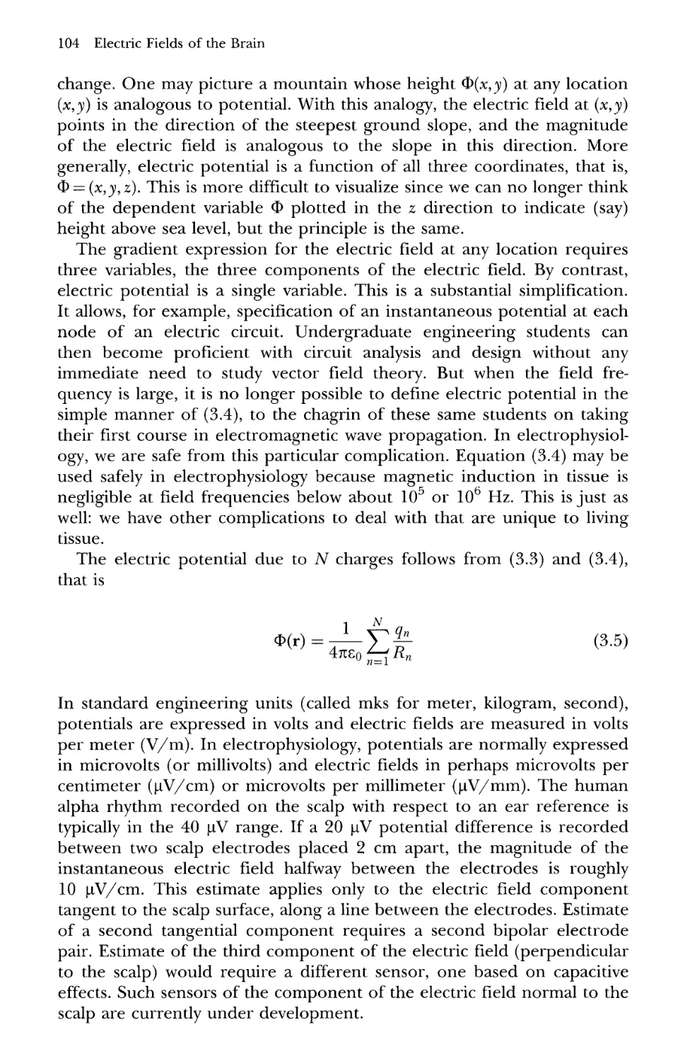
2 Electric Charge 101
3 Electric Fields 102
4 Electric Potential 103
5 Electric Circuits and Tissue Volume Conduction 105
6 Current Sources and Voltage Sources 106
7 Dipole and Multipole Fields 108
8 What are Yields* 111
9 Charges in Physical Dielectrics and Tissue 114
10 Macroscopic Polarization in Living Tissue 118
11 Charges in Conductors 119
12 Electric Current in Physical Media and Tissue 121
13 Electroneutrality of Tissue 122
14 Ohm's Law for Linear Conductors 123
15 Nonlinear Conductors 126
16 The Brain's Magnetic Field 127
17 Maxwell's Equations 128
18 Electromagnetic Radiation and Other Waves 131
19 Near and Far Fields 134
20 Transmission Lines 135
21 Schumann Resonances 139
22 Microwave Ovens, Spectroscopy, and Top-Down Resonance 142
23 Summary 145
Electric Fields and Currents in Biological Tissue 147
1 Basic Equations for Macroscopic Fields in Conductive Media 147
2 Comments on the Basic Equations in the Context
of Macroscopic Electrophysiology 149
3 Resistive Tissue Properties 151
4 Skull Resistivity 153
5 Capacitive Effects in Tissue 158
6 Boundary Conditions for Inhomogeneous Media 160

Contents xiii
7 Brain Current Sources 163
8 Explicit Use of Macroscopic Current Source Regions 166
9 Synaptic Current Sources and the Core Conductor Model of the Neuron 169
10 Solutions to the Cable Equation 174
11 Synaptic Input to Branched Dendrites 178
12 Mesoscopic Source Strength as Dipole Moment per Unit Volume 179
13 Simulations of Mesosources Generated in a Tissue Mass 183
14 Simple Interpretation of Mesosource Sources in an Idealized Tissue Mass 187
15 Low-Pass Filtering of the Mesosources Pfr, t) 189
16 Broad Classification of the Mesosource Field Pfr, I) Based on Scalp EEG 193
17 Macroscopic Potentials Generated by the Mesosources 196
18 Summary 198
Current Sources in a Homogeneous and Isotropic Medium 203
1 General Issues 203
2 Currents and Potentials in a Saltwater Fish Tank 204
3 The Monopolar Source 207
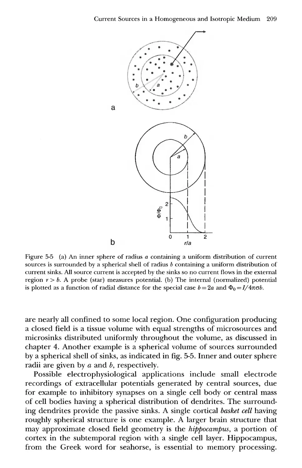
4 Concentric Spherical Surfaces and Closed Fields 208
5 The Branched Dendrite Model: A Partially Closed Field 211
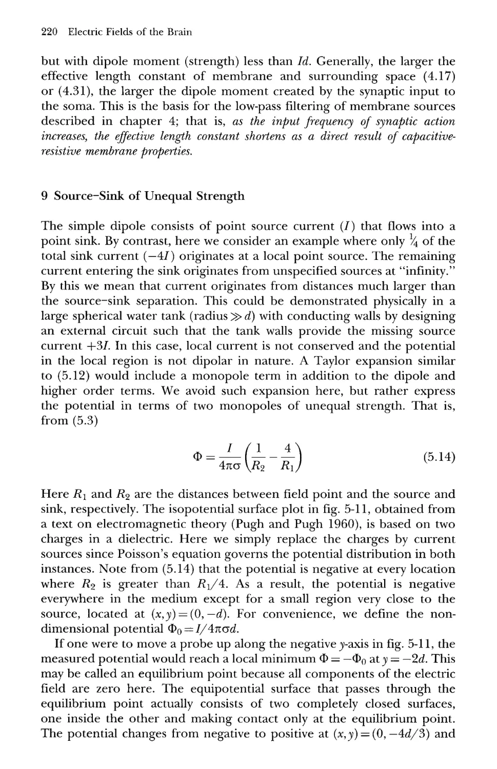
6 The Dipole Current Source 214
7 Two Dipoles Below a Surface 217
(9 The Distributed Line Source 218
9 Source-Sink of Unequal Strength 220
10 Distributed Source-Sink of Unequal Strength 222
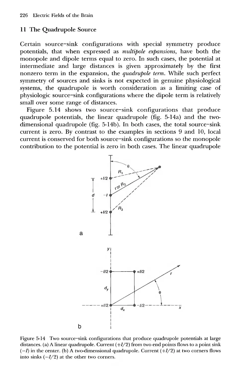
11 The Qiiadrupole Source 226
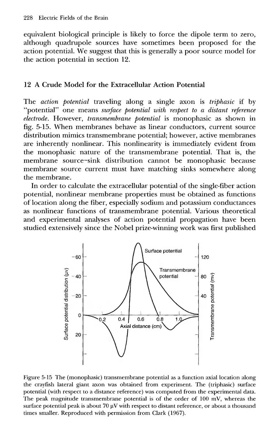
12 A Crude Model for the Extracellular Action Potential 228
13 Experimental Measurement of the Extracellular Action Potential 230
14 Dipole Potentials Measured in the Superior Olive of Cats 234
15 Dipole Layers: The Most Important Sources of Spontaneous EEG 237
16 Summary 240
Current Sources in Inhomogeneous and Isotropic Media 244
1 General Considerations 244
2 The Two-Layered Plane Medium 246
3 Dipole Inside a Homogeneous Sphere 249
4 Dipole in Multilayer Plane Media 250
5 Dipole Inside Concentric Spherical Surfaces 251
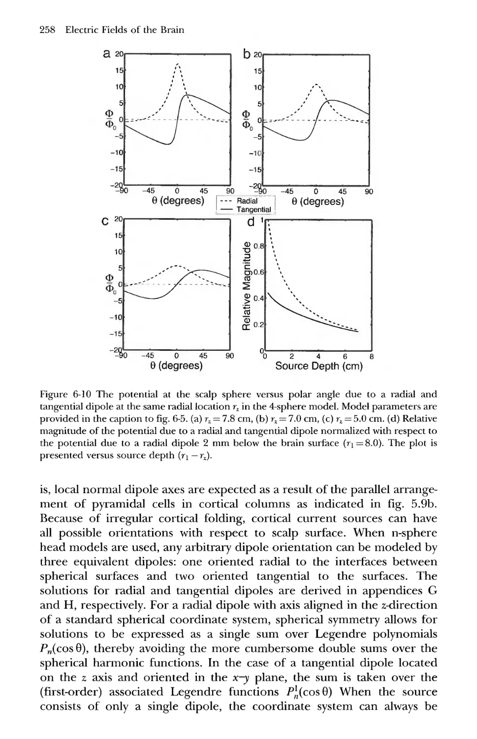
6 Relative Magnitudes of Potentials Generated by Radial and
Tangential Dipoles 257
7 Scalp Potentials Due to Dipole Layers 260

xiv Contents
8 Spatial Transfer Functions for n-Sphere Models 261
9 Comparisons of n-Sphere Models with More "Advanced" Head Models 264
10 Effects of Variable Skull Conductivity 267
11 Summary of Effects in the Inhomogeneous Models 271
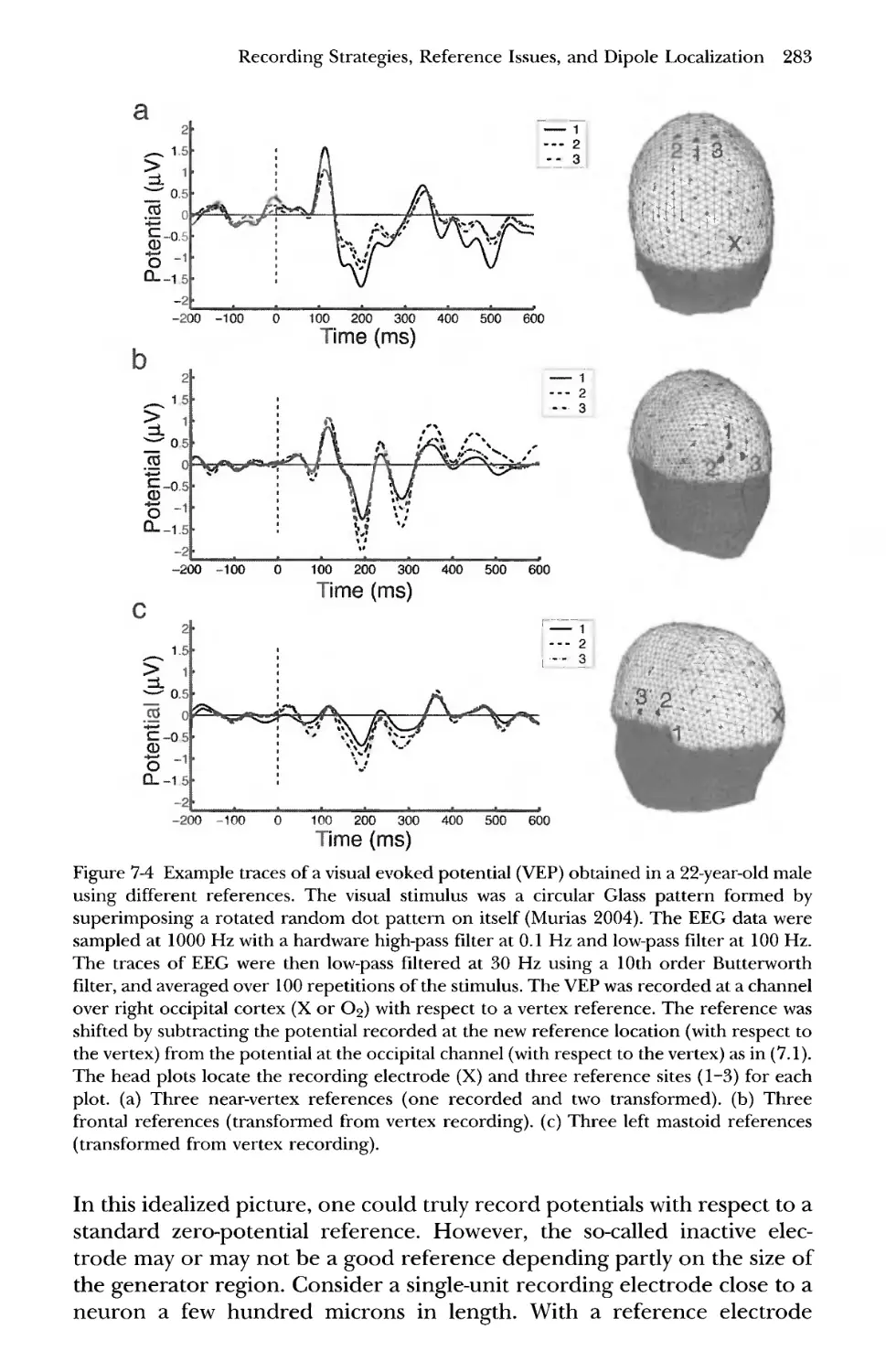
7 Recording Strategies, Reference Issues, and Dipole
Localization 275
1 EEG Recording Systems 275
2 The Quest for an Ideal Reference 282
3 Reciprocity and EEG Lead Fields 286
4 Bipolar Recordings 289
5 Linked-Ears or Linked-Mastoids Reference 291
6 The Average Reference 294
7 Spatial Sampling of EEG 298
8 Addressing the Inverse Problem with Dipole Localization 305
9 Summary 310
8 High-Resolution EEG 313
1 Improved Spatial Resolution versus Source Localization 313
2 Spatial Properties of EEG Sources 315
3 Physical Basis for Surface Laplacian Estimates 317
4 The Surface Laplacian as a Band-Pass Spatial Filter 325
5 Simulation Studies 330
6 Methods to Estimate Surface Laplacians from EEG Data 334
7 Comparison of Spline Laplacian and Dura Imaging Estimates 337
8 Applications to Spontaneous EEG 344
9 Conclusions and Caveats 348
9 Measures of EEG Dynamic Properties 353
1 Computer Analyses of EEG Data 353
2 Synaptic Action Generates EEG 355
3 Fourier Analysis 357
4 Time Domain Spectral Analysis 363
5 The Impact of Source Synchrony and Spatial Filtering on
EEG Power Spectra 368
6 Coherence and Phase Synchronization 372
7 Effects of Spatial Filtering by Volume Conduction on
Coherence Estimates 381
8 Effects of Surface Laplacians on Coherence Estimates 389
9 Are EEG Power and Coherence Independent Measures'? 396
10 Spatial Filtering Implies Temporal Filtering 401

Contents
11 Steady-State Visually Evoked Potentials 402
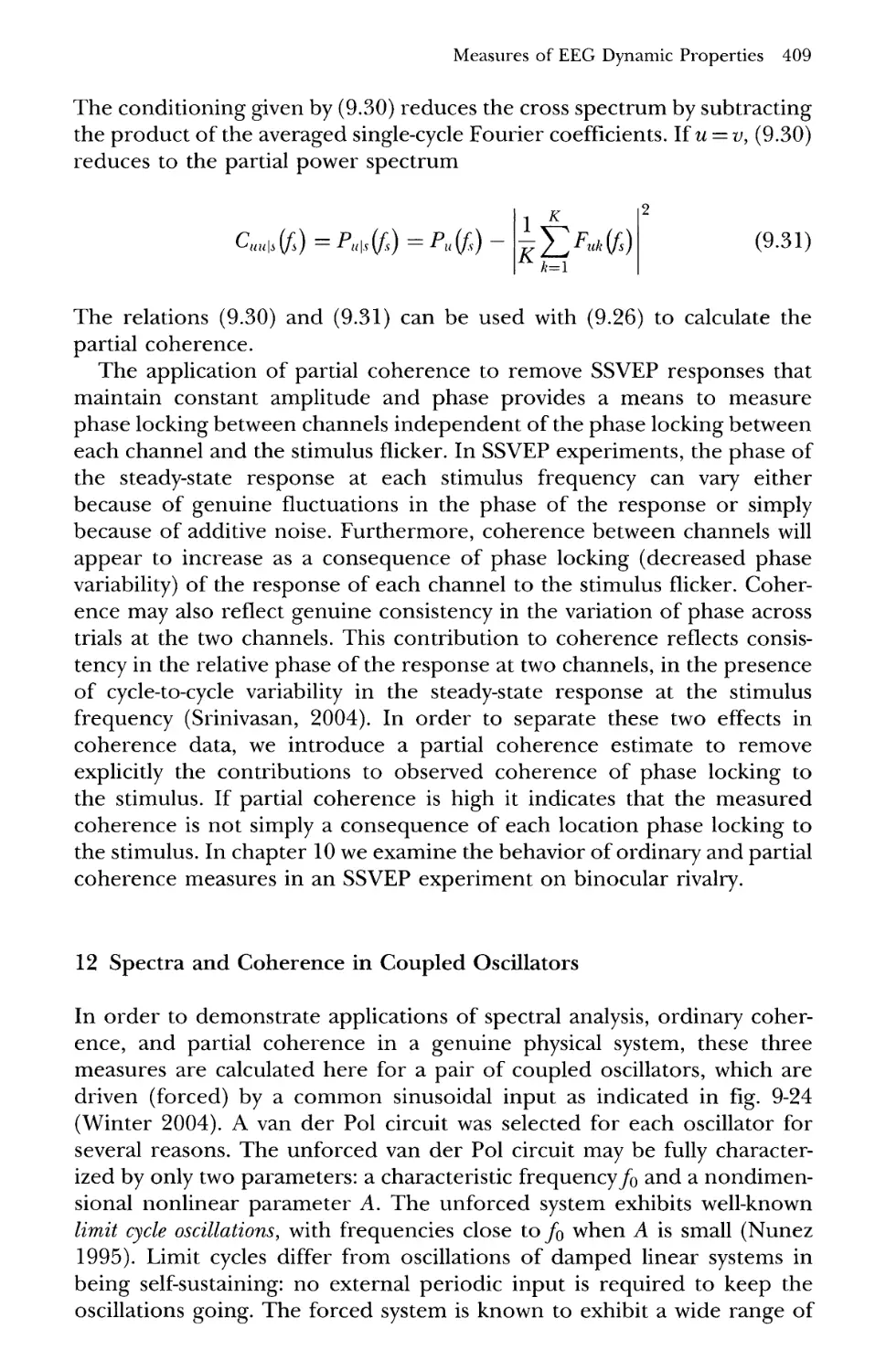
12 Spectra and Coherence in Coupled Oscillators 409
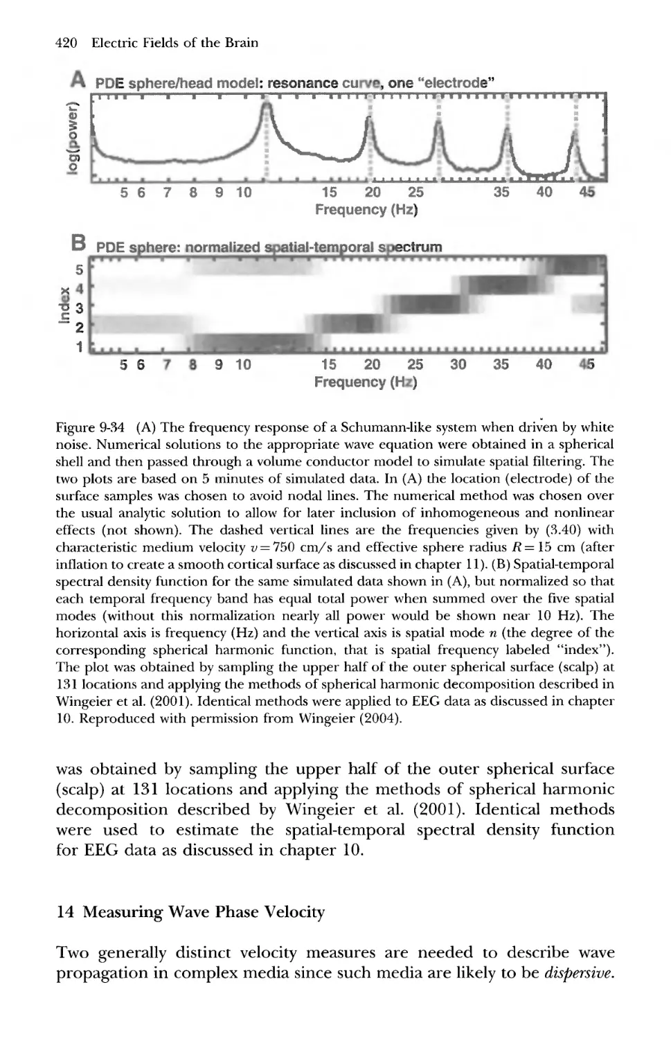
13 Spatial-Temporal Spectral Density Functions and Wave Propagation 416
14 Measuring Wave Phase Velocity 420
15 Empirical Orthogonal Functions and PCA 425
16 Summary 428
Spatial-Temporal Properties of EEG 432
1 Complementary Measures of EEG Dynamics 432
2 An Overview of Human Alpha Rhythms 434
3 A High-Resolution Experimental Study of Human Rhythms 437
4 Topography of Resting Alpha Rhythms 442
5 Spectral Properties of Resting Alpha 445
6 Spectral Power as a Function of Brain State 448
7 Stability of Alpha Phase Structure 451
8 Alpha and Theta Coherence 457
9 Theta Phase Synchronization During the Cognitive Task 458
10 SSVEP Dynamics During Binocular Rivalry 460
11 Coherence and Partial Coherence of the SSVEP in
Binocular Rivalry 467
12 Estimates of EEG Phase Velocity 471
13 Dispersion Relations and Group Velocity 476
14 Summary of the Complementary Dynamic Measures of
EEG and SSVEP 480
Neocortical Dynamics, EEG, and Cognition 486
1 Neocortical Dynamic Properties for the Millennium 486
2 A Tentative Framework for Brain Dynamics and Several Conjectures 490
3 Multiscale Dynamic Theory Illustrated with a Metaphorical Field 492
4 A Simple Model for Global Fields 494
5 More Realistic Approximations to the Neocortical Dynamic
Global Theory 505
6 Experimental Connections to Global Theory 507
7 Weakly Connected Resonant Oscillators and Binding by Resonance 514
8 Synaptic Action Fields and Global (Top-Down) Control of
Local Networks 515
9 Relationships to Other Theoretical Models and Criticisms of
the Global Theory 518
10 Summary 523

xvi Contents
Appendices
A Introduction to the Calculus of Vector Fields 531
B Quasi-Static Reduction of MaxwelVs Equations 535
C Surface Magnetic Field Due to a Dipole at an Arbitrary Location in
a Volume Conductor 541
D Derivation of the Membrane Diffusion Equation 545
E Solutions to the Membrane Diffusion Equation 549
F Point Source in a Five-Layered Plane Medium 555
G Radial Dipole and Dipole Layer Inside the 4-Sphere Model 560
H Tangential Dipole Inside Concentric Spherical Shells 568
/ Spherical Harmonics 576
J The Spline Laplacian 579
K Impressed Currents and Cross-Scale Relations in Volume Conductors 592
L Outline of Neocortical Dynamic Global Theory 598
Index

Electric Fields of the Brain

1
The Physics-EEG Interface
1 A Window on the Mind
The electroencephalogram (EEG) is a record of the oscillations of brain
electric potential recorded from electrodes on the human scalp. Consider
the following experiment. Place a pair of electrodes on someone's scalp
and feed the unprocessed EEG signal to a computer display in an isolated
location. Independently monitor the subject's state of consciousness
and provide both this information and the EEG signal to an external
observer. Even a naive observer, unfamiliar with EEG, will recognize that
the voltage record during deep sleep has larger amplitudes and contains
much more low-frequency content. In addition, the (eyes closed waking)
alpha state will be revealed as a widespread, near-sinusoidal oscillation
repeating about 10 times per second A0 Hz). More sophisticated
monitoring allows for accurate identification of distinct sleep stages, depth
of anesthesia, seizures, and other neurological disorders. Other methods reveal
robust EEG correlations with cognitive processes associated with mental
calculations, working memory, and selective attention.
Scientists are now so accustomed to these EEG correlations with brain
state that they may forget just how remarkable they are. The scalp EEG
provides very large-scale and robust measures of neocortical dynamic
function. A single electrode provides estimates of synaptic action averaged
over tissue masses containing between roughly 100 million and 1 billion
neurons. The space averaging of brain potentials resulting from
extracranial recording is a fortuitous data reduction process forced by
current spreading in the head volume conductor. Much more detailed
local information may be obtained from intracranial recordings in
animals and epileptic patients. However, intracranial electrodes implanted in
3

4 Electric Fields of the Brain
living brains provide only very sparse spatial coverage, thereby failing to
record the "big picture" of brain function. Furthermore, the dynamic
behavior of intracranial recordings depends fundamentally on
measurement scale, determined mostly by electrode size. Different electrode sizes
and locations can result in substantial differences in recorded dynamic
behavior, including frequency content and coherence. Thus, in practice,
intracranial data provide different information, not more information, than is
obtained from the scalp.
The critical importance of spatial scale in electrophysiology can be
emphasized by reference to a sociological metaphor. Experimental data
obtained from large metropolitan areas will generally differ from data
collected at the city, neighborhood, family, and person scales. Similarly, we
expect brain electrical dynamics to vary substantially across spatial scales.
Although cognitive scientists and clinicians have reason to be partly
satisfied with the very low spatial resolution obtained from scalp EEG data,
explorations of new EEG methods to provide somewhat higher spatial
resolution continue. A reasonable goal is to record averages over "only"
10 million neurons at the 1 cm scale in order to extract more details of the
spatial patterns correlated with cognition and behavior. This resolution is
close to the theoretical limit of spatial resolution caused by the physical
separation of sensor and brain current sources.
Scalp data are largely independent of electrode size because scalp
potentials are severely space-averaged by volume conduction between
brain and scalp. Intracranial recordings provide much smaller scale
measures of neocortical dynamics, with scale depending on the electrode
size, which may vary over four orders of magnitude in various practices
of electrophysiology. A mixture of coherent and incoherent sources
generates the small- and intermediate-scale intracranial data. Generally,
the smaller the scale of intracranial potentials, the lower the expected
contribution from coherent sources and the larger the expected
differences from scalp EEG. That is, scalp data are due mostly to sources
coherent at the scale of at least several centimeters with special geometries
that encourage the superposition of potentials generated by many local
sources.
In practice, intracranial EEG may be uncorrected or only weakly
correlated with cognition and behavior. The information content in such
recordings is limited by sparse spatial sampling and scale-dependent
dynamics. Furthermore, most intracranial EEG data are recorded in lower
mammals; extrapolation to humans involves additional issues. Thus, higher
brain function in humans is more easily observed at large scales. Scientists
interested in higher brain function are fortunate in this respect. The
technical and ethical limitations of human intracranial recording force us
to emphasize scalp recordings. These extracranial recordings provide
estimates of synaptic action at the large scales closely related to cognition
and behavior. Thus, EEG provides a window on the mind, albeit one that
is often clouded by technical and other limitations. This book strives for

The Physics-EEG Interface 5
improved methods to clean up this window, allowing for more transparent
imaging of the majesty of brain dynamics.
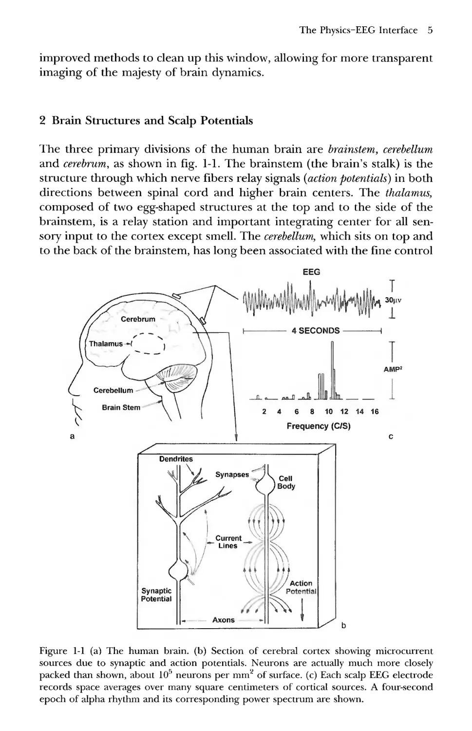
2 Brain Structures and Scalp Potentials
The three primary divisions of the human brain are brainstem, cerebellum
and cerebrum, as shown in fig. 1-1. The brainstem (the brain's stalk) is the
structure through which nerve fibers relay signals (action potentials) in both
directions between spinal cord and higher brain centers. The thalamus,
composed of two egg-shaped structures at the top and to the side of the
brainstem, is a relay station and important integrating center for all
sensory input to the cortex except smell. The cerebellum, which sits on top and
to the back of the brainstem, has long been associated with the fine control
EEG
i ¦ n
M|
Jt 1
W(r
4 SECONDS -
.ill T
|fn M[
\
AMP2
IL a nn 0 ,a.fli Mill JiilS
2 4 6 8 10 12 14 16
Frequency (C/S)
/-
Dendrites
hI
vj
<;
v
Synaptic
Potential
\j Synapses^ l^Ce!|
rJ" \
n 4
\ I Current
\ /- Lines -y^\
y i\
n %
XV
/f\
L— Axons *-|
J Body
>
\JJJ Action
Ygy Potential
~7\
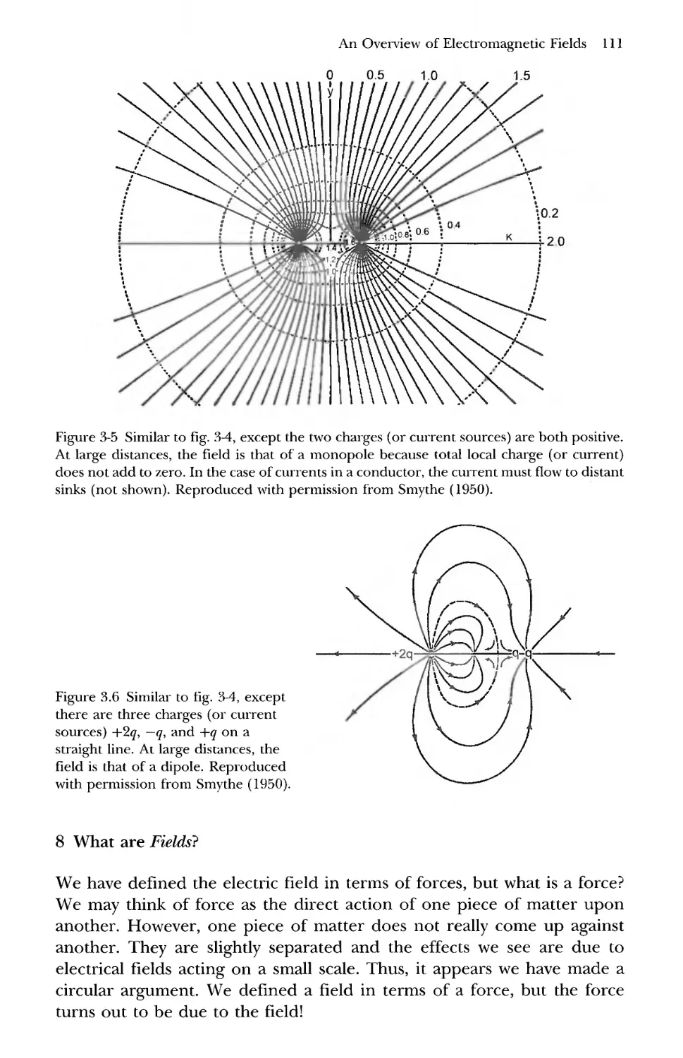
Figure 1-1 (a) The human brain, (b) Section of cerebral cortex showing microcurrent
sources due to synaptic and action potentials. Neurons are actually much more closely
packed than shown, about 105 neurons per mm2 of surface, (c) Each scalp EEG electrode
records space averages over many square centimeters of cortical sources. A four-second
epoch of alpha rhythm and its corresponding power spectrum are shown.

6 Electric Fields of the Brain
of muscle movements. More recently, the cerebellum has been shown to
play additional roles in cognition.
The large part of the brain that remains when the brainstem and
cerebellum are excluded is the cerebrum, which is divided almost equally into
two halves. The outer portion of the cerebrum, the cerebral cortex (or
neocortex in mammals), is a folded structure varying in thickness from about
2 to 5 mm, having a total surface area of roughly 1600 to 4000 cm2 and
containing about 101 neurons (nerve cells). Cortical neurons are strongly
interconnected. For example, the surface of a large cortical neuron may
be covered with as many as 104 to 105 synapses that transmit inputs from
other neurons. The synaptic inputs to a neuron are of two types: those that
produce excitatory postsynaptic potentials (EPSPs) across the membrane of
the target neuron, thereby making it easier for the target neuron to fire an
action potential and the inhibitory postsynaptic potentials (IPSPs), which act in
the opposite manner on the output neuron. EPSPs produce local
membrane current sinks with corresponding distributed passive sources to
preserve current conservation. IPSPs produce local membrane current
sources with more distant distributed passive sinks. In addition, several
other interaction mechanisms, not involving action potentials, have been
discovered by neurophysiologists. Much of our conscious experience must
involve, in some largely unknown manner, the interaction of cortical
neurons. The cortex is also believed to be the structure that generates most
of the electric potential measured on the scalp.
The cortex is composed of gray matter, so called because it contains a
predominance of cell bodies that turn gray when stained by anatomists,
but gray matter is actually pink when alive. Just below the gray matter is a
second major region, the white matter, composed of nerve fibers (axons).
In humans, white matter volume is somewhat larger than that of the
neocortex. White matter interconnections between cortical regions
(association fibers or corticocortical fibers) are quite numerous. Each square
centimeter of human neocortex may contain 107 input and output
fibers, mostly corticocortical axons interconnecting different regions of
the cortex, as shown in fig. 1-2. A much smaller fraction of axons that
enter or leave the underside of human cortical surface radiates from (and
to) the thalamus (thalamocortical fibers). This fraction is only a few percent
in humans, but substantially larger in lower mammals. This difference
partly accounts for the strong emphasis on thalamocortical interactions
(versus corticocortical interactions), especially in physiology literature
emphasizing animal studies. Anatomists have attached hundreds of
labels to various substructures within the brain, but here we are most
interested in larger structures near the surface that are more capable of
generating potentials sufficiently coherent to be observed on the scalp.
Neocortical neurons within each cerebral hemisphere are connected
by short intracortical fibers with axon lengths mostly less than 1 mm.
In addition, human neocortex is interconnected by about 1010
corticocortical fibers with axon lengths in the roughly 1 to 15 cm range. Cross

The Physics-EEG Interface 7
Figure 1-2 (a) Some of the superficial corticocortical fibers of the lateral aspect of the
cerebrum obtained by dissection, (b) A few of the deeper corticocortical fibers of the lateral
aspect of the cerebrum. The total number of corticocortical fibers is rou ghly 1010, that is,
for every fiber shown here, about 100 million are not shown. Reproduced with permission
from Krieg A963, 1973).
hemisphere interactions occur by means of about 108 callosal axons through
the corpus callosum and several smaller structures connecting the two
brain halves. A common view of brain operation is that of a complex circuit
or neural network. In this view, groups of cortical cells may be imagined as
analogous to electric circuit elements. The imagined circuit elements
might be individual neurons or cortical columns of different sizes, perhaps
containing anything between a hundred (minicolumn scale) and a hundred
thousand neurons (macrocolumn scale). Intracortical axons plus
corticocortical, callosal and thalamocortical axons might then be imagined as
analogous to wires connecting the circuit elements. In this oversimplified
(and probably mostly wrong) electric network picture, "circuit elements"
are under external control by means of electrical and chemical input from

8 Electric Fields of the Brain
the brainstem. More realistic views may adopt parts of this picture, but
acknowledge that even a single neuron is far more complex than the most
complex artificial neural network likely to be created in the near future
(Scott 1995). Furthermore, neurons interact by multiple mechanisms that
may not easily conform to conventional network models.
One obvious issue that arises whenever models are compared with
genuine electrophysiological data is that of spatial scale. Any neural network
description of brain operation must be scale-dependent so, for example,
macroscopic network elements are themselves complex circuits containing
smaller (mesoscopic) network elements. The mesoscopic elements are, in
turn, composed of still smaller scale elements. Even the best imagined
neural network model must break down at the membrane scale where
dynamics are governed by biochemistry and ultimately Maxwell's
microscopic equations and quantum mechanics. Other breakdowns of circuit
analogs are evident at large scales. For example, in a simple electric circuit,
signal delays take place only at circuit elements, that is, the delays are all
local. However, neocortical interactions over large distances involve both
local and global delays, the latter due to action potential propagation along
axons at finite speeds. In this sense, they share some properties with
electrical transmission lines like power lines or coaxial TV cables.
Transmission times for action potentials along corticocortical axons
may range from roughly 10 to 30 ms between the most remote cortical
regions. Local delays due to capacitive-resistive properties of single
neurons are typically in the 1 to 10 ms range, but may also be longer. The
brain's awareness of an external event seems to require multiple feedback
between remote regions. Consciousness takes several hundred milliseconds to
develop. The multiple mechanisms by which neurons can interact may
not fit naturally into standard neural network models. Partly for these
reasons, neuroscientists often prefer the term cell assemblies, originating
with the pioneering work of Donald Hebb A949). The label "cell
assembly" denotes a diffuse cell group capable of acting briefly as a
single structure. We may reasonably postulate cooperative activity within
cell assemblies without explicitly specifying interaction mechanisms or
relying on electric circuit metaphors.
Brain processes may involve the formation of cell assemblies at several
spatial scales (Freeman 1975; Ingber 1982, 1995). We conjecture that such
groups of neurons may produce a wide range of local delays and associated
characteristic (or resonant) frequencies (Nunez 1995). Neural network
models can incorporate some physiologically realistic features that are not
normally present in electric circuits. However, field descriptions of brain
dynamics may be required to model dynamic behavior and make contact
with macroscopic EEG data. In this context, the word "field" refers to
mathematical functions expressing, for example, the numbers of active
synaptic or action potentials in macroscopic tissue volumes. Alternately,
probability of neural firing in a tissue mass may be treated as afield variable
(Ingber 1995). In the view adopted in this book, cell assemblies are pictured

The Physics-EEG Interface 9
as embedded tuithin synaptic and action potential fields (Nunez 1995, 2000a, b;
Jirsa and Haken 1997; Haken 1999). Electric and magnetic fields (EEG
and MEG) provide large-scale, short-time measures of the modulations of
synaptic and action potential fields around their background levels. These
synaptic fields are analogous to common physical fields, for example,
sound waves, which are short-time modulations of pressure or mass density
about background levels. We distinguish these short-time modulations of
synaptic activity from long-timescale (seconds to minutes) modulations of
brain chemistry controlled by neuromodulators.
Dynamic brain behaviors are conjectured by many neuroscientists to
result from the interaction of neurons and assemblies of neurons that
form at multiple spatial scales (Freeman 1975; Harth 1993, Scott 1995;
Nunez 1995, 2000a, b). Part of the dynamic behavior at macroscopic
scales may be measured by scalp EEG electrodes. This electrical activity is
divided into two major categories: spontaneous potentials such as alpha
and sleep rhythms and evoked potentials or event-related potentials. Evoked
potentials are the direct response to some external stimulus like a light
flash or auditory tone. Event-related potentials depend additionally on
state-dependent brain processing of the stimulus (Regan 1989).
In addition to such EEG studies, electrophysiologists study potentials
generated by single neurons or small cell assemblies, recorded with
microelectrodes or mesoelectrodes (between micro and macro). Much work has
been published on potentials recorded at smaller scales (Cole 1968; Abeles
1982; Segev et al. 1995; Destexhe and Sejnowski 2001), but this book is
concerned with oscillating macroscopic potentials measured on the scalp,
or in the brain, called the electroencephalogram or EEG. Meso- and
microelectrode data are considered here mainly in the context of relating
scalp potentials to their underlying sources.
The scalp EEG is an important clinical tool for following and treating
certain illnesses (Kellaway 1979; Niedermeyer and Lopes da Silva 1999).
Brain tumors, strokes, epilepsies, infectious diseases, mental
retardation, severe head injury, drug overdose, sleep and metabolic disorders,
and ultimately brain death are some of the medical conditions that may
show up in the spontaneous EEG. EEG also provides quantitative measures
of depth of anesthesia and severity of coma. Evoked and event-related
potentials measured on the scalp may be used in the diagnosis and
treatment of central nervous system diseases as well as illuminating
cognitive processes, but often EEG abnormalities are nonspecific, perhaps
only confirming diagnoses obtained with independent clinical tests.
A summary of clinical and research EEG is provided in fig. 1-3. The
arrows indicate common relations between subfields. The numbered
superscripts in the boxes indicate the following. A) Physiologists record
EEG from inside the skulls of animals using electrodes with diameters
typically ranging from about 0.01 to 1 mm. Observed dynamic behavior
generally depends on location and measurement scale, determined mostly
by electrode size for intracranial recordings. By contrast, scalp-recorded

10 Electric Fields of the Brain
Clinical Applications
epilepsy
head trauma
drug overdose
brain infection
sleep disorder
coma
stroke
Alzheimer's disease8
brain tumor9
multiple sclerosis10
surgical monitoring10
Cognitive Science
sensory pathwaysl 1
stimulus encoding
motor process
spatial task
verbal task
mathematics
short term memory
memory encoding
selective attention
task context
general intelligence12
dynamic brain theory1'
Figure 1-3 Common relationships between EEG subfields. Clinical applications are mostly
related to neurological diseases. EEG research is carried out by neurologists, cognitive
neuroscientists, physicists, and engineers who have a special interest in EEG. See text for a
discussion of numbered superscripts. Reproduced with permission from Nunez B002).
EEG dynamics is exclusively large scale and mosdy independent of
electrode size. B) Human spontaneous EEG occurs in the absence of
specific sensory stimuli, but may be easily altered by such stimuli. C)
Averaged evoked potentials (EPs) are associated with specific sensory stimuli
like repeated light flashes, auditory tones, finger pressure, or mild electric
shocks. They are typically recorded by time averaging of single-stimulus
waveforms to remove the spontaneous EEG. D) Event-related potentials
(ERPs) are recorded in the same way as EPs, but normally occur at longer
latencies from the stimuli and are more associated with endogenous brain
state. E) Because of ethical considerations, EEG recorded in brain depth
or on the brain surface (ECoG) of humans is limited to patients,
mostly candidates for epilepsy surgery. F) With transient EPs or ERPs
the stimuli consist of repeated short stimuli. The number of stimuli
required to produce an averaged evoked potential may be anything
between about ten and several thousand, depending on application. The
scalp response to each stimulus or pulse is averaged over the individual
pulses. The EP or ERP in any experiment consists of a waveform
containing a series of characteristic peaks (local maxima or minima),
typically occurring less than 0.5 seconds after presentation of each
stimulus. The amplitude, latency from the stimulus or covariance (in the

The Physics-EEG Interface 11
case of multiple electrode sites) of each component may be studied, in
connection with a cognitive task (ERP) or with no task (EP). G) Steady-state
visually evoked potentials (SSVEP) use a continuous sinusoid modulated
stimulus (a flickering light, for example), typically superimposed in front
of a computer monitor providing a cognitive task. The brain response in
a narrow frequency band containing the stimulus frequency is measured.
Magnitude, phase, and coherence (in the case of multiple electrode sites)
may be related to different parts of the cognitive task. (8) Alzheimer's
disease and other dementias typically cause substantial slowing of normal
alpha rhythms. Traditional EEG has been of little use in dementia because
EEG changes are often only evident late in the illness when other clinical
signs are obvious. New efforts to apply EEG to early detection of
Alzheimer's disease are under study. (9) Cortical tumors that involve the
white matter layer (just below neocortex) cause substantial low-frequency
(delta) activity over the hemisphere with the tumor. Application of EEG to
tumor diagnosis has been mostly replaced by magnetic resonance imaging
(MRI), which reveals structural abnormalities in tissue. A0) Most clinical
work uses spontaneous EEG; however, multiple sclerosis and surgical
monitoring often involve evoked potentials. A1) Studies of sensory
pathways involve early components of evoked potentials (latency from
stimuli less than perhaps 10 to 50 ms) because the transmission times for
signals traveling between sense organ and brain are short compared to the
duration of multiple feedback processes associated with cognition. A2)
The study of general intelligence associated with IQ tests is controversial, but
a number of studies have reported significant correlations between scores
on written tests and quantitative EEG measures. A3) Mathematical models
of large-scale brain function are used to explain or predict observed
properties of EEG in terms of basic physiology and anatomy. Although
such models must represent vast oversimplifications of genuine brain
function, they contribute to our conceptual framework and may guide the
design of new experiments to test parts of this framework.
The clinical usefulness of quantitative EEG methods in various diseases
has been assessed jointly by the American Academy of Neurology and the
American Clinical Neurophysiology Society (Nuwer 1998). Clinical and
cognitive applications of EEG have been covered extensively elsewhere,
and are largely avoided here, except in some important cases where
electric field concepts seem to shed new light on clinical or cognitive
issues. One of our aims is to provide scientific and technical information
that may lead to new EEG applications for disease states for which clinical
utility has been disappointing thus far. These include mild or moderate
closed head injury, learning disabilities, attention disorders, schizophrenia,
depression, and Alzheimer's disease. Given the relatively crude methods of
data processing currently used in most clinical settings, we simply do
not now know if these brain abnormalities cause EEGs with clinically
useful information. There is, however, reason to be optimistic about
future clinical developments because quantitative methods to recognize

12 Electric Fields of the Brain
spatial-temporal EEG patterns have been studied only sporadically. For
example, high-resolution coherence and other measures of phase
synchronization, which indicate the strength of functional connections between
brain regions, are rarely used in clinical settings. High-resolution EEG
generally and EEG phase synchronization are txxated in chapters 8-10.
We are concerned here with the physiological bases for EEG: the nature
and location of the so-called generators of potential and how these
potentials and currents spread through brain, skull, and scalp (volume
conduction). We also consider the possible origins of time-dependent
behavior of EEG [neocortical dynamics), especially when this issue overlaps
volume conduction considerations. These topics are directly related to the
practical problems faced in recording and interpreting the EEG.
Misunderstanding of electric fields and potentials often leads to fallacious
and, in some cases, even absurd physiologic interpretations, as outlined in
chapter 2. This book attempts to lay a more solid theoretical foundation
upon which clinical and cognitive studies may rest more securely. A deeper
understanding of volume conduction and dynamical issues and improved
recording and computer methods should provide clinicians with more
finely tuned diagnostic tools and cognitive scientists with enlightened
experimental methods.
3 Human Alpha Rhythms
A central problem for the electroencephalographer or cognitive scientist
is to relate potentials measured on the scalp to the underlying
physiological processes. Such scalp potentials are characterized by their temporal
and spatial characteristics. For example, an important human EEG
category embodies several kinds of alpha rhythms, which are usually
identified as near-sinusoidal oscillations at frequencies near 10 Hz. Alpha
rhythm in an awake relaxed human subject is illustrated by the temporal
plots and corresponding frequency spectra in fig. 1-4. The amplitude of
scalp alpha oscillations is typically 20 to 50 |iV, when measured between
one electrode over the occipital cortex and a second electrode some 5 to
10 cm or so distant. Alpha rhythm amplitudes are typically smaller over
frontal regions, depending partly on the subject's state of relaxation.
Other alpha rhythms may occur in other brain states, for example in
alpha coma or with patients under halothane anesthesia. In addition to
alpha rhythms, a wide variety of human EEG activity may be recorded,
a proverbial zoo of dynamic signatures, each waveform dependent in its
own way on time and scalp location. EEG is often labeled according to
apparent frequency range: delta A-4 Hz), theta D-8 Hz), alpha (8-13 Hz),
beta A3-20 Hz), and gamma (roughly >20 Hz). These qualitative labels
are often applied based only on visual inspection or by counting zero
crossings. They must be used carefully because actual EEG is composed of

The Physics-EEG Interface 13
BMW, relaxed, scalp potential amplitude spectra
10 20 30 40
Frequency (Hz)
10 20 30 40
Frequency (Hz)
10 20 30 40
Frequency (Hz)
10 20 30 40
Frequency (Hz)
1 35
BMW, scalp potential
-35
35 f
W^A/vM^
O -35
35
U/VVArVVV^^
O -35
35
! ok/u#-^^
f A
g .35 I . . . ,
Time (s)
Figure 1-4 (b) Alpha rhythm recorded from a healthy 25-year-old relaxed male with eyes
closed using a neck electrode as reference. Four seconds of data are shown from four scalp
locations (left frontal-30; right frontal-26; left posterior-108; right posterior-100).
Amplitudes are given in uV. (a) Amplitude spectra for the same alpha rhythms shown in (b) but
based on the full five-minute record to obtain accurate spectral estimates. Amplitudes are
given in \xV per root Hz. Frequency resolution is 0.25 Hz. The double peak in the alpha
band represents oscillations near 8.5 and 10.0 Hz. These lower and upper alpha band
frequencies have different spatial properties and behave differently during cognitive tasks
as shown in chapter 10.
mixtures of multiple frequency components as revealed more clearly
by spectral analysis.
A posterior rhythm of approximately 4 Hz develops in babies in the first
few months of age. Its amplitude increases with eye closure and is believed
to be a precursor of mature alpha rhythms. Maturation of the alpha

14 Electric Fields of the Brain
rhythms is characterized by increased frequency and reduced amplitude
between ages of about three and ten. Normal resting alpha rhythms may
be substantially reduced in amplitude by eye opening, drowsiness, and,
in many subjects, by moderate to difficult mental tasks. Alpha rhythms,
like most EEG phenomena, typically exhibit an inverse relationship
between amplitude and frequency. For example, hyperventilation and
some drugs (alcohol, for example) may cause reductions of alpha
frequencies together with increased amplitudes. Other drugs (barbiturates,
for example) are associated with increased amplitude of low-amplitude
beta activity superimposed on scalp alpha rhythms. The physiological bases
for the inverse relation between amplitude and frequency and most
other properties of EEG are largely unknown, although physiologically
based dynamic theories have provided several tentative explanations.
For example, several salient properties of EEG are consistent with limit
cycle modes as discussed in chapter 11.
Alpha rhythms provide an appropriate starting point for clinical EEG
exams (Kellaway 1979; Niedermeyer and Lopes da Silva 1999). Some initial
clinical questions are as follows. Does the patient show an alpha rhythm
with eyes closed, especially over posterior scalp? Are its spatial-temporal
characteristics appropriate for the patient's age? How does it react to eyes
opening, hyperventilation, drowsiness, and so forth? For example,
pathology is often associated with pronounced differences in EEG
recorded over opposite hemispheres or with low alpha frequencies. A resting
alpha frequency lower than about 8 Hz in adults is considered abnormal
in all but the very old.
These characteristics of scalp EEG depend not only on the nature and
location of the current sources, but also on the electrical and geometrical
properties of brain, skull, and scalp. The connection between surface and
depth events is thus intimately dependent on the physics of electric field
behavior in biological tissue. Electric fields in physical media were
understood at least 50 years before the first scalp recordings of the human EEG
in the mid-1920s by the German psychiatrist Hans Berger A928). Physical
principles are directly applicable to neural tissue; we need only interpret
variables and supply tissue properties to provide a good picture of head
volume conduction.
There are many possible sources of electrical activity on the scalp. Eye
or tongue movements, muscle contractions, and EKG can produce scalp
potentials larger than EEG amplitudes. In particular, since the alpha
rhythm tends to disappear with eyes open, its origin was first suspected
to be a rhythmic beat of eye muscles. Convincing evidence that alpha
rhythms are generated in the brain was obtained in experiments with
patients having abnormal skull openings (Adrian and Mathews 1934),
although this early work suggested (erroneously) that alpha rhythms
originate primarily in posterior regions. Averaged over time, the largest
contributions do come from occipital and parietal regions with somewhat
lesser contributions from frontal regions. Modern potential maps based

The Physics-EEG Interface 15
on long-time averages often show "hot spots" over posterior regions,
thereby contributing to the (often erroneous) view of alpha as a strictly
localized phenomenon. We examine this issue further later in this chapter
and again in chapters 9-11 and show that multiple alpha rhythms occur with
both local and global properties.
We now have a more accurate picture of the properties of human
alpha rhythms, obtained from early cortical surface and depth recordings
in epileptic patients (Jasper and Penfield 1949; Penfield and Jasper 1954;
Sem-Jacobsen et al. 1953; Cooper et al. 1965; Pfurtscheller and Cooper
1975) and later with high-resolution scalp recordings (Nunez et al. 2001)
reviewed in chapter 10. Some of the early findings of cortical surface
recordings have recently been rediscovered. These results are consistent
with the following description by EEG pioneer Grey Walter in 1964
(Basar et al. 1997).
We have managed to check the alpha band rhythm with intra cerebral
electrodes in the occipital-parietal cortex; in regions which are practically
adjacent and almost congruent one finds a variety of alpha rhythms, some
are blocked by opening and closing the eyes, some are not, some respond in
some way to mental activity and some do not. What one can see on the scalp
is a spatial average of a large number of components, and whether you see
an alpha rhythm of a particular type or not depends on which component
happens to be the most highly synchronized process over the largest
superficial area; there are complex rhythms in everybody.
Other early EEG pioneers were electroencephalographer Herbert Jasper
and neurosurgeon Wilder Penfield, famous for his studies of patient
response to electrical stimulation of cortical tissue, a procedure sometimes
evoking reports of past memories in patients. Numerous EEG studies
of epilepsy surgery patients were also carried out by Penfield and Jasper.
They recorded EEG from different regions of exposed cortex in a large
number of patients. Figure 1-5 indicates that alpha rhythm was recorded
(in different subjects) from almost the entire upper cortical surface. The
exception was the region near the central motor strip where beta rhythms
were mainly recorded.
In order to interpret these early results, note that spectral (Fourier)
analysis of EEG was not in use at that time. Rather, EEG waveforms were
characterized by visual inspection and number of zero crossings. This
procedure tends to emphasize faster frequencies (for example, beta
activity) in data containing mixed frequency content as demonstrated in
chapter 9. For this reason, it is not clear how much overlap occurred
between regions with dominant beta and alpha rhythms in these early
cortical studies. Another issue is that widespread alpha production is
mostly associated with relaxed, healthy subjects. Penfleld's epilepsy
patients were recorded in the operating room while awake with parts of their
skulls removed, apparently not ideal conditions for relaxed subjects and
robust alpha rhythm production. We have not found such detailed modern

16 Electric Fields of the Brain
F. Rofandi
Beta fH Alpha <*/\f\J\f\p*
Figure 1-5 Cortical surface regions where alpha rhythms were recorded in a large
population of epilepsy surgery patients are indicated by wavy lines. Dotted region near the
central motor strip indicates beta activity. ECoG activity was characterized by counting zero
crossings before Fourier transforms were used in EEC Reproduced with permission from
Jasper and Penfield A949).
studies of human cortical rhythms, perhaps due partly to changing ethical
standards. Another factor limiting modern data is that today's epilepsy
surgery patients typically have a history of drug therapy to control seizures.
Chronic drug use (whether for medical or recreational purposes) can cause
long-lasting and perhaps permanent effects on normal brain rhythms.
These issues complicate the extrapolation of patient data to the healthy
population.
Relatively high spatial resolution EEG may now be obtained with scalp
recordings using a combination of dense electrode arrays and computer
algorithms to project scalp potentials to the dura surface, as discussed in
chapters 2, 8, and 10. By contrast to true inverse solutions like dipole
localization, dura imaging requires no a priori assumptions about sources.
The accuracy of dura potential estimates is limited "only" by electrode
density, noise, and accuracy of volume conductor model. Figure 1-6 shows
eight instantaneous dura image plots; time slices are taken at
successive maxima and minima of the alpha rhythm waveform in one subject.
These plots are based on 131-channel scalp recordings with approximately
2.3 cm (center-to-center) electrode separation. Signal to noise ratio is quite
high in these data. Furthermore, with such high spatial sampling,
dura image estimates are relatively robust with respect to head model

The Physics-EEG Interface 17
Figure 1-6 High-resolution estimates of dura potential for resting alpha rhythm at eight
successive times separated by about 50 ms are shown. The plotting times correspond to
alternating positive and negative peaks in the potential recorded by a posterior-midline
electrode. The plots were obtained by passing 131-channel (average reference) data
through the Melbourne dura imaging algorithm. The New Orleans spline-Laplacian yields
similar patterns of dura potential, that is, correlation coefficients between the two high-
resolution estimates are about 0.95 with the LSI spatial samples. These plots appear in
color in fig. 10 of Nunez et al. B001).
uncertainty. In fact, another high-resolution method, the New Orleans
spline-Laplacian, which is nearly independent of head model, yields
contour plots that are almost identical to those obtained by Melbourne
dura imaging as discussed in chapters 8-10.
Based on these data and other evidence outlined in this book, we view
alpha rhythm as a spatial-temporal dynamic modulation of cortical synaptic
action, with sources widely distributed over neocortical surface. At any
fixed time, patches of positive and negative potentials occur on the dura
surface as suggested by fig. 1-6. These suggest alternating regions of
correlated cortical source activity of opposite sign. Larger correlated
regions tend to produce larger scalp potentials, which may account for
observed anterior-posterior magnitude differences of alpha rhythm
amplitudes. This dependence of scalp potential amplitude on
characteristic correlated patch size (or effective correlation length) is demonstrated
by the simulations shown in fig. 1-7. Each grid space represents a cortical
macrocolumn source expressed in terms of transcortical potential,
which varies between ±200 \xV (root mean square fixed at 116 |aV).
These transcortical potentials are consistent with intracranial recordings
of spontaneous EEG in animals (Lopes da Silva and Storm van Leeuwen
1978). Filled and empty grid spaces indicate positive and negative macro-
column sources, respectively. A head model consisting of three concentric
spheres is used to estimate scalp potential contours generated by each
of the source patterns.

18 Electric Fields of the Brain
RMS = 1.30 pV % + = 51.2
Figure 1-7 Simulated distribution of neocortical source activity over a 150 cm2 square of
(assumed) smooth cortical surface. Each grid space represents a cortical macrocolumn
(~ 3.5 mrrr). The columnar mesosources are expressed here as local transcortical potentials
to roughly match depth recordings in animals. Positive (black) or negative (white) potential
differences are distributed between ±200 uV. Calculated surface potential maps (obtained
with the 3-sphere head model) have progressively larger magnitudes as effective correlation
lengths of the source distributions increase, that is, as source clumps become larger. The
percentages of positive mesosources and corresponding RMS scalp potential magnitudes
are (a) 51%, 1.3 uV; (b) 50%, 3.6 uV; (c) 55%, 7.4 uV; (d) 73%, 18.8 jiV. Reproduced with
permission from Nunez A995).
The simulations shown in fig. 1-7 demonstrate that scalp potential
amplitudes depend strongly on the characteristic size of the underlying
correlated source patches (the amount of source synchronization). In these
examples, the root mean square (rms) source strengths are held fixed at
116 |uV for each simulation; only the sizes of correlated regions vary (plots
a~d). When cortical source pattern is random (plot a), predicted rms scalp
potential is 1.3 (iV. By contrast, the large source clumps (plot d) produce
a rms scalp potential of 18.8 |iV. The idea that scalp potential
magnitudes depend largely on source synchrony is widely recognized in clinical
and research EEG environments where scalp potential amplitude
reduction is often characterized as "desynchronization" (Kellaway 1979;
Pfurtscheller and Lopes da Silva 1999). However, if source patterns
are held fixed, scalp potential magnitudes increase in proportion to
source magnitudes. These intermediate-scale (mesoscale) columnar sources
are defined in terms of synaptic current sources in chapter 4. The

The Physics-EEG Interface 19
1*¦¦¦¦¦" t""»"*"»"~""*. "** / ""*,"~'u: *u*n*
Figure 1-7 Continued.
meso-sources (P(r9t) or dipole moments per unit volume) are simply
weighted averages of membrane current sources over millimeter scale
tissue masses, as given by D.26).
Alpha rhythms can also exhibit both local and global behavior, possibly
suggesting that larger amplitudes tend to occur in regions where both local
and global mechanisms contribute strongly as discussed in chapters 9-11.
This general picture is bolstered by volume conductor models of the head
(chapters 6 and 8) that agree with observations of differences in magnitude
and spectral content between cortex and scalp (Pfurtscheller and Cooper
1975) and with cortical depth recordings obtained with small electrodes to
record alpha source activity in dogs (Lopes da Silva and Storm van
Leeuwen 1978). Although this experimental description of sources of
alpha phenomena rests on relatively solid ground, there is still no general
agreement about the physiological bases for its dynamic behavior. We
return to this issue in chapters 9-11.
4 A Conceptual Framework for Neocortical Dynamics
and EEG
Figure 1-8 summarizes a general conceptual framework for neocortical
dynamics and EEG (and magnetoencephalograpy, MEG). While parts of
this framework are speculative, it accurately indicates, in a general sense,
how volume conduction (causal connection 1-E) relates to the much

20 Electric Fields of the Brain
Correlative
E/B
Correlative
M/B
EEG, MEG
Behavior/Cognition
MRI, PET
A
Causal
1-E
A-B
A-1
A
Speculative
A-2
Causal
2-M
Cell Groups 1
A
! CELL ASSEMBLIES \\1
A
Cell Groups 2
Causal
F-1
F-A
A-F
A
i Speculative
Causal
F-2
Synaptic Action Fields W,(r, t) and 4>e(r, t)
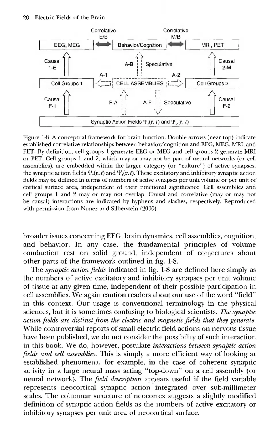
Figure 1-8 A conceptual framework for brain function. Double arrows (near top) indicate
established correlative relationships between behavior/cognition and EEG, MEG, MRI, and
PET. By definition, cell groups 1 generate EEG or MEG and cell groups 2 generate MRI
or PET. Cell groups 1 and 2, which may or may not be part of neural networks (or cell
assemblies), are embedded within the larger category (or "culture") of active synapses,
the synaptic action fields H'X1", 0 an<^ ^/(r, t). These excitatory and inhibitory synaptic action
fields may be defined in terms of numbers of active synapses per unit volume or per unit of
cortical surface area, independent of their functional significance. Cell assemblies and
cell groups 1 and 2 may or may not overlap. Causal and correlative (may or may not
be causal) interactions are indicated by hyphens and slashes, respectively. Reproduced
with permission from Nunez and Silberstein B000).
broader issues concerning EEG, brain dynamics, cell assemblies, cognition,
and behavior. In any case, the fundamental principles of volume
conduction rest on solid ground, independent of conjectures about
other parts of the framework outlined in fig. 1-8.
The synaptic action fields indicated in fig. 1-8 are defined here simply as
the numbers of active excitatory and inhibitory synapses per unit volume
of tissue at any given time, independent of their possible participation in
cell assemblies. We again caution readers about our use of the word "field"
in this context. Our usage is conventional terminology in the physical
sciences, but it is sometimes confusing to biological scientists. The synaptic
action fields are distinct from the electric and magnetic fields that they generate.
While controversial reports of small electric field actions on nervous tissue
have been published, we do not consider the possibility of such interaction
in this book. We do, however, postulate interactions between synaptic action
fields and cell assemblies. This is simply a more efficient way of looking at
established phenomena, for example, in the case of coherent synaptic
activity in a large neural mass acting "top-down" on a cell assembly (or
neural network). The field description appears useful if the field variable
represents neocortical synaptic action integrated over sub-millimeter
scales. The columnar structure of neocortex suggests a slightly modified
definition of synaptic action fields as the numbers of active excitatory or
inhibitory synapses per unit area of neocortical surface.

The Physics-EEG Interface 21
The idea of synaptic action fields is partly motivated by its causal
connection to current sources, that is, the so-called generators of EEC For
example, a minicolumn of human neocortex has roughly a 0.03 mm radius,
3 mm height, and contains about 100 pyramidal cells and a million
synapses (Szentagothai 1979). In mouse at least, there are perhaps six
excitatory synapses for each inhibitory synapse (Braitenberg and Schuz
1991). If for the purposes of discussion we conjecture that 10% of all
synapses are active at some given time, the excitatory and inhibitory
synaptic action densities are about 80,000 and 14,000 per area of
minicolumn, respectively. The number densities of active excitatory and
inhibitory synapses, expressed as functions of time and cortical location
are here assigned the symbols ^(r, t) and ^(r, t), respectively; these are
field variables.
Each active inhibitory synapse produces a local current source at a
membrane surface plus additional membrane sinks (negative sources)
required by current conservation. Each active excitatory synapse produces
a local negative source (sink) plus distributed membrane sources in a
similar manner. The magnitude of electric potential at large distances (for
example, at the local scalp) generated by a cortical column depends mainly
on the distribution of synaptic and return sources over its depth and the
synchrony of synaptic activation. For example, if excitatory and inhibitory
synapses are distributed relatively uniformly through the column depth, or
if synapses are randomly active in time, the strengths (dipole moments or
mesosources) of column source regions will be small. Relatively large dipole
moments occur if, for example, synchronous excitatory synapses act in
superficial cortex (say on pyramidal cell dendrites) and inhibitory synapses
act at deeper layers (say near cell bodies), a picture roughly consistent with
anatomical data (Mountcastle 1979; Szentagothai 1979; Braitenberg and
Schuz 1991) and electrophysiological depth recordings (Lopes da Silva and
Storm van Leeuwen 1978).
A single minicolumn or even a single macrocolumn (containing about
1000 mincolumns or 100,000 pyramidal cells) is not expected to generate
a dipole moment of sufficient strength to produce scalp potentials in the
recordable range of a few microvolts. As a general "rule of head," about
6 cm" of cortical gyri tissue (containing about 600,000 minicolumns or
60,000,000 neurons forming a dipole layer) must be "synchronously active"
to produce recordable scalp potentials without averaging (Cooper et al.
1965; Ebersole 1997). The tissue label "synchronously active" in this
context is based on cortical recordings with macroscopic electrodes and
must be viewed mainly as a qualitative description. In the case of dipole
layers in fissures and sulci, tissue areas larger than 6 cm2 are apparently
required to produce measurable scalp potentials.
Action potential current sources contribute substantially to local
extracellular potentials recorded at small scales; however, their
contribution to distant scalp potentials is believed to be much smaller than that
of synaptic potentials. This is expected partly because the parallel

22 Electric Fields of the Brain
arrangement of pyramidal cell dendritic axes encourages superposition
of fields from many individual synaptic sources, by forming large dipole
layers. By contrast, neocortical axon orientations are more varied. The
connection between current sources and extracranial magnetic field
(MEG) follows similar arguments (see chapter 2). MEG is believed to be
generated mainly by intracellular currents in cortical pyramidal cells rather
than synaptic membrane sources. However, these currents are closely
related by current conservation so no obvious advantage of this MEG
feature is readily apparent.
The time dependence of EEG (or MEG) is believed to be due to
modulation of synaptic action fields about background levels. To use a simple
example, consider a simplified cortical model in which superficial and
deep cortical layers are dominated by inhibitory ^(r, t) and excitatory
^(r, t) synaptic action, respectively, consistent with superficial current
sources and deep current sinks. Short-time modulations of the
synaptic action fields around background levels at cortical location rj is
crudely simulated in fig. 1-9. The cortical surface potential (with respect
to infinity) generated by such synaptic action may be estimated at
cortical location ri by
d>(r1,0^C1^:(r1,0-C2^(r1?0 A.1)
The constants Ci and C2 depend on the detailed distribution of sources
and sinks across the cortex (including passive return current produced
by each synapse) as well as volume conductive properties of the tissue.
Equation A.1) is only an approximation because genuine potentials
depend on the geometric arrangement of sources (including passive return
sources) across the cortex as described in chapter 4, but it serves
adequately for the semiquantitative arguments of this section. Example surface
potential plots calculated from A.1) are shown in the lower row of fig. 1-9.
However, an actual recorded potential in experimental work is always a
potential difference between two locations. If an electrode pair is
placed near locations rx and r2, this potential difference is given by
V(rur2,t) = <l>(rut)-<S>(r2,t) A.2)
A second simulation for location r2 (perhaps an assumed reference
location) with similar (but not identical) spectral content to that of
fig. 1-9 plus a 1 Hz identical component (not shown), as might occur if the
1 Hz component were widespread in the cortex. The resulting potential
difference is plotted in fig. 1-10. Because the 1 Hz component is common
to both local potentials 0(r1? t) and 0(r2, t), it is absent from the simulated
EEG given by V(ri,r2,?). This discussion emphasizes that experimental
potentials are always functions of two locations. The so-called reference
location is nearly always provided in EEG publications, but often ignored

*(ri.O
"""}
V/frt.O
neocortex
V#(r„f)
^
IVV'Wi^^nlWWA^l^:
\w^pJ$h^^4N{}
0
0.5
1
sec
1.5
2
Figure 1-9 Modulations of inhibitory *F/(ri,f) and excitatory ^(r^) synaptic action
densities are imagined here to occur in superficial and deeper cortical layers, respectively.
Each waveform shown here consists of five arbitrary frequency components in the delta,
alpha, and beta ranges. The simulated cortical surface potential 0(ri, t) is plotted as a linear
combination of these synaptic field variables. A more realistic simulation might have
excitatory synaptic action mainly in layers I and VI, and inhibitory synaptic action in
layers II through V as indicated in fig. 11-4.
Figure 1-10 In genuine EEG experiments the actual recorded potential V(ri,r2,0 is the
potential difference between two locations ri and r2. In this simulation the 1 Hz delta
component included in the simulation shown in fig. 1-9 is common to both locations
and does not appear in the recording.
23

24 Electric Fields of the Brain
in the interpretations of recorded data. We focus on the reference issue
in chapters 2 and 7.
As implied by these simulations and shown in more detail in chapter 4,
the dominant EEG frequencies below about 50 to 100 Hz are essentially
the dominant modulation frequencies of synaptic action fields. Capacitive-
resistive membrane properties provide low-pass filtering of these synaptic
fields as a consequence of reducing mesoscopic source magnitudes, but
this filtering appears to be small in the normal frequency range of EEG
(below about 20 to 50 Hz).
We do not imply that EEG and synaptic field dynamic behavior are
identical. Quite the contrary, we expect the neocortex to produce very
complicated synaptic field dynamics that are never recorded on the scalp.
This may include certain preferred frequency ranges as discussed in
chapters 2, 9, and 10. Some of this "missing" dynamics may be recorded
from inside the cranium. For example, relatively localized dura (outer brain
membrane) potentials may not be sufficiently robust to appear on the
scalp. But there is also a wealth of cortical dynamic behavior that cannot
even be recorded on the dura. Potentials recorded inside the cranium
generally depend on the size and location of the recording electrode,
which determines measurement scale. Measurement scale is the region over
which potentials are space-averaged, because of physical separation
between sources and electrode, volume conduction smearing by
cerebrospinal fluid (CSF) and skull (scalp potentials), or by the electrode of
nonzero size (intracortical potentials).
What role is envisioned for cell assemblies within this conceptual
framework? We view the cell assembly concept broadly here to indicate
any group of neurons or neural masses (minicolumns, corticocortical columns,
macrocolumns, and so forth) for which preferential interactions persist
over time intervals of perhaps several tens of milliseconds or more.
Defined this way, the existence of cell assemblies is noncontroversial,
although their putative roles in behavior and cognition are poorly
understood. Cell assemblies in neocortex appear more likely to form in
contiguous structures as a result of dense intracortical connections, but cortical
regions separated by large distances (say 10 to 20 cm) may evidently also
interact preferentially. This latter idea is plausible because of the extreme
interconnectedness of human brains, greatly facilitated by the numerous
corticocortical fibers (fig. 1-2). For example, the typical path length between any
tiuo cortical neurons is estimated to be only two or three synapses (Braitenberg
and Schuz 1991).
Given their broad definition here, cell assemblies could overlap so that,
for example, one column could simultaneously be part of several cell
assemblies. In this broad view of possibilities, cell assemblies could
also have substantial hierarchical structures so that, for example, the 100
neurons in a minicolumn, the 100 minicolums in a corticocortical column,
and (say) 10,000 corticocortical columns in remote cortical regions
(connected by corticocortical or association fibers) could theoretically form

The Physics-EEG Interface 25
cell assemblies at different spatial scales. However, our simple definition of
synaptic action fields does not depend on such conjectures or even on the
existence of cell assemblies or neural networks. Synaptic fields cause the
current sources that generate EEG and MEG irrespective of whether the active
synapses are part of one or more cell assemblies. Large scalp potentials occur
because columnar dipole moments are lined up in parallel and
synchronously active. There are many details to be discovered. However,
the general causal connections F-l (field-source) and 1-E (source-EEG) of
fig. 1-8 appear to rest on relatively solid theoretical and experimental
ground.
The synaptic synchrony requirement for large scalp potential
production may favor somewhat the recording of synaptic sources that are parts of
cell assemblies. However, several other source properties, apparently
unrelated to cell assembly formation, are important for the relatively large
scalp potentials that occur with spontaneous EEG or event related
potentials. These properties include neuron geometry, synaptic
distributions and source depth. The issues of overlapping and hierarchical
assemblies further complicate the picture. Event related potential studies
attempt to tie specific cognitive processes to averaged data. It may be
argued that this averaging process tends to remove the influence of fields
unrelated to the matching (time-locked) cell assembly that generates the
evoked potential. Nevertheless, synaptic synchrony will still favor large
evoked potentials. Furthermore, cell assembly dynamics are still expected
to be influenced by synaptic fields. For these reasons, we are not generally
justified in assuming that scalp EEG primarily records specific neural
network activity (the A-l, 1-E path in fig. 1-8), perhaps in contrast to the
hopeful views of some scientists. More generally, EEG may originate with a
mixture of network and nonnetwork synaptic action. However, even if the
cell assembly contribution A-l to EEG is zero, correlations between EEG
and behavior/cognition (E/B) could occur through the speculative
connections A-F, F-l, 1-E in fig. 1-8. In chapter 11, we explore these
ideas in more depth, including consideration of the conjecture that remote
cell assemblies having no overlapping cells may become synchronized
(phase locked) through resonant interactions between themselves or
indirectly through global synaptic action fields.
These ideas address the so-called binding problem of brain science from
the viewpoint of neocortical dynamics—the problem of how brains
integrate disparate functions performed by different networks into
coherent action and an (apparent) single consciousness. Our approach
may be viewed loosely as a marriage of Gestalt psychology to Hebbian
neurophysiology. However, unlike the abstract "fields" imagined by Gestalt
psychologists, the synaptic action fields [^(r, i) and %(r, t)] defined here
have both a straightforward physiological interpretation and a direct
connection to EEG measurements. The manner in which these synaptic
fields may act on (top-down) or be acted on (bottom-up) by cell
assemblies is, of course, quite speculative. Nevertheless, this approach has

26 Electric Fields of the Brain
considerable precedent in other sciences, which further encourages our
proposed conceptual framework. That is, many kinds of interactions
between fields and the elements that make up the fields have been studied
in sociology, economics, physics, and other disciplines. The field of
synergetics (the science of cooperation), which deals generally with complex
systems in this manner, is especially pertinent to brain dynamics (Haken
1983, 1987, 1999; Ingber 1995; Jirsa and Haken 1996; Uhl 1999). We return
to synergetics as a relatively new way of thinking about thinking in
chapter 11.
5 Currents and Potentials in Electric Circuits and Brains
A central problem for electroencephalography is to relate scalp data to
brain current sources {generators). In a few applications like focal epilepsy,
clinicians may be primarily interested in locating sources that are
somewhat isolated, perhaps occupying something like 6 to 20 cm2 of
cortical surface. Or, perhaps cognitive scientists may identify specific brain
regions producing large potentials associated with a particular cognitive
task. However, most EEG phenomena appear to be generated by widely
distributed sources, even if certain local regions (primary sensory cortex,
for example) produce more consistent sources, thereby producing
relatively large-magnitude waveforms in the time-averaged evoked
potentials. In such cases, our goal is not localization of sources that may be
anywhere and everywhere at a given time, but rather quantitative
characterization of the dynamic behavior (perhaps at different scales) of multiple
distributed sources. For convenience, we may view localized source
activity (that generated in relatively localized cell assemblies) as a special case
of generally distributed source activity. However, proper
physiological interpretation of EEG data requires explicit indication of whether
such localization is essentially instantaneous or refers to an average over
longer times (seconds to minutes) as in the case of averaged evoked
potentials.
Several concepts from electrical engineering illustrate basic source
issues. Figure 1-11 shows two circuits. An ideal voltage source (an AC
generator) is shown in (a). The circuit (b) contains an ideal current source
(typically a separate circuit containing transistors and voltage sources). By
"ideal" we mean that the magnitudes of voltage and current produced by
each device are fixed properties; they are not affected by elements in the
rest of the circuit (represented by the box X). Of course, this idealized
representation cannot be universally valid. For example, if we open a
switch in series with the current source so as to disconnect it from the rest
of the circuit, its current must go to zero unless the source supplies enough
power to cause electrons to jump the air gap in the switch (sparks).
However, with proper source design, the ideal source assumption will be
valid for any normal circuit elements in box X. The ideal voltage source

The Physics-EEG Interface 27
_r
Figure 1-11 (a) A voltage source V in series with a resistor R is connected to an arbitrary
electrical network represented by the box X. (b) A current source I— V/R in parallel with
the same resistor R is equivalent in the following sense: all the currents and voltages in the
arbitrary electrical network represented by the box X (no matter how complicated) are the
same when connected to either pair of ports (a, b), a result that follows from Thevenin's
theorem of electrical engineering.
(V=IR) in series with the resistor R is equivalent to the ideal current
source / in parallel with the resistor R in the following sense. All the
currents and voltages in the network represented by box X are unchanged
by connecting the terminals of box X to either source circuit. This
electric circuit principle (Thevenin's theorem) is valid irrespective of the
complexity of the network in box X, which could contain hundreds of
nonlinear circuit elements.
The equivalence of voltage and current sources also occurs in volume
conductors. Small-scale electrophysiology is typically concerned with
membrane potentials measured by micro- or mesoelectrodes. However,
large-scale EEG data are more conveniently and intuitively related to
multiple synaptic current sources produced within a macroscopic volume
of tissue rather than voltage sources at complex membrane surfaces in
volumes containing many cells. The current and voltage source
descriptions can be regarded as equivalent in electrophysiology, just as they
are in electric circuits.
An important aspect of macroscopic volume conduction of currents
and potentials in brains is linearity. In this context, a macroscopic mass of
tissue is said to be linear if Ohm's law is valid. For a circuit resistor of
resistance R, Ohm's law is expressed as
Vi-V2= RI
A.3)

28 Electric Fields of the Brain
Here V\ — V2 is the potential difference across the terminals of the
resistor, and / is the current through the resistor. By convention, positive
current is defined as the direction of positive charge movement even
though current in metal is composed of negative electron flux. By
contrast, current in semiconductors is often carried by positive holes, that is,
regions of missing electrons in a manner somewhat analogous to the flow
of air bubbles in a liquid. By definition, electrons move in the
direction opposite to the direction of positive current. Current moves from
higher to lower potentials so positive I in A.3) is consistent with V\ being
greater than V2; current like water flows "downhill." We emphasize that
potential differences, not "potentials" cause current flux, a common source
of confusion in evaluating reference electrode effects by the EEG
community.
In living tissue, the current carriers are positive and negative ions. The
positive and negative ions move in opposite directions, and both
contribute to measured current. Positive current is still defined as the
direction of positive charge flow. Impedance is the AC equivalent of
resistance and accounts for possible phase shifts due to capacitive and
inductive properties of circuit elements. However, inductive effects are
entirely negligible and capacitive effects are evidently very small in
macroscopic neural tissue masses at interesting EEG frequencies (roughly
1 to 40 Hz) as indicated in appendix B. Thus, in this book we mostly
use impedance and resistance interchangeably in applications of large-scale
tissue volume conduction. However, even at macroscopic scales, capacitive
effects may be important at electrode/tissue interfaces so the separate
concept of impedance is required in such applications. Capacitive effects
are, of course, critical at the microscale of individual cells.
Ohm's law in volume conductors is a more general statement than its
usual form in electric circuits. It is a linear relationship between vector
current density J (microamps per square millimeter or |iA/mm2) and the
electric field E (microvolts per millimeter or |iV/mm):
J=<?E A.4)
Here a (l/(?2 mm) or Siemens/mm or S/mm) is the conductivity of the
physical or biological material, typically used in mathematical models.
Resistivity r\ = 1/a (Q mm) is a standard parameter mostly preferred by
experimentalists. Note that when conductivity is a scalar, A.4) is a vector
equation, equivalent to three scalar equations in three directions. The
simple, one dimensional version of Ohm's law A.3) is easily obtained
from A.4) for the special case of current passing through a material
of constant cross section as shown in fig. 1-12. Suppose current I is
constant across the cross section (area A) of a conductor of resistivity r| and
length Ax, as in the case of 60 Hz current in the copper wire. In this
example J —Jxi and E = Exi, where x indicates the direction of current and

The Physics-EEG Interface 29
Ax
Figure 1-12 Cylindrical volume conductor of cross sectional area A composed of some
conductive material with resistivity r\ A/conductivity). Resistance (or impedance) to
current flux / depends on both material and geometric properties of the conductor.
electric field and i is a unit vector in the x direction. The x component
of current density is JX = I/A and electric field is Ex = (Vi~V2)/Ax.
Substitution of these relations into A.2) yields
V,-V2=^ A.5)
Comparison of A.3) and A.4) shows that the resistance of a wire or
other cylindrical medium of resistivity r|, length Ax, constant cross section
A, and constant current density across the cross section is given by
R = ^ A-6)
A
Thus, resistivity is a basic property of the medium through which current
passes and resistance depends on both medium and its geometric
properties. By analogy, the volume of fluid that flows through a
drainpipe or blood vessel per second (current) depends on the pressure
gradient (voltage difference), frictional force of fluid flowing over surface
(resistivity), and geometry (Ax/A). Note that pressure difference not
"pressure" causes fluid to flow in a manner analogous to voltage difference
causing current flux.
Current flux in the head volume conductor involves several
complications not normally present in simple circuits. The most obvious is that
current spreads out from sources nonuniformly so that current density
J(r, t) at each location r is not generally constant over any cross section
A. Also, head resistivity varies with type of tissue so that r| = r|(r); that is,
the medium is an inhomogeneous volume conductor. Here the scalar
resistivity is expressed as a function of vector location r; an alternative
form is r| = r\(x,y,z). Finally, tissue may be anisotropic, meaning that
resistivity (or conductivity) is direction dependent. In white matter, for
example, resistivity is evidently lower for current flux in directions parallel
to axons. In anisotropic media, conductivity is a tensor (or matrix) with
elements that may or may not be functions of location r (inhomogeneous
or homogeneous).

30 Electric Fields of the Brain
In anisotropic conductors, Ohm's law A.4) involves matrix
multiplication. All serious volume conductor models of the head include major
inhomogeneities (brain, CSF layer, skull, and scalp). However, because of
the paucity of detailed experimental data and mathematical complexity of
methods, today's head models nearly always assume isotropic tissue
properties. Despite this approximation, head volume conductor models
appear to provide good semiquantitative predictions of relations between
intracranial sources and scalp potentials in most applications, as discussed
throughout this book.
We should emphasize that despite the complications of conductive
inhomogeneity and anisotropy, experiments indicate that living tissue is
linear at macroscopic scales (at least for fields that are not too large).
That is, Ohms law A.4) is valid (but perhaps only in matrix form).
This experimental fact is fully consistent with nonlinear conductive
properties of active membranes because most externally applied current in a
macroscopic mass of tissue (say 1 mm3) flows through the extracellular
fluid. Thus, we expect the addition of more cells to extracellular fluid to
reduce the macroscopic conductivity of a tissue mass, but for it to remain
linear. This means that tissue resistivity can vary widely with measurement
scale. For example, a microelectrode with tip diameter of perhaps 10-3 to
10-4 cm may "see" only intracellular or extracellular fluid having
substantially lower resistivity than a macroscopic tissue mass.
The fact that tissue is a linear conductor at macroscopic scales means
that the principle of superposition is valid. That is, suppose current source Ij
at location rx causes the potential V\ at any location r on the head; current
source h at location r2 causes the potential V2 at the same location r,
and so on to source /„.. Then the superposition principle says that if we
"turn on" all sources (I}+I2-\ h/w) at the same time, the potential at
location r will be the linear superposition or sum of individual potentials
(Vi + V2 H h V^). Linearity of tissue also allows use of the reciprocity
theorem as discussed in chapter 6. We emphasize that inhomogeneous
and anisotropic tissue is expected to be linear; the word "linear" is not a
synonym for "simple".
Ideal current sources in electric circuits can actually be composed of
many circuit elements, including nonlinear elements. However, once
the current source is fixed, this internal nonlinearity need not be
considered in the large-scale circuit analysis. In an analogous manner, the
macroscopic brain current sources discussed here are idealizations of
complicated nonlinear processes at smaller scales. The number of synapses
in a region roughly the size of a cortical macrocolumn (diameter ^1-3
mm) is about 101 . Microcurrent sources may occur near active synapses
and near other parts of membranes to provide (return) current flow
required to preserve current conservation. Some subset of these current
sources will generally be correlated {synchronous) depending on
the microscopic dynamical details of local cell groups. Our idealized
macroscopic current sources represent space averages over such tissue

The Physics-EEG Interface 31
volumes. We may expect macroscopic current source magnitudes to
depend strongly on the degree of clustering of positive and negative
microsources, as discussed in more detail in chapter 4.
6 Fluid Flow and Current Flux
In order is gain some insight into current flow in volume conductors,
consider the analogy between fluid flow and electric current. The flow of
fluid over an airplane wing in a wind tunnel and current in the volume
conductor between the two metal plates are shown in fig. 1-13. It is
customary to illustrate current flux by current lines that, in a homogeneous
and isotropic conductor, have patterns identical to the electric field lines.
At locations where the current density is largest, the lines of current are
drawn closest together. Also, the current lines are everywhere
perpendicular to the lines of constant electric potential (not shown).
When the material between the metal plates is a homogeneous
and isotropic conductor, the lines of current flow are parallel and equally
spaced; that is, the current density is constant everywhere between the
plates, except for edge effects. If, however, an insulating body is placed
between the plates as shown in fig. 1-13, the current must flow around
the obstruction. One can visualize correctly that the current lines may then
be squeezed together at locations close to the insulating body. It is often
important to know in a quantitative way just how the current lines (and
potential) are altered by the presence of the insulating body.
The lines of airflow (called streamlines) shown in fig. 1-13 are analogous
to current lines. Every particle of air follows one of the streamlines around
the wing. The volume of air crossing a unit cross-sectional area is largest
Figure 1-13 (a) Cross section of a wing placed in the test section of a wind tunnel. Arrows
indicate air streamlines, (b) An insulating body placed in a conductive material between
two metal plates. Arrows indicate current lines.

32 Electric Fields of the Brain
Figure 1-14 Spherical nozzles emit (source) and accept (sink) flow of some substance due to
pump action. This source-sink combination is called a dipole source.
when the streamlines are closest together. The streamlines show the
direction and magnitude of the airflow just as the current lines show the
direction and magnitude of the current flow. In fact, to the extent that
the air behaves as a perfect fluid and both the generator voltage and fan
speed do not vary too rapidly with time, the pattern of streamlines around
the wing is identical to the pattern of current lines around an insulating
body of the same size and shape.
Consider now a different kind of air source, as shown in fig. 1-14. A
hose is connected to an air pump. At each end of the hose are spherical
nozzles with many small holes to allow air to flow in a radial direction from
the nozzle surface. The pump forces air through the hose to the source
on the left, through the air space between the nozzles, and into the sink
(or negative source) on the right. It has proven convenient to use a single
name for the source-sink geometry pictured in fig. 1-14. This source-sink
combination is called a dipole source, an important concept in EEG
applications.
Suppose now we replace the pump by an AC current source, the hose
by an insulated wire and the nozzles by electrodes. If we then immerse
the electrodes in a tank of conducting fluid as shown in fig. 1-15, the device
consists of a current source (+) and sink (—), as indicated by the circuit on
the left side of the tank. This circuit generates a potential field <J>(r, t)
in the salt water tank. If several conditions are met (refer to figure caption),
we may record a small current i(t) that is simply related to the potential
difference V12(?) between tank locations r} and r2.
If the stimulating electrodes are placed sufficiently close together, we
speak of the combined source and sink as a current dipole. The current lines
(solid) and lines of constant potential (dashed) for a dipole source are
shown in fig. 1-16. These current lines are identical to the streamlines in
a perfect fluid created by the pump of fig. 1-13. (The streamlines can, of
course, be much more complicated if the fluid is not a perfect fluid.)
This picture applies only to low-frequency fields. High-frequency fields
cause a coupling between currents (or electric field) and an induced
magnetic field. This leads to an alteration of the pattern of current
flow pictured in fig. 1-16. When the field frequency is sufficiently low,
magnetic induction is negligible. The currents still cause magnetic fields,

r©n i-0-D
Figure 1-15 A current source /(/) is used to inject AC current, thereby generating a
potential field 3>(r, t) in a salt water tank. A second circuit may be used to record potentials
V12@ at any location (i*i) in the tank with respect to a "reference" electrode at another
location (r2) provided that two conditions are met: (i) the series impedance Z is much larger
than the impedance of the water plus electrode-water interfaces so that the small measured
current i(t) is simply related to V12@; and (")trie total impedance of the measuring circuit is
not too large. That is, the current i(t) must be large enough to meet the sensitivity
requirement of the current instrument but small enough to avoid distorting the field <?(r, t).
For example, if electrode r2 were removed from the water and attached to a perfectly
insulating tank wall (dashed arrow), the measuring circuit resistance would be infinite and
the current i(t) zero. As a result, no potential would be recorded other than noise. The
electrode (r2) will be a genuine reference only if placed sufficiently far from both
stimulating electrodes and the recording electrode (i*i). In this idealized case, the potential
difference V12(/) = ®(r2,t) — Q>(r-[,t) will not change when r2 is moved to any other tank
location that satisfies the same "far away" conditions. We can approximate this condition
with a very large tank by placing electrodes far from the walls and water surface. However,
in general, Vi2(t) depends on the location of both electrodes (r],r2) and the reference
electrode concept fails.
T [• + l
Figure 1-16 Current lines (solid) due to a current dipole source embedded in a conductive
material are shown. Current density is highest when solid lines are closest together. Dashed
lines are surfaces of constant potential. The current and potential patterns shown here are
valid only if the medium is infinite (no boundary effects), homogeneous, and isotropic;
however, the dipole concept is quite general.
33

34 Electric Fields of the Brain
but in the low-frequency approximation, such magnetic fields are
uncoupled to the electric field and can be studied separately in MEG
applications.
Finally, even when the field frequency is very high, the dipole pattern of
current flow (and potential distribution) of fig. 1-16 is roughly accurate
at locations close to the dipole. The electric field or potential not too far
from the dipole is called the near field. Alternatively, the electric field
pattern at very large distances from a high-frequency dipole generator is quite
different from that shown in fig. 1-16. The potential at large distances is
called the far field or wave field. The term electromagnetic radiation refers
only to the far field. In appendix B, it is shown that all known practical
problems in electrophysiology are low frequency in this context, that is,
well below the megahertz range. The terms near field and far field as
sometimes used in electrophysiology bear minimal resemblance to their
precise definitions in the physical sciences. One never encounters a far
field in electrophysiology. All potentials measured on the scalp have the
same basic character (in the sense of this paragraph) regardless of whether
they are generated in cortex or brainstem. Misuse of the term far field
to describe potentials at locations "far away" from a source region is
an illustration of noisy communication between physics/engineering
and EEC
7 Scalp Potentials and Electric Field Theory
How can theoretical input make a significant contribution to our
understanding of the physiological basis for surface potentials? Perhaps
we can obtain a tentative answers to this question in the context of
locating sources of some EEG phenomenon, say the auditory evoked
potential (AEP) and its early components known as the brainstem auditory
evoked response (BAER). An auditory stimulus produces a potential variation
with time in the midbrain that can be measured on the scalp with
suitable techniques for averaging out spontaneous EEG and noise (biologic,
environmental, and instrumental). A plot of the time course of scalp
potential consists of at least 15 reproducible components in humans as
shown in fig. 1-17. This phenomenon has clinical application since
abnormality of a specific part of the BAER can be used to locate the origin of
pathology. For example, abnormal delay between successive wave
components may indicate reduced axon propagation speed in a specific part
of the auditory nerve due to demyelination (as in multiple sclerosis). It is not
certain to what degree the BAER reflects the passage of the compound
action potential or synaptic potentials generated at the several relay
stations between the auditory (Vlllth) nerve and cortex, although a stronger
case for action potential origins is suggested in chapter 5.
One can imagine a number of experiments that may help to determine
the origins of the BAER: for example, depth recordings from various

The Physics-EEG Interface 35
5.0
1.0
_ 0.5
<D
1 0.1
"a.
E
< 0.5
1.0
5.0
1.0 2.0 5.0 10 20 50 100 200 500 1000
Latency (msec)
Figure 1-17 The auditory evoked potential waveform as recorded from the human scalp.
A subject is presented with a series of up to several thousand tones or clicks and the time-
locked EEG is averaged over the stimuli to remove the (much larger) spontaneous EEC
The first few ms of the waveform is also known as the brainstem averaged evoked response
(BAER). Physiologists have assigned standard labels to each peak (Ni, P2, and so forth).
Reproduced with permission from Picton et al. A974).
neural structures in the midbrain of an animal. From knowledge of the
approximate magnitudes of these potentials, one can perhaps infer their
expected magnitudes at the human scalp surface. This connection may
not be so easy, however. The equations of electric field theory tell us that
potentials at the surface depend on the nature of the current sources
and the electrical properties of the medium. What anatomical or
physiological features determine the current sources? How does the fall-off of
potential with distance from a synapse differ from that of the action
potential? How important is the geometrical arrangement of synapses
within a nucleus in determining the magnitude of potential outside the
nucleus? What about the relative sizes of different neural structures?
How can we extrapolate the results of our experience with animal anatomy
to that of human? What are the electrical parameters of the brain that
have the most influence on the behavior of potentials? What about the
effect of the skull and scalp? How can estimates of magnitudes of
potential in an infinite, homogeneous medium be applied to a head
surrounded by air? What can we infer from information about spatial
distributions of potential over the scalp? Where should the electrodes be
placed in order to maximize the information contained in the signal?
What are the theoretical limits to the location of sources using surface
potential information? Are the spatial properties of the BAER dependent
on duration (or frequency) of the individual components?
Such questions need answers, but it is just not practical to obtain all
the answers experimentally. In the absence of theory, the number of
experiments required is far too large for all the physiologists and electro-
encephalographers to accomplish in multiple lifetimes. A comprehensive

36 Electric Fields of the Brain
Cortical Surface
Figure 1-18 Synaptic action at membrane surfaces causes local current sources (or sinks)
balanced by distributed sinks (or sources) in order to preserve current conservation.
InhibitorO and excitatory synapses cause local sources and sinks, respectively. The negative
surface potentials (with respect to depth or with respect to infinity) shown here may or may
not be negative with respect to some other surface location.
theoretical approach is badly needed in EEG in order to construct the
robust scientific framework needed for parsimonious experimental
designs.
Consider how electric field theory can shed light on the basic questions
surrounding the origin of scalp potentials. We know that the spatial
properties of all potentials generated inside the head depend on the kind of
current sources causing these potentials. The dipole source, for example,
is clearly important in electrophysiology. Consider the effect of synaptic
activity on a single neuron. An inhibitory synapse at the soma causes
current to pass across the local membrane, through the extracellular fluid,
across the dendritic and axon membranes, and back to the soma through
the intercellular fluid, as shown in fig. 1-18. When viewed at the level of
the single cell, this current distribution does not appear dipolar since the
effective sources and sinks are distributed along the membrane surface.
What then does this neuronal pattern of current flow have to do with our
idealized dipoles? Here is one place where an elementary theory tells us
something very important. At locations not too close to the neuron the
details of the source distribution around a single neuron are not very
important in determining the manner of fall-off of potential with distance.
At distances larger than about three or four times the diameter of the
local source region, the potential behaves as if it were produced by
current flow between two poles. This is called the dipole approximation. It has
been shown, for example, that the potential fall-off with distance from
a midbrain structure (the superior olive) is approximately that of a dipole
as outlined in chapter 5.
An important feature of a dipole is that it produces a potential in the
surrounding medium that falls off as the inverse square of the distance
(ignoring angular dependence for now). Thus, if we were to measure a
potential of 25 \xV at a distance of 1 cm from a dipole source, we would
Potential Difference

The Physics-EEG Interface 37
expect the potential due to the same dipole to be 1 |J.V at a distance of 5 cm.
Of course, this inverse square law holds only in a homogeneous and
isotropic medium; that is, in a conductor with conductivity constant in
both location and current direction. We can, however, make estimates of
the magnitudes of potentials based on the assumption of a homogeneous,
isotropic medium and then estimate approximate corrections due to
various tissue inhomogeneities.
How does the dipole concept fit known properties of cortical sources?
Suppose we were to measure a potential of 100 uV at the top of the CSF.
Might we imagine this potential to be generated by a single cortical
dipole at a distance of 1 mm? How large should we expect the potential
generated by this same dipole to be at the scalp surface? The inverse square
law tells us to expect a potential of 1 uV at a distance of 1 cm. But
this result appears to contradict experiment. We know that much of the
EEG activity on the scalp is about 1/2 to 1/5 the magnitude of the
corresponding cortical activity. It is true that we have not accounted for the
effects of inhomogeneity, particularly those of the skull and finite size of
the head. But these complications tend to reduce the estimate of scalp
surface potential based on a homogeneous medium, so how can we
reconcile the dipole idea with experimental EEG?
The dilemma above is resolved by realizing that we have made an
incorrect choice of the source of the potential. Whereas the synaptic
activity on a single neuron produces a dipole potential, the activity of many
parallel and synchronously active neurons produces a potential due to
the sum of all of them. We really have a layer (or sheet) of many dipoles.
The potential fall-off with distance from a dipole layer is much slower than
in the case of a single dipole. In fact, if the dipole layer involves many
square centimeters of cortical surface, the magnitude difference between
potentials at the cortical and scalp surfaces may be due only to the effects of
tissue inhomogeneity, with no significant drop-off of potential due to
increased distance from the source.
Many kinds of current sources (or source-sink geometries) exist in
nature. Each one produces its own characteristic spatial behavior in the
surrounding conductive medium. In order to understand the spatial
behavior of potentials generated by neurons, electric field theory must be
integrated with anatomical and physiological considerations. We must ask
what effective sources and sinks most closely model the neural structure
in question. It appears, for example, that much of the potential activity
measured on the scalp can be pictured as originating from cortical dipole
layers of various sizes and shapes, in and out of fissures and sulci.
Once the spatial behavior of the potential generated by a particular kind
of source in a homogeneous medium is understood, we can consider the
effects of inhomogeneity. Exact solutions for potentials generated in an
inhomogeneous medium may require involved computations. However,
there are many practical instances where approximate answers are of
considerable value, particularly when partly supported by experimental data.

38 Electric Fields of the Brain
For example, suppose we suspect that a particular component of the
human BAER is generated by the superior olivary nucleus (a deep brain
auditory structure). We might first use depth recordings in cat to establish
that the potential exhibits a dipolar behavior. Next, we may consider
anatomical differences between the cat and human to scale our potential
measurements to the human brain. Are potentials of this magnitude
sufficiently large to be measured on the human scalp? It is easy to estimate
the homogeneous potential at the location of the scalp; however, this
estimate does not take into account the effects of various inhomogeneities.
We might guess correctly that the effect of the skull on a dipole current
source is to cause a reduction in scalp potential over the homogeneous
case, but by how much? Another important inhomogeneity is due to the
fact that current is confined to the head; it cannot flow into the
nonconducting space above the head (the electric field and potential,
however, do extend into space). This current line compression near the
surface actually increases the scalp potential over its homogeneous value. It
is of interest to note that, when the source is near the midbrain, the effect
of finite brain size is somewhat stronger than that of the skull. That is, the
scalp surface potential due to a central dipole is roughly twice the
potential that would have been generated by the same dipole in an infinite,
homogeneous medium. If the dipole source is close to the surface,
however, the effect of the skull on surface potential is stronger than that of
finite volume conductor size. The net effect is a reduction to perhaps
1/4 the homogeneous potential. There are, of course, other important
inhomogeneities in the head. White matter, gray matter, and CSF have
different conductivities; some of their effects may be taken into account
in more exact analyses.
8 Cortical Dipoles and Dipole Layers
Suppose a dipole current source is placed in an infinite tank of salt zvater.
By the term "infinite" we just mean that all measurements of potential
are obtained far away from tank walls and water surface as in fig. 1-15. In
this case the potential ®(r, 9) in the tank at location (r, 9) in spherical
coordinates can be expressed in terms of the current source /, separation
of the electrodes d, and fluid conductivity a, that is
*(r,9)^^ r»d A.7)
Here 9 is the angle between the dipole axis and the radius vector r, as
shown in fig. 1-19. Equation A.7) is valid at locations r (measured from
the center point of the two poles ) that are "far" from the source region.
In practice, "far" normally means r > 3d or 4d, A more accurate formula

The Physics-EEG Interface 39
Figure 1-19 A dipole (either current or charge dipole) may be embedded in a material
(either a conductor or dielectric) with the usual spherical coordinates (r,0,<\>) used to
identify location. The potential in a conductive material generated by a current dipole is
given exactly by A.8) but is normally approximated by the more useful expression A.7).
Source symmetry about the vertical axis causes potentials to be independent of the angle (\>
in the absence of boundaries.
is based on the potentials of two monopoles located at distances r\ and r2
from the measuring point, that is
<J>(n,r2) =
4nc
Tl
A.8)
For example, if we approximate local current source flow from cortical
layer III to layer VI in a single macrocolumn (or smaller structure), the pole
separation is d^ 1 mm. Suppose the current source is /= 10 \iA and the
medium is an infinite, homogeneous cortex (r| = a~1^350 ?2 cm). At
locations close to the source region, A.8) for two monopolar sources is
required to obtain the potential (with respect to infinity). Equations A.7)
or A.8) may be used to predict potentials along the dipole axis (9 = 0):
<P(r, 0) ^ 464 |iV at r = 2.5 mm
<J>(r\0) = 12 (iV at r= 1.5 cm
A.9)
These estimates neglect the effects of the layers of CSF, skull, scalp, and air
space above the dipole. As shown in chapter 6, the net effect of these
layers of different conductivity is to reduce scalp potential due to a
superficial cortical dipole to about 1/4 of the equivalent potential produced
by the same sources in an infinite, homogeneous cortex. From these
estimates, we can make a crude prediction of the ratio of scalp to cortical
surface potential due to a dipole source in deep cortical layers. That is,
for isolated cortical sources, the estimated ratio is D64)/A2/4), or roughly
Cortical potential/scalp potential % 100 to 200 A.10)

Experiment A
Theory —
resistivity
10 15
Area SqCm
25
Figure 1-20 Theoretical estimates of the ratio of dura potential to scalp potential expressed
as a function of "synchronous area" of active cortical sources. The three curves were
generated by assuming cortical dipole layers of constant (mesoscopic) sources in the
3-sphere head model. The assumed skull to brain (or scalp) resistivity ratios are shown
D0,80,120). The two triangles are the only available experimental points known to us
(Abraham and Ajmone-Marsan 1958; Goldensohn 1979). The large arrow near the steep
upturn in the curves indicates the clinical observation that epileptic spikes must be
"synchronous" over at least 6 cm" of cortex in order be recognized on the scalp (Cooper
et al. 1965; Ebersole 1997). Reproduced with permission from Nunez et al. B001).
Many (if not most) EEG phenomena are generated by large numbers of
correlated sources. In particular, if cortical sources are correlated over
large distances parallel to the dura or scalp surface, scalp potential is due
to the superposition of potentials due to each dipole source. We may
model such cortical regions of correlated source activity as dipole layers
with variable surface areas as discussed in more detail in chapters 5 and 6.
Figure 1-20 shows the predicted ratio of cortical to scalp potential in a
(three concentric spheres) head model as a function of area of the dipole
layer on an idealized smooth cortex. The only two experimental points
known to us are also plotted showing good qualitative agreement with
the head model. Also shown is an arrow indicating that a dipole area of
6 cm" corresponds to a region of steep upward slope of the curves. This is
consistent with the neurologist's rule that an epileptic spike must involve
about 6 cm2 of synchronously active "cortex" (normally meaning cortical
gyri where recordings are obtained) in order to be recordable on the scalp.
When the dipole area is small (less than about 1 cm"), the cortical-to-scalp
potential ratio is very large in qualitative agreement with the single-dipole
estimates A.9) and A.10). By contrast, if a dipole layer is larger than about
10 or 20 cm2, the ratio A.10) is substantially reduced to
Cortical potential/scalp ^ 2 to 5
(lid

The Physics-EEG Interface 41
Estimates A.10) and A.11) largely explain the following experimental
observations:
(i) Root mean square amplitudes of spontaneous EEG recorded
from cortex in the waking state are typically about 2 to 5 times
the amplitude of simultaneously recorded scalp potentials
(Penfield and Jasper 1954; Sem-Jacobsen et al. 1953; Cooper
et al. 1965). These observations suggest that some focal epileptic
spikes and evoked potentials from primary sensory cortex (over
limited latency ranges) can apparently be crudely modeled as
one or a few isolated dipoles, but, most EEG phenomena appear
to originate from widely distributed sources.
(ii) At least 6 cm2 of cortex must be synchronously active for cortical
potentials (epileptic spikes for example) to be recorded on the
scalp without averaging (Cooper et al. 1965; DeLucci et al. 1975;
Ebersole 1997). We expect spontaneous cortical rhythms to be
in the range of a few hundred microvolts based on cortical
recordings in dogs (Lopes da Silva and Storm van Leeuwen
1978), cats (Abeles 1982), rabbits (Petsche et al. 1984), and
humans (Cooper et al. 1965). This is consistent with fig. 1-20
since a potential range of 100 to 200 jiV on the cortex implies
roughly 20 to 100 jlxV on the scalp if the sources are widespread,
but closer to 1 |iV if the source is an isolated cortical dipole.
Expressed another way, if a scalp alpha rhythm of 40 |iV
amplitude were generated by a few isolated dipoles, we would expect
to record cortical potentials in the several millivolt range near
the sources, based on the estimate A.10). To the best of our
knowledge, no such "super alpha" sources have been reported
using macroelectrodes.
(iii) The amplitudes of alpha and sleep rhythms recorded from
several centimeters deep within the brain have similar
magnitudes to cortical surface potentials (Sem-Jacobsen et al. 1953).
That is, no sharp increase of potential with inward movement
of electrodes is evident as would be expected from deep, isolated
cortical sources. In fact, potential appears to remain constant or
fall off gradually with inner movement of electrodes from
cortex. This is qualitatively consistent with large cortical dipole
layers as the sources of such potentials.
(iv) Alpha rhythm has been recorded from a large population of
epilepsy surgery patients over almost the entire upper surface of
neocortex, excluding only regions near the central motor strip
as indicated in fig. 1-5 (Jasper and Penfield 1949; Penfield
and Jasper 1954). Widespread coverage of neocortex was not
obtained in individual subjects in these studies. However,
the most likely explanation for these data involves widely
distributed cortical sources in each subject.

42 Electric Fields of the Brain
(v) In the resting alpha state, EEG frequency spectra recorded
simultaneously on (subdural) cortex and scalp are similar in the
range 0-15 Hz. However, much more beta activity A5-30 Hz)
is recorded on the cortex (Pfurtscheller and Cooper 1975),
perhaps suggesting some sort of low-pass filtering effect in
tissue. However, passive temporal filtering by tissue is not
consistent with published experiments or any obvious
theoretical mechanism in volume conductors. Confirming this
observation, these same scientists implanted dipole sources in the
subject and varied current source frequency between 2 and
25 Hz. The attenuation of these signals at the scalp was
independent of frequency, establishing that tissue does not act as
a passive temporal filter in this frequency range.
(vi) Another explanation for the observations of paragraph (v) is
clearly required. In chapter 9 we present data indicating that as
temporal frequencies in the eyes-closed resting state increase
from about 10 to 30 Hz in scalp data, average spatial frequencies
also tend to increase. Such spatial-temporal dynamic
correspondence is a near universal property of standing or traveling
waves in closed systems. While the reasons for this dynamic
behavior in neocortex may be controversial, ultimately they
must be rooted in cortical interaction mechanisms as discussed
in chapter 11. If this property of neocortical dynamics is
accepted (based only on experiment with no commitment to
any particular theory), we expect temporal filtering as an
indirect consequence of spatial filtering by the volume
conductor. That is, higher temporal frequency bands tend, on the
average, to be associated with progressively smaller patches of
correlated sources as temporal frequency increases. The smaller
dipole layers associated with higher spatial frequencies (implying
higher temporal frequencies) are more strongly attenuated as
indicated in fig. 1-20, thereby accounting for observed EEG
differences between cortex and scalp in the alpha state.
9 The Reference Electrode
An ongoing issue for both spontaneous and evoked potentials concerns
the choice of electrode placements. Which are more suitable in a given
experiment, bipolar or reference recordings? How does the reference
affect physiological interpretations of EEG data? In attempting to settle
such questions, much of the difficulty originates with a misunderstanding
of the basic concept of electric potential. One may state that the potential
at point I*] in fig. 1-15 is (say) 10 |iV, but the absolute value of this potential
has no physical meaning. When we say that the potential at point rj is
10 |iV, we often mean that the difference of potential between point ri and

The Physics-EEG Interface 43
another point at infinity is 10 jiV. By ''infinity" we mean a location that is
"far" from all sources of potential in an electrical sense. Thus, in actual
measurements one might place one electrode near the sources of potential
and a second electrode (the so-called "reference") at a much larger
distance from all sources. For example, the electrode (r2) in fig. 1-15 will
be a genuine reference only if placed sufficiently far from both stimulating
electrodes and the recording electrode (ri). In this idealized case, the
potential difference Vi2(t) — ^{riJ) — ^(r2,t) and recorded potentials will
not change significantly when r2 is moved to any other location that
satisfies the same "far away" conditions. However, because all current is
confined to the tank, the there may be no location in the tank that qualifies
as a genuine reference. In general, Vi2(t) depends on the location of both
electrodes (r1? r2) and the reference electrode concept fails.
One obvious trouble with this procedure in EEG applications is that
we do not generally have prior knowledge of source locations. If the so-
called reference electrode is placed anywhere near the head, we do not usually
know in advance that it is (electrically) far enough from all sources to be
considered a so-called quiet reference (a hopeful term long popular in EEG).
If our EEG machine measured potential differences directly, a possible
solution to the reference problem might be to place one electrode on the
scalp and the reference electrode on, say, a distant wall of the laboratory
("infinity") as indicated in fig. 1-21. Of course, this procedure will not
work. Our EEG machine would measure zero potential difference (or just
Figure 1-21 Current and potentials in the head are shown here as generated by a posterior
source region. The voltage sensor V does not measure voltage directly; rather it measures
the current in some measuring circuit. This measuring current (and the implied voltage)
always depends on the location of both electrodes. Modern amplifiers allow accurate
recording of scalp potentials when the resistance in the measuring circuit is very large.
However, if one electrode (the "reference") is located off the body, the measuring circuit
will have infinite resistance and no current due to brain sources will be measured. Thus,
in EEG practice, one never measures potentials with respect to "infinity" and the common
idea that one electrode may be characterized as "the reference" is typically misleading as
illustrated in fig. 1-15.

44 Electric Fields of the Brain
noise) between the two locations even though the actual potential
difference is far from zero. We must face the fact that our EEG machine
actually measures the deflection of some recording needle, which is
proportional to the current in the measuring circuit as shown in fig. 1-15.
The measured current can then be related to a potential difference only
when the resistance of the path for current flow between the two
electrodes is sufficiently low. If the resistance of the current path between
electrodes is too large, current through the measuring circuit will be too
small to meet the sensitivity requirement of our instrument. This fact is, of
course, well known by EEG technicians, who must often scrape a little dead
skin off the scalp in order to lower the so-called electrode resistance (actually,
the resistance of the electrode-gel-scalp interface plus the head). The
resistance of this path (say 5 to 20 \Sl) must be sufficiently lower than the
input impedance of the amplifiers.
Even if we could measure the potential difference between a point on
the head and infinity (or the laboratory wall), we would not be interested
in the result. Various noise sources from the environment cause the
body potential to oscillate with time with voltages (with respect to infinity)
many times larger than EEG magnitudes. This can be an important
problem at power line frequencies E0 or 60 Hz, depending on country),
but such external noise sources can also occur in other frequency ranges.
Thus, in EEG applications, we are not really interested in scalp potential
with respect to infinity. If the body is not located too close to the external
electromagnetic sources, potentials induced by these environment sources
will tend to be relatively constant over the body surface in the low-
frequency range of EEG. This is a consequence of the fundamental
property of electromagnetic fields—low temporal frequencies correspond
to very low spatial frequencies.
For the above reasons, two electrodes on the head may not record
environmentally generated potentials, even if the head potential with
respect to infinity is quite large. Furthermore, by measuring potential
differences on the head, any artifact generated by the body that produces
relatively constant potentials over the head tends to be canceled. We help
this measuring process by passing scalp currents through differential
amplifiers that are grounded to a location close to the two recording
electrodes. The grounding assists the common-mode rejection properties of
the amplifier by allowing it to more accurately measure differences of
potential between two recording electrodes (Cadwell and Villarreal 1999).
The usual idea of a so-called EEG "reference electrode" is somewhat
misleading. It is more accurate to think in terms of two recording
electrodes, with the amplifier ground considered a sort of "reference."
The use of shielded rooms will, of course, help to reduce the magnitude
of the environment potentials but not artifact generated by the body.
In the case of isolated sources in the cortex, the usual concept of an EEG
reference electrode on the head may be approximately valid. In this special
case, the "recording" electrode may be located at a distance of perhaps

The Physics-EEG Interface 45
1 to 3 cm from a local cortical source, whereas an electrode on the
opposite ear may be 10 cm or more distant. The EEG may then be sensitive
to small movements of the "recording" electrode relative to sources, but
fairly insensitive to movements of the "reference" electrode. It is only in
this sense that we can make a distinction between recording and reference
electrodes on the scalp. Clearly, such distinctions become blurred if the
sources occupy large areas of cortex, are located in the midbrain or mesial
(underside) cortex or have unknown locations.
Actually, the problem of distinguishing "reference" and "recording"
electrodes is even more severe than implied by the paragraph above. There
is more to the question than actual distances between source and
electrodes. As shown in chapters 6 and 7, the effect of the skull is to
make the current flux from a source much more widespread on the
scalp than would occur in a homogeneous medium. When an electrode is
(say) 1 or 2 cm from a source, but separated by high-resistivity skull tissue,
it is actually much further away from the source in an electrical sense.
That is, the electrical concept of a "distant" reference depends on the
relative resistances of different current paths. Furthermore, we expect
some tendency for current from brain sources to be focused through holes
in the skull, low resistance CSF paths or both, possibly increasing local
scalp potential due to distant sources. Thus, one might be careful about
using the ear or nose as a reference. Another consideration is the
possibility of mesial (underside) cortical sources that may contribute
substantially to ear, nose, or mastoid potentials, as discussed in chapter 2.
The search for a so-called quiet reference, a sort of mini-holy grail of early
EEG studies, has extended as far as the toe. It is argued in chapter 7 that,
aside from the introduction of more EKG artifact, the toe reference is
roughly equivalent to a reference on the neck. This may satisfy, in a limited
sense, the requirements of a reference point. However, as a general rule,
the position of both electrodes determines the EEG, and the concept of
reference electrode for scalp recordings is of very limited value. The
reference issue is discussed further in chapters 2, 7, and 8. The Laplacian
estimate of dura potential (chapter 8) is reference-independent, providing
additional incentive to employ this measure.
10 Philosophical Conflicts
This introductory chapter begins the task of bridging communication
gaps between the distinct scientific cultures represented by clinician,
cognitive scientist, physiologist, engineer, physicist, computer scientist,
and mathematician whose disparate backgrounds converge on EEG work.
Later, we will be concerned with the specifics of electric field behavior
in the brain. Many such connections may be of practical use in EEG
research. Unfortunately, the real obstacles to meaningful communication
between disparate sciences cannot be overcome by simply redefining

46 Electric Fields of the Brain
terms or by the introduction of mathematics into EEG. Problems exist at
the more fundamental level of philosophical differences of approach to
science. Scientists with different backgrounds often think differently,
and the ultimate usefulness of the following chapters very much depends
on facing up to this fact. Some of the differences are brought out by
the following ratio:
Time spent in preparation and performance of an experiment
Time spent deciding which experiments are worth doing
This ratio seems much larger in EEG research than in physics or
engineering. In the physical sciences, well-developed theories suggest
experiments that are most likely to illuminate natural phenomena. In
engineering, cost considerations nearly always ensure that theoretical
models are developed before hardware. Engineers who fail to follow this
approach tend to be eliminated by marketplace natural selection. In fact,
many physicists and engineers believe that any experiment that lacks a
good theoretical basis is probably not worth doing. Upon hearing of an unusual
experimental observation, one famous physicist is reported to have asked,
"Have these data been confirmed by theory?" Of course, if this restriction
on experiments were applied to EEG, its voluminous data output would be
sharply curtailed. EEG theory is still in a relatively primitive state so the
choice of experiments must be, of necessity, less systematic than in the
physical sciences.
Although electric field theory has played a critical role in the
development of physiology at the single neuron level (Cole 1968; Rail
1997; Segev et al. 1995), the relationship of theory to research on scalp
EEG has been more tenuous. Certainly, physical science has had an impact:
Modern machines measure and record the EEG. Data analysis is
accomplished by computer. But these technological advances should not be
confused with the input of fundamental ideas of electric fields and
currents in inhomogeneous media. During much of the period 1930-1970 or
1980, scientists with strong physics or engineering backgrounds made
minimal contribution to large-scale (scalp) EEG. Perhaps the attitude of
the EEG establishment was partly responsible the slow development of a
solid physical foundation for EEG research. Consider, for example,
the following statement by one of the famous EEG pioneers W. Grey
Walter A961):
When the system is homogeneous (that is, consists of identical or
indistinguishable units) and when the interaction between units or systems
is smoothly graded over the range of observations, a mathematical or
logical description is adequate and explicit. But in biological systems,
particularly in the very complex ones such as the human brain, we cannot
assume either homogeneity or linearity, and conventional mathematics is of
limited value.

The Physics-EEG Interface 47
Although it would be inaccurate to ascribe the above opinion to all
electroencephalographers, variations on this theme have often been
repeated at EEG conferences (not to mention study sections making
grant funding decisions). The philosophy expressed by Grey Walter's
statement would seem to lie at the heart of communication barriers
between electroencephalographers and physical scientists. A physicist or
engineer may feel lost without equations to provide concise, unambiguous
quantitative information. Equations provide a mental picture of physical
phenomena that cannot be conveyed with mere words. They are the
physical scientist's book of anatomical drawings, the detailed map, the
tools of the trade. The equations provide the principal guidelines for
choice of experiment and details of experimental design. Walter's heresy
(from a physical scientist's viewpoint) must be examined closely because,
if taken too seriously, the practical value of many of the following chapters
of this book would be in considerable doubt.
Prospective physiologists or electroencephalographers typically take a
series of elementary physics courses and later confine their studies mostly
to biology. Their elementary physics courses are mostly concerned with
homogeneous, linear systems. It is then perhaps not surprising that,
lacking more advanced physics or engineering experience, they are left
with a distorted picture. Simple systems are studied first in physics and
engineering for obvious reasons. One must learn the easy material before
moving on to more advanced study. There are, in fact, a large number of
inhomogeneous physical systems for which our understanding is
excellent. The entire field of quantum mechanics is concerned with
probability waves in inhomogeneous media. There are experiments in the field
of quantum electrodynamics which are in agreement with theory to an
accuracy of one part in 10 . Much of the industrial efforts of engineers
and applied physicists are directed toward the understanding of
electromagnetic radiation, plasma waves, ocean waves, seismic waves, and so
forth in inhomogeneous media. Thus, the idea that the inhomogeneity of
the brain itself distinguishes it from physical media is absurd.
The question of linearity is more complicated. There is no question
that both linear and nonlinear processes are important in the brain. The
subthreshold membrane behaves as a linear conductive medium. When
its transmembrane potential approaches threshold, the neuron exhibits
a conductive nonlinearity that makes possible the propagation of action
potentials. However, even in this active state, the capacitive properties of
the membrane seem to remain linear (Cole 1968). Furthermore, the
volume conducted field of the action potential, which extends from nerve
fiber to the surrounding tissue, is apparently well described by a linear
equation. Over the past 30 years, the senior author has often been
informed by pundits that "the brain is nonlinear." However, this statement
conveys only minimal information. The question of brain linearity depends
on context and the level of brain hierarchy addressed.

48 Electric Fields of the Brain
The question of linearity in the brain is at least partly analogous to
similar questions of physical media. Consider, for example, a room full of
air molecules. The interaction of two molecules is described by the linear
Schrodinger equation of quantum mechanics. The interaction of a large
number of molecules is described statistically by the nonlinear Boltzmann
equation. If the air is not too tenuous, its movement can be described by
the nonlinear Navier-Stokes equations of fluid mechanics. There are a
number of applications, including the flow of air over an airplane wing
(external to the inner boundary layer), for which these nonlinear fluid
equations can be accurately reduced to linear equations. It is only in
mathematics that a sharp distinction exists between "linear" and
"nonlinear" systems. Genuine physical systems typically exhibit both
kinds of behavior. Shock waves, shallow water waves, large-amplitude
vibrations of structures like bridges and airplane wings, black holes,
nonlinear electric circuits, and the propagation of the action potential
are just some of the nonlinear phenomena that have been extensively
studied, especially since the 1970s and 1980s when fast computers became
more readily available. Clearly, it is invalid to associate nonlinearity only
with biological systems.
It is often said that physicists oversimplify biology. But it must be pointed
out that physicists (and engineers) also oversimplify physics. That is, they
construct models of systems that contain only a small part of the real
system. Once the simple system is understood, a little more is added to the
model and the effects of these new complications are considered.
Experience has shown that we can learn much about real physical systems
from theoretical models, even though such models often neglect much
that is inherent in the real systems. Thus, nonlinear systems are often
studied by first obtaining a deep understanding of a similar linear system
that mimics the genuine system in very special circumstances. In the
following chapters, we first consider various kinds of current sources in a
homogeneous and isotropic medium. Later the complication of inhomo-
geneity is added. In this way we can hope for a rough, semi-quantitative
picture of how electric fields behave in brain, skull, and scalp.
The early chapters of this book deal with electric field theory, thereby
serving as a foundation for the discussions of practical EEG problems
in the later chapters. Although many practicing electroencephalographers
may not wish to concern themselves with this theoretical basis, progress in
EEG research is clearly dependent on someone having such concerns. Let
us finally dispel of any notion that the theoretical is opposite to the practical.
An excellent example of the critical importance of theoretical studies
to practical outcomes is provided by the development of the science of
fluid mechanics over the past century. We consider this story, hoping that
it may provide insight into the scientific method and technological
development generally, and more specifically to the importance of theory
in EEG.

The Physics-EEG Interface 49
While sitting in an airplane, we may have looked out at the flexing wing
and thought "I hope the aeronautical engineers knew what they were
doing." The earliest airplane designers were not necessarily engineers or
scientists. Some simply tried many new designs. Although we admire such
heroic efforts, we must remember that the trial-and-error method has very
serious limitations. It is one thing to build a small wood and cloth airplane
that travels at low altitude and slow speeds. It is quite another to build a
large plane that must fly over a wide range of speeds at both sea level
and at high altitudes where the air is quite thin. It can be safely stated that
without developments that took place in the science of fluid mechanics in
the late 19th and early 20th centuries, there would be no airplane travel
in the modern sense.
To illustrate the importance of the theory of fluid mechanics, let us
imagine ourselves as early airplane designers with little knowledge of
theory. Our imagined airplane must fulfill certain minimum requirements.
In order to fly, the lift force developed by airflow over the wings must
exceed the weight of the airplane. Also, the drag force must not be so large
that the engine cannot bring our airplane to the desired speed. There are
many other requirements, but considerations of the lift and drag will,
in themselves, be quite complex. We may realize intuitively that the lift
force depends on the cross-sectional shape of the wing. Air flowing over
the top of the wing must move at a higher speed than the air flowing over
the bottom so as to create a low-pressure region on top. The drag force is
more difficult to understand. There will be resistance to the motion of
the plane because of the air impinging on surfaces perpendicular to the
flow. There will also be another kind of drag force due to friction between
the air and the surface of the plane. Suppose that we have a particular wing
in mind and wish to measure its lift and drag. We can build a physical
model of the wing and put it into a wind tunnel. The wind tunnel is a
circular chamber through which air is forced by a large fan. It contains a
section for placing the wing model, so that forces, pressures, and air
velocities at various locations along the surface can be measured, as shown
in fig. 1-13.
When we try to apply the results of such measurements to our imagined
airplane, substantial problems become evident. Our model wing is actually
much smaller than the real wing, which would require a very large wind
tunnel and be prohibitively expensive. How do we apply the values of lift
and drag obtained in the laboratory experiment to the much larger
airplane wing? But this is only the beginning of our troubles. Our wind
tunnel contains air at sea level, but we wish to know the lift and drag when
our plane is flying at various altitudes where the air has much different
properties. The density, pressure, temperature, and viscosity are all quite
variable with altitude. What do changes in these parameters do to lift
and drag? What about the speed of our airplane? It is true that we can vary
the air speed in the wind tunnel and measure the resulting effects on lift
and drag, but how many measurements must be made? Can we assume

50 Electric Fields of the Brain
that the variation of lift and drag with airflow velocity is smooth so that
only a reasonable number of measurements need be made? Or must we
consider the possibility of abrupt changes in lift with small speed changes?
Suppose this same wing shape were to be used on a boat as a hydrofoil?
Are any of our wind tunnel results applicable to water flow?
Considering all the uncertainties implicit in relating our wind tunnel
results to the real airplane, we might well decide to forgo the wind tunnel
experiments altogether. We might then go ahead and build our plane
based on some intuitive feeling for shape, size, and strength, but even if
we are lucky enough to produce a product that actually gets off the
ground, our trial and error airplane will leave much to be desired. It is
unlikely that we have even come close to building the most efficient
machine. It will certainly require excess fuel to stay up. More importantly,
we cannot predict how our plane will behave under the varying
conditions of speed, attitude, and weather. Flying in our trial-and-error plane is
likely to be quite dangerous.
Perhaps several accidents involving trial-and-error planes will
motivate us to turn to the science of fluid mechanics. The flow of a viscous
fluid over our airplane wing is described by the Navier-Stokes equations.
These are a very complicated set of nonlinear differential equations, which
have never been solved in the most general sense. They relate flow
velocities, pressures, and frictional forces. If we were mathematicians, we might
first try to obtain solutions to these equations. However, we are not
mathematicians, we are airplane designers. Thus, we choose to become
theoreticians for the early design stage. We are then interested in
mathematics only to the extent that it can help build better airplanes. Rather than
try to solve the equations, we simply take a close look at each of the
individual parts of the equations and consider their physical significance.
Without too much difficulty, we see that the lift and drag of a wing of a
given shape depends on exactly four parameters: the size of the wing, the
air velocity, the air density, and the air viscosity. This knowledge represents
an enormous step forward. We have gone from knowing almost nothing
about lift and drag to knowing quite a bit. We are still a long way from
solving our problems of airplane design, but at least now we know some
of the right questions to ask with our wind tunnel experiments.
If wings of various sizes (but fixed shape) are to operate over a wide
range of velocity, air density, and air viscosity, prediction of lift and
drag will depend on obtaining a large number of measurements. Let us
suppose that we require 100 data points to cover the range of each
parameter. We make lift and drag measurements for 100 different flow
velocities in our wind tunnel. However, for each velocity, we must consider
100 different wing sizes, 100 different air densities, and 100 different
viscosities. The total number of measurements required to cover the range
of all four parameters is A00L= 108 measurements, for each wing shape!
Even if it were possible to make a new measurement every minute for
24 hours every day, it would take us over 200 years to complete our task.

The Physics-EEG Interface 51
This experience has finally cured our addiction to experiments lacking
genuine theoretical bases. We return to the Navier-Stokes equations, and a
little manipulation shows us something rather amazing (Schlichting 1960).
Although the lift and drag of a wing of a given shape depend on four
parameters, the four parameters can be combined into a single nondimen-
sional parameter, called the Reynolds number:
The Reynolds number is simply the product of the air density p, the air
velocity v, and the wing scale L, divided by the air viscosity \i. The lift
and drag depend only on this parameter. If two wings of different size
but the same shape are operating at different air density, velocity, and
viscosity, the lift and drag of the wings will be equal as long as the
Reynolds number for each is equal. Thus, we can predict lift and drag
for wings of various sizes operating over a wide range of conditions by
making only 100 measurements instead of 108. We can even relate our
wind tunnel results to the lift and drag of a hydrofoil. Although the density
and viscosity of water is quite different from that of air, water flow also
satisfies the Navier-Stokes equations. The lift and drag of our wing in
airflow of a certain velocity will be equal to that produced by a hydrofoil
of the same shape at a somewhat slower velocity. This slower velocity is
determined by the condition that the Reynolds number for the two flows
be equal. Thus, we have used the Navier-Stokes equations to transform
the field of "seat of the pants" airplane design into a science, and we have
done this without ever solving the equations!
We will, of course, want to do a number of experiments to make sure
that we have correctly applied the Navier-Stokes equations to our airplane
wing. Once this is accomplished, we are ready to go to the next step-
solving the equations. Such solutions will tell us values for the lift and drag
of an airplane wing of a given length, cross-sectional shape, and Reynolds
number. Solving the Navier-Stokes equations thus represents our second
major step forward in the field of airplane design. Intuitive feelings based
on past experience will suggest that certain kinds of wings will deliver the
performance desired in a particular kind of airplane. Now we can check
this intuition with mathematics, perhaps discarding many potential designs
as impractical. Once we have settled on several candidates, wind tunnel
experiments will determine the final selection.
A deeper understanding of the fluid mechanics of airplane design
depends on our ability to solve the equations; thus a summary of the
historical development of practical mathematical methods in fluid
mechanics is of interest (Schlichting 1960). Towards the end of the 19th
century the science of fluid mechanics began to develop in two directions
that had practically no points in common. On one side was theoretical
hydrodynamics, which described the flow of a frictionless fluid. Elegant

52 Electric Fields of the Brain
mathematical solutions were obtained, but unfortunately these solutions
stood in glaring contradiction to experimental results. In particular, the
mathematics had little relevance to the important problems of pressure
losses in pipes or the drag of a body moving through fluid. For this reason,
engineers, prompted by the need to solve the important problems arising
from the rapid progress in technology, developed their own highly
empirical field of hydraulics. The mathematicians and engineers had little
contact.
At the beginning of the 20th century, these two divergent branches of
fluid mechanics were unified by the famous German engineer Ludwik
Prandtl. It had been long suspected that the major reason for the
discrepancy between the mathematical solutions and the experiments
was due to the neglect of fluid friction in the mathematics. However,
owing to the great mathematical difficulties connected with the solution
of these nonlinear equations (long before the development of computers),
theoretical descriptions of fluid motion had not been obtained. Prandtl's
genius was to show that the flow about a solid body can be artificially
divided into two regions: a very thin layer close to the body (the boundary
layer) where friction plays an essential part and the remaining region
outside this layer where friction may be neglected. By this approach,
Prandtl introduced a fictitious inhomogeneity into the mathematics in order
to overcome the fundamental problem of nonlinearity. His solutions
achieved a high degree of correlation between theory and experiment
that paved the way for the remarkable success of fluid mechanics in the
past century.
Considering the lack of connection between much of the current
mathematics of EEG, neural networks, and other so-called "brain theory"
to experimental results, one would love to mimic some of the success
of 19th century fluid mechanics. In the following chapters, we pursue
this goal vigorously.
11 Brain Volume Conduction versus Brain Dynamics
The physical aspects of EEG are naturally separated into two mostly
disparate areas of study, volume conduction and brain dynamics (or more
specifically, neocortical dynamics). The first area is concerned with the
relationships between current sources in the brain (the so-called "EEG
generators") and the scalp potentials that they produce. The fundamental
laws (charge conservation and Ohm's law) that govern volume conduction
are well known, although their application to EEG is nontrivial. The time
variable in these laws is essentially a parameter such that the time
dependence of EEG at any location is just the weighted space average of
the time dependencies of all contributing brain sources. The fact that EEG
waveforms can look quite different at different scalp locations and be quite
different when recorded inside the cranium is due only to different

The Physics-EEG Interface 53
weights given each brain source in the linear sum of contributions. The
resulting simplification of both theory and practice in EEG is substantial.
This important idea of linear superposition of source effects represents
one dry island in the sea of brain ignorance. It is to be treasured in a
manner similar to the Reynolds number in fluid mechanics.
The issue of brain dynamics, that is, the origins of time-dependent
behavior of brain current sources producing EEG, is quite a different story.
While a number of plausible physiologically based mathematical theories
have been developed, we are far from a comprehensive theory.
Nevertheless, even very approximate, speculative or incomplete dynamic
theories can have substantial value in the formation of a conceptual
framework for brain function. We have considered several such theories
in earlier publications (Nunez 1995, 2000a,b) and revisit this issue in
chapter 11. This book mainly considers brain dynamic behavior when
this topic clearly overlaps volume conduction, medical issues, or cognitive
science. Most advances in our understanding of the dynamic behavior of
neural sources must be left to future generations.
References
Abeles M, 1982, Local Cortical Circuits, New York: Springer-Verlag.
Abraham K and Ajmone-Marsan C, 1958, Patterns of cortical discharges and their
relation to routine scalp electroencephalography. Electroencephalography and
Clinical Neurophysiology 10: 447-461.
Adrian ED and Mathews BHC, 1934, The berger rhythm: potential changes from
the occipital lobe in man. Brain 57: 355-385.
Basar E, Schurmann M, Basar-Eroglu C, and Karakas S, 1997, Alpha
oscillations in brain functioning: an integrative theory, International Journal of
Psychophysiology 26: 5-29.
Berger H, 1929, Uber das Elektroenzephalorgamm des Menschen. Arch. Psychiatr.
Nervenk. 87: 527-570.
Braitenberg V and Schuz A, 1991, Anatomy of the Cortex: Statistics and Geometiy,
New York: Springer-Verlag.
Cadwell MJ and Villarreal RA, 1999, Electrophysiological equipment and electrical
safety. In: MJ Aminoff (Ed.), Electrodiagnosis in Clinical Neurology, 4th Edition,
New York: Churchill Livingstone, pp. 15-33.
Cole K, 1968, Membranes, Ions and Impulses, Berkeley: University of California
Press.
Cooper R, Winter AL, Crow HJ, and Walter WG, 1965, Comparison of
subcortical, cortical, and scalp activity using chronically indwelling electrodes
in man. Electroencephalography and Clinical Neurophysiology 18: 217-228.
Delucchi MR, Garoutte B, and Aird RB, 1975, The scalp as an electro-
encephalographic averager. Electroencephalography and Clinical Neurophysiology
38:191-196.
Destexhe A and Sejnowski TJ, 2001, Thalamocortical Assemblies, New York: Oxford
University Press.
Ebersole JS, 1997, Defining epileptogenic foci: past, present, future. Journal of
Clinical Neurophysiology 14: 470-483.
Freeman WJ, 1975, Mass Action in the Nervous System, New York: Academic Press.

54 Electric Fields of the Brain
Goldensohn ES, 1979, Neurophysiological substrates of EEG activity. In: DW Klass
and DD Daly (Eds.), Current Practice of Clinical Electroencephalography, New York:
Raven Press, pp. 421-439.
Haken H, 1983, Synergetics. An Introduction, 3rd Edition, Berlin: Springer.
Haken H, 1987, Advanced Synergetics, 2nd Edition, Berlin: Springer.
Haken H, 1996, Principles of Brain Functioning: A Synergetic Approach to Brain
Activity, Behavior and Cognition, Berlin: Springer.
Haken H, 1999, What can synergetics contribute to the understanding of
brain functioning? In: C Uhl (Ed.), Analysis of Neurophysiological Brain
Functioning, Berlin: Springer, pp. 7-40.
Harth E, 1993, The Creative Loop, New York: Addison-Wesley.
Hebb DO, 1949, The Organization of Behavior, New York: Wiley.
Ingber L, 1982, Statistical mechanics of neocortical interactions: I. basic
formulation. Physica D 5: 83-107.
Ingber L, 1995, Statistical mechanics of multiple scales of neocortical interactions.
In: PL Nunez (Au.), Neocortical Dynamics and Human EEG Rhythms, New York:
Oxford University Press, pp. 628-674.
Jasper HD and Penfield W, 1949, Electrocorticograms in man. Effects of voluntary
movement upon the electrical activity of the precentral gyrus. Archiv. Fur
Psychiatrie und Zeitschrift Neurologie 183: 163-174.
Jirsa VK and Haken H, 1997, A derivation of a macroscopic field theory of the
brain from the quasi-microscopic neural dynamics. Physica D 99: 503-526.
Kellaway P, 1979, An orderly approach to visual analysis: the parameters of
the normal EEG in adults and children. In: DW Klass and DD Daly (Eds.),
Current Practice of Clinical Electroencephalography, New York: Raven Press,
pp. 69-147.
Krieg WJS, 1963, Connections of the Cerebral Cortex, Evanston, IL: Brain Books.
Krieg WJS, 1973, Architectronics of Human Cerebral Fiber System, Evanston, IL:
Brain Books.
Lopes da Silva FH and Storm van Leeuwen W, 1978, The cortical alpha rhythm
in dog: the depth and surface profile of phase. In: MAB Brazier and
H Petsche (Eds.), Architectonics of the Cerebral Cortex, New York: Raven Press,
pp. 319-333.
Mountcastle VB, 1979, An organizing principle for cerebral function: the
unit module and the distributed system. In: FO Schmitt and FG Worden
(Eds.), The Neurosciences 4th Study Program, Cambridge, MA: MIT Press.
Niedermeyer E and Lopes da Silva FH (Eds.), 1999, Electroencephalography. Basic
Principals, Clinical Applications, and Related Fields, 4th Edition, London:
Williams and Wilkins.
Nunez PL, 1995, Neocortical Dynamics and Human EEG Rhythms, New York: Oxford
University Press.
Nunez PL, 2000a, Toward a quantitative description of large scale neocortical
dynamic function and EEG. Behavioral and Brain Sciences 23: 371-398.
Nunez PL, 2000b, Neocortical dynamic theory should be as simple as possible,
but not simpler. Behavioral and Brain Sciences 23: 415-437.
Nunez PL, 2002, EEG. In: VS Ramachandran (Ed.), Encyclopedia of the Human
Brain, La Jolla: Academic Press, pp. 169-179.
Nunez PL and Silberstein RB, 2000, On the relationship of synaptic activity to
macroscopic measurements: does co-registration of EEG with fMRI make
sense? Brain Topography 13: 79-96.
Nunez PL, Wingeier BM, and Silberstein RB, 2001, Spatial-temporal structures
of human alpha rhythms: theory, micro-current sources, multiscale
measurements, and global binding of local networks. Human Brain Mapping
13: 125-164.

The Physics-EEG Interface 55
Nuwer MR, 1998, Assessing digital and quantitative EEG in clinical settings.
Journal of Clinical Neurophysiology 15: 458-463.
Penfleld W and Jasper HD, 1954, Epilepsy and the Functional Anatomy of the Human
Brain, London: Little Brown.
Petsche H, Pockberger H, and Rappelsberger P, 1984, On the search for sources
of the electroencephalogram. Neuroscience 11: 1-27.
Pfurtscheller G and Cooper R, 1975, Frequency dependence of the transmission
of the EEG from cortex to scalp. Electroencephalography and Clinical
Neurophysiology 38: 93-96.
Pfurtscheller G and Lopes da Silva FH, 1999, Event related EEG/MEG
synchronization and desynchronization: basic principles. Electroencephalography
and Clinical Neurophysiology 110:1842-1857.
Picton TW, Hillyard SA, Krausz HL, and Galambos R, 1974, Human auditory
evoked potentials: I. evaluation of components. Electroencephalography and
Clinical Neurophysiology 36:179-190.
Rail W, 1977, Core conductor theory and cable properties of neurons. In: ET
Kandel (Ed.), Handbook of Physiology: Vol I. The Nervous System, Bethesda, MD:
American Physiological Society, pp. 39-97.
Regan D, 1989, Human Brain Electrophysiology: Evoked Potentials and Evoked
Magnetic Fields in Science and Medicine, New York: Elsevier.
Schlichting H, 1960, Boundary Layer Theory, New York: McGraw-Hill.
Scott A, 1995, Stairway to the Mind, New York: Springer-Verlag.
Segev I, Rinzel J, and Shepherd GM, 1995, The Theoretical Foundation of Dendritic
Function, Cambridge, MA: MIT Press.
Sem-Jacobsen CW, Bickford RG, Petersen MC, and Dodge HW, 1953, Depth
distribution of normal electroencephalographic rhythms. Proceedings of the Staff
Meetings of the Mayo Clinic 28: 156-161.
Szentagothai J, 1979, Local neuron circuits of the neocortex. In: FO Schmitt
and FG Worden (Eds.), The Neurosciences 4th Study Program, Cambridge, MA:
MIT Press, pp. 399-415.
Uhl C (Ed.), 1999, Analysis of Neurophysiological Brain Functioning. Berlin: Springer.
Walter G, 1961, The Living Brain, London: Penguin Books, p. 15.

2
Fallacies in EEG
1 Mokita
The word mokita, from the Kiriwina language of New Guinea, translates
roughly as, "that which we all know to be true, but agree not to discuss."
Human cultures and their scientific subcultures often embrace mokita,
apparently as a means of avoiding uncomfortable or self-contradictory
ideas and feelings. However, there is a cost of maintaining such truths
in isolation—that which we cannot discuss, we cannot change. This chapter
on common EEG fallacies is presented with such human frailties in
mind. Some fallacies have been repeated often, others are mainly implied.
We do not suggest that EEG is necessarily more error prone than other
scientific fields, but this chapter aims to be unusually proactive in the
explicit acknowledgment of common fallacies, irrespective of mokita-like
taboos.
When critical technical issues are properly addressed, EEG can
provide robust measures of large-scale neocortical dynamic behavior that is
closely correlated with brain state. It can open a revealing window on the
mind, critical for new advancements in neuroscience. This feature should
encourage vigorous consideration of EEG data and related theoretical
tools by neuroscientists. However, EEG advances have been limited by
persistent fallacies, thereby inhibiting scientific progress since the first
recordings of human EEG in about 1925.
The causes of this flawed condition may be controversial, but certainly
the highly interdisciplinary nature of EEG is partly to blame. Cognitive
science, neurology, physiology, physics, engineering, mathematics, and
computer science all have roles to play in EEG, and no one person can
be expert in all these areas. In another context, the problem is not that
EEG is too hard, but rather that it is too easy. As one veteran EEG expert
56

Fallacies in EEG 57
is fond of saying, "the problem with EEG is that the entry requirements
are too low/' That is, EEG recording and computer processing with
modern hardware and software can be accomplished with relatively small
investments in time and money. Nearly anybody off the street can do it,
but producing good EEG science is another matter entirely.
The fallacies outlined in this chapter are both explicit and implicit.
Explicit examples involve incorrect or inappropriate experimental
methods, erroneous physiological interpretations, misstatements of fact, or
development of specious theories. By contrast, implicit fallacies are more
analogous to crimes for which the perpetrators cannot be found guilty
beyond reasonable doubt in criminal court, but are judged liable in civil
proceedings. Perpetrators of implicit fallacies appear to misunderstand
important principles, have failed to carry out the necessary background
work or both.
Specific references to the guilty are omitted here. Gray areas separate
explicit from implicit errors and from marginal fallacies; it is difficult
to make such fine distinctions. Second, full citation of all errors in the EEG
literature would be impossible. Thus, we avoid singling out a few unlucky
targets for criticism. Our purpose is to extinguish errors not punish
sinners. Finally, if the sinners were identified, fairness would require that
the authors of this book cite their own errors!
This chapter's goal is to discourage both new and old EEG fallacies.
Our main targets are ideas and methods that re-emerge periodically, even
after they have been proven false. Our goal is facilitated by discouraging
guru science, in which scientists or clinicians follow methods dictated
by pundits without proper scrutiny. In highly interdisciplinary fields
like EEG, even the so-called experts cannot be expert in all of the critical
subfields. We could cite at least one publication corresponding to each
of the fallacies outlined in this chapter. In most cases, multiple citations
would be possible, sometimes involving citation chains where errors are
propagated and even amplified. Some of our examples may seem out
of date; perhaps we can be accused of beating proverbial dead horses.
But old EEG horses (and the sacred cows of Reginald Bickford's Foreword
to the 1981 edition) have proved remarkably robust. This time we want to
ensure that they stay dead.
2 Denial of EEG as an Epiphenomenon
Some have dismissed EEG as a so-called epiphenomenon, apparently
meaning a measure peripheral to genuine scientific interest. Yet even
a naive observer will quickly recognize that human and animal EEG
generally contain different frequency and amplitude content during
different brain states. More sophisticated monitoring and training
allows for accurate identification of distinct sleep stages, depth of

58 Electric Fields of the Brain
anesthesia, seizures, and other brain states. Other methods reveal robust
connections of EEG to more detailed medical or cognitive events.
Smaller scale animal data recorded by physiologists and intracranial
human data are available, the latter mostly from epileptic surgery patients.
Such data are incorporated into our conceptual framework supporting
brain function. However, let us remember that all experiments and
mathematical models apply to specific temporal and spatial scales of electro-
physiology and brain dynamic behavior. An important, but often difficult,
task is to relate small-spatial-scale electrophysiological recordings to large-
scale EEG. To date, development of such cross-scale quantitative
connections has been minimal. One should be wary of hand waving
arguments that trivialize efforts to bridge these gaps of scale in the neuro-
sciences. The development of theoretical methods to relate distinct scales
of measurement is responsible for the many of the successes in the physical
sciences and engineering over the past century or so. The relationship
between the microscopic and macroscopic versions of Maxwell's equations
provides a prominent example (see chapter 3). Unfortunately, proficiency
with either physiology or mathematics does not ensure that this idea is fully
appreciated in neuroscience.
Modern science is rife with examples of imperfect matches between
system variables that are actually measured and other variables of the
corresponding model system, even in some of the most productive
scientific fields. Experimental limitations often force compromises. For
example, let some general experimental variable be represented by
E(rk, tj), indicating data recorded at discrete times and spatial locations.
The relationship of such data to supposedly similar, but continuous
variables T(r, t) predicted by theory is often obscure. Such ambiguity does
not mean that the data ?(rk, ^) are ''epiphenomena." Rather it means that a
separate theory, new experiments, or both are needed to forge quantitative
relations between the ?(rk, ?,) data and the theoretical T(r, t) variables,
thereby allowing proper tests of the theory that predicted T(r, t) in the
first place.
The mismatch between experimental and theoretical variables may be
due to mismatch of spatial or temporal scale, or for other reasons. To take
one example, imagine such mismatch in the electrophysiology of the action
potential. The transmembrane potential of the action potential from a
single axon T(r, ?) is predicted by the nonlinear membrane theory
developed by Hodgkin and Huxley. Transmembrane potential is a mono-
phasic traveling waveform with maximum potential in the 100 mV range.
Suppose the (extracellular) compound action potential of a nerve fiber
containing hundreds or thousands of axons is the measured variable
?(rk, tj), Do we dismiss these data as epiphenomena because they are not
direct measurements of T(v, t)? We do not. Rather, a plausible approach is
to first obtain the theoretical connection between transmembrane
potential T(r,t) and the single axon extracellular potential 3>(r, t), a
triphasic traveling waveform with maximum potential in the 100 |iV

Fallacies in EEG 59
range (a thousand times smaller than the transmembrane potential).
With this connection accomplished, we are in position to compare theory
with experiment. We can accomplish this by a separate theory that relates
transmembrane to extracellular potential, and appropriately summing
the extracellular potential from individual axons (accounting for different
propagation speeds and source distributions) to predict the compound
action potential. In chapters 4 and 5, quantitative relations between
synaptic micropotentials and scalp EEG are derived for certain idealized
source configurations. It is shown that several important qualitative and
semiquantitative predictions of this procedure are robust, despite the
obvious uncertainties and complications of living tissue.
Intracranial recordings provide smaller scale measures of neocortical
dynamics, with scale dependent on electrode size. A mixture of coherent
and incoherent sources generates the small- and intermediate-scale
intracranial data. Scalp EEG is due mostly to coherent sources with the
special geometries that support superposition of fields generated by many
local sources. The best candidates for EEG generators appear to be the
synaptic sources of large cortical pyramidal cells that are aligned in
parallel and perpendicular to the cortical surface. Human intracranial EEG may
be uncorrelated or only weakly correlated with cognition and behavior,
which is typically more easily observed at large scales.
Given more than 70 years in which robust correlations between EEG
and many of the most interesting aspects of higher brain function have
been discovered, attempts to trivialize EEG as an "epiphenomenon" can
perhaps be attributed to a chauvinism of spatial scale, the assumption that
data and theory at one's favored scale is the most useful, or in extreme
cases, an inability to recognize scientific merit outside of one's own sub-
field. Scale chauvinism arises in other fields as well, including economics
and physics. Readers may be aware, for example, of books on particle
physics aimed at the general public that adopt provocative titles like
"theory of everything" or "the end of science," thereby trivializing the vast
gaps between advances in particle physics and higher complex systems.
The formidable problems associated with crossing hierarchies of scale
in physics and neuroscience are convincingly addressed by Scott A995).
Unfortunately, some neuroscientists appear unaware of such limitations,
adopting a viewpoint that one may label as autistic reductionism.
3 EEG Practice Divorced from Theory
As discussed in chapter 1, both theoretical and physical models are critical
to advances in science and engineering. In complex or even relatively
simple systems, a hierarchy of models is often evident. For example,
consider the example of current sources or amplifiers containing transistors.
Transistors are made of semiconductors, for example silicon (a poor
conductor) doped with some added arsenic to provide donor electrons to

60 Electric Fields of the Brain
cany small currents. At the lowest level in the scientific/engineering
hierarchy are quantum mechanical models of semiconductor properties
developed by solid-state physicists often having minimal interest or
knowledge of circuit applications.
Up one level from these physicists are fundamentalist engineers and
applied physicists, often having moderate, but not expert, knowledge of
quantum mechanics. These engineers use level two models to design the
current sources and amplifiers. Another group of engineers works at the
third hierarchical level to design specific circuits, for example, those used
in EEG systems. This higher engineering group typically takes the
properties of circuit elements, provided by fundamentalist engineers at
the second level, for granted in developing level three systems. Finally, the
users of these circuits (EEG scientists, for example) operate at the fourth
level. This outline of science and engineering hierarchy has many parallels
in other fields. For example, engineers at perhaps the third or fourth level
may build bridges or airplanes made of synthetic material developed by
solid-state physicists, chemists, and material scientists at the first and
second levels. In this book we are mainly concerned with macroscopic
models, but when convenient (without drifting too far from our central
focus) we forge connections to smaller scales, that is, to meso- and
microelectrode data and models.
Mathematical models in EEG are of two general types: volume
conductor models and models of the dynamic behavior of brain current
sources. We emphasize the distinction between these two kinds of models
because of the large differences in complexity, necessary assumptions, and
accuracy. Brain volume conduction is far simpler than brain dynamics
because we know the basic governing equation relating current sources
to macroscopic currents and potentials produced in the volume conductor.
The basic formulation is normally presented in terms of Poisson's
equation:
V-[a(r)V<D] = -5(r,*) B.1)
Here s(r, t) is the volume current source function and V is the vector
gradient (mathematical) operator involving spatial derivatives in three
spatial coordinates. Expression B.1) involves the vector dot product,
defined in appendix A. <J>(r, t) is the usual scalar potential, expressed as
a function of vector location r and time t. Tissue conductivity is given
by a(r); it is a function of location r in inhomogeneous tissue. The left-hand
side of B.1) is read, "del dot sigma grad phi." The volume current source
(microamperes/mm3) on the right-hand side of B.1) accounts for effects
at some bounding surface (usually a membrane in electrophysiology)
through which known source current passes, as discussed in chapter 4
and appendix K.

Fallacies in EEG 61
The neuron or neural network generating this source current s(r, t) is
expected to involve complicated, nonlinear processes; however, B.1) is
linear in the potential 0(r, t) and may be used to determine this potential at
all locations external to the source volumes. Note that if conductivity a(r) is
a real function (meaning negligible capacitive effects at large scales), the
time dependence of a potential is identical to the time dependence of its
source. Typically, there are many EEG sources with different frequencies.
The resulting tissue potential is simply the sum of all these contributions,
but with unequal weights depending on volume conductor and source
characteristics as given precisely by B.1). If capacitive properties were
important in macroscopic tissue volumes, conductivity would be expressed
as a complex function, equal to a real plus an imaginary part, similar to
capacitors in parallel with resistors in electric circuits. In this case, the
imaginary part of the conductivity function describes phase shifts between
source and potential. However, all tissue experiments known to us have
shown negligible macroscopic capacitive properties in the 1 to 40 Hz range
of interest to EEG. Thus, to a good approximation, each scalp potential is
in phase with its corresponding current source. The net potential at any
location is due to a linear superposition of contributions from all brain
sources, generally having different frequencies and phases.
Poisson's equation B.1) follows directly from the vector form of Ohm's
law for an isotropic conductor A.4), the law of current conservation, and
the low-frequency approximation that the curl of the electric field (a basic
vector operation described in appendix A) is zero everywhere in the
volume conductor, essentially the neglect of magnetic induction in
tissue (see appendix B). The latter two conditions are generalizations of
Kirchhoffs laws for electric circuits. Equations A.7) and A.8) for dipole
fields in an infinite, homogeneous conductor are special case solutions to
B.1). The anisotropic version of B.1), applicable to tissue having different
conductivities for current flux in different directions, is somewhat more
complicated. However, the basic equation is still linear so that one may
use superposition to calculate potentials due to multiple sources at
different locations. While pundits may declare "the brain is nonlinear,"
volume conduction in macroscopic tissue masses is linear, at least to a
first approximation. The separation of this linear theory from nonlinear
source dynamics provides a critical step towards construction of a
conceptual EEG framework.
An alternative formulation of volume conduction makes use Laplace's
equation, obtained by setting the current source term in B.1) to zero
and specifying the appropriate boundary conditions at the surfaces of
source regions (normally cell membranes). The alternative forms of B.1)
are closely related to the equivalence of voltage and current sources
(Thevenin's theorem) as indicated in fig. 1-11. The alternative formulation
of Laplace's equation is often appropriate for calculation of potentials
at the membrane scale. However, cell surfaces are very complicated in
neural tissue masses so that macroscopic potentials are more conveniently

62 Electric Fields of the Brain
estimated using Poisson's equation B.1). This issue is discussed in more
detail in chapter 4.
While the underlying principles of volume conduction in the head
are well understood, important engineering applications of volume
conduction remain. The so-called fonvard problem in electrophysiology is
to solve B.1) for potentials <f>(r,t) due to known source magnitudes
and locations. The forward problem always has unique solutions in the
head when constrained by the boundary condition of no current flux
across the outer head surface into the surrounding space. Of course, this
is only an approximation (but evidently a good one) in the neck region.
Obtaining accurate forward solutions (analytic or numerical) depends
on knowledge of tissue conductivities and boundaries. In actual EEG
practice, the scale of the microsource function s(r, t) is too far removed
from large-scale scalp data to be used directly. Rather we employ the
mesosource function (dipole moment per unit volume, P(r, t)) discussed
in chapter 4. When we loosely apply the word ''dipole" to a tissue mass in
this book without elaboration, we mean P(r, t), consistent with common
EEG parlance.
Poisson's equation B.1) may be used to solve forward problems, thereby
using simulations to address common EEG questions. One such question
concerns possible relations between local scalp potentials and the
underlying synaptic action. For example, can we associate positive
scalp potentials with local dendritic inhibitory postsynaptic potentials
(IPSPs)? After all, IPSPs are known to produce local membrane sources
and local positive intracortical potentials at the mesoscopic scale. To
address this question, a simulation of surface potentials produced by 4200
(millimeter scale) dipole sources in a 3-sphere head model is shown in
fig. 2-1. The source distribution includes two negative and one positive
centimeter-scale source regions which remain unchanged as the
background source distribution changes from random (upper left) to clumped
(upper right). The lower row shows simulated scalp potential maps for
each source distribution based on a right ear reference. There are no
sources within about 5 cm of the right ear location, approximating a so-
called "quiet reference." Comparison of the two potential maps shows that
the potential over part of the positive clump changes from positive to
negative and the potential over both negative clumps switches from
negative to positive even though the underlying source clumps are
unchanged. This simulation illustrates the general nonlocal character of
scalp potentials even when no sources are located close to the reference
electrode. Generally, the potential difference between any two scalp locations
depends on all sources plus the volume conductive properties of the head.
The inverse problem in EEG is to find the locations and strengths of
the current sources on the right-hand side of B.1) from discrete samples
of the potential Vj (with respect to some reference) on the surface of the
volume conductor, as indicated in fig. 2-2. In practice, dipole searches
employing sophisticated computer algorithms are based on potentials

Fallacies in EEG 63
Random sources Clumped sources
Quiet Rt ear Quiet Rt. ear
Figure 2-1 A simulation using 4200 radial dipoles (macrocolumn-scale mesosources) in a
3-sphere model of the head (brain, skull, and scalp). (Upper row) Filled and empty spaces
indicate positive and negative source regions, respectively, with random magnitudes.
The region near the right ear labeled " has no sources. The three clumped regions
indicated by the ± signs remain unchanged as the background source pattern changes from
random (upper left) to clumped (upper right). (Lower row) Calculated scalp potential maps
predicted for a reference electrode on the right ear or mastoid. Reproduced with
permission from Nunez and Westdorp A994).
Figure 2-2 Dipole searches employing sophisticated computer algorithms are based on
potentials recorded at perhaps 20 to 128 surface locations, either for fixed time slices or
over some time window. If N dipoles are assumed, the algorithms attempt to calculate the
6N parameters that best fit the recorded data—three location coordinates, two axis angles,
and one strength (dipole moment) for each dipole. Application of additional constraints
(often assumptions) may be used to reduce the number of parameters to be found.
recorded at perhaps 20 to 128 surface locations, either for fixed time
slices or over some time window. Six parameters specify each dipole:
three spatial coordinates, two dipole axis angles, and the dipole moment
(product of dipole current and pole separation, usually measured in
microampere millimeters, |iA mm). By contrast to the forward problem,

64 Electric Fields of the Brain
the inverse problem has no unique solution. If one dipole provides a
reasonable fit to the surface data, two or three or ten dipoles can provide
an even better fit. (Although algorithms for obtaining inverse solutions
for more than several dipoles often fail.) Scalp surface potentials can
always be made to fit a wide range of distributed cortical sources. For
example, any scalp potential map can be made to fit source distributions
that are exclusively cortical, or even made to fit sources that are
exclusive to cortical gyri. Of course, the constraints (physiological
assumptions) required to obtain these fits may not be accurate, and the inverse
solutions (computed source locations) are generally no better than the model
assumptions.
Neocortical sources can be pictured generally as dipole layers (or folded
''dipole sheets" in and out of cortical fissures and sulci) with source
strength varying as a function of cortical location as indicated in figs. 2-1
and 2-3. Cortical sources are closer to scalp electrodes than deep sources.
Furthermore, cortical neurons are strongly interconnected and aligned in
parallel, facilitating the production of relatively large potentials due to
superposition of many aligned and synchronous dipole sources. Cortical
depth recordings have located important cortical sources of EEG
rhythms. For these reasons, cortical dipole layers are believed to produce
nearly all spontaneous scalp EEG of moderate to large magnitude.
It should be emphasized again that the inverse problem is very non-
unique. Constraints (possibly unjustified assumptions) based on separate
physiological considerations must be invoked to obtain genuine inverse
Figure 2-3 Neocortical sources can be generally pictured as dipole layers (or "dipole sheets,''
in and out of cortical fissures and sulci) with mesosource strength varying as a function of
cortical location. EEG is most sensitive to correlated dipole layer in gyri (regions ab, de, gh),
less sensitive to correlated dipole layer in sulcus (region hi), and insensitive to opposing
dipole layer in sulci (regions bed, efg) and random layer (region ijklm). MEG is most
sensitive to correlated and minimally apposed dipole layer (hi) and much less sensitive to
all other sources shown, which are opposing, random, or radial dipoles. Modified version
reproduced with permission from Nunez A995).

Fallacies in EEG 65
solutions, as discussed in section 8 of this chapter and in chapters 6 and 8.
However, in many cases the most plausible constraint is that the sources
are exclusively cortical. That is, if the sources are truly unknown,
application of a cortical-only constraint may be a better guess than constraints
based on a few isolated sources. Exceptions may occur if certain deep
brain structures are implicated by other considerations, for example by
known physiology (as with brainstem-evoked potential) or possibly by
independent fMRI or PET imaging (Nunez and Silberstein 2000).
Given our very limited understanding of brain operation, we must view
today's large-scale dynamic models very differently than volume conductor
models or dynamic models of single neurons (action potential
propagation, for example). Even with substantial oversimplification, dynamic
models at large scales are very complex and typically contain unknown
parameters, thereby making experimental connections difficult for some
models and impossible for others. However, we argue that such models
are critical to forming a well-posed conceptual framework in neuro-
science. Such framework determines the priority of experiments to be
undertaken, the specifics of experimental design, and interpretation of
the resulting data. For example, our proposed framework involves meso-
scopic synaptic fields generating EEG, as indicated in fig. 1-8. The term field
as used here just indicates any continuous function of space and time,
analogous to modulations of pressure or mass density in a fluid about
background levels. Such so-called field theories may follow the number of
active excitatory or inhibitory synapses in a tissue mass independent of
their functional significance for brain operation. The field concept
facilitates theoretical connections between dynamic theory and experimental
EEG. That is, the inhibitory and excitatory synaptic action fields, ^(r^J)
and ^(r^tf), niay be viewed as the origins of the macroscopic electric
and magnetic fields that we record. Cell assemblies (or neural networks),
believed to underlie cognition and behavior, are pictured here as
immersed in these synaptic action fields. Mathematical models show how
hierarchical interactions might occur with neural networks influencing
macroscopic synaptic action fields (bottom-up) and these fields acting
back on the networks (top-down). Brain (or specifically neocortical)
dynamical issues that interface with volume conduction considerations
are considered in chapters 9 through 11.
4 Misuse of Physical or Mathematical Models
Electroencephalographers are evidently more trusting of physical than
mathematical models. Physical head models have been used to evaluate
electrode placement strategies (including nearest-neighbor Laplacians)
and accuracy of dipole localization. Other possible applications include
construction of laboratory standards {phantom heads) with implanted
current sources. One may envision EEG electrodes placed on the

66 Electric Fields of the Brain
phantom's surface and recording potentials to be passed through the
laboratory's hardware and software systems. Phantom source dynamics
could also be varied to simulate different experimental subjects (producing
virtual populations). In this manner, the laboratory's EEG hardware and
software systems could be conveniently evaluated. For example, one might
test software designed to improve spatial resolution, locate sources, map
amplitude, covariance, or coherence, perform statistical tests on virtual
subject populations, and so forth. Such a device would be welcomed
in EEG laboratories. By contrast, mathematical models, even if
conveniently implemented as computer software, may not be as easily accepted to
test laboratory methods.
Given the (often justified) suspicion of mathematical models by medical
scientists, we consider established marriages of physical and mathematical
models to a variety of engineering applications where cost considerations
and market-based natural selection have optimized methods to create
profitable products. The following general approach can be expected in many
branches of engineering:
(i) Physical principles are used to develop mathematical models of
a proposed device, albeit models employing simplifying
assumptions. However, an important caveat is appropriate here:
industrial managers are well aware of the risk of being sidetracked
by interesting mathematics not directly relevant to the physical
system under study, an issue with some relevance to EEG.
(ii) The mathematical models are used to guide the construction
of physical prototypes to be tested in the laboratory.
(iii) A multiple feedback process between steps (i) and (ii) may be
required, depending on the accuracy of the original
mathematical model and later modifications. A certain amount of trial and
error is likely at step (ii), but step (i) is used to minimize such
costly processes.
(iv) Production and sales of the new system.
Engineers do not waste time building physical models if theory predicts
they will not work; however, the reverse is not true. That is, a successful
mathematical model is normally a necessary, but insufficient condition
to allow advance to the production step. A prototype must be shown to
work first.
With this background in mind, we note that the development of
anything approaching a realistic physical model of the head volume
conductor must combine theory and experiment. For example, the relative
conductivities of tissue layers and the electrical contact between layers,
which can result in large contact impedance if one is not careful, must
be fully tested. The locations and orientations of implanted sources must
be known accurately. One obvious early approach is to compare potentials
measured in layered spherical physical models with known mathematical

Fallacies in EEG 67
solutions for concentric spherical shells. Success at this step is required
before physical models can be taken seriously.
EEG fallacies associated with mathematical or physical models of volume
conduction or brain dynamics have included:
(i) Attributing strange nonohmic electrical properties to living
tissue. A lesser error involves the erroneous belief that
oscillating sources produce scalp potentials that have reduced
magnitude at higher frequencies; that is, passive tissue is a
low-pass filter. There are, in fact, observed frequency effects on
the measured ratio of cortical to scalp potential magnitude.
But this is dynamic low-pass filtering, due to the nature of source
dynamics, not to passive volume conduction, as discussed in
chapters 1, 4, and 10.
(ii) Confusion of magnetic induction (negligible at EEG
frequencies) with the ever present quasi-static magnetic field (magneto-
encephalography, MEG) generated by low-frequency current
sources. Magnetic induction involves the coupling of electric
and magnetic fields and allows for wave propagation in the
far field. But, inductive effects in tissue are not important below
frequencies in roughly the 10b Hz range as shown in appendix B.
There is no electromagnetic propagation or far field associated
with any measurable EEG phenomenon. Also, action potential
propagation is not "electromagnetic" in a macroscopic sense,
but rather owes its origin to nonlinear membrane properties.
(iii) Confusion of charge sources that produce potentials in dielectrics
(insulators) with current sources that produce potentials in
conductors. These processes are mathematically identical, but
quite different physically, as discussed in chapter 4.
(iv) "Correcting" volume conduction distortion of EEG using tissue
boundary information obtained from CT or MRI. The problem
here is that accurate corrections require both geometric and
electric information. For example, knowledge of local skull
thickness will not necessarily improve volume conductor
models. The skull has three layers, and most of its current-
passing ability is due to fluid permeating the bone, especially
the inner layer (cancellous bone). If a thicker skull region occurs
with thicker cancellous layer, a thick skull may pass current
normal to its surface as easily as a thin skull. Furthermore, a
larger inner layer may provide for more shunting of tangential
current, as discussed in chapters 4 and 6. Naive corrections of
volume conductor models (based only on geometry) may
actually reduce their accuracies.
(v) Placing all mathematical models in a single category. For
example, head models based on a homogeneous sphere or two
spherical shells have minimal use in EEG. By contrast, three or

68 Electric Fields of the Brain
four shell models, which include the critical skull and scalp
current paths, appear to provide good semiquantitative
predictions of EEG observations. An essential issue is whether
mathematical solutions are robust with respect to small changes
in assumptions. Today's mathematical models in brain science
include robust examples and others that are quite fragile.
(vi) Confusing metaphor with genuine theory. It is important to
distinguish genuine mathematical theories of biological
phenomena from metaphor by reserving the word "theory" for models
that contain only physiological parameters. Such parameters are
potentially measurable, even though they may have not yet been
measured. In addition at least one predicted variable must be
measurable. Thus, genuine theories make quantitative contact
with existing experiments and encourage new experiments.
Metaphorical models are often useful as a means to
communicate theoretical ideas or as precursors to genuine theory.
Metaphorical models are not able to make quantitative
predictions of the outcomes of genuine physiological experiments. For
example, neural network models often depend on a myriad of
connection weights not easily connected to genuine physiology.
In the absence of such relations between network parameters
and genuine physiology and anatomy, neural network models
must be judged as metaphor not theory. An obvious warning
sign is use of words like "activity" to describe tissue state. We
can measure several things in tissue: extracellular electric and
magnetic fields, transmembrane potentials, different kinds of
metabolic signatures, and so forth. However, the abstract entity
"activity" can never be measured. Consequently, the so-called
theories predicting "activity" may be predicting nothing at all.
(vii) Inappropriate crossing of spatial scales (hierarchical levels). One
way to judge the issue of metaphor versus theory in electro-
physiology is to determine the spatial scale of the candidate
"theory." For example, one should ask the location and size of
the electrode needed to record potentials appropriate for
comparison with the "theoretical" potentials (if any). For many
so-called "brain theories" there is no apparent answer to this
question. The authors of such pseudo-theory may not even be
aware that such questions are central to the creation of genuine
theory. For some published material it appears that one of the
following applies: (a) the mathematics is supposed to apply to
all spatial and temporal scales, (b) others with stronger
theoretical skills are supposed to magically find some scale that
matches the derived mathematics, or (c) the author is ignorant
of the importance of spatial or temporal scales in connecting
genuine theory to experiment. A somewhat less serious error is
the application of a successful theory at one scale to a much

Fallacies in EEG 69
different scale without theoretical or experimental justification.
For example, the theoretical transition from mesoscopic
potentials at the membrane level to macroscopic field potentials
is a nontrivial step.
(viii) Belief that spectral analysis (fast Fourier transform, FFT) is
applicable only to linear systems analysis because it is
accomplished by linear transformation of data. Surprisingly, this fallacy
occasionally occurs even in engineering publications,
apparently because of the connection to input-output relations and
transfer functions in linear systems analysis. In practice, FFT
methods are routinely applied to both linear and nonlinear
systems (including chaotic systems) as well as stochastic systems
whose origins are poorly understood. Interpretations of
experimental spectra are, of course, likely to be simpler when the
system is approximately linear. For the record, any mathematical
function defined (or recorded) on the interval [0, T] has a
Fourier transform provided three conditions are met. It must be
piecewise continuous (any discontinuities must be finite and finite
in number), its mean square integral over [0, T] must exist, and it
must have a. finite number of maxima and minima on [0, T]. These
restrictions are so lax that nearly any function representing a
genuine physical or biological process must satisfy them—it is
difficult to cite even a single exception. A fourth condition is
sometimes included stating that the function must be periodic;
however, we are free to force any function defined only on [0, T]
to be periodic with period T. The latter condition does have
practical implications for data analysis as discussed in chapter 9.
5 The Quiet Reference Myth
Searches for a so-called quiet reference location on the body have long
occupied many EEG scientists and clinicians. Their motivation is to
record scalp potentials that are essentially monopolar in nature. In
extreme versions of this fantasy, recorded potentials are imagined as
generated exclusively by sources directly under or at least very close to
the so-called monopolar electrode. In order to address this issue, consider the
electric circuit in fig. 2-4, which illustrates in a crude manner some of
the issues of head volume conduction and reference. The circuit contains a
single current source /] = 50 |iA and several resistors mimicking brain,
cerebrospinal fluid (CSF), skull, and scalp tissue. Of course, this is not
a genuine equivalent circuit for the head volume conductor in which
current spreads out nonuniformly in three dimensions rather than being
confined to wires and resistors. Concentric spherical shells or more
complicated volume conductor models are considered for this purpose
in chapters 6 and 7. However, the resistors in fig. 2-4 are chosen in roughly

70 Electric Fields of the Brain
o1
<1>9
ion
ion
-200n~
XQ.
f ) 50 nA
Figure 2-4 The electric circuit illustrates in a crude manner some head volume conduction
and reference electrode issues. The circuit contains a current source I\ = 50 uA and several
resistors crudely mimicking brain/CSF (lower cylinders with horizontal axes), skull (shaded
cylinders), and scalp tissue (upper cylinder with horizontal axis). The resistance path
between location 2 and the reference location 3 is X Q as shown. All the <P indicate
potentials with respect to infinity, but these cannot be measured. Rather we can measure
only potential differences like V13 = Oj — 0$.
the right range to match head volume conduction qualitatively. For
example, a 208 Q skull resistance occurs if uniform current is passed
through a cylindrical skull plug of thickness 0.5 cm, cross section 12 cm2,
and resistivity 5 kQ cm (see fig. 1-12).
Scalp and brain are represented by resistance per until length so that
longer current paths have larger resistance. Consider two possible
placements of a putative "reference" point 3, corresponding to (scalp)
resistance between locations 2 and 3 of X=50 ?2 or 200 Q, to simulate
crudely different electrical distances from the current source. The surface
potential difference Oi — <D2 (bipolar recording) is about 14 \xV in either
case. However, the reference potential Ox — O3 changes from 14 (iV (when
X = 50 Q) to 81 jliV (when X— 200 Q) as the simulated reference is moved.
The general problems with the simplistic reference idea in EEG
applications are as follows:
(i) We normally do not know the locations of brain sources so we
do not know where to locate a reference electrode that is
electrically "far" from all sources, assuming such location even
exists on the body.
(ii) Sources of EEG are typically distributed throughout large
regions of neocortex (and possibly the whole brain). Neocortex
covers nearly all of brain surface, including the mesial surface
(ventral or underside of the brain). To a first approximation,
the neocortex of one hemisphere is topologically equivalent
to a spherical shell In fig. 2-4, the current path between
source I\ and reference has a resistance in the range of several
hundred ohms. Other sources (not shown) will make even larger

Fallacies in EEG 71
contributions to the reference potential <J>3 if they are electrically
closer (lower resistance paths). Because of possible complexities
of brain current paths, such sources may or may not be
physically closer than J1? for example, a mesial cortical dipole
layer producing a potential (with respect to infinity) at the
"reference" in the range of several tens of microvolts and
producing a much smaller potential at location 1. A large ear or
mastoid reference potential might occur if source magnitudes
are large, correlated over large regions, physically close to the
reference or if current is shunted through CSF or thin skull
regions. In such cases, the potential difference 3>! — <D3 may be
due mostly to mesial sources affecting the reference and only
minimally to the source 7^
(iii) Even if all sources other than Jj are electrically "far" from the
reference location, a serious problem with the simplistic
reference idea remains, for example if the number of (perhaps
weak) sources is large and partly correlated. Suppose, for
example, that our circuit contains an additional 100 sources
G2 through 7101), all located electrically much further away from
the reference than /]. Let these sources be sufficiently
synchronous so that each source contributes (on the average) +0.2
|iV to the so-called "reference" potential $3. In this case, the
measured reference potential difference <I>i — O3 would be
decreased by about 20 jiV. As in the example (ii), the source I\
makes only a part of the contribution to the potential difference
<&i — O3 and the simplistic reference idea fails. In chapters 7
and 8, the advantages and limitations of "reference-free"
measures (the surface spline-Laplacian and average reference)
are considered.
(iv) If the putative reference location actually qualifies as a genuine
reference, a number of alternative reference sites should be
readily available, and the EEG should not change substantially
as a result of reference changes to alternative sites. However,
such fundamental tests of the chosen reference are rarely (if
ever) published. Unfortunately, the extra degree of freedom
provided by somewhat arbitrary placement of the so-called
"reference electrode" has allowed for presentation of
questionable results, perhaps consistent with preconceived notions
about the underlying sources. Perhaps such action is justified
in certain instances. For example, a clinical neurologist may
use reference EEG to confirm a diagnosis obtained by
independent tests. Adopting a certain reference may also be
motivated by a desire to reproduce results from other laboratories.
However, in cases of unknown sources, freedom to choose
pseudo-references can easily lead to misinterpretation of actual
brain sources.

72 Electric Fields of the Brain
(v) The physically linked-ears and linked-mastoid references gained
popularity in early cognitive studies of event-related potentials
(ERPs). There are three potential problems with this approach.
First, the linked-ears reference does not generally accomplish
an approximation of potential at infinity as shown in chapter 7.
Second, electrically linking the two hemispheres may distort
natural scalp current paths, thereby distorting surface potential
maps, an effect that will be more pronounced when electrode
contact impedances are low in the linked path or when sources
are close to the linked regions. In many cases, the resulting
distortion is probably small (Miller et aL 1991); however, the
physically linked ears reference violates the normal boundary
conditions of zero current flux from the scalp (Katznelson 1981).
It is generally difficult to estimate the distortion of scalp
potentials induced by this reference choice. A third (and probably
more serious) problem is that if the two contact impedances in
the linked path are unequal, the effective reference is
unbalanced to one side (Nunez 1991). Because normal EEG practice
involves checking only that contact impedances are below some
standard (say 5 to 40 kQ) rather than matching them, the
physically linked ears reference may actually be a random reference,
as shown in chapter 7.
6 The Myth of Artifact-Free Data
EEG scientists sometimes adopt the mantra "artifact-free data" to reassure
their readers. Normally this just means that the data have been examined
visually and portions containing obvious artifact discarded. In studies that
are insensitive to moderate artifact, this procedure may accomplish its
goal nicely. However, the sensitivity of a study's main conclusions to small
or moderate artifact is often difficult to determine. For example, many
studies have reported small but statistically significant differences in
EEG measures between populations. Such studies may be sensitive to
artifact contamination, especially when population differences involve
substantial contributions from delta, beta, or gamma bands. EEG power
in these frequency bands is especially difficult to distinguish from small or
even moderate artifact because of low signal to noise ratios. The amplitude
of scalp-recorded beta and gamma activity is nearly always quite small
and difficult to distinguish from muscle and other possible artifact sources.
For this reason, some projects that have focused on EEG beta or gamma
activity may be veiled studies of muscle artifact. The delta, beta and gamma
bands are apparently quite important to brain function; however, rigorous
tests are required to eliminate the possibility of artifact dominance of
these frequency bands. Such tests may include the purposeful addition

Fallacies in EEG 73
of known artifact and a focus on very narrow frequency bands using
steady-state evoked potentials, as discussed in chapters 8 through 10.
Consider an extreme example of a naive student attempting to reduce
the influence of muscle artifact. Suppose the student tinkers with the
EEG system's low-pass filter settings and finds that by removing most
signal power above (say) 20 Hz, the remaining signal appears to the eye
to be mostly free of artifact. In this imagined study, the student then
proceeds with the analysis of activity in the beta band in the "artifact-free"
data. However, muscle artifact is broad band, falling off with frequency as
something like f~a, where a is some small positive exponent. Thus, the beta
band may still be substantially contaminated (perhaps even dominated)
by muscle artifact even though the filtered data appear clean. While we
are not aware of published papers in this category, it is not beyond the
realm of possibilities.
Obvious artifact should, of course, be removed before submission to
computer algorithms, even if artifact rejection is automated. However,
more proactive measures may be required to prevent small to moderate
artifact from altering major conclusions of EEG studies. Perhaps the
most convincing approach involves adding separately recorded artifact
(or simulated artifact) of magnitude somewhat larger than that expected
in the raw data (Silberstein 1995; Nunez et al. 2001). Data analysis
procedures can then be carried out with and without the added artifact.
If the addition of small to moderate artifact does not cause changes in
the study's central conclusions, it may be argued with more conviction that
the natural artifact also did not compromise the project.
One advantage of steady-state evoked potentials, discussed in chapters 9
and 10, is the ability to follow brain responses in very narrow frequency
bands (say 0.01 Hz) in which artifact contamination is small (Silberstein
1995). This is possible because artifact tends to be relatively broad band
so that it may contribute minimal power in such very narrow bands.
7 Misrepresentation of Surface Laplacians
or Dura Imaging
An important application of Poisson's equation B.1) is dura imaging
discussed in chapters 8, 9, and 10. This method projects measured
scalp potentials to the dura surface. It depends on Poisson's equation B.1),
the boundary condition of no current flow out of the head, and the
measured scalp potential distribution V5. This inward continuation
solution has been given several labels—spatial deconvolution, software lens, de-
blurring, cortical imaging, and dura imaging—the latter being the most
descriptive. Such estimates of dura potential can be obtained provided that
no sources are located between scalp and dura surfaces, an excellent
assumption, at least if muscle and other artifact is minimal. Dura imaging

74 Electric Fields of the Brain
will, of course, be most accurate when applied to data with relatively large
signal-to-noise ratio.
The large-scale dura potential solution is unique in the sense that its
accuracy depends "only" on noise, spatial sampling, and volume conductor
model, independent of prior assumptions about the underlying sources.
These are nontrivial limitations and studies to improve dura imaging may
occupy EEG scientists well into the future. However, even today's relatively
crude methods based on limited volume conductor knowledge appear to
provide substantial improvements in spatial resolution over conventional
EEG (Le and Gevins 1993; Gevins et al. 1994). One apparent reason is that
the high-resistivity skull tends to dominate head volume conduction in
EEG applications, thereby making other features of the head model
relatively less important.
In chapter 8 it is shown that the spline-Laplacian provides an alternative
method to estimate dura potential, a method largely independent of head
model details. In both simulations and genuine EEG data, the Melbourne
dura imaging algorithm (Cadusch et al. 1992; Silberstein 1995) and New
Orleans spline-Laplacian (Law et al. 1993; Nunez et al. 1994; Srinivasan
et al. 1996; Nunez et al. 2001) yield progressively more similar estimates
of dura potential distribution as electrode density increases. This
correspondence occurs even though the two algorithms are quite distinct.
We have obtained many comparisons of the dual (Melbourne and New
Orleans) estimates of dura potential from spontaneous EEG and steady-
state visually evoked potentials, as well as in several thousand simulations.
The correlation coefficients obtained by comparing these scalp measures
to each other (electrode site by site) are in approximate ranges 0.80 F4
electrodes) to 0.95 A31 electrodes). In simulated data with zero noise,
correlations between actual and estimated inner surface (dura) potential
are in the same ranges (see table 8-1). Some published misunderstandings
of Laplacian or dura image methods are as follows:
(i) Confusion with inverse solutions. Estimates of potential on the
dura surface are just that: they are not true inverse solutions
because no estimate of source location is attempted. That
said, the dura potential estimate can always be matched to an
equivalent set of cortical sources if this constraint is applied.
Such source fits are nonunique, but are not required in many
applications where good use is made of correlations of dura
potential dynamics with behavior, cognition, or medical state,
regardless of whether any (perhaps unnecessary) identification
of dura potentials with cortical sources is obtained.
(ii) Lumping nearest-neighbor Laplacians, due originally to Hjorth
A975), spline-Laplacians, and even one-dimensional cortical
depth methods into the single category current source density
or CSD. The CSD depth methods are based on a different
principle from the scalp Laplacian, which depends for its

Fallacies in EEG 75
accuracy on the focusing of cortical currents by the high-
resistivity skull, an issue not involved with cortical depth
recordings. Nearest-neighbor scalp Laplacian estimates are
often useful, but are generally much less accurate than spline-
Laplacians.
(iii) Claims that coherence estimates based on spline-Laplacians are
erroneously high. This idea is superficially plausible because
spline fits to surface potential maps have a global character
that could result in long-range spurious correlations. However,
such claims have been supported only by inappropriate
simulations. Later studies showed that spline-Laplacians do not
inflate coherence estimates, but rather they may sometimes
underestimate coherence as a consequence of the high pass
nature of surface Laplacians (Nunez et al. 1997, 1999). We
illustrate these ideas in chapter 8.
(iv) Belief that accurate estimates of second derivatives, as required
by Laplacian algorithms, cannot be obtained in noisy data.
The influence of noise on such estimates of dura potential
depends on signal to noise ratio in the raw data, which varies
substantially in different EEG applications. A critical issue is
whether single time slices or averaged (including Fourier
transformed) data are followed. When estimates are obtained
from single time slices, noise may indeed be a serious
limitation. However, there are also applications like estimating
coherence that are based on multiple time slices. In such
applications, Laplacian estimates of dura potential are minimally
influenced by moderate noise levels, as shown by the
purposeful addition of noise to both simulated and genuine data (see
chapters 8 and 9).
(v) Belief that inward continuation solutions based on spherical
surface models, which are assumed by most dura imaging and
Laplacian algorithms, cannot provide useful estimates of dura
potential because of inaccurate head models. There are several
answers to this claim. For one thing, the goals of different EEG
studies may differ substantially. For example, suppose we find
that certain measures of EEG dynamic behavior are correlated
with cognition at certain electrode locations, or pairs of
locations in the cases of covariance or coherence estimates
obtained from spline-Laplacians or dura images. Such regional
cortical correlations with brain state may be important scientific
findings, even if we are unable to pinpoint the specific gyri
or sulci responsible due to our imperfect head model. The
practical application of estimated spatial-temporal patterns on
(say) a best-fit sphere in cognitive or medical studies does not
require accurate localization, only robust correlations of these
patterns with brain state. We emphasize that EEG's main

76 Electric Fields of the Brain
strength lies in the quantification of spatial-temporal patterns
with excellent temporal and mediocre (or worse) spatial
resolution. Source localization and high spatial resolution are
not natural applications of EEG or MEG, even though they have
enjoyed success in certain instances.
(vi) "Proving" that some approach like the nearest-neighbor
Laplacian is inaccurate using a physical model of the head
with large (say 6 or 7 cm) electrode separations. Mathematical
models are much more robust and convincing in making such
negative evaluations; they show clearly that accurate Laplacian
estimates require much smaller electrode spacing. The
appropriate physical models should use small electrode separations
(say 2 to 3 cm center-to-center) for which mathematical
models predict moderate to good accuracy. In this manner the
outer limitations of the mathematical models can be better
understood.
We do not claim that that high-resolution EEG obtained with Laplacian
or dura image methods approaches anything close to panacea status.
However, these transformations reveal new dynamic properties of EEG
by band pass spatial filtering scalp data. In general, local source effects
are enhanced and global effects are suppressed by the Laplacian algorithm.
In this context, the labels "local" and "global" refer to more dominant
high and low spatial frequencies, respectively, somewhat analogous to the
time-domain labels "fast" and "slow" oscillations. Laplacian estimates have
the additional advantage of being reference free. In chapters 8-10, we
demonstrate that high-resolution EEG can substantially complement (but not
replace) raw scalp potential data.
8 Too Much Faith in Minimally Constrained Inverse
Solutions in EEG or MEG
Ideally, scientists and clinicians would like to use EEG or MEG data to
locate sources within the brain. All such procedures in EEG must involve
inverse solutions of Poisson's equation B.1). The nonuniqueness of
unconstrained inverse solutions has been widely cited in the EEG and
MEG literature. However, ubiquitous citation has not ensured full
appreciation of the severity of this fundamental limitation. In particular,
publications that emphasize particular algorithms used to estimate inverse
solutions may appear, at first reading, to overcome nonuniqueness,
implying that fancy mathematics can somehow trump fundamental physical
limitations. In this section, we examine the uncomplicated issue of
inverse solutions unconstrained by smoothing or other physiological
constraints. By contrast, constrained inverse solutions are much more
easily justified as discussed in chapter 6.

Fallacies in EEG 77
The potential at any location in the head volume conductor due to
brain sources can be expressed as the following volume integral over the
entire brain (see appendix K):
<J>(r,0
^G(r,r')-F(r\t)dV(rf)
B.2)
Brain
Here P(r, t) is the tissue dipole moment per unit volume, that is, the mesosource
strength at location r and time t. This mesosource strength is defined
in chapter 4 in terms of the (micro) membrane current sources. The
integral in B.2) is weighted by the Green's function G(r, r'), which accounts
for all geometric and conductive properties of the volume conductor.
Generally, G(r, r') is large when the "electrical distance" between
recording location r and source location r' is small. In an
infinite, homogeneous and isotropic medium, the electrical distance equals
the actual distance, but this idealization is not accurate for the head volume
conductor.
In order to place the inverse problem in EEG (or MEG) in a
fundamental context, we may parcel the entire brain volume into N voxels of
volume AV, each having a mesosource strength pn(rn, ^) = P(rn, t^AV
as shown in fig. 2-5. With this approximation, the scalp potential given
by B.2) may be replaced by a sum over contributions from each voxel,
that is
N
<J>5(rft, U) = ^ Gn(n, rn)pn(rn, k)
B.3)
w.= l
The notation in B.3) reflects the fact that, in EEG or MEG applications,
scalp potential is sampled at discrete times ^ and discrete locations rk.
Figure 2-5 A brain volume conductor is indicated in which surface potentials 0$(r*, tj) are
recorded at discrete surface locations rk and time t{. The surface potentials are generated by
dipole moments p(r„, tj) in tissue masses (voxels) A V located at rn. All volume conductor
properties are included in the Green's function G(r*,rn). Mesosources are defined in
chapter 4 as dipole moments per unit volume p(rn,*f-)/AV.

78 Electric Fields of the Brain
In attempting inverse solutions using B.3), our choice of voxel size is
limited by knowledge of the head volume conductor. There is no point
in seeking source resolution at subcentimeter scales if location errors
due only to uncertain resistivity or tissue boundary information are likely
to be in the 1 or 2 cm range or larger as appears to be the case. On this
basis, it can be argued that somewhat smaller voxels are justified for MEG
than for EEG applications because in the MEG inverse problem
accurate head models are much closer to a homogeneous, isotropic medium.
In EEG studies we might choose AV^l cm3 or N= 1400 in a typical
brain volume. In this case one might naively imagine the idealized goal
of assigning a source vector p,?(r„, ti) to each 1 cm3 volume of brain tissue-
in a manner somewhat similar to assigning metabolic signatures to each
voxel in MRI or PET studies. Of course, in EEG or MEG practice, the
actual goal is much more modest—to identify a few voxels (n) located at
rn and their mesosources pw(rn, ti) that can account for the observed
surface data.
In order to consider the fundamental nonuniqueness of the general
inverse problem, here we mostly ignore algorithm, noise, and volume
conductor issues. We focus only on nonuniqueness, an issue that will
remain unaltered by more efficient algorithms, superfast computers,
cleaner recordings, or improved head models developed in the future.
Assuming a perfect head model (all Gn's known perfectly) and infinite
signal to noise ratio (perfect knowledge of Os(rk,tj))9 the inverse
problem boils down to solving a system of KI equations. K is the number of
surface electrodes and / is the number of time samples used to determine
the 3NI unknowns, where Af is the number of voxels (number of "dipoles")
and the factor of three accounts for the three components of the vector
dipoles or mesosources pw(rw, ?,).
If inverse solutions are unconstrained by smoothing in the time domain,
the problem reduces to finding voxel dipole moments at each instant
in time tr Several early dipole localization schemes proceeded as
follows. Develop K equations from the forward solution B.3) for potentials
at K scalp locations generated by some assumed number Q dipoles,
where Q is typically in the range 1-5. One may start by assuming a single
dipole pi(r1? tj) and find the location r1 and dipole moment pi (a total of
six scalar unknowns) that best fit the experimental data. If the EEG is
recorded with K electrodes (excluding reference), K equations are available
to solve for the six unknown parameters that characterize a single dipole.
These equations may be solved in the least-squares sense and error criteria
tested to see if the single-dipole solution adequately fits the experimental
data. If this one-dipole test fails, a two-dipole solution may be assumed
and a new set of K equations solved to find the best two-dipole solution
(r1? r2, pi, P2). The error test is applied to the two-dipole solution; if this test
fails a three-dipole solution is attempted and so forth.
The number of dipoles that may be recruited to fit the data in this
manner is limited by the number of surface samples (electrodes) K. That is,

Fallacies in EEC 79
the number of equations K must equal or exceed the number of unknowns
6Q. Thus, if EEG is recorded with i?=64 electrodes, it might be
theoretically possible to fit the data to as many as 10 dipoles. Of course, in
practice, the limitations are more severe. For one thing, separate
recordings from close scalp locations may yield nearly redundant data
resulting in ill-conditioned equations that produce nonsense solutions.
With deep dipoles accurate inverse solutions are more difficult.
The dipole localization scheme outlined above makes good sense in
applications where the underlying sources are known in advance to consist
of only a few isolated sources. The best examples of this are provided
by implanted sources in phantom head models or epileptic patients
(Cohen et al. 1990; Leahy et al. 1998), but what about the more general
case where no such prior knowledge is available? We may plausibly assume
that any surface distribution of potential (or magnetic field) at fixed time
ti can, within the limits of head model and experimental error, be fully
accounted for by fewer than Q,nax dipoles. With today's head models, the
number of maximum required dipoles in this context is probably less than 10.
That is, the recruitment of dipoles in excess of Qmax is not expected
to improve the accuracy of our data fit, even if the algorithm is able to
find many more dipoles.
An essential question concerning dipole localization is then clear. How
close to the actual source distribution is the solution based on Qniax dipoles
likely to be? We can address this issue by noting that nearly every tissue
mass in the brain is potentially capable of producing a dipole moment.
To make our discussion more concrete, we assume a parceling of the
brain into N— 1400 voxels and recording with K—60 electrodes (or MEG
sensors). A search for (say) 10 equivalent dipoles involves the implicit
assumption that only 10 voxels produce significant dipole moments
pn(rn, h), the remaining 1390 in B.3) are arbitrarily set to zero.
Rather than start with the assumption of a few isolated sources, we can
just as reasonably (from a strictly physiological perspective) approach
this problem from the opposite view of distributed sources. Ideally, we
could pick any combination of 60/3 = 20 voxels from the pool of 1400
voxels and solve the resulting i?=60 equations for the 20 corresponding
vectors pw(rw, fy), thereby obtaining a near perfect match to the
experimental data. The number of combinations of N voxels taken k = K/3 at a
time then yields a rough estimate of the number of inverse solutions
that can be expected to fit the data perfectly. From standard probability
theory
This guess is too high because we have ignored equation sets with no
solutions or ill-conditioned solutions. For example, solutions with all

80 Electric Fields of the Brain
voxel sources located close to each other are unlikely to fit maps with large
potentials over the entire scalp. Nevertheless, the number of solutions
that can provide near perfect matches to scalp data appears to be greater
than the number of grains of sand that could be packed into the volume
of the earth (~1030). The estimate B.4) provides some perspective on the
meaning of the term "nonunique" in the context of inverse solutions.
Even if we were to parcel the brain into 10 cm3 voxels such that N= 140,
the number of "near perfect" 20-dipole solutions is about 1024. If we
assume that a perfect data fit is obtained with only five dipoles and N= 140
voxels, there are still nearly a billion such solutions.
The arguments of this section suggest that unconstrained inverse
solutions in EEG or MEG will remain forever intractable. Practical inverse
solutions require substantial additional information so that plausible
constraints may be incorporated into the analyses. The most common
constraint is to force all but a few of the pn(rn, tj) to be zero, a procedure
requiring substantial justification in each application. The demonstration
that a few dipoles provide near-perfect fits to recorded data is, of itself, a very weak
argument to support the genuine presence of such isolated sources. More
information is required to support such claims. Much more plausible
constraints involve smoothing in the time and spatial domains. We address
the constraint question in the next section and again in chapter 6.
9 Dipole Localization: Genuine or Virtual?
Sophisticated algorithms have been developed by EEG scientists to locate
implanted dipoles in mathematical and physical models and in human
patients. These methods have also been applied to interictal spikes (between
seizures) and seizure discharges in epilepsy surgery patients due to
unknown sources. Both EEG and MEG localization methods have been
applied. Here we summarize some of the main results:
(i) In the case of implanted dipoles in a patient (Cohen et al. 1990),
dipole localization was successful using surface EEG and MEG
with accuracy typically in the 1 to 2 cm range for both methods.
With a single dipole planted in a physical head model (Leahy
et al. 1999), both EEG and MEG methods also worked well.
Typical EEG accuracy was in the 1 to 2 cm range and MEG
accuracy was in the 0.5 to 1 cm range.
(ii) In simulations, several dipoles can often be successfully located
accurately in concentric spheres models. The issue of how
many isolated sources may be found depends partly on their
locations. This number is expected to be larger if most of
the sources are close to the surface. For example, the BESA
algorithm (with temporal smoothing) successfully located five
superficial dipoles in one blind test (Nunez et al. 1994).

Fallacies in EEG 81
(iii) In epilepsy surgery patients with unknown sources, the issues are
much more complicated. Dipole localization algorithms are
currently used in only a few clinical settings, where they are
typically employed to categorize seizures much more generally
than implied by the label "localization." That is, dipole
algorithms are applied in combination with other clinical
information to select good candidates for surgery and to
choose locations for intracranial electrodes. Intracranial
recordings then follow to find legitimate surgery candidates and to
determine the location and volume of brain tissue to surgically
remove in these patients (the resection strategy). Decisions to
resection brain tissue based only on scalp data are made only in
a carefully selected sub-set of patients.
Ebersole A997) has discussed examples of how dipole localization
algorithms are used effectively to study epilepsy surgery patients. Scalp
potential distributions are expected to be more sensitive to dipole
orientation than to location. Focal seizures may start in a relatively isolated
deep neural structure, say in a single gyrus or sulcus of mesial cortex
(underside of brain). Correctly determining the dipole axis direction may
be very helpful even if the estimated location is wrong. For example, the
neurologist may line up the putative dipole axis with an MRI scan of mesial
cortex and assume that the equivalent dipole of the offending tissue is
probably perpendicular to the local cortical surface. The area of active
cortical surface is a critical issue. As a general rule, about 6 cm" of cortex
must be synchronously active in order for the activity to be recorded on
the scalp (Cooper et al. 1965; Delucchi et al. 1975; Ebersole 1997). That is,
in order for epileptic tissue dynamics to be recorded from the scalp, a seizure focus
must have spread to a size that violates the dipole assumption. Typical source
regions of epileptic spikes occupy perhaps 10 to 20 cm" of gyral surface. In
clinical practice, "dipole localization" of such activity may be interpreted
as the approximate location of the center of this epileptic EEG activity,
but the label "dipole" does not accurately represent such extended
sources.
The examples above show how physiological interpretations of dipole
localization in various circumstances can vary from genuine dipoles (say
with known implanted sources or averaged evoked potentials from primary
sensory cortex) to much less well defined ideas where the dipole
solution is interpreted as a virtual dipole used mainly to quantify data, that is,
obtain data reduction parameters. We do not argue against any method
that works effectively in clinical practice. However, the following caveats
apply to cases of putative locations of genuine dipoles.
Many publications of putative brain dipoles have been published
without mentioning dipole strength. Dipole location (three parameters)
and axis orientation (two parameters) may be published, but not dipole
moment. Consider, for example, some EEG phenomenon with scalp

82 Electric Fields of the Brain
potential magnitude in the 10 to 100 jiV range, say one of the usual alpha
or sleep rhythms or perhaps a seizure discharge. Suppose the dipole
localization algorithm predicts that the measured scalp potential
distribution is due to a dipole (or a few dipoles) near the center of the head.
We can use A.7) to estimate the dipole moment required to generate
this measured potential, assuming the characteristic size of the source
region is actually much smaller than its depth.
Consider first the case of an infinite, homogeneous conductor with
resistivity rj = 300 Q cm (brain). The maximum potential occurs along the
dipole axis F = 0). We may solve for the dipole moment Id in A.7) for
potentials at r=9 cm (scalp) in (say) the 10 (iV range. However, in
chapter 6, it is shown that the combined effects of confining current to the
head and adding the skull/scalp layers is to increase surface potential due
to a central source to roughly twice its magnitude in an infinite
homogeneous medium. From these considerations we obtain a rough estimate
of the central dipole source strength in layered spherical medium:
Id ?* 20 ixA cm B.5)
Given this source strength, we can estimate the potential at (say) r= 1 cm
above the dipole. The equation for potentials a homogeneous medium
provides a reasonable estimate at such distances far from the surface. Thus
A.5) yields a rough estimate of the maximum potentials one would expect
to record in depth with millimeter-scale electrodes. The predicted
potential 1 cm from central dipole is then something like
<D(l,0)^500jiV B.6)
Seizures producing intracranial potentials in the 500 |iV range are quite
possible; however, such potentials are probably too large for normal
spontaneous EEC Actually, we have been rather conservative by making
the estimate B.6) at r= 1 cm. Predicted potentials closer to the dipole are
higher, as might be recorded by mesoscopic electrodes, with diameters in
(say) the 0.1 mm range. To make the estimates somewhat more realistic,
the dipole potential A.7) can be expressed in terms of the potential
difference AV5 across a small radial dipole layer of area As as shown in
chapter 5. That is, the maximum potential in A.7) occurs directly above
the dipole layer F = 0) and may be expressed as
*(r,O)s0A^ B.7)
Here the equation for a radial dipole layer in an infinite, homogeneous
medium has been multiplied by the correction factor q to account for
the finite, inhomogeneous head. For dipole sources near the middle of the
head, q is roughly equal to 2. For radial sources near the scalp surface,

Fallacies in EEG 83
q should be set to something like 1/4 to obtain the corresponding
correction for finite head size and tissue inhomogeneity. For dipole source
regions in the general range of a cortical macrocolumn, As is roughly
0.01 cm". Solving B.7) for the effective potential difference across a small
dipole layer near the center of the head required to produce scalp
potentials in the 10 (iV range yields
AVs^S x 106 nV B.8)
If the putative small central dipole were taken seriously, we would
anticipate potentials in the roughly 5 V range to be recorded from meso-
scopic electrodes (diameter in the 0.1 mm range or smaller) close to the
source region. Of course, such extracellular potentials are too large by a
factor of 1000 or more to be physiologically realistic. However, such
considerations have not prevented reports of such magical dipoles. One
wonders if this explains why source magnitudes are often not reported.
By contrast to the single dipole source, suppose the source region is a
dipole layer of area (say) As ^ 30 cm2. Our estimate of the required source
strength B.8) from B.7) is then reduced by a factor of 3000. Furthermore,
in the case of a large mesial source region (on the underside of cortical
surface), a good part of this region may be much closer than the assumed 9
cm to one side of the head. If, for example, the center of a 30 cm" mesial
source region is 3 cm from the surface, our estimate B.8) is reduced by
an additional factor of (9/3J = 9 so that B.8) is replaced by
AVs « 100 [iV B.9)
where the correction factor q was assumed to be roughly equal to one.
The source strength indicated by B.9) is quite plausible in this example of
a distributed mesial source region.
By contrast to dipole localization, estimates of dura potential at large
scales are unique in the sense of being limited only by sampling density,
head model accuracy and noise. Model-induced errors in dura potential
estimates may be smaller than the corresponding errors in deep dipole
parameter estimates. This is expected because of the larger distances
between scalp and locations of parameter estimation in the deep dipole
case. Thus, in cases of putative isolated dipoles, it may make sense to estimate
dura potential before resorting to dipole localization algorithms. That is,
estimates of dura potential should be at least as accurate (more accurate
in many cases) as estimates of dipole parameters, even when the sources
are known in advance to consist of only a few isolated dipoles. One can see
if the estimated dura potential distribution is too complicated to have
been generated by one or two isolated sources; if so, dipole analysis could
be abandoned at the outset.

84 Electric Fields of the Brain
In contrast, if estimated dura potential is relatively simple, it may be
appropriate to use this estimated dura potential as input to dipole
algorithms in place of the raw scalp data. A possible advantage of this
two-step procedure (in addition to avoiding publication of absurd
solutions) is that the appropriate new model for dipole localization
is much closer to a homogeneous medium. That is, with potentials
specified on the dura surface, one can ignore scalp and skull currents to a
first approximation. Current distribution in a brain fully surrounded by a
low-resistivity skull is similar to current distribution brain surrounded by
empty space. If scalp potential data are the inputs to the dipole algorithm,
the skull and scalp must obviously be included in the head model. By
contrast, if dura potentials are the input data, the first approximation to
the appropriate volume conductor is a homogeneous sphere, making the
inverse EEG problem more similar to the MEG inverse problem.
10 EEG versus MEG Controversies
MEG is a relatively new and impressive technology developed to record
the brain's extremely small magnetic field (Hamalainen et al. 1993). MEG
has been applied mainly to evoked and event-related potentials since the
early 1980s. Enthusiasm for MEG (relative to EEG) has been boosted
by both genuine scientific considerations and poorly justified commercial
pressures. We consider here whether MEG can add information not
available in EEG or offer other advantages. A popular (but erroneous) idea,
addressed below, is that MEG spatial resolution is generally superior to
EEG spatial resolution.
One possible advantage (or disadvantage) of MEG versus EEG is the
selective sensitivity of these measures. The external magnetic field
generated by a radial dipole in a spherically symmetric volume conductor
(layered or homogeneous) is zero. Thus, MEG recordings tend to filter out
signals from dipole sources with axes oriented perpendicular to the scalp
surface. These mesosources lay mostly along the gyral surfaces in the
cortex. Gyral dipole sources tend to be more nearly perpendicular to the
scalp surface than sources in fissures and sulci, although cortical surface
symmetry is not fully satisfied in genuine brains. Given the irregularity
of cortical surfaces, gyral sources can easily have nonnegligible dipole
moments in tangential directions. For example, suppose a local gyral
surface makes an angle P with local scalp. Consider a local gyral source of
strength Id perpendicular to local cortex. The component of the dipole
moment in the direction tangent to the scalp surface is Idsin C. If p is (say)
20°, the maximum extracranial magnetic field due to the gyral source is
then expected to be roughly sin B0°) or 34% of the maximum extracranial
magnetic field due to a dipole tangent to the local scalp with the same
strength and depth. However, for the most part, MEG appears to be more

Fallacies in EEG 85
sensitive to tangential dipole sources which lie principally on sulcal walls
and less sensitive to sources along gyral surfaces.
By contrast, the maximum outer surface potential due to a superficial
radial dipole (cortical) in a four concentric spheres model (brain, CSF,
skull, and scalp) is about two to three times the maximum surface potential
of a tangential dipole at the same strength and depth, as discussed in
chapter 6. Thus, we expect EEG to be more sensitive to sources in cortical
gyri as indicated by fig. 2-3 and less sensitive to sources in cortical sulci.
MEG and EEG are preferentially sensitive to different cortical sources. The
relative merits of MEG and EEG, either in the context of source
localization or for more general analyses of spatial-temporal patterns, depend
on the nature of the underlying mesosoui ces. Unfortunately, such source
information is not generally available in advance of the decision to choose
between EEG and MEG systems.
Identification of special source regions may be particularly important
in certain applications. Epileptic foci and primary sensory cortex located
in fissures and sulci come to mind in this context. These special sources
may be difficult or impossible to isolate with EEG because they are masked
by larger potentials originating from other brain regions, especially cortical
gyri. Thus, one can easily imagine clinical or other applications in which
MEG may locate or otherwise characterize such special sources, especially
in candidates for epilepsy surgery. We emphasize that MEG's advantage
in this example occurs because of its relative insensitivity to gyral sources, not
because it is generally more accurate than EEG.
MEG does indeed have an important advantage for source
localization because skull and other tissues are transparent to magnetic fields.
Magnetic fields generated inside the cranium are minimally distorted
by tissue and form external patterns apparently close to those produced by
sources in a homogeneous sphere. For this reason, there appears to be
much less uncertainty in models that relate current sources in the brain
to MEG, as compared to EEG, where head properties (tissue
conductivities and boundaries) are only known approximately. However, in practice,
EEG has an important advantage over MEG because EEG electrodes are
about twice as close to cortical sources as typical MEG coils that are
maintained at some distance from the scalp in a cold chamber (near absolute
zero).
Some of the practical consequences of these features are demonstrated
with simulations in fig. 2-6 showing a comparison of the field spreads
in tangential directions due to dipole sources with axes tangent to the
scalp. A 4-sphere head model predicts EEG (scalp potential), cortical
potential (potential on the inner sphere) and the surface Laplacian (along
the surface of the outer spherical shell). MEG (radial magnetic field)
is calculated using a homogeneous sphere as head model. The plots at
left and right correspond to different choices of skull conductivity and
different distances between source and MEG magnetometer coils. Scalp
potential and radial magnetic field (due to a tangential cortical dipole

86 Electric Fields of the Brain
0 5 10 15 0 5 10 15
Distance (cm) Distance (cm)
Figure 2-6 Theoretical spread of MEG and EEG measures in tangential directions from a
tangential mesosource (dipole) in a spherical volume conductor. For the MEG calculation,
the volume is assumed to be homogeneous with spherical symmetry. In the EEG example,
the volume consists of an inner sphere and three concentric spherical shells representing
brain, CSF, skull, and scalp with radii (8.0, 8.2, 8.6, 9.2 cm), our standard 4-sphere model.
The brain to CSF conductivity ratio equals 0.2 and brain and scalp conductivities are
assumed equal. The tangential dipole is located 0.8 cm below the surface of the inner
sphere (brain). {Left plot) Brain to skull conductivity ratio is 40 and the MEG coil is located
2.8 cm above the scalp. The calculated fall-off with distance from the dipole source (along
the outer spherical surface) of four different measures is shown. Measures plotted are:
radial magnetic field (MEG) on a sphere of fixed distance above the scalp, potential on the
scalp (EEG), potential on the surface of the brain (cortical), and analytic surface Laplacian
of the scalp potential (Laplacian). Each measure is normalized with respect to its maximum
value to emphasize relative magnitudes. (Right plot) Brain to skull conductivity ratio is 20
and the MEG coil located 0.8 cm above the scalp.
2.2 cm below the scalp) fall to 50% of their maxima at tangential scalp
distances in the 8-14 cm range depending on head model and MEG
coil location. Parameters used to construct the two plots are: brain-to-skull
conductivity ratios D0 left, 20 right) and MEG coil distances from scalp
B.8 cm left, 0.8 cm right). With today's magnetometer systems, the EEG
and MEG point spread functions are in the same general range, depending
critically on MEG sensor distance from the sources. By contrast to both EEG and
MEG, the surface Laplacian and other high-resolution EEG measures have
theoretical point spread functions that closely follow the cortical
potential with a 50% fall-off points of about 3 cm (see chapter 8). More detailed
studies generally support these conclusions (Malmivuo and Plonsey 1995).
Improvements in MEG spatial resolution can be obtained by using planar
gradiometer coils, which are somewhat analogous to bipolar EEG
recordings. The planar gradiometer configuration is less common in commercial
MEG systems and can be either an advantage or disadvantage, depending
on the depth of the source.
Additional insight into the differences between MEG, unprocessed
EEG, and high-resolution EEG estimates obtained from the surface
Laplacian is facilitated by the simulations shown in fig. 2-7. The locations
of three radial dipoles are indicated by open (negative pole up) and closed

Fallacies in EEG 87
MEG EEG
Figure 2-7 Example spatial distributions of magnetic field (simulated MEG) and potential
(simulated EEG) generated by four dipole sources. Three radial dipoles are indicated by
open (negative pole up) and filled (positive pole up) circles. The ± signs indicate the two
poles of a single tangential dipole. Radial dipoles are located 0.2 cm below the brain surface
in the spherical model. The tangential dipole is located 0.8 cm below the brain surface.
The MEG field is plotted on a sphere 2.8 cm above the scalp surface. The EEG, cortical
potential, and surface Laplacian were calculated using the 4-sphere model of fig. 2.6 (with
brain to skull conductivity equal to 40). Each map was normalized with respect to its
maximum value to emphasize relative magnitudes. Contours are plotted in steps of 10% of
the maximum value. Positive field values are indicated by solid contour lines and negative
fields indicated by dashed contours. (Upper row) All four dipoles have identical dipole
moments. (Lower roxu) The strength of the tangential dipole is five times the strength of the
three radial dipoles.
(positive pole up) circles. The ± signs indicate the two poles of a single
tangential dipole. EEG, cortical potential (potential on the surface of the
brain sphere), and scalp surface Laplacian were calculated using a four-
concentric-spheres model of the head. The two rows of plots show the
same four-source configuration. In row A, the four dipoles have equal
dipole moments; in row B the tangential dipole has a dipole moment
five times larger than the radial dipoles. In each row, the plotted spatial
distribution of magnetic field is due only to the single tangential dipole,
but with magnitude five times larger in case B. In case A, scalp potential
is dominated by the radial dipoles. The surface Laplacian accurately locates
the three radial sources and closely mimics the cortical potential. In row B,
the scalp potential plot reveals the strong influence of the tangential dipole
and a generally more complex potential distribution. For instance, the
potential directly over the radial source in the upper left is zero, due to
cancellation by the potential generated by stronger tangential dipole. In
both rows, the Laplacian is effective in locating the three radial sources
and closely approximates the cortical potential.
The examples in fig. 2-7 illustrate that arguments about the relative
accuracies of MEG, EEG, and high-resolution EEG must depend critically
LAPLACIAN CORTICAL

88 Electric Fields of the Brain
on the nature of the sources. This general idea has also been confirmed
experimentally in animal models using depth recordings, cortical surface
recordings, and extracranial MEG and EEG (Okada et al. 1999). Row A
shows that spatial distributions of potential and Laplacian indicate the
positions of the three radial sources. In the examples of row A, MEG
provides information that is entirely distinct from the EEG. By contrast,
the examples in row B (stronger tangential dipole) show substantial
similarities between EEG and MEG. Both measures provide good evidence for
the stronger tangential source, while the surface Laplacian provides
additional information about superficial radial dipoles that is not apparent
in either the MEG or unprocessed EEG.
Several caveats are required when interpreting the plots in fig. 2-7. The
MEG simulations apply only to magnetometer coils; better resolution
may be obtained from gradiometer coils subject to signal-to-noise
considerations. These simple simulations also fail to address issues associated
with sampling density, noise, head model, and reference electrode (EEG
only). Furthermore, accurate Laplacian estimates require sophisticated
algorithms. For these reasons, fig. 2-6 (one point source) and fig. 2-7
(multiple point sources) cannot be used in isolation for estimating the
relative accuracies of different measures. Nevertheless, we conclude that
the common question of whether MEG is superior or inferior to EEG
is the wrong question. The right question is whether MEG can add
substantial information to that available from EEG, especially given the much
higher cost of MEG. In this regard, we note that in the examples of
fig. 2-7, the combination of MEG to detect deeper tangential dipoles and
high-resolution EEG to detect superficial radial dipoles yields an accurate
picture of the source distribution.
MEG does enjoy advantages over EEG for special applications. For
example, dipole localization with MEG appears to be somewhat better
than with EEG, although some controversy on this issue may remain. One
reason to expect some MEG advantage in dipole localization is that the
appropriate head model for MEG is much closer to a homogeneous
sphere. That is, tissue conductivities and boundaries, which are known
only approximately, have less influence on magnetic fields than electric
fields (or potentials). Thus, accurate localization of a few isolated sources
by multichannel MEG (perhaps 64 to 128 or even more coils) can be
obtained using the appropriate computer algorithm and dense spatial
sampling even though the point spread function for each dipole is quite
broad (Leahy et al. 1998). Another reason is that the selective sensitivity
of MEG to tangential dipoles reduces the number of sources to be fit.
Thus, an MEG signal is inherently more likely to be accurately explained by
a small number of discrete sources (Okada et al. 1999). This is not necessarily
an MEG advantage; in most brain states we want information about all
active sources.
In general, the source distributions underlying the EEG and MEG
are complex and distributed over the cortex. The sources are plausibly

Fallacies in EEG 89
pictured as dipole layers composed of synchronous dipoles oriented
perpendicular to the local cortical surface. Each dipole, or mesosonrce
P(r, t), represents a small volume of cortical tissue as discussed in chapters
4 and 6. EEG is preferentially sensitive to large dipole layers, consisting of
many gyral surfaces and the intervening sulcal folds. MEG is relatively
insensitive to these types of large source distributions that appear to
dominate most EEG recordings. Rather, MEG tends to detect the
portions of large dipole layers that extend into sulcal walls, especially when
only one side of the sulcus active, as suggested by fig. 2-3.
We have developed these arguments to identify common MEG/EEG
fallacies. The sum of these fallacies is the idea that better laboratories are
developed by replacing EEG systems with MEG systems. When judged in
the context of specific scientific or clinical applications, it can be argued
that an EEG laboratory will be substantially improved by an added MEG
system. In other contexts, however, the MEG system may add minimally
to scientific capability. In either case, it is far more difficult to justify
using MEG exclusively, if only because its initial cost is perhaps 30 times
the cost of EEG. In summary, common MEG/EEG fallacies include:
(i) The idea that EEG and MEG are equivalent, that is, they
necessarily duplicate each other's performance in locating or
otherwise characterizing brain sources. MEG and EEG are
preferentially sensitive to different subsets of sources in the
brain.
(ii) The idea that MEG is generally more accurate than EEG. This
common belief is false since MEG is mainly insensitive to
superficial radial sources and is thus likely to provide an incomplete
picture of the sources relative to EEG.
(hi) The idea that MEG can generally be used to "check" the results
of EEG or vise versa. While approximate correspondence
between the two measures often occurs, there is good reason
to view EEG and MEG as independent measures of brain
function. The two methods are selectively sensitive to different
sources, especially dipoles having different axis orientations.
Figure 2.7 demonstrates that, depending on the number,
location, and strength of the sources, MEG can be either consistent
or inconsistent with EEG.
(iv) Because MEG is reference free, it has an important advantage
over any EEG recording whose properties depend on choice of
the reference electrode. As discussed in chapter 7, EEG
potentials depend equally on the location of recording and reference
electrodes. When large electrode arrays are used, the average
reference often approximates reference-free recordings.
Furthermore, high-resolution EEG measures such as the surface
Laplacian are reference free, but require dense electrode
arrays and computer processing as discussed in chapter 8.

90 Electric Fields of the Brain
These high-resolution EEG measures appear complementary
to the MEG by emphasizing the superficial radial sources that
MEG is not expected to detect. In addition, it is theoretically
possible (and perhaps practical) to build capacitive-coupled
sensors that measure the brain's electric field in the region
approximately 1 cm above the scalp. Such electric field measures
are also reference free.
11 New Data Analysis Methods in Search of Applications
Neurologists are trained to read raw (unprocessed) EEG written on vast
reams of paper or, in the modern version, appearing on computer screens.
For the most part, clinical data analysis has been left entirely to the
clinician's well-trained brain. Similarly, cognitive scientists typically follow
computer traces of evoked or event-related potentials for which simple
averages over trials (stimuli) are the only automated part. Arguments
against under-use of computer methods appear throughout this book.
Revolutionary improvements in computer speed, cost, and convenience
have occurred over the past 20 years. Thus, from one viewpoint, the
general arguments for more automation of records are stronger today
than when the first edition of this book was published in 1981. Despite
this, substantial resistance to EEG computer analyses by some clinicians
and cognitive scientists remains for both valid and invalid reasons as
discussed in the context of the following data reduction fallacies:
(i) One old idea is that all the useful information in EEG is
contained in the raw data and nothing is added by computer
transformation, a view expressed to the senior author several
times over the past 30 years by clinical electroencephalo-
graphers. This view does, in fact, have some credibility.
Highly trained EEG clinicians can be very skilled at picking
out several different frequency components, including muscle
or eye movement artifact, in a raw record without resorting
to spectral analysis. Or, they may use a combination of bipolar
EEG and EEG employing several different reference electrodes
to (hopefully) locate an epileptic focus. We should not
underestimate the importance of these skills based on years of
experience. However, the essential argument here is that computer
methods should complement, not replace, these human talents.
(ii) A multichannel EEG contains spatial as well as temporal
information. It is very difficult to interpret such data in three
dimensions (one time and two scalp coordinates), especially if
the number of channels is large. The EEG literature contains
many questionable physiological interpretations of raw data.
As data become more complicated, the ability of even highly skilled
brains to reduce this data fails rapidly. Consider raw data from a

Fallacies in EEG 91
radar system displayed as wavy lines similar to an EEG. Yes,
all the "information" is in the raw traces, but how well could air
traffic controllers use these raw traces to estimate the
simultaneous locations, speeds, and directions of several airplanes?
Or, suppose raw data from CT or MRI is presented as sheets
of wavy lines, each representing a different brain slice. Would
such traces satisfy the neurologist or neurosurgeon?
(iii) For a long time, the dominant view in EEG, often expressed
to the senior author, was that adding more electrodes beyond
the standard 10/20 system provides no useful information.
This view may be correct if only unprocessed EEG traces are
studied, but computer methods provide an excellent means to
make better sense of this raw data. Given the preeminent
complexity of brains, we conjecture that EEG contains many subtle
dynamic properties that will be discovered only with the
assistance of sophisticated data analysis tools. The studies in chapter
10 support this conjecture by establishing several global EEG
properties that were unknown to earlier scientists and clinicians.
(iv) Having argued the case for more effective use of computer
methods, a caveat is appropriate: some EEG computer methods are
entirely lacking in merit. The number of ways to
mathematically transform data is infinite. Transformations picked without
solid theoretical reasons can be expected to obscure rather than
illuminate the underlying dynamic processes. Thus, the views
of the so-called old-fashioned EEG scientists cited above are
partly correct. Inappropriate computer methods are worse than no
computer methods at all. In the examples of radar signal, CT, or
MRI data, physical principles are employed to transform data in
ways that human brains are able to interpret in terms of genuine
physical processes. A similar philosophy is required for EEG.
(v) Several tests should be considered before computer methods
are applied to EEG. First, the clinical or scientific questions to
be asked of the data should be clearly articulated. Does the
proposed analysis work effectively in answering similar questions
in other fields? If not, there is no apparent reason why it should
work in EEG. Next, new methods should be tested with
simulated EEG. The best simulated sources encompass a range of dynamic
properties {reflecting the uncertain dynamics of genuine data) and are
located in a volume conductor model of the head. Since the simulated
source characteristics are known, the proposed methods can be
evaluated for the idealized volume conductor. Of course, success
at this step does not guarantee the method will work effectively
with genuine brains. However, failure at this first step ensures
that the proposed methods will fail when applied to EEG. The
use of simulated data has the added benefit of providing a partial
check on computer codes. Given our experience with many faulty

92 Electric Fields of the Brain
programs, written by engineering students as well as ourselves,
we are often surprised by published EEG papers where no
mention is made of this critical verification step.
(vi) No matter hoiu sophisticated the computer method, rato data should
never be ignored. This step is especially critical for data that may
contain important artifact as discussed earlier. Some glaring
software errors may be discovered in this manner, for example,
accidentally interchanging right and left hemisphere measures.
The central issue is to remove as much as possible of the "black
box" character of computer methods by matching scientific
intuition with mathematics, even if this intuition is applied
post hoc.
(vii) It is difficult to make blanket statements evaluating specific
computer methods in EEG since any given method may be
appropriate for some applications and inappropriate for others.
Some methods have limited use, but are easily over-interpreted.
When applied in inappropriate contexts, erroneous computer
methods have included amplitude maps (especially color maps),
dipole localization, correlation dimension estimates, wavelets,
and even standard spectral analysis. We have been surprised,
for example, at how much our subjective impressions of EEG
contour maps can change with choice of color scheme. The color
red often seems more important than other colors, as traffic
engineers can attest. The issue of EEG computer processing
is considered in more detail in chapters 8 and 9.
12 Treating the Entire Alpha Band as a
Unitary Phenomenon
Modern studies of alpha rhythms recorded from human scalp with
high-density electrode arrays and processed by dura imaging or spline-
Laplacian algorithms have rediscovered several essential features observed
in cortical recordings by pioneers Walter, Penfield, Jasper, Cooper, and
others as discussed in chapter 1. The modern studies have also provided
more detail about spectral content, spatial properties, and relationships to
cognitive events (Nunez et al. 2001). The alpha band in waking humans
encompasses a complex mixture of (at least partly) distinct
phenomena determined by different reactivity, spatial distribution over the scalp,
and frequency sub-band. For example, some tasks cause upper and lower
band alpha amplitudes to change in different directions (Petsche and
Etlinger 1998; Klimesch et al. 1999).
Coherence or other estimates of phase synchronization between widely
separated cortical regions provide evidence of functional connections.
Such measures are often sensitive to 1 or 2 Hz changes within the alpha
band (Nunez 1995). For example, during moderate to difficult mental

Fallacies in EEG 93
calculations in some subjects, low-alpha coherence (near 8 Hz) may be
reduced over many pairs of scalp locations, whereas high-alpha coherence
(near 10 or 11 Hz) and narrow band theta coherence (near 6 Hz) may
mostly increase in these same data (Nunez et al. 2001). Short- (<5 cm)
and long-range (> 8 cm) coherence can also change in opposite directions
within the same data set, consistent with changes in the spatial extents of
putative cell assemblies.
These data are qualitatively consistent with cell assembly formation
operating in preferred frequency bands and immersed in dynamic global
environments that we characterize here as action potential and synaptic
action fields, as discussed in chapters 1, 4, 9, 10, and 11. However, this
(partly speculative) interpretation is not required to make the essential
point that the entire alpha band (8 to 13 Hz) cannot be safely treated as
a single phenomenon. Yet most of the earlier alpha studies have done so,
for example, by following amplitude or coherence changes over the full
bandwidth. Many such studies have reported small but statistically
significant differences in such measures between populations (Often
individual subject differences do not pass statistical tests.) The strategy
of lumping all measures in the broad 8 to 13 Hz band into the single
category "alpha" may also be confounded by the (admittedly difficult)
problems associated with different subjects exhibiting different spatial
and temporal dynamics associated with cognitive processes.
13 Pacemaker Icons as Means of Avoiding Brain Dynamics
The classic EEG pacemaker idea imagines isolated local networks, typically
in the thalamus, producing signals at preferred (perhaps resonant)
frequencies. This dynamical output is imagined to be forced on (input
to) neocortex so that neocortical sources oscillate at the same preferred
frequencies as the pacemakers. For the purposes of these general
arguments concerning the standard pacemaker idea, it does not matter
if the putative local pacemaker network is located in the thalamus, a region
of neocortex, or some other structure.
The essential idea of a pacemaker is that its dominant frequencies
are determined by local internal mechanisms, not by feedback from
external tissue masses as indicated in fig. 2-8. Such pacemakers might
conceivably occur at any hierarchical level between membrane and large-
scale multiple networks. However, pacemakers at any spatial scale must
have very restricted input in order to preserve the autonomy essential
to qualify them as "pacemakers." The existence of such autonomy has
been critically questioned (Lopes da Silva 1995, 1999; Basar 1997; Steriade
1999). Another problem is that the pacemaker's target system (say
neocortex) can be expected to respond most strongly when the target's input
frequency matches one its own resonant frequencies. However, in this
case, the distinction between target system and pacemaker may be lost;

94 Electric Fields of the Brain
A
Figure 2-8 The EEG pacemaker idea is represented in the left-hand column. Oscillations in
the upper system (cortex) are expected to have dominant frequencies (ppfj) due to internal
feedback mechanisms within each system (thalamus and cortex). By contrast, the right-hand
column illustrates interactions where the "pacemaker" concept is inappropriate. In this
case, oscillations in the upper system are expected to have different dominant frequencies
{qpej) due to both internal and external feedback mechanisms. That is, with the addition
of sufficient feedback, the two systems act as a single system.
that is, we can just as easily think of the target driving the pacemaker as the
pacemaker driving its target (Nunez 1995).
To illustrate this idea, the left-hand column in fig. 2-8 indicates one-way
interactions (no external feedback) between systems (or tissue masses).
In this case, pacemaker frequencies pf (resulting from internal feedback
mechanisms in the lower box) are forced on the upper box. The upper box
(perhaps representing a local cortical region or the entire neocortex)
tends to produce oscillations with both the pacemaker frequencies pj and
the natural (or resonant) frequencies of the upper box f. By contrast,
substantial interaction (external feedback) between the systems occurs
in the right-hand column, thereby essentially creating a single system for
purposes of dynamic description with natural frequencies {qpej) that
depend on both internal and external interactions and can differ
substantially from the resonant frequencies of the isolated systems (ppfj). This
general kind of behavior is demonstrated in a nonlinear (van der Pol)
oscillator with variable interaction strength in chapter 9.
Some physiologists have insisted on crediting each EEG frequency
component to a distinct pacemaker. They apparently view brain dynamic
behavior as caused by many such pacemakers, each associated with a local
network, perhaps similar to multiple electric circuits with independent
current sources. However, in a brain with dense thalamocortical, intra-
cortical, and corticocortical connections, we may expect substantial
interactions between sources, in a manner somewhat analogous to the
dependent current sources in electric circuits discussed in chapter 3. In
this case, the dynamic behavior of each so-called pacemaker is likely to be

Fallacies in EEG 95
influenced by many other pacemakers, thereby rendering the label
"pacemaker" inappropriate. The traditional pacemaker can be viewed as
a special case of much more general dynamic behavior, a limiting case
in which local brain sources undergo very minimal feedback from external
sources. However, we suggest that substantial two-way interaction of brain
sources is likely to be closer to the truth, at least in most brain states as
discussed in chapters 9 through 11.
We have found minimal experimental evidence supporting EEG
pacemakers, leading to suspicion that "pacemakers" are psychological
crutches used to lump poorly understood physiological mechanisms into
a single category, a means of dismissing scientific questions deemed
inconvenient or just too hard to deal with. The pacemaker idea may work
in concert with a source localization conceptual framework in which a
single oscillating source underlies each EEG signal. If a genuine
autonomous pacemaker of a particular brain rhythm were actually verified
for an isolated tissue mass, the arguments put forward here discourage
unsubstantiated extrapolation to other EEG phenomena. In essence, a
common EEG fallacy is selection of the label "pacemaker" as a catchall term,
a means of avoiding difficult questions about the nature and origins of brain
dynamic behavior.
14 Summary
This chapter reviews common technical mistakes and more general errors
in practice and thinking about EEG. It is presented with only minimal
supporting evidence, which is distributed in other parts of the book. In
contrast to much of the so-called soft sciences, the issues addressed here
cannot be settled by democratic processes. Distinct schools of thought in
economics, clinical psychology, and religion have their own followers.
Success in these fields depends largely on finding converts with similar
viewpoints. By contrast, the correct answers in brain physics are provided
by nature, the ultimate dictator. We do not suggest that our interpretations
are unique or that they should be immune from criticism. However, by the
explicit discussions of this chapter, we invite feedback from the scientific
community to facilitate scientific progress by successive approximations to
the truth. Some of our views of EEG fallacies may be controversial, but as
far as we can tell at this time, these views are well supported by the physical
principles described in later chapters.
The major philosophical difference that distinguishes source localization
from high-resolution algorithms is emphasized here. Source localization
makes use of constraints based on physiological assumptions to overcome
the fundamental nonuniqueness of the inverse problem. These inverse
solutions depend critically on the accuracy of the chosen constraints,
regardless of algorithmic sophistication or beautiful computer graphics.
In other words, fancy mathematics can never trump fundamental physics.

96 Electric Fields of the Brain
High resolution EEG methods emphasized in this book do not provide
non-unique inverse solutions. Rather, these methods obtain unique
estimates of dura potential by inward continuation of recorded scalp potential
distribution to the dura surface. The practical limitations of both source
localization and high resolution methods and are discussed in more depth
in chapters 6-9.
References
Basar E, Schurmann M, Basar-Eroglu C, and Karakas S, 1997, Alpha oscillations
in brain functioning: an integrative theory. International Journal of Psychophysio-
logy 26: 5-29.
Cadusch PJ, Breckon W, and Silberstein RB, 1992, Spherical splines and the
interpolation, deblurring and transformation of topographic EEG data. Brain
Topography 5: 59.
Cohen D, Cuffin BN, Yunokuchi K, Maniewski R, Purcell C, Cosgrove GR,
Ives J, Kennedy JG, and Schomer DL, 1990, MEG versus EEG localization test
using implanted sources in the human brain. Annals of Neurology 28: 811-817.
Cooper R, Winter AL, Crow HJ, and Walter WG, 1965, Comparison of
subcortical, cortical, and scalp activity using chronically indwelling electrodes in
man. Electroencephalography and Clinical Neurophysiology 18: 217-228.
Delucchi MR, Garoutte B, and Aird RB, 1975, The scalp as an electroencephalo-
graphic averager. Electroencephalography and Clinical Neurophysiology 38:191-196.
Ebersole JS, 1997, Defining epileptogenic foci: past, present, future. Journal of
Clinical Neurophysiology 14: 470-483.
Gevins AS, Le J, Martin N, Brickett P, Desmond J, and Reutter B, 1994, High
resolution EEG: 124-channel recording, spatial enhancement, and MRI
integration methods. Electroencephalography and Clinical Neurophysiology
90: 337-358.
Hamaleinen M, Hari R, Ilmoniemi RJ, Knuutila J, and Lounasmaa OV, 1993,
Magnetoencephalography: theory, instrumentation, and applications to
noninvasive studies of the working human brain. Reviews of Modern Physics
65: 413-497.
Hjorth B, 1975, An on-line transformation of EEG scalp potentials into
orthogonal source derivations. Electroencephalography and Clinical Neurophysiology
39: 526-530.
Katznelson RD, 1981, EEG recording, electrode placement and aspects of
generator localization. In: PL Nunez (Au.), Electric Fields of the Brain:
The Neurophysics of EEG, 1st Edition, New York: Oxford University Press,
pp. 176-213.
Klimesch W, Doppelmayr M, Schwaiger J, Auinger P, and Winker TH, 1999,
"Paradoxical" alpha synchronization in a memory task. Cognitive Brain Research
7: 493-501.
Law SK, Nunez PL, and Wijesinghe RS, 1993, High resolution EEG using spline
generated surface Laplacians on spherical and ellipsoidal surfaces. IEEE
Transactions on Biomedical Engineering 40: 145-153.
Le J and Gevins AS, 1993, Method to reduce blur distortion from EEGs using a
realistic head model. IEEE Transactions on Biomedical Engineering 40: 517-528.
Leahy RM, Mosher JC, Spencer ME, Huang MX, and Lewine JD, 1998, A study
of dipole localization accuracy for MEG and EEG using a human skull
phantom. Electroencephalography and Clinical Neurophysiology 107: 159-173.

Fallacies in EEG 97
Lopes da Silva FH, 1995, Dynamics of electrical activity of the brain, local
networks and modulating systems. In: PL Nunez (Au.), Neocortical Dynamics
and Human EEG Rhythms, New York: Oxford University Press, pp. 249-271.
Lopes da Silva FH, 1999, Dynamics of EEGs as signals of neuronal
populations: models and theoretical considerations. In: E Niedermeyer
and FH Lopes da Silva (Eds.), Electroencephalography. Basic Principals, Clinical
Applications, and Related Fields, 4th Edition, London: Williams and Wilkins,
pp. 76-92.
Malmivuo J and Plonsey R, 1995, Bioelectromagetism, New York: Oxford University
Press.
Miller GA, Lutzenberger W, and Elbert T, 1991, The linked-reference issue in
EEG and ERP recording. Journal of Psychophysiology 5: 276-279.
Nunez PL, 1990, Physical principles and neurophysiological mechanisms
underlying event-related potentials. In: JW Rohrbaugh, R Parasuraman,
and R Johnson Jr. (Eds.), Event-related Brain Potentials, New York: Oxford
University Press, pp. 19-36.
Nunez PL, 1991, Comments on the paper by Miller, Lutzenberger and Elbert.
Journal of Psycholophysiology 5: 279-280.
Nunez PL, 1995, Neocortical Dynamics and Human EEG Rhythms, New York: Oxford
University Press.
Nunez PL and Silberstein RB, 2000, On the relationship of synaptic activity to
macroscopic measurements: does co-registration of EEG with fMRI make
sense? Brain Topogi'aphy 13: 79-96.
Nunez PL and Westdorp AF, 1994, The surface Laplacian, high resolution EEG
and controversies, Brain Topography 3: 221-226.
Nunez PL, Silberstein RB, Cadusch PJ, Wijesinghe R, Westdorp AF, and
Srinivasan R, 1994, A theoretical and experimental study of high resolution
EEG based on surface Laplacians and cortical imaging. Electroencephalography
and Clinical Neurophysiology 90: 40-57.
Nunez PL, Silberstein RB, Shi Z, Carpenter MR, Srinivasan R, Tucker DM,
Doran SM, Cadusch PJ, and Wijesinghe RS, 1999, EEG coherence: II.
Experimental measures of multiple coherence measures. Electroencephalography
and Clinical Neurophysiology 110: 469-486.
Nunez PL, Srinivasan R, Westdorp AF, Wijesinghe RS, Tucker DM, Silberstein RB,
and Cadusch PJ, 1997, EEG coherency: I. statistics, reference electrode, volume
conduction, Laplacians, cortical imaging, and interpretation at multiple scales.
Electroencephalography and Clinical Neurophysiology 103: 516-527.
Nunez PL and Westdorp AF, 1994, The surface Laplacian, high resolution EEG
and controversies. Brain Topography 3: 221-226.
Nunez PL, Westdorp AF, and Tucker DM, 1994, A blind test of the BESA
algorithm using multiple oscillating dipoles in a head model. Unpublished data.
Nunez PL, Wingeier BM, and Silberstein RB, 2001, Spatial-temporal structures
of human alpha rhythms: theory, micro-current sources, multiscale
measurements, and global binding of local networks. Human Brain Mapping 13:
125-164.
Okada Y, Lahteenmaki A, and Xu C, 1999, Comparison of MEG and EEG on
the basis of somatic evoked responses elicited by stimulation of the snout in
the juvenile swine. Clinical Neurophysiology 110:214-229.
Petsche H and Etlinger SC, 1998, EEG and Thinking. Power and Coherence Analysis
of Cognitive Processes, Vienna: Austrian Academy of Sciences.
Scott A, 1995, Stairway to the Mind, New York: Springer-Verlag.
Silberstein RB, 1995, Steady-state visually evoked potentials, brain resonances,
and cognitive processes. In: PL Nunez (Au.), Neocortical Dynamics and Human
EEG Rhythms, Oxford University Press, pp. 272-303.

98 Electric Fields of the Brain
Srinivasan R, Nunez PL, Tucker DM, Silberstein RB, and Cadusch PJ, 1996, Spatial
sampling and filtering of EEG with spline-Laplacians to estimate cortical
potentials. Brain Topography 8: 355-366.
Steriade M, 1999, Cellular substrates of brain rhythms. In: E Niedermeyer and
FH Lopes da Silva (Eds.), Electroencephalography. Basic Principals, Clinical
Applications, and Related Fields, 4th Edition, London: Williams and Wilkins,
pp. 28-75.

3
An Overview of
Electromagnetic Fields
1 Introduction
This chapter consists of a "review" of electromagnetic fields in
material media, although many of the ideas may be new to clinicians and
cognitive scientists. The more down-to-earth EEG applications of other
chapters are based on the fundamentals presented here. Readers wishing
to use this book more as a handbook may skip this chapter and still make
good use of the discussions of volume conduction and dynamic source
behavior in later chapters. However, we do not recommend such an
omission, which may deny electroencephalographers, physiologists, or
cognitive scientists a richness of experience in their work that comes
through a good fundamental understanding of currents and fields in living
tissue as well as conceptual connections to familiar physical phenomena.
There are, of course, a number of physics and engineering books that
do an excellent job of presenting electromagnetic theory at various
mathematical levels. Why not replace this chapter by a list of references?
There are several answers to this question. Books on circuits and
electromagnetic fields are focused on issues of minimal interest in electrophysi-
ology and, by themselves, are not very useful in EEG. Elementary electrical
engineering texts are concerned with one-dimensional current in wires,
rather than current flow in three spatial dimensions. Elementary physics
courses emphasize fields due to charges in dielectrics (insulators) rather
than membrane current sources in tissue generating the macroscopic
electric fields recorded as EEG. Although the background provided by
exercises with dielectric fields is a prerequisite for advanced physics study,
the practical problems in electrophysiology require a different emphasis,
one focused on current sources in conductive media.
99

100 Electric Fields of the Brain
Knowing the usual elementary relation between charges and electric
fields is, by itself, of minimal use in electrophysiology. Static membrane
charge produces no electric field in tissue at the macroscopic distances of interest in
EEC The reason is that many other charges in the conductive medium
(Na, CI, and other ions) change position so as to shield membrane charge,
thereby making the electric field essentially zero at macroscopic distances
from any local charge accumulation. This charge shielding issue has often
been misunderstood by cognitive scientists and electrophysiologists (and
even some engineers and physicists), apparently because their physics
education emphasized charges as electric field sources. Another important
issue in electrophysiology is the distinction between microscopic, mesoscopic
(between micro and macro), and macroscopic fields in tissue. In particular,
the nature of brain electric fields depends very much on the hierarchy of
the brain level under study. Electric fields measured with the physiologist's
microelectrode or the somewhat larger mesoelectrode have enjoyed
comprehensive treatment elsewhere. Here emphasis is placed on electric
fields measured by the scalp electrode. Relationships between electric
fields (or potentials) recorded at different spatial scales are discussed in
chapter 4.
A second justification for this chapter is that electrophysiological
applications are nearly always concerned with fields of relatively low
frequency. Later we shall be much more precise about just what is meant
by "low frequency." However, it can be said with complete generality that
when the field frequency is sufficiently low, electric fields are uncoupled
from magnetic fields. We may calculate electric fields as if magnetic fields
do not exist and calculate magnetic fields from the current source
distribution in tissue, ignoring explicit interactions with the electric field.
We can use pre-Maxwellian knowledge, whereby electricity and magnetism
were thought to be separate phenomena. It would be difficult to overstate
the enormous simplification provided by the low-frequency
approximation, which makes possible this single chapter emphasizing quasi-static
electric fields as compared to large volumes covering electromagnetic fields.
A third motivation for this chapter is to propose several physical analogs
of possible neocortical dynamic behavior. Several physical systems are
considered here in which electromagnetic fields are confined in (or near)
some wave propagation medium. We are able to describe the dynamic
characteristics of these electromagnetic waves in detail, with emphasis on
those general properties that may be similar to certain dynamic properties
of EEG, even though the underlying mechanisms, while poorly
understood, are known to be quite distinct from classic electromagnetism.
The fourth reason for this chapter is perhaps both the most obvious and
most important. The behavior of electric currents and fields depends very
much on the medium that contains them. Fields in a plasma (ionized gas)
may do quite different things from fields in a metal, liquid, or neutral gas,
although, in each case, the fields are governed by Maxwell's equations. The
study of fields and currents in living tissue also presents some unique

An Overview of Electromagnetic Fields 101
problems unfamiliar to physicists lacking biological knowledge. However,
biological fields are also governed by Maxwell's equations, although in
nonlinear tissue like the active membrane, the connection is obscure.
In the context of electric field theory, we may describe living tissue as the
"fifth state of matter" (plasma being the fourth), with an apology if this
seems like an overzealous characterization.
Electromagnetic theory developed largely as a result of experiments
carried out over a period of roughly 80 years. Coulomb's observations
of the forces between charged bodies were made around 1785. By
1864, Maxwell had published his famous paper, which contains a
complete quantitative description of electromagnetism. Modern science
and technology have become so dependent on knowledge of currents and
fields—indeed, all our lives are so intimately involved with machines
that depend on Maxwell's laws—that it is difficult to argue with the
following statement by the eminently quotable physicist Richard
Feynman A962):
From the long view of the history of mankind—seen from, say, ten thousand
years from now—there can be little doubt that the most significant event of
the 19th century will be judged as Maxwell's discovery of the laws of
electrodynamics. The American Civil War will pale into provincial
insignificance in comparison with this important scientific event of the
same decade.
2 Electric Charge
There are two kinds of substance in the universe that we call positive and
negative charge. We distinguish these two substances based on
experimental observation of the forces between them. Charges with the same
sign produce a strong repelling force and unlike charges have a similar
attracting force. All matter contains a mixture of positive protons and
negative elections that are attracting and repelling with great force. The
force (in newtons) between two charges q\ and q% (in coulombs) is given by
Coulomb's law:
Here s0 is a constant called the permittivity of empty space and R is
the charge separation in meters. The constant l/D7rs0) equals 9.0 x
109 Nm2C-2 and one newton equals about 2.2 pounds. Thus, two charges
of ±1 coulomb separated by 1 meter are attracted by a force of 2.2 billion
pounds. Obviously, a coulomb is an enormous charge. The force vector
is directed along a line between the two charges. Equation C.1) illustrates
the classic inverse square law that applies also to the gravitational force.

102 Electric Fields of the Brain
If we double the distance between charges, the force is reduced to 1/4
of its original value. If we triple the distance, the force is down to 1/9, and
so on.
3 Electric Fields
The electric field at vector location r is defined as the force acting on a test
charge of strength equal to one unit A coulomb, for example). From this
definition and C.1), it follows that the electric field at location r due to
point charge at location ri is given by
E(r)
qa.
4k?0R2
C.2)
as shown in fig. 3-1. Electric fields in physical media are typically measured
in volts per meter (V/m). Here a is a unit vector pointing in the direction
of a line between the charge and the field point r. R is the magnitude
of the vector r —ri, that is, the scalar distance between charge and field
point. Of course, if only one point charge is involved, it may be placed
at the origin of a coordinate system so that r: = 0 and R — |r| or just r in
less cumbersome notation. The more general expression C.2) is required
since most applications involve many charges. In such cases the electric
field at location r is due to the linear superposition of contributions
from charges at locations rn at different distances from the field point,
given by Rn = |r — rn|, that is
1
N
^=itX
* fyi&n
4jI?o tl Rl
C.3)
Here the sum sign (sigma) simply means that we are to add up the
contribution of each (nth) charge to the field until we have included all N
Figure 3-1 A positive charge q located at position ri produces an electric field at position r.
The scalar distance between rx and r is R = | r — ri |. The direction of the electric field
is along the line between end points of the vectors given by r! and r.

An Overview of Electromagnetic Fields 103
of them. The principle of superposition of electric fields embodied in C.3)
has been verified in many experiments. For macroscopic fields, typical
accuracies in such experiments are one part in a thousand. At microscopic
scales, accuracies of better than one part in a million have been achieved
(Jackson 1975).
Note that the expression E(r) is a vector function of a vector, as
indicated by the boldface symbols. That is, E has both magnitude and
direction and it depends on the vector location r. If there are multiple
charges, C.3) is a vector sum involving the unit vectors an pointing away
from each charge qn to the field point. One can also have a scalar function
of a vector, say temperature T(r) or electric potential <P(r) as a function
of location r. An example of a vector function of a scalar is electric field as
a function of time E(^), equivalent to three scalar functions of time, Ex(t),
Ey(t), and Ez(t), the three Cartesian components of the vector E. Other
common coordinate systems include cylindrical and spherical coordinates
(radial coordinate, longitude, latitude) plus more than 10 other
specialized coordinate systems useful for particular geometries. One example
is prolate spheroidal coordinates to describe locations on the scalp or to
account for nonspherical geometry in head models of volume conduction
(Law et al. 1993). There are several motivations for the use of vector
notation in science. It is shorter and less cumbersome than the equivalent
scalar form. Equation derivation and other theoretical analyses are often
much quicker and easier using vectors. Most importantly, the laws of
physics are written in vector form to indicate their independence from
human choices of coordinate system.
4 Electric Potential
All of electromagnetics, including electric circuits and electrophysiology,
could be carried out without ever using the concept of electric potential.
Electric potential was first introduced to make calculations simpler and
has become part of universal practice in circuit analysis. In particular, when
the oscillation frequency of fields is sufficiently low, magnetic induction
is negligible and it is possible to express the electric field vector in terms
of the scalar potential 3>(r) by the relation
E(r) = -VO(r) = -(^—i + —j +— kj C.4)
The vector V is the gradient mathematical operator, often called "del" or
"grad". V is defined for Cartesian (rectangular) coordinates by the terms
on the far right-hand side of C.4). The gradient of potential (electric
field) is a vector whose magnitude indicates the maximum spatial rate of
change of potential and whose direction is the direction of this maximum

104 Electric Fields of the Brain
change. One may picture a mountain whose height $>(x,y) at any location
(x,y) is analogous to potential. With this analogy, the electric field at (x,y)
points in the direction of the steepest ground slope, and the magnitude
of the electric field is analogous to the slope in this direction. More
generally, electric potential is a function of all three coordinates, that is,
<& = (x,y,z). This is more difficult to visualize since we can no longer think
of the dependent variable <D plotted in the z direction to indicate (say)
height above sea level, but the principle is the same.
The gradient expression for the electric field at any location requires
three variables, the three components of the electric field. By contrast,
electric potential is a single variable. This is a substantial simplification.
It allows, for example, specification of an instantaneous potential at each
node of an electric circuit. Undergraduate engineering students can
then become proficient with circuit analysis and design without any
immediate need to study vector field theory. But when the field
frequency is large, it is no longer possible to define electric potential in the
simple manner of C.4), to the chagrin of these same students on taking
their first course in electromagnetic wave propagation. In electrophysiol-
ogy, we are safe from this particular complication. Equation C.4) may be
used safely in electrophysiology because magnetic induction in tissue is
negligible at field frequencies below about 105 or 106 Hz. This is just as
well: we have other complications to deal with that are unique to living
tissue.
The electric potential due to N charges follows from C.3) and C.4),
that is
*(r) = T-^F!^ C-5)
In standard engineering units (called mks for meter, kilogram, second),
potentials are expressed in volts and electric fields are measured in volts
per meter (V/m). In electrophysiology, potentials are normally expressed
in microvolts (or millivolts) and electric fields in perhaps microvolts per
centimeter (jiV/cm) or microvolts per millimeter (|iV/mm). The human
alpha rhythm recorded on the scalp with respect to an ear reference is
typically in the 40 |iV range. If a 20 |iV potential difference is recorded
between two scalp electrodes placed 2 cm apart, the magnitude of the
instantaneous electric field halfway between the electrodes is roughly
10 |iV/cm. This estimate applies only to the electric field component
tangent to the scalp surface, along a line between the electrodes. Estimate
of a second tangential component requires a second bipolar electrode
pair. Estimate of the third component of the electric field (perpendicular
to the scalp) would require a different sensor, one based on capacitive
effects. Such sensors of the component of the electric field normal to the
scalp are currently under development.

An Overview of Electromagnetic Fields 105
Although electric potential is very useful, it introduces an ambiguity
that has caused electroencephalographers substantial grief associated with
reference electrode questions in EEC When mathematicians or physicists
speak of the "potential" at a point, they normally mean the potential
difference between that point and some other point at infinity. Just
where is this place "infinity"? In practice, it means any location where the
sources of interest (charges, current sources, or voltage sources) produce
negligible potentials. Thus, we use the word "infinity" to indicate not
one location, but an infinite number of locations, all of which are a long
way away (in the electrical sense) from all sources of interest. Inherent
in the idea of a reference at infinity is the implied independence of
any experimental data or theoretical calculation on the location of the
reference, as long as it remains sufficiently far away. While this is a very
useful concept in many physical applications, it generally fails in scalp
recorded EEG because reference electrodes on the body are seldom
"far away" from brain sources in the electrical sense, as discussed in
chapters 2 and 7.
Do the force and electric field due to a point charge fall off exactly as
1/i?2, or is this just a good approximation? The extent of human
knowledge of this important exponent is perhaps surprising. Experiments
have shown that Coulomb's exponent differs from two by less than one
part in 1016! This accuracy is possible because it turns out that the inverse
square law implies that the electric field inside a conducting shell due
to external static charges is always zero. This electrical shielding of the
inner space occurs because charges in the shell arrange themselves in
response to the external field so as to fully cancel its effects. This is also
essentially the reason why static membrane charge produces zero field
in the tissue. Any deviation from the inverse square law would produce
a field inside the conducting shell, but no field has been measured in
such experiments. The inverse law is exact as far as we can tell, at least
for distances larger than about 10~13 cm and less than about 10 cm
(Jackson 1975).
5 Electric Circuits and Tissue Volume Conduction
A typical electric circuit consists of various circuit elements where
all voltage changes occur. We normally assume that the connecting wires
are made of material with zero resistivity so that no voltage drop occurs
between circuit elements. Wire current consists mainly of free electrons
moving through the metal. At relatively low frequencies (say the US
standard 60 Hz power frequency), current is distributed nearly uniformly
across wire cross sections. By contrast, at very high frequencies, current
flows mainly in a thin layer close to the wire surface called the skin depth.
The circuit behavior is fully determined by the circuit elements and
the pattern of wire connections between elements. Wire lengths and the

106 Electric Fields of the Brain
actual positions of circuit elements in three-dimensional space have no
influence on circuit behavior in this approximation. The term ''lumped-
parameter system" is often used to signify that the spatial dimensions
of the system do not enter the circuit model. An important exception to
this usual circuit behavior is the transmission line (for example, a coaxial
TV cable) where system size definitely counts. In tissue, subthreshold
membrane potentials are modeled by cable equations, similar to
transmission line models, but without the inductive effects of transmission
lines (Cole 1968; Rail 1977).
These features of normal circuits differ from tissue volume conduction
in several important ways. The resistance of current pathways in tissue
is proportional to the product of path length and tissue resistivity,
essentially the frictional drag of the conductive medium on the movement
of current carriers. Tissue current consists of positive and negative ions
that move in opposite directions under the influence of electric fields.
Current distribution is nonuniform in the head, depending on the
locations of tissue boundaries, resistivities of different tissue, and
locations of the biological current sources. The current sources themselves
are products of brain dynamic behavior generated at the membrane-
synapse level.
6 Current Sources and Voltage Sources
An ideal independent voltage source is a circuit element providing
a specified voltage across its terminals, regardless of the current in the
device and independent of the circuit in which it is placed. The circuit
characteristics determine the current passing through the device. Similarly,
an ideal independent current source provides a specified current,
regardless of the voltage across its terminals and independent of the
circuit in which it is placed. The voltage across the current source (as
well as the power provided) depends on circuit characteristics. Obviously,
these are idealizations that cannot always be valid. For example, an open
circuit is defined as a path where no current flows, as in the example of
an open switch. Suppose we place a current source in series with a switch.
The idealizations of current source and open circuit are inconsistent when
we open the switch. Either current must jump the switch gap (sparks!)
or the current source must fail. One way or another the actual physical
system no longer conforms to the model system.
Current sources and voltage sources are interchangeable in the
following sense. The left-hand side of fig. 1-1 la shows a resistor R in series
with the AC or DC voltage source V(t). Suppose we connect these two
elements to some other network (represented by the rectangular box) at
terminals a and b. The network in the box may be large or small. It may
or may not contain nonlinear circuit elements. It may or may not contain
additional current or voltage sources; it is fully arbitrary. As a result

An Overview of Electromagnetic Fields 107
t V*=PVy
Figure 3-2 A controlled (or dependent) current source is indicated by diamond symbols
in electric circuit analysis. In this example, the current through the dependent current
source is Ix = $Vy (based on interactions hidden from our view) where Vy is the voltage
across the element (or network) K Network Y and the other two networks (empty boxes)
are arbitrary.
of the connections at a and b, some pattern of currents and voltages
will occur in the boxed network. Suppose now we replace the voltage
source with a current source I(t) — V(t)/R in parallel with the same resistor
R and reconnect these elements to the boxed network at a and b, as
shown on the right-hand side of fig. 1-1 lb. We know from circuit theory
that all the currents and voltages in the boxed network will be exactly
the same when connected to the current source as they were when
connected to the voltage source. We make use of a very similar idea when
we model EEG in terms of current sources, rather than transmembrane
potentials.
Thus far, we have discussed only independent current and voltage
sources, but dependent (or controlled) sources are also important in
both circuits and electrophysiology. An ideal dependent voltage source
provides terminal voltage determined by either a voltage or current
existing at some other location in the circuit. An ideal dependent current
source is similarly defined. Dependent current and voltage sources are
represented by triangles; an example dependent current source is shown in
fig. 3-2. An immediate question is how do the dependent sources "know"
to change their output based on changes in some other (perhaps distant)
part of the circuit? The answer is that some method of interaction between
the two elements (a separate circuit) must occur, but such interaction is not
shown in the circuit diagram. All we are shown is the net result of this
interaction, for example that the current Ix in the dependent source on the
left-hand side of fig. 3-2 is proportional to the voltage across some element
Y. That is, modeling of the physical system has been separated into two
parts. The relationship Ix=$Vy is obtained in the first part (based on
interactions hidden from our view); and analysis of the circuit in fig. 3-2
is the second part.
A similar multistep approach to modeling is often appropriate in
electrophysiology. For example, we might first assume several independent
current sources and determine scalp potentials using a volume conductor
model. Alternately, we might calculate dependent current sources based
on some dynamic model. Such dynamic model may occur at the level of

108 Electric Fields of the Brain
membrane, neural net, macroscopic field, or some combination. However,
once the current source distribution is obtained, these same sources
can be used to predict scalp potential distribution using volume conductor
theory, the so-called forward problem in EEC
7 Dipole and Multipole Fields
Dipoles are important actors in both physical and biological theater.
We start here with the usual charge dipole studied in elementary physics,
even though it is the current dipole not the charge dipole that matters in
electrophysiology. In fact, the two concepts are often confused, partly
because the mathematical formulations are formally identical. Consider
two charges ±q of equal magnitude and opposite sign placed a distance d
apart, as shown in fig. 3-3. The potential at any vector location r is given by
the sum of individual contributions from each charge:
*W = -T— (i- - tt\ C-6)
In order for this expression to be more useful, the two distances Ri and #9
should be expressed in some convenient coordinate system, thereby
making C.6) more complicated. A more useful expression for dipole
potential, valid at moderate to large distances, is
, x ad cos 0
O(r) 9* \ T C.7)
Figure 3-3 Two fixed charges of equal magnitude but opposite sign ±^ form a charge
dipole. Here the charges are located on the z-axis with separation distance d. The charges
cause an electric (and potential) field in the surrounding dielectric (insulating) medium.
The dipole field at any location in spherical coordinates 0(r, 9,4>) is the "net" field due to
both charges. Because of symmetry about the z-axis, this field is independent angle cj)
(longitude) measured from the (x,z) plane (normal to plane of page).

An Overview of Electromagnetic Fields 109
Figure 3-4 The dipole field. Solid lines are electric field lines, which point in the direction
of the local electric field. Dashed lines are equipotentials. The field patterns are drawn for
a charge dipole in a homogeneous, isotropic dielectric medium (no current). The axes
of fig. 3-3 have been rotated 90° clockwise. These field lines are identical for a current
dipole placed in a homogeneous, isotropic conductor, in which case, the electric field lines
are identical to current lines. Reproduced with permission from Smythe A950).
Here r and G are spherical coordinates and d is the distance between
charges. In summary, we started with two charges, each producing a
potential that falls off like l/R. When we combine two such charges of
opposite sign, there is a substantial cancellation effect and the two charges
combine to produce a potential that falls off much faster, as 1/r". (At large
distances, the R and r values are approximately equal.) Equation C.7)
becomes a pretty good approximation when r = 3d or 4d. Electric field lines
and lines of constant potential for the dipole are shown in fig. 3-4.
Most charge configurations of interest in physics and current source
distributions in electrophysiology are far more complicated than the
simple example of two equal sources of opposite sign. A number of other
examples are shown in chapter 5; it turns out that the potential due to
all charge (or current source) configurations can be expressed as the
following series of terms called a multipole expansion:
V(r) = (monopole contribution, 1/r) + (dipole contribution, 1/r2)
+ (quadrupole contribution, 1/r3)
+ (octupole contribution, 1/r4)
+ (infinite number of other contributions)

110 Electric Fields of the Brain
We have shown the appropriate radial dependence (but not the
angular dependence) in each parenthesis. In special cases, most of
the terms in the series will be zero. For example, in the case of a single
point source, all terms except the monopole term are zero, as indicated
by C.5). But at large distances (r^d), all other terms are much smaller
than the dipole term so that the approximate dipole expression C.7)
becomes accurate. When we are far enough away from a source containing
an equal number of positive and negative charges (or current sources in
the case of electrophysiology), the monopole term is zero (local charge or
current conservation) and the potential typically falls off like a dipole,
regardless of the detailed nature of the source distribution. Exceptions are
very special cases, like that of the quadrupole source configuration where
both the monopole and dipole terms are zero and the potential consists of
quadrupole, octupole, and higher terms.
For the dipole approximation to be valid, the field point must lie at a
moderate to large distance compared to the maximum dimension of the
source region. It is for this reason that the dipole concept is so important
to several branches of science. Note that the term "tripole" is not useful in
this context. Two positive and one negative sources of equal strength along
a line would produce a monopole plus dipole field. Electric field lines and
lines of constant potential produced by a charge dipole in a homogeneous,
isotropic dielectric medium are shown in fig. 3-4. Note that the current is
zero everywhere in the dielectric. The electric field lines and potential
produced by a current dipole in a homogeneous, isotropic conductor are
identical to the pattern in fig. 3-4, and current lines in the conductor are
identical to the electric field lines.
The field pattern due to two equal charges of the same sign in a
homogeneous, isotropic dielectric medium is shown in fig. 3-5. At large
distances, the field is that of a monopole since there is no cancellation effect
due to the sources of opposite sign, as in the case of the dipole. A third
example of charge configuration is shown in fig. 3-6. At large distances
the field is that of a dipole because the total local charge sums to zero. The
electric field lines and potential produced by similar current source and
sink locations in a homogeneous, isotropic conductor are identical to the
patterns in fig. 3-4 through 3-6, and current lines in the conductor are
identical to the electric field lines.
It should be emphasized that the term "dipole field" typically refers to
the approximation associated with keeping only the dipole term in the
multipole expansion shown above. Electrophysiologists have sometimes
confused this concept with the simple physical dipole consisting of two
point sources. Such simple source geometry is clearly not applicable
to membrane biophysics where sources and sinks are distributed in
complicated patterns, but this view of two point sources misses the
essential issues concerning "dipoles". Even very complicated source
geometry will yield dipole fields at distances that are large compared to
the characteristic diameter of the source region.

An Overview of Electromagnetic Fields 111
Figure 3-5 Similar to fig. 3-4, except the two charges (or current sources) are both positive.
At large distances, the field is that of a monopole because total local charge (or current)
does not add to zero. In the case of currents in a conductor, the current must flow to distant
sinks (not shown). Reproduced with permission from Smythe A950).
Figure 3.6 Similar to fig. 3-4, except
there are three charges (or current
sources) +2q, —q, and +q on a
straight line. At large distances, the
field is that of a dipole. Reproduced
with permission from Smythe A950).
8 What are Fields?
We have defined the electric field in terms of forces, but what is a force?
We may think of force as the direct action of one piece of matter upon
another. However, one piece of matter does not really come up against
another. They are slightly separated and the effects we see are due to
electrical fields acting on a small scale. Thus, it appears we have made a
circular argument. We defined a field in terms of a force, but the force
turns out to be due to the field!

112 Electric Fields of the Brain
The narrow-minded macroscopic view of forces encourages a
mechanical view of nature, which dominated the thinking of physicists of the
19th century. Of course, we now call it narrow minded with the advantage
of hindsight! Gradually physics was forced to move away from the
mechanical viewpoint, to de-emphasize the idea of force, and to elevate the
status of abstract fields (Einstein and Infield 1961). Nearly any measurable
quantity that takes on values that depend on location in space and time
can be considered to be a field, as depicted in figs. 3-4 through 3-6.
For example, when an oven is turned on, the kitchen air is heated. If
the air temperature at a large number of locations near the hot oven is
measured, this spatial and temporal variation can be expressed with some
sort of contour map or by a mathematical function T(r, t) or T(x,y,z,t).
This symbolism for temperature T simply means that the temperature
depends on the location r of our thermometer and the time of
measurement. Three scalar numbers are always required to locate a point in space.
If we have chosen a rectangular coordinate system, the three numbers
are the x, y, and z coordinates of the point. In spherical coordinates the
field would be expressed as T(r, 0, (j), t), for example, the worldwide
atmospheric temperature, pressure, or density in terms of altitude, latitude,
longitude, and time.
There are, of course, an unlimited number of quantities that can be
considered as fields. For example, the altitude of the surface of the earth
above sea level is a scalar function of two earth surface coordinates
(latitude and longitude serve well). We could express altitude as /z(latitude,
longitude) or h(x,y) or h(r). The geological survey map gives us a good
picture of the functional dependence of h on location. In most
applications, surface height may be considered independent of time;
however, inclusion of the time variable might be required for studies at
geological time scales.
Temperature, mass density, pressure, and electric potential are all
examples of scalar fields because they have no direction. In contrast, the
gradients of these scalar fields are vector fields that point in the directions
of maximum spatial rate of change. Another vector field is fluid velocity.
Consider the air flow near a fan. As in the example of a temperature field,
we can measure the velocity of air at various locations near the fan.
However, at each location, we must know three numbers, the three
components of velocity, in order to know the vector field v(r, t). We can
express the vector field as vx(r, t), vy(r, t), or vz(r, t) for the three velocity
components, which are each functions of location r. We could express
the same idea with the expression v(x,y,z,t) or use vx(x9y,z,t), vy(x,y9z,t),
vz(x,y, z, t). All mean the same thing, but in most cases the shortest notation
v(r, t) is best because it is independent of the coordinate system.
An example two-dimensional vector field plot v(x,y) is shown in fig. 3-7.
In neuroscience, we may define excitatory ^(r, t) and inhibitory ^(r, t)
synaptic action fields. Short-time modulations 8^(r, t) and 8vI/2(r, t) of active
excitatory or inhibitory synapses per unit volume (or cortical surface area)

An Overview of Electromagnetic Fields 113
^/*-^-sv\ \\\\\t\\\t
\ \ t I t f M
\ * t M / / / / j f
J/S ^ *¦"•*-*• ~ . * * ~* ^ s> ;,/> / f
l/SSSS*** * V. -* — -* ~* ^r S / f
) |!Jliu\\\s
\\\\I\\\\\^
Figure 3.7 A vector field is represented by arrows with direction and length indicating
local field direction and magnitude, respectively. This plot might represent a circulating
fluid or an electric field, for example.
about constant background levels are shown in the example simulation
of fig. 1-9. These synaptic action fields are analogous to physical fields
like pressure or density fields, which are typically expressed relative
to background levels. The synaptic fields are purposely defined
independently of brain function because this connection is poorly understood.
By contrast, the connection of synaptic fields to EEG and MEG is relatively
well understood, that is, electric and magnetic fields are generated by
the membrane current sources associated with synaptic action fields. We
conjecture that the cell assemblies (neural networks), believed to underlie
behavior and cognition, are immersed within and interact with the synaptic
action fields.
Other than mathematical convenience and elegance, most field
concepts are not unusually profound. For example, an excitatory synaptic
action field at some cortical location (at say the millimeter scale) is
just determined by mentally adding up the active excitatory synapses
in (say) the local macrocolumn. Scale-dependent smoothing in time
and space is implied by this definition, and the coordinate r associated with
this scale of description locates the center of the macrocolumn.
Alternatively, we may define synaptic action fields at smaller (say
mincolumn) or larger scales.
Such biological fields as well as most physical fields have a known
underlying structure. Temperature is due to the random motion of air
molecules; velocity is their directed motion. We can also associate energy
with these fields. The temperature field energy in a given volume of air
is simply the total kinetic energy of the air molecules contained therein.
Given this background, physicists of the 19th century tried to find an
underlying structure for electric and magnetic fields for many years.

114 Electric Fields of the Brain
So strong was the bias toward the mechanical view of nature that all
kinds of attempts were made to find the ether, the putative structure
required to support electromagnetic fields. The ether was obliged to have
somewhat strange properties in order not to disagree with known
facts (Feynman 1963). For instance, the ether had to have zero mass,
but also have elastic properties in order to sustain the vibrations that
are inherent in the idea of wave motion. Despite such difficulties, the ether
concept seemed, at the time, to be much more attractive than the
alternative, which was to assume that electromagnetic disturbances could
propagate without a supporting medium. After all, sound waves, water
waves, and seismic waves involve physical structures in motion. However,
a number of experiments failed to reveal any evidence of the ether. The
most famous of these was the Michelson-Morley experiment of 1887 to
measure the velocity of the earth relative to the ether. No such relative
motion was found, and an alternative possibility of ether attached to the
earth was in conflict with astronomical observations. These experiments,
together with Einstein's special theory of relativity A905), eventually
forced the abandonment of the idea that electric and magnetic fields
require a physical medium in which to propagate.
We now regard the electromagnetic field as something much more
profound than did the early physicists. In the modern view, electric and
magnetic fields retain an abstract quality (Einstein and Infield 1961). The
fields are defined only in terms of the effects that they produce on charges
and currents. Such measurable effects are entirely predictable by Maxwell's
equations. We have mentioned that temperature and velocity fields have
energy, which is simply the kinetic energy of the underlying structure.
Electric and magnetic fields also have energy, an energy contained in the field
itself The energy density of an electric field is proportional to E~. The
energy density of a magnetic field is proportional to B2. In mks units, the
energy density is expressed in joules per cubic meter A joule = 2.78 x 1(T7
kilowatt-hour). The fact that electric and magnetic fields can cany energy,
without requiring an underlying mechanical structure, makes possible the
transmission of the sun's energy over millions of miles of empty space,
making life on earth possible.
9 Charges in Physical Dielectrics and Tissue
If the location of a number of charges is known, the potential at any
location may be calculated rather easily using C.5). Such calculations are
fine exercises in elementary physics and provide useful solutions to
practical problems involving dielectrics (insulators). However, in most
practical problems in physical media and in all biological tissue,
specification of the problem in terms of individual charges is impossible.
A macroscopic sample of matter may contain 1020 or more charges, all in
motion because of thermal agitation. Even if we were somehow able to

An Overview of Electromagnetic Fields 115
know the instantaneous position of all charges in a piece of matter, the
resulting microscopic potential given by C.5) would fluctuate wildly as our
probe at the observation point r is moved by very small distances (of the
order of atomic dimensions).
Fortunately, the microscopic field is not the field of interest to either
electrophysiologists or to many engineers and physicists working at
macroscopic scales. They are interested in fields measured by electrodes
that have dimensions much larger than the average distance between
electrons and protons. For example, the neurophysiologist's microelectrode,
which may have a tip diameter as small as 10~ cm, is still much larger than
atomic dimensions. Typically, it measures field strengths averaged over
regions larger than A0-4K = 10~~ cm'. Since atomic volumes are of the
order of 10~~4 cm', there are perhaps 10 " atoms in the volumes displaced
by the electrode tip. It is the potential averaged over this and much larger
volumes (in the case of the scalp electrode) for which we wish to present a
theoretical basis in this and the next chapter. Of course, there are
more than just two levels in the brain's hierarchy of fields, as depicted
in table 3-1, and we will need to keep our electrode size in mind when
interpreting measurements or making calculations of electrophysiological
fields. We will often employ the term mesoscopic to indicate a spatial
scale intermediate between microscopic and macroscopic, but in cortical
tissue the number of distinct scales associated with tissue structure is
actually more than three. Electrophysiology spans about five orders of
magnitude of spatial scale, due partly to choice of electrode size. When
we speak of "field" or "potential" we always mean the space average of these
quantities over some volume of tissue, and we must be clear about just
what size volume this is. Furthermore, related experimental parameters
like tissue conductivity must be specified at the appropriate scale.
The distinction between microscopic and macroscopic fields is an old
story in the physical sciences. Much effort has been directed by solid state,
liquid, gas, and plasma physicists toward understanding the relationship
between fields measured by macroelectrodes and the microfields that are
more amenable to accurate theoretical description. There are, in fact, two
Table 3-1 Typical probe sizes for mapping electric
fields at disparate spatial scales
Probe size
Electric field location (mm)
Inside DNA molecule
Inside cell membrane
Inside cell body
Over minicolumn radius
Over macrocolumn radius
Over neocortical Broadman area
Scalp EEG
io-7
10-6
IO
i<rs
IO
1
10

116 Electric Fields of the Brain
versions of electromagnetic theory. The microscopic Maxwell's equations
are entirely self-contained. Together with the Lorentz force on a charge
equation, they provide a complete, unique description of the relationship
between charges, currents, and the electric and magnetic fields that they
generate. In contrast, the macroscopic version of Maxwell's equations,
which is expressed in terms of space-averaged fields, contains more
unknowns than equations even when the charges and currents are fully
specified. Maxwell's macroscopic equations must be supplemented by
purely experimental relations required to fill the knowledge gap between
the micro- and macroscales. The three principal experimental relations
needed to form a complete description of macroscopic media involve the
dielectric constant for insulators, the conductivity (or resistivity) for
conductors, and the permeability for magnetic materials.
We consider here the physical basis for these new parameters since
their applicability to brain fields should be examined carefully. A dielectric
(insulator) is a material in which charges are free to move only over atomic
distances. Charge is stored by the material at microscopic scales. By
contrast, charges in a conductor flow freely under the influence of electric
fields. In practice, this distinction between dielectrics and conductors is not
so clear-cut. Many materials, especially biological tissue, exhibit properties
of both dielectrics and conductors. This is not surprising because all
materials contain different kinds of charges that may be distinguished
by their different mobility.
Dielectric (or capacitive) effects in all materials are due to electronic,
molecular, or other polarization of internal charge separation. First,
consider electronic polarization. An atom has a positive charge on the
nucleus, which is surrounded by a cloud of negative electrons. When an
external field is applied, the nucleus will be attracted in one direction and
the electrons in the other. The electron cloud will be distorted, and the
"center of gravity" of the negative charge will no longer coincide with
the positive nuclear charge. To a first approximation, the distorted atom
is a tiny charge dipole, which produces a very small electric field pointed
in a direction opposite the applied (or external) field. This induced field,
due to polarization, reduces the net field inside the dielectric. As shown by
our earlier discussion of dipoles, the induced field is proportional to the
distance of charge separation. Furthermore, if the external field is not
too large, this charge separation will itself be proportional to the local
field. This latter condition defines linearity in a dielectric, and it has
been verified in a wide variety of materials over a wide range of field
strengths and field frequencies.
Next we consider molecular polarization in polar molecules. For
example, in the water molecule, the location of the hydrogen and oxygen
atoms results in a separation of charge. Each molecule has a permanent
charge separation that produces a microscopic electric field. When there is
no external field acting on a macroscopic volume of water, the individual
molecules point in random directions, and the net electric field due to all

An Overview of Electromagnetic Fields 117
molecules is zero. However, when an external field is applied, there is a
tendency for the individual molecules to rotate so that the dipole axis
lines up with the external field. At physiological temperatures, collisions
between molecules in thermal motion keep them from lining up very
much. However, there is some net alignment, and so some induced field.
This induced electric field is called molecular polarization. Molecular
polarization in water is a much larger effect than electronic polarization.
It also acts in a direction opposite the external field. Molecular
polarization shows up at the macroscopic level through the dielectric constant,
which is large in substances like water that have relatively large internal
charge separations. The relative dielectric constant of pure water is
about 80.
The charge polarization effects described above can be expected with
varying importance in all materials. Suppose an electric field E inside a
conductor encounters a small dielectric body as shown in fig. 3-8. Bound
charges in the dielectric will be distorted producing an electric field called
the polarization Pc inside the dielectric. The net effect of many
such small dielectric bodies is accounted for in electromagnetic theory
by introduction of a new kind of electric field called the displacement
vector D given by
D = 80E + PC C.8)
That is, the displacement field D (due only to free charges) depends on the
total field E (due to all charges) plus the polarization Pc (due to bound
charges). In the mks system of units, D and Pc have different units from E,
but this is only due to choice of units. Equation C.8) is quite general.
However, in a linear dielectric, the polarization itself is proportional to the
net field, that is
Pc = (const)E C.9)
D = 80E + PC
— ¦ »
0
O *
^ 0
Figure 3-8 An electric field E inside a conductor encounters dielectric bodies (perhaps
molecules or living cells). The bound charges in the dielectric bodies are slightly distorted
by this field, producing an opposing electric field and polarization vector Pc in the same
direction. The displacement vector D is essentially an electric field, but it is associated
only with the free positive charges shown moving from left to right. The total current
includes negative charges (negative ions in tissue) moving right to left. For more detail,
see Jackson A975).

118 Electric Fields of the Brain
Relation C.9) is not always valid. It must be verified by experiment for any
particular material. However, experience with a wide range of physical
materials has shown that it is often an excellent approximation, provided
that the applied field is not extremely large. By combining C.8) and C.9),
we obtain the usual description of a linear dielectric medium:
D = eE C.10)
Here the proportionality constant s is called the permittivity of the medium.
As suggested by fig. 3-8, a macroscopic mass of living tissue has both
conductive and dielectric properties due to extracellular fluid and
membrane charge storage, respectively. Dielectric effects are often
expressed in terms of the relative dielectric constant of the material, defined
by k — e/eo, where e0 is the permittivity of empty space. Equation C.10)
implies that, to a good approximation, all our ignorance about the
repositioning of perhaps 1020 bound charges due to an applied electric
field can be lumped into a single parameter 8 (or k). It is perhaps surprising
that this linear description works so well in a very wide variety of materials
and over a broad range of field strengths. In a nonlinear dielectric
material, one can use the idea of permittivity or dielectric constant in an
approximate sense only if the field is not too strong.
Linear ideas must be applied to living tissue with care; however, it
appears that both the intracellular and extracellular fluids are probably
well described by linear dielectric constants similar to water, that is, with
k ^ 80. The membrane may also be a linear dielectric in most instances.
A number of experiments have found a membrane capacitance of about
1 microfarad/cm2, a value that appears to be independent of both field
frequency and excitation (Cole 1968). This fact implies linearity of the
membrane in the dielectric sense since capacitance is, by definition,
directly proportional to dielectric constant. For example, the capacitance
(charge capacity) of a parallel plate capacitor is (in mks units)
Here A is the area of the plate and d is the plate separation. Note that the
dimensions of capacitance in mks units are farads (F). If C/A = 1 |iF/cnT,
and the membrane has a thickness d— 100 A= 10-8 m, C.11) implies that
the relative dielectric constant of membrane material is /c = e/eo~ll
(Plonsey 1969). Note that capacitance depends on the geometry, whereas
dielectric constant (or permittivity) is only a property of the material itself.
10 Macroscopic Polarization in Living Tissue
The electronic and molecular polarization effects discussed thus far occur
on a microscopic level. There is, however, a third source of polarization,

An Overview of Electromagnetic Fields 119
which originates at mesoscopic levels and is a critical property of living
tissue. We have shown that polarization effects occur in materials when
there is some internal mechanism to effect (bound) charge separations,
thereby producing local dipole fields at relatively small scales. Quantum
mechanical effects keep electrons at distances of roughly 10~13 cm from
nuclei and keep hydrogen and oxygen atoms separated by distances of the
order of 10~8 cm. In living tissue, the semipermeable membrane provides
for charge separations of 10~6 cm. We often wish to consider electric fields
in a mass of tissue large enough to contain many cells. This mass of tissue
may then be treated as if it were a homogeneous medium with a certain
average electrical polarization. The detailed mechanisms of tissue
polarization are not as well understood as the analogous phenomena in
physical media. However, we expect applied fields to cause membrane
charge rearrangement that produces an internal field to oppose the
applied field as in fig. 3-8. Experiments have indicated that a macroscopic
mass of living tissue can have a relative dielectric constant of /c^lO6
or 107 at field frequencies below about 10 Hz (Polk and Postow 1986).
At higher field frequencies, the dielectric constant is considerably reduced.
In chapter 4, we consider experiments that compare dielectric and
conductive effects in tissue.
11 Charges in Conductors
A dielectric can be thought of as a material in which positive and negative
charges are tied together by elastic strings. When acted on by an external
field, the charges are allowed to move slightly further apart and to align
themselves with the field, but they cannot move beyond atomic distances.
In a conductor, the strings between some charges are cut. Free charges
move large distances under the influence of external fields, although
charge motion is impeded by collisions with other charges as measured by
medium resistivity. In biological tissue, the charges are carried by positive
and negative ion flux through the extracellular fluid and to a much lesser
extent through cell membranes having large resistivity. Because tissue
contains both bound and free charges, it exhibits some of the properties
of both dielectric and conductor, although it is the conductive behavior
that is of most interest in applications involving the low frequencies of
interest in EEC
Consider the following thought experiment involving the introduction
of a single new charge (a test charge) in any conductor, including biologic
tissue. When we place a positive test charge inside the conductor, two
separate effects occur. A polarization effect due only to fixed charges
(dielectric properties) will occur. In addition, free charges will produce a
second (conductive) effect. In either laboratory electrolyte solutions or
tissue, charged ions are free to rearrange themselves. The positive test
charge will be very quickly surrounded by a "cloud" of negative charge,

120 Electric Fields of the Brain
+ -
+ -
+ - "ESSO
-H -
+ -
Outside
Cell b
Figure 3-9 (a) Debye shielding of a test charge q by other charges in a conductive medium.
The resulting electric field is due to all charges, (b) Similarly, the field due to a double layer
of membrane charge is zero at all macroscopic distances because of the same shielding
behavior.
which then shields most of the electric field, as shown in fig. 3-9. In other
words, the effect of the (induced) cloud of negative charges almost but not
quite cancels the effect of the positive test charge.
The potential due to a test charge in an electrolyte solution was
developed using statistical arguments in the mid-20th century and is given by
<D(r) = 9 -RfRD C 12)
Here RD is called the Debye shielding distance. Equation C.12) is an
extension of C.5) with N = 1 charge in a vacuum, but here polarization effects
of the medium are included with division by k, and medium conductive
shielding causes multiplication by the exponential function. When N = 1,
k=1, and R<^RD, C.12) is essentially identical to C.5). However, RD
is on the order of several angstroms in biological tissue. Thus,
modification of the vacuum formula for potential C.5) by the exponential function
(due to conductive shielding) is a drastic one. For example with a typical
RD = 3x 10~7 mm, the exponential part of C.12) is roughly 1(T4'000'000 at
a field point R = S mm. This gives us an idea of the size of the error
created by ignoring charge shielding in a conductor. Equation C.12)
indicates the potential due to a test charge in biological tissue is negligibly small at
all macroscopic distances. Debye shielding depends on the freedom of
motion of the ions in solution, and thus RD is a function of temperature
and charge density. Equation C.12) does not apply to regions inside
membranes, where the statistical arguments used in its derivation are
not valid.
Elementary physics courses emphasize the fields due to charges in
dielectrics with no conductive shielding. In contrast, fields in the brain
must be calculated in a different manner since the location of all
+ -
E30 +
+ -
+ -
Inside
Cell

An Overview of Electromagnetic Fields 121
contributing charges is never known in practical problems. This difference
has led to much confusion in the physiology literature. For example,
it is not uncommon to find statements to the effect that potentials in
the brain are due to some specified charge distribution. The problem
with this idea is that the field is due not only to the specified charge, but
also to all other charges in the conductive medium. In biologic tissue,
current sources at membrane surfaces rather than charges are the so-
called generators of EEC
12 Electric Current in Physical Media and Tissue
Electric current is the movement of charge, regardless of the actual
carriers of the charge. In living tissue, both positive and negative ions
contribute to current. This situation is somewhat different than that of
current in a metal, where free electrons are the principal current carriers.
Regardless of the nature of the medium, current flux in a volume
conductor is more complicated than current in an elementary electric
circuit. In the latter case, (low-frequency) currents are uniform over
the cross-section of metal wires, and one is only concerned with how
the total current and node voltages vary with time in the circuit. The
concept of total current will be of limited use in problems of tissue volume
conduction, so it is necessary to define the more general idea of current
density J. Current density due to several different ions may be expressed as
a sum over individual contributions from ions having charge density p?::
j = I>Vi C-13)
z"
By convention, the current direction is defined as the direction of
movement of positive charge, even in a metal where no positive charges
move and the negatively charged electrons determine the current. Thus,
electrons in a metal move in the direction opposite to the current
direction. In C.13), the p? are free charge densities of various positive and
negative ions in a ionic conductor like tissue. Free charge is free to move
over distances of many molecules (or many cells); polarization charge is
not free. The charge densities are equal to the value of an electron (or
ion) charge multiplied by the number of free ions in a given volume of
tissue. In mks units, charge density is measured in coulombs/ms (C/m3).
The vz are the average velocities of the ions in meters per second. The
current density is the amount of current passing through a cross-section of
unit area measured in units of C/(sm") or amperes/m" {A/mr). The
current density is the amount of current passing through a cross section of
unit area. Note that the term "current density" is somewhat of a misnomer,
since it the word "density" often implies something per unit volume, but

122 Electric Fields of the Brain
here it is current per unit area. In general, current density is a function of
both location and time in the conductive medium, that is, we may write
it as J(r, t), a current density field. In the special case when the current
passes through a conductor of uniform cross section A, the scalar current
density/ is related to total current / by the relation
J='- C.14)
In a wire, the current flux is only in one direction, along the wire, so there
is no need for the boldface vector sign for/.
13 Electroneutrality of Tissue
The previous discussion of Debye shielding of ions in an electrolyte
solution is closely related to the condition of electroneutrality. This condition
requires that the positive ionic charge per unit volume does not deviate
appreciably from the negative ionic charge density in a macroscopic
volume of electrolyte. If this were not the case, very strong electrostatic
forces would be created to restore the neutrality implied by the
Debye shielding effect. The membrane provides a mechanism for charge
separation at mesoscopic levels; however, for the calculation of EEG
fields, the volumes of interest contain many cells so that the numbers of
positive and negative charges are essentially equal. When an electric field
is applied to an electrolytic solution (or living tissue), both positive and
negative ions contribute to the resulting current.
To illustrate the process of current flux, imagine a rude crowd,
considered here to be crudely analogous to ions in solution. An
announcement is made requesting that all men walk north and all women walk
south. The crowd moves as directed with much pushing and shoving. We
might further suppose that each person tries not to bump into someone
of the same sex (charge), but does have a tendency to bump persons of
the opposite sex. This crowd will have a strong tendency to preserve
''sex neutrality" so that in any region of the crowd, which is large enough
to contain many persons, the number of men roughly equals the number
of women. If lines were drawn at the north and south ends of the crowd,
we might count the number of men crossing the north line plus
women crossing the south lines, thereby measuring a "current of
men" or a "current of women." Since the average speed of the men and
women may differ, the total current may have unequal contributions from
the men and women, even though their numbers in any mesoscopic
volume are nearly equal. This same analogy can be used to illustrate
electrical resistance, since the average person velocity is clearly limited by
the frequency and strength of all the pushing and shoving. We might
further imagine other physical obstacles to the movement that most people

An Overview of Electromagnetic Fields 123
go around, but a few energetic ones manage to climb over. Such
physical obstacles are analogous to membranes that have large resistance
to current flow.
14 Ohm's Law for Linear Conductors
Thus far in this chapter our discussions of current flow have been general;
they apply to both linear and nonlinear conductors. We have avoided an
important question. What will be the average velocity of ions in an
electrolyte or the velocity of electrons in a metal? The current density is
proportional to this velocity, which is limited by collisions with other ions.
The details of this process can be quite difficult to work out. Statistical
mechanics and either Newton's law (in fluids) or quantum mechanics
(in solids) may be used to calculate how many collisions per second
are experienced by a charge and how its velocity is changed by each
collision. Despite all the complications, it often turns out that the drag
force on a charge moving in a conductor is proportional to its velocity.
This result is consistent with Ohm's law, a relation between current density
and applied electric field that defines the medium as linear in the conductive
sense, that is
J = gE C.15)
Current density is proportional to electric field with the proportionality
constant a called the electrical conductivity of the medium. In mks units,
conductivity has units of l/(ohm m) (same as Siemens/m or S/m) but
in biologic tissue it is often more convenient to use the units l/(ohm cm)
or l/(ohm mm) or (S/mm). Resistivity is the inverse of conductivity and
may be measured in ohm cm or ohm mm. The experimental resistivities of
several physical and biological tissues are listed in table 4-1. For example,
macroscopic resistivity of neocortex is about a million times larger
than copper resistivity. Whereas C.15) can be derived from microscopic
theories (making use of plausible assumptions), it is its widespread
experimental verification that makes it so important to macroscopic field
theory.
Biological membranes selectively pass some ions more readily than
others, thus membranes provide a mechanism to maintain different
concentrations of each ion across the membrane, that is, between the
inside and outside of living cells. The concentration gradients produce
diffusion currents that occur in addition to ohmic currents caused by electric
fields. The total current density across the membrane due to both electric
fields and diffusion is given by the Nernst-Planck equation:
J = aE + ?>,Vp, C.16)

124 Electric Fields of the Brain
Equation C.16) is only valid for membranes operating well below the
threshold transmembrane potential at which action potentials are initiated.
Action potentials are remarkable nonlinear phenomena "designed" by
natural selection so that the conductivities of individual ions become
separate functions of transmembrane potential (or electric field), that is
o —> G;(E) in C.16). The Dj are ion diffusion coefficients and the pz are
charge densities of the individual ions. The gradient operator V indicates
that diffusion current is proportional to concentration gradient for each
ion. Electrochemical equilibrium occurs when the total current density
is zero, that is, when ohmic current just balances diffusion current.
In genuine biological membranes, an important additional process is the
active transport of specific ions across the membrane, for example, the
sodium and potassium pumps. If such processes occur, more terms must
be added to the right-hand side of C.16).
Equation C.15) is the usual form of Ohm's law for a linear volume
conductor; C.16) is the linear modification to account for membrane
diffusion. Low-frequency currents in circuits are uniformly distributed
across wire cross sections and C.15) relates total current / to current
density/. Furthermore, the voltage difference between two points A and 2)
separated by a small distance d follows directly from the definition of
electric potential C.4):
Vi -V2^Ed C.17)
By combining C.14), C.15), and C.17), the elementary form of Ohm's
law for current in an electric circuit is obtained as
Vi-V2=IR C.18)
Note that the sign of the current / is consistent with current moving from
a region of higher to lower potential, analogous to water flowing down
hill in a pipe. The resistance R of a length of wire d is related to the
wire conductivity a and geometry by
i? = 4 C-19)
The resistance R is expressed in ohms. Resistance (like capacitance)
depends on the geometry of the conductor, whereas resistivity or
conductivity (like dielectric constant) depends only on the property of
the material. For example, it makes no sense to speak of the resistance of
copper or tissue. Rather, we speak of the resistivity of materials. The
resistance of a long wire (or long tissue path) of small cross section is larger

An Overview of Electromagnetic Fields 125
than the resistance of a short wire (or short tissue path) of large cross
section, if the materials are the same.
As shown in chapter 4, a volume conductor having important capacitive
effects (charge storage) in addition to conduction can be described by
a complex conductivity g = gr+joj. In this case, a mass of tissue acts
like a resistor in parallel with a capacitor, and the resistance R in C.19)
may be interpreted as impedance. While capacitive effects are critical
at membrane scales, their effects in macroscopic tissue appear negligible
at EEG frequencies.
One must be somewhat careful about interpretations of "constant
conductivity." Conductivity is independent of electric field strength (or
potential) in linear media. In fact, this condition defines a linear conductive
medium. However, both conductivity and dielectric constants of linear
media generally vary with field frequency. For example, the conductivity of
a macroscopic mass of cortical tissue has been reported to increase by
about 25% as frequency is increased from 5 to 1000 Hz (Polk and Postow
1986). Small conductivity changes with frequency do not appear
important in EEG applications where only a narrow frequency range is of
interest and much larger conductivity differences are, in any case, associated
with different tissues.
The conductivity of head tissue is considered in chapter 4. In summary,
cortex, blood, cerebrospinal fluid, white matter and scalp have
conductivities that may vary by perhaps a factor of five or so. Bulk skull conductivity
is apparently between 1/80 and 1/20 of cortical conductivity. In
addition to the effects of tissue inhomogeneity, head volume conduction
is influenced to an unknown degree by tissue anisotropy. White matter
appears to be anisotropic because current evidently flows more easily
parallel to axon fibers. Skull is composed of three layers; the inner layer
has the largest conductivity because it contains the largest spaces
containing fluid. This implies that bulk skull (treated as a single tissue
layer) must be anisotropic because, for a fixed path length, current evidently
passes more easily inside the middle layer. Note that tissue homogeneity
(no variation with location) and isotropy (no variation with direction) are
separate issues, an occasional source of confusion in electrophysiology.
The tissue properties discussed above complicate our picture of electric
fields in the brain and make practical calculations and algorithm
development more difficult. Nevertheless, we emphasize that tissue
inhomogeneity, anisotropy, dielectric (capacitive) effects, and their variations with
field frequency are usually all linear effects. In a general sense, these
complications are not unique to living tissue; however some important
details evidently are unique. As much as possible, we build on known
phenomena involving electric fields in physical media. In some cases new
analyses are required. In other cases, we need only provide the proper
physiological interpretation of existing physical theory.

126 Electric Fields of the Brain
15 Nonlinear Conductors
For the most part, violations of Ohm's law in physical media occur only
under conditions incompatible with life. The electric field may be very
large or the material very hot or very cold. Superconductivity, in which
current may flow with essentially no impressed electric field, is a
phenomenon that occurs in special materials at very low temperatures.
By contrast, nonlinear effects in brain tissue are caused by the peculiar
properties of cell membranes. The cell membrane also provides a good
example of a medium that simultaneously exhibits both dielectric
and conductive properties. To a first approximation, membranes well
below threshold for action potential generation have linear conductive
properties, and linear dielectric properties even during active action
potentials. The core conductor model of the neuron, which is based on
an idealized linear network of resistors and capacitors, has been quite
successful in explaining important aspects of subthreshold membrane
behavior.
The active membrane presents quite a different story. When
transmembrane potential (or electric field inside the membrane) is changed
from its equilibrium value of roughly —65 mV (inside negative with respect
to outside) closer to its threshold of perhaps —40 mV, the membrane
becomes a nonlinear conductor. At threshold, the membrane exhibits
a remarkable nonlinear conductive behavior, the propagation of the
action potential. As a result, (naturally selective) violations of Ohm's law
within the membrane allow signals to be transmitted over large distances
within the body with no appreciable spatial attenuation. This process
is quite distinct from volume conduction in which potentials are strongly
attenuated with distance from a small source region, but spread out nearly
instantaneously. By contrast, action potentials propagate with velocities
in the approximate range 0.1 to 100 m/s, depending on axon diameter
and myelination. Typical action potential speeds in myelinated cortico-
cortical axons (forming most of the subcortical white matter in humans)
are 5 to 10 m/s. The fastest speeds occur in sensory and motor axons that
carry signals between the brain and remote body regions.
Linear phenomena are often conveniently characterized as either
wave or diffusion processes, although many important phenomena
involve both, as in electromagnetic wave propagation through a conductive
medium. The action potential can be described as a nonlinear diffusion
process from the perspective of the basic theory of Hodgkin-Huxley, but
in several important ways it behaves as a propagating ivave, analogous
to wave propagation along transmission lines. The fact that axons allow
for propagation at relatively low speeds in a closed medium, suggests
the possible existence of traveling and standing waves of synaptic action
at macroscopic scales. Supporting experimental evidence for such waves
is discussed in chapters 9 and 10; a theoretical basis is proposed in
chapter 11.

An Overview of Electromagnetic Fields 127
The fundamentals of electric field theory underlying electrophysiology
have been presented in the first part of this chapter. The remaining
material in this chapter is not generally required in electrophysiological
applications. Thus, some readers may wish to go directly to chapter 4.
The remainder of this chapter is concerned with magnetic fields in
physical media and in brains, the relationship of electrostatics to
electromagnetic fields, near and far fields, and electromagnetic resonant
phenomena. The latter subject provides a metaphor for ideas about the
nature of neocortical dynamics and the so-called brain binding problem,
discussed in chapter 11.
16 The Brain's Magnetic Field
At the low frequencies of brain dynamics, electric and magnetic fields
are uncoupled. Thus, magnetic fields are due only to currents and
may be calculated from the Biot-Savart law, a special case of Maxwell's
equation C.24):
p x r
H = ^ C-20)
Here H is the magnetic field, p = Id is the vector current dipole moment,
and r is the vector from the dipole to the field point. It is assumed in C.20)
that r is much larger than the spatial extent d of the dipole. Consider a
straight current element of length 1 mm, for example, inside a pyramidal
cell or bundle of cells oriented tangent to the local scalp surface. If the total
current magnitude is 4n |uA, the magnitude of magnetic field at a distance
of r— 1 cm is
4ft x 1 mm x 10 mm
H = —5 = 0.01 LiA/mm
4tt x 103mm
2
The direction of H is circular, wrapped around the dipole axis so that
magnetic field lines exit and reenter the scalp with field intensity that first
increases and then decreases at progressively larger distances from the
scalp location directly above the dipole axis, as indicated by the tangential
dipole in fig. 2-6. Currents form closed paths. Ideally, we may imagine the
magnetic dipole current to be exclusively intercellular and its return
current to be distributed in a symmetric manner about a cylindrical cell in
the extracellular fluid. In this idealized picture, the net contribution to H
from all the external return loops will be zero due to perfect cancellation.
The magnetic field at the scalp will then be due only to intercellular
current (Hamaleinen et al. 1993). While this picture is quite plausible, it
is not known how closely it matches genuine brain sources. Advances in
superconductors have made it possible to record the extremely small

128 Electric Fields of the Brain
magnetic fields of the brain, called magnetoencephalography or MEG.
In chapter 2, we consider the selective sensitivity of MEG and EEG
to different kinds of sources and compare their relative accuracies.
17 Maxwell's Equations
There are two versions of Maxwell's equations, the microscopic and
macroscopic formulations. These equations, representing one of the
supreme intellectual achievements in human history, are listed in table 3-2
(Jackson 1975). We have numbered the equations for easy reference;
there is no standard order. The microscopic version of Maxwell's
equations together with the Lorentz equation (force on a moving charge) and
Newton's laws provide a complete classical description of the dynamic
interaction of charged particles and electromagnetic fields. In fact, by
adding one more equation, the gravitational force between two bodies, all
of classical physics (everything known before Einstein's special relativity in
1905) would be expressed by these few equations (Feynman 1963)! If we
think of the enormous variety of physical phenomena that result from
these simple-looking equations, "the unreasonable success of mathematics
in science" (Wigner 1960) is suggested. The rather smug attitude of many
19th century physicists is perhaps also understandable. A common idea at
the time was that all physical laws had been discovered and that physicists
of the future would be mainly concerned with the dull task of finding the
next decimal point in preexisting calculations.
Table 3-2 Microscopic and macroscopic versions of Maxwell's equations
Macroscopic
Microscopic fields fields Approximate description
The first kind of spatial rate of C.21)
change {divergence) of electric field
(E or D) is proportional to charge
density (p, or p)
The second kind of spatial rate of C.22)
change {curl) of electric field E is
proportional to time rate of change
of magnetic field B
The first kind of spatial rate of C.23)
change of magnetic field B is zero
The second kind of spatial rate of C.24)
change of magnetic field (B or H)
is proportional to the current
density J plus the time rate of
change of electric field (E or D)
V • E = p,/eo
V D = p
VxE =
3B
"dt
V x E=
dt
V-B = 0
V.B = 0
v. „ Jt 1 dE
Zqcz cz dt
dD
VxH=J + -

An Overview of Electromagnetic Fields 129
The microscopic equations relate electric and magnetic fields to each
other and to sources of total charge density and current. If we know all
the charges and currents (that is, all charges and their velocities) in some
region, we can unambiguously determine the resulting electric E and
magnetic B fields. By "total charge" we mean both free and polarization
charge. We must also know the currents of all bound atomic electrons
in addition to free election current. The microscopic equations work
very well for a few charges and currents isolated in a near vacuum.
However, in a macroscopic medium like tissue, they are of no use except
to shed light on the macroscopic version.
Since we cannot possibly know the positions of all charges in biological
tissue, only the macroscopic version of Maxwell's equation in the second
column of table 3-2 is useful in electrophysiology. The displacement vector
D was introduced by C.8) to include the cumulative effects of internal
charge polarization of any medium with capacitive properties. In order to
account for molecular currents, the macroscopic magnetic field H (due
only to macroscopic currents) is defined in terms of the magnetic
induction B (due to all currents) and the material magnetization M:
|i0H = B - M C.25)
The relationship of magnetic field H to the magnetic induction B is
analogous to the relationship of the displacement field D to the electric
field E. The field B is often called the magnetic induction to distinguish it
from the magnetic field H.The lack of perfect similarity between C.8) and
C.25) results from their early relations to experiments rather than any
theoretical issue. Here jliq is a constant called the permeability of free space.
In linear magnetic materials, the fields are simply related by
H = - C.26)
where \i is the permeability of the magnetic material. Linear relation C.26)
is analogous to linear relation C.10). In nonlinear magnetic materials,
especially ferromagnetic substances, C.26) must be replaced by a
nonlinear relationship. While the distinction between the B and H fields
is very important in magnetic materials, its only consequence in MEG
applications is that the two fields have different units. This follows because
normal tissue is nonmagnetic. In tissue as in empty space, C.26) connects
the two fields with |i replaced by |i0.
Having defined the new fields D and H for macroscopic volumes of
material, we turn our attention to the differences between the microscopic
and macroscopic versions of Maxwell's equations in table 3-2. Suppose
that, in each case, the currents and charges are known and we wish to
calculate the fields. The microscopic version consists of 8 scalar equations

130 Electric Fields of the Brain
B vector plus 2 scalar) and 6 scalar unknowns B vector fields). This tells
us right away that Maxwell's microscopic equations contain redundancy.
The macroscopic version also consists of 8 scalar equations, but it contains
12 scalar unknowns D vector fields). Thus, the macroscopic version
cannot be solved without additional information. Here is where the
experimental relations for a linear conductor C.15), a linear dielectric
C.10), and a linear magnetic material C.26) come to the rescue. If all three
experimental vector relations are valid, 9 more scalar equations are
obtained for a total of 17 scalar equations and 12 unknowns, again
a redundant system. Of course, a linear dielectric need not be a linear
conductor or linear magnetic material so the count can be somewhat
different in different applications. However, often the macroscopic
equations plus experimental (constitutive) relations provide a redundant
system.
In formal electromagnetic theory, the inherent redundancy of Maxwell's
equations is typically removed by expressing the electric and magnetic
fields in terms of one scalar and one vector potential D scalar equations)
in 4 scalar equations. From a purely mathematical viewpoint, this is far
more satisfactory; however, the untransformed Maxwell's equations are
normally viewed as the fundamental equations perhaps partly for
historical reasons, but especially because of their close connection to the
experiments that led to their original formulation.
Nearly all materials can have capacitive (polarization), conductive, and
magnetic properties. If a material is linear in all three senses, three
parameters (a, 8, \\) characterize the material. If any of the three properties
is nonlinear, more parameters are required. Perhaps we can see why some
scientists appear confused by the term linear, A linear conductor can, at
the same time, be a nonlinear dielectric or magnetic material. A nonlinear
conductor can also be a linear dielectric as in the active membrane. In
biological tissue especially, linearity can also depend very much on the
hierarchical level considered. A macroscopic mass of tissue, containing
many conductively nonlinear membranes with substantial capacitive
properties, can typically be described as a linear conductor with negligible
capacitive properties.
In this chapter, we have glossed over many of the subtle aspects
concerning the connections between microscopic and macroscopic electric
and magnetic fields, as well as the (perhaps surprising) widespread validity
of the linear constitutive relations. In fact, many physicists have spent
a large fraction of their professional lives working on theoretical and
experimental projects that forge cross-scale connections. In this
abbreviated description, we may appear to have justified the macroscopic
equations based on the more concise microscopic equations, but the
historical record is quite the opposite. The microscopic version of
Maxwell's equations was developed largely on the basis of experiments
performed at macroscopic scales. Extension of these principles to
microscopic scales was far from obvious and required a mix of intuition,

An Overview of Electromagnetic Fields 131
mathematical skills, and clever new experiments (Jackson 1975). There is an
important lesson here for scientists who ivould trivialize relationships betiveen
electrophysiological data recorded at different spatial scales, ranging from the
"microelectrode" with tip diameter in the 10~4 cm range to the scalp electrode
recording source activity from at least several square centimeters of cortical tissue.
Implicit within Maxwell's equations are energy and charge
conservation. In particular, the conservation of free charge follows directly from
macroscopic equations C.21) and C.24):
V-J+ |^ = 0 C.27)
where J is the macroscopic current density. This expresses the
fundamental law that charge is neither created nor destroyed. This principle
was known early on and was, in fact, used by Maxwell to obtain C.24).
Although his derivation was mostly wrong, his answer was correct!
Equation C.2V) is a basic conservation equation; the same formalism
describes mass and radiation energy conservation, the latter also implicit
in Maxwell's equations.
18 Electromagnetic Radiation and Other Waves
This brief summary of Maxwell's equations would be absurdly inadequate
without some discussion of electromagnetic radiation. This phenomenon
requires substantial coupling between the electric and magnetic fields. It is
a high-frequency phenomenon of little apparent importance in electro-
physiology. Before 1864, knowledge of electricity and magnetism was
essentially that which we now formalize as Maxwell's equations, with the
exception of the far right-hand term in C.24), 3D/3t. It was Maxwell's
genius to realize that this critical addition was required to preserve the
principle of charge conservation C.27). Forging this connection was far
more difficult at the time because vector field theory had not yet been
developed. With this powerful tool we can now show that the 3D/3t term is
required in a few short steps. The addition of the new term on the right-
hand side of C.24) led to an uncountable number of changes in the world
because the complete equations yield a quantitative understanding of
electromagnetic radiation. The equations show that phenomena
associated with static charges, magnets, microwaves, radio waves, visible light,
and more are all part of the same fundamental process and allow us to
manipulate this process in a myriad of new ways into the foreseeable
future.
Maxwell's equations combine to form wave equations, either in terms
of the electric and magnetic fields components or, in a more concise
formulation, the scalar and vector potentials. The equations tell us that
a local AC current distribution (in an antenna, for example), if oscillating

132 Electric Fields of the Brain
at sufficiently high frequency, will produce an electromagnetic field that
becomes "detached" at some distance from the source region and
propagates through empty space with the velocity of light, given by
c = -^= C.28)
Electromagnetic fields consist of electric and magnetic fields that oscillate
in both time and space, but remain perpendicular to each other and
perpendicular to the direction of propagation; they are transverse waves.
The field vectors may either have fixed direction or rotate about the
propagation direction in various ways described as wave polarization Here
the word "polarization" is used as in optics, a different usage than in a
dielectric. For the special case of one-dimensional propagation in a wave
guide, one might picture an active spatial region containing a wave packet
(a local group of wave components) traveling in a straight line. With no
wave guide, wave packets generally spread out from the source region
with energy contained in an expanding spherical shell. A two-dimensional
analog is a water wave packet spreading out from a surface disturbance
like a raindrop.
Electromagnetic waves travel through material media with velocity given
by C.28) with the permittivity \i0 and permeability e0 of empty space
replaced by their equivalents (i and s for the particular medium. As a
result, electromagnetic propagation through a material medium is
somewhat slower than in a vacuum. Up until the time of Maxwell's contribution,
the constant c was just an "electromagnetic constant." Maxwell realized
that c was, in fact, the velocity of light. Thus, one of the great unifications
of science was made. Light is just electromagnetic ivaves with field frequencies
in a rather narrow range, and electromagnetic waves occur over a very
broad frequency range. Wave phenomena generally involve transmission of
energy or information over long distances with minimal attenuation of
signal and no permanent distortion of the wave medium. Another
important characteristic of waves is that many of their properties depend
on the wave medium, independent of the source of the waves. Wave
dispersion and propagation speed depend only on the medium, for example.
The dispersive properties of the medium determine how the wave packet
distorts and spreads out as it propagates. Electromagnetic wave packets in
a vacuum maintain constant form as they propagate: they are nondispersive
waves. By contrast, electromagnetic waves propagating in a material
medium, water waves, and most other waves in nature are dispersive. The
dispersion relation for a particular kind of wave and medium follows directly
from the Fourier transform of the appropriate linear wave equation. For
waves propagating in one dimension, the dispersion relation takes the
general form
co = (o(k)
C.29)

An Overview of Electromagnetic Fields 133
Here co = 2tt/ is the angular frequency where / is frequency in Hz. The
spatial frequency or wavenumber is k — 2n/X, where X is the spatial
wavelength. In the case of nondispersive waves, the dispersion relation is
(o = ck or f = c/X C.30)
This is the familiar relation indicating that wave frequency is proportional
to the medium's characteristic velocity and inversely proportional to the
wave's spatial wavelength. It holds for electromagnetic propagation in a
vacuum, simple sound waves, standing waves in a violin string, and other
phenomena. In fact, many engineers take this relation for granted by
referring to certain frequency ranges in terms of their corresponding
spatial wavelengths X; the label "microwaves" is an example.
Most waves in nature are dispersive; that is, they spread out and distort
as they propagate. The relationship between frequency and spatial
wavelength is more complicated in this general case—we cannot so easily
infer temporal frequency from spatial wavelength. We emphasize that
linear partial differential equations produce, by Fourier transform,
nonlinear dispersion relations in all but the simplest case, but such
waves are still "linear". The single fiber action potential behaves similarly to a
linear nondispersive wave pulse in a wave guide or transmission line, even
though the underlying physiological bases involve nonlinear diffusion of
various ions across the membrane. The traveling transmembrane potential
of the single fiber action potential satisfies C.30) with propagation speed c
dependent on axon diameter and axon myelination. The compound action
potential of a bundle of axons (a nerve) behaves as a dispersive wave due to
a mix of contributions from axons of different diameter having different
action potential speeds. We have suggested that some EEG phenomena
consist at least partly of standing waves of synaptic action, as discussed in
chapters 9-11. Such EEG waves are predicted by physiological theory to
occur at higher hierarchical levels, but owe their origins to the nonlinear
membrane properties that allow for axon propagation at relatively low
speeds.
Electromagnetic propagation through a material is generally much more
complicated than vacuum propagation. The reason is that the
electromagnetic fields that make up the wave induce new currents in the medium,
which act back on the wave to alter the wave's properties. A number of new
phenomena occur, and their study in a variety of materials (in the four or
more states of matter) occupied many scientists and engineers throughout
the 20th century. Typically, the focus is on wave dispersion, which is closely
aligned with both theory and experiment. When dispersion is very large,
it may not even be possible to define a clear propagation velocity. This
ambiguity can occur as a result of large wave distortion so there is no
identifiable reference point in the wave packet after it has traveled some
distance. Several different kinds of wave velocity are defined for radiation

134 Electric Fields of the Brain
through a material, or for other dispersive waves, like water waves. For
example, phase velocity refers to the velocity of a single component wave in
a wrave packet. Group velocity is normally the velocity of energy transfer for
the entire wave packet; it is sort of the velocity of the "center of mass" of
the wave packet. Phase and group velocities are equal for nondispersive
waves.
In many applications, the complications of wave dispersion are entirely
linear. Linear partial differential equations produce, by Fourier transform,
nonlinear dispersion relations in all but the simplest case. In many
applications, the complications of wave dispersion are entirely linear;
however, important nonlinear effects may also occur. A propagating
wave may grow steep and then break, as in ocean waves approaching
the shore. Shock waves caused by supersonic jets are nonlinear sound
waves.
19 Near and Far Fields
Consider what happens to Maxwell's equations when all fields are constant
with the passage of time. The time derivatives in C.22) and C.24) are zero.
C.21) and C.22) govern the electric field, independent of magnetic field.
Also C.23) and C.24) govern the magnetic field behavior, independent of
electric field. This limiting case provides an enormous simplification. We
can calculate or measure electric fields as if magnetic fields do not exist
and call this subfield electrostatics. We can calculate or measure magnetic
fields as if there were no electric fields (provided we know all the
currents) and call this study magnetostatics. If the fields are changing with
time, but at sufficiently low frequency, the fields will be uncoupled to
a first approximation and we may speak of a quasi-static approximation
to Maxwell's equations. EEG and MEG are quasi-static phenomena, as
shown in appendix B.
At high frequencies, electric and magnetic fields become closely linked
and we speak properly of electromagnetic fields. Consider the dipole antenna
of characteristic size d with current oscillating at frequency/as shown in
fig. 3-10. The electromagnetic fields generated in empty space by antennas
generally have complicated spatial characteristics. To simplify matters, it
will prove useful to distinguish two regions occupying two spherical shells
surrounding the antenna. The near zone is defined for intermediate
distances r from the antenna such that d <?C r <?C A,. The near fields vary with
distance and frequency according to
Eoc^ Boc^ (nearfields) C.31)

An Overview of Electromagnetic Fields 135
K
Figure 3-10 Dipole antenna used to generate an
electromagnetic field (a far field). The electric
and magnetic fields close to the antenna
comprise the near field.
The near electric field is just the static dipole field, but oscillating in time.
The near magnetic induction field vanishes as/-> 0. The far zone (or wave
or radiation zone) is defined as d < X <? r. The far fields satisfy
f2 f2
EocJ- BocJ- (far fields) C.32)
r r
In C.31) and C.32) we have shown the field dependence only on radial
distance from the antenna r and field frequency/; the more complicated
angular dependence is not shown. The near electric field falls off as 1/r3,
an identical fall-off to the quasi-static dipole (potential falls off as 1/r2) as
expected. In the far zone, both electric and magnetic fields go to zero if
source frequency is zero. The far electric and magnetic fields have identical
attenuations with distance r, which is not surprising since they comprise
the unitary electromagnetic field. The terms "near field" and "far field" have
been occasionally used in EEG to distinguish scalp potentials due to
midbrain sources from potential due to cortical sources. Such use of these
terms in EEG bears minimal relation to their standard use in
electromagnetic theory.
The electromagnetic field carries energy, energy contained in the field
itself. The electric and magnetic field energy densities (joules/mm3) are
proportional to E2 and B", respectively. Imagine that the antenna current is
turned on for a fixed time x so that the resulting wave packet is located
entirely in an expanding spherical shell of thickness ct and average
radius r. The volume of this shell increases as r\ Thus, the total energy in
the electromagnetic wave packet (product of energy density with volume)
remains constant as the spherical shell expands. Radiation energy is
conserved in a vacuum as expected.
20 Transmission Lines
In the next two sections, we consider electromagnetic wave propagation in
confined spaces, thereby causing multiple traveling waves to interfere and
form standing waves. Often standing waves occur as a result of reflection
from boundaries, as in the mechanical example of a violin string. However,
here we consider a different kind of boundary condition, the periodic
boundary condition that also leads to wave interference and standing waves.

136 Electric Fields of the Brain
These physical systems with periodic boundary conditions are chosen as
metaphors to conjecture possible aspects of EEG dynamic behavior. The
reason is that the neocortex-white matter system carries signals with finite
velocity and each cortical hemisphere is approximately topologically
equivalent to a spherical shell, thereby making periodic boundary conditions
on synaptic action variables the appropriate choice.
The first analog system is the transmission line. Transmission line waves
transmit electromagnetic power and information, typically using power,
telephone, television, and computer lines. The fundamental processes that
cause action potentials and transmission line waves are quite different. The
action potential is based on selective nonlinear ion diffusion across neural
membranes. Transmission line waves result from linear inductive,
capacitive, and resistive properties of the lines; however, the net results
of these disparate processes have important properties in common. Both
processes typically involve pulses of electric potential traveling over long
distances with finite speeds, minimal attenuation and dispersion of the
waveform, and no permanent alteration of the underlying medium. In
addition, both processes can repeatedly transmit coded information along
their respective "fibers" to local "computers" or "relay stations."
When viewed from the higher hierarchical levels of EEG dynamic
behavior or cognitive science, the general operational features of action
potentials discussed above may be as important as the underlying
membrane details. In other words, we are suggesting that a plausible
conceptual framework for macroscopic dynamic EEG behavior can be
formulated based partly on higher-level properties of action potentials,
largely independent of their underlying physiological mechanisms. To use
another analogy, the physical mechanisms underlying Ohm's law for solids
differ from those for fluids. However, if Ohm's law is valid, it can be used
effectively in macroscopic electromagnetic study, independent of the
microscopic details supporting this law.
A transmission line typically consists of two conductors separated by a
dielectric (insulating) material. The line may have any of several cross
sections, the coaxial cable being a convenient choice. The line carries
transverse electromagnetic waves in one dimension along the line. The
equivalent circuit for an incremental section of a transmission line is shown in
fig. 3-11. In the coaxial line, the inner and outer conductors are
represented by a series resistance R\ and inductance L2 per unit length. The
dielectric material between the conductors is represented by a capacitance
C% and conductance G2 per unit length. The conductance is acknowledged
as nonzero to account for current leakage across the dielectric. If a voltage
is applied between the inner and outer conductors at one end of the line,
the voltage difference propagates along the line according to the standard
transmission line equation. When Fourier transformed, this wave equation
yields the dispersion relation (real part) given by
G32 = CO2 + v2k2
C.33)

^WW-
An Overview of Electromagnetic Fields 137
|l,ax
-WW-
G2AX<
V + AV
Figure 3-11 The equivalent circuit for a transmission line in terms of resistance R\ and
inductance Ll5 per unit length. Dielectric conductance G2 and capacitance per unit
length C2 are indicated. If inductance Li = 0, this is also the equivalent circuit for a
subthreshold membrane with intracellular and extracellular fluids analogous to inner and
outer conductors of the transmission line. The membrane is analogous to the dielectric
with conductance (current leakage) per unit length G2. Reproduced with permission from
Nunez A995).
The oscillation frequency co has two parts, a local part given by
G30 =
L\Cz
C.34)
and a global part v2k~, where k is the wavenumber of a propagating wave
component.
The labels "local" and "global" refer here to physical mechanisms
underlying the field oscillations, parlance consistent with the neocortical
dynamic theory outlined in chapter 11. This is a somewhat different
context than our discussions of EEG data, in which case "local" and
"global" refer to more dominant high and low spatial frequencies,
respectively.
The transmission line dispersion relation also has an imaginary part (not
shown) corresponding to resistive losses that convert wave energy into
heat. Wave packets are typically composed of some mixture of wavenum-
bers (or spatial wavelengths) determined by the spatial details of the initial
disturbance at the end of the line. The characteristic speed of the
transmission line v is given by
1
1
v —
*s/LiCz
8|H
C.35)
Here |i and 8 are the permeability of the conductive material (inner
cylinder and outer cylindrical shell of the line) and permittivity of the
dielectric (middle cylindrical shell), respectively. When [i and 8 are
replaced by their values for empty space, (i0 and ?o> respectively, v equals
c the velocity of light in a vacuum.

138 Electric Fields of the Brain
Generally, a wave packet will contain some distribution of waves with
different wavenumbers k. Phase velocity vP and group velocity vG for the
packet are given by
03 i dm
vP = T and vG = — C.36)
k dk
In the transmission line this yields
VpVQ — V
The velocity of the wave packet (group velocity vG) is less than v and the
velocity of a single k component (phase velocity vP) is greater than v. Thus,
transmission line waves are generally dispersive so that a wave packet
spreads out and distorts as it propagates. The transmission line wave
packet behaves like a compound action potential in this sense, even though
the two underlying mechanisms differ substantially. The equivalent circuit
for a section of transmission line (shown in fig. 3-11) is identical to that
used to describe the spatial-temporal subthreshold membrane responses
to synaptic input, except for the critical inclusion of electromagnetic
induction in the transmission line. Without induction, potential follows a
linear diffusion process. The induction parameter Li represents concisely
the coupling of electric and magnetic fields, thereby allowing for wave
propagation (with some diffusion) in the transmission line. By contrast,
action potential propagation occurs as a result of selective nonlinear
resistive (conductive) properties of the membrane as described by
Hodgkin and Huxley.
While physical transmission lines are not normally constructed in closed
loops, we consider this example as a useful metaphor for putative standing
waves in neocortex. In a closed transmission line loop, waves propagate
with the speeds vP and vG and distort according to the same dispersion
relation C.33). Waves traveling in opposite directions around a loop of
length a interfere in such a manner that only the following wavenumbers
are allowed:
27271
kn= n = 1,2,3,... C.38)
a
That is, only standing waves with an integer number of waves with
wavelengths given by X = 2n/kn = a/n can persist in the closed line. This
restriction is necessary to satisfy periodic boundary conditions, essentially
that any genuine potential must be a single-valued function of position
in the closed line. This is similar to standing waves in a violin string
or other systems where waves are reflected from boundaries, except that
with periodic boundary conditions, no wave reflection occurs in the
circumference direction and no half-integer waves are allowed such that

An Overview of Electromagnetic Fields 139
derivatives of potential are also continuous. Rather, wave interference and
the resulting standing waves in the closed transmission line are due to
periodic boundary conditions. The resonant frequencies of the closed
transmission line are then given by C.33), but with wavenumbers restricted
by C.38), that is
©2 = a)§ + i/2*2 n= 1,2,3,... C.39)
The resonant frequencies consist of the fundamental frequency or mode
(n—1) and the overtones (ft = 2, 3,4,...). Because of the local
contribution co0, the overtones are not harmonics in this system, in contrast to the
resonant frequencies in a simple violin string. Our use of the terms "local"
and "global" to describe the separate frequency contributions in C.39) is
hopefully now clear to our readers. The local part can be determined from
analysis of a small section of the line, independent of its length a and
characteristic line speed v. This is also the case if different sections of the
line produce somewhat different local frequencies. Local frequencies
coq will then depend on location along the line. By contrast, the global
frequencies are the same everywhere in the transmission line, but
theoretically an infinite number may occur.
21 Schumann Resonances
The Schumann resonances and standing transmission line waves provide
useful metaphors to facilitate our proposed conceptual framework for
EEG dynamic behavior at large scales (Jackson 1975). A number of
scientists have proposed local cortical or cortical-thalamic networks in
which characteristic (or resonant) EEG frequencies are due to local
neuronal delays, especially postsynaptic rise and decay times of
transmembrane potential near cell bodies (see chapter 11). Others have proposed
global resonant frequencies due to finite axonal propagation in the
closed cortical-white matter system, which is topologically equivalent to
a spherical shell (Nunez 1974, 1981a,b,c, 1995; Katznelson 1981). This
makes the system somewhat analogous to the spherical shell formed by
the earth's surface and the bottom of the ionosphere. In this region
electromagnetic waves generated by multiple, near-simultaneous lighting
strikes travel with velocity c and interfere to form standing waves, the
so-called Schumann resonances (see fig. 3-12). In chapter 11, we suggest
that characteristic EEG frequencies may have both local and global
contributions, with relative contribution strength depending on brain
state. The recorded scalp potentials are not generally due to action
potentials. Rather scalp EEG is believed to be the summed synaptic potentials
from generally large cortical regions. Nevertheless, action potentials may

140 Electric Fields of the Brain
Ionosphere
boundary
Vn(n+ 1) v
Schumann Resonances
Figure 3-12 (Top) Spherical shell formed by the earth's surface and the inner surface of the
ionosphere. Electromagnetic waves created by multiple on-going lighting strikes cause
waves traveling away from each epicenter with the velocity of light v — c. Wave interference
and periodic boundary conditions in the shell result in discrete preferred frequencies of
field oscillations, the Schumann resonances given by the expression for/n C.41). (Bottom) A
similar phenomenon is postulated for brain loaves. The brain-like structure results from
mentally inflating the folded cortical surface of one hemisphere. The characteristic velocity
corresponds to the peak in the velocity distribution function for corticocortical
transmission of roughly 6 to 9 m/s. Reproduced with permission from Katznelson A981)
and Nunez A995).
provide important time delays that partly determine EEG dynamic
behavior.
Maxwell's equations may be solved in a thin spherical shell of (average)
radius R, that is, with periodic boundary conditions applied to waves
traveling around all circumferences within the shell (Jackson 1975). These
electromagnetic waves are generated by near continuously on-going
lighting strikes in the atmosphere. Each lighting flash is an electric field
source that produces a wave packet spreading out from the source in a
manner analogous to a water wave packet on a pond surface generated by a
rain drop. Multiple wave packets interfere to produce a large cancellation
effect. As a result of this interference, only waves with wavelengths dictated
by the shell geometry can persist. For a homogeneous medium with

An Overview of Electromagnetic Fields 141
characteristic speed v and no local frequency contributions, the resonant
frequencies in a thin spherical shell are
ran = V^TT) n = 1>2>3>_ C40)
As in the transmission line, the resonant frequencies consist of
fundamental (n = l) and overtones (n = 2,3,4,...). Also in this example,
the overtones are not harmonics, but here lack of harmonic overtones is
due to the spherical geometry, rather than local properties in the
transmission line. In neocortex, we conjecture the possibility of both local
and global effects on characteristic frequencies so that EEG overtones are
not expected to be harmonic.
For electromagnetic waves in the atmosphere, R is the earth's radius
and v is the velocity of light. The first seven Schumann resonances from
C.40), expressed in Hz are
fn = <on/2n = 10.6,18.3,25.8,33.4,40.9,48.4,55.8 C.41)
These frequencies were predicted by Schumann in 1952. If they are
multiplied by the constant correction factor 0.78, they agree closely with
the experimental frequencies (8,14,20,26,32,37,43 Hz) first recorded
in the 1960s. The correction factor is required because the original
theory depended on the crude approximation that the ionosphere and
earth boundaries are perfectly conducting.
Suppose we naively apply C.41) to human neocortex, using the square
root of folded cortical surface area A600 to 4000 cm2) to determine
an effective radius R& 11 to 18 cm and an estimated range for the
propagation speeds in corticocortical axons of f~600 to 900 cm/s
(Nunez 1995). This exercise yields an estimated fundamental mode for
putative "brain waves":
/n = 7 to 18 Hz C.42)
with overtone frequencies similar to those in C.41). This estimate of
brain wave frequencies does not, by any stretch of the imagination,
constitute a theory. It is merely a preliminary calculation to see if the
idea of standing waves in the brain is worth additional consideration.
Equation C.42) predicts EEG frequencies in roughly the correct range
for humans. Perhaps it has sufficient physiological substance to have
motivated an experimental search for human EEG frequencies in this general
range had the estimate been obtained before the first human EEG
recordings in the mid-1920s. In chapter 11, we consider both a general
conceptual framework and a specific physiological theory of brain waves
that includes both global effects analogous to Schumann resonances and

142 Electric Fields of the Brain
local network effects. Such theory will ultimately be judged by its
consistency with existing data and its ability to make predictions that are
both new and correct.
22 Microwave Ovens, Spectroscopy, and
Top-Down Resonance
Our proposed conceptual framework for brain operation in general and
neocortical dynamics in particular, described in chapters 1 and 11, involves
cell assemblies (or probably less accurately neural networks) immersed within
synaptic action fields. We propose that both top-down and bottom-up
interactions between the synaptic action fields and cell assemblies may be
important to brain function. We here consider two electromagnetic
analogs that illustrate the general concepts of top-down energy transfer
and resonant interaction between oscillating systems. The first example
is microwave cooking, popular because food is cooked more rapidly and
uniformly than with conventional cooking. In a conventional oven, inner
oven walls and air are heated. Heat energy is then transferred from the
oven's internal air to the food surface and into the food interior by
ordinary conduction. This process is relatively slow and inefficient and
provides much faster cooking at the surface than in the interior. By
contrast, microwaves do not heat the air and walls so nearly all microwave
energy is absorbed by the food, mostly over a depth of 1 to 2 cm, at least
when the food is placed in a nonabsorbing container. Deeper heating
occurs mostly by conventional conduction heating from the outer layer.
For our purposes the critical issue is that electromagnetic fields (and
other waves) interact with matter in three basic ways. Waves may be
reflected (or scattered) at the walls of a microwave oven. Waves may be
transmitted with minimal distortion, as in the examples of air inside an
oven or microwave-safe containers used to hold food. Finally, wave energy
may be absorbed, as in the example of cooking food in microwave ovens
(similar to energy losses in transmission lines). The deep heating effect of
microwaves is also the basis for medical microwave diathermy, in which
beneficial heating may be delivered to injured or inflamed tissue inside
the body without overheating the skin.
The question of whether electromagnetic wave energy is reflected,
transmitted, or absorbed by a material depends on several factors,
including the frequency of the field. Electric fields passing through
electrically conductive media induce currents. If a medium is a very good
conductor (for example, a metal with free electrons to carry current),
penetration of fields into the medium (the skin depth) is very small. Most
wave energy is reflected from the region near the surface. In the case of
food or tissue, the current carriers are ions. Electrical conductivity of food
is much lower than that of a metal (typically by a factor of a million or so)
and skin depth is much larger. The ions collide to produce heat. This Joule

An Overview of Electromagnetic Fields 143
heating is apparently the main mechanism by which food is cooked in a
microwave oven. The second heating mechanism is due to interactions
between the electric field and polar molecules that attempt to align with
the applied field. The molecules tend to oscillate back and forth at the
frequency of the field, but such oscillations are resisted by intei molecular
forces. The work done by the electric field in overcoming these forces is
converted into heat. By contrast to Joule heating, this dielectric heating
occurs in both conductors and insulators.
Dielectric heating in materials can be a very sensitive function of field
frequency because intermolecular or interatomic interactions typically
involve resonant behavior. Such resonance is analogous to mass/spring
systems, electric circuits designed as filters, closed transmission lines, and
violin strings that respond much more easily to external forces or fields at
their resonant frequencies. For example, water and oxygen cause
substantial attenuation of microwave energy from extraterrestrial sources
passing through our atmosphere. This effect occurs with water when
microwave frequency matches the water molecule's resonant frequencies.
Such resonance is also the basis of molecular microwave spectroscopy. Each
molecule has electronic, vibrational, and rotational energy and absorbs
electromagnetic energy preferentially in narrow frequency bands, the
resonant frequencies of the absorption lines. In spectroscopy, the
absorption lines provide signatures indicating the presence of specific
molecules.
The resonant interaction of physical wave fields with matter provides a
metaphor for putative global/local synaptic interactions in brain tissue.
First, it should be emphasized that such physical interactions are not
limited to electromagnetic fields (which have no underlying mechanical
structure). Consider the dramatic demonstration of an opera singer
producing a pure tone at one of the resonant frequencies of a wine glass,
causing it to break. This experiment is analogous to microwave
spectroscopy if we imagine a room filled with many glasses of different sizes and
shapes, each with its own set of known resonant frequencies (fundamental
and overtones that are not generally harmonics). These sets of frequencies
provide signatures for each glass, depending on size, shape, thickness,
material, and so forth. We further imagine perfectly reflecting walls of the
room and very sensitive instruments to measure sound wave energy as a
function of frequency. A singer or microphone produces a wide range of
pure tones. The resonant absorption lines of the recorded sound can tell
us which glasses are present in the room.
Chapter 11 is concerned with neocortical dynamics, that is, the dynamic
behavior of the current sources of EEC The proposed conceptual
framework adopts the idea of synaptic action fields ^(r, t) and 4>?;(r, i).
These fields are defined simply as the numbers of active excitatory and
inhibitory synapses per unit volume of neocortical tissue at macroscopic
location r and time t, independently of whether or not the synapses are
part of cell assemblies. Such synaptic action densities are analogous to

144 Electric Fields of the Brain
the mass densities of (say) two kinds of molecules in some medium. Sound
is produced by short-time modulation of total mass density (or pressure)
about some equilibrium level. The two kinds of molecules correspond
metaphorically to short-time modulations of excitatory and inhibitory
action about background levels in a neural tissue mass.
The introduction of synaptic action fields should be noncontroversial.
There is no doubt that such fields exist: it is merely a question of whether
the idea is useful to neuroscience. Following the classic ideas of Donald
Hebb A949, 1980), we conjecture cell assemblies operating at multiple
hierarchical levels as the principal structures underlying behavior and
cognition. Hebb viewed cell assemblies as diffuse cell structures, acting as
closed systems for short periods. However, if we accept Hebb's ideas, why
do we even need a synaptic field theory? The first reason is
straightforward: EEG is generally not a direct measure of cell assembly activity.
Rather, EEG is a selective large-scale measure of brain activity that depends
on passive volume conduction. EEG is directly related to synaptic field
oscillations, independent of their function. Thus, synaptic fields are
practical constructs to help us bridge the gap between the putative cell
assemblies and scalp potentials.
The second reason for introducing synaptic action fields is more
speculative. We conjecture that these fields may have a more profound
significance that just a convenient bridge between theory and EEG data.
That is, we advance the speculative idea that preferred (resonant)
interactions may take place between the global fields and cell assemblies
having matching resonant frequencies. Such fields may be modulated
at certain preferred (resonant) frequencies determined partly by global
properties of the cortical/corticocortical fiber system, an idea with several
kinds of experimental support.
This speculative top-down mechanism addresses the so-called binding
problem in neuroscience. For example, it allows for selective interactions
(phase locking, for example) between remote cell assemblies having no
direct fiber connections. The proposed phenomenon is somewhat similar
to microwave spectroscopy or the resonant sound wave experiment, with
the molecules or wine glasses analogous to local cell assemblies. However,
in the neocortical system, a precisely tuned external source (opera singer)
is not required to act as a "pacemaker." Rather, the neocortical system is
conjectured to act similarly to a resonant cavity (as in the example of
Schumann resonances in the atmosphere) in that it band-passes synaptic
noise input and selects only certain preferred frequency ranges for the
global synaptic action fields. These macroscopic fields can then act on local
cell assemblies (top-down) and be influenced in turn (bottom-up) by the
local cell assemblies (or neural networks). It should be emphasized that
the existence of such resonant mechanisms in the brain is based mainly
on dynamic theory and apparent consistency with known phenomena.
It fits nicely into a conceptual framework for brain operation and serves as
a useful working hypothesis. In a very general sense, our proposed

An Overview of Electromagnetic Fields 145
conceptual framework combines Hebb 's cell assembly idea with that of brain
fields, providing a loose connection between cell assemblies and the
abstract "fields" imagined by Gestalt psychologists.
23 Summary
We have presented a brief overview of electromagnetic theory with
special emphasis on topics that appear relevant to large-scale neocortical
dynamics and EEG (electroencephalography). In particular, quasi-static
approximations to Maxwell's equations are considered with focus
on electric potentials generated by current sources in conductive
media. The quasi-static approximation applies to all volume conduction
properties of interest in EEG; that is, the passive spread of currents
and potentials in a spatially extended but finite conductive medium.
We emphasize that any local distribution of sources and sinks at
membrane surfaces, no matter how complicated, generates a potential
that can be expressed in terms of a multipole expansion. Retaining
only the dipole term in such expansions is sufficiently accurate in many
EEG applications.
Our motivation for outlining electromagnetic phenomena differs from
that of quasi-statics. The outline of electromagnetics is mainly intended
to suggest plausible metaphors for some neocortical dynamic behavior.
The physiological mechanisms underlying neocortical dynamic behavior
(the collective behavior of membrane current sources) have little to
do with mechanisms responsible for the physical waves discussed in this
chapter. Nevertheless, the macroscopic dynamic behavior of neocortex
may exhibit several phenomena that appear similar to physical waves,
including propagation of disturbances with finite speeds, interference
phenomena, dispersion relations, influence of periodic boundary
conditions, and linear approximations to inherently nonlinear phenomena. The
apparent importance of these generic properties of spatially extended
dynamic systems and their connection to genuine physiology is discussed
in chapters 9-11.
References
Cole K, 1968, Membranes, Ions and Impulses, Berkeley: University of California
Press.
Einstein A and Infield L, 1961, The Evolution of Physics, New York: Simon and
Schuster.
Feynman RP, 1963, Lectures on Physics, Vol. 2, Palo Alto, CA: Addison-Wesley.
Hamaleinen M, Hari R, Ilmoniemi RJ, Knuutila J, and Lounasmaa OV, 1993,
Magnetoencephalography-theory, instrumentation, and applications to
noninvasive studies of the working human brain. Reviews of Modern Physics
65: 413-497.

146 Electric Fields of the Brain
Hebb DO, 1949, The Organization of Behavior, New York: Wiley.
Hebb DO, 1980, The structure of thought. In: PWJusczyk and RM Klein (Eds.),
The Nature of Thought, Hillsdale, NJ: Lawrence Erlbaum Associates, pp. 19-35.
Jackson JD, 1975. Classical Electrodynamics, 2nd Edition, New York: Wiley.
Katznelson RD, 1981, Normal modes of the brain: neuroanatomic basis and
a physiologic theoretical model. In: PL Nunez (Au.), Electric Fields of the Brain:
The Neurophysics of EEG, 1st Edition, New York: Oxford University Press,
pp. 401-442.
Law SK, Nunez PL, and Wijesinghe RS, 1993, High-resolution EEG using spline-
generated surface Laplacians on spherical and ellipsoidal surfaces. IEEE
Transactions on Biomedical Engineering 40: 145-152.
Nunez PL, 1974, The brain wave equation: a model for the EEG. Mathematical
Biosciences 21: 279-297.
Nunez PL, 1981a, Electric Fields of the Brain: The Neurophysics of EEG, 1st Edition,
New York: Oxford University Press.
Nunez PL, 1981b, A study of the origins of time dependencies of scalp EEG: I.
Theoretical basis. IEEE Transactions on Biomedical Engineering 28: 271-280.
Nunez PL, 1981c, A study of the origins of time dependencies of scalp EEG: II.
Experimental support of theory. IEEE Transactions on Biomedical Engineering
28: 271-280.
Nunez PL, 1995, Neocortical Dynamics and Human EEG Rhythms, New York: Oxford
University Press.
Plonsey R, 1969, Bioelectric Phenomena, New York: McGraw-Hill.
Polk C and Postow E, 1986, CRC Handbook of Biological Effects of Electromagnetic
Fields, Boca Raton, FL: CRC Press.
Smythe WR, 1950, Static and Dynamic Electricity, New York: McGraw-Hill.
Wigner E, 1960, The unreasonable effectiveness of mathematics in the natural
sciences. In: Communications in Pure and Applied Mathematics, Vol. 13,
New York: Wiley.

4
Electric Fields and Currents
in Biological Tissue
1 Basic Equations for Macroscopic Fields in
Conductive Media
Electric fields and currents at the macroscopic scale in neural tissue obey
a simplified version of Maxwell's macroscopic equations (table 3-2)
together with the purely experimental (constitutive) relations that depend
on tissue properties. The formulation of well-posed problems in
electrophysiology, in which the number of equations equals the number
of dependent variables (unknowns) requires this combination of
fundamental and experimental relations. These basic field equations of linear
electrophysiology are introduced in chapter 3 in the much broader context of
general electromagnetic theory and are summarized here as follows:
Conservation of charge: V • J + -J- = 0 C.27)
Gauss' law: V D = p C.21)
Ohm's constitutive law for linear conductors: J = aE C.15)
Constitutive law for linear dielectrics: D = eE C.10)
Defines scalar potential for low-frequency
(quasi-static) fields: E = -V© C.4)
For convenience, these symbols are redefined here with their mks (meter,
kilogram, second) units in parentheses.
147

148 Electric Fields of the Brain
• E(r, t) The net macroscopic electric field (volts/meter or V/m) at
location r and time t in a tissue mass. By "net" we mean that E
is proportional to the field due to free {conduction) charges D, less
the field due to dielectric {polarization) charges Po In tissue Pc is
due mainly to membrane charge, which is much larger than the
molecular and atomic charge effects common to physical materials.
• D(r, t) The macroscopic electric displacement vector (couloumbs/meter
or C/m2) in a tissue mass, proportional to the electric field due only
to free (conduction) charges.
• 0(r, t) The scalar potential (volts or V).
• J(r, t) The free macroscopic current density (amperes/meter2 or A/m2
or jiA/mnr) in a tissue mass. The word "free" distinguishes this
conduction current from polarization currents that occur at atomic,
molecular, and cellular scales.
• p(r, t) The free (conduction) charge density (coulombs/meter2 or
C/m2).
• a(r) The macroscopic electrical conductivity (l/( ft m) or Siemens/meter
or S/m) of a mass of tissue. In an inhomogeneous medium, a varies
with location r, for example, across boundaries separating
different tissues. In tissue, a varies weakly with field frequency, but is
normally considered constant within the EEG band.
• r|(r) Resistivity (ohm meter or ftm) equals inverse conductivity
l/o(r).
• e(r) The permittivity (second/(meter ohm) or Ss/m) of a tissue
mass that measures the ability of tissue to store charge. Tissue
permittivity is a sensitive function of field frequency, typically
becoming very large at the low frequencies of EEG as a result of
membrane charge accumulation. The permittivity of empty space
in mks units is s0 = 8.84 x 10-12.
• K(r) The relative dielectric constant of a tissue mass equal to s/s0
(unitless).
• V The vector gradient operator A/m) involving first spatial
derivatives in three spatial coordinates. A mathematical operator is just
a rule to be applied to the expression to its immediate right, as in
the definition of potential in terms of electric field given by C.4).
Appendix A contains more discussion of mathematical operators.
In addition to the variables listed above, several additional variables are
defined that are convenient for describing macroscopic currents and fields
in tissue. These are:
• s(r, t) The volume current source function or membrane microsources
(|iA/mm3).
• P(r, t) The mesosource function of a tissue mass ((iA/mm2). This
terminology or simply mesosources is shorthand for current dipole
moment per unit volume at mesoscopic scales, for example in cortical

Electric Fields and Currents in Biological Tissue 149
columns or other tissue masses with linear dimensions in the
approximate range 0.1 to 1.0 mm.
• ^(r, t) or *,(r, t) The synaptic action fields, that is, the numbers
of active excitatory or inhibitory synapses per unit volume of tissue
A/mm') at mesoscopic scales. Or, numbers of active synapses per
unit area of cortical surface A/mm"*).
2 Comments on the Basic Equations in the Context of
Macroscopic Electrophysiology
A microelectrode with tip diameter ~-10-4 cm records potentials at a small
electrophysiological scale. The tissue volume displaced by the
microelectrode tip is then on the order of 10~12 cm3, containing roughly 1012
molecules. The macroscopic fields of Maxwell's equations (and the quasi-
static versions above) are accurate as space averages over material volumes
containing many molecules. Thus, even the so-called microelectrode
recordings of electrophysiology qualify as "macroscopic" from the
viewpoint of Maxwell's equations. For historical reasons, we must live with this
inconsistent terminology that developed mostly independently in the
physical and biological sciences.
The basic field equations of linear electrophysiology listed above consist of
three vector plus two scalar equations, or a total of 11 scalar equations.
Experimental electrophysiology spans about five orders of magnitude of
spatial scale, ranging from microelectrode (^10~4cm) to scalp recordings
(~10 cm). The 10 cm scale is cited as the upper limit because scalp
electrodes actually record neural activity space averaged over cortical
surface regions much larger than scalp electrode diameter due to field
spreading between electrode and sources. How do we apply our basic
field equations at these disparate spatial scales? The answer depends on
experimental circumstances. Charge conservation C.27) and Gauss' law
C.12) are fundamental laws: they apply to all scales and experiments. The
scalar potential equation C.4) is valid whenever magnetic induction is
negligible, essentially in all electrophysiological applications as discussed
in chapter 3 and appendix B. By contrast, the (linear) experimental
conductive C.15) and dielectric C.10) relations may or may not be valid.
Even when these relations are valid, their interpretations must be
considered carefully.
The conductivity a and dielectric constant k must always refer to space
averages over tissue volumes of a certain size. These parameters have
different meanings that depend on measurement scale. For example, the
neuron is a large structure compared to the microelectrode tip. Field
measurements can be expected to fluctuate greatly when small electrodes
are moved over distances of the order of cell body diameters, as pictured
in fig. 4-1. Theory at this small scale is concerned with the parameters (a, k)
defined separately for intercellular and extracellular fluid and membrane.

150 Electric Fields of the Brain
f- 3 mm
Figure 4-1 The macrocolumn scale in neocortex is defined by the spatial extent of axon
branches E that remain within the cortex (recurrent collaterals). The large pyramidal cell (C)
is one of 105 to 106 neurons in the macrocolumn. Nearly all pyramidal cells send an axon
(G) into the white matter, most re-enter the cortex at some distant location (corticocortical
fibers). Each large pyramidal cell has 10 to 10' synaptic inputs (F) causing microcurrent
sources and sinks s(rf, w, t). Field measurements can be expected to fluctuate greatly when
small electrode contacts (A) are moved over distances of the order of cell body diameters.
Small-scale recordings measure space-averaged potential over some volume (B) depending
mostly on the size of the electrode contact. An instantaneous imbalance in sources or sinks
in regions D and E will cause a diffuse current density J and potential difference A® across
the cortex. Reproduced with permission from Nunez A995).
The fluid and membrane electrical properties, which are lumped into
just these two parameters, owe their origins to complicated processes
at the much smaller molecular scales.
Macroelectrode recordings present quite a different picture. For
example, the scalp electrode measures fields due to neural activity in
tissue masses containing perhaps 10 to 10 neurons. In this case,
conductivity and dielectric constant must refer to average properties in a similar
size volume of tissue. The dielectric constant of a tissue mass depends
much more on membrane charge separation than on the microscopic
effects at atomic and molecular scales. The conductivity (or resistivity)
of tissue can be expected to depend strongly on the packing density of
the cells because membranes provide relatively high-resistance current
pathways.
The membrane microsources currents s(r9t) and synaptic action fields
^(r, t), ^i(r,t) are distinct but closely related physiological variables.
Separate variables are defined here to describe similar physiological

Electric Fields and Currents in Biological Tissue 151
processes for several reasons. First, our membrane current microsource
function $(r, t) must include both active sources at the synapses and
passive (return) current from more distant locations on the cell, whereas the
synaptic action fields ^(r, t), ^(r, t) simply indicate the number densities
of active synapses in mesoscopic (millimeter scale) tissue volumes.
Thus, microcurrent source distributions depend on capacitive-resistive
membrane properties of cells within the volume in addition to synaptic
action density. Second, nonsynaptic current sources like action
potentials may in some instances contribute to recorded potentials, and we want
our theoretical formalism to be expressed in the general terms of current
sources, irrespective of their physiological origins.
3 Resistive Tissue Properties
The validity of Ohm's law C.15) in tissue depends on measurement
scale. At the membrane scale, membrane state is critical. That is, Ohm's
law is strongly and (naturally) selectively violated inside active membranes,
making action potential propagation possible. However, we are mostly
concerned here with much larger spatial scales, for which the appropriate
tissue mass contains many cells. Most of the current in a macroscopic cell
suspension (consisting of a mixture of cells and fluid) is expected to bypass
the cells. Partly for this reason, the medium is expected to be linear in
the conductive sense, at least for the relatively weak electric fields of EEC
Discussions in this book refer both to conductivity and its inverse, resistivity.
We need both terms because conductivity is more commonly used in
equations, whereas resistivity is the more common experimental measure.
Over a century ago, Maxwell A891) calculated the theoretical resistivity
of a homogeneous suspension of uniform spheres of certain resistivity,
as indicated in fig. 4-2. Rayleigh A892) obtained a similar expression for
a suspension of cylinders for the case of current direction normal to
cylinder axes. For the special case where the spheres or cylinders are
1 11 '
v
Figure 4-2 Current passing through a fluid containing nonconducting bodies in
suspension. The macroscopic mass of material (or tissue) has a resistivity that is higher than the
resistivity of the conducting fluid and depends on the density of the added material.

152 Electric Fields of the Brain
nonconductive, the Maxwell-Rayleigh formula for the ratio of suspension
resistivity r| to fluid resistivity r|5 is
a = i±^ D.i)
r[s 1 - a
Here a is the fraction of volume occupied by the insulating bodies. The
parameter h is determined by their geometrical shape: h is lA for spheres
and 1 for cylinders. It has been estimated that neurons comprise perhaps
40 to 50% of cortical volume and glial cells about 35 to 56%. The
extracellular space has been estimated to occupy between 2 and 20% of cortex
(Van Harreveld 1966). Although the original derivation of D.1) was based
on the assumption that the fractional volume occupied by the insulating
bodies was small (a«l), later experiments and theory indicate that D.1)
is valid for high concentrations, that is, a -> 1 (Cole 1935; Cole et al. 1969).
As a —> 1, the resistivity of the cell suspension predicted by D.1)
approaches infinity since the cells are assumed in this context to be
perfect insulators. In this limit, the cell suspension theoretically becomes
a perfectly insulating wall blocking all current. Of course, genuine cells
will pass some current, but tissue cell resistivity is at least several orders
of magnitude higher than that of extracellular fluid. This theory and a
number of experiments establish the conductive linearity of tissue masses
containing large numbers of cells, at least for the small electric fields
of EEC
If a tissue mass is linear in both the conductive and dielectric senses, its
electrical properties can be fully described by just two parameters: either
the resistivity r\(r,f) or conductivity ci(r,/) and the relative dielectric
constant K(r,/). The functional dependencies of these parameters on tissue
location r and field frequency / are indicated explicitly. In EEG
applications, a fixed conductivity is normally assigned to each kind of
tissue so that conductivity changes occur only at the borders between
distinct tissues, especially neocortex, cerebrospinal fluid (CSF), skull, and
brain. The linear constitutive relations C.10) and C.15) provide for an
enormous simplification of the most general case where fields and currents
are due to the repositioning of massive numbers of charges at atomic,
molecular, and cellular scales.
The brain is inhomogeneous; that is, conductivity cr(r,/) and dielectric
constant K(r,/) vary with location. In addition, fibrous tissue like
white matter is expected to be anisotropic in the conductive sense. That
is, conductivity is generally expected depend on whether current
passes parallel to or across nerve fibers. However, in macroscopic tissue
volumes, this issue may be complicated by lack of consistent fiber
directions within tissue masses so that measurements of tissue aniso-
tropy appear to be sensitive to spatial scale and tissue location. In EEG
applications, skull properties are of major importance, apparently more

Electric Fields and Currents in Biological Tissue 153
Table 4-1 Typical resistivity of several materials and tissues
Material
Copper
Seawater
CSF
Blood
Spinal cord (longitudinal)
Cortex E kHz)
Cortex E Hz)
White matter (average)
Spinal cord (transverse)
Bone A00 Hz)
Pure water
Active membrane (squid axon)
Passive membrane (squid axon)
Resistivity (Q cm)
2 x 10
20
64
150
180
230
350
650
1200
8,000-16,000
2xl07
2xl07
109
important than any other tissue in determining volume conduction
between cortical sources and scalp.
Resistivities for a variety of biological materials are listed in table 4-1. For
comparative purposes, a few physical materials are also included. For the
most part, the approximate values listed have been confirmed by several
investigators. The experimental methods used to measure resistivity can
be found elsewhere (Schwan and Kay 1957; Ranck 1963a, b; Ranck and
BeMent 1965; Geddes and Baker 1967; Plonsey 1969). In some instances,
resistivity was measured in vitro, but the neurological data are mostly
from in vivo studies. A few generalizations about the resistivity of
biological materials are possible (Geddes and Baker 1967; Kosterich et al.
1983, 1984; Polk and Postow 1986). The resistivities of all body fluids are
relatively small because they are rich in dissolved salts. Materials with
the lowest resistivities are the cell-free fluids—urine, amniotic fluid, bile,
CSF, and blood plasma. The addition of cells in normal concentrations
to blood plasma may increase experimental resistivity by factors of two or
three, consistent with the theoretical relation D.1). Brain tissue resistivity
is variable. Average white matter resistivity is higher than gray matter
resistivity, and white matter resistivity is apparently anisotropic.
4 Skull Resistivity
The resistivity of skull tissue strongly influences EEG volume
conduction. Because the skull resistivity question is complicated and remains
unsettled, we have included this separate section to outline the issues
involved. Human skull consists of a sandwich of three layers: two compact
layers, the inner and outer tables (cortical bone), plus a spongy middle layer
(diploe or cancellous bone) with more fluid spaces as indicated in fig. 4-3.
Most of the skull's current-passing ability is due to fluid permeating the

154 Electric Fields of the Brain
Inner table (cortical bone)
Outer table (cortical bone)
Diploe
(cancellous bone)
Figure 4-3 Human skull consists of
three layers, the compact inner and outer
tables {conical bone) and a midde layer
with more spaces for fluid {diploe or
cancellous bone).
bone, and the inner layer contains more spaces for fluid. Thus, we expect
skull taken as a whole to be both inhomogeneous and anisotropic. At
the same time, the tissue within each individual skull layer may be
closer to homogeneous and isotropic at large scales. If tissue is linear but
anisotropic in the conductive sense, Ohm's law C.15) remains valid,
but conductivity is a tensor (or matrix), with at least three conductivity
components (the diagonal elements of the matrix) required to indicate
separate tissue properties in three perpendicular directions.
A number of scientists have proposed corrections to inverse
solutions or high-resolution EEG estimates by using CT or MRI to find
local variations in skull thickness. In a single-layered skull (homogeneous
in directions normal to its local surface), the local resistance of a skull
plug of constant resistivity r|, thickness d, and cross-sectional area A is
given by
A
A.6)
Since local skull current is largely determined by this resistance, the
product of local resistivity with local thickness acts as a single parameter
to a first approximation (Nunez 1987). Thus, if skull resistivity
variations over the surface were small compared to thickness variations,
corrections to volume conductor models based on more accurate skull
boundaries would be expected to improve head models. Several tests of
this idea were obtained by measuring resistance of hydrated skull plugs
of different thicknesses drilled from multiple surface locations (Poulnot
et al. 1989; Law 1993). It was found that the resistance of skull plugs
was uncorrelated or perhaps even negatively correlated with skull
thickness; that is, A.6) does not apply to skulls (at least dead skulls).
The apparent reason for this discrepancy is that thicker skull regions occur

Electric Fields and Currents in Biological Tissue 155
mainly as a result of increased thickness of the middle layer of cancellous
bone, which may be largely absent in thin skull sections (Law 1993). The
resistance of a three-layered skull plug is given by
R = J D.2)
Resistivity measurements on live human skull flaps indicate that
resistivities of the inner and outer compact layers (r|i and r\$) generally differ
from each other and are perhaps three to six times larger than the
resistivity of the middle layer r|2 (Akhtari et al. 2002). Given these data,
it is plausible that an experimental scatter plot of R versus total
skull thickness {d\ + d% + d?) could have a zero or even negative slope as
observed experimentally. For this reason, attempts to correct volume
conduction models of the head using only total skull thickness information
may actually reduce model accuracy. While corrections based on individual
thickness variations of the three layers appear to be more promising,
the important issue of resistivity variations within each layer over the
surface remains.
The ratios of skull resistivity to other tissue resistivities determine
current flow patterns in the head and, as a result, scalp potential
distribution. Over the past three decades many theoretical papers have
adopted an assumed skull-to-brain resistivity ratio of 80 based on the
classic study of Rush and Driscoll A968, 1969). This 80 ratio was suggested
as an overall average fit between recorded data and predictions made
using a 3-sphere head model with (assumed constant) skull and scalp
thicknesses of 6 mm each. The resistivity ratio estimate was based partly
on experiments in a dead, hydrated skull (Rush and Driscoll 1968) and
partly on estimates obtained in four living subjects using frontal scalp
current injection (Driscoll 1970). Estimates of in vivo skull resistivity
ratio ranged from 33 to 93 with an average of 58.
These large skull resistivity ratio estimates have been challenged in
studies of a fresh cadaver skull and two living subjects (Oostendorp
et al. 2000). The in vivo studies used scalp current injection and
three-layered head models constructed from MRI images. Skull thickness
varied over the surface with an average value of 7 mm. The average skull
to brain resistivity ratio was estimated to be about 16. Interpretations of
these (apparently conflicting) estimates of skull resistivity ratio or direct
skull resistivity measurements should take into account the following
arguments.
In the usual 3 and 4-sphere head models, the skull-to-brain resistivity
ratio is based on the assumption that all other tissues close to the surface
have equal, isotropic resistivities. This is only a rough approximation.
Thus, when evaluating skull resistivity measurements, there may be
substantial differences between the resistivity of skull plugs measured in vivo
and the effective resistivity that is most appropriate for the particular volume

156 Electric Fields of the Brain
Scalp
t
Homogeneous skull d
3 P(r, 0 I Brain
-
Scalp
->
Outer skull table
+-
Diploe
—
Inner skull table
—
f
White matter
*-
Figure 4-4 (a) A common volume conductor model of the head is the three-sphere model.
It consists of an inner sphere (brain) and surrounded by two concentric spherical
shells (skull and scalp). More complicated models may not be more accurate if tissue
boundaries and (especially) tissue resistivities are not known with sufficient accuracy,
(b) A more realistic geometric model consists of two additional skull layers and a layer of
cerebral spinal fluid (CSF). Current shunting through the middle skull layer (diploe),
CSF, and scalp is indicated by arrows. The effective skull resistivity in the three-sphere model
(a) is larger than the actual skull resistivity in (b).
conductor model of the head. Figure 4-4 illustrates some of the issues. Imagine
two skull plugs of equal resistance, one homogeneous and one three
layered as indicated in fig. 4-3. The arrows depict shunting of current
through the relatively low resistance pathways of the CSF and inner
skull layers. Other factors to consider are possible tangential current
shunting by blood vessels in the skull and by anisotropic white matter.
Such current shunting may cause additional spread of the scalp potential
due to a local cortical mesosource P(r, i). Thus, the effective resistivity
ratio appropriate for a 3-sphere model of the head may be substantially
larger than the actual resistivity ratio. Also, the "best" resistivity ratio
used with a 3-sphere model may differ substantially from the "best" ratio
used with a 4-sphere model (including a CSF layer) or a model with varying
skull thickness. In chapter 6, we show that a 4-sphere model with an actual

Electric Fields and Currents in Biological Tissue 157
brain-to-skull conductivity ratio of 30 spreads currents due to
intracranial sources in a manner nearly identical to a 3-sphere model with
a brain-to-skull conductivity ratio of roughly 40 to 60, where this
ratio depends on thickness and conductivity of the CSF layer. Since the
thickness of the CSF layer tends to be larger in old age, the effective
skull-to-brain resistivity ratio appropriate for n-sphere models may also
increase with age.
Many other volume conduction parameters can influence the effective
brain-to-skull conductivity ratio for idealized head models. For example,
one experimental study using scalp current injection in six living adult
subjects found wide range of brain-to-skull conductivity ratios with an
average ratio of 72 when a spherical model was adopted as the head
model (Goncalves et al. 2003a,b). But with realistic geometry, the effective
ratios were in the 20-50 range. In a study of five children (ages 8-12)
using a 3-sphere model, Lai et al. B004) found effective conductivity
ratios in the 18 to 34 range.
Not surprisingly, several experiments have reported large resistivity
differences between hydrated dead and living skulls as well as variations
between and within subjects (Oostendorp et al. 2000; Akhtari et al. 2002;
Hoekema et al. 2003). For all the reasons outlined above, estimates of
skull resistivity obtained by scalp current injection in living subjects
are not generally expected to match direct measurements of dead
(or perhaps even living) skull plug resistance. Skull resistivity
measurements are summarized in table 4-2. Taking into account all these data, our
best guess for the effective brain-to-skull conductivity ratio recommended
for use with the 3-sphere model is in the range 20-80, with substantial
variation between individual subjects expected.
Relatively accurate cortical dipole localization can be obtained from
EEG using inaccurate head models if the dipoles are widely separated.
Deep dipole localization accuracy appears to be limited to something
like 1 or 2 cm by the uncertainty of tissue resistivities, even if perfect
knowledge of tissue boundaries is available. However, such limitations
on localization do not invalidate high-resolution estimates of regional
Table 4-2 Skull resistivity reported in the literature
Skull condition
Dead, dry
Dead, hydrated
Dead, hydrated
Dead, suitures
Dead, hydrated
Live, 3 layers
Live
Dead, hydrated
Live
Resistivity (?2 cm)
10"
10,000-20,000
13,000-21,000
3,500-10,000
13,000-86,000
4,600-21,000
7,700
6,700
1,200-3,100
Frequency (Hz)
500
100
100
20
20
10-1000
10-105
10
Reference
Rush and Driscoll 1969
Rush and Driscoll 1969
Law 1993
Law 1993
Akhatari et al. 2000
Akhatari et al. 2000
Oostendorp et al. 2000
Oostendorp et al. 2000
Hoekema et al. 2003
Modified from Hoekema et al. B003).

158 Electric Fields of the Brain
dura potential patterns and associated measures. For example, high-
resolution estimates of coherence between electrode pairs separated by
more than several centimeters may reveal robust changes with changes
in brain state. These data can provide important insight into relationships
between large-scale brain dynamic behavior and brain function, even
when accurate estimates of source locations are not obtained. We return
to this issue in chapters 8-11.
5 Capacitive Effects in Tissue
A macroscopic tissue mass with relatively high conductivity and low
charge storage at the field frequency of interest is labeled purely resistive,
indicating that capacitive effects are negligible for the analysis at hand.
However, different experimental or theoretical studies of the same tissue
might require inclusion of capacitive (dielectric) effects. Small-scale
analysis might require such inclusion, for example. Capacitive effects, that is,
charge storage effects, are described by the second term on the left-hand
side of the conservation of charge equation C.27). In appendix B, it is
shown that a macroscopic mass of tissue subjected to an oscillating electric field
of frequency f behaves similarly to a resistor in parallel with a capacitor.
The frequency-dependent condition by which capacitive effects may be
neglected in tissue is
Capacitive current 2nfe(f)
Resistive current o(f)
The ratio D.3) may expressed in terms of relative dielectric constant
for specific tissue. Using a cortical conductivity of 0.3 S/m (table 4-1), the
ratio D.3) is about 2 x 10~9kA0) at 10 Hz. Thus, for most EEG purposes,
large-scale capacitive effects are negligible in neocortex if kA0) is less
than about 108. As shown in appendix B, even if large-scale capacitive
effects were to reach this level, they would apparently have minimal
influence on practical EEG studies. Small-scale capacitive effects are quite
a separate issue as discussed below.
Relation D.3) also holds for nonperiodic fields if B7c/) is interpreted
as a characteristic time for substantial change in field magnitudes.
Similar to the condition for the neglect of magnetic induction, D.3) is
frequency dependent, but it is quite a different condition. The neglect
of magnetic induction becomes a progressively better approximation as
the field frequency is reduced. As a result, magnetic induction is
negligible in tissue at frequencies below about 105 or 106 Hz, as shown in
appendix B. The frequencies for which capacitive effects are small are
not immediately obvious from D.3) because the permittivity s(/), or
relative dielectric constant k(/), increases sharply at very low frequencies.

Electric Fields and Currents in Biological Tissue 159
That is, membranes are able to store substantial charge for short times if
local field directions change sufficiently slowly.
The dielectric constant (or permittivity) of many materials can be
expected to be a sensitive function of field frequency since charges take
some time to rearrange themselves when acted on by external fields.
Such short-time charge storage in tissue can occur at atomic, molecular,
and cellular scales. Tissue resistivity also varies with frequency, but in the
EEG frequency range, resistivity changes with frequency are much smaller
than the larger variations due to differences in tissue type and scale of
measurement. Thus, in EEG applications we normally assume that
resistivity is independent of field frequency.
The frequency dependence of both resistivity and dielectric constant
of a mass of excised muscle tissue over the approximate range 10 to 105 Hz
is shown in fig. 4-5. This plot provides a rough guess of what we might
expect in cortical tissue. In one study of rabbit cortex over the frequency
range 0.5 to 50,000 Hz, a maximum capacitive-to-resistive current ratio
of 0.12 was obtained in the 50 to 100 Hz range (Ranck 1963). The ratio
D.3) has been reported to lie in the approximate range 0.1 to 10 for
a wide range of electromagnetic field frequencies and tissue types (Polk
and Postow 1986). The detailed (macroscopic) dielectric properties of
neocortex at the very low frequencies of most interest in EEG (~-l to 20
Hz) have not been widely studied, but the available evidence suggests that
capacitive effects at macroscopic scales have minimal influence
on EEG volume conduction. In contrast, the following discussion in
section 14 suggests that dielectric (capacitive) effects at membrane scales
can have an important influence on the strength of mesosources of EEG,
that is, on cortical dipole moments per unit volume P(r, t) produced by the
(smaller scale) synaptic current sources.
In tissue with negligible capacitive effects, the question of dielectric
linearity is of no practical importance. If future applications occur
where capacitive effects are important, we are likely to assume dielectric
linearity in order to obtain solutions to volume conduction problems.
The linearity assumption appears to have solid experimental support.
107
K
106
Figure 4-5 The frequency
dependence of both resistivity r| 5
and dielectric constant k of a mass
of excised muscle tissue over the
approximate range 10 to 105 Hz. 1Q4
Reproduced with permission from
Schwan and Kay A957).
0.1 1 10 100
Frequency (KC)

160 Electric Fields of the Brain
Even the active membrane, which is a highly nonlinear conductor seems
to exhibit linear dielectric properties to good approximation (Cole 1968).
The Hodgkin-Huxley equations describing action potential
propagation make this assumption, for example. When tissue is linear in both
dielectric and conductive senses and the field oscillates with frequency/,
capacitive effects are easily included in theory by introducing the complex
conductivity:
°c = CT(/)
.27^00'
. 7 <*(f) .
D.4)
Complex conductivity is the volume conductor analog of impedance in
a normal linear electric circuit containing resistors and capacitors. The
real and imaginary parts of the complex conductivity correspond
to conductive and dielectric properties, respectively. The main
consequence of the imaginary (capacitive) part is to cause phase shifts between
brain source waveforms and the corresponding potentials. The phase
difference (or phase angle) between applied current and measured potential
is simply a measure of the ratio of capacitive to resistive current. This phase
angle may be measured by implanting dipole current sources in tissue
and varying the source frequency. To the best of our knowledge, no
human studies (for example, in epilepsy patients) have yielded measurable
phase shifts between implanted sources and scalp potential at EEG
frequencies.
Such putative capacitive phase shift due only to volume conduction
is a phenomenon quite distinct from the ubiquitous phase differences
observed between potentials at various scalp locations. The latter are due
to phase differences between the many underlying current sources. Current
source phase differences between brain regions can be modeled only with dynamic
brain theory, quite separate from volume conduction and possible
macroscopic capacitive effects. The dynamic problem is somewhat
analogous to one involving dependent current sources in an electric
circuit as discussed in chapters 2 and 3. That is, the interaction controlling
the source current, which could involve a complicated nonlinear circuit,
is hidden in the linear circuit diagram.
6 Boundary Conditions for Inhomogeneous Media
Different regions of the brain have different conductivities; thus,
problems of practical interest involve tissue boundaries. At macroscopic
scales, the most obvious boundaries involve the poorly conducting skull
and air space surrounding the head. At cellular scales, membrane-fluid
interfaces provide critical boundaries between tissues with different
electrical properties. Generally, we are interested in volume conduction
problems in layered tissue separated into distinct regions, with constant

Electric Fields and Currents in Biological Tissue 161
conductivity within each region. The electric potential 0(r, t) will normally
have a different solution <D,(r, t) in each of the regions i having constant
conductivity a,. When no sources occur in the head regions i or j the
basic field equations of linear electrophysiology reduce to a simple form in
each region:
V20>2 = 0 D.5)
V^a^+s^^O D.6)
The subscript i indicates source-free brain regions in which capacitive
effects are negligible or the fields are sinusoidal and the tissue behaves
as a linear capacitor. In this case, D.5) is the governing principle; that
is, potentials are solutions of Laplace's equation. Thus, D.5) essentially
applies to all of large-scale electrophysiology and D.6) is not needed
in such applications. The subscript j refers to regions in which linear
capacitive effects occur, but the fields are nonsinusoidal. In
electrophysiology D.6) is applied to membranes and fields generated at small
scales. Equation D.6) depends on the validity of Ohm's law. Thus, it is
not strictly valid inside membranes where the electric field and diffusion
currents due to concentration gradients, indicated by the Nernst-Planck
equation C.16), as well as active ion transport (the Na~K pump and so
forth) govern membrane behavior (Plonsey 1969; Malmivuo and Plonsey
1995). Nevertheless, the basic cable equation describing spread of
transmembrane potential due to an applied synaptic (or electrode) stimulus
across a subthreshold membrane is derived from D.5) and D.6) in section
8 and appendix D by treating the membrane as a simple passive j region.
This is a crude (but useful) approximation based on lumping all membrane
properties into two parameters—an effective composite conductivity (or
resistance) for all ions that cross the membrane and an effective dielectric
constant (or capacitance).
There will always be one equation for the one unknown potential [Q>j{t)
or Q>j{t)] for each region. Each of these equations has an infinite number
of solutions, but 19th century mathematicians have established the
required mathematical foundation by determining the necessary and
sufficient conditions required to obtain unique solutions. The proper choice
of these field constraints (the boundary conditions) is based on physical
not mathematical considerations. Equations D.5) and D.6) are to be solved
subject to the following boundary conditions at the interface between
any two regions labeled m and n:
ou ou
^ = ^ D.8)
dzv dw

162 Electric Fields of the Brain
The boundary conditions are expressed in terms of coordinate u, defined
as everywhere normal to the local interface between regions, and two
tangential coordinates, say w^ and w^. Condition D.7) expresses the
physical requirement that the normal component of current density
must be continuous across any interface. This follows directly from the
conservation of charge C.27); it is similar to Kirchhoff 's current law in
electric circuits. The only exception to D.7) occurs when sources are
located on the boundary; an example is shown in appendix H.
Condition D.8) states that the tangential component of electric field must be
continuous across the interface. This follows from Maxwell's equation
C.22). In the case of our n-sphere head models, D.8) is identical to
continuity of potential across interfaces. These two boundary conditions
are fundamental to all electric field theory, linear or not.
Consider the implications of boundary conditions D.7) and D.8)
for scalp potential problems. Let region m be the scalp and region n
the surrounding air space. Since air conductivity is near zero, D.7) just
indicates that no current flows outside the scalp surface, that is
du
As in the case of the brain's magnetic field, the potential and electric field due to
brain sources extend into the surrounding air space (as implied by our book cover
design), but the current is confined inside. When applying volume conductor
theory, we are generally not allowed to specify potential at the outer
surface in advance (called a Dirichlet boundary condition). Rather, we must
specify zero normal derivative at the outer surface (Neumann boundary
condition). Laplace's equation is known to have a unique solution in any
volume of material if either the potential or normal derivative of potential
is specified over the entire surface. Or, a unique solution exists if potential
is specified over part of the surface and normal derivative is given over the
remaining part, that is, mixed boundary conditions (Morse and Feshbach
1951). However, we cannot specify both potential and normal derivative
for the same surface region and obtain a forward solution.
An interesting variation on these boundary conditions occurs in
the application of dura imaging to EEC EEG is recorded at (say) 64
to 131 scalp locations to obtain estimates (at each time step) of the
distribution of potential on the scalp. The normal derivative of scalp
potential at its outer surface is known to be zero so this procedure
involves over-specification of the normal boundary value problem
associated with Laplace's equation. Suppose both the potential and
normal derivative were known over the entire outer surface (as in the
idealized case of a detached head). With this idealization, the potential
on any inner surface (say, the dura) can be uniquely calculated, provided
no current sources are active between the two surfaces. That is, the
tissue volume to which Laplace's equation applies is bounded by outer

Electric Fields and Currents in Biological Tissue 163
(scalp-air) and inner (dura-CSF) surfaces. If we over-specify the outer
boundary conditions, the inner boundary condition (dura potential)
may be calculated uniquely. While the idealization of complete outer
surface sampling is not fully accurate in real applications, it is sufficiently
close to provide a practical means of estimating dura potential from
scalp potential measurements. This approach of dura imaging to high-
resolution EEG is discussed in chapter 8.
7 Brain Current Sources
The so-called forward problem in EEG involves calculation of scalp potentials
from known current sources, where the current across some boundary
is specified (the current source). In EEG applications, this boundary might
be an outer cell membrane for mesoscopic treatments or a large group
of cells in the case of macroscopic studies. The combination of head
model, current source distribution, and outer surface boundary condition
(zero normal current) then uniquely determines the potential at every
point in the head. In this section, we are concerned only with the
physiological bases for these brain current sources.
Equations D.5) and D.6) are fully accurate representations for passive
linear media (excluding active membrane processes), but require
modification to be fully useful in electrophysiology. The unmodified
versions require knowledge of potential or normal derivative of
potential on bounding surfaces, but bounding surfaces in tissue are
complicated membrane surfaces at cellular scales. We cannot easily specify
the required boundary conditions in such complicated geometry.
However, since the normal derivative of potential is proportional
to current density in a conductor, we have the option of replacing
boundary conditions on parts of the bounding surfaces by current sources.
This procedure is similar to a well-known procedure in electric circuits.
A voltage source in series with a resistor may be replaced by its equivalent:
a current source in parallel with the same resistor as shown in fig. 1-11.
Consider first the membrane current due to a synaptic action as
shown in fig. 4-6. An action potential in the presynaptic axon activates
a neurotransmitter in the synaptic knob. This chemical diffuses across
the synaptic cleft into the subsynaptic membrane. When the cell is in
electrochemical equilibrium, the inner membrane surface potential is
about —65 mV with respect to the outer surface. If the synapse is excitatory,
the net transmitter effect is to increase the membrane permeability to
positive ions that move through the local membrane surface. The
resulting transmembrane potential change is called the excitatory postsynaptic
potential or EPSP. The EPSP reduces the magnitude of the potential
difference, thereby bringing the postsynaptic neuron a little closer to
the threshold for firing its own action potential, perhaps — 40 mV or so.
The subsynaptic membrane acts as a current sink (or negative source) as

164 Electric Fields of the Brain
Action
Potential
Subsynaptic
Membrane
Current
Flow
Postsynaptic
Neuron
Figure 4-6 Membrane current due to local excitatory synaptic action. An action potential
propagating along the presynaptic axon activates a neurotransmitter in the synaptic
knob that changes local membrane conductivities to select ions, thereby producing a
local current sink and more distant distributed sources to preserve current conservation.
shown in fig. 4-6 since positive ions move inward. This current flows
in the intracellular fluid and exits the membrane at more distant
(distributed) locations to form closed current loops. The total inward
membrane current in must equal the total outward current as a result of
current conservation C.27). If the synapse is inhibitory, the
transmembrane potential change is called the inhibitory postsynaptic potential
or IPSP. It acts in the opposite manner to the EPSP (with generally
different magnitude) and lessens the likelihood of an action potential
in the postsynaptic neuron. The IPSP then provides a local current source
that must be matched by distributed sinks along the more distant cell
surface.
The extracellular potential due to a synaptic event is determined by
the full distribution of membrane sources and sinks s(r, t), not just the local
current near the active synaptic knob. The manner in which source-sinks
are distributed depends on the conductivities of intracellular and
extracellular fluids and on both the conductivity and capacitive
properties of the membrane. Owing to the complicated three-dimensional
geometry of neurons, the details of the source-sink distribution and
resulting extracellular potential can be difficult to calculate. This may
pose substantial problems in relating theory to experiment for electro-
physiologists engaged in animal recordings with small electrodes.
However, in EEG applications, we are able to bypass much of this
complexity by traversing the spatial scales of current generation and defining
an effective current dipole moment for each tissue volume. The current
dipole moment per unit volume P(r, t) in cortical tissue may be considered as
a cortical mesosource field that generates the macroscopic electric and magnetic
fields observed on the scalp.
To see (qualitatively) how this crossing of spatial scales occurs, consider
the large cortical pyramidal cell shown in fig. 4-1. The dendritic tree

Electric Fields and Currents in Biological Tissue 165
provides a large surface area for perhaps 104 to as many as 105 synaptic
inputs. Furthermore, there are roughly 105 neurons under each square
millimeter of cortical surface. At any instant in time, a large number of
synapses on local neurons may be active so as to produce a net current
source distribution, due to both active synapses and passive (return)
current. The extracellular potential measured by a small electrode
within this (say) 1 mmr cortical column will be very complicated,
with large changes in recorded potential typically resulting from small
electrode movements. At distances large compared to the characteristic
size of the column, the potential due to sources and sinks confined to
the column can be represented by the dipole term of a multipole expansion,
as discussed in chapter 3. If many such columns are active, scalp
potential will be due to the weighted sum of dipole contributions from
each column. We may then describe overlapping mesoscopic source
regions in terms of a continuous function P(r, t)9 the mesoscopic neocortical
source strength or neocortical dipole moment per unit volume, described in
sections 12~16.
A major advantage of adopting this mesoscopic descriptive scale is
that the results are generally independent of the detailed nature of the
multiple interaction mechanisms that may occur between closely spaced
neurons (Bullock 1980; Abeles 1982; Llinas 1988; Koch and Zador 1993;
Stuart and Sakmann 1994). Membrane current sources may be due to
synaptic or action potentials, or to active or passive transport. It does
not matter if the synapses are chemical or electrical or whether action
potentials occur in cell bodies, axons, or dendrites. Reciprocal synapses
between dendrites, fast chemical transport, or "short-circuits" between
adjacent neurons do not alter the general formalism. Retrograde signaling
in which postsynaptic membranes release chemicals to prevent the release
of inhibitory neurotransmitters in presynaptic neurons also fails to alter
our picture. Of course, all these phenomena generally influence the
magnitude and direction of the resulting mesosources. However, they
do not change the basic idea that some source distribution will always occur
within a local tissue mass, and that the (net) mesosource P(r, t) essentially
behaves as a dipole at distances large compared to source-sink regions.
Pyramidal cell source-sink regions evidentially have characteristic
separations less than cortical thickness (a few millimeters), and the closest scalp
locations are about 1 to 1.5 cm distant. Thus, the dipole approximation
to sources generated in cortical columns with diameters smaller than
a few millimeters (macrocolumn diameter) appears to be quite acceptable
in EEG studies.
The considerations above show why this book's emphasis is quite
different from publications directed to electrophysiologists tuorking at cellular
scales. Such scientists are properly concerned with details of the very
neural interaction mechanisms that we have so glibly glossed over. EEG
scientists working at macroscopic scales have a different set of complications
to worry about. In this book, we are particularly interested in scalp

166 Electric Fields of the Brain
potentials generated by individual dipoles or more generally by dipole
layers (or dipole sheets) that follow the folded cortical surface. The resulting
scalp potential distributions must depend on the nature and location
of the mesosources P(r, t) forming such dipole layers and the macroscopic
inhomogeneity of the head volume conductor, that is, the boundaries and
resistivities of brain, CSF, skull, and scalp tissue.
8 Explicit Use of Macroscopic Current Source Regions
Unless otherwise noted, further discussion in this book considers media
to be purely resistive and linear so that conductivity is real and currents
obey the following simplified version of C.27):
V.J = 0 D.10)
It will prove useful to introduce the idea of a macroscopic current density
source Js such that Ohm's law C.15) is modified to read (Geselowitz 1967;
Malmivuo and Plonsey 1995)
J = aE+Js D.11)
That is, total current in a volume conductor is often imagined to be
composed of ohmic current gE plus source current crossing some boundary,
the so-called impressed current Js. However, this interpretation is not quite
as straightforward as sometimes implied in the literature. We may also
think of Js simply as a convenient means of specifying boundary
conditions on complicated inner surfaces as shown in appendix K. The
introduction of this pseudo-current may, at first, appear artificial and
mysterious, but turns out to be quite useful.
One can substitute D.11) into D.10) and make use of the definition of
electric potential C.4) to obtain
V.[a(r)V0>] = -5(r,f) D.12)
where the volume source current is defined by
S(r,0 = -V-Js(r,<) D.13)
The conductivity a(r) (S/mm or S/cm) is generally spatially dependent
so it appears inside the outer operator V. The microsource function s(r, t)
has dimensions of current per unit volume (|iA/mm3). It can be viewed
as a volume source of potential generated in a macroscopic medium.
The reasoning supporting this idea is as follows. Any tissue volume
may be subdivided such that all current source activity takes place in
certain subvolumes, as indicated by the gray regions in fig. 4-7. Since
the remaining tissue volumes (white) contain no sources, the potential in

Electric Fields and Currents in Biological Tissue 167
O or ao/au given on outer surfaces
r
V
<? or a$/au given on inner surfaces
o
^ or d<3Vdu given on outer surfaces
Figure 4-7 A general volume conductor is indicated by the rounded rectangle, (a) The
inner regions (circles) are excluded from the volume. The potential is uniquely determined
by Laplace's equation D.5) everywhere in the volume conductor if either the potential or
the normal derivative of potential is specified on outer and inner surfaces. The positive
surface normal coordinate u is directed outward from the volume (into the small
inner regions), (b) Rather than specify boundary conditions on the inner surfaces, we may
specify volume current sources s(r, t) at these surfaces. In this case a unique solution
for potential in the volume conductor may be obtained by solving Poisson's equation D.12).
See appendix K for a mathematical description of s(v, t).
these regions is determined by Laplace's equation, either D.5) in
homogeneous volumes or D.12) in regions with variable conductivity with
s(r, t) set to zero. However, unique solutions require that potential or
its normal derivative be specified on all surfaces bounding the white
regions. In the formalism of Poisson's equation D.11), we have replaced
standard conditions at source region boundaries by the volume current
source term s(r, t). The negative sign in D.12) is consistent with positive
current flowing into the white (non source) regions, as discussed in
appendix K. We interpret s(r, t) as current generated per unit volume.
Boundary conditions at surfaces not involving source regions are applied
in the usual manner, as in conditions D.7) and D.8).
Another point is that, in a purely resistive medium, the time
dependence of potential 0(r, t) is identical to the time dependence of its source
s(r, t). In a medium with important capacitive effects and a single oscillatory
source s(r, t) ~ smBnft), the potential consists of an oscillation at the same
frequency, but with phase shift Pcap; that is, 0(r, t) ^ smBnft — PCaP)- In EEG

168 Electric Fields of the Brain
applications, the phase shift Pcap between source and potential
may evidently be set to zero based on studies indicating negligible
capacitive effects in tissue at macroscopic scales. Generally, however, there
will be many source regions oscillating with different frequencies and
phases. The scalp potential at any location is a linear superposition of
the contributions from individual source regions, but with unequal
weighting due to volume conductor properties and varying distances
between sources and scalp measurement location. The manner in which
such sources are weighted is considered in chapters 6 and 8.
While the mathematical transformation discussed above may seem
artificial, it turns out to be quite useful in macroscopic volume conduction
problems. One way to emphasize this is to compare D.12) for the potential
in a conductor (due to a current source region) to the equation for
potential in a dielectric (due to a charge source region). The dielectric equation
is obtained by combining C.21), C.10), and C.4). This algebra also leads
to Poisson 's equation for potentials in a dielectric:
V.[e(r)VO(r,0] = -p(r,0 D.14)
Here p(r, t) is free charge density (C/m3 in mks units) and e(r) (s/(m Q))
is the permittivity of the dielectric. The relations D.12) and D.14) are both
Poisson's equation, but with changed symbols; they are mathematically
identical, yet their physical bases are quite different. The macroscopic
free charge density p(r, t) in a conductor is essentially zero; thus D.14) is
of no direct practical use in macroscopic electrophysiology. However,
many solutions of D.14) have been published in physics texts,
corresponding to various kinds of inhomogeneous properties in dielectric materials.
All that is needed to apply these same solutions to conductors is to
replace the medium parameter e(r, t) by a(r, t) and change the source
term p(r, t) to s(r, t). For example, consider the special case of N "point"
current sources, that is, source regions with volumes much smaller than
the distances to recording electrodes. In an infinite, homogeneous,
isotropic, and purely resistive volume conductor, the potential external
to the source regions is analogous to the expression for potential due
to point charges C.5), that is
*<'•<> = ^?f D.15,
With a typical set of consistent units for EEG applications, the In(t) are
monopolar current sources (|iA) flowing from source regions n into
a volume conductor of conductivity a(l/(Q cm)). The Rn — | r — xn | are the
distances between the measuring (field) point r (cm) and the source
locations rn as indicated in fig. 3-1 with q replaced by /. For example, the
potential at a distance of 1 cm generated by a current source of Dtt) \±A
in an idealized cortex with resistivity r| = 1/a = 300 Q cm is 300 jliV. In the

Electric Fields and Currents in Biological Tissue 169
assumed purely resistive medium, the potential has a time dependence
given by the weighted sum of all sources. In media with capacitive effects,
phase shifts occur between sources and potential. For oscillatory
potentials, such capacitive effects are accounted for in D.15) by allowing
the conductivity to be complex.
The mathematical equivalence of D.12) and D.14), or C.5) and D.15),
has led to much confusion in electrophysiology. It would be easy to
cite texts (not to mention "experts") in which this fundamental issue
is misunderstood. Let us emphasize again that the two versions of Poisson's
equation represent different physical processes. Only D.12) or D.15) is directly
applicable to macroscopic electrophysiology. Macroscopic potentials in
tissue cannot be calculated from charge sources because we cannot know the
locations of all the chargesl Any reader still confused on this point should
revisit the discussion of Debye shielding and electroneutrality in section 11
of chapter 3.
The methods of calculating potentials using D.15) or more generally
D.12) do not require distinctions between sources at subsynaptic
membranes and sources at more distant locations required for current
conservation. The latter have sometimes been referred to as "passive
loads." However, as used in this book, the terms "source" and "sink" refer
to current passing some boundary surface, which is defined separately
in each application. Often this boundary surface will coincide with a
physiological boundary like a membrane or skull surface, but D.12)
and D.15) do not require this. The general relationship of current sources
to potentials produced in macroscopic neural tissue is summarized
in fig. 4-8.
9 Synaptic Current Sources and the Core Conductor
Model of the Neuron
Current sources at membrane surfaces are responsible for extracellular
potentials. These current sources may occur as a result of several known
processes at the cellular scale, including the action potential. Here we
focus on the origin of currents generated by synaptic inputs to the
subthreshold neuron. Synaptic current sources in neocortex are believed
to be the principal sources of scalp-recorded EEC
The core conductor model describes the subthreshold electrical response
of a cylindrical nerve fiber (axon or dendrite) to some stimulus (current
source) as pictured in fig. 4-9.
As usually presented, the model consists of an equivalent network
with resistors representing increments of intracellular and
extracellular fluid and resistors in parallel with capacitors representing increments
of membrane (Cole 1968; Malmivuo and Plonsey 1995). This
approach is often referred to as a lumped parameter model. The circuit model
is identical to that of the transmission line (fig. 3-11) except that

170 Electric Fields of the Brain
Potential differences across cell membranes apparently change with
time because of either chemical changes in the surrounding medium
or by their interaction (synaptic or nonsynaptic) with other neurons.
These membrane potentials create sources and sinks of current which
flows in the medium.
Electrotonus due to the
linear, capacitive resistive
properties of the membrane.
X
Traveling waves due to
nonlinear membrane
properties.
±v-
&L-
For either subthreshold phenomenon or travelling waves, the
membrane potential causes electric fields in the surrounding medium by
means of volume conduction. In the applications discussed here, it is
convenient to assume that the current source/sink produced by these
membrane potentials is known and calculate the resulting macroscopic
potentials. This calculation depends on the nature of the macroscopic
medium.
Medium is linear: it is possible to
define conductivities and
dielectric constants for each brain
region.
_^i
Medium is
nonlinear.
Macroscopic medium is purely
resistive: its electrical properties
are completely described by its
conductivity.
Microscopic waves of
action potential.
Macroscopic waves due
to sum of many
membrane potentials.
* ?
Medium is capacitive-
resistive: source current
and field are out of phase.
\k
Inhomogenous medium with
separate conductivites,a(, o%,
...for each brain region.
Homogenous
medium of
conductivity, a.
Each brain region is either isotropic (scalar conductivity) or
anisotropic (tensor conductivity).
Figure 4-8 The general relationship of current sources to potentials produced in
macroscopic media is summarized.
electromagnetic induction in the nerve fiber is negligible as shown in
appendix B. In comparing the nerve fiber to a coaxial cable, the intracellular
fluid, membrane, and extracellular fluid are equivalent to the inner
cylindrical conductor, insulating (but leaky) dielectric surrounding the
inner cylinder, and outer conductor covering the dielectric. Both linear
diffusion and linear wave propagation occur in the transmission line, but
the wave process must dominate if the line is to transmit signals over long
distances with minimal attenuation (loss of electromagnetic energy to heat

Electric Fields and Currents in Biological Tissue 171
Ar
A |
LI U
' ~1
!* r-1 *
! *,
! Inside
! Axon (a-,)
J Current
I Source (Js)
*3
Outside
1 Axon (o3) i
Membrane Adjacent
(o2, e2) axon
Figure 4-9 Cylindrical fiber geometry. The fiber may be either axon or dendrite subject
to the assumptions listed in Section 8. A current source disturbs the equilibrium
potential difference across the membrane. The core conductor model of the fiber describes the
subthreshold electrical response of the transmembrane potential V(z, t), which is governed
by the membrane cable equation D.16). Solutions D.22) and D.24) indicate the change
in V(z, t) with time t and distance z from the input location for transient (impulse response)
and steady-state inputs, respectively.
energy associated with current flux). By contrast, there are no waves in the
subthreshold nerve fiber, only diffusion.
The equivalent network model makes good intuitive sense; however,
it must be based on D.5) in the fluid media (where capacitive effects
are negligible) and D.6) inside the membrane (where capacitive effects
are critical). That is, the essential problem involves solving three partial
differential equations, one in each of the two fluid media and one in
the membrane. It is instructive to use this more general approach of
volume conduction. After all, we are concerned throughout this book with
volume conductor problems for which equivalent circuits, if they exist
at all, are unknown. A second reason for deriving the membrane equation
from the fundamental principles of volume conduction is that we are forced
to make simplifying assumptions explicit. The core conductor description
of the nerve fiber is based on assumptions that are (mostly) implicit
in the equivalent circuit model. We can apply the core conductor
analysis to either axon or dendrite provided the following conditions are
satisfied:
1. The nerve fiber is cylindrical and infinite in extent (no end
conditions to worry about).
2. The adjacent cells force the extracellular current to flow mainly
in the axial direction; intracellular current is also mainly axial.
Current density in the extracellular space between nerve fibers
is approximately constant in directions normal to the axis. This

172 Electric Fields of the Brain
assumption appears to be most accurate when applied to axons
within a nerve (a tight bundle of axons), but is expected to be
approximately valid for cylindrical dendrites surrounded by the
closely packed cells of cortical tissue.
3. Membrane thickness is much smaller than the diameter of the
extracellular space and the space between cells.
4. The initial stimulus is symmetric with respect to the angular
location on the circular cross section of the target cell.
5. The axons are unmyelinated.
6. Inductive effects are negligible in the tissue (an excellent
approximation).
7. The media are all linear (the membrane potential is well below
threshold).
8. All the complications of membrane physiology (including
diffusion and active transport) can be lumped into just two
parameters—the effective bulk membrane conductivity (accounting for all
ion transfer across the membrane) and the effective dielectric
constant.
Any good electrophysiologist attempting to connect this idealized theory
with intracranial electrode recordings must, of course, evaluate the
accuracy of each one of these assumptions for each new scientific study. For
our purposes, such details at small scales are not critical. We mainly
need to understand the general character of subthreshold membrane
behavior.
Let 077(z, t) represent the potential at axial location z, with n = l, 2,
and 3 indicating the three regions: inside axon, membrane, and outside
axon, as shown in fig. 4-9. We consider the potential difference across the
membrane, that is, the transmembrane potential V(z, t) = <I>i(z, t) — 0.3B, t). It is
always possible to add an arbitrary constant to any electric potential.
It is convenient to use such constant so as to define the equilibrium
transmembrane potential as V—0, Here we provide a warning to those
students (and even some seasoned neuroscientists) who may carelessly
use words like "potential," "dendritic potential," or similar imprecise
language. Transmembrane potential is quite different from
intracellular, membrane, or extracellular potential. Such distinctions are important
in both intracranial electrophysiology and scalp EEG applications.
Generally, our task is to solve Laplace's equation D.5) in the two fluid
regions 1 and 3 (where capacitive effects are negligible), and solve D.6)
in the membrane, region 2. The equation for region 1 requires inclusion
of a source term due either to current injection with an electrode or
synapse. The solutions are to be joined at interfaces A, 2) and B, 3)
using boundary conditions D.7) and D.8). In complicated geometry,
this is generally a difficult problem. However, the simplifying
assumptions above allow for the easy solution in appendix D. That is, the
subthreshold transmembrane produced by a localized current sources is

Electric Fields and Currents in Biological Tissue 173
shown to satisfy the following linear diffusion equation, the basic cable
equation of electrophysiology (Cole 1968):
k2^?~T~di~V = ~S(Z't) D'16)
The term S(z, t) has dimensions of potential and is proportional to the
magnitude of the current source (due to either synapse or stimulating
electrode). The space and time variables are expressed in nondimensional
form, that is, z —>z/A. and t —> t/x. Here X is the space constant of the axon and
surrounding space given by
r3 i \ Qi
9
^4;- Ja\ D.i7)
Vl CT-V
The axon radius is r\ and (r3 — r\) is the average space between adjacent
axons. Membrane thickness is Ar. By contrast to the space constant, the
time constant x of the membrane is independent of geometric properties;
it depends only on membrane capacitive-resistive properties, that is
x = ^ D.18)
In neuroscience texts, the membrane time constant is normally written
in terms of membrane capacitance and resistance. From C.11) and C.19),
we obtain
Z = ~A- °=AR D-19)
Here C is the capacitance and R is the resistance for current flow in
any material over a distance Ar across an area of cross section A.
By substituting D.19) into D.18), we obtain the usual expression for the
membrane time constant:
x=RC D.20)
Actually, D.18) is a little more illuminating than D.20) because it shows
explicitly that the time constant is independent of axon geometry, whereas
the space constant depends on geometry. Thus, it is proper to refer to
"membrane time constant," but not strictly correct to use "membrane
space constant." Using relations D.19), it is shown in appendix D
that D.17) yields the more familiar expression for the space constant
associated with a portion of axon of length Az, that is

174 Electric Fields of the Brain
The membrane, internal, and external resistances are R9, R\, and R$,
respectively. Equation D.21) may seem to suggest that the space constant
depends on the arbitrary choice of axon segment Az, but this is not
so. Because of the cylindrical geometry, membrane resistance to radial
current is inversely proportional to Az, whereas the two fluid resistances
are proportional to Az. Thus, the right-hand side of D.21) is independent
of Az as shown explicitly with our preferred expression for the space
constant D.17).
10 Solutions to the Cable Equation
The transmembrane potential due to a current source impulse at time
? = 0 and location z = 0 is easily obtained as a solution to D.16) by setting
S(z, t) = b(z)b(t). The solution corresponds approximately to a single
synaptic input at (say) some part of the dendritic tree. From Rail A977)
and appendix E, the transmembrane potential at a distance z from the
synapse and time t, measured from its activation is
V(z,t) = J-exp
iz/kf t
4t/x t
D.22)
Equation D.22) takes the indeterminate form 0/0 when ^ = 0 as a result
of the mathematical properties of the delta function input; however,
it is valid in the limit t —>> 0 and may be used for calculations with any t > 0.
According to D.22), transmembrane potential V(z,t) at some distance z
from the point source increases to a maximum at some time that we
identify as the postsynaptic potential (PSP) rise time given by
(-) —
Vx/rt 4
4(z/AJ + 1-1
D.23)
For example, at a distance from the source of one space constant, D.23)
predicts that the PSP rise time is about 0.3 x. At two space constants,
PSP rise time is about 0.8x as shown in fig. 4-10. Suppose the cortical
pyramidal cell membrane time constant is 8 ms (Lux and Pollen 1966)
and estimate that most dendritic synapses are located within one or
two space constants of the soma (Rail 1977). From D.23) the maximum
soma potential due to (simultaneously active) synapses distributed over
the dendritic tree is reached in something like 3 to 7 ms from synaptic
activation. We can compare these estimates with experimental work
indicating the existence of at least two types of excitatory and two types of
inhibitory synapses. Excitatory rise times are roughly in the 1 and 10 ms
range for the two types (Segev et al. 1995).
After the maximum transmembrane potential is obtained, V(z, t)
decreases more slowly to zero. The time constant x is the characteristic

Electric Fields and Currents in Biological Tissue 175
0.6
0.5
0.4
^ 0.3
0.2
0.1
0
0 0.5 1 1.5 2
tk
Figure 4-10 Transient solutions D.22) to the cable equation D.16). The transmembrane
potential V(z,t) is plotted at three non-dimensional distances (z/X= 1.0,1.5,2.0) from the
input location. The input impulse (delta function) stimulus occurs at t = 0. Potential is
plotted in arbitrary units. Time is normalized with respect to membrane time constant x.
PSP rise time at a distance of one space constant (upper curve) is about 0.3i.
time for the transmembrane potential inducted by an external stimulus
(synapse or electrode) to spread (diffuse) along the axial direction. It is
a measure of the time required for membrane charge to redistribute
itself in accordance with Maxwell's microscopic equations. Such relaxation
times are short in good conductors and long in poor conductors. Some
reported experimental time constants are as follows: squid giant axon
(lms), cortical pyramidal cell (8 ms), muscle fibers C0 ms) (Lux and
Pollen 1966) and thalamic relay cells B3 ms) (Destexhe and Sejnowski
2001). The subthreshold conductivity of membrane tissue can be
estimated from D.18) and the measured time constant because membrane
capacity is relatively constant over a wide variety of species (Cole 1968).
Measurement of axon magnetic fields has made possible more accurate
estimates of cable properties (Woosley et al. 1985).
The space constant of the axon and extracellular space is roughly
the spatial extent along the membrane's axial direction that exhibits a
substantial change in resting potential (at some fixed time) under the
influence of a localized external stimulus, as indicated by D.22) with
t/x fixed. When membrane conductivity a2 is small, transmembrane
potential charges from equilibrium tend to spread out over larger
distances, as in the case of myelinated axons. Alternatively, membranes with
large conductivity tend to confine potential changes locally. In the limit
of high conductivity, membrane charges are more free to move, and the
space constant becomes somewhat analogous to the Debye shielding
distance for fluid conductors C.12). The space constant X in D.17) is
proportional to the square root of axon radius r\ provided r$/r\ is fixed.
As extracellular space becomes small (r3—>rj), A also becomes small
since the model allows for very little extracellular current.
The transient solution to the basic cable equation for a nerve fiber D.16)
is given by D.22). The steady-state solution is also of interest in EEC

176 Electric Fields of the Brain
If a localized input is a sinusoidal function of time, S(z, t) = 5(z)cos(co?),
the transmembrane response is derived in appendix E as
exp
V(z9 0 oc
-yi(yrr^+i)i
^TT
,2T2
CO-T
cos(co/ - 6) D.24)
The exponential factor in D.24) was derived by Plonsey A969) with the
frequency-dependent denominator treated as a general constant. Here
we consider all frequency-dependent terms because of our interest in
cortical low-pass effects on EEC
Transmembrane potential V(z, t) decreases exponentially along the
fiber from the location of source input with characteristic length A,. In
the low-frequency limit cokJCI, V(z,t) is independent of frequency.
At higher frequencies, cox > 1, V(z,t) decreases with frequency. In D.24)
0 is the phase difference between input and output to the membrane,
given in appendix E. This phase shift 6 at the cellular scale should not
be confused with the putative macroscopic potential phase shift pcap
discussed in section 8. The phase angle 6 applies to transmembrane potential,
which is roughly proportional to cellular source strength in subthreshold fibers.
By contrast, the angle Pcap refers to a putative phase shift between fixed
sources and macroscopic potential, strictly a volume conduction effect. Several
studies indicate that PCaP — 0 *n applications associated with EEC By
contrast, transmembrane potential (and by implication dipole source
strength) is predicted by D.24) to exhibit a low pass filtering behavior.
Source strength is affected because dipole moments generated by cortical
columns depend on source-sink separations. Larger spreads of V(z,t)
over the dendrites produce larger effective pole separations leading to
larger mesosources.
Any fiber input function S(z, t) can be expressed as a Fourier series,
that is, a sum of separate inputs with different frequencies. Thus, D.24)
provides a plausible (if substantially oversimplified) estimate of the
low-pass filter properties of cortical dendrites. For example, consider a
cortical pyramidal cell with time constant x and synaptic input
concentrated at nondimensional distances from the input region, expressed
in effective length constants z$/X = l, 2, and 3. Figure 4-11 shows the
decay of transmembrane potential with frequency for these distances
from the input region (any part of the dendrite) for x = 8 ms (upper) and
16 ms (lower). Each curve is normalized with respect to transmembrane
potential at zero input frequency. For example at 40 Hz and x = 8 ms,
transmembrane potential is predicted to fall by about 40% to 70% of
its value at zero frequency depending on distance from the input region
zs/X. Genuine neural input is distributed over dendrites with varying
diameters, violating the simple cable model based on constant diameter,
infinite length, and localized input. However, the discussion in the next

Electric Fields and Currents in Biological Tissue 177
0 10 20 30 40 50
Frequency Hz
0 10 20 30 40 50
Frequency Hz
Figure 4-11 The steady-state solution D.24) to D.16) shows the decay of transmembrane
potential magnitude with input frequency for time-dependent synaptic input at three
non-dimensional distances (zs/X =1,2, 3) from the input region (any part of the fiber). Each
curve is normalized with respect to transmembrane potential at zero input frequency to
emphasize frequency dependence. (Upper) membrane time constant x = 8ms. (Lower)
x = 16 ms.
section indicates that a more realistic model may plausibly replace zs/X
by an effective electrotonic length. For cortical pyramidal cells, this electro-
tonic length appears to be of order one or two; that is, in the general range
assumed for Zs/A, in fig. 4-11.
Local membrane source strength for passive neurons well below
threshold is approximately proportional to transmembrane potential.
Thus, D.24) provides an estimate of membrane microsource strength s(r,f)
as a function of frequency and distance from the synaptic input region.
As indicted in section 15, the strength of mesosources produced by a
cortical tissue volume is similarly reduced at higher frequencies. These
arguments suggest that the low-pass characteristics of the model nerve
fiber derived above are in general agreement with the observation that
mammalian cortical EEG is strongly attenuated at frequencies higher
than roughly 50 to 100 Hz, in contrast to much higher frequency field
potentials recorded in invertebrates (Bullock 1977).

178 Electric Fields of the Brain
At the very large scale of scalp EEG, nearly all the signal normally
occurs below about 15 or 20 Hz. This EEG frequency attenuation between
cortex and scalp is believed to be caused by a mechanism quite apart
from the capacitive-resistive membrane properties outlined in this
section. Rather, the attenuation of higher frequencies between cortex
and scalp is apparently a combined effect of spatial filtering by the head
volume conductor and the dynamic nature of cortical sources, as discussed
in chapters 2, 9, and 11. In other words, temporal filtering between cortex and
scalp is believed to be a byproduct of spatial filtering by the volume conductor
and the tendency for higher temporal frequencies to occur with higher spatial
frequencies above the alpha band (due to the dynamic behavior of cortical sources).
11 Synaptic Input to Branched Dendrites
The quantitative effect of synaptic input to the branched dendrites of
cortical pyramidal cells is important for our understanding of neocortical
dynamics and its large-scale EEG signature. Pyramidal cell dendrites
have many branches that extend horizontally in the cortex as shown
in fig. 4-1. The complicated geometry makes analysis of the branched
dendrite system more difficult than that of the single, cylindrical fiber.
However, detailed theoretical studies have been carried by Wilfred Rail,
well known for his seminal contributions to neuron cable theory. His
approach to fiber branching involves the transformation of a particular
class of dendritic tree into an equivalent cylinder (Rail 1967). For a class
of dendritic tree that appears to be physiologically plausible for cortical
pyramidal cells and others with substantial branching, the basic cable
equation for the cylindrical axon D.16) is again appropriate, but with
the space constant interpreted as an effective length constant for the
entire dendritic tree. In the branched dendrite model, the nondimensional
distance z/X for the cylindrical fiber in D.16) is replaced by a
nondimensional electrotonic distance Z, which accounts for the variation of local length
"constant" X(z) with dendritic diameter, that is
L
)X{z)
0
An important observation is that a typical electrotonic length, obtained
by integrating D.25) from soma to the end of a typical dendritic terminal (L)
is only 1 or 2 (Rail 1977; Redman and Walmsley 1983). This implies that
the functional distance of a cortical pyramidal cell synapse is often much less
than the actual distance. By "functional distance" we mean the ability of a
distant synapse to alter soma transmembrane potential, that is, to influence
the firing of an action potential in its target neuron. For example, a distant
synapse may easily be located 1 or 2 mm from the soma. The length constant

Electric Fields and Currents in Biological Tissue 179
for cortical pyramidal cells has been estimated to be about 0.2 mm
(Jacobson and Pollen 1968). The branched dendrite model then suggests
that the effective (functional) distance of distant synapses may be much
shorter than 1 mm, perhaps only 0.2 to 0.4 mm.
Rail's theoretical studies have encouraged electrophysiologists to
cany out experimental work to check his predictions. For example, one
application of D.25) to a thalamic relay cell yielded a calculated electro-
tonic length of 2.7 and a predicted time constant of 17 ms (Destexhe
and Sejnowski 2001). However, the measured time constant was 23 ms.
Evidently the discrepancy between theory and experiment occurred
because this neuron had minimal branching compared to cortical
pyramidal cells, thereby violating Rail's assumed branching behavior.
The issue of synaptic functional distance has important implications
for neocortical dynamics (Nunez 1995). It is estimated that about 85%
of cortical synapses are excitatory (Braitenberg and Schuz 1991), but
excitatory synapses occur mainly on spines and dendritic branches,
whereas inhibitory synapses are more concentrated near soma. That
is, excitatory synapses tend to have more influence because of their
higher density, but inhibitory synapses tend to compensate by acting closer
to cell bodies. The branched dendrite model then suggests a relatively
more important role for excitatory synapses (versus inhibitory synapses)
than does the single fiber model.
A closely related issue is the relative importance of corticocortical versus
thalamocortical input to cortical columns. In humans, about 98% of
the input fibers are corticocortical; only a few percent are
thalamocortical (Braitenberg 1977, 1978; Katznelson 1981; Nunez 1995), suggesting a
dominance of corticocortical interactions in dynamic behavior. The
corticocortical axons, which number about 10 (, are believed to be
exclusively (or nearly so) excitatory and terminate mainly on the branches of
dendrites of pyramidal and stellate cells with relatively few on soma
(Scheibel and Scheibel 1970). The specific (primary sensory)
thalamocortical axons (total number about 10b) provide disproportionate
inputs near cell bodies in cortical layer IV (Szentagothai 1979). The
nonspecific thalamocortical axons (total number about 10') are apparently
much more diffusely distributed. The branched dendrite model
then suggests a more important role for corticocortical synapses (versus
specific thalamocortical synapses) than does the single fiber model
(Nunez 1995). We return to this issue in the context of neocortical
dynamics in chapter 11.
12 Mesoscopic Source Strength as Dipole Moment
per Unit Volume
Each 1 mm volume of human neocortex contains, on average, about a
hundred thousand neurons and a billion or so synapses. Each active

180 Electric Fields of the Brain
synapse produces local membrane current, as well as return current from
more distant membrane surfaces as required by current conservation.
Excitatory synapses produce negative source regions (sinks) at local
membrane surfaces and distributed positive sources at more distant membrane
locations, as indicated in figs. 4-1 and 4-6. Inhibitory synapses produce
current in opposite directions, that is, local membrane sources and
more distant distributed sinks. The distribution of passive sources and
sinks over each cell depends on capacitive-resistive properties of the
cell and surrounding space. The membrane time constant and cell
space constant are discussed in section 9, with subthreshold
transmembrane potentials estimated by the diffusion equation D.16). Action
potential sources may also contribute to scalp potential; however,
action potential contributions appear to be much smaller than those
of synaptic sources. The reason has to do with microsource geometry
and synchrony rather than microsource strength, as discussed in section 13
and chapter 5.
The detailed nature of cortical potentials measured with small
electrodes may be of considerable interest to electrophysiologists
working at small or intermediate scales of neocortical dynamics. The
intracranial electrode may record so-called field potentials, a label often used
to indicate extracellular rather than transmembrane potentials in
the physiologist's parlance. These extracellular potentials may be
generated by anything between one and perhaps 105 or so neurons, depending
on size and location of the intracranial electrode (Abeles 1982).
Electrophysiology spans about five or six orders of magnitude of spatial
scale, ranging from microelectrode with tip diameter in the 10~4cm range
to the 0.5 to 1 cm diameter (with contact gel included) scalp electrode.
Scalp potential is an experimental measure of dynamic activity at scales
larger than 1 cm due to field spreading by the volume conductor. Each
scalp electrode records space-averaged potentials from tissue containing
something like 100 million to 1 billion neurons, depending on scalp
electrode density and on whether high-resolution methods are employed
to project scalp data to the dura surface, as described in chapter 8.
How are the disparate spatial scales of electrophysiology related?
In order to address this fundamental question, we here recruit the
powerful theoretical tools developed by physicists in the 19th and 20th
centuries. Recall from chapter 3 that there are two versions of Maxwell's
equations, the microscopic and macroscopic formulations listed in
table 3-2. The microscopic equations allow exact calculations of electric
and magnetic fields, provided the locations and magnitudes of all
charges and currents (charges and their velocities) are known in advance.
The obvious trouble with Maxwell's microscopic formulation is that we
cannot possibly know the details of all the atomic, molecular, and cellular
charges in even a very small volume of tissue. Thus, Maxwell's microscopic
theory is of no direct use in macroscopic problems: we must use the
macroscopic version.

Electric Fields and Currents in Biological Tissue 181
The issue of cross-scale connections in electromagnetic field theory
is similar to cross-scale connections in electrophysiology. We can make
good use of the mathematical identity of the two versions of Poisson's
equation, that is, D.14) for the electric potential due to charges in a
dielectric and D.12) for potential due to current sources in a conductor.
This means that our comparison is not just qualitative: it is quantitative.
We can make excellent use of the established formalism developed for
physical dielectric materials (Jackson 1975) by changing the names of
the variables and parameters. The remaining discussions in this chapter
make substantial use of established physical theory.
The current dipole moment per unit volume P(r, t) of a tissue mass is
defined as a weighted space average of all the microsources s(r, t) within
the volume as shown in fig. 4-12. The vector r to locates the center of
the volume W within the brain and the vector w locates the microsources
inside this volume; thus, we replace the notation s(r, t) by s(r, w, i) when
appropriate. We are relatively free to choose the size of the tissue volume
between (say) 1 and 10~2/mm3 in various applications involving electrodes
of different size. Thus, we refer to P(r, t) as a mesoscopic source function
or dipole moment per unit volume. It is defined by the following triple integral
over the tissue volume element W:
P(r
•<>4IJ
ws(r,wj)dW(w)
D.26)
The weighting vector w locates each current source within the volume W.
Equation D.26) is useful in EEG when the volume sizes W are roughly
between the minicolumn and macrocolumn scales. At these scales,
neocortex may be treated as a continuum so that P(r, t) is a continuous
field variable. There are, however, some limitations to this approach. First,
the tissue volume should be large enough to contain many microsources
s(r, w, t) due to local synaptic activity as well as their passive return currents,
but its characteristic size should be much smaller than the closest distance
to the scalp. The former condition suggests that the total strength of
P(r, 0
i
Figure 4-12 A mesoscopic tissue volume W, for example a millimeter-
scale cortical column containing millions of membrane microcurrent
sources s(r, t) is indicated by stars. The tissue mass produces a current
dipole moment per unit volume P(r, t), also called the local mesosource
strength. The notation .y(r,w,f) indicates the explicit dependence of
microsource strength on the column vector coordinate r and its
vector location within the column w. Cortical or scalp potential O (r, t)
due to brain sources is the weighted integral of P(r, t) over the
brain volume, or in the case of exclusively cortical sources, the integral
over the cortical surface.
si
, ,*
.
*
;
$
r, w, t)
**\
/ *
w
*
*
W |

182 Electric Fields of the Brain
microsources will be approximately balanced by an equal strength of
microsinks such that the monopole contribution of the tissue volume W is
approximately zero, that is
[[[s(r,w,0dW(w)^0 D.27)
w
The second condition that the volume W be sufficiently small ensures that
quadrupole and higher order terms will make negligible contributions
to scalp potential. If both conditions on W are satisfied, the dipole term
in the general multipole expansion expressing scalp potential is dominant.
Refer to Jackson A975) and chapter 3 for the analogous discussion of
microscopic effects in physical dielectrics.
Equation D.26) is identical to the definition of charge polarization
in a dielectric if the current sources $(r,w, t) are replaced by charge
sources. As discussed in chapter 3, the condition of electroneutrality holds
in any macroscopic mass of conductive tissue so that macroscopic
charge polarization Pc is everywhere zero. However, current polarization
or current dipole moment per unit volume P(r, t) is generally not zero.
The volume microsources s(r, w, t) and mesoscopic source strength P(r, t)
have typical units of (iA/mm3 and \iA/ram2, respectively. Thus, P(r, t)
has units of current density. In section 13, it is shown that for idealized
source distributions, this dipole moment per unit volume is essentially the
(negative) diffuse macroscopic current density across the cortex.
The mesoscopic source strength P(r, t) is a vector, indicating that it
has separate strengths in each of three directions. However,
approximately 85% of neurons in mammalian cortex are pyramidal cells oriented
normal to the cortical surface (Braitenberg and Schuz 1991). For this
reason, we emphasize the local cortex-normal component of P(r, t),
which is a function of time t and cortical macroscopic location r of
the volume element W. The time dependence of P(r,?) is determined
by the time-dependent behaviors of the microsources s(r,w, t). The
distribution of such sources within W and the resulting mesoscopic
source strength (dipole moment per unit volume P(r, t)) depend on capacitive-
resistive membrane properties, as discussed in section 15.
For purposes of visualizing the relationship between microsources s(r, w, t)
and mesosources P(r, t), it is may be convenient to think of P(r, t) as
generated by sources s(r,w, t) in volumes W of roughly 1 mm3. This
particular choice, made largely independent of cortical morphology, is
a good one for two reasons. First, the macrocolumn scale is well below
the typical spatial resolution of extracranial recordings, even with the
best high-resolution EEG or MEG. We cannot distinguish spatial patterns
at this scale; the mixing of positive and negative mesosources within a
cortical column of this size will simply tend to reduce its dipole moment.
All we are able to record from the scalp is the net result from a large

Electric Fields and Currents in Biological Tissue 183
tissue volume. The 1 mm scale is also much less than the 1.0 to 1.5 cm
distance between cortex and scalp. Thus, scalp potential due to a 1 mm
scale mesosource is, to a reasonable approximation, a characteristic dipole
potential, such that the quadrupole and higher order terms discussed in
chapters 3 and 5 may be neglected. Second, the orientation of the axes
of cortical pyramidal cells, which varies greatly in cortical fissures and
sulci, is approximately constant over each 1 mm area of macrocolumn.
Thus the concept of local normal sources at this scale appears well-
justified. We are free to define P(r, t) in D.26) based on cubical volume
elements (voxels) as long as the volume W is large enough to contain
a large number of calls. This implies that P(r, t) is a continuous function
of cortical location r. In applications involving scalp potentials, it is
perhaps more convenient to think of W in terms of overlapping cortical
columns with diameter in the 1 mm range and height roughly equal to
cortical thickness, approximately in the 3 mm range. If each 1 mm2 cortical
column were a discrete entity any neocortical source activity would consist
of a hundred thousand or so macrocolumn "dipoles" (the mesosources) of
varying strength and direction given by P(r, t). However, macrocolumn
boundaries overlap and vary with brain activity, thus P(r, t) is usually more
accurately pictured as a continuous field variable.
The explicit relation between the microsources s(r, w, t) and mesosource
strength P(r, t), given succinctly by D.26), yields several useful insights
even in the absence of any calculations. This fundamental equation shows
that mesosource strength at any fixed time is generally proportional to the
instantaneous strength of the microsources as expected. However, there is much
more to the relation than this. Mesosource strength increases as the typical
separation between positive and negative microsources increases. Thus, if
both positive and negative microsources are nearly equally distributed
through the volume W, mesosource strength will tend to be small, even
with relatively large microsources. The so-called closed field of electro-
physiology is an example of uniform mixing of positive and negative
microsources. In contrast, clustering of positive sources in one part of
the tissue mass W and negative sources in another part can lead to
relatively large mesosources P(r, t) even when the underlying microsource
magnitudes are not large.
13 Simulations of Mesosources Generated in a Tissue Mass
The importance of microsource distribution within cortical columns
is demonstrated here by several numerical simulations. For convenience,
we assume discrete microsources rather than more realistic distributed
microsources. This assumption has minimal influence on the central
ideas presented in this section. In the first example, 2000 synchronous
microsources are assumed to be randomly distributed (random
locations w) throughout a volume W as shown in fig. 4-13 (upper). This

184 Electric Fields of the Brain
Figure 4-13 (Upper) The dots indicate 2000 synchronous microsources and sinks 5(r,w,f)
mixed with random locations w within a tissue volume W. The mesosource or dipole moment
per unit volume Pfl(r, /) is small, due only to statistical fluctuation. (Lower) 100 synchronous
microsources s(r,w,t) constrained to the upper half of the volume W plus another
100 microsinks constrained to the lower half of the tissue volume. P/,(r, /) is about 4.5 times
larger (on average) than P„(i\ t) even though the synaptic action densities ^(r> 0 and
ty/(r, t) are only 10% as large as those indicated in the upper plot. This occurs because of
the relatively large average separation between sources and sinks in the lower plot.
random source simulation was repeated 50 times. We can think of the
repeated simulations as representing estimates of mesosource strength
P(r,fy) at different times tj. The microsource magnitudes s(r,w, tj) are
assumed to vary randomly between 0 and 100 (say in units of |iA/mnr ),
but for each of the 1000 positive current sources a negative source (sink)
of the same magnitude is included. This procedure was chosen to satisfy
the condition of local current conservation; that is, that the integral of s(r, w, tj)
over the volume W is zero D.27). Note that the integrand in D.26) is
weighted by the vector w, so the integral in D.26) is generally not zero.
There is essentially no difference between the average magnitudes of
the x, y, and z components of Pa(r, tj) as expected. The magnitude of the
z component of the mesosource vector |Pza(r,tj)\ is plotted for a
succession (j = l,50) of random microsource distributions, indicated by
the lower plot in fig. 4-14. Note that Pza(r, tj) can be positive or negative,

Electric Fields and Currents in Biological Tissue 185
Time (arbitrary units)
Figure 4-14 Simulated dipole moments per unit volume (z component of P in arbitrary
units) generated by the model tissue masses (or cortical column) of fig. 4-13 are simulated
for 50 discrete "times," that is, with different choices of random source magnitudes
and locations. The lower trace shows the simulated Pza due to 1000 microsources and
1000 matching microsinks with random magnitudes and locations corresponding to the
lower plot in fig. 4-13. The upper plot is the estimated Pzb due to 100 microsources
randomly placed in the upper half of the tissue mass and 100 microsinks of matching
magnitudes placed in the lower half. The same (random) magnitude range of microsources
was used to generate both plots. As expected the 200 microsource-sinks with nonrandom
location produce about four or five times the average magnitude of the 2000 random
microsource- sinks, as predicted by the ratio 200/B000I/2 = 4.47.
but its sign is not indicated. Mesosource strengths in this first example are
due only to statistical fluctuation in the tissue volume. That is, although
every microsource was balanced by another microsource of the opposite
sign (sink), the average separation distances are not fully balanced.
As a result, small mesosource strengths roughly in the 0.5]xA/miTT range
were obtained (assuming a 1 mm3 volume W).
The second simulation study is similar to the first. The strength
distribution of the microsources is unchanged. However, the 2000 randomly
located sources are replaced by a much smaller set of 100 microsources
that are constrained to the lower half of the volume W plus another
100 microsinks constrained to the upper half, as partly indicated in
fig. 4-13 (lower). The idea is to simulate inhibitory and excitatory synaptic
action occurring at deep and superficial cortical depths, respectively,
consistent with genuine cortical anatomy and physiology.
The magnitude of the z component of the tissue mesosource
vector \Pzh(r,tj)\ is shown in the upper plot in fig. 4-14. This simulation
demonstrates that only 200 sources with nonrandom locations
generate mesosource magnitudes in the 2|iA/mirT range, or on average
about four or five times larger than mesosources generated by the
2000 randomly placed microsources of the same average strength.
This magnitude difference is easily explained as the ratio of the
number of nonrandom sources to the square root of random sources or
200/B000I/2 = 4.47. A more realistic simulation might compare two
macrocolumns each containing 101 sources (roughly the number of

186 Electric Fields of the Brain
synapses). In this case, the estimated ratio of nonrandom to random
mesosource magnitude is 1010/A010I//2. In this example, the average
magnitude of the mesosource generated by the nonrandom column is
about a hundred thousand times larger than that generated by a column
with random distributions of microsources.
Equation D.26) has important implications for determining the
underlying sources of scalp-recorded potentials. EEG, like other brain
data, provides a selective measure of the underlying microsources. In
each application, we should do our best to understand what brain activity
we are most likely to be measuring with EEG and what we are almost
certainly not measuring. Discussions of these issues occur in various
contexts throughout this book. These mesosource simulations have
implications for studies of co-registration of fMRI or PET with EEG. Several
possible physiological causes for mismatches between metabolic and
electrical measures of brain function are discussed by Nunez and
Silberstein B001). As a first guess, we might expect that the tissue mass
with the largest density of microsources (fig. 4-13 upper), which in this
example produces the smaller mesosource, should produce the stronger
metabolic signatures. However, this issue is unclear for a number of
reasons, for example, the neural mass with nonrandom sources (fig. 4-13
lower) might generate more action potentials, substantially increasing local
metabolic activity.
By adopting the concept of meso-sources as the so-called generators
of EEG, we can, to a large degree, divorce our macroscopic description
from many of the detailed issues that occupy electrophysiologists
working at smaller scales. The scale-crossing arguments may be illustrated
as follows. Suppose, for purposes of argument, that future scientists
somehow overturn much of today's neurophysiology. Perhaps intracortical
action potentials (rather than synaptic potentials) are shown to make
the dominant contribution to EEG (unlikely). Or new mechanisms of
neuron-neuron interaction may be discovered. It has been suggested that
the computational complexity of a neuron is greatly increased over
the classic model by reciprocal synaptic interaction between dendrites
(Segev et al. 1995). Or, chemical release by subsynaptic neurons can inhibit
the release of GABA in the presynaptic neuron; such inhibition
of inhibition is equivalent to excitation (Nicoll and Alger 2004).
Such advances in our understanding of small-scale electrophysiology
may dramatically influence our views of neurophysiology and micro-
source dynamics s(r,w, t) and have profound scientific consequences.
However, these events will not change the validity of D.26): they only
influence the details of the calculations. That is, the only factors
determining mesosource strength in any tissue volume W are microsource
strengths and the distribution of these microsources within the volume.
In theory, many distinct physiological processes can produce the same
distribution of microsources s(r,w,t), and many different distributions of
s(r,w,t) can produce the same mesosources P(r, t). We must remember,

Electric Fields and Currents in Biological Tissue 187
however, that scalp potential is determined by P(r, t), independent of
the underlying details of the microsources.
All microsources s(r, w, t) considered in these simulations are assumed to
be synchronous. That is, they tend to "turn on" together for some interval
and then "turn off" together. Clearly, the contribution of asynchronous
microsources to P(r, tj) will be much lower. Random-in-time contributions
of microsources to mesosources are expected to be similar to the random-
in-space contributions of fig. 4-13; that is, proportional to the square root
of the number density of active microsources. The idea of coarse graining
in time is appropriate in this context; that is, if our volume element W
contains many synapses, we expect temporal overlap of synaptic
activation within each volume to facilitate microsource synchrony at the
relatively low temporal frequencies of EEC
14 Simple Interpretation of Mesosource Sources in an
Idealized Tissue Mass
Figure 4-15 depicts a cortical macrocolumn, although any mesoscopic
tissue mass (or voxel) will do just as well. Small electrode studies
in animal cortex often record only minimal changes in extracellular
potential as electrodes are moved parallel to the cortical surface over
small distances (Mountcastle 1979; Eccles 1984; Abeles 1982). This
electrophysiological data reflects columnar cortical morphology, that is
it matches anatomical observations that changes in neocortical tissue
characteristics are much larger in surface normal (depth) than in tangential
directions.
In order to provide an idealized example of a mesosource, we here
choose a case where inhibitory and excitatory synaptic sources are
1 Pz(r,t)
z
Figure 4-15 A cortical macrocolumn is suggested,
although any mesoscopic tissue mass (or voxel)
will do just as well. In this greatly oversimplified
example, excitatory sinks (upper) and inhibitory
sources (lower) are assumed to occur only within
narrow depths of the column (distributed return
membrane current neglected here). In this
idealized case, the dipole moment per unit volume
P(r, t) equals —J(r, I), the diffuse extracellular
current density across the cortex.
p^ye(r, 0
trrl
-E3C=3 \
E3
J(r,0 I
t!
3. _ d=i^
¦AZ
Synaptic action % (r, t)

188 Electric Fields of the Brain
confined to the deep and superficial disk regions, respectively. In this
idealized picture, current sources are confined to two thin layers: a
deep layer of positive sources due to inhibitory synapses and a superficial
layer of negative sources (sinks) due to excitatory synapses (Szentagothai
1979, 1987). For simplicity, we assume that the passive (return) currents,
mainly from regions between the two synaptic layers, cancel perfectly.
The volume source density is also assumed to be constant over each
thin cylindrical layer. Column cross-sectional area and volume are given
by A and W, respectively. The magnitude of total extracellular current
generated in each disk-shaped source region is /. The microsource
current density is assumed to be independent of coordinates parallel to
the surface and is given by
s(r,z,t) = ^- D.28)
AAz
Here the assumed positive source region is @ < z < Az) and the negative
source region is (d— Az < z < d). All other regions are assumed to lack
sources. The dipole moment per unit volume (mesosource) is directed
along the column axis with unit vector direction az. Its magnitude follows
from D.26) and D.28) with w = zaz (Nunez 1995), that is
P(r,*) = -J(r,0 D.29)
In this idealized example the dipole moment per unit volume is simply
the diffuse extracellular current density across the column, J = —/zaz. The
sign of Jz is determined by the direction of movement of positive ions
from deep sources to superficial sinks. Some of this current exits
the bottom of the column, passes through brain, CSF, skull, and scalp
and returns to superficial sinks. Most current remains inside the cranium,
but some passes through the skull into the scalp. Such skull "sources"
cause the scalp potentials we record as EEC The positive ion current
flow is matched by the movement of negative ions from sink to source
regions, consistent with the condition of electroneutrality. This example
corresponds crudely to the case of clustered excitatory and inhibitory
synaptic input to superficial and deep cortex, respectively. While we
have failed to include several effects, including return current distributed
along dendritic surfaces, such inaccuracies do not change our main
point: the mesosource strength is an approximate measure of the diffuse current
density along the column axis.
While the simple physical interpretation of the mesosource function
P(r,?) embodied in D.29) depends on an idealistic view of cortical
microsource distribution, the fundamental integral given in D.26) is not
so limited. That is, the mesosource function may be determined from
D.26) regardless of the complications of genuine cortical morphology
and physiology, and this mesosource function provides a parsimonious
bridge of the large gap between microsources and scalp potentials.

Electric Fields and Currents in Biological Tissue 189
15 Low-Pass Filtering of the Mesosources P(r, t)
We have emphasized that volume conduction is, for most practical
purposes, independent of source frequency in the range of EEG
frequencies, roughly 1 to 50 or 100 Hz. Thus, if we were to implant a physical
dipole in a subject's brain and vary the frequency of its (constant
amplitude) AC current source, we would expect no change in scalp amplitude
with frequency. In fact, this prediction was verified experimentally in at
least one human experiment (Cooper et al. 1965); there is no attenuation
of scalp potential due to increasing source frequency provided the rms
amplitude of the implanted dipole current and pole separation (that
is, dipole moment) are held fixed. This is not to say that mesosource
strength of genuine physiological sources P(r, t) might not be attenuated
at high frequencies, as suggested by the following analysis.
In this example, we illustrate the variable contribution from passive
membrane sources that depend on the temporal behavior of the synaptic
input. Inhibitory synapses are again assumed to be confined to a thin deep
layer in fig. 4-16; no excitatory synapses are included in this example. The
inhibitory synaptic action causes local current sources at membrane
surfaces and return current sinks mostly distributed over more superficial
cortical layers. The distribution of sources in the cortical depths depends
on the capacitive-resistive properties of cells and extracellular fluid. If most
of the pyramidal cells are passive (well below threshold), the cable equation
D.16) provides a rough approximation to transmembrane potential V;(z, t)
for each cell i as a function of distance along dendritic axes aligned in the
z direction. The effects of dendritic branching are accounted for
approximately by expressing solutions to D.16) in terms of an effective space
constant of the cells given by D.25) rather than the space constant for a
cylindrical axon D.17).
1 Pz(r,t)
Figure 4-16 Inhibitory synapses are again assumed
to be confined to a thin deep layer, but no
excitatory7 synapses are included in this example.
The inhibitory synaptic action causes local current
sources s(r, w, t) at membrane surfaces and return
current sinks distributed over more superficial
cortical layers. In this idealization, symmetry across
the column (identical parallel fibers) is assumed so
that microsource strength depends only on depth
within the column, that is, s(r, w, t) —> s(r, z,t).
c^: <?=i
\s(r,z,t)\ j
1
¦ :~«
E3
Synaptic action % (r, t)

190 Electric Fields of the Brain
In order to account for temporal filtering by membrane capacitive-
resistive properties, we note that any input function due to a large number
of synapses that become active at generally different times can be Fourier
transformed. In this manner, synaptic input may be expressed as a
function of frequency rather than time. The resulting (Fourier transformed)
transmembrane potentials V*(z,/) are functions of distance z from the
input region and frequency f=(o/2n. For pyramidal cells well below
threshold, the membrane current source distribution is approximately
proportional to transmembrane potential. Thus, D.24) provides an estimate
of the (return) current source density distributed across the cortex due to synaptic
input that is localized to a thin cortical layer.
Equation D.24) may be used to define a new, nondimensional length
constant r(/) that includes the effects of both dendritic branching and
input frequency to dendrites. The transmembrane potential amplitude
may be expressed as a function of distance z from the input region as
exp
\V(z,f)\ oc
L n/)j
jl+Bnfx?
D.30)
Comparison of D.30) with D.24) yields our estimate of axon
transmembrane potential in terms of the new nondimensional length constant
r(/), where
r(/)= , X D.31)
v/o.5(v/l+B7t/xJ + l)
Here X is the length constant associated with constant input (/-> 0), which
may include the effects of dendritic branching effects if A is interpreted
as the effective (electrotonic) length constant as indicated by D.25).
This definition is based on the dominance of the exponential term in
D.30). As the frequency / becomes large compared to 1/x, the effective
length constant T(f) falls off approximately as/~1/2.
An example application of these ideas is provided by an estimate of
the expected source strength of a model minicolumn consisting of
a clump of parallel, cylindrical dendrites as indicated in fig. 4-17. If
the dendrites in the minicolumn are essentially identical, mesosource
strength across the cortex may be estimated from D.26). We idealize
the source region as a thin disk of area A from which membrane current
I emerges in the upward direction and re-enters cells higher in the cortex.
In this approximation, D.30) provides a rough estimate of membrane
microsource strength expressed as a function of frequency:
s(z,f) = ^ - Const|V(z,/)| D.32)

Electric Fields and Currents in Biological Tissue 191
1 Pz@
f U^3!
j : «"«l b^ \ :
j j <=^ ifes i |
: j c^i i*=3 i :
—^ J4— |
j :S(Z, f) ^ bsD i :
~~*. N—
—^ !<_
! : r=* fc^ ¦ : |
II HI
It!!
Synaptic action ft (r, f)
Figure 4-17 An alternative view of the process in fig. 4-16, with total source current / (due to
synapses on many cells) assumed to be generated inside a thin disk of area A in the lower
part of the column. In this example, we imagine the Fourier transformation of all variables
to express them as functions of frequency rather than time. Synaptic action ^(r, f)-^
^j(r,f) may cause microcurrent source strengths in the deep layer that are independent of
frequency, but the passive return currents that spread vertically at low frequencies (gray
horizontal arrows) tend to be more confined to lower layers at high frequencies (black
horizontal arrows). This is expressed in terms of the frequency-dependent space constant
r(/) given by D.31). As a result of this shortening of the effective pole separations at high
frequencies, mesosource strength is reduced as simulated in fig. 4-18.
Here the delta function 8(z) indicates that all synaptic input is assumed
to occur in a thin layer located near z — 0. The constant
multiplying the transmembrane potential | V(z,f) | must be chosen to force the
electroneutrality condition D.27). Substitution of D.32) into D.26)
yields the following expression for our rough estimate of the mesosource
strength of the cortical column as a function of frequency:
Pz(f) =
A
1
n/)
i
exp
Lrwl I
1 — exp
UXA
D.33)
Columns containing fibers with effective space constants equal to fiber
length (r(f) = d) produce mesosources strengths Pz(f) = 0A2I/A. The
limit of very large length constants T(f)/d-> oo yields Pz(f) = 0.5I/A.
This mesosource strength is half the strength that would have occurred
if both sources and sinks were confined to thin layers separated by
distance d as in fig. 4-15. In the latter approximation, the dipole moment
and volume of the column are Id and Ad, respectively, yielding a dipole
moment per unit volume I/A. If the space constant is not much shorter

192 Electric Fields of the Brain
1
0.9
0.8
o
9: 0.7
CL
0.6
0.5
0 20 40 60 80 100
Freq Hz
1
0.9
0.8
o
9: 0.7
Q.
0.6
0.5
" 0 20 40 60 80 100
Freq Hz
Figure 4-18 Estimates of the magnitude of the normalized mesosource function
\Pz(J)/Pz@)\ generated in a cortical column are plotted versus synaptic input frequency
based on the simple cortical model shown in fig. 4-17 and the assumption that membrane
microsource magnitude |s(r, f)| is proportional to transmembrane potential. The four
plots on each graph correspond to four ratios of the effective space constant to axon
length (bottom to top) X/d= 1/4 (solid line), 1/2,1, and 2. (Upper) Bulk membrane time
constant x = 10 ms. (Lower) x = 30 ms.
than dendrite length, the dipole moment per unit volume is not sensitive
to moderate changes in length constant. In contrast, the limit T(f)/d —> 0
yields Pz{f) -> 0, that is, very short length constants result in small
columnar mesosources as in the lower plot of fig. 4-13.
The estimated normalized mesosource strength of the column \Pz(f)/
Pz{0) | given by D.33) is plotted versus synaptic input frequency for various
space constants X/d in fig. 4-18. The plots correspond to (bulk) cortical cell
membrane time constants t equal to 10 ms (upper plot group) and 30 ms
(lower plot group). In each example, mesosource strength magnitude
(dipole moment per unit volume) is normalized with respect to its
maximum value at zero frequency, thereby emphasizing frequency effects while
suppressing other influences. We have plotted curves for a wide range
of time and space constants because the issue of their effective values
in genuine (bulk) cortical tissue appears to be quite unsettled (Segev et al.
1995; Koch et al. 1996).

Electric Fields and Currents in Biological Tissue 193
Any temporal modulation of synaptic action fields can be expressed
in terms of its frequency components; high-frequency components are
predicted to make smaller contributions to mesosources. While this crude
calculation is based on an idealized dendritic model that neglects end
effects (and many other effects), more accurate analyses are likely to agree
qualitatively with the following general conclusion. Mammalian neocortex
can be expected to low pass filter its mesosources (and by implication macroscopic
EEG signals) below the high-frequency range f> l/x, consistent with EEG
recordings in a wide variety of mammalian species. That is, nearly all
EEG power observed in mammal cortex lies below about 100 Hz.
By contrast, invertebrate EEG spectra typically exhibit substantial relative
power above 100 Hz (Bullock 1977). We emphasize that this predicted
low-pass filtering is due to high-frequency reductions in mesoscopic dipole
moment, not bulk tissue properties.
16 Broad Classification of the Mesosource Field P(r, t)
Based on Scalp EEG
For ease of discussion, it is convenient to define the following broad
classification of dipole sources at scales between roughly 1 mm (macro-
column) and about 1 cm, depending on application and experimental
accuracy of the data being considered. Our theoretical framework has
emphasized P(r, t) at more idealized scales in the minicolumn range
(^0.03 mm and 100 neurons) to macrocolumn range (^1.0 mm and
105 neurons). These structures are defined anatomically and have been
proposed as basic functional units of neocortex (Moun teas tie 1979;
Szentagothia 1979, 1987). Perhaps they are better candidates than
individual neurons because of the substantial redundancy observed within
columns (see review by Nunez 1995). Scalp data are, however, limited
to much larger scales. The characterizations below depend on both the
temporal and spatial scales of the mesosources, as dictated by specific
EEG experiments. Generally, we view the mesosource function P(r, t)
as a continuous function of time and cortical location, with localized
mesosources treated as a special case.
16.1 Type I. Localized and Time Stationary
In this approximation, cortical mesosources are considered to consist of
a single or perhaps a few isolated dipoles that do not change location
with time. A single localized mesosource of EEG at position Tq may be
approximated by
P(rj)^g(t)8(r-r0)an(r) D.34)
Here aw(r) is the unit vector normal to the local cortical surface, in and
out of cortical folds. The mesosource magnitude varies with time
according to the function g(t). Evoked potential waveforms are obtained by

194 Electric Fields of the Brain
averaging EEG over periods T in order to separate small potentials time-
locked to the stimulus from spontaneous EEG. In this case t may be
interpreted as the latency from the stimulus. In the example of the
somatosensory evoked potential (SEP), 1080 electric shocks to the wrist at a
typical stimulus rate of six per second requires T=3 minutes. The SEP is
represented here by the function g(t) and appears to fit category I sources
approximately for some latency range, perhaps something like 20-50 ms.
The lower latency corresponds to the period before arrival of substantial
synaptic input from thalamus at primary sensory cortex. The later latency
corresponds to the time when substantial spread of synaptic activity
to secondary cortical regions has occurred, thereby invalidating even the
crude dipole approximation. Of course, the appropriate latency range
depends on just how serious one takes the approximation D.34). A mixture
of time-stationary and nonstationary sources in secondary cortex can be
expected at longer latencies. Because of the time-averaging procedure,
only the time-stationary sources contribute substantially to the evoked
potential waveform.
16.2 Type II. Localized and Nonstationary
Here each dipole (mesosource) is confined to a relatively small tissue
volume for short time periods, but changes its location over time. In the
case of K nonstationary dipoles:
K
P(r> 0 = ?>@*[r " rk«]a*(r) D.35)
k=i
Epileptic spikes with multiple, moving foci at locations rk(t) and with time-
varying amplitudes gk(t) may fit the Type II definition approximately.
16.3 Type III. Spatially Distributed and
Time Stationary
In this category, current sources are distributed over relatively large
cortical regions (say from a few square centimeters to the entire cortical
surface) so that neither Type I nor II approximations is valid. However,
characteristic spatial patterns of amplitude are approximately constant
over time when one period (perhaps a long record) T is compared to the
next period. For example, the amplitude distribution of human alpha
rhythm may fit this category approximately in a given subject if the
averaging period T is (say) one minute and physiological state is held
fixed. The time-averaged potential distribution C>(r, t)) is simply related
to the time-average dipole moment per unit volume (P(r, t)). That is, from
the basic relation D.39) of section 17
(<D(r,0>^ | 0(r
J)d? = [
Gs(r,rO-(P(r^)W) D.36)

Electric Fields and Currents in Biological Tissue 195
where the time-averaged mesosource function is defined by
t+T
(P(M)>^
P(r, t')dt' D.37)
The condition for a crude kind of stationarity based on time averages is
(F(rj))^(F(rJ+T)) D.38)
It must be emphasized strongly that this approximate equality of time
averages for large T does not imply equality for small or intermediate T.
For example, the human alpha rhythm is a dynamic process for which
substantial changes in spatial distribution occur on timescales in the
range of several tens of milliseconds. Successive instantaneous maps
(based on 500 Hz sampling) of 3>(r, t) are quite different when separated
by about 50 ms (half a cycle for a 10 Hz rhythm), with a typical reversal
of positive and negative potentials in most scalp regions, as shown in
chapter 10. With 100 ms separation, potential distributions are more
similar, but still vary substantially on such short timescales. This behavior
is superficially similar to standing waves in a drum membrane (Nunez
1995). When time averages over T^\ s are compared, correlation
coefficients comparing successive amplitude and phase distributions tend
to be small to moderate (Nunez et al. 2001). Thus, the human alpha
rhythm's spatial properties are nonstationary, except perhaps in the very
crude sense of similarity of successive long-time averages (T&l minute).
This experimental observation has led some scientists to promote fixed
equivalent dipoles as an "explanation" of alpha rhythm. This extreme local
interpretation might be taken more seriously if alpha variability could
be attributed mainly to noise; however, many alpha studies have refuted
this picture. We address this issue in chapters 8-10.
16.4 Type IV. Spatially Distributed and
Nonstationary in Time
In this case none of the idealizations of mesosource Types I through III
is valid. While such approximations may be poor in some applications
and acceptable in others, the theoretical considerations of this chapter
as well as much of the available EEG data suggest that Type IV sources are
the rule rather than the exception. That is, in the most general case, the
mesosource field (or dipole moment per unit volume) P(r, t) changes with
time and is continuously distributed over the entire neocortex (and the
entire brain, excluding tissue mass that is effectively passive). More
localized or stationary mesosource fields are, by the basic definition D.26),
special cases of this general picture. Given this background, a prudent
approach for both experimentalists and theoreticians is to select Type IV

196 Electric Fields of the Brain
as the preliminary classification of unknown EEG or MEG phenomena.
In this manner, unbiased experimental design or theoretical development
is more likely. If evidence for more localized or stationary dynamic
behavior is obtained, the preliminary view can be re-evaluated. For
example, data presented in chapter 10 indicate that human alpha rhythms
can exhibit both local and global properties based on the same data sets.
In this context, the labels "local" and "global" refer to more dominant
high and low spatial frequencies, respectively, somewhat analogous to the
time-domain labels "fast" and "slow" oscillations. A comprehensive view
of brain dynamics must encompass a wide range of potential dynamic
behaviors.
17 Macroscopic Potentials Generated by the Mesosources
The mesosource function or dipole moment per unit volume P(r, t) is
viewed as a continuous function of cortical location r, measured in and
out of cortical folds. The function P(r, t) forms a dipole layer (or dipole
sheet) covering the entire folded neocortical surface. Localized mesosource
activity is then just a special case of this general picture, occurring when
only a few small cortical regions produce substantial dipole moments,
perhaps because the microsources s(r, t) are asynchronous or more
randomly distributed within most columns. Or perhaps, contiguous
mesosources P(r, t) are themselves too asynchronous to generate recordable
scalp potentials. For example, in the case of so-called focal sources
occurring in some epilepsies, the corresponding P(r, t) appears to be relatively
large only in selective cortical regions at the centimeter scale. Most scalp
EEG is believed to be generated in neocortex, for the reasons outlined
in chapters 5 and 6. In such cases, potentials 0(r, t) at scalp locations r may
be expressed as an integral over the cortical surface, that is
O(r,0 =
G5(r,r') • P(r', t)dS(r) D.39)
as outlined in appendix K. This integral is an important special case of the
volume integral B.2) when subcortical sources may be neglected. Some
of the smaller components of evoked potentials may have significant
subcortical sources, but these components are generally too small to be
recorded at the scalp without time averaging. If extracortical brain
regions make substantial contributions to scalp potential, D.39) may
be replaced to the volume integral over the entire brain B.2). However,
here we focus the following discussion on the most important case where
EEG sources are mainly in neocortex.
As indicated in fig. 4-19, all geometric and conductive properties of
the volume conductor are accounted for by the (surface) Green's function

Electric Fields and Currents in Biological Tissue 197
Figure 4-19 A cortical column located at r'
produces a mesosource (dipole moment
per unit volume) P(r\ t) in cortical tissue with
Green's function G$(r, r'). The potential <I>(r, l)
at any location r in the head is given by the
weighted integral D.39) of P(r', t) over the cortex,
where the (surface) Green's function Gv(r,r') is
the weighting function containing all geometric
and conductive information about the
volume conductor.
Gs(r, r'), which weighs the contribution of the mesosource field P(r',f)
according to source location r' and the location of the recording point r
on the scalp. Contributions from different cortical regions may or may
not be negligible in different brain states and applications. For example,
source activity in central parts of mesial (underside) cortex and the
longitudinal fissure (separating the brain hemispheres) may make
negligible contributions to scalp potential in most brain states. Exceptions
to this picture may occur in the case of mesial sources contributing to
potentials at an ear or mastoid reference, an influence that has sometimes
confounded clinical interpretations of EEG (Ebersole, 1997; Niedermeyer
and Lopes da Silva 1999).
An accurate Green's function for the head volume conductor must
include the geometric and conductive information and weight the integral
in D.39) accordingly. That is, G,$(r,r') will be small when the electrical
distance between scalp location r and mesosource location r' is large. In an
infinite, inhomogeneous medium the electrical distance equals the
physical distance. However, in the head volume conductor, the two distances
can differ substantially because of current paths distorted by variable
tissue conductivities. Green's functions provide a standard mathematical
tool used to facilitate solutions and provide physical insight for many of
the partial differential equations that represent physical processes (Morse
and Feshbach 1953).
In theory, a single macrocolumn could possibly produce a sufficiently
large dipole moment to be scalp-recorded, but in most cases, such
activity is likely to be masked by a myriad of other sources. A time-stationary
macrocolumn dipole might possibly be extracted by averaging if only
a single time-stationary dipole were active locally. However, this
idealized case is not likely to occur in practice. In some applications
source activity space averaged over (say) 10 cm*" or more of neocortex
has been characterized as a single dipole source. The use of such (often
misleading) description is considered in chapter 6.
P(r; t) <r>(r, t)

198 Electric Fields of the Brain
18 Summary
The theoretical bases for linear mesoscopic and macroscopic electro-
physiology have been outlined. The theoretical framework supporting
all applications involving spreading of currents and fields generated
by current sources in volume conductors is developed from fundamental
principles. Current conservation, electroneutrality, tissue resistivity, and boundary
conditions are the main structural members supporting this framework. The
framework will remain valid into the foreseeable future even if future
advances in physiology substantially alter our views of membrane micro-
sources. In order to facilitate both physiological interpretations and field
calculations, we emphasize volume current sources s(r, t) that replace
internal boundary conditions at source region boundaries as discussed in
more detail in appendix K. This framework will remain valid into the
foreseeable future even if future advances in physiology substantially alter
our views of membrane microsources.
The subthreshold (linear) membrane diffusion equation is presented
in the dual contexts of a single cylindrical cable and branched dendritic
trees. The basic cable equation is derived in appendix D, and solutions
obtained in appendix E. Following Rail's classic theoretical studies, an
effective neuronal space constant, the electrotonic length, for neurons
with branched dendrites is discussed. It is suggested that electrotonic
lengths may be substantially shorter than expected from (constant
diameter) cylindrical dendrite models. This result generally supports the
idea that synaptic input to remote dendrites can have substantial influence
on transmembrane potential at cell bodies, a conclusion seeming more
consistent with natural selection. That is, if remote synapses do not do
anything, why are they there?
The definition of effective space constant due to branching was
extended to include the effects of synaptic input frequency on meso-
source strength. At high synaptic input frequencies (perhaps 50 to 100 Hz),
this length constant is predicted to shorten substantially due to capacitive-
resistive membrane properties. This reduction in electrotonic length
implies shorter average source-sink separations in neocortex at higher
frequencies, thereby reducing the magnitude of the cortical mesosource
function P(r, t) and suggesting a macroscopic loiu-pass filtering mechanism
in cortical tissue that tends to reduce cortical potential amplitudes at higher
frequencies.
The predicted phenomenon of reduced mesosource strength at higher
frequencies is quite distinct from bulk tissue capacitive effects that could
theoretically cause phase shifts between oscillating sources of fixed
magnitude and scalp potentials. Several experiments with living tissue,
including one using an implanted dipole source in a human patient,
indicate that this capacitive phase shift effect (due to mesosources of constant

Electric Fields and Currents in Biological Tissue 199
strength) is negligible at EEG frequencies. Furthermore, no attenuation
of tissue potential occurs at higher frequencies if source strength is held
fixed across frequencies.
One of the great hallmarks of human scientific progress is the ability
to break down complex problems into a subset of simpler problems.
Two such breakdown simplifications are presented here. First, the
fundamental relationship between the membrane microsources s(r9 w, t) and tissue
mesosources F(r,t), given by D.26), allows us to avoid many
complications inherent in smaller-scale electrophysiology. The term "mesosource"
is our shorthand for current dipole moment per unit volume at mesoscopic
scales, for example in cortical columns or other tissue masses with linear
dimensions in approximately the 0.01 to 1.0 mm range. The idealized
example of section 14 shows that P(r, t) is an approximate measure of
diffuse current density across the cortex. Alternatively, mesosource
strength may be expressed (approximately) in terms of mesoscopic
transcortical potential Vc, cortical conductivity ac, and cortical thickness
dc using D.29), that is
QcVc
dc
D.40)
Using a typical value from animal experiments Vq ^ 300 \iV and a cortical
resistivity r|c^3000Q mm, D.40) yields P^ 0.1 |iA/mm2, which represents
the net dipole moment per unit area after substantial cancellation effects at
smaller scales (Nunez 1995).
It is also shown that scalp potential can generally be expressed in terms of
dipole moment per unit volume (or per unit area of cortex) at macrocolumn or
smaller scales as given by D.39) or its equivalent volume integral over the
entire brain B.2). This formalism conveniently separates the effects of
distributed source strength P(r, t) from properties of the (generally subject-
dependent) head volume conductor, given by the Green's function
Gs(r, r'). Thus, the dynamic (time-dependent) behavior of scalp potential
<D(r, t) in a linear conductive medium like the human head is just a linear
weighted sum (or integral) of all the mesosource activity P(r, t). Of course,
the mesosources themselves owe their origins to both linear and
nonlinear neural interaction mechanisms producing the underlying micro-
sources s(r,w, t).
Evidently, this underlying dynamic behavior of microsources s(r,w, t)
may originate at multiple spatial scales ranging from single neurons to
cell assemblies of different sizes to the entire neocortex and its (white
matter) corticocortical and thalamocortical interconnections. The
possible physiological bases for the dynamic behavior of brain sources or the
closely associated synaptic actions fields ^(r, t) and ^/(r, t) are considered
in chapter 11.

200 Electric Fields of the Brain
References
Abeles M, 1982, Local Cortical Circuits, New York: Springer-Verlag.
Akhtari M, Bryant HC, Mamelak AN, Heller L, Shih JJ, Mandelkern M,
Matlachov A, Ranken DM, Best ED, and Sutherling WW, 2000, Conductivities
of three-layer human skull. Brain Topography 13: 29-42.
Braitenberg V, 1977, On Texture of Brains, New York: Springer-Verlag.
Braitenberg V, 1978, Cortical architechtonics. General and areal. In: MAB Brazier
and H Petsche (Eds.), Architectonics of the Cerebral Cortex, New York: Raven Press,
pp. 443-465.
Braitenberg V and Schuz A, 1991, Anatomy of the Cortex. Statistics and Geometry,
New York: Springer-Verlag.
Bullock TH, 1977, Introduction to Nervous Systems, San Francisco: WH
Freeman.
Bullock TH, 1980, Reassessment of neural connectivity and its specification.
In: HM Pinsker and WD Willis (Eds.), Information Processing in the Nervous
System, New York: Raven Press, pp. 119-220.
Cole KS, 1935, Electrical impedance of suspensions of Hipponoe eggs. Journal of
General Physiology 18: 877-887.
Cole K, 1968, Membranes, Ions and Impulses, Berkeley: University of California
Press.
Cole KS, Choh-luh L, and Bak AF, 1969, Electrical analogs for tissues. Experimental
Neurology 24: 459-473.
Cooper R, Winter AL, Crow HJ, and Walter WG, 1965, Comparison of
subcortical, cortical, and scalp activity using chronically indwelling electrodes
in man. Electroencephalography and Clinical Neurophysiology 18: 217-228.
Destexhe A and Sejnowski TJ, 2001, Thalamocortical Assemblies, New York: Oxford
University Press.
Driscoll DA, 1970, An Investigation of a Theoretical Model of the Human Head
with Application to Current Floiv Calculations and EEG Interpretation, Ph.D.
Dissertation, University of Vermont.
Ebersole JS, 1997, Defining epileptogenic foci: past, present, future. Journal of
Clinical Neurophysiology 14: 470-483.
Eccles JC, 1984, The cerebral cortex: a theory of its operation. In: EC Jones and
A Peters (Eds.), Cerebral Cortex: Vol 2. Functional Properties of Cortical Cells,
New York: Plenum.
Geddes LA and Baker LE, 1967, The specific resistance of biological material—a
compendium of data for the biological engineer and physiologist. Medical and
Biological Engineering 5: 271-293.
Geselowitz DB, 1967, On bioelectric potentials in an inhomogeneous volume
conductor. Biophysical Journal 7: 1-11.
Goncalves S, de Munck JC, Verbunt JPA, Bijma F, Heethaar RM, and Lopes da
Silva FH, 2003a, In vivo measurements of the brain and skull resistivities using
an EIT-based method and realistic models for the head. IEEE Transactions on
Biomedical Engineering 50: 754-767.
Goncalves S, de Munck JC, Verbunt JPA, Heethaar RM, and Lopes da Silva FH,
2003b, In vivo measurements of the brain and skull resistivities using an EIT-
based method and the combined analysis of SEF/SEP data. IEEE Transactions
on Biomedical Engineering 50: 1124-1128.
Hoekema R, Wieneke GH, Leijten FSS, van Veelen CWM, van Rijen PC,
Huiskamp GJM, Ansems J, and van Huffelen AC, 2003, Measurement of
the conductivity of skull temporarily removed during epilepsy surgery. Brain
Topography 16: 29-38.

Electric Fields and Currents in Biological Tissue 201
Jackson JD, 1976, Classical Electrodynamics, 2nd Edition, New York: Wiley.
Jacobson S and Pollen DA, 1968, Electronic spread of dendritic potentials in feline
pyramidal cells. Science 161: 1351-1353.
Katznelson RD, 1981, Normal modes of the brain: neuroanatomic basis and a
physiologic theoretical model. In: PL Nunez (Au.), Electric Fields of the Brain: The
Neurophysics of EEC, New York: Oxford University Press, pp. 401-442.
Koch C, Rapp M, and Segav I, 1996, A brief history of time (constants). Cerebral
Cortex 6: 93-101.
Koch C and Zador A, 1993, The function of dendritic spines. Devices subserving
biochemical rather than electrical compartmentalization. Journal of'Neuroscience
13: 413-422.
Kosterich JD, Foster KR, and Pollack SR, 1983, Dielectric permittivity and
electrical conductivity of fluid saturated bone. IEEE Transactions on Biomedical
Engineering 30: 81-86.
Kosterich JD, Foster KR, and Pollack SR, 1984, Dielectric properties of fluid
saturated bone: effect of variation in conductivity of immersion fluid. IEEE
Transactions on Biomedical Engineering 31: 369-374.
Lai Y, van Drongelen W, Ding L, Hecox KE, Towle VL, Frim DM, and He B, 2005,
Estimation of in vivo human brain-to-skull conductivity ratio from simultaneous
extra- and intra-cranial electrical potential recordings. Clinical Neurophysiology
116:456-465.
Law S, 1993, Thickness and resistivity variations over the upper surface of human
skull. Brain Topogr-aphy 3: 99-109.
Llinas R, 1988, The intrinsic electrophysiological properties of mammalian
neurons: insights into central nervous system function. Science 242: 1654-1664.
Lord Rayleigh (JW Strutt), 1892, On the influence of obstacles arranged in
rectangular order upon the properties of a medium, Phil. Mag. 34: 481-502.
Lux HD and Pollen DA, 1966, Electrical constants of neurons in the motor cortex
of the cat. Journal of Neurophysiology 29: 207-220.
Malmivuo J and Plonsey R, 1995, Bioelectromagetism, New York: Oxford University
Press.
Maxwell JC, 1891, A Treatise on Electricity and Magnetism, 3rd Edition, New York:
Dover, pp. 310-314.
Morse PM and Feshbach H, 1953, Methods of Theoretical Physics, Vol. 1, New York:
McGraw-Hill.
Mountcastle VB, 1979, An organizing principle for cerebral function: the unit
module and the distributed system. In: FO Schmitt and FG Worden (Eds.), The
Neurosciences 4th Study Program, Cambridge, MA: MIT Press.
Nicoll RA and Alger BE, 2004, The brain's own marijuana. Scientific American
(Dec.) 291: 68-74.
Niedermeyer E and Lopes da Silva FH (Eds.), 1999, Electroencephalography. Basic
Principals, Clinical Applications, and Related Fields, 4th Edition, London:
Williams and Wilkins.
Nunez PL, 1987, A method to estimate local skull resistance in living subjects.
IEEE Transactions on Biomedical Engineering 34: 902-904.
Nunez PL, 1995, Neocortical Dynamics and Human EEG Rhythms, New York: Oxford
University Press.
Nunez PL and Silberstein RB, 2001, On the relationship of synaptic activity to
macroscopic measurements: does co-registration of EEG with fMRI make
sense? Brain Topography 13: 79~96.
Nunez PL, Wingeier BM, and Silberstein RB, 2001, Spatial-temporal structure
of human alpha rhythms: theory, micro-current sources, multi-scale
measurements, and global binding of local networks. Human Brain Mapping
13: 125-164.

202 Electric Fields of the Brain
Oostendorp T, Delbeke J, and Stegeman DF, 2000, The conductivity of human
skull: results of in vivo and in vitro measurements. IEEE Transactions on
Biomedical Engineering 47: 1487-1492.
Plonsey R, 1969, Bioelectric Phenomena, New York: McGraw-Hill.
Polk C and Postow E, 1986, CRC Handbook of Biological Effects of Electromagnetic
Fields, Boca Raton, FL: CRC Press.
Poulnot M, Lesser G, Law SK, Westdorp AF, and Nunez PL, 1989, Unpublished
study, Brain Physics Group, Tulane University, New Orleans.
Rail W, 1967, Distinguishing theoretical synaptic potentials computed for
different soma-dendritic distributions of synaptic input. Journal of Physiology
30: 1138-1168.
Rail W, 1977, Core conductor theory and cable properties of neurons. In: ET
Kandel (Ed.), Handbook of Physiology: Vol. I The Nervous System, Bethesda,
MD: American Physiological Society, pp. 39-97.
Ranck JB, Jr, 1963a, Specific impedance of rabbit cerebral cortex. Experimental
Neurology 7: 144-152.
Ranck JB, Jr, 1963b, Analysis of specific impedance of rabbit cerebral cortex.
Experimental Neurology 7: 153-174.
Ranck JB, Jr and BeMent SL, 1965, The specific impedance of the dorsal columns
of cat: an anisotropic medium. Experimental Neurology 11: 451-463.
Redman SJ and Walmsley B, 1983, The time course of synaptic potentials evoked
in cat spinal motoneurons at identified group la synapses. Journal of Physiology
343: 117-133.
Rush S and Driscoll DA, 1968, Current distribution in the brain from surface
electrodes. Anesthesia Analgesia 47: 717-723.
Rush S and Driscoll DA, 1969, EEG electrode sensitivity: an application of
reciprocity. IEEE Transactions on Biomedical Engineering 16: 15-22.
Scheibel ME and Scheibel AB, 1970, Elementary processes in selected thalamic
and cortical subsystems: the structural substrates. In: FO Schmitt (Ed.),
The Neurosciences 2nd Study Program, New York: Rockefeller University Press,
pp. 443-457.
Schwan HP and Kay CF, 1957, Capacitive properties of body tissues. Circulation
Research 5: 439-443.
Segev I, Rinzel J, and Shepherd GM, 1995, The Theoretical Foundation of Dendritic
Function, Cambridge, MA: MIT Press.
Stuart GJ and Sakmann B, 1994, Active propagation of somatic action potentials
into neocortical cell dendrites. Nature 367: 69-72.
Szentagothai J, 1978, The neural network of the cerebral cortex: a functional
interpretation. Proceedings of the Royal Society of London B201: 219-248.
Szentagothai J, 1987, Architectectonics, modular, of neural centers. In: G
Adelman (Ed.), Encyclopedia of Neuroscience, Vol. I, Boston: Birkhauser,
pp. 74-77.
Van Harreveld A, 1966, Brain Tissue Electrolytes, Washington, DC: Butterworths.
WoosleyJK, Roth BJ, and Wikswo JP, Jr, 1985, The magnetic field of a single axon:
a volume conductor model. Mathematical Biosciences 76: 1-36.

5
Current Sources in a
Homogeneous and Isotropic
Medium
1 General Issues
The relationship of microsources at cell membranes to mesosources is
discussed in chapter 4. At large scales, the brain closely approximates an
electrical medium in which magnetic induction is negligible and Ohm's
law is valid. These tissue properties allow for considerable simplification
of the general problem of the interaction of electromagnetic fields with
matter. The potentials generated in a volume conductor by known current
sources then depend on just two conditions: the magnitudes and
locations of the current sources and the conductivities and geometric
shapes of various parts of the (generally) inhomogeneous and anisotropic
medium.
In this chapter, sources in an idealized infinite homogeneous, isotropic
medium are studied so that only the source issue applies. By "infinite" we
mean that all boundaries between regions with different conductivity are
far from all current sources and measuring points. All calculations in this
chapter are based on current conservation at low frequencies D.10),
Ohm's law C.15), and the low-frequency definition of potential C.4).
Medium linearity means that the potential due to any source-sink
combination may be obtained by simply adding up (or integrating) the
contributions from multiple point sources at different locations. Thus, the
problems of this chapter are essentially problems of elementary geometry
and calculus. Explicit application of Poisson's equation D.12) is delayed
until media with variable conductivity are treated in chapters 6 through 8.
The solutions presented here represent only rough approximations to
genuine volume conduction in human heads. However, as we shall see
in studies of inhomogeneous media in chapter 6, such approximations
provide important intuitive insights into tissue volume conduction and,
203

204 Electric Fields of the Brain
in any case, provide a necessary step to the more accurate descriptions
required for inhomogeneous media.
2 Currents and Potentials in a Saltwater Fish Tank
This discussion of volume conductor current sources starts with a simple
experiment using a fish tank full of saltwater, as pictured in fig. 5-1. An
external circuit is used to generate an AC current I(t) between two
stimulating electrodes (star symbols at left). A second circuit containing
recording electrodes measures the potential difference F12@ in the water.
In order to have an accurate measuring circuit, the input impedance of
the amplifier must be large. It must be much larger than the impedance
of electrode-fluid interfaces (plus water path) in order for the potential
difference at the amplifier inputs to reflect the actual potential difference
between tank locations ri and r2. Amplifier impedance must also be
sufficiently large so that the current i(t) in the measuring circuit is much
smaller than tank current to ensure that volume current is not distorted
by addition of the measuring circuit. That is, one attempts to avoid
the classic experimental error of inappropriate experimental methods
distorting the natural processes to be measured.
To compare this simple experiment to EEG applications, note that the
input impedance of modern amplifiers is typically in the 100 mega ohm
(Mfl) range, whereas electrode contact impedance is typically in the 5 or
40 kilo ohm (kQ) range (Caldwell and Villarreal 1999; Ferree et al. 2001).
The impedance of a 10 cm diameter head (with electrodes placed on
Figure 5-1 A current source I(t) is used to inject AC source current into a saltwater tank.
The (star) electrodes form a dipole source with arrow indicating the dipole "strength"
(vector dipole moment, p = /d), where d is the pole separation. A second circuit may be
used to record potential differences V]_2(l) between locations r] and r2 using a differential
amplifier (triangle). The amplifier is designed to produce an amplified replica of very small
potential differences between its two inputs. The electrode-water interfaces produce large
impedances (see fig. 5-2). A very small current through the amplifier i(t) may be converted
to the amplified potential difference. The ground electrode provides the amplifier with
reference to (common mode) water voltages with respect to external equipment.

Current Sources in a Homogeneous and Isotropic Medium 205
Figure 5-2 A simple model of the
equivalent injection circuit of fig. 5-1
showing water resistance (R\y) plus
electrode contact resistance (RE) and
capacitance (C/r). The equivalent
amplifier circuit has similar behavior
at electrode-water interfaces.
'(f)
opposite sides) is perhaps 300 Q (Ferree et al. 2001). Thus, in this example,
head current is roughly a million times larger than amplifier current so
potentials generated in the brain may be accurately measured without
distorting the natural patterns of current due to internal brain sources.
A possible exception involves the physically linked ears reference
discussed in chapter 7.
The choice of a constant current source in the experiment of fig. 5-1,
rather than a constant voltage source, allows us to largely avoid the electrode
polarization issue. Substantial voltage changes can be expected at the
interfaces between electrodes and water. That is, fish tank potentials
are measured in an electrolytic medium where current consists of the
movement of positive and negative ions. However, current in the metal
wires consists of election motion. Thus, chemical reactions must occur at
all metal-electrolyte interfaces (Plonsey 1969; Regan 1989). Such junctions
contribute their own potential changes, as indicated by an approximate
equivalent circuit shown in fig. 5-2. For the purposes of this chapter, we can
bypass generator circuit details, provided the current in the generator
circuit is held constant.
We may also want to place the electrode shown at r2 at the magical place
called "infinity/' that is, sufficiently far (electrically far) from the other three
electrodes so that it qualifies as a genuine reference electrode. For location r2
to be a genuine reference, we should be able to move it to many alternative
locations (also far from the other electrodes) with minimal change in
recorded potentials. For example, we might try moving the reference
electrode to alternative locations close to the far right-hand wall. However,
if such experiments were to yield substantial changes in recorded potential
with the other three electrodes held at fixed locations, the electrode at
r2 would fail to qualify as a genuine reference. Essentially, the same
arguments apply to so-called reference electrodes placed on human
scalp, except that the head volume conductor typically causes more severe
reference problems than suggested in fig. 5-1. This is expected because of
more current and field spreading by skull and cerebrospinal fluid (CSF)
tissue than occurs in the fish tank. Partly for this reason, genuine head
references are more difficult to find than fish tank references. More

206 Electric Fields of the Brain
Figure 5-3 Current sources in the saltwater tank and the various distances used to calculate
potentials are shown. Equation E.1) may be used for this purpose provided all electrodes
are far from tank walls and water surface.
importantly, we rarely know brain source locations in advance of our
recordings (and often we still do not know locations after recording).
Thus, finding a genuine reference location is not so easy.
In the idealized case where electrode 2 is a genuine reference, the
potential at point i*i depends only on the distances RAi and Rm between
generating electrodes A and B and the recording electrode at i*i. In the
notation appropriate for fig. 5-3
The approximately equal sign in E.1) is used since this formula applies
only to an infinite, homogeneous medium. The actual medium in this
example consists of water of constant conductivity a, tank walls, and
surrounding air space with essentially zero conductivity. However, if the
source-sink at electrodes A-B is located near the center of a large tank,
an estimate of the effect of finite tank size can be obtained based on the
discussion in chapter 6. The predicted effect of finite tank size is to
increase the actual (or inhomogeneous) potential O over homogeneous
potential because of compression of current paths by tank walls and water
surface.
The additional error in E.1) due to a so-called active reference at r2 can
be estimated easily by treating electrode 2 as a second recording electrode,
that is, in the same manner as electrode 1. The potential difference
between locations Y\ and r2 is then simply
Vn = <Di - <D2 E.2)
Location r2 is a true reference only if <D2 <$C $i for many different choices of
electrode locations r2. The EEG reference electrode issue in considered in
detail in chapters 2 and 7. However, it should be emphasized that EEG

Current Sources in a Homogeneous and Isotropic Medium 207
practice has often involved the assumption of a so-called quiet reference
without application of such simple tests of the veracity of this concept.
3 The Monopolar Source
If point r2 is a genuine reference and our recording electrode at i*i is
placed close to the single point source (electrode A) but far from the sink
(electrode B), the potential close to point A may be approximated as a
monopole, that is
•fr-^sl <5-3)
where r = RM in this case. Equation E.3) may be derived with a simple
argument. Surround the point source with an imaginary surface of radius r.
Since total current is conserved, the current density at this surface must
be current/(surface area), all in the radial direction. Application of Ohm's
law C.4) to this current density yields E.3).
In this example, local current from the source A is mostly in the radial
direction away from point A. Here r is the radial coordinate in a spherical
coordinate system with origin at point A. Equation E.3) predicts that the
potential in the tank becomes infinite if either the distance r or the water
conductivity a is zero. This physical impossibility results from two
implicit assumptions used in deriving E.3). First, we have assumed point
electrodes, but genuine electrodes have nonzero size so r cannot actually
be zero in E.3). Also, various chemical processes can be expected near the
metal-water interface. Thus, a small region near the electrode surface
could have a conductivity that differs from the bulk water conductivity.
It is then useful to imagine the source current emanating from a small
spherical surface surrounding the electrode tip.
The second implicit assumption is that we are able to maintain constant
current in the generating circuit independent of water conductivity.
However, as water conductivity becomes progressively smaller, larger and
larger generator voltages are required to maintain constant tank current.
Thus, as water conductivity approaches zero (i?w~> °° in fig. 5-2), the
current source / must also approach zero so that water potential remains
finite.
Another source structure consists of uniformly distributed sources
inside a saltwater-filled spherical volume. This might be simulated
approximately in the tank with an electrode grid structure consisting of
fine noninsulated wire. Figure 5-4 shows the case of moderate point source
density within the sphere; the potential recorded by a small electrode (X)
is expected to fluctuate substantially as the electrode is moved. However,
when the electrode diameter is larger than the average space between
point sources, we expect a relatively smooth change of potential with

208 Electric Fields of the Brain
Figure 5-4 A distribution of current sources within a homogeneous spherical region is
shown with a probe to record potential at point X. The total current exiting the sphere and
flowing to distant sinks is I(t). If the sources are continuously distributed, the potential may
be calculated from E.4). For this approximation of continuously distributed sources to be
accurate, the probe diameter must be larger than the average space between sources, as
indicated by the definition of coarse-grained potentials E.30).
location because the electrode records a space-averaged potential. A
possible electrophysiological analog involves small electrode
measurements of extracellular potentials within the dense branches of a cortical
dendritic tree or basket cell. If there are only sources (no sinks) within
or near the spherical region of radius a, the potential inside the sphere
(with respect to infinity) is predicted to vary with radial distance r from
the center of the sphere according to
O(r,0^-/W
8noa
&
E.4)
Equation E.4) is obtained by adding up (integrating over) the
contributions from elemental point sources using E.3), but here I(t) is the total
current generated in the entire sphere. (Sophomore physics students learn
how to derive relations like E.4) using the integral form of Gauss's law.)
When r — a, the potential E.4) equals that of a point source as expected.
For locations r > a, E.4) is not valid, but E.3) still applies. In both
examples of this section, local current is not conserved; that is, local
current must enter sinks assumed to lie far outside the region of
measurement. Obviously, such an assumption must be evaluated carefully
in the context of any experiment, but these simple examples serve as
building blocks that prepare us for studies of more representative source
configurations.
4 Concentric Spherical Surfaces and Closed Fields
Here we present an example of what electrophysiological pioneer Lorente
de No called a closed field. This simply means that sources and sinks have
a certain symmetric geometric relationship so that currents and potentials

Current Sources in a Homogeneous and Isotropic Medium 209
Figure 5-5 (a) An inner sphere of radius a containing a uniform distribution of current
sources is surrounded by a spherical shell of radius b containing a uniform distribution of
current sinks. All source current is accepted by the sinks so no current flows in the external
region r > b. A probe (star) measures potential, (b) The internal (normalized) potential
is plotted as a function of radial distance for the special case b = 2a and <$>$=¦ 1/AiiGb.
are nearly all confined to some local region. One configuration producing
a closed field is a tissue volume with equal strengths of microsources and
microsinks distributed uniformly throughout the volume, as discussed in
chapter 4. Another example is a spherical volume of sources surrounded
by a spherical shell of sinks, as indicated in fig. 5-5. Inner and outer sphere
radii are given by a and b, respectively.
Possible electrophysiological applications include small electrode
recordings of extracellular potentials generated by central sources, due
for example to inhibitory synapses on a single cell body or central mass
of cell bodies having a spherical distribution of dendrites. The
surrounding dendrites provide the passive sinks. A single cortical basket cell having
roughly spherical structure is one example. A larger brain structure that
may approximate closed field geometry is the hippocampus, a portion of
cortex in the subtemporal region with a single cell layer. Hippocampus,
from the Greek word for seahorse, is essential to memory processing.

210 Electric Fields of the Brain
The structure is folded onto itself in a peculiar shape that may substantially
limit the spread of currents and potentials outside its boundaries.
It is not necessary that the volumes of sphere and spherical shell in
fig. 5-5 be equal for this source-sink structure to produce a closed field.
It is only required that all the source current from the inner spherical
volume enters sinks in the outer shell. While such perfect idealizations
are not expected in genuine electrophysiological applications, they provide
a useful framework supporting experimental studies. Separate expressions
are required for the potential in the inner sphere and outer spherical
shell, that is
"=sh>{^fLl[2b/a+WbJ-3]-(r"'f + 1} 0<r<a F5)
[2b/r + (r/bf-3] a<r<b E.6)
• = '
Snab
' {b/af
{b/af - 1J
The potential is continuous across each interface as shown in fig. 5-5b.
The potential at the outer surface (r = b) and at every other external
location (r > b) is zero. That is, the spherically symmetric source-sink
regions produce a closed external field. Equations E.5) and E.6) also
satisfy boundary conditions D.7) and D.8). In this example, all three
regions have the same conductivity so that the both the radial r and
tangential @, <j)) components of the electric field are continuous across
both interfaces, that is
C<Di/9r)r=a = (W2/dr)r=a and (W2/dr)r=h = (Ms/dr)r=b = 0 E.7)
OOi/ae)^ = 0<D2/ae)r=a = o<D2/ae)r=, = o E.8)
C<D,/a(|)),.=G = C02/3(t))r=a = 0<D2/3cj))r=, = 0 E.9)
Here O3 = 0 is the potential external to the outer shell. Note that we are
free to add an arbitrary constant to the potential, as long as we do this
consistently in each region. Such constant cannot change electric field or
current patterns. It is customary to choose the constant so that theoretical
potential goes to zero as r—> 00. With this choice, potential is zero
everywhere for r > b. The derivatives of potential must also be zero
everywhere in this region (since external current is zero), thus the zeros in
E.7) through E.9). With another choice for the arbitrary constant, the
derivatives must still be zero. In chapter 6, we apply the appropriate
(generally nonzero) boundary conditions at interfaces between regions
having different conductivity.
Figure 5-5b shows the potential E.5) and E.6) as a function of radial
location for the example of an outer shell with radius b — 2a, The volume
of the shell is 7 times the volume of the inner sphere, and the density of

Current Sources in a Homogeneous and Isotropic Medium 211
outer sinks is 1/7 that of inner sources. If the total current emanating from
sinks is a little larger than that entering sinks, some current will leak from
the outer surface and the field will no longer be fully closed. If this leaking
current is strictly radial, the potential in the region r > b will be that of
a monopole E.3), except that the current / in this expression then refers
to the excess (leaking) current. Departures from spherical symmetry can
be expected to lead to such current leaks.
5 The Branched Dendrite Model: A Partially Closed Field
The core-conductor model outlined in chapter 4 makes use of the assumption
that extracellular current is confined to a small region next to the fiber and
flows only in the axial direction. Thus, the core-conductor model is most
applicable to axons in fiber tracts. We also wish to model neurons of finite
length with multiple dendritic branches. Several assumptions of the core-
conductor model are replaced here with the condition that the neuron
lies in an infinite homogeneous conductor. For this picture to correspond
to realistic physiology, the external medium must be composed of a
mixture of cells and extracellular fluid. Thus, the conductivity of this
composite medium must be lower than that used in the core-conductor
model. We expect that the extracellular potential predicted with this model
will correspond in a semiquantitative way to small electrode recordings
of extracellular potential.
Here we describe the branched dendrite model developed by Rail
A962), which like the core-conductor model is based on D.5) and D.6).
The problem is to find the distribution of extracellular potential due to
synaptic input to the soma. The dendritic membrane is assumed to be
passive (linear) since the possibility of action potential propagation into
the dendritic region is not considered. Rail solved this problem in two
steps. First, he found the transmembrane potential as a function of time
and location along the dendrites in a manner similar to the core-conductor
model. Second, he used the calculated transmembrane potential to
calculate the extracellular potential distribution. The extracellular
potential can be viewed as generated by a distribution of current sources in
the dendrites with strength proportional to transmembrane potential,
plus a sink region at the soma.
A simple model neuron consisting of soma and cylindrical dendrite is
shown in fig. 5-6. The isopotential labels correspond to a nondimensional
potential, making the results more general. However, for the particular
case of the cat motoneuron near its action potential threshold, the
isopotential labels correspond roughly to millivolts. Potentials very close to
the soma are in the —1 mV range, as measured with respect to a distant
(reference) electrode. Positive potentials at one soma diameter distance
from the single dendrite are typically in the 100 |iV range. Thus, if an
imagined small electrode (with tip diameter small compared to soma

212 Electric Fields of the Brain
Figure 5-6 A simple model neuron consists only of soma and single passive cylindrical
dendrite. The theoretical dendritic source distribution corresponds roughly to that of the
peak action potential in the soma. Isopotential line labels are nondimensional potential.
For the particular case of the cat motoneuron, the isopotential labels correspond roughly to
millivolts. Reproduced with permission from Rail A962).
diameter) were to be moved parallel to the neuron axis, the recorded
extracellular potential (with respect to a distant reference) would change
from positive to negative as the electrode tip approached the soma. The
behavior is similar to that predicted by the standard core-conductor
model (infinite cylindrical fiber).
As the number of dendritic branches increases, the surface area for
source current increases, making current density through each source
region smaller. A model neuron with seven dendritic branches is indicated
in fig. 5-7, although only the three branches in the plane of the page are
shown. The potential contours also apply to potentials in the plane of the
page. The extracellular potential is negative everywhere within about eight
soma radii of the soma, or about 0.3 mm for a typical soma radius of
35 |im. The positive potential is everywhere less than about 10 |iV except

Current Sources in a Homogeneous and Isotropic Medium 213
Figure 5-7 Isopotential map similar to fig. 5-6 except the model neuron has seven branches
in three dimensions (only the three branches in the plane of paper are shown). The
potential contours are drawn in the plane defined by these three dendrites. Reproduced
with permission from Rail A962).
for regions very close to each dendritic cylinder at intermediate distances
from the soma. This model exemplifies to some extent the closed field of
section 4. One similarity is that potential magnitudes fall off by factors of
100 to 1000 or more at relatively small distances. Another similarity is
that if the source and sink regions of the idealized closed field model of
section 4 are interchanged, the potential inside both the outer spherical
shell and inner sphere are everywhere negative. Similarly, in the branched
dendrite model all large potential magnitudes are negative.
Consider some of the experimental implications of Rail's theoretical
work. If a small electrode were used to measure extracellular potentials
near a neuron with many branches like those of fig. 5-7, the potential
contours might look qualitatively different from potentials near a neuron
with minor branching, as in the example of fig. 5-6. If the electrode is
passed parallel to the axis of a neuron with only one branch, we may
reasonably expect the sign of the potential to switch from positive to
negative as the electrode passes close to the soma, as in fig. 5-6. However,

214 Electric Fields of the Brain
a neuron with many branches might produce only very small positive
potentials as in fig. 5-7. Such small positive potentials might easily be
made negative by the additional effects of other neurons nearby.
The electrophysiologist would then observe only a rise and fall of the
magnitude of a negative potential as the electrode moved pass the soma.
Rail A962) pointed out that this result contradicts earlier intuitive
thinking by many experimental physiologists. It was once widely believed
that an electrode must record a positive potential with respect to a distant
(reference) electrode when placed near a portion of the membrane from
which current flows into the extracellular medium. By contrast, fig. 5-7
shows that such reference potentials near the dendritic sources are
negative within eight soma radii of the soma. With more branches, this
distance from a soma source to a region of positive potential will generally
be expected to increase. This kind of error can perhaps be avoided
by keeping in mind that current direction is determined by the local gradient
of potential, as estimated by two closely spaced electrodes. In the inner regions
of the model neuron in fig. 5-7, current flows from places of small
negative potential (with respect to distance reference) to places with
negative potentials of larger magnitude near the soma surface. This
occurs in accordance with Ohm's law C.15) and the convention that
current density direction is defined as the direction of positive charge
movement, although both positive and negative ions contribute to
electrolyte (or tissue) current. The branched dendrite provides an example
of the pitfalls of imprecise concepts and associated language that place
significance on labels such as "negativity" and "positivity" that sometime
emerge from the lips of neuroscientists.
6 The Dipole Current Source
The usual current dipole consists of a point source I and sink —7, separated
by a distance d, as shown in fig. 5-8a. The term "dipole" has two distinct
meanings in this context. One interpretation is simply the two-monopole
configuration shown in fig. 5-8a. This is perhaps the picture that comes
to the minds of many physiologists and electroencephalographers when
they hear the word "dipole." As a result, they may be quite skeptical of
the relevance of neural dipoles because the complex source geometry
associated with genuine neurophysiology looks nothing like two simple
point sources. However, the word "dipole" has a second and more
profound meaning that makes it generally applicable to nearly all complex
source-sink configurations of interest in EEC Perhaps it is unfortunate
that physicists have adopted the same label for the two ideas, but we are
stuck with this convention for historical reasons.
The dipole's importance in electrophysiology and in science generally
far exceeds that of any other source configuration. The reason is that nearly
any source-sink region where the total source and sink currents are equal (local or

Current Sources in a Homogeneous and Isotropic Medium 215
a
T
d
i
+ /
3- o-l
Figure 5-8 (a) The usual current dipole consisting of a point source +/ and a point sink —/,
separated by a distance d. (b) A region of distributed sources and sinks. If local current
is conserved, the potential at large distances is also dipolar, but with an effective pole
separation den smaller than d. With perfect source-sink symmetry, dCff—> 0 and a so-called
closed field is generated, as in fig. 5-5. (c) Dipole current lines (solid) and equipotentials
(dashed) are plotted. These patterns occur in the saltwater tank if the tank walls and water
surface are all located far from the dipole and both recording electrodes. Boundary
surfaces tend to compress current lines and increase potentials.
regional current conservation) will produce an approximate dipole potential at
distances large compared to the characteristic dimensions of the source-sink region.
For example, the random collection of sources and sinks shown in fig. 5-8b
produces a dipolar potential at distances r large compared to d. The
branched dendrite models depicted in figs. 5-6 and 5-7 also produce dipole

216 Electric Fields of the Brain
potentials at large distances, perhaps in the several millimeters to
cemtimeters range in these examples. In other words, all source-sink
configurations produce external potentials that can be expanded in
multipole expansions as indicated in chapter 3. With local current
conservation, the monopole contribution is zero. At sufficiently large distances,
only the dipole term in the expansion makes a substantial contribution to
the total potential at that point. Some special source geometries produce
zero dipole moment so that only higher ordered terms contribute, but
these require special symmetry not expected in genuine physiology.
The exact potential generated by the source-sink in fig. 5-8a in the
surrounding medium is simply the sum of the two monopole contributions
given by E.1) in terms of the two distances between poles and measuring
point. However, it is much more useful to express this potential in terms of
a single radial coordinate r, measured from the midpoint of the two poles.
That is, for distances r greater than about 3d or 4d, the following dipole
equation provides a reasonable approximation:
_ IdcosQ /n . x
where 0 is the angle between the dipole axis and the vector r to the point
of measurement, as shown in fig. 5-8a. The potential fall-off from the
collection of sources and sinks shown in fig. 5-8b is also given by A.7), but
with an effective pole separation deff<d, as indicated by the examples
in chapter 4. We emphasize that the potential due to the two monopoles
in fig. 5-8a or the collection in fig. 5-8b may be generally expanded in
a multipole expansion consisting of dipole, quadrupole, octupole, and higher
order terms that are nonnegligible close to the sources. This fact may
appear to be in conflict with our choice of language, that is, one might
think that the physical dipole of fig. 5-8a would produce only a dipole term.
Unfortunately, the "dipole" of conventional physics has led to some
confusion in physiology.
Isopotential lines (dashed) and current lines (solid), which are identical
to electric field lines in a linear conductor, are shown for the dipole in
fig. 5-8c. In the case of the current dipole, the current density is highest
where the lines are closest together. Potentials are maximum with respect
to orientation along a line connecting the two poles (8 = 0°). Potentials are
zero at all locations in the plane perpendicular to this line and halfway
between the poles F = 90°). At locations above the upper (positive) pole or
below the lower (negative) pole, potentials fall off rapidly with increased
distance from the center of the poles. One can infer the special importance
of dipoles normal to the scalp surface in producing relatively large scalp
potentials because the dipole axis (of scalp surface normal dipoles)
intersects the scalp surface at the shortest possible distance from the dipole
center.

Current Sources in a Homogeneous and Isotropic Medium 217
*i—^h *2— —H
*^ r-
P
h\ 8TV' \ /\ !
Figure 5-9 (a) Two dipole current sources located at depth h below a surface, (b) Rotated
dipole sources in a cortical fissure are indicated. The potential at location P is due to the
sum of contributions from each dipole. At locations large compared to the separation of
the dipoles, these contributions tend to cancel. The net field is approximately quadrupolar
at large distances.
7 Two Dipoles Below a Surface
Roughly 85% of cortical neurons are pyramidal cells oriented
perpendicular to the local cortical surface (Braitenberg and Schuz 1991). Thus, it
is of interest to consider the example of two synchronous dipole sources
at equal depths h, as shown in fig. 5-9a. If the separation of the dipoles
and their depths h are much smaller than the effective radius of the head,
we may neglect scalp curvature in this semiquantitative argument. Also,
we will first assume a homogeneous medium. Dipole 1 contributes a
surface potential <t>! at horizontal distance X\ as shown. Dipole 2 makes
a similar contribution so that the potential at surface point P is Q> = <S>i +
<D2. From A.5) it follows that the relative contribution of the two dipoles to
surface potential is given by
$1 _ /xl + h2\V2
$2 ~ \x? + hV
1 h —>¦ oo
E-10)
X\
The arrows indicate two limiting cases. When the dipoles are relatively
deep (compared to surface separations xx and x2), their contributions to
surface potential are nearly equal. When they are shallow, the dipole
closest to the surface point P makes the largest contribution. Although
E.10) was obtained for a homogeneous plane medium, similar qualitative
behavior can be generally expected in an inhomogeneous nonplaner head
medium.

218 Electric Fields of the Brain
This rough picture also allows us to provide a pretty good qualitative
picture of surface potential due to dipoles in cortical fissures and sulci.
If the upper poles are rotated towards each other, and the dipoles are
close together, the dipole angles tend to satisfy the relation 8] + O2 ~ ft
at all surface locations, as shown in fig. 5-9b. Thus, cos@i)^cos(tt — 62) =
—cos@2) in the two expressions of A.7) for the two dipoles. Also, if the
dipoles are close together, as in the case of equal depths in a fissure or
sulci, ri^r2. In this case, the surface potential from A.7) for one dipole
roughly cancels surface potential due to the other dipole; that is, net
surface potential is very small. In other words, the dipole contribution
to the multipole expansion becomes progressively weaker compared to
the quadrupole contribution as the upper poles are rotated towards each
other. If many synchronous dipoles on both sides of the fissure occur, a
substantial cancellation effect also occurs. This cancellation effect applies
to both EEG and MEG.
If only one side of a fissure is active, there is no cancellation effect.
In this case, we may apply the following "rule of head" based on the 3 or
4-sphere model of the head (chapter 6). The maximum scalp potential due to a
tangential dipole is something like 1/2 to 1/3 the maximum potential of a radial
dipole of the same strength and depth. Of course, the potential maxima do not
occur at the same location. The maximum surface potential due to a radial
dipole occurs directly above the dipole on its axis. The maximum surface
potential due to a tangential dipole occurs at a point intermediate between
the surface intersection of the dipole axis and the point directly above the
center of the dipole, typically several centimeters from a shallow
tangential dipole. An additional effect that tends to reduce surface potential due
to dipole sources in fissures and sulci is the increased distance between the
dipoles and scalp surface as compared to dipoles in the crowns of cortical
gyri. For example, a dipole in a cortical gyrus may be 1.0 to 1.5 cm
from the nearest scalp location, whereas dipoles deep in sulci could be
2.0 to 3.0 cm from the local scalp. The combined effects of distance
and orientation can be expected to decrease the relative contributions of
dipoles in fissures or sulci (compared to gyral dipoles) to something like 1/2 to
1/6, other things (like source synchronization) being equal.
8 The Distributed Line Source
Here we consider the example of sources distributed uniformly over a
distance d along a vertical axis, as shown in fig. 5-10. The source current all
flows into a thin disk-shaped sink on the same axis. This source-sink
geometry corresponds roughly to the case of extracellular current flow
from a single vertical dendrite due to an excitatory postsynaptic potential
(EPSP) at the soma. Of course, it is much more realistic to have the source
current decrease with distance from the soma as in the Rail model neuron
described in section 5. The actual manner in which source strength falls off

Current Sources in a Homogeneous and Isotropic Medium 219
Figure 5-10 Current sources distributed over
distance d along the z-axis flow into a thin sink
region at z = 0. This source-sink geometry
corresponds roughly to the case of extracellular
current flow from a single vertical dendrite
due to an excitatory postsynaptic potential (EPSP)
at the soma.
<=^
with dendritic distance depends on capacitive-resistive membrane
properties, as governed by the cable equation D.16) or more complicated
equations for branched dendrites. Nevertheless, our simple model reveals
useful information about the extracellular (including scalp) potential using
only elementary mathematics. As such it may be viewed as a first step
toward more exact studies. By assuming a uniform distribution of sources
along the z-axis and a thin sink at z — 0, E.3) yields the following expression
for extracellular potential along the z-axis:
<I>e=o =
Id
471GZ2
(i)V^)
E.11)
The term in front of the square bracket is that of the dipole formula A.5)
with (r, 0) = (z, 0). The first and second terms inside the square bracket
are contributed by the distributed sources and point sink, respectively.
The more general expression for locations off the z-axis may be expanded
in a Taylor series to obtain the multipole expansion:
«^=^\^+^<-
E.12)
For distances r^d, the first term inside the brackets in E.12) is much
larger than the sum of all remaining terms. Thus, at relatively large
distances, the potential is well-approximated by the dipole potential
<D(r,6)
Id cos 0
8nor2
E.13)
The next term in E.12) is the quadrupole term; it falls off as r_v. Equation
E.13) is identical to the usual dipole formula A.7), but with the original
pole separation d replaced by d/2. That is, the effect of having sources
uniformly distributed along the z axis @ < z < d) rather than a point source
at z — d is to reduce the effective strength of the dipole to half its original value.
In more realistic cases of nonuniform source distributions over a distance
d, the potential at large distances (r^d) will always be that of a dipole A.7),

220 Electric Fields of the Brain
but with dipole moment (strength) less than Id. Generally, the larger the
effective length constant of membrane and surrounding space D.17)
or D.31), the larger the dipole moment created by the synaptic input to
the soma. This is the basis for the low-pass filtering of membrane sources
described in chapter 4; that is, as the input frequency of synaptic action
increases, the effective length constant shortens as a direct result of capacitive-
resistive membrane properties.
9 Source-Sink of Unequal Strength
The simple dipole consists of point source current (/) that flows into a
point sink. By contrast, here we consider an example where only \ of the
total sink current (—47) originates at a local point source. The remaining
current entering the sink originates from unspecified sources at "infinity."
By this we mean that current originates from distances much larger than
the source-sink separation. This could be demonstrated physically in a
large spherical water tank (radius 5> d) with conducting walls by designing
an external circuit such that the tank walls provide the missing source
current +37. In this case, local current is not conserved and the potential
in the local region is not dipolar in nature. A Taylor expansion similar
to E.12) would include a monopole term in addition to the dipole and
higher order terms. We avoid such expansion here, but rather express
the potential in terms of two monopoles of unequal strength. That is,
from E.3)
4tcg \R2 R\)
Here R\ and i?2 are the distances between field point and the source and
sink, respectively. The isopotential surface plot in fig. 5-11, obtained from
a text on electromagnetic theory (Pugh and Pugh 1960), is based on two
charges in a dielectric. Here we simply replace the charges by current
sources since Poisson's equation governs the potential distribution in both
instances. Note from E.14) that the potential is negative at every location
where i?2 *s greater than i?i/4. As a result, the potential is negative
everywhere in the medium except for a small region very close to the
source, located at (x,y) = @,—d). For convenience, we define the non-
dimensional potential Q>0 = I/4nod.
If one were to move a probe up along the negative y-zxis in fig. 5-11, the
measured potential would reach a local minimum O = — <D0 at y — —2d. This
may be called an equilibrium point because all components of the electric
field are zero here. The equipotential surface that passes through the
equilibrium point actually consists of two completely closed surfaces,
one inside the other and making contact only at the equilibrium point.
The potential changes from negative to positive at (x,y) = @,—4d/S) and

Current Sources in a
Homogeneous and Isotropic Medium 221
Figure 5-11 Isopotential surfaces for a point source (+/) and sink (—47) of unequal strength.
Local current is not conserved; that is, the sink must accept current (+37) from sources
at infinity in addition to current (+•/) from the local source. Here "infinity" means any
distance from the origin much larger than the local scale d. Modified from the
corresponding electrostatic example in Pugh and Pugh A960).
back to negative at (x,y) = @, —4d/5). As our imagined probe approaches
the sink at @,0), larger magnitude negative potentials are observed.
For distances from the origin that are large compared to the pole
separation d (but still close enough to the origin to be far from the other
sources at "infinity"), the potential is essentially that of a monopole of
strength (-37).
This example source distribution demonstrates some of the
complications that can confound attempts to map extracellular potentials from even
relatively simple source geometry. Suppose, for illustrative purposes, that
the required (balancing) distant source +3/is located aty = R (not shown).
We can identify three distinct regions where potential is measured with
an electrode of tip diameter ^:
1. Close to the source-sink (say r < Ad), the potential map will
generally be quite complicated. Each electrode records a space-
averaged potential over the volume occupied by the electrode
tip. If the potential changes rapidly over a distance of the order of
?, the measured potential will generally be sensitive to changes
in ?, say as recorded from two different laboratories.
2. In the monopole region (d<^r<^R), the potential may be
approximated from E.3), with total current —31, that is

222 Electric Fields of the Brain
3. In the dipole region (r^>R), the potential may be approximated
from A.7) with total current +3/ and pole separation R, that is
<D(x,3i,z) =
SIRy
47ia(x2+^+z2K/2
E.16)
In a genuine experiment, actual recorded potentials might differ
substantially from those predicted by E.14)-E.16) depending on the
radius of the electrode tip ?, as discussed in section 16.
10 Distributed Source-Sink of Unequal Strength
When currents emanate from point sources, the basic monopole formula
predicts infinite potentials at the sources. This is a consequence of
idealizing current source regions as having zero size, but genuine physical or
biological sources must be distributed over some volume. Here we
consider a source-sink of unequal strength similar to that shown in fig. 5-11,
except both are distributed over some volume. This might be expected,
for example, if the source and sink regions each contain cell populations
producing synaptic activity. The source (+/) and sink (-QI) are
distributed over spherical volumes of radii a and b, respectively, with the sink
region surrounding the origin as indicated in fig. 5-12 (left). For the sake
of simplicity, we consider here only the potential and its derivatives along
¦7+1
,Jy-i
a^H
Figure 5-12 (Left) A source-sink of unequal strength similar to fig. 5-11 except here the
source and sink regions are distributed over spherical volumes of radii a and b, respectively.
Here d is the center-to-center source-sink separation. (Right) A probe with multiple
electrode contacts of diameter ? used to record closely spaced potential measurements at
locations spaced by Ay in the cortical depths (or other tissue). The probe may be used to
estimate second derivatives of potential in the axial direction}), an indicator of local current
sources provided the sensor scales (Ay,^) are sufficiently small compared to the source
scales (a, b, d), and second derivatives of potential are sufficiently small in directions normal
to the )'-axis.

Current Sources in a Homogeneous and Isotropic Medium 223
the )i-axis. Such one-dimensional profiles might be of interest to
physiologists recording extracellular potentials across the cortical depth,
an important kind of study useful to establish the underlying causes of
EEC A probe to record such measurements is shown in fig. 5-12 (right).
There are five separate expressions for potential in the five regions
along the ^-axis. These follow directly from the expression for a
monopolar source E.3) and the equation for potential inside a spherical source
region E.4). To simplify the expressions, potentials are normalized with
respect to <50 = I/4n<jd and upper case letters indicate normalization with
respect to the separation of the centers of the source and sink regions d,
that is Y=y/d, A~a/d, and B — b/d,
Below the positive source region y < —(d + a):
O _ -1
^~1 + F
Y
Inside the positive source region — (d + a) <y < —(d — a):
«D0
2A
A + Y f
A*
+ ¦
Between the source and sink regions —(d — a) <y < —b:
0 _ 1 Q
®~0~ \ + Y+Y
Inside the sink region —b<y< +b:
<D _
#o ~
Above the sink region y > b:
-i a
l + Y 2B
U-Y-]
<D 1 Q
O0 l + Y
Y
E.17)
E.18)
E.19)
E.20)
E.21)
It is easily verified that O and d<&/dy are continuous across all interfaces
between the five regions, as must be the case in a medium of constant
conductivity as indicated by the general boundary conditions E.7)-E.9).
By contrast, the second derivative 320/9)J is discontinuous across these
interfaces.
The potential <1> and its derivatives 30/9y and 32<D/9)J are plotted verses
vertical location y for the special case (A, B9Q) = @.1,0.4,4) in fig. 5-13. By
choosing the sink strength Q=4, this example is made similar to that of
the point sources in fig. 5-11. Except for a very narrow region near the
positive source, the potential is everywhere negative. An electrode probe
sampling discrete locations in the cortical depth might easily miss this
region. Furthermore, if measurements were made below a physiological
source region of this kind, only negative potentials would be recorded,
perhaps fooling the experimentalist by suggesting a nearby sink. As in the

224 Electric Fields of the Brain
-1
2
-3
0
-10 -5 0 5 10
<DA&0
-100 -50
50 100
-1
-3h
J
-1000 -500 0
500 1000 1500 2000
Figure 5-13 (a) The potential generated by the source-sink configuration in fig. 5-12 is
plotted as a function of normalized vertical distance Y=y/d. Parameters are normalized
such that A = a/d, B = b/d. All plots correspond to the case [A,B,Q] = @.1,0.4,4.0).
(b) The first derivative 3<P/9F is plotted versus Y. (c) The second derivative d2(&/dY2 is
plotted versus Y. These analytic variables are defined at points rather than the experimental
space-averaged potentials recorded by the probe in fig. 5-12.
examples of the Rail model neuron (section 5) and point sources
(section 9), the sign of local potential does not necessarily match the
sign of the nearest source or sink.
The presence of localized source or sink regions is more clearly
indicated by the second spatial derivative of potential 320/Sty2, which is
discontinuous in their vicinity, as indicted in fig. 5-13c. Negative second
derivatives are associated with positive source regions. The second
derivative at any vertical location ji may be approximated by a variety of
expressions, the simplest being
A/
E.22)
where the 3>2 refer to potential measurements at successive vertical
locations separated by Ay. Thus, second derivatives may be estimated from
experimental potential profiles in cortical depth as shown in figs. 4-1 and

Current Sources in a Homogeneous and Isotropic Medium 225
5-12. Experimentalists must, of course, be concerned with the sensor scales
(Ay, ?,) in comparison with the source scales (a, b, d). The theoretical depth
profiles shown in fig. 5-13 can only be achieved experimentally when the
former (recording) scales are much smaller than the source scales.
The second derivative measure obtained with this procedure is
sometimes called current source density (CSD), but it should not be confused with
scalp surface Laplacian estimates described in chapter 8, also sometimes
referred to as current source density. Both methods involve estimation
of second derivatives, but the underlying theoretical bases differ in
important ways. For one thing, the utility of the scalp surface Laplacian
depends on the presence of a poorly conducting skull layer to focus
intracranial current in the direction normal to its surface. This current
focusing property makes the outer skull surface act as a "source", but this
is not a physiological source. By contrast, cortical depth recordings make
use of second derivatives of potential in the direction of columnar axes,
taking advantage of experimental observations (columnar morphology
and electrophysiology) that derivatives in directions normal to columnar
axes tend to be small. If axis-normal derivatives of potential are not small
compared to axial derivatives, source location must be based on estimates
of second derivatives in all three directions, a difficult, if not impossible,
task in living tissue (Lopes da Silva et al. 1978; Petsche et al. 1984; review
in Nunez 1995). The fact that the two approaches are both called "CSD"
has led to some confusion in the EEG literature. We make additional
efforts to clarify this distinction in chapters 2 and 8.
In order to obtain accurate estimates of second spatial derivatives
from discrete measurements of potential as in E.21), a number of closely
spaced samples are required. If A3; is too large (fig. 5-12), large errors in
estimates of the second derivative will occur even with accurate potential
estimates. Discontinuity of the second derivative only occurs when there is
a distinct boundary separating source from nonsource regions in the
surrounding medium. Despite these experimental limitations, estimation
of second derivatives of potential across the cortical surface has proven to
be of considerable value in locating sources of activity evoked by nerve
stimulation (Humphrey 1968), alpha rhythm in dogs (Lopes da Silva et al.
1978), spontaneous and evoked potentials in rabbit (Petsche et al. 1984),
and evoked potentials in cat (Mitzdorf and Singer 1978) and macaque
(Mitzdorf and Singer 1979). Generally, it is recommended that second
derivative plots be presented together with potential and first derivative
plots to make interpretations easier.
We again remind readers that any attempt to interpret experimental
recordings in the brain depth must account for electrode size ?. For
example, if the electrodes shown in fig. 5-12 were to represent actual
size relative to the indicated source distribution, only a smeared version
of the potential profile of fig. 5-13 would be recorded, missing the small
source region entirely.

226 Electric Fields of the Brain
11 The Quadrupole Source
Certain source-sink configurations with special symmetry produce
potentials, that when expressed as multipole expansions, have both the
monopole and dipole terms equal to zero. In such cases, the potential at
intermediate and large distances is given approximately by the first
nonzero term in the expansion, the quadrupole term. While such perfect
symmetry of sources and sinks is not expected in genuine physiological
systems, the quadrupole is worth consideration as a limiting case of
physiologic source-sink configurations where the dipole term is relatively
small over some range of distances.
Figure 5.14 shows two source-sink configurations that produce
quadrupole potentials, the linear quadrupole (fig. 5-14a) and the two-
dimensional quadrupole (fig. 5-14b). In both cases, the total source-sink
current is zero. By contrast to the examples in sections 9 and 10, local
current is conserved for both source-sink configurations so the monopole
contribution to the potential is zero in both cases. The linear quadrupole
T +1/2
d -t
+1/2
Figure 5-14 Two source-sink configurations that produce quadrupole potentials at large
distances, (a) A linear quadrupole. Current (H-//2) from two end points flows to a point sink
(— I) in the center, (b) A two-dimensional quadrupole. Current (+//2) at two corners flows
into sinks (—1/2) at the other two corners.

Current Sources in a Homogeneous and Isotropic Medium 227
consists of two sources (+1/2) and a sink (—1) along a line with the two
pole separations equal to d. As such, it bears some similarity to the triphasic
source distribution of the action potential. The potential at any point in the
surrounding conductive medium follows directly from the relation for the
monopolar source D.15) or E.3):
^'^{wrh^) E-23)
Here the three values of R are the three distances between sources and sink
and measurement point as shown in fig. 5-14a. At intermediate or large
distances, the potential may be expressed more simply in the spherical
coordinate system (r, 8,4>). The first nonzero term in the multipole
expansion is given by Panofsky and Phillips A955)
Id2
®-w^{?,cmH-l) E-24)
The fact that the potential falls off as 1/r3 identifies it as a quadrupole
potential. The potential is independent of the angle (j) (longitude), but
depends on the angle 6 (latitude measured from north pole) between the
quadrupole axis and vector r as shown. Unlike the dipole, the quadrupole
potential is not zero on the horizontal axis passing half way between the
two outer poles, rather zero potential occurs along two lines defined by
cos2 9= 1/3, or 9^54.7°, 125.3°, 234.7°, and 305.3°. The potential of the
two-dimensional quadrupole in fig. 5-14b is given by
3Idxdx cos 9 sin 9
** w* <5'25)
The potential E.25) also falls off as 1/r3, but with different angular
dependence from that of the linear quadrupole.
A short intuitive explanation for the relationship between monopole,
dipole, and quadrupole potentials follows. Monopoles produce a potential
that falls off as 1/r. When two monopoles of equal magnitude but opposite
sign are combined, there is a large cancellation effect so that the net result
is a dipole potential that falls off as 1/r2 at distances large compared to
the pole separation. Similarly, when two dipoles are combined with
certain perfect symmetries, the cancellation effect results in a quadrupole
potential that falls of as 1/r3 at distances large compared to the pole
separation. Octupoles with potential falling off as 1/r4 may be produced by
combining quadrupoles, and so on. Multipoles are defined only in terms
of their radial dependence on potential; the angular dependence depends
on the actual configuration of sources and sinks and has no simple
description. When local current conservation holds, the cancellation
effect forcing the monopole contribution to zero is perfect. However, no

228 Electric Fields of the Brain
equivalent biological principle is likely to force the dipole term to zero,
although quadrupole sources have sometimes been proposed for the
action potential. We suggest that this is generally a poor source model for
the action potential in section 12.
12 A Crude Model for the Extracellular Action Potential
The action potential traveling along a single axon is triphasic if by
''potential" one means surface potential with respect to a distant reference
electrode. However, transmembrane potential is monophasic as shown in
fig. 5-15. When membranes behave as linear conductors, current source
distribution mimics transmembrane potential; however, active membranes
are inherently nonlinear. This nonlinearity is immediately evident from
the monophasic nature of the transmembrane potential. That is, the
membrane source-sink distribution cannot be monophasic because
membrane source current must have matching sinks somewhere along
the membrane.
In order to calculate the extracellular potential of the single-fiber action
potential, nonlinear membrane properties must be obtained as functions
of location along the fiber, especially sodium and potassium conductances
as nonlinear functions of transmembrane potential. Various theoretical
and experimental analyses of action potential propagation have been
studied extensively since the Nobel prize-winning work was first published
-60
o
n
To 0
75
Q-
Q)
O
CO
? 20
CO
Figure 5-15 The (monophasic) transmembrane potential as a function axial location along
the crayfish lateral giant axon was obtained from experiment. The (triphasic) surface
potential (with respect to a distance reference) was computed from the experimental data.
The peak magnitude transmembrane potential is of the order of 100 mV, whereas the
surface potential peak is about 70 aV with respect to distant reference, or about a thousand
times smaller. Reproduced with permission from Clark A967).
Surface potential
Transmembrane
potential
*0.2
0.4 | 0.6 0.8
Axial distance (cm)
120
80
40 ?
2
JQ
?
CD

Current Sources in a Homogeneous and Isotropic Medium 229
Figure 5-16 A crude model for the source
distribution of the action potential. A
triphasic line source similar to the linear
quadrupole discussed in section 11 is
proposed, except that the point sources
and sink of fig. 5-14a are replaced here by
distributed source and sink regions. The
lower source region has total current +1/2
uniformly distributed over a region of length
d/4, and the middle sink region has total
current —/ uniformly distributed over a
length d/2. An asymmetry not present in
the discrete quadrupole is introduced by
uniformly distributing the upper source
+1/2 over a length d{\ + s)/4.
dA +c)/4
d/2
f
of/4
i
by Hodgkin and Huxley in 1952. Readers may be interested in excellent
accounts by a leading electrophysiologist of the time, Cole A968), or to a
more recent summary by Malmivuo and Plonsey A995). We do not repeat
these analyses here. Rather, we focus on the general triphasic nature of
the action potential current source distribution.
Figure 5.16 shows a triphasic line source similar to the linear quadrupole
discussed in section 11, except here the point sources and sink of fig. 5-14a
are replaced by distributed source and sink regions. The lower source
region has total current +1/2 distributed over a region of length d/4, and
the middle sink region has total current — I distributed over a length d/2.
We introduce an asymmetry not present in the discrete quadrupole by
distributing the upper source +1/2 over a length d(e+l)/4. Since total
source current equals total sink current, the monopole contribution
to extracellular potential must be zero. We may expect (correctly) that
when there is perfect source-sink symmetry about the horizontal axis
(the case 8 = 0), the dipole contribution is also zero and the extracellular
potential at large distances (r^>d) from the fiber must be quadrupolar.
This quadrupole potential is
0(r, G) ^
7^2Ccos29-l)
64tt ar3
E.26)
This is exactly half the potential E.24) produced by the point quadrupole
(fig. 5-14a). Both the fall-off with r and angular variation of potential are
identical; only the strength is reduced by distributing the source regions.
In comparing the symmetric, idealized triphasic current source
distribution of fig. 5-16 with the genuine source distribution of an action
potential (Malmivuo and Plonsey 1995), we note two obvious differences.
First, there is no physiological reason for the source distribution to be

230 Electric Fields of the Brain
symmetric; that is, we expect 8/0 for genuine action potentials. This is
easily accounted for—the multipole expansion for the extracellular
potential is obtained by integrating over the distributed source-sink
regions in E.16), that is
<D(r, 9) 9* U
4nor2
s cos 9 C + 5s + 4s2)C cos2 9 - 1) (d \ /dx2
4 + 48 \r)+ [r
E.27)
The first term inside the square bracket of E.27), which shows the
characteristic \/r~ dipole behavior, is zero for the special case when the
line source is symmetric (s — 0). The second term is that of the quadrupole
E.26). The symbol -& in the far right-hand term stands for standard
mathematical jargon indicating multipole terms of order (d/rJ (and higher).
When multiplied by the factor in front of the bracket, these are the
octupole plus all other terms. Equation E.27) reduces to E.26) when 8 = 0
as expected. When s is not zero but small, dipole, quadrupole, and higher
order terms generally contribute to the potential at intermediate distances with
relative contributions dependent on the magnitude of 8 and measurement
location (r, 9).
Our motivation for expressing extracellular potential as multipole
expansions is to produce analytic expressions that are easily interpreted
intuitively, especially for applications where only one term, usually the
dipole term, need be retained. However, when plotting the extracellular
action potential, the exact expression is required because, in the case of
myelinated fibers, we are interested in potentials at locations closer than
the action potential length, that is, r < d. The exact expression is equivalent
to a multipole expansion in which an infinite number of terms is retained.
Figure 5.17 shows plots of extracellular potential as a function of radial
distance (r/d) along the horizontal axis (9 = ti/2) for symmetry parameter
8 = 0 (lower curve) and 8 = 4 (upper curve). The potential is normalized
with respect to its value at r/d — 0.0167. If the action potential length is
d = 60 mm, this normalization matches that used in the frog nerve
experiment discussed in the next section. The qualitative behavior of
extracellular potential close to the line source is relatively insensitive to
the symmetry parameter s. Of course, at very large distances, the
symmetry parameter makes a big difference. However, in the case of genuine
brain compound action potentials, such locations are typically far outside
the head.
13 Experimental Measurement of the
Extracellular Action Potential
Our idealized triphasic source is expected to differ from the genuine
action potential in several ways. Genuine action potential source and sink

Current Sources in a Homogeneous and Isotropic Medium 231
Figure 5-17 The theoretical extracellular potential of the triphasic line source of fig. 5-16 is
plotted as a function of radial distance (r/d) along the horizontal axis F = 0) for symmetry
parameter 8 = 0 (lower curve) and 8 = 4 (upper curve). The calculation involves integrating
the monopolar source function E.3) over the line source with /-> Kdz, where K is source
current per unit length of "fiber." The behavior of the predicted extracellular potential
near the axis is shown to be insensitive to the symmetry parameter s. The potential is
normalized with respect to its value at r/d — 0.0167. If the action potential length is d — 60
mm, this normalization matches the experimental plot in fig. 5-18b reasonably well.
current will vary with location within each source or sink region (Malmivuo
and Plonsey 1995), rather than be constant over each region as assumed in
fig. 5-16. While the actual source-sink distribution of the action potential
may be of great interest to electrophysiologists working at cellular scales,
such detailed information does not appear critical to EEG studies as
suggested by the theoretical-experimental comparison of this section.
Additional complications to consider are action potentials in myelinated
fibers and compound action potentials. The action potential length d,
which is the nonlinear (active) analog of the neuron length constant, is
much longer in myelinated than in nonmyelinated fibers. The extracellular
potential from the compound action potential can then be expected to
be considerably larger at large distances. If a nerve contains a mixture
of myelinated and nonmyelinated axons, we expect the extracellular
compound action potential to be due mainly to the myelinated fibers at
centimeter-scale distances.
In support of these arguments, consider the following experiment to
measure the extracellular potential generated by a compound action
potential in the frog sciatic nerve, shown in fig. 5-18a (Flick et al. 1977).
The compound action potential has a reported length d = 6 or 7 cm. The
measured fall-off of potential with radial distance r, roughly along the
horizontal direction 8 = 71/2, is shown in fig. 5-18b. Extracellular potential
varies from approximately 50 |iV near the nerve surface (=1 mm) to about

232 Electric Fields of the Brain
a
1.0
0.5
o
e
e
0.1
0.05
1 2 4 6 8 10 15 20 30 40
b r (mm)
Figure 5-18 (a) Tank containing a frog sciatic nerve and probe used to measure the action
potential as a function of distance r from the nerve axis. The compound action potential
has a length of 60 or 70 mm. (b) Log-log plot of the potential (with respect to a distant
reference) normalized with respect to its value at r— 1 mm. Reproduced with permission
from Flick et al. A977).
3 |iV at a perpendicular distance of 3 cm. The experimental data in
Fig. 5-18b and the idealized extracellular potential generated by the
triphasic line source of figs. 5-16 and 5-17 are in semiquantitative
agreement even though many details were omitted from the idealized
model. For example, if the action potential length is d = 60 mm, the
measurement at r—\ mm (shown in fig. 5-18b) corresponds to the
normalization used in fig. 5-17. Both theoretical and experimental
potentials fall by about 95% as r is increased from 1 to 30 mm. More
accurate calculations are required to determine the genuine action
potential source distribution (Plonsey 1974) and the effect of the finite
J 1 I I L

Current Sources in a Homogeneous and Isotropic Medium 233
Table 5-1 Action potential characteristics of several mammalian nerve fibers
Fiber type A B C drC
Diameter (um)
Conduction velocity (m/s)
Spike duration (ms)
Action potential length (cm)
1-22
5-120
0.4-0.5
0.2-6.0
<3
3-15
1.2
0.4-2.0
0.1-1.3
0.7-2.3
2.0
0.1-0.6
0.4-1.2
0.6-2.0
2.0
0.1-0.4
medium. For example, the free surface of the water (fig. 5-18a) can be
expected to slow the fall-off of potential near the fiber.
Table 5-1 shows data for various mammalian nerve fibers (Rush et al.
1965). The action potential length dAP is related to its duration TAp (with
respect to a fixed electrode) and propagation velocity vAF by the relation
dA? = Tap^ap E.28)
The compound action potential of the auditory nerve has been suggested
as a source of at least some components of the brainstem auditory evoked
response (BAER) shown in Fig 1-17 (Jewett 1970; Jewett and Williston 1971).
The theory and experiment discussed here suggest that axons generating
long action potentials (implying myelinated fibers) can easily produce
potentials in the few microvolt range at several centimeters distance from
such axons. This picture is consistent with mammalian auditory nerve
fibers, which are mainly myelinated.
Our idealized theoretical and experimental studies are limited to
potentials generated in an infinite homogeneous medium, making our
estimates of surface potential inaccurate. If we were to place a long nerve
inside a homogeneous volume conductor (say to simulate the auditory
evoked potential), potentials near the surface would be much larger than
those predicted for an infinite medium. The multiplying factors due to
confining the current inside an inhomogeneous medium like the head
differ for each portion of the action potential. That is, chapter 6 indicates
that multiplying factors for deep sources are greater than one (by
compressing distant current lines), whereas multiplying factors for
superficial sources will be less than one (due to dominant skull effects). Such
effects will substantially distort action potential waveforms measured on
the surface that travel between superficial and deep head locations, as in
the auditory nerve. Additional waveform distortion is expected as an
action potential passes between regions of different conductivity or when
it passes a bent portion of axon (Stegeman et al. 1987). Because the
auditory nerve does not follow a straight line, any theoretical prediction of
scalp surface potential waveform must also account for this geometry as
well as effects occurring when the action potential reaches the axon end.
Several of these issues were addressed in experiments with frog sciatic
nerves placed in cylindrical (Deupree and Jewett 1988) and spherical tanks
(Jewett et al. 1990). For example, extracellular potentials in the cylindrical

234 Electric Fields of the Brain
tank showed no attenuation with axial distance over the tank dimensions.
This may be explained by the compression of extracellular current lines
by the nonconducting cylindrical walls. Action potentials recorded at the
walls of the spherical tank were qualitatively consistent with the cos 6
dependence of the dipole term in E.27).
Given the severe limitations on making realistic predictions of surface
waveforms due to long action potentials in a genuine nerve fiber, readers
can perhaps appreciate why we presented such an oversimplified action
potential source model in this section. For purposes of predicting scalp
potential waveforms, errors associated with the complications of genuine
nerves and volume conductors outlined above are likely to be much
larger than errors due to our oversimplification of the source model.
Nevertheless, we argue here that predicted scalp potential magnitudes due to
compound action potential sources appear to be quite adequate to account for the
brainstem auditory evoked potential. In section 14 we suggest that synaptic
action along the auditory pathway may also produce scalp potentials of sufficient
magnitude to contribute to the BAER, although the case for action potential
contributions appears to be much stronger because of the large size of
the source-sink regions of compound action potentials.
14 Dipole Potentials Measured in the Superior Olive
of Cats
In this section we discuss depth electrode measurements at various
distances from a mass of neurons with known geometric structure: the
superior olivary nucleus of cats, closely following the work of Biedenbach
and Freeman A964) and Freeman A975). The anatomy of superior olive,
the second relay station in the auditory pathway, has been described in
detail (Stotler 1953). It has two major cell groups as pictured in fig. 5-19a.
The medial segment of the superior olive is a flat plate of spindle-shaped
cells. Their dendrites project in two directions, medially and laterally,
perpendicular to the plate. The medial dendrites receive synaptic input
from libers from the contralateral cochlear nucleus, whereas the lateral
dendrites receive input from the ipsilateral cochlear nucleus.
The potentials measured in the surrounding tissue due to synaptic
activity in the superior olive are expected to be strongly influenced by the
geometric arrangement of the cells. In the medial segment, the dendrites
are oriented in parallel, and the afferent axons that are stimulated end
on the same side of the cell layer. If these neurons are activated by
synchronous input, the resulting evoked potentials of individual cells are
expected to sum in accordance with the principle of linear superposition,
discussed in chapter 4.
If local current is conserved, the potential at intermediate and large
distances is expected to exhibit approximate dipolar behavior. We do not
expect exact agreement for several reasons. First, the potential close to the

Current Sources in a Homogeneous and Isotropic Medium 235
SUPERIOR OLIVE
I Medial Lateral
f segment segment
Click
0.5 1.0 2.0
Xh mm
Figure 5-19 (a) The anatomy of the cat superior olive, the second relay station in the
auditory pathway, is outlined. Cells in the medial segment are oriented in parallel, whereas
cells in the lateral segment form an S-shaped plate. Modified from Stotler A953).
(b) Potential as a function of location along a tract through the superior olive, evoked by
a contralateral ear click as recorded by Biedenbach and Freeman A964). The origin is
defined by the isopotential line, (c) Log-log plot of potentials recorded at the four most
distant locations in plot (b). The line's slope is n = —1.83 corresponding roughly to the
fall-off of potential from a dipole.
neural mass will be determined mostly by the three-dimensional shape of
the cell plate, which partly determines the particular source-sink
distribution. Second, the prediction of a dipolar fall-off of potential is based on
the assumption of an infinite homogeneous medium.
The geometry of the lateral segment of the superior olive is quite
different from that of the medial segment. The lateral segment is
composed of a tightly curved S-shaped plate of cells receiving input from
the ipsilateral cochlear nucleus. Thus, the synaptic current sources appear
to consist of many small dipoles oriented in different directions. As a
result, we expect a large cancellation effect. The net potential generated
by the lateral segment should be much smaller than that generated by the
medial segment at locations outside the neural mass. In other words the
lateral segment should produce a reasonable approximation to a closed field.
The predictions outlined above were verified by the experiments of
Biedenbach and Freeman. A series of click sounds were presented to the
cat's ears to stimulate the superior olivary nucleus. Depth recordings were
obtained a various locations, and spatial maps of the averaged evoked

236 Electric Fields of the Brain
potential were constructed for various histological sections at a number
of stereotaxic levels. Ipsilateral clicks cause EPSPs on the lateral side of the
medial segment. This synaptic input causes current sinks on the lateral side
that accept source current from the medial side of the medial segment.
Thus, potentials recorded on the medial side are positive with respect to
potentials on the lateral side. Medial side potentials are also positive with
respect to a distant reference in this case because of the simple source-sink
geometry. Contralateral clicks produce EPSPs on the medial side,
producing sinks on the medial side and sources on the lateral side;
the sign of all potentials is reversed from those of the ipsilateral clicks.
In each experiment, there was a clear-cut zero isopotential. The S-shaped
lateral segment apparently contributed very little to the potential as
expected. That is, the potential of the lateral segment is approximately that
of a closed field.
Potentials measured at multiple locations along a single electrode tract
are plotted for the case of ipsilateral stimulation in fig. 5-19b. Position is
measured from the isopotential line: positive is towards the medial side.
The largest recorded amplitudes were in the 500 to 700 |iV range; however,
the plots shown here reflect clicks of submaximal intensity, producing
maximum potentials in the 150 |iV range. The precise spatial variation of
potential within the nucleus must depend on source details; however,
fig. 5-19b shows roughly the expected potential profile of a source-sink
combination, involving either point or more realistically distributed line
sources.
At relatively large distances, we expect the potential to fall off
approximately as a dipole. Figure 5.19c shows a log-log plot of the four most
remote potential measurements. At such distances, the potential is seen to
fall off roughly as l/rn, where n ~ 1.83 is the negative slope of the log-log
plot. Within the limits of accuracy expected (from both the experiment
and idealization of an infinite homogeneous medium), the potential fall-off
is close to the expected dipolar behavior n — 2. The data suggest that the
potential at even larger distances r can be estimated from the relation
O^<l>o(-j cosG E.29)
Here <D0 is the maximum potential (recorded for 0 = 0) at an intermediate
or relatively large distance r0. The usual dipole angle 9 is ambiguous at
short distances because of the two-dimensional nature of the plate of cells
forming the medial segment. However, at larger distances, the plate can
be viewed as a single dipole so that 0 is well defined as suggested by
fig. 5-19a. In the case of the particular submaximal data shown in
fig 5-19c, potentials in the 20 |iV range were recorded at r0~2 mm. The
largest potentials at this distance were in roughly the 50 jiV range. From

Current Sources in a Homogeneous and Isotropic Medium 237
E.28) we estimate that the corresponding potentials at locations r % 1 cm
are 1 or 2 (iV.
It was suggested in section 13 that the compound action potential of
the human auditory nerve might produce potentials in the range of several
microvolts or more at distances of several centimeters from the nerve. This
is sufficient magnitude to be recorded on the scalp with appropriate
averaging techniques. We can put forth a similar argument about synaptic
potentials generated at the various relay stations along the auditory
pathway. However, if such argument is to be based on the data shown
in fig. 5-19, an appropriate extrapolation from cat to human anatomy is
required. If cat and human brains scaled similarly, human pole separation
in the superior olive would be about 3.5 times larger than the same
structure in cat (Nunez 1995). This scale factor is simply the cube root of
the ratio of the human to cat brain volumes. If this simple transformation
were valid, human potentials due to a dipole in the superior olive would be
3.5 times larger than the equivalent cat potentials because dipole moment
is proportional to pole separation. Anatomical reality is not so simple; the
olfactory bulb of cat is actually about the same size as the human olfactory
bulb, reflecting the much greater importance of cat's sense of smell.
An additional consideration is the effect of conductive inhomogeneity
on these estimates, especially those of the high-resistance skull and finite
size of the head. Whereas the skull acts to reduce scalp potentials due to
internal sources, the effect of confining currents inside the head is to
increase scalp potentials over estimates based on the assumption of an
infinite, homogeneous volume conductor. It is shown in chapter 6 that, in
the case of deep sources, the net result of skull and finite head size is to
increase scalp potentials by roughly a factor of two over the homogeneous
case. From these semiquantitative arguments, we tentatively conclude that
both synaptic and action potentials generated along the auditory pathway are
capable of contributing to BAER component waveforms at the scalp, although the
argument supporting action potential origins appears much stronger.
15 Dipole Layers: The Most Important Sources of
Spontaneous EEG
Dipole layers or "sheets" appear to be the most important source
configurations for studies of spontaneous EEG. The reason is that nearly
all scalp potentials recorded without averaging are believed to owe
much of their origins to cortical dipole layers with differing locations, sizes,
and shapes, perhaps generated mainly in the crowns of cortical gyri
for reasons discussed below. Isolated cortical dipoles, often used as
models for somatosensory evoked potentials and epileptic spikes, are
simply special cases of dipole layers with very small dimensions. The single
dipole description is appropriate when dipole layer sources occupy cortical

238 Electric Fields of the Brain
regions with characteristic size much smaller than the local distance
between cortex and scalp or about 1 cm.
The mesosource vector P(r, t) of each tissue mass is defined as the dipole
moment per unit volume in chapter 4. Cortical dipole layers occur when
any of the components of P(r, t) tend to line up in parallel and become
synchronously active. As a result, the potentials generated by each tissue
mass add by superposition. At any fixed time the potential above (or
below) the dipole layer is due to the combined effect of all parts of the
layer. While this combination of favorable geometry and timing of sources
might occur in several brain structures, the crowns of contiguous cortical
gyri appear capable of forming the largest dipole layers. Whereas the
mesosources P(r, t) in adjacent fissures and sulci may also exhibit
synchronous synaptic action, cortical geometry is less favorable for lining
up the P(r, t) vectors from cortical folds. We do not claim that sources in
fissures and sulci are unimportant, but they are more likely to be observed
in MEG or time-averaged EEG as discussed in chapters 2 and 6.
Consider the case of a circular dipole layer of radius b placed in an
infinite, homogeneous medium as shown in fig. 5-20. To be consistent with
the other topics in this chapter, we first assume that brain, CSF, skull, scalp,
and air space are infinite in extent and have equal conductivities. While
Figure 5-20 A circular dipole layer of radius b is placed in an infinite, isotropic, and
homogeneous conductive medium. The effects of inhomogeneity (the separate layers
indicating brain, CSF, skull, and scalp) are excluded from the calculations of fig. 5-21, but
are included in figs. 1-20 and 8-1.

Current Sources in a Homogeneous and Isotropic Medium 239
this assumption is quite unrealistic, it facilitates our discussion of the most
important property of dipole layers in EEG studies. First, suppose that
our dipole layer is "infinite" in extent. By this we mean that the field point
y above the dipole layer is much smaller that layer radius b and the distance
to the edge. In this case, the potential above (or below) the dipole layer is
approximately constant as our imagined electrode is moved to larger
vertical distances y. This result can be explained as follows. As we increase
electrode position y9 it moves progressively further away from dipoles
directly underneath it, implying that potential due only to these relatively
local dipoles falls off as \/y . This is correct, but we must remember that
the potential at any point is due to all dipoles in the layer. When y<^b>
movement of electrode in the y direction has only minimal influence on
contributions from more distant dipoles in the layer. Thus, minimal net
fall-off in potential is experienced in this region.
The opposite limiting case occurs when the imagined electrode far
above the dipole layer, that is, y^>b. In this region the potential just falls
off as a single dipole, l/y2. In considering all the controversy concerning
dipoles at EEG/MEG conferences observed by the authors over the past
30 years or so (perhaps second only to reference electrode controversies),
we mention that the entire brain may be viewed as nothing but a single
oscillating dipole if recorded by putative electric or magnetic field
sensors (imagined to be very sensitive) from (say) the location of a distant
laboratory door. Obviously, the issue of when a particular source
configuration can be considered dipolar must be evaluated in the proper
context. Our approach throughout this book is to view brain tissue as
composed of small millimeter-scale volume elements. If these tissue
elements are sufficiently large to contain all sources and sinks associated
with a particular neural event, they will produce no monopole
contributions to potential external to the elements. In addition, if their
characteristic size is small compared the nearest scalp location, we may
safely treat each such tissue mass as a dipole mesosource of strength P(r, t).
In order to illustrate the importance of dipole layers in EEG, imagine
that a disk-shaped "cortical" dipole layer is placed in an infinite
homogeneous medium as indicated in fig. 5-20. Imagine further that
potentials are recorded at a vertical distance y above (a disk-shaped) dipole
layer of thickness d and radius b, roughly equivalent to sources in an
(idealized) flat cortex. The plots in fig. 5-21 show the attenuation of
potential above the center of dipole layers with different sizes. The vertical
distance varies between y — 2 mm and 12 mm, roughly the distance
between dura and scalp surfaces. In the case of the point dipole (b —> 0),
the potential between (imagined) dura and scalp locations is reduced
by a factor of 122/22 = 36. The corresponding relative attenuations for
dipole layer of radii b = 0.5,3,10, and 50 mm are 34.4, 10.8, 3.5, and 1.3.
In the case of larger dipole layers, minimal attenuation of potential
occurs between dura and scalp locations. We have, of course, omitted the
important effects of tissue inhomogeneity, especially those of the skull and

240 Electric Fields of the Brain
2 4 6 8 10 12
Distance above dipole layer (mm)
Figure 5-21 The attenuation of potential in an infinite, isotropic, and homogeneous
conductive medium due to several dipole layers (shown in fig. 5-20) is plotted versus vertical
distance y above the center of dipole layers of radii 6 = 0.5, 3, 10, and 50 mm. In order to
emphasize the different fall-off rates, potentials <? are normalized with respect to their
separate values <J>2 at y = 2 mm. The larger the dipole layer, the slower the fall-off of
potential.
air space above the scalp. The net result of these effects is to cause faster
attenuation, as discussed in chapter 6. However, an important qualitative
point is made here: in order for the ratio of dura to scalp potential to be in
the general range of about two to five (the general rule observed for most
spontaneous EEG), cortical sources must form dipole layers with diameters
much larger than cortical-scalp separations. This issue is discussed in the
context of a much more realistic (layered) head model in chapters 1, 6, and
8. In particular, fig. 1-20, based on our standard 3-sphere model of the
head, shows estimates of the ratio of dura to scalp potential directly above
dipole layers of varying size, together with experimental data. This plot
accurately predicts the observed ratio of cortical to scalp potential within
the limits of available experimental data. Figure 6-9 shows the attenuation
of dipole potential with radial location through CSF, skull, and scalp.
16 Summary
We have discussed potentials generated in an infinite, isotropic, and
homogeneous volume conductor by various source-sink distributions.
Physiological current sources, generated at membrane surfaces, are caused
by synaptic input to cells or by action potentials. Membrane sources
and sinks may be arranged in many different ways in three-dimensional
space. Potentials measured inside a distribution of sources and sinks will
generally be quite complicated as in the examples of cortical basket cells,
the lateral segment of the superior olive, and any cells with many branched

Current Sources in a Homogeneous and Isotropic Medium 241
dendrites. Generally, if sources and their sinks are widely separated,
external potentials will be relatively large as in the examples of cortical
sources and sinks at remote surfaces of large pyramidal cells and the
medial segment of the superior olive. By contrast, a mixing of sources and
sinks within the same small region tends to produce small external fields
as in the examples of cortical basket cells and the lateral segment of the
superior olive.
In estimating the fall-off of external potentials generated within local
source-sink regions, the issue of local current conservation is critical.
If all local membrane sources are matched by local sinks, current is
conserved locally and we expect external potentials to be roughly dipolar at
large distances (with respect to the size of the local region), that is, to fall
off as 1/r2. In contrast, if local sources in some region A are matched by
distant sinks in another region B, the potential fall-off is expected to
be roughly monopolar at locations close to either A or B, that is, potentials
fall off as 1/r.
The external potentials generated by distributed sources are discussed.
At large distances, the potential is dipolar but with smaller effective pole
separations (and effective source strength) that would have been generated
by a pair of point sources. A crude model for the extracellular potential of
the action potential is presented and shown to match experimental data to
a reasonable approximation.
Multiple source-sink combinations in tissue masses, even when quite
complicated, are often conveniently described as "dipoles," or more
accurately as dipole moments per unit volume or mesosources P(r, t) at
intermediate and large locations from the generating tissue. Such
approximations are especially useful in studies of the underlying sources of scalp
potentials since the scalp typically lies "far" from intracranial tissue
volumes in the millimeter or smaller ranges.
The large spatial extent of the many dipole layers that evidently generate
EEG disqualifies them as single dipoles. In the case of dipole layers, we
must add up individual dipole contributions in a manner similar to adding
up contributions from multiple sources (superficial or deep) at any
combination of brain locations. Compound action potential source-sink
regions in myelinated fibers are apparently too large for the dipole
approximation to be accurate at locations inside the head.
The study of potentials generated in the idealized infinite,
homogeneous medium provides several useful estimates of physiological
phenomena, including scalp potentials generated by synaptic and (in the
case of the brainstem auditory evoked potential) action potentials. They
also provide a necessary introduction to the study of potentials in
inhomogeneous media of finite extent, presented in chapter 6.
Finally, we note that the theoretical functions of chapters 5 and 6
predict potentials at points. By contrast, experimental potentials are space-
averaged potentials over electrode volumes. The potential recorded by

242 Electric Fields of the Brain
a spherical electrode of radius ?, is related to theoretical point potentials
by the (space-average) volume integral:
0SA(r, t\ Q =
4<
Volft)
0(r',f)dV E.30)
Given the fractal-like nature of cortical anatomy and the fact that
experimental electrophysiology spans about five orders of magnitude of
spatial scale, we expect the dynamic behavior of potentials inside the
cranium to be very scale-sensitive. That is, the magnitude, spatial
dependence, and time dependence of intracranial potentials <I>sa depend
critically on the scale 2,. Some experimental data supporting this view are
reviewed in Abeles A992) and Nunez A995). By contrast, scalp potentials
are severely space averaged between cortex and scalp; scalp potentials are
mostly insensitive to electrode size. Nevertheless, we are able to observe
dynamic behavior at somewhat smaller scales using the band-pass spatial
filtering of high-resolution EEG discussed in chapter 8. As expected,
somewhat different dynamic properties are observed on the scalp at
different spatial scales as shown in chapter 10. Equation E.30) is an
example of experimental coarse-graining of a dynamic variable. The
mesosource definition D.26) and scalp potential expression D.39) provide
examples of theoretical coarse-graining of dynamic variables. Additional
examples are discussed in chapter 11.
References
Abeles M, 1992, Local Cortical Circuits, New York: Springer-Verlag.
Biedenbach MA and Freeman WJ, 1963, Click evoked potential map from the
superior olivary nucleus of cats. American Journal of Physiology 206: 423-439.
Braitenberg V and Schuz A, 1991, Anatomy of the Cortex: Statistics and Geometry,
New York: Springer-Verlag.
Caldwell JA and Villarreal RA, 1999, Electrophysiological equipment and
electrical safety. In: MJ Aminoff (Ed.), Electrodiagnosis in Clinical Neurology,
4th Edition, New York: Churchill Livingstone, pp. 15-33.
Clark J, 1967, Bioelectric Field Interaction Between Adjacent Nerve Fibers, Ph.D.
Dissertation, Case Western Reserve University.
Cole K, 1968, Membranes, Ions and Impulses, Berkeley: University of California
Press.
Deupree DL and Jewett DL, 1988, Far-field potentials due to action potentials
traversing curved verves, reaching cut nerve ends, and crossing boundaries
between cylindrical volumes. Electroencephalography and Clinical Neurophysiology
70: 355-362.
Ferree TC, Luu P, Russell GS, and Tucker DM, 2001, Scalp electrode impedance,
infection risk, and EEG data quality. Clinical Neurophysiology 112: 536-544.
Flick J, Bickford RG, and Nunez P, 1977, Average evoked potentials from brain
fiber tracts: a volume conduction model. Proceedings of the San Diego Biomedical
Symposium 16: 281-284.

Current Sources in a Homogeneous and Isotropic Medium 243
Freeman WJ, 1975, Mass Action in the Nervous System, New York: Academic Press.
Humphrey DR, 1968, Re-analysis of the antidromic cortical response: I. potentials
evoked by stimulation of the isolated pyramidal tract. Electroencephalography and
Clinical Neurophysiology 24: 116-129.
Jewett DL, 1970, Volume conducted potentials in response to auditory stimuli as
directed by averaging in the cat. Electroencephalography and Clinical
Neurophysiology 28: 609-618.
Jewett DL, Deupree DL, and Bommannan D, 1990, Far-field potentials generated
by action potentials of isolated frog sciatic nerves in a spherical volume.
Electroencephalography and Clinical Neurophysiology 75: 105-117.
Jewett DL and Willis ton JS, 1971, Auditory-evoked far fields averaged from the
scalp of humans. Brain 94: 681-696.
Lopes da Silva FH and Storm van Leeuwen W, 1978, The cortical alpha rhythm in
dog: the depth and surface profile of phase. In: MAB Brazier and H Petsche
(Eds.), Architectonics of the Cerebral Cortex, New York: Raven Press, pp. 319-333.
Malmivuo J and Plonsey R, 1995, Bioelectromagetism, New York: Oxford University
Press.
Mitzdorf U and Singer W, 1978, Prominent excitatory pathways in the cat visual
cortex (A17 and A18): a current source density analysis of electrically evoked
potentials. Experimental Brain Research 33: 371-394.
Mitzdorf U and Singer W, 1979, Excitatory synaptic ensemble properties in the
visual cortex of the macaque monkey. A current source density analysis of
electrically evoked potentials. Journal of Comparative Neurology 187: 71-83.
Nunez PL, 1995, Neocortical Dynamics and Human EEG Rhythms, New York: Oxford
University Press.
Panofsky WKH and Phillips M, 1955, Classical Electricity and Magnetism, Reading,
MA: Addison-Wesley.
Petsche H, Pockberger H, and Rappelsberger P, 1984, On the search for sources
of the electroencephalogram. Neuroscience 11: 1~27.
Plonsey R, 1969, Bioelectric Phenomena, New York: McGraw-Hill.
Plonsey R, 1974, The active fiber in a volume conductor. IEEE Transactions on
Biomedical Engineering 21: 371-381.
Pugh EM and Pugh EW, 1960, Principles of Electricity and Magnetism, Reading,
MA: Addison-Wesley, p. 416.
Rail W, 1962, Electrophysiology of a dendritic neuron model. Biophysics Journal
2: 145-167.
Regan D, 1989, Human Brain Electrophysiology: Evoked Potentials and Evoked
Magnetic Fields in Science and Medicine. New York: Elsevier.
Rush TC, Patton HD, Woodberry JW, and Towe AL, 1965, Neurophysiology,
Philadelphia: WB Saunders.
Stegeman DF, van Oosterom A, and Colon EJ, 1987, Far-field evoked potential
components induced by a propagating generator: computational evidence.
Electroencephalography and Clinical Neurophysiology 67: 176-187.
Stotler WA, 1953, An experimental study of the cells and connections of the
superior olive of the cat. Journal of Comparative Neurology 98: 401-431.

6
Current Sources in
Inhomogeneous and Isotropic
Media
1 General Considerations
This chapter considers the calculation of potentials in media having
conductivity that varies with location, that is a = a(r). In practice, we are
normally concerned with layered media that are distinctly separated
into two or more regions having different conductivities. Thus, the
function a(r) is replaced by conductivities al5 a2,... <JN, which are
constant within each of the N distinct regions. We limit our discussion to
isotropic inhomogeneous media in which electrical properties are
independent of current direction. All conductivities are assumed to be
scalars. While the equation for potentials in anisotropic media is known,
contemporary studies of volume conduction in the head are severely
limited by a paucity of accurate data on anisotropic tissue properties.
Table 4-1 shows that the skull bone and the space surrounding the
head are only two of the many kinds of inhomogeneity found in electro-
physiology. The scalp, gray matter, white matter, blood, and cerebrospinal
fluid (CSF) all have different conductivities. For EEG applications, the
most important inhomogeneities are skull tissue and the external space
(air) since both of these media have much lower conductivities than
brain tissues, CSF, or scalp. Furthermore, the skull is actually a three-
layered (sandwich) structure, with the middle layer substantially more
conductive than the outer layers (see chapter 4). The introduction of
these conductive inhomogeneities considerably complicates the picture
of potentials due to current sources in comparison to the homogeneous
(and isotropic) medium presented in chapter 5. In a homogeneous
medium, potentials depend only on the magnitude and locations of
the current sources. However, in an inhomogeneous medium, current
paths and potentials are generally distorted because current follows the
244

Current Sources in Inhomogeneous and Isotropic Media 245
path of least resistance. In a homogeneous medium, the path of least
resistance is the shortest path, but this need not be true if media
conductivities vary with location.
The path of current flow in an inhomogeneous medium is, in fact,
mathematically identical to current flow in a homogeneous medium but
due to a different (but usually unknown) set of current sources. In most
cases, it is difficult if not impossible to determine the magnitude and
locations of these fictitious secondary sources (also called "virtual" or
"image" sources). Instead, potentials generated in an inhomogeneous
medium can be determined by the appropriate solution of Poisson's
equation D.12). These solutions depend on the magnitudes and locations
of the current sources and the conductivities and the geometrical
configurations of various regions of the medium.
Poisson's equation has been studied extensively in the physical
sciences. Although the solutions can be computationally involved, our
knowledge of potentials in an inhomogeneous medium due to known
current sources is limited theoretically only by the availability of data on
the conductive and geometrical properties of each region. This
restriction can be quite severe in EEG studies since the brain and head are
complex in both conductive and geometrical senses. Even though exact
solutions are impractical, the fact that we can write a single, linear equation
relating current sources to the resultant potential is an enormous advance.
Not only does the equation give us a way to estimate the magnitudes of
errors in our approximate theoretical solutions, it also provides critical
guidelines for new experiments to check theory. The problem of volume
conduction in the head is inherently far simpler than the problem of the
origins of time-dependent EEG behavior, discussed in chapters 10 and 11,
for which we are not even sure of the right equations.
As in the homogeneous case discussed in chapter 5, potentials in
inhomogeneous media will normally fall off with distance from any
source-sink configuration. In either instance, the nature of this spatial
attenuation depends on the location of the sources and sinks. We can most
easily understand how potentials behave in an inhomogeneous medium
by separating the effects of the inhomogeneity from source characteristics.
In order to simplify the discussion, we often express our solutions as the
ratio of the potential in the inhomogeneous medium (O) to the potential
generated by the same source when placed in an infinite homogeneous
and isotropic medium (<!>//). A summary of some general effects of
conductivity inhomogeneity in head models is given at the end of the chapter.
The potential due to a number of point sources in a homogeneous
medium is just the sum of the contributions of each source taken
separately, and is given in terms of source strength and distance by D.15).
The validity of this expression is a direct consequence of the linearity
of Poisson's equation D.12). Recall from chapter 4 that Poisson's
equation follows directly from the basic law of current conservation and
Ohm's law. If a number of point sources are placed in an inhomogeneous

246 Electric Fields of the Brain
Figure 6-1 {Left) A current source placed at location A is "turned on" and generates
potential <&A at location x. (Middle) Source A is turned off and source B is turned on and
generates potential 0B at the same location x. (Right) The two sources at A and B are turned
on simultaneously generating a potential at x given by <t>A + <$>B. The result follows from
the linearity of Poisson's equation and remains valid in inhomogeneous and anisotropic
volume conductors.
media, anisotropic media, or both, D.15) is no longer valid; however,
we can still exploit the linearity of Poisson's equation by summing the
potentials due to each source. For example, consider a medium consisting
of three different regions with different conductivities a1} a2, and a3 as
shown in fig. 6-1. If a single source is placed at location A in region 1, a
potential <J>A(r) will be produced at location r (or x) in region 3, although
not with the simple \/r behavior characteristic of monopolar sources in
a homogeneous medium. Similarly, if a source is placed at location B, a
different potential <D#(r) will be produced at location r. The linearity of
Poisson's equation implies that if we now place the two sources at
locations A and B, respectively, the potential at location r is simply the linear
superposition 0A(r) + 05(r).
Several of the expressions presented here have been obtained directly
from the literature on electrostatics. In classic electrostatics, a charge q
placed in an inhomogeneous dielectric medium consisting of several
regions with permittivities E\, e2, ?3,... produces a potential O(r). If instead
a current source / is placed in an inhomogeneous conductive medium
consisting of several parts with conductivities <j},g2><jz- • • with identical
geometrical configuration to the dielectric, we can use the classic
electrostatic solutions for O(r). The procedure is simply to replace the
charge source q by the current source / and replace permittivities
?i>?2>?3>--- with conductivities o^, g2, G3..., respectively. This simple
formal substitution is possible because potentials in both kinds of media
are governed by Poisson's equation, albeit with entirely different physical
interpretation of the variables, as discussed in chapter 4.
2 The Two-Layered Plane Medium
We first consider the problem of a current source embedded in a medium
with conductivity <J\ (Jackson 1975). The source is located at a distance h
below an interface with a second medium of conductivity a2 as pictured
in fig. 6-2. Both media are assumed "semi-infinite," which in physics

Current Sources in Inhomogeneous and Isotropic Media 247
Figure 6-2 (a) Current source / located below an interface separating two regions
having conductivities (at and a2 produces a potential in the upper material, (b) The
potential in the lower material can be pictured as due to a real source / plus a fictitious
source /'.
parlance means that the media extend in both directions over distances
much larger than the characteristic scale h. Of course, the current that flows
away from the source must eventually pass into sinks. For the present
discussion we assume that all sinks are also located at distances that are
large compared to h. Once the effect of the inhomogeneity is understood,
we can consider as many sources and sinks as needed.
If the medium were homogeneous (a2 = CTi), the potential at any
location would be given by E.3). In the inhomogeneous medium, Poisson's
equation D.12) tells us that the potential in the upper material (or
medium) is that which would have been produced by a different source
/ located at the same point as /. This method of solution to Poisson's
equation is called the "method of images" discussed in nearly any
electrostatics text. The magnitude of the fictitious (image) source is such that the
potential in the upper material (z > 0) is given by
" 27t(G] + G2)R '
Here R is the distance between the source / and the field point, given
in cylindrical coordinates by
R = Jri + (h + z?; z>0
F.2)
and r is the perpendicular distance between the z-axis and the field point
(not necessarily in the plane of the paper). Equation F.1) tells us that the
potential at any location in the upper material is simply obtained from the
homogeneous formula E.3) by replacing the homogeneous conductivity a
by the average conductivity of the two regions ^(<J\ + oi)- When there are
n sources (or sinks) in the lower material, the potential in the upper
material is then given by
<J>2 =
1
Ii
2k(<ji +<j2)jrfR
?
z>0
F.3)

248 Electric Fields of the Brain
This is analogous to D.15) for the case of a homogeneous medium. It
should be noted that F.3) does not apply if any sources are located in the
upper material. Furthermore, the very direct procedure of replacing the
conductivity of the homogeneous medium in D.15) with the average
conductivity of the inhomogeneous medium is not generally applicable
to inhomogeneities with more complicated boundaries.
The potential in the lower material due to sources in the lower material is
the potential due to two sources, as shown in fig. 6-2. One source is the
real source / and the other source is a fictitious source / = I(<3\ — a2)/
(<j\ + 02) located in the upper material at an equal distance h from the
interface. The potential in the lower material due to n sources in the
lower material is then given by
47TCJ1 *-{
h_ (<3\ - G2\ l{
Ri \<j] + 02/ Sj
z>0 F.4)
Here the i?z refer to the distances between the real sources 7Z and the
field point, and the S, are the distances between the fictitious sources I\
and the field point as indicated in fig. 6-2b. When g\ — g^ F.4) reduces
to the expression for the potential in a homogeneous medium, D.15).
When Ri = S2- for every i, the field point is located at the interface between
the two materials, and the potential calculated with F.4) for the lower
material equals the potential calculated with F.3) for the upper material.
Thus, the potential is shown to be continuous across the interface, as it
must be in all conductive media.
We can make a few generalizations about the two-layered plane medium
by comparing the potential <J> at a fixed location in the inhomogeneous
medium with the potential <D/./ that would have been generated by the
same sources in a homogeneous medium of conductivity Gj. From F.3),
it is easy to show that the potential in the upper material due to a number
of sources all in the lower material is always related to the equivalent
homogeneous potential by the relation
<J>? 2gi
<$>h C7i + Gi
z>0 F.5)
Thus, if the upper material is a better conductor than the lower material,
the potential in the upper material is reduced in comparison to the case of
a homogeneous medium composed entirely of the lower material.
Conversely, if the upper material is a poorer conductor than the lower
material the potential is increased in comparison to the homogeneous
medium. When the upper material is a perfect insulator (g2 = 0), all of the
current must be confined to the lower material. The potential in the upper
material is then increased to twice its homogeneous value.

Current Sources in Inhomogeneous and Isotropic Media 249
The ratio analogous to F.5) for potentials in the lower material due to
a number of sources in the lower material depends on the location of
the field point. For example, if there is a single source in the lower
material, the ratio analogous to F.5) is given by
1 +
F.6)
Thus, if the upper material is a better conductor than the lower material
(cr2 > ai), the potential in the lower material will be reduced from its
equivalent homogeneous value. In contrast, if the upper material is a poorer
conductor than the lower material, the potential in the lower material will
be increased from its equivalent homogeneous value. If the source is located
far from the interface, and the field point is close to the source (R <^ 5), the
upper material will have negligible effect on the potential in the lower
material.
3 Dipole Inside a Homogeneous Sphere
The potential due to a current dipole inside a conducting sphere of radius
a and conductivity ax, surrounded by air (a2 = 0) is considered here. The
potential on the surface of the sphere due to a dipole oriented along
the radial direction, as measured from the center of the sphere, is given by
<D =
Id
2(cos9-/)
+ -
1
47ia,a2 l(l+/2_2/coseK/2 /
A+/2
2/cos9I/2
a » d
F.7)
Here /= rz/a locates the dipole along the radial direction as shown in
fig. 6-3. This expression is only valid for potentials measured on the surface
of the sphere r — a. The general expression for the potential at any radial
Figure 6-3 (a) A radial dipole inside a sphere of radius a. (b) A dipole with eccentric
location and orientation inside a sphere.

250 Electric Fields of the Brain
location is given by Wilson and Bayley A950). When the dipole is located
at the center of the sphere, that is, in the limit f—> 0, this expression
reduces to three times the potential due to the same dipole in an infinite
homogeneous medium, given by D.15). The increased potential over the
homogeneous case is due to the fact that all current is confined inside the
sphere.
Another limiting case of F.7) occurs when / is close to 1, which
means the dipole is just below the surface of the sphere. If we further
restrict the expression to surface locations close to the dipole such that
the angle 0 is small, it can be shown that F.7) reduces to the potential due
to a dipole in a two-layered plane medium with the upper conductivity
equal to zero. To show this, let/= 1—s and expand F.7) in a double Taylor
series about 6 = 0 and 8 = 0. This value of potential on the surface of the
sphere is twice that of the potential due to the same dipole in an infinite
homogeneous medium, shown in section 2.
4 Dipole in Multilayer Plane Media
The problem of a dipole current source located below multiple interfaces
that separate planar regions having different conductivities is indicated
in fig. 6-4. Each layer is assumed to be semi-infinite in extent; that is, the
layers extend to large distances in horizontal directions. This
approximation may be reasonable in the case of the CSF, skull, and scalp. The
problem of a source in a multilayered plane medium has been studied
in detail (Stefanesco and Schlumberger 1930; Zhadin 1969). Expressions
for the potential in each of the three regions is typically given in terms
of integrals of the form
<?>(r, z) =
At(k)J0(kr)e±nzdk F.8)
where the Aj(k) are coefficients that depend on the magnitudes and
locations of the current sources, Jo(kr) is the zeroth order Bessel function, and
(r,z) refers to a cylindrical coordinate system, with z as the vertical
coordinate. The details of the calculation are provided in appendix F.
Figure 6.4 shows a five-layered model representing the five principal
tissue compartments of the head: brain, CSF layer, skull, scalp, and
surrounding air. Here we consider a simpler case of three layers by assuming
skull conductivity equal to zero (a3 = 0). This example corresponds to
calculating the potential on the surface of the CSF; that is, the potential
inside the cranium is expected to be minimally influenced by small
skull currents. (When calculating scalp potentials, this approximation
obviously fails.) When Oi = a2, the problem reduces to that of two layers,
and the ratio of the potential 0 to the potential at the same location in an

Current Sources in Inhomogeneous and Isotropic Media 251
AIR a5
SCALP
SKULL
CSF
a4
c3
a2
Figure 6-4 Five-layered plane medium used to model
surface potentials due to a cortical dipole located
CORTEX <y1 at z = q? r _ q The solution for potential on the
surface is outlined in appendix F (but with layers 1-5
numbered from the top down).
SOURCE
I-
infinite homogeneous medium <X>0 equals two. If a2 > cii this potential
ratio is decreased. The effect of confining current to the region below the
top of the CSF (by the zero-conductivity skull) is to increase O. By contrast,
the effect of the CSF layer, having higher conductivity than the brain, is to
reduce O. Example values of parameters are a^^i^b (CSF conductivity
is five times higher than brain conductivity) and s/h = 1 (CSF thickness =
0.5 mm and dipole center located 0.5 mm below cortical surface). For
these parameters 0>/$>H~\. Thus, the two effects nearly cancel one
another at locations directly above the dipole source, so that the potential
is roughly the same as that which would have occurred if the same source
were placed in an infinite homogeneous medium of conductivity aa.
5 Dipole Inside Concentric Spherical Surfaces
A radial dipole is shown inside a model consisting of three concentric
spherical shells (scalp, skull and CSF) and an inner sphere (brain) in fig. 6-5.
We refer to this standard head model as the 4-sphere model When the CSF
layer is omitted, we call this the 3-sphere model This model captures several
of the critical features of volume conduction in the head, and is used
extensively in theoretical developments and simulation studies in
chapters 7, 8, and 9. For mathematical convenience, we orient the
coordinate system such that the dipole is located on the z axis. The dipole
may be located arbitrarily within the spheres since we can always rotate the
coordinate system such that the z axis passes through the center of the
dipole axis. In fig. 6-5, the dipole is located at position rz along the z axis
with dipole axis oriented normal to the spherical surfaces. In section 6
dipoles oriented tangential to the spherical surfaces are considered. Any
arbitrarily oriented dipole on the z axis of the coordinate system can be
replaced by two tangential dipoles oriented along the x and y axes and one
(radial) dipole along the z axis, with relative magnitudes depending on the
orientation of the dipole source.
The 4-sphere model consists of an inner sphere representing the brain
(ri — 8.0 cm), surrounded by a thin shell of CSF layer (r2 ~ 8.1 cm), a skull
layer (r3~8.6 cm), and scalp layer (r4 —9.2 cm). Scalp and brain are soft
tissues assumed to have approximately equal conductivities (ai/a4~l).

252 Electric Fields of the Brain
-
z
BRAIN
CSF —
SKULL
SCALP
Figure 6-5 A dipole is shown in the inner sphere of our standard 4-sphere head model
consisting of the inner sphere (brain) and three spherical shells representing CSF, skull, and
scalp. The parameters of model are the radii (ri,r2,r$, r4) of each shell and the conductivity
ratios (a1/a2/a1/a3/a1/a4). Typical values for the radii are (8,8.1,8.6,9.2 cm) and the
conductivity ratios @.2,40,1). Surface potential magnitudes due to a fixed current source
depend on the individual radii and conductivities; however, relative potentials as functions
of surface location depend only on the ratios.
The spherical layer representing the skull has conductivity much lower
than that of the brain, 0\/<5$ is perhaps in the range of 20 to 80. As
discussed in chapter 4, the brain-to-skull conductivity ratio is not well
known, but the most important predictions of the model depend only on
the fact that skull tissue has a much lower conductivity than brain tissue.
The thin layer representing the CSF has higher conductivity than brain
tissue, something like Gi/G2^0.2. The 3-sphere model is obtained by
excluding the CSF layer, either by setting a2 = ai or forcing the CSF
thickness to zero. The outer spherical shell (scalp) is surrounded by a
medium of zero conductivity (air). All such multisphere models can be
reduced to a single homogeneous sphere by setting all the conductivity
ratios to one.
The 4-sphere model is clearly only a rough approximation to genuine
heads in both the geometric and conductive senses, but it provides a useful
way to gain insight on the general effects of the conductive inhomo-
geneities. The potential in any such volume conductor model is given by
the appropriate solution of Poisson's equation, which in spherical
geometry involves the Legendre polynomials rather than the Bessel
functions characteristic of the planar medium (section 4). The methods of
obtaining solutions to Poisson's equation in n-sphere models have been
widely published (Rush and Driscoll 1969; Nunez 1981; Srinivasan et al.
1996, 1998); they are outlined in appendices F, G, and H.
In order to define a standard potential for normalization purposes,
suppose that a dipole is place in the center of the inner sphere
(conductivity <Ti). We define the homogeneous potential as the potential in an

Current Sources in Inhomogeneous and Isotropic Media 253
30 60 90 120
9 (degrees)
0 (degrees)
180
Figure 6-6 The potential on the surface of the outer spherical shell due to a radial dipole in
three n-sphere models is plotted as a function of the polar angle 0 measured from the z axis,
(a) The dipole is located at the center (outer sphere radius is 9.2 cm), (b) The dipole is
located at a radius of 5 cm D.2 cm below the surface of the outer sphere). The three curves
in each figure correspond to the 1-sphere, 3-sphere, and 4-sphere models.
infinite medium that would be generated at the radial coordinate
corresponding to the outer sphere (r~r4). From A.7), the homogeneous
potential due to a central dipole falls off with angular distance G from
the dipole axis according to
*
H
Id cos 6
4no\rl
F.9)
In fig. 6-6, the scalp potential O in the 4-sphere model has been scaled
by the potential O0 = O/j(r4,0). Figure 6.6a shows the fall of the potential
ratio O/Oo with angle 0 for a dipole source at the center of the spheres in
1-sphere, 3-sphere, and 4-sphere models. In all three spherical volume
conduction models, the surface potential above the dipole is larger than
the potential that would have been produced by the same source in an
infinite homogenous medium. This occurs because of confinement of current
flow entirely within the spherical conductive volume. That is, current lines are
compressed, especially near the outer surface resulting in larger current
densities and, by implication, larger potentials. The introduction of the
poorly conducting skull in the 3-sphere model decreases the ratio of
inhomogeneous to homogeneous potential from three to about two by
confining substantial current inside the skull. The consequence of
including the CSF layer D-sphere model) is an additional small decrease
in surface potential. In each example shown in fig. 6-6a, the potential falls
off with angular distance at the same rate as in the infinite homogenous
medium <!>//. When a dipole is placed at the center of a homogeneous
sphere, the potential at any angular location on the surface of a
homogeneous sphere is exactly three times larger than that which would
have been produced by the same dipole in an infinite homogeneous
medium Q)H.

254 Electric Fields of the Brain
3' ' ' ¦ ¦ 0' ¦ ' i i i
0 0.5 1 1.5 0 0.2 0.4 0.6 0.8 1
Skuit Thickness (cm) CSF Thickness (cm)
Figure 6-7 The dependence of maximum surface potential on skull and CSF thickness
in the 4-sphere head model. In each plot, the four curves correspond to the brain-to-skull
conductivity ratios 20, 40, 80, and 160. Scalp potential directly above the radial dipole is
normalized with respect to potential at the same location due to the same source placed
in the center of an infinite homogeneous medium, (a, b) Central dipole. (c, d) Dipole at
radial location rz = 5 cm. (a, c) Variation of maximum potential with skull thickness when
CSF thickness is zero, (b, d) Variation of maximum potential with CSF thickness when
skull thickness is fixed at 0.5 cm.
Figure 6.6b shows the surface potential due to a dipole oriented in the
radial direction located at an intermediate depth r=5 cm. The potential
directly above the dipole @ = 0) in the 4-sphere model is now four times
larger than the homogeneous potential produced by a dipole at the center
of the spheres, (JH = (J>H(r4,0). Scalp potential is doubled by moving the
dipole from r— 0 to 5. By contrast, this same dipole movement in a
homogeneous sphere increases surface potential by a factor of four from 3<B0 to
12$o- The smearing of the potentials, mainly by the skull, is also evident.
The surface potentials in the 3-sphere and 4-sphere models fall off much
more slowly with angular location in comparison to the surface potential
on a homogeneous sphere.
In the n-sphere models, the potential ratio <D/<I>o is determined by the
conductivity ratios and relative radii of the spherical shells. Figure 6.7
shows the dependence of the surface potential on skull conductivity and
thickness for the 3-sphere model with a central dipole (fig. 6-7a) and a

Current Sources in Inhomogeneous and Isotropic Media 255
radially oriented dipole at r — 5 cm (fig. 6-7c). In both cases, the potential
ratio O/Oo decreases as skull thickness increases as expected. In the
idealized (but unrealistic) case of a homogeneous skull, the skull resistance
per unit area is proportional to the ratio between skull thickness and
skull conductivity. For example, a 50% increase in skull thickness and 50%
decrease in skull conductivity have roughly the same influence on the
potential ratio O/Oq. The effect of the skull on surface potential is stronger
when the dipole is closer to the scalp surface than when the dipole is
located at the center of the spheres. Figure 6.7b and d show similar
plots for increasing CSF thickness in the 4-sphere model assuming a skull
of fixed thickness equal to 0.5 cm. As CSF thickness increases, the potential
ratio ®/®o decreases gradually due to shunting of currents in directions
tangent to the inner skull surface.
The effects of variation in the brain-to-skull conductivity ratio become
stronger as the source is located closer to the surface of the inner sphere
(brain). Figure 6.8 shows the fall-off of the potential ratio O/Oq with
angular distance on the outer sphere (scalp) of a 4-sphere model when the
dipole is moved progressively closer to the surface. For the case of a dipole
at the center of the spheres (fig. 6-8a), the potentials fall off
similarly with angular distance (minimal smearing) and show less than 25%
a 3
2
1
-1
-2
-3
<-^T^^N
v^w
- - 20 |
40
- - - 80 U
C id.
60 90 120
0 (degrees)
150
u
8
6
4
2
¦?
^\\
^^S^c^.
- - 20 I
40 |
- - - 80 I
u a
4
3
0> «
*01
-1
-2
^
>\\
V \\
~- 20 |
40 j
- - - 80 1
"^¦^"¦XT" - *. \
60 90 120
0 (degrees)
180
60 90 120
0 (degrees)
150
U OU
25
20
O 15
5
0
i \
¦» \i
*VJL
¦— 20 1
40 1
- - - 80 H
J
30
60 90 120
0 (degrees)
150
Figure 6-8 Potential on the outer surface of the 4-sphere head model as a function of polar
angle 9. The four figures correspond to different radial locations (r2) of the radial dipole:
(a) 0 cm, (b) 2.5 cm, (c) 5 cm, (d) 7.5 cm. In each, the three curves correspond to brain-
to-skull conductivity ratios of 20, 40, and 80.

256 Electric Fields of the Brain
a
4*P
10
10
10'
UL
CO
o
~ 1 sphere I
— 3 sphere
- - - 4 sphere ||
v^\ '
SKULL ; SCALP J
8 8.2 8.4 8.6 8.8 9 9.2
r (cm)
C 92l
18.6
8.4
8.2
\jjj
1 ft*™
'¦
I If
ft
k
^~- 1 sphere I
3 sphere II
— 4 sphere fl
SCALP
SKULL
17 , .._ _ CSF]
10 15 20 25 30
0 (degrees)
0 5 10 15 20 25 30
8 (degrees)
Figure 6-9 Potential inside the n-sphere models generated by a radial dipole located at
rz = 7.0 cm. (a) Fall-off of potential directly above the dipole (radial direction along the
z axis) through the thickness of the CSF, skull, and scalp. The three curves correspond to
the 1-sphere, 3-sphere, and 4-sphere models. Note the logarithmic scale, (b) Fall-off of
potential directly above the dipole (radial direction along the z axis) through the thickness
of the CSF, skull, and scalp in the 4-sphere model. Similar to (a) except the three curves
correspond to brain-to-skull conductivity ratios 20, 40, and 80. (c) Angular spread of
potential in the skull and scalp in 1-sphere, 3-sphere, and 4-sphere models. The curves
represent the angular distance at which potential is 50% of its maximum directly above the
dipole F = 0), shown for each radial location, (d) Similar to (c) except the angular spread
of potential in the 4-sphere model is shown for different values of the brain-to-skull
conductivity ratio, 20, 40, and 80.
variation in the potential directly over the source F = 0) for the labeled
range of conductivity ratios B0 to 80). In the cases of fig. 6-8b, c, and d, as
the radial location of the dipole increases within the brain sphere, the
surface potential becomes more sensitive to the brain-to-skull conductivity
ratio. For smaller values of the brain-to-skull conductivity ratio (better skull
conductor), the magnitude of the potential is larger over the dipole source
and falls off more rapidly with tangential distance.
The solution to the 4-sphere model presented in appendix G can be
used to compute potential anywhere in the volume conductor. Figure 6.9a
shows potential as a function of radial position above a radial dipole source
(located at r=7 cm) in a homogeneous sphere A-sphere model), 3-sphere,
and 4-sphere models. In the homogenous sphere A-sphere model), the
potential gradually falls off towards the boundary of the outer sphere

Current Sources in Inhomogeneous and Isotropic Media 257
(r = r4 = 9.2 cm). Within the thickness of the skull, the potential in the
3-sphere or 4-sphere models fall off by more than an order of magnitude
because of low skull conductivity. By contrast, the potential change across
the thickness of the scalp is negligible in both 3-sphere and 4-sphere
models. The addition of a CSF layer (the 4-sphere model) causes a
reduction in surface potential directly above the dipole, an effect also
demonstrated with the three-layered planar model of section 4. This occurs
because of tangential current shunting by the relatively high-conductivity
CSF layer. For the same value of the brain-to-skull conductivity ratio
(or/a = 40), the potential in the 3-sphere model is larger than the potential
in the 4-sphere model throughout the thickness of the skull and scalp.
Figure 6.9b shows the fall-off in potential with radial position above
the source in the 4-sphere model for different values of the brain-to-skull
conductivity ratio. For all three cases the potential decreases in an identical
manner through the CSF and most of the thickness of the skull, but
decreases more rapidly at the skull-scalp boundary if the skull has lower
conductivity (higher brain-to-skull conductivity ratio).
Figure 6.9c shows the distribution of potentials with radial position
and angular distance to the dipole axis 0 within the homogeneous sphere
A-sphere model) and 3-sphere and 4-sphere models. In these examples,
the same radial dipole source is located at rz = 7.0 cm. At each radial
location r, the potential at each angular position is normalized with respect
to the potential directly above the dipole. The contour lines indicate the
angular distance at which the potential is 50% of the peak potential at each
radial position directly above the dipole in each head model. Within the
CSF layer and skull, potentials are only slightly smeared as radial position
increases. The main spreading of potentials occurs near the skull-scalp
boundary. A similar but much smaller effect occurs in the 4-sphere model
at the brain-CSF boundary and partly accounts for the greater angular
spread of potentials in the 4-sphere model in comparison to the 3-sphere
model. This spreading effect is small in this simulation because the CSF
layer is only 1 mm thick. In both 3-sphere and 4-sphere models, the main
factor that determines the spatial smearing of scalp potentials is the
poor conductivity of the skull in comparison to scalp and brain tissue.
Figure 6.9d shows that the effect of lower skull conductivity (higher
brain-to-skull conductivity ratio) is to increase the tangential spread of
potentials in addition to reducing the peak potential magnitude over
the dipole.
6 Relative Magnitudes of Potentials Generated by Radial
and Tangential Dipoles
The location and orientation of cortical dipole mesosources P(r, t) are
constrained by the geometry of the folded cortical surface with dipole
axis expected to be everywhere normal to the local cortical surface. That

258 Electric Fields of the Brain
-45 0 45
0 (degrees)
2 4 6
Source Depth (cm)
Figure 6-10 The potential at the scalp sphere versus polar angle due to a radial and
tangential dipole at the same radial location rz in the 4-sphere model. Model parameters are
provided in the caption to fig. 6-5. (a) rz = 7.8 cm, (b) rz = 7.0 cm, (c) rz = 5.0 cm. (d) Relative
magnitude of the potential due to a radial and tangential dipole normalized with respect to
the potential due to a radial dipole 2 mm below the brain surface (ri = 8.0). The plot is
presented versus source depth (r^ —rz).
is, local normal dipole axes are expected as a result of the parallel
arrangement of pyramidal cells in cortical columns as indicated in fig. 5.9b.
Because of irregular cortical folding, cortical current sources can have
all possible orientations with respect to scalp surface. When n-sphere
head models are used, any arbitrary dipole orientation can be modeled by
three equivalent dipoles: one oriented radial to the interfaces between
spherical surfaces and two oriented tangential to the surfaces. The
solutions for radial and tangential dipoles are derived in appendices G
and H, respectively. For a radial dipole with axis aligned in the z-direction
of a standard spherical coordinate system, spherical symmetry allows for
solutions to be expressed as a single sum over Legendre polynomials
jPn(cosO), thereby avoiding the more cumbersome double sums over the
spherical harmonic functions. In the case of a tangential dipole located
on the z axis and oriented in the x-y plane, the sum is taken over the
(first-order) associated Legendre functions P\(cosQ) When the source
consists of only a single dipole, the coordinate system can always be

Current Sources in Inhomogeneous and Isotropic Media 259
rotated so that the dipole is located on the z axis. In this case the
potential due to any arbitrarily oriented dipole can be obtained as the weighted
sum of the potentials generated by two tangential dipoles oriented along
the x and y axes and a radial dipole oriented along the z axis. When
multiple sources occur, the potential at any location can be calculated
separately for each single dipole using rotated coordinates and the
solutions combined by linear superposition.
Tangential dipoles generally make a smaller contribution to scalp
potentials than radial dipoles of the same strength and depth.
Figure 6-10a-c shows scalp potentials due to a pair of dipoles (one radial
and one tangential with equal strengths) at different radial locations r in
the 4-sphere head model. For simplicity, we selected an x-oriented
tangential dipole and plot the normalized potential versus the spherical
coordinate 9 (see figure caption). Unlike the radial dipole, the potential
due to a tangential dipole is antisymmetric about the polar (z) axis and
reaches its peak magnitude at a distance of 10 or more degrees from the
dipole center, depending on dipole depth. Figure 6-10a shows scalp
potentials due to superficial dipoles (one radial and one tangential) located
2 mm below the surface of the brain sphere at r=7.8 cm. The maximum
potential directly above the radial dipole is more than twice the maximum
potential generated by the equivalent tangential dipole at an angular
distance of about 10°.
Superficial gyral surfaces are expected to produce dipoles with larger
radial components. By contrast, sulcal walls are expected to produce
dipoles with larger tangential components, although the irregularity of
cortical surfaces limits the accuracy of this generalization. Consequently,
tangential cortical dipoles are expected to be at deeper locations more
often than radial dipoles and generate even smaller relative potentials than
indicated in fig. 6-10a. Figure 6-10b shows that a radial dipole 1 cm below
the surface of the brain sphere produces maximum potentials about twice
as large as the maximum potential due to a tangential dipole at the same
depth. At a depth of 3 cm the radial dipole produces slightly higher
maximum potentials than the tangential dipole, as shown in 6-10c. Equal
maximum potentials occur when both dipoles are placed in the center of
the spheres.
Figure 6-10d shows the relative peak magnitude of radial and tangential
dipoles normalized with respect to the peak potential generated by a
superficial radial dipole considered in fig. 6-10a. Radial dipoles produce
larger potentials than tangential dipoles at any depth above the center of
the sphere (where they are equivalent). This effect is more pronounced for
superficial sources that generate larger potentials than deeper sources. The
effect of source orientation is expected to be even larger than these
comparisons imply since radial dipole sources in gyral surfaces may generally
be located more superficially than tangential dipoles in (even superficial)
sulcal walls. Still another advantage of radial dipoles is the apparent
cortical ability to produce synchronous sources in many gyral crowns that

260 Electric Fields of the Brain
have nearly parallel dipole axes. This advantage of radial over tangential
dipoles can be large. Tangential dipoles can certainly make important
contributions to scalp potential measurements. However, when a mixture
of radial and tangential dipole sources contribute to the scalp potential, radial
sources are normally expected to make the largest contributions.
7 Scalp Potentials due to Dipole Layers
We have considered examples of single dipole sources in n-sphere models
representing the head volume conductor. To determine the potential
due to several current sources, the coordinate system can be successively
rotated so that the z axis passes through each dipole and the single dipole
potentials summed at any scalp location. Our simulations in this chapter
suggest that superficial radial dipole sources generate larger scalp
potentials than deeper radial sources or tangential dipoles at any depth
in the n-sphere models. However, a single dipole source can only be used
to describe the current source activity in a volume of tissue much smaller
(of the order of a few millimeter) than the distance between superficial
cortex and scalp (about 1 cm). Thus, sources in the superficial cortical
gyri are better described as dipole layers, consisting of synchronous dipole
sources oriented mainly perpendicular to the cortical surface. As
discussed in chapter 5, the most important sources of EEG apparently consist
of dipole layers or sheets of aligned radial dipoles in crowns of the cortical
gyri. When these dipole layers occur in contiguous gyral crowns,
widespread alignment of radial sources can produce large scalp potentials.
Figure 6-11 shows the potential over the center F = 0) of a dipole
layer (or spherical cap) of transcortical potential equal to 100 |iV and
located at a fixed depth (r= 7.8 cm) in the 4-sphere models. The size of the
0 45 90 135 180
CAP ANGLE
Figure 6-11 The simulated scalp potential over the center of a dipole layer (or spherical
cap) of radial sources at a fixed depth (rz = 7.8 cm) in the 4-sphere model. The four curves
correspond to brain-to-skull conductivity ratios 20, 40, 80, and 160.

Current Sources in Inhomogeneous and Isotropic Media 261
dipole layer (or cap angle) is varied for different values of the brain-to-skull
conductivity ratio. In each case, the potentials increase up to a cap angle
of about 60° (which roughly corresponds to 2/3 of the upper hemisphere)
and then decrease as the sources at the edge of the cap begin to contribute
negative potential at the measurement location above the center of the
cap. It is clear from fig. 6-11 that scalp potentials progressively increase
as the sizes of the dipole layers increase up to a size larger than the
superficial surface of a cerebral hemisphere. Thus, a reasonable conclusion is
that scalp potential magnitudes are strongly influenced by the sizes of
underlying dipole layers. The scalp potential generated by a large,
synchronous dipole layer with radius greater than 3 or 4 cm can be 50-
100 times larger than potentials due to dipole layers with radii smaller than
1 cm. However, one caveat is appropriate here: larger layers may be less
likely to exhibit as much synchrony over their surfaces.
Radial dipole layers covering a larger extent of the superficial cortex
will make a much larger contribution to scalp potentials than smaller
dipole layers. Since deeper dipole layers (for instance, in the thalamus)
make much smaller contributions to scalp potentials due to the greater
distance between sources and electrodes, we can generally conclude that
most spontaneous EEG is generated by large dipole layers, and that larger
synchronous dipole layers generate larger EEG signals. Although
averaging (including Fourier methods) can be used to extract signals possibly
generated by smaller dipole layers from the background spontaneous
EEG, averaged signals are as sensitive to dipole layer size as spontaneous EEG.
8 Spatial Transfer Functions for n-Sphere Models
In this section we investigate properties of potentials generated on the
external surface (scalp) of the head model for the general case of complex
source patterns distributed spatially within the inner sphere (brain). Again,
we adopt the 4-sphere head model. Since superficial radial dipoles
produce larger potentials than other sources, we consider spherical layers
composed of radial dipoles all at the same radial location. We develop the
concept of a spatial transfer function, originally suggested by Katznelson
A982), to summarize how the distribution of source strength over the
spherical layer of sources is represented in the scalp potential.
The potential distribution on the surface of the outer sphere r = r4
due to a radial dipole at an arbitrary location (/, 6', §') in the innermost
sphere (/ < r{) can be expressed as sum over the spherical harmonics
Ynm(Q, <!>)> that is
7/7 _°C 4-rr U
G(e,(|>y,e',<|>') = -——^——h„(/) J2 Ynm(Q,<\>>Y„m(d'A')
F.10)

262 Electric Fields of the Brain
The spherical harmonics form an orthogonal basis set for functions
defined on a spherical surface. Appendix I provides mathematical
background and example plots of spherical harmonics. They are the natural
functions typically used to describe nearly any static or dynamic behavior
on the surface of a sphere or in a spherical shell. The coefficients Hn
depend on the radial position of the dipole source / and the radii and
conductivities of the spherical layers. The formula for Hn in the 4-sphere
model is given in appendix G. In F.10), the Green's function G is
expressed for the case of potentials on the outer sphere due to radially
oriented sources in the innermost sphere. For any instantaneous
mesosource distribution composed of radial dipoles in the inner sphere,
P(r\ 0', 40, the potential on the outer sphere can be obtained by first
multiplying the source distribution by the Green's function and then
integrating over the volume of the inner sphere, that is
<D(r,0,4>) =
T\ n In
\l\
0 0 0
P(r', 0', <j>) • G(r, 0, <|>; r', 0', ty)r'z sin ffdr'd&dV
F.11)
Here we introduce a spherical source distribution at a fixed depth r' = rz.
With rz = 7.8 cm and r\ — 8 cm, P(rz, 0', 40 *s a useful approximation to
superficial gyral sources 2 mm below the cortical surface. This distribution
can also be expressed as a sum over spherical harmonics:
oo
P(rz, 0', cj>') - S(r -rz)J2J2 P™ Y™^' *') F-X2>
n—\ m=
Here, 5(r — rz) is the usual delta function indicating that all sources are
located at the same depth and the expansion coefficients Pnm are calculated
as described in appendix I. The potential on the outer sphere due to a
dipole layer P(rz, Q\ 40 is calculated by substituting F.12) and F.10) into
F.11) and integrating to obtain (Srinivasan et al. 1998)
^^^EE *»»y«»(e,<|))=x; ? ^-Hn{rz).pnmYnm^A)
^o *—r a—' a—: *—~ In + 1
X} n—\ m=—n n—\ m——n
F.13)
Here the potentials have been normalized by the homogeneous potential
above the dipole Q>H obtained by evaluating $>H at r = r4 and 0 = 0, as in
F.9). Each component of the source distribution Pnm is multiplied by
the transfer function Tnm to obtain the corresponding component of the
scalp potential:
Tnm=^ = -^-Hn{rz) F.14)
Pnm 2n + 1

Current Sources in Inhomogeneous and Isotropic Media 263
¦ 1 sphere
? 3 sphere H
? 4 sphere
¦ ¦ ¦ ¦
20
¦ 20
? 40 N
? 80 |
5 10 15 20
n
Figure 6-12 The magnitudes of the spatial transfer functions F.14) for the n-sphere models
are plotted versus surface spatial frequency index n (degree of the spherical harmonic
function). The transfer functions are based on dipole layer sources at fixed depth
rz — 7.S cm. (a) Spatial transfer function for 1-sphere, 3-sphere, and 4-sphere models.
(b) Spatial transfer function for the 4-sphere model with brain-to-skull conductivity ratios
20, 40, and 80.
The transfer function depends only on the degree n of each component of
the spherical harmonic expansions, that is, Tnm —> Tn. This allows for
concise expression of spatial filtering by the head volume conductor in
terms of the n index.
The dependence of the transfer function on the spherical harmonic
degree n is closely related to the dependence of the transfer function
on one-dimensional spatial frequency. Latitudinal wavenumber or spatial
frequency k on a spherical surface is approximately related to the (n, m)
indices and sphere radius R by
kMi?m <6,5)
Here spatial frequency is expressed in cycles/cm, analogous to Hz (cycles/
sec) for temporal frequencies by including the factor Btt) in the
denominator. This approximation is valid only if the index m is small.
The index n is a measure of the "overall spatial frequency" of each
spherical harmonic Ynm, involving a sort of "average" over the m indices. On a
spherical cortex of 8 cm radius, n — 8 corresponds to a wavenumber
k = 1/271 cycles/cm or a spatial wavelength of 2tt cm.
Figure 6-12a shows the magnitude of the transfer function | Tn\ for the
homogeneous sphere A-sphere model), 3-sphere model, and 4-sphere
model. Introducing the skull in the 3-sphere and 4-sphere models has the
10
10
1111111111111.
5 10
n
i i
lllllllllllnllirrilv.l^i-uB^-,.-, - -
LL
15

264 Electric Fields of the Brain
effect of attenuating the potentials generated by source components at
all spatial frequencies with a greater reduction at higher degrees n. Thus,
the skull acts as a loiv-pass spatial filter of cortical source activity. Large dipole
layers distributed over the brain surface contain low spatial frequencies
and contribute large scalp potentials. Smaller dipole layers have more
relative energy at higher spatial frequencies and are selectively attenuated.
The 4-sphere model introduces a CSF layer, which slightly increases the
spatial low-pass filtering effect. Figure 6-12b shows that this spatial low-
pass filtering characteristic is very similar over the relatively wide range of
assumed brain-to-skull conductivity ratios. The main effect of increasing
the brain-to-skull conductivity ratio is to decrease potential magnitudes,
but such relative decreases are fairly uniform over the spatial frequency
spectrum.
In chapter 8 we show that the spatial filtering properties associated
with the (spline) surface Laplacian are more band-pass than low-pass,
generally allowing for more accurate estimates of small superficial dipole
layers. The concept of spatial filtering is also used in chapter 9 to
understand the influence of head volume conduction on statistical properties
of EEG time series measures such as coherence.
9 Comparisons of n-Sphere Models with More ''Advanced"
Head Models
The next four chapters of this book make extensive use of n-sphere head
models that consist of concentric spherical shells representing tissues with
different conductivity: brain, CSF, skull, and scalp. These idealized models
have obvious shortcomings: genuine heads are not spherical, tissue layers
have nonuniform thicknesses and conductivities, bulk skull and white
matter are anisotropic, and so forth. Nevertheless, the layered spherical
models apparently include the most important features of large-scale
volume conduction in genuine heads—the large conductivity changes that
occur at three critical interfaces: CSF-skull, skull-scalp, and scalp-air.
Examples of the robust nature of 3-sphere and 4-sphere head models are
provided here and in chapter 8. These models have also been useful to test
and develop source localization algorithms. Dipole localization algorithms
based on n-sphere models typically provide location accuracy in the 1 to 2
cm range in both simulations and physical experiments when the source
is known to consist of only a single dipole. The accuracy of these
algorithms in simulations with n-sphere models is limited only by sampling
density (number of electrodes) and noise. This feature sharply
distinguishes 3-sphere or 4-sphere models from models based on a
homogeneous sphere A-sphere model).
The 3-sphere and 4-sphere models have also provided a means to
develop and test high-resolution EEG methods. The spline-Laplacian and
dura imaging algorithms discussed in chapter 8 work well in simulations

Current Sources in Inhomogeneous and Isotropic Media 265
provided that brain conductivity in forward solutions is greater than about
five times skull conductivity, thereby forcing skull currents to be mostly
radial. Although published estimates of the brain-to-skull conductivity
ratio vary considerably as discussed in chapter 4, all the various estimates
all satisfy this criterion.
If the 3-sphere model is much better than a 1-sphere model, does this
automatically imply that the 4-sphere model is even better? Taking this
idea even further, would we expect even more accuracy from models
with realistic tissue boundaries, perhaps finite element or boundary element
models using data from MRI images? In practice, these questions do
not have simple answers. The main reason is that accurate tissue
conductivities are just as important as accurate geometric information to the
construction of accurate head models. That is, the resistance of current
paths depends on the product of distance with tissue resistivity as given
by A.6). Several tissue conductivities (notably skull) are poorly known and
may (apparently) vary by 50 to 100% or more between subjects (and
perhaps within the same subject). Furthermore, both bulk skull (with three
distinct layers) and white matter are substantially anisotropic, meaning
that each tissue conductivity is an inhomogeneous tensor (or 3 x 3 matrix),
whose individual components are poorly known. Data indicating that bulk
skull plug resistance is apparently uncorrelated to thickness are reported
in chapter 4. This is apparently a consequence of different conductivities in
each skull layer; that is, thicker skulls may occur largely with thicker middle
layers having the largest conductivity.
Figure 6-13 demonstrates that the 3-sphere model (no CSF) with a
particular brain-to-skull conductivity ratio is essentially equivalent to the
4-sphere model with a smaller brain-to-skull conductivity ratio. This near
equivalence occurs because the CSF layer provides an additional low-
resistance pathway for tangential current spread. That is, the high-
resistance skull and inner layer of low-resistance CSF conspire to spread
out scalp potentials due to a local source, thereby confounding localization
efforts. In the comparison presented in fig. 6-13a, the solid curve was
calculated from the 4-sphere model with a brain-to-skull conductivity ratio
of 40, CSF-to-brain conductivity ratio of 5, and a CSF thickness of 2 mm.
The lower (dashed) curve was calculated using a 3-sphere model (no CSF)
and a brain-to-skull conductivity ratio equal to 80. The two curves are
nearly identical except directly above the dipole. In fig. 6-13b, the lower
curve (dashed) was calculated using a 4-sphere model with 1 mm CSF
thickness and brain-to-skull conductivity ratio equal to 30. The upper
(solid) curve was calculated with a three-sphere model with no CSF (layer
added to brain) and a brain-to-skull conductivity ratio equal to 40. These
simulations indicate that effective value of skull conductivity is model dependent.
It can differ substantially from actual skull conductivity depending
critically on CSF thickness (which typically depends on age of subject) and
other assumed features of the volume conductor model.

266 Electric Fields of the Brain
20
15
10
>
5
0
0 10 20 30 40 50
a e + 1 (deg)
30
25
20
>15
10
5
0
0 10 20 30 40 50
b e + 1 (deg)
Figure 6-13 The predicted fall-off of scalp surface potential as a function of spherical
coordinate 0 (degrees) from similar head models is compared. Each degree corresponds to
0.157 cm of surface distance. The horizontal axis spans 50° or 7.86 cm on a 9.0 cm radius
sphere, (a) The solid curve was calculated from the 4-sphere model with a brain-to-skull
conductivity ratio of 40, CSF to brain conductivity of 5, and radial locations of the spherical
shells given by [dipole, brain, CSF, skull, scalp] = [7.8, 7.801, 8.0,8.5,9.0 cm]; that is, a CSF
thickness equal to 2 mm. The lower (dashed) curve was calculated using the 3-sphere model
with a brain-to-skull conductivity ratio of 80 and the radial locations of the spherical shells
given by [dipole, brain, skull, scalp] = [7.8,8.0,8.5,9.0 cm], (b) The heavy dashed curve was
calculated using the 4-sphere model with a 1 mm CSF thickness and brain-to-skull
conductivity ratio of 30. The light solid curve was calculated with the 3-sphere model with
no CSF (space added to brain) and a brain-to-skull conductivity ratio of 40.
The development of progressively more accurate head models can
be expected to continue into the foreseeable future. More accurate
impedance imaging using scalp current injection (Nunez 1987; Ferree et al.
2000) or relations between tissue conductivities and MRI-based diffusion
coefficients (Ueno and Iriguchi 1998) can eventually lead to more accurate
head models. In the meantime, the most obvious application of finite
element models is in directed studies of specific n-sphere model defects.
For example, one finite element model indicates that differences in
predicted scalp potential between spherical and realistic head models are
typically in the 10 to 20% range (Yan et al. 1991). This finite element model
cannot claim to be more accurate than a similarly layered spherical model
because of the large uncertainty of the tissue conductivities. Finite element
or boundary element models can provide a rough idea of the magnitude
i i i I i i i i t i i i i i i i i i i i i t i i i i

Current Sources in Inhomogeneous and Isotropic Media 267
of inaccuracy of spherical models due only to approximating the surface
geometry with a sphere.
10 Effects of Variable Skull Conductivity
The n-sphere models discussed in the previous sections account for each
tissue compartment as a spherical shell of uniform thickness and
conductivity. The low skull conductivity in comparison to scalp and brain tissue
largely determines the magnitude and spatial extent of potentials
measured on the outer sphere (scalp). Variations within a spherical layer
such as openings in the skull or very thin skull regions (for example, the
eye sockets) are not included in symmetric spherical models. Such skull
regions can provide preferential current paths that can strongly
influence scalp potentials. These effects may be particularly important in
infants. Infant skulls are only partly closed; skull openings known as
fontanelles are found over both anterior and posterior regions of the head.
Even in the completely formed adult skull, skull thickness varies over its
surface (Law 1993). However, evidence to support the idea that thicker
skull has lower conductance is lacking, as discussed in chapter 4. Thus,
although the details about head shape and spatial variations in skull
thickness can be obtained from MRI or CT, skull conductivity variations
cannot be surmised from the geometric information. Variation in skull
conductivity is likely to have greater impact on scalp potentials than
geometric features such as irregular head shape.
In order to model some effects of variable conductivity in a portion of
the skull, we make use of an earlier 2-sphere approximation to the 3-sphere
model (Plonsey 1969; Nunez 1987). The solution involves new boundary
conditions applied across the skull layer. We call this head model the two
spheres with skull (TSS) model. The two regions are the inner sphere (brain
conductivity <Ti) and outer spherical shell (scalp conductivity a3 = Gi). In
between the two regions is the shell representing the skull, with
conductivity dependent on angular position about the z axis, that is,
G9 = a2@). In order to preserve symmetry with respect to the spherical
coordinate <j), our solution is restricted to the case of a radial dipole on
the z axis, that is, directly below the region of skull inhomogeneity.
The essential approximations of TSS are that the skull is very thin and
that current flow through the poorly conducting skull is assumed to be
strictly radial across the thickness of the skull; that is, tangential skull
current is assumed to be zero, as shown in fig. 6-14. Boundary conditions
are then applied between brain and scalp regions (across the skull) so that
no explicit solution for potential inside the skull region is required.
By dropping the skull solution <J>2 we lose the two associated sets of
coefficients in the expansion (see appendix G) and the four boundary
conditions at the brain-skull and skull-scalp interfaces, given by D.7) and

268 Electric Fields of the Brain
*1
BRAIN
SKULL
SCALP
Figure 6-14 An elemental volume of the two sphere with skull (TSS) model is shown. The
essential assumption of the TSS model is that current flow in the skull is only in the radial
direction as indicated by the vector Jr. In the elemental volume shown, total current
entering the inner surface of the skull at r\ through the area A i equals the total current
leaving the outer surface of the skull at r% through area A%. See text for details.
D.8). Thus, we require two additional relations between solutions <!>i and
<J>3 to solve for the required coefficients in the solution expansion.
If all skull current is radial, the total current entering an area A\ at the
inner surface of skull (r = r{) must equal the total current passing through
area A2 at the outer skull surface (r—r^). This requires skull potential <D2
to vary according to \/r over the (assumed) very thin skull. The two new
relations between brain and scalp potentials are
*3(ri)-*,(r,) = (ri-r1)(^)(^)
\ri02J\ dr Jr=n
/9$i\ = /r2\2/o3\/3cD3\
\dr)r=n {rj \vj\dr)r=ri
F.16)
F.17)
These new boundary conditions, applied across the skull, allow for
solutions for scalp potential when skull conductivity varies over spherical
cap regions centered on the z axis, that is, a2 = a2@).
To validate the solution, first consider the case where skull conductivity
is constant, that is, o2(9) — g2. In this case, TSS model should closely
approximate the 3-sphere model if the approximation of radial current
flow in the skull is valid. Figure 6-15a shows the potential above a
superficial radial dipole in standard 3-sphere model with identical radius
and conductivity parameters. The TSS model overestimates the potential
directly above the dipole, but its accuracy is within about 7% of the
solution to the three-sphere model when the brain-to-skull conductivity
ratio is 80. Figure 6-15b shows the error in the TSS model estimate of the
potential directly above the dipole as a function of the brain-to-skull
conductivity ratio. When conductivity ratio is sufficiently large (>20), scalp
potentials obtained with the TSS model provide a reasonable
approximation to the standard three-sphere model. This constraint limits the

Current Sources in Inhomogeneous and Isotropic Media 269
?.\J -
15 -
f 10-
e
5 -
0 -
-^
\
1 1 1 1
10
20 30
6 DEGREES
40
— THREE SPHERE--TSS
5 25 45 65 85 105
BRAIN/SKULL CONDUCTIVITY RATIO
Figure 6-15 Approximation of the 3-sphere model by the TSS model under conditions of
uniform skull conductivity. Scalp potentials are normalized by the potential at the same
location in an infinite homogeneous medium, (a) Scalp potential as a function of spherical
coordinate 9 in the 3-sphere model (solid) and TSS model (dashed). The radii of the brain,
skull, and scalp layers are 8.0, 8.5, and 9.0 cm, respectively, and the radial dipole source is
placed at rz = 7.8 and 9 = 0. The brain-to-skull conductivity ratio is 80. (b) Scalp potential
directly above the dipole source (9 = 0) is plotted versus brain-to-skull conductivity ratio in
the 3-sphere model (solid line) and TSS model (dashed). Other model parameters are
identical.
range of allowed brain-to-skull conductivity ratio in simulations of variable
skulls.
The main factor that determines the spatial smearing of scalp potentials
is low skull conductivity in comparison to brain and scalp conductivities.
To investigate the effects of variable skull conductivity, the TSS model
was used to examine a spherical cap having either higher or lower
conductivity than the remaining skull. The spherical cap is located
(symmetrically) directly above a radial dipole source on the z axis. A smooth
transition between higher and lower conductivity (near the edge of the
spherical cap) was obtained with a sigmoid function to ensure convergence
of the solution. Figure 6-16a (upper) shows four profiles of the functional
dependence of conductivity ratio on angular position for a spherical cap
of higher skull conductivity (lower ratio) directly above the radial dipole
source located at 6 = 0. The profiles indicate a lower brain-to-skull
conductivity ratio of 20 directly above the dipole; the remaining skull has
a constant ratio of 80. For a skull radius of 8.25 cm (at the midpoint of
the skull thickness), these profiles correspond to skull caps of radii along

270 Electric Fields of the Brain
60 90 120
6 DEGREES
60 90 120
0 DEGREES
e
e
40 : ;
30 H J 1
20 1 1
10 11
o Inl.ll
1 a 2 H 3 a 4 m
SKULL - 80
¦ 1 rFTi
IHI.fflliim.ffi
20 40 60 80 100 120 140 160
SKULLCAP CONDUCTIVITY RATIO
SKULLCAP - 80
¦¦Mi
20 40 60 80 100 120 140 16
SKULL CONDUCTIVITY RATIO
Figure 6-16 (Column a) Example profiles of variable skull cap conductivity were
constructed using a sigmoid function. Each profile labeled 1-4 is characterized by a half-
width (radius) where the brain-to-skull conductivity ratio is halfway between the ratio for the
local skull cap and the remainder of the skull. Assuming a skull radius of 8.25 cm at the
midpoint of the thickness of the skull, the half-width for each profile shown is A) 1.9 cm,
B) 3.4 cm, C) 6.1 cm, D) 11.6 cm. (Upper row, column a) A higher skull cap conductivity
(local brain to skull conductivity ratio = 20) than the remaining homogeneous portion of
the skull (brain-to-skull conductivity ratio = 80) is shown. (Upper roxo, column b) Effects of
near and distant skull layer on scalp potential above a radial dipole source. The horizontal
axis is the skull cap conductivity ratio (only one example ratio of eight is shown in the upper
part of (a)) with the ratio over the remaining skull fixed at 80. Other TSS head model
parameters are fixed with brain, skull, and scalp radii of 8, 8.5, and 9 cm, respectively. Scalp
potentials are generated by a dipole source at (r2,0) = G.8 cm, 0) and normalized with
respect to the potential generated by the same source at the same location in an infinite
homogeneous medium. In each figure the bars correspond to the four different widths of
variable skulls as shown in (a). (Lower row, a) Lower skull cap conductivity (brain-to-skull
cap conductivity ratio = 80) than the remainder of the skull (brain-to-skull conductivity
ratio = 20). (Lower row, b) Skull cap conductivity ratio is held fixed at 80 while this
ratio for the remainder of the skull is varied from 20 to 160. Note that scalp potential
above the skull cap region is not influenced by the conductivity of distant (or even nearby)
skull.
the surface of A) 1.9 cm, B) 3.4 cm, C) 6.1 cm, and D) 11.6 cm.
Figure 6-16a (lower) shows four profiles of the dependence of conductivity
ratio on angular position for a spherical cap with lower skull conductivity
directly above the dipole (conductivity ratio of 80 compared to the
constant value of 20 over the remainder of the skull).
Figure 6.16b (upper) shows normalized scalp potential directly above
@ = 0) a radial dipole in the TSS model for four spherical skull caps of

Current Sources in Inhomogeneous and Isotropic Media 271
varying size with brain-to-skull cap conductivity ratios ranging from
20 to 160. In each case, the homogeneous parts of the skull have a brain-
to-skull conductivity ratio of 80. As is our usual practice, scalp potential is
normalized with respect to the potential generated at the same location by
the same dipole in an infinite homogeneous medium <f)H. The scalp
potential is strongly influenced by local skull cap conductivity, but is not
substantially influenced by the spatial extent of the skull cap over this
range of skull cap sizes. Obviously, if the skull cap is smaller than these
examples, cap size will also have an effect on surface potential.
Figure 6-16b (lower) shows the normalized scalp potential directly above
a radial dipole in the TSS model for four spherical skull caps of varying size
and a fixed brain-to-skull cap conductivity ratio of 80, with brain-to-skull
conductivity ratio of the larger homogeneous portion of the skull varying
from 20 to 160. In all four cases scalp potential above the dipole is not
influenced by the value of brain-to-skull conductivity ratio in the
homogeneous portion of the skull.
These simulations suggest the following, (i) If the local skull conductivity
is high, scalp potentials due to local sources will be substantially increased
over those in a homogeneous skull as expected. In the case of a source
directly below the center of this "hole," the size of the hole (above a certain
minimum size) has minimal influence on scalp potential, (ii) If local skull
conductivity is very low, scalp potentials due to local sources will be
minimally influenced, if the rest of skull is also a relatively poor conductor.
These results are, of course, severely limited by our requirement that the
dipole source be placed directly below the center of the inhomogeneous
region. This model is perhaps most useful as a check on finite element
models that allow for variable skull conductivity and arbitrary source
placement.
11 Summary of Effects in the Inhomogeneous
Models
In chapter 5, the homogeneous potential ®H due to a number of current
source-sink distributions (or in more concise language, simply "sources")
is given. Different sources produce potentials that fall off differently
with distance r. This chapter focuses on dipoles and dipole layers and
estimates the effects of various kinds of inhomogeneity on surface (scalp)
potential generated in spherical head models. This focus is justified
because of the relatively large distance of scalp from cortical sources,
thereby allowing the convenient treatment of cortical sources in terms of
dipole moment per unit volume or cortical mesosources P(r, t) defined in
chapter 4.
The simplest inhomogeneity of interest in EEG is the confinement of
current inside a volume conductor of finite size, thereby compressing
current lines near the inner surface and increasing potential over the

272 Electric Fields of the Brain
Os/Oh = 2 ^V^H ~ 1 ^s^h * 1/4
Scalp
Skull
CSF
Brain
cds/<dh = 3
<V<r>H * 2
Figure 6-17 A summary of some general effects of head model inhomogeneity. In each
example, the arrow represents a current dipole of fixed strength in a linear, isotropic
conductive medium. Surface potentials 05 are normalized with respect the potentials
<DW that would have been generated at the same locations if the same dipole had been
placed in an infinite, homogeneous medium. Dashed lines indicate lower boundaries of
cerebrospinal fluid (CSF). In all examples the conductivity outside (or above) the volume
conductor is zero. Q>s/^>h generally depends on the conductivity ratios and material
boundaries; however, in two cases (semi-infinite plane and homogeneous sphere) the
conductivity ratio is infinite and Qs/^h is exact.
homogeneous case. One example is the potential due to a dipole at the
center of a homogeneous sphere of radius R (Plonsey 1969; appendix H):
^, m /d cosG A 2r3
F.18)
The term multiplying the expression in parenthesis is the usual dipole
potential for a homogeneous medium <?//, given by A.7). Near the dipole
the inhomogeneous and homogeneous potentials are nearly identical,
but as the measuring point approaches the surface, the ratio O/O//
becomes progressively larger reaching exactly 3.0 at r = R.
The second major inhomogeneity emphasized here is the low skull
conductivity compared to brain and scalp conductivities, a property that is
especially important in EEG applications. Addition of the poorly
conducting skull layer reduces the surface ratio O^/O// to approximately
two (depending on the actual tissue conductivity ratios) as summarized
in fig. 6-17.
The 4-sphere model can be used to construct estimates of scalp
potentials based on measured conductivities and thicknesses of brain, CSF,
skull, and scalp. Using this model, we find that scalp potentials are
preferentially sensitive to large dipole layers and much less sensitive to smaller

Current Sources in Inhomogeneous and Isotropic Media 273
dipole layers. The effect of volume conduction can be summarized by
a transfer function, which has low-pass spatial filtering characteristics.
Sources distributed over larger regions will generate larger potentials
over the scalp than focal sources.
The 3-sphere or 4-sphere models are approximate models of the head
in both geometric and electrical (conductivity) senses. We emphasize that
an exact geometric model is still an approximate electrical model, an
inconvenient fact of EEG science that severely limits the efficacy of advanced
computer head models. Better estimates of tissue properties are required
to improve volume conduction models. For example, variation of skull
conductivity over its surface appears to be a potentially significant issue for
EEG. As suggested by the TSS model, local scalp potentials depend
strongly on skull conductivity in the region directly above their associated
sources.
The appropriate range of skull conductivity variations in living heads is
not well known at this time. Furthermore, effective skull conductivity
can be quite different from the actual conductivity depending on head
model details. Thus, we cannot easily evaluate the overall importance of
variable skull effects on measured potentials in EEG experiments.
However, one preliminary conclusion is that normalized measures like
phase and coherence may be more effective indicators of cortical source dynamics
than simple amplitude or power measures, the latter being more obviously
influenced by local skull properties.
References
Ferree TC, Eriksen KJ, and Tucker DM, 2000, Regional head tissue conductivity
estimation for improved EEG analysis. IEEE Transactions on Biomedical
Engineering 47: 1584-1592.
Jackson JD, 1975, Classical Electrodynamics, 2nd Edition, New York: Wiley.
Katznelson RD, 1982, Deterministic and Stochastic Field Theoretic Models in the
Neurophysics of EEG, Ph.D. Dissertation, La Jolla: University of California at
San Diego.
Law SK, 1993, Thickness and resistivity variations over the upper surface of
the human skull. Brain Topography 6: 99-110.
Nunez PL, 1981, Electric Fields of the Brain: The Neurophysics of EEG, 1st Edition,
New York: Oxford University Press.
Nunez PL, 1987, A method to estimate local skull resistance in living subjects.
IEEE Transactions on Biomedical Engineering 34: 902-904.
Plonsey R, 1969, Bioelectric Phenomena, New York: McGraw-Hill.
Rush S and Driscoll DA, 1969, EEG electrode sensitivity: an application of
reciprocity. IEEE Transactions on Biomedical Engineering 16: 15-22.
Srinivasan R, Nunez PL, and Silberstein RB, 1998, Spatial filtering and neocortical
dynamics: estimates of EEG coherence. IEEE Transactions on Biomedical
Engineering 45: 814-825.
Srinivasan R, Nunez PL, Tucker DM, Silberstein RB, and Cadusch PJ, 1996, Spatial
sampling and filtering of EEG with spline-Laplacians to estimate cortical
potentials. Brain Topography 8: 355-366.

274 Electric Fields of the Brain
Stefanesco S and Schlumberger CM, 1930, Sur la distribution electrique
potentielle autour d'une prise de terre ponctuelle dans un terrain a couches
horizontals, homogenes et isotropes. Journal de Physique 1: 132-140.
Ueno S and Iriguchi N, 1998, Impedance magnetic resonance imaging: a method
for imaging impedance distributions based on magnetic resonance imaging.
Journal oj Applied Physics 83: 6450-6452.
Wilson FN and Bayley RH, 1950, The electric field of an eccentric dipole in a
homogeneous spherical conducting medium. Circulation 1: 84-92.
Yan Y, Nunez PL, and Hart RT, 1991, Finite element model of the human
head: scalp potentials due to dipole sources. Medical and Biological Engineering
and Computing 29: 475-481.
Zhadin MN, 1969, Mechanisms of the origin of synchronization of
biopotentials in the cerebral cortex: I. Model of independent sources. Biophysics
14:732-743.

7
Recording Strategies,
Reference Issues, and
Dipole Localization
1 EEG Recording Systems
EEG recordings from the scalp provide an indirect means to extract
information about brain current sources. In this chapter we focus on
certain aspects of experimental design and EEG recording that have been
only sparsely covered in other publications. The more conventional
recording issues in EEG are mostly left to the references (Regan 1989;
Fisch 1999; Picton et al. 2000; Niedermeyer and Lopes da Silva 2005).
We make extensive use of the analyses in chapter 6, which is concerned
with the distribution of the electric potentials due to known configurations
and locations of current sources and sinks in n-sphere models of volume
conduction in the head. Here, the head models of chapter 6 are recruited
to assess impacts of different experimental strategies on information
obtained from scalp recordings. We are concerned with determining the
location and dynamic behavior of the mesosources P(r, t) that cause
observed potentials. In order to address such questions, information about
the dynamic distribution of potential over the scalp is required. Recorded
scalp potentials generally depend on three factors: the spatial extents
and locations of the mesosources, head volume conduction, and the
specific experimental methods adopted to record these potentials.
Figure 7-1 indicates both similarities and contrasts between today's
EEG systems and the systems in common use in the 1970s. The upper
photograph shows cup electrodes being pasted on the scalp with collodion
and dried with an air gun. After attachment, the scalp was abraded and
conductive gel injected through a hole in the cup. In this laboratory, EEG
was displayed on a 16-channel paper chart on a Grass EEG machine
and stored on a PDP-12 computer. Later, fast Fourier transforms (FFTs)
were calculated on the PDP12, which could only be programmed in
275

276 Electric Fields of the Brain
Figure 7-1 (Upper) Paul Nunez pastes electrodes on assistant Larry Reid in a study to check
the postulated negative correlation between brain size and peak alpha frequency A976, see
Chapter 11). EEG was recorded and displayed by paper and ink chart with the 16-channel
Grass EEG machine in the background. FFT was accomplished with machine language
programming on the PDP12 computer. This laboratory, headed by Reginald Bickford, was
located at the Medical School of the University of California, San Diego (Lower) Ramesh
Srinivasan fits a Geodesic Sensor Net (Electrical Geodesies, Inc., Eugene, Oregon) with
128 channels to assistant Sam Thorpe's head in his laboratory at the University of
California, Irvine while Paul Nunez checks computer traces in a SSVEP experiment B005).
Data reported in this book were recorded either with the geodesic net A28 electrodes, 2.7
cm average spacing) in Irvine or an electrode cap (Electro-Cap International, Inc., Eaton,
Ohio; 131 electrodes, 2.2 cm average spacing; see fig. 10-1) at the Brain Sciences Institute,
then headed by Richard Silberstein, in Melbourne, Australia.
cumbersome assembly language. More advanced data analyses strategies
(like spatial-temporal Fourier transforms or PCA) required a special
purpose tape drive to convert the PDP12 tape to an IBM-compatible tape
(in this case only available at a remote laboratory). Once the EEG data were
stored on the IBM mainframe, advanced data analyses were
accomplished with Fortran programs. Such studies were limited by finite budgets

Recording Strategies, Reference Issues, and Dipole Localization 277
Amplifier Ground j
Figure 7-2 Brain mesosources P(r, t) generate scalp potential differences V2(t) — Vi(t). The
potentials at scalp locations 1 and 2 are V\(t) + VcmW and V2(t) + VCM(t), respectively,
where the common-mode potential Vcm@ is typically due mostly to capacitive coupling
with power line fields. The amplifier circuit may contain several amplifier stages plus
external circuit elements. The EEG system is designed to reject the common-mode
potential Vcm@ and amplify the potential difference between pairs of scalp locations such that the
output voltage is proportional to scalp potential differences, that is, E(t) = A[V2(t) — Vi(t)],
where A is the total system gain. The amplifier system makes no distinction between
recording electrodes and the so-called EEG "reference electrode." By contrast, the
(internal) ground electrode placed on the scalp, nose, or neck provides a reference voltage
to the amplifier to prevent amplifier drift and to facilitate better common mode rejection.
as mainframe computer time was expensive. The lower photograph shows
a much more convenient modern system using a Geodesic net containing
128 electrodes that can be applied and impedance checks completed in
about 20 minutes. Raw traces and processed data can be readily displayed
on a fast (and relatively low-cost) computer.
Figure 7-2 depicts EEG recording from a human subject (conductively)
isolated from the ground of the power supply. The amplifier (internal)
ground is also isolated from the ground of the power supply. Brain
mesosources P(r, t) (current dipole moments per unit volume) and
biological artifacts generate scalp potential differences V2(t) — Vi(t).
Environmental electric and magnetic fields also generate scalp potentials
typically due mostly to capacitive coupling of body and electrode leads to
power line fields. The potentials with respect to an external ground
("infinity") at scalp locations 1 and 2 are given by Vi(t) + VcM(t) and
Vz(t) + Vcm@> respectively, where the common-mode potential VcmW is
typically caused mostly by power line fields, but can also have cardiac
(EKG) and other contributions. This EEG system is designed to reject the
(spatially constant) common-mode potential VcmW and amplify the
potential difference between pairs of scalp locations such that the output
voltage is proportional to scalp potential differences generated within
the body, that is
E(t)**A[ V2(t)-Vx (/)]
G.1)
where A is the total system gain often due to several amplifier stages. The
amplifier system makes no distinction between recording electrodes and

278 Electric Fields of the Brain
the so-called EEG "reference electrode." By contrast, the (internal)
amplifier ground electrode placed on the scalp, nose, or neck provides a distinct
reference voltage to the amplifier to prevent amplifier drift and
facilitate better common mode rejection. The internal ground is isolated from
true ground.
One study of a practical differential amplifier system by Ferree
et al. B001) found the following approximate relationship between
amplifier output E(t), scalp potential difference [V2(t) — V\(t)],
recording electrode contact impedances (Z\ and Z2), and amplifier input
impedance ZIN:
?(" = (' - ^r}VM ~vm+(^r) K»«+»D) <7'2)
The approximations leading to G.2) are based on the assumption of
large amplifier input impedance typical of modern EEG systems. The
first term on the right-hand side is proportional to the desired scalp
potential difference, but with reduced amplitude. It may be amplified
in a later stage provided that signal loss in this first stage is not too
severe. The unwanted contribution from the common-mode signal (second
term on the right-hand side) is due mainly to an imbalance of recording
electrode contact impedances. When using modern amplifiers with large
input impedances (say 200 MQ), relatively large electrode contact
impedances (compared to traditional guidelines, say >50 \Sl) can easily
be tolerated. While G.2) is independent of the amplifier (internal) ground
electrode impedance, a separate analysis of environmental fields induced
in electrode leads suggests the importance of the (internal) ground
electrode (Ferree et al. 2001). More details about EEG amplifier systems
may be found in the references (see also Simpson 1998 and Kamp et al.
2005).
Figure 7-3 shows a simple schematic diagram of a generic EEG recording
system. The system records potential differences between electrode pairs
placed on the scalp. The goal is to record potentials due only to brain
sources (arrows), but biological artifact can never be completely eliminated
by the amplifiers and filters. That is, any current source in the body (EKG,
muscle, tongue movement, and so forth) that produces scalp potential
differences in frequency bands that overlap EEG will contribute to the
recorded signal. The amplifier-filter system cannot, in principle,
distinguish such artifact from brain sources. Rejection of obvious artifact is
accomplished by visual inspection and, in some cases, computer analysis.
But rejection of subtle artifact is another matter entirely.
Typically one electrode is singled out as the "reference electrode"; the
remaining electrodes are characterized as "recording" electrodes.
However, electrode pairs are always required to measure scalp potentials
because such recording depends on current passing through a measuring
circuit analogous to the fish tank example of fig. 5-1. The (internal) ground

Recording Strategies, Reference Issues, and Dipole Localization 279
Ground ¦"*
Electrode
Gain
Figure 7-3 The major components of a typical EEG recording system. Electrodes record
scalp signals due to brain current sources (arrows) that are passed through differential
amplifiers sensitive to potential differences between electrode pairs and insensitive to the
(generally much larger) spatially constant potentials over the scalp (common modes).
Modern EEG systems record simultaneously from about 32 to 131 scalp locations. Analog
filters low pass the input signal, typically removing substantial EEG power above about 50
to 100 Hz. High-pass analog EEG filters typically remove substantial power below about
0.5 Hz, depending on application and filter roll-off characteristics. A notch filter may or
may not be used to remove power line frequencies F0 Hz in the US). The scalp potential
difference signal is substantially boosted by amplifier gains. In modern EEG systems, the
analog signals are sampled and numbers assigned to each part of the waveforms (ADC,
analog to digital conversion). This step requires measuring ADC output produced by a
calibration signal. EEG waveforms may then be displayed on a paper chart or computer
screen and stored for additional processing, typically starting with application of fast
Fourier transforms (FFT) to each data channel. Adapted from Cadwell and Villarreal A999)
and Fisch A999).
serves as a reference for the differential amplifier as shown in figs. 7-2
and 7-3. The measured signal is then amplified and filtered by analog
circuits to remove both low- and high-frequency noise plus power at
frequencies greater than the Nyquist limit established by the sampling rate
of the analog to digital converter (ADC). The analog signal from each
channel is sampled at perhaps 200 to 1000 times per second, assigned
numbers proportional to instantaneous amplitude (digitized), and
converted from ADC units to volts.
Choice of filter settings requires some care. For example, EEG systems
typically have notch filters to remove power line interference F0 Hz in the
US; 50 Hz in other countries). However, the presence of power line noise
in the recorded EEG signal can provide an excellent "canary in the mine
shaft" test to detect electrodes that develop high contact impedances
(or come off entirely) during the recording as shown by G.2) when one of
the contact impedances becomes very large, that is (Zj or Z2) —> ZIN. If EEG
processing is based on FFT analysis, the presence of moderate 60 Hz noise

280 Electric Fields of the Brain
will have no practical effect on results at lower frequencies. Thus, it may be
better engineering practice to avoid the notch filter in many instances.
Another issue concerns the low-pass analog filter. Clearly, this filter must
be set to ensure removal of power at the very high frequencies greater than
the Nyquist limit. However, severe low-pass filtering runs the risk of
removing obvious muscle artifact (data that would normally be discarded),
while passing subtle muscle artifact that can be easily mistaken for EEG
(Fisch 1999). To take an extreme example, imagine using an analog filter
to remove most power at frequencies greater than 30 Hz, thereby
obtaining a much cleaner-looking signal. However, muscle artifact is broad band
so that the remaining signal might well contain subtle but significant
muscle artifact in roughly the 15-30 Hz range, where genuine EEG
power is typically low. Such subtle artifact could substantially reduce
signal-to-noise ratio in the beta band.
In most EEG practice, one electrode location is chosen as the reference
location and the potentials at all the other electrode sites are recorded with
respect to the reference by exploiting the properties of the differential
amplifiers. This reference point is largely arbitrary; it is special only
because we choose to record potential differences with respect to one
fixed location. We have the option of changing the effective reference
to another recording site further down the processing chain of fig. 7-3
by simple subtraction. That is, the original Af-channel recording with
respect to reference location r yields the signals
V„-Vr; n=l,N G.3)
We are free to re-reference to any one of the original recording sites y
by the transformation
Vn - Vy == (V» - Vr) ~ (Vy - Vr) G.4)
where the potential difference inside the second parenthesis is obtained
in the original recording. This transformation can be applied to any
recording location y other than one with noisy data. Other simple linear
transformations are often useful, including the nearest-neighbor (Hjorth)
Laplacian and common average reference discussed in this chapter.
The old EEG myth that makes a sharp distinction between reference and
recording electrodes is exposed here, extending the discussions in chapters
1,2, and 5. There are no monopolar recordings in EEG; all recordings are bipolar.
Every EEG recording depends on the location of both recording and
"reference" electrodes; any particular choice of reference placement
offers possible advantages and disadvantages depending on actual source
locations. However, in general, we do not know the location of the
sources prior to recording EEG so no ideal reference location is likely
to be found in advance. Reference strategies have often been adopted in

Recording Strategies, Reference Issues, and Dipole Localization 281
EEG laboratories without a clear understanding of the attendant biases
imposed on the recording. The linked-ears or linked-mastoids reference, a
historically popular reference choice with cognitive scientists, is one such
idea with minimal theoretical justification, but nevertheless persists in a
number of laboratories. Another popular choice is the common average
reference. We consider the properties of these two approaches in detail
in this chapter.
Another important practical question is how closely electrodes must
be spaced in order to obtain accurate representations of continuous
potential distributions on the scalp. We consider this problem in terms of
the familiar Nyquist theorem: to represent a continuous signal by discrete
sampling, the sampling rate must exceed twice the highest frequency in the signal.
In other words, at least two samples per cycle are required to avoid
aliasing. This requirement is quite familiar to scientists who digitally sample
EEG time series. The spatial sampling of scalp potentials is subject to a
similar requirement. To assess this issue, we provide estimates of the
highest spatial frequencies that can be expected to contribute significantly
to EEG recordings and consider the number of electrodes required to
discretely sample the scalp potentials.
Let us first pose the fundamental question of EEG. Can we use the
potential distribution over the scalp to obtain reasonably accurate
estimates of the locations and dynamic behaviors of the underlying
current sources? As discussed in this and eariier chapters, this basic
question cannot be answered satisfactorily in the absence of some
knowledge of the sources. An effectively infinite number of possible source
distributions can give rise to the same scalp potential distribution. Despite
this fundamental limitation on our knowledge of current source
locations and dynamics, we are able to obtain nearly unique estimates of
the dynamic behavior of potentials on the dura surface as discussed in
chapter 8. In many EEG applications, this is all the information we need.
That is, the establishment of robust relationships between dura potential
dynamics and brain state is^ of itself, an important achievement. Often, we
can reasonably assume that the most dominant sotirces are located in
cortical gyri, in which case the cortical mesosource function P(r,?) and
dura potential behavior are nearly identical.
The n-sphere models discussed in chapter 6 satisfactorily predict important
properties of volume conduction in the head. We make extensive use of
these models to investigate aspects of EEG recording in this chapter.
Of course, real heads are not spherical shells, and skulls have openings and
irregularities that cause deviations from our idealized models. Such
deviations from our idealized head models may be quite important in
some applications and unimportant in others. Generally, skull openings or
regions with lower resistance tend to distort scalp potentials because
current follows paths of lowest resistance. The ratio of skull resistivity
to brain or scalp resistivity (perhaps 20 to 80) is the same order of
magnitude as the ratio of the circumference to thickness of the skull. Hence,

282 Electric Fields of the Brain
the effective resistance of a long current path through a distant skull
opening is comparable to the effective resistance through the thickness of
a local portion of the skull. As a result, EEG electrodes may record
substantial scalp currents due to generators located far from the recording
site. These and other considerations such as signal-to-noise ratio and
electrode density must be accounted for when assessing the advantages
and drawbacks of the recording methods discussed in this chapter.
2 The Quest for an Ideal Reference
One of the most important issues in any EEG recording strategy is the
choice of reference electrode location. Figure 7-4 shows examples of a
visual evoked potential (VEP) recorded at a right occipital electrode (O2 in
the 10/20 electrode system) with the reference mathematically shifted by
G.1) to different electrode positions. Since the occipital cortex contains
striate and extrastriate visual areas, the VEP is expected to include signals
generated by sources in occipital cortex. The upper figure (fig. 7-4a) shows
the VEP with reference shifted to three different electrodes within 2.7 cm
of the vertex electrode (Cz), which was the reference electrode position
chosen for recording. The VEP is often characterized in terms of the
magnitudes of positive and negative voltage peaks. The first positive peak
(approximately 100 ms poststimulus) has its amplitude reduced by 33% as
the reference site is changed from the midline position A) to either of the
other two positions. Amplitude differences are also evident at other peaks
in the evoked potential waveform. The middle figure (fig. 7-4b) shows the
same VEP with the reference site shifted to three midline frontal
locations separated by less than 2.7 cm. The first positive peak is reduced in
comparison to reference positions near the vertex shown in fig. 7-4, a and
the shape of the evoked potential is considerably altered between 100 and
350 ms poststimulus. The VEP is dominated by a faster oscillation when
the reference is located at frontal sites in comparison to the waveform
obtained when the reference is close to the vertex. The lower figure
(fig. 7-4c) shows the VEP with the reference site mathematically shifted
to the left mastoid A) and temporal electrodes B and 3) separated by
approximately 3 cm. The positive peak 100 ms poststimulus is no longer
distinguishable from noise, and the first distinct peak occurs 200 ms post-
stimulus. Thus, we find that both the amplitude and temporal structure of
the VEP recorded at a channel over the occipital lobe (Og) can be altered
considerably by the choice of reference site, even though the dominant
VEP sources are expected to be close to the electrode.
Is there an ideal or "correct" reference position? The EEG folklore
suggesting that an "inactive" electrode is the ideal reference electrode
stems from the idea that if the recording electrode is near a "generator"
(mesosource) and the reference electrode is "far" from the generator, the
reference electrode can be thought of as being at an infinite distance.

Recording Strategies, Reference Issues, and Dipole Localization 283
-200 -100 0 100 200 300 400 500 600
Time (ms)
Figure 7-4 Example traces of a visual evoked potential (VEP) obtained in a 22-year-old male
using different references. The visual stimulus was a circular Glass pattern formed by
superimposing a rotated random dot pattern on itself (Murias 2004). The EEG data were
sampled at 1000 Hz with a hardware high-pass filter at 0.1 Hz and low-pass filter at 100 Hz.
The traces of EEG were then low-pass filtered at 30 Hz using a 10th order Butterworth
filter, and averaged over 100 repetitions of the stimulus. The VEP was recorded at a channel
over right occipital cortex (X or 02) with respect to a vertex reference. The reference was
shifted by subtracting the potential recorded at the new reference location (with respect to
the vertex) from the potential at the occipital channel (with respect to the vertex) as in G.1).
The head plots locate the recording electrode (X) and three reference sites A-3) for each
plot, (a) Three near-vertex references (one recorded and two transformed), (b) Three
frontal references (transformed from vertex recording), (c) Three left mastoid references
(transformed from vertex recording).
In this idealized picture, one could truly record potentials with respect to a
standard zero-potential reference. However, the so-called inactive
electrode may or may not be a good reference depending partly on the size of
the generator region. Consider a single-unit recording electrode close to a
neuron a few hundred microns in length. With a reference electrode

284 Electric Fields of the Brain
located at a distance of (say) 5 cm, the distance between reference
electrode and recording electrode is about 100 times the size of the
generator region. If the reference electrode were moved to any distance
greater than 5 cm from the generator region, we would expect no
perceptible difference in the recording since both locations of the
reference are, for practical purposes, at infinity. By contrast, the examples
of an occipital electrode recording the VEP in fig. 7-4 suggest that
no point on the upper surface of the head is "far" from the generators
(mesosources) of the VEP.
Dipole layers of synchronous and partly aligned cortical neurons
extending over large areas of the cortical surface (multiple gyri) are
apparently the primary generators of scalp EEG as discussed in chapter 6.
Hence, generator dimensions can be as large as tens of centimeters
whereas head diameters are on the order of 20 cm. Thus, for the
common case of large generator (source) regions, it is not generally possible
to find a point on the head at a sufficiently large distance from the
generator regions {compared to their sizes) to be considered at "infinity." The
requirement that the electrode be located at a place where there is no underlying
generator is not sufficient for it to be considered at infinity. An example
simulation illustrating this point is given in fig. 2-1. Furthermore, low-
resistance current paths in an inhomogeneous or anisotropic head can
make electrical distances shorter than actual distances as discussed in
chapter 3. For a reference to be considered "at infinity," the electrical
distance between reference and recording electrodes must be very large
in comparison to the generator region, even if there is no generator
activity directly beneath the electrode. These ideas are also illustrated in
fig. 2-1 by simulations with several thousand sources in a head model
(Nunez and Westdorp 1994).
Is it possible for an EEG scientist to use a sufficiently distant reference
on the body to approximate a reference at infinity? Figure 7-5a illustrates
a reference on a portion of the body below the head, in this case the
hand. Because all sources and sinks of interest in EEG are located in the
head, which is partly isolated (electrically) from the body except for a path
through the neck, the current produced by brain sources is expected to
be mostly confined to the head (Katznelson 1981). We expect minimal
current flow through the more narrow neck region. If the neck geometry
did not severely restrict neck currents, scalp potentials would likely be
more contaminated by EKG sources, which are about 100 times stronger
than EEG sources.
It follows from Ohm's law that the potential difference between points
A and B in fig. 7-5a is nearly zero for generators located only in the head.
Thus, the effective reference is not distant at all, but is essentially located
on the neck (Katznelson 1981). This is illustrated by fig. 7-5b which shows
the equivalent circuit for the layout in fig. 7-5a. The body resistance
from point A to B is roughly several thousand ohms, which is very small
compared to the input impedance of the EEG amplifiers. Thus, the effect

Recording Strategies, Reference Issues, and Dipole Localization 285
EEG
AMP
10-150 MG INPUT RESISTANCE
4-
Figure 7-5 This figure addresses the general question—Can a "distant" reference for scalp
EEG be found? (a) The physically distant reference at the hand (B) is electrically equivalent
to a reference at the neck (A) with respect to sources in the head. The hand reference can
be expected to pick up more EKG and other artifact, (b) The circuit equivalent to (a), but
ignoring non-brain sources. Reproduced with permission from Katznelson A981).
of the body resistance (from A to B) is negligible, and the EEG record will
be practically identical to that obtained by using point A as the reference
except for the probable addition of new artifact. A similar situation occurs
for a reference placed on any "distant" part of the body like the toe,
for example. The effective reference location for all lower body locations
is essentially the neck with minimal additional series resistance due to the
lower body.
A simple test of EEG will reveal if any putative reference location can
be considered a true reference; that is, a reference at infinity. Suppose, for
example, that we suspect localized (epileptic) spike activity in right
temporal cortex. If this assumption of a localized generator region is
correct, any location on the left side of the head may qualify as a
suitable reference. We might, for example, choose a putative reference over
left frontal cortex. The critical reference test is to see if the essential
dynamic behavior of the spike activity remains constant as we change the
reference location from left frontal to (say) left temporal or left mastoid
or left neck. If the spike timing, waveform and amplitude are unchanged
with change of trial reference, then the true reference test is passed.
If, however, the recorded spike dynamics changes with choice of trial
reference location, the true reference test fails, probably because the postulate
of a localized source region is incorrect. For example, unexpected sources
in mesial (underside) cortex have been known to confound clinical
electroencephalographers investigating epileptic discharges.
The examples of a VEP recorded at an occipital channel shown in fig. 7-4
indicate that none of the reference sites examined meet the true reference
test. The peak amplitudes and temporal waveforms both depend on the
so-called reference location. At each reference location (fig. 7-4a-c),
shifting the reference locally among three closely spaced electrodes
produces substantial effects on peak amplitudes. The implication is that

286 Electric Fields of the Brain
with every reference location, the potential difference between recording
and reference electrode are sensitive to different sets of sources. The
source distribution underlying this example VEP may be sufficiently large
and distributed to prevent any location on the head from qualifying as a
true reference.
To summarize the ideas of this section, the unavoidable conclusion is
that no ''distant" reference point is generally available in EEG recording.
We rarely know in advance where such sources are located (or if they
are indeed localized at all) so as to know where to place the so-called
reference. Even in cases where the sources (generators) are truly localized,
the reference electrode concept is meaningless if we do not know source
locations in advance. Thus, we are forced to face the (perhaps)
painful truth about EEG references—there is essentially no difference
between recording and reference electrodes. In EEG, potential differences
between pairs of locations on the head are measured, and these differences depend
on both electrode locations, as well as all brain generator configurations and
locations.
3 Reciprocity and EEG Lead Fields
We have suggested that the sharp distinction between recording and
reference electrode is a myth that has often obscured EEG studies. The
reference issue has also been addressed by making use of the
reciprocity theorem and lead fields associated with EEG electrodes (Plonsey
1969; Rush and Driscoll 1968, 1969; Katznelson 1981; Malmivuo and
Plonsey 1995).
The basic approach of the reciprocity theorem is that knowledge of the
current density (or electric field) through a volume conductor caused by
an injection of current between two stimulating electrodes (placed on the
scalp, for example) completely specifies how those same electrodes, when
serving as recording electrodes, pick up potentials caused by dipole
sources in the volume conductor. Suppose that a pair of
stimulating electrodes is placed at locations A and B on the scalp as indicated
in fig. 7-6. An external current source will cause current to flow from
electrode B through the brain, cerebrospinal fluid (CSF), skull, and scalp to
electrode A. The total current 7Ab passing through electrode A must equal
the total current through electrode B. However, because of the geometry,
inhomogeneity, and anisotropy of the head, there will be considerable
variation of the current density with location. For example, there will be
some tendency for current to flow only through the scalp rather than
through the low-conductivity skull. The fraction of the current that actually
passes through the brain depends critically on the spacing of the
electrodes: the closer the electrodes, the lower the brain currents (Rush
and Driscoll 1968). The electric field at various locations can be
determined theoretically or experimentally in a saline filled skull or

Recording Strategies, Reference Issues, and Dipole Localization 287
Figure 7-6 (Left) Current 7AB is injected into the surface of the (general) linear volume
conductor using electrodes at A and B. As a result, current passes through the volume
conductor, and the electric field EAB (arrow) at any inner location is proportional to local
current density (Ohm's law). The dashed grey areas represent regions with different
conductivity than the remainder of the inner material, emphasizing that the reciprocity
theorem applies to volume conductors of arbitrary shape and consisting of material that
may be inhomogeneous and anisotropic. (Right) The identical volume conductor
containing a dipole current source (p = /d) is shown. The surface potential difference <J>AB is
recorded with electrodes placed at identical locations (A and B). The reciprocity theorem
provides a simple relationship between this potential difference 0AB and the lead field EAB
given by G.5).
animal brain. Let this electric field be denoted EAB with corresponding
current density JAB given by Ohm's law.
If we double the injected current, the current density doubles at each
location due to linearity of the volume conductor. The electric field
normalized by the injected current LAB = EAB/JAB is independent of the
strength of the external current source and depends only on the geometry
and electrical properties of the volume conductor and electrode
placement. This normalized lead field characterizes a kind of "electrical access"
property of a pair of electrodes to any point in the volume conductor.
The reciprocity theorem states that this access applies equally when these same
electrodes are used to record potentials generated from brain sources instead of
being used for stimulation. We emphasize that the reciprocity theorem is valid in
any linear conductive medium; for example, it is valid in inhomogeneous and
anisotropic media.
The reciprocity theorem played an important role in the early
development of n-sphere models of the head described in chapter 6. The
3-sphere model was used to predict current flow in the brain due to
injected surface current. The validity of this model was tested using an
electrolytic tank containing a human skull and by comparison with in
vivo data recorded within the brain of a monkey and on the surface of
the human head (Rush and Driscoll 1968, 1969). Good agreement
between theory and measured currents in the tank experiment was
obtained if the skull had an effective resistivity of about 80 times that of

288 Electric Fields of the Brain
the fluid inside. The theoretical model was also reported to be capable of
predicting measured potentials of the human scalp and potentials
measured within a monkey brain due to current introduced at the surface
of the scalp. These data, together with the reciprocity theorem, have
encouraged use of n-sphere models with skull conductivity of the order
of 80 times lower than brain or scalp to predict scalp potentials due to
dipole sources. More recent experiments suggest that this ratio for living
skull may be lower, perhaps closer to 40 or even 20 as discussed in
chapter 4.
The reciprocity theorem can be written mathematically in terms of
the potential difference between recording electrode A and B due to a
dipole source:
<$>b - ®a = —T = Lab • p G.5)
Iab
where p = /d is the dipole moment vector of a mesosource, essentially
the product of P(r, i) with its tissue volume element. IAB is the current
flowing between source and sink poles and d is the direction vector
between the poles. The dot product between lead field vector and dipole
vector means that the location of the dipole source alone does not
fully specify the sensitivity of the electrodes to that dipole. Dipole
orientation is also needed for this purpose. Imagine that we somehow
knew the lead field at every location within the volume conductor (for a
given electrode placement). Then any dipole placed at locations where
the lead field is large and oriented parallel to the local lead field will
generate relatively large potential differences between the given
electrodes. By contrast, any dipole oriented perpendicular to the local lead
field vector (regardless of magnitude) will produce zero potential
difference between the same electrode pair. Thus, the reciprocity theorem
provides a very convenient intuitive feeling for the probable surface
potentials expected from internal dipole sources.
Malmivuo and Plonsey A995) carried out calculations of lead fields
for different EEG electrode configurations in n-sphere models of the
head. For a fixed pair of electrodes, the lead field vectors can be calculated
as a function of position throughout the volume conductor. In n-sphere
models, the lead field vectors are of equal length but opposite direction
in the brain volume beneath stimulating and reference electrode positions.
This distribution of lead field vectors is essentially the sensitivity of the
same electrode pair to dipole sources as a function of their location
and orientation in the volume conductor. Thus, at each location, the
orientation of the lead field vector L,AB is the orientation of the dipole
source that produces the largest potential difference between the
electrodes.
The actual sensitivity of any electrode pair depends on the orientation of
the dipole source, which is expected to be determined by the local

Recording Strategies, Reference Issues, and Dipole Localization 289
orientation of the folded cortical surface. In actual heads, complex source
orientations (typically along the folded cortex), inhomogeneity, and
anisotropy of tissue conductivities further complicate the picture. In
such cases, we can expect more complex forms of the sensitivity
distribution for any pair of electrodes than in the idealized case of a spherical
head model. However, our main point is that we cannot in principle
distinguish sources near the recording electrode from sources near the
reference electrode, given only the information provided by the measured
potential difference between two locations. Reversing the conceptual role
of "recording" and "reference" electrodes only reverses the sign of recorded
potentials.
4 Bipolar Recordings
The notion that every EEG recording is a bipolar recording is made obvious
by the above analysis of EEG lead fields. Of course, the term "bipolar
recording" in EEG often refers to the special case where the potential
difference between two electrodes that are relatively closely spaced is
measured. Bipolar recording is more popular in clinical work than in
cognitive studies. As demonstrated in more detailed papers (Srinivasan
et al. 1996; Nunez et al. 1997), bipolar recordings with very close electrodes
(say 1 to 3 cm) typically offer much better spatial resolution than
conventional reference recordings. Of course, raw EEG data may be recorded
with respect to a fixed reference and later converted to bipolar recording
provided that electrodes are sufficiently close together to provide the
desired estimate.
As the electrodes of any pair are moved closer together, they provide
progressively better estimates of the local gradient of the potential
(or electric field) along the scalp surface, in the direction (along the
scalp) between the electrodes. By Ohm's law, the electric field is
proportional to current density along the scalp surface. When the two electrodes
are placed close together, the recorded potential difference is roughly
proportional to the current density tangential to the scalp. The direction
of this current is from higher to lower potentials.
Bipolar recordings (with close electrodes, say less than 3 cm) are better
localized than recordings with fixed reference at some "far" distance at
least for idealized superficial generators. The use of bipolar electrode pairs to
estimate local tangential electric fields is an improvement over reference recordings
in the sense that both recording and reference electrode are explicitly acknowledged
and the reference issue becomes moot If the bipolar pair is placed across
isopotential lines, the bipolar pair is sensitive to current flow from regions
of higher to lower potential. However, if the bipolar pair is placed along an
isopotential line, zero potential is recorded. Clinical electroencephalo-
graphers often make use of different bipolar pairs to emphasize different
sources, and make qualitative judgments of their orientation and

290 Electric Fields of the Brain
»200 -100 0 100 200 300 400 500 600
Time (ms)
-200 -100 0 100 200 300 400 500 600
Time (ms)
Figure 7-7 Example bipolar potentials for a visual evoked potential (VEP). The details of
the recording are given in the caption of fig. 7-3. Bipolar potentials are calculated by taking
the difference between the potential recorded at the central electrode (with reference at
the vertex) and the potential at each of six surrounding electrodes (with reference at the
vertex). The separation distance between electrode pairs is 2.7 cm. Each plot (a-c)
corresponds to the center electrode X in a different location in the right posterior area. The
six black lines in each plot correspond to each bipolar evoked potential. The thick gray lines
are the average of the six bipolar evoked potentials in each plot (a-c).
localization based on long experience with such methods (Pilgreen 1995;
Fisch 1999).
Figure 7-7 provides three additional examples of the VEP shown in
fig. 7-4 using bipolar pairs obtained using one fixed (central) recording
electrode with the second electrode mathematically shifted to six

Recording Strategies, Reference Issues, and Dipole Localization 291
surrounding positions all at roughly 2.7 cm distance. In each plot, the six
black curves indicate the bipolar potentials while the thick gray line is the
mean of all six bipolar potentials. The temporal structure of the bipolar
potentials is considerably different from the "distant" reference potentials
shown in fig. 7-4. Peaks are still evident at 100 and 200 ms poststimulus, but
the slower oscillation evident in fig. 7-4a and potentials at 300 ms or later
are reduced in each set of bipolar pairs shown in fig. 7-7. The positive peak
100 ms poststimulus is most clear in fig. 7-7b, where five of six bipolar pairs
exhibit a positive peak. The potential at this central electrode is larger than
any surrounding potential for almost all bipolar pair directions, which
suggests that some of the source activity is localized to tissue beneath the
recording electrode. In fig. 7-7 a and c, individual bipolar pairs show peaks
but with opposite polarity, which average to near zero at the 100 ms peak
poststimulus. This indicates that tangential current passing from regions of
higher potential to lower potential at the central electrodes mostly passes
to other regions of even lower potential than the central electrode. This
comparison of all bipolar pairs involving one central electrode is closely
related to the nearest-neighbour estimate of the surface Laplacian
discussed in chapter 8. A small signal estimated by the nearest-neighbor
Laplacian is indicated by the average gray line in fig. 7-7a and c and
a large signal is indicated by the average gray line in fig. 7-7b. Thus we
have strong evidence of a local source under the central electrode in
fig. 7-7b, and little evidence of sources near the central electrodes for the
arrays of fig. 7-7a and c.
The analysis of EEG recorded with close bipolar pairs can be an effective
strategy to identify local generators. By placing the "reference" electrode
nearby rather than at a distant location on the head, the sensitivity of each
pair of electrodes is mainly limited to local sources. With a limited number of
electrodes, bipolar recordings are perhaps the best option available to improve the
spatial resolution of the EEG. Closely related to this strategy is the nearest-
neighbor Laplacian or Hjorth Laplacian. If enough electrodes are
available, better estimates of local sources are obtained with spline
Laplacians, discussed in chapter 8.
5 Linked-Ears or Linked-Mastoids Reference
The linked-ears or linked-mastoids reference is a popular choice,
apparently mostly for historical reasons. The origins of this reference
choice appear obscure; its common use in many laboratories today seems
to be an historical epiphenomenon given the minimal theoretical basis
supporting this approach. As shown below, there is no compelling reason
to believe that the linked-ears approach approximates reference-free
potentials (potentials with respect to infinity). Furthermore, the apparent
symmetry of the method that has apparently seduced so many EEG
scientists is largely an illusion.

292 Electric Fields of the Brain
Figure 7-8 Schematic of the physically linked-ear or linked-mastoid reference, (a) The
physically linked ear reference imposes a new boundary condition forcing the two sites to
essentially the same potential, thereby generally changing the potential distribution over
the head. The magnitude of this effect depends on the source distribution and the contact
resistances Ri and R2. (b) The link between electrodes has a resistance that is equal to the
combined resistance of the two ear contacts, Rt -1- R2. (c) The problem of current flowing
in the wire can be minimized by adding a large series resistance R, but this may result in
a substantial rise in noise level depending on the imbalance between this linked-reference
and the contact resistances of the recording electrodes (Ferree et al. 2001). This implies
that as the effective resistance of the linked-reference varies during an experiment, the
corresponding noise level also varies.
There are two ways in which the linked-ears/linked-mastoids reference
has been implemented in published studies. One approach is to physically
link the ears (or mastoids) by a wire to serve as the reference as shown in
fig. 7-8. We label this the physical linked-ears reference. Alternatively, with the
mathematical linked-ears reference all scalp potentials are recorded with
respect to a reference placed at one ear (V—Vi), with the second ear
potential measured with respect to the first ear (V9 — Vi). The
mathematically linked-ears reference is calculated by subtracting half this
potential difference from all the measured potentials, creating an artificial
reference at the average potential of the two ears or mastoids, that is
(V- VX) ~y^= V ^-* G.6)
The mathematically linked-ears reference has grown in popularity
principally because it is now more widely (but not universally) recognized

Recording Strategies, Reference Issues, and Dipole Localization 293
that the physical linked-ears reference suffers from serious problems
detailed below.
The first possible problem is that the physical linked-ears reference
illustrated in fig. 7-8 imposes a new boundary condition on head volume
conduction (Katznelson 1981). In chapter 6 the potential due to a dipole
source was calculated in the 4-sphere model with the boundary condition
forcing zero radial current flow from the scalp surface. Physically linking
the ears or mastoids provides a low resistance path for current to flow
out of the scalp at one location and back into the scalp at another
location. Let V be the potential with respect to infinity at some scalp location,
and let V\ and V2 be the left and right ear (or mastoid) potentials,
respectively. When the ears are linked, some current will flow through the
wire connecting the ears. Thus, the potentials V, Vh and V2 all change from
their values before linkage. This generally means that all potentials on the scalp
also change. As illustrated in fig. 7-8b, the properties of the current path
between ears depend on the electrode contact resistances R\ and R2 at
each ear. The magnitude of change in the natural distribution of potential
depends on the magnitude of contact resistance relative to head tissue
resistance and on the locations of the current sources relative to the ears.
The resulting distortion of potential may be negligible in many or even
most cases (Miller et al. 1991), but it is difficult to estimate this effect
without knowing the orientation and location of the sources; the lower the
contact resistance the larger the distortion of the surface potential. Thus, the
experimenter must aim for contact resistances that are low compared to
the amplifier input impedances, but not so low that significant current
flows in the wire between the ears. One suggested strategy to minimize
current flowing in the wire is to add a series resistance much larger than
Ri or R2 to the wire and using the midpoint of the resistor as the reference,
as shown in fig. 7-8c, although this procedure may add substantial noise
to recordings.
The second problem afflicting the physically linked-ears reference is
probably more serious than the first in many applications. Even if the
contact resistances are in the right range to prevent shorting the two sides
of the head, balancing the contact resistances to create a symmetric
reference is a remaining problem (Nunez 1991). The potential across
the wire connecting the ears or mastoids is given by
RiV\ + R\V2 /nn^
If the ear contact resistances are equal, R\ — i?2> the linked-ears reference
potential is simply the average potential of the two ears as in G.6). The
opposite limit occurs when one of the electrodes comes off making its
contact resistance infinite (say R2 -» oo), in which case the reference
potential is the potential at the opposite ear (V\2 -> V\). In actual EEG

294 Electric Fields of the Brain
practice, neither of these limiting cases is likely to occur so that the actual
reference is unbalanced to one side or the other. Thus, one of the common
motivations for using a linked-ears reference, to achieve a "balanced"
(symmetric) reference for studies of lateralization of brain function,
is self-defeating. To make the physical linked-ears reference symmetric,
we must ensure that ear contact resistances are equal, rather than the
common practice of checking only to see if they are less than (typically)
10 or 20 k?2. We note that the implementation of modern amplifiers
with very high input impedances (>200 MQ) has allowed for good
recordings with contact impedances of 50 k?2 or more (Ferree et al. 2001).
However, this technical advance has the potential to make the
physically linked-ears imbalance G.7) even worse. For example, with 3 k?2 left
electrode and 30 kQ right electrode resistances, the effective reference
is the left ear. If electrode resistances change, either during individual
recording sessions or from subject to subject, the physically linked-ears
reference may become a random reference, switching back and forth from ear
to ear.
The mathematical linked-ears or linked-mastoids reference may seem to
provide a "solution" to these problems associated with the physical linked
reference. However, does the original goal of using the average potential
of the two ears as the reference make sense? The motivation for this
procedure is not based on any physical properties of head volume
conduction. The measured potential difference between a pair of electrodes
depends on sources located near both electrode positions. With the
mathematical linked-ears reference, the recorded potential depends on sources at
three different locations. This approach may further complicate the
interpretation of scalp potentials and possible source locations rather than
simplifying it. One rationalization often argued to support the linked-ears
or linked-mastoids reference is its purported tendency to be a "symmetric"
reference with respect to both brain hemispheres, thereby providing a
tool for characterizing hemispheric asymmetries in EEG studies.
However, this is not generally true; the effect of the average mastoids
reference is artificially to correlate data from recording electrodes near the
two mastoids (Srinivasan et al. 1998), potentially reducing estimates of
dynamic hemispheric source asymmetries. We will consider several
simulations in the next section where we introduce the average reference
and compare it to the mathematical linked-ears reference.
6 The Average Reference
The average reference (also called the common average reference) has
become commonplace in EEG studies and has some theoretical
justification (Bertrand et al. 1985). As has been emphasized throughout this
chapter there is essentially no difference between recording electrode
and reference electrode. Thus, when one records EEG data from N

Recording Strategies, Reference Issues, and Dipole Localization 295
electrodes, the measured potentials Vn (n — 1,2,... N) are related to the
scalp potential <l>(r) with respect to "infinity" by
Vn = cD(r7?) - cfrfa) G.8)
where rn is the position of the nth electrode and rR is the reference
electrode site. Note that the average of these measured potentials can
be written in terms of the scalp potentials as
n=\ n—\
Rearranging the terms, scalp potential at the reference location is
*(r*) = ^X>(rn)-^X>„ G.10)
n—\ n=\
The first term on the right-hand side of G.10) is the average of the scalp
surface potential at all recording sites. Theoretically, this term vanishes
if the electrodes are positioned such that the mean of the potentials
approximates a surface integral over a closed surface containing all
current within the volume. As noted in section 2, apparently only minimal
current flows from the head through the neck even with reference
electrode placed on the body, so a reasonable approximation considers
the head to be a closed volume that confines all current. The surface
integral of the potential over a volume conductor containing dipole
sources must be zero as a consequence of current conservation (Bertrand
et al. 1985). In this case, the surface integral can be estimated by the second
term on the right-hand side of G.10); that is, by averaging the measured
potentials and changing the sign of this average. This potential <J>(rR)
can be added to each measurement Vn using G.8), thereby estimating
the reference-free potential (potential with respect to "infinity") at each
location On.
Since we cannot measure the potentials on a closed surface
surrounding the brain, the first term on the right-hand side of G.10) will not
generally vanish. The distribution of potential on the underside of the
head (within the neck region) cannot be measured. Furthermore, the
average potential for any group of electrode positions, given by the second
term on the right-hand side of G.10), can only approximate the surface
integral over the volume conductor. For example, this is expected to be a very
poor approximation if applied with the standard 10/20 electrode system. As the
number of electrodes increases the error in the approximation is expected
to decrease. Thus, like any other choice of reference, the average
reference provides biased estimates of reference-independent potentials.

296 Electric Fields of the Brain
Nevertheless, when used in studies with large numbers of electrodes (say
128 or more), we have found that the average reference often performs
reasonably well as an estimate of reference-independent potentials in
simulation studies (Srinivasan et al. 1998).
Figure 7-9 illustrates a simulation of scalp potentials generated by two
dipole sources, one radial and one tangential in the 4-sphere model. The
radial source is located at a depth approximating superficial gyral surfaces,
while the tangential dipole is located somewhat deeper approximating a
sulcal wall. Figure 7-9a shows the location of the two sources and the
reference independent potentials (with respect to infinity) obtained on the
surface of the outer sphere in a 4-sphere model at 111 electrode locations.
The average nearest-neighbor (center-to-center) separation between these
electrodes is 2.7 cm. The topographic maps were interpolated from the
potentials calculated at the electrode positions. The positive and
negative lobes of the potential distribution associated with the tangential
dipole are readily apparent, reversing over the midline, while the radial
dipole generates a more restricted potential distribution close to the
mastoid electrode. Figure 7-9b shows the potential distribution with
reference electrode placed at the vertex, indicated by an X. Directly
above the center of the tangential dipole, the potential generated by the
tangential dipole is zero and a small positive potential is contributed by
the radial dipole. This results in an apparent asymmetry in the potential
distribution due to the tangential dipole, with a reduced magnitude of
the positive peak on the right-hand side of the array, and an increase in
the magnitude of the negative peak. Figures 7-9c and 7.9d show the
potential distribution with the reference placed at the left and right
mastoid, respectively. The left-mastoid reference produces little change in
the potential distribution, as the potential at the left mastoid is close to
zero. By contrast, placing the reference electrode at the right mastoid
(fig. 7-9d) significantly distorts potentials by adding a positive potential to
all locations. This effect is also present but with smaller magnitude when a
mathematical linked-ears reference is used, as shown in fig. 7-9e. The
average reference was computed from 110 electrodes using the vertex-
referenced potentials. In this particular case, the average reference
provides a reasonable estimate of reference independent potentials as
shown in fig. 7-9f.
The redistribution of recorded potential resulting from changing the
reference location makes intuitive sense since this approach involves
subtracting the potential at one location on the head from all the other
potentials. This will impact not only the estimated spatial properties of
the EEG but also temporal properties since the potential at the
reference location generally varies over time. This essential idea is evident
in fig. 7-5 where the time course of the VEP depends on the reference
electrode position. The main point is that any specific reference, including
the mathematical linked-ears or linked-mastoids reference, contributes
potentials from distant sites to each so-called recording electrode.

Recording Strategies, Reference Issues, and Dipole Localization 297
Figure 7-9 Potential maps on the surface of the 4-sphere head model due to two dipole
sources - one radial at lower right and one tangential in the center. The tangential source is
located 3.2 cm below the scalp; it has twice the strength of the radial dipole located 1.4 cm
below the scalp. The four concentric spheres model parameters are given in fig. 6-5.
Potentials were calculated at 111 surface sites, with nearest-neighbour separation of about
2.7 cm and subtending an angle of 109 degrees from vertex. The simulated electrode
positions are indicated by small gray circles. Topographic maps of the potential distribution
were obtained from a spline interpolation as discussed in chapter 8. (a) Potential map with
respect to infinity, (b) Potential map with reference indicated by an X located at the vertex.
(c) Potential map with reference X at the left mastoid, (d) Potential map with reference to a
right mastoid electrode, (e) Potential map with respect to the mathematically linked
(averaged) mastoids, (f) Average reference potential map obtained by first calculating the
potentials at 110 electrode sites with respect to the vertex and then calculating the average
reference using G.10) with the first sum set to zero.
The specific effects of any choice of reference will depend on the
configuration of generators. The point that we have made repeatedly is that
ivith any reference strategy we record the potential at one head location with
respect to some other head location. By definition, this potential difference is
the result of integration of the electric field over any path connecting
the reference point and the point in question. We say any path because
electric potentials are fundamentally path-independent. The average
reference can provide a good estimate of reference-independent potentials
because it integrates many possible paths to the point, depending on the
number of electrodes.

298 Electric Fields of the Brain
One concern often expressed about the average reference is that the
presence of strong sources deep in the brain may result in major
misinterpretations of recorded data. In typical EEG recording, there are few if any
electrodes on the lower surface of the head. Thus a dipole near the center
of the head contributes more positive potential to the array of electrodes
than negative potential. By taking the average reference, we force the
potential distribution to have zero mean over the portion of the head
covered by the electrodes (typically 50-70% of the head surface).
The average reference recording will certainly distort the potentials
generated by these deep sources. However, the size of this effect depends
on the relative strength of deep sources versus superficial sources.
In EEG practice, the effectiveness of the average reference also depends
on the number of electrodes used to record the potentials and on the
nature and number of sources. While the average reference offers
theoretical as well as practical advantages, it is effective only if there are
a sufficient number of electrodes (perhaps 64 to 128 or more) distributed
over the entire scalp, including (if practical) samples on the lower surface
of the head. Practical considerations that limit information from the lower
surface of the head include muscle sources and other artifacts. The average
reference is probably a poor choice for use with the standard 10/20 system
(Fein et al. 1988). That is, the first term on the right-hand side of G.12)
is expected to yield very inaccurate estimates of the surface integral
of potential when sparse electrode arrays are used.
7 Spatial Sampling of EEG
Topographic mapping of scalp potentials is now commonplace in clinical
and research laboratories. The brain's current sources generate potential
distributions that are continuous over the scalp and lower surface of the
head. In this section we consider the number of electrodes needed to map
accurately surface potentials in order to interpret the measured potentials
at discrete locations as a continuous function of surface location. The
discrete sampling of continuous signals is a well-characterized problem
in time series acquisition and analysis (Bendat and Piersol 2001). The
central concept is the Nyquist criterion: /dig > 2/max where /dig is the
digitization rate or sampling rate and/max is the highest frequency present
in the time series. For instance, if the highest frequency in a signal is 20 Hz
(cycles/second), a minimum sampling rate of 40 Hz (one sample every 25
ms) is required to record the signal discretely without aliasing. Aliasing is
the misrepresentation of a high-frequency signal as a low-frequency signal
because the sampling rate used during analog-to-digital conversion is
lower than the Nyquist limit. If a time series has been aliased by under-
sampling, no digital signal processing method can undo the aliasing
because the necessary information has been lost. In conventional digital
EEG practice, a sampling rate is selected and the aliasing error is avoided

Recording Strategies, Reference Issues, and Dipole Localization 299
by applying a low-pass filter to the analog signal, thereby eliminating power
at frequencies greater than the maximum frequency determined by the
Nyquist limit (fig. 7-3). The low-pass filter is typically applied with a cut-off
frequency 2.5 times smaller than the sampling rate. This more
restrictive limit, known as the Engineer's Nyquist criterion, accounts for the
possibility of phase locking between the sampling and high-frequency
components of the signal (Bendat and Piersol 2001).
The Nyquist criterion for discrete sampling of any analog signal applies
to spatial sampling as well as temporal sampling. The scalp surface
potential at any point in time is a continuous field variable over the surface
of the head. The EEG electrode array provides a discrete sampling of this
field, and is therefore subject to the Nyquist criterion. Unlike the time
series of a single amplifier channel, the spatial signal is acquired discretely.
The temporal signal can be easily low-pass filtered to meet the Nyquist
criterion implied by the sampling rate. However, the raw spatial signal
cannot be treated in the same manner because no continuous
representation of the spatial signal is ever available. As a consequence of this
limitation, any aliasing due to under-sampling cannot be prevented; adequate
sampling of the potentials must be accomplished from the outset. The
electrode density (assuming relatively uniformly distributed electrode
placements) and electrode size determine the highest spatial frequency
that can be observed without aliasing. If the EEG contains signals with
spatial frequencies that are too high, they will be spatially aliased; that is,
they will appear in topographical maps or spatial spectra as signals of lower
spatial frequency, thereby distorting spatial maps of potential, and other
dynamic measures. We note in this context that when the EEG is under-
sampled spatially (for example, with only one recording electrode and
one reference electrode), the measured time series is a valid measurement
of the potential difference between the two sites, but the spatial
distribution of the potential is unknown.
To illustrate spatial sampling issues, we consider the problem of discrete
sampling of the potential distribution on a spherical surface containing
dipole current sources. As discussed in chapter 6, any distribution (or
function) on a spherical surface can be expressed as a sum of spherical
harmonics Ynm, mathematical functions analogous to the sine and cosine
functions used in spectral analysis of EEG time series (see chapter 9). The n
and m indices of the Ynm functions denote spatial frequencies in the two
surface directions. The surface coordinates are the angles 0 (essentially
latitude, but measured from the north pole) and (j) (longitude). Any
potential distribution due to dipole sources in a spherical head model
may be represented by a double sum of spherical harmonic functions,
called a generalized Fourier series.
Examples of spherical harmonics of degree n = 4,5, 7, and 9, with order
m fixed at 4 are shown in each column of fig. 7-10. The first column
(fig. 7-9a) shows each spherical harmonic under assumptions of perfect
sampling, while the successive rows show the same spherical harmonic,

Figure 7-10 Spatial sampling of spherical harmonics. Each row corresponds to a different
spherical harmonic of degree n = 4, 5, 7, and 9 with order fixed at m = —3. These functions
are plotted on a sphere as viewed from the north pole with latitude angle (measured
from the pole) in the range 0° < 0 < 109°. The spatial patterns contain progressively
higher spatial frequencies as the degree n increases down the plot, (a) The gold standard,
that is, the functions are plotted with infinite or perfect sampling, (b) The map obtained
by sampling each spherical harmonic with 111 electrodes B.7 cm spacing) and
spline-interpolation, (c) The map obtained by sampling each spherical harmonic with
36 electrodes E.8 cm spacing) and spline interpolation. Small gray circles indicate the
electrode positions.
300

Recording Strategies, Reference Issues, and Dipole Localization 301
discretely sampled with 111 (simulated) electrodes (fig. 7-9b) and 36
electrodes (fig. 7-9c). The samples are assumed to cover the upper sphere
to a maximum "latitude" somewhat below the equator @ < 6 < 109).
With these 111 assumed electrode positions the average (center-to-center)
nearest-neighbor separation between electrodes is 2.7 cm, while with 36
electrode positions the average separation is 5.8 cm (similar to the spacing
of the 10/20 system). The topographic maps in fig. 7-10 were produced
by interpolation. It is clear that discrete sampling distorts the spherical
harmonics of higher degree as the index (n) increases. In this simulation,
aliasing appears as the erroneous appearance of low spatial frequencies
(broad, smooth spatial distributions). The spherical harmonic of degree
4 is accurately represented using both 36 and 111 electrode arrays, but
serious aliasing of the spherical harmonic of degree 5 takes place with 36
electrodes. With 111 electrodes the spherical harmonic of degree 7 is well
represented, but loss of spatial detail is evident in the spherical harmonic
of degree 9.
From these examples it is evident that the highest spatial frequency
present in the scalp potential will determines the required sampling
density to accurately sample the spatial signal. Scalp potentials are believed
to be generated by dipole layers mainly from upper regions of cortex. Here
we use information gained from the 4-sphere model in chapter 6 to
investigate spatial sampling. We restrict our attention to columnar source regions
confined to a smooth model cortex at fixed radial location in an idealized
spherical head model. The vector dipole moment per unit volume P(r, t)
is assumed to have only a radial component (although this approximation
is not required for most of this description). Any distribution of this
scalar mesosource strength P(9, ((), t) over the smooth part of cortex may
be expanded in a series of spherical harmonic functions, that is
oo n
P(Q,<$>,t) = J2I2 P"»M F«»'(e'(t)) G- *n
>7=0 m—~n
Equation G.11) is a generalized Fourier series where the basis functions
are the (orthogonal) spherical harmonics Ynm(Q, (()) replacing sine and/or
cosine terms of common Fourier series (Morse and Feshbach 1953;
Jackson 1975). The double sum in G.11) is over spatial frequencies in the
(9, (j)) directions with the indices (n, m) defined such that larger indices
indicate higher spatial frequencies.
The (unknown) functions pnm(t) are determined by the dynamic
properties of neocortical sources. Regardless of the nature of the
underlying neocortical dynamics, G.11) is general in the sense that it
applies to localized sources, distributed sources, or anything in between.
Furthermore, G.11) applies just as well to nonlinear as to linear dynamic
processes. The pnm(t) are functions that weigh different parts of the spatial
spectrum differently. Widespread synchronous sources are generally
described accurately by a relatively small number of terms in G.11), that

302 Electric Fields of the Brain
is, the pnm{t) tend to be small for moderate and large n and m. More focal
sources require more terms in the sums, that is, more contributions from
higher spatial frequencies.
Scalp potential in the 4-sphere model can then be expressed by
substituting G.11) into D.39), that is
oo n
<$>(Q,<\>, 0 = VJ E Pnm{t)gn,n{r:)Ynm{^ 4>) G-12)
n=0 m=—n
Here the functions gnm(rz) involve integrals of the Green's function. They
depend only on the properties of the volume conductor and the radial
position on the source distribution rz as discussed in chapters 4 and 6.
As suggested in fig. 6-12 the functions gnm decrease rapidly as the index
n increases. Source activity with spatial frequency corresponding to a
spherical harmonic of degree n=\0 will generate less than 10% of the
potentials due to source activity corresponding to a spherical harmonic of
degree n—\. While it is evident that the smearing of potentials by volume
conduction is "bad" because it severely limits the spatial resolution of
the EEG, it actually makes the problem of discrete sampling of scalp
potentials more manageable. The effect of the skull is to spatially low-pass
filter cortical potentials as demonstrated with n-sphere models of the
head. Thus, it is possible to achieve valid spatial sampling of the scalp
potentials with a reasonable number of electrodes. Nature has conveniently
provided us with an anti-aliasing spatial filter in the form of the poorly conducting
skull. This filter is absent in cortical arrays, thereby adding (perhaps
substantially) the problem of spatial aliasing to mapping ECoG in animal
and epileptic patient studies.
There does exist one method to (analog) filter EEG signals spatially
that will prevent spatial aliasing of signals with power at high spatial
frequencies. It is analogous to analog filtering in the time domain. In our
simulations, we have assumed that potentials are measured at discrete
points, but this is not strictly true. Each electrode forces the contiguous
scalp tissue to constant potential, essentially averaging the potential over
the scalp region under that electrode, or over a somewhat larger region
due to spread of electrode gel or other conductive interface under the
electrode. Space averaging of potentials by electrodes of nonzero size
provides an analog filter, thereby eliminating spatial frequencies with
wavelengths approximately shorter than electrode diameters from the
recorded data (Nunez et al. 1988).
Figure 7-11 considers simple examples of one-dimensional spatial signals
that are discretely sampled over a spatial extent of 30 cm. In the first case
(fig. 7-1 la), the spatial signal has wavelength of 15 cm, which is discretely
sampled using (point) electrodes separated by 1.9 cm (circles) and 3.8 cm
(triangles). Both electrode arrays capture the essential spatial variation of
the signal. Figure 7-1 lb shows a spatial signal of higher spatial frequency

a
2
1.5
1
0.5
0
-0.5
-1
-1.5
-2
10 15 20 25
x (cm)
30
5 10 15 20 25 30
x (cm)
10 15 20 25 30
x (cm)
Figure 7-11 Several examples of aliasing of spatial signals. Each figure has plots of spatial
signals composed of sine functions along the horizontal coordinate x. Each sine function is
discretely sampled at points spaced by 1.9 cm (circles) and 3.8 cm (triangles); samples
are linearly interpolated. The horizontal lines represent extended disk electrodes of width
Ax = 3.8 cm and 3.8 cm center-to-center spacing. Note that edges of extended electrodes
are close together, (a) Sine wave of wavelength 15 cm. Both the point electrodes and
extended electrodes reasonably represent this spatial sine function, (b) Sine wave of
wavelength 3.3 cm. With coarse point samples (triangles) the signal is spatially aliased and
appears (falsely) as a signal of wavelength 30 cm. Note that even at the finer sampling with
point electrodes (circles) some spatial aliasing takes place. When sampled with disk
electrodes of width 3.8 cm, the signal averages towards zero, (c) The simulated signal consists of
the sum of waveforms in (a) and (b). In this case, point electrode measures are severely
aliased. Spatially extended disk electrodes accurately indicate the longer wavelength
A5 cm) sine wave and filter out the short wavelength C.3 cm) sine wave.
303

304 Electric Fields of the Brain
which is aliased by both arrays. The coarse array (triangles) falsely
represents the signal as having spatial wavelength of 30 cm (one oscillation
over 30 cm). The aliasing is less severe in the case of the finer array with
a spacing of 1.9 cm. Figure 7-1 lc shows that the sum of the two signals
is also severely aliased by sampling with a spacing of 3.8 cm.
Consider an electrode array consisting of electrodes of diameter D
(including the extent of spreading of conductive gel) and uniform center-
to-center spacing d. The Nyquist criterion requires at least two spatial
samples per spatial wavelength A. With spatially extended sampling, we
apply this criterion to the edge-to-edge distance between adjacent
electrodes, that is, d — D< X/2. However, space averaging by electrodes
ensures that recorded data will have most of the power in wavelengths
X < 2D. This filtering occurs because shorter wavelengths present mixtures
of positive and negative potentials to electrode surfaces leading to signal
canceling. (This is essentially the reason that a ship tends not to be rolled
by waves shorter than its width nor pitched by waves shorter than its
length.) Thus, by choosing the electrode diameter D > d/2 (edge-to-edge
spacing less than or equal to electrode diameter), spatial aliasing is largely
avoided.
Consider the extended disk electrodes indicated by horizontal lines in
fig. 7-11 with center-to-center spacing d = 3.8 cm, which equals the point
electrode spacing indicated by triangles. These extended electrodes
average the potential over a width Ax equal to the center-to-center
electrode separation, Ax = d. Figure 7-1 la shows that for a signal of longer
wavelength, the use of a large electrode has little effect on the measured
signal. Figure 7-1 lb shows that a signal that is severely aliased by point
electrodes has magnitude close to zero with the disk electrodes. In the
combined signal shown in fig. 7-1 lc, the point electrodes indicated by
triangles are severely aliased, while the disk electrodes reflect mainly
the long-wavelength signal, but with reduced magnitude. This means that
spatial aliasing can be largely avoided if electrode diameter is chosen to equal
the edge-to-edge distance between electrodes (or spread of the gel layer), or fully half
the upper portion of the scalp covered by electrode contact!
This is probably a very counterintuitive experimental strategy for
many electroencephalographers who may equate smaller electrodes with
increased accuracy. However, we do not have to worry about
implementing this extreme strategy. That is, we expect spatial filtering by the head
volume conductor generally to eliminate most spatial aliasing effects when
more than about 64 electrodes are distributed uniformly over the scalp
(approximately 3 cm center-to-center spacing). However, we note that
many topographical EEG maps have been published based on the standard
10/20 montage (about 6 to 7 cm center-to-center spacing). Needless to say,
the accuracy of such maps is in serious question.
In conclusion, we note that strict application of the Nyquist criterion
to EEG requires a priori knowledge of spatial spectra of EEG,
implying prior knowledge of source distributions. Such information is not

Recording Strategies, Reference Issues, and Dipole Localization 305
generally available, in part because knowledge of the adequate number of
electrodes for a specific EEG signal would first require over-sampling of
the potential distribution to determine that the highest spatial frequencies
present in the data. Our simulations using head models suggest that in
most applications, spatial aliasing is minimal with modern EEG systems
using 64-256 electrodes (Spitzer et al. 1989). Using the example of the VEP
shown in figs. 7-4 and 7-7, we can ask how much information is present at
any particular electrode site that is absent at neighboring sites. Figure 7-12
shows the average reference potential at the identical three central
electrodes X shown in fig. 7-7. In each plot, the measured (average reference)
potential is compared to the average potential at the six electrode sites
that entirely surround the central electrode (all 6 are average-reference
potentials). The positive potential 100 ms poststimulus is well estimated by
the average of potentials recorded at neighboring electrode sites in the
examples of fig. 7-12a and fig. 7-12c. However, in the example of fig. 7-12b
the potential at this electrode site 100 ms poststimulus is underestimated
by neighboring electrodes. Other peaks in the evoked potential waveforms
may fall in either category. These data suggest that the optimal number
of electrodes remains somewhat of an open question that deserves
further attention, especially in the context of the potential information
yield in high-resolution EEG methods discussed in chapter 8.
8 Addressing the Inverse Problem with Dipole Localization
The forward problem in EEG is the task of obtaining solutions to Poisson's
equation B.1) for surface potential due to known sources as discussed in
chapter 6. A convenient form of this solution is D.39) expressed as a
cortical surface integral for exclusively cortical sources, or more generally,
a volume integral over the whole brain. In this manner, the volume
microsources s(r, t) are replaced by the mesosources P(r, t), the dipole moments
per unit volume, and our description is moved up one level in the brain's
hierarchy. The potential at any location in the volume conductor may
be expressed as the following volume integral in which the mesosources
are a function of location r' and all electrical and geometric properties of
the volume conductor are given by the volume Green's function G(r, r'):
Brain
G(r,r,)-P(r,,0^H(O G.13)
The integral is over the entire brain volume $i because any mesoscopic
tissue mass containing synaptic or action potential activity can be expected
to produce a dipole moment per unit volume P(r, t)9 even though the
contributions of most brain regions to surface potential may be negligible
because of smaller weighting by G(r, r') or smaller magnitude of P(r, t).
The forward problem in EEG involves solving G.13) using a head model, that

-200-100
100 200 300 400 500 600
Time (ms)
Figure 7-12 Predictions of visual evoked potentials (VEPs) from the average potential
recorded by six nearest-neighbor electrodes. The VEP data here are identical to the data
shown in fig. 7-4a-c. Each plot corresponds to a different central electrode as indicated
in fig. 7-7 by the X. The average reference potentials at each electrode site are shown as
solid lines, based on a full Ill-channel recording (labeled "Original"). The dashed line
shows the average potential of 6 surrounding electrodes located at an average distance of
2.7 cm. All 6 electrodes are average-referenced potentials. These electrode positions are
shown in the corresponding plot (a-c) in fig. 7-7. In cases (a) and (c) the early evoked
potential component 100 ms poststimulus can be estimated from the (average reference)
potentials recorded at the surrounding electrode sites. However, in case (b), the actual
recorded potential is larger than the average potential of the surrounding electrodes. Some
evoked potential components are well represented by the local average; others are less well
represented.
306

Recording Strategies, Reference Issues, and Dipole Localization 307
is, a Green's function G(r, r') and some (assumed known) mesosource
distribution P(r, t). This is formally the approach outlined in chapters 5 and 6 to
obtain solutions for surface potential distribution due to known sources.
The basic inverse problem in EEG is to use experimental estimates of the
potential distribution at the scalp surface 0(r5, t) to "invert" G.13), that is,
to solve the integral equation G.13) for the function P(r, t) using a head
volume conductor model to specify the function G(r, r'). Our description
of the inverse problem in EEG is based on the fundamental integral
equation G.13). Alternative formulations of this problem and many
possible algorithms used to find solutions of one kind or another are
available, but none of these computational methods can alter the physical
fundamentals presented here. Thus, if 22nd century scientists armed with
vastly improved algorithms, computer power, and perfect head models choose to
estimate inverse solutions using only surface potentials, they will be bound by these
same fundamentals.
The basic inverse problem is nonunique, that is, there are a very large
number of functions P(r, t) that will yield the same surface distribution
<I>(rs, t) for any fixed volume conductor as discussed in chapters 1 and 2.
Note that this source indeterminacy in EEG and MEG is fundamental;
that is, it results not from imperfect head models or noise, but occurs
whenever the data are limited to surface potentials Q>(rs,t) rather than
potentials throughout the volume <D(r, t). Given the nonuniqueness of
the inverse problem, any inverse solution must depend partly on added
information, the solution constraints. The origins of these required constraints in
published works have included plausible conjectures based on physiology,
independent anatomical information perhaps obtained from MRI, fMRI,
or PET data, hopeful assumptions, or combinations of these constraints.
Common constraints are listed as follows:
1. The mesosource function P(r, t) is negligible at all but a few
discrete locations. In other words, the sources consist of one or
perhaps several dipoles. This constraint is, of course, quite
appropriate for implanted sources. It may also apply approximately to
some fMRI and PET co-registration studies, to some epileptic
discharges, and to some evoked potentials (EPs), notably early
or mid-latency sensory EPs. However, this is clearly not the
appropriate constraint for most spontaneous EEG and late EPs.
2. All mesosources are located in neocortical tissue, perhaps with tissue
boundaries located with MRI. Actually, this constraint by itself
is not sufficiently restrictive to ensure a unique solution because
of the difficulty of distinguishing superficial gyral mesosources
from mesosources in fissures and sulci. The more restrictive
constraint of confining all assumed mesosources to the crowns of cortical
gyri can be expected to yield an inverse solution that will closely
match dura image estimates (obtained with either dura image or
spline-Laplacian algorithms discussed in chapter 8).

308 Electric Fields of the Brain
3. Placing spatial smoothness criteria on the mesosource function P(r, t),
or perhaps finding the inverse solution that maximizes the
smoothness of P(r, t). We can think of no physiological justification for
employing the spatial smoothness assumption generally in brain
tissue. However, arguments supporting such spatial smoothness
appear much stronger when P(r, t) is doubly constrained by
assuming that mesosources are both smooth and located in neocortex.
This follows from the high density of excitatory intracortical
connections presumably facilitating smooth spatial behavior of the
mesosource function, although the effects of lateral inhibition may
counter this effect by sharpening functional boundaries.
4. Placing temporal smoothness criteria on the mesosource function P(r, t)
(Scherg and von Cramon 1985). The justification for this
constraint is that mesosources are unlikely to turn on and off abruptly.
EEG (and ECoG) power in mammals tends to fall off sharply
above 50 or 100 Hz, apparently reflecting cortical cell time
constants in the 10 ms range as indicated in chapter 4. That is, we
expect minimal changes in the mesosource function P(r, t) over
mesoscopic "relaxation times" in the range of 10 ms or perhaps
several tens of milliseconds. Thus, this temporal constraint appears
to rest on solid physiological ground, at least if applied with
relatively short relaxation times. Given this basis, we outline an
example application using this temporal smoothing constraint in
the following paragraphs, showing that it substantially improves
the prospects for locating multiple dipoles.
Consider an EEG experiment where potential is recorded at K scalp
locations at / discrete times. Typically, an average reference is used; this is
more justified if the number of electrodes is large (say > 64). We assume N
dipole sources that have fixed locations rn and vector orientations 0n
over some (short) chosen time interval (i= 1,1). For convenience, we make
the notation change <S>(rk9ti) = Q>ki (k — l,K and i = l,7). Given the
assumption of N discrete dipoles, the mesoscopic source function is
TV
P(r,0 = ?^@S(r-r„K(r) G.14)
Here the delta functions 8(r — rn) locate each mesosource (dipole) at the
vector locations rn, a„(r) is the location-dependent unit vector pointing in
the axial direction of each dipole, and the functions gn(t) provide the
time courses of dipole moments (strengths). Substitution of G.14) into
G.13) yields a set of KI equations of the form
<t>ki =/(PlMr1?ei; P2/,r2,e2; ... PNi,rN,QN); k=l9K;i=\J G.15)
That is, each potential measurement <$>& at surface location k and
time point i yields a separate equation relating the dipole moments

Recording Strategies, Reference Issues, and Dipole Localization 309
(mesosource strengths) Pni, their locations rn, and the angles of their two
axes 0n to the surface potential. We have separated the mesosource
strengths Pni from their locations and orientations because only the
strengths are allowed by the chosen smoothness constraint to vary over the
assumed relaxation time, indicated by the time period i = l9L Dipole
locations and axis orientations are assumed fixed within this time period.
Each dipole (n) is defined by five time-independent scalar parameters
(rn, 9n) plus I time-dependent parameters Pni. Thus, G.15) represents KI
equations and N(I + 5) unknowns.
These ideas may be illustrated by a hypothetical study of some evoked
potential over the latency range (from the stimulus) 20 to 200 ms using
K — 64 surface electrodes (plus reference). Suppose waveforms are
digitized at 250 Hz (every 4 ms) and we apply our basic constraint to
each 20 ms block of data separately. Thus, a different set of dipoles may be
obtained for each of the 9 data blocks. In each 20 ms data block there are
7=5 time slices. Assume that N=5 mesosources (dipoles) can adequately
represent the surface potential over any 20 ms data block. In this example,
G.15) yields 320 equations for the 50 unknown dipole parameters. These
dipole parameters may be obtained by standard optimization algorithms,
in which a least squared error measure is minimized to obtain the
"optimal" solution to the 320 equations. Another option is to obtain many
different solutions using different subsets of the 320 equations, thereby
allowing for variance estimates on the optimal solution. This is just one
of several important issues associated with choice of computer algorithm
that we avoid here; however, such operational issues do not change the
fundamental physics underlying dipole localization.
In practice, many spatial patterns of EEG can be reasonably fit (in a
least squares sense) by a few equivalent dipoles. Of course, as the number
of dipoles (and hence parameters) increases, the confidence intervals on
the solutions become broader. Other than in cases where the experimenter
has independent evidence that only a few dipole sources generate the
EEG, such as in the case of early sensory evoked potentials, equivalent
dipole solutions are suspect. For example, these equivalent dipoles may
(at best) reflect "centers" of complex patterns of activity distributed
throughout many regions of the brain. In many applications, it may make
more sense to replace the constraint of one or two equivalent dipoles by
the constraint that all sources are cortical. This approach is to seek
distributed solutions, by using thousands of dipole sources whose positions
and orientations are fixed by the folded cortical surface, and solve this
under-constrained (but linear) problem of determining the moments
(strength) of the dipole sources (Russell et al. 1998).
The limited evidence available from intracranial recordings in humans
does not support the contention that only a few sites in the brain are active
in generating most EEG signals (Aoki et al. 2001; Ragavachari et al. 2001;
Menon et al. 1996). Theoretical arguments developed in chapter 6 also
support the notion that the sources of the EEG are dipole layers rather

310 Electric Fields of the Brain
than point dipole sources. Although evidence from other methods (fMRI
or PET) is often provided as support for inverse solutions, or even used
to seed these inverse solutions, there may be only minimal theoretical
bases to make such connection (Nunez and Silberstein 2000; Horowitz
and Poeppel 2002). Thus, there remains considerable motivation to approach
the problem of locating the generators of the EEG by making improvements to
spatial resolution rather than making assumptions about the nature or number of
sources. High-resolution EEG methods that provide reference-independent
estimates of the dura surface (inner skull surface) potential from scalp
potentials are discussed in the next chapter. Unlike the inverse problem,
which effectively has an infinite number of possible solutions, the scalp
potential distribution is closely related to the dura surface potential. The
relationship is unique if there are no sources between the dura and the
scalp, and the (noise free) potential on an entire outer closed surface is
known perfectly.
9 Summary
The spatial information available in EEG is severely limited. EEG
electrodes are separated from current sources in the brain by CSF, skull,
and scalp resulting in the smearing of potentials and poor spatial
resolution as discussed in chapter 6. In this chapter, we find that every
EEG measurement depends on the locations of both the recording and
so-called reference electrode. The measured potential difference is a
property of the path between the electrode pairs. Every EEG recording is a
bipolar recording, an idea that appears more widely appreciated in clinical
EEG than in cognitive science.
This basic fact applies to any choice of reference including linked-ears
or linked-mastoid reference. The physical linked-ears reference poses two
possible problems. First, by imposing a new boundary condition, the scalp
potential distribution may be changed. Second (and probably more
importantly), it provides an unbalanced "random" reference. The
mathematical linked-ears reference avoids the problems associated with
physically linking the ears, but offers no obvious advantages over other
references. The average reference enjoys some advantages in
approximating reference independent potentials if used with a large number of
electrodes. However, like any reference strategy, the average reference
method has inherent biases, mainly as a consequence of limited sampling
of the potentials over the lower surface of the head.
Modern EEG systems with 64-256 channels of EEG have facilitated
spatial mapping of scalp potentials. Are these number of electrodes
sufficiently large to accurately represent continuous potential distributions
over the scalp? The answer depends on the properties of head volume
conduction and source configurations. The effect of volume conduction is
to reduce potentials at higher spatial frequencies, which allows the

Recording Strategies, Reference Issues, and Dipole Localization 311
potentials to be spatially sampled without aliasing. No matter the nature of
the sources, the EEG is low-pass filtered spatially, making discrete sampling
of the potential distribution feasible.
Any potential distribution on the scalp can be fit (in a least-squared
sense) by an equivalent dipole distribution by solving the inverse problem.
However, these solutions are far from unique: they require additional
assumptions about the sources. By contrast, the high-resolution EEG
methods considered in chapter 8 offer improved spatial resolution
compared to conventional EEG methods, without making assumptions about
the underlying neural sources.
References
Aoki F, Fetz EE, Shupe L, Lettich E, and Ojemann GA, 2001, Changes in power
and coherence of brain activity in human sensorimotor cortex during
performance of visuomotor tasks. Biosystems 63: 89-99.
Bendat JS and Piersol, A, 2001, Random Data: Analysis and Measurement Procedures,
3rd Edition, New York: Wiley.
Bertrand O, Perrin F, and PernierJ, 1985, A theoretical justification of the average
reference in topographic evoked potential studies. Electroencephalography and
Clinical Neurophysiology. 62: 462-464.
Cadwell JA and Villarreal RA, 1999, Electrophysiological equipment and electrical
safety. In: MJ Aminoff (Ed.), Electrodiagnosis in Clinical Neurology, 4th Edition,
New York: Churchill Livingstone, pp. 15-33.
Fein G, Raz J, Brown FF, and Merrin EL, 1988, Common reference coherence
data are confounded by power and phase effects. Electroencephalography
and Clinical Neurophysiology 69: 581-584.
Ferree TC, Luu P, Russell GS, and Tucker DM, 2001, Scalp electrode
impedance, infection risk, and EEG data quality. Clinical Neurophysiology
112:536-544.
Fisch BJ, 1999, Fisch & Spehlmann's EEG Primer, Amsterdam: Elsevier, 1999.
Horowitz B and Poeppel D, 2002, How can EEG/MEG and fMRI/PET be
combined? Human Brain Mapping 17: 1-3.
Jackson JD, 1975, Classical Electrodynamics, 2nd Edition, New York: Wiley.
Kamp A, Pfurtscheller G, Edlinger G, and Lopes da Silva FH, 2005, Technological
basis of EEG recording. In: E Niedermeyer and FH Lopes da Silva (Eds.),
Electroencephalography. Basic Principals, Clinical Applications, and Related Fields,
5th Edition, London: Williams and Wilkins, pp. 127-138.
Katznelson RD, 1981, EEG recording, electrode placement, and aspects of
generator localization. In: PL Nunez (Au.), Electric Fields of the Brain: The
Neurophysics of EEG, 1st Edition, New York: Oxford University Press.
Malmivuo J and Plonsey R, 1995, Bioelectromagnetism, New York: Oxford
University Press.
Menon V, Freeman WJ, Cutillo BA, Desmond JE, Ward MF, Bressler SL,
Laxer KD, Barbaro N, and Gevins AS, 1996, Spatio-temporal correlations
in human gamma band electrocorticograms. Electroencephalography and
Clinical Neurophysiology 98: 89-102.
Miller GA, Lutzenberge W, and Elbert T, 1991, The linked-reference issue in EEG
and ERP recording. Journal of Psychophysiology 5: 273-276.
Morse PM and Feshbach H, 1953, Methods of Theoretical Physics, Vols 1 and 2,
New York: McGraw Hill.

312 Electric Fields of the Brain
Murias M, 2004, Oscillatory Brain Electric Potentials in Developmental Psychopathology
and Form Perception, Ph.D. Dissertation, University of California, Irvine.
Niedermeyer E and Lopes da Silva FH (Eds.), 2005, Electroencephalography.
Basic Principals, Clinical Applications, and Related Fields, 5th Edition, London:
Williams and Wilkins.
Nunez PL, 1988, Spatial filtering and experimental strategies in EEG. In:
D Samson-Dollfus (Ed.), Functional Brain Imaging, Paris: Elsevier, pp. 196-209.
Nunez PL, 1991, Comments on the paper by Miller, Lutzenberger and Elbert.
Journal of Psychophysiology 5: 279-280.
Nunez PL and Silberstein RB, 2000, On the relationship of synaptic activity
to macroscopic measurements: does co-registration of EEG with fMRI
make sense? Brain Topography 13: 79-96.
Nunez PL, Srinivasan R, Westdorp AF, Wijesinghe RS, Tucker DM, Silberstein RB,
and Cadusch PJ, 1997, EEG coherence: I. Statistics, reference electrode, volume
conduction, Laplacians, cortical imaging, and interpretation at multiple scales.
Electroencephalography and Clinical Neurophysiology 103: 516-527.
Nunez PL and Westdorp AF, 1994, The surface Laplacian, high resolution
EEG and controversies. Brain Topography 6: 221-226.
Picton TW, Bentin S, Berg P, Donchin E, Hillyard SA, Johnson Jr. R,
Miller GA, Ritter W, Ruchkin DS, Rugg MD, and Taylor MJ, 2000, Guidelines
for using human event-related potentials to study cognition: recording
standards and publication criteria. Psychophysiology 37: 127-152.
Pilgreen KL, 1995, Physiologic, medical and cognitive correlates of
electroencephalography. In: PL Nunez (Au.), Neocortical Dynamics and Human EEG Rhythms,
New York: Oxford University Press, pp. 195-248.
Plonsey R, 1969, Bioelectric Phenomena, New York: McGraw-Hill.
Ragavachari S, Kahana MJ, Rizzuto DS, Caplan JB, Kirschen MP, Bourgeois B,
Madsen JR, and Lisman JE, 2001, Gating of human theta oscillations by a
working memory task. Journal of Neuroscience 21: 3175-3183.
Regan D, 1989, Human Brain Electrophysiology, New York: Elsevier.
Rush S and Driscoll A, 1968, Current distribution in the brain from surface
electrodes. Anesthesia Analgesia 47: 717-723.
Rush S and Driscoll A, 1969, EEG electrode sensitivity: an application of
reciprocity. IEEE Transactions on Biomedical Engineering 16: 15-22.
Russell GS, Srinivasan R, and Tucker DM, 1998, Bayesian estimates of error
bounds for EEG source imaging. IEEE Transactions on Medical Imaging
17: 1084-1089.
Scherg M and von Cramon D, 1989 Dipole source potentials of the auditory
cortex in normal subjects and in patients with temporal lobe lesions In:
M Hoke, F Grandori, GL Romani (Eds). Auditory Evoked Magnetic Fields
and Potentials, Advances in Audiology, vol 6, Basel: Karger.
Simpson DG, 1998, Instrumentation for high spatial resolution steady state visual
evoked potentials. Brain Sciences Institute & Biophysical Sciences and
Electrical Engineering, Swinburne University of Technology, Melbourne,
Australia.
Spitzer AR, Cohen LG, Fabrikant J, and Hallett M, 1989, A method for
determining the optimal interelectrode spacing for cerebral topographic
mapping. Electroencephalography and Clinical Neurophysiology 72: 355-361.
Srinivasan R, Nunez PL, and Silberstein RB, 1998, Spatial filtering and neocortical
dynamics: estimates of EEG coherence. IEEE Transactions on Biomedical
Engineering 45: 814-826.
Srinivasan R, Nunez PL, Tucker DM, Silberstein RB, and Cadusch PJ, 1996,
Spatial sampling and filtering of EEG with spline Laplacians to estimate
cortical potentials. Brain Topography 8: 355-366.

8
High-Resolution EEG
1 Improved Spatial Resolution versus Source Localization
Spatial information in EEG is limited by uncertainty of head current
patterns (volume conduction, chapter 6) and reference electrode effects
(chapter 7). Spatial EEG patterns may often be fit accurately to a few
equivalent dipoles in the sense of minimizing mean-square errors between
predicted and actual scalp potential distribution; however, the
physiological basis for fitting spatial patterns to just a few isolated dipoles is often
lacking. The putative dipoles could easily reflect "centers" of complex
patterns of synaptic activity distributed in multiple brain regions. It is
also possible that best-fit dipoles have no relation at all to genuine brain
sources. They might, for example, occur in deep tissue when the actual
sources occupy cortical surface areas ranging from a few to hundreds of
squared centimeters as discussed in chapters 2 and 6. Clearly, any
interpretation of equivalent dipoles depends critically on the spatial
extent of these sources. Although evidence from methods like fMRI or
PET may provide additional support for inverse dipole solutions, or may
be used to explicitly bias inverse solutions, the theoretical bases for such
connections has yet to be established (Nunez and Silberstein 2000;
Horowitz and Poeppel 2002).
This background on EEG spatial analysis provides substantial
motivation to improve EEG spatial resolution rather than making (often) unsupported
assumptions about the nature or number of sources. High-resolution EEG
methods have been developed to estimate dura surface (or the CSF/skull
boundary) potentials from scalp potential recorded at multiple locations.
Unlike estimating the location of brain sources, an exercise with an
effectively infinite number of possible solutions, the procedure of estimating
dura potentials from scalp potentials has solutions that are theoretically
313

314 Electric Fields of the Brain
unique, subject to engineering limitations associated with sampling,
noise, and head model uncertainty.
Two distinct high-resolution EEG methods have been developed
independently: (i) skull current density estimates obtained by means of
surface Laplacian algorithms (Perrin et aL 1987, 1989; Nunez 1988, 1989,
1990, 1995; Nunez et al. 1991, 1994; Law et al. 1993; Babiloni et al. 1996;
Srinivasan 1999; Srinivasan et al. 1996, 1998) and (ii) estimates of dura
surface potential using dura imaging algorithms (Gevins et al. 1991, 1994;
Sidman 1991; Cadusch et al. 1992; Edlinger et al. 1998). Estimates obtained
by dura imaging (also known as spatial deconvolution, deblurring, or cortical
imaging) require no assumptions about EEG sources, but do require a
volume conductor head model, typically 3-sphere or 4-sphere models. All
high-resolution analyses in this book are based on either the Melbourne
dura imaging algorithm or the New Orleans spline-Laplacian. We expect
that similar estimates are obtained with (apparent) equivalent algorithms
developed in other laboratories, but we have no direct confirmation of
this expected similarity. We have, however, confirmed the practical
equivalence of Melbourne dura imaging and New Orleans spline-Laplacian
algorithms when used with a 131-electrode array.
The surface Laplacian of scalp potential (or second spatial derivative
in two surface coordinates) is an estimate of current density entering
(or exiting) the scalp through a local region of the skull. The Laplacian
method requires only that the outer surface shape of the volume
conductor be specified; typically a best-fit spherical surface is adopted.
Despite the independent theoretical bases of the two high-resolution
methods, both yield robust estimates of (relative) spatial distribution of
dura surface potentials in simulation studies and in applications to EEG
data (Nunez et al. 1994, 2001). The surface Laplacian algorithm requires
less detailed information about volume conduction in the head and is
emphasized in this chapter.
Laplacian estimates are independent of the choice of reference electrode. One
of the complicating factors in interpreting scalp EEG involves reference
electrode effects as discussed in chapter 7. At any instant, the potential
recorded at the reference electrode is subtracted from potentials recorded
at all the other electrodes. Since the surface Laplacian is a second spatial
derivative, the potential common to all electrodes is automatically removed
in the surface Laplacian estimate. Thus, the reference electrode can be
moved to any position on the head without influencing the surface
Laplacian. Since the surface Laplacian requires estimates of derivates
of the potential along the scalp surface, high spatial sampling of scalp
potentials, using 64-131 (or more) closely spaced electrodes, is
recommended to obtain good spatial resolution.
The theory and examples presented in this chapter demonstrate that
the surface Laplacian algorithm acts as a band-pass spatial filter that tends to
isolate effects due to sources localized in superficial cortex, with typical
resolution in the 2 to 3 cm range in surface tangential directions. The portion

High-Resolution EEG 315
of the EEG signal removed by the surface Laplacian filter is not as easily
localized; it may be generated by very deep sources or, more likely,
by coherent sources distributed over large cortical areas on the lobeal or
even larger scales. In the latter case, the question of EEG source
localization is essentially meaningless, since the underlying phenomena
are regional or global (Nunez 2000). A more useful approach is to
characterize the spatial and temporal dynamics of EEG signals by spectra,
coherence, and other dynamic measures as discussed in chapters 9
through 11.
This chapter begins by bi~iefly reviewing the nature of EEG sources and
their associated scalp potential and surface Laplacian signatures. The
relationships between the surface Laplacian, dura imaging algorithms,
skull current density, dura surface potential, and the underlying source
distribution are investigated using a 4-sphere model of volume conduction
in the head. We use the term surface Laplacian to refer to a theoretical
estimate, which is usually obtained analytically from the 4-sphere model
with known sources. The practical engineering issues associated with EEG
experimental design, such as electrode density and choice of surface
Laplacian algorithm, are considered here in the context of real EEG data.
We use the term spline Laplacian to refer to the surface Laplacian
estimates using a spline interpolation of potentials measured (or simulated
with the 4-sphere model) at a set of discrete electrode locations; this refers
specifically to the New Orleans spline Laplacian estimate. In our example
applications to genuine EEG data, the abbreviated term Laplacian is often
used. Finally, we present several caveats appropriate for implementation
and interpretation of high-resolution EEG. Appendix J presents details
of the New Orleans three-dimensional spline Laplacian algorithm and
MATLAB (Natick, MA) source code for convenient implementation of
this high-resolution method.
2 Spatial Properties of EEG Sources
Localized generators are not a general property of EEG data. In some cases,
such as short-latency sensory evoked potentials or focal epileptic
discharges, the assumption that a single localized cortical region is the
main EEG generator may justify modeling signals with a single dipole
source. However, most EEG signals are evidently generated regionally or
even globally, involving neural populations acting in concert and
distributed throughout several brain regions (Nunez 2000). The underlying
sources of most EEG phenomena are generally unknown; however, EEG
signals related to cognitive processes probably involve distributed cortical
tissue, perhaps often in multiple, widely separated brain regions. Large-
scale theoretical models suggest that mixtures of local, regional, and
global sources is the most likely picture (Nunez 1989, 1995, 2000, 2001).

316 Electric Fields of the Brain
In this context, the issue of the multiple spatial scales of brain dynamics
and EEG sources is discussed in chapters 1, 10, and 11.
The dipole approximation to cortical current sources provides the
basis for most source localization algorithms. It is based on the idea that
at large distances, any complex current distribution in a region of the
cortex can be approximated by a "dipole" or, more accurately, a dipole
moment per unit volume (see chapters 1, 4, and 5). A "large distance" in
this case is at least three or four times the effective pole separation of the
dipole. Superficial gyral surfaces are located at roughly 1.5 cm from scalp
electrodes. In this context, the dipole approximation appears valid only for
superficial cortical tissue with a maximum extent in any dimension of
roughly 0.5 cm or less. If we choose tissue at this scale or smaller to describe
single dipoles, there can be multiple active dipole sources within a 2 cm2
gyral crown; that is, the crown actually forms a small dipole layer.
Macrocolumns (of approximately 3 mm diameter) provide a convenient
scale to picture dipoles. In this case, the sources of many (if not most)
EEG phenomena may then be pictured as thousands (or even tens of
thousands) of cortical dipoles, mainly oriented perpendicular to the
cortical surface forming dipole layers (or folded dipole sheets). We
emphasize that the word "dipole" is actually just convenient jargon for the
continuously varying dipole moment per unit volume or mesosources
P(r, t) defined generally by D.26).
If we assume that EEG sources consist of thousands of dipoles oriented
perpendicular to the cortical surface, "localization" can be defined
approximately in terms of dipole layers of nonzero spatial extent and
relatively segregated from the surrounding areas of cortex. In the context of EEG
dynamics, segregation of a dipole layer implies that the time-dependencies
of dipole source strengths in the layer are temporally correlated to each
other and relatively uncorrelated to other dipoles in the surrounding
cortex. In general, we expect that EEG signals are generated by multiple
contributions from many dipole layers of different sizes and locations,
perhaps overlapping in location. Thus, localizing the so-called generators
of EEG is only meaningful in this context. For instance, EEG signals may
be generated in one region of the brain by both strongly correlated dipole
sources at a small spatial scale (say a dipole layer of about 1 cm diameter)
and moderately correlated dipole layers at larger spatial scales (say
5-10 cm). The usual dipole localization approach may be meaningful for
locating the smaller source regions, but is inappropriate for larger source
regions.
High-resolution EEG methods are based on a quite different conceptual
framework from that pertaining to source localization. As discussed in
chapters 2 and 7, the EEG signal recorded at each electrode is a spatial
average of active current sources distributed over a volume of brain
space. The size and shape of this volume depends on a number of factors
including the volume conduction properties of the head and choice of
reference electrode location. The contribution of each source to this spatial

High-Resolution EEG 317
average depends on the electrical distance between source and electrode, source
orientation, and source strength. When two electrodes are very closely spaced,
similar signals are recorded because they record the average activity in
largely overlapping volumes of tissue. High-resolution EEG methods, such
as the surface Laplacian, have the effect of reducing the effective volume
that each electrode averages, thereby improving spatial resolution.
As discussed in this chapter, the surface Laplacian emphasizes certain
types of source activity: mainly superficial, localized sources (as defined
above). At the same time, the surface Laplacian deemphasizes other kinds
of activity- deep sources and widespread coherent superficial sources.
3 Physical Basis for Surface Laplacian Estimates
The dominant properties of volume conduction in real heads are due to
the poorly conducting skull layer located between the much more highly
conductive brain and cerebrospinal fluid (CSF) layers and the scalp. The
4-sphere model of chapter 6 incorporates this critical feature and can
be used to compute potential anywhere in the volume in order to further
develop our intuition about potentials and current paths in the head.
The upper part of fig. 8-1 shows potential as a function of radial location
above a radial dipole in the 4-sphere model consisting of brain, CSF,
skull, and scalp. The potential falls off by two orders of magnitude within
the thickness of the skull because of its poor conductivity. By comparison,
the potential fall-off across the thickness of the scalp is negligible. The
lower part of fig. 8-1 shows the potential fall-off from the dipole axis in
tangential directions, indicating very little tangential current spread within
most of the skull layer. The main spreading of current in tangential
directions occurs near the skull/scalp boundary. Within the (idealized) skull
layer minimal tangential current occurs; most current flows in the radial
direction through the skull into the scalp.
From these simulations we can develop an intuitive picture of current
flow in the scalp due to dipole sources in the brain as shown schematically
in fig. 8-2. In brain regions with dense source activity, current flows mainly
in the radial direction through the skull into the scalp and spreads
tangentially, while in other regions with less source activity current
converges and flows through the skull into the brain. With mesosources
P(r, t) oscillating in time, the current direction reverses every half cycle.
There can also be regions that neither inject nor accept much scalp
current. Thus, different surface regions of the skull behave as skull "sources,"
"sinks," or "quiet regions" with respect to the scalp current injection,
as a consequence of genuine physiological source activity within the
brain. In genuine heads the picture is more complicated because the
conductivity and thickness of the skull and scalp are not uniform. Also,
holes or regions of low skull resistance may act as preferential current
paths, but the general qualitative idea expressed by fig. 8-2 is valid.

318 Electric Fields of the Brain
103
101
8 &2 ^4 ai Si 9 a 2
r(cm)
9.2
9
8.8
38.6
8.4
8.2
 5 10 15 20 25 30
e
Figure 8-1 Potential in our standard 4-sphere model due to a radial dipole source in the
inner sphere (the model brain). The model consists of four spherical layers: sphere radii
are (brain, CSF, skull, scalp) = (8.0, 8.1, 8.6, 9.2). Brain and scalp are assumed to have the
same conductivity; CSF conductivity is five times brain conductivity. Three brain-to-skull
conductivity ratios are plotted B0,40,80). (Upper) Fall-off of potential in the radial
direction through the thickness of the skull and scalp. Potential is plotted on a logarithmic scale.
(Lower) Angular spread of potential in the skull and scalp. Each curve represents the
distance at which potential is 50% of its maximum directly above the dipole (9 = 0).
Total scalp current passing a particular scalp region can change only as
a result of a skull "source" or "sink" of current directly below the local
scalp. In order to determine whether a given skull location serves as a
source or sink for scalp currents, the change in current density (Js) along
the two-dimensional scalp surface may be evaluated. Ohm's law for linear
conductors indicates that current density in the scalp is proportional to the
spatial gradient of the potential C.15). The divergence of current
density along the scalp is then equivalent to the surface Laplacian (V|) of the
scalp potential 05:
vs Js = v* ¦ c*V5<I>s - asV|cDs (8.1)
where as is the (assumed constant) conductivity of the scalp. Note that
the gradient operator V5 is the derivative along the scalp surface S9
s
F
SKULL
; scalp
- - 20 1
40
- - - 80 H

High-Resolution EEG 319
Sink Area
Sink Area
Figure 8-2 Schematic view of cortical dipole layer sources and volume-conducted currents.
For the temporary purposes of this description, we may define a scalp ''source" as the
scalp region into which current is injected by brain current sources and a scalp "sink" as
that scalp region in which current is flowing back into the skull. Reproduced with
permission from Katznelson A981).
Current
Source
Region
Scalp
Skull
Figure 8-3 Scalp source region. EEG scalp currents are indicated by the flat arrows. The
cylinder through the thickness of the scalp ds indicates the basis for the nearest-neighbor
Laplacian estimate (8.5). Reproduced with permission from Katznelson A981).
expressed in the two surface coordinates that define the local geometry of
the scalp. The surface Laplacian operator L$ = V| is the second spatial
derivative along the two surface coordinates. On a planar surface with
x and y coordinates:
Ls = V|(<DS) =
82<Es 923>s
dx2 dy2
(8.2)
In spherical or ellipsoidal geometries, the expression for the surface
Laplacian can be written as derivatives in the corresponding system
coordinates (See appendices G and H and Law et al. 1993). The surface
Laplacian can also be calculated for an arbitrary surface geometry, for

320 Electric Fields of the Brain
instance a realistic scalp geometry derived from MRI images (Babiloni
et al. 1996) by making use of local surface normals and electrode positions.
Any change in tangential current flow in the scalp must be due to the
emergence of current into the scalp from the skull or the convergence
of current into the skull. Thus, the surface Laplacian can be used to detect
sources and sinks of current flow betioeen the scalp and skull We expect that
within the skull, most current flows in the radial direction with minimal
flow in tangential directions. Simulations using a spherical model with
a poorly conducting skull layer shown in fig. 8-1 suggest that this intuition
is quite reasonable. Very little smearing of the potential distribution
takes place within most of the skull, suggesting minimal tangential skull
current.
Consider a small cylinder of scalp tissue of thickness ds with principal
axis perpendicular to the scalp surface, as shown in fig. 8-3. Since no
current passes across the scalp-air boundary, the current entering (or
exiting) this cylinder from (or to) the skull at the base of the cylinder must
equal the total current exiting (or entering) the cylinder walls. The total
current exiting the cylinder walls into the nonlocal scalp is
Is =
]s ds = os
Es • ds (8.3)
We have used Ohm's law C.15) to express tangential current density in the
skull in terms of the tangential (surface) components of the electric field
(Es). To estimate this integral, five electrodes, labeled 0-4 in fig. 8-3, may
be used. Electrode 0 is located on the principal axis of the cylinder of scalp
tissue, and electrodes 1 through 4 are equally spaced at a tangential
distance d as shown. To estimate the integral in (8.3) we partition the
cylinder wall surface into four equal sections, and estimate the electric
field Es at the center of each section by the potential gradients halfway
between the electrodes:
C J~l
where the surface area of the cylinder wall is Sc = ndds- Rearranging
terms, the total current exiting the cylinder walls can be rewritten as
Is - ^7-^ [4^o - <J>i - <*>2 - <*>3 - *4] (8-5)
The current entering the cylinder can also be approximated by the radial
current density at the outer surface of the skull (JK) multiplied by the
surface area of the cylinder face at the skull-scalp interface. By dividing

High-Resolution EEG 321
Is by the surface area of the base of the cylinder we obtain an
approximation for the current density entering the scalp from the skull through
the cylinder base:
I [4<D0 - Oi - <&2 - *3 - *4] ,Q ,,
jK"^m^ °sds * (8'6)
The ratio in the right-hand term in (8.6) is a finite difference
approximation to the negative surface Laplacian of <J>$ at the location of electrode
0. Hence, we can approximate (8.6) as
Jk ~ -osdsLs (8.7)
That is, the radial current density in the skull that enters or exits the scalp
under an electrode is approximately proportional to the surface Laplacian of
the potential at the electrode.
The physical basis for relating the surface Laplacian of the scalp
potential to the dura (inner skull) surface potential is based on Ohm's
law, the assumptions that the skull is very thin, and that most current flows
in the radial direction through the skull into the scalp. In this case, the
potential difference between the inner and outer surfaces of the skull is
given approximately by F.16). In order to keep the notation consistent
within this chapter, we use corresponding symbols
{<&i(r0, <D3(r2), J*(r2\ tf2, (r2 - n)} -> {$c, <*>*, Jk, <**, dK]
and rewrite F.16) in terms of (outer surface) skull current density/#,
that is
QK-Qc*dK(-^-)jK (8.8)
Here <DC is the potential on the outer surface of the CSF (or the inner
surface of the skull), 0# is the potential on the outer surface of the skull,
and skull thickness is given by dK.
Substitute (8.7) into (8.8) to obtain the following approximate
expression for the surface Laplacian Ls in terms of the inner skull (or
outer CSF) surface potential <DC, outer surface skull potential O^, and
surface Laplacian Ls:
^(ss)®0'-*d
Figure 8-1 indicates that for a single dipole, the potential on the inner
surface of the skull is two or three orders of magnitude larger than the
potential on the outer surface of the skull (or scalp). Thus, in the case of
a single dipole (or small dipole layer), the magnitude of the outer skull

322 Electric Fields of the Brain
surface potential <3>k is negligible in comparison to the inner skull
surface potential 3>c- It then follows from (8.9) that in the case of localized
conical sources, the (negative) surface Laplacian (Ls) is roughly proportional to
the potential on the inner surface of the skull <DC (or equivalently the outer surface
of the CSF). In high resolution EEG we adopt the label "surface Laplacian"
to indicate the negative surface Laplacian. Whereas the derivation of (8.9)
is based on physical arguments (Nunez et al. 1994), it has recently been
derived mathematically (Kramer and Szeri 2004), thereby allowing for
analytic error estimates, which appear to be minimal.
This close correspondence between surface Laplacians and dura
potential does not occur for broadly distributed sources, for which the
ratio of cortical to scalp potential is typically in the range of two to four
(see fig. 1-20). That is, Oc and <t>x are in the same general range for broadly
distributed sources. As indicated by (8.9), the surface Laplacian is then
no longer proportional to cortical potential for such broad source
distributions, and raw scalp potentials may provide better estimates of cortical
potential distribution. In summary, the surface Laplacian provides good
estimates of dura surface potential when the underlying source regions are
relatively localized, with areas smaller than perhaps 10 or 20 cm2. By
contrast, very broadly distributed sources cause the surface Laplacian to
underestimate substantially dura surface potentials. Expressed another
way, the surface Laplacian is relatively insensitive to very low spatial
frequency source activity. It tends to filter out such sources, along with low
spatial frequency potentials due only to volume conduction. The surface
Laplacian filters out potentials due to genuine brain sources that are not
localized in addition to unwanted contributions from current spreading
due to volume conduction.
To test the validity of the rough approximations leading to (8.9), scalp
potential <J>5, scalp surface Laplacian Ls, radial skull current density/#, and
dura surface potential 3>c due to a dipole source in a 4-sphere model are
simulated here. The surface Laplacian may be calculated using the 4-sphere
model by applying the Laplacian operator in spherical coordinates to the
solution for scalp potential (Srinivasan et al., 1998). Figure 8-4
demonstrates the fall-off of these quantities with tangential distance measured
along the outer spherical surface. The two sets of plots correspond to
brain-to-skull conductivity ratios of 80 and 20, roughly consistent with
reported ranges of tissue impedance measurements (see chapter 4). With
either a radial or tangential dipole source, scalp potential falls off very
slowly with tangential distance. By contrast, the surface Laplacian, dura
surface potential, and radial skull current density fall off much more
rapidly—all three measures have much tighter point-spread functions than
scalp potential. The approximation of dura potential by surface Laplacian
improves somewhat if these quantities are averaged over the nonzero
electrode surface area (Srinivasan et al. 1996), consistent with the large-
scale approximation inherent in assuming purely radial current flow in
the skull.

High-Resolution EEG 323
RADIAL DIPOLE TANGENTIAL DIPOLE
0246802468
Tangential Distance (cm) Tangential Distance (cm)
0 2 4 6 8 0 2 4 6 8
Tangential Distance (cm) Tangential Distance (cm)
Figure 8-4 Simulations of scalp potential and analytic scalp Laplacian are used to verify the
theoretical basis for the surface Laplacian method. Scalp potential O^, scalp Laplacian Ls,
radial skull current density JK (evaluated here in the middle of the skull layer), and cortical
surface potential <&c due to a radial dipole source (left column) and tangential dipole source
(right column) in our standard 4-sphere model. Each variable is normalized with respect
to the peak value. Row (a): brain-to-skull conductivity ratio = 80. Row (b): brain-to-skull
conductivity ratio = 20. In each example, the surface Laplacian provides a biased estimate
of cortical potential, but the estimate is far more accurate than raw scalp potential (even
when ignoring the attendant reference problem with raw potential).
This approximation of dura potential by surface Laplacian is even better
for deeper dipoles, but surface Laplacian magnitudes are sharply reduced
as source depth increases. Figure 8-5 shows magnitudes of potential
and surface Laplacian due to radial and tangential dipoles as a function
of source depth. The most superficial position shown is 2 mm below the
surface of the brain sphere; the deepest position is 1 cm above the center
of the brain sphere. The two plots correspond to brain-to-skull
conductivity ratios of 80 and 20. The plots for the potential show that at any
depth, radial dipoles generate larger scalp potentials than tangential
dipoles. This relative sensitivity to radial dipoles increases for dipoles
placed superficially in the brain sphere. The surface Laplacian shows the
same advantage for recording radial dipoles over tangential dipoles, but
the surface Laplacian falls off rapidly as source depth increases for both
dipole orientations. At depths greater than 3 cm below the surface of the

324 Electric Fields of the Brain
POTENTIAL LAPLACIAN
a 1
0.8
CD
¦a
1,0.6
CO
9?
¦g 0.4
CO
CD
CC
0.2
\
L:
 2 4 6 E
Source Depth (cm)
h 1
0.8
CD
¦D
lo.6|
CO
? 0.4
CO
CD
cr
0.2
i
Relative Magnitude
o o o o
5 bo ^ b> bo
T~
1 I J
1 1
\ I
1 \
' \ \ l\
\ \
V \
1 U0
Radial
Tangential
2 4 6
Source Depth (cm)
?
i
0.8
0
3 i
&0.6
CO
CD
1 0.4
co !
0) !
cr i
0.2l
°c
2 4 6 8
Source Depth (cm)
LI
2 4 6 8
Source Depth (cm)
Figure 8-5 Maximum scalp potential generated by a radial (solid line) and tangential dipole
(dashed line) as a function of depth in the brain sphere. (Left column) Scalp potential. (Right
column) surface Laplacian. Row (a): brain-to-skull conductivity ratio = 80. Row (b): brain-to-
skull conductivity ratio = 20.
brain sphere, the surface Laplacian due to either source configuration
falls to less than 5% of the surface Laplacian generated by a superficial
source B mm brain depth). In other words, deeper sources produce
more broadly distributed cortical potentials, and the surface Laplacian is
relatively insensitive to very low spatial frequency activity.
At the macrocolumn scale, dipoles {mesosources) in the cortex are
generally oriented perpendicular to the cortical surface, implying that
tangential dipoles are located mainly in sulci and fissures; that is, further
from EEG electrodes than radial dipoles in the gyri. Thus for most EEG
phenomena, the ratio of scalp potential generated by radial dipoles to
scalp potential generated by tangential dipoles is generally expected to be
larger than indicated in fig. 8-5. Dipole orientation contributes a factor
of about two to the ratio, and fissure or sulci depth contributes factors of
about one to three, yielding a crude estimate for the ratio of two to six.
This greater sensitivity to radial dipoles is also evident in the surface

High-Resolution EEG S25
Laplacian. Furthermore, the surface Laplacian reduces the contribution
of deep sources relative to superficial sources. These combined effects
indicate that the surface Laplacian is likely to be dominated by conical sources
oriented in the radial direction, and these dominant sources probably occur mostly
in the superficial gyral surfaces of neocortex.
This selective sensitivity of the surface Laplacian may be of substantial
importance when the objective is source localization, as in the example
of focal epilepsy. Without making any assumptions about the underlying
sources, the surface Laplacian provides estimates of local source activity
in superficial areas of the brain, which can be compared to estimates
obtained with source localization algorithms. In the more general use of
EEG data in cognitive and clinical studies, the surface Laplacian provides
a spatial filtering of the EEG that limits electrode sensitivity to more local
sources (within a few centimeters of each electrode), thereby revealing
source dynamics at smaller spatial scales than scalp potentials. Estimates
of the spatial resolution of the surface Laplacian are obtained in the
next section.
4 The Surface Laplacian as a Band-Pass Spatial Filter
Here we compare the sensitivity of conventional EEG potentials to
surface Laplacians in the general case of complex patterns of cortical source
activity. In chapter 6 a spatial transfer function based on the 4-sphere
model is introduced. We use this transfer function to demonstrate low-
pass spatial filtering by tissue layers between cortex and scalp. This same
approach is extended here to surface Laplacians. The surface Laplacian
operator is a high-pass spatial filter. For any well-behaved function defined
on the surface of a sphere, this high pass operation may be written
(oo n \ oo n
n=\ m——n / n—\ m=—n
(8.10)
Here we have represented the potential <J>5 on the outer surface (scalp)
in terms of an expansion in the spherical harmonic basis functions Ynm
with weights given by the coefficients 0,7W. The spherical harmonics form a
set of basis functions on a spherical surface, analogous to the sine and cosine
basis functions used in the usual Fourier series in the time domain (see
appendix I). Equation (8.10) shows that the surface Laplacian is a spatial
high-pass filter, with increasing weight given to each term in the spherical
harmonic expansion by a factor roughly equal to the square of the spatial
frequency index (n).
If we assume a source distribution at a fixed depth (say in an
idealized smooth cortex), the potential on the outer sphere (scalp) is a spatially

326 Electric Fields of the Brain
low-pass filtered representation of underlying source distribution, that is,
from the arguments of chapter 6
0>»
4n
2»+l
H„(r:)
F.14)
Here Tnm is the transfer function relating the (radial) source distribution
PF, cj)) to scalp potential; both are expanded in spherical harmonic
series. The transfer function relating sources and potentials depends only
on the degree n of the spherical harmonic expansion, which provides a
convenient index of the overall spatial frequency ''averaged" over the m
indices. The formula for Hn(rz) depends on the 4-sphere model
parameters (conductivities and sphere radii) and the source layer's radial
location (rz) as provided in appendix G. The potential transfer function F.14)
is plotted for different values of the brain to skull conductivity ratio in
the upper portion of fig. 8-6. The low-pass filtering characteristics of the
layered spherical model are due mostly to the poor conductivity of
1
0.5
n
III
ill
i ¦¦ ¦¦ i i
1 li 1 1] 1 i i
1 WUU
10
15
20
Figure 8-6 (Upper) Spatial transfer function for scalp potential \Tnm\ —»• \Tn\ obtained from
F.14). (Lower) Spatial transfer function for surface Laplacian \T„m\ -> \Tj;\ obtained from
(8.11). Each transfer function relates the strength of a radial dipole of fixed depth A.2 cm
below the scalp) to the corresponding scalp variable: potential or surface Laplacian.
The horizontal axis n is the degree of the corresponding spherical harmonic function,
essentially the spatial frequency index. The rapid fall-off of | Tn | with n (upper histograms)
shows that high (and even moderate) spatial frequency source activity in the cortex is
sharply attenuated at the scalp. By contrast, the surface Laplacian transfer function |T?|
(lower histograms) falls off slowly at large n.

High-Resolution EEG 327
the skull compared to brain, CSF, and scalp tissue and the physical
separation between sources and scalp.
If we similarly expand the surface Laplacian of the scalp potential in
a series of spherical harmonics with coefficients Lnm, the transfer
function relating the source distribution to the surface Laplacian may be
expressed as
The surface Laplacian transfer function (8.11) is expressed in terms of
the spatial frequency index n. It involves the product of low-pass filtering
by the 4-sphere model given in F.14) with the n(n+\) term, which
indicates the high-pass filtering of the surface Laplacian operator. The
combined effect is a band-pass filter of the source distribution as shown
in the lower portion of fig. 8-6. Given a spherical source distribution uniformly
distributed over spatial frequencies (spatial white noise) in the 4-sphere model, the
surface Laplacian selectively passes the influence of the source distribution over
the middle range of spatial frequencies. It suppresses both high spatial
frequencies (due to low-pass filtering by the head volume conductor) and low
spatial frequencies (due to the high-pass filtering of the surface Laplacian
operator on a sphere). By contrast, unprocessed scalp potentials strongly
emphasize low spatial frequency components of the source distribution,
as shown in the upper plot in fig. 8-6. We emphasize that this limitation
of raw scalp potentials occurs in addition to reference electrode issues.
Of special note is that the relative magnitudes of different spatial
frequencies passed by surface Laplacian spatial filtering do not depend
strongly on brain-to-skull conductivity ratio. Absolute magnitudes of the
surface Laplacian do depend strongly on the conductivity ratio. Thus, surface
Laplacian magnitudes are influenced by small changes in tissue properties
(in a manner similar to influences on the potential), but relative spatial
properties are not as strongly influenced. Of course, if tissue properties
vary spatially (in tangential directions) more complex effects can be
expected in both potential and surface Laplacian, as discussed in the
context of a skull with variable resistance in section 10 of chapter 6.
In comparison to unprocessed potentials, band-pass filtering of cortical
source distributions by the surface Laplacian operator tends to reduce the
surface contribution of very large dipole layers (more power at low spatial
frequencies) in favor of smaller dipole layers (more power at higher
spatial frequencies). The upper part of fig. 8-7 shows the ratio of scalp to
cortical potential as a function of dipole layer size. In these simulations,
source distributions consist of radial dipole layers located 1.4 cm below
the outer scalp surface, forming spherical caps of uniform
transcortical potential Vq. As shown in chapter 4, V0 is a measure of the strength of
sources in the dipole layer. The ratio of scalp potential to transcortical

328 Electric Fields of the Brain
5 10 15
CAP RADIUS (cm)
Figure 8-7 (Upper) Maximum scalp potentials due to dipole layers of varying angular extent,
forming superficial spherical caps in the 4-sphere model. Each curve shows the ratio of scalp
potential to transcortical potential Vc. (Lower) The surface Laplacian due to the same dipole
layers. The ratios of surface Laplacian to transcortical potential are plotted. The four curves
shown in each figure correspond to four different ratios of brain-to-skull conductivity as
indicated by the labels. Note that potentials are primarily sensitive to broad dipole layers
while surface Laplacians are sensitive to smaller dipole layers, as implied by figs. 8-6 and 8-8.
potential is maximum for a dipole layer with angular extent of
approximately 60 degrees, expressed here as cap "radius" (measured
along the spherical cap surface). The cap radius that generates the
maximum scalp potential lies between about 7 and 10 cm depending on brain-
to-skull conductivity ratio. The lower part of fig. 8-7 shows the ratio of
surface Laplacian to transcortical potential. This ratio is maximum for a
spherical cap of angular extent equal to about 20 degrees, corresponding
to a cap radius of less than 2.5 cm.
These simulations emphasize that the surface Laplacian is preferentially
sensitive to source activity at spatial scales substantially smaller than
the preferential scale of raw scalp potentials. The surface Laplacian
selectively measures activity within short distances (less than about 2-3 cm)
of the electrode both in depth and in tangential directions. By contrast,
unprocessed potentials are maximally sensitive to the very large scale
source distributions over tangential directions and to deeper sources

High-Resolution EEG 329
Scalp
Skull
U HH I
Pi (r. 0 P2 (r. f)
Neocortical layer
Figure 8-8 The scalp potential and surface Laplacian depend on the mesosource functions
Pi(r, t) and p2(r, t) integrated over the surfaces of their respective regions as given by D.39).
Here we picture two cortical dipole layers defined as follows. The mesosource functions
Pi(r, t) and P2(r,/) are synchronous over their respective regions and asynchronous with
other cortical tissue. The scalp potential and surface Laplacian are due to the sum of
contributions from each dipole layer, given by 3>.si + <J>?> and L51+L52, respectively.
However, the relative contributions of the individual regions (dipole layers) can differ
substantially. For example, if the small and large regions have diameters in the 2 cm and
10cm ranges, respectively, we expect l^si/O^I ^ I^51/^x21- That is, smaller regions
tend to make larger relative contributions to the surface Laplacian while larger regions
contribute more to potential. If the two regions generate dynamics with different dominant
temporal frequencies, scalp potential spectra will differ from surface Laplacian spectra,
as demonstrated with alpha rhythm data in chapter 10.
(see fig. 8-5). This sensitivity distinction has several important implications
as indicated in fig. 8-8. A large superficial dipole layer generating a large scalp
potential may contribute only minimally to the surface Laplacian. By contrast, a
small dipole layer (possibly overlapping spatially with the larger dipole layer) tends
to make a larger relative contribution to the surface Laplacian, while contributing
only small signals to the potential.
Based on these arguments, time series of unprocessed potentials and
surface Laplacians may differ substantially. To picture some expected
effects of this preferential spatial filtering on temporal waveforms, imagine
that different sized dipole layers contribute mainly to different frequency
bands as suggested in fig. 8-8. The surface potential and Laplacian are sums
of the contributions from each dipole layer, given by $>s\ + ®si and
Ls\ + Ls2, respectively. Based on the simulations in fig. 8-7, we expect
&S2 ^> ®s\ and Ls\ S> Ls2—the scalp potential is due mostly to the large
dipole layer and the scalp Laplacian is due mostly to the small layer. For
purposes of this general argument, it does not matter if multiple dipole
layers overlap as in fig. 8-8 or are spatially separated in neocortex.
In the case of multiple dipole layer source regions, different frequency
bands may be expected to make different contributions to cortical
potentials, scalp potentials, and surface Laplacians. We will examine these issues
first using simulations and then by examining EEG data in section 9 of
this chapter and again in chapters 9 and 10.
^sz) / (
@>S1 +<DS2) / (LS1 +LS

330 Electric Fields of the Brain
5 Simulation Studies
Here several example simulations of the surface Laplacian as an estimate of
dura potential are presented. The simulations are in two categories. The
first examples are based on a small number of dipole sources; the second
and third example sets consist of distributed source configurations with
more than a thousand dipoles. The term "dipole" indicates a discrete
version of the local dipole moment per unit volume or mesosource P(r, t)
defined in chapter 4. We have carried out several thousand simulations to
test the surface Laplacian method using both spherical and more realistic
shape volume conduction models (Nunez et al. 1991; Law et al. 1993; Yan
et al. 1993; Nunez et al. 1994; Srinivasan 1994, 1999; Srinivasan et al. 1996,
1998). In addition, multiple comparisons of the New Orleans spline
Laplacian algorithm with the Melbourne dura imaging algorithm have
yielded consistent estimates of dura surface potential in both simulations
and experimental studies (Nunez et al. 1994, 2001).
Figure 8-9 shows a simple example of three superficial dipole sources as
indicated on the source map. Two radial dipoles are located at a depth
of 1.4 cm below the scalp surface, corresponding to sources in cortical
gyri. One dipole is oriented with the positive pole up (solid contour lines)
and one is oriented with the negative pole up (dashed contour lines). The
third dipole is tangential, as indicated by the positive (+) and negative (—)
poles, and located at a depth of 2.2 cm below the scalp, corresponding
to synaptic action in a sulcal wall. The three examples correspond to
different strengths of the tangential source. In the case of fig. 8-9a the three
dipoles have the same dipole moment; in fig. 8-9b the tangential dipole
moment is twice that of the radial dipoles; and in fig. 8-9c the tangential
dipole moment is four times the radial dipole moment. The scalp
potential, surface Laplacian, and dura surface potential were calculated using
the 4-sphere model (see caption for details). Each of the topographic maps
has been normalized by its peak magnitude, and the contour lines are
plotted in steps of 10% of the peak value with solid lines indicating positive
values and dashed lines indicating negative values.
In the example of fig. 8-9a, radial and tangential dipoles have equal
strength; the two radial dipoles provide much stronger contributions to
potential than the tangential dipole, with only a weak positive region
evident over the right side of the map. The potential generated by the
negative radial dipole appears to fall off with tangential distance more
slowly than the positive dipole and have larger magnitude, due to the
influence of the tangential dipole. The surface Laplacian and cortical
potential maps are nearly identical, revealing positive and negative radial
dipoles with nearly equal magnitudes, but these maps fail to indicate the
presence of the tangential dipole.
In fig. 8-9b, tangential dipole strength is twice radial dipole strengths;
the broad field of the tangential dipole becomes evident over the right side
of potential map, while a complex distribution is apparent over the left,

High-Resolution EEG 331
SCALP SURFACE CORTICAL
POTENTIAL LAPLACIAN POTENTIAL
Figure 8-9 Simulation of scalp potential, cortical potential, and surface Laplacian due to
multiple isolated dipole sources in the 4-sphere model of the head. The model consists of
four spherical layers with parameters given in the caption for fig. 8-1. Two radial dipole
sources, one positive (solid contours) and one negative (dashed contours), are located at
spherical coordinates (r,9,<|>) = G.8,20,180) and G.8,45,270) degrees. The tangential
dipole is oriented along the x axis (<\> = 0) as indicated by the positive (+) and negative (—)
poles. The maps have been normalized with respect to the maximum value of each variable
in order to display relative values. The three examples correspond to the same dipole
locations, but different strengths of the tangential dipole source, (a) Dipole moment of the
tangential dipole equals the radial dipole moments, (b) Dipole moment of the tangential
dipole is twice the radial dipole moments, (c) Dipole moment of the tangential dipole is
four times the radial dipole moments.
reflecting a mixture of the potentials due to both radial and tangential
dipoles. The scalp potential is strongly influenced by the positive pole of
the tangential dipole and the negative radial dipole. The potential fields
generated by the negative pole of the tangential dipole and the positive
radial dipole partly cancel. The net effect is a reversal of the field over
the lower right portion of the sphere, an area that contains no source.
The surface Laplacian and cortical potential again identify the two radial
sources with magnitude unaffected by the tangential dipole.
In fig. 8-9c, tangential dipole strength is four times radial dipole
strengths; the potential distribution is dominated by the broad positive
and negative potentials over the left and right parts of the map. To first
approximation, this is the scalp potential of a single tangential dipole.
The surface Laplacian again reveals the radial dipoles, but also detects a
much smaller field that appears to have the structure of a tangential dipole,

SOURCES
SCALP
POTENTIAL
SURFACE
LAPLACIAN
CORTICAL
POTENTIAL
Figure 8-10 Simulations of scalp potential, cortical potential, and surface Laplacian due to
distributed radial sources. Here, 1600 radial dipole sources are uniformly spaced in the
upper surface of the brain sphere, located in a spherical shell 1.2 cm below the scalp
surface. The 4-sphere model parameters are identical to those used in fig. 8-1. However,
332

High-Resolution EEG 333
with sharp inversion of the sign of the field over the center of the map.
However, this field is much smaller than the surface Laplacian field
generated by the more superficial radial dipoles, even though the tangential
dipole has four times the strength of the radial dipoles. Interestingly,
the simulated cortical potentials, corresponding to recordings on the
brain surface (ECoG), are even less sensitive to the deeper, stronger
tangential source than the surface Laplacian.
These simulations show that the effectiveness of the surface Laplacian as
a tool to identify EEG sources depends strongly on the spatial properties
(depth and orientation) of the sources. The surface Laplacian is a spatial
filter that emphasizes the contributions of superficial radial sources.
The unprocessed EEG signal is expected to contain more relative
contributions generated by deeper sources like tangential dipoles. As suggested by
fig. 8-5, superficial sources produce surface Laplacian magnitudes that are
much larger than those produced by sources that are only 1 or 2 cm
deeper. Given that tangential dipoles produce smaller potentials at the
outset, it follows that the surface Laplacian detects primarily superficial
radial sources with good spatial resolution in tangential directions.
If superficial radial sources are not the primary contributors to a particular
EEG signal, the surface Laplacian will simply filter out most of the signal!
As noted in chapter 2, MEG may be a useful adjunct to high-resolution
EEG since it is mainly sensitive to the tangential sources (that tend to be
deeper). Thus, MEG can perhaps be used to clarify the presence of deeper
tangential sources (producing broad scalp potentials) that contribute
minimally to the surface Laplacian.
In general, the source configurations underlying the EEG are expected
to be complex and distributed over large regions. In fig. 8-10 we present
simulations of 1600 radial dipoles sources uniformly distributed over the
upper surface of a hemispherical "cortex" in the 4-sphere model. Thus,
each surface voxel (and corresponding dipole) represents cortical tissue
at the scale of several macrocolumns. The left-hand column of fig. 8-10
shows six different source distributions. In these plots a filled space (voxel)
indicates a radial dipole source with positive pole up; an empty space
indicates a negative pole up. In these simulations every location in the
here every dipole source has equal strength but possibly unequal sign. The left column
shows source distributions. In each small region (voxel) positive pole is indicated by a filled
space and negative pole is indicated by an empty space. The source configurations differ
only in their dominant spatial frequency or effective correlation length. The source
distributions were obtained by randomly averaging the set of 2rc + 1 spherical harmonics of
fixed degree in) and adding random noise of equal magnitude to each average. Source
strength at each location is expressed in terms of an assumed transcortical potential
Vc = ±250 uV, consistent with cortical depth experiments (reviewed in Nunez 1995)
Contour line intervals are as follows: (scalp potential, surface Laplacian, cortical
potential) = F uV, 3 jiV/cm2, 30 jiV). (a-f) Spatial frequencies n = 4 through 9, respectively,
where n is the degree of the spherical harmonic.

334 Electric Fields of the Brain
(simulated) smooth cortex contains a source of equal magnitude.
Figure 8-10a-f have source configurations generated with equal numbers
of positive and negative sources, but with decreasing effective correlation
lengths. That is, the sources become progressively less clumped from
fig. 8-10a to f. Large dipole layers are evident in fig. 8-10a; only small
dipole layers are evident in fig. 8-10fi
Scalp potential, surface Laplacian, and cortical potential maps
corresponding to each source distribution are shown in fig. 8-10 A fixed contour
interval for each measure has been adopted in order to compare maps
across fig. 8-10a-f. Comparing the highest peak in each potential map,
we notice a dramatic reduction in potential extrema as the source
correlation length is decreased. By contrast, the average cortical potential
magnitude is approximately constant across all cases. This indicates that
the cortical potentials are influenced mainly by local sources and much less
by the size of the dipole layers. In each example, the major features of the
source distribution are evident in cortical potential maps and appear with
matching magnitudes. In fig. 8-10a-d, surface Laplacian maps closely
approximate corresponding cortical potential maps, but unlike cortical
potential maps, surface Laplacian magnitudes decrease as the dipole layer
size decreases. Even in the case of relatively small dipole layers (fig. 8-10e
and f), the main features of source distributions are still captured by the
surface Laplacian.
These simulations with known sources demonstrate that the surface
Laplacian can often provide excellent estimates of cortical potential. When
the sources are superficial radial dipoles, even very complex patterns of
cortical source activity can be reasonably estimated by the surface
Laplacian. By contrast, very little information about deeper tangential
sources is available in the surface Laplacian. Thus, the surface Laplacian
provides an effective means to estimate exclusively superficial radial
sources, and can do so with remarkable spatial resolution, comparable in
these simulations to the cortical potentials. Of course, these idealized
simulations avoid several practical issues that are addressed in the
following sections: surface Laplacian estimates with limited spatial
sampling of (possibly) noisy data and errors due to local variations in
skull resistance.
6 Methods to Estimate Surface Laplacians from EEG Data
Thus far our demonstrations of surface Laplacian properties have been
based only on an analytic calculation of the surface Laplacian, a variable
that cannot be measured directly. Methods to estimate the surface
Laplacian from scalp potentials have evolved considerably since the
simple nearest-neighbor Laplacian was first suggested (Hjorth 1975; Nunez
1981; Gevins et al. 1983; Gevins and Cutillo 1986). A simple nearest-
neighbor Laplacian algorithm follows closely from fig. 8-3 suggesting a

High-Resolution EEG 335
finite-difference approximation to the second spatial derivative of scalp-
recorded potential. The Laplacian may be estimated (crudely) at each
electrode location by averaging potential differences between a central
location and four surrounding electrode locations as given by the ratio
on the right-hand side of (8.6). Although we may now characterize these
simple nearest-neighbor Laplacian methods as "crude," they were very
useful when most EEG was recorded with only a small number of
electrodes (fewer than 21). The nearest-neighbor Laplacian often provided
a more accurate picture of local cortical source distributions than
conventional EEG by eliminating volume conducted signals from distant
regions and removing reference electrode effects (Nunez and Pilgreen
1991). The nearest-neighbor Laplacian remains a practical and easily
implemented method to improve spatial resolution in EEG recorded with a small
number of electrodes, provided its limitations are appreciated.
Surface Laplacian algorithms designed for multichannel EEG systems
with (approximately) 64 or more electrodes are based on fitting
instantaneous scalp potentials to spline functions and then evaluating
surface Laplacians of spline functions at each time step. If waveforms are
not required, it is not necessary to spline each time slice of multichannel
data. Alternatively, spline functions may be obtained for real and
imaginary parts of Fourier transforms representing (say) one second of data as
discussed in chapter 10. Mathematical splines are smooth interpolations
through fixed points, the electrode locations in EEG applications. The
general concept originated in the ship and aircraft industries in which
thin wooden planks were held at fixed points while plank curvature
between these points assumed shapes of minimum strain energy.
Various spline functions have been applied to this task, including
spherical splines <I>SSF, 4>) for interpolation of recorded potential on an
(assumed) spherical scalp surface (Wahba, 1981), two-dimensional splines
O2o(w,^) (Perrin et al. 1989) for interpolating projections of the scalp
surface onto a plane, and splines OsdOx^z) f°r which interpolation of
potential occurs in three-dimensional Cartesian coordinates (Law
et al. 1993; Nunez et al. 1994; Srinivasan et al. 1996; Srinivasan 1999).
The three-dimensional spline involves interpolation of potential in space,
independent of scalp surface shape. The spline functions employ a
regularization parameter to smooth the data, allowing matrix inversion
to fit the spline, prior to the surface Laplacian calculation. The value of
the regularization parameter is somewhat arbitrary (over a small range) in
this algorithm. One of the main factors determining this choice of
smoothing is the electrode separation, which fixes the upper limit on spatial
information available in the EEG record (see chapter 7 and Srinivasan
et al. 1996). Essentially, we try to avoid showing more detail in the surface
Laplacian estimate than is warranted by the spatial sampling density.
The three-dimensional spline function developed for EEG
interpolation and surface Laplacian estimates offers at least one advantage over
the spherical spline method (Law et al. 1993; Nunez et al. 1994;

336 Electric Fields of the Brain
Srinivasan et al. 1996; Srinivasan 1999). The main motivation for using
the three-dimensional spline is that it can be used to fit the scalp potential
on any surface that passes through the electrodes. That is, the function
®3D(x,)?,z) is constructed from recorded data and is expected to be
accurate for a small range of locations near the scalp surface. An estimate
of the potential at location (xS9ys,zs) on a surface of any shape is given by
<&ST)(xs,yS9zs). By contrast to this three-dimensional interpolated potential,
the surface Laplacian calculation depends on the local surface geometry:
a sphere or prolate spheroid, for example (Law et al. 1993).
Theoretically, the regularization parameter in the spline function is
mostly fixed by the effective electrode diameter, including gel or saline
interface with the scalp (Srinivasan et al. 1996). This reflects the fact that
recorded potential is a space average over the electrode rather than a point
measure. The details of this spline function are presented in appendix J.
In order to compare three-dimensional splines to spherical splines
(Perrin et al. 1989), the three-dimensional spline has been expressed in a
spherical harmonic expansion for the case of electrodes on a best-fit
spherical surface (Srinivasan et al. 1996). The three-dimensional spline
intrinsically smooths the data at high spatial frequencies above the Nyquist
limit implied by the electrode size and spacing (Srinivasan et al. 1996).
In applications with fewer electrodes, more smoothing may be necessary to
avoid spatial aliasing. Thus, both electrode size and electrode spacing
determine the amount of smoothing to be applied. In simulations,
improvements in surface Laplacian estimates are obtained if center-to-
center electrode spacing is about 2 cm or less, corresponding to more than
180 electrodes on the upper surface of the head. Spatial aliasing of scalp
data is generally believed to be small because of spatial filtering by the head
volume conductor. It may be eliminated entirely by spatial filtering by
choosing electrode plus gel diameters equal or larger than edge-to-edge
electrode spacing as discussed in chapter 7.
The three-dimensional spline functions have been used to calculate the
surface Laplacian along best-fit spherical and ellipsoidal surfaces, showing
similar results (Law et al. 1993). In principle, the three-dimensional spline
can be used to interpolate the potential along any realistic scalp surface
if electrode positions and scalp surface position are accurately known.
Some improvement in the accuracy of surface Laplacian estimates is
expected if scalp surface is extracted from MRI so that spatial derivatives in
local surface coordinates may be more accurately estimated (Babiloni
et al. 1996). However, our comparisons of spherical and ellipsoidal surface
Laplacians (Law et al. 1993) suggest that the surface Laplacian based on a
spherical surface is relatively insensitive to the variations in local geometry
of the scalp.
We have carried out extensive tests of the New Orleans three-
dimensional spline surface Laplacian estimate (Nunez et al. 1993, 1994,
2001; Law et al. 1993; Srinivasan et al. 1996; Srinivasan 1999). These
simulations have mainly tested the effects of spatial sampling and noise

High-Resolution EEG 337
using a wide range of local and distributed cortical sources. To a more
limited extent, we have also used finite element models to test the effects
of surface geometry and local variations in skull resistance. Examples
comparing analytic calculation of the surface Laplacians to calculation
of spline Laplacians with a finite number of samples (electrodes) are
presented in appendix J.
7 Comparison of Spline Laplacian and Dura Imaging
Estimates
Dura imaging (also known as spatial deconvolution, cortical imaging, or
deblurring) provides an alternative approach to obtaining high-resolution
EEG estimates from scalp potential recordings. Dura imaging methods are
theoretically distinct from surface Laplacian estimates. Surface Laplacians
provide estimates of radial current flux through local skull. It so happens
that this local current is closely related to local cortical surface potential
as shown by (8.9) and fig. 8-4. This close relationship (which is not obvious)
is a direct consequence of the large brain-to-skull conductivity ratio.
In this sense, surface Laplacian-based high-resolution EEG is independent
of any specific volume conductor model. Variations in skull resistance
over its surface will, of course, introduce distortions in dura potential
estimates obtained with Laplacians or any other method that fails to
account for such inhomogeneous tissue properties.
By contrast to surface Laplacians, dura imaging methods provide an
inward continuation solution of scalp potential to the dura surface by
explicit use of a volume conductor model, usually one of the familiar
3-sphere or 4-sphere models. The basis for this approach is as follows: if
the potential everywhere on the outer surface of a volume conductor is
known perfectly, the potential on any inner closed surface may be
calculated uniquely, without knowledge of the location or number of
sources, provided no sources are located between the two surfaces, in this
case outer scalp and inner CSF. Of course, in practice we are only able to
sample part of the outer surface (scalp) and only at discrete locations.
Nevertheless, because the inner surface of interest (dura) is close to the
outer surface, these limitations do not appear overly severe. Thus, the
potential on the inner surface of the skull can be estimated directly from the scalp
potential, given a volume conductor model of the head. We note that dura
imaging and surface Laplacians estimate different physical quantities,
dura potential and radial skull current density, respectively, both of
which are closely related to cortical surface potential and superficial
cortical source distribution in simulations as suggested by the rough
approximation (8.9).
We do not know the potential on the scalp surface perfectly due to
finite spatial sampling primarily restricted to the upper surface of the
head. Furthermore, all volume conduction models, including finite

338 Electric Fields of the Brain
element models derived from MRI, are only approximate due to minimal
knowledge of tissue conductivities. In spite of these limitations, our
simulations show that the Melbourne dura imaging algorithm (Cadusch
et al. 1992), which uses a 3-sphere model, provides estimates of cortical
potential patterns that are very similar to those obtained by the New
Orleans spline-Laplacian based on a spherical surface. Correlation
coefficients between cortical patterns generated by the two algorithms are
typically in the 0.80-0.85 and 0.95 ranges for 64 and 131 surface samples,
respectively. These cross correlation ranges comparing the two high-
resolution methods apply approximately to both simulated and genuine
EEG data. If a perfect head model were used with dense spatial
sampling, one might expect dura imaging to provide more accurate estimates
of dura potential than spline Laplacian estimates. However, with 131
electrodes on the upper surface of the head (approximately 2.3 cm
center-to-center spacing of electrodes), the two methods yield essentially
identical estimates as indicated below.
A number of simulation and experimental studies of the high-resolution
EEG estimates obtained with spline Laplacian and dura imaging are
outlined here (Nunez et al. 1994, 2001). These studies have tested
the effects of noise, limited spatial sampling, and (to a lesser degree)
head model errors. The results are summarized in table 8-1. Group 1
simulations show correlation coefficients between high-resolution EEG
estimates obtained from 100 simulated cortical source distributions, each
consisting of 3602 randomly clumped radial dipole sources as
demonstrated in fig. 8-1 la The head volume conductor model used to create
forward solutions is our standard 4-sphere model. For each source
Table 8-1 Correlation coefficients for simulated and genuine EEG
Measurement Correlation coefficient
Group 1 simulations: 100 source distributions with perfect skull model, imperfect CSF
Spline-Laplacian/inner surface 0.965 ±0.010
Dura Image/inner surface 0.957 ±0.012
Spline-Laplacian/dura image 0.986 ± 0.006
Group 2 simulations: 100 source distributions with skull resistivity variations D0 to 120)
Spline-Laplacian/inner surface 0.963 ± 0.010
Dura Image/inner surface 0.957 ±0.014
Spline-Laplacian/dura image 0.983 ± 0.007
Group 3 simulations: 100 source distributions with 15% noise added to surface potentials
Spline-Laplacian/inner surface 0.736 ± 0.082
Dura Image/inner surface 0.692 ± 0.087
Spline-Laplacian/dura image 0.970 ± 0.006
Group 4 EEG data: 600 time slices of alpha rhythm
Spline-Laplacian/dura image 0.950 ±0.017
Group 5 EEG data: 20 one-second epochs. Phase estimates obtained with and without 15% noise
added to genuine data
Spline-Laplacian clean/noise 0.950 ± 0.040
Dura Image clean/noise 0.952 ± 0.032

High-Resolution EEG 339
distribution, outer surface potentials were calculated at 131 locations
corresponding to the electrode positions of genuine EEG data studied
separately. Inner skull surface potentials estimated from the dura image
and spline Laplacian algorithms were compared with actual (computed)
inner skull surface potential at 131 "dura" locations. Each table entry in
Group 1 is a correlation coefficient calculated by comparing the two high-
resolution estimates (point by point) with calculated dura potential and
with each other at 131 dura surface locations. Estimates of the variance of
the correlation coefficient were obtained from 100 different simulations.
A typical source distribution used to construct table 8.1 is shown in
fig. 8-11. The simulated scalp potential calculated from the 4-sphere model
is shown in fig. 8-1 lb. The spline Laplacian estimate of dura potential
(obtained only from the 131 scalp potential samples) is shown in fig. 8-1 lc
and the corresponding dura imaging estimate is shown in fig. 8-1 Id (also
obtained only from the 131 scalp potential samples). These figures are
printed in large size to demonstrate the practical equivalence of spline
Laplacian and dura image methods when applied to 131-channel
simulations (or EEG data). Note that the performances indicated in
fig. 8-11 do not represent a "best case" simulation: rather it is a typical
example. We emphasize again that the two estimates of dura potential
were obtained "blind"; that is, by submitting only the 131 surface
potentials to the two algorithms. Algorithm outputs were then normalized
with respect to individual maxima so that dura potential maps ((iV) and
spline Laplacian maps (jiV/cnr) could be compared directly. The spline
Laplacian estimates are independent of both head model (except for the
assumption of a spherical surface) and reference location. The dura
image estimates depend only weakly on spherical head model
parameters provided that skull conductivity is much lower than brain and
scalp conductivity.
The dura image estimates were calculated by first converting scalp
potentials (simulated or genuine EEG data) so the potential at each
sampled location is referenced to the average potential of the 131 surface
locations (the common average reference discussed in chapter 7). Correlation
coefficients were obtained by electrode-by-electrode comparisons of
the calculated dura potential (not shown) at 131 locations to simulated
scalp potential @.627), spline Laplacian @.974), and dura image @.954)
at corresponding surface locations. In all similar simulations high-
resolution methods provide much more accurate representations of dura
potential distribution than maps obtained from unprocessed scalp
potentials. The spline Laplacian is slightly more accurate in this particular
example, but this is a coincidence. The two methods are operationally
identical when electrode arrays are sufficiently dense.
In Group 1 simulations of table 8-1, the brain-to-skull conductivity ratio
used by the 4-sphere model in forward solutions was fixed at 80. The dura
imaging algorithm used a 3-sphere model (no CSF), also with a brain to
skull conductivity ratio of 80. As shown in chapter 6, the 4-sphere model

Figure 8-11 A simulation study using 3602 radial dipole sources in the 4-sphere model
with radii (brain, CSF, skull, scalp) = (8.0,8.2,8.7,9.2) cm. Relative shell layer conductivities
are A,5,1/80,1). (a) A moderately clumped source distribution in a thin spherical
shell centered at 7.8 cm radius. Filled and empty spaces indicate positive and negative
dipole moments, respectively. Magnitudes vary randomly in contrast to fig. 8-10. (b). The
scalp surface potential map calculated from the forward solution at 131 discrete scalp
locations with subsequent interpolation B.2 cm average spacing between samples).
These locations match the electrode locations used in our experiments in Melbourne
(see chapter 10). The correlation coefficient between scalp and cortical potential (not
shown) is 0.627, obtained by comparing the two variables at the 131 discrete angular
locations, (c) The New Orleans spline-Laplacian calculated "blind"; that is, by using only
potentials at the 131 sampled locations. The spline Laplacian/cortical potential correlation
coefficient is 0.974. (d) The Melbourne dura imaging estimate (based on a three-sphere
model) was calculated from the same 131 sampled potentials. The dura image/cortical
potential correlation coefficient is 0.954.
340

High-Resolution EEG 341
Figure 8-11 Continued.
is roughly equivalent to a 3-sphere model with a lower brain-to-skull
conductivity ratio (depending on CSF conductivity and thickness). In any
case, simulations in table 8-1 indicate that dura image estimates are
insensitive to these parameters.
Correlation coefficients are shown in Group 1 of table 8.1 for three
electrode-by-electrode comparisons: spline Laplacian/cortical potential,
dura image/cortical potential, and spline Laplacian/dura image. The
smoothing parameter in the dura imaging algorithm was set to zero for all
calculations shown in table 8-1. The agreement between cortical potential,
spline Laplacian, and dura imaging is excellent. In Group 2 simulations,
the brain-to-skull conductivity ratio used in the forward solutions D-sphere
model) was drawn from a uniform distribution on the interval D0,120)
while the dura imaging algorithm C-sphere model) was based on a fixed

342 Electric Fields of the Brain
ratio of 80. The correlations for Group 2 simulations are just as strong
as in Group 1, indicating that the correlations are insensitive to brain-to-
skull conductivity ratios over a broad range. Only absolute magnitudes are
sensitive to this ratio. In Group 3 simulations, a perfect head model was
used with 15% (RMS) uncorrelated noise added to each surface potential
calculated with forward solutions. In this case, dura potential estimates
obtained with both methods are much less accurate as shown by reduced
correlations with inner skull surface potential. Nevertheless, the spline
Laplacian and dura imaging estimates remain in close agreement @.970
correlation). These correlations are based on single slices, but time
averages are often employed in actual EEG practice. In many such
cases, noise distortions can be substantially reduced as shown in Group 5
simulations of table 8-1.
In Group 4 EEG studies of table 8-1, correlation coefficients were
obtained by comparing spline Laplacian and dura image predictions of
dura potential using 131-channel EEG data (eyes closed alpha) recorded
in two human subjects. The average correlation @.950) is based on 600
individual time slices, taken at one-second intervals without consideration
of EEG amplitude. That is, spatial maps of surface Laplacian and potential
were obtained for each time slice, and correlation coefficients for each
pair of maps calculated from electrode-by-electrode comparisons. Thus,
the two high-resolution methods agree closely when applied to genuine
data recorded with 131 electrodes.
In Group 5 EEG studies of table 8-1, correlation coefficients were
obtained from 20 one-second epochs of alpha rhythm as follows. First,
the Fourier transform of each one-second epoch at each of the 131 surface
locations was calculated. For each epoch, we passed the 131 complex
Fourier coefficients (real and imaginary parts separately) corresponding
to the peak alpha frequency A0 Hz) through dura image and spline
Laplacian algorithms. High-resolution phase estimates of this 10 Hz signal
at each of the 131 electrode sites were then calculated. Phases were
rotated so that all were expressed with respect to zero phase at electrode
Cz. (This later step is required for studies described in chapter 10 in which
phase structure in successive epochs is compared.) Each high-resolution
phase estimate was obtained twice: first from the recorded scalp potentials
and second from the same potentials with noise added to the raw EEG
data A5% of RMS potentials). Correlation coefficients were obtained by
comparing the two cosine phase sets (zero noise and 15% noise) at each
of the 131 locations for both dura image and spline Laplacian phase
estimates.
The correlations are all greater than 0.95 showing that noise of this
magnitude had minimal influence on phase estimates, which are much
more sensitive to noise than amplitude estimates. Note that correlations
obtained by passing the raw potential data (at individual time slices)
through high-resolution algorithms before Fourier transformation are
identical to those shown here, but the computation time is several

High-Resolution EEG 343
hundred times longer. This computational time difference occurs because
each second of data requires up to 500 passes through the dura
imaging algorithm E00/3 passes if 3 successive time slices are averaged).
By contrast, each second of Fourier transformed data requires only two
passes through the algorithm for each frequency component (real and
imaginary parts). Of course, if we were to calculate phases over broad
frequency ranges, computational times would be similar.
The addition of uncorrelated noise to the actual data (Group 3)
substantially reduced the accuracy of single time slice high-resolution
EEG. However, the addition of uncorrelated noise presented minimal
problems for frequency domain measures. The reason is clear. Fourier
transforms of one-second epochs involved 500 time points, thereby
reducing the noise effect by the factor 500-1' . Thus, the effect of noise
on phase estimates is minimal as shown in Group 5 of table 8-1; the
corresponding effect on amplitude is even smaller (not shown). The
possibility of such enormous reduction in noise effects (especially
biological artifact) provides one strong motivation to use frequency-
domain measures in the EEG and steady-state visually evoked potential
(SSVEP) studies, as discussed in chapters 9 and 10.
Accuracy of high-resolution EEG is determined by signal-to-noise level,
electrode density, and volume conductor model. Remarkably, these two
distinct high-resolution EEG algorithms (having different theoretical
bases) produce very similar estimates of cortical potentials across all the
simulations summarized in table 8-1. In several parts of this book we
emphasize the spline Laplacian algorithm for high-resolution EEG
estimates rather than dura imaging. This choice is based partly on the
surface Laplacian's independence of head model, but mostly on our longer
experience with the New Orleans spline Laplacian algorithm presented in
appendix J. In any case, the two methods yield nearly identical estimates
of dura potential maps when applied to 131-channel data. It should
be noted, however, that the spline Laplacian is more computationally
intensive than dura imaging, but speed is an important issue only in some
applications.
Dura image methods require an electrical head model. In principal,
MRI can be used to construct accurate geometrical head models. Tissue
boundaries can be estimated for individual subjects, and may be used to
construct computer models that incorporate the geometry of the cortical
surface, inner and outer skull surfaces, and scalp surface (Gevins
et al. 1994). However, no matter how sophisticated the geometric model,
the corresponding volume conductor model will be severely limited by
the current lack of detailed information on tissue conductivity.
The effective resistance of each compartment in numerical models
depends on the product of tissue resistivity with thickness. Thus, for
example, a 50% uncertainty in conductivity is generally just as critical as
a 50% uncertainty in geometry. In chapter 4 we cited several studies
indicating rather large uncertainties in skull conductivity (perhaps 50 to

344 Electric Fields of the Brain
100%). Furthermore, both radial and tangential conductivity variations
appear to be large. For example, the resistance of 1 cm diameter skull
plugs (in vitro) was found to be independent of their thickness (Law 1993),
apparently because of their three-layered structure, as discussed in
chapter 4. If these in vitro experimental results are valid in living skulls,
MRI methods used to determine the thickness of tissue compartments
could easily yield head models that are less accurate than those based on
a uniform skull layer. In the absence of better information about human
heads, the surface Laplacian appears to provide a relatively robust
approach to high-resolution EEC Of course, surface Laplacian methods
have their own limitations, as outlined in sections 6 and 9. Should detailed
information about tissue conductivity become available in the future,
perhaps by impedance imaging techniques (Nunez 1987; Ferree et al.
1999) or from MRI data (Ueno and Iriguchi 1998), dura imaging methods
offer the possibility of highly accurate estimates of dura surface potential,
thereby dramatically improving EEG spatial resolution.
It should be emphasized, however, that advances of volume conduction
models will do nothing to overcome the fundamental nonuniqueness
of the inverse problem as discussed in chapter 2. By comparison,
high-resolution EEG methods (dura imaging and surface Laplacians)
yield estimates of dura surface potential that are "unique" in the sense
discussed here. Despite this obvious advantage, practitioners of EEG
source localization have rarely made use of information available with
high-resolution EEG methods. We suspect that part of the reason is that
source localization methods lend themselves naturally to local views of brain
function, where a small (or even just one) location in the brain is assumed to
generate the measured potentials, whereas high-resolution EEG is neutral
tuith respect to any specific model (local versus distributed) of the underlying
sources. When the assumption of a small number of sources is warranted,
for instance in early sensory evoked potentials, high-resolution EEG
can provide a useful check on source localization methods. More
importantly, high-resolution EEG can provide a means to test the validity
of the basic assumption of a small number of sources.
8 Applications to Spontaneous EEG
The accuracy and spatial resolution achieved by the spline Laplacian
depends mainly on electrode density and signal-to-noise ratio: both are
crucial experimental conditions. The spline Laplacian algorithm is most
effective when signal-to-noise ratio is high, since the underlying
operation of taking spatial derivatives will not only emphasize local sources,
as discussed in this chapter, but will also emphasize the noise signals
present at each electrode site. In general, averaging (in the time domain as
in evoked potentials or by Fourier methods described here and in chapter
9) is an important step to obtain signals suitable for surface Laplacian

High-Resolution EEG 345
analysis. This step can substantially reduce the effect of noise that is
uncorrelated between electrode sites.
The issue of optimal electrode density for surface Laplacians may be
considered theoretically. In practice, we expect that beyond some limiting
electrode density no additional information can be obtained from
adding more electrodes (Srinivasan et al. 1996). This expectation is based
on the spatial filtering properties of the head volume conductor, which
severely limits the power in short spatial wavelengths that can be recorded
on the scalp. These issues are considered in detail for scalp potential
recordings in chapter 7. As in the case of sampling in the time domain, the
Nyquist criterion requires two spatial samples per cycle. A 1 cm effective
electrode diameter (including conductive gel) and a 2 cm center-to-center
electrode spacing ensures than any signal power not removed by the
volume conductor with wavelengths shorter than 1 cm will be removed
as a result of spatial averaging by individual electrodes (in a manner
analogous to the action of analog filtering of EEG time series). Simulations
using a 4-sphere model suggest that a center-to-center electrode spacing
of about 2 cm is sufficient to record the highest spatial frequencies likely to
be recordable in EEG data (Srinivasan et al. 1996; Srinivasan et al. 1998).
The actual limiting electrode density for genuine heads may be a little
different, but in any case, measurements of a variety of EEG signals in
different heads would be required to obtain a more comprehensive
estimate. In this context, we again emphasize that without high-resolution
algorithms, the information yield of dense electrode arrays F4-128 or
more) appears to be quite limited.
In order to demonstrate the effect of the surface Laplacian on EEG
data, we applied the spline-Laplacian algorithm to eyes closed resting
spontaneous EEG data using a best-fit sphere to 111 electrode positions
B.7 cm center-to-center electrode spacing, with 1 cm effective diameter
electrodes). Experimental conditions were chosen to generate alpha
oscillations, which have large amplitudes and high signal-to-noise ratio
without averaging. Figure 8-12a shows two seconds of average-referenced
EEG potentials at nine midline electrodes. Not surprisingly, with this dense
electrode array neighboring electrodes show very similar potentials. Two
dashed vertical lines are drawn on each time plot to direct the reader
to two common time slices. At these two times electrode sites over occipital
cortex (electrodes 1-3) show a peak positive potential of the alpha rhythm
while electrode sites near the frontal pole (electrodes 8 and 9) show
a peak negative potential at the same time slice. The back-to-front
spatial distribution of the alpha rhythm gives the appearance of very low
spatial frequency (long wavelength) source activity, with minimum
potential magnitude at electrodes near the vertex.
Figure 8-12b shows the spline Laplacian at these nine midline
electrodes. The Laplacian-transformed alpha oscillations demonstrate
maximum amplitude (among these electrodes) at two electrode sites
near the vertex (electrodes 5, and 6). The dashed vertical lines indicate the

346 Electric Fields of the Brain
5a/v\ AAA /\/¦, --^v.-l A A A/\ ,-,aA ^a/
4 A^VVW A/VVWVA/
\r^4^^
+30 f
-301 ms
0 250
:6
>-.. ^a!A A A a. a a A AiA/x^-AA/W,^ T
w\j/\/\/Vi/v/\A^ 9
sa^-VIAa^WIA/^^/V'
+101 ^y
-101crn2 _ tns
0 250
4,-,/v *\jrvVW\A/\AAAy^A/V"^
>ArJ\j\l^^r^
5 6 7
^/v\/\/\/v^aa^ ^yy^^vy/^Ayv^ 7
2 /\AAAAy^\^AAjNy\y\/\/xA^NAvAA/ 1 g
v—r^~-*f*"\>N/*-
^/Vv«^^^^-^^^/\/^!A^^"
^"^^ 8
Figure 8-12 EEG (alpha rhythm) waveforms recorded along the midline (with respect to the
global average reference). Nine out of a total of 111 channels (electrodes) are shown.
The two dashed lines on each waveform indicate fixed time slices and phase differences
between oscillations recorded from different locations, (a) Potential waveforms, (b) Spline-
Laplacian waveforms calculated from the entire Ill-channel array. The combined
information from (a) and (b) suggests both global and local (near electrodes 5 and 6)
source contributions to alpha rhythm, as depicted conceptually in fig. 8-8.
same time slices as the potential plots in fig. 8-12a. Note that the alpha
burst has a different time course at these two electrodes, with a peak
occurring at the first marked time slice (vertical line) in electrode 6 with no
corresponding peak at electrode 5. The distinctness of the time course
of Laplacians at these two electrodes is also evident just prior to the
second time slice (vertical line) where a strong alpha oscillation is
evident at electrode 5 but not at electrode 6. The electrodes over occipital
and frontal areas show the strongest alpha signal in the potential plots,
but much smaller amplitude Laplacian signals.

High-Resolution EEG 347
3 i.-vv^.-^ ^/-^/\A/V'^'VWv''V\/ >^ ^ ^ -^A./yvV^-^-« 'vA?Vn^A'^a/NaA 6
Figure 8-13 Same data epoch shown in fig. 8-12, but electrode positions over right posterior
regions are shown, (a) Potential waveforms, (b) Spline-Laplacian waveforms calculated from
the entire Ill-channel array. The combined information from (a) and (b) suggests both
global and local (near electrode 5) source contributions to alpha rhythm, as depicted
conceptually in fig. 8-8.
The striking difference between potentials and Laplacians reflects the
fact that the potentials and Laplacians are sensitive to different spatial
bandwidths of sources as discussed in section 4. The potentials are
dominated by long-wavelength source activity that extends from frontal
to occipital poles. By contrast, the Laplacian is insensitive to this low spatial
frequency source activity, but rather emphasizes (apparent) local sources
near the two electrodes close to the vertex. Such local sources are masked
in the potential plots apparently due to the dominant contribution from
the low spatial frequency (global) source distribution.
Figure 8-13 shows potentials (fig. 8-13a) and Laplacians (fig. 8-13b)
for the same recording of alpha rhythm from seven electrodes over the
right occipital cortex. Very similar results were obtained for electrodes
over left occipital cortex (not shown). Note that electrodes at the edge of
the array have been excluded in producing these plots. Laplacian estimates
are relatively inaccurate at the edge of the array because the spline

348 Electric Fields of the Brain
estimates are not well constrained. Figure 8-13a shows alpha rhythm
potentials that are very similar at all seven right occipital electrodes.
At both marked time slices (vertical lines), the potential reaches a positive
peak at all electrode locations shown. The largest potentials were recorded
at electrode 5, which is closer to parietal cortex. Figure 8-13b shows the
Laplacian at these same electrode sites. A strong Laplacian signal is evident
at electrode 5; smaller signals are present at electrodes 4, 6, and 7, and
much weaker signals at electrodes 1-3. Note that the marked time slices
(vertical lines) elicit a positive peak in the alpha rhythm at electrode 5 and
a peak with lower magnitude at electrode 7. By contrast, electrodes 4 and 6
show a negative peak at the same time slice.
Again, we can interpret the scalp potential distribution shown in figs.
8-12 and 8-13 as generated partly by a low spatial frequency source
distribution, which appears relatively uniform under these electrodes. This
can be pictured as a large dipole layer. The larger potential magnitude at
electrode 5 suggests that local source activity is also contributing to
potentials recorded by this electrode. This local activity is confirmed by the
Laplacian plot at electrode 5 that places more emphasis on this local
source activity. We emphasize that the source activity identified by the surface
Laplacian does not generally represent all the sources that generate the EEG
potentials. Rather, the surface Laplacian identifies a subset of sources that
are more superficial and tangentially local (within 2-3 cm of an electrode).
By contrast, the potential map includes signals generated by sources that
are broadly distributed and, perhaps in some cases, deep sources. Thus,
surface Laplacian and dura image estimates should be used to complement, but not
replace, raw scalp potentials. Contrasting potential and Laplacian signals can
clarify the nature of EEG generators. Neither measure is as informative
when used in isolation.
9 Conclusions and Caveats
Most EEG phenomena are apparently generated by coherent neural
sources organized at macroscopic (centimeter) scales in the neocortex
(Nunez, 1995, 2000; see chapter 11). The source distribution underlying
any particular EEG waveform need not be generated by a single dipole
source located in a restricted cortical area. Such a simple model can
explain very few EEG phenomena and typically down-plays dynamic
interactions between the densely interconnected cortex and thalamic input
from sensory stimuli. Such interactions apparently take place at many
spatial and temporal scales including macroscopic scales observable
with EEG, as discussed in chapters 2,4,10, and 11. In this case, source
localization obtained by fitting dipoles to measured scalp potentials is
neither technically feasible nor physiologically realistic.
High-resolution EEG methods apply spatial filters rather than fitting the
data to a source model. This offers a number of advantages for EEG

High-Resolution EEG 349
analysis. The results of such spatial filtering can be evaluated objectively
since the operation does not depend on assumptions about the sources.
Instead, high-resolution filters isolate those aspects of the EEG that are
associated with superficial cortical tissue in the immediate neighborhood
surrounding the electrode (typically 2-3 cm). Signals that are removed by
applying this spatial filter can be eliminated as local source candidates. Thus,
the surface Laplacian acts to increase the sensitivity of each electrode to
superficial cortical sources near the electrode. Such Laplacian-identified
sources are likely to be mainly radial dipoles in the proximal gyral surfaces.
High-resolution EEG offers the advantage of viewing cortical dynamics
at smaller spatial scales than is possible with raw scalp potentials. In this
chapter, we demonstrate theoretically that the surface Laplacian is a
bandpass filtered representation of source activity, as compared to scalp
potentials which are dominated by very low spatial frequencies in the
source distribution. Thus, the surface Laplacian allows examination of the
dynamics of more localized sources than do raw potentials. In the next
chapter, we discuss methods to characterize EEG dynamics. The
information yield of methods used to study spatial properties (such as EEG
coherence) is greatly enhanced by high-resolution methods.
The alpha rhythm data of figs. 8-12 and 8-13 demonstrate how
potential and Laplacian measures may complement each other to provide
plausible explanations for the underlying mechanisms. Our tentative
conclusions from these data are that this alpha rhythm(s) is generated
by a combination of global activity represented by a large dipole layer
covering most or all of the electrode array and more local activity
represented by multiple smaller dipole layers as depicted conceptually in
fig. 8-8. This interpretation is fully consistent with the cortical surface
recordings of Grey Walter and Penfield and Jasper cited in chapter 1. The
oscillations produced by smaller dipole layers can have similar (but not
necessarily identical) temporal frequencies within the alpha band. Humans
generate multiple alpha rhythms over a range of spatial and temporal frequencies.
Both the magnitudes and strengths of interaction between these rhythms is expected
to vary with brain state.
We conclude this chapter with several caveats concerning high-
resolution EEG:
(i) The surface Laplacian is a spatial filter: it emphasizes some
sources and suppresses the effects of others. Thus, this approach
represents an alternative to source localization in the sense that
it does not attempt to account for all the sources of the EEG
potentials. Even when (apparent) localized superficial sources
are identified using Laplacian or dura imaging methods, more
widely distributed sources are probably making substantial
contributions to scalp potential,
(ii) The surface Laplacian estimate is distorted by variations in
local skull properties. Similar distortions occur with raw EEG,

350 Electric Fields of the Brain
dura imaging, or any source localization method that assumes
uniform tissue properties. No method of analysis is perfect
(or even close to perfect). Since different strengths and
weaknesses characterize different analysis methods, physiological
interpretations of EEG are most convincing when based on
multiple methods. It follows that Laplacian or dura imaging
estimates should be used to complement, but not replace, raw scalp
potentials.
(iii) The Laplacian can be distorted by noise and can be inaccurate
when applied to un-averaged potentials (single time slices).
A substantial improvement in accuracy can be obtained by using
averaging over N samples (either in the time or frequency
domains) to obtain N~l/2 reductions in uncorrected noise
effects.
(iv) All simulations and EEG data analyses involving high-resolution
methods presented in this book are based on specific algorithms:
the New Orleans spline-Laplacian and Melbourne dura imaging.
Algorithms developed in other laboratories that are based on the
same physical principles should, in theory, provide similar
estimates. If discrepancies between algorithms developed in
different laboratories are identified, multiple tests using
identical sets of simulated data should help to resolve such
discrepancies.
References
Babiloni F, Babiloni C, Carducci F, Fattorini L, Onaratti P, and Urbano A, 1996,
Spline Laplacian estimate of EEG potentials over a realistic magnetic
resonance-constructed scalp surface model. Electroencephalography and Clinical
Neurophysiology 98: 204-215.
Cadusch PJ, Breckon W, and Silberstein RB, 1992, Spherical splines and the
interpolation, deblurring, and transformation of topographic EEG data, Brain
Topography 5: 59.
Edlinger G, Wach P, and Pfurtscheller G, 1998, On the realization of an analytic
high-resolution EEG. IEEE Transactions on Biomedical Engineering 45: 736-745.
Ferree T, Eriksen K, and Tucker DM, 2000, Regional head tissue conductivity
estimation for improved EEG analysis. IEEE Transactions on Biomedical
Engineering 47: 1584-1592.
Gevins AS and Cutillo BA, 1986, Signals of cognition. In: FH Lopes da Silva
(Ed.), Handbook of Electroencephalography and Clinical Neurophysiology, Vol. 2,
Amsterdam: Elsevier, pp. 335-381.
Gevins AS, Le J, Brickett P, Reutter B, and Desmond J, 1991, Seeing through the
skull: advanced EEGs use MRIs to accurately measure cortical activity from the
scalp. Brain Topography 4:125-131.
Gevins AS, Le J, Martin N, Brickett P, Desmond J, and Reutter B, 1994, High-
resolution EEG: 124 channel recording, spatial enhancement and MRI
integration methods. Electroencephalography and Clinical Neurophysiology
90: 337-3.58.

High-Resolution EEG 351
Gevins AS, Schaffer RE, Doyle JC, Cutillo BA, Tannehill RL, and Bressler SL,
1983, Shadows of thought: rapidly changing asymmetric brain-potential
patterns of a brief visuo-motor task. Science 220: 97-99.
Horowitz B and Poeppel D, 2002, How can EEG/MEG and fMRI/PET be
combined? Human Brain Mapping 17: 1-3.
Hjorth B, 1975, An on line transformation of EEG scalp potentials into
orthogonal source derivations. Electroencephalography and Clinical
Neurophysiology 39: 526-530.
Katznelson RD, 1981, EEG recording, electrode placement and aspects of
generator localization. In: PL Nunez (Au.), Electric Fields of the Brain:
The Neurophysics of EEG, 1st Edition, New York: Oxford University Press,
pp. 176-213.
Kramer MA and Szeri AJ, 2004, Quantitative approximation of the cortical surface
potential from EEG and ECoG measurements. IEEE Transactions on Biomedical
Engineering 51: 1358-1365.
Law SK, 1993, Thickness and resistivity variations over the upper surface of
human head. Brain Topography 6: 11-15.
Law SK, Nunez PL, and Wijesinghe RS, 1993, High-resolution EEG using spline-
generated surface Laplacians on spherical and ellipsoidal surfaces. IEEE
Transactions on Biomedical Engineering 40: 145-152.
Nunez PL, 1981, Electric Fields of the Brain: The Neurophysics of EEG, 1st Edition,
New York: Oxford University Press.
Nunez PL, 1988, Spatial filtering and experimental strategies in EEG.
In: D Samson-Dollfus (Ed.), Functional Brain Imaging, Paris: Elsevier,
pp. 196-209.
Nunez PL, 1990, Localization of brain activity with EEG. In S Sato (Ed.),
Advances in Neurology, Vol 54, Magnetoencephalography, Raven Press, New York,
pp. 39-65.
Nunez PL, 1995, Neocortical Dynamics and Human EEG Rhythms, New York: Oxford
University Press.
Nunez PL, 2000, Toward a quantitative description of large-scale neocortical
dynamic function and EEG. Behavioral and Brain Sciences 23:371-437.
Nunez PL and Pilgreen KL, 1991, The Spline-Laplacian is clinical
neurophysiology: a method to improve EEG spatial resolution. Journal of Clinical
Neurophysiology 8: 397-413.
Nunez PL and Silberstein RB, 2000, On the relationship of synaptic activity to
macroscopic measurements: does co-registration of EEG with fMRI make
sense? Brain Topography 13: 79-96.
Nunez PL, Pilgreen KL, Westdorp AF, Law SK, and Nelson AV, 1991, A
visual study of surface potentials and Laplacians due to distributed
neocortical sources: computer simulations and evoked potentials. Brain
Topography 2: 151-168.
Nunez PL, Silberstein RB, Cadusch PJ, Wijesinghe RS, Westdorp AF, and
Srinivasan R, 1994, A theoretical and experimental study of high resolution
EEG based on surface Laplacians and cortical imaging. Electroencephalography
and Clinical Neurophysiology 90: 40-57.
Nunez PL, Wingeier BM, and Silberstein RB, 2001, Spatial-temporal structure
of human alpha rhythms: theory, micro-current sources, multi-scale
measurements, and global binding of local networks. Human Brain Mapping,
13:125-164.
Perrin F, Bertrand O, and Perniei J, 1987, Scalp current density mapping: value
and estimation from potential data. IEEE Transactions on Biomedical Engineering
34: 283-289.

352 Electric Fields of the Brain
Perrin F, Pernier J, Bertrand O, and Echalier JF, 1989, Spherical splines for scalp
potential and current density mapping. Electroencephalography and Clinical
Neurophysiology 72: 184-187.
Sidman RD, 1991, A method for simulating intracerebral fields: the cortical
imaging method. Journal of Clinical Neurophysiology 8: 432-441.
Srinivasan R, 1999, Methods to improve the spatial resolution of EEC
International Journal of Bioelectromagnetism 1: 102_ 111.
Srinivasan R, Nunez PL, and Silberstein RB, 1998, Spatial filtering and neocortical
dynamics: estimates of EEG coherence. IEEE Transactions on Biomedical
Engineering 45: 814-826.
Srinivasan R, Nunez PL, Tucker DM, Silberstein RB, and Cadusch PJ, 1996, Spatial
sampling and filtering of EEG with spline Laplacians to estimate cortical
potentials. Brain Topography 8: 355-366.
Ueno S and Iriguchi N, 1998, Impedance magnetic resonance imaging: a method
for imaging impedance distributions based on magnetic resonance imaging.
Journal of Applied Physics 83: 6450-6452.
Wahba G, 1981, Spline interpolation and smoothing on a sphere. SIAM Journal
on Scientific and Statistical Computing 2: 5-16.
Yan Y, Nunez PL, and Hart RT, 1991, Finite element model of the human
head: scalp potentials due to dipole sources. Medical and Biological Engineering
and Computing 29: 475-481.

9
Measures of EEG Dynamic
Properties
1 Computer Analyses of EEG Data
Here we are concerned with computer analyses used to reveal EEG
dynamic properties that are difficult or impossible to discover by looking
only at unprocessed data. Several signal processing methods are outlined
and demonstrations using simulated data are provided. These same
computer methods are applied to genuine EEG data in chapter 10. A wide
range of computer methods have been applied successfully in the physical
sciences by scientists, mathematicians, and engineers, but perhaps only a
few of these methods are useful in EEG analysis. EEG scientists must be
especially wary of mathematics in search of applications—after all, the
number of ways to transform data is infinite. In evaluating new methods,
the central question is not what EEG can do for mathematics, but rather what
mathematics can do for EEG.
Several complementary issues motivate the methods outlined in this
chapter. First, we may wish simply to reduce data to a more manageable
form. Clinical or research EEG records often occupy many pages (or
computer screens) containing information that is both redundant and
difficult to interpret. A natural question is—how can we compress this
information into more convenient formats? Because the spatial and
temporal properties of EEG can vary widely, no universal answer to this
question is expected. Research and clinical applications benefit from
spectral analysis in which temporal waveforms are decomposed into their
discrete frequency components. One reason is that complex systems, for
which human brains provide the preeminent examples, typically exhibit
distinct dynamic behavior at multiple spatial and temporal scales. Thus, if
all we knew about EEG data are their origins in complex systems, we could
plausibly conjecture several general properties of EEG dynamics. We
353

354 Electric Fields of the Brain
might expect that different frequency ranges would be associated with
different brain functions. We might also guess that dynamic measures
recorded at different spatial scales differ substantially. Indeed, these
predictions have substantial experimental support. By transforming raw
data in ways suggested by our guesses about EEG properties, we attempt to
establish new relationships between the transformed data and brain state
that would be difficult or impossible with only the raw data.
Several general methods are emphasized here because they seem to be
effective in our quest to understand the physiological bases for EEG. We
focus on spectral analysis and mostly avoid some of the more esoteric
transformations like correlation dimension estimates. While such methods
have potential applications in EEG, we suggest they should normally be
used to complement rather than replace more traditional time series
analyses. One reason is that the application of multiple methods to the
same data set facilitates both its interpretation and communication to the
EEG community. This is especially true when unfamiliar methods are
adopted. We do not attempt to evaluate specific algorithms that may find
application in specific clinical or psychophysical settings. We take the
approach that spectral analysis is the obvious entry point for studying EEG
dynamics. While spectral analysis is widely used in EEG time series analysis,
proper interpretation of EEG spectra in terms of the source dynamics
does not consist of simply assigning one source to each frequency band (as
is occasionally suggested). Analyses of spatial properties of the EEG
spectrum are required—measures of phase synchronization between
different brain regions appear especially promising. Such phase
synchronization may be anticipated if we view cell assemblies (or networks) as
structures underlying cognitive events. Chapters 9 and 10 emphasize
coherence, a method to estimate phase synchronization based on Fourier
analysis, but also consider other methods of spatial analysis, including
principal components analysis, frequency-wavenumber spectra, and
estimates of propagation velocity across the scalp.
A second reason for adopting these data analysis methods is to provide
more direct links between the underlying physiology and experimental
EEG. That is, mathematical models based on genuine physiology make
predictions of EEG dynamics that can be tested in the laboratory. Many
such predictions involve subtleties that are not readily observed in raw
data. Our choice of analysis methods must depend partly on the imagined
theoretical model (either explicit or implicit) so an iterative process is
often required. We try hard to avoid the pitfall of becoming stuck in local
psychological minima, that is, tied only to one method of analysis in any
given experiment. If one type of data transformation suggests genuine
brain properties, we should be able to find supplementary computer
methods that yield similar physiological or cognitive conclusions.
Otherwise, we run the well-known scientific risk that our conclusions are no more
than the summation of assumptions made in the process of choosing experimental
and analysis methods. For example, some physiological interpretations

Measures of EEG Dynamic Properties 355
have depended on the unwarranted assumption that a few isolated sources
generate EEG. Another example is the implicit assumption that the brain
is a system with only a few degrees of freedom when interpreting measures
of chaotic dynamics.
Thus far, computer analyses have played mostly minimal roles in clinical
EEG as compared to cognitive science applications. The varied reasons for
this omission include time constraints in clinical environments, problems
with artifact, and limitations of local technical expertise. Misguided
attempts by some mathematicians or physical scientists to sell computer
methods high on sophistication but low on practical benefits may cause
clinicians to be wary of new computer analyses, thereby erecting obstacles
to the adoption of truly beneficial methods. Given these caveats, this
chapter focuses on research methods that appear to be especially
illuminating of dynamic properties. Some of these methods are currently used
in clinical settings; others may later find their way to clinical practice.
Choice of analysis methods to study complex EEG dynamics requires
grasps of the interactions between several issues specific to EEG—volume
conduction, dynamic theory, and signal processing methods are of special
importance. Experimental methods can either reveal or obscure dynamic
behavior due to physical aspects of EEG recording, introduced in chapter
7. The n-sphere models of chapter 6 are adopted to investigate theoretical
limitations on EEG dynamic properties as estimates of brain dynamics. The
resulting mathematical models provide a conceptual framework for
understanding EEG data that should guide experimental design and
physiological interpretation. Improved communication between clinicians,
experimental neuroscientists, and theoreticians is required for successful
implementation of these new methods of analysis. The central goal of this
chapter is to facilitate such communication.
2 Synaptic Action Generates EEG
Our choice of analysis methods must depend partly on our conceptual
framework supporting brain function as outlined in fig. 1-8. Like many
neuroscientists, we view higher brain functions as originating with cell
assemblies that develop, disconnect, and reform on roughly 10 to 100 ms
timescales. Cell assemblies (or probably less accurately neural networks)
can apparently range from local networks to networks distributed over
regions with sizes varying up to brain dimensions. These cell assemblies are
immersed in a brain environment that (we conjecture) may facilitate
interactions between such networks, thereby potentially providing a
solution to the binding problem (Habeck and Srinivasan, 2000). EEG is a
very large-scale measure of brain source activity, apparently recording
some mixture of cell assembly and global activity organized over
macroscopic (centimeter) and even whole-brain spatial scales. Tentative
adoption of this general conceptual framework does not appear restrictive

356 Electric Fields of the Brain
of our choice of data analysis methods. For example, localized source
activity like focal epilepsy or short-latency evoked potentials (for example,
from primary sensory cortex) are just special cases where isolated cell
assemblies generate the dynamic properties of EEG signals.
Large-scale cortical and scalp potentials are believed to be generated by
millisecond-scale modulations of synaptic current sources at the surfaces of
neocortical neurons (Lopes da Silva and Storm van Leeuwen 1978; Nunez
1981, 1995, 2000a,b; Lopes da Silva 1999). We distinguish these short-time
modulations of synaptic current sources about background synaptic action
from the chemical actions of neurotransmitters, which act as neuromodulators
over much longer time scales. For example, we might imagine a 40 Hz
natural frequency in a local neural network (due to millisecond synaptic
source modulations) to change as network parameters vary over relatively
long timescales (seconds to minutes) because of neurotransmitter action. A
physical analog may help to distinguish modulation time scales. Ordinary
sound waves are short-timescale pressure modulations about background
air pressure, analogous to short-time-scale modulations of synaptic action
in neocortex. Sound properties (say propagation speed) may be changed
by external influences like long-time scale modulations in air temperature,
analogous to the actions of chemicals (neuromodulators) in neocortex.
While cortical and scalp potentials are generated by the microsources
s(rn, t) associated with synaptic action, potentials are more conveniently
described in terms of the intermediate-scale mesosource function P(r, t) or
dipole moment per unit volume defined in terms of the microsources by
D.26). The potential anywhere in the brain or scalp surface is then
expressed as a weighted sum (or integral) of contributions from all
mesosources as indicated generally by B.2), or by D.39) in the case of
exclusively cortical sources. For convenience of this discussion, the brain
volume may be parceled into N tissue masses or voxels of volume A V, each
producing its own time-dependent mesosource strength pn(t) =
P(rn, t)AV(r) as in B.3). Expressing this relation in a more simplified
form, scalp potential at any location is given by
*s@ = gipi (!) + g2p2(t) + • • • + g$Np$N(t) (9.1)
Each weighting coefficient gn depends on the properties of the volume
conductor and the location of nth source and measurement location; it is
essentially the inverse electrical distance between source and surface location.
We might, for example, parcel a 1400 cm1 brain into N=one million A.4
mm3) voxels. Equation (9.1) has three million terms in this case because
each voxel generates three scalar dipole moments. As discussed throughout
this book, most of the terms in (9.1) will generally be negligible because the
coefficients are small. Thus, although scalp potential is theoretically
generated by all brain voxels, (excluding ventricles or tissue with no source
activity) only the voxels "close" to the surface make substantial
contributions. Thus, the existence of millisecond modulations of P(r, t) does not

Measures of EEG Dynamic Properties 357
guarantee that corresponding scalp (or even cortical) surface potentials will
be observed. Calling on our physical analog, the presence of sound waves
in a room does not guarantee that they will be heard outside the room.
The ability to record potentials on the scalp surface requires sufficient
modulation of synaptic action, that is, relatively large changes in meso-
source strengths pn(t) with time. These can be measured indirectly as
potential differences between deep and superficial cortex, typically in the
several hundred microvolt range for spontaneous EEG (Lopes da Silva and
Storm van Leeuwen 1978; Petsche et al. 1984). A second requirement,
discussed above, is that the mesosources must be electrically close to scalp
electrodes. The so-called electrical distances are defined by the inverse
coefficients g~l in (9.1). Often, this favors cortical sources generally and
sources in cortical gyri in particular. A third requirement for recordable
scalp potentials (obtained without averaging) is that cortical mesosources
pn(t) must be approximately "synchronously active" at scales of at least
several centimeters (Cooper et al. 1965; Delucchi et al. 1975; Nunez 1981;
Ebersole 1997) as indicated by fig. 1-20.
3 Fourier Analysis
Since the first recording of human EEG in the mid-1920s, temporal
waveforms have often been characterized by counting zero crossings. This
was even more common before spectral analysis came to more use in EEG
in the 1970s. If a signal is near sinusoidal, the number of zero crossings
accurately indicates the frequency of the signal. For example, a 10 Hz sine
wave has 20 zero crossings per second. However, when the signal contains
a broad mix of frequencies, the zero crossing measure can yield a
misleading picture.
Some of the advantages of using Fourier analysis as opposed to simply
counting zero crossings are illustrated by the following simulations. A
short B s) simulated waveform composed of many frequency components
and its amplitude spectrum (based on 62 s of data) are shown in fig. 9-la
and b. There are 878 zero crossings in the 62 s record (not shown). If this
waveform were to be characterized only by zero crossings, it would be
classified as a theta rhythm of 7.1 Hz. However, its amplitude spectrum
shown in fig. 9-lb reveals broad frequency contributions from the delta,
theta, and alpha bands. The peak frequency actually occurs in the alpha
band. Another simulated waveform is shown in fig. 9-1 c. In this example,
there are 1875 zero crossings in the 62 s record. If this waveform were to
be characterized only by zero crossings, it would be classified as a beta
rhythm of 15.1 Hz. However, its amplitude spectrum shown in fig. 9-Id
reveals broad frequency contributions from the alpha and beta bands. The
peak frequency again occurs in the alpha band.
In these examples, Fourier analysis reveals much more accurate
information about the underlying dynamic properties of the signal than

50 100
Time x 100 sec
150
200
<
Figure 9-1 (a) A two-second simulated waveform composed of many frequency
components producing an average of 14.2 zero crossings per second G.1 Hz), (b) The
amplitude spectrum of waveform (a) obtained by averaging the spectra of 31 two-second
epochs, (c) A two-second simulated waveform producing an average of 30.2 zero crossings
per second A5.1 Hz), (d) The amplitude spectrum of waveform (c) obtained by averaging
the spectra of 31 two-second epochs.
358

Measures of EEG Dynamic Properties 359
the number of zero crossings. The power spectrum (squared amplitude)
provides a measure of the energy (or variance) in the signal as a function of
temporal frequency. In many brain states, the EEG is characterized by
power spectra (or amplitude spectra) with peaks at multiple frequencies.
These frequency peaks are modulated by changes in brain state (for
example, sleep versus awake), by sensory stimulation, and so forth. We do
not expect most EEG phenomena to be purely sinusoidal, although many
examples such as the alpha rhythms consist of oscillations concentrated
over a narrow frequency range. Nearly pure sinusoidal oscillations can
appear in the EEG when forced by a periodic external input such as flicker
(see section 11). However, Fourier analysis of the EEG signals can be
accomplished whether or not the signals are sinusoidal, but will be most
useful when near-sinusoidal signals occur in the record, thereby providing
spectra that are simpler than the raw waveform. Perhaps the most
important point is that when strongly oscillatory activity is concurrent in
different frequency bands, they can be separated by spectral analysis and
estimates of the energy in each frequency band can be obtained.
Any sinusoidal function is fully described by three parameters:
amplitude A, frequency/, and phase (j),that is
E(t) = AsinBnfi + <b) (9.2)
Fourier analysis is concerned with expressing any arbitrary time series,
such as an EEG signal, as a sum of sine waves with different frequencies:
V(t) = J2A" M2nfnt + <K) (9-3)
n
Many texts cover the theory and application of Fourier analysis. In addition
there are several ways to obtain the representation (9.3) given a time series
V(t). We focus here on the fast Fourier transform (FFT), the most widely
used Fourier analysis method in EEG and readily accessible as packaged
software. The FFT algorithm accepts time series sampled at discrete
times tn — nAt, n = 1, 2,... N for a total duration T=NAt. The appropriate
choice of sampling interval A* is essential. As shown in fig. 9-2, the
appropriate At depends on the frequency content of the underlying signal.
In the example shown in fig. 9-2a, the sum of two sinusoids of equal
amplitude but distinct frequencies A and 3 Hz) is sampled with an
interval of At = 40 ms or a sampling rate/dig = 1/Af = 25 Hz capturing the
oscillation (fig. 9-2c). But if the time series also contains a 19 Hz sinusoid as
in fig. 9-2b, sampling the time series at 25 Hz is inadequate and significant
aliasing takes place (fig. 9-2d). Aliasing refers to the misrepresentation of
a high-frequency signal by a lower-frequency signal due to under-sampling.
In this example, the 19 Hz sinusoid is aliased into a 6 Hz sinusoid.
No signal analysis method can undo aliasing once it has occurred because

360 Electric Fields of the Brain
01 23456789 10 11 12
Frequency (Hz)
0 1 23456789 10 11 12
Frequency (Hz)
Figure 9-2 (a) A 1 s simulated waveform composed of 1 and 3 Hz sine waves of equal
amplitude. The composite waveform is sampled every 40 ms as indicated by the gray dots,
(b) A 1 s simulated waveform composed of a 1 Hz, 3 Hz, and 19 Hz sine waves of equal
amplitude. Sampling every 40 ms (gray dots) aliases the signal because peaks and troughs
of the 19 Hz oscillation are missed, (c) Amplitude spectrum obtained by applying the FFT
to the signal (a) sampled every 40 ms. The 1 Hz and 3 Hz components have amplitude 1.
(d) Amplitude spectrum obtained by applying the FFT to the signal of example (b) sampled
every 40 ms. This aliased signal has an additional component at 6 Hz due to aliasing of
the 19 Hz component.
the appropriate information has been lost. To avoid aliasing, the discrete
sampling of the signal must take place at a sampling rate more than twice
the highest frequency present in the unprocessed signal. This is known as
the Nyquist criterion for discrete sampling of a continuous signal (Bendat
and Piersol 2001). In essence this criterion expresses the idea that without
at least two samples per cycle, it is not possible to detect the time course of
a sinusoidal function. In practice, a more rigorous test known as the
Engineer's Nyquist criterion is recommended, that is
Jdig > 2Jn-
(9.4)
where/max is the highest frequency in the signal. Equation (9.4) accounts
for the experience that power in frequencies close to the theoretical

Measures of EEG Dynamic Properties 361
Nyquist limit is typically underestimated (Bendat and Piersol 2001). The
EEG machine should apply analog filtering to the raw signal in order to
remove frequencies that are too high to be sampled accurately at the
selected sampling rate.
Given the time series V(tn) as its input, the FFT algorithm calculates the
amplitude An and phase ())n of the frequencies:
fn = ±nAf n = 0,1, ...(N/2) (9.5)
The frequency resolution Af depends on the epoch length T submitted to
the FFT:
Af = - = —*— (9.6)
J T NAt V }
At each frequency fn, the Fourier coefficient F is usually calculated in
complex-valued form as
1 N
Fifn) = An A = - J2 V^y2nfn (9-7)
Each Fourier coefficient has a real and imaginary part; together these
contain the amplitude and phase information in the signal at each
frequency. This complex-valued formulation of the Fourier coefficient is
mathematically convenient and is used throughout this chapter. Note that
both positive and negative frequencies from 0 to Nyquist limit are included
in (9.5); frequencies/n above n — 2N/b (the Engineer's Nyquist frequency)
are poorly estimated (Bendat and Piersol 2001) and should be discarded.
The coefficient F0 at the lowest frequency fo — 0 is the mean of the
signal, that is, the DC component. In practice, the mean and any linear
trend are usually removed from the signal before calculating the FFT.
Since our time series is real valued, the Fourier coefficients at positive
and negative frequencies are complex conjugates. Following convention,
only positive frequencies are retained by doubling estimates (Bendat and
Piersol 2001).
Equations (9.6) and (9.7) express the basic ideas of Fourier analysis. By
multiplying the time series by sine and cosine functions of frequency fn and
averaging over all N samples, estimates of the real and imaginary parts of
the corresponding Fourier coefficient are obtained. The estimates are
obtained only at the discrete frequencies fn given in (9.5). To apply the
Fourier transform, which is defined over the interval t = [—oo, oo] to a short
time series over the interval t = [Q,T], we require the observed signal
recorded on this interval to be periodic, that is, V(t) = V(t + T). Some texts
claim that the signal is "assumed" to be periodic, implying a fundamental
limitation on FFT applications, but this may be misleading terminology.
When a signal is recorded on [0, T], we do not care how the associated

362 Electric Fields of the Brain
function behaves outside the recording interval. We always force the
function to be periodic with period T, in order to characterize the signal
only on the interval [0, T]. Proper interpretation of spectral estimates
obtained on finite intervals requires scrutiny as discussed below.
The use of a finite interval T restricts fn to frequencies which complete
an integer number of periods within the interval T as given by (9.5), that
is, Tf= integer. Any other frequencies in the signal will fail to meet this
periodicity condition, leading to power spillage into sidebands in the
estimated spectra. An and <\>n are estimates of the amplitude and phase over
the bandwidth Af centered on frequency fn. In the examples shown in
fig. 9-2, T=l s and A/= 1 Hz. Figure 9-2c shows the amplitude spectrum
An corresponding to the time series plotted in fig. 9-2a, indicating unit
amplitude at frequencies of 1 and 3 Hz corresponding to the original
signal. Figure 9-2d shows an additional peak at 6 Hz corresponding to the
aliased 19 Hz signal plotted in fig. 9-2b. With a 1 Hz bandwidth, when we
refer to the 3 Hz component, we are actually referring to a band of
frequencies 2.5-3.5 Hz.
In all the examples of fig. 9-2 the center frequencies fn are exactly equal
to the frequencies of each oscillation. In general, oscillations in an EEG
record will take place with different center frequencies and bandwidths.
When the FFT is applied to the same epoch (T=l s), but the signal
includes a 9.5 Hz component (fig. 9-3) in addition to the 1 and 3 Hz
components, the energy of the 9.5 Hz oscillation is mainly divided between
the frequency bands centered on 9 and 10 Hz, with lower power
distributed in other frequency components, as shown by the amplitude
spectrum in fig. 9-3b. That is, the spectrum of the 9.5 Hz sinusoid is
smeared across the spectrum because this signal is aperiodic over 7=1 s.
Multiplying the original signal by a window function as shown in fig. 9-3c
reduces this smearing of the aperiodic signal at 9.5 Hz. The window
function forces the data towards zero at the boundaries of the epoch, artificially
making the signal closer to periodic. Figure 9-3d shows the amplitude
spectrum of the windowed epoch. The 9.5 Hz oscillation contributes only
to the 8-11 Hz band. However, the use of this window function effectively
reduces frequency resolution, and the two peaks at 1 and 3 Hz become
smeared. In practice, window functions become increasingly more
important as epoch length T is reduced.
A number of important issues in practical FFT analysis are detailed in
several texts (for example, Bendat and Piersol 2001). For our purposes, the
estimation of the Fourier coefficients for each epoch is the starting point
for the development of various statistical tools based on spectral analysis. A
number of new approaches to Fourier analysis including wavelet analysis
(Lachaux et al. 2002), multi-taper analysis (Percival and Walden, 1993),
autoregressive models (Ding et al. 2000), and Hilbert transforms (Bendat
and Piersol 2001; le van Quyen et al. 2001) have potential applications in
EEG, particularly in the analysis of short data epochs. For example, these
may be used to obtain estimates of the temporal evolution of spectra

a a
Measures of EEG Dynamic Properties 363
b
0.4 0.6
Time(secs)
01 23456789 10 11 12
Frequency (Hz)
Figure 9-3 (a) A 1 s simulated waveform composed of 1 Hz, 3 Hz, and 9.5 Hz sine waves of
equal amplitude sampled every 40 ms as indicated by the gray dots, (b) Amplitude spectrum
of the signal shown in (a). The 1 Hz and 3 Hz sine waves are clearly identified, but the
9.5 Hz signal appears mainly at 9 and 10 Hz and is smeared throughout the spectrum, (c) A
Hanning window function, shown by the dashed lines, is applied to the data of (a). The
windowed data are shown by the solid lines, (d) The amplitude spectrum after windowing
shows that the 9.5 Hz oscillation appears mainly in the 8-11 Hz bins. However, the 1 Hz and
3 Hz oscillations are now smeared due to loss of frequency resolution.
following an external sensory stimulus. All such methods yield estimates
of "Fourier coefficients" that reflect the amplitude and phase of the
oscillations within one frequency band (and perhaps for one window in
time). Any of these Fourier coefficients can support spectral analysis of
time series. However, interpretations using different techniques depend
on the assumptions and parameter choices built into the specific methods
chosen to estimate Fourier coefficients. These limitations are probably not
as widely appreciated as those associated with conventional FFT methods,
again suggesting advantages of comparing multiple methods applied to
the same data.
4 Time Domain Spectral Analysis
In EEG applications, spectral analysis provides a means to assess statistical
properties of oscillations in different frequency bands. It is customary to

364 Electric Fields of the Brain
view any experimental data record as one realization of a random process (or
stochastic process) (Bendat and Piersol 2001). In this context, the word
"random" does not imply lack of statistical structure or possibly
deterministic origins of the signals, only that its statistical properties are
yet to be discovered. For, example, a casino "experiment" with loaded dice
can be considered a random process even though there may be a simple
mechanical explanation for the bias. Because the word "random" may
carry some misleading baggage for some readers, we emphasize the word
"stochastic" in this text. The amplitude spectrum obtained by applying the
FFT to a single EEG epoch provides information about the frequency
content of that particular epoch. Any observed time series is just one
physical realization (sample) of the underlying stochastic process, but is not
sufficient to represent the stochastic process. Thus, the amplitude spectrum
of one epoch of EEG is an exact representation of the frequency content of
that particular signal epoch, but only provides one observation about the
stochastic process. An ensemble of K observations {Vk(t)} must be used to
make a statistical estimate the power spectrum (auto spectral density function)
of an EEG signal. The power spectrum provides a decomposition of the
variance of the signal as a function of frequency.
In engineering applications of spectral analysis it is often useful to
assume that the stochastic process is a Gaussian random process. In this
case, the ensemble mean of observations
M = ^X>0 (9-8)
and the power spectrum provide all that is required to estimate the signal
probability density function (Bendat and Piersol 2001). However, even if
the stochastic process is non-Gaussian, the EEG power spectrum provides
an estimate of the signal variance as a function of frequency.
A more important assumption in spectral analysis is stationarity. A
stochastic process is weakly stationary if the mean (9.8) and the power
spectrum are invariant to shifts in the time at which the sample records are
obtained. Thus, the mean (9.8) is assumed to be constant, \i(t) = \i, and the
power spectrum of the stochastic process is assumed to be independent of
the starting point of the epoch. Many studies have contrasted the EEG in
different brain states such as eyes closed resting, eyes open resting, during
mental calculations, and different sleep stages under the assumption that
within these states the EEG power spectrum can be reasonably assumed to
be stationary. By contrast, EEG data collected following a sensory stimulus
clearly violate the stationarity assumption since the mean of the ensemble
of signals given by (9.8) is the evoked potential (EP) or event-related
potential which varies as a function of time over the epoch. We can still use
spectral analysis in this case but the interpretations of the results may be
more difficult. We consider the use of spectral analysis in experiments with

Measures of EEG Dynamic Properties 365
external stimuli in the specific case of steady-state evoked potentials in
section 11.
In EEG and many other fields, the auto spectral density function or in the
more common parlance "power spectrum" of a time series is of special
interest. The amplitude spectrum, the square root of the power spectrum,
places more emphasis on nondominant spectral peaks and is often our
measure of choice for visualization. As in the case of any other statistical
measure, we can never know the actual power spectrum of a stochastic
process. Rather, we find estimates of the power spectrum. The power
spectrum may be estimated from an ensemble of observations by averaging
over K epochs, that is
p(A)=lEM^^ « = 1.2,...JV/2-l (9.9)
For each sample epoch Vk(tn)y Fourier coefficients Fk(fn) can be obtained
using the FFT procedure indicated by (9.7). The factor of two occurs
because we use only the positive frequencies defined in (9.5) here; note
that we have excluded the DC signal at/0 and the Nyquist frequency fN/% in
(9.9) for convenience of notation. The form of the power spectrum
estimate in (9.9) does not depend on the specific algorithm used to estimate
the Fourier coefficients. The power spectrum summed over all positive
and negative frequencies (including f0 and fN/2) is equal to the variance
in the signal, a relationship known as ParsevaVs theorem (Bendat and
Piersol 2001). If the EEG time series is recorded in units of microvolts,
(9.9) provides a definition of the EEG power spectrum in units of \iV~*
with magnitudes that depend on the bandwidth A/. The power spectrum
is sometimes normalized with respect to A/ to express power in units of
|iV2/Hz.
Implementation of (9.9) forces tradeoffs involving frequency resolution,
statistical power, and putative stationarity. For example, consider the
choices involved in analyzing a 60-second EEG record. Figure 9-4
demonstrates power spectra of two EEG channels, one occipital and one
frontal, recorded with the subject's eyes closed and at rest. The power
spectral estimates were obtained using an epoch length T—60 s (A/=
0.017 Hz) and no epoch averaging (K=l). With this choice, the exact
spectra of the two EEG signals (FFT of the entire record) is obtained, but
no information about the statistical properties of the underlying stochastic
process is gained. Note that the power spectrum of the occipital channel
(fig. 9-4a) contains two peaks, one below 10 Hz and a larger peak above
10 Hz. The frontal channel (fig. 9-4b) shows a larger peak below 10 Hz. By
examining the other channels it was found that the two peaks have distinct
spatial distributions over the scalp, suggesting they have different source
distributions. Each peak is surrounded by power in sidebands (adjacent

366 Electric Fields of the Brain
frequency bins) of the two peak frequencies. The signals are stochastic
processes occupying relatively narrow bands in the frequency spectrum.
To analyze the 60 s signal properly, we must decide how to divide the
record into epochs to implement (9.9). The choice is a compromise
between the advantage of good frequency resolution yielded by long
epochs (large T and small K) and the statistical power of our estimate
gained by using a larger number of epochs (small T and large K). If
a frequency resolution of A/= 0.5 Hz is chosen, the record is segmented
into K—?>0 epochs of length T=2s. If frequency resolution is reduced to
A/= 1 Hz, we divide the record into jK = 60 epochs of length T—ls.
Figures 9-4c and d show the power spectra of the frontal and occipital
a 15,
5 10 15
Frequency(Hz)
10 15 20 25
Frequency(Hz)
Figure 9-4 Example EEG power spectra from a single subject (female, 22 years). The
subject is at rest with eyes closed, (a) Power spectrum of a midline occipital channel with
epoch length T=60 s and K— 1 epochs. The power spectrum appears to have two distinct
peaks, one below 10 Hz and one above 10 Hz. (b) Power spectrum at a midline frontal
channel with epoch length T=60 s and K— 1 epochs. Here only the peak below 10 Hz is
prominent, (c) Power spectra of a midline occipital channel calculated with two different
choices of epoch length T and number of epochs K. The gray circles indicate the power
spectrum with 7=1 s and K=60 epochs. The black circles indicate the power spectrum
with T—2 s and K = 30 epochs, (d) Power spectra of a midline frontal channel calculated
as in (c).

Measures of EEG Dynamic Properties 367
channels with A/= 1 Hz (gray circles) and A/=0.5 Hz (black circles). The
power spectra at the occipital and frontal channels are both dominated
by alpha rhythm oscillations. At the occipital electrode (fig. 9-4c) two
separate peak frequencies at 9.5 and 10.5 Hz are evident with Af—0.5 Hz,
but this is not revealed with A/= 1 Hz, where only a single peak frequency
at 10 Hz is evident. Lowering frequency resolution has a similar effect at
the frontal channel (fig. 9-4d), but since there is very little power at 10.5
Hz, the only clear peak appears at 9 Hz. By choosing lower frequency
resolution we produce a signal representation having different (single)
peak frequencies at the two sites, while choosing higher frequency
resolution results in pairs of frequency peaks at both sites but with
different relative magnitudes.
By examining the power spectra for the occipital (fig. 9-5a) and frontal
sites (fig. 9-5b) for individual epochs with A/=0.5 Hz, support for two
different oscillations within the alpha band is obtained. At the occipital
channel individual epochs display two distinct peaks at 9.5 Hz and 10.5 Hz.
The first 15 epochs show a strong response at 10.5 Hz but the later epochs
show a stronger response at 9.5 Hz. The dominant frequency in each
epoch is summarized in the peak power histograms in fig. 9-5c showing
that individual epochs displayed peak frequencies at both 9.5 Hz and
10.5 Hz. By contrast, very few epochs have a peak frequency of 10.5 Hz
Peak Frequency (Hz) Peak Frequency (Hz)
c d
Figure 9-5 EEG power spectra and peak power histograms, (a) Plots of 30 (individual
epoch) power spectra for the occipital channel shown in fig. 9-4a and c. (b) Plots of the same
30 individual epoch spectra for the frontal channel, (c) Peak power histograms show the
distribution of peak frequencies for the 30 epochs shown in (a), (d) Peak power histograms
for the 30 epochs shown in (b).

368 Electric Fields of the Brain
at the frontal site; most epochs have peak frequencies either at 9.5 Hz or
in the delta band (<2 Hz). Note that during most epochs with strong delta
activity in fig. 9-5b the alpha peaks are attenuated.
In summary, estimating the power spectrum from an ensemble of epochs
provides a decomposition of the variance of the signal as a function of
frequency. This is a particularly useful approach because EEG contains
oscillatory activity in distinct frequency bands that are associated with
different brain states. In the simple example we presented here of the
alpha rhythm in figs. 9-4 and 9-5, electrodes at different locations show
different magnitudes of two distinct oscillations with center frequencies at
9.5 Hz and 10.5 Hz. In the next section, factors that determine the
magnitude of peaks in the EEG power spectrum are considered. In later
sections, methods to quantify spatial properties of EEG rhythms, which
are evidently different for the two peak frequencies in this example, are
investigated.
5 The Impact of Source Synchrony and Spatial Filtering on
EEG Power Spectra
Scalp potential amplitude at any frequency can change for several reasons
related to "synchrony" The large changes in scalp amplitude that occur
when brain state changes are believed to be due mostly to such synchrony
changes; thus EEG scientists and clinicians have adopted the label
desynchronization to indicate large amplitude reductions, particularly in
the alpha band (Pfurtscheller and Lopes da Silva 1999). However, the so-
called synchrony so often discussed in the EEG literature may actually refer
to several distinct phenomena. For example, synchrony may occur in
different directions and at different spatial scales, and may occur with zero
phase lag or with substantial phase differences.
For convenience, we can divide the brain into several thousand voxels
(or essentially mesosource elements) each having a dipole moment per
unit volume P(r, t). There are several (possibly overlapping) means by
which synchrony can influence the power spectrum. We first note that
microscale changes in synaptic source synchrony across cortical columns
change mesosource strength P(r, t) by changing the effective pole
separation of the equivalent dipoles as discussed in chapter 4. By this
mechanism, the source strength can change, and such changes can be
observed using intracranial electrodes by recording potential differences
across local cortex as discussed in chapter 4. As the mesosource strength
increases, we expect scalp potential to increase proportionately if there are
no other changes. As the dipole layer enlarges with diameters in the
approximate range 1 to 3 cm, large increases in scalp potential magnitudes
are expected based on the exponential parts of the curves in fig. 1-20.
Finally, even larger increases in dipole layer diameter (from about 3 cm to
more than 10 cm), corresponding to the flatter parts of the curves in

Measures of EEG Dynamic Properties 369
fig. 1-20, result in only modest increases in scalp magnitudes. Scalp
potential magnitudes may actually begin to decrease when dipole layer
diameters become larger than about 10 cm due to the canceling effects of
the curved scalp surface as shown in fig. 8-7.
Figure 9-6 shows examples of simulated scalp potentials due to a single
dipole and dipole layers of diameter ranging from 3 to 5 cm composed
only of radial dipole sources. Each dipole layer is composed of dipole
sources with time series that are constructed by adding a 6 Hz sinusoid of
fixed amplitude A = 15 |iV to a Gaussian random processes with mean \i —
0 and standard deviation a =150 |iV. The 6 Hz components are phase
locked across the dipole layers, whereas all other components have
random phases. Each source signal is an independent stochastic time series
representing transcortical potential across the dipole layer. The source
time series of a single dipole source (dipole layer of very small size) is
plotted in fig. 9-6a and the corresponding power spectrum is plotted in
fig. 9-6b. The power spectrum shows that the source signal is broadband,
with some power at 6 Hz but even higher power at other frequencies. The
power of the 6 Hz sinusoid is only 1% of the total power of each dipole
source, and does not stand out in either the time series or the power
spectrum. Figure 9-6c and d show the estimated potential on the scalp
directly above the center of a superficial dipole layer of diameter 3 cm,
based on our standard 4-sphere model. The time series shows considerably
less power at higher frequencies because of cancellation of potential from
asynchronous sources and exhibits a smooth appearance compared to the
source time series. The corresponding power spectrum (fig. 9-6d) shows a
clear peak at 6 Hz and no other peak frequencies. As the diameter of the
dipole layer is increased from 3 to 4 to 5 cm, the calculated surface
potential becomes more obviously sinusoidal (fig. 9-6e-h). The power
substantially increases at 6 Hz, but the power distributed across the rest of
the spectrum is essentially unchanged.
Clearly, source synchrony is as important as source size in the
generation of scalp potentials. Most (99%) of the source activity in these
examples is uncorrelated; as a result, the uncorrelated sources contribute
minimally to scalp potential even as the size of the source region increases.
By contrast, relatively small-magnitude A%) source activity that is
synchronous across all sources in the dipole layer generates a large scalp
potential that increases dramatically as dipole layer diameter increases by
a few centimeters. In chapter 6, we quantified this effect of the size of
a dipole layer on scalp potential which results from spatial filtering
by volume conduction. One important implication of fig. 9-6 is that spatial
filtering by volume conduction can lead to temporal filtering of source activity
in the scalp EEG. If synchronous source activity in different frequency
bands takes place in dipole layers of different sizes, frequency bands
that are synchronized broadly over the cortical surface can easily generate
higher power in the scalp potentials than a stronger but smaller dipole
layer. The power at any frequency in the spectrum of scalp EEG is

0.2 0.4 0.6 0.
Time(secs)
¦ 0 10 20 30 40 50 60 70 80 90 100
Frequency (Hz)
I An A ii iW«
*8tt
wAKUd
0.2 0.4 0.6 0.6
Time(secs)
0 10 20 30 40 50 60 70 80 90 100
Frequency (Hz)
IfcMhaiM r'irr -1r rr Bflftl
?»
*rfUU
0.2 0.4 0.6 O.e
Time(secs)
0 10 20 30 40 50 60 70 80 90 100
Frequency (Hz)
Figure 9-6 Simulated data, (a) time series of a dipole mesosource P(r, t) composed of a
15 uV sine wave added to Gaussian random noise with standard deviation 150 uV. The
Gaussian random noise was low-pass filtered at 100 Hz. The sine wave has variance (power)
equal 1% of the noise, (b) Power spectrum of the time series shown in (a). The power
spectrum has substantial power at frequencies other than 6 Hz. (c) Time series recorded by
an electrode on the outer sphere (scalp) of a 4-sphere model above the center of a dipole
layer of diameter 3 cm. The dipole layer is composed of 32 dipole sources P(r, t) with time
series constructed similar to (a) with independent Gaussian noise (uncorrelated) at each
dipole source. Scalp potential was calculated for a dipole layer at a radius r2 — 7.8 cm in a
370

Measures of EEG Dynamic Properties 371
determined not only by the source strength but also by spatial properties
of the source such as its size and synchrony. Thus, we anticipate that EEG
recorded within the brain can have quite different spectra than EEG
recorded on the scalp, a prediction well supported by experimental
studies. EEG dynamic behavior is generally expected to be a sensitive function of
the spatial scale of the recording
Figure 9-7 summarizes this idea for dipole layer sources of different
strength and size. Each set of symbols represents a different mesosource
strength of the 6 Hz oscillation as a percentage of the total generated
mesosource strength (variance). The choice of 6 Hz is only for ease of
description; any other oscillation that is phase locked over the dipole layer
will do just as well. For purposes of comparison we have normalized power
with respect to power generated by a dipole layer of diameter 1.5 cm with
very weak 6 Hz relative mesosource strength @.5%). One strong dipole
layer source B0%) with 1.5 cm diameter underneath the recording
electrode produces the same scalp power at 6 Hz as a weak source A%) of
larger diameter D.2 cm). It is evident from the parallel curves in fig. 9-7
that changes in dipole layer source size and strength can independently
change scalp potential power. An increase in source diameter from 2.5 to 7
cm results in an order of magnitude increase in power. A similar increase
would be observed if the relative 6 Hz source strength increases from 1 to
10% of the source variance.
Another factor that potentially influences the power spectrum is the
relative phases of the 6 Hz sources within the dipole layer. Figure 9-6f
shows the power spectrum at a scalp electrode generated by a dipole layer
of radius 4 cm, with 6 Hz source strength equal to 1% of the total source
variance. In this simulation the 6 Hz source activity was added with the
same phase at each source. Figure 9-8 considers the effect of variability of
phase across the sources in the dipole layer, with identical source strengths.
In each plot a source distribution is shown, with the phase of the 6 Hz
component of each source indicated by the gray scale. Figure 9-8a shows an
example with the phase of each source randomly selected between ±45°.
Source activity at 6 Hz is still synchronized across the sources but with
nonzero phase difference. The introduction of phase differences reduces
power at the scalp since scalp potential represents a space average of
source activity, leading to partial cancellation of individual contributions to
4-sphere model. The model parameters were radii (rri,r2,r3,r4) = (8,8.1,8.6,9.2) and
conductivity ratios (ai/a2, a1/a3,a1/a4) = @.2,40,1). Notice the time series is smoother
than in the case of the individual dipole source, (d) Power spectrum of the time series
shown in (c). Note the peak at 6 Hz. (e) Time series similar to (c), but due to a dipole layer
of diameter of 4 cm composed of 68 dipole sources, (f) Power spectrum of the time series
shown in (e). (g) Similar time series to (c), but with a dipole layer of diameter 5 cm
composed of 112 dipole sources. The presence of the 6 Hz sinusoid is obvious from the
time series, (h) Power spectrum of the time series shown in (g). A large spectral peak at 6 Hz
is evident.

372 Electric Fields of the Brain
4 6
Source Diameter (cm)
12
Figure 9-7 A simulated summary of the dependence of scalp power on the size and strength
of a synchronous dipole layer, based on the simulation of fig. 9-6. Both source strength and
source size independently contribute to the power at a scalp electrode. Source strength is
expressed as the ratio of the power of sinusoid to the power of noise in the source activity
and labeled with different symbols as indicated by the legend. Source diameter varies from
1.5 to 11.4 cm. Power is expressed relative to the power of the smallest dipole layer with
weakest strength.
potential. In fig. 9-8b, source phases are randomly selected between ±90°
(white and black circles are 180° out of phase), resulting in more
cancellation of scalp potentials. This results in a substantial reduction in
the power at 6 Hz.
In summary, these simulations demonstrate that relative EEG power in
different frequency bands and power changes between brain states can
easily result from changes in source synchrony (with zero phase lag),
source region size, and mesosource strength. Furthermore, mesosource
strength P(r, t), measured as dipole moment per unit volume, is itself
a measure of source synchrony at smaller scales because synaptic
(microsource) synchrony influences effective pole separation as shown in
chapter 4. Thus, the relative power level measured by an EEG electrode at
any one frequency is closely related to the degree of synchronization
of synaptic currents at that frequency (with no phase lag) over tangential
cortical distances up to roughly 10 cm.
6 Coherence and Phase Synchronization
In this section we introduce spatial analysis of the EEG by means of the
analysis of a joint observation of time series {Vmk(t)} consisting of k — 1, K
observations in m — 1, M data channels. These joint observations of time
series are the realization of a stochastic process distributed in space and
time over the cortical surface and recorded on the scalp with EEG

Measures of EEG Dynamic Properties 373
a 150,
LU
GL
JOOl
50f
0
"I I I I II I I I
b i«a
0 10 20 30 40 50 60 70 80 90 100
Frequency (Hz)
tr
LU
O
CL
100
50
0
10 20 30 40 50 60 70 80 90 100
Frequency (Hz)
Figure 9-8 Simulation similar to fig. 9-6, but considering the phases of the sources P(r, t).
Dipole layer of diameter 4 cm with sinusoid power equal to 1% of noise power for each
dipole source. The phase of the sinusoid varies within the dipole layer, (a) Source phase
varies randomly by ±45°. The phase of each dipole source is indicated by the color of the
dipole on the inset. Grey circles (sources) have phase zero, lighter shades are leading and
darker shades are lagging. Note the loss of power at 6 Hz compared to fig. 9-6f, which plots
the power spectrum with no phase differences between the dipoles. (b) Phase varies
randomly by ±90°. White and black circles (sources) are 180° out of phase and generate
potentials that mostly cancel at the scalp electrode. Power is lower than the examples in
fig. 9-6f and (a).
electrodes. The coherence between pairs of EEG channels provides an entry
point to examine the spatial properties of the stochastic source activity.
As in the case of other statistical measures, we can never know the
coherence of a stochastic process, we can only obtain estimates. In this section
we define coherence as a linear correlation coefficient that primarily estimates
the amount of phase synchronization between any two data channels.
The idea of phase synchronization between two sinusoids is illustrated
in fig. 9-9 where three types of phase relationships between two oscillatory

374 Electric Fields of the Brain
Figure 9-9 Examples of two simulated sine waves with different kinds of phase
relationships, shown for four epochs, (a) The two sine waves have the same phase on every trial
(b) The two sine waves have random phase across the trials, but the phase difference is
fixed at 45°. (c) The two sine waves have random phase and random phase difference across
the trials.
waveforms (solid and dashed lines) are presented using four observations
(epochs) of a 2 Hz sinusoid. In the first example (fig. 9-9a), the sinusoids
have equal amplitudes and phases across epochs, but there is a constant
phase difference of 45° between the two waveforms. This example does not
represent a stationary stochastic process but rather a deterministic signal
with fixed amplitude and phase at each channel on every observation,
yielding a coherence of one.
In the second example (fig. 9-9b) the two signals represent a coherent
stochastic process. At each observation, the phases of the sinusoids vary
randomly, but the relative phase or phase difference between sinusoids is
fixed at 45° and the amplitudes are equal; again the coherence is one. The
third example (fig. 9-9c) represents two sinusoids from incoherent stochastic

Measures of EEG Dynamic Properties 375
processes. For each realization, the absolute phases are random and the
relative phases are also random. The main point of this example is that the
coherence of a random process is a statistical measure of the relationship
between two time series (or data channels) across observations. As we shall
see, coherence is a measure very similar to a squared correlation
coefficient, which measures the proportion of variance in one data
channel that can be explained by a linear transformation of another data
channel.
To calculate coherence we first define a cross spectrum (Bendat and
Piersol 2001), which is a measure of the joint spectral properties of two
data channels. The cross spectrum Cuv[fn) of two channels u and v at
frequency fn can be estimated from pairs of Fourier coefficients as an
average over K epochs, that is
2 K
Cuoifn) = Awj*°° =^YtFuk(fn)Kk{fn) n = l,2,iV/2 - 1 (9.10)
When u — v the cross spectrum reduces to the power spectrum (9.9),
and the factor of two again reflects the fact that our spectra are
restricted to positive frequencies. The cross spectrum (9.10) is a
measure of the covariance between two signals at one frequency across
observations analogous to the ordinary covariance between two time
series. Unlike the power spectrum, which is real valued, the cross
spectrum is complex valued, and can be expressed as magnitude (or cross
power) Auv and phase §uv. The phase of the cross spectrum is the average
phase difference between the two channels which we also label the
relative phase.
If we normalize the squared magnitude of the cross spectrum by the
power spectrum of each channel we obtain the coherence y^v(fn) between
the two data channels:
2 (f\ = \cAfn)\ n = 0 1 2 (N- l)/2 (9 11)
Juv[Jn) Pu{fn)Pv(fn) l j/ ^ '
This quantity is sometimes labeled "coherency" or "squared coherency" in
EEG studies. We will use only "coherence" in this text. The form of (9.11)
follows closely from the equation for a Pearson correlation coefficient
(squared). The numerator is the squared magnitude of the cross spectrum
(or squared cross power), analogous to squared covariance. The power
spectrum is analogous to the variance of the signal. Thus (9.11) is
analogous to dividing squared covariance by the variance of each channel,
which is a squared correlation coefficient. Like the usual r~ statistic,
coherence Y^w(fn) measures the fraction of variance of channel u at
frequency fn that can be explained by a constant linear transformation of
the Fourier coefficients obtained at channel v. In the frequency domain, a

376 Electric Fields of the Brain
constant linear transformation means both constant relative amplitude and
constant relative phase.
The form of (9.10) indicates that the coherence measure is quite
sensitive to the relative phase between two channels. If the relative phase is
constant over epochs, the average of the product on the right-hand side of
(9.10) is equal to the average product of the magnitude of the Fourier
coefficients and coherence is equal to one. If the relative phase varies
across the K epochs, then some cancellation will take place and coherence
(9.11) will be less than one. If the phase difference is purely random from
epoch to epoch, the coherence estimate will approach zero as the number
of epochs K is increased.
Figure 9-10 shows power and coherence spectra obtained from a pair of
simulated channels each containing a sinusoidal oscillation of 6 Hz added
to independent Gaussian random noise with 100 times the variance of the
sinusoid. For each epoch, the phase of the sinusoid at one channel is
random, but the phase of the sinusoid at the other channel is shifted by a
random phase less than ±45°. The examples in fig. 9-10 show the estimated
power spectrum of each channel (left column) and estimated coherence
spectra between channels (right column) obtained by averaging over
a different number of epochs K. With only 5 epoch averages (fig. 9-10a),
the power spectrum of each channel clearly shows the peak at 6 Hz while
other frequency peaks are reduced. The coherence spectrum show
multiple peaks but none at 6 Hz. As the number of epochs is increased
to 10 (fig. 9-10b), the power peak is reduced and a small peak becomes
evident in the coherence spectrum at 6 Hz, although spurious peaks are
also apparent at 3 and 16 Hz. As the number of epochs is increased to 20
(fig. 9-10c) and 40 (fig. 9-10d), coherence estimates at frequencies other
than 6 Hz become negligible. With a 40 epoch average the coherence
estimate is near 0.5.
A coherence of 0.5 in one frequency band indicates that at this
frequency 50% of the variance in one channel can be explained by a linear
transformation of the other channel. This interpretation does not imply that
there is a linear relationship between possible dynamic processes linking the data
channels. A coherence of 0.5 only indicates that we can partly account for
the data by a linear model. If the relationship were purely linear, the
coherence estimate would be close to one if enough epochs were averaged
to remove noise effects. In the example of fig. 9-10 coherence is less than
one because the linear relationship between channels is stochastic as the
signal was constructed using random phase differences between channels
restricted to a narrow range. In the case of genuine EEG data, another
possibility is that the relationship between the channels is deterministic but
nonlinear, in which case coherence provides a measure of the degree of
linearity.
How many epochs must we average to obtain satisfactory coherence
estimates? There is no easy answer since robust coherence estimates
require averaging to remove noise and uncorrelated source activity whose

10 15
Frequency (Hz)
J L~ 40 e.p?.ch?_ I
10 15
Frequency (Hz)
20
25
10 15 20
Frequency (Hz)
25
Figure 9-10 Simulated power and coherence spectra for a simulation with two channels
with a 6 Hz sine wave added to Gaussian random noise with 100 times the variance of the
sinusoid. In each epoch, the phase of the oscillators is random but the phase difference is
less than 45°. (a) Power spectra of the channels indicated by circles and triangles, using only
a 5 epoch average is shown on the left. Coherence spectrum estimate for the two channels
based on the same 5 epoch average shown on the right. Same as (a) using (b) 10 epochs,
(c) 20 epochs, (d) 40 epochs.
377

378 Electric Fields of the Brain
statistical properties are generally unknown in EEC The examples in
fig. 9-10 indicate that even in a relatively simple case, 40 epochs is required
to obtain a reasonable coherence estimate. Somewhat fewer averages are
required to estimate power spectra. In a manner similar to the usual
estimates of correlation coefficients, uncertainty of coherence estimates
increases as the coherence estimate becomes smaller when the number of
epochs is fixed (Bendat and Piersol 2001). As a practical matter, coherence
estimates should be obtained by averaging as many epochs as possible,
balancing the competing goals of obtaining good frequency resolution and
robust estimates, subject to the usual issue of signal stationarity. One
obvious test is to determine if adding additional epochs results in
negligible changes in coherence estimates.
The statistical error in coherence estimates depends on both the actual
coherence of the stochastic process (which we can never know) and the
number of epochs used in the coherence estimate. An approximate
relation for the 95% confidence interval for the actual coherence (y2) is
given in terms of the standard error in the coherence estimate ey<> (Bendat
and Piersol 2001):
9 2
Y" < Y2 < , Yc (9.12)
1 + 2efi ~ ~ 1 - 2ey.
where
(9.13)
In (9.13) we approximate the actual coherence (which we cannot know)
with the estimated coherence, which is reasonable for ey2 <0.2 (Bendat and
Piersol 2001). The implication of (9.12) and (9.13) is that larger
coherence values have narrower confidence intervals. For instance, with K— 100
epochs:
9
7^ = 0.2=^0.13 <r <0.40
Y2 = 0.5 => 0.41 < y2 < 0.63
y2 = 0.8 => 0.75 < y2 < 0.85 (9.14)
This suggests that with K—100 epochs, a coherence of 0.2 can be
distinguished from a coherence of 0.5, as their confidence intervals do not
overlap. However, we have more confidence in the difference between
stochastic processes with estimated coherences of 0.5 and 0.8, as they have
narrower confidence intervals.

Measures of EEG Dynamic Properties 379
In describing coherence effects in EEG, we emphasize that coherence is
a measure of phase synchronization. However, as defined by (9.10) and
(9.11) coherence depends both on relative amplitude and on relative phase
between the two channels. If the phases at two channels are identical
(phase difference = 0) coherence is still less than one if the amplitudes
fluctuate independently at each channel. If our main goal is to estimate
phase synchronization independent of amplitude fluctuations, we can
measure coherence by normalizing each Fourier coefficient by its
amplitude {phase-only coherence) or use entropy measures on the relative
phase distribution across epochs to measure synchronization (Tass et al.
1998). One reason to use coherence measures rather than directly
measuring phase correlation is that coherence measures are weighted in
favor of epochs with large amplitudes. This makes good practical sense
because phase estimates are likely to be more reliable when amplitudes are
large if large amplitudes indicate large signal-to-noise ratio as is usually the
case in EEG, assuming obvious artifacts have been excluded. If only epoch
phase information is used (independent of epoch amplitudes), equal
emphasis is placed on low and high amplitude epochs in estimates of phase
synchronization.
This point is illustrated by fig. 9-11, where two simulated waveforms
each contain 6 Hz sinusoids with relative phase varying randomly (epoch to
epoch) by angles less than 45° and amplitude varying randomly across 40
epochs. In these simulations, the standard coherence estimate (fig. 9-11, left
column) is compared to a phase-only coherence estimate (fig. 9-11, right
column) with different levels of added noise. The first row shows the
estimated coherence with minimal added Gaussian random noise (variance
equal to 1% of the power of the 6 Hz sinusoid). Figure 9-1 la shows the
usual measure of coherence with amplitude treated in the usual way (9.11)
indicating a coherence of about 0.55 at 6 Hz. Figure 9-1 lb shows the phase-
only coherence estimate obtained by normalizing the Fourier coefficients
from individual epochs to equal amplitudes. In the latter case estimated
coherence is about 0.8 and reflecting the strong phase synchronization.
However, if signals are noisy, the advantage of removing amplitude
variations is lost. Figure 9.11c and d show the standard and phase-only
coherence estimates when the noise variance is twice the average power
of the 6 Hz sinusoid. The standard coherence estimate with large noise
(fig. 9-11c) is similar to the estimate obtained with minimal noise
(fig. 9-1 la). By contrast, the phase-only coherence estimate (fig. 9-1 Id) is
reduced from about 0.8 to about 0.6. If the noise variance is increased
to 4 times the sinusoid variance, both the standard coherence estimate
(fig. 9-1 le) and phase-only coherence estirnate (fig. 9-1 If) are reduced, but
a greater reduction occurs in the phase-only coherence estimate (—0.2)
than the reduction in standard coherence estimate (—0.4). Apparently,
phase-only coherence estimates increase sensitivity to noise. In the
examples here standard coherence estimates are reduced from about
0.55 to about 0.4 by adding additional noise to the data. By contrast, the

So.eJ
g 0.4
0.21
0
40 epochs
^AAVvsl
b 1
0.8
S 0.6
O0.4
0.2
40 epochs!
10 15 20
Frequency (Hz)
40 epochs
25 0
d 1
A^A
*±3h
10 15 20
Frequency (Hz)
Zi
25
^Vs/Wl
0.8
8 0.6
0.4
0.2
40 epochs
r** ^^r^VvVvf
10 15
Frequency (Hz)
10 15
Frequency (Hz)
Figure 9-11 Simulated comparison of conventional coherence estimates (left column)
calculated with (9.11) to coherence estimates obtained by first normalizing each Fourier
coefficient from each epoch by its magnitude (right column), (a) Coherence between two
channels with small variability in the phase difference between channels (less than ±45°)
and random amplitudes between 0 and 100 jiV for each channel and each epoch. Minimal
noise is added A% of the sinusoid power), (b) Coherence of the same channel pair in
(a) calculated by first normalizing each Fourier coefficient from each epoch by its
magnitude. This phase-only coherence is higher reflecting only the phase variability.
(c) Same as in (a) with noise power increased to 2 times the average power of the sinusoids.
(d) Same as (b) with noise power increased to 2 times the average power of the sinusoid.
(e) Same as (a) with noise power increased to 4 times the average power of the
sinusoid, (f) Same as (b) with noise power increased to 4 times the average power of the
sinusoid. Removing amplitude information makes coherence estimates more sensitive to
noise. Note that in fig. 9-10 conventional coherence estimates are robust even when noise
power is 100 times the sinusoid power.
380

Measures of EEG Dynamic Properties 381
phase-only coherence estimates fall from 0.8 to 0.2 with added noise.
Additionally, note that the noise used here is very small compared to the
noise used to obtain fig. 9-10 where the noise variance was 100 times the
power of the 6 Hz sinusoid. These simulations suggest that ignoring
amplitude information in estimates of coherence dramatically increases sensitivity to
noise.
To summarize, coherence estimates provide a measure of phase
synchronization between EEG channel pairs. Fluctuations in EEG
amplitude are expected to produce relatively small changes in coherence,
when used with epochs containing minimal artifact. Coherence can be
greater than zero or less than one for several reasons, (i) The presence
of additive noise at each channel—the effects of additive noise can be
minimized by averaging over a larger number of epochs, (ii) The
system that gives rise to the amplitude and phase relationship between
the two channels is stochastic and fluctuates across the observations.
In the simulations of fig. 9-11, we have constructed signals with
coherence estimates between zero and one by introducing random phase
differences that were limited to less than 45°. (iii) The system that
gives rise to the relationship between the two channels is nonlinear, (iv)
A mutual influence between the two systems is present in the same
frequency band.
7 Effects of Spatial Filtering by Volume Conduction on
Coherence Estimates
In EEG applications two other important factors determine the estimated
coherence between pairs of data channels (scalp electrodes): spatial
filtering by volume conduction and choice of reference electrode location.
In this section we consider the effects of these factors using theoretical
calculations, simulations, and examples of EEG data. In the next section
this discussion is extended to consider the effects of high-resolution EEG
methods on coherence estimates.
Our goal in obtaining coherence estimates is to estimate statistical
properties of stochastic source processes distributed in space and time
over the cortical surface. In order to develop a theoretical model relating
scalp potential statistics to source statistics, it is useful to think of source
statistics in terms of continuous variables of time and space rather than
discrete sets of sources. EEG sources are most likely dipole layers of
varying size and shape which are described in terms of continuous
functions of cortical location; discrete sources are simply special cases of
this picture. The so-called "EEG generators" can be expressed generally in
terms of the mesosource field P(r, t) defined over the three-dimensional
volume of the brain, which generates a scalp potential field V(r, t).
If the mesosource field P(r, t) represents a stochastic process, we can
characterize it by its mean |Hp(r, t) and cross-spectral density function

382 Electric Fields of the Brain
Cp(ri,r2,j0. The cross-spectral density function is a spatial correlation
function that depends on temporal frequency. The mean depends on
brain location r, and the cross-spectral density function depends on
pairs of locations (r1? r2). The mean \iy(r, t) and cross-spectral density
function Cv(ri, r^ /) of the scalp potential field V(r,t) are similarly
defined, but are now considered continuous functions of position rather
than being defined only at discrete locations by (9.8) and (9.10) for EEG
channels.
For the purpose of this discussion we assume the stochastic process is
weakly stationary, so that we can assume zero mean without loss of
generality. The cross-spectral density function of the scalp potential is
related to the cross-spectral density function of the source distribution by
Cv(ri,r*,/) = ^ G^(r1?r/1)Cp(r;,r2,)Gv(r2,r20rf5/1^ (9.15)
s\ s{,
where Gv(r, r') is the Green's function that gives the potential at location r
due to a dipole source of unit strength located at r' and the integration is
over the entire source distribution. The general form of (9.15) was initially
developed in the theory of random vibrations in structural dynamics and
was introduced to EEG by Katznelson A982). In general, (9.15) is an
integral over the volume of the brain, but practically this volume is
constrained to conform to the geometry of the cortical surface E). The
Green's function depends on the volume conduction properties of the
head, source locations, and measurement locations. For example, if all
sources are radial dipoles at fixed radial location inside the brain sphere of
the 4-sphere model and potentials are measured on the outer scalp sphere,
Gv(r, r;) is given in spherical coordinates by F.10).
Equation (9.15) defines a spatial filtering of the mesosource cross-
spectral density function to obtain the scalp cross-spectral density function.
The details depend on the volume conduction model. In chapter 6 we
characterized the Green's function for scalp potentials due to a spherical
surface of radial dipoles as a low-pass spatial filter, with examples shown in
fig. 6-12. To examine the effects of spatial filtering on the cross spectrum
or coherence estimates, we consider a simple case where the source activity
is a spatially uncorrected stationary stochastic process defined on a sphere
of radius rz in a spherical model of the head:
CpF1,(tI,02,(tJ,/) =p2(/)8(cosei -cos92)8(<|>1 -c|>2) (9.16)
Here 4> and 6 are the azimuth and elevation coordinates (essentially
longitude and latitude) on a spherical surface, and p2(f) is the source
variance as a function of frequency, in other words the power spectrum of
the sources. If we place the sources in a 4-sphere model of the head, the

Measures of EEG Dynamic Properties 383
cross-spectral density function of the scalp potentials can be calculated by
substituting the Green's function F.10) and (9.16) into (9.15) to obtain
(Srinivasan et al. 1998)
Cv^,^,^^,/) =/(/)^^-^Pn(cosXl2) (9.17)
where %i2 is the angle between two electrodes positioned at @i,(|)i)
and @2,4>2)> the Pn(x) are the Legendre polynomials (Morse and
Feshbach 1953), and the Hn depend on the source radial position (rz)
and the thicknesses and conductivities of the spherical model, as discussed
in appendix G. The power spectral density function can be obtained
from (9.17) for the case of identical electrode positions, that is, %12 = 0.
The coherence function yy for the scalp potential can then be
derived by substituting the cross-spectral density function given in (9.17)
and the corresponding power spectral density function into (9.11) to
obtain
Yv(Xi2) =
oo
Ef^P„(cosXl2)
w=l
oo
y Hn(rz)
^ 2?i+l
(9.18)
The coherence function given by (9.18) is the scalp potential
coherence predicted by the 4-sphere model if the source distribution is a
spatially uncorrected Gaussian random process. Thus, when coherence
in the brain sphere between all possible source locations is zero, we
can predict the scalp potential coherence that is due only to volume
conduction.
We note immediately that the coherence function (9.18) is independent
of frequency, which does not appear as a parameter on the right-hand
side of the equation; the effects of volume conduction on EEG coherence are
independent of temporal frequency. Second, we note that in a 4-sphere model
this theoretical coherence does not depend on the position of the
electrodes but only on the angular distance between electrodes Xi2-
Figure 9-12a shows the coherence function plotted as a function of
the separation distance between electrodes measured in centimeters
along the spherical scalp surface. The sources consist of a superficial
spherical dipole layer placed in 4-sphere models with different ratios of
brain-to-skull conductivity. Coherence introduced by volume conduction
falls off with distance, reaching a minimum at a surface distance of about
10 cm. At very large distances there is a small rise in the coherence as
each source contributes a small negative potential at long distances due
to the curvature of the closed head surface. The implication is that over

384 Electric Fields of the Brain
a 1
0.8
§0.6
<D
8 0.4
0.2
0 5 10 15 20 25 30
Electrode Separation (cm)
b 1
0.8
§0.4
0.2
ov-^---- L .._________, ___ ,
0 5 10 15 20 25 30
Electrode separation (cm)
Figure 9-12 (a) Theoretical predictions of coherence between scalp potentials due to
volume conduction alone, with an assumed spatial white-noise source distribution in the
4-sphere model of volume conduction in the head given by (9.15). The source is a spherical
dipole layer at a radial location rz = 7.8 cm. The model parameters are radii (ri,r2,r3, r4) =
(8,8.1,8.6,9.2) and conductivity ratios (ct_/ct2, o^/o^, <Ji/a4) = @.2,40,1). Source
coherence is zero and scalp potential coherence depends only on distance, (b) A numerical
simulation in the 4-sphere model using ~3600 dipole sources distributed under an
electrode array of 111 electrodes, with average electrode separation of 2.7 cm (matching
the geodesic net shown in fig. 7-1). Dipole sources are independent Gaussian random
processes. Again scalp potential falls off with electrode separation similar to the theoretical
fall-off shown in (a).
short to moderate interelectrode distances (<8—10 cm in the spherical
model) we may expect a significant contribution of volume conduction to
coherence. This effect is similar at the three values of brain-to-skull
conductivity ratio that span the range of most estimates as discussed
in chapter 4. The same picture emerges from a numerical simulation
(fig. 9-12b) in which roughly 3600 dipole sources were placed in the
upper surface of the 4-sphere model distributed in a layer covering the
extent of a Ill-channel recording array A09° of elevation from the vertex).
ill :
Hi :
ill
, i
1 «\» :
i \ i :
m
i * \ =»
1 i^.- .
-— 20 I
40
--- 80 J
; J
*-- J

Measures of EEG Dynamic Properties 385
At each source location in the spherical cortical layer the source activity
was treated as an independent Gaussian random process and
coherences were calculated between predicted scalp potentials from the
4-sphere model using 100 epochs and 111 electrodes, thereby obtaining
a similar curve to the analytic solution (fig. 9-12a). The analytic solution
shows slightly lower coherence than the numerical solution, reflecting
the accuracy of using an (essentially) infinite number of samples and
sources versus the 100 samples and 3600 dipole sources used to generate
fig. 9-12b.
This theoretical prediction of coherence due to volume conduction
suggests that the main effect of volume conduction is to artificially inflate
coherences at short to moderate distances, and that this effect is
independent of frequency. This prediction may be evaluated with genuine
EEG data. Figure 9-13 shows the coherences between an electrode labeled
X and a ring of electrodes at progressively greater distances from X labeled
Frequency(Hz}
x:6
'
1°
E 0 4
D
Frequency (Hz)
x:5
-¦¦-¦; ••••• ¦,
kJ
Frequency! Hz)
x:3
Figure 9-13 EEG coherence spectra estimates based on 100 s averages. The subject is a
36-year-old male (with eyes open to minimize alpha band coherence). Coherence was
estimated with T— 2 s epoch lengths (A/= 0-5 Hz). The head plot shows the location of nine
electrodes, labeled X and 1 through 8. Coherence spectra estimates are shown between
electrode X and each of the electrodes 1-8, at increasing distances along the scalp. Very
close electrodes have high coherence independent of frequency as expected from the
theoretical model.

386 Electric Fields of the Brain
1-9. The subject is at rest with eyes open, a state in which coherence is
usually lower than in the eyes closed resting state or while performing a
mental task (Nunez 1995). The estimated coherence between electrode X
and electrode n is labeled X: n. The electrode positions are indicated and
the typical distance between adjacent electrodes is 2.7 cm. At the closest
electrode pair X: 1, coherence is very high (above 0.8) at all frequencies,
and except for a slight decline at higher frequencies (perhaps due to
artifact); coherence between these neighboring electrodes is generally
independent of temporal frequency. As the electrode separation is
increased, the pair X: 2 shows lower coherences, but at most frequencies
coherence is still above 0.5 suggesting a strong contribution to coherence
that is independent of frequency. As the sensor separation is further
increased (X: 3) the floor of the coherence spectrum is reduced to about
0.2, and a peak becomes more evident in the 24-28 Hz range. For pairs of
electrodes involving temporal electrodes (X: 4, and X: 5) the floor of the
coherence spectrum approaches zero at most frequencies and a peak is
evident in the beta band B4-28 Hz). At the still longer distances of
electrodes over frontal areas (X: 6 and X: 7) the 24-28 Hz coherence peak
disappears, and coherence is quite low at most frequencies. At a very long
separation distance, a pair with a prefrontal electrode (X:8), the
coherences are slightly elevated across all frequencies, suggesting a very small
volume conduction effect at long distances consistent with the theoretical
model demonstrated in fig. 9-12-
The coherence spectra shown in fig. 9-13 have strong qualitative
similarity to the coherence effects predicted by volume conduction of
uncorrected source activity. At short distances coherence is high across all
frequencies. The level of coherence that is independent of frequency
systematically decreases as distance increases. This suggests that it is very
difficult to interpret coherence between closely spaced electrodes. The
electrode pair X:4 and X:5 show a clear coherence peak of about 0.4 at
28 Hz, while the pair X:3 shows a peak of about 0.7, but with elevated
coherences at all frequencies. Clearly we cannot easily determine if the
mesosource coherence of the pair X: 3 is genuinely higher than X: 4 or
X: 5, since we observe a strong contribution by volume conduction that
is independent of frequency. In addition, there is even a small rise in
coherence at very large distances as predicted by the theoretical model
(due to the head's closed surface). Many experimental papers on EEG
coherence have ignored volume conduction effects by reasoning
(incorrectly) that volume conduction effects are additive and can be ignored
in the comparison of two or more conditions in the same subject or
between groups of subjects. It is important to appreciate the underlying
process is spatial filtering as expressed by (9.15). The implication of the curves
shown in fig. 9-12 is that EEG electrodes separated by less than about 10 cm are
averaging over many of the same sources. If two closely spaced electrodes
record from the same source region and the power of the source region
increases, coherence between these electrodes will also increase. If there

Measures of EEG Dynamic Properties 387
are two source regions, one close to each electrode, changes in
source power and changes in source coherence will both cause increases
in scalp coherence when the distance between electrode pairs is small
to moderate.
In fig. 9-13, potentials were expressed with respect to the (common)
average reference before calculating coherence estimates. As discussed in
chapter 7, any choice of reference strategy (including the average
reference) introduces biases into the measured potential, although the
average reference appears to be the best strategy if a sufficient number of
electrode sites is used to obtain the space-averaged potential. In fig. 9-14
we consider some effects of reference electrode choice by extending the
simulation of fig. 9-12b. In fig. 9-14a coherence between all pairs of A10)
Figure 9-14 Simulations following the procedure used in fig. 9-12b with different reference
electrodes. Simulated coherence between 111 electrodes using 3600 dipoles sources
distributed under an array of 111 electrodes in the 4-sphere model. Dipole sources were
independent Gaussian random processes. Coherence plotted as function of electrode
separation excluding reference electrode, (a) Vertex reference using 110 electrodes,
(b) Left mastoid reference, (c) Digitally averaged mastoids reference, (d) Coherence
calculated by first referencing the potentials to the vertex and then calculating the average
reference potential at 111 electrode sites. Note the average reference coherence curve
closely follows reference-independent potentials.

388 Electric Fields of the Brain
electrodes is shown as a function of electrode separation when the
potentials are referenced to the vertex electrode. For most electrode pairs
coherence is elevated by more than 0.1 in comparison to reference-
independent potentials shown in 9-12b. The few exceptions are sensor
pairs involving electrodes very near the vertex where most of the signal
cancels leaving mainly noise that yields very low coherences. Figure 9-14b
shows coherences between all pairs with the reference at the left mastoid.
Coherences are greatly elevated by this choice of reference. The use of a
single reference site increases coherence since a common signal is being
added to each channel. Figure 9-14c shows the case where all coherences
are calculated based on using the average potential of the two mastoids as
the reference potential. Coherences are reduced in comparison to the left
mastoid reference, except for a few pairs involving one electrode over each
hemisphere. Coherences are still elevated in comparison to reference-
independent potentials shown in fig. 9-12- Figure 9-14d shows the
coherences from potentials that were first referenced to the vertex and
then the average reference was calculated before coherence estimates were
obtained. With the choice of average reference, coherences are almost
identical to the reference-independent coherences showing both the highly
elevated coherences at short distances and a somewhat larger rise at long
distances. All of the average-reference coherence estimates are within
0.1 of the reference-independent coherence estimates. These simulations
and data suggest that averaged reference coherence estimates obtained from
dense electrode arrays accurately mimic theoretical reference-free coherence estimates
but remain elevated by volume conduction for electrode pairs closer than about
8-10 cm.
In this theoretical example the effect of reference electrode was to add
the identical signal to all the channels, thereby artificially inflating
coherences. In all cases, mesosources at the reference location were
incoherent with the mesosources at each recording location. In genuine
EEG data, the potential at the reference site may be partly coherent with
the potential at the recording site. In this case more complicated effects
can occur depending on the level of coherence and phase difference
between recording and reference electrodes. For example, mesosource
activity that is coherent with zero phase lag between recording and
reference location will simply cancel. This can lead to changes in the
pattern of coherence between the recording electrode and other recording
electrodes by emphasizing the contributions from other sources. By
contrast, our simulations with 111 electrodes suggest that the use of the
average reference yields coherence estimates that closely approximate
reference-independent potentials.
The use of average-reference potentials substantially reduces reference
electrode problems associated with scalp coherence estimates, provided a
large number of electrodes are available to estimate the space-averaged
potential over the upper surface of the head. However, the serious
problem of volume conduction "smearing" of scalp potentials remains.

Measures of EEG Dynamic Properties 389
Scalp potentials can be used primarily only to investigate source coherence
between widely-separated electrodes over large-scale source regions. To
illustrate this point, coherence between all pairs of 111 electrodes
estimated from 100 seconds of eyes-open EEG are plotted against electrode
separation in fig. 9-15 for six different frequency bands. Each of the plots
has the distinguishing feature of elevated coherences at very short
distances that fall off as electrode separation increases. In all cases,
coherences appear to reach a minimum at about 12 cm and rise again at
greater distances. Elevated long-range (>12 cm) coherences are stronger
in the alpha band (9.5-12.5 Hz) than low- (<7.5 Hz) or high-frequency
(>14.5 Hz) coherencies. At these frequencies power is relatively low, and
the shape of the coherence versus distance is qualitatively similar to the
effects of volume conduction alone. The long-range coherences in the
alpha band appear to reflect large-scale coherence between electrodes that
record potentials generated by large but distant source regions. These
alpha coherence patterns are relatively weak compared to the coherence
usually observed in eyes-closed resting conditions (Nunez, 1995). There are
also differences in short-range (<12 cm) coherences between frequency
bands, but these are difficult interpret because of the strong effects of
volume conduction.
8 Effects of Surface Laplacians on Coherence Estimates
In chapter 8, we introduced high-resolution EEG methods with emphasis
on the surface Laplacian method, which provides a reference-independent
estimate of dura (inner skull surface) potential. The surface Laplacian
entirely eliminates the reference electrode distortion of coherence estimates. For this
reason alone, surface Laplacian coherence estimates appear to be a
substantial improvement over conventional referenced EEG coherences.
In addition, the improved spatial resolution of the surface Laplacian
eliminates much of the volume conduction distortion of coherence
estimates.
The theory and simulations discussed in chapter 8 indicate that the
surface Laplacian improves the spatial resolution of EEG. The simplest
summary of this effect is provided by fig. 8-7, which shows the scalp
potential and surface Laplacian magnitude directly above a superficial
radial dipole layer in a 4-sphere model. Scalp potentials are maximum
when generated in a dipole layer (spherical cap) of about 7-8 cm (surface)
radius. By contrast, the surface Laplacian is maximally sensitive to a dipole
layer of radius equal to about 2 cm. The effect of the surface Laplacian
estimate is to limit the sensitivity of each electrode to superficial sources
within a radius of about 2-3 cm of the scalp electrode. Moreover, the
surface Laplacian is much less sensitive to the dipole layer of radius 7-8 cm
which contributes maximally to the scalp potential. Thus, the surface
Laplacian is sensitive to a different spatial scale of mesosource activity

Figure 9-15 EEG coherence at different frequencies as a function of electrode separation
for a 36-year-old male subject at rest with eyes open (chosen to minimize alpha band
coherence), based on 111 electrode sites and the average reference potential. Detailed
coherence spectra for this subject are shown in fig. 9-13. (a) 7.5 Hz coherence, (b) 9.5 Hz
coherence, (c) 10,5 Hz coherence, (d) 11.5 Hz coherence, (e) 12.5 Hz coherence, (f) 14.5 Hz
coherence. In (a) and (f) power is low and the coherence follows electrode separation
consistent with the effects of volume conduction. At the other frequencies, coherence is
elevated at large electrode separations.
390

Measures of EEG Dynamic Properties 391
than scalp potentials. In comparison to the low-pass spatial filtering of
scalp potentials, surface Laplacians are band-pass spatial filtered as shown
in fig. 8-6.
After applying the surface Laplacian to each time slice in an EEG time
series recorded at many (>64) electrodes, we obtain the surface Laplacian
(transformed) time series, which is then Fourier transformed using the
standard FFT algorithm. In practice, these two operations can be carried
out in either order since both are linear transformations. When applying
the surface Laplacian to a Fourier coefficient, the real and imaginary parts
are passed through the surface Laplacian separately. Given an ensemble of
surface Laplacian Fourier coefficients we can calculate the power at each
channel and coherence between channels following (9.9) and (9.11).
Appendix J provides algorithmic details for the New Orleans spline
Laplacian including Matlab code allowing easy implementation in any
laboratory. Issues related to calculating power and coherence are identical
to the discussion of section 3. As a practical matter, surface Laplacian time
series are generally noisier than potential time series since the second
spatial derivative tends to enhance noise effects at each electrode site.
Thus, the use of surface Laplacians for coherence estimates generally
requires averaging over many epochs.
Although in practice we estimate the surface Laplacian at a set of
discrete electrode sites, the surface Laplacian may be generally considered
as a stochastic field L(r,t) over the scalp surface. The statistics of this
field can be characterized by the mean |^L(r> 0 and cross-spectral density
function C^(rh Y%f). For the purpose of this discussion we assume the
stochastic process is weakly stationary, so that we can assume zero mean
without loss of generality. The cross-spectral density function of the surface
Laplacian is related to the cross-spectral density function of the source
distribution by
CL(n,r2,/) = jfGl(rur\)CF(r,ur/2)GL(r2,r,2)dS,1dS^ (9.19)
s\s'2
where GiXr, r') is the Green's function that gives the surface Laplacian
at location r on the scalp surface due to a dipole source of unit strength
located at r and the integrals are taken over the entire source distribution.
The surface Laplacian Green's function can be obtained for the 4-sphere
model by applying the definition of the surface Laplacian on a spherical
surface given in (8.10) to the Green's function for scalp potentials given
by F.10).
Following the analysis of scalp potential coherence we consider the
simple case where the source activity is a spatially uncorrelated stationary
stochastic process defined on a sphere of radius rz in a spherical model
of the head with cross-spectral density function Cp given by (9.16). By
substituting into (9.6) to obtain the cross-spectral density function of the

392 Electric Fields of the Brain
surface Laplacian Cl, and applying the definition of coherence (9.11) we
obtain the coherence of the surface Laplacian:
YLOC12) =
n=\
oo
n{r
2n+l
y- n(w+l)//„(rt)
n=l
(9.20)
Here the coefficients Hn depend on the radial position of the source
sphere rz and the conductivities and thicknesses of the tissue layers as given
in appendix G.
The coherence function given by (9.20) is the coherence predicted for
the surface Laplacian in the 4-sphere model if the source distribution is a
spatially uncorrected Gaussian random process. Similar to the coherence
function for the scalp potentials (9.18), this theoretical surface Laplacian
coherence is independent of frequency and depends only on the angular
distance %12 between electrodes. Figure 9-16a shows this coherence
function for different values of the brain-to-skull conductivity ratio. In
each case coherence falls off very rapidly with electrode separation,
reaching zero at a distance of 3 cm as compared to 10 cm for the potentials
shown in fig. 9-12a. The brain-to-skull conductivity ratio has negligible
effect in this model (provided the ratio is large, greater than roughly 5 or
10). Figure 9.16b shows a numerical simulation in which roughly 3600
dipole sources were placed in the upper surface of the 4-sphere model
distributed in a layer covering the extent of a Ill-channel recording
array A09° of elevation from the vertex) identical to the simulation of
scalp potential coherence shown in fig. 9-12b. At each mesosource
location in the spherical layer in the brain, the mesosource activity is
an independent Gaussian random process, and coherences were estimated
between surface Laplacians, that is, calculated with the 4-sphere
model using 100 epochs at 111 electrode positions. Remarkably, the surface
Laplacian shows essentially zero coherence even at the closest electrode separation
of 2.7 cm, accurately reflecting the spatially uncorrelated source activity.
In simulations, we have found that calculating Laplacian coherences
using 111 electrodes and the New Orleans spline algorithm (appendix J)
retains a small amount of inflated coherences but only between nearest-
neighbor electrodes at the edge of the array (Srinivasan et al. 1998). These
errors can be avoided by removing the edge electrodes from the coherence
analysis (although continuing to use them to constrain the Laplacian
estimate).
This result seems to suggest that the surface Laplacian solves once and
for all the problem of volume conduction in EEG coherence estimates by
entirely removing artificial coherence. However, life is not so simple! It is
important to remember that the contribution of volume conduction to
potential or Laplacian coherence is not simply additive. The underlying

Measures of EEG Dynamic Properties 393
process is spatial filtering, expressed mathematically as the Green's
functions for the potential Gy and surface Laplacian GL and as summarized
graphically in figs. 8-7 and 8-8. The potential and surface Laplacian are
sensitive to different spatial scales of sources, a physical property that is
reflected in coherence estimates. Large correlated dipole layers (mostly
low spatial frequency components) will make large relative contributions
to coherence estimates based on scalp potentials, while smaller dipole
layers (composed of higher spatial frequency components) will make larger
relative contributions to Laplacian coherence estimates. This implies that
a 1
0.8
§0.6J
of
0.2
b 1r
I
L-WM^M^
¦ —¦ 20 li
40 p
--- 80 \]
• - • ¦ -
5 10 15 20 25
Electrode Separation (cm)
30
5 10 15 20 25
Elecrode Separation (cm)
30
Figure 9-16 (a) Theoretical predictions of coherence between surface Laplacians due to
volume conduction alone with an assumed spatial white-noise source distribution in the
4-sphere model given by (9.15). The source is a spherical dipole layer at a radial position of
rz = 7.8 cm. The model parameters were radii (n, r2, r3, r4) = (8,8.1,8.6,9.2) and conductivity
ratios (o^/ao, 0*1/0-3, <j1/g4) = @.2,20-80,1). Source coherence is zero, (b) A numerical
simulation of Laplacian coherence using 3600 dipole sources distributed in the 4-sphere
model under an electrode array of 111 electrodes with average electrode separation of
2.7 cm. Dipole sources were independent Gaussian random processes. Simulated
coherence is essentially zero between all possible electrode pairs at this minimum separation
distance.

394 Electric Fields of the Brain
Figure 9-17 EEG (scalp potential) ordinary coherence spectra from a 22-year-old female
subject at rest with eyes closed (to maximize alpha coherence). Coherence was estimated
with T= 2 s (A/= 0.5 Hz) in a 60 s record. The head plot shows the location of 9 electrodes,
labeled x and 1 through 8. Coherence spectra between electrode X and each of the
other electrodes 1-8 are shown, with increasing separations along the scalp. Note that very
close electrodes have higher coherence independent of frequency as predicted by the
theoretical model. Alpha band coherence is high for large electrode separations, apparently
reflecting the large cortical source coherence. Power spectra for this subject are shown
in fig. 9-2.
higher coherence can be observed in either potentials or Laplacians depending on
the spatial bandwidth of coherent source activity.
Coherence between one electrode (labeled X) and set of electrodes
A-8) at progressively larger distances from posterior to anterior locations
of the left hemisphere is shown in fig. 9-17 based on average-reference
potentials and in fig. 9-18 for Laplacian-based estimates of the same data
sets (spline Laplacians are estimated using the entire Ill-channel data
sets). The subject was at rest with eyes closed to facilitate a robust alpha
rhythm. Power spectra for two midline channels of this subject are shown
in fig. 9-2, demonstrating two peaks in the alpha band (9.5 and 10.5 Hz).
The potential-based coherence estimates show the characteristic volume
conduction effect of very high coherences at all frequencies between
neighboring electrodes (X:l). As the electrode separation increases this

Measures of EEG Dynamic Properties 395
Figure 9-18 EEG (spline Laplacian) coherence spectra using the same data in fig. 9-17: the
female subject at rest with eyes closed for 60 s. All 111 channels of data were submitted to
the New Orleans spline Laplacian to estimate coherence spectra for these few channel
pairs. The spline Laplacian coherence spectra show distinct coherence spectra between
electrode X and even very closely spaced electrodes as the result of filtering out volume
conduction effects.
volume conduction effect disappears. Inflated coherences at all
frequencies are again apparent (more clearly than in the subject in fig. 9-13) at
very large electrode separations (X:7 and X:8). The potential-based
coherences show distinct peaks at 9.5 Hz and 10.5 Hz with much lower
coherences at 10 Hz. For closely spaced pairs there is evidence of the 9.5
Hz coherence peak but almost no evidence of the peak at 10.5 Hz.
Electrode pairs including temporal and frontal channels (X with 4-8) show
two distinct coherence peaks.
Figure 9.18 shows the spline Laplacian-based coherence for the same
electrode pairs. There is little evidence of elevated coherence due to
volume conduction in any electrode pair. Even the closest neighbors (X: 1)
indicate very low coherence except at the coherence peaks at 9.5 and 10.5
Hz. At the next closest pair (X: 2) a different pattern is seen with larger
coherence at 10.5 Hz. For two pairs (X:3 and X:6) coherence is very low
over the entire frequency range. This suggests that the source activity
generating signals at these electrodes in the potentials was not local activity

396 Electric Fields of the Brain
(small dipole layer) but rather activity generated by a larger (or deeper)
dipole layer. The electrode pairs involving prefrontal electrodes (X: 7 and
X:8) show higher coherence at 9.5 Hz than 10.5 Hz. Coherences at these
locations in the potential data are similar, although elevated over the entire
spectrum by apparent volume conduction effects. The highest coherences
at 9.5 Hz and 10.5 Hz involve temporal electrodes (X:4 and X:5). For
these pairs additional peaks can be seen at the harmonics A9 Hz and
21 Hz). In summary, unlike the nearly homogeneous pattern of coherence
seen in the potential-based coherence estimates the Laplacian-based
coherence estimates show significant spatial specificity and reveal much more detailed
coherence patterns.
Average-reference potential-based coherence between all pairs of 111
electrodes from 60 seconds of eyes closed EEG are plotted against electrode
separation in fig. 9-19 for six different frequencies. Not surprisingly, at
frequencies in the alpha band (9.5-12.5 Hz), coherences are very high at
both short and long distances, and theta coherence G.5 Hz) is lower than
alpha coherence but still higher at large distances than the coherence
expected due only to volume conduction. At 14.5 Hz coherences are
reduced and more closely resemble the characteristics of coherence due
only to volume conduction, that is, due to uncorrelated sources. Figure 9-20
shows surface Laplacian coherences at the same frequencies. At 14.5 Hz
only a few coherences are greater than 0.2, and many of these involve
nearest-neighbor pairs, again suggesting that potential coherence at 14,5
Hz is mostly due to volume conduction. The largest coherences occur at
9.5 and 10.5 Hz in both the potential and Laplacian-based estimates. These
data provide evidence for both a very large-scale dipole layer and smaller dipole
layers that are coherent across long distances. Many pairs of electrodes over the
entire range of separation distances have high Laplacian coherences at
these frequency peaks. Outside of these bands (at 7.5, 11.5, and 12.5 Hz),
mainly short-range coherences remain elevated. This outcome strongly
suggests that the long-range coherences observed at these frequencies are
mainly due to correlated source activity in a very large-scale dipole layer.
The important point emphasized with these simulations is that more
information is gained by comparing potential and Laplacian-based
coherences than is obtained by considering either in isolation. The
potential and Laplacian-based coherence estimates provide complementary views
of mesosource dynamics by emphasizing different spatial scales (or spatial
bandwidths) of correlated source activity.
9 Are EEG Power and Coherence Independent Measures?
The coherence estimate (9.11) normalizes the cross spectrum of two
channels by the power spectrum of each channel. This suggests that if we
increase power at both channels but keep relative power and relative phase
constant across observations coherence should be unchanged. In practice,

Measures of EEG Dynamic Properties 397
Figure 9-19 EEG (scalp potential) coherence at different frequencies as a function of
electrode separation for the female subject of figs. 9-17 and 9-18 at rest with eyes closed.
Detailed coherence spectra for this subject are shown in fig. 9-13. (a) 7.5 Hz coherence,
(b) 9.5 Hz coherence, (c) 10.5 Hz coherence, (d) 11.5 Hz coherence, (e) 12.5 Hz coherence,
(f) 14.5 Hz coherence. In (f) power is low and coherence follows electrode separation
consistent with the effects of volume conduction. At the other frequencies, coherence is
elevated at long distances.
this is not true because changes in power are usually correlated to changes
in signal-to-noise ratio (SNR). Consider an ensemble of records each
containing a sinusoid with random phase at one channel and the same
sinusoid with a fixed phase difference at the other channel. Random noise

398 Electric Fields of the Brain
7.5
5 10 15 20 25
Electrode separation (cm)
10.5
-id 1,
5 10 15 20 25
Electrode separation (cm)
11.5
10 15 20 25
Electrode separation (cm)
12.5
5 10 15 20 25
Electrode separation (cm)
14.5
10 15 20 25
Electrode separation (cm)
30
10
15
20
Electrode separation (cm)
25
30
30
30
Figure 9-20 EEG (spline Laplacian) coherence at different frequencies as a function of
electrode separation using the same data used in fig. 9-19. (a) 7.5 Hz coherence, (b) 9.5 Hz
coherence, (c) 10.5 Hz coherence, (d) 11.5 Hz coherence, (e) 12.5 Hz coherence, (f) 14.5 Hz
coherence. In (f) coherence is small for most electrode pairs. At the alpha frequencies
9.5 Hz and 10.5 Hz, a broad range of high and low Laplacian coherences are found at all
distances.
at the same frequency is added to both channels. The signal-to-noise ratio
(SNR) is the ratio of the sinusoid power to the noise power (or variance) at
the sinusoid frequency. If sinusoid power goes up at both channels in each
epoch, SNR increases. Since the sinusoids have fixed relative phase and

Measures of EEG Dynamic Properties 399
amplitude, coherence is directly related to SNR by (Bendat and Piersol
2001)
(l+S?fc)(l+SFfc)
The relationships between amplitude measures (power) and coherence
measures in applications to EEG are more complex, since each electrode
site reflects the response to a mixture of different sources and only some of
these sources are coherent. Thus, when increased power in one
mesosource region causes an increase in SNR, coherence goes up only
for electrode sites that are recording from other coherent source regions.
Furthermore, SNR is not easily measured in EEG, so it is not clear how we
can make use of (9.21) to investigate the relationship between power and
coherence in genuine EEG data.
Because of the effects of volume conduction, changes in power of a
source region can have strong effects on the coherence obtained from
closely spaced electrodes. This follows from (9.21), with signal power
reflecting the power of one source and noise power reflecting the power of
all other sources (including added noise). Closely spaced electrodes may
record from overlapping source regions located in an area larger than the
separation distance between electrodes. This is reflected in figs. 9-12, 9-13,
and 9-17 as high coherence between neighboring electrodes even when the
underlying sources are completely uncorrected. If one source becomes
stronger, its SNR (relative to all other possible sources) increases at
both channels. This leads to an increase in coherence between channels.
Power and coherence between closely spaced electrodes are expected
to be correlated due to the effect of volume conduction. At longer
separation distances the effect of power on coherence is related mainly
to increased SNR of distinct coherent sources that contribute signal to
each electrode.
EEG power changes cannot always be predicted by changes in
coherence or other measures of phase synchrony. Imagine a hypothetical
cortex where phase synchrony is initially large only in some local cortical
region, as indicated by the small mesosource region P(r, t) in fig. 9-21.
Suppose the synchronous region enlarges over time, starting with a
synchrony scale (diameter) in the submillmeter range and spreading out to
several centimeters or more as indicated in fig. 9-2 lb. As in the simulation
shown in fig. 1-20, the synchronous region may be modeled by a dipole
layer of increasing diameter. Scalp potential magnitudes depend on the
(short) time averaged mesosource strength P(r, t), here assumed be
constant across the dipole layer and have constant amplitude over time.
As the dipole layer enlarges with diameters in the approximate range 1 to
3 cm, large increases in scalp potential magnitudes are expected based
on the exponential parts of the curves in fig. 1-20. Finally, even larger

400 Electric Fields of the Brain
increases in dipole layer diameter (from about 3 cm to more than 10 cm),
corresponding to the flatter parts of the curves in fig. 1-20, result in only
modest increases in scalp potential magnitudes.
Suppose we place an electrode pair on the scalp in order to estimate
coherence between two remote cortical regions as shown in fig. 9-21.
Suppose further that the estimated coherence (after accounting for volume
conduction) is small to moderate, but statistically significant. We can
picture the underlying source distribution as composed of a large
(correlated) dipole layer underneath both electrodes, plus other
(uncorrected) sources that cause scalp coherence to be less than one. In this
example, the smaller scale coherence near each electrode (small dipole
layer in fig. 9-2la) strongly influences scalp potential magnitudes, whereas
the long-range coherence generated by the large dipole layer (fig. 9-2 lb)
has minimal influence on magnitudes. In summary, we might anticipate
that long-range coherence (in some frequency band) can either increase or
decrease in different brain states independent of scalp amplitude, an effect
reported for a variety of mental tasks (Petsche and Etlinger 1999). By
contrast, we expect small and intermediate-range synchrony changes to
result in large changes in scalp potential magnitudes, as shown in
simulations (Nunez 1995).
Scalp
Skull
j | P (r, t)
Scalp
Skull
mmmimmmmm
Figure 9-21 (a) A small source region modeled as a single dipole P(r, t). (b) Large source
region modeled as a dipole layer. As the dipole layer enlarges, power at the scalp electrodes
depends on the synchronization of sources in the dipole layer.

Measures of EEG Dynamic Properties 401
Changes in synchrony as indicated in fig. 9-21 can be expected to have
more complex effects on the surface Laplacian. Similar to the case of
potentials, short-range synchrony increases should cause surface Laplacian
magnitudes to increase up to about the 3 cm scale. For still larger dipole
layers (larger correlated mesosource regions), the surface Laplacian
magnitude should decrease even though the potential magnitude continues
to increase (albeit slowly). At the same time, Laplacian coherence between
two remote locations may increase; however, as Laplacian magnitude
decreases coherence estimates become more limited by external noise.
10 Spatial Filtering Implies Temporal Filtering
Suppose some genuine dynamic system produces a signal (the dependent
field variable ty(x,t)) that varies in time t and space x (the independent
variables). Any such field variable (no matter how complicated) can be
Fourier transformed so as to characterize the system dynamics in terms of
its temporal and spatial frequency components; that is, the field may be
expressed in the double Fourier series:
00 OO
*(*,*)=? E ^^'"M] (9-22)
?i=—oo m=—oo
Physical signals are measured over some finite time interval T and finite
spatial extent L. In this case, the discrete frequencies and wavenumbers
(spatial frequencies) are given by
«- = ^ K = 2-^ (9.23)
Longer epochs T and sensor array lengths L result in better temporal and
spatial frequency resolutions, respectively. The square of the coefficients
| Znm |2 is called the spectral density function and may be expressed as a
contour plot with m (or temporal frequency) plotted along the horizontal
axis and n (or wavenumber or spatial frequency) plotted vertically. This
picture requires modification in the case of data recorded on a two-
dimensional surface such as a sphere or cortical surface. However, as a
convenient approximation for recordings on a spherical surface of radius
i?, we adopt the rough correspondence
n
k„~- (9.24)
For the remainder of this chapter, the index n is used to indicate both the
one-dimensional wavenumber for waves traveling in a closed loop and the

402 Electric Fields of the Brain
degree of the spherical harmonic function Ynm(Q, (j)) for two-dimensional
waves on a spherical surface. Given that genuine brains are neither one-
dimensional nor spherical, corticocortical fibers are apparently
anisotropic, cortical tissue may be inhomogeneous, and many other anatomical
and physiological complications, this crude approximation is appropriate
for our purposes.
For example, suppose we imagine a long narrow brain hemisphere
(approximately one-dimensional) with multiple imbedded networks
operating in different frequency ranges. Suppose further that widely
distributed networks tend to operate at low temporal frequencies, but
more localized networks tend to operate at higher temporal frequencies as
is often the case in physical systems. If we compute the spectral density
function of the source activity P(x,t) using (9.22), we would find this
relationship between network size and frequency expressed as a
relationship between frequency and wavenumber. The spectral density function
representing this stochastic process would exhibit more relative power at
low wavenumbers for low temporal frequencies and high wavenumbers
for high temporal frequencies. While such simple relationships may
never occur in genuine brains, a plausible conjecture is that cortical
source activities generally exhibit spatiotemporal organization of some
kind, giving rise to some (probably complicated) relationships between
frequency and wavenumber, which may be expected to change with
brain state.
The scalp EEG potential field V(x,t), perhaps recorded from an
anterior-posterior line of scalp electrodes, can also be expanded in a
spectral density function following (9.22) as in Nunez A974). The scalp
potential spectral density function is a low-pass spatial filtered version of
the cortical spectral density function. The low-pass spatial filtering is given
for a spherical model as a function of index n in fig. 8-8a. Since we
anticipate that lower spatial frequencies kn have spectral power at some
preferred temporal frequencies com, scalp EEG emphasizes these temporal
frequencies. Thus, we anticipate that EEG will exhibit a different power
spectrum than ECoG (or cortical source activity). The band-pass filtering of
the surface Laplacian (fig. 8-8b) selects for intermediate spatial
frequencies, which may then emphasize a third set of temporal frequencies. Thus,
the spatial filtering of EEG and surface Laplacians can be expected to lead to
temporal filtering. Well-known changes in temporal frequency content with
brain state change might also occur with characteristic changes in spatial
frequency content as suggested by Wingeier B004) and summarized in
chapter 10.
11 Steady-State Visually Evoked Potentials
In this section, signal processing approaches are introduced for
experimental paradigms that (apparently) impose synchrony on populations of

Measures of EEG Dynamic Properties 403
cortical neurons with a periodic external stimulus. This approach,
pioneered by Regan A989) and others in the 1960s, makes use of Fourier
analysis to isolate the steady-state visual evoked potential (SSVEP). Recent
studies have made use of periodic contrast or luminance modulation of
fixed frequency, which is usually superimposed on cognitive task-related
images. Steady-state evoked potentials or magnetic fields can be easily
detected by Fourier analysis of EEG or MEG signals (Regan 1989;
Srinivasan et aL 1999; Srinivasan 2004; Silberstein 1995; Silberstein et al.
2001; Chen et al. 2003). Steady-state responses are measured in the narrow
(usually <0.1 Hz) frequency band centered on the stimulus frequency.
Figure 9-22a shows the power spectrum at a channel over right occipital
cortex, while the subject was presented a stimulus flickering at^ = 5 Hz for
50 seconds. The power spectrum was obtained by applying the FFT to a
record of length T~50 seconds corresponding to an integer number of
cycles of the flicker frequency yielding a frequency resolution A/~ 0.02 Hz,
with only K— 1 epoch. The exact interval used varies with stimulus
frequency in order to center one of the FFT frequency bins on the stimulus
frequency. This is accomplished by choosing an epoch length T that exactly
fits a sine wave of the stimulus frequency; that is, an integer number of
samples per cycle. Any other choice will split the power at the stimulus
frequency into multiple bands, as shown by the example in fig. 9-3. The
power spectrum shows a very large peak at 5 Hz. There is also a clear peak
at 15 Hz, the third harmonic of the flicker frequency. Some alpha rhythm
near 10 Hz is observed but is broadband compared to the narrow response
at 5 Hz. Figure 9-22b shows the response to the same stimulus flickering
at ^ = 8.14 Hz. Again, there is a clear peak at the stimulation frequency,
but in this case no harmonic response is evident in this channel. The
steady-state evoked potential method concentrates stimulus responses into
a narrow frequency band surrounding the stimulus frequency, resulting
in a very large response in this narrow band.
Since typical EEG/MEG artifacts (such as muscle potentials) have
broadband spectra, the narrow-band signal-to-noise ratio of the steady-state
response can be made arbitrarily large by increasing the duration of
stimulation. This approach has substantial practical value in segregating
stimulus-related brain activity from both artifacts and spontaneous
brain activity. This feature is illustrated in fig. 9-22c and d where Gaussian
random noise (standard deviations of 50 and 100 jxV, respectively) is
added to the EEG data from the experiment with stimulation z.tfs = b Hz
(fig. 9-22a). In both cases the SSVEP peak at 5 Hz is visible despite the
presence of large-amplitude noise. In fig. 9-22d we see that 100 (iV noise
is sufficient to obscure both the alpha rhythm and harmonic power at
15 Hz, but not the 1.3 |iV rms amplitude (square root of power) SSVEP.
Such broadband noise is much larger than typical EEG artifact. It has
been demonstrated that adding large EEG artifact such as eye blinks
and eye movements to the SSVEP data typically produces minor effects
on SSVEP amplitude (Silberstein 1995). Of course, if the subject is

404 Electric Fields of the Brain
continuously moving the eyes or blinking, the SSVEP may become
contaminated.
A common misconception is that the characteristic narrow band
response of the SSVEP indicates that the SSVEP is a deterministic signal
rather than a stochastic process (Regan 1989). At first glance such
determinism seems intuitive, since in both fig. 9-22a and b the SSVEP
appears to occupy a single frequency bin with no obvious sidebands, as
compared to the alpha rhythm which is distributed over 50 bins (9.5-10.5
Hz). Consider the example simulations (fig. 9-23) of amplitude modulated
2if
1.51
° 1
a. 1
0.5l
^^^^
kJ
],,}
LLwidL -1
ifciidli
WUMrfM
i toJ
1.5
0.5,
10 15
Frequency(Hz)
a
20
25
i 1
5
v ¦ , —n, " ^_j
1C
15 20 25
Frequency(Hz)
b
1.5
o
Q.
0.5
f ""¦" 'I * I ' v ' I
10 15
Frequency(Hz)
c
20
25
10 15
Frequency(Hz)
d
20
25
Figure 9-22 SSVEP spectra, (a) Spectrum of steady-state visually evoked potential in the
female subject recorded from a channel over the right occipital lobe. The stimulus is a 5 Hz
square wave flicker B0% duty cycle), in the shape of an annulus at 6° of visual angle
presented for ~50 s. The exact duration was always an integer number of stimulus
presentations. The spectrum shown is calculated with T— 50 s and A/~0.02 Hz. These
exact parameters were selected so that Fourier transforms were calculated over an integer
number of cycles of the stimulus frequency. A clear peak can be seen in the spectrum at
5 Hz with a third harmonic at 15 Hz. An alpha peak near 10 Hz is also visible, (b) Same
experiment as in (a) with the stimulus frequency equal to 8.1 Hz. (c) Same as (a) with
Gaussian random noise with a = 50 mV added to EEG data, (d) Same as (a) with Gaussian
random noise with a= 100 mV added to the EEG data.

Measures of EEG Dynamic Properties 405
Time(secs)
a
4 6 8 10 12
Frequency (Hz)
4 6 8
Frequency (Hz)
c
2 6 8 10 12
Frequency(Hz)
d
Figure 9-23 (a) Simulation of an amplitude-modulated sine wave obtained by multiplying
a 6 Hz sinusoid with a 1 Hz square wave. The gray line is the 6 Hz sinusoid with 0%
modulation depth, the solid line indicates 50% modulation depth, and the dashed line
indicates 25% modulation depth. Only 2 s are shown of the 50 s simulation, (b) Power
spectrum of the sine wave with 0% amplitude modulation, (c) Power spectrum of the sine
wave with 25% amplitude modulation, (d) Power spectrum of the sine wave with 50%
amplitude modulation. Even with 50% amplitude modulation, the largest sidebands at
5 and 7 Hz are only 10% of the power at 6 Hz.
6 Hz sinusoids in a 50 s record. The amplitude modulation is a 1 Hz square
wave. Two seconds of the waveforms are shown in fig. 9-23a corresponding
to no amplitude modulation (gray line), 25% amplitude modulation (solid
line), and 50% amplitude modulation (dashed line). The corresponding
power spectra are shown in fig. 9-23b-d. We see that the amplitude-
modulated sine waves produce a power peak at the sinusoid frequency plus
sideband power spaced by 1 Hz due to the 1 Hz square wave amplitude
modulation. However, these sideband peaks are very small; even at 50%
modulation the power at the sinusoid frequency is about 10 times the
largest sideband peak. In the case of 25% amplitude modulation, the
corresponding ratio is about 50.
In SSVEP studies signal-to-noise ratio (SNR) estimates have been
obtained by comparing power in stimulation bands to power in
surrounding bands yielding SNR of 3-50 (Srinivasan 2004; Srinivasan et al. 1999).

406 Electric Fields of the Brain
In the example SSVEPs of fig. 9-22 a and b the SNR obtained by comparing
the power at the stimulus frequency to the average power in a 1 Hz band
surrounding the stimulus frequency is about 15-20. We might expect that
the amplitude modulation of the SSVEP is a stochastic process, and as
a consequence sideband energy is unlikely to be concentrated into a single
frequency band. Thus, given the typical ratio of SSVEP power to spontaneous
EEG power and other sources of noise, we cannot distinguish between sidebands
and spontaneous EEG activity at these frequencies. Thus the SSVEP response
can modulate in amplitude over the interval, perhaps by up to 50%.
Similarly the SSVEP can be partly phase modulated (up to ±90°) over the
recording interval and the sidebands produced cannot be distinguished
from background EEG activity (Srinivasan et al. 1999).
The implication of these simulations and SSVEP data is that we cannot
conclude that the SSVEP is a deterministic signal embedded in
background noise based only on properties of the power spectrum. SSVEP
power is a statistical measure of average amplitude and phase consistency
over a large number of cycles of the flicker. Both amplitude and
phase modulation can take place during the recording interval up to a
modulation depth of about 50% and still be consistent with experimental
observations. Of course, as amplitude modulation approaches 100% and
phase modulation approaches ±180°, sideband power becomes larger than
the power at the sinusoid frequency.
In order examine the time course of amplitude and phase in more detail
during the recording, the method of complex demodulation (also called
single-cycle Fourier coefficients) is used. This method estimates single-cycle
Fourier coefficients by directly applying (9.7) to epochs of duration
T = nAt = j (9.25)
which corresponds exactly to the period of a single cycle of the stimulus
frequency. These single-cycle coefficients are of course broadband
estimates of Fourier coefficients, since with a stimulus frequency of
10 Hz, T= 100 ms and Af= 10 Hz. To improve frequency resolution, the
single-cycle Fourier coefficients can be averaged (as complex numbers)
over cycles. If all single-cycle coefficients are averaged the result is identical
to the FFT estimate of the Fourier coefficient at f using the same epoch of
data. In typical applications, a running average of the single-cycle Fourier
coefficients may be used to obtain a compromise between frequency
resolution and information about the fluctuation of the SSVEP response
using coherence measures. In applications to cognitive tasks, the single-
cycle Fourier coefficients can be averaged separately in different
experimental conditions.
Coherence estimates can be obtained from the single-cycle Fourier
coefficients following the usual formula (9.11). However, interpretation of

Measures of EEG Dynamic Properties 407
these results is more complicated because the recording apparently does
not meet the condition of stationarity (since the mean of the signal defined
by (9.11) is not constant). The mean signal [i(t) over K epochs (each the
length of one stimulus cycle) is a waveform consisting of oscillations at the
stimulus frequency and any harmonics that are present with consistent
amplitude and phase across the cycles. This signal is represented by
the FFT estimate using the entire record or equivalently the average of
all the single-cycle Fourier coefficients.
The presence of time-varying mean signals (nonstationarity) implies that
there are two independent mechanisms that can lead to increased
coherence computed by (9.11) between the SSVEP (single-cycle Fourier
coefficients) recorded at a pair of channels, (i) Each channel can become
better synchronized to the stimulus resulting in the amplitude and phase
becoming less variable across cycles. If there is no such variability,
coherence is close to 1 (limited only by noise) and the signal is
deterministic. This condition should cause an increase in SSVEP power
and coherence due to improved signal-to-noise ratio, (ii) Alternatively,
channel pairs can become better synchronized, that is, the phase difference
between channels may become less variable even though the phase with
respect to the stimulus remains variable. In this condition, coherence is
expected to increase while SSVEP power is expected to remain constant at
both channels. Of course, in most instances, both effects can occur
simultaneously (and in opposite directions) leading to a more complicated
relationship between SSVEP power and coherence.
Partial coherence measures are useful to elucidate the difference
between synchronization to the stimulus (external synchrony) and
synchronization between channels (internal synchrony) as discussed with
experimental data in chapter 10. Partial coherence J^w(f) between two
channels (u and v) is a frequency-dependent measure of the proportion of
variance at channel u that can be explained by a linear transformation of v
after removing the influence of another channel w on both u and v (Bendat
and Piersol 2001):
^uu\w \J) ^vv\w \J )
The form of this equation is identical to the usual coherence (9.11) except
that the cross spectrum has been replaced by the conditioned cross
spectrum. Here Cuv\w(f) is the conditioned cross spectrum:
L"uv\w\J) — t"uv\j)
^uw \J )
Cww[f)
C^f) (9.27)

408 Electric Fields of the Brain
where Cuv(f) and the similar terms are the usual cross spectrum estimates
given by (9.10). For this purpose, the factor of 2 introduced in (9.10) to
account for negative frequencies is not used. If necessary, the conditioned
estimates can be doubled to account for negative frequencies but for the
purpose of coherence estimates the factor of 2 is irrelevant as coherence is
identical at positive and negative frequencies.
If u — v the conditioned cross spectrum reduces to the conditioned or
partial power spectrum (Bendat and Piersol 2001):
CuuUf) = p«Uf) = t1 - yL(f)]Pu(f) (9-28)
The conditioned power spectrum Pu\w(f) is the power spectrum of channel
u after removing the portion of variance that is coherent with w. Similarly,
conditioned cross spectrum defined in (9.27) conditions the cross
spectrum of u and v by removing signals that are coherent with w. Partial
coherence is closely analogous to the usual partial correlation coefficients
of ordinary statistics.
In the application of partial coherence analysis to SSVEP data, we
are interested in studying dynamic properties of the amplitude and
phase changes at the stimulating frequency (f). We want to separate
coherence reflecting the synchronization of two channels from the
synchronization of each channel to the stimulus. In SSVEP analysis
partial coherence is used to condition coherence estimates by removing the effect
of signals that are coherent with stimulus. Thus, w in (9.27) is the stimulus
record s which maintains constant amplitude and phase throughout
the recording. Without loss of generality, we assume that the stimulus
amplitude is one and phase is zero. In other words, the Fourier coefficient
at the stimulus frequency ^ of the stimulus signal from each cycle k, Fsk is
always one. Then the cross spectrum Cus(f) estimated with K epochs (or
cycles) reduces to
Thus, the cross spectrum of each channel u with the stimulus s reduces
to the average of the single-cycle Fourier coefficients Fuh(fs) or equivalently
the FFT estimate of the Fourier coefficient from the entire record. Note
that in (9.29) we do not double the estimate of cross spectrum to account
for negative frequencies. The conditioned cross spectrum (9.27) then
reduces to
Cm\s{fs) = Cm{fs) - Cm(fs)Cvs(fs) (9.30)

Measures of EEG Dynamic Properties 409
The conditioning given by (9.30) reduces the cross spectrum by subtracting
the product of the averaged single-cycle Fourier coefficients. If u = v, (9.30)
reduces to the partial power spectrum
Cuu\s\fs) = Pu\s(fs) = Pu(fs)
1 K
*A=1
(9.31)
The relations (9.30) and (9.31) can be used with (9.26) to calculate the
partial coherence.
The application of partial coherence to remove SSVEP responses that
maintain constant amplitude and phase provides a means to measure
phase locking between channels independent of the phase locking between
each channel and the stimulus flicker. In SSVEP experiments, the phase of
the steady-state response at each stimulus frequency can vary either
because of genuine fluctuations in the phase of the response or simply
because of additive noise. Furthermore, coherence between channels will
appear to increase as a consequence of phase locking (decreased phase
variability) of the response of each channel to the stimulus flicker.
Coherence may also reflect genuine consistency in the variation of phase across
trials at the two channels. This contribution to coherence reflects
consistency in the relative phase of the response at two channels, in the presence
of cycle-to-cycle variability in the steady-state response at the stimulus
frequency (Srinivasan, 2004). In order to separate these two effects in
coherence data, we introduce a partial coherence estimate to remove
explicitly the contributions to observed coherence of phase locking to
the stimulus. If partial coherence is high it indicates that the measured
coherence is not simply a consequence of each location phase locking to
the stimulus. In chapter 10 we examine the behavior of ordinary and partial
coherence measures in an SSVEP experiment on binocular rivalry.
12 Spectra and Coherence in Coupled Oscillators
In order to demonstrate applications of spectral analysis, ordinary
coherence, and partial coherence in a genuine physical system, these three
measures are calculated here for a pair of coupled oscillators, which are
driven (forced) by a common sinusoidal input as indicated in fig. 9-24
(Winter 2004). A van der Pol circuit was selected for each oscillator for
several reasons. The unforced van der Pol circuit may be fully
characterized by only two parameters: a characteristic frequency f0 and a nondimen-
sional nonlinear parameter A. The unforced system exhibits well-known
limit cycle oscillations, with frequencies close to /0 when A is small (Nunez
1995). Limit cycles differ from oscillations of damped linear systems in
being self-sustaining: no external periodic input is required to keep the
oscillations going. The forced system is known to exhibit a wide range of

410 Electric Fields of the Brain
Vs (t) + Noise
a
i—***
—+-
fv*t
k\
\
/
/
f2,A2
^=> vA (t)
c=> v2 (t)
K A I.
^m&J
'c2 U
R2
^=cP
W
^v,
92
Figure 9-24 (a) A pair of coupled oscillators, which are driven (forced) by a common
sinusoidal input voltage Vs(t) = cosBnfot) + noise. The output voltages from each oscillator
are V^(t) and V2(t). Coupled van der Pol circuits were selected for simulations. Each
oscillator is characterized by two dimensionless parameters: the resonance frequencies
(fi and/2 held fixed) and nonlinearity parameters (Ai and A2, varied with A2 = 1.2Ai) (see
Nunez 1995 for derivation of differential equation for single oscillator). The strength of
inductive interaction between oscillators is given by K. (b) The van der Pol circuits are
shown coupled by the pair of inductors indicated by the gray (metal) bar. The vacuum tubes
(circles) provide the nonlinearity; Vg\ = V\(t) and Vg2 = V2{t) are their nondimensional grid
voltages (system outputs). The common input voltage is Vs. Reproduced with permission
from Winter B004).
behavior, including simple oscillations at the driving frequency, oscillations
containing multiple harmonics of the driving frequency, and chaotic
oscillations.
These properties of the van der Pol system make it a useful
(but, of course, vastly oversimplified) analog for the SSVEP studies
described in chapter 10. The driving AC voltage of the two oscillators
is then analogous to steady-state visual input to two brain hemispheres.
The internal characteristic (resonant) frequencies f\ and /2 provide an
analog to spontaneous EEC The two oscillator outputs V\{i) and V2{t)
may be considered crudely analogous to SSVEP signals recorded from
the right and left hemispheres. We can vary the strengths of just two
nondimensional parameters—the nonlinearity (A) and coupling between
oscillators (K)—to see the effects on the two spectral outputs, as well as

Measures of EEG Dynamic Properties 411
3
2.5
0 \ , i -* i B
0 2.5 5 7.5 10 12.5 15
6
5
4
> 3
2
1
0
0 2.5 5 7.5 10 12.5 15
frequency
Figure 9-25 Amplitude spectra of the two outputs V\(t) and V2(t) for the linear (A} = A2 = 0)
uncoupled (X = 0) case. Both oscillators produce peaks at the driving frequency (f0 in
arbitrary units). The higher frequency peak in each output is the resonant frequency of the
corresponding oscillator (fi = 8.33 and f2 = 6.53). Reproduced with permission from
Winter B004).
the coherence and partial coherence between the two outputs. This is
accomplished by numerically solving the appropriate set of four first-
order differential equations governing the behavior of the coupled
oscillators and adding a small amount of white noise to the outputs. In
the following simulations, the ratio of nonlinear parameters is held fixed,
that is, A2/A1 = 1.2.
Figure 9-25 shows the amplitude spectra of the two outputs for the
linear, uncoupled case. Both oscillators produce peaks at the driving
frequency (/0 = 5). The higher frequency peak in each output spectrum is
the (uncoupled) resonant frequency of the corresponding oscillator
(/i=8.33 and fe = 6.53). Figure 9-26 shows the two amplitude spectra for
uncoupled oscillators when nonlinear effects are small (A2 = 0.3).
Interestingly, the addition of nonlinear interactions makes the outputs simpler
in this example. Stronger nonlinearity does not alter this general result;
that is, oscillations occur mainly at the driving frequency in the examples
studied here.
Figure 9-27 shows the amplitude spectra for linear coupled oscillators
(i? = 0.3). Each oscillator produces three frequency peaks: one peak at the
driving frequency f0 and two additional peaks occurring as a result of the
interaction between the two systems. These new peak frequencies (f% and
/4) are functions of the individual resonant frequencies and coupling
V
L

3
2.5
2
> 1.5
0.5
0
|_j^ !
5 7.5 10
frequency
Figure 9-26 Amplitude spectra for uncoupled oscillators (K = 0) when nonlinear effects are
small (A2 = 0.3). The inclusion of non-linear dynamic behavior makes the outputs simpler
in this example. Stronger nonlinearity does not alter this general result; oscillations occur
mainly at the driving frequency as in the examples shown here. Reproduced with
permission from Winter B004).
3
2.5
2
1
1 1
I
0 2.5 5 7.5 10 12.5 15
6
5
4
> 3
2
1
0
I
u
La
0 2.5 5 7.5 10 12.5 15
frequency
Figure 9-27 Amplitude spectra for linear coupled oscillators (A2 = 0, i? = 0.3). Each
oscillator produces three frequency peaks: one peak at the driving frequency/0 and two
additional peaks/^ and/4 that differ from/i and/> as a result of the interaction between the
two systems. Reproduced with permission from Winter B004).
412

Measures of EEG Dynamic Properties 413
strength (/i,/2, and K ) as illustrated in many similar systems, for example,
coupled mechanical oscillators (Nunez 1995). The joint characteristic
frequencies (f$ and /4) are approximately independent of the nonlinear
parameters (Ax and A2) when these parameters are small. Figure 9-28
shows the nonlinear, coupled case (Ai — 0.3, K—0.3). Again, the addition
of nonlinearity largely eliminates all but the driving frequency from the
output signals.
The effects of coupling and nonlinearity on the ordinary and partial
coherence between the two output signals V\(t) and V%(t) are illustrated
in the following examples. The partial coherence estimate attempts to
remove the common influence of the driving signal on the two outputs.
Figure 9-29 shows the ordinary (top) and partial (bottom)
coherence spectrum of V\(t) and V<z{i) for linear, uncoupled oscillators. As
expected, the ordinary coherence exhibits a sharp peak at the common
driving frequency, whereas the partial coherence is essentially zero at
all frequencies, accurately reflecting the fact that the oscillators are
uncoupled.
The uncoupled, nonlinear example in fig. 9-30 is similar to the linear
case; however, the effect of nonlinearity is to broaden the coherent band
near the driving frequency and to introduce some nonzero ordinary and
partial coherence outside the coherent band. Very strong nonlinearity
(A2 = 6.0, not shown) enhances this effect, notably by producing
substantial peaks in both ordinary and partial coherence spectra at the third
harmonic of the driving frequency Sf0.
The ordinary and partial coherence for the coupled, nonlinear case
(A2 = 0.3, K =0.3) is shown in fig. 9-31. The three broad peaks in the
ordinary coherence spectrum occur at /0, /$, and /4. Note the contrast
between the coherence spectra for this case and its amplitude spectra; the
latter contain only a single dominant peak at/0. That is, the coherence
function is normalized to be mostly independent of amplitude differences
so that small signals can produce large coherence. The partial coherence
spectrum shown here is similar to the ordinary coherence spectrum except
for the absence of coherence at the driving frequency f0. Strong non-
linearity (A2 = 6.0, not shown) tends to reduce both the ordinary and
partial coherence at/3 and/4 and increase both coherence measures at the
harmonic 3/0, as well as higher odd harmonics.
What have these simulations of coupled oscillators to do with real
brains? First, we have presented these simulations primarily as a way to
demonstrate the behaviors of coherence and partial coherence measures
on an actual physical system. Second, these simulation results may
stimulate our thinking about the origins of SSVEP power and
coherence, and the ample evidence of harmonic responses, thereby helping
us to interpret existing SSVEP data as well as to suggest experimental
modifications or entirely new experiments. We must, of course, be quite
cautious about extrapolating ideas about dynamic behaviors of driven
physical systems to genuine brain science.

1
0.8
? 0.6
o
u
0.4
0.2
I
Aa^ —.—1 A_ . .
.._-~. ^>^_/
5 7.5 10
frequency
Figure 9-28 Amplitude spectra for the nonlinear, coupled case (A2 = 0.3, ? = 0.3). Again,
the addition of nonlinearity largely eliminates all but the driving frequency from the output
signals. Reproduced with permission from Winter B004).
1
0.8
O 0.6
0.4
0.2
0 2.5 5 7.5 10 12.5 15
2.5
5 7.5 10 12.5
frequency
Figure 9-29 Coherence spectra. The ordinary (top) and partial (bottom) coherence
spectrum of Vj(t) with V2(t) for linear, uncoupled (A2 = 0, K = 0) oscillators. As expected, the
ordinary coherence exhibits a sharp peak at the common driving frequency, whereas
the partial coherence is essentially zero at all frequencies, accurately reflecting the fact that
the oscillators are uncoupled. Reproduced with permission from Winter B004).
414

1
0.8
.c 0.6
o
u
0.4
0.2
..v\//>t/
¦ JA^^AVw i*---!^
1
0.8
o 0.6
ro
0.4
0.2
0
_*-
^s^C
2.5
^At
5
.Ks
7.5
Ji^y
10 12.5
"^A^ M^ .
15
7.5 10
frequency
Figure 9-30 Coherence spectra. The uncoupled, nonlinear (A2 = 0.3, K=0) example is
similar to the linear case shown in fig. 9-29; however, the effect of nonlinearity is to broaden
the coherent band near the driving frequency and to introduce some nonzero ordinary and
partial coherence outside the coherent band.
7.5 10 12.5 15
o 0.6
A/V\—/s«^w-/
I)
. ,\w?s/V**'VwHw'S
5 7.5 10
frequency
Figure 9-31 Coherence spectra. The ordinary and partial coherence for the coupled,
nonlinear case (A2 = 0.3, K=0.3). The three broad peaks in the ordinary coherence
spectrum occur at fo, /3, and /4. Note the contrast between the coherence spectrum for
this case and its amplitude spectra (fig. 9-28); the latter contain only a single dominant peak
at f0. That is, the resonant frequencies of the coupled system show up clearly in the
coherence spectra, but are largely absent from the amplitude spectra.
415

416 Electric Fields of the Brain
13 Spatial-Temporal Spectral Density Functions and
Wave Propagation
Scientists who typically think of brains in terms of isolated sources or
networks may find these sections on wave phenomena unnecessary or even
rather tedious. They may ask what these physical waves have to do with real
brains (Tucker 2000). One answer is that brain networks and waves can
coexist, as in the case of networks immersed in a global environment of
standing waves. Or, perhaps in some brain states, waves and networks can
be complementary descriptions of the similar brain phenomena. To cite an
example from another field, descriptions of traveling waves in automobile
traffic are sometimes useful, but this does not mean that traffic patterns are
generally waves, or that individual automobiles are unimportant, or wave
descriptions are useful most of the time. Thus, the question Are brain waves
really waves'? is not the right question for this chapter. A better question is
whether the temporary adoption of a wave-like picture of EEG recorded
in some brain states may facilitate experimental designs that reveal new
information about neocortical dynamics and cognition. The question of
whether we are measuring genuine EEG waves is addressed in chapters 10
and 11.
The spectral density function of a field ^(x, t) given by (9.22) can
generally be applied to any physical phenomenon. A special category of
fields is given the label waves in the physical sciences. Waves normally have
the property that higher temporal frequencies occur with higher spatial
frequencies as described by a relationship between spatial and temporal
frequencies, the so-called dispersion relation:
co = ©(*) C.29)
In this case, most of the coefficients Znm in the sum (9.22) are small (ideally
zero). For example, consider the instantaneous potential *(x, t) in a
transmission line forming a closed loop of length L = 100 m. The transmission
line's physical properties include a characteristic velocity v (somewhat less
than light velocity in a vacuum) and electromagnetic theory yields the
dispersion relation:
©2=0J+^2 C33)
The oscillation frequency con has two parts, a local part given by co0 and a
global part v kn .
The transmission line potential ^(x, t) is the sum of all modes as given
by (9.22); however, each spatial mode n oscillates at a single frequency
given by C.33) so that the double sum over (n, m) in (9.22) may be
replaced by a single sum over n. For example, the second spatial mode
(n = 2) has a wavenumber (spatial frequency) k^ — 0.1257 m" or a spatial
wavelength of 50 m. Suppose t;=10 m/s and cd0 = 105/s> then the
oscillation frequency of the n — 2 mode {second harmonic or first overtone)

Measures of EEG Dynamic Properties 417
is @= 1.26 x 106/s or/=200 kHz. In chapters 10 and 11, we discuss
reasons why our putative brain waves may be expected to show some
rough correspondence between frequency and wavenumber. Generally,
however, each temporal frequency is likely to be associated with a range
of wavenumbers because of medium inhomogeneity, nonlinearity, and
other factors.
The Schumann resonances discussed in chapter 3 provide an example of
wave phenomena in two spatial dimensions; in this case wave propagation
takes place in a thin spherical shell (topologically similar to one
hemisphere of neocortex and its white matter layer). Like the closed loop of
transmission line, the spherical shell dictates periodic boundary conditions
to any continuous field variable. As a result, only waves with wavelengths
dictated by the shell geometry can persist. For a linear, homogeneous
medium with characteristic speed v and no local frequency contributions,
the resonant frequencies in a thin spherical shell are given by
vjn(n +1)
(On= V KR } n= 1,2,3... C.40)
As in the transmission line, the resonant frequencies consist of the
fundamental mode (n = l) and overtones (n = 2, 3, 4, ...). Also, as in the
example of the transmission line, the overtones are not harmonics.
However, in this case lack of harmonic overtones is due to the two
dimensional geometry, rather than local properties in the transmission line.
A theoretical dispersion relation for quasi-linear brain tuaves is discussed in
chapter 11.
Figure 9-32 provides a simple example of undamped waves (that
propagate without loss of energy) passing under a line of simulated "electrodes"
spaced by 2.7 cm starting at electrode 1 (x = 0). In all the examples, the
waves have a characteristic temporal frequency fn = 3 Hz and spatial
frequency with magnitude \kn\ =0.028 cycles/cm. The first example
(fig. 9-32a) shows a wave traveling from the bottom of the electrode array
A3) to the top A). The second example (fig. 9-32b) shows a wave traveling
from the top A) to the bottom of the electrode array A3). These two waves
have different spectral density function with one peaked at k = —0.028
cycles/cm and the other peaked at k — +0.028 cycles/cm. The third
example (fig. 9-32c) shows a case where both waves are present. In this case
the two waves interfere constructively at some locations (electrodes 1, 7,
and 13, doubling local amplitude) and interfere destructively at other
locations (electrodes 4 and 10, canceling the signal). Perfect interference
(in this idealized case) results in a standing wave. The spectral density
function of this process exhibits two peaks: one at positive k and one at
negative k.
Figure 9-33 shows the wavenumber spectra obtained from a linear array
of 13 electrodes on the midline in an SSVEP experiment with different

418 Electric Fields of the Brain
Figure 9-32 Simulation of a 2 Hz traveling under an array of 13 electrodes with zero
damping. A 1 s window is displayed, (a) Wave traveling from the bottom to the top of the
array, with k = —0.028 cycles/cm. A progressive phase shift in the sine waves is evident,
(b) Wave traveling from the top to the bottom of the array with k = +0.028 cycles/cm.
The phase shift occurs in the opposite direction, (c) The two waves shown in (a) and
(b) are plotted on the same axes to illustrate the origins of interference, (d) Sum of the
two waves shown in (a) and (b) showing the end result of wave interference: a standing
wave.
Figure 9-33 Wavenumber spectra of the SSVEP calculated with an array of 13 electrodes
along the midline. The frequency label for each curve indicates the stimulating
(driving) frequency. The wavenumber spectra were calculated using only the Fourier
coefficient at the stimulating frequency at each electrode. Positive k indicates waves
traveling from the back to the front (away from visual cortex). Negative k indicates waves
traveling from front to back. Equal power at positive and negative k indicates a standing
wave. The large peak [/, &]^{10 Hz, 0.025 cycles/cm} or [co, &]^{63/s, 0.16 cm-1}
indicates a back-to-front traveling wave with phase velocity ( 400 cm/s along the scalp
or about 800 cm/s along the folded cortical surface, consistent with corticocortical
propagation speeds.

Measures of EEG Dynamic Properties 419
stimulation frequencies. Example power spectra at one channel from this
experiment are shown in fig. 9-21. The wavenumber spectra in fig. 9-33
were obtained using (Nunez 1981)
P(/s, kx) = i ? ? W^W (9.32)
i=l 7=1
where C^ is the cross spectrum between channels i and j located at x{
and Xj.
The wavenumber spectra were calculated at the stimulus frequency
along one spatial dimension using N— 13 channels located on the midline.
The coordinate system was selected so that positive k corresponds to
waves traveling from the back to the front of the head, and negative k
to waves traveling from the front to the back. The wavenumber spectra
shown depend strongly on the stimulus frequency with a strong peak when
/s = 10.0 Hz. The wavenumber spectrum at 10.0 Hz is peaked sharply at
k ~ 0.025 cycles/cm (~0.16 cm" ) indicating that the spatial structure of
the signal resembles a wave traveling from the back to the front on the
scalp (away from visual cortex), approximately resembling fig. 9-32a.
The phase velocity of this (apparent) wave packet is about 400 cm/s
along the scalp or about 800 cm/s along the folded cortical surface as
discussed in section 13. When the stimulus frequency is 9 Hz, power is
comparable at k ~ +0.025 and k — — 0.025 cycles/cm, more resembling
a standing wave pattern, approximately like the simulation in fig. 9-32d.
When the stimulus frequency is 4 Hz, waves are detected in both
directions but slightly stronger in front to back directions. At least over this
limited set of electrodes, it appears that different input frequencies
can elicit different wave patterns in SSVEP experiments, although we
have only examined a small number of electrodes on the midline in this
example.
We presented this example in order to illustrate wavenumber spectra
in a simple one-dimensional case where the waves can be easily visualized.
In EEG, we are often more interested in spatial spectra on a two-
dimensional surface. In order to prepare our readers for the experimental
EEG spatial spectra discussed in chapter 10, we show the frequency
response function for waves in a spherical shell in fig. 9-34A. These are the
Schumann resonances (driven by white noise), but with spatial filtering to
simulate the effects of volume conduction on EEG. Figure 9-34B shows the
spatial-temporal spectral density function for the same simulated data
shown in fig. 9-34A, but normalized so that each temporal frequency band
has equal total power when summed over the five spatial modes (without
this normalization nearly all power would be shown near 10 Hz). The
horizontal axis is frequency (Hz) and the vertical axis is spatial mode n (the
degree of the corresponding spherical harmonic function). Figure 9-34B

420 Electric Fields of the Brain
A PDE sphere/head model: resonance curve, one "electrode'1
5 6 7 8 9 10
15 20 25
Frequency (Hz)
35 40 45
B
x4
i
c *¦

1
PDE sphere: normalized spatial-temporal spectrum
m i1 i i i i i lii iiiiiiHiimiiiiiin
ii i i
.1 I I I I I i M i I I I i
i * i » iii ii ¦ t « i
JLXJLwImJL
5 6 7 8 9 10
15 20 25 30 35 40 45
Frequency (Hz)
Figure 9-34 (A) The frequency response of a Schumann-like system when driven by white
noise. Numerical solutions to the appropriate wave equation were obtained in a spherical
shell and then passed through a volume conductor model to simulate spatial filtering. The
two plots are based on 5 minutes of simulated data. In (A) the location (electrode) of the
surface samples was chosen to avoid nodal lines. The numerical method was chosen over
the usual analytic solution to allow for later inclusion of inhomogeneous and nonlinear
effects (not shown). The dashed vertical lines are the frequencies given by C.40) with
characteristic medium velocity ^ = 750 cm/s and effective sphere radius R= 15 cm (after
inflation to create a smooth cortical surface as discussed in chapter 11). (B) Spatial-temporal
spectral density function for the same simulated data shown in (A), but normalized so that
each temporal frequency band has equal total power when summed over the five spatial
modes (without this normalization nearly all power would be shown near 10 Hz). The
horizontal axis is frequency (Hz) and the vertical axis is spatial mode n (the degree of the
corresponding spherical harmonic function, that is spatial frequency labeled "index").
The plot was obtained by sampling the upper half of the outer spherical surface (scalp) at
131 locations and applying the methods of spherical harmonic decomposition described in
Wingeier et al. B001). Identical methods were applied to EEG data as discussed in chapter
10. Reproduced with permission from Wingeier B004).
was obtained by sampling the upper half of the outer spherical surface
(scalp) at 131 locations and applying the methods of spherical harmonic
decomposition described by Wingeier et al. B001). Identical methods
were used to estimate the spatial-temporal spectral density function
for EEG data as discussed in chapter 10.
14 Measuring Wave Phase Velocity
Two generally distinct velocity measures are needed to describe wave
propagation in complex media since such media are likely to be dispersive.

Measures of EEG Dynamic Properties 421
In such media, waves generally distort as they propagate. The measures are
phase velocity and group velocity. Generally, a wave packet is composed of
many component waves with individual velocities labeled phase velocities.
Group velocity refers to velocity of the entire packet. In the case of
nondispersive waves, phase and group velocities are equal. In this section
we focus on phase velocity estimates. Group velocity estimates for EEG
data are obtained in chapter 10.
Consider a field *I>(x, t) in a one-dimensional medium like a transmission
line loop. For simplicity, we first focus on a single spatial mode n. From
(9.22) the sum of two wave components traveling in opposite directions is
given by
vj/,?(x, t) = A cos[(x)(kn)t - knx] + B cos[(o(kn)t + knx] (9.33)
When the constant B — 0, the wave travels in the positive x direction.
Similarly, when A = 0, the wave travels in the negative x direction. When
A = B, the two traveling waves perfectly interfere and form a standing
wave. However, the most general case Aj^B, A and 5^0 results in a
mixture of traveling and standing waves.
How can we apply these ideas to EEG? Suppose we obtain bipolar
recordings from an array of closely placed electrodes along the
midline. The potential difference between adjacent electrode sites then
yields an approximation to the scalp tangential electric field (halfway
between adjacent electrodes). This measured field *!>(%, t) is
independent of the reference electrode and is generally a more local measure
than referenced potentials. The next step is to estimate the relative
phase angle associated with the frequency (o(kn) at each location of
electric field estimate. For example, 12 midline electrodes yield 11 bipolar
phase estimates. Phase estimates may be obtained several ways. Fourier
transform methods are appropriate if (i) long records are used so that
estimated phases correspond to narrow temporal frequency bands and
(ii) most of the raw EEG signal is contained in a relatively narrow
frequency band.
To connect the following examples more closely to EEG, we imagine a
model cortical hemisphere with an anterior-posterior circumference (in
and out of cortical folds) of about 80 cm (about 40 cm along the smooth
dura). Our first imagined electrode array spans 20 cm of cortex A0 cm
along the scalp). Electrode spacing is 2 cm (cortex) or about 1 cm on the
scalp.
The phase function for (9.33) at frequency co(fen) obtained by Fourier
transform is
[A-B
Qn(x) = arctan -t3.n(knx)
[_A + B
(9.34)

422 Electric Fields of the Brain
1.5
1.25
1
0.75
0.5
0.25
0
• x^^
^/^%
0
0
'o
©•
—T\
10
x
15
20
Figure 9-35 (Upper) The simulated phase is obtained from a mixture of traveling and
standing waves, that is (9.31) with 5/A — 0.3 (traveling wave mostly in the positive x
direction), wave of cortical wavelength 81 cm (spatial frequency k\ = 2tc/81 = 0.0776 cm-1),
and sampling at 11 locations B cm spacing) over a little less than 1/4 of this spatial
wavelength, that is, 0 < x < 20 cm on the cortex or 0 < x < 10 cm at the scalp. Linear
regression indicates excellent agreement with the traveling wave hypothesis. The
correlation coefficient is 0.977 and the slope of the linear regression line is 0.0735 cm-1
in close agreement with the actual spatial frequency kn. (Lower) The spatial mode is chosen
to have a 41 cm wavelength (k% = 2tt/41 = 0.0153 cm-1). Linear increase of phase angle with
x only occurs up to the location &2x = 7r/2, at which point the estimated angle abruptly
changes sign due to the ambiguity associated with the arctan operation.
The spatial derivative of this phase angle is
dx A2 + B2 + 2AB cosBA„x)
(9.35)
which reduces to ±kn if B or A equals zero. Figure 9-35 (upper)
demonstrates the results of a study for which the simulated phase is
obtained from (9.34) with B/A = 0.3 (traveling wave mostly in the positive
x direction with partial interference), cortical mode spatial frequency
kx = 2tc/81 = 0.0776 cm , and sampling at 11 locations B cm spacing)

Measures of EEG Dynamic Properties 423
over a little less than 1/4 of this spatial wavelength, that is, 0 < x < 20 cm
on the cortex. The linear regression indicates excellent agreement with
the traveling wave hypothesis. The correlation coefficient is 0.977 and
the slope of the linear regression line is 0.0735 cm-1 in close agreement
with the actual spatial frequency kn.
The second simulation, illustrated in fig. 9-35 (lower), is identical to the
first, except that the spatial mode is chosen to have a 41 cm wavelength,
that is, &2 = 2tc/41 = 0.0153 cm-1. A near linear increase of phase angle
with x is again obtained, but only up to the location k2x = n/2 at which
point the estimated angle abruptly changes sign due to the ambiguity
associated with the arctan operation. We could try to avoid this by basing
phase velocity estimates on progressively shorter parts of the sensor array,
but this procedure is severely limited by the poor spatial resolution
available at the scalp.
In order to overcome the difficulty of phase angle flip when the
EEG contains substantial power at wavelengths shorter than four
times the length of the electrode array, the following procedure may
be adopted.
(i) Use a Fourier transform to estimate the phase angle Qn(x) at each
location x along the array for some segment of data, defining
zero phase at x —0. For example, suppose SSVEP power is
confined to a narrow band centered at the driving frequency.
Accurate phase angle estimates for single cycles may be obtained
if data are digitized with an integer number of points per cycle as
discussed in section 10.
(ii) Calculate the phases associated with a range of wavenumbers kq
(q=l, Q) from the expression
Qq(x) — arctan[tan(&^)] (9.36)
(iii) Calculate the root mean square error associated with each trial
wavenumber kq using
Error —
1 Q
^?[en(*)-e,(x)]2 (9.37)
The best estimate of kn is expected for the choice of kq that results in the
minimum error.
Simulations of the above procedure are demonstrated in fig. 9-36. In
each of these examples, the (simulated) experimental phase was calculated
from (9.35) with 5 = 0.1 (minimal wave interference) and a ±15% random
noise term (uniform distribution) added to each experimental phase
calculation. The algorithm found rms errors from (9.37) by stepping

424 Electric Fields of the Brain
1.75
Figure 9-36 The wavenumber estimates kn are based on trial values of kq that minimize the
error function (9.34) in several simulations. In each of these examples, the (simulated)
experimental phase was calculated from (9.31) with B — 0.1 (minimal wave interference)
and a uniformly distributed ±15% random noise term added to each experimental phase
calculation. RMS errors are plotted versus kq using (9.34) by stepping through trial values
of kq in increments of 0.001 cm-1. This error function is shown in the upper plot for
a traveling wave of length 8.45 cm or wavenumber kn — 0.744 cm-1. The sharp minimum
in the upper plot occurs for a trial kq close to the actual wavenumber. The traveling
wave used to obtain the lower plot has a length of 36.27 cm or wavenumber of 0.173 cm-1,
also correctly identified by the error function (9.34).
through trial values of kq = [0, 1] cm in increments of 0.001 cm-1. This
error function is shown in the upper plot of fig. 9-36 for a traveling wave of
length 8.45 cm or wavenumber kn — 0.744 cm-1. The sharp minimum in
the upper plot occurs for a trial kq close to the actual wavenumber. The
traveling wave used to obtain the lower plot of fig. 9-36 has a wavelength
of 36.27 cm. Overall, the wavenumber estimates are quite accurate,
although shorter waves result in broader minima in the error function.
The error minima are quite robust even with much larger noise levels. For
example, an error minima for the 8.45 cm wave was found at

Measures of EEG Dynamic Properties 425
approximately the correct kq with ±100% noise added to calculated phase
in the simulated data. The statistical significance of these error minima can
be tested in separate simulations by using identical phase sets, but
associated with random locations x along the array. A similar statistical test
is to replace the simulated experimental data with random numbers and
determine the magnitudes of false minima in the error function. When
applied with these conditions, such false minima are typically in the 0.6
to 0.8 range as compared to the 0.2 range shown in fig. 9-36.
15 Empirical Orthogonal Functions and PC A
The spectral density function (9.22) requires the choice of a basis functions
(a set of orthogonal functions) for the time and space variables. The
time variables are naturally decomposed in Fourier series. If there is one
spatial dimensional as in (9.22) Fourier series can also be applied to model
the spatial dimension. If there are two spatial dimensions, as in a plane
medium, a double Fourier series, one over each spatial dimension, is the
natural choice. On a spherical surface, spherical harmonics are a useful set
of basis functions. Spherical harmonic decompositions are used in chapter
10 to examine the spatial spectra of EEG data.
An alternative approach is to make no assumptions about the
appropriate spatial basis functions, but rather to obtain the basis functions
directly from the data itself (Nunez 1981). At any frequency, these empirical
orthogonal functions can be estimated by principal components analysis (PCA)
(Johnson and Wichern 1998). New developments in these techniques such
as independent component analysis (ICA) (Bell and Sejnowski 1995) and
second-order blind identification (Belouchrani et al. 1997) improve the
statistical properties of this estimate by taking into consideration higher-
order moments and correlation at different lags, respectively. Since these
methods are relatively new, we do not attempt to evaluate them here,
rather we consider some general spatial properties of the EEG covariance
matrix that will influence estimates obtained with any of these techniques.
As discussed throughout this chapter, volume conduction significantly
influences the structure of EEG covariance as defined by the spatial
filtering of cross-spectral density function (9.15).
In principal components analysis the eigenvalues and eigenvectors of
the covariance matrix are evaluated to estimate the spatial basis functions.
Although often applied to time series data, this method can also be applied
to the cross-spectral density matrix C(/) with each row containing the cross
spectrum of one channel with every other channel at a single frequency.
This matrix is Hermitian, a mathematical label meaning here that the cross
spectrum between channels u and v is the complex conjugate of the cross
spectrum between channels v and u, a result following directly from the
definition of the cross spectrum (9.10). As a consequence the eigenvalues

Figure 9-37 The effect of volume conduction on principal components analysis (PCA)
methods to estimate empirical orthogonal functions. In this simulation, 3600 Gaussian
random noise mesosources were used to simulate scalp potentials in the 4-sphere model of
volume conduction in the head. Each simulation consisted of 1000 epochs, and was
repeated 100 times. Scalp potential and surface Laplacians were calculated at 111 electrode
locations for a dipole layer at a radius rz = 7.8 cm in the 4-sphere model. Model parameters
are: shell radii (ri,r2,r3,r4) = (8,8.1,8.6,9.2) and conductivity ratios (ai/a2, ai/as, Gi/a4)
= @.2, 40, 1). (a) Horizontal axis is the eigenvalue component; vertical axis is the
percentage of variance accounted for by each eigenvalue. Eigenvalues of the cross spectral
density matrix are obtained at one arbitrary frequency with the potentials, surface
Laplacians, and random noise at 111 electrodes. Eigenvalues are expressed as a percentage
of the total power (or variance) of the signals. The estimates were averaged over 100
simulations. In the case of random noise, each (mesosource) eigenvalue (large empty
circles) is a small percentage of the total variance. By contrast, the first two simulated scalp
potential eigenvalues (black squares) reflect 45% of the variance in the signal. The surface
Laplacian eigenvalues (small black circles) are nearly identical to the random noise case.
426

Measures of EEG Dynamic Properties 427
are real and positive and reflect the variance (or power) associated with
the spatial pattern given by the eigenvectors. The eigenvectors are complex
valued and represent the normalized amplitude and phase at each
electrode. Each set of eigenvectors represents uncorrelated modes of
variability of the oscillations in one frequency band.
Estimating empirical orthogonal functions can be a useful means of data
compression, perhaps as an aid to statistical analysis in cognitive tasks.
However, the orthogonal functions based on scalp potentials are not
connected to the underlying physiology in any obvious way. One
important reason is that volume conduction imposes spatial structure on the
covariance matrix, so that estimated spatial structure is caused by both volume
conduction plus any genuine mesosource spatial structure (Silberstein and
Cadusch 1992). Figure 9-37 illustrates this idea using a simple simulation of
3600 Gaussian random noise sources in a 4-sphere model of the head.
Scalp potentials and surface Laplacians were calculated at 111 scalp
electrodes for 100 different simulations, each consisting of 1000 epochs.
For comparison purposes, we also made use of 111 uncorrelated Gaussian
random noise signals with the same number of epochs. The eigenvalues
of the cross spectrum matrix at one frequency obtained in each case were
averaged over the 100 simulations and are expressed as a percentage of
total variance (the sum of the eigenvalues) in fig. 9-37a. As expected in the
simulations using Gaussian random-noise signals, the eigenvalues have
similar magnitudes so that the largest eigenvalue represents less than 5% of
the total variance. In the ideal case of perfectly uncorrelated signals
generating an infinite data set, all eigenvalues should be equal, and each
eigenvector should be sharply peaked at one electrode.
In order to simulate scalp potentials, the Gaussian random-noise sources
were first passed through the 4-sphere head model. Simulated scalp
potentials were then used to form the cross-spectral density matrix. In this
case, the largest eigenvalue accounts for 25% of the variance and the
second largest eigenvalue accounts for another 20% of the variance, even
though none of the underlying sources are correlated. Figure 9-37b and c
show the power (squared magnitude) and phase distribution for the first
two eigenvectors (corresponding to the two largest eigenvalues). These
eigenvectors show remarkably simple spatial structure, reminiscent of the
potential distribution due to a tangential dipole. These patterns are also
qualitatively similar to spherical harmonics of degree 1.
Volume conduction effects cause substantial spatial structure in scalp potentials even
though the underlying sources have no such structure. The Laplacian removes this
erroneous structure, (b) The eigenvector corresponding to largest eigenvalue for scalp
potentials from one simulation. The eigenvector is complex valued, and represented here
as power (squared amplitude) and phase. Note that the pattern resembles the field of a
tangential dipole or a spherical harmonic of degree n=l. (c) Same as (b), but showing the
eigenvector corresponding to the second largest eigenvalue.

428 Electric Fields of the Brain
The implication of this simulation is that simple spatial structure can be found
in volume-conducted EEG signals, even when there is no spatial structure in the
underlying mesosource dynamics. Of course, in applications to real EEG
data, genuine source coherence will also give rise to spatial structure but
these two origins of spatial structure are not easily distinguished and may
in fact interact with each other. By comparison to the results based
on simulated scalp potentials, the surface Laplacian estimate (obtained
by sampling the surface potentials) removes the artificial spatial
structure due to volume conduction so that the Laplacian-based eigenvalues
are nearly identical to the noise-based eigenvalues (fig. 9-37a). In this
example, the Laplacian-based PCA provides a much more realistic
representation of the underlying dynamics than is obtained from the
potential-based PCA.
Potential-based (Nunez 1981) and Laplacian-based (Nunez 1995)
eigenvalues for resting alpha rhythm suggest much more spatial structure
than can be accounted for by volume conduction alone, but the relative
contributions of mesosource structure and volume conduction to the
eigenvectors remains unclear.
16 Summary
A general working framework for the experimental study of the large-scale
dynamics of EEG is suggested here, including interpretation of data
recorded at different spatial and temporal scales. This stochastic field
framework is neutral with respect to local, regional, and global
mechanisms generating EEG. We suggest that the relative importance of these
contributions to EEG dynamics can vary substantially with animal species,
brain state, frequency band, and measurement scale. We view source
dynamics as a stochastic ("random") process having statistical properties
that change with changes in behavior and cognition. This general
framework has an important advantage over viewpoints that may prejudge
the nature of EEG dynamics, thereby biasing experimental design. For
example, dipole localization studies can only provide accurate pictures of
underlying dynamics when applied to EEG phenomena that are genuinely
generated by a few isolated sources. We recognize that the physiological
bases for EEG are controversial and that several competing models have
been widely published. The general dynamic framework advocated here
for EEG analysis encompasses each of these models as a special case. As
such it should be relatively noncontroversial.
We explicitly acknowledge here that brains are complex systems that can
be studied with a wide range of experimental and data analysis methods.
We avoid any attempts to choose the "best" methods of EEG or SSVEP
data analysis because any such optimization procedure requires prior
knowledge of the underlying source dynamics. Given this limitation, we
have emphasized Fourier-based methods to estimate power, phase,

Measures of EEG Dynamic Properties 429
coherence, and closely related dynamic measures in distinct frequency
bands. Our stochastic field framework does not limit our methods in any
obvious way. We retain complete freedom to measure important dynamic
properties without prejudging the underlying nature of the source
dynamics. This freedom is demonstrated with genuine EEG and SSVEP
data in chapter 10.
References
Bell AJ and Sejnowski TJ, 1995, An information-maximation approach to blind
separation and blind deconvolution. Neural Computation 7: 1129-1159.
Belouchrani A, Abed-Meriam K, Cardoso JF, and Moulines E, 1997, A blind source
separation technique using second-order statistics. IEEE Transactions on Signal
Processing 45: 434-444.
Bendat JS and Piersol AG, 2001, Random Data. Analysis and Measurement
Procedures, 3rd Edition, New York: Wiley.
Chen Y, Seth AK, Gaily JA, and Edelman GM, 2003, The power of human brain
magnetoencephalographic signals can be modulated up or down by changes in
an attentive visual task. Proceedings of the National Academy of Sciences USA 100:
3501-3506.
Cooper R, Winter AL, Crow HJ, and Walter WG, 1965, Comparison of
subcortical, cortical, and scalp activity using chronically indwelling electrodes
in man. Electroencephalography and Clinical Neurophysiology 18: 217-228.
Delucchi MR, Garoutte B, and Aird RB, 1975, The scalp as an electroence-
phalographic averager. Electroencephalography and Clinical Neurophysiology 38:
191-196.
Ding M, Bressler SL, Yang W, and Liang H, 2000, Short-window spectral analysis
of cortical event-related potentials by adaptive multivariate autoregressive
(AMVAR) modeling: data preprocessing, model validation, and variability
assessment, Biological Cybernetics, 83:35-45.
Ebersole JS, 1997, Defining epileptogenic foci: past, present, future. Journal of
Clinical Neurophysiology 14: 470-483.
Habeck CG and Srinivasan R, 2000, Natural solutions to the problem of functional
integration. Behavioral and Brain Sciences 23:402-403.
Johnson RA and Wichern DW, 1998, Applied Multivariate Statistical Analysis, 4th
Edition, New Jersey: Prentice Hall, pp. 458-513.
Katznelson RD, 1982, Deterministic and Stochastic Field Theoretic Models in the
Neurophysics of EEG, Ph.D. Dissertation, La Jolla: University of California at
San Diego.
LachauxJP, Lutz A, Rudrauf D, Cosmelli D, Le Van Quyen M, MartinerieJ, and
Varela F, 2002, Estimating the time-course of coherence between single-trial
brain signals: an introduction to wavelet coherence. Electroencephalography and
Clinical Neurophysiology 32: 157-174.
Le Van Quyen M, Foucher J, Lachaux J, Rodriguez E, Lutz A, Martinerie J,
and Varela FJ, 2001, Comparison of Hilbert transform and wavelet methods
for the analysis of neuronal synchrony. Journal of Neuroscience Methods 111:
83-98.
Lopes da Silva FH, 1999, Dynamics of EEGs as signals of neuronal populations:
models and theoretical considerations. In: E Niedermeyer and FH Lopes da
Silva (Eds.), Electroencephalography. Basic Principals, Clinical Applications, and
Related Fields, 4th Edition, London: Williams and Wilkins, pp. 76-92.

430 Electric Fields of the Brain
Lopes da Silva FH and Storm van Leeuwen W, 1978, The cortical alpha rhythm
in dog: the depth and surface profile of phase. In: MAB Brazier and
H Petsche (Eds.), Architectonics of the Cerebral Cortex, New York: Raven Press,
pp. 319-333.
Morse PM and Feshbach H, 1953, Methods of Theoretical Physics, New York:
McGraw Hill.
Nunez PL, 1974, Wave4ike properties of the alpha rhythm. IEEE Transactions on
Biomedical Engineering 21: 473-482.
Nunez PL, 1981, Electric Fields of the Brain: The Neurophysics of EEG, 1st Edition,
New York: Oxford University Press.
Nunez PL, 1995, Neocortical Dynamics and Human EEG Rhythms, New York: Oxford
University Press.
Nunez PL, 2000a, Toward a quantitative description of large scale neocortical
dynamic function and EEG. Behavioral and Brain Sciences 23: 371-398 (target
article).
Nunez PL, 2000b, Neocortical dynamic theory should be as simple as possible, but
not simpler. Behavioral and Brain Sciences 23: 415-437 (response to commentary
by 18 neuroscientists).
Percival DB and Walden AT, 1993, Spectral Analysis for Physical Applications:
Multitaper and Conventional Univariate Techniques, Cambridge, UK: Cambridge
University Press.
Petsche H and Etlinger SC, 1998, EEG and Thinking. Power and Coherence Analysis
of Cognitive Processes, Vienna: Austrian Academy of Sciences.
Petsche H, Kaplan S, von Stein A, and Filz O, The possible meaning of the upper
and lower alpha frequency ranges for cognitive and creative tasks. International
Journal of Psychophysiology 26: 77-97.
Petsche H, Pockberger H, and Rappelsberger P, 1984, On the search for sources
of the electroencephalogram. Neuroscience 11: 1-27.
Pfurtscheller G and Lopes da Silva FH, 1999, Event-related EEG/MEG
synchronization and desynchronization: basic principles. Electroencephalography
and Clinical Neurophysiology 110: 1842-1857.
Regan D, 1989, Human Brain Electrophysiology, New York: Elsevier.
Silberstein RB, 1995, Steady state visually evoked potentials, brain resonances and
cognitive processes. In PL Nunez (Ed.), Neocortical Dynamics and Human EEG
Rhythms, New York: Oxford University Press.
Silberstein RB and Cadusch PJ, 1992, Measurement processes and spatial
principal components analysis. Brain Topography 4: 267-276.
Silberstein RB, Nunez PL, Pipingas A, Harris P, and Danieli F, 2001, Steady state
visually evoked potential (SSVEP) topography in a graded working memory
task. International Journal of Psychophysiology 42: 219-232.
Srinivasan R, 2004, Internal and external neural synchronization during conscious
perception. International Journal of Bifurcation and Chaos, 14: 825-842.
Srinivasan R, Russell DP, Edelman GM, and Tononi G, 1999, Increased
synchronization of neuromagnetic responses during conscious perception.
Journal of Neuroscience 19: 5435-5448.
Tass P, Rosenblum M, Weule J, Kurths J, Pikovsky A, Volkmann J, Schnitzler A,
and Freund H-J, 1998, Detection of n:m phase locking from noisy
data: application to magnetoencephalography. Physical Revieiu Letters 81:
3291-3294.
Tucker DM, 2000, Real brain waves. Behavioral and Brain Sciences 23: 412-413.
Wingeier BM, 2004, A High Resolution Study of Coherence and Spatial Spectral in
Human EEG, Ph.D. Dissertation, New Orleans: Tulane University.

Measures of EEG Dynamic Properties 431
Wingeier BM, Nunez PL, and Silberstein RB, 2001, Spherical harmonic
decomposition applied to spatial-temporal analysis of human high-density
electroencephalogram. Physical Review E 64: 051916-1-9.
Winter W, 2005, A Study of the Interaction Between Coupled Nonlinear Oscillators: A
Metaphor for Brain Wave Dynamics, Honors Thesis, New Orleans: Tulane
University.

10
Spatial-Temporal Properties
of EEG
1 Complementary Measures of EEG Dynamics
The motivations for this chapter are twofold: (i) to provide example
applications of time series analysis and high-resolution methods to genuine
EEG and steady-state visually evoked potential (SSVEP) data and (ii) to
provide an overview of scalp EEG's most salient dynamic properties. Such
efforts to pin down robust dynamic properties should require no
justification for physical scientists. In contrast, animal physiologists,
cognitive scientists, and medical scientists often think in terms of cortical
or thalamocortical networks with emphasis on localized cell groups.
Coherence and other measures of phase locking between tissue masses
appear to fit naturally into this network picture. However, other dynamic
measures like phase and group velocity, dispersion relations, phase
transitions, and so forth, which are normally associated with physical
phenomena, may seem less interesting to neuroscientists (Tucker 2000).
The short answer to this implied criticism is that complex systems,
including brains, may be studied with many seemingly disparate dynamic
measures. The conceptual framework outlined in chapter 1 and
summarized in fig. 1-8 is based on this general idea. We conjecture cell
assemblies (or networks) embedded within global cortical fields of synaptic
activity. Why introduce these synaptic fields in the first place? Because they
appear to be much more closely related to scalp recorded EEG than
network activity. That is, in any particular cognitive experiment, a scalp
electrode measures some (unknown) combination of network and global
field activity. However, even if the cognitive network makes no direct
contribution to measured scalp potential, it may still make an indirect
contribution by altering the global field as suggested in fig. 1-8. In either
432

Spatial-Temporal Properties of EEG 433
case, a robust relationship between cognitive processing and EEG
dynamics may be established.
Throughout this book, we use the labels local and global in two distinct
but closely related contexts. When discussing experimental EEG data, our
labels "local" and "global" refer to more dominant high and low spatial
frequencies, respectively, somewhat analogous to the time-domain labels
"fast" and "slow" oscillations. When discussing physical theory (chapter 3)
or neocortical dynamic theory (chapter 11), the labels "local" and "global"
refer to the basic mechanisms underlying the field oscillations. Local and
global physiological mechanisms may tend to facilitate more local and
global dynamic EEG behaviors, respectively. However, substantial two-way
interactions between local networks and global fields are expected to cloud
distinctions between "local" and "global" in both theory and experiment.
We here adopt the working hypothesis that local network dynamics,
interactions between networks, and network-global field interactions
(both bottom-up and top-down) are all potentially important. However,
one of the central messages of this book is that different experimental
designs and data analysis methods can bias EEG toward either local or
global physiological interpretations. For example, a number of excellent
studies have examined oscillatory activity at cellular and local network
scales (Freeman 1975, 1992; Lopes da Silva 1991, 1995, 1999; Singer 1993;
Steriade 1999). But millimeter-scale dynamic properties are not generally
observed on the scalp because of spatial filtering by the volume conductor.
That is, scalp EEG is strongly biased towards the more globally coherent
dynamics that occupies the very low end of the spatial frequency spectrum.
By contrast, we expect intracranial electrodes to record much larger
potentials just because of their close proximity to local sources.
Furthermore, smaller intracranial electrodes often record larger potentials
because of less cancellation of positive and negative source contributions (review
in Nunez 1995). Thus, in distinct contrast to scalp recordings, intracranial
recordings are generally biased toward more locally dominated dynamic
properties.
Given this picture, one can easily see why an animal physiologist or
clinician recording from human cortex might observe quite different
dynamic properties than those reported for scalp EEG, even when both
groups focus on the same frequency band. One scientist sees only the trees; the
other sees only the forest. One example is that reported ECoG propagation
velocities across the cortex are typically in the millimeter/second range,
consistent with intracortical propagation. By contrast, in states for which
robust propagation can be identified at the human scalp, measured
velocities are roughly 100 times faster, in the 5 to 10 cm/s range. Such
velocities are consistent with propagation in corticocortical fibers as
discussed in sections 10 and 11 of this chapter and again in chapter 11.
One of the central challenges in EEG is to forge the appropriate cross-scale
connections between intra- and extracranial data. By studying this issue of
distinct scales with both experiments and theory, EEG scientists can design

434 Electric Fields of the Brain
more thoughtful experiments to interpret global dynamic properties like
long-range phase locking as well as locally dominated dynamics.
To illuminate the differing viewpoints of scientists recording scalp EEG
and those recording from inside the cranium, consider the following
musical metaphor. Imagine an orchestra playing Tchiakovsky's Piano
Concerto No. 1 in New York's Central Park. Consider the different sounds
heard or recorded by (i) an audience at substantial distance from the stage
and (ii) a microphone attached to one of the flutes. The former group
observes the (large-scale) coordinated activity of the entire orchestra,
reflecting the vision of the composer. By contrast, local microphones
mainly record the local instruments. Two "musical scientists" observing
the same orchestra may come to quite different conclusions about the
observed musical dynamics. The scientist recording more distant (global)
musical data appreciates the vision of the composer and the coordination
of multiple instruments to create a rewarding experience. By contrast, the
scientist monitoring local flute sounds may hear only the local music,
although with increased clarity. This local scientist, along with colleagues
monitoring the clarinets, strings, and so forth will have valuable
information to pass on to any global scientist attempting to understand
the underlying bases for the concerto. At the same time, the global scientist
has important large-scale information unavailable to the local scientist.
Of course, if every instrument in the orchestra had an attached
microphone, the concerto could perhaps be constructed by suitable integration
of the local sounds.
In the brain context, genuine intracranial recordings have enormous
practical limitations: severe under-sampling, uncertain cross-species
extrapolations, and the apparent fractal-like dependence of measured dynamics
on electrode size. For these reasons the lesson of our musical metaphor is
substantially understated. In summary, while intracranial data provide critical
information, they fall short of providing the gold standard for characterizing large-
scale neocortical dynamic behavior. We have to be very clever to relate
successfully the multiple data scales of electrophysiology.
2 An Overview of Human Alpha Rhythms
Discussion of human spontaneous EEG begins appropriately with
alpha rhythms for both historical and clinical reasons (Kellaway 1979;
Niedermeyer 1999a). Scalp alpha rhythms provide the appropriate starting
point for clinical EEG exams. Initial clinical questions ask whether the
patient exhibits an alpha rhythm with spatial-temporal characteristics that
are age appropriate. In most adults, alpha rhythms consist of frequencies
in the 9-11 Hz range when recorded from the scalp with eyes closed.
Classic alpha rhythms may be recorded in roughly 95% of healthy
adults with closed eyes. By "classic" we refer to the common clinical
definition of near-sinusoidal oscillations observed in raw paper or computer

Spatial-Temporal Properties of EEG 435
traces; however, "nonalpha" EEG classified this way may actually
exhibit substantial spectral power in the alpha band as suggested by the
simulations of chapter 9. In fact, clinicians may label rhythms with
dominant 10 Hz components as nonalpha if they are not sufficiently
"clean"; that is, containing a broad range of frequency components
superimposed on the alpha rhythm. Normal waking alpha rhythms usually
have larger amplitudes over posterior regions, but are typically recorded
over widespread scalp regions. Alpha amplitude in 75% of normal adults
lies in the range 15 to 45 uV when recorded from the posterior bipolar
electrodes P4-02 F.5 cm spacing); amplitudes recorded from frontal
electrodes are lower (Kellaway 1979). Tangential electric fields in the scalp
are in the range of approximately 5 to 20 uV/cm for a variety of EEG
phenomena.
A posterior rhythm of approximately 4 Hz develops in babies in the first
three months after birth. It increases in amplitude with eye closure and is
believed to be the precursor of mature alpha rhythm (Niedermeyer 1999b;
Fisch 1999). Posterior scalp alpha amplitudes in children older than about
three years are substantially larger than adult amplitudes, perhaps due
partly to volume conduction effects, for example, incomplete skull
"closure" (in the electrical if not physical sense). By contrast, anterior
amplitudes and anterior-posterior coherence is substantially lower in
children than in adults (Srinivasan 1999). Maturation of the alpha rhythm
is characterized by increased alpha frequency and coherence between ages
of about three and ten (Thatcher 1996). A corresponding reduction in
delta activity @ to 4 Hz) is also common. Such delta reductions may
continue through age 25 to 30 (Pilgreen 1995; Niedermeyer 1999b), a time
when myelination of corticocortical fibers is nearly complete (Yakovlev
and Lecours 1967; Courchesne 1990).
Normal awake alpha rhythms may be "blocked" (substantially reduced
in amplitude) by eye opening, drowsiness, and by moderate to difficult
mental tasks. EEG phenomena typically exhibit an inverse relationship
between amplitude and frequency (Barlow 1993). Hyperventilation and
some drugs often cause reduction of alpha frequencies together with
increased amplitudes (Bickford 1979). This effect may occur with alcohol,
for example (Shichijo et al. 1999). Other drugs, notably barbiturates, are
associated with increased amplitude of the small amount of beta activity
often superimposed on scalp alpha rhythms (Niedermeyer and Lopes da
Silva 1999). The physiological bases for inverse relations between
amplitude and frequency and most other salient characteristics of EEG
are unknown, although several physiologically based theories have been
advanced to account for such properties, as outlined in chapter 11. For
example, limit cycle oscillations typically occur at larger amplitudes with
lower frequencies. The most obvious influence on scalp amplitudes is the
spatial scale of the synchronous sources forming the underlying cortical
dipole layer (the effective correlation length) as indicated in figs. 1-20, 9-7, and
9-8. To the extent that higher temporal frequencies are generated by

436 Electric Fields of the Brain
smaller dipole layers (more relative power at higher spatial frequencies),
we expect lower scalp amplitudes to be associated with higher frequencies.
The EEG literature sometimes treats alpha primarily as a unitary
occipital-parietal rhythm. In extreme cases, a few "equivalent alpha
dipoles" have been proposed to account for observed data. Yet in the
classic studies by Jasper and Penfield A949), alpha rhythms were recorded
from nearly the entire upper cortical surface (including frontal and
prefrontal areas) in a large population of patients awake prior to surgery as
indicated in fig. 1-5. The exceptions involved regions close to the central
motor strip where dominant beta activity (>13 Hz) was reported. These
classic studies were published without using spectral analysis so the
magnitude of alpha contribution to rhythms reported as "nonalpha" is
unknown.
Some discrepancy of views about the spatial distribution of alpha can be
explained as follows. First, EEG clinical populations are biased toward
patients who are older, have neurological problems, and may be anxious
during the recording. These factors tend to work against production of
robust, widespread alpha rhythms. Second, the clinical definition of alpha
is based on raw waveforms rather than spectra. With this view, "alpha
rhythms" have quasi-sinusoidal waveforms, that is, a distinct spectral peak
(or peaks) between 8 and 13 Hz. Often alpha is identified clinically by
simply counting zero crossings. While this definition of alpha is apparently
appropriate clinically, it can provide misleading views of possible
physiological bases. The reason is that raw EEG composed of broad
frequency bands can appear very "nonalpha" to visual inspection, even
though amplitude spectra show a substantial (or even maximum)
contribution from the alpha frequency band as in the simulations of
chapter 9. This potential misconception can be especially pronounced
when the raw record contains substantial beta activity (>13 Hz), which
tends to attract the eye and increase number of zero crossings, perhaps
leading to overemphasis in qualitative descriptions. A third reason for
differing views about spatial properties of alpha is that the human alpha
band contains multiple rhythms and origins that potentially interact to
varying degrees in different brain states. Some alpha phenomena are
widely distributed and some are more localized. In this context, we repeat
the following description by EEG pioneer Grey Walter (quoted in Basar
et al. 1997) based on extensive intracranial recordings
We have managed to check the alpha band rhythm with intra cerebral
electrodes in the occipital-parietal cortex; in regions which are practically
adjacent and almost congruent one finds a variety of alpha rhythms, some
are blocked by opening and closing the eyes, some are not, some respond in
some way to mental activity, some do not. What one can see on the scalp is
a spatial average of a large number of components, and whether you see
an alpha rhythm of a particular type or not depends on which component
happens to be the most highly synchronized processes over the largest
superficial area; there are complex rhythms in everybody.

Spatial-Temporal Properties of EEG 437
In scalp recordings, larger frontal alpha is often observed as subjects
become more relaxed, for example, while slowly counting breaths or with
other relaxation techniques. Alpha rhythm of unusually large amplitude,
occurring over the entire scalp, and sometimes exhibiting frontal
dominance, may be associated with mental retardation in children (Bickford
1973) or some types of epilepsy (Kellaway 1979). Large amplitude frontal
alpha rhythms may also be recorded in coma and anesthesia states
(Nunez 1981, 1995; Niedermeyer and Lopes da Silva 1999; Fisch 1999).
In summary, frontal alpha rhythms of moderate amplitude are common
in healthy relaxed subjects with closed eyes as shown in figs. 1-4 and 10-5.
Widespread alpha of large amplitude (often larger in frontal regions) may
occur with trauma, disease, or anesthesia. The physiological relationships
between these disparate alpha phenomena are unknown. Nevertheless,
because they have similar frequencies (similar time constants), one may
conjecture that they share some underlying physiology.
3 A High-Resolution Experimental Study of
Human Rhythms
Sections 3 through 9 of this chapter outline an experimental study
of relationships between spontaneous EEG and cognition carried out
at the Brain Sciences Institute in Melbourne, Australia, over the period
1999-2001 (Nunez et al. 2001; Wingeier et al. 2001; Wingeier 2004). Our
motivation for presenting these data and analyses methods is to
demonstrate: (i) high-resolution EEG, (ii) quantitative measures
emphasizing both local and global dynamic behavior, (iii) the quasi-stable global
phase structure of alpha rhythm, (iv) the sensitivity of EEG dynamic
properties to measurement scale, and (v) upper alpha and theta phase
locking during mental calculations. The cognitive task was chosen mainly
as a convenient means to manipulate EEG properties, rather than to study
specific cognitive functions. Our experimental measures directly address
theoretical dynamic models, brain binding, and the functional significance
of EEG. We show that different measures of EEG dynamics can
substantially bias physiological interpretations toward either extreme
local or extreme global physiological interpretations.
Spontaneous EEG was recorded from five healthy subjects with eyes
closed. One subject (BMW) was studied a second time on another day. The
general dynamic behavior of his EEG was found to be reproducible (unless
otherwise noted below). The resting state was alternated each minute with
a mental calculation task (the "cognitive period," also eyes closed). Resting
and cognitive periods were each repeated four to six times (depending on
subject) to obtain a series of one-minute alternating periods with 7 to 11
transitions between distinct brain states. Three subjects were chosen for
detailed analyses based on data being nearly free of obvious artifact in all
channels.

438 Electric Fields of the Brain
A commercial electrode cap with 131 embedded electrodes
(diameter = 0.5 cm) was used to record EEG. Electrode placement and
impedance checks required approximately one hour. Average center-to-
center and edge-to-edge electrode spacing were 2.2 and 1.2 cm,
respectively. Because of gel spreading beyond electrodes, the effective
edge-to-edge separation was somewhat less than 1 cm. Each data channel
was tested individually to ensure that no salt bridges between electrode
pairs occurred due to excessive gel spreading. In order to maintain good
electrode contact, reference and ground electrode impedances were
checked regularly and kept below 10 kQ by re-abrading the local scalp or
shifting the electrode. In addition EEG raw waveform signal spectra were
monitored visually to maintain minimal line noise E0 Hz in Australia) as
suggested in chapter 7. Electrode positions are shown in fig. 10-1. Signals
were band-pass filtered with cutoffs at 0.5 and 80 Hz and subsequently
digitized at 500 Hz.
Data were recorded with respect to a right ear reference with amplifiers
grounded to the nose using the EEG system described by Simpson A998).
A separate channel recorded left ear potential with respect to the right ear.
Figure 10-1 These 131 electrode positions were used in several simulations in chapters 8
and 9 and for EEG recordings in sections S-9 of this chapter. Circles shown are smaller
than effective electrode sizes @.5 cm diameter plus gel). Average center-to-center and edge-
to-edge electrode spacings are 2.2 and 1.2 cm, respectively. The electrode cap was
purchased from Electro-Cap International Inc., Eaton, Ohio. Reproduced with permission
from Nunez et al. B001).

Spatial-Temporal Properties of EEG 439
Prior to analyses, data were transformed to the instantaneous digital
average potential of the two ears to provide data consistent with other
laboratories; however, almost none of the results shown here are based on
this mathematically linked-ears reference. Rather, data were transformed
to the common average reference and then passed through the Melbourne
dura imaging algorithm. Artifact rejection was by visual inspection of raw
data. In several cases a few bad data channels (less than five) were replaced
by nearest-neighbor interpolations because of high impedance, degraded
connections, or other malfunctions. Muscle and eye blink artifact were also
recorded in two subjects, mainly to facilitate interpretation of power and
coherence results for the delta, beta, and gamma bands where the ratio of
signal to artifact noise is typically low in EEG studies.
Recording sessions started with a five-minute period when subjects were
asked to relax with eyes closed, using slow breath counting or other
personal relaxation exercises. Each one-minute mental calculation period
was seeded with a two digit integer X and involved summing the series
X + (X + 1) + (X + 2) + (X + 3) H to sums of several hundred. A break of
10 seconds between each one-minute period allowed subjects to make
comfortable transitions between states, that is, to get back into relaxed
states after each cognitive pressure period. This mental task had several
important technical features making it easy to implement with EEG:
minimal artifact because of closed eyes and lack of motor components,
ease of task lengthening to improve statistics, and robust changes of
amplitude and coherence with brain state changes (Nunez 1995; Nunez
et al. 1997, 1999). However, the task was not "clean" from a cognitive
science viewpoint. That is, the task combined a short-term memory
component (holding both the last number and the partial sum of the series
in short term memory) and an active component (adding the partial sum
to the next largest integer). Obtaining fine distinctions between these
mental processes is appropriate for separate studies, hopefully putting
the methods and data reported here to efficient use. However, this project
was mainly concerned with robust dynamical properties of human
spontaneous EEG, which were easily and reliably manipulated with this
simple mental task.
Standard (MATLAB release 11) fast Fourier analysis was applied to each
data channel using a Hanning window, often with one-second epochs
providing 1.0 Hz frequency resolution. Other studies involved five-second
epochs to obtain 0.2 Hz frequency resolution. Real and imaginary Fourier
coefficients yielded magnitude, phase, and coherence estimates based on
the average potential of the two ears or common average reference. In a
few cases, phase estimates were based on the Hilbert transform (MATLAB
release 11) for comparative purposes. For dura imaging calculations, raw
data were transformed to potentials referenced to the instantaneous
average potential of all 131 electrode sites (the common average reference).
With large electrode arrays, the common average reference potential
normally approximates the theoretical potential at infinity (Bertrand et al.

440 Electric Fields of the Brain
Scalp EEG: Record 131-channel potentials using ear reference
FFT: Real and imaginary coefficients
Noise check
Common average reference
Laplacian
Check
Dura image
Scalp amplitude spectra,
phase and coherence
Dura amplitude spectra,
phase and coherence
Figure 10-2 Outline of methods used in the high-resolution study of spontaneous EEG.
Laplacian and dura image algorithms may be applied either before or after the fast Fourier
transform (FFT), but the latter approach is computationally much faster when only very
limited frequency ranges are analyzed. Periods with obvious artifact were eliminated by
visual inspection (not shown). The check for agreement between Laplacian and dura
imaging was applied to a subset of the data. No one-second epochs with substantial
differences in spatial properties were found. (Note that such close agreement requires
dense electrode arrays.) The "Noise check" box refers to the purposeful addition of noise
to raw data (or Fourier coefficients) to test robustness of high-resolution estimates
(especially phase). See Group 5 of table 8-1 for a noise check example.
1986; Srinivasan 1999) as discussed in chapter 7. As such, it is the
appropriate reference for submission to the Melbourne dura imaging
algorithm. Transformation to average reference has no effect on spline-
Laplacian estimates, which are entirely reference free.
The average-referenced data were passed through the dura imaging
algorithm to obtain spatially filtered (high-resolution) estimates of
amplitude, phase, and coherence as indicated in fig. 10-2. Dura estimates
were spot checked against the spline-Laplacian algorithm (using ear-
referenced data), which also provided estimates of dura potential as shown
in chapter 8. No substantive differences between Melbourne dura image
(with zero smoothing parameter) and New Orleans spline-Laplacian
estimates of dura potential were found (see table 8-1). Note that Laplacian
and dura imaging algorithms may be applied either before or after Fourier
transform. That is, the algorithms may accept either raw EEG data or real
and imaginary Fourier coefficients, but not power which lacks phase
information. Computation is much faster if the fast Fourier transform
(FFT) is applied first because only the part of the bandwidth with relatively
large signal-to-noise ratio is of interest. Dura imaging of raw data was only
implemented to check software and to produce a few example dura image
time series.
Peak power plots, used to supplement information obtained from
average amplitude spectra, were obtained as follows. Four- to six-minute
records corresponding to estimates of resting scalp potential, resting dura

Spatial-Temporal Properties of EEG 441
potential, cognitive scalp potential, and cognitive dura potential were
divided into five-second epochs for each of the 131 channels. Fourier
transforms then yielded estimates of amplitude (or power) versus
frequency with 0.2 Hz resolution for each channel and for each epoch.
The frequency component on the interval C </<20 Hz) with maximum
power for a particular channel and epoch was stored for plotting. The
lower delta range (/< 2.8 Hz) was excluded from the peak power test
because delta artifact (due to subject movement, eye blinks and movement,
EKG, and so forth) is very difficult to distinguish from genuine source
dynamics. Power at frequencies greater than 15 or 20 Hz was generally very
low. We were not confident that we could reliably distinguish beta and
gamma brain rhythms from artifact in the spontaneous EEG so these
frequency ranges are not emphasized here, although some of our beta
band results may be brain related.
The method of peak power defines each five-second epoch at each
electrode site by a single frequency that best characterizes that epoch. This
procedure has several motivations. First, a better feeling for nonstationary
EEG behavior is obtained than by using only average amplitude spectra.
Second, it allows spectral properties over the entire scalp to be viewed in
a single plot. Most importantly, the dominant frequency components in
low-amplitude signals show up nicely. This feature is important for frontal
regions, which often exhibit lower EEG amplitudes over most frequency
bands.
Phase estimates were obtained at each electrode site for each one-
second epoch by transforming real and imaginary Fourier coefficients so
that a zero phase angle was obtained at Cz (site 88 in fig. 10-1). Without
such transformation, "phase" would be physiologically meaningless,
depending on the arbitrary separation times of records into epochs.
Phase estimates are often sensitive to noise, especially at locations with low
amplitude signals or when based on short time segments. In order to test
this sensitivity, phase estimates presented here were spot-checked by
purposely adding 15% uncorrelated noise directly to raw EEG data and, in
separate tests, by first passing the noise through a forward head model to
simulate intracranial biologic noise, which was spatially correlated only
because of the head volume conductor (see "Noise check," fig. 10-2). Thus,
our conclusions about EEG phase estimates are based on the conservative
proposition that genuine noise of this magnitude might have contaminated
raw data. Delta, beta, and gamma frequency ranges typically have much
lower signal to (artifact) noise ratios than theta and alpha bands. Delta or
beta phase appeared to be much less well defined in our data because of
phase instability, low signal to noise ratio, or some combination of factors.
As discussed in chapter 9, coherence is a correlation coefficient
(squared); it provides one important measure of dynamic relations
between signals (scalp or dura) recorded at pairs of electrode sites.
We defined phase based on records over a range of epochs, between
one second and one minute with FFT methods. In addition, a 1 Hz band

442 Electric Fields of the Brain
instantaneous phase, based on the Hilbert transform, was also used to check
FFT-based phase estimates. Tests for consistency of such phase estimates
over time and frequency band provided supplementary information about
accuracy and stability of neocoi tical phase structures.
Our coherence estimates are based on Fourier coefficients for one-
second epochs, averaged over five-minute periods. Such averages over
300 epochs provide high statistical confidence, but fail to provide
information about variations in phase synchrony over time. Coherence issues
relating to statistical significance, volume conduction, reference electrode,
high-resolution estimates, and interpretation at multiple spatial scales are
discussed in chapters 8 and 9 and in several references (Nunez 1995; Nunez
et al. 1997, 1999). In the current study, each coherence estimate was
associated with one minute of data (resting or cognitive periods) for each of
the 131 x 130/2 = 8515 electrode pairs and each 1 Hz band. Many
coherence changes were fully consistent with all G to 11) transitions between
brain states, as demonstrated in an earlier study (Nunez et al. 1999).
4 Topography of Resting Alpha Rhythms
Scalp amplitude distributions of resting alpha rhythm at six successive
times are displayed in fig. 10-3. Individual plots are separated by about
> ***
f
Figure 10-3 The alpha potential topography for one subject. Amplitude distributions of
(average referenced) resting alpha rhythm at six successive times separated by about 90 ms
are shown in (a-f). The times correspond to positive peaks in the potential recorded by
posterior-midline electrode 130. Each plot was constructed by averaging over five adjacent
time slices with 2 ms separation between adjacent slices. Amplitudes were normalized with
respect to the maximum positive and negative potentials. Plots generated by Wingeier
B004).

Spatial-Temporal Properties of EEG 443
100 ms and correspond to positive peaks in the average reference potential
recorded by posterior-midline electrode 130. Each plot was constructed by
averaging over five adjacent time slices to minimize noise effects, a 10 ms
average with the 500 Hz sample rate. This step was not needed for raw
potentials since single time slices (very short time averages) were very
similar to the 10 ms averages. Rather the averaging was introduced to
smooth the dura imaging waveforms. Generally, anterior and posterior
scalp potentials oscillate out of phase, dynamics corresponding to the low
end of the spatial frequency spectrum (mostly n = 1 or 2 of the spherical
harmonics). Dura spatial patterns shown in fig. 10-4 exhibit far more
complexity than the corresponding raw scalp potentials as a result of filtering
out the very low spatial frequencies, which are associated with volume
conduction as well as any genuine low spatial frequency dynamic source
patterns that may occur (as discussed in chapter 8). We have no way to
distinguish these two contributions to the loiv end of the scalp spatial frequency
spectrum. The New Orleans spline-Laplacian and Melbourne dura imaging
algorithms yield nearly identical patterns as expected from table 8-1.
All magnitudes in figs. 10-3 and 10-4 were normalized with respect to
potential extrema observed within the 10 ms period in order to
facilitate comparisons between scalp and dura estimates. This is an appropriate
step because, in simulations, dura imaging and spline-Laplacian algorithms
accurately estimate relative, but not absolute, potential magnitudes. The
reasons are clear: absolute scalp potentials and Laplacians depend strongly
Figure 10-4 Estimates of dura potential for the same data shown in fig. 10-3, obtained
by passing average referenced data through the Melbourne dura imaging algorithm
(with smoothing parameter set to zero). Normalized dura potentials are plotted. The
New Orleans spline-Laplacian yields very similar patterns of dura potential; correlation
coefficients obtained with an electrode-by-electrode comparison are in the 0.95 range. Plots
generated by Wingeier B004).

444 Electric Fields of the Brain
on skull tissue resistance and Laplacians (microvolts/cm2) do not even
have electric potential units.
The plots in figs. 10-3 and 10-4 demonstrate that alpha rhythms present
distinct maps when different cycles are observed or when viewed at
different spatial and temporal scales. Each time slice of scalp potential
(roughly the 5-10 cm spatial scale and 10 ms temporal scale) exhibits a
generally different spatial distribution. The corresponding dura image
estimates (roughly the 2-3 cm and 10 ms scales) show that when low spatial
frequency scalp potentials (due to some unknown combination of volume
conduction and genuine source dynamics) are filtered out, the remaining
spatial patterns are complex and quite variable over time.
Time averaging, obtained by either averaging amplitude maps or
Fourier coefficients, generally produces a potentially misleading picture
of the spatial distribution of alpha sources. Time averaging over (say) one-
minute records may produce topographic maps that are relatively
consistent from minute to minute, that is, stable spatial structures at
one-minute time scales. However, no such stability is observed at the 10 ms
timescale. In summary, the better the time and spatial resolutions, the
more detail is observed in amplitude maps, at least down to some limiting
resolution. This fractal-like behavior of scalp EEG appears to be limited to
timescales greater than about 10 ms. That is, with most phenomena we do
not find more detail by increasing the sampling rate above about 100 Hz,
the brainstem auditory evoked potential being an exception. We are not
able to approach an equivalent limiting spatial scale with scalp recordings.
No such scale is likely to be found even with intracortical electrodes where
dynamic behavior is likely to be a sensitive function of electrode size and
location; that is, fractal all the way down to the molecular level and below.
Subject BMW produced two distinct frequency peaks in the alpha band,
at 8.5 and 10.0 Hz. Lower and upper alpha peaks generally have different
spatial distributions over the scalp, as shown in earlier studies (Nunez
1974, 1981; Nunez et al. 2001); this dynamic property held for subject
BMW. Our conceptual framework outlined in fig. 1-8 and the data shown
in figs. 8-12 and 8-13 suggest that local alpha (and other) networks may be
immersed in a global alpha environment as discussed in more detail in
chapter 11. If these alpha networks are relatively fixed in location, this idea
suggests that cross-frequency dura amplitude estimates of alpha rhythm
may be more similar to each other than the corresponding cross-frequency
scalp amplitudes. That is, we conjecture that if we compare amplitude
(square root of power) maps across different parts of the alpha band,
the dura image maps will be more similar to each other than the potential
maps. This conjecture is based on the idea that smaller regions of alpha
generation are more spatially stable than the global process. Fixed dipoles
provide an extreme example in which the local regions are quite small.
By contrast, substantial changes in global mode spatial patterns are
conjectured to occur as frequency changes, as in the case of standing waves
in physical systems and possibly neocortex (see chapters 3 and 11).

Spatial-Temporal Properties of EEG 445
To investigate this idea in a subject with a double alpha peak, we
computed cross-frequency (8.5 and 10.0 Hz) correlation coefficients for
300 successive one-second epochs, for both log(scalp potential amplitude)
and log(dura image amplitude). Correlation coefficients were obtained
from 92 electrode-by-electrode comparisons, excluding the outer ring of
39 electrodes where dura estimates are less accurate. The average (over 300
epochs) cross-frequency scalp potential correlation was 0.169, whereas the
average cross-frequency dura image correlation was 0.307. That is, the local
spatial properties of low- and high-frequency alpha oscillations were more similar
to each other than the corresponding global spatial properties.
This result may, at first, appear counterintuitive: the smooth maps of
potential are less stable across frequencies than the complex dura maps.
However, this outcome is consistent with the presence of relatively stable (in space)
local networks operating over several frequencies within the alpha band (or the
entire band), but immersed in global standing waves of synaptic action that
encompasses the same range of frequencies. This result is very tentative because
it has been verified in only the one subject with a clear double alpha peak.
Furthermore, we do not have a direct check of dura image accuracy, which
is somewhat limited by head model accuracy. For these reasons, we do not
claim verification of any theory. Rather, the methods are presented here as
a suggestion for future study.
5 Spectral Properties of Resting Alpha
Amplitude spectra recorded in two subjects in the resting state are shown
in figs. 1-4 and 10-5. Potentials in fig. 10-5 were recorded with respect to
the digital average potential of the two ears, mainly for easier comparisons
with other laboratories. The four scalp locations are channels 30 and 26
(left and right frontal, upper row) and channels 108 and 100 (left and right
posterior, lower row). These electrode positions are shown in fig. 10-1.
These are typical spectra for young, healthy, relaxed subjects (and many
not so young). They indicate dominance of alpha rhythms over most of the
scalp. In order to view changes in spectral properties over the entire scalp
with changes in brain state and spatial scale, we adopted plots of peak
power in five-second epochs as discussed in section 2.
The global effects of spatial filtering are illustrated by the estimates of
peak power in fig. 10-6. As discussed in section 3, each five-second epoch of
each data channel was Fourier transformed to find the single frequency
component with the highest amplitude @.2 Hz resolution). All smaller
frequency peaks were excluded by this procedure. The scalp (left) and dura
(right) peak power estimates for three subjects are shown. The smaller
electrode numbers on vertical axes near the upper parts of these plots
correspond to frontal scalp locations (see fig. 10-1). Each peak power plot
contains F0 five-second epochs) x A31 electrodes) or 7860 plotted points.
The dominance of alpha band activity over the entire scalp is evident in all

446 Electric Fields of the Brain
10 15 20 25 30 35 40
10 15 20 25 30 35 40
10 15 20 25 30 35 40
10 15 20 25 30 35 40
Figure 10-5 Amplitude spectra based on 5 minutes of resting EEC @.2 Hz resolution) with
eyes closed, referenced to the digitally averaged potential of the two ears. The subject is a
38-year-old female engineering graduate student. The four locations correspond to left and
right frontal and left and right posterior scalp, roughly sites F3, F4, P3, and P4 in this order
(nose up).
three subjects in the plots based on unprocessed scalp potential. All three
subjects show two or three (apparently) distinct bands of global alpha
rhythm in the scalp potential plots.
These data are consistent with multiple local alpha rhythms, multiple
modes of a global standing wave field, or some combination of source
activity. By contrast, the corresponding dura image plots show more
sparsely patched alpha activity, perhaps highlighting local alpha networks
after removal of the global alpha field by the dura image spatial filter.
Other data (Nunez 1995, 2000a,b; Andrew and Pfurtscheller 1996, 1997;
Nunez et al. 1997, 1999; Florian et al. 1998) also suggest that the usual eyes
site, the frequency component @.2 Hz resolution) with the largest power in the range
3.0 <f< 20.0 Hz was selected by the FFT. Each plot contains 60 epochs x 131 electrodes =
7860 points. Other frequency components at each site are not plotted, even though they
may be nearly as large as the peak components. The test was repeated with the same data
first passed through the dura imaging algorithm (right column). The dominance of alpha
band activity over the entire scalp is evident in all three subjects in the average reference
potential plots, but somewhat less evident in the dura image plots as a result of filtering out
the more global activity. Reproduced with permission from Nunez et al. B001).

BMW, relaxed state, scalp potential
BMW, relaxed state, dura imaging
10 15
Frequency (Hz)
10 15
Frequency (Hz)
1
20
40
V
¦D
2 60
o
m 80
100
120
CVR, relaxed state, scalp potential
i : t \ * 1+ fs
v.- E
100
120
CVR, relaxed state, dura imaging
f*&&AU-M* -
10
Frequency
10 15
Frequency (Hz)
20
RS, relaxed state, scalp potential
RS, relaxed state, dura imaging
10 15
Frequency (Hz)
10 15
Frequency (Hz)
Figure 10-6 Peak power histograms for scalp potential (left column) and corresponding
dura image (right column) estimates for the three subjects (BMW, CVR, and RS). Smaller
electrode numbers on vertical axes near the upper portions of the plots correspond to
more frontal scalp locations (see fig. 10-1). For each five-second epoch and each electrode
447

448 Electric Fields of the Brain
closed resting EEG in humans has at least several distinct contributions:
long-wavelength (low spatial frequency) activity near the alpha peak
frequency that often exhibits moderate to high coherence over large scalp
distances A0 to 25 cm) and more localized, incoherent delta, theta,
(additional) alpha, and beta activity contributing mainly to dynamics at
shorter spatial wavelengths, perhaps as part of specific networks.
These data may be interpreted naturally in the context of cortical source
activity expressed in the spherical harmonic expansion (8.11) for the
idealized case of spherical scalp and cortical surfaces. Cortical mesosource
strength, that is, dipole moment per unit volume P(9, (|), t) at surface
locations (G, <j)), may be expressed as a sum over spherical harmonic
functions (a sum over characteristic spatial functions or eigenfunctions) with
progressively higher spatial frequencies. The coefficients in this expansion
$>nm(t) are generally determined by the underlying dynamics.
The combined effects of spatial filtering by the volume conductor and
high-pass high-resolution estimates of source activity are illustrated by
fig. 8-6. These data show the effects of filtering out the lowest spatial
frequencies (mainly the n = 0 and 1 modes of the spherical harmonics)
with Laplacian or dura imaging algorithms. That is, measured EEG on an
idealized spherical head may be generally expressed as a sum over the
spherical harmonic functions, but with weighting coefficients <J>nm(?)
depending partly on spatial filtering. By mostly removing the lowest
modes (n = 0, m — 0 and n = l,m = —1,0,1) with Laplacian or dura imaging
methods, we shift the weighting away from the more global towards
more local dynamics. Whereas globally dominated dynamics (as measured
by peak power potentials) occurs mostly in the alpha band, more locally
dominated dynamics (as measured by dura imaging) was more evident in
delta, theta, and beta bands.
6 Spectral Power as a Function of Brain State
Figure 10-7 shows peak power estimates obtained from average reference
potentials (left) and dura image estimates (right) for the cognitive periods.
Comparison with the corresponding resting plots in fig. 10-6 indicates that
alpha blocking of scalp potential in subjects BMW and RS was minimal.
Both subjects have engineering Ph.D. degrees. Alpha blocking was more
evident in subject CVR, a psychology student having less experience with
computational exercises. This outcome suggests adding a verbal task to
future experiments to possibly differentiate subjects with distinct
educational backgrounds.
Subject RS showed a robust theta rhythm at many frontal and central
sites in the resting state. His theta was enhanced, became more narrow
band, and more widespread during cognition. The other two subjects
produced dominant theta mainly during cognitive periods. While theta

BMW, cognitive state, scalp potential
BMW, cognitive state, dura imaging
40
2 60
o
w 80
100
120
y&AJSM3&J&
^3*Bm
**** ~*nY3a
"*"*^fv?S
• ? 'SB
^& •*
j8*T*
Br**1"
5 10 15 20
Frequency (Hz)
CVR, cognitive state, scalp potential
10 15
Frequency (Hz)
RS, cognitive state, scalp potential
1
20
40
0)
¦u
2 60
o
a
W 80
100
120
P* t H
P**vif ***'^j
^ / Jw«#/**t|
* •** * *M*K.* Ajvjj
Mpfcffij
fc-'^^H
fc.v*** &**** -&¦
1 * .? «l
E *
¦ t
B
l?v*
HE* **
R *****'
¦n
¦J***
Kr
t* ¦
*¦
**.
# *«
*
5 10 15 20
Frequency (Hz)
CVR, cognitive state, dura imaging
*• .
*k*t>*V*SL ** ** ~ *»¦
>»!/»>* * * *•'» *"~ *** ****¦**»** ***»?¦
??3*?; ^*. •• ¦ HV
^S^*V*""***i»— ****** * *
|N*fe*M *** v.+***> ** * *
%&?•*&»,* *** *
10 15
Frequency (Hz)
20
RS, cognitive state, dura imaging
KMftM** * *
yn***v>**i:***v
?vt;^«^**5*
15
Frequency (Hz)
20
10 15
Frequency (Hz)
Figure 10-7 Peak power estimates obtained from average referenced potentials (left) and
dura image estimates (right) for the cognitive periods. The methods are identical to those
used in fig. 10-6. Reproduced with permission from Nunez et al. B001).
449

450 Electric Fields of the Brain
activity was often evident in frontal regions, it was more widespread
than implied by the usual description "frontal midline theta," reported
in several working memory studies (review by Gevins et ak 1997). If
theta were highly localized, locally dense clusters of points in the
peak power dura image plots would be expected. Instead, upper theta
E to 6 Hz) was actually quite evident in the peak power potential
plots, indicating dynamics at relatively low spatial frequencies. Of course,
theta could have multiple origins, occur in both low and high spatial
frequency bands, be sensitive to task details, or some combination of
all these effects.
Subject RS showed pronounced narrowing of both theta and alpha band
activity (peak power points) during cognitive states. Some shifting of alpha
to theta activity occurred over both anterior and posterior scalp. Subject
BMW produced somewhat similar behavior, but theta production was
mostly frontal. Subject CVR, female and physically smaller than the other
two subjects, showed a substantial number of peak power points in the beta
band, especially during the cognitive state. This could have been due to
subtle muscle artifact, an indirect consequence of more alpha blocking,
genuine cortical source activity in the beta band that was more evident
because of a lower resistance or perhaps thinner skull (implied by her
smaller size), or a combination of these factors. CVR's cognitive peak
power plots (fig. 10-7) indicate a number of electrode sites with sparse
points in the approximate range 13 </< 16 Hz, but a much higher density
of peak power points in the range 17</<20 Hz. This suggests
contribution from brain rather than muscle sources in the beta range since muscle
spectra are normally relatively flat over 13</<20 Hz, falling off slowly
with increasing frequency. On the other hand, many of these channels
were located near temporal muscles. Thus, our best guess is that these beta
points reflect some combination of brain activity and subtle muscle
artifact.
One should keep in mind that the peak power plots present a very
conservative view of dominant frequencies of cortical source activity. That
is, each plotted point in the theta or beta band means for that particular
electrode site and five-second epoch, a particular frequency was the single
component (with 0.2 Hz resolution) with the largest power in the range
3 </< 20 Hz. Thus, absence of theta or beta points (especially in posterior
regions) does not necessarily mean absence of substantial theta or beta
activity. Generally, it means that whatever theta or beta power was
produced, it was dominated by larger alpha or high-end (> 3 Hz) delta power.
Similarly, absence of alpha points in frontal regions during the cognitive
task does not imply absence of alpha rhythm.
Additional observations on so-called alpha blocking are of interest here
(Wingeier 2004). In four of the six studies (five subjects, one repeated), the
following spectral changes were observed when comparing cognitive
with resting states. Power in the lower part of each subject's alpha band
A or 2 Hz below the peak) decreased at the same time that power in the

Spatial-Temporal Properties of EEG 451
upper part A or 2 Hz above the subject's peak) increased. However, the
changes were asymmetric in at least two ways, (i) The magnitudes of lower
alpha band reductions were larger than the magnitudes of upper alpha
band increases. Thus, if the entire alpha band had been studied as a unitary
process, traditional alpha blocking would have been observed. The subjects
in this category include RS, but not CVR. Subject BMW showed this
behavior in the first experiment; his behavior in the second experiment
was more mixed, (ii) Alpha band power decreases with cognition were
sometimes biased towards lower spatial modes, and increases with
cognition were sometimes biased toward higher spatial modes. The spatial
modes of the spherical harmonic functions) provide an overall measure of
the spatial frequencies in the scalp potential topography as discussed in
section 11.
Five of the six experiments resulted in increased theta power during
cognitive states; three of these showed simultaneous increases in upper
alpha band power. The one subject (KR) that failed to show increases in
theta power during cognitive periods had increased upper alpha power
with cognition. She (and two other subjects) also exhibited scattered
increased power and coherence in beta and gamma bands that were not
obviously caused by muscle artifact, but we cannot be certain that this
effect was brain-generated. In summary, all subjects exhibited power
increases in the theta band, upper alpha band, or both during cognitive
periods. These data suggest that an updated vieiu of traditional alpha blocking
is needed. Our results are consistent with the formation of regional cognitive
networks that operate in the theta, upper alpha, and (probably) higher frequency
bands. Activation of these networks appears partly to disrupt lower alpha
band oscillations, which have more global structure than upper alpha, theta, or
higher frequency bands. Thus, the traditional term "alpha blocking" is someiohat
misleading.
7 Stability of Alpha Phase Structure
Dura image phase plots indicate many alternating regions out of phase as
indicated in fig. 10-8. Regions of constant phase ("zero phase lag") were
separated by several centimeters. In other words, regions 180° out of phase
were typically separated by about 2 to 3 cm, or roughly the dura image
spatial resolution. Many alpha phase structures based on dura imaging with
epochs ranging from one second to one minute were studied. All dura
phase structures obtained with zero smoothing parameter showed
qualitatively similar complex structures at the same approximate scale of
the EEG spatial resolution, suggesting even more complexity at scales too
small to observe from the scalp. Dura image with nonzero smoothing
parameters had levels of detail intermediate between those of raw scalp
potential and dura image with zero smoothing parameter.

Figure 10-8 Estimated phase structures of human alpha rhythm on the dura surface based
on dura imaging of 131-channel scalp data. Cosine (phase) plots are based on successive
20-second epochs with zero phase fixed at Cz (white dot). Phase is calculated at the peak
alpha frequency A0 Hz) with 1 Hz bandwidth. The centers of white ( — 1) and black (+1)
regions are 180° out of phase. Plots generated by Wingeier B004).
452

¦
/
itinued.
453

454 Electric Fields of the Brain
In order to test whether these phase structures genuinely represented
cortical source dynamics, the accuracy and stability of dura phase estimates
were studied as follows:
(i) Correlation coefficients comparing successive estimates of cosine
phase over the 131 electrode sites at all integer frequencies on
3 </< 40 Hz were calculated for 5 minutes of resting alpha using
one-second epochs. That is, phase at each electrode site was
determined for each one-second block of data by conventional
Fourier transform methods. Each resulting phase map was then
compared with the successive phase map. Correlation
coefficients (obtained from electrode-by-electrode phase
comparisons), averaged over all 299 successive epoch pairs, are plotted
versus frequency in the upper part of fig. 10-9. The correlation
coefficients were all less than 0.2, reflecting large second-
to-second changes in dura phase structure. However, these
correlation coefficients were substantially larger in the
approximate range 6 <f< 11 Hz, indicating much more stability of dura
phase estimates in this frequency range.
(ii) Phase stability at the peak alpha frequency was also studied by
using different epoch lengths in five-minute records of resting
alpha. Correlation coefficients comparing successive epochs at
individual alpha peaks 10 Hz (subject BMW) and 10 Hz (subject
RS) are plotted versus epoch length in lower part of fig. 10-10.
Correlation coefficients, averaged over all epoch pairs, increased
monotonically with epoch length, ranging from about 0.1 for
1-second epochs to about 0.35—0.50 for 20-second epochs.
Adjacent frequency bins were averaged to hold frequency
resolution fixed at 1 Hz. The result for the alpha and upper
theta band was: the longer the epoch used to define phase, the more
stable the phase estimates,
(iii) Uncorrelated Gaussian noise with amplitude equal to 15% of
the RMS amplitude of the raw data (averaged over all electrodes)
was added directly to raw scalp potential measurements. This
purposely contaminated data (noise plus genuine EEG) were
then passed through the dura image algorithm. All phase
correlation coefficients in fig. 10-10 were re-calculated with
this purposeful addition of noise. No substantial differences
were obtained, as suggested by Group 5 of table 8-1.
(iv) Uncorrelated 1//noise with amplitude equal to 15% of the RMS
amplitude of the raw data was passed through the forward
solution of the 4-sphere head model to produce simulated, spatially
correlated noise. This noise was then passed to the dura image
and Fourier transform algorithms to produce phase estimates
for successive epochs of varying lengths. The circles in the lowest
plot of fig. 10-10 (the random simulation) show epoch-to-epoch

0.16
15 20 25
frequency (Hz)
0 5
0
0.3
S3
o
o
Q.-i
a-a'
L o-co-^.o-O'
O- * ¦ O random simulation
0* * • O subject BMW
D-'-O subject RS
.XT**
.•O.
.4*
.XT
• o..
8 10 12 14
Epoch length (s)
16 18 20
Figure 10-9 (Upper) Correlation coefficients comparing successive (one-second epoch)
estimates of cosine dura image phase over the 131 electrode sites are plotted versus integer
frequencies. Phase plots were calculated for 5 minutes of resting alpha using one-second
epochs with phase at site 88 (Cz) defined as zero for each epoch. Correlation coefficients
(obtained from electrode-by-electrode phase comparisons) were averaged over all 299
successive epoch pairs. Subject BMW. (Lower) Dura cosine phase correlation coefficients
comparing successive epochs at individual alpha peaks A0 Hz for both BMW and RS) are
plotted versus FFT epoch length. Correlation coefficients, averaged over all epoch pairs,
increase monotonically with epoch length, ranging between about 0.1 for one-second
epochs to about 0.4 to 0.5 for 20-second epochs (frequency resolution held fixed at 1 Hz by
bin averaging). The lower plot ("random simulation") was generated using 1//noise passed
through the 4-sphere head model (forward solution) to simulate spatially correlated scalp
noise, which was then passed through the dura imaging and FFT algorithms to estimate
dura phase. These data suggest the existence of phase structure within the upper theta and
alpha bands, which becomes progressively more stable when based on longer epochs
(essentially longer time averages). No such phase structure is evident at other frequencies.
Reproduced with permission from Nunez et al. B001).
455

456 Electric Fields of the Brain
Figure 10-10 Dura image interelectrode coherence for subject RS in the relaxed state
(RLX) and cognitive state (COG). Each coherence map is based on 5 minutes of data. All
interelectrode coherences greater than 0.1 at the 99% confidence level are indicated by
lines between the appropriate electrode pair, excluding nearest-neighbor edge electrodes.
Actual coherence estimates indicated by lines vary widely. For example, all are in the range
0.33 to 0.65 for electrode separations greater than 10 cm. Both upper 6.5 Hz theta
coherence {upper row) and 10.0 Hz upper alpha coherence (lower row) generally increased
during the cognitive task. By contrast, 8.0 Hz alpha coherence decreased during the
cognitive task (not shown). Simulations confirmed that these patterns represent genuine
source coherence, rather than volume conduction or statistical artifact. Reproduced with
permission from Nunez et al. B001).
phase correlations as a function of epoch length resulting from
this spatially correlated noise. All noise-simulated correlation
coefficients are close to zero as expected, thereby supporting the
idea that the EEG dura phase correlations in fig. 10-9 represent
genuine brain dynamic processes.
These studies show that the phase structure of the alpha rhythm in these
subjects is quasi-stable. From one viewpoint this result is perhaps expected;
however, our data differ substantially from that expected in either of two
distinct dynamic models. In the simplest possible model, alpha sources

Spatial-Temporal Properties of EEG 457
would have some fixed spatial distribution, due perhaps to a few fixed
dipole layers. If this dynamic model were correct, the phase correlations of
fig. 10-9 would be uniformly high and independent of epoch length in
sharp contrast to actual observations. The other extreme model is spatial-
temporal white noise in which the phase correlations should be low and
independent of both frequency and epoch length, again in sharp contrast
to observations. This latter model is roughly consistent with data outside
the alpha band, but inconsistent with alpha band observations. Thus, EEG
dynamics within the alpha band lies betiueen the extremes of full determinism and
full randomness.
This alpha quasi-stability depends on both the temporal and spatial
scales of phase estimates. That is, phase estimated with long epochs shows
much less epoch-to-epoch variation. Furthermore, phase estimated at large
scales with raw potentials shows less epoch-to-epoch variation than
(smaller-scale) dura image phase (not shown). We conjecture that the
observed phase structures may represent interference patterns of standing
waves of synaptic action. Such synaptic action may be superimposed on
and interact with local networks that are embedded within the synaptic
action fields as discussed in chapters 1, 8, and 11.
8 Alpha and Theta Coherence
Theta and upper alpha coherence patterns in subject RS are shown in
fig. 10-10. Electrode pairs with dura coherence greater than 0.1 at the 99%
confidence level (Bendat and Piersol 2001) have connecting lines drawn.
The columns represent five minutes of relaxed (left, RLX) and five minutes
of cognitive (right, COG) state. During states of mental calculation,
coherence at both 6.5 Hz and 10.0 Hz were generally higher in subject RS
(averaged over five-minute periods), whereas lower alpha band coherence
was reduced (not shown). That is, widespread coherence increases were
observed at integer frequencies F,7,10,11) Hz simultaneously with
coherence decreases at (8,9) Hz as shown in Wingeier B004). The
coherence estimates between specific electrode pairs vary widely. For example,
for electrode pairs separated by 10 cm or more, coherence estimates (with
lines drawn) varied from 0.33 to 0.65. The lower coherence estimate is
the minimum required to satisfy the criterion for coherence greater than
0.1 at the 99% confidence level. Since coherence is a correlation coefficient
squared, these data imply estimated alpha band dynamic correlations
in the 0.57 to 0.81 range between remote cortical locations, providing
some justification for our characterization of resting alpha rhythm as more
globally dominated dynamics.
The general behavior of coherence patterns varied substantially between
the three subjects studied, but was robust over different periods within
individual subjects. It is further emphasized that dura coherence estimates
are conservative in the sense that they may be artificially low because of the

458 Electric Fields of the Brain
spatial filtering by the dura imaging algorithm. That is, removal of erroneous
high coherence due to volume conduction by dura imaging may also remove
genuine source coherence associated xvith very low spatial frequency source activity
(Nunez et al. 1997, 1999). Finally, coherence can vary substantially over
time even with our attempts to fix brain states over one-minute periods.
Such time variations in phase locking are described in section 9.
The significance of these coherence estimates was first checked by
passing random noise through the 4-sphere head model to simulate scalp
potentials generated by uncorrelated dura sources. These simulated scalp
potentials were then passed through the dura imaging and Fourier
transform algorithms to obtain dura coherence estimates. The resulting
coherence plots based on the same 99% confidence level used for the EEG
data were empty as expected, except for adjacent electrode positions on
the outer ring. These erroneous coherence estimates resulted from
inaccurate dura estimates at edge electrodes. Thus, all lines connecting
adjacent electrodes in the outer ring were removed from the coherence
plots for the genuine data in fig. 10-10. In a second test, the coherence
pattern at 37 Hz was obtained for subject RS. Only five pairs of electrodes
passed the 99% test and all such sites were closer together than 5 cm. This
test shows that 37 Hz gamma activity was globally incoherent, and that neither
volume conduction nor the dura imaging algorithm could substantially inflate
dura coherence estimates, a finding consistent with earlier high resolution
coherence studies (Nunez et al. 1997, 1999; Srinivasan et al. 1996, 1998;
Srinivasan 1999).
9 Theta Phase Synchronization During the Cognitive Task
Subjects BMW and RS displayed more coherent theta band activity at many
frontal and frontal-parietal electrode pairs during mental calculations
than in the resting state. Several such electrode pairs were selected for
more detailed phase analyses so that changes over shorter times could
be observed. Phase estimates for each signal were obtained by Fourier
transforms at the (observed) maximum coherent theta frequency.
A Hanning window and overlapping one-second epochs were used. The
window was stepped by 0.1 second to obtain successive phase estimates.
A series of relative phase offsets between pairs of recording sites
was calculated for signals over the entire recording (approximately
10 minutes). In order to visualize the phase offsets, statistical distributions
of phase estimates were computed in a series of 10-second sliding windows.
When phase offset was near random over the immediate 10-second
window, phase distributions were relatively uniform. However, when phase
offset was more consistent over multiple phase measurements within the
10-second window, phase distribution was peaked at this phase offset.
In fig. 10-11, the upper rows of each plot pair display 10-second phase
distributions (represented as grayscale histograms) through successive

phase histogram
'
rtx
cog rtx
Qtoff hislnnmm
"-'" '
cog
cog
cog
cog
cog
Figtire 10-11 The upper rows of each plot pair display 10-second phase offset distributions (phase differences between electrode pairs) represented as
grayscale histograms. Successive 1-minute periods of constant brain state are shown, alternating between resting and cognitive states (the mental
summing of series). Cognitive periods are indicated by shaded bars and the word "cog." The lower row of each plot pair is the synchronization index
used by lass et al A998). Phase offset peaks at approximately 140 to 180 degrees. (Upper pair) Electrode sites 9-55. (Loioer pair) Sites 16-55 (essentially
frontal midline theta), see fig. 10-1. Subject RS. Reproduced with permission from Nunez et al. B001).

460 Electric Fields of the Brain
one-minute periods of constant state, alternating between resting and
cognitive states, the latter indicated by the word "cog." Example plots
are presented for subject RS for electrode pair 45-54 (cross hemispheric
frontal-central) in the upper plot pair, and sites 9-55 (frontal-central) in
the lower plot pair. In these examples, phase offset distributions peak
in roughly the 140° to 180° range. Additional examples may be found in
Nunez et al. B001).
A synchronization index was adopted to quantify divergence of these
phase distributions from uniformity (Tass et al. 1998; Lechaux et al. 1999).
For each phase distribution, the index was calculated from p = Emax — S)/
Smax> where Smax — \nN and N is the number of bins in the distribution. S is
the entropy, defined in the context of information theory as
S = 5>log2tt A0.1)
where q{ is the probability that a phase estimate falls within bin i. The
synchronization index p ranges from 0 to 1, where indices of 0 and 1
indicate no synchronization and perfect synchronization, respectively. The
theta synchronization index (phase offset consistency) increased with
mental calculation in these electrode pairs, as shown in the lower row plots
of each pair. The synchronization effect tended to increase as the one-
minute cognitive periods progressed. This was contrary to habituation
often observed in extended mental tasks. Facilitation of cell assembly
formation by repetition of the mental task is a possible explanation.
In order to check further the statistical significance of phase estimates,
phase distribution and synchronization index were also calculated for a
surrogate data set with amplitude retained and phase estimates presented
in random order, independent of brain state. The residual synchronization
was low (<0.2) so no task effect was found in the surrogate data as
expected. Finally, instantaneous phase was estimated with the Hilbert transform
after band passing A Hz band) raw data, as described in Rosenblum et al.
A996). Comparison of Hilbert transform and FFT methods revealed no
substantial differences in several spot checks of phase estimates.
10 SSVEP Dynamics During Binocular Rivalry
The SSVEP is a method to elicit stimulus-related responses in the EEG for
cognitive and clinical studies. In SSVEP studies, a stimulus is luminance or
contrast modulated at a fixed frequency, and scalp potential responses are
examined in a narrow frequency band surrounding the stimulus frequency.
The simulations and genuine data shown in chapter 9 demonstrate that
the SSVEP response is robust in the face of artifacts. This property
is itself a strong motivation to choose SSVEPs in experimental studies.

Spatial-Temporal Properties of EEG 461
The methods used to estimate SSVEPs are detailed in chapter 9. In this
section some of the general properties of the SSVEP that are known at this
time are examined using an example experiment on binocular rivalry
(Srinivasan et al.1999; Srinivasan 2004).
Early studies of steady-state responses used electrodes positioned over
occipital and parietal cortex in humans (Tyler et al. 1978; Regan 1989),
and local field potentials recorded in monkey visual cortex (Nakayama
and Mackeben 1982) demonstrated that steady-state responses in visual
cortex are sensitive to the temporal frequency of the visual input. The
dependence of the steady-state response magnitude on input frequency
is characterized by at least three different "resonant" frequencies, that
is, peaks in the response amplitude at the stimulation frequency. The
reported resonant bands are 7-10 Hz (alpha), 15-30 Hz (beta), and
40-50 Hz (gamma) (Regan, 1989). Even at a single electrode site, individual
subjects can show multiple peaks within these resonant bands. A more
recent study of multiunit activity (MUA) in the cat visual cortex with
periodic stimulation have also shown a similar banded structure with
response peaks at multiple stimulus frequencies in the 4-8 Hz, 16-30 Hz,
and 30-50 Hz ranges (Rager and Singer 1998). Steady-state responses
in these different frequency bands show quite different sensitivities to
physical stimulus parameters (color, spatial frequency, modulation depth,
etc.) suggesting that flicker can entrain functionally distinct although
spatially overlapping (at the cm scale of EEG) neocortical dynamic
processes (Regan, 1989).
Because of the limited number of electrodes used in these earlier
studies, only minimal information about the spatial properties of dynamics
within these different frequency bands was obtained. With the advantages
of modern technology, the power, phase, coherence, and partial coherence
of steady-state responses have been studied more recently using large
numbers of EEG electrodes and MEG sensors covering the entire scalp.
These SSVEPs were recorded in subjects performing a number of cognitive
tasks such as binocular rivalry (Srinivasan et al. 1999; Srinivasan 2004)
selective attention (Chen et al. 2003) and higher cognitive functions such
as working memory (Silberstein et al. 2001, 2003, 2004). In these studies,
task-related modulations of steady-state responses to visual input were
recorded at many scalp locations including temporal, frontal, and
prefrontal regions far from primary visual cortex. These experiments
have also shown that the amplitude and spatial distribution of the SSVEP
or steady-state MEG over the scalp is a sensitive function of stimulus
frequency fs.
Figure 10-12 illustrates this exquisite sensitivity to stimulus frequency
in a binocular rivalry experilment (Srinivasan 2004). Generally, binocular
rivalry experiments involve presentation of two incongruent flickers (one
to each eye), and subjects report that their percept spontaneously changes
from perceiving only one flicker (red) to perceiving only the other (blue).
Figure 10-12 shows the power spectrum recorded at one channel over the

462 Electric Fields of the Brain
8.6 Hz
"pz
^i/M/t MjIbU
1.5
0
9.2 Hz
UAfi/W
Fpz;
¦JPuiJw '
10.0 Hz
8 9 10
FREQUENCY (Hz)
Figure 10-12 SSVEP power spectra (average referenced) at two channels calculated from
individual epochs G~20 s, A/=0.05 Hz) in subject RY B2-year-old male). Each epoch
corresponds to a period where a blue stimulus was flickered at 8.6, 9.2, and 10 Hz. The red
stimulus was presented at another, higher frequency. The two electrodes (two rows) are
located along the midline and are labeled by the closest 10/20 electrode. Power spectra
were calculated using conventional FFT methods and are expressed in units of \xV2 In each
case, the epoch submitted to the FFT algorithm was equal to an integer number of cycles of
the stimulus frequency. Reproduced with permission from Srinivasan B004).
occipital pole and another channel over the frontal pole with stimulus
frequencies fs equal to 8.6, 9.2, and 10 Hz. The stimulus is a blue pattern
flickered into the left eye while a different red pattern is flickered into the
right eye at another frequency (not shown). The magnitude of the response
depends sensitively on the stimulation frequency at both scalp locations.
With fs = 8.6 Hz, no SSVEP response is observed at either channel. With
fs = 9.2 Hz, a robust response is recorded at both locations. With^ = 10 Hz
only the occipital channel shows a response, but it is substantially smaller
than the 9.2 Hz response. Figure 10-13 indicates the SSVEP responses at all
111 channels for this subject for each of the selected stimulation
frequencies. The channels have been organized into regional groups.
The largest SSVEP magnitudes were recorded with^ = 9.2 Hz at occipital
and parietal electrodes. At 9.2 Hz a response is also apparent at central,
frontal, and prefrontal channels, but the magnitudes are much smaller
than responses at occipital and parietal electrodes. However, the sharp
spectral peak shown at electrode Fpz in fig. 10-12 indicates that even these
smaller responses are well above the noise level (in SSVEP studies, "noise"
is mostly spontaneous EEG). To measure whether a stimulus frequency
peak is obtained above the spontaneous EEG, a measure of signal to noise
ratio may be obtained by comparing the power at the stimulus frequency
fs with power at neighboring frequencies (Srinivasan et al. 1999) or using
the power measured at fs in trials where the stimulus is flickered at a
different frequency (Srinivasan 2004).
This finding suggests cortical rather than subcortical resonance since
we expect small changes in input frequency (with all other stimulus

Spatial-Temporal Properties of EEG 463
F(Hz)
12
7.1
F(Hz)
JU
i.
.,».«,».
¦
fhw
12
LFFPRF FR CE PA LT OC RT
12
8.0
8.6
Aw*
dyyJi
10.9
12.0
ilkJ
I
0
LF FP RF
FR
CE
PA
LT
OC
RT
J
~
2
0
LFFPRF
FR
CE
PA
.rib
LT
_^j
OC
LLLi
RT
U_
12
13.3
0
LFFPRF
FR
CE
PA
LT
oc;
*
RT
bfa^J
LFFPRF FR
PA LT OC RT
12
15.0
LF FP RF
FR
CE
PA
LT
L«J
oc
I Jit II
RT
|
!
10.0
'd
0
LFFPRF
_
_
FR
CE
AJ Affi
PA
4
LT
-J
OC
ilk
RT
¦kJ
1
17.1
c
LF FP RF
FR
CE
PA
LT
OC
RT
j
LFFPRF FR CE PA LT OC RT
LFFPRF FR CE PA LT OC RT
Figure 10-13 SSVEP power at the stimulus frequency at 111 channels for subject RY
B2-year-old male). Each bar plot corresponds to a different stimulus frequency and
is organized according to channel groups: LF, left prefrontal; FP, frontal pole; RF, right
prefrontal; CF, central frontal; CE, central; PA, parietal; LT, left temporal; OC, occipital;
RT, right temporal. Power values are given in \xV Note that the magnitude and spatial
distribution of the steady-state response at the stimulus flicker frequency depend strongly
on the flicker frequency. Reproduced with permission from Srinivasan B004).
parameters held constant) not to change the spatial location of cortical
inputs (Silberstein 1995). In this subject, the response at 9.2 Hz appears
to cover a large number of electrode sites in a large-scale pattern over the
scalp. Robust SSVEP responses can usually be detected by electrodes or
sensors positioned over the frontal pole (far from primary visual areas) but
only at specific frequencies, usually around 10 Hz for structured stimuli
such as gratings (Narici et al. 1998; Srinivasan et al. 1999; Srinivasan 2004).
The dynamics of these frontal responses appears sensitive to both the input
frequency and the cognitive task (Srinivasan et al. 1999; Srinivasan 2004;
Silberstein et al. 2001).
In binocular rivalry experiments, SSVEP responses recorded at
frontal electrodes are sensitive to whether the subject consciously
perceives the stimulus flicker. This observation applies to both SSVEP
(Srinivasan 2004) and steady-state evoked magnetic field recordings

464 Electric Fields of the Brain
DOMINANT NONDOMINANT
0 dB 20 0 dB 20
Figure 10-14 SSVEP topographic maps of SNR (signal-to-noise ratio) at two different
stimulus frequencies for subject RY B2-year-old male). The rows corresponds to stimulus
frequencies of 9.2 and 10.0 Hz. The column on the left shows a map of SNR during
perceptual dominance (subject is perceiving the target stimulus at the given frequency).
The column on the right shows maps of SNR during perceptual nondominance (the subject
is perceiving a rival stimulus presented at a different frequency). Contour lines are
at intervals of 3.3 dB, with solid contour lines at and above 20 dB and dashed lines
below 20 dB.
(Srinivasan et al. 1999). The episodes of conscious perception of one
flickering stimulus {perceptual dominance) typically last about 1 to 3 seconds.
There are also periods when the subject does not perceive the stimulus
flicker {perceptual nondominance) but instead perceives the rival stimulus
flickering at a different frequency. By contrasting data recorded in these
distinct states (while the stimuli characteristics are held fixed), we seek
information about the SSVEP (and by implication, source) dynamics of
consciousness. In order to distinguish SSVEP dynamic behavior between
periods of perceptual dominance and nondominance, complex
demodulation was used to calculate single-cycle Fourier coefficients at the stimulus
frequency as discussed in chapter 9. The single-cycle Fourier coefficients
were selectively averaged over episodes of dominance and
nondominance. Figure 10-14 shows topographic maps of the power at the stimulus
frequency fs during periods of dominance (left column) and
nondominance (right column) expressed in units of signal to noise ratio (SNR) at

Spatial-Temporal Properties of EEG 465
9.2 and 10 Hz for the same subject indicated in figs. 10-12 and 10-13. SNR
is defined by
SNR = 201og(^|^ A0.2)
In this case the noise power N(fs) was estimated by applying the identical
complex demodulation procedure at/v and selectively averaging during
dominance and nondominance periods to trials with the stimulus
flickering at a different frequency iromfs. Solid lines indicate that the SNR is
greater than 20 dB, in other words signal power is 10 times noise power.
The response at 9.2 Hz during dominance is around 7-10 times the noise
power at a large number of frontal channels. This response is significantly
reduced when the subject is not aware of the stimulus flicker (and is aware
of the rival stimulus flicker). Changes of power between the two states at
occipital channels is somewhat smaller, and right temporal channels
appear to increase power when the subject is unaware of the stimulus.
At this subject's 9.2 Hz resonant frequency we note strong effects of
consciousness of the stimulus across the array of electrodes. At 10 Hz,
similar but weaker effects are observed. Figure 10-15 shows the SSVEP
response at resonant frequencies in four other subjects, two with peak
response at 9.2 Hz and two with apparent peak response at 10 Hz
(technical limitations limited the spacing of possible stimulus frequencies).
In each case, power is modulated by awareness of the stimulus, an effect
that is largest at frontal electrodes and smaller at occipital electrodes. This
basic finding is consistent with earlier MEG studies (Srinivasan et al. 1999)
in which the most significant effects were found at frontal channels with
weaker effects at occipital and parietal channels.
Modulation of SSVEP power has been reported in other cognitive tasks,
most notably tasks involving selective attention (Chen et al. 2003; Morgan
et al. 1996; Muller et al. 1998). What mechanisms can modulate SSVEP
power? As discussed in chapters 4 and 9, the two ways EEG power can
increase at some location are by increased mesosource strength P(r, t) and
increased size of correlated source region, both of which reflect changes
in the synchronization of cortical source activity in the local region, that is,
a tissue volume within roughly 5 to 10 cm of the electrode. These general
physiological mechanisms of EEG power modulation discussed in chapters
4 and 8 apply also to the SSVEP. In addition to the influences on estimated
SSVEP power, we note that the single-cycle Fourier coefficients obtained
by complex demodulation are averaged (as complex numbers) over several
cycles of the stimuli to improve SNR. In the examples shown in figs. 10-13
and 10-14 the averages were obtained over several hundred cycles. SSVEP
power is sensitive to distribution of phase across these cycles. If the
distribution of phase of the response over the cycles is narrow, SSVEP
power is high. If the phase is highly variable across the cycles, SSVEP

F(Hz) DOMINANT NONDOMINANT
0 dB 20 0 dB 20
Figure 10-15 SSVEP topographic maps of SNR at the frequency that exhibited highest
power over the array for four other subjects. Each row corresponds to a different subject
and stimulus frequency: MM at 10 Hz, RS at 9.2 Hz, RY at 9.2 Hz, and SC at 10 Hz. The
column on the left shows maps of SNR during perceptual dominance The column on the
right shows maps of SNR during perceptual nondominance . Contour lines are shown at
intervals of 3.3 dB, with solid contour lines plotted at and above 20 dB and dashed lines
plotted below 20 dB. Reproduced with permission from Srinivasan B001).
466

Spatial-Temporal Properties of EEG 467
power is dramatically reduced. SSVEP power is a statistical measure of
average amplitude and phase consistency over a large number of cycles of
the flicker.
11 Coherence and Partial Coherence of the SSVEP
in Binocular Rivalry
In SSVEP experiments, both coherence and partial coherence provide a
means to study synchronization between distant brain areas due to
cognitive processes (Silberstein et al. 2001). Partial coherence is a measure
of coherence between two signals, after removing signals at each channel
that are linearly related to a third signal, as discussed in chapter 9.
In SSVEP applications, partial coherence is used to remove signals that are
linearly related to the stimulus flicker. With this method, we remove any
signals that maintain constant amplitude and phase with respect to the
stimulus throughout the record.
Figure 10-16 summarizes the ordinary and partial SSVEP coherence
obtained during periods of perceptual dominance and nondominance in
the binocular rivalry experiment. Coherence and partial coherence
measures are shown only at the stimulus frequency in the form of matrices
containing all channel pairs. The channels are grouped into regions, as
indicated by the labels, according to their proximity to 10/20 electrodes as
detailed in the figure caption. Ordinary coherence is very high (>0.8)
between many electrode pairs during both dominance and nondominance.
Such high coherence reflects both genuine mesosource phase correlation
and volume conduction effects. In chapter 9, it was shown that coherences
between distant electrodes (> 12 cm) are much less influenced by volume
conduction (Nunez et al.1997; Srinivasan et al. 1998) and indicate genuine
correlations between large-scale source regions in distant cortical areas.
In all the subjects, ordinary coherence at the stimulus frequency almost
always increased during conscious perception of the stimulus; only a few
channel pairs show significant decreases in coherence. Increases in
coherence as large as 0.4 were observed during perceptual dominance,
indicating large increases in cortical synchrony. However, specific
coherence patterns varied considerably between subjects. All subjects
showed increases in long-range coherence including coherences between
occipital or parietial electrodes and frontal or prefrontal electrodes. By
contrast, relatively few of the coherences within any local area, for example
among occipital electrodes, are modulated by conscious perception.
Volume conduction dominates these coherences between closely spaced
electrodes (as discussed in chapter 9) making it difficult to observe changes
related to cognitive or perceptual processes.
Synchronization of each electrode site to the stimulus flicker ("external"
synchronization) narrows the width of the phase distribution at each
channel and is associated with increases in both SSVEP power and

ORDINARY COHERENCE PARTIAL COHERENCE
L
PF
RF
FR
CE
PA
LT
OC
RT
a -
WW
I*
1
m- ""'
""i
a:: i ¦¦• :H I
'I t. ^.
M
)
N
3
0
I
I
A
i
LFFPRFFR CE PA LT OC RT LFFPRF FR CE PA LT OC RT
0.8
LF
PF
RF
FR
CE
PA
LT
OC
RT
¦ 1 "% \\% Ilk. "f'R:
LllVliUW 'Mi
!t«>S.
~if its-""
1 t'^xrr
)
LFFPRF FR CE PA LT OC RT LFFPRF FR CE PA LT OC RT
^MMsmamatMMQMm lfi
1 i%ir4! uau^g pf[
RFBi^»r«?hift+:'JHi---iHH RF|
FR|
+0.4
-0.4
LFFPRF FR CE PA LT OC RT
LFFPRF FR CE PA LT OC RT
Figure 10-16 Matrix plots of SSVEP ordinary (left column) and partial coherence (right
column) at 10 Hz between all possible pairs of 111 electrodes in subject MM. Each matrix has
rows and columns organized according to channel groups: LF, left prefrontal; FP, frontal
pole; RF- right prefrontal; CF, central frontal; CE, central; PA, parietal; LT, left temporal;
OC, occipital; RT, right temporal. The top row shows ordinary and partial coherence
during perceptual dominance. The middle row shows ordinary and partial coherence
during perceptual nondominance. The bottom row shows the difference in ordinary and
partial coherence between dominance and nondominance. Only significant differences are
shown as indicated by white for positive and gray for negative. Insignificant differences are
set to zero (black).
468

Spatial-Temporal Properties of EEG 469
coherence. Partial coherences were also computed, thereby removing the
average stimulus-locked response from each epoch at each channel. Partial
coherences are substantially reduced in comparison to ordinary
coherence, but still remain high between many electrode pairs. High partial
coherences indicate that the residual signal, after removing responses that
maintain constant amplitude and phase with respect to the stimulus across
epochs, exhibits phase correlation between electrodes. This phase
correlation reflects consistency in relative phase between channels within
the portion of the steady-state response that varies in phase and amplitude
across epochs. Ordinary coherence reflects a mixture of this "internal"
synchronization and "external" synchronization imposed by the stimulus
flicker. It should be noted that volume conduction influences partial and
ordinary coherence in essentially the same way. Partial coherence between
distant electrode pairs can be meaningfully interpreted as a measure of
large-scale phase synchronization between distant cortical areas,
independent of the local synchronization of each area by the stimulus flicker.
Figure 10-16 shows that partial coherences are also modulated by
conscious perception of the stimulus as shown by the matrix plot of the
difference between partial coherence during dominance and nondomi-
nance periods. At some electrode pairs partial coherence increases during
perceptual dominance similar to ordinary coherence (indicated in white).
At other channel pairs, partial coherence decreases (indicated in gray),
even though ordinary coherence increases. In addition, a few electrode
pairs that show no significant change in ordinary coherence modulate
partial coherence during conscious perception. Figure 10-17 shows the
relationship between ordinary coherence differences and partial
coherence differences in each subject. Each point shown on the plots indicates a
channel pair with a significant modulation of ordinary coherence. The
large black dots represent channel pairs where both ordinary and partial
coherence were significantly modulated. Three distinct clusters of channel
pairs, occupying three quadrants of the diagram which we describe as two
different patterns of ordinary and partial coherence modulation during
conscious perception were observed. No electrode pairs showed
significant increases of partial coherence while ordinary coherence decreased
(lower left).
Two groups of electrode pairs, located in the upper right and lower left
quadrants of each plot, show ordinary and partial coherence that both
significantly increase or significantly decrease during dominance.
Examining these pairs of electrode sites, we found that increases in both power
and partial power were coupled with these increases in ordinary coherence
and partial coherence. Partial power is estimated from the power spectrum
by removing the portion of the power spectrum that is phase locked to the
stimulus across epochs as discussed in chapter 9. A smaller group of
electrodes show decreases in both ordinary and partial coherence with
corresponding decreased power and partial power. These complementary
patterns suggest that at these electrode sites modulation of power and

470 Electric Fields of the Brain
coherence by conscious perception is independent of the synchronization
of each channel with respect to the stimulus flicker. This result implies an
"internal" synchronization that measures functional integration of (often)
widely separated cortical areas. Another group of electrode pairs, in the
0.5i
J 0A\
l °-3r
! 0.2j
I 0.1
)
i oi
Ui
! ~°4
: -0.3f
: -0.4
JT
0
uj 0
o
S 0.3
EC
E 0.2]
—
i o|
cc
?-0.1
o
3 -02l
<
E ~°-3I
<
°--0.4
JRY
5.5
0.5;
I 0-4
)
\ 03r
! o.2[
| 0.1
i o|
1-0.1
j-0.2!
: -0.3J
' -0.4
-0.4 -0.3 -0.2 -0.1
MM
-0.2 -0.1 0 0.1 0.2 0.3 0.4
COHERENCE DIFFERENCE
0.5
-&5 -0.4 -0.3 -0.2 -0.1 0 0.1 0.2 0.3 0.4 0.5
COHERENCE DIFFERENCE
0.5
w 0.4
o
g 0.3
E 0.2^
IL
2 w
o
m 0
I -0.1
ci °
--0.4
~*b.5
0.5,
f 0.4
i
j 0.3
j 0.2
; -a2
i -°-3
¦ -0.4
-0.4 -0.3 -0.2 -0.
rnucac
RS
-0.2 -0.1 0 0.1 0.2 0.3 0.4 0.5
COHERENCE DIFFERENCE
m* * *
".'
sc
-0.2 -0.1 0 0.1 0.2
COHERENCE DIFFERENCE
fc?-;
• ••
V
.5 -0.4
-0.3 -0.2 -0.1 0 0.1 0.2 0.3 0.4 0.5
COHERENCE DIFFERENCE
-0.5 -0.4 -0.3 -0.2 -
-0.2 -0.1 0 0.1 0.2 0.3 0.4 0.5
COHERENCE DIFFERENCE
Figure 10-17 Modulation of SSVEP ordinary and partial coherence by conscious
perception. The difference in ordinary coherence between perceptual dominance and
nondominance is plotted against the equivalent difference in partial coherence for five
subjects. Each dot in each graph represents a channel pair with significant modulation of
ordinary coherence during conscious perception. Large dots indicate channel pairs that
significantly modulate both ordinary coherence and partial coherence. Small dots indicate
channel pairs that significantly modulate ordinary7 coherence but not partial coherence.
Note that some channels modulate both ordinary and partial coherence in the same
direction, while others increase ordinary coherence while decreasing partial coherence.
Reproduced with permission from Srinivasan B004).

Spatial-Temporal Properties of EEG 471
lower right quadrant of each plot, shows increased ordinary coherence but
decreased partial coherence during dominance versus nondominance.
These channels were characterized by small increases in power and
significant decreases in partial power. This pattern is consistent if the main
effect at these channels is increased synchronization with respect to the
stimulus flicker during conscious perception. This "external"
synchronization of cortical sources in each area by the flicker gives rise to increased
coherence between electrodes.
Internal and external synchronization give rise to distinct modulation
patterns of the statistical structure of the steady-state response, as analyzed
using the ordinary and partial coherence measures described here. One
naturally asks what neural mechanisms produce these distinct patterns of
coherence modulation during conscious perception of the stimulus.
External synchronization is a phenomenon of reduced variability of the
mesosources in a cortical area in response to the stimulus, that is, a more
precise synchronization of individual cortical areas to the stimulus.
Although this effect could be a consequence of feedback from other
areas, strictly local models can adequately explain the observed external
synchronization. As demonstrated in the cat, neurons in primary visual
cortex can be precisely synchronized at the stimulus flicker frequency
(Rager and Singer 1998). Internal synchronization is necessarily mediated
by mechanisms involving feedback interactions between cortical areas,
since internal synchronization is independent of the phase of the response
with respect to the stimulus. As the phase of each channel varies with
respect to the stimulus, the relative phase between channels is constrained.
We present this example experiment to illustrate ordinary and partial
SSVEP coherence to study neocortical dynamics related to behavior
and cognition. SSVEP is an active research area so we anticipate that
much more information about SSVEP dynamic behavior will be obtained
in the near future. Again, we emphasize that even if one were to calculate
only SSVEP power (ignoring coherence, partial coherence, and other
measures), the substantial benefit of obtaining robust estimates in the
presence of (perhaps) subtle artifacts provides strong motivation for
adopting SSVEPs in cognitive and clinical studies. SSVEPs are also
interesting as a means to study dynamic source properties to facilitate
connections to theoretical models of source dynamics and the underlying
physiology as discussed in chapter 11.
12 Estimates of EEG Phase Velocity
As outlined in chapter 9, two generally distinct velocity measures are
needed to describe wave propagation when the waves are dispersive (wave
distorts as it propagates). The measures are phase velocity and group velocity.
Generally, a wave packet is composed of many component waves with
individual phase velocities. We may visualize the wave packet as similar to a

472 Electric Fields of the Brain
compound action potential in a nerve with axons of different diameter
(having different action potential speeds). Group velocity refers to velocity
of the entire packet. In the case of nondispersive waves, phase and group
velocities are equal.
One fundamental question concerning EEG dynamics is whether
evidence of propagating activity can be observed in scalp data. Even if
traveling waves actually occur, but they propagate in multiple directions
along the scalp, can we ever observe them in scalp recordings? One
indication of traveling waves is observation of continuous phase shifts along a
line of electrodes as discussed in chapter 9. By estimating phase shifts in
relatively narrow temporal frequency bands, we tend to pick out velocities
of single components of putative wave packets, that is, phase velocities.
A number of phase velocity estimates have been published for putative
waves traveling in posterior-to-anterior or anterior-to-posterior directions
near the midline, for example with SSVEPs (Hughes et al. 1992, 1995).
However, many early studies have relied on monopolar (reference)
recordings, which are distorted by volume conduction and reference electrode
effects. These phenomena tend to add common signals to closely placed
electrodes (volume conduction) and to all electrodes (reference). We then
expect reference recordings to overestimate phase velocity because the
addition of these common signals is essentially instantaneous; it occurs
with infinite velocity. A more accurate approach uses bipolar recordings
from closely spaced electrodes (Nunez 1974). With this experimental
design, the reference effect is eliminated and volume conduction effects
are substantially reduced. The bipolar pairs provide estimates of
instantaneous tangential electric fields halfway between each electrode pair. The
propagation velocity of electric field components may then be estimated.
One comprehensive study of propagation velocity adopted a
combination of MEG and bipolar EEG (Silberstein 1995; Burkitt et al. 2000). In
14 of 18 subjects, traveling waves were indicated in scalp-recorded SSVEPs
(driven at peak alpha frequency) and magnetic fields (MEG). Measured
phase velocities were generally in the range 3-7 m/s along the scalp or
about 6-14 m/s along the folded cortical surface, as shown in fig. 10-18.
As expected, propagation velocity estimates obtained with reference
recordings were substantially higher. These data agree nicely with the
estimated peak in the distribution of myelinated corticocortical
propagation speeds of roughly 6-9 m/s (Katznelson 1981; Nunez 1995).
Checkerboard patterns were more likely to produce the posterior to
anterior negative phase shift associated with (back to front) traveling
waves. By contrast, the unstructured stimulus had more tendency to
produce an abrupt phase change in central regions of the array, more
consistent with standing waves, as summarized in fig. 10-19. One possible
interpretation is that standing waves occur as a result of the interference of
waves traveling in opposite directions as discussed in chapters 3, 9, and 11.
In the SSVEP phase velocity studies cited above, it was conjectured that
the checkerboard stimulus was more likely than the unstructured stimulus

Spatial-Temporal Properties of EEG 473
6r
5h
DMEG
¦ EEG Bipolar
D EEG Monopolar
0 2 4 6 8 10 12 14 16 18 20
Phase velocity (m/sec)
Figure 10-18 Histograms of estimated SSVEP phase velocities along the midline using three
different measures are shown. These velocities are double scalp recorded velocities to
estimate velocities along the folded cortical surface. Monopolar SSVEP recordings were
referenced to the digital average potential of the two earlobes. Bipolar SSVEP recordings
were obtained from closely placed electrode pairs, thereby obtaining estimates of tangential
electric field halfway between each pair. Phase velocity estimates require a smooth phase
change across the nine midline recording sites. This test was based on linear regression of
phase versus distance w7ith a correlation coefficient greater than 0.9. The SSVEP was elicited
by a checkerboard 10 Hz flicker. An unstructured flicker tends to produce more abrupt
phase changes more consistent with standing waves (due perhaps to the interference
of waves traveling in opposite directions). Reproduced with permission from Silberstein
A995).
Phase topography class
2,
CO
Checker I
board
i i
k i
1-T
\J-i
k
Jniform
flicker
JT
i
J~
Figure 10-19 Classification of general SSVEP phase topography. The two left-hand
columns depict four different combinations of progressive and discontinuous phase shifts
along the midline driven by either a checkerboard pattern or full-field flicker. The
histogram at right shows the number of subjects with each type of phase topography
combination. For example, the six class A subjects switched their general phase topography
with stimulus change. Reproduced with permission from Burkitt et al. B000).

474 Electric Fields of the Brain
to produce spatially damped waves that would propagate from primary
visual cortex to anterior regions. If so, the propagation direction could be
expected to remain constant and long data records (several minutes) used
to estimate phase velocity in a narrow frequency band centered on the
driving frequency. In order to test both the robustness of these SSVEP
phase velocity estimates and a modified approach more appropriate for
spontaneous EEG, new data were recorded in five subjects and analyzed
as follows (Silberstein et al. 1993; Nunez 1995): SSVEP data were recorded
with respect to a neck reference and transformed to sets of eight bipolar
signals from the nine midline electrodes C cm spacing). Data xoere digitized
at exactly 16 samples per stimulus cycle to obtain accurate estimates of single-cycle
Fourier coefficients used to determine phases for each short epoch. The choice of
an integer number of samples per cycle is essential to prevent power spillage into
side bands by the Fourier transform (see discussion below and chapter 9).
SSVEP (integer) frequency was varied from 9 to 13 Hz so epoch lengths
varied from 142 to 77 ms. Each stimulus frequency lasted approximately
3 minutes.
Two separate issues were addressed. First, we asked if the number of
cycles satisfying the linear regression test (based on phase versus distance)
was sufficiently large to justify the claim of posterior to anterior traveling
waves. About 8% of the approximately 50,000 cycles satisfied the statistical
criterion (^ = 0.01). Alternative tests of statistical significance of traveling
wave cycles were based on (i) random (simulated) data and (ii) the genuine
phases at random electrode locations. Less than 0.1% of these surrogate
data satisfied the statistical test, thereby providing evidence for substantial
propagating activity in the genuine data. The second task was to estimate
the phase velocities in these data. Phase velocity estimates along the scalp
were obtained from the slope of the linear regression fit to phase versus
distance. That is, the phase velocity of a wave component of frequency
/traveling over a distance x and exhibiting a phase shift 0 in the x-direction
is given by Vp—2nfx/Q. (see Nunez 1995 for details). Nearly all phase
velocity estimates were in the 2 to 6 m/s range along the scalp,
corresponding to about 4 to 12 m/s along the cortical surface in approximate
agreement with the earlier study of figs. 10-18 and 10-19.
In contrast to SSVEP, spontaneous EEG has no obvious preferred
propagation direction. Even if traveling waves do occur, they might
propagate in multiple directions, interfere, and generally produce very
complex patterns as indicated by the topography shown in figs. 10-3
and 10-4. Thus, the identification of any kind of wave propagation at the
scalp might seem unlikely. In order to investigate this idea, the SSVEP
single-cycle analysis method was applied to resting alpha rhythm data A0
Hz) in one subject (Silberstein et al. 1993). This subject's alpha bandwidth
was relatively narrow A-2 Hz), but broader than the SSVEP response.
Thus, we were not able to eliminate side-band spillage of the Fourier
transform by choosing an integer number of samples per cycle. This
suggests that our phase velocity estimates for the spontaneous EEG are less

Spatial-Temporal Properties of EEG 475
accurate than SSVEP velocities. Nevertheless, we present these tentative
estimates. About 8% of the cycles were found to satisfy the statistical test
for posterior-to-anterior midline traveling waves. Another 8% satisfied the
same test for anterior-to-posterior midline traveling waves (Nunez 1995).
Again, the expected percentage based on the (random) surrogate data tests
was less than 0.1%. Propagation velocity estimates for single cycles were
nearly all in the 3 to 7 m/s range along the scalp or about 6 to 14 m/s
along the folded cortical surfaces. In summary, about 84% of alpha cycles
could not be associated with midline propagation. We conjecture several
confounding influences that might prevent such wave observation:
interference of midline waves traveling in opposite directions (forming
standing waves), oblique propagation, spatially damped waves, lack of
good frequency resolution, waves originating under the electrode array,
and nonwave phenomena. Nevertheless, 16% of the cycles showed
evidence for midline traveling waves.
The search for traveling EEG waves has been extended to slow-wave
sleep using a 256-electrode array (Massimini et al. 2004). Sleep data
were band passed @.1 <f< 4.0 Hz) and single cycles were defined by
zero crossing and extrema criteria. Such cycles were identified as waves
(or perhaps wave packets) originating in definite regions and traveling over
the scalp. Waves originated more frequently in prefrontal regions and
propagated in an anterior-posterior direction. Their rate of occurrence
increased progressively, reaching almost one per second as sleep
deepened. Phase velocities were estimated for a subset of waves that
traveled in midline directions E5% of cycles in all subjects). Estimated
scalp velocities were all in the 1 to 7 m/s range, with most scalp velocities
in the 2 to 3 m/s range or 4 to 6 m/s along the folded cortex. The authors
suggest that wave propagation is probably mediated by corticocortical fibers
because slow sleep oscillations survive surgical isolation of the thalamus
(Steriade et al. 1993) but are disrupted by disconnection of cortical
pathways by surgical and pharmacological means (Amzica and Steriade 1995).
The following caveats are offered to facilitate interpretation of EEG
phase velocity estimates.
(i) In many studies, the SSVEP frequency closely matches the
driving frequency as shown in fig. 10-12. That is, the scalp signal
is close to a sinusoidal oscillation of known frequency. Fourier
coefficients for single cycles may then be calculated by
integrating the signal with sine and cosine functions of this
frequency, thereby obtaining slow Fourier transforms (complex
demodulation) (Silberstein 1995). The usual power spillage into
side bands, which occurs when Fourier transforms of unknown
signals are calculated, is avoided if the signal is digitized at an
integer number of samples per (known) cycle length. That is, the
signal bandwidth A/normally equals 1/T, where Tis the chosen
epoch (integration period). The single cycles used in the second

476 Electric Fields of the Brain
SSVEP study cited above (Silberstein et al. 1993; Nunez 1995)
had epochs T of 77 to 142 ms, corresponding to very poor
frequency resolutions Af in the range 7 to 13 Hz. However, if
brain response is such that nearly all SSVEP is contained in a
narrow band Af centered on the driving frequency f, narrow
band Fourier transforms and the corresponding phase estimates
are essentially achieved with short epochs.
(ii) Application of the single-cycle methods to spontaneous EEG
is more problematical because of multiple and possibly drifting
frequencies in typical signals. However, when relaxed with eyes
closed, many healthy subjects produce relatively narrow band
A to 2 Hz) alpha rhythms with peak frequency variations over
time less than about 0.5 Hz. The single cycle phases in the slow
wave sleep study (Massimini et al. 2004) were not determined by
Fourier transforms, rather data were band-pass filtered so that
phase velocity estimates apply to a 4 Hz bandwidth probably
centered near 1 Hz. Lack of good frequency resolution may
contribute to distributing phase velocity estimates over a wider
velocity range. One possible reason is that phase velocity may
change with wave frequency as discussed in chapter 9 and in
section 13. Also, the slow sleep wave phase velocity estimates
were obtained with ear reference recordings of potential which
tend to overestimate phase velocity as demonstrated in earlier
studies (Silberstein 1995; Burkitt et al. 2000).
13 Dispersion Relations and Group Velocity
As discussed in chapter 9, wave phenomena constitute a special subset of
spatial-temporal functions that satisfy dispersion relations, given by some
relation between temporal and spatial frequencies; that is, co = co(&) in one
spatial dimension. In the case of waves in a spherical or prolate spheroidal
shell like the Schumann resonances discussed in chapters 3 and 9,
dispersion relations may take the form co = co„w, where n and m specify the
particular spherical harmonic function corresponding to different spatial
frequencies in latitudinal and longitudinal directions. A plausible question
to ask of EEG phenomena that appear to be globally dominant is whether
we can observe a consistent increase in spatial frequency with increased
temporal frequency.
An early attempt to address the issue of possible wave dispersion effects
adopted a midline array of nine electrodes so that tangential electric
field estimates were obtained at eight midline locations (Nunez 1974,
1981). In each subject, the peak alpha frequency /0 was determined.
One-dimensional spatial spectra for power in the low and high alpha
frequency bands (/() — Af) and (f0 + Af) were obtained, where A/= 1.5 Hz.
In all 13 experiments (8 subjects with repeat experiments), the spatial

Spatial-Temporal Properties of EEG 477
spectra shifted such that higher alpha frequencies were found to occur with
higher spatial frequencies. Accurate estimates of phase and group
velocities were not obtained due to experimental limitations: notably the
small number of electrodes and limited length of the electrode array
(making accurate estimates of long-wave activity impossible). Recently, this
experiment was repeated on one subject with similar results (Wingeier
2004, unpublished).
A second approach to determine if alpha rhythms show evidence for a
dispersion relation used an electrode array around a horizontal
circumference F0 cm) of the head (Shaw 1991, reviewed in Nunez 1995). This
array allowed much more accurate estimates of long-wavelength scalp
potentials. Spatially aliased power was estimated as a function of frequency
by comparing power obtained with 2 and 5 cm electrode spacings. In the
four subjects studied, aliased power showed a minimum near the peak
alpha frequency/o in both eyes open and eyes closed states. Aliased power
increased monotonically for frequencies/o </< 40 Hz, consistent with the
existence of a dispersion relation (or multiple dispersion relations) for
dynamic activity above /0.
In a third experiment to test for an alpha wave dispersion relation(s),
two-dimensional spatial spectra were obtained from the 131-channel array
shown in fig. 10-1 (Wingeier et al. 2001; Wingeier 2004). The methods
involve fitting spatial data to a series of spherical harmonic functions
corresponding to progressively higher spatial frequencies as discussed in
chapter 9. This process involves a number of technical issues discussed in
the references. The most obvious limitation occurs because of sampling
only part of a surface (roughly the upper half of an equivalent sphere). The
n = 0 mode (zero spatial frequency) corresponds to a constant potential
over the entire sphere, whereas the n — \ mode corresponds to constant
potential over each half of the sphere, but with opposite signs on the two
halves. Thus, we cannot distinguish between the spatial modes n — 0 and 1
by sampling on only one half the surface. Of course, we do not know in
advance where a nodal line separating the two halves might be located, but
this does not alter the general argument.
Figure 10-20 shows spatial-temporal spectral power (frequency-
wavenumber spectra) in five subjects recorded in the eyes closed, resting
state. Power is normalized so that each temporal frequency band has the
same total power in the six spatial modes shown (n=l,6). Without this
normalization nearly all power would occur neai/= 10 Hz and n — \. The
plots indicate greater power in lower left (low temporal and spatial
frequencies) and upper right (high temporal and spatial frequencies),
again consistent with the existence of a dispersion relation (or multiple
dispersion relations) for dynamic activity above f0. During the cognitive
task, this general result held, but some changes occurred with apparent
biases toward certain n ranges. For example, both power increases (at large
values of n) and power decreases (at small values of n) can occur within a
single temporal frequency band.

5
X A
*0 !
2
1
BW1
I I I' I t I I 1 I II II I | I II ill! Ill
5 6 7 8 9
BW2
I 1 1 i t t i I f i i i t t i i i i i i < i i i i i i t i i i i i i i
15 20 25 30 35 40 45
5 6 7 8 9 10
15 20 25 30 35 40 45
i iii tiiit
5 6 7 8 9 10
,i, mtiiiiiiiini iiiiiiiiiiii
15 20 25 30 35 40 45
8 9 10
15 20 25 30 35 40 45
Frequency {Hz)
Figure 10-20 Spontaneous EEC Normalized spatial-temporal {frequency-wavenumher)
spectral power in five subjects (one repeat). Power is normalized so that each temporal
frequency band has the same total power in the six spatial frequencies shown (spherical
harmonics of degree n, plotted as / here). Without this normalization nearly all power
478

Spatial-Temporal Properties of EEG 479
We must be skeptical of all scalp studies of high-frequency activity,
including these involving putative EEG dispersion relations, because of
likely artifact contamination. To address this question, four subjects were
subjected to arduous studies using sinusoidal driving of their visual systems
(SSVEP) by Wingeier B004). Normalized spatial-temporal SSVEP spectral
power in four subjects is shown in fig. 10-21. Single-cycle Fourier
coefficients were decomposed into spatial power spectra for each of 60 stimulus
frequencies (mostly integer frequencies, some half integer near 10 Hz).
Each stimulus frequency was presented in random order for one minute.
Figure 10-21 suggests again that higher spatial frequency dynamics tends to
occur with higher temporal frequencies. Since SSVEP power occurred mainly
at the driving frequency in these studies, fig. 10-21 adds additional support
to validity of the spontaneous EEG spectra shown in fig. 10-20, although
the problem of possible artifact contamination was not fully solved.
There were two complementary motivations for this study of spatial
spectra: (i) to see if EEG and SSVEP dynamics exhibit consistent
relationships between temporal and spatial frequencies and (ii) if such
relationships were established with spatial frequencies increasing mono-
tonically with temporal frequencies, an apparent group velocity may
be defined. Such apparent group velocities were estimated in terms of
smoothed estimates of the function co = oo(&), where the one-dimensional
spatial frequency was identified as
i n
where R^\b cm is an effective sphere radius (for the anterior-posterior
circumference) of the unfolded cortex (see chapter 11). Group velocity
may then be estimated as
Aco
Ak
We emphasize that general dynamic patterns do not usually show
evidence for wave-like behavior; no phase or group velocity estimates are
possible in such dynamics. Rather statistical tests indicating monotonic
increases in co with increasing k must be passed as in these EEG data. In all,
15 estimates of group velocity in the 5 subjects were obtained for the 3
states for frequencies in the range 7.25</<40 Hz, where possible
dispersion relations were conjectured. Based on an effective cortical radius
of R — 15 cm, group velocity estimates expressed in terms of propagation
along the folded cortical surface are: resting F.9 to 8.5 m/s), cognitive
would occur near/= 10 Hz and n—\. Each plot is based on 5 minutes of 131-channel data
recorded in the eyes closed, relaxed state using a common average reference. Darker
shades indicated greater power. All plots indicate greater power in lower left quadrants
(low temporal and spatial frequencies) and upper right quadrants (high temporal and
spatial frequencies). Methods are identical to analysis of Shumann resonances shown in
fig. 9-34. Reproduced with permission from Wingeier B004).

480 Electric Fields of the Brain
BW
5j
-a \
? :
1
5 6 7 8 9 10
cv
i i i i I I I i i i 1 i i i 1 i I i i i i i i i i t i i i i t
15 20 25 30 35 40 45
Frequency (Hz)
5 6 7 8 9 10
RS
15 20 25 30 35 40 45
Frequency (Hz)
,?3
1
r
111! 1
_1 ( 1 - ¦! 1 |" |—|—r
-I . tlM Wi g? . , l
"'i""i"'»"r,'t'T''»''' * n
1
I
t II I I 1 I 1
i i i i j i r.ii «¦ i r ii
1
i ¦ i i i i i t i i t i i ,if|
5 6 7 8 9 10
15 20 25 30 35 40 45
Frequency (Hz)
5
a ...
"J :
¦V':;
""a
1
""I ""I - » I 1 1 1 1 '.!'IIIT
5 6 7 8 9 10
yUllliifl
iii i ; i i i i i i i i i i i i m i i t i i i i i i i i i i ii
15 20 25 30 35 40 45
Frequency (Hz)
Figure 10-21 SSVEP spectra. Normalized spatial-temporal {frequency-wavenumber) spectral
power in five subjects (relaxed state) calculated in a similar manner to the spontaneous EEG
in fig. 10-20. The subjects viewed 60 flicker frequencies presented in random order. Single-
cycle Fourier coefficients were decomposed into spatial power spectra for each stimulus
frequency. Reproduced with permission from Wingeier B004).
G.1 to 9.1 m/s), and SSVEP G.4 to 12.8 m/s). The grand mean and
standard deviation are 8.4 ±1.6 m/s. The effective cortical radius R is
not well known in this study because the frequency-wavenumber spectra
mix waves traveling in the long anterior-posterior direction with
transverse waves. With an effective R ( 11 cm, the grand mean of estimated
group velocity is 6.2 ±1.2 m/s. Group velocities along the scalp are about
half these values.
14 Summary of the Complementary Dynamic
Measures of EEG and SSVEP
Example applications of time series analysis and high-resolution methods
to genuine EEG and SSVEP data are outlined. A brief overview of dynamic

Spatial-Temporal Properties of EEG 481
properties observed from the scalp is furnished. Like most neuroscientists,
we view brain function in terms of cell assemblies (or less precisely neural
networks). Evidence is presented that is consistent with multiple alpha
and theta networks immersed within the global synaptic fields closely
associated with scalp potentials. Alpha rhythms are shown to exhibit quasi-
stable stable spatial structure; both networks and fields may contribute to
such structure. We demonstrate here that coherence and other measures
of phase locking in specific frequency bands, often between remote
scalp locations, are reliably associated with behavior and cognition as in
the experiment using mental calculations. Phase locking seems to fit
naturally in the network picture, suggesting that different brain functions
require phase synchronization between remote cell groups. In a prominent
example of this general phenomenon, the conscious perception of a
target stimulus was shown to occur with substantial coherence increases
between remote cortical regions. These data support the idea that
consciousness is associated with widespread cortical interactions required
to provide some minimal level of "binding" of remote cell groups.
Other dynamic measures discussed here—phase and group velocity,
dispersion relations, and standing and traveling waves—which are more
closely aligned with physical phenomena, may seem less compatible with
genuine neural networks. However, we argue that such measures are
complementary to coherence and other synchronization measures,
especially in the context of conjectured interactions between networks
and global fields as suggested by fig. 1-8. One may properly question, Are
brain waves really "waves"? Rather, let us pose an easier question: is the
depiction of large-scale EEG dynamics in terms of traveling or standing
waves useful in some experiments? Or, do such physical measures provide
important information that can help in the design of better cognitive
experiments? The experimental data and theoretical arguments of this
book suggest affirmative answers to these questions. To cite a simple
example, no fixed dipole can account for either the progressive phase shifts or
coherence patterns described here. Such vastly oversimplified views of complex
neocortical dynamics are quickly discredited when exposed to even
moderately sophisticated experimental studies. By contrast, a combination
of network and global field processes is tentatively proposed here, with
different brain states based on different mixtures of local and global
processes. The best global wave candidates appear to be associated with
minimal cognition: anesthesia, deep sleep, some SSVEP, and the more
global alpha rhythms. We conjecture that low levels of cognition involve
cell assemblies embedded within such global environments, but higher
cognitive loads may obviate such wave-like behavior. That is, if too much of
the global environment is devoted to specific networks, the global
wavelike picture is expected to fail. Alpha blocking when the eyes are opened
may be the simplest example.
In this general context of locally versus globally dominated dynamics,
Penfield and Jasper's A954) extensive studies of cortical rhythms

482 Electric Fields of the Brain
concluded that the normal ECoG differentiation between cortical
areas is eliminated with anesthesia. This observation of transitions from
a conscious to unconscious states with anesthesia may apply, at least
in part, to hypoxia, coma, some epilepsies, and to a lesser extent normal
deep sleep. It also appears consistent with our SSVEP binocular rivalry
study. Thus, the general idea of local networks embedded in global
fields provides one theoretical "entry point" to the complex world of
large-scale neuroscience that can perhaps facilitate future studies of brain
dynamics and cognition in a more parsimonious manner. We outline more
details concerning such theoretical entry point to neocortical dynamics
in chapter 11.
References
Amzica F and Steriade M, 1995, Disconnection of intracortical synaptic
linkages disrupts synchronization of a slow oscillation. Journal of Neuroscience
15: 4658-4677.
Andrew C and Pfurtscheller G, 1997, On the existence of different alpha band
rhythms in the hand area of man. Neuroscience Letters 222: 103-106.
Barlow JS, 1993, The Electroencephalogram. Its Patterns and Origins, Cambridge,
MA: MIT Press.
Basar E, Schurmann M, Basar-Eroglu C, and Karakas S, 1997, International Journal
of Psychophysiology 26: 5~29.
Bendat JS and Piersol AG, 2001, Random Data. Analysis and Measurement
Procedures, 3rd Edition, New York: Wiley.
Bertrand O, Perrin F, and PernierJ, 1986, A theoretical justification of the average
reference in topographic evoked potential studies. Electroencephalography and
Clinical Neurophysiology 62: 464.
Bickford RG, 1973, Clinical Electroencephalogi~aphy, New York: Medcom.
Burkitt GR, Silberstein RB, Cadusch PJ, and Wood AW, 2000, The steady-state
visually evoked potential and travelling waves. Clinical Neurophysiology, 111:
246-258.
Chen Y, Seth AK, Gaily JA, and Edelman GM, 2003, The power of human brain
magnetoencephalographic signals can be modulated up or down by changes in
an attentive visual task. Proceedings of the National Academy oj Sciences USA 100:
3501-3506.
Courchesne E, 1990, Chronology of postnatal brain development: event-
related potential, positron emission tomography, myelinogenesis, and synap-
togenesis studies. In: JW Rohrbaugh, R Parasuraman, and R Johnson (Eds.),
Event-Related Potentials of the Brain, New York: Oxford University Press, pp.
210-241.
Fisch BJ, 1999, Fisch & Spehlmann's EEC Primer, Amsterdam: Elsevier.
Florian G, Andrew C, and Pfurtscheller G, 1998, Do changes in coherence always
reflect changes in functional coupling? Electroencephalography and Clinical
Neurophysiology 106: 87-91.
Freeman WJ, 1975, Mass Action in the Nervous System, New York: Academic
Press.
Freeman WJ, 1992, Predictions on neocortical dynamics derived from studies in
paleocortex. In: E Basar and TH Bullock (Eds.), Induced Rhythms in the Brain,
Boston: Birhauser, pp. 183-201.

Spatial-Temporal Properties of EEG 483
Gevins AS, Smith ME, McEvoy L, and Yu D, 1997, High-resolution mapping of
cortical activation related to working memory: effects of task difficulty, type
of processing, and practice. Cerebral Cortex 7: 374-385.
Hughes JR, Ikram A, and Fino JJ, 1995, Characteristics of traveling waves
under various conditions. Electroencephalography and Clinical Neurophysiology
26: 7-22.
Hughes JR, Kuruvilla A, and Kino JJ, 1992, Topographic analysis of visual evoked
potentials from flash and pattern reversal stimuli: evidence for "traveling
waves". Brain Topography 4: 215-228.
Jasper HD and Penfield W, 1949, Electrocorticograms in man. Effects of voluntary
movement upon the electrical activity of the precentral gyrus. Archiv. Fur
Psychiatrie una1 Zeitschrift Neurologie 183: 163-174.
Katznelson RD, 1981, Normal modes of the brain: neuroanatomical basis and a
physiological theoretical model. In PL Nunez (Au.), Electric Fields of the Brain:
The Neurophysics of EEG, 1st Edition, New York: Oxford University Press,
pp. 401-442.
Kellaway P, 1979, An orderly approach to visual analysis: the parameters of
the normal EEG in adults and children. In: DW Klass and DD Daly (Eds.),
Current Practice of Clinical Electroencephalography, New York: Raven Press,
pp. 69-147.
Lachaux JP, Rodriguez E, Martinerie J, and Varela FJ, 1999, Measuring phase
synchrony in brain signals. Human Brain Mapping 8: 194-208.
Lopes da Silva FH, 1991, Neural mechanisms underlying brain waves: from
membranes to networks. Electroencephalog-aphy and Clinical Neurophysiology
79: 81-93.
Lopes da Silva FH, 1995, Dynamics of electrical activity of the brain, local
networks, and modulating systems. In: PL Nunez (Au.), Neocortical Dynamics and
Human EEG Rhythms, New York: Oxford University Press, pp. 249-271.
Lopes da Silva FH, 1999, Dynamics of EEGs as signals of neuronal populations:
models and theoretical considerations. In: E Niedermeyer and FH Lopes da
Silva (Eds.), Electroencephalography. Basic Principals, Clinical Applications, and
Related Fields, 4th Edition, London: Williams and Wilkins, pp. 76-92.
Massimini M, Huber R, Ferrarelli F, Hill S, and Tononi G, 2004, The sleep slow
oscillation as a traveling wave. Journal of Neuroscience 24: 6862-6870.
Morgan ST, Hansen JC, and Hillyard SA, 1996, Selective attention to stimulus
location modulates the steady-state visually evoked potential. Proceedings of the
National Academy of Sciences USA 93: 4770-4774.
Muller MM, Picton TW, Valdes-Sosa P, Riera J, Teder-Salejarvi WA, and Hillyard
SA, 1998, Effects of spatial selective attention on the steady-state visually
evoked potential in the 20-28 Hz range. Brain research. Cognitive Brain Research
6: 249-261.
Nakayama K and Mackeben M, 1982, Steady-state visual evoked potentials in the
alert primate. Vision Research 22: 1261-1271.
Narici L, Portin K, Salmelin R, and Hari R, 1998, Responsiveness of human
cortical activity to rhythmical stimulation: a three-modality, whole cortex
neuromagnetic investigation. Neuroimage 7: 209-223.
Niedermeyer E, 1999a, The normal EEG of the waking adult. In: E Niedermeyer
and FH Lopes da Silva (Eds.), Electroencephalography. Basic Principals, Clinical
Applications, and Related Fields, 4th Edition, London: Williams and Wilkins,
pp. 149-173.
Niedermeyer E, 1999b, Maturation of the EEG: development of waking and sleep
patterns. In: E Niedermeyer and FH Lopes da Silva (Eds.),
Electroencephalography. Basic Principals, Clinical Applications, and Related Fields, 4th Edition,
London: Williams and Wilkins, pp. 189-214.

484 Electric Fields of the Brain
Niedermeyer E and Lopes da Silva FH (Eds.), 1999, Electroencephalography. Basic
Principals, Clinical Applications, and Related Fields, 4th Edition, London:
Williams and Wilkins.
Nunez PL, 1974, Wave-like properties of the alpha rhythm. IEEE Transactions on
Biomedical Engineering 21: 473-482.
Nunez PL, 1995, Neocortical Dynamics and Human EEG Rhythms, New York: Oxford
University Press.
Nunez PL, 2000a, Toward a large-scale quantitative description of neocortical
dynamic function and EEG (Target article), Behavioral and Brain Sciences 23:
371-398.
Nunez PL, 2000b, Neocortical dynamic theory should be as simple as possible, but
not simpler (Response to 18 commentaries on target article). Behavioral and
Brain Sciences 23: 415-437.
Nunez PL, Silberstein RB, Shi Z, Carpenter MR, Srinivasan R, Tucker DM, Doran
SM, Cadusch PJ, and Wijesinghe RS, 1999, EEG coherence: II. Experimental
measures of multiple EEG coherence measures. Electroencephalography and
Clinical Neurophysiology 110: 469-486.
Nunez PL, Srinivasan R, Westdorp AF, Wijesinghe RS, Tucker DM, Silberstein RB,
and Cadusch PJ, 1997, EEG coherency: I. Statistics, reference electrode, volume
conduction, Laplacians, cortical imaging, and interpretation at multiple scales.
Electroencephalography and Clinical Neurophysiology 103: 516-527.
Nunez PL, Wingeier BM, and Silberstein RB, 2001, Spatial-temporal structures
of human alpha rhythms: theory, micro-current sources, multiscale
measurements, and global binding of local networks. Human Brain Mapping 13:
125-164.
Penfield W and Jasper HD, 1954, Epilepsy and the Functional Anatomy of the Human
Brain, London: Little Brown.
Pilgreen KL, 1995, Physiologic, medical and cognitive correlates of
electroencephalography. In: PL Nunez (Au.), Neocortical Dynamics and Human EEG Rhythms,
New York: Oxford University Press, pp. 195-248.
Rager G and Singer W, 1998, The response of the cat visual cortex to
flicker stimuli of variable frequency. European Journal of Neuroscience 10:
1856-1877.
Regan D, 1989, Human Brain Electrophysiology, New York: Elsevier.
Rosenblum M, Pikovsky A, and Kurths J, 1996, Phase synchronization of chaotic
oscillators. Physical Revieiu Letters 76: 1804-1807.
Shichijo F, Nagahiro S, Kubo S, and Takimoto O, 1999, Acute effects of alcohol
drinking on the EEG, International Society of Brain Electromagnetic
Topography, Adelaide, Australia (Poster).
Silberstein RB, 1995, Steady-state visually evoked potentials, brain resonances, and
cognitive processes. In: PL Nunez (Au.), Neocortical Dynamics and Human EEG
Rhythms, New York: Oxford University Press, pp. 272-303.
Silberstein RB, Danieli F, and Nunez PL, 2003, Fronto-parietal evoked
potential synchronization is increased during mental rotation. NeuroReport
14: 67-71.
Silberstein RB, Nunez PL, Pipingas A, Harris P, and Danieli F, 2001, Steady-state
visually evoked potential topography in a graded working memory task.
International Journal of Psychophysiology 42: 219-232.
Silberstein RB, Nunez PL, and Wijesinghe R, 1993, Unpublished data recorded in
Melbourne and partly analyzed in New Orleans.
Silberstein RB, Song J, Nunez PL, and Park W, 2004, Dynamic sculpting of brain
functional connectivity is correlated with performance measures. Brain
Topography 16: 249-254.

Spatial-Temporal Properties of EEG 485
Simpson DG, 1998, Instrumentation for high spatial resolution steady state visual
evoked potentials. Report of the Brain Sciences Institute & Biophysical
Sciences and Electrical Engineering, Swinburne University of Technology,
Melbourne, Australia.
Singer W, 1993, Synchronization of cortical activity and its putative role
in information processing and learning. Annual Reviews of Physiology 55:
349-374.
Srinivasan R, 1999, Spatial structure of the human alpha rhythm: global
correlation in adults and local correlation in children. Clinical Neurophysiology
110: 1351-1362.
Srinivasan R, 2004, Internal and external neural synchronization during conscious
perception. International Journal of Bifurcation and Chaos 14: 825-842.
Srinivasan R, Nunez PL, and Silberstein RB, 1998, Spatial filtering and neocortical
dynamics: estimates of EEG coherence. IEEE Transactions on Biomedical
Engineering 45: 814-826.
Srinivasan R, Russell DP, Edelman GM, and Tononi G, 1999, Frequency tagging
competing stimuli in binocular rivalry reveals increased synchronization of
neuromagnetic responses during conscious perception. Journal of Neuroscience
19: 5435-5448.
Steriade M, 1999, Cellular substrates of brain rhythms. In: E Niedermeyer and
FH Lopes da Silva (Eds.), Electroencephalography. Basic Principals, Clinical
Applications, and Related Fields, 4th Edition, London: Williams and Wilkins,
pp. 28-75.
Steriade M, Contreras D, Curro Dossi R, and Nunez A, 1993, The slow (<1 Hz)
oscillation in reticular thalamic and thalamocortical neurons: scenario of sleep
rhythm generation in interacting thalamic and neocortical networks. Journal of
Neuroscience 13: 3284-3299.
Tass P, Rosenblum M, Weule J, Kurths J, Pikovsky A, Volkmann J, Schnitzler A,
and Freund H-J, 1998, Detection of n:m phase locking from noisy data:
application to magnetoencephalography. Physical Review Letters 81: 3291—3294.
Thatcher RW, 1996, Neuroimaging of cyclic cortical reorganization during human
development. In: RW Thatcher, LG Reid, J Rumsey, and N Krasnegor (Eds.),
Developmental Neuroimaging: Mapping and Development of Brain and Behavior,
San Diego: Academic Press.
Tucker DM, 2000, Real brain waves. Behavioral and Brain Sciences 23: 412-413.
Tyler CW, Apkarian P, and Nakayama K, 1978, Multiple spatial frequency tuning
of electrical responses from the human visual cortex. Experimental Brain
Research 33: 535-550.
Wingeier BM, 2004, A High Resolution Study of Coherence and Spatial Spectral
in Human EEG, Ph.D. Dissertation, New Orleans: Tulane University.
Wingeier BM, Nunez PL, and Silberstein RB, 2001, Spherical harmonic
decomposition applied to spatial-temporal analysis of human high-density
electroencephalogram. Physical Review E 64: 051916-1-9.
Yakovlev PI and Lecours AR, 1967, The myelogenetic cycles of regional
maturation of the brain. In: A Minkowski (Ed.), Regional Development of the
Brain in Early Life, Philadelphia: FA Davis, pp. 3-70.

11
Neocortical Dynamics, EEG,
and Cognition
1 Neocortical Dynamic Properties for the Millennium
For more than a century, neuroscientists have pursued the Holy Grail of
connecting psychology with physiology, but such achievements have been quite
difficult to accomplish. Many robust EEG links to psychology have been
established over the past 80 years. General states of consciousness, brain
pathology, and specific cognitive processes have been shown to be
moderately to strongly correlated with EEG dynamic measures (Kellaway
1979; Gevins and Cutillo 1995; Silberstein 1995a; Uhl 1998; Klimesch
1999; Niedermeyer and Lopes da Silva 1999; Aminoff 1999). Thus,
an indirect approach to establishing connections between psychology
and physiology is to link EEG data to the underlying physiology as
indicated in fig. 11-1; this chapter provides several views at this issue from
a theoretical perspective. Several preliminary mathematical theories are
proposed so that stronger links may be added to the serial chain
physiology-EEG-psychology.
New relations between cognitive events and EEG measures are
discovered on a regular basis. We have not described many such connections in
this book. Rather, a few cognitive experiments are cited mainly as a means
to demonstrate the data analyses that seem effective in revealing dynamic
properties of EEG. Naturally, we would also like to focus on critical
cognitive experiments that are most likely to endure, but who can say what
cognitive science will look like in 50 or 100 years? By contrast to the
cognitive theories that motivate many of today's experiments, EEG
dynamic properties are determined by natural selection; they will be just
as valid in a century or so as they are today. We guess that future
cognitive experiments, whatever form they may take, will benefit from such
486

EEG
Neocortical Dynamics, EEG, and Cognition 487
Cognition
Dynamic theory
Neocortical physiology of synaptic action fields
1ra(rlf)l<F/(rlf)le(r,f)
Cell assemblies (networks)
Figure 11-1 Indirect connections between cognitive science and physiology may be
achieved through the established EEG-cognitive links (solid arrow) and new links between
EEG and physiology (dashed arrow) facilitated by mathematical theory. In the lower box,
synaptic and action potential fields are shown above networks suggesting that such fields
are more directly related to EEG data than neural networks (or probably more accurately,
cell assemblies).
dynamic knowledge. An abbreviated summary of some of today's
established dynamic EEG properties is as follows.
(i) Eyes closed, resting alpha rhythms with frequencies in the 8 to
13 Hz range are easily recorded from the scalp in perhaps 95%
of the adult population. Alpha rhythms have been recorded
from nearly the entire upper surface of exposed neocortex
(Jasper and Penfield 1949). High-density scalp EEG also reveals
widespread alpha rhythms over the entire scalp as discussed in
chapter 10 (Nunez et al. 2001). Cortical and scalp recordings
have revealed the existence of multiple alpha rhythms in
different parts of cortex (Pfurtscheller and Neuper 1992; Andrew and
Pfurtscheller 1997; Florian et al. 1998; Sarnthein et al. 1998;
Pfurtscheller and Lopes da Silva 1999). Some are blocked by
eyes opening; some are not. Some are blocked by mental
activity; some are not. Scalp recordings of alpha rhythm are space
averages of apparent multiple processes. As a result of this
spatial filtering, scalp potentials are biased towards cortical global
activity; that is, activity in the low end of the spatial frequency
spectrum (Nunez 1974b; Wingeier et al. 2001). Comparison
of temporal frequency spectra obtained from high-resolution
and conventional scalp recordings reveals that alpha rhythms
show both global and local dynamic behavior (Nunez et al.
2001). That is, high-resolution EEG methods spatially filter
out both the global source dynamics and volume conducted
potentials leaving only mid-scale dynamics (which is still
much larger scale than cortical recordings). These scalp EEG
studies are fully consistent with Grey Walter's early ECoG
observations.

488 Electric Fields of the Brain
(ii) When recorded from the scalp, the low and high frequencies
of the alpha band have somewhat different spatial
distributions. The high alpha band has more relative power at higher
spatial frequencies (Nunez 1974b, 1995; Shaw 1991; Wingeier
et al. 2001; Wingeier 2004). Furthermore, power and coherence
changes with transitions between resting and cognitive states
(mental tasks) can occur in opposite directions in the upper and
lower alpha bands (Klimesch et al. 1999; Nunez et al. 2001;
Wingeier 2004). Again, these data are consistent with Walter's
ECoG observations of multiple alpha rhythms.
(iii) Scalp recordings during deep sleep and some coma and
anesthesia states produce large-amplitude, widespread delta
@ to 4 Hz) activity over the scalp. With halothane anesthesia, it
is possible to "tune" the brain (Stockard 1996; Nunez et al. 1976,
1977, 1995). Halothane-dominant oscillation frequency can vary
from about 4 to 16 Hz depending on inspired concentration; high
concentrations result in lower frequencies and larger amplitudes.
Multimode oscillation frequencies go up and down together
with inspired concentration as shown in the example of fig. 11-2.
EEG POWER SPECTRUM [HALOTHANE].
-33
-22
minutes
-11
-0
Figure 11-2 Anesthesia time-frequency plot. Multimode oscillation frequencies go up
and down together with inspired concentration of halothane (sine wave modulated
shown at right). EEG is large amplitude (~50-100 uV) over the entire scalp. All eight
subjects in the study showed similar EEG behavior, but with differences in number
and intensity of apparent modes. Reproduced with permission from Stockard A976) and
Nunez et al. A977).
I I I I I M I I
4 8
Frequency (Hz)

Neocortical Dynamics, EEG, and Cognition 489
(iv) Differences in observed ECoG dynamic behavior between
cortical areas disappear during anesthesia based on visual
inspection of raw time series (Bickford 1950; Penfield and
Jasper 1954). That is, transitions from normal waking to
anesthesia states appear to correspond to transitions from more
local to more global dynamic states. A large variety of EEG
behavior may be observed depending on depth and type of
anesthesia as well as type of coma. These include sinusoidal
oscillations and complex waveforms (combinations of
oscillations) in the delta, theta, alpha, and beta bands. However, as a
general rule of head, lower temporal frequency oscillations tend
to occur with larger amplitudes in a wide range of brain states
(Barlow 1993).
(v) Mental activity of various sorts tends to enhance EEG power in
certain frequency bands and suppress power in other bands.
Many of the details are subject and task dependent, but increased
frontal power in the theta band D-7 Hz) during mental activity
is a common finding (Gevins et al. 1997; Klimesch 1999). In
some subjects, power increases may also occur in upper alpha
A0-13 Hz) and perhaps beta bands (>13Hz), while power in
the lower alpha band (8-9 Hz) decreases (Petsche et al. 1997;
Petsche and Etlinger 1998; Klimesch et al. 1999; Nunez et al.
2001). Based on evidence from intracranial studies in animals
(Singer 1993; Bressler 1995) and scalp experiments in humans
(Lachaux et al. 1999), there are reasons to believe that mental
activity is also associated with changes in the 40 Hz range
(and possibly higher); however, the high probability of muscle
artifact contamination has limited interpretations of gamma
recordings from the human scalp.
(vi) Changes in the long-range covariance of transient event-related
potentials are associated with correct performance on various
mental tasks (Gevins and Cutillo 1995). These covariance
patterns are presumably due to selective source synchrony at
the relatively low temporal frequencies of the theta and alpha
bands. These data suggest that cognition is associated with
rapidly shifting patterns of statistical interdependency between
(often) remote cortical locations.
(vii) Amplitude, phase, and coherence changes of 13 Hz steady-state
visually evoked potentials (SSVEPs) are correlated with
performance on mental tasks (Silberstein 1995a; Silberstein et al.
2001, 2003, 2004). Long-range coherence between some regions
increases during mental activity (suggesting formation of
regional networks) while coherence between other regions
decreases. The latter effect can be interpreted as indicating
dissolution of irrelevant networks, reduction in global field
effects (discussed in section 3) or some combination.

490 Electric Fields of the Brain
(viii) In studies of binocular rivalry, where two incongruent images
are flickered (one to each eye) at 7-12 Hz, steady-state evoked
magnetic fields and SSVEPs show that conscious perception of
only one of the two images (a unitary consciousness) is associated
with increased inter-hemispheric coherence (Srinivasan et al.
1999; Edelman and Tononi 2000).
(ix) Mental activity of various sorts tends to enhance EEG coherence
in certain frequency bands and electrode pairs and suppress
coherence in other bands and electrode pairs (Nunez et al. 1997,
1999). Many of the details are subject dependent, but increased
coherence in frontal electrodes in the theta band D-8 Hz)
during mental activity is a common finding (Nunez et al. 2001).
Coherence changes may be either coincident or occur
independently of power changes (Petsche et al. 1997, 1998), apparently
depending on the spatial scale of coherent source activity as
discussed in chapter 9 and Nunez B001). One study has
reported coupling of theta and gamma band activity during
human short-term memory processing, as measured by bicoher-
ence (Schack et al. 2002). These data have direct relevance to the
resonance phenomena outlined in sections 7 and 8.
2 A Tentative Framework for Brain Dynamics
and Several Conjectures
The framework outlined in chapter 1 (see fig. 1-8) appears to be well
supported by these general properties of EEG data together with the
various theoretical considerations discussed throughout this book, including
both dynamic and volume conduction theory. That is, neocortical source
dynamics may be viewed in terms of rapidly changing cell assemblies
(or networks) embedded within a global environment. We choose to
express this global environment in terms of synaptic and action potential
fields. Scalp potentials evidently provide signatures of some (generally
unknown) combination of the synaptic action fields and network activity,
but are strongly biased towards dynamics with low spatial frequencies,
suggesting substantial (or perhaps dominant) contributions from globally
coherent synaptic fields. We further conjecture that both bottom-up
(networks to global) and top-down (global to networks) interactions
provide important contributions to the neocortical dynamics of behavior
and cognition. Such two-way interactions appear to substantially facilitate
so-called brain binding, the ability to coordinate separate functions into
unified behavior and consciousness. Our proposed framework is
consistent with the following descriptions by other scientists.
(i) In the following quote by Mountcastle A979) we may substitute
local networks or small-scale cell assemblies for "systems":

Neocortical Dynamics, EEG, and Cognition 491
The brain is a complex of widely and reciprocally interconnected
systems and the dynamic interplay of neural activity within and
between these systems is the very essence of brain function.
(ii) Based on extensive studies of evoked potential covariance
associated with mental activity, Gevins and Cutillo A995) state:
... many (cortical) areas probably are involved in a constellation of
rapidly changing functional networks that provide the delicate balance
between stimulus-locked behavior and purely imaginary ideation.
(iii) Based on synchronization and other studies in human and
nonhuman primates, Bressler A995) conjectures:
... elementary functions are localized in discrete cortical areas,
whereas complex functions are processed in parallel in widespread
cortical networks. Control processes, operating at cortical and
subcortical levels by a variety of mechanisms, dynamically organize and
regulate large-scale cortical networks.
(iv) The following view is expressed by Edelman and Tononi B000)
in the context of a quantitative complexity measure associated
with consciousness and brain binding:
... high values of complexity correspond to an optimal synthesis of
functional specialization and functional integration within a system.
This is clearly the case for systems like the brain—different areas and
different neurons do different things (they are differentiated) at the
same time they interact to give rise to a unified conscious scene and to
unify behaviors (they are integrated).
In this latter view complexity (and by implication, cognition) tends to
maximize between the extremes of isolated networks and global
coherence. We find this to be a compelling working hypothesis. It then
follows that both local network dynamics and interactions between
networks are important for brain function. However, one of the central
messages of this book is that different experimental designs and methods
of data analysis can bias EEG (or MEG or fMRI or PET) physiological
interpretations in either local or global directions.
Silberstein A995b) has taken this general local versus global dynamic
picture a step further in the physiological and clinical directions by
suggesting several ways in which brainstem neurotransmitter systems
might act to change the coupling strength between global fields and local
or regional networks. He outlines how different neurotransmitters might
alter the coupling strengths by selective actions at different cortical depths,
thereby changing resonance properties. He further conjectures that several
diseases (Parkinson disease, some schizophrenias) may be manifestations of hyper-
coupled or hypocotipled dynamic states brought on by the faulty actions of the
neurotransmitters. With this background in mind, we examine possible
properties of networks and global fields in the following sections.

492 Electric Fields of the Brain
3 Multiscale Dynamic Theory Illustrated with a
Metaphorical Field
Throughout this book, we have emphasized the importance of spatial scale
in both experimental and theoretical studies of brain dynamics. In order to
facilitate better understanding of relationships between dynamic variables
defined at different scales and their association with putative brain
networks, a metaphorical theory is outlined here. Our general conceptual
framework is expressed by fig. 1-8, in which we imagine cell assemblies (or
probably less accurately neural networks) immersed in global fields of
synaptic action. These synaptic fields are distinguished from the electric
and magnetic fields that they generate. The existence of these fields is
noncontroversial. For example, all we mean by the excitatory synaptic action
field ^(r, t) is simply the number density of active excitatory synapses in
some tissue voxel located at r, defined over the entire cortical surface. Such
definition implies a coarse graining over small time and space scales so
that tye(r, t) varies relatively smoothly in time and space. The only possible
controversy is whether the introduction of such field concepts is helpful
to neuroscience.
Modern theories of large-scale neocortical dynamics are likely to be field
theories (or mean-field theories) for both theoretical and experimental reasons.
In order facilitate better communication between biological and physical
scientists and between experimentalists and theoreticians, we here consider
a fanciful field theory of human alcohol consumption over the earth's
surface. Suppose our first choice of dependent variable is *«(r, t), the
volume of alcohol consumed at surface location r and time t. This choice
causes immediate problems for theory development. The variable ^.(r, t)
can only be nonzero at the discrete locations of human drinkers, and
humans are continually on the move. Also, the drinking process also tends
to be discontinuous in time. Thus, our variable ^(r, t) must fluctuate widely
in both space and time in a manner similar to very small-scale (perhaps
fractal) measurements of synaptic current source activity. Such
discontinuous dynamic behavior creates substantial problems, not only for theory
development, but also for experimental attempts to measure alcohol
consumption and check the theory. For these reasons, we may define
a set of coarse-grained variables (fields) in terms of time and space averages,
that is
V(x9y9t;X9Y9T)
x+X y+Y t+T
dx
XYT
[ dy' f dt'^(x\yf)y^>a{x,,yfJ,) A1.1)
x y t
Here the (x,y) are surface coordinates and V(x, y) is some weighting
function. The spatial and temporal scales of the theory or experiment are

Neocortical Dynamics, EEG, and Cognition 493
given by the coarse graining parameters (X, Y, T). The weighting function
(or distribution function or kernel) V(x, y) is constant (equal to one) if the
field 4* is a simple space-average of alcohol consumption. Alternatively, ^
might represent another large-scale variable that depends on small-scale
consumption, say alcohol-related traffic accidents, in which case the
integral weighted by V(x,y) would effect the transformation from small-
scale variable ^(r, t) to the new field. Of course, finding the appropriate
weighting function T(x,y) typically requires a separate theory. Some poorly
informed sociologist working at the small scales of individual family
behaviors might display scale chauvinism by labeling the macroscopic field
4> as an epiphenomenon, displaying an attitude found in several scientific
fields. A more enlightened viewpoint would consider the large-scale
variable ^(r, t) to result from a bottom-up interaction across spatial scales.
Even this would not be fully accurate if the small-scale drinking rate ^(r, t)
were substantially influenced by (say) global laws or police action resulting
from excessive alcohol-related accidents, a top-down interaction across spatial
scales. This system would then experience circular causality as discussed
in section 10, or symbolically *fl(r, t) ^> *I>(r, t).
A theory developed for particular spatial and temporal scales, say the
A mile, 1 day) scales might provide some prediction of the rate of alcohol
consumption in neighborhoods on a day-by-day basis. Such theory might
predict "fast" sinusoidal oscillations in time with a constant period of one
week and "spikes" at holidays, but would be unable to predict hourly
oscillations. These particular scales might be chosen in the theory with
the aim of matching experimental data, perhaps obtained by contacting
neighborhood merchants every morning. Alternatively, we might imagine
that alcohol data are available only at quite different scales, say at city or
state levels. Naturally, we want our theory to match these experimental
scales. Just as in the case of synaptic fields, any global alcohol function *
must satisfy two fundamental mathematical conditions: * must be finite
at all earth surface locations, and it must be a single-valued function of
surface coordinates. The latter condition requires that *I> satisfy periodic
boundary conditions. By contrast, strictly local theories do not require
global boundary conditions. We might, for example, just prohibit drinking
in the countryside, that is set 4^ = 0 at the boundaries of our cities of
interest.
Several physiological examples of this kind of coarse graining are
provided in this book. One such example (but in three spatial dimensions)
is the definition of the mesosource function in terms of the synaptic
microcurrent sources D.26). In this case, the weighting function T is simply
the location vector w of microsources within the tissue mass and no time
averaging is needed. Another example, is the expression for (macroscopic)
scalp potential in terms of the mesosource function given by B.2), where
the weighting function T is the Green's function containing all information
about the head volume conductor. The standard scalp-recorded evoked

494 Electric Fields of the Brain
or event-related potential represents an experimental coarse graining of
cortical potential with space averaging forced by the head volume
conductor. Finally, we note that investors in financial markets are
intimately familiar with the coarse graining of experimental data. The usual
running average of market indices over perhaps T=90 or 200 days
provides the time averaging, while the market index itself (say the S&P500)
is essentially the space average, calculated with the market capitalizations
of individual stocks forming the weighting function T.
4 A Simple Model for Global Fields
In order to distinguish the various theories of large-scale neocortical
dynamics, we adopt the label local theory to indicate mathematical models
of cortical or thalamocortical interactions (feedback loops) for which
corticocortical propagation delays are assumed to be zero. The underlying
timescales in these theories are typically postsynaptic potential (PSP) rise
and decay times. Thalamocortical networks are also "local" from the
viewpoint of a surface electrode, which cannot distinguish purely cortical
from thalamocortical networks. Finally, these theories are "local" in the
sense of being independent of global boundary conditions dictated by
the size and shape of the cortical-white matter system.
By contrast, we adopt the label global theory to indicate mathematical
models in which delays in the corticocortical fibers forming most of
the white matter in humans provide the important underlying timescale
for the large-scale EEG dynamics recorded by scalp electrodes.
Periodic boundary conditions are generally essential to global theories
because the cortical-white matter system of one hemisphere is
topological^ close to a spherical shell as indicated in figs. 11-3 and 3-12. The most
recent theories of neocortical dynamics include selected aspects of
both local and global theories, but typically with more emphasis on one
or the other.
Figure ll-4a indicates the two halves of the cerebral cortex with several
modular columns of diameter ~300 |im, each containing about 1,000 to
10,000 neurons (Szentagothai 2004). Several axons are shown crossing
through the corpus callosum (the total number is of the order of 10 in
the human brain), one corticocortical axon (total number about 1010) and
two corticothalamic axons (total number about 108). Figure ll-4b shows
just a few network details in a single column through the entire cortex
(with transverse diameter stretched to show more detail). In this section,
we imagine a neocortex entirely devoid of networks. That is, all preferential
cell interactions are ignored and only global synaptic fields due to simple
input-output relations in cortical tissue masses are considered. We do not
suggest that this is a realistic picture for all (or even most) brain states.
Rather, we conjecture some approximate correspondence with sleep,
resting, or anesthesia states. We further suggest that global fields may play

Figure 11-3 Periodic boundary conditions are generally essential to global theories because the cortical-white matter system of one hemisphere is
topologically nearly identical to a spherical shell. Here a computer algorithm progressively inflates each brain hemisphere and transforms them into
spheres. The figure was generated by Armin Fuchs and kindly transmitted to Nunez for this publication. The computer algorithm was developed by Dale
et al. A993, 1999) and Fischl et al. A999).

Figure 11-4 (a) Several corticocortical columns (modules) with diameters ~200 to 300 urn
through the entire cortex are shown. Column widths are greatly exaggerated to show
interiors. The modules are defined as the width of aborization of corticocortical afferents,
that is, the input scale for long-range cortical connections. Several callosal and one
corticocortical axons are shown. The human brain has about 1010 corticocortical and
perhaps 108 thalamocortical fibers (Braitenberg and Schuz 1991). (b) Some details of
networks inside one column are shown. Each corticocortical column has about 1,000 to
10,000 neurons and most neurons send an axon into the white matter to connect to other
cortical regions or to thalamus. The hourglass shape was chosen to suggest the dynamic
distortion of a cylindrical module by the tendency for lateral (intracortical and
corticocortical) excitation to spread to neighboring columns from layers I and VI (white
arrows) with inhibitory interactions act mainly on middle layers III, IV, and V (black
arrows). Reproduced with permission from Szentagothia B004).
496

Neocortical Dynamics, EEG, and Cognition 497
important roles in facilitating communication between separate networks.
Mainly, this basic global theory should be considered a crude limiting
approximation that suggests some general global properties to look for in
experimental EEG data. For purposes of the simplest version of the global
brain theory we assume the following:
(i) Excitatory action potentials are transmitted along intracortical
and the corticocortical axons that form most of the white matter
layer directly below neocortex. Since axon propagation
velocities are finite, action potentials at one cortical location produce
synaptic activity at distant locations after time delays that are
proportional to separation distance on an inflated (idealized)
smooth surface.
(ii) The intracortical and corticocortical axons are parceled into
M excitatory systems. For each fiber system (m — l,M), the
density of connections between any two cortical regions falls
off exponentially with separation distance. The characteristic
lengths of the individual exponential decays are given by X~ .
An example three-fiber system is depicted in fig. 11-5.
^>
ft
Dynamic thalamic input
[#-*il
p Neocortex
White matter axons
Sub-cortical control
Figure 11-5 In the global theory, the assumed fall-off in excitatory fiber density between any
two cortical locations separated by distance \x—Xi\ is given by a sum of M exponential
decays corresponding to M fiber systems with characteristic lengths }t~ . This example
pictures M=S fiber systems: a short-range intracortical system {recurrent collaterals,
Xl > 10 cm) represented by the short arrow, an intermediate length system (U fibers
and somewhat longer corticocortical fibers, h> < 1 cm-1) represented by the dashed line, and a
long corticocortical fiber system (A.3^0.1 to 0.2 cm-1) represented by the solid line. Only
efferent fibers exiting the gray column are indicated in this picture except for dynamic input
from the thalamus (vertical gray arrow). All cortical tissue masses are assumed to have both
afferent and efferent fibers. In the simplest version of the global theory, the influences of
the shorter excitatory fibers (larger Xrn values) and all inhibitory fibers are lumped into the
cortical excitability parameter p, which acts to control neocortex by means of chemical and
electrical input from subcortical regions (dashed white arrow). This input is assumed to act
on much longer timescales (seconds to minutes) than the millisecond-scale dynamic input
from the thalamus. See appendix L and Nunez A995) for details.

498 Electric Fields of the Brain
Ve <x'f) ! J e (x' f>
| Extra-cortical chemical or
p a ^G/SH'g ! I electrical input determines
[j control parameter
Figure 11-6 A mesoscopic cortical tissue mass (say millimeter scale) is represented with
excitatory synaptic input We(x, t) from other cortical tissue indicated by the gray arrow
(intracortical and corticocortical). As a result the tissue mass produces a certain number
of action potentials (per volume or cortical surface area): the tissue mass output @(x, t).
The linear approximation of the global theory postulates that small changes in this input
Sty^x, /) cause proportional changes in output bS(x, t). The text uses the simplified notation
Stye(x, t) = ty{x,t). The proportionality constant C depends on tissue excitability as
determined by chemical and electrical cortical input that occurs on timescales much longer than
synaptic field cycle times. In the quasi-linear approximation proposed in this chapter, it is
conjectured that large excitatory fields | tye{x} t) | cause recruitment of additional inhibitory
input to prevent instability (epilepsy) in healthy brains.
(iii) An incremental change in number density of action potentials
8Q(r, t) produced in a mesoscopic mass of cortical tissue
increases roughly in proportion to small increases in number
density of excitatory synaptic inputs 8^(r, t) as suggested in
fig. 11-6. Similarly, action potential density tends to decrease
in approximate proportion to small increases in number density
inhibitory synaptic inputs 5^(r, t). This is the basic linear
approximation that ignores nonlinear feedback as well as all
local network effects expected in most brain states.
(iv) The magnitudes of the action potential changes in (iii) are
determined by a single control parameter C, the background
excitability of neocortex. This excitability parameter C, which partly
determines brain state, may be changed by unspecified chemical
and electrical input from midbrain or neocortex. In the simplest
version of the global theory, influences of the inhibitory input
8^-(r, t) and shorter corticocortical fibers (excitatory) are
lumped into C. Changes in C occur on much longer timescales
(seconds to minutes) than EEG cycle times.
(v) As the excitatory synaptic action density | ^(r, t) | in some neo-
cortical region r becomes progressively larger, extra inhibitory
input to the local tissue mass is recruited in healthy brains as
a result of negative feedback from contiguous cortex, thalamus,
or both. This is a quasi-linear approximation that may cause
limit cycle-like oscillations of global modes, but still ignores
the local network effects expected in most brain states.
The model cortex outlined above has been considered in a series of
theoretical papers (Nunez 1972, 1974, 1989, 1995, 2000a, b; Katznelson

Neocortical Dynamics, EEG, and Cognition 499
1981). A short summary of the one-dimensional version appears in
appendix L. The general predictions of this theory are as follows.
The modulation of excitatory neocortical synaptic action may be
expressed as a weighted sum of contributions of the form
8*,(r,0 = XX(M,tt (H.2)
n
Here the functions ^n(t) are called the order parameters in the field of
synergetics, the science of cooperation (Haken 1983). The general form of
the expression A1.2) applies to a large variety of complex physical systems.
In some quasi-linear approximations, the order parameters ^n(t) in the
sum may be approximated by
U0 = Cncos[GV-en] A1.3)
The spatial functions (eigenfunctions) \|/n(r) are severely restricted by cortical
boundary conditions; that is, by the size and shape of the cortical surface.
For example, the theory predicts standing waves in a spherical shell
(Katznelson 1981; Nunez 1995), in which case the v|/n(r) are the spherical
harmonics Ynm(Q, 4>). Here we outline the simplest version of this work in
which oscillation frequencies of multiple modes occur in a closed one
dimensional loop representing the anterior-posterior circumference of
one cortical hemisphere. As outlined in appendix L, each spatial mode
oscillates with its characteristic mode frequency
The neocortical parameters in A1.4) and their probable ranges are as
follows:
(i) Characteristic velocity (peak in the velocity distribution function)
for propagation in corticocortical fibers (review in Nunez 1995):
v ^ 600-900 cm/s A1.5)
(ii) Effective front-to-back circumference of one cortical hemisphere
after inflation to smooth the surface as shown in fig. 11-3.
For waves on a spherical surface with area equal to 1500 cm",
the effective radius is about 11 cm, corresponding to a
circumference of about 70 cm. However, each brain hemisphere is
shaped more like an eccentric prolate spheroid with a long
(smooth) circumference in roughly the range
80<L<90cm
A1.6)

500 Electric Fields of the Brain
(iii) Nondimensional cortical excitability control parameter C. The
excitability control parameter is roughly proportional to the
incremental increase in action potential density 8©(r, t)
produced within a cortical mass element (the output) due to
an incremental increase in excitatory synaptic input, that is
A plot of action potential output 0 versus excitatory input ^e is
expected to have a sigmoid shape if there are no local circuit
effects. In this case, C is proportional to the local slope of the
sigmoid. In the linear limiting case, C > 1 causes all modes to
become unstable. However, we assume here that natural selection
has provided for enhanced negative feedback from thalamus or
contiguous cortex to prevent such instability in healthy brains. We
do not now have accurate estimates for the range of C, which
is expected to vary with brain state, but a plausible guess is
something like 0<|3<10 (Nunez 1995). As discussed below,
ignorance of C does not prevent us from obtaining several rough
theoretical predictions.
(iv) The longest corticocortical fiber system density is assumed to fall
off according to
exp[-A,M/r-n/]
between any two cortical locations r and ri (or x and %\ in the
one-dimensional version), as indicated in fig. 11-5. The effects of
short excitatory fibers (larger Xm values in both intracortical and
corticocortical systems) are included (approximately) in the
excitability parameter |3 (for details see pp. 488-490 of Nunez
1995). This assumed exponential fall off in fiber connection
density is chosen for mathematical convenience rather than
physiological reality in order to facilitate analytic solutions.
Nevertheless, by fitting a slightly more complicated function to
the measured (and scaled) fall-off of corticocortical fiber density
in mouse brain, very similar theoretical results are obtained (for
details see pp. 506-511 of Nunez 1995). We simplify the notation
using XM ->X. An estimated range for the average (long) fiber
length AT1 for an inflated cortex is 5 to 10 cm (Nunez 1995).
Thus, the following nondimensional parameter range is
suggested:
l<(gJ<3 A1.8)

Neocortical Dynamics, EEG, and Cognition 501
By applying these estimates to the predicted angular frequencies
A1.4) yields
7<^<11 Hz A1.9)
In this case of one-dimensional waves around the circumference,
the n — 1 mode appears to be nonoscillatory (imaginary
frequency). Both the n = l and n — 2 modes appear to be
roughly consistent with the average spatial distribution of scalp
alpha rhythms. To consider a (partly arbitrary) numerical
example, the parameter choices
(v, L, K P) = G50 cm/s, 80 cm, 0.1 cm, 1.3) A1.10)
yield the following predicted mode frequencies:
/2 = 10.5 Hz, /3 = 23.5 Hz, /4 = 34.1 Hz (H.H)
While the exact frequencies cannot be taken seriously, one
general prediction is multiple global oscillatory modes with
progressively higher frequencies. These overtones are not harmonics,
which are normally associated with nonlinear effects. We have
ignored many details; for example, the mode frequencies of
standing waves in a closed surface (a prolate spheroidal shell, for
example) tend to occur in clusters near the frequencies of the
major modes associated with the largest circumference (Nunez
1995). Thus, we might expect to find several modes clustered
near 10 Hz due only to the shape of the two-dimensional surface.
The frequencies predicted by A1.4) are generally in the EEG
range, suggesting that the general global picture of standing
waves warrants deeper study. However, parameter uncertainty
prevents quantitative verification of the theory based only on
frequency estimates.
Each hemisphere of neocortex is topologically very close to a spherical
shell as indicated in fig. 11-3. The choice of the eigenfunctions v|/n(r) is
severely restricted in closed systems for two fundamental physical reasons.
First, because they represent genuine (measurable) variables, the
functions \|/n(r) must be finite everywhere on the closed surface. Second, they
must be single-valued functions of surface coordinates. For example,
suppose we choose some function to represent population density over the
earth. The population of (say) New York predicted by our function cannot
depend on whether the coordinate path is measured east to west or west
to east. The most common eigenfunctions used on spherical surfaces are
the spherical harmonics Ynm(Q9§). These functions satisfy both physical
constraints and arise naturally as a result of the spherical geometry and

502 Electric Fields of the Brain
t= 1/16 t-3/32
Traveling waves on a sphere
Figure 11-7 Traveling waves in a spherical shell. Wave packets originate at eight cortical
locations perhaps as a result of subcortical input. Dark and light patches indicate regions of
positive and negative variations of the excitatory synaptic action field 5^(r, t) = ^(r, t),
respectively. Empty spaces show regions with excitatory synaptic action close to the
background field ^(r, t). Constructive and destructive interference is observed in all but
the first plot. These plots represent generic weakly damped waves; they do not depend on
any specific model. Reproduced with permission from Nunez A995).
the Laplacian operator, which occurs in the equations of physics that are
most frequently applied to physical systems as well as in volume
conduction in the head.
Nondispersive and weakly damped traveling waves in a thin spherical
shell are illustrated in fig. 11-7. These example wave packets are
generated at eight discrete locations and spread out in the shell in a manner
similar to water waves due to raindrops in a pond or electromagnetic waves
due to multiple lighting strikes in the atmosphere. Overlapping wave
packets exhibit interference phenomena; that is, regions of with negative
field values tend to cancel regions of positive field values. After the
external input stops, the fields settle into standing wave patterns for some
additional time (depending on the magnitude of damping) as in the
examples shown in fig. 11-8. A similar interference phenomenon is
postulated in neocortical tissue at mesoscopic scales. That is, if a portion of
a wave packet having excess excitatory synaptic action 4>(r, t) = 5^(r, t),
that is, a positive perturbation about the background level, encounters
a wave portion with locally reduced synaptic action, we expect partial
cancellation of synaptic action in tissue masses containing large numbers
of neurons. This interference effect may or may not be approxmately
linear depending partly on the magnitudes of the perturbations 8^(r, t).

Neocortical Dynamics, EEG, and Cognition 503
Standing waves on a sphere
Figure 11-8 Standing waves in a spherical shell similar to the Schumann resonances discussed
in chapter 3. The surface waves were driven by 100 point sources, random in both location
and time (for example, lightning strikes in the atmosphere). The resulting spatial patterns
(analogous to fig. 11-7) are quite complicated and not shown here. Rather we Fourier
transform these data and show magnitude (upper row) and cosine (phase) plots (lower row)
for the broad frequency bands associated with the sum of several of the spherical harmonic
functions. {Left column) {n — 2 through 5, labeled / in the plot). {Right column) {n = 2
through 7) showing more contributions from higher spatial frequencies. Reproduced with
permission from Srinivasan A995) and Nunez A995).
Predicted global modes for standing brain waves in a spherical shell
fig. 3-12) were obtained by Katznelson A981) as a solution to the global
wave equation (Nunez 1972, 1974, 1981). The model assumptions listed
above are all unchanged except that the closed loop becomes a spherical
shell of radius R (reviewed and updated in Nunez 1995). The nondimen-
sional mode frequencies (<onR/v) and damping (ynR/v) are plotted
versus the spherical control parameter p5 in fig. 11-9 (mode n=l),
fig. 11-10 (mode n — 2), and fig. 11-11 (mode n = 3). With the choice of
parameters (L, R, X, t;) = (80 cm, 12.7 cm, 0.1 cm-1, 750 cm/s), the
fundamental mode/i is about 9 Hz when the nondimensional frequency (OiR/v
equals one. With this choice of XR—1.27, the two-dimensional control
parameter used here (Ps) is roughly equivalent to the one-dimensional
version P (for details see pages 521-528 of Nunez 1995). Mode damping
is independent of mode number in the simplest version of the one-
dimensional linear theory; all modes become unstable for P>1. By
contrast, the spherical model exhibits a mode scanning property in following
sense. As Ps increases from values less than one, lower modes become
more weakly damped and oscillate at progressively lower frequencies.

504 Electric Fields of the Brain
1.5
1
0.5
>
C 0
-0.5
-1
-1.5
1
0.8
I 0.6
0.4
0.2
0
0 5 10 15 20
10ps
Figure 11-9 The fundamental mode (n=l) in the spherical global model. (Upper) The
nondimensional global mode damping (y^R/v) is plotted versus the spherical cortical
excitability parameter $$> chosen here to match approximately the equivalent one-
dimensional parameter C for the case XR= 1.27. (Lower) The nondimensional global mode
frequency ((&iR/v) is plotted versus the spherical cortical excitability parameter $s. See
Katznelson A981) and Nunez A995) for more detail.
At still larger \SS these lower modes become unstable (in the strictly linear
theory); their frequencies fall to zero and become nonoscillatory.
An example of this mode scanning feature (adopting the above
parameters for ease of the description) is as follows. For very small Ps,
the fundamental mode (n = l) oscillates at about 9 Hz, but is strongly
damped as shown in fig. 11-9. We might guess that this mode can be
observed in EEG only if the global field is coupled to local oscillatory
networks with similar resonance frequencies (perhaps generating the
multiple alpha rhythms discussed in section 1). As ps increases towards
one, the fundamental mode frequency falls sharply while its damping
decreases. The fundamental mode becomes nonoscillatory for ps>l as
shown in fig. 11-9. The second mode (first overtone, n — 2) is strongly
damped for small Ps, but damping falls to zero for C$^ 1.6 as indicated in
fig. 11-10. At this point the second mode oscillates with a frequency of
about 13 Hz. Larger values of ps then cause the frequency of the second
mode to fall while instability increases (in the strictly linear theory). The
second mode becomes nonoscillatory at ps~3.2. When p5 reaches about
1.7, the third mode becomes unstable and oscillates at about 23 Hz,
as indicted by the solid curves in fig. 11-11. As p5 increases further, the

2
1.5
1
> 0.5
| 0
-0.5
-1
-1.5
2
1.5
>
0.5
0
0 10 20 30 40
Figure 11-10 The first overtone (w = 2) in the spherical global model. {Upper) The
nondimensional global mode damping (y2R/v) is plotted versus the spherical cortical
excitability parameter ps. (Lower) The nondimensional global mode frequency (co2i?/^) is
plotted versus the spherical cortical excitability parameter CS.
frequency of the third mode progressively decreases and becomes non-
oscillatory at ps%6.1. This general behavior is repeated for higher modes
with additional increases in C$ except that multiple branches of the
dispersion relation appear as indicated in the fig. 11-11; the (dashed)
branches shown are strongly damped. In summary, at about the same time
that lower modes disappear from the field oscillations, higher modes become
progressively more weakly damped and oscillate with lower frequencies. As in the
one-dimensional version of the global theory, we conjecture enhanced
negative feedback in healthy brains to prevent instability.
5 More Realistic Approximations to the Neocortical
Dynamic Global Theory
Because of the extreme oversimplification inherent in the "toy brain"
outlined in section 4, its predictive value is expected to be quite limited.
Nevertheless, it may provide a genuine "entry point" to more
comprehensive brain theory. One obvious place to start is to re-examine the
assumed linear relation between action potential output 0(x, t) and
excitatory synaptic input given by A1.6). By backtracking one step in the
Neocortical Dynamics, EEG, and Cognition 505
0 10 20 30 40

506 Electric Fields of the Brain
Figure 11-11 The second overtone (n = 3) in the spherical global model. {Upper) The
nondimensional global mode damping (y^R/v) is plotted versus the spherical cortical
excitability parameter p5. {Lower) The nondimensional global mode frequency (co3/?/v) is
plotted versus the spherical cortical excitability parameter CS. The solid and dashed lines
indicate two branches of the dispersion relation.
one-dimensional global theory (see appendix L) we obtain equation (A. 10)
of the appendix of Nunez A995) or equation D6) of Jirsa and Haken
A997), both of which are of the form
d2V
9*
,#*
,2^2
f- 2vX— + v'X'y - vl —5- = p(vW + vX-)8& + Z(x, t) A1.12)
dt
9x2
df
Here *!>(*:, t) = 5^(^c? t) and 80(x, t) are the modulations of the excitatory
synaptic action and action potential fields about their background
levels, respectively, and Z(x, t) includes additional cortical input, such as
sensory input. In the simplest case of no local circuit effects, we may expect
a sigmoid relation between excitatory input and action potential output
(Freeman 1975). A straightforward mathematical approach to this general
idea is to expand the sigmoid function in a Taylor series (Nunez 1995).
By suitable linear transformation of ^(x, t) and keeping the first nonzero
nonlinear term, Jirsa and Haken A997) obtain the simple relation
p50(x, t) = 2p*(x?, t) - a*(*, if
A1.13)

Neocortical Dynamics, EEG, and Cognition 507
With the approximation A1.13), equation D6) of Jirsa and Haken A997)
is of the form
A1.14)
In the linear limit (a —> 0), the spatial-temporal Fourier transform of
A1.14) recovers equation (A. 10) of Nunez A995) and the dispersion
relation A1.4). The most important effect of the nonlinear terms is to
prevent the instability that occurs in the one-dimensional linear theory
when C>1. Equation A1.14) may be solve numerically and/or one may
seek approximate solutions of the form
*(*,*)^ ? UOexpf7-^) A1.15)
n=-N \ ^ /
Equation A1.15) is the one-dimensional version of A1.2) with the complex
spatial function chosen to satisfy periodic boundary conditions; that is,
forcing ^(x, t) and its spatial derivatives to be continuous functions of
x everywhere in the cortical loop (— L/2, L/2). Note that only integer waves
are allowed in the closed loop, in contrast to also allowing half integer
waves in (say) a violin string fixed at each end.
While A1.14) is apparently an improvement over the linear theory,
treatment of Z(x, t) simply as a known forcing function neglects local circuit
effects. Furthermore, our conjecture that natural selection may have
provided multiple mechanisms for negative feedback to prevent
instabilities in healthy brains suggests that the assumption of the sigmoidal input/
output relation is probably inadequate. Thus, a more accurate dynamic
theory might couple the equation for the excitatory modulation field
vl/(x, t) = 6^(x, t) given by A1.12) with separate equations for the inhibitory
modulation field 54>7(x, t) and action potential field 6©(x, t), for example
50 = 50[8*e(*, *),8*i(*, t)] A1.16)
Z = Z[8tf«(x, *),8*i(x, t)9S(x91)] A1. IV)
where 5(x, t) is due only to sensory input. Various models of large-scale
neocortical dynamics have been published that mostly fit this general
approach as outlined in section 9.
6 Experimental Connections to Global Theory
Any neocortical dynamic theory that attempts to include cortical or
thalamocortical network effects must contain several (more likely many)
physiological parameters that vary with brain state and are probably

508 Electric Fields of the Brain
poorly known (if at all), as suggested by fig. 11-4. This provides motivation
to start simply in our attempts to connect theory to EEG data. Thus, we
consider several experimental implications of A1.4) that may enjoy some
very approximate connections to brains in their more globally dominated
states: apparently anesthesia, deep sleep, and the more globally dominant
components of resting alpha rhythms. The reader should note that we only
claim connections not comprehensive explanations to complex physiological
processes!
(i) The faster the propagation, the faster the global mode temporal
frequencies. If all parameters except the corticocortical
propagation velocity v are fixed, brains with faster velocities will tend to
produce higher global frequencies. Axon velocity depends on
axon diameter and myelination. Myelination of axons increases
propagation velocity by a factor of perhaps five or ten. Thus,
corticocortical velocities are distributed according to these
factors. Velocities tend to increase in the developing human
brain because corticocortical axon myelination is not fully
developed until roughly age 25 to 30 (Yakovlev and Lecours
1967; Courchesne 1990). What about brain size differences
during maturation? A typical brain weight for a 5-year-old
child is 93% of the adult weight (Blinkov and Glezer 1968),
corresponding to 98% of the adult linear scale L. Thus, the
approximation of constant L with maturation appears valid
(Nunez 1995). What about EEG maturation? A posterior rhythm
of about 4 Hz develops in babies in the first few months.
It attenuates with eye closure and is believed to be the precursor
of a corresponding adult alpha rhythm (Bickford 1973; Kellaway
1979; Niedermeyer and Lopes da Silva 1999). This dominant
rhythm's frequency gradually increases until the adult-like
10 Hz rhythm is achieved at about age 10. In addition to this
dominant rhythm, a more constant 8 Hz rhythm is usually
evident by age 2 (Pilgreen 1995). We are not claiming that axon
myelination is the only contributor or even the major contributor to
EEG frequency increases during maturation. For example, even in
the very limited context of A1.4), we expect frequency changes
due to changes in the feedback gain parameter C. Rather, these
data are consistent with the existence of multiple alpha rhythms
with the more global rhythms partly dependent on characteristic
axon speed v. More detailed discussion of this issue may be
found in a critical commentary (Wright 2000) and the reply to
this commentary (Nunez 2000b).
(ii) The larger the cortex, the sloiver the global mode frequencies. Suppose
we were to compare a large number of brains in which the
longest corticocortical fiber tracts scale with cortical size, that is,
with XL ^ constant. Suppose further that axon diameters and

Neocortical Dynamics, EEG, and Cognition 509
myelination do not tend to increase with brain size (no change
in axon velocity v). In this case, each global mode frequency co?7
would be inversely proportional to characteristic cortical size L.
We are aware of only one human study in which this predicted
size-frequency relationship was tested (Nunez et al. 1978; Nunez
1995). Participants were chosen through newspaper
advertisements seeking volunteers with either very large or very small
heads. Brain size is strongly correlated with skull volume
(correlation coefficient = 0.83) (Blinkov and Glezer 1968).
Head sizes and peak alpha frequencies were measured (blind)
in 123 subjects with identifiable spectral peaks in the alpha band.
Linear regression revealed a small (r=—0.206) but significant
(p = 0.02) negative correlation between peak alpha frequency
and head size. In addition, a "maximum frequency" was defined
for each subject by the peak power histogram. That is, for each
four-second epoch, the single frequency within the alpha band
with the largest power was identified. A similar correlation
between maximum frequency and head size was obtained
(correlation coefficient = —0.233; p = 0.01). Strong correlations
cannot be expected in such studies because brain sizes vary over
only a small range, and many other parameters are expected to
influence oscillation frequencies.
(iii) Both standing and traveling ivaves toith long spatial wavelengths
should occur across neocortex and be measurable on the scalp. As
background, note that several studies have reported propagating
activity when recording from animal cortex with small electrodes
(Petsche et al. 1984, 1988; Lopes da Silva and Storm van
Leeuwen 1978). These cortical spatial wavelengths are in the mm
range and phase velocities are generally in the 1 mm/s range.
Such waves apparently propagate by means of intracortical
processes. These short-wavelength waves cannot be recorded
from the scalp; volume conduction removes essentially all power
at the mid and high ends of the spatial spectrum. That is, wave
components with wavelengths shorter than a few centimeters
cannot be recorded on the scalp. The data cited in chapter 10
show that (long-wavelength) traveling scalp waves can indeed be
recorded in several experimental conditions.
(iv) Phase velocities measured at the scalp should be in the general range of
the characteristic corticocortical propagation speed v. This is
confirmed; supporting data are outlined in chapter 10.
(v) Higher temporal frequencies should be associated with higher spatial
frequencies above the fundamental mode. Group velocities should be in
the general range of v. Phase and group velocity are defined by
©(A) d(x)(k)
vp = —r- va=—^- A1.18)
k an

510 Electric Fields of the Brain
Application of A1.4) to the definitions A1.15) yields
vPvG=v2 A1.19)
The data presented in chapter 10 are consistent with the
(approximate) existence of dispersion relations for oscillations
above the low end of the alpha band. Both phase and
group velocities apparently occur in some (globally dominant)
brain states and the velocities are in the general range of v.
Our experimental estimates are not sufficiently refined to check
A1.19) to see if group and phase velocities change in opposite
directions. In any case, this test may be asking too much of such
a crude theory.
(vi) The ECoG should contain more high-frequency content above the low
end of the alpha band than the corresponding EEG. We know that
volume conduction causes low-pass spatial filtering of potentials
passing from cortex to scalp. We also know that the amplitudes
and phases of scalp potentials generated by implanted dipole
sources are unaltered by source frequency; tissue is purely
resistive at large scales (Cooper et al. 1965). If our proposed
global wave picture is correct, higher temporal frequencies
should tend to occur with higher spatial frequencies in ECoG
(above the low end of the alpha band). In this case, spatial
filtering by the volume conductor implies temporal filtering of
frequencies above the lower alpha band between cortex and
scalp, as reported in a number of studies (Penfield and Jasper
1954; Delucchi et al. 1975; Pfurtscheller and Cooper 1975;
Nunez 1981).
(vii) Higher frequency oscillations should tend to have lower scalp
amplitudes. Scalp EEG amplitudes depend on two factors: the
magnitude of the cortical mesosource function P(r, t) and the
phase synchrony of the oscillations. Source function magnitude
is roughly proportional to the modulation depth of the
excitatory synaptic field ^(r, t). Source synchrony over large
distances {long effective correlation lengths) is closely associated
with large power in the low end of the spatial frequency
spectrum. Thus, if the magnitude of the cortical mesosource
function is fixed and higher temporal frequencies are associated
with higher spatial frequencies (only above the lower end of the
alpha band), we expect high-end alpha, beta, and gamma
oscillations to have progressively lower scalp amplitudes. This
is roughly consistent with observations.
However, we cannot apply these arguments to delta and theta
bands. First, we have no evidence of wave dispersion for
frequencies lower than the lower end of the alpha band. More
importantly, the large frequency difference between alpha and

Neocortical Dynamics, EEG, and Cognition 511
delta rhythms cannot be accounted for by changes in the spatial
spectrum (by means of some putative dispersion relation).
Nevertheless, increases in the cortical excitability parameter C
is predicted to lower frequency in A1.4) and increase the
amplitude of the synaptic action field modulation in A1.14). While
the details of these changes depend on model specifics, several
versions predict larger *I> and lower mode frequencies with
increasing p (Nunez 2000a).
(viii) Globally dominated EEG generally consists of multiple modes
(frequency components) that increase and decrease together as the cortical
excitability parameter P changes. The general effect of several
modes going up and down together is demonstrated for one
subject under varying concentrations of halothane anesthesia
in fig. 11-2 and in fig. 11-12. These oscillations have large
amplitudes over the entire scalp, generally in the range of
I
0 15
Frequency (C/S)
30 0
15 30 3 0.5
Frequency (C/S) Inspired
halothane (%)
Subject F.K.
Figure 11-12 Anesthesia time-frequency plot. One subject is anesthetized to varying depths
with halothane. Inspired concentration is shown as a function of time at right
side. Increased halothane concentrations cause frequency reductions and amplitude
increases in several modes. The oscillations generally have large amplitudes over the entire
scalp, but different modes are emphasized by electrode pairs with different locations and
orientations as shown. In the case of standing waves, placing both electrodes near a
(cortical) nodal line of one mode is expected to reduce substantially the scalp amplitude of
that particular mode, but not the amplitudes of other modes. Data recorded in connection
with a separate cardiovascular study by Nunez et al. A976). Reproduced with permission
from Katznelson A981).

512 Electric Fields of the Brain
approximately 50-100 |uV at moderate inspired concentrations
of halo thane. However, different modes are emphasized by
different electrode pairs as expected of standing waves and
indicated in fig. 11-12 (Nunez 1995). Furthermore, the inverse
relationship between amplitude and frequency expected of
limit cycle modes was observed in all eight subjects (Nunez
et al. 1976).
Equation A1.4) may be differentiated with respect to C to
predict fractional changes in mode frequency as a function of
excitability changes (due perhaps to halothane concentration
changes), that is
/wA/"*~(y PAP AL20)
To provide a numerical example, we choose the parameters
A1.10) leading tofy — 10.5 Hz and suppose a brain state change
causing a AC = 0.2. In this case A1.14) predicts a frequency
reduction of the nth mode A/^3.5 Hz, that is, from 10.5 Hz to
7.0 Hz. Of course, this is just a numerical example; we have very
little idea of the magnitude of P and no idea of the size of AP
associated with any state change. However, a more accurate
quasi-linear approximation might predict the relationship
between the amplitudes of (conjectured) limit cycle-like modes
Cn and their frequencies (Nunez 2000b), that is
C„ = C„(P) A1.21)
For example, a combination of coordinate transformations
and numerical solutions of A1.14) suggests the following
approximation:
Cn oc yp - 1 A1.22)
for p somewhat larger than one. In summary, brain state changes
provide experimental amplitude and frequency changes
(ACn, Afn). In principle, equations like A1.21) and A1.4) provide
partly independent equations to estimate P, AP, or both. A
measure of the consistency of these estimates provides a rough
quantitative test of theory. For example, by combining A1.20)
with A1.22), we obtain an estimate for P based only on fraction
changes in field amplitude and frequency:

Neocortical Dynamics, EEG, and Cognition 513
The first factor on the right-hand side of A1.23) is of the order
of one if fn is in the alpha band. In principal, the fractional
changes of amplitude and frequency may be estimated in
transitions involving hyperventilation or drugs that alter alpha
frequency and amplitude (alcohol, for example) or anesthesia.
A lot of assumptions are required to obtain A1.23) so this
estimate should be viewed mainly as providing ideas for more
sophisticated studies,
(ix) Transitions between states due to increasing the parameter P can
involve both decreases and increases in dominant frequencies.
Consider the following EEG behavior of a patient after
introduction of cyclopropane anesthesia (Sadove et al. 1967); these
general changes are common to the actions of many anesthetics
(Stockard and Bickford 1975). C0 seconds after anesthesia
induction: 20 |iV resting alpha rhythm disappears and is replaced
by low voltage "fast activity" ~ 5 to 10 (iV), (90 seconds: low
voltage fast activity superimposed on 4 to 8 Hz dominant rhythm
^ 30 (iV), A00 seconds: low voltage fast activity superimposed on
3 to 4 Hz dominant rhythm ^35 |iV), A20 seconds: deep
anesthesia, 3 Hz irregular rhythm % 40 (iV), C minutes:
respiration depressed, 1 Hz irregular waveforms more—"nonlinear
looking" ^40 (iV), (Very deep anesthesia: progressively longer
intervals of near-isoelectric EEG with occasional bursts of fast
activity in the 5 to 10 \N range).
The actions of anesthetics on neural tissue are quite complicated so that
corresponding EEG changes are believed to reflect the actions of many
different neurotransmitters on both cortical and subcortical tissue.
Therefore, any attempt to "explain" EEG in anesthesia by the single
parameter P (or ps) is likely to be viewed as farfetched. Nevertheless, the
simple global theory provides us with some general ideas of how the
observed EEG behavior during progressively deeper anesthesia might
occur. Consider the plots of mode frequency versus cortical excitability
Ps in figs. 11-9 through 11-11. The initial abrupt transition from alpha
to low voltage fast activity is not well explained by the purely global theory;
perhaps the inclusion local alpha networks that interact with the global
field might accomplish this. However, imagine a progressive increase in
P5 associated with deepening anesthesia. For small p5, the higher modes
are strongly damped. As p5 increases lower mode frequencies become
progressively slower until they become unstable in the linear theory. Again,
we conjecture that, in healthy brains, additional negative feedback is
recruited to prevent instability as in the example of A1.14). Brains that
fail to accomplish this may suffer excessive net positive feedback, perhaps resulting
in epilepsy. At the same time the lower modes become nonoscillatory,
higher modes become more weakly damped and begin to appear as high-
frequency oscillations in the total signal. Thus, for each P (or Ps) we expect

514 Electric Fields of the Brain
a characteristic mixture of slow and fast frequencies, roughly consistent
with EEG observations in anesthesia.
7 Weakly Connected Resonant Oscillators and
Binding by Resonance
Here we outline a general mathematical theory by Hoppensteadt
and Izhikevich A998) and Izhikevich A999) to suggest how "soft-wired"
brain networks might continually interact and disconnect on roughly 10 on
100 ms timescales. A very general class of weakly connected oscillators
was considered. The main attraction of this approach is that very minimal
restrictions need be placed on the oscillators—the results are largely
independent of specific network model. An arbitrary number N of
semiautonomous oscillators is assumed to be pair-wise weakly connected to
themselves and to a central oscillator X0. By this we mean that the system is
described in terms of vector dynamic variables Xn of the form
dX N
^ = Fn(XB) + 6^Gny(XfI,X/,Xo,6) n = l9N e«l A1.24)
The vector functions Fw and Gnj are largely arbitrary. For example, simple
mechanical or electrical oscillators, whether linear or nonlinear, might
each be described by two scalar variables xn and)?n (say position and velocity
or current and voltage) so that Xn = (xn,yn). When disconnected from
the larger system (the limit e—>0), each oscillator (n) is assumed to
undergo quasi-periodic motion consisting of a set of discrete
characteristic frequencies fn\9fn2,fnfi •• • . For example, the coupled van der Pol
oscillators in chapter 9 fit these criteria. Hoppensteadt and Izhikevich
A998) showed that the individual oscillators cannot substantially interact
(that is, interact on a time scale of the order of 1/z) unless certain resonant
relations exist betiveen the characteristic frequencies of the autonomous oscillators.
To consider one example, suppose a central oscillator with dependent
variables X(), perhaps representing tissue in thalamus, is assumed to have
a single characteristic frequency /0i- The central oscillator is weakly
connected to a pair of other oscillators (Xi,X2) also weakly connected to
each other. This later pair of oscillators may represent two cortical
networks of arbitrary size, as long as the conditions of semiautonomy and
quasi-periodic oscillations are satisfied. Assume that each of the two
cortical networks has a single characteristic frequency (fu and/21). In this
example, the cortical networks substantially interact (that is, on a time-
scale 1/e) only when the three frequencies (/oi>/n>/2i) satisfy the resonant
relation
w</oi + m /n + m2 /21 = 0
A1.25)

Neocortical Dynamics, EEG, and Cognition 515
where (^1,^9) are any combination of nonzero integers and m() is any
integer including zero. Two simple cases are
/ii=/2i and /oi=/ii-/2i A1.26)
The first case is the well-known resonant interaction between two
oscillators with the same resonant frequency. The second case is
illustrated by the following example. Suppose that two cortical networks
composed of groupings of columns (at any scale) are formed as a result of
strong internal interconnections. Let the two networks with characteristic
gamma frequencies /2i — ^ Hz and/n = 42 Hz be weakly connected to each
other and to the thalamus (/01). The two cortical networks may substantially
interact, perhaps even forming a temporary single network in some sense,
when the thalamic characteristic frequencies satisfy A1.26); several
examples are/01 = 2.5, 5, 15.67, 23.5 Hz.
Suppose several networks (Xi,X2, . ..Xjv) each have several
characteristic frequencies, that is (/i 1, /12,... f\a\ t/21, fn,.. Jib),. •. (fn\, fni, . •. fn=),
where the subscripts a,b,... z indicate the number of characteristic
frequencies associated with each network. The central network X0 is then
able to control interactions between the peripheral networks by changing
its own characteristic frequencies (fo\,fo2, • • -foa)- Furthermore, the central
network X0 may allow cortical network Xw to interact with several other
networks Xy, X&,... that do not interact among themselves, that is, by
multiplexing. Following the analysis of Izhikevich A999), we conjecture
that cortical columns or larger networks may use rhythmic activity to
communicate selectively. Such oscillating systems may not interact even
when they are directly connected. Or, the systems may interact even
with no direct connections, provided their characteristic frequencies
satisfy the appropriate resonance criteria. Functional coupling between
small elements or networks is then pictured as dynamic rather than
hard-wired. Coupling strengths may easily change on short timescales.
8 Synaptic Action Fields and Global (Top-Down)
Control of Local Networks
This section begins with yet another metaphor, but readers are reminded
that metaphor is not theory. Our metaphor is used only to facilitate
communication between the global theory of sections 1-4 through 1-6 and
the oscillator theory of section 1-7 and to suggest new or modified
physiologically based theory. A metaphor that roughly describes the
putative local and global brain processes suggested by fig. 1-8 involves
sound in an opera hall, analogous to the system composed of neocortex
and corticocortical axons (Nunez 2000b). The synaptic and action
potential fields [^(r, /), */(r, t), 0(r, t)} are analogous to physical fields in

516 Electric Fields of the Brain
the opera hall like air pressure, density, temperature, molecular velocity,
and so forth. Note that we comfortably use the label "field" for these
physical variables even though they all originate with the dynamics of
individual molecules {active synapses).
We replace the opera singers (pacemakers) by external sound sources
(subcortical input). Global sound resonance occurs at multiple frequencies
(fundamental and overtones) depending on sound speed (corticocortical axon
propagation speed) and the opera hall size and shape. To avoid
physiologically unrealistic reflective boundary conditions at the walls of a normal
opera hall, let the opera hall take the shape of a torus or spherical shell
with sound-absorbing walls. External sound sources (say from speakers on
the wall) cause traveling waves in the air that interfere because of the
periodic boundary conditions due to the hall's size and shape. Thus, certain
spatial wavelengths (and corresponding temporal frequencies) dominate
the sound (pressure) field. These frequencies and their corresponding
spatial patterns (the eigenfunctions) are called the normal modes of the opera
hall, the resonant frequencies of air pressure modulations around
background pressure (analogous to short time synaptic field modulations).
Our imagined opera hall contains many water glasses of different sizes
and shapes (local and regional networks) that vibrate when driven by global
sound waves at glass resonant frequencies. Valves (neurotransmitters)
control the amount of water in each glass, thereby controlling local
resonant frequencies. Sensors on an outside wall of the hall (scalp electrodes)
record only the long-wavelength part of the internal sound because of the
opera wall's physical properties (CSF, skull, scalp) and physical separation of
sensors from air molecules (active synapses). A purely global opera hall
theory (the purely global theory of section 4) might attempt to predict
resonant frequencies of air pressure modulations around background pressure
(synaptic field modulations) by ignoring all influences of the internal glass
structures as a first approximation. The normal modes of the opera hall
can be controlled by heating the air (changing the molecular velocities),
but here our metaphor breaks down since the neocortical global
mode frequencies in section 4 are controlled by the background
excitability parameter p.
In the next approximation, an oversimplified local/global theory of the
opera hall might attempt to consider some of the effects of air-glass
interactions. For example, we might generally expect selective top-down
interactions between the sound (pressure field or synaptic field) and the
water glasses. Each water glass should respond to sound waves at one of its
particular resonant frequencies (interaction F-A in fig. 1-8). We also expect
bottom-up interactions. That is, the resonating glasses will generally modify
the air waves (interaction A-F in fig. 1-8). In this manner, widely separated
glasses with at least one resonant frequency in common can become
parts of the same network if driven by a sound wave field containing
substantial power in a "matching" (in the sense of section 7) frequency
band. A particular glass having several resonant frequencies could easily

Neocortical Dynamics, EEG, and Cognition 517
participate simultaneously in multiple networks. Adding water to each
glass (long-timescale neuromodulation by chemical input to cortex) changes its
resonant frequencies so that it participates in a different collection of
networks, perhaps contributing to a global phase change {brain state
change).
To make the opera hall a more realistic metaphor for neocortex,
hierarchical interactions that appear critical to neocortical dynamic
behavior may be included (Freeman 1975; Ingber 1982, 1995). Replace
the water glasses by complex networks of test tubes and beakers connected
by glass rods that fill a substantial part of the space in the opera hall.
Imagine rods inside tubes inside small beakers inside larger vessels with
overlapping structures (cortical columns at various scales), the chemistry
laboratory from hell! One can imagine progressively more complications
of opera hall glass networks. However, if an important source of
experimental data for this system is externally measured sound, the idea
of macroscopic waves should be maintained, despite the enormous
complexity of dynamics within the glass networks. One obvious reason is
that the externally measured sound will be substantially biased towards low
spatial frequencies (scalp potentials), and with nearly any wave
phenomenon, low spatial frequencies imply low temporal frequencies. Thus,
our external measurements (sound, EEG) will be biased towards more
towards global fields than local networks.
These arguments suggest that we should retain synaptic field concepts as
long as EEG is an important data source, even as discrete networks
believed to underlie behavior and cognition become better understood.
Separation of synaptic field and network concepts, even when they interact
strongly and the separation is somewhat artificial, helps to simplify a very
messy picture.
Given the general picture provided by the opera hall metaphor, we now
consider how these general ideas might apply to the oscillator theory
outlined in section 7. In that description, we imagined a central oscillator
X0, perhaps a small midbrain structure like thalamus or hippocampus.
However, the mathematical analysis summarized in section 7 is more
general; it does not restrict the size or location of this oscillator. Suppose
now we identify X0 as the synaptic action field in A1.1) which has multiple
global resonant frequencies given (in this very crude approximation) by
A1.4), that is
/oi(P),/oi(P),/oi(P),.-- A1.27)
Suppose also that several brain networks (X1?X2,.. .X/v) are embedded
within this global field, and each network has its own set of
characteristic frequencies determined by local control parameters. In this
imagined system, the global field Xq is able to control interactions between the
local networks by changing its own characteristic frequencies; that is, by

518 Electric Fields of the Brain
changing C. Furthermore, the global field X0 may allow cortical network
Xn to interact simultaneously with several other networks Xj, X^,... that
do not interact among themselves. Given this general framework, it is not
so implausible to conjecture that diffuse chemical input to the cortex may
change global dynamic behavior, especially characteristic global
frequencies, by changing C. Similarly, we imagine networks with local control
parameters that modify local resonant frequencies (van Rotterdam et al.
1982; Nunez 1989, 1995). This global neocortical dynamics can perhaps
act (top down) to influence functional coupling between specific
networks embedded within the global neocortical/corticocortical system.
In principle, these networks could be cortical, corticothalamic, or any
other combination of brain structures, large or small.
9 Relationships to Other Theoretical Models and
Criticisms of the Global Theory
Perhaps a dozen serious large-scale neocortical dynamic theories have been
published over the past four decades that attempt to explain various
aspects of EEG dynamic behavior. Many more excellent small-scales
theories of interacting neurons have been developed, but our restriction to
the adjective "large scale" is critical if our goal is to explain EEG dynamics
recorded with large electrodes on the scalp and cortex. Some published
theories are competitive with the global theory of section 4 while others
are more complementary; many have both features. To the best of our
knowledge, no general survey of these works has been published. It is not
hard to see why. Any comprehensive survey would require quite a large
effort and could easily fill an entire book—a book that would probably
be read by only a few of today's scientists, some fraction of EEG scientists
having appropriate mathematical and theoretical backgrounds. Future
generations with strong training in both physical science and neuroscience
will be required to fill the gap.
We do not attempt any survey of neocortical dynamic theories here;
however, several general citations seem appropriate. One is Ingber's A982,
1995) ambitious statistical mechanics of neocortical interactions, which
derives large-scale dynamic variables from the smaller scales in the spirit of
our alcohol metaphor of section 3. This work identifies multiple stable
firing patterns that are candidates for storing short-term memory. A widely
cited paper is Wilson and Cowan's A973) quasi-linear treatment of
coarsegrained synaptic and action potential fields predicting local limit cycle
behavior in corticothalamic cell assemblies. Their coarse graining
operation is also similar to our metaphor in section 3. Similar theories of note
were published by Freeman A975, 1992), van Rotterdam et al. A982), and
Zhadin A984).
The theory of van Rotterdam et al. A982) and Lopes da Silva A991,
1995) is based on thalamocortical feedback with PSP delays. Nunez A989,

Neocortical Dynamics, EEG, and Cognition 519
1995, 2000a,b) showed that the original linear global theory (Nunez 1972,
1974) combines naturally with the linear local theory of van Rotterdam
et al. A982) so that observed oscillation frequencies may occur naturally as
a result of both local synaptic and corticocortical axon delays. The idea is
based on differential equations for local tissue networks of the form
D[8Q(x9t)]=f[V(x,t)] A1.28)
Here D is some local differential operator acting on the modulation of
action potential density 80(x, t) with the synaptic action modulation
function f[^(x,t)] appearing as a forcing function. Equation A1.28) may
then replace A1.13) so that A1.12) and A1.28) provide a coupled set of
differential equations, thereby allowing for both global and local
contributions to oscillation frequencies. Linear approximations of A1.28) lead to
multiple local-global branches of dispersion relations (see pages 494-498
and 694-698 of Nunez 1995). Local networks and global fields interact in both
directions (bottom up and top down) in contrast to the usual pacemaker idea
(exclusively bottom up).
In more complicated versions of this approach, inhomogeneous
local properties may be modeled by varying the parameters in A1.28).
For example, local resonant frequencies may vary because of neurotrans-
mitter-based differences in local or regional feedback gains (Silberstein
1995b). Because of the many idealizations of genuine tissue, we expect
most details to be wrong even if the general approach is correct.
Nevertheless, this model provides a compelling argument that macroscopic
fields of synaptic action and local or regional neural networks coexist
naturally. Different dominant frequencies are expected at different cortical
locations, but local dynamic behaviors (including local oscillation frequencies)
are due to combined local and global mechanisms. We further propose that local
networks are bound to each other by the global field.
Comprehensive theoretical work by Jirsa and Haken A997) and Haken
A999) advanced this idea of complementary local and global processes by
showing that the Wilson and Cowan local model and the Nunez global
model are fully compatible. These scientists conclude that the brain may
act as a parallel computer at small scales by means of local or regional neural
networks, while simultaneously producing global field patterns at macroscopic
scales.
Haken's A999) work also showed that the global field equations have a
general character, in the sense that the synaptic field dispersion relation
for long-wavelength dynamics is relatively insensitive to corticocortical
fiber distribution, thereby adding additional support to similar studies
(Nunez 1995). The latter work also considered effects of distributed
axon propagation velocities, which tends to eliminate higher modes by
increasing their damping. Some effects of inhomogeneity of dynamic
parameters on a linear cortex, say C —> C(x) can be anticipated from studies

520 Electric Fields of the Brain
of waves in physical media (Morse and Ingard 1968; Nunez 1995). For
example, each mode frequency can be expected to oscillate with a range
of spatial frequencies, thereby "smearing" simple dispersion relations. In
an inhomogeneous closed loop
co„ = ($n(kn) might be replaced by con = co„(&i, &9, k$ ...) A1.29)
where the wavenumbers (spatial frequencies) kn are still required to satisfy
the periodic boundary conditions. However, even with smeared version
of the dispersion relation, we expect some correspondence between
higher spatial and temporal frequencies, for example in the frequency-
wavenumber spectra shown in chapter 10.
Jirsa and Haken's local-global theory was used to describe evoked
magnetic field behavior (Jirsa and Haken 1997; Kelso et al. 1999; Fuchs
et al. 1999; Jirsa et al. 1999, 2002). Subject performance on a motor task
identified a brain state change or phase transition in the parlance of
complex physical systems. The spatial-temporal MEG dynamics were described
in terms of a competition between two spatial modes, with time-dependent
amplitudes as order parameters as in A1.2). The first order parameter ?>\(t)
(the first time-dependent spatial mode coefficient) dominated the pre-
transition state and oscillated with the stimulus frequency. The second
order parameter ^@> having twice the stimulus frequency, dominated
the posttransition state. A differential equation was derived with auditory
and sensory cortices considered as local circuits embedded within the
global field of A1.12). The theoretical model was able to reproduce
essential features of MEG dynamics, including the phase transition. Thus, a
triple correspondence was achieved relating behavior, MEG data and
physiologically based theory. In later work from this group, spreading of
wave fronts in folded cortex and scalp have been generated with a dynamic
brain model coupled to a volume conductor model (Jirsa et al. 2002).
Robinson et al. A997, 1998, 2002) have argued that the isolated cortex is
relatively stable, leading to strongly damped waves and minimal influence
of boundary conditions. When corticothalamic feedback is included,
weakly damped waves become possible at low frequencies and near the
alpha frequency; these are sensitive to boundary conditions and can display
modal structure (Robinson et al. 2003). These authors have obtained
a number of analytic results for their model in its linear regime. In the
context of the local-global framework advocated in this chapter, these
scientists are essentially saying that weakly damped waves require local
network contributions. In another version of this work (Robinson et al.
2004), EEG data are used to "work backwards" to determine ranges of the
model's physiological parameters that might plausibly account for
experimental observations. More studies of this kind can be expected in
the future by attempting to include progressively more of observed spatial
temporal dynamics on the scalp and cortex, thereby narrowing the
plausible range of theory parameters.

Neocortical Dynamics, EEG, and Cognition 521
The work of Liley et al. B002, 2003) and Bojak et al. B003, 2004) is also
a field theory that minimizes the effects of boundary conditions. Here EEG
rhythms emerge as a consequence of reverberant activity within and
between cortical excitatory and inhibitory neuronal populations, rather
than through thalamocortical or corticocortical delays. This model predicts
a variety of cortical oscillations by focusing on different magnitudes
and time courses of postsynaptic excitation and inhibition; it is mostly a
"local" theory in our chosen parlance. A range of EEG effects induced
by sedatives and anesthetic agents is predicted by the model based on the
experimentally determined influence of the agents on postsynaptic
potentials. For example, insights into some of the effects of anesthesia outlined
in section 5 and a basis for benzodiazepine-induced accelerations of resting
EEG are suggested.
The works described above rely on a large number of physiological
parameters. As in the case of all models, questions arise about the
sensitivity of model predictions to parameter uncertainty. Nevertheless, we
regard these studies as plausible approaches to (mainly) local theory and
consistent with the idea of local networks immersed in a global
environment, although the authors may argue (correctly) that such
separation of the dynamics into two distinct parts is somewhat artificial (Liley
2000). The counter argument is that the purely global theory outlined
above is able to make perhaps a dozen testable qualitative (and some
semiquantitative) predictions that are a relatively robust to parameter
uncertainty. Furthermore, many of the dynamic effects generated by local
models are not directly observable at the scalp because of severe spatial
filtering. Thus, we argue that separation of the dynamic behavior into two parts
provides convenient entry into more complex dynamic models and generally
facilitates our primitive attempts at thinking about thinking. Similar separations
have proved quite convenient in the physical sciences. The separation of
(global) longitudinal waves due to particle motion from (local) particle
collisions in hot plasma theory comes to mind in this context.
A plausible criticism of the global theory outlined in section 4 is that
genuine operating ranges of the physiological parameters cause
propagating cortical waves to be spatially overdamped (Robinson et al. 1997;
Liley et al. 1999; Wright 2000; Wright et al. 2001). If this criticism is
correct, EEG may owe its origins more to local networks: cortical,
thalamocortical, or both. In this view long-range corticocortical interactions are
not required to explain EEG phenomena. It then follows that global
boundary conditions may be neglected as in the local theories developed
by these same scientists. Our answers to this criticism are as follows.
(i) We readily acknowledge the importance of local network effects
on EEG and that cortical waves may be strongly damped
in many brain states. However, our experimental focus for
testing the global theory has been directed to brain states of
minimal cognition where cortical waves may be weakly damped.

522 Electric Fields of the Brain
We contrasted EEG recorded in these resting states with
recordings during mental calculations (see chapters 9 and 10).
We also note that theories attempting contacts with intracranial
recordings naturally focus more on local network effects that
may dominate any possible global behavior in the recorded data.
(ii) Spatial damping is proportional to temporal damping through
the group velocity of the wave packet. The two parameters
involved with global damping are the fall-off rate X'1 of the long
corticocortical fiber system and the cortical excitability
parameter p. Longer fibers and higher excitability reduce damping
and produce instability in the purely linear theory or perhaps
limit cycle-like modes in quasi-linear approximations; X is fixed
by the anatomy and is in the appropriate range for undamped
cortical wave propagation provided that p is sufficiently large.
A very crude estimate of p suggests it can be in the range to
produce undamped or unstable waves (Nunez 1995, see pages
492-494 with ? = 2P). However, we are skeptical that accurate
knowledge of the effective P range for cortical tissue will be
available anytime soon, noting the vast complexity of local cortical
networks.
(iii) The question of cortical wave damping is addressed
experimentally by measurement of EEG propagation at the scalp. As shown
in chapter 10, such propagation is observed in several brain
states, and phase and group velocity estimates match
corticocortical axon speeds. Of course, critics may point out that
weak damping of cortical waves could require local network
influences.
(iv) EEG recorded on the scalp is spatially filtered by the volume
conductor. Thus, scalp EEG is strongly biased towards the low
end of the spatial frequency spectrum. In the case of resting
alpha rhythm, most scalp power occurs in the first few
spherical harmonics as discussed in chapters 7 through 10. This
has several implications. One question concerns the neglect of
global boundary conditions when describing a phenomenon
whose dominant wavelengths are comparable to brain
dimensions. Local theories appear quite appropriate for local alpha
rhythms, but only the parts of such fields with large-scale phase
synchrony are observed at the scalp. The corticocortical fibers
provide a compelling means to facilitate such synchrony as
shown clearly in studies of EEG maturation (Thatcher et al. 1987;
Srinivasan 1999; Thatcher 2004) and split brain subjects (Nunez
1981). It may be a bit implausible to recruit corticocortical fibers
into a theory to obtain the required synchrony, and at the same
time neglect the influence of their propagation delays (were this
to be proposed by competing theories).

Neocortical Dynamics, EEG, and Cognition 523
(v) The relative importance of corticocortical versus thalamocortical
dynamics appears to be much higher in humans than lower
mammals that provide much of the intracranial data (see fig. 1-2).
That is, the number of thalamocortical axons entering (or
leaving) a typical patch of the underside of human cortex is
only a few percent of the number of corticocortical fibers
(Braitenberg and Schuz 1991). Theoretical strategies that focus
on the (minority) thalamocortical interactions but neglect
the (majority) corticocortical interactions require compelling
justification. This issue is discussed in more detail in the context
of possibly stronger thalamocortical interactions (at least in
primary sensory cortex) in Nunez A995).
While we disagree with this criticism of the basic global theory for the
reasons given above, such issues raised by critics are essential to genuine
scientific progress and will likely be debated and (hopefully) tested
experimentally in the future.
10 Summary
We have outlined the rationale for our conceptual framework in which
cell assemblies are embedded within synaptic and action potential fields
as summarized in fig. 1-8. The inclusion of the synaptic fields in our
conceptual framework is motivated first by the close relationship of synaptic
fields to scalp potentials, a connection more easily justified than putative
(direct) relationships between neural networks and scalp potentials.
Furthermore, this conceptual framework does not appear restrictive.
It does not prejudge issues like the relative importance of local versus
global delays to EEG dynamics or whether various behavioral and cognitive
states are better associated with functional localization or integration. Such
questions may be conveniently addressed experimentally in the context
of the chosen framework.
Some of the most robust dynamic properties of scalp recorded EEG
are summarized here. A global theory of large-scale neocortical dynamics
is shown to have some limited predictive value for EEG despite its neglect
of all network effects. This "toy brain" is presented first as a plausible
entry point to more realistic theory in which cell assemblies (or networks)
play a central role in cognition and behavior. Second, we conjecture that
the synaptic action fields of the global theory may act (top-down) on local
networks in a manner analogous to human cultural influences on social
networks (Nunez 2000a). Such interactions across spatial scales are
generally expected in a wide range of complex systems (for some simple
examples, see Nunez 1995). The ubiquitous phenomenon of top-down/
bottom-up interactions across scales in complex systems has been labeled
circular causality by Haken A983, 1987) and studied widely under the

524 Electric Fields of the Brain
rubric synergetics. Systems in which circular causality forms an essential
part of dynamic behavior include weather, magnetic materials, DNA
dynamics, combat, societies, and financial markets (Ingber 1995). The
preeminent complexity of human brains suggests that circular causality should be
treated as a central issue in both EEG and cognitive theory.
Our conjecture that cell assembly interactions may be substantially
facilitated by resonance effects is based on three known phenomena:
(i) cognitive and behavioral events are associated with power changes in
certain preferred EEG frequency bands; (ii) coherence and other measures
of phase synchronization change during mental tasks, also in preferred
frequency bands; and (iii) resonance interactions are critical in a wide
range of physical and biological systems. Circuit resonance of analog
filters, resonant interactions between the strings and wooden bodies of
violins, and quantum wave function resonance associated with chemical
bonds provide prominent examples.
Several local EEG theories are cited. We argue that much of this work
complements the global theory because local networks must operate while
immersed in a global field environment. There is no shortage of
physiological mechanisms able to predict many of EEG's dynamic
properties; rather, the difficulty is picking the right ones. The large number
of parameters that must be included in most serious brain theories
presents a major obstacle to the cornerstone of genuine theory: the
opportunity for experimental falsification. We emphasize the global theory
here because of its ability to make several correct experimental predictions
of general EEG properties, while acknowledging its vast oversimplification
of genuine brain dynamics. Perhaps the greatest shortcoming of the global
theory is that it is difficult to falsify. We could, for example, conjecture that
any dynamic behavior not predicted by the global theory is due to
embedded networks not included in the theory. Nevertheless, we adopt the
strategy of searching for brain states and other experimental conditions
that appear to minimize network effects; thereby providing opportunities
to check the global theory in these limited circumstances. Our emphasis on
(low spatial frequency) scalp-recorded data and resting alpha and
anesthesia states supports this goal. With this strategy in mind, "falsification"
may be associated with failing to find brain states in which the simplified
global theory has substantial predictive value.
Finally, we note that local characteristic tirnescales like rise and decay
times of postsynaptic potentials and global tirnescales like the cortico-
cortical transmission times across the entire brain appear to be in the same
general range. Perhaps this is no coincidence. The dynamic properties
of individual neurons and small neural assemblies appear to be quite
variable and critically dependent on the details of the experimental
environment. Thus, we offer one additional conjecture—top-down, multiscale,
neocortical dynamic plasticity—in which individual neurons and networks
adjust their time constants for (perhaps resonant) compatibility with other

Neocortical Dynamics, EEG, and Cognition 525
networks and the global environment. By "top-down plasticity'' we imply
that fixed global boundary conditions might constrain global mode
frequencies, thereby forcing networks at multiple spatial scales to conform
to the global field in healthy brains. Perhaps nonconforming networks
become schizophrenic and these brains tend to be eliminated by natural
selection. Who knows? Maybe consciousness is a resonance phenomenon and
only properly tuned brains can orchestrate beautiful music of sentience.
References
Aminoff MJ, 1999, Electroencephalography: general principles and clinical
applications. In: MJ Aminoff (Ed.), Electrodiagnosis in Clinical Neurology,
4th Edition, Amsterdam: Elsevier.
Andrew C and Pfurtscheller G, 1997, On the existence of different alpha
band rhythms in the hand area of man. Neuroscience Letters 222: 103-106.
Barlow JS, 1993, The Electroencephalogram. Its Patterns and Origins, Cambridge,
MA: MIT Press.
Bickford RG, 1950, Automatic electroencephalographic control of general
anesthesia. Electroencephalography and Clinical Neurophysiology 2: 93-96.
Bickford RG, 1973, Clinical Electroencephalography, New York: Medcom.
Blinkov SM, Glezer II, 1968, The Human Brain in Figures and Tables, New York:
Plenum Press.
Bojak I, Liley DTJ, Cadusch PJ, and Kan Cheng K, 2004, Electrorhythmo-
genesis and anaesthesia in a physiological mean field theory. Neurocomputing
58-60: 1197-1202.
Braitenberg V and Schuz A, 1991, Anatomy of the Cortex. Statistics and Geometry,
New York: Springer-Verlag.
Bressler SL, 1995, Large scale cortical networks and cognition. Brain Research
Reviews 20: 288-304.
Cooper R, Winter AL, Crow HJ, and Walter WG, 1965, Comparison of
subcortical, cortical, and scalp activity using chronically indwelling electrodes
in man. Electroencephalography and Clinical Neurophysiology 18: 217-228.
Courchesne E, 1990, Chronology of postnatal brain development: event-related
potential, positron emission tomography, myelinogenesis, and synaptogenesis
studies. In: JW Rohrbaugh, R Parasuraman, and R Johnson (Eds.), Event-Related
Potentials of the Brain, New York: Oxford University Press, pp. 210-241.
Dale AM, Fischl B and Sereno MI, 1999, Cortical surface-based analysis:
I. Segmentation and surface reconstruction, Neurolmage 9: 179-194.
Dale AM and Sereno MI, 1993, Improved location of cortical activity by
combining EEG and MEG with MRI cortical surface reconstruction: a linear
approach. Journal of Cognitive Neuroscience 5: 162-176.
Delucchi MR, Garoutte B, and Aird RB, 1975, The scalp as an
electroencephalographic averager. Electroencephalography and Clinical Neurophysiology 38:191-196.
Edelman GM and Tononi G, 2000, A Universe of Consciousness, New York: Basic
Books.
Fischl B, Sereno MI, and Dale AM, 1999, Cortical surface-based analysis: II.
Inflation, flattening, a surface-based coordinate system. Neurolmage 9: 195-207.
Florian G, Andrew C, and Pfurtscheller G, 1998, Do changes in coherence always
reflect changes in functional coupling? Electroencephalography and Clinical
Neurophysiology 106: 87-91.
Freeman WJ, 1975, Mass Action in the Neivous System, New York: Academic Press.

526 Electric Fields of the Brain
Freeman WJ, 1992, Predictions on neocortical dynamics derived from studies in
paleocortex. In: E Basar and TH Bullock (Eds.), Induced Rhythms in the Brain,
Birhauser.
Fuchs A, Jirsa VK, and Kelso JAS, 1999, Transversing scales of brain and
behavioral organization: II. Analysis and reconstruction. In: C Uhl
(Ed.), Analysis of Neurophysiological Brain Functioning, Berlin: Springer-Verlag,
pp. 90-106.
Gevins AS and Cutillo BA, 1995, Neuroelectric measures of mind. In: PL Nunez
(Au.), Neocortical Dynamics and Human EEG Rhythms, New York: Oxford
University Press, pp. 304-338.
Gevins AS, Smith ME, McEvoy L, and Yu D, 1997, High-resolution mapping
of cortical activation related to working memory: effects of task difficulty, type
of processing, and practice. Cerebral Cortex 7: 374-385.
Haken H, 1983, Synergetics: An Introduction, 3rd Edition, Berlin: Springer-Verlag.
Haken H, 1999, What can synergetics contribute to the understanding of
brain functioning? In: C Uhl (Ed.), Analysis of Neurophysiological Brain
Functioning, Berlin: Springer-Verlag, pp. 7-40.
Hoppensteadt FC and Izhikevich EM, 1998, Thalamo-cortical interactions
modeled by weakly connected oscillators: could brain use FM radio principles?
Biosystems 48: 85-92.
Ingber L, 1982, Statistical mechanics of neocortical interactions: I. Basic
formulation. Physica D 5: 83-107.
Ingber L, 1995, Statistical mechanics of multiple scales of neocortical interactions.
In: PL Nunez (Au.), Neocortical Dynamics and Human EEG Rhythms, New York:
Oxford University Press, pp. 628-681.
Izhikevich EM, 1999, Weakly connected quasi-periodic oscillators, FM
interactions, and multiplexing in the brain. SI AM Journal of Applied Mathematics
59: 2193-2223.
Jasper HD and Penfield W, 1949, Electrocorticograms in man. Effects of voluntary
movement upon the electrical activity of the precentral gyrus. Archiv. Fur
Psychiatrie und Zeitschrift Neurologie 183: 163-174.
Jirsa VK and Haken H, 1997, A derivation of a macroscopic field theory of the
brain from the quasi-microscopic neural dynamics. Physica D 99: 503-526.
Jirsa VK, Jantzen KJ, Fuchs A, and Kelso JAS, 2002, Spatiotemporal forward
solution of the EEG and MEG using network modeling. IEEE Transactions
on Medical Imaging 21: 493-504.
Jirsa VK, Kelso JAS, and Fuchs A, 1999, Traversing scales of brain and behavioral
organization: III. Theoretical modeling. In: C Uhl (Ed.), Analysis of
Neurophysiological Brain Functioning, Berlin: Springer-Verlag, pp. 107-125.
Katznelson RD, 1981, Normal modes of the brain: neuroanatomical basis and a
physiological theoretical model. In PL Nunez (Au.), Electric Fields of the Brain:
The Neurophysics of EEG, 1st Edition, New York: Oxford University Press,
pp. 401-442.
Kellaway P, 1979, An orderly approach to visual analysis: the parameters of
the normal EEG in adults and children. In: DW Klass and DD Daly (Eds.),
Current Practice of Clinical Electroencephalography, New York: Raven Press,
pp. 69-147.
Kelso JAS, Fuchs A, and Jirsa VK, 1999, Traversing scales of brain and behavioral
organization: I. Concepts and experiments. In: C Uhl (Ed.), Analysis of
Neurophysiological Brain Functioning, Berlin: Springer-Verlag, pp. 73-89.
Klimesch W, 1999, EEG alpha and theta oscillations reflect cognitive and memory
performance: a review and analysis. Brain Research Reviews 29: 169-195.
Lachaux JP, Rodriguez E, Martinerie J, and Varela FJ, 1999, Measuring phase
synchrony in brain signals. Human Brain Mapping 8: 194-208.

Neocortical Dynamics, EEG, and Cognition 527
Liley DTJ, 2000, Local and global dynamic control parameters are not so easily
separated. Behavioral and Brain Sciences 23: 407-408.
Liley DTJ, Cadusch PJ, and Dafilis MP, 2002, A spatially continuous mean
field theory of electrocortical activity network. Computation in Neural Systems
13: 67-113.
Liley DTJ, Cadusch PJ, Gray M, and Nathan PJ, 2003, Drug-induced modification
of the system properties associated with spontaneous human electroncepha-
lographic activity. Physical Revieiu E 68: 051096.
Liley DTJ, Cadusch PJ, and Wright JJ, 1999, A continuum theory of electro-cortical
activity. Neurocomputing 26-27: 795-800.
Lopes da Silva FH, 1991, Neural mechanisms underlying brain waves: from
membranes to networks. Electroencephalography and Clinical Neurophysiology
79: 81-93.
Lopes da Silva FH, 1995, Dynamics of electrical activity of the brain, local
networks, and modulating systems. In: PL Nunez (Au.), Neocortical Dynamics and
Human EEG Rhythms, New York: Oxford University Press, pp. 249-271.
Lopes da Silva FH and Storm van Leeuwen W, 1978, The cortical alpha rhythm
in dog: the depth and surface profile of phase. In: MAB Brazier and
H Petsche (Eds.), Architectonics of the Cerebral Cortex, New York: Raven Press,
pp. 319-333.
Morse PM and Ingard KU, 1968, Theoretical Acoustics, New York: McGraw-Hill.
Mountcastle VB, 1979, An organizing principle for cerebral function: the unit
module and the distributed system. In: FO Schmitt and FG Worden (Eds.), The
Neurosciences 4th Study Program, Cambridge, MA: MIT Press.
Niedermeyer E and Lopes da Silva FH (Eds.), 1999, Electroencephalography.
Basic Principals, Clinical Applications, and Related Fields, 4th Edition, London:
Williams and Wilkins.
Nunez PL, 1972, The brain wave equation: a model for the EEG, paper presented
to the American EEG Society meeting, Houston, TX.
Nunez PL, 1974a, The brain wave equation: a model for the EEG. Mathematical
Biosciences 21: 279-297.
Nunez PL, 1974b, Wave-like properties of the alpha rhythm. IEEE Transactions on
Biomedical Engineering 21: 473-482.
Nunez PL, 1981, Electric Fields of the Brain: The Neurophysics of EEG, 1st Edition,
New York: Oxford University Press.
Nunez PL, 1989, Generation of human EEG by a combination of long and short
range neocortical interactions. Brain Topography 1: 199-215.
Nunez PL, 1995, Neocortical Dynamics and Human EEG Rhythms, New York: Oxford
University Press.
Nunez PL, 2000a, Toward a large-scale quantitative description of neocortical
dynamic function and EEG (Target article). Behavioral and Brain Sciences
23: 371-398.
Nunez PL, 2000b, Neocortical dynamic theory should be as simple as possible,
but not simpler (Response to 18 commentaries on target article). Behavioral
and Brain Sciences 23: 415-437.
Nunez PL, Reid L, and Bickford RG, 1977, The relationship of head size to
alpha frequency with implications to a brain wave model. Electroencephalography
and Clinical Neurophysiology 44: 344-352.
Nunez PL, Silberstein RB, Shi Z, Carpenter MR, Srinivasan R, Tucker DM,
Doran SM, Cadusch PJ, and Wijesinghe RS, 1999, EEG coherence:
II. Experimental measures of multiple EEG coherence measures.
Electroencephalography and Clinical Neurophysiology, 110: 469-486.
Nunez PL, Srinivasan R, Westdorp AF, Wijesinghe RS, Tucker DM, Silberstein RB,
and Cadusch PJ, 1997, EEG coherency: I. Statistics, reference electrode,

528 Electric Fields of the Brain
volume conduction, Laplacians, cortical imaging, and interpretation at multiple
scales. Electroencephalography and Clinical Neurophysiology 103: 516-527.
Nunez PL, Stockard JJ, and Smith NT, 1976, Data recorded at the VA Hospital,
San Diego.
Nunez PL, Wingeier BM, and Silberstein RB, 2001, Spatial-temporal structures
of human alpha rhythms: theory, micro-current sources, multiscale
measurements, and global binding of local networks. Human Brain Mapping
13: 125-164.
Penfield W and Jasper HD, 1954, Epilepsy and the Functional Anatomy of the Human
Brain, London: Little Brown.
Petsche H and Etlinger SC, 1998, EEG and Thinking. Power and Coherence Analysis
of Cognitive Processes, Vienna: Austrian Academy of Sciences.
Petsche H, Kaplan S, von Stein A, and Filz O, 1997, The possible meaning of the
upper and lower alpha frequency ranges for cognitive and creative tasks.
International Journal of Psychophysiology 26: 77-97.
Petsche H, Pockberger H, and Rappelsberger P, 1984, On the search for sources
of the electroencephalogram. Neuroscience 11: 1-27.
Pfurtscheller G and Cooper R, 1975, Frequency dependence of the transmission
of the EEG from cortex to scalp. Electroencephalography and Clinical
Neurophysiology 38: 93-96.
Pfurtscheller G and Lopes da Silva FH, 1999, Event related EEG/MEG
synchronization and desynchronization: basic principles. Electroencephalography
and Clinical Neurophysiology 110: 1842-1857.
Pfurtscheller G and Neuper C, 1992, Simultaneous EEG 10 Hz
desynchronization and 40 Hz synchronization during finger movements. Neurology Report
3: 1057-1060.
Pilgreen KL, 1995, Physiologic, medical and cognitive correlates of
electroencephalography. In: PL Nunez (Au.), Neocortical Dynamics and Human EEG Rhythms,
New York: Oxford University Press, pp. 195-248.
Robinson PA, Rennie CJ, Rowe DL, and O'Conner SC, 2004, Estimation of
multiscale neurophysiologic parameters by electroencephalographic means.
Human Brain Mapping 23: 53-72.
Robinson PA, Rennie CJ, and Wright JJ, 1997, Propagation and stability
of waves of electrical activity in the cerebral cortex. Physical Review E 55:
826-840.
Robinson PA, Whitehouse RW, and Rennie CJ, 2003, Nonuniform
corticothalamic continuum model of electroencephalographic spectra with application to
split alpha peaks. Physical Review E 68: 021922; 1-10.
Robinson PA, Wright JJ, and Rennie CJ, 1998, Synchronous oscillations in the
cerebral cortex. Physical Review E 57: 4578-4580.
Sadove MS, Becka D, and Gibbs FA, 1967, Electroencephalography for
Anesthesiologists and Surgeons, Philadelphia: JB Lippincott.
Sarnthein J, Petsche H, Rappelsberger P, Shaw GL, and von Stein A, 1998,
Synchronization between prefrontal and posterior association cortex
during human working memory. Proceedings of the National Academy of Sciences
USA 95: 7092-7096.
Schack B, Vath N, Petsche H, Geissler HG, and Moller E, 2002, Phase-coupling of
theta-gamma EEG rhythms during short-term memory processing. International
Journal of Psychophysiology 44: 143-163.
Shaw GR, 1991, Spherical Harmonic Analysis of the Electroencephalogram. Ph.D.
Dissertation. Alberta, Canada: The University of Alberta.
Silberstein RB, 1995a, Steady-state visually evoked potentials, brain resonances,
and cognitive processes. In: PL Nunez (Au.), Neocortical Dynamics and Human
EEG Rhythms, New York: Oxford University Press, pp. 272-303.

Neocortical Dynamics, EEG, and Cognition 529
Silberstein RB, 1995b, Neuromodulation of neocortical dynamics. In: PL Nunez
(Au.), Neocortical Dynamics and Human EEG Rhythms, New York: Oxford
University Press, pp. 591-627.
Silberstein RB, Danieli F, and Nunez PL, 2003, Fronto-parietal evoked potential
synchronization is increased during mental rotation. NeuroReport 14: 67-71.
Silberstein RB, Nunez PL, Pipingas A, Harris P, and Danieli F, 2001, Steady state
visually evoked potential (SSVEP) topography in a graded working memory
task. International Journal of Psychophysiology 42: 219-232.
Silberstein RB, Song J, Nunez PL, and Park W, 2004, Dynamic sculpting of
brain functional connectivity is correlated with performance measures. Brain
Topography 16: 249-254.
Singer W, 1993, Synchronization of cortical activity and its putative role
in information processing and learning. Annual Reviews of Physiology 55:
349-374.
Srinivasan R, 1995, A Theoretical and Experimental Study of Neocortical Dynamics,
Ph.D. Dissertation, New Orleans: Tulane University.
Srinivasan R, 1999, Spatial structure of the human alpha rhythm: global
correlation in adults and local correlation in children. Clinical Neurophysiology
110:1351-1362.
Srinivasan R, Russell DP, Edelman GM, and Tononi G, 1999, Frequency tagging
competing stimuli in binocular rivalry reveals increased synchronization of
neuromagnetic responses during conscious perception. Journal of Neuroscience
19: 5435-5448.
Stockard JJ, 1976, Epiteptogenicity of General Anesthetics. Basic Mechanisms and
Clinical Significance, Ph.D. Dissertation, San Diego: University of California.
Stockard JJ and Bickford RG, 1975, The neurophysiology of anesthesia. In:
E Gordon (Ed.), A Basis and Practice of Neuroanesthesia II, Amsterdam: Excerpta
Medica, pp. 3-46.
Szentagothai J, 2004, Architectonics, modular of neural centers. In: G Adelman
and BH Smith (Eds.), Encyclopedia of Neuroscience, 3rd Edition, New York:
Elsevier.
Thatcher RW, 2004, Neuroimaging of cyclic cortical reorganization during human
development. In: RW Thatcher, LG Reid, J Rumsey, and N Krasnegor (Eds.),
Developmental Neuroimaging: Mapping the Development of Brain and Behavior,
San Diego: Academic Press.
Thatcher RW, Walker WA, and Giudice S, 1987, Human cerebral hemispheres
develop at different rates and ages. Science 236: 1110-1113.
Tononi G and Edelman GM. 1998, Consciousness and complexity. Science
282: 1846-1851.
Uhl C, 1999, Analysis of Neurophysiological Brain Functioning, Berlin: Springer-
Verlag.
Van Rotterdam A, Lopes da Silva FH, van der Ende J, Viergever MA, and Hermans
AJ, 1982, A model of the spatial-temporal characteristics of the alpha
rhythm. Bulletin of Mathematical Biology 44: 283-305.
Wilson HR and Cowan JD, 1973, A mathematical theory of the functional
dynamics of cortical and thalamic nervous tissue. Kybernetik 13: 55-80.
Wingeier BM, 2004, A High resolution Study of Coherence and Spatial Spectra in
Human EEG, Ph.D. Dissertation, New Orleans: Tulane University.
Wingeier BM, Nunez PL, and Silberstein RB, 2001, Spherical harmonic
decomposition applied to spatial-temporal analysis of human high-density
EEG. Physical Review E 64: 051916-1, 9.
Wright JJ, 2000, Developing testable theories of brain dynamics: the global
mode theory and experimental falsification. Behavioral and Brain Sciences
23: 414-415.

530 Electric Fields of the Brain
Wright JJ, Robinson PA, Rennie CJ, Gordon E, Bourke PD, Chapman CL,
Hawthorn N, Lees GJ, and Alexander D, 2001, Toward an integrated
continuum model of cerebral dynamics: the cerebral rhythms, synchronous
oscillations and cortical stability. Biosystems 63: 71-88.
Yakovlev PI and Lecours AR, 1967, The myelogenetic cycles of regional
maturation of the brain. In: A Minkowski (Ed.), Regional Development of the
Brain in Early Life, Philadelphia: FA Davis, pp. 3-70.
Zhadin MN, 1984, Rhythmic processes in cerebral cortex. Journal of Theoretical
Biology 108: 565-595.

APPENDIX A
Introduction to the Calculus
of Vector Fields
This appendix attempts to relieve symptoms of vectorphobia known to afflict
engineering students when they encounter their first course in mechanics,
electromagnetic theory, or fluid mechanics. There are at least two
compelling reasons to adopt vector calculus. First, it often makes cumbersome
calculations easy. Second, vector expressions are independent of
coordinate systems. Genuine physical laws must be expressible in vector form
because nature is not constrained by human choices of coordinate systems.
Here we summarize the properties of vector fields in terms of the three
component scalar fields. The treatment is brief since vector calculus is
developed extensively in the literature. We stick mostly to rectangular
coordinate systems, but the reader should not lose sight of the fact that
physical laws do not depend on coordinate system.
Consider two vectors A and B and a scalar T. These are mathematical
functions that need not represent physical quantities; however, the ideas
are perhaps rendered less abstract by thinking in terms of the movement
objects through a fluid, say a bird flock flying through an air stream. In this
case, the vectors A and B might be identified as the individual velocities
of birds and local air particles and T might be local bird density.
The dot product of the two vectors is defined as
A B = scalar = AXBX + AyBy + AZBZ (A. 1)
The cross product is
A x B = vector
= (AyBz - AzBy)i + (AZBX - AxBz)j + (AxBy - AyBx)k
531

532 Introduction to the Calculus of Vector Fields
Here the vectors are defined in terms of their components along the x, y,
and z axes and the corresponding unit vectors i, j, k, which point in the
directions of the three axes. Thus, (A.2) involves three distinct quantities
and the unit vectors are just category labels.
The vector operator V (Del or Grad) was introduced in the context of ion
diffusion in a concentration gradient and in the definition of electrostatic
potential. By the term "operator," we mean that V does something to
(operates on) whatever is written just to its right by following a fixed rule.
The Grad operator is defined in terms of spatial derivatives such that
3T. 3T. 3T
VT= vector - — i + —j + — k (A.3)
Thus the gradient ofTis defined as the spatial rate of change of the scalar
field T, where T might represent temperature, altitude, ion concentration,
potential, and so forth.
Although T is a scalar, VT is a vector. The x component of VT is a
measure of how fast T changes in the x direction; the y and z components
have similar interpretations. What is the direction of the vector VT? It is
the direction in which T changes fastest. For example, if T were to
represent altitude at horizontal location (x,y) of a mountain range, as on
a geological survey map, VT points in the direction of the steepest local
uphill slope. Of course, VT itself is a function of position; the direction of
steepest slope generally changes as we follow a mountain trail. In another
example, electric potential is defined in terms of the electric field by
E(r) = -Vd)(r) = -^— i + — j + —kj C.4)
Thus, electric field is a vector that points "downhill" in the direction of the
steepest local change in electric potential. In appendix B we indicate that
electric potential can be defined by C.4) only for relatively low frequency
fields, a category that includes all of EEC
Two common kinds of vector multiplication are defined, the dot
product and the cross product. The operator Del may also operate on a vector,
thus we define
„ A dAx dAy 8AZ
V-A = -^ + -^ + -^ (A.4)
ox ay oz
"Del dot A" is also called the "Divergence of A." Like the gradient, the
divergence is a measure of spatial rate of change of a field; however, the
divergence itself is a scalar. Of special interest in electrophysiology is
the expression for divergence in spherical coordinates
V-A = 4|l(^)+-^4(^sine) + ^-s^ (A.5)
Yi firi\ / r sin 0 90 r sin q 9^

Introduction to the Calculus of Vector Fields 533
V x A = vector
\dy dz J \ dz
dAZ\. /dAy
~ ~dxK + \~dx '
dA:
~ly
For example, consider a spherically symmetric point source of current
flux / from the origin r = 0. Since current is conserved, the current density
at any radial location r is the current divided by the surface area of a sphere
of radius r, that is
J = ? <A.6)
where ar is a unit vector in the radial direction. Application of (A.5)
to (A.6) yields
V-J = 0 (A.7)
We emphasize that (A.4) and (A.5) have identical physical meanings:
only the coordinate system is different. That is, if the divergence of J
is zero in spherical coordinates, it is also zero in any other coordinate
system, it may just be a little harder to show this.
The cross product of Del with a vector is
(A.8)
"Del cross A" is also called the "Curl of A." Again it is a kind of spatial rate of
change of a vector field. An important kind of electric field is one in which
the net rotation or circulation of the field around any closed loop is zero.
Most fields in nature have nonzero curl, the velocity field of water in a
flushed toilet is one example. It can be shown that a field with zero
circulation is also one in which the right side of (A.8) is zero. Only electric
fields having this property can be expressed as the gradient of a scalar
potential.
Finally, since VT is itself a vector, it can also be operated on by Del,
that is
92T d2T 32T
V . (VT) = scalar = — + — + — (A.9)
We normally write V • (VT) as V2T, which is called the Laplacian of T.
The Laplacian of a scalar field is a measure of the spatial rate of change
of the spatial rate of change of the field. It is the low-frequency
approximation of electrophysiology (neglect of magnetic induction) that allows
the EEG investigator to use the relatively simple scalar formulas of later
chapters and to avoid most of vector field theory. However, magnetic
field calculations require vectors even at low frequency. The Laplacian in
spherical coordinates is given by
^2^ I d f 2dT\ 1 3/ A3T\ 1 92T /A n^

534 Introduction to the Calculus of Vector Fields
Again, (A.9) and (A. 10) have the same physical meaning, only the
coordinate system has changed. The two terms on the far right-hand side
of (A. 10) involving the angles @,4>) form the surface Laplacian for a
spherical surface. We make extensive use of the surface Laplacian of the
scalp potential in chapters 8 through 10.
Two vector identities that are often useful are
V-(Vx A) = 0 (A. 11)
Vx(VT) = 0 (A. 12)
Relations (A.ll) and (A.12) are not physical laws. They are mathematical
identities that hold for any well-behaved functions A and T, that is,
functions whose first and second derivatives exist. Naturally, these identities are
valid in any coordinate system. An excellent physical description of vector
and scalar fields is given in the first three chapters of Feynman's famous
introduction to electromagnetic theory (Feynman 1963).
Reference
Feynman R, 1963, Lectures on Physics, Vol. 2, Palo Alto, CA: Addison-Wesley.

APPENDIX B
Quasi-Static Reduction of
Maxwell's Equations
V-
Vx
V
Vx
D:
E:
B:
H:
= P
3B
= 0
T 9D
Maxwell's macroscopic equations for fields in material media (including
living tissue) are
C.21)
C.22)
C.23)
C.24)
The constitutive relations are based on experimental evidence for media
that are linear in the conductive, dielectric and magnetic senses, that is
J = gE C.15)
D = eE C.10)
B = uH C.26)
Equation C.24) tells us that magnetic fields may be generated in two
distinct ways, either by currents J of any frequency or by a time varying
electric field (the displacement vector D). Equation C.22) tells us that
any time-varying magnetic field will act back on the electric field, which
then influences the magnetic field through C.24) and so forth. Thus, when
this coupling process is significant, electric and magnetic fields are properly
labeled as electromagnetic fields.
535

536 Quasi-Static Reduction of Maxwell's Equations
1 Comparison of Conductive Effects with
Capacitive Effects
Take the dot product of C.24) and make use of the mathematical identity
(A. 11) to obtain
-K)-
0 (B.l.l)
Consider a component of the electric field oscillating with frequency/
E(r, t) = Ei(r) exp [ftnft] (B.1.2)
and express (B.l.l) in terms of the electric field using C.15) and C.10):
V • (aE +7'2ti/sE) = 0 (B. 1.3)
The two terms inside the parentheses represent conductive and
capacitive effects in a material medium, that is, the effects of free charge and
stored (or bound) charge, respectively. In living tissue, the free charges of
interest are positive and negative ions; additionally charges are stored
locally by cell membranes. Thus we find that capacitive effects in
macroscopic tissue masses may be neglected if
Ratio = \ \\ } « 1 D.3)
As an example, consider the above ratio for muscle tissue at
frequencies near 100 Hz. From fig. 4-5, the tissue resistivity is approximately
1 am u 1,-1 -i 100cm 1 _! _!
ri = — ~ 400 ohm cm or a = —— ohm cm x = - ohm m
1 a 400 m 4
Also, from Fig. 4-5, the relative dielectric constant of muscle tissue is
roughly
k = — 2^ 106 (unitless)
The permittivity of free space is a fixed constant
?0 = 8.84 x 102 s ohm-1 m
Thus, the ratio of capacitive to resistive current D.3) in this example is
2tt x 100 s x 8.84 x 10 s • ohm • m rt _
Ratio = = ~ 0.02
0.25 ohm • m

Quasi-Static Reduction of Maxwell's Equations 537
As a second example, consider the ratio D.3) for the passive membrane of
the squid giant axon. In order to estimate the conductivity of the
membrane, use
g = - D.18)
x
where x is the membrane time constant, about 10" s. Thus, D.3) and
D.18) yield
Ratio = 2nfz
It is also of interest to estimate passive membrane conductivity and
dielectric constant from fundamental equations. Permitivity is related
to capacity C by
-^ D.19)
Biological membranes are known to have a capacity per unit area of
surface of
— ~ 1 jaF/cm2
A
and a thickness of
Thus
Ar ~ 10 cm
8 ~ A0~6 F/cm2)(l0 cm)A00 cm/m)- KT10 F/m
or 100 s • ohm • m
The relative dielectric constant of the membrane is then given by
k ~ 12 (unitless)
To first approximation the relative dielectric constant of the membrane is
independent of biological material or field frequency. This is apparently
also valid for the active membrane. Passive membrane conductivity may
also be estimated from D.18), that is, for the squid giant axon
10~12 s • ohm • cm-1 _, rt_q , _i i
a ~ « ^10 ohm • cm
10 s
In contrast to dielectric constant, conductivity can be expected to vary
considerably with biological material and to a much lesser degree with

538 Quasi-Static Reduction of Maxwell's Equations
field frequency. The conductivity of the active squid membrane is roughly
40 times that of the passive membrane (Plonsey 1969).
2 Comparison of Conductive Effects with Magnetic Effects
The fundamental equations that describe electric field behavior in living
tissue are summarized at the beginning of chapter 4. No magnetic field
appears. Thus, all solutions of the equations for electric fields or potentials
are independent of any magnetic field that might be present in the tissue.
While this is only an approximation, we show here that it is an excellent
approximation in EEC Take the Curl of C.22) to obtain
VxVxE = -Vxffl = -|(V x B) (B.2.1)
Combine C.24), C.15), C.10), and C.26) to obtain
V x V x E = -\ijt (gE + 8^ (B.2.2)
Comparison of (B.2.2) with C.22) reminds us that the right-hand side of
(B.2.2) represents the "feedback effect" of a time-varying magnetic field
acting back on the electric field, that is, magnetic induction. For example,
inductors in electric circuits consist of coils of wire that produce magnetic
fields, mainly directed along the axis of the coils, that act on the electric
field in and around the wire, thereby producing a potential difference
across the inductor proportional to the first time derivative of electric field
(or potential), that is, proportional to field frequency. We may calculate
the inductance of any wire coil geometry using (B.2.2), dropping the
capacitive term on the far right, which is negligible in copper wires. From
C.22) we see that magnetic induction may be neglected when
VxE^O (B.2.3)
However, we must have something to compare to this Curl in order
to quantify the approximation. From (B.2.2) the condition is
d / 3E
— ( <tE + ? —
dt\ dt
|Vx VxE|
« 1 (B.2.4)
Like the condition for neglect of capacitive effects with respect to
conductive effects D.3), (B.2.4) is a frequency-dependent condition; however, it is
quite a different condition. For example, the ratio D.3) decreases with medium
conductivity o, so the approximation D.3) becomes progressively better in
better conductors. By contrast, the ratio (B.2.4) increases with
conductivity, so the approximation (B.2.4) becomes progressively worse in better
conductors. Furthermore, (B.2.4) involves spatial derivatives of the electric

Quasi-Static Reduction of Maxwell's Equations 539
field as well as the time derivative leading to D.3). To estimate the ratio
(B.2.4) we note that smallest values in the denominator occur for relatively
smooth spatial changes in electric field. Consider a Fourier component
of the electric field component of the form
E(r, t) = exp[jBnft + K . r)]i
(B.2.5)
where x indicates the "smoothest" direction for electric field changes.
Here the wavenumber vector is defined by
K = kxi + kyj + kzk (B.2.6)
The Curl(Curl) operation of (B.2.4) applied to (B.2.5) yields
VxVxE=[(iJ+ kfji - kxkyj - fcAk] exp[jBnft + K . r)] (B.2.7)
| V x V x E| = |^y(^+^2)|? ~ K2E (B.2.8)
where K and E are the magnitudes of the associated vectors. Substitution
into (B.2.4) yields the condition for neglect of magnetic induction in
terms of field frequency /, smallest characteristic wavenumber K, and
medium properties, that is
K*
]pi
if)
«1
(B.2.9)
A numerical estimate of (B.2.9) is as follows. The permeability u of a
nonmetallic material like tissue is essentially that of empty space
Ho
= -^— ohm • s • m 1
where the velocity of light is c = 3 x 108 m/s. A conservative (largest) value
for the characteristic spatial wavelength on a human body is (say) 1 m or
K ~ 6 m-1. Take a conservative (large) estimate for the conductivity (see
table 4-1) of a ~ 1 ohm-1 • m_1 and dielectric constant k ~ 108 (unitless).
Then (B.2.9) yields
271/A.25 x It) ohm • s • m-1)(l ohm • m)
36 m
-2
N
4712/2(8.84 x 10-4 s • ohm • m)"
A ohm-1 • mJ
Y
«1

540 Quasi-Static Reduction of Maxwell's Equations
or
2 x I0~7f^l + 3 x 10/2 « 1
Thus, the neglect of magnetic induction is an excellent approximation in
the calculation of electric fields generated in the brain, apparently for
frequencies up to roughly one mega Hz.
References
Plonsey R, 1969, Bioelectric Phenomena, New York: McGraw Hill.
Polk C and Postow E, 1986, CRC Handbook of Biological Effects of Electromagnetic
Fields, Boca Raton, FL: CRC Press.

APPENDIX C
Surface Magnetic Field Due
to a Dipole at an Arbitrary
Location in a Volume
Conductor
The radial and tangential magnetic fields at spherical coordinates (r, 9,4>)
due to a tangential current dipole located at coordinates (r"i>9i><|>i) in a
volume conductor are derived here (see fig. C-l). The expression for the
radial field component when the dipole is located on the z axis is readily
available in the MEG literature. If only one dipole is present, the
coordinate system may be rotated so the dipole is located on the z axis;
however, with more than one dipole, this more general expression is
required (Nunez 1986a). This derivation (Nunez 1986b) has undoubtedly
been published earlier by others, but they are unknown to us.
Figure C-l Spherical coordinate system and radial component of the magnetic field Hr due
to current dipole p. The angle between the radial vectors r and ri is y (not shown). The
distance between the dipole and field point is R = |r — ri|.
541

542 Surface Magnetic Field Due to a Dipole
Maxwell's equation C.24) shows that even when the displacement
current is negligible (that is, magnetic induction may be neglected), any
static or low-frequency current produces a magnetic field. The dipole
source p = Id consists of a current element flowing over a distance d as
shown in fig. C-l. The Biot-Savart law is a special case of C.24) when
magnetic induction is negligible, that is
Here R is the vector from the dipole at ra to the field (measurement)
point r. By inspection of fig. C-l, the unit vectors along r± and r are
given by
arl = (cos 4>2i + sin c^j) sin Oi + cos Gik
2l? — (cos (|)i + sin cj)j) sin 0 + cos Ok
a i~~„ a^z i ~:~ a^z\ „:~ u i —„ m- ^ * ^
Here {i, j, k} are the usual unit vectors along the (x, y, z) axes. Using (C.2)
the vector distance between dipole and field point may be expressed
R = r — ri = (r sin 6 cos cj> — ri sin 0i cos <fy{)i
(C.3)
+ (r sin 0 sin (j) — r\ sin 0i sin §x)) + (r cos 0 — r\ cos 0i)k
If the dipole moment is directed along the positive x axis, p = pi, and
the radial component of the magnetic field follows directly from (C.I),-
that is
"• = %?-- <c'4)
The relationship between the distance R and the angle y between r and
ri is given by the following trigonometric relations (Jackson 1975):
R2 =r2 +r\ - 2rri cos y
cos y = cos 0 cos 0i + sin 0 sin 0i cosD> — 4>i)
Substitution of (C.2), (C.3), and (C.5) into (C.4) yields the radial magnetic
field due to an ^-directed dipole:
/>ri(cos 0i sin 0 sin (j) — cos 0 sin Q\ sin (j^)
Hr = gjn (C6)
47i{r2 + r\ — 2rri[cos0cos0i + sin0sin0i cos((j) — 4>i)]}
When the dipole is located on the z axis, (C.6) reduces to the familiar
expression (Cuffin and Cohen 1977)
Ht= M sine sin <D
4n(r2+rf-2rTlCos0) '

Surface Magnetic Field Due to a Dipole 543
In this case, the surface radial magnetic field increases from zero (at 0 = 0)
in directions perpendicular to the dipole axis D>= ±7t/2) to a maximum
magnitude at the angle
Qmax = ArcCos
"^4 + 14r2r2 + r4 _ (r2 + r2}'
2m
(C.8)
A numerical example is as follows. Let the dipole be located at r\ — 7.2 cm
(say, 0.8 cm below a 8.0 cm brain radius). Let the MEG sensor location be
r=12 cm (say 2.8 cm above a 9.2 cm scalp radius). In this example, the
peak radial field occurs at 9Max = 20.5° or a surface distance of 4.3 cm on
the 12 cm sphere defined by MEG sensor locations. The field then falls to
half its maximum magnitude at O^ = 54.0° or 11.3 cm along the same
sensor sphere. When the dipole is ^-directed p — p}, the derivation of the
radial magnetic field is identical except for the evaluation of the cross
product in (C.4).
The expression for the tangential magnetic fields due to a tangential
dipole may also be derived in a similar manner. From fig. C-l, the two
tangential unit vectors are
ae = cos 9 cos <bi + cos 0 sin cbj — sin 9k
a^ = — sin cpi + cos <pj
The tangential fields due to an x-directed dipole are obtained from
(C.l) and (C.9)
p\r\ sin 9 sin 9i sin <\>1 + sin cj>(ri cos 9 cos 9i — r)]
4n{r2 + r\ — 2rr\ [cos 9 cos 9i + sin 9 sin 9i cos(cj) — §\)\}
(CIO)
p cos c|>[ri cos 9i — r cos 9]
4n{r2 +r\ — 2rr\ [cos 9 cos 9i + sin 9 sin 9i cos(<(> — (J^)]}
3/2
(C.ll)
The magnetic field expressions derived here provide only contributions
from the primary (dipole) source current. In anisotropic and inhomoge-
neous media, the magnetic field may be expressed
¦tl — Wprimary + -H-seconciary \\j.lZ,)
The so-called secondary currents are actually mathematical constructs
used to quantify the distortion of current patterns by inhomo-
geneity and anisotropy (Cuffin and Cohen 1977; Nunez 1986a;

544 Surface Magnetic Field Due to a Dipole
Hamaleinen et al. 1993). These fictitious sources "turn off" when the
primary sources turn off. If the volume conductor is a spherically
symmetric layered medium, as in our standard volume conductor model
used to calculate scalp electric potentials, the contribution of secondary
sources to the radial magnetic field is zero and (C.6)-(C8) may be used
with impunity. However, the contribution of secondary sources to the
tangential fields (CIO) and (C.ll) is generally not zero, evidentally making
them more difficult to interpret in terms of the underlying sources.
References
Cuffln BN and Cohen D, 1977, Magnetic fields of a dipole in special volume
conductor shapes. IEEE Transactions on Biomedical Engineering 24: 372-381.
Hamaleinen M, Hari R, Ilmoniemi RJ, Knuutila J, and Lounasmaa OV,
1993, Magnetoencephalography theory, instrumentation, and application to
noninvasive studies of the working human brain. Reviews of Modern Physics
65: 413-497.
Jackson JD, 1975, Classical Electodynamics, 2nd Edition, New York: Wiley.
Nunez PL, 1986a, The brain's magnetic field: some effects of multiple sources
on localization methods. Electroencephalography and Clinical Neurophysiology
63: 75-82.
Nunez PL, 1986b, Locating sources of the brain's electric and magnetic fields:
some effects of inhomogeneity and multiple sources with implications for the
future. Biophysics Lab, Navy Personnel Research and Development Center,
San Diego, Technical Note 71-86-12.

APPENDIX D
Derivation of the Membrane
Diffusion Equation
Here we obtain the differential equation describing the potential
difference across the membrane of a cylindrical fiber due to an external
current source Js, as shown in fig. 4-9. It is assumed that Js is symmetrical
about the z axis. Capacitive effects are assumed to be negligible except
inside the membrane, as discussed in appendix B. From C.27), D.6), and
D.12) we obtain the fundamental equation for current conservation with
an external source term
V.(oE + S^)=-V.Js(r,0 (D.l)
In order to integrate (D.l) over the cylindrical volume of intracellular
fluid of radius r\ + Ar/2 and height Az as in fig. 4-9, we make use of
the mathematical identity relating volume and surface integrals of any
vector B:
[ V • BdV = f B dA (D.2)
JV JA
to obtain
| ^aE + e^VdA^-j Js < dAx = +IS (D.3)
where Is is the source current injected into the axon, due either to
electrode stimulation or synaptic input. If the conductivity of the membrane is
much less than that of the intracellular fluid, and the axon length is much
545

546 Derivation of the Membrane Diffusion Equation
larger than its radius, the axial current flow/lz = Gi?iz is approximately
constant with radial location. Furthermore, current inside the membrane
will be mostly in the radial direction. Using these approximations, (D.3)
can be approximated by
tfi[?izlz+Az-?izlz]™f + 2nrxAz
<J^2r + ?2
dt
+h (D.4)
r=ri+Ar/2
where the axial and radial components of the electric field are given
by Ez and Er, respectively, in regions given by the numbered subscript.
A second expression is obtained by integrating (D.l) over a volume of
extracellular fluid located between the concentric cylindrical surfaces,
r\ + Ar/2 <r<r$ and height Az. It is assumed that adjacent axons contain
both conductive and capacitive current flow inside the outer cylindrical
wall r = r$. Extracellular axial current flow is also assumed to be constant
over the radial dimension. No current source contributes here since Js is
assumed to be supplied externally, for example by a stimulating electrode.
In this case (D.l) can be approximated by
Gz[Ezz\z+Az-E$z\z][n{rt - rf)] - Bnr1Az)
Subtract (D.5) from (D.4) to obtain
j-z[(Eu-E5z)\z+Az-(Eu-ESz)\z]
G^E^r + ?2
dEfr
= 0
r=n+Ar/2
(D.5)
+ 2
n
¦b
2^2r + ^2
dE%r
Is
Of - rl)a3j L <" J lr=r1+Ar/2
We are interested in the potential difference across the membrane
nr(<j\Az
(D.6)
V = <Di - <D3 (D.7)
The electric field is related to the potential by derivatives such as
3*1
'¦>lz
dz
(D.8)
Since the membrane is very thin, we can make use of the approximation
i2rlr+Ar/2 =
3<D2|
lr+Ar/2
$1 -4>3
At
V_
At
(D.9)

Derivation of the Membrane Diffusion Equation 547
and allow Az —> 0 to write (D.6) as
32V
dz*
+ 2
1
+
n
noi (r|-rf)a3.
Ar Ar dt
+ -
Is
nrf<j\Az
(D.10)
which may be rearranged to yield
X4
,d2v
x— V
-A2/,
(D.ll)
3z2 " dt nr*oiAz
Here the space constant of the axon and extracellular space is given by
r\Ar
r\ J a2
•-1 +
<^3
D.17)
and the time constant of the membrane is
T = —
a2
D.18)
in accordance with the text. When the appropriate geometrical factors
are inserted, D.18) identical to the membrane time constant D.20)
derived from the usual core conductor network (Davis and Lorente de
No 1947; Plonsey 1969).
The usual expression for the space constant of the core conductor
model may be retrieved from D.17) as follows. From D.19), membrane
conductivity a2 is related to the radial current resistance R^ of a length
Az and thickness Ar of membrane by the relation
Ar
a2
27iri Azi?2
(D.12)
The inner ai and outer ct3 conductivities of the same section of cylindrical
fiber are related to axial current resistances R\ and R3 by the relations
CTl =
Az
nr\R\
a3^
Az
n(rj - rf)R$
(D.13)
Substitute (D.12) and (D.13) into D.17) to obtain the space constant in
its more familiar form
x2=/R2AzJ
Ri+Rz
D.21)

548 Derivation of the Membrane Diffusion Equation
Some scientists may find D.17) and D.18) to be a bit more physical than
the more familiar forms D.20) and D.21).
References
Davis L and Lorente de No R, 1947, Contribution to the mathematical theory
of electronics. In: A study of nerve physiology, New York: Rockefeller Institute
for Medical Research, Chapter 9.
Plonsey R, 1969, Bioelectric Phenomena, New York: McGraw-Hill.

APPENDIX E
Solutions to the Membrane
Diffusion Equation
1 Transmembrane Potential Due to a Local Impulse
Input to an Infinite, Cylindrical Fiber
The basic cable equation with point (delta function) input at z = 0 and
t = 0 is
g-!-, = -«WS<0 (E.1.1)
Here g(z, i) is nondimensional transmembrane potential and the
independent variables are expressed in nondimensional form in terms
of cable parameters, that is, z-> Xz and t —> tx. Define the Fourier
transform pair
+00 +00
G(k,&)= [ e>kzdz { g(zj)e>Mdt (E.1.2)
—CO —OO
+00 +00
?(M) = A [ e~JkZdk f G(K®)e-J&td<» (E.1.3)
-CO —CO
Use (E.1.2) to take the (double) Fourier transform of (E.1.1) and substitute
G(&,co) into (E.1.3) to obtain
+CO +CO
-co -co
549

550 Solutions to the Membrane Diffusion Equation
Im (co)
C2
V-
Pole
Re(co)
\
C\
Figure E.l The complex co plane used to invert the Fourier transform.
The co-integrand has a simple pole at — j(k +1). Consider the closed
contour in the co plane shown in fig. E.l. The clockwise integral around
the closed path C may be expressed as the sum of the integral along
the real co axis and the integral along the semicircular contour CI in the
lower half plane, that is
<h
e~JtG)dG)
co +j(k* + 1)
-I
-imd<s>
+ <P
CO +j(k2 + 1) J CO +)(& + 1)
R CI
->todco
(?.1.5)
To evaluate the integral over contour CI, let co — R e-7 , where R is constant
on CI, obtaining
e-imd(>)
co + j(fe2 + 1)
-jR
\ exp[/@ - tR cos 9) + tR sin 6]d0
Re>e +j(k2 + 1)
(E.1.6)
We now let the radius R of the semicircle approach infinity. Note that sin 9
is negative everywhere in the lower half plane, and the imaginary
parts of exponential functions have magnitudes less than or equal to
one. Thus
lim Ici = 0 t > 0
(E.1.7)
Using (E.L7), evaluate the contour integral (E.1.5) to find the co
integral in (E.1.4) for t > 0 using Cauchy's integral formula for clockwise

Solutions to the Membrane Diffusion Equation 551
integration around the lower semicircle in fig. E-1 (Morse and
Feshbach 1953), that is
+00
f e~J(otd(&
/w= (o + vflg + i) = (~^'27l) [(Residue of PQle at <° = ~J(k +1)] (E-18)
— 00
4 = -;2to"^2+1) *>0 (E.1.9)
Substitute (E.1.9) into (E.1.4) and note that on the interval {—oo,+oo}
integrals of odd functions of k vanish and integrals of even functions
are double their semi-infinite values, that is
+oo oo
g(z, t) = e— f e-tk2-Jkzdk = — [ e-tk2 cos(kz)dk z>0 (E.1.10)
^(Z'° = ^eXP
z2
---t\ (E.1.11)
Or in terms of dimensional variables and cable parameters
4{t/x) ' .
(E.1.12)
2 Transmembrane Potential Due to Local Sinusoidal
Input to an Infinite, Cylindrical Fiber
In this example, an oscillatory input with frequency Q occurs at a point
(z = 0) on the axis of the cylindrical fiber. The basic axon cable equation
in nondimensional variables is
0-f-g = -8(z)cos(fiO (E.2.1)
We seek a steady-state solution of the form
g(z,t) = Re[q(zy™] (E.2.2)
Equation (E.2.1) then becomes
^-(l+jd)q=-8(z) (E.2.3)

552 Solutions to the Membrane Diffusion Equation
Take the Fourier transform of (E.2.3) and apply the inverse spatial
transform in (E.1.3) to obtain
The integrand in (E.2.4) has simple poles at k = ±ko, where
k2 = -A +JQ) (E.2.5)
Let ko — a—jb or k\ = a2 — b2 — j2ab. Thus, b — Q,/2a and a2 — b2 — — 1.
Combine these last two expressions to obtain
Q2
a4 + a2 - — = 0 (E.2.6)
a2 = -^±^VTTn (E.2.7)
a = ±^(Vl + Sl2-l) (E.2.8)
6 = ±^(v/l + n2 + i) (E.2.9)
Since b — ($/2a, a and b have the same sign for co > 0. Thus, taking only
positive roots for a and b is consistent with poles at
k0 = ±{a-jb) (E.2.10)
Consider the closed contour in the k plane similar to the equivalent
contour in the co plane shown in fig. E-1. The integral around the closed
path C may be expressed as the sum of the integral along the real k axis and
the integral along the semicircular contour C2 in the upper half plane. The
same arguments are applied as in (E.1.5) and (E.1.6). That is, to evaluate
the integral over contour C2, let k = R eJ0, where R is constant on C2,
obtaining
Ic2 = ll^M=J \ v^^o ( }
C2 0
We now let the radius of the semicircle R approach infinity. Note that
sin0 is positive everywhere in the upper half plane. Also, imaginary parts

Solutions to the Membrane Diffusion Equation 553
of exponential functions are limited to maximum magnitudes equal
to one. Thus
lim Iq2 -> oo z > 0
*~*°° (E.2.12)
lim Ic2 -> 0 z < 0
Using (E.2.11) and (E.2.12), we evaluate the contour integral (E.2.4) to
find the function q(z) for z < 0, again using Cauchy's integral formula
based on counterclockwise integration
1 f e~izkdk 1
q{^ = 2n Jfe2 - k2 = Zk (^2Tc)[Res Pole at k = ~k°] z < °
(E.2.13)
To evaluate the contour integral (E.2.4) for z > 0, we follow a similar
procedure except we close the contour in the lower half plane. In this case,
the integral over the semicircle CI has limits 0 = 0 to —ti (clockwise).
Noting that Cauchy's integral formula treats closed integrals in the
counterclockwise direction as positive, we obtain
e~izkdk 1
2_ 2 = g- (-j'27i)[Res pole at k = +k0] z > 0
—OO
(E.2.15)
Comparison of (E.2.14) and (E.2.16) shows that the solution for q(z) may
be written more concisely as
(b - ia)e~bM~JaM
q(z) = ?a* + P) ~ °° K Z K + °° (E-2-1?)
Substitute (E.2.17) into (E.2.2) to obtain
g(z, t) = 2 + &2 Re{F -ja) exp[-*|z| +j(Qt - a\z\)]}
(E.2.18)
= o, 9 , ,9Jfrcos(fi* - a|z|) + asin(^ - a\z\)]
2(ar + bl)

554 Solutions to the Membrane Diffusion Equation
The solution may be expressed more usefully by making use of the
identity
cos(C — D) = cos C cos D + sin C sin D
(E.2.19)
D = Qt-a\z\
(E.2.20)
cosC =
Va2 + *2
sinC
Va2 + &2
(E.2.21)
g(z, 0 = -^==cos[^ - a\z\ - ArcTanQ] (E.2.22)
Express a and ft in terms of Qx and the membrane potential in terms of
dimensional variables and cable parameters to obtain
gfo*)= 1
exp
[-^(vTTsv + i)^
2^1 + ^2t2
X COS
?2* - J0.5Gl + ^2T2 + l) ^ - ArcTan
yo.5(VTTl2V-i)
^yo.5(yrr«v+i)j
(E.2.23)

APPENDIX F
Point Source in a
Five-Layered Plane Medium
Here we consider a point source located at (z = 0, r = 0) in the five-
layered plane medium. Dipole and other source distributions may be
constructed from the monopole solution by linear superposition. The
general problem of a source located in layered media was solved before
the Great Depression by Stefanesco and Schlumberger A930) and applied
more recently to neocortical potentials by Zhadin A969). The approach is
to solve Poisson's equation D.12) for <$>(r,z), where r and z refer to
cylindrical coordinates. The potential in each of the five regions is given
by 4>i through <J>5 (top to bottom). The interface boundary conditions are
given by D.7) and D.8), which require the normal component of current
density and the tangential component of electric field to be continuous
at the four interfaces (z = hi9i = l9 4), that is
a,-—= ct,'+i—r— 1 = 1,4 (F.l)
az oz
dr dr
i=l,4 (F.2)
Here J14 is the vertical distance between the monopolar source and 4-5
interface (lowest interface), A3 is measured to the 3-4 interface, and so
forth. We require symmetry about the z axis such that
9*i
dr
= 0 i=l,5 (F.3)
r=0
555

556 Point Source in a Five-Layered Plane Medium
We also require finite solutions in the appropriate limits, that is
<&i(r,z) finite for r — 0 and r -» oo i = 1,5 (F.4)
<1>1 (r,z) finite for z -> +oo
05(r,%) finite for z -> — oo
(F.5)
The conditions (F.5) are required since the upper and lower media are
semi-infinite. We further require that the potential in the lower layer
approach the potential due to a point source in a homogenous medium,
that is
<&5Uo-> j== (F.6)
Within each of the five layers, a* is constant so we seek solutions of
Laplace's equation
V^^O ?=1,5 (F.7)
The usual separated solution to (F.7) yields
<D(r,z) = (ae+kz + be'kz)[cj0(kr) + dN0(kr)] (F.8)
Here, (a,b9c,d) are arbitrary constants, Jo(kr) and No(kr) are zero-order
Bessel functions of the first and second kinds, respectively, and k is the
separation constant. The Bessel functions of the second kind are infinite
at r=0, thus boundary condition (F.4) forces us to choose d — 0. This
choice occurs in all similar problems in cylindrical coordinates when the
cylinder axis (r=0) occurs inside the medium. However, when problems
involving the Laplacian operator are solved in the cylindrical shell
r\<r<T2, both Bessel functions are retained and boundary conditions
must be specified at the inner surface r = r\. The calculation of external
fields due to cylindrical fibers provides one biological example. A physical
example is that of heat transfer in a heated toilet paper holder in an
Alaskan outhouse, a problem chosen more to bedevil engineering students
than to prevent frostbite.
Due to the linearity of Laplace's equation, we may add up (or integrate)
solutions associated with different arbitrary constants. Thus, using (F.4)
and (F.8) solutions in each layer are expressed in the form
<&i =
Ai(A)/o(*r>-terfft (F.9)
o

Point Source in a Five-Layered Plane Medium 557
pOO
Jo
(kr)e~«zdk +
B2{k)J0(kr)e+kzdk (F.10)
pOO pOO
<1>3= A3(k)J0(kr)e-kzdk+ B3(k)J0(kr)e+kzdk (F.ll)
Jo Jo
poo poo
04= A4(k)J0(kr)e-hzdk+ Bi(k)J0(kr)e+kzdk (F.12)
Jo Jo
1 pOO pOO
$5=-; /o(Ar>_fadk+ Bb{k)h(kr)e+kzdk (F.13)
4na5 Jo Jo
The integral at the near right side of (F.13) was chosen to satisfy (F.6), that
is, use was made of the identity
1
V^T?
J0(kr)e~klzldk (F.14)
The above formal solutions are expressed in terms of eight unknown
parameters, A\{k) through A4(k) and B%(k) through B$(k). We make use of
the derivative of the zero order Bessel function
3f2=-tf.(*r) (F.15)
There are eight interface boundary conditions (F.l) and (F.2) so that we
may obtain the eight parameters in terms of the various conductivities Oi,
interface separations hi and current source /. The solution is outlined here
for the special case when the uppermost medium is a perfect insulator
(cji=0), which is of most interest in EEC By applying boundary
conditions at the A,2) interface, we obtain
IT) = (^) °r -Mk) = -A2(k)-B2(k)<Pk> (F.16)
(?L-
,2*Ai
or - A2(A) + B2(*yMl = 0 (F.17)
Applying boundary conditions at the B,3) and C,4) interfaces yields
(for 2 = 2 and 3)
or
drJz=hi V dr Jz=h, (F.18)
Ai(k) - Bi{k)eUhi = -Ai+l(k) - Bi+l(k)enh-

558 Point Source in a Five-Layered Plane Medium
*(?LS
CT'+i ~~5— or
A dz /z=h,
(F.19)
Oi[-Ai(k) + Bi{k)enh'} = ai+1 [-Ai+1(k) + BM{k)e2khi]
The boundary conditions at the lowest D,5) interface are
/ z=hA \ / z=h4 /J- 20)
- A4(A) - B4(k)e2kh4 = - — Bb(k)e2kh*
47ia5
or
(F.21)
a4[-A4(*) + fi4(*>2**4] = a5|
— ^B5(k)e2kh*
4kg5
(F.16) through (F.21) include eight linearly independent equations for the
eight unknown coefficients A\(k) through A4(k) and B^k) through .85(A).
These equations were solved manually by brute force and a solution
provided in the first edition of this book. With modern software, especially
Mathematica (Wolfram Research, Inc.), finding the algebraic solution is
trivial, but requires several pages to print out. Since any application of
this solution is likely to be carried out within Mathematica, we omit the
printed version here.
Given the algebraic solutions, it is then a simple matter to calculate
the eight parameters for a range of k if kmax is large enough such that
the integrals J^° ...dk may be approximated by integrals J0max ...dk.
The solution outlined here reduces to the following proper limiting cases.
• Two-layered medium
(i) h\ — fa = fa — fa — distance of source below single interface, or
(ii) G2 = a 3 = 04 = 05 = conductivity of lower medium
• Three-layered medium (Zhadin 1969)
(iii) h\ = fa = fa
(iv) fa = fa = fa
(v) g2 = vi = cr4
(vi) o3 = <j4 = g5
Due to the linearity of Poisson's equation, the potential due to any
combination of sources and sinks located in layer five (including a dipole)

Point Source in a Five-Layered Plane Medium 559
may be obtained by adding up the contributions from each monopolar
source, given by the analysis above.
References
Stefanesco S and Schlumberger CM, 1930,/. de Physique 1: 132.
Zhadin MN, 1969, Mechanisms of origin of synchronization of the biopotentials
of the cerebral cortex: I. model of independent sources. Biophysics (Russian)
14: 734-743.

APPENDIX G
Radial Dipole and
Dipole Layer Inside the
4-Sphere Model
Here we outline the method of calculating the potentials inside head
models composed an inner sphere surrounded by concentric spherical
shells with each having a different conductivity (see fig. 6.5). The source is
either a single dipole that is oriented radial to the surfaces or a dipole layer
composed of many radial dipoles located at equal radii in the innermost
sphere.
These s-sphere models are used throughout the book, usually with four
spherical regions (an inner sphere and three spherical shells) representing
brain, cerebrospinal fluid (CSF), skull, and scalp or with three spherical
regions by excluding the CSF layer. We refer to these models as the n-sphere
model, 4-sphere model, and 3-sphere model in the text. Although the 4-sphere
model is far from perfect, it provides an excellent means to estimate the
consequences of many experimental designs, including reference
electrode effects and distortion of coherence estimates by volume conduction.
Such applications are discussed throughout this book.
1 Methods for a Single Radial Dipole in s Spheres
We consider solutions for radially oriented dipoles, which simplifies the
mathematics due to azimuthal D>) symmetry. In this case, the solutions to
Laplace's equation
V2d> = 0 (G.1.1)
560

Radial Dipole and Dipole Layer Inside the 4-Sphere Model 561
for the potential 3> depend only on the two spherical coordinates r and 9
and the formal solution can be expressed in each sphere as (Jackson 1976)
oo
d>L(r, 9) = J2 [Anrn + Bnr-{n^]Pn(cos 9) (G.1.2)
n=0
The functions Pn(cos 9) are the Legendre polynomials of order n, which
are described in appendix I. The coefficients An and Bn depend on
the sources and boundary conditions of continuous tangential electric
field (or continuous potential) and radial current flow at the interface
between spheres. In addition, we require the solution to be finite at r—0
and as r —> oo. The former condition requires that Bn = 0 in the
innermost sphere and the latter condition requires that An = 0 in the infinite
medium surrounding the outer surface (air).
The innermost sphere, with conductivity ai, contains a dipole source at
radius rz on the polar axis (9 — 9) with current / and pole separation dz. The
potential at any location in this sphere is a solution to Poisson's equation:
V2<D = - 8(cos9-l)
47TC71
5(r"r2"f)~5(r"rz + f)] (GL3)
The product of delta functions on the right-hand side locates the two poles
of the dipole with radial orientation. A solution to (G.l.l) for <I> in an
inhomogeneous medium is the sum of the solution to (G.1.3) for a dipole
in a homogeneous medium <bH and the formal solution to Laplace's
equation Ol as given in (G.1.2).
In order to compute the homogeneous potential due to the dipole
source, we begin by noting that the potential due to a monopolar source
in a homogeneous medium of conductivity &i is
c*) = :r-^ (G.1.4)
where R is the distance from the source to the field point. The distance R
can be expanded as a series of Legendre polynomials
1 ^_ rn
where rz and r are the radial coordinates of the source and field point,
respectively, and 9 is the angular separation between the two locations.
The potential due to a dipole of pole separation dz at radius rz in a
homogeneous medium can then be expressed as sum of the potential due
to two monopolar sources:
*« = 4^rE
n~0 L
Xrz + dz/2f (rz-dJ2f
rn+1 y-n-\~ 1
Pn(cos6) (G.1.6)

562 Radial Dipole and Dipole Layer Inside the 4-Sphere Model
Note that
^ + 0"=<(l + |r)^^(l +
nd \
(G.1.7)
Since d<<?rz higher order terms in the expansion can be dropped.
Substituting this approximation into (G.1.6) yields
Jfi ^2- /r x n+l
* z n—1
Note that terms corresponding to n — 0 cancel consistent with current
conservation in the case of a dipole source.
The potential in the innermost sphere O1 can then be written as
<l>1(r) = QH + <t>L
ItL
-Y
4kg\t} *—?
Ail-J +1
¦0'
nPn(cos0) rz<r <r\
(G.1.9)
Here r\ is the radius of the innermost sphere. In each of the other spherical
shells, s — 2,S...n, the potential <1>S follows from the formal solution to
Laplace's equation given in (G.1.2)
--^g [«GHr:
nPn(cosQ) rs_i <r<rs
(G.1.10)
The unknown coefficients in each spherical shell are determined from
boundary conditions of continuous potentials
<f>
,*-i
= <D*
and continuous radial current density
3<J>
.9-1
cv-r
dr
<V
d<S>s
dr
(G.l.ll)
(G.1.12)
at the s — 1 interfaces between s spheres. At the outermost shell s = n of an
n-sphere model, the surrounding medium (air) has a conductivity of zero,
so that radial current density at the outer surface must be zero:
¦~3r"
= 0
(G.1.13)

Radial Dipole and Dipole Layer Inside the 4-Sphere Model 563
Equations (G.1.11), (G.1.12), and (G.1.13) yield 2s-1 equations that
are solved for an equal number of unknown coefficients.
2 Solution for the 4-Sphere Model (Srinivasan et al. 1998)
The 4-sphere model consists of brain (s= 1), CSF E = 2), skull E = 3), and
scalp E = 4). For convenience we introduce the notation
Tii
¦Til
Tj and Gij = Oj/Oj to indicate radii and conductivity ratios. In addition,
we define the quantities
^34"
n + l
jn+\
n
V»=-
<^34
n+ 1
ji j_ «+l
34 "•" '43
r^-r:
n+1
43
n+ 1
'34
+ r;
,»+!
43
(G.2.1)
n
<*23
Yn
n + l
— Tt
n U+\
V rw+1
23
% + v«r32
.rc+1
CF93 +
r23 n+l V" :
.n+l
32
23 ' vn'32
n+l
(G.2.2)
^n
r12
n+lY rn+l
1 n'9
'21
'12 "¦ -*>?• 21
(G.2.3)
The model coefficients are
rzl
A =¦
At
Z„ + a12
(^):
(Gl2 ~ Zn)
An + rzl
*?z'9i ¦* 1.2
Bl=AlYn
Al =
r23 ^ vn'$2
(G.2.4)
(G.2.5)
(G.2.6)
(G.2.7)

564 Radial Dipole and Dipole Layer Inside the 4-Sphere Model
Bl=AlVn (G.2.8)
At+Bi
n '34 "^ r43
Bt=At^J (G-2.10)
The potential on the scalp surface due to a radial dipole on the polar axis
of the coordinate system @ = 0) is
ti OO n OO
*V4'9) = 4W E « + B>Pn(cos 6) = —72 ? HnPn(cos 0)
1 z w=l 2 n=l
(G.2.11)
The coefficients //n depend on the model parameters and the radial
position of the source rz. The potential on the surface of the brain sphere
is given by (G.1.9) evaluated at r = rx.
3 Dipole Layers
Equation F.2.11) can be used for radial dipoles at arbitrary locations
by computing the angular separation 0 between source and scalp
locations. As discussed throughout this book, a dipole layer of synchronous
aligned dipole sources is a more realistic source geometry for EEG than a
single dipole. In any case, the single dipole is merely a special case of the
dipole layer when its size is much smaller than distance to the scalp
surface. Here we provide the formula for the potential due to a dipole
layer located at radius rz in the form a spherical cap of width 0Z centered
on the z axis.
The potential due to a dipole located at (/, 0', §') can also be expressed
by using the addition theorem for spherical harmonics to expand F.2.11):
<d4@,4>) = -—_?__ifB(ro J2 iwe,ct>>C@',4>0 (G.s.i)
The spherical harmonics Ynm(Q, <\>) are discussed in appendix I. Equation
(G.3.1) can be expressed in terms of the potential Vq across a dipole layer
of size A to obtain the normalized potential due to a small element of
active surface area AAf at location (r\ 0', §'):
<t>4 °° jj (J\ n
T = EStT E «' WJP> <t>')AA' (G.3.2)
0 n=l m=—n

Radial Dipole and Dipole Layer Inside the 4-Sphere Model 565
For a spherical cap, centered on the z axis and of extent 0Z, integration of
(G.3.2) over the area of the cap yields the following expression for the
normalized potential:
JF ^^T^^iPn-licO^-PnUcO^PnicOsQ) (G.3.3)
4 Approximation to the 4-Sphere Model
The surface potential generated by a single radial dipole in the 4-sphere
model is expressed as an infinite sum over Legendre polynomials (G.2.11).
Surface potential distributions due to multiple sources may be obtained
by simply adding the effects of individual sources. In order to make such
simulations more widely available (especially in laboratories with
minimal physics expertise), we present simple analytic expressions that closely
match three solutions for surface potentials in the 4-sphere model. These
solutions all assume a spherical head with 9.0 cm radius, brain conductivity
equal to scalp conductivity (gi = g4), and CSF conductivity equal to five
times brain conductivity (a2 = 5a1). The radial locations of the dipole,
brain surface, top of CSF, outer skull surface and scalp are fixed as
[rz, n, r2, r3, r4] = {7.8,7.9,8.0,8.5,9.0}. The black dots in fig. G.l represent
the potential on the scalp surface as a function of the angle 0 (degrees)
measured from the dipole axis as calculated from (G.2.11). Each degree
corresponds to a scalp surface distance of 0.157 cm; the horizontal
axis spans 50° or 7.86 cm on the outer surface. The solid lines are simple
fits to these solutions, given below for brain-to-skull conductivity ratios
ai/cr3 = 20,40,80.
The equations used to fit the genuine solutions on 0° < 0 < 50° are
^ = 34.1 exp[-0.15G] + 1.29 - 0.1230 + 0.0016402 (G.4.1)
^ = 27.4 exp[-0.100] - 5.49 + 0.2030 - O.OO23402 (G.4.2)
<Po
— ^ 13.4 exp[-0.100]- 0.155 -0.01350 (G.4.3)
We emphasize that these functional forms are largely arbitrary; many other
combinations might be used and even more accurate fits obtained. The
fits on the dipole axis @ = 0) are rather poor, but this inaccuracy has
minimal practical consequences. A scalp electrode and conductive gel
covers an angular range of 2° or 3°, such electrode records the potential
averaged over this region. One warning is appropriate for any reader that might

566 Radial Dipole and Dipole Layer Inside the 4-Sphere Model
35 i
20 30
0 + 1 <deg)
> 10
20 30
I + 1 <deg)
Figure G-1 Comparison of 4-sphere solutions (G.2.11) (dots) to approximate fits given by
(G.4.1)-(G.4.3) (solid lines) for outer surface potential due to a radial dipole (parameters
given in text). Normalized potential is plotted versus surface angle from dipole axis
(degrees). Brain-to-skull conductivity ratios = 20, 40, and 80, plots top to bottom.
attempt to be too creative: do not attempt to estimate surface Laplacians by taking
derivatives of these curve fit functions! Rather, one may use these simple
functions to simulate scalp potentials due to an arbitrary number of
dipoles at fixed depth (r2 = 7.8 cm), either as single time slices or as time
series.

Radial Dipole and Dipole Layer Inside the 4-Sphere Model 567
The potentials (G.4.1)-(G.4.3) are normalized with respect to the
potential that would be generated in an infinite medium of conductivity a
by a dipole at distance i? = r4 (radius of scalp surface), that is
*> = *?# <G'4-4)
As an example, consider a current of 1 |iA passing between poles separated
by d— 1 mm in a cortical-like medium of resistivity r| = l/a = 300 ficm.
If such dipole were placed at the location of the center of the spheres (but
in an infinite, homogeneous and isotropic medium), the potential at the
location of the outer surface would be
0>0 = 0.0295 |iV (G.4.5)
The potentials directly above dipoles close to the scalp are larger by factors
of 12 to 35 in the examples of fig. G.l, yielding scalp surface potentials
in roughly the 0.1 to 0.4 |iV range. Multiple synchronous dipoles that
form a dipole layer will, of course, produce much large potentials due to
linear superposition.

APPENDIX H
Tangential Dipole Inside
Concentric Spherical Shells
1 Tangential Dipole in Homogeneous Sphere
In order to calculate potentials generated by a tangential dipole in head
models consisting of concentric spherical shells, we first require the
solution for the case of a single homogeneous sphere in terms of a
spherical harmonic expansion. The following derivation is rather
cumbersome, but has the advantage of illustrating several subtle issues in
mathematical physics. The potential <E>(r, 0, <|>) in a homogeneous, isotropic
conducting sphere of conductivity a due to (point) monopolar current
sources of strength +/ located at (ri, 0i, <J>2) and —/ located at (r*i, Gi, 4>2)
is a solution of Poisson's equation D.12):
V2d> = —U(r - nM(cosG - cos9i)[8(c|> - <j>2) - 8(<|> - <\>x)] (H.l.l)
Figure C-l (appendix C) shows the appropriate spherical coordinates.
When the monopoles are close together, they form a dipole. In contrast to
the (mathematically) equivalent electrostatics problem involving charges
in a dielectric, we require a balance of sources and sinks because of the
physical requirement of current conservation. To find the solution to
(H.l.l), note the expression for the Laplacian of <J>(r,0,(J)) in spherical
coordinates
568

Tangential Dipole Inside Concentric Spherical Shells 569
where the surface Laplacian is given by
**»¦=?
1 3 / . a*\ 1 32<D'
sin 0 -^- I +
sin
eae
aey sin2ea<|JJ
(H.1.3)
The spherical harmonic functions Ynm(Q, (j)) have the property
(Jackson 1975)
vfrnm(e,4>) =
n(n + l)Ynm(QA)
(H.1.4)
Any well-behaved function h(Q, 4>) may be expanded in the generalized
Fourier series (spherical harmonic expansion):
ft(9,<|)) = ? ^A„FM(8i)
(H.1.5)
n=Qm=—n
The expansion coefficients follow directly from the orthogonal property
of the spherical harmonic functions and are given by the surface integral
**-nm —
Me,c|>)C(e,4>)^
(H.1.6)
Thus, we expand the angular function on the right-hand side of (H.l.l),
that is
5(C0S8 - COSGO^CI) - <|>2) - 8(()) - <)>,)] = ? L ^nmYnm^A) (H.1.7)
n=0 m=—n
Anm = Y:m(bu<bz)-Y:m(^i)
(H.1.8)
Note that the spherical harmonics are defined in terms of the associated
Legendre functions by (Jackson 1975)
y 4n(n + m)\
The associated Legendre functions are defined in terms of the Legendre
polynomials
P-w = (-ini-x2r/2—pn(x)
(H.1.10)
Suppose we place the two monopoles close together in the y-z plane such
that 6i is small and D>i, c^g) = (—tc/2, +k/2). These sources create a dipole
with axis directed in the positive ^-direction (see fig. C-l). Note that the

570 Tangential Dipole Inside Concentric Spherical Shells
Pn(x) are polynomials with powers ranging from x° to xn> With x —> cos 9i,
the term in front of the derivative is (sin 61)™. Thus, if we expand the
coefficients Anm(Qi) in (H.1.8) in a Taylor series about 0i = O, the only
first-order contributions in &i occur for ra = ±l. (This step is easier
using Mathematica). For the case (c^, (JJ) = (—71/2, +tu/2), we expand
the coefficients Anl about 61 = 0 to obtain
AnX = -^=Vw(n + l)Bn + l)9i + #($)
Alu-\ — An\
Anm = &(Q\) m = ±3,5,7...
Anm = 0 m = ±0,2,4,... (H.l.ll)
The last result in (H.l.ll) occurs because Anm is proportional to
sin(m7i/2). The double sum in (H.1.7) may be reduced to a single sum
using (H.1.10), (H.l.ll), and the following relation:
F„_m(9, <|>) = (-If Y*m(Q, <|>) (H.1.12)
thereby reducing the double sum in (H.1.7) to
00 n oq
J2 ? AnmYnm(Q, ()>) = ? [AnlyBl(9, <|>) + A„._! K„,_!(9, <|>)]
n=0m——n n=l
^t*4^^^
4^ ^T '"V (n + l)!
n=l
= -0gn^gBn + 1)jPl(cose) (H113)
n=l
We seek a solution to Poisson's equation of the form
00 n
<D(r, 8, <t>) = J^ ? ?»»tolWe, <M (H. 1.14)
•»=() m=-n
Substitute (H.1.14) into (H.l.l), make use of (H.1.4) and (H.1.12), and
equate terms with m = ±l, that is
71=0
' d ( 2dgn\\ . . n.
pi(cos9)
1 5(r-nM^Bn + l)P*(cose) (H.1.15)
2no

Tangential Dipole Inside Concentric Spherical Shells 571
From (H.1.15) obtain an ordinary differential equation for the radial
functions gv?i(V):
d { 2dgnl\ /9iBn + l)g,
— I r -2— I - n[n + \)gn\ = ^^ 5(r - n)
2no
(H.1.16)
Because of the equation discontinuity at r = ri, we seek separate solutions
to the homogeneous version of (H.1.16) in two regions, that is
g^(r) = anrn + bnr
gti(r) = cnrn +dnr
-(»+D
-(n+1)
r<r\
r>r\
(H.1.17)
(H.1.18)
In order to find relations between the coefficients in (H.1.17) and (H.1.18),
we apply boundary conditions at the surface r — ri\ however, the presence
of the delta function makes this procedure a little tricky in this case.
Application of continuous tangential electric field D.8) to (H.1.16) and
(H.1.17) is identical to forcing a continuous potential across the boundary.
However, the presence of the dipole source on the boundary means
that the normal derivative of potential is discontinuous even though
conductivity is constant, thus D.7) does not apply at r—ri. With this in
mind, boundary conditions are applied as follows:
(i) gw+i@) is finite, thus bn — 0
(ii) Solution continuous gan\{r\) — gJ^O'i), thus anr\ = cnf\ + d„jyn^
(iii) Derivative discontinuous at r = rl as shown by (H.1.19)
ri+e
n -e
i(^i-»<»+*'
n+e
dr = Kn
b(r-n)dr (H.1.19)
n-s
For a dipole with pole separation d, located at radial location rl5 the
angular separation of the poles is 9] = d/2r\. The terms Kn are defined
by (H.1.15), that is
Kn
IdBn + 1)
4nar\
Relation (H.1.19) then yields
nr\n+\cn - an) - (n + l)dn = tfnr?
Combine (H.1.21) with (ii) to obtain
-Knf{ _ -Idrnx-1
dn =
2n + 1 4na
(H.1.20)
(H.1.21)
(H.1.22)

572 Tangential Dipole Inside Concentric Spherical Shells
From (H.11.14), (H.11.15), and (H.11.18):
OO / J \
d>(r, 9, 4)) = sin c() J2[ cnrn + -^ ^(cos 0) (H. 1.23)
where the dn are given by (H.1.22) and the cn are determined by the
boundary condition on the surface of the outer sphere r~R. Consider first
the case of a dipole located at the origin (rj —> 0). A finite solution then
requires that d0 = 0. The constant term involving cq may be subtracted from
(H.1.23) without loss of generality since only potential gradients
have physical meaning. We can generally drop the n = 0 terms in
(H.1.14) for all problems in which current is conserved inside the
volume conductor (in contrast to the mathematically equivalent
electrostatics problem involving charges). Apply boundary condition D.9) at the
surface r = R indicating that all current is confined inside to obtain
n + \
Cn " nR^ n
(H.1.24)
Thus, the potential due to a ))-directed tangential dipole in a homogeneous
sphere is
*(r,9,<|>) =
-Id sin 4>
4nor2
OO
71=1
-^(«) +h) (s) i>'(cose) <H125)
We can check (H.1.25) against the expression for a radial dipole in the
center of the sphere by letting rx —> 0. In this limit only the n—\ term in
the sum is nonzero. The associated Legendre function follows from
(H.1.10), Pj(cos 0) = — sin@), so the potential due to a central dipole with
axis along the y axis is given by
<&(r,9,(|>) =
Id sin 0 sin <j>
4nor2
>+*©
(H.1.26)
Compare (H.1.26) to the expression F.18), noting that the dipole axis is
aligned with the z axis. Replace 0 in F.18) by the angle y between they axis
and the vector r:
*(r,e,<|>) =
Id cos y
47i ar2
l+2ir
(H.1.27)

Tangential Dipole Inside Concentric Spherical Shells 573
Use (C.5) and fig. C-l to find that cosy = sin9 sinc|) so that (H.1.26)
and (H.1.27) agree. In the case of an infinite homogeneous medium
(R —> oo), both equations reduce to the basic dipole formula A.7).
2 Tangential Dipole in Concentric Spheres Model
Equation (H.1.23) may be used as the basis for constructing solutions for
head models consisting of concentric spherical shells. Formal solutions
are constructed for each shell and interface boundary conditions used to
find the unknown coefficients in the expansions as described in appendix
G. Rewrite (H.1.23) using (H.1.22) and the notation of appendix G:
<D(r, 0, <|>) = - sin <j>J^
47iair;
M <r
Pln(cosQ) (H.2.1)
Here we have changed the label for the radial location of the dipole ri to rz
to be consistent with appendix G. In order to simplify the following
expressions, we normalize potentials with respect to
$0 =
Id
47TGirf
(G.4.4)
and normalize sphere radii with respect to outer sphere radius by setting
r4 = 1. CSF and skull conductivities @2,0$) are normalized with respect
to brain (or scalp) conductivity by setting <J\ — 04 = 1. Thus, (H.2.1)
expressed in nondimensional form is
<Efr,e,<|>)
On
00 1-
n=0 L
rz\n+i'
r.
^(cos9)
(H.2.2)
where all radii are interpreted as fractions of r4 in the following
expressions. Solutions are expressed formally in each of the four shells
as in appendix G. For example, the potential in the outer (scalp) shell is
given by
<&M,<I>)
Oo
= - sin * ? [C4nrn + Dy^]Pln(cos 6)
(H.2.3)
n=0
Applying the usual boundary condition of zero current flux normal to the
scalp at the scalp surface (r= 1) allows the coefficients D\ to be expressed
in terms of the C„ so that (H.2.3) simplifies to
<KUU)
On
= -sin
in*EC«(TTT)Pn(COS0) (R2-4)

574 Tangential Dipole Inside Concentric Spherical Shells
Here the coefficients are given in terms of ratios of radii and
conductivities by
4 = -(n + l)Bn + l^c^r V2r3)"+1 ,„ g-.
" GF+JlH + nHKi+Kz+Kd + niPi+Pz)] K 'j
where individual terms in the denominator are defined as follows:
G = nBn + l>f+1rf"(n + rf"+1 + nrfB+1) (H.2.6)
F = ct3[(<72 - l)(a2 + no2 + nCT3)rfn+1
+ (tJ3 - cr2)(n + a2 + na2)r|B+1] (H.2.7)
J = -n(r2r3)-"[l + (a3 - l)rf"+1 + n(l + a3 + (a3 - l)r|B+1)]
(H.2.8)
H = G2G3(r2r3Yn+l (H.2.9)
Ki = (a2 - l)(a3 - a2)(nr3J" (H.2.10)
^2 - (a2 + l)(a3 - cr2)rf+2 (H.2.11)
^3 = r2(a2 + a3)[(o-2 - lMfY^J^ (a2 + l)r3(r2r3Jn] (H.2.12)
Pj = n(a2 - l)[a2r2(nr2f" + (a3 - a^CW] (H.2.13)
P2 = r2[a2(a3 - a2)rp+1 + (a2 + a3 + 2a2a3)r3(r2r3J"] (H.2.14)
3 Checking the Solution
Four-shell solutions in appendices G and H may be checked by considering
several limiting cases, for example
(i) Applying either of the limits {c?2 -» 1,<S3 ~> 1} or {ri -»- 1,
r2 —> l,r3 —> 1} to (H.2.5) yields the solution for a dipole in a
homogeneous sphere
rf~f1 (H.3.1)

Tangential Dipole Inside Concentric Spherical Shells 575
Substitution of (H.3.1) into (H.2.4) yields
•f.-^f!±lW», (H.3,)
Equation (H.3.2) agrees with (H.1.25) for the case of potentials
on the sphere's surface r ~R— 1.
(ii) Other checks involve comparing different ways to obtain
three-shell solutions
l<*U=i= K\^,= Kl^= Kl=r, (h.3.3)
(iii) The tangential dipole solution may be checked against the radial
dipole solution in appendix G when the dipole is located at the
center of the shells. For example, the tangential coefficient for
a two-shell model may be obtained from (H.2.5) in the limit
{/*2 -> 1, /'3 —>• 1, n -> 1} yielding
Cf = — k (H.3.4)
1 1 + 2a2 - 2(a2 - l)ns v J
Equation (H.3.4) agrees with the two-shell radial dipole solution
when angles are interpreted to account for rotation of the dipole
axis by 90° as in the example of the one-sphere case (H.1.27).

APPENDIX I
Spherical Harmonics
The spherical harmonics Ynm(B, <\>) are a set of orthogonal basis functions
on a spherical surface. Any physical quantity measured on a spherical
surface can be expressed as a sum of spherical harmonics, in the same
general manner that a time series can be expressed as a sum of its Fourier
components. For instance, the potential <I>F, (j)) on a spherical surface
can be expanded as an infinite series of spherical harmonics as
oo n
d>(9,4>) = E ? F™ Y™(Q> <W <L J)
n=0m=—n
The double sum is over the spherical harmonic degree n and order m, and
Fnm are the spherical harmonic expansion coefficients. The terms are
ordered such that larger n and m indicate higher spatial frequencies.
The derivation of the spherical harmonics can be found in almost any
mathematical physics book as the solution to the eigenvalue problem for
Laplace's equation in spherical coordinates, including the classic text by
Morse and Feshbach A953). The spherical harmonics are written as
y„„<e,«=r+H;:,riy>w«» <» o*>
V 4tt (n + \m\)\
where the P^(cosQ) are the associate Legendre functions. If ra = 0, the
associated Legendre functions reduce to the Legendre polynomials
Pn(cos 9). The Legendre polynomials are the basis functions for solutions
to concentric spheres models of the head when the solution is independent
of the angle <|> as in the case of the radial dipole treated in appendix G.
The spherical harmonics have a number of applications in this book. We
have used spherical harmonics to estimate the transfer function between
576

Spherical Harmonics 577
cortical source distribution and scalp potential or surface Laplacian in
chapters 6 and 8. In chapter 9 we make use of spherical harmonic
expansions to define a spatial white noise source distribution to estimate
the effects of volume conduction on coherence between potentials
recorded at different locations on the sphere. In chapter 10 we have
calculated spherical harmonic expansions of EEG data to plot their spatial
spectra. The global dynamic theory outlined in chapter 11 may be applied
to any geometry; when applied to a spherical shell, the solutions are
expressed in spherical harmonic expansions.
To improve readers' intuition about these basis functions, we have
made plots of spherical harmonics using the real-valued formulation of
the spherical harmonics:
1^(9, 4>) = fr4+ * ^ + ]^j cos m4>/*"(co8 6) m>0 A.3)
Ynm(S, 4>) = /2w + 1^ |m|)-sinm(t)pN(cose) m<0 A.4)
y 4tc (n + \m\)\
Figure I-la shows the spherical harmonics of degree n = l and orders
m — — 1, 0, and 1. In each case, one hemisphere is positive and the other
half is negative. Figure I-2b shows the spherical harmonics for n — 2
and m=—2,1, —1, 0,1,2. Note that the only difference between spherical
harmonics with positive and negative m (of the same degree n) is a rotation
Figure 1-1 (a) Spherical harmonics of degree n — 1 and order m = —\, 0, +1. (b) Spherical
harmonics of degree n — 1 and order m = —2, —1, 0, +1, +2.

578 Spherical Harmonics
Y50 Y51 Y52
b Y53 Y54 Y55
Figure 1-2 (a) Spherical harmonics of degree n = 4 and order m = 0, 1,2, 3, 4. (b) Spherical
harmonics of degree n = 5 and order m — 0, 1, 2, 3, 4, 5.
of 90°, consistent with a change of basis from sine)) to cos(j). Also, the
spherical harmonics of order 0 (the Legendre polynomials) are always
spherically symmetric. Figure 1-2 shows the spherical harmonics of degree
n = 4 and n = 5 and nonnegative w. As the degree n increases the spatial
frequency increases in the same way as frequency increases in a Fourier
series expansion. Latitudinal wavenumber or spatial frequency k on a
spherical surface is approximately related to the (n, m) indices and sphere
radius R by
Here spatial frequency is expressed in cycles/cm if the factor Bn) is
included in the denominator or cm-1 if not included. This approximation
is valid only if the index m is small. The index n is a measure of the "overall
spatial frequency" of each spherical harmonic Ynm involving a sort of
"average" over the m indices.
Reference
Morse PM and Feshbach H, 1953, Methods of Theoretical Physics, Parts I and II,
New York: McGraw-Hill.

APPENDIX J
The Spline Laplacian
The surface Laplacian algorithm is the principal high-resolution EEG
method described in this book. Our discussion applies specifically to the
New Orleans spline Laplacian algorithm developed by the Brain Physics
Group at Tulane University. Various versions were created and tested
during the period 1988-1995. The first version relied on planar
interpolation based on the seminal work of the French group (Perrin
et al. 1987). The discussion here refers to our latest version which involves
interpolation of potential in three-dimensional space. While other spline
Laplacian algorithms (often based on interpolation on a sphere) are
expected to behave similarly, we only have experience with the New
Orleans algorithm. However, the Melbourne dura imaging algorithm
(Cadusch et al. 1992), which is based on a 3-sphere model, uses
interpolation on a sphere. As shown in chapters 8 and 10, the New Orleans
spline Laplacian and Melbourne dura imaging algorithms yield nearly
identical spatial patterns when applied to either EEG or simulated data
obtained with the 4-sphere head model, provided dense sampling is used
(say more than 100 electrodes or simulated surface samples). With 131
electrodes, the electrode-by-electrode correlation coefficients comparing
the two methods are typically in the 0.95 range. With 64 electrodes, the
correlation coefficients fall to roughly the 0.80 to 0.85 range.
Chapter 8 presents the theoretical background to the surface Laplacian,
while chapters 9 and 10 consider the use and interpretation of the
surface Laplacian with experimental EEG data. The surface Laplacian is the
second spatial derivative of the scalp potential estimated along a
geometric model of the scalp surface that passes through the electrode
positions. To estimate the surface Laplacian, a continuous potential
distribution Q>(x,y,z) is estimated on the model scalp surface from the
579

580 The Spline Laplacian
discrete potentials Vj(t) measured at i — 1,2,... n electrode sites distributed
(mostly) over the upper surface of the head.
Splines are apparently the best choice for the interpolation of EEG data.
The surface Laplacian is estimated by applying the surface Laplacian
operator to the interpolating function. This spline Laplacian estimate is then
evaluated at each electrode position and any other location on the model
scalp. Spherical splines (Perrin et al. 1989; Wahba 1981) have come into
widespread use to interpolate potentials for topographic maps, by
approximating the electrode positions on a sphere. In section 1 of this
appendix we provide the formulation of a three-dimensional spline
interpolation that can be used to interpolate potentials on any surface
that approximates head shape and passes through each electrode. The
details of calculation of the surface Laplacian on a spherical surface are
given in section 3. Better approximations to the scalp surface, perhaps
derived from MRI can be used with this algorithm potentially to improve
Laplacian estimates. For instance, the New Orleans spline Laplacian
algorithm has been applied to prolate spheroidal and ellipsoidal surfaces
(Law et al. 1993). MATLAB (Natick, MA) programs to implement
the interpolation on arbitrary surfaces and the surface Laplacian on a
spherical surface are provided here and may be downloaded from
www.electricfieldsofthebrain.com.
1 Three-Dimensional Spline Interpolation
A three-dimensional interpolation of the potential distribution 0 at one
instant in time can be obtained from n electrode sites using a third-order
thin-plate spline, defined as
n
where (x^y^Zi) are the Cartesian coordinates of the electrode sites and
(x,y,z) are the interpolated coordinates. Table J-1 provides a set of
coordinates for 111 electrodes on a spherical surface. In principle, these
coordinates can be on an arbitrary surface that passes through the
electrode positions. While we have tested this spline on prolate spheroidal and
ellipsoidal surfaces, our experience with spherical surfaces is much more
extensive. That is, we have run several thousand simulations over 12 years
using different noise levels, sampling densities, and head models (for
forward solutions) with the spline algorithm based on a spherical surface.
This version appears to be quite robust.
The basis function P(x,y,z) is the sum in (J.1.1) whose terms are
K(x,y, z,xi9yi9 zu w) = K(x - xi9y -yi9 z - zi9 w)
= (d2 + w2J log(d2 + w2) (J. 1.2)

Table J-l The positions of 111 electrodes on a sphere of radius 9.2 cm are listed
X Y Z
Electrode
1
2
3
4
5
6
7
8
9
10
11
12
13
14
15
16
17
18
19
20
21
22
23
24
25
26
27
28
29
30
31
32
33
34
35
36
37
38
39
40
41
42
43
44
45
46
47
48
(cm)
-5.014
-6.691
-7.511
-7.864
-6.687
-4.875
-2.052
-6.901
-8.224
-8.664
-8.269
-6.687
-3.944
-8.112
-9.037
-9.060
-9.037
-8.617
-7.864
-5.531
-8.112
-8.224
-7.330
-6.689
-6.901
-6.691
-5.578
-4.861
-3.418
-1.507
0.784
-5.014
-4.574
-3.247
-2.556
-0.715
1.507
-2.636
-2.059
-0.632
0.000
2.113
0.000
0.638
2.038
2.556
3.279
4.530
(cm)
6.901
6.240
5.066
2.556
1.422
0.000
-1.490
5.014
4.011
2.649
0.000
-1.422
-2.865
2.636
1.431
0.000
-1.431
-2.800
-2.556
-4.018
-2.636
-4.011
-5.326
-4.861
-5.014
-6.240
-7.139
-6.689
-5.921
-.637
-2.411
-6.901
-7.924
-8.459
-7.864
-6.800
-4.637
-8.112
-8.915
-9.038
-8.269
-6.502
-8.530
-9.127
-8.828
-7.864
-8.542
-7.847
(cm)
-3.447
-0.962
1.598
4.033
6.156
7.802
8.843
-3.447
-0.962
1.598
4.033
6.156
7.802
-3.447
-0.962
1.598
-0.962
1.598
4.033
6.156
-3.447
-0.962
1.598
4.033
-3.447
-0.962
1.598
4.033
6.156
7.802
8.843
-3.447
-0.962
1.598
4.033
6.156
7.802
-3.447
-0.962
1.598
4.033
6.156
-3.447
-0.962
1.598
4.033
-0.962
1.598
Continued

Table J-l Continued
Electrode
49
50
51
52
53
54
55
56
57
58
59
60
61
62
63
64
65
66
67
68
69
70
71
72
73
74
75
76
77
78
79
80
81
82
83
84
85
86
87
88
89
90
91
92
93
94
95
96
97
X
(cm)
4.861
4.574
3.944
2.536
3.317
5.633
6.626
6.689
6.246
4.875
5.565
7.495
8.143
7.864
6.837
7.234
8.702
8.949
8.269
8.401
9.150
8.949
7.864
6.246
3.944
0.784
8.401
8.702
8.143
6.689
4.574
1.507
7.312
7.495
6.626
4.861
2.113
5.597
5.633
4.530
2.556
3.333
3.279
2.038
0.000
-0.715
-1.507
-2.052
0.638
Y
(cm)
-6.689
-5.080
-2.865
0.000
-7.859
-7.210
-6.179
-4.861
-2.780
0.000
-6.465
-5.248
-3.971
-2.556
0.000
-4.520
-2.827
-1.418
0.000
-1.481
0.000
1.418
2.556
2.780
2.865
2.411
1.481
2.827
3.971
4.861
5.080
4.637
4.394
5.248
6.179
6.689
6.502
6.438
7.210
7.847
7.864
7.852
8.542
8.828
8.269
6.800
4.637
1.490
9.127
Z
(cm)
4.033
6.156
7.802
8.843
-3.447
-0.962
1.598
4.033
6.156
7.802
-3.447
-0.962
1.598
4.033
6.156
-3.447
-0.962
1.598
4.033
-3.447
-0.962
1.598
4.033
6.156
7.802
8.843
-3.447
-0.962
1.598
4.033
6.156
7.802
-3.447
-0.962
1.598
4.033
6.156
-3.447
-0.962
1.598
4.033
-3.447
-0.962
1.598
4.033
6.156
7.802
8.843
-0.962
Continued

The Spline Laplacian 583
Table J-l Continued
Electrode
98
99
100
101
102
103
104
105
106
107
108
109
110
111
where
X
(cm)
-0.632
-2.556
-3.418
-3.944
0.000
-2.059
-3.247
-4.861
-5.531
-2.636
-4.574
-5.578
-6.689
0.000
Y
(cm)
9.038
7.864
5.921
2.865
8.530
8.915
8.459
6.689
4.018
8.112
7.924
7.139
4.861
0.000
Z
(cm)
1.598
4.033
6.156
7.802
-3.447
-0.962
1.598
4.033
6.156
-3.447
-0.962
1.598
4.033
9.200
<? = (x - Xif + (y- yif + (z - Zif (J. 1.3)
is the square of the distance between the interpolation point (x,y,z) and
the electrode position (xhyhZi). The osculating function
Q(x,y, z) = qi+ q2x + q$y + q4x2 + q5xy + q6y2 + q7z + q8zx + q9zy + q\0z2
(J-l-4)
serves to smooth the resulting distribution. The interpolation has been
tested on spherical and ellipsoidal surfaces (Srinivasan et al. 1996; Law
et al. 1993). The p and q coefficients depend on the potential as given in
section 2 of this appendix.
The parameter w serves to distribute the loading of the interpolation
function over a finite-sized region of width w rather than a point. In EEG
applications it makes sense to select a; = 0.5—1.0 cm, which is the typical
effective electrode size (with gel or other conductive contact material).
The simulations shown here and examples in chapters 8—10 were
calculated with o;= 1.0 cm. The effect of loading the spline over a finite
size region is to spatially low-pass filter the potential distribution reducing
the contribution of very high spatial frequencies, thereby tending to
minimize spatial aliasing (Srinivasan et al. 1996).
2 Method of Solution for the Three-Dimensional Spline
Law et al. A993) published a general method of solution for the three
dimensional spline of different orders. We present here the solution for
the third-order spline, which is implemented as MATLAB code.

584 The Spline Laplacian
Let Q = [q\, q2 ..., #io]T, P = \p\,p2, • • • »jMT represent the spline
coefficients in (J. 1.1) and (J. 1.4) and V = [Vi,V2>... ,Vn] are the scalp potentials
(with any reference strategy) at n electrode positions. Q and P are
solutions to the following matrix equations (Law et al. 1993):
KP + EQ = V Q.2.1)
ETP = 0 (J.2.2)
where K is a square matrix whose elements are
Ky =K(xi,yi,Zi9Xj,yj,Zj) i,j = 1,2... n (J-2.3)
and E is an n by 10 matrix whose n rows are given by
Ei = [l Xi yi x2t xiji y* Zi ZiXi Ziyi z? ] (J.2.4)
The solutions to (J.2.1) and (J.2.2) for the coefficient vectors P and Q are
Q = [ETK-iE] EtK_1V (J.2.5)
P = KV - K_1EQ (J.2.6)
The solution is presented in two MATLAB functions in figs. J-l and J-2.
The algorithm is separated into two separate functions for computational
speed. The first function calculates quantities that only depend on the
electrode positions. The second function solves the matrix equations
(J.2.5) and (J.2.6). The use of these two functions to interpolate potentials
at another set of coordinates {xS9yS9zs) is given as a function in fig. J-3.
3 Solution for the Surface Laplacian on a Spherical Surface
The surface Laplacian operator is defined as
hihzhz \_du2 \ /*2 dii2 J du% \ h<$ du% )\
where u2 and u<$ are two spatial coordinates on the surface, and the
coordinate U\ is normal to the surface. Spheres, prolate spheroids, and
ellipsoids can all be described in their own coordinate systems using two
surface coordinates with the other coordinate held fixed. The parameters
Ai, h2, and A3 are scale factors that depend on the coordinate system
(Morse and Feshbach 1953). Law et al. A993) provide the details for

function [k,kinv,a,ainv,e] = k_and_e(w,x,y,z)
%This function calculates the matrix K, its inverse, the matrix E
, and intermediate matrix A
%and its inverse in the three-dimensional spline fit. All of these matrices only depend on the
%electrode positions an parameter w. The outputs are passed
%INPUTS
%x,y,z : electrode positions
%w : smoothing parameter
%
%OUTPUTS
%k,kinv : The matrix K A.2.3)
%e : The matrix E A.2.4)
%a,ainv: intermediate quantities used by mateqs
n = size(x,2); % number of electrodes
for i=1 :n % Add noise to electrode coordinates that are
if x(i) == 0
x(i) = 0.001;
end;
ify(i)==0
y(i) = 0.001;
end;
if z(i) = 0
z(i) = 0.001;
end;
end;
for i=1 :n % Calculate matrix K
for j=1:n
s = x(i)-x(j);
t = y(i)-yG);
r = z(i)-z(j);
str = s.~2 +t.~2 + r.;
k(i,j) = ((str + w.*2). ~2)*log(str + w.*2);
end;
end;
kinv = inv(k); % Invert K
for i=1 :n % Calculate matrix E
e(i.1) = 1;
e(i,2) = x(i);
e(i,3) = y(i);
e(i,4) = x(i)/2;
e(i,5) = x(i)*y(i);
e(i,6) = y(i)/2;
e(i,7) = z(i);
e(i,8) = z(i)*x(i);
e(if9) = z(i)*y(i);
e(l,10) = z(i).-2;
end;
ke = kinv*e; % Intermediate matrix A and its inverse
et = e';
a = et*ke;
ainv = inv(a);
to mateqs to solve for P and Q
exactly zero.
Figure J-l MATLAB program to calculate matrices K, E, A, K \ and A \
585

function [p,q,error_check] = mateqs(v,k,kinv,a,ainv,e)
%lmplements solution for P and Q. Requires variables calculated by k_and_e.m
%
%INPUTS
%v : row vector of potential distribution at 1 time sample
%k,kinv,a,ainv,e : all outputs from k_and_e.m
n = size(x,2); %number of electrodes
%SOLUTION FOR Q (I.2.4)
et = e';
kv = kinvV;
ev = et*kv;
q = ainv*ev;
%SOLUTION FOR P (I.2.5)
eq = e*q;
keq = kinv*eq;
p = kv - keq;
%ERROR CHECK - SHOULD BE ZERO
kp = k*p;
verror = v' - (kp + eq);
etp = et*p;
error_checkA) = sum(verror);
error_checkB) = sum(etp);
Figure J-2 MATLAB program to calculate matrices P and Q.
function image_3d = interp_3d(w,xelecIyelec,zelec)xs,ys)zs,p,q)
%lnterpolates the potentials at locations (xs,ys,zs) from the coefficients P and Q obtained
%from mateqs.
%INPUTS
%w : smoothing parameter
%xelec,yelec,xelec : row vectors of electrode position coordinates
%xs,ys,zs : matrices of interpolation position coordinates
%p,q : the coefficient vectors obtained from mateqs
%OUTPUT
%image_3d = interpolated values
n = size(xelec,2); % number of electrodes
ms = size(xs,1);
ns = size(xs,2);
image_3d = zeros(ms,ns);
qm = zeros(ms,ns);
qm = qA) + qB)*xs + qC)*ys + q{4)*xs. + qE)*xs.*ys + qF)*ys.~2 + qG)*zs
+ q(8)*zs.*xs + q(9)*zs.*ys + qA0)*zs.;
sum = zeros(ms,ns);
s = zeros(ms,ns);
t = zeros(ms.ns);
r = zeros(ms.ns);
str = zeros(ms,ns);
fori=1:n
s = xs - xelec(i)*ones(ms,ns);
t = ys - yelec(i)*ones(ms,ns);
r = zs - zelec(i)*ones(ms,ns);
str = s.^2 + V2 + r.;
sum = sum + p(i)*((str + w*ones(ms,ns)/2)^2).*log(str + w*ones(ms,ns)/2);
end;
image_3d = sum + qm; %output interpolated values
Figure J-3 MATLAB program to interpolate potentials on any surface using the 3-
dimensional spline.
586

The Spline Laplacian 587
calculating surface Laplacians on prolate spheroidal and ellipsoidal
surfaces. In spherical coordinates (8,40, the surface Laplacian is written as
Alternatively, the surface Laplacian can be calculated by first calculating
the three-dimensional Laplacian:
V2<D =
dx2 &y2 3z2J
$ (J.3.3)
and then subtracting the radial Laplacian:
S/j<t> = V2<S>-~l(r2l<l>) (J.3.4)
The surface Laplacian operator is applied to the interpolating function
(J. 1.1) to obtain the spline interpolation for the surface Laplacian.
For computational speed and numerical stability, we have made use of
the definition (J.3.2) to calculate the surface Laplacian of the osculating
function Q(x,y,z) and the definition (J.3.4) to calculate the surface
Laplacian of the basis function P(x,y,z). To calculate the surface Laplacian
for a set of potential measurements V at locations (x,y,z), the spline
interpolation coefficients P and Q are calculated using the functions
given in figs. J-1 and J-2. Figure J-4 provides a function that uses these
spline coefficients to evaluate the surface Laplacian at a set of positions
on the sphere (xs,ys,zs). Since the accuracy of the interpolation is best
at the electrode locations, we normally evaluate the surface Laplacian at
electrode locations.
Table J-2 provides two examples using potentials due to a single radial
dipole source in a four concentric spheres model of the head. The 4-sphere
model of the head is described in appendix G. The potentials were
calculated at 111 simulated electrode sites whose (x9y,z) coordinates are
given in table J-1. Head model parameters are spherical shell radii
(r1,r2,r3,r4) = (8,8.1,8.6,9.2) cm and conductivity ratios are (a12, a^,
cJi4) = @.2,40,1). The dipoles were placed directly under the vertex
electrode A11). In example 1, the dipole is 4.2 cm below the scalp
surface, while in example 2 the dipole is 2.2 cm below the scalp surface.
Scalp potentials and analytic surface Laplacians were calculated at the 111
simulated electrode sites using the 4-sphere model. The spline
Laplacian was calculated from the potentials at these sites using the
functions in figs. J-1, J-2, and J-4. The spline Laplacian is very
strongly correlated to the analytic surface Laplacian in both examples.
Note that in EEG applications we are only interested in relative values
of the spline Laplacian over the surface.

function vjap = sphericaljap(w,x,y,z,xs,ys,zs,p,q)
%calculates Laplacian on spherical surface
%INPUTS
%w : smoothing parameters
%x,y,z : electrode position coordinates
%xs,ys,zs : Laplacian position coordinates
%p,q : Spline coefficients calculated using mateqs
%OUTPUT
%v_lap : surface Laplacian at positions given by xs,ys,zs
w = w/2;
n = size(x,2);
ns = size(xs,2);
[azs,els,rs] = cart2sph{xs,ys,zs);
els = (pi/2)*ones(size(els,1),size(els,2)) - els;
[az.el.r] = cart2sph(x,y,z);
el = (pi/2)*ones(size(el,1),size(el,2)) - el;
%calculate trig functions to keep things easier
st = sin(els);
ct = cos(els);
sp = sin(azs);
cp = cos (azs);
s2t = sinB*els);
c2t = cosB*els);
s2p = sinB*azs);
c2p = cosB*azs);
%surface Laplacian of osculating function Q(x,y,z)
uuxyz = 2*qD) + 2*qF) + 2*qA0) - B*st.*(qB)*cp + qC)*sp)./rs + 2*qG)*ct./rs ... %line contd
+ 6*(sT2).*(qD)*(cp.~2) + qF)*(sp.*2) + qE)*sp.*cp) + 6*st.*ct.*(q(8)*cp + q(9)*sp) + 6*qA0)*ct.~2);
smpp = zeros(size(st,1),size(st,2));
smtt = zeros(size(st,1),size(st,2));
smp = zeros(size(st,1),size(st,2));
smt = zeros(size(st,1),size(st,2));
ttcomp = zeros(size(st,1),size(st,2));
rrcomp = zeros(size(st,1),size(st,2));
%surface Laplacian of spline finction P(x,y,z). The three dimensional Laplacian is
%calculated and then the second derivative in the radial direction is subtracted.
for j = 1 :n
a = r(j)*(st.*cp - sin(el(j))*cos(az(j))*ones(size(st,1),size(st,2)));
b = r(j)*(st.*sp - sin(el(j))*sin(az(j))*ones(size(st,1),size(st,2)));
c = r(j)*(ct - cos(el(j))*ones(size(st,1),size(st,2)));
str = a.*2 + b.*2 + c.;
strw = str + w*ones(size(st,1),size(st,2));
comterm = 4*str./strw - ((str./strw).) + 2*log(strw);
comterm2 = 2*B*str.*log(strw) + (str. ). /strw);
tcomp = 3*compterm2 + 4*str.*comterm;
dr = 2*(a.*st.*cp + b.*st.*sp + c.*ct);
d2r2 = 2;
rcomp = dr.*comterm2 + d2r2*r(j)*comterm2/2 + r(j)*(dr.*2).*comterm;
ttcomp = ttcomp + p(j)*tcomp;
rrcomp = rrcomp + p(j)*rcomp/r(j);
end;
v_lap = - (ttcomp + uuxyz - rrcomp)
Figure J-4 MATLAB program to calculate surface Laplacian on a sphere at electrode
positions.
588

^^4^K^4^^^O0O0O0O0O0O0O0O0O0O0hOI\DrN0ls0lsDrv0lN0h0rs0K)H-H-
OiOi^WK)HOtOOONj^tJi^OOWHOcDOO<r^Oi^OOK)HOOOO
vJO^U'^OONOHO^OOvJOai^OOKlH
I I I
I I
boooi-'ooo
I
o
W M (JT 00 M 00 M
oo oo <r oo id oo oo
^ CJT ^ 00 OO 4^ Ul
(jv 00
<r oo
I I I
p p o o
jsO m OO m Or 00
nJ^O 00 00 vT OO
I
OO KJ >-» O O
I I
o o o
I
O i-» O
I I I I I
o o o o o
ISO K-t O O
I I
O O W W h
I
^0000O0^Oi^00O)O0O0^Ut
K)HO0i-'Ul00O0h-'OT00i-'O0HOlMOi00K}MO0MOi00^
--"- — — ^OOOOOO^OOCDOOOO^OO-^roo^rtooooo
^oo^on^oooo^ar^a^^oooooo^oi
I I
o o
^ <r cd oo oo
_ _. .. Ko l~» oo >—» bx bo
vJOO^vI^OOOOvJOO
^OOOOOOOh^Oi^OO
1
o
.023
1
o
.023
1
o
.020
]
o
b
1
o
.007
1 I
o o
b b
NO l\D
oo oo
1
o
.020
1
o
b
o
,059
1
o
.007
1 1
o o
b b
K) NO
00 Oo
II I I I I I I I I I I
oopooooooooooo
© © fo © © © ©
tO i—» OO Or O KJ K)
O <T CD (D vl OO OO
I I I I I I I I I I I I I I I I
ooooopppooooopppopo
bbbbbbbbbbbbbbbbbbbKobbbbbb
K)MKllsOKiMOK)K)Js5K)K)MOnONOK)N)HOOOiOi\OK3NOM
o<iooooo<i<ioooooooo<rcD"<rooooo<r<D^D»<rooooo<i
I I I I I I I I I I I 1 I
pppppppppppppp
©©©©©©©©©©©©©©
K)JsOK)i-'MlsOKiMHOTt-'ls9JsOK)
ooiooooocjicnooo-TOoa^^-
o o © o o o
I I I I I
o o o o o
I I
o o
I I I I I I
o o o © o o o
I I I I I I I I I I
oooooooooooo
OK5O00000O00
^OtOK)WhhNON3ND
(DOOH000W!D^K)Wh(?)
OOOOOOOOOOOOOOlsOOOOOOO
K)K)mK)NOKH50K)K)mK)OOOtOmK)mK>
O ^ CD tn OO
(DM^tDO^U^DcDOOcDO
I
o
i I
o o o o
I I
o o
I I
o o o o
NO
III III I I I I I
oooooooooooooooo
NO
I I I
o o o o o
>?. NO
I I I
o o © o o
ppppppppptoppppp^
MOobbobMOoboooobMoobboboobMOo^boMOob^
hO^OOMl^Is04^00MOWN5^00MC?)OhONO^OOMhO^OOMNOhO^OO^OOMONON2
0^cD<DCDNDO*CO<D<01sO^CJ*<?>0<0^^^0^0
I I I I I I I I
©©©©©©©©
I I I I I I I I I I I I I I I I I I I I I I I I I I I I I I I I I I I I
pppppppppppppppppppppppppppppppppppppp
bbbbbbbbbbbbbbbNobbbbbbbbbbbbbbbbbbbbbbbKobbbbbb
00WMM^00WWM00^00WMM(D00^00WMM00h0MM^00h0Mh0MM00^00h0MMO
Oi^sJWa50ii^NjJsDOOa5^^NjhOOOOOO^Oi^sJWOi^vjhOO)Oi^<I^vINOOOC^
I
©
©
© © ©
I III III
©©©©©©©©©©
I I I
© © ©
I I I I I
©©©©©©
I I I I
© © © © ©
I I I I I I
©©©©©©
I III
© © © © ©
I I I I I I I
©©©©©©©©
©©©©©©©©©©©©NO©©©©©©©©©©©©©©©©©©©©©©©^©©©©©©
O00M00MOO00M^MOMM(^00WOOWMN5O^M00M00l\0M00vlMN2)-'KH0MsjOOiMh0
<I<rO0Ux<rCJ*4^4^^^cO^N0^cD^©<r0000<DO*00O0hD4^4^i^
w
o
a
o
3
H
?3"
Q.
p3*
3
r
apla
o
?*
3
*0
0
n>
3
>
3
P
^<f
<-*•
O*
Spli
3
n>
Q. 3
3
c?
c
¦-s
n
O
3
r>
rt>
3
trie
Tabl
o
t-H
NO
w
X
3
n o
3
o
0-
2-
v
H3
3
(/>
CD
3
0)
<T)
spl
3*
<T)
r
H
I3'
3
H
3
o
ro
X
p
a
c
o
3
a
>3'
o,
rT
c«
O
c
3

Table J-2 Continued
Example 1 Example 2
Analytic Spline Analytic Spline
Electrode Potential Laplacian Laplacian Potential Laplacian Laplacian
47
48
49
50
51
52
53
54
55
56
57
58
59
60
61
62
63
64
65
66
67
68
69
70
71
72
73'
74
75
76
77. •
78
79 «
80
81
82
83
84
85 '
86
87 •• • -
88
89
90
91
92
93 • «
-0.574
-0.185
0.384
1.193
2.273
3.446
-0.838
-0.574
-0.185
0.384
1.193
2.273
-0.838
0.574
-0.185
0.384
1.193
-0.838
-0.574
-0.185
0.384
-0.838
-0.574
-0.185
0.384
1.193
2.273
3.446
-0.838
-0.574
-0.185
0.384
• 1.193
2.273
-0.838
-0.574
-0.185
0.384
1.193
-0.838
-0.574
-0.185
0.384
-0.838
-0.574
-0.185
0.384
-0.020
-0.023
-0.023
-0.007
0.059
0.239
-0.017
-0.020
-0.023
-0.023
-0.007
0.059
-0.017
-0.020
-0.023
-0.023
-0.007
-0.017
-0.020
-0.023
-0.023
-0.017
-0.020
-0.023
-0.023
-0.007
0.059
0.239
-0.017
,-0.020
-0.023
-0.023
-0.007
0.059
-0.017
-0.020
-0.023
-0.023
-0:007
-0.017
-0.020
-0.023
-0.023
-0.017
-0.020
-0.023
-W.023
-0.018
-0.020
-0.025
-0.004
0.060
0.233
-0.019
-0.023
-0.022
-0.024
-0.009
0.054
-0.018
-0.016
-0.025
-0.019
-0.007
-0.021
-0.020
-0.024
-0.025
-0.018
-0.020
-0.024
-0.019
-0.009
0.060
0.241
0.020
-0.020
-0.025
-0.024
-0.004
0.055
-0.020
-0.018
-0.022
-0.025
-0.011
-0.020
-0,025
-0.020
-0.019
-0.021
-0:019
-0.028
-0:022
-0.639
-0.349
0.125
0.922
2.302
4.694
-0.819
-0.639
-0.349
0.125
0.922
2.302
-0.819
-0.639
-0.349
0.125
0.922
-0.819
-0.639
-0.349
0.125
-0.819
-0.639
-0.349
0.125
0.922
2.302
4.694
-0.819
-0.639
-0.349
0.125
0.922
2.302
-0.819
-0.639
-0.349
0.125
0.922
-0.819
-0,639
-0.349
0.125
-0.819
-0.639
-0:349
0.125
-0.017
-0.024
0.035
-0.046
-0.033
0.298
-0.012
-0.017
-0.024
-0.035
-0.046
-0.033
-0.012
-0.017
-0.024
-0.035
-0.046
-0.012
-0.017
-0.024
-0.035
-0.012
-0.017
-0.024
-0.035
-0.046
-0.033
0.298
-0.012
-0.017
-0.024
-0.035
-0.046
-0.033
-0.012
-0.017
-0.024
-0.035
-0.046
-0.012
-0.017
-0.024
-0.035
-0.012
-0.017
-0.024
-0.035
0.001
0.000
-0.048
-0.044
0.013
0.160
0.002
-0.035
-0.014
-0.040
-0.076
-0.008
0.006
0.015
-0.034
-0.003
-0.060
-0.016
0.016
-0.032
-0.041
-0.002
-0.020
-0.033
-0.002
-0.071
0.020
0.219
-0.021
-0.025
-0.036
-0.038
-0.031
0.006
-0.022
-0.007
-0.017
-0.044
-0.082
-0.027
-0.056
-0.005
-0.003
-0.033
-0.019
-0.056
-0.021
Continued
590

The Spline Laplacian 591
Table J-2 Continued
Example 1 Example 2
Analytic Spline Analytic Spline
Electrode Potential Laplacian Laplacian Potential Laplacian Laplacian
94
95
96
97
98
99
100
101
102
103
104
105
106
107
108
109
110
111
1.193
2.273
3.446
-0.574
-0.185
0.384
1.193
2.273
-0.838
-0.574
-0.185
0.384
1.193
-0.838
-0.574
-0.185
0.384
4.033
-0.007
0.059
0.239
-0.020
-0.023
-0.023
-0.007
0.059
-0.017
-0.020
-0.023
-0.023
-0.007
-0.017
-0.020
-0.023
-0.023
0.403
-0.005
0.055
0.237
-0.022
-0.021
-0.020
-0.008
0.062
-0.020
-0.017
-0.028
-0.022
-0.011
-0.020
-0.022
-0.020
-0.020
0.425
0.922
2.302
4.694
-0.639
-0.349
0.125
0.922
2.302
-0.819
-0.639
-0.349
0.125
0.922
-0.819
-0.639
-0.349
0.125
7.050
-0.046
-0.033
0.298
-0.017
-0.024
-0.035
-0.046
-0.033
-0.012
-0.017
-0.024
-0.035
-0.046
-0.012
-0.017
-0.024
-0.035
2.381
-0.042
-0.009
0.193
-0.042
-0.013
-0.012
-0.062
0.048
-0.031
-0.006
-0.056
-0.023
-0.086
-0.030
-0.036
-0.007
-0.007
2.390
The 4-sphere model parameters are radii (ri,r2,r%,nj) = (8,8.1,8.6,9.2) cm and conductivity ratios
(a12, Gjs, a14) = @.2,40,1) of the spheres. The sources are a radial dipole under the vertex electrode
A11), either 4.2 cm (example 1) or 2.2 cm (example 2) below the outer sphere (scalp). The first column
is the electrode number, with locations on the sphere specified in table J-l.
References
Cadusch PJ, Breckon W, and Silberstein RB, 1992, Spherical splines and the
interpolation, deblurring and transformation of topographic EEG data. Brain
Topography 5: 59.
Law SK, Nunez PL, and Wijesinghe RS, 1993, High-resolution EEG using
spline-generated surface Laplacians on spherical and ellipsoidal surfaces.
IEEE Transactions on Biomedical Engineering 40: 145—152.
Morse PM and Feshbach H, 1953, Methods of Theoretical Physics, Parts I and II,
New York: McGraw-Hill.
Perrin F, Bertrand O, and Pernier J, 1987, Scalp current density mapping:
value and estimation from potential data. IEEE Transactions on Biomedical
Engineering. 34: 283-388.
Perrin F, Pernier J, Bertrand O, and Echalier JF, 1989, Spherical splines for
scalp potential and current density mapping. Electroencephalography and
Clinical Neurophysiology 72: 184—187.
Srinivasan R, Nunez PL. Tucker DM, Silberstein RB, and Cadusch PJ, 1996,
Spatial sampling and filtering of EEG with spline Laplacians to estimate
cortical potentials. Brain Topography 8: 355—366.
Wahba G, 1981, Spline interpolation and smoothing on the sphere. SI AM Journal
on Scientific and Statistical Computing 2: 5—16.

APPENDIX K
Impressed Currents and
Cross-Scale Relations in
Volume Conductors
1 Simple Interpretation of the "Impressed Current" in a
Volume Conductor
Low-frequency current in a volume conductor satisfies
V-J = 0 D.10)
In electrophysiology, it is useful to introduce a fictitious macroscopic
current density J$ called the "impressed current" such that Ohm's law
C.15) is modified to read (Geselowitz 1967; Malmivuo and Plonsey 1995)
J = gE+Js D.11)
Substitute D.10) into D.9) and make use of the definition of electric
potential C.4) to obtain
V.[a(r)Vd>] = -5(r,0 D.12)
where the volume source current is defined by
s(r,t) = -V.Js(r,t) D.13)
A simple interpretation of the impressed current and source function
makes use of fig. K-l. Imagine a spherical region of radius a that
uniformly produces current in the radial direction with volume current
592

Impressed Currents and Cross-cale Relations in Volume Conductors 593
Figure K-1 Current source region with sources uniformly distributed over a sphere of
radius a. Boundary surface is chosen at radius R.
density s0 (say in units of |iA/mm3). The total current produced inside
any inner sphere of radius R < a (dashed line) is
IR = ^nR$s0 R<a (K.l.l)
3
The surface current density JR at the dashed surface R is then obtained
by dividing by its surface area, that is
Jr = ^Y R<a (K-L2)
Since the current is assumed to be exclusively radial, the general
expression for divergence of a vector in spherical coordinates (A.5) yields
VJ*=^4(i?2/*)=*° R<a (K13)
Comparison of (K.1.3) with D.13) above suggests that the function s(r, t)
may be identified as a volume current source density for current generated
at macroscopic location r provided that Js is interpreted as —JR.
The negative sign is due to the fact that the outward normal coordinates
from the inner regions of fig. 4-7 point in the opposite direction to
outward normal coordinates of the outer regions. This sign discrepancy
could have been avoided by changing the original definition of impressed
current D.11) to J = gE— Js; however, we retained the form D.11) to be

594 Impressed Currents and Cross-cale Relations in Volume Conductors
consistent with the historical definition of J5. At locations outside the
source region, current conservation yields
IaaR a3s0HR D^
J* = 4^ = ^~ ^>a (KL4)
Here 7a is the total current produced inside the sphere of radius a and a^ is
the unit vector in the radial direction. The general expression for the
divergence of a vector in spherical coordinates (A.5) shows that
V-J/l = 0 R>a (K.1.5)
Comparison of (K.1.2) with (K.1.4) shows that the current source density
is continuous across the interface R — a, whereas comparison of (K.1.3)
with (K.1.5) shows that the divergence is discontinuous at R — a. Thus, if
we place the boundaries of our general volume conductor in fig. 4-7
just inside the source region boundaries, we may reasonably identify
]s as the negative source current density crossing these boundaries.
However, if the boundary surface is chosen outside the source region
(R > a), the connection between the fictitious Js and the genuine ]R is lost.
In this case we interpret Js only as a construct to specify boundary
conditions on the inner surfaces of fig. 4-7.
2 Interpretation of the Impressed Current Using
Green's Theorem
With the help of Green's theorem, a convenient general form for
the solution to Poisson's equation D.12) inside a volume conductor of
constant conductivity a is given by (equation A.42) of Jackson 1975) with
the identification p -> ^/47ta
<D(r)= *
^rOG^rOAi+^f
471G
Volume Surface
OU\ 0U\
(K.2.1)
Here G(r, ri) is the (scalar) Green's function for the volume conductor
and the coordinate u\ is the local outward normal coordinate of the
closed surface of the volume conductor. A unique solution to Poisson's
equation may be obtained if we specify either the potential (Dirichlet
boundary condition) or its normal derivative (Neumann boundary condition)
everywhere on the outer surface. Alternatively, we may specify potential on
parts and normal derivative on other parts (mixed boundary condition).
Consider the case where all current is confined to the volume in question.

Impressed Currents and Cross-cale Relations in Volume Conductors 595
In this case, the normal derivative of potential in (K.2.1) is zero on
the outer surface. Furthermore, we may choose the Green's function
such that (Jackson 1975, equation A.45))
^(r,n) = ~ for n on Sl (K.2.2)
where S\ is the total surface area. In this case, the solution (K.2.1)
reduces to
<*>(r) = (*>si +
4kg
Volume
^rOG^rO^n (K.2.3)
The first term on the right-hand side is the potential averaged over the
entire surface. If all currents are confined inside the volume, this average
potential is zero. In cases where current can cross part of the chosen
boundary of the volume (say the lower head or neck region), an integral
involving the normal derivative of surface potential must be added to
(K.2.3), as in Jackson A975), equation A.46).
3 Mesosource as Dipole Moment per Unit Volume
in Electrophysiology
The mathematical formalism required for the transition from
"microscopic" (synaptic scale) to mesoscopic (columnar scale) source functions
in electrophysiology is based largely on the mathematical equivalence of
two versions of Poisson's equation: the electric potential due to a charge
distribution in a dielectric
V.[e(r)V*(r,0] = -p(r,0 D.14)
and the electric potential generated by multiple small-scale (synaptic or
other) current sources in a conductive medium (the brain, heart, muscle,
and so forth) given by D.12), above. In either case, the solution for
potential is expressed as a volume integral over the source region by
(K.2.3). Generally, in neurophysiology, this "source region" may be any
mass of neural tissue. In EEG applications, the entire neocortex may
contribute to scalp potentials.
How can we make practical use of (K.2.3)? The surface density of
synapses in neocortex is roughly 1014/mmi and the scalp electrode records
potentials averaged over perhaps 10 cm , a space average over something
like 1017 synaptic sources at cell membranes plus the return currents
required for current conservation. Our answer is to make full use of a
century of advances in classical physics by dozens of physicists, many

596 Impressed Currents and Cross-cale Relations in Volume Conductors
who devoted entire careers to establishing connections between
microscopic and macroscopic fields in dielectric media. A brief (mostly
qualitative) outline of similar cross-scale connections applied in electro-
physiology follows.
The first step is to express the volume integral in (K.2.3) in terms of
subvolumes W at location r that are sufficiently large such that local
current is conserved within the volumes (see fig. 4-12):
s(r9wj)dW(w)^0
D.27)
w
Here the coordinate w locates current sources within the volume W,
for example, inside a millimeter-scale cortical column. Within such small
volume W, the Green's function is essentially that of an infinite
homogeneous medium | r — ra | . Define the (vector) current dipole moment
per unit volume at the mesoscale W, that is
*fco-w
w$(r, w, t)d W(w)
D.26)
w
If the mesoscopic volume W is taken at the millimeter scale (or smaller),
scalp potentials at macroscopic (centimeter) scales receive negligible
contributions from quadrupole and higher order terms resulting from
the multipole expansion of the microscopic Green's function in (K.2.3).
If, in addition, the monopole contribution is zero because of D.27), scalp
potential may be expressed in terms of an integral over the cortical
mesosource function, that is, over contributions from all brain tissue
(<J>(r, 0) = ^ G(r, r') • P(r', t)dV{x')
B-2)
Brain
Here the volume Green's function G(r, r') contains all macroscopic
information about the volume conductor. The brackets around the
potential emphasize that this is a macroscopic potential to be recorded with
centimeter-scale scalp electrodes. Most scalp EEG is believed to be
generated by cortical sources. In this case B.2) may be conveniently replaced
by a surface integral over the cortical mesosource function (essentially
over cortical columns) involving the surface Green's function, that is
(<D(r,0)
Gs(r,r')-P(r',«r')
D.39)

Impressed Currents and Cross-cale Relations in Volume Conductors 597
References
Geselowitz DB, 1967, On bioelectric potentials in an inhomogeneous volume
conductor, Biophysical Journal 7: 1-11.
Jackson JD, 1975, Classical Electrodynamics, 2nd Edition, New York: Wiley.
Malmuvino J and Plonsey R, 1995, Bioelectromagetism, New York: Oxford
University Press.

APPENDIX L
Outline of Neocortical
Dynamic Global Theory
1 Brief Description
The label global theory is used here to indicate mathematical models in
which action potential delays in the corticocortical fibers forming most
of the white matter in humans provide the underlying timescale for the
large-scale EEG dynamics. Periodic boundary conditions are generally
essential to global theories because the cortical-white matter system of
each hemisphere is topologically close to a spherical shell.
As used in this book, the label local theory indicates mathematical models
of cortical or thalamocortical interactions for which corticocortical
propagation delays are neglected. The underlying timescales in these
theories are typically PSP (postsynaptic potential) rise and decay times due
to membrane capacitive-resistive properties. Thalamocortical networks are
also "local" from the viewpoint of a surface electrode, which cannot
distinguish purely cortical from thalamocortical networks. These theories
are also "local" in the sense of being independent of global boundary
conditions.
A brief outline of the simplest version of the global theory follows in
sections 2 and 3 of this appendix. More detail may be found in chapters 11
and 12 and the appendix of Nunez A995) and in Nunez B000a, b).
These references also discuss methods to combine local and global
theories. The global theory proposes equations for the three field variables:
^(r, i) excitatory synaptic action density, or
S^(r, t) = ^(r, t) modulation of excitatory synaptic action density
598

Outline of Neocortical Dynamic Global Theory 599
^(r, i) inhibitory synaptic action density
0(r, t) action potential density
The excitatory synaptic action density is the number of active
excitatory synapses per unit area of cortical surface in the two-dimensional
version of theory or number per unit length of a strip of cortex in the
one-dimensional version. The modulation of cortical synaptic output
5v^(r, t) due to modulation of action potential input S0(r, i) about
background is considered first. In the linear version of the theory, a dynamic
transfer function (or its inverse, the dispersion function) is obtained.
The dispersion relation is determined by the poles of the transfer function
in the usual manner of linear systems analysis. A linear differential
equation in the variable 54^(r, t) = *I>(r, t) follows directly from the
dispersion relation. Nonlinear versions of this equation are suggested based
on plausible physiological conjectures, especially the postulate that
instability is prevented in healthy brains by recruitment of additional
inhibitory mechanisms (negative feedback) from thalamus, contiguous
cortex (lateral inhibition), or both.
2 Derivation of a Nonlinear One-Dimensional Differential
Equation for Excitatory Modulation of Synaptic Action
The excitatory synaptic action at cortical location r may be expressed
in terms of an inner integral over the cortical surface and outer integral
over distributed axon propagation speeds as
5vl/,(r,0 = 5vl/0(r,;) +
oo
0 Cortex
(L.2.1)
The corticocortical and thalamocortical fibers are believed to be
exclusively excitatory (or nearly so). Thus, (L.2.1) is based on the simple,
noncontroversial idea that excitatory synaptic action at cortical location
r is due to excitatory subcortical input S4>o(r, t) plus excitatory action
potential density 80(r, t) integrated over the entire neocortex. The inner
integrals in (L.2.1) are over cortical surface coordinates, but action
potentials at location i*i produce synaptic activity at location r only after a
delay that is assumed to be proportional to cortical separation distance and
inversely proportional to axon speed v\. Distances are defined on an
equivalent smooth cortex as indicated in fig. 11-3. All the complications of
white matter (corticocortical) fiber tracts (after smoothing) are included in

600 Outline of Neocortical Dynamic Global Theory7
the distribution function 9}(r,ri,^i). The outer integral is over the
generally distributed over corticocortical propagation velocities v\.
In the simplest one-dimensional version of the global theory (Nunez
1972, 1974), axons are assumed to run only in the anterior-posterior
direction of each hemisphere (perhaps not such a bad assumption based
on known anatomy). The corticocortical axons are parceled into M fiber
systems with connection densities that fall off exponentially with
separation | x — X\ |, that is
n M
5R(*,*i,vi) = 2^Pm^fm(vi)exp[-ln\x--x\\} (L.2.2)
where pm is the number of excitatory synapses per m-system axon.
Substitution of (L.2.2) into (L.2.1) and obtaining its spatial-temporal
Fourier transform (based on an infinite medium) yields
M
b%(k9 co) - 8*0(*, co) + 80(A, co) J^ P»
m=\
f Xmv\ +j(oKmvi
jfm(v\)dVi
(KiV\ +7'coJ + k2t%"
(L.2.3)
We can convert (L.2.3) to a plausible differential equation and apply
boundary conditions afterwards, a procedure with some precedent in
physical theories. For a model cortex with a single fiber system containing
axons with equal propagation velocity v, the velocity distribution function
isfm(v\) — 8(v\ — v) and (L.2.3) reduces to
S%(k, co) = 5*0(&, co) + p
.2„,2
(Xv+jtif+kW
S0(&,co) (L.2.4)
Here we have dropped the fiber system subscripts on p and X since the
following analyses are limited to a single fiber system. The differential
equation equivalent to (L.2.4) is
d2^ + 2vX^ + v2X2^-v2^=p(v2X2 + vX^)b@ + Z(xJ) A1.12)
dt2 dt dx2 V dt,
Here the notation has been simplified with the definition 5^(r, t) = ^(r, t),
and the subcortical driving terms involving S*I>o(x? t) are lumped into the
variable Z{x,t). By expanding an assumed sigmoid relationship between
action potential density and synaptic action, one may obtain the relation
(Jirsa and Haken 1997)
p5©0c, t) = 2P*(x, 0 - a*(x, 03 A1.13)

Outline of Neocortical Dynamic Global Theory 601
Substitute A1.13) into A1.12) to find a relatively simple nonlinear
equation for the modulation of synaptic action density:
A1.14)
3 Dispersion Relation Obtained with Linear Theory
We can shed a little light on the origin of the parameter C in A1.13) and
the expected behavior of A1.14) as follows. The relation between
inhibitory synaptic action field ^{(x, i) and action potential density
provides an additional equation relating inhibitory action to action
potential density; however, this relation is much simpler than (L.2.1)
since inhibitory synapses occur only on (local) intracortical axons so zero
inhibitory delays are assumed. That is, for the scalp waves of moderate to
long wavelength k <$C h., the equivalent of (L.2.4) is simply (Nunez 1995)
§Vt(k, co) « p?:50(&, co) (L.3.1)
The third equation relating the three field variables is the basic linear
approximation (Nunez 1972, 1974, 1995)
80 = ~We + ^5*f- = Q,8*, - Q,8*,- (L.3.2)
The Qs in (L.3.2) are defined as the partial derivatives indicating the
incremental changes in action potential output from a neural mass due to
excitatory or inhibitory input. The incremental increase in action
potentials 86 produced in a cortical tissue mass is assumed proportional
to the weighted difference between incremental increases in excitatory
synaptic input and inhibitory synaptic input. Essentially, we expand about a
fixed background "state" of the brain where the above partial derivatives
are assumed to be constant over the short timescales of interest. An infinite
cortex is assumed to allow for easy Fourier transform and the above three
equations combined so that the basic input-output relation for cortex may
be expressed in terms of Fourier transform variables as
DG{K «)
Here the global cortical dispersion function is defined as the inverse global
cortical dynamic transfer function
Dg(*,g>) = 7^1(*,cd) (L.3.4)

602 Outline of Neocortical Dynamic Global Theory
Consider the idealized case where all but one (m = M) corticocortical axon
systems have essentially infinite propagation speeds (zero global delays).
The dispersion relation then takes on the form
oo
1 - B(k) f *Wi +JfMVi ^ = Q (L 3 5)
0
where the excitatory control function is defined by
B(k) = T *&-
(L.3.6)
Here the sum in the denominator of (L.3.6) is over all excitatory systems
with negligible global delays. With this idealization, we have separated
the corticocortical and intracortical fiber systems into two categories—a
single long fiber system M with substantial global delays and multiple
systems (m^M) that provide the background excitability of neocortex
as measured by B(k) in (L.3.6). If we restrict the analysis to moderate to
long wavelengths such that
A,„
2
« 1 for all m ^ M (L.3.8)
the control function becomes the excitability parameter B(k) —> 2C. To a
first approximation, we assume only a single propagation speed for the
Mth fiber system, that is
fM(vi) = b(vi-v) (L.3.9)
The complex frequency is given in terms of real and imaginary parts by
co(A) = coR(k) -jy(k) (L.3.10)
This yields the dispersion relation in terms of real and imaginary
frequencies
7 / i I P^MX
G>R=VMkJl
k J (L.3.11)
Y = vMXM($ - 1)
For dynamics in a closed cortical loop of length L, periodic boundary
conditions require
2^271
k = — n= 1,2,3, ... (L.3.12)

Outline of Neocortical Dynamic Global Theory 603
In this case the real mode frequencies in (L.3.11) are restricted to
fn = T^-(^fj » = 1,2,3,... (L.3.13)
Equation (L.3.13) is identical to A1.4) if we drop the M subscripts to
simplify notation. Equation (L.3.11) indicates that all modes are unstable
for C > 1 in this crude linear theory. The equivalent differential equation is
^ + 2tA(l - P)^ + (l -2P)i^2? = v2^ + Z(x,t) (L.3.14)
which is identical to A1.14) when the nonlinear parameter a —> 0. Because
of the different physiological assumptions leading to A1.13) and (L.3.2),
the excitability parameter p has a somewhat different interpretation in the
nonlinear version A1.14) than in the linear version (L.3.14). The nonlinear
version appears more physiologically realistic, whereas the linear version
has the advantage of allowing an analytic solution.
4 More Elaborate Global Theory
Various assumptions characterize the basic global theory. These may be
evaluated in the context of more detailed focus on specific issues,
including:
(i) Linear solution in a spherical shell (Katznelson 1981, Nunez
1995).
(ii) Interface with neocortical statistical mechanics (Ingber 1995).
(iii) Inclusion of local feedback processes (Nunez 1989, 1995,
2000a, b; Jirsa and Haken 1997; Jirsa et al. 1999; Haken 1999).
(iv) Effects of multiple fibers systems and alternative corticocortical
distribution functions on the linear version of the theory (Nunez
1995; Haken 1999).
(v) Distributed corticocortical velocities (Nunez 1974, 1995).
(vi) More realistic brain geometry (Jirsa et al. 2002).
(vii) Heterogeneous fiber systems (Jirsa and Kelso 2000; Jirsa 2004).
References
Haken H, 1999, What can synergetics contribute to the understanding of brain
functioning? In: C Uhl (Ed.), Analysis of Neurophysiologies Brain Functioning,
Berlin: Springer-Verlag, pp. 7-40.
Ingber L, 1995, Statistical mechanics of multiple scales of neocortical interactions.
In: PL Nunez (Au.), Neocortical Dynamics and Human EEG Rhythms. New York:
Oxford University Press, pp. 628-681.

604 Outline of Neocortical Dynamic Global Theory
Jirsa VK, 2004, Information processing in brain and behavior displayed in large-
scale topographies such as EEG and MEG. International Journal of Bifurcation
and Chaos 14: 679-692.
Jirsa VK and Haken H, 1997, A derivation of a macroscopic field theory of the
brain from the quasi-microscopic neural dynamics. Physica D 99: 503-526.
Jirsa VK, Jantzen KJ, Fuchs A, and Kelso JAS, 2002, Spatio temporal forward
solution of the EEG and MEG using network modeling. IEEE Transactions on
Medical Imaging 21: 493-504.
Jirsa VK and Kelso JAS, 2000, Spatiotemporal pattern formation in continuous
systems with heterogeneous connection topologies. Physical Review E
62: 8462-8465.
Jirsa VK, Kelso JAS, and Fuchs A, 1999, Traversing scales of brain and behavioral
organization: III. Theoretical modeling. In: C Uhl (Ed.), Analysis of Neurophy-
siological Brain Functioning, Berlin: Springer-Verlag, pp. 107-125.
Katznelson RE), 1981, Normal modes of the brain: neuroanatomical basis and
a physiological theoretical model. In PL Nunez (Au.), Electric Fields of the
Brain: The Neurophysics of EEG, 1st Edition, New York: Oxford University Press,
pp. 401-442.
Nunez PL, 1972, The brain wave equation: a model for the EEG, paper presented
to the American EEG Society meeting, Houston, TX.
Nunez PL, 1974, The brain wave equation: a model for the EEG, Mathematical
Biosciences 21: 279-297.
Nunez PL, 1981, Electric Fields of the Brain: The Neurophysics of EEG, 1st Edition,
New York: Oxford University Press.
Nunez PL, 1989, Generation of human EEG by a combination of long and short
range neocortical interactions. Brain Topography 1: 199-215.
Nunez PL, 1995, Neocortical Dynamics and Human EEG Rhythms, New York: Oxford
University Press.
Nunez PL, 2000a, Toward a large-scale quantitative description of neocortical
dynamic function and EEG (Target article). Behavioral and Brain Sciences
23: 371-398.
Nunez PL, 2000b, Neocortical dynamic theory should be as simple as possible, but
not simpler (Response to 18 commentaries on target article). Behavioral and
Brain Sciences 23: 415-437.

Index
Action potential
density field, 498-500, 506-507, 549
extracellular potential, 228-234
model, 228-231
propagation velocity, 8, 141, 233, 499
transmembrane potential, 228-229
see also Auditory evoked potential;
Global theory
Aliasing
spatial, 298-305
temporal, 288-289, 359-363
see also Spatial sampling
Alpha rhythm
amplitude versus frequency, 435,
512-513
blocking, 447-451
clinical significance, 14
cognition, 445-451
coherence, 394-398, 451-458
dynamic theory, 494-505
general properties, 487-490
high resolution, 17, 437-457
Laplacian, 345-348
maturation, 435
multiple, 15, 92-93, 436-437
normal characteristics, 435-437
phase structure, 451-457
spatial properties, 15-17, 442-445
spectra, 5, 15
unitary fallacy, 92-93, 451, 456-458
wavenumber spectra, 476-480
see also Coherence; Dipole layer; ECoG;
Spectral analysis
Amplitude spectrum, see Power spectrum
Anesthesia, 481-482, 513, 521, see also
Halo thane rhythm
Artifact, 72-73, 279-280, 450-451, 460, 477
Association fibers, see Corticocortical fibers
Auditory evoked potential, 34-38
Auto spectral density function, see Power
spectrum
Average reference, 294-298, 387-388,
see also Reference electrode
BAER, see Auditory evoked potential
Beta rhythm, 72-73, 280, 386, 450-451,
478, 480, 501, 504-506, see also
Artifact; Global theory; Local
theory; Overtones
Binding problem, 25, 355-356, 144-145,
480-481, 514-515, see also Global
theory; Synaptic action fields
Binocular rivalry, 461-471
Bipolar recording, 22-23, 90, 289-292,
473, 476, see also Electric field;
Reference electrode
Boundary condition, 138, 141, 160-163,
166, 210, 493, 499, see also Green's
function
Brain fields outside the head, 104, 162,
see also Boundary condition;
Electric field; MEG
605

606 Index
Brain metaphor
alcoholic population, 492-494
coupled oscillators, 409-413
neuron sociology, 523-525
opera hall, 515-518
piano concerto, 434
Schumann resonances, 139-142
Brain size
alpha frequency, 276, 508-509
n-sphere model, 251-252
top-down influence, 524-525
unfolded cortical circumference, 479,
499
unfolded cortical surface, 141, 479,
495, 499
see also Boundary condition
Brain waves, see Dispersion relation;
Global theory; Group velocity;
Phase velocity
Braitenberg, Valentino, see Corticocortical
fibers; Path length
Capacitive effects, 114-121, 158-160
Cell assembly, 8-9, 20, 24, 144-145, 443,
514-518, see also Binding problem;
Local theory
Cerebral cortex
dipole layer, 38-42, 64, 260-261,
425-428
ECoG, 16
fissures and sulci, 86-90
inflated to sphere, 495, 501-506
intracortical interactions, 496
mesial, 83
mesosource, 181
white noise source, 425-428
see also Cortical column; Corticocortical
fibers; Dura imaging
Charge, 101-105, 114-121, see also
Capacitive effects; Debye shielding
Circular causality, see Global theory; Scale;
Synergetics
Clinical EEG, 10-12, 81, 355, 434,
436, see also Epilepsy;
Schizophrenia
Coarse graining, 241-242, 492-494,
see also Scale; Synergetics
Coherence
alpha rhythm, 394-398
beta rhythm, 385, 390
confidence interval, 378
defined, 375
Laplacian-based, 389-398
partial, 407-409, 414-415
phase-only versus conventional,
379-381
reference distortion, 387-388
relation to power, 398-401
signal-to-noise ratio, 379, 397-400
simulation plots, 374, 377, 380, 384, 387,
390-393, 414-415
volume conduction distortion, 381-396
see also Spectral analysis; Synchronous
sources
Cole, Kacy, see Action potential; Core
conductor model
Common average reference, see Average
reference
Common-mode potential, 277-278
Complex demodulation, 406, 465, 474,
475, see also Side band spillage;
Spectral analysis; SSVEP
Concentric sphere, see n-Sphere model
Conceptual framework for EEG, 19-23,
490-491
Conductivity, see Inhomogeneity;
Ohm's law; Tissue resistivity
Conscious perception, 463-464, 480-481,
see also Binding problem; Binocular
Rival ry
Consciousness and EEG dynamics, 3-5,
463-471, 480-481, 486-491, 511,
524-525, see also Alpha rhythm;
Binding problem; Binocular
rivalry; Cell assembly; Global
theory; Halothane rhythm; Mental
calculation; Neuromodulator;
Resonance; SSVEP; Synergetics;
Theta rhythm
Core conductor model, 169-178, see also,
Space constant; Time constant
Co-registration, 186, see also MRI
Correlation length, 435, see also Dipole
layer; Synchronous sources
Cortical column, 7, 21, 150, 184-185, 187,
189, 191, 496-498
Corticocortical fibers, 6-7, 494-500, 523
Corticothalamic interactions, 518-523,
see also Local theory
Cross spectral density function, 375,
382-383, see also Coherence;
Power spectrum
CSD, 74-75, 224-225
Current source, 36, 106-108, 163-169,
204-207, see also Dipole; Impressed
current; Mesosource; Thevenin's
theorem; Volume source function
Current source density, see CSD

Index 607
Debye shielding, 119-121
Dendrite
branched, 212-214, 178-179
cylindrical, 169-178, 211-212
see also Core conductor model; Space
constant; Time constant
Dielectric, see Capacitive effects
Dipole
charge, 108-111
cortical fold, 217-218
current, 33, 38-40, 82-84, 214-217
fluid, 32-33
mesosource, 181
moment, 77-79, 127, 288
n-sphere model, 253-260
radial versus tangential, 257-260
superior olive, 234-237
Dipole layer
brain waves, 502-503
EEG versus MEG, 64-65
mesosource composition, 400
n-sphere model, 260-261
phase synchrony in, 371-373
potential fall-off, 237-240
scalp potential, 37-42
size effects, 38-42, 260-261, 327-329,
333-334, 368-372, 400
source localization, 316
see also Synchronous sources
Dipole localization, 63, 76-84, 95-96,
305-310, see also Inverse solution
Dispersion relation
experimental EEG, 476-480
physical wave, 132-133, 136-139, 141
theoretical brain wave, 416-418, 499,
504-506, 509-510
see also Global theory; Group velocity
Dura imaging, 17, 73-76, 337-338, 341,
440, 443, 447, 449, 451-460,
see also Inverse solution; Laplacian;
Poisson's equation
ECoG, 15-16, 371, 433-434
Edelman, Gerald, see Binocular rivalry;
Global theory; Scale, spatial
Electric current
circuit, 26-28, 69-72, 106-108,
124-125
volume conductor, 28-31, 69-72,
121-127
see also Current source; Ohm's law
Electric field, 102-104, 111-114, 117-118,
see also Bipolar recording
Electric potential, 103-105
Electrical distance, 356-357,
see also Green's function
Electrode array
Inane, 276
Melbourne, 438
Electrode density, see Aliasing, spatial;
Spatial sampling
Electrode ground, 277-279
Electrode impedance, 42-45, 204-205, 278
Electromagnetic field, 111-114, 131-145,
see also Maxwell's equations
Electroneutrality, 119-123, see also Debye
shielding
Electrotonic distance, 178-179, 190,
see also Dendrite, branched
Empirical orthogonal functions, see PCA
Epilepsy, 10-11, 81, 359, 513
EPSP, see Postsynaptic potential
Event related potential, 10-11, 364, see also
Auditory evoked potential; SSVEP
Evoked potential, 10-11, 364, see also
Auditory evoked potential; SSVEP
Filter
analog, 278-280
spatial implies temporal, 369, 401-402,
510
temporal low pass, 189-193
see also Aliasing; Mesosource;
Synchronous sources
Forward problem, 163, see also Green's
function; Poisson's equation
Fourier transform, see Core conductor
model; Spectral analysis;
Wavenumber spectrum
Freeman, Walter, see Dipole, superior olive;
Local theory; Scale, spatial
Gamma rhythm, 458, see also Artifact; Beta
rhythm; Global theory; Local theory;
Overtones
Generator, see Current source; Dipole;
Dipole layer; Mesosource
Gestalt psychology, 25-26, 145, see also
Binding problem; Global theory;
Synaptic action fields
Gevins, Alan, see Dura Imaging; Mental
calculation; Theta rhythm
Global theory
combined with local theory, 518-525
criticisms, 521-523
defined, 494
experimental predictions, 507-513,
523-525

608 Index
Global theory (continued)
nonlinear, 506-507, 520-521
standing physical waves, 139-142
Green's function, 77-78, 196-197, 356,
382, see also Electrical distance;
Inverse solution
Ground electrode, see Electrode ground
Group velocity
global theory, 509-510
physical waves, 138, 420
scalp experimental, 479
Haken, Herman, see Global theory; Scale;
Synergetics
Halothane rhythm, 488, 511, see also Global
theory
Harmonics, 403-404, 413, 416-417, see also
Global theory; Overtones; SSVEP;
Standing waves; Van der Pol
coupled oscillators
Hebb, Donald, see Cell assembly
Hierarchical level, see Scale, spatial
High resolution EEG, see Dura imaging;
Laplacian
Impedance, see Electrode impedance;
Ohm's law
Impressed current, 166-169, see also
Boundary condition; Thevenin's
theorem; Volume source function
Inhomogeneity, 244-245, 264-265,
271-273, see also n-Sphere model
Inverse solution, 62-63, 74, 76-80, 84-90,
see also Dipole localization
Inward continuation solution, see Dura
imaging
IPSP, see Postsynaptic potential
Jasper, Herbert, see Alpha rhythm, ECoG
Krieg, Wendell, see Corticocortical fibers
Laplacian
caveats, 349-351, 392-393, 396
versus CSD, 74-75, 225
dipole layer, 327-329, 333-334
dipole source, 322-325, 330-333
dura imaging comparison, 338-344
dura potential, 321-322
PCA simulation, 426-428
reference electrode, 314
skull current density, 317-323
spatial filtering, 325-327
spatial sampling, 334-345
spline, 334-337
Lead field, 288-289, see also Reciprocity
theorem; Reference electrode
Linear electrical medium, 129-131, see also
Capacitive effects; Ohm's law
Linked-ears (or mastoids) reference
mathematical, 294
physical, 292-294
Local theory
alternate approaches, 520-521
combine with global, 139, 505-507,
518-521
defined, 433-434
transmission line, 139
Local versus global EEG defined, 433
Lopes da Silva, Fernando, see Alpha
rhythm; Clinical EEG; CSD;
Local theory
Macrocolumn, see Cortical column
Magnetic field, see MEG
Magnetic resonance imaging, see MRI
Magnetoencephalography, see MEG
Maturation of EEG, 435, 508, 522
Maxwell's equations, 128-131
MEG, 20, 127-130, 461, 472, 520
Membrane diffusion, see Core conductor
model
Mental calculation, 448-451, 458-460, 490
Mesosource, P(r, t)
calculated 187-188
classified, 193-199
defined, 181
dipole layer, 18-19, 40, 237-240,
329-333, 340, 373, 400
general, 18-19, 164-165, 179-188
inverse solution, 62-63
low pass filtered, 189-193
scalp potential, 196-197, 355-357
simulated, 183-187
transcortical potential, 199
volume source function, 181
see also Dipole moment
Minicolumn, see Cortical column
Monopole, 207-208, see also Electroneu-
trality; Multipole expansion
Mountcastle, Vernon, see Cerebral cortex;
Cortical column; Global theory
MRI, 20, 186
Multipole expansion, 109-110, 219, 230
Myelination, see Action potential; Auditory
evoked potential; Corticocortical
fibers; Maturation of EEG

Index 609
Near and far fields, 134-135
Neural mass, see Action potential, density
field; Synaptic action fields
Neural networks, see Cell assembly
Neuromodulator, 491, 497-500, 513,
see also Synaptic action fields
n-Sphere model
3 versus 4-sphere, 265-266
brain-to-skull conductivity ratio,
254-257, 260-261
CSF layer, 253-255
dipole layer, 260-261, 328-329
general, 370-373
parameters, 251-252
PCA simulation, 425-428
phase synchronization, 373
radial versus tangential dipole,
257-260
skull layer, 253-257
smearing of potential, 256-257
source depth, 255-256
spatial transfer function, 261-264
variable skull, 267-271
Nunez, Paul, 276
Nyquist criterion, see Aliasing
Ohm's law, 26-31, 70-72, 123-127
Overtones, 139, 141, 416-417, 501,
504-506, see also Global theory;
Harmonics; Standing waves
Pacemaker, 93-95, see also Local theory
Parseval's theorem, 365
Path length, 24, see also Binding problem;
Corticocortical fibers; Global theory
PCA, 425-428
Peak power histogram, 367, 445-448
Penfield, Wilder, see Alpha rhythm; ECoG
Phase structure, 427-428, 437, 451-457
Phase synchronization, 371-375, 456-458,
see also Coherence; Synchronous
sources
Phase velocity
alpha rhythm, 418
estimation caveats, 475-476
global theory, 509-510
physical wave, 138
scalp EEG, 420-425, 471-476
simulation plot, 418, 422, 424
spontaneous EEG, 474-476
SSVEP, 471-474
Plane layered medium, 246-251
Point spread function, 86, see also MEG
Poisson's equation, 59-62, 166-168,
245-246, see also Inverse solution;
Volume source function
Postsynaptic potential, 164-165, 175
Power spectrum, 365-368, see also
Spectral analysis; Wavenumber
spectrum
Principal components analysis, see PCA
Propagation velocity, see Corticocortical
fibers; Dispersion relation; Group
velocity; Phase velocity
Quadrupole, 109, 226-230
Rail, Wilfred, see Dendrite; Electrotonic
distance
Realistic head model, 264-265, see also
n-Sphere model
Reciprocity theorem, 286-288, see also
Lead field; Poisson's equation;
Reference electrode
Reference electrode
bipolar, 289-291
coherence effects, 387-388
common average, 387-388, 294-298
electric circuit, 70-72
fish tank, 33, 204
ideal, 282-286
infinity, 42-45, 71
linked ears (or mastoids), 291-294,
387-388
quiet, 62-63, 69-72
reciprocity, 286-289
re-reference, 280
Regan, David, see Auditory evoked
potential; Resonance; SSVEP
Resonance
binding by, 514-518
cell assembly, 514-515
consciousness, 523-525
oscillators, 409-415, 514-515
Schumann, 139-142, 418, 420
spectroscopy, 143
SSVEP, 402-403, 461
top down, 515-518, 524-525
transmission line, 135-139, 417
Scale
crossing, 131
Maxwell's equations, 128-131
spatial, 9-10, 25-26, 59, 62, 68-69,
114-119, 186-187, 242,354,
433-434, 492-494
temporal, 442-444, 492-494

610 Index
Scale (continued)
top-down interaction, 433, 493,
515-519
see also Coarse graining; Synergetics
Schizophrenia, 491
Side band spillage, 362, 365-367, 465, 474,
see also Spectral analysis; Window
function
Signal to noise ratio, see Artifact;
Coherence; Spectral analysis;
SSVEP
Silberstein, Richard, see Dura imaging;
Neuromodulator; SSVEP
Skull properties, 67, 153-158, 244-245,
263-271, see also Tissue resistivity
Sleep waves, 475-476
Space constant, 173-174, 178-179,
see also Electrotonic distance
Spatial aliasing, see Aliasing, spatial
Spatial filter, see Filter, spatial implies
temporal
Spatial sampling, 298-305, see also Aliasing,
spatial
Spatial scale, see Scale, spatial
Spatial spectrum
alpha rhythm, 476-480
n-sphere models, 261-264
see also Wavenumber spectrum
Spatial-temporal spectral density function,
420, 478, 480, see also Alpha
rhythm; Resonance, Schumann;
Wavenumber spectrum
Spectral analysis
alpha rhythm, 5, 13, 92-93, 367, 446
FFT algorithm, 365-368
mathematical limitations, 69
power, 365
simulation plots, 363, 366, 370, 373,
377
source synchrony, 368-371
window function, 362
see also Coherence; Zero crossings
Spectral density function, see Wavenumber
spectrum
Spherical harmonics
aliasing, 298-305
electrode size, 302-305
global theory, 501-505
mesosource expansion, 301
n-sphere model, 261-262
spatial frequency, 263
spatial sampling density, 298-301
see also Dipole; Global theory; n-Sphere
model
Spherical medium, 249-250,
see also n-Sphere model
Spline function, 334-337, 340-341,
see also Laplacian
Srinivasan, Ramesh, 276
SSVEP
artifact, 477
binocular rivalry, 460-471
coherence, 467-471
frequency response, 460-464
partial coherence, 406-409, 467-471
phase velocity, 471-476
resonance, 402-403
side bands, 405-406
simulation plots, 405, 411-415
spectrum, 404
stochastic versus deterministic,
404-406
wavenumber spectrum, 418, 477
see also Binocular rivalry; Side band
spillage; Spectral analysis
Standing waves, 135-142, 418, 472, 503,
515-518, see also Global theory;
Transmission line
Steady state visually evoked potential,
see SSVEP
Stochastic process, 364
Surface Laplacian, see Laplacian
Synaptic action fields, ^(r, t), ^"(r, t)
action potential field, 498-500, 506-507,
549
binding problem, 144-145
cell assembly, 65
coarse graining, 493
cognition, 487
conceptual framework, 20-21
defined, 20-23, 149
equation, 499
scalp potential relation, 20-23
traveling and standing waves, 502-503
Synchronization index, 459-460
Synchronous sources, 18-19, 368-381, 399,
see also Dipole layer; Volume source
function
Synergetics, 26, 499, 523-524, see also Scale,
spatial
Szentagothai, Janos, see Cerebral cortex;
Cortical column
Theta rhythm, 450-451, 457-460, see also
Mental calculation; Peak power
histogram
Thevenin's theorem, 27, 106-107
Time constant, 173

Index 611
Tissue resistivity, 151-158, see also Skull
properties
Transfer function, see Dispersion relation;
Laplacian; n-Sphere model
Transmission line, 135-139, 416-417
Traveling wave, see Group velocity;
Phase velocity
Van der Pol coupled oscillators,
409-413, see also Harmonics;
SSVEP
Voltage source, 106-108, see also Current
source; Thevenin's theorem
Volume source function, s(r, t\ 148,
166-168, 181-182, 188-190, see also
Current source; Impressed current;
Poisson's equation
Walter, Grey, see Alpha rhythms
Wavenumber spectrum, 400-402, 416-420,
476-480
Window function, 362, see also Spectral
analysis
Zero crossings, 15, 357-359, see also
Spectral analysis