Solutions Manual
Econometric Analysis
Fifth Edition
William H. Greene
New York University
Prentice Hall, Upper Saddle River, New Jersey 07458
Contents and Notation
Chapter 1	Introduction 1
Chapter 2	The Classical Multiple Linear Regression Model 2
Chapter 3	Least Squares 3
Chapter 4	Finite-Sample Properties of the Least Squares Estimator 7
Chapter 5	Large-Sample Properties of the Least Squares and Instrumental Variables Estimators 14
Chapter 6	Inference and Prediction 19
Chapter 7	Functional Form and Structural Change 23
Chapter 8	Specification Analysis and Model Selection 30
Chapter 9	Nonlinear Regression Models 32
Chapter 10	Nonspherical Disturbances - The Generalized Regression Model 37
Chapter 11	Heteroscedasticity 41
Chapter 12	Serial Correlation 49
Chapter 13	Models for Panel Data 53
Chapter 14	Systems of Regression Equations 63
Chapter 15	Simultaneous Equations Models 72
Chapter 16	Estimation Frameworks in Econometrics 78
Chapter 17	Maximum Likelihood Estimation 84
Chapter 18	The Generalized Method of Moments 93
Chapter 19	Models with Lagged Variables 97
Chapter 20	Time Series Models 101
Chapter 21	Models for Discrete Choice 1106
Chapter 22	Limited Dependent Variable and Duration Models 112
Appendix A	Matrix Algebra 115
Appendix В	Probability and Distribution Theory 123
Appendix C	Estimation and Inference 134
Appendix D	Large Sample Distribution Theory 145
Appendix E	Computation and Optimization 146
In the solutions, we denote:
•	scalar values with italic, lower case letters, as in a or a
•	column vectors with boldface lower case letters, as in b,
•	row vectors as transposed column vectors, as in b',
•	single population parameters with greek letters, as in p,
•	sample estimates of parameters with English letters, as in b as an estimate of P,
•	sample estimates of population parameters with a caret, as in a
•	matrices with boldface upper case letters, as in M or S,
•	cross section observations with subscript z, time series observations with subscript t.
These are consistent with the notation used in the text.
Chapter 1 Introduction
There are no exercises in Chapter 1.
Chapter 2
The Classical Multiple Linear Regression Model
There are no exercises in Chapter 2.
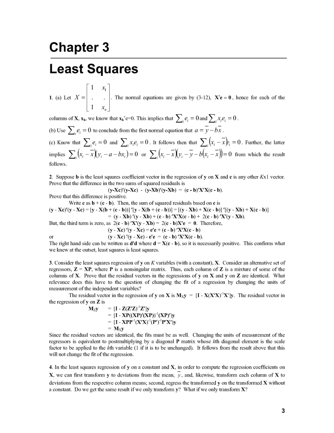
Chapter 3
Least Squares
1

1. (a) Let X =
. The normal equations are given by (3-12), X'e = 0, hence for each of the
1
columns of X, xk, we know that xk’e=0. This implies that / ,	= 0 and / ,.X.g. = 0 .
(b) Use ei = 0 1° conclude from the first normal equation that a — у — bx .
(c) Know that ^ <2, — 0 and '^^i.Xiei — 0 . It follows then that —	= 0  Further, the latter
implies (x — x^jv — a — bxt) — 0 or (x — xjjx — у — b{xt — xj) = 0 from which the result follows.
2.	Suppose b is the least squares coefficient vector in the regression of у on X and c is any other /Cxi vector. Prove that the difference in the two sums of squared residuals is
(y-Xc)'(y-Xc) - (y-Xb)'(y-Xb) = (c-b)'X'X(c-b).
Prove that this difference is positive.
Write c as b + (c - b). Then, the sum of squared residuals based on c is
(y - Xc)'(y - Xc) = [y - X(b + (c - b))] '[y - X(b + (c - b))] = [(y - Xb) + X(c - b)] '[(y - Xb) + X(c - b)]
= (y - Xb) '(y - Xb) + (c - b) 'X'X(c - b) + 2(c - b) 'X'(y - Xb).
But, the third term is zero, as 2(c - b) 'X'(y - Xb) = 2(c - b)X'e = 0. Therefore,
(y - Xc) '(y - Xc) = e'e + (c - b) 'X'X(c - b)
or	(y - Xc) '(y - Xc) - e'e = (c - b) 'X'X(c - b).
The right hand side can be written as d'd where d = X(c - b), so it is necessarily positive. This confirms what we knew at the outset, least squares is least squares.
3.	Consider the least squares regression of у on К variables (with a constant), X. Consider an alternative set of regressors, Z = XP, where P is a nonsingular matrix. Thus, each column of Z is a mixture of some of the columns of X. Prove that the residual vectors in the regressions of у on X and у on Z are identical. What relevance does this have to the question of changing the fit of a regression by changing the units of measurement of the independent variables?
The residual vector in the regression of у on X is Mxy = [I - X(X'X)-1X']y. The residual vector in the regression of у on Z is
Mzy = [I - Z(Z'Z)-1Z']y
= [I - XP((XP)'(XP))-1(XP)')y
= [I - ХРР'^Х'Ху^Р'У'Р'ХЭу
= Mxy
Since the residual vectors are identical, the fits must be as well. Changing the units of measurement of the regressors is equivalent to postmultiplying by a diagonal P matrix whose /rth diagonal element is the scale factor to be applied to the /rth variable (1 if it is to be unchanged). It follows from the result above that this will not change the fit of the regression.
4.	In the least squares regression of у on a constant and X, in order to compute the regression coefficients on X, we can first transform у to deviations from the mean, у, and, likewise, transform each column of X to deviations from the respective column means; second, regress the transformed у on the transformed X without a constant. Do we get the same result if we only transform y? What if we only transform X?
Iii the regression of у on i and X, the coefficients on X are b = (X'M0X)’1X'M°y. M° = I -is the matrix which transforms observations into deviations from then column means. Since M° is idempotent and symmetric we may also write the preceding as [(X'M0')(M0X)]'1(X'M0'M°y) which implies that the regression of M°y on M°X produces the least squares slopes. If only X is transformed to deviations, we would compute [(X'M0')(M0X)]'1(X'M°')y but, of course, this is identical. However, if only у is transformed, the result is (X'X)-1X'M°y which is likely to be quite different. We can extend the result in (6-24) to derive what is produced by this computation. In the formulation, we let Xi be X and X2 is the column of ones, so that b2 is the least squares intercept. Thus, the coefficient vector b defined above would be b = (X'X)-1X'(y - ui). But, a = у - b' x so b = (X'X)-1X'(y - i( у - b' x)). We can partition this result to produce
(X'X)’1X'(y-iy)= b - (X'X)’1X'i(b'i)= (I-nfX'Xy'x ?)b.
(The last result follows from X'i = n x.) This does not provide much guidance, of course, beyond the observation that if the means of the regressors are not zero, the resulting slope vector will differ from the correct least squares coefficient vector.
5.	What is the result of the matrix product MjM where M! is defined in (3-19) and M is defined in (3-14)? M1M = (I - X1(X1'X1)-1X1')(I - X(X'X)-1X') = M - X1(X1'X1)-1X1'M
There is no need to multiply out the second tern. Each column of MX! is the vector of residuals in the regression of the corresponding column of Xi on all of the columns in X. Since that x is one of the columns in X, this regression provides a perfect fit, so the residuals are zero. Thus, MX! is a matrix of zeroes which implies that MjM = M.
6.	Adding an observation. A data set consists of n observations on X„ and y„. The least squares estimator based on these n observations is Ьи = (Х„ХИ) 'Х^уи. Another observation, x, and ys, becomes available. Prove that the least squares estimator computed using this additional observation is
b	+;—(хХГЧ(л ~x'bJ
1 + xXx„xJ x.
Note that the last term is es, the residual from the prediction of jq using the coefficients based on X„ and b„. Conclude that the new data change the results of least squares only if the new observation on у cannot be perfectly predicted using the information already in hand.
7.	A common strategy for handling a case in which an observation is missing data for one or more variables is to fill those missing variables with Os or add a variable to the model that takes the value 1 for that one observation and 0 for all other observations. Show that this ‘strategy’ is equivalent to discarding the observation as regards the computation of b but it does have an effect on R2. Consider the special case in which X contains only a constant and one variable. Show that replacing the missing values of X with the mean of the complete observations has the same effect as adding the new variable.
8.	Let Y denote total expenditure on consumer durables, nondurables, and services, and E* E„, and Es are the expenditures on the three categories. As defined, Y=Ed + E„ + Es. Now, consider the expenditure system
Ed	OL	+	(f/T + yddPd	+	'(di-,Pи	+ ydsPs +	&yd
En	сьп	+	₽„ Y + yndPd	+	'УгРn	+ У^Рs +	sn
Es	oq	+	pfT + ysdPd	+	ysnPn	+ qJ’ +
Prove that if all equations are estimated by ordinary least squares, then the sum of the income coefficients will be 1 and the four other column sums in the preceding model will be zero.
For convenience, reorder the variables so that X = [i, Pd, P„, Pt. Y]. The three dependent variables are Ed, E„, and E„ and Y = E„> + E„ + Ef. The coefficient vectors are
b, = (Х'ХУ'Х'Е,;, b„ = (X'X)-1X'E„, and b, = (X'Xy'X'E,.
The sum of the three vectors is
b = (X'X)-1X'[Erf + E„ + EJ = (X'X)-1X'Y.
Now, Y is the last column of X, so the preceding sum is the vector of least squares coefficients in the regression of the last column of X on all of the columns of X, including the last. Of course, we get a perfect
fit. Iii addition, X'[Ed + E„ + EJ is the last column of X'X, so the matrix product is equal to the last column of an identity matrix. Thus, the sum of the coefficients on all variables except income is 0, while that on income is 1.
9.	Prove that the adjusted R2 in (3-30) rises (falls) when variable x/c is deleted from the regression if the square of the t ratio on x/c in the multiple regression is less (greater) than one.
The proof draws on the results of the previous problem. Let Rk denote the adjusted R in the full regression on К variables including x/c, and letRi denote the adjusted R in the short regression on KA variables when x/c is omitted. Let R% and R2 denote their unadjusted counterparts. Then,
Rk= 1 - e'e/y'M°y
Ri= 1 - e/e^y'lVfy
where e'e is the sum of squared residuals in the full regression, efei is the (larger) sum of squared residuals in the regression which omits x/o and y'M°y = S,- (у, - у )2
Then,	Rk= 1 - [(n-l)/(n-X)](I - R%)
and	Ri= 1 - [(n-l)/(n-(X-l))](l -A2).
The difference is the change in the adjusted R2 when xk is added to the regression,
~Rk- Ri= [(n-l)/(n-A?+l)][ei'ei/y'M°y] - [(n-l)/(n-^][e'e/y'M°y].
The difference is positive if and only if the ratio is greater than 1. After cancelling terns, we require for the adjusted A2 to increase that ei'ej/(n-A+l)]/[(n-A?)/e'e] > 1. From the previous problem, we have that e/ej = e'e + ^(x/M^), where M! is defined above and bk is the least squares coefficient in the frill regression of у on Xj and x/c. Making the substitution, we require [(e'e + />^2(х/М1Х/())(и-К)]/[(и-К)е'е + e'e] > 1. Since e'e = (n-K)s2, this simplifies to [e'e + ^(x/M^jJ/fe'e + № | > 1. Since all terms are positive, the fraction is greater than one if and only ^(x/MiX/c) > s2 or /vlx/VIix/v2) > 1. The denominator is the estimated variance of bk, so the result is proved.
10.	Suppose you estimate a multiple regression first with then without a constant. Whether the A2 is higher in the second case than the first will depend in part on how it is computed. Using the (relatively) standard method, R2 = 1 - e'e I y'My, which regression will have a higher A2?
This A2 must be lower. The sum of squares associated with the coefficient vector which omits the constant term must be higher than the one which includes it. We can write the coefficient vector in the regression without a constant as c = (0,b ) where b = (W'WjW'y, with W being the other KA columns of X. Then, the result of the previous exercise applies directly.
11. Three variables, N, D, and Y all have zero means and unit variances. A fourth variable is C = N+ D. In the regression of C on Y, the slope is .8. In the regression of C on N, the slope is .5. In the regression of D on Y, the slope is .4. What is the sum of squared residuals in the regression of C on Z>? There are 21 observations and all moments are computed using l/(n-l) as the divisor.
We use the notation ‘Var[.]’ and ‘Cov[.]’ to indicate the sample variances and covariances. Our
information is	Var[A] = 1, Var[Z>] = 1, Var[Y] = 1.
Since C = N+D, Var[C] = Var[A] + Var[Z>] + 2Cov[N,D] = 2(1 + Cov[A,Z>]). From the regressions, we have
	Cov[C,Y]/Var[Y] = Cov[C,T] = .8.
But, Also, but, so that And, Since Finally,	Cov[C,F] = Coxj.V. Ij + Cov[Z>,Y]. Cov[C,A]/Var[A] = Cov| C-Aj = -5, Cov| C.A| = Var[A] + Cov[A,Z>] = 1 + Cov[A,Z>], so Cov[A,Z>] = -.5, Var[C]=2(l+-.5)=L Cov[Z>,Y]/Var[Y] = Cov[Z>,Y] = .4. Cov[C,F] = .8 = C'oxj.V. Ij + Cov[Z>,Y], Cov|MF| = .4. Cov[C,Z>] = Cov[A,Z>] + Var[Z>] = -.5 + 1 = .5.
Now, in the regression of C onZ), the sum of squared residuals is (nA ){Var[C] - (Cov[C,Z)]/Var[Z)])2Var[Z)]}
based on the general regression result Se2 = S(y, - у )2 - /t(i, - x )2. All of the necessary figures were obtained above. Inserting these and n-1 = 20 produces a sum of squared residuals of 15.
12.	Using the matrices of sums of squares and cross products immediately preceding Section 3.2.3, compute the coefficients in the multiple regression of real investment on a constant, real GNP and the interest rate. Compute A2. The relevant submatriccs to be used in the calculations are
	Investment	Constant	GNP	Interest
Investment	*	3.0500	3.9926	23.521
Constant		15	19.310	111.79
GNP			25.218	148.98
Interest				943.86
The inverse of the lower right 3x3 block is (X'X)-1, 7.5874
(X'X)-1 =	-7.41859	7.84078
.27313	-.598953	.06254637
The coefficient vector is b = (X'X)-1X'y = (-.0727985, .235622,-.00364866)'. The total sum of squares is y'y = .63652, so we can obtain e'e = y'y - b'X'y. X'y is given in the top row of the matrix. Making the substitution, we obtain e'e = .63652 - .63291 = .00361. To compute 7?2, we require S, (x, - y)2 = .63652 - 15(3.05/15)2 = .01635333, so A2 = 1 - .00361/.0163533 = .77925.
13.	In the December, 1969, American Economic Review (pp. 886-896), Nathanial Leff reports the following least squares regression results for a cross section study of the effect of age composition on savings in 74 countries in 1964:
log S/Y= 7.3439 + 0.1596 log Y/N+ 0.0254 log G - 1.3520 log A - 0.3990 log D2 (R2 = 0.57)
logSWV = 8.7851 + 1.1486 log Y/N+ 0.0265 log G - 1.3438 log A - 0.3966 log A f/?2 - 0.96)
where S/Y= domestic savings ratio, S/N = per capita savings, Y/N = per capita income, A = percentage of the population under 15, A = percentage of the population over 64, and G = growth rate of per capita income. Are these results coirect? Explain.
The results cannot be coirect. Since log S/N = log S/Y + log Y/N by simple, exact algebra, the same result must apply to the least squares regression results. That means that the second equation estimated must equal the first one plus log Y/N. Looking at the equations, that means that all of the coefficients would have to be identical save for the second, which would have to equal its counterpart in the first equation, plus 1. Therefore, the results cannot be coirect. In an exchange between Leff and Arthur Goldberger that appeared later in the same journal, Leff argued that the difference was simple rounding error. You can see that the results in the second equation resemble those in the first, but not enough so that the explanation is credible.
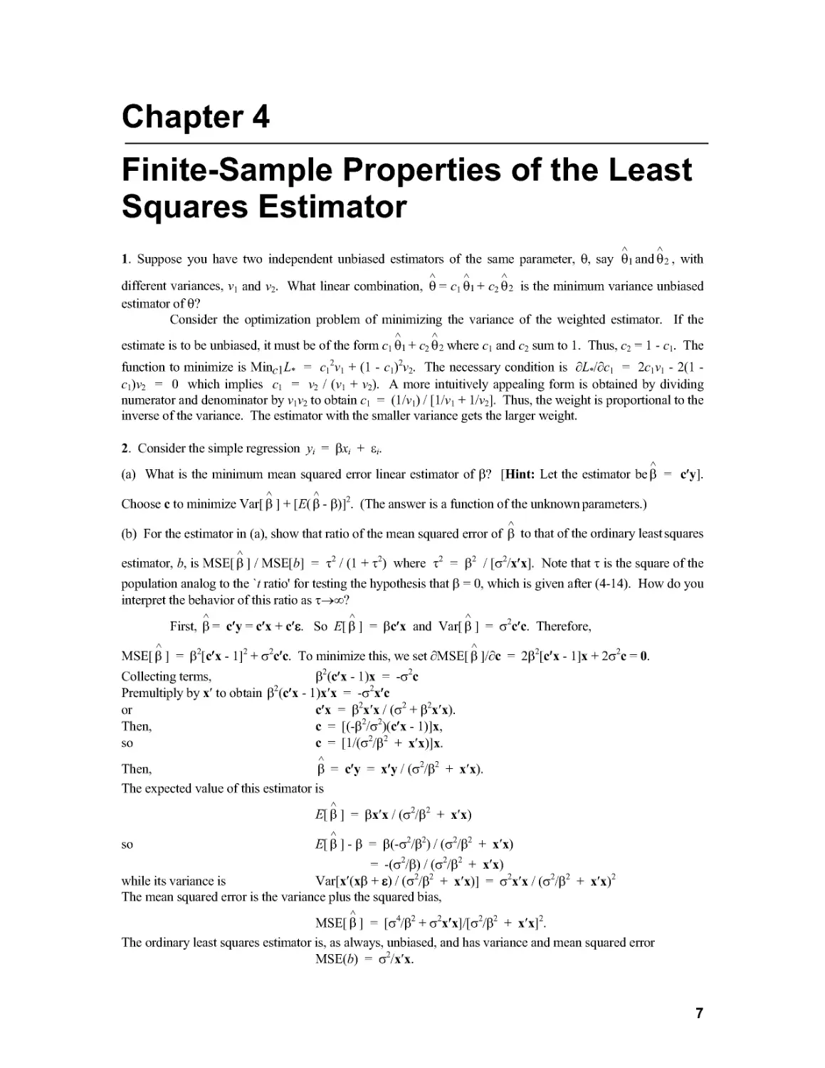
Chapter 4
Finite-Sample Properties of the Least Squares Estimator
1.	Suppose you have two independent unbiased estimators of the same parameter, 0, say 0iand02, with
different variances, Vi and v2. What linear combination, 0 = cj 0i + c2 02 is the minimum variance unbiased estimator of 0?
Consider the optimization problem of minimizing the variance of the weighted estimator. If the
estimate is to be unbiased, it must be of the form cq 0i + c2 02 where cq and c2 sum to 1. Thus, c2 = 1 - cb The function to minimize is Minr|L» = c12v1 + (1 - Cj)2v2. The necessary condition is dL»/dcx = Zcqv! - 2(1 -ci)v2 = 0 which implies Ci = v2 / (vi + v2). A more intuitively appealing form is obtained by dividing numerator and denominator by V[V2 to obtain cq = (1/vi) / [1/vj + l/v2]. Thus, the weight is proportional to the inverse of the variance. The estimator with the smaller variance gets the larger weight.
2.	Consider the simple regression y, = [k, + e,.
(a)	What is the minimum mean squared error linear estimator of P? [Hint: Let the estimator beP = c'y].
Choose c to minimize Var[ P ] + [E( p - P)]2. (The answer is a function of the unknown parameters.)
(b)	For the estimator in (a), show that ratio of the mean squared error of P to that of the ordinary least squares
estimator,/>, is MSE[ p ]/MSE[/>] = r2 / (1 + r2) where r2 = p2 / |g2/x'x|. Note that t is the square of the population analog to the 't ratio' for testing the hypothesis that P = 0, which is given after (4-14). How do you interpret the behavior of this ratio as t—>oo?
First, P = c'y = c'x + e'e. So E[ p ] = Pc'x and Var[ p ] = g2c'c. Therefore,
MSE[ p ] = p2[c'x - I]2 + g2c'c. To minimize this, we set 6MSE[ p ]/6c = 2p2[c'x - l]x + 2g2c = 0.
Collecting terms,	p2(c'x - l)x = -g2c
Premultiply by x'to obtain p2(c'x - l)x'x = -g2x'c
or	c'x = p2x'x / (a2 + p2x'x).
Then,	с = [(-p2/a2)(c'x - l)]x,
so	c = [l/(a2/p2 + x'x)]x.
Then,	p = c'y = x'y / (a2/p2 + x'x).
The expected value of this estimator is
Др] = рх'х/(ст2/р2 + x'x)
so	E[ P ] - P = p(-a2/p2) / (a2/p2 + x'x)
= -(ст2/р) / (ст2/р2 + x'x)
while its variance is	Var[x'(xP + e) / (ст2/р2 + x'x)] = g2x'x / (ст2/р2 + x'x)2
The mean squared error is the variance plus the squared bias,
MSE[ P ] = | C74 P2 + g2x'x |/| C72/p2 + x'x]2.
The ordinary least squares estimator is, as always, unbiased, and has variance and mean squared error MSE(fo) = g2/x'x.
The ratio is taken by dividing each term in the numerator
MSE p
(cr4 / p2) / (cr2 / x'x) + cr2x'x / (cr2 / x'x)
MSE(p)
= | G2x'x/p2 + (х'х)2]/(ст2/р2 + x'x)2
= x'x| G2/p2 + x'x |/(G2/p2 + x'x)2
= х'х/(ст2/р2 + x'x)
Now, multiply numerator and denominator by р2/ст2 to obtain
MSE[ p ]/MSE[&] = р2х'х/с2/| I + P2x'x/g2| = r2/[l+r2]
As r—>oo, the ratio goes to one. This would follow from the result that the biased estimator and the unbiased estimator are converging to the same thing, either as g2 goes to zero, in which case the MMSE estimator is the same as OLS, or as x'x grows, in which case both estimators are consistent.
3.	Suppose that the classical regression model applies, but the true value of the constant is zero. Compare the variance of the least squares slope estimator computed without a constant tern to that of the estimator computed with an unnecessary constant term.
The OLS estimator fit without a constant term is b = x'y / x'x. Assuming that the constant tern is, in fact, zero, the variance of this estimator is Var[b] = g2/x'x. If a constant tern is included in the regression, !=1VL -	~x)
The appropriate variance is ст2/ (хг-х) as always. The ratio of these two is
Var|/?|/Var|/?'| = |g2/x'x| / [ст2/ (хг--x) ]
But,	j (хг _ x) ~ x'x + n x2
so the ratio is	Var|/?|/Var|/?'| = [x'x + n x 2]/x'x = l-nx2/x'x = 1 - { n x + n x2]} < 1
It follows that fitting the constant term when it is unnecessary inflates the variance of the least squares estimator if the mean of the regressor is not zero.
4.	Suppose the regression model is y, = a + Px, + t:, fa) = (l/X)exp(-s,/X) > 0.
This is rather a peculiar model in that all of the disturbances are assumed to be positive. Note that the disturbances have E\t:,| = Show that the least squares constant tern is unbiased but the intercept is biased.
We could write the regression as y, = (a + /.) + Px, + (s, - /.) = a + Px, + s, . Then, we know that E[s, ] = 0, and that it is independent of x,. Therefore, the second fonn of the model satisfies all of our assumptions for the classical regression. Ordinary least squares will give unbiased estimators of a and p. As long as /. is not zero, the constant tern will differ from a.
5.	Prove that the least squares intercept estimator in the classical regression model is the minimum variance linear unbiased estimator.
Let the constant tern be written as a = 'Ejdyi =	+ Px, + s,) = uEyl, + [ЕДл', + S,ri,s,. In
order for a to be unbiased for all samples of x„ we must have S,ri, = 1 and S,rijX, = 0. Consider, then, minimizing the variance of a subject to these two constraints. The Lagrangean is
L» = Vaij«| +I) + X2S,rijX, where Var[a] = S,ct2^,2.
Now, we minimize this with respect to and X2. The (n+2) necessary conditions are
dLdddi = 2ctv/, + Xj + X2x,-, SL*/6Xi = ^di- 1, SL*/6X2 = Tyly,
The first equation implies that ri, = [-1/(2ct2)](Xj + X2x,).
Therefore,	= I = [-1/(2ст2)][иХ[ + (Т,х;)Х2]
and	ТДд, = 0 = [-1/(2ст2)][(Т,х,)Х1 + (Т,х,2)Х2].
We can solve these two equations for Xi and /-2 by first multiplying both equations by -2g2 then writing the
	n	^ixi		-2g2		^7		И	Тг-Хг.	-1	-2cr2
resulting equations as	_^ixi	\xi _	X2 к 7	0	. The solution is	7^2 7		^ixi ^ixi		0
Note, first, that S, x, = n x . Thus, the determinant of the matrix is nS, x,2 - (n x )2 = n(S, x,2 - n x2) = nSxx
where (хг--x) . The solution is, therefore.
nS-
- nx
- nx
-2cr2
0
1
0
or
Xj = (-2ст2)(Т,х,2/и)/5„
/.2 = (2o2x)/5„
Then,	di = [S,x,2/n - xx,]/57v
This simplifies if we writeSx,2 =	+ и x2, so S,x,2/n = Sxx/n+x2. Then,
dt = l/n + x (x - x,)/5TO or, in a more familiar form, d, = l/n - x (x, - x )//>,„.
This makes the intercept term = (l/n)T<y, - x Jxz - xp /S^ = у -bx which was to be shown.
6.	As a profit maximizing monopolist, you face the demand curve Q = a + PP + s. In the past, you have set the following prices and sold the accompanying quantities:
to	3 3 7 6 10	15 16	13 9 15 9	15 12 18	21
p	18 16 17 12 15	15 4	13 11 68	10 7 7	7
Suppose your marginal cost is 10. Based on the least squares regression, compute a 95% confidence interval for the expected value of the profit maximizing output.
Let q = P[g], Then, q = a + PP, or	P = (-a/p) + (1/P)9.
Using a well known result, for a linear demand curve, marginal revenue is MR = (-a/$) + (2/p)^. The profit maximizing output is that at which marginal revenue equals marginal cost, or 10. Equating MR to 10 and solving for q produces q = a/2 + 5p, so we require a confidence interval for this combination of the parameters.
. The estimate of q is 6.1816. The estimate of the variance
of the coefficients is
The least squares regression results are Q = 20.7691 - .840583. The estimated covariance matrix 7.96124	-0.624559
- 0.624559 0.0564361
of q is (1/4)7.96124 + 25(.056436) + 5(-.0624559) or 0.278415, so the estimated standard error is 0.5276.
The 95% cutoff value for a t distribution with 13 degrees of freedom is 2.161, so the confidence interval is 6.1816 - 2.16Ц.5276) to 6.1816 + 2.16Ц.5276) or 5.041 to 7.322.
7. The following sample moments were computed from 100 observations produced using a random number
		"100 123 96 109’		46(	)’	
		123 252 125 189		81(	)	
generator: X'X	=		,X'y =			
		96 125 167 146		6k		
		109 189 146 168		_7k	)	
	’ 0.03767	-0.06263 -.06247 0.1003’					
			0.06263	1.129	1.107	-2.102				
(X'X)-'=					, y’y-3924	
	—	0.06247	1.107	1.110	-2.170				
		0.1003	-2.192	-2.170	4.292				
The true model underlying these data is у = Xi + x2 + x3 + s.
(a)	Compute the simple correlations among the regressors.
(b)	Compute the ordinary least squares coefficients in the regression of y on a constant, xb x2, and x3.
(c)	Compute the ordinary least squares coefficients in the regression of у on a constant, xb and x2, on a constant, xb and x3, and on a constant, x2, and x3.
(d)	Compute the variance inflation factor associated with each variable).
(e)	The regressors are obviously collinear. Which is the problem variable?
The sample means are (1/100) times the elements in the first column of X'X. The sample covariance matrix for the three regressors is obtained as (1/99)[(X'X) у -100 хг х7 ].
Sample Var[x] =
1.0127
0.069899
0.555489
0.069899 0.555489
0.755960 0.417778
0.417778 0.496969
The simple correlation matrix is
1	.07971	.78043
.07971	1	.68167
.78043 .68167	1
The vector of slopes is (X'X/'X'y = [-.4022, 6.123, 5.910, -7.525]'. For the
three short regressions, the coefficient vectors are
(1)	one, xb andx2: [--223, 2.28, 2.11]'
(2)	one, xb and x3 [-.0696, .229, 4.025]'
(3)	one, x2, andx3: [-.0627, -.0918, 4.358]'
The magnification factors are
forxb [(1/(99(1.01727))/ 1.129]2 = .094
forx2: [(l/99(.75596)) / l.ll]2 = .109 forx3: [(l/99(.496969))/4.292]2 = .068.
The problem variable appears to be x3 since it has the lowest magnification factor. In fact, all three are highly intercorrelated. Although the simple correlations are not excessively high, the three multiple correlations are .9912 forxi onx2 andx3, .9881 forx2 onxj andx3, and .9912 forx3 onxj andx2.
8.	Consider the multiple regression of у on К variables, X and an additional variable, z. Prove that under the assumptions Al through A6 of the classical regression model, the true variance of the least squares estimator of the slopes on X is larger when z is included in the regression than when it is not. Does the same hold for the sample estimate of this covariance matrix? Why or why not? Assume that X and z are nonstochastic and that the coefficient on z is nonzero.
We consider two regressions. In the first, у is regressed on К variables, X. The variance of the least squares estimator, b = (X'X)-1X'y, Var[b] = ct2(X'X)-1. In the second, у is regressed on X and an additional variable, z. Using result (6-18) for the partitioned regression, the coefficients on X when у is regressed on X andzareb.z = (X'MzX)-1X'Mzy where Mz = I - z(z'z)-1z'. The true variance of b z is the upper left K*.K "X'X X'zn 1 z'X z'X
matrix in Var[b,c] = s2
. But, we have already found this above. The submatrix is Var[b z] =
52(X'MzX)-1 . We can show that the second matrix is larger than the first by showing that its inverse is smaller. (See Section 2.8.3). Thus, as regards the true variance matrices (Var[b])-1 - (Var[bz])-1 = (1/ct2)z(z'z)-1z' which is a nonnegative definite matrix. Therefore Var[b]-1 is larger than Var[b z]-1, which implies that Var[b] is smaller.
Although the true variance of b is smaller than the true variance of b z, it does not follow that the estimated variance will be. The estimated variances are based on s2, not the true g2. The residual variance estimator based on the short regression is s2 = е'е/(и - K) while that based on the regression which includes z is s2 = e z'e z/(n - К - 1). The numerator of the second is definitely smaller than the numerator of the first, but so is the denominator. It is uncertain which way the comparison will go. The result is derived in the previous problem. We can conclude, therefore, that if t ratio on c in the regression which includes z is larger than one in absolute value, then s2 will be smaller than s2. Thus, in the comparison, Est.Var[b] = 52(X'X)-1 is based on a smaller matrix, but a larger scale factor than Est.Var[b z] = 5Z2(X'MZX)-1. Consequently, it is uncertain whether the estimated standard ewors in the short regression will be smaller than those in the long one. Note
that it is not sufficient merely for the result of the previous problem to hold, since the relative sizes of the matrices also play a role. But, to take a polar case, suppose z and X were uncorrelated. Then, XNMZX equals XNX. Then, the estimated variance of b z would be less than that of b without z even though the true variance is the same (assuming the premise of the previous problem holds). Now, relax this assumption while holding the t ratio on c constant. The matrix in Var[bz] is now larger, but the leading scalar is now smaller. Which way the product will go is uncertain.
9.	For the classical regression model у = XP + E with no constant tern and К regressors, assuming that the true value of P is zero, what is the exact expected value of F\K. n-K\ = (IclK)l[(1 -Ic)l(n-K)]?
The Fratio is computed as [b'X'Xb/X]/[e'e/(n - X)]. We substitute e = M, and b = P + (X'X)-1X'e = (X'X)-1X'e. Then, F = [e'X(X'X)'1X'X(X'X)'1X'e/X]/[e W(b - X)] = [e'(I - М)е/Х]/[е'Ме/(и - X)].
The exact expectation of Fean be found as follows: F = [(и-Х)/Х][е'(1 - M)e]/[e'Me] . So, its exact expected value is (n-K)IK times the expected value of the ratio. To find that, we note, first, that M, and
(I - M), are independent because M(I - M) = 0. Thus, £{[e(I - M)e]/[e'Me]} = E[e'(I- M)e]x£{1/[e'Me]} . The first of these was obtained above, E[e'(I - M)s] = Xa2. The second is the expected value of the reciprocal of a chi-squared variable. The exact result for the reciprocal of a chi-squared variable is Е[1//2(и-Х)] = 1/(и - X - 2). Combining terns, the exact expectation is E[F] = (n - X) / (n - К - 2). Notice that the mean does not involve the numerator degrees of freedom. ~
10.	Prove that E[b'b] = P'P + g2E/; (1/X/c ) where b is the ordinary least squares estimator and X/c is a characteristic root of X'X.
We write b = p + (X'X/'X'e, so b'b = P'P + e'X(X'X)-1(X'X)'1X'e + zp'tX'X/'X's. The expected value of the last tern is zero, and the first is nonstochastic. To find the expectation of the second term, use the trace, and permute e'X inside the trace operator. Thus,
E[P'P] = P'P + Де'ХСХ'Ху'СХ'Ху'Х'Е]
= p'p + гме'хсх'ху'сх'ху'х'Е}]
= P'P + E|/r|(X'XrlX'£E'X(X'Xfl;|
= P'P + /г|Е|(Х'ХГ1Х'££'Х(Х'Х/1}|
= P'P + F[(X'X)-1X'E[ee']X(X'X)-1]
= P'P + F[(X'X)’1X'(ct2I)X(X'X)’1 ]
= P'P + a2tr[(X'X)'1X'X(X'X)'1 ]
= P'P + c2tr[(X'X)-1]
= P'P + c2S/c(W)
The trace of the inverse equals the sum of the characteristic roots of the inverse, which are the reciprocals of the characteristic roots of X'X.
11.	Data on U.S. gasoline consumption in the United States in the years 1960 to 1995 are given in Table F2.2.
(a)	Compute the multiple regression of per capita consumption of gasoline, G/Pop, on all of the other explanatory variables, including the time trend, and report all results. Do the signs of the estimates agree with your expectations?
(b)	Test the hypothesis that at least in regard to demand for gasoline, consumers do not differentiate between changes in the prices of new and used cars.
(c)	Estimate the own price elasticity of demand, the income elasticity, and the cross price elasticity withrespect to changes in the price of public transportation.
(d)	Reestimate the regression in logarithms, so that the coefficients are direct estimates of the elasticities. (Do not use the log of the time trend.) How do your estimates compare to the results in the previous question? Which specification do you prefer?
(e)	Notice that the price indices for the automobile market are normalized to 1967 while the aggregate price indices are anchored at 1982. Does this discrepancy affect the results? How? If you were to renormalize the indices so that they were all 1.000 in 1982, how would your results change?
Part (a) The regression results for the regression of G/Pop on all other variables are:
| Ordinary		least squares	regression	Weighting variable		= none	|	
I Dep. var	=	G	Mean=	100.700811	4	, S . D	14.08790232		1
I Model si	ze :	Observations =	36, Parameters =		10, Deg.	Fr.=	26	1
I Residuals:		Sum of squares	= 117.5342920	, Std.	Dev. =	2.12616	1
I Fit:		R-squared= .983080, Adjusted R-squared =				.97722	1
I Model test:		F[ 9,	26]	=	167.85,	Prob value =		.00000	1
| Diagnost	io:	Log-L =	-72	.3796, Restri	cted(b=0)	Log-L =	-145.8061	1
I		LogAmemiyaPrCrt.=	1.754,		Akaike Info. Crt.=		4.577	1
I Autocorrel:		Durbin-Watson	Statistic =	.94418,	Rho =	.52791	1
							
							
+		+--		+__	—	-+		+		-+		-+
|Variable	I Coefficient I Standard Error			1t-ratio	|P[1TI>t]	I Mean of X|	
+		+--		+__	—	-+		+		-+		-+
Constant	-18	59.389661	1699.6133	-1.094	.2840		
YEAR	. 9485446803		.87693228	1.082	.2893	1977.5000	
PG	-12	.18681017	2.6071552	-4.674	.0001	2.3166111	
Y	. 1	110971600E-01	.32230846E-02	3.447	.0019	9232.8611	
PNC	6 .	889686945	13.203241	. 522	. 6062	1.6707778	
PUC	-4 .	121840732	2.8707832	-1.436	.1630	2.3436389	
PPT	6.	034560575	4.0693845	1.483	. 1501	2.7448611	
PN	20	.50251499	16.556303	1.238	. 2267	2.0851111	
PD	14	.18819749	17.122006	. 829	.4148	1.6505636	
PS	-31	.48299999	12.795328	-2.461	. 0208	2.3689802	
The price and income coefficients are what one would expect of a demand equation (if that is what this is — see Chapter 16 for extensive analysis). The positive coefficient on the price of new cars would seem counterintuitive. But, newer cars tend to be more fuel efficient than older ones, so a rising price of new cars reduces demand to the extent that people buy fewer cars, but increases demand if the effect is to cause people to retain old (used) cars instead of new ones and, thereby, increase the demand for gasoline. The negative coefficient on the price of used cars is consistent with this view. Since public transportation is a clear substitute for private cars, the positive coefficient is to be expected. Since automobiles are a large component of the ‘durables’ component, the positive coefficient on PD might be indicating the same effect discussed above. Of course, if the linear regression is properly specified, then the effect of PD observed above must be explained by some other means. This author had no strong prior expectation for the signs of the coefficients on PD and PN. Finally, since a large component of the services sector of the economy is businesses which service cars, if the price of these services rises, the effect will be to make it more expensive to use a car, i.e., more expensive to use the gasoline one purchases. Thus, the negative sign on PS was to be expected.
Part (b) The computer results include the following covariance matrix for the coefficients on PNC and PUC
174.326 2.62732
2.62732 8.2414
The test statistic for testing the hypothesis that the slopes on these two variables are
equal can be computed exactly as in the first Exercise. Thus,
/[26] = [6.889686945-(-4.121840732)]/[(174.326+8.2414-2(2.62732)]1/2 = 0.827.
This is quite small, so the hypothesis is not rejected.
Part (c) The elasticities for the linear model can be computed using q = b( x / G / Pop ) for the various xs.
The mean of G is 100.701. The calculations for own price, income, and the price of public transportation are
Variable
PG Y
PPT
Coefficient
-12.18681017
0.011109716
6.034560575
Mean
2.3166111
9232.8611
2.7448611
Elasticity
-0.280
+1.019
+0.164
Part (d) The estimates of the coefficients of the loglinear and linear equations are
Constant	2.276660667	-1859.389661
YEAR	- .00440933049	0.9485446803
LPG	-.5380992257	-12.18681017	(Elasticity = -0.28)
LY	1.217805741	0.01110971600 (Elasticity = +1.019)
LPNC	.09006338891	6.889686945
LPUC	-.1146769420	-4.121840732
LPPT	.1232808093	6.034560575 (Elasticity = +0.164)
LPN	1.224804198	20.50251499
LPD	.9484508600	14.18819749
LPS	-1.321253144	-31.48299999
The estimates are roughly similar, but not as close as one might hope. There is little prior information which would suggest which is the better model.
Part (e) We would divide P,i by .483, P„ by .375, and Ps by .353. This would have no effect on the fit of the regression or on the coefficients on the other regressors. The resulting least squares regression coefficients would be multiplied by these values.
Chapter 5
Large-Sample Properties of the Least Squares and Instrumental Variables Estimators
1.	For the classical regression model у = XP + E with no constant term and К regressors, what is plimX[X,n-X] = plim (X2/X)/[( l-X2)/(n-X)]
assuming that the true value of P is zero? What is the exact expected value?
The Fratio is computed as [b'X'Xb/X]/[e'e/(n - X)]. We substitute e = M, and b = P + (X'X)-1X'e = (X'X)-1X'e. Then, F = [е'Х(Х'Х)'1Х'Х(Х'Х)'1Х'е/Х]/[е W(b - X)] = [e'(I - М)е/Х]/[е'Ме/(и - X)]. The denominator converges to g2 as we have seen before. The numerator is an idempotent quadratic fonn in a normal vector. The trace of (I - M) is К regardless of the sample size, so the numerator is always distributed as g2 times a chi-squared variable with К degrees of freedom. Therefore, the numerator of F does not converge to a constant, it converges to ct2/X times a chi-squared variable with К degrees of freedom. Since the denominator of F converges to a constant, ст2, the statistic converges to a random variable, (1/X) times a chi-squared variable with X degrees of freedom.
2.	Let e, be the rth residual in the ordinary least squares regression of у on X in the classical regression model and let s, be the coiTesponding true disturbance. Prove that plim(e, - s,) = 0.
We can write e, as e, = y, - b'x, = (P'x, + s;) - b'x, = s, + (b - P)'x,
We know that plim b = P, and x, is unchanged as n increases, so as n—>oo, e, is arbitrarily close to e,.
3.	For the simple regression model, у, = p + e„ s, ~ N(0,ct2), prove that the sample mean is consistent and asymptotically normally distributed. Now, consider the alternative estimator p = S,- wy„ where
Wj = z7(n(n+l)/2) = z/T, i. Note that S,w,- = 1. Prove that this is a consistent estimator of p and obtain its asymptotic variance. [Hint: S, z2 = и(и+1)(2и+1)/6.]
The estimator is y= (l/n)S,y, = (l/n)S, (p + s,) = p + (l/n)S, s,. Then,X[y ] p+ (1/и)Т,Е[е;] = p andVar[y]= (l/n2)S,S7Cov[E„E7] = ст2/и. Since the mean equals p and the variance vanishes as и—»оо, у is consistent. In addition, since у is a linear combination of normally distributed variables, у has a normal distribution with the mean and variance given above in every sample. Suppose that s; were not normally distributed. Then, Jn (у -p) = (1/Jn )(S,s,) satisfies the requirements for the central limit theorem. Thus, the asymptotic normal distribution applies whether or not the disturbances have a normal distribution.
For the alternative estimator, p = S,- мда, so E[ p ] = S,- w,X[y;] = S,- w,p = pT, w, = p and
Var[ p ]= S,- w,2ct2 = ct2Z, w,2. The sum of squares of the weights is S,w,2 = S,- z2/[T, z]2 = [и(и+1)(2и+1)/6]/[и(и+1)/2]2 = [2(и2 + Зп/2 + l/2)]/[1.5n(n2 + 2n + 1)]. As n—>oo, the fraction will be dominated by the tern (l/n) and will tend to zero. This establishes the consistency of this estimator. The last expression also provides the asymptotic variance. The large sample variance can be found as Asy.Var[ p ] = (IZn)lim „-^Varf Jn (p - p)]. For the estimator above, we can use Asy.Var[ p ] = (IZn)lim „^„nVarf p - p] = (IZn)lim „_>К1ст2[2(и2 + 3n/2 + l/2)]/[1.5(n2 + 2n + 1)] = ТЗЗЗЗст2. Notice that this is unambiguously larger than the variance of the sample mean, which is the ordinary least squares estimator.
4.	In the discussion of the instrumental variables estimator, we showed that the least squares estimator, b, is biased and inconsistent. Nonetheless, b does estimate something; plim b = 0 = P + Q-1y. Derive the asymptotic covariance matrix of b and show that b is asymptotically normally distributed.
To obtain the asymptotic distribution, write the result already in hand as b = (P + Q-1y) + (X'X)-1X'e -Q-1e. We have established that plim b = P + Q-1y. For convenience, let 0 p denote P + Q-1y = plim b. Write the preceding in the form b - 0 = (Х'Х/и)-1(Х'е/и) - Qy. Since plim(X'X/n) = Q, the large sample behavior of the right hand side is the same as that of plim (b - 0) = Q-1plim(X'E/n) - Q-1y. That is, we may replace (X'X/n) with Q in our derivation. Then, we seek the asymptotic distribution of Vn (b - 0) which is the same as that of
I—	i	i	ii— I 1 V1”	I
y/п [Q plim(X'e/rc) - Q_1y] = Q'Wra <-> . xzsz - у 1. From this point, the derivation is exactly the [П = 1	J
same as that when у = 0, so there is no need to redevelop the result. We may proceed directly to the same asymptotic distribution we obtained before. The only difference is that the least squares estimator estimates 0, not p.
5.	For the model in (5-25) and (5-26), prove that when only x is measured with error, the squared correlation between у and x is less than that between у and x . (Note the assumption that у = у.) Does the same hold true if у is also measured with error?
Using the notation in the text, Var[x ] = Q so, if у = P% + e, coiT2[y,x*] = (pe‘)2/[(p2e‘+ae2)e‘] = pw2e*+ae2)]
In tenus of the erroneously measured variables,
Cov[y,x] = Cov| |17 + e,x* + u] = pg*,
so	Согт2[у,х] = (pe‘)2/[(p2e‘+Ee2xe‘+^2)]
= [QW + <U2)]Corr2[y,x‘]
If у is also measured with error, the attenuation in the correlation is made even worse. The numerator of the squared correlation is unchanged, but the term (p2(? + °7) in the denominator is replaced with (p2(? + && + g, 2) which reduces the squared correlation yet further. □
6.	Christensen and Greene (1976) estimate a generalized Cobb-Douglas function of the form log(C/Pz) = a + piogg +ylog2T + Sdog^/Py) + 5zlog(Pz/Py) + e.
Pk, Pi, and Pf indicate unit prices of capital, labor, and fuel, respectively, Q is output and C is total cost. The purpose of the generalization was to produce a и-shaped average total cost curve. (See Example 7.3 for discussion of Nerlove’s (1963) predecessor to this study.) We are interested in the output at which the cost curve reaches its minimum. That is the point at which |clogC7clogQ||Q = q* = 1, or Q = 10^ (You can simplify the analysis a bit by using the fact that 10' = exp(2.3026x). Thus, Q = exp(2.3026[(l-P)/(2?)]).
The estimated regression model using the Christensen and Greene (1970) data are as follows, where estimated standard errors are given in parentheses:
ln(c/Pf) = - 7.294+ 0.39091 InQ + 0.06241 з(1п2 О]/2 + 0.07479 ln(p /Pf) + 0.2608 ln(p /Pf)
4 J '	(0.34427)	(0.036988)	(0.0051548) V 7	(0.061645)	4	1 '	(0.068109)	1
The estimated asymptotic covariance of the estimators of P and у is -0.000187067. R2=0.991538, e’e = 2.443509.
Using the estimates given in the example, compute the estimate of this efficient scale. Estimate the
asymptotic distribution of this estimator assuming that the estimate of the asymptotic covariance of P and у is -.00008.
The estimate is Q* = exp[2.3026(1 - .151)/(2(.117))] = 4248. The asymptotic variance of Q* = exp[2.3026(1 - p )/(2 у ) is [6(?7бр 6Q*/riy] Asy.Var[ p , у ][6(?7бр 6Q*/riy]'. The derivatives are
ag7a₽ = Q*(-2.3026 P )/(2y ) = -6312. ag7ay = Q*[-2.3026(l-P)]/(2y2) = -303326. The estimated
asymptotic covariance matrix is
.00384 -.00008
-.00008 .000144
. The estimated asymptotic variance of the estimate of
Q* is thus 13,095,615. The estimate of the asymptotic standard deviation is 3619. Notice that this is quite large compared to the estimate. A confidence interval fomed in the usual fashion includes negative values. This is common with highly nonlinear functions such as the one above.
7.	The consumption function used in Example 5.3 is a very simple specification. One might wonder if the meager specification of the model could help explain the finding in the Hausman test. The data set used for the example are given in Table F5.1. Use these data to carry out the test in a more elaborate specification
ct = P\ + fryt + РъЬ + Aq-i + St
where ct is the log of real consumption, yt is the log of real disposable income and it is the interest rate (90 day T bill rate).
Results of the computations are shown below. The Hausman statistic is 25.1 and the t statistic for the Wu test is -5.3. Both are larger than the table critical values by far, so the hypothesis that least squares is consistent is rejected in both cases.
-	-> samp;l-204$
-	-> crea;ct=log(realcons);yt=log(realdpi);it=tbilrate$
-	-> crea;ctl=ct[-l];ytl=yt[-l]$
-	-> samp;2-204$
-	-> name;x=one,yt,it,ctl;z=one,it,ctl,ytl$
-	-> regr;lhs=ct;rhs=x$
-	-> calc;s2=ssqrd$
-	-> matr;bls=b;xx=<x'x>$
-	-> 2sls;lhs=ct;rhs=x;inst=z$
-	-> matr;biv=b;xhxh=l/ssqrd*varb$
-	-> matr;d=biv-bls;vb=xhxh-xx$
-	-> matr;list;h=l/s2*d'*mpnv(vb)*d$
-	-> regr;lhs=yt;rhs=z;keep=ytf$
-	-> regr;lhs=ct;rhs=x,ytf$
| Ordinary least squares regression Weighting variable = none
I Dep. var. = CT	Mean= 7.884560181	, S.D.=	.5129509097
I Model size: Observations =	203, Parameters =	4, Deg.Fr.= 199
I Residuals: Sum of squares= . 1318216478E-01, Std.Dev.=	.00814
I Fit:	R-squared= .999752, Adjusted R-squared =	.99975
I Model test: F[ 3,	199] =********л Prob value =	.00000
| Diagnostic: Log-L =	690.6283, Restricted(b=0) Log-L =	-152.0255
|	LogAmemiyaPrCrt.=	-9.603, Akaike Info. Crt.=	-6.765
I Autocorrel: Durbin-Watson Statistic =	1.90738, Rho =	.04631
IVariable | Coefficient | Standard Error |t-ratio |P[|T|>t] | Mean of X|
Constant - . 4413074204E-01 .12917632E-01	-3.416	.0008
YT	.1833744954	.32943409E-01	5.566	.0000	7.9953259
IT	-. 165414768IE-02 .29350320E-03	-5.636	.0000	5.2499007
CT1	.8216667186	.32285244E-01	25.450	.0000	7.8757433
I Two stage least squares regression Weighting variable = none
I Dep. var. = CT	Mean= 7.884560181	, S.D.=	.5129509097
I Model size: Observations =	203, Parameters =	4, Deg.Fr.= 199
I Residuals: Sum of squares= .1344364458E-01, Std.Dev.=	.00822
I Fit:	R-squared= .999742, Adjusted R-squared =	.99974
I	(Note: Not using OLS. R-squared is not bounded in [0,1]
I Model test: F[ 3,	199] =********r Prob value =	.00000
I Diagnostic: Log-L =	688.6346, Restricted(b=0) Log-L =	-152.0255 |
|	LogAmemiyaPrCrt.=	-9.583, Akaike Info. Crt.=	-6.745 |
I Autocorrel: Durbin-Watson Statistic =	2.02762, Rho =	-.01381 |
Variable | Coefficient | Standard Error |b/St.Er. |P [ |Z|>z] | Mean of X
Constant - . 2023353156E-01
YT	.9004120016E-01
IT	-.1168585850E-02
CT1	.9130592037
(Note: E+nn or E-nn means
. 13906118E-01	-1.455
.38219830E-01	2.356
. 31214268E-03	-3.744
. 37448694E-01	24.382
multiply by 10 to + or
.1457
.0185	7.9953259
.0002	5.2499007
.0000	7.8757433
-nn power.)
Matrix H	has 1 rows and 1 columns.
1
1|	25.0986
| Ordinary least squares regression Weighting variable = none
I Dep. var. = YT	Mean= 7.995325935	, S.D.=	.5109250627
Model size: Observations =	203, Parameters =	4, Deg.Fr.= 199
Residuals: Sum of squares= . 1478971099E-01, Std.Dev.=	.00862
Fit:	R-squared= .999720, Adjusted R-squared =	.99972
Model test: F[ 3,	199] =********, Prob value =	.00000
Diagnostic: Log-L =	678.9490, Restricted(b=0) Log-L =	-151.2222
LogAmemiyaPrCrt.=	-9.488, Akaike Info. Crt.= -6.650
Autocorrel: Durbin-Watson Statistic =	1.77592, Rho =	.11204
(Variable | Coefficient | Standard Error |t-ratio |P[|T|>t] | Mean of X|
Constant	. 4045167318E-01	.13493797E-01	2.998	.0031	
IT	.2943892707E-03	.32000803E-03	. 920	.3587	5.2499007
CT1	.9130171904E-01	. 35621085E-01	2.563	.0111	7.8757433
YT1	.9057719332	.36310045E-01	24.945	.0000	7.9868448
| Ordinary least squares regression Weighting variable = none
I Dep. var. = CT	Mean= 7.884560181	, S.D.=	.5129509097
Model size: Observations =	203, Parameters =	5, Deg.Fr.= 198
Residuals: Sum of squares= .1151983043E-01, Std.Dev.=	.00763
Fit:	R-squared= .999783, Adjusted R-squared =	.99978
Model test: F[ 4,	198] =********r Prob value =	.00000
Diagnostic: Log-L =	704.3099, Restricted(b=0) Log-L =	-152.0255
LogAmemiyaPrCrt.=	-9.728, Akaike Info. Crt.= -6.890
Autocorrel: Durbin-Watson Statistic =	2.35530, Rho =	-.17765
(Variable | Coefficient | Standard Error |t-ratio |P[|T|>t] | Mean of X|
Constant	- . 2023559983E-01	. 12905160E-01	-1.568	.1185	
YT	. 4752021457	. 62720658E-01	7.576	.0000	7.9953259
IT	- . 1168629424E-02	. 28967486E-03	-4.034	.0001	5.2499007
CT1	. 9130504994	. 34753056E-01	26.273	.0000	7.8757433
YTF	-.3851520841	. 72054899E-01	-5.345	.0000	7.9953259
8. Suppose we change the assumptions of the model in Section 5.3 to AS5: (x„£) are an independent and identically distributed sequence of random vectors such that x, has a finite mean vector, /4, finite positive definite covariance matrix Sxx and finite fourth moments Е[хуХ7даи] = ф^т for all variables. How does the proof of consistency and asymptotic normality of b change? Are these assumptions weaker or stronger than the ones made in Section 5.2?
The assumption above is considerably stronger than the assumption AD5. Under these assumptions, the Slutsky theorem and the Lindberg Levy versions of the central limit theorem can be invoked.
9. Now, assume only finite second moments of x; £[x,2] is finite. Is this sufficient to establish consistency of b? (Hint: the Cauchy-Schwartz inequality (Theorem D. 13), E[\xy|] < {E\x2]}1/2 {E\y2]}1/2 will be helpful.) Is
The assumption will provide that (l/n)X'X converges to a finite matrix by virtue of the Cauchy-Schwartz inequality given above. If the assumptions made to ensure that plim (1/и)Х'е = 0 continue to hold, then consistency can be established by the Slutsky Theorem.
Chapter 6
Inference and Prediction
1.	A multiple regression ofy on a constant, xb and x2 produces the results below:
у = 4 + .4Xl + _9x2, A2 = 8/60, e'e = 520, n = 29, X'X =
0	0
50 10
10 80
Test the hypothesis that the two
slopes sum to 1.
The estimated covariance matrix for the least squares estimates is
	"3900/29	0	0		.69	0	0	
Лх'х/1 = ^QAA	0	80	-10	=	0	.40	-.051	where s2 = 520/(29-3) = 20. Then,
	0	-10	80		0	-.051	.256	
the test may be based on t = (.4 + .9 - l)/[.410 + .256 - 2(.O51)]1/2 = .399. This is smaller than the critical value of 2.056, so we would not reject the hypothesis.
2.	. Using the results in Exercise 1, test the hypothesis that the slope on is zero by running the restricted regression and comparing the two sums of squared deviations.
In order to compute the regression, we must recover the original sums of squares and cross products fory. These areX'y = X'Xb = [116,29,76]'. The total sum of squares is found using R1 = 1 - e'e/y'M°y, so y'M°y = 520/(52/60) = 600. The means are xi= 0, хг= 0, y= 4, so, y'y = 600 + 29(42) = 1064. The slope in the regression of у on x2 alone is b2 = 76/80, so the regression sum of squares is b22(80) = 72.2, and the residual sum of squares is 600 - 72.2 = 527.8. The test based on the residual sum of squares is F = [(527.8 - 520)/l]/[520/26] = .390. In the regression of the previous problem, the /-ratio for testing the same hypothesis would be t = .4/(.41O)12 = .624 which is the square root of .39.
3.	The regression model to be analyzed is у = XjPj + X2p2 + , where Xi and X2 have /<i and K2 columns, respectively. The restriction is p2 = 0.
(a)	Using (6-14), prove that the restricted estimator is simply [bi',0']' where bi is the least squares coefficient vector in the regression of у on Xb
(b)	Prove that if the restriction is p2 = p2° for a nonzerop2°, the restricted estimator of Pi is bi* = (X/XO-'X/fr-XzP).
For the current problem, R = [0,1] where I is the last K2 columns. Therefore, R(X'X)-1RN is the lower right /<2x/<2 block of (X'X)-1. As we have seen before, this is (X2'MiX2)-1. Also, (X'X)-1R' is the last
K2 columns of (X'X)-1. These are (X'X)-1R'
-(X1'X1)-1X1'X2(X2'M1X2)-1 (Х/МД)’1
[See (2-74).] Finally,
since q = 0, Rb - q = (Obi + Ib2) - 0 = b2. Therefore, the constrained estimator is
b
bi b2
.(X1'X1)-1X1'X2(X2'M1X2)-1
(X.'MjXJ-1
(X2'MjX2)b2, where bi and b2 are the multiple regression
coefficients in the regression of у on both Xi and X2. (See Section 6.4.3 on partitioned regression.)
Collecting terns, this produces b*
bi b2
-(Xj'Xjr'Xj'x^ b2
But, we have from Section 6.3.4
that bi = (Xi'Xi)-1Xi'y - (Xi'Xi)-1Xi'X2b2 so the preceding reduces to b* =
(X/XJ-’X/y
v 1 17 which was to
0
be shown.
If, instead, the restriction is p2 = p2° then the preceding is changed by replacing Rp - q = 0 with RP - p2° 0. Thus, Rb - q = b2 - p2°. Then, the constrained estimator is
bi
b2
b
-(X1'X1)4X1'X2(X2'M1X2)4 (X.'MjXJ-1
(X/MjX^-Pz0)
or
b*
bj + (Xj'XJ-'Xj'X^-pO) b2J [	(P° - b2)
Using the result of the previous paragraph, we can rewrite the first part as
bi* = (X1'X1)-1X1'y-(X1'X1)-1X1'X2p2°= (Х/ХО-'ХДу-ХгР?) which was to be shown.
4.	The expression for the restricted coefficient vector in (6-14) may be written in the fom b | I - CR]b + w, where w does not involve b. What is C? Show that covariance matrix of the restricted least squares estimator is ct2(X'X)-1 - ct2(X'X)'1R'[R(X'X)'1R']'1R(X'X)’1 and that this matrix may be written as
VartbREVarCb)]’1 - R'[Var(Rb)]_1R}Var[b]
By factoring the result in (6-14), we obtain b* = [I - CR]b + w where C = (X'Xy'R'P^X'Xy'R']’1 and w = Cq. The covariance matrix of the least squares estimator is
Var[b»] = [I - CR]o2(X'X)’1[I - CR]'
= CT2(X'X)-1 + g2CR(X'X) R'C' - ct2CR(X'X)-1 - aTX'Xf'R'C'.
By multiplying it out, we find that CR(X'X) = (X'X)'1R'(R(X'X)'1R')-1R(X'X)-1 = CRtX'XfR'C'
so Var[b*] = ct2(X'X)-1 - g2CR(X'X) R'C' = ct2(X'X)-1 - ct2(X'X)'1R'[R(X'X)'1RT1R(X'X)-1
This may also be written as Var[b] = cTX'Xf1 {I - R'(R(X'X)'1R')-1R(X'X)'1}
= ct2(X'X)'1{[ct2(X'X)'1]’1 - R'[Rct2(X'X)'1R']'1R}ct2(X'X)'1
Since Var[Rb] = Rg2(X'X)R' this is the answer we seek.
5.	Prove the result that the restricted least squares estimator never has a larger variance matrix than the unrestricted least squares estimator.
The variance of the restricted least squares estimator is given in the second equation in the previous exercise. We know that this matrix is positive definite, since it is derived in the form B'gTX'XJB'. and ct2(X'X)-1 is positive definite. Therefore, it remains to show only that the matrix subtracted from Var[b] to obtain Var[b*] is positive definite. Consider, then, a quadratic form in Var[b*]
z'Var[b*]z = z'Var[b]z - ct2z'(X'X)_1(R'[RtX'Xf1 R']’1 R)(X'X)-1z
= z'Var[b]z - w'[R(X'X)-1R']_1w where w = oR(X'X)-1z.
It remains to show, therefore, that the inverse matrix in brackets is positive definite. This is obvious since its inverse is positive definite. This shows that every quadratic form in Var[b*] is less than a quadratic form in Var[b] in the same vector.
6.	Prove the result that the R2 associated with a restricted least squares estimator is never larger than that associated with the unrestricted least squares estimator. Conclude that imposing restrictions never improves the fit of the regression.
The result follows immediately from the result which precedes (6-19). Since the sum of squared residuals must be at least as large, the coefficient of determination, COD = 1 - sum of squares / S, (у, - у )2, must be no larger.
7.	The Lagrange multiplier test of the hypothesis Rp-q O is equivalent to a Wald test of the hypothesis that X = 0, where X is defined in (6-14). Prove that /_2 = X' lEst.VarlXlT'X. = (и-Х)[е*'е*/е'е - 1]. Note that the fraction in brackets is the ratio of two estimators of g2. By virtue of (6-15) and the preceding section, we know that this is greater than 1. Finally, prove that the Lagrange multiplier statistic is simply JF, where Jis the number of restrictions being tested and F is the conventional F statistic given in (6-20).
For convenience, let F = [R(X'X)-1R']-1. Then, X = F(Rb - q) and the variance of the vector of Lagrange multipliers is Var[8] = FRg2(X'X)R'F = g2F. The estimated variance is obtained by replacing g2 with s1. Therefore, the chi-squared statistic is
X2 = (Rb - q) 'F'(s2F) FtRb - q) = (Rb - q) '[(l/?)F](Rb - q)
= (Rb - q) '[R(X'X)-1R']_1(Rb - q)/[e'e/(n - X)]
This is exactly / times the F statistic defined in (6-19) and (6-20). Finally, / times the F statistic in (6-20) equals the expression given above.
8.	Use the Lagrange multiplier test to test the hypothesis in Exercise 1.
We use (6-19) to find the new sum of squares. The change in the sum of squares is e*'e* - e'e = (Rb - q) '[R(X'X)’'R'] (Rb - q)
For this problem, (Rb - q) = b2 + b2 - 1 = .3. The matrix inside the brackets is the sum of the 4 elements in the lower right block of (X'X)1. These are given in Exercise 1, multiplied by s2 = 20. Therefore, the required sum is [R(X'X)-1R'] = (l/20)(.410 + .256 - 2(.O51)) = .028. Then, the change in the sum of squares is .32 / .028 = 3.215. Thus, e'e = 520, e*'e* = 523.215, and the chi-squared statistic is 26(523.215/520 - 1] = .16. This is quite small, and would not lead to rejection of the hypothesis. Note that for a single restriction, the Lagrange multiplier statistic is equal to the F statistic which equals, in tan, the square of the t statistic used to test the restriction. Thus, we could have obtained this quantity by squaring the .399 found in the first problem (apart from some rounding error).
9.	Using the data and model of Example 2.3, carry out a test of the hypothesis that the three aggregate price indices are not significant determinants of the demand for gasoline.
The sums of squared residuals for the two regressions are 207.644 when the aggregate price indices are included and 586.596 when they are excluded. The F statistic is F= [(586.596 - 207.644)/3]/[207.644/17] = 10.342. The critical value from the F table is 3.20, so we would reject the hypothesis.
10.	The model of Example 2.3 may be written in logarithmic terns as
InG/Pop = a + P/jnP,, + [Tin Y + уис1пРис + уыс1пРыс + y^lnP^ + ^year + 8dlnPd + 8„lnP„ + <5,1 n/T + s.
Consider the hypothesis that the micro elasticities are a constant proportion of the elasticity with respect to thefr corresponding aggregate. Thus, for some positive 2 (presumably between 0 and 1),
Уис 2<5f/. y;/(	2<5„-.	2<5,.
The first two imply the simple linear restriction y„c = yuc. Taking ratios, the first (or second) and third imply the nonlinear restriction ynJyPt = 8/8.,.
(a)	Describe in detail how you would test the validity of the restriction.
(b)	Using the gasoline market data in Table F2.2, test the restrictions separately and jointly.
Since the restricted model is quite nonlinear, it would be quite cumbersome to estimate and examine
the loss in fit. We can test the restriction using the unrestricted model. For this problem,
f [Уис ” "//< Ун< 6, -
The matrix of derivatives, using the order given above and " to represent the entire parameter vector, is dj\ Ida.	0
df2! da	0
о 0
0 0 8
1 -1 0
0
0
0
0
0
0
0
. The parameter estimates are
-ypt
nc
a = 18.5454, cuc = -.201536, dd = 1.50607, b„ = -.581437, c,„ = .0805074, d„ = .999474, bv = 1.39438,
bt = -.0125129, ds = -.817896, c„c = -.294769.
Thus, f = [-.092322, .119841]'. The covariance matrix to use for the tests is
9	, Г .053285	-.0362998
G52(X'X)-1G' =
-.0362998 .0342649
The statistic for the joint test is %2 = f[Gs2(X'X)’1G']’1f = .5789. This is less than the critical value for a chi-squared with two degrees of freedom, so we would not reject the joint hypothesis. For the individual hypotheses, we need only compute the equivalent of a t ratio for each element of f. Thus,
Z1 = -,092322/(.053285)2 = .3999
and	z2 = . 119841/(.0342649)2 = .6474.
Neither is large, so neither hypothesis would be rejected. (Given the earlier result, this was to be expected.).
11.	Prove that under the hypothesis that RP = q, the estimator \ = (y - Xb*)'(y - Xb*)/(n - K + J), where Jis the number of restrictions, is unbiased for g2.
First, use (6-19) to write e*'e* = e'e + (Rb - q)'[R(X'X)’1R']’1(Rb - q). Now, the result that E[e'e] = (и - /<)g2 obtained in Chapter 6 must hold here, so E[e*'e*] = (и - /<)g2 + E\(Rb - q)'[R(X'X)-1R']-1(Rb - q)]. Now, b = P + (X'X/'X'e, so Rb - q = RP - q + RCX'X/'X'e. But, RP - q = 0, so under the hypothesis, Rb - q = R(X'X)-1X'e. Insert this in the result above to obtain
E[e*'e*] = (n-K)<52 + E[e'X(X'X)'1R'[R(X'X)'1R']'1R(X'X)'1X'e]. The quantity in square brackets is a scalar, so it is equal to its trace. Permute e'X(X'X)-1R' in the trace to obtain
E[e*'e*] = (n-K)a2 + ^[^{[RCX^-'R'l-'RCX^-'X'EE'XCX'Xy'R']}
We may now carry the expectation inside the trace and use E[ee'] = g2I to obtain
E[e*'e*] = (n-X)o2+ tr{[R(X'X)’1R']’1R(X'X)’1X'o2IX(X'X)’1R']}
Carry the g2 outside the trace operator, and after cancellation of the products of matrices times their inverses, we obtain E[e*'e*] = (n -Куз2 + G2tr|[/| = (n-K + J)<52.
12.	Show that in the multiple regression of у on a constant, xb and x2, while imposing the restriction
Pi + Рг ~ 1 leads to the regression of у - xj on a constant and x2 - xb
For convenience, we put the constant tern last instead of first in the parameter vector. The constraint is Rb - q = 0 where R = [1 1 0] so Ri = [1] andR2 = [1,0]. Then, pi = [1]-1[1 - p2] = 1 - p2. Thus, у = (1 - p2)xj + p2x2 + ai + e or у - Xj = p2(x2 - Xj) + ai + e.
Chapter 7
Functional Form and Structural
Change
1.	Iii Solow's classic (1957) study of technical change in the U.S. Economy, he suggests the following aggregate production function: q(t) = A(t)/[fc(t)J where q(t) is aggregate output per manhour, k(t) is the aggregate capital labor ratio, and ,4(7) is the technology index. Solow considered four static models,
q/A = a + pin/c, q/A = a - p/к, hi(q/A) = a + pin/c, ln(q/A) = a - p//c.
(He also estimated a dynamic model, q(t)/A(t) - q(t-l)/A(t-l) = a + p/c.)
(a)	Sketch the four functions.
(b)	Solow's data for the years 1909 to 1949 are listed in Table A8.1: (Op. cit., page 314. Several variables are omitted.) Use these data to estimate the a and P of the four functions listed above. (Note, your results will not quite match Solow’s. See the next problem for resolution of the discrepancy.) Sketch the functions using your particular estimates of the parameters.
The least squares estimates of the four models are
q/A	= .45237 + .238151n/c
q/A	= .91967 - .61863/Zc
ln(9M) = -.72274 + .351601n/c
ln(9M) = -.032194 - .91496//c
At these parameter values, the four functions are nearly identical. A plot of the four sets of predictions from the regressions and the actual values appears below.
2.	In the aforementioned study, Solow states
“A scatter of q/A against k is shown in Chart 4. Considering the amount of a priori doctoring which the raw figures have undergone, the fit is remarkably tight. Except, that is, for the layer of points which are obviously too high. These maverick observations relate to the seven last years of the period, 1943-1949. From the way they lie almost exactly parallel to the main scatter, one is tempted to conclude that in 1943 the aggregate production function simply shifted.
(a)	Draw a scatter diagram of q/A against k. [Or, obtain Solow’s original study and examine his. An alternative source of the original paper is the volume edited by A. Zellner (1968).]
(b)	Estimate the four models you estimated in the previous problem including a dummy variable for the years 1943 to 1949. How do your results change? (Note, these results match those reported by Solow, though he did not report the coefficient on the dummy variable.)
(c)	Solow went on to surmise that, in fact, the data were fundamentally different in the years before 1943 than during and after. If so, one would guess that the regression should be as well (though whether the change is merely in the data or in the underlying production function is not settled). Use a Chow test to examine the difference in the two subperiods using your four functional forms. Note that with the dummy variable, you can do the test by introducing an interaction term between the dummy and whichever function of k appears in the regression. Use an F test to test the hypothesis.
The regression results for the various models are listed below, (d is the dummy variable equal to 1 for the last seven years of the data set. Standard errors for parameter estimates are given in parentheses.)
a	₽	Y		5	R2	e'e
Model 1:	q/A = a + pink + yd + 5(dink) + £				
. 4524	.2381			.94355	.00213
(.00903)	( .00932)				
. 4477	.2396	.01900		.99914	. 000032
(.00113)	( .00117)	( .000384)			
. 4476	.2397	.02746	. 08883	.99915	. 000032
(.00115)	( .00118)	(.0119)	(.0126)		
Model 2:	q/A = a -	P (l/3c) + yd +	8(d/k) + e		
. 9168	. 6186			.94915	.001915
( .00891)	( . 0229)				
. 9167	. 6185	.01961		. 99321	.000256
( .00331)	( . 00849)	( .00108)			
. 9168	. 6187	.008651	.02140	. 99322	.000255
(.00336)	( .00863)	( .0354)	(.0917)		
Model 3:	In (q/A) =	a + pink + yd	+ 8(dink)	+ s	
-.7227	.3516			. 94069	.004882
(.0137)	( .0141)				
-.7298	.3538	.002881		.99918	.000068
(.00164)	(.00169)	(.000554)			
-.7300	.3540	.04961	-.02182	.99921	.000065
( .00164)	( .00148)	( .0171)	( .0179)		
Model 4:	In (q/A) =	a - P (1/k) +	yd + 8(d/k)	+ s	
- . 03219	. 9150			. 94964	.004146
( .0131)	( .0337)				
-.03665	. 9148	.02572		. 99629	.000305
( .00361)	( .00928)	(.00118)			
- . 03646	. 9153	.004290	.05556	. 99632	.000303
(.00366)	( .00941)	( . 0386)	(.0999)		
The scatter diagram is shown below.
.60 —
।—i—i—i—i—।—i—i—i—i—।—i—i—i—i—।—i—i—i—i—।—i—i—i—i—।—i—i—i—i—।—i—i—i—i—।
2.00	2.20	2.40	2.60	2.80	3.00	3.20	3.40
К
The last seven years of the data set show clearly the effect observed by Solow.
For the four models, the F test of the third specification against the first is equivalent to the Chow-test. The statistics are:
Model 1:	F	= (.002126 - ,000032)/2 / (.000032/37) - 1210.6
Model 2:	C-	=120.43
Model 3:	F	=	=1371.0
Model 4:	F	=	= 234.64
The critical value from the F table for 2 and 37 degrees of freedom is 3.26, so all of these are statistically significant. The hypothesis that the same model applies in both subperiods must be rejected.
3. A regression model with К = 16 independent variables is fit using a panel of 7 years of data. The sums of squares for the seven separate regressions and the pooled regression are shown below. The model with the pooled data allows a separate constant for each year. Test the hypothesis that the same coefficients apply in every year.
1954	1955	1956	1957	1958	1959	1960 All
Observations 65	55	87	95	103	87	78	570
e'e	104	88	206	144	199	308	211 1425
The F statistic could be computed as
F = {[1425 - (104 + 88 + ... + 211)] / (70 -16)}/[(104 + 88 + ... + 211) / (570 - 70)] = 1.343
The 95% critical value for the F distribution with 54 and 500 degrees of freedom is 1.363.
4. Reverse Regression A common method of analyzing statistical data to detect discrimination in the workplace is to fit the following regression:
(1)	у = a + P'x + yd + s,
where у is the wage rate and d is a dummy variable indicating either membership (<7= 1) or nonmembership (<7=0) in the class toward which it is suggested the discrimination is directed. The regressors, x, include factors specific to the particular type of job as well as indicators of the qualifications of the individual. The hypothesis of interest is Ho: у < 0 vs. Ну у = 0. The regression seeks to answer the question "in a given job, are individuals in the class (<7=1) paid less than equally qualified individuals not in the class (<7=0)?" Consider, however, the alternative possibility. Do individuals in the class in the same job as others, and receiving the
same wage, uniformly have higher qualifications? If so, this might also be viewed as a form of discrimination. To analyze this question, Conway and Roberts (1983) suggested the following procedure:
(a)	Fit (1) by ordinary least squares. Denote the estimates a, b,and c.
(b)	Compute the set of qualification indices,
(2)	q = ai + Xb.
Note the omission of cd from the fitted value.
(c) Regress q on a constant, y, and d. The equation is
(3)	q = a* + P*y + y*d + e*.
The analysis suggests that if у < 0, y* > 0.
(1)	Prove that the theory notwithstanding, the least squares estimates, c and c* are related by (-_-)(1_Л2)
(4)
c*
(l-P)(l-r^)
where	yx is the mean of у for observations with d = 1,
у is the mean of у for all observations,
and
P is the mean of d, R2 is the coefficient of determination for (1) r2cl is the squared correlation betweeny and d.
[Hint: The model contains a constant term. Thus, to simplify the algebra, assume that all variables are measured as deviations from the overall sample means and use a partitioned regression to compute the coefficients in (3). Second, in (2), use the fact that based on the least squares results,
у = ai + Xb + cd + e,
so	q = у - cd - e.
From here on, we drop the constant term.] Thus, in the regression in (c), you are regressing [y - cd - e] on у and d. Remember, all variables are in deviation form.
(2) Will the sample evidence necessarily be consistent with the theory? [Hint: suppose c = 0?]
Using the hint, we seek the c* which is the slope on d in the regression of q = у - cd - e on у and d.
The regression coefficients are
У'У y'dl ’Fy'Cy-cd-e)
У'У y'dl 'Fy'y-cy'd-y'e
d'y d'dj [d'(y-cd-e)
d'y d'dj Ld'y-cd'd-d'e
In the
preceding, note that (y'y,d'y)' is the first column of the matrix being inverted while c(y'd,d'd)' is c times the second. An inverse matrix times the first column of the original matrix is the first column of an identity
matrix, and likewise for the second. Also, since d was one of the original regressors in (1), d'e = 0, and, of
course, y'e = e'e. If we combine all of these, the coefficient vector is
1
0,
y'y y'd Ye'e d'y d'dj I 0 z
fol
- c
y'y y'dl V11 , I pp d'y d'dj loj
We are interested in the
F°1
- c
second (lower) of the two coefficients. The matrix product at the end is e'e times the first column of the inverse matrix, and we wish to find its second (bottom) element. Therefore, collecting what we have thus far, the desired coefficient is c* = -c - e'e times the off diagonal element in the inverse matrix. The off diagonal
-d'y / [(y'y)(d'd) - (y'd)2] = -d'y / {[(y'y)(d'd)][l - (y'd)2/[(y'y)(d'd)]]} = -d'y/[(y'y)(d'd)(l-r^)].
Therefore,	c. = [(e'e)(d'y)] / [(y'y)(d'd)(l - r2d)] - c
(The two negative signs cancel.) This can be further reduced. Since all variables are in deviation form, e'e/y'y is (1 - R2) in the full regression. By multiplying it out, you can show that d = P so that
d'd = ^fifi-P)2 = nP(l-P)
and	d'y = S,(d, - P)(y,- у) = S,(d,-P)y, = ni(yx - y)
where nj is the number of observations which have dl = 1. Combining terms once again, we have
c. = {[W1(7j - y)(l-R2)}/{nP(l-P)(l-^)} - c
Finally, since P = njn, this further simplifies to the result claimed in the problem,
с* - {(ki - ^)(1-7?2)}/{(1-Р)(1-^)} - с
The problem this creates for the theory is that in the present setting, if, indeed, c is negative, (y} - у) will almost surely be also. Therefore, the sign of c* is ambiguous.
5.	Reverse Regression. This and the next exercise continue the analysis of Exercise 10, Chapter 8. In the earlier exercise, interest centered on a particular dummy variable in which the regressors were accurately measured. Here, we consider the case in which the crucial regressor in the model is measured with error. The paper by Kamlich and Polachek (1982) is directed toward this issue.
Consider the simple errors in variables model, у = a + [lv + ; uncorrelated, and x is the erroneously measured, observed counterpart to x .
(a)	Assume that x , u, and s are all normally distributed with means p , 0, and 0, variances ст*2, ctu2, and сте2 and zero covariances. Obtain the probability limits of the least squares estimates of a and p.
(b)	As an alternative, consider regressing x on a constant and y. then computing the reciprocal of the estimate. Obtain the probability limit of this estimate.
(c)	Do the direct' and 'reverse' estimators bound the true coefficient?
+ u, where u and s are
( у
0
1
We first find the joint distribution of the observed variables.
a
0,
so [y,x]
have a joint normal distribution with mean vector E\
ц*' 0
0,
a + Pp
and p* J
1 0
s
a
0
1
1
0
0
1
0
0
P 1 0
1 0 1
covariance matrix Var\
0
0
n2 2	2	Pz-t-
p СУ* + (?£	per*
n 2	2 .	2
рСУ*	C)« + <5 u
The probability
limit of the slope in the linear regression of у on x is, as usual,
plim b = Cov[y,x]/Var[x] = p/(l + ctu2/ct*2) < p.
The probability limit of the intercept is plim
a = E\y\ - (plim b)E[x] = a + Pp* - Pp7(l + ctu2/ct*2) = a + P[p Стц / (ст*2 + Стц2)] > a (assuming P > 0).
If x is regressed on у instead, the slope will estimate plim|/?'| = Cov[y,x]/Var[y] = рст*2/(р2ст*2 + сте2). Then,plim[ W] = P + сте2/р2ст*2 > p. Therefore, b and b' will bracket the true parameter (at least in their probability limits). Unfortunately, without more infomation about ctu2, we have no idea how wide this bracket is. Of course, if the sample is large and the estimated bracket is narrow, the results will be strongly suggestive.
6.	Reverse Regression - Continued: Suppose that the model in Exercise 5 is extended to у = P% + yd + s, x = x + u.
For convenience, we drop the constant tern. Assume that x , s, and u are independent normally distributed with zero means. Suppose that d is a random variable which takes the values one and zero with probabilities л and l-л in the population, and is independent of all other variables in the model. To put this in context, the preceding model (and variants of it) have appeared in the literature on discrimination. We viewy as a "wage" variable, x as "qualifications" and x as some imperfect measure such as education. The dummy variable, d. is membership (d= 1) or nonmembership (d= 0) in some protected class. The hypothesis of discrimination tans on y<0 versus y=0.
(a)	What is the probability limit of c, the least squares estimator of (, in the least squares regression of у on x and d‘! [Hints: The independence of x and d is important. Also, plim d'd/и = Var[d\ + E2[d\ = л(1-л) + л - л. This minor modification does not effect the model substantively, but greatly simplifies the algebra.] Now, suppose that x and d are not independent. In particular, suppose E[x |cZ=l] = p1 and E\x \d=0] = p°. Then, plim[x 'd/и] will equal яр1. Repeat the derivation with this assumption.
(b)	Consider, instead, a regression of x on у and d. What is the probability limit of the coefficient on d in this regression? Assume that x and d are independent.
(c)	Suppose that x and d are not independent, but у is, in fact, less than zero. Assuming that both
preceding equations still hold, what is estimated by у |б/=1 - у |t/=0? What does this quantity estimate if у
does equal zero?
In the regression of у on x and d, if d and x are independent, we can invoke the familiar result for least squares regression. The results are the same as those obtained by two simple regressions. It is instructive
to verify this, plim
х'х/ и x'd/ n У x'y / и d'x/и d'd/и ^d'y/n.
although the coefficient on x is distorted, the effect of interest, namely, y, is correctly measured. Now consider what happens if x and d are not independent. With the second assumption, we must replace the off diagonal zero above with plim(x'dZn). Since и and d are still uncorrelated, this equals Cov[x ,d\. This is
Со\'|л'.б/| = E\x*d\ = nE\x* d\d=Y\ + (l-n)E[x*ri|ri=O] = лц1.
Also, plim[y'd/n] is now PCov[x ,d\ + yplim(d'd/n) = [Inii + ул and plim[y'x /и] equals Pplim[x 'x /и] + yplim[x 'd/и] = P<r*2 + улц1. Then, the probability limits of the least squares coefficient estimators is
plim
x'x / и d'x/n
x'd / n
d'd/n
x'y / и d'y / n,
2	2
G, + T 71Ц1
___________1__________
Л(<Т.2+<Т2) + Л2(|?)2
Л - ТГЦ1
12	2
-ЛЦ G* +<JU
Pg* н-улц1 Ртгц1 + ул
1	f Р(л<т2+Л2(ц1)2)
л(сг2 +сг2)+л2(ц1)2 1у(л(сг2 + о-2) + л2 (ц1 )2) + Рлсг2^
The second expression does reduce to plim с = у + Рлц1сти2/[л(ст*2 + gu2) - л2(ц')2], but the upshot is that in the presence of measurement error, the two estimators become an unredeemable hash of the underlying parameters. Note that both expressions reduce to the true parameters if gu2 equals zero.
Finally, the two means are estimators of
E\y\d=Y\ = рДх>М]+У= Ph1 +Y
and	E[y|ri=0] = pE[xV=0] = pq°,
so the difference is ptii - q°) + y, which is a mixture of two effects. Which one will be larger is entirely indeterminate, so it is reasonable to conclude that this is not a good way to analyze the problem. If у equals zero, this difference will merely reflect the differences in the values of x , which may be entirely unrelated to the issue under examination here. (This is, unfortunately, what is usually reported in the popular press.)
7.	Data on the number of incidents of damage to a sample of ships, with the type of ship and the period when it was constructed, are given in Table 7.8 below There are five types of ships and four different periods of construction. Use F tests and dummy variable regressions to test the hypothesis that there is no significant “ship type effect” in the expected number of incidents. Now, use the same procedure to test whether there is a significant “period effect.”
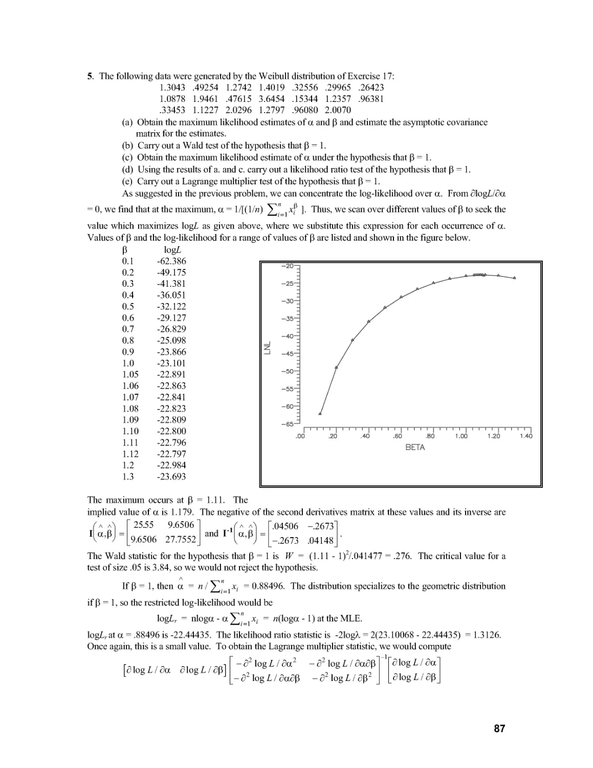
TABLE 7.8 Ship Damage Incidents
Ship		Period Constructed		
Type	1960-1964	1965-1969	1970-1974	1975-1979
A	0	4	18	11
В	29	53	44	18
C	1	1	2	1
D	0	0	11	4
E	0	7	12	1
Source: Data from McCullagh and Nelder (1983, p. 137).
According to the full model, the expected number of incidents for a ship of the base type A built in the base period 1960 to 1964, is 3.4. The other 19 predicted values follow from the previous results and are left as an exercise. The relevant test statistics for differences across ship type and year are as follows:
^r/1	(3925.2-660.9)/4 л л	™	(Ю90.3 - 660.9)/3 ,
type: F[4,12] - -----------------— -14.82, year: F[3,12] - -------------------— - 2.60.
660.9/12	660.9/12
The 5 percent critical values from the F table with these degrees of freedom are 3.26 and 3.49, respectively, so we would conclude that the average number of incidents varies significantly across ship types but not across years.
Chapter 8
Specification Analysis and Model Selection
1.	Suppose the true regression model is given by (8-2). The result in (8-4) shows that if either PL2 and fa are nonzero, then regression of у on Xi alone produces a biased and inconsistent estimator of fa. Suppose the objective is to forecast y, not to estimate the parameters. Consider regression of у on Xj alone to estimate fa with bi (which is biased). Is the forecast of computed using Xibi also biased? Assume that E[X2|X1] is a linear function of Xb Discuss your findings generally. What are the implications for prediction when variables are omitted from a regression?
The result cited is E[bj] = Pi + P1.2P2 where Pj.2 = (Xi'Xi)-1Xi'X2, so the coefficient estimator is biased. If the conditional mean function E[X2|X1] is a linear function of Xb then the sample estimator Pj 2 actually is an unbiased estimator of the slopes of that function. (That result is Theorem B.3, equation (B-68), in another form). Now, write the model in the form
у = XjPj + E[X2|Xj]p2 + e + (X2 - E[X2|Xj])p2
So, when we regress у on X! alone and compute the predictions, we are computing an estimator of Xj(Pj + Pi.2p2) = X1P1 + E[X2|X1]P2. Both parts of the compound disturbance in this regression s and (X2 - E[X2|X!])p2 have mean zero and are uncorrelated with X! and EIX^XJ, so the prediction error has mean zero. The implication is that the forecast is unbiased. Note that this is not true if E[X2|Xi] is nonlinear, since PL2 does not estimate the slopes of the conditional mean in that instance. The generality is that leaving out variables wil bias the coefficients, but need not bias the forecasts. It depends on the relationship between the conditional mean function E[X2|Xj] and XjPj 2.
2.	Compare the mean squared errors of bi and bi,2 in Section 8.2.2. (Hint, the comparison depends on the data and the model parameters, but you can devise a compact expression for the two quantities.)
The “long” estimator, bi,2 is unbiased, so its mean squared error equals its variance, ct2(Xi'M2Xi)'
The short estimator, bi is biased; E[bj] = Pj + P12p2. It’s variance is ct2(X1'X1)'1. It’s easy to show that this latter variance is smaller. You can do that by comparing the inverses of the two matrices. The inverse of the first matrix equals the inverse of the second one minus a positive definite matrix, which makes the inverse smaller hence the original matrix is larger - Var[bi,2] > Var[bj]. But, since bi is biased, the variance is not its mean squared error. The mean squared error of bi is Var[bi] + biasxbias'. The second term is Pi.2p2p2'Pi,2'. When this is added to the variance, the sum may be larger or smaller than Var[bj 2]; it depends on the data and on the parameters, p2. The important point is that the mean squared error of the biased estimator may be smaller than that of the unbiased estimator.
3.	The J test in Example is carried out using over 50 years of data. It is optimistic to hope that the underlying structure of the economy did not change in 50 years. Does the result of the test carried out in Example 8.2 persist if it is based on data only from 1980 to 2000? Repeat the computation with this subset of the data.
The regressions are based on real consumption and real disposable income. Results for 1950 to 2000 are given in the text. Repeating the exercise for 1980 to 2000 produces: for the first regression, the estimate of a is 1.03 with a t ratio of 23.27 and for the second, the estimate is -1.24 with a t ratio of -3.062. Thus, as before, both models are rejected. This is qualitatively the same results obtained with the full 51 year data set.
4.	The Cox test in Example 8.3 has the same difficulty as the J test in Example 8.2. The sample period might be too long for the test not to have been affected by underlying structural change. Repeat the computations using the 1980 to 2000 data.
Repeating the computations in Example 8.3 using the shorter data set produces qOi = -383.10 compared to -15,304 using the full data set. Though this is much smaller, the qualitative result is very much the same, since the critical value is -1.96. Reversing the roles of the competing hypotheses, we obtain qio = 2.121 compared to the earlier value of 3.489. Though this result is close to borderline, the result is, again, the same.
Chapter 9
Nonlinear Regression Models
1.	Describe how to obtain nonlinear least squares estimates of the parameters of the model у = ax13 + s.
We cannot simply take logs of both sides of the equation as the disturbance is additive rather than multiplicative. So, we must heat the model as a nonlinear regression. The linearized equation is y® a°x|3 +xp (a-a°) + a°(logx)x|3 (0-0°)
where a0 and 0° are the expansion point. For given values of a0 and 0°, the estimating equation would be y-aV + a°x|3 + a°(logx)x|3 = a^x13 j+ 0^a°(logx)x|3 j + s*
or	у + a°(logx)x|3 = a^x13 j + 0^a°(logx)x|3 j +s*.
Estimates of a and 0 are obtained by applying ordinary least squares to this equation. The process is repeated with the new estimates in the role of a0 and 0°. The iteration could be continued until convergence. Starting values are always a problem. If one has no particular values in mind, one candidate would be a0 = у and 0° = 0 or 0° = 1 and a0 either x'y/x'x or у I x . Alternatively, one could search directly for the a and 0 to minimize the sum of squares, 5(a,0) = S,(y, - ах13)2 = The first order conditions for minimization are
65(а,0)/6а = -2S,-(у,-- ax^jx13 = 0 and 65(a,0)/60 = -2S, (y, - ax|3)a(lnx)x|3 = 0.
Methods for solving nonlinear equations such as these are discussed in Chapter 5.
2.	Use Mackinnon, et. al's PE test to determine whether a linear or log-linear production model is more appropriate for the data in Table F6.1. (The test is described in Section 9.4.3 and Example 9.8.)
First, the two simple regressions produce
	Linear	Log-linear
Constant	114.338 (173.4)	1.17064 (.3268)
Labor	2.33814 (1.039)	.602999 (.1260)
Capital	.471043 (.1124)	.37571 (.08535)
R2	.9598	.9435
Standard Error	469.86	.1884
In the regression of У on 1, K, L, and the predicted values from the loglinear equation minus the predictions from the linear equation, the coefficient on a is -587.349 with an estimated standard error of 3135. Since this is not significantly different from zero, this evidence favors the linear model. In the regression of 1пУ on 1, ln/<. In£ and the predictions from the linear model minus the exponent of the predictions from the loglinear model, the estimate of a is .000355 with a standard error of .000275. Therefore, this contradicts the preceding result and favors the loglinear model. An alternative approach is to fit the Box-Cox model in the fashion of Exercise 4. The maximum likelihood estimate of/, is about -.12, which is much closer to the log-linear model than the lonear one. The log-likelihoods are -192.5107 at the MLE, -192.6266 at /.~0 and -202.837 at /. = 1. Thus, the hypothesis that /. = 0 (the log-linear model) would not be rejected but the hypothesis that /. = 1 (the linear model) would be rejected using the Box-Cox model as a framework.
3.	Using the Box-Cox transformation, we may specify an alternative to the Cobb-Douglas model as 111У = a +	- 1)/X + pz(Z? - 1)/X + s.
Using Zellner and Revankar's data in Table A9.1, estimate a, [U Р/, and X by using the scanning method suggested in Section F9.2. (Do not forget to scale У, K, and L by the number of establishments.) Use (9-16), (9-12) and (9-13) to compute the appropriate asymptotic standard errors for your estimates. Compute the two output elasticities, dlnY/dhiK and dhiY/dhiL at the sample means of К and L. [Hint: dlnY/dhiK = KdlnY/dK.] How do these estimates compare to the values given in Example 10.5?
The search for the minimum sum of squares produced the following results:
X e'e
-.500 .78477
-.400 .67033
-.300 .60587
-.250 .59479
-.245 .59451
-.244 .59447
-.243 .59444
-.242 .59441
-.241 .59439
-.240 .59438
-.239 .59437
-.238 .59436
-.237 .59437
-.235 .59440
-.225 .59492
-.200 .59897
-.100 .65598
0.000 .78143
LAMBDA
.100 .97742
.200 1.24354
The sum of squared
residuals is minimized at X = -.238. At this value, the regression results are as follows:
Parameter	Estimate	OLS Std.Error	Correct Std.Error
a	2.06092	.07718	.09723
	.178232	.04638	.04378
Р/	.737988	.06996	.12560
X	-.238	—	.07710
Estimated Asymptotic Covariance Matrix
a	Pk	Pi x
a .00945		
₽/r .00262	.00192	
Р/ .00511	-.00199	.01578
X .00500	.00037	.00825 .00594
The output elasticities for this function evaluated at the sample means are dlnY/dhiK = ₽кКл = (. 178232). 175905”238 = .2695 dlnY/dhiL = PjL* = (.443954).737988"238 = .7740.
The estimates found for Zellner and Revankar's model were .254 and .882, respectively, so these are quite similar. For the simple log-linear model, the coiTesponding values are .2790 and .927.
4.	For the model in Exercise 3, test the hypothesis that /. = 0 using a Wald test, a likelihood ratio test, and a Lagrange multiplier test. Note, the restricted model is the Cobb-Douglas, log-linear model.
The Wald test is based on the unrestricted model. The statistic is the square of the usual t-ratio, W = (-.232 / .0771)2 = 9.0546. The critical value from the chi-squared distribution is 3.84, so the hypothesis that /. = 0 can be rejected. The likelihood ratio statistic is based on both models. The sum of squared residuals for both unrestricted and restricted models is given above. The log-likelihood is Ink = -(/7 2)11 + ln(2n) + ln(e'e/n)], so the likelihood ratio statistic is
LR = n[ln(e'e//7)|X=0 - ln(e'e/n)| X=-.238] = п1п[(е'е|Х=0)/ (e'e|X=-.238) = 251n(.78143/.54369)= 6.8406.
Finally, to compute the Lagrange Multiplier statistic, we regress the residuals from the log-linear regression on a constant, Ink? Ink. and (l/2)(/?klirК + k/lirk) where the coefficients are those from the log-linear model (.27898 and .92731). The R2 in this regression is .23001, so the Lagrange multiplier statistic is LM = nR2 = 25(.23001) = 5.7503. All three statistics suggest the same conclusion, the hypothesis should be rejected.
5.	To extend Zellner and Revankar's model in a fashion similar to theirs, we can use the Box-Cox transformation for the dependent variable as well. Use the method of Section 10.5.2 (with 0 = L) to repeat the study of the previous two exercises. How do your results change?
Instead of minimizing the sum of squared deviations, we now maximize the concentrated log-likelihood function, InZ, = -(/7/2)ln(l+ln(2n)) + (L - l)S,lnT, - (/7/2)ln(s's/n).
The search for the maximum of Ink produced the following results:
L Ink
-.200 -13.6284
-.150 -12.8568
-.100-12.2423
-.050-11.7764
0.000-11.4476
.050 -11.2427
.100 -11.1480
.110-11.1410
.120 -11.1378
.121 -11.1377
.122 -11.1376
.123 -11.1376
.124 -11.1375
.125 -11.1376
.130 -11.1383 .140-11.1423 .200 -11.2344 .300 -11.6064
.400 -12.8371
The log-likelihood is maximized at /. = . 124. At this value, the regression results are as follows:
Parameter	Estimate	OLS Std.Error	Correct Std.Error
(X	2.59465	.1283	.7151
Pk	.378094	.1070	.3228
Pl	1.13653	.1117	.4121
X	.124	—	.2482
G2	.036922		.0179
Estimated Asymptotic Covariance Matrix
	a	Pk	Pi		G2
(X	.5114				
Pk	.2203	.1042			
Pl	.2612	.0951	.1698		
X	.1747	.0730	.0953	.0617	
G2	.0104	.0044	.0059	.0038	.00032
The output elasticities for this function evaluated at the sample means, К = .175905, £ = .737988, K = 2.870777, are dlnY/dlnK =	= .2674
ainT/ainZ, = b^LIYf = .9017.
These are quite similar to the estimates given above. The sum of the two output elasticities for the states given in the example in the text are given below for the model estimated with and without transforming the dependent variable. Note that the first of these makes the model look much more similar to the Cobb Douglas model for which this sum is constant.
State Full Box-Cox Model InQ on left hand side
Florida	1.2840	1.6598
Louisiana	1.2019	1.4239
California	1.1574	1.1176
Maryland	1.1657	1.0261
Ohio	1.1899	.9080
Michigan	1.1604	.8506
Once again, we are interested in testing the hypothesis that X = 0. The Wald test statistic is
W = (.123 / .2482)2 = .2455. We would now not reject the hypothesis that X = 0. This is a surprising outcome. The likelihood ratio statistic is based on both models. The sum of squared residuals for the restricted model is given above. The sum of the logs of the outputs is 19.29336, so the restricted log-likelihood is ln£°= (0-l)(19.29336) - (25/2)[l + ln(2n) + ln(.781403/25)] = -11.44757. The likelihood ratio statistic is -2[ -11.13758 - (-11.44757)] = .61998. Once again, the statistic is small. Finally, to compute the Lagrange multiplier statistic, we now use the method described in Example 10.12. The result is LM = 1.5621. All of these suggest that the log-linear model is not a significant restriction on the Box-Cox model. This rather peculiar outcome would appear to arise because of the rather substantial reduction in the log-likelihood function which occurs when the dependent variable is transformed along with the right hand side. This is not a contradiction because the model with only the right hand side transformed is not a parametric restriction on the model with both sides transformed. Some further evidence is given in the next exercise.
6.	Verify the following differential equation which applies to the Box-Cox transformation d'xw/dV =	(1/X)[x\lnx)' - zd'-1xw/dX'-1]	(9-33)
Show that the limiting sequence for /. = 0 is
d'xw/dXjX=o = (lnx)7(z+l).	(9-34)
(These results can be used to great advantage in deriving the actual second derivatives of the log likelihood function for the Box-Cox model. Hint: See Example 10.11.)
The proof can be done by mathematical induction. For convenience, denote the rth derivative by/. The first derivative appears in Equation (9-34). Just by plugging in z=l, it is clear that / satisfies the relationship. Now, use the chain rule to differentiate/,
/ = (-l/X2)[x\hixO-x(zV(l/^)[(M^(M-/i]
Collect terns to yield / = (-1/X)/ + (1/X)[x\hix)2 -/] = (1/X)[x\lnx)2 - 2/].
So, the relationship holds for i = 0, 1, and 2. We now assume that it holds for i = KA, and show that if so, it also holds for i = K. This will complete the proof. Thus, assume
A-i = (1/Х)[х\1пх)&1 - (^-W2]
Differentiate this to give fK = (-l/X)/f.i + (1/X)[(hix)xz(lnx)7r'1 - (A?-l)/f.i].
Collect terns to give fK = (l/XXx^lnx)^ - KfK.\\, which completes the proof for the general case.
Now, we take the limiting value
Шп^оУ/ = hm^otAlnx)'- z/m]/X.
Use L'Hospital's rule once again.
limx->o^ ~ 1йп^ой?{[^(1пх)'- z^.i]/tZX}/lim^o<^/^-
Then,	lim^o^ = lim^0 {[/(tax)*1 - ifj\ }
Just collect terns, (г+1)1ш1^0У/ = lim^0 [/(tax)*1]
or	lim^o/ ~ 1йп^о[лЛ(1пх)'+1]/(;+1) = (lnx)'+1/(z+l).
Chapter 10
Nonspherical Disturbances - The Generalized Regression Model
1.	What is the covariance matrix, Cov|/?./?-b |. of the GLS estimator 0 = (X'Q 'xj 'x'Q 'y and the difference between it and the OLS estimator, b = (X'X)'X'y? The result plays a pivotal role in the development of specification tests in Hausman (1978).
Write the two estimators as 0 = 0 + (X'Q’1X)’1X'Q’1e and b = P + (X'X)-1X'e. Then,
(P-b) = [(X'Q-1X)_1X'Q-1 - (X'X)-1X']e has E[ 0 - b] = 0 since both estimators are unbiased. Therefore,
Cov[P,P-b] = E[(P-P)(P-b)'].
Then,
E{(X'Q-1X)'1X'Q'1ee'[(X'Q'1X)'1X'Q'1 - (X'Xy'X']'}
= (X'Q'1X)'1X'Q'1(g2Q)[Q'1X(X'Q‘1X)'1 - XtX'Xf11
= ct2(X'Q-1X)-1X'Q-1QQ-1X(X'Q-1X)-1 - (X'Q-1X)-1X'Q-1QX(X'X)-1
= (X'Q'1X)'1(X'Q'1X)(X'Q'1X)’1 - (X'Q'1X)'1(X'X)(X'X)'1 = 0
once the inverse matrices are multiplied.
2.	This and the next two exercises are based on the test statistic usually used to test a set of J linear restrictions in the generalized regression model:
(R^-q)'[R(X'Q-1X)-1R']_1(R^-q)/J
F[J, n-K\ =-------------------—;-----------------------,
(y-X^)'Q \у-ХЗ)/(и-^)
where p is the GLS estimator. Show that if Q is known, if the disturbances are normally distributed and if the null hypothesis, RP = q, is true, then this statistic is exactly distributed as F with J and n К degrees of freedom. What assumptions about the regressors are needed to reach this conclusion? Need they be nonstochastic?
First, (RP - q) = R[0 + (X'Q-'XX'X'Q-'e)] - q = R(X'Q 'X) 'X'Q 'e if RP - q = 0.
Now, use the inverse square root matrix of Q, P = Q12 to obtain the transformed data, X* = PX = Q 12X, y* = Py = Q 12y, and E* = Pe = Q 1 2e.
Then,	£|ee'| = ДО’1/2ee'Q'2] = Q /2(g2Q)Q-12 = gI.
and,	p	= (X'Q-'xy'X'Q-'y = (Х‘'ХУхУ
= the OLS estimator in the regression of y* on X*.
Then,	Rp - q = R(X*'X*)-1X*'e‘
and the numerator is e*'X*(X*'X*)'1R'[R(X*'X*)'1R']'1R(X*'X*)’1X*'e* / J. By multiplying it out, we find that the matrix of the quadratic fom above is idempotent. Therefore, this is an idempotent quadratic fom in a normally distributed random vector. Thus, its distribution is that of g2 times a chi-squared variable with degrees of freedom equal to the rank of the matrix. To find the rank of the matrix of the quadratic forni, we can find its trace. That is
fr{X*(X*'X*)'1R'[R(X*'X*)'1R']'1R(X*'X*)'1X*}
= fr{(X*'X*)'1R'[R(X*'X*)'1R']'1R(X*'X*)'1X*'X*}
= fr{(X*'X*)-1R'[R(X*'X*)'1R']'1R}
= tr{[R(X*'X*)’1R'][R(X*'X*)’1R']’1} = tr'I/l = J,
which might have been expected. Before proceeding, we should note, we could have deduced this outcome from the forni of the matrix. The matrix of the quadratic form is of the forni Q = X ABA'X ' where В is the
nonsingular matrix in the square brackets and A = (X*'X*)-1R', which is a KkJ matrix which cannot have rank higher than J. Therefore, the entire product cannot have rank higher than J. Continuing, we now find that the numerator (apart from the scale factor, ст2) is the ratio of a chi-squared[J] variable to its degrees of freedom.
We now turn to the denominator. By multiplying it out, we find that the denominator is
(у* - X* p )'(y* - X* p )/(и - К). This is exactly the sum of squared residuals in the least squares regression of y* on X*. Since y* = X*p + e* and P = (X*'X*)-1X*'y* the denominator is е*'М*е7(и - К), the familiar form of the sum of squares. Once again, this is an idempotent quadratic form in a normal vector (and, again, apart from the scale factor, g2. which now cancels). The rank of the M matrix is n - K, as always, so the denominator is also a chi-squared variable divided by its degrees of freedom.
It remains only to show that the two chi-squared variables are independent. We know they are if the two matrices are orthogonal. They are since MX 0. This completes the proof, since all of the requirements for the F distribution have been shown.
3.	Now suppose that the disturbances are not normally distributed, although Q is still known. Show that the limiting distribution of previous statistic is (1 /.У) times a chi-squared variable with /degrees of freedom. (Hint: The denominator converges to cr2.) Conclude that in the generalized regression model, the limiting distribution of the Wald statistic
W = (R£-q)'{R(Est. Var[3])R'}-1(R3-q)
is chi-squared with J degrees of freedom, regardless of the distribution of the disturbances, as long as the data are otherwise well behaved. Note that in a finite sample, the true distribution may be approximated with an F[J,n-K] distribution. It is a bit ambiguous, however, to interpret this fact as implying that the statistic is asymptotically distributed as F with J and n-K degrees of freedom, because the limiting distribution used to obtain our result is the chi-squared, not the F. In this instance, the F[J, n-K\ is a random variable that tends asymptotically to the chi-squared variate.
First, we know that the denominator of the F statistic converges to g2. Therefore, the limiting distribution of the F statistic is the same as the limiting distribution of the statistic which results when the denominator is replaced by ст2. It is useful to write this modified statistic as
W* = (l/G2)(Rp - q)'[R(X*'X*)’1R']’1(Rp - q)/J.
Now, incorporate the results from the previous problem to write this as
W* = e*'X*(X*'X*)'1R'[Rct2(X*'X*)'1R']'1R(X*'X*)'1X*'e/J
Let	e° = R(X*'X*)'1X*'e*.
Note that this is a Jxl vector. By multiplying it out, we find that E[e°e0'] = Var[8°] = R{g2(X*'X*)_1}R'. Therefore, the modified statistic can be written as W = E0'Var[s0]'1E0// This is the ‘full rank quadratic form’ discussed in Appendix B. For convenience, let C = Var[E°], T = C'12, and v = Te°. Then, W* = v'v. By construction, v = Var[E°]'1/2E0, so E[v] = 0 and Var[v] = I. The limiting distribution of v'v is chi-squared J if the limiting distribution of v is standard normal. All of the conditions for the central limit theorem apply to v, so we do have the result we need. This implies that as long as the data are well behaved, the numerator of the F statistic will converge to the ratio of a chi-squared variable to its degrees of freedom.
4.	Finally, suppose that Q must be estimated, but that assumptions (10-27) and (10-31) are met by the estimator. What changes are required in the development of the previous problem?
The development is unchanged. As long as the limiting behavior of (1/и) X' X = (1/и)Х' Q -IX is the same as that of (1/и)Х 'X , the limiting distribution of the test statistic will be the same as if the true Q were used instead of the estimate Q .
5.	In the generalized regression model, if the К columns of X are characteristic vectors of Q, then ordinary least squares and generalized least squares are identical. (The result is actually a bit broader; X may be any linear combination of exactly К characteristic vectors. This result is Kruskal’s Theorem.)
a.	Prove the result directly using matrix algebra.
b.	Prove that if X contains a constant term and if the remaining columns are in deviation form (so that the column sum is zero), then the model of Exercise 8 below is one of these cases. (The seemingly unrelated regressions model with identical regressor matrices, discussed in Chapter 14, is another.)
first, in order to simplify the algebra somewhat without losing any generality, we will scale the columns of X so that for each X/c, x/x^ = 1. We do this by beginning with our original data matrix, say, X° and obtaining X as X = X°D'1/2, where D is a diagonal matrix with diagonal elements D/* = x/c°'x/c°. By multiplying it out, we find that the GLS slopes based on X instead of X° are
P~ [(X0D'1/2)'Q'1(X0D'1/2)]'1[(X°D'1/2)'Q'1y] = D1/2[X'Q-1X](D')1/2(D')'1/2X'Q-1y = D1/2 P°
with variance Var[p] = D1/2a2[X'Q-1X]-1(D')1/2 = D1/2Var[p °](D')1/2. Likewise, the OLS estimator based on X instead of X° is b = D1/2b° and has variance Var[b] = D1/2Var[b°](D')1/2. Since the scaling affects both estimators identically, we may ignore it and simply assume that X'X = I.
If each column of X is a characteristic vector of Q, then, for the /rth column, X/o Qx/C = X/Cx/C. Further, x/Qx/c = Д and x/Qx, = 0 for any two different columns of X. (We neglect the scaling of X, so that X'X = I, which we would usually assume for a set of characteristic vectors. The implicit scaling of X is absorbed in the characteristic roots.) Recall that the characteristic vectors of Q1 are the same as those of Q while the characteristic roots are the reciprocals. Therefore, X'QX = A.K, the diagonal matrix of the К characteristic roots which correspond to the columns of X. In addition, X'Q-1X = A.Kso (X'Q-'X)-1 =ЛЙ andX'Q'y = Л/'Х'у. Therefore, the GLS estimator is simply P = X'y with variance Var[P] = g2A/<. The OLS estimator is b = (X'X)-1X'y = X'y. Its variance is Var[b] = а2(Х'Х)-1Х'ОХ(Х'Х)-1 = g2Aa-. which means that OLS and GLS are identical in this case.
6.	In the generalized regression model, suppose that Q is known.
a.	What is the covariance matrix of the OLS and GLS estimators of
b.	What is the covariance matrix of the OLS residual vector e = у - Xb?
c.	What is the covariance matrix of the GLS residual vector s = у - ХД ?
d.	What is the covariance matrix of the OLS and GLS residual vectors?
Write b = P + (X'X)-1X'e and P = P + (X'Q’1X)’1X'Q’1e. The covariance matrix is
E[(b-P)(P -P)'] = E[(X'X)-1X'e£'Q'1X(X'Q-1X)-1] = (X'X)-1X'(a2Q)Q’1X(X'Q-1X)-1 = o^X'S^X)’1.
For part (b), e = Me as always, so E[ее'] = a2MQM. No further simplification is possible for the general case.
For part (с), £= у - XP = у - X[P + (X'Q 'X/'X'Q 'e]
= xp + E - X[P + (X'Q-'xy'X'Q-'s]
= [I - X(X'Q-1X)'1X'Q'1]e.
Thus, Дее'] = [I - X(X'Q-1X)-1X'Q-1]E[ee'][I - X(X'Q-1Xy1X'Q-1] '
= [I - X(X'Q-1X)'1X'Q-1 |(g2Q)|I - X(X'Q-1X)'1X'Q-1]'
= |g2Q - o2X(X'Q’1X)’1X'][I - X(X'Q-1X)-1X'Q-1]'
= |g2Q - o2X(X'Q’1X)’1X'][I - Q-1X(X'Q'1X)-1X']
= g2Q- a2X(X'Q-1X)-1X' - a2X(X'Q-1X)-1X' + ct2X(X'Q'1)X)'1X'Q-1X(X'Q-1X)-1X'
= g2|Q - X(X'Q'1X)’1X']
The GLS residual vector appears in the preceding part. As always, the OLS residual vector is e = Me =
[I - X(X'X)-1X']e. The covariance matrix is
Де ё'] = Д(1 - Х(Х'Х)-1Х')ее'(1 - x(x,Q-1xy1x'Q-1)']
= (I - X(X'X)-1X')(ct2Q)(I - Q-'XCX'Q-'xy'X')
= g2Q - ст2Х(Х'Х)" X'Q - o2J2£2’1X(X'Q’1X)’1X' + a2X(X'X)‘ X'QQX(X'QX) 'X'
= g2Q - а2Х(Х'Х)-1Х'
= gVIQ.
7.	Suppose that у has the pdf f (y | x) = (l/x'/?)e
Then E\y | x] = P'x and Var[y | x] = (P 'x)2. For this model, prove that GLS and MLE are the same, even though this distribution, like the one in Exercise 2, involves the same parameters in the conditional mean function and the disturbance variance.
The GLS estimator is P= (X'Q'1X)'1X'-1y = [T,x,x,7(P'x,)2]'1[T,xjV(P'x,)2]. The log-likelihood for this model is InL = -S,ln(P'x,) - S,y,/(P'x,).
The likelihood equations are
ainL/ap = -Si(l/p'x,)x, + S,[y,/(P'x,)2]x, = 0
or	S,(Xjy/(P'x,)2) = S,x/(P'x,).
Now, write	S,x,/(P'x,) = S,x,x/p/(P'x,)2,
so the likelihood equations are equivalent to Т,(х<у,/(Р'х ,).2) = S,x,x,'P/(P'x ,).2, or X'Qy = (X'Q-1X)p. These are the normal equations for the GLS estimator, so the two estimators are the same. We should note, the solution is only implicit, since Q is a function of p. For another more common application, see the discussion of the FIML estimator for simultaneous equations models in Chapter 15.
8.	Suppose that the regression model is у = ;zz + s, where s has a zero mean, constant variance, and equal correlation p across observations. Then Cov| v,.v;| = стр if i j. Prove that the least squares estimator of ;zz is inconsistent. Find the characteristic roots of Q and show that Condition 2. after Theorem 10.2 is violated.
The covariance matrix is
P P
1 P
P 1
P
P
P
PPP
The matrix X is a column of Is, so the least squares estimator of /z is y. Inserting this Q into (10-5), we 2 _ cr	2
obtain Var|y | =----(1 - p + np). The limit of this expression is pc , not zero. Although ordinary least
n
squares is unbiased, it is not consistent. For this model, X'QX/и = 1 + p(n - 1), which does not converge. Using Theorem 10.2 instead, X is a column of Is, so X'X = n, a scalar, which satisfies condition 1. To find the characteristic roots, multiply out the equation Qx = /.x = (l-p)Ix + pii'x = Lx. Since i'x = Т;х;, consider any vector x whose elements sum to zero. If so, then it’s obvious that /. = p. There are n-1 such roots. Finally, suppose that x = i. Plugging this into the equation produces X = 1 - p + np. The characteristic roots of Q are (1 - p) with multiplicity n-1 and (1 - p + np}, which violates condition 2.
Chapter 11
Heteroscedasticity
1.	Suppose the regression model is yt = p + s„ where E[e,|x,] = 0, but Var[e,|x,] = ct2x,2, x,> 0.
(a)	Given a sample of observations on yt and x,-, what is the most efficient estimator of s? What is its variance?
(b)	What is the ordinary least squares estimator of p and what is the variance of the ordinary least squares estimator?
(c)	Prove that the estimator in (a) is at least as efficient as the estimator in (b).
This is a heteroscedastic regression model in which the matrix X is a column of ones. The efficient estimator is the GLS estimator, ₽= (X'Q-'X/'X'Q-'y = [T,ly,/x,2] / [T, l2/x,2] = [T,(y,/x,2)] / [S,(l/x,2)]. As always, the variance of the estimator is Var[P] = o^X'S^'X)’1 = <j2/[T,(l/x,2)]. The ordinary least squares estimator is (X'X)-1X'y =y. The variance of у is <j2(X'X)_1(X'QX)(X'X)_1 = (a2/n2)Tp,2. To show that the variance of the OLS estimator is greater than or equal to that of the GLS estimator, we must show that (ст2/и2)Т,х,2 > a2/S,(l/x,2) or (l/n2)(Sp,2)(Si(l/x,2)) > 1 or S,S,(x,-2/x-2) > n2. The double sum contains и terms equal to one. There remain n(n-l)/2 pahs of the fom (х2/х2 + x7-/x,-2). If it can be shown that each of these sums is greater than or equal to 2, the result is proved. Just let z; = x,2. Then, we require z,/z7 + z7/z, - 2 > 0. But, this is equivalent to (z,2 + z/ - 2z,z7) / z,z7 > 0 or (z, - zfi/zjZj > 0, which is certainly true if Z; and z7 are positive. They are since z, equals x,-2. This completes the proof.
2.	For the model in the previous exercise, what is the probability limit of s2 = (1/(и-1))2)(у - у )2? Note that this is the least squares estimate of the residual variance. It is also n times the conventional estimator of the variance of the OLS estimator, Est.Var[ у ]= ?(X'X)-' = s2/n. How does this compare to the true value you found in part (b) of Exercise 1? Does the conventional estimator produce the correct estimate of the true asymptotic variance of the least squares estimator?
Consider, first, y. We saw earlier that Var[y ] = (a2/n2)Sp,2 = (a2/n)(l/n)Sp,2. The expected value is E[ у ] = E[(l/n)T,y,] = a. If the mean square of x converges to something finite, then у is consistent fora. That is, if plim(l/n)SjX,2 = q where q is some finite number, then, plim у = a. As such, it follows that s2 and s2 = (l/(n-l))T,(y, - a)2 have the same probability limit. We consider, therefore, plim s2 = plim(l/(n-l))S,e,2. The expected value ofv2 is E[(l/(n-l)) S,s,2] = ст2(1/Тр,2). Once again, nothing more can be said without some assumption about x;. Thus, we assume again that the average square of x, converges to a finite, positive constant, q . Of course, the result is unchanged by division by (n-l) instead of n, so lim^x, E[s2] = g2 q . The variance of s2 is Var|.s*21 = T,Var[s,2]/(n - I)2. To characterize this, we will require the variances of the squared disturbances, which involves their fourth moments. But, if we assume that every fourth moment is finite, then the preceding is (n/(n-l)2) times the average of these fourth moments. If every fourth moment is finite, then the term is dominated by the leading (n/(n-l)2) which converges to zero. It follows that plim s2 = g2 q . Therefore, the conventional estimator estimates Asy.Var[y]= <52q/n.
The appropriate variance of the least squares estimator is Var[ у ]= (<j2/n2)Tp,2, which is, of course, precisely what we have been analyzing above. It follows that the conventional estimator of the variance of the OLS estimator in this model is an appropriate estimator of the true variance of the least squares estimator. This follows from the fact that the regressor in the model, i, is unrelated to the source of heteroscedasticity, as discussed in the text.
3.	Two samples of 50 observations each produce the following moment matrices: (In each case, X is a constant and one variable.)
Sample 1
Sample 2
	"50	300 ’		"50	300 ’
X'X			
	300 1200		300 1200
y'X	[300 2000	[300 2200	
y'y	2100	2800	
(a)	Compute the least squares regression coefficients and the residual variances, s2, for each data set. Compute the R2 for each regression.
(b)	Compute the OLS estimate of the coefficient vector assuming that the coefficients and disturbance variance are the same in the two regressions. Also compute the estimate of the asymptotic covariance matrix of the estimator.
(c)	Test the hypothesis that the variances in the two regressions are the same without assuming that the coefficients are the same in the two regressions.
(d)	Compute the two step feasible GLS estimator of the coefficients in the regression assuming that the constant and slope are the same in both regressions. Compute the estimate of the covariance matrix and compare it to the result of (b)
The sample moments are obtained using, for example, Sxx = x'x - nx2 and so on. For the two
samples, we obtain	У	%	Sxx	Syy	5xy			
Sample 1 Sample 2 The parameter estimates Sample 1	6	6	300	300	200 6	6	300	1000	400 are computed directly using the results of Chapter 6. Intercept	Slope	R2	s2 2	2/3	4/9	(1500/9/48 = 3.472				
Sample 2	-2	4/3	16/30	(4200/9/48 = 9.722			
The pooled moments based on 100 observations are X'X =		"100 600 ’ 600 4200	,X'y =	’ 600 ’ 4200	, У'У = 4900. The
coefficient vector based on these data is [a,b\ = [0,1]. This might have been predicted since the two X'X matrices are identical. OLS which ignores the heteroscedasticity would simply average the estimates. The sum of squared residuals would be e'e = y'y - b'X'y = 4900 - 4200 = 700, so the estimate of g2 is s2 = 700/98 = 7.142. Note that the earlier values obtained were 3.472 and 9.722, so the pooled estimate is between the two, once again, as might be expected. The asymptotic covariance matrix of these estimates is /(X'X/
= 7.142
.07
-.01
-.01
.167
To test the equality of the variances, we can use the Goldfeld and Quandt test. Under the null hypothesis of equal variances, the ratio F = [ei'ei/(ni - 2)]/[e2'e2/(n2 - 2)] (or vice versa for the subscripts) is the ratio of two independent chi-squared variables each divided by then- respective degrees of freedom. Although it might seem so from the discussion in the text (and the literature) there is nothing in the test which requires that the coefficient vectors be assumed equal across groups. Since for our data, the second sample has the larger residual variance, we refer 7^48,48] = s22/s 2 = 9.722 / 3.472 = 2.8 to the F table. The critical value for 95% significance is 1.61, so the hypothesis of equal variances is rejected.
The two step estimator is P [(1/s/jX/X! + (l/s/jX/Xz/'Kl/s/jXi'yi + (l/s22)X2'y2], The X'X matrices are the same in this problem, so this simplifies to
P= |(l/.s’|2 + IZ^jX'XJ'^QA/jXj'yj + (L.s’22)X2'y’21-  The estimator is, therefore 7 1	17 50 зооЛТ'Г i (зоо'1 i (зооЛ~| /9469'1
13.472 + 9.722Дзоо 21OoJ 3.472 l.2OOoJ + 9.722 l.22OoJ ” L-8422J ’
4.	Using the data in the previous exercise, use the Oberhofer-Kmenta method to compute the maximum likelihood estimate of the common coefficient vector.
The estimator must be based on maximum likelihood estimators of the two disturbance variances, so they must be recomputed first. Our initial estimators of them are у2 = (1500/9)/50 = 3.3333 and s22 = (4200/9)/50 = 9.3333. Beginning from this point, we iterate between the estimator of the coefficient vector
described above and the two variance estimators s2 = (l/50)[(y'y)j - 2P '(X'y)j + P 'X'XP ]. The iterations
are
	2 Si	2 S2	a	₽
(0)	3.333333	9.33333	.947366	.824106
(1)	3.518005	10.78117	1.01588	.830686
(3)	3.494747	10.84926	1.02545	.829092
(4)	3.491626	10.85889	1.02676	.828873
(5)	3.491199	10.86021	1.02694	.828843
(6)	3.491141	10.86039	1.02697	.828839
(7)	3.491134	10.86042	1.02697	.828839 (Converged)
5. This exercise is based on the following data set:								
50 observations on Y:								
-1.42	2.75	2.10	-5.08	1.49	1.00	.16	-1.11	1.66
-.26	-4.87	5.94	2.21	-6.87	. 90	1.61	2.11	-3.82
-.62	7.01	26.14	7.39	.79	1.93	1.97	-23.17	-2.52
-1.26	-.15	3.41	-5.45	1.31	1.52	2.04	3.00	6.31
5.51	-15.22	-1.47	-1.48	6.66	1.78	2.62	-5.16	-4.71
-.35	-.48	1.24	. 69	1.91				
50 observations on A):								
-1.65	1.48	.77	. 67	. 68	.23	-.40	-1.13	.15
-.63	.34	.35	.79	.77	-1.04	.28	.58	-.41
-1.78	1.25	.22	1.25	-.12	. 66	1.06	-.66	-1.18
-.80	-1.32	.16	1.06	-.60	.79	.86	2.04	-.51
.02	.33	-1.99	.70	-.17	.33	.48	1.90	-.18
-.18	-1.62	.39	.17	1.02				
50 observations onX2:								
-.67	.70	.32	2.88	-.19	-1.28	-2.72	-.70	-1.55
-.74	-1.87	1.56	.37	-2.07	1.20	.26	-1.34	-2.10
. 61	2.32	4.38	2.16	1.51	.30	-.17	7.82	-1.15
1.77	2.92	-1.94	2.09	1.50	-.46	.19	-.39	1.54
1.87	-3.45	-.88	-1.53	1.42	-2.70	1.77	-1.89	-1.85
2.01	1.26	-2.02	1.91	-2.23				
(a)	Compute the ordinary least squares regression of Y on a constant, X\, and X2. Be sure to compute the conventional estimator of the asymptotic covariance matrix of the OLS estimator also.
(b)	Compute the White estimator of the appropriate asymptotic covariance matrix for the OLS estimates. (See (12-9).)
(c)	Test for the presence of heteroscedasticity using White's general test. Do your results suggest the nature of the heteroscedasticity?
(d)	Use the Breusch and Pagan Lagrange multiplier test to test for heteroscedasticity.
(e)	Sort the data keying on Xq and use the Goldfeld-Quandt test to test for heteroscedasticity. Repeat using X2. What do you find?
(f)	Use one of Glesjer's tests to test for heteroscedasticity.
The ordinary least squares regression of Yon a constant, Aq, and Aq produces the following results:	
Sum of squared residuals	1911.9275
R2	.03790
Standard error of regression	6.3780
Variable	Coefficient	Standard Error t-ratio	
One	.190394	.9144	.208
Xi	1.13113	.9826	1.151
X2	.376825	.4399	.857
Covariance Matrix	White’s Corrected Matrix
.836212	.524589
-.115451 .96551	.076578 .282366
-.047133 .051081 .193532	.399218 -.091608 1.14447
To apply White's test, we first obtain the residuals from the regression of Yon a constant, X\, and AS. Then, we regress the squares of these residuals on a constant, Aq, X2, X2, X22, and ХгХ2. The R2 in this regression is .78296, so the chi-squared statistic is 50x0.78296 = 39.148. The critical value from the table of chi-squared with 6 degrees of freedom is 12.5916, so we would conclude that there is evidence of heteroscedasticity.
Referring back to the ordinary least squares regression, we now compute the mean squared residual, 1911.9275/50 = 38.23855. Then, we compute v; = (1/38.23855)e;2 for each observation. In the regression of v on a constant, Aq, and Aq, the regression sum of squares is 145.551, so the chi-squared statistic is 145.551/2 = 72.775. We reach the same conclusion as in the previous paragraph. In this case, the degrees of freedom for the test are only two, so the conclusion is somewhat stronger.
To carry out the Goldfeld-Quandt test, we order the data first based on Aq then on X2. The regressions are computed using the first and last 17 observations, so the F statistic in each case is F[14,14] = efei / e2'e2 where e/ej is the larger of the two sums of squares and e2'e2 is the smaller. For our data set, we
find	Sorted on А/		Sorted on Aq
	e'eforobs. 1-17	385.974	246.026
	e'e for obs. 34-50	273.404	1165.683
	/*’[14,14]	1.412	4.738
The second is considerably larger than the critical value of 2.48. We would conclude, therefore, that there is evidence of heteroscedasticity and it is related to X2 but not Aq. In view of this finding, it is instructive to go back to the White and Breusch and Pagan tests considered earlier. Consider the Lagrange multiplier test, first. In the regression of the squared residuals from the original regression divided by e'e/и first on 1 and X1 then on 1 and A52, the regression sums of squares are .01805 and 105.906, respectively. Therefore, the chi-squared statistics are .009025 and 52.953, respectively. The implication is, once again, that there is substantial heteroscedasticity, of the fom g,2 = ст2Л(1+уА/2). The White test involves regressing the squared residuals first on 1, Aq, and X2 then on 1, Aq, and X2. The //2s in these two regressions are .02216 and .61380, respectively. The test statistics are thus 1.108 and 30.69. The conclusion is the same.
Finally, we compute Glesjer's test statistics for the three models discussed in Section 14.3.5. We regress e2, |e|, and log|e| on 1, Aq, and X2. We use the White estimator for the covariance matrix of the parameter estimates in these regressions as there is ample evidence now that the disturbances are heteroscedastic related to X2. To compute the Wald statistic, we need the two slope coefficients, which we denote q, and the 2x2 submatrix of the 3x3 covariance matrix of the coefficients, which we denote Vq. The statistic is W = q'Vq-1q. For the three regressions, the values are 4.13, 6.51, and 6.60, respectively. The critical value from the chi-squared distribution with 2 degrees of freedom is 5.99, so the second and third are statistically significant while the first is not.
The disturbance variance underlying these data is, in fact, <52 = ct2( 1 + yXi2) so the Goldfeld-Quandt and Glejser tests have given the right diagnosis. For the Glejser test, the finding that the linear model is inappropriate makes sense since Aq takes negative values.
6.	Using the data of Exercise 5, reestimate the parameters, using a two step feasible GLS estimator. Try (12-19), (12-20), and (12-21). Which one appears to be most appropriate?
The ordinary least squares estimates are given above. The estimates of the disturbance variances are based on the residuals from this regression. For the three models, the disturbance variances are estimated as follows:
(1)	ст,2 = <j2(a'z,): Regress c2 on 1. Aj-U. Estimates of o,2 are the fitted values in this regression.
This produces numerous negative values and is clearly inappropriate.
(2)	ст,2 = CT2(a'z,)2: Regress |e,| on 1, X\, andW2. The estimates of ст,2 are the squares of the predicted values from this regression.
(3)	ст,2 = CT2exp(a'z,): Regress log(e,2) on l,Aj, and W2. The estimates of ст,2 are the exponents of the fitted values in this regression.
Weighted least squares regressions based on the second and third sets of weights (l/ст,2) produces the following estimates (standard errors are shown in parentheses). In each case, the weights are the reciprocals of the estimated standard deviations as described above.
	Unweighted	(2)
One	.190394 (.9144)	1.48129(1.817)
Xr	1.13113 (.9826)	1.44651 (.9716)
X2	.376825 (.4399)	.894613 (.7451)
There is little in the way of guidance as to which model is the better one.
(3)
.166626 (.7198)
.776487 (.6388)
.847177 (.3633)
The OLS estimates are suggestive
since they are consistent under all specifications. The second set of estimates resemble the OLS estimates
slightly more than the third. As we discussed above, model (2) is, in fact, the right one. Unfortunately, one would be hard pressed to reach that as a ffrm conclusion based on just these results. Of course, the results of
the tests in the previous exercise are much more convincing. □
7.	For the model in Exercise 1, suppose , is normally distributed with mean zero and variance ct2(1 + (yx)2). Show that ст2 and y2 can be consistently estimated by a regression of the least squares residuals on a constant and л'2. Is this estimator efficient?
The residuals from the least squares regression are e, = y, - у = a + s, - (a + s ) = s, - s . The expected value of the squared residual is
E[e,2]	= E[s,2] +£[ s 2] - 2E[s, s | ~ ст,2 + (l/n2)E[(T,s,)2] - (2/n)E[s,(T,s,)]
= ст,2 + (1/и2)Т;Е[е,2] - (2/n)E[s,2]
since the disturbances are uncorrelated. We can write this as
E[e;2] = ст2 + ст2у2х,2 + (1/и){[(1/и)Т,ст,2] - [2ct,2]}.
And, of course, e;2 = E[e,2] + (e,2 - E[e,2]) = E[e,2] + v„ where v, is uncorrelated with E[e,2] by construction. Now, if we regress e,2 on a constant and x,2, the estimates of ст2 and (ст2у2) will be biased in a finite sample because of the left out variable, namely the tern multiplied by (l/n) in the expression for E[e,2]. But, if the two terns inside the curled brackets above converge to finite quantities as n—>oo, then the entire term will vanish, and the omitted variable problem will vanish with it. Surely the second does since it is the variance of s,2, assuming that x,2 is finite. To make the first converge, we will require that (1/и)Т,[ст2 + ст2у2х,2] = ст2 + CT2y2(l/n)TjX,2 converge to a finite quantity, or that the mean square of the xs converge to a finite quantity. This is a minimal requirement for a heteroscedastic regression, and would surely be met. As such, if e,2 is regressed on a constant and x,2, we obtain consistent estimators of ст2 and сту . The estimator of ст is the square root of the ratio of the slope to the constant.
The estimator is not efficient. The expected fourth moment of a normally distributed variable is 3 times the square of the variance. Therefore, in the regression above, the variance of v, must be a function of [ct2(1 + y2x,2)]2. Since the regression is heteroscedastic in a way which is not dependent on the sample size, OLS will not be efficient, but it will be consistent.
= -n/(2o2) + (1/(2ct4))S,[s,2/(y'z,)2)].
= <j2(y'z,)2, this also has expected value zero. The second derivatives are
= T,x,(as,/ap')/[CT2(Y'z,)2] = -Si[l/o2(Y'z,)2]x,x,'
= Т;{-е;/[(g2)2(y'z,TI }x,
= ТЕ;{-2е,/[ст2(/г,)3 ]}x,z/
= w/(2g4) - (l/CT4)Ti{s,2/[o2(y'z,)2]}
= [W^JTJs^Wz,)3)]^ = [-1/(2cj2)]T,{s,2[-2/(y'z,)2)]}{l/(Y'z,)2}{2Y'z, }z,
= S,{s,2/[ct2(y'z,)2] - 1}[-1/(y'z,)2]z,z,' + S,{-2s,2/[ct2(y'z,)3]}[1/(y'z,)]z,z,'
8.	Derive the log-likelihood function, first order conditions for maximization, and information matrix for the modcl r, = P'x, + e„ s,~A[0,o2(y'z,)2].
first. logL = - (n/2) log(2n) - 2EllogG,2 - 2Sj(e,-2/o,-2)
= - (n/2)ln(2n) - (и/2) logo2 - 2E,log(Y'zl)2 - [1/(2g2)]S,[(y, - P'x,)2/(y'z,)2] aiogL/ap = -(l/(2c2))T,(l/(Y'z,)2)(2)(y, - P'x,)(-x,) = Si{Ei/[o2(Y'z,)2]}x, aiog£/ay = - 2T,(l/(Y'z,)2)(2Y'z,)zi - (1/(2ст2))Т,(у; - P'x,)2[-2/(y'z,)3]z,
= -Ti[l/(Y'z,)]zi + (1/cj2)S,[s,2/(y'z,)2][ 1/(y'z/)]z,
= Si{E,2/[o2(Y'z,)2] - IHWzOJz,
It is useful to note in passing that we can write this as = 2Т;{е,2/[ст2(у'г,)2] - 1}[1/(y'z,)2]2(y'z,)z, which is what appears in (12-28). It is obvious that these first derivatives have expectation zero, the first since E\t:,| = 0 and the second because the first tern in large brackets has expectation zero. Finally, clog£/cG2 Since E[s,2] 62logT/6p6P' a2iog£/apaa2 a2iog£/apay' a2iog£/a(a2)2 a2iog£/aF2ay' a2iog£/ayay'
In the notation of (12-26) - (12-28), f = (y'z,)2 and g, = 2(y'z,)z,. Therefore, Q = diag[(Y'z,)2] and G = the matrix whose rows are g,'. The negatives of the expected second derivatives are simple to obtain since £|t:,| = 0 and E[s,2] = g2(y'z,)2. We will write them in the fonn of (14-29). Thus,
= (1/ст2)Т;[1/(у'г,)2]х,х/
= 0
= 0
= и/(2ст4)
= [1/2cj2]T,{1/(y'z,)2}2(y'z,)z, = [l/a2]Si{l/(Y'z,)}z,
= 2T,{l/(Y'z,)4}[2(Y'z,)zi][2(Y'z,)zi]' = 2T,[1/(y'z,)2]z,z,'. □
-E[a2iog£/apap'] -/?| a2iog£/apaG21 -E[a2iogi/apay'] -E[a2iog£/a(a2)2] -/? । a2ioga/aG2cy'।
-/? । a2ioga/aycy'।
9.	See Exercise 7 of Chapter 10.
10.	In the discussion of Harvey’s model in Section 11.7, it is noted that the initial estimator of Yi, the constant tern in the regression of loge,2 on a constant and z, is inconsistent by the amount 1.2704. Harvey points out that if the purpose of this initial regression is only to obtain starting values for the interations, then the correction is not necessary. Explain why this would be the case.
The constant is just an estimate of g2 in g2Q. Let W equal g2Q. Then, the GLS estimator is P = [X'W’1X]’1[X'W’1y]. The scale factor is immaterial. The estimator will be the same whether W is scaled or not, since the scale factor will fall out of the result.
11.	(This exercise requires appropriate computer software. The computations required can be done with RATS, EViews, Stata, TSP, LIMDEP, and a variety of other software using only preprogrammed procedures.) Quarterly data on the consumer price index for 1950.1 to 2000.4 are given in Appendix Table F5.1. Use these data to fit the model proposed by Engle and Kraft (1983). The model is
я, = Д + /?i ям + /%я,.2 + /%я,.3 + Дям + £t
where я, = 1001n[pr/^2r_i] and pt is the price index.
a.	Fit the model by ordinary least squares, then use the tests suggested in the text to see if ARCH effects appear to be present.
b.	The authors fit an ARCH(8) model with declining weights,
2	, у 8 f 9-/^1 о
CT, - «,+ Lmj —- \£t_i
у 36 J
Fit this model. If the software does not allow constraints on the coefficients, you can still do this with a two step least squares procedure, using the least squares residuals from the first step. What do you find?
c.	Bollerslev (1986) recomputed this model as a GARCH(1,1). Use the GARCH(1,1) form and refit your model.
a. We used LIMDEP with the macroeconomics data in table F5.1. The rate of inflation was computed with all observations, then observations 6 to 204 were used to remove the missing data due to lags. Least squares results were obtained first. The residuals were then computed and squared. Using observations 15-204, we then computed a regression of the squared residual on a constant and 8 lagged values. The chi-squared statistic with 8 degrees of freedom is 28.24. The critical value from the table for 95% significance and 8 degrees of freedom is 15.51, so at this level of significance, the hypothesis of no GARCH effects is rejected.
crea;pt=100*log(cpi_u/cpi_u[-1])$
crea;ptl=pt[-1];pt2=pt[-2];pt3=pt[-3];pt4=pt[-4]$
samp;6-204$
regr;lhs=pt;rhs=one,ptl,pt2,pt3,pt4;res=et$$
crea;vt=et*et$
crea;vtl=vt[-1];vt2=vt[-2];vt3=vt[-3];vt4=vt[-4];vt5=vt[-5];vt6=vt[-6];vt7=vt[-7];vt8=vt[-8]$
s amp; 15-2 0 4 $
regr;lhs=vt;rhs=one,vtl,vt2,vt3,vt4,vt5,vt6,vt7,vt8$
calc;list;lm=n*rsqrd$
| Ordinary least squares regression Weighting variable = none
I Dep. var. = PT	Mean= .9589185961	, S.D.=	.8318268241
Model size; Observations =	199, Parameters =	5, Deg.Fr.= 194
Residuals; Sum of squares= 61.97028507	, Std.Dev.=	.56519
Fit:	R-squared= .547673, Adjusted R-squared =	.53835
Model test: F[ 4,	194] =	58.72, Prob value =	.00000
Diagnostic: Log-L =	-166.2871, Restricted(b=0) Log-L =	-245.2254
LogAmemiyaPrCrt.=	-1.116, Akaike Info. Crt.=	1.721
Autocorrel: Durbin-Watson Statistic =	1.80740, Rho =	.09630
IVariable | Coefficient | Standard Error |t-ratio |P[|T|>t] | Mean of X|
Constant	.1296044455	.67521735E-01	1.919	.0564
PT1	.2856136998	.69863942E-01	4.088	.0001	.97399582
PT2	.1237760914	.70647061E-01	1.752	.0813	.98184918
PT3	.2516837602	.70327318E-01	3.579	.0004	.99074774
PT4	.1824670634	.69251374E-01	2.635	.0091	.98781131
LM =	. 28240022492847690D+02
For the second step, we need an estimate of a0, which is the unconditional variance if there are no ARCH effects. We computed this based on the ARCH specification by a regression of et2 - (8/36)et-i2 - ... -(l/36)et_82 on just a constant term. This produces a negative estimate of ao, but this is not the variance, so we retain the result. We note, the problem that this reflects is probably the specific, doubtless unduly restrictive, ARCH structure assumed.
samp;6-204$
crea;vt=et*et$
crea;ht=vt-8/36*vt[-l]-7/36*vt[-2]-6/36*vt[-3]-5/36*vt[-4]-4/36*vt[-5]-3/36*vt[-6]-2/36*vt[-7]-1/36*vt[-8]$
s amp; 15-2 0 4 $
calc;list;a0=xbr(ht)$
samp;6-204$
crea;qt=a0+8/36*vt[-l]+7/36*vt[-2]+6/36*vt[-3]+5/36*vt[-4]+4/36*vt[-5]+3/36*vt[-6]+2/36*vt[-7]+1/36*vt[-8]$
s amp; 15-2 0 4 $
plot;rhs=qt$
crea;wt=l/qt$
regr;lhs=pt;rhs=one,ptl,pt2,pt3,pt4;wts=wt$
regr;lhs=pt;rhs=one,ptl,pt2,pt3,pt4;model=garch(1,1)$
Once we have an estimate of ao in hand, we then computed the set of variances according to the ARCH(8) model, using the lagged squared residuals. Finally, we used these variance estimators to compute a weighted least squares regression accounting for the heteroscedasticity. This regression is based on observations 15-204, again because of the lagged values. Finally, using the same sample, a GARCH(1,1) model is fit by maximum likelihood.
| Ordinary least squares regression Weighting variable = WT
I Dep. var. = PT	Mean= .8006997687	, S.D.=	.6327877239
Model size: Observations =	190, Parameters =	5, Deg.Fr.= 185
Residuals: Sum of squares= 38.67492770	, Std.Dev.=	.45722
Fit:	R-squared= .488964, Adjusted R-squared =	.47791
Model test: F[ 4,	185] =	44.25, Prob value =	.00000
Diagnostic: Log-L =	-147.7324, Restricted(b=0) Log-L =	-211.5074
LogAmemiyaPrCrt.=	-1.539, Akaike Info. Crt.=	1.608
Autocorrel: Durbin-Watson Statistic =	1.90310, Rho =	.04845
IVariable | Coefficient | Standard Error |t-ratio |P[|T|>t] | Mean of X|
Constant	. 1468553158	. 60127085E-01	2.442	.0155	
PT1	. 976005111OE-01	. 88469908E-01	1.103	.2714	.77755556
PT2	. 3328520370	.86772549E-01	3.836	.0002	.76745308
PT3	. 1428889148	.85420554E-01	1.673	.0961	.76271761
PT4	.2878686524	. 84090832E-01	3.423	.0008	.74173558
The 8 period ARCH model produces quite a substantial change in the estimates. Once again, this probably results from the restrictive assumption about the lag weights in the ARCH model. The GARCH model follows.
GARCH MODEL
Maximum Likelihood Estimates
Model estimated: Jul 31, 2002 at 01:19:14PM.
Dependent variable	PT
Weighting variable	None
Number of observations	190
Iterations completed	22
Log likelihood function	-135.5043
Restricted log likelihood	-147.6465
Chi squared	24.28447
Degrees of freedom	2
Prob[ChiSqd > value] =	.5328953E-05
GARCH Model, P = 1, Q = 1
Wald statistic for GARCH =	521.483
IVariable | Coefficient | Standard Error |b/St.Er. |P [ |Z|>z] | Mean of X|
+		- +	+	+	+ - Regression parameters		+ _		+
Constant	.1308478127	.61887183E-01	2.114	.0345	
PT1	.1749239917	. 70912277E-01	2.467	.0136	. 98810078
PT2	.2532191617	.73228319E-01	3.458	.0005	. 98160455
PT3	.1552879436	. 68274176E-01	2.274	.0229	. 97782066
PT4	.2751467919	. 63910272E-01	4.305	.0000	. 97277700
	Unconditional Variance		
Alpha(0)	. 1005125676E-01	.11653271E-01	.863	.3884	
	Lagged Variance Terms		
Delta(1)	.8556879884	.89322732E-01	9.580	.0000	
	Lagged Squared Disturbance Terms		
Alpha(1)	.1077364862	. 60761132E-01	1.773	.0762	
	Equilibrium variance, a0/[1-D(1)-A(1)]		
EquilVar	.2748082674	2.0559946	.134	.8937	
Chapter 12
Autocorrelation
1. Does first differencing reduce autocorrelation? Consider the models yt = P'x, + s,, where s, = ps,.j + u, and s, = и, - ’kUf.i- Compare the autocorrelation of s, in the original model to that of v, in vt- Гм = P'(xt - xt. i) + vt where v, = s,-s,.b
For the first order autoregressive model, the autocorrelation is p. Consider the first difference, v, = s,-S,-1 which has Var[v,] = 2Var[e,] - 2Cov[(e,,e,.i)] = 2a„2[l/(l - p2) - p/(l - p2)] = 2c>„2/(1 + p) and Cov[v„v,.i] = 2Cov[s„s,.i] - Var[e,] - Cov[e„e,.i] = g„2| 1/(1 - p2)][2p - 1 - p2] = a,,2[(p - 1)/(1 + p)]. Therefore, the autocorrelation of the differenced process is Cov[v,,v,.i] / Var[v,] = (p - 1) / 2. As the figure below on the left shows, first differencing reduces the absolute value of the autocorrelation coefficient when p is greater than 1/3. For economic data, this is likely to be fairly common.
R
For the moving average process, the first order autocorrelation is Cov[(s,,s,.i)]/Var[s,] = -X/(l + X2). To obtain the autocorrelation of the first difference, write s, - s,.j = ut - (1 + X)w,.i + Xw,_2 and s,.j - s,.2 =
iit-i - (1 + X)w,_2 + Xw,.3. The variance of the difference is Var[s, - s,.i] = g„2| (1 + X)2 + (1 + X2)]. The covariance can be found by taking the expected product of terns with equal subscripts. Thus, Cov[s, - s,.bs,.i - et-2] ~ -g«2(1 + X)2. The autocorrelation is Cov[s, - s,.bs,.i - e,.2]/Var[e, - s,.j] = - (1 + /_)2/| (1 + X)2 + (1 + /-2) |. A plot of the relationship between the differenced and undifferenced series is shown in the right panel above. The horizontal axis plots the autocorrelation of the original series. The values plotted are the absolute values of the difference between the autocorrelation of the differenced series and the original series. The results are similar to those for the AR(1) model. For most of the range of the autocorrelation of the original series, differencing increases autocorrelation. But, for most of the range of values that are economically meaningful, differencing reduces autocorrelation.
2. Derive the disturbance covariance matrix for the model yt = P'x, + s,, s, = ps,.j + ut - Xu,.b What parameter is estimated by the regression of the ordinary least squares residuals on theft lagged values?
Solve the disturbance process in its moving average form. Write the process as s, - ps,.j = ut - Xw,.j or, using the lag operator, s,( 1 - pZ) = ut - Хг/,4 or s, = w,/(l - pZ) - Хнь1/(1 - pZ). After multiplying these out, we obtain s, = ut + рн,_ + р2г/,_2 + p3w,.3 + ... - Xw,.i - pXw,_2 - p2Xw,.3 -...
= w,+ (p-X)w,.! + p(p-X)w,.2 + p2(p-X)w,.3 + ...
Therefore, Var[s,] = ct,,2(1 + (p-X)2)(l + p2 + p4 + ...) = c>„2(l + (p-X)2/(l - p2))
= ОД1 + X2 - 2pX)/(l - p2)
Cov[e„e,.i] = pVar[s,.i]+ Cov[s,.bw,]-XCov[s,.bw,.i].
To evaluate this expression, write
s,.i = г/,.1 + (p-X)w,_2 + p(p-X)w,.3 + p2(p-X)w,.4+ ...
Therefore, the middle term is zero and the third is simply /.g„2. Thus,
Cov[s„s,.i] = g,,2 '[p( 1 + X2 - 2pX)]/(l - p2) - X]} = G„2|(p - X)(l - Xp)/(1 - p2)]
For lags greater than 1, Cov[sfes,.7] = pCov[s,.i,s,_7] + Cov[s,.7,m,] - XCov[s,.7,m,.i].
Since s,_7- involves only ms up to its current period, s,.7 is uncorrelated with ut and m,.j if j is greater than 1.
Therefore, after the first lag, the autocovariances behave in the familiar fashion, Cov[s,,s,_7] = pCov[s,,s,.7+i] The autocorrelation coefficient of the residuals estimates Cov[s„s,.i]/Var[s,] = (p - X)(l - pX)/(l + /? - 2pX).
3.	The following regression is obtained by ordinary least squares using 21 observations: (Estimated asymptotic standard deviations are shown in parentheses). yt = 1.3(0.3) + .97(0.18)yt-i + 2.31(1.04)xt, DW
= 1.21. Test for the presence of autocorrelation in the disturbances.
Since the regression contains a lagged dependent variable, we cannot use the Durbin-Watson statistic directly. The h statistic in (15-34) would be h = (1 - 1.21/2)[21 / (1 - 21(. 182)]2 = 3.201.
The 95% critical value from the standard normal distribution for this one-tailed test would be 1.645.
Therefore, we would reject the hypothesis of no autocorrelation.
4.	It is commonly asserted that the Durbin-Watson statistic is only appropriate for testing for first order autoregressive disturbances. What combination of the coefficients of the model is estimated by the Durbin-Watson statistic in each of the following cases: AR(1), AR(2), MA(1)? In each case, assume that the regression model does not contain a lagged dependent variable. Comment on the impact on your results of relaxing this assumption.
In each case, plim d = 2 - 2pi where pi = Coit[s,,s,.i]. The first order autocorrelations are as follows: AR(1): p (see (15-9)) andAR(2): 0j/(l - 02). For the AR(2), a proof is as follows: First, s, = 0jSm + 02<-/-2 + ut- Denote Vaij t:,| as c0 and Co\j ] as cb Then, it follows immediately that cq = 0ico + 02ci since m, is independent of s,.j. Therefore pi = ci/c0 = 0i/(l - 02). For the MA(1): -/. / (I + /.2) (See (15-43)). To prove this, write s, = ut - Xm,.j. Then, since the ms are independent, the result follows just by multiplying out p! = Cov[s,,s,.i]/Var[s,] = -АУаг[мм]/{Уаг[м,] + /.2VaijMH |} = -X/(l + X2).
5.	The data used to fit the expectations augmented Phillips curve in Example 12.3 are given in Table F5.1. Using these data, reestimate the model given in the example. Carry out a formal test for first order autocorrelation using the LM statistic. Then, reestimate the model using an AR(1) model for the disturbance process. Since the sample is large, the Prais-Winsten and Cochrane-Orcutt estimators should give essentially the same answer. Do they? After fitting the model, obtain the transformed residuals and examine them for first order autocorrelation. Does the AR(1) model appear to have adequately “fixed” the problem?
--> date;1950.1$
--> peri;1950.1-2000.4$
--> crea;dp=infl-infl[-1]$
--> crea;dy=loggdp-loggdp[-1]$
--> peri;1950.3-2000.4$
--> regr;lhs=dp;rhs=one,unemp$;arl;res=u$
Ordinary	least squares regression	Weighting variable =	none
Dep. var. =	DP	Mean= -.192699628	3E-01, S.D.=	2.818214558	
Model size;	Observations =	202, Par	ameters =	2, Deg.Fr.	200
Residuals:	Sum of squares= 1592.321197	, Std.Dev.=	2.82163
Fit:	R-squared= .002561, Adjusted R-squared =		- . 00243
Model test:	F[ 1,	200] =	.51,	Prob value =	.47449
Diagnostic;	Log-L =	-495.1583, Restri	cted(b=0) Log-L =	495.4173
	LogAmemiyaPrCrt.=	2.084,	Akaike Info. Crt.=	4.922
Autocorrel;	Durbin-Watson Statistic =	2.82755, Rho =	- .41378
IVariable | Coefficient | Standard Error |t-ratio |P[|T|>t] | Mean of X|
Constant .4918922148	.74047944	.664	.5073
UNEMP -.9013159906E-01	.12578616	-.717	.4745	5.6712871
--> peri;1951.2-2000.4$
--> regr;lhs=u;rhs=one,u[-l],u[-2]$
| Ordinary least squares regression Weighting variable = none
I Dep. var. = U	Mean= -.3890391012E-01, S.D.=	2.799476915
Model size: Observations =	199, Parameters =	3, Deg.Fr.= 196
Residuals: Sum of squares= 1079.052269	, Std.Dev.=	2.34635
Fit:	R-squared= .304618, Adjusted R-squared =	.29752
Model test: F[ 2,	196] =	42.93, Prob value =	.00000
Diagnostic: Log-L =	-450.5769, Restricted(b=0) Log-L =	-486.7246
LogAmemiyaPrCrt.=	1.721, Akaike Info. Crt.=	4.559
Autocorrel: Durbin-Watson Statistic =	1.99273, Rho =	.00363
IVariable | Coefficient | Standard Error |t-ratio |P[|T|>t] | Mean of X|
Constant -.5048615289E-01
U[-l]	-.5946344724
U[-2]	-.3824653303
(Note: E+nn or E-nn means
.16633422	-.304
.65920584E-01	-9.020
.65904378E-01	-5.803
multiply by 10 to + or
.7618
.0000 -. 10234931E-01
.0000 -.14370453E-01
-nn power.)
--> calc;list;lm=n*rsqrd$
LM =	. 60618960968412850D+02
AR(1) Model: e(t) = rho * e(t-l) + u(t) Initial value of rho = -.41378 Maximum iterations = 100 Method = Prais - Winsten
Iter=	1, SS=	1299.275,	Log-L=-474.710175
Final	value of	Rho	=	-.413779
Iter=	1, SS=	1299.275,	Log-L=-474.710175
Durbi	n-Watson:	e (t) =	2.827557
Std.	Deviation:	e (t) =	2.799716
Std.	Deviation:	u (t) =	2.548799
Durbi	n-Watson:	u (t) =	2.340706
Autoc	orrelation	: u(t) =	-.170353
N[0,l	] used for	significance levels	
IVariable | Coefficient | Standard Error |b/St.Er. |P [ |Z|>z] | Mean of X|
Constant	.4704274598	.47671946	.987	.3237
UNEMP -. 8709854633E-01	.80962277E-01	-1.076	.2820	5.6712871
RHO	-.4137785986	.64213081E-01	-6.444	.0000
Regression results are almost unchanged. Autocorrelation of transformed residuals is 17, less than -.41 in original model.
6.	Data for fitting an improved Phillips curve model can be obtained from many sources, including the Bureau of Economic Analysis’s (BEA) own website, Economagic.com, and so on. Obtain the necessary data and expand the model of example 12.3. Does adding additional explanatory variables to the model reduce the extreme pattern of the OLS residuals that appears in Figure 12.3?
We added a dummy variable for the period after the 1973 oil shock. The new variable did not seem to improve the model much, and the pattern of the residuals was unchanged.
--> crea;newecon=dmy(1974.1,2000.4)$
--> regr;lhs=dp;rhs=one,unemp,newecon;plot$
+-----------------------------------------------------------------------
| Ordinary least squares regression Weighting variable = none
I Dep. var. = DP	Mean= -. 1926996283E-01, S.D.=	2.818214558
I Model size: Observations =	202, Parameters =	3, Deg.Fr.= 199
I Residuals: Sum of squares= 1586.260338	, Std.Dev.=	2.82332
|	Fit:	R-squared= .006357,	Adjusted R-squared =	-.00363
I Model test: F[ 2,	199] =	.64, Prob value =	.53017
|	Diagnostic:	Log-L =	-494.7731,	Restricted(b=0) Log-L	=	-495.4173
|	LogAmemiyaPrCrt.=	2.091, Akaike Info. Crt.=	4.928
I	Autocorrel:	Durbin-Watson Statistic =	2.83473, Rho	=	-.41737
IVariable | Coefficient | Standard Error |t-ratio |P[|T|>t] | Mean of X|
Constant	. 5507626279	. 74399306	. 740	.4600	
UNEMP	- . 9835166981E-01	. 12621412	-.779	.4368	5.6712871
NEWECON	-2.474910396	2.8382661	-.872	.3843	. 49504950E-02
Chapter 13
Models for Panel Data
1. The following is a panel of data on investment (i) and profit (x) for n=3 firms over 7M0 periods. i=l	i=2	i=3
		У	X	У	X	У	X
t=	1	13.32	12.85	20.30	22.93	8.85	8.65
t=	2	26.30	25.69	17.47	17.96	19.60	16.55
t=	3	2.62	5.48	9.31	9.16	3.87	1.47
t=	4	14.94	13.79	18.01	18.73	24.19	24.91
t=	5	15.80	15.41	7.63	11.31	3.99	5.01
t=	6	12.20	12.59	19.84	21.15	5.73	8.34
t=	7	14.93	16.64	13.76	16.13	26.68	22.70
t=	8	29.82	26.45	10.00	11.61	11.49	8.36
t=	9	20.32	19.64	19.51	19.55	18.49	15.44
t=	10	4.77	5.43	18.32	17.06	20.84	17.87
(a)	Pool the data and compute the least squares regression coefficients of the model y„ =a+ P'x„ + s;,.
(b)	Estimate the fixed effects model of (13-2), then test the hypothesis that the constant tern is the same for all three firms.
(c)	Estimate the random effects model of (13-18), then carry out the Lagrange multiplier test of the hypothesis that the classical model without the common effect applies.
(d)	Carry out Hausman’s specification test for the random versus the fixed model.
The pooled least squares estimator is
y =	-.747476 +	1.058959%, e'e = 120.6687
(.95595)	(.058656)
The fixed effects regression can be computed just by including the three dummy variables since the sample sizes are quite small. The results are
y = - 1.4684/1-2.8362/2 + .12166/3 + 1.102192% e'e = 79.183.
(.050719)
The F statistic for testing the hypothesis that the constant terns are all the same is
7^26,2] = [(120.6687 -79.183)/2]/[79.183/26] = 6.811.
The critical value from the Z7 table is 19.458, so the hypothesis is not rejected.
In order to estimate the random effects model, we need some additional parameter estimates. The
group means are	у	%
Group 1 15.502 14.962
Group 2 15.415 16.559
Group 3 14.373 12.930
In the group means regression using these three observations, we obtain
y, = 10.665 + .29909%, with e**'e** = .19747.
There is only one degree of freedom, so this is the candidate for estimation of g.2/T + g,,2. In the least squares dummy variable (fixed effects) regression, we have an estimate of g? of 79.183/26 = 3.045. Therefore, our л2
estimate of gu2 is g,, ~ .19747/1 - 3.045/10 = -.6703. Obviously, this won't do. Before abandoning the random effects model, we consider an alternative consistent estimator of the constant and slope, the pooled ordinary least squares estimator. Using the group means above, we find
S2=1[y,. - (-.747476) - 1.058959%,.]2 = 3.9273.
One ought to proceed with some caution at this point, but it is difficult to place much faith in the group means regression with but a single degree of freedom, so this is probably a preferable estimator in any event. (The true model underlying these data — using a random number generator — has a slope, p of 1.000 and a true constant of zero. Of course, this would not be known to the analyst in a real world situation.) Continuing, we
now use ст2 = 3.9273 - 3.045/10 = 3.6227 as the estimator. (The true value of p = сты2/(сты2+сте2) is .5.) This leads to 0 = 1 - [3.04551/2/(10(3.6227) + 3.045)I/2] = .721524. Finally, the FGLS estimator computed according to (16-48) is у = -1.3415(.786) + 1.0987 (.028998)%.
For the LM test, we return to the pooled ordinary least squares regression. The necessary quantities are e'e = 120.6687, Y,telt = -.55314, S,e2z = -13.72824, S,e3, = 14.28138. Therefore,
LM - {[3(10)]/[2(9)]} {[(-.55314)2 + (13.72824)2 + (14.28138)2]/120.687 - I}2 = 8.4683
The statistic has one degree of freedom. The critical value from the chi-squared distribution is 3.84, so the hypothesis of no random effect is rejected. Finally, for the Hausman test, we compare the FGLS and least squares dummy variable estimators. The statistic is %2 = [(1.0987 - 1.058959)2]/[(.058656)2 - (.05060)2] = 1.794373. This is relatively small and argues (once again) in favor of the random effects model.
2.	Suppose that the model of (13-2) is formulated with an overall constant term and n-1 dummy variables (dropping, say, the last one). Investigate the effect that this has on the set of dummy variable coefficients and on the least squares estimates of the slopes.
There is no effect on the coefficients of the other variables. For the dummy variable coefficients, with the full set of n dummy variables, each coefficient is
у, * = mean residual for the zth group in the regression ofy on the xs omitting the dummy variables. (We use the partitioned regression results of Chapter 6.) If an overall constant tern and n-1 dummy variables (say the last n-1) are used, instead, the coefficient on the zth dummy variable is simply у * - у i* while the constant tern is still у j* For a full proof of these results, see the solution to Exercise 5 of Chapter 8 earlier in this book.
3.	Use the data in Section 13.9.7 (these are the Grunfeld data) to fit the random and fixed effects models. There are five firms and 20 years of data for each. Use the F, LM, and/or Hausman statistics to determine which model, the fixed or random effects model, is preferable for these data.
The regression model is Iit = Pi, + [L/7,, + p3C„ + P„. We first fit the model by pooled OLS, ignoring the specific firm effect.
+---------------------------------------------------------------------------+
| OLS Without	Group	Dummy Variables	I
| Ordinary	least	squares regression	I
I Dependent variable is I	Mean =	248.95700, S.D. =	267.8654 |
I Model size: Observations =	100, Parameters =	3, Deg.Fr. =	97 |
I Residuals: Sum of squares= 0.157088E+07 Std.Dev. =	127.25831 |
| Fit:	R-squared = 0.77886, Adjusted R-squared =	0.77430 |
I Model test: F[ 2,	97] =	170.81, Prob value =	0.00000 |
| Diagnostic: Log-L =	-624.9928, Restricted(B=0) Log-L =	-700.4398 |
I Panel Data Analysis of I	[ONE way]	I
|	Unconditional ANOVA (No regressors)	I
I Source Variation	Deg. Free. Mean Square	|
I Between 0.487817E+07	4.	0.121954E+07	|
I Residual	0.222527E+07	95.	23423.9	|
| Total	0.710344E+07	99.	71751.9	|
+----------------------------------------------------------------------------+
Variable Coefficient Standard Error t-ratio P[*T*$t] Mean of X
F	0.10509	0.11378E-01	9.236	0.00000	1922 .
C	0.30537	0.43508E-01	7.019	0.00000	311.1
Constant	-48.030	21.480	-2.236	0.02764	
The least squares regression with firm specific effects is
| Least Squares with Group Dummy Variables
| Ordinary least squares regression Weighting variable = ONE
| Dependent variable is I	Mean =	248.95700, S.D. =	267.8654
| Model size: Observations =	100, Parameters =	7, Deg.Fr. =	93
| Residuals: Sum of squares= 444288. Std.Dev. =	69.11797
| Fit:	R-squared = 0.93745, Adjusted R-squared =	0.93342
| Model test: F[ 6,	93] =	232.32, Prob value =	0.00000
| Diagnostic: Log-L =	-561.8468, Restricted(B=0) Log-L =	-700.4398
Variable Coefficient Standard Error t-ratio P[*T*$t] Mean of X
F	0.10598	0.15891E-01	6.669	0.00000	1922.
C	0.34666	0.24161E-01	14.348	0.00000	311.1
To estimate the variance components for the random effects model, we also computed the group means regression. The sum of squared residuals from the LSDV estimator is 444,288. The sum of squares from the group means regression is 22382.1. The estimate of сте2 is 444,288/93 = 4777.29. The estimate of g,,2 is 22,382.1/2 - (1/20)4777.29 = 10,952.2. The model is then reestimated by FGLS using these estimates:
+-----------------------------------------------------+
|	Random Effects Model: v(i,t) = e(i,t) + u(i)	|
|	Estimates:	Var[e]	=	0.477729E+04	|
|	Var[u]	=	0.109522E+05	|
|	Corr[v(i,t),v(i,s)]	=	0.696284	|
|	Lagrange Multiplier Test vs. Model	(3) =	453.82	|
I	( 1 df, prob value = 0.000000)	|
|	Fixed vs. Random Effects (Hausman)	=	3.14	|
|	( 2 df, prob value = 0.208081)	|
Variable Coefficient Standard Error z=b/s.e. P[*Z*$z] Mean of X
F
C
Constant
0.10489 0.34602 -60.291
0.14711E-01	7.130	0.00000	1922.
0.24112E-01	14.350	0.00000	311.1
54.167	-1.113	0.26568
The F and LM statistics are not useful for comparing the fixed and random effects models. The Hausman statistic can be used. The value appears above. Since the Hausman statistic is small (only 3.14 with two degrees of freedom), we conclude that the GLS estimator is consistent. The statistic would be large if the two estimates were significantly different. Since they are not, we conclude that the evidence favors the random effects model.
4.	Derive the log-likelihood function for the model in (13-18) assuming that ,it and u; are normally distributed. [Hints: Write the log-likelihood function as InX = S ”=1 InX, where InX, is the log-likelihood function for the T observations in group i. These T observations are joint normally distributed with covariance matrix given in (14-20).] The log-likelihood is the sum of the logs of the joint normal densities of the n sets of T observations, s„ + u, = yit - a - Р'хй.
This will involve the inverse and determinant of Q. Use (2-66) to prove that
Q1 = (1/сте2){1 - [сты2/(сте2+ Zcr„2)|ii'|;
To find the determinant, use the product of the characteristic roots. Note first that
|ol + oii'| = (ae2)|I + (cT,,2/cw2)ii'|-
The roots are determined by [I + (сты2/сте2)п']с = Xc or (сты2/сте2)п'с = (X-l)c. Any vector whose elements sum to zero is a solution. There are T-l such independent vectors, so T-l characteristic roots are (X-1)=0 or X=l. Premultiply the expression by i' to obtain the remaining characteristic root. (Remember to add 1 to the result.) Now, collect terns to obtain the log-likelihood. The rth group of T observations,
L/ + ut
Ун -₽'хй Z-2-₽'\2
, is normally distributed with mean vector 0 and the covariance
fiT P'X,T
matrix given in (14-20). We have included the constant term in X;. The joint density of these T observations is, therefore, Lt = flvf) = (2л) W2|Q| 1/2exp[(-l/2)w,'Q_1w,]. The log of the joint density is
InLj = -(772)ln(2n) - (l/2)ln|Q| - (l/2)w,'Q-1w,
and, finally, for the full sample, liT = ZJnZ.,. Consider the log-determinant first. As suggested above, we write Q = g,2|I + ('G„2/G?)ii'|. Then, |Q| = (сте2)г|1+(сты2/сте2)й'| or ln|Q| = 71пое2 + ln|I + (оы2/ое2)й'|.
The determinant of a matrix equals the product of its characteristic roots, so the log determinant equals the sum of the logs of the roots. The characteristic roots of the matrix above remain to be determined. As shown in the exercise, T-l of the T roots equal 1. Therefore, the logs of these roots are zero, so the log-determinant equals the log of the remaining root. It remains only to find the other characteristic root. Premultiply the result (сты2/сте2)й'с = (X-l)c by i'to obtain (ou2/CTe2)i'ii'c = (X-l)i'c.
Now, i'i = T. Divide both sides of the equation by i'c — remember, we now seek the characteristic root which corresponds to the characteristic vector whose elements do not sum to zero — and obtain
7Yg„2/g,2) = /. - 1 or /. = 1 + 7Yg„2/g,2).
Therefore, ln|Q| = 71псте2 + ln[l + До„2/ое2)].
By writing 1 + 7Tg„2/g/) = (l/o,2)| g,2 + 7g„2|
we obtain ln|Q| = (T-l )Iiig,2 + Iii|g,2 + 7g„2|
We now turn to the exponential term. The inverse matrix is given in the exercise, so it remains only to multiply it out. Thus,	w,'Q-1w, = w,'w,/oe2 - ('vvl'i)2/|G? + 7g„2|
Since w, = y, -X,P	w/ff'w, = (y, - X,P)'(y, - X,P)/oe2 - [i'(y, - X,P)]2/[ cre2 + Tg„2|.
The first term is the usual sum of squared deviations. The numerator in the second can be written as [i'(y. -X,P)]2 = [Ду.P'x,)]2.
Collecting terns, 1пД = -(772)1п(2л) - [(7т-1)/2]1псте2 - Xy, - X,P)'(y, - X,P)/g? - ^[Ду,- - Р'х,)]2/[сте2 + To„2]. Finally, the log-likelihood for the full sample is the sum of these expressions over the i=l to n groups.
5.	Unbalanced design for random effects. Suppose that the random effects model of Section 13.4 is to be estimated with a panel in which the groups have different numbers of observations. Let f be the number of observations in group i.
(a)	Show that the pooled least squares estimator in (13-11) is unbiased and consistent in spite of this complication.
(b)	Show that the estimator in (13-29) based on the pooled least squares estimator of P (or, for that matter, any consistent estimator of P) is a consistent estimator of G,2.
The model in (13-11) is a generalized regression model. As we saw in Chapter 10, OLS is consistent in the GR model. The unequal group sizes here does not have any effect on the result. The residual using any estimators of a and P is e„ = yti - a - P'x,, and e, = yt - a - P'x,.. Thus the estimator in (13-29) is [1/(иТ-и-Х)]Т,Т, (e„-ег-)2 = [1/(иТ-и-Х)]ДТ, [(y„ - уг-) - P'(x„ - x,-. )]2. The probability limit is the same as the probability limit of the statistic which results whenP is replaced with its probability limit. If p is a consistent estimator of P, then the estimator converges to plim[l/(nT-n-Kf\TfLt [(yit - y,) - P'(x„ - x,. )]2. But, (y„ - y,) - P'(x„ - Xi.) = Si, - s,. So, our estimator has the same limiting behavior as g2 = [1/(иТ-и-Х)]Тй (б;, - s,. )2. Write this as g2 = (1/и)Т "=1 [S, (e„ - e, )2]/[(T-l) - К/n]. The expected value of sum of squared deviations in the brackets is (T-l)g,2. Each term in the outer sum has the same expectation, so the exact expectation is 1/n times n times this expectation, or
До*] = [(Т-1) се2]/[(Т-1) -К/п]
This obviously converges to g.. 2as и—>oo. The exact variance of the estimator depends upon what we assume about the fourth moment of s„. If we assume only that the fourth moment of 8;t is finite, then the variance of each tern in the inner sum is of the form
\T/(T- I - А7л)||ф|/Т+ф2/Т2 + <|ЫГ| = ф.
If ф is finite, then the variance of the entire expression is ф/и which converges to 0. This completes the proof. To summarize the argument, we have shown that the limiting behavior of the statistic in (13-27) based on any consistent estimator of p is the same as that of a statistic which converges in mean square to g,..2 if the fourth moment of s is finite.
6.	What are the probability limits of (l/n)LM, where LM is defined in (13-31) under the null hypotheses that g,,2 = 0 and under the alternative that g,,2 v 0?
To find plim(l/n)LM = plim [77(2(T-1))] {[Т,(5фей)2]/[ТДфей2] - 1 }2 we can concentrate on the sums inside the curled brackets. First, S,(S/e,()2 = n72{(l/n)T,[(l/7)Tze„]2} and L,Zzc„2 = nT(l/(nT)yZ^ieu. The ratio equals [S/(Sze,Y)2]/[S/Xze/72] = T{(l/n)T,[(l/T)Tze„]2}/{(l/(nT))T,Lze„2}. Using the argument used in Exercise 8 to establish consistency of the variance estimator, the limiting behavior of this statistic is the same as that which is computed using the true disturbances since the OLS coefficient estimator is consistent. Using the true disturbances, the numerator may be written (l/n)S,[(l/7)S,s,J = (l/n)S,e/. Since Де/. ] = 0, plim(l/n)S, 8/. = Var[s/. ] = g. T + gu The denominator is simply the usual variance estimator, so plim(l/(n7))T,L,8„2 = Var[s„] = g..2+ o„2Therefore, inserting these results in the expression for LM, we find that plim (l/n)LM = [77(2(T-1))]{[T(gi2T+ g„2)|/|gz2+ g„2| - I}2. Under the null hypothesis that o„2 = 0, this equals 0. By expanding the inner term then collecting terns, we find that under the alternative hypothesis that g„2 is not equal to 0, plim (l/n)LM = [Т(Т-1)/2][ сты2/(сте2+сты2)]2. Within group i, Coit2|8„.8„ | = p2 = Gi/2/(g„2+ Ge2) so plim (l/n)LM = [T(T-l )/2](p2)2. It is worth noting what is obtained if we do not divide the LM statistic by n at the outset. Under the null hypothesis, the limiting distribution of LM is chi-squared with one degree of freedom. This is a random variable with mean 1 and variance 2, so the statistic, itself, does not converge to a constant; it converges to a random variable. Under the alternative, the LM statistic has mean and variance of order n (as we see above) and hence, explodes. It is this latter attribute which makes the test a consistent one. As the sample size increases, the power of the LM test must go to 1.
7.	A two way fixed effects model: Suppose the fixed effects model is modified to include a time specific dummy variable as well as an individual specific variable. Then, yit = a, + y, + P'x„ + s„. At every observation, the individual- and time-specific dummy variables sum to one, so there are some redundant coefficients. The discussion in Section 13.3.3 shows one way to remove the redundancy. Another useful way to do this is to include an overall constant and to drop one of the time specific and one of the timedummy variables. The model is, thus, yit = 5 + (a, - cq) + (y(-yi) + P'x„ + s„. (Note that the respective time or individual specific variable is zero when t or i equals one.) Ordinary least squares estimates of p can be obtained by regression of yit - yt - у t + у on x„ - x/. - x.t + x Then, (a-cq) and (yrYi) are estimated using the expressions in (13-17) while d = у - b' x .
Using the following d			ata, estimate the full set of coefficients					for the	least squares dummy variable	
model:	t=l	t=2	t=3	t=4	t=5	t=6 =1	t=7	t=8	t=9	t=10
У	21.7	10.9	33.5	22.0	17.6	16.1	19.0	18.1	14.9	23.2
X1	26.4	17.3	23.8	17.6	26.2	21.1	17.5	22.9	22.9	14.9
x2	5.79	2.60	8.36	5.50	5.26	1.03 =2	3.11	4.87	3.79	7.24
У	21.8	21.0	33.8	18.0	12.2	30.0	21.7	24.9	21.9	23.6
X1	19.6	22.8	27.8	14.0	11.4	16.0	28.8	16.8	11.8	18.6
x2	3.36	1.59	6.19	3.75	1.59	9.87 =3	1.31	5.42	6.32	5.35
У	25.2	41.9	31.3	27.8	13.2	27.9	33.3	20.5	16.7	20.7
X1	13.4	29.7	21.6	25.1	14.1	24.1	10.5	22.1	17.0	20.5
x2	9.57	9.62	6.61	7.24	1.64	5.99	9.00	1.75	1.74	1.82
i=4
15.3	25.9	21.9	15.5	16.7	26.1	34.8	22.6	29.0	37.1
14.2	18.0	29.9	14.1	18.4	20.1	27.6	27.4	28.5	28.6
4.09	9.56	2.18	5.43	6.33	8.27	9.16	5.24	7.92	9.63
Test the hypotheses that (1) the "period" effects are all zero, (2) the "group" effects are all zero, and (3) both period and group effects are zero. Use an F test in each case.
The ordinary least squares regression results are
R2 = .92803,	e'e = 146.761,	40 observations
Variable	Coefficient	Standard Error
Д	.446845	.07887
U	1.83915	.1534
Constant	3.60568	2.555
Period 1	-3.57906	1.723
Period 2	-1.49784	1.716
Period 3	2.00677	1.760
Period 4	-3.03206	1.731
Period 5	-5.58937	1.768
Period 6	-1.49474	1.714
Period 7	1.52021	1.714
Period 8	-2.25414	1.737
Period 9	-3.29360	1.722
Group 1	-.339998	1.135
Group 2	4.39271	1.183
Group 3	5.00207	1.125
Estimated covariance matrix for the slopes:
Pl	P2
Pi	.0062209
P2	.00030947	.023523
For testing the hypotheses that the sets of dummy variable coefficients are zero, we will require the sums of squared residuals from the restrictions. These are
Sum of squares
146.761
318.503
369.356
Regression
All variables included Period variables omitted Group variables omitted
Period and group variables omitted 585.622 The F statistics are therefore,
(1)	Д9,25]	=	[(318.503 -	146.761)/9]/[146.761/25]
(2)	Д3,25]	=	[(369.356 -	146.76l)/3]/[146.761/25]
(3)	Д12,25]	=	[(585.622-	146.761)/12]/[ 146.761/25]
The critical values for the three distributions are 2.283, 2.992, and 2.165, respectively. All sample statistics are larger than the table value, so all of the hypotheses are rejected. □
= 3.251
= 12.639
= 6.23
8.	Two way random effects model: We modify the random effects model by the addition of a time specific disturbance. Thus, yit = a + P'x„ + s„ + u, + vt, where Де,J = Ди,] = Ду] = 0, E[situt] = Де„г] = E[uyt] = 0, for all ift,s, Var[e,] = oe2Cov[e„,e7J = 0 for all tfs, Var[u,] = ctu2Cov[u„u] = 0 for all ij Var[v,] = g,2. Cov[v„v] = 0 for all t,s. Write out the full covariance matrix for a data set with w=2 and Г=2.
The covariance matrix would be
	z = l,t = l	i = l,t = 2
= 1,/ = 1		
= 1,/ = 2		^+^u+^V
= 2,/ = 1		0
= 2,t = 2	0	
z = 2,t = 1
z = 2,t = 2
0
2	2	2
x2j LS2
9. The model
_У2
satisfies the groupwise hetero sc edastic regression model of Section
11.7.2. All variables have zero	means.	The following sample second moment matrix is obtained from a		
sample of 20 observations:	У1	У2	X'i	x2
У1	20	6	4	3
У2	6	10	3	6
xi	4	3	5	2
x2	3	6	2	10
(a) Compute the two separate OLS estimates of P, their sampling variances, the estimates of G|2 and g22, and the R2s in the two regressions.
(b) Carry out the Lagrange Multiplier test of the hypothesis that Oi = g22.
(c)	Compute the two step FGLS estimate of P and an estimate of its sampling variance. Test the hypothesis
that P equals one.
(d)	Cany out the Wald test of equal disturbance variances.
(e)	Compute the maximum likelihood estimates of P, Gj2, and g22 by iterating the FGLS estimates to
convergence.
(f)	Cany out a likelihood ratio test of equal disturbance variances.
(g)	Compute the two step FGLS estimate of P assuming that the model in (14-7) applies. [That is, allow for cross sectional correlation.] Compare your results to those of part (c).
The two separate regressions are as follows:
	Sample 1	Sample 2
b = x'y/x'x	4/5 = .8	6/10 = .6
e'e = y'y - bx'y	20 - 4(4/5) = 84/5	10-6(6/10) = 64/10
R2 = 1 - e'e/y'y	1 - (84/5)/20 = .16	1 - (64/10)/10 = .36
s2 = e'e/(n-l)	(84/5)/19 = .88421	(64/10)/19 = .33684
Est. Var[b ] = s2/x'x	.88421/5 = .17684	.33684/10 = .033684
To cany out a Lagrange multiplier test of the hypothesis of equal variances, we require the separate and common variance estimators based on the restricted slope estimator. This, in tan, is the pooled least squares estimator. For the combined sample, we obtain
b = [х/yl + x2'y2]/[xi'xi + x2'x2] = (4 + 6)/(5 + 10) = 2/3.
Then, the variance estimators are based on this estimate. For the hypothesized common variance, e'e = (y/y 1 + y2'y2) - 6(*1'У1 + x2'y2) = (20 + 10) - (2/3)(4 + 6) = 70/3,
so the estimate of the common variance is e'e/40 = (70/3)/40 = .58333. Note that the divisor is 40, not 39, because we are comptuting maximum likelihood estimators. The individual estimators are
ei'ei/20 = (yi'yi - 2&(x/yi) + 62(xi'xi))/20 = (20 - 2(2/3)4 + (2/3)25)/20 = .84444 and e2'e2/20 = (y2'y2 - 26(x2'y2) + 62(x2'x2))/20 = (10 - 2(2/3)6 + (2/3)210)/20 = .32222. The LM statistic is given in Example 16.3,
LM-(Tll^s^ls2 - I)2 + t.sy/s2 - I)2] = 10[(.84444/.58333 - I)2 + (.32222/.58333 - I)2] = 4.007. This has one degree of freedom for the single restriction. The critical value from the chi-squared table is 3.84, so we would reject the hypothesis.
In order to compute a two step GLS estimate, we can use either the original variance estimates based on the separate least squares estimates or those obtained above in doing the LM test. Since both pairs are consistent, both FGLS estimators will have all of the desirable asymptotic properties. For our estimator, we used g i2 = e/e/T from the original regressions. Thus, O|2_ .84 and g22 = .32. The GLS estimator is p= [(1/СТ12)х1'у1+(1/ст22)х2'у2]/[(1/ст12)х1'х1 + (1/ст22)х2'х2] = [4Z.84 + 6/.32]/[5/.84 + 10/.32] =.632.
The estimated sampling variance is l/[ (1/g i2 jx/xi + (1/ g 22)x2'x2] = .02688. This implies an asymptotic standard error of (.02688)2 = .16395. To test the hypothesis that p = 1, we would refer z = (.632 - 1) / .16395 = -2.245 to a standard normal table. This is reasonably large, and at the usual significance levels, would lead to rejection of the hypothesis.
The Wald test is based on the unrestricted variance estimates. Using b = .632, the variance estimators are g j2 = [yi'yi - 2&(x1'y1) + ^(x/xJj^O = .847056 and g 22~ [Уг'Уг - 2/>(x2'y2) + fo2(x2'x2)]/20 = .320512
while the pooled estimator would be g2= [y'y - 2fo(x'y) + fo2(x'x)]/40 = .583784. The statistic is given at the end of Example 16.3, W = (772)[(o/g i2 -1)2 + (g/g 22 - I)2]
- 10Ц.583784/.847056 - I )2 + (.583784/.320512 - 1)2| = 7.713.
We reach the same conclusion as before.
To compute the maximum likelihood estimators, we begin our iterations from the two separate ordinary least squares estimates of b which produce estimates g i2 = .84 and g 22= .32. The iterations are
Iteration	G I2	g22	₽
0	.840000	.320000	.632000
1	.847056	.320512	.631819
2	.847071	.320506	.631818
3	.847071	.320506	converged
Now, to compute the likelihood ratio statistic for a likelihood ratio test of the hypothesis of equal variances, we refer '/_2 = 40111.58333 - 20111.847071 - 20111.320506 to the chi-squared table. (Under the null hypothesis, the pooled least squares estimator is maximum likelihood.) Thus, '/_2 = 4.5164, which is roughly equal to the LM statistic and leads once again to rejection of the null hypothesis.
Finally, we allow for cross sectional correlation of the disturbances. Our initial estimate of b is the pooled least squares estimator, 2/3. The estimates of the two variances are .84444 and .32222 as before while the cross sectional covariance estimate is
ei'e2/20 = [yi'y2 - fo(xi'y2 + x2'yi) + fo2(xi'x2)]/20 = .14444.
Before proceeding, we note, the estimated squared correlation of the two disturbances is r = .14444 / [(.84444)(.32222)]I/2 = .277,
which is not particularly large. The LM test statistic given in (16-14) is 1.533, which is well under the critical value of 3.84. Thus, we would not reject the hypothesis of zero cross section correlation. Nonetheless, we proceed. The estimator is shown in (16-6). The two step FGLS and iterated maximum likelihood estimates
appear below.	Iteration	t2	g22	G i2	₽
	0	.84444	.32222	.14444	.5791338
	1	.8521955	.3202177	.1597994	.5731058
	2	.8528702	.3203616	.1609133	.5727069
	3	.8529155	.3203725	.1609873	.5726805
	4	.8529185	.3203732	.1609921	.5726788
	5	.8529187	.3203732	.1609925	converged
Because the correlation is relatively low, the effect on the previous estimate is relatively minor. □
10.	Suppose that in the model of Section 15.2.1, X, is the same for all i. What is the generalized least squares estimator of p? How would you compute the estimator if it were necessary to estimate g,2?
If all of the regressor matrices are the same, the estimator in (15-6) reduces to
₽ = (X'X)-1S”=1 {(1/g,2)/[S ”=1 (l/G,2)]}X'y,. = S”=1 w,b,
a weighted average of the ordinary least squares estimators, b, = (X'X)-1X'y, with weights
w, = (1/g,2)/[S "=1 (1/g72)] . If it were necessary to estimate the weights, a simple two step estimator could be based on individual variance estimators. Either of s,2 = e,'e,/T based on separate least squares regressions (with different estimators of P) or based on residuals computed from a common pooled ordinary least squares slope estimator could be used.
11.	Repeat Exercise for the model of Section 13.9.1.
The estimator is shown in (15-11). If all of the X matrices are the same, the estimator reduces to a weighted average of the OLS estimators again. Using (15-11) directly with a common X,
p = [S^c/X'Xl-'PiSXX'y,] = [l/ZiSXHSiSXtX'Xl-'X'yy = [1/S,(S,ctO][S,(S,ct%]
The disturbance variances and covariances can be estimated as suggested in the previous exercise. ~
12. The following table presents a hypothetical panel of data : i=l	i=2	i=3
		У	X	У	X	У	X
t=	1	30.27	24.31	38.71	28.35	37.03	21.16
t=	2	35.59	28.47	29.74	27.38	43.82	26.76
t=	3	17.90	23.74	11.29	12.74	37.12	22.21
t=	4	44.90	25.44	26.17	21.08	24.34	19.02
t=	5	37.58	20.80	5.85	14.02	26.15	18.64
t=	6	23.15	10.55	29.01	20.43	26.01	18.97
t=	7	30.53	18.40	30.38	28.13	29.64	21.35
t=	8	39.90	25.40	36.03	21.78	30.25	21.34
t=	9	20.44	13.57	37.90	25.65	25.41	15.86
t=	10	36.85	25.60	33.90	11.66	26.04	13.28
(a)	Estimate the groupwise heteroscedastic model of Section 11.7.2. Include an estimate of the asymptotic variance of the slope estimator. Use a two step procedure, basing the FGLS estimator at the second step on residuals from the pooled least squares regression.
(b)	Carry out the Wald, Lagrange multiplier, and likelihood ratio tests of the hypothesis that the variances are all equal. For the likelihood ratio test, use the FGLS estimates.
(c)	Carry out a Lagrange multiplier test of the hypothesis that the disturbances are uncorrelated across individuals.
The various least squares estimators of the parameters are
	Sample 1	Sample 2	Sample 3	Pooled
a	11.6644	5.42213	1.41116	8.06392
	(9.658)	(10.46)	(7.328)	
b	.926881	1.06410	1.46885	1.05413
	(.4328)	(.4756)	(.3590)	
e'e	452.206	673.409	125.281	
	(464.288)	(732.560)	(171.240)	(1368.088)
<7.17889'1
b =	, Est.Asy.Var[b] =
<1.13792/
(Values of e'e in parentheses above are based on the pooled slope estimator.) The FGLS estimator and its estimated asymptotic covariance matrix are
22.8049 -1.0629’
-1.0629 0.05197
Note that the FGLS estimator of the slope is closer to the 1.46885 of sample 3 (the highest of the three OLS estimates). This is to be expected since the third group has the smallest residual variance. The LM test statistic is based on the pooled regression,
LM = (10/2){[(464.288/10)/(1368.088/30) - I]2 + ...} = 3.7901
To compute the Wald statistic, we require the unrestricted regression. The parameter estimates are given above. The sums of squares are 465.708, 785.399, and 145.055 for i = 1, 2, and 3, respectively. For the common estimate of ст2, we use the total sum of squared GLS residuals, 1396.162. Then,
W = (10/2){[(1396.162/30)/(465.708/10) - I]2 + ...} = 25.21.
The Wald statistic is far larger than the LM statistic. Since there are two restrictions, at significance levels of 95% or 99% with critical values of 5.99 or 9.21, the two tests lead to different conclusions. The likelihood ratio statistic based on the FGLS estimates is '/_2 = 30111(1396.162/30)- 10111(465.708/10)... = 6.42 which is between the previous two and between the 95% and 99% critical values.
The correlation matrix for the residuals from the pooled OLS regression is
	1.000	-.0704	-.7619
R =	-.0704	1.000	-.0825
	-.7619	-.0825	1.000
so the LM statistic is LM = 10[(-.0704)2 + (-.7619)2 + (-.0825)2] = 5.9225. The 95% critical value from the chi-squared distribution with 3 degrees of freedom is 7.82, so we would not reject the hypothesis of uncorrelated disturbances.
Chapter 14
Systems of Regression Equations
1.	A sample of 100 observations produces the following sample data:
У1= У2 = 2’ У'1У1 = 150 У'гУ2 = 550,	y'iy2~260
The underlying bivariate regression model is jy = p + eb y2 = P + £2-
(a)	Compute the ordinary least squares estimate of p and estimate the sampling variance of this estimator.
(b)	Compute the FGLS estimate of p and the sampling variance of your estimator.
The model can be written as
El
E2
У1
У2
Therefore, the OLS estimator is
m = (i'i + i'i)-1(i'yi + i'y2) = (nyx + ny2) I (n + n) = (jq+y2)/2 =1.5.
The sampling variance would be Var[m] = (l/2)2{Var[ jq ] + Var[y2] +2Cov[(yj b y2)]J-
We would estimate the parts with Est.Var[jq]	= sn/n = ((150 - 100(l)2)/99)/100 = .0051
Est.Var[y2]	= s22/n = ((550 - 100(2)2)/99)/l00 = .0152
Est.Cov[jq, y2] = sl2/n = ((260- 100(l)(2))/99)/100 = .0061 Combining terms, Est.Var[m] = .0079.
The GLS estimator would be
[(ст11 + c12)i'y 1 + (ст22 + c12)i'y2]/[(o11 + ст12)i'i + (ст22 + ст12)i'i| = wy} + (1-w) y2
where w = (cth + ст12)/(стп +g22 + 2g12).
Denoting S =
rtn
° 12
°I2	_-i _	1	°22	°I2
’	2
°22j	G||G22 - O12 L“ °I2 °ll
The weight simplifies a bit as the determinant appears in both the denominator and the numerator. Thus, w = (ct22 - o12) / (стц + ct22 - 2o[2). For our sample data, the two step estimator would be based on the variances computed above and 5ц = .5051, s22 = 1.5152, s12 = .6061. Then, w = 1.1250. The FGLS estimate is 1.125(1) + (1 - 1.125)(2) = .875. The sampling variance of this estimator is
u^Varfyj ] + (1 - w)2Var[y2] + 2w(l - w)Cov[ jq , y2] = .0050 as compared to .0079 for the OLS estimator.
У1 — Pl + Ej
2.	Consider estimation of the following two equation model	. A sample of 50 observations
У2 = XP2 + s2
produces the following moment matrix:
1	1 50	У1	У2	X
У1	150	500		
У2	50	40	90	
X	100	60	50	100
(a)	Write out the explicit formula for the GLS estimator of [Рг,(3г]- What is the asymptotic covariance matrix of the estimator?
(b)	Derive the OLS estimator and its sampling variance in this model.
(c)	Obtain the OLS estimates of Pi and p2 and estimate the sampling covariance matrix of the two estimators.
Use n instead of (n-1) as the divisor to compute the estimates of the disturbance variances.
(d)	Compute the FGLS estimates of Pi and p2 and the estimated sampling covariance matrix.
(e)	Test the hypothesis that p2 = 1.
i 0
The model is у =
У1
У2
- xp + £ -
CTll1
CT12I
°12Z
CT22l.
The generalized least squares estimator is
P =[X'Q-1X]-1X'Q_1y
12i'x
<712i'x Г cr1'i'y,+crl2i'y2
22 j	12 ,	,	22 ,
O’ XX \O x yj+cy x y2.
12” A	( 11“ , 12“
о x о y^ + a y2
22	\ 12	22
° -W	*xl+° *x2-
5XX = х'х/и, Xxi = x'yi/и, S-a = gij = the z/th element of the 2x2 S’
x'y2/n
where and
To obtain the explicit fom, note, first, that all terns g'1 are of the fom о/(оцо22 - g2|2) But, the denominator in these ratios will be cancelled as it appears in both the inverse matrix and in the vector. Therefore, in terms
of the original parameters, (after cancelling n), we obtain
---Ir-	-	-
°22	-G|2a'	°22.1| -	..l2
-CT12X G||2,,_ G + G| |.S',2
_______________1______________
° I I°22'S', , “ (CT12X)2
CT12X
°12л'	° 22
G223j	GI2.1'2
- CT12sxl + CTllsx2
The two elements are
P] [<7ц5хх(<722У] ’ <712У2) ’ <712 x (<7j25xi “G| |.S\2) |/| G| |G222\v - (Gi2X )2]
P2~ [<712X (<J22lj - G|2 J'2 ) - <722(G125xi - СТц5х2)]/[СТцСТ225хх - (G|2X )2]
The asymptotic covariance matrix is
[X'Q-'X]’1 =
П	<722
_ 2	_	—
^И^22	a12 x a12X
The OLS estimator is b = (X'X)-1X'y =	1	. The sampling variance is
^x'y / x'xj
(X'X)’1X'QX(X'X)’1
П 0 <7цИ О]2ИХ 0 nsxx] |_<712ПХ O22nsxx
and reduce to (l/n). This leaves Var[b]
G| । / n
0 Г
ITS,,
The ns are earned outside the product
T2a/K)
<722 /(жхх)2.
xJlp2J |_e2
, g2Q =
<7|	,
n
0
Using the results above, the OLS coefficients are b\ = yj = 150/50 = 3 and b2 = x'y2/x'x = 50/100 = 1/2. The estimators of the disturbance (co-)variances are
511 = S,(y,;-yi)2/n = (500 - 50(3)2)/50 = 1
s22 = ^,(y,2 - b2x^/n = (90 - (l/2)50)/50 = 1.3
512 = ILfyn - yx)(yi2 - b2x-)2/n = [у/уг-иу; y2- fo2x'yi +nb2yx x]/n = (40 - 50(3)(l) - (1/2)60 + 50(l/2)(3)(2)/50 = .2
Therefore, we estimate the asymptotic covariance matrix of the OLS estimates as
.02	.0000888
.0000888	.01444
1/50	,2(2)[50(90)]
,2(2)[50/90]	1.3/90
Est.Var[b] =
To compute the FGLS estimates, we use our results from part a. The necessary statistics for the
computation are 5ц = 1, s22 = 1.3, 150/50 = 3, 5xj = 60/50 = 1.2,
5ii = -2,5xx = 100/50 = 2, x= 100/50 = 2, y2- 50/50 = 1
5x2 = 50/50 = 1
Then,
p1= {1(2)[1.3(3) - .2(1)] - .2(2)[.2(1.2) - 1(1)]}/{1(1.3) - [.2(2)]2} = 3.157
Р2 = {2(2)[1.3(3) - .2(1)] - 1.3[.2(1.2) - 1(1)]}/{1(1.3) - [,2(2)]2} = 1.011
The estimate of the asymptotic covariance matrix is
(l/50)[l(1.3) - (.2)2]/{ 1 (1.3)2 - [,2(2)]2}
1(2)
2(2)
2(2)
1.3
.020656 .004131
.004131 .007945
Notice that the
estimated variance of the FGLS estimator of the parameter of the first equation is larger. The result for the true GLS estimator based on known values of the disturbance variances and covariance does not guarantee that the estimated variances will be smaller in a finite sample. However, the estimated variance of the second parameter is considerably smaller than that for the OLS estimate.
Finally, to test the hypothesis that pL ~ 1 wc use the z-statistic (asymptotically distributed as standard normal), z = (1.011 - 1)/(.007945)2 = .123. The hypothesis cannot be rejected.
У1 ~ Pi-И
3.	The model	satisfies all of the assumptions of the classical multivariate regression model.
У 2 = ₽2X2 + s2
All variables have zero means. The following sample second moment matrix is obtained from a sample of 20
observations:	У1	У2	Xj	x2
У1	20	6	4	3
У2	6	10	3	6
X1	4	3	5	2
x2	3	6	2	10
(Note: These are the data from Exercise 1 in Chapter 16.)
(a)	Compute the FGLS estimates of Pi and p2.
(b)	Test the hypothesis that P = p2.
(c)	Compute the maximum likelihood estimates of the model parameters.
(d)	Use the likelihood ratio test to test the hypothesis in part (b).
The ordinary least squares estimates of the parameters are
= х/уД/х! = 4/5 = .8 and b2 = x2'y2/x2'x2 = 6/10 = .6
Then, the variances and covariance of the disturbances are
rii = (yi'yi - &iXi'yi)/n = (20 - ,8(4))/20 = .84
S22 = (Уг'Уг - &2X2'y2)/n = (10 - ,6(6))/20 = .32
S12 = (У1'У2 - &2Х2'У1 - &1Х1'у2 + &1&2Х1'х2 )/и = (6 - .6(3) - .8(3) + ,8(.6)(2))/20 = .246
We will require S1
.84 .246
.246 .32
п
12 5
12
Then, the FGLS estimator is
( л b
Pl
Ф22
11	>	12	>	11	1	12	>
5 Xj'Xj 5 X]X2	5 Xj'yj+5 Х]У2
12	,	22	,	12	,	, 22	,
s Xj'x2 5 X2'x2j |_s x/yj+s x2'y2
Inserting the values given in the problem produces
the FGLS estimates, Pj = .505335, P2 = .541741 with estimated asymptotic covariance matrix equal to the
inverse matrix shown above, Est.Var p
.132565 .0077645
.0077645 .0252505
To test the hypothesis, we use the t
statistic, /= (.505335 - .541741)/[.132565 + .0252505 - 2(.0077645)]2 = -.0965 which is quite small. We would not reject the hypothesis.
To compute the maximum likelihood estimates, we would begin with the OLS estimates of olb g22.
and Oi2. Then, we iterate between the following calculations (1) Compute the 2x2 matrix, S'1
(2) Compute the 2x2 matrix
[X'PS'^IjX] =
11	'-v
j X j X j ?2X1'X2
?2Xi'x2
22	,
5 X2'X2
[X'(S-1®I)y] =
5ПХ1'У1 +512X!'y2
12	,	, 22	,
X X2 У] + S x2 у2
(3)	Compute the coefficient vector p = [X'(S’1®I)X]’1[X'(S’1®I)y]
Compare this estimate to the previous one. If they are similar enough, exit the iterations.
(4)	Recompute Susing = y/y, - Рг-х/у - y'y, + 0г- P^x/Xj, i,j = 1,2.
(5)	Go back to step (1) and continue.
Our iterations produce the two slope estimates
1:	.505335 .541741
2:	.601889 .564998
3:	.614884 .566875
4:	.616559 .567186
5:	.616775 .567227
6:	.616803 .567232
7:	.616807 .567232 converged.
At convergence, we find the estimate of the asymptotic covariance matrix of the estimates as
.8483899 .1573814“
.1573814 .3205369
To use the likelihood ratio method to test the hypothesis, we will require the restricted maximum likelihood estimate. Under the hypothesis,the model is the one in Section 15.2.2. The restricted estimate is given in (15-12) and the equations which follow. To obtain them, we make a small modification in our algorithm above. We replace step (3) with
(3') p = [ХНХ1'У1 + ?2x2'y2 + ?2(Х!'у2 + X2'yj)]/[51 'x/Xj + ?2x2'x2 + 2512X!'x2].
.155355	.00576887
[XN(S_1®I)X]_1 =
.00576887	.029348
Step 4 is then computed using this common estimate for both P । and P2  The iterations produce
1:	.5372671
2:	.5703837
3:	.5725274
4:	.5726687
5:	.5726780
6:	.5726786 converged.
At this estimate, the estimate of S is
.8529188 .1609926
.1609926 .3203732
The likelihood ratio statistic is given in (15-56).
Using our unconstrained and constrained estimates, we find |WU| = .2471714 and |Wr| = .2473338. The statistic is /. = 20(111.2473338 - ln.2471714) = .0131. This is far below the critical value of 3.84, so once again, we do not reject the hypothesis.
У; = XjPj +E;
4.	Prove that in the model	, generalized least squares is equivalent to equation by equation
Уг = X2P2 +e2
ordinary least squares if Xj = X2. Does your result hold if it is also known that Pi = p2? The GLS estimator is
g"X’X gi2X’X
₽ =
ст12Х’хТ1Г ст“Х' У1 + Gl2X'y2 c?2X'X_| |_ст12Х'У1 +G22X'y2
The matrix to be inverted equals [S'1 ®X'X]-1. But, [S’1®X'X]’1 = S®(X'X)-1. (See (2-76).) Therefore,
an(X'X)-1 aiJX'X)-1
₽ =
о12(Х'Х)-1Т1Го11Х'у1+о12Х'у2
а22(Х'ХГЧ |_ст12Х'У1 +O22X'y2
We now make the replacements X'yi = (X'X)bj and X'y2 = (X'X)b2. After multiplying out the product, we find that
*=	+GHGl2b2 +a12CT12b1 +G|2G22b2 = (Сцо" +G|2Gl2)b, +(G||G12 +G|2G22)b2
_CTl2CT11bi + G|2Gl2b2 + G22Gl2b| + ст22ст22Ь2_ _(ст12стп + c> 22c12 )bI + (<J12<J12 + a22a22)b2_
The four scalar terms in the matrix product are the corresponding elements of SS'1 = I. Therefore, p =

. Assume the disturbance variances and
У1
5.	Consider the two equation system
T2
covariance are known. Now, suppose that the analyst of this model applies GLS, but erroneously omits x3 from the second equation. What effect does this specification error have on the consistency of the estimator of
The algebraic result is a little tedious, but straightforward. The GLS estimator which is computed is
^Рг/
,1U	„12„ .
1 Xj Xj О Xj X2
12	»	22	»
x2 X1 ° x2 x2
ст11х1'У1 +ст12х1'у2 ст12х2'У1 +с22х2'у2
It helps at this point to make some simplifying substitutions. The elements in the inverse matrix, gv. are all equal to elements of the original matrix divided by the determinant. But, the determinant appears in the leading matrix, which is inverted and in the hailing vector (which is not). Therefore, the determinant will
cancel out. Making the substitutions.
Ф2/
C>22xl'xl -ОпХг'Хг
-CT12X2'X1	CT11X2'X2
°22Х1'У1 -^12Х1'У2
“ ° 12x2'У1 + ст22хг'У2
. Now,
we are concerned with probability limits. We divide every element of the matrix to be inverted by n, then
because of the inversion, divide the vector on the right by n as well. Suppose, for simplicity, that
linv^Xj'x/n =
qip i,j = 1,2,3. Then, plim
( Л A
Pl
^Рг/
CT22?11	C7I26/|2	C> 22x I' У l / /7 СТ|2Х|'У2 / /7
plim
“<712912	<711922 _	G 12^2' V1 //7 + G1 1X2' У2 //7
Then, we will useplim (l/n)x1'y1 = Р17Ц +plim (l/n)xjNsi = Pi^n plim (l/n)xi'y2 = P2712 + Рз91з plim (l/n)x2'yi = Pi7i2 pZztn (l/n)x2'y2 = Р2722 + Рз923-
Therefore, after multiplying out all the terms,
plim
^Рг/
c722£/l I C7I26/|2
“ C7I26/|2	°||722
P1CT22?11 Ргст12?12 Рзст12?13 “ Pl<7]2912 + P2011922 + Рз°||923
The inverse matrix is
° 11° 22911922
plim
( л A Pl
^Рг/
<711922
(CT12?12)2 L° 12912
° 12912
° 22922
, so with A = (giiF227h722 - (F12712)2)
1 1^11922 °I29|2| Pl°229ll Ргст12912 Рз°129|3 A ' G|29|2 <722911/	P|G|29|2 + Рг°| |922 + Рз°1 |923
Taking the first coefficient
1
separately and collecting terns,
plimPj = Pi[giiG227ii722-(gi27i2)2]/A + P2[gh722Gi27i2 + Oi^^On^J/A + Рз[<7ц722<71291з + <712912<7п92з]/Д The first term in brackets equals Л while the second equals 0. That leaves
plim Pj = Pi - Рз[стцСТ12(72271з - q 12723)]/A which is not equal to [1|. There are two special cases worthy of note, though. The righthand side does equal Pi if either (1) o12 = 0; the regressions are actually unrelated, or (2) 712 = 7i3 = 0; the regressors in the two equations are uncorrelated. The second of these is similar to our finding for omitted variables in the classical regression model.
6.	Consider the system	.The disturbances are freely correlated. Prove that GLS applied to
У1 = a2 + s2
the system leads to the OLS estimates of cq and cq but to a mixhire of the least squares slopes in the regressions of уг and y2 on x as the estimator of p. What is the mixhire? To simplify the algebra, assume
(with no loss of generality) that x = 0.
i x
The model is
У1
У2
The GLS estimator of the full coefficient vector, 0,
(jiif пУ^ 'О’г']
Ix'yJ	lx'y2J
12 —	22 —
G Пу} + G ny2
Let qxx equal x'x/и, qA = x'yj/и and, qx2
= x'y2/n. The ns in the inverse and in the vector cancel. Also, as suggested, we assume that x = 0. As in the previous exercise, we replace elements of the inverse with elements from the original matrix and cancel the determinant
which
multiplies the matrix (after inversion) and divides the vector. Thus,
°I2
CT22?xx
0
°I2
0
°22.'j	OI2..V2
“ °l2.'j +°l 1У2
directly, we obtain 0 =-------------------------—
ст22?хх(ст11ст22 -ст1г)
. The inverse of the matrix is straightforward. Proceeding
CT11CT22?.
0
CT12CT22?xx
0
_ 2
°l l°22	°I2
0
G|2°22<:/,,
0
^22^/xx
°22.'j	OI2..V2
“ °l2.'j +°l 1У2
0 =
0
0
0
0
°ll':/,l	CT12?x2
1
°ll':/,l	CT12?x2
It remains only to multiply the matrices and collect terns. The result is
ai = y13 a2-.V2.p- [(qxi/Qxx) - (а^ОггХОй/Чкх)] = Ъх-уЪ2.
7.	For the model yi = cq + p.v + Sj
>'2 — a2	+ s2
Уз = a3	+ s3
assume that yi2 + ya = 1 at every observation. Prove that the sample covariance matrix of the least squares residuals from the three equations will be singular, thereby precluding computation of the FGLS estimator. How could you proceed in this case?
Once again, nothing is lost by assuming that x = 0. Now, the OLS estimators are
«1 -y,. «2 -,v2. Яз =Уз, ъ = x'yi/x'x.
The vector of residuals is ez l = ya - y} - bx.
ea = Уа - У2
во = To - y3
Now, if у i2 +y,3 = 1 at every observation, then (1/и)Т;(у,2 + y,3) = y2+ y3 = 1 as well. Therefore, by just adding the two equations, we see that ei2 + ea = 0 for every observation. Let e, be the 3x1 vector of residuals. Then, e/c = 0, where c = [0,1,1]'. The sample covariance matrix of the residuals is
S = [(l/n)S, e,e,']. Then, Sc = [(l/n)S, e,e,']c = [(l/n)S, e,e,'c] = [(l/n)S, e,x0] = 0, which means, by definition, that S is singular.
We can proceed simply by dropping the third equation. The adding up condition implies that a3 = 1 - a2. So, we can treat the first two equations as a seemingly unrelated regression model and estimate a3 using the estimate of a2.
8.	Continuing the analysis of Section 14.3.2, we find that a translog cost function for one output and three factor inputs which does not impose constant retails to scale is
InC = a+ P|ln/i| + p2ln/22 + Рз1прз+ §n(ln2p1)/2
+ <512ln/71 ln/?2 + §1з1пр11пр3 + 822(hi2/22)/2 + 82з1пр21пр3 + 8зз(1п2/23)/2 + yyllnHn/2i + уу21п У1пр2	+ УузЬтИпрз + Ру1пУ + Pw(ln2y)/2 + ес
The factor share equations are
= Pi + 8i iln/21 + 8i2lnp2 + 813I11/23 + УуДпУ + si
S2 = p2 + 8i2ln/ii + 822lnp2 + 823I11/23 + Ууг1пУ + s2
53 = рз + 8131 n/i 1 + o22lii/?2 + 833I11/23 + уу31пУ + s3.
[See Christensen and Greene (1976) for analysis of this model.]
(a)	The three factor shares must add identically to 1. What restrictions does this place on the model parameters?
(b)	Show that the adding up condition in (14-39) can be imposed directly on the model by specifying the translog model in (С/р3), (jp/рз), and (р2/рз) and dropping the third share equation. (See Examplel7.10.) Notice that this reduces the number of free parameters in the model to 10.
(c)	Continuing part (b), the model as specified, with the symmetry and equality restrictions has 15 parameters. By imposing the constraints, you reduce this to 10 in the estimating equations? How would you obtain estimates of the parameters not estimated directly?
The remaining parts of this exercise will require specialized software. The TSP, LIMDEP, Shazam, Gauss, and Е-Views programs are five that could be used. All estimation is to be done using the data in Section 14.3.1.
(d)	Estimate each of the three equations you obtained in part (b) by ordinary least squares. Do the estimates appear to satisfy the cross equation equality and symmetry equations implied by the theory?
(e)	Using the data in Section 14.3.1, estimate the full system of three equations (cost and the two independent shares) imposing the symmetry and cross equation equality constraints.
(f)	Using your parameter estimates, compute the estimates of the elasticities in (15-7) at the means of the variables.
(g)	Use a likelihood ratio to test the joint hypothesis that y,,\ = 1, i= 1,2,3. [Hint: just drop the relevant variables from the model.]
By adding the share equations vertically, we find the restrictions
Pi + P2 + Рз ~ 1
8ц + 812 + Зв = 0
812 822 823 = 0
813 + 823 833 = 0
Yyl + Уу2 + УуЗ = 0.
Note that the adding up condition also implies £1 + £2 + £3 = 0.
We will eliminate the third share equation. The restrictions imply
Рз ~ 1 ~ Pi ~ Рз
Зв ~ - 8ц - 812
823 ~  812 - §22
833 = -813-823 = 811 + 822 + 2812
УуЗ = - 7,4 - Уу2-
By inserting these in the three share equations, we find
5i = Pi + Siilnpi + 6i2lnp2 - 811I11/23 - 8i2ln/23 + Y^ihiT + ei
= Pl + 8ц111(/21//2з) + 812111(/22//2з) + ^ДпУ + El
52	= p2 + 812111/2 + 822hip2 - 812I11/23 - 8221n/23 + уу21пУ + £2
= P2 + 8121п(/21//2з) + 8221п(р2/рз) + уу21пУ + е2
53	= 1 - Р1 - р2 - 81 [111/21 - 812111/21 - 812111/22 - 8221пр2 + 6ц1п/2з + 8121п/2з + 8121п/2з
+ 822I11/23 - Уу11прз - уу21пр3 - £1 - е2
= 1 - 51 - 52
For the cost function, making the substitutions for p3, 5i3,523, 533, and yy3 produces
InC = a + P i(lnp! - lnp3) + p2(lnp2 - lnp3)
+ §u((ln2pi)/2 - lnpjlnp3 + (ln2p3)/2)
+ 522((ln2p2)/2 - lnp2lnp3 + (ln2p3)/2) + 5i2(lnpilnp2 - lnpilnp3 - lnp2lnp3 + (ln2p3))
+ уУ11п ИI up - hip3) + yy2ln У(1пр2 - lnp3) + РУ1пУ + Руу(1п2У)/2 + sc
= a + PilnWft) + Р21п(р2/рз)
+ 5i i(ln2(pi/p3))/2 + 522(ln2(p2/p3))/2 + 5i2ln(pi/p3)hi(p2/p3)
+ Yyilnyhi(pi/p3) + уу2111У1п(р2/р3) + РУ1пУ + Руу(1п2У)/2 + sc
The system of three equations (cost and two shares) can be estimated as discussed in the text. Invariance is achieved by using a maximum likelihood estimator. The five parameters eliminated by the restrictions can be estimated after the others are obtained just by using the restrictions. The restrictions are linear, so the standard errors are also striaghtforward to obtain.
The least squares estimates are shown below. Estimated standard errors appear in parentheses.
Variable	Cost Function	Capital	Share	Labor	Share
One	51.32 (45.91)	-.0174	( . 4697)	.2172	(.2408)
In (pk/pf)	-21.74 (20.14)	.2380	(.1045)	.0033	(.0534)
In (Pi/pf)	32.39 (21.81)	.0065	(.1059)	.0168	(.0542)
In2 (pk/pf) /2 In2 (pi/pf) /2 In (pk/pf) In (pi/pf) InY ln2Y/2 InYin (pk/pf) InYin (pk/pf)	4.596 (4.604) 8.216 (5.159) -6.238 (4.684) 1.674 (.9297) ,006997 (.0313) -.3223 (.2652) .08631 (.1981)	-.0007	(.0098)	-.0117	(.0050)
The estimates do not even come close to satisfying the cross equation restrictions. The parameters in the cost function are extremely large, owing primarily to rather severe multicollinearity among the price terms.
The results of estimation of the system by direct maximum likelihood are shown. The convergence criterion is the value of Belsley (discussed near the end of Section 5.5). The value a shown below is g'H-1g where g is the gradient and H is the Hessian of the log-likelihood.
Iteration 0,	F=46.76391, ln*S’	l= -7.514268,	. oc=	2.054399
Iteration 1,	F=136.7448, ln*S’	l= -16.51236,	. a=	. 5796486
Iteration 2,	F=146.9803, ln*S’	l= -17.53591,		. 02179947
Iteration 3,	F=147.2268, ln*S’	l= -17.56055,	. a=	.0004222
Residual	covariance matrix			
	Cost	Capital	Labor	
Cost	.0145572			
Capital	.000304768	00303853		
Labor	-.000317554	-.	000887258	.000798128	
Coeffi	cient Estimate S	>td. Error		
a	-6.41878	. 6637		
₽,	-.0546555	.2422		
Pi	.250976	.2138		
3kk	.245259	.06904		
5ц	.0245770	.04788		
3k2	-.00403448	.04779		
Py	.572452	.1340		
Pyy	.0456587	.01908		
Yyi	-.00124236	.008409		
Yyi	-.0116921	.004442		
Pr	.8036795			
0,-	-.2412245			
Sir	-.0205425			
8ff	.261767			
Yyr	.0129345			
The means	, of the variables are:	У = 3531.8,	Pk =	169.35, p, = 2.039, pf -26.41. The
three factor shares computed at these means are St = .4182,5/ = .0865, 5/= .4953. (The sample means are .411, .0954, and .4936.) The matrix of elasticities computed according to (15-72) is
к I f
.01115	к
S =	.8885 -7.2756	I
-.1646 .5206 .04819 f
(Two of the three diagonals have the 'wrong' sign. This may be due to the very small sample size. The cross elasticities however do conform to what one might expect, the primary one being the evident substitution between capital and fuel.
To test the hypothesis that = 0, we reestimate the model without the interaction terns between InT and the prices in the cost function and without InT in the factor share equations. The iterations for this restricted model are shown below.
Iter- 0,F=46.76391,log|S|=-7.514268, a= 1.912223
Iter- l,F=123.7521,log|S|=-15.21308, a= .5888180
Iter - 2, Г-136.3410. log|S|= -16.47198, a= .2771995
Iter- 3,F=141.3491,log|S|=-16.97279, a= .08024513
Iter - 4, F=142.5591, log|S|= -17.09379, a= .01636212
Converged achieved
Since we are interested only in the test statistic, we have not listed the parameter estimates. The test statistic given in (17-26) is X = T(ln|Sr| - ln|S„|) = 20(-17.09379 - (-17.56055)) = 9.3352. There are two restrictions since only two of the three parameters are free. The critical value from the chi-squared table is 5.99, so we would reject the hypothesis.
Chapter 15
Simultaneous Equations Models
1.	Consider the following two equation model:
У1 ~ Y 1.T2 + PiA'i + P21W2 + Рз 1*з + £i
У1 — У2У1 + Р12-Г1 + Ргг-Г'г + Рзг-Г'з + S2.
(a)	Verify that as stated, neither equation is identified.
(b)	Establish whether or not the following restrictions are sufficient to identify (or partially identify) the
model:
(1)	Р21 Рз2 0,
(2)	Pi2 ~ P22 ~ 0,
(3)	Yi -0.
(4)	Yi = Y2 and p32 = 0,
(5)	o12 = 0 and p3i = 0,
(6)	yi = 0 and O12 ~ 0,
(7)	P21 + P22 ~ 1,
(8)	O12 ~ О, P21 = P22 ~ P31 ~ Рзг — О,
(9)	Oi2 — 0, Pii = Р21 = Р22 — Рз1 — Рзг ~ 0.
Since nothing is excluded from either equation and there are no other restrictions, neither equation passes the order condition for identification.
(1)	We use (15-12) and the equations which follow it. For the first equation, [A3',A5'] = P22, a scalar which has rankAf-l = 1 unless P22 = 0. For the second, [A3',A5'] = p3[. Thus, both equations are identified.
(2)	This restriction does not restrict the first equation, so it remains unidentified. The second equation is now identified, as [A3',A5'] = [Pi 1,Рг 1] has rank 1 if either of the two ceofficients are nonzero.
(3)	If yi equals 0, the model becomes partially recursive. The first equation becomes a regression which can be estimated by ordinary least squares. However, the second equation continues to fail the order condition. To see the problem, consider that even with the restriction, any linear combination of the two equations has the same variables as the original second eqation.
(4)	We know from above that if p32 = 0, the second equation is identifiable. If it is, then y2 is
identified. We may treat it as known. As such, Yi is known. By regressing yi - Y1У2 on the xs, we would obtain estimates of the remaining parameters, so these restrictions identify the model. It is instructive to analyze this from the standpoint of false structures as done in the text. A false structure which incorporates
the known restrictions would be
P11
P21
P31
-Y
1
P12
P22
0
fn
If the false structure is to obey the restrictions,
then/n - Y/21 = //22 - y/12 ~ 1,721 - Y/11 =fn - ifn, P31/12 = 0. It follows then that/h = 0 so/ц = 1. Then,/21 -Yfn = -Y or = (/11 - 1)Y 80 that/11 - Y2(/i 1 - 1) ~ 1- This can only hold for all values of у if/ц = 1 and, then,/1 = 0. Therefore, F = I which establishes identification.
(5)	If Рз 1 = 0, the first equation is identified by the usual rank and order conditions. Consider, then, the off-diagonal element of S = Г'ОГ. Q is identified since it is the reduced form covariance matrix. The off-diagonal element is o12 = (0ц + co22 - (Yi + Y2)®i2 = 0. Since Yi is zero, Y2 = a>i2/(<0n + <022)- WitliY2 known, the remaining parameters are estimable by least squares regression of (y2 - угУ1) on the xs. Therefore, the restrictions identify the model.
(6)	Since this is only a single restriction, it will not likely identify the entire model. Consider again the false structure. The restrictions implied by the theory are/ц - Y2/21 = 1, fn-lxfn = 1, P2/11 + P22/21 ~
Р21/12 + Ргз/зг- The three restrictions on four unknown elements of F do not serve to pin down any of them. This restriction does not even partially identify the model.
(7)	The last four restrictions remove x2 and x3 from the model. The remaining model is not identified by the usual rank and order conditions. From part (5), we see that the first restriction implies o[2 = (On + o>22 - (Yi + y2)a>j2 ~ 0. But, with neither yi nor y2 specified, this does not identify either parameter.
(8)	The first equation is identified by the conventional rank and order conditions. The second equation fails the order condition. But, the restriction o12 = 0 provides the necessary additional information needed to identify the model. For simplicity, write the model with the restrictions imposed as
У1 = Yik2 + Si and y2 = У2У1 + P* + S2-
The reduced fonn is	jy = njx + v! and y2 = n2x + v2
where iti = yiP/A and n2 = p/A with A = (1 - yiy2), and vi = (si + yjS2)/A and v2 = (s2 + y2Sj)/A. The reduced fonn variances and covariances are (0ц = (yi2n22 + Стц)/А2, a>22 = (у22стц + ct22)/A2, o>i2 = (у । с22 + у2СТц)/А2.
All reduced fonn parameters are estimable directly by using least squares, so the reduced fonn is identified in all cases. Now, yi = ni/n2. Оц is the residual variance in the euqation (yi - yjy2) = eb so Оц must be estimable (identified) if yi is. Now, with a bit of manipulation, we find thatyj(Oi2 - а>ц = -Стц/А. Therefore, with on and yi "known" (identified), the only remaining unknown is y2, which is therefore identified. With yi and y2 in hand, P may be deduced from n2. With y2 and P in hand, g22 is the residual variance in the equation (y2 - P% -У2У1) ~ s2, which is directly estimable, therefore, identified.
2. Verify the rank and order conditions for identification of the second and third behavioral equation 111
Klein's Model I. [Hint: See Example 15.6.]
Following the method in Example 15.6, for identification of the investment equation, we require that
	’(I)	(2)	(3)	(4)	(5)
	-1	a3	0	0	a3
the matrix	0	-1	Yi	0	0
	0	0	-1	0	0
	0	-1	1	0	0
	0	0	0	1	0
(6)	(7)	(8)	(9)’	
0	0	0	0	
0	0	7з	ъ	have rank 5
1	0	0	0	
0	-1	0	0	
0	0	0	0	
Columns (1), (4), (6), (7), and (8)
each have one element in a different row, so they are linearly independent. Therefore, the matrix has rank
			(1)	(2)	(3)	(4)	(5)	(6)	(7)	(8)	(9)	(10)’
			-1	0	(Xj	0	a3	0	0	0	a2	0
five. For the third equation, the required matrix is			0 1	-1 1	Pl 0	0 0	0 0	0 01	0 0	0 0	P2 0	Рз 0
			0	0	-1	0	0	0	-1	0	0	0
			0	1	0	-1	0	0	0	0	0	1
Columns (4), (6), (7), (9), and (10) are linearly independent.												
3. Check the identifiability of the parameters of the following model:												
[fl У2 Уз Ул]	1	y12	0	0 7 21	1	7 23 7 24 0	7 32	1	7 34 _741	742	°	1 _	“1“ [%i %2 "^3	^5]			’ 0 P21 P31 0 0	P12 1 P32 0 P52	P13 0 Рзз P43 0	P14 P24 0 P44 0	— [S1,S2,S3,S4].			
We find [A3',A5']' for each equation.
(1)	(2)	(3)		(4)
Y 32	1 Y 34		1	Y12 0		r-
P12 P13 P14		Y41 Y42 1		1 Y12	0
0	P43	P4 P32	0	0	, [О P43 P44],	P21 1	0 _ 0 p52 00		Р31 Рз2 Рзз o	p52	0
Identification requires that the rank of each matrix be M-l = 3. The second is obviously not identified. In (1), none of the three columns can be written as a linear combination of the other two, so it has rank 3. (Although the second and last columns have nonzero elements in the same positions, for the matrix to have short rank, we would require that the third column be a multiple of the second, since the first cannot appear in the linear combination which is to replicate the second column.) By the same logic, (3) and (4) are identified.
4.	Obtain the reduced form for the model in Exercise 1 under each of the assumptions made in parts (a) and (bl), (b6), and (b9).
(1)	. The model is jq = yy2 + Pipq + p2[x2 + РзА'з + Si
У2 — YiVi + P12-V + РггЛ'г + Рзгл'з + s2.
Therefore, Г =
a nd В =
P12
“ P22 0
and S is unrestricted. The reduced fonn is
П--------
I-Y1Y2
P11 +Y1P21
Y1P22 P31
Y2P11 + P12
P22
Y2P31
and
	°ll + Y1ct22	Y2°ll +Y|G22
1	+ 2YiG12	+ (Y1 + Y2)°I2
Q = (r1)'S(r1)= 				
(1 — Y1Y2)		2
	Y2°11 + Y l°22	Y 2е7 11 +°22
	+ (Y1 +Y2)°I2	+ 2YiG12
(6)	The model is yi = Pn*i + P2M2 + РзМЬ + si
У2 = YO' I + P12х 1 + Р22-Г2 + Рз2х3 + £2
The first equation is already a reduced fonn. Substituting it into the second provides the second reduced form.
P11
The coefficient matrix is P= p21
P31
P12 + Y2P11
P22 + Y2P21
P32 + Y 2P31
Y2
1
so Q - (Г'/ДГ1)
Y2°ll
y2°11
Y2ct11 +°22
(9) The model is
У1 = Y1A2 + Si
У2 = Y2fl + P12-X1 + S2
Then, П = -ВГ 1 = [Р12У1/(1-У1У2)
Pi2/(1-YiY2)] andQ =
°ll +Y1ct22
Y2°l 1 +Y|°22
Y2°ll +Y|G22
2
Y 2°" I I +°22
5.	The following model is specified:
У1 = Y1T2 + P1A1 + Si
У2 ~ YiVi + P22-V + Рзг^'з + s2
All variables are measured as deviations from their means. The sample of 25 observations produces the following matrix of sums of squares and cross products:
	У1	У2		x2	X3
yi	20	6	4	3	5
У2	6	10	3	6	7
X1	4	3	5	2	3
x2	3	6	2	10	8
x3	5	7	3	8	15
(a) Estimate the two equations by ordinary least squares.
(b)	Estimate the parameters of the two equations by two stage least squares. Also estimate the asymptotic covariance matrix of the two stage least squares estimates.
(c)	Obtain the LIML estimates of the parameters of the first equation.
(d)	Estimate the two equations by three stage least squares.
(e)	Estimate the reduced form coefficient matrix by ordinary least squares and indirectly by using your
structural estimates from part b.
20, y2'y2
The two OLS coefficient vectors are
di = (X'X)-1X'yi = [.439024,.536585] '
d2 = (X'X)-1X'y2 = [.193016,.384127,.19746]'.
The two stage least squares estimators are
S^tZj'XCX'Xy'X'ZJ-'tZ/XCX'Xy'X'yj] = [.368816,.578711]'.
82=[Z2'X(X'X)’1X'Z2]’1[Z2'X(X'X)’1X'y2] = [.484375,.367188,.109375]'.
CT11 = (y/yi - 2y/Z5i + 8i'Z1'Z18i)/25 = .610397, 022 = .268384.
The estimated asymptotic covariance matrices are
Est.Var[8i] = on [ZfXCX'Xy'X'Z!]’1 =
.215858 .129035
.129036	.1995
Est.Var[Est.Var[82]] =
.132423 -.007699
-.007688 .047259
-.040035 -.022638
-.040035
-.022538
.043311
The three stage least squares estimate is
	o11[Z1'X(X'X)-1X'y1] +
’л	a	"I-1 g"|Zi'X(X'X) ’X'Z, 1 ct12[Z1'X(X'X)-1X'Z2] ct12[Z2'X(X'X)-1X'Z1] o22[Z2'X(X'X)-1X'Z2]	(AZfXtX'Xr'X'yJ o12[Z2'X(X'X)-1X'y1] + G22|Z2'X(X'X) 'X'Z2|
= [.368817,.578708,.4706,.306363,.168294]'.
The estimated standard errors are the square roots of the diagonal elements of the inverse matrix, [.4637,.4466,.3626,. 1716,. 1628], compared to the 2SLS values, [.4637,.4466,.3639,.2174,.2081].
To compute the limited information maximum likelihood estimator, we require the matrix of sums of squares and cross products of residuals of the regressions of yi and y2 on Xi and on xb x2, and x3. These are
W° = Y'Y - Y'x^x/xO-'x/Y =
16.5 3.60
3.60 8.20
,W*
= Y'Y
Y'X(X'X)-1X'Y =
16.2872
2.55312
2.55312
5.3617
The two characteristic roots of (W'/'W0 are 1.53157 and 1.00837. We carry the smaller one into the /c-class computation [see, for example, Theil (1971) or Judge, et al (1985)];
Si/ =	’10-1.00837(5.3617) 3"	-1	6-1.00837(2.55312)		.367116
Ol/c	3	5		4		.57973
Finally, the two estimates of the reduced form are
	’.680851	.329787"	
(OLS) P =	.010638	.37243	
	.191489	.202128	
	—		
	’-.578711	0	Г.704581 .341281’
A			1	-.484375
and (2SLS) П =	0	-.367188	= .104880 .447051	
			-.368816	1
	0	—.109375J	J |_'049113 -133164	
6.	For the model	yi = yLy2 + Рцлу + 021x2 + si
У2 = YiVi + РзгА + Р42-Г4 + s2
show that there are two restrictions on the reduced fonn coefficients, model while incorporating the restrictions.
Describe a procedure for estimating the
The structure is [yi y2]
1
“Yi
-Y2
1
Oil
0
0
P32
P42
or у' Г + x'B = s'. The reduced form coefficient matrix is
	’ Pn	Y2P1I		7Гц	7121	
П = -ВГ1 = 				P21	Y2P2I	—	7121	7122	The two restrictions are Лц/яп = п22/тг2 and
1 - Y1Y2	Y1P32	Р32		Л31	л32	
	_Y1P42	P42		_л41	л42_	
л31/л32 = л41/л42. If we write the reduced fonn as
У\ = ЛцХ1 + 7121-^2 + 7I31X3 + Л41Х4 “Ь Vj
У2 = 7112-^1 + 7122-^-2 + 7132-^3 + 7Г42Х4 + V2.
We could treat the system as a nonlinear seemingly unrelated regressions model. One possible way to handle the restrictions is to eliminate two parameters directly by making the substitutions
ТГ12 = 7i 11Л22/7121 and Л31 = 71327141/7142-
The pah of equations would be
У\ = ЛцХ1 + 7121-^2 + (^327141/7142)^3 + 7I41X4 + Vj
У2 = (л 11^22/7^21)^1 "I" ^22-^2 "l" Л 32-^3 “I- 7I42X4 “I- V2.
This nonlinear system could now be estimated by nonlinear GLS. The function to be minimized would be
v и 2 11 1	2 22 1	12	< /v’^lxnzx
Zi=1 v,i g +v,2 g +2v,ivco = wtr(L W).
Needless to say, this would be quite involved.
7.	An updated version of Klein’s Model I was estimated. Using the two stage least squares estimates, the
relevant submatrix of A (see (15-42)) is Ai =
-.1899 0
-.0656
-.9471
1.0287
-.0791
-.8991
0 .0952
Is the model stable?
We would require that all three characteristic roots have modulus less than one. An intuitive guess that the diagonal element greater than one would preclude this would be correct. The roots are the solutions to
—.1899 —A. -.9471	-.8991
0
det
1.0287 -	0	= 0. Expanding this produces
-(.1899 + X)(1.0287 - X)(.O952 - X)
-.0656	-.0791	.0952-X
- .0565(1.0287 - /.).8991 = 0. There is no need to go any further. It is obvious that /. = 1.0287 is a solution, so there is at least one characteristic root larger than 1. The system is unstable.
8. Prove plim Y/e/T = (Dj -
Consistent with the partitioning	y' = [y7 Y/ Y, '], partition Q into
(B,	<D/	®7
Q =	<b7	Q77	Q/
<d,	Q*.	
1
and, as in the equation preceding (15-8), partition the jth column of Г as Г7 =
Since the full set of
0
reduced fonn disturbances is V = ЕГ'1, it follows that E = VT. In particular, the jth column of E is e7 = VT7. In the reduced form, now referring to (15-8), Y7 = ХП7 + V7, where Ц is the Mj columns of П corresponding to the included endogenous variables and V7 is the T/.M matrix of then- reduced form disturbances. Since X is uncorrelated with all columns of E, we have
1
plim Y7'e7/T’=plim V/Г7/Т’= [co7 Q77 Q,*]
= <n7 - Q77y7 as required. □
9. Prove that an underidentified equation cannot be estimated by two stage least squares.
If the equation fails the order condition, then the number of excluded exogenous variables is less than the number of included endogenous. The matrix of instrumental variables to be used for two stage least squares is of the form Z = [XA,X7], where XA is Mj linear combination of all К columns in X and X7 is K, columns of X. In total, K = K* + Kj. If the equation fails the order condition, then K* < Mj, so Z is M} + Kj columns which are linear combinations of К = К* + Kj < Mj + Kj. Therefore, Z cannot have frill column rank. In order to compute the two stage least squares estimator, we require (Z'Z)'1, which cannot be computed.
Chapter 16
Estimation Frameworks in
Econometrics
1.	Compare the fully parametric and semiparametric approaches to estimation of a discrete choice model such as the multinomial logit model discussed in Chapter 21. What are the benefits and costs of the semiparametric approach?
A fully parametric model/estimator provides consistent, efficient, and comparatively precise results. The semiparametric model/estimator, by comparison, is relatively less precise in general terms. But, the payoff to this imprecision is that the semiparametric formulation is more likely to be robust to failures of the assumptions of the parametric model. Consider, for example, the binary probit model of Chapter 21, which makes a strong assumption of normality and homoscedasticity. If the assumptions are correct, the probit estimator is the most efficient use of the data. However, if the normality assumption or the homoscedasticity assumption are incorrect, then the probit estimator becomes inconsistent in an unknown fashion. Lewbel’s semiparametric estimator for the binary choice model, in contrast, is not very precise in comparison to the probit model. But, it will remain consistent if the normality assumption is violated, and it is even robust to certain kinds of heteroscedasticity.
2.	Asymptotics take on a different meaning in the Bayesian estimation context, since parameter estimators do not “converge” to a population quantity. Nonetheless, in a Bayesian estimation setting, as the sample size increases, the likelihood function will dominate the posterior density. What does this imply about the Bayesian “estimator” when this occurs.
The Bayesian estimator must “converge” to the maximum likelihood estimator as the sample size grows. The posterior mean will generally be a mixhire of the prior and the maximizer of the likelihood function. We do note, however, that the likelihood will only dominate an informative prior asymptotically - the Bayesian estimator in this case will ultimately be a mixture of a prior with a finite precision and a likelihood based estimator whose variance converges to zero (thus, whose precision grows infinitely). Thus, the domination will not be complete in a finite sample.
3.	Referring to the situation in question 2, one might think that an informative prior would outweigh the effect of the increasing sample size. With respect to the Bayesian analysis of the linear regression, analyze the way in which the likelihood and an informative prior will compete for dominance in the posterior mean.
The Bayesian estimator with an informative prior in (16-10) is
E[p|data,a2] = Fp0 + (I-F)b
where Po is the prior mean, b is the least squares estimator and F = [So-1 + [o’2(X'X)’1]’1]’1S01 where So is the prior variance. Now, with well behaved data, F must ultimately converge to a zero matrix because the OLS estimator’s variance is shrinking, so it’s inverse is increasing inside the large square brackets.
The following exercises require specific software. The relevant techniques are available in several packages that might be in use, such as SAS, Stata, or LIMDEP. The exercises are suggested as departure points for explorations using a few of the many estimation techniques listed in this chapter.
4.	Using the gasoline market data in Appendix Table F2.2, use the partially linear regression method in Section 16.3.3 to fit an equation of the form
)n(GIPop)	+ [3q\\}P new cars + £P\T^Pused cars + g(\ftPgasoline) + &
crea;gp=lg;ip=ly;ncp=lpnc;upp=lpuc;pgp=lpg$ sort;lhs=pgp;rhs=gp,ip,nep,upp$
crea;dgp=.809*gp - .5*gp[-l] - .309*gp[-2]$ crea;dip=.809*ip - .5*ip[-l] - .309*ip[-2]$ crea;dnc=. 8 09 *ncp -.5*ncp[-l]-.309*ncp[-2]$ crea; d.uc=. 8 09 *upp - . 5*upp [-1 ] - . 309*upp [-2 ] $ s amp;3-3 6 $
regr;lhs=dgp;rhs=dip,dne, duc;res=e$
| Ordinary least squares regression Weighting variable = none
I Dep. var. = DGP Mean= .9708646870E-02, S.D.=	.4738748109E-01
I Model size: Observations =	34, Parameters =	3, Deg.Fr.= 31
I Residuals: Sum of squares= .1485994289E-01, Std.Dev.=	.02189
I Fit:	R-squared= .799472, Adjusted R-squared =	.78653
I Model test: F[ 2,	31] =	61.80, Prob value =	.00000
| Diagnostic: Log-L =	83.2587, Restricted(b=0) Log-L =	55.9431
|	LogAmemiyaPrCrt.= -7.559, Akaike Info. Crt.= -4.721
I Model does not contain ONE. R-squared and F can be negative!
I Autocorrel: Durbin-Watson Statistic =	1.34659, Rho =	.32671
IVariable | Coefficient | Standard Error |t-ratio |P[|T|>t] | Mean of X|
DIP	.9629902959	.11631885	8.279	.0000	.14504254E-01
DNC	-.1010972781	.87755182E-01	-1.152	.2581	.20153536E-01
DUG	-. 3197058148E-01	.51875022E-01	-.616	.5422	.35656776E-01
--> matr;varpl={1+1/(2*2)}*varb$
--> matr;stat(b,varpl)$
|Number of	observations in current sample	=	34	|
|Number of	parameters computed here	=	3	|
|Number of	degrees of freedom	=	31	|
IVariable | Coefficient | Standard Error |b/St.Er. |P [ | Z|>z] |
B_	1	.9629902959	. 13004843	7.405	.0000
B_	~2	-.1010972781	. 98113277E-01	-1.030	.3028
в	A	- . 3197058148E-01	. 57998037E-01	-.551	.5815
5.	To continue the analysis in question 4, consider a nonparametric regression of G/Pop on the price. Using the nonparametric estimation method in Section 16.4.2, fit the nonparametric estimator using a range of bandwidth values to explore the effect of bandwidth
Nonparametric Regression for G Observations = 36
Points plotted = 36 Bandwidth = .468092 Statistics for abscissa values----- Mean = 2.316611 Standard Deviation = 1.251735 Minimum = .914000 Maximum = 4.109000
Kernel Function	=	Logistic
Cross val. M.S.E.	=	121.084982
Results matrix	=	KERNEL
6.	(You might find it useful to read the early sections of Chapter 21 for this exercise.) The extramarital affairs data analyzed in Section 22.3.7 can be reinterpreted in the context of a binary choice model. The dependent variable in the analysis is a count of events. Using these data, first recode the dependent variable 0 for none and 1 for more than zero. Now, first using the binary probit estimator, fit a binary choice model using the same independent variables as in the example discussed in Section 22.3.7. Then using a semiparametric or nonparametric estimator, estimate the same binary choice model. A model for binary choice can be fit for at least two purposes, for estimation of interesting coefficients or for prediction of the dependent variable. Use your estimated models for these two purposes and compare the two models. A. Using the probit model and the Klein and Spady semiparametric models, the two sets of coefficient estimates are somewhat similar.
Binomial Probit Model	
Maximum Likelihood Estimates	
Model estimated: Jul 31, 2002	at 05:16:40PM.
Dependent variable	P
Weighting variable	None
Number of observations	601
Iterations completed	5
Log likelihood function	-307.2955
Restricted log likelihood	-337.6885
Chi squared	60.78608
Degrees of freedom	5
Prob[ChiSqd > value] =	.0000000
Hosmer-Lemeshow chi-squared =	5.74742
P-value= .67550 with deg.fr.	8
IVariable | Coefficient | Standard Error |b/St.Er. |P [ |Z|>z] | Mean of X|
Index function for probability
Z2	-.2202376072E-01	.10177371E-01	-2.164	.0305	32.487521
z3	.5990084920E-01	.17086004E-01	3.506	.0005	8.1776955
Z5	-.1836462412	.51493239E-01	-3.566	.0004	3.1164725
Z7	.3751312008E-01	. 32844576E-01	1.142	.2534	4.1946755
Z8	-.2729824396	. 52473295E-01	-5.202	.0000	3.9317804
Constant	.9766647244	.36104809	2.705	.0068	
Seimparametric Binary Choice Model Maximum Likelihood Estimates Model estimated: Jul 31, 2002 Dependent variable Weighting variable Number of observations Iterations completed Log likelihood function Restricted log likelihood Chi squared Degrees of freedom Prob[ChiSqd > value] = Hosmer-Lemeshow chi-squared = P-value= .00000 with deg.fr. Logistic kernel fn. Bandwidth
at 11:01:24PM.
P
None
601
13
-334.7367
-337.6885
5.903551
4
.2064679
118.69649
8
=	.34423
IVariable | Coefficient | Standard Error |b/St.Er. |P [ |Z|>z] | Mean of X|
	Characteristics :	Ln numerator of	Prob[Y = 1]		
Z2	-.3284308221E-01	. 52254249E-01	-.629	.5297	32.487521
z3	. 1089817386	. 86483083E-01	1.260	.2076	8.1776955
Z5	-.2384951835	.23320058	-1.023	.3064	3.1164725
Z7	-.1026067037	. 17130225	-.599	.5492	4.1946755
Z8	-.1892263132	.21598982	-.876	.3810	3.9317804
Constant	.0000000000 .		(Fixed	Parameter)..		
The probit model produces a set of marginal effects, as discussed in the text. These cannot be computed for the Klein and Spady estimator.
I Partial derivatives of E[y] = F[*] with |
I respect to the vector of characteristics. |
I They are computed at the means of the Xs. | | Observations used for means are All Obs.	|
+	 I Variable	- + - 1		+ _ Coefficient |		+	 Standard Error |b/St.Er.	- +	 |P[|Z|>z]	- +	+ I Mean of X|
					
	Index function for probability				
Z2	—	. 6695300413E-02	.30909282E-02	-2.166	.0303	32.487521
za		. 1821006800E-01	.51704684E-02	3.522	.0004	8.1776955
Z5	-	. 5582910069E-01	.15568275E-01	-3.586	.0003	3.1164725
Z7		. 1140411992E-01	.99845393E-02	1.142	.2534	4.1946755
Z8	-	. 8298761795E-01	.15933104E-01	-5.209	.0000	3.9317804
Constant		.2969094977	.11108860	2.673	.0075	
These are the various fit measures for the probit model
+				+		
1 1	Fit Measures for Binomial Choice Model Probit model for variable P			1 1
1 1 1 1	Proportions N =	601 LogL =	-307 Estrella = 1	P0= .750416 N0=	451 .29545 LogLO -(L/L0)л(-2L0	Pl= .249584 Nl —	150 = -337.6885 /n) = .10056	1 1 1 1
1 1 1 1	Efron | .10905 | Cramer | .10486 |	McFadden | .09000	| Veall/Zim. | .17359	|	Ben./Lerman .66451 Rsqrd—ML .09619	1 1 1 1
1 1 + -	Information Criteria	Akaike I.C. 1.04258	Schwarz I.C. 652.98248	1 1 - +
Frequencies of actual & predicted outcomes Predicted outcome has maximum probability. Threshold value for predicting Y=1 = .5000 Predicted
Actual	0	1	1 + 1	Total
0	437	14		451
1	130	20	1 + 1	150
Total	567	34		601
These are the fit measures for the probabilities computed for the Klein and Spady model. The probit model fits better by all measures computed.
Fit Measures	for Binomial	Choice Model
Observed = P	Fitted = KSPROBS	
Proportions	P0= .750416	Pl= .249584
N =	601	N0=	451	Nl —	150
LogL =	-320	.37513 LogLO :	= -337.6885
Estrella = 1	- (L/L0)л(-2L0/n) = .05743	
Efron |	McFadden |	Ben./Lerman
.05686 |	.05127	|	.64117
Cramer |	Veall/Zim. |	Rsqrd ML
.03897 |	.10295	|	.05599
The first figure below plots the probit probabilities against the Klein and Spady probabilities. The models are obviously similar, though there is substantial difference in the fitted values.
Finally, these two figures plot the predicted probabilities from the two models against the respective index functions, b’x. Note that the two plots are based on different coefficient vectors, so it is not possible to merge the two figures.
Chapter 17
Maximum Likelihood Estimation
1.	Assume the distribution of x is fix) = 1/0, O<x<0. In random sampling from this distribution, prove that the sample maximum is a consistent estimator of 0. Note: you can prove that the maximum is the maximum likelihood estimator of 0. But, the usual properties do not apply here. Why not? (Hint: Attempt to verify that the expected first derivative of the log-likelihood with respect to 0 is zero.)
Using the result of the previous problem, the density of the maximum is n[z/0]'”1(l/0), O<z<0.
Therefore, the expected value is E\z\ = f z7/z = [0"+1/(и+1)][и/0и] = и0/(и+1). The variance is found *0
likewise, E[z2] = f z1n(zln)"'1(llQ)dz = и02/(и+2) so Var[z] = E[z2] - (E[z])2 = и02/[(и + 1)2(и+2)]. Jo
Using mean squared convergence we see that lim E[z] = 0 and lim Var[z] = 0, so that plim z = 0. П—n—
1
2.	In random sampling from the exponential distribution, fix) =—e 9 , x > 0, 0> 0, find the maximum 0
likelihood estimator of 0 and obtain the asymptotic distribution of this estimator.
The log-likelihood is In/. = -и1п0 - (1/0) xi  The maximum likelihood estimator is obtained as the solution to dlnL/дв = -и/0 + (1/02) 2Z”_jхг- = 0, or 0M£ = (1/и) J^.jXj = x. The asymptotic variance of the MLE is|-/?|<?2ln£/<?02| у = {-Е[и/02 - (2/03)	;x,||-1. To find the expected value of this random
variable, we need E[x;] = 0. Therefore, the asymptotic variance is 02/и. The asymptotic distribution is normal with mean 0 and this variance.
3.	Suppose the joint distribution of the two random variables x and у is fix,y) = бИ₽+е)г(Ру)х/х! (3,0 0, y$0,x = 0,l,2,...
(a)	Find the maximum likelihood estimators of P and 0 and their asymptotic joint distribution.
(b)	Find the maximum likelihood estimator of 0/((3+0) and its asymptotic distribution.
(c)	Prove thaty(x) is of the fomi/(x) = yt I -у/. x = 0,1,2,...
Then, find the maximum likelihood estimator of у and its asymptotic distribution.
(d)	Prove that f(y*x) is of the form ХеД;'(Ay) 7x! Prove that Ду|х) integrates to 1. Find the maximum likelihood estimator of/, and its asymptotic distribution. (Hint: In the conditional distribution, just carry the xs along as constants.)
(e)	Prove that fiy) = 0c/0, then find the maximum likelihood estimator of 0 and its asymptotic variance.
(1)	Prove that /(л'|у) =	(Py)7x! . Based on this distribution, what is the maximum likelihood
estimator of P?
The log-likelihood is 1пТ = и1п0-(P+0) ^”=1уг. +1пР£”=1хг + ^”=i^ logT/’ S-=ilog(7!)
The first and second derivatives are	dlnL/дв = и/0- уг
Ей	x—< n
i=lyt + атшао2 = -и/02 aW/ap2 =	z₽2
a2inz./apa0 = o.
Therefore, the maximum likelihood estimators are в = 1/у and /? = x / у and the asymptotic covariance
matrix is the inverse of E
n/tf
0
0
In order to complete the derivation, we will require the
expected value of У” txt = nE[x,]. In order to obtain E[x,], it is necessary to obtain the marginal distribution
of x„ which is f(x) = [ 0e ^+e^J'(Py)x /x\dy = px(0/x!) [ e ^+e^'yxt/y. This is P'v(0/x!) times a Jo	Jo
gamma integral. This is/Cv) = рх(0/х!)[Г(х+1)]/(Р+0)'ж. But, Г(х+1) =x!, so the expression reduces to » = [0/(p+0)][p/(p+<.
Thus, x has a geometric distribution with parameter л = 0/(P+0). (This is the distribution of the number of fries until the first success of independent trials each with success probability l-л. Finally, we require the expected value of x„ which is E[x] = [0/(P+0)]	x[p/(P+0)]x= p/0. Then, the required asymptotic
covariance matrix is
n/02
0
0 n(p/0)/p2
02 /п 0
О Р0/и
The maximum likelihood estimator of 0/(P+0) is is A ________________________________
0/(p + 0)= (l/y)/[x/y + 1/y] = 1/(1+ x ). Its asymptotic variance is obtained using the variance of a nonlinear function
V - [p/(p+0)]2(02/n) + [-0/(p+0)]2(p0/n) = p02/[n(p+0)3].
The asymptotic variance could also be obtained as [-1/(1 + E[x])2]2Asy.Var[x ].)
For part (c), we just note that у = 0/(P+0). For a sample of observations on x, the log-likelihood would be	ln£ = лIny + hi(l-y) 22”_jхг
ainL/dy = n/y - ^ZiVOy)-
A solutionis obtained by first noting that at the solution, (l-y)/y =x = 1/y - 1. The solution for у is, thus, у = 1/(1+x ).Of course, this is what we found in part b., which makes sense.
T- ,	, x /(x,y)	0e-(₽+e)j'(Py)x(P + 0)X(P + 0)	л , •
For part (d) y(y|x) = ——— =---------------------------------. Cancelling terms and gathering
f (x)	x! 0 Px
the remaining like terns leavesy(y|x) = (P + 0)[(P + 0) i- 1 °)r / x! so the density has the required fom
with /. = (P+0). The integral is <[Xx+1]/x![ ekyyxdy. This integral is a Gamma integral which equals I	J Jo
Г(х+1)/Хж, which is the reciprocal of the leading scalar, so the product is 1. The log-likelihood function is
InT = и1пХ-Х^”=1уг. +1пХ£”=1хг. - £”=11пхг !
ainc/ax = (^"=1хг- + и)/х - £"=1Л..
aW/ax2 = -(^"=1хг-+и)/х2.
Therefore, the maximum likelihood estimator of X is (1 + x )/y and the asymptotic variance, conditional on
the xs is Asy.Var. /. = (X2/n)/(l + x)
Part (e.) We can obtain fly) by summing over x in the joint density. First, we write the joint density as f(x,y) = Qe~e>’e~^y (fiy)x / x!. The sum is, therefore, / (4 ) = 0c Qe (Pk)x / +1  The sum is that of the probabilities for a Poisson distribution, so it equals 1. This produces the required result. The maximum likelihood estimator of 0 and its asymptotic variance are derived from
InL = И1п0-е^”=1^.
ainA/ae = и/е- £”=1yz a2ina/ae2 = -и/е2.
Therefore, the maximum likelihood estimator is 1/у and its asymptotic variance is 02/n. Since we found fiy) by factoringy(x,y) into /(v)/(a'[i) (apparently, given our result), the answer follows immediately. Just divide the expression used in part e. by fiy). This is a Poisson distribution with parameter ph;. The log-likelihood function and its first derivative are
!=lU +1пД=1л'г- + А=1л'г1пуг- - Д=11пхг-1 ainL/ap = -Yi=iyi + Z”=1V₽>
from which it follows that /? = x I у .
4.	Suppose x has the Weibull distribution, fix) = aPxp iexp(-axp), x, a, P > 0.
(a)	Obtain the log-likelihood function for a random sample of n observations.
(b)	Obtain the likelihood equations for maximum likelihood estimation of a and p. Note that the first provides an explicit solution for a in terms of the data and p. But, after inserting this in the second, we obtain only an implicit solution for p. How would you obtain the maximum likelihood estimators?
(c)	Obtain the second derivatives matrix of the log-likelihood with respect to a and p. The exact expectations of the elements involving p involve the derivatives of the Gamma function and are quite messy analytically. Of course, your exact result provides an empirical estimator. How would you estimate the asymptotic covariance matrix for your estimators in part (b)?
(d)	Prove that apCov[lnx,x^] = 1. (Hint: Use the fact that the expected first derivatives of the log-likelihood function are zero.)
The log-likelihood and its two first derivatives are
logL = nloga + nlogP + tP-l^^log^- -а^"=1хг₽
SlogL/Sa = и/a -
aiogL/ap = n/p+ ^^logxA-a^^logxJxf
Since the first likelihood equation implies that at the maximum, а = n /	।> 011e approach would be to
scan over the range of P and compute the implied value of a. Two practical complications are the allowable range of P and the starting values to use for the search.
The second derivatives are
a2lnZ,/aa2 = -n/a2
aW/ap2 =
dfiiL/dadf) = -^"^(logxjxf .
If we had estimates in hand, the simplest way to estimate the expected values of the Hessian would be to evaluate the expressions above at the maximum likelihood estimates, then compute the negative inverse. First, since the expected value of dhiL/da is zero, it follows that E[x^] = l/а. Now,
£[ainL/ap] = и/p + E[ ^"=1 logX; ] - aE[ £”=1 (log xt )x? ]= 0
as well. Divide by n, and use the fact that every tern in a sum has the same expectation to obtain 1/P +£[lnx,] - E[(lnxi)x,₽]/E[x,₽] = 0.
Now, multiply through by E[x/] to obtain E[x/] = E[(hix,)x,p] - Е[1пх;]Е[х/]
or	1/(аР) = Cov[lnx'i,x/].
5.	The following data were generated by the Weibull distribution of Exercise 17: 1.3043	.49254	1.2742	1.4019	.32556	.29965	.26423
1.0878	1.9461	.47615	3.6454	.15344	1.2357	.96381
.33453	1.1227	2.0296	1.2797	.96080	2.0070
(a)	Obtain the maximum likelihood estimates of a and P and estimate the asymptotic covariance matrix for the estimates.
(b)	Carry out a Wald test of the hypothesis that P = 1.
(c)	Obtain the maximum likelihood estimate of a under the hypothesis that P = 1.
(d)	Using the results of a. and c. carryout a likelihood ratio test of the hypothesis that P = 1. (e) Carry out a Lagrange multiplier test of the hypothesis that P = 1.
As suggested in the previous problem, we can concentrate the log-likelihood over a. From SlogL/Sa = 0, we find that at the maximum, a = l/[( 1/n) У” txf ] Thus, we scan over different values of P to seek the value which maximizes logZ as given above, where we substitute this expression for each occurrence of a. Values of P and the log-likelihood for a range of values of P are listed and shown in the figure below.
P	logl
0.1	-62.386
0.2	-49.175
0.3	-41.381
0.4	-36.051
0.5	-32.122
0.6	-29.127
0.7	-26.829
0.8	-25.098
0.9	-23.866
1.0	-23.101
1.05	-22.891
1.06	-22.863
1.07	-22.841
1.08	-22.823
1.09	-22.809
1.10	-22.800
1.11	-22.796
1.12	-22.797
1.2	-22.984
1.3	-23.693
and I
.04506 -.2673
-.2673 .04148
The maximum occurs at P = 1.11. The
implied value of a is 1.179. The negative of the second derivatives matrix at these values and its inverse are
P лЛ Г 25.55	9.6506
f|p,PJ = 965()6 27J552
The Wald statistic for the hypothesis that P = 1 is W = (1.11 - l)2/.O41477 = .276. The critical value for a test of size .05 is 3.84, so we would not reject the hypothesis.
If p = 1, then a = n / У” tx,- = 0.88496. The distribution specializes to the geometric distribution
if P = 1, so the restricted log-likelihood would be
log!,,. = nloga - «22” x,- = n(loga - 1) at the MLE.
logZ, at a = .88496 is -22.44435. The likelihood ratio statistic is -2log/_ = 2(23.10068 - 22.44435) = 1.3126.
Once again, this is a small value. To obtain the Lagrange multiplier statistic, we would compute
aiogZ/ da
aiogZ/ 6p
-S^logL/Sa2 - d9 log Z / dadp
-a2iogz/aaap - a2 log и ap2
[SlogL/Sa SlogL/Sp]
at the restricted estimates of a = .88496 and P = 1. Making the substitutions from above, at these values, we would have
SlogL/Sa = 0
SlogL/SP = n+ ^"-jlogXj -	logX; = 9.400342
S2logL/Sa2 = -nx2 = -25.54955
a2iog£/ap2 = -n- =У"_ XjCiogX;)2 = -30.79486
x 1 1
a2iog£/aaap =	~ -8.265.
The lower right element in the inverse matrix is .041477. The LM statistic is, therefore, (9.40032)2.041477 = 2.9095. This is also well under the critical value for the chi-squared distribution, so the hypothesis is not rejected on the basis of any of the three tests.
6.	(Limited Information Maximum Likelihood Estimation). Consider a bivariate distribution for x and у that is a function of two parameters, a and /?. The joint density is f(x.y\We consider maximum likelihood estimation of the two parameters. The full information maximum likelihood estimator is the now familiar maximum likelihood estimator of the two parameters. Now, suppose that we can factor the joint distribution as done in Exercise 3, but in this case, we have f(x.y\a.fl) = f(y\x.a.fl)f(x\a). That is, the conditional density for у is a function of both parameters, but the marginal distribution for x involves only a.
a.	Write down the general form for the log likelihood function using the joint density.
b.	Since the joint density equals the product of the conditional times the marginal, the log likelihood function can be written equivalently in terms of the factored density. Write this down, in general terms.
c.	The parameter a can be estimated by itself using only the data on x and the log likelihood formed using the marginal density for x. It can also be estimated with P by using the full log likelihood function and data on both у and x. Show this.
d.	Show that the first estimator in part c has a larger asymptotic variance than the second one. This is the difference between a limited information maximum likelihood estimator and a full information maximum likelihood estimator.
e.	Show that if S2ln/(ijx.cz.P)/SczSp = 0, then the result in d. is no longer true.
a.	The full log likelihood is logL = S log fy,(y.x|cz.[l).
b.	By factoring the density, we obtain the equivalent logL = S[ log fy|x (y|x,a,P) + logfx(x|a)] c. We can solve the first order conditions in each case. From the marginal distribution for x,
S d log fx (x|a)/6a = 0
provides a solution for a. From the joint distribution, factored into the conditional plus the marginal, we have
S[ Slog fy|x (y|x,a,P)/6a + Slog fx (x|a)/Sa = 0
S[ Slog fy|x (y|x,a,P)/Sp	= 0
d.	The asymptotic variance obtained from the first estimator would be the negative inverse of the expected second derivative, Asy.Var[a] = ||-E|Z2S log fx (x|a)/Sa2]}'. Denote this Aaa . Now, consider the second estimator for a and P jointly. The negative of the expected Hessian is shown below. Note that the Aaa from the marginal distribution appears there, as the marginal distribution appears in the factored joint distribution.
д2 log L
	Bap	+	Aaa	o’			^aa + ^aa	Bap
В (Sa	B№ _		0	0		В pa	Bpp
The asymptotic covariance matrix for the joint estimator is the inverse of this matrix. To compare this to the asymptotic variance for the marginal estimator of a, we need the upper left element of this matrix. Using the formula for the partitioned inverse, we find that this upper left element in the inverse is
[(- (BapBpp B[1(,) |1 - [Aaa + (Baa - BapB|3|3 B[1(,) |1
which is smaller than A„„ as long as the second term is positive.
e.	(Unfortunately, this is an error in the text.) In the preceding expression, Bap is the cross derivative. Even if it is zero, the asymptotic variance from the joint estimator is still smaller, being [Aaa + Baa]’1. This makes sense. If a appears in the conditional distribution, then there is additional information in the factored joint likelhood that is not in the marginal distribution, and this produces the smaller asymptotic variance.
7.	Show that the likelihood inequality in Theorem 17.3 holds for the Poisson distribution used in Section 17.3 by showing that E[(l/n)lnL(6> | у )] is uniquely maximized at 0 = 0O. Hint: First show that the expectation is -0+ 0oln0 - Eo[lny,!].
The log likelihood for the Poisson model is
LogL = -11/. + log/.L, У; - Si log У;!
The expected value of 1/n times this function with respect to the true distribution is
E[(l/n)logL] = -X + logXE0[y ]-E0(l/n)Silogyi!
The first expectation is Xo. The second expectation can be left implicit since it will not affect the solution for X - it is a function of the true Xo. Maximizing this function with respect to /. produces the necessary condition
SEo (l/n)logL]/aX = -1 + Xo/X = 0
which has solution /. = /.(l which was to be shown.
8.	Show that the likelihood inequality in Theorem 17.3 holds for the normal distribution. The log likelihood for a sample from the normal distribution is
LogL = -(n/2)log2n - (n/2)loga2 - 1/(2ct2) (y; - p)2.
Eo [(l/n)logL] = -(l/2)log2n - (1 /2)logG2 - 1/(2ct2) E0[(l/n) S, (y, - p)2].
The expectation term equals Е0[(у; - p)2] = Е0[(у; - po)2] + (po - p)2 = Go2 + (po - p)2  Collecting terms,
Eo [(l/n)logL] = -(l/2)log2n - (1 /2)logc2 - 1/(2ct2)[ g(i2 + (p0 - q)2]
To see where this is maximized, note first that the term (p0 - p)2 enters negatively as a quadratic, so the maximizing value of p is obviously p0. Since this term is then zero, we can ignore it, and look for the ст2 that maximizes -(l/2)log2n - (1 /2)logc2 - ct02/(2ct2). The -1/2 is irrelevant as is the leading constant, so we wish to minimize (after changing sign) logo2 + CTq2/ct2 with respect to ст2. Equating the first derivative to zero produces l/ст2 = ct02/(ct2)2 or ст2 = ст02, which gives us the result.
9.	For random sampling from the classical regression model in (17-3), reparameterize the likelihood function in terms of 77 = 1/cr and 8 =	Find the maximum likelihood estimators of 77 and 8 and
obtain the a symptotic covariance matrix of the estimators of these parameters.
The log likelihood for the classical normal regression model is
LogL =	-(l/2)[log2n + logo2 + (1 /02)(y; - x/P)2]
If we reparameterize this in terms of q = l/o and 5 = p/c, then after a bit of manipulation,
LogL = S; -(l/2)[log2n - logr]2 + (qy; - x/5)2]
The first order conditions for maximizing this with respect to q and 5 are
clogL/cl] = 11/q - Si У; (г]У; - x/5) = 0
aiogL/65 = S; X; (qy, - Xj'5) = 0
Solve the second equation for 5, which produces 5 = q (X'X)-1X'y = q b. Insert this implicit solution into the first equation to produce n/q = S; y; (qy; - qx/b). By taking q outside the summation and multiplying the entire expression by q, we obtain n = q2 S; у; (у; - x/b) or q2 = n/[S; у; (у; - x/b)]. This is an analytic solution for q that is only in terms of the data - b is a sample statistic. Inserting the square root of this result into the solution for 5 produces the second result we need. By pursuing this a bit further, you canshow that the solution for q2 is just n/e'e from the original least squares regression, and the solution for 5 is just b times this solution for q. The second derivatives matrix is
62logL/6q2 = -n/q2 - Т;у;2
62logL/65 65' = -S; XjXj'
62logL/65 6q = S; х;у;.
We’ll obtain the expectations conditioned on X. Е[у;|х;] is x/P from the original model, which equals x/5/q. Е[у;2|х;] = 1/q2 (5'x;)2 + 1/q2. (The cross term has expectation zero.) Summing over observations and collecting terms, we have, conditioned on X,
E[62logL/6q2|X] = -2n/q2 - (l/q2)5'X'X5
E[62logL/65 65jX] = -X'X
E[a2logL/a5 aq|X] = (l/q)X'X8
The negative inverse of the matrix of expected second derivatives is
XX
-(1/t7)X'X8
Asy.Var[d,h] =
-(1/?7)8'Х'Х (1/?72)[2и + 8Х'Х8
(The off diagonal tern does not vanish here as it does in the original parameterization.)
10.	Section 14.3.1 presents estimates of a Cobb-Douglas cost function using Nerlove’s 1955 data on the U.S. electric power industry. Christensen and Greene’s 1976 update of this study used 1970 data for this industry. The Christensen and Greene data are given in Table F5.2. These data have provided a standard
test data set for estimating different forms of production and cost functions, including the stochastic frontier model examined in Example 17.5. It has been suggested that one explanation for the apparent finding of economies of scale in these data is that the smaller firms were inefficient for other reasons. The stochastic frontier might allow one to disentangle these effects. Use these data to fit a frontier cost function which includes a quadratic term in log output in addition to the linear term and the factor prices. Then examine the estimated Jondrow et al. residuals to see if they do indeed vary negatively with output, as suggested. (This will require either some programming on your part or specialized software. The stochastic frontier model is provided as an option in TSP and LIMDEP. Or, the likelihood function can be programmed fairly easily for RATS or GAUSS. Note, for a cost frontier as opposed to a production frontier, it is necessary to reverse the sign on the argument in the Ф function.)
We used LIMDEP to fit the cost frontier. The dependent variable is log(CostZPfuel). The regressors are a constant, log(Pcapital/Pfuel), log(Plabor/Pfuel), logQ and log2Q. The Jondrow measure was then computed and plotted against output. There does not appear to be any relationship, though the weak relationship such as it is, is indeed, negative. +-----------------------------------------------+
I Limited Dependent Variable Model - FRONTIER |
I	Dependent variable	LCF	|
I	Number of observations	123	|
I	Log likelihood function	66.86502	|
I	Variances: Sigma-squared(v)=	.01185	|
I	Sigma-squared(u)=	.02233	|
|	Sigma(v)	=	.10884	|
|	Sigma(u)	=	.14944	|
|	Sigma = Sqr[(зл2(u)+зл2(v)]=	.18488	|
I Stochastic Cost Frontier, e=v+u.	|
IVariable I Coefficient I Standard Error |b/St.Er.|P[|Z|>z] | Mean of X|
Primary Index Equation for Model
Constant	-7.494211759	.30737742	-24.381	.0000	
LPK	.5531289074E-01	70211904E-01	.788	. 4308	.88666047
LPL	.2605889758	67708437E-01	3.849	.0001	5.5808828
LQ	.4109789313	29495035E-01	13.934	.0000	8.1794715
LQ2	.6058235980E-01	.	43732083E-02	13.853	.0000	35.112527
	Variance parameters	for compound	error		
Lambda	1.373117163	.33353523	4.117	.0000	
Sigma	.1848750589	28257115E-01	6.543	.0000	
11.	Consider, sampling from a multivariate normal distribution with mean vector ц = (//i, ;zz2. . . . , и and covariance matrix a2!. The log likelihood function is
, T -nM,	. nM,	9	1 v /	4,/ x
In L = —— ln(2^) —— In ст - —— £ (yt - ц) (yf - д).
2	2	2cr Z=1
Show that the maximum likelihood estimates of the parameters are
n M	___
1 j (X'm	У n,rn)	i M 1 и	__ 1 M
^ML =	—м------------= ~й £ ” £ f = T7 £ °™ •
nM	M^
Derive the second derivatives matrix and show that the asymptotic covariance matrix for the maximum likelihood estimators is
G2 In £	_ CT2I/« 0
дОдО'\\ 0 2ct4 /(nM)
Suppose that we wished to test the hypothesis that the means of the M distributions were all equal. First, we might have a particular value ;zz° in mind. Show that the Wald statistic would be
I A-2
FF = (x-//°i)' —I
I n
0 • \ I I	0 • \ t	0 • \
(x-// 1),= — (x-// l)(x-// 1), к )
where x is the vector of sample means.
The first derivatives of the log likelihood function are SlogL/Sq = -(1 /2а2) S, -2(y; - q). Equating this to zero produces the vector of means for the estimator of jj.. The first derivative with respect to g2 is
clogL/co2 = -nM/(2a2) + l/(2a4)S; (y; - q)Ty, - q). Each term in the sum is (yiin - qm)2. We already deduced that the estimators of qm are the sample means. Inserting these in the solution for g2 and solving the likelihood equation produces the solution given in the problem. The second derivatives of the log likelihood are
62logL/6q6q' = (I/g2)!, -I
tdogL/tjitG2 = (1 /2g4) Si -2(y; - q)
</2logL/tG2tG2 = nM/(2a4) - I /g6 Sj (yi - q)'(y, - q)
The expected value of the first term is (-n/o2)I. The second term has expectation zero. Each term in the summation in the third term has expectation Ma2, so the summation has expected value nMa2. Adding gives the expectation for the third term of -nM/(2a4). Assembling these in a block diagonal matrix, then taking the negative inverse produces the result given earlier.
For the Wald test, the restriction is
Ho: q - q°i = 0.
The unrestricted estimator of q is x. The variance of x is given above, so the Wald statistic is simply (x - q°i)' Var[( x - q°i )]-1( x - q°i). Inserting the covariance matrix given above produces the suggested statistic.
Chapter 18
The Generalized Method of Moments
1.	For the normal distribution j.iit =	and /z2/c+i = 0, к = 0, 1, . . . . Use this result to analyze
the two estimators
and b2 - —2Г . m2
where mk — ± S”=1 (хг- — x )k. The following result will be useful:
Asy.Cov[^mj, 4nmk ] -	- /л^к + jk^j_^k_i - j/л^/лш - кцк_^+г
Use the delta method to obtain the asymptotic variances and covariance of these two functions assuming the data are drawn from a normal distribution with mean ;zz and variance cr2. (Hint: Under the assumptions, the sample mean is a consistent estimator of ;zz. so for purposes of deriving asymptotic results, the difference between x and /z may be ignored. As such, no generality is lost by assuming the mean is zero, and proceeding from there. Obtain V, the 3x3 covariance matrix for the three moments, then use the delta method to show that the covariance matrix for the two estimators is
JVJ' =
6 0
0 24
where J is the 2x3 matrix of derivatives. The elements of J are
r ,/r. -5/2
------=	(-3 /
dm2 3	2
-3
-----= m4 (~2)m2 om2
Ж
—?- = 0 dm3
db2 -2 ----= bn. 2
Using the formula given for the moments, we obtain, ц2 ~ g2, Цз ~ 0, Щ ~ 3g4. Insert these in the derivatives above to obtain
0 o- 3	0
-6a~2	0	<t~4
Since the rows of J are orthogonal, we know that the off diagonal term in JVJ' will be zero, which simplifies things a bit. Taking the parts directly, we can see that the asymptotic variance of у/Ь\ will be g-6 Asy.Var[m3], which will be
Asy.Var[] = G-6(p6 - p32 + 9li22 - Зц2ц4 - Зц2ц4).
The parts needed, using the general result given earlier, are p6 = 15g6, p3 = 0, p2 = g2. p4 = 3g4. Inserting these in the parentheses and multiplying it out and collecting terms produces the upper left element of JVJ' equal to 6, which is the desired result. The lower right element will be
Asy.Var[b2] = 36g-4 Asy.Var[m2] + a^Asy.Varfnu] - 2(6)G-6Asy.Cov[m2,m4].
The needed parts are
Asy.Var[m2] = 2g4
Asy.Varfnu] = pg - ьц2 = 105а8 - (За4)2
Asy.Cov[m2,m4] = р6 - р2р4 = 15 а6 - а2(3а4).
Inserting these parts in the expansion, multiplying it out and collecting terns produces the lower right element equal to 24, as expected.
2.	Using the results in Example 18.7, estimate the asymptotic covariance matrix of the method of moments estimators of P and /. based on nt and m'2. [Note: You will need to use the data in Example C.l to estimate V.]
The necessary data are given in Examples 18.5 and 18.7. The two moments are m[ =31.278 and m2. =1453.96. Based on the theoretical results mf = P/X and m2' = PtP+l)//.2. the solutions are P = pi'2/(p2' - p/2) and /. = pi'/(p2' - pf2). Using the sample moments produces estimates P = 2.05682 and /. = 0.065759. The matrix of derivatives is
cii^'/ SP d/.i^ 7 8Л
8/^2 '/ d? 3^2 '/ 52
1/2	-P/22
(2P+l)/22 -2P(P+l)/23
15.207	-475.648
1,182.551 -44,221.20
The covariance matrix for the moments is given in Example 18.7;
1	25.0339	2313.4163
— Ф =
20	2313.4163 228047.8
The estimated asymptotic covariance matrix for the two estimators is
(l^OXG'O-'G]’1 =
.003752
.0084037
.0084037
.266831
so the two standard errors for the estimators of /. and P are
0.01937 and 0.51656, respectively.
3.	Exponential Families of Distributions) For each of the following distributions, determine whether it is an exponential family by examining the log likelihood function. Then, identify the sufficient statistics.
a.	Normal distribution with mean p and variance a2.
b.	The Weibull distribution in Exercise 4 in Chapter 17.
c.	The mixture distribution in Exercise 3 in Chapter 17.
a.	The log likelihood for sampling from the normal distribution is
logL = (-l/2)[nlog2n + nloga2 + (l/a2)S; (x; - p)2]
write the summation in the last term as Lx,2 + np2 - 2р2)х;. Thus, it is clear that the log likelihood is of the form for an exponential family, and the sufficient statistics are the sum and sum of squares of the observations.
b.	The log of the density for the Weibull distribution is
logf(x) = loga + logP + (P-l)logXi - aS; хД
The log likelihood is found by summing these functions. The third term does not factor in the fashion needed to produce an exponential family. There are no sufficient statistics for this distribution.
c.	The log of the density for the mixture distribution is
logf(x,y) = log0 - (P+0)y + XjlogP + x.logy, - log(x!)
This is an exponential family; the sufficient statistics are Yy, and Т;Х;..
4.	In the classical regression model with heteroscedasticity, which is more efficient, ordinary least squares or GMM? Obtain the two estimators and their respective asymptotic covariance matrices, then prove your assertion.
The question is (deliberately) misleading. We showed in Chapter 11 that in the classical regression model with heteroscedasticity, the OLS estimator is the GMM estimator. The asymptotic covariance matrix of the OLS estimator is given in Section 11.2. The estimator of the asymptotic covariance matrices are s2(X'X)-1 for OLS and the White estimator for GMM.
5.	Consider the probit model analyzed in Section 17.8. The model states that for given vector of independent variables,
Probfv, = 11 xf] = Ф[х'/?], Probjv, = 01 xz] = 1 — Probfv, = 11 xj.
We have considered maximum likelihood estimation of the parameters of this model at several points. Consider, instead, a GMM estimator based on the result that
£Ьл|хг] = Ф(хгт?)
This suggests that we might base estimation on the orthogonality conditions
£[(y,-®(x7U)x,] = 0
Construct a GMM estimator based on these results. Note that this is not the nonlinear least squares estimator. Explain - what would the orthogonality conditions be for nonlinear least squares estimation of this model?
The GMM estimator would be chosen to minimize the criterion
q - n m'Wm
where W is the weighting matrix and m is the empirical moment,
m = (1/и)Т; (у, - Ф(х;'Р))х;
For the first pass, we’ll use W = I and just minimize the sumof squares. This provides an initial set of estimates that can be used to compute the optimal weighting matrix. With this first round estimate, we compute
W = [(1/n2) Tj (yj - Ф(х/Р))2 X; x;']’1
then return to the optimization problem to find the optimal estimator. The asymptotic covariance matrix is computed from the first order conditions for the optimization. The matrix of derivatives is
G = 6m/SP' = (l/n)Sj -ф(Х;'Р)Х;Х;'
The estimator of the asymptotic covariance matrix will be
V = (l/n)[G'WG]-'
6.	Consider GMM estimation of a regression model as shown at the beginning of Example 18.8. Let W| be the optimal weighting matrix based on the moment equations. Let W2 be some other positive definite matrix. Compare the asymptotic covariance matrices of the two proposed estimators. Show conclusively that the asymptotic covariance matrix of the estimator based on W1 is not larger than that based on W2.
This is the comparison between (18-12) and (18-11). The proof can be done by comparing the inverses of the two covariance matrices.
7.	Suppose in a sample of 500 observations from a normal distribution with mean p and standard deviation a, you are told that 35% of the observations are less than 2.1 and 55% of the observations are less than 3.6. Estimate p and g.
If 35% of the observations are less than 2.1, we would infer that
Ф[(2.1 - p)/o] = .35, or (2.1 - p)/o = -.385 => 2.1 - p = -,385o.
Likewise, Ф[(3.6 - p)/o] = .55, or (3.6 - p)/o = .126	3.6 - p = ,126g.
The joint solution is p = 3.2301 and g = 2.9354. It might not seem obvious, but we can also derive asymptotic standard errors for these estimates by constructing them as method of moments estimators. Observe, first, that the two estimates are based on moment estimators of the probabilities. Let x, denote one of the 500 observations drawn from the normal distribution. Then, the two proportions are obtained as follows: Let z,(2.1) = l[x, < 2.1] and z,(3.6) = l[x, < 3.6] be indicator functions. Then, the proportion of 35% has been obtained as z (2.1) and .55 is z (3.6). So, the two proportions are simply the means of functions of the sample observations. Each z, is a draw from a Bernoulli distribution with success probability л(2.1) = Ф((2.1 -ll)/g) for z,(2.1) and л(3.6) = Ф((3.6-р)/ст) for z,(3.6). Therefore, E\ z (2.1)] = n(2.1), and E\ z (3.6)] = n(3.6). The variances in each case are Var[z (.)] = 1/и[л(.)(1-л(.))]. The covariance of the two sample means is a bit trickier, but we can deduce it from the results of random sampling. Cov[ z (2.1), z (3.6)]]
= l/n Cov[z,(2.1),z,(3.6)], and, since in random sampling sample moments will converge to their population counterparts, Cov[z,(2.1),z,(3.6)] = plim [{(l/n)^” ^ ,(2.1)z,(3.6)} - л(2.1)л(3.6)]. But, z,(2.1)z,(3.6) must equal [z,(2.1)]2 which, in turn, equals z,(2.1). It follows, then, that
Cov[z,(2.1),z,(3.6)] = n(2.1)[l - n(3.6)]. Therefore, the asymptotic covariance matrix for the two sample
proportions is Asy.Var[p(2.1),p(3.6)] = S = — n
л(2.1)(1 - тг (2.1)) л(2.1)(1 - л(3.6))
n(2.1)(l - л(3.6)) л(3.6)(1 - л(3.6))
sample estimates, we obtain Est.Asy.Ear[p(2.1),p(3.6)] = S =
0.000455 0.000315
0.000315 0.000495
Now, ultimately, our
estimates of p and g are found as functions of />>(2.1) and />(3.6), using the method of moments. The moment equations are
1 X—’ И	. .
"h.i = “Ez-i^C2'1) _и
0,
Now, let Г =
dm2 ] /6p 6m3 6 / 6p
dm2 ] /6g 5m361 / 6g
and let G be the sample estimate of Г.
Then, the estimator of the
asymptotic covariance matrix of (p, cr) is [GS 'G']1. The remaining detail is the derivatives, which are just 6m2.i/6p = (1/о)ф((2.1-р)/о) and 6///2.i/6g = (2.1-р)/с[6т2.1/6с] and likewise for m3 6. Inserting our sample
estimates produces G =
0.37046 -0.14259
0.39579 0.04987
Finally, multiplying the matrices and computing the
necessary inverses produces [GS^G']1 =
0.10178
-0.12492
- 0.12492
0.16973
The asymptotic distribution would be
normal, as usual. Based on these results, a 95% confidence interval for p would be 3.2301 ± 1.96(. 10178)2 = 2.6048 to 3.8554.
Chapter 19
Models with Lagged Variables
1.	Obtain the mean lag and the long and short run multipliers for the following distributed lag models.
(a)	yt = ,55[.02x(+ ,15xm + .43x,_2 + .23x,_3 + .17xM] +
(b)	The model in Exercise 5.
(6)	The model in Exercise 8. (Do for either x or z.)
For the first, the mean lag is .55(.02)(0) + .55(.15)(1) + ... + .55(.17)(4) = 1.31 periods. The impact multiplier is .55(.O2) = .011 while the long run multiplier is the sum of the coefficients, .55.
For the second, the coefficient on xt is .6, so this is the impact multiplier. The mean lag is found by applying (18-9) to B(L) = [.6 + 2L]/[1 - ,6L + ,5L2] = A(L)/D(L). Then, 5(1)/5(1) = {[D(l)ri'(l)-ri(l)D'(l)]/[D(l)]2}/[ri(l)/D(l)]= ri'(l)M(l)-D'(l)/D(l) = (2/2.6) / (,4/.9) = 1.731 periods. The long ran multiplier is 5(1) = 2.6/.9 = 2.888 periods.
For the third, since we are interested only in the coefficients on xt, write the model as yt = a + pk'z| I + yL + y2/.2 + ...]+ 5z, + ut. The lag coefficients onxy are simply P times powers of y.
2.	Explain how to estimate the parameters of the following model:
y, - u. + p%, + уу,.г + 5y,.2 + s„ s, = peM + ut.
Is there any problem with ordinary least squares? Using the method you have described, fit the model above to the data in Table F5.1. Report your results.
Because the model has both lagged dependent variables and autocorrelated disturbances, ordinary least squares will be inconsistent. Consistent estimates could be obtained by the method of instrumental variables. We can use xt-i and Xt-2 as the instruments for y,.j and yt.2. Efficient estimates can be obtained by a two step procedure. We write the model asy, - pyM = a(l-p) + P(x, - рхм) + у(ум - py,_2) + &(yt-2 - py,.3) + ut. With a consistent estimator of p, we could use FGLS. The residuals from the IV estimator can be used to estimate p. Then OLS using the transformed data is asymptotically equivalent to GLS. The method of Hatanaka discussed in the text is another possibility.
Using the real consumption and real disposable income data in Table F5.1, we obtain the following results: Estimated standard errors are shown in parentheses. (The estimated autocorrelation based on the IV estimates is .9172.) All three sets of estimates are based on the last 201 observations, 1950.4 to 2000.4
OLS		IV	2 Step FGLS
(X	-1.4946 (3.8291)	-64.5073 (46.1075)	-4.6614 (3.2041)
₽	.007569 (.001662)	.7003 ( . 4910)	. 3477 ( .0432)
Y	1.1977 (.006921)	.5726 ( .9043)	.2332 (.05933)
5	-0.1988 (.07109)	-.3324 (. 4962)	.4072 (.05500)
3.	Show how to estimate a polynomial distributed lag model with lags of 6 periods and a third order polynomial using restricted least squares.
Using (18-22), we would regress yt on a constant, xt, x,.,,..., xt.6. Constrained least squares using
1 -5 10 -10 5 -1 0 0	0
R =	0 1 -5 10 -10 5 -1 0 , q = 0
0 0 1 -5 10 -10 5 -1	0
would produce the PDL estimates. □
4.	Expand the rational lag model у, = {[.6 + 2£]/[l - ,6L + .5£2]} xt + s,. What are the coefficients onxft xt.i, xt.2, xt.3, and xM?
The ratio of polynomials will equal B(L) = [.6 + 2£]/[l - ,6L + ,5£2|. This will expand to B(L) = [l(l + [11£ + pTf-2 +  Multiply both sides of the equation by (1 - .6L + ,5L2) to obtain (Po + Pi£ + P2L2 + )( 1 - -6L + ,5L2) = .6 + 2L. Since the two sides must be equal, it follows that po = .6 (the only tern not involving L) 6p0 + Pi = 2 (the only term involving only L. Therefore, Pi = 2.36. All remaining terms, involving L2, L3,... must equal zero. Therefore, P7 - .6P7.i + .5P7.2 = 0 for ally >1, or P7 = .6P7.i - .5P7.2. This provides a recursion for all remaining coefficients. For the specified coefficients, P? = .6(2.36) - ,5(.3) = 1.266. p3 = .6(1.266)-.5(2.36) = -.4204, p4 = .6(-.42O4) - .5(1.266) = -.88524 and so on.
5.	Suppose the model of Exercise 4 were respecified as yt = a + {[p + y£]/[l + 5i£ + 52£2]} xt + s,.
Describe a method of estimating the parameters. Is ordinary least squares consistent?
By multiplying through by the denominator of the lag function, we obtain an autoregressive fom yt = a(l+5i+52) + Px, + yr,., - 51ум - 5^ + s, + 5iSM + 52s,.2
= a(l+5i+52) + Px, + yx,.i - 5iy,-i - 5^ + v,
The model cannot be estimated consistently by ordinary least squares because there is autocorrelation in the presence of a lagged dependent variable. There are two approaches possible. Nonlinear least squares could be applied to the moving average (distributed lag) form. This would be fairly complicated, though a method of doing so is described by Maddala and Rao (1973). A much simpler approach would be to estimate the model in the autoregressive form using an instrumental variables estimator. The lagged variables x,„2 and x,.3 can be used for the lagged dependent variables.
6.	Describe how to estimate the parameters of the model y, = a + Px,/(1 - y£) + <5z,( I - ф£) + s, where s, is a serially uncorrelated, homoscedastic classical disturbance.
The model can be estimated as an autoregressive or distributed lag equation. Consider, first, the autoregressive fom. Multiply through by (1 - y£)( 1 - ф£) to obtain
у, = а(1-у)(1-ф) + Px, - (Рф)х,.[ + 5z, - (5y)z,.! + (у + ф)у,.1 - (уф)у,.2 + st -(у+ф)е,.1 + (уф)е,.2.
Clearly, the model cannot be estimated by ordinary least squares, since there is an autocorrelated disturbance and a lagged dependent variable. The parameters can be estimated consistently, but inefficiently by linear instrumental variables. The inefficiency arises from the fact that the parameters are overidentified. The linear estimator estimates seven functions of the five underlying parameters. One possibility is a GMM estimator. Let v, = s, -(у+ф)е,.1 + (уф)е,.2. Then, a GMM estimator can be defined in terms of, say, a set of moment equations of the fom E[v,w,] = 0, where w, is current and lagged values of x and z. A minimum distance estimator could then be used for estimation.
The distributed lag approach might be taken, instead. Each of the two regressors produces a recursions x, = x, + yx,4 and z, = z, + yz,4 . Thus, values of the moving average regressors can be built up recursively. Note that the model is linear in 1, x,, and z,. Therefore, an approach is to search a grid of values of (у,ф) to minimize the sum of squares.
7.	We are interested in the long run multiplier in the model
6
yt =a + X0jxt-j+£t
7=0
Assume that xt is an autoregressive series, xt = rx^ + vt where |r| < 1.
a.	What is the long run multiplier in this model?
b.	How would you estimate the long run multiplier in this model?
c.	Suppose you that the preceding is the true model but you linearly regress yt
only on a constant and the first 5 lags of xt. How does this affect your estimate of the long run multiplier?
d.	Same as c. for 4 lags instead of 5.
e.	Using the macroeconomic data in Appendix F5.1, lety, be the log of real investment and xt be the log of real output. Cany out the computations suggested and report your findings. Specifically, how does the omission of a lagged value affect estimates of the short run and long run multipliers in the unrestricted lag model.
The long run multiplier is p0 + Pi +  + Рб- The model is a classical regression, so it can be estimated by ordinary least squares. The estimator of the long run multiplier would be the sum of the least
squares coefficients. If the sixth lag is omitted, then the standard omitted variable result applies, and all the
coefficients are biased. The orthogonality result needed to remove the bias explicitly fails here, since xt is
an AR(1) process. All the lags are correlated. Since the form of the relationship is, in fact, known, we can derive the omitted variable formula. In particular, by construction, xt will have mean zero. By implication,
yt will also, so we lose nothing by assuming that the constant term is zero. To save some cumbersome
algebra, we’ll also assume with no loss of generality that the unconditional variance of xt is 1. Let Xi =
[xt,xt.i,...,xt.5] and X2 = xt-6. Then, for the regression of у on Xb we have by the omitted variable formula,
We can derive a formal solution to the bias in this estimator. Note that the column that is to the right of the inverse matrix is r times the last column matrix. Therefore, the matrix product is r times the last column of an identity matrix. This gives us the complete result,
Therefore, the first 5 coefficients are unbiased, and the last one is an estimator of p5 + rp6. Adding these up, we see that when the last lag is omitted from the model, the estimator of the long run multiplier is biased downware by (l-r)p6. For part d, we will use a similar construction. But, now there are five variables in Xj and xt_5 and xt.6 in X2. The same kind of computation will show that the first four coefficients are unbiased while the fifth now estimates P4 + rp5 + r2p6. The long run multiplier is estimated with downward bias equal to (l-r)p5 + (l-r2)p6.
+			+ .		+-		+--		+_		+-		+
I Var:	table I	Coefficient I	Standard Error |t-	-ratio |P[|T|>t] I		Mean of X|
+			+-		+_		+__		+-		+-		+
XT		. 9726595701	1.9258818	. 505	. 6141	8.3384522
XTl		.7709686332	3.1555811	. 244	.8072	8.3301663
XT2		.5450409860	3.1761465	. 172	.8639	8.3218191
XT3		-.6061007409	3.1903388	- .190	. 8495	8.3134324
XT4		- . 2272352746	3.1729930	- . 072	. 9430	8.3050260
XT5		-1.916555094	3.1414210	- . 610	. 5425	8.2964570
XT 6		1.218771893	1.8814874	. 648	. 5179	8.2878393
Matr:	lx LRM	has 1 rows	and 1 columns.			
	+		1				
	11	. 7575				
XT		1.101551478	1.9126777	. 576	. 5653	8.3384522
XTl		.6941982792	3.1485851	. 220	. 8257	8.3301663
XT2		.5287939572	3.1712435	.167	.8677	8.3218191
XT3		-.7300170198	3.1797815	- . 230	.8187	8.3134324
XT4		-.5552651191	3.1275848	- . 178	. 8593	8.3050260
XT5		-.2826674399	1.8697065	- . 151	.8800	8.2964570
Matr:	lx LRM	has 1 rows	and 1 columns.			
	+		1				
	11	.7566				
+			+-		+ _		+__		+-		+-		+
| Var:	table I	Coefficient I	Standard Error |t-	-ratio |P[|T|>t] I		Mean of X|
+			+-		+_		+__		+-		+-		+
XT		1 . 077633667	1.9012923	. 567	. 5715	8.3384522
XTl		.7070443138	3.1394606	. 225	. 8221	8.3301663
XT2		. 5633400685	3.1549830	. 179	. 8585	8.3218191
XT3		- . 6608149939	3.1386871	- .211	. 8335	8.3134324
XT4		-.9304013056	1.8990464	- .490	. 6247	8.3050260
Matr:	lx LRM	has 1 rows	and 1 columns.			
	+		1				
	11	. 7568				
— > <	calc;list;cor(xt,xtl)$					
]	lesult	=	.99978740920470700D+00				
The results of the three suggested regressions are shown above. We used observations 7 - 204 of the logged real investment and real GDP data in deviations from the means for all regressions. Note that although there are some large changes in the estimated individual parameters, the long run multiplier is almost identical in all cases. Looking at the analytical results we can see why this would be the case. The correlation between current and lagged log gdp is r = 0.9998. Therefore, the biases that we found, (l-r)p6 and (l-r)₽5 + (l-r2)₽6 are trivial.
Chapter 20
Time Series Models
1.	Find the autocorrelations and partial autocorrelations for the MA(2) process St = vt -	- 02vt.2.
The autocorrelations are simple to obtain just by multiplying out vt2, vtvt.i and so on. The autocovariances are l+0j2 + 022, -02(1 - 02), -02, 0, 0, 0-- which provides the autocorrelations by division by the first of these. The partial autocorrelations are messy, and can be obtained by the Yule Walker equations. Alternatively (and much more simply), we can make use of the observation on page 615 that the partial autocorrelations for the MA(2) process mirror tha autocorrelations for an AR(2). Thus, the results on page 615 for the AR(2) can be used directly.
2.	Carry out the ADF test for a unit root in the bond yield data of Example 20.1.
The regression results are shown below. We fit the regression using a constant, a time trend, the lagged dependent variable and three lagged first differences. The coefficient on “Rl” is used for the test. +--------------------------------------------------------------------------------+
| Ordinary least squares regression Weighting variable = none |
I Dep. var. = R	Mean= 8.212678571	, S.D.=	.7762719558	|
Model size: Observations =	56, Parameters =	6, Deg.Fr.= 50
Residuals: Sum of squares= .9651001703	, Std.Dev.=	.13893
Fit:	R-squared= .970881, Adjusted R-squared =	.96797
Model test: F[ 5,	50] =	333.41, Prob value =	.00000
Diagnostic: Log-L =	34.2439, Restricted(b=0) Log-L =	-64.7739
LogAmemiyaPrCrt.=	-3.846, Akaike Info. Crt.= -1.009
Autocorrel: Durbin-Watson Statistic =	1.91589, Rho =	.04205
IVariable | Coefficient | Standard Error |t-ratio |P[|T|>t] | Mean of X|
Constant	.2565690959		.47172815	.544	.5889	
T	. 4401352136E-03	.25092142E-02	. 175	.8615	32.500000
Rl	.9653227410	. 48183346E-01	20.034	.0000	8.2305357
DR1	.5600009441	. 14342088	3.905	.0003 -	.12321429E-01
DR2	-.1739775168	. 14781417	-1.177	.2448 -	. 20535714E-01
DR3	-.7792177815E-03	. 11072916	-.007	.9944 -	. 11607143E-01
(Note:	E+nn or E-nn means	multiply by 10	to + or -nn	power. 1	
--> wald;fnl=b_rl-l$
WALD procedure. Estimates and standard errors for nonlinear functions and joint test of nonlinear restrictions.
Wald Statistic	=	.51796
Prob, from Chi-squared[ 1] =	.47171
IVariable | Coefficient | Standard Error |b/St.Er. |P [ |Z|>z] | +----------+---------------+-----------------+---------+---------+
Fncn(l) -.3467725900E-01	.48183346E-01	-.720	.4717
Unit root hypothesis is definitely not rejected.
3.	Using the macroeconomic data in Appendix Table F5.1, estimate by least squares the parameters of the model
ct = ft, + Au + Acm + Acz-2 + st,
where ct is the log of real consumption andy, is the log of real disposable income.
a.	Use the Breusch and Pagan test to examine the residuals for autocorrelation.
b.	Is the estimated equation stable? What is the characteristic equation for the autoregressive part of this model? What are the roots of the characteristic equation, using your estimated parameters?
c.	What is your implied estimate of the short run (impact) multiplier for change ini', on c,? Compute the estimated long run multiplier.
--> samp;l-204$
--> crea;c=log(realcons);y=log(realdpi)$
--> crea;cl=c[-1];c2=c[-2]$
--> samp;3-204$
--> regr;lhs=c;rhs=one,у,cl,c2$
| Ordinary least squares regression Weighting variable = none
I Dep. var. = C	Mean= 7.889033683	, S.D.=	.5102401315
Model size: Observations =	202, Parameters =	4, Deg.Fr.= 198
Residuals: Sum of squares= . 1519097328E-01, Std.Dev.=	.00876
Fit:	R-squared= .999710, Adjusted R-squared =	.99971
Model test: F[ 3,	198] =********, Prob value =	.00000
Diagnostic: Log-L =	672.4019, Restricted(b=0) Log-L =	-150.2038
LogAmemiyaPrCrt.=	-9.456, Akaike Info. Crt.= -6.618
Autocorrel: Durbin-Watson Statistic =	1.89384, Rho =	.05308
IVariable | Coefficient | Standard Error |t-ratio |P[|T|>t] | Mean of X|
Constant	. 8165780259E-03	. 10779352E-01	. 076	. 9397	
Y	. 7869591065E-01	. 29020268E-01	2.712	.0073	7.9998985
Cl	. 9680839747	. 72732869E-01	13.310	.0000	7.8802520
C2	- . 4701660339E-01	. 70076193E-01	-.671	.5030	7.8714299
—> crea;el=e[-1];e2=e[-3];e3=e[-3]$
--> crea;el=e[-1];e2=e[-2];e3=e[-3]$
--> regr;lhs=e;rhs=one,el,e2,e3$
| Ordinary least squares regression Weighting variable = none
I Dep. var. = E	Mean= -.6947138134E-15, S.D.=	.8693502258E-02
Model size: Observations =	202, Parameters =	4, Deg.Fr.= 198
Residuals: Sum of squares= . 1339943625E-01, Std.Dev.=	.00823
Fit:	R-squared= .117934, Adjusted R-squared =	.10457
Model test: F[ 3,	198] =	8.82, Prob value =	.00002
Diagnostic: Log-L =	685.0763, Restricted(b=0) Log-L =	672.4019
LogAmemiyaPrCrt.=	-9.581, Akaike Info. Crt.= -6.743
Autocorrel: Durbin-Watson Statistic =	1.85371, Rho =	.07314
IVariable | Coefficient | Standard Error |t-ratio |P[ |T|>t] | Mean of X|
Constant . 2437121418E-04	.57884755E-03	.042	.9665
El	- . 25534627 53E-01 .70917392E-01	-.360	.7192 -.21497022E-04
E2	.3385045374	.66904365E-01	5.060	.0000 -.56959898E-04
E3	.6894158132E-01	. 71101163E-01	.970	.3334 - . 81793147E-04
--> calc;list;chisq=n*rsqrd$
CHISQ =	. 23822731697405480D+02
--> matrix ; g=[.968083974,-.04701660339];root(g)$
The two roots of the matrix of the characteristic equation are 1.0688 and 19.8378. Since the smallest is larger than one, the equation is stable.
The short run multiplier is [3 .07869. Long run is |M 1 -y - уг) ~ 12.669. (Not very plausible.)
4.	Verify the result in (20-10).
The model is yt = p + Yiyt-i + y2yt.2 + st - 0st.i. Write the MA(1) disturbance as (1 - 0L)st where L is the lag operator. Now, divide both sides of the equation by (1 - 0L). This produces
yt/(l - 0L) = p/(l - 0L) + Yiyt-i/(l - 0L) + y2yt.2/(l - 0L) + st.
Recall 1/(1 - 0L) = 1 + 0L + 02L2 + .... Multiply out all the terms and assemble the sums to obtain
EL +n EL e'y^+EL e'y^+
By expanding the sums and collecting the term in the respective lags of yt, we find the coefficients for the first several lags are (yi - 0) for lag 1, (yi© + y2 - 02) for lag 2, (yi02 + y20 - 03) for lag 3, and so on. This is the pattern suggested in the text. The constant term is obvious, as given.
5.	Show the Yule-Walker equations for an ARMA(1,1) process. These are given on page 616 of the text.
6.	Carry out an ADF test for a unit root in the rate of inflation using the subset of the data in Table F5.1 since 19741. (This is the first quarter after the oil shock of 1973.)
To carry out the test, the rate of inflation is regressed on a constant, a time trend, the previous year’s value of the rate of inflation, and three lags of the first difference. The test statistic for the ADF is (0.7290534455-l)/.011230759 = -2.373. The critical value in the lower part of Table 20.4 with about 100 observations is -3.45. Since our value is large than this, it follows that the hypothesis of a unit root cannot be rejected.
-	-> samp;1-204$
-	-> crea;ddpl=infl[-1]-infl[-2]$
-	-> crea;ddp2=ddpl[-1]$
-	-> crea;ddp3=ddpl[-2]$
-	-> crea;dp=infl[-1]$
-	-> samp;97-204$
-	-> crea;t=trn(1,1)$
-	-> regr;lhs=inf1;rhs=one,t,dp,ddpl,ddp2,ddp3$
I Ordinary least squares regression Weighting variable = none
| Dep. var. = INFL Mean= 4.907672727	, S.D.=	3.617392978
I Model size: Observations =	108, Parameters =	6, Deg.Fr.= 102
| Residuals: Sum of squares= 608.5020156	, Std.Dev.=	2.44248
| Fit:	R-squared= .565403, Adjusted R-squared =	.54410
| Model test: F[ 5,	102] =	26.54, Prob value =	.00000
IVariable I Coefficient I Standard Error |t-ratio |P[|T|>t] I Mean of X|
Constant	2.226039717	1.1342702	1.963	. 0524	
T	- . 1836785769E-01	.11230759E-01	-1.635	.1050	54.500000
DP	. 7290534455	.11419140	6.384	.0000	4.9830886
DDP1	-.4744389916	.12707255	-3.734	.0003	-.58569323E-01
DDP2	-.4273030624	.11563482	-3.695	.0004	-.46827528E-01
DDP3	-.2248432703	.98954483E-01	-2.272	. 0252	- . 86558444E-02
--> wald;fnl=b_dp-l$
IVariable I Coefficient I Standard Error |b/St.Er.|P[|Z|>z] |
Fncn(l) -.2709465545	.11419140	-2.373	.0177
7.	Estimate the parameters of the model in Example 15.1 using two stage least squares. Obtain the residuals from the two equations. Do these residuals appear to be white noise series? Based on your findings, what do you conclude about the specification of the model?
The two stage least squares regressions are shown below. Box-Jenkins analyses of the residuals shows fairly small, but significant autocorrelation of both sets of residuals. Thus, the specification may not be quite complete. There may be missing lags or other variables.
--> samp;l-204$
--> crea;ct=realcons;yt=realgdp;gt=realgovt;rt=tbilrate$
--> crea;ctl=ct[-l];ytl=yt[-l]$
--> samp;2-204$
--> samp;l-204$
--> crea;ct=realcons;yt=realgdp;gt=realgovt;rt=tbilrate;it=realinvs$
--> crea;ctl=ct[-l];ytl=yt[-l]$
--> crea;dy=yt-ytl$
--> samp;2-204$
--> name;x=one,rt,ctl,ytl,gt$
-	-> 2sis;lhs=ct;rhs=one,yt,ctl;inst=x;res=ec$
-	-> 2sis;lhs=it;rhs=one,rt,dy;inst=x;res=ei$
-	-> iden;rhs=ec;pds=10$
-	-> iden;rhs=ei;pds=10$
I Two stage least squares regression Weighting variable = none
I Dep. var. = CT	Mean= 3008.995074	, S.D.=	1456.900152
I Model size: Observations =	203, Parameters =	3, Deg.Fr.= 200
I Residuals: Sum of squares= 96595.67529	, Std.Dev.=	21.97677
I	Fit:	R-squared= .999771, Adjusted R-squared =	.99977
I	(Note: Not using OLS. R-squared is not bounded	in [0,1]
I Model test: F[ 2,	200] =********, Prob value =	.00000
|	Diagnostic:	Log-L =	-913.8005, Restricted(b=0) Log-L =	-1766.2087
|	LogAmemiyaPrCrt.=	6.195, Akaike Info. Crt.=	9.033
I	Autocorrel:	Durbin-Watson Statistic =	1.61078, Rho =	.19461
Variable | Coefficient |	Standard Error	I b/St	• Er. | P [ |Z|>z]	I Mean of X
Constant	6.666079115	8.6211817		773	.4394	
YT	- . 2932041745E-01	.35260653E-01	-	832	.4057	4577.1882
CT1	1.051478712	. 51482187E-01	20.	424	.0000	2982.9744
(Note: E+nn or E-nn means	multiply by 10	to +	or -nn power.]	1
I Two stage least squares regression Weighting variable = none
I Dep. var. = IT	Mean= 654.5295567	, S.D.=	391.3705005
I Model size: Observations =	203, Parameters =	3, Deg.Fr.= 200
I Residuals: Sum of squares= 54658669.31	, Std.Dev.=	522.77466
I	Fit:	R-squared= -.793071, Adjusted R-squared =	-.81100
I	(Note: Not using OLS. R-squared is not bounded	in [0,1]
|	Diagnostic:	Log-L =	-1557.1409, Restricted(b=0) Log-L =	-1499.3832
|	LogAmemiyaPrCrt.=	12.533, Akaike Info. Crt.=	15.371
I	Autocorrel:	Durbin-Watson Statistic =	1.49055, Rho =	.25473
IVariable | Coefficient | Standard Error |b/St.Er. |P [ |Z|>z] | Mean of X|
Constant	-141.8297176	103.57113	-1.369	.1709		
RT	52.04340559	12.971223	4.012	.0001	5.	2499007
DY	13.80361384	1.7499250	7.888	.0000	37	.898522
Time series identification for EC
Box-Pierce Statistic =	40.8498	Box-Ljung Statistic	=	41.7842
Degrees of freedom =	10	Degrees of freedom	=	10
Significance level =	.0000	Significance level	=	.0000
*	=> |coefficient| > 2/sqrt(N) or > 95% significant.
PACF is computed using Yule-Walker equations.
xxxxxxxxxxxxxxxxxxxxxxxxxxxxxxxxxxxxxxxxxxxxxxxxxxxxxxxxxxxxxxxxxxxxxxxxxxxxx Lag | Autocorrelation Function |Box/Prc| Partial Autocorrelations X xxxxxxxxxxxxxxxxxxxxxxxxxxxxxxxxxxxxxxxxxxxxxxxxxxxxxxxxxxxxxxxxxxxxxxxxxxxxx
1	.194*		* *	7 . 65*	.194*	
2	.264*		* * *	21.82*	.236*	
3	.273*		* * *	36.93*	.207*	
4	.067		*	37.85*	-.063	*
5	. 054		*	38.44*	-.068	*
6	. 073		*	39.52*	. 018	
7	. 009		*	39.53*	. 003	
8	-.078	*		40.78*	-.109	*
9	. 019		*	40.85*	. 023	
10	. 002		*	40.85*	. 050	
Time series identification for El Box-Pierce Statistic =	27.4753	Box-Ljung Statistic
Degrees of freedom =	10	Degrees of freedom
Significance level =	.0022	Significance level
*	=> |coefficient| > 2/sqrt(N) or > 95% significant.
PACF is computed using Yule-Walker equations.
28.3566
10 .0016
K/i K/I K/I K/I K/I K/I K/I K/I K/I K/I	K/I	K/I K/I K/I K/I K/I K/I K/I K/I K/I K/I
rS rS	rS
|Box/Prc| Partial Autocorrelations
Lag | Autocorrelation Function
1	.244*		* * *	12.13*	.244*	
2	. 143*		* *	16.27*	.096	
3	. 037		*	16.55*	-.019	*
4	-.001	*		16.55*	-.017	*
5	-.066	*		17.42*	-.078	*
6	. 003		*	17.43*	. 043	
7	-.042	*		17.79*	-.033	*
8	-.107	*		20.10*	-.107	*
9	. 108		*	22.46*	.194*	
10	. 157*		* *	27.48*	. 142*	
xxxxxxxxxxxxxxxxxxxxxxxxxxxxxxxxxxxxxxxxxxxxxxxxxxxxxxxxxxxxxxxxxxxxxxxxxxxxx
Chapter 21_______________
Models for Discrete Choice
1. A binomial probability model is to be based on the following index function model: у = a + Pt/ + s у = 1 if/ > 0,
у = 0 otherwise.
The only regressor, d. is a dummy variable. The data consist of 100 observations that have the following:
d у 0 1 0 Г24 28~
1	32 26
Obtain the maximum likelihood estimators of a and P and estimate the asymptotic standard
errors of your estimates. Test the hypothesis that p equals zero by using a Wald test (asymptotic t test) and a likelihood ratio test. Use the probit model and then repeat, using the logit model. Do your results change? [Hint: Formulate the log-likelihood in terns of a and 5 = a+p.]
The log-likelihood is
ln£ = Z(l(llnProb|rHL/-0| + Eo.ilnProb|iH).6/-l | + Tj 0hiProb[}=l,flH)] + SijlnProb[)^l,6/=l]
where Sjj indicates the sum over observations for which у = i and d =j. Since there are no other regressors, this reduces to ln£ = 241n(l - F(a)) + 321n(l - F(5)) + 281nF(a) + 161nF(5). Although it is straightforward to maximize the log-likelihood directly in terms of a and 5, an alternative, convenient approach is to estimate F(a) and F(6). These functions can then be inverted to estimate the original parameters. The invariance of maximum likelihood estimators to transformation will justify this approach. One virtue of this approach is that the same procedure is used for both probit and logit models. Let A = F(a) and D = F(8). Then, the log likelihood is simply InL = 241n(l - A) + 321n(l - D) + 281il4 + 161nD. The necessary conditions are
dhiL/dA = -24/(1 - A) + 28/A = 0
dhiL/dD = -32/(1 - D) + 16/D = 0.
Simple manipulations produce the two solutions A = 28/(24+28) = .539 and D = 16/(32+16) = .333. Then,
these functions can be inverted to produce the MLEs of a and p. Thus, a = F'(A} and P = F\D) - a . The two inverse functions are Ф-1(А) for the probit model, which must be approximated, and ln[F/(l-F)] for the logit model. The estimates are,
Probit Logit a	.098	.156
5	-.431	-.694
P	-.529	-.850
(Notice the proportionality relationship,. 156/.098 = 1.592 and -.848/-.529 = 1.607.)
We will compute the asymptotic covariance matrix fora and P directly using (19-24) for the probit model and (19-22) for the logit model. We will require A, = <32lnL/6(a+P<7)2 for the four cells. For the computation, we will require ф(с)/Ф(с) and -ф(с)/[1-Ф(с)]. These are listed in the table below.
Xo
у d a+P<7 Ф ф ф/Ф -ф/(1-Ф) /-o/-0	0	.098	.539	.397	.737	-.861	-.636
1	0	.098	.539	.397	.737	-.861	-.636
0	1	-.431	.333	.364	1.093	-.546	-.597
1	1	-.431	.333	.364	1.093	-.546	-.597
The estimated asymptotic covariance matrix is the inverse of the estimate of -D[H].
1 0
0 0
1 0
0 0
1
-H = 24(.636)
+ 28(.636)
+ 32(.597)
1 1 1 + 16(.597)
Then,
61.728 28.656
28.656 28.656
.03024 -.03024
-.03024 .06513
The asymptotic standard errors are the square roots
of the diagonal elements, which are .1739 and .2552, respectively. To test the hypothesis that p = 0, we would refer z = -.529 / .2552 = -2.073 to the standard normal table. This is larger than the 1.96 critical value, so we would reject the hypothesis. To compute the likelihood ratio statistic, we will require the two log-likelihoods. The restricted log-likelihood (for both the probit and logit models) is given in (19-28). This would be InZLo ~ 100[.44111.44 + .56111.56] = -68.593. Let the predicted values above be denoted
Poo = Prob[y=0,d=0] = .461 (i.e., 1 - .539)
P10 = Prob[y=l,d=0] = .539
Poi=Prob[y=0,d=l] = .667
Pn=Prob[y=0,d=l] = .333
and let rty equal the number of observations in each cell Then, the unrestricted log-likelihood is
InL = 24hi.461 +28hi.539 + 321n.667 + 161n.333 = -66.442. The likelihood ratio statistic would be
/. = -2(-66.6442 - (-68.593)) = 4.302. The critical value from the chi-squared distribution with one degree of freedom is 3.84, so once again, the test statistic is slightly larger than the table value.
We now compute the Hessian for the logit model. The predicted probabilities are
Prob[y = 0	,	d = 0] = Poo	=	1/(1 + e156)	=	.462
Prob[y = 1,	d = 0] = P10	=	1 - Poo	-.538
Prob[y = 0	,	d = 1] = Poi	=	1/(1 + e"431)	=	.667
Prob[y=l,d=l]=Pn	=	1-Poi	-	.333.
Notice that in spite of the quite different coefficients, these are identical to the results for the probit model. Remember that we originally estimated the probabilities, not the parameters, and these were independent of the distribution. Then, the Hessian is computed in the same manner as for the probit model using hy ~ Fy(l-Fii) instead ofin each cell. The asymptotic covariance matrix is the inverse of
1
0
0
0
1
1
1
1
(28+24)(.462)(.538)
+(32+16)(.667)(.333)
The standard errors are .2782 and .4137. For
testing the hypothesis that P equals zero, the t-statistic is z = -.850/.4137 = -2.055, which is almost the same as that for the probit model. The unrestricted log-likelihood is InL = 241n.4285 + ... + 161n.3635 = -66.442 (again). The chi-squared statistic is 4.302, as before.
2. Suppose that a linear probability model is to be fit to a set of observations on a dependent variable, y, which takes values zero and one, and a single regressor, x, which varies continuously across observations. Obtain the exact expressions for the least squares slope in the regression in terns of the mean(s) and variance of x and interpret the result.
Using the usual regression statistics, we would have a= у - bx, b = \(xt - x)(yi - y) / (xt - x)2 .
For data in which у is a binary variable, we can decompose the numerator somewhat further. First, divide both numerator and denominator by the sample size. Second, since only one variable need be in deviation form, drop the deviation in x. That leaves b = |Тг-хг- (уг- - у) / и] / (хг- - х)2 / и]. The denominator is the sample variance of x. Since y, is only 0s and Is, у is the proportion of 1 s in the sample, P. Thus, the numerator is (l/njSjXy, - (l/n)S,x, y= (l/n)SjX,-P x= (пу/п) x j -P[P x +(1-P) x 0] = P(1 - P)( X j - x o).
Therefore, the regression is essentially measuring how much the mean of x varies across the two groups of observations. The constant term does not simplify into any intuitively useful form.
3.	Given the following data set:
У| 1 0 0 1 1 0 0 1 1 1
Y| 9254673526
Estimate a probit model, and test the hypothesis that X is not influential in determining the probability that Y equals one.
The model was estimated using Newton's method as described in the text. The estimated coefficients
and their standard are shown below:	y = -.51274 + .15964X
(1.042)	(.202)
Log-likelihood = -6.403 Restricted log-likelihood = -6.9315.
The t-ratio for testing the hypothesis is .15964/.202 = .79. The chi-squared for the likelihood ratio test is 1.057. Neither is large enough to lead to rejection of the hypothesis.
4.	Construct the Lagrange multiplier statistic for testing the hypothesis that all of the slopes (but not the constant tern) equal zero in the binomial logit model. Prove that the Lagrange multiplier statistic is nR2 in the regression of (у, - P) on the xs, where P is the sample proportion of ones.
The derivatives of the log-likelihood are given in (19-19). If all coefficients except the constant term are zero, then the first order condition for maximizing the log-likelihood would be SlnL/Sp = S,(y, - X)( 1) = 0
since with no regressors, X, will not vary with i. This leads to the constrained maximum /. = Ly,//? = P,
ea л
which might be expected. Thus, we estimate the constant term such that P = ------—, or a = logit(P).
1 + e
The LM statistic based on the BHHH estimator of the covariance matrix of the first derivatives would be
LM = [T,g,]'[T,g,g,']_1[T,g,] where g, = S,(y,-P)x,.
In full, the statistic is LM = [T,(y, - P)x,]'[T,(y, - P)2x,x,']-1[T,(y, - P)x,].
The actual (and expected) Hessian can be used instead by replacing (у, - P)2 with P(1 - P) in the inverse matrix. The statistic could then be written
LM = [X'(y-Pi)]'[(X'X)-1][X'(y-H)]/P(l -P) = e'X(X'X)-1X'e/P(l - P)
In the preceding, e'e = S,(y, - P)2 = иР(1 - P). Therefore, LM = n[e'X(X'X)1X'e/e'e], which establishes the result. To compute the statistic, we regress (у, - P) on the xs, then carry nR2 into the chi-squared table.
5.	We are interested in the ordered probit model. Our data consist of 250 observations, of which the responses are	Y 0 1 2 3 4
n 50 40 45 80 35
Using the data above, obtain maximum likelihood estimates of the unknown parameters of the model. [Hint: Consider the probabilities as the unknown parameters.]
Since there is no regressor, we may write the log-likelihood as
InL = 501пФ(-а) + 401п[Ф(Ц1-а) - Ф(-а)] + 451п[Ф(ц2-а) - Ф(Ц1-а)] +
80111[Ф(ц3-а) - Ф(ц2-а)] + 351п[1 - Ф(ц3-а)].
There are four unknown parameters to estimate and four free probabilities. Suppose, then, we treat Ф(-а), Ф(цга), Ф(ц2-а), and Ф(ц3-а) as the unknown parameters, я0, яь я2, and я3, respectively. If we can find estimators of these, we can solve for the underlying parameters. We may write the log-likelihood as
InL = 501пя0 + 401п(я1 - я0) + 451п(я2 - Я1) + 801n(n3 - n2) + 351n(l - я3).
The necessary conditions are
SlnL/Эяо	= 50/тго - 4О/(Я1-Яо)	= 0
SlnL/Sni	= 40/(Я1 - По) - 45/(я2 - Ki)	= 0
<Э1пТ/5я2	= 45/(я2 - яi) - 80/(я3 - я2)	= 0
<Э1пТ/5я3	= 80/(я3 - я2) - 35/(1 - я3)	= 0.
By a simple rearrangement, these can be recast as a set of linear equations. Thus,
	)0n(l -	5ОЛ1				=	0
45ло-		85Л[ + 40л2				=	0
		80л1 - 125л2 +	45л3			=	0
		- 35л2 + 115л3				=	80
	90	-50	0	00 ’		7Г0		"О’	
	45	-85	40	0		7Г1		0	
or	0	80 -125 45		"2		0	
	0	0	-35 115		_лз_		80	
The solution (as might be expected) is no = .2	(50/250)
Л1 = .36 ((50+40)7250) n2 = .54 ((50+40+45)7250) n3 = .86 ((50+40+45+80)7250).
Now, we can solve for the underlying parameters.
-a= Ф-1(.2) = -.841, so a-.841.
Pi-a = Ф-1(.36) = -.358, so pi = .483 q2-a ~ Ф-1(.54) = .101, so p2 = .942 jj3-a = Ф-1(.86) = 1.081, so q3 = 1.922.
6.	The following hypothetical data give the participation rates in a particular type of recycling program and the number of trucks purchased for collection by ten towns in a small mid-Atlantic state:
Town	Trucks	Participation
1	160	11%
2	250	74%
3	170	8%
4	365	87%
5	210	62%
6	206	83%
7	203	48%
8	305	84%
9	270	71%
10	340	79%
The town of Eleven is contemplating initiating a recycling program but wishes to achieve a 95% rate of participation. Using a probit model for your analysis,
(a)	How many trucks would the town expect to have to purchase in order to achieve their goal? [Hint: See Section 19.4.3.] Note that you will use и; = 1.
(b)	If trucks cost $20,000 each, is a goal of 90% reachable within a budget of $6.5 million? (That is, should they expect to reach the goal.)
(c)	According to your model, what is the marginal value of the 301st truck in terms of the increase in the percentage participation?
To estimate the coefficients, we will use a two step FGLS procedure. Ordinary least squares estimates based on Section 19.4.3 are consistent, but inefficient. The OLS regression produces
Ф_1(Р;)= = -2.18098 + .00988987
(.7404) (.002883).
The predicted values from this regression can then be used to compute the weights in (21-39). The weighted
least squares regression produces	z;, = -2.3116 + .0106467
(.8103) (.003322)
In order to achieve a predicted proportion of 95%, we will require z; = 1.645. The 7required to achieve this is
T = (1.645 + 2.3116)7.010646 = 372.
The Zj which corresponds to 90% is 1.282. Doing the same calculation as above, this requires T = 338 trucks. At $20,000 per truck, this requires $6.751 million, so the budget is inadequate.
The marginal effect is MfcT = .010646ф(2;). At T = 300, z; = .8822, so ф(^) = .2703 and the marginal effect is .00288.
7.	A data set consists of n = nj + n2 + n3 observations ony and x. For the first nx observations, у = 1 and x = 1. For the next n2 observations, у = 0 and x = 1. For the last n3 observations, у = 0 and x = 0. Prove that neither (19-19) nor (19-21) has a solution.
This is similar to Exercise 1. It is simplest to prove it in that framework. Since the model has only a dummy variable, we can use the same log likelihood as in Exercise 1. But, in this exercise, there are no observations in the cell (y=l,x=0). The resulting log likelihood is, therefore,
ln£ = So,olnProb[)H),x=0] + Z(l |lnProb|y^0.A~l | + Zb ilnProb[y=l,x=l] or	ln£ = n3lnProb|jM),x=0] + /72lnProb| vH).A~l | + n1lnProb[j^lyr=l].
Now, let 5 = a + p. The log likelihood function is ln£ = n3ln(l - F(a)) + n2ln(l - F(8)) + nilnF(5). For estimation, let A = F(a) and D = F(8). We can estimate A and D. then a = F\A) and P = F'(D) - a. The first order condition for estimation of A is dhiL/dA = -n3/(l -A) = 0, which obviously has no solution. If A cannot be estimated then a cannot either, nor, in him, can p. This applies to both probit and logit models.
8.	Data on t = strike duration and x = unanticipated industrial production for a number of strikes in each of 9 years are given in Table 22.7. Use the Poisson regressin model discussed in Section 21.8 to determine whether x is a significant determinant of the number of strikes in a given year.
Maximum likelihood estimates of the Poisson regression parameters are given below.
ln£ = 1.90854 + 5.16577a
(.1299)	(2.51307)
The log-likelihood function at the maximum likelihood estimates is -28.993171. For the model with only a constant term, the value is -31.19884. The t statistic for testing the hypothesis that P equals zero is 5.16577/2.51307 = 2.056. This is a bit larger than the critical value of 1.96, though our use of the asymptotic distribution for a sample of 10 observations might be a bit optimistic. The chi squared value for the likelihood ratio test is 4.411, which is larger than the 95% critical value of 3.84, so the hypothesis that P equals zero is rejected on the basis of these two tests.
9.	Asymptotics. Explore whether averaging individual marginal effects gives the same answer as computing the marginal effect at the mean.
In general, the conditional mean function in the discrete choice models is of the form E[y|x] = g(x,P) where g is a smooth and continuous function of both x and the parameters, p. Thus, the marginal effect is 6g(x,P)/6x = h(x,P) which we have to assume is a set of also smooth and continuous functions in x and p. The question then is whether evaluating h(x,P) at the mean of the xs gives the same answer as averaging the sample values of h(x,P) each evaluated at the individual data points. The answer certainly is no in a finite sample since h(x,P) is nonlinear. Do they converge to the same thing? Suppose we assume that the data are well behaved so that the sample mean of the xs, x converges to a true mean vector, jj. Then, the question is whether h(x,P) converges to the same thing as (l/n)Sh(x;,P). Since h(x;,P) is continuous and smooth, h(x,P) converges to h(jj,P) by the Slutsky theorem. Write each term in the average marginal effect as a linear Taylor series, and use the mean value theorem, so h(x;,P) = h(jj,P) + Н(р.*,Р)(хгц) where jj.* is a point somewhere between x and jj and H is the second derivatives matrix. Presumably, H(ji*,P) is a matrix of constants. When we average h(x;,P), the first term is constant and the second term converges to zero by our assumption of well behaved data. So, at least in large samples, the answer is yes.
10.	Prove (21-28). We’ll do this more generally for any model F(a). Since the ‘model’ contains only a constant, the log likelihood is logL = S0log[l-F(a)] + SjlogF(a) = ii0log[l-F(a)]+n1logF(a) . The likelihood equation is 61ogL/6a = S0[-f(a)/[l-F(a)] + Sjf(a)/F(a) = 0 where f(a) is the density (derivative of F(a) so that at the solution, nof(a)/[l-F(a)] = iijf(a)/F(a). Divide both sides of this equation by f(a) and solve it for F(a) = iii/(iio+iii), as might be expected. You can then insert this solution for F(a) back into the log likelihood, and (21-28) follows immediately.
11.	In the panel data models estimated in Example 21.5.1, neither the logit nor the probit model provides a framework for applying a Hausman test to determine whether fixed or random effects is preferred. Explain. (Hint: Unlike our application in the linear model, the incidental parameters problem persists here.) Look at the two cases. Neither case has an estimator which is consistent in both cases. In both cases, the unconditional fixed effects effects estimator is inconsistent, so the rest of the analysis falls apart. This is the incidental parameters problem at work. Note that the fixed effects estimator is inconsistent because in both models, the estimator of the constant terms is a function of 1/T. Certainly in both cases, if the fixed effects model is appropriate, then the random effects estimator is inconsistent, whereas if the random effects model is appropriate, the maximum likelihood random effects estimator is both consistent and efficient. Thus, in this instance, the random effects satisfies the requirements of the test. In fact, there does exist a consistent estimator for the logit model with fixed effects - see the text. However, this estimator must be based on a restricted sample observations with the sum of the ys equal to zero or T muust be discarded, so the mechanics of the Hausman test are problematic. This does not fall into the template of computations for the Hausman test.
Chapter 22_______________________________________________________________________________
Limited Dependent Variable and
Duration Models
1.	The following 20 observations are drawn from a censored normal distribution:
3.8396, 7.2040, .00000, .00000, 4.4132, 8.0230, 5.7971, 7.0828, .00000, .80260, 13.0670, 4.3211, .00000, 8.6801, 5.4571, .00000, 8.1021, .00000, 1.2526, 5.6015. The applicable model is
у* = p + s,
у, = yt if p + s, > 0, 0 otherwise.
e, ~ N[0,g2].
All exercises in this section are based on the preceding.
The OLS estimator of p in the context of this tobit model is simply the sample mean. Compute the mean of all 20 observations. Would you expect this estimator to over- or underestimate p? If we consider only the nonzero observations, the truncated regression model applies. The sample mean of the nonlimit observations is the least squares estimator in this context. Compute it, then comment on whether this should be an overestimate or an underestimate of the true mean.
The sample mean of all 20 observations is 4.18222. For the 14 nonzero observations, the mean is (20/14)4.18222 = 5.9746. Both of these should overestimate p. In the first case, all negative values have been transformed to zeroes. Therefore, if we had had the original data, our estimator would include the negative values as well as the positive ones. Since we have only the zeroes, instead, our estimator includes, for every negative у a number which is larger than the true у . This will inflate the estimate. Likewise, for the truncated mean, whereas a complete sample might include some negative values, the observed one will not. Once again, this will serve to inflate the estimator of the mean.
2.	We now consider the tobit model that applies to the full data set.
(a)	Formulate the log-likelihood for this very simple tobit model.
(b)	Reformulate the log-likelihood in terms of 0 = l/o and у = p/о. Then, derive the necessary conditions for maximizing the log-likelihood with respect to 0 and y.
(c)	Discuss how you would obtain the values of 0 and у to solve the problem in part (b).
(d)	Obtain the maximum likelihood estimators of p and g.
The log-likelihood for the Tobit model is given in (22-13). With only a constant term, this is InL = (-И1/2)[1п(2л) + Ina2] - (l/(2a2))Si(y, - p)2+ Т01пФ(-р/ст)
In terms of у and 0, this is InL = (-n1/2)[ln(2n) - ln02] - (l/2)SI(0y/ - у)2 + S0W>(-y) = (-ni/2)ln(2л) + И11п0 - (1/2)Т[(0у, - у)2 + Т01пФ(-у).
The necessary conditions for maximizing this with respect to у and 0 are
ainL/riy = Si(0y, - у) - £оф(-у)/Ф(-у) = 0Т1У/-И1У - и0[ф(-у)/Ф(у)] = 0 ainL/60 = И[/0 - Siy,(0y, - у) = И[/0 - 0Т1у,2+ yTiy, = 0.
There are a few different ways one might solve these two equations. A grid search over the values of у and 0 is a possibility. A direct maximum likelihood estimator for the tobit model is the simpler choice if one is available. The model with only a constant tern is otherwise the same as the usual model. Using the data above, the tobit maximum likelihood estimates are p= 3.2731, g = 5.0303.
3.	Using only the nonlimit observations, repeat the Exercise 2 in the context of the truncated regression model. Estimate p and g by using the method of moments estimator outlined in Example 20.4. Compare your results to those in the previous problems.
The log-likelihood for the truncated regression is given in (20-9). With only a constant term, InZ, = (-n/2)[ln(2n) + Ihg2] - (l/(2o2))Si(у,- - ll)2 - Т,1пФ(р/с)
Once again transforming to у and g. this is
In A = -(n/2)ln(2n) + nln0 - (l/2)T,(0y, - у)2 - п1пФ(у).
The necessary conditions for maximizing this are
61nZ,/3y = Т;(0у, - у) - иф(у)/Ф(у) = 0
dlnL/дв = и/0 - Т(У/(0у/ - у)
The first of the two equations can be у = y/0 + X/0, where X = ф(у)/Ф(у). Now, reverting back to p and g, this is
y= p + gX which is (20-5). The second equation can be manipulated to produce - pу = g2. Once again, trial and error could be used to find a solution. As before, estimating the model as a truncated
regression with only a constant tern will also produce a solution. The solution by this method is p = 3.3439,
o= 5.6368.
With the data of the first problem, we would have the following: Estimated Prob[y > 0] = 14/20 = .7. This is an estimate of Ф(р/с), so we would have p/G = Ф-1(.7) = .525 or p = .525g. Now, we can use the relationship
E[y[y > 0] = p + оф(р/о)/Ф(р/о) = p + gX. Since p/G is now known, we have X = ф(.525) / Ф(.525) =
.496 so a second equation is 5.9746 = p + .496g. The joint solution is p= 3.0697, g= 5.8470. The three solutions are surprisingly close.
4.	Continuing to use the data in Exercise 1, consider, once again, only the nonzero observations. Suppose that the sampling mechanism is as follows: у and another normally distributed random variable, z, have population correlation 0.7. The two variables, у and z are sampled jointly. When z is greater than zero, у is reported. When z is less than zero, both z and у are discarded. Exactly 35 draws were required in order to obtain the preceding sample. Estimate p and g. [Hint: Use Theorem 20.4.]
Using Theorem 21.4, we have 1 - Ф(а2) = 14/35 = .4, az = Ф-1(.6) = .253, X(az) = .9659,
5(az) = .6886. The two moment equations are based on the mean and variance of у in the observed data, 5.9746 and 9.869, respectively. The equations would be 5.9746 = p + g(.7)(.9659) and 9.869 = g2(1 -
.72(.6886)). The joint solution is p= 3.3651, g= 3.8594.
5.	Derive the marginal effects for the tobit model with heteroscedasticity that is described in Section 22.3.4.a.
The conditional mean function is E[y|x] = Ф('|Ух|/о|)|Ух + о.Фф'х./о,) using the equation before (22-12). Suppose that g, = Gcxptcz'x,) for the same vector x,. (We’ll relax that assumption shortly.) Now, differentiate this expression with respect to x. We differentiate the two parts, first with respect to P'x then with respect to g;.
After collecting the terms, we obtain 6E[y,|x,]/<3x, = Ф(арр + с;ф(а;)а where a, = P'x./g,. Thus, the marginal effect has two parts, one for P and one for a. Now, if a variable appears in G; but not in x,, then
only the second term appears while if a variable appears only in x, and not in о,, then only the first term appears in the marginal effect.
6.	Prove that the Hessian for the tobit model in (22-14) is negative definite after Olsen’s transformation is applied to the parameters.
The transformed log likelihood function is
logL = Ty>0 (-l/2)[log2n - logO2 + (Oy - x'y)2] + Zv (l log[l-®(x'y)]
It will be convenient to define a, = x/y. Note also that 1 - Ф(а^) = Фf-a,). The first derivatives and Hessian in the transformed parameters are
OU	1
= Yyi>V \	+ Ел.=0 !>(-«/)/ф(-«г)] (-X-)
a2iogT v	2	2
—-^ = Ел>о	-л-
oU
ds^ = ^>0 “ XX'+ ^Л=0 “ к(-«г) /Ф(-«г)] {-«/ + |>(-«г) /Ф(-«г)]}х X.1
a2iogT v
-/> ~~ УXi^‘
дудв
The second derivatives can be collected in a matrix format:
k^J k^J
where <5, is the last scalar term in c2logL/cdc'/. By Theorem 22.2 (see (22-4)), we know that <5, is negative. Thus, all three parts of the matrix are negative semidefinite. Assuming the data are not linearly dependent and there are more than К observations, the Hessian will have full rank and be negative definite.
Appendix A
Matrix Algebra
1. For the matrices A =
and В =
compute AB, A'B', and BA.
23
14
2
25
30
	’10	22	10’		’10	11	10
BA	11	23	8	, A'B' = (BA)' =	22	23	26
	10	26	20		10	8	20

2.	Prove that tr(AB) = tr(BA) where A and В are any two matrices that are conformable for both multiplications. They need not be square.
The zth diagonal element of AB is Xj aijbji  Summing over i produces tr(AB) = Xi Е/ aij^ji 
The jth diagonal element of BA is X i b цаи . Summing over i produces tr(BA) = Xi X i b цаи .
J J1 LJ	J J1 LJ
3.	Prove that hfA'A) = Xi Xi^f; .
J LJ
2
The jth diagonal element of A'A is the inner product of the jth column of A, or Xi ay  Summing
2	2
over j produces tr{A'A) = XjXia^ = XiXjay .
4.	Expand the matrix product X = {[AB + (CD)'][(EF)-1 + GH]}'. Assume that all matrices are square and E and F are nonsingular.
In parts, (CD)' = D'C' and (EF)1 = E 'E1. Then, the product is
{[AB + (CD)'][(EF)1 + GH]}'	= (ABF E 1 + ABGH + D'C'F E 1 + D'C'GH)'
= (E ')'(F )'B'A' + H'G'B'A' + (E ')'(F )'CD + H'G'CD.
5.	Prove for that for Kx 1 column vectors, x,i = I.... .л. and some nonzero vector, a,
22” Дхг- - а)(хг _ a)' = X'M°X + n(x - a)(x - aj1.
Write x, - a as [( x; - x ) + ( x - a)]. Then, the sum is
X”=1 К x-' x ) + (x ' a)] [(x- - x ) + (x - a)]' =
S”=i (x>-xXx>-x)'+S”=i (x -a)(x -a)'
+ 22-=1 (x,-x)(x -a)'+ X”=1 (x-a)(x--x)'
Since ( x - a) is a vector of constants, it may be moved out of the summations. Thus, the fourth tenu is (x - a) 22 j (xix )' — 0. The third term is likewise. The first tenu is X'M°X by the definition while the second is n( x -a)(x - a/.
6.	Let A be any square matrix whose columns are [a1,a2,...,aM] and let В be any rearrangement of the columns of the MxM identity matrix. What operation is performed by the multiplication AB? What about BA?
В is called a permutation matrix. Each column of B, say, b„ is a column of an identity matrix. The jth column of the matrix product AB is A b, which is the jth column of A. Therefore, post multiplication of A by В simply rearranges (permutes) the columns of A (hence the name). Each row of the product BA is one of the rows of A, so the product BA is a rearrangement of the rows of A. Of course, A need not be square for us to permute its rows or columns. If not, the applicable permutation matrix will be of different orders for the rows and columns.
7.	Consider the 3x3 case of the matrix В in Exercise 6. For example, В
0 0 1
0 1 0
1 0 0
Compute B2 and
В3. Repeat for a 4x4 matrix. Can you generalize your finding?
Since each power of В is a rearrangement of I, some power of В will equal I. If n is this power, we also find, therefore, that В"1 = B1. This will hold generally.
8.	Calculate |A|, /riA) and A-1 for A =
1
3
4
2
7
5
5 2 8
|A| = l(2)(8)+4(5)(5)+3(2)(7)-5(2)(7)-l(5)(2)-3(4)(8) = -18,
	r(A)= 1+2 + 8-11
	(2 5)	f 4 7f	(4 7f det	- det	det
	12 8j	12 8j	12 5)
A-1= —	f3 5)	fl 7f	fl 7 - det	det	- det
18	f5 8j	f5 8j	l3 5
	f3 2f	fl 4f	fl 4" det	- det	det
	15 2j	f5 2j	l3 2,
-6/18	18/18
-1/18	27/18
4/18	-18/18
-6/18
-16/18 10/18
9.	Obtain the Cholesky decomposition of the matrix A =
7
13
Recall that the Cholesky decomposition of a matrix, A, is the matrix product LU = A where L is a
lower triangular matrix and U = L'. Write the decomposition as
25 7
7 13
A-n 0
^“21	^“22
Хц Х21
0	/_22
 By
direct multiplication, 25 = /f । so Xu = 5. Then, ХцХ21= 7, so X2[ = 7/5 = 1.4. Finally, 2|j + Z22 = 13, so /.„-.3.322.
10.	A symmetric positive definite matrix, A, can also be written as A = UL, where U is an upper triangular matrix and L = U'. This is not the Cholesky decomposition, however. Obtain this decomposition of the matrix in Exercise 9.
Using the same logic as in the previous problem,
Hll P12	Iln
0	P22_ _hl2
0
I122
Working
from the bottom up, p22 = V13 = 3.606. Then, 7 = Ц12Ц22 so Ц12 = 7/V13 = 1.941. Finally, 25 =
2	2	?
so Pii ~ 25 - 49/13 = 21.23, or Цц = 4.61.
11.	What operation is performed by postmultiplying a matrix by a diagonal matrix? What about premultiplication?
The columns are multiplied by the corresponding diagonal element. Premultiplication multiplies the rows by the corresponding diagonal element.
12.	Are the following quadratic forms positive for all values of x? (a) y = xf -28X]X2 + (11x2),
(b) у 5xj + x2 И- 7x3 + 4xjX2 + бх^Хд + 8x2x3 ?
The first may be written [xj
л'г]
1
-14
-14
11
The determinant of the matrix is 121 - 196
= -75, so it is not positive definite. Thus, the first quadratic form need not be positive. The second uses the
5
2 3
1 4
4 7
matrix 2
There are several ways to check the definiteness of a matrix. One way is to check the
3
signs of the principal minors, which must be positive. The first two are 5 and 5(1)-2(2)=1, but the third, the determinant, is -34. Therefore, the matrix is not positive definite. Its three characteristic roots are 11.1, 2.9, and -1. It follows, therefore, that there are values of Xj, x2 , and x3 for which the quadratic form is negative.
13.	Prove that fr(A®B) = tr(A)fr(B).
The jth diagonal block of the product is я72В. Its rth diagonal element is а^Ьц. If we sum in the jth block, we obtain а^Ьи = bit . Summing down the diagonal blocks gives the trace, /riAJ/riB).
14.	A matrix, A, is nilpotent if lim A/c = 0. Prove that a necessary and sufficient condition for a symmetric k—>co
matrix to be nilpotent is that all of its characteristic roots be less than one in absolute value. (For an application, see Section 17.3.3.)
Use the spectral decomposition to write A as СЛС' where A is the diagonal matrix of characteristic roots. Then, the Arth power of A is СЛАС'. Sufficiency is obvious. Also, since if some /. is greater than one, Aa must explode, the condition is necessary as well.
2 4
15.	Compute the characteristic roots of A = 4 8
3
6
5
3 6
The roots are determined by |A - X I| = 0. For the matrix above, this is
|A - XI| = (2-X)(8-X)(5-X) + 72 + 72 - 9(8-X) - 36(2-X) - 16(5-X)
= -X3 + 15X2 - 5X = -X (X2- 15X + 5) = 0.
One solution is obviously zero. (This might have been apparent. The second column of the matrix is twice the first, so it has rank no more than two, and therefore no more than two nonzero roots.) The other two roots are (15±V205)/2 .341 and 4.659.
16.	Suppose A = A(z) where z is a scalar. What is rix'Ax/riz? Now, suppose each element of x is also a function of z. Once again, what is 5x'Ax/&?
The quadratic form is Yi'^jjXixjaij , so
rix'A(z)x/riz =	Xj (cby / dz) = x'(6A(z)/6z)x where 6A(z)/& is a matrix of partial derivatives.
Now, if each element of x is also a function of z, then,
rix'Ax/riz = YiE;xixj 1	+ E7 7 ^xjaij + Д E7 xi (3xj ! &)aij
= x'(aA(z)/az)x + (5x(z)/az)'A(z)x(z) + x(z)'A(z)(5x(z)/az)
If A is symmetric, this simplifies a bit to x'(6A(z)/6z)x + 2(5x(z)/az)'A(z)x(z).
17.	Show that the solutions to the determinantal equations |B - XA| = 0 and A1 В - XI| = 0 are the same. How do the solutions to this equation relate to those of the equation B1 A - pl| = 0? (For an application of the first of these equations, see Section 16.5.2d.)
Since A is assumed to be nonsingular, we may write
В - XA A(A 1 В - XI). Then, |B - XA| = |A|x|A-1B - XI|.
The determinant of A is nonzero if A is nonsingular, so the solutions to the two determinantal equations must be the same. B1 A is the inverse of A-1B, so its characteristic roots must be the reciprocals of those of A-1B. There might seem to be a problem here since these two matrices need not be symmetric, so the roots could be complex. But, for the application noted, both A and В are symmetric and positive definite. As such, it can be shown (see Section 16.5.2d) that the solution is the same as that of a third determinantal equation involving a symmetric matrix.
18.	Using the matrix A in Exercise 9, find the vector x that minimizes у = x'Ax + 2xi + 3x2 - 10. What is the value of у at the minimum? Now, minimize у subject to the constraint xj + x2 = 1. Compare the two solutions.
The solution which minimizes у = x'Ax + b'x + d will satisfy Cyrix = 2Ax + b = 0. For this problem,
25
13/276
-7/276
-7/276
25/276
so the solution is xj =-5/552
7
= -.0090597 andx2 = -61/552 = -.110507.
The constrained maximization problem may be set up as a Lagrangean,
X* = x'Ax + b'x + d + 2 (c'x - 1) where c = [1,1]'. The necessary conditions for the solution are dL */5x = 2Ax + b + Xc = 0
6Z*/6X = c'x -1 = 0,
or,
2A c x
c' 0 2
-b
1
50 14
Inserting A, b, and c produces the solution 14 26
1
1
0
-2
-3
1
The solution to the three equations
1 1
is obtained by premultiplying the vector on the right by the inverse of the matrix on the left. The solutions are 0.27083, 0.72917, and, -25.75. The function value at the constrained solution is 4.240, which is larger than the unconstrained value of-10.00787.
19.	What is the Jacobian for the following transformations? (A note for aspiring technical writers, about a common error in the literature. A Jacobian is a determinant. The term "Jacobian determinant" has superfluous redundancy.) yj = xq /x2,
I n i x	~ In lnx2 + lnx3,
and	y3	= x x2x3 
Let capital letters denote logarithms. Then, the three transformations can be written as
Ti
Y2	-у-Т+Т
T3	=Ai+A2+A3.
1-10
This linear transformation is Y = 1 -1 1 X
JX . The inverse transformation is
1 1 1
1 -1/2 1/2
X= 0
-1/2 1/2 Y = j'Y. In terms of the original variables, then, X! =у1(у2/уз)12, x2 = (уз/уг)12?
1	1	0
and
x3 = у1у2. The matrix of partial derivatives can be obtained directly, but an algebraic shortcut will prove useful
for obtaining the Jacobian. Note first that dxjdyj = (x/y7)(61ogx/61ogy,). Therefore, the elements of the partial derivatives of the inverse transformations are obtained by multiplying the rth row by x„ where we will
substitute the expression for x, in tenus of the ys, then multiplying the jth column by (l/y7). Thus, the result of
Exercise 11 will be useful here. The matrix of partial derivatives will be
0	0	1
Эху / бу] Эху &2 / Sy; &2 &3 / Sy] 6x3
/ dy2 / Эуз / 6y2 6x2 / Эуз / dy2 Sx3 / Эуз
Xj
0
0
x2 0	0
0 x3 1
-1/2 1/2
-1/2 1/2
1	0
1/yi
0
0
о 0
l/y2 0
0 l/y3
The determinant of the product matrix is the product of the three determinants. The determinant of the center matrix is -1/2. The determinants of the diagonal matrices are the products of the diagonal elements. Therefore, the Jacobian is J ~ abs(|6x/6y'|)= 1/2(х1х2х'з)/(у1У2Уз) = 2(y1/y2) (after making the substitutions for x,).
20.	Prove that exchanging two columns of a square matrix reverses the sign of its determinant. (Hint: use a permutation matrix. See Exercise 6.)
Exchanging the first two columns of a matrix is equivalent to postmultiplying it by a permutation matrix В = [e2,ei,e3,e4,...] where e, is the rth column of an identity matrix. Thus, the determinant of the matrix is |AB| = |A| |B|. The question turns on the determinant of B. Assume that A and В have n columns. To obtain the determinant of B, merely expand it along the first row. The only nonzero term in the determinant is (-l)|I„_i | = -1, where I„.i is the (n-1) x (и-l) identity matrix. This completes the proof.
21.	Suppose x=x(z) where z is a scalar. What is 6[(x'Ax)/(x'Bx)]/z?
The required derivatives are given in Exercise 16. Let g = dxldz and let the numerator and denominator be a and b, respectively. Then,
d(alb)ld z = [Ыда/дг) - a(dbldz)}lb2
= [x'Bx(2x'Ag) - x'Ax(2x'Bg)] / tx'Bx)2 2[x'Ax/x'Bx][x'Ag/x'Ax - x'Bg/x'Bx].
22.	Suppose у is an uxl vector and X is an пкК matrix. The projection of у into the column space of X is defined in the text after equation (2-55), у = Xb. Now, consider the projection of y* = cy into the column space of X* = XP where c is a scalar and P is a nonsingular K/K matrix. Find the projection of y* into the column space of X . Prove that the cosine of the angle between у and its projection into the column space of X is the same as that between у and its projection into the column space of X. How do you interpret this result?
The projection of у into the column space of X is X b where b is the solution to the set of equations X 'у = X 'X b or P'X'(cy) = P'X'XPb . Since P is nonsingular, P' has an inverse. Premultiplying the equation by (P')‘\ we have cX'y = X'X(Pb*) or X'y = X'X[(l/c)Pb*]. Therefore, in terms of the original у and X, we see that b = (l/c)Pb which implies b = cP’1 b. The projection is X b = (XP)(cP-1b) = cXb. We conclude, therefore, that the projection of у into the column space of X is a multiple c of the projection of у into the space of X. This makes some sense, since, if P is a nonsingular matrix, the column space of X is exactly the same as the same as that of X. The cosine of the angle between у and its projection is that between cy and cXb. Of course, this is the same as that between у and Xb since the length of the two vectors is unrelated to the cosine of the angle between them. Thus, cos0 = (cy) '(cXb))/(||cy||x||cXb||) = (y'Xb))/(||y||x||Xb||).
1
4
23.
For the matrix X' =
, compute P = X(X 'Xf’X' and M = (I - P). Verify that MP = 0.
Let Q =
(Hint: Show that M and P are idempotent.)
(a)	Compute the P and M based on XQ instead of X.
(b)	What are the characteristic roots of M and P?
First, X'X =
49
M = I-P = —
108
-11
-51
-11
73
-15
13 -47
-51	13
-15 -47
63	3
3	31
(a)	There is no need to recompute the matrices M and P for XQ, they are the same. Proof: The counterpart to P is (XQ)[(XQ) '(XQjJ^XQ)' = XQ[Q 'X 'XQ] Q 'X' =
XQQ-1(X 'X)-1(Q ')-1Q 'X ' = X(X'X)-1X '. The M matrix would be the same as well. This is an application of the result found in the previous exercise. The P matrix is the projection matrix, and, as we found, the projection into the space of X is the same as the projection into the space of XQ.
(b)	Since M and P are idempotent, theft characteristic roots must all be either 0 or 1. The trace of the matrix equals the sum of the roots, which tells how many are 1 and 0. For the matrices above, the traces of both M and P are 2, so each has 2 unit roots and 2 zero roots.
24.	Suppose that A is an лхи matrix of the form A = (l-pl) + pii', where i is a column of Is and 0 < p < 1. Write out the format of A explicitly for n = 4. Find all of the characteristic roots and vectors of A. (Hint: There are only two distinct characteristic roots, which occur with multiplicity 1 and n-1. Every c of a certain type is a characteristic vector of A.) For an application which uses a matrix of this type, see Section 14.5 on the random effects model.
For n = 4, A =
1 P
P 1
P P
P P
P P
P P 1 P
P !.
There are several ways to analyze this matrix. Here is a simple
shortcut. The characteristic roots and vectors satisfy [(l-p)I + pii']c = Xc. Multiply this out to obtain
(l-p)c + pii'c = /.c or pii'c = |/.- (l-p)]c. Let ц= /- - (1 -p), so pii'c^iic. We need only find the characteristic roots of pii'.ii. The characteristic roots of the original matrix are just /. = p + (1-p). Now, pii' is a matrix with rank one, since every column is identical. Therefore, n-1 of the ps are zero. Thus, the original matrix has n-1 roots equal to 0 + (1-p) = (1 -p). We can find the remaining root by noting that the sum of the roots of pii' equals the trace of pii'. Since pii' has only one nonzero root, that root is the trace, which is np. Thus, the remaining root of the original matrix is (1 - p+np). The characteristic vectors satisfy the equation pii'c = pc. For the nonzero root, we have pii'c = яре. Divide by np to obtain i(l/n)i'c = c. This equation states that for each element in the vector, с, = (1/и) ct . This implies that every element in the characteristic vector corresponding to the root (l-p+np) is the same, or c is a multiple of a column of ones. In particular, so that it will have unit length, the vector is (1 / Vn) i. For the remaining zero roots, the characteristic vectors must satisfy pi(i'c) = Oc = 0. If the characteristic vector is not to be a column of zeroes, the only way to make this an equality is to require i'c to be zero. Therefore, for the remaining n-1 characteristic vectors, we may use any set of orthogonal vectors whose elements sum to zero and whose inner products are one. There are an infinite number of such vectors. For example, let D be any arbitrary set of n-1 vectors containing n elements. Transform all columns of D into deviations from their own column means. Thus, we let F = M°D where M° is defined in Section 2.3.6. Now, let C = F(F'F)-2. C is a linear combination of the columns of F, so its columns sum to zero. By multiplying it out and using the results of Section 2.7.10, you will find that C'C = I, so the columns are orthogonal and have unit length.
25.	Find the inverse of the matrix in Exercise 24. [Hint: Use (2-66).] Using the hint, the inverse is
[(I-P)IF1
[(l-p)I] 1[pii’][(l-p)I]1
1+(Vpi)'[(1- p)1]-^-^)
{I - [p/(l-p + np)]n'} 1-P
26.	Prove that every matrix in the sequence of matrices H,+j = H, + d,d,', where Ho = I, is positive definite. For an application, see Section 5.5. For an extension, prove that every matrix in the sequence of matrices defined in (5-22) is positive definite if Ho = I.
By repeated substitution, we find H,+j = I +	'  A quadratic form in H,+j is, therefore
x'H,+ix = x'x + 22Z7-=1(x'd7-)(d/x) x'x + ^^=i(x'd7-)2
This is obviously positive for all x. A simple way to establish this for the matrix in (5-22) is to note that in spite of its complexity, it is of the form H,+1 = H, + d,d,' + f,f,'. If this starts with a positive definite matrix, such as I, then the identical argument establishes its positive definiteness.
27. What is the inverse matrix of P =
cost A') - sin(x)
sin(x) cos(x)
? What are the characteristic roots of P?
The determinant of P is cos2(x) + sin2(x) = 1, so the inverse just reverses the signs of the two off diagonal elements. The two roots are the solutions to |P-XI| = 0, which is cos2(x) + sin2(x) - 2/.cos(x) + X2 = 0. This simplifies because cos2(x) + sin2(x) = 1. Using the quadratic formula, then, X= cos(x) ± (cos2(x) - I)12. But, cos2(x) - 1 = -sin2(x). Therefore, the imaginary solutions to the resulting quadratic are Xi,X2 = cos(x) ± zsin(x).
28.	Derive the off diagonal block of A1 in Section 2.6.4.
For the simple 2x2 case, F2 is derived explicitly in the text, as F2 = (x'M°x)-1 = 1/^2.(хг- - x)2 . Using (2-74), the off diagonal element is just F2(^ хг- )/и = x /	(x, - x)2 . To extend this to a matrix
containing a constant and K-l variables, use the result at the end of the section. The off diagonal vector in A1 when there is a constant and К-1 other variables is -F2A2j(Aj j)1 = [Х'М°Х]-1 x . In all cases, An is just n, so (Ац)-1 is l/n.
29.	(This requires a computer.) For the X'X matrix at the end of Section 6.4.1,
(a)	Compute the characteristic roots of X'X.
(b)	Compute the condition number of X'X. (Do not forget to scale the columns of the matrix so that the diagonal elements are 1.)
	"15.000	120.00	19.310	111.79	99.770
	120.00	1240.0	164.30	1035.9	875.60
The matrix is	19.310	164.30	25.218	148.98	131.22
	111.79	1035.9	148.98	943.86	799.02
	99.770	875.60	131.22	799.02	716.67
Its characteristic roots are 2486, 72.96, 19.55, 2.027, and .007354. To compute the condition number, we first extract D = diag(15,1240,25.218,943.86,716.67). To scale the matrix, we compute V = D'2X'XD’2.
	1	.8798823	.992845	.939515	.962265
	.879883	1	.929119	.957532	.928828
The resulting matrix is	.992845	.929119	1	.965648	.976079
	.939515	.957532	.965648	1	.971503
	.962265	.928828	.976079	.971503	1
The characteristic roots of this matrix are 4.801, .1389, .03716, .02183, and .0003527. The square root of the largest divided by the smallest is 116.675. These data are highly collinear by this measure
Appendix В
Probability and Distribution Theory
1.	How many different 5 card poker hands can be dealt from a deck of 52 cards?
<52^
There are I I = (52x51x51...xl)/[(5x4x3x2xl)(47x46x...xl)] = 2,598,960 possible hands.
2.	Compute the probability of being dealt 4 of a kind in a poker hand.
There are 48(13) possible hands containing 4 of a kind and any of the remaining 48 cards. Thus, given the answer to the previous problem, the probability of being dealt one of these hands is 48(13)72598960 =.00024, or less than one chance in 4000. □
3.	Suppose a lottery ticket costs $1 per play. The game is played by drawing 6 numbers without replacement from the numbers 1 to 48. If you guess all six numbers, you win the prize. Now, suppose that N = the number of tickets sold and P = the size of the prize. N and P are related by
N = 5 + 1.2P
P = 1 + ,47V
N and P are in millions. What is the expected value of a ticket in this game? (Don't forget that you might have to share the prize with other winners.)
The size of the prize and number of tickets sold are jointly determined. The solutions to the two equations are N = 11.92 million tickets and P = $5.77 million. The number of possible combinations of 48 <48^
numbers without replacement is	= (48x47x46...xl)/[(6x5x4x3x2xl)(42x41x...xl)] = 12,271,512 so the
v 6 J
probability of making the right choice is 1/12271512 = .000000081. The expected number of winners is the expected value of a binomial random variable with N trials and this success probability, which is N times the probability, or 11.92/12.27 = .97, or roughly 1. Thus, one would not expect to have to share the prize. Now, the expected value of a ticket is Prob[win](5.77 million -1) + Prob[lose](-1). -53 cents.
4.	Ifx has a normal distribution with mean 1 and standard deviation 3, what are
(a)	Prob[|x|>2],
(b)	Prob[x > -1 | x < 1.5].
Using the normal table,
(a)	Prob[|x| >2]	= 1 - Prob[|x| < 2]
= 1 - Prob[-2 < x < 2]
= 1 -Prob[(-2-l)/3 <z<(2-l)/3]
= 1 - [F(l/3) - F(-l)] = 1 - .6306 + .1587 = .5281
(b)	Prob[x>-1 |x< 1.5] = Prob[-1 <x< 1.5]/Prob[x< 1.5]
Prob[-1 <x< 1.5]	= Prob[(-l-l)/3 <z < (1.5-l)/3)]
= Prob[z < 1/6] - Prob[z < -2/3] = .5662 - .2525 = .3137.
The conditional probability is .3137/.5662 = .5540.
5.	Approximately what is the probability that a random variable with chi-squared distribution with 264 degrees of freedom is less than 297?
We use the approximation in (3-37), z = [2(297)]2 - [2(264) - I]2 = 1.4155, so the probability is approximately .9215. To six digits, the approximation is .921539 while the correct value is .921559.
6.	Chebychev Inequality For the following two probability distributions, find the lower limit of the probability of the indicated event using the Chebychev inequality (3-18) and the exact probability using the appropriate table:
(a)	x ~ Normal[0,32], and -4 < x < 4.
(b)	x ~ chi-squared, 8 degrees of freedom, 0 < x < 16.
The inequality given in (3-18) states that Prob[|x - p| < ko\ > 1 - 1/Zc2. Note that the result is not informative if к is less than or equal to 1.
(a)	The range is 4/3 standard deviations, so the lower limit is 1 - (3/4)2 or 7/16 = .4375. From the standard normal table, the actual probability is 1 - 2Prob[z < -4/3] = .8175.
(b)	The mean of the distribution is 8 and the standard deviation is 4. The range is, therefore, p ± 2g. The lower limit according to the inequality is 1 - (1/2)2 = .75. The actual probability is the cumulative chi-squared(8) at 16, which is a bit larger than .95. (The actual value is .9576.)
7.	Given the following joint probability distribution, x
|	0	1	2
0|	.05	.1	.03
Y 1|	.21	.11	.19
2|	.08	.15	.08
(a)	Compute the following probabilities: Prob[T<2], Prob[T<2, X> 0], Prob[K= 1,J5> 1].
(b)	Find the marginal distributions ofX and Y.
(c)	Calculate E[X], E[Y], Var[JV], Var[Y], Cov[JT,Y], and E[X2Y3].
(d)	Calculate Cov[Y,X2].
(e)	What are the conditional distributions of Y given X= 2 and of X given Y> 0?
(f)	Find E\ T|X| and Var[T|X|. Obtain the two parts of the variance decomposition
Var[Y] = Ev[Var[T|X|] + Varv[E[T|X|].
We first obtain the marginal probabilities. For the joint distribution, these will be
X:	P(0) = .34, P(l) = .36, P(2) = .30
Y:	P(0) = .18, P(l) = .51, P(2) = .31
Then,
(a)	Prob[K<2] = .18 + .51 = .69.
Prob[T< 2, X> 0] = .1 + .03 + .11 + .19 = .43.
Prob[T=l,X$ 1] = .11 + .19 = .30.
(b)	They are shown above.
(c)	E[X\ = 0(.34) + 1(.36) + 2(.3O) = .96 Е[У] = 0(. 18) + 1(.51) + 2(.31) = 1.13 E[W2] E[T2] Var[/q Var[Y] E\XY\ Cov[Y,F] E\X2Y'\
(d)	Е[И52] Cov|KW|
(e)	Prob[T=0 Prob[T= 1 Prob[T= 1*1=2] Prob[J5= 0 * Y> 0] Prob[Y= 1 * Y> 0] Prob[Y= 2 * Y> 0]
= 02(.34) + 12(.36) + 22(.3O) = 1.56
-0T. 18) + 12(.51) + 22(.31) -1.75
= 1.56 - ,962 -.6384
= 1.75 - 1.132 = .4731
= l(l)(.ll)+l(2)(.15)+2(l)(.19)+2(2)(.08) = 1.11
= 1.11 -.96(1.13) -.0252
= .11 + 8(. 15) + 4(. 19) + 32(.O8) = 4.63.
= 1(12).1 1+1(22).19+2(12).15+2(22).08 = 1.81
= 1.81 - 1.13(1.56) -.0472.
= .03/.3 = .1
= . 19/.3 = .633
= .08/.3 = .267
= (.21 + ,08)/(.51 + .31) = .3537
= (.11 + ,15)/(.51 + .31) = .3171
= (.19 + ,08)/(.51 + .31) = .3292.
(f)	£[K*JV=O] = 0(.05/.34)+l(.21/.34)+2(.08/.34)= 1.088
E\Y2 * JV=0] = l2(.21/.34)+22(.08/.34) = 1.559
Var[T* JV=0] = 1.55 9 - 1.08 82 = .3 751
E\Y*X=\\	= 0(. l/.36)+l(. 11/.36)+2(. 15/.36) = 1.139
E|r2*Y-||	= 12C1 1/.36)+22(. 15/.36) ~ 1.972
Var[T*A=l] = 1.972 - 1.1392 = .6749
E\Y*X=2\	= 0(.03/.30)+l(.19/.30)+2(.08/.30) = 1.167
E\Y2*X=2]	= 12(. 19/.30)+22(.08/.30) = 1.700
Var[T*A=2] = 1.700 -1.1672 -.6749-.3 3 81
E[Var[T*jq] = ,34(.3751)+.36(.6749)+.30(.3381) = .4719
Var[£[T*Jt]] = .34(1,0882)+.36(l. 1392)+.30(l. 1672) - 1.132 = 1.2781 - 1.2769 = .0012
E[Var[T*jq] + Var[£|T*J£]] = .4719 + .0012 = .4731 = Var[Y],
8. Minimum mean squared error predictor. For the joint distribution in Exercise 7, compute
E\y - E[y|x]]2. Now, find the a and b which minimize the function E\y - a - fa]2. Given the solutions, verify that E[y - £|у|л'||2 < E[y - a - fa]2. The result is fundamental in least squares theory. Verify that the a and b which you found satisfy (3-68) and (3-69).
(x=2)
(x=0)	(x=l)
.05(0 - 1.088)2 + .10(0 - 1.139)2 + .03(0 - 1.167):
+ .21(1 - 1.088)2 + .11(1 - 1.139)2
+ .08(2 - 1.088)2 + .15(2 - 1.139)2 + .08(2 - 1.167):
= .4719 = E[Var[y|x]].
The necessary conditions for minimizing the function with respect to a and b are dE\y - a- bx]2/da = 2E{[y - a - fa](-1)} = 0 dE\y - a- bx]2/db = 2E{[y - a - bx](-x)} = 0.
First dividing by -2, then taking expectations produces
E\y\ - a - bE\x\ = 0 E[xy] - aE[x] - /?Е|л'2| = 0.
Solve the first for a = E\y\ - bE\x\ and substitute this in the second to obtain E\xy\ - E[x](E[y] - 6E[x]) - bE[x2] = 0
or	(£[xy] - ВДВД	= b(E\x2] - (E[x])2)
or	b = Cov[x,y]/Var[x] = -.0708/.4731 = -.150
and	a = E\y\ - bE\x\ = 1.13 - (-. 1497)(.96) = 1.274.
The linear function compared to the conditional mean produces
x=l x=2
1.139 1.167
1.124 .974
E[y- E| vM|2-	(y=0)
0=1) 02)
I2 + .19(1 -1.167)2 .2
x=0
1.088
1.274
E[y|x] a + fa
Now, repeating the calculation above using a + fa instead of E| i |x| produces
(x=0)	(x=l)	(x=2)
.05(0 - 1.274)2 + .10(0 - 1.124)2 + .03(0 - ,974)2
+ .21(1 - 1.274)2 + .11(1 - 1.124)2 + .19(1 - ,974)2
+ .08(2 - 1.274)2 + .15(2 - 1.124)2 + .08(2 - ,974)2
E[y - a - fa]2 =
6^0) (y=l) (+=2) = .4950 > .4719.
9.	Suppose x has an exponential distribution, fix) = 0e’0x, x>0. (For an application, see Examples 3.5, 3.8, and 3.10.) Find the mean, variance, skewness, and kurtosis of x. (Hints: The latter two are defined in Section 3.3. The Gamma integral in Section 5.4.2b will be useful for finding the raw moments.)
«•00
hi order to find the central moments, we will use the raw moments, E\xr ] = Qx' e 'dx. These Jo
can be obtained by using the gamma integral. Making the appropriate substitutions, we have E[xr] = [6Г(г+1)]/0,+1 = r!/0r.
The first four moments are:E[x] = 1/0, E[x2] = 2/02, E[x3] = 6/03, and E[x4] = 24/04. The mean is, thus, 1/0 and the variance is 2/02 - (1/0)2 = 1/02. For the skewness and kurtosis coefficients, we have
E[x - 1/0]3 ~ £|+’| - 3E[x2]/0 + 3E[x]/02 - 1/03 = 2/03.
The normalized skewness coefficient is 2. The kurtosis coefficient is
E[x - 1/0]4 = E|x4| - 4E[x3]/0 + 6E|x21/02 - 4E|x|/02 + 1/04 = 9/04.
The degree of excess is 6.
10.	For the random variable in Exercise 9, what is the probability distribution of the random variable у = ex? What is E\y\l Prove that the distribution of this у is a special case of the beta distribution in (3-40).
Ify = +'. then x = -Iny, so the Jacobian is |dx/dy| = 1/y. The distribution of у is, therefore, » = 0ee(-M(l/y) = (0ye)/y = Oy0-1 for0<y< 1.
This is in the form of (3-40) withy instead ofx, c = 1, 0 = 1, and a= 0.
11.	If the probability density of у is ay2( 1 -y)3 for у between 0 and 1, what is a? What is the probability that у is between .25 and .75?
This is a beta distribution of the form in (3-40) with a = 3 and 0 = 4. Therefore, the constant is Г(3+4)/(Г(3)Г(4)) = 60. The probability is
Г75 60y2(l-y)3r/y = 60 Г75 (у2 - 3y3 + 3y4 -y5)dy = 60(y3/3 - 3y4/4 + 3y5/5 -y6/6)|	= .79296.
J .25	J.25
12.	Suppose x has the following discrete probability distribution: X	12 3 4
Prob[JT=x] .1 .2 .4 .3.
Find the exact mean and variance ofW. Now, suppose Y = \!X. Find the exact mean and variance of Y. Find the mean and variance of the linear and quadratic approximations to Y=fiX). Are the mean and variance of the quadratic approximation closer to the true mean than those of the linear approximation?
We will require a number of moments of x, which we derive first:
E[x] = .1(1)+ .2(2)+ .4(3)+ .3(4) -2.9- q
E[x2]	= .1(1)+ .2(4)+ .4(9)+ .3(16)	-9.3
Var[x] = 9.3 - 2.92 = .89	= ст2.
For later use, we also obtain
E[x- q]3 = .1(1 -2.9)3 + ...	--.432
E[x-q]4 = .1(1 -2.9)4 + ...	= 1.8737.
The approximation is у = 1/x. The exact mean and variance are
E\y\ = .1(1) + .2(1/2) + .4(1/3) + .3(1/4) -.40833
Var[y] = .1(12) + .2(1/4) + .4(1/9) + .3(1/16) - .408332 = .04645.
The linear Taylor series approximation around q is у ® 1/q + (-l/q2)(x - q). The mean of the linear approximation is 1/q = .3448 while its variance is (l/q4)Var[x-q] = CT2/q4 = .01258. The quadratic approximation is	У ~ 1/fi + (-l/q2)(x - q) + (l/2)(2/q3)(x - q)2
= 1/q - (l/q2)(x - q) + (l/q3)(x - q)2.
The mean of this approximation is E\y\ ® 1/q + CT2/q3 = .3813 while the variance is approximated by the variance of the right hand side,
(l/q4)Var[x - q] + (l/q6)Var[x - q]2 - (2/q5)Cov[(x-q),(x-q)2] = (l/q4)CT2 + (l/q6)(E[x - q]4 - ст4] - (2/q5)E[x - q]3 = .01498.
Neither approximation provides a close estimate of the variance. Note that in both cases, it would be possible simply to evaluate the approximations at the four values of x and compute the means and variances directly. The virtue of the approach above is that it can be applied when there are many values of x, and is necessary when the distribution of x is continuous.
13.	Interpolation in the chi-squared table. In order to find a percentage point in the chi-squared table which is between two values, we interpolate linearly between the reciprocals of the degrees of freedom. The chi-squared distribution is defined for noninteger values of the degrees of freedom parameter [see (3-39)], but your table does not contain critical values for noninteger values. Using linear interpolation, find the 99% critical value for a chi-squared variable with degrees of freedom parameter 11.3. (For an application of this calculation, see Section 8.5.1. and Example 8.6.)
The 99% critical values for 11 and 12 degrees of freedom are 24.725 and 26.217. To interpolate linearly between these values for the value coiTesponding to 11.3 degrees of freedom, we use
c = 26.217 + (1113~1/12) (24.725 - 26.217) = 25.2009.
(1/11-1/12)
14.	Suppose x has a standard normal distribution. What is the pdf of the following random variable?
1 1
у = .— e 2 ,0<y<  ----------[Hints: You know the distribution of z = x2 from (3-30). The density of this z
у2л	V2n
is given in (3-39). Solve the problem in terns of у = g(z).]
We know that z = x2 is distributed as chi-squared with 1 degree of freedom. We seek the density of у = kezl2 where k = (2л)'2. The inverse transformation is z = 21n/c - 21ny, so the Jacobian is |-2/y| = 2/y. The density ofz is that of Gamma with parameters 1/2 and 1/2. [See (3-39) and the succeeding discussion.] Thus,
Az) = (^e--z-2,z>0.
Г(1/2)
Note, Г(1/2) = JU. Making the substitution for z and multiplying by the Jacobian produces
fiy) = ^^11е(-1/2)(2Ь/с-21лГ)(2111/с_21п};)-1/2
The exponential tern reduces to y/к. The scale factor is equal to 2k/y. Therefore, the density is simply » = 212ln/f-2lnvy12-7? lln/c-lmy12 = {2/[1п(1/(у(2л)1/2))]}, 0 <y < (2л)'1/2.
15.	The fundamental probability transformation. Suppose that the continuous random variable x has cumulative distribution F(x). What is the probability distribution of the random variable у = F(x)1 (Observation: This result forms the basis of the simulation of draws from many continuous distributions.)
The inverse transformation is x(y) = Fx(y), so the Jacobian is dx/dy = Fx'(y) = l//(x(y)) where AO is the density of x. The density of у is Af) ~ flF1 (y)] x 1/f (x(y)) = 1, 0 < у < 1. Thus, у has a continuous uniform distribution. Note, then, for purposes of obtaining a random sample from the distribution, we can sample y\,...,yn from the distribution ofy. the continuous uniform, then obtain xq = Xifjq),... x„ = x„(y„).
16.	Random number generators. Suppose x is distributed uniformly between 0 and 1, so /(x) = 1, 0 < x <_1. Let 0 be some positive constant. What is the pdf ofy = -(l/0)lnx. (Hint: See Section 3.5.) Does this suggest a means of simulating draws from this distribution if one has a random number generator which will produce draws from the uniform distribution? To continue, suggest a means of simulating draws from a logistic distribution, fix) = e'7(l+e'v)2.
The inverse transformation is x = so the Jacobian is dx/dy = 0e'0y. Since fix) = 1, this Jacobian is also the density of y. One can simulate draws у from any exponential distribution with parameter 0 by drawing observations x from the uniform distribution and computing у = -(l/0)lnx. Likewise, for the logistic distribution, the CDF is F(x) = 1/(1 + e v). Thus, draws у from the uniform distribution may be taken as draws on Fix). Then, we may obtain x as x = ln[F(x)/(l - F(x)] = ln[y/(l-y)].
17.	Suppose that xi and x2 are distributed as independent standard normal. What is the joint distribution of y = 2 + 3%i + 2x2 and y2 = 4 + 5xi? Suppose you were able to obtain two samples of observations from independent standard normal distributions. How would you obtain a sample from the bivariate normal distribution with means 1 and 2 variances 4 and 9 and covariance 3?
We may write the pair of transformations as
The problem also states that x ~ Aj (I.I |. From (3-103), therefore, we have у ~ Aj b + AO, ALAN] where
Ду] = b+AO = b =
, Var[y] = AA' =
13 15
15 25
For the second part of the problem, using our result above, we would require the A and b such that
b+AO = (1,2)' and AA'
. The vector is obviously b = (1,2)'. In order to find the elements of A,
there are a few ways to proceed. The Cholesky factorization used in Exercise 9 is probably the simplest. Let y1 = 1 + 2xj. Thus, yi has mean 1 and variance 4 as required. Now, let y2 = 2 + w1x1+w2x2. The covariance between jy and y2 is 2wb since xi and x2 are uncorrelated. Thus, 2wj = 3, or wj = 1.5. Now, Var[y2] =
ну +	9, so = 9 - 1.52 = 6.75. The transformation matrix is, therefore, A
2
1.5
0 2.598
. This is
the Cholesky factorization of the desired AA' above. It is worth noting, this provides a simple method of finding the requisite A matrix for any number of variables. Finally, an alternative method would be to use the characteristic roots and vectors of AA'. The inverse square root defined in Section 2.7.12 would also provide a method of transforming x to obtain the desired covariance matrix.
18.	The density of the standard normal distribution, denoted ф(х), is given in (3-28). The function based on the zth derivative of the density given by //, = [(- 1)'</ф (х)/й?х‘]/ф(х), i = 0,1,2,... is called a Hermite polynomial. By definition, Ho = 1.
(a)	Find the next three Hermite polynomials.
(b)	A useful device in this context is the differential equation
</ф(х)/<Д'г +х</'1ф(х)/<Д'г'1 + (г-1)</-2ф(х)/Лг-2 = 0.
Use this result and the results of part a. to find H4 and H5.
The crucial result to be used in the derivations is ^(x)/dx = -хф(х). Therefore, d2^x)/dx2 = (x2 - 1)ф(х)
and	й?3ф(х)/й!х3 = (Зх - х3)ф(х).
The polynomials are Hi = x, H2 = x - 1, and H2 = x - 3x.
For part (b), we solve for </ф(х)/<Я' = -x</'^(x)/rix'_1 - (г-1)йГ2ф(х)/й?х''2
Therefore,	ri4ф(х)/<Л4 = -x(3x - х3)ф(х) - 3(x2 - 1)ф(х) = (x4 - 6x2 + 3)ф(х)
and	</ф(х)/<Я5 = (-x5 + 10x3 - 15х)ф(х).
Thus,	H4 = x4 - 6x2 + 3 and IE = x5 - 10x3 + 15x.
19.	Continuation: orthogonal polynomials'. The Hermite polynomials are orthogonal if x has a standard normal distribution. That is, E\HiHj\ = 0 if i j. Prove this for the Hi, H2, and IE which you obtained above.
ДЯ1(х)Я2(х)] = E\x(x - 1)] = E[x3 - x] = 0
since the normal distribution is symmetric. Then,
ДЯ1(х)Я3(х)] = E[x(x3 - 3x)] =E[x4 - 3x2] = 0.
The fourth moment of the standard normal distribution is 3 times the variance. Finally, Е[Я2(х)Я3(х)] =E[(x - l)(x3 - 3x)] = E[x5 - 4x3 + 3x] = 0 because all odd order moments of the normal distribution are zero. (The general result for extending the preceding is that in a product of Hermite polynomials, if the sum of the subscripts is odd, the product will be a sum of odd powers of x, and if even, a sum of even powers. This provides a method of determining the higher moments of the normal distribution if they are needed. (For example, E\II,IE\ = 0 implies that Дх4] = ЗДх2].)
20.	If x and у have means px and jjj, and variances cr2 and cr2 and covariance g1?1. what is the approximation of the covariance matrix of the two random variables /1 = x/y and f2 = xy?
'У 2 x n
СУ Ovllo ZC7rviir
The elements of JSJN are (1,1) = —ч—--------------------—
Ц у
(1,2) = Цх/ It*
(2,2) = о2 It* +	+ 2стрр1хр,„
21. Factorial Moments. For finding the moments of a distribution such as the Poisson, a useful device is the factorial moment. (The Poisson distribution is given in Example 3.1.) The density is
fix) = Л7х!,х=0,1,2,...
To find the mean, we can use	E\x]	II	II	II im M M Mj 8 8 i 8 “to J TO	'"S s J -J 11 ~ * M v
= К
since the probabilities sum to 1. To find the variance, we will extend this method by finding Дх(х-1)], and likewise for other moments. Use this method to find the variance and third central moment of the Poisson distribution. (Note that this device is used to transform the factorial in the denominator in the probability.)
Using the same technique, Дх(х-1)]	= £”=2e-Jx-2/(x-2)! = /.T e-4}’/y\ = X2 = E[x2] - E[x]
So,	Дг|	= X2 + X.
Since Дх] = it follows that Var[x] = (X2 + X) - X2 = Following the same pattern, the preceding produces
Дх(х-1)(х-2)]	= Дх3] - ЗДх2] + 2Дх]. = J.
Therefore,	/Г|л'21	= J + 3(X + X2) - 2X = J + 3J + X.
Then,	Дх-Дх]]3	= Дх3] - З/.Дг | + ЗХ2Дх] - J = X.
22.	Ifx has a normal distribution with mean p and standard deviation g. what is the probability distribution of у = ex?
If i = ex, then x = Iny and the Jacobian is dxldy = 1/y. Making the substitution,
» =
1 суу/~2л
e 2
This is the density of the lognormal distribution.
23.	Ify has a lognormal distribution, what is the probability distribution ofy2?
Let z = y2. Then, у = Vz and dy/dz = 1/(2 Vz ). Inserting these in the density above, we find
1 1 1
-^=—y=—i=e
fix)
,z > 0
1
--[(1пг-2ц)/(2а)]2
e 2	,z>0.
(2cr)zV2^
Thus, z has a lognormal distribution with parameters 2p and 2 g. The general result is that ify has a lognormal distribution with parameters p and g, у' has a lognormal distribution with parameters rp and m.
24.	Supposey, %i, and x2 have a jointnormal distribution with parameters pN = [1,2,4]
and covariance matrix S =
2
3
1
3
5
2
1
2
6
and and
(a)	Compute the intercept and slope in the function E[y*xi], Var[y*xi], and the coefficient of determination in this regression. (Hint: See Section 3.10.1.)
(b)	Compute the intercept and slopes in the conditional mean function, E[y*x1,x2]. What is E[y*xi=2.5,x2=3.3]? What is Var[y*xi=2.5,x2=3.3]?
First, for normally distributed variables, we have from (3-102), E[y*x]	= jjj, + Cov[y,x]{Var[x]}-1(x - :x)
Var[y*x] = Var[y] - Cov[y,x]{Var[x]}-1Cov[x,y]
COD	= Var[E[y * x] ] / Var[y]
= Cov[y,x]{Var[x]}-1Cov[x,y] / Var[y].
We may just insert the figures above to obtain the results.
Ely^xj] Var[y*xi] COD
E[y*A'i,X2]
= 1 + (3/5)(xj - 2) = -.2 + ,6x
= 2 - 3(l/5)3 = 1/5 = .2
= ,62(5) /2 = .9
Г i Г5 2
= ‘ + [з 1] 2 6
Var[y*xi,x2]
£[у*Х1=2.5Л=3.3] = 1.3017.
The conditional variance is not a function of Xi or x2. ~
3
1
= -.4615+ .6154xj - .03846x2,
= 2 - (,6154,-.03846)(3,l)N = .1923.
25.	What is the density ofy = 1/x ifx has a chi-squared distribution?
The density of a chi-squared variable is a gamma variable with parameters 1/2 and n/2 where n is the degrees of freedom of the chi-squared variable. Thus, fl /2)и/2 --/(Х) = А£1±2-------------------------------e г
T(n!T)
Ify = 1/x then x = 1/y and \dx/dy\ = 1/y2. Therefore, after multiplying by the Jacobian,
r2
0.
Г(и/2) lyj
0.
26.	What is the density and what are the mean and variance of у = 1/x if x has the gamma distribution described in Section 3.4.5.
The density of x is/(x) = e ',x > 0.
If у = 1/x, then x = 1/y, and the Jacobian is \dx/dy\
= 1/y2. Using the change of variable formula, as usual, the density ofy is
yP 1 i/V’ 1	r°° 7P 1	/V’1
f(y) =------A1—	,y>®- The mean is E(y) = у------------A1— dy . This is a
Г(Р)у2 Ы 7	JoZr(P)y2 Ы 7
f00 Ус	ill
gamma integral (see Section 5.2.4b). Combine terms to obtain E(y) =	-------e''\ — dy. Now, in
Jo Г(Р)	kyJ
order to use the results for the gamma integral, we will have to make a change of variable. Let z = \/y, so |dy/dz| =	1/z2.	Making the change of variable, we
г00 /J3	( 1	c00 Ус?
find //Ту) =	-------e^zp\ — \dz= --------------e ':zp 2dz . Now, we can use the gamma integral directly.
Jo Г(Р)	kz2/	Jo Г(Р)
to find E(y) = X —— = ~P—1 ^ote f°r th*8 t0 ex'st- ? must he greater than one. We can use the same approach to find the variance. We start by finding E[y2]. Fust, n	/ xP-1	n	/ XJ>-1
2 f” 2 L 1 _!/,( 1|	f” X J 1 j
E(y ) = у----------------T- e y — dy = I ------------e y — dy . Once again, this is a gamma integral,
Jo Г(Р) у \y) Jo Г(Р)
C 2
which we can evaluate by first making the change of variable to z = 1/y. The integral is 2>i f°°	p-if 1	f°°	  ^P Г(Р-2)
E(у ) =	-----e z — \dz =	------e z dz . This is ---------~ —--------
Jo Г(Р) lz2J Jo Г(Р)	Г(Р)
т3
Now, Var[y] = E\y2} - E2\y] = -----------, P > 2.
(P-l)2(P-2)
X2 (P-l)(P-2)
27.	Suppose xj and x2 have the bivariate normal distribution described in Section 3.8. Consider an extension of Example 3.4, where the bivariate normal distribution is obtained by transforming two independent standard normal variables. Obtain the distribution of z = exp(yj)exp(y2) where yi and y2 have a bivariate normal distribution and are correlated. Solve this problem in two ways. First, use the transformation approach described in Section 3.6.4. Second, note that z = cxp(y i+y2) = exp(w), so you can first find the distribution of w, then use the results of Section 3.5 (and, in fact, Section 3.4.4 as well).
The ('extremely) hard way to proceed is to define the joint transformations z\ = exp(yj)exp(y2) and z2 = exp(y2). The Jacobian is l/(zjz2). The joint distribution is the Jacobian times the bivariate normal distribution, evaluated at yj = logzj - logz2 and y2 = logz2, from which it is now necessary to integrate out z2. Obviously, this is going to be tedious, but the hint gives a much simpler way to proceed. The variable w = yi+y2 has a normal distribution with mean p = pi+p2 and variance g2 = f g ।2 + g22 + 2oi2). We already have a simple result for exp(w) in Exercise 22; this has a lognormal distribution.
28.	Probability Generating Function. For a discrete random variable, x, the function
= E"=o/'Probiy = -<i
is called the probability generating function because in the function, the coefficient on f is Prob[A=i]. Suppose that x is the number of the repetitions of an experiment with probability л of success upon which the first success occurs. The density of x is the geometric distribution,
Prob[A=x] = (1 - n)'v-1n.
What is the probability generating function?
£|/'1 ~ ZL/X(1_7i)X’171
ТГ ч 1 00
-----«1-Л)]
(1 — 7t) ^—‘x=o
71	1
(l-я) 1-/(1-л)
29.	Moment Generating Function. For the random variable X, with probability density function fix), if the function M(t) = T| cj exists, it is the moment generating function. Assuming the function exists, it can be shown that </M(t)/df\t=0 = E\xi ]. Find the moment generating functions for
(a)	The Exponential distribution of Exercise 9.
(b)	The Poisson distribution of Exercise 21.
For the continuous variable in (a), For^x) = 0exp(-0x), M(t) = [ е'"‘ве 11 Xdx = [ 0c 10 ~l , ' dx .
Jo	Jo
This is 0 times a Gamma integral (see Section 5.4.2b) withp=\, c=l, and a = (0-/). Therefore, M(t) = 0/(0-t).
For the Poisson distribution,
M(t) = У”еЛе^Г/х! = У” ex('/.efi:' / x! ^^.Y = 0	^^x = 0
—X.	—Xez /л txx / ।
о e e e (Ле ) / x!
—X+Xe? 1	— 't.e1	txx / ।
= e у о e (Ле ) / x!
The sum is the sum of probabilities for a Poisson distribution with parameter /.c ‘, which equals 1, so the term before the summation sign is the moment generating function, M(t) = exp[X(e‘ - 1)].
28.	Moment generating function for a sum of variables. When it exists, the moment generating function has a one to one correspondence with the distribution. Thus, for example, if we begin with some random variable and find that a transformation of it has a particular MGF, we may infer that the function of the random variable has the distribution associated with that MGF. A useful application is the following: ffx and у are independent, the MGF ofx + у is Mx(t)Mfit).
(a)	Use this result to prove that the sum of Poisson random variables has a Poisson distribution.
(b)	Use the result to prove that the sum of chi-squared variables has a chi-squared distribution.
[Note, you must first find the MGF for a chi-squared variate. The density is given in (3-39).]
(c)	The MGF for the standard normal distribution is Mz = cxpf-/2/2). Find the MGF for the N| li.g2 | distribution, then find the distribution of a sum of normally distributed variables.
(a)	From the previous problem, Mfit) = exp[X(e' - 1)]. Suppose у is distributed as Poisson with parameter p. Then, M/t)=exp[p(er-l)]. The product of these two moment generating functions is Mfit)Mfit)-= exp[X(e' - l)]exp[p(e' - 1)] = exp[(X+p)(e' - 1)], which is the moment generating function of the Poisson distribution with parameter X+p. Therefore, on the basis of the theorem given in the problem, it follows that x+y has a Poisson distribution with parameter X+p.
(b)	The density of the Chi-squared distribution with n degrees of freedom is [from (3-39)]
Let the constant term be к for the present. The moment generating function is M(t) = кГ e^e^^x^'^dx
= кГе-^^х^-Чх .
Jo
This is a gamma integral which reduces to Л-Я7) = /c(l/2 - /)'и/2Г(и/2). Now, reinserting the constant к and simplifying produces the moment generating function M(t) = (1-2/) '"/2. Suppose that x, is distributed as chi-squared with n, degrees of freedom. The moment generating function of S,x, is
IIM(0 = (1 - 2/)"^‘",/2
which is the MGF of a chi-squared variable with n = S, degrees of freedom.
(c)	Welety = oz + ja. Then,My(t) = E[exp((y)] = е[с'|пг'!"
/// -(<t/)2/2 Г . - cc' = exp yd
Using the same approach as in part b., it follows that the moment generating function for a sum of random variables with means p, and standard deviations g, is
m^Xi =exp Хгнг- -

2
Appendix С Estimation and Inference
1.	The following sample is drawn from a normal distribution with mean p and standard deviation a: x = 1.3, 2.1, .4, 1.3, .5, .2, 1.8, 2.5, 1.9, 3.2.
Compute the mean, median, variance, and standard deviation of the sample.
5 = .97
median = 1.55, midway between 1.3 and 1.8.
2.	Using the data in the previous exercise, test the following hypotheses:
(a)	p > 2.
(b)	p < .7.
(с)	ст2 -.5.
(d)	Using a likelihood ratio test, test the following hypothesis p = 1.8, g2 = .8.
(a)	We would reject the hypothesis if 1.52 is too small relative to the hypothesized value of 2. Since the data are sampled from a normal distribution, we may use a t test to test the hypothesis. The t ratio is
/[9] = (1.52-2)/[.97/V10 ]= -1.472.
The 95% critical value from the t distribution for a one tailed test is -1.833. Therefore, we would not reject the hypothesis at a significance level of 95%.
(b)	We would reject the hypothesis if 1.52 is excessively large relative to the hypothesized mean of .7. The t ratio is /|9| = (1.52 - .7) / [.97/Vl"o ]= 2.673. Using the same critical value as in the previous problem, we would reject this hypothesis.
(c)	The statistic (л-1 ).s2/g2 is distributed as %2 with 9 degrees of freedom. This is 9(.94)/.5 = 16.920. The 95% critical values from the chi-squared table for a two tailed test are 2.70 and 19.02. Thus we would not reject the hypothesis.
(d)	The log-likelihood for a sample from a normal distribution is
InZ, = -(n/2)ln(2n) - (и/2)1пст2 —(xz - p)2 2(7 z=i
Л _	Л У" L-x?
The sample values are p = x = 1.52, cr2 = —-— --------— = .8476.
n
The maximized log-likelihood for the sample is -13.363. A useful shortcut for computing the log-likelihood at En	2	— 2	(—	\2
(xz - p) = 2-nSxi ~ x) +	 For the hypothesized value of p
= 1.8, this is	—1.8)2 = 9.26. The log-likelihood is-5(ln(2n)-5(ln.8)-(1/1.6)9.26 = -13.861. The
likelihood ratio statistic is -2tln£ - ln£„) = .996. The critical value for a chi-squared with 2 degrees of freedom is 5.99, so we would not reject the hypothesis.
3.	Suppose that the following sample is drawn from a normal distribution with mean p and standard deviation a: у = 3.1, -.1, .3, 1.4, 2.9, .3, 2.2, 1.5, 4.2, .4. Test the hypothesis that the mean of the distribution which produced these data is the same as that which produced the data in Exercise 1. Test the hypothesis assuming that the variances are the same. Test the hypothesis that the variances are the same using an F test and using a likelihood ratio test. (Do not assume that the means are the same.)
If the variances are the same,
xi ~	/ nJ and X2 ~ МН2,°2 I>
Xj -x2 ~ Mpj -ц2,о2{(1/и1) + (1/и2)}], (иi-1>2/g2 ~ X2[nrl] and (л2-1 ).v22/g2 ~ %2[n2-1] f/7 |- 1 ).V 12/<J2 + (n2-l)S22/<52 ~	Х2[и1 + n2- 2]
Thus, the statistic
t =
V{(«1 - l)fr / °2 + («2 - 0^2
is the ratio of a standard normal variable to the square root of a chi-squared variable divided by its degrees of freedom which is distributed as t with + n2 - 2 degrees of freedom. Under the hypothesis that the means are
equal, the statistic is
The sample statistics are
/- I	=
v{(”l “W + («2 - ^s2 J / (r m = 10, XI = 1.52, .v2- .9418 n2 = 10, x2 = 1.62, .sf-2.0907
so/|18| = .1816. This is quite small, so we would not reject the hypothesis of equal means.
For random sampling from two normal distributions, under the hypothesis of equal variances, the Г(И] - 1 j.vj2 / G2 / (И] - 1)
statistic .F[ni-l,n2-l] = f---------------------is the ratio of two independent chi-squared variables, each
[(n2-l)s2/G2]/(n2-l)
divided by its degrees of freedom. This has the F distribution with nrl and n2-l degrees of freedom. If л = n2, the statistic reduces to Ftr^-ly^-l] = s2 /s2 . For our purposes, it is more convenient to put the larger variance in the denominator. Thus, for our sample data, _F[9,9] = 2.0907 / .9418 = 2.2199. The 95% critical value from the F table is 3.18. Thus, we would not reject the hypothesis of equal variances.
The likelihood ratio test is based on the test statistic 7. = -2(lnL r - hiLu). The log-likelihood for the joint sample of 20 observations is the sum of the two separate log-likelihoods if the samples are a ssumed to be independent. A useful shortcut for computing the log-likelihood arises when the maximum likelihood
estimates are inserted: At the maximum likelihood estimates, ln£ = (-n/2)[l + ln(2n) + In g2 ]. So, the loglikelihood for the sample is 1пА2=(-5/2)[1 + ln(2n) + ln((9/l 0)2.0907)]= -17.35007. (Remember, we don't make the degrees of freedom correction for the variance estimator.) The log-likelihood function for the sample of 20 observations is just the sum of the two log-likelihoods if the samples are completely independent. The unrestricted log-likelihood function is, thus, -13.363+(-17.35001) = -30.713077. To compute the restricted log-likelihood function, we need the pooled estimator which does not assume that the
means are identical. This would be g2 = [(nj-ljs2 + (n2-l) s2 ]/[nj + n2]
= [9(.9418) + 9(2.0907)]/20 = 1.36463.
So, the restricted log-likelihood is \nL, = (-20/2)[l + ln(2n) + ln(l.36463)] = -31.4876. Minus twice the difference is 7. = -2[-31.4876 - (-30.713077)] = 1.541. This is distributed as chi-squared with one degree of freedom. The critical value is 3.84, so we would not reject the hypothesis.
4.	A common method of simulating random draws from the standard normal distribution is to compute the sum of 12 draws from the uniform [0,1] distribution and subtract 6. Can you justify this procedure?
The uniform distribution has mean 2 and variance 1/12. Therefore, the statistic 12(x- 1/2) = 22'2j л', - 6 is equivalent to z (x - p) / ст. As n—>oo, this converges to a standard normal variable. Experience suggests that a sample of 12 is large enough to approximate this result. However, more recently developed random number generators usually use different procedures based on the truncation error which occurs in representing real numbers in a digital computer.
5.	Using the data in Exercise 1, fonn confidence intervals for the mean and standard deviation.
Since the underlying distribution is normal, we may use the t distribution. Using (4-57), we obtain a 95% confidence interval for the mean of 1.52 - 2.262[.97/VTo ] < li< 1.52 + 2.262[.97/VTo ] or .826 < p < 2.214. Using the procedure in Example 4.30, we obtain a 95% confidence for ст2 of 9(.941)/19.02 < ст2 < 9(.941)/2.70 or .445 < ст2 < 3.137. Taking square roots gives the confidence interval for ст, .667 < ст < 1.771.
6.	Based on a sample of 65 observations from a normal distribution, you obtain a median of 34 and a standard deviation of 13.3. Fonn a confidence interval for the mean. (Hint: Use the asymptotic distribution. See Example 4.15.) Compare your confidence interval to the one you would have obtained had the estimate of 34 been the sample mean instead of the sample median.
The asymptotic variance of the median is лст2/(2и). Using the asymptotic normal distribution instead of the t distribution, the confidence interval is 34 - 1.96(13.32n/130)2 < p < 34 + 1.96(13.32n/130)2 or 29.95 < p < 38.052. Had the estimator been the mean instead of the median, the appropriate asymptotic variance would be ст2/и, instead, which we would estimate with 13.32/65 = 2.72 compared to 4.274 for the median. The confidence interval would have been (30.77,37.24), which is somewhat narrower.
7.	The random variable x has a continuous distributionДх) and cumulative distribution function F(x). What is the probability distribution of the sample maximum? (Hint: In a random sample of n observations, xb x2, ..., x„, if z is the maximum, then every observation in the sample is less than or equal to z. Use the cdf.)
If z is the maximum, then every sample observation is less than or equal to z. The probability of this is Prob[xj # z, x2 # z,..., x„ # z] = F(z)F(z)...F(z) = [F(z)]". The density is the derivative, n[F(z)X xfi.z).
8.	Assume the distribution of x is Дх) = 1/0, O<x<0. In random sampling from this distribution, prove that the sample maximum is a consistent estimator of 0. Note: you can prove that the maximum is the maximum likelihood estimator of 0. But, the usual properties do not apply here. Why not? (Hint: Attempt to verify that the expected first derivative of the log-likelihood with respect to 0 is zero.)
Using the result of the previous problem, the density of the maximum is ф/ЬГ'а/Ь), O<z<0.
Therefore, the expected value is E\z\ = [ zdz = [0и+1/(п+1)][п/0и] = и0/(и+1). The variance is found *0
likewise, F[z2] = f z2n(z/n)"'1(l/0)riz = n02/(n+2) so Var[z] = E[z2] - (E[z])2 = и02/[(и + l)2(n+2)]. *0
Using mean squared convergence we see that lim E[z] = 0 and lim Var[z] = 0, so that plim z = 0. П—n—
1 zl
9.	In random sampling from the exponential distribution, Дх) =—e 9 , x > 0, 0> 0, find the maximum 0
likelihood estimator of 0 and obtain the asymptotic distribution of this estimator.
The log-likelihood is ln£ = -nln0 - (1/0)	%  The maximum likelihood estimator is obtained as
the solution to dlnL/дв = -и/0 + (1/02) 2Z”_jхг- = 0, or 0M£ = (l/и) 2Z”_jхг- = x. The asymptotic variance of the MLE is|-/?|<?2ln£/</02||< = {-E[n/Q2 - (2/03) tx,||-1. To find the expected value of this random
variable, we need £[%;] = 0. Therefore, the asymptotic variance is 02/n. The asymptotic distribution is normal with mean 0 and this variance.
10.	Suppose in a sample of 500 observations from a normal distribution with mean p and standard deviation ст, you are told that 35% of the observations are less than 2.1 and 55% of the observations are less than 3.6. Estimate p and ст.
If 35% of the observations are less than 2.1, we would infer that
Ф[(2.1 - р)/ст] = .35, or (2.1 - р)/ст = -.385 => 2.1 - p = -,385ct.
Likewise, Ф[(3.6 - р)/ст] = .55, or (3.6 - р)/ст = .126	3.6 - p = . 126ct.
The joint solution is p = 3.2301 and ст = 2.9354. It might not seem obvious, but we can also derive asymptotic standard errors for these estimates by constructing them as method of moments estimators. Observe, first, that the two estimates are based on moment estimators of the probabilities. Let x, denote one of the 500 observations drawn from the normal distribution. Then, the two proportions are obtained as follows: Let z,(2.1) = l[x, < 2.1] and z,(3.6) = l[x, < 3.6] be indicator functions. Then, the proportion of 35% has been obtained as z (2.1) and .55 is z (3.6). So, the two proportions are simply the means of functions of the sample observations. Each z, is a draw from a Bernoulli distribution with success probability л(2.1) = Ф((2.1-р)/ст) for z,(2.1) and л(3.6) = Ф((3.6-р)/ст) for z,(3.6). Therefore, E[ z (2.1)] = n(2.1), and E[ z (3.6)] = n(3.6). The variances in each case are Var[z (.)] = 1/и[л(.)(1-л(.))]. The covariance of the two sample means is a bit trickier, but we can deduce it from the results of random sampling. Cov[ z (2.1), z (3.6)]]
= l/и Cov[z,(2.1),z,(3.6)], and, since in random sampling sample moments will converge to their population counterparts, Cov[z,(2.1),z,(3.6)] = plim [{(l/n)^” ^ ,(2.1)z,(3.6)} - л(2.1)л(3.6)]. But, z,(2.1)z,(3.6) must equal [z,(2.1)]2 which, in turn, equals z,(2.1). It follows, then, that
Cov[z,(2.1),z,(3.6)] = n(2.1)[l - n(3.6)]. Therefore, the asymptotic covariance matrix for the two sample
proportions is Asy.Var[p(2.1),p(3.6)] = Z = — n
л(2.1)(1 - тг (2.1)) л(2.1)(1 - л(3.6))
n(2.1)(l - л(3.6)) л(3.6)(1 - л(3.6))
If we insert our
sample estimates, we obtain Est.Asy.Ear[p(2.1),p(3.6)] = S =
0.000455 0.000315
0.000315 0.000495
Now, ultimately, our
estimates of p and ст are found as functions of />>(2.1) and />(3.6), using the method of moments. The moment equations are
0,
0.
Now, let Г =
dm2 ] /6p дт36/6p
дт2 ] /Эст
<5m3 6i / Эст
and let G be the sample estimate of Г.
Then, the estimator of the
asymptotic covariance matrix of (p, g ) is [GS 'G']1. The remaining detail is the derivatives, which are just 6m2.i/6p = (1/ст)ф((2.1-р)/ст) and ы»2|/сст = (2.1-р)/ст[Мт2.1/Мст] and likewise for m3 6. Inserting our sample
estimates produces G =
0.37046 -0.14259
0.39579 0.04987
Finally, multiplying the matrices and computing the
necessary inverses produces [GS^G']1 =
0.10178
-0.12492
- 0.12492
0.16973
The asymptotic distribution would be
normal, as usual. Based on these results, a 95% confidence interval for p would be 3.2301 ± 1.96(. 10178)2 = 2.6048 to 3.8554.
11.	For random sampling from a normal distribution with nonzero mean p and standard deviation a, find the asymptotic joint distribution of the maximum likelihood estimators of o/p and ll2/ct2.
л	л	2
The maximum likelihood estimators, p = (l/n) ^^xf and ст2 = (l/n)	^х,- - xj were given
in (4-49). By the invariance principle, we know that the maximum likelihood estimators of p/о and ll2/ct2 are p / cr and Li / ст2 and the maximum likelihood estimate of ст is Vct . To obtain the asymptotic joint distribution
of the two functions of /z and ст , we first require the asymptotic joint distribution of p and ст2 . This is normal with mean vector ('ll.ст2) and covariance matrix equal to the inverse of the information matrix. This is the inverse of
62 log L / г/li2 c2 log L / Эрбст2 а21оёт/аст2ар а21оёт/а(ст2)2
-и/ст2	-(1/ст3)^”=1(хг- -p)
-(1/ст3)^г=/Хг “10 и/(2ст4)-(1/ст6)^г = 1(Хг “I1)2
The off diagonal tenu has expected value 0. Each term in the sum in the lower right has expected value ст2, so, after collecting terms, taking the negative, and inverting, we obtain the asymptotic covariance matrix,
ст2 / и 0
0 2ст4 / n
To obtain the asymptotic joint distribution of the two nonlinear functions, we use
the multivariate version of Theorem 4.4. Thus, we require H = JVJ'where
a(p / ст) / ар a(p / ст) / аст2 а(р2/ст2)/ар а(р2/ст2)/аст2
1/ст
2р / ст2
- р / (2ст3) - р / ст4
The product is
12.	The random variable x has the following distribution: fix) = e'2U7x!, x = 0,1,2,... The following random sample is drawn: 1,1,4,2,0,0,3,2,3,5,1,2,1,0,0. Carry out a Wald test of the hypothesis that X= 2.
For random sampling from the Poisson distribution, the maximum likelihood estimator of /.is x = 25/15. (See Example 4.18.) The second derivative of the log-likelihood is - t х,- /X2, so the the asymptotic variance is X/и. The Wald statistic would be /- \2 x-2
IV -	’ = [(25/15 - 2)2]/[(25/15)/15] = 1.0.
X/ n
The 95% critical value from the chi-squared distribution with one degree of freedom is 3.84, so the hypothesis would not be rejected. Alternatively, one might estimate the variance of with s2/n = 2.38/15 = 0.159. Then, the Wald statistic would be (1.6 - 2)2/. 159 = 1.01. The conclusion is the same.
13.	Based on random sampling of 16 observations from the exponential distribution of Exercise 9, we wish to test the hypothesis that 0 =1. We will reject the hypothesis if x is greater than 1.2 or less than .8. We are interested in the power of this test.
(a) Using the asymptotic distribution of x graph the asymptotic approximation to the true power function, (b) Using the result discussed in Example 4.17, describe how to obtain the true power function for this test.
The asymptotic distribution of x is normal with mean 0 and variance 02/n. Therefore, the power function based on the asymptotic distribution is the probability that a normally distributed variable with mean equal to 0 and variance equal to 02/n will be greater than 1.2 or less than .8. That is,
Power = Ф[(.8 - 0)/(0/4)] + 1 - Ф[(1.2 - 0)/(0/4)].
Some values of this power function and a sketch are given below:
POWER b^NJ^blbcoCDQNj OU^IOU^IOUSqo 1 l l l l 1 l l l l 1 l l l l 1 l l l l 1 l l l l 1 l l l l 1 l l l l 1 l l l l 1 l l l l 1	
.c	>0	.28	.56	.83	1.11	1.39	1.67	1.94	2.22	2.E THETA
The skewness coefficient is .14192 and the kurtosis is 1.8447. (These are the third and fourth moments divided by the third and fourth power of the sample standard deviation.) Inserting these in the expression above produces L = 10{.141922/6 + (1.8447 - 3)2/24} = .59. The critical value from the chi-squared distribution with 2 degrees of freedom (95%) is 5.99. Thus, the hypothesis of normality cannot be rejected.
16.	Suppose the joint distribution of the two random variables x and у is
7(x,y) = 6H₽+e)j'(Py)x/x! (3,0 0, у $ 0, x = 0,l,2,...
(a)	Find the maximum likelihood estimators of P and 0 and their asymptotic joint distribution.
(b)	Find the maximum likelihood estimator of 0/(P+0) and its asymptotic distribution.
(c)	Prove thaty(x) is of the fomi/(x) = y( 1 -y)', x = 0,1,2,...
Then, find the maximum likelihood estimator of у and its asymptotic distribution.
(d)	Prove that f(y*x) is of the form ХеД;'(Ху) 7х! Prove that Ду|х) integrates to 1. Find the maximum likelihood estimator of/, and its asymptotic distribution. (Hint: In the conditional distribution, just cany the xs along as constants.)
(e)	Prove that fly) = 0c/0, then find the maximum likelihood estimator of 0 and its asymptotic variance.
(I)	Prove that /(л'|у) = ё$у (Py)7x! . Based on this distribution, what is the maximum likelihood estimator of P?
The log-likelihood is InZ, = nhi0 - (P+0) ^2” ) уг + 1пР22”_1хг + ^^x,logy,, - ^L”_1log(x;,!)
The first and second derivatives are
dlnL/дв = n/Q-^”=1yi
ainA/ap =-Z”=1y/ a2inz./a02 = -и/02
aW/ap2 = -£"=1хг. /p2
a2inz./apa0 = o.
Therefore, the maximum likelihood estimators are 0 = 1/y and fl = x / у and the asymptotic covariance
matrix is the inverse of E
n/tf
0
In order to complete the derivation, we will require the
expected value of ” t xi ~ пЕ[х,]. In order to obtain E[x,], it is necessary to obtain the marginal distribution
of x„ which is f(x) = [ 0e <₽+0)J'(py)x / x\dy = px(0/x!)[ e ^+e)J'yx<7y. This is P'v(0/x!) times a Jo	Jo
gamma integral. This is/f.v) = рх(0/х!)[Г(х+1)]/(Р+0)'ж. But, Г(х+1) =x!, so the expression reduces to flx) = [0/(p+0)][p/(p+0)]x.
Thus, x has a geometric distribution with parameter л = 0/(P+0). (This is the distribution of the number of fries until the first success of independent trials each with success probability l-л. Finally, we require the expected value of x„ which is E[x] = [0/(P+0)]	x[p/tp+0)]x= p/0. Then, the required asymptotic
covariance matrix is
и/02
0
0 n(p/0)/p2
02 In 0
0 Р0/и
The maximum likelihood estimator of 0/(P+0) is is A _______________________________
0/(p + 0)= (l/y)/[x/y + 1/y] = 1/(1+ x).
Its asymptotic variance is obtained using the variance of a nonlinear function
V - [p/(p+0)]2(02/n) + [-0/(p+0)]2(p0/n) = p02/[n(p+0)3].
The asymptotic variance could also be obtained as [-1/(1 +E[x])2]2Asy.Var[x ].)
For part (c), we just note that у = 0/(P+0). For a sample of observations on x, the log-likelihood would be	ln£ = nlny + In(1 -y) 22”_j хг-
SlnL/dy = n/y - ^ZiVOy).
A solutionis obtained by first noting that at the solution, (l-y)/y = x = 1/y - 1. The solution for у is, thus,
у = 1/(1+x ).Of course, this is what we found in part b., which makes sense.
T- z,.,, f(x,y) 0e-(₽+e)j'(₽y)x(₽ + 0)x(₽ + 0)	л , •
For part (d) y(y|x) = —-------- =-----------------------------. Cancelling terms and gathering
f (x)	x! 0 Px
the remaining like terns leavesy(y|x) = (P + 0)[(P + 0) i- | '	1 °) r / x! so the density has the required foim
with /. = (P+0). The integral is 1 [11 ]/ x! > e ''''y'dy . This integral is a Gamma integral which equals l J Jo
r(x+l)/Xv+1, which is the reciprocal of the leading scalar, so the product is 1. The log-likelihood function is
InL = и1пХ-Х^"=1уг- + ln^"=1+!- - Е-=11п+г !
ainc/ax = (^"=1хг- + и)/х - £"=1Л..
aW/ax2 = -(^"=1хг-+и)/х2.
Therefore, the maximum likelihood estimator of X is (1 + x)/ у and the asymptotic variance, conditional on
the xs is Asy.Var. /. = (X2/n)/(l + x)
Part (e.) We can obtain fiy) by summing over x in the joint density. First, we write the joint density as / Cyy) = 0c °’ c 'i’ ('Py) ' Z x!. The sum is, therefore, f(y) = 0c c ‘ / x!. The sum is that of the probabilities for a Poisson distribution, so it equals 1. This produces the required result. The maximum likelihood estimator of 0 and its asymptotic variance are derived from
InZ. = nhi0 - 0 2Z”_j Тг
ainL/a© = n/0- E-=iT-a2inz./a02 = -n/02.
Therefore, the maximum likelihood estimator is 1/у and its asymptotic variance is 02/n. Since we found fiy) by factoringy(x,y) into fiyfix'y) (apparently, given our result), the answer follows immediately. Just divide the expression used in part e. by fiy). This is a Poisson distribution with parameter Py. The log-likelihood function and its first derivative are
hiZ. = -P^''=|.v, +1пЕ-=1+г- + Е-=1+г1пуг- - £>хг!
ainc/ap =	+2X1VP,
from which it follows that = x / у .
17.	Suppose x has the Weibull distribution, fix) = aPx₽’1exp(-ax|3), x, a, P > 0.
(a)	Obtain the log-likelihood function for a random sample of n observations.
(b)	Obtain the likelihood equations for maximum likelihood estimation of a and p. Note that the first provides an explicit solution for a in terms of the data and p. But, after inserting this in the second, we obtain only an implicit solution for p. How would you obtain the maximum likelihood estimators?
(c)	Obtain the second derivatives matrix of the log-likelihood with respect to a and p. The exact expectations of the elements involving P involve the derivatives of the Gamma function and are quite messy analytically. Of course, your exact result provides an empirical estimator. How would you estimate the asymptotic covariance matrix for your estimators in part (b)?
(d)	Prove that apCov[lnx,x^] = 1  (Hint: Use the fact that the expected first derivatives of the log-likelihood function are zero.)
The log-likelihood and its two first derivatives are logL = nloga + nlogP + QJ-l^^log^. -а^"=1хг₽
61ogL/6a = и/a -
aiogL/ap = n/p+ 2j”=1logX; - «^.^(logxjx!3
Since the first likelihood equation implies that at the maximum, а = n / 22”_j x? , one approach would be to scan over the range of P and compute the implied value of a. Two practical complications are the allowable range of P and the starting values to use for the search.
The second derivatives are
62lnL/6a2 = -n/a2
a2lnZ,/ap2 = -n/p^a^XjClogx,)2*!3
d2lnL/dad(i= -^"^(logxjxf .
If we had estimates in hand, the simplest way to estimate the expected values of the Hessian would be to evaluate the expressions above at the maximum likelihood estimates, then compute the negative inverse. First, since the expected value of cln£/ccz is zero, it follows that E[x^] = l/а. Now,
£[ainL/ap] = и/p + E[ ^"=1 logx; ] - aE[ £”=1 (log xt )х? ]= 0
as well. Divide by n, and use the fact that every tern in a sum has the same expectation to obtain 1/P + Д1пх,] - Е[(1пх;)х,₽]/Е[х,₽] = 0.
Now, multiply through by Дх,13] to obtain Дх/] = Д (lnx,)x,^] - Д1пх;]Дх/]
or	1/(аР) = Cov[lnxi,x/].
18.	The following data were generated by the Weibull distribution of Exercise 17:
1.3043	.49254	1.2742	1.4019	.32556	.29965	.26423
1.0878	1.9461	.47615	3.6454	.15344	1.2357	.96381
.33453	1.1227	2.0296	1.2797	.96080	2.0070
(a)	Obtain the maximum likelihood estimates of a and P and estimate the asymptotic covariance matrix for the estimates.
(b)	Carry out a Wald test of the hypothesis that P = 1.
(c)	Obtain the maximum likelihood estimate of a under the hypothesis that P = 1.
(d)	Using the results of a. and c. carry out a likelihood ratio test of the hypothesis that P = 1.
(e)	Carry out a Lagrange multiplier test of the hypothesis that P = 1.
As suggested in the previous problem, we can concentrate the log-likelihood over a. From 61ogL/6a = 0, we find that at the maximum, а = l/[(l/n) '^J”_ixf ]. Thus, we scan over different values of P to seek the value which maximizes logL as given above, where we substitute this expression for each occurrence of a.
Values of p and the log-likelihood for a range of values of P are listed and shown in the figure below. P	logl
0.1	-62.386
0.2	-49.175
0.3	-41.381
0.4	-36.051
0.5	-32.122
0.6	-29.127
0.7	-26.829
0.8	-25.098
0.9	-23.866
1.0	-23.101
1.05	-22.891
1.06	-22.863
1.07	-22.841
1.08	-22.823
1.09	-22.809
1.10	-22.800
1.11	-22.796
1.12	-22.797
1.2	-22.984
1.3	-23.693
The maximum occurs at P = 1.11. The
implied value of a is 1.179. The negative of the second derivatives matrix at these values and its inverse are
25.55	9.6506	p q Г.04506 -.2673
and I a,P =
9.6506 27.7552	<	-.2673 .04148
The Wald statistic for the hypothesis that P = 1 is W = (1.11 - l)2/.O41477 = .276. The critical value for a test of size .05 is 3.84, so we would not reject the hypothesis.
If p = 1, then a = n / У ” tx,- = 0.88496. The distribution specializes to the geometric distribution if P = 1, so the restricted log-likelihood would be
log!,,. = nloga - a ^2" x;- = n(loga -1) at the MLE.
log!,, at a = .88496 is -22.44435. The likelihood ratio statistic is -2log/_ = 2(23.10068 - 22.44435) = 1.3126. Once again, this is a small value. To obtain the Lagrange multiplier statistic, we would compute
Slog LI da
SlogZ/ 6p
at the restricted estimates of a = .88496 and p = 1. Making the substitutions from above, at these values, we would have
dlogL/da = 0
SlogL/SP = n + V" logx, - = У” x,-logx;- = 9.400342 '-1 x '-1
62logZ,/6a2 = - nx = -25.54955
a2iogi,/ap2 = -n- iy" x,(iogx,)2 = -30.79486 x ' 1
a2iogz,/aaap = -2Z”_jX,iogx,. = -8.265.
The lower right element in the inverse matrix is .041477. The LM statistic is, therefore, (9.40032)2.041477 = 2.9095. This is also well under the critical value for the chi-squared distribution, so the hypothesis is not rejected on the basis of any of the three tests.
- д’ log l /да'’ -a2 log L/a«ap -a2iogz/aaap - a2 logl /ар2
[aiogi/aa aiogi/ap]
19.	We consider forming a confidence interval for the variance of a normal distribution. As shown in Example 4.29, the interval is fonned by finding cfower and cupper such that Prob[cfower < %2[n-1 ] < cupper] = 1 - a. The endpoints of the confidence interval are then (n-l)s2/cupper and (n-l)s2/c/ower. How do we find the narrowest interval? Consider simply minimizing the width of the interval, cupper - ciower subject to the constraint that the probability contained in the interval is (1-a). Prove that for symmetric and asymmetric distributions alike, the narrowest interval will be such that the density is the same at the two endpoints.
The general problem is to minimize Upper - Lower subject to the constraint F(Upper) - F(Lower) = 1 - a, where F(.) is the appropriate chi-squared distribution. We can set this up as a Lagrangean problem, min^yL = U-L + X{(F(U) - F(£)) - (1 - a)}
The necessary conditions are
dL./dU = 1 + Ef{U) = 0
cF/cL = -1 - X/L) = 0
az./ax = (F(U) - F(LJ) - (1 - a) = 0
It is obvious from the first two that at the minimum, fiJJ) must equaiy(£).
20.	Using the results in Example 4.26, and Section 4.7.2, estimate the asymptotic covariance matrix of the method of moments estimators of P and /. based on m_A' and . (Note: You will need to use the data in
Table 4.1 to estimate V.)
Using the income data in Table 4.1, (l/и) times the covariance matrix of l/x; and x2 is
.000068456
-2.811
228050.
The moment equations used to estimate P and /. are
£[»;_]' - X/(P-l)] = 0 and E{m2' - P(P +1) / /.| = 0 . The matrix of derivatives with respect to P
and A. is G =
X / (P-I)2 -(2P + 1)/X2
-X/(P-1)
2P(P + 1)/X3
The estimated asymptotic covariance matrix is
[GV'G]1 =
.17532	.0073617
.0073617 .00041871
Appendix D
Large Sample Distribution Theory
There are no exercises for Appendix D.
Appendix E
Computation and Optimization
1.	Show how to maximize the function
ЛР) =
e-(₽-)2/2
with respect to P for a constant, c, using Newton's method. Show that maximizing log/f f3) leads to the same solution. Plot ДР) and log/ff3).
The necessary condition for maximizing ДР) is
<P)T/P	(|i 'P2|-(p-c)| = 0 = -(p-c)f(p).
The exponential function can never be zero, so the only solution to the necessary condition is P = c. The second derivative is d2/(P)/dp2 = -fP-r )d/f P)/dp - f(P) = | ( p3-r )2 - 11/(p3). At the stationary value Ъ = c, the second derivative is negative, so this is a maximum. Consider instead the function g(P) = log/fp3) = -(l/2)ln(2n) - (1/2)(P - c)2. The leading constant is obviously irrelevant to the solution, and the quadratic is a negative number everywhere except the point p = c. Therefore, it is obvious that this function has the same maximizing value as ДР). Fomally, <7g(P)/<7p = -(P - c) = 0 at P = c, and <72g(P)/dp2 = -1, so this is indeed the maximum. A sketch of the two functions appears below.
Note that the transformed function is concave everywhere while the original function has inflection points.
2.	Prove that Newton’s method for minimizing the sum of squared residuals in the linear regression model will converge to the minimum in one iteration.
The function to be maximized is /fP) = (y - Xp)'(y - Xp). The required derivatives are 6/(P)/6P = -X'(y - XP) and S^PySpspS = X'X. Now, consider beginning a Newton iteration at an arbitrary point, p°. The iteration is defined in (12-17), p1 = P° - (Х'ХУ |-Х'(у-ХР°)| = p° + (X'X)-1X'y - IX'Xf'X'Xp" = (X'X)-1X'y = b.
Therefore, regardless of the starting value chosen, the next value will be the least squares coefficient vector.
C 1 К,-	R’
3.	For the Poisson regression model, РгоЬ[У = у;|х;] = --------------—where У = epx‘ . The log-likelihood
Z-!
function is InL = 22”-i logProb [ У = у;|х,].
(a)	Insert the expression for X, to obtain the log-likelihood function in terns of the observed data .
(b)	Derive the first order conditions for maximizing this function with respect to p.
(c)	Derive the second derivatives matrix of this criterion function with respect to p. Is this matrix negative definite?
(d)	Define the computations for using Newton’s method to obtain estimates of the unknown parameters.
(e)	Write out the full set of steps in an algorithm for obtaining the estimates of the parameters of this model. Include in your algorithm a test for convergence of the estimates based on Belsley’s suggested criterion.
(f)	How would you obtain starting values for your iterations?
(g)	The following data are generated by the Poisson regression model with log/. = a + [Ir.
y674	10	10	6472365334
xl.5 1.8	1.8	2.0	1.3	1.6	1.2	1.9	1.8	1.0	1.4	.5	.8	1.1	.7
Use your results from parts (a) - (f) to compute the maximum likelihood estimates of a and p. Also obtain estimates of the asymptotic covariance matrix of your estimates.
The log-likelihood is
[-5 +>№-iiiyiU = -L,”.,'’’1'+ У.уУч) -E’.jogx!
= -si/-
The necessary condition is MlnZL/Mp = -S-=1\e₽'x‘ +	= 0 or XNy ~Z”= jXjT; . It is usefid to
note, since 1 =	= e^, the first order condition is equivalent to 22” ^^ = 22”_] xiA’| v-i A xi| or
XNy = XNE[y], which makes sense. We may write the first order condition as MlnZ/MP =22	х;(у; - У) =
0
which is quite similar to the counterpart for the classical regression if we view (у, - X;) = (y; - Е[у;*х;]) as a residual. The second derivatives matrix is м1п£/мрмри = -22” X| )x,-x,-' = Хгхгхг'. This is a
negative definite matrix. To prove this, note, first, that A, must always be positive. Then, let Q be a diagonal matrix whose zth diagonal element is and let Z = QX. Then, м1п£/мрмрм = -ZNZ which is clearly
negative definite. This implies that the log-likelihood function is globally concave and finding its maximum using NewtonNs method will be straightforward and reliable.
The iteration for NewtonNs method is defined in (5-17). We may apply it directly in this problem.
The computations involved in using Newton's method to maximize ln£ will be as follows:
(1) Obtain starting values for the parameters. Because the log-likelihood function is globally concave, it will usually not matter what values are used. Most applications simply use zero. One suggestion which does
appear in the literature is P° = [22”_](?гхгхг'
q,x,y, where
7; = log(max(l,yi)).
(2) The iteration is computed asPz+1
(3)	Each time we compute Pz+1, we should check for convergence. Some possibilities are
(a)	Gradient: Are the elements of MlnL/MP small?
(b)	Change: Is PZ+1~PZ small?
(c)	Function rate of change: Check the size of
8(= Х”=1хг(^-^)' Х”=Лхл'
before computing Pz+1. This measure describes what will happen to the function at the next value of p. This is Belsley's criterion.
(4)	When convergence has been achieved, the asymptotic covariance matrix for the estimates is estimated with the inverse matrix used in the iterations.
Using the data given in the problem, the results of the above computations are
Iter	a	P	InL	MlnL/Ma	MlnL/MP	Change
0	0	0	-102.387	65.	95.1	296.261
1	1.37105	2.17816	-1442.38	-1636.25	-2788.5	1526.36
2	.619874	2.05865	-461.989	-581.966	-996.711	516.92
3	.210347	1.77914	-141.022	-195.953	-399.751	197.652
4	.351893	1.26291	-51.2989	-57.9294	-102.847	30.616
5	.824956	.698768	-33.5530	-12.8702	-23.1932	2.75855
6	1.05288	.453352	-32.0824	-1.28785	-2.29289	.032399
7	1.07777	.425239	-32.0660	-.016067	-.028454	.0000051
8	1.07808	.424890	-32.0660	0	0	0
At the final values, the negative inverse of the second derivatives matrix is
.151044 -.095961
-.095961 .0664665
4.	Use Monte Carlo Integration to plot the function g(r) = F[xr*x>0] for the standard normal distribution.
The expected value from the truncated normal distribution is
-oo	f xr$(x)dx 2	_P_
F[xr|x>0] = xr/(x|x > 0)rix = —------------------= —=1 xre 2 dx.
Jo	f°?z 4 , -Jtt Jo
ф(х)й?х v 1 Jo
To evaluate this expectation, we first sampled 1,000 observations from the truncated standard normal distribution using (5-1). For the standard normal distribution, p = 0, g = 1, PL = Ф((0 - 0)/l) = 2, and Pv= Ф((+4 - 0)/l) = 1. Therefore, the draws are obtained by transforming draws from U(0,l) (denoted F,) to x, = Ф[2(1 + F,)]. Since 0 < F, < 1, the argument in brackets must be greater than 2, so x, > 0, which is to be expected. Using the same 1,000 draws each time (so as to obtain smoothness in the figure), we then plot the values of xr =	У,.10;°Тг  r ~ 0. .2, .4,.6, ..., 5.0. As an additional experiment, we generated a second
sample of 1,000 by drawing observations from the standard normal distribution and discarding them and redrawing if they were not positive. The means and standard deviations of the two samples were (0.8097,0.6170) for the first and (0.8059,0.6170) for the second. Drawing the second sample takes approximately twice as long as the second. Why?
5.	For the model
in Example 5.10, derive the LM statistic for the test of the hypothesis that p=0.
The derivatives of the log-likelihood with p = 0 imposed are g, = nx/ ст2 and
The estimator for ст2 will be obtained by equating the second of these to 0, which
will give (of course), v = x'x/n. The terns in the Hessian are = -nl<s\ H г =-nx / and// 2 2 = и/(2ст4)-х'х/стб. At the MLE, g^2 = 0, exactly. The off diagonal term in the expected Hessian is
n
also zero. Therefore, the LM statistic is LM = nx / v
T1
0 nx / v
n 0
2v2 J
This resembles the square of the standard /-ratio for testing the hypothesis that p = 0. It would be exactly that save for the absence of a degrees of freedom correction in v. However, since we have not estimated p with x in fact, LM is exactly the square of a standard normal variate divided by a chi-squared variate over its degrees of freedom. Thus, in this model, LM is exactly an F statistic with 1 degree of freedom in the numerator and n degrees of freedom in the denominator.
6.	In Example 5.10, what is the concentrated over p log likelihood function?
It is obvious that whatever solution is obtained for ст2, the MLE for p will be x, so the concentrated log-likelihood function is logLc = ~(log2n + logo2
2
7.	In Example 5.13, suppose that £[y,] = p, for a nonzero mean.
(a)	Extend the model to include this new parameter. What are the new log likelihood, likelihood equation, Hessian, and expected Hessian?
(b)	How are the iterations carried out to estimate the full set of parameters?
(c)	Show how the LIMDEP program should be modified to include estimation of p.
(d)	Using the same data set, estimate the full set of parameters.
If у, has a nonzero mean, p, then the log-likelihood is
1W	л n (f	A
lnL(y, p|Z) = - у log(2n) - -	tog ст2 - - Z f
• 1	1 \	C;	/
i = 1	i =1 v	I	z
1	n	1 n
n	J-	J-	2
= -ylog(2n)-y2j z/Y“2^ Ck-iO exp(-z/y).
Z=1	Z=1
The likelihood equations are
1Д	f(z--h)2	?	1 V	1 V	z ,2 z , ,
= 7Л ------------------1 = “ZZ^ + U-Ц) zf exp(-z-у)
2	! T	J	2 z/	2 z/
= gr(Y40 = 0
and	(уг-р)ехр(-гг'у) = gR(y,p) = 0.
Ф г=1
TT •	•	^lnL
The Hessian is ----
_ly z z 'I ~ ц)2 ’2tr г ч c2
1 у
~2^ (Т-Ц)Чл'ехр(-гг'у) = Hn.
g>2 InL
d1 In L
- X!=1 z! О/ - h) exp(-zz-' у) = Нц, “Z^=1exP(“z/'Y)= Hi'i'
The expectations in the Hessian are found as follows: Since E[y,[ = p, E[Hy!,] = 0. There are no stochastic terms in Hw, soE[Hw] =HW = -V._ ^-. Finally, E[(y, - p)2] = ст,2, so £[!!„] = -l/2(Z'Z).
There is more than one way to estimate the parameters. As in Example 5.13, the method of scoring (using the expected Hessian) will be straightforward in principle - though in our example, it does not work well in practice, so we use Newton’s method instead. The iteration, in which we use index 7’ to indicate the estimate at iteration t, will be
E[H(t)]-1 g(Z).
If we insert the expected Hessians and first derivatives in this iteration, we obtain
у» у,- -p(Z) a,2(0
1V" zfa--h(0)2 J
2^=1 \ ct2(Z) )
The zero off diagonal elements in the expected Hessian make this convenient, as the iteration may be broken into two parts. We take the iteration for p first. With current estimates p(Z) and у (7). the method of E” yi - h(0
i=i о2 (t)
scoring produces this iteration: p(t+l) = p(t) + ----------------. As will be explored in Chapters 12 and
^'=l
13, this is generalized least squares. Let i denote an nxl vector of ones, let e,(Z) = y, - p(Z) denote the ‘residual’ at iteration t and let e(t) denote the nxl vector of residuals. Let Q(t) denote a diagonal matrix which has ст,2 on its diagonal (and zeros elsewhere). Then, the iteration for p is
p(t+l) = p(t) + [i'Q(t)'1i]'1[i'Q(t)'1e(t)]. This shows how to compute p(t+l). The iteration for y(t+l) is exactly as was shown in Example 5.13, save for the single change that in the computation, y,2 is changed to (y, - p(t))2. Otherwise, the computation is identical. Thus, we would have
y(t+l) ~ y(t) + (Z'Z)-1Z'v(y(t),p(t)), where v,(y(t),p(t)) is the term in parentheses in the iteration shown above. This shows how to compute y(t+l).
/*================================================================ Program Code for Estimation of Harvey’s Model
The data set for this model is 100 observations from Greene (1992)
Variables are: Y = Average monthly credit card expenditure
QI = Age in years! 12ths of a year
Q2 = Income, divided by 10,000
Q3 = OwnRent; individual owns (1) or rents (0) home
Q4 = Self employed (l=yes, 0=no)
Read ; Nobs = 200 ; Nvar = 6 ; Names = y, ql, q2, q3, q4
; file=d:\DataSets\A5-l.dat$
Namelist ; Z = One,ql,q2,q3,q4 $
Step 1 is to get the starting values and set some values for the iterations- iter=iteration counter, delta=value for convergence. */
Create	; yO = у - Xbr(y) ; ui = log(yOA2) $
Matrix	; gammaO = <Z'Z> * Z'ui ; EH = 2*<Z'Z> $
Calc ; cO = gammaO(1)+1.2704	? Correction to start value
; s20 = yO'yO/n ; delta = 1 ; iter=0 $
Create ; viO = уОл2 / s20 - 1 $ (Used in LM statistic) ? Correct first element in gamma, then set starting vector.
Matrix	; GammaO(1) = cO ; Gamma = GammaO $ Start value for gamma
Calc	; muO = Xbr(y); mu = mu0$	Start value for mu
Procedure-----------[This does the iterations]----------------------
Create ; vari = exp(ZTGamma) ; ei = y-mu ; varinv=l/vari ; hi = eiA2 / vari ; gigamma = .5* (hi - 1); gimu = ei/vari ; logli = -.5*(log(2*pi) + log(vari) + hi) $
Matrix ; ggamma = Z’gigamma ; gmu= 1'gimu
; H = 2*<Z' [hi]Z> ; gupdate = H*ggamma
? scoring, update = EH*ggamma
; Gamma = Gamma + gupdate $
Calc ; muupdate = Sum(gimu)/Sum(varinv) ; mu = mu + muupdate $ Matrix ; update = [gupdate/muupdate] ; g = [ggamma/gmu] $
Calc ; list ; Iter = Iter+1 ; LogLU = Sum(logli);delta=g’update$
EndProcedure
Execute ; While delta > .00001 $ ------------------------------------
Matrix ; Stat (Gamma,H) $
Calc	; list ; mu ; vmu = 1/Sum(varinv)	; tmu = mu/Sqr(Vmu) $
Calc	; list ; Sigmasq = Exp(Gamma(1))	; К = Col(Z)
; SE = Sigmasq * Sqr(H(l,l)) ; TRSE = Sigmasq/SE ; LogLR = -n/2*(l + log(2*pi)+ log(s20)) ; LRTest = -2*(LogLR - LogLU) $
Matrix	; Alpha = Gamma(2:K) ; VAlpha = Part(H,2,K,2,K)
; list ; WaldTest = Alpha ' <VAlpha> Alpha
; LMTest = .5* viO’Z * <Z’Z> * Z’viO
; EH ; H ; VB = BHHH(Z,gi) ; <VB> $
Ill the Example in the text, p was constrained to equal у. In the program, p is allowed to be a free
parameter. The comparison of the two sets of results appears below.
(Constrained model, p = у)
(Unconstrained model)
Iteration	log likelihood	5	log-l;ikelihood	5
1	-698.3888	19.7022	-692.2987	22.8406
2	-692.2986	4.5494	-683.2320	6.9005
3	-689.7029	0.406881	-680.7028	2.7494
4	-689.4980	0.01148798	-679,7461	0.63453
5	-689.4741	0.0000125995	-679.4856	0.27023
6	-689.47407	0.000000000016	-679.4856	0.08124
			-679.4648	0.03079
			-679.4568	0.0101793
			-679.4542	0.00364255
			-679.4533	0.001240906
			-679.4530	0.00043431
			-679.4529	0.0001494193
			-679.4528	0.00005188501
			-679.4528	0.00001790973
			-679.4528	0.00000620193
Estimated Paramaters
Variable	Estimate	Std Error	t-ratio
Age	0.013042	0.02310	0.565	-0.0134	0.0244	-0.550
Income	0.6432	0.120001	5.360	0.9953	0.1375	7.236
Ownrent	-0.2159	0.3073	-0.703	0.0774	0.3004	0.258
SelfEmployed	-0.4273	0.6677	-0.640	-1.3117	0.6719 -1.952
Yi	8.465		7.867
o2	4,745.92		2609.72
J.L	189.02	fixed	91.874	15.247	6.026
Tests of the	joint hypothesis that		all slope coefficients are zero:
LW	40.716		60.759
Wald:	39.024		69.515
LM	35.115		35.115 (same by construction)