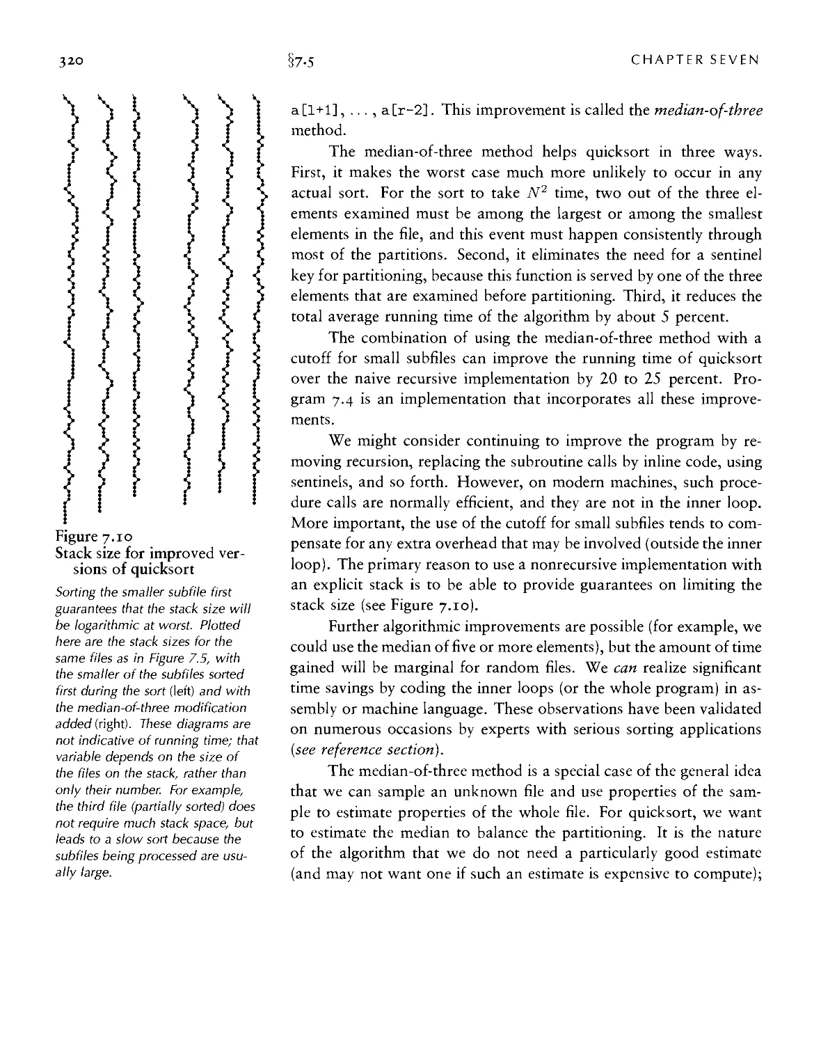
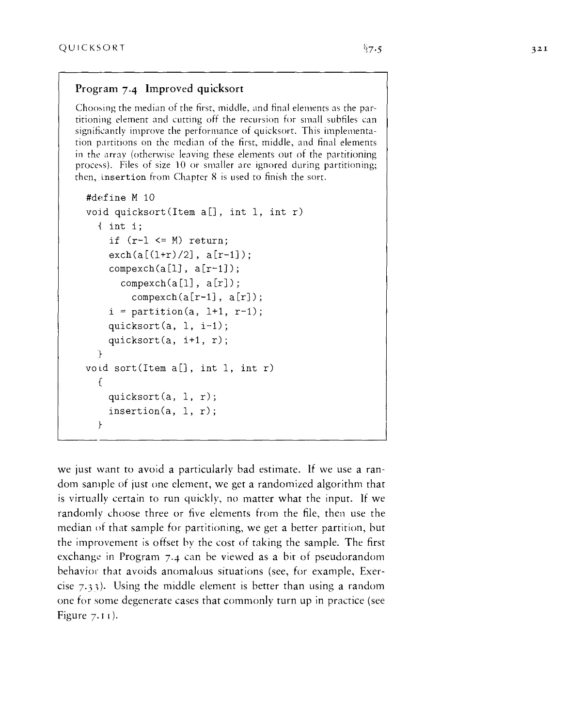
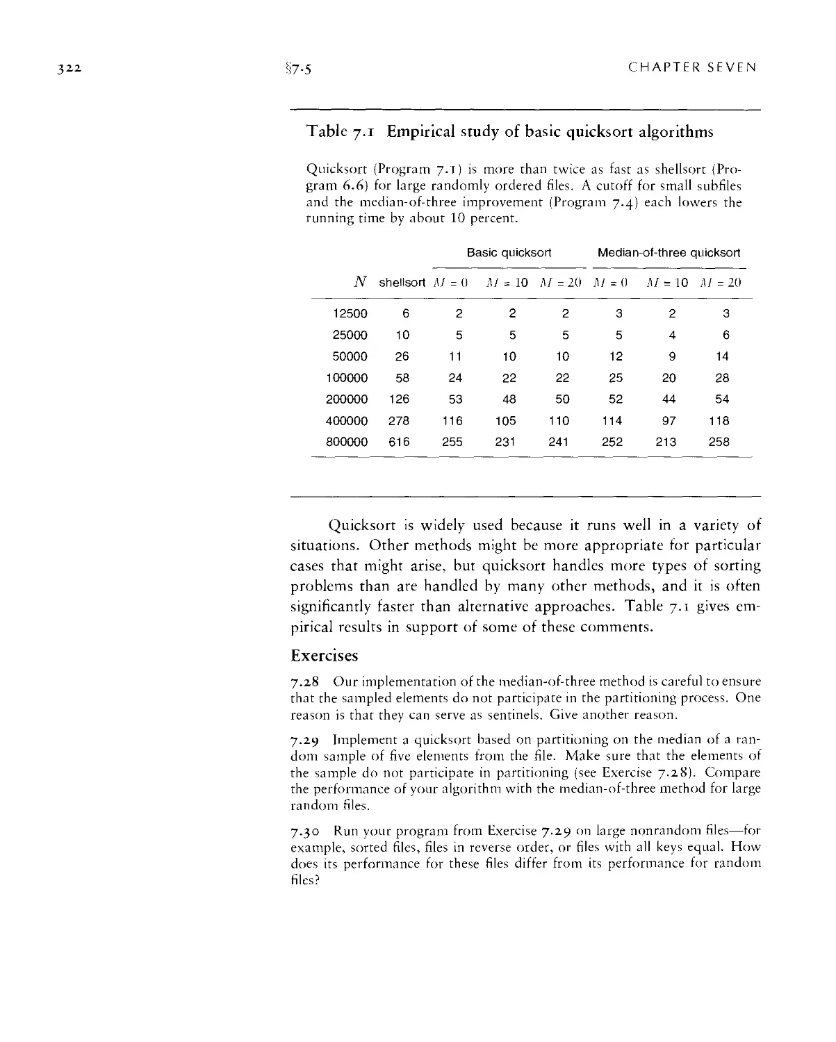
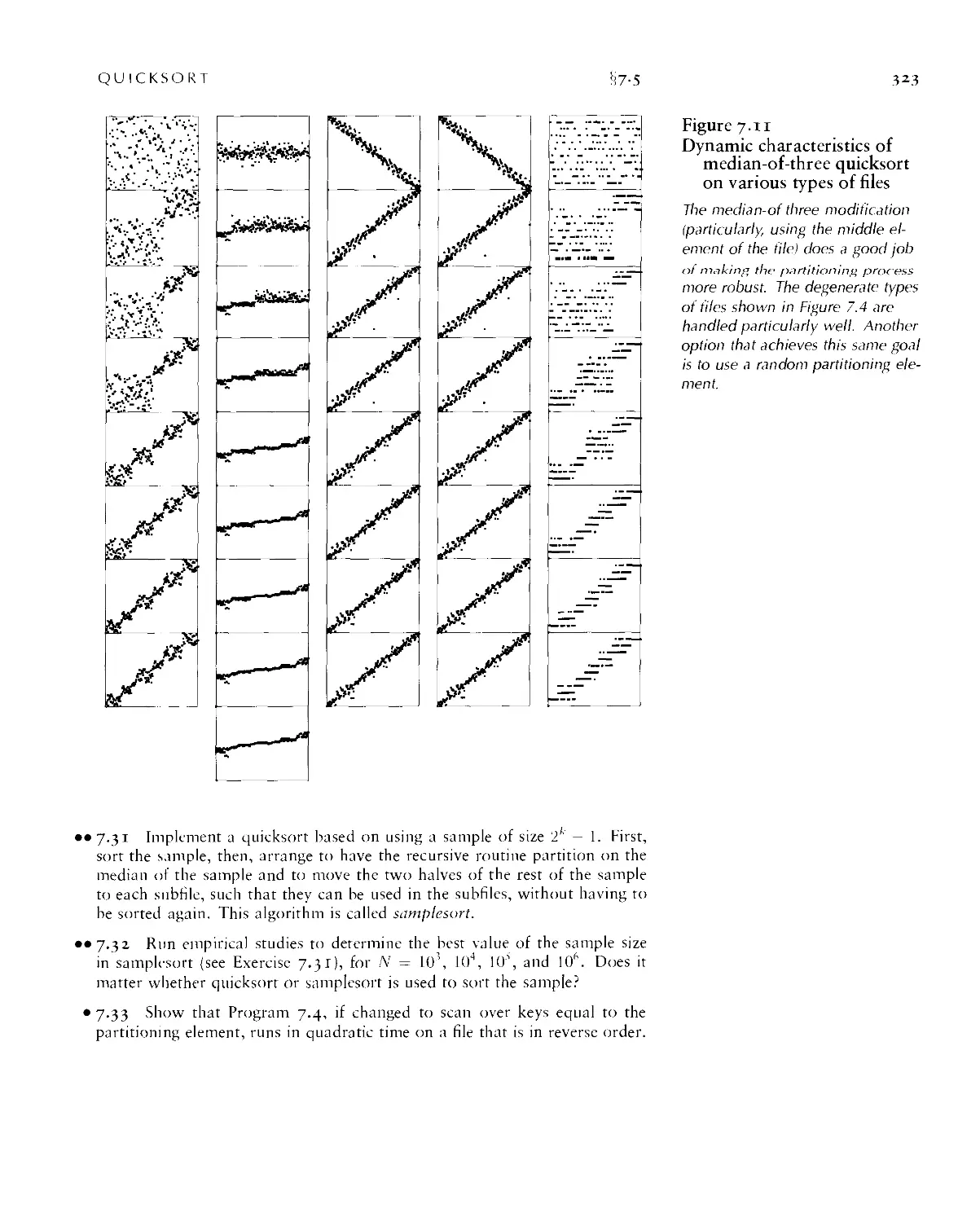
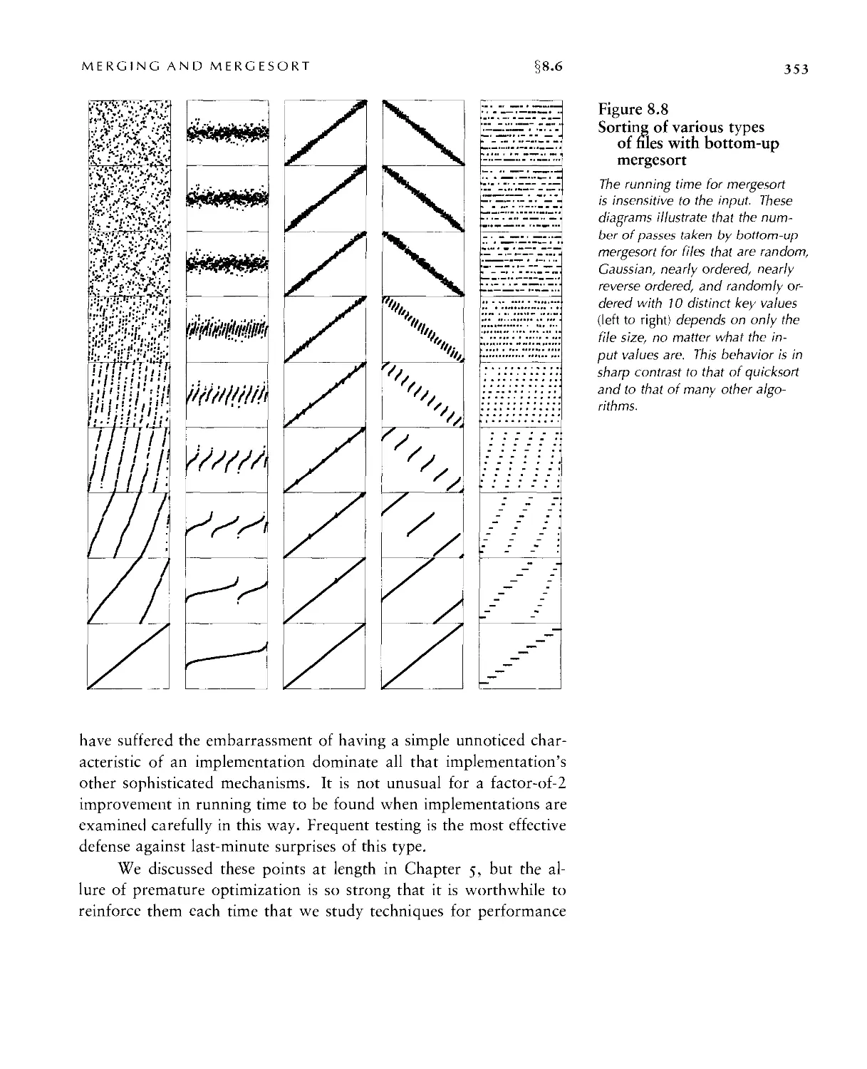
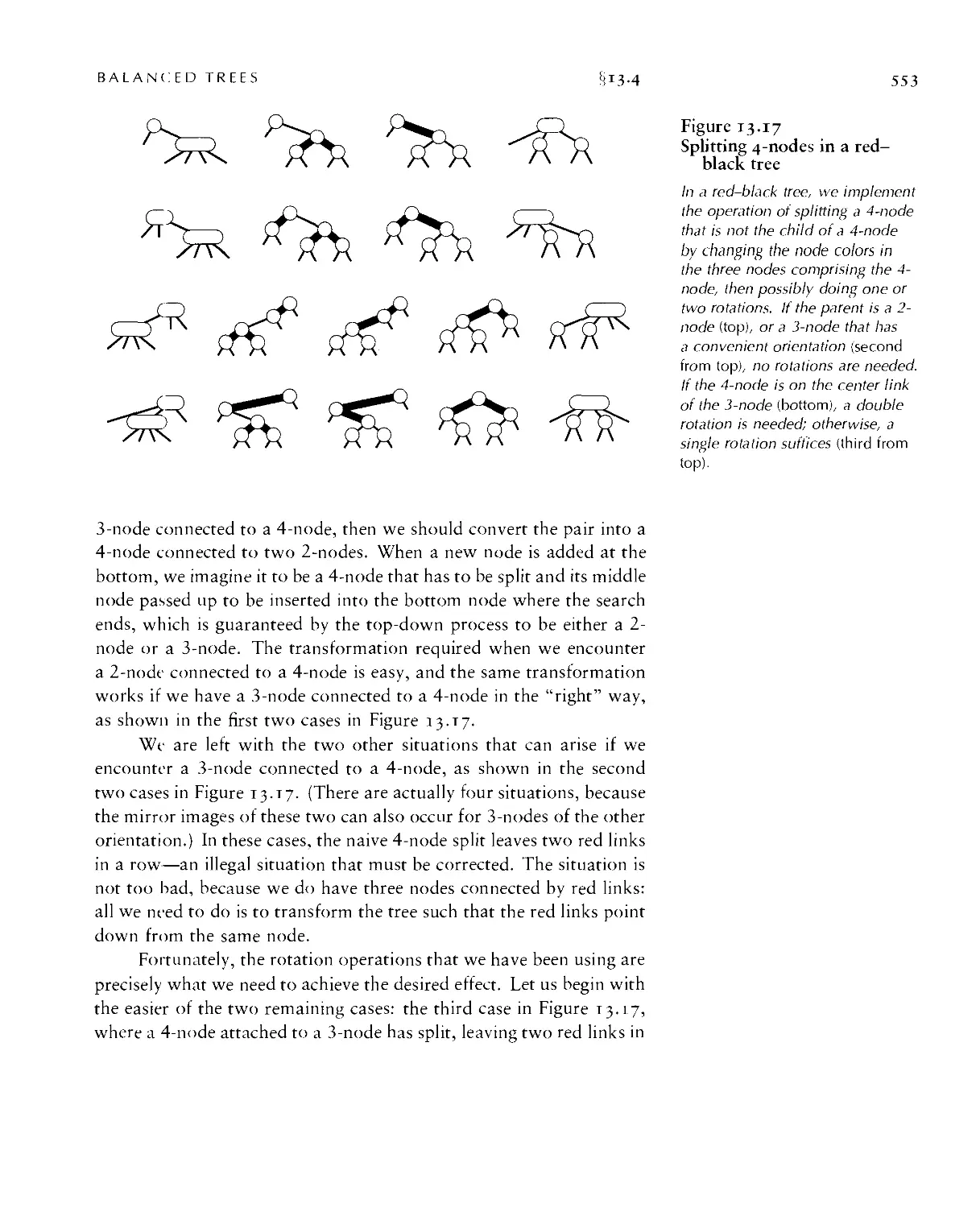
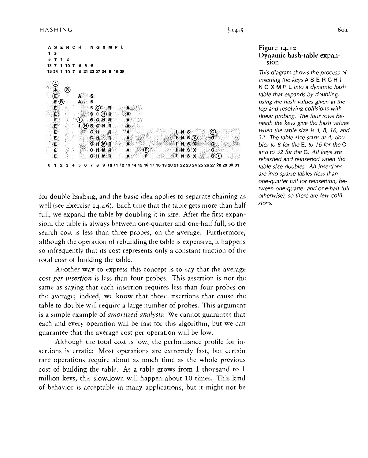
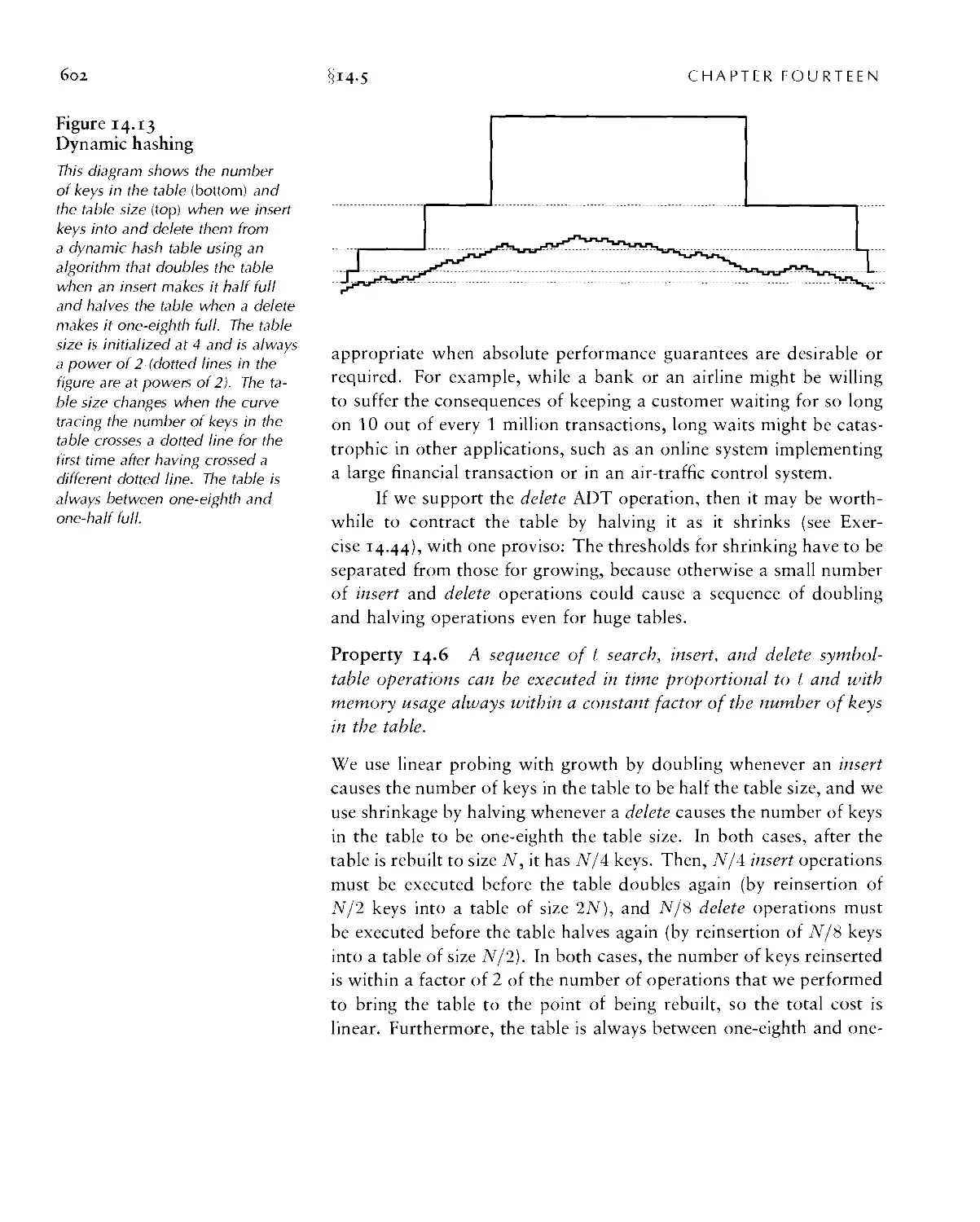
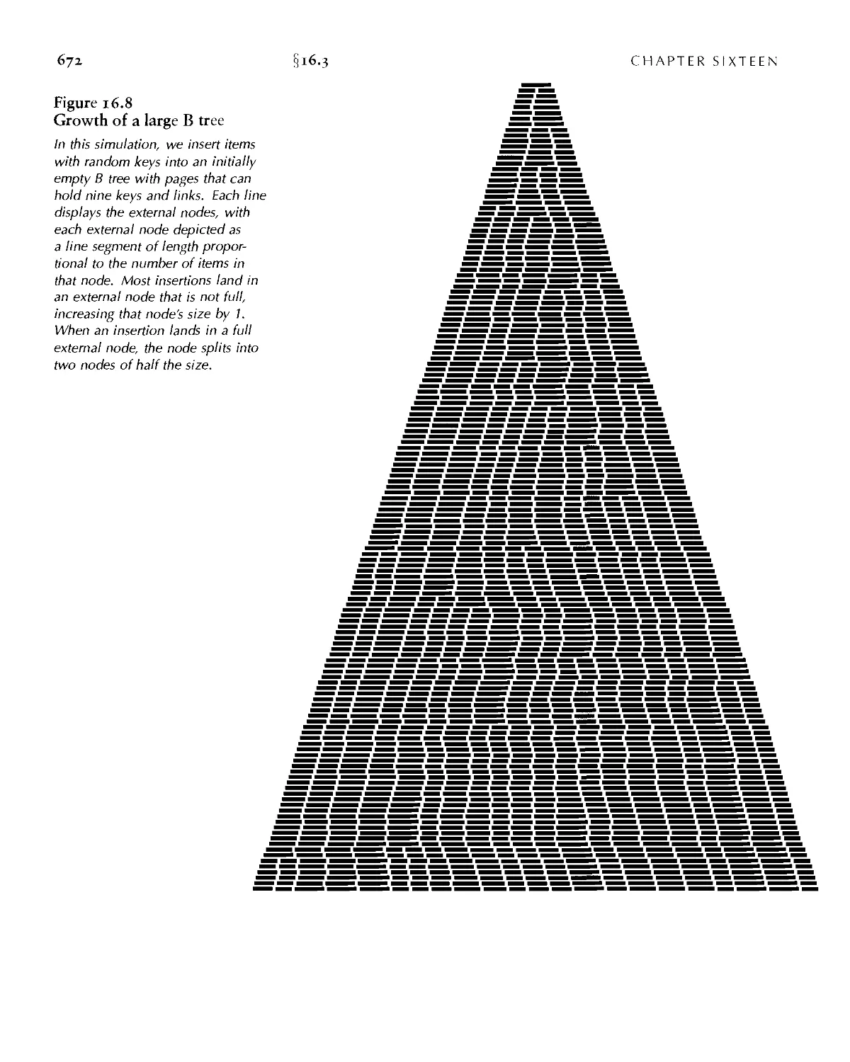
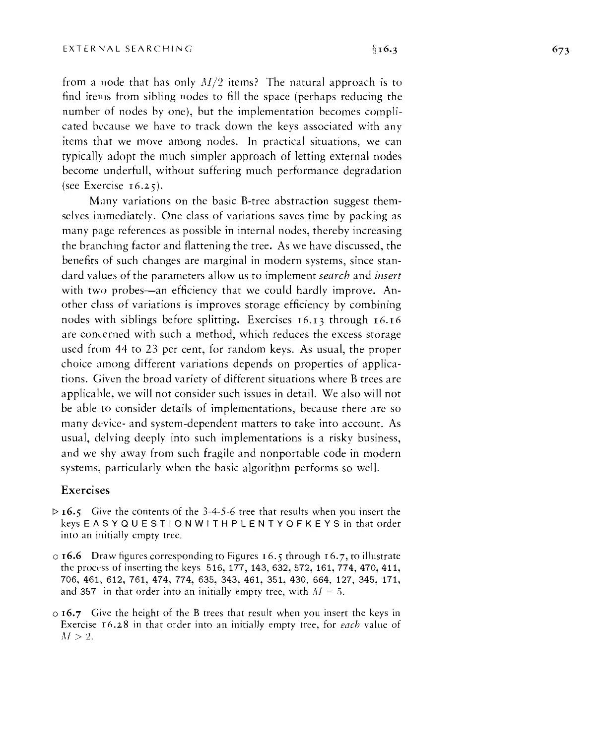
/


Текст
r » e»
P. s 1-4
FUNDAMENTALS
DATA STRUCTURES
SORTING
SEARCHING
' —S Mill
: •: —-
• T SE ■ E IC
Algorithms
THIRD EDITION
inC
PARTS 1-4
FUNDAMENTALS
DATA STRUCTURES
SORTING
SEARCHING
Robert Sedgewick
Princeton University
TT
ADDISON-WESLEY
An imprint of Addison Wesley Longman, Inc.
Reading, Massachusetts • Harlow, England • Menlo Park, California
Berkeley, California • Don Mills, Ontario • Sydney • Bonn • Amsterdam
Tokyo • Mexico City
Publishing Partner: Peter S. Gordon
Associate Editor: Deborah Lafferty
Cover Designer: Andre Kuzniarek
Production Editor: Amy Willcutt
Copy Editor: Lyn Dupre
The programs and applications presented in this book have been
included for their instructional value. They have been tested with care,
but are not guaranteed for any particular purpose. The publisher
neither offers any warranties or representations, nor accepts any
liabilities with respect to the programs or applications.
Library of Congress Cataloging-in-Publication Data
Sedgewick, Robert, 1946 -
Algorithms in C / Robert Sedgewick. — 3d ed.
720 p. 24 cm.
Includes bibliographical references and index.
Contents: v. 1, pts. 1-4. Fundamentals, data structures,
sorting, searching.
ISBN 0-201-31452-5
1. C (Computer program language) 2. Computer algorithms.
I. Title.
QA76.73.C15S43 1998
005.13'3—dc21 97-23418
CIP
Reproduced by Addison-Wesley from camera-ready copy supplied by
the author.
Copyright © 1998 by Addison-Wesley Publishing Company, Inc.
Reprinted with corrections, December 1997.
All rights reserved. No part of this publication may be reproduced,
stored in a retrieval system, or transmitted, in any form or by any
means, electronic, mechanical, photocopying, recording, or
otherwise, without the prior written permission of the publisher. Printed
in the United States of America.
23456789 10- CRW - 010099897
Preface
THIS BOOK IS intended to survey the most important computer
algorithms in use today, and to teach fundamental techniques
to the growing number of people in need of knowing them. It can
be used as a textbook for a second, third, or fourth course in
computer science, after students have acquired basic programming skills
and familiarity with computer systems, but before they have taken
specialized courses in advanced areas of computer science or
computer applications. The book also may be useful for self-study or
as a reference for people engaged in the development of computer
systems or applications programs, since it contains implementations
of useful algorithms and detailed information on these algorithms'
performance characteristics. The broad perspective taken makes the
book an appropriate introduction to the field.
I have completely rewritten the text for this new edition, and I
have added more than a thousand new exercises, more than a
hundred new figures, and dozens of new programs. I have also added
detailed commentary on all the figures and programs. This new
material provides both coverage of new topics and fuller explanations
of many of the classic algorithms. A new emphasis on abstract data
types throughout the book makes the programs more broadly useful
and relevant in modern object-oriented programming environments.
People who have read old editions of the book will find a wealth of
new information throughout; all readers will find a wealth of
pedagogical material that provides effective access to essential concepts.
Due to the large amount of new material, we have split the new
edition into two volumes (each about the size of the old edition) of
which this is the first. This volume covers fundamental concepts, data
structures, sorting algorithms, and searching algorithms; the second
volume covers advanced algorithms and applications, building on the
basic abstractions and methods developed here. Nearly all the
material on fundamentals and data structures in this edition is new.
PREFACE
This book is not just for programmers and computer-science
students. Nearly everyone who uses a computer wants it to run faster
or to solve larger problems. The algorithms in this book represent
a body of knowledge developed over the last 50 years that has
become indispensible in the efficient use of the computer, for a broad
variety of applications. From TV-body simulation problems in physics
to genetic-sequencing problems in molecular biology, the basic
methods described here have become essential in scientific research; and
from database systems to Internet search engines, they have become
essential parts of modern software systems. As the scope of computer
applications becomes more widespread, so grows the impact of many
of the basic methods covered here. The goal of this book is to serve
as a resource for students and professionals interested in knowing and
making intelligent use of these fundamental algorithms as basic tools
for whatever computer application they might undertake.
Scope
The book contains 16 chapters grouped into four major parts:
fundamentals, data structures, sorting, and searching. The descriptions here
are intended to give readers an understanding of the basic properties
of as broad a range of fundamental algorithms as possible. Ingenious
methods ranging from binomial queues to patricia tries are described,
all related to basic paradigms at the heart of computer science. The
second volume consists of four additional parts that cover strings,
geometry, graphs, and advanced topics. My primary goal in developing
these books has been to bring together the fundamental methods from
these diverse areas, to provide access to the best methods known for
solving problems by computer.
You will most appreciate the material in this book if you have
had one or two previous courses in computer science or have had
equivalent programming experience: one course in programming in
a high-level language such as C, Java, or C++, and perhaps another
course that teaches fundamental concepts of programming systems.
This book is thus intended for anyone conversant with a modern
programming language and with the basic features of modern computer
systems. References that might help to fill in gaps in your background
are suggested in the text.
w
Most of the mathematical material supporting the analytic
results is sell-contained (or is labeled as beyond the scope of this book),
so little specific preparation in mathematics is required for the bulk
of the book, although mathematical maturity is definitely helpful.
Use in the Curriculum
There is a great deal of flexibility in how the material here can be
taught, depending on the taste of the instructor and the preparation
of the students. The algorithms described here have found widespread
use for years, and represent an essential body of knowledge for both
the practicing programmer and the computer-science student. There
is sufficient coverage of basic material for the book to be used for a
course on data structures, and there is sufficient detail and coverage
of advanced material for the book to be used for a course on
algorithms. Some instructors may wish to emphasize implementations
and practical concerns; others may wish to emphasize analysis and
theoretical concepts.
A complete set of slide masters for use in lectures, sample
programming assignments, interactive exercises for students, and other
course materials may be found via the book's home page.
An elementary course on data structures and algorithms might
emphasize the basic data structures in Part 2 and their use in the
implemeniations in Parts 3 and 4. A course on design and analysis of
algorithms might emphasize the fundamental material in Part 1 and
Chapter 5, then study the ways in which the algorithms in Parts 3
and 4 achieve good asymptotic performance. A course on software
engineering might omit the mathematical and advanced algorithmic
material, and emphasize how to integrate the implementations given
here into large programs or systems. A course on algorithms might
take a survey approach and introduce concepts from all these areas.
Earlier editions of this book have been used in recent years at
scores of colleges and universities around the world as a text for
the second or third course in computer science and as supplemental
reading for other courses. At Princeton, our experience has been that
the breadih of coverage of material in this book provides our majors
with an introduction to computer science that can be expanded upon
in later courses on analysis of algorithms, systems programming and
v
PREFACE
theoretical computer science, while providing the growing group of
students from other disciplines with a large set of techniques that
these people can immediately put to good use.
The exercises—most of which are new to this edition—fall into
several types. Some are intended to test understanding of material
in the text, and simply ask readers to work through an example or
to apply concepts described in the text. Others involve implementing
and putting together the algorithms, or running empirical studies to
compare variants of the algorithms and to learn their properties. Still
others are a repository for important information at a level of detail
that is not appropriate for the text. Reading and thinking about the
exercises will pay dividends for every reader.
Algorithms of Practical Use
Anyone wanting to use a computer more effectively can use this book
for reference or for self-study. People with programming experience
can find information on specific topics throughout the book. To a
large extent, you can read the individual chapters in the book
independently of the others, although, in some cases, algorithms in one
chapter make use of methods from a previous chapter.
The orientation of the book is to study algorithms likely to be of
practical use. The book provides information about the tools of the
trade to the point that readers can confidently implement, debug, and
put to work algorithms to solve a problem or to provide functionality
in an application. Full implementations of the methods discussed are
included, as are descriptions of the operations of these programs on
a consistent set of examples. Because we work with real code, rather
than write pseudo-code, the programs can be put to practical use
quickly. Program listings are available from the book's home page.
Indeed, one practical application of the algorithms has been to
produce the hundreds of figures throughout the book. Many
algorithms are brought to light on an intuitive level through the visual
dimension provided by these figures.
Characteristics of the algorithms and of the situations in which
they might be useful are discussed in detail. Although not
emphasized, connections to the analysis of algorithms and theoretical
computer science are developed in context. When appropriate, empirical
VI
and analytic results are presented to illustrate why certain algorithms
are preferred. When interesting, the relationship of the practical
algorithms being discussed to purely theoretical results is described.
Specific information on performance characteristics of algorithms and
implementations is synthesized, encapsulated, and discussed
throughout the book.
Programming Language
The programming language used for all of the implementations is C.
Any particular language has advantages and disadvantages; we use
C because it is widely available and provides the features needed for
our implementations. The programs can be translated easily to other
modern programming languages, since relatively few constructs are
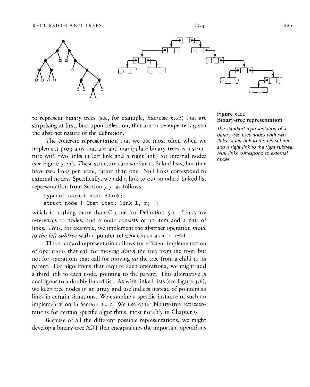
unique to C. We use standard C idioms when appropriate, but this
book is not intended to be a reference work on C programming.
There are many new programs in this edition, and many of the
old ones have been reworked, primarily to make them more readily
useful as abstract-data-type implementations. Extensive comparative
empirical tests on the programs are discussed throughout the text.
Previous editions of the book have presented basic programs in
Pascal, C++, and Modula-3. This code is available through the book
home page on the web; code for new programs and code in new
languages such as Java will be added as appropriate.
A goal of this book is to present the algorithms in as simple
and direct a form as possible. The style is consistent whenever
possible, so that programs that are similar look similar. For many of
the algorithms in this book, the similarities hold regardless of the
language: Quicksort is quicksort (to pick one prominent example),
whether expressed in Algol-60, Basic, Fortran, Smalltalk, Ada, Pascal,
C, PostScript, Java, or countless other programming languages and
environments where it has proved to be an effective sorting method.
We strive for elegant, compact, and portable implementations,
but we take the point of view that efficiency matters, so we try to
be aware of the performance characteristics of our code at all stages
of development. Chapter 1 constitutes a detailed example of this
approach to developing efficient C implementations of our algorithms,
and sets the stage for the rest of the book.
Vll
PREFACE
Acknowledgments
Many people gave me helpful feedback on earlier versions of this
book. In particular, hundreds of students at Princeton and Brown
have suffered through preliminary drafts over the years. Special
thanks are due to Trina Avery and Tom Freeman for their help in
producing the first edition; to Janet Incerpi for her creativity and
ingenuity in persuading our early and primitive digital computerized
typesetting hardware and software to produce the first edition; to
Marc Brown for his part in the algorithm visualization research that
was the genesis of so many of the figures in the book; and to Dave
Hanson for his willingness to answer all of my questions about C. I
would also like to thank the many readers who have provided me with
detailed comments about various editions, including Guy Almes, Jon
Bentley, Marc Brown, Jay Gischer, Allan Heydon, Kennedy Lemke,
Udi Manber, Dana Richards, John Reif, M. Rosenfeld, Stephen Seid-
man, Michael Quinn, and William Ward.
To produce this new edition, I have had the pleasure of working
with Peter Gordon and Debbie Lafferty at Addison-Wesley, who have
patiently shepherded this project as it has evolved from a standard
update to a massive rewrite. It has also been my pleasure to work with
several other members of the professional staff at Addison-Wesley.
The nature of this project made the book a somewhat unusual
challenge for many of them, and I much appreciate their forbearance.
I have gained two new mentors in writing this book, and
particularly want to express my appreciation to them. First, Steve
Summit carefully checked early versions of the manuscript on a technical
level, and provided me with literally thousands of detailed comments,
particularly on the programs. Steve clearly understood my goal of
providing elegant, efficient, and effective implementations, and his
comments not only helped me to provide a measure of consistency
across the implementations, but also helped me to improve many of
them substantially. Second, Lyn Dupre also provided me with
thousands of detailed comments on the manuscript, which were invaluable
in helping me not only to correct and avoid grammatical errors, but
also—more important—to find a consistent and coherent writing style
that helps bind together the daunting mass of technical material here.
vui
I am extremely grateful for the opportunity to learn from Steve and
Lyn—their input was vital in the development of this book.
Much of what I have written here I have learned from the
teaching and writings of Don Knuth, my advisor at Stanford. Although
Don had no direct influence on this work, his presence may be felt
in the book, for it was he who put the study of algorithms on the
scientific footing that makes a work such as this possible. My friend
and colleague Philippe Flajolet, who has been a major force in the
development of the analysis of algorithms as a mature research area,
has had a similar influence on this work.
I am deeply thankful for the support of Princeton University,
Brown University, and the Institut National de Recherce en Informa-
tique et Automatique (INRIA), where I did most of the work on the
book; and of the Institute for Defense Analyses and the Xerox Palo
Alto Research Center, where I did some work on the book while
visiting. Many parts of the book are dependent on research that has
been generously supported by the National Science Foundation and
the Office of Naval Research. Finally, I thank Bill Bowen, Aaron
Lemonick, and Neil Rudenstine for their support in building an
academic environment at Princeton in which I was able to prepare this
book, despite my numerous other responsibilities.
Robert Scdgewick
Marly-lc-Roi, France, February, 1983
Princeton, New Jersey, January, 1990
famestown, Rhode Island, August, 1997
IX
To Adam, Andrew, Brett, Robbie,
and especially Linda
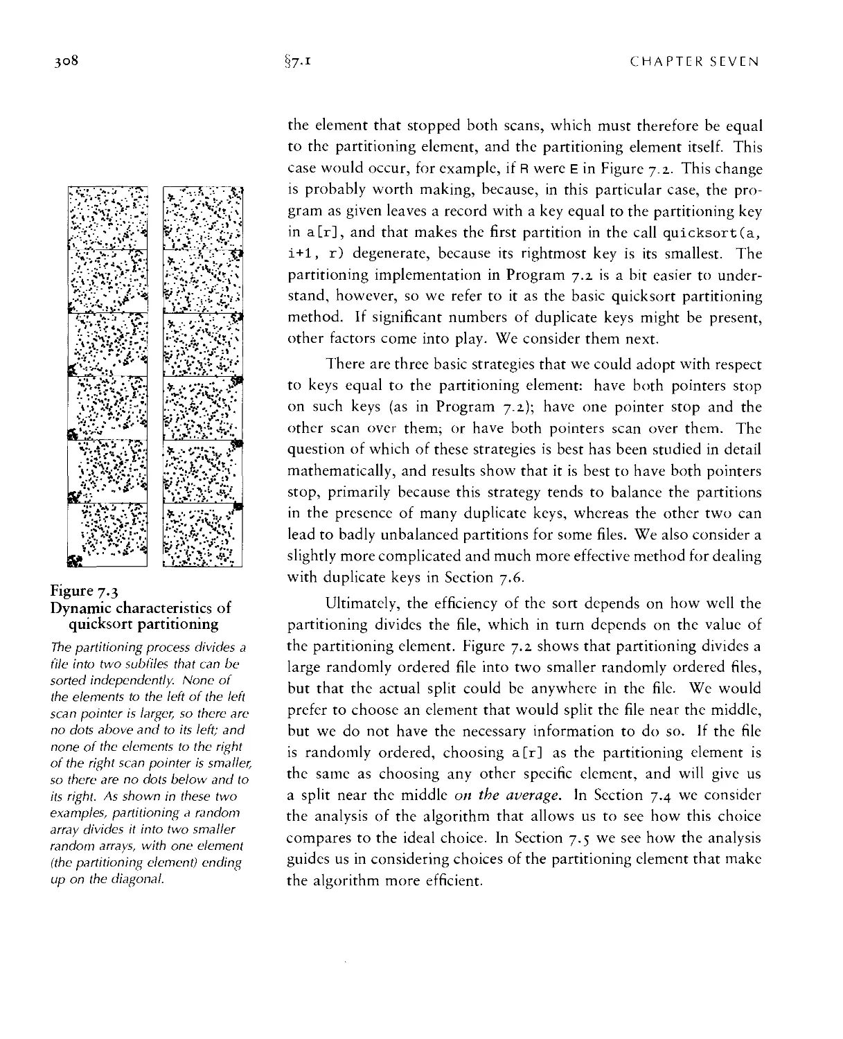
Notes on Exercises
Classifying exercises is an activity fraught with peril, because readers
of a book such as this come to the material with various levels of
knowledge and experience. Nonetheless, guidance is appropriate, so
many of the exercises carry one of four annotations, to help you
decide how to approach them.
Exercises that test your understanding of the material are marked
with an open triangle, as follows:
I> 9.57 Give the binomial queue that results when the keys E A S
YQUESTION are inserted into an initially empty binomial
queue.
Most often, such exercises relate directly to examples in the text.
They should present no special difficulty, but working them might
teach you a fact or concept that may have eluded you when you read
the text.
Exercises that add new and thought-provoking information to the
material ;ire marked with an open circle, as follows:
o 14.20 Write a program that inserts N random integers into a
tabic of size N/100 using separate chaining, then finds the length
of the shortest and longest lists, for N = 10', 104, 10\ and 10\
Such exercises encourage you to think about an important concept
that is related to the material in the text, or to answer a question that
may have occurred to you when you read the text. You may find it
worthwhile to read these exercises, even if you do not have the time
to work them through.
Exercises that are intended to challenge you are marked with a
black dot, as follows:
• 8.46 Suppose that mergesort is implemented to split the file at
a random position, rather than exactly in the middle. How many
comparisons are used by such a method to sort N elements, on
the average?
Such exercises may require a substantial amount of time to complete,
depending upon your experience. Generally, the most productive
approach is to work on them in a few different sittings.
A few exercises that are extremely difficult (by comparison with
most others) are marked with two black dots, as follows:
XI
• • i5-^9 Prove that the height of a trie built from N random bit-
strings is about 2 lg N.
These exercises are similar to questions that might be addressed in
the research literature, but the material in the book may prepare you
to enjoy trying to solve them (and perhaps succeeding).
The annotations are intended to be neutral with respect to your
programming and mathematical ability. Those exercises that require
expertise in programming or in mathematical analysis are self-evident.
All readers are encouraged to test their understanding of the
algorithms by implementing them. Still, an exercise such as this one is
straightforward for a practicing programmer or a student in a
programming course, but may require substantial work for someone who
has not recently programmed:
1.23 Modify Program 1.4 to generate random pairs of integers
between 0 and N — \ instead of reading them from standard input,
and to loop until N - 1 union operations have been performed.
Run your program for N = 10', 104, 10\ and 106and print out
the total number of edges generated for each value of N.
In a similar vein, all readers are encouraged to strive to appreciate
the analytic underpinnings of our knowledge about properties of
algorithms. Still, an exercise such as this one is straightforward for a
scientist or a student in a discrete mathematics course, but may require
substantial work for someone who has not recently done
mathematical analysis:
1.13 Compute the average distance from a node to the root in
a worst-case tree of 2" nodes built by the weighted quick-union
algorithm.
There are far too many exercises for you to read and assimilate
them all; my hope is that there are enough exercises here to stimulate
you to strive to come to a broader understanding on the topics that
interest you than you can glean by simply reading the text.
Contents
Fundamentals
Chapter 1. Introduction 3
1.1 Algorithms ■ 4
1.2 A Sample Problem—Connectivity ■ 6
1.,} Union-Find Algorithms ■ //
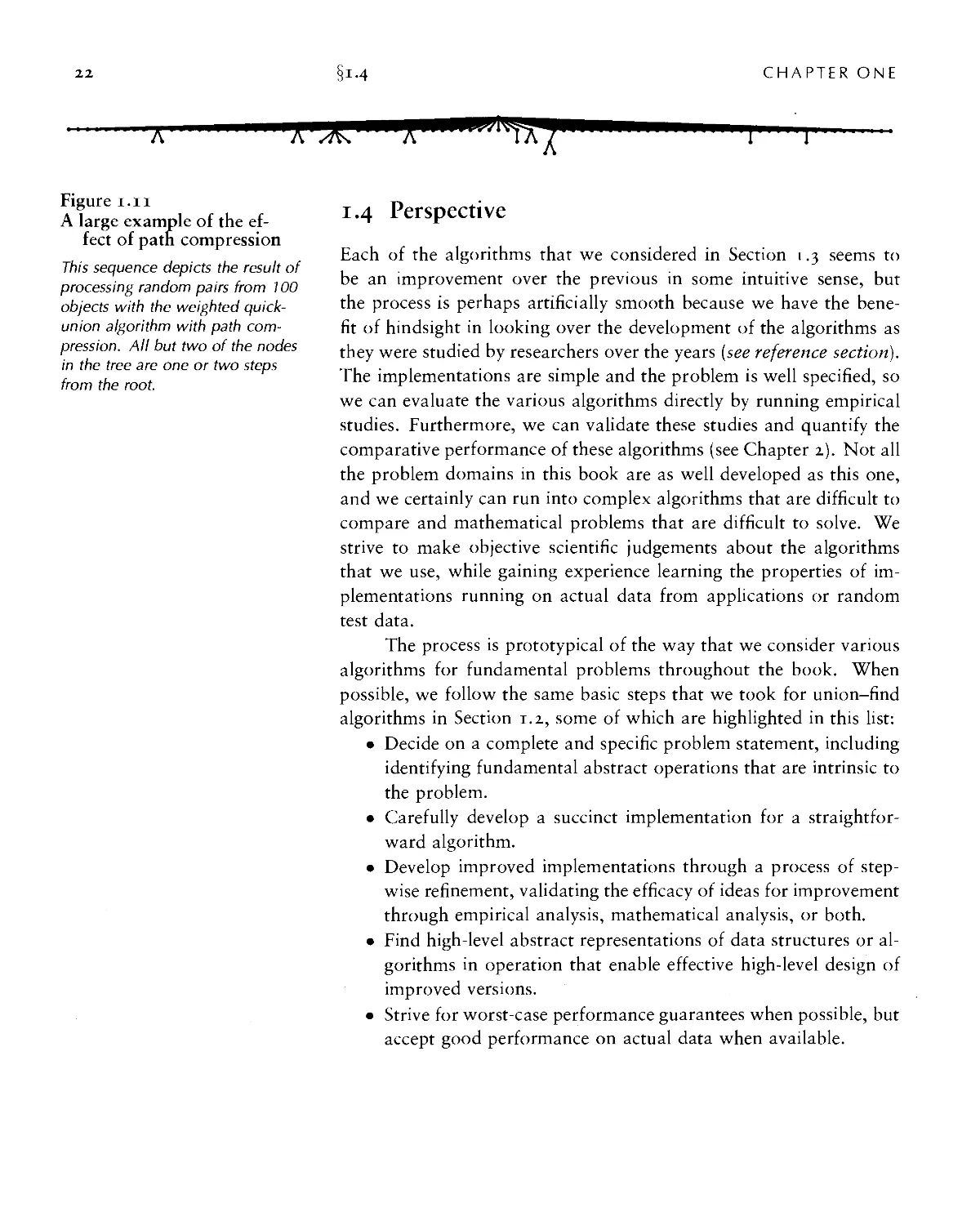
1.4 Perspective ■ 22
1..S Summary of Topics ■ 2,5
Chapter 2. Principles of Algorithm Analysis 27
2.1 Implementation and Empirical Analysis ■ 28
2.2 Analysis of Algorithms ■ 33
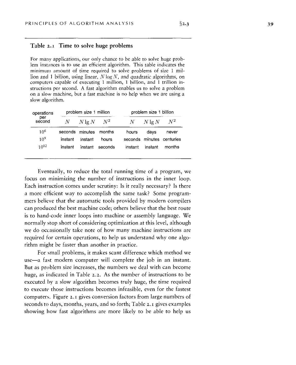
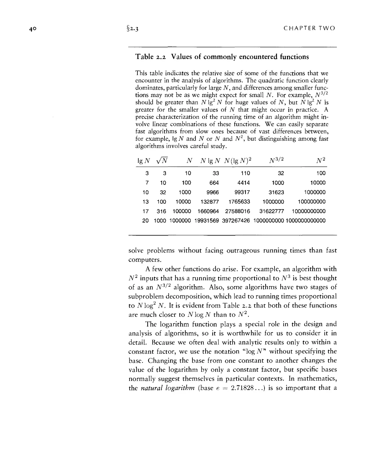
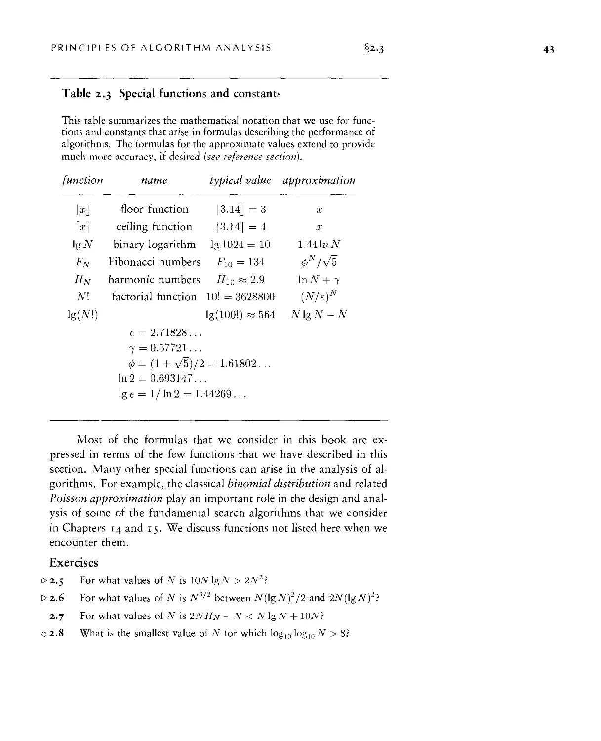
2..i Growth of Functions ■ 36
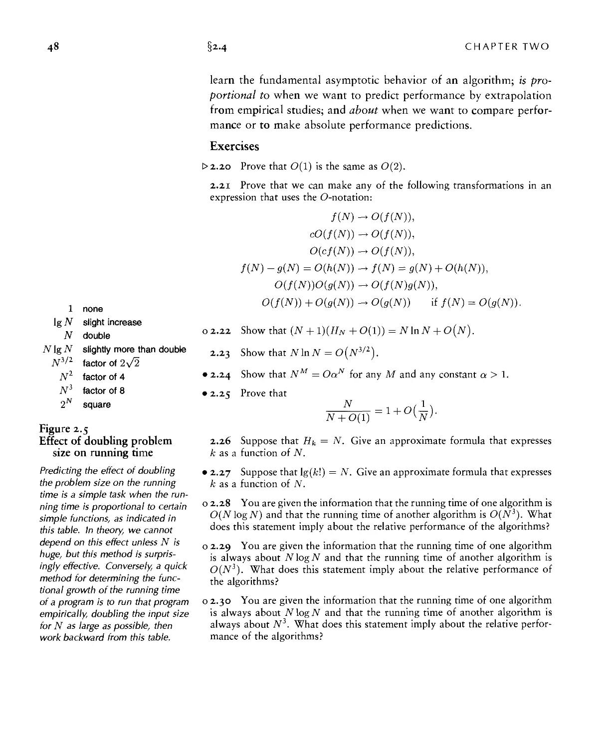
2.4 Big-Oh notation • 44
2.5 Basic Recurrences ■ 49
2.(> Examples of Algorithm Analysis ■ S3
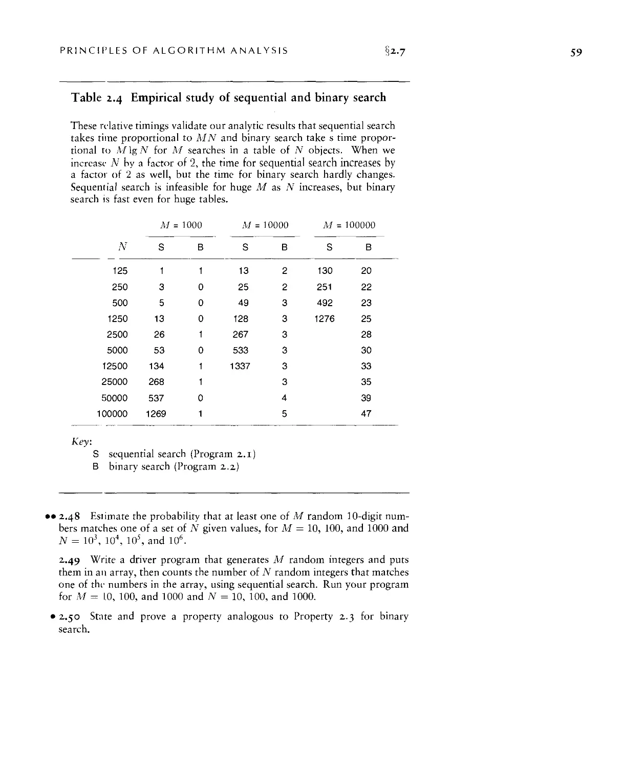
2.7 Guarantees, Predictions, and Limitations ■ 60
TABLE OF CONTENTS
Data Structures
Chapter 3. Elementary Data Structures 69
3.1 Building Blocks ■ 70
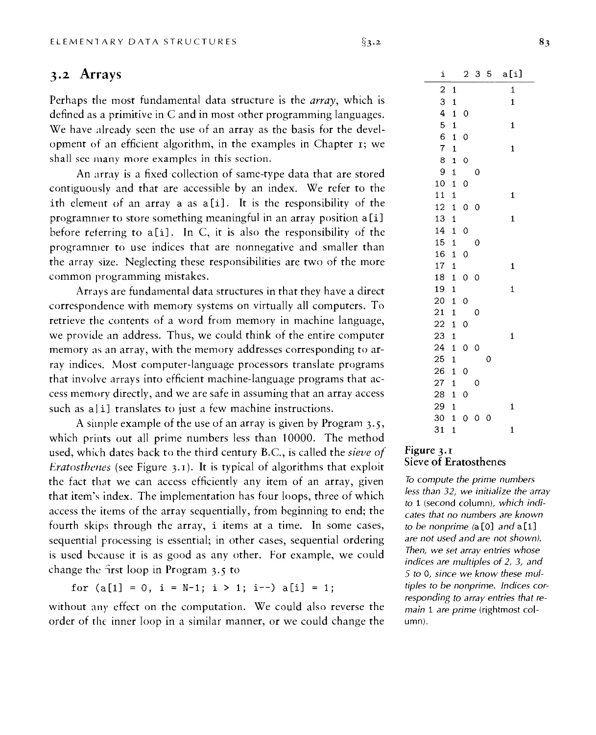
3.2 Arrays ■ 83
3.3 Linked Lists ■ 90
3.4 Elementary List Processing ■ 96
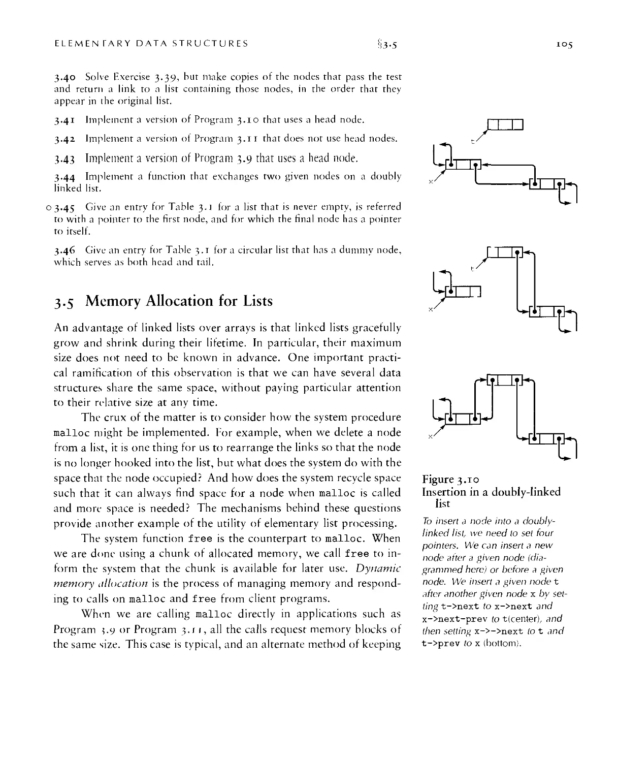
3.5 Memory Allocation for Lists ■ 105
3.6 Strings ■ 108
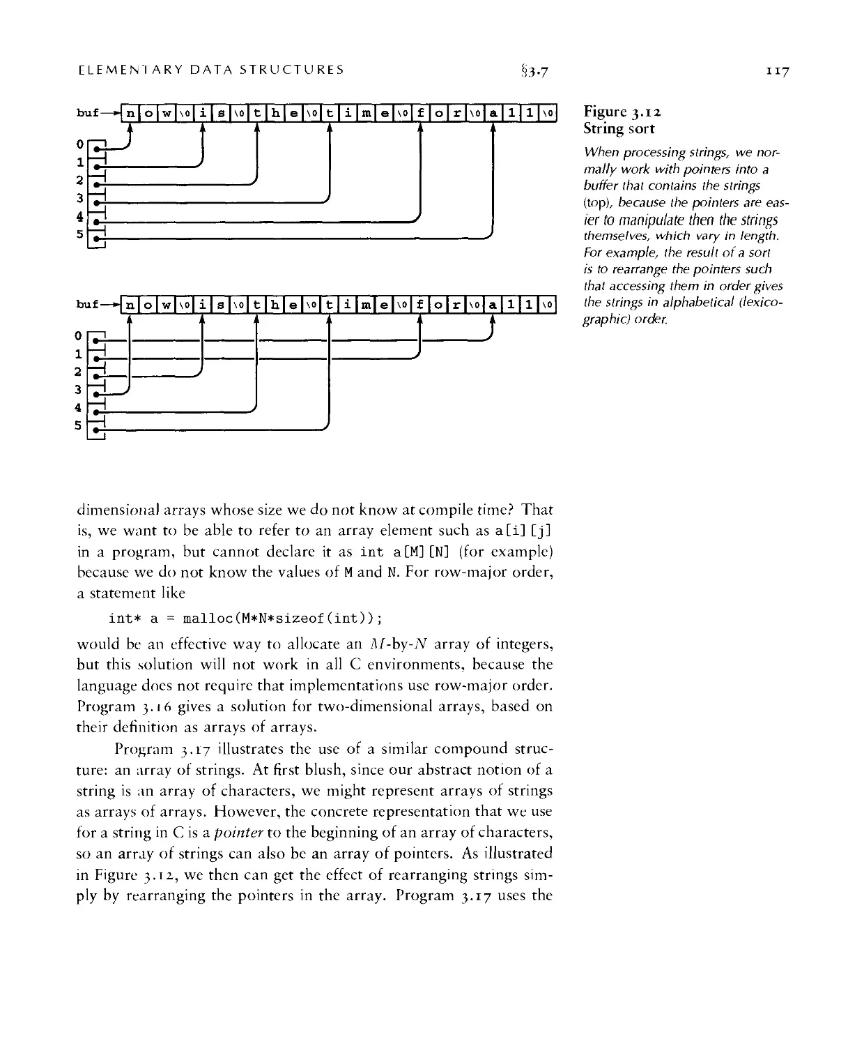
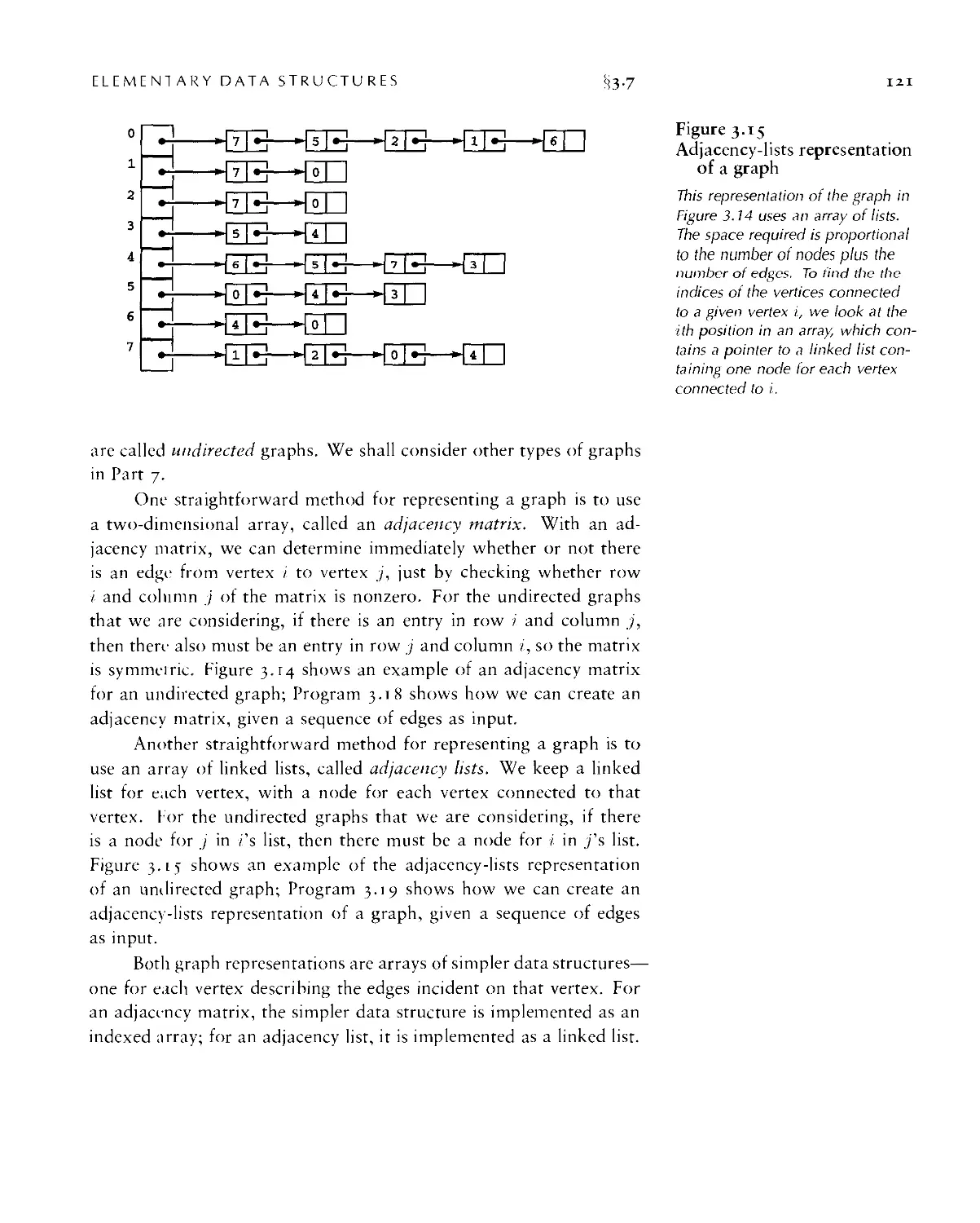
3.7 Compound Data Structures ■ 115
Chapter 4. Abstract Data Types 127
4.1 Abstract Objects and Collections of Objects ■ 131
4.2 Pushdown Stack ADT • 135
4.3 Examples of Stack ADT Clients • 138
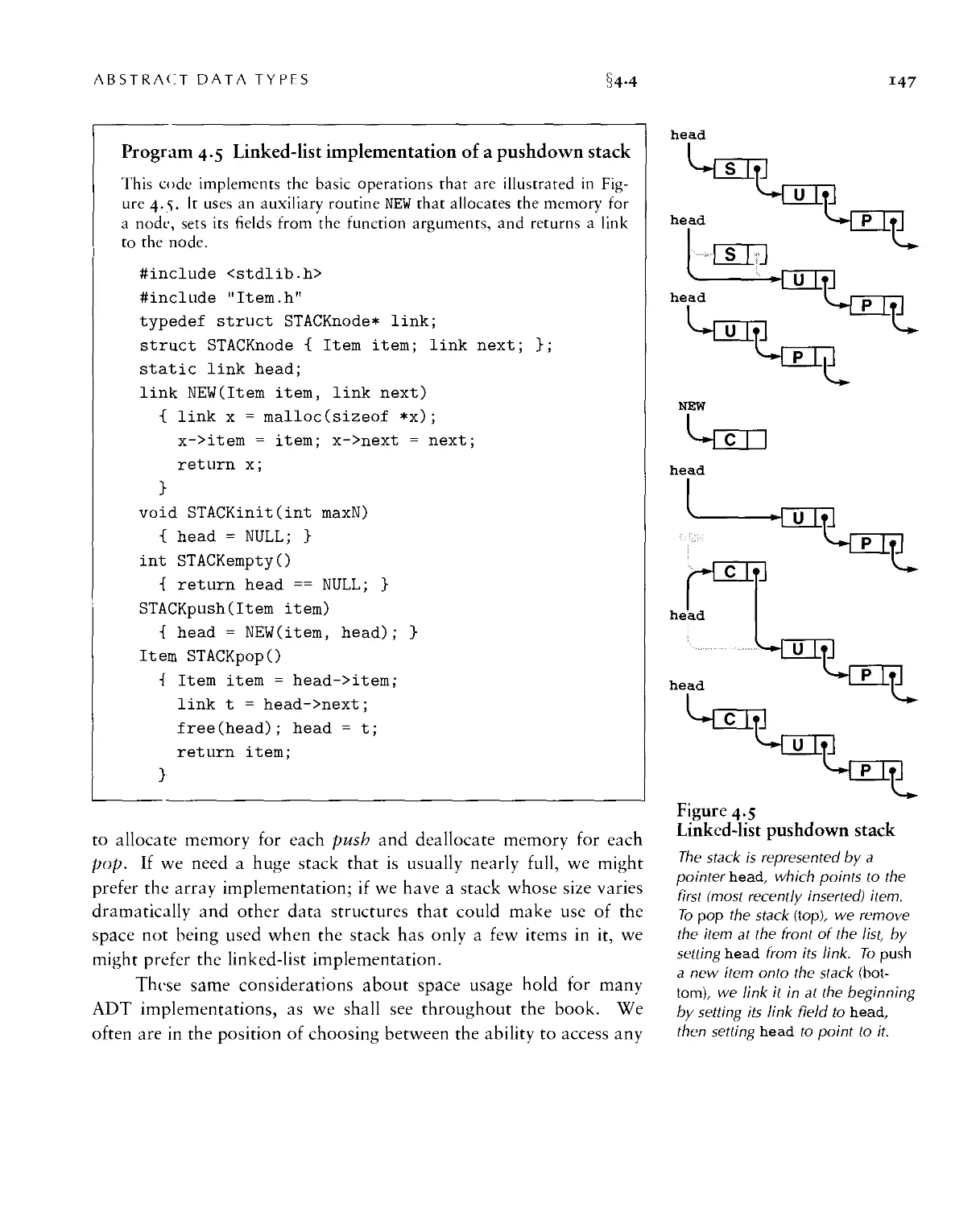
4.4 Stack ADT Implementations • 145
4.5 Creation of a New ADT • 149
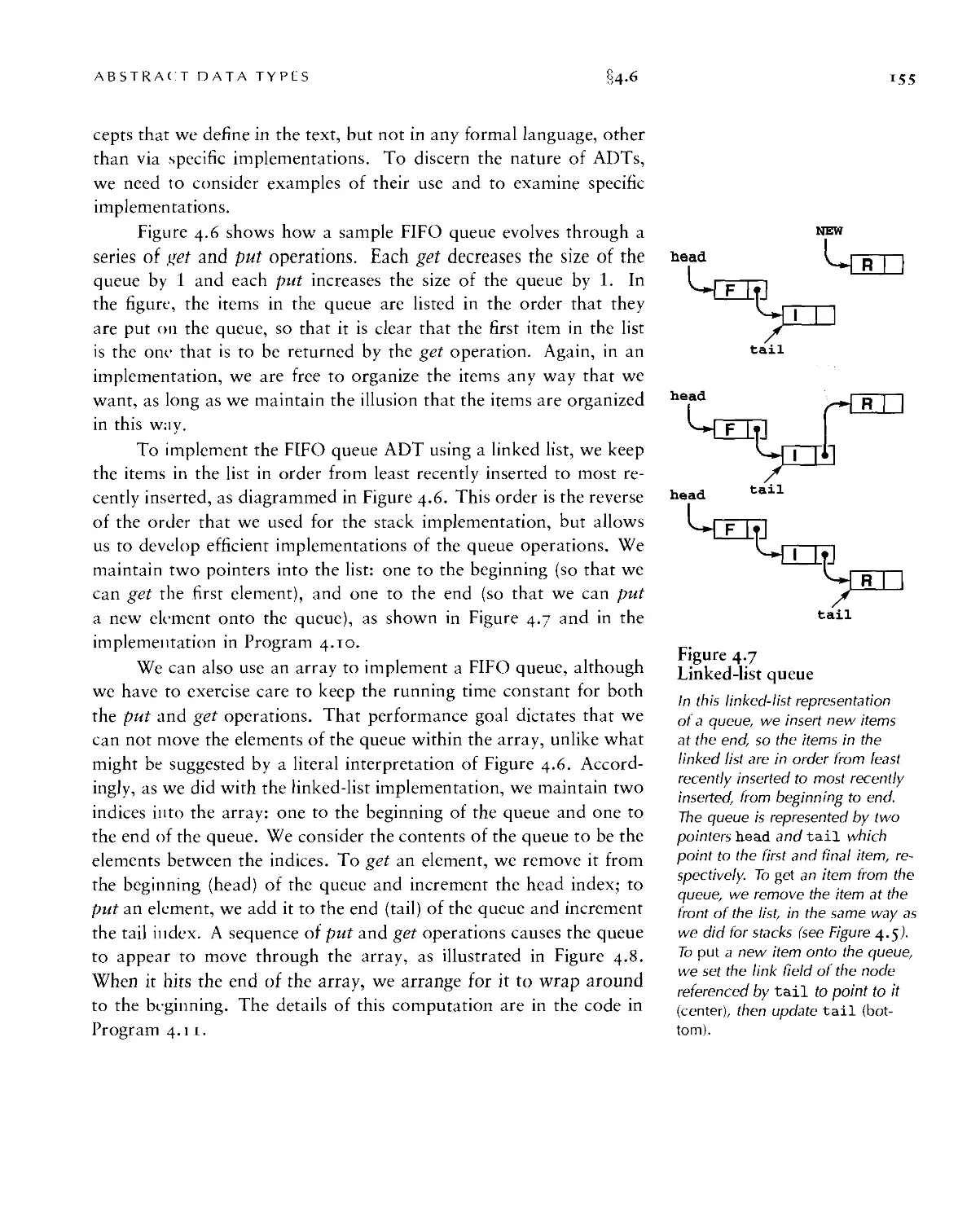
4.6 FIFO Queues and Generalized Queues • 153
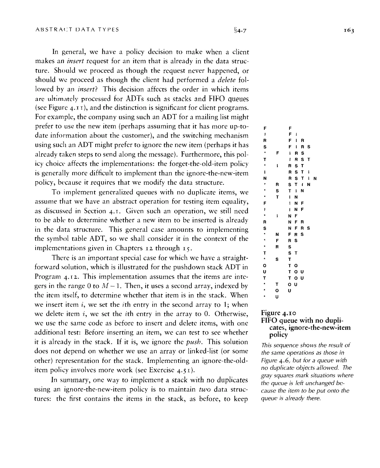
4.7 Duplicate and Index Items • 161
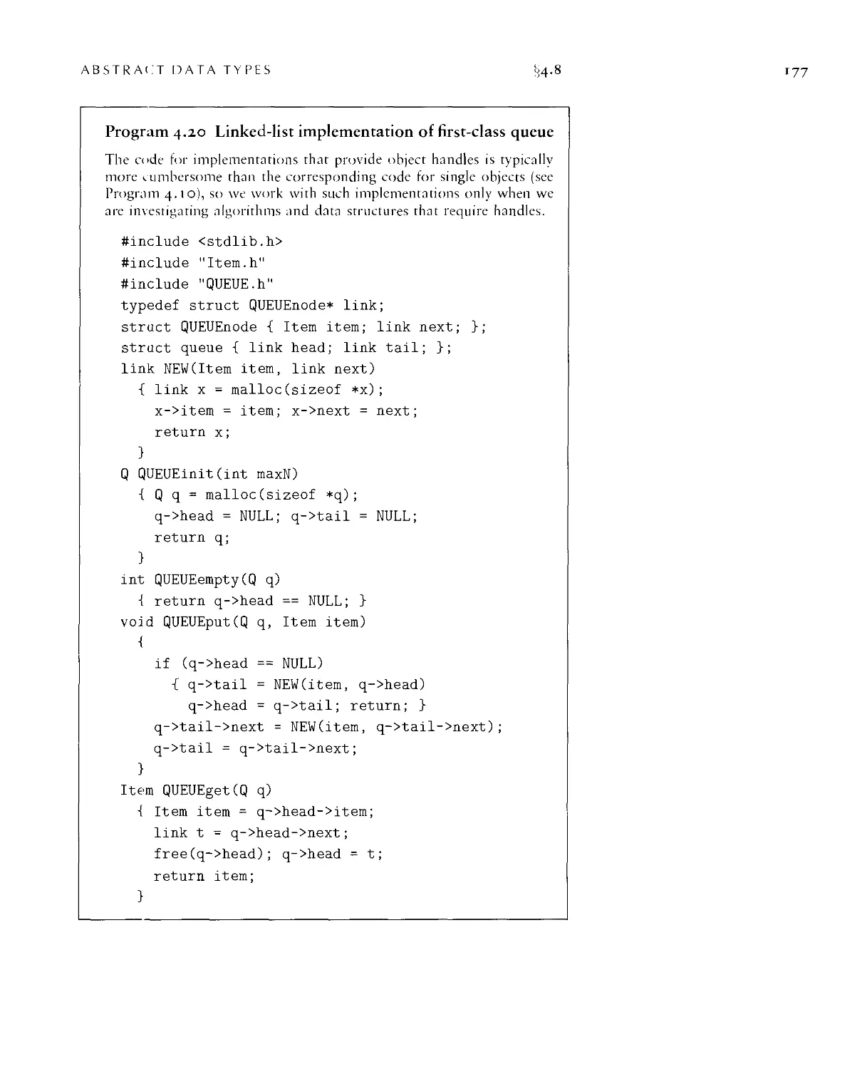
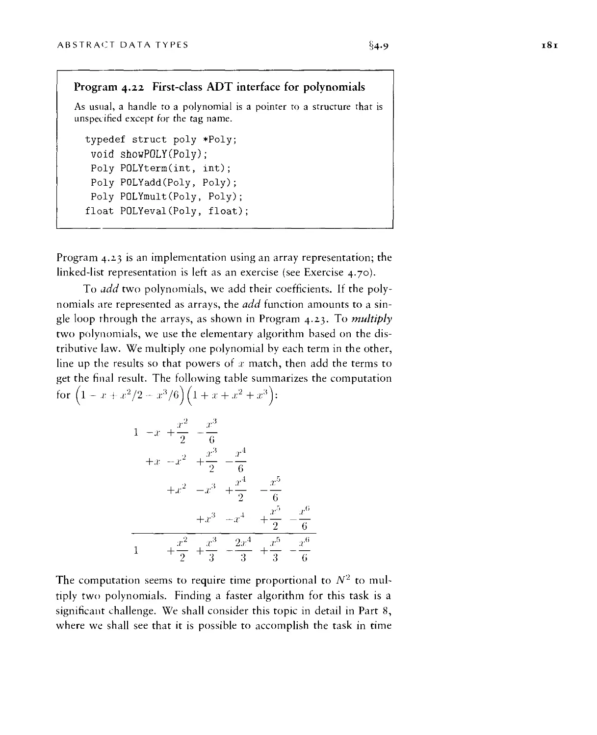
4.8 First-Class ADTs • 166
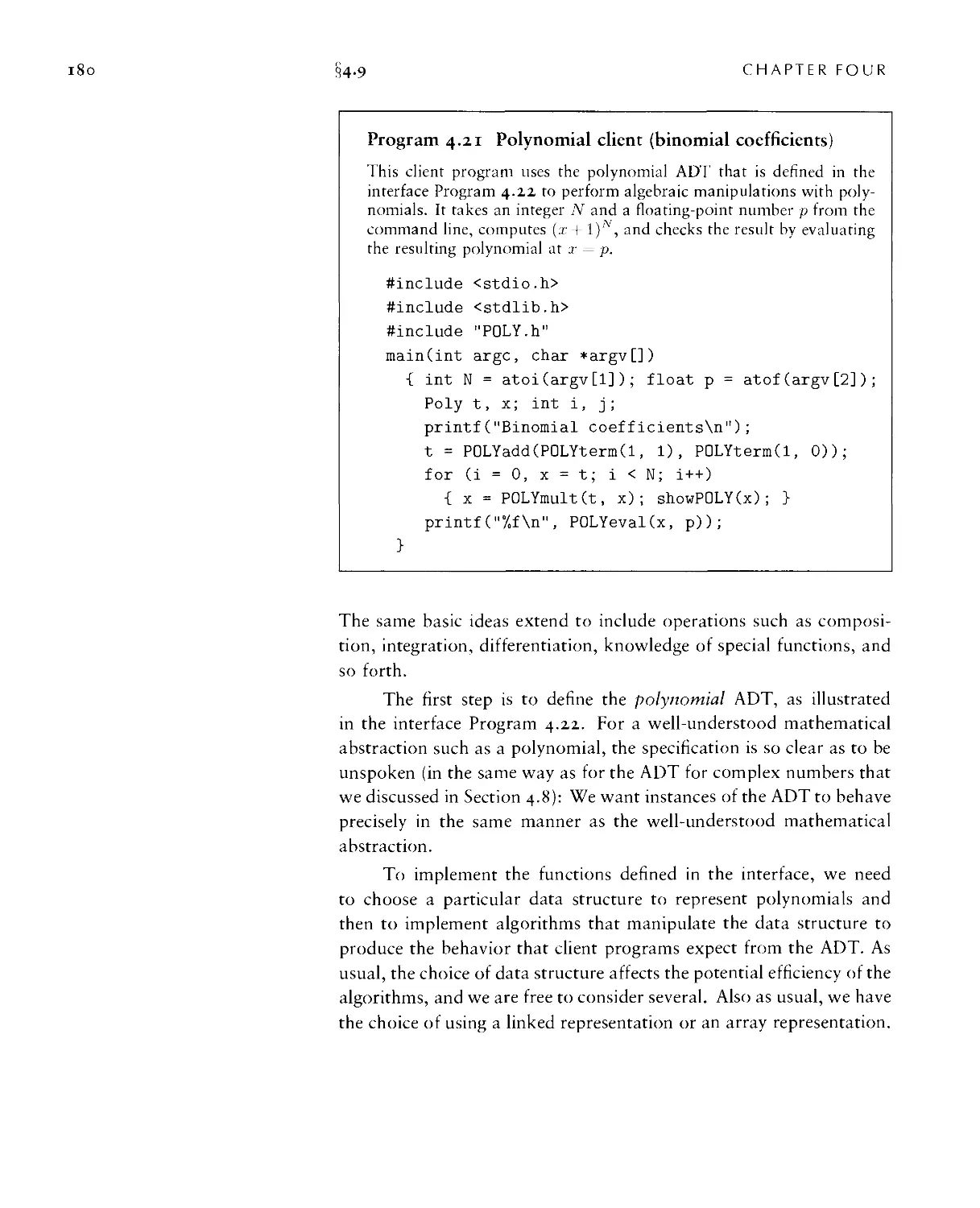
4.9 Application-Based ADT Example • 179
4.10 Perspective • 185
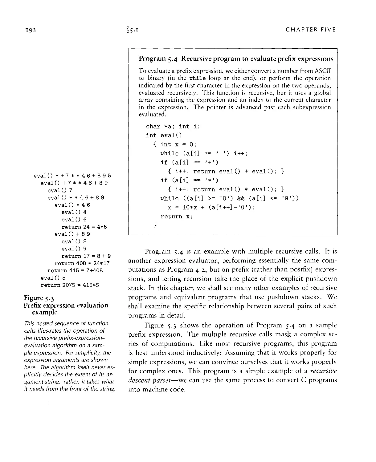
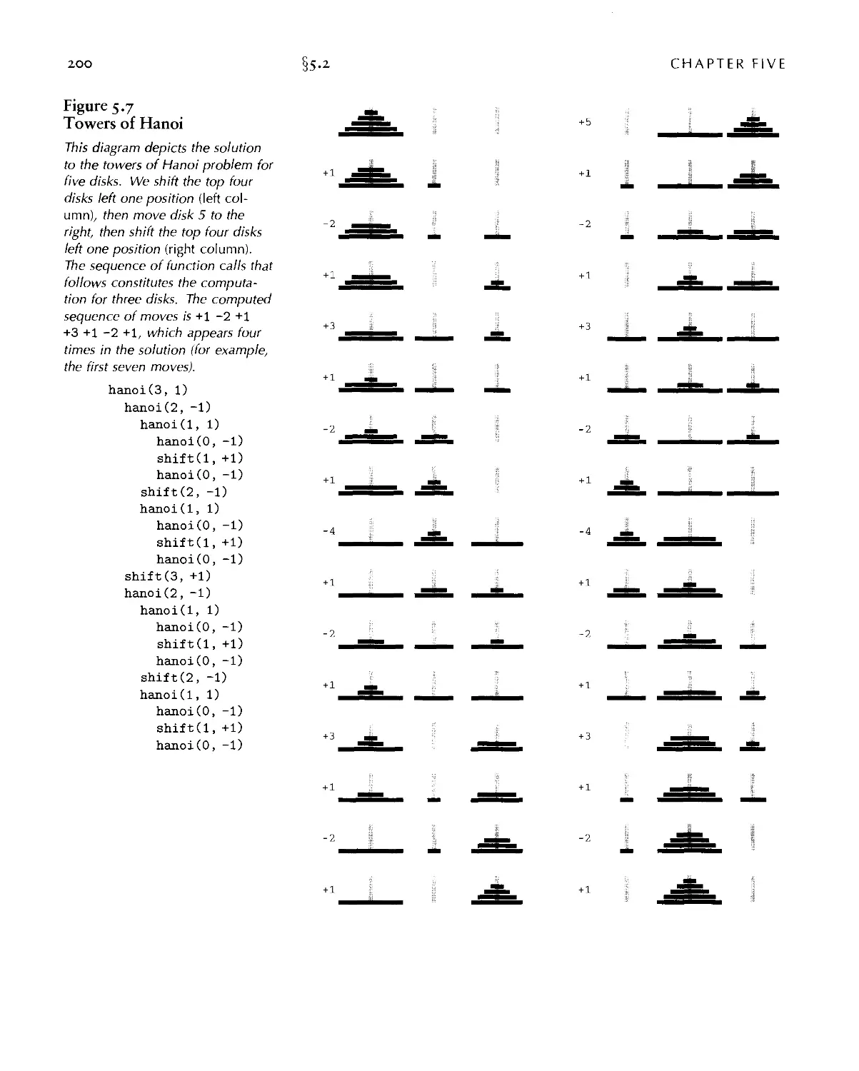
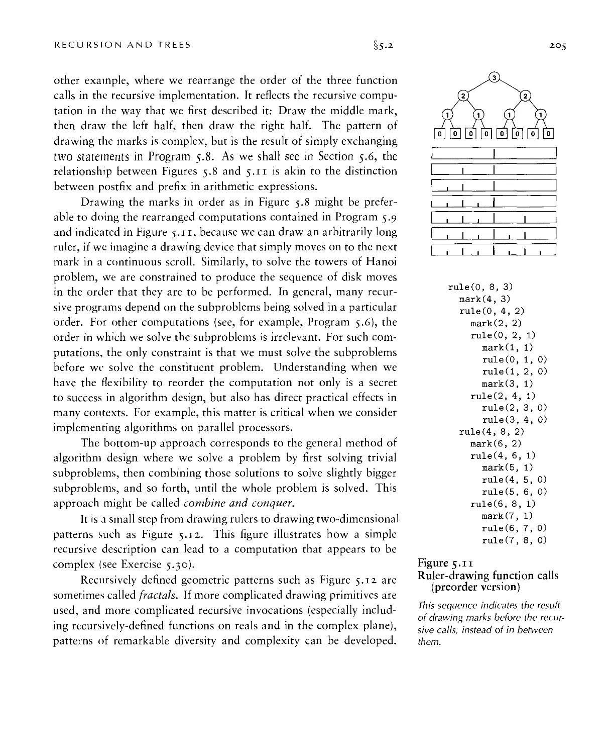
Chapter 5. Recursion and Trees 187
5.1 Recursive Algorithms • 188
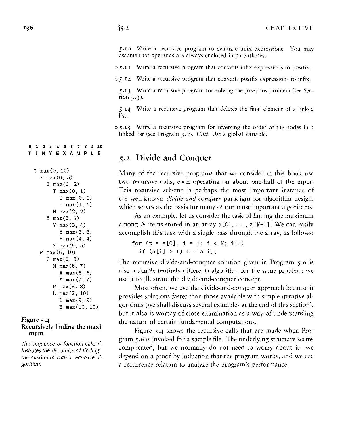
5.2 Divide and Conquer • 196
5.3 Dynamic Programming • 209
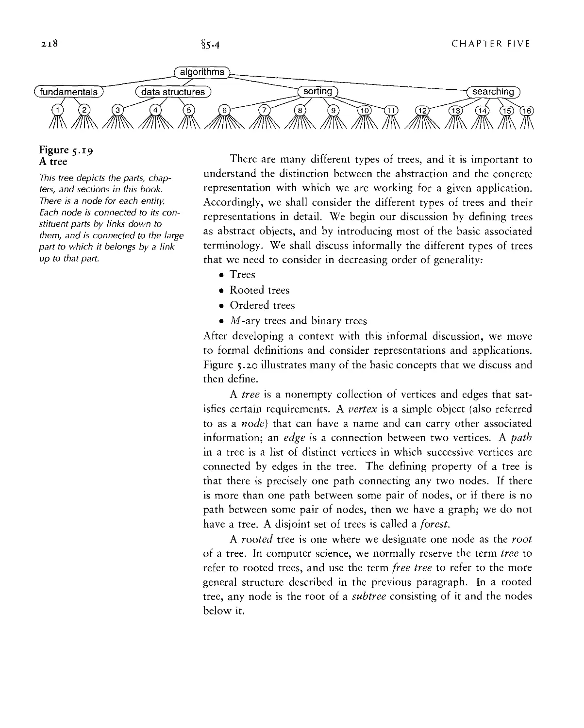
5.4 Trees • 217
5.5 Mathematical Properties of Trees • 226
5.6 Tree Traversal • 230
5.7 Recursive Binary-Tree Algorithms • 236
5.8 Graph Traversal ■ 241
5.9 Perspective • 248
Sorting
Chapter 6. Elementary Sorting Methods 253
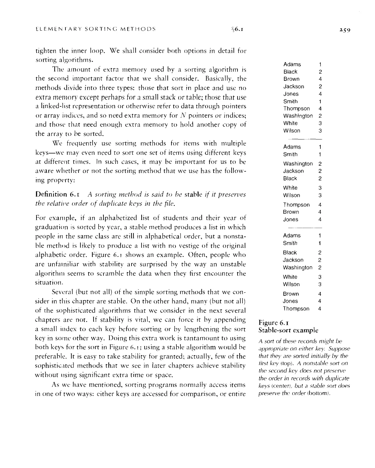
6.1 Rules of the Game • 2.S.S
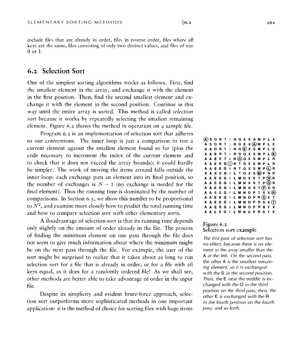
6.2 Selection Sort • 26/
6.3 Insertion Sort ■ 262
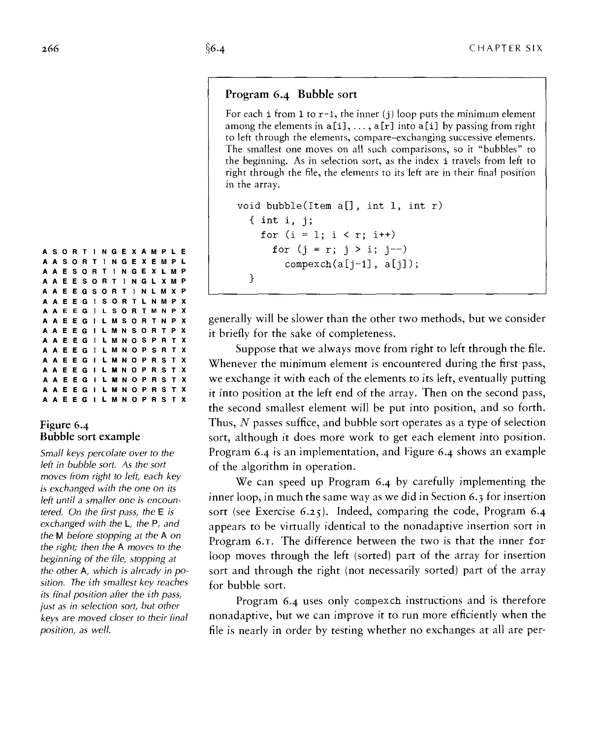
6.4 Bubble Sort ■ 265
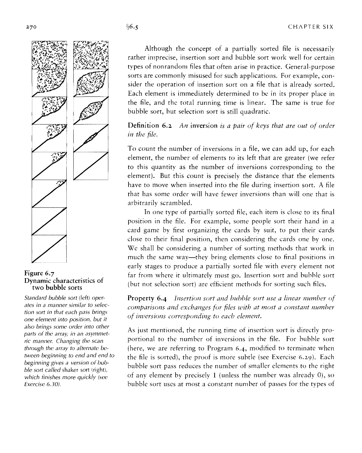
6.5 Performance Characteristics of Elementary Sorts • 267
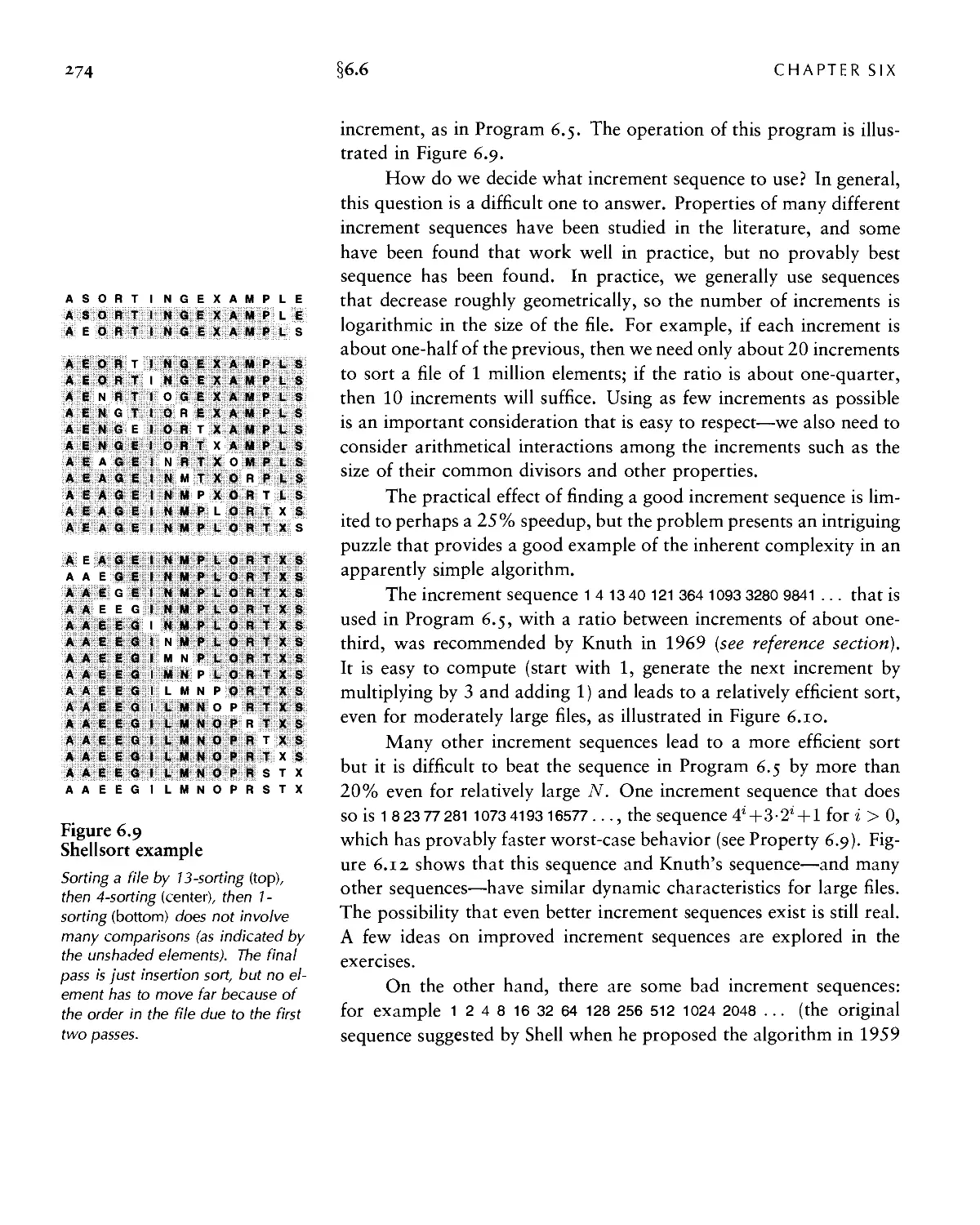
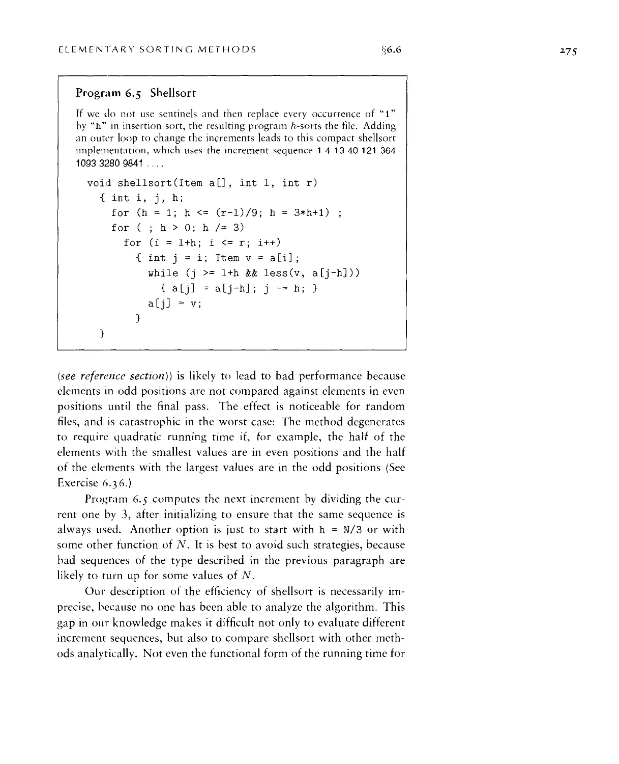
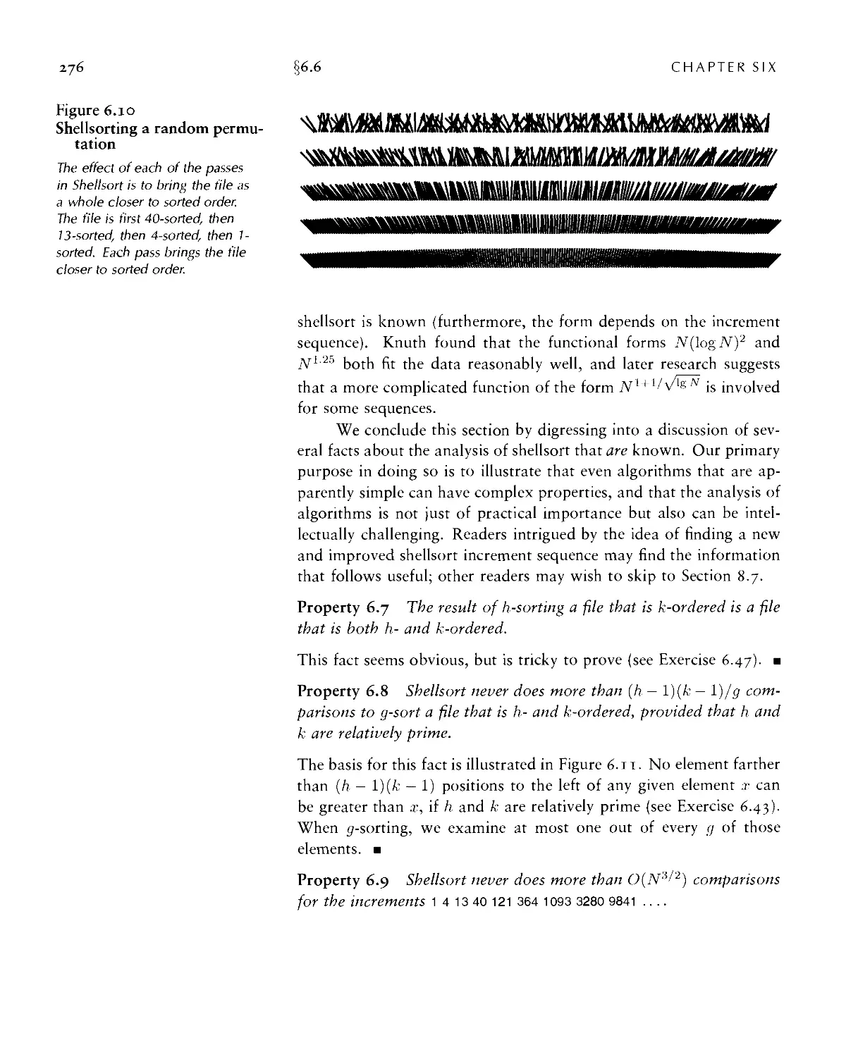
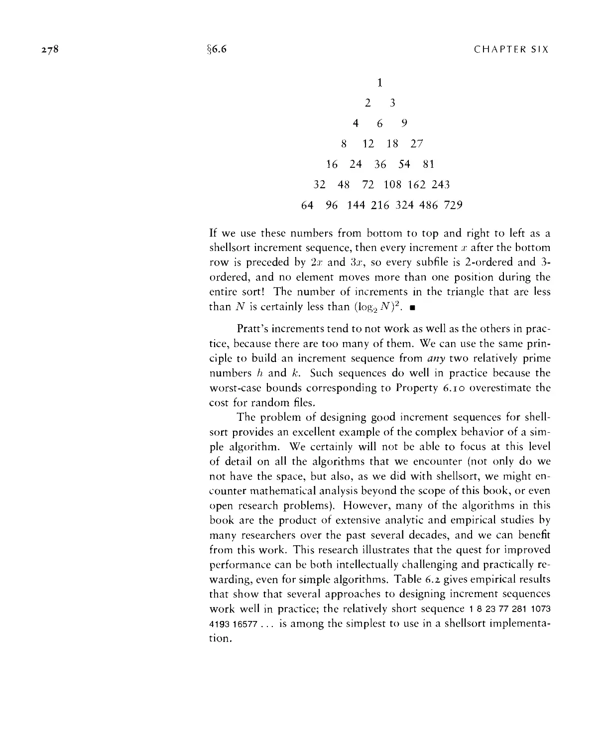
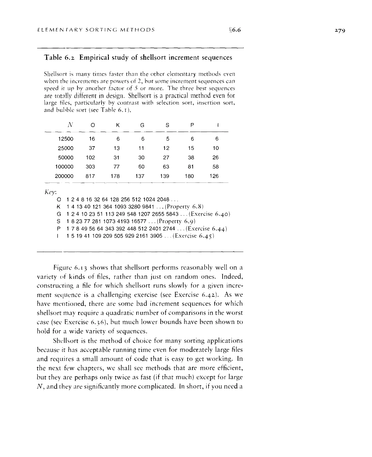
6.6 Shellsort ■ 273
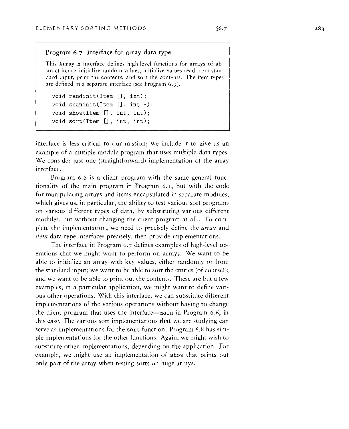
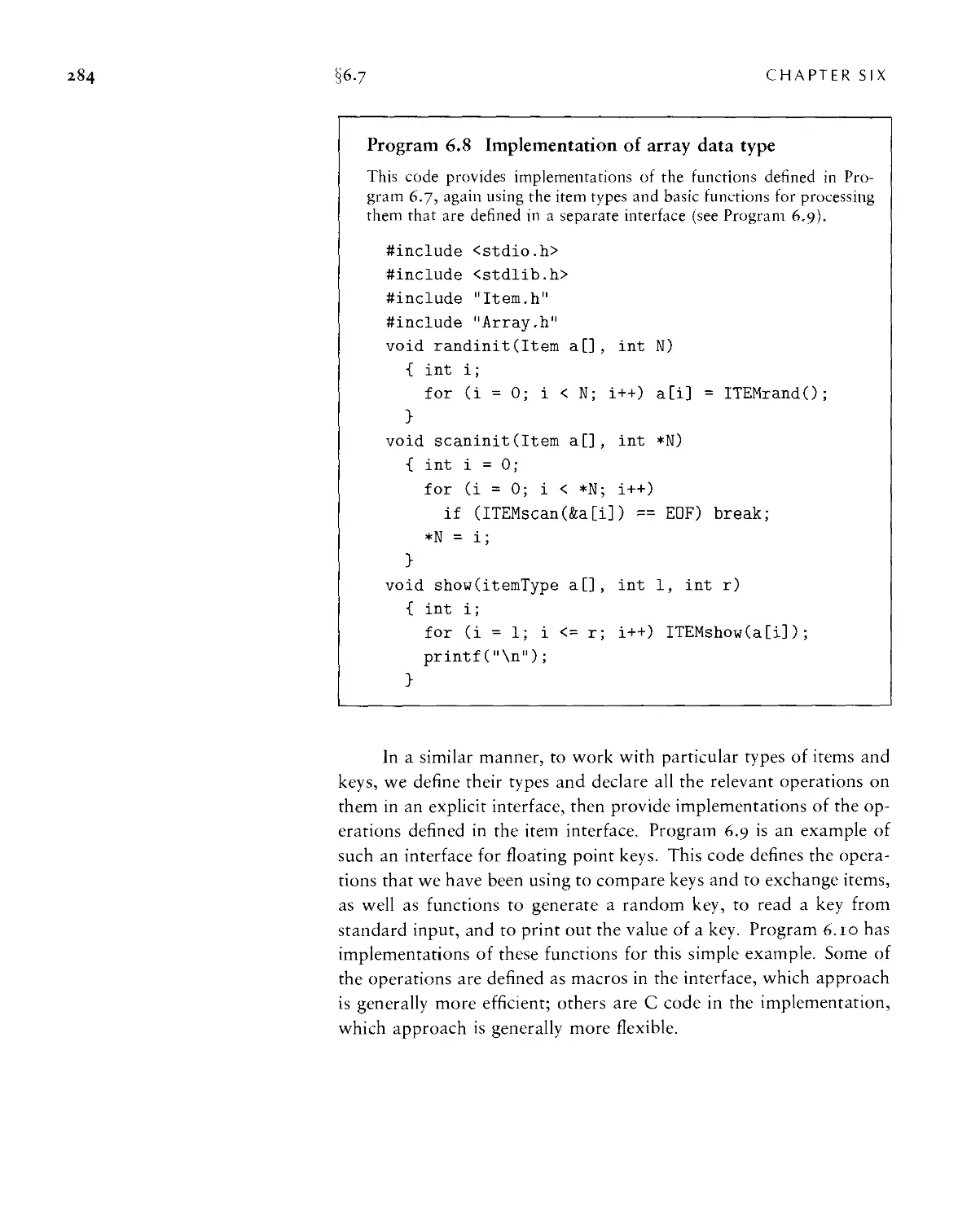
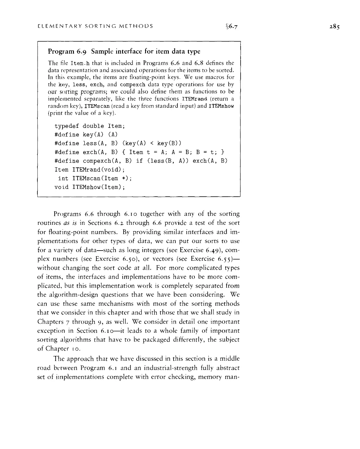
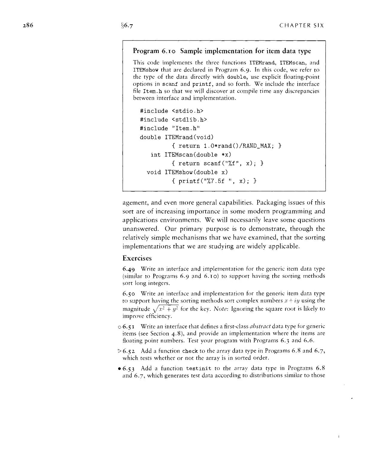
6.7 Sorting Other Types of Data • 282
6.8 Index and Pointer Sorting • 287
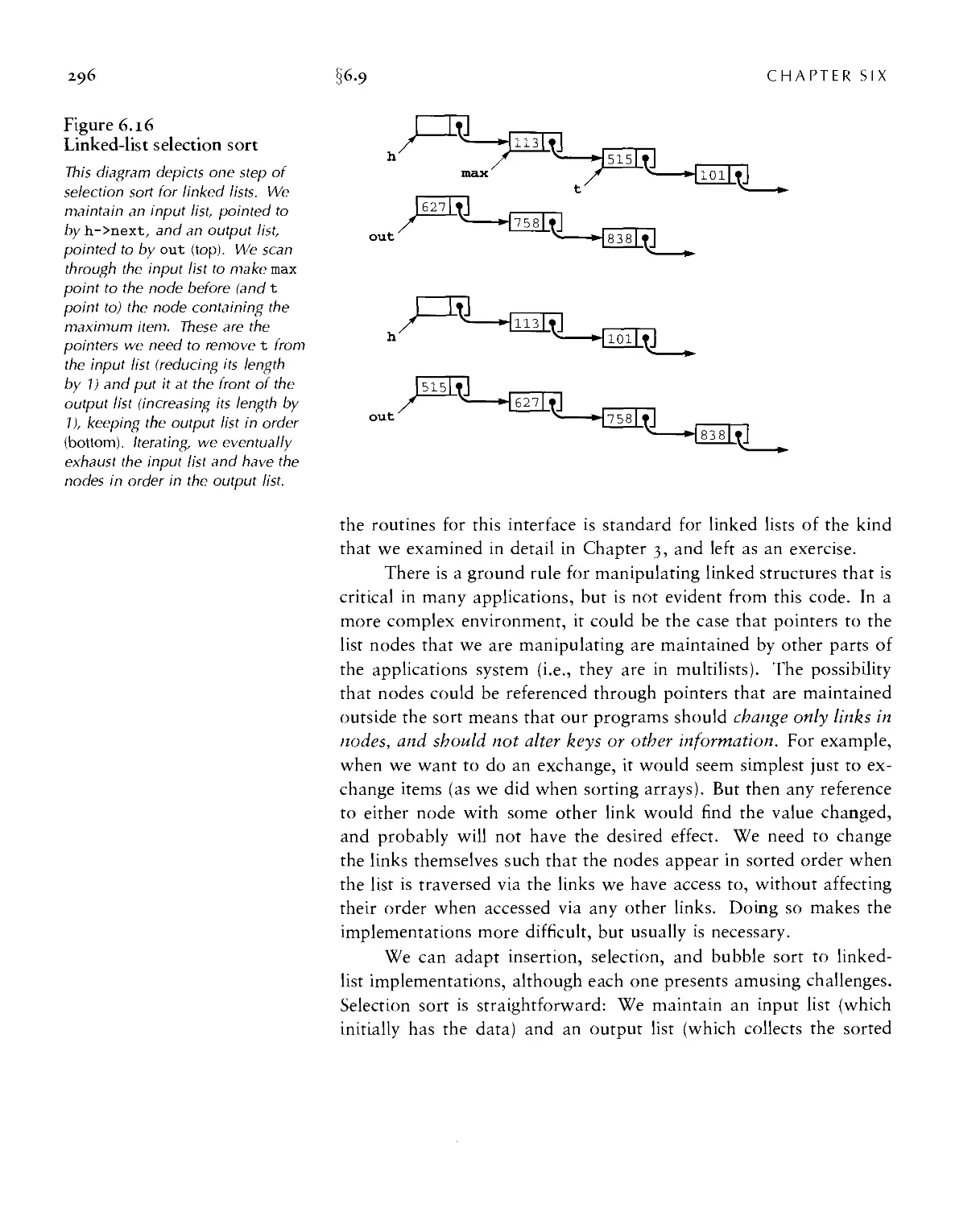
6.9 Sorting Linked Lists ■ 295
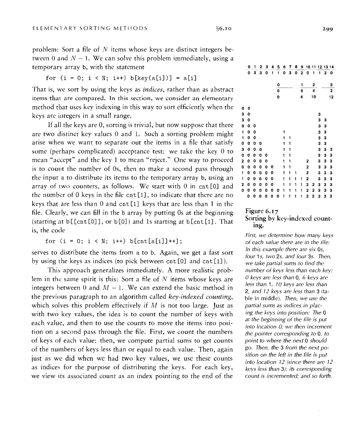
6.10 Key-Indexed Counting ■ 298
Chapter 7. Quicksort 303
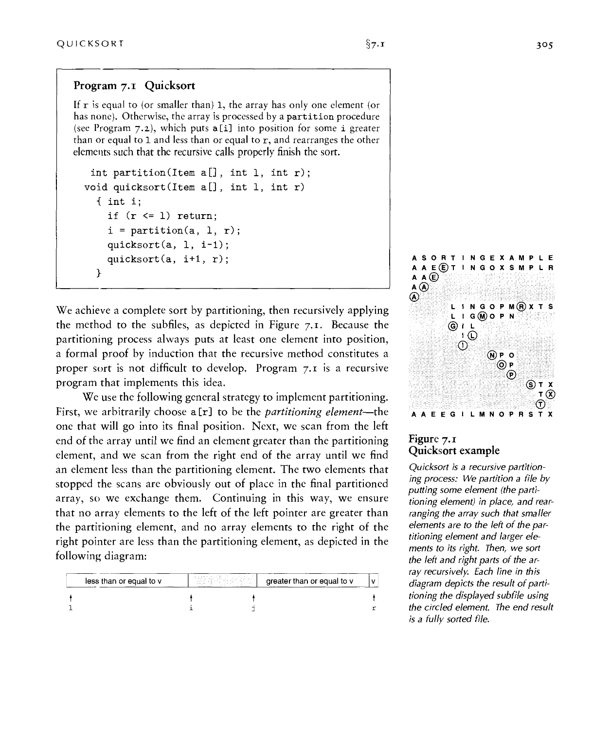
7.1 The Basic Algorithm • 304
7.2 Performance Characteristics of Quicksort • 309
7.3 Stack Size ■ 313
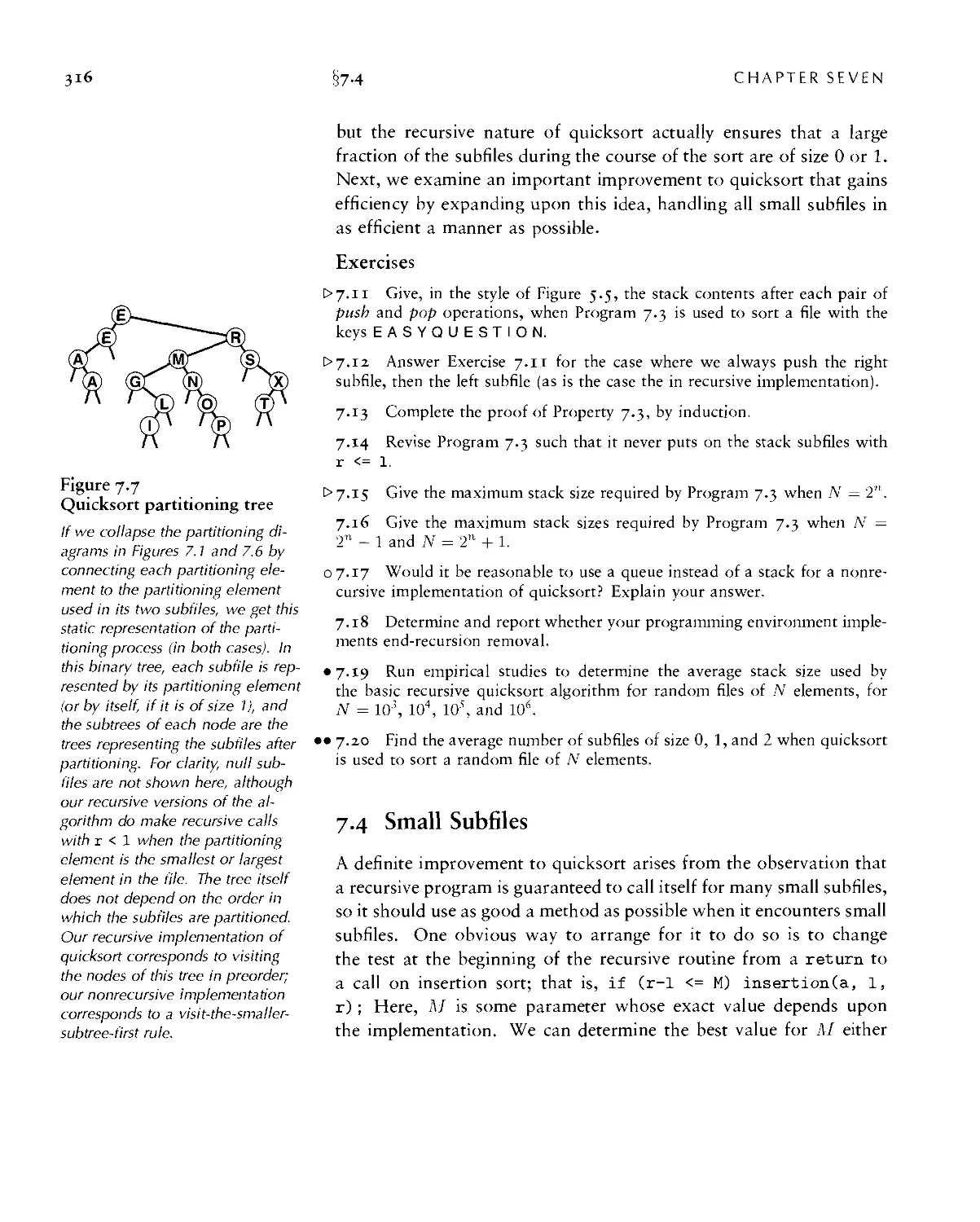
7.4 Small Subfiles ■ 316
7.5 Median-of-Three Partitioning • 319
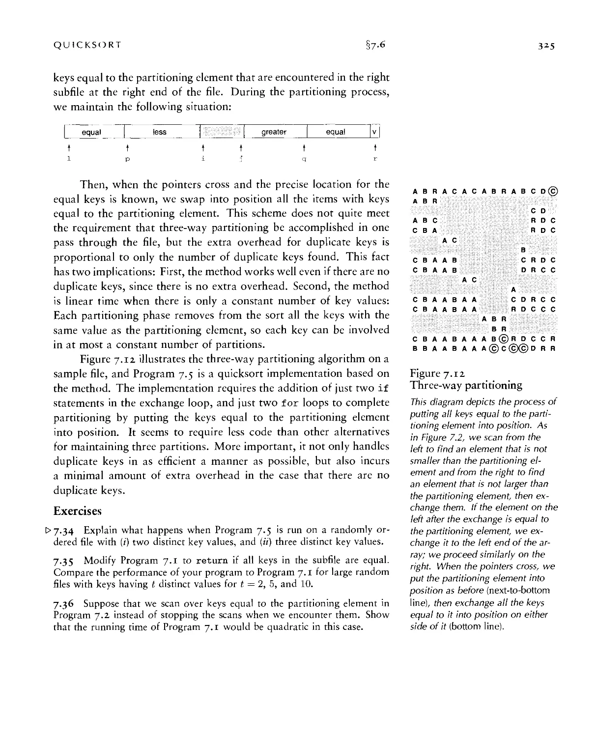
7.6 Duplicate Keys • 324
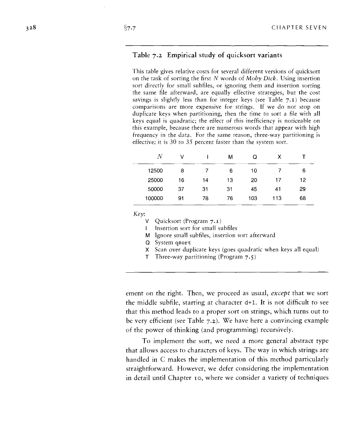
7.7 Strings and Vectors • 327
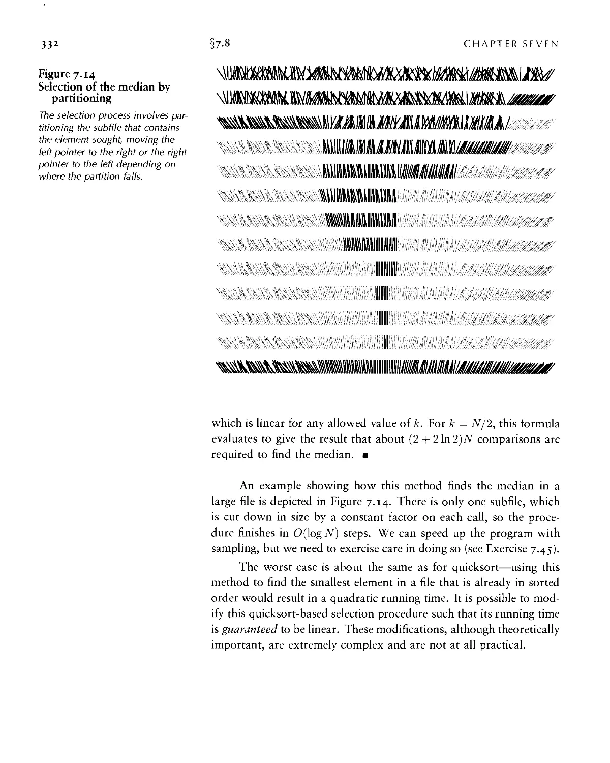
7.8 Selection ■ .529
Chapter 8. Mergesort 335
8.1 Two-Way Merging • 336
8.2 Abstract In-place Merge • 339
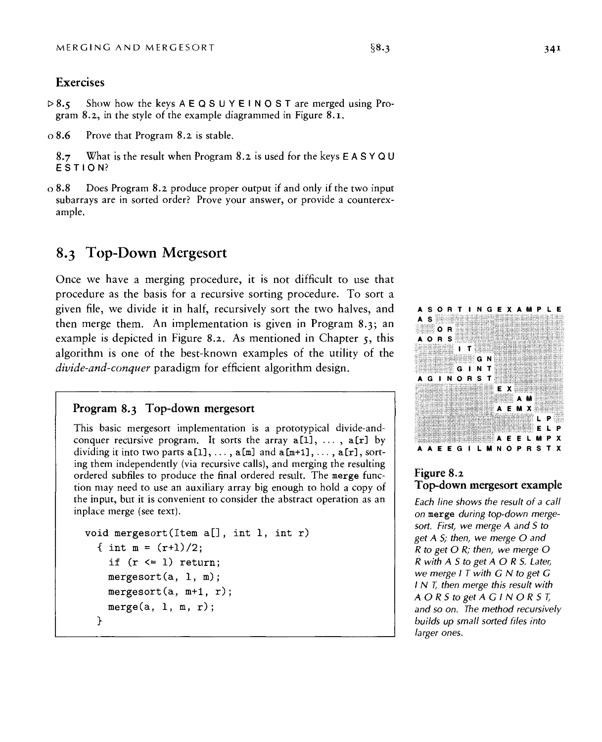
8.3 Top-Down Mergesort • 341
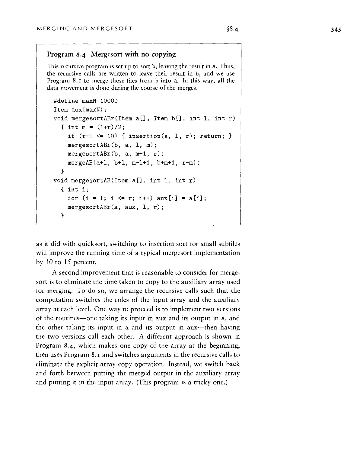
8.4 Improvements to the Basic Algorithm ■ 344
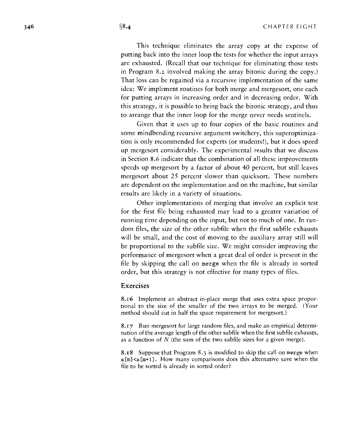
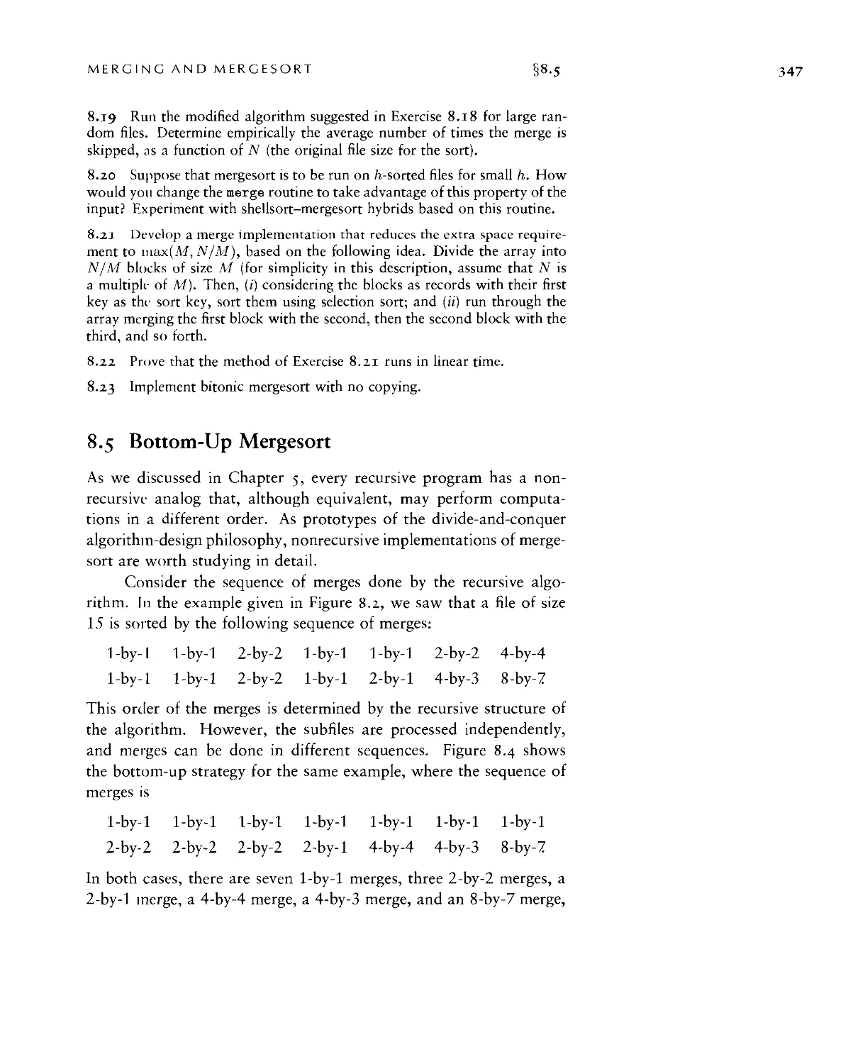
8.5 Bottom-Up Mergesort • 347
8.6 Performance Characteristics of Mergesort • 351
8.7 Linked-List Implementations of Mergesort • 354
8.8 Recursion Revisited • 357
Chapter 9. Priority Queues and Heapsort 361
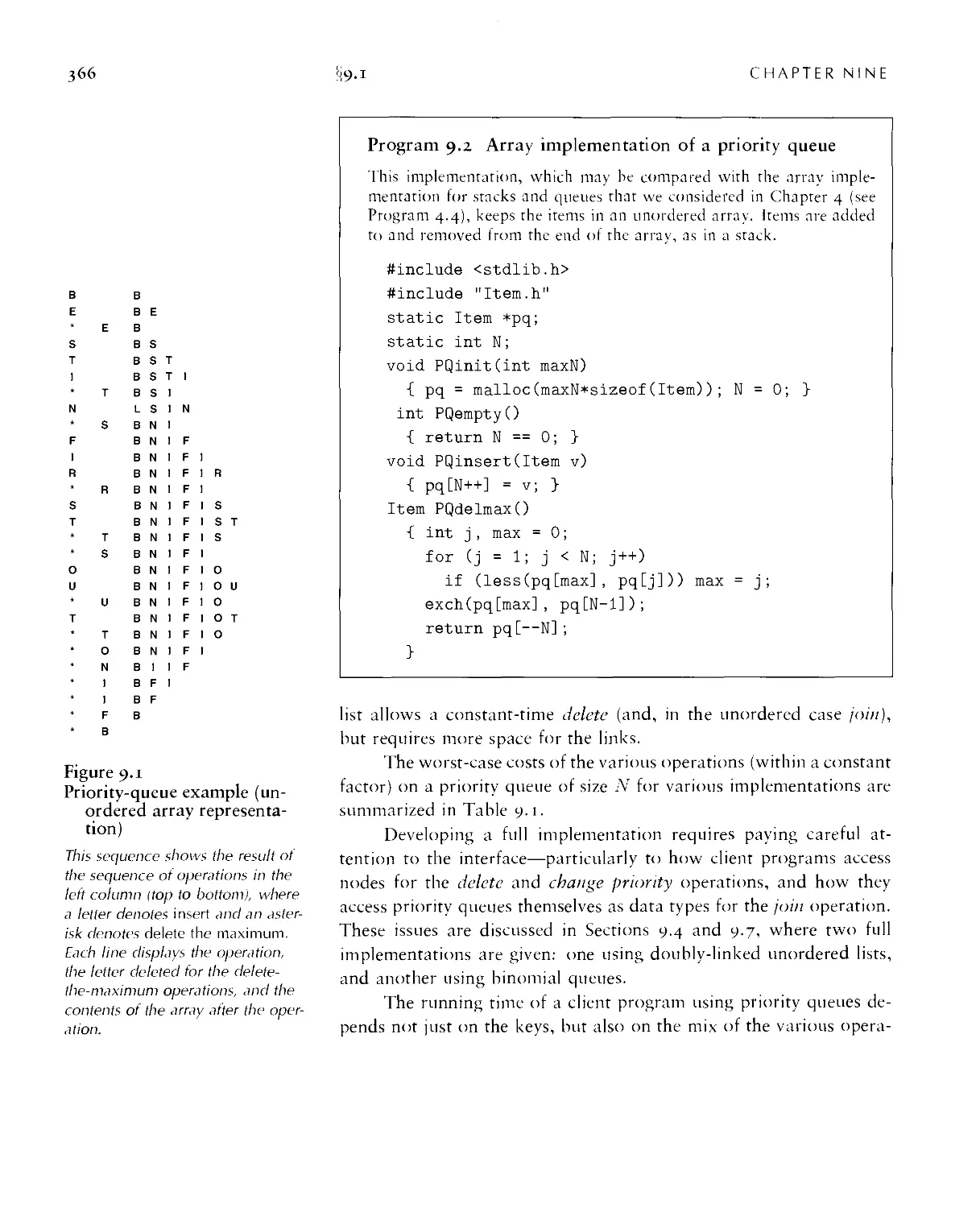
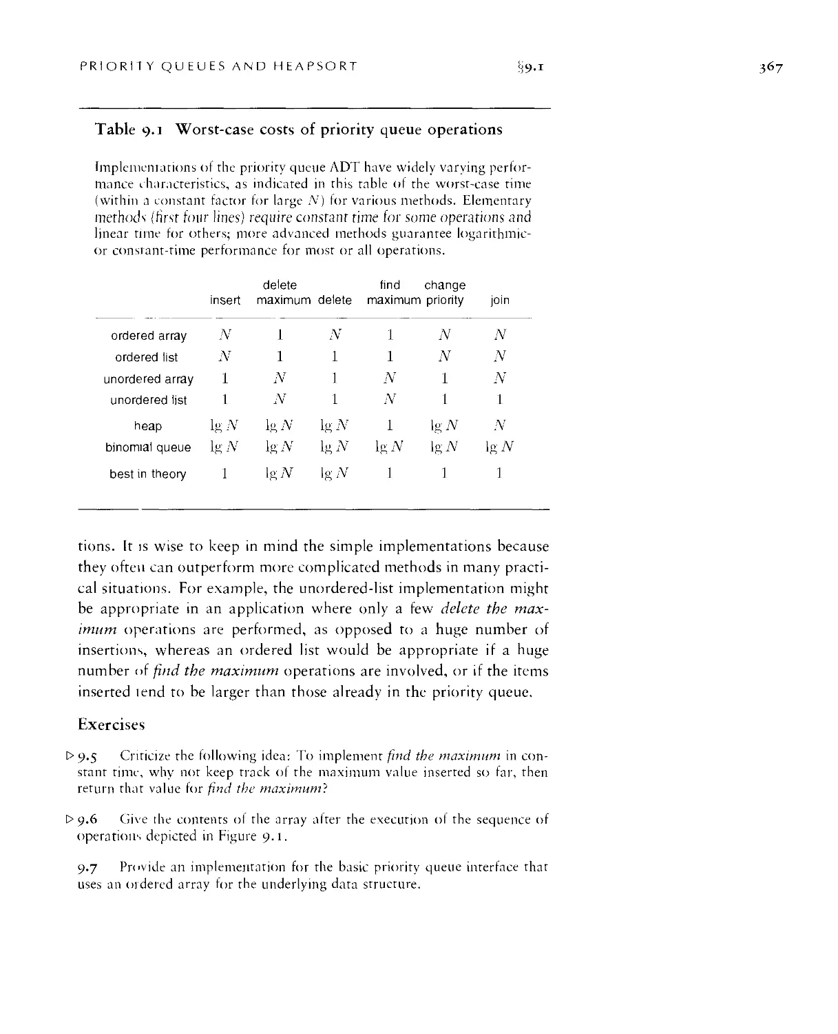
9.1 Elementary Implementations ■ 365
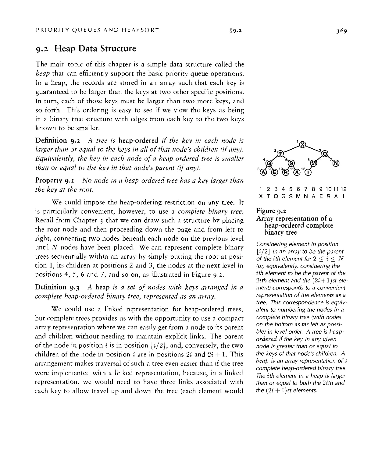
9.2 Heap Data Structure • .569
xv
TABLE OF CONTENTS
9.3 Algorithms on Heaps ■ 371
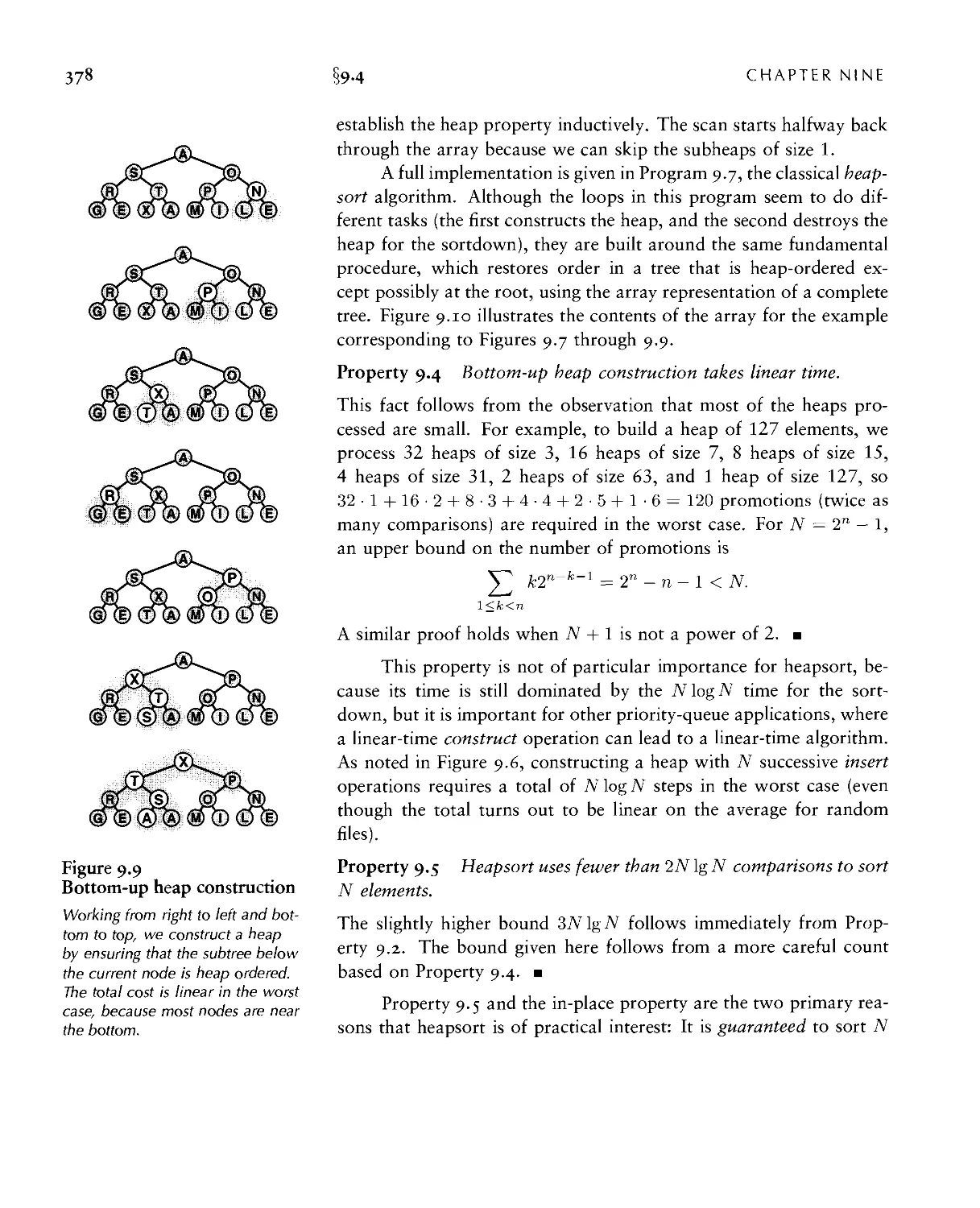
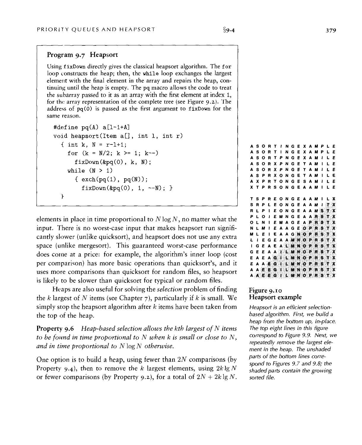
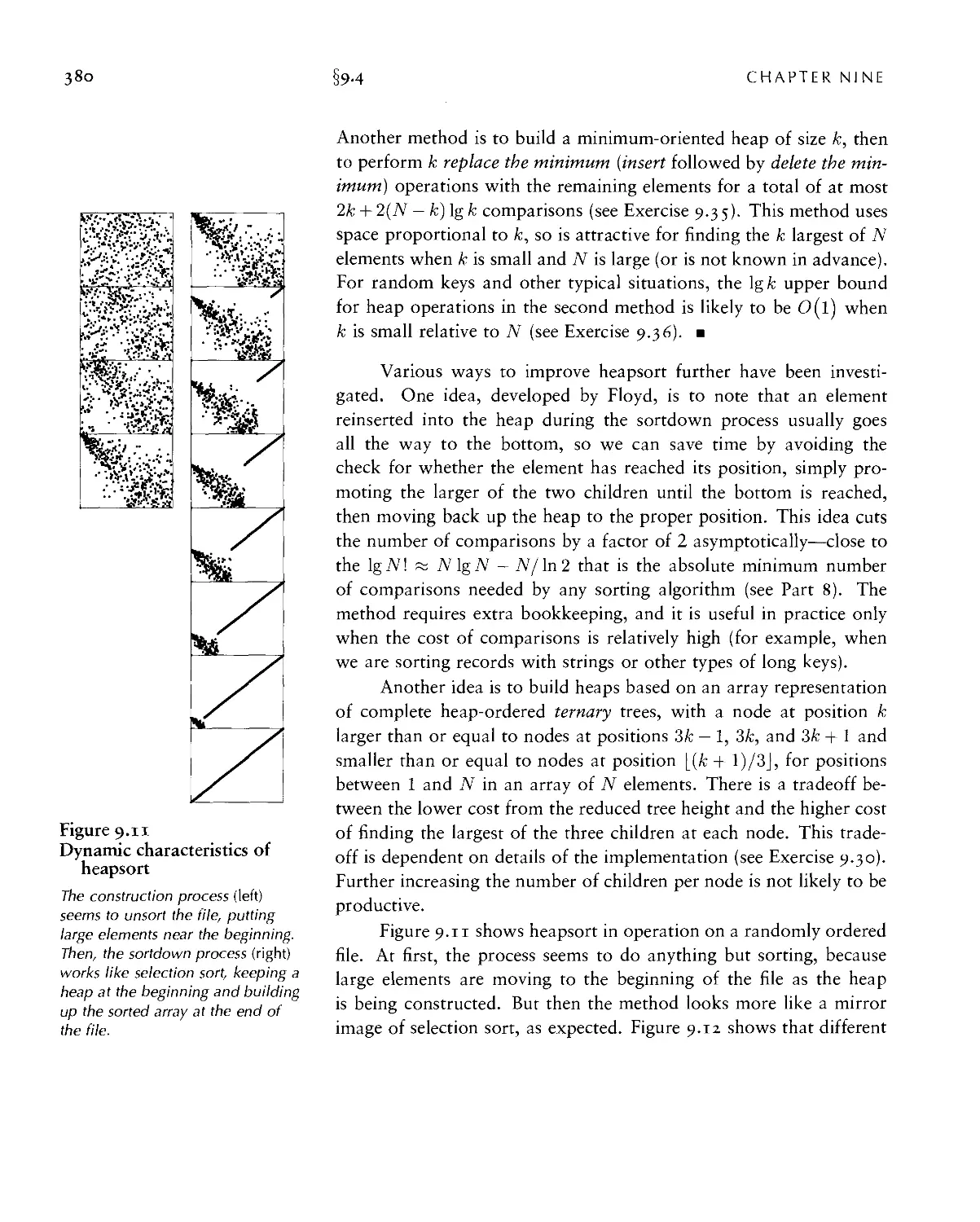
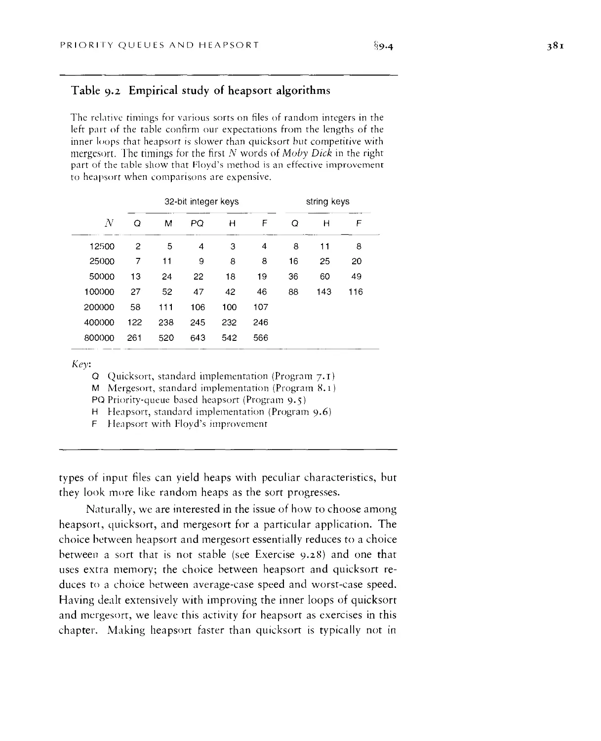
9.4 Heapsort ■ 377
9.5 Priority-Queue ADT • 384
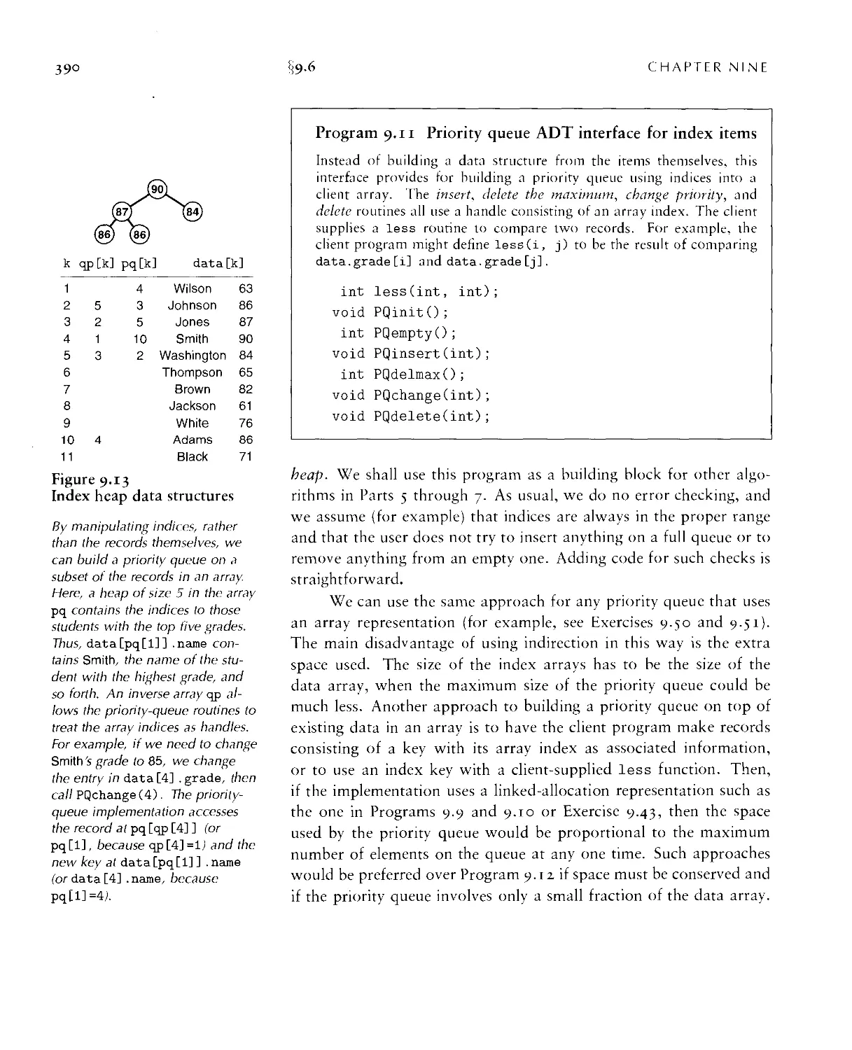
9.6 Priority Queues for Index Items • 389
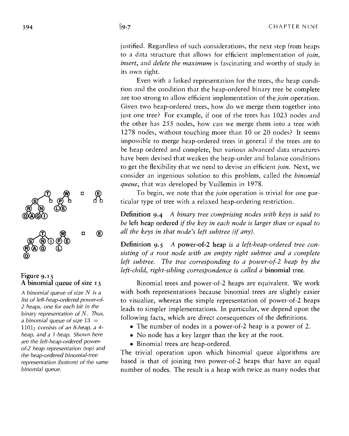
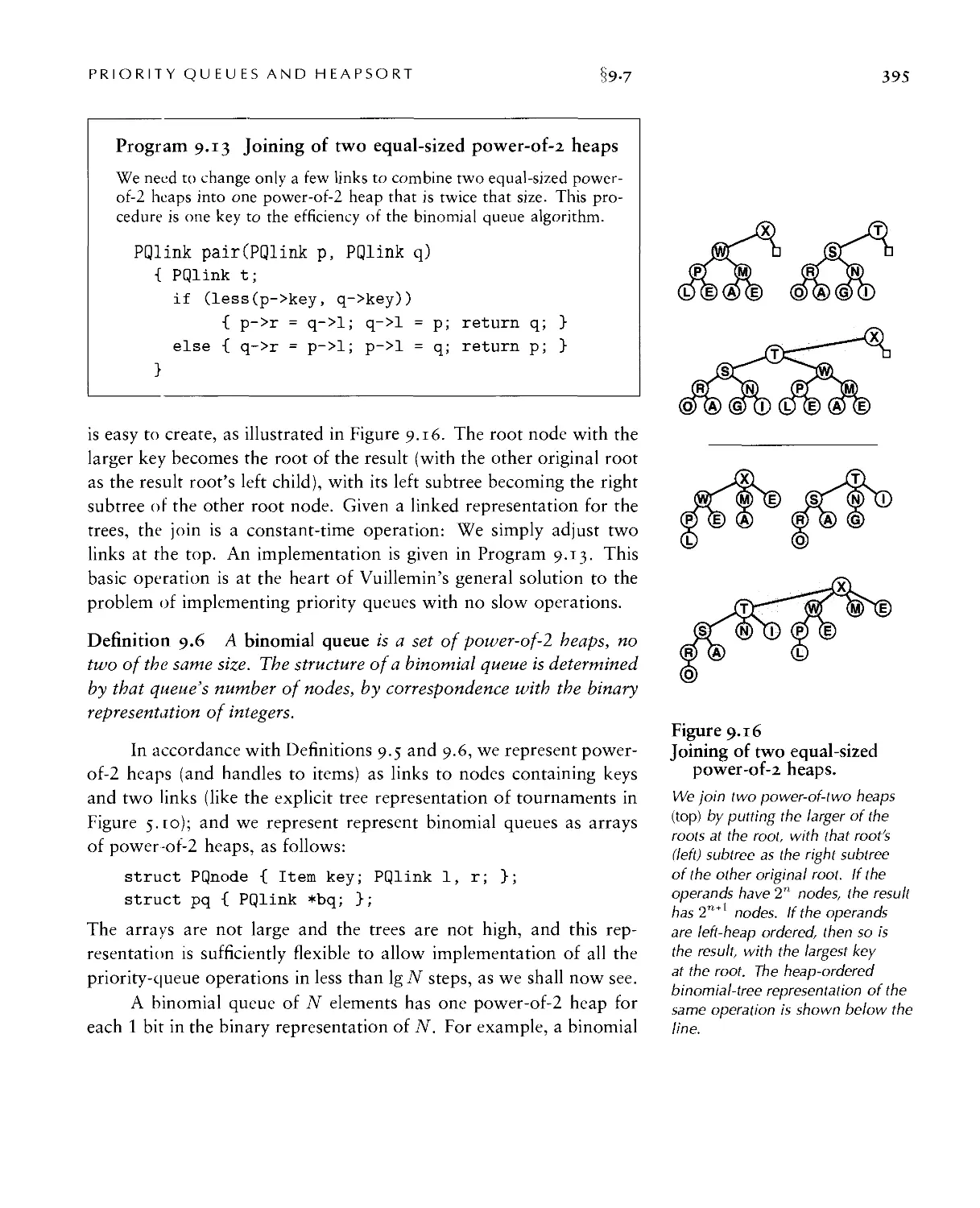
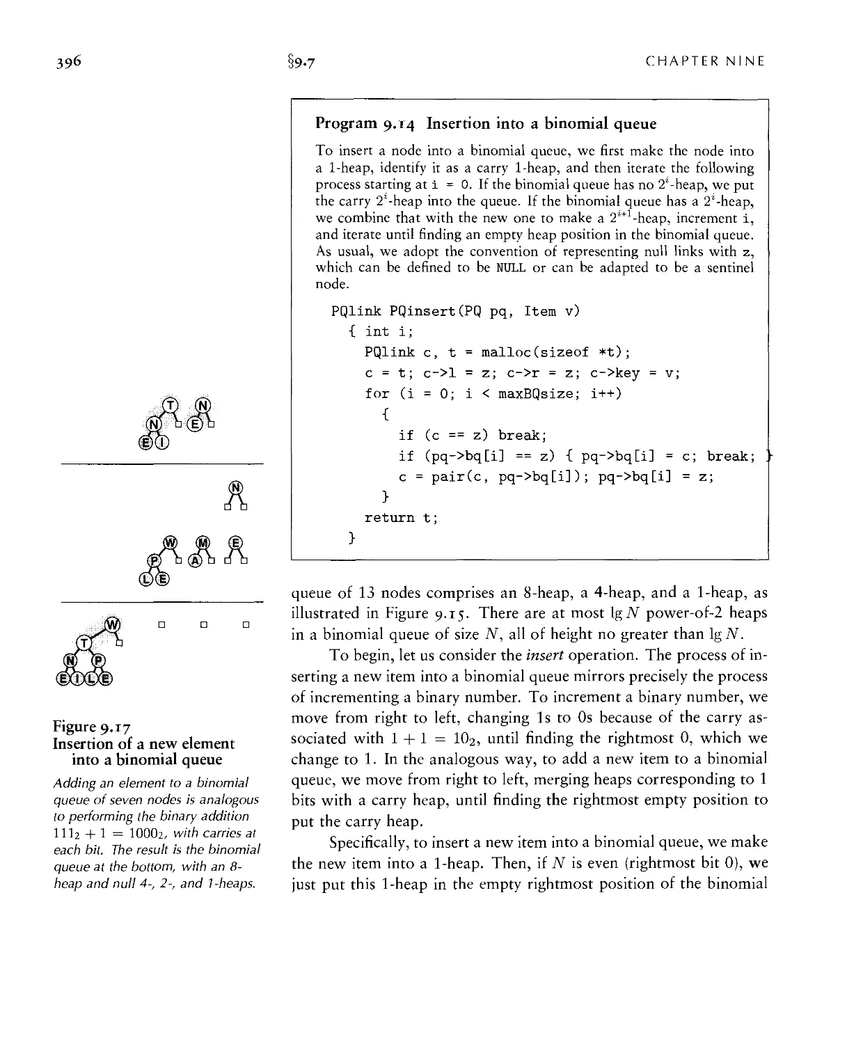
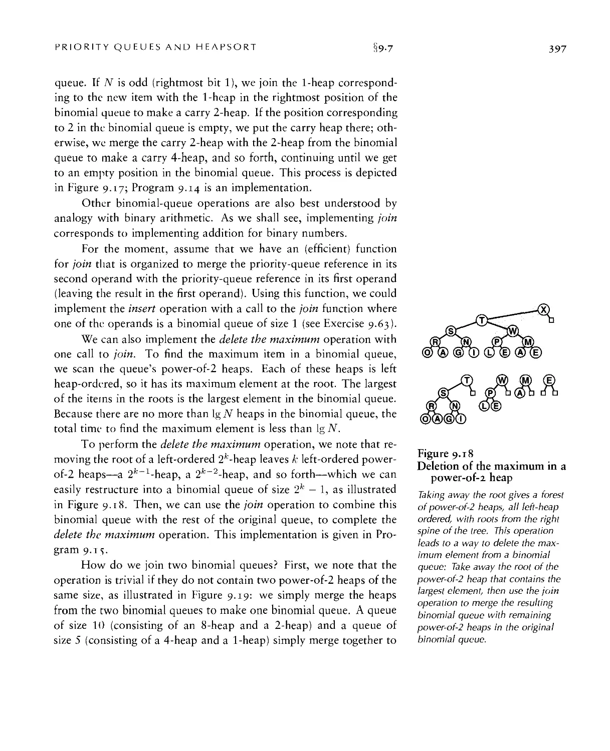
9.7 Binomial Queues ■ 392
Chapter 10. Radix Sorting 403
10.1 Bits, Bytes, and Words • 40.S
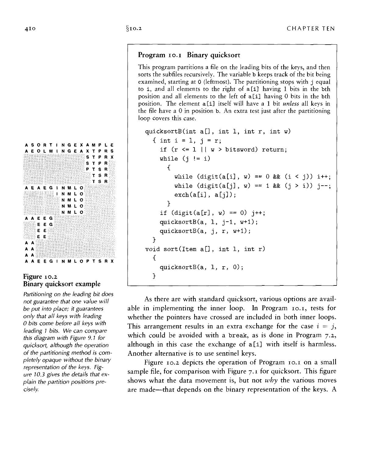
10.2 Binary Quicksort ■ 409
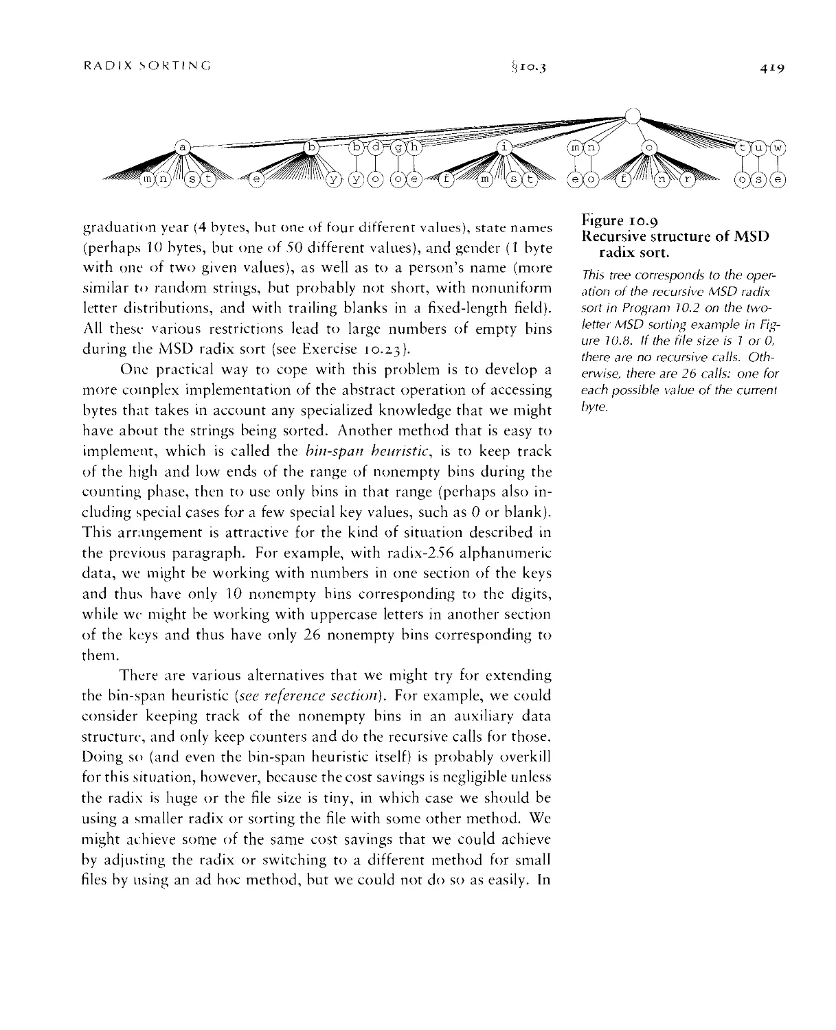
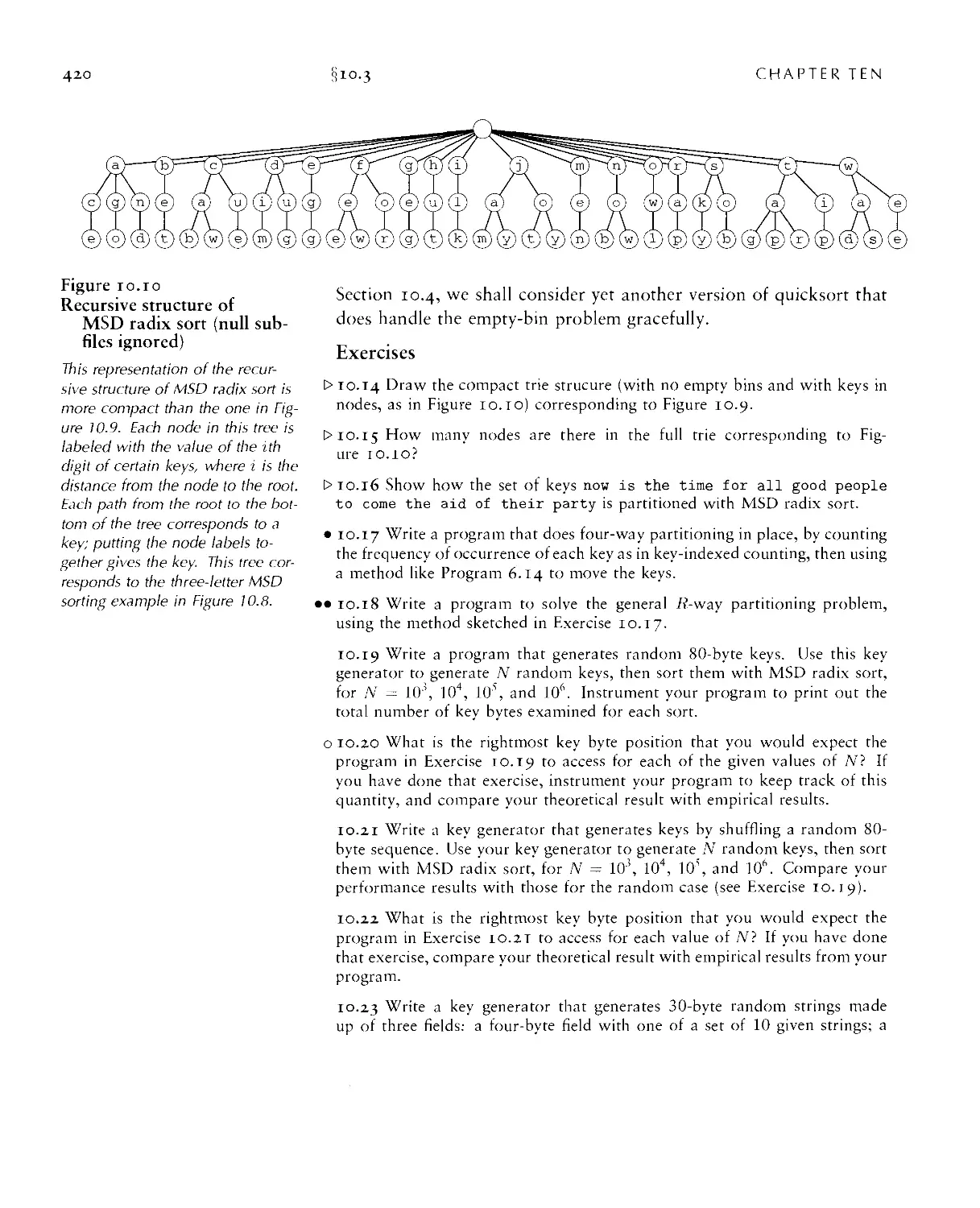
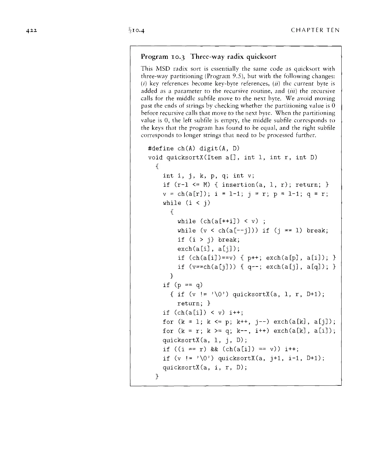
10.3 MSD Radix Sort ■ 413
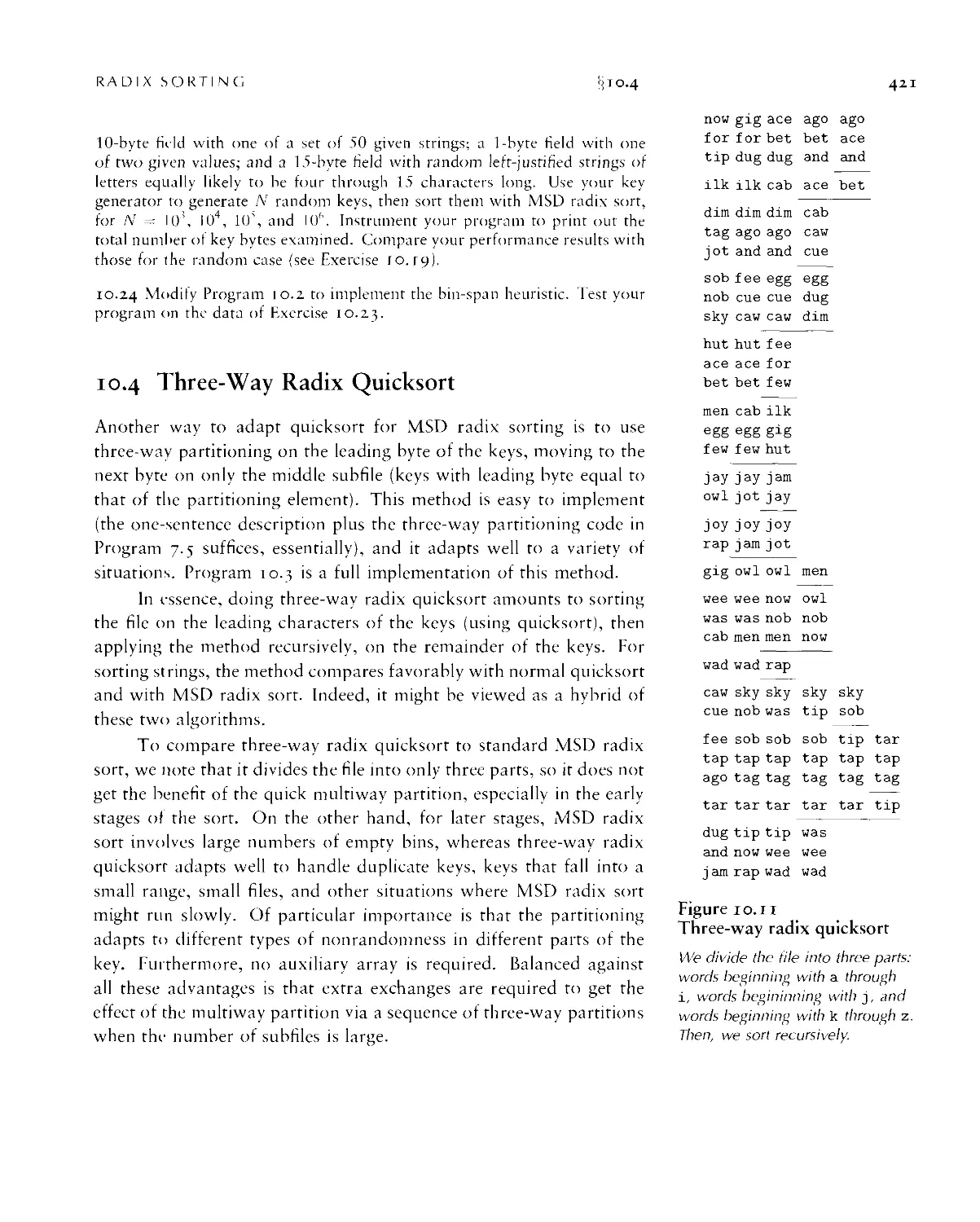
10.4 Three-Way Radix Quicksort • 421
10.5 LSD Radix Sort ■ 425
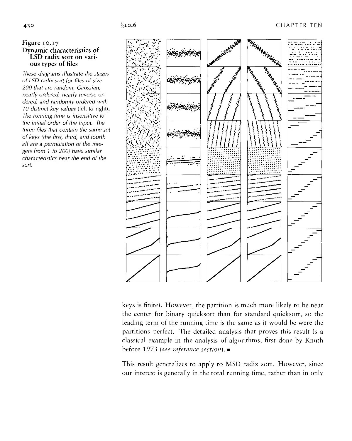
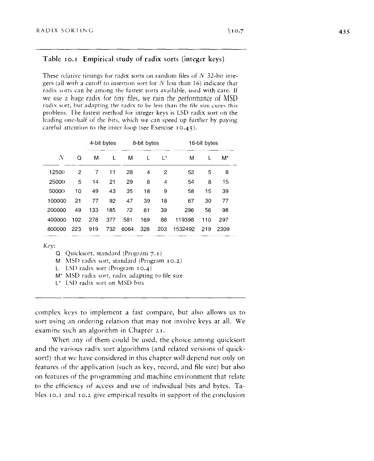
10.6 Performance Characteristics of Radix Sorts • 429
10.7 Sublinear-Time Sorts • 433
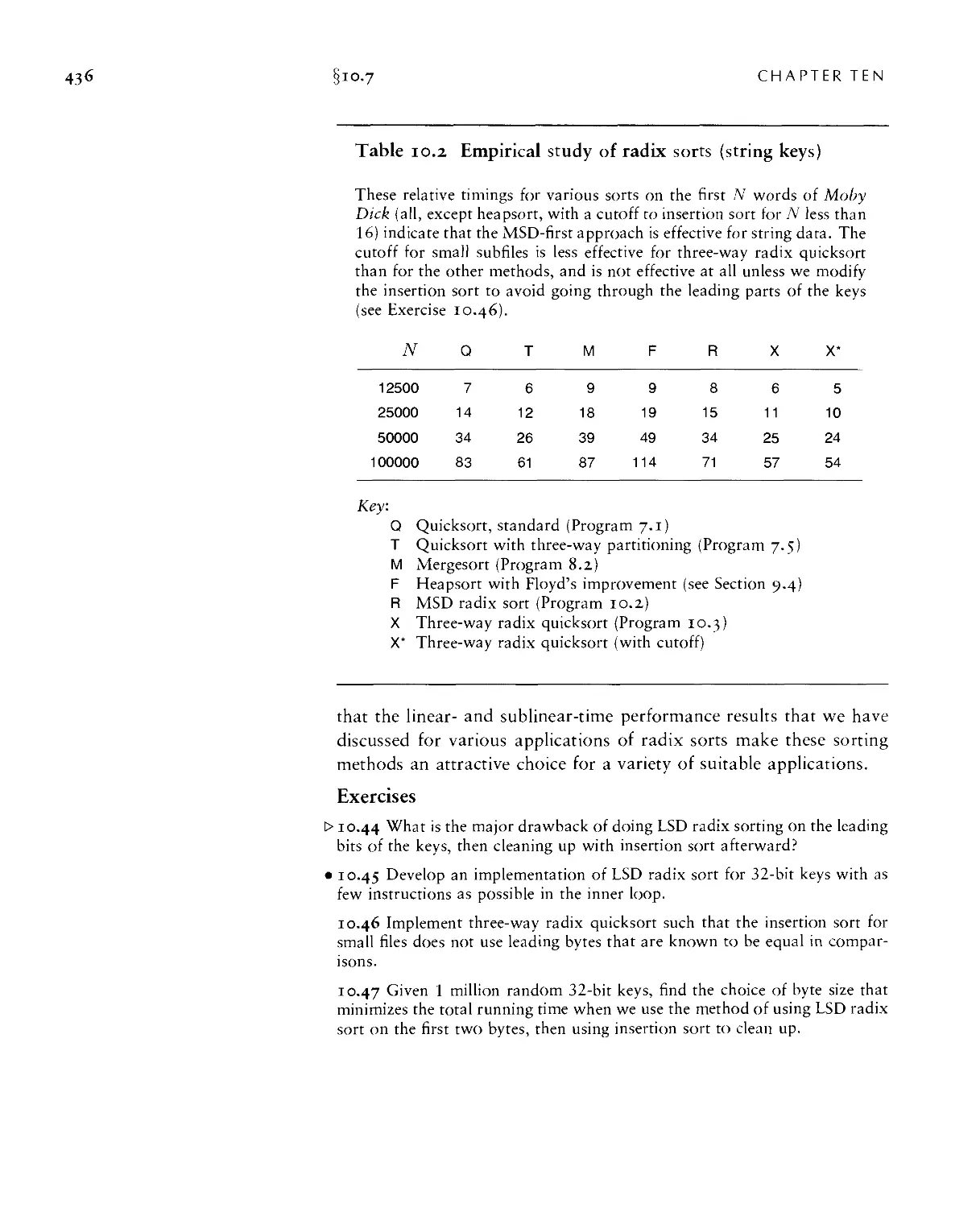
Chapter 11. Special-Purpose Sorts 439
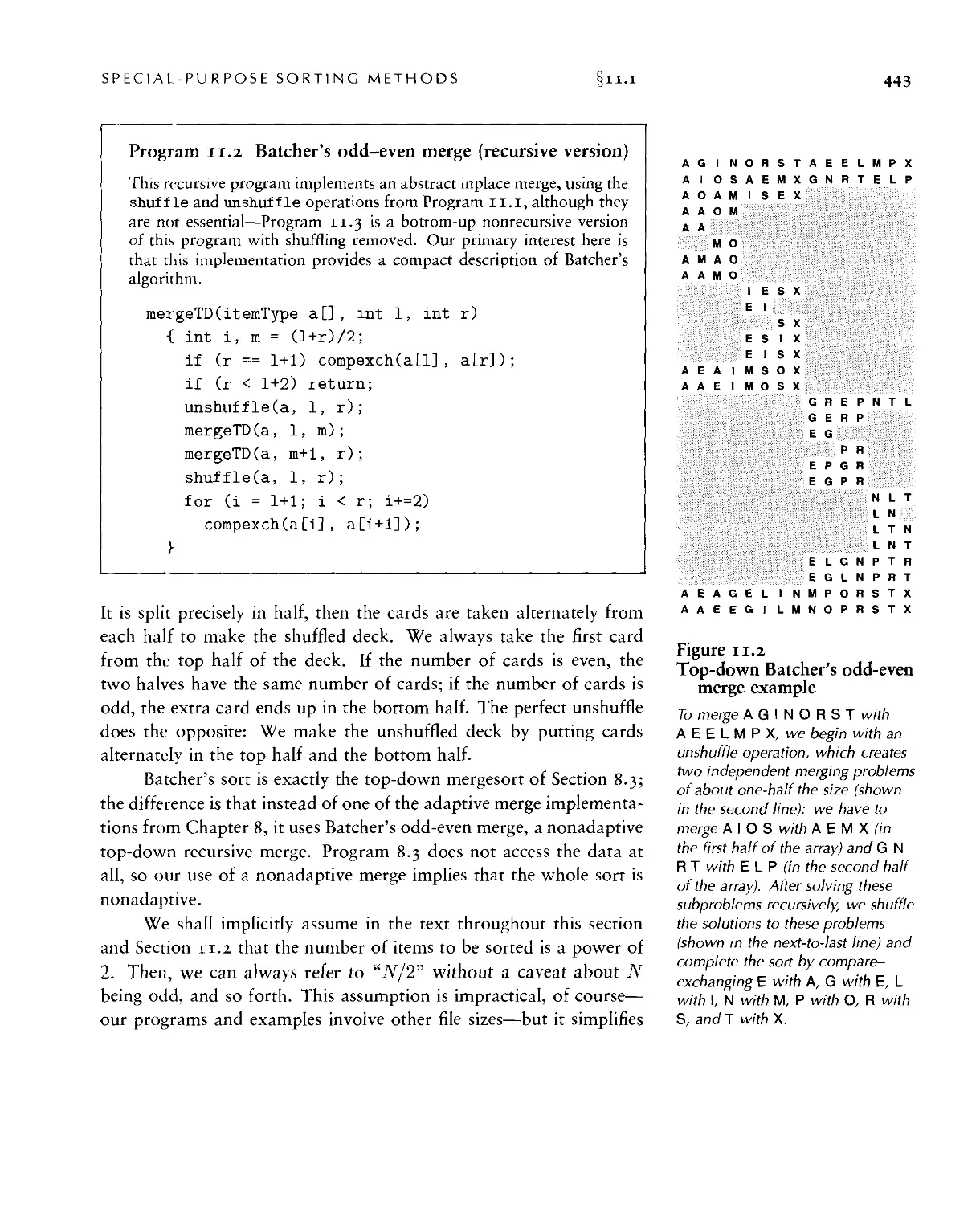
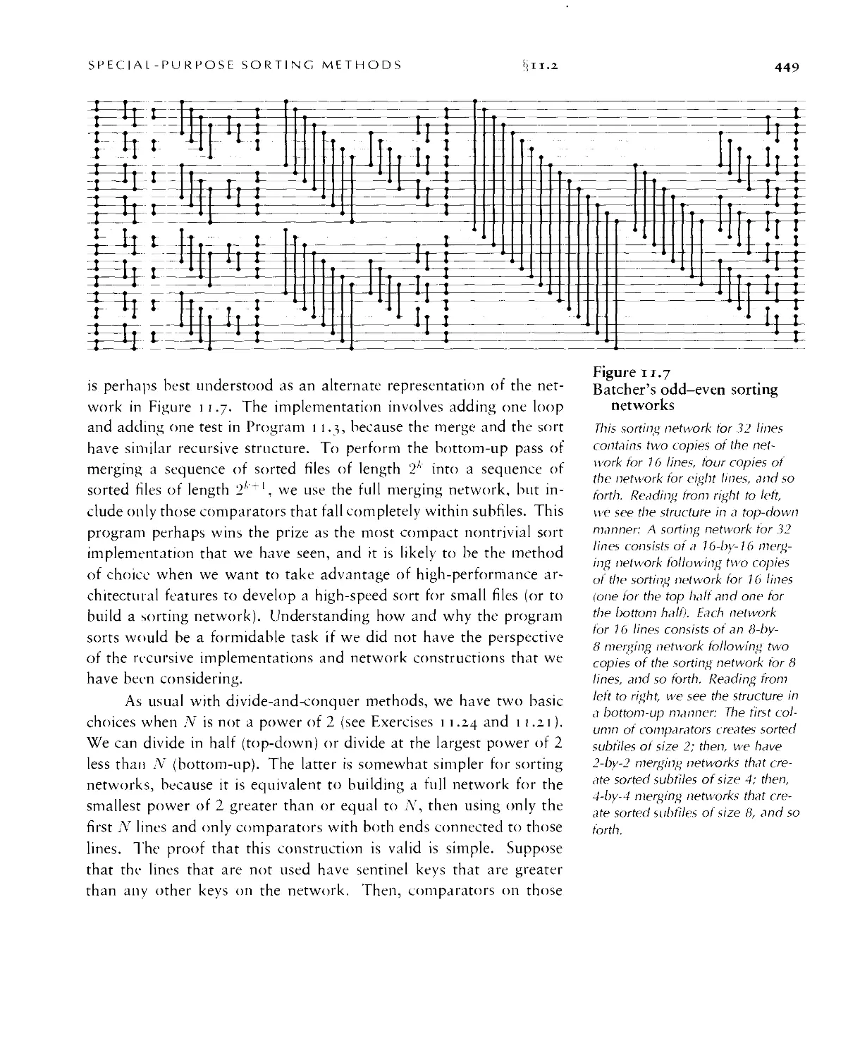
11.1 Batcher's Odd-Even Mergesort ■ 441
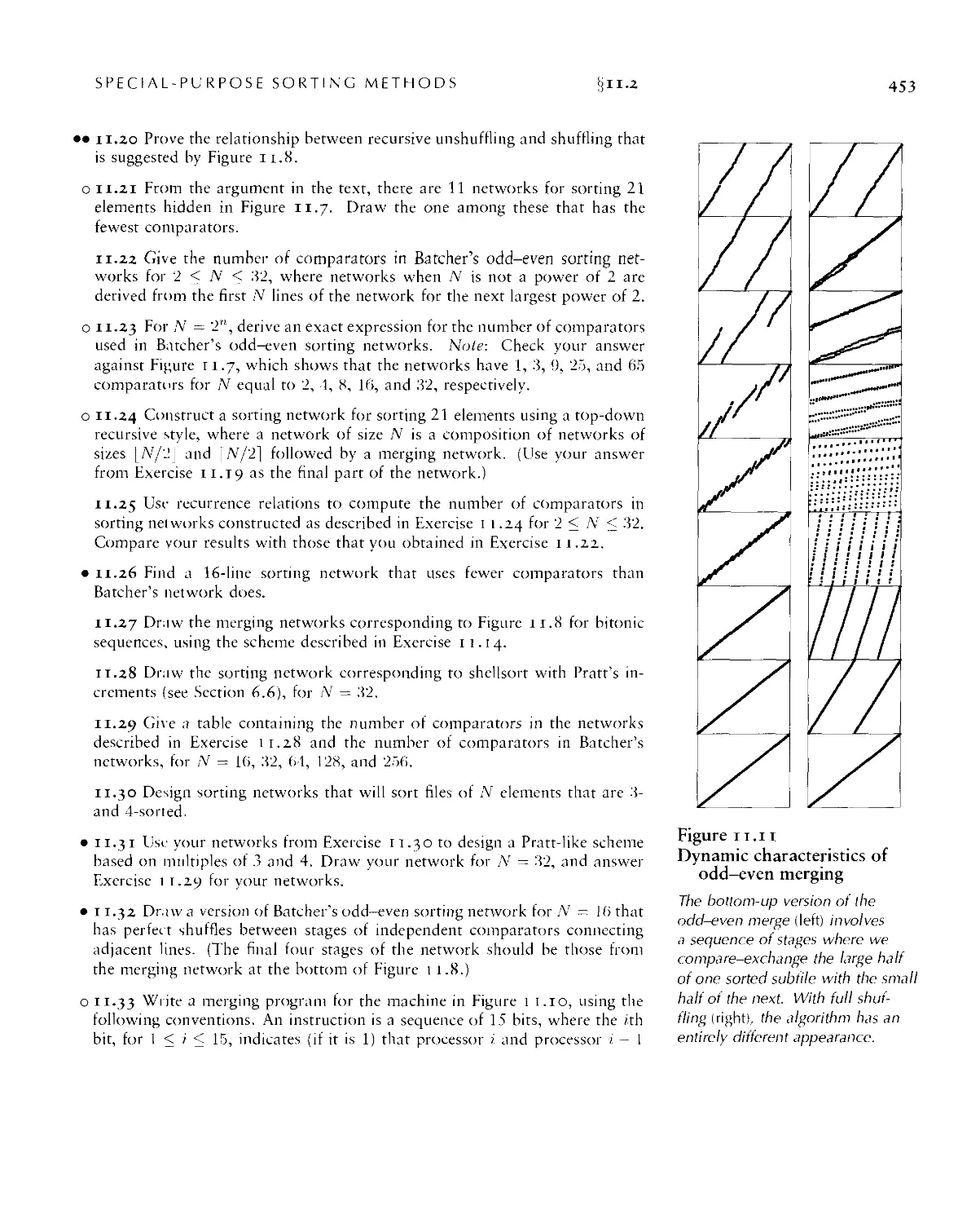
11.2 Sorting Networks • 446
11.3 External Sorting • 4S4
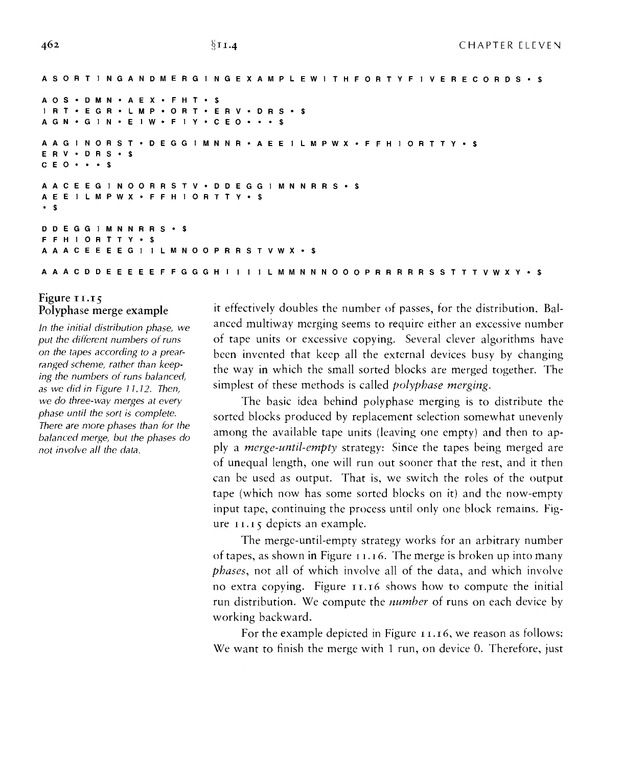
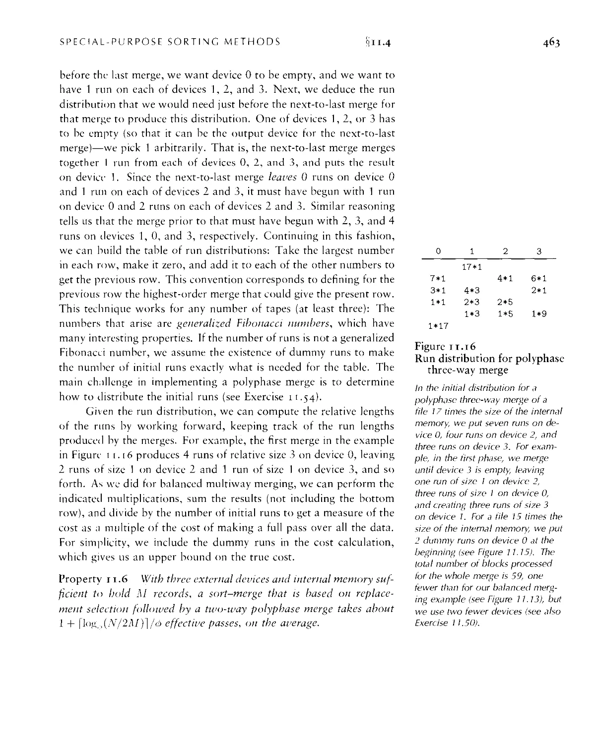
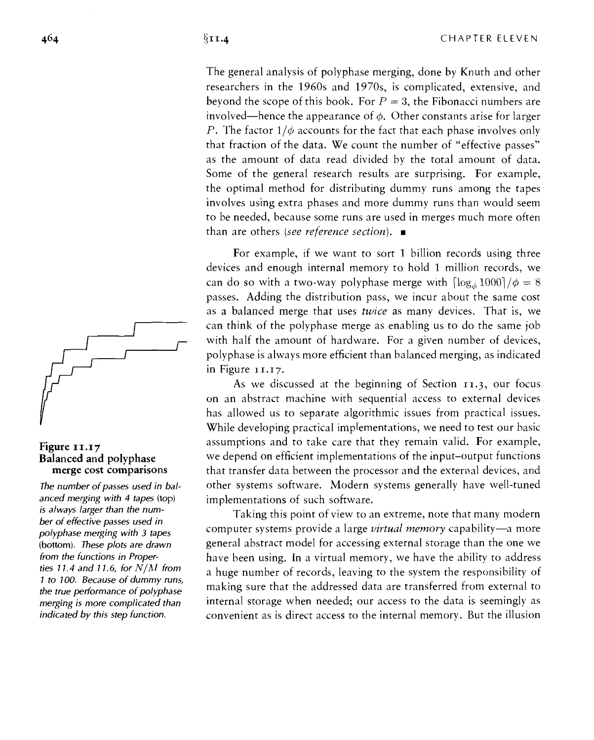
11.4 Sort-Merge Implementations ■ 460
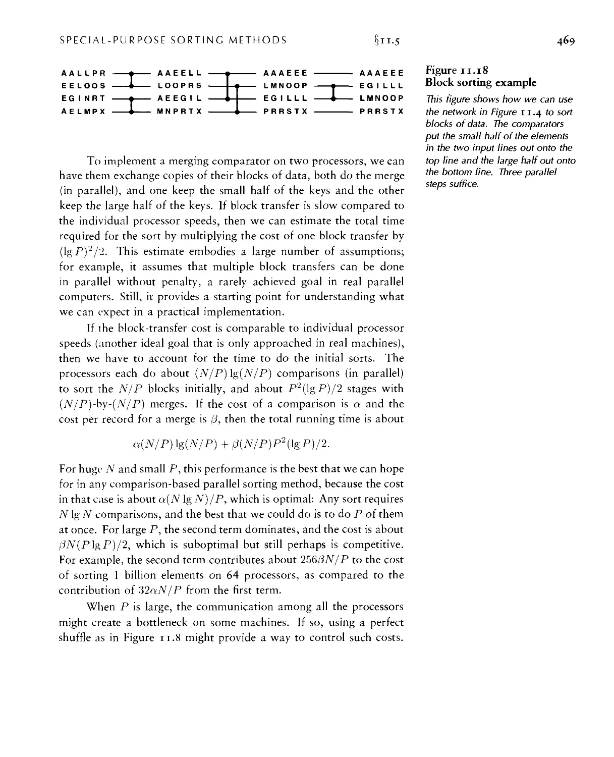
11.5 Parallel Sort/Merge ■ 467
Searching
Chapter 12. Symbol Tables and BSTs 477
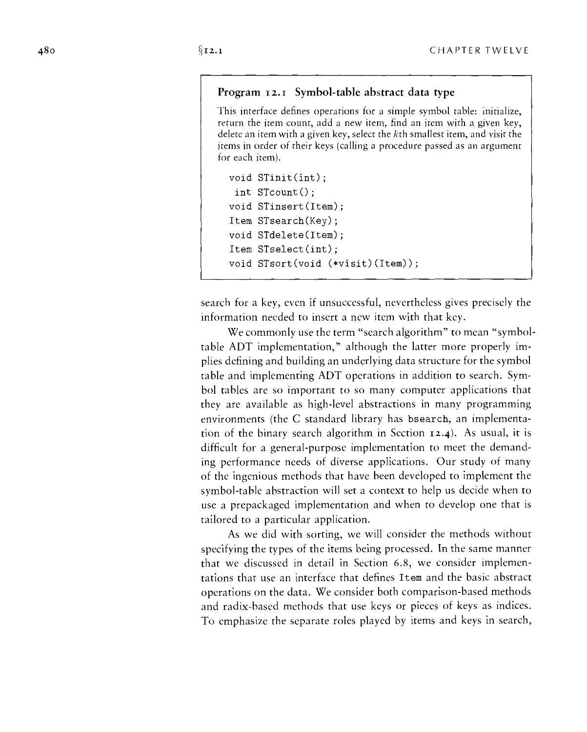
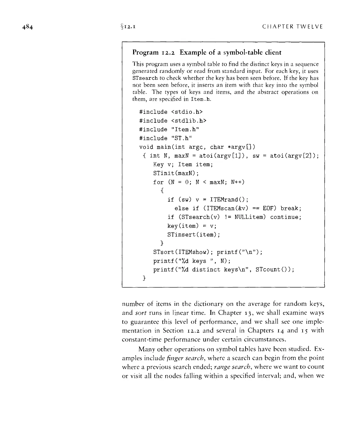
12.1 Symbol-Table Abstract Data Type • 479
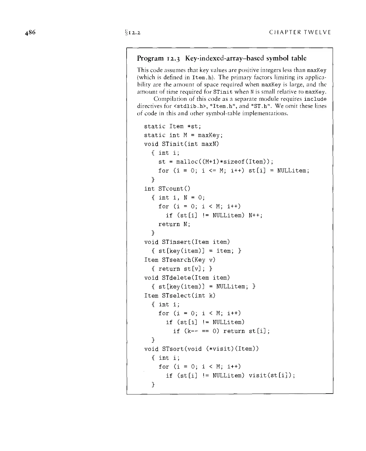
12.2 Key-Indexed Search • 485
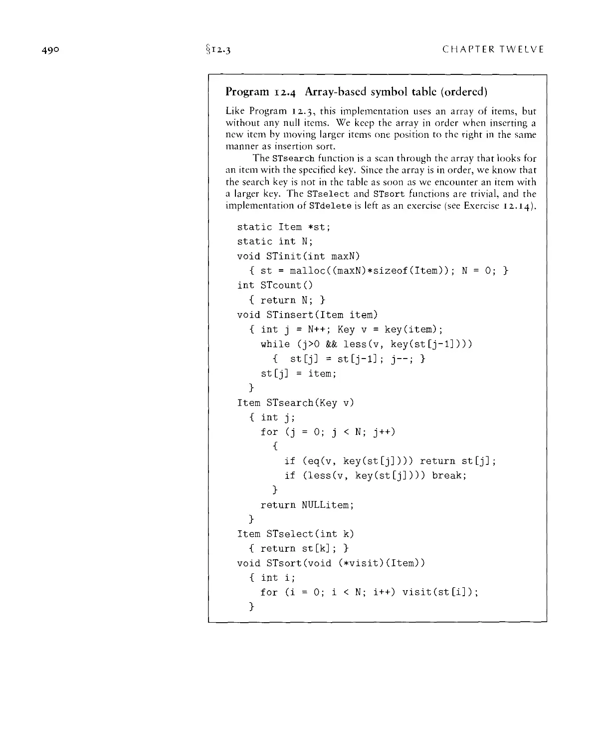
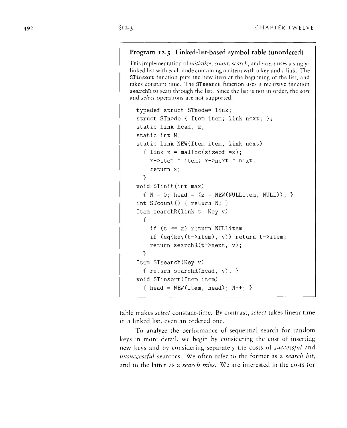
12.3 Sequential Search • 489
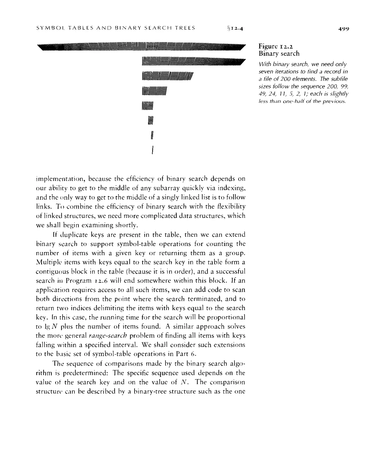
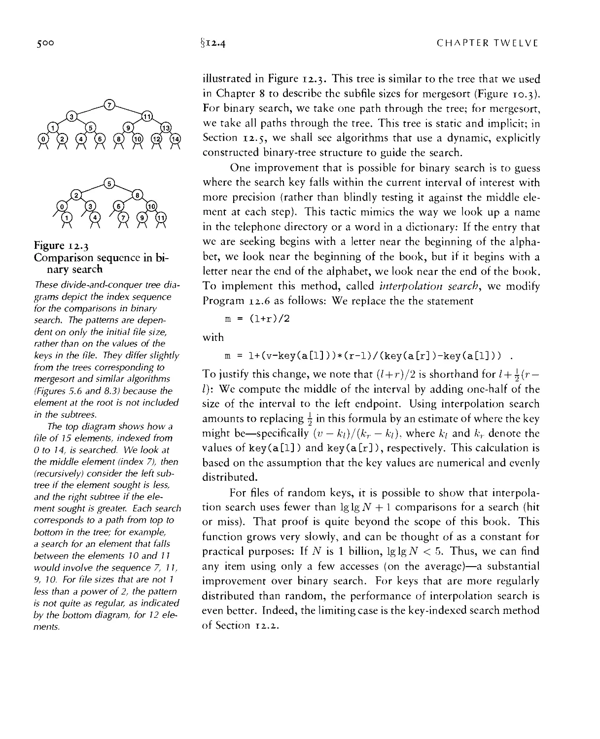
12.4 Binary Search ■ 497
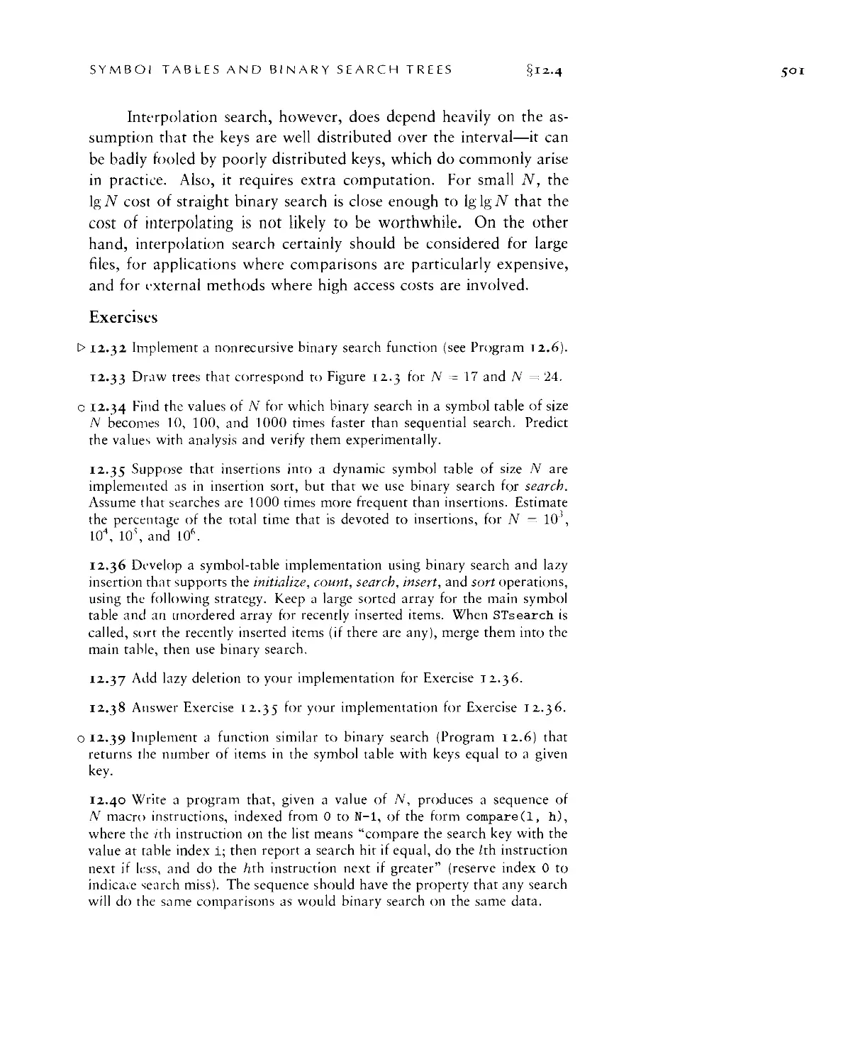
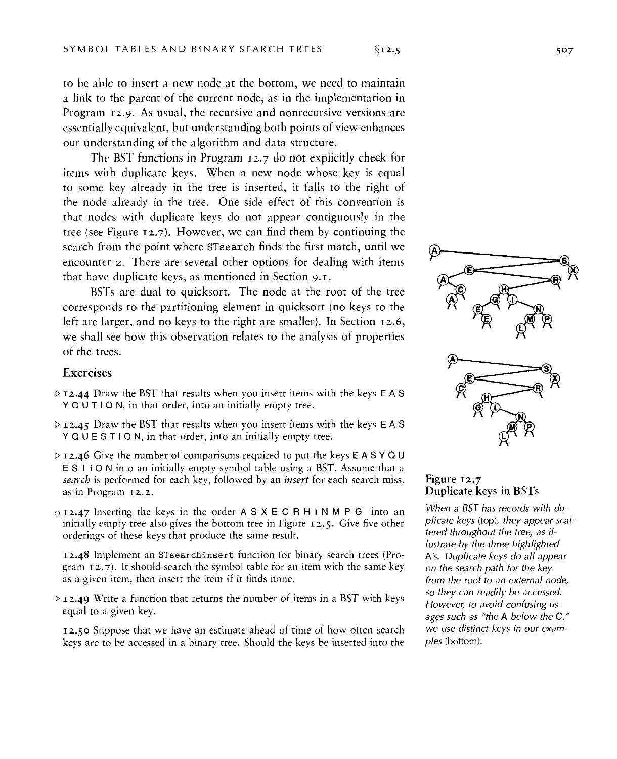
12.5 Binary Search Trees (BSTs) • 502
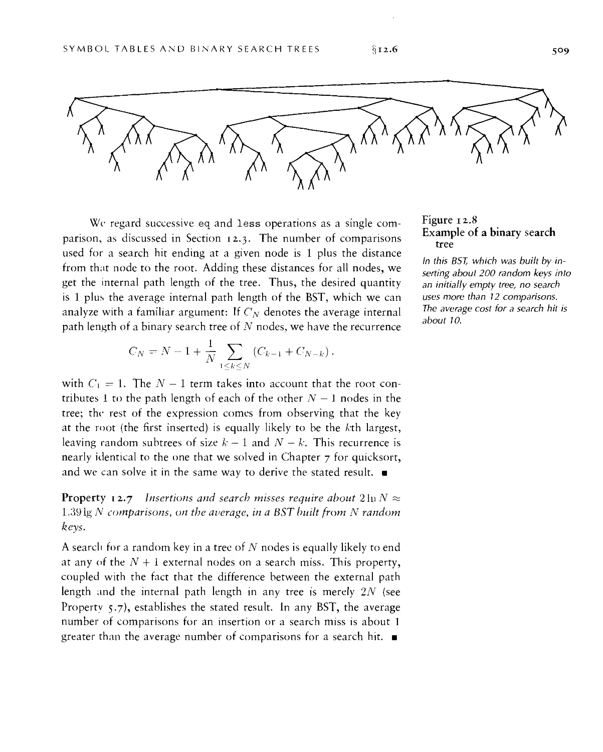
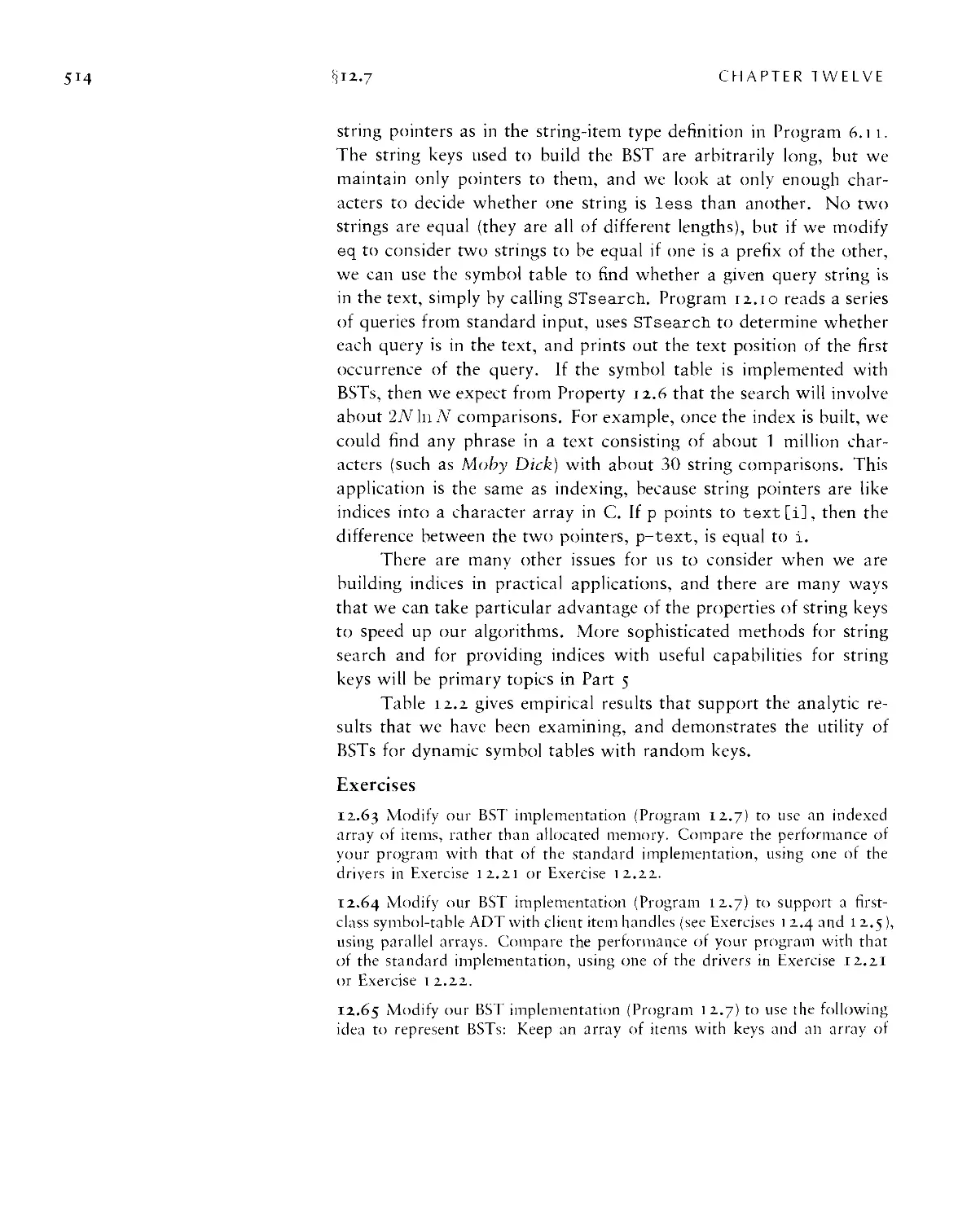
12.6 Performance Characteristics of BSTs ■ 50S
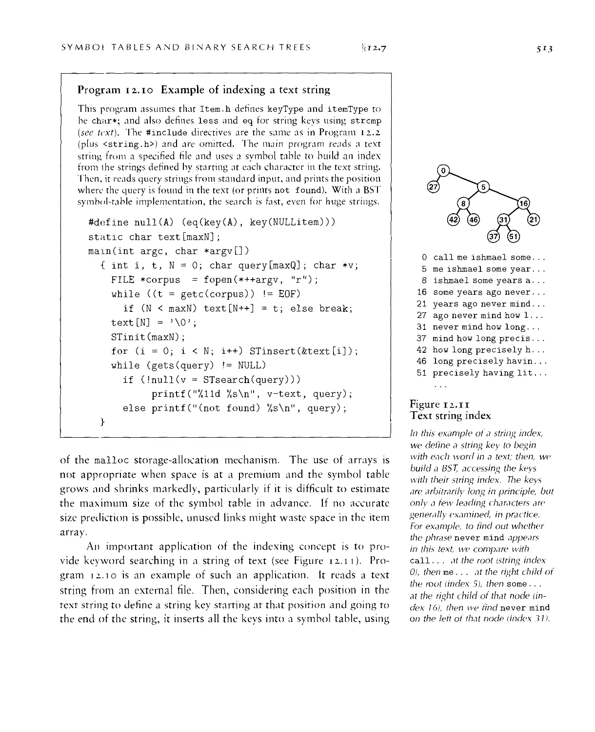
12.7 Index Implementations with Symbol Tables • 5//
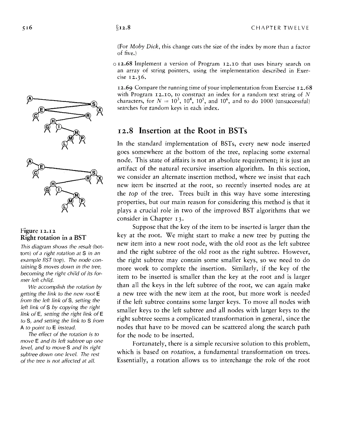
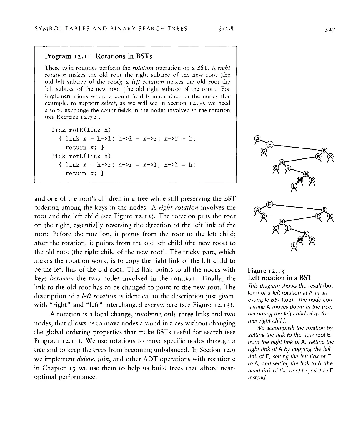
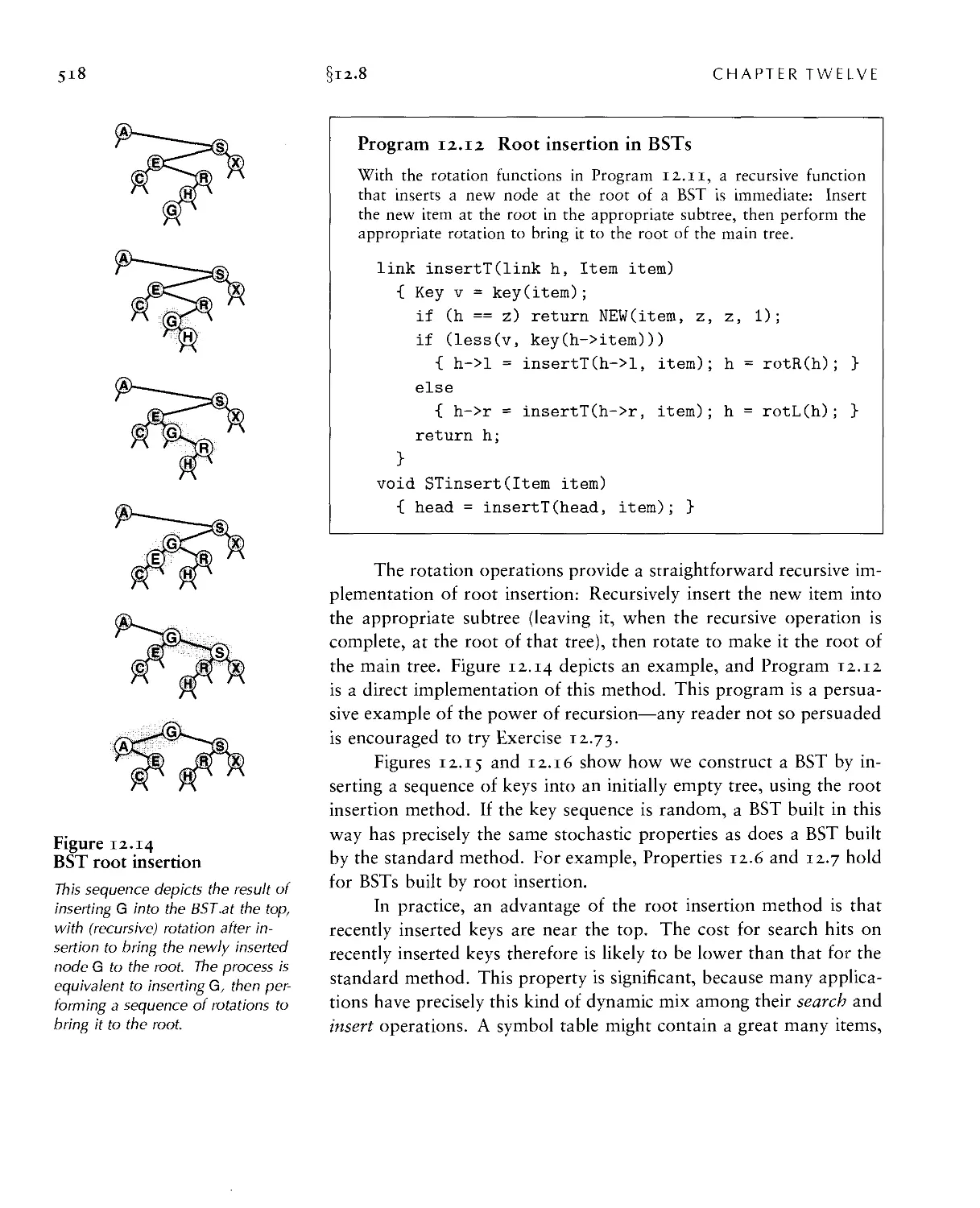
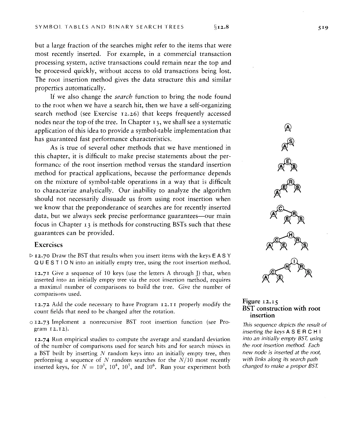
12.8 Insertion at the Root in BSTs -516
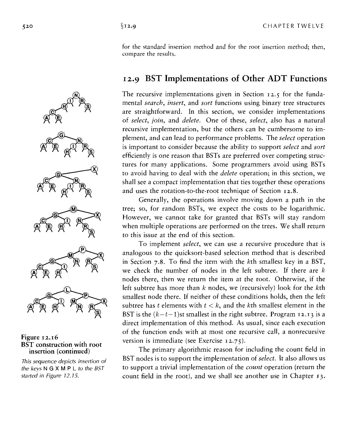
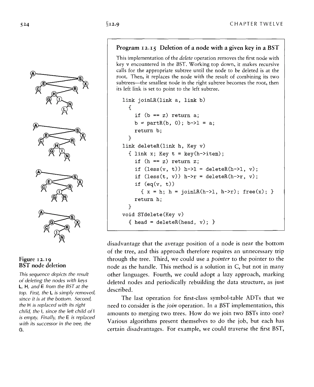
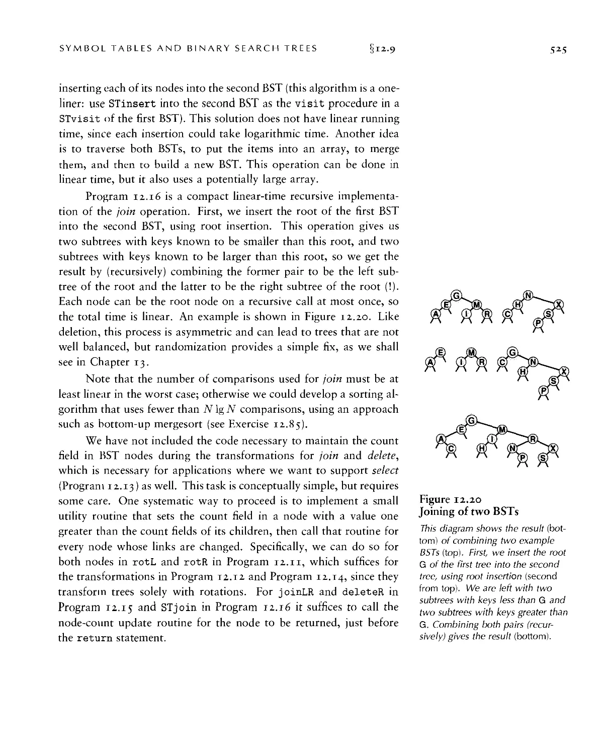
12.9 BST Implementations of Other ADT Functions ■ 520
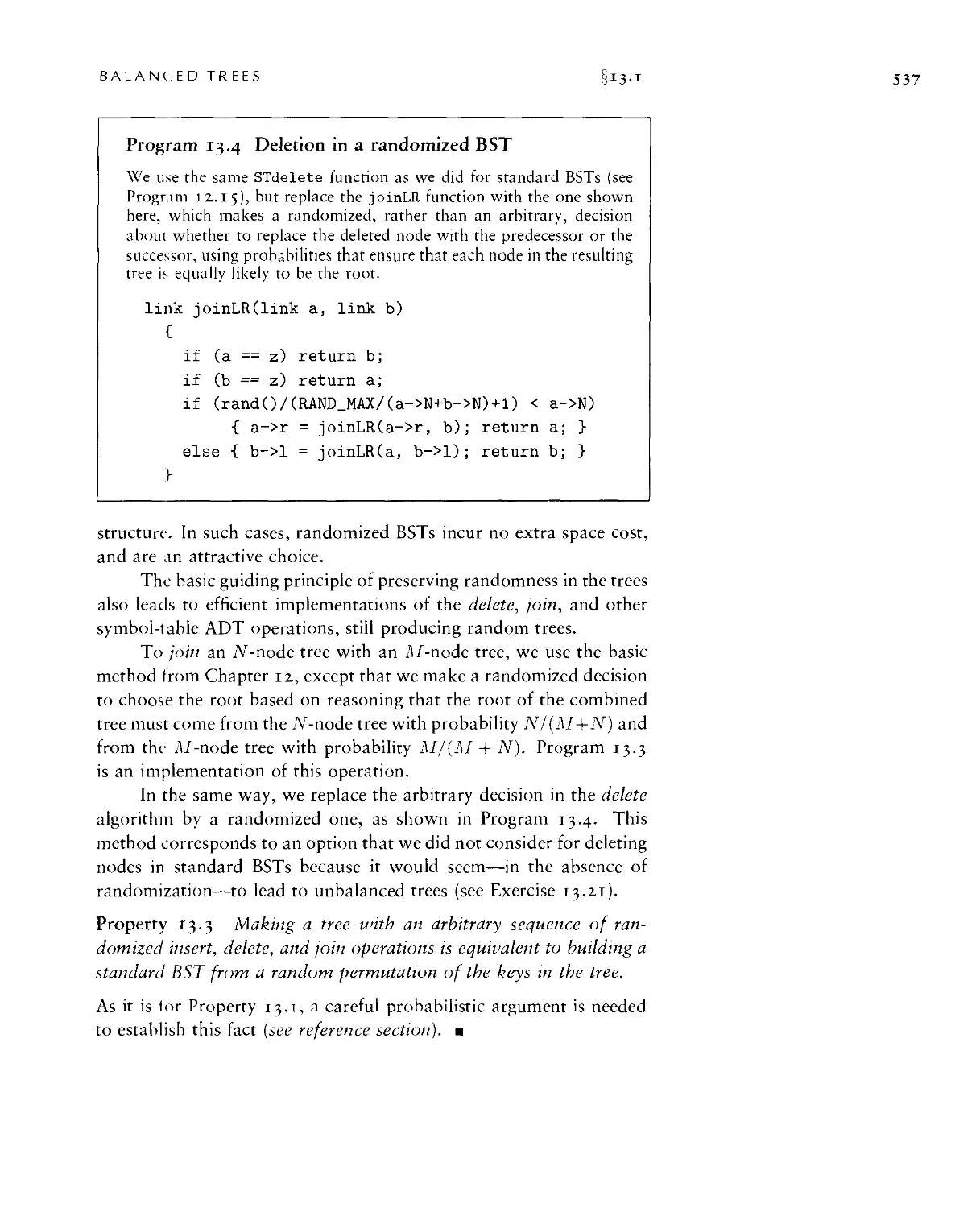
Chapter 13. Balanced Trees
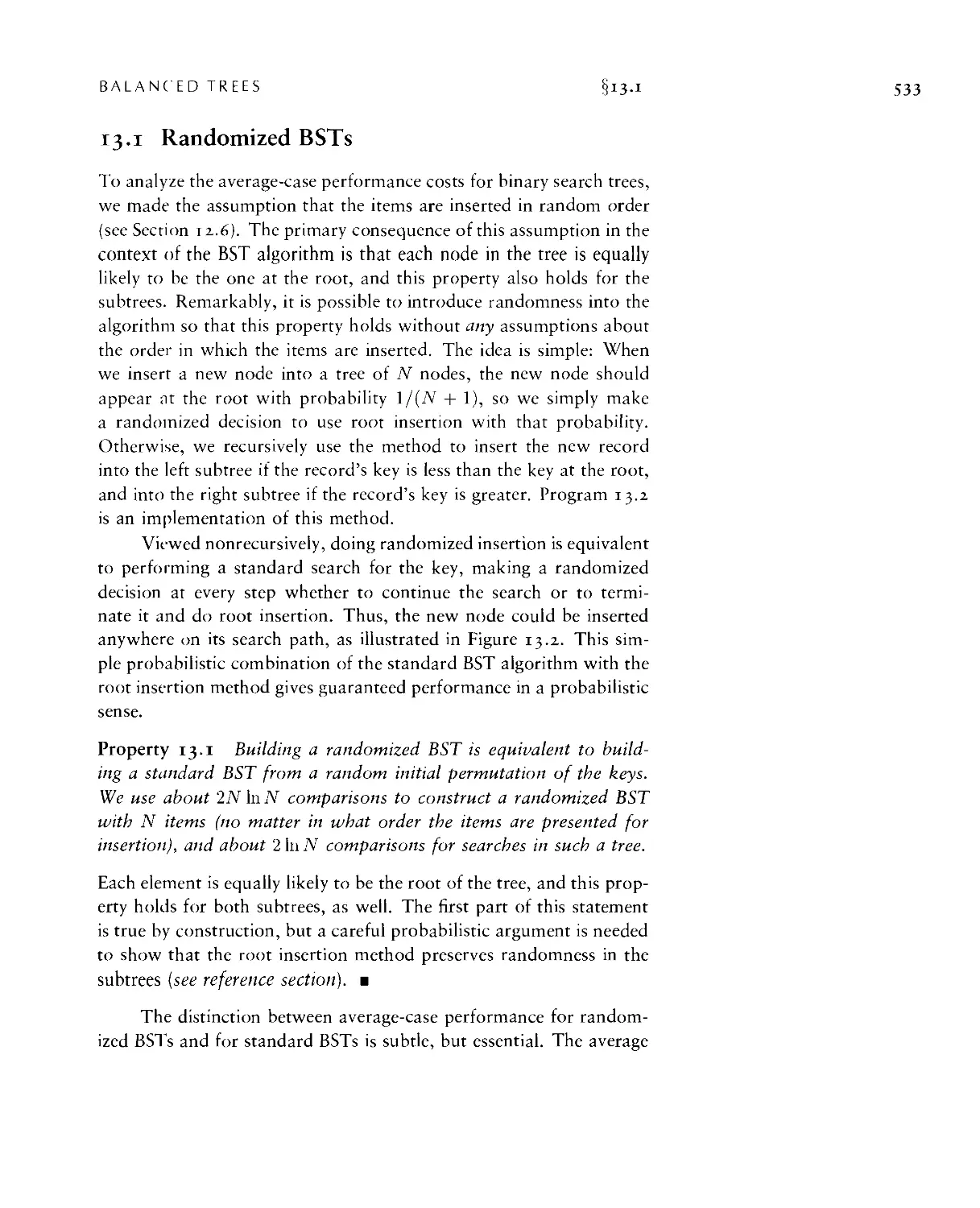
13.1 Randomized BSTs ■ 555
13.2 Splay BSTs • S40
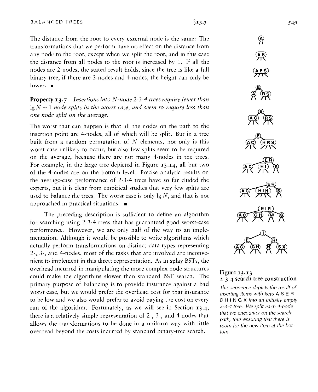
13.3 Top-Down 2-3-4 Trees • 546
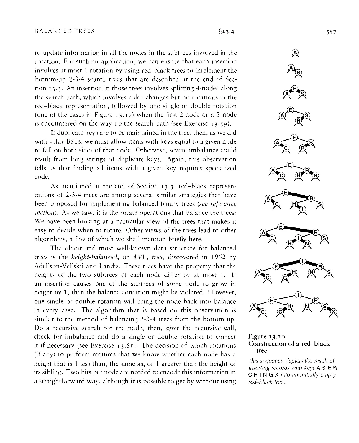
13.4 Red-Black Trees ■ SSI
13.5 Skip Lists • 56/
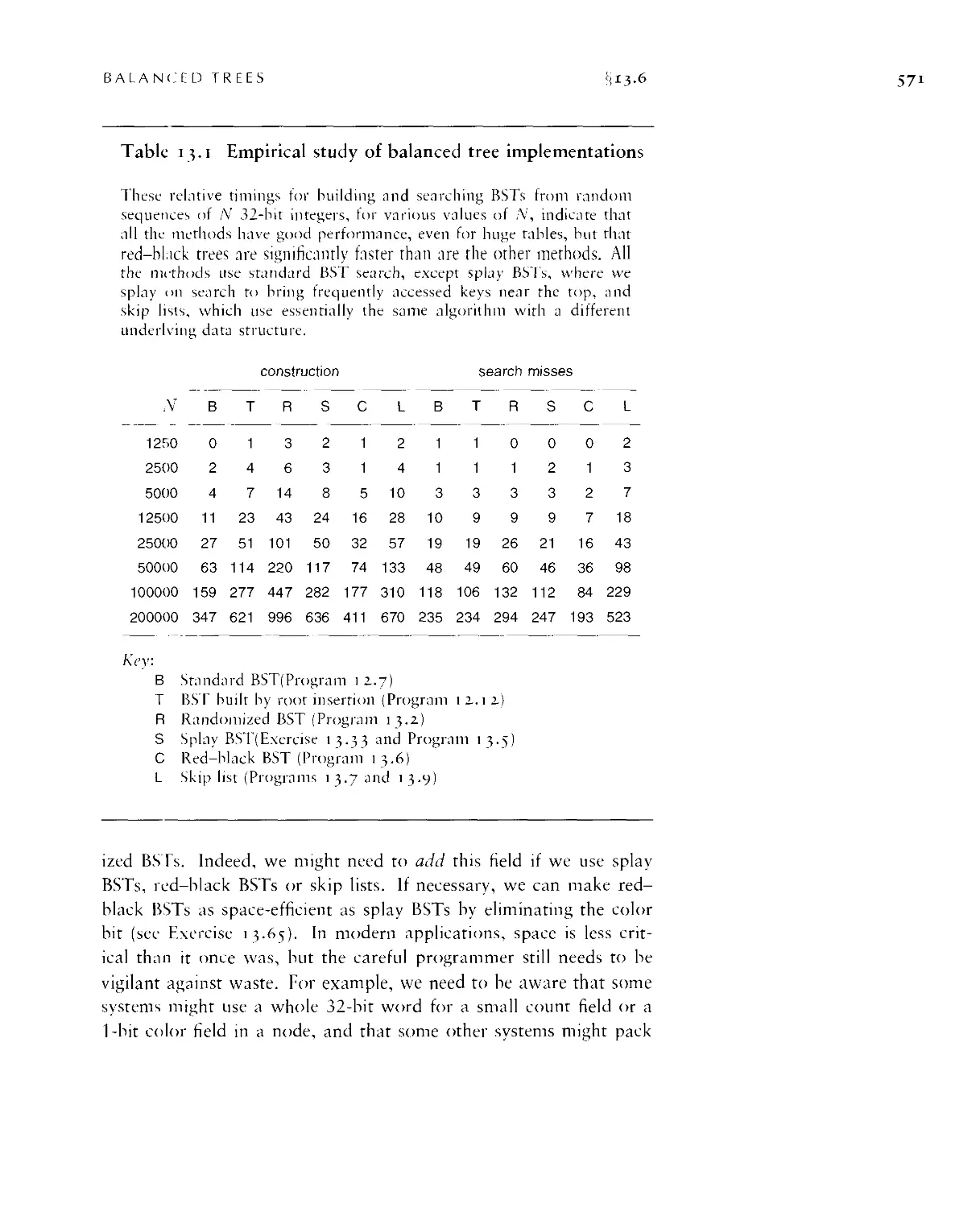
13.6 Performance Characteristics • 569
Chapter 14. Hashing
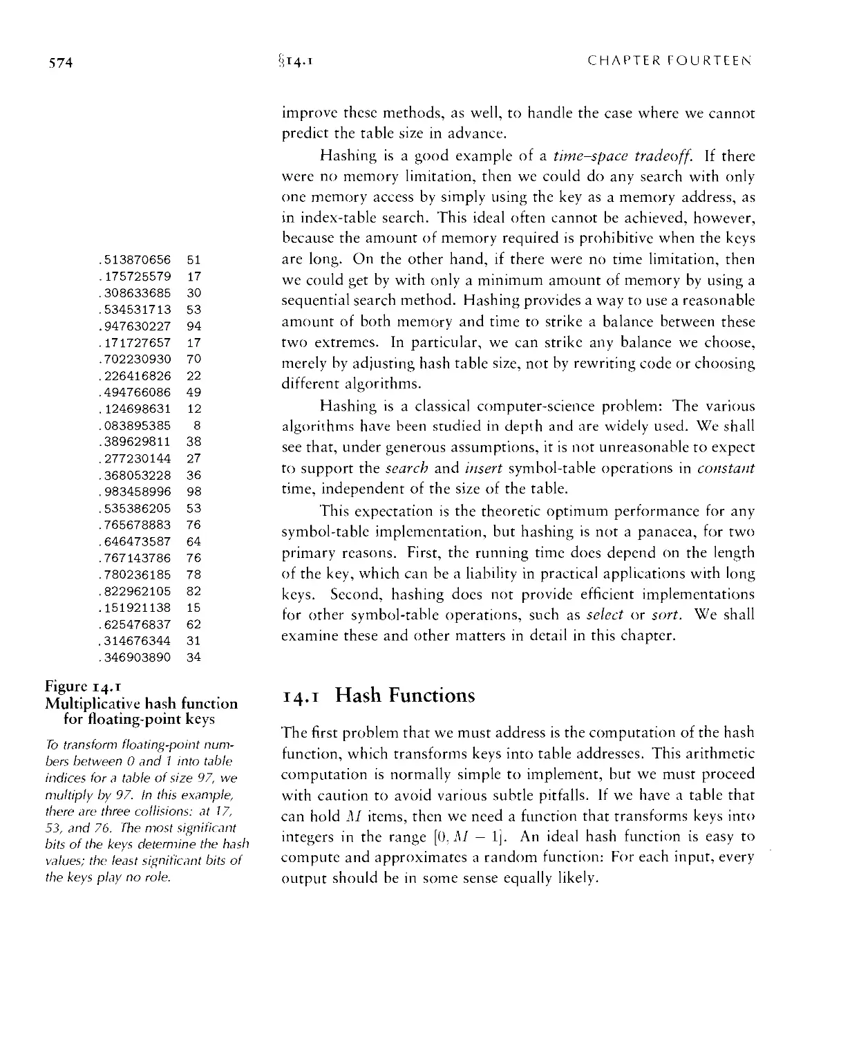
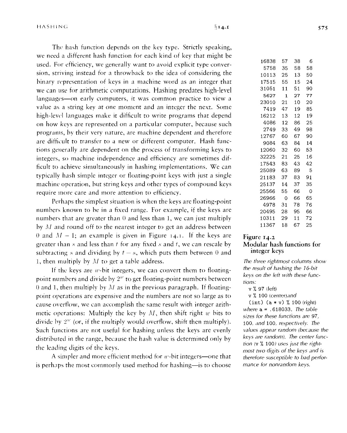
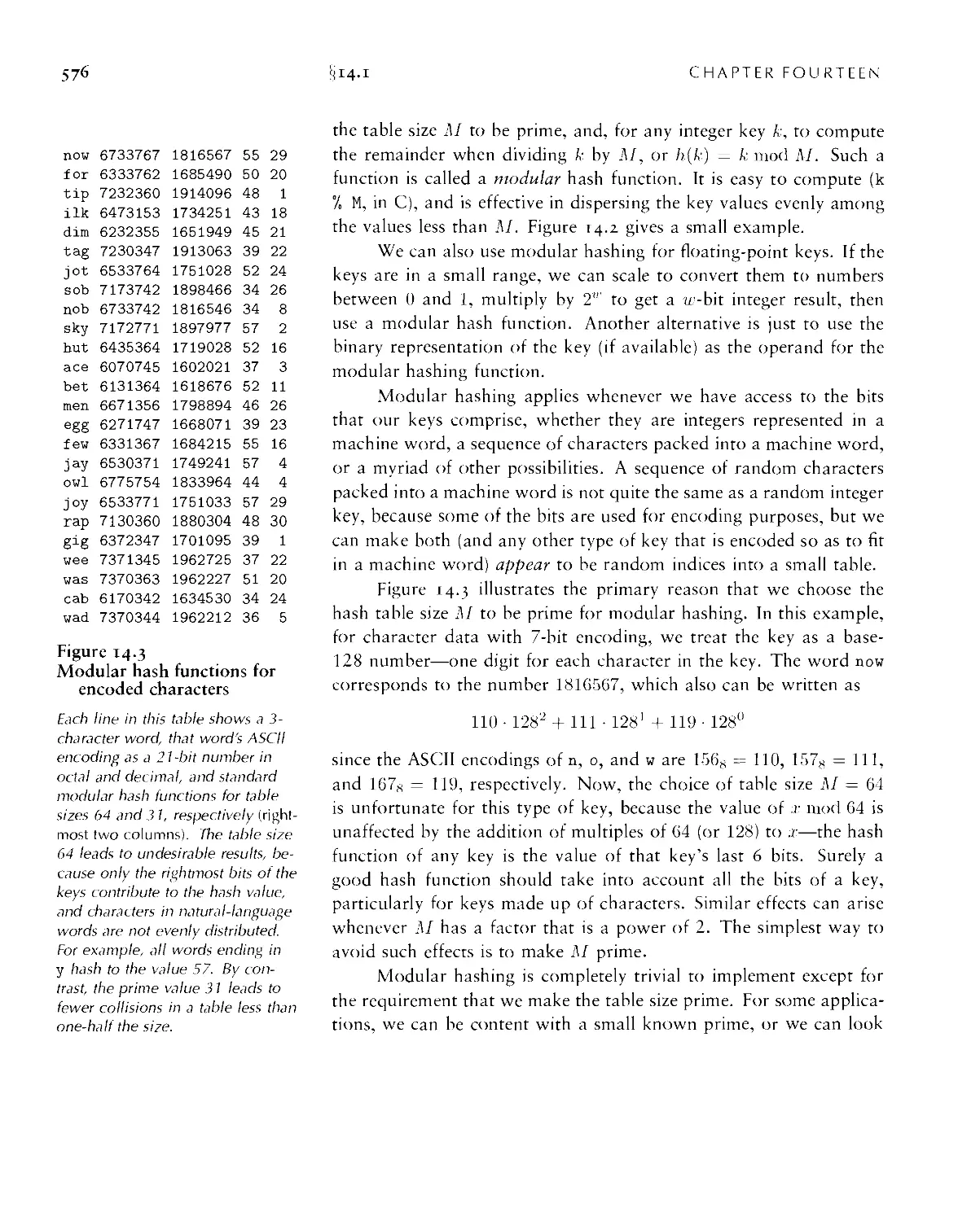
14.1 Hash Functions • S74
14.2 Separate Chaining • 5,SYi
14.3 Linear Probing • SSS
14.4 Double Hashing • 594
14.5 Dynamic Hash Tables ■ 599
14.6 Perspective ■ 605
Chapter 15. Radix Search
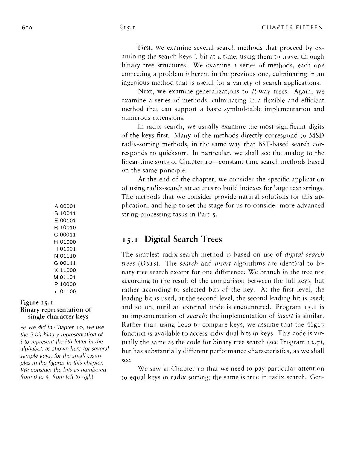
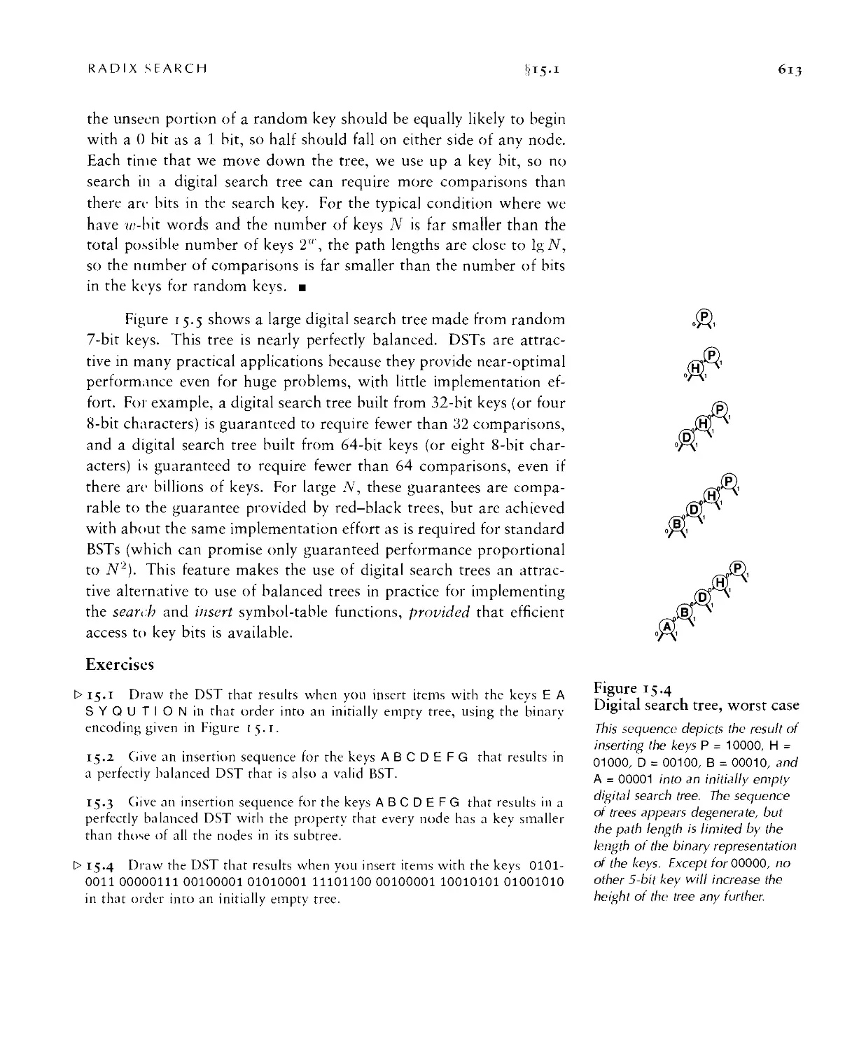
15.1 Digital Search Trees -6/0
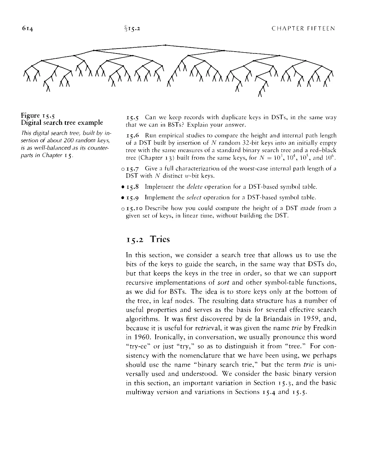
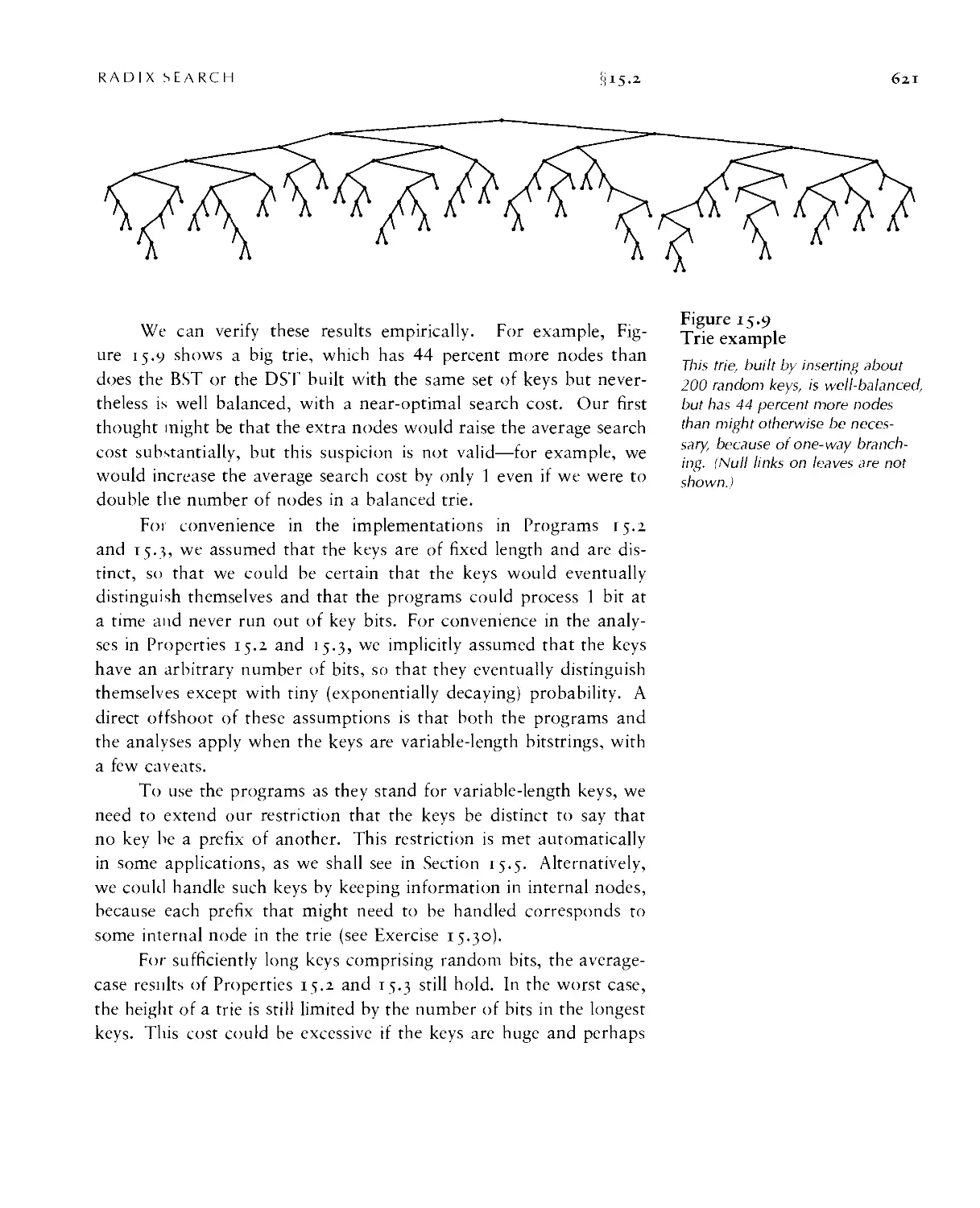
15.2 Tries -6/4
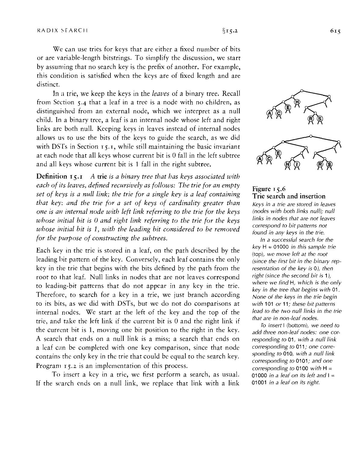
15.5 Patricia Tries ■ 62.>
15.4 Vlultiway Tries and TSTs • 652
15.5 Text String Index Applications ■ 649
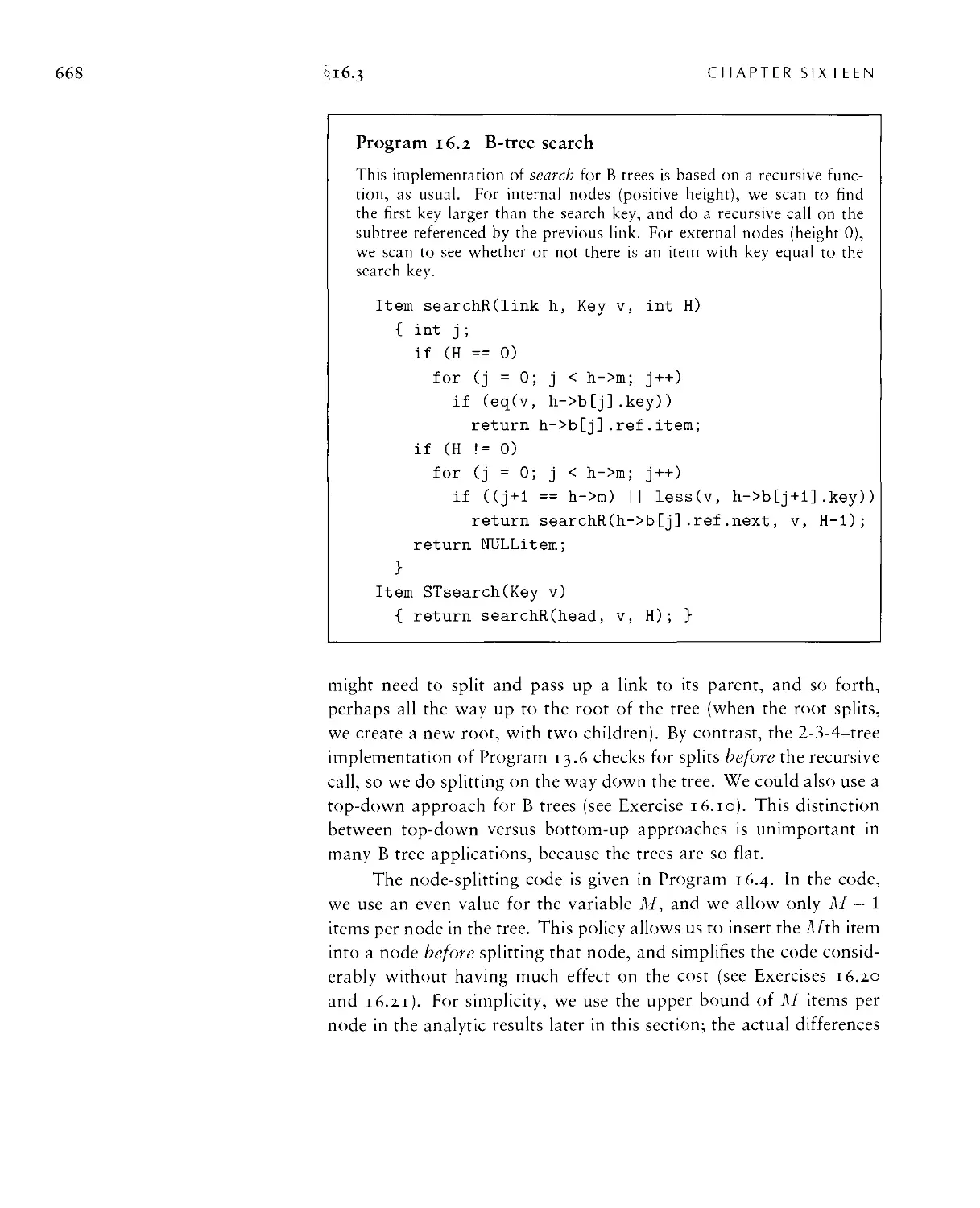
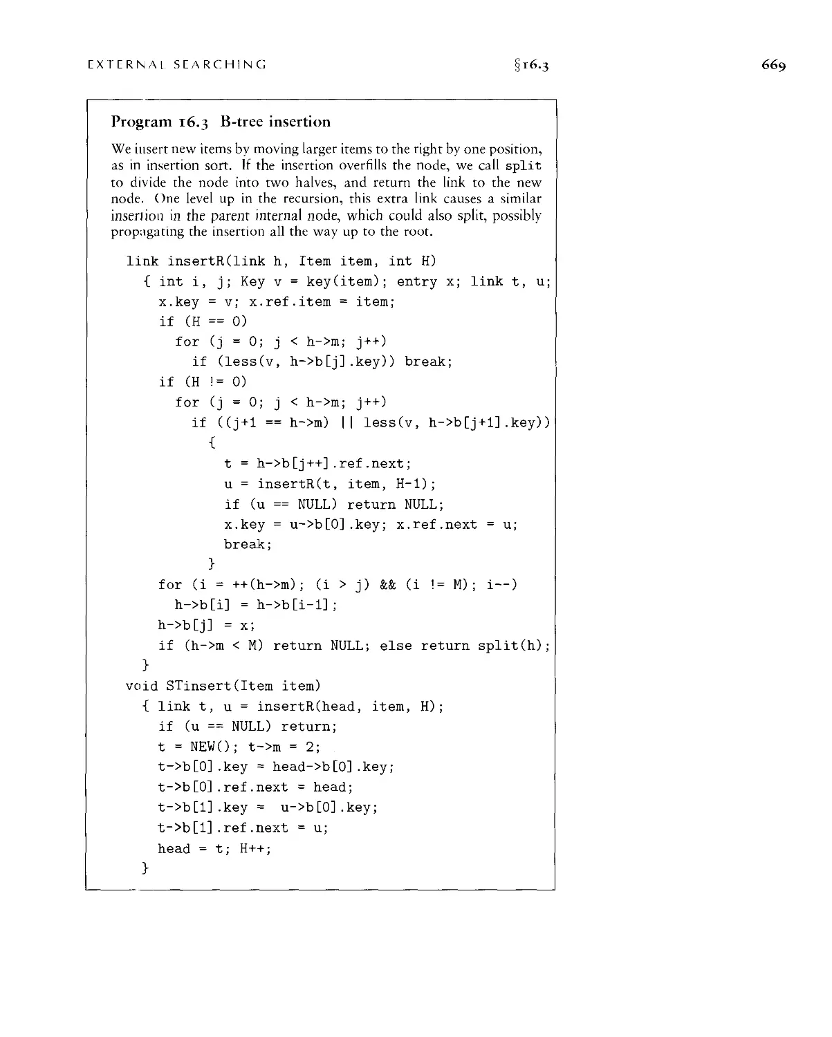
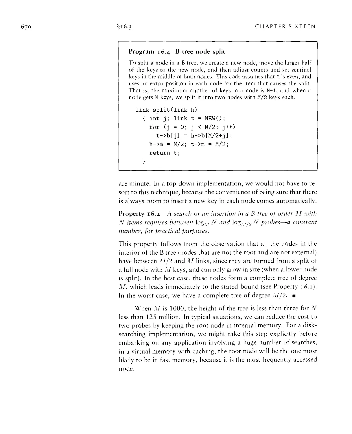
Chapter 16. External Searching
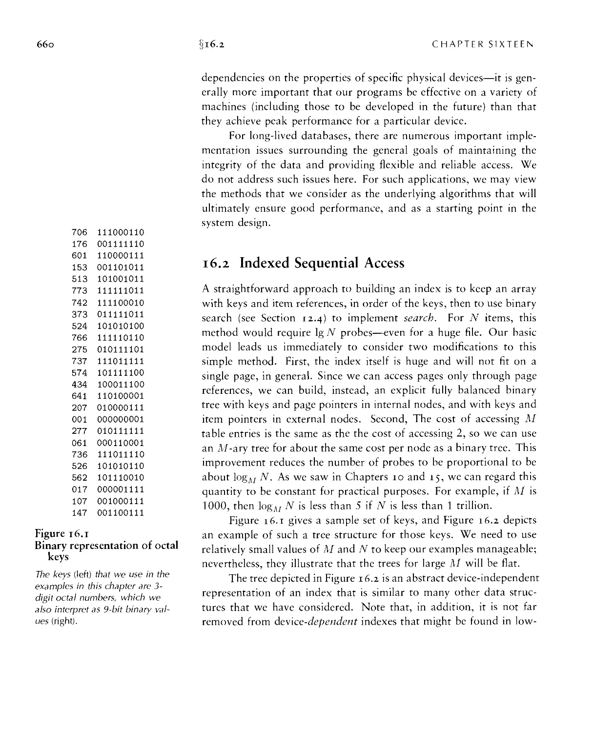
16.1 Rules of the Game • 657
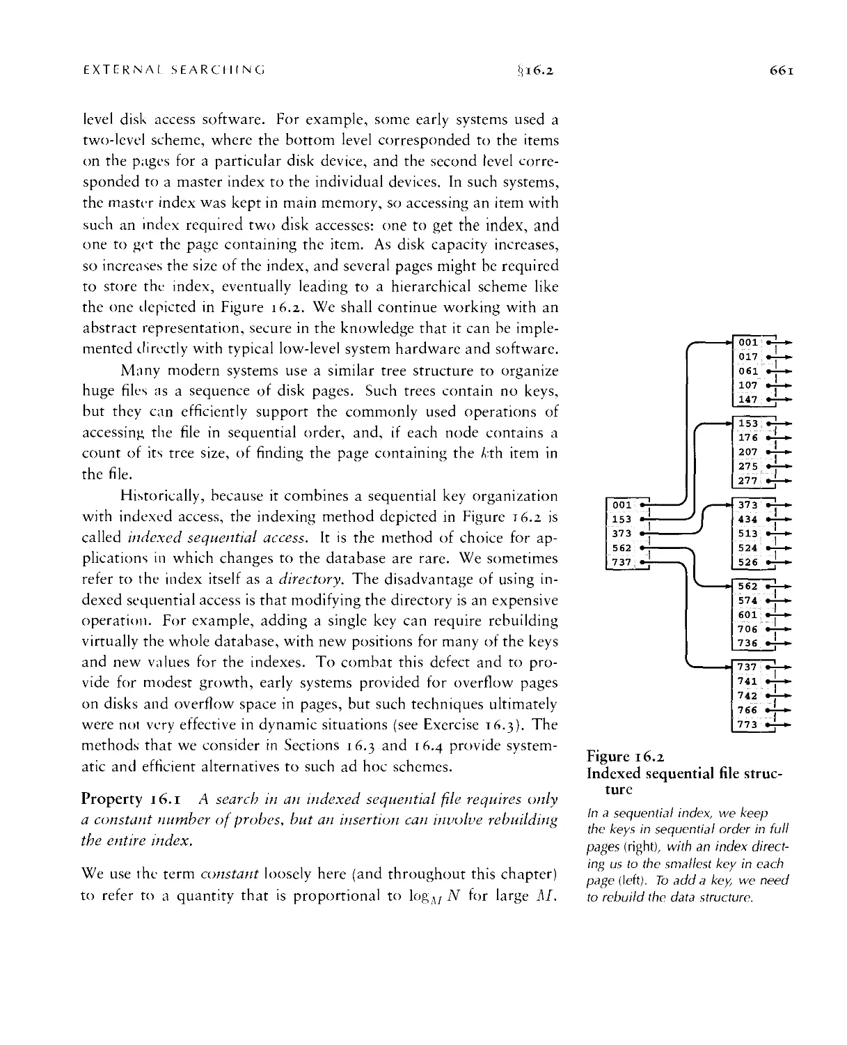
16.2 Indexed Sequential Access ■ 660
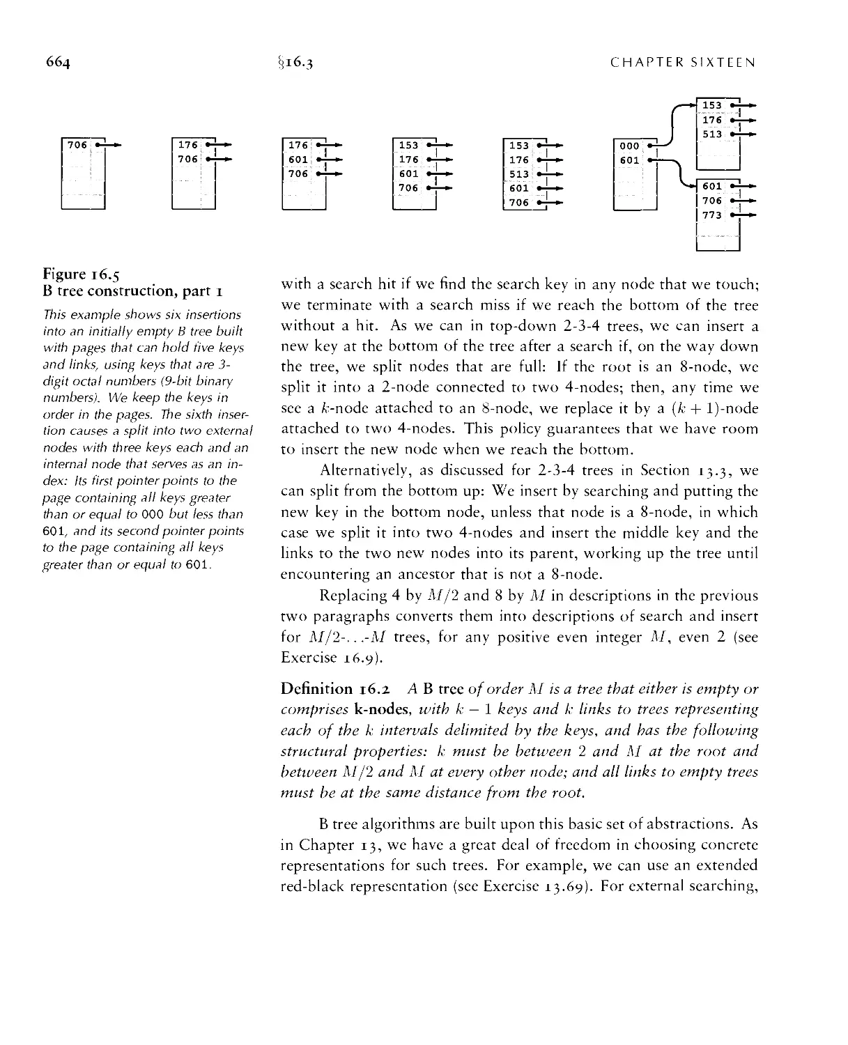
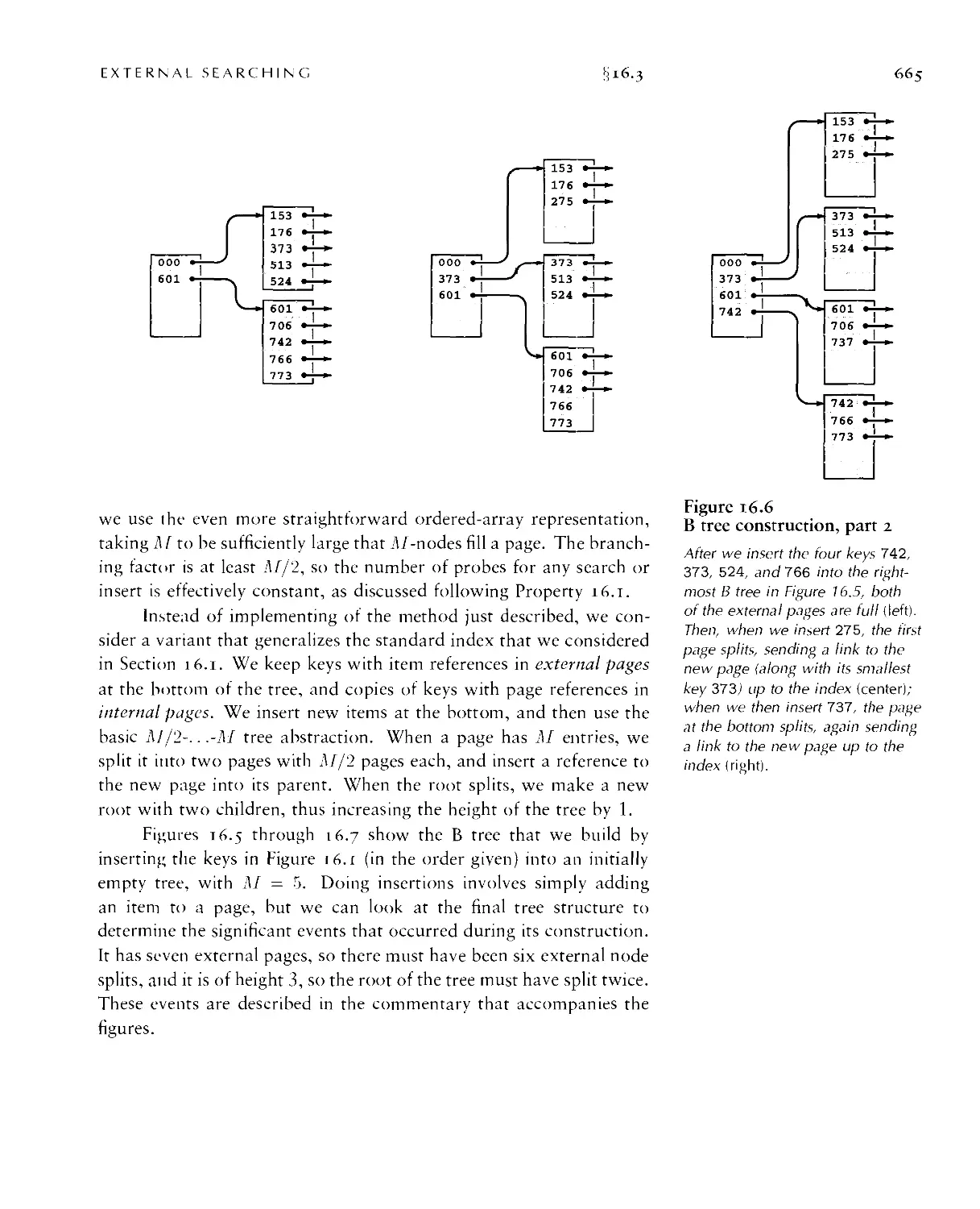
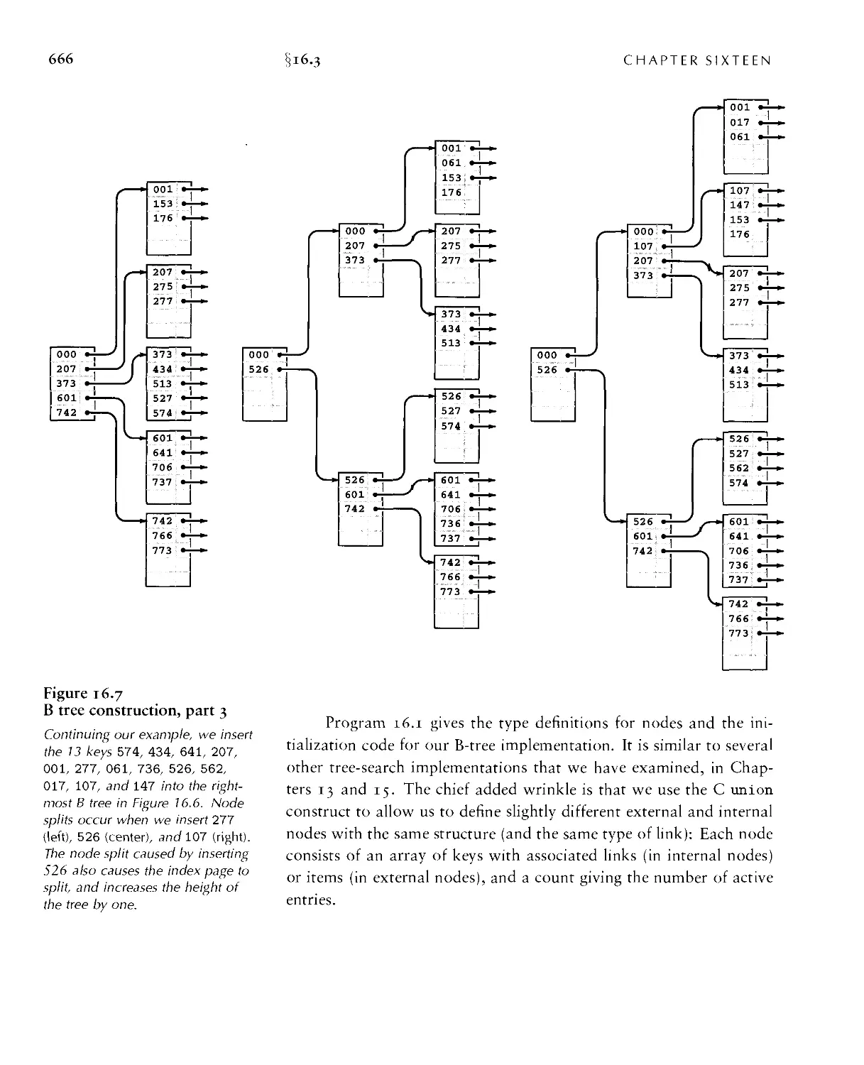
16.? B Trees • 662
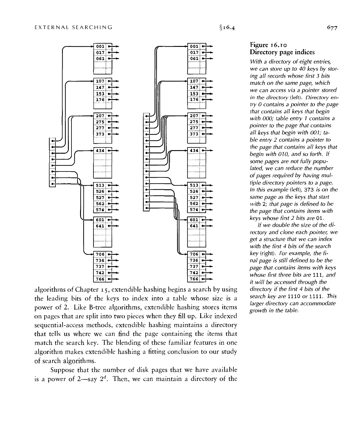
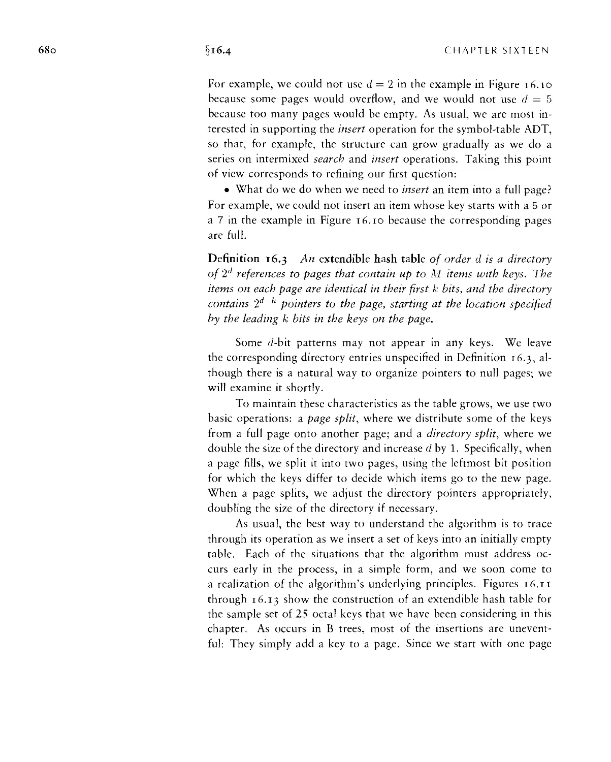
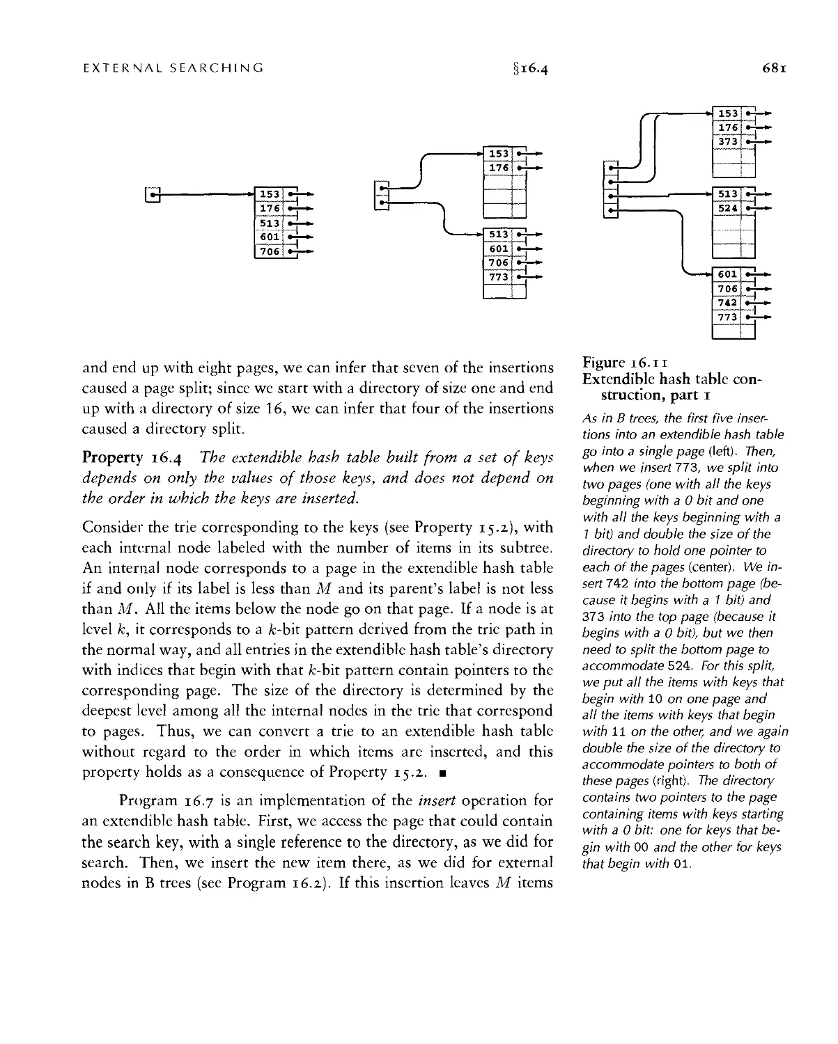
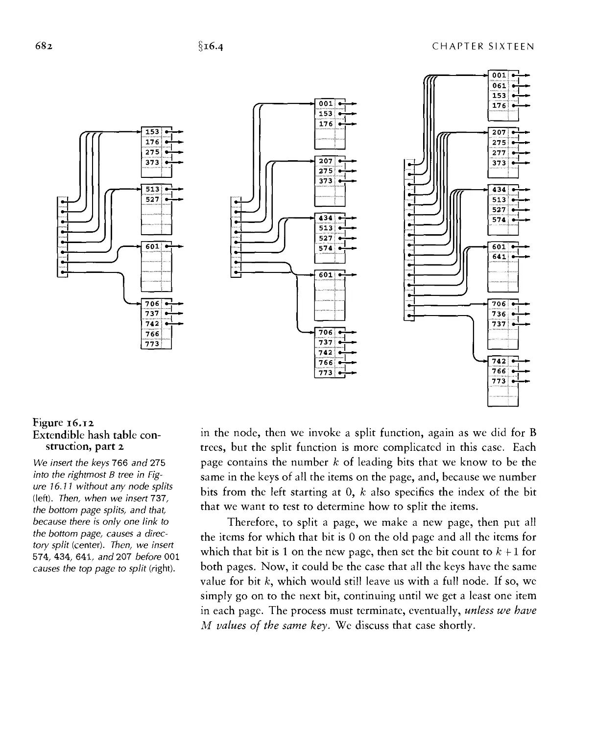
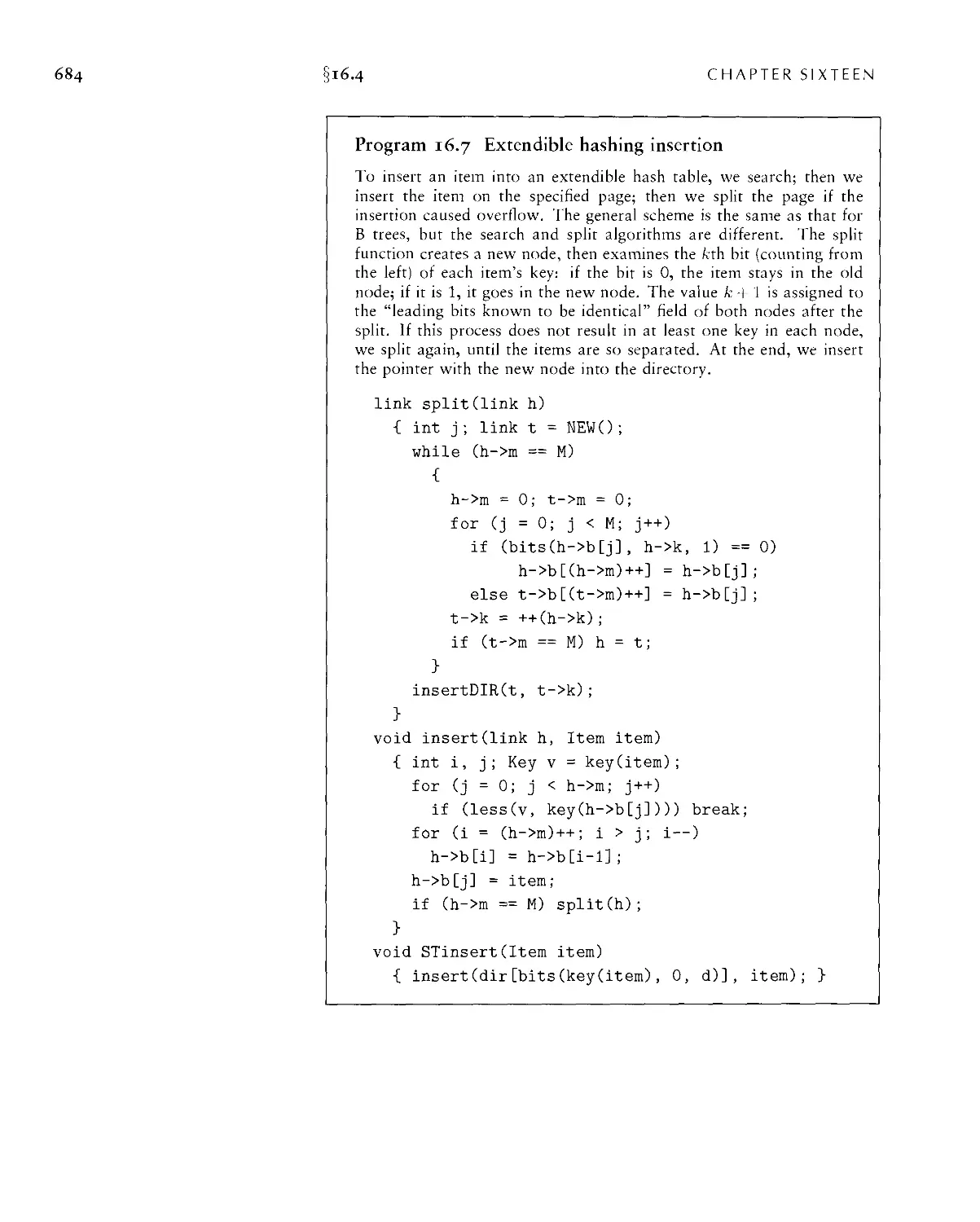
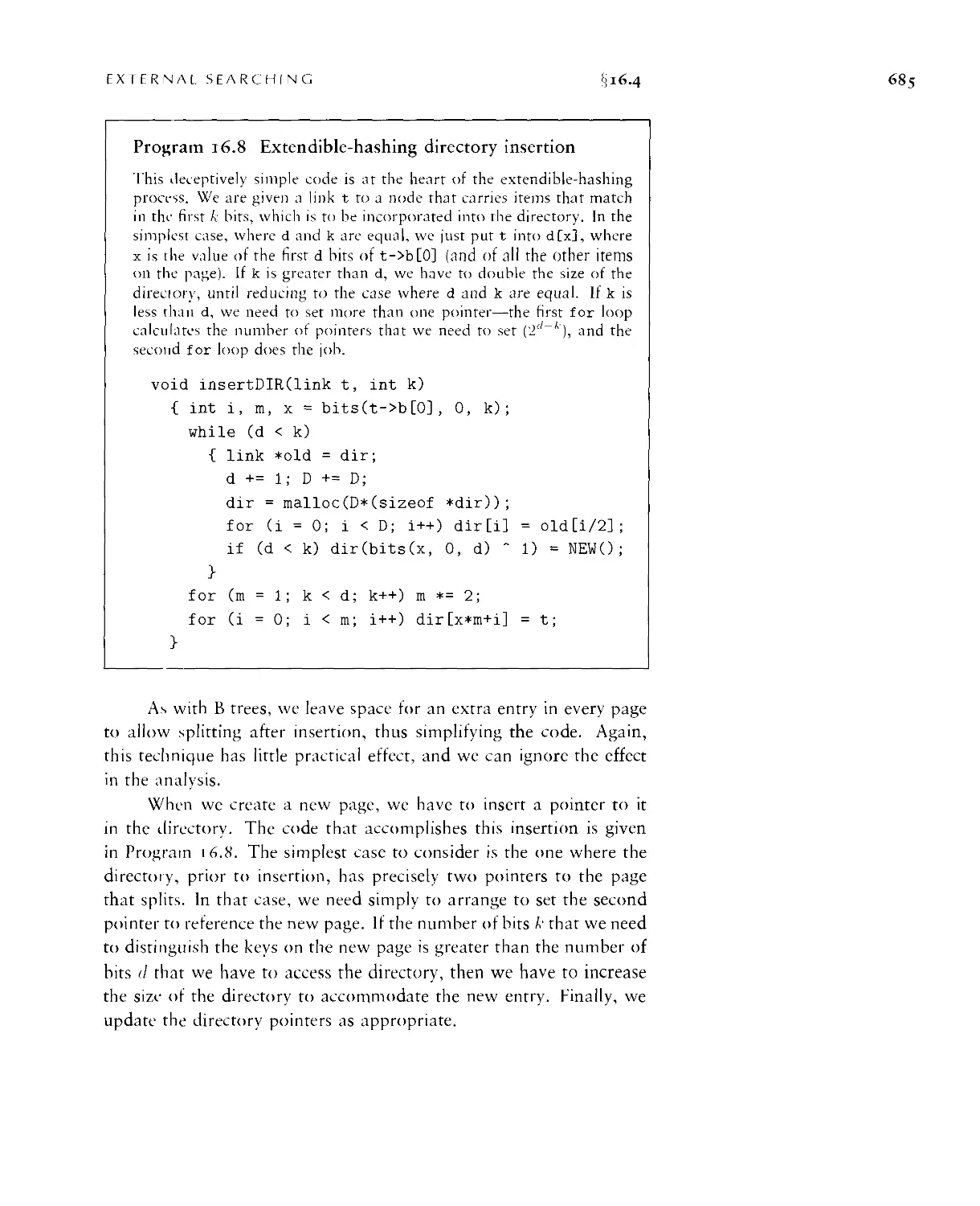
16.4 Extendible Hashing ■ 676
16.5 Perspective ■ 6<S'9
Index
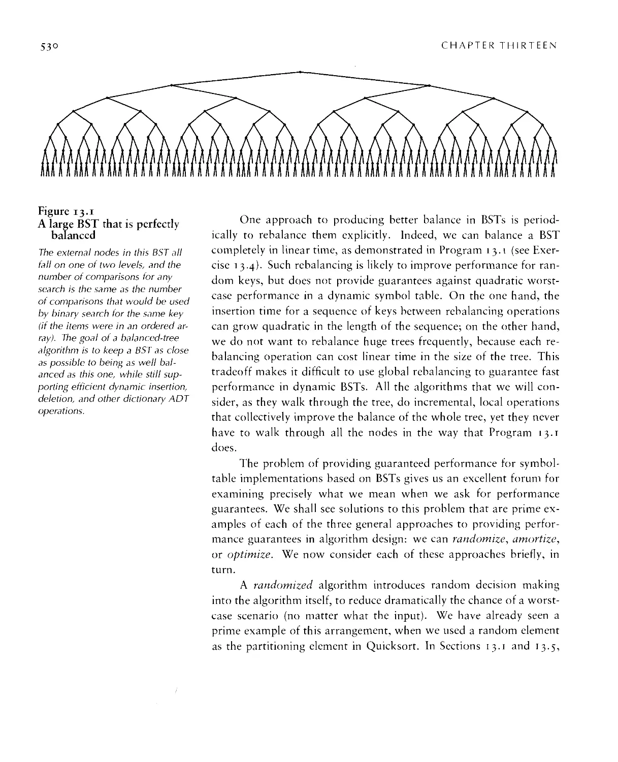
529
609
655
693
xi'ii
PART
ONE
Fundamentals
CHAPTER ONE
Introduction
THE OBJECTIVE OF this book is to study a broad variety of
important and useful algorithms: methods for solving problems
that are suited for computer implementation. We shall deal with
many dilferent areas of application, always concentrating on
fundamental algorithms that are important to know and interesting to
study. We shall spend enough time on each algorithm to understand
its essential characteristics and to respect its subtleties. Our goal is
to learn a large number of the most important algorithms used on
computers today, well enough to be able to use and appreciate them.
The strategy that we use for understanding the programs
presented in this book is to implement and test them, to experiment with
their variants, to discuss their operation on small examples, and to
try them out on larger examples similar to what we might encounter
in practice. We shall use the C programming language to describe the
algorithms, thus providing useful implementations at the same time.
Our programs have a uniform style that is amenable to translation
into other modern programming languages, as well.
We also pay careful attention to performance characteristics of
our algorithms, to help us develop improved versions, compare
different algorithms for the same task, and predict or guarantee
performance for large problems. Understanding how the algorithms
perform might require experimentation or mathematical analysis or both.
We consider detailed information for many of the most important
algorithms, developing analytic results directly when feasible, or calling
on results from the research literature when necessary.
3
§1.1
CHAPTER ONE
To illustrate our general approach to developing algorithmic
solutions, we consider in this chapter a detailed example comprising a
number of algorithms that solve a particular problem. The problem
that we consider is not a toy problem; it is a fundamental
computational task, and the solution that we develop is of use in a variety
of applications. We start with a simple solution, then seek to
understand that solution's performance characteristics, which help us
to see how to improve the algorithm. After a few iterations of this
process, we come to an efficient and useful algorithm for solving the
problem. This prototypical example sets the stage for our use of the
same general methodology throughout the book.
We conclude the chapter with a short discussion of the contents
of the book, including brief descriptions of what the major parts of
the book are and how they relate to one another.
i.i Algorithms
When we write a computer program, we are generally implementing
a method that has been devised previously to solve some problem.
This method is often independent of the particular computer to be
used—it is likely to be equally appropriate for many computers and
many computer languages. It is the method, rather than the computer
program itself, that we must study to learn how the problem is being
attacked. The term algorithm is used in computer science to describe
a problem-solving method suitable for implementation as a computer
program. Algorithms are the stuff of computer science: They are
central objects of study in many, if not most, areas of the field.
Most algorithms of interest involve methods of organizing the
data involved in the computation. Objects created in this way are
called data structures, and they also are central objects of study in
computer science. Thus, algorithms and data structures go hand in
hand. In this book we take the view that data structures exist as
the byproducts or end products of algorithms, and thus that we must
study them in order to understand the algorithms. Simple algorithms
can give rise to complicated data structures and, conversely,
complicated algorithms can use simple data structures. We shall study the
properties of many data structures in this book; indeed, the book
might well have been called Algorithms and Data Structures in C.
INTRODUCTION
§1.1
When we use a computer to help us solve a problem, we typically
are faced with a number of possible different approaches. For small
problems, it hardly matters which approach we use, as long as we
have one that solves the problem correctly. For huge problems (or
applications where we need to solve huge numbers of small problems),
however, we quickly become motivated to devise methods that use
time or space as efficiently as possible.
The primary reason for us to learn about algorithm design is
that this discipline gives us the potential to reap huge savings, even
to the point of making it possible to do tasks that would otherwise
be impossible. In an application where we are processing millions of
objects, it is not unusual to be able to make a program millions of
times faster by using a well-designed algorithm. We shall see such an
example in Section 1.2 and on numerous other occasions throughout
the book. By contrast, investing additional money or time to buy and
install a new computer holds the potential for speeding up a program
by perhaps a factor of only 10 or 100. Careful algorithm design is
an extremely effective part of the process of solving a huge problem,
whatever the applications area.
When a huge or complex computer program is to be developed,
a great deal of effort must go into understanding and denning the
problem 10 be solved, managing its complexity, and decomposing it
into smaller subtasks that can be implemented easily. Often, many
of the algorithms required after the decomposition are trivial to
implement. In most cases, however, there are a few algorithms whose
choice is critical because most of the system resources will be spent
running those algorithms. Those are the types of algorithms on which
we concentrate in this book. We shall study a variety of
fundamental algorithms that are useful for solving huge problems in a broad
variety ol applications areas.
The sharing of programs in computer systems is becoming more
widespread, so, although we might expect to be using a large fraction
of the algorithms in this book, we also might expect to have to
implement only a smaller fraction of them. However, implementing simple
versions of basic algorithms helps us to understand them better and
thus to use advanced versions more effectively. More important, the
opportunity to reimplement basic algorithms arises frequently. The
primary reason to do so is that we are faced, all too often, with com-
§1.2
CHAPTER ONE
pletely new computing environments (hardware and software) with
new features that old implementations may not use to best advantage.
In other words, we often implement basic algorithms tailored to our
problem, rather than depending on a system routine, to make our
solutions more portable and longer lasting. Another common reason
to reimplement basic algorithms is that mechanisms for sharing
software on many computer systems are not always sufficiently powerful
to allow us to tailor standard programs to perform effectively on
specific tasks (or it may not be convenient to do so), so it is sometimes
easier to do a new implementation.
Computer programs are often overoptimized. It may not be
worthwhile to take pains to ensure that an implementation of a
particular algorithm is the most efficient possible unless the algorithm is
to be used for an enormous task or is to be used many times.
Otherwise, a careful, relatively simple implementation will suffice: We can
have some confidence that it will work, and it is likely to run perhaps
five or 10 times slower at worst than the best possible version, which
means that it may run for an extra few seconds. By contrast, the
proper choice of algorithm in the first place can make a difference of
a factor of 100 or 1000 or more, which might translate to minutes,
hours, or even more in running time. In this book, we concentrate
on the simplest reasonable implementations of the best algorithms.
The choice of the best algorithm for a particular task can be
a complicated process, perhaps involving sophisticated mathematical
analysis. The branch of computer science that comprises the study
of such questions is called analysis of algorithms. Many of the
algorithms that we study have been shown through analysis to have
excellent performance; others are simply known to work well through
experience. Our primary goal is to learn reasonable algorithms for
important tasks, yet we shall also pay careful attention to comparative
performance of the methods. We should not use an algorithm
without having an idea of what resources it might consume, and we strive
to be aware of how our algorithms might be expected to perform.
i.2 A Sample Problem: Connectivity
Suppose that we are given a sequence of pairs of integers, where each
integer represents an object of some type and we are to interpret the
INTRODUCTION
§1.2
7
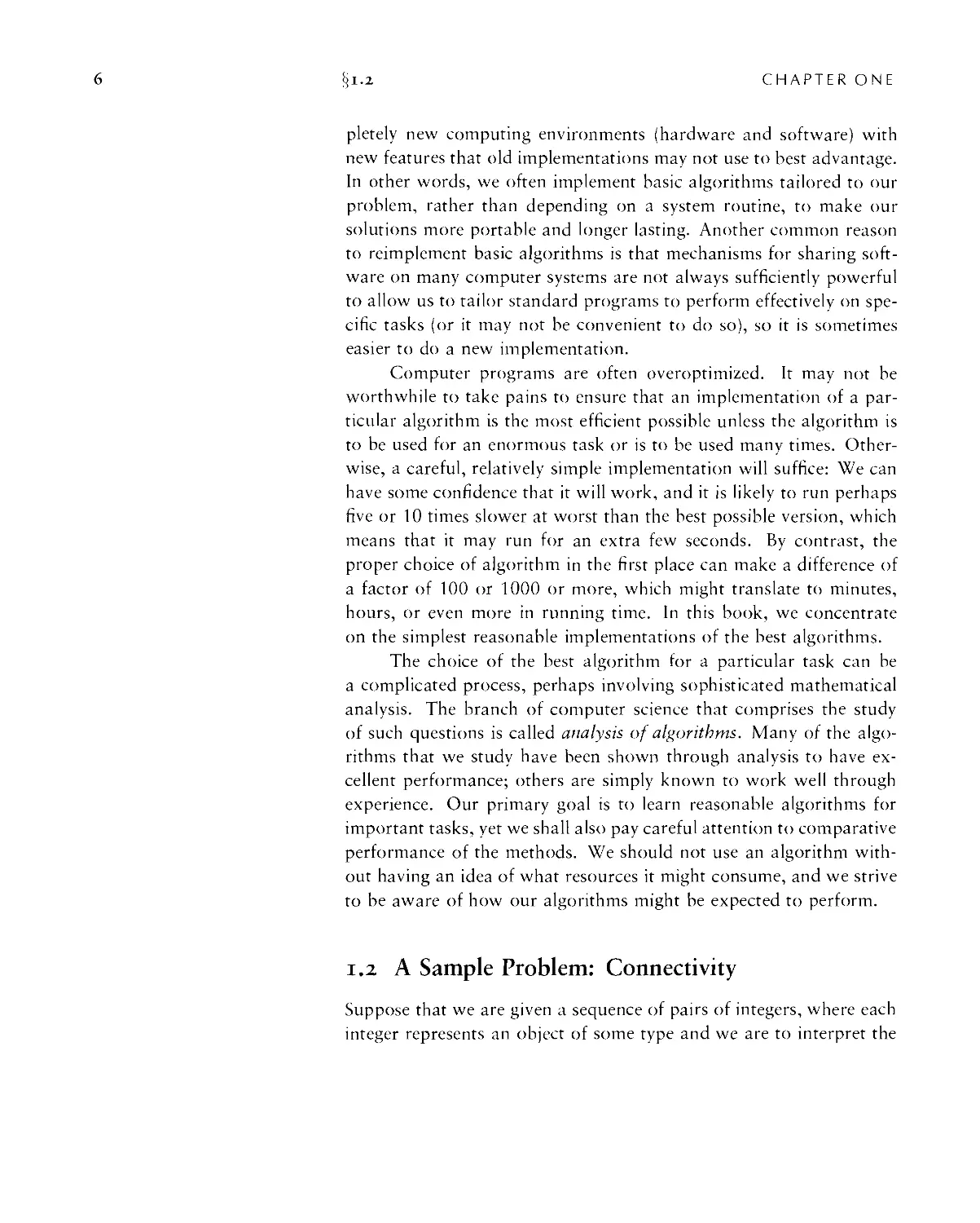
pair p-q as meaning "p is connected to q." We assume the relation
"is connected to" to be associative: If p is connected to q, and q
is connected to r, then p is connected to r. Our goal is to write a
program to filter out extraneous pairs from the set: When the program
inputs a pair p-q, it should output the pair only if the pairs it has seen
to that point do not imply that p is connected to q. If the previous
pairs do imply that p is connected to q, then the program should
ignore p-q and should proceed to input the next pair. Figure t.t
gives an example of this process.
Our problem is to devise a program that can remember sufficient
information about the pairs it has seen to be able to decide whether
or not a new pair of objects is connected. Informally, we refer to the
task of designing such a method as the connectivity problem. This
problem arises in a number of important applications. We briefly
consider three examples here to indicate the fundamental nature of
the problem.
For example, the integers might represent computers in a large
network, and the pairs might represent connections in the network.
Then, our program might be used to determine whether we need to
establish a new direct connection for p and q to be able to
communicate, or whether we could use existing connections to set up a
communications path. In this kind of application, we might need to
process millions of points and billions of connections, or more. As
we shall see, it would be impossible to solve the problem for such an
application without an efficient algorithm.
Similarly, the integers might represent contact points in an
electrical network, and the pairs might represent wires connecting the
points. In this case, we could use our program to find a way to
connect all the points without any extraneous connections, if that is
possible. There is no guarantee that the edges in the list will suffice
to connect all the points—indeed, we shall soon see that determining
whether or not they will could be a prime application of our program.
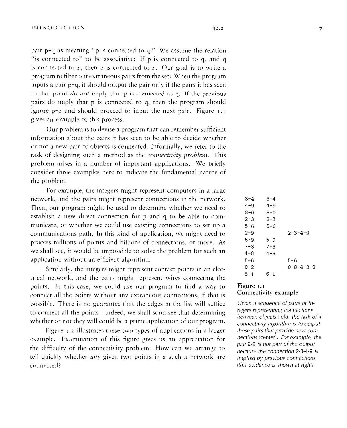
Figure 1.2 illustrates these two types of applications in a larger
example. F,xamination of this figure gives us an appreciation for
the difficulty of the connectivity problem: How can we arrange to
tell quickly whether any given two points in a such a network are
connected?
3-4
4-9
8-0
2-3
5-6
2-9
5-9
7-3
4-8
5-6
0-2
6-1
Figure 1.
3-4
4-9
8-0
2-3
5-6
5-9
7-3
4-8
6-1
,1
2-3-4-9
5-6
0-8-4-3-2
Connectivity example
Given a sequence of pairs of
integers representing connections
between objects (left), the task of a
connectivity algorithm is to output
those pairs that provide new
connections {center). For example, the
pair 2-9 is not part of the output
because the connection 2-3-4-9 is
implied by previous connections
(this evidence is shown at right).
8
§1.2
CHAPTER ONE
Still another example arises in certain programming
environments where it is possible to declare two variable names as
equivalent. The problem is to be able to determine whether two given
names are equivalent, after a sequence of such declarations. This
application is an early one that motivated the development of several of
the algorithms that we are about to consider. It directly relates our
problem to a simple abstraction that provides us with a way to make
our algorithms useful for a wide variety of applications, as we shall
see.
Applications such as the variable-name-equivalence problem
described in the previous paragraph require that we associate an integer
with each distinct variable name. This association is also implicit
in the network-connection and circuit-connection applications that
INTRODUCTION
Si"
we have described. We shall be considering a host of algorithms in
Chapters 10 through r6 that can provide this association in an
efficient manner. Thus, we can assume in this chapter, without loss
of generality, that we have N objects with integer names, from 0 to
N-l.
We are asking for a program that does a specific and well-
defined task. There are many other related problems that we might
want to have solved, as well. One of the first tasks that we face in
developing an algorithm is to be sure that we have specified the problem
in a reasonable manner. The more we require of an algorithm, the
more time and space we may expect it to need to finish the task. It is
impossible to quantify this relationship a priori, and we often modify
a problem specification on finding that it is difficult or expensive to
solve, or, in happy circumstances, on finding that an algorithm can
provide information more useful than was called for in the original
specification.
For example, our connectivity-problem specification requires
only that our program somehow know whether or not any given
pair p-q is connected, and not that it be able to demonstrate any or
all ways to connect that pair. Adding a requirement for such a
specification makes the problem more difficult, and would lead us to a
different family of algorithms, which we consider briefly in Chapter 5
and in detail in Part 7.
The specifications mentioned in the previous paragraph asks us
for more information than our original one did; we could also ask
for less information. For example, we might simply want to be able
to answer the question: "Are the M connections sufficient to connect
together all N objects?" This problem illustrates that, to develop
efficient algorithms, we often need to do high-level reasoning about
the abstract objects that we are processing. In this case, a fundamental
result from graph theory implies that all N objects are connected if
and only if the number of pairs output by the connectivity algorithm
is precisely N — 1 (see Section 5.4). In other words, a connectivity
algorithm will never output more than N — 1 pairs, because, once it
has output N —I pairs, any pair that it encounters from that point on
will be connected. Accordingly, we can get a program that answers
the yes-no question just posed by changing a program that solves the
connectivity problem to one that increments a counter, rather than
§1.2
CHAPTER ONE
writing out each pair that was not previously connected, answering
"yes" when the counter reaches N—l and "no" if it never does. This
question is but one example of a host of questions that we might
wish to answer regarding connectivity. The set of pairs in the input is
called a graph, and the set of pairs output is called a spanning tree for
that graph, which connects all the objects. We consider properties of
graphs, spanning trees, and all manner of related algorithms in Part 7.
It is worthwhile to try to identify the fundamental operations
that we will be performing, and so to make any algorithm that we
develop for the connectivity task useful for a variety of similar tasks.
Specifically, each time that we get a new pair, we have first to
determine whether it represents a new connection, then to incorporate the
information that the connection has been seen into its understanding
about the connectivity of the objects such that it can check
connections to be seen in the future. We encapsulate these two tasks as
abstract operations by considering the integer input values to
represent elements in abstract sets, and then design algorithms and data
structures that can
• Find the set containing a given item.
• Replace the sets containing two given items by their union.
Organizing our algorithms in terms of these abstract operations does
not seem to foreclose any options in solving the connectivity problem,
and the operations may be useful for solving other problems.
Developing ever more powerful layers of abstraction is an essential process
in computer science in general and in algorithm design in
particular, and we shall turn to it on numerous occasions throughout this
book. In this chapter, we use abstract thinking in an informal way to
guide us in designing programs to solve the connectivity problem; in
Chapter 4, we shall see how to encapsulate abstractions in C code.
The connectivity problem is easily solved in terms of the find
and union abstract operations. After reading a new pair p-q from
the input, we perform a find operation for each member of the pair.
If the members of the pair are in the same set, we move on to the next
pair; if they are not, we do a union operation and write out the pair.
The sets represent connected components: subsets of the objects with
the property that any two objects in a given component are connected.
This approach reduces the development of an algorithmic solution for
connectivity to the tasks of defining a data structure representing the
INTRODUCTION
§i-3
ii
sets and developing union and find algorithms that efficiently use that
data structure.
There are many possible ways to represent and process abstract
sets, which we consider in more detail in Chapter 4. In this chapter,
our focus is on finding a representation that can support efficiently
the union and find operations that we see in solving the connectivity
problem.
Exercises
1.1 Give the output that a connectivity algorithm should produce when
given the input 0-2, 1-4, 2-5, 3-6, 0-4, 6-0, and 1-3.
1.2 List all the different ways to connect two different objects for the
example in Figure 1.1.
1.3 Describe a simple method for counting the number of sets remaining
after using the union and find operations to solve the connectivity problem
as described in the text.
1.3 Union-Find Algorithms
The first step in the process of developing an efficient algorithm to
solve a given problem is to implement a simple algorithm that solves
the problem. If we need to solve a few particular problem instances
that turn out to be easy, then the simple implementation may finish
the job foi" us. If a more sophisticated algorithm is called for, then the
simple implementation provides us with a correctness check for small
cases and a baseline for evaluating performance characteristics. We
always care about efficiency, but our primary concern in developing
the first program that we write to solve a problem is to make sure
that the program is a correct solution to the problem.
The first idea that might come to mind is somehow to save all
the input pairs, then to write a function to pass through them to
try to discover whether the next pair of objects is connected. We
shall use a different approach. First, the number of pairs might be
sufficiently large to preclude our saving them all in memory in
practical applications. Second, and more to the point, no simple method
immediately suggests itself for determining whether two objects are
connected from the set of all the connections, even if we could save
them all! We consider a basic method that takes this approach in
Chapter 5, but the methods that we shall consider in this chapter are
0123456789
3
4
8
2
5
2
5
7
4
5
0
6
4
9
0
3
6
9
9
3
8
6
2
1
0
0
0
0
0
0
0
0
0
0
0
1
1
1
1
1
1
1
1
1
1
1
1
1
2
2
2
9
9
9
9
9
0
0
0
1
4
9
9
9
9
9
9
9
0
0
0
1
4
9
9
9
9
9
9
9
0
0
0
1
5
5
5
5
6
6
9
9
0
0
0
1
6
6
6
6
6
6
9
9
0
0
0
1
7
7
7
7
7
7
7
9
0
0
0
1
8
8
0
0
0
0
0
0
0
0
0
1
9
9
9
9
9
9
9
9
0
0
0
1
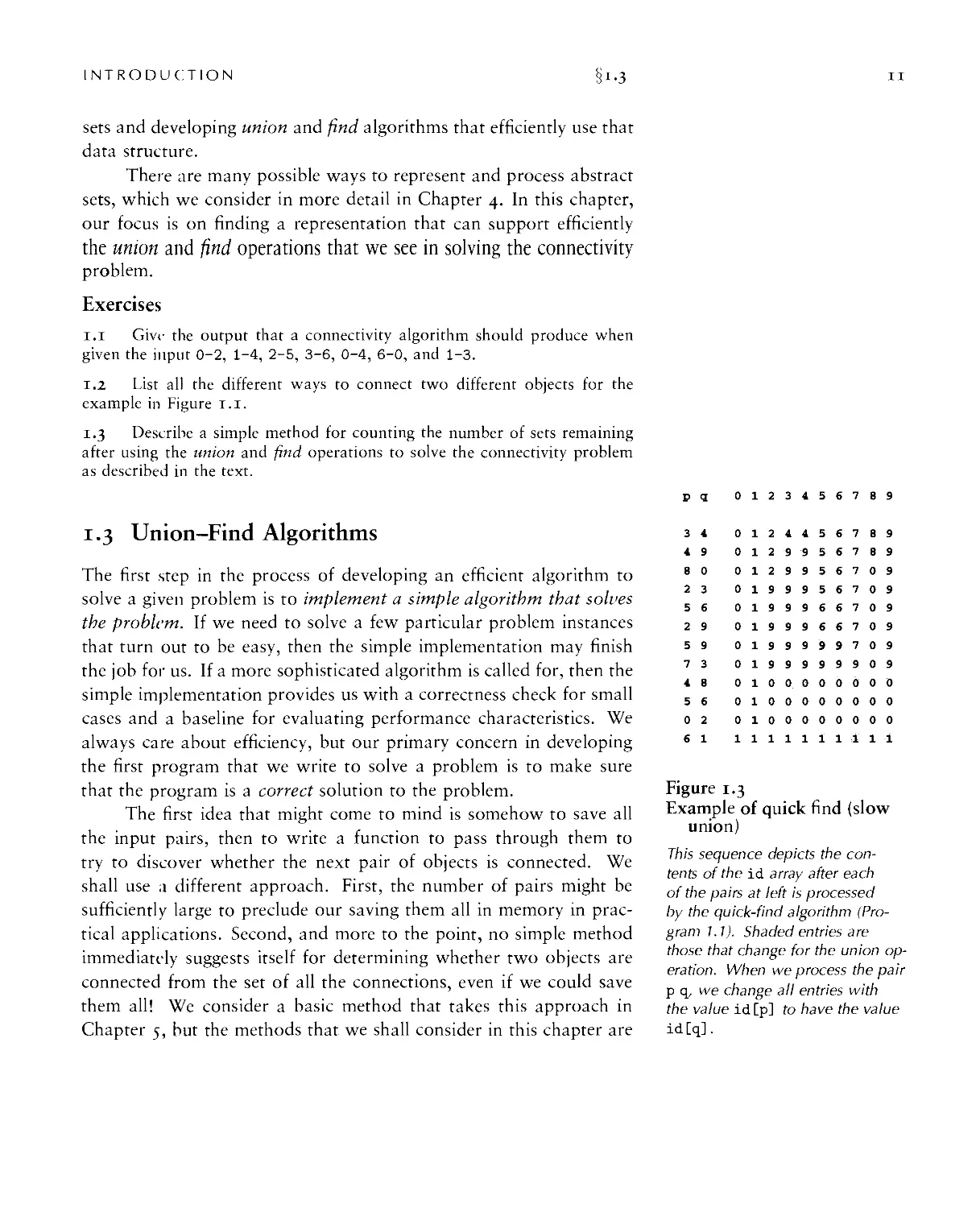
Figure 1.3
Example of quick find (slow
union)
This sequence depicts the
contents of the id array after each
of the pairs at left is processed
by the quick-find algorithm
(Program 1.1). Shaded entries are
those that change for the union
operation. When we process the pair
p q, we change all entries with
the value id [p] to have the value
id[q].
§i-3
CHAPTER ONE
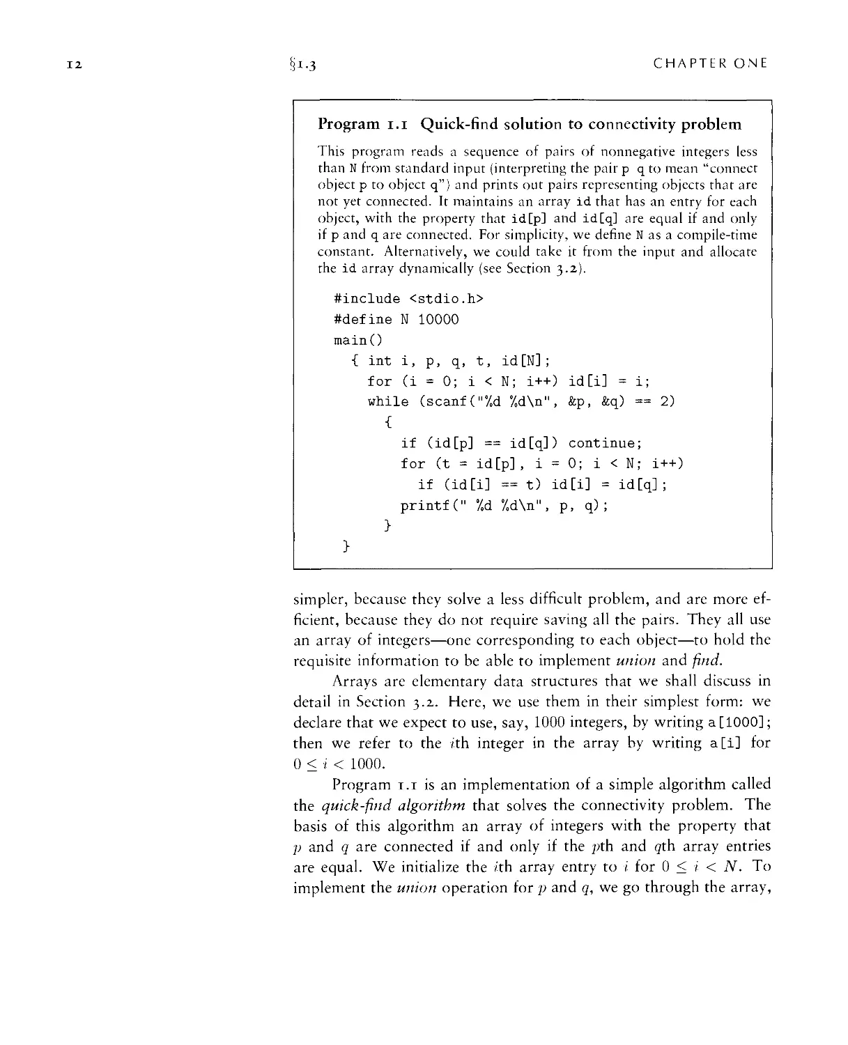
Program i.i Quick-find solution to connectivity problem
This program reads a sequence of pairs of nonnegative integers less
than N from standard input (interpreting the pair p q to mean "connect
object p to object q") and prints out pairs representing objects that are
not yet connected. It maintains an array id that has an entry for each
object, with the property that id[p] and id[q] are equal if and only
if p and q are connected. For simplicity, we define N as a compile-time
constant. Alternatively, we could take it from the input and allocate
the id array dynamically (see Section 3.2).
#include <stdio.h>
#define N 10000
mainO
{ int i, p, q, t, id[N];
for (i = 0; i < N; i++) id[i] = i;
while (scanf('7.d 7.d\n", &p, &q) == 2)
{
if (id[p] == id[q]) continue;
for (t = id[p], i = 0; i < N; i++)
if (id[i] == t) id[i] = id[q] ;
printf (" %d °/.d\n", p, q) ;
>
>
simpler, because they solve a less difficult problem, and are more
efficient, because they do not require saving all the pairs. They all use
an array of integers—one corresponding to each object—to hold the
requisite information to be able to implement union and find.
Arrays are elementary data structures that we shall discuss in
detail in Section 3.2. Here, we use them in their simplest form: we
declare that we expect to use, say, 1000 integers, by writing a [1000];
then we refer to the ?th integer in the array by writing a[i] for
0 < 1 < 1000.
Program 1.1 is an implementation of a simple algorithm called
the quick-find algorithm that solves the connectivity problem. The
basis of this algorithm an array of integers with the property that
p and q are connected if and only if the 77th and qth array entries
are equal. We initialize the v'th array entry to i for 0 < / < N. To
implement the union operation for p and q, we go through the array,
INTRODUCTION
§i-3
13
changing all the entries with the same name as p to have the same
name as (/. This choice is arbitrary—we could have decided to change
all the entries with the same name as q to have the same name as p.
Figure 1.3 shows the changes to the array for the union
operations in the example in Figure i.t. To implement find, we just test
the indicated array entries for equality—hence the name quick find.
The union operation, on the other hand, involves scanning through
the whole array for each input pair.
Property i.r The quick-find algorithm executes at least MN
instructions to solve a connectivity problem with M pairs of N objects.
For each of the M pairs, we iterate the for loop N times. Each
iteration requires at least one instruction (if only to check whether
the loop is finished). ■
We can execute tens or hundreds of millions of instructions per
second on modern computers, so this cost is not noticeable if M and
N are small, but we also might find ourselves with millions of objects
and billions of input pairs to process in a modern application. The
inescapable conclusion is that we cannot feasibly solve such a problem
using the quick-find algorithm (see Exercise 1.10). We consider the
process of quantifying such a conclusion precisely in Chapter 2.
Figure 1.4 shows a graphical representation of Figure 1.3. We
may think of some of the objects as representing the set to which they
belong, and all of the other objects as pointing to the representative
in their set. The reason for moving to this graphical representation
of the array will become clear soon. Observe that the connections
between objects in this representation are not necessarily the same as
the connections in the input pairs—they are the information that the
algorithm chooses to remember to be able to know whether future
pairs are connected.
The next algorithm that we consider is a complementary method
called the quick-union algorithm. It is based on the same data
structure—an array indexed by object names—but it uses a
different interpretation of the values that leads to more complex abstract
structures. Each object points to another object in the same set, in
a structure with no cycles. To determine whether two objects are in
the same set, we follow pointers for each until we reach an object
that points to itself. The objects are in the same set if and only if this
® ®©®®©® ® ®
@
®©@ ® ®®@®
@®
®@ ® ®®®®
® ® ®
® ® ®®®®
df®® &
®® ®(5) ®
Figure 1.4
Tree representation of quick
find
This figure depicts graphical
representations for the example in
Figure 1.3. The connections in these
figures do not necessarily represent
the connections in the input. For
example, the structure at the
bottom has the connection 1-7, which
is not in the input, but which is
made because of the string of
connections 7-3-4-9-5-6-1.
14
!-3
CHAPTER ONE
® © © ® © © ® © ®
(D
®©©®©©®®
®
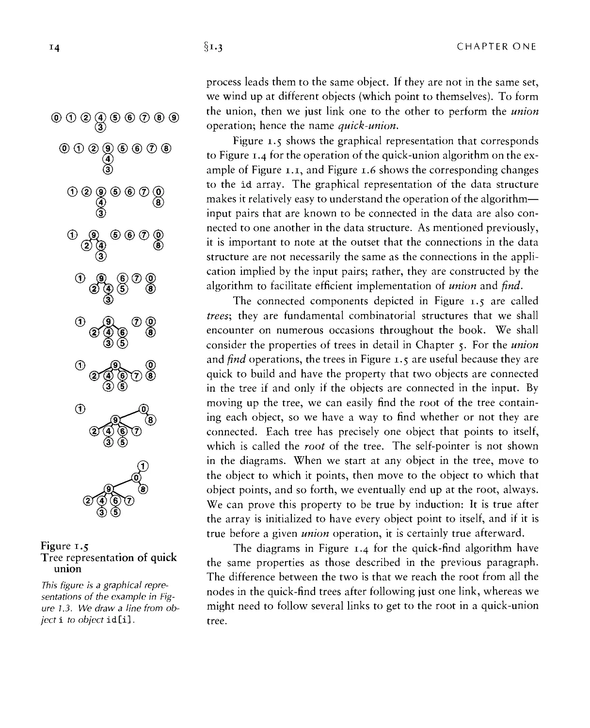
Figure 1.5
Tree representation of quick
union
This figure is a graphical
representations of the example in
Figure 1.3. We draw a line from
object i to object id [i].
process leads them to the same object. If they are not in the same set,
we wind up at different objects (which point to themselves). To form
the union, then we just link one to the other to perform the union
operation; hence the name quick-union.
Figure 1.5 shows the graphical representation that corresponds
to Figure 1.4 for the operation of the quick-union algorithm on the
example of Figure 1.1, and Figure 1.6 shows the corresponding changes
to the id array. The graphical representation of the data structure
makes it relatively easy to understand the operation of the algorithm—
input pairs that are known to be connected in the data are also
connected to one another in the data structure. As mentioned previously,
it is important to note at the outset that the connections in the data
structure are not necessarily the same as the connections in the
application implied by the input pairs; rather, they are constructed by the
algorithm to facilitate efficient implementation of union and find.
The connected components depicted in Figure 1.5 are called
trees; they are fundamental combinatorial structures that we shall
encounter on numerous occasions throughout the book. We shall
consider the properties of trees in detail in Chapter 5. For the union
and find operations, the trees in Figure 1.5 are useful because they are
quick to build and have the property that two objects are connected
in the tree if and only if the objects are connected in the input. By
moving up the tree, we can easily find the root of the tree
containing each object, so we have a way to find whether or not they are
connected. Each tree has precisely one object that points to itself,
which is called the root of the tree. The self-pointer is not shown
in the diagrams. When we start at any object in the tree, move to
the object to which it points, then move to the object to which that
object points, and so forth, we eventually end up at the root, always.
We can prove this property to be true by induction: It is true after
the array is initialized to have every object point to itself, and if it is
true before a given union operation, it is certainly true afterward.
The diagrams in Figure 1.4 for the quick-find algorithm have
the same properties as those described in the previous paragraph.
The difference between the two is that we reach the root from all the
nodes in the quick-find trees after following just one link, whereas we
might need to follow several links to get to the root in a quick-union
tree.
INTRODUCTION
3i-3
15
Program 1.2 Quick-union solution to connectivity problem
If we replace the body of the while loop in Program 1.1 by this code,
we have a program that meets the same specifications as Program 1.1,
but does less computation for the union operation at the expense of
more computation for the find operation. The for loops and
subsequent if statement in this code specify the necessary and sufficient
conditions on the id array forp and q to be connected. The assignment
statement id[i] = j implements the union operation.
for (i = p; i != id[i]; i
for (j = q; j ! = id[j]; j
if (i == j) continue;
id[i] = j;
printfC" 7.d 7,d\n", p, q);
id[i])
idEj])
Program 1.2 is an implementation of the union and find
operations that comprise the quick-union algorithm to solve the
connectivity problem. The quick-union algorithm would seem to be faster
than the quick-find algorithm, because it does not have to go through
the entire array for each input pair; but how much faster is it? This
question is more difficult to answer here than it was for quick find,
because the running rime is much more dependent on the nature of
the input. By running empirical studies or doing mathematical
analysis (see Chapter 2), we can convince ourselves that Program 1.2 is
far more efficient than Program 1.1, and that it is feasible to consider
using Program 1.2 for huge practical problems. We shall discuss one
such empirical study at the end of this section. For the moment, we
can regard quick union as an improvement because it removes quick
find's main liability (that the program requires at least NM
instructions to process M pairs of N objects).
This difference between quick union and quick find certainly
represents an improvement, but quick union still has the liability that
we cannot guarantee it to be substantially faster than quick find in
every case, because the input data could conspire to make the find
operation slow.
Property 1.2 For M > N, the quick-union algorithm could take
more than MN/2 instructions to solve a connectivity problem with
M pairs of N objects.
pq 0123456789
34 0124456789
49 0124956789
80 0124956709
23 0194956709
56 0194966709
29 0194966709
59 0194969709
73 0194969909
48 0194969900
56 0194969900
02 0194969900
61 1194969900
58 1194969900
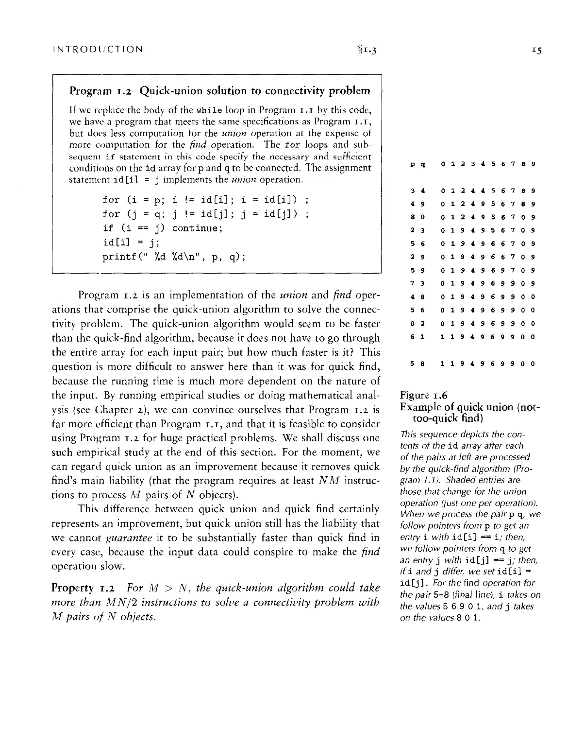
Figure 1.6
Example of quick union (not-
too-quick find)
This sequence depicts the
contents of the id array after each
of the pairs at left are processed
by the quick-find algorithm
(Program 1.1). Shaded entries are
those that change for the union
operation (just one per operation).
When we process the pair p q, we
follow pointers from p to get an
entry i with id[i] == i; then,
we follow pointers from q to get
an entry j with id[j] == j; then,
if i and j differ, wesefid[i] =
id [j ]. For the find operation for
the pair 5-8 (final line), i takes on
the values 5 6 9 0 1, and j takes
on the values 8 0 1.
i6
5i-3
CHAPTER ONE
© ® ® © © © © ® ®
®®® ® ©®@®
@®
®0® ® ©®®
® ®®
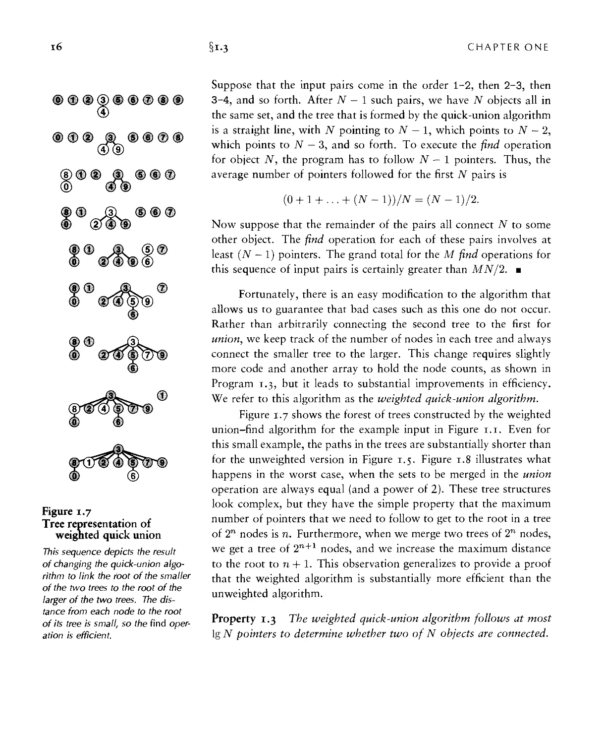
Figure 1.7
Tree representation of
weighted quick union
This sequence depicts the result
of changing the quick-union
algorithm to link the root of the smaller
of the two trees to the root of the
larger of the two trees. The
distance from each node to the root
of its tree is small, so the find
operation is efficient.
Suppose that the input pairs come in the order 1-2, then 2-3, then
3-4, and so forth. After N — 1 such pairs, we have N objects all in
the same set, and the tree that is formed by the quick-union algorithm
is a straight line, with N pointing to N — 1, which points to N — 2,
which points to AT — 3, and so forth. To execute the find operation
for object N, the program has to follow N — 1 pointers. Thus, the
average number of pointers followed for the first N pairs is
(0 + 1 + ... + (N - 1))/N = (N - l)/2.
Now suppose that the remainder of the pairs all connect N to some
other object. The find operation for each of these pairs involves at
least (N — 1) pointers. The grand total for the M find operations for
this sequence of input pairs is certainly greater than MN/2. m
Fortunately, there is an easy modification to the algorithm that
allows us to guarantee that bad cases such as this one do not occur.
Rather than arbitrarily connecting the second tree to the first for
union, we keep track of the number of nodes in each tree and always
connect the smaller tree to the larger. This change requires slightly
more code and another array to hold the node counts, as shown in
Program 1.3, but it leads to substantial improvements in efficiency.
We refer to this algorithm as the weighted quick-union algorithm.
Figure 1.7 shows the forest of trees constructed by the weighted
union-find algorithm for the example input in Figure 1.1. Even for
this small example, the paths in the trees are substantially shorter than
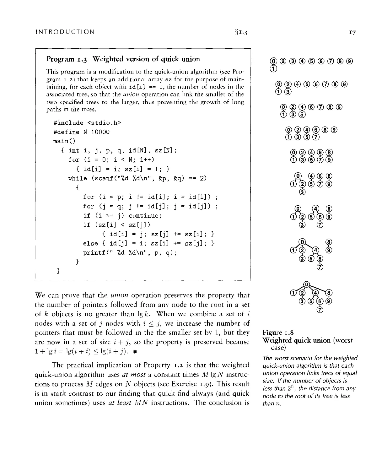
for the unweighted version in Figure 1.5. Figure 1.8 illustrates what
happens in the worst case, when the sets to be merged in the union
operation are always equal (and a power of 2). These tree structures
look complex, but they have the simple property that the maximum
number of pointers that we need to follow to get to the root in a tree
of 2n nodes is n. Furthermore, when we merge two trees of 2n nodes,
we get a tree of 2n+1 nodes, and we increase the maximum distance
to the root to n + 1. This observation generalizes to provide a proof
that the weighted algorithm is substantially more efficient than the
unweighted algorithm.
Property 1.3 The weighted quick-union algorithm follows at most
lg N pointers to determine whether two of N objects are connected.
INTRODUCTION
?i-3
17
Program 1.3 Weighted version of quick union
This program is a modification to the quick-union algorithm (see
Program 1.2) that keeps an additional array sz for the purpose of
maintaining, for each object with id[i] == i, the number of nodes in the
associated tree, so that the union operation can link the smaller of the
two specified trees to the larger, thus preventing the growth of long
paths in the trees.
#include <stdio.h>
#define N 10000
mainQ
{ int i, j, p, q, id[N], sz [N] ;
for (i = 0; i < N; i++)
{ id[i] = i; sz[i] = 1; }
while (scanf("7,d y,d\n", &p, &q) == 2)
{
for (i = p; i != id[i]; i = id[i]) ;
for (j = q; j != id[j]; j = id[j]) ;
if (i == j) continue;
if (sz[i] < sz[j])
{ id[i] = j; sz[j] +
else { id[j] = i; sz [i] +
printf(" 7,d 7„d\n" , p, q);
sz[i]; }
sz[j]; }
}
}
We can prove that the union operation preserves the property that
the number of pointers followed from any node to the root in a set
of k objects is no greater than lgfc. When we combine a set of i
nodes with a set of j nodes with i < j, we increase the number of
pointers that must be followed in the the smaller set by 1, but they
are now in a set of size i + j, so the property is preserved because
l + lgi = lg(i + i) <lg(i+j). ■
The practical implication of Property 1.2 is that the weighted
quick-union algorithm uses at most a constant times M\gN
instructions to process M edges on JV objects (see Exercise 1.9). This result
is in stark contrast to our finding that quick find always (and quick
union sometimes) uses at least MN instructions. The conclusion is
® © © 0 © © ® ® ®
®©®©©®®®
®©®©®®®
© © ©
® @ ©©© ©
© ® ©@
© © © © (8)
©® ©® (9)
Figure 1.8
Weighted quick union (worst
case)
The worst scenario for the weighted
quick-union algorithm is that each
union operation links trees of equal
size. If the number of objects is
less than 2n, the distance from any
node to the root of its tree is less
than n.
i8
§i-3
CHAPTER ONE
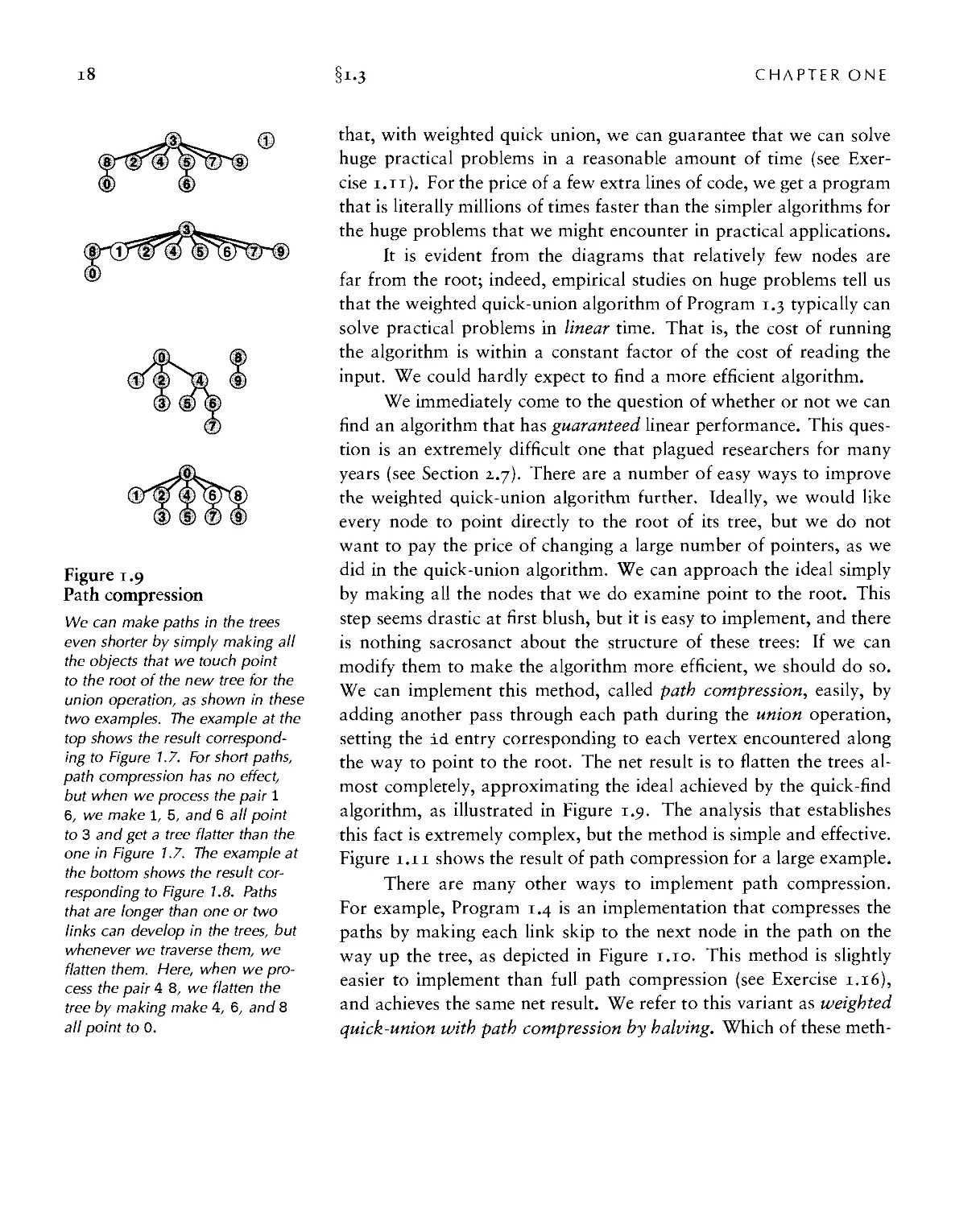
Figure 1.9
Path compression
We can make paths in the trees
even shorter by simply making all
the objects that we touch point
to the root of the new tree for the
union operation, as shown in these
two examples. The example at the
top shows the result
corresponding to Figure 1.7. For short paths,
path compression has no effect,
but when we process the pair 1
6, we make 1, 5, and 6 all point
to 3 and get a tree flatter than the
one in Figure 7.7. The example at
the bottom shows the result
corresponding to Figure 1.8. Paths
that are longer than one or two
links can develop in the trees, but
whenever we traverse them, we
flatten them. Here, when we
process the pair 4 8, we flatten the
tree by making make 4, 6, and 8
all point to 0.
that, with weighted quick union, we can guarantee that we can solve
huge practical problems in a reasonable amount of time (see
Exercise 1.11). For the price of a few extra lines of code, we get a program
that is literally millions of times faster than the simpler algorithms for
the huge problems that we might encounter in practical applications.
It is evident from the diagrams that relatively few nodes are
far from the root; indeed, empirical studies on huge problems tell us
that the weighted quick-union algorithm of Program 1.3 typically can
solve practical problems in linear time. That is, the cost of running
the algorithm is within a constant factor of the cost of reading the
input. We could hardly expect to find a more efficient algorithm.
We immediately come to the question of whether or not we can
find an algorithm that has guaranteed linear performance. This
question is an extremely difficult one that plagued researchers for many
years (see Section 2.7). There are a number of easy ways to improve
the weighted quick-union algorithm further. Ideally, we would like
every node to point directly to the root of its tree, but we do not
want to pay the price of changing a large number of pointers, as we
did in the quick-union algorithm. We can approach the ideal simply
by making all the nodes that we do examine point to the root. This
step seems drastic at first blush, but it is easy to implement, and there
is nothing sacrosanct about the structure of these trees: If we can
modify them to make the algorithm more efficient, we should do so.
We can implement this method, called path compression, easily, by
adding another pass through each path during the union operation,
setting the id entry corresponding to each vertex encountered along
the way to point to the root. The net result is to flatten the trees
almost completely, approximating the ideal achieved by the quick-find
algorithm, as illustrated in Figure 1.9. The analysis that establishes
this fact is extremely complex, but the method is simple and effective.
Figure 1.11 shows the result of path compression for a large example.
There are many other ways to implement path compression.
For example, Program 1.4 is an implementation that compresses the
paths by making each link skip to the next node in the path on the
way up the tree, as depicted in Figure 1.10. This method is slightly
easier to implement than full path compression (see Exercise 1.16),
and achieves the same net result. We refer to this variant as weighted
quick-union with path compression by halving. Which of these meth-
INTRODUCTION
51-3
19
Program 1.4 Path compression by halving
If we replace the for loops in Program 1.3 by this code, we halve the
length of any path that we traverse. The net result of this change is
that the trees become almost completely flat after a long sequence of
operations.
for (i = p; i != id[i]; i = id[i])
{ int t = i; i = id[id[t]] ; id[t] = i; }
for (j = q; j != id[j]; j = id[j]) ;
{ int t = j; j = id[id[t]]; id[t] = j; }
ods is the more effective? Is the savings achieved worth the extra time
required to implement path compression? Is there some other
technique that we should consider? To answer these questions, we need
to look more carefully at the algorithms and implementations. We
shall return to this topic in Chapter 5, in the context of our discussion
of basic approaches to the analysis of algorithms.
The end result of the succession of algorithms that we have
considered to solve the connectivity problem is about the best that
we could hope for in any practical sense. We have algorithms that
are easy to implement whose running time is guaranteed to be within
a constant factor of the cost of gathering the data. Moreover, the
algorithms are online algorithms that consider each edge once, using
space proportional to the number of objects, so there is no limitation
on the number of edges that they can handle. The empirical studies
in Table 1.1 validate our conclusion that Program 1.3 and its path-
compression variations are useful even for huge practical applications.
Choosing which is the best among these algorithms requires careful
and sophisticated analysis (see Chapter 2).
Exercises
> 1.4 Show the contents of the id array after each union operation when you
use the quick-find algorithm (Program 1.1) to solve the connectivity problem
for the sequence 0-2, 1-4, 2-5, 3-6, 0-4, 6-0, and 1-3. Also give the number
of times the program accesses the id array for each input pair.
O 1.5 Do Kxercise 1.4, but use the quick-union algorithm (Program 1.2).
O 1.6 Give the contents of the id array after each union operation for the
weighted quick-union algorithm running on the examples corresponding to
Figure 1.7 and Figure 1.8.
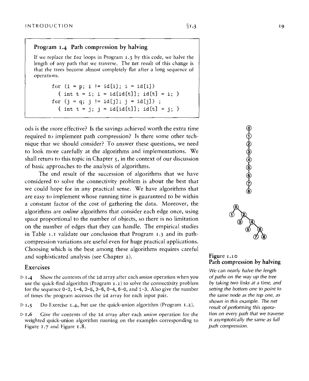
Figure 1.10
Path compression by halving
We can nearly halve the length
of paths on the way up the tree
by taking two links at a time, and
setting the bottom one to point to
the same node as the top one, as
shown in this example. The net
result of performing this
operation on every path that we traverse
is asymptotically the same as full
path compression.
§i-3
CHAPTER ONE
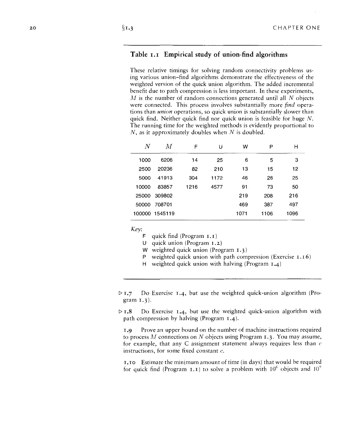
Table i.i Empirical study of union-find algorithms
These relative timings for solving random connectivity problems
using various union-find algorithms demonstrate the effectiveness of the
weighted version of the quick union algorithm. The added incremental
benefit due to path compression is less important. In these experiments,
M is the number of random connections generated until all N objects
were connected. This process involves substantially more find
operations than union operations, so quick union is substantially slower than
quick find. Neither quick find nor quick union is feasible for huge N.
The running time for the weighted methods is evidently proportional to
N, as it approximately doubles when N is doubled.
N
1000
2500
5000
10000
25000
50000
100000
M
6206
20236
41913
83857
309802
708701
1545119
F
14
82
304
1216
U
25
210
1172
4577
W
6
13
46
91
219
469
1071
P
5
15
26
73
208
387
1106
H
3
12
25
50
216
497
1096
Key:
F quick find (Program i.i)
U quick union (Program 1.2)
W weighted quick union (Program 1.3)
P weighted quick union with path compression (Exercise 1.16)
H weighted quick union with halving (Program 1.4)
O 1.7 Do Exercise 1.4, but use the weighted quick-union algorithm
(Program 1.3).
O1.8 Do Exercise 1.4, but use the weighted quick-union algorithm with
path compression by halving (Program 1.4).
1.9 Prove an upper bound on the number of machine instructions required
to process M connections on N objects using Program 1.3. You may assume,
for example, that any C assignment statement always requires less than c
instructions, for some fixed constant c.
1.10 Estimate the minimum amount of time (in days) that would be required
for quick find (Program 1.1) to solve a problem with 106 objects and 109
INTRODUCTION
§i-3
input pairs, on a computer capable of executing 109 instructions per second.
Assume that each iteration of the while loop requires at least 10 instructions.
i.ii Estimate the maximum amount of time (in seconds) that would be
required for weighted quick union (Program 1.3) to solve a problem with
10* objects and 109 input pairs, on a computer capable of executing 109
instructions per second. Assume that each iteration of the while loop requires
at most 100 instructions.
1.12 Compute the average distance from a node to the root in a worst-case
tree of 2" nodes built by the weighted quick-union algorithm.
O 1.13 Draw a diagram like Figure 1.10, starting with eight nodes instead of
nine.
o 1.14 Give a sequence of input pairs that causes the weighted quick-union
algorithm (Program 1.4) to produce a path of length 4.
• 1.15 Give a sequence of input pairs that causes the weighted quick-union
algorithm with path compression by halving (Program 1.4) to produce a path
of length 4.
1.16 Show how to modify Program 1.3 to implement full path compression,
where we complete each union operation by making every node that we touch
point to the root of the new tree.
O1.17 Answer Exercise 1.4, but using the weighted quick-union algorithm
with full path compression (Exercise 1.16).
• • 1.18 Give a sequence of input pairs that causes the weighted quick-union
algorithm with full path compression (Exercise 1.16) to produce a path of
length 4.
o 1.19 Give an example showing that modifying quick union (Program 1.2)
to implement full path compression (see Exercise 1.16) is not sufficient to
ensure that the trees have no long paths.
• 1.20 Modify Program 1.3 to use the height of the trees (longest path from
any node 10 the root), instead of the weight, to decide whether to set id[i]
= j or id[j] = i. Run empirical studies to compare this variant with
Program 1.3.
•• 1.21 Show that Property 1.3 holds for the algorithm described in
Exercise 1.20.
• 1.22 Modify Program 1.4 to generate random pairs of integers between 0
and N — 1 instead of reading them from standard input, and to loop until N — 1
union operations have been performed. Run your program for N = 10"', 104,
10\ and 10 and print out the total number of edges generated for each value
of TV.
• 1.23 Modify your program from Exercise 1.22 to plot the number of edges
needed to connect N items, for 100 < N < 1000.
•• 1.24 Give an approximate formula for the number of random edges that is
required to connect N objects, as a function of /V.
22
§i-4
CHAPTER ONE
IT
'A'A111
iv
^TJ
Figure i.ii
A large example of the
effect of path compression
This sequence depicts the result of
processing random pairs from WO
objects with the weighted quick-
union algorithm with path
compression. All but two of the nodes
in the tree are one or two steps
from the root.
1.4 Perspective
Each of the algorithms that we considered in Section 1.3 seems to
be an improvement over the previous in some intuitive sense, but
the process is perhaps artificially smooth because we have the
benefit of hindsight in looking over the development of the algorithms as
they were studied by researchers over the years (see reference section).
The implementations are simple and the problem is well specified, so
we can evaluate the various algorithms directly by running empirical
studies. Furthermore, we can validate these studies and quantify the
comparative performance of these algorithms (see Chapter 2). Not all
the problem domains in this book are as well developed as this one,
and we certainly can run into complex algorithms that are difficult to
compare and mathematical problems that are difficult to solve. We
strive to make objective scientific judgements about the algorithms
that we use, while gaining experience learning the properties of
implementations running on actual data from applications or random
test data.
The process is prototypical of the way that we consider various
algorithms for fundamental problems throughout the book. When
possible, we follow the same basic steps that we took for union-find
algorithms in Section 1.2, some of which are highlighted in this list:
• Decide on a complete and specific problem statement, including
identifying fundamental abstract operations that are intrinsic to
the problem.
• Carefully develop a succinct implementation for a
straightforward algorithm.
• Develop improved implementations through a process of
stepwise refinement, validating the efficacy of ideas for improvement
through empirical analysis, mathematical analysis, or both.
• Find high-level abstract representations of data structures or
algorithms in operation that enable effective high-level design of
improved versions.
• Strive for worst-case performance guarantees when possible, but
accept good performance on actual data when available.
INTRODUCTION
§i-5
The potential for spectacular performance improvements for practical
problems such those that we saw in Section 1.2 makes algorithm
design a compelling field of study; few other design activities hold the
potential to reap savings factors of millions or billions, or more.
More important, as the scale of our computational power and
our applications increases, the gap between a fast algorithm and a
slow one grows. A new computer might be 10 times faster and be
able to process 10 times the data as an old one, but if we are
using a quadratic algorithm such as quick find, the new computer will
take 10 times as long on the new job as the old one took to finish
the old job! This statement seems counterintuitive at first, but it is
easily verified by the simple identity (10iV)'2/10 = ION2, as we shall
see in Chapter 2. As computational power increases to allow us to
take on larger and larger problems, the importance of having efficient
algorithms increases, as well.
Developing an efficient algorithm is an intellectually satisfying
activity that can have direct practical payoff. As the connectivity
problem indicates, a simply stated problem can lead us to study
numerous algorithms that are not only both useful and interesting,
but also intricate and challenging to understand. We shall encounter
many ingenious algorithms that have been developed over the years
for a host of practical problems. As the scope of applicability of
computational solutions to scientific and commercial problems widens, so
also grow the importance of being able to apply efficient algorithms to
solve known problems and of being able to develop efficient solutions
to new problems.
Exercises
1.25 Suppose that we use weighted quick union to process 10 times as many
connections on a new computer that is 10 times as fast as an old one. How
much longer would it take the new computer to finish the new job than it
took the old one to finish the old job?
1.26 Answer Exercise 1.25 for the case where we use an algorithm that
requires /V' instructions.
1.5 Summary of Topics
This section comprises brief descriptions of the major parts of the
book, giving specific topics covered and an indication of our general
§i-5
CHAPTER ONE
orientation toward the material. This set of topics is intended to
touch on as many fundamental algorithms as possible. Some of the
areas covered are core computer-science areas that we study in depth
to learn basic algorithms of wide applicability. Other algorithms
that we discuss are from advanced fields of study within computer
science and related fields, such as numerical analysis and operations
research—in these cases, our treatment serves as an introduction to
these fields through examination of basic methods.
The first four parts of the book, which are contained in this
volume, cover the most widely used set of algorithms and data structures,
a first level of abstraction for collections of objects with keys that can
support a broad variety of important fundamental algorithms. The
algorithms that we consider are the products of decades of research
and development, and continue to play an essential role in the ever-
expanding applications of computation.
Fundamentals (Part i) in the context of this book are the basic
principles and methodology that we use to implement, analyze, and
compare algorithms. The material in Chapter i motivates our study
of algorithm design and analysis; in Chapter 2, we consider basic
methods of obtaining quantitative information about the performance
of algorithms.
Data Structures (Part 2) go hand-in-hand with algorithms: we
shall develop a thorough understanding of data representation
methods for use throughout the rest of the book. We begin with an
introduction to basic concrete data structures in Chapter 3, including
arrays, linked lists, and strings; then we consider recursive programs
and data structures in Chapter 5, in particular trees and algorithms for
manipulating them. In Chapter 4, we consider fundamental abstract
data types (ADTs) such as stacks and queues, including
implementations using elementary data structures.
Sorting algorithms (Part 3) for rearranging files into order are of
fundamental importance. We consider a variety of algorithms in
considerable depth, including Shellsort, quicksort, mergesort, heapsort,
and radix sorts. We shall encounter algorithms for several related
problems, including priority queues, selection, and merging. Many
of these algorithms will find application as the basis for other
algorithms later in the book.
INTRODUCTION
§i-5
Searching algorithms (Part 4) for finding specific items among
large collections of items are also of fundamental importance. We
discuss basic and advanced methods for searching using trees and
digital key transformations, including binary search trees, balanced
trees, hashing, digital search trees and tries, and methods appropriate
for huge files. We note relationships among these methods,
comparative performance statistics, and correspondences to sorting methods.
Parts 5 through 8, which are contained in a separate volume,
cover advanced applications of the algorithms described here for a
diverse sei of applications—a second level of abstractions specific to
a number of important applications areas. We also delve more deeply
into techniques of algorithm design and analysis. Many of the
problems that we touch on are the subject on ongoing research.
String Processing algorithms (Part 5) include a range of
methods for processing (long) sequences of characters. String searching
leads to pattern matching, which leads to parsing. File-compression
techniques are also considered. Again, an introduction to advanced
topics is given through treatment of some elementary problems that
are important in their own right.
Geometric Algorithms (Part 6) are methods for solving problems
involving points and lines (and other simple geometric objects) that
have only recently come into use. We consider algorithms for finding
the convex hull of a set of points, for finding intersections among
geometric objects, for solving closest-point problems, and for
multidimensional searching. Many of these methods nicely complement
the more elementary sorting and searching methods.
Graph Algorithms (Part 7) are useful for a variety of difficult
and important problems. A general strategy for searching in graphs
is developed and applied to fundamental connectivity problems,
including shortest path, minimum spanning tree, network flow, and
matching. A unified treatment of these algorithms shows that they
are all based on the same procedure, and that this procedure depends
on the basic priority queue ADT.
Advanced Topics (Part 8) are discussed for the purpose of
relating the material in the book to several other advanced fields of study.
We begin with major approaches to the design and analysis of
algorithms, including divide-and-conquer, dynamic programming, ran-
§i-5
CHAPTER ONE
domization, and amortization. We survey linear programming, the
fast Fourier transform, NP-completeness, and other advanced topics
from an introductory viewpoint to gain appreciation for the
interesting advanced fields of study suggested by the elementary problems
confronted in this book.
The study of algorithms is interesting because it is a new field
(almost all the algorithms that we study are less than 50 years old,
and some were just recently discovered) with a rich tradition (a few
algorithms have been known for thousands of years). New
discoveries are constantly being made, but few algorithms are completely
understood. In this book we shall consider intricate, complicated, and
difficult algorithms as well as elegant, simple, and easy algorithms.
Our challenge is to understand the former and to appreciate the latter
in the context of many different potential applications. In doing so,
we shall explore a variety of useful tools and develop a style of
algorithmic thinking that will serve us well in computational challenges
to come.
CHAPTER TWO
Principles of Algorithm Analysis
ANALYSIS IS THE key to being able to understand algorithms
sufficiently well that we can apply them effectively to practical
problems. Although we cannot do extensive experimentation and
deep maihematical analysis on each and every program that we run,
we can work within a basic framework involving both empirical
testing and approximate analysis that can help us to know the important
facts about the performance characteristics of our algorithms, so that
we may compare those algorithms and can apply them to practical
problems.
The very idea of describing the performance of a complex
algorithm accurately with a mathematical analysis seems a daunting
prospect at first, and we do often call on the research literature for
results based on detailed mathematical study. Although it is not our
purpose in this book to cover methods of analysis or even to
summarize these results, it is important for us to be aware at the outset that
we are on firm scientific ground when we want to compare different
methods. Moreover, a great deal of detailed information is available
about many of our most important algorithms through careful
application of relatively few elementary techniques. We do highlight
basic analytic results and methods of analysis throughout the book,
particularly when such understanding helps us to understand the
inner workings of fundamental algorithms. Our primary goal in this
chapter is to provide the context and the tools that we need to work
intelligently with the algorithms themselves.
The example in Chapter i provides a context that illustrates
many ot the basic concepts of algorithm analysis, so we frequently
2-7
§2.1
CHAPTER TWO
refer back to the performance of union-find algorithms to make
particular points concrete. We also consider a detailed pair of new
examples, in Section 2.6.
Analysis plays a role at every point in the process of designing
and implementing algorithms. At first, as we saw, we can save
factors of thousands or millions in the running time with appropriate
algorithm design choices. As we consider more efficient algorithms,
we find it more of a challenge to choose among them, so we need
to study their properties in more detail. In pursuit of the best (in
some precise technical sense) algorithm, we find both algorithms that
are useful in practice and theoretical questions that are challenging to
resolve.
Complete coverage of methods for the analysis of algorithms is
the subject of a book in itself (see reference section), but it is
worthwhile for us to consider the basics here, so that we can
• Illustrate the process.
• Describe in one place the mathematical conventions that we use.
• Provide a basis for discussion of higher-level issues.
• Develop an appreciation for scientific underpinnings of the
conclusions that we draw when comparing algorithms.
Most important, algorithms and their analyses are often intertwined.
In this book, we do not delve into deep and difficult mathematical
derivations, but we do use sufficient mathematics to be able to
understand what our algorithms are and how we can use them effectively.
2.1 Implementation and Empirical Analysis
We design and develop algorithms by layering abstract operations
that help us to understand the essential nature of the computational
problems that we want to solve. In theoretical studies, this process,
although valuable, can take us far afield from the real-world problems
that we need to consider. Thus, in this book, we keep our feet on the
ground by expressing all the algorithms that we consider in an actual
programming language: C. This approach sometimes leaves us with
a blurred distinction between an algorithm and its implementation,
but that is small price to pay for the ability to work with and to learn
from a concrete implementation.
PRINCIPLES OF ALGORITHM ANALYSIS
§2.1
Indeed, carefully constructed programs in an actual
programming language provide an effective means of expressing our
algorithms. In this book, we consider a large number of important and
efficient algorithms that we describe in implementations that are both
concise and precise in C. English-language descriptions or abstract
high-level representations of algorithms are all too often vague or
incomplete; actual implementations force us to discover economical
representations to avoid being inundated in detail.
We express our algorithms in C, but this book is about
algorithms, rather than about C programming. Certainly, we consider
C implementations for many important tasks, and, when there is a
particularly convenient or efficient way to do a task in C, we will
take advantage of it. But the vast majority of the implementation
decisions that we make are worth considering in any modern
programming environment. Translating the programs in Chapter i, and
most of the other programs in this book, to another modern
programming language is a straightforward task. On occasion, we also note
when some other language provides a particularly effective
mechanism suited to the task at hand. Our goal is to use C as a vehicle for
expressing the algorithms that we consider, rather than to dwell on
implementation issues specific to C.
If an algorithm is to be implemented as part of a large
system, we use abstract data types or a similar mechanism to make it
possible to change algorithms or implementations after we determine
what part of the system deserves the most attention. From the start,
however, we need to have an understanding of each algorithm's
performance characteristics, because design requirements of the system
may have a major influence on algorithm performance. Such initial
design decisions must be made with care, because it often does turn
out, in the end, that the performance of the whole system depends on
the performance of some basic algorithm, such as those discussed in
this book.
Implementations of the algorithms in this book have been put to
effective use in a wide variety of large programs, operating systems,
and applications systems. Our intention is to describe the algorithms
and to encourage a focus on their dynamic properties through
experimentation with the implementations given. For some applications,
the implementations may be quite useful exactly as given; for other
§2.1
CHAPTER TWO
applications, however, more work may be required. For example,
using a more defensive programming style than the one that we use
in this book is justified when we are building real systems. Error
conditions must be checked and reported, and programs must be
implemented such that they can be changed easily, read and understood
quickly by other programmers, interface well with other parts of the
system, and be amenable to being moved to other environments.
Notwithstanding all these comments, we take the position when
analyzing each algorithm that performance is of critical importance,
to focus our attention on the algorithm's essential performance
characteristics. We assume that we are always interested in knowing about
algorithms with substantially better performance, particularly if they
are simpler.
To use an algorithm effectively, whether our goal is to solve a
huge problem that could not otherwise be solved, or whether our goal
is to provide an efficient implementation of a critical part of a system,
we need to have an understanding of its performance characteristics.
Developing such an understanding is the goal of algorithmic analysis.
One of the first steps that we take to understand the performance
of algorithms is to do empirical analysis. Given two algorithms to
solve the same problem, there is no mystery in the method: We run
them both to see which one takes longer! This concept might seem
too obvious to mention, but it is an all-too-common omission in the
comparative study of algorithms. The fact that one algorithm is 10
times faster than another is unlikely to escape the notice of someone
who waits 3 seconds for one to finish and 30 seconds for the other to
finish, but it is easy to overlook as a small constant overhead factor
in a mathematical analysis. When we monitor the performance of
careful implementations on typical input, we get performance results
that not only give us a direct indicator of efficiency, but also provide
us with the information that we need to compare algorithms and to
validate any mathematical analyses that may apply (see, for example,
Table i.i). When empirical studies start to consume a significant
amount of time, mathematical analysis is called for. Waiting an hour
or a day for a program to finish is hardly a productive way to find
out that it is slow, particularly when a straightforward analysis can
give us the same information.
PRINCIPLES OF ALGORITHM ANALYSIS
§2.1
The first challenge that we face in empirical analysis is to
develop a correct and complete implementation. For some complex
algorithms, this challenge may present a significant obstacle.
Accordingly, we typically want to have, through analysis or through
experience with similar programs, some indication of how efficient a
program might be before we invest too much effort in getting it to
work.
The second challenge that we face in empirical analysis is to
determine the nature of the input data and other factors that have
direct influence on the experiments to be performed. Typically, we
have three basic choices: use actual data, random data, or perverse
data. Actual data enable us truly to measure the cost of the program
in use; random data assure us that our experiments test the algorithm,
not the data; and perverse data assure us that our programs can
handle any input presented them. For example, when we test sorting
algorithms, we run them on data such as the words in Moby Dick,
on randomly generated integers, and on files of numbers that are all
the same value. This problem of determining which input data to use
to compare algorithms also arises when we analyze the algorithms.
It is easy to make mistakes when we compare implementations,
particularly if differing machines, compilers, or systems are involved,
or if huge programs with ill-specified inputs are being compared. The
principal danger in comparing programs empirically is that one
implementation may be coded more carefully than the other. The inventor
of a proposed new algorithm is likely to pay careful attention to every
aspect of its implementation, and not to expend so much effort on
the details of implementing a classical competing algorithm. To be
confident of the accuracy of an empirical study comparing algorithms,
we must be sure to give the same attention to each implementation.
One approach that we often use in this book, as we saw in
Chapter i, is to derive algorithms by making relatively minor
modifications to other algorithms for the same problem, so comparative
studies really are valid. More generally, we strive to identify
essential abstract operations, and start by comparing algorithms on the
basis of their use of such operations. For example, the
comparative empirical results that we examined in Table i.i are likely to be
robust across programming languages and environments, as they
involve programs that are similar and that make use of the same set of
§2.1
CHAPTER TWO
basic operations. For a particular programming environment, we can
easily relate these numbers to actual running times. Most often, we
simply want to know which of two programs is likely to be faster,
or to what extent a certain change will improve the time or space
requirements of a certain program.
Perhaps the most common mistake made in selecting an
algorithm is to ignore performance characteristics. Faster algorithms are
often more complicated than brute-force solutions, and implementors
are often willing to accept a slower algorithm to avoid having to deal
with added complexity. As we saw with union-find algorithms,
however, we can sometimes reap huge savings with just a few lines of
code. Users of a surprising number of computer systems lose
substantial time waiting for simple quadratic algorithms to finish when
N log N algorithms are available that are only slightly more
complicated and could run in a fraction of the time. When we are dealing
with huge problem sizes, we have no choice but to seek a better
algorithm, as we shall see.
Perhaps the second most common mistake made in selecting an
algorithm is to pay too much attention to performance
characteristics. Improving the running time of a program by a factor of 10 is
inconsequential if the program take only a few microseconds. Even
if a program takes a few minutes, it may not be worth the time and
effort required to make it run 10 times faster, particularly if we
expect to use the program only a few times. The total time required to
implement and debug an improved algorithm might be substantially
more than the time required simply to run a slightly slower one—we
may as well let the computer do the work. Worse, we may spend
a considerable amount of time and effort implementing ideas that
should improve a program but actually do not do so.
We cannot run empirical tests for a program that is not yet
written, but we can analyze properties of the program and estimate
the potential effectiveness of a proposed improvement. Not all
putative improvements actually result in performance gains, and we need
to understand the extent of the savings realized at each step.
Moreover, we can include parameters in our implementations, and can use
analysis to help us set the parameters. Most important, by
understanding the fundamental properties of our programs and the basic
nature of the programs' resource usage, we hold the potentials to eval-
PRINCIPLES OF ALGORITHM ANALYSIS
§2.2
uate their effectiveness on computers not yet built and compare them
against new algorithms not yet designed. In Section 2.2, we outline
our methodology for developing a basic understanding of algorithm
performance.
Exercises
2.1 Translate the programs in Chapter 1 to another programming
language, and answer Exercise 1.22 for your implementations.
2.2 How long does it take to count to 1 billion? Determine the amount
of time it takes the program
int i, j, k, count = 0;
for (i = 0; i < N; i++)
for (j = 0; j < N; j++)
for (k = 0; k < N; k++)
count++;
to complete in your programming environment, for N = 10, 100, and 1000. If
your compiler has optimization features that are supposed to make programs
more efficient, check whether or not they do so for this program.
2.2 Analysis of Algorithms
In this section, we outline the framework within which mathematical
analysis can play a role in the process of comparing the performance
of algorithms, to lay a foundation for us to be able to consider basic
analytic results as they apply to the fundamental algorithms that we
consider throughout the book. We shall consider the basic
mathematical tools that are used in the analysis of algorithms, both to allow
us to study classical analyses of fundamental algorithms and to make
use of results from the research literature that help us understand the
performance characteristics of our algorithms.
The following are among the reasons that we perform
mathematical analysis of algorithms:
• To compare different algorithms for the same task
• To predict performance in a new environment
• To set values of algorithm parameters
We shall see many examples of each of these reasons throughout the
book. Empirical analysis might suffice for some of these tasks, but
mathematical analysis can be more informative (and less expensive!),
as we shall see.
§2.2
CHAPTER TWO
The analysis of algorithms can be challenging indeed. Some of
the algorithms in this book are well understood, to the point that
accurate mathematical formulas are known that can be used to predict
running time in practical situations. People develop such formulas
by carefully studying the program, to find the running time in terms
of fundamental mathematical quantities, and then doing a
mathematical analysis of the quantities involved. On the other hand, the
performance properties of other algorithms in this book are not fully
understood—perhaps their analysis leads to unsolved mathematical
questions, or perhaps known implementations are too complex for a
detailed analysis to be reasonable, or (most likely) perhaps the types
of input that they encounter cannot be characterized accurately.
Several important factors in a precise analysis are usually
outside a given programmer's domain of influence. First, C programs are
translated into machine code for a given computer, and it can be a
challenging task to figure out exactly how long even one C statement
might take to execute (especially in an environment where resources
are being shared, so even the same program can have varying
performance characteristics at two different times). Second, many programs
are extremely sensitive to their input data, and performance might
fluctuate wildly depending on the input. Third, many programs of
interest are not well understood, and specific mathematical results
may not be available. Finally, two programs might not be
comparable at all: one may run much more efficiently on one particular kind
of input, the other runs efficiently under other circumstances.
All these factors notwithstanding, it is often possible to
predict precisely how long a particular program will take, or to know
that one program will do better than another in particular situations.
Moreover, we can often acquire such knowledge by using one of a
relatively small set of mathematical tools. It is the task of the
algorithm analyst to discover as much information as possible about the
performance of algorithms; it is the task of the programmer to apply
such information in selecting algorithms for particular applications.
In this and the next several sections, we concentrate on the idealized
world of the analyst. To make effective use of our best algorithms,
we need to be able to step into this world, on occasion.
The first step in the analysis of an algorithm is to identify the
abstract operations on which the algorithm is based, to separate the
PRINCIPLES OF ALGORITHM ANALYSIS
§z.z
analysis from the implementation. Thus, for example, we separate
the study of how many times one of our union-find implementations
executes the code fragment i = a [i] from the analysis of how many
nanoseconds might be required to execute that particular code
fragment on our computer. We need both these elements to determine
the actual running time of the program on a particular computer.
The former is determined by properties of the algorithm; the latter by
properties of the computer. This separation often allows us to
compare algorithms that are independent of particular implementations
or of particular computers.
Although the number of abstract operations involved can be
large, in principle, the performance of an algorithm typically depends
on only a few quantities, and typically the most important
quantities to analyze are easy to identify. One way to identify them is to
use a profiling mechanism (a mechanism available in many C
implementations that gives instruction-frequency counts) to determine the
most frequently executed parts of the program for some sample runs.
Or, like the union-find algorithms of Section 1.3, our implementation
might be built on a few abstract operations. In either case, the analysis
amounts to determining the frequency of execution of a few
fundamental operations. Our modus operandi will be to look for rough
estimates of these quantities, secure in the knowledge that we can
undertake a fuller analysis for important programs when necessary.
Moreover, as we shall see, we can often use approximate analytic
results in conjunction with empirical studies to predict performance
accurately.
We also have to study the data, and to model the input that
might be presented to the algorithm. Most often, we consider one of
two approaches to the analysis: we either assume that the input is
random, and study the average-case performance of the program, or
we look for perverse input, and study the worst-case performance of
the program. The process of characterizing random inputs is difficult
for many algorithms, but for many other algorithms it is
straightforward and leads to analytic results that provide useful information.
The average case might be a mathematical fiction that is not
representative of the data on which the program is being used, and the
worst case might be a bizarre construction that would never occur in
practice, but these analyses give useful information on performance in
§2.-3
CHAPTER TWO
most cases. For example, we can test analytic results against empirical
results (see Section 2.1). If they match, we have increased confidence
in both; if they do not match, we can learn about the algorithm and
the model by studying the discrepancies.
In the next three sections, we briefly survey the mathematical
tools that we shall be using throughout the book. This material is
outside our primary narrative thrust, and readers with a strong
background in mathematics or readers who are not planning to check our
mathematical statements on the performance of algorithms in detail
may wish to skip to Section 2.6 and to refer back to this material
when warranted later in the book. The mathematical underpinnings
that we consider, however, are generally not difficult to comprehend,
and they are too close to core issues of algorithm design to be ignored
by anyone wishing to use a computer effectively.
First, in Section 2.3, we consider the mathematical functions
that we commonly need to describe the performance characteristics
of algorithms. Next, in Section 2.4, we consider the O-notation,
and the notion of is proportional to, which allow us to suppress
detail in our mathematical analyses. Then, in Section 2.5, we consider
recurrence relations, the basic analytic tool that we use to capture
the performance characteristics of an algorithm in a mathematical
equation. Following this survey, we consider examples where we use
the basic tools to analyze specific algorithms, in Section 2.6.
Exercises
• 2.3 Develop an expression of the form co + c\N + C2N2 + cjN3 that
accurately describes the running time of your program from Exercise 2.2.
Compare the times predicted by this expression with actual times, for N = 10,
100, and 1000.
• 2.4 Develop an expression that accurately describes the running time of
Program 1.1 in terms of M and N.
2.3 Growth of Functions
Most algorithms have a primary parameter N that affects the running
time most significantly. The parameter N might be the degree of a
polynomial, the size of a file to be sorted or searched, the number of
characters in a text string, or some other abstract measure of the size
of the problem being considered: it is most often directly proportional
PRINCIPLES OF ALGORITHM ANALYSIS §2.3 37
to the size of the data set being processed. When there is more than
one such parameter (for example, M and N in the union-find
algorithms that we discussed in Section 1.3), we often reduce the analysis
to just one parameter by expressing one of the parameters as a
function of the other or by considering one parameter at a time (holding
the other constant), so we can restrict ourselves to considering a
single parameter JV without loss of generality. Our goal is to express the
resource requirements of our programs (most often running time) in
terms of N, using mathematical formulas that are as simple as
possible and that are accurate for large values of the parameters. The
algorithms in this book typically have running times proportional to
one of the following functions:
1 Most instructions of most programs are executed once or
at most only a few times. If all the instructions of a
program have this property, we say that the program's
running time is constant.
log TV When the running time of a program is logarithmic, the
program gets slightly slower as N grows. This running
time commonly occurs in programs that solve a big
problem by transformation into a series of smaller problems,
cutting the problem size by some constant fraction at each
step. For our range of interest, we can consider the
running time to be less than a large constant. The base of the
logarithm changes the constant, but not by much: When
N is 1 thousand, log N is 3 if the base is 10, or is about 10
if the base is 2; when N is 1 million, log N is only double
these values. Whenever N doubles, logN increases by a
constant, but log N does not double until N increases to
N2.
N When the running time of a program is linear, it is
generally the case that a small amount of processing is done
on each input element. When N is 1 million, then so is
the running time. Whenever N doubles, then so does the
running time. This situation is optimal for an algorithm
that must process JV inputs (or produce JV outputs).
TV log TV The NlogN running time arises when algorithms solve
a problem by breaking it up into smaller subproblems,
3«
§2.-3
CHAPTER TWO
jnds
10z
104
105
106
107
108
109
101(
1011
1.7 minutes
2.8 hours
1.1 days
1.6 weeks
3.8 months
3.1 years
3.1 decades
3.1 centuries
never
Figure 2.1
Seconds conversions
The vast difference between
numbers such as 104 and 108 is more
obvious when we consider them
to measure time in seconds and
covert to familiar units of time. We
might let a program run for 2.8
hours, but we would be unlikely
to contemplate running a program
that would take at least 3.1 years
to complete.
Because 210 is approximately
103, this table is useful for
powers of 2 as well. For example, 232
seconds is about 124 years.
N'
N-:
solving them independently, and then combining the
solutions. For lack of a better adjective (linearithmic?), we
simply say that the running time of such an algorithm is
TV log TV. When TV is 1 million, TV log TV is perhaps 20
million. When TV doubles, the running time more (but not
much more) than doubles.
When the running time of an algorithm is quadratic, that
algorithm is practical for use on only relatively small
problems. Quadratic running times typically arise in algorithms
that process all pairs of data items (perhaps in a double
nested loop). When TV is 1 thousand, the running time is 1
million. Whenever TV doubles, the running time increases
fourfold.
Similarly, an algorithm that processes triples of data items
(perhaps in a triple-nested loop) has a cubic running time
and is practical for use on only small problems. When TV is
100, the running time is 1 million. Whenever TV doubles,
the running time increases eightfold.
Few algorithms with exponential running time are likely
to be appropriate for practical use, even though such
algorithms arise naturally as brute-force solutions to problems.
When TV is 20, the running time is 1 million. Whenever
TV doubles, the running time squares!
The running time of a particular program is likely to be some
constant multiplied by one of these terms (the leading term) plus some
smaller terms. The values of the constant coefficient and the terms
included depend on the results of the analysis and on implementation
details. Roughly, the coefficient of the leading term has to do with the
number of instructions in the inner loop: At any level of algorithm
design, it is prudent to limit the number of such instructions. For
large TV, the effect of the leading term dominates; for small TV or
for carefully engineered algorithms, more terms may contribute and
comparisons of algorithms are more difficult. In most cases, we will
refer to the running time of programs simply as "linear," "TV log TV,"
"cubic," and so forth. We consider the justification for doing so in
detail in Section 2.4.
->N
PRINCIPLES OF ALGORITHM ANALYSIS
§2-3
Table 2.1 Time to solve huge problems
For many applications, our only chance to be able to solve huge
problem instances is to use an efficient algorithm. This table indicates the
minimum amount of time required to solve problems of size 1
million and 1 billion, using linear, NlogN, and quadratic algorithms, on
computers capable of executing 1 million, 1 billion, and 1 trillion
instructions per second. A fast algorithm enables us to solve a problem
on a slow machine, but a fast machine is no help when we are using a
slow algorithm.
operations problem size 1 million problem size 1 billion
per
second N N\gN N2 N N\gN N2
106 seconds minutes months hours days never
109 instant instant hours seconds minutes centuries
1012 instant instant seconds instant instant months
Eventually, to reduce the total running time of a program, we
focus on minimizing the number of instructions in the inner loop.
Each instruction comes under scrutiny: Is it really necessary? Is there
a more efficient way to accomplish the same task? Some
programmers believe that the automatic tools provided by modern compilers
can produced the best machine code; others believe that the best route
is to hand-code inner loops into machine or assembly language. We
normally stop short of considering optimization at this level, although
we do occasionally take note of how many machine instructions are
required for certain operations, to help us understand why one
algorithm might be faster than another in practice.
For small problems, it makes scant difference which method we
use—a fast modern computer will complete the job in an instant.
But as problem size increases, the numbers we deal with can become
huge, as indicated in Table 2.2. As the number of instructions to be
executed by a slow algorithm becomes truly huge, the time required
to execute those instructions becomes infeasible, even for the fastest
computers. Figure 2.1 gives conversion factors from large numbers of
seconds to days, months, years, and so forth; Table 2.1 gives examples
showing how fast algorithms are more likely to be able to help us
§2-3
CHAPTER TWO
Table 2.2 Values of commonly encountered functions
This table indicates the relative size of some of the functions that we
encounter in the analysis of algorithms. The quadratic function clearly
dominates, particularly for large N, and differences among smaller
functions may not be as we might expect for small N. For example, A3/2
should be greater than N lg2 N for huge values of N, but N lg2 N is
greater for the smaller values of N that might occur in practice. A
precise characterization of the running time of an algorithm might
involve linear combinations of these functions. We can easily separate
fast algorithms from slow ones because of vast differences between,
for example, lg JV and N or N and N2, but distinguishing among fast
algorithms involves careful study.
IsN VN
N NlgN N(lgN)<
AT3/2
N2
3
7
10
13
17
20
3
10
32
100
316
1000
10
100
1000
10000
100000
1000000
33
664
9966
132877
1660964
19931569
110
4414
99317
1765633
27588016
397267426
32
1000
31623
1000000
31622777
100
10000
1000000
100000000
10000000000
1000000000 1000000000000
solve problems without facing outrageous running times than fast
computers.
A few other functions do arise. For example, an algorithm with
A~2 inputs that has a running time proportional to A^3 is best thought
of as an N3/2 algorithm. Also, some algorithms have two stages of
subproblem decomposition, which lead to running times proportional
to Adog2 N. It is evident from Table 2.2 that both of these functions
are much closer to N log N than to A~2.
The logarithm function plays a special role in the design and
analysis of algorithms, so it is worthwhile for us to consider it in
detail. Because we often deal with analytic results only to within a
constant factor, we use the notation "log A^" without specifying the
base. Changing the base from one constant to another changes the
value of the logarithm by only a constant factor, but specific bases
normally suggest themselves in particular contexts. In mathematics,
the natural logarithm (base e = 2.71828...) is so important that a
PRINCIPLES OF ALGORITHM ANALYSIS
§2-3
special abbreviation is commonly used: loge N = In N. In computer
science, the binary logarithm (base 2) is so important that the
abbreviation log2 N = lg N is commonly used.
Rounded up to the nearest integer, lg N is the number of bits
required to represent N in binary, in the same way that log10 N rounded
up to the nearest Integer is the number of digits required to represent
AT in decimal. The C statement
for (IgN =0; N > 0; lgN++, N /= 2) ;
is a simple way to compute the smallest integer larger than lg N, A
similar method for computing this function is
for (IgN =0,t=l;t<N; lgN++, t += t) ;
This version emphasizes that 2" < N < 2n+1 when n is the smallest
integer larger than lg N.
Occasionally, we iterate the logarithm: We apply it successively
to a huge number. For example, lglg2256 = lg 256 = 8. As
illustrated by this example, we generally regard log log N as a constant,
for practical purposes, because it is so small, even when N is huge.
We also frequently encounter a number of special functions and
mathematical notations from classical analysis that are useful in
providing concise descriptions of properties of programs. Table 2.3
summarizes the most familiar of these functions; we briefly discuss them
and some of their most important properties in the following
paragraphs.
Our algorithms and analyses most often deal with discrete units,
so we often have need for the following special functions to convert
real numbers to integers:
[./'J : largest integer less than or equal to x
{x~\ : smallest integer greater than or equal to x.
For example, |_7rJ and [~e] are both equal to 3, and [IgA'] is the
number of bits in the binary representation of N. Another important
use of these functions arises when we want to divide a set of N objects
in half. We cannot do so exactly if N is odd, so, to be precise, we
divide into one subset with [N/2\ objects and another subset with
\N/2] objects. If N is even, the two subsets are equal in size ([N/2\ =
[A72]); if N is odd, they differ in size by 1 {[N/2\ + 1 = \N/2]). In
C, we can compute these functions directly when we are operating on
42
§^•3
CHAPTER TWO
Figure 2.2
Harmonic numbers
The harmonic numbers are an
approximation to the area under the
curve y — 1/x. The constant 7
accounts for the difference between
Hn and In N = J dx/x.
integers (for example, N / 2 is [N/2\ and N - (N / 2) is fTV/2]),
and we can use floor and ceil from math.h to compute them when
we are operating on floating point numbers.
A discretized version of the natural logarithm function called
the harmonic numbers often arises in the analysis of algorithms. The
Nth harmonic number is defined by the equation
1
H
N
l + \ + \+-
+
TV
The natural logarithm In TV is the area under the curve 1/x between 1
and TV; the harmonic number H^ is the area under the step function
that we define by evaluating 1/x at the integers between 1 and TV.
This relationship is illustrated in Figure 2.2. The formula
Jffiv«lnTV + 7 + l/(12TV),
where 7 = 0.57721... (this constant is known as Ruler's constant)
gives an excellent approximation to H^. By contrast with fig TV] and
flgTVj, it is better to use the library log function to compute HN
than to do so directly from the definition.
The sequence of numbers
0 1 2 3 5 8 13 21 34 55 89 144 233 377...
that are defined by the formula
FN = FN^X + FN-2, for TV > 2 with F0 = 0 and Fx = 1
are known as the Fibonacci numbers, and they have many interesting
properties. For example, the ratio of two successive terms approaches
the golden ratio <f> = (1 + y/E)/2 « .61803 More detailed analysis
shows that Fn is tpN /V& rounded to the nearest integer.
We also have occasion to manipulate the familiar factorial
function TV!. Like the exponential function, the factorial arises in the
brute-force solution to problems and grows much too fast for such
solutions to be of practical interest. It also arises in the analysis of
algorithms because it represents all the ways to arrange TV objects.
The formula
lg TV! « TV lg TV - TV/e + VZk,
which is known as Stirling's formula, gives an approximation to TV!.
The number of bits in the binary representation of TV! is about TV lg TV.
PRINCIPI ES OF ALGORITHM ANALYSIS
§2.-3
Table 2.3 Special functions and constants
This table summarizes the mathematical notation that we use for
functions and constants that arise in formulas describing the performance of
algorithms. The formulas for the approximate values extend to provide
much more accuracy, if desired (see reference section).
function name typical value approximation
[x\
\x]
lg/V
FN
HN
N\
lg(AH)
floor function L3-14J = 3
ceiling function f3.14] = 4
binary logarithm lg 1024 = 10
Fibonacci numbers Fw = 134
harmonic numbers H\o « 2.9
factorial function 10! = 3628800
lg(100!) « 564
e = 2.71828...
7 =0.57721...
0= (l + v/5)/2= 1.61802...
hi 2 = 0.693147...
lge= l/ln2 = 1.44269...
X
X
1.44 In TV
4>N/V5
In N + 7
(N/e)N
NlgN -N
Most of the formulas that we consider in this book are
expressed in terms of the few functions that we have described in this
section. Many other special functions can arise in the analysis of
algorithms. For example, the classical binomial distribution and related
Poisson approximation play an important role in the design and
analysis of some of the fundamental search algorithms that we consider
in Chapters 14 and 15. We discuss functions not listed here when we
encounter them.
Exercises
> 2.5 For what values of N is 107V lg N > 27V2?
>2.6 For what values of N is N3/2 between iV(lgiV)2/2 and 2iV(lgiV)2?
2.7 For what values of TV is 2NHN - N < N lg TV + 10/V?
o 2.8 Wh;it is the smallest value of jV for which log10 log10 N > 8?
§2-4
CHAPTER TWO
02.9 Prove that pgiV] is the number of bits required to represent N in
binary.
2.10 Add columns to Table 2.1 for N(\gN)2 and N3/2.
2.11 Add rows to Table 2.1 for 107 and 108 instructions per second.
2.12 Write a C function that computes Hn, using the log function from
the standard math library.
2.13 Write an efficient C function that computes [lglgJV]. Do not use a
library function.
2.14 How many digits are there in the decimal representation of 1 million
factorial?
2.15 How many bits are there in the binary representation of lg(JV!)?
2.16 How many bits are there in the binary representation of Hn?
2.17 Give a simple expression for [lg-FivJ.
02.18 Give the smallest values of N for which [Hn] = i for 1 < i < 10.
2.19 Give the largest value of N for which you can solve a problem that
requires at least f(N) instructions on a machine that can execute 109
instructions per second, for the following functions f(N): N3^2, Ns^, 2NHn,
NlgNlglgN, and N2lgN.
2.4 Big-Oh Notation
The mathematical artifact that allows us to suppress detail when we
are analyzing algorithms is called the O-notation, or "big-Oh
notation," which is defined as follows.
Definition 2.1 A function g(N) is said to be 0(f(N)) if there exist
constants cq and N0 such that g(N) is less than cof(N) for all N > 7V0.
We use the O-notation for three distinct purposes:
• To bound the error that we make when we ignore small terms
in mathematical formulas
• To bound the error that we make when we ignore parts of
a program that contribute a small amount to the total being
analyzed
• To allow us to classify algorithms according to upper bounds
on their total running times
We consider the third use in Section 2.7, and discuss briefly the other
two here.
PRINCIPLES OF ALGORITHM ANALYSIS
52.4
45
The constants cq and -/V0 implicit in the O-notation often hide
implementation details that are important in practice. Obviously,
saying that an algorithm has running time 0(f(N)) says nothing about
the running time if TV happens to be less than TV0, and cq might be
hiding a large amount of overhead designed to avoid a bad worst
case. We would prefer an algorithm using N2 nanoseconds over one
using log IV centuries, but we could not make this choice on the basis
of the O-notation.
Often, the results of a mathematical analysis are not exact, but
rather are approximate in a precise technical sense: The result might
be an expression consisting of a sequence of decreasing terms. Just as
we are most concerned with the inner loop of a program, we are most
concerned with the leading terms (the largest terms) of a mathematical
expression. The O-notation allows us to keep track of the leading
terms while ignoring smaller terms when manipulating approximate
mathematical expressions, and ultimately allows us to make concise
statements that give accurate approximations to the quantities that
we analyze.
Some of the basic manipulations that we use when working
with expressions containing the O-notation are the subject of
Exercises 2.20 through 2.25. Many of these manipulations are intuitive,
but mathematically inclined readers may be interested in working
Exercise 2.21 to prove the validity of the basic operations from the
definition. Essentially, these exercises say that we can expand algebraic
expressions using the O-notation as though the O were not there,
then can drop all but the largest term. For example, if we expand the
expression
(TV + 0(1))(TV + 0(log TV) + O(l)),
we get six terms
TV2 +0 (TV) +0 (TV log TV) +0 (log TV) +0 (TV) +0(1),
but can drop all but the largest O-term, leaving the approximation
TV2+0 (TV log TV).
That is, TV2 is a good approximation to this expression when TV is
large. These manipulations are intuitive, but the O-notation allows
us to express them mathematically with rigor and precision. We refer
to a formula with one O-term as an asymptotic expression.
Figure 2.3
Bounding a function with an
O-approximation
In this schematic diagram, the
oscillating curve represents a
function, g(N), which we are trying
to approximate; the black smooth
curve represents another function,
f(N), which we are trying to use
for the approximation; and the gray
smooth curve represents cf(N) for
some unspecified constant c. The
vertical line represents a value No,
indicating that the approximation is
to hold for N > No. When we say
thatg(N) = 0(f(N)), we expect
only that the value of g(N) falls
below some curve the shape of
f(N) to the right of some vertical
line. The behavior of f(N) could
otherwise be erratic (for example,
it need not even be continuous).
46
;2.4
CHAPTER TWO
Figure 2.4
Functional approximations
When we say that g(N) is
proportional to f(N) (top), we expect
that it eventually grows like f{N)
does, but perhaps offset by an
unknown constant. Given some value
of g(N), this knowledge allows us
to estimate it for larger N. When
we say that g(N) is about /(TV)
(bottom), we expect that we can
eventually use f to estimate the
value of g accurately.
For a more relevant example, suppose that (after some
mathematical analysis) we determine that a particular algorithm has an
inner loop that is iterated NHn times on the average (say), an outer
section that is iterated TV times, and some initialization code that
is executed once. Suppose further that we determine (after careful
scrutiny of the implementation) that each iteration of the inner loop
requires a0 nanoseconds, the outer section requires a\ nanoseconds,
and the initialization part a2 nanoseconds. Then we know that the
average running time of the program (in nanoseconds) is
2a0NHN +aiN + a2.
But it is also true that the running time is
2a0NHN + O{N).
This simpler form is significant because it says that, for large TV,
we may not need to find the values of a\ or a2 to approximate the
running time. In general, there could well be many other terms in the
mathematical expression for the exact running time, some of which
may be difficult to analyze. The O-notation provides us with a way
to get an approximate answer for large TV without bothering with
such terms.
Continuing this example, we also can use the O-notation to
express our running time in terms of a familiar function, In TV. In
terms of the O-notation, the approximation in Table 2.3 is expressed
as HN — In TV + O(l). Thus, a0N In N + O(N) is an asymptotic
expression for the total running time of our algorithm. We expect
the running time to be close to the easily computed value 2a0TVlnTV
for large TV. The constant factor ao depends on the time taken by the
instructions in the inner loop.
Furthermore, we do not need to know the value of ao to predict
that the running time for input of size 2TV will be about twice the
running time for input of size TV for huge TV because
2a0(2TV)ln(2TV)+O(2TV) _ 21n(2TV) + O(l)
2a0TVlnTV + O(TV)
lnTV + 0(l)
2 + 0
1 ,
log TV;
That is, the asymptotic formula allows us to make accurate
predictions without concerning ourselves with details of either the
implementation or the analysis. Note that such a prediction would not be
PRINCIPLES OF ALGORITHM ANALYSIS
§2-4
possible if we were to have only an O-approximation for the leading
term.
The kind of reasoning just outlined allows us to focus on the
leading term when comparing or trying to predict the running times
of algorithms. We are so often in the position of counting the number
of times that fixed-cost operations are performed and wanting to use
the leading term to estimate the result that we normally keep track of
only the leading term, assuming implicitly that a precise analysis like
the one just given could be performed, if necessary.
When a function /(TV) is asymptotically large compared to
another function g{N) (that is, g{N)/f(N) —> 0 as TV —> oc), we
sometimes use in this book the (decidedly nontechnical) terminology about
/(TV) to mean f(N)+0(g(N)). What we seem to lose in mathematical
precision we gain in clarity, for we are more interested in the
performance of algorithms than in mathematical details. In such cases, we
can rest assured that, for large TV (if not for all TV), the quantity in
question will be close to /(TV). For example, even if we know that
a quantity is TV(TV — l)/2, we may refer to it as being about TV2/2.
This way of expressing the result is more quickly understood than
the more detailed exact result, and, for example, deviates from the
truth only by 0.1 percent for TV = 1000. The precision lost in such
cases pales by comparison with the precision lost in the more
common usage C)(/(TV)). Our goal is to be both precise and concise when
describing the performance of algorithms.
In a similar vein, we sometimes say that the running time of
an algorithms is proportional to /(TV) when we can prove that it is
equal to cf(N) + g(N) with g(N) asymptotically smaller than /(TV).
When this kind of bound holds, we can project the running time for,
say, 2TV from our observed running time for TV, as in the example just
discussed. Figure 2.5 gives the factors that we can use for such
projection for functions that commonly arise in the analysis of algorithms.
Coupled with empirical studies (see Section 2.1), this approach frees
us from the task of determining implementation-dependent constants
in detail. Or, working backward, we often can easily develop an
hypothesis about the functional growth of the running time of a program
by determining the effect of doubling TV on running time.
The distinctions among O-bounds, is proportional to, and about
are illustrated in Figures 2.3 and 2.4. We use O-notation primarily to
48
§2-4
CHAPTER TWO
1
lgAT
AT
r\gN
Nm
N2
N3
2N
none
slight increase
double
slightly more than double
factor of 2\/2
factor of 4
factor of 8
square
Figure 2.5
Effect of doubling problem
size on running time
Predicting the effect of doubling
the problem size on the running
time is a simple task when the
running time is proportional to certain
simple functions, as indicated in
this table. In theory, we cannot
depend on this effect unless N is
huge, but this method is
surprisingly effective. Conversely, a quick
method for determining the
functional growth of the running time
of a program is to run that program
empirically, doubling the input size
for N as large as possible, then
work backward from this table.
learn the fundamental asymptotic behavior of an algorithm; is
proportional to when we want to predict performance by extrapolation
from empirical studies; and about when we want to compare
performance or to make absolute performance predictions.
Exercises
>2.2o Prove that O(l) is the same as 0(2).
2.21 Prove that we can make any of the following transformations in an
expression that uses the O-notation:
/(TV) ^ 0(f(N)),
c0(f(N))^O(f(N)),
0(cf(N)) ^ 0(f(N)),
/(TV) - g(N) = 0(h(N)) ^ /(TV) = g(N) + 0(h(N)),
0(f(N))0(g(N)) ^0(f(N)g(N)),
0(f(N)) + 0(g(N)) -+ 0(g(N)) if /(TV) = 0(g(N)).
o 2.22 Show that (N + 1)(HN + O(l)) = N In N + O(n).
2.23 Show that NInN = 0(N3/1).
• 2.24 Show that NM = OaN for any M and any constant a > 1.
• 2.25 Prove that
N
N + 0(1)
1 + °(n)-
2.26 Suppose that Hk =
k as a function of iV.
• 2.27 Suppose that lg(fc!)
k as a function of N.
N. Give an approximate formula that expresses
N. Give an approximate formula that expresses
o 2.28 You are given the information that the running time of one algorithm is
0(N log iV) and that the running time of another algorithm is 0(N3). What
does this statement imply about the relative performance of the algorithms?
o 2.29 You are given the information that the running time of one algorithm
is always about iV log iV and that the running time of another algorithm is
0(N3). What does this statement imply about the relative performance of
the algorithms?
o 2.30 You are given the information that the running time of one algorithm
is always about iV log iV and that the running time of another algorithm is
always about iV3. What does this statement imply about the relative
performance of the algorithms?
PRINCIPLES OF ALGORITHM ANALYSIS
§2-5
o 2.31 Yon are given the information that the running time of one algorithm
is always proportional to NlogN and that the running time of another
algorithm is always proportional to N3. What does this statement imply about
the relative' performance of the algorithms?
02.32 Derive the factors given in Figure 2.5: For each function f(N) that
appears on the left, find an asymptotic formula for f(2N)/f(N).
2.5 Basic Recurrences
As we shall see throughout the book, a great many algorithms are
based on the principle of recursively decomposing a large problem
into one or more smaller ones, using solutions to the subproblems
to solve the original problem. We discuss this topic in detail in
Chapter $, primarily from a practical point of view, concentrating
on implementations and applications. We also consider an example
in detail in Section 2.6. In this section, we look at basic methods
for analyzing such algorithms and derive solutions to a few standard
formulas that arise in the analysis of many of the algorithms that
we will be studying. Understanding the mathematical properties of
the formulas in this section will give us insight into the performance
properties of algorithms throughout the book.
Recursive decomposition in an algorithm is directly reflected in
its analysis. For example, the running time of such algorithms is
determined by the size and number of the subproblems and the time
required for the decomposition. Mathematically, the dependence of the
running time of an algorithm for an input of size N on its running time
for smaller inputs is captured easily with formulas called recurrence
relations. Such formulas describe precisely the performance of the
corresponding algorithms: To derive the running time, we solve the
recurrences. More rigorous arguments related to specific algorithms
will come up when we get to the algorithms—here, we concentrate
on the formulas themselves.
Formula 2.1 This recurrence arises for a recursive program that
loops through the input to eliminate one item:
CN = Cjv-i + TV, for TV > 2 with C\ = 1.
5°
§2-5
CHAPTER TWO
Solution: CV is about TV2/2. To solve such a recurrence, we telescope
it by applying it to itself, as follows:
C.
N
Cjv-i + N
CN-2 + {N -
CN-3 + (TV -
-1)+N
-2) + (N
1)+TV
N (N)2[lgN]+l
1
2
3
4
5
6
7
8
9
10
11
12
13
14
15
1
10
11
100
101
110
111
1000
1001
1010
1011
1100
1101
1110
1111
1
2
2
3
3
3
3
4
4
4
4
4
4
4
4
Figure 2.6
Integer functions and binary
representations
Given the binary representation of
a number N (center), we obtain
[N/2] by removing the the
rightmost bit. That is, the number of
bits in the binary representation of
N is 1 greater than the number of
bits in the binary representation of
[TV/2J. Therefore, [lg TV J + 1, the
number of bits in the binary
representation of N, is the solution to
Formula 2.2 for the case that N/2
is interpreted as [N/2].
= Cx + 2 + • ■ • + (TV - 2) + (TV - 1) + TV
= 1 + 2 + • • • + (TV - 2) + (TV - 1) + N
_ N{N+1)
2
Evaluating the sum 1 + 2 H h(Ar-2) + (7V-l)+7Vis elementary:
The given result follows when we add the sum to itself, but in reverse
order, term by term. This result—twice the value sought—consists of
TV terms, each of which sums to TV + 1.
Formula 2.2 This recurrence arises for a recursive program that
halves the input in one step:
CN = CN/2 + 1, for TV > 2 with d = 1.
Solution: Cn is about lgTV. As written, this equation is meaningless
unless TV is even or we assume that TV/2 is an integer division. For the
moment, we assume that TV = 2", so the recurrence is always well-
defined. (Note that n = lgTV.) But then the recurrence telescopes
even more easily than our first recurrence:
C21
C2"-i
C2r.-2
C2n-3
C20 +
ra + 1.
+ 1
+ 1 + 1
+ 3
n
The precise solution for general TV depends on the interpretation of
TV/2. In the case that N/2 represents [TV/2J, we have a simple
solution: Cn is the number of 1 bits in the binary representation of TV,
and that number is |_lg iVJ + 1, by definition. This conclusion follows
PR I NCI PIES OF ALGORITHM ANALYSIS
:*-5
immediately from the fact that the operation of eliminating the
rightmost bit of the binary representation of any integer TV > 0 converts
it into L-^/2J (see Figure 2.6).
Formula 2.3 This recurrence arises for a recursive program that
halves the input, but perhaps must examine every item in the input.
C'jv = CN/2 + TV, for TV > 2 with Cx = 0.
Solution: CV is about 27V. The recurrence telescopes to the sum
TV + TV/2 h TV/4 + N/8 + (Like Formula 2.2, the recurrence is
precisely defined only when N is a power of 2). If the sequence is
infinite, this simple geometric sum evaluates to exactly 27V. Because
we use integer division and stop at 1, this value is an approximation
to the exact answer. The precise solution involves properties of the
binary representation of TV.
Formula 2.4 This recurrence arises for a recursive program that
has to make a linear pass through the input, before, during, or after
splitting that input into two halves:
CN = 2CN/2 + TV, for TV > 2 with d = 0.
Solution: Cn is about iVlgTV. This solution is is the most widely
cited of those we are considering here, because the recurrence applies
to a family of standard divide-and-conquer algorithms.
i^2n = 2G 2*1-1 + 2
2„ - 2n-i +
— n.
We develop the solution very much as we did in Formula 2.2, but
with the additional trick of dividing both sides of the recurrence by
2n at the second step to make the recurrence telescope.
Formula 2.5 This recurrence arises for a recursive program that
splits the input into two halves and then does a constant amount of
other work (see Chapter 5).
CN = 2CN/2 + 1, for TV > 2 with d = 1.
§2.5
CHAPTER TWO
Solution: Cn is about 27V. We can derive this solution in the same
manner as we did the solution to Formula 2.4.
We can solve minor variants of these formulas, involving
different initial conditions or slight differences in the additive term, using
the same solution techniques, although we need to be aware that
some recurrences that seem similar to these may actually be rather
difficult to solve. There is a variety of advanced general techniques
for dealing with such equations with mathematical rigor (see
reference section). We will encounter a few more complicated recurrences
in later chapters, but we defer discussion of their solution until they
arise.
Exercises
>2.33 Give a table of the values of Cn in Formula 2.2 for 1 < TV < 32,
interpreting TV/2 to mean [N/2].
>2.34 Answer Exercise 2.33, but interpret N/2 to mean [N/2],
>2.35 Answer Exercise 2.34 for Formula 2.3.
o 2.36 Suppose that /jv is proportional to a constant and that
CN = Cjv/2 + /jv, for TV > t with 0 < CN < c for TV < t,
where c and t are both constants. Show that Cn is proportional to lgiV.
• 2.37 State and prove generalized versions of Formulas 2.3 through 2.5 that
are analogous to the generalized version of Formula 2.2 in Exercise 2.36.
2.38 Give a table of the values of Cn in Formula 2.4 for 1 < TV < 32, for
the following three cases: (/') interpret N/2 to mean [7V/2J; (ii) interpret N/2
to mean \N/2~\; (Hi) interpret 2CN/i to mean CyN/i\ +C^n/t\-
2.39 Solve Formula 2.4 for the case when TV'/2 is interpreted as \_N/2\, by
using a correspondence to the binary representation of N, as in the proof of
Formula 2.2. Hint: Consider all the numbers less than N.
2.40 Solve the recurrence
Cn = Cjv/z + TV2, for TV > 2 with C\ = 0,
when TV is a power of 2.
2.41 Solve the recurrence
CN = CN/a + 1, for TV > 2 with C\ = 0,
when TV is a power of a.
o 2.42 Solve the recurrence
Cn = aCjv/2, for TV > 2 with C\ = 1,
PRINCIPLES OF ALGORITHM ANALYSIS
2.6
when N is a power of 2.
o 2.43 Solve the recurrence
CN = (CN/2)2, for N > 2 with C\ = 1,
when TV is a power of 2.
• 2.44 Solve the recurrence
Cn = (2 + —^)Cjv/2, for N > 2 with d = 1,
when N is a power of 2.
• 2.45 Consider the family of recurrences like Formula 2.1, where we allow
N/2 to be interpreted as [N/2] or \N/2~\, and we require only that the
recurrence hold for N > Co with Cat = O(l) for N < co- Prove that
lgiV +0(1) is the solution to all such recurrences.
•• 2.46 Develop generalized recurrences and solutions similar to Exercise 2.45
for Formulas 2.2 through 2.5.
2.6 Examples of Algorithm Analysis
Armed with the tools outlined in the previous three sections, we now
consider the analysis of sequential search and binary search; two
basic algorithms for determining whether or not any of a sequence of
objects appears among a set of previously stored objects. Our
purpose is to illustrate the manner in which we will compare algorithms,
rather than to describe these particular algorithms in detail. For
simplicity, wc assume here that the objects in question are integers. We
will consider more general applications in great detail in Chapters 12
through ] 6. The simple versions of the algorithms that we consider
here not only expose many aspects of the algorithm design and
analysis problem, but also have many direct applications.
For example, we might imagine a credit-card company that has
TV credit risks or stolen credit cards, and that wants to check whether
any of M given transactions involves any one of the TV bad numbers.
To be concrete, we might think of TV being large (say on the order
of 103 to 106) and M being huge (say on the order of 106 to 109) for
this application. The goal of the analysis is to be able to estimate the
running times of the algorithms when the values of the parameters
fall within these ranges.
§2.6
CHAPTER TWO
Program 2.1 implements a straightforward solution to the search
problem. It is packaged as a C function that operates on an array
(see Chapter 3) for better compatibility with other code that we will
examine for the same problem in Part 4, but it is not necessary to
understand the details of the packaging to understand the algorithm:
We store all the objects in an array; then, for each transaction, we
look through the array sequentially, from beginning to end, checking
each to see whether it is the one that we seek.
To analyze the algorithm, we note immediately that the running
time depends on whether or not the object sought is in the array. We
can determine that the search is unsuccessful only by examining each
of the TV objects, but a search could end successfully at the first,
second, or any one of the objects.
Therefore, the running time depends on the data. If all the
searches are for the number that happens to be in the first position in
the array, then the algorithm will be fast; if they are for the number
that happens to be in the last position in the array, it will be slow. We
discuss in Section 2.7 the distinction between being able to guarantee
performance and being able to predict performance. In this case, the
best guarantee that we can provide is that no more that TV numbers
will be examined.
To make a prediction, however, we need to make an
assumption about the data. In this case, we might choose to assume that
all the numbers are randomly chosen. This assumption implies, for
example, that each number in the table is equally likely to be the
object of a search. On reflection, we realize that it is that property
of the search that is critical, because with randomly chosen numbers
we would be unlikely to have a successful search at all (see
Exercise 2.48). For some applications, the number of transactions that
involve a successful search might be high; for other applications, it
might be low. To avoid confusing the model with properties of the
application, we separate the two cases (successful and unsuccessful)
and analyze them independently. This example illustrates that a
critical part of an effective analysis is the development of a reasonable
model for the application at hand. Our analytic results will depend
on the proportion of searches that are successful; indeed, it will give
us information that we might need if we are to choose different
algorithms for different applications based on this parameter.
PRINCIPLES OF ALGORITHM ANALYSIS §2.6 55
Program 2.1 Sequential search
This function checks whether the number v is among a previously
stored set of numbers in a[l], a [1+1], ..., a[r], by comparing against
each number sequentially, starting at the beginning. If we reach the
end without finding the number sought, then we return the value -1.
Otherwise, we return the index of the array position containing the
number.
int search(int a[], int v, int 1, int r)
{ int i;
for (i = 1; i <= r; i++)
if (v == a[i]) return i;
return -1;
}
Property 2.1 Sequential search examines N numbers for each
unsuccessful search and about N/2 numbers for each successful search
on the average.
If each number in the table is equally likely to be the object of a
search, then
(1 + 2 + ... + N)/N = (N + l)/2
is the average cost of a search. ■
Property 2. t implies that the running time of Program 2.1 is
proportional to N, subject to the implicit assumption that the average
cost of comparing two numbers is constant. Thus, for example, we
can expect that, if we double the number of objects, we double the
amount of time required for a search.
We can speed up sequential search for unsuccessful search by
putting the numbers in the table in order. Sorting the numbers in the
table is the subject of Chapters 6 through 11. A number of the
algorithms that we will consider get that task done in time proportional
to TV log N, which is insignificant by comparison to the search costs
when M is huge. In an ordered table, we can terminate the search
immediately on reaching a number that is larger than the one that we
seek. This change reduces the cost of sequential search to about N/2
numbers examined for unsuccessful search, the same as for successful
search.
§2.6
CHAPTER TWO
Program 2.2 Binary search
This program has the same functio
more efficient.
int search(int
{
while (r >=
{ int m =
if (v =
if (v <
}
return -1;
}
a[] , int
1)
(l+r)/2,
nality of Prog
v, int
= a[m]) return
a[m]) r
= m-1;
1,
m;
el
;ram 2
int
se 1
.1, but it is much
r)
= m+1;
Property 2.2, Sequential search in an ordered table examines TV
numbers for each search in the worst case and about TV/2 numbers
for each search on the average.
We still need to specify a model for unsuccessful search. This result
follows from assuming that the search is equally likely to terminate
at any one of the TV + 1 intervals defined by the TV numbers in the
table, which leads immediately to the expression
(1 + 2 + ... + TV + N)/N = (TV + 3)/2.
The cost of an unsuccessful search ending before or after the TVth
entry in the table is the same: TV. ■
Another way to state the result of Property 2.2 is to say that
the running time of sequential search is proportional to MTV for M
transactions, on the average and in the worst case. If we double
either the number of transactions or the number of objects in the
table, we can expect the running time to double; if we double both,
we can expect the running time to go up by a factor of 4. The result
also tells us that the method is not suitable for huge tables. If it
takes c microseconds to examine a single number, then, for M = 109
and N = 106, the running time for all the transactions would be at
least (c/2)109 seconds, or, by Figure 2.1, about 16c years, which is
prohibitive.
PRINCIPLES OF ALGORITHM ANALYSIS
§2.6
Program 2.2 is a classical solution to the search problem that
is much more efficient than sequential search. It is based on the idea
that, if the numbers in the table are in order, we can eliminate half
of them from consideration by comparing the one that we seek with
the one at the middle position in the table. If it is equal, we have a
successful search. If it is less, we apply the same method to the left
half of the table. If it is greater, we apply the same method to the
right half of the table. Figure 2.7 is an an example of the operation
of this method on a sample set of numbers.
Property 2.3 Binary search never examines more than |_lg iVJ + 1
numbers.
The proof of this property illustrates the use of recurrence relations
in the analysis of algorithms. If we let T/v represent the number of
comparisons required for binary search in the worst case, then the
way in which the algorithm reduces search in a table of size TV to
search in a table half the size immediately implies that
TN < Tin/2\ + 1, for TV > 2 with T} = 1.
To search in a table of size N, we examine the middle number, then
search in a table of size no larger than |_7V/2j. The actual cost could
be less than this value because the comparison might cause us to
terminate a successful search, or because the table to be searched
might be of size |_iV/2J — 1 (if TV is even). As we did in the solution
of Formula 2.2, we can prove immediately that T/v < n +1 if TV = 2™
and then verify the general result by induction. ■
Property 2.3 allows us to solve a huge search problem with up to 1
million numbers with less than 20 comparisons per transaction, and
that is likely to be less than the time it takes to read or write the
number on many computers. The search problem is so important
that several methods have been developed that are even faster than
this one, as we shall see in Chapters 12 through 16.
Note that we express Property 2.1 and Property 2.2 in terms
of the operations that we perform most often on the data. As we
noted in the commentary following Property 2.1, we expect that each
operation should take a constant amount of time, and we^can
conclude that the running time of binary search is proportional to lg TV as
compared to TV for sequential search. As we double TV, the running
5»
2.6
CHAPTER TWO
1488
1578
1973
3665
4426
4548
5435
5446
6333
6385
6455
6504
6937
6965
7104
7230
8340
8958
9208
9364
9550
9645
9686
1488
1578
1973
3665
4426
4548
5435
5446
6333
6385
6455
igure 2.7
iinary
5435
5446
6333
6385
6455
search
5435 5435
5446
To see whether or not 5025 is in
the table of numbers in the left
column, we first compare it with
6504; that leads us to consider
the first half of the array. Then we
compare against 4548 (the
middle of the first half); that leads us
to the second half of the first half.
We continue, always working on
a subarray that would contain the
number being sought, if it is in the
table. Eventually we get a subarray
with just 7 element, which is not
equal to 5025, so 5025 is not in
the table.
time of binary search hardly changes, but the running time of
sequential search doubles. As N grows, the gap between the two methods
becomes a chasm.
We can verify the analytic evidence of Properties 2.1 and 2.2
by implementing and testing the algorithms. For example, Table 2.4
shows running times for binary search and sequential search for M
searches in a table of size TV (including, for binary search, the cost
of sorting the table) for various values of M and N. We will not
consider the implementation of the program to run these experiments
in detail here because it is similar to those that we consider in full
detail in Chapters 6 and 11, and because we consider the use of library
and external functions and other details of putting together programs
from constituent pieces, including the sort function, in Chapter 3.
For the moment, we simply stress that doing empirical testing is an
integral part of evaluating the efficiency of an algorithm.
Table 2.4 validates our observation that the functional growth
of the running time allows us to predict performance for huge cases
on the basis of empirical studies for small cases. The combination
of mathematical analysis and empirical studies provides persuasive
evidence that binary search is the preferred algorithm, by far.
This example is a prototype of our general approach to
comparing algorithms. We use mathematical analysis of the frequency
with which algorithms perform critical abstract operations, then use
those results to deduce the functional form of the running time, which
allows us to verify and extend empirical studies. As we develop
algorithmic solutions to computational problems that are more and more
refined, and as we develop mathematical analyses to learn their
performance characteristics that are more and more refined, we call on
mathematical studies from the literature, so as to keep our attention
on the algorithms themselves in this book. We cannot do thorough
mathematical and empirical studies of every algorithm that we
encounter, but we strive to identify essential performance
characteristics, knowing that, in principle, we can develop a scientific basis for
making informed choices among algorithms in critical applications.
Exercises
>2.47 Give the average number of comparisons used by Program 2.1 in the
case that aN of the searches are successful, for 0 < a < 1.
PRINCIPLES OF ALGORITHM ANALYSIS
§2-7
Table 2.4 Empirical study of sequential and binary search
These R-lative timings validate our analytic results that sequential search
takes time proportional to MN and binary search take s time
proportional to M\gN for M searches in a table of N objects. When we
increase JV by a factor of 2, the time for sequential search increases by
a factor of 2 as well, but the time for binary search hardly changes.
Sequential search is infeasible for huge M as N increases, but binary
search is fast even for huge tables.
M = 1000 M = 10000 M = 100000
N
125
250
500
1250
2500
5000
12500
25000
50000
100000
S
1
3
5
13
26
53
134
268
537
1269
B
1
0
0
0
1
0
1
1
0
1
S
13
25
49
128
267
533
1337
B
2
2
3
3
3
3
3
3
4
5
S
130
251
492
1276
B
20
22
23
25
28
30
33
35
39
47
Key:
S sequential search (Program 2.1)
B binary search (Program 2.2)
•• 2.48 Eslimate the probability that at least one of M random 10-digit
numbers matches one of a set of N given values, for M = 10, 100, and 1000 and
N = 103, 104, 105, and 106.
2.49 Write a driver program that generates M random integers and puts
them in an array, then counts the number of N random integers that matches
one of the numbers in the array, using sequential search. Run your program
for M = 10, 100, and 1000 and N = 10, 100, and 1000.
• 2.50 St;ite and prove a property analogous to Property 2.3 for binary
search.
§2-7
CHAPTER TWO
2.7 Guarantees, Predictions, and Limitations
The running time of most algorithms depends on their input data.
Typically, our goal in the analysis of algorithms is somehow to
eliminate that dependence: We want to be able to say something about
the performance of our programs that depends on the input data,
to as little an extent as possible, because we generally do not know
what the input data will be each time the program is invoked. The
examples in Section 2.6 illustrate the two major approaches that we
use toward this end: worst-case analysis and average-case analysis.
Studying the worst-case performance of algorithms is attractive
because it allows us to make guarantees about the running time of
programs. We say that the number of times certain abstract
operations are executed is less than a certain function of the number of
inputs, no matter what the input values are. For example,
Property 2.3 is an example of such a guarantee for binary search, as is
Property 1.3 for weighted quick union. If the guarantees are low, as
is the case with binary search, then we are in a favorable situation,
because we have eliminated cases for which our program might run
slowly. Programs with good worst-case performance characteristics
are a basic goal in algorithm design.
There are several difficulties with worst-case analysis, however.
For a given algorithm, there might be a significant gap between the
time required for it to solve a worst-case instance of the input and the
time required for it to solve the data that it might encounter in
practice. For example, quick union requires time proportional to N in
the worst case, but only log N for typical data. More important, we
cannot always prove that there is an input for which the running time
of an algorithm achieves a certain bound; we can prove only that it
is guaranteed to be lower than the bound. Moreover, for some
problems, algorithms with good worst-case performance are significantly
more complicated than are other algorithms. We often find ourselves
in the position of having an algorithm with good worst-case
performance that is slower than simpler algorithms for the data that occur in
practice, or that is not sufficiently faster that the extra effort required
to achieve good worst-case performance is justified. For many
applications, other considerations—such as portability or reliability—are
more important than improved worst-case performance guarantees.
PRINCIPLES OF ALGORITHM ANALYSIS
§^•7
For example, as we saw in Chapter i, weighted quick union with
path compression provides provably better performance guarantees
than weighted quick union, but the algorithms have about the same
running time for typical practical data.
Studying the average-case performance of algorithms is
attractive because it allows us to make predictions about the running time
of programs. In the simplest situation, we can characterize precisely
the inputs to the algorithm; for example, a sorting algorithm might
operate on an array of TV random integers, or a geometric algorithm
might process a set of N random points in the plane with coordinates
between 0 and 1. Then, we calculate the average number of times
that each instruction is executed, and calculate the average running
time of the program by multiplying each instruction frequency by the
time required for the instruction and adding them all together.
There are also several difficulties with average-case analysis,
however. First, the input model may not accurately characterize
the inputs encountered in practice, or there may be no natural
input model at all. Few people would argue against the use of input
models such as "randomly ordered file" for a sorting algorithm, or
"random point set" for a geometric algorithm, and for such models it
is possible to derive mathematical results that can predict accurately
the performance of programs running on actual applications. But
how should one characterize the input to a program that processes
English-language text? Even for sorting algorithms, models other
than randomly ordered inputs are of interest in certain applications.
Second, the analysis might require deep mathematical reasoning. For
example, the average-case analysis of union-find algorithms is
difficult. Although the derivation of such results is normally beyond the
scope of this book, we will illustrate their nature with a number of
classical examples, and we will cite relevant results when appropriate
(fortunately, many of our best algorithms have been analyzed in the
research literature). Third, knowing the average value of the running
time might not be sufficient: we may need to know the standard
deviation or other facts about the distribution of the running time, which
may be even more difficult to derive. In particular, we are often
interested in knowing the chance that the algorithm could be dramatically
slower than expected.
§2-7
CHAPTER TWO
In many cases, we can answer the first objection listed in the
previous paragraph by turning randomness to our advantage. For
example, if we randomly scramble an array before attempting to sort
it, then the assumption that the elements in the array are in random
order is accurate. For such algorithms, which are called randomized
algorithms, the average-case analysis leads to predictions of the
expected running time in a strict probabilistic sense. Moveover, we are
often able to prove that the probability that such an algorithm will be
slow is negligibly small. Examples of such algorithms include
quicksort (see Chapter 9), randomized BSTs (see Chapter 13), and hashing
(see Chapter 14).
The field of computational complexity is the branch of analysis
of algorithms that helps us to understand the fundamental limitations
that we can expect to encounter when designing algorithms. The
overall goal is to determine the worst-case running time of the best
algorithm to solve a given problem, to within a constant factor. This
function is called the complexity of the problem.
Worst-case analysis using the O-notation frees the analyst from
considering the details of particular machine characteristics. The
statement that the running time of an algorithm is 0(f(N)) is
independent of the input and is a useful way to categorize algorithms in
a way that is independent of both inputs and implementation details,
separating the analysis of an algorithm from any particular
implementation. We ignore constant factors in the analysis; in most cases, if we
want to know whether the running time of an algorithm is
proportional to N or proportional to log N, it does not matter whether the
algorithm is to be run on a nanocomputer or on a supercomputer, and
it does not matter whether the inner loop has been implemented
carefully with only a few instructions or badly implemented with many
instructions.
When we can prove that the worst-case running time of an
algorithm to solve a certain problem is 0(f(N)), we say that f(N) is
an upper bound on the complexity of the problem. In other words,
the running time of the best algorithm to solve a problem is no higher
than the running time of any particular algorithm to solve the
problem.
We constantly strive to improve our algorithms, but we
eventually reach a point where no change seems to improve the running
PRINCIPLES OF ALGORITHM ANALYSIS
I2.-7
time. For every given problem, we are interested in knowing when to
stop trying to find improved algorithms, so we seek lower bounds on
the complexity. For many problems, we can prove that any algorithm
to solve the problem must use a certain number of fundamental
operations. Proving lower bounds is a difficult matter of carefully
constructing a machine model and then developing intricate theoretical
constructions of inputs that are difficult for any algorithm to solve.
We rarely touch on the subject of proving lower bounds, but they
represent computational barriers that guide us in the design of
algorithms, so we maintain awareness of them when they are relevant.
When complexity studies show that the upper bound of an
algorithm matches the lower bound, then we have some confidence
that it is Iruitless to try to design an algorithm that is fundamentally
faster than the best known, and we can start to concentrate on the
implementation. For example, binary search is optimal, in the sense
that no algorithm that uses comparisons exclusively can use fewer
comparisons in the worst case than binary search.
We also have matching upper and lower bounds for pointer-
based union-find algorithms. Tarjan showed in 1975 that weighted
quick union with path compression requires following less than
(9(lg* V) pointers in the worst case, and that any pointer-based
algorithm must follow more than a constant number of pointers in the
worst case for some input. In other words, there is no point looking
for some new improvement that will guarantee to solve the problem
with a linear number of i = a[i] operations. In practical terms, this
difference is hardly significant, because lg* V is so small; still,
finding a simple linear algorithm for this problem was a research goal
for many years, and Tarjan's lower bound has allowed researchers
to move on to other problems. Moreover, the story shows that there
is no avoiding functions like the rather complicated log* function,
because such functions are intrinsic to this problem.
Many of the algorithms in this book have been subjected to
detailed mathematical analyses and performance studies far too complex
to be discussed here. Indeed, it is on the basis of such studies that we
are able (o recommend many of the algorithms that we discuss.
Not all algorithms are worthy of such intense scrutiny; indeed,
during the design process, it is preferable to work with approximate
performance indicators to guide the design process without extrane-
§2-7
CHAPTER TWO
ous detail. As the design becomes more refined, so must the analysis,
and more sophisticated mathematical tools need to be applied.
Often, the design process leads to detailed complexity studies that lead
to theoretical algorithms that are rather far from any particular
application. It is a common mistake to assume that rough analyses from
complexity studies will translate immediately into efficient practical
algorithms; such assumptions can lead to unpleasant surprises. On
the other hand, computational complexity is a powerful tool that tells
us when we have reached performance limits in our design work and
that can suggest departures in design in pursuit of closing the gap
between upper and lower bounds.
In this book, we take the view that algorithm design, careful
implementation, mathematical analysis, theoretical studies, and
empirical analysis all contribute in important ways to the development
of elegant and efficient programs. We want to gain information about
the properties of our programs using any tools at our disposal, then
to modify or develop new programs on the basis of that information.
We will not be able to do exhaustive testing and analysis of every
algorithm that we run in every programming environment on every
machine, but we can use careful implementations of algorithms that
we know to be efficient, then refine and compare them when peak
performance is necessary. Throughout the book, when appropriate,
we shall consider the most important methods in sufficient detail to
appreciate why they perform well.
Exercise
o 2.51 You are given the information that the time complexity of one problem
is NlogN and that time complexity of another problem is N3. What does
this statement imply about the relative performance of the algorithms?
References for Part One
There are a large number of introductory textbooks on programming.
Still, the best source for specific facts about C and examples of C
programs, in the same spirit as those found in this book, is Kernighan
and Ritchie's book on the language.
The many variants on algorithms for the union-find problem or
Chapter 1 are ably categorized and compared by van Leeuwen and
Tarjan.
Bentley's books describe, again in the same spirit as much of the
material here, a number of detailed case studies on evaluating various
approaches to developing algorithms and implementations for solving
numerous interesting problems.
The classic reference on the analysis of algorithms based on
asymptotic worst-case performance measures is Aho, Hopcroft, and
Ullman's book. Knuth's books cover average-case analysis more fully
and are the authoritative source on specific properties of numerous
algorithms. The books by Gonnet and Baeza-Yates and by Cormen,
Leiserson, and Rivest are more recent works; both include extensive
references to the research literature.
The book by Graham, Knuth and Patashnik covers the type of
mathematics that commonly arises in the analysis of algorithms, and
such material is also sprinkled liberally throughout Knuth's books.
The book by Sedgewick and Flajolet is a thorough introduction to
the subject.
A. V. Aho, J. E. Hopcroft, and J. D. Ullman, The Design and Analysis
of Algorithms, Addison-Wesley, Reading, MA, 1975.
J. L. Bent ley, Programming Pearls, Addison-Wesley, Reading, MA,
1985; More Programming Pearls, Addison-Wesley, Reading,
MA, 1988.
R. Baeza-Yates and G. H. Gonnet, Handbook of Algorithms and
Data Structures, second edition, Addison-Wesley, Reading, MA,
1984.
R. L. Graham, D. E. Knuth, and O. Patashnik, Concrete Mathematics,
Addison-Wesley, Reading, MA, 1988.
T. H. Cormen, C. E. Leiserson, and R. L. Rivest, Introduction to
Algorithms, MIT Press, 1990.
66
B. W. Kernighan and D. M. Ritchie, The C Programming Language
(Second Edition), Prentice-Hall, Englewood Cliffs, NJ, 1988.
D. E. Knuth, The Art of Computer Programming. Volume 1:
Fundamental Algorithms, second edition, Addison-Wesley, Reading,
MA, 1973; Volume 2: Seminumerical Algorithms, second
edition, Addison-Wesley, Reading, MA, 1981; Volume 3: Sorting
and Searching, second printing, Addison-Wesley, Reading, MA,
1975.
R. Sedgewick and P. Flajolet, An Introduction to the Analysis of
Algorithms, Addison-Wesley, Reading, MA, 1996.
J. van Leeuwen and R. E. Tarjan, "Worst-case analysis of set-union
algorithms," Journal of the ACM, 1984.
PART
TWO
Data Structures
CHAPTER THREE
Elementary Data Structures
ORGANIZING THE DATA for processing is an essential step
in the development of a computer program. For many
applications, (he choice of the proper data structure is the only major
decision involved in the implementation: once the choice has been
made, the necessary algorithms are simple. For the same data, some
data structures require more or less space than others; for the same
operations on the data, some data structures lead to more or less
efficient algorithms than others. The choices of algorithm and of data
structure are closely intertwined, and we continually seek ways to
save time or space by making the choice properly.
A data structure is not a passive object: We also must consider
the operations to be performed on it (and the algorithms used for these
operations). This concept is formalized in the notion of a data type. In
this chapter, our primary interest is in concrete implementations of the
fundamental approaches that we use to structure data. We consider
basic methods of organization and methods for manipulating data,
work through a number of specific examples that illustrate the benefits
of each, and discuss related issues such as storage management. In
Chapter 4, we discuss abstract data types, where we separate the
definitions of data types from implementations.
We discuss properties of arrays, linked lists, and strings. These
classical data structures have widespread applicability: with trees (see
Chapter 5), they form the basis for virtually all the algorithms
considered in this book. We consider various primitive operations for
manipulating these data structures, to develop a basic set of tools that
we can use to develop sophisticated algorithms for difficult problems.
69
§3-i
CHAPTER THREE
The study of storing data as variable-sized objects and in linked
data structures requires an understanding of how the system
manages the storage that it allocates to programs for their data. We do
not cover this subject exhaustively because many of the important
considerations are system and machine dependent. However, we do
discuss approaches to storage management and several basic
underlying mechanisms. Also, we discuss the specific (stylized) manners
in which we will be using C storage-allocation mechanisms in our
programs.
At the end of the chapter, we consider several examples of
compound structures, such as arrays of linked lists and arrays of arrays.
The notion of building abstract mechanisms of increasing
complexity from lower-level ones is a recurring theme throughout this book.
We consider a number of examples that serve as the basis for more
advanced algorithms later in the book.
The data structures that we consider in this chapter are
important building blocks that we can use in a natural manner in C and
many other programming languages. In Chapter 5, we consider
another important data structure, the tree. Arrays, strings, linked lists,
and trees are the basic elements underlying most of the algorithms
that we consider in this book. In Chapter 4, we discuss the use of
the concrete representations developed here in building basic abstract
data types that can meet the needs of a variety of applications. In the
rest of the book, we develop numerous variations of the basic tools
discussed here, trees, and abstract data types, to create algorithms
that can solve more difficult problems and higher-level abstract data
types that can serve us well in diverse applications.
3.1 Building Blocks
In this section, we review the primary low-level constructs that we use
to store and process information in C. All the data that we process
on a computer ultimately decompose into individual bits, but
writing programs that exclusively process bits would be tiresome indeed.
Types allow us to specify how we will use particular sets of bits and
functions allow us to specify the operations that we will perform on
the data. We use C structures to group together heterogeneous pieces
of information, and we use pointers to refer to information indirectly.
ELEMENTARY DATA STRUCTURES
§3-i
In this section, we consider these basic C mechanisms, in the context
of presenting a general approach to organizing our programs. Our
primary goal is to lay the groundwork for the development, in the
rest of the chapter and in Chapters 4 and 5, of the higher-level
constructs that will serve as the basis for most of the algorithms that we
consider in this book.
We write programs that process information derived from
mathematical or natural-language descriptions of the world in which we
live; accordingly, computing environments provide built-in support
for the basic building blocks of such descriptions—numbers and
characters. In C, our programs are all built from just a few basic types of
data:
• Integers (ints).
• Floating-point numbers (floats).
• Characters (chars).
It is customary to refer to these basic types by their C names—int,
float, and char—although we often use the generic terminology
integer, floating-point number, and character, as well. Characters are
most often used in higher-level abstractions—for example to make
words and sentences—so we defer consideration of character data to
Section 3.6 and look at numbers here.
We use a fixed number of bits to represent numbers, so ints
are by necessity integers that fall within a specific range that depends
on the number of bits that we use to represent them. Floating-point
numbers approximate real numbers, and the number of bits that we
use to represent them affects the precision with which we can
approximate a real number. In C, we trade space for accuracy by choosing
from among the types int, long int, or short int for integers and
from among float or double for floating-point numbers. On most
systems, these types correspond to underlying hardware
representations. The number of bits used for the representation, and therefore
the range of values (in the case of ints) or precision (in the case of
floats), is machine-dependent (see Exercise 3.1), although C
provides certain guarantees. In this book, for clarity, we normally use
int and float, except in cases where we want to emphasize that we
are working with problems where big numbers are needed.
In modern programming, we think of the type of the data more
in terms of the needs of the program than the capabilities of the
§3-i
CHAPTER THREE
machine, primarily, in order to make programs portable. Thus, for
example, we think of an int as an object that can take on values
between —32,767 and 32,767, instead of as a 16-bit object. Moreover,
our concept of an integer includes the operations that we perform on
them: addition, multiplication, and so forth.
Definition 3.1 A data type is a a set of values and a collection of
operations on those values.
Operations are associated with types, not the other way around.
When we perform an operation, we need to ensure that its operands
and result are of the correct type. Neglecting this responsibility is a
common programming error. In some situations, C performs implicit
type conversions; in other situations, we use casts, or explicit type
conversions. For example, if x and N are integers, the expression
((float) x) / N
includes both types of conversion: the (float) is a cast that converts
the value of x to floating point; then an implicit conversion is
performed for N to make both arguments of the divide operator floating
point, according to C's rules for implicit type conversion.
Many of the operations associated with standard data types (for
example, the arithmetic operations) are built in to the C language.
Other operations are found in the form of functions that are defined
in standard function libraries; still others take form in the C
functions that we define in our programs (see Program 3.1). That is, the
concept of a data type is relevant not just to integer, floating point,
and character built-in types. We often define our own data types, as
an effective way of organizing our software. When we define a
simple function in C, we are effectively creating a new data type, with
the operation implemented by that function added to the operations
defined for the types of data represented by its arguments. Indeed,
in a sense, each C program is a data type—a list of sets of values
(built-in or other types) and associated operations (functions). This
point of view is perhaps too broad to be useful, but we shall see that
narrowing our focus to understand our programs in terms of data
types is valuable.
One goal that we have when writing programs is to organize
them such that they apply to as broad a variety of situations as
possible. The reason for adopting such a goal is that it might put us in the
ELEMENTARY DATA STRUCTURES
§3-i
Program 3.1 Function definition
The mechanism that we use in C to implement new operations on data
is the function definition, illustrated here.
All functions have a list of arguments and possibly a return value.
The function lg here has one argument and a return value, each of type
integer. The function main has neither arguments nor return value.
We declare the function by giving its name and the types of its
return values. The first line of code here references a system file that
contains declarations of system functions such as printf. The second
line of code is a declaration for lg. The declaration is optional if
the function is defined (see next paragraph) before it is used, as is the
case with main. The declaration provides the information necessary for
other functions to call or invoke the function, using arguments of the
proper type. The calling program can use the function in an expression,
in the same way as it uses variables of the return-value type.
We define functions with C code. All C programs include a
definition of the function main, and this code also defines lg. In a function
definition, we give names to the arguments (which we refer to as
parameters) and express rhe computation in terms of those names, as if
they were local variables. When the function is invoked, these variables
are initialized with the values of the arguments and the function code
is executed. The return statement is the instruction to end execution
of the function and provide the return value to the calling program. In
principle, the calling program is not to be otherwise affected, though
we shall see many exceptions to this principle.
The separation of definition and declaration provides flexibility
in organizing programs. For example, both could be in separate files
(see text). Or, in a simple program like this one, we could put the
definition of lg before the definition of main and omit its declaration.
#include <stdio.h>
int. lg(int) ;
mainO
{ int i, N;
for (i = 1, N = 10; i <= 6; i++, N *= 10)
printf ('7.7d °/.2d °/,9d\n\ N, lg(N) , N*lg(N));
>
int lg(int N)
{ int i;
for (i = 0; N > 0; i++, N /= 2) ;
return i;
>
§3-i
CHAPTER THREE
position of being able to reuse an old program to solve a new
problem, perhaps completely unrelated to the problem that the program
was originally intended to solve. First, by taking care to understand
and to specify precisely which operations a program uses, we can
easily extend it to any type of data for which we can support those
operations. Second, by taking care to understand and to specify
precisely what a program does, we can add the abstract operation that it
performs to the operations at our disposal in solving new problems.
Program 3.Z implements a simple computation on numbers
using a simple data type defined with a typedef operation and a
function (which itself is implemented with a library function). The main
program refers to the data type, not the built-in type of the number.
By not specifying the type of the numbers that the program processes,
we extend its potential utility. For example, this practice is likely to
extend the useful lifetime of a program. When some new
circumstance (a new application, or perhaps a new compiler or computer),
presents us with a new type of number with which we would like to
work, we can update our program just by changing the data type.
This example does not represent a fully general solution to the
problem of developing a type-independent program for computing
averages and standard deviations—nor is it intended to do so. For
example, the program depends on converting a number of type numType
to a float to be included in the running average and variance, so we
might add that conversion as an operation to the data type, rather
than depend on the (float) cast, which only works for built-in types.
If we were to try to do operations other than arithmetic operations,
we would soon find the need to add more operations to the data type.
For example, we might want to print the numbers, which would
require that we implement, say, a printNum function. Such a function
would be less convenient than using the built-in format conversions
in printf. Whenever we strive to develop a data type based on
identifying the operations of importance in a program, we need to strike a
balance between the level of generality and the ease of implementation
and use.
It is worthwhile to consider in detail how we might change the
data type to make Program 3.Z work with other types of numbers,
say floats, rather than with ints. There are a number of different
mechanisms available in C that we could use to take advantage of
ELEMENTARY DATA STRUCTURES §3.1 75
Program 3.2 Types of numbers
This program computes the average //. and standard deviation a of a
sequence .i;\.xi. ■ ■ ■ ■ t.v of integers generated by the library procedure
rand, following the mathematical definitions
1 i /' 1 .V I < ; < .V I < 1 < .V
Note that a direct implementation from the definition of a' requires
one pass to compute the average and another to compute the sums of
the squares of the differences between the members of the sequence
and the average, but rearranging the formula makes it possible for us
to compute a~ in one pass through the data.
We use the typedef declaration to localize reference to the fact
that the type of the data is int. For example, we could keep the
typedef and the function randNum in a separate file (referenced by an
include directive), and then we could use this program to test random
numbers of a different type by changing that file (see text).
Whatever the type of the data, the program uses ints for indices
and floats to compute the average and standard deviation, and will be
effective only if conversion functions from the data to float perform
in a reasonable manner.
#in<;lude <stdlib.h>
typodef int numType;
numType randNum()
{ return randO ; }
main(int argc, char *argv[])
{ int i, N = atoi(argv[l]);
float ml = 0.0, m2 = 0.0;
numType x;
for (i = 0; i < N; i++)
{
x = randNum();
ml += ((float) x)/N;
m2 += ((float) x*x)/N;
}
printf(" Average: °/,f\n", ml);
printfC'Std. deviation: °/,f\n", sqrt (m2-ml*ml)) ;
}
§3-i
CHAPTER THREE
the fact that we have localized references to the type of the data. For
such a small program, the simplest is to make a copy of the file, then
to change the typedef to
typedef float numType
and the procedure randNum to
return 1.0*rand()/RAND_MAX;
(which will return random floating-point numbers between 0 and 1).
Even for such a small program, this approach is inconvenient because
it leaves us with two copies of the main program, and we will have
to make sure that any later changes in that program are reflected in
both copies. In C, an alternative approach is to put the typedef and
randNum into a separate header file—called, say, Num.h—replacing
them with the directive
#include "Num.h"
in the code in Program 3.2. Then, we can make a second header file
with different typedef and randNum, and, by renaming one of these
files or the other Num.h, use the main program in Program 3.2 with
either, without modifying it at all.
A third alternative, which is recommended software engineering
practice, is to split the program into three files:
• An interface, which defines the data structure and declares the
functions to be used to manipulate the data structure
• An implementation of the functions declared in the interface
• A client program that uses the functions declared in the interface
to work at a higher level of abstraction
With this arrangement, we can use the main program in Program 3.2
with integers or floats, or extend it to work with other types, just by
compiling it together with the specific code for the type of interest.
Next, we shall consider the precise changes needed for this example.
We think of the interface as a definition of the data type. It is a
contract between the client program and the implementation program.
The client agrees to access the data only through the functions defined
in the interface, and the implementation agrees to deliver the promised
functions.
ELEMENTARY DATA STRUCTURES
§3-1
For the example in Program 3.2, the interface would consist of
the declarations
typedef int numType;
numType randNumO ;
The first line specifies the type of the data to be processed, and the
second specifies operations associated with the type. This code might
be kept, for example, in a file named Num.h.
The implementation of the interface in Num.h is an
implementation of the randNum function, which might consist of the code
#include <stdlib.h>
#include "Num.h"
numType randNumO
{ return randO; }
The first line refers to the system-supplied interface that describes
the randO function; the second line refers to the interface that we
are implementing (we include it as a check that the function we are
implementing is the same type as the one that we declared), and the
final two lines give the code for the function. This code might be
kept, for example, in a file named int.c. The actual code for the
rand function is kept in the standard C run-time library.
A client program corresponding to Program 3.2 would begin
with the include directives for interfaces that declare the functions
that it uses, as follows:
#include <stdio.h>
#include <math.h>
#include "Num.h"
The function main from Program 3.2 then can follow these three lines.
This code might be kept, for example in a file named avg.c.
Compiled together, the programs avg.c and int.c described in
the previous paragraphs have the same functionality as Program 3.2,
but they represent a more flexible implementation both because the
code associated with the data type is encapsulated and can be used
by other client programs and because avg.c can be used with other
data types without being changed.
There are many other ways to support data types besides the
client-interface-implementation scenario just described, but we will
not dwell on distinctions among various alternatives because such
3-1
CHAPTER THREE
distinctions are best drawn in a systems-programming context, rather
than in an algorithm-design context (see reference section). However,
we do often make use of this basic design paradigm because it
provides us with a natural way to substitute improved implementations
for old ones, and therefore to compare different algorithms for the
same applications problem. Chapter 4 is devoted to this topic.
We often want to build data structures that allow us to handle
collections of data. The data structures may be huge, or they may
be used extensively, so we are interested in identifying the important
operations that we will perform on the data and in knowing how to
implement those operations efficiently. Doing these tasks is taking the
first steps in the process of incrementally building lower-level
abstractions into higher-level ones; that process allows us to conveniently
develop ever more powerful programs. The simplest mechanisms for
grouping data in an organized way in C are arrays, which we consider
in Section 3.2, and structures, which we consider next.
Structures are aggregate types that we use to define collections
of data such that we can manipulate an entire collection as a unit, but
can still refer to individual components of a given datum by name.
Structures are not at the same level as built-in types such as int or
float in C, because the only operations that are defined for them
(beyond referring to their components) are copy and assignment. Thus,
we can use a structure to define a new type of data, and can use it to
name variables, and can pass those variables as arguments to
functions, but we have specifically to define as functions any operations
that we want to perform.
For example, when processing geometric data we might want
to work with the abstract notion of points in the plane. Accordingly,
we can write
struct point { float x; float y; };
to indicate that we will use type point to refer to pairs of
floatingpoint numbers. For example, the statement
struct point a, b;
declares two variables of this type. We can refer to individual
members of a structure by name. For example, the statements
a.x = 1.0; a.y = 1.0; b.x = 4.0; b.y = 5.0;
set a to represent the point (1,1) and b to the point (4, 5).
ELEMENT ARY DATA STRUCTU RES §3.1 79
Program 3.3 Point data type interface
This interface defines a data type consisting of the set of values "pairs
of floating-point numbers" and the operation consists of a function
that computes the distance between two points.
typedef struct { float x; float y; } point;
flo;it distance (point a, point b) ;
We can also pass structures as arguments to functions. For
example, the code
float distance(struct point a, struct point b)
{ float dx = a.x - b.x, dy = a.y - b.y;
return sqrt(dx*dx + dy*dy);
}
defines a function that computes the distance between two points in
the plane. This example illustrates the natural way in which structures
allow us to aggregate our data in typical applications.
Program 3.3 is an interface that embodies the definition of a
data type for points in the plane, uses a structure to represent the
points, and includes an operation to compute the distance between
two points. Program 3.4 is a function that implements the operation.
We use interface-implementation arrangements like this to define data
types whenever possible, because they encapsulate the definition (in
the interface) and the implementation in a clear and direct manner.
We make use of the data type in a client program by including the
interface and by compiling the implementation with the client program
(or by using appropriate separate-compilation facilities). Program 3.4
uses a typedef to define the point data type so that client programs
can declare points as point instead of struct point, and do not have
to make ;iny assumptions about how the data types are represented.
In Chapter 4, we shall see how to carry this separation between client
and implementation one step further.
We cannot use Program 3.Z to process items of type point
because arithmetic and type conversion operations are not defined for
points. Modern languages such as C++ and Java have basic constructs
that make it possible to use previously defined high-level abstract
operations, even for newly defined types. With a sufficiently general
!3-i
CHAPTER THREE
Program 3.4 Point data type
This implementation provides the
implementation
definition for the c
for points that is declared in Program 3.3. It makes
function to compute the square root.
#include <math.h>
#include "Point.h"
float distance(point a,
point b)
{ float dx = a.x - b.x, dy = a.y - b
return sqrt(dx*dx +
}
dy*dy);
istance
use
y;
of
function
a library
interface, we could make these arrangements, even in C. In this book,
however, although we strive to develop interfaces of general utility,
we resist obscuring our algorithms or sacrificing good performance
for that reason. Our primary goal is to make clear the effectiveness
of the algorithmic ideas that we will be considering. Although we
often stop short of a fully general solution, we do pay careful
attention to the process of precisely defining the abstract operations that
we want to perform, as well as the data structures and algorithms
that will support those operations, because doing so is at the heart
of developing efficient and effective programs. We will return to this
issue, in detail, in Chapter 4.
The point structure example just given is a simple one that
comprises two items of the same type. In general, structures can mix
different types of data. We shall be working extensively with such
structures throughout the rest of this chapter.
Beyond giving us the specific basic types int, float, and char,
and the ability to build them into compound types with struct, C
provides us with the ability to manipulate our data indirectly. A
pointer is a reference to an object in memory (usually implemented
as a machine address). We declare a variable a to be a pointer to
(for example) an integer by writing int *a, and we can refer to the
integer itself as *a. We can declare pointers to any type oi data.
The unary operator & gives the machine address of an object, and is
useful for initializing pointers. For example, *&a is the same as a. We
restrict ourselves to using & for this purpose, as we prefer to work at
ELEMENTARY DATA STRUCTURES
§3-*
a somewhat higher level of abstraction than machine addresses when
possible.
Referring to an object indirectly via a pointer is often more
convenient than referring directly to the object, and can also be more
efficient, particularly for large objects. We will see many examples of
this advantage in Sections 3.3 through 3.7. Even more important, as
we shall see, we can use pointers to structure our data in ways that
support efficient algorithms for processing the data. Pointers are the
basis for many data structures and algorithms.
A simple and important example of the use of pointers arises
when we consider the definition of a function that is to return multiple
values. For example, the following function (using the functions sqrt
and atan2 from the standard library) converts from Cartesian to polar
coordinates:
polar(float x, float y, float *r, float *theta)
{
*r = sqrt(x*x + y*y);
♦theta = atan2(y, x);
}
In C, all function arguments are passed by value—if the function
assigns a new value to an argument variable, that assignment is local
to the function and is not seen by the calling program. This function
therefore cannot change the pointers to the floating-point numbers r
and theta, but it can change the values of the numbers, by indirect
reference. For example, if a calling program has a declaration float
a, b, the function call
polard.O, 1.0, &a, &b)
will result in a being set to 1.414214 (\/2) and b being set to 0.785398
(tt/A). The & operator allows us to pass the addresses of a and b to the
function, which treats those arguments as pointers. We have already
seen an example of this usage, in the scanf library function.
So far, we have primarily talked about defining individual pieces
of information for our programs to process. In many instances, we
are interested in working with potentially huge collections of data,
and we now turn to basic methods for doing so. In general, we
use the term data structure to refer to a mechanism for organizing
our information to provide convenient and efficient mechanisms for
accessing and manipulating it. Many important data structures are
§3-2
CHAPTER THREE
based on one or both of the two elementary approaches that we shall
consider in this chapter. We may use an array, where we organize
objects in a fixed sequential fashion that is more suitable for access
than for manipulation; or a list, where we organize objects in a logical
sequential fashion that is more suitable for manipulation than for
access.
Exercises
>3-l Find the largest and smallest numbers that you can represent with
type int, long int, short int, float, and double in your programming
environment.
3.2 Test the random-number generator on your system by generating N
random integers between 0 and r — 1 with randO 7, r and computing the
average and standard deviation for r = 10, 100, and 1000 and N — 10', 104,
10\and 106.
3.3 Test the random-number generator on your system by generating Ar
random numbers of type double between 0 and 1, transforming them to
integers between 0 and r — 1 by multiplying by r and truncating the result,
and computing the average and standard deviation for r = 10, 100, and 1000
and N = 10\ 104, 10\ and 106.
03.4 Do Exercises 3.2 and 3.3 for r = 2, 4, and 16.
3.5 Implement the necessary functions to allow Program 3.2 to be used
for random bits (numbers that can take only the values 0 or 1).
3.6 Define a struct suitable for representing a playing card.
3.7 Write a client program that uses the data type in Programs 3.3 and 3.4
for the following task: Read a sequence of points (pairs of floating-point
numbers) from standard input, and find the one that is closest to the first.
• 3.8 Add a function to the point data type (Programs 3.3 and 3.4) that
determines whether or not three points are collinear, to within a numerical
tolerance of 10~4. Assume that the points are all in the unit square.
3.9 Define a data type for points in the plane that is based on using polar
coordinates instead of Cartesian coordinates.
• 3.10 Define a data type for triangles in the unit square, including a
function that computes the area of a triangle. Then write a client program that
generates random triples of pairs of floats between 0 and 1 and computes
empirically the average area of the triangles generated.
ELEMENTARY DATA STRUCTURES
§3-*
83
3.2 Arrays
Perhaps the most fundamental data structure is the array, which is
defined as a primitive in C and in most other programming languages.
We have already seen the use of an array as the basis for the
development of an efficient algorithm, in the examples in Chapter 1; we
shall see many more examples in this section.
An array is a fixed collection of same-type data that are stored
contiguously and that are accessible by an index. We refer to the
ith element of an array a as a[i]. It is the responsibility of the
programmer to store something meaningful in an array position a[i]
before referring to a[i]. In C, it is also the responsibility of the
programmer to use indices that are nonnegative and smaller than
the array size. Neglecting these responsibilities are two of the more
common programming mistakes.
Arrays are fundamental data structures in that they have a direct
correspondence with memory systems on virtually all computers. To
retrieve the contents of a word from memory in machine language,
we provide an address. Thus, we could think of the entire computer
memory as an array, with the memory addresses corresponding to
array indices. Most computer-language processors translate programs
that involve arrays into efficient machine-language programs that
access memory directly, and we are safe in assuming that an array access
such as ali] translates to just a few machine instructions.
A simple example of the use of an array is given by Program 3.5,
which prints out all prime numbers less than 10000. The method
used, which dates back to the third century B.C., is called the sieve of
Eratosthenes (see Figure 3.1). It is typical of algorithms that exploit
the fact that we can access efficiently any item of an array, given
that item's index. The implementation has four loops, three of which
access the items of the array sequentially, from beginning to end; the
fourth skips through the array, i items at a time. In some cases,
sequential processing is essential; in other cases, sequential ordering
is used because it is as good as any other. For example, we could
change the nrst loop in Program 3.5 to
for (a[l] = 0, i = N-l; i > 1; i—) a[i] = 1;
without any effect on the computation. We could also reverse the
order of the inner loop in a similar manner, or we could change the
2 3 5 a[i]
2
3
4
5
6
7
8
9
10
11
12
13
14
15
16
17
18
19
20
21
22
23
24
25
26
27
28
29
30
31
l
l
l
l
l
l
1
l
l
l
l
l
l
l
l
l
l
l
l
l
l
l
l
l
l
l
l
l
l
l
0
0
0
0
0
0
0
0
0
0
0
0
0
0
0
0
0
0
0
0
0
0
0 0
Figure 3.1
Sieve of Eratosthenes
1
1
1
1
1
1
1
1
1
1
1
To compute the prime numbers
less than 32, we initialize the array
to 1 (second column), which
indicates that no numbers are known
to be nonprime (a[0] and a[l]
are not used and are not shown).
Then, we set array entries whose
indices are multiples of 2, 3, and
5 to 0, since we know these
multiples to be nonprime. Indices
corresponding to array entries that
remain 1 are prime (rightmost
column).
§3-2
CHAPTER THREE
Program 3.5 Sieve of Eratosthenes
The goal of this program is to set a[i] to 1 if i is prime, and to 0 if
i is not prime. First, it sets to 1 all array elements, to indicate that no
numbers are known to be nonprime. Then it sets to 0 array elements
corresponding to indices that are known to be nonprime (multiples of
known primes). If a[i] is still 1 after all multiples of smaller primes
have been set to 0, then we know it to be prime.
Because the program uses an array consisting of the simplest
type of elements, 0-1 values, it would be more space efficient if we
explicitly used an array of bits, rather than one of integers. Also, some
programming environments might require the array to be global if N
is huge, or we can dynamically allocate it (see Program 3.6).
#define N 10000
mainO
{ int i, j, a[N];
for (i = 2; i < N; i++) a[i] = 1;
for (i = 2; i < N; i++)
if (a[i])
for (j = i; j < N/i; j++) a[i*j] = 0;
for (i = 2; i < N; i++)
if (a[i]) printf('7.4d ", i);
printf("\n");
}
final loop to print out the primes in decreasing order, but we could not
change the order of the outer loop in the main computation, because
it depends on all the integers less than i being processed before a[i]
is tested for being prime.
We will not analyze the running time of Program 3.5 in detail
because that would take us astray into number theory, but it is clear
that the running time is proportional to
N + N/2 + N/3 + N/5 + N/7 + N/11 + ...
which is substantially less than N'i/I2.
One of the distinctive features of C is that an array name
generates a pointer to the first element of the array. Moreover,
simple pointer arithmetic is allowed: if p is a pointer to an
object of a certain type, then we can write code that assumes that
ELEMENTARY DATA STRUCTURES §3.1 85
Program 3.6 Dynamic memory allocation for an array
To change the value of the maximum prime computed in Program 3.5,
we need to recompile the program. Instead, we can take the maximum
desired number from the command line, and use it to allocate space
for the array at execution time, using the library function malloc from
stdlib.c. For example, if we compile this program ana use 1000000
as a command-line argument, then we get all the primes less than 1
million (as long as our computer is big and fast enough to make the
computation feasible); we can also debug with 100 (without using much
time or space). We will use this idiom frequently, though, for brevity,
we will omit the insufficient-memory test.
#include <stdlib.h>
main(int argc, char *argv[])
{ long int i, j, N = atoi(argv[1]);
int *a = malloc(N*sizeof(int));
if (a == NULL)
{ printf("Insufficient memory.\n"); return; }
objects of that type are arranged sequentially, and can use *p
to refer to the first object, *(p+l) to refer to the second object,
*(p+2) to refer to the third object, and so forth. In other words,
*(a+i) and a[i] are equivalent in C.
This equivalence provides an alternate mechanism for accessing
objects in arrays that is sometimes more convenient than indexing. This
mechanism is most often used for arrays of characters (strings); we
discuss it again in Section 3.6.
Like structures, pointers to arrays are significant because they
allow us to manipulate the arrays efficiently as higher-level objects.
In particular, we can pass a pointer to an array as an argument to
a function, thus enabling that function to access objects in the array
without having to make a copy of the whole array. This capability
is indispensable when we write programs to manipulate huge arrays.
For example, the search functions that we examined in Section 2.6
use this feature. We shall see other examples in Section 3.7.
The implementation in Program 3.5 assumes that the size of the
array must be known beforehand: to run the program for a different
value of N, we must change the constant N and recompile the program
86
§3-2
CHAPTER THREE
0
1
2
3
4
5
6
7
8
9
10
11
12
13
14
15
16
17
18
19
20
21
22
23
24
25
26
27
28
29
30
31
32
Figure 3.2
Coin-flipping simulation
This table shows the result of
running Program 3.7 with N = 32
and M = 1000, simulating WOO
experiments of flipping a coin 32
times. The number of heads that
we should see is approximated by
the normal distribution function,
which is drawn over the data.
before executing it. Program 3.6 shows an alternate approach, where
a user of the program can type in the value of N, and it will respond
with the primes less than N. It uses two basic C mechanisms, both of
which involve passing arrays as arguments to functions. The first is
the mechanism by which command-line arguments are passed to the
main programs, in an array argv of size argc. The array argv is a
compound array made up of objects that are arrays (strings)
themselves, so we shall defer discussing it in further detail until Section 3.7,
and shall take on faith for the moment that the variable N gets the
number that the user types when executing the program.
The second basic mechanism that we use in Program 3.6 is
malloc, a function that allocates the amount of memory that we
need for our array at execution time, and returns, for our exclusive
use, a pointer to the array. In some programming languages, it is
difficult or impossible to allocate arrays dynamically; in some other
programming languages, memory allocation is an automatic
mechanism. Dynamic allocation is an essential tool in programs that
manipulate multiple arrays, some of which might have to be huge. In
this case, without memory allocation, we would have to predeclare
an array as large as any value that the user is allowed to type. In a
large program where we might use many arrays, it is not feasible to
do so for each array. We will generally use code like Program 3.6
in this book because of the flexibility that it provides, although in
specific applications when the array size is known, simpler versions
like Program 3.5 are perfectly suitable. If the array size is fixed and
huge, the array may need to be global in some systems. We discuss
several of the mechanisms behind memory allocation in Section 3.5,
and we look at a way to use malloc to support an abstract dynamic
growth facility for arrays in Section 14.5. As we shall see, however,
such mechanisms have associated costs, so we generally regard arrays
as having the characteristic property that, once allocated, their sizes
are fixed, and cannot be changed.
Not only do arrays closely reflect the low-level mechanisms for
accessing data in memory on most computers, but also they find
widespread use because they correspond directly to natural methods
of organizing data for applications. For example, arrays also
correspond directly to vectors, the mathematical term for indexed lists of
objects.
ELEMENTARY DATA STRUCTURES
33-2
87
Program 3.7 Coin-flipping simulation
If we Hip a coin N times, we expect to get N/2 heads, but could get
anywhere from 0 to N heads. This program runs the experiment M
times, taking both A'- and M from the command line. It uses an array /
to keep track of the frequency of occurrence of the i heads, then prints
out a histogram of the result of the experiment, with one asterisk for
each 10 occurrences.
The operation on which this program is based—indexing an
array with a computed value—is critical to the efficiency of many
computational procedures.
#include <stdlib.h>
int heads()
{ return randO < RAND_MAX/2; }
main(int argc, char *argv [])
{ int i, j, cnt;
int N = atoi(argv[l]), M = atoi(argv [2]);
int *f = malloc((N+l)*sizeof(int));
for (j = 0; j <= N; j++) f[j] = 0;
for (i =0; i < M; i++, f [cnt]++)
for (cnt = 0, j = 0; j <= N; j++)
if (headsO) cnt++;
for (j = 0; j <= N; j++)
{
printf('7.2d \ j);
for (i = 0; i < f[j]; i+=10) printf("*");
printf("\n");
}
}
Program 3.7 is an example of a simulation program that uses
an array. It simulates a sequence of Bernoulli trials, a familiar
abstract concept from probability theory. If we flip a coin N times, the
probability that we see k heads is
0-(k-N/2)2/N
1
2^
V^V/2
The approximation is known as the normal approximation: the
familiar bell-shaped curve. Figure 3.2 illustrates the output of Program 3.7
§3-2
CHAPTER THREE
Program 3.8 Closest-point computation
This program illustrates the use of an array of structures, and is
representative of the typical situation where we save items in an array to
process them later, during some computation. It counts the number of
pairs of JV randomly generated points in the unit square that can be
connected by a straight line of length less than d, using the data type
for points described in Section 3.1. The running time is O(N'), so this
program cannot be used for huge N. Program 3.20 provides a faster
solution.
#include <math.h>
#include <stdio.h>
#include <stdlib.h>
#include "Point.h"
float randFloatO
{ return 1.0*rand()/RAND_MAX; }
maindnt argc, char *argv[])
{ float d = atof(argv[2]);
int i, j, cnt = 0, N = atoi(argv[1]);
point *a = malloc(N*(sizeof(*a)));
for (i = 0; i < N; i++)
{ a[i].x = randFloatO; a[i] .y = randFloatO; }
for (i = 0; i < N; i++)
for (j = i+1; j < N; j++)
if (distance(a[i], a[j]) < d) cnt++;
printf("°/,d edges shorter than %f \n", cnt, d);
}
for 1000 trials of the experiment of flipping a coin 32 times. Many
more details on the Bernoulli distribution and the normal
approximation can be found in any text on probability, and we shall encounter
these distributions again in Chapter 13. In the present context, our
interest in the computation is that we use the numbers as indices into
an array to count their frequency of occurrence. The ability of arrays
to support this kind of operation is one of their prime virtues.
Programs 3.5 and 3.7 both compute array indices from the data
at hand. In a sense, when we use a computed value to access an array
of size N, we are taking N possibilities into account with just a single
operation. This gain in efficiency is compelling when we can realize
ELEMENTARY DATA STRUCTURES
§3-2
it, and we shall be encountering algorithms throughout the book that
make use of arrays in this way.
We use arrays to organize all different manner of types of
objects, not just integers. In C, we can declare arrays of any built-in
or user-defined type (i.e., compound objects declared as structures).
Program 5.X illustrates trie use of an array of structures for points
in the plane using the structure definition that we considered in
Section 3.1. This program also illustrates a common use of arrays: to
save data away so that they can be quickly accessed in an organized
manner in some computation. Incidentally, Program 3.8 is also
interesting as a prototypical quadratic algorithm, which checks all pairs
of a set of N data items, and therefore takes time proportional to
N2. In this book, we look for improvements whenever we see such
an algorithm, because its use becomes infeasible as N grows. In this
case, we shall see how to use a compound data structure to perform
this computation in linear time, in Section 3.7.
We can create compound types of arbitrary complexity in a
similar manner: We can have not just arrays of structs, but also
arrays of arrays, or structs containing arrays. We will consider these
different options in detail in Section 3.7. Before doing so, however,
we will examine linked lists, which serve as the primary alternative
to arrays for organizing collections of objects.
Exercises
>3.ll Suppose that a is declared as int a[99]. Give the contents of the
array after the following two statements are executed:
for (i = 0; i < 99; i++) a[i] = 99-i;
for (i = 0; i < 99; i++) a[i] = a[a[i]];
3.12 Modify our implementation of the sieve of Eratosthenes (Program 3.5)
to use an array of (i) chars; and (/'/') bits. Determine the effects of these changes
on the amount of space and time used by the program.
>3-l3 Use the sieve of Eratosthenes to determine the number of primes less
than N, for N = 10\ 104, 1()\ and 106.
o 3.14 Use the sieve of Eratosthenes to draw a plot of N versus the number
of primes less than N for N between 1 and 1000.
3.15 Empirically determine the effect of removing the test if a[i] from
Program 3.5, for N = 10\ 104, 10\ and 106.
• 3.16 Analyze Program 3.5 to explain the effect that you observed in
Exercise 3.15.
§3-3
CHAPTER THREE
t> 3.17 Write a program that counts the number of different integers less than
1000 that appear in an input stream.
03.18 Write a program that determines empirically the number of random
positive integers less than 1000 that you can expect to generate before getting
a repeated value.
03.19 Write a program that determines empirically the number of random
positive integers less than 1000 that you can expect to generate before getting
each value at least once.
3.20 Modify Program 3.7 to simulate a situation where the coin turns up
heads with probability p. Run 1000 trials for an experiment with 32 flips
with p = 1/6 to get output that you can compare with Figure 3.2.
3.21 Modify Program 3.7 to simulate a situation where the coin turns up
heads with probability X/N. Run 1000 trials for an experiment with 32 flips
to get output that you can compare with Figure 3.2. This distribution is the
classical Poisson distribution.
03.22 Modify Program 3.8 to print out the coordinates of the closest pair
of points.
• 3.23 Modify Program 3.8 to perform the same computation in d
dimensions.
3.3 Linked Lists
When our primary interest is to go through a collection of items
sequentially, one by one, we can organize the items as a linked list:
a basic data structure where each item contains the information that
we need to get to the next item. The primary advantage of linked lists
over arrays is that the links provide us with the capability to rearrange
the items efficiently. This flexibility is gained at the expense of quick
access to any arbitrary item in the list, because the only way to get
to an item in the list is to follow links from the beginning.
Definition 3.2 A linked list is a set of items where each item is part
of a node that also contains a link to a node.
We define nodes in terms of references to nodes, so linked lists
are sometimes referred to as self-referent structures. Moreover,
although a node's link usually refers to a different node, it could refer
to the node itself, so linked lists can also be cyclic structures. The
implications of these two facts will become apparent as we begin to
consider concrete representations and applications of linked lists.
ELEMENTARY DATA STRUCTURES
§3-3
Normally, we think of linked lists as implementing a sequential
arrangement of a set of items: Starting at a given node, we consider its
item to be first in the sequence. Then, we follow its link to another
node, which gives us an item that we consider to be second in the
sequence, and so forth. Since the list could be cyclic, the sequence
could seem infinite. We most often work with lists that correspond
to a simple sequential arrangement of the items, adopting one of the
following conventions for the link in the final node:
• It is a null link that points to no node.
• It ri-fers to a dummy node that contains no item.
• It refers back to the first node, making the list a circular list.
In each case, following links from the first node to the final one defines
a sequential arrangement of items. Arrays define a sequential ordering
of items as well; in an array, however, the sequential organization is
provided implicitly, by the position in the array. (Arrays also support
arbitrary access by index, which lists do not.)
We first consider nodes with precisely one link, and, in most
applications, we work with one-dimensional lists where all nodes except
possibly the first and the final each have precisely one link referring
to them. This corresponds to the simplest situation, which is also the
one that interests us most, where linked lists correspond to sequences
of items. We will consider more complicated situations in due course.
Linked lists are defined as a primitive in some programming
environments, but not in C. However, the basic building blocks that
we discussed in Section 3.1 are well suited to implementing linked
lists. Specifically, we use pointers for links and structures for nodes.
The typedef declaration gives us a way to refer to links and nodes,
as follows:
typedef struct node *link;
struct node { Item item; link next; };
which is nothing more than C code for Definition 3,2. Links are
references to nodes, and nodes consist of items and links. We assume
that items are an unspecified data type (which uses typedef or some
other mechanism to allow us to declare variables of type Item). We
shall see more complicated representations in Chapter 4 that provide
more flexibility and allow more efficient implementations of certain
operations, but this simple representation will suffice for us to con-
92
33-3
CHAPTER THREE
to
t
/
m
t
Figure 3.3
Linked-list deletion
To delete, or remove, the node
following a given node x from a
linked list, we set t to point to the
node to be removed, then change
x's link to point to t->next. The
pointer t can be used to refer to
the removed node (to return it to
a free list, for example). Although
its link still points into the list, we
generally do not use such a link
after removing the node from the
list.
sider the fundamentals of list processing. We use similar conventions
for linked structures throughout the book.
Memory allocation is a central consideration in the effective use
of linked lists. Although we have defined a single structure (struct
node), it is important to remember that we will have many instances
of this structure, one for each node that we want to use. To begin,
whenever we want to use a new node, we need to reserve memory
for it—for example, the line of code
link x = malloc(sizeof *x);
uses the malloc function from stdlib.h and the sizeof operator to
reserve enough memory for a node and to return a pointer to it in x.
In Section 3.5, we shall consider how to allocate memory efficiently
when we use huge numbers of list nodes. However, for simplicity,
we regard this line of code as a C idiom for creating new nodes.
Now, once a list node is created, how do we refer to the
information it comprises—its item and its link? We have already seen the
basic operations that we need for this task: We simply dereference
the pointer, then use the structure member names—the item in the
node referenced by link x (which is of type Item) is (*x) .item and
the link (which is of type link) is (*x) .link. These operations are
so heavily used, however, that C provides the shorthand x->item and
x->link, which are equivalent forms. Also, we so often need to use
the phrase "the node referenced by link x" that we simply say "node
x"—the link does name the node.
The correspondence between links and C pointers is essential,
but we must bear in mind that the former is an abstraction and the
latter a concrete representation. For example, we can also represent
links with array indices, as we shall see at the end of this section.
Figures 3.3 and 3.4 show the two fundamental operations that
we perform on linked lists. We can delete any item from a linked list,
to make it shrink by 1 in length; and we can insert an item into a
linked list at any point, to make it grow by 1 in length. For simplicity,
we assume in these figures that the lists are circular and never become
empty. We will consider null links, dummy nodes, and empty lists
in Section 3.4. As shown in the figures, insertion and deletion each
ELEMENTARY DATA STRUCTURES
33-3
93
require just two statements in C. To delete the node following node
x, we use the statements
t = x->next; x->next = t->next;
or simply
x->next = x->next->next;
To insert node t into a list at a position following node x, we use the
statements
t->next = x->next; x->next = t;
The simplicity of insertion and deletion is the raison d'etre of linked
lists. The corresponding operations are unnatural and inconvenient
in arrays, because they require moving all of the array's contents
following the affected item.
By contrast, linked lists are not well suited for the find the ktb
item (find an item given its index) operation that characterizes efficient
access in arrays. In an array, we find the kxh item simply by accessing
a [k]; in a list, we have to traverse k links. Another operation that is
unnatural on singly linked lists is "find the item before a given item."
We will see many examples of applications of these and other
basic operations on linked lists in later chapters. Since the operations
involve only a few statements, we often manipulate the lists directly
rather than defining functions for inserting, deleting, and so forth.
As an example, we consider next a program for solving the Josephus
problem in the spirit of the sieve of Eratosthenes. We imagine that
N people have decided to elect a leader by arranging themselves in
a circle and eliminating every Afth person around the circle, closing
ranks as each person drops out. The problem is to find out which
person will be the last one remaining (a mathematically inclined
potential leader will figure out ahead of time which position in the circle
to take). The identity of the elected leader is a function of N and M
that we refer to as the Josephus function. More generally, we may
wish to know the order in which the people are eliminated. For
example, as shown in Figure 3.5, if N = 9 and M = 5, the people are
eliminated in the order 5174369 2, and 8 is the leader chosen.
Program 3.9 reads in N and M and prints out this ordering.
Program 3.9 uses a circular linked list to simulate the election
process directly. First, we build the list for 1 to N: We build a circular
list consisting of a single node for person 1, then insert the nodes for
}
IS
t
X"
3S
t
r-i.
T£
t
<n^
33
t
Figure 3.4
Linked-list insertion
To insert a given node t into a
linked list at a position following
another given node x (top), we set
t->next to x->next (center), then
set x->next to t (bottom).
§3-3
CHAPTER THREE
Program 3.9 Circular list example (Josephus problem)
To represent people arranged in a circle, we build a circular linked list,
with a link from each person to the person on the left in the circle.
The integer i represents the ith person in the circle. After building a
one-node circular list for 1, we insert 2 through N after that node,
resulting in a circle with 1 through TV, leaving x pointing to TV. Then,
starting at 1, we traverse 71/ - 1 nodes and set the link of the 71/ - 1st
to skip the A/fh, continuing until only one node is left.
#include <stdlib.h>
typedef struct node* link;
struct node { int item; link next; };
main(int argc, char *argv[])
{ int i, N = atoi(argv[l]), M = atoi(argv[2]);
link t = malloc(sizeof *t) , x = t;
t->item = 1; t->next = t;
for (i = 2; i <= N; i++)
■C
x = (x->next = malloc(sizeof *x));
x->item = i; x->next = t;
}
while (x != x->next)
{
for (i = 1; i < M; i++) x = x->next;
x->next = x->next->next; N—;
}
printf ("7,d\n", x->item) ;
}
people 2 through TV, in that order, following that node in the list,
using the insertion code illustrated in Figure 3.4. Then, we proceed
through the list, counting through M — 1 items, deleting the next one
using the code illustrated in Figure 3.3, and continuing until only one
node is left (which then points to itself).
The sieve of Eratosthenes and the Josephus problem clearly
illustrate the distinction between using arrays and using linked lists
to represent a sequentially organized collection of objects. Using a
linked list instead of an array for the sieve of Eratosthenes would be
ELEMENTARY DATA STRUCTURES
§3-3
costly because the algorithm's efficiency depends on being able to
access any array position quickly, and using an array instead of a linked
list for the Josephus problem would be costly because the algorithm's
efficiency depends on the ability to delete items quickly. When we
choose a data structure, we must be aware of the effects of that choice
upon the efficiency of the algorithms that will process the data. This
interplay between data structures and algorithms is at the heart of the
design process and is a recurring theme throughout this book.
In C, pointers provide a direct and convenient concrete
realization of the abstract concept of a linked list, but the essential value of
the abstraction does not depend on any particular implementation.
For example, Figure 3.6 shows how we could use arrays of integers
to implement the linked list for the Josephus problem. That is, we
can implement linked lists using array indices, instead of pointers.
Linked lists are thus useful even in the simplest of programming
environments. Linked lists were useful well before pointer constructs were
available in high-level languages such as C. Even in modern systems,
simple array-based implementations are sometimes convenient.
Exercises
t>3.24 Write a function that returns the number of nodes on a circular list,
given a pointer to one of the nodes on the list.
3.25 Write a code fragment that determines the number of nodes that are
between the nodes referenced by two given pointers x and t to nodes on a
circular list.
3.26 Write a code fragment that, given pointers x and t to two disjoint
circular lists, inserts the list pointed to by t into the list pointed to by x, at
the point following x.
• 3.27 Given pointers x and t to nodes on a circular list, write a code fragment
that moves the node following t to the position following the node following
x on the list.
3.28 When building the list, Program 3.9 sets twice as many link values
as it needs to because it maintains a circular list after each node is inserted.
Modify the program to build the circular list without doing this extra work.
3.29 Give the running time of Program 3.9, within a constant factor, as a
function of M and N.
3.30 Usi- Program 3.9 to determine the value of the Josephus function for
M = 2, ;$, 5, 10, and N = 10\ 104, 105, and 106.
3.31 Usi- Program 3.9 to plot the Josephus function versus N for M = 10
and N from 2 to 1000.
Figure 3.5
Example of Josephus election
This diagram shows the result of
a Josephus-style election, where
the group stands in a circle, then
counts around the circle,
eliminating every fifth person and closing
the circle.
96
§3-4
CHAPTER THREE
01234567
item
next
5
1
7
4
3
1 1
| 1
1
1
1
1
1
1
1
1
1
1
2
2
2
2
2
2
2
2
2
2
2
5
3
3
3
3
3
3
3
3
3
5
3
5
4
4
4
5
4
5
4
5
4
5
4
5
5
5
5
5
5
5
5
S
5
5
S
5
6
6
6
6
6
6
6
7
6
7
6
7
7
7
7
7
7
7
7
7
7
7
7
7
8
8
8
8
8
8
8
8
8
8
8
8
9
0
9
0
9
1
9
1
9
1
9
1
123456789
175557781
123456789
175557711
123456789
175557771
Figure 3.6
Array representation of a
linked list
This sequence shows the linked list
for the Josephus problem (see
Figure 3.5), implemented with array
indices instead of pointers. The
index of the item following the item
with index 0 in the list is next [0],
and so forth. Initially (top three
rows), the item for person i has
index i-1, and we form a circular
list by setting next [i] to i+1 for
i from 0 to 8 and next [8] to 0.
To simulate the Josephus-election
process, we change the links (next
array entries) but do not move the
items. Each pair of lines shows the
result of moving through the list
four times with x = next [x], then
deleting the fifth item (displayed
at the left) by setting next [x] to
next [next [x] ] .
o 3.32 Redo the table in Figure 3.6, beginning with item i initially at position
N-i in the array.
3.33 Develop a version of Program 3.9 that uses an array of indices to
implement the linked list (see Figure 3.6).
3.4 Elementary List Processing
Linked lists bring us into a world of computing that is markedly
different from that of arrays and structures. With arrays and structures,
we save an item in memory and later refer to it by name (or by index)
in much the same manner as we might put a piece of information in
a file drawer or an address book; with linked lists, the manner in
which we save information makes it more difficult to access but
easier to rearrange. Working with data that are organized in linked lists
is called list processing.
When we use arrays, we are susceptible to program bugs
involving out-of-bounds array accesses. The most common bug that we
encounter when using linked lists is a similar bug where we reference
an undefined pointer. Another common mistake is to use a pointer
that we have changed unknowingly. One reason that this problem
arises is that we may have multiple pointers to the same node without
necessarily realizing that that is the case. Program 3.9 avoids several
such problems by using a circular list that is never empty, so that
each link always refers to a well-defined node, and each link can also
be interpreted as referring to the list.
Developing correct and efficient code for list-processing
applications is an acquired programming skill that requires practice and
patience to develop. In this section, we consider examples and
exercises that will increase our comfort with working with list-processing
code. We shall see numerous other examples throughout the book,
because linked structures are at the heart of some of our most
successful algorithms.
As mentioned in Section 3.3, we use a number of different
conventions for the first and final pointers in a list. We consider some
of them in this section, even though we adopt the policy of reserving
the term linked list to describe the simplest situation.
Definition 3.3 A linked list is either a null link or a link to a node
that contains an item and a link to a linked list.
ELEMENTARY DATA STRUCTURES
83-4
97
Pro
This
nod
the
this
list.
1
gram 3.10 List reversal
function reverses the links in a list,
e, which then points to the
ink in the first node of the <
task, we need to maintain
ink reverse(link x)
{ link t, y = x, r =
while (y != NULL)
{ t = y->next; y
return r;
}
next-to
returning a
final
node,
pointer
and so
>riginal list set to NULL. To
inks to
NULL;
->next
three
= r
to the
forth,
final
with
accomplish
consecutive nodes in the
; r
= y; y
= t;
}
This definition is more restrictive than Definition 3.2, but it
corresponds more closely to the mental model that we have when we
write list-processing code. Rather than exclude all the other various
conventions by using only this definition, and rather than provide
specific definitions corresponding to each convention, we let both stand,
with the understanding that it will be clear from the context which
type of linked list we are using.
One of the most common operations that we perform on lists is
to traverse them: We scan through the items on the list sequentially,
performing some operation on each. For example, if x is a pointer to
the first node of a list, the final node has a null pointer, and visit is
a procedure that takes an item as an argument, then we might write
for (t = x; t != NULL; t = t->next) visit(t->item);
to traverse the list. This loop (or its equivalent while form) is as
ubiquitous in list-processing programs as is the corresponding
for (i = 0; i < N; i++)
in array-processing programs.
Program 3.10 is an implementation of a simple list-processing
task, reversing the order of the nodes on a list. It takes a linked list as
an argument, and returns a linked list comprising the same nodes, but
with the order reversed. Figure 3.7 shows the change that the
function makes for each node in its main loop. Such a diagram makes
it easier for us to check each statement of the program to be sure
}
IB
IS
t
CZffi
us
.^t
Figure 3.7
List reversal
To reverse the order ot a list, we
maintain a pointer r to the
portion of the list already processed,
and a pointer y to the portion of
the list not yet seen. This diagram
shows how the pointers change
tor each node in the list. We save
a pointer to the node following y
in t, change j's link to point to r,
and then move r to y and y to t.
^3-4
CHAPTER THREE
Program 3.11 List insertion sort
This code generates N random integers between 0 and 999, builds a
linked list with one number per node (first for loop), and then
rearranges the nodes so that the numbers appear in order when we traverse
the list (second for loop). To accomplish the sort, we maintain two
lists, an input (unsorted) list and an output (sorted) list. On each
iteration of the loop, we remove a node from the input and insert it into
position in the output. The code is simplified by the use of head nodes
for each list, that contain the links to the first nodes on the lists. For
example, without the head node, the case where the node to be inserted
into the output list goes at the beginning would involve extra code.
struct node heada, headb;
link t, u, x, a = feheada, b;
for (i = 0, t = a; i < N; i++)
{
t~>next = malloc(sizeof *t);
t = t->next; t->next = NULL;
t->item = randO % 1000;
>
b = feheadb; b->next = NULL;
for (t = a->next; t != NULL; t = u)
{
u = t->next;
for (x = b; x->next != NULL; x = x->next)
if (x->next->item > t->item) break;
t->next = x->next; x->next = t;
>
that the code changes the links as intended, and programmers
typically use these diagrams to understand the operation of list-processing
implementations.
Program 3.11 is an implementation of another list-processing
task: rearranging the nodes of a list to put their items in sorted order.
It generates A" random integers, puts them into a list in the order that
they were generated, rearranges the nodes to put their items in sorted
order, and prints out the sorted sequence. As we discuss in Chapter 6,
the expected running time of this program is proportional to A^2,
so the program is not useful for large Ar. Beyond this observation,
ELEMENTARY DATA STRUCTURES
33-4
99
J=^
)
627
n~1
zmLtJ
y *—Hioiltl
"^—4IHt1
/-^-LzIIfl ir—r-l
1 v H 113| f I
3 H515|t|
H627|^J
Figure 3.8
Linked-list sort
This diagram depicts one step in
transforming an unordered linked
list (pointed to by b) into an
ordered one (pointed to by a.),
using insertion sort. We take the first
node of the unordered list,
keeping a pointer to it in t (top). Then,
we search through b to find the
first node x with x->next->item
> t->item (or x->next = NULL,),
and insert t into the list following
x (center). These operations reduce
the length of a by one node, and
increase the length of b by one
node, keeping b in order (bottom).
Iterating, we eventually exhaust a
and have the nodes in order in b.
\ Itl
we defer discussing the sort aspect of this program to Chapter 6,
because we shall see a great many methods for sorting in Chapters 6
through 1 o. Our purpose now is to present the implementation as an
example of a list-processing application.
The lists in Program 3.n illustrate another commonly used
convention: We maintain a dummy node called a bead node at the
beginning of each list. We ignore the item field in a list's head node, but
maintain its link as the pointer to the node containing the first item
in the list. The program uses two lists: one to collect the random
input in the first loop, and the other to collect the sorted output in
the second loop. Figure 3.8 diagrams the changes that Program 3.n
makes during one iteration of its main loop. We take the next node
off the input list, find where it belongs in the output list, and link it
into position.
§3-4
CHAPTER THREE
The primary reason to use the head node at the beginning
becomes clear when we consider the process of adding the first node to
the sorted list. This node is the one in the input list with the smallest
item, and it could be anywhere on the list. We have three options:
• Duplicate the for loop that finds the smallest item and set up a
one-node list in the same manner as in Program 3.9.
• Test whether the output list is empty every time that we wish
to insert a node.
• Use a dummy head node whose link points to the first node on
the list, as in the given implementation.
The first option is inelegant and requires extra code; the second is
also inelegant and requires extra time.
The use of a head node does incur some cost (the extra node),
and we can avoid the head node in many common applications. For
example, we can also view Program 3.10 as having an input list (the
original list) and an output list (the reversed list), but we do not need
to use a head node in that program because all insertions into the
output list are at the beginning. We shall see still other applications
that are more simply coded when we use a dummy node, rather than
a null link, at the tail of the list. There are no hard-and-fast rules
about whether or not to use dummy nodes—the choice is a matter
of style combined with an understanding of effects on performance.
Good programmers enjoy the challenge of picking the convention that
most simplifies the task at hand. We shall see several such tradeoffs
throughout this book.
For reference, a number of options for linked-list conventions
are laid out in Table 3.1; others are discussed in the exercises. In all
the cases in Table 3.1, we use a pointer head to refer to the list, and we
maintain a consistent stance that our program manages links to nodes,
using the given code for various operations. Allocating and freeing
memory for nodes and filling them with information is the same for all
the conventions. Robust functions implementing the same operations
would have extra code to check for error conditions. The purpose of
the table is to expose similarities and differences among the various
options.
Another important situation in which it is sometimes convenient
to use head nodes occurs when we want to pass pointers to lists as
arguments to functions that may modify the list, in the same way that
ELEMENTARY DATA STRUCTURES
§3-4
Table 3.1 Head and tail conventions in linked lists
This table gives implementations of basic list-processing operations with
five commonly used conventions. This type of code is used in simple
applications where the list-processing code is inline.
Circular, never empty
first insert: head = head->next;
insert t after x: t->next = x->next; x->next = t;
delete after x: x->next = x->next->next;
traversal loop: for (t = head; t != head; t = t->next)
test if one item: if (head->next == head)
Head pointer, null tail
initialize: head = NULL;
insert t after x: if (x == NULL) { head = t; head->next = NULL; >
else t->next = x->next; x->next = t;
delete after x: t = x->next; x->next = t->next;
traversal loop: for (t = head; t != NULL; t = t->next)
test if empty: if (head == NULL)
Dummy head node, null tail
initialize: head = malloc(sizeof *head);
head->next = NULL;
insert t after x: t->next = x->next; x->next = t;
delete after x: t = x->next; x->next = t->next;
traversal loop: for (t = head->next; t != NULL; t = t->next)
test if empty: if (head->next == NULL)
Dummy head and tail nodes
initialize: head = malloc(sizeof *head);
z = malloc(sizeof *z);
head->next = z; z->next = z;
insert t after x: t->next = x->next; x->next = t;
delete after x: x->next = x->next->next;
traversal loop: for (t = head->next; t != z; t = t->next)
test if empty: if (head->next == z)
§3-4
CHAPTER THREE
Program 3.12 List-processing interface
This code, which might be kept in an interface file list.h, specifies
the types of nodes and links, and declares some of the operations that
we might want to perform on them. We declare our own functions for
allocating and freeing memory for list nodes. The function initNodes
is for the convenience of the implementation. The typedef for Node
and the functions Next and Item allow clients to use lists without
dependence upon implementation details.
typedef struct node* link;
struct node { itemType item; link next; };
typedef link Node;
void initNodes(int);
link newNode(int);
void freeNode(link);
void insertNext(link, link);
link deleteNext(link);
link Next(link);
int Item(link);
we do for arrays. Using a head node allows the function to accept
or return an empty list. If we do not have a head node, we need
a mechanism for the function to inform the calling program when
it leaves an empty list. One such mechanism—the one used for the
function in Program 3.10—is to have list-processing functions take
input-list pointers as arguments and return output-list pointers. With
this convention, we do not need to use head nodes. Furthermore, it
is well suited to recursive list processing, which we use extensively
throughout the book (see Section 5.1).
Program 3.12 illustrates declarations for a set of black-box
functions that implement the basic list operations, in case we choose not
to repeat the code inline. Program 3.13 is our Josephus-election
program (Program 3.9) recast as a client program that uses this interface.
Identifying the important operations that we use in a computation
and defining them in an interface gives us the flexibility to consider
different concrete implementations of critical operations and to test
their effectiveness. We consider one implementation for the
operations defined in Program 3.12 in Section 3.5 (see Program 3.14), but
ELEMENT ARY DATA STRUCTURES §3.4 103
Program 3.13 List allocation for the Josephus problem
This program for the Josephus problem is an example of a client
program utilizing the list-processing primitives declared in Program 3.12
and implemented in Program 3.14.
#include "list.h"
maindnt argc, char *argv[])
{ int i, N = atoi(argv[l]), M = atoi(argv [2]);
Node t, x;
initNodes(N);
for (i = 2, x = newNode(l); i <= N; i++)
{ t = newNode(i); insertNext(x, t); x = t; >
while (x != Next(x))
{
for (i = 1; i < M; i++) x = Next(x);
freeNode(deleteNext(x));
>
printf 07,d\n", Item(x));
>
we could also try other alternatives without changing Program 3.13
at all (see Exercise 3.52-). This theme will recur throughout the book,
and we will consider mechanisms to make it easier to develop such
implementations in Chapter 4.
Some programmers prefer to encapsulate all operations on low-
level data structures such as linked lists by defining functions for
every low -level operation in interfaces like Program 3.12; others
prefer to implement the low-level operations directly. In this book, we
normally take the latter course, using low-level operations on linked
structures to implement higher-level interfaces. We shall see many
examples in Chapter 4.
By adding more links, we can add the capability to move
backward through a linked list. For example, we can support the
operation "find the item before a given item" by using a doubly linked
list in which we maintain two links for each node: one (prev) to
the item before, and another (next) to the item after. With dummy
nodes or a circular list, we can ensure that x, x->next->prev, and
x->prev->next are the same for every node in a doubly linked list.
104
§3-4
CHAPTER THREE
^
Figure 3.9
Deletion in a doubly-linked
list
In a doubly-linked list, a pointer
to a node is sufficient information
for us to be able to remove it, as
diagrammed here. Given t, we
set t->next->prev to t->prev
(center)and t->prev->next to
t->next (bottom).
Figures 3.9 and 3.10 show the basic link manipulations required to
implement delete, insert after, and insert before, in a doubly linked
list. Note that, for delete, we do not need extra information about
the node before it (or the node after it) in the list, as we did for singly
linked lists—that information is contained in the node itself.
Indeed, the primary significance of doubly linked lists is that they
allow us to delete a node when the only information that we have
about that node is a link to it. Typical situations are when the link
is passed as an argument in a function call, and when the node has
other links and is also part of some other data structure. Providing
this extra capability doubles the space needed for links in each node
and doubles the number of link manipulations per basic operation,
so doubly linked lists are not normally used unless specifically called
for. We defer considering detailed implementations to a few specific
situations where we have such a need—for example in Section 9.5.
We use linked lists throughout this book, first for basic ADT
implementations (see Chapter 4), then as components in more complex
data structures. Linked lists are many programmers' first exposure
to an abstract data structure that is under the programmers' direct
control. They represent an essential tool for our use in developing
the high-level abstract data structures that we need for a host of
important problems, as we shall see.
Exercises
>3>34 Write a function that moves the largest item on a given list to be the
final node on the list.
3.35 Write a function that moves the smallest item on a given list to be the
first node on the list.
3.36 Write a function that rearranges a linked list to put the nodes in even
positions after the nodes in odd positions in the list, preserving the relative
order of both the evens and the odds.
3.37 Implement a code fragment for a linked list that exchanges the
positions of the nodes after the nodes referenced by two given links t and u.
o 3.38 Write a function that takes a link to a list as argument and returns a
link to a copy of the list (a new list that contains the same items, in the same
order).
3.39 Write a function that takes two arguments—a link to a list and a
function that takes a link as argument—and removes all items on the given
list for which the function returns a nonzero value.
ELEMENTARY DATA STRUCTURES
^3-5
i°5
3.40 Solve Exercise 3.39, but make copies of the nodes that pass the test
and return a link to a list containing those nodes, in the order that they
appear in the original list.
3.41 Implement a version of Program 3.10 that uses a head node.
3.42 Implement a version of Program 3.11 that does not use head nodes.
3.43 Implement a version of Program 3.9 that uses a head node.
3.44 Implement a function that exchanges two given nodes on a doubly
linked list.
03.45 Give an entry for Table 3. J for a list that is never empty, is referred
to with a pointer to the first node, and for which the final node has a pointer
to itself.
3.46 Give an entry for Table 3.1 for a circular list that has a dummy node,
which serves as both head and tail.
3.5 Memory Allocation for Lists
An advantage of linked lists over arrays is that linked lists gracefully
grow and shrink during their lifetime. In particular, their maximum
size does not need to be known in advance. One important
practical ramification of this observation is that we can have several data
structures share the same space, without paying particular attention
to their relative size at any time.
The crux of the matter is to consider how the system procedure
malloc might be implemented. For example, when we delete a node
from a list, it is one thing for us to rearrange the links so that the node
is no longer hooked into the list, but what does the system do with the
space that the node occupied? And how does the system recycle space
such that it can always find space for a node when malloc is called
and more space is needed? The mechanisms behind these questions
provide another example of the utility of elementary list processing.
The system function free is the counterpart to malloc. When
we are done using a chunk of allocated memory, we call free to
inform the system that the chunk is available for later use. Dynamic
memory allocation is the process of managing memory and
responding to calls on malloc and free from client programs.
When we are calling malloc directly in applications such as
Program ?.y or Program ^.t t, all the calls request memory blocks of
the same size. This case is typical, and an alternate method of keeping
Hj
UWi
^
Figure 3.10
Insertion in a doubly-linked
list
To insert a node into a doubly-
linked list, we need to set four
pointers. We can insert a new
node after a given node
(diagrammed here) or before a given
node. We insert a given node t
after another given node x by
setting t->next to x->next and
x->next-prev to t(center), and
then setting x->->next fo t and
t->prev to x (bottom).
§3-5
CHAPTER THREE
Program 3.14 Implementation of list-processing interface
This program gives implementations of the functions declared in
Program 3.12, and illustrates a standard approach to allocating memory
for fixed-size nodes. We build a free list that is initialized to the
maximum number of nodes that our program will use, all linked together.
Then, when a client program allocates a node, we remove that node
from the free list; when a client program frees a node, we link that
node in to the free list.
By convention, client programs do not refer to list nodes except
through function calls, and nodes returned to client programs have self-
links. These conventions provide some measure of protection against
referencing undefined pointers.
#include <stdlib.h>
#include "list.h"
link freelist;
void initNodes(int N)
{ int i;
freelist = mallocC(N+l)*(sizeof *freelist));
for (i = 0; i < N+l; i++)
freelist [i].next = &freelist [i+1];
freelist [N].next = NULL;
}
link newNode(int i)
{ link x = deleteNext(freelist);
x->item = i; x->next = x;
return x;
}
void freeNode(link x)
{ insertNext(freelist, x); }
void insertNext(link x, link t)
{ t->next = x->next; x->next = t; }
link deleteNext(link x)
{ link t = x->next; x->next = t->next; return t; }
link Next(link x)
{ return x->next; }
int Item(link x)
{ return x->item; }
ELEMENTARY DATA STRUCTURES
§3-5
107
track of memory available for allocation immediately suggests itself:
Simply use a linked list! All nodes that are not on any list that is in
use can be kept together on a single linked list. We refer to this list
as the free list. When we need to allocate space for a node, we get it
by deleting it from the free list; when we remove a node from any of
our lists, we dispose of it by inserting it onto the free list.
Program 3.14 is an implementation of the interface defined in
Program 5.12, including the memory-allocation functions. When
compiled with Program 3.13, it produces the same result as the direct
implementation with which we began in Program 3.9. Maintaining
the free list for fixed-size nodes is a trivial task, given the basic
operations for inserting and deleting nodes from a list.
Figure 3.11 illustrates how the free list grows as nodes are freed,
for Program 3.13. For simplicity, the figure assumes a linked-list
implemeniation (no head node) based on array indices.
Implementing a general-purpose memory allocator by a C
environment is much more complex than is suggested by our simple
examples, and the implementation of malloc in the standard library
is certainly not as simple as is indicated by Program 3.14. One
primary difference between the two is that malloc has to handle storage-
allocation requests for nodes of varying sizes, ranging from tiny to
huge. Several clever algorithms have been developed for this
purpose. Another approach that is used by some modern systems is to
relieve the user of the need to free nodes explicitly by using garbage-
collection algorithms to remove automatically any nodes not
referenced by any link. Several clever storage management algorithms
have also been developed along these lines. We will not consider
them in further detail because their performance characteristics are
dependent on properties of specific systems and machines.
Programs that can take advantage of specialized knowledge
about an application often are more efficient than general-purpose
programs for the same task. Memory allocation is no exception to
this maxim. An algorithm that has to handle storage requests of
varying sizes cannot know that we are always going to be making requests
for blocks of one fixed size, and therefore cannot take advantage of
that fact. Paradoxically, another reason to avoid general-purpose
library functions is that doing so makes programs more portable—we
can protect ourselves against unexpected performance changes when
item
next
01234567
6 7
6 7
123456789
1235 6780
123456789
4235 6781
123456789
4235 7081
123456789
4256 7081
123456789
4536 7081
123456789
4736 2081
123456789
4736 2015
123456789
4836 2075
Figure 3.11
Array representation of
a linked list, with free list
This version of Figure 3.6 shows
the result of maintaining a free list
with the nodes deleted from the
circular list, with the index of first
node on the free list given at the
left. At the end of the process, we
have a linked list with all the items
that were deleted on it. Following
the links, starting at 1, we see the
items in the order 29634715,
which is the reverse of the order in
which they were deleted.
§3-6
CHAPTER THREE
the library changes or when we move to a different system. Many
programmers have found that using a simple memory allocator like
the one illustrated in Program 3.14 is an effective way to develop
efficient and portable programs that use linked lists. This approach
applies to a number of the algorithms that we will consider
throughout this book, which make similar kinds of demands on the memory-
management system.
Exercises
o 3.47 Write a program that frees (calls free with a pointer to) all the nodes
on a given linked list.
3.48 Write a program that frees the nodes in positions that are divisible by
5 in a linked list (the fifth, tenth, fifteenth, and so forth).
• 3.49 Write a program that frees the nodes in even positions in a linked list
(the second, fourth, sixth, and so forth).
3.50 Implement the interface in Program 3.12 using malloc and free
directly in allocNode and f reeNode, respectively.
3.51 Run empirical studies comparing the running times of the memory-
allocation functions in Program 3.14 with malloc and free (see
Exercise 3.50) for Program 3.13 with M = 2 and N = 10;, 104, 10\ and
10*.
3.52 Implement the interface in Program 3.12 using array indices (and no
head node) rather than pointers, in such a way that Figure 3.11 is a trace of
the operation of your program.
o 3.53 Suppose that you have a set of nodes with no null pointers (each node
points to itself or to some other node in the set). Prove that you ultimately
get into a cycle if you start at any given node and follow links.
• 3.54 Under the conditions of Exercise 3.53, write a code fragment that,
given a pointer to a node, finds the number of different nodes that it ultimately
reaches by following links from that node, without modifying any nodes. Do
not use more than ()(1) extra memory space.
• •3.55 Under the conditions of Exercise 3.54, write a function that
determines whether or not two given links, if followed, eventually end up on the
same cycle.
3.6 Strings
In C, we use the term string to refer to a variable-length array of
characters, defined by a starting point and by a string-termination
ELEMENTARY DATA STRUCTURES
§3-6
character marking the end. Strings are valuable as low-level data
structures, for two basic reasons. First, many computing
applications involve processing textual data, which can be represented
directly with strings. Second, many computer systems provide direct
and efficient access to bytes of memory, which correspond directly to
characters in strings. That is, in a great many situations, the string
abstraction matches needs of the application to the capabilities of the
machine.
The abstract notion of a sequence of characters ending with
a string-termination character could be implemented in many ways.
For example, we could use a linked list, although that choice would
exact a cost of one pointer per character. The concrete array-based
implemeniation that we consider in this section is the one that is built
into C. We shall also examine other implementations in Chapter 4.
The difference between a string and an array of characters
revolves around length. Both represent contiguous areas of memory,
but the length of an array is set at the time that the array is created,
whereas the length of a string may change during the execution of a
program. This difference has interesting implications, which we shall
explore shortly.
We need to reserve memory for a string, either at compile
time, by declaring a fixed-length array of characters, or at
execution time, by calling malloc. Once the array is allocated, we can
fill it with characters, starting at the beginning, and ending with the
string-termination character. Without a string-termination character,
a string is no more or no less than an array of characters; with the
string-termination character, we can work at a higher level of
abstraction, and consider only the portion of the array from the beginning to
the string-termination character to contain meaningful information.
In C, the termination character is the one with value 0, also known
as ;\0\
For example, to find the length of a string, we count the
number of characters between the beginning and the string-termination
character. Table 3.2 gives simple operations that we commonly
perform on strings. They all involve processing the strings by scanning
through them from beginning to end. iMany of these functions are
available as library functions declared in <string.h>, although many
programmers use slightly modified versions in inline code for simple
te-6
CHAPTER THREE
Program 3.15 String search
This program discovers all occurrences of a word from the command
line in a (presumably much larger) text string. We declare the text
string as a fixed-size character array (we could also use malloc, as in
Program 3.6) and read it from standard input, using getcharC).
Memory for the word from the command line-argument is allocated by the
system before this program is invoked, and we find the string pointer
in argv[l]. For each starting position i in a, we try matching the
substring starting at that position with p, testing for equality character
by character. Whenever we reach the end of p successfully, we print
out the starting position i of the occurrence of the word in the text.
#include <stdio.h>
#define N 10000
main(int argc, char *argv[])
{ int i, j, t;
char a[N], *p = argvfl];
for (i = 0; i < N-l; a[i] = t, i++)
if ((t = getcharQ) == EOF) break;
a[i] =0;
for (i = 0; a[i] != 0; i++)
{
for (j = 0; p[j] != 0; j++)
if (a[i+j] != p[j]) break;
if (p[j] == 0) printf("*/.d ", i);
}
printf("\n");
}
applications. Robust functions implementing the same operations
would have extra code to check for error conditions. We include the
code here not just to highlight its simplicity, but also to expose its
performance characteristics plainly.
One of the most important operations that we perform on
strings is the compare operation, which tells us which of two strings
would appear first in the dictionary. For purposes of discussion,
we assume an idealized dictionary (since the actual rules for strings
that contain punctuation, uppercase and lowercase letters, numbers,
and so forth are rather complex), and compare strings character-
ELEMENTARY DATA STRUCTURES
§3-6
by-character, from beginning to end. This ordering is called
lexicographic order. We also use the compare function to tell whether
strings an- equal—by convention, the compare function returns a
negative number if the first argument string appears before the second in
the dictionary, returns 0 if they are equal, and returns 1 if the first
appears after the second in lexicographic order. It is critical to take
note that doing equality testing is not the same as determining whether
two string pointers are equal—if two string pointers are equal, then
so are the referenced strings (they are the same string), but we also
could have different string pointers that point to equal strings
(identical sequences of characters). Numerous applications involve storing
information as strings, then processing or accessing that information
by comparing the strings, so the compare operation is a particularly
critical one. We shall see a specific example in Section 3.7 and in
numerous other places throughout the book.
Program 3.15 is an implementation of a simple string-processing
task, which prints out the places where a short pattern string appears
within a long text string. Several sophisticated algorithms have been
developed for this task, but this simple one illustrates several of the
conventions that we use when processing strings in C.
String processing provides a convincing example of the need to
be knowledgeable about the performance of library functions. The
problem is that a library function might take more time than we
expect, intuitively. For example, determining the length of a string
takes time proportional to the length of the string. Ignoring this
fact can lead to severe performance problems. For example, after a
quick look at the library, we might implement the pattern match in
Program 3.15 as follows:
for (i = 0; i < strlen(a); i++)
if (strncmp(&a[i], p, strlen(p)) == 0) break;
Unfortunately, this code fragment takes time proportional to at least
the square of the length of a, no matter what code is in the body
of the loop, because it goes all the way through a to determine its
length each time through the loop. This cost is considerable, even
prohibitive: Running this program to check whether this book (which
has more than 1 million words) contains a certain word would require
trillions of instructions. Problems such as this one are difficult to
detect because the program might work fine when we are debugging
§3-6
CHAPTER THREE
it for small strings, but then slow down or even never finish when it
goes into production. Moreover, we can avoid such problems only if
we know about them!
This kind of error is called a performance bug, because the code
can be verified to be correct, but it does not perform as efficiently as
we (implicitly) expect. Before we can even begin the study of efficient
algorithms, we must be certain to have eliminated performance bugs
of this type. Although standard libraries have many virtues, we must
be wary of the dangers of using them for simple functions of this
kind.
One of the essential concepts that we return to time and again
in this book is that different implementations of the same abstract
notion can lead to widely different performance characteristics. For
example, if we keep track of the length of the string, we can support a
function that can return the length of a string in constant time, but for
which other operations run more slowly. One implementation might
be appropriate for one application; another implementation might be
appropriate for another application.
Library functions, all too often, cannot guarantee to provide
the best performance for all applications. Even if (as in the case of
strlen) the performance of a library function is well documented, we
have no assurance that some future implementation might not involve
performance changes that will have adverse effects on our programs.
This issue is critical in the design of algorithms and data structures,
and thus is one that we must always bear in mind. We shall discuss
other examples and further ramifications in Chapter 4.
Strings are actually pointers to chars. In some cases, this
realization can lead to compact code for string-processing functions. For
example, to copy one string to another, we could write
while (*a++ = *b++) ;
instead of
for (i = 0; a[i] != 0; i++) a[i] = b[i];
or the third option given in Table 3.2. These two ways of
referring to strings are equivalent, but may lead to code with different
performance properties on different machines. We generally use the
array version for clarity and the pointer version for economy, reserv-
ELEMENTARY DATA STRUCTURES
§3-6
ing detailed study of which is best for particular pieces of frequently
executed code in particular applications.
Memory allocation for strings is more difficult than for linked
lists because strings vary in size. Indeed, a fully general mechanism
to reserve space for strings is neither more nor less than the system-
provided malloc and free functions. As mentioned in Section 3.6,
various algorithms have been developed for this problem, whose
performance characteristics are system and machine dependent. Often,
memory allocation is a less severe problem when we are working with
strings than it might first appear, because we work with pointers to
the strings, rather that with the characters themselves. Indeed, we
do not normally assume in C code that all strings sit in individually
allocated chunks of memory. We tend to assume that each string sits
in memory of indeterminate allocation, just big enough for the string
and its termination character. We must be very careful to ensure
adequate allocation when we are performing operations that build or
lengthen strings. As an example, we shall consider a program that
reads strings and manipulates them in Section 3.7.
Exercises
> 3.56 Write a program that takes a string as argument, and that prints out
a table giving, for each character that occurs in the string, the character and
its frequency of occurrence.
t> 3.57' Write a program that checks whether a given string is a palindrome
(reads the same backward or forward), ignoring blanks. For example, your
program should report success for the string if i had a hif i.
3.58 Suppose that memory for strings is individually allocated. Write
versions of strcpy and strcat that allocate memory and return a pointer to the
new string for the result.
3.59 Write a program that takes a string as argument and reads a sequence
of words (sequences of characters separated by blank space) from standard
input, printing out those that appear as substrings somewhere in the argument
string.
3.60 Write a program that replaces substrings of more than one blank in a
given string by exactly one blank.
3.61 Implement a pointer version of Program 3.15.
o 3.62. Write an efficient program that finds the length of the longest sequence
of blanks in a given string, examining as few characters in the string as
possible. Hint: Your program should become faster as the length of the
sequence of blanks increases.
§3-7
CHAPTER THREE
Table 3.2 Elementary string-processing operations
This table gives implementations of basic string-processing operations,
using two different C language primitives. The pointer approach leads
to more compact code, but the indexed-array approach is a more
natural way to express the algorithms and leads to code that is easier to
understand. The pointer version of the concatenate operation is the
same as the indexed array version, and the pointer version of prefixed
compare is obtained from the normal compare in the same way as for
the indexed array version and is omitted. The implementations all take
time proportional to string lengths.
Indexed array versions
Compute string length (strlen(a))
for (i = 0; a[i] != 0; i++) ; return i;
Copy (strcpy(a, b))
for (i = 0; (a[i] = b[i]) != 0; i++) ;
Compare (strcmp(a, b))
for (i = 0; a[i] == b[i]; i++)
if (a[i] == 0) return 0;
return a[i] - b[i] ;
Compare (prefix) (strncmp(a, b, strlen(a))
for (i = 0; a[i] == b[i]; i++)
if (a[i] == 0) return 0;
if (a[i] == 0) return 0;
return a[i] - b[i] ;
Append (strcat(a, b))
strcpy(a+strlen(a), b)
Equivalent pointer versions
Compute string length (strlen(a))
b = a; while Ob++) ; return b-a;
Copy (strcpy(a, b))
while Oa++ = *b++) ;
Compare (strcmp(a, b))
while Oa++ == *b++)
if Oa) return 0;
return *a - *b;
ELEMENTARY DATA STRUCTURES
§3-7
3.7 Compound Data Structures
Arrays, linked lists, and strings all provide simple ways to structure
data sequentially. They provide a first level of abstraction that we
can use to group objects in ways amenable to processing the objects
efficiently. Having settled on these abstractions, we can use them in
a hierarchical fashion to build up more complex structures. We can
contemplate arrays of arrays, arrays of lists, arrays of strings, and so
forth. In this section, we consider examples of such structures.
In the same way that one-dimensional arrays correspond to
vectors, two-dimensional arrays, with two indices, correspond to
matrices, and are widely used in mathematical computations. For example,
we might use the following code to multiply two matrices a and b,
leaving the result in a third matrix c.
for (i = 0; i < N; i++)
for (j = 0; j < N; j++)
c[i][j] = 0.0;
for (i = 0; i < N; i++)
for (j = 0; j < N; j++)
for (k = 0; k < N; k++)
c[i][j] += a[i][k]*a[k][j];
We frequently encounter mathematical computations that are
naturally expressed in terms of multidimensional arrays.
Beyond mathematical applications, a familiar way to structure
information is to use a table of numbers organized into rows and
columns. A table of students' grades in a course might have one row
for each student, and one column for each assignment. In C, such
a table would be represented as a two-dimensional array with one
index for the row and one for the column. If we were to have 100
students and 10 assignments, we would write grades [100] [10] to
declare the array, and then refer to the /th student's grade on the jth
assignment as grade [i] [j]. To compute the average grade on an
assignment, we sum together the elements in a column and divide by
the number of rows; to compute a particular student's average grade
in the course, we sum together the elements in a row and divide by
the number of columns, and so forth. Two-dimensional arrays are
widely used in applications of this type. On a computer, it is often
convenient and straightforward to use more than two dimensions: An
§3-7
CHAPTER THREE
Program 3.16
Two-dimensional array allocation
This function dynamically allocates the memory for a two-dimensional
array, as an arra>
allocate memory
int **a =
of arrays. We first allocate an array of pointers,
for each row. With this function, the statement
malloc2d(M, N);
allocates an M-by-N array of integers.
int **mallo
{ int i;
int **t
for (i
t[i]
return
}
c2d(int r, int c)
= malloc(r * sizeof(int *));
= 0; i < r; i++)
= malloc(c * sizeof(int));
t;
then
instructor might use a third index to keep student-grade tables for a
sequence of years.
Two-dimensional arrays are a notational convenience, as the
numbers are ultimately stored in the computer memory, which is
essentially a one-dimensional array. In many programming
environments, two-dimensional arrays are stored in row-major order in a
one-dimensional array: In an array a[M] [N], the first N positions
would be occupied with the first row (elements a[0] [0] through
a[0] [N-l]), the second N positions with the second row (elements
a[l] [0] through a[l] [N-l]), and so forth. With row-major order,
the final line in the matrix-multiplication code in the previous
paragraph is precisely equivalent to
c[N*i+j] = a[N*i+k]*b[N*k+i]
The same scheme generalizes to provide a facility for arrays with more
dimensions. In C, however, multidimensional arrays are implemented
in a more general manner: they are defined to be compound data
structures (arrays of arrays). This provides the flexibility, for example,
to have an array of arrays that differ in size.
We saw a method in Program 3.6 for dynamic allocation of
arrays that allows us use our programs for varying problem sizes
without recompiling them, and would like to have a similar method
for multidimensional arrays. How do we allocate memory for multi-
ELEMENTARY DATA STRUCTURES §3.7
117
buf—>■ nlolw|\olils|\o|tlhle|\o|tli|m|e|\olf|o|r|\o|a|l|l \o
buf—*
0
1
2
3
4
5
j—|
i_
-3Z
fn
TH
q[o
w|\o
i
:
)
s|\o| t|h|e|\o| t|i|m|e|\o
.
J
*
1
>
f |o|r|\o|a|l|l|\o
A
..
Figure 3.12
String sort
When processing strings, we
normally work with pointers into a
buffer that contains the strings
(top), because the pointers are
easier to manipulate then the strings
themselves, which vary in length.
For example, the result of a sort
is to rearrange the pointers such
that accessing them in order gives
the strings in alphabetical
(lexicographic) order.
dimensional arrays whose size we do not know at compile time? That
is, we want to be able to refer to an array element such as a[i] [j]
in a program, but cannot declare it as int a[M] [N] (for example)
because we do not know the values of M and N. For row-major order,
a statement like
int* a = malloc(M*N*sizeof(int));
would be an effective way to allocate an Al-by-N array of integers,
but this solution will not work in all C environments, because the
language does not require that implementations use row-major order.
Program 3.(6 gives a solution for two-dimensional arrays, based on
their definition as arrays of arrays.
Program 3.17 illustrates the use of a similar compound
structure: an array of strings. At first blush, since our abstract notion of a
string is an array of characters, we might represent arrays of strings
as arrays of arrays. However, the concrete representation that we use
for a string in C is a pointer to the beginning of an array of characters,
so an array of strings can also be an array of pointers. As illustrated
in Figure 3.12., we then can get the effect of rearranging strings
simply by rearranging the pointers in the array. Program 3.17 uses the
n8
§3-7
CHAPTER THREE
Program 3.17 Sorting an array of strings
This program illustrates an an important string-processing function:
rearranging a set of strings into sorted order. We read strings into a
buffer large enough to hold them all, maintaining a pointer to each
string in an array, then rearrange the pointers to put the pointer to
the smallest string in the first position in the array, the pointer to the
second smallest string in the second position in the array, and so forth.
The qsort library function that actually does the sort takes four
arguments: a pointer to the beginning of the array, the number of
objects, the size of each object, and a comparison function. It achieves
independence from the type of object being sorted by blindly
rearranging the blocks of data that represent objects (in this case string pointers)
and by using a comparison function that takes pointers to void as
argument. This code casts these back to type pointer to pointer to pointer
to char for strcmp. To actually access the first character in a string
for a comparison, we dereference three pointers: one to get the index
(which is a pointer) into our array, one to get the pointer to the string
(using the index), and one to get the character (using the pointer).
We use a different method to achieve type independence for our
sorting and searching functions (see Chapters 4 and 6).
#include <stdio.h>
#include <stdlib.h>
#include <string.h>
#define Nmax 1000
#define Mmax 10000
char buf[Mmax]; int M = 0;
int compare(void *i, void *j)
{ return strcmp(*(char **)i, *(char **)j); }
mainO
{ int i, N;
char* a[Nmax];
for (N = 0; N < Nmax; N++)
{
a [N] = febuf [M] ;
if (scanf C7.s", a[N]) == EOF) break;
M += strlen(a[N])+l;
}
qsort(a, N, sizeof(char*), compare);
for (i = 0; i < N; i++) printf ("7.s\n", a[i]);
}
ELEMENTARY DATA STRUCTURES
§3-7
119
qsort library function—implementing such functions is the subject of
Chapters 6 through 9 in general and of Chapter 7 in particular. This
example illustrates a typical scenario for processing strings: we read
the characters themselves into a huge one-dimensional array, save
pointers 10 individual strings (delimiting them with string-termination
characters), then manipulate the pointers.
We have already encountered another use of arrays of strings:
the argv array that is used to pass argument strings to main in C
programs. The system stores in a string buffer the command line
typed by the user and passes to main a pointer to an array of pointers
to strings in that buffer. We use conversion functions to calculate
numbers corresponding to some arguments; we use other arguments
as strings, directly.
We can build compound data structures exclusively with links,
as well. Figure 3.13 shows an example of a multilist, where nodes
have multiple link fields and belong to independently maintained
linked lists. In algorithm design, we often use more than one link
to build up complex data structures, but in such a way that they are
used to allow us to process them efficiently. For example, a
doubly linked list is a multilist that satisfies the constraint that x->l->r
and x->r->l are both equal to x. We shall examine a much more
important example in Chapter 5.
For example, if a multidimensional matrix is sparse (relatively
few of the entries are nonzero), then we might use a multilist rather
than a multidimensional array to represent it. We could use one node
for each value in the matrix and one link for each dimension, with the
link pointing to the next item in that dimension. This arrangement
reduces the storage required from the product of the maximum indices
Figure 3.13
A multilist
We can link together nodes with
two link fields in two independent
lists, one using one link field, the
other using the other link field.
Here, the right link field links
together nodes in one order (for
example, this order could be the
order in which the nodes were
created) and the left link field links
together nodes in a different order
(for example, in this case, sorted
order, perhaps the result of
insertion sort using the left link field
only). Following right links from
a, we visit the nodes in the order
created; following left links from b,
we visit the nodes in sorted order.
33-7
CHAPTER THREE
0
1
2
3
4
5
6
7
0
1
1
1
0
0
1
1
1
1
1
1
0
0
0
0
0
1
2
1
0
1
1
0
0
0
1
3
0
0
0
1
1
1
0
0
4
0
0
0
1
1
1
1
1
5
1
0
0
0
1
1
0
0
6
1
0
0
0
1
0
1
0
7
1
1
1
0
0
0
0
1
Program 3.18 Adjacency-matrix graph representation
This program reads a set of edges that define an undirected graph
and builds an adjacency-matrix representation for the graph, setting
a[i] [j] and a[j] [i] to 1 if there is an edge from i to j or j to i
in the graph, or to 0 if there is no such edge. The program assumes
that the number of vertices V is a compile-time constant. Otherwise,
it would need to dynamically allocate the array that represents the
adjacency matrix (see Exercise 3.72.).
#include <stdio.h>
#include <stdlib.h>
mainO
{ int i, j , adj [V] [V] ;
for (i = 0; i < V; i++)
for (j = 0; j < V; j++)
adj[i][j] = 0;
for (i = 0; 1 < V; i++) adj[1][i] = 1;
while (scanf 07„d 7.d\n", &i, &j) == 2)
{ adjLi] [j] = 1; adj[j] [i] = 1; >
}
Figure 3.14
Graph with adjacency matrix
representation
A graph is a set of vertices and a
set of edges connecting the
vertices. For simplicity, we assign
indices (nonnegative integers,
consecutively, starting at 0) to the
vertices. An adjacency matrix is a
two-dimensional array where we
represent a graph by putting a 1 bit
in row i and column j if and only
if there is an edge from vertex i to
vertex j. The array is symmetric
about the diagonal. By convention,
we assign 1 bits on the diagonal
(each vertex is connected to itself).
For example, the sixth row (and the
sixth column) says that vertex 6 is
connected to vertices 0, 4, and 6.
in the dimensions to be proportional to the number of nonzero entries,
but increases the time required for many algorithms, because they
have to traverse links to access individual elements.
To see more examples of compound data structures and to
highlight the distinction between indexed and linked data structures, we
next consider data structures for representing graphs. A graph is a
fundamental combinatorial object that is defined simply as a set of
objects (called vertices) and a set of connections among the vertices
(called edges). We have already encountered graphs, in the
connectivity problem of Chapter 1.
We assume that a graph with V vertices and E edges is defined
by a set of E pairs of integers between 0 and V-l. That is, we assume
that the vertices are labeled with the integers 0, 1, ..., V-l, and that
the edges are specified as pairs of vertices. As in Chapter 1 we take
the pair i-j as defining a connection between i and j and thus having
the same meaning as the pair j-i. Graphs that comprise such edges
ELEMENTARY DATA STRUCTURES
§3-7
121
Figure 3.15
Adjacency-lists representation
of a graph
This representation of the graph in
Figure 3.14 uses an array of lists.
The space required is proportional
to the number of nodes plus the
number of edges. To find the the
indices of the vertices connected
to a given vertex i, we look at the
ith position in an array, which
contains a pointer to a linked list
containing one node for each vertex
connected to i.
are called undirected graphs. We shall consider other types of graphs
in Part 7.
One straightforward method for representing a graph is to use
a two-dimensional array, called an adjacency matrix. With an
adjacency matrix, we can determine immediately whether or not there
is an edge from vertex / to vertex j, just by checking whether row
/ and column j of the matrix is nonzero. For the undirected graphs
that we are considering, if there is an entry in row / and column j,
then there also must be an entry in row j and column /, so the matrix
is symmetric. Figure 3.14 shows an example of an adjacency matrix
for an undirected graph; Program 3.18 shows how we can create an
adjacency matrix, given a sequence of edges as input.
Another straightforward method for representing a graph is to
use an array of linked lists, called adjacency lists. We keep a linked
list for e.ich vertex, with a node for each vertex connected to that
vertex. For the undirected graphs that we are considering, if there
is a node for j in /'s list, then there must be a node for ■/, in j's list.
Figure 3.15 shows an example of the adjacency-lists representation
of an undirected graph; Program 3.19 shows how we can create an
adjacency-lists representation of a graph, given a sequence of edges
as input.
Both graph representations are arrays of simpler data structures—
one for each vertex describing the edges incident on that vertex. For
an adjacency matrix, the simpler data structure is implemented as an
indexed array; for an adjacency list, it is implemented as a linked list.
0 _*i -7k
1 jH—*7I*-
2 ~H—*7i*-
3 -5|^
4 . .mr
513—*°'^
613—*4'*"
7 "J—*i|-
—* 5 ^-
—lid
■■I21 ■ 1
—tin
—IE-
-H* H-
» 1 7~T. '
•I71•,
—»■ 3
— 0 +
— l"=f-
.TTTl
"I3 1 1
—tin
§3-7
CHAPTER THREE
Program 3.19 Adjacency-lists graph representation
This program reads a set of edges that define a graph and builds an
adjacency-matrix representation for the graph. An adjacency list for
a graph is an array of lists, one for each vertex, where the j/th list
contains a linked list with the nodes connected to the jth vertex.
#include <stdio.h>
#include <stdlib.h>
typedef struct node *link;
struct node
{ int v; link next; };
link NEW(int v, link next)
{ link x = malloc(sizeof *x);
x->v = v; x->next = next;
return x;
>
mainQ
{ int i, j ; link adj [V] ;
for (i = 0; i < V; i++) adj[i] = NULL;
while (scanf ('"/.d °/.d\n", &i, &j) == 2)
{
adj[j] = NEW(i, adj[j]);
adj[i] = NEWCj, adj[i]);
}
}
Thus, we face straightforward space tradeoffs when we
represent a graph. The adjacency matrix uses space proportional to V2;
the adjacency lists use space proportional to V + E. If there are few
edges (such a graph is said to be sparse), then the adjacency-lists
representation uses far less space; if most pairs of vertices are connected
by edges (such a graph is said to be dense), the adjacency-matrix
representation might be preferable, because it involves no links. Some
algorithms will be more efficient with the adjacency-matrix
representation, because it allows the question "is there an edge between vertex
■/ and vertex j}" to be answered in constant time; other algorithms
will be more efficient with the adjacency-lists representation, because
it allows us to process all the edges in a graph in time proportional to
ELEMENTARY DATA STRUCTURES
!!3-7
V + E, rather than to V2. We see a specific example of this tradeoff
in Section 5.8.
Both the adjacency-matrix and the adjacency-lists graph
representations can be extended straightforwardly to handle other types
of graphs (see, for example, Exercise 3.71). They serve as the basis
for most of the graph-processing algorithms that we shall consider in
Part 7.
To conclude this chapter, we consider an example that shows
the use ol compound data structures to provide an efficient solution
to the simple geometric problem that we considered in Section 3.2..
Given d, we want to know how many pairs from a set of TV points
in the unit square can be connected by a straight line of length less
than (I. Program 3.20 uses a two-dimensional array of linked lists to
improve ihe running time of Program 3.8 by a factor of about 1/7/2
when TV is sufficiently large. It divides the unit square up into a grid of
equal-sized smaller squares. Then, for each square, it builds a linked
list of all the points that fall into that square. The two-dimensional
array provides the capability to access immediately the set of points
close to a given point; the linked lists provide the flexibility to store
the points where they may fall without our having to know ahead of
time how many points fall into each grid square.
The space used by Program 3.2.0 is proportional to l/c/2+TV, but
the running time is ()(d2N2), which is a substantial improvement over
the brute-force algorithm of Program 3.8 for small d. For example,
with TV = 1()(> and d = 0.001, we can solve the problem in time
and space that is effectively linear, whereas the brute-force algorithm
would require a prohibitive amount of time. We can use this data
structure as the basis for solving many other geometric problems,
as well. For example, combined with a union-find algorithm from
Chapter 1, it gives a near-linear algorithm for determining whether a
set of TV random points in the plane can be connected together with
lines of length d—a fundamental problem of interest in networking
and circuit design.
As suggested by the examples that we have seen in this section,
there is no end to the level of complexity that we can build up from the
basic abstract constructs that we can use to structure data of differing
types into objects and sequence the objects into compound objects,
either implicitly or with explicit links. These examples still leave us
§3-7
CHAPTER THREE
Program 3.20 A two-dimensional array of lists
This program illustrates the effectiveness of proper data-structure
choice, for the geometric computation of Program 3.8. It divides the
unit square into a grid, and maintains a two-dimensional array of linked
lists, with one list corresponding to each grid square. The grid is
chosen to be sufficiently fine that all points within distance d of any given
point are either in the same grid square or an adjacent one. The
function malloc2d is like the one in Program 3.16, but for objects of type
link instead of int.
#include <math.h>
#include <stdio.h>
#include <stdlib.h>
#include "Point.h"
typedef struct node* link;
struct node { point p; link next; };
link **grid; int G; float d; int cnt = 0;
gridinsert(float x, float y)
{ int i, j; link s;
int X = x*G +1; int Y = y*G+l;
link t = malloc(sizeof *t);
t->p.x = x; t->p.y = y;
for (i = X-l; i <= X+l; i++)
for (j = Y-l; j <= Y+l; j++)
for (s = grid[i][j]; s != NULL; s = s->next)
if (distance(s->p, t->p) < d) cnt++;
t->next = grid[X][Y]; grid[X][Y] = t;
}
main(int argc, char *argv[])
{ int i, j, N = atoi(argv[l]);
d = atof(argv[2]); G = 1/d;
grid = malloc2d(G+2, G+2);
for (i = 0; i < G+2; i++)
for (j = 0; j < G+2; j++)
grid[i][j] = NULL;
for (i = 0; i < N; i++)
gridinsert (randFloatO , randFloatO);
printf("7,d edges shorter than °/0f \n" , cnt, d) ;
}
ELEMENTARY DATA STRUCTURES
§3-7
one step away from full generality in structuring data, as we shall see
in Chapter <;. Before taking that step, however, we shall consider the
important abstract data structures that we can build with linked lists
and arrays—basic tools that will help us in developing the next level
of generality.
Exercises
3.63 Write a version of Program 3.16 that handles ^ree-dimensional
arrays.
3.64 iVIodity Program 3.17 to process input strings individually (allocate
memory tor each string after reading it from the input). You can assume that
all strings have less than 100 characters.
3.65 Write a program to fill in a two-dimensional array of 0-1 values by
setting a[:L] [j] to 1 if the greatest common divisor of i and j is 1, and to 0
otherwise.
3.66 Use Program 3.20 in conjunction with Program 1.4 to develop an
efficient program that can determine whether a set of N points can be connected
with edges ot length less than d.
3.67 Write a program to convert a sparse matrix from a two-dimensional
array to a multilist with nodes for only nonzero values.
• 3.68 Implement matrix multiplication for matrices represented with
multilists.
> 3.69 Show the adjacency matrix that is built by Program 3.18 given the
input pairs 0-2, 1-4, 2-5, 3-6, 0-4, 6-0, and 1-3.
>3-70 Show the adjacency lists that are built by Program 3.19 given the
input pairs 0-2, 1-4, 2-5, 3-6, 0-4, 6-0, and 1-3.
03.71 A directed graph is one where vertex connections have orientations:
edges go from one vertex to another. Do Exercises 3.69 and 3.70 under
the assumption that the input pairs represent a directed graph, with i-j
signifying that there is an edge from i to j. Also, draw the graph, using
arrows to indicate edge orientations.
3.72 Modify Program 3.1 8 to take the number of vertices as a command-
line argument, then dynamically allocate the adjacency matrix.
3.73 Modify Program 3.1 9 to take the number of vertices as a command-
line argument, then dynamically allocate the array of lists.
o 3.74 Write a function that uses the adjacency matrix of a graph to calculate,
given verlices a and 6, the number of vertices r. with the property that there
is an edge from a to c and from c to h.
03.75 Answer Exercise 3.74, but use adjacency lists.
CHAPTER FOUR
Abstract Data Types
DEVELOPING ABSTRACT MODELS for our data and for the
ways in which our programs process those data is an essential
ingredient in the process of solving problems with a computer. We
see examples of this principle at a low level in everyday
programming (for example when we use arrays and linked lists, as discussed
in Chapter 3) and at a high level in problem-solving (as we saw in
Chapter 1, when we used union-find forests to solve the connectivity
problem). In this chapter, we consider abstract data types (ADTs),
which allow us build programs that use high-level abstractions. With
abstract data types, we can separate the conceptual transformations
that our programs perform on our data from any particular data-
structure representation and algorithm implementation.
All computer systems are based on layers of abstraction: We
adopt the abstract model of a bit that can take on a binary 0-1 value
from certain physical properties of silicon and other materials; then,
we adopt the abstract model of a machine from dynamic properties of
the values of a certain set of bits; then, we adopt the abstract model of
a programming language that we realize by controlling the machine
with a machine-language program; then, we adopt the abstract notion
of an algorithm implemented as a C language program. Abstract data
types allow us to take this process further, to develop abstract
mechanisms for certain computational tasks at a higher level than provided
by the C system, to develop application-specific abstract mechanisms
that are suitable for solving problems in numerous applications areas,
and to build higher-level abstract mechanisms that use these basic
127
CHAPTER FOUR
mechanisms. Abstract data types give us an ever-expanding set of
tools that we can use to attack new problems.
On the one hand, our use of abstract mechanisms frees us from
detailed concern about how they are implemented; on the other hand,
when performance matters in a program, we need to be cognizant
of the costs of basic operations. We use many basic abstractions
that are built in to the computer hardware and provide the basis for
machine instructions; we implement others in software; and we use
still others that are provided in previously written systems software.
Often, we build higher-level abstract mechanisms in terms of more
primitive ones. The same basic principle holds at all levels: We want
to identify the critical operations in our programs and the critical
characteristics of our data, to define both precisely at an abstract
level, and to develop efficient concrete mechanisms to support them.
We consider many examples of this principle in this chapter.
To develop a new layer of abstraction, we need to define the
abstract objects that we want to manipulate and the operations that we
perform on them; we need to represent the data in some data
structure and to implement the operations; and (the point of the exercise)
we want to ensure that the objects are convenient to use to solve an
applications problem. These comments apply to simple data types
as well, and the basic mechanisms that we discussed in Chapter 3
to support data types will serve our purposes, with one significant
extension.
Definition 4.1 An abstract data type (ADT) is a data type (a set
of values and a collection of operations on those values) that is
accessed only through an interface. We refer to a program that uses
an ADT as a client, and a program that specifies the data type as an
implementation.
The key distinction that makes a data type abstract is drawn by the
word only: with an ADT, client programs do not access any data
values except through the operations provided in the interface. The
representation of the data and the functions that implement the
operations are in the implementation, and are completely separated from
the client, by the interface. We say that the interface is opaque: the
client cannot see the implementation through the interface.
For example, the interface for the data type for points
(Program 3.3) in Section 3.1 explicitly declares that points are represented
ABSTRACT DATA TYPES
as structures with pairs of floats, with members named x and y.
Indeed, this use of data types is common in large software systems: we
develop a set of conventions for how data is to be represented (and
define a number of associated operations) and make those conventions
available in an interface for use by client programs that comprise a
large system. The data type ensures that all parts of the system are in
agreement on the representation of core system-wide data structures.
While valuable, this strategy has a flaw: if we need to change the
data representation, then we need to change all the client programs.
Program 5.3 again provides a simple example: one reason for
developing the data type is to make it convenient for client programs to
manipulate points, and we expect that clients will access the
individual coordinates when needed. But we cannot change to a different
representation (polar coordinates, say, or three dimensions, or even
different data types for the individual coordinates) without changing
all the client programs.
Our implementation of a simple list-processing interface in
Section 3.4 (Program 3.12.) is an example of a first step towards an ADT.
In the client program that we considered (Program 3.13), we adopted
the convention that we would access the data only through the
operations defined in the interface, and were therefore able to consider
changing the representation without changing the client (see
Exercise 3.52). Adopting such a convention amounts to using the data
type as though it was abstract, but leaves us exposed to subtle bugs,
because the data representation remains available to clients, in the
interface, and we would have to be vigilant to ensure that they do
not depend upon it, even if accidentally. With true ADTs, we provide
no information to clients about data representation, and are thus free
to change it.
Definition 4.1 does not specify what an interface is or how the
data type and the operations are to be described. This imprecision
is necessary because specifying such information in full generality
requires a formal mathematical language and eventually leads to
difficult mathematical questions. This question is central in programming
language design. We shall discuss the specification problem further
after we consider examples of ADTs.
ADTs have emerged as an effective mechanism for organizing
large modern software systems. They provide a way to limit the size
CHAPTER FOUR
and complexity of the interface between (potentially complicated)
algorithms and associated data structures and (a potentially large
number of) programs that use the algorithms and data structures. This
arrangement makes it easier to understand a large applications
program as a whole. Moreover, unlike simple data types, ADTs provide
the flexibility necessary to make it convenient to change or improve
the fundamental data structures and algorithms in the system. Most
important, the ADT interface defines a contract between users and
implementors that provides a precise means of communicating what
each can expect of the other.
We examine ADTs in detail in this chapter because they also
play an important role in the study of data structures and algorithms.
Indeed, the essential motivation behind the development of nearly
all the algorithms that we consider in this book is to provide
efficient implementations of the basic operations for certain fundamental
ADTs that play a critical role in many computational tasks.
Designing an ADT is only the first step in meeting the needs of applications
programs—we also need to develop viable implementations of the
associated operations and underlying data structures that enable them.
Those tasks are the topic of this book. Moreover, we use abstract
models directly to develop and to compare the performance
characteristics of algorithms and data structures, as in the example in
Chapter 1: Typically, we develop an applications program that uses
an ADT to solve a problem, then develop multiple implementations of
the ADT and compare their effectiveness. In this chapter, we consider
this general process in detail, with numerous examples.
C programmers use data types and ADTs regularly. At a low
level, when we process integers using only the operations provided by
C for integers, we are essentially using a system-defined abstraction
for integers. The integers could be represented and the operations
implemented some other way on some new machine, but a program
that uses only the operations specified for integers will work
properly on the new machine. In this case, the various C operations for
integers constitute the interface, our programs are the clients, and
the system hardware and software provide the implementation.
Often, the data types are sufficiently abstract that we can move to a
new machine with, say, different representations for integers or float-
ABSTRACT DATA TYPES
!!4-i
ing point numbers, without having to change programs (though this
ideal is not achieved as often as we would like).
At a higher level, as we have seen, C programmers often define
interfaces in the form of .h files that describe a set of operations on
some data structure, with implementations in some independent .c
file. This arrangement provides a contract between user and imple-
mentor, and is the basis for the standard libraries that are found in
C programming environments. However, many such libraries
comprise operations on a particular data structure, and therefore
constitute data types, but not abstract data types. For example, the C
string library is not an ADT because programs that use strings know
how strings are represented (arrays of characters) and typically access
them directly via array indexing or pointer arithmetic. We could not
switch, for example, to a linked-list representation of strings
without changing the client programs. The memory-allocation interface
and implementation for linked lists that we considered in Sections 3.4
and 3.5 has this same property. By contrast, ADTs allow us to
develop implementations that not only use different implementations of
the operations, but also involve different underlying data structures.
Again, the key distinction that characterizes ADTs is the requirement
that the data type be accessed only through the interface.
We shall see many examples of data types that are abstract
throughout this chapter. After we have developed a feel for the
concept, we shall return to a discussion of philosophical and practical
implications, at the end of the chapter.
4.1 Abstract Objects and Collections of Objects
The data structures that we use in applications often contain a great
deal of information of various types, and certain pieces of information
may belong to multiple independent data structures. For example, a
file of personnel data may contain records with names, addresses,
and various other pieces of information about employees; and each
record may need to belong to one data structure for searching for
particular employees, and to another data structure for answering
statistical queries, and so forth.
Despite this diversity and complexity, a large class of computing
applications involve generic manipulation of data objects, and need
§4-i
CHAPTER FOUR
access to the information associated with them for a limited number
of specific reasons. Many of the manipulations that are required are
a natural outgrowth of basic computational procedures, so they are
needed in a broad variety of applications. Many of the fundamental
algorithms that we consider in this book can be applied effectively
to the task of building a layer of abstraction that can provide client
programs with the ability to perform such manipulations efficiently.
Thus, we shall consider in detail numerous ADTs that are associated
with such manipulations. They define various operations on
collections of abstract objects, independent of the type of the object.
We have discussed the use of simple data types in order to write
code that does not depend on object types, in Chapter 3, where we
used typedef to specify the type of our data items. This approach
allows us to use the same code for, say, integers and floating-point
numbers, just by changing the typedef. With pointers, the object
types can be arbitrarily complex. When we use this approach, we are
making implicit assumptions about the operations that we perform
on the objects, and we are not hiding the data representation from
our client programs. ADTs provide a way for us to make explicit any
assumptions about the operations that we perform on data objects.
We will consider a general mechanism for the purpose of
building ADTs for generic data objects in detail in Section 4.8. It is based
on having the interface defined in a file named Item.h, which
provides us with the ability to declare variables of type Item, and to use
these variables in assignment statements, as function arguments, and
as function return values. In the interface, we explicitly define any
operations that our algorithms need to perform on generic objects.
The mechanism that we shall consider allows us to do all this
without providing any information about the data representation to client
programs, thus giving us a true ADT.
For many applications, however, the different types of generic
objects that we want to consider are simple and similar, and it is
essential that the implementations be as efficient as possible, so we
often use simple data types, not true ADTs. Specifically, we often
use Item.h files that describe the objects themselves, not an interface.
Most often, this description consists of a typedef to define the data
type and a few macros to define the operations. For example, for
an application where the only operation that we perform on the data
ABSTRACT DATA TYPES
§4-1
(beyond the generic ones enabled by the typedef) is eq (test whether
two items are the same), we would use an Item.h file comprising the
two lines of code:
typedef int Item
#define eq(A, B) (A == B) .
Any client program with the line ttinclude Item.h can use eq to test
whether two items are equal (as well as using items in declarations,
assignment statements, and function arguments and return values) in
the code implementing some algorithm. Then we could use that same
client program for strings, for example, by changing Item.h to
typedef char* Item;
#define eq(A, B) (strcmp(A, B) == 0) .
This arrangement does not constitute the use of an ADT because the
particular data representation is freely available to any program that
includes Item.h. We typically would add macros or function calls
for other simple operations on items (for example to print them, read
them, or set them to random values). We adopt the convention in our
client programs that we use items as though they were defined in an
ADT, to allow us to leave the types of our basic objects unspecified
in our code without any performance penalty. To use a true ADT
for such ;i purpose would be overkill for many applications, but we
shall discuss the possibility of doing so in Section 4.8, after we have
seen many other examples. In principle, we can apply the technique
for arbitrarily complicated data types, although the more complicated
the type, the more likely we are to consider the use of a true ADT.
Having settled on some method for implementing data types
for generic objects, we can move on to consider collections of
objects. Many of the data structures and algorithms that we consider
in this book are used to implement fundamental ADTs comprising
collections of abstract objects, built up from the following two
operations:
• insert a new object into the collection.
• delete an object from the collection.
We refer to such ADTs as generalized queues. For convenience, we
also typically include explicit operations to initialize the data structure
and to count the number of items in the data structure (or just to
test whether it is empty). Alternatively, we could encompass these
§4-i
CHAPTER FOUR
operations within insert and delete by defining appropriate return
values. We also might wish to destroy the data structure or to copy
it; we shall discuss such operations in Section 4.8.
When we insert an object, our intent is clear, but which object
do we get when we delete an object from the collection? Different
ADTs for collections of objects are characterized by different criteria
for deciding which object to remove for the delete operation and by
different conventions associated with the various criteria. Moreover,
we shall encounter a number of other natural operations beyond
insert and delete. Many of the algorithms and data structures that we
consider in this book were designed to support efficient
implementation of various subsets of these operations, for various different delete
criteria and other conventions. These ADTs are conceptually simple,
used widely, and lie at the core of a great many computational tasks,
so they deserve the careful attention that we pay them.
We consider several of these fundamental data structures, their
properties, and examples of their application while at the same time
using them as examples to illustrate the basic mechanisms that we
use to develop ADTs. In Section 4.2, we consider the pushdown
stack, where the rule for removing an object is to remove the one
that was most recently inserted. We consider applications of stacks
in Section 4.3, and implementations in Section 4.4, including a
specific approach to keeping the applications and implementations
separate. Following our discussion of stacks, we step back to consider the
process of creating a new ADT, in the context of the union-find
abstraction for the connectivity problem that we consider in Chapter 1.
Following that, we return to collections of abstract objects, to
consider FIFO queues and generalized queues (which differ from stacks
on the abstract level only in that they involve using a different rule
to remove items) and generalized queues where we disallow duplicate
items.
As we saw in Chapter 3, arrays and linked lists provide basic
mechanisms that allow us to insert and delete specified items.
Indeed, linked lists and arrays are the underlying data structures for
several of the implementations of generalized queues that we
consider. As we know, the cost of insertion and deletion is dependent
on the specific structure that we use and the specific item being
inserted or deleted. For a given ADT, our challenge is to choose a data
ABSTRACT DATA TYPES
§4-2
structure that allows us to perform the required operations efficiently.
In this chapter, we examine in detail several examples of ADTs for
which linked lists and arrays provide appropriate solutions. ADTs
that support more powerful operations require more sophisticated
implementations, which are the prime impetus for many of the
algorithms that we consider in this book.
Data types comprising collections of abstract objects
(generalized queues) are a central object of study in computer science because
they directly support a fundamental paradigm of computation. For a
great many computations, we find ourselves in the position of having
many objects with which to work, but being able to process only one
object at a time. Therefore, we need to save the others while
processing that one. This processing might involve examining some of
the objects already saved away or adding more to the collection, but
operations of saving the objects away and retrieving them according
to some criterion are the basis of the computation. Many classical
data structures and algorithms fit this mold, as we shall see.
Exercises
I> 4.1 Give a definition for Item and eq that might be used for floating-point
numbers, where two floating-point numbers are considered to be equal if the
absolute value of their difference divided by the larger (in absolute value) of
the two numbers is less than 1CT6.
> 4.2 Give a definition for Item and eq that might be used for points in the
plane (see Section 3.1).
4.3 Add a macro ITEMshow to the generic object type definitions for
integers and strings described in the text. Your macro should print the value of
the item on standard output.
I> 4.4 Give definitions for Item and ITEMshow (see Exercise 4.3) that might
be used in programs that process playing cards.
4.5 Rewrite Program 3.1 to use a generic object type in a file Item.h.
Your object type should include ITEMshow (see Exercise 4.3) and ITEMrand,
so that the program can be used for any type of number for which + and /
are defined.
4.2 Pushdown Stack ADT
Of the d.ita types that support insert and delete for collections of
objects, the most important is called the pushdown stack.
i36
§4-2
CHAPTER FOUR
L
A
*
S
T
1
*
N
*
F
1
R
*
S
T
*
*
0
U
*
T
*
*
*
'
«
A
1
N
R
T
S
U
T
0
1
F
T
S
L
L
L
L
L
-l -l
L
L
L
L
L
L
L
L
L
L
L
L
L
L
L
L
L
L
-I _l _l
A
S
S
S
S
S
S
S
S
S
S
S
S
s
s
s
s
s
s
s
s
s
s
s
T
T
T
T
T
T
T
T
T
T
T
T
T
T
T
T
T
T
T
T
T
1
N
F
F
F
F
F 1
F 1
F
F
F
F
F 1
F 1
F
F
F
1
1 R
1
1 S
1 S
1 S
1
1 0
1 0
1 0
1 0
1 0
1
Figure 4.1
Pushdown stack (LIFO queue)
example
This list shows the result of the
sequence of operations in the left
column (top to bottom), where a
letter denotes push and an
asterisk denotes pop. Each line displays
the operation, the letter popped for
pop operations, and the contents of
the stack after the operation, in
order from least recently inserted to
most recently inserted, left to right.
A stack operates somewhat like a busy professor's "in" box:
work piles up in a stack, and whenever the professor has a chance to
get some work done, it comes off the top. A student's paper might
well get stuck at the bottom of the stack for a day or two, but a
conscientious professor might manage to get the stack emptied at the
end of the week. As we shall see, computer programs are naturally
organized in this way. They frequently postpone some tasks while
doing others; moreover, they frequently need to return to the most
recently postponed task first. Thus, pushdown stacks appear as the
fundamental data structure for many algorithms.
Definition 4.2 A pushdown stack is an ADT that comprises two
basic operations: insert ('push) a new item, and delete fpopj the item
that was most recently inserted.
That is, when we speak of a pushdown stack ADT, we are referring to
a description of the push and pop operations that is sufficiently well
specified that a client program can make use of them, and to some
implementation of the operations enforcing the rule that characterizes
a pushdown stack: items are removed according to a last-in, first-out
(LIFO) discipline. In the simplest case, which we use most often, both
client and implementation refer to just a single stack (that is, the "set
of values" in the data type is just that one stack); in Section 4.8, we
shall see how to build an ADT that supports multiple stacks.
Figure 4.1 shows how a sample stack evolves through a series
of push and pop operations. Each push increases the size of the stack
by 1 and each pop decreases the size of the stack by 1. In the figure,
the items in the stack are listed in the order that they are put on the
stack, so that it is clear that the rightmost item in the list is the one
at the top of the stack—the item that is to be returned if the next
operation is pop. In an implementation, we are free to organize the
items any way that we want, as long as we allow clients to maintain
the illusion that the items are organized in this way.
To write programs that use the pushdown stack abstraction, we
need first to define the interface. In C, one way to do so is to declare
the four operations that client programs may use, as illustrated in
Program 4.1. We keep these declarations in a file STACK.h that is
referenced as an include file in client programs and implementations.
Furthermore, we expect that there is no other connection
between client programs and implementations. We have already seen,
ABSTRACT DATA TYPES i)4.2 137
Program 4.1 Pushdown-stack ADT interface
This interface defines the basic operations that define a pushdown stack.
We assume that the four declarations here are in a file STACK.h, which is
referenced as an include file by client programs that use these functions
and implementations that provide their code; and that both clients
and by implementations define Item, perhaps by including an Item.h
file (which may have a typedef or which may define a more general
interface). The argument to STACKinit specifies the maximum number
of elements expected on the stack.
void STACKinit(int);
int STACKemptyO ;
void STACKpush(Item);
Item STACKpopO;
in Chapter 1, the value of identifying the abstract operations on which
a computation is based. We are now considering a mechanism that
allows us to write programs that use these abstract operations. To
enforce the abstraction, we hide the data structure and the
implementation from the client. In Section 4.3, we consider examples of client
programs that use the stack abstraction; in Section 4.4, we consider
implementations.
In an ADT, the purpose of the interface is to serve as a contract
between client and implementation. The function declarations ensure
that the calls in the client program and the function definitions in
the implementation match, but the interface otherwise contains no
information about how the functions are to be implemented, or even
how they are to behave. How can we explain what a stack is to a
client program? For simple structures like stacks, one possibility is to
exhibit the code, but this solution is clearly not effective in general.
Most often, programmers resort to English-language descriptions, in
documentation that accompanies the code.
A rigorous treatment of this situation requires a full
description, in some formal mathematical notation, of how the functions are
supposed to behave. Such a description is sometimes called a
specification. Developing a specification is generally a challenging task.
It has to describe any program that implements the functions in a
mathematical metalanguage, whereas we are used to specifying the
^4-3
CHAPTER FOUR
behavior of functions with code written in a programming language.
In practice, we describe behavior in English-language descriptions.
Before getting drawn further in epistemological issues, we move on.
In this book, we give detailed examples, English-language
descriptions, and multiple implementations for most of the ADTs that we
consider.
To emphasize that our specification of the pushdown stack ADT
is sufficient information for us to write meaningful client programs,
we consider, in Section 4.3, two client programs that use pushdown
stacks, before considering any implementation.
Exercises
> 4.6 A letter means push and an asterisk means pop in the sequence
EAS'Y*QUE"*ST"*IO*N***.
Give the sequence of values returned by the pop operations.
4.7 Using the conventions of Exercise 4.6, give a way to insert asterisks
in the sequence EASY so that the sequence of values returned by the pop
operations is (1) E A S Y ; («') Y S A E ; (Hi) A S Y E ; (iv) A Y S E ; or, in
each instance, prove that no such sequence exists.
• • 4.8 Given two sequences, give an algorithm for determining whether or not
asterisks can be added to make the first produce the second, when interpreted
as a sequence of stack operations in the sense of Exercise 4.7.
4.3 Examples of Stack ADT Clients
We shall see a great many applications of stacks in the chapters that
follow. As an introductory example, we now consider the use of
stacks for evaluating arithmetic expressions. For example, suppose
that we need to find the value of a simple arithmetic expression
involving multiplication and addition of integers, such as
5*(((9 + 8)*(4*6))+7)
The calculation involves saving intermediate results: For example, if
we calculate 9 + 8 first, then we have to save the result 17 while,
say, we compute 4 * 6. A pushdown stack is the ideal mechanism
for saving intermediate results in such a calculation.
We begin by considering a simpler problem, where the
expression that we need to evaluate is in a form where each operator
appears after its two arguments, rather than between them. As we shall
ABSTRACT DATA TYPES
§4-3
139
see, any arithmetic expression can be arranged in this form, which is
called postfix, by contrast with infix, the customary way of writing
arithmetic expressions. The postfix representation of the expression
in the previous paragraph is
598 + 46**7 + *
The reverse of postfix is called prefix, or Polish notation (because it
was invented by the Polish logician Lukasiewicz).
In infix, we need parentheses to distinguish, for example,
5*(((9+8)*(4*6))+7)
from
((5*9)+8)*((4*6)+7)
but parentheses are unnecessary in postfix (or prefix). To see why, we
can consider the following process for converting a postfix expression
to an infix expression: We replace all occurrences of two operands
followed by an operator by their infix equivalent, with parentheses,
to indicate that the result can be considered to be an operand. That
is, we replace any occurrence of a b * and a b + by (a * b) and
(a + b), respectively. Then, we perform the same transformation on
the resulting expression, continuing until all the operators have been
processed. For our example, the transformation happens as follows:
598 + 46**7 + *
5(9 + 8) (4*6)*7 + *
5((9 + 8)*(4*6))7+*
5(((9 + 8)*(4*6))+7)*
(5*(((9 + 8)*(4*6))+7))
We can determine the operands associated with any operator in the
postfix expression in this way, so no parentheses are necessary.
Alternatively, with the aid of a stack, we can actually perform
the operations and evaluate any postfix expression, as illustrated in
Figure 4.2.. Moving from left to right, we interpret each operand
as the command to "push the operand onto the stack," and each
operator as the commands to "pop the two operands from the stack,
perform the operation, and push the result." Program 4.2 is a C
implementation of this process.
Postfix notation and an associated pushdown stack give us a
natural way to organize a series of computational procedures. Some
calculators and some computing languages explicitly base their method
5
9
8
+
4
6
*
*
7
+
5
5
5
5
5
5
5
5
5
5
9
9
17
17
17
17
408
408
415
8
4
4
24
7
2075
Figure 4.2
Evaluation of a postfix
expression
This sequence shows the use of a
stack to evaluate the postfix
expression 598 + 46**7 + *.
Proceeding from left to right through
the expression, if we encounter a
number, we push it on the stack;
and if we encounter an operator,
we push the result of applying the
operator to the top two numbers
on the stack.
§4-3
CHAPTER FOUR
Program 4.2 Postfix-expression evaluation
This pushdown-stack client reads any postfix expression involving
multiplication and addition of integers, then evaluates the expression and
prints the computed result.
When we encounter operands, we push them on the stack; when
we encounter operators, we pop the top two entries from the stack and
push the result of applying the operator to them. The order in which
the two STACKpopO operations are performed in the expressions in this
code is unspecified in C, so the code for noncommutative operators such
as subtraction or division would be slightly more complicated.
The program assumes that at least one blank follows each integer,
but otherwise does not check the legality of the input at all. The
final if statement and the while loop perform a calculation similar
to the C atoi function, which converts integers from ASCII strings to
integers for calculation. When we encounter a new digit, we multiply
the accumulated result by 10 and add the digit.
The stack contains integers—that is, we assume that Item is
defined to be int in Item.h, and that Item.h is also included in the stack
implementation (see, for example, Program 4.4).
#include <stdio.h>
#include <string.h>
#include "Item.h"
#include "STACK.h"
main(int argc, char *argv[])
{ char *a = argv[l]; int i, N = strlen(a);
STACKinit(N);
for (i = 0; i < N; i++)
{
if (a[i] == '+')
STACKpush(STACKpop()+STACKpop());
if (a[i] == '*')
STACKpush(STACKpop()*STACKpop());
if C(a[i] >= '0') && (a[i] <= '9'))
STACKpush(O);
while C(a[i] >= '0') && (a[i] <= '9'))
STACKpush(10*STACKpop() + (a[i++]-'0'));
}
printf('7.d \n\ STACKpopO);
}
ABSTRACT DATA TYPES
§4-3
141
of calculation on postfix and stack operations—every operation pops
its arguments from the stack and returns its results to the stack.
One example of such a language is the PostScript language,
which is used to print this book. It is a complete programming
language where programs are written in postfix and are interpreted with
the aid of an internal stack, precisely as in Program 4.2.. Although we
cannot cover all the aspects of the language here (see reference
section), it is sufficiently simple that we can study some actual programs,
to appreciate the utility of the postfix notation and the pushdown-
stack abstraction. For example, the string
5 9 8 add 4 6 mul mul 7 add mul
is a PostScript program! Programs in PostScript consist of operators
(such as add and mul) and operands (such as integers). As we did in
Program 4.2 we interpret a program by reading it from left to right: If
we encounter an operand, we push it onto the stack; if we encounter
an operator, we pop its operands (if any) from the stack and push the
result (if nny). Thus, the execution of this program is fully described
by Figure 4.2.: The program leaves the value 2075 on the stack.
PostScript has a number of primitive functions that serve as
instructions to an abstract plotting device; we can also define our own
functions. These functions are invoked with arguments on the stack
in the same way as any other function. For example, the PostScript
code.
0 0 moveto 144 hill 0 72 moveto 72 hill stroke
corresponds to the sequence of actions "call moveto with arguments
0 and 0, then call hill with argument 144," and so forth. Some
operators refer directly to the stack itself. For example the operator
dup duplicates the entry at the top of the stack so, for example, the
PostScript code
144 dup 0 rlineto 60 rotate dup 0 rlineto
corresponds to the sequence of actions "call rlineto with arguments
144 and 0, then call rotate with argument 60, then call rlineto
with arguments 144 and 0," and so forth. The PostScript program in
Figure 4.3 defines and uses the function hill. Functions in PostScript
are like macros: The sequence /hill { A } def makes the name
hill equivalent to the operator sequence inside the braces. Figure 4.3
/hill {
dup 0 rlineto
60 rotate
dup 0 rlineto
-120 rotate
dup 0 rlineto
60 rotate
dup 0 rlineto
pop
} def
0 0 moveto
144 hill
0 72 moveto
72 hill
stroke
Figure 4.3
Sample Postscript program
The diagram at the top was drawn
by the Postscript program below
it. The program is a postfix
expression that uses the built-in
functions moveto, rlineto, rotate,
stroke and dup; and the user-
defined function hill (see text).
The graphics commands are
instructions to a plotting device:
moveto instructs that device to go
to the specified position on the
page (coordinates are in points,
which are 1/72 inch); rlineto
instructs it to move to the
specified position in coordinates relative
to its current position, adding the
line it makes to its current path;
rotate instructs it to turn left the
specified number of degrees; and
stroke instructs it to draw the
path that it has traced.
142
§4-3
CHAPTER FOUR
(
5
*
(
(
(
g
+
8
)
*
(
4
*
6
)
)
+
7
)
)
5
g
8
+
4
6
*
*
7
+
*
*
*
*
*
*
" +
* +
*
* *
* *
* *
* *
* *
* *
*
* +
* +
*
Figure 4.4
Conversion of an infix
expression to postfix
This sequence shows the use of a
stack to convert the infix
expression (5*(((9+8)*(4*6))+7))
to its postfix form expression 5 9
8 + 46**7+*. We proceed
from left to right through the
expression: If we encounter a
number, we write it to the output; if we
encounter a left parenthesis, we
ignore it; if we encounter an
operator, we push it on the stack; and
if we encounter a right parenthesis,
we write the operator at the top of
the stack to the output.
is an example of a PostScript program that defines a function and
draws a simple diagram.
In the present context, our interest in PostScript is that this
widely used programming language is based on the pushdown-stack
abstraction. Indeed, many computers implement basic stack
operations in hardware because they naturally implement a function-call
mechanism: Save the current environment on entry to a procedure by
pushing information onto a stack; restore the environment on exit by
using information popped from the stack. As we see in Chapter 5,
this connection between pushdown stacks and programs organized as
functions that call functions is an essential paradigm of computation.
Returning to our original problem, we can also use a pushdown
stack to convert fully parenthesized arithmetic expressions from infix
to postfix, as illustrated in Figure 4.4. For this computation, we push
the operators onto a stack, and simply pass the operands through to
the output. Then, each right parenthesis indicates that both
arguments for the last operator have been output, so the operator itself
can be popped and output.
Program 4.3 is an implementation of this process. Note that
arguments appear in the postfix expression in the same order as in the
infix expression. It is also amusing to note that the left parentheses
are not needed in the infix expression. The left parentheses would
be required, however, if we could have operators that take differing
numbers of operands (see Exercise 4.11).
In addition to providing two different examples of the use of the
pushdown-stack abstraction, the entire algorithm that we have
developed in this section for evaluating infix expressions is itself an exercise
in abstraction. First, we convert the input to an intermediate
representation (postfix). Second, we simulate the operation of an abstract
stack-based machine to interpret and evaluate the expression. This
same schema is followed by many modern programming-language
translators, for efficiency and portability. The problem of compiling
a C program for a particular computer is broken into two tasks
centered around an intermediate representation, so that the problem of
translating the program is separated from the problem of executing
that program, just as we have done in this section. We shall see a
related, but different, intermediate representation in Section 5.7.
ABSTRACT DATA TYPES §4.3 143
Program 4.3 Infix-to-postfix conversion
This program is another example of a pushdown-stack client. In this
case, the stack contains characters—we assume that Item is defined to
he char (that is, we use a different Item.h file than for Program 4.2.).
To convert (A+B) to the postfix form AB+, we ignore the left parenthesis,
convert A to postfix, save the + on the stack, convert B to postfix, then,
on encountering the right parenthesis, pop the stack and output the +.
#include <stdio.h>
#include <string.h>
#include "Item.h"
#include "STACK.h"
maindnt argc, char *argv[])
{ char *a = argv[l]; int i, N = strlen(a);
STACKinit(N);
for (i = 0; i < N; i++)
i
if (a[i] == ')')
printf("7.c ", STACKpopO);
if ((a[i] == '+') 11 (a[i] == '*'))
STACKpush(a[i]);
if C(a[i] >= '0') && (a[i] <= '9'))
printf C7.c ", a[i]);
}
printf("\nM);
}
This application also illustrates that ADTs do have their
limitations. For example, the conventions that we have discussed do not
provide an easy way to combine Programs 4.2 and 4.3 into a single
program, using the same pushdown-stack ADT for both. Not only
do we need two different stacks, but also one of the stacks holds
single characters (operators), whereas the other holds numbers. To
better appreciate the problem, suppose that the numbers are, say,
floating-point numbers, rather than integers. Using a general
mechanism to allow sharing the same implementation between both stacks
(an extension of the approach that we consider in Section 4.8) is likely
to be more trouble than simply using two different stacks (see Exer-
§4-3
CHAPTER FOUR
cise 4.16). In fact, as we shall see, this solution might be the approach
of choice, because different implementations may have different
performance characteristics, so we might not wish to decide a priori that
one ADT will serve both purposes. Indeed, our main focus is on the
implementations and their performance, and we turn now to those
topics for pushdown stacks.
Exercises
t>4-9 Convert to postfix the expression
(5*((9*8) + (7*(4 + 6)))).
>4.Io Give, in the same manner as Figure 4.2, the contents of the stack as
the following expression is evaluated by Program 4.2
59*8746 + *2 13* + * + * .
[>4.ii Extend Programs 4.2 and 4.3 to include the - (subtract) and / (divide)
operations.
4.12 Extend your solution to Exercise 4.11 to include the unary operators
- (negation) and $ (square root). Also, modify the abstract stack machine in
Program 4.2 to use floating point. For example, given the expression
(-(-1) + $((-1) * (-l)-(4 * (-l))))/2
your program should print the value 1.618034.
4.13 Write a PostScript program that draws this figure: . .
• 4.14 Prove by induction that Program 4.2 correctly evaluates any postfix
expression.
04.15 Write a program that converts a postfix expression to infix, using a
pushdown stack.
• 4.16 Combine Program 4.2 and Program 4.3 into a single module that uses
two different stack ADTs: a stack of integers and a stack of operators.
• •4.17 Implement a compiler and interpreter for a programming language
where each program consists of a single arithmetic expression preceded by
a sequence of assignment statements with arithmetic expressions involving
integers and variables named with single lower-case characters. For example,
given the input
(x = 1)
(y = (x + D)
(((x + y) * 3) + (4 * x))
your program should print the value 13.
ABSTRACT DATA TYPES
§4-4
4.4 Stack ADT Implementations
In this section, we consider two implementations of the stack ADT:
one using arrays and one using linked lists. The implementations
are both straightforward applications of the basic tools that we
covered in Chapter 3. They differ only, we expect, in their performance
characteristics.
If we use an array to represent the stack, each of the functions
declared in Program 4.1 is trivial to implement, as shown in
Program 4.4. We put the items in the array precisely as diagrammed in
Figure 4.1, keeping track of the index of the top of the stack. Doing
the push operation amounts to storing the item in the array
position indicated by the top-of-stack index, then incrementing the index;
doing the pop operation amounts to decrementing the index, then
returning the item that it designates. The initialize operation involves
allocating an array of the indicated size, and the test if empty
operation involves checking whether the index is 0. Compiled together
with a client program such as Program 4.2 or Program 4.3, this
implementation provides an efficient and effective pushdown stack.
We know one potential drawback to using an array
representation: As is usual with data structures based on arrays, we need to
know the maximum size of the array before using it, so that we can
allocate memory for it. In this implementation, we make that
information an argument to the function that implements initialize. This
constraint is an artifact of our choice to use an array implementation;
it is not .in essential part of the stack ADT. We may have no easy
way to estimate the maximum number of elements that our program
will be putting on the stack: If we choose an arbitrarily high value,
this implementation will make inefficient use of space, and that may
be undesirable in an application where space is a precious resource.
If we choose too small a value, our program might not work at all.
By using an ADT, we make it possible to consider other alternatives,
in other implementations, without changing any client program.
For example, to allow the stack to grow and shrink gracefully,
we may wish to consider using a linked list, as in the implementation
in Program 4.5. In this program, we keep the stack in reverse order
from the array implementation, from most recently inserted element
to least recently inserted element, to make the basic stack operations
146
§4-4
CHAPTER FOUR
Program 4.4 Array implementation of a pushdown stack
When there are N items in the stack, this implementation keeps them
in s[0], ... , s[N-l]; in order from least recently inserted to most
recently inserted. The top of the stack (the position where the next item
to be pushed will go) is s [N]. The client program passes the maximum
number of items expected on the stack as the argument to STACKinit,
which allocates an array of that size, but this code does not check for
errors such as pushing onto a full stack (or popping an empty one).
#include <stdlib.h>
#include "Item.h"
#include "STACK.h"
static Item *s;
static int N;
void STACKinit(int maxN)
{ s = malloc(maxN*sizeof(Item)); N = 0; }
int STACKemptyO
{ return N == 0; }
void STACKpushdtem item)
{ s[N++] = item; }
Item STACKpopO
{ return s [—N]; }
easier to implement, as illustrated in Figure 4.5. To pop, we remove
the node from the front of the list and return its item; to push, we
create a new node and add it to the front of the list. Because all
linked-list operations are at the beginning of the list, we do not need
to use a head node. This implementation does not need to use the
argument to STACKinit.
Programs 4.4 and 4.5 are two different implementations for
the same ADT. We can substitute one for the other without making
any changes in client programs such as the ones that we examined in
Section 4.3. They differ in only their performance characteristics. The
array implementation uses the amount of space necessary to hold the
maximum number of items expected throughout the computation; the
list implementation uses space proportional to the number of items,
but always uses extra space for one link per item and uses extra time,
ABSTRACT DATA TYPES
34-4
147
Program 4.5 Linked-list implementation of a pushdown stack
This code implements the basic operations that are illustrated in
Figure 4.5. It uses an auxiliary routine NEW that allocates the memory for
a node, sets its fields from the function arguments, and returns a link
to the node.
#include <stdlib.h>
#include "Item.h"
typedef struct STACKnode* link;
struct STACKnode { Item item; link next; };
static link head;
link NEW(Item item, link next)
{ link x = malloc(sizeof *x) ;
x->item = item; x->next = next;
return x;
}
void STACKinitCint maxN)
{ head = NULL; }
int STACKemptyO
{ return head == NULL; }
STACKpushCltem item)
{ head = NEWCitem, head); >
Item STACKpopO
{ Item item = head->item;
link t = head->next;
free(head); head = t;
return item;
}
head
to allocate memory for each push and deallocate memory for each
pop. If we need a huge stack that is usually nearly full, we might
prefer the array implementation; if we have a stack whose size varies
dramatically and other data structures that could make use of the
space not being used when the stack has only a few items in it, we
might prefer the linked-list implementation.
These same considerations about space usage hold for many
ADT implementations, as we shall see throughout the book. We
often are in the position of choosing between the ability to access any
lHAlt]
"MjI
IS
head
LM
AID
-enns
head 1^1 p 1,1
'nana
Un^
NEW
H
head
r<cJi[
►LXLt]
head
head
MXLr]
^c
C3S
'WjT
IB
t
t
EM
*L
t
t
Figure 4.5
Linked-list pushdown stack
The stack is represented by a
pointer head, which points to the
first (most recently inserted) item.
To pop the stack (top), we remove
the item at the front of the list, by
setting head from its link. To push
a new item onto the stack
(bottom), we link it in at the beginning
by setting its link field to head,
then setting head to point to it.
§4-4
CHAPTER FOUR
item quickly but having to predict the maximum number of items
needed ahead of time (in an array implementation) and the flexibility
of always using space proportional to the number of items in use
while giving up the ability to access every item quickly (in a linked-
list implementation).
Beyond basic space-usage considerations, we normally are most
interested in performance differences among ADT implementations
that relate to running time. In this case, there is little difference
between the two implementations that we have considered.
Property 4.1 We can implement the push and pop operations for
the pushdown stack ADT in constant time, using either arrays or
linked lists.
This fact follows immediately from inspection of Programs 4.4
and 4.5. ■
That the stack items are kept in different orders in the array and the
linked-list implementations is of no concern to the client program.
The implementations are free to use any data structure whatever, as
long as they maintain the illusion of an abstract pushdown stack. In
both cases, the implementations are able to create the illusion of an
efficient abstract entity that can perform the requisite operations with
just a few machine instructions. Throughout this book, our goal is to
find data structures and efficient implementations for other important
ADTs.
The linked-list implementation supports the illusion of a stack
that can grow without bound. Such a stack is impossible in practical
terms: at some point, malloc will return NULL when the request for
more memory cannot be satisfied. It is also possible to arrange for an
array-based stack to grow dynamically, by doubling the size of the
array when the stack becomes half full, and halving the size of the
array when the stack becomes half empty. We leave the details of
this implementation as an exercise in Chapter 14, where we consider
the process in detail for a more advanced application.
Exercises
>4.i8 Give the contents of s[0], ... , s[4] after the execution of the
operations illustrated in Figure 4.1, using Program 4.4.
o 4-19 Suppose that you change the pushdown-stack interface to replace test if
empty by count, which should return the number of items currently in the data
ABSTRACT DATA TYPES
§4-5
structure. Provide implementations for count for the array representation
(Program 4.4) and the linked-list representation (Program 4.5).
4.20 Modify the array-based pushdown-stack implementation in the text
(Program 4.4) to call a function STACKerror if the client attempts to pop
when the stack is empty or to push when the stack is full.
4.21 Modify the linked-list-based pushdown-stack implementation in the
text (Program 4.5) to call a function STACKerror if the client attempts to
pop when the stack is empty or if there is no memory available from malloc
for a push.
4.22 Modify the linked-list-based pushdown-stack implementation in the
text (Program 4.5) to use an array of indices to implement the list (see
Figure 3.4).
4.23 Write a linked-list-based pushdown-stack implementation that keeps
items on the list in order from least recently inserted to most recently inserted.
You will need to use a doubly linked list.
• 4.24 Develop an ADT that provides clients with two different pushdown
stacks. Use an array implementation. Keep one stack at the beginning of the
array and the other at the end. (If the client program is such that one stack
grows while the other one shrinks, this implementation uses less space than
other alternatives.)
• 4.25 Implement an infix-expression-evaluation function for integers that
includes Programs 4.2 and 4.3, using your ADT from Exercise 4.24.
4.5 Creation of a New ADT
Sections 4.2 through 4.4 present a complete example of C code that
captures one of our most important abstractions: the pushdown
stack. The interface in Section 4.2 defines the basic operations; client
programs such as those in Section 4.3 can use those operations
without dependence on how the operations are implemented; and
implementations such as those in Section 4.4 provide the necessary concrete
representation and program code to realize the abstraction.
To design a new ADT, we often enter into the following
process. Starting with the task of developing a client program to solve an
applications problem, we identify operations that seem crucial: What
would we like to be able to do with our data? Then, we define an
interface and write client code to test the hypothesis that the existence
of the ADT would make it easier for us to implement the client
program. Next, we consider the idea of whether or not we can implement
§4-5
CHAPTER FOUR
Program 4.6 Equivalence-relations ADT interface
The ADT interface mechanism makes it convenient for us to encode
precisely our decision to consider the connectivity algorithm in terms
of three abstract operations: initialize, find whether two nodes are
connected, and perform a union operation to consider them connected
henceforth.
void UFinit(int);
int UFfindCint, int);
int UFunion(int, int);
the operations in the ADT with reasonable efficiency. If we cannot,
we perhaps can seek to understand the source of the inefficiency and
to modify the interface to include operations that are better suited
to efficient implementation. These modifications affect the client
program, and we modify it accordingly. After a few iterations, we have a
working client program and a working implementation, so we freeze
the interface: We adopt a policy of not changing it. At this moment,
the development of client programs and the development of
implementations are separable: We can write other client programs that
use the same ADT (perhaps we write some driver programs that allow
us to test the ADT), we can write other implementations, and we can
compare the performance of multiple implementations.
In other situations, we might define the ADT first. This
approach might involve asking questions such as these: What basic
operations would client programs want to perform on the data at
hand? Which operations do we know how to implement efficiently?
After we develop an implementation, we might test its efficacy on
client programs. We might modify the interface and do more tests,
before eventually freezing the interface.
In Chapter 1, we considered a detailed example where
thinking on an abstract level helped us to find an efficient algorithm for
solving a complex problem. We consider next the use of the general
approach that we are discussing in this chapter to encapsulate the
specific abstract operations that we exploited in Chapter 1.
Program 4.6 defines the interface, in terms of two operations
(in addition to initialize) that seem to characterize the algorithms that
we considered in Chapter 1 for connectivity, at a high abstract level.
ABSTRACT DATA TYPES §4.5
Program 4.7 Equivalence-relations
The ADT of Program 4.6 separates
union-find implementation, making
#include <stdio.h>
#include "UF.h"
maindnt argc, char *arg\
■( int p, q, N = atoi (ai
UFinit(N);
while (scanf("0/,d %d",
if (!UFfind(p, q))
{ UFunionCp, q);
}
ADT client
the connectivity
that
[])
algon
gv[l]);
&p,
&q)
printf("
thm
==
*/.d
algori
more
2)
7.d\n
thm from the
accessible.
". p. q); >
Whatever the underlying algorithms and data structures, we want to
be able to check whether or not two nodes are known to be connected,
and to declare that two nodes are connected.
Program 4.7 is a client program that uses the ADT defined in
the interface of Program 4.6 to solve the connectivity problem. One
benefit of using the ADT is that this program is easy to understand,
because it is written in terms of abstractions that allow the
computation to be expressed in a natural way.
Program 4.8 is an implementation of the union-find interface
defined in Program 4.6 that uses a forest of trees represented by two
arrays as the underlying representation of the known connectivity
information, as described in Section 1.3. The different algorithms
that we considered in Chapter 1 represent different implementations
of this ADT, and we can test them as such without changing the client
program at all.
This ADT leads to programs that are slightly less efficient than
those in Chapter 1 for the connectivity application, because it does
not take advantage of the property of that client that every union
operation is immediately preceded by a find operation. We sometimes
incur exi ra costs of this kind as the price of moving to a more abstract
representation. In this case, there are numerous ways to remove the
inefficiency, perhaps at the cost of making the interface or the
implementation more complicated (see Exercise 4.2.7). In practice, the
15*
S4-5
CHAPTER FOUR
Program 4.8 Equivalence-relations ADT implementation
This implementation of the weighted-quick-union code from Chapter 1,
together with the interface of Program 4.6, packages the code in a form
that makes it convenient for use in other applications. The
implementation uses a local function find.
#include <stdlib.h>
#include "UF.h"
static int *id, *sz;
void UFinit(int N)
{ int i;
id = malloc(N*sizeof(int)) ;
sz = malloc(N*sizeof(int));
for (i = 0; i < N; i++)
{ id[i] = i; sz[i] = 1; }
}
int find(int x)
{ int i = x;
while (i != id[i]) i = id[i]; return i; }
int UFfind(int p, int q)
{ return (find(p) == find(q)); }
int UFunion(int p, int q)
{ int i = find(p), j = find(q);
if (i == j) return;
if (sz[i] < sz[j])
{ id[i] = j; sz[j] += sz[i]; }
else { id[j] = i; sz[i] += sz[j]; }
}
paths are extremely short (particularly if we use path compression),
so the extra cost is likely to be negligible in this case.
The combination of Programs 4.6 through 4.8 is operationally
equivalent to Program 1.3, but splitting the program into three parts
is a more effective approach because it
• Separates the task of solving the high-level (connectivity)
problem from the task of solving the low-level (union-find) problem,
allowing us to work on the two problems independently
ABSTRACT DATA TYPES
§4.6
• Gives us a natural way to compare different algorithms and data
structures for solving the problem
• Defines, through the interface, a way to check that the software
is operating as expected
• Provides a mechanism that allows us to upgrade to new
representations (new data structures or new algorithms) without
changing the client program at all
• Gives us an abstraction that we can use to build other algorithms
These benefits are widely applicable to many tasks that we face when
developing computer programs, so the basic tenets underlying ADTs
are widely used.
Exercises
4.26 Modify Program 4.8 to use path compression by halving.
4.27 Remove the inefficiency mentioned in the text by adding an operation
to Program 4.6 that combines union and find, providing an implementation
in Program 4.8, and modifying Program 4.7 accordingly.
o 4.28 Modify the interface (Program 4.6) and implementation (Program 4.8)
to provide a function that will return the number of nodes known to be
connected ro a given node.
4.29 Modify Program 4.8 to use an array of structures instead of parallel
arrays for rhe underlying data structure.
4.6 FIFO Queues and Generalized Queues
The ftrst-m, first-out (FIFO) queue is another fundamental ADT that
is similar to the pushdown stack, but that uses the opposite rule to
decide which element to remove for delete. Rather than removing the
most recently inserted element, we remove the element that has been
in the queue the longest.
Perhaps our busy professor's "in" box should operate like a
FIFO queue, since the first-in, first-out order seems to be an intuitively
fair way to decide what to do next. However, that professor might
not get to class on time! In a stack, a memorandum can get buried at
the bottom, but emergencies are handled when they arise; in a FIFO
queue, we work methodically through the tasks, but each has to wait
its turn.
154
§4-6
CHAPTER FOUR
F
1
R
S
*
T
*
1
N
*
*
*
F
1
*
R
S
*
•
*
T
*
0
U
T
*
*
*
*
*
Fig
FIF
F
1
R
S
T
1
N
F
1
R
S
T
0
U
T
ure
F
F
F
F
1
1
R
R
R
S
T
1
1
1
N
N
N
F
1
R
R
S
S
S
S
T
0
U
T
4.6
i
i
i
R
R
S
S
S
T
1
N
N
N
F
F
F
1
R
S
S
T
T
T
T
0
U
T
R
R
S
S
T
T
T
1
N
F
F
1
1
1
R
S
T
0
0
0
u
T
s
T
1
1 N
N
1
R
R S
S
U
U T
T
O queue example
This list shows the result of the
sequence of operations in the left
column (top to bottom), where a
letter denotes put and an asterisk
denotes get. Each line displays the
operation, the letter returned for
get operations, and the contents
of the queue in order from least
recently inserted to most recently
inserted, left to right.
Program 4.9 FIFO queue ADT interface
This interface is identical to the pushdown stack interface of
Program 4.1, except for the names of the structure. The two ADTs differ
only in the specification, which is not reflected in the code.
void QUEUEinit(int);
int QUEUEemptyO ;
void QUEUEput(Item);
Item QUEUEgetO ;
FIFO queues are abundant in everyday life. When we wait in
line to see a movie or to buy groceries, we are being processed
according to a FIFO discipline. Similarly, FIFO queues are frequently used
within computer systems to hold tasks that are yet to be accomplished
when we want to provide services in a first-come, first-served basis.
Another example, which illustrates the distinction between stacks and
FIFO queues, is a grocery store's inventory of a perishable product.
If the grocer puts new items on the front of the shelf and customers
take items from the front, then we have a stack discipline, which is
a problem for the grocer because items at the back of the shelf may
stay there for a very long time and therefore spoil. By putting new
items at the back of the shelf, the grocer ensures that the length of
time any item has to stay on the shelf is limited by the length of time
it takes customers to purchase the maximum number of items that fit
on the shelf. This same basic principle applies to numerous similar
situations.
Definition 4.3 A FIFO queue is an ADT that comprises two basic
operations: insert ('put,) a new item, and delete (get,) the item that was
least recently inserted.
Program 4.9 is the interface for a FIFO queue ADT. This
interface differs from the stack interface that we considered in Section 4.2
only in the nomenclature: to a compiler, say, the two interfaces are
identical! This observation underscores the fact that the abstraction
itself, which programmers normally do not define formally, is the
essential component of an ADT. For large applications, which may
involve scores of ADTs, the problem of defining them precisely is
critical. In this book, we work with ADTs that capture essential con-
ABSTRACT DATA TYPES
§4-6
155
cepts that we define in the text, but not in any formal language, other
than via specific implementations. To discern the nature of ADTs,
we need 10 consider examples of their use and to examine specific
implemen tations.
Figure 4.6 shows how a sample FIFO queue evolves through a
series of get and put operations. Each get decreases the size of the
queue by 1 and each put increases the size of the queue by 1. In
the figure, the items in the queue are listed in the order that they
are put on the queue, so that it is clear that the first item in the list
is the one that is to be returned by the get operation. Again, in an
implementation, we are free to organize the items any way that we
want, as long as we maintain the illusion that the items are organized
in this w:iy.
To implement the FIFO queue ADT using a linked list, we keep
the items in the list in order from least recently inserted to most
recently inserted, as diagrammed in Figure 4.6. This order is the reverse
of the order that we used for the stack implementation, but allows
us to develop efficient implementations of the queue operations. We
maintain two pointers into the list: one to the beginning (so that we
can get the first element), and one to the end (so that we can put
a new element onto the queue), as shown in Figure 4.7 and in the
implementation in Program 4.10.
We can also use an array to implement a FIFO queue, although
we have to exercise care to keep the running time constant for both
the put and get operations. That performance goal dictates that we
can not move the elements of the queue within the array, unlike what
might be suggested by a literal interpretation of Figure 4.6.
Accordingly, as we did with the linked-list implementation, we maintain two
indices into the array: one to the beginning of the queue and one to
the end of the queue. We consider the contents of the queue to be the
elements between the indices. To get an element, we remove it from
the beginning (head) of the queue and increment the head index; to
put an element, we add it to the end (tail) of the queue and increment
the tail index. A sequence of put and get operations causes the queue
to appear to move through the array, as illustrated in Figure 4.8.
When it hits the end of the array, we arrange for it to wrap around
to the beginning. The details of this computation are in the code in
Program 4.11.
NEW
head
kr
Mir
EE5J
tail
head
WtTtI
r~UL
head tail
V™
Uxra
us
tail
Figure 4.7
Linked-list queue
In this linked-list representation
of a queue, we insert new items
at the end, so the items in the
linked list are in order from least
recently inserted to most recently
inserted, from beginning to end.
The queue is represented by two
pointers head and tail which
point to the first and final item,
respectively. To get an item from the
queue, we remove the item at the
front of the list, in the same way as
we did for stacks (see Figure 4.5J.
To put a new item onto the queue,
we set the link field of the node
referenced by tail to point to it
(center), then update tail
(bottom).
156
§4.6
CHAPTER FOUR
Program 4.10 FIFO queue linked-list implementation
The difference between a FIFO queue and a pushdown stack
(Program 4.5) is that new items are inserted at the end, rather than the
beginning.
Accordingly, this program keeps a pointer tail to the last node
of the list, so that the function QUEUEput can add a new node by
linking that node to the node referenced by tail and then updating
tail to point to the new node. The functions QUEUEget, QUEUEinit,
and QUEUEempty are all identical to their counterparts for the linked-list
pushdown-stack implementation of Program 4.5.
#include <stdlib.h>
#include "Item.h"
#include "QUEUE.h"
typedef struct QUEUEnode* link;
struct QUEUEnode { Item item; link next; };
static link head, tail;
link NEW(Item item, link next)
{ link x = malloc(sizeof *x) ;
x->item = item; x->next = next;
return x;
}
void QUEUEinit(int maxN)
{ head = NULL; }
int QUEUEempty0
{ return head == NULL; }
QUEUEput(Item item)
{
if (head == NULL)
{ head = (tail = NEW(item, head)); return; }
tail->next = NEW(item, tail->next);
tail = tail->next;
}
Item QUEUEget()
{ Item item = head->item;
link t = head->next;
free(head); head = t;
return item;
}
ABSTRACT DATA TYPES
§4-6
157
Program 4. n FIFO queue array implementation
The contents of the queue are all the elements in the array between
head and tail, taking into account the wraparound back to 0 when
the end of the array is encountered. If head and tail are equal, then
we consider the queue to be empty; but if put would make them equal,
then we consider ir to be full. As usual, we do not check such error
conditions, bur we make the size of the array 1 greater than the
maximum number of elements that the client expects to see in the queue,
so thai we could augment this program to make such checks.
#ii)clude <stdlib.h>
#include "Item.h"
static Item *q;
static int N, head, tail;
void QUEUEinitCint maxN)
{ q = malloc((maxN+l)*sizeof(Item));
N = maxN+1; head = N; tail = 0; }
int QUEUEemptyO
i return head "/„ N == tail; }
void QUEUEput(Item item)
•( q[tail++] = item; tail = tail 7„ N; }
Item QUEUEgetO
■( head = head '/„ N; return q[head++] ; }
Property 4.2 We can implement the get and put operations for the
FIFO queue ADT in constant time, using either arrays or linked lists.
This fact is immediately clear when we inspect the code in
Programs 4.10 and 4.11. ■
The same considerations that we discussed in Section 4.4 apply
to space resources used by FIFO queues. The array representation
requires that we reserve enough space for the maximum number of
items expected throughout the computation, whereas the linked-Iist
representation uses space proportional to the number of elements in
the data structure, at the cost of extra space for the links and extra
time to allocate and deallocate memory for each operation.
Although we encounter stacks more often than we encounter
FIFO queues, because of the fundamental relationship between stacks
Figure 4.8
FIFO queue example, array
implementation
This sequence shows the data
manipulation underlying the abstract
representation in Figure 4.6 when
we implement the queue by
storing the items in an array, keeping
indices to the beginning and end
of the queue, and wrapping the
indices back to the beginning of the
array when they reach the end of
the array In this example, the tail
index wraps back (0 the beginning
when the second T is inserted, and
the head index wraps when the
second S is removed.
:4-6
CHAPTER FOUR
and recursive programs (see Chapter 5), we shall also encounter
algorithms for which the queue is the natural underlying data structure.
As we have already noted, one of the most frequent uses of queues
and stacks in computational applications is to postpone computation.
Although many applications that involve a queue of pending work
operate correctly no matter what rule is used for delete, the overall
running time or other resource usage may be dependent on the rule.
When such applications involve a large number of insert and delete
operations on data structures with a large number of items on them,
performance differences are paramount. Accordingly, we devote a
great deal of attention in this book to such ADTs. If we ignored
performance, we could formulate a single ADT that encompassed insert
and delete; since we do not ignore performance, each rule, in essence,
constitutes a different ADT. To evaluate the effectiveness of a
particular ADT, we need to consider two costs: the implementation cost,
which depends on our choice of algorithm and data structure for the
implementation; and the cost of the particular decision-making rule
in terms of effect on the performance of the client. To conclude this
section, we will describe a number of such ADTs, which we will be
considering in detail throughout the book.
Specifically, pushdown stacks and FIFO queues are special
instances of a more general ADT: the generalized queue. Instances of
generalized queues differ in only the rule used when items are
removed. For stacks, the rule is "remove the item that was most
recently inserted"; for FIFO queues, the rule is "remove the item that
was least recently inserted"; and there are many other possibilities, a
few of which we now consider.
A simple but powerful alternative is the random queue, where
the rule is to "remove a random item," and the client can expect to
get any of the items on the queue with equal probability. We can
implement the operations of a random queue in constant time using
an array representation (see Exercise 4.42.)- As do stacks and FIFO
queues, the array representation requires that we reserve space ahead
of time. The linked-list alternative is less attractive than it was for
stacks and FIFO queues, however, because implementing both
insertion and deletion efficiently is a challenging task (see Exercise 4.43).
We can use random queues as the basis for randomized algorithms, to
ABSTRACT DATA TYPES
§4-6
avoid, with high probability, worst-case performance scenarios (see
Section 2.7).
We have described stacks and FIFO queues by identifying items
according to the time that they were inserted into the queue.
Alternatively, we can describe these abstract concepts in terms of a sequential
listing of the items in order, and refer to the basic operations of
inserting and deleting items from the beginning and the end of the list.
If we insert at the end and delete at the end, we get a stack
(precisely as in our array implementation); if we insert at the beginning
and delete at the beginning, we also get a stack (precisely as in our
linked-list implementation); if we insert at the end and delete at the
beginning, we get a FIFO queue (precisely as in our linked-list
implementation); and if we insert at the beginning and delete at the end,
we also get a FIFO queue (this option does not correspond to any
of our implementations—we could switch our array implementation
to implement it precisely, but the linked-list implementation is not
suitable because of the need to back up the pointer to the end when
we remove the item at the end of the list). Building on this point of
view, we are led to the deque ADT, where we allow either insertion
or deletion at either end. We leave the implementations for exercises
(see Exercises 4.37 through 4.41), noting that the array-based
implementation is a straightforward extension of Program 4.1:1, and that
the linked-list implementation requires a doubly linked list, unless we
restrict the deque to allow deletion at only one end.
In Chapter 9, we consider priority queues, where the items have
keys and the rule for deletion is "remove the item with the smallest
key." The priority-queue ADT is useful in a variety of applications,
and the problem of finding efficient implementations for this ADT has
been a research goal in computer science for many years. Identifying
and using the ADT in applications has been an important factor in
this research: we can get an immediate indication whether or not a
new algorithm is correct by substituting its implementation for an
old implementation in a huge, complex application and checking that
we get the same result. Moreover, we get an immediate indication
whether a new algorithm is more efficient than an old one by noting
the extent to which substituting the new implementation improves
the overall running time. The data structures and algorithms that
§4-6
CHAPTER FOUR
we consider in Chapter 9 for solving this problem are interesting,
ingenious, and effective.
In Chapters 12. through 16, we consider symbol tables, which
are generalized queues where the items have keys and the rule for
deletion is "remove an item whose key is equal to a given key, if
there is one." This ADT is perhaps the most important one that we
consider, and we shall examine dozens of implementations.
Each of these ADTs also give rise to a number of related, but
different, ADTs that suggest themselves as an outgrowth of careful
examination of client programs and the performance of
implementations. In Sections 4.7 and 4.8, we consider numerous examples
of changes in the specification of generalized queues that lead to yet
more different ADTs, which we shall consider later in this book.
Exercises
04.30 Give the contents of q[0], ... , q[4] after the execution of the
operations illustrated in Figure 4.6, using Program 4.11. Assume thatmaxN is 10,
as in Figure 4.8.
04.31 A letter means put and an asterisk means get in the sequence
EAS*Y'QUE***ST***IO*N*'*.
Give the sequence of values returned by the get operations when this sequence
of operations is performed on an initially empty FIFO queue.
4.32 Modify the array-based FIFO queue implementation in the text
(Program 4.n) to call a function QUEUEerror if the client attempts to get when
the queue is empty or to put when the queue is full.
4.33 Modify the linked-list-based FIFO queue implementation in the text
(Program 4.10) to call a function QUEUEerror if the client attempts to get
when the queue is empty or if there is no memory available from malloc for
a put.
04.34 An uppercase letter means put at the beginning, a lowercase letter
means put at the end, a plus sign means get from the beginning, and an
asterisk means get from the end in the sequence
EAs + Y + QUE** + st + * + IO*n + + *.
Give the sequence of values returned by the get operations when this sequence
of operations is performed on an initially empty deque.
04.35 Using the conventions of Exercise 4.34, give a way to insert plus
signs and minus signs in the sequence E a s Y so that the sequence of values
returned by the pop operations is (i) E s a Y ; («) Y a s E ; (Hi) a Y s E ; (iv)
a s Y E ; or, in each instance, prove that no such sequence exists.
ABSTRAt T DATA TYPES
!<4-7
• 4.36 Given two sequences, give an algorithm for determining whether or
not it is possible to add plus signs and asterisks to make the first produce the
second when interpreted as a sequence of deque operations in the sense of
Exercise 4.35.
O4.37 Wrile an interface for the deque ADT.
4.38 Provide an implementation for your deque interface (Exercise 4.37)
that uses an array for the underlying data structure.
4.39 Provide an implementation for your deque interface (Exercise 4.37)
that uses a doubly linked list for the underlying data structure.
4.40 Provide an implementation for the FIFO queue interface in the text
(Program 4.9) that uses a circular list for the underlying data structure.
4.41 Write a client that tests your deque ADTs (Exercise 4.37) by reading,
as the first argument on the command line, a string of commands like those
given in Exercise 4.34 then performing the indicated operations. Add a
function DQdump to the interface and implementations, and print out the contents
of the deque after each operation, in the style of Figure 4.6.
o 4.42 Build a random-queue ADT by writing an interface and an
implementation thai uses an array as the underlying data structure. Make sure that
each operation takes constant time.
• •4.43 Build a random-queue ADT by writing an interface and an
implementation that uses a linked list as the underlying data structure. Provide
implememations for insert and delete that are as efficient as you can make
them, and analyze their worst-case cost.
t> 4.44 Write a client that picks numbers for a lottery by putting the numbers
1 through 99 on a random queue, then prints the result of removing five of
them.
4.45 Write a client that takes an integer N from the first argument on the
command line, then prints out N poker hands, by putting N items on a
random queue (see Exercise 4.4), then printing out the result of picking five
cards at a time from the queue.
• 4.46 Write a program that solves the connectivity problem by inserting all
the pairs on a random queue and then taking them from the queue, using the
quick-find-weighted algorithm (Program 1.3).
4.7 Duplicate and Index Items
For many applications, the abstract items that we process are unique,
a quality that leads us to consider modifying our idea of how stacks,
l62
§4-7
CHAPTER FOUR
Figure 4.9
Pushdown stack with no
duplicates
This sequence shows the result of
the same operations as those in
Figure 4.1, but for a stack with
no duplicate objects allowed. The
gray squares mark situations where
the stack is left unchanged because
the item to be pushed is already on
the stack. The number of items on
the stack is limited by the number
of possible distinct items.
FIFO queues, and other generalized ADTs should operate.
Specifically, in this section, we consider the effect of changing the
specifications of stacks, FIFO queues, and generalized queues to disallow
duplicate items in the data structure.
For example, a company that maintains a mailing list of
customers might want to try to grow the list by performing insert
operations from other lists gathered from many sources, but would not
want the list to grow for an insert operation that refers to a customer
already on the list. We shall see that the same principle applies in a
variety of applications. For another example, consider the problem of
routing a message through a complex communications network. We
might try going through several paths simultaneously in the network,
but there is only one message, so any particular node in the network
would want to have only one copy in its internal data structures.
One approach to handling this situation is to leave up to the
clients the task of ensuring that duplicate items are not presented to
the ADT, a task that clients presumably might carry out using some
different ADT. But since the purpose of an ADT is to provide clients
with clean solutions to applications problems, we might decide that
detecting and resolving duplicates is a part of the problem that the
ADT should help to solve.
The policy of disallowing duplicate items is a change in the
abstraction: the interface, names of the operations, and so forth for
such an ADT are the same as those for the corresponding ADT
without the policy, but the behavior of the implementation changes in a
fundamental way. In general, whenever we modify the specification
of an ADT, we get a completely new ADT—one that has completely
different properties. This situation also demonstrates the precarious
nature of ADT specification: Being sure that clients and
implementations adhere to the specifications in an interface is difficult enough,
but enforcing a high-level policy such as this one is another matter
entirely. Still, we are interested in algorithms that do so because clients
can exploit such properties to solve problems in new ways, and
implementations can take advantage of such restrictions to provide more
efficient solutions.
Figure 4.9 shows how a modified no-duplicates stack ADT
would operate for the example corresponding to Figure 4.1;
Figure 4.10 shows the effect of the change for FIFO queues.
ABSTRACT DATA TYPES
§4-7
163
In general, we have a policy decision to make when a client
makes an insert request for an item that is already in the data
structure. Should we proceed as though the request never happened, or
should we proceed as though the client had performed a delete
followed by an insert} This decision affects the order in which items
are ultimately processed for ADTs such as stacks and FIFO queues
(see Figure 4.11), and the distinction is significant for client programs.
For example, the company using such an ADT for a mailing list might
prefer to use the new item (perhaps assuming that it has more up-to-
date information about the customer), and the switching mechanism
using such an ADT might prefer to ignore the new item (perhaps it has
already taken steps to send along the message). Furthermore, this
policy choice affects the implementations: the forget-the-old-item policy
is generally more difficult to implement than the ignore-the-new-item
policy, because it requires that we modify the data structure.
To implement generalized queues with no duplicate items, we
assume that we have an abstract operation for testing item equality,
as discussed in Section 4.1. Given such an operation, we still need
to be able to determine whether a new item to be inserted is already
in the data structure. This general case amounts to implementing
the symbol table ADT, so we shall consider it in the context of the
implementations given in Chapters 12 through 15.
There is an important special case for which we have a
straightforward solution, which is illustrated for the pushdown stack ADT in
Program 4.12. This implementation assumes that the items are
integers in the range 0 to M — 1. Then, it uses a second array, indexed by
the item itself, to determine whether that item is in the stack. When
we insert item i, we set the ith entry in the second array to 1; when
we delete item i, we set the ith entry in the array to 0. Otherwise,
we use the same code as before to insert and delete items, with one
additional test: Before inserting an item, we can test to see whether
it is already in the stack. If it is, we ignore the push. This solution
does not depend on whether we use an array or linked-list (or some
other) representation for the stack. Implementing an ignore-the-old-
item policy involves more work (see Exercise 4.51).
In summary, one way to implement a stack with no duplicates
using an ignore-the-new-item policy is to maintain two data
structures: the first contains the items in the stack, as before, to keep
F
1
R
S
*
T
*
1
N
*
*
*
F
1
•
R
S
*
*
*
T
*
0
U
T
*
*
*
F
1
R
S
T
1
N
F
R
S
T
0
U
F
F
F
F
1
1
R
R
R
S
T
1
1
1
N
N
N
F
R
S
S
T
T
T
T
0
U
1
1
1
R
R
S
S
s
T
1
N
N
N
F
F
F
R
S
T
0
0
0
u
R
R
S
S
T
T
T
1
N
F
F
R
R
S
U
U
S
T
1
1
N
S
Figure 4.10
FIFO queue with no
duplicates, ignore-the-new-item
policy
This sequence shows the result of
the same operations as those in
Figure 4.6, but for a queue with
no duplicate objects allowed. The
gray squares mark situations where
the queue is left unchanged
because the item to be put onto the
queue is already there.
164
§4-7
CHAPTER FOUR
Program 4.12 Stack with index items and no duplicates
This pushdown-stack implementation assumes that all items are
integers between 0 and maxN-1, so that it can maintain an array t that has
a nonzero value corresponding to each item in the stack. The array
enables STACKpush to test quickly whether its argument is already on
the stack, and to take no action if the test succeeds. We use only one
bit per entry in t, so we could save space by using characters or bits
instead of integers, if desired (see Exercise 12.12).
#include <stdlib.h>
static int *s, *t;
static int N;
void STACKinitCint maxN)
{ int i;
s = malloc(maxN*sizeof(int)) ;
t = malloc(maxN*sizeof(int));
for (i = 0; i < maxN; i++) t[i] =0;
N = 0;
}
int STACKemptyO
{ return !N; }
void STACKpush(int item)
{
if (t [item] == 1) return;
s[N++] = item; t [item] = 1;
}
int STACKpopO
{ N—; t[s[N]] = 0; return s [N] ; }
Figure 4.11
FIFO queue with no
duplicates, forget-the-old-item
policy
This sequence shows the result
of the same operations as in
Figure 4.10, but using the (more
difficult to implement) policy by which
we always add a new item at the
end of the queue. If there is a
duplicate, we remove it.
track of the order in which the items in the stack were inserted; the
second is an array that allows us to keep track of which items are
in the stack, by using the item as an index. Using an array in this
way as is a special case of a symbol-table implementation, which is
discussed in Section 12.2. We can apply the same technique to any
generalized queue ADT, when we know the items to be integers in
the range 0 to M — 1.
This special case arises frequently. The most important example
is when the items in the data structure are themselves array indices,
ABSTRACT DATA TYPES
S4-7
so we refer to such items as index items. Typically, we have a set of
M objects, kept in yet another array, that we need to pass through a
generalized queue structure as a part of a more complex algorithm.
Objects are put on the queue by index and processed when they are
removed, and each object is to be processed precisely once. Using
array indices in a queue with no duplicates accomplishes this goal
directly.
Each of these choices (disallow duplicates, or do not; and use
the new item, or do not) leads to a new ADT. The differences may
seem minor, but they obviously affect the dynamic behavior of the
ADT as seen by client programs, and affect our choice of algorithm
and data structure to implement the various operations, so we have
no alternative but to treat all the ADTs as different. Furthermore,
we have other options to consider: For example, we might wish to
modify the interface to inform the client program when it attempts
to insert a duplicate item, or to give the client the option whether to
ignore the new item or to forget the old one.
When we informally use a term such as pushdown stack, FIFO
queue, deque, priority queue, or symbol table, we are potentially
referring to a family of ADTs, each with different sets of defined
operations and different sets of conventions about the meanings of
the operations, each requiring different and, in some cases, more
sophisticated implementations to be able to support those operations
efficiently.
Exercises
04.47 Draw a figure corresponding to Figure 4.9 for the stack ADT that
disallows duplicates using a forget-the-old-item policy.
4.48 Modify the standard array-based stack implementation in Section 4.4
(Program 4.4) to disallow duplicates with an ignore-the-new-item policy. Use
a brute-force approach that involves scanning through the whole stack.
4.49 Modify the standard array-based stack implementation in Section 4.4
(Program 4.4) to disallow duplicates with a forget-the-old-item policy. Use a
brute-force approach that involves scanning through, and possibly
rearranging, the whole stack.
• 4.50 Do Exercises 4.48 and 4.49 for the linked-list-based stack
implementation in Section 4.4 (Program 4.5).
04.51 Develop a pushdown-stack implementation that disallows duplicates,
using a forget-the-old-item policy for integer items between 0 and M - 1, and
§4-8
CHAPTER FOUR
that uses constant time for both push and pop. Hint: Use a doubly linked
list representation for the stack and keep pointers to nodes, rather than 0-1
values, in an item-indexed array.
4.52 Do Exercises 4.48 and 4.49 for the FIFO queue ADT.
4.53 Do Exercise 4.50 for the FIFO queue ADT.
4.54 Do Exercise 4.51 for the FIFO queue ADT.
4.55 Do Exercises 4.48 and 4.49 for the randomized-queue ADT.
4.56 Write a client program for your ADT from Exercise 4.55, which
exercises a randomized queue with no duplicates.
4.8 First-Class ADTs
Our interfaces and implementations of stack and FIFO queue ADTs
in Sections 4.2 through 4.7 provide clients with the capability to use
a single instance of a particular generalized stack or queue, and to
achieve the important objective of hiding from the client the particular
data structure used in the implementation. Such ADTs are widely
useful, and will serve as the basis for many of the implementations
that we consider in this book.
These objects are disarmingly simple when considered as ADTs
themselves, however, because there is only one object in a given
program. The situation is analogous to having a program, for
example, that manipulates only one integer. We could perhaps increment,
decrement, and test the value of the integer, but could not declare
variables or use it as an argument or return value in a function, or
even multiply it by another integer. In this section, we consider how
to construct ADTs that we can manipulate in the same way that we
manipulate built-in types in client programs, while still achieving the
objective of hiding the implementation from the client.
Definition 4.4 A first-class data type is one for which we can have
potentially many different instances, and which we can assign to
variables which we can declare to hold the instances.
For example, we could use first-class data types as arguments and
return values to functions.
The method that we will use to implement first-class data types
applies to any data type: in particular, it applies to generalized queues,
ABSTRACT DATA TYPES
§4-8
so it provides us with the capability to write programs that manipulate
stacks and FIFO queues in much the same way that we manipulate
other types of data in C. This capability is important in the study of
algorithms because it provides us with a natural way to express high-
level operations involving such ADTs. For example, we can speak of
operations to join two queues—to combine them into one. We shall
consider the problem of implementing such operations for the priority
queue ADT (Chapter 9) and for the symbol table ADT (Chapter 12).
Some modern languages provide specific mechanisms for
building first-class ADTs, but the idea transcends specific mechanisms.
Being able to manipulate instances of ADTs in much the same way that
we manipulate built-in data types such as int or float is an
important goal in the design of many high-level programming languages,
because it allows any applications program to be written such that
the program manipulates the objects of central concern to the
application; it allows many programmers to work simultaneously on
large systems, all using a precisely defined set of abstract operations;
and it provides for those abstract operations to be implemented in
many different ways without any changes to the applications code—
for example for new machines and programming environments. Some
languages even allow operator overloading, which allows us to use
basic symbols such as + or * to define operators. C does not provide
specific support for building first-class data types, but it does provide
primitive operations that we can use to achieve that goal. There are
a number of ways to proceed in C. To keep our focus on algorithms
and data structures, as opposed to programming-language design
issues, we do not consider all the alternatives; rather, we describe and
adopt just one convention that we can use throughout the book.
To illustrate the basic approach, we begin by considering, as
an example, a first-class data type and then a first-class ADT for
the complex-number abstraction. Our goal is to be able to write
programs like Program 4.13, which performs algebraic operations on
complex numbers using operations defined in the ADT. We implement
the add and multiply operations as standard C functions, since C does
not support operator overloading.
Program 4.13 uses few properties of complex numbers; we now
digress to consider these properties briefly. In one sense, we are not
digressing at all, because it is interesting to contemplate the relationship
§4-8
CHAPTER FOUR
Program 4.13 Complex numbers driver (roots of unity)
This client program performs a computation on complex numbers
using an ADT that allows it to compute directly with the abstraction
of interest by declaring variables of type Complex and using them as
arguments and return values of functions. This program checks the
ADT implementation by computing the powers of the roots of unity.
It prints the table shown in Figure 4.12.
#include <stdio.h>
#include <math.h>
#include "COMPLEX.h"
#define PI 3.141592625
maindnt argc, char *argv[])
{ int i, j, N = atoi(argv[l]);
Complex t, x;
printf ("y.dth complex roots of unity\n" , N) ;
for (i = 0; i < N; i++)
{ float r = 2.0*PI*i/N;
t = COMPLEXinit(cos(r), sin(r));
printf 07„2d °/.6.3f °/,6.3f ", i, Re(t), Im(t));
for (x = t, j = 0; j < N-l; j++)
x = COMPLEXmult(t, x);
printf 07.6.3f y,6.3f\n", Re(x), Im(x));
}
}
between complex numbers themselves as a mathematical abstraction
and this abstract representation of them in a computer program.
The number i = 1/—1 is an imaginary number. Although \f—\
is meaningless as a real number, we name it /', and perform algebraic
manipulations with i, replacing i2 with —1 whenever it appears. A
complex number consists of two parts, real and imaginary—complex
numbers can be written in the form a + bi, where a and b are reals.
To multiply complex numbers, we apply the usual algebraic rules,
replacing i2 with — 1 whenever it appears. For example,
(a + bi)(c + di) = ac + bed + adi + bdi2 = (ac - bd) + (ad + bc)i.
ABSTRACT DATA TYPES
!i4-8
169
The real or imaginary parts might cancel out (have the value 0) when
we perform a complex multiplication. For example,
(1
-2*,
0(i-/) = v-i-i + i2
(1 +/)'= 4v2 = -4,
(1 + if = 16.
Scaling the preceding equation by dividing through by 1G = {\f2
we find that
1
= 1.
In general, there are many complex numbers that evaluate to 1 when
raised to a power. These are the complex roots of unity. Indeed, for
each N, there are exactly N complex numbers z with ;A = 1. The
numbers
/Ink. . /2rrA-
<'"*( — ) +'sm(^)-
for k = (I, 1, ..., Ar — 1 are easily shown to have this property (see
Exercise 4.63). For example, taking k — 2 and N = 8 in this formula
gives the particular eighth root of unity that we just discovered.
Program 4.1 3 is an example of a client program for the complex-
numbers ADT that raises each of the iVth roots of unity to the Arth
power, using the multiplication operation defined in the ADT. The
output that it produces in shown in Figure 4.12: We expect that each
number raised to the Arth power gives the same result: 1, or 1 + ()/.
This client program differs from the client programs that we
have considered to this point in one major respect: it declares
variables of type Complex and assigns values to such variables, including
using them as arguments and return values in functions. Accordingly,
we need ro define the type Complex in the interface.
Program 4.14 is an interface for complex numbers that we might
consider using. It defines the type Complex as a struct comprising
two floats (for the real and imaginary part of the complex number),
and declares four functions for processing complex numbers:
initialize, extract real and imaginary parts, and multiply. Program 4.15
gives implementations of these functions, which are straightforward.
Together, these two functions provide an effective implementation of
a complex-number ADT that we can use successfully in client
programs such as Program 4.1 3.
0 1.000 0.000 1
1 0.707 0.707 1
2 -0.000 1.000 1
3 -0.707 0.707 1
4 -1.000 -0.000 1
5 -0.707 -0.707 1
6 0.000-1.000 1
7 0.707-0.707 1
Figure 4.12
Complex roots of 1
.000
.000
.000
.000
.000
.000 ■
.000
.000 ■
unity
0
0
0
0.
0
-0
0.
-0
.000
.000
.000
.000
.000
.000
.000
.000
This table gives the output that is
produced by Program 4.13 when
invoked with a.out 8. The eighth
complex roots of unity are ±1, ±/,
and
, v/2 v/2 .
(left two columns). Each of these
eight numbers gives the result 1 4
0/ when raised to the eighth power
(right two columns).
^4-8
CHAPTER FOUR
Program 4
.14 First-class data t
This interface for complex numbers
implementations to declare variables
variables as
type is not
clients.
typedef
Complex
float
float
Complex
"unction arguments and
ype for complex numbers
includes a typedef that a
of type Complex and to use
return values
abstract, because this representation
struct { float Re
COMPLEXinit(float
Re(Complex);
Im(Complex);
float Im;
float);
COMPLEXmult(Complex, Complex
However, ths
is not hidden
} Complex
);
Hows
these
data
from
The interface in Program 4.14 specifies one particular
representation for complex numbers—a structure containing two integers (the
real and imaginary parts). By including this representation within
the interface, however, we are making it available for use by client
programs. Programmers often organize interfaces in this way.
Essentially, doing so amounts to publishing a standard representation for
a new data type that might be used by many client programs. In this
example, client programs could refer directly to t.Re and t. Im for
any variable t of type Complex. The advantage of allowing such
access is that we thus ensure that clients that need to directly implement
the own manipulations that may not be present in the type's suite of
operations at least agree on the standard representation. The
disadvantage of allowing clients direct access to the data is that we cannot
change the representation without changing all the clients. In short,
Program 4.14 is not an abstract data type, because the representation
is not hidden by the interface.
Even for this simple example, the difficulty of changing
representations is significant because there is another standard representation
that we might wish to consider using: polar coordinates (see
Exercise 4.62). For an application with more complicated data structures,
the ability to change representations is a requirement. For example,
our company that needs to process mailing lists needs to use the same
client program to process mailing lists in different formats. With a
first-class ADT, the client programs can manipulate the data
without direct access, but rather with indirect access, through operations
ABSTRACT DATA TYPES f.4.8 171
Program 4.15 Complex-numbers
These function implementations for the
straightforward. However, we would p
data-type
implementation
complex numbers data type are
refer not to
the definition of the Complex type, which is defined
the convenience of the client.
#include "COMPLEX.h"
Complex COMPLEXinit(float Re, float
{ Complex t; t.Re = Re; t
float Re(Complex z)
{ return z.Re; >
float Im(Complex z)
{ return z.Im; >
Complex COMPLEXmult(Complex
{ Complex t;
t.Re = a.Re*b.Re - a.Im*
t.Im = a.Re*b.Im + a.Im*
return t;
}
Im = Im;
separate them from
in the interface for
Em)
return t; }
a, Complex b)
b. Im ;
b.Re;
defined in the ADT. An operation such as extract customer name
then can have different implementations for different list formats.
The mosi important implication of this arrangement is that we can
change the data representation without having to change the client
programs.
We use the term handle to describe a reference to an abstract
object. Our goal is to give client programs handles to abstract objects
that can be used in assignment statements and as arguments and
return values of functions in the same way as built-in data types, while
hiding the representation of the objects from the client program.
Program 4.16 is an example of such an interface for complex
numbers that achieves this goal, and exemplifies the conventions that
we shall use throughout this book. The handle is defined as a pointer
to a structure that has a name tag, but is otherwise not specified. The
client can use this handle as intended, but there can be no code in
the client program that uses the handle in any other way: It cannot
access a field in a structure by dereferencing the pointer because it
does not have the names of any of the fields. In the interface, we
§4-8
CHAPTER FOUR
Program 4
16 First-class ADT for complex numbers
This interface provides clients with handles to complex number objects,
but does not give any information about the representation-
struct that
typedef
Complex
float
float
Complex
is not specified, except for its tag name.
struct complex *Complex;
COMPLEXinit(float, float);
Re(Complex);
Im(Complex);
COMPLEXmult(Complex, Complex);
-it is a
define functions which accept handles as arguments and also return
handles as values; and client programs can use those functions, all
without knowing anything about the data structure that will be used
to implement the interface.
Program 4.17 is an implementation of the interface of
Program 4.16. It defines the specific data structure that will be used
to implement handles and the data type itself; a function that
allocates the memory for a new object and initializes its fields; functions
that provide access to the fields (which we implement by
dereferencing the handle pointer to access the specific fields in the argument
objects); and functions that implement the ADT operations. All
information specific to the data structure being used is guaranteed to
be encapsulated in the implementation, because the client has no way
to refer to it.
The distinction between the data type for complex numbers in
the code in Programs 4.14 and 4.15 and the ADT for complex
numbers in the code in Programs 4.16 and 4.17 is essential and is thus well
worth careful study. It is a mechanism that we can use to develop
and compare efficient algorithms for fundamental problems
throughout this book. We shall not treat all the implications of using such
a mechanism for software engineering in further detail, but it is a
powerful and general mechanism that will serve us well in the study
of algorithms and data structures and their application.
In particular, the issue of storage management is critical in the
use of ADTs in software engineering. When we say x = t in
Program 4.13, where the variables are both of type Complex, we simply
ABSTRACT DATA TYPES SJ4.8 173
Program 4.17 Complex-numbers ADT implementation
By contrast with Program 4.15, this implementation of the complex-
numbers ADT includes the structure definition (w
the client), as well as the function implementations
ers to structures, so we dereference the pointer to
#include <stdlib.h>
#include "COMPLEX.h"
struct complex { float Re; float Im;
Complex COMPLEXinit(float Re, float
{ Complex t = malloc(sizeof *t) ;
t->Re = Re; t->Im = Im;
return t;
>
float Re(Complex z)
{ return z->Re; >
float Im(Complex z)
{ return z->Im; >
Complex COMPLEXmult(Complex a, Compl
{
return COMPLEXinit(Re(a)*Re(b) -
Re(a)*Im(b) +
}
lich is hidden from
. Objects are point-
refer to the fields.
>;
Im)
ex b)
Im(a)*Im(b),
Im(a)*Re(b));
are assigning a pointer. The alternative would be to allocate
memory for a new object and define an explicit copy procedure to copy
the values in the object associated with t to the new object. This
issue of copy semantics is an important one to address in any ADT
design. We normally use pointer assignment (and therefore do not
consider copy implementations for our ADTs) because of our focus
on efficiency—this choice makes us less susceptible to excessive
hidden costs when performing operations on huge data structures. The
design of the C string data type is based on similar considerations.
The implementation of COMPLEXmult in Program 4.15 creates a
new object for the result. Alternatively, more in the spirit of reserving
explicit object-creation operations for the client, we could return the
value in one of the arguments. As it stands, COMPLEXmult has a defect
174
§4-8
CHAPTER FOUR
Program 4.18 First-class ADT interface for queues
We provide handles for queues in precisely the same manner as we
did for complex numbers in Program 4.16: A handle is a pointer to a
structure that is unspecified except for the tag name.
typedef struct queue *Q;
void QUEUEdump(Q);
Q QUEUEinitCint maxN);
int QUEUEempty(Q);
void QUEUEputCQ, Item);
Item QUEUEget(Q);
6 13 51 64 71 84 90
4 23 26 34 38 62 78
8 28 33 48 54 56 75 81
2 15 17 37 43 47 50 53 61 80 82
12 25 30 32 36 49 52 63 74 79
3 14 22 27 31 42 46 59 77
9 19 20 29 39 45 69 70 73 76 83
5 11 18 24 35 44 57 58 67
0 1 21 40 41 55 66 72
7 10 16 60 65 68
Figure 4.13
Random-queue simulation
This table gives the output that is
produced when Program 4.19 is
invoked with 84 as the command-
line argument. The 10 queues have
an average of 8.4 items each,
ranging from a low of six to a high of
11.
called a memory leak, that makes the program unusable for a huge
number of multiplications. The problem is that each multiplication
allocates memory for a new object, but we never execute any calls to
free. For this reason, ADTs often contain explicit destroy operations
for use by clients. However, having the capability for destroy is no
guarantee that clients will use it for each and every object created, and
memory leaks are subtle defects that plague many large systems. For
this reason, some programming environments have automatic
mechanisms for the system to invoke destroy; other systems have automatic
memory allocation, where the system takes responsibility to figure
out which memory is not longer being used by programs, and to
reclaim it. None of these solutions is entirely satisfactory. We rarely
include destroy implementations in our ADTs, since these
considerations are somewhat removed from the essential characteristics of our
algorithms.
First-class ADTs play a central role in many of our
implementations because they provide the necessary support for the abstract
mechanisms for generic objects and collections of objects that we
discussed in Section 4.1. Accordingly, we use Item for the type of the
items that we manipulate in the generalized queue ADTs in this book
(and include an Item.h interface file), secure in the knowledge that an
appropriate implementation will make our code useful for whatever
data type a client program might need.
To illustrate further the general nature of the basic mechanism,
we consider next a first-class ADT for FIFO queues using the same
ABSTRACT DATA TYPES §4.8 175
Program 4.19 Queue client program
(queue simulation)
The availability of object handles makes it possible to build compound
data structures with ADT objects, such as the array of queues in this
sample client program, which simulates a situation where customers
waitinj', for service are assigned at random to one of M service queues.
#include <stdio.h>
#include <stdlib.h>
#include "Item.h"
#include "QUEUE.h"
#de
fine M 10
main(int argc, char *argv[])
{
}
int i, j, N = atoi(argv[1])
Q queues[M];
for (i = 0; i < M; i++)
queues[i] = QUEUEinit(N)
for (i = 0; i < N; i++)
;
QUEUEput (queues [rand 0 '/, M] , j);
for (i = 0; i < M; i++, printf("\n"))
for (j = 0; !QUEUEempty(queues[i]); j++)
printf ("7,3d ", QUEUEget (queues [i] )) ;
basic scheme that we just used for complex numbers. Program 4.18
is the interface for this ADT. It differs from Program 4.9 in that it
defines a queue handle (to be a pointer to an unspecified structure,
in the standard manner) and each function takes a queue handle as
an argument. With handles, client programs can manipulate multiple
queues.
Program 4.19 is a driver program that exemplifies such a client.
It randomly assigns N items to one of M FIFO queues, then prints
out the contents of the queues, by removing the items one by one.
Figure 4.13 is an example of the output produced by this program.
Our interest in this program is to illustrate how the first-class
datatype mechanism allows it to work with the queue ADT itself as a
high-level object—it could easily be extended to test various methods
of organizing queues to serve customers, and so forth.
§4.8
CHAPTER FOUR
Program 4.20 is an implementation of the FIFO queue ADT
defined in Program 4.18, using linked lists for the underlying data
structure. The primary difference between these implementations and
those in Program 4.10 has to do with the variables head and tail.
In Program 4.10, we had only one queue, so we simply declared and
used these variables in the implementation. In Program 4.20, each
queue q has its own pointers head and tail, which we reference with
the code q->head and q->tail. The definition of struct queue in
an implementation answers the question "what is a queue?" for that
implementation: In this case, the answer is that a queue is pointer to
a structure consisting of the links to the head and tail of the queue.
In an array implementation, a queue is a pointer to a struct consisting
of a pointer to an array and two integers: the size of the array and
the number of elements currently on the queue (see Exercise 4.65). In
general, the members of the structure are exactly the global or static
variables from the one-object implementation.
With a carefully designed ADT, we can make use of the
separation between client and implementations in many interesting ways.
For example, we commonly use driver programs when developing or
debugging ADT implementations. Similarly, we often use incomplete
implementations of ADTs, called stubs, as placeholders while
building systems to learn properties of clients, although this exercise can be
tricky for clients that depend on the ADT implementation semantics.
As we saw in Section 4.3, the ability to have multiple instances
of a given ADT in a single program can lead us to complicated
situations. Do we want to be able to have stacks or queues with different
types of objects on them? How about different types of objects on the
same queue? Do we want to use different implementations for queues
of the same type in a single client because we know of performance
differences? Should information about the efficiency of
implementations be included in the interface? What form should that information
take? Such questions underscore the importance of understanding the
basic characteristics of our algorithms and data structures and how
client programs may use them effectively, which is, in a sense, the
topic of this book. Full implementations, however, are exercises in
software engineering, rather than in algorithms design, so we stop
short of developing ADTs of such generality in this book (see
reference section).
ABSTRACT DATA TYPES
^4-8
Program 4.20 Linked-list implementation of first-class queue
The code for implementations that provide object handles is typically
more cumbersome than the corresponding code for single objects (see
Program 4.10), so we work with such implementations only when we
are investigating algorithms and data structures that require handles.
#include <stdlib.h>
#include "Item.h"
#include "QUEUE.h"
typedef struct QUEUEnode* link;
struct QUEUEnode { Item item; link next; >;
struct queue { link head; link tail; >;
link NEWCitem item, link next)
{ link x = malloc(sizeof *x);
x->item = item; x->next = next;
return x;
}
Q QUEUEinit(int maxN)
{ Q q = malloc(sizeof *q);
q->head = NULL; q->tail = NULL;
return q;
}
int QUEUEemptyCQ q)
i return q->head == NULL; >
void QUEUEput(Q q, Item item)
i
if (q->head == NULL)
{ q->tail = NEWCitem, q->head)
q->head = q->tail; return; >
q->tail->next = NEWCitem, q->tail->next);
q->tail = q->tail->next;
}
Item QUEUEgetCQ q)
-( Item item = q->head->item;
link t = q->head->next;
free(q->head); q->head = t;
return item;
}
§4-8
CHAPTER FOUR
Despite its virtues, our mechanism for providing first-class ADTs
comes at the (slight) cost of extra pointer dereferences and slightly
more complicated implementation code, so we shall use the full
mechanism for only those ADTs that require the use of handles as
arguments or return values in interfaces. On the one hand, the use of
first-class types might encompass the majority of the code in a small
number of huge applications systems; on the other hand, an only-one-
object arrangement—such as the stacks, FIFO queues, and generalized
queues of Sections 4.2 through 4.7—and the use of typedef to specify
the types of objects as described in Section 4.1 are quite serviceable
techniques for many of the programs that we write. In this book, we
introduce most of the algorithms and data structures that we consider
in the latter context, then extend these implementations into first-class
ADTs when warranted.
Exercises
D>4-57 Add a function COMPLEXadd to the ADT for complex numbers in the
text (Programs 4.16 and 4.17).
4.58 Convert the equivalence-relations ADT in Section 4.5 to a first-class
type.
4.59 Create a first-class ADT for use in programs that process playing cards.
• 4.60 Write a program to determine empirically the probability that various
poker hands are dealt, using your ADT from Exercise 4.59.
4.61 Create an ADT for points in the plane, and change the closest-point
program in Chapter 3 Program 3.16 to a client program that uses your ADT.
o 4.62 Develop an implementation for the complex-number ADT that is based
on representing complex numbers in polar coordinates (that is, in the form
re10).
• 4.63 Use the identity c'° = c.osO + is'mO to prove that c'7" = 1 and that
the N complex Nth roots of unity are
/2nk\ . . /2irk\
cos(_)+,,sm(_).
for A' = 0, 1, ..., N - 1.
4.64 List the Afth roots of unity for N from 2 through 8.
4.65 Develop an implementation of the FIFO queue first-class ADT given in
the text (Program 4.1 8) that uses an array as the underlying data structure.
04.66 Write an interface for a first-class pushdown-stack ADT.
ABSTRACT DATA TYPES
§4-9
4.67 Develop an implementation of your first-class pushdown-stack ADT
from Exeaise 4.66 that uses an array as the underlying data structure.
4.68 Develop an implementation of your first-class pushdown-stack ADT
from Exercise 4.66 that uses a linked list as the underlying data structure.
o 4.69 Modify the postfix-evaluation program in Section 4.3 to evaluate
postfix expressions consisting of complex numbers with integer coefficients, using
the first-class complex numbers ADT in the text (Programs 4.16 and 4.17).
For simplicity, assume that the complex numbers all have nonnull integer
coefficients for both real and imaginary parts and are written with no spaces.
For example, your program should print the output 7+4i when given the
input
1+li 0+li + l-2i * 3+4i + .
4.9 Application-Based ADT Example
As a final example, we consider in this section an application-specific
ADT that is representative of the relationship between applications
domains and the algorithms and data structures of the type that we
consider in this book. The example that we shall consider is the
polynomial ADT. It is drawn from symbolic mathematics, where we
use the computer to help us manipulate abstract mathematical objects.
Our goal is to be able to perform computations such as
/ x2 .r'w ., .,\ , x2 ,r'! 2x4 xr> x''
We also want to be able to evaluate the polynomial for a given
value of x. For x = 0.5, both sides of this equation have the value
1.1328125. The operations of multiplying, adding, and evaluating
polynomials are at the heart of a great many mathematical
calculations. Program 4.21 is a simple example that performs the symbolic
operations corresponding to the polynomial equations
(.r + 1)2 = .):-+ 2x + 1,
(j-+l)3 = j::,4-3.j:2+3t + 1,
(r + l)'1 = .r' + 4.r* + 6./:2 + 4* + 1.
(.,• + l)r> = ./' + Tj.r1 + 10:r:l + 10;;:2 + 5.r + 1,
§4-9
CHAPTER FOUR
Program 4.21 Polynomial client (binomial coefficients)
This client program uses the polynomial ADT that is defined in the
interface Program 4.22 to perform algebraic manipulations with
polynomials. It takes an integer N and a floating-point number p from the
command line, computes (x + 1)N, and checks the result by evaluating
the resulting polynomial at x = p.
#include <stdio.h>
#include <stdlib.h>
#include "POLY.h"
maindnt argc, char *argv[])
{ int N = atoi(argv[l]); float p = atof(argv [2]);
Poly t, x; int i, j;
printf("Binomial coefficients\n");
t = POLYadd(POLYterm(l, 1), POLYtermCl, 0));
for (i = 0, x = t; i < N; i++)
{ x = POLYmult(t, x); showPOLY(x); }
printf07.f\n", POLYevaKx, p));
}
The same basic ideas extend to include operations such as
composition, integration, differentiation, knowledge of special functions, and
so forth.
The first step is to define the polynomial ADT, as illustrated
in the interface Program 4.22. For a well-understood mathematical
abstraction such as a polynomial, the specification is so clear as to be
unspoken (in the same way as for the ADT for complex numbers that
we discussed in Section 4.8): We want instances of the ADT to behave
precisely in the same manner as the well-understood mathematical
abstraction.
To implement the functions defined in the interface, we need
to choose a particular data structure to represent polynomials and
then to implement algorithms that manipulate the data structure to
produce the behavior that client programs expect from the ADT. As
usual, the choice of data structure affects the potential efficiency of the
algorithms, and we are free to consider several. Also as usual, we have
the choice of using a linked representation or an array representation.
ABSTRACT DATA TYPES
§4-9
181
Program
As usual,
4.22 First-class ADT in
a handle to a poly
unspecified except for the tag
typedef struct poly
void
Poly
Poly
Poly
float
showPOLY(Poly)
POLYtermCint,
POLYadd(Poly,
POLYmultCPoly,
POLYevaKPoly,
nomial is
name.
*Poly;
>
int) ;
Poly);
Poly) ;
float)
terface for polynomi
a pointer to a structure
>
als
that is
Program 4.23 is an implementation using an array representation; the
linked-list representation is left as an exercise (see Exercise 4.70).
To add two polynomials, we add their coefficients. If the
polynomials are represented as arrays, the add function amounts to a
single loop through the arrays, as shown in Program 4.23. To multiply
two polynomials, we use the elementary algorithm based on the
distributive law. We multiply one polynomial by each term in the other,
line up the results so that powers of x match, then add the terms to
get the final result. The following table summarizes the computation
for (l - 7: + x'2/2 - x*/6) (l + x + x2 + x
1 ~* +Y -T
+ 7: -J.'' +■
2 6
+x2 -i;i +-
2 6
'I S ■'
+^ -** +Y
x2 x3 2x4 :r'
+y +y -— +y
The computation seems to require time proportional to N'2 to
multiply two polynomials. Finding a faster algorithm for this task is a
significant challenge. We shall consider this topic in detail in Part 8,
where we shall see that it is possible to accomplish the task in time
§4-9
CHAPTER FOUR
proportional to TV3/'2 using a divide-and-conquer algorithm, and in
time proportional to N\gN using the fast Fourier transform.
The implementation of the evaluate function in Program 4.23
uses a classic efficient algorithm known as Homer's algorithm. A
naive implementation of the function involves a direct computation
using a function that computes a;^. This approach takes quadratic
time. A less naive implementation involves saving the values of x'
in a table, then using them in a direct computation. This approach
takes linear extra space. Horner's algorithm is a direct optimal linear
algorithm based on parenthesizations such as
042; + C13X' + a-ix + a\x + cio = (((afx + a-s)x + a-i)x + a{)x + «o-
Horner's method is often presented as a time-saving trick, but it is
actually an early and outstanding example of an elegant and efficient
algorithm, which reduces the time required for this essential
computational task from quadratic to linear. The calculation that we
performed in Program 4.2 for converting ASCII strings to integers is
a version of Horner's algorithm. We shall encounter Horner's
algorithm again, in Chapter 14 and Part 5, as the basis for an important
computation related to certain symbol-table and string-search
implementations.
For simplicity and efficiency, POLY add modifies one of its
arguments; if we choose to use this implementation in an application, we
should note that fact in the specification (see Exercise 4.71).
Moreover, we have memory leaks, particularly in POLYmult, which creates
a new polynomial to hold the result (see Exercise 4.72).
As usual, the array representation for implementing the
polynomial ADT is but one possibility. If exponents are huge and there
are not many terms, a linked-list representation might be more
appropriate. For example, we would not want to use Program 4.23 to
perform a multiplication such as
(I _i_ „. 1000000 wi 1 2000000\ _ 1 1 1000000 , 2000000 1 3000000
because it would use an array with space for hundreds of thousands
of unused coefficients. Exercise 4.70 explores the linked list option
in more detail.
ABSTRACT DATA TYPES
§4-9
Program 4.23 Array im
In this implementation of a
plementation of polynomial ADT
first-class ADT for polynomials, a
nomial is a structure containing the degree and a pointer to an
of coefficients. Each operation creates a new object, so an extra
operation to destroy objects
be needed.
#include <stdlib.h>
#include "POLY.h"
struct poly { int N
(and to free the associated memory)
int *a; };
Poly POLYterm(int coeff, int exp)
{ int i; Poly t =
malloc(sizeof *t);
t->a = malloc((exp+l)*sizeof(int));
t->N = exp+1; t-
for (i = 0; i <
return t;
}
Poly POLYaddCPoly p
{ int i; Poly t;
if (p->N < q->N;
for (i = 0; i <
return p;
1
->a[exp] = coeff;
exp; i++) t->a[i] = 0;
Poly q)
{ t = p; p = q; q = t; }
q->N; i++) p->a[i] += q->a
r
Poly POLYmultCPoly p, Poly q)
{ int i, j;
Poly t = P0LYterm(0, (p->N-l)+(q->N-l));
for (i = 0; i <
for (j = 0; j
t->a[i+j] +=
return t;
float POLYevaKPoly
{ int i; double t
for (i = p->N-l
p->N; i++)
< q->N; j++)
= p->a[i]*q->a[j];
p, float x)
= 0.0;
i >= 0; i —)
t = t*x + p->a[i];
return t;
poly-
arrav
ADT
might
[i];
§4-9
CHAPTER FOUR
Exercises
4.70 Provide an implementation for the polynomial ADT given in the text
(Program 4.22) that uses linked lists as the underlying data structure. Your
lists should not contain any nodes corresponding to terms with coefficient
value 0.
I>4.7i Modify the implementation of POLYadd in Program 4.23 such that it
operates in a manner similar to POLYmult (and does not modify either of its
arguments).
04.72, Modify the polynomial ADT interface, implementation, and client in
the text (Programs 4.21 through 4.23) such that there are no memory leaks.
To do so, define new operations POLYdestroy and POLYcopy, which should
free the memory for an object and copy one object's values to another,
respectively; and modify POLYadd and POLYmult to destroy their arguments and
return a newly created object, by convention.
04.73 Extend the polynomial ADT given in the test to include integration
and differentiation of polynomials.
04.74 Modify your polynomial ADT from Exercise 4.73 to ignore all terms
with exponents greater than or equal to an integer M, which is provided by
the client at initialization.
•• 4.75 Extend your polynomial ADT from Exercise 4.73 to include
polynomial division and composition.
• 4.76 Develop an ADT that allows clients to perform addition and
multiplication of arbitrarily long integers.
• 4.77 Modify the postfix-evaluation program in Section 4.3 to evaluate
postfix expressions consisting of arbitrarily long integers, using the ADT that you
developed for Exercise 4.76.
• • 4.78 Write a client program that uses your polynomial ADT from
Exercise 4.75 to evaluate integrals by using Taylor series approximations of
functions, manipulating them symbolically.
4.79 Develop an ADT that provides clients with the ability to perform
algebraic operations on vectors of floating-point numbers
4.80 Develop an ADT that provides clients with the ability to perform
algebraic operations on matrices of abstract objects for which addition,
subtraction, multiplication, and division are defined.
4.81 Write an interface for a character-string ADT, which includes
operations for creating a string, comparing two strings, concatenating two strings,
copying one string to another, and returning the string length.
4.82 Provide an implementation for your string ADT interface from
Exercise 4.81, using the C string library where appropriate.
ABSTRAC T DATA TYPES
§4.10
4.83 Provide an implementation for your string ADT interface from
Exercise 4.81, using a linked list for the underlying representation. Analyze the
worst-case running time of each operation.
4.84 Wrile an interface and an implementation for an index set ADT, which
processes sets of integers in the range 0 to M - 1 (where M is a defined
constant) and includes operations for creating a set, computing the union of
two sets, computing the intersection of two sets, computing the complement
of a set, computing the difference of two sets, and printing out the contents of
a set. In your implementation, use an array of M — 1 0-1 values to represent
each set.
4.85 Write a client program that tests your ADT from Exercise 4.84.
4.10 Perspective
There are three primary reasons for us to be aware of the fundamental
concepts underlying ADTs as we embark on the study of algorithms
and data structures:
• ADTs are an important software-engineering tool in widespread
use, and many of the algorithms that we study serve as
implementations for fundamental ADTs that are widely applicable.
• ADTs help us to encapsulate the algorithms that we develop, so
that we can use the same code for many different purposes.
• ADTs provide a convenient mechanism for our use in the process
of developing and comparing the performance of algorithms.
Ideally, ADTs embody the common-sense principle that we are
obligated to describe precisely the ways in which we manipulate our data.
The client-interface-implementation mechanism that we have
considered in detail in this chapter is convenient for this task in C, and
provides us with C code that has a number of desirable properties. Many
modern languages have specific support that allows the development
of programs with similar properties, but the general approach
transcends particular languages—when we do not have specific-language
support, we adopt programming conventions to maintain the
separation that we would like to have among clients, interfaces, and
implementations.
As we consider an ever-expanding set of choices in specifying
the behavior of our ADTs, we are faced with an ever-expanding set
of challenges in providing efficient implementations. The numerous
examples that we have considered illustrate ways of meeting such
§4-io
CHAPTER FOUR
challenges. We continually strive to achieve the goal of implementing
all the operations efficiently, but we are unlikely to have a general-
purpose implementation that can do so for all sets of operations.
This situation works against the principles that lead us to ADTs in
the first place, because in many cases implementors of ADTs need to
know properties of client programs to know which implementations
of associated ADTs will perform most efficiently, and implementors
of client programs need to know performance properties of various
implementations to know which to choose for a particular
application. As ever, we must strike a balance. In this book, we consider
numerous approaches to implementations for variants of fundamental
ADTs, all of which have important applications.
We can use one ADT to build another. We have used the pointer
and structure abstractions provided by C to build linked lists, then we
have used linked lists or the array abstraction provided by C to build
pushdown stacks, then we use pushdown stacks to get the capability
to evaluate arithmetic expressions. The ADT concept allows us to
construct large systems on different layers of abstraction, from the
machine-language instructions provided by the computer, to the
various capabilities provided by the programming language, to sorting,
searching and other higher-level capabilities provided by algorithms
as discussed in Parts 3 and 4 of this book, to the even higher levels
of abstraction that the various applications require, as discussed in
Parts 5 through 8. ADTs are one point on the continuum of
developing ever more powerful abstract mechanisms that is the essence of
using computers effectively in problem solving.
CHAPTER FIVE
Recursion and Trees
THE CONCEPT OF recursion is fundamental in mathematics and
computer science. The simple definition is that a recursive
program in a programming language is one that calls itself (just as a
recursive function in mathematics is one that is defined in terms of
itself). A recursive program cannot call itself always, or it would
never stop (just as a recursive function cannot be defined in terms of
itself always, or the definition would be circular); so a second
essential ingredient is that there must be a termination condition when the
program can cease to call itself (and when the mathematical function
is not defined in terms of itself). All practical computations can be
couched in a recursive framework.
The study of recursion is intertwined with the study of
recursively defined structures known as trees. We use trees both to help
us understand and analyze recursive programs and as explicit data
structures. We have already encountered an application of trees
(although not a recursive one), in Chapter i. The connection between
recursive programs and trees underlies a great deal of the material in
this book. We use trees to understand recursive programs; we use
recursive programs to build trees; and we draw on the fundamental
relationship between both (and recurrence relations) to analyze
algorithms. Recursion helps us to develop elegant and efficient data
structures and algorithms for all manner of applications.
Our primary purpose in this chapter is to examine recursive
programs and data structures as practical tools. First, we discuss the
relationship between mathematical recurrences and simple recursive
187
5-i
CHAPTER FIVE
programs, and we consider a number of examples of practical
recursive programs. Next, we examine the fundamental recursive scheme
known as divide and conquer, which we use to solve fundamental
problems in several later sections of this book. Then, we consider a
general approach to implementing recursive programs known as
dynamic programming, which provides effective and elegant solutions
to a wide class of problems. Next, we consider trees, their
mathematical properties, and associated algorithms in detail, including
basic methods for tree traversal that underlie recursive tree-processing
programs. Finally, we consider closely related algorithms for
processing graphs—we look specifically at a fundamental recursive program,
depth-first search, that serves as the basis for many graph-processing
algorithms.
As we shall see, many interesting algorithms are simply
expressed with recursive programs, and many algorithm designers prefer
to express methods recursively. We also investigate nonrecursive
alternatives in detail. Not only can we often devise simple stack-based
algorithms that are essentially equivalent to recursive algorithms, but
also we can often find nonrecursive alternatives that achieve the same
final result through a different sequence of computations. The
recursive formulation provides a structure within which we can seek more
efficient alternatives.
A full discussion of recursion and trees could fill an entire book,
for they arise in many applications throughout computer science, and
are pervasive outside of computer science as well. Indeed, it might be
said that this book is filled with a discussion of recursion and trees,
for they are present, in a fundamental way, in every one of the book's
chapters.
5.1 Recursive Algorithms
A recursive algorithm is one that solves a problem by solving one or
more smaller instances of the same problem. To implement recursive
algorithms in C, we use recursive functions—a recursive function is
one that calls itself. Recursive functions in C correspond to
recursive definitions of mathematical functions. We begin our study of
recursion by examining programs that directly evaluate mathematical
RECURSION AND TREES §5.1 189
Program 5.1 Factorial function (recursive implementation)
This recursive function computes the function AM, using the standard
recursive definition. It returns the correct value when called with N
nonnegarive and sufficiently small that AM can be represented as an
int.
int factorial(int N)
if (N == 0) return 1;
return N*factorial(N-l);
}
functions. The basic mechanisms extend to provide a general-purpose
programming paradigm, as we shall see.
Recurrence relations (see Section 2.5) are recursively defined
functions. A recurrence relation defines a function whose domain
is the nonnegative integers either by some initial values or
(recursively) in terms of its own values on smaller integers. Perhaps the
most familiar such function is the factorial function, which is defined
by the recurrence relation
AH = N ■ (N - 1)!, for N > 1 with 0! = 1.
This definition corresponds directly to the recursive C function in
Program 5.1.
Program 5.1 is equivalent to a simple loop. For example, the
following for loop performs the same computation:
for ( t = 1, i = 1; i <= N; i++) t *= i;
As we shall see, it is always possible to transform a recursive program
into a nonrecursive one that performs the same computation.
Conversely, we can express without loops any computation that involves
loops, using recursion, as well.
We use recursion because it often allows us to express complex
algorithms in a compact form, without sacrificing efficiency. For
example, the recursive implementation of the factorial function obviates
the need for local variables. The cost of the recursive implementation
is borne by the mechanisms in the programming systems that
support function calls, which use the equivalent of a built-in pushdown
stack. Most modern programming systems have carefully engineered
190
§5-i
CHAPTER FIVE
Program 5.2, A questionable recursive program
If the argument N is odd, this program calls itself with 3N + 1 as an
argument; if N is even, it calls itself with N/2 as an argument. We
cannot use induction to prove that this program terminates, because
not every recursive call uses an argument smaller than the one given.
int puzzle(int N)
{
if (N == 1) return 1;
if (N 7. 2 == 0)
return puzzle(N/2);
else return puzzle(3*N+1);
>
puzzle(3)
puzzle(10)
puzzle(5)
puzzle(16)
puzzle(8)
puzzle(4)
puzzle(2)
puzzle(1)
Figure 5.1
Example of a recursive call
chain
This nested sequence of function
calls eventually terminates, but
we cannot prove that the recursive
function in Program 5.2 does not
have arbitrarily deep nesting for
some argument. We prefer
recursive programs that always invoke
themselves with smaller arguments-
mechanisms for this task. Despite this advantage, as we shall see, it
is all too easy to write a simple recursive function that is extremely
inefficient, and we need to exercise care to avoid being burdened with
intractable implementations.
Program 5.1 illustrates the basic features of a recursive program:
it calls itself (with a smaller value of its argument), and it has a
termination condition in which it directly computes its result. We can
use mathematical induction to convince ourselves that the program
works as intended:
• It computes 0! (basis).
• Under the assumption that it computes k\ for k < N (inductive
hypothesis), it computes AH.
Reasoning like this can provide us with a quick path to developing
algorithms that solve complex problems, as we shall see.
In a programming language such as C, there are few restrictions
on the kinds of programs that we write, but we strive to limit
ourselves in our use of recursive functions to those that embody inductive
proofs of correctness like the one outlined in the previous paragraph.
Although we do not consider formal correctness proofs in this book,
we are interested in putting together complicated programs for
difficult tasks, and we need to have some assurance that the tasks will be
solved properly. Mechanisms such as recursive functions can provide
such assurances while giving us compact implementations. Practically
RECURSION AND TREES
35-i
191
Program 5.3 Euclid's algorithm
One ol the oldest-known algorithms, dating back over 2000 years, is
this recursive method for finding the greatest common divisors of two
integers.
int gcd(int m, int n)
{
if (n == 0) return m;
return gcd(n, m 7, n) ;
>
speaking, the connection to mathematical induction tells us that we
should ensure that our recursive functions satisfy two basic properties:
• They must explicitly solve a basis case.
• Each recursive call must involve smaller values of the arguments.
These points are vague—they amount to saying that we should have a
valid inductive proof for each recursive function that we write. Still,
they provide useful guidance as we develop implementations.
Program 5.2 is an amusing example that illustrates the need for
an induclive argument. It is a recursive function that violates the rule
that each recursive call must involve smaller values of the arguments,
so we cannot use mathematical induction to understand it. Indeed, it
is not known whether or not this computation terminates for every
TV, if there are no bounds on the size of TV. For small integers that can
be represented as ints, we can check that the program terminates (see
Figure 5. t and Exercise 5.4), but for large integers (64-bit words, say),
we do not know whether or not this program goes into an infinite
loop.
Program 5.3 is a compact implementation of Euclid's algorithm
for finding the greatest common divisor of two integers. It is based
on the observation that the greatest common divisor of two integers x
and y with x > y is the same as the greatest common divisor of y and
x mod y (the remainder when x is divided by y). A number t divides
both x and y if and only if t divides both y and x mod y , because x
is equal to x mod y plus a multiple of y. The recursive calls made for
an example invocation of this program are shown in Figure 5.2. For
Euclid's algorithm, the depth of the recursion depends on arithmetic
properties of the arguments (it is known to be logarithmic).
gcd(314159, 271828)
gcd(271828, 42331)
gcd(42331, 17842)
gcd(17842, 6647)
gcd(6647, 4458)
gcd(4458, 2099)
gcd(2099, 350)
gcd(350, 349)
gcd(349, 1)
gcd(l, 0)
Figure 5.2
Example of Euclid's algorithm
This nested sequence of function
calls illustrates the operation of
Euclid's algorithm in discovering that
314159 and 271828 are relatively
prime.
192
§5-i
CHAPTER FIVE
evalQ * + 7**46 + 895
evalO +7**46 + 89
evalO 7
evalO * * 4 6 + 8 9
evalO * 4 6
evalO 4
evalO 6
return 24 = 4*6
evalO +89
evalO 8
evalO 9
return 17 = 8 + 9
return 408 = 24*17
return 415 = 7+408
evalO 5
return 2075 = 415*5
Figure 5.3
Prefix expression evaluation
example
This nested sequence of function
calls illustrates the operation of
the recursive prefix-expression-
evaluation algorithm on a
sample expression. For simplicity, the
expression arguments are shown
here. The algorithm itself never
explicitly decides the extent of its
argument string: rather, it takes what
it needs from the front of the string.
Program 5.4 Recursive program to evaluate prefix expressions
To evaluate a prefix expression, we either convert a number from ASCII
to binary (in the while loop at the end), or perform the operation
indicated by the first character in the expression on the two operands,
evaluated recursively. This function is recursive, but it uses a global
array containing the expression and an index to the current character
in the expression. The pointer is advanced past each subexpression
evaluated.
char *a; int i;
int eval()
{ int x = 0;
while (a[i] == ' ') i++;
if (a[i] == '+')
{ i++; return evalO + evalO; >
if (a[i] == '*')
{ i++; return evalO * eval(); >
while C(a[i] >= '0') && (a[i] <= '9'))
x = 10*x + (a[i++]-'0');
return x;
>
Program 5.4 is an example with multiple recursive calls. It is
another expression evaluator, performing essentially the same
computations as Program 4.2, but on prefix (rather than postfix)
expressions, and letting recursion take the place of the explicit pushdown
stack. In this chapter, we shall see many other examples of recursive
programs and equivalent programs that use pushdown stacks. We
shall examine the specific relationship between several pairs of such
programs in detail.
Figure 5.3 shows the operation of Program 5.4 on a sample
prefix expression. The multiple recursive calls mask a complex
series of computations. Like most recursive programs, this program
is best understood inductively: Assuming that it works properly for
simple expressions, we can convince ourselves that it works properly
for complex ones. This program is a simple example of a recursive
descent parser—we can use the same process to convert C programs
into machine code.
RECURSION AND TREES
§5-i
A precise inductive proof that Program 5.4 evaluates the
expression properly is certainly much more challenging to write than are the
proofs for functions with integer arguments that we have been
discussing, and we shall encounter recursive programs and data
structures that are even more complicated than this one throughout this
book. Accordingly, we do not pursue the idealistic goal of providing
complete inductive proofs of correctness for every recursive program
that we write. In this case, the ability of the program to "know" how
to separate the operands corresponding to a given operator seems
mysterious at first (perhaps because we cannot immediately see how
to do this separation at the top level), but is actually a
straightforward calculation (because the path to pursue at each function call is
unambiguously determined by the first character in the expression).
In principle, we can replace any for loop by an equivalent
recursive program. Often, the recursive program is a more natural way to
express the computation than the for loop, so we may as well take
advantage of the mechanism provided by the programming system
that supports recursion. There is one hidden cost, however, that we
need to bear in mind. As is plain from the examples that we examined
in Figures 5.1 through 5.3, when we execute a recursive program, we
are nesting function calls, until we reach a point where we do not
do a recursive call, and we return instead. In most programming
environments, such nested function calls are implemented using the
equivalent of built-in pushdown stacks. We shall examine the nature
of such implementations throughout this chapter. The depth of the
recursion is the maximum degree of nesting of the function calls over
the course of the computation. Generally, the depth will depend on
the input. For example, the depths of the recursions for the
examples depicted in Figures 5.2 and 5.3 are 9 and 4, respectively. When
using a recursive program, we need to take into account that the
programming environment has to maintain a pushdown stack of size
proportional to the depth of the recursion. For huge problems, the
space needed for this stack might prevent us from using a recursive
solution.
Dal a structures built from nodes with pointers are inherently
recursive. For example, our definition of linked lists in Chapter 3
(Definition 3.3) is recursive. Therefore, recursive programs provide
natural implementations of many commonly used functions for ma-
5-i
CHAPTER FIVE
nipulating such data structures. Program 5.5 comprises four
examples. We use such implementations frequently throughout the book,
primarily because they are so much easier to understand than are their
nonrecursive counterparts. However, we must exercise caution in
using programs such as those in Program 5.5 when processing huge
lists, because the depth of the recursion for those functions can be
proportional to the length of the lists, so the space required for the
recursive stack might therefore become prohibitive.
Some programming environments automatically detect and
eliminate tail recursion, when the last action of a function is a recursive
call, because it is not strictly necessary to add to the depth of the
recursion in such a case. This improvement would effectively
transform the count, traversal, and deletion functions in Program 5.5 into
loops, but it does not apply to the reverse-order traversal function.
In Sections 5.2 and 5.3, we consider two families of recursive
algorithms that represent essential computational paradigms. Then,
in Sections 5.4 through 5.7, we consider recursive data structures that
serve as the basis for a very large fraction of the algorithms that we
consider.
Exercises
> 5.1 Write a recursive program to compute lg(JV!).
5.2 Modify Program 5.1 to compute N\ mod M, such that overflow is no
longer an issue. Try running your program for M = 997 and N = 103, 104,
10s, and 106, to get an indication of how your programming system handles
deeply nested recursive calls.
05.3 Give the sequences of argument values that result when Program 5.2
is invoked for each of the integers 1 through 9.
• 5.4 Find the value of N < 106 for which Program 5.2 makes the maximum
number of recursive calls.
[> 5.5 Provide a nonrecursive implementation of Euclid's algorithm.
t> 5.6 Give the figure corresponding to Figure 5.2 for the result of running
Euclid's algorithm for the inputs 89 and 55.
05.7 Give the recursive depth of Euclid's algorithm when the input values
are two consecutive Fibonacci numbers (FN and -Fjv+i)-
r> 5.8 Give the figure corresponding to Figure 5.3 for the result of recursive
prefix-expression evaluation for the input + * * 12 12 12 144.
5.9 Write a recursive program to evaluate postfix expressions.
RECURSION AND TREES
35-i
195
Program 5.5 Examples of recursive functions for linked lists
These recursive functions for simple list-processing tasks are easy to
express, but may not be useful for huge lists because the depth of the
recursion may be proportional to the length of the list.
The first function, count, counts the number of nodes on the list.
The second, traverse, calls the function visit for each node on the
list, from beginning to end. These two functions are both also easy to
implement with a for or while loop. The third function, traverseR,
does not have a simple iterative counterpart. It calls the function visit
for evi-ry node on the list, but in reverse order.
The fourth function, delete, makes the structural changes
needed for a given item to be deleted from a list. It returns a link
to the (possibly altered) remainder of the list—the link returned is
x->next, except for the node to be deleted, when the link returned
is x->next->next (and the recursion stops).
int. count (link x)
{
if (x == NULL) return 0;
return 1 + count(x->next);
>
void traverse(link h, void (*visit)(link))
{
if (h == NULL) return;
(*visit)(h);
traverse(h->next, visit);
>
void traverseR(link h, void (*visit)(link))
{
if (h == NULL) return;
traverseR(h->next, visit);
(*visit)(h);
r
link delete(link x, Item v)
{
if (x == NULL) return NULL;
if (eq(x->item, v))
{ link t = x->next; free(x); return t; >
x->next = delete(x->next, v);
return x;
>
196
:5-2.
CHAPTER FIVE
0123456789 10
T I NYEXAMPLE
Y max(0, 10)
X max(0, 5)
T max(0, 2)
T max(0, 1)
T max(0, 0)
I max(l, 1)
N max(2, 2)
Y max(3, 5)
Y max(3, 4)
Y max(3, 3)
E max(4, 4)
X max (5, 5)
P max(6, 10)
P max(6, 8)
M max(6, 7)
A max(6, 6)
M max(7, 7)
P max(8, 8)
L max(9, 10)
L max(9, 9)
E max(10, 10)
Figure 5.4
Recursively finding the
maximum
This sequence of function calls
illustrates the dynamics of finding
the maximum with a recursive
algorithm.
5.10 Write a recursive program to evaluate infix expressions. You may
assume that operands are always enclosed in parentheses.
05.11 Write a recursive program that converts infix expressions to postfix.
05.12 Write a recursive program that converts postfix expressions to infix.
5.13 Write a recursive program for solving the Josephus problem (see
Section 3.3).
5.14 Write a recursive program that deletes the final element of a linked
list.
05.15 Write a recursive program for reversing the order of the nodes in a
linked list (see Program 3.7). Hint: Use a global variable.
5.2 Divide and Conquer
Many of the recursive programs that we consider in this book use
two recursive calls, each operating on about one-half of the input.
This recursive scheme is perhaps the most important instance of
the well-known divide-and-conquer paradigm for algorithm design,
which serves as the basis for many of our most important algorithms.
As an example, let us consider the task of finding the maximum
among JV items stored in an array a[0], ... , a[N-l]. We can easily
accomplish this task with a single pass through the array, as follows:
for (t = a[0], i = 1; i < N; i++)
if (a[i] > t) t = a[i];
The recursive divide-and-conquer solution given in Program 5.6 is
also a simple (entirely different) algorithm for the same problem; we
use it to illustrate the divide-and-conquer concept.
Most often, we use the divide-and-conquer approach because it
provides solutions faster than those available with simple iterative
algorithms (we shall discuss several examples at the end of this section),
but it also is worthy of close examination as a way of understanding
the nature of certain fundamental computations.
Figure 5.4 shows the recursive calls that are made when
Program 5.6 is invoked for a sample file. The underlying structure seems
complicated, but we normally do not need to worry about it—we
depend on a proof by induction that the program works, and we use
a recurrence relation to analyze the program's performance.
RECURSION AND TREES
§5-2
197
Program 5.6 Divide-and-conquer to find the maximum
This function divides a file a[1], ... , a[r] into a[l], ... , a[m] and
a[m+l], . .. , a[r], finds the maximum elements in the two parts
(recursively), and returns the larger of the two as the maximum element
in the whole file. It assumes that Item is a first-class type for which >
is defined. Tf the file size is even, the two parts are equal in size; if the
file size is odd, the size of the first part is f greater than the size of the
second part.
Item max(Item a[], int 1, int r)
{ Item u, v; int m = (l+r)/2;
if (1 == r) return a[l];
u = max(a, 1, m);
v = max(a, m+1, r);
if (u > v) return u; else return v;
}
As usual, the code itself suggests the proof by induction that it
performs the desired computation:
• It finds the maximum for files of size 1 explicitly and
immediately.
• For N > 1, it partitions the file into two files of size less than TV,
finds the maximum of the two parts by the inductive hypothesis,
and returns the larger of these two values, which must be the
maximum value in the whole file.
Moreover, we can use the recursive structure of the program to
understand its performance characteristics.
Property 5.1 A recursive function that divides a problem of size TV
into two independent (nonempty) parts that it solves recursively calls
itself less than TV times.
If the parts are one of size k and one of size N — k, then the total
number of recursive function calls that we use is
TA
Tk+Z
N-k
+ 1,
for TV > 1 with T, = 0.
The solution Tn = TV — 1 is immediate by induction. If the sizes sum
to a value less than TV, the proof that the number of calls is less than
TV — 1 follows the same inductive argument. We can prove analogous
results under general conditions (see Exercise 5.20). ■
0 10
0 5
0 2
0 1
0 0
1 1
2 2
3 5
3 4
3 3
4 4
5 5
6 10
6 8
6 7
6 6
7 7
8 8
9 10
9 9
10 10
Figure
6
3
2
1
2
3
6
5
4
5
6
9
8
7
8
9
10
10
5
2
1
2
5
10
5
4
5
10
10
8
7
8
10
10
5-5
Example
6
3
2
3
6
6
5
6
9
8
9
10
5
2
5
10
10
5
10
10
8
10
6 10
3 5 6 10
6 10
6 10
9 10
of internal stack dy-
namics
This sequence is an idealistic
representation of the contents of the
internal stack during the sample
computation of Figure 5.4. We
start with the left and right indices
of the whole subarray on the stack.
Each line depicts the result of
popping two indices and, if they are
not equal, pushing four indices,
which delimit the left subarray and
the right subarray after the popped
subarray is divided into two parts.
In practice, the system keeps
return addresses and local variables
on the stack, instead of this
specific representation of the work to
be done, but this model suffices to
describe the computation.
198
§5-2
CHAPTER FIVE
Figure 5.6
Recursive structure of find-
the-maximum algorithm.
The divide-and-conquer algorithm
splits a problem of size 7 7 into one
of size 6 and one of size 5, a
problem of size 6 into two problems of
size 3, and so forth, until reaching
problems of size I (top). Each
circle in these diagrams represents a
call on the recursive function, to
the nodes just below connected
to it by lines (squares are those
calls for which the recursion
terminates). The diagram in the middle
shows the value of the index into
the middle of the file that we use
to effect the split; the diagram at
the bottom shows the return value.
Program 5.6 is representative of many divide-and-conquer
algorithms with precisely the same recursive structure, but other examples
may differ in two primary respects. First, Program 5.6 does a
constant amount of work on each function call, so its total running time
is linear. Other divide-and-conquer algorithms may perform more
work on each function call, as we shall see, so determining the
total running time requires more intricate analysis. The running time
of such algorithms depends on the precise manner of division into
parts. Second, Program 5.6 is representative of divide-and-conquer
algorithms for which the parts sum to make the whole. Other divide-
and-conquer algorithms may divide into smaller parts that constitute
less than the whole problem, or overlapping parts that total up to
more than the whole problem. These algorithms are still proper
recursive algorithms because each part is smaller than the whole, but
analyzing them is more difficult than analyzing Program 5.6. We shall
consider the analysis of these different types of algorithms in detail
as we encounter them.
For example, the binary-search algorithm that we studied in
Section 2.6 is a divide-and-conquer algorithm that divides a problem
in half, then works on just one of the halves. We examine a recursive
implementation of binary search in Chapter 12.
Figure 5.5 indicates the contents of the internal stack maintained
by the programming environment to support the computation in
Figure 5.4. The model depicted in the figure is idealistic, but it gives
useful insights into the structure of the divide-and-conquer
computation. If a program has two recursive calls, the actual internal stack
contains one entry corresponding to the first function call while that
function is being executed (which contains values of arguments, local
variables, and a return address), then a similar entry corresponding to
the second function call while that function is being executed. The
alternative that is depicted in Figure 5.5 is to put the two entries on the
stack at once, keeping all the subtasks remaining to be done explicitly
on the stack. This arrangement plainly delineates the computation,
and sets the stage for more general computational schema, such as
those that we examine in Sections 5.6 and 5.8.
Figure 5.6 depicts the structure of the divide-and-conquer find-
the-maximum computation. It is a recursive structure: the node at
the top contains the size of the input array, the structure for the left
RECU RSION AN D TREES §5.1 199
Program 5.7 Solution to the towers of Hanoi
We shift the tower of disks to the right by (recursively) shifting all but
the bottom disk to the left, then shifting the bottom disk to the right,
then (recursively) shifting the tower back onto the bottom disk.
void hanoiCint N, int d)
•C
if (N == 0) return;
hanoi(N-l, -d);
shift(N, d);
hanoiCN-l, -d);
>
subarray is drawn at the left and the structure for the right subar-
ray is drawn at the right. We will formally define and discuss tree
structures of this type in in Sections 5.4 and 5.5. They are useful for
understanding the structure of any program involving nested function
calls—recursive programs in particular. Also shown in Figure 5.6 is
the same tree, but with each node labeled with the return value for
the corresponding function call. In Section 5.7, we shall consider the
process of building explicit linked structures that represent trees like
this one.
No discussion of recursion would be complete without the
ancient towers of Hanoi problem. We have three pegs and N disks that
fit onto the pegs. The disks differ in size, and are initially arranged
on one ot the pegs, in order from largest (disk N) at the bottom to
smallest (disk 1) at the top. The task is to move the stack of disks
to the right one position (peg), while obeying the following rules: (i)
only one disk may be shifted at a time; and (ii) no disk may be placed
on top of a smaller one. One legend says that the world will end
when a certain group of monks accomplishes this task in a temple
with 40 golden disks on three diamond pegs.
Program 5.7 gives a recursive solution to the problem. It
specifies which disk should be shifted at each step, and in which direction
(+ means move one peg to the right, cycling to the leftmost peg when
on the rightmost peg; and - means move one peg to the left, cycling to
the rightmost peg when on the leftmost peg). The recursion is based
on the following idea: To move N disks one peg to the right, we first
200
§
Figure 5.7
Towers of Hanoi
This diagram depicts the solution
to the towers of Hanoi problem for
five disks. We shift the top four
disks left one position (left
column), then move disk 5 to the
right, then shift the top four disks
left one position (right column).
The sequence of function calls that
follows constitutes the
computation for three disks. The computed
sequence of moves is +1 -2 +1
+3 +1 -2 +1, which appears four
times in the solution (for example,
the first seven moves).
hanoi(3, 1)
hanoi(2, -1)
hanoi(l, 1)
hanoi(0, -1)
shift(1, +1)
hanoi(0, -1)
shift(2, -1)
hanoi(l, 1)
hanoiCO, -1)
shift(1, +1)
hanoi(0, -1)
shift (3, +1)
hanoi(2, -1)
hanoi(l, 1)
hanoi(0, -1)
shift (1, +1)
hanoi(0, -1)
shift(2, -1)
hanoi(l, 1)
hanoiCO, -1)
shift (1, +1)
hanoiCO, -1)
RECURSION AND TREES
§5-*
zoi
move the top AT — 1 disks one peg to the left, then shift disk N one
peg to the right, then move the N — 1 disks one more peg to the left
(onto disk TV). We can verify that this solution works by induction.
Figure 5.7 shows the moves for N = 5 and the recursive calls for
N = 3. An underlying pattern is evident, which we now consider in
detail.
First, the recursive structure of this solution immediately tells us
the number of moves that the solution requires.
Property 5.2 The recursive divide-and-conquer algorithm for the
towers of Hanoi problem produces a solution that has 2A — 1 moves.
As usual, it is immediate from the code that the number of moves
satisfies a recurrence. In this case, the recurrence satisfied by the
number of disk moves is similar to Formula 2.5:
TN = 2TJV_1 + 1. for N > 2 with Tx = 1
We can verify the stated result directly by induction: we have T(l) =
21 — 1 = L; and, if T(k) = 2k - 1 for k < N, then T(N) = 2(2^ -
1) + 1 = 2N - 1. .
If the monks are moving disks at the rate of one per second,
it will take at least 348 centuries for them to finish (see Figure 2.1),
assuming that they do not make a mistake. The end of the world is
likely be even further off than that because those monks presumably
never have had the benefit of being able to use Program 5.7, and
might not be able to figure out so quickly which disk to move next.
We now consider an analysis of the method that leads to a simple
(nonrecursive) method that makes the decision easy. While we may
not wish to let the monks in on the secret, it is relevant to numerous
important practical algorithms.
To understand the towers of Hanoi solution, let us consider
the simple task of drawing the markings on a ruler. Each inch on
the ruler has a mark at the 1/2 inch point, slightly shorter marks at
1/4 inch intervals, still shorter marks at 1/8 inch intervals, and so
forth. Our task is to write a program to draw these marks at any
given resolution, assuming that we have at our disposal a procedure
mark(x, h) to make a mark h units high at position x.
If the desired resolution is 1/2" inches, we rescale so that our
task is to put a mark at every point between 0 and 2", endpoints not
§5-2
CHAPTER FIVE
1 ■ I
rule(0, 8, 3)
rule(0, 4, 2)
rule(0, 2, 1)
rule(0, 1, O)
mark(l, 1)
ruled, 2, 0)
mark(2, 2)
rule(2, 4, 1)
rule(2, 3, 0)
mark(3, 1)
rule(3, 4, 0)
mark(4, 3)
rule(4, 8, 2)
rule(4, 6, 1)
rule(4, 5, 0)
mark(5, 1)
rule(5, 6, 0)
mark(6, 2)
rule(6, 8, 1)
rule (6, 7, 0)
mark(7, 1)
rule(7, 8, 0)
Figure 5.8
Ruler-drawing function calls
This sequence of function calls
constitutes the computation for
drawing a ruler of length 8,
resulting in marks of lengths 7, 2, 7, 3,
1, 2, and 7.
Program 5.8 Divide and conquer to draw a ruler
To draw the marks on a ruler, we draw the marks on the left half, then
draw the longest mark in the middle, then draw the marks on the right
half. This program is intended to be used with r — I equal to a power of
2—a property that it preserves in its recursive calls (see Exercise 5.27).
1<
•c
3(int 1,
int m =
if (h >
•c
int
r,
int h)
(l+D/2;
0)
ruled,
mark(m,
rule(m,
m,
h)
r,
h-
h-
-1);
-1);
included. Thus, the middle mark should be n units high, the marks in
the middle of the left and right halves should be n—1 units high, and so
forth. Program 5.8 is a straightforward divide-and-conquer algorithm
to accomplish this objective; Figure 5.8 illustrates it in operation on
a small example. Recursively speaking, the idea behind the method is
the following. To make the marks in an interval, we first divide the
interval into two equal halves. Then, we make the (shorter) marks
in the left half (recursively), the long mark in the middle, and the
(shorter) marks in the right half (recursively). Iteratively speaking,
Figure 5.8 illustrates that the method makes the marks in order, from
left to right—the trick lies in computing the lengths. The recursion
tree in the figure helps us to understand the computation: Reading
down, we see that the length of the mark decreases by 1 for each
recursive function call. Reading across, we get the marks in the order
that they are drawn, because, for any given node, we first draw the
marks associated with the function call on the left, then the mark
associated with the node, then the marks associated with the function
call on the right.
We see immediately that the sequence of lengths is precisely
the same as the sequence of disks moved for the towers of Hanoi
problem. Indeed, a simple proof that they are identical is that the
RECURSION AND TREES
§5-*
203
recursive programs are the same. Put another way, our monks could
use the marks on a ruler to decide which disk to move.
Moreover, both the towers of Hanoi solution in Program 5.7
and the ruler-drawing program in Program 5.8 are variants of the
basic divide-and-conquer scheme exemplified by Program 5.6. All
three solve a problem of size 2™ by dividing it into two problems of
size 2n_1. For finding the maximum, we have a linear-time solution
in the size of the input; for drawing a ruler and for solving the towers
of Hanoi, we have a linear-time solution in the size of the output.
For the towers of Hanoi, we normally think of the solution as being
exponential time, because we measure the size of the problem in terms
of the number of disks, n.
It is easy to draw the marks on a ruler with a recursive program,
but is there some simpler way to compute the length of the ith mark,
for any given i? Figure 5.9 shows yet another simple computational
process that provides the answer to this question. The ith number
printed out by both the towers of Hanoi program and the ruler
program is nothing other than the number of trailing 0 bits in the binary
representation of i. We can prove this property by induction by
correspondence with a divide-and-conquer formulation for the process
of printing the table of n-bit numbers: Print the table of (n — l)-bit
numbers, each preceded by a 0 bit, then print the table of (n — l)-bit
numbers each preceded by a 1-bit (see Exercise 5.25).
For the towers of Hanoi problem, the implication of the
correspondence with n-bit numbers is a simple algorithm for the task. We
can move the pile one peg to the right by iterating the following two
steps until done:
• Move the small disk to the right if n is odd (left if n is even).
• Make the only legal move not involving the small disk.
That is, after we move the small disk, the other two pegs contain two
disks, one smaller than the other. The only legal move not involving
the small disk is to move the smaller one onto the larger one. Every
other move involves the small disk for the same reason that every
other number is odd and that every other mark on the rule is the
shortest. Perhaps our monks do know this secret, because it is hard to
imagine how they might be deciding which moves to make otherwise.
A formal proof by induction that every other move in the towers
of Hanoi solution involves the small disk (beginning and ending with
Figure 5.9
Binary counting and the ruler
function
Computing the ruler function is
equivalent to counting the number
of trailing zeros in the even N-bit
numbers.
§5-2
CHAPTER FIVE
Program 5.9 Nonrecursive program to draw a ruler
In contrast to Program 5.8, we can also draw a ruler by first drawing
all the marks of length 1, then drawing all the marks of length 2, and so
forth. The variable t carries the length of the marks and the variable
j carries the number of marks in between two successive marks of
length t. The outer for loop increments t and preserves the property
j = 2t_1. The inner for loop draws all the marks of length t.
rule(int 1, int r, int h)
{
int i, j, t;
for (t = 1, j = 1; t <= h; j += j, t++)
for (i = 0; 1+j+i <= r; i += j+j)
mark(l+j+i, t);
}
Figure 5.10
Drawing a ruler in bottom-up
order
To draw a ruler nonrecursively, we
alternate drawing marks of length
7 and skipping positions, then
alternate drawing marks of length 2
and skipping remaining positions,
then alternate drawing marks of
length 3 and skipping remaining
positions, and so forth.
such moves) is instructive: For n = 1, there is just one move, involving
the small disk, so the property holds. For n > 1, the assumption that
the property holds for n — 1 implies that it holds for n by the recursive
construction: The first solution for n—1 begins with a small-disk
move, and the second solution for n—1 ends with a small-disk move,
so the solution for n begins and ends with a small-disk move. We put
a move not involving the small disk in between two moves that do
involve the small disk (the move ending the first solution for n — 1 and
the move beginning the second solution for n — 1), so the property
that every other move involves the small disk is preserved.
Program 5.9 is an alternate way to draw a ruler that is inspired
by the correspondence to binary numbers (see Figure 5.10). We refer
to this version of the algorithm as a bottom-up implementation. It
is not recursive, but it is certainly suggested by the recursive
algorithm. This correspondence between divide-and-conquer algorithms
and the binary representations of numbers often provides insights for
analysis and development of improved versions, such as bottom-up
approaches. We consider this perspective to understand, and
possibly to improve, each of the divide-and-conquer algorithms that we
examine.
The bottom-up approach involves rearranging the order of the
computation when we are drawing a ruler. Figure 5.11 shows an-
RECURSION AND TREES
§5-2-
205
other example, where we rearrange the order of the three function
calls in the recursive implementation. It reflects the recursive
computation in the way that we first described it: Draw the middle mark,
then draw the left half, then draw the right half. The pattern of
drawing the marks is complex, but is the result of simply exchanging
two statements in Program 5.8. As we shall see in Section 5.6, the
relationship between Figures 5.8 and 5.11 is akin to the distinction
between postfix and prefix in arithmetic expressions.
Drawing the marks in order as in Figure 5.8 might be
preferable to doing the rearranged computations contained in Program 5.9
and indicated in Figure 5.11, because we can draw an arbitrarily long
ruler, if we imagine a drawing device that simply moves on to the next
mark in a continuous scroll. Similarly, to solve the towers of Hanoi
problem, we are constrained to produce the sequence of disk moves
in the order that they are to be performed. In general, many
recursive programs depend on the subproblems being solved in a particular
order. For other computations (see, for example, Program 5.6), the
order in which we solve the subproblems is irrelevant. For such
computations, the only constraint is that we must solve the subproblems
before we solve the constituent problem. Understanding when we
have the flexibility to reorder the computation not only is a secret
to success in algorithm design, but also has direct practical effects in
many contexts. For example, this matter is critical when we consider
implementing algorithms on parallel processors.
The bottom-up approach corresponds to the general method of
algorithm design where we solve a problem by first solving trivial
subproblems, then combining those solutions to solve slightly bigger
subproblems, and so forth, until the whole problem is solved. This
approach might be called combine and conquer.
It is a small step from drawing rulers to drawing two-dimensional
patterns such as Figure 5.12. This figure illustrates how a simple
recursive description can lead to a computation that appears to be
complex (see Exercise 5.30).
Recursively defined geometric patterns such as Figure 5.12 are
sometimes called fractals. If more complicated drawing primitives are
used, and more complicated recursive invocations (especially
including recursively-defined functions on reals and in the complex plane),
patterns of remarkable diversity and complexity can be developed.
rule(0, 8, 3)
mark(4, 3)
rule(0, 4, 2)
mark(2, 2)
rule(0, 2, 1)
markCl, 1)
rule(0, 1, 0)
ruled, 2, 0)
mark(3, 1)
rule(2, 4, 1)
rule(2, 3, 0)
rule (3, 4, 0)
rule (4, 8, 2)
mark(6, 2)
rule(4, 6, 1)
mark(5, 1)
rule(4, 5, 0)
rule(5, 6, 0)
rule(6, 8, 1)
mark(7, 1)
rule (6, 7, 0)
rule(7, 8, 0)
Figure 5.11
Ruler-drawing function calls
(preorder version)
This sequence indicates the result
of drawing marks before the
recursive calls, instead of in between
them.
§5-2
CHAPTER FIVE
Table 5.1 Basic divide-and-conquer algorithms
Binary search (see Chapters 2 and 12) and mergesort (see Chapter 8)
are prototypical divide-and-conquer algorithms that provide guaranteed
optimal performance for searching and sorting, respectively. The
recurrences indicate the nature of the divide-and-conquer computation for
each algorithm. (See Sections 2.5 and 2.6 for derivations of the
solutions in the rightmost column.) Binary search splits a problem in half,
does 1 comparison, then makes a recursive call for one of the halves.
Mergesort splits a problem in half, then works on both halves
recursively, then does JV comparisons. Throughout the book, we shall
consider numerous other algorithms developed with these recursive schema.
approximate
recurrence solution
binary search
comparisons Cn = CN/2 + 1 lg N
mergesort
recursive calls AN = 2AN/2 +1 N
comparisons Cn = 2Cjv/2 + N N\gN
Another example, demonstrated in Figure 5.13, is the Koch star,
which is defined recursively as follows: A Koch star of order 0 is
the simple hill example of Figure 4.3, and a Koch star of order n
is a Koch star of order n — 1 with each line segment replaced by the
star of order 0, scaled appropriately.
Like the ruler-drawing and the towers of Hanoi solutions, these
algorithms are linear in the number of steps, but that number is
exponential in the maximum depth of the recursion (see Exercises 5.29
and 5.33). They also can be directly related to counting in an
appropriate number system (see Exercise 5.34).
The towers of Hanoi problem, ruler-drawing problem, and
fractals are amusing; and the connection to binary numbers is surprising,
but our primary interest in all of these topics is that they provide us
with insights in understanding the basic algorithm design paradigm
of divide in half and solve one or both halves independently, which
is is perhaps the most important such technique that we consider in
this book. Table 5.1 includes details about binary search and merge-
RECURSION AND TREES
§5-2
207
sort, which not only are important and widely used practical
algorithms, hut also exemplify the divide-and-conquer algorithm design
paradigm.
Quicksort (see Chapter 7) and binary-tree search (see
Chapter 12) represent a significant variation on the basic divide-and-
conquer theme where the problem is split into subproblems of size
k — 1 and N — k, for some value k, which is determined by the input.
For random input, these algorithms divide a problem into
subproblems that are half the size (as in mergesort or in binary search) on the
average. We study the analysis of the effects of this difference when
we discuss these algorithms.
Other variations on the basic theme that are worthy of
consideration include these: divide into parts of varying size, divide into more
than two parts, divide into overlapping parts, and do various amounts
of work in the nonrecursive part of the algorithm. In general, divide-
and-conquer algorithms involve doing work to split the input into
pieces, or to merge the results of processing two independent solved
portions of the input, or to help things along after half of the input
has been processed. That is, there may be code before, after, or in
between the two recursive calls. Naturally, such variations lead to
algorithms more complicated than are binary search and mergesort,
and are more difficult to analyze. We consider numerous examples in
this book; we return to advanced applications and analysis in Part 8.
Exercises
5.16 Write a recursive program that finds the maximum element in an
array, based on comparing the first element in the array against the maximum
element in the rest of the array (computed recursively).
5.17 Write a recursive program that finds the maximum element in a linked
list.
5.18 Modify the divide-and-conquer program for finding the maximum
element in an array (Program 5.6) to divide an array of size N into one part
of size k = 2^'8JV^' and another of size N — k (so that the size of at least
one of the parts is a power of 2).
5.19 Draw the tree corresponding to the recursive calls that your program
from Exercise 5.18 makes when the array size is 11.
• 5.20 Prove by induction that the number of function calls made by any
divide-and-conquer algorithm that divides a problem into parts that constitute
the whole, then solves the parts recursively, is linear.
H „#, K m. X * X X
"% > >. :-. X K >' f>
j --** -" X ji* %" »
*£ *;
m.
Figure 5.12
Two-dimensional fractal star
This fractal is a two-dimensional
version of Figure 5.10. The
outlined boxes in the bottom diagram
highlight the recursive structure of
the computation.
208
§5.2
CHAPTER FIVE
/kochR
{
2 copy ge {dup 0 rlineto >
{
3 div
2 copy kochR
60 rotate
2 copy kochR
-120 rotate
2 copy kochR
60 rotate
2 copy kochR
y ifelse
pop pop
> def
0 0 moveto
27 81 kochR
0 27 moveto
9 81 kochR
0 54 moveto
3 81 kochR
0 81 moveto
1 81 kochR
stroke
Figure 5.13
Recursive Postscript for Koch
fractal
This modification to the Postscript
program of Figure 4.3 transforms
the output into a fractal (see text).
• 5.21 Prove that the recursive solution to the towers of Hanoi problem
(Program 5.7) is optimal. That is, show that any solution requires at least 2^ — 1
moves.
I>5.22 Write a recursive program that computes the length of the ith mark
in a ruler with 2" — 1 marks.
••5.23 Examine tables of n-bit numbers, such as Figure 5.9, to discover a
property of the ith number that determines the direction of the ith move
(indicated by the sign bit in Figure 5.7) for solving the towers of Hanoi
problem.
5.24 Write a program that produces a solution to the towers of Hanoi
problem by filling in an array that holds all the moves, as in Program 5.9.
05.25 Write a recursive program that fills in an n-by-2n array with 0s and
Is such that the array represents all the n-bit binary numbers, as depicted in
Figure 5.9.
5.26 Draw the results of using the recursive ruler-drawing program
(Program 5.8) for these unintended values of the arguments: rule(0, 11, 4),
rule(4, 20, 4),and rule(7, 30, 5).
5.27 Prove that the ruler-drawing program (Program 5.8) preserves the
property that the difference between its first two arguments is a power of 2,
in both its recursive calls.
o 5.28 Write a function that computes efficiently the number of trailing 0s in
the binary representation of an integer.
05.29 How many squares are there in Figure 5.12 (counting the ones that
are covered up by bigger squares)?
05.30 Write a recursive C program that outputs a PostScript program that
draws the bottom diagram in Figure 5.12, in the form of a list of function
calls x y r box, which draws an r-by-r square at (x,y). Implement box in
PostScript (see Section 4.3).
5.31 Write a bottom-up nonrecursive program (similar to Program 5.9)
that draws the bottom diagram in Figure 5.12, in the manner described in
Exercise 5.30.
• 5.32 Write a PostScript program that draws the bottom diagram in
Figure 5.12.
I>5.33 How many line segments are there in a Koch star of order n?
•• 5.34 Drawing a Koch star of order n amounts to executing a sequence of
commands of the form "rotate a degrees, then draw a line segment of length
1/3™." Find a correspondence with number systems that gives you a way to
draw the star by incrementing a counter, then computing the angle a from
the counter value.
RECURSION AND TREES
§5-3
209
•5-35 Modify the Koch star program in Figure 5.13 to produce a different
fractal based on a five-line figure for order 0, defined by 1-unit moves east,
north, east, south, and east, in that order (see Figure 4.13).
5.36 Write a recursive divide-and-conquer function to draw an
approximation to a line segment in an integer coordinate space, given the endpoints.
Assume that all coordinates are between 0 and M. Hint: First plot a point
close to the middle.
5.3 Dynamic Programming
An essential characteristic of the divide-and-conquer algorithms that
we considered in Section 5.2 is that they partition the problem into
independent subproblems. When the subproblems are not independent,
the situation is more complicated, primarily because direct recursive
implementations of even the simplest algorithms of this type can
require unthinkable amounts of time. In this section, we consider a
systematic technique for avoiding this pitfall for an important class
of problems.
For example, Program 5.10 is a direct recursive implementation
of the recurrence that defines the Fibonacci numbers (see Section 2.3).
Do not use this program: It is spectacularly inefficient. Indeed, the
number of recursive calls to compute Fn is exactly .F/v+i- But F^
is about ij)N, where <j> sy 1.618 is the golden ratio. The awful truth
is that Program 5.10 is an exponential-time algorithm for this trivial
computation. Figure 5.14, which depicts the recursive calls for a small
example, makes plain the amount of recomputation that is involved.
By contrast, it is easy to compute Fn in linear (proportional
to N) time, by computing the first N Fibonacci numbers and storing
them in an array:
F[0] =0; F[l] =1;
for (i = 2; i <= N; i++)
F[i] = F[i-1] + F[i-2];
The numbers grow exponentially, so the array is small—for
example, F45 = 1836311903 is the largest Fibonacci number that can be
represented as a 32-bit integer, so an array of size 46 will do.
This technique gives us an immediate way to get numerical
solutions for any recurrence relation. In the case of Fibonacci
numbers, we can even dispense with the array, and keep track of just the
§5-3
CHAPTER FIVE
Program 5.10 Fibonacci numbers (recursive implementation)
This program, although compact and elegant, is not usable because it
takes exponential time to compute Fn . The running time to compute
Fjv+i is <f> w 1.6 times as long as the running time to compute Fjv. For
example, since <f>9 > 60, if we notice that our computer takes about a
second to compute F;v, we know that it will take more than a minute
to compute Fjv+9 and more than an hour to compute Fn+\h-
int F(int i)
{
if (i < 1) return 0;
if (i == 1) return 1;
return F(i-l) + F(i-2);
}
previous two values (see Exercise 5.37); for many other commonly
encountered recurrences (see, for example, Exercise 5-40), we need to
maintain the array with all the known values.
A recurrence is a recursive function with integer values. Our
discussion in the previous paragraph leads to the conclusion that we
can evaluate any such function by computing all the function values
in order starting at the smallest, using previously computed values at
each step to compute the current value. We refer to this technique as
bottom-up dynamic programming. It applies to any recursive
computation, provided that we can afford to save all the previously
computed values. It is an algorithm-design technique that has been used
successfully for a wide range of problems. "We have to pay
attention to a simple technique that can improve the running time of an
algorithm from exponential to linear!
Top-down dynamic programming is an even simpler view of the
technique that allows us to execute recursive functions at the same
cost as (or less cost than) bottom-up dynamic programming, in an
automatic way. We instrument the recursive program to save each value
that it computes (as its final action), and to check the saved values
to avoid recomputing any of them (as its first action). Program 5.11
is the mechanical transformation of Program 5.10 that reduces its
running time to be linear via top-down dynamic programming.
Figure 5.15 shows the drastic reduction in the number of recursive calls
RECU RSION AND TREES
§5-3
211
achieved by this simple automatic change. Top-down dynamic
programming is also sometimes called memoization.
For a more complicated example, consider the knapsack
problem: A thief robbing a safe finds it filled with N types of items of
varying size and value, but has only a small knapsack of capacity
M to use to carry the goods. The knapsack problem is to find the
combination of items which the thief should choose for the knapsack
in order to maximize the total value of all the stolen items. Then the
thief can take five A's (but not six) for a total take of 20, or a D
and an E for a total take of 24, or one of many other combinations.
Figure 5.16 shows a number of possible ways for the thief to fill the
knapsack. Our goal is to find an efficient algorithm that somehow
finds the maximum among all the possibilities, given any set of items
and knapsack capacity.
There are many applications in which solutions to the knapsack
problem are important. For example, a shipping company might wish
to know the best way to load a truck or cargo plane with items for
shipment. In such applications, other variants to the problem might
arise as well: for example, there might be a limited number of each
kind of item available, or there might be two trucks. Many such
variants tan be handled with the same approach that we are about
to examine for solving the basic problem just stated; others turn out
to be much more difficult. There is a fine line between feasible and
infeasible problems of this type, which we shall examine in Part 8.
In a recursive solution to the knapsack problem, each time that
we choose an item, we assume that we can (recursively) find an
optimal way 10 pack the rest of the knapsack. For a knapsack of size cap,
we determine, for each item i among the available item types, what
total value we could carry by placing i in the knapsack with an opti-
Figure 5.14
Structure of recursive
algorithm for Fibonacci
numbers
The picture of the recursive calls
needed to used to compute Fs by
the standard recursive algorithm
illustrates how recursion with
overlapping subproblems can lead to
exponential costs. In this case, the
second recursive call ignores the
computations done during the first,
which results in massive recompu-
tation because the effect multiplies
recursively. The recursive calls to
compute F6 = 8 (which are
reflected in the right subtree of the
root and the left subtree of the left
subtree of the root) are listed
below.
8F(6)
5F(5)
3F(4)
2 F(3)
1 F(2)
1F(1)
0F(0)
1F(1)
1 F(2)
1F(1)
0 F(0)
2 F(3)
1 F(2)
1F(1)
0F(0)
1 F(l)
3F(4)
2 F(3)
1 F(2)
1F(1)
0F(0)
1F(1)
1 F(2)
1 F(l)
0F(0)
35-3
CHAPTER FIVE
Program 5.11 Fibonacci numbers (dynamic programming)
By saving the values that we compute in an array external to the
recursive procedure, we explicitly avoid any recomputation. This program
computes Fn in time proportional to N, in stark contrast to the 0(</>JV)
time used by Program 5.10.
int F(int i)
{ int t;
if (knownF[i]
if (i == 0) t
if (i == 1) t
!= unknown) return knownF[i];
= 0;
= 1;
if (i > 1) t = F(i-l) + F(i-2);
return knownF[i] = t;
Figure 5.15
Top-down dynamic
programming for computing
Fibonacci numbers
This picture of the recursive calls
used to compute Fg by the top-
down dynamic programming
implementation of the recursive
algorithm illustrates how saving
computed values cuts the cost from
exponential (see Figure 5.14) to
linear.
mal packing of other items around it. That optimal packing is simply
the one we have discovered (or will discover) for the smaller knapsack
of size cap-items [i] . size. This solution exploits the principle that
optimal decisions, once made, do not need to be changed. Once we
know how to pack knapsacks of smaller capacities with optimal sets
of items, we do not need to reexamine those problems, regardless of
what the next items are.
Program 5.12 is a direct recursive solution based on this
discussion. Again, this program is not feasible for use in solving actual
problems, because it takes exponential time due to massive
recomputation (see Figure 5.17), but we can automatically apply top-down
dynamic programming to eliminate this problem, as shown in
Program 5.13. As before, this technique eliminates all recomputation, as
shown in Figure 5.18.
By design, dynamic programming eliminates all recomputation
in any recursive program, subject only to the condition that we can
afford to save the values of the function for arguments smaller than
the call in question.
Property 5.3 Dynamic programming reduces the running time of
a recursive function to be at most the time required to evaluate the
function for all arguments less than or equal to the given argument,
treating the cost of a recursive call as constant.
RECURSION AND TREES
§5-3
2.13
Program 5.12 Knapsack problem (recursive implementation)
As we warned about the recursive solution to the problem of computing
the Fibonacci numbers, do not use this program, because it will take
exponential time and therefore may not ever run to completion even
for small problems. It does, however, represent a compact solution
that we can improve easily (see Program 5.13). This code assumes
that items are structures with a size and a value, defined with
typedef struct -C int size; int val; } Item;
and that we have an array items of type Item. For each possible item,
we calculate (recursively) the maximum value that we could achieve by
including that item, then take the maximum of all those values.
int knap(int cap)
{ int i, space, max, t;
for (i = 0, max =0; i < N; i++)
if ((space = cap-items[i].size) >= 0)
if ((t = knap(space) + items[i].val) > max)
max = t;
return max;
}
See Exercise 5.50. ■
For the knapsack problem, this property implies that the running time
is proportional to NM. Thus, we can solve the knapsack problem
easily when the capacity is not huge; for huge capacities, the time and
space requirements may be prohibitively large.
Bottom-up dynamic programming applies to the knapsack
problem, as well. Indeed, we can use the bottom-up approach any time
that we use the top-down approach, although we need to take care to
ensure that we compute the function values in an appropriate order,
so that each value that we need has been computed when we need it.
For functions with single integer arguments such as the two that we
have considered, we simply proceed in increasing order of the
argument (sec Exercise 5.53); for more complicated recursive functions,
determining a proper order can be a challenge.
For example, we do not need to restrict ourselves to recursive
functions with single integer arguments. When we have a function
with multiple integer arguments, we can save solutions to smaller sub-
item
size
val
I I
D
A C C
\L
AA B C
0 12 3 4
A B C D E
3 4 7 8 9
4 5 10 11 13
DO
CZE
I I I
AAAB B
Figure 5.16
Knapsack example
An instance of the knapsack
problem (top) consists of a knapsack
capacity and a set of items of
varying size (horizontal dimension) and
value (vertical dimension). This
figure shows four different ways to
fill a knapsack of size 17, two of
which lead to the highest possible
total value of 24.
2I4
§5-3
CHAPTER FIVE
|1 (A)(5) | 1 | 2
Figure 5.17
Recursive structure of
knapsack algorithm.
The simple recursive knapsack
algorithm in Program 5.12 suffers the
same basic problem of
exponential performance due to massive
recomputation for overlapping sub-
problems that we considered in
computing Fibonacci numbers (see
Figure 5.14).
problems in multidimensional arrays, one for each argument. Other
situations involve no integer arguments at all, but rather use an
abstract discrete problem formulation that allows us to decompose
problems into smaller ones. We shall consider examples of such problems
in Parts 5 through 8.
In top-down dynamic programming, we save known values; in
bottom-up dynamic programming, we precompute them. We
generally prefer top-down to bottom-up dynamic programming, because
• It is a mechanical transformation of a natural problem solution.
• The order of computing the subproblems takes care of itself.
• We may not need to compute answers to all the subproblems.
Dynamic-programming applications differ in the nature of the sub-
problems and in the amount of information that we need to save
regarding the subproblems.
A crucial point that we cannot overlook is that dynamic
programming becomes ineffective when the number of possible function
values that we might need is so high that we cannot afford to save
(top-down) or precompute (bottom-up) all of them. For example,
if M and the item sizes are 64-bit quantities or floating-point
numbers in the knapsack problem, we will not be able to save values by
indexing into an array. This distinction causes more than a minor
annoyance—it poses a fundamental difficulty. No good solution is
known for such problems; we will see in Part 8 that there is good
reason to believe that no good solution exists.
Dynamic programming is an algorithm-design technique that
is primarily suited for the advanced problems of the type that we
shall consider Parts 5 through 8. Most of the algorithms that we
discuss in Parts 2. through 4 are divide-and-conquer methods with
nonoverlapping subproblems, and we are focusing on subquadratic
or sublinear, rather than subexponential, performance. However,
top-down dynamic programming is a basic technique for developing
efficient implementations of recursive algorithms that belongs in the
toolbox of anyone engaged in algorithm design and implementation.
RECURSION AND TREES
S5-3
215
Program 5.13 Knapsack problem (dynamic programming)
This mechanical modification to the code of Program 5.12 reduces the
running time from exponential to linear. We simply save any
function values that we compute, then retrieve any saved values
whenever we need them, rather than making recursive calls. We also
save tlie index of the item, so that we can reconstruct the contents
of the knapsack after the computation, if we wish. By definition,
itemKnown[M] is in the knapsack; the remaining contents are the same
as for the optimal knapsack of size M-itemKnown[M] .size. Therefore,
itemKnown[M-items [M] .size] is in the knapsack, and so forth.
int knap(int M)
{ int i, space, max, maxi, t;
if (maxKnown[M] != unknown) return maxKnown[M];
for (i = 0, max =0; i < N; i++)
if ((space = M-items[i].size) >= 0)
if ((t = knap(space) + items[i].val) > max)
{ max = t; maxi = i; }
maxKnown[M] = max; itemKnown[M] = items[maxi];
return max;
}
Exercises
^5-37 Write a function that computes Fn mod M, using only a constant
amount of space for intermediate calculations.
5.38 What is the largest N for which Fn can be represented as a 64-bit
integer?
05.39 Draw the tree corresponding to Figure 5.15 for the case where we
exchange the recursive calls in Program 5.11.
5.40 Write a function that uses bottom-up dynamic programming to
compute the value of Pn defined by the recurrence
P.\ = [N/2\ + P\N/2\ + P\n/i\ , for N > 1 with P0 = 0.
Draw a plot of N versus PN -Nig N/2 for 0 < N < 1024.
5.41 Write a function that uses top-down dynamic programming to solve
Exercise ^.40.
05.42 Draw the tree corresponding to Figure 5.15 for your function from
Exercise ^.41, when invoked for N = 23.
2l6
§5-3
CHAPTER FIVE
Figure 5.18
Top-down dynamic
programming for knapsack
algorithm
As it did for the Fibonacci
numbers computation, the technique
of saving known values reduces
the cost of the knapsack algorithm
from exponential (see Figure 5.17)
to linear. This tree also
demonstrates that the method does not
necessarily involve computing all
the function values. In this
example, we never need to calculate the
values corresponding to knapsack
sizes 12, 15, and 16.
5.43 Draw a plot of N versus the number of recursive calls that your
function from Exercise 5.41 makes to compute Pjv, for 0 < N < 1024. (For the
purposes of this calculation, start your program from scratch for each N).
5.44 Write a function that uses bottom-up dynamic programming to
compute the value of Cn defined by the recurrence
CV
1
N+N ^
\<k<N
(Cfe_i + Cjv-fe),
for N > 1 with C0 = 1.
5.45 Write a function that uses top-down dynamic programming to solve
Exercise 5.44.
05.46 Draw the tree corresponding to Figure 5.15 for your function from
Exercise 5.45, when invoked for N = 23.
5.47 Draw a plot of N versus the number of recursive calls that your
function from Exercise 5.45 makes to compute Cn, for 0 < N < 1024. (For the
purposes of this calculation, start your program from scratch for each N).
> 5.48 Give the contents of the arrays maxKnown and itemKnown that are
computed by Program 5.13 for the call knap(17) with the items in Figure 5.16.
O5.49 Give the tree corresponding to Figure 5.18 under the assumption that
the items are considered in decreasing order of their size.
• 5.50 Prove Property 5.3.
o 5.51 Write a function that solves the knapsack problem using a bottom-up
dynamic programming version of Program 5.12.
• 5.52 Write a function that solves the knapsack problem using top-down
dynamic programming, but using a recursive solution based on computing
the optimal number of a particular item to include in the knapsack, based
on (recursively) knowing the optimal way to pack the knapsack without that
item.
o5-53 Write a function that solves the knapsack problem using a bottom-up
dynamic programming version of the recursive solution described in
Exercise 5.52.
• 5.54 Use dynamic programming to solve Exercise 5.4. Keep track of the
total number of function calls that you save.
RECURSION AND TREES
§5-4
5.55 Write a program that uses top-down dynamic programming to
compute the binomial coefficient ft), based on the recursive rule
with ft) = ft) = 1.
5.4 Trees
Trees are a mathematical abstraction that play a central role in the
design and analysis of algorithms because
• We use trees to describe dynamic properties of algorithms.
• We build and use explicit data structures that are concrete
realizations of trees.
We have already seen examples of both of these uses. We designed
algorithms for the connectivity problem that are based on tree
structures in Chapter 1, and we described the call structure of recursive
algorithms with tree structures in Sections 5.1 and 5.2.
We encounter trees frequently in everyday life—the basic
concept is a familiar one. For example, many people keep track of
ancestors or descendants with a family tree; as we shall see, much of our
terminology is derived from this usage. Another example is found
in the organization of sports tournaments; this usage was studied by
Lewis Carroll, among others. A third example is found in the
organizational chart of a large corporation; this usage is suggestive of
the hierarchical decomposition that characterizes divide-and-conquer
algorithms. A fourth example is a parse tree of an English sentence
into its constituent parts; such trees are intimately related to the
processing of computer languages, as discussed in Part 5. Figure 5.19
gives a typical example of a tree—one that describes the structure of
this book. We touch on numerous other examples of applications of
trees throughout the book.
In computer applications, one of the most familiar uses of tree
structures is to organize file systems. We keep files in directories
(which are also sometimes called folders) that are defined recursively
as sequences of directories and files. This recursive definition again
reflects a natural recursive decomposition, and is identical to the
definition of a certain type of tree.
2l8
§5-4
CHAPTER FIVE
(fundamentals ) (data structures)
:i) (2) (zT (4) (5) (6
Figure 5.19
A tree
This tree depicts the parts,
chapters, and sections in this book.
There is a node for each entity.
Each node is connected to its
constituent parts by links down to
them, and is connected to the large
part to which it belongs by a link
up to that part.
There are many different types of trees, and it is important to
understand the distinction between the abstraction and the concrete
representation with which we are working for a given application.
Accordingly, we shall consider the different types of trees and their
representations in detail. We begin our discussion by defining trees
as abstract objects, and by introducing most of the basic associated
terminology. We shall discuss informally the different types of trees
that we need to consider in decreasing order of generality:
• Trees
• Rooted trees
• Ordered trees
• M-ary trees and binary trees
After developing a context with this informal discussion, we move
to formal definitions and consider representations and applications.
Figure 5.2.0 illustrates many of the basic concepts that we discuss and
then define.
A tree is a nonempty collection of vertices and edges that
satisfies certain requirements. A vertex is a simple object (also referred
to as a node) that can have a name and can carry other associated
information; an edge is a connection between two vertices. A path
in a tree is a list of distinct vertices in which successive vertices are
connected by edges in the tree. The defining property of a tree is
that there is precisely one path connecting any two nodes. If there
is more than one path between some pair of nodes, or if there is no
path between some pair of nodes, then we have a graph; we do not
have a tree. A disjoint set of trees is called a forest.
A rooted tree is one where we designate one node as the root
of a tree. In computer science, we normally reserve the term tree to
refer to rooted trees, and use the term free tree to refer to the more
general structure described in the previous paragraph. In a rooted
tree, any node is the root of a subtree consisting of it and the nodes
below it.
RECURSION AND TREES
§5-4
219
internal node-
root-
leaf
external node
sibling
Figure 5.20
Types of trees
These diagrams show examples of
a binary tree (top left), a ternary
tree (top right), a rooted tree
(bottom left), and a free tree (bottom
right).
There is exactly one path between the root and each of the other
nodes in the tree. The definition implies no direction on the edges;
we normally think of the edges as all pointing away from the root or
all pointing towards the root, depending upon the application. We
usually draw rooted trees with the root at the top (even though this
convention seems unnatural at first), and we speak of node y as being
below node x (and x as above y) if x is on the path from y to the
root (that is, if y is below x as drawn on the page and is connected to
x by a path that does not pass through the root). Each node (except
the root) has exactly one node above it, which is called its parent; the
nodes directly below a node are called its children. We sometimes
carry the analogy to family trees further and refer to the grandparent
or the sibling of a node.
Nodes with no children are called leaves, or terminal nodes.
To correspond to the latter usage, nodes with at least one child are
sometimes called nonterminal nodes. We have seen an example in
this chapter of the utility of distinguishing these types of nodes. In
trees that we use to present the call structure of recursive algorithms
(see, for example, Figure 5.14) the nonterminal nodes (circles)
represent function invocations with recursive calls and the terminal nodes
(squares) represent function invocations with no recursive calls.
In certain applications, the way in which the children of each
node are ordered is significant; in other applications, it is not. An
ordered tree is a rooted tree in which the order of the children at
§5-4
CHAPTER FIVE
every node is specified. Ordered trees are a natural representation:
for example, we place the children in some order when we draw a
tree. As we shall see, this distinction is also significant when we
consider representing trees in a computer.
If each node must have a specific number of children appearing
in a specific order, then we have an M-ary tree. In such a tree, it is
often appropriate to define special external nodes that have no children.
Then, external nodes can act as dummy nodes for reference by nodes
that do not have the specified number of children. In particular, the
simplest type of M-ary tree is the binary tree. A binary tree is an
ordered tree consisting of two types of nodes: external nodes with no
children and internal nodes with exactly two children. Since the two
children of each internal node are ordered, we refer to the left child
and the right child of internal nodes: every internal node must have
both a left and a right child, although one or both of them might be
an external node. A leaf in an M-ary tree is an internal node whose
children are all external.
That is the basic terminology. Next, we shall consider formal
definitions, representations, and applications of, in increasing order
of generality,
• Binary trees and M-ary trees
• Ordered trees
• Rooted trees
• Free trees
By starting with the most specific abstract structure, we shall be able
to consider concrete representations in detail, as will become clear.
Definition 5.1 A binary tree is either an external node or an internal
node connected to a pair of binary trees, which are called the left
subtree and the right subtree of that node.
This definition makes it plain that the binary tree itself is an
abstract mathematical concept. When we are working with a computer
representation, we are working with just one concrete realization of
that abstraction. The situation is no different from representing real
numbers with floats, integers with ints, and so forth. When we
draw a tree with a node at the root connected by edges to the left
subtree on the left and the right subtree on the right, we are choosing
a convenient concrete representation. There are many different ways
RECURSION AND TREES
§5-4
221
£?-tL
£?
£?
to represent binary trees (see, for example, Exercise 5.62) that are
surprising at first, but, upon reflection, that are to be expected, given
the abstract nature of the definition.
The concrete representation that we use most often when we
implement programs that use and manipulate binary trees is a
structure with two links (a left link and a right link) for internal nodes
(see Figure 5.21). These structures are similar to linked lists, but they
have two links per node, rather than one. Null links correspond to
external nodes. Specifically, we add a link to our standard linked list
representation from Section 3.3, as follows:
typedef struct node *link;
struct node { Item item; link 1, r; };
which is nothing more than C code for Definition 5.1. Links are
references to nodes, and a node consists of an item and a pair of
links. Thus, for example, we implement the abstract operation move
to the left subtree with a pointer reference such as x = x->l.
This standard representation allows for efficient implementation
of operations that call for moving down the tree from the root, but
not for operations that call for moving up the tree from a child to its
parent. For algorithms that require such operations, we might add
a third link to each node, pointing to the parent. This alternative is
analogous to a doubly linked list. As with linked lists (see Figure 3.6),
we keep tree nodes in an array and use indices instead of pointers as
links in certain situations. We examine a specific instance of such an
implementation in Section 12.7. We use other binary-tree
representations for certain specific algorithms, most notably in Chapter 9.
Because of all the different possible representations, we might
develop a binary-tree ADT that encapsulates the important operations
Figure 5.21
Binary-tree representation
The standard representation of a
binary tree uses nodes with two
links: a left link to the left subtree
and a right link to the right subtree.
Null links correspond to external
nodes.
§5-4
CHAPTER FIVE
that we want to perform, and that separates the use and
implementation of these operations. We do not take this approach in this book
because
• We most often use the two-link representation.
• We use trees to implement higher-level ADTs, and wish to focus
on those.
• We work with algorithms whose efficiency depends on a
particular representation—a fact that might be lost in an ADT.
These are the same reasons that we use familiar concrete
representations for arrays and linked lists. The binary-tree representation
depicted in Figure 5.2.1 is a fundamental tool that we are now adding
to this short list.
For linked lists, we began by considering elementary operations
for inserting and deleting nodes (see Figures 3.3 and 3.4). For the
standard representation of binary trees, such operations are not
necessarily elementary, because of the second link. If we want to delete a
node from a binary tree, we have to reconcile the basic problem that
we may have two children to handle after the node is gone, but only
one parent. There are three natural operations that do not have this
difficulty: insert a new node at the bottom (replace a null link with
a link to a new node), delete a leaf (replace the link to it by a null
link), and combine two trees by creating a new root with a left link
pointing to one tree and the right link pointing to the other one. We
use these operations extensively when manipulating binary trees.
Definition 5.2 An M-ary tree is either an external node or an
internal node connected to an ordered sequence of M trees that are also
M-ary trees.
We normally represent nodes in M-ary trees either as structures
with M named links (as in binary trees) or as arrays of M links. For
example, in Chapter 15, we consider 3-ary (or ternary) trees where
we use structures with three named links (left, middle, and right) each
of which have specific meaning for associated algorithms. Otherwise,
the use of arrays to hold the links is appropriate because the value
of M is fixed, although, as we shall see, we have to pay particular
attention to excessive use of space when using such a representation.
RECURSION AND TREES
§5-4
223
•A%
j-see
n^-
^x
*->
fULA^J—\
Definition 5.3 A tree (also called an ordered tree,) is a node (called
the root) connected to a sequence of disjoint trees. Such a sequence
is called a forest.
The distinction between ordered trees and Af-ary trees is that
nodes in ordered trees can have any number of children, whereas
nodes in Af-ary trees must have precisely M children. We sometimes
use the term general tree in contexts where we want to distinguish
ordered trees from Af-ary trees.
Because each node in an ordered tree can have any number of
links, it is natural to consider using a linked list, rather than an array,
to hold the links to the node's children. Figure 5.2.2. is an example of
such a representation. From this example, it is clear that each node
then contains two links, one for the linked list connecting it to its
siblings, the other for the linked list of its children.
Property 5.4 There is a one-to-one correspondence between binary
trees and ordered forests.
The correspondence is depicted in Figure 5.22. We can represent any
forest as a binary tree by making the left link of each node point to
its leftmost child, and the right link of each node point to its sibling
on the right. ■
Figure 5.22
Tree representation
Representing an ordered tree by
keeping a linked list of the
children of each node is equivalent
to representing it as a binary tree.
The diagram on the right at the
top shows a linked-list-of-children
representation of the tree on the
left at the top, with the list
implemented in the right links of nodes,
and each node's left link pointing
to the first node in the linked list
of its children. The diagram on the
right at the bottom shows a slightly
rearranged version of the diagram
above it, and clearly represents the
binary tree at the left on the
bottom. That is, we can consider the
binary tree as representing the tree.
§5-4
CHAPTER FIVE
Definition 5.4 A rooted tree (or unordered tree,) is a node (called
the root) connected to a multiset of rooted trees. (Such a multiset is
called an unordered forest.)
The trees that we encountered in Chapter 1 for the connectivity
problem are unordered trees. Such trees may be defined as ordered
trees where the order in which the children of a node are considered
is not significant. We could also choose to define unordered trees
as comprising a set of parent-child relationships among nodes. This
choice would seem to have little relation to the recursive structures
that we are considering, but it is perhaps the concrete representation
that is most true to the abstract notion.
We could choose to represent an unordered tree in a computer
with an ordered tree, recognizing that many different ordered trees
might represent the same unordered tree. Indeed, the converse
problem of determining whether or not two different ordered trees
represent the same unordered tree (the tree-isomorphism problem) is a
difficult one to solve.
The most general type of tree is one where no root node is
distinguished. For example, the spanning trees resulting from the
connectivity algorithms in Chapter 1 have this property. To define
properly unrooted, unordered trees, or free trees, we start with a
definition for graphs.
Definition 5.5 A graph is a set of nodes together with a set of edges
that connect pairs of distinct nodes (with at most one edge connecting
any pair of nodes).
We can envision starting at some node and following an edge
to the constituent node for the edge, then following an edge from
that node to another node, and so on. A sequence of edges leading
from one node to another in this way with no node appearing twice
is called a simple path. A graph is connected if there is a simple path
connecting any pair of nodes. A path that is simple except that the
first and final nodes are the same is called a cycle.
Every tree is a graph; which graphs are trees? We consider a
graph to be a tree if it satisfies any of the following four conditions:
• G has JV — 1 edges and no cycles.
• G has JV — 1 edges and is connected.
• Exactly one simple path connects each pair of vertices in G.
RECURSION AND TREES
§5-4
• G is connected, but does not remain connected if any edge is
removed.
Any one of these conditions is necessary and sufficient to prove the
other three. Formally, we should choose one of them to serve as a
definition of a free tree; informally, we let them collectively serve as
the definition.
We represent a free tree simply as a collection of edges. If we
choose to represent a free tree as an unordered, ordered or even a
binary tree, we need to recognize that none of these representations
are unique.
The tree abstraction arises frequently, and the distinctions
discussed in this section are important, because knowing different tree
abstractions is often an essential ingredient in finding an efficient
algorithm and corresponding data structure for a given problem. We often
work directly with concrete representations of trees without regard to
a particular abstraction, but we also often profit from working with
the proper tree abstraction, then considering various concrete
representations. We shall see numerous examples of this process
throughout the book.
Before moving back to algorithms and implementations, we
consider a number of basic mathematical properties of trees; these
properties will be of use to us in the design and analysis of tree algorithms.
Exercises
C> 5.56 Give representations of the free tree in Figure 5.2.0 as a rooted tree
and as a binary tree.
• 5-57 How many different ways are there to represent the free tree in
Figure 5.20 ;\s an ordered tree?
C>5-58 Draw three ordered trees that are isomorphic to the ordered tree in
Figure 5.20. That is, you should be able to transform the four trees to one
another by exchanging children.
o 5-59 Assume that trees contain items for which eq is defined. Write a
recursive program that deletes all the leaves in a binary tree with items equal
to a given item (see Program 5.5).
o 5.60 Change the divide-and conquer function for finding the maximum item
in an array (Program 5.6) to divide the array into A- parts that differ by at
most 1 in size, recursively find the maximum in each part, and return the
maximum of the maxima.
§5-5
CHAPTER FIVE
5.61 Draw the 3-ary and 4-ary trees corresponding to using k = 3 and
k = 4 in the recursive construction suggested in Exercise 5.60, for an array
of 11 elements (see Figure 5.6).
05.62 Binary trees are equivalent to binary strings whose number of 0 bits
exceed their number of 1 bits by 1, with the additional constraint that, reading
from left to right, the number of 0 bits never exceeds the number of 1 bits. A
binary tree is either a 0 or two such strings concatenated together, preceded
by a 1. Draw the binary tree that corresponds to the string
111001011000101100 0.
05.63 Ordered trees are equivalent to balanced strings of parentheses: An
ordered tree either is null or is a sequence of ordered trees enclosed in
parentheses. Draw the ordered tree that corresponds to the string
((()(()())())(()()())).
• • 5.64 Write a program to determine whether or not two arrays of N integers
between 0 and AT— 1 represent isomorphic unordered trees, when interpreted
(as in Chapter 1) as parent-child links in a tree with nodes numbered between
0 and N — 1. That is, your program should determine whether or not there
is a way to renumber the nodes in one tree such that the array representation
of the one tree is identical to the array representation of the other tree.
•• 5.65 Write a program to determine whether or not two binary trees
represent isomorphic unordered trees.
C>5.66 Draw all the ordered trees that could represent the tree defined by the
set of edges 0-1, 1-2, 1-3, 1-4, 4-5.
• 5.67 Prove that, if a connected graph of N nodes has the property that
removing any edge disconnects the graph, then the graph has A^ — 1 edges
and no cycles.
5.5 Mathematical Properties of Binary Trees
Before beginning to consider tree-processing algorithms, we continue
in a mathematical vein by considering a number of basic properties
of trees. We focus on binary trees, because we use them frequently
throughout this book. Understanding their basic properties will lay
the groundwork for understanding the performance characteristics of
various algorithms that we will encounter—not only of those that use
binary trees as explicit data structures, but also of divide-and-conquer
recursive algorithms and other similar applications.
Property 5.5 A binary tree with N internal nodes has N+l external
nodes.
RECURSION ANDTREES
§5-5
227
We prove this property by induction: A binary tree with no internal
nodes has one external node, so the property holds for N = 0. For
N > 0, any binary tree with N internal nodes has k internal nodes in
its left subtree and N — I — k internal nodes in its right subtree for
some k between 0 and N — 1, since the root is an internal node. By
the inductive hypothesis, the left subtree has k + 1 external nodes and
the right subtree has N — k external nodes, for a total of N + 1. ■
Property 5.6 A binary tree with N internal nodes has 2N links:
N — 1 links to internal nodes and N + 1 links to external nodes.
In any rooted tree, each node, except the root, has a unique parent,
and every edge connects a node to its parent, so there are N — 1 links
connecting internal nodes. Similarly, each of the 7V+1 external nodes
has one link, to its unique parent. ■
The performance characteristics of many algorithms depend not
just on the number of nodes in associated trees, but on various
structural properties.
Definition 5.6 The level of a node in a tree is one higher than the
level of its parent (with the root at level 0). The height of a tree is
the maximum of the levels of the tree's nodes. The path length of a
tree is the sum of the levels of all the tree's nodes. The internal path
length of a binary tree is the sum of the levels of all the tree's internal
nodes. The external path length of a binary tree is the sum of the
levels of all the tree's external nodes.
A convenient way to compute the path length of a tree is to sum, for
all k, the product of k and the number of nodes at level k.
These quantities also have simple recursive definitions that
follow directly from the recursive definitions of trees and binary trees.
For example, the height of a tree is 1 greater than the maximum of
the height of the subtrees of its root, and the path length of a tree
with N nodes is the sum of the path lengths of the subtrees of its
root plus N — 1. The quantities also relate directly to the analysis
of recursive algorithms. For example, for many recursive
computations, the height of the corresponding tree is precisely the maximum
depth of the recursion, or the size of the stack needed to support the
computation.
Figure 5.23
Three binary trees with 10
internal nodes
The binary tree shown at the top
has height 7, internal path length
31 and external path length 51. A
fully balanced binary tree (center)
with 10 internal nodes has height
4, internal path length 19 and
external path length 39 (no binary
tree with 10 nodes has smaller
values for any of these quantities). A
degenerate binary tree (bottom)
with 10 internal nodes has height
10, internal path length 45 and
external path length 65 (no binary
tree with 10 nodes has larger
values for any of these quantities).
§5-5
CHAPTER FIVE
Property 5.7 The external path length of any binary tree with N
internal nodes is 2N greater than the internal path length.
We could prove this property by induction, but an alternate proof
(which also works for Property 5.6) is instructive. Observe that any
binary tree can be constructed by the following process: Start with
the binary tree consisting of one external node. Then, repeat the
following N times: Pick an external node and replace it by a new
internal node with two external nodes as children. If the external
node chosen is at level k, the internal path length is increased by k,
but the external path length is increased by k + 2 (one external node
at level k is removed, but two at level k + 1 are added). The process
starts with a tree with internal and external path lengths both 0 and,
for each of N steps, increases the external path length by 2 more than
the internal path length. ■
Property 5.8 The height of a binary tree with N internal nodes is
at least lg N and at most N — 1.
The worst case is a degenerate tree with only one leaf, with N — 1
links from the root to the leaf (see Figure 5.2.3). The best case is a
balanced tree with 2l internal nodes at every level i except the bottom
level (see Figure 5.23). If the height is h, then we must have
2h~1 < N + l <2h,
since there are N+l external nodes. This inequality implies the
property stated: The best-case height is precisely equal to lg N rounded
up to the nearest integer. ■
Property 5.9 The internal path length of a binary tree with N
internal nodes is at least N\g(N/A) and at most N(N — l)/2.
The worst case and the best case are achieved for the same trees
referred to in the discussion of Property 5.8 and depicted in Figure 5.23.
The internal path length of the worst-case tree is 0 + 1 + 2 + ...+
(N - 1) = N(N - l)/2. The best case tree has (N + 1) external
nodes at height no more than [lg N\. Multiplying these and applying
Property 5.7, we get the bound (N + 1)[lg ATj - 2N < Nlg(N/4). m
As we shall see, binary trees appear extensively in computer
applications, and performance is best when the binary trees are fully
balanced (or nearly so). For example, the trees that we use to describe
RECURSION AND TREES
§5-5
229
divide-arul-conquer algorithms such as binary search and mergesort
are fully balanced (see Exercise 5.74). In Chapters 9 and 13, we shall
examine explicit data structures that are based on balanced trees.
These basic properties of trees provide the information that we
need to develop efficient algorithms for a number of practical
problems. More detailed analyses of several of the specific algorithms
that we shall encounter require sophisticated mathematical analysis,
although we can often get useful estimates with straightforward
inductive arguments like the ones that we have used in this section.
We discuss further mathematical properties of trees as needed in the
chapters that follow. At this point, we are ready to move back to
algorithmic matters.
Exercises
C>5.68 How many external nodes are there in a M-ary tree with N nodes?
Use your answer to give the amount of memory required to represent such a
tree, assuming that links and items require one word of memory each.
5.69 Give upper and lower bounds of the height of A/-ary tree with N
internal nodes.
o 5.70 Give upper and lower bounds on the internal path length of a M-ary
tree with N internal nodes.
5.71 Give upper and lower bounds on the number of leaves in a binary tree
with N nodes.
• 5.72 Show that if the levels of the external nodes in a binary tree differ by
a constant, then the height is O (log N).
o 5.73 A Fibonacci tree of height n > 2 is a binary tree with a Fibonacci tree
of height n — 1 in one subtree and a Fibonacci tree of height n — 2 in the
other subtree. A Fibonacci tree of height 0 is a single external node, and a
Fibonacci tree of height 1 is a single internal node with two external children
(see Figure 5.14). Give the height and external path length of a Fibonacci
tree of height n, as a function of N, the number of nodes in the tree.
5.74 A divide-and-conquer tree of N nodes is a binary tree with a root
labeled iV, a divide-and-conquer tree of |_^/2J nodes in one subtree, and a
divide-and-conquer tree of [iV/2] nodes in the other subtree. (Figure 5.6
depicts a divide-and-conquer tree.) Draw divide-and-conquer trees with 11,
15, 16, and 23 nodes.
05.75 Prove by induction that the internal path length of a divide-and-
conquer tree is between N lg N and N lg N + N.
5.76 A combine-and-conquer tree of N nodes is a binary tree with a root
labeled N, a combine-and-conquer tree of L^/2J nodes in one subtree, and
A A A A
AAA
Figure 5.24
Complete binary trees
with seven and 10
internal nodes
When the number of external
nodes is a power of 2 (top), the
external nodes in a complete binary
tree are all at the same level.
Otherwise (bottom), the external nodes
appear on two levels, with the
internal nodes to the left of the
external nodes on the next-to-bottom
level.
130
§5-6
CHAPTER FIVE
a combine-and-conquer tree of \N/2~\ nodes in the other subtree (see
Exercise 5.18). Draw combine-and-conquer trees with 11, 15, 16, and 23 nodes.
5.77 Prove by induction that the internal path length of a combine-and-
conquer tree is between NlgN and NlgN + N.
5.78 A complete binary tree is one with all levels filled, except possibly
the final one, which is filled from left to right, as illustrated in Figure 5.2.4.
Prove that the internal path length of a complete tree with N nodes is between
N lg N and N lg N + N.
5.6 Tree Traversal
Before considering algorithms that construct binary trees and trees,
we consider algorithms for the most basic tree-processing function:
tree traversal: Given a pointer to a tree, we want to process every
node in the tree systematically. In a linked list, we move from one
node to the next by following the single link; for trees, however, we
have decisions to make, because there may be multiple links to follow.
We begin by considering the process for binary trees. For linked
lists, we had two basic options (see Program 5.5): follow the link
and then process the node (in which case we would visit the nodes in
order), or process the node and then follow the link (in which case
we would visit the nodes in reverse order). For binary trees, we have
two links, and we therefore have three basic orders in which we might
visit the nodes:
• Preorder, where we visit the node, then visit the left and right
subtrees
• Inorder, where we visit the left subtree, then visit the node, then
visit the right subtree
• Postorder, where we visit the left and right subtrees, then visit
the node
We can implement these methods easily with a recursive program, as
shown in Program 5.14, which is a direct generalization of the linked-
list-traversal program in Program 5.5. To implement traversals in the
other orders, we permute the function calls in Program 5.14 in the
appropriate manner. Figure 5.26 shows the order in which we visit the
nodes in a sample tree for each order. Figure 5.25 shows the sequence
of function calls that is executed when we invoke Program 5.14 on
the sample tree in Figure 5.26.
RECURSION AND TREES
§5-6
2.31
Program 5.14 Recursive tree traversal
This recursive function takes a link to a tree as an argument and calls
the function visit with each of the nodes in the tree as argument. As
is, the function implements a preorder traversal; if we move the call to
visit between the recursive calls, we have an inorder traversal; and if
we move the call to visit after the recursive calls, we have a postorder
traversal.
void traverse(link h, void Ovisit)(link))
{
if (h == NULL) return;
(♦visit)(h);
traverse(h->l, visit);
traverse(h->r, visit);
>
We have already encountered the same basic recursive processes
on which the different tree-traversal methods are based, in divide-
and-conquer recursive programs (see Figures 5.8 and 5.11), and in
arithmetic expressions. For example, doing preorder traversal
corresponds to drawing the marks on the ruler first, then making the
recursive calls (see Figure 5.11); doing inorder traversal corresponds
to moving the biggest disk in the towers of Hanoi solution in between
recursive calls that move all of the others; doing postorder traversal
corresponds to evaluating postfix expressions, and so forth. These
correspondences give us immediate insight into the mechanisms
behind tree traversal. For example, we know that every other node
in an inorder traversal is an external node, for the same reason that
every other move in the towers of Hanoi problem involves the small
disk.
It is also useful to consider nonrecursive implementations that
use an explicit pushdown stack. For simplicity, we begin by
considering an abstract stack that can hold items or trees, initialized with
the tree to be traversed. Then, we enter into a loop, where we pop
and process the top entry on the stack, continuing until the stack is
empty. If the popped entity is an item, we visit it; if the popped entity
is a tree, then we perform a sequence of push operations that depends
on the desired ordering:
traverse E
visit E
traverse D
visit D
traverse B
visit B
traverse A
traverse *
traverse *
traverse C
traverse *
traverse *
traverse *
traverse H
visit 'H
traverse F
traverse *
traverse G
traverse *
traverse *
traverse *
Figure 5.25
Preorder-traversal function
calls
This sequence of function calls
constitutes preorder traversal for
the example tree in Figure 5.26.
232
§5-6
CHAPTER FIVE
Figure 5.26
Tree-traversal orders
These sequences indicate the order
in which we visit nodes for pre-
order (left), inorder (center), and
postorder (right) free traversal.
RECURSION AND TREES §5.6 2.33
Program 5.15 Preorder traversal (nonrecursive)
This nonrecursive stack-based function is functionally equivalent to its
recursive counterpart, Program 5.14.
void traverse(link h, void Ovisit)(link))
■C
STACKinit(max); STACKpush(h);
while (ISTACKemptyO)
{
(♦visit) (h = STACKpopO);
if (h->r != NULL) STACKpush(h->r);
if (h->l .'= NULL) STACKpush(h->l);
>
}
• For preorder, we push the right subtree, then the left subtree,
and then the node.
• For inorder, we push the right subtree, then the node, and then
the left subtree.
• For postorder, we push the node, then the right subtree, and
then the left subtree.
We do not push null trees onto the stack. Figure 5.27 shows the
stack contents as we use each of these three methods to traverse the
sample tree in Figure 5.26. We can easily verify by induction that
this method produces the same output as the recursive one for any
binary tree.
The scheme described in the previous paragraph is a conceptual
one that encompasses the three traversal methods, but the
implementations that we use in practice are slightly simpler. For example, for
preorder, we push each item onto the stack, then immediately visit
it, so we can use a simple stack that contains only one type of items
(tree link), as in the nonrecursive implementation in Program 5.15.
The system stack that supports the recursive program contains return
addresses and argument values, rather than items or nodes, but the
actual sequence in which we do the computations (visit the nodes) is
the same for the recursive and the stack-based methods.
2-34
§5-6
CHAPTER FIVE
Figure 5.27
Stack contents for tree-
traversal algorithms
These sequences indicate the stack
contents for preorder (left), inorder
(center), and postorder (right) free
traversal (see Figure 5.26), for an
idealized model of the
computation, similar to the one that we
used in Figure 5.5, where we put
the item and its two subtrees on
the stack, in the indicated order.
©
E®®
©®
D®®
®®
B®@®
®@®
A©®
©®
C®
®
H©
©
F©
©
G
A
B
C
D
E
F
G
H
©
®E®
® D E®
© B©D E
A B © D E
:®
©
B © D E ®
© D E®
C D E ®
D E®
E®
©
©H
F©H
©H
G H
H
A
C
B
D
G
F
H
E
©
@® E
® D ® E
®© B D ® E
A © B D (h) E
© B D ® E
C B D © E
B D @ E
D® E
®E
©H E
© F H E
G F H E
F H E
H E
E
A fourth natural traversal strategy is simply to visit the nodes
in a tree as they appear on the page, reading down from top to
bottom and from left to right. This method is called level-order traversal
because all the nodes on each level appear together, in order.
Figure 5.28 shows how the nodes of the tree in Figure 5.26 are visited
in level order.
Remarkably, we can achieve level-order traversal by substituting
a queue for the stack in Program 5.15, as shown in Program 5.16.
For preorder, we use a LIFO data structure; for level order, we use
a FIFO data structure. These programs merit careful study, because
they represent approaches to organizing work remaining to be done
that differ in an essential way. In particular, level order does not
correspond to a recursive implementation.
Preorder, postorder, and level order are well defined for forests
as well. To make the definitions consistent, think of a forest as a tree
with an imaginary root. Then, the preorder rule is "visit the root,
then visit each of the subtrees," the postorder rule is "visit each of the
subtrees, then visit the root." The level-order rule is the same as for
binary trees. Direct implementations of these methods are
straightforward generalizations of the stack-based preorder traversal programs
(Programs 5.14 and 5.15) and the queue-based level-order traversal
RECURSION AND TREES
§5-7
2-35
Program 5.16 Level-order traversal
Switching the underlying data structure in preorder traversal (see
Program 5.15) from a stack to a queue transforms the traversal into a
level-order one.
void traverse(link h, void Ovisit)(link))
{
QUEUEinit(max); QUEUEput(h);
while (IQUEUEemptyO)
{
(♦visit) (h = QUEUEgetO);
if (h->l != NULL) qUEUEput(h->l);
if (h->r != NULL) qUEUEput(h->r);
>
>
program (Program 5.16) for binary trees that we just considered. We
omit consideration of implementations because we consider a more
general procedure in Section 5.8.
Exercises
O5.79 Givi- preorder, inorder, postorder, and level-order traversals of the
following binary trees:
O5.80 Show the contents of the queue during the level order traversal
(Program 5.16) depicted in Figure 5.2.8, in the style of Figure 5.2.7.
5.81 Show that preorder for a forest is the same as preorder for the
corresponding binary tree (see Property 5.4), and that postorder for a forest is the
same as inorder for the binary tree.
o 5.82 Give a nonrecursive implementation of inorder traversal.
• 5.83 Give a nonrecursive implementation of postorder traversal.
• 5.84 Write a program that takes as input the preorder and inorder traversals
of a binary tree, and produces as output the level-order traversal of the tree.
Figure 5.28
Level-order traversal
This sequence depicts the result of
visiting nodes in order from top to
bottom and left to right in the tree.
§5-7
CHAPTER FIVE
5.7 Recursive Binary-Tree Algorithms
The tree-traversal algorithms that we considered in Section 5.6
exemplify the basic fact that we are led to consider recursive algorithms
for binary trees, because of these trees' very nature as recursive
structures. Many tasks admit direct recursive divide-and-conquer
algorithms, which essentially generalize the traversal algorithms. We
process a tree by processing the root node and (recursively) its subtrees;
we can do computation before, between, or after the recursive calls
(or possibly all three).
We frequently need to find the values of various structural
parameters for a tree, given only a link to the tree. For example,
Program 5.17 comprises recursive functions for computing the number
of nodes in and the height of a given tree. The functions follow
immediately from Definition 5.6. Neither of these functions depends on
the order in which the recursive calls are processed: they process all
the nodes in the tree and return the same answer if we, for
example, exchange the recursive calls. Not all tree parameters are so easily
computed: for example, a program to compute efficiently the internal
path length of a binary tree is more challenging (see Exercises 5.88
through 5.90).
Program 5.17 Computation of tree parameters
We can use simple recursive procedures such as these to learn basic
structural properties of trees.
int count(link h)
{
if (h == NULL) return 0;
return count(h->l) + count(h->r) + 1;
}
int height(link h)
{ int u, v;
if (h == NULL) return -1;
u = height(h->l); v = height(h->r);
if (u > v) return u+1; else return v+1;
}
RECURSION AND TREES
§5-7
237
Program 5.18 Quick tree-print function
This recursive program keeps track of the tree height and uses
information for indentation in printing out a representation of the
that we can use to debug tree-processing programs (see Figure 5
It assumes that items in nodes are characters.
void printnode(ch.ar c, int h.)
{ int i;
for (i = 0; i < h; i++) printf(" ");
printf (""/.cAn", c);
}
void show(link x, int h)
{
if (x == NULL) { printnodeO'*", h); return;
show(x->r, h+1);
printnode(x->item, h);
show(x->l, h+1);
}
that
tree
29).
}
Another function that is useful whenever we write programs that
process trees is one that prints out or draws the tree. For example,
Program 5.18 is a recursive procedure that prints out a tree in the
format illustrated in Figure 5.29. We can use the same basic recursive
scheme to draw more elaborate representations of trees, such as those
that we use in the figures in this book (see Exercise 5.85).
Program 5.18 is an inorder traversal—if we print the item before
the recursive calls, we get a preorder traversal, which is also illustrated
in Figure 5.29. This format is a familiar one that we might use, for
example, for a family tree, or to list files in a tree-based file system,
or to make an outline of a printed document, For example, doing
a preorder traversal of the tree in Figure 5.19 gives a version of the
table of contents of this book.
Our first example of a program that builds an explicit binary
tree structure is associated with the find-the-maximum application
that we considered in Section 5.2. Our goal is to build a tournament:
a binary tree where the item in every internal node is a copy of the
larger of the items in its two children. In particular, the item at the
root is a copy of the largest item in the tournament. The items in the
Figure 5.29
Printing a tree (inorder and
preorder)
The output at the left results from
using Program 5.18 on the sample
tree in Figure 5.26, and exhibits
the tree structure in a manner
similar to the graphical representation
that we have been using, rotated
90 degrees. The output at the right
is from the same program with the
print statement moved to the
beginning; it exhibits the tree
structure in a familiar outline format.
§5-7
CHAPTER FIVE
Program 5.19 Construction of a tournament
This recursive function divides a file a [1], ... , a[r] into the two parts
a[l], ... , a[m] and a[m+l], ... , a[r], builds tournaments for the
two parts (recursively), and makes a tournament for the whole file by
setting links in a new node to the recursively built tournaments and
setting its item value to the larger of the items in the roots of the two
recursively built tournaments.
typedef struct node *link;
struct node { Item item; link 1, r };
link NEWdtem item, link 1, link r)
{ link x = malloc(sizeof *x);
x->item = item; x->l = 1; x->r = r;
return x;
}
link max(Item a[], int 1, int r)
{ int m = (l+r)/2; Item u, v;
link x = NEW(a[m], NULL, NULL);
if (1 == r) return x;
x->l = max(a, 1, m);
x->r = max(a, m+1, r);
u = x->l->item; v = x->r->item;
if (u > v)
x->item = u; else x->item = v;
return x;
}
leaves (nodes with no children) constitute the data of interest, and the
rest of the tree is a data structure that allows us to find the largest of
the items efficiently.
Program 5.19 is a recursive program that builds a tournament
from the items in an array. A modification of Program 5.6, it thus
uses a divide-and-conquer recursive strategy: To build a tournament
for a single item, we create (and return) a leaf containing that item. To
build a tournament for N > 1 items, we use the divide-and-conquer
strategy: Divide the items in half, build tournaments for each half,
and create a new node with links to the two tournaments and with
RECURSION AND TREES
§5-7
239
i
, r»l M 1—5 ,
♦ *
A M
■^|P|*f-|
1 |P|
]
-f.| P|^ ,
♦ *
1 1 UN 1 lEl |
an item that is a copy of the larger of the items in the roots of the
two tournaments.
Figure 5.30 is an example of an explicit tree structure built by
Program 5.19. Building a recursive data structure such as this one is
perhaps preferable to finding the maximum by scanning the data, as
we did in Program 5.6, because the tree structure provides us with
the flexibility to perform other operations. The very operation that
we use to build the tournament is an important example: Given two
tournaments, we can combine them into a single tournament in
constant time, by creating a new node, making its left link point to one of
the tournaments and its right link point to the other, and taking the
larger of the two items (at the roots of the two given tournaments) as
the largest item in the combined tournament. We also can consider
algorithms for adding items, removing items, and performing other
operations. We shall not consider such operations here because we
consider similar data structures with this flexibility in Chapter 9.
Indeed, tree-based implementations for several of the
generalized queue ADTs that we discussed in Section 4.6 are a primary topic
of discussion for much of this book. In particular, many of the
algorithms in Chapters 12 through 15 are based on binary search trees,
which are explicit trees that correspond to binary search, in a
relationship analogous to the relationship between the explicit structure
of Figure 5.30 and the recursive find-the-maximum algorithm (see
Figure 5.6). The challenge in implementing and using such structures
is to ensure that our algorithms remain efficient after a long sequence
of insert, delete, and other operations.
Our second example of a program that builds a binary tree is
a modification of our prefix-expression-evaluation program in
Section 5.j (Program 5.4) to construct a tree representing a prefix
expression, instead of just evaluating it (see Figure 5.31). Program 5.20
uses the same recursive scheme as Program 5.4, but the recursive func-
Figure 5.30
Explicit tree for finding the
maximum (tournament)
This figure depicts the explicit tree
structure that is constructed by
Program 5.7 9 from the input A M
P L E. The data items are in the
leaves. Each internal node has a
copy of the larger of the items in
its two children, so, by induction,
the largest item is at the root.
240
§5-7
CHAPTER FIVE
Figure 5.31
Parse tree
This tree is constructed by
Program 5.20 for the prefix expression
* + a * * b c + d e f. It is a
natural way to represent the expression:
Each operand is in a leaf, (which
we draw here as an external node)
and each operator is to be applied
to the expressions represented by
the left and right subtrees of the
node containing the operator.
Program 5.20 Construction of a parse tree
Using the same strategy that we used to evaluate prefix expressions (see
Program 5.4), this program builds a parse tree from a prefix expression.
For simplicity, we assume that operands are single characters. Each call
of the recursive function creates a new node with the next character
from the input as the token. If the token is an operand, we return the
new node; if it is an operator, we set the left and right pointers to the
tree built (recursively) for the two arguments.
char *a; int i;
typedef struct Tnode* link;
struct Tnode { char token; link 1, r; };
link NEW(char token, link 1, link r)
{ link x = malloc(sizeof *x);
x->token = token; x->l = 1; x->r = r;
return x;
}
link parse()
{ char t = a[i++];
link x = NEW(t, NULL, NULL);
if ((t == '+') || (t == '*'))
{ x->l = parseO; x->r = parseO; }
return x;
}
tion returns a link to a tree, rather than a value. We create a new
tree node for each character in the expression: Nodes corresponding
to operators have links to their operands, and the leaf nodes contain
the variables (or constants) that are inputs to the expression.
Translation programs such as compilers often use such
internal tree representations for programs, because the trees are useful
for many purposes. For example, we might imagine operands
corresponding to variables that take on values, and we could generate
machine code to evaluate the expression represented by the tree with a
postorder traversal. Or, we could use the tree to print out the
expression in infix with an inorder traversal or in postfix with a postorder
traversal.
RECURSION AND TREES
§5-8
We considered the few examples in this section to introduce the
concept that we can build and process explicit linked tree structures
with recursive programs. To do so effectively, we need to consider the
performance of various algorithms, alternate representations, nonre-
cursive alternatives, and many other details. However, we shall
defer consideration of tree-processing programs in further detail until
Chapter 12, because we use trees primarily for descriptive purposes
in Chapters 7 through 11. We return to explicit tree implementations
in Chapter 12 because they form the basis of numerous algorithms
that we consider in Chapters 12 through 15.
Exercises
o 5.85 Modify Program 5.18 to output a PostScript program that draws the
tree, in a format like that used in Figure 5.23, but without the small boxes
to represent the external nodes. Use moveto and lineto to draw lines, and
the user-defined operator
/node { newpath moveto currentpoint 4 0 360 arc fill}- def
to draw nodes. After this definition, the call node draws a black dot at the
coordinates on the stack (see Section 4.3).
> 5.86 Write a program that counts the leaves in a binary tree.
> 5.87 Write a program that counts the number of nodes in a binary tree that
have one external and one internal child.
> 5.88 Write a recursive program that computes the internal path length of a
binary tree, using Definition 5.6.
5.89 Determine the number of function calls made by your program when
it is computing the internal path length of a binary tree. Prove your answer
by induction.
• 5.90 Write a recursive program that computes the internal path length of a
binary tree in time proportional to the number of nodes in the tree.
o 5.91 Write a recursive program that deletes all the leaves with a given key
from a tournament (see Exercise 5.59).
5.8 Graph Traversal
For our final example of a recursive program in this chapter, we
consider one of the most important of all recursive programs: recursive
graph traversal, or depth-first search. This method for systematically
visiting all the nodes in a graph is a direct generalization of the tree-
traversal methods that we considered in Section 5.6, and it serves as
§5-8
CHAPTER FIVE
the basis for many basic algorithms for processing graphs (see Part 7).
It is a simple recursive algorithm. Starting at any node v, we
• Visit v.
• (Recursively) visit each {unvisited) node attached to v.
If the graph is connected, we eventually reach all of the nodes.
Program 5.21 is an implementation of this recursive procedure.
For example, suppose that we use the adjacency-list
representation depicted in the sample graph in Figure 3.15. Figure 5.32 shows
the recursive calls made during the depth-first search of this graph,
and the sequence on the left in Figure 5.33 depicts the way in which
we follow the edges in the graph. We follow each edge in the graph,
with one of two possible outcomes: if the edge takes us to a node
that we have already visited, we ignore it; if it takes us to a node that
we have not yet visited, we follow it there via a recursive call. The
set of all edges that we follow in this way forms a spanning tree for
the graph.
The difference between depth-first search and general tree
traversal (see Program 5.14) is that we need to guard explicitly against
visiting nodes that we have already visited. In a tree, we never
encounter any such nodes. Indeed, if the graph is a tree, recursive
depth-first search starting at the root is equivalent to preorder
traversal.
Property 5.10 Depth-first search requires time proportional to V +
E in a graph with V vertices and E edges, using the adjacency lists
representation.
In the adjacency lists representation, there is one list node
corresponding to each edge in the graph, and one list head pointer corresponding
to each vertex in the graph. Depth-first search touches all of them,
at most once. ■
Because it also takes time proportional to V + E to build the
adjacency lists representation from an input sequence of edges (see
Program 3.19), depth-first search gives us a linear-time solution to
the connectivity problem of Chapter 1. For huge graphs, however,
the union-find solutions might still be preferable, because representing
the whole graph takes space proportional to E, while the union-find
solutions take space only proportional to V.
RECURSION AND TREES
55-8
243
Program 5.21 Depth-first search
To visit all the nodes connected to node A: in a graph, we mark it
as visited, then (recursively) visit the all the unvisited nodes on k's
adjacency list.
void traverse(int k, void (*visit)(int))
{ link t;
(♦visit)(k); visited[k] = 1;
for (t = adj[k]; t != NULL; t = t->next)
if (!visited[t->v]) traverse(t->v, visit);
}
As we did with tree traversal, we can define a graph-traversal
method that uses an explicit stack, as depicted in Figure 5.34. We
can think of an abstract stack that holds dual entries: a node and
a pointer into that node's adjacency list. With the stack initialized
to the start node and a pointer initialized to the first node on that
node's adjacency list, the depth-first search algorithm is equivalent to
entering into a loop, where we visit the node at the top of the stack
(if it has not already been visited); save the node referenced by the
current adjacency-list pointer; update the adjacency list reference to
the next node (popping the entry if at the end of the adjacency list);
and push a stack entry for the saved node, referencing the first node
on its adjacency list.
Alternatively, as we did for tree traversal, we can consider the
stack to contain links to nodes only. With the stack initialized to the
start node, we enter into a loop where we visit the node at the top of
the stack (if it has not already been visited), then push all the nodes
adjacent to it onto the stack. Figure 5.34 illustrates that both of these
methods are equivalent to depth-first search for our example graph,
and the equivalence indeed holds in general.
The visit-the-top-node-and-push-all-its-neighbors algorithm is a
simple formulation of depth-first search, but it is clear from
Figure 5.34 that it suffers the disadvantage of possibly leaving multiple
copies of each node on the stack. It does so even if we test whether
each node that is about to go on the stack has been visited and refrain
from putting the node in the stack if it has been. To avoid this
problem, we can use a stack implementation that disallows duplicates by
visit 0
visit 7 (first on O's list)
visit 1 (first on 7's list)
check 7 on 1 's list
check 0 on 1 's list
visit 2 (second on 7's list)
check 7 on 2's list
check 0 on 2's list
check 0 on 7's list
visit 4 (fourth on 7's list)
visit 6 (first on 4's list)
check 4 on 6's list
check 0 on 6's list
visit 5 (second on 4's list)
check 0 on 5's list
check 4 on 5's list
visit 3 (third on 5's list)
check 5 on 3's list
check 4 on 3's list
check 7 on 4's list
check 3 on 4's list
check 5 on O's list
check 2 on O's list
check 1 on O's list
check 6 on O's list
Figure 5.32
Depth-first-search function
calls
This sequence of function calls
constitutes depth-first search for
the example graph in Figure 3.15.
The tree that depicts the recursive-
call structure (top) is called the
depth-first-search tree.
244
Figure 5.33
Depth-first search and
breadth-first search
Depth-first search (left) moves from
node to node, backing up to the
previous node to try the next
possibility whenever it has tried
every possibility at a given node.
Breadth-first search (right) exhausts
all the possibilities at one node
before moving to the next.
§5-8
CHAPTER FIVE
RECURSION AND TREES
35-8
MS
0
7
1
2
4
6
5
3
7©0©
1 © 7 © 0 ©
1 © 7 © 0 ©
7®0©
2 © 7 © 0 ©
2 ® 7 © 0 ©
7 ® 0 ©
7®0©
4 © 0 ©
6 © 4 © 0 ©
6 ® 4 © 0 ©
4 ® 0 ©
5 © 4 © 0 ©
5 © 4 © 0 ©
5 © 4 © 0 ©
3 © * © 0 ©
3 ® 4 © 0 ©
4©0©
4®0©
o®
o®
o©
0
7
1
2
4
6
5
3
7
1
7
0
2
7
0
0
4
6
4
0
5
0
4
3
5
4
7
3
5
1
2
5
2
0
2
0
0
0
4
5
5
0
5
7
4
3
7
4
7
3
5
1
2
6
2
0
2
0
4
0
4
5
1
7
5
7
3
3
7
3
7
3
5
1
2
6
1
4
0
4
5
4
5
1
2
3
7
3
5
7
3
5
3
5
1
2
6
6
5 12 6
4 5 12
5 12 6
1 2 6
5 12 6
1 2 6
2 6
6
5 12 6
3 5 12
5 12 6
1 2 6
3 5 12
5 12 6
1 2 6
5 12 6
1 2 6
2 6
6
Figure 5.34
Depth-first-search stack
dynamics
We can think of the pushdown
stack supporting depth-first search
as containing a node and a
reference to that node's adjacency
list (indicated by a circled node)
(left). Thus, we begin with node 0
on the stack, with reference to the
first node on its list, node 7. Each
line indicates the result of popping
the stack, pushing a reference to
the next node on the list for nodes
that have been visited, and
pushing an entry on the stack for nodes
that have not been visited.
Alternatively, we can think of the process
as simply pushing all nodes
adjacent to any unvisited node onto
the stack (right).
using a forget-the-old-item policy, because the copy nearest the top
of the stack is always the first one visited, so the others are simply
popped.
The stack dynamics for depth-first search that are illustrated in
Figure 5.34 depend on each adjacency list ending up on the stack in
the same order that they appear in the list. To get this ordering for a
given adjacency list when pushing one node at a time, we would have
to push the last node first, then the next-to-last node, and so forth.
Moreover, to limit the stack size to the number of vertices while at
the same time visiting the nodes in the same order as in depth-first
search, we need to use a stack discipline with a forget-the-old-item
policy. If visiting the nodes in the same order as depth-first search is
not important to us, we can avoid both of these complications and
directly formulate a nonrecursive stack-based graph-traversal method:
With the stack initialized to the start node, we enter into a loop
where we visit the node at the top of the stack, then proceed through
§5-8
CHAPTER FIVE
Program 5.22 Breadth-first search
To visit all the nodes connected to node k in a graph, we put k onto a
FIFO queue, then enter into a loop where we get the next node from the
queue, and, if it has not been visited, visit it and push all the unvisited
nodes on its adjacency list, continuing until the queue is empty.
void traverse(int k, void (*visit)(int))
{ link t;
QUEUEinit(V); QUEUEput(k);
while (IQUEUEemptyO)
if (visited[k = QUEUEgetQ] == 0)
{
(♦visit)(k); visited[k] = 1;
for (t = adj[k]; t != NULL; t = t->next)
if (visited[t->v] == 0) QUEUEput(t->v);
>
>
its adjacency list, pushing each node onto the stack (if the node has
not been visited already), using a stack implementation that disallows
duplicates with a ignore-the-new-item policy. This algorithm visits all
the nodes in the graph in a manner similar to depth-hrst-search, but
it is not recursive.
The algorithm in the previous paragraph is noteworthy because
we could use any generalized queue ADT, and still visit each of the
nodes in the graph (and generate a spanning tree). For example, if
we use a queue instead of a stack, then we have breadth-first search,
which is analogous to level-order traversal in a tree. Program 5.22
is an implementation of this method (assuming that we use a queue
implementation like Program 4.12); an example of the algorithm in
operation is depicted in Figure 5.35. In Part 6, we shall examine
numerous graph algorithms based on more sophisticated generalized
queue ADTs.
Breadth-first search and depth-first search both visit all the nodes
in a graph, but their manner of doing so is dramatically different, as
illustrated in Figure 5.36. Breadth-first search amounts to an army
of searchers fanning out to cover the territory; depth-first search
corresponds to a single searcher probing unknown territory as deeply
RECURSION AND TREES
§5-8
247
Figure 5.35
Breadth-first-search queue
dynamics
We start with 0 on the queue, then
get 0, visit it, and put the nodes
on its adjacency list 7 5 2 1 6, in
that order onto the queue. Then
we get 7, visit it, artel put the nodes
on its adjacency list, and so forth.
With duplicates disallowed with an
ignore-the-new-item policy (right),
we get the same result without any
extraneous queue entries.
as possible, retreating only when hitting dead ends. These are basic
problem-solving paradigms of significance in many areas of computer
science beyond graph searching.
Exercises
5.92 Show how recursive depth-first search visits the nodes in the graph
built for the edge sequence 0-2, 1-4, 2-5, 3-6, 0-4, 6-0, and 1-3 (see
Exercise 3.70), by giving diagrams corresponding to Figures 5.33 (left) and 5.34
(right).
5.93 Show how stack-based depth-first search visits the nodes in the graph
built for the edge sequence 0-2, 1-4, 2-5, 3-6, 0-4, 6-0, and 1-3, by giving
diagrams corresponding to Figures 5.33 (left) and 5.34 (right).
5.94 Show how (queue-based) breadth-first search visits the nodes in the
graph built for the edge sequence 0-2, 1-4, 2-5, 3-6, 0-4, 6-0, and 1-3, by
giving diagrams corresponding to Figures 5.33 (right) and 5.35 (left).
o 5-95 Why is the running time in Property 5.10 quoted as V + E and not
simply E'i
5.96 Show how stack-based depth-first search visits the nodes in the
example graph in the text (Figure 3.15) when using a forget-the-old-item policy,
by giving diagrams corresponding to Figures 5.33 (left) and 5.35 (right).
5.97 Show how stack-based depth-first search visits the nodes in the
example graph in the text (Figure 3.15) when using an ignore-the-new-item policy,
by giving diagrams corresponding to Figures 5.33 (left) and 5.35 (right).
>5-98 Implement a stack-based depth first search for graphs that are
represented with adjacency lists.
o 5.99 Implement a recursive depth-first-search for graphs that are
represented with adjacency lists.
248
55-9
CHAPTER FIVE
Figure 5.36
Graph-traversal trees
This diagram shows depth-first
search (center) and breadth-first
search (bottom), halfway through
searching in a large graph (top).
Depth-first search meanders from
one node to the next, so most
nodes are connected to just two
others. By contrast, breadth-first
search sweeps through the graph,
visiting all the nodes connected to
a given node before moving on,
so several nodes are connected to
many others.
5.9 Perspective
Recursion lies at the heart of early theoretical studies into the nature
of computation. Recursive functions and programs play a central role
in mathematical studies that attempt to separate problems that can
be solved by a computer from problems that cannot be.
It is certainly impossible to do justice to topics as far-reaching
as trees and recursion in so brief a discussion. Many of the best
examples of recursive programs will be our focus throughout the
book—divide-and-conquer algorithms and recursive data structures
have been applied successfully to solve a wide variety of problems.
For many applications, there is no reason to go beyond a simple, direct
recursive implementation; for others, we will consider the derivation
of alternate nonrecursive and bottom-up implementations.
In this book, our interest lies in the practical aspects of recursive
programs and data structures. Our goal is to exploit recursion to
produce elegant and efficient implementations. To meet that goal, we
need to have particular respect for the dangers of simple programs that
lead to an exponential number of function calls or impossibly deep
nesting. Despite this pitfall, recursive programs and data structures
are attractive because they often provide us with inductive arguments
that can convince us that our programs are correct and efficient.
We use trees throughout the book, both to help us understand
the dynamic properties of programs, and as dynamic data structures.
Chapters 12 through 15 in particular are largely devoted to the
manipulation of explicit tree structures. The properties described in this
chapter provide us with the basic information that we need if we are
to use explicit tree structures effectively.
Despite its central role in algorithm design, recursion is not a
panacea. As we discovered in our study of tree- and graph-traversal
algorithms, stack-based (inherently recursive) algorithms are not the
only option when we have multiple computational tasks to manage.
An effective algorithm-design technique for many problems is the use
of generalized queue implementations other than stacks to give us the
freedom to choose the next task according to some more subjective
criteria than simply choosing the most recent. Data structures and
algorithms that efficiently support such operations are a prime topic of
Chapter 9, and we shall encounter many examples of their application
when we consider graph algorithms in Part 7.
249
References for Part Two
There are numerous introductory textbooks on data structures. For
example, the book by Standish covers linked structures, data
abstraction, stacks and queues, memory allocation, and software engineering
concepts at a more leisurely pace than here. Summit's book (and its
source on the web) is an invaluable source of detailed information
about C implementations, as is, of course, the Kernighan and Ritchie
classic. The book by Plauger is a thorough explanation of C library
functions.
The designers of PostScript perhaps did not anticipate that their
language would be of interest to people learning basic algorithms and
data structures. However, the language is not difficult to learn, and
the reference manual is both thorough and accessible.
The technique for implementing ADTs with pointers to
structures thai are not specified was taught by Appel in the systems
programming course at Princeton in the mid 1980s. It is described in full
detail, with numerous examples, in the book by Hanson. The Hanson
and Summit books are both outstanding references for programmers
who want to write bugfree and portable code for large systems.
Knuth's books, particularly Volumes 1 and 3, remain the
authoritative source on properties of elementary data structures. Baeza-
Yates and Gonnet has more up-to-date information, backed by an
extensive bibliography. Sedgewick and Flajolet cover mathematical
properties of trees in detail.
Adobe Systems Incorporated, PostScript Language Reference Manual
(Second Edition), Addison-Wesley, Reading, MA, 1990.
R. Baeza-Yates and G. H. Gonnet, Handbook of Algorithms and
Data Structures, second edition, Addison-Wesley, Reading, MA,
1984.
D. R. Hanson, C Interfaces and Implementations: Techniques for
Creating Reusable Software, Addison-Wesley, 1997.
B. W. Kernighan and D. M. Ritchie, The C Programming Language
(Second Edition), Prentice-Hall, Englewood Cliffs, NJ, 1988.
D. E. Knuth, The Art of Computer Programming. Volume 1:
Fundamental Algorithms, second edition, Addison-Wesley, Reading,
MA, 1973; Volume 2: Seminumerical Algorithms, second
edition, Addison-Wesley, Reading, MA, 1981; Volume 3: Sorting
and Searching, second printing, Addison-Wesley, Reading, MA,
1975.
P. J. Plauger, The Standard C Library, Prentice-Hall, Englewood
Cliffs, NT, 1992.
R. Sedgewick and P. Flajolet, An Introduction to the Analysis of
Algorithms, Addison-Wesley, Reading, MA, 1996.
T. A. Standish, Data Structures, Algorithms, and Software Principles
in C, Addison-Wesley, 1995.
S. Summit, C Programming FAQs, Addison-Wesley, 1996.
PART
THREE
Sorting
CHAPTER SIX
Elementary Sorting Methods
FOR OUR FIRST excursion into the area of sorting algorithms,
we shall study several elementary methods that are appropriate
for small files, or for files that have a special structure. There are
several reasons for studying these simple sorting algorithms in detail.
First, they provide context in which we can learn terminology and
basic mechanisms for sorting algorithms, and thus allow us to
develop an adequate background for studying the more sophisticated
algorithms. Second, these simple methods are actually more effective
than the more powerful general-purpose methods in many
applications of sorting. Third, several of the simple methods extend to better
general-purpose methods or are useful in improving the efficiency of
more sophisticated methods.
Our purpose in this chapter is not just to introduce the
elementary methods, but also to develop a framework within which we can
study sorting in later chapters. We shall look at a variety of
situations th;it may be important in applying sorting algorithms, examine
different kinds of input files, and look at other ways of comparing
sorting methods and learning their properties.
We begin by looking at a simple driver program for testing
sorting methods, which provides a context for us to consider the
conventions that we shall follow. We also consider the basic properties of
sorting methods that are important for us to know when we are
evaluating the utility of algorithms for particular applications. Then, we
look closely at implementations of three elementary methods:
selection sort, insertion sort, and bubble sort. Following that, we examine
the performance characteristics of these algorithms in detail. Next,
M3
CHAPTER SIX
we look at shellsort, which is perhaps not properly characterized as
elementary, but is easy to implement and is closely related to insertion
sort. After a digression into the mathematical properties of shellsort,
we delve into the subject of developing data type interfaces and
implementations, along the lines that we have discussed in Chapters 3
and 4, for extending our algorithms to sort the kinds of data files
that arise in practice. We then consider sorting methods that refer
indirectly to the data and linked-list sorting. The chapter concludes
with a discussion of a specialized method that is appropriate when
the key values are known to be restricted to a small range.
In numerous sorting applications, a simple algorithm may be the
method of choice. First, we often use a sorting program only once,
or just a few times. Once we have "solved" a sort problem for a set
of data, we may not need the sort program again in the application
manipulating those data. If an elementary sort is no slower than
some other part of processing the data—for example reading them in
or printing them out—then there may be no point in looking for a
faster way. If the number of items to be sorted is not too large (say,
less than a few hundred elements), we might just choose to implement
and run a simple method, rather than bothering with the interface to
a system sort or with implementing and debugging a complicated
method. Second, elementary methods are always suitable for small
files (say, less than a few dozen elements)—sophisticated algorithms
generally incur overhead that make them slower than elementary ones
for small files. This issue is not worth considering unless we wish
to sort a huge number of small files, but applications with such a
requirement are not unusual. Other types of files that are relatively
easy to sort are ones that are already almost sorted (or already are
sorted!) or ones that contain large numbers of duplicate keys. We
shall see that several of the simple methods are particularly efficient
when sorting such well-structured files.
As a rule, the elementary methods that we discuss here take time
proportional to N2 to sort N randomly arranged items. If N is small,
this running time may be perfectly adequate. As just mentioned, the
methods are likely to be even faster than more sophisticated methods
for tiny files and in other special situations. But the methods that we
discuss in this chapter are not suitable for large, randomly arranged
files, because the running time will become excessive even on the
ELEMENTARY SORTING METHODS
§6.1
fastest computers. A notable exception is shellsort (see Section 6.6),
which takes many fewer than N2 steps for large N, and is arguably
the sorting method of choice for midsize files and for a few other
special applications.
6.1 Rules of the Game
Before considering specific algorithms, we will find it useful to discuss
general terminology and basic assumptions for sorting algorithms.
We shall be considering methods of sorting files of items containing
keys. All these concepts are natural abstractions in modern
programming environments. The keys, which are only part (often a small part)
of the items, are used to control the sort. The objective of the
sorting method is to rearrange the items such that their keys are ordered
according to some well-defined ordering rule (usually numerical or
alphabetical order). Specific characteristics of the keys and the items
can vary widely across applications, but the abstract notion of putting
keys and associated information into order is what characterizes the
sorting problem.
If the file to be sorted will fit into memory, then the sorting
method is called internal. Sorting files from tape or disk is called
external sorting. The main difference between the two is that an
internal sort can access any item easily whereas an external sort must
access items sequentially, or at least in large blocks. We shall look at
a few external sorts in Chapter i i, but most of the algorithms that
we consider are internal sorts.
We shall consider both arrays and linked lists. The problem
of sorting arrays and the problem of sorting linked lists are both of
interest: during the development of our algorithms, we shall also
encounter some basic tasks that are best suited for sequential
allocation, and other tasks that are best suited for linked allocation.
Some of the classical methods are sufficiently abstract that they can
be implemented efficiently for either arrays or linked lists; others are
particularly well suited to one or the other. Other types of access
restrictions are also sometimes of interest.
We begin by focusing on array sorting. Program 6.1 illustrates
many ot the conventions that we shall use in our implementations.
It consists of a driver program that fills an array by reading integers
§6.1
CHAPTER SIX
Program 6.1 Example of array sort with driver program
This program illustrates our conventions for implementing basic array
sorts. The main function is a driver that initializes an array of
integers (either with random values or from standard input), calls a sort
function to sort that array, then prints out the ordered result.
The sort function, which is a version of insertion sort (see
Section 8.3 for a detailed description, an example, and an improved
implementation), assumes that the data type of the items being sorted
is Item, and that the operations less (compare two keys), exch
(exchange two items), and compexch (compare two items and exchange
them if necessary to make the second not less than the first) are
defined for Item. We implement Item for integers (as needed by main)
with typedef and simple macros in this code. Use of other data types
is the topic of Section 8.7, and does not affect sort.
#include <stdio.h>
ttinclude <stdlib.h>
typedef int Item;
#define key(A) (A)
#define less(A, B) (key(A) < key(B))
#define exch(A, B) { Item t = A; A = B; B = t; }
#define compexch(A, B) if (less(B, A)) exch(A, B)
void sort(Item a[], int 1, int r)
{ int i, j;
for (i = 1+1; i <= r; i++)
for (j = i; j > 1; j —)
compexch(a[j-l], a[j]);
}
maindnt argc, char *argv[])
{ int i, N = atoi(argv[l]), sw = atoi(argv[2]);
int *a = malloc(N*sizeof(int));
if (sw)
for (i = 0; i < N; i++)
a[i] = 1000*(1.0*rand()/RAND_MAX);
else
while (scanf 07.d", &a[N]) == 1) N++;
sort(a, 0, N-l);
for (i = 0; i < N; i++) printf 07.3d ", a[i]);
printfO'W);
}
ELEMENTARY SORTING METHODS
§6.1
from standard input or generating random ones (as dictated by an
integer argument); then calls a sort function to put the integers in the
array in order; then prints out the sorted result.
As we know from Chapters 3 and 4, there are numerous
mechanisms available to us to arrange for our sort implementations to be
useful for other types of data. We shall discuss the use of such
mechanisms in detail in Section 6.7. The sort function in Program 6.1
uses a simple inline data type like the one discussed in Section 4.1,
referring Co the items being sorted only through its arguments and a
few simple operations on the data. As usual, this approach allows us
to use the same code to sort other types of items. For example, if the
code for generating, storing, and printing random keys in the function
function main in Program 6.1 were changed to process floating-point
numbers instead of integers, the only change that we would have
to make outside of main is to change the typedef for Item from
int to float (and we would not have to change sort at all). To
provide such flexibility (while at the same time explicitly identifying
those variables that hold items) our sort implementations will leave
the data type of the items to be sorted unspecified as Item. For the
moment, we can think of Item as int or float; in Section 6.7, we
shall consider in detail data-type implementations that allow us to
use our sort implementations for arbitrary items with floating-point
numbers, strings, and other different types of keys, using mechanisms
discussed in Chapters 3 and 4.
We can substitute for sort any of the array-sort
implementations from this chapter, or from Chapters 7 through 10. They all
assume that items of type Item are to be sorted, and they all take
three arguments: the array, and the left and right bounds of the sub-
array to be sorted. They also all use less to compare keys in items
and exch to exchange items (or the compexch combination). To
differentiate sorting methods, we give our various sort routines different
names. It is a simple matter to rename one of them, to change the
driver, or to use function pointers to switch algorithms in a client
program such as Program 6.1 without having to change any code in
the sort implementation.
These conventions will allow us to examine natural and concise
implementations of many array-sorting algorithms. In Sections 6.7
and 6.8, we shall consider a driver that illustrates how to use the
^6.i
CHAPTER SIX
implementations in more general contexts, and numerous data type
implementations. Although we are ever mindful of such packaging
considerations, our focus will be on algorithmic issues, to which we
now turn.
The example sort function in Program 6.1 is a variant of
insertion sort, which we shall consider in detail in Section 6.3.
Because it uses only compare-exchange operations, it is an example of
a nonadaptive sort: The sequence of operations that it performs is
independent of the order of the data. By contrast, an adaptive sort
is one that performs different sequences of operations, depending on
the outcomes of comparisons (less operations). Nonadaptive sorts
are interesting because they are well suited for hardware
implementation (see Chapter u), but most of the general-purpose sorts that we
consider are adaptive.
As usual, the primary performance parameter of interest is
the running time of our sorting algorithms. The selection-sort,
insertion-sort, and bubble-sort methods that we discuss in Sections 6.2
through 6.4 all require time proportional to N2 to sort A" items, as
discussed in Section 6.5. The more advanced methods that we
discuss in Chapters 7 through 10 can sort N items in time proportional
to A" log A", but they are not always as good as the methods
considered here for small A" and in certain other special situations. In
Section 6.6, we shall look at a more advanced method (shellsort) that
can run in time proportional to A"3/2 or less, and, in Section 6.10, we
shall see a specialized method (key-indexed sorting) that runs in time
proportional to A" for certain types of keys.
The analytic results described in the previous paragraph all
follow from enumerating the basic operations (comparisons and
exchanges) that the algorithms perform. As discussed in Section 2.2, we
also must consider the costs of the operations, and we generally find
it worthwhile to focus on the most frequently-executed operations
(the inner loop of the algorithm). Our goal is to develop efficient
and reasonable implementations of efficient algorithms. In pursuit of
this goal, we will not just avoid gratuitous additions to inner loops,
but also look for ways to remove instructions from inner loops when
possible. Generally, the best way to reduce costs in an application
is to switch to a more efficient algorithm; the second best way is to
ELEMENTARY SORTING METHODS
$6.1
^59
tighten the inner loop. We shall consider both options in detail for
sorting algorithms.
The amount of extra memory used by a sorting algorithm is
the second important factor that we shall consider. Basically, the
methods divide into three types: those that sort in place and use no
extra memory except perhaps for a small stack or table; those that use
a linked-hst representation or otherwise refer to data through pointers
or array indices, and so need extra memory for N pointers or indices;
and those that need enough extra memory to hold another copy of
the array to be sorted.
We frequently use sorting methods for items with multiple
keys—we may even need to sort one set of items using different keys
at different times. In such cases, it may be important for us to be
aware whether or not the sorting method that we use has the
following property:
Definition 6.1 A sorting method is said to be stable if it preserves
the relative order of duplicate keys in the file.
For example, if an alphabetized list of students and their year of
graduation is sorted by year, a stable method produces a list in which
people in the same class are still in alphabetical order, but a
nonstable method is likely to produce a list with no vestige of the original
alphabetic order. Figure 6.1 shows an example. Often, people who
are unfamiliar with stability are surprised by the way an unstable
algorithm seems to scramble the data when they first encounter the
situation.
Several (but not all) of the simple sorting methods that we
consider in this chapter are stable. On the other hand, many (but not all)
of the sophisticated algorithms that we consider in the next several
chapters are not. If stability is vital, we can force it by appending
a small index to each key before sorting or by lengthening the sort
key in some other way. Doing this extra work is tantamount to using
both keys for the sort in Figure 6.1; using a stable algorithm would be
preferable. It is easy to take stability for granted; actually, few of the
sophisticated methods that we see in later chapters achieve stability
without using significant extra time or space.
As we have mentioned, sorting programs normally access items
in one of two ways: either keys are accessed for comparison, or entire
Adams
Black
Brown
Jackson
Jones
Smith
Thompson
Washington
White
Wilson
Adams
Smith
Washington
Jackson
Black
White
Wilson
Thompson
Brown
Jones
Adams
Smith
Black
Jackson
Washington
White
Wilson
Brown
Jones
Thompson
1
2
4
2
4
1
4
2
3
3
1
1
2
2
2
3
3
4
4
4
1
1
2
2
2
3
3
4
4
4
Figure 6.1
Stable-sort example
A sort of these records might be
appropriate on either key. Suppose
that they are sorted initially by the
first key (top). A nonstable sort on
the second key does not preserve
the order in records with duplicate
keys (center), but a stable sort does
preserve the order (bottom).
§6.1
CHAPTER SIX
items are accessed to be moved. If the items to be sorted are large, it
is wise to avoid shuffling them around by doing an indirect sort: we
rearrange not the items themselves, but rather an array of pointers
(or indices) such that the first pointer points to the smallest item, the
second pointer points to the next smallest item, and so forth. We
can keep keys either with the items (if the keys are large) or with the
pointers (if the keys are small). We could rearrange the items after the
sort, but that is often unnecessary, because we do have the capability
to refer to them in sorted order (indirectly). We shall consider indirect
sorting in Section 6.8.
Exercises
>6.i A child's sorting toy has i cards that fit on a peg in position i for i
from 1 to 5. Write down the method that you use to put the cards on the
pegs, assuming that you cannot tell from the card whether it fits on a peg
(you have to try fitting it on).
6.2 A card trick requires that you put a deck of cards in order by suit
(in the order spades, hearts, clubs, diamonds) and by rank within each suit.
Ask a few friends to do this task (shuffling in between!) and write down the
method(s) that they use.
6.3 Explain how you would sort a deck of cards with the restriction that
the cards must be laid out face down in a row, and the only allowed
operations are to check the values of two cards and (optionally) to exchange
them.
o 6.4 Explain how you would sort a deck of cards with the restriction that
the cards must be kept stacked in the deck, and the only allowed operations
are to look at the value of the top two cards, to exchange the top two cards,
and to move the top card to the bottom of the deck.
6.5 Give all sequences of three compare-exchange operations that will sort
three elements (see Program 6.r).
06.6 Give a sequence of five compare-exchange operations that will sort
four elements.
• 6.7 Write a client program that checks whether the sort routine being used
is stable.
6.8 Checking that the array is sorted after sort provides no guarantee
that the sort works. Why does it not?
• 6.9 Write a performance driver client program that runs sort multiple
times on files of various sizes, measures the time taken for each run, and
prints out or plots the average running times.
• 6.io Write an exercise driver client program than runs sort on difficult
or pathological cases that might turn up in practical applications. Examples
ELEMENTARY SORTING METHODS
§6.2
261
include files that are already in order, files in reverse order, files where all
keys are the same, files consisting of only two distinct values, and files of size
Oor 1.
6.2 Selection Sort
One of the simplest sorting algorithms works as follows. First, find
the smallest element in the array, and exchange it with the element
in the first position. Then, find the second smallest element and
exchange it with the element in the second position. Continue in this
way until the entire array is sorted. This method is called selection
sort because it works by repeatedly selecting the smallest remaining
element. Figure 6.2 shows the method in operation on a sample file.
Program 6.2 is an implementation of selection sort that adheres
to our conventions. The inner loop is just a comparison to test a
current element against the smallest element found so far (plus the
code necessary to increment the index of the current element and
to check that it does not exceed the array bounds); it could hardly
be simpler. The work of moving the items around falls outside the
inner loop: each exchange puts an element into its final position, so
the number of exchanges is N — 1 (no exchange is needed for the
final element). Thus the running time is dominated by the number of
comparisons. In Section 6.5, we show this number to be proportional
to N2, and examine more closely how to predict the total running time
and how to compare selection sort with other elementary sorts.
A disadvantage of selection sort is that its running time depends
only slightly on the amount of order already in the file. The process
of finding the minimum element on one pass through the file does
not seem to give much information about where the minimum might
be on the next pass through the file. For example, the user of the
sort might be surprised to realize that it takes about as long to run
selection sort for a file that is already in order, or for a file with all
keys equnl, as it does for a randomly ordered file! As we shall see,
other methods are better able to take advantage of order in the input
file.
Despite its simplicity and evident brute-force approach,
selection sort outperforms more sophisticated methods in one important
application: it is the method of choice for sorting files with huge items
®s 0
A S 0
A A 0
A A E
A A E
A A E
A A E
A A E
A A E
A A E
A A E
A A E
A A E
A A E
A A E
A A E
R
R
R
R
E
E
E
E
E
E
E
E
E
E
E
E
T 1
T 1
T 1
T 1
T 1
NGEXAMPLE
N G E X(A)M P L E
N G(|)X S M P L E
NGOXSMPL©
N©OXSMPLR
G®NTOXSMPLR
G 1
G 1
G 1
G 1
G 1
G 1
G 1
G 1
G 1
G 1
ntoxsmp(l)r
ltoxs(m)pnr
lmoxstp(n)r
LMNXSTP@R
LMNOST(?)XR
LMNOPTSX®
LI»NOPR(f)XT
LMNOPRSX©
LMNOPRSTX
LMNOPRSTX
Figure 6.2
Selection sort example
The first pass of selection sort has
no effect, because there is no
element in the array smaller than the
A at the left. On the second pass,
the other A is the smallest
remaining element, so it is exchanged
with the S in the second position.
Then, the E near the middle is
exchanged with the O in the third
position on the third pass; then, the
other E is exchanged with the R
in the fourth position on the fourth
pass; and so forth.
262
§6.3
CHAPTER SIX
Program 6.2 Selection sort
For each i from 1 to r-1, exchange a[i] with the minimum element in
a[i], . . . , a[r]. As the index i travels from left to right, the elements
to its left are in their final position in the array (and will not be touched
again), so the array is fully sorted when i reaches the right end.
void selectiondtem a [] , int 1, int r)
{ int i, j;
for (i = 1; i < r; i++)
{ int min = i;
for (j = i+1; j <= r; j++)
if (less(a[j], a [min])) min = j;
exch(a[i], a[min]);
}
}
and small keys. For such applications, the cost of moving the data
dominates the cost of making comparisons, and no algorithm can sort
a file with substantially less data movement than selection sort (see
Property 6.5 in Section 6.5).
Exercises
>6.n Show, in the style of Figure 6.2, how selection sort sorts the sample
fileEASYQUESTION.
6.12 What is the maximum number of exchanges involving any particular
element during selection sort? What is the average number of exchanges
involving an element?
6.13 Give an example of a file of N elements that maximizes the number of
times the test less(a[j] , a[min]) fails (and, therefore, min gets updated)
during the operation of selection sort.
06.14 Is selection sort stable?
6.3 Insertion Sort
The method that people often use to sort bridge hands is to consider
the elements one at a time, inserting each in its proper place among
those already considered (keeping them sorted). In a computer
implementation, we need to make space for the element being inserted
ELEMEN TARY SORTING METHODS §6.3 263
by moving larger elements one position to the right, and then
inserting the element into the vacated position. The sort function in
Program 6. r is an implementation of this method, which is called
insertion sort.
As in selection sort, the elements to the left of the current index
are in sorted order during the sort, but they are not in their final
position, as they may have to be moved to make room for smaller
elements encountered later. The array is, however, fully sorted when
the index reaches the right end. Figure 6.3 shows the method in
operation on a sample file.
The implementation of insertion sort in Program 6.1 is
straightforward, but inefficient. We shall now consider three ways to improve
it, to illustrate a recurrent theme throughout many of our
implementations: We want code to be succinct, clear, and efficient, but these
goals sometimes conflict, so we must often strike a balance. We do
so by developing a natural implementation, then seeking to improve
it by a sequence of transformations, checking the effectiveness (and
correctness) of each transformation.
First, we can stop doing compexch operations when we
encounter a key that is not larger than the key in the item being inserted,
because the subarray to the left is sorted. Specifically, we can break
out of the inner for loop in sort in Program 6.1 when the condition
less(a[j-l] , a[j]) is true. This modification changes the
implementation into an adaptive sort, and speeds up the program by about
a factor of 2 for randomly ordered keys (see Property 6.2).
With the improvement described in the previous paragraph, we
have two conditions that terminate the inner loop—we could recode
it as a while loop to reflect that fact explicitly. A more subtle
improvement of the implementation follows from noting that the test
j>l is usually extraneous: indeed, it succeeds only when the element
inserted is the smallest seen so far and reaches the beginning of the
array. A commonly used alternative is to keep the keys to be sorted
in a[l] to a[N], and to put a sentinel key in a[0], making it at least
as small as the smallest key in the array. Then, the test whether a
smaller key has been encountered simultaneously tests both conditions
of interest, making the inner loop smaller and the program faster.
Sentinels are sometimes inconvenient to use: perhaps the
smallest possible key is not easily defined, or perhaps the calling routine
a s o r
A(|)0 R
A@ S R
A O® S
A O R S
A©0 R
A I ® O
A© I N
A©G I
A E G I
A® E G
A A E G
A A E G
A A E G
A A® E
A A E E
T 1 N
T 1 N
T 1 N
T 1 N
© 1 N
S T N
R S T
0 R S
NOR
NOR
1 N 0
1 ® N
1 M N
1 ©M
G 1 L
G 1 L
G E X
G E X
G E X
G E X
G E X
G E X
G E X
TEX
S T X
S T®
R S T
0 R S
0® R
NOP
M N 0
M N 0
Figure 6.3
Insertion sort example
During the first pass of insertion
sort, the S in the second position
is larger than the A, so it does not
have to be moved. On the
second pass, when the O in the third
position is encountered, it is
exchanged with the S to put A O S
in sorted order, and so forth.
Unshaded elements that are not
circled are those that were moved
one position to the right.
§6-3
CHAPTER SIX
Program 6.3 Insertion sort
This code is an improvement over the implementation of sort in Pro
gram 6.T because (/") it first puts the smallest element in the array into
the first position, so that that element can serve as a sentinel; (/'/') it does
a single assignment, rather than an exchange, in the inner loop; and
(/'/'/') it terminates the inner loop when the element being inserted is in
position. For each i, it sorts the elements a[l], . . . , a[i] by moving
one position to the right elements in the sorted list a[l], ... , a[i-l]
that are larger than a[i], then putting a[i] into its proper position.
void insertion(Item a[], int 1, int r)
{ int i;
for (i = 1+1; i <= r; i++) compexch(a[l], a[i]);
for (i = 1+2; i <= r; i++)
{ int j = i; Item v = a[i];
while (less(v, a[j-l]))
{ a[j] = a[j-l]; j-; }
a[j] = v;
}
}
has no room to include an extra key. Program 6.3 illustrates one way
to overcome these two problems for insertion sort: Make an explicit
first pass over the array to find the item with the smallest key,
exchange that item with the first item, then sort the rest of the array,
with the first item now serving as sentinel. We generally shall avoid
sentinels in our code, because it is often easier to understand code
with explicit tests, but we shall note situations where sentinels might
be useful in making programs both simpler and more efficient.
The third improvement that we shall consider also involves
removing extraneous instructions from the inner loop. It follows from
noting that successive exchanges involving the same element are
inefficient. If there are two or more exchanges, we have
t = a[j]; a[j] = a[j-l] ; a[j-l] = t;
followed by
t = a[j-l]; a[j-l] = a[j-2] ; a[j-2] = t;
and so forth. The value of t does not change between these two
sequences, and we waste time storing it, then reloading it for the next
ELEMEN TARY SORTING METHODS §6.4 265
exchange. Program 6.3 moves larger elements one position to the
right instead of using exchanges, and thus avoids wasting time in this
way.
Program 6.3 is an implementation of insertion sort that is more
efficient than the one given in Program 6.1 (in Section 6.5, we shall
see that it is nearly twice as fast). In this book, we are interested
both in elegant and efficient algorithms and in elegant and efficient
implementations of them. In this case, the underlying algorithms
do differ slightly—we should properly refer to the sort function in
Program 6.1 as a nonadaptive insertion sort, A good understanding
of the properties of an algorithm is the best guide to developing an
implementation that can be used effectively in an application.
Unlike that of selection sort, the running time of insertion sort
primarily depends on the initial order of the keys in the input. For
example, if the file is large and the keys are already in order (or even
are nearly in order), then insertion sort is quick and selection sort is
slow. We compare the algorithms in more detail in Section 6.5.
Exercises
>6.i5 Show, in the style of Figure 6.3, how insertion sort sorts the sample
file EASY QUESTION.
6.16 Give an implementation of insertion sort with the inner loop coded as
a while loop that terminates on one of two conditions, as described in the
text.
6.17 For each of the conditions in the while loop in Exercise 6.1 6, describe
a file of N elements where that condition is always false when the loop
terminates.
06.18 Is insertion sort stable?
6.19 Give a nonadaptive implementation of selection sort based on finding
the minimum element with code like the first for loop in Program 6.3.
6.4 Bubble Sort
The first sort that many people learn, because it is so simple, is bubble
sort: Keep passing through the file, exchanging adjacent elements that
are out ol order, continuing until the file is sorted. Bubble sort's prime
virtue is that it is easy to implement, but whether it is actually easier
to implement than insertion or selection sort is arguable. Bubble sort
266
§6-4
CHAPTER SIX
A S
A A
A A
A A
A A
A A
A A
A A
A A
A A
A A
A A
A A
A A
A A
A A
0
S
E
E
E
E
E
E
E
E
E
E
E
E
E
E
R
0
S
E
E
E
E
E
E
E
E
E
E
E
E
E
T
R
0
S
G
G
G
G
G
G
G
G
G
G
G
G
1
T
R
0
S
1
1
1
1
1
1
1
1
1
1
1
N
1
T
R
0
S
L
L
L
L
L
L
L
L
L
L
G
N
1
T
R
0
S
M
M
M
M
M
M
M
M
M
E
G
N
1
T
R
0
S
N
N
N
N
N
N
N
N
X
E
G
N
1
T
R
0
S
0
0
0
0
0
0
0
A
X
E
G
N
L
T
R
0
S
P
P
P
P
P
P
M
E
X
L
L
N
M
T
R
P
S
R
R
R
R
R
P
M
L
X
M
M
N
N
T
R
R
S
S
S
S
S
L
P
M
M
X
P
P
P
P
T
T
T
T
T
T
T
E
L
P
P
P
X
X
X
X
X
X
X
X
X
X
X
Figure 6.4
Bubble sort example
Small keys percolate over to the
left in bubble sort. As the sort
moves from right to left, each key
is exchanged with the one on its
left until a smaller one is
encountered. On the first pass, the E is
exchanged with the L, the P, and
the U before stopping at the A on
the right; then the A moves to the
beginning of the file, stopping at
the other A, which is already in
position. The ith smallest key reaches
its final position after the ith pass,
just as in selection sort, but other
keys are moved closer to their final
position, as well.
Program 6.4 Bubble sort
For each i from 1 to r-1, the inner (j) loop puts the minimum element
among the elements in a [i], ... , a [r] into a [i] by passing from right
to left through the elements, compare-exchanging successive elements.
The smallest one moves on all such comparisons, so it "bubbles" to
the beginning, As in selection sort, as the index i travels from left to
right through the file, the elements to its left are in their final position
in the array,
void bubble(Item a[], int 1, int r)
{ int i, j;
for (i = 1; i < r; i++)
for (j = r; j > i; j—)
compexch(a[j-l], a[j]);
}
generally will be slower than the other two methods, but we consider
it briefly for the sake of completeness.
Suppose that we always move from right to left through the file.
Whenever the minimum element is encountered during the first pass,
we exchange it with each of the elements to its left, eventually putting
it into position at the left end of the array. Then on the second pass,
the second smallest element will be put into position, and so forth.
Thus, N passes suffice, and bubble sort operates as a type of selection
sort, although it does more work to get each element into position.
Program 6.4 is an implementation, and Figure 6.4 shows an example
of the algorithm in operation.
We can speed up Program 6.4 by carefully implementing the
inner loop, in much the same way as we did in Section 6.3 for insertion
sort (see Exercise 6.25). Indeed, comparing the code, Program 6.4
appears to be virtually identical to the nonadaptive insertion sort in
Program 6.1. The difference between the two is that the inner for
loop moves through the left (sorted) part of the array for insertion
sort and through the right (not necessarily sorted) part of the array
for bubble sort.
Program 6.4 uses only compexch instructions and is therefore
nonadaptive, but we can improve it to run more efficiently when the
file is nearly in order by testing whether no exchanges at all are per-
ELEMENTARY SORTING METHODS
!i6.5
267
formed on one of the passes (and therefore the file is in sorted order,
so we can break out of the outer loop). Adding this improvement
will make bubble sort faster on some types of files, but it is generally
not as effective as is changing insertion sort to break out of the inner
loop, as discussed in detail in Section 6.5.
Exercises
t>6.20 Show, in the style of Figure 6.4, how bubble sort sorts the sample file
EASYQUESTION.
6.21 Give an example of a file for which the number of exchanges done by
bubble sort is maximized.
06.22 Is bubble sort stable?
6.23 Explain how bubble sort is preferable to the nonadaptive version of
selection sort described in Exercise 6.19.
• 6.24 Do experiments to determine how many passes are saved, for random
files of ,V elements, when you add to bubble sort a test to terminate when
the file is sorted.
6.25 Develop an efficient implementation of bubble sort, with as few
instructions as possible in the inner loop. Make sure that your "improvements"
do not slow down the program!
6.5 Performance Characteristics of Elementary Sorts
Selection sort, insertion sort, and bubble sort are all quadratic-time
algorithms both in the worst and in the average case, and none requires
extra memory. Their running times thus differ by only a constant
factor, but they operate quite differently, as illustrated in Figures 6.5
through (1.7.
Generally, the running time of a sorting algorithm is
proportional to the number of comparisons that the algorithm uses, to the
number of times that items are moved or exchanged, or to both. For
random input, comparing the methods involves studying constant-
factor differences in the numbers of comparisons and exchanges and
constant-factor differences in the lengths of the inner loops. For
input with special characteristics, the running times of the methods may
differ by more than a constant factor. In this section, we look closely
at the analytic results in support of this conclusion.
Figure 6.5
Dynamic characteristics of
insertion and selection sorts
These snapshots of insertion sort
(left) and selection sort (right) in
action on a random permutation
illustrate how each method
progresses through the sort. We
represent an array being sorted by
plotting i vs. a[i] for each i. Before
the sort, the plot is uniformly
random; after the sort, it is a diagonal
line from bottom left to top right.
Insertion sort never looks ahead
of its current position in the array;
selection sort never looks back.
§6.5
CHAPTER SIX
Property 6.1 Selection sort uses about N2/2 comparisons and N
exchanges.
We can verify this property easily by examining the sample run in
Figure 6.2., which is an N-by-N table in which unshaded letters
correspond to comparisons. About one-half of the elements in the table
are unshaded—those above the diagonal. The A^ — 1 (not the final
one) elements on the diagonal each correspond to an exchange. More
precisely, examination of the code reveals that, for each / from 1 to
N — 1, there is one exchange and A^ — / comparisons, so there is a total
of N - 1 exchanges and (N - 1) + (N - 2) + ■ ■ ■ + 2 + 1 = N(N - l)/2
comparisons. These observations hold no matter what the input data
are; the only part of selection sort that does depend on the input
is the number of times that min is updated. In the worst case, this
quantity could also be quadratic; in the average case, however, it is
just 0(N logN) (see reference section), so we can expect the running
time of selection sort to be insensitive to the input. ■
Property 6.2 Insertion sort uses about N2 /4 comparisons and N2/i
half-exchanges (moves) on the average, and twice that many at worst.
As implemented in Program 6.3, the number of comparisons and of
moves is the same. Just as for Property 6.1, this quantity is easy to
visualize in the A^-by-A" diagram in Figure 6.3 that gives the details of
the operation of the algorithm. Here, the elements below the diagonal
are counted—all of them, in the worst case. For random input, we
expect each element to go about halfway back, on the average, so
one-half of the elements below the diagonal should be counted. ■
Property 6.3 Bubble sort uses about N2/2 comparisons and N2/2
exchanges on the average and in the worst case.
The v'th bubble sort pass requires N — / compare-exchange operations,
so the proof goes as for selection sort. When the algorithm is modified
to terminate when it discovers that the file is sorted, the running time
depends on the input. Just one pass is required if the file is already
in order, but the rth pass requires A" — / comparisons and exchanges
if the file is in reverse order. The average-case performance is not
significantly better than the worst case, as stated, although the analysis
that demonstrates this fact is complicated (see reference section), m
ELEMENTARY SORTING METHODS
§6.5
269
l/x\Mili
/
//
\i/
\\//
///
//
\\i///
\\\i///
\\\i///
////
////
::MI/////
WWW!//////
\\\\\\\///////
Ml/////
WWW//////
///////
WWII/////
Will////
/
//
llll///////
mmwuii///////
1MM1I1
1MMII1
^M/lMIl
t/X\AMIl
fM/X/MU
IXk/X/XiM
MM/MM
W/1///U
\/l///U
\/l///U
/MM J'
MM A
l//M/Jr
///MM
/Ml///
///I///
//I///
/////
////
////
///
//
/
1M4UI1
\AI%\/%\\I\\//
\AIX\/l\\\l\//
\All\/MI//
\ANhMI//
\AI^\ll\\l//
\ Am/Ml//
\AIWhl//
\AIY\\I/I//
\AI/\II///
\ AM/III//
\A\IMI//
\AIU///
\AI////
IA/1///
Mil///
l/ll///
l/l///
/////
////
///
//
/
WWWWWIII///////^ WWWWWIII///////^
Figure 6.6
Comparisons and exchanges
in elementary sorts
This diagram highlights the
differences in the way that insertion
sort, selection sort, and bubble sort
bring a file into order. The file to
be sorted is represented by lines
that are to be sorted according
to their slopes. Black lines
correspond to the items accessed during
each pass of the sort; gray lines
correspond to items not touched.
For insertion sort (left), the element
to be inserted goes about halfway
back through the sorted part of the
file on each pass. Selection sort
(center) and bubble sort (right) both
go through the entire unsorted part
of the array to find the next
smallest element there for each pass; the
difference between the methods
is that bubble sort exchanges any
adjacent out-of-order elements that
it encounters, whereas selection
sort just exchanges the minimum
into position. The effect of this
difference is that the unsorted part
of the array becomes more nearly
sorted as bubble sort progresses.
27°
§6.5
CHAPTER SIX
Figure 6.7
Dynamic characteristics of
two bubble sorts
Standard bubble sort (left)
operates in a manner similar to
selection sort in that each pass brings
one element into position, but it
also brings some order into other
parts of the array, in an
asymmetric manner. Changing the scan
through the array to alternate
between beginning to end and end to
beginning gives a version of
bubble sort called shaker sort (right),
which finishes more quickly (see
Exercise 6.30).
Although the concept of a partially sorted file is necessarily
rather imprecise, insertion sort and bubble sort work well for certain
types of nonrandom files that often arise in practice. General-purpose
sorts are commonly misused for such applications. For example,
consider the operation of insertion sort on a file that is already sorted.
Each element is immediately determined to be in its proper place in
the file, and the total running time is linear. The same is true for
bubble sort, but selection sort is still quadratic.
Definition 6.2 An inversion is a pair of keys that are out of order
in the file.
To count the number of inversions in a file, we can add up, for each
element, the number of elements to its left that are greater (we refer
to this quantity as the number of inversions corresponding to the
element). But this count is precisely the distance that the elements
have to move when inserted into the file during insertion sort. A file
that has some order will have fewer inversions than will one that is
arbitrarily scrambled.
In one type of partially sorted file, each item is close to its final
position in the file. For example, some people sort their hand in a
card game by first organizing the cards by suit, to put their cards
close to their final position, then considering the cards one by one.
We shall be considering a number of sorting methods that work in
much the same way—they bring elements close to final positions in
early stages to produce a partially sorted file with every element not
far from where it ultimately must go. Insertion sort and bubble sort
(but not selection sort) are efficient methods for sorting such files.
Property 6.4 insertion sort and bubble sort use a linear number of
comparisons and exchanges for files with at most a constant number
of inversions corresponding to each element.
As just mentioned, the running time of insertion sort is directly
proportional to the number of inversions in the file. For bubble sort
(here, we are referring to Program 6.4, modified to terminate when
the file is sorted), the proof is more subtle (see Exercise 6.29). Each
bubble sort pass reduces the number of smaller elements to the right
of any element by precisely 1 (unless the number was already 0), so
bubble sort uses at most a constant number of passes for the types of
ELEMENTARY SORTING METHODS
§6.5
files under consideration, and therefore does at most a linear number
of comparisons and exchanges. ■
In another type of partially sorted file, we perhaps have
appended a few elements to a sorted file or have edited a few elements
in a sorted file to change their keys. This kind of file is prevalent
in sorting applications. Insertion sort is an efficient method for such
files; bubble sort and selection sort are not.
Property 6.5 Insertion sort uses a linear number of comparisons
and exchanges for files with at most a constant number of elements
with more than a constant number of corresponding inversions.
The running time of insertion sort depends on the total number of
inversions in the file, and does not depend on the way in which the
inversions are distributed. ■
To draw conclusions about running time from Properties 6.1
through 6.5, we need to analyze the relative cost of comparisons and
exchanges, a factor that in turn depends on the size of the items
and keys (see Table 6.1). For example, if the items are one-word
keys, then an exchange (four array accesses) should be about twice as
expensive as a comparison. In such a situation, the running times of
selection and insertion sort are roughly comparable, but bubble sort
is slower. But if the items are large in comparison to the keys, then
selection sort will be best.
Property 6.6 Selection sort runs in linear time for files with large
items and small keys.
Let M be the ratio of the size of the item to the size of the key. Then
we can assume the cost of a comparison to be 1 time unit and the cost
of an exchange to be M time units. Selection sort takes about JV2/2
time uniis for comparisons and about NM time units for exchanges.
If M is larger than a constant multiple of N, then the NM term
dominates the N'2 term, so the running time is proportional to NM,
which is proportional to the amount of time that would be required
to move all the data. ■
For example, if we have to sort 1000 items that consist of 1-
word keys and 1000 words of data each, and we actually have to
rearrange the items, then we cannot do better than selection sort,
§6-5
CHAPTER SIX
Table 6.1 Empirical study of elementary sorting algorithms
Insertion sort and selection sort are about twice as fast as bubble sort
for small files, but running times grow quadratically (when the file size
grows by a factor of 2, the running time grows by a factor of 4). None
of the methods are useful for large randomly ordered files—for example,
the numbers corresponding to those in this table are less than 2 for the
shellsort algorithm in Section 6.6. When comparisons are expensive—
for example, when the keys are strings—then insertion sort is much
faster than the other two because it uses many fewer comparisons. Not
included here is the case where exchanges are expensive; then selection
sort is best.
32-bit integer keys string keys
N S I* I B B* S IB
1000 5 7 4 11 8 13 8 19
2000 21 29 15 45 34 56 31 78
4000 85 119 62 182 138 228 126 321
Key:
S Selection sort (Program 6.2)
I* Insertion sort, exchange-based (Program 6.1)
I Insertion sort (Program 6.3)
B Bubble sort (Program 6.4)
B* Shaker sort (Exercise 6.30)
since the running time will be dominated by the cost of moving all
1 million words of data. In Section 6.8, we shall see alternatives to
rearranging the data.
Exercises
>6.26 Which of the three elementary methods (selection sort, insertion sort,
or bubble sort) runs fastest for a file with all keys identical?
6.27 Which of the three elementary methods runs fastest for a file in reverse
order?
6.28 Give an example of a file of 10 elements (use the keys A through J)
for which bubble sort uses fewer comparisons than insertion sort, or prove
that no such file exists.
ELEMENTARY SORTING METHODS
6.6
*73
• 6.29 Show that each bubble sort pass reduces by precisely 1 the number of
elements to the left of each element that are greater (unless that number was
already 0).
6.30 Implement a version of bubble sort that alternates left-to-right and
right-to-lelt passes through the data. This (faster but more complicated)
algorithm is called shaker sort (see Figure 6.7).
• 6.31 Show that Property 6.5 does not hold for shaker sort (see
Exercise 6.30).
•• 6.32 Implement selection sort in PostScript (see Section 4.3), and use your
implementation to draw figures like Figures 6.5 through 6.7. You may try a
recursive implementation, or read the manual to learn about loops and arrays
in PostScript.
6.6 Shellsort
Insertion sort is slow because the only exchanges it does involve
adjacent items, so items can move through the array only one place at
a time. For example, if the item with the smallest key happens to be
at the end of the array, N steps are needed to get it where it belongs.
Shellsort is a simple extension of insertion sort that gains speed by
allowing exchanges of elements that are far apart.
The idea is to rearrange the file to give it the property that taking
every hth element (starting anywhere) yields a sorted file. Such a file is
said to be h-sorted. Put another way, an /i-sorted file is h independent
sorted files, interleaved together. By /i-sorting for some large values
of h, we can move elements in the array long distances and thus make
it easier to /i-sort for smaller values of h. Using such a procedure for
any sequence of values of h that ends in 1 will produce a sorted file:
that is the essence of shellsort.
One way to implement shellsort would be, for each h, to use
insertion sort independently on each of the h subfiles. Despite the
apparent simplicity of this process, we can use an even simpler approach,
precisely because the subfiles are independent. When /i-sorting the
file, we simply insert it among the previous elements in its /i-subfile
by moving larger elements to the right (see Figure 6.8). We
accomplish this task by using the insertion-sort code, but modified to
increment or decrement by h instead of 1 when moving through the
file. This observation reduces the shellsort implementation to
nothing more than an insertion-sort-like pass through the file for each
ASORT I NGEXAMPLE
ASORE I NGTXAMPLE
ASOREINGPXAMTLE
A I ORESNGPXAMTLE
A I ORESNGPXAMTLE
A I ORELNGPSAMTXE
A I NRELOGPSAMTXE
A I ARELNGPSOMTXE
A I ARELEGPSNMTXO
A G
A G
ELERPSNMTXO
ELEMPSNRTXO
N
N
O
O
O
O
N
S N M
S N M
N M
E M
Figure 6.8
Interleaving 4-sorts
The top part of this diagram shows
the process of 4-sorting a file of 15
elements by first insertion sorting
the subfile at positions 0, 4, 8, 12,
then insertion sorting the subfile at
positions 1, 5, 9, 13, then insertion
sorting the subfile at positions 2, 6,
10, 14, then insertion sorting the
subfile at positions 3,7, 11. But
the four subfiles are independent,
so we can achieve the same result
by inserting each element into
position into its subfile, going back
four at a time (bottom). Taking the
first row in each section of the top
diagram, then the second row in
each section, and so forth, gives
the bottom diagram.
^74
§6.6
CHAPTER SIX
ASORT I NGEXAMPLE
ASORT I NGEXAMPLE
AEORT I NGEXAMPLS
N M
N M
N M
N M
N M
N M
N M
N M
N M
N M
M N
M N
L
L
L
L
L
L
L
P
P
P
P
P
P
P
P
M N
M N
M N
M N
M N
M N
M N
Figure 6.9
Shellsort example
Sorting a file by 13-sorting (top),
then 4-sorting (center), then 1-
sorting (bottom) does not involve
many comparisons (as indicated by
the unshaded elements). The final
pass is just insertion sort, but no
element has to move far because of
the order in the file due to the first
two passes.
increment, as in Program 6.5. The operation of this program is
illustrated in Figure 6.9.
How do we decide what increment sequence to use? In general,
this question is a difficult one to answer. Properties of many different
increment sequences have been studied in the literature, and some
have been found that work well in practice, but no provably best
sequence has been found. In practice, we generally use sequences
that decrease roughly geometrically, so the number of increments is
logarithmic in the size of the file. For example, if each increment is
about one-half of the previous, then we need only about 20 increments
to sort a file of 1 million elements; if the ratio is about one-quarter,
then 10 increments will suffice. Using as few increments as possible
is an important consideration that is easy to respect—we also need to
consider arithmetical interactions among the increments such as the
size of their common divisors and other properties.
The practical effect of finding a good increment sequence is
limited to perhaps a 25% speedup, but the problem presents an intriguing
puzzle that provides a good example of the inherent complexity in an
apparently simple algorithm.
The increment sequence 1 4 13 40 121 364 1093 3280 9841 ... that is
used in Program 6.5, with a ratio between increments of about one-
third, was recommended by Knuth in 1969 (see reference section).
It is easy to compute (start with 1, generate the next increment by
multiplying by 3 and adding 1) and leads to a relatively efficient sort,
even for moderately large files, as illustrated in Figure 6.10.
Many other increment sequences lead to a more efficient sort
but it is difficult to beat the sequence in Program 6.5 by more than
20% even for relatively large N. One increment sequence that does
so is 1 8 23 77 281 1073 419316577..., the sequence 4*+3-2' + ! for i > 0,
which has provably faster worst-case behavior (see Property 6.9).
Figure 6.12. shows that this sequence and Knuth's sequence—and many
other sequences—have similar dynamic characteristics for large files.
The possibility that even better increment sequences exist is still real.
A few ideas on improved increment sequences are explored in the
exercises.
On the other hand, there are some bad increment sequences:
for example 1 2 4 8 16 32 64 128 256 512 1024 2048 ... (the original
sequence suggested by Shell when he proposed the algorithm in 1959
ELEMENTARY SORTING METHODS §6.6
Program 6.5
Shellsort
If we clo not use sentinels
by "h" in insertion sort, the
an outer loop to change the
implementation
1093 3280 9841
void shell
{ int i,
for (h
for (
for
{
}
}
, which uses
sort(Item
j, h;
= 1; h <
; h > 0;
(i = 1+h;
int j = i
while (j
i a[j]
a[j] = v;
and then replace every occurrence
resulting program /i-sorts the file.
increments leads to this compact s
of
"1"
Adding
hell
the increment sequence 1 4 13 40 121
a[] , int 1, int r)
= (r-l)/9; h = 3*h+l) ;
h /= 3)
i <= r; i++)
; Item v = a[i] ;
>= 1+h && less(v, a[j-h]))
= a[j-h]; j -= h; }
sort
364
(see reference section)) is likely to lead to bad performance because
elements in odd positions are not compared against elements in even
positions until the final pass. The effect is noticeable for random
files, and is catastrophic in the worst case: The method degenerates
to require quadratic running time if, for example, the half of the
elements with the smallest values are in even positions and the half
of the elements with the largest values are in the odd positions (See
Exercise 6.36.)
Program 6.5 computes the next increment by dividing the
current one by 3, after initializing to ensure that the same sequence is
always used. Another option is just to start with h = N/3 or with
some other function of N. It is best to avoid such strategies, because
bad sequences of the type described in the previous paragraph are
likely to turn up for some values of N.
Our description of the efficiency of shellsort is necessarily
imprecise, because no one has been able to analyze the algorithm. This
gap in our knowledge makes it difficult not only to evaluate different
increment sequences, but also to compare shellsort with other
methods analytically. Not even the functional form of the running time for
276
§6-6
CHAPTER SIX
Figure 6.10
Shellsorting a random
permutation
The effect of each of the passes
in Shellsort is to bring the file as
a whole closer to sorted order.
The file is first 40-sorted, then
13-sorted, then 4-sorted, then 1-
sorted. Each pass brings the file
closer to sorted order.
shellsort is known (furthermore, the form depends on the increment
sequence). Knuth found that the functional forms N(logN)2 and
JV1-25 both fit the data reasonably well, and later research suggests
that a more complicated function of the form jV1+1/vlgJV is involved
for some sequences.
We conclude this section by digressing into a discussion of
several facts about the analysis of shellsort that are known. Our primary
purpose in doing so is to illustrate that even algorithms that are
apparently simple can have complex properties, and that the analysis of
algorithms is not just of practical importance but also can be
intellectually challenging. Readers intrigued by the idea of finding a new
and improved shellsort increment sequence may find the information
that follows useful; other readers may wish to skip to Section 8.7.
Property 6.7 The result of h-sorting a file that is k-ordered is a file
that is both h- and k-ordered.
This fact seems obvious, but is tricky to prove (see Exercise 6.47). ■
Property 6.8 Shellsort never does more than (h — l)(k — l)/g
comparisons to g-sort a file that is h- and k-ordered, provided that h and
k are relatively prime.
The basis for this fact is illustrated in Figure 6.1 t. No element farther
than (h — 1) (k — 1) positions to the left of any given element x can
be greater than x, if h and k are relatively prime (see Exercise 6.43).
When gr-sorting, we examine at most one out of every g of those
elements. ■
Property 6.9 Shellsort never does more than 0(N:^2) comparisons
for the increments 1 4 13 40 121 364 1093 3280 9841
ELEMENTARY SORTING METHODS
§6.6
277
m :::
TC
li
1
1
1
J
1
- +
3
111111 1 11 1111 1111 1111 1 111 11111 1 1 1 1 1 1 11 1 1 11
For large increments, there are h subfiles of size about N/h, for a
worst-case cost about N2/h. For small increments, Property 6.7
implies that the cost is about Nh. The result follows if we use the better
of these bounds for each increment. It holds for any relatively prime
sequence that grows exponentially. ■
Property 6.10 Shellsort never does more than 0(N4,>3) comparisons
for the increments 1 8 23 77 281 1073 4193 16577
The proof of this property is along the lines of the proof of
Property 6.8, but the property analogous to Property 6.7 that is needed
requires number theory that is beyond the scope of this book. ■
The increment sequences that we have discussed to this point
are effective because successive elements are relatively prime. Another
family of increment sequences is effective precisely because successive
elements are not relatively prime.
In particular, Property 6.7 implies that, in a file that is 2-ordered
and 3-ordered, each element moves at most one position during the
final insertion sort. That is, such a file can be sorted with one bubble-
sort pass (the extra loop in insertion sort is not needed). Now, if a
file is 4-ordered and 6-ordered, then it also follows that each element
moves at most one position when we are 2-sorting it (because each
subfile is 2-ordered and 3-ordered); and if a file is 6-ordered and
9-ordered, each element moves at most one position when we are
3-sorting it. Continuing this line of reasoning, we are led to the
following idea, which was developed by Pratt in 1971 (see reference
section).
Property 6.11 Shellsort never does more than 0(N(\ogN)2)
comparisons for the increments 1 2 3 4 6 9 8 12 18 27 16 24 36 54 81
Consider the following triangle of increments, where each number in
the triangle is two times the number above and to the right of it and
also three times the number above and to the left of it.
Figure 6. n
A 4- and 13- ordered file.
The bottom row depicts an
array, with shaded boxes depicting
those items that must be smaller
than or equal to the item at the far
right, if the array is both 4- and
13-ordered. The four rows at top
depict the origin of the pattern. If
the item at right is at array position
i, then 4-ordering means that items
at array positions i—4, i — 8, i —12,
... are smaller or equal (top); 13-
ordering means that the item at
i — 13, and, therefore, because
of 4-ordering, the items ati — 17,
i — 21, i — 25, ... are smaller
or equal (second from top); also,
the item ati — 26, and, therefore,
because of 4-ordering, the items at
i-30, i-34, i-38, ... are smaller
or equal (third from top); and so
forth. The white squares
remaining are those that could be larger
than the item at left; there are at
most 18 such items (and the one
that is farthest away is ati — 36).
Thus, at most 187V comparisons
are required for an insertion sort of
a 13-ordered and 4-ordered file of
size N.
§6.6
CHAPTER SIX
1
2 3
4 6 9
8 12 18 27
16 24 36 54 81
32 48 72 108 162 243
64 96 144 216 324 486 729
If we use these numbers from bottom to top and right to left as a
shellsort increment sequence, then every increment x after the bottom
row is preceded by 2x and 3a;, so every subfile is 2-ordered and 3-
ordered, and no element moves more than one position during the
entire sort! The number of increments in the triangle that are less
than N is certainly less than (log2iV)2. ■
Pratt's increments tend to not work as well as the others in
practice, because there are too many of them. We can use the same
principle to build an increment sequence from any two relatively prime
numbers h and k. Such sequences do well in practice because the
worst-case bounds corresponding to Property 6.io overestimate the
cost for random files.
The problem of designing good increment sequences for shell-
sort provides an excellent example of the complex behavior of a
simple algorithm. We certainly will not be able to focus at this level
of detail on all the algorithms that we encounter (not only do we
not have the space, but also, as we did with shellsort, we might
encounter mathematical analysis beyond the scope of this book, or even
open research problems). However, many of the algorithms in this
book are the product of extensive analytic and empirical studies by
many researchers over the past several decades, and we can benefit
from this work. This research illustrates that the quest for improved
performance can be both intellectually challenging and practically
rewarding, even for simple algorithms. Table 6.2 gives empirical results
that show that several approaches to designing increment sequences
work well in practice; the relatively short sequence 1 8 23 77 281 1073
4193 16577 ... is among the simplest to use in a shellsort
implementation.
ELEMENTARY SORTING METHODS
§6.6
Table 6.2 Empirical study of shellsort increment sequences
Shellsorr is many times faster than the other elementary methods even
when the increments are powers of 2, hut some increment sequences can
speed it up by another factor of 5 or more. The three best sequences
are totally different in design. Shellsort is a practical method even for
large tiles, particularly by contrast with selection sort, insertion sort,
and bubble sort (see Table 6.1).
Ar
12500
25000
50000
100000
200000
0
16
37
102
303
817
K
6
13
31
77
178
G
6
11
30
60
137
S
5
12
27
63
139
P
6
15
38
81
180
I
6
10
26
58
126
Key:
0 1 2 4 8 16 32 64 128 256 512 1024 2048 . . .
K 1 4 13 40 121 364 1093 3280 9841 . .. (Property 6.8)
G 1 24 10 23 51 113 249 548 1207 2655 5843 . . .(Exercise 6.40)
S 1 8 23 77 281 1073 4193 16577 . . . (Property 6.9)
P 1 7 8 49 56 64 343 392 448 512 2401 2744 . . . (Exercise 6.44)
1 1 5 19 41 109 209 505 929 2161 3905 . . . (Exercise 6.45)
Figure 6.13 shows that shellsort performs reasonably well on a
variety of kinds of files, rather than just on random ones. Indeed,
constructing a file for which shellsort runs slowly for a given
increment sequence is a challenging exercise (see Exercise 6.42). As we
have mentioned, there are some bad increment sequences for which
shellsort may require a quadratic number of comparisons in the worst
case (see Exercise 6.36), but much lower bounds have been shown to
hold for a wide variety of sequences.
Shellsort is the method of choice for many sorting applications
because it has acceptable running time even for moderately large files
and requires a small amount of code that is easy to get working. In
the next few chapters, we shall see methods that are more efficient,
but they are perhaps only twice as fast (if that much) except for large
N, and they are significantly more complicated. In short, if you need a
28o
%6.6
CHAPTER SIX
set-
mwm
- bs&H
82«* • •
Figure 6.12
Dynamic characteristics of
shellsort (two different
increment sequences)
In this representation of shellsort
in operation, it appears as though
a rubber band, anchored at the
corners, is pulling the points
toward the diagonal. Two increment
sequences are depicted: 121 40
13 4 1 (left) and 209 109 41 19
5 1 (right). The second requires
one more pass than the first, but is
faster because each pass is more
efficient.
quick solution to a sorting problem, and do not want to bother with
interfacing to a system sort, you can use shellsort, then determine
sometime later whether the extra work required to replace it with a
more sophisticated method will be worthwhile.
Exercises
>6.33 Is shellsort stable?
6.34 Show how to implement a shellsort with the increments 1 8 23 77 281
1073 4193 16577 ..., with direct calculations to get successive increments in
a manner similar to the code given for Knuth's increments.
>6.35 Give diagrams corresponding to Figures 6.8 and 6.9 for the keys E A
SYQUESTION.
6.36 Find the running time when you use shellsort with the increments 1 2
4 8 16 32 64 128 256 512 1024 2048 ... to sort a file consisting of the integers
1,2,... , TV in the odd positions and N+l,N+2,... ,27V in the even positions.
6.37 Write a driver program to compare increment sequences for shellsort.
Read the sequences from standard input, one per line, then use them all
to sort 10 random files of size TV for TV = 100, 1000, and 10000. Count
comparisons, or measure actual running times.
• 6.38 Run experiments to determine whether adding or deleting an increment
can improve the increment sequence 1 8 23 77 281 1073 4193 16577 ... for
TV = 10000.
• 6.39 Run experiments to determine the value of x that leads to the lowest
running time for random files when the 13 is replaced by x in the increment
sequence 1 4 13 40 121 364 1093 3280 9841 ... used for TV = 10000.
6.40 Run experiments to determine the value of a that leads to the lowest
running time for random files for the increment sequence 1, [aj, [a2J, [a3 \,
[a4J, . ..;for TV = 10000.
• 6.41 Find the three-increment sequence that uses as small a number of
comparisons as you can find for random files of 1000 elements.
•• 6.42 Construct a file of 100 elements for which shellsort, with the
increments 1 8 23 77, uses as large a number of comparisons as you can find.
• 6.43 Prove that any number greater than or equal to (ft — l)(k — 1) can be
expressed as a linear combination (with nonnegative coefficients) of ft and
k, if ft and k are relatively prime. Hint: Show that, if any two of the first
ft — 1 multiples of k have the same remainder when divided by ft, then ft and
k must have a common factor.
6.44 Run experiments to determine the values of ft and k that lead to the
lowest running times for random files when a Pratt-like sequence based on ft
and k is used for sorting 10000 elements.
ELEMENTARY SORTING METHODS
^6.6
r. r ••; ' . ■«>.rK'.ri
>•'.::£■ •■•.*J:?!.,
niim
Isfcs
**#**
Figure 6.13
Dynamic characteristics of
shellsort for various types
of files
These diagrams show shellsort,
with the increments 209 109 41 19
5 ], in operation on files that are
random, Gaussian, nearly ordered,
nearly reverse-ordered, and
randomly ordered with 10 distinct key
values (left to right, on the top).
The running time for each pass
depends on how well ordered the file
is when the pass begins. After a
few passes, these files are similarly
ordered; thus, the running time is
not particularly sensitive to the
input.
6.45 The increment sequence 1 5 19 41 109 209 505 929 2161 3905 . . . is based
on merging the sequences 9--1' — 9-2' + 1 and 4' -3-2' + 1 for i > 0. Compare
the results of using these sequences individually and using the merged result,
for sorting 10000 elements.
6.46 We derive the increment sequence 1 3 7 21 48 112 336 861 1968 4592
13776 ... by starting with a base sequence of relatively prime numbers, say
1 3 7 16 41 101, then building a triangle, as in Pratt's sequence, this time
generating the /th row in the triangle by multiplying the first element in the
i - 1st row by the ith element in the base sequence; and multiplying every
element in the i - 1st row by the i + 1st element in the base sequence. Run
experiments to find a base sequence that improves on the one given for sorting
10000 elements.
• 6.47 Complete the proofs of Properties 6.7 and 6.8.
• 6.48 Implement a shellsort that is based on the shaker sort algorithm of
Exercise (1.30, and compare with the standard algorithm. Note: Your
increment sequences should be substantially different from those for the standard
algorithm,
§6.7
CHAPTER SIX
6.7 Sorting of Other Types of Data
Although it is reasonable to learn most algorithms by thinking of
them as simply sorting arrays of numbers into numerical order or
characters into alphabetical order, it is also worthwhile to recognize
that the algorithms are largely independent of the type of items being
sorted, and that is not difficult to move to a more general setting.
We have talked in detail about breaking our programs into
independent modules to implement data types, and abstract data types (see
Chapters 3 and 4); in this section, we consider ways in which we
can apply the concepts discussed there to build implementations,
interfaces, and client programs for sorting algorithms. Specifically, we
consider interfaces for:
• Items, or generic objects to be sorted
• Arrays of items
The item data type provides us with a way to use our sort code for
any type of data for which certain basic operations are defined. The
approach is effective both for simple data types and for abstract data
types, and we shall consider numerous implementations. The array
Program 6.6 Sort driver for arrays
This driver for basic array sorts uses two explicit interfaces: one for
the functions that initialize and print (and sort!) arrays, and the other
for a data type that encapsulates the operations that we perform on
generic items. The first allows us to compile the functions for arrays
separately and perhaps to use them in other drivers; the second allows
us to sort other types of data with the same sort code.
#include <stdlib.h>
#include "Item.h"
#include "Array.h"
main(int argc, char *argv[])
{ int i, N = atoi(argv[l]), sw = atoi(argv[2]);
Item *a = malloc(N*sizeof(Item));
if (sw) randinit(a, N); else scaninit(a, &N);
sort(a, 0, N-l);
show(a, 0, N-l);
}
ELEMEN TARY SORTING METHODS §6.7 283
Program 6.7 Interface for array data type
This Array.h interface defines h
stract items: initialize random va
igh-level functions for arrays of ab-
ues, initialize values
dard input, print the contents, and sort the contents.
are defined in a separate interface
void randinit(Item [],
void scaninitdtem [] ,
void show(Item [] , int,
void sort(Item [], int,
(see Program 6.9).
int) ;
int *) ;
int) ;
int) ;
read from
The item
stan-
types
interface is less critical to our mission; we include it to give us an
example of a mutiple-module program that uses multiple data types.
We consider just one (straightforward) implementation of the array
interface.
Program 6.6 is a client program with the same general
functionality of the main program in Program 6.1, but with the code
for manipulating arrays and items encapsulated in separate modules,
which gives us, in particular, the ability to test various sort programs
on various different types of data, by substituting various different
modules, but without changing the client program at all.. To
complete the implementation, we need to precisely define the array and
item data type interfaces precisely, then provide implementations.
The interface in Program 6.7 defines examples of high-level
operations that we might want to perform on arrays. We want to be
able to initialize an array with key values, either randomly or from
the standard input; we want to be able to sort the entries (of course!);
and we want to be able to print out the contents. These are but a few
examples; in a particular application, we might want to define
various other operations. With this interface, we can substitute different
implementations of the various operations without having to change
the client program that uses the interface—main in Program 6.6, in
this case. The various sort implementations that we are studying can
serve as implementations for the sort function. Program 6.8 has
simple implementations for the other functions. Again, we might wish to
substitute other implementations, depending on the application. For
example, we might use an implementation of show that prints out
only part of the array when testing sorts on huge arrays.
284
§6-7
CHAPTER SIX
Program 6.8 Implementation of array data type
This code provides implementations of the functions defined in
Program 6.7, again using the item types and basic functions for processing
them that are defined in a separate interface (see Program 6.9).
#include <stdio.h>
#include <stdlib.h>
#include "Item.h"
#include "Array.h"
void randinitQtem a[], int N)
{ int i;
for (i = 0; i < N; i++) a[i] = ITEMrandO ;
}
void scaninit(Item a[], int *N)
{ int i = 0;
for (i = 0; i < *N; i++)
if (ITEMscan(&a[i]) == EOF) break;
*N = i;
}
void show(itemType a[], int 1, int r)
{ int i;
for (i = 1; i <= r; i++) ITEMshow(a[i]);
printf("\n");
}
In a similar manner, to work with particular types of items and
keys, we define their types and declare all the relevant operations on
them in an explicit interface, then provide implementations of the
operations defined in the item interface. Program 6.9 is an example of
such an interface for floating point keys. This code defines the
operations that we have been using to compare keys and to exchange items,
as well as functions to generate a random key, to read a key from
standard input, and to print out the value of a key. Program 6.10 has
implementations of these functions for this simple example. Some of
the operations are defined as macros in the interface, which approach
is generally more efficient; others are C code in the implementation,
which approach is generally more flexible.
ELEMENTARY SORTING METHODS §6.7 285
Program 6.9 Sample interface for item data type
The file Item.h that is included in Programs 6.6 and 6.8 defines the
data representation and associated operations for the items to be sorted.
In this example, the items are floating-point keys. We use macros for
the key, less, exch, and compexch data type operations for use by
our sorting programs; we could also define them as functions to be
implemented separately, like the three functions ITEMrand (return a
random key), ITEMscan (read a key from standard input) and ITEMshow
(print the value of a key).
typedef double Item;
#define key(A) (A)
#define less(A, B) (key(A) < key(B))
#define exch(A, B) { Item t = A; A=B; B=t; }
#define compexch(A, B) if (less(B, A)) exch(A, B)
Item ITEMrand(void);
int ITEMscanCItem *);
void ITEMshow(Item);
Programs 6.6 through 6.10 together with any of the sorting
routines as is in Sections 6.2 through 6.6 provide a test of the sort
for floating-point numbers. By providing similar interfaces and
implementations for other types of data, we can put our sorts to use
for a variety of data—such as long integers (see Exercise 6.49),
complex numbers (see Exercise 6.50), or vectors (see Exercise 6.55)—
without changing the sort code at all. For more complicated types
of items, the interfaces and implementations have to be more
complicated, but this implementation work is completely separated from
the algorithm-design questions that we have been considering. We
can use these same mechanisms with most of the sorting methods
that we consider in this chapter and with those that we shall study in
Chapters 7 through 9, as well. We consider in detail one important
exception in Section 6.10—it leads to a whole family of important
sorting algorithms that have to be packaged differently, the subject
of Chapter to.
The approach that we have discussed in this section is a middle
road bftween Program 6.1 and an industrial-strength fully abstract
set of implementations complete with error checking, memory man-
286 §6.7 CHAPTER SIX
Program 6.10 Sample implementation
for item data type
This code implements the three functions ITEMrand
ITEMshow that are declared in Program 6.9. In this
the type of the data directly with double, use expl
options in scanf and printf, and so forth. We inc
file Item.h so that we will discover at compile time
between interface and implementation.
#include <stdio.h>
#include <stdlib.h>
#include "Item.h"
double ITEMrand(void)
{ return 1.0*rand()/RAND_MAX;
int ITEMscan(double *x)
{ return scanf ('"/.f", x)
void ITEMshow(double x)
{ printf ("7.7. 5f ", x) ;
; }
}
, ITEMscan, and
code, we refer to
cit floating-point
ude the interface
any discrepancies
}
agement, and even more general capabilities. Packaging issues of this
sort are of increasing importance in some modern programming and
applications environments. We will necessarily leave some questions
unanswered. Our primary purpose is to demonstrate, through the
relatively simple mechanisms that we have examined, that the sorting
implementations that we are studying are widely applicable.
Exercises
6.49 Write an interface and implementation for the generic item data type
(similar to Programs 6.9 and 6.to) to support having the sorting methods
sort long integers.
6.50 Write an interface and implementation for the generic item data type
to support having the sorting methods sort complex numbers x + iy using the
magnitude yjx1 + y1 for the key. Note: Ignoring the square root is likely to
improve efficiency.
o 6.51 Write an interface that defines a first-class abstract data type for generic
items (see Section 4.8), and provide an implementation where the items are
floating point numbers. Test your program with Programs 6.3 and 6.6.
t> 6.52 Add a function check to the array data type in Programs 6.8 and 6.7,
which tests whether or not the array is in sorted order.
• 6.53 Add a function testinit to the array data type in Programs 6.8
and 6.7, which generates test data according to distributions similar to those
ELEMENTARY SORTING METHODS
S6.8
illustrated in Figure 6.13. Provide an integer argument for the client to use
to specify the distribution.
• 6.54 Change Programs 6.7 and 6.8 to implement an abstract data type.
(Your implementation should allocate and maintain the array, as in our
implementations for stacks and queues in Chapter 3.)
6.55 Write an interface and implementation for the generic item data type
for use in having the sorting methods sort multidimensional vectors of d
integers, putting the vectors in order by first component, those with equal
first component in order by second component, those with equal first and
second components in order by third component, and so forth.
6.8 Index and Pointer Sorting
The development of a string data type implementation similar to
Programs 6.9 and 6. ro is of particular interest, because character strings
are widely used as sort keys. Using the C library string-comparison
function, we can change the first three lines in Program 6.9 to
typedef char *Item;
#define key(A) (A)
#define less(A, B) (strcmp(key(A), key(B)) < 0)
to convert it to an interface for strings.
The implementation is more challenging than Program 6.10
because, when working with strings in C, we must be aware of the
allocation of memory for the strings. Program 6.it uses the method
that we examined in Chapter 3 (Program 3.17), maintaining a buffer
in the data-type implementation. Other options are to allocate
memory dynamically for each string, or to keep the buffer in the client
program. We can use this code (along with the interface described in
the previous paragraph) to sort strings of characters, using any of the
sort implementations that we have been considering. Because strings
are represented as pointers to arrays of characters in C, this program
is an example of a pointer sort, which we shall consider shortly.
We are faced with memory-management choices of this kind
any time that we modularize a program. Who should be responsible
for managing the memory corresponding to the concrete realization
of some type of object: the client, the data-type implementation, or
the system? There is no hard-and-fast answer to this question (some
programming-language designers become evangelical when the
question is raised). Some modern programming systems (not C) have
§6.8
CHAPTER SIX
Program 6.11 Data-type impl
This implementation allows us to
strings. A string is a pointer to a
an array of pointers to characters,
strings are in alphanumeric order.
ementation for
use
our sorting
character, so a
string items
programs
sort will
to sort
process
rearranging them so the indicated
We
buffer containing the string characters
cation is perhaps more appropriate
omitted.
#include <stdio.h>
#include <stdlib.h>
#include <string.h>
#include "Item.h"
static char buf[100000];
static int cnt = 0;
int ITEMscan(char **x)
{ int t;
*x = &buf [cnt];
t = scanf ("7.s", *x) ;
return t;
}
void ITEMshow(char *x)
{ printf 07.s ", x) ; }
Th
cnt
statically allocate the
n this modu
e ITEMrand
storage
le; dynamic allo-
mplementation is
+= strlen(*x)+l;
general mechanisms for dealing with memory management
automatically. We will revisit this issue in Chapter 9, when we discuss the
implementation of a more sophisticated abstract data type.
One simple approach for sorting without (intermediate) moves
of items is to maintain an index array with keys in the items accessed
only for comparisons. Suppose that the items to be sorted are in an
array data[0], ... , data[N-l], and that we do not wish to move
them around, for some reason (perhaps they are huge). To get the
effect of sorting, we use a second array a of item indices. We begin by
initializing a[i] to i for i = 0, ..., N-l. That is, we begin with a[0]
having the index of the first data item, a[l] having the index of the
second data item, and so on. The goal of the sort is to rearrange the
index array a such that a[0] gives the index of the data item with the
smallest key, a[l] gives the index of the data item with the second
ELEMENTARY SORTING METHODS
§6.8
289
smallest key, and so on. Then we can achieve the effect of sorting by
accessing the keys through the indices—for example, we could print
out the array in sorted order in this way.
Now, we take advantage of the fact that our sort routines access
data only through less and exch. In the item-type interface
definition, we specify the type of the items to be sorted to be integers (the
indices in a) with
typedef int Item;
and leave the exchange as before, but we change less to refer to the
data through the indices:
#define less(A, B) (data[A] < data[B]).
For simplicity, this discussion assumes that the data are keys, rather
than full items. We can use the same principle for larger, more
complicated items, by modifying less to access specific keys in the items.
The sort routines rearrange the indices in a, which carry the
information that we need to access the keys. An example of this
arrangement, with the same items sorted by two different keys, is shown in
Figure 6.14.
This index-array approach to indirection will work in any
programming language that supports arrays. Another possibility,
especially attractive in C, is to use pointers. For example, defining the
data type
typedef dataType *Item;
and then initializing a with
for (i = 0; i < N; i++) a[i] = &data[i];
and doing comparisons indirectly with
#define less(A, B) (*A < *B)
is equivalent to using the strategy described in the preceding
paragraph. This arrangement is known as a pointer sort. The string
data-type implementation that we just considered (Program 6.11) is
an example of a pointer sort. For sorting an array of fixed-size items,
a pointer sort is essentially equivalent to an index sort, but with the
address of the array added to each index. But a pointer sort is much
more general, because the pointers could point anywhere, and the
items being sorted do not need to be fixed in size. As is true in index
sorting, if a is an array of pointers to keys, then a call to sort will
0
1
2
3
4
5
6
7
8
9
10
10
4
5
6
8
7
2
3
9
0
1
9 Wilson
2 Johnson
1 Jones
0 Smith
4 Washington
8 Thompson
3 Brown
10 Jackson
6 White
5 Adams
7 Black
63
86
87
90
84
65
82
61
76
86
71
Figure 6.14
Index sorting example
By manipulating indices, rather
than the records themselves, we
can sort an array simultaneously
on several keys. For this sample
data that might represent students'
names and grades, the second
column is the result of an index sort
on the name, and the third column
is the result of an index sort on the
grade. For example, Wilson is last
in alphabetic order and has the
tenth highest grade, while Adams
is first in alphabetic order and has
the sixth highest grade.
A rearrangement of the N
distinct nonnegative integers less
than N is called a permutation in
mathematics: an index sort
computes a permutation. In
mathematics, permutations are normally
defined as rearrangements of the
integers 1 through N; we shall use
0 through N — 1 to emphasize the
direct relationship between
permutations and C array indices.
§6.8
CHAPTER SIX
Program 6.12 Data-type interface for record items
The records have two keys: a string key (for example, a name) in the
first field, and an integer key (for example, a grade) in the second field.
The comparison less is defined as a function, rather than as a macro,
so we can change sort keys by changing implementations,
struct record { char name[30]; int num; };
typedef struct record* Item;
#define exch(A, B) { Item t = A; A = B; B = t; }
#define compexch(A, B) if (less(B, A)) exch(A, B);
int less(Item, Item);
Item ITEMrandO ;
int ITEMscan(Item *);
void ITEMshow(Item);
result in the pointers being rearranged such that accessing them
sequentially will access the keys in order. We implement comparisons
by following pointers; we implement exchanges by exchanging the
pointers.
The standard C library sort function qsort is a pointer sort (see
Program 3.17). The function takes four arguments: the array; the
number of items to be sorted; the size of the items; and a pointer
to a function that compares two items, given pointers to them. For
example, if Item is char*, then the following code implements a string
sort that adheres to our conventions:
int compare(void *i, void *j)
{ return strcmp(*(Item *)i, *(Item *)j); }
void sortdtem a[], int 1, int r)
{ qsort(a, r-1+1, sizeof(Item), compare); }
The underlying algorithm is not specified in the interface, but
quicksort (see Chapter 7) is widely used. In Chapter 7 we shall consider
many of the reasons why this is true. We also, in this chapter and
in Chapters 7 through 11, develop an understanding of why other
methods might be more appropriate for some specific applications,
and we explore approaches for speeding up the computation when
the sort time is a critical factor in an application.
ELEMENTARY SORTING METHODS
§6.8
In typical applications, the pointers are used to access records
that may contain several possible keys. For example, records
consisting of students' names and grades or people's names and ages might
be defined by
struct record { char[30] name, int num }
and we might wish to sort them using either of the fields as key.
Programs 6. i 2 and 6.13 provide an example of a pointer sort interface
and implementation that can allow us to do so. We use an array of
pointers to records, and declare less as a function, rather than a
macro. Then we can provide different implementations of less for
different sort applications. For example, if we compile Program 6.13
together with a file containing
#include "Item.h"
int less(Item a, Item b)
{ return a->num < b->num; }
then we get a data type for the items for which any of our sort
implementations will do a pointer sort on the integer field; and if we
compile Program 6.13 together with a file containing
#include <string.h>
#include "Item.h"
int less(Item a, Item b)
{ return strcmp(a->name, b->name) < 0; }
then we get a data type for the items for which any of our sort
implementations will do a pointer sort on the string field.
The primary reason to use indices or pointers is to avoid
intruding on the data being sorted. We can "sort" a file even if read-only
access is all that is available. Moreover, with multiple index or pointer
arrays, we can sort one file on multiple keys (see Figure 6.T4). This
flexibility to manipulate the data without actually changing them is
useful in many applications.
A second reason for manipulating indices is that we can avoid
the cost of moving full records. The cost savings is significant for files
with large records (and small keys), because the comparison needs to
access just a small part of the record, and most of the record is not
even touched during the sort. The indirect approach makes the cost
of an exchange roughly equal to the cost of a comparison for general
situations involving arbitrarily large records (at the cost of the extra
§6.8
CHAPTER SIX
Program 6.13 Data-type implementation for record items
These implementations of the ITEMscan and ITEMshow functions for
records operate in a manner similar to the string data-type
implementation of Program 6.11, in that they allocate and maintain the memory
for the records. We keep the implementation of less in a separate
file, so that we can substitute different implementations, and therefore
change sort keys, without changing any other code.
struct record data[maxN];
int Nrecs = 0;
int ITEMscan(struct record **x)
{
*x = &data[Nrecs];
return scanf 07.30s 0/.d\n",
data[Nrecs].name, &data[Nrecs++].num);
}
void ITEMshowCstruct record *x)
{ printf 07.3d 7.-30s\n", x->num, x->name); }
space for the indices or pointers). Indeed, if the keys are long, the
exchanges might even wind up being less costly than the comparisons.
When we estimate the running times of methods that sort files of
integers, we are often making the assumption that the costs of
comparisons and exchanges are not much different. Conclusions based
on this assumption are likely to apply to a broad class of applications,
if we use pointer or index sorts.
For many applications, the data never need to be rearranged
physically to match the order indicated by the indices, and we can
simply access them in order using the index array. If this approach is
not satisfactory for some reason, we are led to a classic programming
exercise: How do we rearrange a file that has been sorted with an
index sort? The code
for (i = 0; i < N; i++) datasorted[i] = data[a[i]];
is trivial, but requires extra memory sufficient for another copy of
the array. What about the situation when there is not enough
room for another copy of the file? We cannot blindly set data[i]
= data [a [i]], because that would overwrite the previous value of
data[i], perhaps prematurely.
ELEMENTARY SORTING METHODS
§6.8
2-93
Figure 6.15 illustrates how we can solve this problem, still using
a single pass through the file. To move the first element where it
belongs, we move the element at that position to where it belongs,
and so forth. Continuing this reasoning, we eventually find an element
to move to the first position, at which point we have shifted a cycle
of elements into position. Then, we move to the second element and
perform the same operation for its cycle, and so forth (any elements
that we encounter that are already in position (a[i] =i) are on a cycle
of length 1 and are not moved).
Specifically, for each value of i, we save the value of data[i]
and initialize an index variable k to i. Now, we think of a hole
in the array at i, and seek an element to fill the hole. That
element is data [a [k] ]—in other words, the assignment data[k] =
data [a [k] ] moves the hole to a [k]. Now the hole is at data [a [k] ],
so we set k to a [k]. Iterating, we eventually get to a situation where
the hole needs to be filled by data[i], which we have saved. When
we move an element into position we update the a array to so
indicate. Any element in position has a[i] equal to i, and the process
just outlined is a no-op in that case. Continuing through the array,
starting a new cycle each time that we encounter an element not yet
moved, we move every element at most once. Program 6.14 is an
implementation of this process.
This process is called in situ permutation, or in-place
rearrangement of the file. Again, although the algorithm is interesting, it is
unnecessary in many applications, because accessing the data
indirectly often suffices. Also, if the records are huge relative to their
number, the most efficient option may be simply to rearrange them
with a conventional selection sort (see Property 6.5).
Indirect sorting requires extra space for the index or pointer
array and extra time for the indirect comparisons. In many
applications, these costs are a small price to pay for the flexibility of not
having to move the data at all. For files consisting of large records,
we will almost always choose to use an indirect sort, and for many
applications, we will find that it is not necessary to move the data
at all. In this book, we normally will access data directly. In a few
applications, however, we do use pointers or index arrays to avoid
data movement, for precisely the reasons mentioned here.
0 1 2 3 4 5 6 7 8 9 10 11 12 13 14
ASORT I NGEXAMPLE
0 10 8 14 7 5 13 11 6 2 12 3 1 4 9
S)
aO
A A
A A
A AQ
A A E
A A E
A A E
A A E O
A A E G
A A E G
A A EOG
A A E E G
A A E E G
O
O N
L N
L N
lOn
L M N
L M N
L M N
O
P S
P S
P S
P SO
P ST
P ST
pOs t
P R S T
P R S TO
LMN@PRSTX
aaeegOlmno
A A E E G I
L M N 0
Figure 6.15
In-place sort
P R S T X
P R S T X
To rearrange an array in place, we
move from left to right, moving
elements that need to be moved in
cycles. Here, there are four cycles:
The first and last are single-element
degenerate cases. The second
cycle starts at 1. The S goes into a
temporary variable, leaving a hole
at 1. Moving the second A there
leaves a hole at 10. This hole is
filled by P, which leaves a hole at
12. That hole is to be filled by the
element at position 1, so the
reserved S goes into that hole,
completing the cycle 1 10 12 that puts
those elements in position.
Similarly, the cycle 2 8 6 13 4 7 113
14 9 completes the sort.
§6.9
CHAPTER SIX
Program 6.14 In-p
The array data[0], . .
directed by the index
a[i] == i is in place ;
wise, save data[i] as
a[a[a[[[i]]], and so
low the process again
ace sort
. , data[N-l] is to be
array a[0], ... , a[N-
md does not need to b
v and work through t
on, until reaching the
rearranged in
1]. Any
: touched
re cycle a
index i a
or the next element which is not
place as
element with
again
[i], a
gain.
in pi
continue in this manner, ultimately rearranging the entire file,
each record only once.
insitu(dataType
{ int i, j , k
for (i = 0;
{ dataTyp
for (k
{ J =
data[k]
}
}
data[] , int a[] ,
j
i < N; i++)
b v = data[i] ;
= i; a[k] != i; k
k; data[k] = data
= v, a[k] = k;
int N)
= a[j],
[a[k]];
a[j]
}
Other-
La [i]],
We fol-
ice, and
moving
= j)
Exercises
6.56 Give an implementation of a data type for items where the items are
records, rather than pointers to records. This arrangement might be
preferable to Programs 6.12 and 6.13 for small records. (Remember that C
supports structure assignment.)
o 6.57 Show how to use qsort to solve the sorting problem that is addressed
in Programs 6.12 and 6.13.
> 6.58 Give the index array that results when the keys EASYQUESTIO
N are index sorted.
> 6.59 Give the sequence of data moves required to permute the keys E A S
Y Q U E S T I O N in place after an index sort (see Exercise 6.58).
6.60 Describe a permutation of size N (a set of values for the array a) that
maximizes the number of times that a[i] != i during Program 6.14.
6.61 Prove that we are guaranteed to return to the key with which we
started when moving keys and leaving holes in Program 6.14.
6.62 Implement a program like Program 6.14 corresponding to a pointer
sort. Assume that the pointers point into an array of N records, of type Item.
ELEMENTARY SORTING METHODS
§6.9
6.9 Sorting of Linked Lists
As we know from Chapter 3, arrays and linked lists provide two of the
most basic ways to structure data, and we considered an
implementation of insertion sort for linked lists as a list-processing example in
Section 3.4 (Program 3.11). The sort implementations that we have
considered to this point all assume that the data to be sorted is in
an array, and are not directly applicable if we are working within a
system that uses linked lists to organize data. In some cases, the
algorithms may be useful, but only if they process data in the essentially
sequential manner that we can support efficiently for linked lists.
Program 6.1 5 gives an interface, which is similar to Program 6.7,
for a linked-list data type. With Program 6.15, the driver program
corresponding to Program 6.6 is a one-liner:
main(int argc, char *argv[])
{ show(sort(init(atoi(argv [1])))); }
Most of the work (including allocation of memory) is left to the
linked-list and sort implementations. As we did with with our array
driver, we want to initialize the list (either from standard input or
with random values), to show the contents of the list, and, of course,
to sort it. As usual, we use an Item for the data type of the items
being sorted, just as we did in Section 6.7. The code to implement
Program 6.15 Linked-list-type
interface definition
This interface for linked lists can be contrasted with the one for arrays
in Program 6.7. The init function builds the list, including storage
allocation. The show function prints out the keys in the list. Sorting
programs use less to compare items and manipulate pointers to
rearrange the items. We do not specify here whether or not lists have head
nodes.
typedef struct node *link;
struct node { Item item;
link NEW(Item, link);
link init(int);
vo:i.d show(link);
link sort(link);
link next; };
296
§6-9
CHAPTER SIX
Figure 6.16
Linked-list selection sort
This diagram depicts one step of
selection sort for linked lists. We
maintain an input list, pointed to
by h->next, and an output list,
pointed to by out (top). We scan
through the input list to make max
point to the node before (and t
point to) the node containing the
maximum item. These are the
pointers we need to remove t from
the input list (reducing its length
by 1) and put it at the front of the
output list (increasing its length by
1), keeping the output list in order
(bottom). Iterating, we eventually
exhaust the input list and have the
nodes in order in the output list.
z^^-EI
H
<L^
/ v—-L°iLtJ_
v—».
^38|^J
1 V Hioil^j
jmEfl .,—r-,
3_
i838|^|_
the routines for this interface is standard for linked lists of the kind
that we examined in detail in Chapter 3, and left as an exercise.
There is a ground rule for manipulating linked structures that is
critical in many applications, but is not evident from this code. In a
more complex environment, it could be the case that pointers to the
list nodes that we are manipulating are maintained by other parts of
the applications system (i.e., they are in multilists). The possibility
that nodes could be referenced through pointers that are maintained
outside the sort means that our programs should change only links in
nodes, and should not alter keys or other information. For example,
when we want to do an exchange, it would seem simplest just to
exchange items (as we did when sorting arrays). But then any reference
to either node with some other link would find the value changed,
and probably will not have the desired effect. We need to change
the links themselves such that the nodes appear in sorted order when
the list is traversed via the links we have access to, without affecting
their order when accessed via any other links. Doing so makes the
implementations more difficult, but usually is necessary.
We can adapt insertion, selection, and bubble sort to linked-
list implementations, although each one presents amusing challenges.
Selection sort is straightforward: We maintain an input list (which
initially has the data) and an output list (which collects the sorted
ELEMEN fARY SORTING METHODS §6.9 297
Program 6.16 Linked-list selection sort
Selection sort of a linked list is straightforward, but differs slightly
from the array version because it is easier to insert at the front of
a list. We maintain an input list (pointed to by h->next), and an
output list (pointed to by out). While it is nonempty, we scan the
input list to find the maximum remaining element, then remove that
element from the input list and insert it at the front of the output list.
This implementation uses an auxiliary routine findmax, which returns
a link 10 the node whose link points to the maximum element on a list
(see Exercise 3.34).
link listselectionClink h)
{ link max, t, out = NULL;
while (h->next != NULL)
■C
max = findmax(h);
t = max->next; max->next = t->next;
t->next = out; out = t;
}
h->next = out;
return(h);
}
result), and simply scan through the list to find the maximum element
in the input list, remove it from the list, and add it to the front of the
output list (see Figure 6.16). Implementing this operation is a simple
exercise in linked-list manipulation, and is a useful method for sorting
short lists. An implementation is given in Program 6a6. We leave
the other methods for exercises.
In some list-processing situations, we may not need to explicitly
implement a sort at all. For example, we could choose to keep the list
in order ;it all times, inserting new nodes into the list as in insertion
sort. This approach comes at little extra cost if insertions are relatively
rare or the list is small, and in certain other situations. For example,
we might need to scan the whole list for some reason before inserting
new nodes (perhaps to check for duplicates). We shall discuss an
algorithm that uses ordered linked lists in Chapter 14, and we shall
see numerous data structures that gain efficiency from order in the
data in Chapters iz and 14.
§6.io
CHAPTER SIX
Exercises
I> 6.63 Give the contents of the input list and output list as Program 6.16 is
used for the keys ASORTINGEXAMPLE.
6.64 Provide an implementation for the linked-list interface given in
Program 6.1 5.
6.65 Implement a performance-driver client program for linked-list sorts
(see Exercise 6.9).
6.66 Implement bubble sort for a linked list. Caution: exchanging two
adjacent elements on a linked list is more difficult than it seems at first.
I>6.67 Package the insertion-sort code in Program 3.11 such that it has the
same functionality as Program 6.16.
6.68 The insertion-sort method used in Program 3.11 makes the linked-list
insertion sort run significantly slower than the array version for some input
files. Describe one such file, and explain the problem.
• 6.69 Implement a linked-list version of shellsort that does not use
significantly more time or space than the array version for large random files. Hint:
Use bubble sort.
•• 6.70 Implement an ADT for sequences, which allows us to use a single
driver program to debug both linked-list and array sort implementations, for
example with the following code:
#include "Item.h"
#include "SEQ.h"
maindnt argc, char *argv[])
{ int N = atoi(argv[l] ) , sw = atoi(argv[2] ) ;
if (sw) SEQrandinit(N); else SEQscaninit(&N);
SEQsortQ ;
SEQshowO ;
}
That is, client programs can create a sequence with N items (either
generated randomly or filled from standard input), sort the sequence, or show its
contents. Provide one implementation that uses an array representation and
another that uses a linked-list representation. Use selection sort.
• • 6.71 Extend your implementation from Exercise 6.70 such that it is a first-
class ADT.
6.10 Key-Indexed Counting
A number of sorting algorithms gain efficiency by taking advantage
of special properties of keys. For example, consider the following
ELEMENTARY SORTING METHODS
§6.10
299
problem: Sort a file of N items whose keys are distinct integers
between 0 and N — 1. We can solve this problem immediately, using a
temporary array b, with the statement
for (i = 0; i < N; i++) b[key(a[i])] = a[i]
That is, we sort by using the keys as indices, rather than as abstract
items that are compared. In this section, we consider an elementary
method that uses key indexing in this way to sort efficiently when the
keys are integers in a small range.
If all the keys are 0, sorting is trivial, but now suppose that there
are two distinct key values 0 and 1. Such a sorting problem might
arise when we want to separate out the items in a file that satisfy
some (perhaps complicated) acceptance test: we take the key 0 to
mean "accept" and the key 1 to mean "reject." One way to proceed
is to count the number of 0s, then to make a second pass through
the input a to distribute its items to the temporary array b, using an
array of two counters, as follows. We start with 0 in cnt [0] and
the number of 0 keys in the file cnt [1], to indicate that there are no
keys that are less than 0 and cnt [1] keys that are less than 1 in the
file. Clearly, we can fill in the b array by putting 0s at the beginning
(starting at b [ [cnt [0] ], or b [0]) and Is starting at b [cnt [1]. That
is, the code
for (i = 0; i < N; i++) b[cnt[a[i]]++];
serves to distribute the items from a to b. Again, we get a fast sort
by using the keys as indices (to pick between cnt [0] and cnt [1]).
This approach generalizes immediately. A more realistic
problem in the same spirit is this: Sort a file of N items whose keys are
integers between 0 and M — 1. We can extend the basic method in
the previous paragraph to an algorithm called key-indexed counting,
which solves this problem effectively if M is not too large. Just as
with two key values, the idea is to count the number of keys with
each value, and then to use the counts to move the items into
position on a second pass through the file. First, we count the numbers
of keys of each value: then, we compute partial sums to get counts
of the numbers of keys less than or equal to each value. Then, again
just as we did when we had two key values, we use these counts
as indices for the purpose of distributing the keys. For each key,
we view its associated count as an index pointing to the end of the
0
0
0 0
3 0
3 0
0 0
1 0
1 0
0 0
3 0
0 0
2 0
0 0
1 0
1 0
2 0
0 0
0
1
~3
0
0
0
0
0
0
0
0
0
0
0
0
0
2
3
0
0
0
0
0
0
0
0
0
0
3
0
0
0
0
0
0
0
0
0
4
1
0
0
0
0
0
0
5 6 7 8 9
10 3 0 2
0 1
0 6
0 6
1111
1111
0 1111
0 1111
10 11
0
2
2
2
2
2
2
2
1
2
4
10
2
2
2
12 13 14
1
3
3
3
3
3
3
3
3
3
3
3
3
3
3
3
2 0
3
2
12
3
3
3
3
3
3 3
3 3
3 3
3 3
3 3
3 3
3 3
3 3
3 3
Figure 6.17
Sorting by key-indexed
counting.
First, we determine how many keys
of each value there are in the file:
In this example there are six 0s,
four 1 s, two 2s, and four 3s. Then,
we take partial sums to find the
number of keys less than each key:
0 keys are less than 0, 6 keys are
less than 1, 10 keys are less than
2, and 12 keys are less than 3
(table in middle). Then, we use the
partial sums as indices in
placing the keys into position: The 0
at the beginning of the file is put
into location 0; we then increment
the pointer corresponding to 0, to
point to where the next 0 should
go. Then, the 3 from the next
position on the left in the file is put
into location 12 (since there are 12
keys less than 3); its corresponding
count is incremented; and so forth.
3oo
§6.io
CHAPTER SIX
Program 6.17 Key-indexed counting
The first for loop initializes the counts to 0; the second for loop sets
the second counter to the number of 0s, the third counter to the number
of 1s, and so forth. Then, the third for loop simply adds these numbers
to produce counts of the number of keys less than or equal to the one
corresponding to the count. These numbers now give the indices of
the end of the part of the file where keys belong. The fourth for loop
moves the keys into an auxiliary array b according to these indices,
and the final loop moves the sorted file back into a. The keys must be
integers less than M for this code to work, although we can easily modify
it to extract such keys from more complex items (see Exercise 6.75).
void distcount(int a[], int 1, int r)
j++) cntLj] = 0;
i++) cnt[a[i]+l]++;
j++) cnt[j] += cnt[j-l] ;
i++) b[cnt [a[i]]++] = a[i]
i++) a[i] = b[i];
{ int
int
for
for
for
for
for
i , j , cnt [M]
b [maxN] ;
(j = 0; j <
(i = 1; i <=
(j = i; j <
(i = 1; i <=
(i = 1; i <=
;
M
r
M
r
r
block of keys with the same value, use the index to distribute the key
into b, and decrement. This process is illustrated in Figure 6.17. An
implementation is given in Program 6.17.
Property 6.12 Key-indexed counting is a linear-time sort, provided
that the range of distinct key values is within a constant factor of the
file size.
Each item is moved twice, once for the distribution and once to be
moved back to the original array; and each key is referenced twice,
once to do the counts and once to do the distribution. The two
other for loops in the algorithm involve building the counts, and will
contribute insignificantly to the running time unless the number of
counts becomes significantly larger than the file size. ■
If huge files are to be sorted, the auxiliary array b can present
memory-allocation problems. We can modify Program 6.17 to
complete the sort in place (avoiding the need for an auxiliary array),
using a method similar to that used in Program 6.14. This operation
ELEMENTARY SORTING METHODS
§6.10
is closely related to the basic methods that we shall be discussing in
Chapters 7 and 10, so we defer it to Exercises 12.16 and 12.17 m
Section iz.3. As we shall see in Chapter 12, this space savings comes
at the cost of the stability property of the algorithm, and thus limits
the algorithm's utility because applications involving large numbers of
duplicate keys often have other associated keys, where order should
be preserved. We shall see a particularly important example of such
an application in Chapter to.
Exercises
o 6.72 Give a specialized version of key-indexed counting for sorting files
where elements can take on only one of three values (a, b, or c).
6.73 Suppose that we use insertion sort on a randomly ordered file where
elements have only one of three values. Is the running time linear, quadratic,
or something in between?
[> 6.74 Show how key-indexed counting sorts the file A B R A C A D A B R A.
6.75 Implement key-indexed counting for items that are potentially large
records with integer keys from a small range.
6.76 Implement key-indexed counting as a pointer sort.
CHAPTER SEVEN
Quicksort
THE SUBJECT OF this chapter is the sorting algorithm that is
probably used more widely than any other, quicksort. The
basic algorithm was invented in 1960 by C. A. R. Hoare, and it has
been studied by many people since that time (see reference section).
Quicksort is popular because it is not difficult to implement, works
well for a variety of different kinds of input data, and consumes fewer
resources than any other sorting method in many situations.
The quicksort algorithm has the desirable features that it is in-
place (uses only a small auxiliary stack), requires only about TV log TV
operations on the average to sort TV items, and has an extremely short
inner loop. Its drawbacks are that it is not stable, takes about TV2
operations in the worst case, and is fragile in the sense that a simple
mistake in the implementation can go unnoticed and can cause it to
perform badly for some files.
The performance of quicksort is well understood. The
algorithm has been subjected to a thorough mathematical analysis, and
we can make precise statements about its performance. The analysis
has been verified by extensive empirical experience, and the algorithm
has been refined to the point where it is the method of choice in a
broad variety of practical sorting applications. It is therefore
worthwhile for us to look more carefully than for other algorithms at ways
of implementing quicksort efficiently. Similar implementation
techniques are appropriate for other algorithms; with quicksort, we can
use theni with confidence, because we know precisely how they will
affect performance.
3°3
§7-i
CHAPTER SEVEN
It is tempting to try to develop ways to improve quicksort: A
faster sorting algorithm is computer science's "better mousetrap," and
quicksort is a venerable method that seems to invite tinkering.
Almost from the moment Hoare first published the algorithm, improved
versions have been appearing in the literature. Many ideas have been
tried and analyzed, but it is easy to be deceived, because the
algorithm is so well balanced that the effects of improvements in one part
of the program can be more than offset by the effects of bad
performance in another part of the program. We examine in detail three
modifications that do improve quicksort substantially.
A carefully tuned version of quicksort is likely to run
significantly faster on most computers than will any other sorting method,
and quicksort is widely used as a library sort utility and for other
serious sorting applications. Indeed, the standard C library's sort is called
qsort, since quicksort is typically the underlying algorithm used in
implementations. However, the running time of quicksort depends on
the input, ranging from linear to quadratic in the number of items to
be sorted, and people are sometimes surprised by undesirable and
unexpected effects for some inputs, particularly in highly tuned versions
of the algorithm. If an application does not justify the work required
to be sure that a quicksort implementation is not flawed, shellsort
might well be a safer choice that will perform well for less
implementation investment. For huge files, however, quicksort is likely to run
five to ten times as fast as shellsort, and it can adapt to be even more
efficient for other types of files that might occur in practice.
7.1 The Basic Algorithm
Quicksort is a divide-and-conquer method for sorting. It works by
partitioning an array into two parts, then sorting the parts
independently. As we shall see, the precise position of the partition depends
on the initial order of the elements in the input file. The crux of
the method is the partitioning process, which rearranges the array to
make the following three conditions hold:
• The element a[i] is in its final place in the array for some i.
• None of the elements in a [1], ... , a [i-1] is greater than a [i].
• None of the elements in a[i+l], ... , a[r] is less than a[i].
QUICKSORT
57-i
305
Program 7.1 Quicksort
If r is equal to (or smaller than) 1, the array has only one element (or
has none). Otherwise, the array is processed by a partition procedure
(see Program 7.2), which puts a[i] into position for some i greater
than or equal to 1 and less than or equal to r, and rearranges the other
elements such that the recursive calls properly finish the sort.
int partition(Item a[], int 1, int r);
void quicksort(Item a[], int 1, int r)
{ int i;
if (r <= 1) return;
i = partition(a, 1, r);
quicksort(a, 1, i-1);
quicksort(a, i+1, r);
}
We achieve a complete sort by partitioning, then recursively applying
the method to the subfiles, as depicted in Figure 7.1. Because the
partitioning process always puts at least one element into position,
a formal proof by induction that the recursive method constitutes a
proper sort is not difficult to develop. Program 7.1 is a recursive
program that implements this idea.
We use the following general strategy to implement partitioning.
First, we arbitrarily choose a [r] to be the partitioning element—the
one that will go into its final position. Next, we scan from the left
end of the array until we find an element greater than the partitioning
element, and we scan from the right end of the array until we find
an element less than the partitioning element. The two elements that
stopped the scans are obviously out of place in the final partitioned
array, so we exchange them. Continuing in this way, we ensure
that no array elements to the left of the left pointer are greater than
the partitioning element, and no array elements to the right of the
right pointer are less than the partitioning element, as depicted in the
following diagram:
less than or equal to v
greater than or equal to v
A S O R T
A A E® T
A A©
A®
G E
G O
®
©I
N G O
G(M)0
L
A M
S M
M® X
N
L E
L R
T S
I®
©
® P O
®P
®
IT X
T®
©
T X
AAEEG 1 LMNOPRS
Figure 7.1
Quicksort example
Quicksort is a recursive
partitioning process: We partition a file by
putting some element (the
partitioning element) in place, and
rearranging the array such that smaller
elements are to the left of the
partitioning element and larger
elements to its right. Then, we sort
the left and right parts of the
array recursively. Each line in this
diagram depicts the result of
partitioning the displayed subfile using
the circled element. The end result
is a fully sorted file.
3o6
§7-i
CHAPTER SEVEN
ASORT I NGEXAMPL(|)
A S
A M P L
A A S M P L E
A A E
E X
O X S M P L E
E R T I N G
A A E(E)T INGOXSMPLR
Figure 7.2
Quicksort partitioning
Quicksort partitioning begin with
the (arbitrary) choice of a
partitioning element. Program 7.2 uses the
rightmost element (E in this case).
Then, the process scans from the
left over smaller elements and from
the right over larger elements,
exchanges the elements that stop the
scans, continuing until the scan
pointers meet. First, we scan from
the left and stop at the S, then we
scan from the right and stop at the
A, and then we exchange the S
and the A. Next, we continue the
scan from the left until we stop at
the O, and continue the scan from
the right until we stop at the E,
then exchange the O and the E.
Next, our scanning pointers cross:
We continue the scan from the left
until we stop at the R, then
continue the scan from the right (past
the RJ until we stop at the E. To
finish the process, we exchange
the partitioning element (the E at
the right) with the R.
Here, v refers to the value of the partitioning element, i to the left
pointer, and j to the right pointer. As indicated in this diagram,
it is best to stop the left scan for elements greater than or equal to
the partitioning element and the right scan for elements less than
or equal to the partitioning element, even though this policy might
seem to create unnecessary exchanges involving elements equal to the
partitioning element (we shall examine the reasons for this policy later
in this section). When the scan pointers cross, all that we need to do
to complete the partitioning process is to exchange a[r] with the
leftmost element of the right subfile (the element pointed to by the
left pointer). Program 7.2 is an implementation of this process, and
Figures 7.2 and 7.3 depict examples.
The inner loop of quicksort increments a pointer and compares
an array element against a fixed value. This simplicity is what makes
quicksort quick: It is hard to envision a shorter inner loop in a sorting
algorithm.
Program 7.2 uses an explicit test to stop the scan if the
partitioning element is the smallest element in the array. It might be
worthwhile to use a sentinel to avoid this test: The inner loop of
quicksort is so small that this one superfluous test could have a
noticeable effect on performance. A sentinel is not needed for this
implementation when the partitioning element is the largest element in
the file, because the partitioning element itself is at the right end of
the array to stop the scan. Other implementations of partitioning
discussed later in this section and elsewhere in this chapter do not
necessarily stop the scan on keys equal to the partitioning element—
we might need to add a test to stop the pointer from running off the
right end of the array in such an implementation. On the other hand,
the improvement to quicksort that we discuss in Section 7.5 has the
side benefit of needing neither the test nor a sentinel at either end.
The partitioning process is not stable, because any key might be
moved past a large number of keys equal to it (which have not even
been examined yet) during any exchange. No easy way to make an
array-based quicksort stable is known.
The partitioning procedure must be implemented carefully.
Specifically, the most straightforward way to guarantee that the
recursive program terminates is that it (i) does not call itself for files of
size 1 or less; and (ii) calls itself for only files that are strictly smaller
QUICKSORT §7.1 307
Program 7.2 Partitioning
The variable v holds the value of the partitioning element a[r], and i
and j are the left and right scan pointers, respectively. The partitioning
loop increments i and decrements j, while maintaining the invariant
property that no elements to the left of i are greater than v and no
elements to the right of j are smaller than v. Once the pointers meet,
we complete the partitioning by exchanging a[i] and a[r], which puts
v into a[i], with no larger elements to v's right and no smaller elements
to its left.
The partitioning loop is implemented as an infinite loop, with a
break when the pointers cross. The test j == 1 protects against the
case that the partitioning element is the smallest element in the file.
int partitiondtem a[], int 1, int r)
{ int i = 1-1, j = r; Item v = a[r];
for (;;)
t
while (less(a[++i], v)) ;
while (less(v, a[—j])) if (j == 1) break;
if (i >= j) break;
exch(a[i] , a[j] ) ;
}
exch(a[i], a[r]);
return i;
}
than given as input. These policies may seem obvious, but it is easy
to overlook a property of the input that can lead to a spectacular
failure. For instance, a common mistake in implementing quicksort is
not ensuring that one element is always put into position, then falling
into an infinite recursive loop when the partitioning element happens
to be the largest or smallest element in the file.
When duplicate keys are present in the file, the pointer crossing
is subtle. We can improve Program 7.2 slightly by terminating the
scans when i < j, and then using j, rather than i-1, to delimit the
right end of the left subfile for the first recursive call. Letting the
loop iterate one more time in this case is an improvement, because,
whenever the scanning loops terminate with j and i referring to the
same element, we end up with two elements into their final positions:
3o8
§7-i
CHAPTER SEVEN
'.-m **: .■':.„-.
M.I *•.-..,.■-..
■V,-'.:= ■;•.■■■< ■-.■■■
■*&#.*
;oy;
'■»>•"•,
C
.•»'
M
&j
a
te:
*■.*-.■■■'.;■■■■■&'
t )■■■>'
5?
■*■"■ ',-tv:-'"' -
ijjiv-j".--''.
I ■■»■■■?. ■ ■ ■•■
to
Figure 7.3
Dynamic characteristics of
quicksort partitioning
The partitioning process divides a
file into two subfiles that can be
sorted independently. None of
the elements to the left of the left
scan pointer is larger, so there are
no dots above and to its left; and
none of the elements to the right
of the right scan pointer is smaller,
so there are no dots below and to
its right. As shown in these two
examples, partitioning a random
array divides it into two smaller
random arrays, with one element
(the partitioning element) ending
up on the diagonal.
the element that stopped both scans, which must therefore be equal
to the partitioning element, and the partitioning element itself. This
case would occur, for example, if R were E in Figure 7.2. This change
is probably worth making, because, in this particular case, the
program as given leaves a record with a key equal to the partitioning key
in a[r], and that makes the first partition in the call quicksort (a,
i+1, r) degenerate, because its rightmost key is its smallest. The
partitioning implementation in Program 7.2 is a bit easier to
understand, however, so we refer to it as the basic quicksort partitioning
method. If significant numbers of duplicate keys might be present,
other factors come into play. We consider them next.
There are three basic strategies that we could adopt with respect
to keys equal to the partitioning element: have both pointers stop
on such keys (as in Program 7.2); have one pointer stop and the
other scan over them; or have both pointers scan over them. The
question of which of these strategies is best has been studied in detail
mathematically, and results show that it is best to have both pointers
stop, primarily because this strategy tends to balance the partitions
in the presence of many duplicate keys, whereas the other two can
lead to badly unbalanced partitions for some files. We also consider a
slightly more complicated and much more effective method for dealing
with duplicate keys in Section 7.6.
Ultimately, the efficiency of the sort depends on how well the
partitioning divides the file, which in turn depends on the value of
the partitioning element. Figure 7.2 shows that partitioning divides a
large randomly ordered file into two smaller randomly ordered files,
but that the actual split could be anywhere in the file. We would
prefer to choose an element that would split the file near the middle,
but we do not have the necessary information to do so. If the file
is randomly ordered, choosing a[r] as the partitioning element is
the same as choosing any other specific element, and will give us
a split near the middle on the average. In Section 7.4 we consider
the analysis of the algorithm that allows us to see how this choice
compares to the ideal choice. In Section 7.5 we see how the analysis
guides us in considering choices of the partitioning element that make
the algorithm more efficient.
QUICKSORT
§7-2
Exercises
\> 7.1 Show, in the style of the example given here, how quicksort sorts the
fileEASYQUESTION.
7.2 Show how the file 1 0 0 1 1 10000010100 is partitioned, using
both Program 7.2 and the minor modifications suggested in the text.
7.3 Implement partitioning without using a break statement or a goto
statement.
• 7.4 Develop a stable quicksort for linked lists.
o 7.5 What is the maximum number of times during the execution of
quicksort that 1 he largest element can be moved, for a file of /V elements?
7.2 Performance Characteristics of Quicksort
Despite its many assets, the basic quicksort program has the definite
liability that it is extremely inefficient on some simple files that can
arise in practice. For example, if it is called with a file of size N that
is already sorted, then all the partitions will be degenerate, and the
program will call itself N times, removing just one element for each
call.
Property 7.1 Quicksort uses about N2 /2 comparisons in the worst
case.
By the argument just given, the number of comparisons used for a file
that is already in order is
N + (N - 1) + (N - 2) + ... + 2 + 1 = (N + l)N/2.
All the partitions are also degenerate for files in reverse order, as well
as for other kinds of files that are less likely to occur in practice (see
Exercise 7.6). ■
This behavior means not only that the time required will be
about N'2/2, but also that the space required to handle the recursion
will be about N (see Section 7.3), which is unacceptable for large
files. Fortunately, there are relatively easy ways to reduce drastically
the likelihood that this worst case will occur in typical applications
of the program.
3IQ
§7-2
CHAPTER SEVEN
Figure 7.4
Dynamic characteristics of
quicksort on various types
of files
The choice of an arbitrary
partitioning element in quicksort results
in differing partitioning scenarios
for different files. These diagrams
illustrate the initial portions of
scenarios for files that are random,
Gaussian, nearly ordered, nearly
reverse ordered, and randomly
ordered with 10 distinct key
values (left to right), using a relatively
large value of the cutoff for small
subfiles. Elements not involved in
partitioning end up close to the
diagonal, leaving an array that could
be handled easily by insertion sort.
The nearly ordered files require an
excessive number of partitions.
tec
m
m
■.'* ■..-. '■■'■■'"'
.V-y..-.
—a
.-•TV*
~w
H
-?
M
~?
m
m.
m
>-V.l-.
m
•*
m
&.
Sfc
Ji^
K
^w#i&**
^w&Sie&ii
rx
X
X
^
s
*«y
X
V
X
S
^
r<£
X
\
>,
r<ii
X
-?
^
%
X
^:
N
W,
^1
. X
\
^7
X
v
%
^
^
S
X
7
1^
X
7
QUICKSORT
§7-2
The best case for quicksort is when each partitioning stage
divides the file exactly in half. This circumstance would make the
number of comparisons used by quicksort satisfy the divide-and-conquer
recurrence
C.v = 2CN/2 + N.
The 1CNi-2, covers the cost of sorting the two subfiles; the N is the
cost of examining each element, using one partitioning pointer or the
other. From Chapter 5, we know that this recurrence has the solution
ClV % JV lg iV.
Although things do not always go this well, it is true that the
partition falls in the middle on the average. Taking into account the
precise probability of each partition position makes the recurrence
more complicated and more difficult to solve, but the final result is
similar.
Property 7.2 Quicksort uses about 2N In N comparisons on the
average.
The precise recurrence formula for the number of comparisons used
by quicksort for N randomly ordered distinct elements is
(<;V = N + I + -1 J2 (^-1 + cn-i.-) for N > 2.
\<h<N
with C\ = (\) = 0. The Ar + 1 term covers the cost of comparing the
partitioning element with each of the others (two extra for where the
pointers cross); the rest comes from the observation that each element
A' is likely to be the partitioning element with probability l/k, after
which we are left with random files of size k — 1 and N — k.
Although it looks rather complicated, this recurrence is actually
easy to solve, in three steps. First, Co + C\ + ■ ■ ■ + C/v-i is the same
as Cv- 1 + C/v-2 + ■ • • + Co, so we have
CN=N + l + ± £ CV,.
Second, we can eliminate the sum by multiplying both sides by Ar and
subtracting the same formula for N — 1:
TVCjv - (N - l)ClV_, = N(N + 1) - (N - 1)N + 2CN-,.
312 §7.2 CHAPTER SEVEN
This formula simplifies to the recurrence
NCN = (N+l)CN-l + 2N.
Third, dividing both sides by N(N + 1) gives a recurrence that
telescopes:
C/v Cn-i 2
N + l N N + l
Cjv-2 .2 2
+ TT +
N - 1 N N + l
%+ £
This exact answer is nearly equal to a sum that is easily approximated
by an integral (see Section 2.3):
-^«2 Y 7*2/ -dx = 21n7V.
which implies the stated result. Note that 2N\nN sa 1.39iVlgiV, so
the average number of comparisons is only about 39 percent higher
than in the best case. ■
This analysis assumes that the file to be sorted comprises
randomly ordered records with distinct keys, but the implementation in
Programs 7.1 and 7.2 can run slowly in some cases when the keys
are not necessarily distinct and not necessarily in random order, as
illustrated in Figure 7.4. If the sort is to be used a great many times
or if it is to be used to sort a huge file (or, in particular, if it is to
be used as a general-purpose library sort that will be used to sort
files of unknown characteristics), then we need to consider several of
the improvements discussed in Sections 7.5 and 7.6 that can make
it much less likely that a bad case will occur in practice, while also
reducing the average running time by 20 percent.
Exercises
7.6 Give six files of 10 elements for which quicksort (Program 7.1) uses
the same number of comparisons as the worst-case file (when all the elements
are in order).
QU ICKSORT
:7-3
313
7.7 Write a program to compute the exact value of Cn, and compare
the exact value with the approximation 2N\nN for N = 1000, 10000, and
100000.
07.8 About how many comparisons will quicksort (Program 7.1) make
when sorting a file of N equal elements?
7.9 About how many comparisons will quicksort (Program 7.1) make
when sorting a file consisting of N items that have just two different key
values (k items with one value, N — k items with the other)?
• 7.10 Write a program that produces a best-case file for quicksort: a file
of N distinct elements with the property that every partition will produce
subfiles that differ in size by at most 1.
7.3 Stack Size
As we did in Chapter 3, we can use an explicit pushdown stack for
quicksort, thinking of the stack as containing work to be done in
the form of subfiles to be sorted. Any time that we need a subfile
to process, we pop the stack. When we partition, we create two
subfiles to be processed and push both on the stack. In the recursive
implementation in Program 7.1, the stack maintained by the system
holds this same information.
For a random file, the maximum size of the stack is proportional
to log N (see reference section), but the stack can grow to size
proportional to N for a degenerate case, as illustrated in Figure 7.5. Indeed,
the very worst case is when the input file is already sorted. The
potential for stack growth proportional to the size of the original file is a
subtle but real difficulty with a recursive implementation of quicksort:
There is always an underlying stack, and a degenerate case on a large
file could cause the program to terminate abnormally because of lack
of memory—behavior obviously undesirable for a library sorting
routine. (Actually, we likely would run out of time before running out of
space.) It is difficult to provide a guarantee against this behavior, but
we shall see in Section 7.5 that it is not difficult to provide safeguards
that make such degenerate cases extremely unlikely to occur.
Program 7.3 is a nonrecursive implementation that addresses
this problem by checking the sizes of the two subfiles and putting the
larger of the two on the stack first. Figure 7.6 illustrates this policy.
Comparing this example with Figure 7.1, we see that the subfiles are
Figure 7.5
Stack size for quicksort
The recursive stack for quicksort
does not grow large for random
files, but can take excessive space
for degenerate files. The stack sizes
for two random files (left, center)
and that for a partially ordered file
(right) are plotted here.
314
§7-3
CHAPTER SEVEN
A S 0 R T
A A E® T
A A®
A®
®
L
L
©
NGEXAMPLE
NGOXSMPLR
N G 0 P M® X T S
®T X
T®
©
G®0 P N
® P 0
©P
®
L
©
®~
A A E E G
Figure 7.6
LMNOPRSTX
Quicksort example (sorting
the smaller subfile first)
The order in which the subfiles
are processed does not affect the
correct operation of the quicksort
algorithm, or the time taken, but
might affect the size of the
pushdown stack underlying the
recursive structure. Here the smaller of
the two subfiles is processed first
after each partition.
Program 7.3 Nonrecursive quicksort
This nonrecursive implementation (see Chapter 5) of quicksort uses
an explicit pushdown stack, replacing recursive calls with stack pushes
(of the parameters) and the procedure call/exit with a loop that pops
parameters from the stack and processes them as long as the stack is
nonempty. We put the larger of the two subfiles on the stack first to
ensure that the maximum stack depth for sorting N elements is lgiV
(see Property 7.3).
#define push2(A, B) push(B); push(A);
void quicksort(Item a[], int 1, int r)
{ int i;
stackinitQ ; push2(l, r);
while (! stackemptyO)
{
1 = popO ; r = popO ;
if (r <= 1) continue;
i = partition(a, 1, r);
if (i-1 > r-i)
{ push2(l, i-1); push2(i+l, r); }
else
{ push2(i+l, r); push2(l, i-1); }
>
}
not changed by this policy; only the order in which they are processed
is changed. Thus, we save on space costs without affecting time costs.
The policy of putting the larger of the small subfiles on the stack
ensures that each entry on the stack is no more than one-half of the
size of the one below it, so that the stack needs to contain room for
only about lg N entries. This maximum stack usage occurs when the
partition always falls at the center of the file. For random files, the
actual maximum stack size is much lower; for degenerate files it is
likely to be small.
Property 7.3 If the smaller of the two subfiles is sorted first, then
the stack never has more than lg N entries when quicksort is used to
sort N elements.
QU ICKSORT
§7-3
The worst-case stack size must be less than Tn, where Tn satisfies the
recurrence T,v = T^N/2\ + 1 with T\ = To = 0. This recurrence is a
standard one of the type considered in Chapter 5 (see Exercise 7.13).
■
This technique does not necessarily work in a truly recursive
implementation, because it depends on end- or tail-recursion removal. If
the last action of a procedure is to call another procedure, some
programming environments will arrange things such that local variables
are cleared from the stack before, rather than after, the call. Without
end-recursion removal, we cannot guarantee that the stack size will
be small for quicksort. For example, a call to quicksort for a file of
size N that is already sorted will result in a recursive call to such a file
of size A' — 1, in turn resulting in a recursive call for such a file of size
N — 2, and so on, ultimately resulting in a stack depth proportional to
N. This observation would seem to suggest using a nonrecursive
implementation to guard against excessive stack growth. On the other
hand, some C compilers automatically remove end recursion, and
many machines have direct hardware support for function calls—the
nonrecursive implementation in Program 7.3 might therefore actually
be slower than the recursive implementation in Program 7.1 in such
environments.
Figure 7.7 further illustrates the point that the nonrecursive
method processes the same subfiles (in a different order) as does the
recursive method for any file. It shows a tree structure with the
partitioning element at the root and the trees corresponding to the left and
right subfiles as left and right children, respectively. Using the
recursive implementation of quicksort corresponds to visiting the nodes of
this tree in preorder; the nonrecursive implementation corresponds to
a visit-the-smaller-subtree-flrst traversal rule.
When we use an explicit stack, as we did in Program 7.3, we
avoid some of the overhead implicit in a recursive implementation,
although modern programming systems do not incur much overhead
for such simple programs. Program 7.3 can be further improved. For
example, it puts both subfiles on the stack, only to have the top one
immediately popped off; we could change it to set the variables 1 and
r directly. Also, the test for r <= 1 is done as subfiles come off the
stack, whereas it would be more efficient never to put such subfiles
on the stack (see Exercise 7.14). This case might seem insignificant,
3i6
§7-4
CHAPTER SEVEN
Figure 7.7
Quicksort partitioning tree
If we collapse the partitioning
diagrams in Figures 7.7 and 7.6 by
connecting each partitioning
element to the partitioning element
used in its two subfiles, we get this
static representation of the
partitioning process (in both cases). In
this binary tree, each subfile is
represented by its partitioning element
(or by itself, if it is of size 1), and
the subtrees of each node are the
trees representing the subfiles after
partitioning. For clarity, null
subfiles are not shown here, although
our recursive versions of the
algorithm do make recursive calls
with r < 1 when the partitioning
element is the smallest or largest
element in the file. The tree itself
does not depend on the order in
which the subfiles are partitioned.
Our recursive implementation of
quicksort corresponds to visiting
the nodes of this tree in preorder;
our nonrecursive implementation
corresponds to a visit-the-smaller-
subtree-first rule.
but the recursive nature of quicksort actually ensures that a large
fraction of the subfiles during the course of the sort are of size 0 or 1.
Next, we examine an important improvement to quicksort that gains
efficiency by expanding upon this idea, handling all small subfiles in
as efficient a manner as possible.
Exercises
[>7.n Give, in the style of Figure 5.5, the stack contents after each pair of
push and pop operations, when Program 7.3 is used to sort a file with the
keys EASYQUESTION.
[>7.i2 Answer Exercise 7.11 for the case where we always push the right
subfile, then the left subfile (as is the case the in recursive implementation).
7.13 Complete the proof of Property 7.3, by induction.
7.14 Revise Program 7.3 such that it never puts on the stack subfiles with
r <= 1.
> 7.15 Give the maximum stack size required by Program 7.3 when N = 2".
7.16 Give the maximum stack sizes required by Program 7.3 when N =
2" - 1 and N = 2n + 1.
o 7.17 Would it be reasonable to use a queue instead of a stack for a
nonrecursive implementation of quicksort? Explain your answer.
7.18 Determine and report whether your programming environment
implements end-recursion removal.
• 7.19 Run empirical studies to determine the average stack size used by
the basic recursive quicksort algorithm for random files of N elements, for
N = 10% 104, 10\ and 10*.
•• 7.20 Find the average number of subfiles of size 0, 1, and 2 when quicksort
is used to sort a random file of N elements.
7.4 Small Subfiles
A definite improvement to quicksort arises from the observation that
a recursive program is guaranteed to call itself for many small subfiles,
so it should use as good a method as possible when it encounters small
subfiles. One obvious way to arrange for it to do so is to change
the test at the beginning of the recursive routine from a return to
a call on insertion sort; that is, if (r-1 <= M) insertion (a, 1,
r) ; Here, M is some parameter whose exact value depends upon
the implementation. We can determine the best value for M either
QUICKSORT
§7-4
317
through analysis or with empirical studies. It is typical to find in such
studies that the running time does not vary much for M in the range
from about 5 to about 25, with the running time for M in this range
on the order of 10 percent less than for the naive choice M = 1 (see
Figure 7.8).
A slightly easier way to handle small subfiles, which is also
slightly more efficient than insertion sorting them as they are
encountered, is just to change the test at the beginning to
if (r-1 <= M) return;
That is, we simply ignore small subfiles during partitioning. In a
nonrecursive implementation, we could do so by not putting any files
of size less than M on the stack, or, alternatively, by ignoring all files
of size less than M that are found on the stack. After partitioning,
what is left is a file that is almost sorted. As discussed in Section 6.5,
however, insertion sort is the method of choice for such files. That
is, insertion sort will work about as well for such a file as for the
collection of little files that it would get if it were being used directly.
This method should be used with caution, because insertion sort is
likely to work even if quicksort has a bug that causes it not to sort at
all. Excessive cost may be the only sign that something went wrong.
Figure 7.9 illustrates this process for a larger file. Even with
a relatively large cutoff for small subfiles, the number of elements
accessed during the quicksort part of the process (those involved in
a subfile that is partitioned) is small. The insertion sort that finishes
the job is presented with a file that is nearly ordered, and it also runs
quickly.
This technique can be used to good advantage whenever we
are dealing with a recursive algorithm. Because of their very nature,
we can be sure that all recursive algorithms will be processing small
problem instances for a high percentage of the time; we generally do
have available a low-overhead brute-force algorithm for small cases;
and we therefore generally can improve overall timings with a hybrid
algorithm.
Exercises
7.21 Aie sentinel keys needed if insertion sort is called directly from within
quicksori ?
7.22 Instrument Program 7.1 to give the percentage of the comparisions
used in partitioning files of size less than 10, 100, and 1000, and print out
f
M = 9
Figure 7.8
Cutoff for small subfiles
Choosing the optimal value for the
cutoff for small subfiles results in
about a 10 percent improvement in
the average running time.
Choosing the value precisely is not
critical; values from a broad range
(from about 5 to about 20) will
work about as well for most
implementations. The thick line (top)
was obtained empirically; the thin
line (bottom) was derived
analytically.
3i8
§74
CHAPTER SEVEN
Comparisons in quicksort
Quicksort subfiles are processed \«MMJt(W\JfMMiii1(IHll#
independently. This picture shows
the result of partitioning each sub- "^m^^m^iMmkMJmMMAMMMM/
file during a sort of 200 elements
with a cutoff for files of size 15 or IJ/MMIMMIMlIi^/^^MT
less. We can get a rough idea of
the total number of comparisons M/MMfMMM
by counting the number of marked
elements by column vertically In
this case, each array position is
involved in only six or seven subfiles
during the sort.
mmmiMMMiMimi
UiMMMMimWl/i
WMMIMMMIMIIMM
iniiiii/Miiiiii
II
M
QUICKSORT
$7-5
the percentages when you sort a random files, for Ar = 10', 104, 10\ and
106.
o 7.23 Implement a recursive quicksort with a cutoff to insertion sort for
subfiles with less than M elements, and empirically determine the value of M
for which Program 7.4 runs fastest in your computing environment to sort
random files of N elements, for N = 10% 104, 10s, and 106.
7.24 Solve Exercise 7.23 using a nonrecursive implementation.
7.25 Solve Exercise 7.23, for the case when the records to be sorted contain
a key and b pointers to other information (but we are not using a pointer
sort).
• 7.26 Write a program that plots a histogram (see Program 3.7) of the subfile
sizes left for insertion sort when you run quicksort for a file of size N with a
cutoff for subfiles of size less than M. Run your program for M — 10, 100,
and 1000 and N = 10!, 104, 10s, and 106.
7.27 Run empirical studies to determine the average stack size used by
quicksort with cutoff for files of size M, when sorting random files of N
elements, for M = 10, 100, and 1000 and A' = !()', 104, 10s, and 106.
7.5 Median-of-Three Partitioning
Another improvement to quicksort is to use a partitioning element
that is more likely to divide the file near the middle. There are several
possibilities here. A safe choice to avoid the worst case is to use a
random element from the array for a partitioning element. Then,
the worst case will happen with negligibly small probability. This
method is a simple example of a probabilistic algorithm—one that
uses randomness to achieve good performance with high probability,
regardless of the arrangement of the input. We will see numerous
examples later in the book of the utility of randomness in algorithm
design, particularly when bias in the input is suspected. For quicksort,
it may be overkill in practice to put in a full random-number generator
just for this purpose: simple arbitrary choices can also be effective.
Another well-known way to find a better partitioning element
is to take a sample of three elements from the file, then to use the
median of the three for the partitioning element. By choosing the three
elements from the left, middle, and right of the array, we can
incorporate sentinels into this scheme as well: sort the three elements (using
the three-exchange method in Chapter 6), then exchange the one in
the middle with a[r-1], and then run the partitioning algorithm on
320
57-5
CHAPTER SEVEN
Figure 7.10
Stack size for improved
versions of quicksort
Sorting the smaller subfile first
guarantees that the stack size will
be logarithmic at worst. Plotted
here are the stack sizes for the
same files as in Figure 7.5, with
the smaller of the subfiles sorted
first during the sort (left) and with
the median-of-three modification
added (right). These diagrams are
not indicative of running time; that
variable depends on the size of
the files on the stack, rather than
only their number. For example,
the third file (partially sorted) does
not require much stack space, but
leads to a slow sort because the
subfiles being processed are
usually large.
a [1+1], ... , a[r-2]. This improvement is called the median-of-three
method.
The median-of-three method helps quicksort in three ways.
First, it makes the worst case much more unlikely to occur in any
actual sort. For the sort to take TV2 time, two out of the three
elements examined must be among the largest or among the smallest
elements in the file, and this event must happen consistently through
most of the partitions. Second, it eliminates the need for a sentinel
key for partitioning, because this function is served by one of the three
elements that are examined before partitioning. Third, it reduces the
total average running time of the algorithm by about 5 percent.
The combination of using the median-of-three method with a
cutoff for small subfiles can improve the running time of quicksort
over the naive recursive implementation by 20 to 25 percent.
Program 7.4 is an implementation that incorporates all these
improvements.
We might consider continuing to improve the program by
removing recursion, replacing the subroutine calls by inline code, using
sentinels, and so forth. However, on modern machines, such
procedure calls are normally efficient, and they are not in the inner loop.
More important, the use of the cutoff for small subfiles tends to
compensate for any extra overhead that may be involved (outside the inner
loop). The primary reason to use a nonrecursive implementation with
an explicit stack is to be able to provide guarantees on limiting the
stack size (see Figure 7.10).
Further algorithmic improvements are possible (for example, we
could use the median of five or more elements), but the amount of time
gained will be marginal for random files. We can realize significant
time savings by coding the inner loops (or the whole program) in
assembly or machine language. These observations have been validated
on numerous occasions by experts with serious sorting applications
(see reference section).
The median-of-three method is a special case of the general idea
that we can sample an unknown file and use properties of the
sample to estimate properties of the whole file. For quicksort, we want
to estimate the median to balance the partitioning. It is the nature
of the algorithm that we do not need a particularly good estimate
(and may not want one if such an estimate is expensive to compute);
QUICKSORT
S7-5
3^i
Program 7.4 Improved quicksort
Choosing the median of the first, middle, and final elements as the
partitioning element and cutting off the recursion for small subfiles can
significantly improve the performance of quicksort. This
implementation partitions on the median of the first, middle, and final elements
in the array (otherwise leaving these elements out of the partitioning
process). Files of size 10 or smaller are ignored during partitioning;
then, Insertion from Chapter 8 is used to finish the sort.
#define M 10
void quicksort(Item a[], int 1, int r)
{ int i;
if (r-1 <= M) return;
exch(a[(l+r)/2] , a [r-1]);
compexch(a[l] , a [r-1]);
compexch(a[l], a[r]);
compexch(a[r-l], a[r]);
i = partition(a, 1+1, r-1);
quicksort(a, 1, i-1) ;
quicksort(a, i+1, r);
>
void sort(Item a[], int 1, int r)
{
quicksort(a, 1, r);
insertion(a, 1, r);
r
we just want to avoid a particularly bad estimate. If we use a
random sample of just one element, we get a randomized algorithm that
is virtually certain to run quickly, no matter what the input. If we
randomly choose three or five elements from the file, then use the
median of that sample for partitioning, we get a better partition, but
the improvement is offset by the cost of taking the sample. The first
exchange in Program 7.4 can be viewed as a bit of pseudorandom
behavior that avoids anomalous situations (see, for example,
Exercise 7.33). Using the middle element is better than using a random
one for some degenerate cases that commonly turn up in practice (see
Figure 7.1 1).
§7-5
CHAPTER SEVEN
Table 7.1 Empirical study of basic quicksort algorithms
Quicksort (Program 7.1) is more than twice as fast as shellsort
(Program 6.6) for large randomly ordered files. A cutoff for small subfiles
and the median-of-three improvement (Program 7.4) each lowers the
running time by about 10 percent.
Basic quicksort Median-of-three quicksort
TV shellsort M = 0 M = 10 M = 20 M = 0 M = 10 M = 20
12500
25000
50000
100000
200000
400000
800000
6
10
26
58
126
278
616
2
5
11
24
53
116
255
2
5
10
22
48
105
231
2
5
10
22
50
110
241
3
5
12
25
52
114
252
2
4
9
20
44
97
213
3
6
14
28
54
118
258
Quicksort is widely used because it runs well in a variety of
situations. Other methods might be more appropriate for particular
cases that might arise, but quicksort handles more types of sorting
problems than are handled by many other methods, and it is often
significantly faster than alternative approaches. Table 7.1 gives
empirical results in support of some of these comments.
Exercises
7.28 Our implementation of the median-of-three method is careful to ensure
that the sampled elements do not participate in the partitioning process. One
reason is that they can serve as sentinels. Give another reason.
7.29 Implement a quicksort based on partitioning on the median of a
random sample of five elements from the file. Make sure that the elements of
the sample do not participate in partitioning (see Exercise 7.28). Compare
the performance of your algorithm with the median-of-three method for large
random files.
7.30 Run your program from Exercise 7.29 on large nonrandom files—for
example, sorted files, files in reverse order, or files with all keys equal. How
does its performance for these files differ from its performance for random
files?
QUICKSORT
§7-5
3^3
,*- .■ ■:■•»
.V. - .* .
m.
#r
.&■
xc
^
.«
^
^
*£
?5
*f
0
:&&!?&i$**
.^SwSfcft&rf
|£
^
\
V
^
&
£
L^
2:
J«
Wr
|£_^_
X
X
h
«C_J—
l£
«£
5?
Figure 7.11
Dynamic characteristics of
median-of-three quicksort
on various types of files
The median-of three modification
(particularly, using the middle
element of the file) does a good job
of making the partitioning process
more robust. The degenerate types
of files shown in Figure 7.4 are
handled particularly well. Another
option that achieves this same goal
is to use a random partitioning
element.
■7.31 Implement a quicksort based on using a sample of size 21'' — 1. First,
sort the sample, then, arrange to have the recursive routine partition on the
median of the sample and to move the two halves of the rest of the sample
to each subfile, such that they can be used in the subfiles, without having to
be sorted again. This algorithm is called samplesort.
■7.32 Run empirical studies to determine the best value of the sample size
in samplesort (see Exercise 7.31), for N = 10', 104, 10\ and 106. Does it
matter whether quicksort or samplesort is used to sort the sample?
7.33 Show that Program 7.4, if changed to scan over keys equal to the
partitioning element, runs in quadratic time on a file that is in reverse order.
§7-6
CHAPTER SEVEN
7.6 Duplicate Keys
Files with large numbers of duplicate sort keys arise frequently in
applications. For example, we might wish to sort a large personnel
file by year of birth, or even to use a sort to separate females from
males.
When there are many duplicate keys present in the file to be
sorted, the quicksort implementations that we have considered do not
have unacceptably poor performance, but they can be substantially
improved. For example, a file that consists solely of keys that are
equal (just one value) does not need to be processed further, but
our implementations so far keep partitioning down to small subfiles,
no matter how big the file is (see Exercise 7.8). In a situation where
there are large numbers of duplicate keys in the input file, the recursive
nature of quicksort ensures that subfiles consisting solely of items with
a single key value will occur often, so there is potential for significant
improvement.
One straightforward idea is to partition the file into three parts,
one each for keys smaller than, equal to, and larger than the
partitioning element:
less than v
equal to v
greater than v
t t t t
1 j i r
Accomplishing this partitioning is more complicated than the
two-way partitioning that we have been using, and various different
methods have been suggested for the task. It was a classical
programming exercise popularized by Dijkstra as the Dutch National
Flag problem, because the three possible key categories might
correspond to the three colors on the flag (see reference section). For
quicksort, we add the constraint that a single pass through the file
must do the job—an algorithm that involves two passes through the
data would slow down quicksort by a factor of two, even if there are
no duplicate keys at all.
A clever method invented by Bentley and Mcllroy in 1993 for
three-way partitioning works by modifying the standard partitioning
scheme as follows: Keep keys equal to the partitioning element that
are encountered in the left subfile at the left end of the file, and keep
QUICKSORT
§7-6
3^5
keys equal to the partitioning element that are encountered in the right
subfile at the right end of the file. During the partitioning process,
we maintain the following situation:
equal
less
greater
equal
Then, when the pointers cross and the precise location for the
equal keys is known, we swap into position all the items with keys
equal to the partitioning element. This scheme does not quite meet
the requirement that three-way partitioning be accomplished in one
pass through the file, but the extra overhead for duplicate keys is
proportional to only the number of duplicate keys found. This fact
has two implications: First, the method works well even if there are no
duplicate keys, since there is no extra overhead. Second, the method
is linear time when there is only a constant number of key values:
Each partitioning phase removes from the sort all the keys with the
same value as the partitioning element, so each key can be involved
in at most a constant number of partitions.
Figure 7.12 illustrates the three-way partitioning algorithm on a
sample file, and Program 7.5 is a quicksort implementation based on
the method. The implementation requires the addition of just two if
statements in the exchange loop, and just two for loops to complete
partitioning by putting the keys equal to the partitioning element
into position. It seems to require less code than other alternatives
for maintaining three partitions. More important, it not only handles
duplicate keys in as efficient a manner as possible, but also incurs
a minimal amount of extra overhead in the case that there are no
duplicate keys.
Exercises
>7.34 Explain what happens when Program 7.5 is run on a randomly
ordered file with (i) two distinct key values, and (ii) three distinct key values.
7.35 Modify Program 7.1 to return if all keys in the subfile are equal.
Compare the performance of your program to Program 7.1 for large random
files with keys having t distinct values for t = 2, 5, and 10.
7.36 Suppose that we scan over keys equal to the partitioning element in
Program 7.2 instead of stopping the scans when we encounter them. Show
that the running time of Program 7.1 would be quadratic in this case.
ACACABRABCD©
A C
A C
CBAABAAA
A
C
R
B R
B R
B©R
D C C R
B B A A B A A A@C©©D R R
Figure 7.12
Three-way partitioning
This diagram depicts the process of
putting all keys equal to the
partitioning element into position. As
in Figure 7.2, we scan from the
left to find an element that is not
smaller than the partitioning
element and from the right to find
an element that is not larger than
the partitioning element, then
exchange them. If the element on the
left after the exchange is equal to
the partitioning element, we
exchange it to the left end of the
array; we proceed similarly on the
right. When the pointers cross, we
put the partitioning element into
position as before (next-to-bottom
line), then exchange all the keys
equal to it into position on either
side of it (bottom line).
326
§7-6
CHAPTER SEVEN
Program 7.5 Quicksort with three-way partitioning
This program is based on partitioning the array into three parts:
elements smaller than the partitioning element (in a[l], ... , a[j]);
elements equal to the partitioning element (in a[j + l], ... , a[i-l]);
and elements larger than the partitioning element (in a[i], .. . , a[r]).
Then the sort can be completed with rwo recursive calls, one for the
smaller keys and one for the larger keys.
To accomplish the objective, the program keeps keys equal to
the partitioning element on the left between 1 and 11 and on the right
between rr and r. In the partitioning loop, after the scan pointers stop
and the items at i and j are exchanged, it checks each of those items to
see whether it is equal to the partitioning element. If the one now on
the left is equal to the partitioning element, it is exchanged into the left
part of the array; if one now on the right is equal to the partitioning
element, it is exchanged into the right part of the array.
After the pointers cross, the two ends of the array with elements
equal to the partitioning element are exchanged back to the middle.
Then those keys are in position and can be excluded from the subfiles
for the recursive calls.
#define eq(A, B) (!less(A, B) && !less(B, A))
void quicksort(Item a[], int 1, int r)
{ int i, j, k, p, q; Item v;
if (r <= 1) return;
v = a[r]; i = 1-1; j = r; p = 1-1; q = r;
for (;;)
{
while (less(a[++i], v)) ;
while (less(v, a[—j])) if (j == 1) break;
if (i >= j) break;
exch(a[i] , a[j]) ;
if (eq(a[i], v)) { p++; exch(a[p], a[i]); }
if (eq(v, a[j])) { q—; exch(a[q], a[j]); }
}
exch(a[i], a[r]); j = i-1
for (k = 1
for (k = r-1
quicksort(a, 1, j);
quicksort(a, i, r);
}
i = i+1;
k < p; k++, j—) exch(a[k], a[j]);
k > q; k—, i++) exch(a[k], a[i]);
QUICKSORT
§7-7
• 7.37 Prove that the running time of the program in Exercise 7.36 is
quadratic for all files with O(l) distinct key values.
7.38 Write a program to determine the number of distinct keys that occur
in a file. Use your program to count the distinct keys in random files of
N integers in the range 0 to M - I, for M = 10, 100, and 1000, and for
N = 10!, \0\ I05, and l()6.
7.7 Strings and Vectors
When the sort keys are strings, we could use an abstract-string type
implementation like Program 6.ti with the quicksort
implementations in this chapter. Although this approach provides a correct and
efficient implementation (faster than any other method we have seen
so far, for large files), there is a hidden cost that is interesting to
consider.
The problem lies in the cost of the strcmp function, which
always compares two strings by proceeding from left to right,
comparing strings character by character, taking time proportional to the
number of leading characters that match in the two strings. For the
later partitioning stages of quicksort, when keys are close together,
this match might be relatively long. As usual, because of the recursive
nature of quicksort, nearly all the cost of the algorithm is incurred in
the later stages, so examining improvements there is worthwhile.
For example, consider a subfile of size 5 containing the keys
discreet, discredit, discrete, discrepancy, and discretion.
All the comparisons used for sorting these keys examine at least seven
characters, when it would suffice to start at the seventh character, if
the extra information that the first six characters are equal were
available.
The three-way partitioning procedure that we considered in
Section 7.6 provides an elegant way to take advantage of this
observation. At each partitioning stage, we examine just one character (say
the one at position d), assuming that the keys to be sorted are equal
in positions 0 through d-1. We do a three-way partition with keys
whose dth character is smaller than the dth character of the
partitioning element on the left, those whose dth character is equal to the dth
character of the partitioning element in the middle, and those whose
dth character is larger than the dth character of the partitioning el-
3"
S7-7
CHAPTER SEVEN
Table 7.2 Empirical study of quicksort variants
This table gives relative costs for several different versions of quicksort
on the task of sorting the first N words of Moby Dick. Using insertion
sort directly for small subfiles, or ignoring them and insertion sorting
the same file afterward, are equally effective strategies, but the cost
savings is slightly less than for integer keys (see Table 7.1) because
comparisons are more expensive for strings. If we do not stop on
duplicate keys when partitioning, then the time to sort a file with all
keys equal is quadratic; the effect of this inefficiency is noticeable on
this example, because there are numerous words that appear with high
frequency in the data. For the same reason, three-way partitioning is
effective; it is 30 to 35 percent faster than the system sort.
N
Key:
M
12500
25000
50000
100000
8
16
37
91
7
14
31
78
6
13
31
76
10
20
45
103
7
17
41
113
6
12
29
68
Quicksort (Program 7.1)
I Insertion sort for small subfiles
M Ignore small subfiles, insertion sort afterward
Q System qsort
X Scan over duplicate keys (goes quadratic when keys all equal
T Three-way partitioning (Program 7.5)
ement on the right. Then, we proceed as usual, except that we sort
the middle subfile, starting at character d+1. It is not difficult to see
that this method leads to a proper sort on strings, which turns out to
be very efficient (see Table 7.2). We have here a convincing example
of the power of thinking (and programming) recursively.
To implement the sort, we need a more general abstract type
that allows access to characters of keys. The way in which strings are
handled in C makes the implementation of this method particularly
straightforward. However, we defer considering the implementation
in detail until Chapter to, where we consider a variety of techniques
QUICKSORT
si7-8
for sorting that take advantage of the fact that sort keys can often be
easily decomposed into smaller pieces.
This approach generalizes to handle multidimensional sorts,
where the sort keys are vectors and the records are to be rearranged
such that the first components of the keys are in order, then those
with first component equal are in order by second component, and
so forth. If the components do not have duplicate keys, the problem
reduces to sorting on the first component; in a typical application,
however, each of the components may have only a few distinct
values, and three-way partitioning (moving to the next component for
the middle partition) is appropriate. This case was discussed by Hoare
in his original paper, and is an important application.
Exercises
7.39 Discuss the possibility of improving selection, insertion, bubble, and
shell sorts for strings.
o 7.40 How many characters are examined by the standard quicksort
algorithm (Program 7.1, using the string type in Program 6.1:1) when sorting a
file consisting of N strings of length t, all of which are equal? Answer the
same question for the modification proposed in the text.
7.8 Selection
An important application related to sorting but for which a full sort
is not required is the operation of finding the median of a set of
numbers. This operation is a common computation in statistics and
in various other data-processing applications. One way to proceed
would be to sort the numbers and to look at the middle one, but we
can do better, using the quicksort partitioning process.
The operation of finding the median is a special case of the
operation of selection: finding the kt\\ smallest of a set of numbers.
Because an algorithm cannot guarantee that a particular item is the
fcth smallest without having examined and identified the k—l elements
that are smaller and the N — k elements that are larger, most selection
algorithms can return all the k smallest elements of a file without a
great deal of extra calculation.
Selection has many applications in the processing of
experimental and other data. The use of the median and other order statistics to
divide a tile into smaller groups is common. Often, only a small part
33°
§7-8
CHAPTER SEVEN
Program 7.6 Selection
This procedure partitions an array about the (k-l)th smallest element
(the one in a[k]): It rearranges the array to leave a[l], ... , a[k-l]
less than or equal to a[k], and a[k+l], ... , a[r] greater than or equal
to a [k].
For example, we could call select (a, 0, N-l, N/2) to
partition the array on the median value, leaving the median in a [N/2].
select(Item a[], int 1, int r, int k)
{ int i;
if (r <= 1) return;
i = partition(a, 1, r);
if (i > k) select(a, 1, i-1, k);
if (i < k) select(a, i+1, r, k);
>
A S
A A
O B T
E©T
L
L
A A E E L
NGEXAMPLE
NGOXSMPLR
NGOPM®XTS
G(M)0
G(M)0
R X T S
Figure 7.13
Selection of the median
For the keys in our sorting
example, partitioning-based selection
uses only three recursive calls to
find the median. On the first call,
we seek the eighth smallest in a
file of size 15, and partioning gives
the fourth smallest (the E); so on
the second call, we seek the fourth
smallest in a file of size 11, and
partitioning gives the eighth
smallest (the RJ; so on the third call, we
seek the fourth smallest in a file of
size 7, and find it (the M). The file
is rearranged such that the median
is in place, with smaller elements
to the left and larger elements to
the right (equal elements could be
on either side), but it is not fully
sorted.
of a large file is to be saved for further processing; in such cases, a
program that can select, say, the top 10 percent of the elements of the
file might be more appropriate than a full sort. Another important
example is the use of partitioning about the median as a first step in
many divide-and-conquer algorithms.
We have already seen an algorithm that we can adapt directly to
selection. If k is extremely small, then selection sort (see Chapter 6)
will work well, requiring time proportional to Nk: first find the
smallest element, then find the second smallest by finding the smallest of
the remaining items, and so forth. For slightly larger k, we shall see
methods in Chapter 9 that we could adapt to run in time proportional
to N\ogk.
A selection method that runs in linear time on the average for
all values of k follows directly from the partitioning procedure used
in quicksort. Recall that quicksort's partitioning method rearranges
an array a[l], ... , a[r] and returns an integer i such that a[l]
through a[i-l] are less than or equal to a[i], and a[i+l] through
a [r] are greater than or equal to a [i]. If k is equal to i, then we are
done. Otherwise, if k < i, then we need to continue working in the
left subfile; if k > i, then we need to continue working in the right
subfile. This approach leads immediately to the recursive program
QUICKSORT §7.8 331
Program 7.7
A nonrecursive
then moves the
position sought,
Nonrecursive selection
implementation of selection
left pointer in if the partiti
simply
on
fell
does a
to the 1
or moves the right pointer in if the partition
right of the position sought.
select(Item a[], int 1, int r, 1
while
(r > 1)
{ int i = partition(a, 1,
if
if
>
>
(i >= k) r = i-1;
(i <= k) 1 = i+1;
nt
r)
k)
>
partition,
eft
fell
of the
to the
for selection that is Program 7.6. An example of this procedure in
operation on a small file is given in Figure 7.13.
Program 7.7 is a nonrecursive version that follows directly from
the recursive version in Program 7.6. Since that program always ends
with a single call on itself, we simply reset the parameters and go back
to the beginning. That is, we remove the recursion without needing
a stack, also eliminating the calculations involving k by keeping k as
an array index.
Property 7.4 Quicksort-based selection is linear time on the
average.
As we did for quicksort, we can argue (roughly) that, on an extremely
large file, each partition should roughly split the array in half, so the
whole process should require about N + N/2 + N/4 + N/H+ ... = 2N
comparisons. And, as it was for quicksort, this rough argument is
not far from the truth. An analysis similar to, but significantly more
complex than, that given in Section 7.2 for quicksort (see reference
section) leads to the result that the average number of comparisons
is about
2N + 2k hi{N/k) + 2{N - k) \n{N/{N - k)).
33*
7-8
CHAPTER SEVEN
Figure 7.14
Selection of the median by
partitioning
The selection process involves
partitioning the subfile that contains
the element sought, moving the
left pointer to the right or the right
pointer to the left depending on
where the partition falls.
WNmm
mm
MMiM/IMlMiA/
mimummmmim/M/M
n
mil
•mh
which is linear for any allowed value of k. For k = N/2, this formula
evaluates to give the result that about (2 + 21n2)7V comparisons are
required to find the median. ■
An example showing how this method finds the median in a
large file is depicted in Figure 7.14. There is only one subfile, which
is cut down in size by a constant factor on each call, so the
procedure finishes in 0(logN) steps. We can speed up the program with
sampling, but we need to exercise care in doing so (see Exercise 7.45).
The worst case is about the same as for quicksort—using this
method to find the smallest element in a file that is already in sorted
order would result in a quadratic running time. It is possible to
modify this quicksort-based selection procedure such that its running time
is guaranteed to be linear. These modifications, although theoretically
important, are extremely complex and are not at all practical.
QUICKSORT
§7-8
Exercises
7.41 About how many comparisons are required, on the average, to find
the smallesl of N elements using select?
7.42 About how many comparisons are required, on the average, to find
the aiVth smallest element using select, for a = 0.1, 0.2, . . ., 0.9?
7.43 How many comparisions are required in the worst case to find the
median of N elements using select?
7.44 Wrile an efficient program to rearrange a file such that all the elements
with keys equal to the median are in place, with smaller elements to the left
and larger elements to the right.
• • 7.45 Investigate the idea of using sampling to improve selection. Hint:
Using the median may not always be helpful.
• 7.46 Implement a selection algorithm based on three-way partitioning for
large random files with keys having / distinct values for t = 2, 5, and 10.
CHAPTER EIGHT
Merging and Mergesort
THE QUICKSORT FAMILY of algorithms that we studied in
Chapter 7 are based on the selection operation: finding the fcth
smallest element in a file. We saw that performing selection is akin to
dividing a file into two parts, the k smallest elements and the N — k
largest elements. In this chapter, we examine a family of sorting
algorithms based on a complementary process, merging: combining two
ordered files to make one larger ordered file. Merging is the basis for
a straightforward divide-and-conquer (see Section 5.2) sorting
algorithm, and for a bottom-up counterpart, both of which are easy to
implement.
Selection and merging are complementary operations in the
sense that selection splits a file into two independent files, whereas
merging joins two independent files to make one file. The contrast
between these operations also becomes evident when we apply the
divide-and-conquer paradigm to create a sorting method. We can
rearrange the file such that, when two parts are sorted, the whole file
is ordered; alternatively, we can break the file into two parts to be
sorted, and then combine the ordered parts to make the whole
ordered file. We have already seen what happens in the first instance:
that is quicksort, which consists of a selection procedure followed
by two recursive calls. In this chapter, we shall look at mergesort,
which is quicksort's complement in that it consists of two recursive
calls followed by a merging procedure.
One of mergesort's most attractive properties is that it sorts a
file of N elements in time proportional to N log N, no matter what the
input. In Chapter 9, we shall see another algorithm that is guaranteed
335
§8.1
CHAPTER EIGHT
to finish in time proportional to iVlogiV; it is called heapsort. The
prime disadvantage of mergesort is that extra space proportional to
N is needed in straightforward implementations. We can overcome
this handicap, but doing so is sufficiently complicated and costly that
it is generally not worthwhile in practice, particularly in light of the
heapsort alternative. Mergesort is no more difficult to code than
is heapsort, and the length of the inner loop is between those of
quicksort and heapsort, so mergesort is worth considering if speed is
of the essence, bad worst-case performance cannot be tolerated, and
extra space is available.
A guaranteed N log N running time can be a liability. For
example, in Chapter 8, we saw that there are methods that can adapt to
run in linear time in certain special situations, such as when there is
a significant amount of order in the file, or when there are only a few
distinct keys. By contrast, the running time of mergesort depends
primarily on only the number of input keys, and is virtually insensitive
to their order.
Mergesort is a stable sort, and this feature tips the balance in its
favor for applications where stability is important. Competitive
methods such as quicksort and heapsort are not stable. Various techniques
to make such methods stable tend to require extra space; mergesort's
extra-space requirement thus becomes less significant if stability is a
prime consideration.
Another feature of mergesort that is important in certain
situations is that mergesort is normally implemented such that it accesses
the data primarily sequentially (one item after the other). For
example, mergesort is the method of choice for sorting a linked list, where
sequential access is the only kind of access available. For similar
reasons, as we shall see in Chapter u, merging is often chosen as the
basis for sorting on special-purpose and high-performance machines,
because it is often the case that sequential access to data is fastest in
such environments.
8.1 Two-Way Merging
Given two ordered input files, we can combine them into one ordered
output file simply by keeping track of the smallest element in each file
and entering a loop where the smaller of the two elements that are
MERGING AND MERCESORT §8.1 337
Program 8.1 Merging
To combine two ordered arrays a and b into an ordered array c, we
use a for loop that puts an element into c at each iteration. If a
is exhausted, the element comes from b; if b is exhausted, the element
comes from a; and if items remain in both, the smallest of the remaining
elements in a and b goes to c. Beyond the implicit assumption that the
arrays are ordered, this implementation assumes that the array c is
disjoint from (that is, does not overlap or share storage with) a and b.
mergeABCltem c [] , Item a[] , int N, Item b[], int M )
{ int i, j , k;
for (i = 0, j=0,k=0;k< N+M; k++)
i
if (i == N) { c[k] = b[j++]; continue; }
if (j == M) { c[k] = a[i++]; continue; }
c[k] = (less(a[i], b[j])) ? a[i++] : b[j++];
}
}
smallest in their files is moved to the output, continuing until both
input files are exhausted. We shall look at several implementations of
this basic abstract operation in this and the next section. The running
time is linear in the number of elements in the output, as long as we
can perform the operation of finding the next smallest element in
a file in constant time, which is certainly the case for files that are
in sorted order and represented with a data structure that supports
constant-time sequential access, such as an array or a linked list. This
procedure is two-way merging; in Chapter 11, we shall look in detail
at multiway merging, when more than two files are involved. The
most important application of multiway merging is external sorting,
which is discussed in detail in that chapter.
To begin, let us suppose that we have two disjoint ordered
arrays a[0], ..., a[N-l] and b [0], ..., b [M-l] of integers that we wish
to merge into a third array c [0], ... , c [N+M-l]. The obvious
strategy, which is easily implemented, is to choose successively for c the
smallest remaining element from a and b, as shown in Program 8.1.
This implementation is simple, but it has two important
characteristics that we shall now examine.
8.i
CHAPTER EIGHT
First, the implementation assumes that the arrays are disjoint. In
particular, if a and b are huge arrays, then a third (also huge) array c is
needed to hold the output. Instead of using extra space proportional
to the size of the merged file, it would be desirable to have an in-place
method, so that, for example, we could combine the ordered files
a[l], ... , a[m] and a[m+l], ... , a[r] into a single ordered file by
moving the elements around within a [1], ... , a [r], without using a
significant amount of other extra space. It is a worthwhile exercise to
pause momentarily to consider how we might do that. This problem
seems to be one that must be simple to solve; actually, however, the
solutions that do exist are complicated, especially by comparison to
Program 8.1. Indeed, it is not easy to develop an algorithm for in-
place merging that can outperform the alternative of using an in-place
sort. We shall return to this issue in Section 8.2.
Merging has specific applications in its own right. For example,
in a typical data-processing environment, we might need to maintain
a large (ordered) data file, to which we will need to regularly add new
entries. One approach is to batch each group of new entries—append
them to the (much larger) main file, then resort the whole file. This
situation is tailor-made for merging: A much more efficient strategy
is to sort the (small) batch of new entries, then to merge the resulting
small file with the large main file. Merging has many other similar
applications that make its study worthwhile. Our prime interest in
this chapter will be the sorting methods that are based on merging.
Exercises
8.1 Suppose that an ordered file of size N is to be combined with an
unordered file of size M, with M much smaller than N. How many times
faster than resorting is the suggested merge-based method, as a function of
M, for N = 103, 106, and 109? Assume that you have a sorting program that
takes about CiAIg N seconds to sort a file of size N and a merging program
that takes about cz(N + M) seconds to merge a file of size N with one of
size M, with c\ « ci-
8.2 How does the strategy of using insertion sort for the whole file
compare with the two methods postulated in Exercise 8.1? (Assume that the
small file is random, so each insertion goes about halfway into the large file,
and the running time is about C3MN/2, with C3 approximately the same as
the other constants.)
8.3 Describe what happens if you try to use Program 8.1 for an in-place
merge, by using the call merge (a, a, N/2, a+N/2, N-N/2) for the keys A
EQSUYEINOST.
MERGING AND MERGESORT
§8.2
339
o 8.4 Dots Program 8.T, called as described in Exercise 8.3, produce proper
output if and only if the two input subarrays are in sorted order? Prove your
answer, or provide a counterexample.
8.2 Abstract In-place Merge
Although implementing a merge seems to require extra space, we still
find the abstraction of an in-place merge useful in the implementations
of sorting methods that we examine here. In our next
implementation of merging, we shall emphasize this point by using the interface
merge (a, 1, m, r) to indicate that the merge subroutine will put
the result of merging a[l], ... , a[m] and a[m+l], ... , a[r] into a
single ordered file, leaving the result in a[l], ... , a[r]. We could
implement this merge routine by first copying everything to an
auxiliary array and then using the basic method of Program 8.1; instead
we shall consider an improvement to that approach. Although the
extra space for the auxiliary array seems to be a fixed practical cost,
we shall consider in Section 8.4 further improvements that allow us
to avoid the the extra time required to copy the array.
The second characteristic of the basic merge that is worthy of
note is that the inner loop includes two tests to determine whether the
ends of the two input arrays have been reached. Of course, these two
tests usually fail, and the situation thus cries out for the use of sentinel
keys to allow the tests to be removed. That is, if elements with a key
value larger than those of all the other keys are added to the ends of
the a and aux arrays, the tests can be removed, because, when the a
(b) array is exhausted, the sentinel causes the next elements for the c
array to be taken from the b (a) array until the merge is complete.
As we saw in Chapters 6 and 7, however, it is not always easy to
use sentinels, either because it might not be easy to know the largest
key value or because space might not be available conveniently. For
merging, there is a simple remedy, which is illustrated in Figure 8.1.
The method is based on the following idea: Given that we are resigned
to copying the arrays to implement the in-place abstraction, we simply
put the second array in reverse order when it is copied (at no extra
cost), so that its associated pointer moves from right to left. This
arrangement leads to the largest element—in whichever array it is—
serving as sentinel for the other array. Program 8.2 is an efficient
A R
R
R
R
R
A R S T G
Figure 8.1
Merging without sentinels
To merge two ascending files, we
copy into an auxiliary array, with
the second file in reverse order
immediately following the first. Then,
we follow this simple rule: Move
the left or right item, whichever
has the smaller key, to the output.
The largest key serves as a
sentinel for the other file, no matter in
which file the key is. This figure
illustrates how the files A Ft ST and
G I N are merged.
8.2
CHAPTER EIGHT
Program 8.2 Abstract in-place merge
This program merges without using sentinels by copying the second
array into aux in reverse order back to back with the first (putting aux
in bitonic order). The first for loop moves the first array and leaves i
pointing to 1, ready to begin the merge. The second for loop moves the
second array, and leaves j pointing to r. Then, in the merge (the third
for loop), the largest element serves as the sentinel in whichever array
it is. The inner loop of this program is short (move to aux, compare,
move back to a, increment i or j, increment and test k).
Item aux[maxN] ;
merge(Item a[], int 1, int m, int r)
{ int i, j, k;
for (i = m+1; i > 1; i—) aux[i-l]
for (j = m; j < r; j++) aux[r+m-j]
for (k = 1; k <= r; k++)
if (less(aux[i], aux[j]))
a[k] = aux[i++]; else a[k] =
}
= a[i-l];
= a[j+l];
aux[j—] ;
implementation of the abstract in-place merge based on this idea; it
serves as the basis for the sorting algorithms that we discuss later in
this chapter. It still uses an auxiliary array of size proportional to
the merge output, but it is more efficient than the straightforward
implementation because it avoids the tests for the ends of the arrays.
A sequence of keys that increases, then decreases (or decreases,
then increases) is referred to as a bitonic sequence. Sorting bitonic
sequences is equivalent to merging, but it is sometimes convenient to
cast a merging problem as a bitonic sorting problem; this method of
avoiding sentinel tests is a simple example.
An important property of Program 8.2 is that the merge is
stable: It preserves the relative order of duplicate keys. This
characteristic is easy to verify, and it is worth making sure that stability is
maintained when we implement an abstract in-place merge, because
a stable merge leads immediately to stable sorting methods, as we
shall see in Section 8.3. It is not always easy to maintain stability:
for example, this consideration further complicates the problem of
developing a true in-place merge.
MERGING AND MERGESORT
§8-3
341
Exercises
> 8.5 Show how the keys AEQSUYEINOSTare merged using
Program 8.2, in the style of the example diagrammed in Figure 8.1.
o 8.6 Prove that Program 8.2 is stable.
8.7 What is the result when Program 8.2 is used for the keys E A S Y Q U
EST I ON?
o 8.8 Does Program 8.2 produce proper output if and only if the two input
subarrays are in sorted order? Prove your answer, or provide a
counterexample.
8.3 Top-Down Mergesort
Once we have a merging procedure, it is not difficult to use that
procedure as the basis for a recursive sorting procedure. To sort a
given file, we divide it in half, recursively sort the two halves, and
then merge them. An implementation is given in Program 8.3; an
example is depicted in Figure 8.2. As mentioned in Chapter 5, this
algorithm is one of the best-known examples of the utility of the
divide-and-conquer paradigm for efficient algorithm design.
Program 8.3 Top-down mergesort
This basic mergesort implementation is a prototypical divide-and-
conquer recursive program. It sorts the array a[l], ... , a[r] by
dividing it into two parts a[l], ... , a[m] and a[m+l], ... , a[r],
sorting them independently (via recursive calls), and merging the resulting
ordered subfiles to produce the final ordered result. The merge
function may need to use an auxiliary array big enough to hold a copy of
the input, but it is convenient to consider the abstract operation as an
inplace merge (see text).
void mergesort(Item a[], int 1, int r)
{ int m = (r+l)/2;
if (r <= 1) return;
mergesort(a, 1, m);
mergesort(a, m+1, r);
merge(a, 1, m, r);
}
AGIN
NGEXAMPLE
I T
A A E E G
A M
A E M X
A
M N
Figure 8.2
Top-down mergesort example
Each line shows the result of a call
on merge during top-down
mergesort. First, we merge A and S to
get A S; then, we merge O and
R to get O R; then, we merge O
R with A S to get A O R S. Later,
we merge I T with G N to get C
I N T, then merge this result with
AORStogetAG I N ORST,
and so on. The method recursively
builds up small sorted files into
larger ones.
§8-3
CHAPTER EIGHT
Top-down mergesort is analogous to a top-down management
style, where a manager gets an organization to take on a big task by
dividing it into pieces to be solved independently by underlings. If
each manager operates by simply dividing the given task in half, then
putting together the solutions that the subordinates develop and
passing the result up to a superior, the result is a process like mergesort.
Not much real work gets done until someone with no subordinates
gets a task (in this case, merging two files of size 1); but management
does much of the work, putting together solutions.
Mergesort is important because it is a straightforward optimal
sorting method (it runs in time proportional to NlgN) that can be
implemented in a stable manner. These facts are relatively easy to
prove.
As we have seen in Chapter 5 (and, for quicksort, in Chapter 7),
we can use tree structures to help us to visualize the recursive call
structure of a recursive algorithm, to help us to understand variants
of the algorithm, and to expedite the analysis of the algorithm. For
mergesort, the recursive call structure depends only upon the size of
the input. For any given N, we define a tree, called a divide-and-
conquer tree, that describes the sizes of the subfiles that are processed
during the operation of Program 8.3 (see Exercise 5.73): If N is 1,
the tree is a single node with label 1; otherwise, the tree is a node
containing the file size N as the root, the tree for [N/2\ as the left
subtree, and the tree for \N/2\ as the right subtree. Each node in the
tree thus corresponds to a call on mergesort, with the label giving
the problem size corresponding to the recursive call. When N is a
power of 2, this construction leads to a complete balanced tree with
powers of 2 in all the nodes and Is in all the external nodes. When
N is not a power of 2, the tree is more complicated. Examples of
both cases are illustrated in Figure 8.3. We have enountered such
trees before, when considering an algorithm with the same recursive
call structure as mergesort, in Section 5.2.
Structural properties of divide-and-conquer trees are directly
relevant to the analysis of mergesort. For example, the total number of
comparisons used by the algorithm is precisely the sum of all the node
labels.
Property 8.1 Mergesort requires about NlgN comparisons to sort
any file of N elements.
MERGING AND MERCESORT
343
30 Em lth ec
In the implementations in Sections 8.1 and 8.2, each (N/2)-by-(N/2)
merge will require N comparisons (this amount could vary by 1 or 2,
depending on how sentinels are used). The total number of
comparisons for the full sort is therefore described by the standard divide-
and-conquer recurrence: A/jv = M[n/2[ + ^I\n/2] + N, w'tn ^1 = 0-
The recurrence also describes the sum of the node labels and the
external path length of a divide-and-conquer tree with N nodes (see
Exercise 5.73). The stated result is easy to verify when N is a power
of 2 (see Formula 2.4) and prove by induction for general N.
Exercises 8.1 l through 8.14 describe a direct proof. ■
Property 8.2 Mergesort uses extra space proportional to N.
This fact is clear from the discussion in Section 8.2. We can take
some steps to reduce the extra space used at the expense of making
the algorithm considerably more complicated (for example, see
Exercise 8.21). As we shall see in Section 8.7, mergesort is also effective
when the file to be sorted is organized as a linked list. In this case,
the property still holds, but the extra space is used for the links. For
arrays, as we noted in Section 8.2 and shall discuss in Section 8.4, it
is possible to do merges in place, although this strategy is unlikely to
be worthwhile in practice. ■
Property 8.3 Mergesort is stable.
Because all the implementations move keys only during merges, it is
necessary to verify merely that the merges themselves are stable. As
Figure 8.3
Divide-and-conquer trees
77iese tree diagrams depict the
sizes of the subproblems created
by top-down mergesort. Unlike
the trees corresponding to
quicksort, for example, these patterns
are dependent on only the initial
file size, rather than on the
values of the keys in the file. The top
diagram shows how a file of 64
elements is sorted. We (recursively)
sort two files of 32 elements, then
merge them. We sort the files of
32 elements by (recursively)
sorting files of 16 elements, and so
forth. For file sizes that are not a
power of 2, the pattern is more
intricate, as indicated by the bottom
diagram.
§8-4
CHAPTER EIGHT
we have already noted, it is easy to show that the relative position of
duplicate keys is undisturbed by merging (see Exercise 8.6). ■
Property 8.4 The resource requirements of mergesort are insensitive
to the initial order of its input.
In our implementations, the input determines only the order in which
elements are processed in the merges. Each pass requires space and a
number of steps proportional to the subfile size, because of the costs
of moving to the auxiliary array. The two branches of if statements
may take slightly different amounts of time in the compiled code,
which could lead to a slight input-dependent variation in running
time, but the number of comparisons and other operations on the
input is not dependent on how it is ordered. Note that this is not the
same as saying that the algorithm is adaptive (see Section 8.1)—the
sequence of comparisons does depend on the input order. ■
Exercises
> 8.9 Show the merges that Program 8.3 does to sort the keys E A S Y Q U
E S T I O N.
8.10 Draw divide-and-conquer trees for N = 16, 24, 31, 32, 33, and 39.
• 8.11 Implement a recursive mergesort on arrays, using the idea of doing
three-way, rather than two-way, merges.
o 8.12 Prove that all the nodes labeled 1 in a divide-and-conquer tree are on
the bottom two levels.
08.13 Prove that the labels on the nodes on each level in the divide-and-
conquer tree of size N sum to N, except possibly for the bottom level.
o 8.14 Using Exercises 8.12 and 8.13, prove that the number of comparisons
required by mergesort is between NigN and NlgN + N.
• 8.15 Find and prove a relationship between the number of comparisons
used by mergesort and the number of bits in the [~lg N] -bit positive numbers
less than N.
8.4 Improvements to the Basic Algorithm
As we saw with quicksort, we can improve most recursive algorithms
by handling small cases differently. The recursion guarantees that the
method will be used often for small cases, so improvements in
handling them lead to improvements in the whole algorithm. Thus, just
MERCI NC AND MERCESORT §8.4 345
Program 8.4 Mergesort
This ri-cursive program is set
with no copying
up to sort b, leaving
the recursive calls are written to leave their resu
Program 8.1 to merge those
files from b into a.
the resu
It in b,
In this
data movement is done during the course of the merges.
#define maxN 10000
Item aux[maxN];
void mergesortABr(It
{ int m = (l+r)/2;
if (r-1 <= 10) -C
mergesortABr(b,
mergesortABr(b,
mergeAB(a+l, b+1
>
void mergesortAB(Ite
{ int i;
for (i = 1; i <=
mergesortABr(a,
>
em a[] , Item b [~
insertion(a, 1
a, 1, m);
a, m+1, r);
, m-1+1, b+m+1,
, int
r);
r-m) ;
m a[] , int 1, int r)
r; i++) aux[i]
aux, 1, r);
= a[i
It in a
and
way,
1,
. Thus,
we
use
all the
int
return;
];
r)
}
as it did with quicksort, switching to insertion sort for small subfiles
will improve the running time of a typical mergesort implementation
by 10 to 15 percent.
A second improvement that is reasonable to consider for
mergesort is to eliminate the time taken to copy to the auxiliary array used
for merging. To do so, we arrange the recursive calls such that the
computation switches the roles of the input array and the auxiliary
array at each level. One way to proceed is to implement two versions
of the routines—one taking its input in aux and its output in a, and
the other taking its input in a and its output in aux—then having
the two versions call each other. A different approach is shown in
Program 8.4, which makes one copy of the array at the beginning,
then uses Program 8.1 and switches arguments in the recursive calls to
eliminate the explicit array copy operation. Instead, we switch back
and forth between putting the merged output in the auxiliary array
and putting it in the input array. (This program is a tricky one.)
§8.4
CHAPTER EIGHT
This technique eliminates the array copy at the expense of
putting back into the inner loop the tests for whether the input arrays
are exhausted. (Recall that our technique for eliminating those tests
in Program 8.2 involved making the array bitonic during the copy.)
That loss can be regained via a recursive implementation of the same
idea: We implement routines for both merge and mergesort, one each
for putting arrays in increasing order and in decreasing order. With
this strategy, it is possible to bring back the bitonic strategy, and thus
to arrange that the inner loop for the merge never needs sentinels.
Given that it uses up to four copies of the basic routines and
some mindbending recursive argument switchery, this superoptimiza-
tion is only recommended for experts (or students!), but it does speed
up mergesort considerably. The experimental results that we discuss
in Section 8.6 indicate that the combination of all these improvements
speeds up mergesort by a factor of about 40 percent, but still leaves
mergesort about 25 percent slower than quicksort. These numbers
are dependent on the implementation and on the machine, but similar
results are likely in a variety of situations.
Other implementations of merging that involve an explicit test
for the first file being exhausted may lead to a greater variation of
running time depending on the input, but not to much of one. In
random files, the size of the other subfile when the first subfile exhausts
will be small, and the cost of moving to the auxiliary array still will
be proportional to the subfile size. We might consider improving the
performance of mergesort when a great deal of order is present in the
file by skipping the call on merge when the file is already in sorted
order, but this strategy is not effective for many types of files.
Exercises
8.16 Implement an abstract in-place merge that uses extra space
proportional to the size of the smaller of the two arrays to be merged. (Your
method should cut in half the space requirement for mergesort.)
8.17 Run mergesort for large random files, and make an empirical
determination of the average length of the other subfile when the first subfile exhausts,
as a function of N (the sum of the two subfile sizes for a given merge).
8.18 Suppose that Program 8.3 is modified to skip the call on merge when
a[m]<a[m+l]. How many comparisons does this alternative save when the
file to be sorted is already in sorted order?
MERGING AND MERGESORT
§8-5
8.19 Run the modified algorithm suggested in Exercise 8.18 for large
random files. Determine empirically the average number of times the merge is
skipped, as a function of N (the original file size for the sort).
8.20 Suppose that mergesort is to be run on /i-sorted files for small h. How
would you change the merge routine to take advantage of this property of the
input? Experiment with shellsort-mergesort hybrids based on this routine.
8.21 Develop a merge implementation that reduces the extra space
requirement to max(M, N/M), based on the following idea. Divide the array into
N/M blocks of size M (for simplicity in this description, assume that N is
a multiple of M). Then, (z) considering the blocks as records with their first
key as the sort key, sort them using selection sort; and (ii) run through the
array merging the first block with the second, then the second block with the
third, and so forth.
8.22 Prove that the method of Exercise 8.21 runs in linear time.
8.23 Implement bitonic mergesort with no copying.
8.5 Bottom-Up Mergesort
As we discussed in Chapter 5, every recursive program has a non-
recursive analog that, although equivalent, may perform
computations in a different order. As prototypes of the divide-and-conquer
algorithm-design philosophy, nonrecursive implementations of
mergesort are worth studying in detail.
Consider the sequence of merges done by the recursive
algorithm. In the example given in Figure 8.2, we saw that a file of size
15 is sorted by the following sequence of merges:
1-by-l 1-by-l 2-by-2 1-by-l 1-by-l 2-by-2 4-by-4
1-by-l 1-by-l 2-by-2 1-by-l 2-by-l 4-by-3 8-by-7
This order of the merges is determined by the recursive structure of
the algorithm. However, the subfiles are processed independently,
and merges can be done in different sequences. Figure 8.4 shows
the bottom-up strategy for the same example, where the sequence of
merges is
1-by-l 1-by-l 1-by-l 1-by-l 1-by-l 1-by-l 1-by-l
2-by-2 2-by-2 2-by-2 2-by-l 4-by-4 4-by-3 8-by-7
In both cases, there are seven 1-by-l merges, three 2-by-2 merges, a
2-by-l merge, a 4-by-4 merge, a 4-by-3 merge, and an 8-by-7 merge,
348
§8-5
CHAPTER EIGHT
ASORTINGEXAMPLE
A S
O R
I T
G N
E X
A M
L P
A O R S
G I N T
A E M X
E L P
AG I N O R S T
A E E L M P X
AAEEG I LMNOPRSTX
Figure 8.4
Bottom-up mergesort example
Each line shows the result of a call
on merge during bottom-up
mergesort. The 1-by-l merges are done
first: A and S are merged to give
A S; then, O and R are merged to
give O R; and so forth. Since the
file size is odd, the last E is not
involved in a merge. On the second
pass, the 2-by-2 merges are done:
We merge A S with O R to get A
O R S, and so forth, finishing with
a 2-by-1 merge. The sort is
completed with a 4-by-4 merge, a 4-
by-3 merge, and, finally, an 8-by-7
merge.
Program 8.5 Bottom-up mergesort
Bottom-up mergesort consists of a sequence of passes over the whole
file doing m-by-m merges, doubling m on each pass. The final subfile is
of size m only if the file size is an even multiple of m, so the final merge
is an m-by-a: merge, for some x less than or equal to m.
#define min(A, B) (A < B) ? A : B
void mergesortBUdtem a[] , int 1, int r)
-C int i, m;
for (m = 1; m < r-1; m = m+m)
for (i = 1; i <= r-m; i += m+m)
merge(a, i, i+m-1, min(i+m+m-l, r));
>
but the merges are done in different orders. The bottom-up strategy
is to merge the smallest remaining files, passing from left to right
through the array.
The sequence of merges done by the recursive algorithm is
determined by the divide-and-conquer tree shown in Figure 8.3: We
simply traverse the tree in postorder. As we saw in Chapter 3, a
nonrecursive algorithm using an explicit stack can be developed that
gives the same sequence of merges. But there is no need to restrict
to postorder: Any tree traversal that traverses the subtrees of a node
before it visits the node itself will give a proper algorithm. The only
restriction is that files to be merged must have been sorted first. For
mergesort, it is convenient to do all the 1-by-l merges first, then all
the 2-by-2 merges, then all the 4-by-4 merges, and so forth. This
sequence corresponds to a level-order traversal, working up from the
bottom of the recursion tree.
We saw in several examples in Chapter 5 that, when we are
thinking in a bottom-up fashion, it is worthwhile to reorient our
thinking towards a combine-and-conquer strategy, where we take
solutions to small subproblems and combine them to get a solution to
a larger problem. Specifically, we get the combine-and-conquer non-
recursive version of mergesort in Program 8.5 as follows: We view
all the elements in a file as ordered sublists of size 1. Then, we scan
through the list performing 1-by-l merges to produce ordered sublists
of size 2; then, we scan through the list performing 2-by-2 merges to
MERGING AND MERGESORT
§8-5
349
produce ordered sublists of size 4; then, we do 4-by-4 merges to get
ordered sublists of size 8; and so on, until the whole list is ordered.
If the file size is a power of 2, the set of merges done by bottom-
up mergesort is precisely the same as that done by the recursive
mergesort, but the sequence of merges is different. Bottom-up mergesort
corresponds to a level-order traversal of the divide-and-conquer tree,
from bottom to top. By contrast, we have referred to the recursive
algorithm as top-down mergesort because the postorder traversal works
from the top of the tree down.
If the file size is not a power of 2, the bottom-up algorithm does
a different set of merges, as shown in Figure 8.5. The bottom-up
algorithm corresponds to a combine-and-conquer tree (see Exercise 5.75),
which is different from the divide-and-conquer tree related to the top-
down algorithm. It is possible to arrange for the sequence of merges
made by a recursive method to be the same as that for a nonrecursive
method, but there is no particular reason to do so, because differences
in cost are slight relative to total cost.
Properties 8.1 through 8.4 hold for bottom-up mergesort, and
we have the following additional properties:
Property 8.5 All the merges in each pass of a bottom-up mergesort
involve file sizes that are a power of 2, except possibly the final file
size.
This fact is easy to prove by induction. ■
Property 8.6 The number of passes in a bottom-up mergesort of N
elements is precisely the number of bits in the binary representation
of N (ignoring leading 0 bits).
Each pass in a bottom-up mergesort doubles the size of the ordered
subfiles, so the size of the sublists after k passes is 2fe. Thus, the
number of passes to sort a file of TV elements is the smallest k for which
Figure 8.5
Bottom-up mergesort file sizes
The merging patterns for bottom-up
mergesort are completely different
from those for top-down mergesort
(Figure 8.3,) when the file size is
not a power of 2. For bottom-up
mergesort, all file sizes except
possibly the final one are a power of
2. These differences are of interest
in understanding the basic
structure of the algorithms, but have
little influence on performance.
35°
§8-5
CHAPTER EIGHT
Figure 8.6
Bottom-up mergesort
We need to do only seven passes
to sort a file of 200 elements
using bottom-up mergesort. Each
pass halves the number of sorted
subfiles and doubles the subfiles'
lengths (except possibly that of the
final one).
2k > N, which is precisely |~lgiV"|, the number of bits in the binary-
representation of TV. We could also prove this result by induction or
by analyzing structural properties of combine-and-conquer trees. ■
The operation of bottom-up mergesort on a larger file is given
in Figure 8.6. We can sort 1 million elements in 20 passes through
the data, 1 billion elements in 30 passes through the data, and so
forth.
In summary, bottom-up and top-down mergesort are two
straightforward sorting algorithms that are based upon the
operation of merging two ordered subfiles into a combined ordered output
file. The algorithms are closely related and indeed perform the same
set of merges when the file size is a power of 2, but they are certainly
not identical. Figure 8.7 is an illustration of their differing dynamic
performance characteristics on a large file. Either algorithm might
be used for practical applications when space is not at premium and
a guaranteed worst-case running time is desirable. Both algorithms
are of interest as prototypes of the general divide-and-conquer and
combine-and-conquer algorithm design paradigms.
Exercises
8.24 Show the merges that bottom-up mergesort (Program 8.5) does for
the keys EASYQUESTION.
8.25 Implement a bottom-up mergesort that starts by sorting blocks of M
elements with insertion sort. Determine empirically the value of M for which
your program runs fastest to sort random files of N elements, for N = 10',
104, 105, and 10*.
MERGING AND MERGESORT
§8.6
35i
8.2.6 Draw trees that summarize the merges that Program 8.5 performs, for
N = 16, 2 1, :(1, 32, 33, and 39.
8.2.7 Write a recursive mergesort that performs the same merges that
bottom-up mergesort does.
8.28 Write a bottom-up mergesort that performs the same merges that top-
down mergesort does. (This exercise is much more difficult than is
Exercise 8.2,7.)
8.29 Suppose that the file size is a power of 2. Remove the recursion from
top-down mergesort to get a nonrecursive mergesort that performs the same
sequence of merges.
8.30 Prove that the number of passes taken by top-down mergesort is also
the number of bits in the binary representation of N (see Property 8.6).
8.6 Performance Characteristics of Mergesort
Table 8.1 shows the relative effectiveness of the various improvements
that we have examined. As is often the case, these studies indicate
that we can cut the running time by half or more when we focus on
improving the inner loop of the algorithm.
In addition to netting the improvements discussed in Section 8.2,
we might achieve further gains by ensuring that the smallest elements
in the two arrays are kept in simple variables or machine registers, to
avoid unnecessary array accesses. Thus, the inner loop of mergesort
can basically be reduced to a comparison (with conditional branch),
two pointer increments (k and either i or j), and a test with
conditional branch for loop completion. The total number of instructions
in the inner loop is slightly higher than that for quicksort, but the
instructions are executed only jVlgjV times, where quicksort's are
executed 39 percent more often (or 29 percent with the median-of-3
modification). Careful implementation and detailed analysis are
required for more precise comparison of the algorithms in particular
environments; nonetheless, we do know that mergesort has an inner
loop that is slightly longer than that of quicksort.
As usual, we must add the caveat that pursuit of improvements
of this nature, although irresistible to many programmers, can
sometimes lead to marginal gains and should be taken on only after more
important considerations have been resolved. In this case, mergesort
has the clear advantages over quicksort that it is stable and is
guaranteed to run fast (no matter what the input), and the clear disadvantage
^ytjd^
■yt.n.
if
m
mvf
Figure 8.7
Bottom-up versus top-down
mergesort
Bottom-up mergesort (left) consists
of a series of passes through the
file that merge together sorted
subfiles, until just one remains. Every
element in the file, except
possibly a few at the end, is involved in
each pass. By contrast, top-down
mergesort (right) sorts the first half
of the file before proceeding to the
second half (recursively), so the
pattern of its progress is decidedly
different.
§8.6
CHAPTER EIGHT
Table 8.1 Empirical study of mergesort algorithms
These relative timings for various sorts on random files of floating point
numbers, for various values of N, indicate that standard quicksort is
about twice as fast as standard mergesort; that adding a cutoff for small
files lowers the running times of both bottom-up and top-down
mergesort by about 15 percent; that top-down mergesort is about 10 percent
faster than bottom-up mergesort for these file sizes; and that even
eliminating the cost of the file copy leaves mergesort 50 to 60 percent slower
than plain quicksort for randomly ordered files (see Table 7.1).
N
12500
25000
50000
100000
200000
400000
800000
Q
2
5
11
24
52
109
241
T
5
12
23
53
111
237
524
top-down
T*
4
8
20
43
92
198
426
O
4
8
17
37
78
168
358
bottom
B
5
11
26
59
127
267
568
i-up
B*
4
9
23
53
110
232
496
Key:
Q Quicksort, standard (Program 7.1)
T Top-down mergesort, standard (Program 8.1)
T* Top-down mergesort with cutoff for small files
O Top-down mergesort with cutoff and no array copy
B Bottom-up mergesort, standard (Program 8.5)
B* Bottom-up mergesort with cutoff for small files
that it uses extra space proportional to the size of the array. If these
factors point to the use of mergesort (and speed is important), then
the improvements that we have suggested may be worth considering.
Furthermore, it may be worthwhile to study carefully the code
produced by compilers, the special properties of the machine architecture,
and so forth.
On the other hand, we must also add the usual caveat that
programmers should always have one eye on performance, to avoid costs
that are completely unnecessary. All programmers (and authors!)
MERGING AND MERGESORT
§8.6
353
<$m&.
Kp#
mm
tt1"-
* : . i • i '.' 11'
mm
. • i•i ■} tit
TTfj!,
1^10.0.1
/M
<*/////'
Figure 8.8
Sorting of various types
of files with bottom-up
mergesort
The running time for mergesort
is insensitive to the input. These
diagrams illustrate that the
number of passes taken by bottom-up
mergesort for files that are random,
Gaussian, nearly ordered, nearly
reverse ordered, and randomly
ordered with W distinct key values
(left to right) depends on only the
file size, no matter what the
input values are. This behavior is in
sharp contrast to that of quicksort
and to that of many other
algorithms.
have suffered the embarrassment of having a simple unnoticed
characteristic of an implementation dominate all that implementation's
other sophisticated mechanisms. It is not unusual for a factor-of-2
improvement in running time to be found when implementations are
examined carefully in this way. Frequent testing is the most effective
defense against last-minute surprises of this type.
We discussed these points at length in Chapter 5, but the
allure of premature optimization is so strong that it is worthwhile to
reinforce them each time that we study techniques for performance
§8.7
CHAPTER EIGHT
improvement at this level of detail. For mergesort, we are comfortable
with optimizing because Properties 8.1 through 8.4 essentially
characterize the performance, and hold for all the implementations that
we have examined: Their running time is proportional to N lg N, and
is insensitive to the input (see Figure 8.8); they use extra space; and
they can be implemented in a stable manner. Maintaining these while
improving the running time is generally not difficult.
Exercises
8.31 Implement bottom-up mergesort with no array copy.
8.32 Develop a three-level hybrid sort that uses quicksort, mergesort, and
insertion sort to get a method that is as fast as the most efficient quicksort
(even on small files), but can guarantee better than quadratic performance in
the worst case.
8.7 Linked-List Implementations of Mergesort
Extra space appears to be required for a practical implementation of
mergesort, so we may as well consider a linked-list implementation.
In other words, rather than use the extra space for an auxiliary array,
we can use it for links. Or, we might be presented with the problem
of sorting a linked list in the first place (see Section 6.9). In fact,
mergesort turns out to be well-suited to linked lists. A full
implementation of the merge function for linked lists is given in Program 8.6.
Note that the code for the actual merge is just about as simple as the
code for array-based merge (Program 8.2).
Given this merge function, a top-down recursive-list mergesort
is easy to derive. Program 8.7 is a direct recursive implementation
of a function that takes as input a pointer to an unordered list, and
returns as its value a pointer to a list comprising the same elements,
in sorted order. The program does its work by rearranging the nodes
of the list: No temporary nodes or lists need to be allocated. It might
be convenient to pass the list length as a parameter to the recursive
program or to store the length with the list; Program 8.7 uses a trick
to find the middle of the list. This program is simple to understand in
a recursive formulation, even though it is a sophisticated algorithm.
We can also use a bottom-up combine-and-conquer approach
for linked-list mergesort, although details of keeping track of links
make this implementation more challenging than it might seem. As
MERGING AND MERGESORT §8.7
Program 8.6 Linked-list merge
This program merges the list pointed to by a with the list pointed to
by b, with the help of an auxiliary pointer c. The key comparison in
merge includes equality, so that the merge will be stable, if the b list is
considered to follow the a list. For simplicity, we adopt the convention
that all lists end with NULL. Other conventions for ending the list would
work as well (see Table 3.1). More important, we do not use list head
nodes, to avoid proliferation of them.
link merge(link a, link b)
{ struct node head; link c = fehead;
while ((a != NULL) && (b != NULL))
if (less(a~>item, b->item))
{ c->next = a; c = a; a = a->next; >
else
{ c~>next = b; c = b; b = b~>next; >
c->next = (a == NULL) ? b : a;
return head.next;
}
we discussed when considering bottom-up array-based methods in
Section S.3, there is no particular reason to adhere precisely to the
set of merges performed by the recursive or array-based versions when
we are developing a bottom-up list mergesort.
An amusing algorithm is available in this case that is simple to
explain and is not difficult to implement: Put the items in a circular
list, then proceed through the list, merging together pairs of ordered
subfiles until done. This method is conceptually simple, but (as with
most low-level programs involving linked lists) it can be tricky to
implement (see Exercise 8.36). Another approach, given in Program 8.8,
is to keep all the lists to be merged on a queue ADT. This method
is also conceptually simple, but (as with many high-level programs
involving ADTs) it can also be tricky to implement.
One important feature is that this method takes advantage of
any order that might be already present in the file. Indeed, the number
of passes through the list is not [lgiV], but rather is flgS1], where S
is the number of ordered subfiles in the original array. The method
is sometimes called natural mergesort. For random files, it offers no
§8-7
CHAPTER EIGHT
Program 8.7 Top-down list mergesort
This program sorts by splitting the list pointed to by c into two
pointed to by a and b, sorting the two halves recursively, an
using merge to produce the final result. The input list must end
(and therefore so does the b list), and the explicit instruction c
= z puts z at the end of the a list.
link merge(link a, link b);
link mergesort(link c)
{ link a, b;
if (c->next == NULL) return c;
a = c; b = c->next;
while ((b != NULL) && (b->next
!= NULL))
{ c = c->next; b = b->next~>next; >
b = c->next; c->next = NULL;
return merge(mergesort(a), mergesort(b));
>
halves
d then
with z
->next
great advantage, because only a pass or two is likely to be saved (in
fact, the method is likely to be slower than the top-down method,
because of the extra cost of checking for order in the file), but it is
not uncommon for a file to consist of blocks of ordered subfiles, and
this method will be effective in such situations.
Exercises
• 8.33 Develop an implementation of top-down list mergesort that carries the
list length as a parameter to the recursive procedure and uses it to determine
how to split the lists.
• 8.34 Develop an implementation of top-down list mergesort that works
with lists that carry their length in header nodes and uses the lengths to
determine how to split the lists.
8.35 Add a cutoff for small subfiles to Program 8.7. Determine the extent
to which proper choice of the cutoff value speeds up the program.
o 8.36 Implement bottom-up mergesort using a circular linked list, as
described in the text.
8.37 Add a cutoff for small subfiles to your bottom-up circular-list
mergesort from Exercise 8.3 6. Determine the extent to which proper choice of the
cutoff value speeds up the program.
8.38 Add a cutoff for small subfiles to Program 8.8. Determine the extent
to which proper choice of the cutoff value speeds up the program.
MERGING AND MERGESORT §8.8 357
Program 8.8 Bottom-up list mergesort
This program uses a queue ADT (Program 4.18, with QUEUE replaced
by Q in identifiers, for brevity) to implement a bottom-up mergesort.
Queue elements are ordered linked lists. After initializing the queue
with lists of length 1, the program simply removes two lists from the
queue, merges them, and puts the result back on the queue, continuing
until there is only one list. This corresponds to a sequence of passes
through all the elements, doubling the length of the ordered lists on
each pass, as in bottom-up mergesort.
link mergesort(link t)
{ link u;
for (QinitO; t != NULL; t = u)
{ u = t->next; t->next = NULL; Qput(t); }
t = QgetO;
while (IQemptyO)
{ Qput(t); t = merge (QgetO, QgetO); >
return t;
}
o 8.39 Dr;iw combine and conquer trees that summarize the merges that
Program 8.8 performs, for N = 16, 24, 31, 32, 33, and 39.
8.40 Dmw combine and conquer trees that summarize the merges that
circular-list mergesort (Exercise 8.38) performs, for N = 16, 24, 31, 32,
33, and 39.
8.41 Run empirical studies to develop a hypothesis about the number of
ordered subfiles in an array of N random 32-bit integers.
• 8.42 Empirically determine the number of passes needed in a natural
mergesort for random 64-bit keys with N = 103, 104, 105, and 106. Hint: You do
not need to implement a sort (or even generate full 64-bit keys) to complete
this exercise.
• 8.43 Convert Program 8.8 into a natural mergesort, by initially populating
the queue with the ordered subfiles that occur in the input.
o 8.44 Implement an array-based natural mergesort.
8.8 Recursion Revisited
The programs of this chapter, and quicksort from the previous
chapter, are typical of implementations of divide-and-conquer algorithms.
§8.8
CHAPTER EIGHT
We shall see several algorithms with similar structure in later chapters,
so it is worthwhile to take a more detailed look at basic characteristics
of these implementations.
Quicksort might perhaps more properly be called a conquer-
and-divide algorithm: In a recursive implementation, most of the
work for a particular activation is done before the recursive calls. On
the other hand, the recursive mergesort has more the spirit of divide
and conquer: First, the file is divided into two parts; then, each part is
conquered individually. The first problem for which mergesort does
processing is a small one; at the finish, the largest subfile is processed.
Quicksort starts with processing on the largest subfile, and finishes up
with the small ones. It is amusing to contrast the algorithms in the
context of the management analogy mentioned at the beginning of
this chapter: quicksort corresponds to each manager investing effort
to make the right decision on how to divide up the task, so the job is
complete when the subtasks are done, whereas mergesort corresponds
to each manager making a quick arbitrary choice to divide the task
in half, then needing to work to cope with the consequences after the
subtasks are done.
This difference is manifest in the nonrecursive implementations
of the two methods. Quicksort must maintain a stack, because it has
to save large subproblems that are divided up in a data-dependent
manner. Mergesort admits a simple nonrecursive version because the
way in which it divides the file is independent of the data, so we
can rearrange the order in which it processes subproblems to give a
simpler program.
We might argue that quicksort is more naturally thought of as a
top-down algorithm, because it does work at the top of the recursion
tree, then proceeds down to finish the sort. We could contemplate a
nonrecursive quicksort that traverses the recursion tree in level order
from top to bottom. Thus, a sort makes multiple passes through the
array, partitioning files into smaller subfiles. For arrays, this method
is not practical, because of the bookkeeping cost of keeping track of
the subfiles; for linked lists, however, it is analogous to bottom-up
mergesort.
We have noted that mergesort and quicksort differ on the issue
of stability. For mergesort, if we assume that the subfiles have been
sorted stably, then we need be sure only that the merge is done in a
MERGING AND MERGESORT
§8.8
stable manner, which is easy to arrange. The recursive structure of the
algorithm leads immediately to an inductive proof of stability. For
an array-based implementation of quicksort, no easy way of doing
the partitioning in a stable manner suggests itself, so the possibility
of stabilily is foreclosed even before the recursion comes into play.
The straightforward implementation of quicksort for linked lists is,
however, stable (see Exercise 7.4).
As we saw in Chapter 5, algorithms with one recursive call
essentially reduce to a loop, but algorithms with two recursive calls, like
mergesort and quicksort, open up the world of divide-and-conquer
algorithms and tree structures, where many of our best algorithms are
found. Mergesort and quicksort are worthy of careful study, not just
because of their practical importance as sorting algorithms, but also
because of the insights they give into the nature of recursion, which
can serve us well in developing and understanding other recursive
algorithms.
Exercises
• 8.45 Suppose that mergesort is implemented to split the file at a random
position, rather than exactly in the middle. How many comparisons are used
by such a method to sort N elements, on the average?
• 8.46 Study the performance of mergesort when it is sorting strings. How
man)- character comparisons are involved when a large file is sorted, on the
average?
• 8.47 Run empirical studies to compare the performance of quicksort for
linked lists (see Exercise 7.4) and top-down mergesort for linked lists
(Program 8.7).
CHAPTER NINE
Priority Queues and Heapsort
MANY APPLICATIONS require that we process records with
keys in order, but not necessarily in full sorted order and not
necessarily all at once. Often, we collect a set of records, then process
the one with the largest key, then perhaps collect more records, then
process the one with the current largest key, and so forth. An
appropriate data structure in such an environment supports the operations
of inserting a new element and deleting the largest element. Such a
data structure is called a priority queue. Using priority queues is
similar to using queues (delete the oldest) and stacks (delete the newest),
but implementing them efficiently is more challenging. The priority
queue is the most important example of the generalized queue ADT
that we discussed in Section 4.6. In fact, the priority queue is a proper
generalization of the stack and the queue, because we can implement
these dara structures with priority queues, using appropriate priority
assignments (see Exercises 9.3 and 9.4).
Definition 9.1 A priority queue is a data structure of items with keys
that supports two basic operations: insert a new item, and delete the
item with the largest key.
Applications of priority queues include simulation systems,
where the keys might correspond to event times, to be processed in
chronological order; job scheduling in computer systems, where the
keys might correspond to priorities indicating which users are to be
served first; and numerical computations, where the keys might be
computational errors, indicating that the largest should be dealt with
first.
361
CHAPTER NINE
We can use any priority queue as the basis for a sorting
algorithm by inserting all the records, then successively removing the
largest to get the records in reverse order. Later on in this book,
we shall see how to use priority queues as building blocks for more
advanced algorithms. In Part 5, we shall develop a file-compression
algorithm using routines from this chapter; and in Part 7, we shall
see how priority queues are an appropriate abstraction for helping
us understand the relationships among several fundamental graph-
searching algorithms. These are but a few examples of the important
role played by the priority queue as a basic tool in algorithm design.
In practice, priority queues are more complex than the simple
definition just given, because there are several other operations that
we may need to perform to maintain them under all the conditions
that might arise when we are using them. Indeed, one of the main
reasons that many priority queue implementations are so useful is
their flexibility in allowing client applications programs to perform
a variety of different operations on sets of records with keys. We
want to build and maintain a data structure containing records with
numerical keys (priorities) that supports some of the following
operations:
• Construct a priority queue from N given items.
• Insert a new item.
• Delete the maximum item.
• Change the priority of an arbitrary specified item.
• Delete an arbitrary specified item.
• Join two priority queues into one large one.
If records can have duplicate keys, we take "maximum" to mean "any
record with the largest key value." As with many data structures, we
also need to add standard initialize, test if empty, and perhaps destroy
and copy operations to this set.
There is overlap among these operations, and it is sometimes
convenient to define other, similar operations. For example, certain
clients may need frequently to find the maximum item in the
priority queue, without necessarily removing it. Or, we might have an
operation to replace the maximum item with a new item. We could
implement operations such as these using our two basic operations
as building blocks: Find the maximum could be delete the maximum
followed by insert, and replace the maximum could be either insert
PRIORITY QUEUES AND HEAPSORT 363
Program 9.1 Basic priority-queue ADT
This interface defines operations for the simplest type of priority queue:
initialize, test if empty, add a new item, remove the largest item.
Elementary implementations of these functions using arrays and linked
lists can require linear time in the worst case, but we shall see
implementations in this chapter where all operations are guaranteed to run
in time at most proportional to the logarithm of the number of items
in the queue. The argument to PQinit specifies the maximum number
of items expected in the queue.
void PQinit(int);
int PQemptyO ;
void PQinsert(Item);
Item PQdelmaxO ;
followed by delete the maximum or delete the maximum followed
by insert. We normally get more efficient code, however, by
implementing such operations directly, provided that they are needed and
precisely specified. Precise specification is not always as
straightforward as it might seem. For example, the two options just given for
replace the maximum are quite different: the former always makes
the priority queue grow temporarily by one item, and the latter
always puts the new item on the queue. Similarly, the change priority
operation could be implemented as a delete followed by an insert,
and construct could be implemented with repeated uses of insert.
For some applications, it might be slightly more convenient to
switch around to work with the minimum, rather than with the
maximum. We stick primarily with priority queues that are oriented
toward accessing the maximum key. When we do need the other kind,
we shall refer to it (a heap ordered so that the key in each node is
smaller than its children's keys) as a minimum-oriented heap.
The priority queue is a prototypical abstract data type (ADT)
(see Chapter 4): It represents a well-defined set of operations on data,
and it provides a convenient abstraction that allows us to separate
applications programs (clients) from various implementations that we
will consider in this chapter. The interface given in Program 9.1
defines the most basic priority-queue operations; we shall consider
a more complete interface in Section 9.5. Strictly speaking, different
subsets of the various operations that we might want to include lead to
CHAPTER NINE
different abstract data structures, but the priority queue is essentially
characterized by the delete-the-maximum and insert operations, so
we shall focus on them.
Different implementations of priority queues afford different
performance characteristics for the various operations to be
performed, and different applications need efficient performance for
different sets of operations. Indeed, performance differences are, in
principle, the only differences that can arise in the abstract-data-structure
concept. This situation leads to cost tradeoffs. In this chapter, we
consider a variety of ways of approaching these cost tradeoffs, nearly
reaching the ideal of being able to perform the delete the maximum
operation in logarithmic time and all the other operations in constant
time.
First, we illustrate this point in Section 9.1 by discussing a few
elementary data structures for implementing priority queues. Next,
in Sections 9.2 through 9.4, we concentrate on a classical data
structure called the heap, which allows efficient implementations of all the
operations but join. We also look at an important sorting algorithm
that follows naturally from these implementations, in Section 9.4.
Following this, we look in more detail at some of the problems
involved in developing complete priority-queue ADTs, in Sections 9.5
and 9.6. Finally, in Section 9.7, we examine a more advanced data
structure, called the binomial queue, that we use to implement all the
operations (including join) in worst-case logarithmic time.
During our study of all these various data structures, we shall
bear in mind both the basic tradeoffs dictated by linked versus
sequential memory allocation (as introduced in Chapter 3) and the problems
involved with making packages usable by applications programs. In
particular, some of the advanced algorithms that appear later in this
book are client programs that make use of priority queues.
Exercises
>9.i A lerrer means insert and an asterisk means delete the maximum in
rhe sequence
PRIO'R"l'T*Y"*QUE**'U'E.
Give rhe sequence of values returned by rhe delete the maximum operarions.
>9.2, Add ro rhe convenrions of Exercise 9.1 a plus sign ro mean join and
parenrheses ro delimir rhe priority queue creared by rhe operarions wirhin
PRIORITY QUEUES AND HEAPSORT
§9-1
them. Give the contents of the priority queue after the sequence
(((PRIO*) + (R**l*T*Y))***) + (QUE***U*E).
o 9.3 Explain how to use a priority queue ADT to implement a stack ADT.
o 9.4 Explain how to use a priority queue ADT to implement a queue ADT.
9.1 Elementary Implementations
The basic data structures that we discussed in Chapter 3 provide
us with numerous options for implementing priority queues.
Program 9.2 is an implementation that uses an unordered array as the
underlying data structure The find the maximum operation is
implemented by scanning the array to find the maximum, then exchanging
the the maximum item with the last item and decrementing the queue
size. Figure 9.1 shows the contents of the array for a sample sequence
of operations. This basic implementation corresponds to similar
implementations that we saw in Chapter 4 for stacks and queues (see
Programs 4.4 and 4.tt), and is useful for small queues. The
significant difference has to do with performance. For stacks and queues,
we were able to develop implementations of all the operations that
take constant time; for priority queues, it is easy to find
implementations where either the insert or the delete the maximum functions take
constant lime, but finding an implementation where both operations
will be fast is a more difficult task, and is the subject of this chapter.
We can use unordered or ordered sequences, implemented as
linked lists or as arrays. The basic tradeoff between leaving the items
unordered and keeping them in order is that maintaining an ordered
sequence allows for constant-time delete the maximum and find the
maximum but might mean going through the whole list for insert,
whereas an unordered sequence allows a constant-time insert but
might mean going through the whole sequence for delete the
maximum and find the maximum. The unordered sequence is the
prototypical lazy approach to this problem, where we defer doing work
until necessary (to find the maximum); the ordered sequence is the
prototypical eager approach to the problem, where we do as much
work as we can up front (keep the list sorted on insertion) to make
later operations efficient. We can use an array or linked-list
representation in either case, with the basic tradeoff that the (doubly) linked
366
!S9-i
CHAPTER NINE
B
E
•
S
T
1
*
N
*
F
1
R
*
S
T
*
*
0
U
*
T
*
*
*
E
T
S
R
T
S
u
T
0
N
1
1
F
B
B
B
B
B
CD CD
B
L
B
CD CD
B
B
B
B
B
B
B
B
B
B
B
B
B
B
B
B
E
S
S T
S T
S 1
S 1
N 1
N 1
N 1
N 1
N 1
N 1
N 1
N 1
N 1
N 1
N 1
N 1
N 1
N 1
N 1
1 1
F 1
F
1
N
F 1 R
F 1 S
F 1 S
F 1 S
F 1 0
F 1 0
F 1 0
F 1 0
F 1 0
Figure 9.1
Priority-queue example
(unordered array
representation)
This sequence shows the result of
the sequence of operations in the
left column (top to bottom), where
a letter denotes insert and an
asterisk denotes delete the maximum.
Each line displays the operation,
the letter deleted for the delete-
the-maximum operations, and the
contents of the array after the
operation.
Program 9.2 Array implementation of a priority queue
This implementation, which may be compared with the array
implementation for stacks and queues that we considered in Chapter 4 (see
Program 4.4), keeps the items in an unordered array. Items are added
to and removed from the end of the array, as in a stack.
#include <stdlib.h>
#include "Item.h"
static Item *pq;
static int N;
void PQinit(int maxN)
{ pq = malloc(maxN*sizeof(Item)); N = 0; >
int PQemptyO
{ return N == 0; >
void PQinsert(Item v)
{ pq[N++] = v; >
Item PQdelmaxQ
{ int j, max = 0;
for (j = 1; j < N; j++)
if (less(pq[max], pq[j])) max = j;
exch(pq[max], pq[N-l]);
return pq[—N];
>
list allows a constant-time delete (and, in the unordered case join),
but requires more space for the links.
The worst-case costs of the various operations (within a constant
factor) on a priority queue of size N for various implementations are
summarized in Table 9.1.
Developing a full implementation requires paying careful
attention to the interface—particularly to how client programs access
nodes for the delete and change priority operations, and how they
access priority queues themselves as data types for the join operation.
These issues are discussed in Sections 9.4 and 9.7, where two full
implementations are given: one using doubly-linked unordered lists,
and another using binomial queues.
The running time of a client program using priority queues
depends not just on the keys, but also on the mix of the various opera-
PRIORITY QUEUES AND HEAPSORT
§9.1
Table 9.1 Worst-case costs of priority queue operations
Implementations of the priority queue ADT have widely varying
performance characteristics, as indicated in this table of the worst-case time
(within a constant factor for large N) for various methods. Elementary
methods' (first four lines) require constant time for some operations and
linear time for others; more advanced methods guarantee logarithmic-
or constant-time performance for most or all operations.
delete find change
insert maximum delete maximum priority join
ordered array
ordered list
unordered array
unordered list
heap
binomial queue
best in theory
N
N
1
1
teN
lg./V
1
1
1
N
N
lgiV
1ft iV
1ft-AT
N
1
1
1
1ft N
lgiV
1ft N
1
1
N
N
1
1R/V
1
N
N
1
1
lgiV
IgN
1
N
N
N
1
N
1ft N
1
tions. [t is wise to keep in mind the simple implementations because
they often can outperform more complicated methods in many
practical situations. For example, the unordered-list implementation might
be appropriate in an application where only a few delete the
maximum operations are performed, as opposed to a huge number of
insertions, whereas an ordered list wouJd be appropriate if a huge
number of find the maximum operations are involved, or if the items
inserted lend to be larger than those already in the priority queue.
Exercises
t> 9.5 Criticize the following idea: To implement find the maximum in
constant time, why not keep track of the maximum value inserted so far, then
return that value for find the maximum?
t> 9.6 Give rhe contents of the array after the execution of the sequence of
operations depicted in Figure 9.1.
9.7 Provide an implementation for the basic priority queue interface that
uses an ordered array for the underlying data structure.
§9-2.
CHAPTER NINE
9.8 Provide an implementation for the basic priority queue interface that
uses an unordered linked list for the underlying data structure. Hint: See
Programs 4.5 and 4.10.
9.9 Provide an implementation for the basic priority queue interface that
uses an ordered linked list for the underlying data structure. Hint: See
Program 3.11.
09.10 Consider a lazy implementation where the list is ordered only when a
delete the maximum or a find the maximum operation is performed.
Insertions since the previous sort are kept on a separate list, then are sorted and
merged in when necessary. Discuss advantages of such an implementation
over the elementary implementations based on unordered and ordered lists.
• 9.11 Write a performance driver client program that uses PQinsert to fill
a priority queue, then uses PQdelmax to remove half the keys, then uses
PQinsert to fill it up again, then uses PQdelmax to remove all the keys,
doing so multiple times on random sequences of keys of various lengths
ranging from small to large; measures the time taken for each run; and prints
out or plots the average running times.
• 9.12 Write a performance driver client program that uses PQinsert to fill
a priority queue, then does as many PQdelmax and PQinsert operations as
it can do in 1 second, doing so multiple times on random sequences of keys
of various lengths ranging from small to large; and prints out or plots the
average number of PQdelmax operations it was able to do.
9.13 Use your client program from Exercise 9.12 to compare the unordered-
array implementation in Program 9.2 with your unordered-list
implementation from Exercise 9.8.
9.14 Use your client program from Exercise 9.T2 to compare your ordered-
array and ordered-list implementations from Exercises 9.7 and 9.9.
• 9.15 Write an exercise driver client program that uses the functions in our
priority-queue interface Program 9.1 on difficult or pathological cases that
might turn up in practical applications. Simple examples include keys that
are already in order, key in reverse order, all keys the same, and sequences
of keys having only two distinct values.
9.16 (This exercise is 24 exercises in disguise.) Justify the worst-case bounds
for the four elementary implementations that are given in Table 9.1, by
reference to the implementation in Program 9.2 and your implementations
from Exercises 9.7 through 9.9 for insert and delete the maximum; and
by informally describing the methods for the other operations. For delete,
change priority, and join, assume that you have a handle that gives you direct
access to the referent.
PRIORITY QUEUES AND HEAPSORT
9-2
369
9.2, Heap Data Structure
The main topic of this chapter is a simple data structure called the
heap that can efficiently support the basic priority-queue operations.
In a heap, the records are stored in an array such that each key is
guaranteed to be larger than the keys at two other specific positions.
In turn, each of those keys must be larger than two more keys, and
so forth. This ordering is easy to see if we view the keys as being
in a binary tree structure with edges from each key to the two keys
known to be smaller.
Definition 9.2 A tree is heap-ordered // the key in each node is
larger than or equal to the keys in all of that node's children (if any).
Equivalently, the key in each node of a heap-ordered tree is smaller
than or equal to the key in that node's parent (if any).
Property 9.1 No node in a heap-ordered tree has a key larger than
the key at the root.
We could impose the heap-ordering restriction on any tree. It
is particularly convenient, however, to use a complete binary tree.
Recall from Chapter 3 that we can draw such a structure by placing
the root node and then proceeding down the page and from left to
right, connecting two nodes beneath each node on the previous level
until N nodes have been placed. We can represent complete binary
trees sequentially within an array by simply putting the root at
position 1, its children at positions 2 and 3, the nodes at the next level in
positions 4, 5, 6 and 7, and so on, as illustrated in Figure 9.2.
Definition 9.3 A heap is a set of nodes with keys arranged in a
complete heap-ordered binary tree, represented as an array.
We could use a linked representation for heap-ordered trees,
but complete trees provides us with the opportunity to use a compact
array representation where we can easily get from a node to its parent
and children without needing to maintain explicit links. The parent
of the node in position i is in position [i/2j, and, conversely, the two
children of the node in position i are in positions 2i and 2i + 1. This
arrangement makes traversal of such a tree even easier than if the tree
were implemented with a linked representation, because, in a linked
representation, we would need to have three links associated with
each key to allow travel up and down the tree (each element would
<s> -® 8sr *®
1 2 3 4 5 6 7 8 9 1011 12
XTOGSMNAERA I
Figure 9.2
Array representation of a
heap-ordered complete
binary tree
Considering element in position
[i/2] in an array to be the parent
of the ith element for 2 < i < N
(or, equivalently, considering the
ith element to be the parent of the
2ith element and the (2i + l)sf
element) corresponds to a convenient
representation of the elements as a
tree. This correspondence is
equivalent to numbering the nodes in a
complete binary tree (with nodes
on the bottom as far left as
possible) in level order. A tree is heap-
ordered if the key in any given
node is greater than or equal to
the keys of that node's children. A
heap is an array representation of a
complete heap-ordered binary tree.
The ith element in a heap is larger
than or equal to both the 2ith and
the (2i + l)sf elements.
§9-2
CHAPTER NINE
have one pointer to its parent and one to each child). Complete binary
trees represented as arrays are rigid structures, but they have just
enough flexibility to allow us to implement efficient priority-queue
algorithms.
We shall see in the Section 9.3 that we can use heaps to
implement all the priority queue operations (except join) such that they
require logarithmic time in the worst case. The implementations all
operate along some path inside the heap (moving from parent to child
towards the bottom or from child to parent toward the top, but not
switching directions). As we discussed in Chapter 3, all paths in a
complete tree of N nodes have about lg N nodes on them: there are
about N/2 nodes on the bottom, N/4 nodes with children on the
bottom, N/8 nodes with grandchildren on the bottom, and so forth.
Each generation has about one-half as many nodes as the next, and
there are at most lg N generations.
We can also use explicit linked representations of tree structures
to develop efficient implementations of the priority-queue operations.
Examples include triply-linked heap-ordered complete trees (see
Section 9.5), tournaments (see Program 5.19), and binomial queues (see
Section 9.7). As with simple stacks and queues, one important reason
to consider linked representations is that they free us from having to
know the maximum queue size ahead of time, as is required with an
array representation. We also can make use of the flexibility
provided by linked structures to develop efficient algorithms, in certain
situations. Readers who are inexperienced with using explicit tree
structures are encouraged to read Chapter 12 to learn basic methods
for the even more important symbol-table ADT implementation
before tackling the linked tree representations discussed in the exercises
in this chapter and in Section 9.7. However, careful consideration of
linked structures can be reserved for a second reading, because our
primary topic in this chapter is the heap (linkless array representation
of the heap-ordered complete tree).
Exercises
[>9.i7 Is an array in reverse sorted order a heap?
o 9.18 The largest element in a heap must appear in position 1, and the second
largest element must be in position 2 or position 3. Give the list of positions
in a heap of size 15 where the fcth largest element (?) can appear, and (ii)
cannot appear, for k = 2, 3, 4.
PRIORITY QUEUES AND HEAP SORT
§9-3
• 9.19 Answer Exercise 9.1 H for general A, as a function of A', the heap size.
• 9.20 Answer Exercises 9.18 and 9. r9 for the Arh smallest element.
9.3 Algorithms on Heaps
The priority-queue algorithms on heaps all work by first making a
simple modification that could violate the heap condition, then
traveling through the heap, modifying the heap as required to ensure that
the heap condition is satisfied everywhere. This process is sometimes
called hcapifyiiig, or just fixing the heap. There are two cases. When
the priority of some node is increased (or a new node is added at the
bottom of a heap), we have to travel up the heap to restore the heap
condition. When the priority of some node is decreased (for example,
if we replace the node at the root with a new node), we have to travel
down the heap to restore the heap condition. First, we consider how
to implement these two basic functions; then, we see how to use them
to implement the various priority-queue operations.
[f the heap property is violated because a node's key becomes
larger than that node's parent's key, then we can make progress
toward fixing the violation by exchanging the node with its parent.
After the exchange, the node is larger than both its children (one is
the old p.irent, the other is smaller than the old parent because it was
a child of that node) but may be still be larger than its parent. We
can fix that violation in the same way, and so forth, moving up the
heap until we reach a node with larger key, or the root. An example
of this process is shown in Figure 9.3. The code is straightforward,
based on the notion that the parent of the node at position k in a heap
is at position k/2. Program 9.3 is an implementation of a function
that restores a possible violation due to increased priority at a given
node in a heap by moving up the heap.
[f the heap property is violated because a node's key becomes
smaller than one or both of that node's childrens' key, then we can
make progress toward fixing the violation by exchanging the node
with the larger of its two children. This switch may cause a violation
at the child; we fix that violation in the same way, and so forth,
moving down the heap until we reach a node with both children smaller,
or the bottom. An example of this process is shown in Figure 9.4.
The code again follows directly from the fact that the children of the
372
§9-3
CHAPTER NINE
Figure 9.3
Bottom-up heapify
The tree depicted on the top is
heap-ordered except for the node
T on the bottom level. If we
exchange T with its parent, the tree
is heap-ordered, except possibly
that T may be larger than its new
parent. Continuing to exchange T
with its parent until we encounter
the root or a node on the path
from T to the root that is larger
than T, we can establish the heap
condition for the whole tree. We
can use this procedure as the basis
for the insert operation on heaps,
to reestablish the heap condition
after adding a new element to a
heap (at the rightmost position on
the bottom level, starting a new
level if necessary).
Program 9.3 Bottom-up heapify
To restore the heap condition when a node's priority is increased, we
move up the heap, exchanging the node at position k with its parent
(at position k/2) if necessary, continuing as long as a[k]>a[k/2] or
until we reach the top of the heap.
fixUp(Item a[], int k)
{
while (k > 1 && less(a[k/2], a[k]))
{ exch(a[k], a[k/2]); k = k/2; }
}
node at position k in a heap are at positions 2k and 2k+l. Program 9.4
is an implementation of a function that restores a possible violation
due to increased priority at a given node in a heap by moving down
the heap. This function needs to know the size of the heap N in order
to be able to test when it has reached the bottom.
These two operations are independent of the way that the tree
structure is represented, as long as we can access the parent (for the
bottom-up method) and the children (for the top-down method) of
any node. For the bottom-up method, we move up the tree,
exchanging the key in the given node with the key in its parent until we reach
the root or a parent with a larger (or equal) key. For the top-down
method, we move down the tree, exchanging the key in the given
node with the largest key among that node's children, moving down
to that child, and continuing down the tree until we reach the bottom
or a point where no child has a larger key. Generalized in this way,
these operations apply not just to complete binary trees, but also to
any tree structure. Advanced priority-queue algorithms usually use
more general tree structures, but rely on these same basic operations
to maintain access to the largest key in the structure, at the top.
If we imagine the heap to represent a corporate hierarchy, with
each of the children of a node representing subordinates (and the
parent representing the immediate superior), then these operations have
amusing interpretations. The bottom-up method corresponds to a
promising new manager arriving on the scene, being promoted up
the chain of command (by exchanging jobs with any lower-qualified
boss) until the new person encounters a higher-qualified boss. The
PRIORITY QUEUES AND HEAPSORT
39-3
373
Program 9.4 Top-down heapify
To restore the heap condition when a node's priority is decreased, we
move clown the heap, exchanging the node at position k with the larger
of thai node's two children if necessary and stopping when the node at
k is not smaller than either child or the bottom is reached. Note that
if N is even and k is N/2, then the node at k has only one child—this
case must be treated properly!
The inner loop in this program has two distinct exits: one for the
case that the bottom of the heap is hit, and another for the case that
the heap condition is satisfied somewhere in the interior of the heap.
It is a prototypical example of the need for the break construct.
f ixDowndtem a[] , int k, int N)
{ int j;
while (2*k <= N)
{ j = 2*k;
if (j < N && less(a[j], a[j+l])) j++;
if (!less(a[k], a[j])) break;
exch(a[k] , a[j]); k = j ;
}
}
top-down method is analogous to the situation when the president of
the company is replaced by someone less qualified. If the president's
most powerful subordinate is stronger than the new person, they
exchange jobs, and we move down the chain of command, demoting the
new person and promoting others until the level of competence of the
new person is reached, where there is no higher-qualified subordinate
(this idealized scenario is rarely seen in the real world). Drawing on
this analogy, we often refer to a movement up a heap as a promotion.
These two basic operations allow efficient implementation of
the basic priority-queue ADT, as given in Program 9.5. With the
priority queue represented as a heap-ordered array, using the insert
operation amounts to adding the new element at the end and moving
that element up through the heap to restore the heap condition; the
delete the maximum operation amounts to taking the largest value off
the top, then putting in the item from the end of the heap at the top
and moving it down through the array to restore the heap condition.
Figure 9.4
Top-down heapify
The tree depicted on the top is
heap-ordered, except at the root. If
we exchange the O with the larger
of its two children (X), the tree is
heap-ordered, except at the
subtree rooted at O. Continuing to
exchange O with the larger of its two
children until we reach the bottom
of the heap or a point where O is
larger than both its children, we
can establish the heap condition
for the whole tree. We can use
this procedure as the basis for the
delete-the-maximum operation on
heaps, to reestablish the heap
condition after replacing the key at the
root with the rightmost key on the
bottom level.
374
§9-3
CHAPTER NINE
®
Figure 9.5
Top-down heap construction
This sequence depicts the insertion
of the keys A S O R T I N G into
an initially empty heap. New items
are added to the heap at the
bottom, moving from left to right on
the bottom level. Each insertion
affects only the nodes on the path
between the insertion point and
the root, so the cost is proportional
to the logarithm of the size of the
heap in the worst case.
Program 9.5 Heap-based priority queue
To implement PQinsert, we increment N by 1, add the new element at
the end of the heap, then use f ixUp to restore the heap condition. For
PQdelmax, the size of the heap has to decrease by 1, so we take the value
to be returned from pq[l], then reduce the size of the heap by moving
pq[N] to pq[l] and using fixDown to restore the heap condition. The
implementations of PQinit and PQempty are trivial. The first position
in the array, pq[0], is not used.
#include <stdlib.h>
#include "Item.h"
static Item *pq;
static int N;
void PQinit(int maxN)
{ pq = malloc((maxN+l)*sizeof(Item)); N = 0; }
int PQempty()
{ return N == 0; }
void PQinsert(Item v)
{ pq[++N] = v; fixUp(pq, N); }
Item PQdelmax()
{
exch(pq[l], pq[N]);
fixDown(pq, 1, N-l);
return pq[N—];
}
Property 9.2. The insert and delete the maximum operations for
the priority queue abstract data type can be implemented with heap-
ordered trees such that insert requires no more than lg N comparisons
and delete the maximum no more than 21g7V comparisons, when
performed on an N-item queue.
Both operations involve moving along a path between the root and
the bottom of the heap, and no path in a heap of size N includes more
than lgN elements (see, for example, Property 5.8 and Exercise 5.77).
The delete the maximum operation requires two comparisons for each
node: one to find the child with the larger key, the other to decide
whether that child needs to be promoted. ■
PRIORITY QUEUES AND HEAPSORT
9-3
375
Figures 9.5 and 9.6 show an example in which we construct a
heap by inserting items one by one into an initially empty heap. In the
array representation that we have been using, this process corresponds
to heap ordering the array by moving sequentially through the array,
considering the size of the heap to grow by 1 each time that we move
to a new item, and using f ixUp to restore the heap order. The process
takes time proportional to AHog N in the worst case (if each new item
is the largest seen so far, it travels all the way up the heap), but it
turns out to take only linear time on the average (a random new item
tends to travel up only a few levels). In Section 9.4 we shall see a
way to construct a heap (to heap order an array) in linear worst-case
time.
The basic fixUp and fixDown operations in Programs 9.3
and 9.4 also allow direct implementation for the change priority and
delete operations. To change the priority of an item somewhere in
the middle of the heap, we use f ixUp to move up the heap if the
priority is increased, and f ixDown to go down the heap if the priority
is decreased. Full implementations of such operations, which refer to
specific data items, make sense only if a reference is maintained for
each item to that item's place in the data structure. We shall consider
implementations that do so in detail in Sections 9.5 through 9.7.
Property 9.3 The change priority, delete, and replace the maximum
operations for the priority queue abstract data type can be
implemented with heap-ordered trees such that no more than 2 Ig A^
comparisons are required for any operation on an N-item queue.
Since they require handles to items, we defer considering
implementations that support these operations to Section 9.6 (see Program 9.12
and Figure 9.14). They all involve moving along one path in the heap,
perhaps from top to bottom or bottom to top in the worst case. ■
Note carefully that the join operation is not included on this
list. Combining two priority queues efficiently seems to require a
much more sophisticated data structure. We shall consider such a
data structure in detail in Section 9.7. Otherwise, the simple heap-
based method given here suffices for a broad variety of applications.
It uses minimal extra space and is guaranteed to run efficiently except
in the presence of frequent and large join operations.
Figure 9.6
Top-down heap construction
(continued)
This sequence depicts insertion
of the keys E X A M P L E to the
heap started in Figure 9.5. The
total cost of constructing a heap of
size N is less than
lgl + lg2+... + lgiV,
which is less than NlgN.
376
§9-3
CHAPTER NINE
Figure 9.7
Sorting from a heap
After replacing the largest element
in the heap by the rightmost
element on the bottom level, we can
restore the heap order by sifting
down on a path from the root to
the bottom.
As we have mentioned, we can use any priority queue to develop
a sorting method, as shown in Program 9.6. We simply insert all the
keys to be sorted into the priority queue, then repeatedly use delete the
maximum to remove them all in decreasing order. Using a priority
queue represented as an unordered list in this way corresponds to
doing a selection sort; using an ordered list corresponds to doing an
insertion sort.
Figures 9.5 and 9.6 give an example of the first phase (the
construction process) when a heap-based priority-queue implementation
is used; Figures 9.7 and 9.8 show the second phase (which we refer
to as the sortdown process) for the heap-based implementation. For
practical purposes, this method is comparatively inelegant, because it
unnecessarily makes an extra copy of the items to be sorted (in the
priority queue). Also, using N successive insertions is not the most
efficient way to build a heap from N given elements. In the next
section, we address these two points as we consider an implementation
of the classical heapsort algorithm.
Exercises
>9.2i Give the heap that results when the keys EASYQUESTIONare
inserted into an initially empty heap.
>9.22 Using the conventions of Exercise 9.1 give the sequence of heaps
produced when the operations
PRIO*R**l*T'Y***QUE"*U*E
are performed on an initially empty heap.
9.23 Because the exch primitive is used in the heapify operations, the items
are loaded and stored twice as often as necessary. Give more efficient
implementations that avoid this problem, a la insertion sort.
9.24 Why do we not use a sentinel to avoid the j<N test in f ixDown?
o 9.25 Add the replace the maximum operation to the heap-based priority-
queue implementation of Program 9.5. Be sure to consider the case when the
value to be added is larger than all values in the queue. Note: Use of pq [0]
leads to an elegant solution.
9.26 What is the minimum number of keys that must be moved during a
delete the maximum operation in a heap? Give a heap of size 15 for which
the minimum is achieved.
9.27 What is the minimum number of keys that must be moved during three
successive delete the maximum operations in a heap? Give a heap of size 15
for which the minimum is achieved.
PRIORITY QUEUES AND HEAPSORT
39-4
377
Program 9.6 Sorting with a priority queue
To sort a subarray a [1], ... , a [r] using a priority-queue ADT, we
simply use PQinsert to put all the elements on the priority queue,
and then use PQdelmax to remove them, in decreasing order. This
sorting algorithm runs in time proportional to N lg N, but uses extra
space proportional to the number of items to be sorted (for the priority
queue).
void PQsort(Item a[], int 1, int r)
{ int k;
PQinitO ;
for (k = 1; k <= r; k++) PQinsert(a [k]);
for (k = r; k >= 1; k—) a[k] = PQdelmax0;
}
9.4 Heapsort
We can adapt the basic idea in Program 9.6 to sort an array without
needing any extra space, by maintaining the heap within the array to
be sorted. That is, focusing on the task of sorting, we abandon the
notion of hiding the representation of the priority queue, and rather
than being constrained by the interface to the priority-queue ADT,
we use f ixUp and f ixDown directly.
Using Program 9.5 directly in Program 9.6 corresponds to
proceeding from left to right through the array, using f ixUp to ensure
that the elements to the left of the scanning pointer make up a heap-
ordered complete tree. Then, during the sortdown process, we put
the largest element into the place vacated as the heap shrinks. That is,
the sortdown process is like selection sort, but it uses a more efficient
way to find the largest element in the unsorted part of the array.
Rather than constructing the heap via successive insertions as
shown in Figures 9.5 and 9.6, it is more efficient to build the heap by
going backward through it, making little subheaps from the bottom
up, as shown in Figure 9.9. That is, we view every position in the
array as the root of a small subheap, and take advantage of the fact
that f ixDown works as well for such subheaps as it does for the big
heap. If the two children of a node are heaps, then calling f ixDown
on that node makes the subtree rooted there a heap. By working
backward through the heap, calling f ixDown on each node, we can
Figure 9.8
Sorting from a heap
(continued)
This sequence depicts removal of
the rest of the keys from the heap
in Figure 9.7. Even if every
element goes all the way back to the
bottom, the total cost of the sorting
phase is less than
lgiV + ...+lg2 + lgl,
which is less than N log N.
378
§94
CHAPTER NINE
Figure 9.9
Bottom-up heap construction
Working from right to left and
bottom to top, we construct a heap
by ensuring that the subtree below
the current node is heap ordered.
The total cost is linear in the worst
case, because most nodes are near
the bottom.
establish the heap property inductively. The scan starts halfway back
through the array because we can skip the subheaps of size 1.
A full implementation is given in Program 9.7, the classical heap-
sort algorithm. Although the loops in this program seem to do
different tasks (the first constructs the heap, and the second destroys the
heap for the sortdown), they are built around the same fundamental
procedure, which restores order in a tree that is heap-ordered
except possibly at the root, using the array representation of a complete
tree. Figure 9.10 illustrates the contents of the array for the example
corresponding to Figures 9.7 through 9.9.
Property 9.4 Bottom-up heap construction takes linear time.
This fact follows from the observation that most of the heaps
processed are small. For example, to build a heap of 127 elements, we
process 32 heaps of size 3, 16 heaps of size 7, 8 heaps of size 15,
4 heaps of size 31, 2 heaps of size 63, and 1 heap of size 127, so
32-l + 16-2 + 8-3 + 4-4+2-5 + l-6 = 120 promotions (twice as
many comparisons) are required in the worst case. For N — 2™ — 1,
an upper bound on the number of promotions is
Kk<r
k2n
-fc-1
= 2n
1 < N.
A similar proof holds when N + 1 is not a power of 2. ■
This property is not of particular importance for heapsort,
because its time is still dominated by the N\ogN time for the sort-
down, but it is important for other priority-queue applications, where
a linear-time construct operation can lead to a linear-time algorithm.
As noted in Figure 9.6, constructing a heap with N successive insert
operations requires a total of N\ogN steps in the worst case (even
though the total turns out to be linear on the average for random
files).
Property 9.5 Heapsort uses fewer than 2N lg N comparisons to sort
N elements.
The slightly higher bound 3N\gN follows immediately from
Property 9.2. The bound given here follows from a more careful count
based on Property 9.4. ■
Property 9.5 and the in-place property are the two primary
reasons that heapsort is of practical interest: It is guaranteed to sort N
PRIORITY QUEUES AND HEAPSORT
39-4
379
Program 9.7 Heapsort
Using f ixDown directly gives the classical heapsort algorithm. The for
loop constructs the heap; then, the while loop exchanges the largest
element with the final element in the array and repairs the heap,
continuing until the heap is empty. The pq macro allows the code to treat
the subarray passed to it as an array with the first element at index 1,
for the array representation of the complete tree (see Figure 9.2.). The
address of pq(0) is passed as the first argument to fixDown for the
same reason.
#define pq(A) a[l-l+A]
void heapsort(Item a[], int 1, int r)
{ int k, N = r-1+1;
for (k = N/2; k >= 1; k—)
fixDown(&pq(0), k, N);
while (N > 1)
{ exch(pqU), pq(N));
fixDown(&pq(0), 1, —N); >
>
elements in place in time proportional to TV log N, no matter what the
input. There is no worst-case input that makes heapsort run
significantly slower (unlike quicksort), and heapsort does not use any extra
space (unlike mergesort). This guaranteed worst-case performance
does come at a price: for example, the algorithm's inner loop (cost
per comparison) has more basic operations than quicksort's, and it
uses more comparisons than quicksort for random files, so heapsort
is likely to be slower than quicksort for typical or random files.
Heaps are also useful for solving the selection problem of finding
the k largest of N items (see Chapter 7), particularly if k is small. We
simply stop the heapsort algorithm after k items have been taken from
the top of the heap.
Property 9.6 Heap-based selection allows the kth largest of N items
to be found in time proportional to N when k is small or close to N,
and in time proportional to N log N otherwise.
One option is to build a heap, using fewer than 2N comparisons (by
Property 9.4), then to remove the k largest elements, using 2klgN
or fewer comparisons (by Property 9.Z), for a total of 2N + 2k\gN.
A S O R
A S O R
I N G E X A M P
I N G E X A M P
P N G E X A M
ASORXPNGETAM
ASORXPNGETAM
ASPRXONGETAM
AXPRTONGESAM
XTPRSONGEAAM
M
M
M S
R S
R S
R
R
R
R
R
R
R
R
R
Figure 9.10
Heapsort example
Heapsort is an efficient selection-
based algorithm. First, we build a
heap from the bottom up, in-place.
The top eight lines in this figure
correspond to Figure 9.9. Next, we
repeatedly remove the largest
element in the heap. The unshaded
parts of the bottom lines
correspond to Figures 9.7 and 9.8; the
shaded parts contain the growing
sorted file.
38o
§9-4
CHAPTER NINE
ass®*
m
W&&:
%
^
•; -fflf
l3BL
Figure 9.11
Dynamic characteristics of
heapsort
The construction process (left)
seems to unsort the file, putting
large elements near the beginning.
Then, the sortdown process (right)
works like selection sort, keeping a
heap at the beginning and building
up the sorted array at the end of
the file.
Another method is to build a minimum-oriented heap of size k, then
to perform k replace the minimum (insert followed by delete the
minimum) operations with the remaining elements for a total of at most
2k + 2(N — k) lg k comparisons (see Exercise 9.35). This method uses
space proportional to k, so is attractive for finding the k largest of N
elements when k is small and N is large (or is not known in advance).
For random keys and other typical situations, the lgfc upper bound
for heap operations in the second method is likely to be O(l) when
k is small relative to N (see Exercise 9.36). ■
Various ways to improve heapsort further have been
investigated. One idea, developed by Floyd, is to note that an element
reinserted into the heap during the sortdown process usually goes
all the way to the bottom, so we can save time by avoiding the
check for whether the element has reached its position, simply
promoting the larger of the two children until the bottom is reached,
then moving back up the heap to the proper position. This idea cuts
the number of comparisons by a factor of 2 asymptotically—close to
the lgAH sa N\gN — Ay In 2 that is the absolute minimum number
of comparisons needed by any sorting algorithm (see Part 8). The
method requires extra bookkeeping, and it is useful in practice only
when the cost of comparisons is relatively high (for example, when
we are sorting records with strings or other types of long keys).
Another idea is to build heaps based on an array representation
of complete heap-ordered ternary trees, with a node at position k
larger than or equal to nodes at positions 2>k — 1, 3k, and 2>k + 1 and
smaller than or equal to nodes at position \_(k + l)/3j, for positions
between 1 and N in an array of N elements. There is a tradeoff
between the lower cost from the reduced tree height and the higher cost
of finding the largest of the three children at each node. This
tradeoff is dependent on details of the implementation (see Exercise 9.30).
Further increasing the number of children per node is not likely to be
productive.
Figure 9.11 shows heapsort in operation on a randomly ordered
file. At first, the process seems to do anything but sorting, because
large elements are moving to the beginning of the file as the heap
is being constructed. But then the method looks more like a mirror
image of selection sort, as expected. Figure 9.12 shows that different
PRIORITY QUEUES AND HEAPSORT
§9-4
Table 9.2 Empirical study of heapsort algorithms
The relative timings for various sorts on files of random integers in the
left part of the table confirm our expectations from the lengths of the
inner loops that heapsort is slower than quicksort but competitive with
mergesort. The timings for the first A7 words of Moby Dick in the right
part of the table show that F;loyd's method is an effective improvement
to heapsort when comparisons are expensive.
32-bit integer keys string keys
A7
12!500
25000
50000
100000
200000
400000
800000
Q
2
7
13
27
58
122
261
M
5
11
24
52
111
238
520
PQ
4
9
22
47
106
245
643
H
3
8
18
42
100
232
542
F
4
8
19
46
107
246
566
Q
8
16
36
88
H
11
25
60
143
F
8
20
49
116
Key:
Q Quicksort, standard implementation (Program 7.1)
M Mergesort, standard implementation (Program 8.1)
PQ Priority-queue based heapsort (Program 9.5)
H Heapsort, standard implementation (Program 9.6)
F Heapsort with Floyd's improvement
types of input files can yield heaps with peculiar characteristics, but
they look more like random heaps as the sort progresses.
Naturally, we are interested in the issue of how to choose among
heapsort, quicksort, and mergesort for a particular application. The
choice between heapsort and mergesort essentially reduces to a choice
between a sort that is not stable (see Exercise 9.28) and one that
uses extra memory; the choice between heapsort and quicksort
reduces to a choice between average-case speed and worst-case speed.
Having dealt extensively with improving the inner loops of quicksort
and mergesort, we leave this activity for heapsort as exercises in this
chapter. Making heapsort faster than quicksort is typically not in
§9-4
CHAPTER NINE
the cards—as indicated by the empirical studies in Table 9.2—but
people interested in fast sorts on their machines will find the
exercise instructive. As usual, various specific properties of machines and
programming environments can play an important role. For example,
quicksort and mergesort have a locality property that gives them a
further advantage on certain machines. When comparisons are
extremely expensive, Floyd's version is the method of choice, as it is
nearly optimal in terms of time and space costs in such situations.
Exercises
9.28 Show that heapsort is not stable.
• 9.29 Empirically determine the percentage of time heapsort spends in the
construction phase for N = 103, I04, 10', and I06.
• 9.30 Implement a version of heapsort based on complete heap-ordered
ternary trees, as described in the text. Compare the number of
comparisons used by your program empirically with the standard implementation,
for N = 10\ 104, 10\ and 106.
• 9.31 Continuing Exercise 9.30, determine empirically whether or not
Floyd's method is effective for ternary heaps.
o 9.32 Considering the cost of comparisons only, and assuming that it takes /
comparisons to find the largest of /. elements, find the value of t that minimizes
the coefficient of N log iV in the comparison count when a t-ary heap is used
in heapsort. First, assume a straightforward generalization of Program 9.7;
then, assume that Floyd's method can save one comparison in the inner loop.
09.33 For N = 32, give an arrangement of keys that makes heapsort use as
many comparisons as possible.
• • 9.34 For JV = 32, give an arrangement of keys that makes heapsort use as
few comparisons as possible.
9.35 Prove that building a priority queue of size k then doing N — k replace
the minimum (insert followed by delete the minimum) operations leaves the
k largest of the N elements in the heap.
9.36 Implement both of the versions of heapsort-based selection referred
to in the discussion of Property 9.6, using the method described in
Exercise 9.25. Compare the number of comparisons they use empirically with
the quicksort-based method from Chapter 7, for N = 106 and k = 10, 100,
1000, 104, 10'", and 106.
• 9.37 Implement a version of heapsort based on the idea of representing the
heap-ordered tree in preorder rather than in level order. Empirically compare
the number of comparisons used by this version with the number used by the
standard implementation, for randomly ordered keys with N = 10', 10 , 10',
and 106.
PRIORITY QUEUES AND HEAPSORT
§9-5
383
%
\rsa:i
.fea
Ji&iSJi;;
7
■■■^t*ii
S*W*S«W
"w,**»«*
^**S»fc
"^"liSSfSB
^,***'
"***!*"
■"*?*'
I///
y1
/
rSs5L
<Sfc
Figure 9.12
Dynamic characteristics of
heapsort on various
types of files
The running time for heapsort is
not particularly sensitive to the
input. No matter what the input
values are, the largest element is
always found in less than lg AT
steps. These diagrams show files
that are random, Gaussian, nearly
ordered, nearly reverse-ordered,
and randomly ordered with 10
distinct key values (at the top, left to
right). The second diagrams from
the top show the heap constructed
by the bottom-up algorithm, and
the remaining diagrams show the
sortdown process for each tile. The
heaps somewhat mirror the initial
file at the beginning, but all
become more like the heaps for a
random file as the process
continues.
§9-5
CHAPTER NINE
9.5 Priority-Queue ADT
For most applications of priority queues, we want to arrange to have
the priority queue routine, instead of returning values for delete the
maximum, tell us which of the records has the largest key, and to
work in a similar fashion for the other operations. That is, we assign
priorities and use priority queues for only the purpose of accessing
other information in an appropriate order. This arrangement is akin
to use of the indirect-sort or the pointer-sort concepts described in
Chapter 6. In particular, this approach is required for operations
such as change priority or delete to make sense. We examine an
implementation of this idea in detail here, both because we shall be
using priority queues in this way later in the book and because this
situation is prototypical of the problems we face when we design
interfaces and implementations for ADTs.
When we want to delete an item from a priority queue, how do
we specify which item? When we want to join two priority queues,
how do we keep track of the priority queues themselves as data types?
Questions such as these are the topic of Chapter 4. Program 9.8 gives
a general interface for priority queues along the lines that we discussed
in Section 4.8. It supports a situation where a client has keys and
associated information and, while primarily interested in the operation
of accessing the information associated with the highest key, may
have numerous other data-processing operations to perform on the
objects, as we discussed at the beginning of this chapter. All
operations refer to a particular priority queue through a handle (a pointer
to a structure that is not specified). The insert operation returns a
handle for each object added to the priority queue by the client
program. Object handles are different from priority queue handles. In
this arrangement, client programs are responsible for keeping track of
handles, which they may later use to specify which objects are to be
affected by delete and change priority operations, and which priority
queues are to be affected by all of the operations.
This arrangement places restrictions on both the client program
and the implementation. The client program is not given a way to
access information through handles except through this interface. It has
the responsibility to use the handles properly: for example, there is no
good way for an implementation to check for an illegal action such as
a client using a handle to an item that is already deleted. For its part,
PRIORITY QUEUES AND HEAPSORT $9.5 385
Program
This interf
9.8 First-class priority-queue ADT
ice for a priority-queue ADT provides handles
(which allow client programs to delete items and to
ties) and h
chan
andles to priority queues (which allow clients to
multiple priority queues and to merge queues together
PQlink anc
specified in
i PQ respectively, are pointers to structures
the implementation (see Section 4.8).
typedef struct pq* PQ;
typedef struct PQnode* PQlink;
PQ
int
PQlink
Item
void
void
void
PQinitO ;
PQempty(PQ);
PQinsertCPQ, Item);
PQdelmax(PQ);
PQchangeCPQ, PQlink, Item);
PQdeleteCPQ, PQlink);
PQjoinCPQ, PQ);
. Th
that
to
ge
items
priori-
maintain
ese
are
types,
to be
the implementation cannot move around information freely, because
client programs have handles that they may use later. This point will
become more clear when we examine details of implementations. As
usual, whatever level of detail we choose in our implementations, an
abstract interface such as Program 9.8 is a useful starting point for
making iradeoffs between the needs of applications and the needs of
implementations.
Straightforward implementations of the basic priority-queue
operations, using an unordered doubly linked-list representation, are
given in Program 9.9. This code illustrates the nature of the interface;
it is easy to develop other, similarly straightforward, implementations
using other elementary representations.
As we discussed in Section 9.1, the implementation given in
Programs 9.9 and 9.10 is suitable for applications where the priority
queue is small and delete the maximum or find the maximum
operations are infrequent; otherwise, heap-based implementations are
preferable. Implementing f ixUp and f ixDown for heap-ordered trees
with explicit links while maintaining the integrity of the handles is a
challenge that we leave for exercises, because we shall be considering
two alternate approaches in detail in Sections 9.6 and 9.7.
386
'!9-5
CHAPTER NINE
Program 9.9 Unordered doubly-linked-list priority queue
This implementation of the initialize, test if empty, insert and delete
the maximum routines from the interface of Program 9.8 uses only
elementary operations to maintain an unordered list, with head and tail
nodes. Both PQ and PQhandle are defined to be pointers to PQnodes.
#include <stdlib.h>
#include "Item.h"
#include "PQfull.h"
struct PQnode { Item key; PQlink prev, next; };
struct pq { PQlink head, tail; };
PQ PQinitO
{ PQ pq = malloc(sizeof *pq);
PQlink h = malloc(sizeof *h),
t = malloc(sizeof *t);
h->prev = t; h->next = t ;
t->prev = h; t->next = h;
pq->head = h; pq->tail = t;
return pq;
}
int PQempty(PQ pq)
{ return pq->head->next->next == pq->head; }
PQlink PQinsert(PQ pq, Item v)
{ PQlink t = malloc(sizeof *t);
t->key = v;
t->next = pq->head->next; t->next->prev = t;
t->prev = pq->head; pq->head->next = t;
}
Item PQdelmaxCPQ pq)
{ Item max; struct PQnode *t, *x = pq->head->next;
for (t = x; t->next != pq->head; t = t->next)
if (t->key > x->key) x = t;
max = x->key;
x->next->prev = x->prev;
x->prev->next = x->next;
free(x); return max;
}
PRIORI I Y QUEUES AND HEAPSORT Sj9.5 387
Program 9.10 Doubly-linked-list
The overhead of maintaining doubly-lii
that the change priority, c
merited in constant time.
priority queue (continued)
iked lists is justified by the
ielete, and join operations all are also im
again using
the lists (see Chapter 3 for more details
void PQchangeCPQ
{ x->key = v; }
void PQdelete(PQ ]
{ PQlink t;
t->next->prev
t->prev->next
free(t) ;
>
void PQjoin(PQ a,
{ PQlink atail,
a->tail->prev
b->head->next
a->head->prev
b->tail->next
free(a->tail)
r
pq, PQlink
sq, PQlink
= t->prev
= t->next
PQ b)
bhead;
->next = b-
->prev = a-
= b->tail
= a->head
only elementary operation;
on doubly linked lists).
x, Item v)
x)
->head->next;
->tail->prev;
free(b->head);
fact
ple-
on
A first-class ADT such as Program 9.8 has many virtues, but it
is sometimes advantageous to consider other arrangements, with
different restrictions on the client programs and on implementations.
In Section 9.6 we consider an example where the client program
keeps the responsibility for maintaining the records and keys, and
the priority-queue routines refer to them indirectly.
Slight changes in the interface also might be appropriate. For
example, we might want a function that returns the value of the
highest priority key in the queue, rather than just a way to reference
that key and its associated information. Also, the issues that we
considered in Section 4.8 associated with memory management and
copy semantics come into play. We are not considering destroy or true
copy operations, and have chosen just one out of several possibilities
for join (see Exercises 9.39 and 9.40).
§9-5
CHAPTER NINE
It is easy to add such procedures to the interface in Program 9.8,
but it is much more challenging to develop an implementation where
logarithmic performance for all operations is guaranteed. In
applications where the priority queue does not grow to be large, or where
the mix of insert and delete the maximum operations has some
special properties, a fully flexible interface might be desirable. On the
other hand, in applications where the queue will grow to be large,
and a where tenfold or a hundredfold increase in performance might
be noticed or appreciated, it might be worthwhile to restrict to the
set of operations where efficient performance is assured. A great deal
of research has gone into the design of priority-queue algorithms for
different mixes of operations; the binomial queihe described in
Section 9.7 is an important example.
Exercises
9.38 Which priority-queue implementation would you use to find the 100
smallest of a set of 106 random numbers? Justify your answer.
• 9.39 Add copy and destroy operations to the priority queue ADT in
Programs 9.9 and 9.10.
• 9.40 Change the interface and implementation for the join operation in
Programs 9.9 and 9.10 such that it returns a PQ (the result of joining the
arguments) and has the effect of destroying the arguments.
9.41 Provide implementations similar to Programs 9.9 and 9.10 that use
ordered doubly linked lists. Note: Because the client has handles into the
data structure, your programs can change only links (rather than keys) in
nodes.
9.42 Provide implementations for insert and delete the maximum (the
priority-queue interface in Program 9.1) using complete heap-ordered trees
represented with explicit nodes and links. Note: Because the client has no
handles into the data structure, you can take advantage of the fact that it is
easier to exchange information fields in nodes than to exchange the nodes
themselves.
• 9.43 Provide implementations for insert, delete the maximum, change
priority, and delete (the priority-queue interface in Program 9.1) using heap-
ordered trees with explicit links. Note: Because the client has handles into
the data structure, this exercise is more difficult than Exercise 9.42, not just
because the nodes have to be triply-linked, but also because your programs
can change only links (rather than keys) in nodes.
9.44 Add a (brute-force) implementation of the join operation to your
implementation from Exercise 9.43.
PRIORITY QUEUES AND HEAP SORT
s!9-6
9.45 Provide a priority queue interface and implementation that supports
construct and delete the maximum, using tournaments (see Section 5.7).
Program 5.iv will provide you with the basis for construct.
• 9.46 Convert your solution to Exercise 9.45 into a first-class ADT.
• 9.47 Add insert to your solution to Exercise 9.45-
9.6 Priority Queues for Index Items
Suppose that the records to be processed in a priority queue are in an
existing array. In this case, it makes sense to have the priority-queue
routines refer to items through the array index. Moreover, we can use
the array index as a handle to implement all the priority-queue
operations. An interface along these lines is illustrated in Program 9.1 1.
Figure 9.13 shows how this approach might apply in the example
we used to examine index sorting in Chapter 6. Without copying or
making special modifications of records, we can keep a priority queue
containing a subset of the records.
Using indices into an existing array is a natural arrangement,
but it leads to implementations with an orientation opposite to that of
Program 9.8. Now it is the client program that cannot move around
information freely, because the priority-queue routine is maintaining
indices into data maintained by the client. For its part, the priority
queue implementation must not use indices without first being given
them by the client.
To develop an implementation, we use precisely the same
approach as we did for index sorting in Section 6.8. We manipulate
indices and redefine less such that comparisons reference the client's
array. There are added complications here, because it is necessary for
the priority-queue routine to keep track of the objects, so that it can
find them when the client program refers to them by the handle (array
index). To this end, we add a second index array to keep track of
the position of the keys in the priority queue. To localize the
maintenance of this array, we move data only with the exch operation, then
define exch appropriately.
A full implementation of this approach using heaps is given in
Program 9.12. This program differs only slightly from Program 9.5,
but it is well worth studying because it is so useful in practical
situations. We refer to the data structure built by this program as an index
39°
§9-6
CHAPTER NINE
k
1
2
3
4
5
6
7
8
9
10
11
qpM
5
2
1
3
4
pq[k]
4
3
5
10
2
dataW
Wilson 63
Johnson 86
Jones 87
Smith 90
Washington 84
Thompson 65
Brown 82
Jackson 61
White 76
Adams 86
Black 71
Figure 9.13
Index heap data structures
By manipulating indices, rather
than the records themselves, we
can build a priority queue on a
subset of the records in an array.
Here, a heap of size 5 in the array
pq contains the indices to those
students with the top five grades.
Thus, data[pq[l]] .name
contains Smith, the name of the
student with the highest grade, and
so forth. An inverse array qp
allows the priority-queue routines to
treat the array indices as handles.
For example, if we need to change
Smith's grade to 85, we change
the entry in data [4] . grade, then
call PQchange (4). The priority-
queue implementation accesses
the record at pq [qp [4] ] (or
pq [1], because qp [4] =1) and the
new key at data[pq[l]] .name
(or data [4] . name, because
pq[l]=4J.
Program 9.11 Priority queue ADT interface for index items
Instead
interface
of building a data structure
from
provides for building a priority
client array. The insert, delete the
the items themselves,
this
queue using indices into a
maximum, change priority,
delete routines all use a handle consisting c
supplies
a less routine to compare
client program might define less(i,
data.grade [i] and data, grade [j].
int
void
int
void
int
void
void
less(int, int);
PQinitO;
PQemptyO ;
PQinsert(int);
PQdelmaxO;
PQchange(int);
PQdelete(int);
two
f an array index. The c
records. For example,
and
lient
the
j) to be the result of comparing
heap. We shall use this program as a building block for other
algorithms in Parts 5 through 7. As usual, we do no error checking, and
we assume (for example) that indices are always in the proper range
and that the user does not try to insert anything on a full queue or to
remove anything from an empty one. Adding code for such checks is
straightforward.
We can use the same approach for any priority queue that uses
an array representation (for example, see Exercises 9-50 and 9-51).
The main disadvantage of using indirection in this way is the extra
space used. The size of the index arrays has to be the size of the
data array, when the maximum size of the priority queue could be
much less. Another approach to building a priority queue on top of
existing data in an array is to have the client program make records
consisting of a key with its array index as associated information,
or to use an index key with a client-supplied less function. Then,
if the implementation uses a linked-allocation representation such as
the one in Programs 9.9 and 9.10 or Exercise 9.43, then the space
used by the priority queue would be proportional to the maximum
number of elements on the queue at any one time. Such approaches
would be preferred over Program 9.12 if space must be conserved and
if the priority queue involves only a small fraction of the data array.
PRIORITY QUEUES AND HEAPSORT
!!9-6
39i
Program 9.12 Index-heap-based priority queue
Using the interface of Program 9.1 1 allows the priority-queue
routines 10 maintain pq as an array of indices into some client array. For
example, if less is defined as indicated in the commentary before
Program 9.1 1, then, when fixUp uses less(pq[j] , pq[k]), it is
comparing data.grade[pq[j]] and data.grade[pq[k]], as desired. The
array qp keeps the heap position of the kth array element. This
mechanism provides index handles, allowing the change priority and delete
(see [vxercise 9.49) operations to be included in the interface. The
code maintains the invariant pq[qp[k]] =qp[pq[k]]=k for all indices k
in the heap (see Figure 9.1 3).
#include "PQindex.h"
typedef int Item;
static int N, pq[maxPQ+l], qp[maxPQ+l];
void exch(int i, int j)
{ int t;
t = i; i = j; j = t;
t = qp[i]; qp[i] = qp[j]; qp[j] = t;
}
voLd PQinitO { N = 0; }
int PQemptyO { return !N; }
voLd PQinsertCint k)
{ qp[k] = ++N; pq[N] = k; fixUp(pq, N); }
int PQdelmaxO
{
exch(pq[l], pq[N]);
fixDown(pq, 1, —N);
return pq[N+l];
r
void PQchangeCint k)
{ fixUp(pq, qp[k]); fixDown(pq, qp[k], N); >
Contrasting this approach to providing a complete priority-
queue implementation to the approach in Section 9.5 exposes
essential differences in abstract-data-type design. In the first case, it is
the responsibility of the priority queue to allocate and deallocate the
memory for the keys, to change key values, and so forth. The client
accesses the keys only through calls to the priority-queue routines. In
392.
§9-7
CHAPTER NINE
Figure 9.14
Changing of the priority of
a node in a heap
The top diagram depicts a heap
that is known to be heap ordered,
except possibly at one given node.
If the node is larger than its
parent, then it must move up, just as
depicted in Figure 9.3. This
situation is illustrated in the middle
diagram, with Y moving up the
tree (in general, it might stop
before hitting the root). If the node
is smaller than the larger of its two
children, then it must move down,
just as depicted in Figure 9.3. This
situation is illustrated in the bottom
diagram, with B moving down the
tree (in general, it might stop
before hitting the bottom). We can
use this procedure as the basis for
the change priority operation on
heaps, to reestablish the heap
condition after changing the key in a
node; or as the basis for the delete
operation on heaps, to reestablish
the heap condition after replacing
the key in a node with the
rightmost key on the bottom level.
the second case, the client program is responsible for the keys and
records, and the priority-queue routines access this information only
through indices provided by the user. Both uses require cooperation
between client and implementation.
Note that, in this book, we are normally interested in
cooperation beyond that encouraged by programming language support
mechanisms. In particular, we want the performance
characteristics of the implementation to match the dynamic mix of operations
required by the client. One way to ensure that match is to seek
implementations with provable worst-case performance bounds, but we
can solve many problems more easily by matching their performance
requirements with simpler implementations.
Exercises
9.48 Suppose that an array is filled with the keys EASYQUESTION.
Give the contents of the pq and qp arrays after these keys are inserted into
an initially empty heap using Program 9.12.
o 9.49 Add a delete operation to Program 9.12.
9.50 Implement the priority-queue ADT for index items (see Program 9.11)
using an ordered-array representation for the priority queue.
9.51 Implement the priority-queue ADT for index items (see Program 9.11)
using an unordered-array representation for the priority queue.
o 9.52 Given an array a of N elements, consider a complete binary tree of 2N
elements (represented as an array pq) containing indices from the array with
the following properties: (i) for i from 0 to N-l, we have pq[N+i]=i; and (ii)
for i from 1 to N-l, we have pq[i]=pq[2*i] if a[pq[2*i]]>a[pq[2*i+l]],
and we have pq[i]=pq[2*i+l] otherwise. Such a structure is called an index
heap tournament because it combines the features of index heaps and
tournaments (see Program 5.19). Give the index heap tournament corresponding
to the keys EASYQUESTION.
o 9.53 Implement the priority-queue ADT for index items (see Program 9.11)
using an index heap tournament (see Exercise 9.45).
9.7 Binomial Queues
None of the implementations that we have considered admit
implementations of join, delete the maximum, and insert that are all
efficient in the worst case. Unordered linked lists have fast join and
insert, but slow delete the maximum; ordered linked lists have fast
PRIORITY QUEUES AND HEAPSORT
si9-7
delete the maximum, but slow join and insert; heaps have fast insert
and delete the maximum, but slow join; and so forth. (See Table 9.1.)
In applications where frequent or large join operations play an
important role, we need to consider more advanced data structures.
In this context, we mean by "efficient" that the operations
should use no more than logarithmic time in the worst case. This
restriction would seem to rule out array representations, because we
can join two large arrays apparently only by moving all the elements
in at least one of them. The unordered doubly linked-list
representation of Program 9.9 does the join in constant time, but requires that
we walk through the whole list for delete the maximum. Use of a
doubly linked ordered list (see Exercise 9.41) gives a constant-time
delete the maximum, but requires linear time to merge lists for join.
Numerous data structures have been developed that can support
efficient implementations of all the priority-queue operations. Most
of them are based on direct linked representation of heap-ordered
trees. Two links are needed for moving down the tree (either to
both children in a binary tree or to the first child and next sibling
in a binary tree representation of a general tree) and one link to the
parent is needed for moving up the tree. Developing implementations
of the heap-ordering operations that work for any (heap-ordered)
tree shape with explicit nodes and links or other representation is
generally straightforward. The difficulty lies in dynamic operations
such as insert, delete, and join, which require us to modify the tree
structure. Different data structures are based on different strategies
for modifying the tree structure while still maintaining balance in the
tree. Generally, the algorithms use trees that are more flexible than
are complete trees, but keep the trees sufficiently balanced to ensure
a logarithmic time bound.
The overhead of maintaining a triply linked structure can be
burdensome—ensuring that a particular implementation correctly
maintains three pointers in all circumstances can be a significant
challenge (see Exercise 9.42.)- Moreover, in many practical situations, it
is difficult to demonstrate that efficient implementations of all the
operations are required, so we might pause before taking on such an
implementation. On the other hand, it is also difficult to demonstrate
that efficient implementations are not required, and the investment to
guarantee that all the priority-queue operations will be fast may be
394
§9-7
CHAPTER NINE
a ©
Figure 9.15
A binomial queue of size 13
A binomial queue of size N is a
list of left-heap-ordered power-of-
2 heaps, one for each bit in the
binary representation of N. Thus,
a binomial queue of size 13 =
IIOI2 consists of an 8-heap, a 4-
heap, and a 1-heap. Shown here
are the left-heap-ordered power-
of-2 heap representation (top) and
the heap-ordered binomial-tree
representation (bottom) of the same
binomial queue.
justified. Regardless of such considerations, the next step from heaps
to a data structure that allows for efficient implementation of join,
insert, and delete the maximum is fascinating and worthy of study in
its own right.
Even with a linked representation for the trees, the heap
condition and the condition that the heap-ordered binary tree be complete
are too strong to allow efficient implementation of the join operation.
Given two heap-ordered trees, how do we merge them together into
just one tree? For example, if one of the trees has 1023 nodes and
the other has 255 nodes, how can we merge them into a tree with
1278 nodes, without touching more than 10 or 20 nodes? It seems
impossible to merge heap-ordered trees in general if the trees are to
be heap ordered and complete, but various advanced data structures
have been devised that weaken the heap-order and balance conditions
to get the flexibility that we need to devise an efficient join. Next, we
consider an ingenious solution to this problem, called the binomial
queue, that was developed by Vuillemin in 1978.
To begin, we note that the join operation is trivial for one
particular type of tree with a relaxed heap-ordering restriction.
Definition 9.4 A binary tree comprising nodes with keys is said to
be left heap ordered if the key in each node is larger than or equal to
all the keys in that node's left subtree (if any).
Definition 9.5 A power-of-2 heap is a left-heap-ordered tree
consisting of a root node with an empty right subtree and a complete
left subtree. The tree corresponding to a power-of-2 heap by the
left-child, right-sibling correspondence is called a binomial tree.
Binomial trees and power-of-2 heaps are equivalent. We work
with both representations because binomial trees are slightly easier
to visualize, whereas the simple representation of power-of-2 heaps
leads to simpler implementations. In particular, we depend upon the
following facts, which are direct consequences of the definitions.
• The number of nodes in a power-of-2 heap is a power of 2.
• No node has a key larger than the key at the root.
• Binomial trees are heap-ordered.
The trivial operation upon which binomial queue algorithms are
based is that of joining two power-of-2 heaps that have an equal
number of nodes. The result is a heap with twice as many nodes that
PRIORITY QUEUES AND HEAPSORT
§9-7
395
Program 9.13 Joining of two equal-sized power-of-2 heaps
We need to change only a few links to combine two equal-sized power-
of-2 heaps into one power-of-2 heap that is twice that size. This
procedure is one key to the efficiency of the binomial queue algorithm.
PQlink pair(PQlink p, PQlink q)
{ PQlink t;
if (less(p->key, q->key))
{ p->r = q->l; q->l = p; return q; }
else { q->r = p->l; p->l = q; return p; }
}
is easy to create, as illustrated in Figure 9.16. The root node with the
larger key becomes the root of the result (with the other original root
as the result root's left child), with its left subtree becoming the right
subtree of the other root node. Given a linked representation for the
trees, the join is a constant-time operation: We simply adjust two
links at the top. An implementation is given in Program 9.13. This
basic operation is at the heart of Vuillemin's general solution to the
problem of implementing priority queues with no slow operations.
Definition 9.6 A binomial queue is a set of power-of-2 heaps, no
two of the same size. The structure of a binomial queue is determined
by that queue's number of nodes, by correspondence with the binary
representation of integers.
In accordance with Definitions 9.5 and 9.6, we represent power-
of-2 heaps (and handles to items) as links to nodes containing keys
and two links (like the explicit tree representation of tournaments in
Figure 5.10); and we represent represent binomial queues as arrays
of power-of-2 heaps, as follows:
struct PQnode { Item key; PQlink 1, r; };
struct pq { PQlink *bq; };
The arrays are not large and the trees are not high, and this
representation is sufficiently flexible to allow implementation of all the
priority-queue operations in less than lg N steps, as we shall now see.
A binomial queue of N elements has one power-of-2 heap for
each 1 bit in the binary representation of N. For example, a binomial
Figure 9.16
Joining of two equal-sized
power-of-2 heaps.
We join two power-of-two heaps
(top) by putting the larger of the
roots at the root, with that root's
(left) subtree as the right subtree
of the other original root. If the
operands have 2n nodes, the result
has2n*[ nodes. If the operands
are left-heap ordered, then so is
the result, with the largest key
at the root. The heap-ordered
binomial-tree representation of the
same operation is shown below the
line.
396
^9-7
CHAPTER NINE
K
a a a
Figure 9.17
Insertion of a new element
into a binomial queue
Adding an element to a binomial
queue of seven nodes is analogous
to performing the binary addition
1112 + 1 = IOOO2, with carries at
each bit. The result is the binomial
queue at the bottom, with an 8-
heap and null 4-, 2-, and 7-heaps.
Program 9.14 Insertion into a binomial queue
To insert a node into a binomial queue, we first make the node into
a 1-heap, identify it as a carry 1-heap, and then iterate the following
process starting at i = 0. If the binomial queue has no 2*-heap, we put
the carry 2*-heap into the queue. If the binomial queue has a 2l-heap,
we combine that with the new one to make a 21+1-heap, increment i,
and iterate until finding an empty heap position in the binomial queue.
As usual, we adopt the convention of representing null links with z,
which can be defined to be NULL or can be adapted to be a sentinel
node.
PQlink PQinsertCPQ pq, Item v)
{ int i;
PQlink c, t = malloc(sizeof *t);
c = t; c->l = z; c->r = z; c->key = v;
for (i = 0; i < maxBQsize; i++)
{
if (c == z) break;
if (pq->bq[i] == z) { pq->bq[i] = c; break;
c = pair(c, pq->bq[i]); pq->bq[i] = z;
}
return t;
}
queue of 13 nodes comprises an 8-heap, a 4-heap, and a 1-heap, as
illustrated in Figure 9.15. There are at most IgN power-of-2 heaps
in a binomial queue of size N, all of height no greater than IgN.
To begin, let us consider the insert operation. The process of
inserting a new item into a binomial queue mirrors precisely the process
of incrementing a binary number. To increment a binary number, we
move from right to left, changing Is to 0s because of the carry
associated with 1 + 1 = IO2, until finding the rightmost 0, which we
change to 1. In the analogous way, to add a new item to a binomial
queue, we move from right to left, merging heaps corresponding to 1
bits with a carry heap, until finding the rightmost empty position to
put the carry heap.
Specifically, to insert a new item into a binomial queue, we make
the new item into a 1-heap. Then, if N is even (rightmost bit 0), we
just put this 1-heap in the empty rightmost position of the binomial
PRIORITY QUEUES AND HEAPSORT
§9-7
397
queue. If N is odd (rightmost bit 1), we join the 1-heap
corresponding to the new item with the 1-heap in the rightmost position of the
binomial queue to make a carry 2-heap. If the position corresponding
to 2 in the binomial queue is empty, we put the carry heap there;
otherwise, we merge the carry 2-heap with the 2-heap from the binomial
queue to make a carry 4-heap, and so forth, continuing until we get
to an empty position in the binomial queue. This process is depicted
in Figure 9.17; Program 9.14 is an implementation.
Other binomial-queue operations are also best understood by
analogy with binary arithmetic. As we shall see, implementing join
corresponds to implementing addition for binary numbers.
For the moment, assume that we have an (efficient) function
for join that is organized to merge the priority-queue reference in its
second operand with the priority-queue reference in its first operand
(leaving the result in the first operand). Using this function, we could
implement the insert operation with a call to the join function where
one of the operands is a binomial queue of size 1 (see Exercise 9.63).
We can also implement the delete the maximum operation with
one call to join. To find the maximum item in a binomial queue,
we scan the queue's power-of-2 heaps. Each of these heaps is left
heap-ordered, so it has its maximum element at the root. The largest
of the items in the roots is the largest element in the binomial queue.
Because there are no more than lg N heaps in the binomial queue, the
total time to find the maximum element is less than lg N.
To perform the delete the maximum operation, we note that
removing the root of a left-ordered 2fc-heap leaves k left-ordered power-
of-2 heaps—a 2fc_1-heap, a 2fc_2-heap, and so forth—which we can
easily restructure into a binomial queue of size 2fc — 1, as illustrated
in Figure 9.18. Then, we can use the join operation to combine this
binomial queue with the rest of the original queue, to complete the
delete the maximum operation. This implementation is given in
Program 9.1 <;.
How do we join two binomial queues? First, we note that the
operation is trivial if they do not contain two power-of-2 heaps of the
same size, as illustrated in Figure 9.19: we simply merge the heaps
from the two binomial queues to make one binomial queue. A queue
of size 10 (consisting of an 8-heap and a 2-heap) and a queue of
size 5 (consisting of a 4-heap and a 1-heap) simply merge together to
Figure 9.18
Deletion of the maximum in a
power-of-2 heap
Taking away the root gives a forest
of power-of-2 heaps, all left-heap
ordered, with roots from the right
spine of the tree. This operation
leads to a way to delete the
maximum element from a binomial
queue: Take away the root of the
power-of-2 heap that contains the
largest element, then use the join
operation to merge the resulting
binomial queue with remaining
power-of-2 heaps in the original
binomial queue.
§9-7 CHAPTER NINE
Program 9.15 Deletion of the maximum in a binomial queue
We first scan the root nodes to find the maximum, and remove the
power-of-2 heap containing the maximum from the binomial queue.
We then remove the root node containing the maximum from its power-
of-2 heap and temporarily build a binomial queue that contains the
remaining constituent parts of the power-of-2 heap. Finally, we use
the join operation to merge this binomial queue back into the original
binomial queue.
Item PQdelmax(PQ pq)
{ int i, j, max; PQlink x; Item v;
PQlink temp[maxBQsize];
for (i = 0, max = -1; i < maxBQsize; i++)
if (pq->bq[i] != z)
if ((max == -1) II (pq->bq[i]->key > v))
{ max = i; v = pq->bq[max]->key; }
x = pq->bq[max]->l;
for (i = max; i < maxBQsize; i++) temp[i] = z;
for (i = max ; i > 0; i—)
{ temp[i-l] = x; x = x->r; temp[i-l]->r = z; }
free(pq->bq[max]); pq->bq[max] = z;
BQjoin(pq->bq, temp);
return v;
}
make a queue of size 15 (consisting of an 8-heap, a 4-heap, a 2-heap,
and a 1-heap). The more general case follows by direct analogy with
performing addition on two binary numbers, complete with carry, as
illustrated in Figure 9.20.
For example, when we add a queue of size 7 (consisting of a
4-heap, a 2-heap, and a 1-heap) to a queue of size 3 (consisting of
a 2-heap and a 1-heap), we get a queue of size 10 (consisting of an
8-heap and a 2-heap); to do the addition, we need to merge the 1-
heaps and carry a 2-heap, then merge the 2-heaps and carry a 4-heap,
then merge the 4-heaps to get an 8-heap result, in a manner precisely
analogous to the binary addition OII2 + IH2 = IOIO2. The example
of Figure 9.19 is simpler than Figure 9.20 because it is analogous to
IOIO2 + 01012 = IIH2, with no carry.
PRIORITY QUEUES AND HEAPSORT
§9-7
399
This direct analogy with binary arithmetic carries through to
give us a natural implementation for the join operation (see
Program 9.16). For each bit, there are eight cases to consider, based
on all the possible different values for the 3 bits involved (carry and
two bits in the operands). The code is more complicated than that
for plain addition, because we are dealing with distinguishable heaps,
rather than with indistinguishable bits, but each case is
straightforward. For example, if all 3 bits are 1, we need to leave a heap in
the result binomial queue, and to join the other two heaps for the
carry into the next position. Indeed, this operation brings us full
cycle on abstract data types: we (barely) resist the temptation to cast
Program 9.16 as a purely abstract binary addition procedure, with the
binomial queue implementation nothing more than a client program
using the more complicated bit addition procedure in Program 9.13.
Property 9.7 All the operations for the priority-queue ADT can
be implemented with binomial queues such that O(lgiV) steps are
required for any operations performed on an N-item queue.
These performance bounds are the goal of the design of the data
structure. They are direct consequences of the fact that the
implementations all have only one or two loops that iterate through the roots
of the trees in the binomial queue. For simplicity, our
implementations loop through all the trees, so their running time is proportional
to the logarithm of the maximum size of the binomial queue. We
can make them meet the stated bound for the case when not many
items are in the queue by keeping track of the size of the queue, or
by using a sentinel pointer value to mark the point where the loops
should terminate (see Exercises 9.61 and 9.62). This change may not
be worth the effort in many situations, since the maximum queue
size is exponentially larger than the maximum number of times that
the loop iterates. For example, if we set the maximum size to be
216 and the queue normally has thousands of items, then our simpler
implementations iterate the loop 15 times, whereas the more
complicated methods still need to iterate perhaps 11 or 12 times, and they
incur extra cost for maintaining the size or the sentinel. On the other
hand, blindly setting a large maximum might cause our programs to
run more slowly than expected for tiny queues. ■
Figure 9.19
Joining of two binomial
queues (no carry)
When two binomial queues to be
joined do not have any power-
of-2 heaps of the same size, the
join operation is a simple merge.
Doing this operation is
analogous to adding two binary
numbers without ever encountering
1 + 1 (no carry). Here, a
binomial queue of 10 nodes is merged
with one of 5 nodes to make one
of 15 nodes, corresponding to
IOIO2 +OIOI2 = 11112-
400
§9-7
CHAPTER NINE
□ JBD □
Figure 9.20
Joining of two binomial
queues
Adding a binomial queue of 3
nodes to one of 7 nodes gives one
of 10 nodes through a process
that mimics the binary addition
0112 + IH2 = 10102. AddingN
to E gives an empty 1-heap in the
result with a carry 2-heap
containing N and E. Then adding the three
2-heaps leaves a 2-heap in the
result with a carry 4-heap containing
T N E I. This 4-heap is added to
the other 4-heap, producing the
binomial queue at the bottom. Few
nodes are touched in the process.
Program 9.16 Joining (merging) of two binomial queues
This code mimics the operation of adding two binary numbers.
Proceeding from right to left with an initial carry bit of 0, we treat the
eight possible cases (all possible values of the operands and carry bits)
in a straightforward manner. For example, case 3 corresponds to the
operand bits being both 1 and the carry 0. Then, the result is 0, but
the carry is 1 (the result of adding the operand bits).
#define test(C, B, A) 4*(C) + 2*(B) + 1*(A)
void BQjoin(PQlink *a, PQlink *b)
{ int i; PQlink c = z;
for (i = 0; i < maxBQsize; i++)
z))
switch(test(c != z, b[i] != z, a[i]
{
case 2:
case 3:
case 4:
case 5:
case 6:
case 7:
a[i] = b[i] ; break;
c = pair(a[i] , b[i] ) ;
a[i] = z; break;
a[i] = c; c = z; break;
c = pair(c, a[i]);
a[i] = z; break;
c = pair(c, b[i]); brea
}
}
void PQjoin(PQ a, PQ b)
{ BQjoin(a->bq, b->bq); }
Property 9.8 Construction of a binomial queue with N insert
operations on an initially empty queue requires O(N) comparisons in the
worst case.
For one-half the insertions (when the queue size is even and there is
no 1-heap) no comparisons are required; for one-half the remaining
insertions (when there is no 2-heap) only 1 comparison is required;
when there is no 4-heap, only 2 comparisons are required; and so
forth. Thus, the total number of comparisons is less than 0 • N/2 +
1 • N/4 + 2 • iV/8 + ... < N. As for Property 9.7, we also need one
of the modifications discussed in Exercises 9.61 and 9.62 to get the
stated linear worst-case time bound. ■
PRIORITY QUEUES AND HEAPSORT
§9-7
As discussed in Section 4.8, we have not considered memory
allocation in the implementation of join in Program 9.T6, so it has
a memory leak, and therefore may be unusable in some situations.
To correct this defect, we need to pay proper attention to memory
allocation for the arguments and return value of the function that
implements join (see Exercise 9.65).
Binomial queues provide guaranteed fast performance, but data
structures have been designed with even better theoretical
performance characteristics, providing guaranteed constant-time
performance for certain operations. This problem is an interesting and
active area of data-structure design. On the other hand, the practical
utility of many of these esoteric structures is dubious, and we need to
be certain that performance bottlenecks exist that we can relieve only
by reducing the running time of some priority-queue operation, before
we delve into complex data-structure solutions. Indeed, for practical
applications, we should prefer a trivial structure for debugging and
for small queues; then, we should use heaps to speed up the
operations unless fast join operations are required; finally, we should use
binomial queues to guarantee logarithmic performance for all
operations. All things considered, however, a priority-queue package based
on binomial queues is a valuable addition to a software library.
Exercises
t> 9.54 Draw a binomial queue of size 29, using the binomial-tree
representation.
• 9-55 Write a program to draw the binomial-tree representation of a
binomial queue, given the size N (just nodes connected by edges, no keys).
9.56 Give the binomial queue that results when the keys EASYQUEST
I O N are inserted into an initially empty binomial queue.
9.57 Give the binomial queue that results when the keys EASY are inserted
into an initially empty binomial queue, and give the binomial queue that
results when the keys QUESTION are inserted into an initially empty
binomial queue. Then give the result of delete the maximum for each queue.
Finally, give the result when the join operation is performed on the resulting
queues.
9.58 Using the conventions of Exercise 9.1 give the sequence of binomial
queues produced when the operations
PRIO*R**l*T*Y***QUE***U*E
are performed on an initially empty binomial queue.
§9-7
CHAPTER NINE
9.59 Using the conventions of Exercise 9.2 give the sequence of binomial
queues produced when the operations
(((PRIO*) + (R**l*T*Y))***) + (QUE***U*E)
are performed on an initially empty binomial queue.
9.60 Prove that a binomial tree with 2n nodes has (") nodes at level i for
0 < i < n. (This fact is the origin of the name binomial tree.)
09.61 Implement binomial queues such that Property 9.7 holds, by
modifying the binomial-queue data type to include the queue size, then using the
size to control the loops.
o 9-6z Implement binomial queues such that Property 9.7 holds, by
maintaining a sentinel pointer to mark the point where the loops should terminate.
• 9.63 Implement insert for binomial queues by just using the join operation
explicitly.
• • 9.64 Implement change priority and delete for binomial queues. Note: You
will need to add a third link, which points up the tree, to the nodes.
• 9.65 Modify the priority queue ADT interface (Program 9.8) and binomial
queue implementations (Programs 9.13 through 9.16) in the text such that
there are no memory leaks (see Exercise 4.72).
• 9.66 Empirically compare binomial queues against heaps as the basis for
sorting, as in Program 9.6, for randomly ordered keys with N — 1000, 104,
10'\ and 106. Note: See Exercises 9.61 and 9.62.
• 9.67 Develop an in-place sorting method like heapsort, but based on
binomial queues. Hint: See Exercise 9.37.
CHAPTER TEN
Radix Sorting
FOR MANY SORTING applications, the keys used to define the
order of the records for files can be complicated. For example,
consider the complex nature of the keys used in a telephone book or a
library catalog. To separate this complication from essential
properties of the sorting methods that we have been studying, we have used
just the basic operations of comparing two keys and exchanging two
records (hiding all the details of manipulating keys in these functions)
as the abstract interface between sorting methods and applications for
most of the methods in Chapters 6 through 9. In this chapter, we
examine a different abstraction for sort keys. For example, processing
the full key at every step is often unnecessary: to look up a person's
number in a telephone book, we often just check the first few letters
in the name to find the page containing the number. To gain
similar efficiencies in sorting algorithms, we shall shift from the abstract
operation where we compare keys to an abstraction where we
decompose keys into a sequence of fixed-sized pieces, or bytes. Binary
numbers are sequences of bits, strings are sequences of characters,
decimal numbers are sequences of digits, and many other (but not
all) types of keys can be viewed in this way. Sorting methods built on
processing numbers one piece at a time are called radix sorts. These
methods do not just compare keys: They process and compare pieces
of keys.
Radix-sorting algorithms treat the keys as numbers represented
in a base-i? number system, for various values of R (the radix), and
work with individual digits of the numbers. For example, when a
machine at the post office processes a pile of packages that have on
403
CHAPTER TEN
them five-digit decimal numbers, it distributes the packages into ten
piles: one having numbers beginning with 0, one having numbers
beginning with 1, one having numbers beginning with 2, and so forth.
If necessary, the piles can be processed individually, by using the same
method on the next digit or by using some easier method if there are
only a few packages. If we were to pick up the packages in the piles
in order from 0 to 9 and in order within each pile after they have
been processed, we would get them in sorted order. This procedure
is a simple example of a radix sort with R = 10, and it is the method
of choice in many real sorting applications where keys are 5- to 10-
digit decimal numbers, such as postal codes, telephone numbers or
social-security numbers. We shall examine the method in detail in
Section 10.3.
Different values of the radix R are appropriate in various
applications. In this chapter, we focus primarily on keys that are integers
or strings, where radix sorts are widely used. For integers, because
they are represented as binary numbers in computers, we most often
work with R. = 2 or some power of 2, because this choice allows
us to decompose keys into independent pieces. For keys that involve
strings of characters, we use R = 128 or R — 256, aligning the radix
with the byte size. Beyond such direct applications, we can ultimately
treat virtually anything that is represented inside a digital computer as
a binary number, and we can recast many sorting applications using
other types of keys to make feasible the use of radix sorts operating
on keys that are binary numbers.
Radix-sorting algorithms are based on the abstract operation
"extract the ith digit from a key." Fortunately, C provides low-level
operators that make it possible to implement such an operation in
a straightforward and efficient manner. This fact is significant
because many other languages (for example, Pascal), to encourage us
to write machine-independent programs, intentionally make it
difficult to write a program that depends on the way that a particular
machine represents numbers. In such languages, it is difficult to
implement many types of bit-by-bit manipulation techniques that
actually suit most computers well. Radix sorting in particular was, for a
time, a casualty of this "progressive" philosophy. But the designer of
C recognized that direct manipulation of bits is often useful, and we
RADIX SORTING
§10.1
405
shall be able to take advantage of C's low-level facilities to implement
radix sorts.
Good hardware support also is required; and it cannot be taken
for granted. Some machines (both old and new) provide efficient ways
to get at small data, but some other machines (both old and new) slow
down significantly when such operations are used. Whereas radix
sorts are simply expressed in terms of the extract-the-digit operation,
the task of getting peak performance out of a radix sorting algorithm
can be a fascinating introduction to our hardware and software
environment.
There are two, fundamentally different, basic approaches to
radix sorting. The first class of methods involves algorithms that
examine the digits in the keys in a left-to-right order, working with
the most significant digits first. These methods are generally referred
to as most-significant-digit (MSD) radix sorts. MSD radix sorts are
attractive because they examine the minimum amount of information
necessary to get a sorting job done (see Figure 10.1). MSD radix sorts
generalize quicksort, because they work by partitioning the file to be
sorted according to the leading digits of the keys, then recursively
applying the same method to the subfiles. Indeed, when the radix
is 2, we implement MSD radix sorting in a manner similar to that
for quicksort. The second class of radix-sorting methods is different:
They examine the digits in the keys in a right-to-left order, working
with the least significant digits first. These methods are generally
referred to as least-significant-digit (LSD) radix sorts. LSD radix sorts
are somewhat counterintuitive, since they spend processing time on
digits that cannot affect the result, but it is easy to ameliorate this
problem, and this venerable approach is the method of choice for
many sorting applications.
10.1 Bits, Bytes, and Words
The key to understanding radix sort is to recognize that (i)
computers generally are built to process bits in groups called machine
words, which are often grouped into smaller pieces call bytes; (ii)
sort keys also are commonly organized as byte sequences; and (Hi)
small byte sequences can also serve as array indices or machine ad-
.396465048
.353336658
.318693642
.015583409
.159369371
.691004885
.899854354
.159072306
.604144269
.269971047
.538069659
.015583409
. 159072306
. 159369371
.269971047
.318693642
.353336658
.396465048
.538069659
.604144269
.691004885
.899854354
Figure 10.1
MSD radix sorting
.0
.1590
.1593
.2
.31
.35
.39
.5
.60
.69
.8
Even though the 11 numbers
between 0 and 1 on this list (left)
each have nine digits for a total
of 99 digits, we can put them in
order (center) by just examining 22
of the digits (right).
§IO.I
CHAPTER TEN
dresses. Therefore, it will be convenient for us to work with the
following abstractions.
Definition io.i A byte is a fixed-length sequence of bits; a string is
a variable-length sequence of bytes; a word is a fixed-length sequence
of bytes.
In radix sorting, depending on the context, a key may be a word or a
string. Some of the radix-sorting algorithms that we consider in this
chapter depend on the keys being fixed length (words); others are
designed to adapt to the situation when the keys are variable length
(strings).
A typical machine might have 8-bit bytes and 32- or 64-bit
words (the actual values may be found in the header file <limits.h>),
but it will be convenient for us to consider various other byte and
word sizes as well (generally small integer multiples or fractions of
built-in machine sizes). We use machine- and application-dependent
defined constants for the number of bits per word and the number of
bits per byte:
#define bitsword 32
#define bitsbyte 8
#define bytesword 4
#define R (1 « bitsbyte)
Also included in these definitions for use when we begin looking at
radix sorts is the constant R, the number of different byte values.
When using these definitions, we generally assume that bitsword is
a multiple of bitsbyte; that the number of bits per machine word
is not less than (typically, is equal to) bitsword; and that bytes are
individually addressable. Different computers have different
conventions for referring to their bits and bytes; for the purposes of our
discussion, we will consider the bits in a word to be numbered, left
to right, from 0 to bitsword-1, and the bytes in a word to be
numbered, left to right, from 0 to bytesword-1. In both cases, we assume
the numbering to also be from most significant to least significant.
Most computers have bitwise and and shift operations, which
we can use to extract bytes from words. In C, we can directly ex-
RADIX SORTING
§10.1
press the operation of extracting the -Bth byte of a binary word A as
follows:
#define digit(A, B)
(((A) » (bitsword-((B)+l)*bitsbyte)) & (R-l))
For example, this macro would extract byte 2 (the third byte) of a
32-bit number by shifting right 32 —3*8 = 8 bit positions, then using
the mask 00000000000000000000000011111111 to zero out all the
bits except those of the desired byte, in the 8 bits at the right.
Another option on many machines is to arrange things such that
the radix is aligned with the byte size, and therefore a single access
will get the right bits quickly. This operation is supported directly
for strings in C:
#define digit(A, B) A[B].
This approach could be used for numbers as well, though differing
number-representation schemes may make such code nonportable. In
any case, we need to be aware that byte-access operations of this
type might be implemented with underlying shift-and-mask operations
similar to the ones in the previous paragraph in some computing
environments.
At a slightly different level of abstraction, we can think of keys
as numbers and bytes as digits. Given a (key represented as a) number,
the fundamental operation needed for radix sorts is to extract a digit
from the number. When we choose a radix that is a power of 2, the
digits are groups of bits, which we can easily access directly using one
of the macros just discussed. Indeed, the primary reason that we use
radices that are powers of 2 is that the operation of accessing groups
of bits is inexpensive. In some computing environments, we can use
other radices, as well. For example, if a is a positive integer, the 6th
digit of the radix-/? representation of a. is
[a/Rb\ mod R.
On a machine built for high-performance numerical calculations, this
computation might be as fast for general R as for R = 2.
Yet another viewpoint is to think of keys as numbers between
0 and 1 with an implicit decimal point at the left, as shown in
Figure io. l. In this case, the feth digit of a is
[aRh\ mod R.
§IO.I
CHAPTER TEN
If we are using a machine where we can do such operations efficiently,
then we can use them as the basis for our radix sort. This model
applies when keys are variable length, such as character strings.
Thus, for the remainder of this chapter, we view keys as radix-i?
numbers (with R. not specified), and use the abstract digit operation
to access digits of keys, with confidence that we will be able to develop
fast implementations of digit for particular computers.
Definition 10.2 A key is a radix-R number, with digits numbered
from the left (starting at 0).
In light of the examples that we just considered, it is safe for us to
assume that this abstraction will admit efficient implementations for
many applications on most computers, although we must be careful
that a particular implementation is efficient within a given hardware
and software environment.
We assume that the keys are not short, so it is worthwhile to
extract their bits. If the keys are short, then we can use the key-
indexed counting method of Chapter 6. Recall that this method can
sort N keys known to be integers between 0 and R — 1 in linear
time, using one auxiliary table of size R for counts and another of
size N for rearranging records. Thus, if we can afford a table of
size 2"', then w-bit keys can easily be sorted in linear time. Indeed,
key-indexed counting lies at the heart of the basic MSD and LSD
radix-sorting methods. Radix sorting comes into play when the keys
are sufficiently long (say w = 64) that using a table of size 2"' is not
feasible.
Exercises
> 10.1 How many digits are there when a 32-bit quantity is viewed as a radix-
256 number? Describe how to extract each of the digits. Answer the same
question for radix 216.
t> 10.2 For N = 105, 10ft, and 10*, give the smallest byte size that allows any
number between 0 and N to be represented in a 4-byte word.
o 10.3 Implement a less function using the digit abstraction (so that, for
example, we could run empirical studies comparing the algorithms in
Chapters 6 and 9 with the methods in this chapter, using the same data).
o 10.4 Design and carry out an experiment to compare the cost of extracting
digits using bit-shifting and arithmetic operations on your machine. How
many digits can you extract per second, using each of the two methods?
RADIX SORTING
§io.z
Note: Be wary; your compiler might convert arithmetic operations to bit-
shifting ones, or vice versa!
• 10.5 Write a program that, given a set of N random decimal numbers (R =
10) uniformly distributed between 0 and 1, will compute the number of digit
comparisons necessary to sort them, in the sense illustrated in Figure 10.1.
Run your program for N - 103, 104, 105, and 106.
• 10.6 Answer Exercise 10.5 for R = 2, using random 32-bit quantities.
• 10.7 Answer Exercise 10.5 for the case where the numbers are distributed
according to a Gaussian distribution.
10.2 Binary Quicksort
Suppose that we can rearrange the records of a file such that all those
whose keys begin with a 0 bit come before all those whose keys begin
with a 1 bit. Then, we can use a recursive sorting method that is a
variant of quicksort (see Chapter 7): Partition the file in this way,
then sort the two subfiles independently. To rearrange the file, scan
from the left to find a key that starts with a 1 bit, scan from the
right to find a key that starts with a 0 bit, exchange, and continue
until the scanning pointers cross. This method is often called radix-
exchange sort in the literature (including in earlier editions of this
book); here, we shall use the name binary quicksort to emphasize
that it is a simple variant of the algorithm invented by Hoare, even
though it was actually discovered before quicksort was (see reference
section).
Program 10.1 is a full implementation of this method. The
partitioning process is essentially the same as Program 7.2, except that
the number 2b, instead of some key from the file, is used as the
partitioning element. Because 2b may not be in the file, there can be
no guarantee that an element is put into its final place during
partitioning. The algorithm also differs from normal quicksort because
the recursive calls are for keys with 1 fewer bit. This difference has
important implications for performance. For example, when a
degenerate partition occurs for a file of N elements, a recursive call for
a subfile of size N will result, for keys with 1 fewer bit. Thus, the
number of such calls is limited by the number of bits in the keys.
By contrast, consistent use of partitioning values not in the file in a
standard quicksort could result in an infinite recursive loop.
4io
CHAPTER TEN
A S
A E
A E A E G I
N G
N G
N M
N M
N M
N M
N M
E G
E G
E
E
A A
A A
A A
A A
EEGI NMLOPTSRX
Figure 10.2
Binary quicksort example
Partitioning on the leading bit does
not guarantee that one value will
be put into place; it guarantees
only that all keys with leading
0 bits come before all keys with
leading 1 bits. We can compare
this diagram with Figure 9.1 for
quicksort, although the operation
of the partitioning method is
completely opaque without the binary
representation of the keys.
Figure 10.3 gives the details that
explain the partition positions
precisely.
Program io.i Binary quicksort
This program partitions a file on the leading bits of the keys, and then
sorts the subfiles recursively. The variable b keeps track of the bit being
examined, starting at 0 (leftmost). The partitioning stops with j equal
to i, and all elements to the right of a[i] having 1 bits in the bth
position and all elements to the left of a[i] having 0 bits in the bth
position. The element a[i] itself will have a 1 bit unless all keys in
the file have a 0 in position b. An extra test just after the partitioning
loop covers this case.
quicksortB(int a[], int 1, int r, int w)
{ int i = 1, j = r;
if (r <= 1 I I w > bitsword) return;
while (j != i)
{
while (digit(a[i], w) ==
while (digit(a[j], w) ==
exch(a[i] , a[j]);
}
if (digit(a[r], w) == 0) j++;
quicksortB(a, 1, j-1, w+1);
quicksortB(a, j, r, w+1);
}
void sort(Item a[], int 1, int r)
{
quicksortB(a, 1, r, 0);
}
0 && (i < j)) i++;
1 && (j > i)) j—;
As there are with standard quicksort, various options are
available in implementing the inner loop. In Program 10.1, tests for
whether the pointers have crossed are included in both inner loops.
This arrangement results in an extra exchange for the case i = j,
which could be avoided with a break, as is done in Program 7.2,
although in this case the exchange of a[i] with itself is harmless.
Another alternative is to use sentinel keys.
Figure 10.2 depicts the operation of Program 10.1 on a small
sample file, for comparison with Figure 7.1 for quicksort. This figure
shows what the data movement is, but not why the various moves
are made—that depends on the binary representation of the keys. A
RADIX SORTING
§10.2
411
more detailed view for the same example is given in Figure 10.3.
This example assumes that the letters are encoded with a simple 5-bit
code, with the ith letter of the alphabet represented by the binary
representation of the number i. This encoding is a simplified version
of real character codes, which use more bits (7, 8, or even 16) to
represent more characters (uppercase or lowercase letters, numbers,
and special symbols).
For full-word keys consisting of random bits, the starting point
in Program 10.1 should be the leftmost bit of the words, or bit 0. In
general, the starting point that should be used depends in a
straightforward way on the application, on the number of bits per word in
the machine, and on the machine representation of integers and
negative numbers. For the one-letter 5-bit keys in Figures 10.2 and 10.3,
the starting point on a 32-bit machine would be bit 27.
This example highlights a potential problem with binary
quicksort in practical situations: Degenerate partitions (partitions with all
keys having the same value for the bit being used) can happen
frequently. It is not uncommon to sort small numbers (with many
leading zeros) as in our examples. The problem also occurs in keys
comprising characters: for example, suppose that we make up 32-bit keys
from four characters by encoding each in a standard 8-bit code and
then putting them together. Then, degenerate partitions are likely to
occur at the beginning of each character position, because, for
example, lowercase letters all begin with the same bits in most character
codes. This problem is typical of the effects that we need to address
Figure 10.3
Binary quicksort example
(key bits exposed)
We derive this figure from
Figure 10.2 by translating the keys to
their binary encoding, compressing
the table such that the independent
subfile sorts are shown as though
they happen in parallel, and
transposing rows and columns. The first
stage splits the file into a subfile
with all keys beginning with 0, and
a subfile with all keys beginning
with 1. Then, the first subfile is
split into one subfile with all keys
beginning with 00, and another
with all keys beginning with 01;
independently, at some other time,
the other subfile is split into one
subfile with all keys beginning with
10, and another with all keys
beginning with 11. The process stops
when the bits are exhausted (for
duplicate keys, in this example) or
the subfiles are of size 1.
4I2
§10.2
CHAPTER TEN
LMNO
Figure 10.4
Binary quicksort partitioning
trie
This tree describes the
partitioning structure for binary quicksort,
corresponding to Figures 10.2
and 10.3. Because no item is
necessarily put into position, the keys
correspond to external nodes in the
tree. The structure has the
following property: Following the path
from the root to any key, taking
0 for left branches and 1 for right
branches, gives the leading bits of
the key. These are precisely the
bits that distinguish the key from
other keys during the sort. The
small black squares represent the
null partitions (when all the keys
go to the other side because their
leading bits are the same). This
happens only near the bottom of
the tree in this example, but could
happen higher up in the tree: For
example, if I or X were not among
the keys, their node would be
replaced by a null node in this
drawing. Note that duplicated keys (A
and E) cannot be partitioned (the
sort puts them in the same
subfile only after all their bits are
exhausted).
when sorting encoded data, and similar problems arise in other radix
sorts.
Once a key is distinguished from all the other keys by its left bits,
no further bits are examined. This property is a distinct advantage
in some situations; it is a disadvantage in others. When the keys are
truly random bits, only about lg N bits per key are examined, and that
could be many fewer than the number of bits in the keys. This fact
is discussed in Section 10.6; see also Exercise 10.5 and Figure 10.1.
For example, sorting a file of 1000 records with random keys might
involve examining only about 10 or 11 bits from each key (even if the
keys are, say, 64-bit keys). On the other hand, all the bits of equal
keys are examined. Radix sorting simply does not work well on files
that contain huge numbers of duplicate keys that are not short. Binary
quicksort and the standard method are both fast if keys to be sorted
comprise truly random bits (the difference between them is primarily
determined by the difference in cost between the bit-extraction and
comparison operations), but the standard quicksort algorithm can
adapt better to nonrandom sets of keys, and 3-way quicksort is ideal
when duplicate keys predominate.
As it was with quicksort, it is convenient to describe the
partitioning structure with a binary tree (as depicted in Figure 10.4): The
root corresponds to a subfile to be sorted, and its two subtrees
correspond to the two subfiles after partitioning. In standard quicksort,
we know that at least one record is put into position by the
partitioning process, so we put that key in the root node; in binary quicksort,
we know that keys are in position only when we get to a subfile of
size 1 or we have exhausted the bits in the keys, so we put the keys
at the bottom of the tree. Such a structure is called a binary trie—
properties of tries are covered in detail in Chapter 15. For example,
one important property of interest is that the structure of the tree is
completely determined by the key values, rather than by their order.
Partitioning divisions in binary quicksort depend on the binary
representation of the range and number of items being sorted. For
example, if the files are random permutations of the integers less
than 171 = 101010112, then partitioning on the first bit is equivalent
to partitioning about the value 128, so the subfiles are unequal (one
of size 128 and the other of size 43). The keys in Figure 10.5 are
random 8-bit values, so this effect is absent there, but the effect is
RADIX SORTING
§10.3
413
worthy of note now, lest it come as a surprise when we encounter it
in practice.
We can improve the basic recursive implementation in
Program 10.1 by removing recursion and treating small subfiles
differently, just as we did for standard quicksort in Chapter 7.
Exercises
> 10.8 Draw the trie in the style of Figure 10.2 that corresponds to the
partitioning process in radix quicksort for the key EASYQUESTION.
10.9 Compare the number of exchanges used by binary quicksort with the
number used by the normal quicksort for the file of 3-bit binary numbers
001, Oil, 101, 110, 000, 001, 010, 111, 110, 010.
o 10.10 Why is it not as important to sort the smaller of the two subfiles first
in binary quicksort as it was for normal quicksort?
o 10.11 Describe what happens on the second level of partitioning (when the
left subfile is partitioned and when the right subfile is partitioned) when we
use binary quicksort to sort a random permutation of the nonnegative integers
less than 171.
10.12 Write a program that, in one preprocessing pass, identifies the number
of leading bit positions where all keys are equal, then calls a binary quicksort
that is modified to ignore those bit positions. Compare the running time of
your program with that of the standard implementation for N = 10', 104,
10\ and 106 when the input is 32-bit words of the following format: The
rightmosi 16 bits are uniformly random, and the leftmost 16 bits are all 0
except with a 1 in position /' if there are i 1s in the right half.
10.13 Modify binary quicksort to check explicitly for the case that all keys
are equal. Compare the running time of your program with that of the
standard implementation for N = 10', 104, 10\ and 106with the input described
in Exercise 1 0.12.
10.3 MSD Radix Sort
Using just 1 bit in radix quicksort amounts to treating keys as radix-
2 (binary) numbers and considering the most significant digits first.
Generalizing, suppose that we wish to sort radix-/? numbers by
considering the most significant bytes first. Doing so requires partitioning
the array into /?, rather than just two, different parts. Traditionally
we refer to the partitions as bins or buckets and think of the
algorithm as using a group of R bins, one for each possible value of the
first digit, as indicated in the following diagram:
m
v.'-.-.' ■■!
v.*
J®
•"•.v.;
- '* ■*.»,,
■ v "...
■ v ■*■-,.
.y*
■•"■.V:;
■ V ■■■■.
-p. ■-.■
-s- ■-.■
Figure 10.5
Dynamic characteristics of
binary quicksort on a large
file
Partitioning divisions in binary
quicksort are less sensitive to key
order than they are in standard
quicksort. Here, two different
random 8-bit files lead to virtually
identical partitioning profiles.
414
§io-3
CHAPTER TEN
keys with
first byte 0
keys with
first byte 1
keys with
first byte 2
keys with
first byte M-1
/
Figure io.6
Dynamic characteristics of
MSD radix sort
lust one stage of MSD radix sort
can nearly complete a sort task, as
shown in this example with
random 8-bit integers. The first stage
of an MSD sort, on the leading 2
bits (left), divides the file into four
subfiles. The next stage divides
each of those into four subfiles.
An MSD sort on the leading 3 bits
(right) divides the file into eight
subfiles, in just one distribution-
counting pass. At the next level,
each of those subfiles is divided
into eight parts, leaving just a few
elements in each.
t
bin[0]
t
bin[l]
t
bin[2]
bin[M-l]
We pass through the keys, distributing them among the bins, then
recursively sort the bin contents on keys with 1 fewer byte.
Figure io.6 shows an example of MSD radix sorting on a
random permutation of integers. By contrast with binary quicksort, this
algorithm can bring a file nearly into order rather quickly, even on
the first partition, if the radix is sufficiently large.
As mentioned in Section to.2, one of the most attractive
features of radix sorting is the intuitive and direct manner in which it
adapts to sorting applications where keys are strings of characters.
This observation is especially true in C and other programming
environments that provide direct support for processing strings. For
MSD radix sorting, we simply use a radix corresponding to the byte
size. To extract a digit, we load a byte; to move to the next digit, we
increment a string pointer. For the moment, we consider fixed-length
keys; we shall see shortly that variable-length string keys are easy to
handle with the same basic mechanisms.
Figure 10.7 shows an example of MSD radix sorting on three-
letter words. For simplicity, this figure assumes that the radix is 26,
although in most applications we would use a larger radix
corresponding to the character encodings. First, the words are partitioned
so all those that start with a appear before those that start with b,
and so forth. Then, the words that start with a are sorted recursively,
then the words that start with b are sorted, and so forth. As is
obvious from the example, most of the work in the sort lies in partitioning
on the first letter; the subfiles that result from the first partition are
small.
As we saw for quicksort in Chapter 7 and Section 10.2 and
for mergesort in Chapter 8, we can improve the performance of most
recursive programs by using a simple algorithm for small cases. Using
a different method for small subfiles (bins containing a small number
of elements) is essential for radix sorting, because there are so many
of them! Moreover, we can tune the algorithm by adjusting the value
of R because there is a clear tradeoff: If R is too large, the cost of
initializing and checking the bins dominates; if it is too small, the
RADIX SORTING
§10.3
415
method tloes not take advantage of the potential gain available by
subdividing into as many pieces as possible. We return to these issues
at the end of this section and in Section 10.6.
To implement MSD radix sort, we need to generalize the
methods for partitioning an array that we studied in relation to quicksort
implementations in Chapter 7. These methods, which are based on
pointers that start from the two ends of the array and meet in the
middle, work well when there are just two or three partitions, but do
not immediately generalize. Fortunately, the key-indexed counting
method from Chapter 6 for sorting files with key values in a small
range suits our needs perfectly. We use a table of counts and an
auxiliary array; on a first pass through the array, we count the number
of occurrences of each leading digit value. These counts tell us where
the partitions will fall. Then, on a second pass through the array,
we use the counts to move items to the appropriate position in the
auxiliary array.
Program 10.2 implements this process. Its recursive structure
generalizes quicksort's, so the same issues that we considered in
Section 7.3 need to be addressed. Should we do the largest of the subfiles
last to avoid excessive recursion depth? Probably not, because the
recursion depth is limited by the length of the keys. Should we sort
small subfiles with a simple method such as insertion sort? Certainly,
because there are huge numbers of them.
To do the partitioning, Program 10.2 uses an auxiliary array
of size equal to the size of the array to be sorted. Alternatively,
we could choose to use in-place key-indexed counting (see
Exercises 10.17 and 10.18). We need to pay particular attention to space,
because the recursive calls might use excessive space for local
variables. In Program 10.2, the temporary buffer for moving keys (aux)
can be global, but the array that holds the counts and the partition
positions (count) must be local.
Extra space for the auxiliary array is not a major concern in
many practical applications of radix sorting that involve long keys
and records, because a pointer sort should be used for such data.
Therefore, the extra space is for rearranging pointers, and is small
compared to the space for the keys and records themselves (although
still not insignificant). If space is available and speed is of the essence
(a common situation when we use radix sorts), we can also eliminate
ace ace ace
now
for
tip
ilk
dim
tag
jot
sob
nob
sky
hut
ace
bet
men
egg
few
jay
owl
joy
rap
gig
wee
was
cab
wad
caw
cue
fee
tap
ago
tar
jam
dug
and
Figure 10.7
MSD radix sort example
We divide the words into 26 bins
according to the first letter. Then,
we sort all the bins by the same
method, starting at the second
letter.
ago
and
bet
cab
caw
cue
dim
dug
egg
for
fee
few
gig
hut
ilk
jam
jay
jot
joy
men
now
nob
owl
rap
sob
sky
tip
tag
tap
tar
wee
ago
and
bet
cab
caw
cue
dim
dug
egg
few
fee
for
gig
hut
ilk
jay
jam
jot
joy
men
now
nob
owl
rap
sky
sob
tag
tap
tar
tip
wad
ago
and
bet
cab
caw
cue
dim
dug
egg
fee
few
for
gig
hut
ilk
jam
jay
jot
joy
men
nob
now
owl
rap
sky
sob
tag
tap
tar
tip
wad
416
§10.3
CHAPTER TEN
Program 10.2 MSD radix sort
We derive this program from Program 8.17 (key-indexed-counting
sort) by changing key references to key-digit references, and adding
a loop at the end that does recursive calls for each subfile of keys
starting with the same digit. For variable-length keys terminated by
0 digits (such as C strings), omit the first if statement and the first
recursive call. This implementation uses an auxiliary array (aux) that
is big enough to hold a copy of the input.
#define bin(A) 1+count [A]
void radixMSD(Item a[], int 1, int r, int w)
{ int i, j, count[R+l];
if (w > bytesword) return;
if (r-1 <= M) { insertion(a, 1, r); return; }
for (j = 0; j < R; j++) count[j] = 0;
for (i = 1; i <= r; i++)
count [digit(a[i], w) + 1]++;
for (j = 1; j < R; j++)
count [j] += count [j-1] ;
for (i = 1; i <= r; i++)
aux[l+count[digit(a[i], w)]++] = a[i];
for (i = 1; i <= r; i++) a[i] = aux[i];
radixMSDCa, 1, bin(0)-l, w+l);
for (j = 0; j < R-1; j++)
radixMSDCa, bin(j), bin(j+l)-l, w+l);
}
the time required for the array copy by recursive argument switchery,
in the same manner as we did for mergesort in Section to.4.
For random keys, the number of keys in each bin (the size of the
subfiles) after the first pass will be N/R on the average. In practice,
the keys may not be random (for example, when the keys are strings
representing English-language words, we know that few start with x
and none start with xx), so many bins will be empty and some of
the nonempty ones will have many more keys than others do (see
Figure to.8). Despite this effect, the multiway partitioning process
will generally be effective in dividing a large file to be sorted into
many smaller ones.
RADIX SORTING
fjio.3
4*7
Another natural way to implement MSD radix sorting is to use
linked lists. We keep one linked list for each bin: On a first pass
through ihe items to be sorted, we insert each item into the
appropriate linked list, according to its leading digit value. Then, we sort
the sublists, and stitch together all the linked lists to make a sorted
whole. This approach presents a challenging programming exercise
(see Exercise 10.36). Stitching together the lists requires keeping track
of the beginning and the end of all the lists, and, of course, many of
the lists are likely to be empty.
To achieve good performance using radix sort for a particular
application, we need to limit the number of empty bins encountered
by choosing appropriate values both for the radix size and for the
cutoff for small subfiles. As a concrete example, suppose that 22'
(about sixteen million) 64-bit integers are to be sorted. To keep
the table of counts small by comparison with the file size, we might
choose a radix of I? = 2K', corresponding to checking 16 bits of the
keys. But after the first partition, the average file size is only 28,
and a radix of 2"' for such small files is overkill. To make matters
worse, there can be huge numbers of such files: about 2"' of them
in this case. For each of those 2Hl files, the sort sets 21'' counters to
zero, then checks that all but about 2* of them are nonzero, and so
forth, for a cost of at least 21- arithmetic operations. Program 10.2,
which is implemented on the assumption that most bins are nonempty,
does more than a few arithmetic operations for each empty bin (for
example, it does recursive calls for all the empty bins), so its running
time would be huge for this example. A more appropriate radix for
the second level might be
9*
or
2 . In short, we should be certain
not to use large radices for small files in a MSD radix sort. We shall
consider this point in detail in Section 10.6, when we look carefully
at the performance of the various methods.
If we set Ft = 250 and eliminate the recursive call for bin 0, then
Program 10.2 is an effective way to sort C strings. If we know that
the lengths of all the strings are less than a certain fixed length, we
can set the variable bytesword to that length, or we can eliminate the
test on bytesword to sort standard variable-length character strings.
For sorting strings, we normally would implement the digit abstract
operation as a single array reference, as we discussed in Section 10.1.
By adjusting R and bytesword (and testing their values), we can easily
no an am
if am an
be at as
do as at
he be be
an by by
by
of
us
do
go
he
do
go
he
on if if
am is in
we it is
is in it
at me me
it no no
to of of
or on on
me or or
go to to
in us us
as we we
Figure 10.8
MSD radix sort example
(with empty bins)
Excessive numbers of empty bins
are encountered, even in the
second stage, for small files.
Sio.3
CHAPTER TEN
modify Program 10.2 to handle strings from nonstandard alphabets
or in nonstandard formats involving length restrictions or other
conventions.
String sorting again illustrates the importance of managing
empty bins properly. Figure 10.8 shows the partitioning process for
an example like Figure ro.7, but with two-letter words and with the
empty bins shown explicitly. In this example, we radix sort two-letter
words using radix 26, so there are 26 bins at every stage. In the first
stage, there are not many empty bins; in the second stage, however,
most bins are empty.
An MSD radix-sorting function divides the file on the first digit
of the keys, then recursively calls itself for subfiles corresponding to
each value. Figure 10.9 shows this recursive-call structure for MSD
radix sorting for the example in Figure 10.8. The call structure
corresponds to a multiway trie, a direct generalization of the trie structure
for binary quicksort in Figure 10.4. Each node corresponds to a
recursive call on the MSD sort for some subfile. For example, the
subtree of the root with root labeled o corresponds to sorting the
subfile consisting of the three keys of, on, and or.
These figures make obvious the presence of significant numbers
of empty bins in MSD sorting with strings. In Section 10.4, we study
one way to cope with this problem; in Chapter 15, we examine
explicit uses of trie structures in string-processing applications.
Generally, we work with compact representations of the trie structures that
do not include the nodes corresponding to the empty bins and that
have the labels moved from the edges to the nodes below, as
illustrated in Figure 10.to, the structure that corresponds to the recursive
call structure (ignoring empty bins) for the three-letter MSD radix-
sorting example of Figure 10.7. For example, the subtree of the root
with root labeled j corresponds to sorting the bin containing the four
keys jam, jay, jot, and joy. We examine properties of such tries in
detail in Chapter 15.
The main challenge in getting maximum efficiency in a practical
MSD radix sort for keys that are long strings is to deal with lack
of randomness in the data. Typically, keys may have long stretches
of equal or unnecessary data, or parts of them might fall in only a
narrow range. For example, an information-processing application
for student data records might have keys with fields corresponding to
RADIX SORTING
",10.3
419
graduation year (4 bytes, but one of four different values), state names
(perhaps 10 bytes, but one of 50 different values), and gender (1 byte
with one of two given values), as well as to a person's name (more
similar to random strings, but probably not short, with nonuniform
letter distributions, and with trailing blanks in a fixed-length field).
All these various restrictions lead to large numbers of empty bins
during the MSD radix sort (see Exercise 10.Z3).
One practical way to cope with this problem is to develop a
more complex implementation of the abstract operation of accessing
bytes that takes in account any specialized knowledge that we might
have about the strings being sorted. Another method that is easy to
implement, which is called the bin-span heuristic, is to keep track
of the high and low ends of the range of nonempty bins during the
counting phase, then to use only bins in that range (perhaps also
including special cases for a few special key values, such as 0 or blank).
This arrangement is attractive for the kind of situation described in
the previous paragraph. For example, with radix-256 alphanumeric
data, we might be working with numbers in one section of the keys
and thus have only 10 nonempty bins corresponding to the digits,
while we might be working with uppercase letters in another section
of the keys and thus have only 26 nonempty bins corresponding to
them.
There are various alternatives that we might try for extending
the bin-span heuristic {see reference section). For example, we could
consider keeping track of the nonempty bins in an auxiliary data
structure, and only keep counters and do the recursive calls for those.
Doing so (and even the bin-span heuristic itself) is probably overkill
for this situation, however, because the cost savings is negligible unless
the radix is huge or the file size is tiny, in which case we should be
using a smaller radix or sorting the file with some other method. We
might achieve some of the same cost savings that we could achieve
by adjusting the radix or switching to a different method for small
files by using an ad hoc method, but we could not do so as easily. In
Figure 10.9
Recursive structure of MSD
radix sort.
This tree corresponds to the
operation of the recursive MSD radix
sort in Program 10.2 on the two-
letter MSD sorting example in
Figure 10.S. If the file size is 1 or 0,
there are no recursive calls.
Otherwise, there are 26 calls: one for
each possible value of the current
byte.
420
§10.3
CHAPTER TEN
(d)(t)(b)
W W
(9) 00
w (t) w
CO (p) (y) (b) © (p)
Figure 10.10
Recursive structure of
MSD radix sort (null
subfiles ignored)
This representation of the
recursive structure of MSD radix sort is
more compact than the one in
Figure 10.9. Each node in this tree is
labeled with the value of the ith
digit of certain keys, where i is the
distance from the node to the root.
Each path from the root to the
bottom of the tree corresponds to a
key; putting the node labels
together gives the key. This tree
corresponds to the three-letter MSD
sorting example in Figure 70.8.
Section 10.4, we shall consider yet another version of quicksort that
does handle the empty-bin problem gracefully.
Exercises
> 10.14 Draw the compact trie strucure (with no empty bins and with keys in
nodes, as in Figure 10.to) corresponding to Figure 10.9.
> 10.15 How many nodes are there in the full trie corresponding to
Figure TO. IO?
> 10.16 Show how the set of keys now is the time for all good people
to come the aid of their party is partitioned with MSD radix sort.
• 10.17 Write a program that does four-way partitioning in place, by counting
the frequency of occurrence of each key as in key-indexed counting, then using
a method like Program 6.T4 to move the keys.
• • 10.18 Write a program to solve the general i?-way partitioning problem,
using the method sketched in Exercise 10.17.
10.19 Write a program that generates random 80-byte keys. Use this key
generator to generate N random keys, then sort them with MSD radix sort,
for N = 10'', 104, 10'\ and 106. Instrument your program to print out the
total number of key bytes examined for each sort.
o 10.20 What is the rightmost key byte position that you would expect the
program in Exercise 10.19 to access for each of the given values of TV? If
you have done that exercise, instrument your program to keep track of this
quantity, and compare your theoretical result with empirical results.
10.21 Write a key generator that generates keys by shuffling a random 80-
byte sequence. Use your key generator to generate N random keys, then sort
them with MSD radix sort, for N = 10', 104, 10\ and 106. Compare your
performance results with those for the random case (see Exercise 10.19).
10.22 What is the rightmost key byte position that you would expect the
program in Exercise 10.2T to access for each value of N} If you have done
that exercise, compare your theoretical result with empirical results from your
program.
10.23 Write a key generator that generates 30-byte random strings made
up of three fields: a four-byte field with one of a set of 10 given strings; a
RADIX SORTING
Sjio.4
421
10-byte field with one of a set of 50 given strings; a 1-byte field with one
of two given values; and a 15-byte field with random left-justified strings of
letters equally likely to be four through 15 characters long. Use your key
generator to generate Ar random keys, then sort them with MSD radix sort,
for N = l()\ 10 , 10\ and I06. Instrument your program to print out the
total number of key bytes examined. Compare your performance results with
those for ihe random case (see Exercise FO.F9).
10.24 Modify Program 10.Z to implement the bin-span heuristic. Test your
program on the data of Exercise 10.Z3.
10.4 Three-Way Radix Quicksort
Another way to adapt quicksort for MSD radix sorting is to use
three-way partitioning on the leading byte of the keys, moving to the
next byte on only the middle subfile (keys with leading byte equal to
that of the partitioning element). This method is easy to implement
(the one-sentence description plus the three-way partitioning code in
Program 7.5 suffices, essentially), and it adapts well to a variety of
situations. Program 10.3 is a full implementation of this method.
In essence, doing three-way radix quicksort amounts to sorting
the file on the leading characters of the keys (using quicksort), then
applying the method recursively, on the remainder of the keys. For
sorting strings, the method compares favorably with normal quicksort
and with MSD radix sort. Indeed, it might be viewed as a hybrid of
these two algorithms.
To compare three-way radix quicksort to standard MSD radix
sort, we note that it divides the file into only three parts, so it does not
get the benefit of the quick multiway partition, especially in the early
stages of the sort. On the other hand, for later stages, MSD radix
sort involves large numbers of empty bins, whereas three-way radix
quicksort adapts well to handle duplicate keys, keys that fall into a
small range, small files, and other situations where MSD radix sort
might run slowly. Of particular importance is that the partitioning
adapts to different types of nonrandomness in different parts of the
key. Furthermore, no auxiliary array is required. Balanced against
all these advantages is that extra exchanges are required to get the
effect of the multiway partition via a sequence of three-way partitions
when the number of subfiles is large.
now gig ace
for for bet
tip dug dug
ilk ilk cab
dim dim dim
tag ago ago
jot and and
sob fee egg
nob cue cue
sky caw caw
hut hut fee
ace ace for
bet bet few
men cab ilk
egg egg gig
few few hut
j aY J aY J am
owl jot jay
joy joy joy
rap jam jot
gig owl owl
wee wee now
was was nob
cab men men
ago
bet
and
ace
cab
caw
cue
egg
dug
dim
men
owl
nob
now
ago
ace
and
bet
wad wad rap
caw sky sky sky sky
cue nob was tip sob
fee sob sob sob tip tar
tap tap tap tap tap tap
ago tag tag tag tag tag
tar tar tar tar tar tip
dug tip tip was
and now wee wee
j am rap wad wad
Figure 10.11
Three-way radix quicksort
We divide the tile into three parts:
words beginning with a through
i, words begininning with j, and
words beginning with k through z.
Then, we sort recursively.
422
'J 10.4
CHAPTER TEN
Program 10.3 Three-way radix quicksort
This MSD radix sort is essentially the same code as quicksort with
three-way partitioning (Program 9.5), but with the following changes:
(1) key references become key-byte references, (ii) the current byte is
added as a parameter to the recursive routine, and (Hi) the recursive
calls for the middle subfile move to the next byte. We avoid moving
past the ends of strings by checking whether the partitioning value is 0
before recursive calls that move to the next byte. When the partitioning
value is 0, the left subfile is empty, the middle subfile corresponds to
the keys that the program has found to be equal, and the right subfile
corresponds to longer strings that need to be processed further.
#define ch(A) digit(A, D)
void quicksortXCltem a[], int 1, int r, int D)
{
int i, j , k, p, q; int v;
if (r-1 <= M) { insertion(a, 1, r); return; }
v = ch(a[r]); i = 1-1; j = r; p = 1-1; q = r;
while (i < j)
{
while (ch(a[++i]) < v) ;
while (v < ch(a[—j])) if (j == 1) break;
if (i > j) break;
exch(a[i] , a[j]);
if (ch(a[i])==v) { p++; exch(a[p]
if (v==ch(a[j])) { q—; exch(a[j]
}
if (p == q)
{ if (v != '\0') quicksortXCa, 1, r
return; }
if (ch(a[i]) < v) i++;
for (k = 1; k <= p; k++
for (k = r; k >= q; k—
quicksortXCa, 1, j, D);
if (Ci == r) && (ch(a[i]) == v)) i++;
if (v != '\0') quicksortXCa, j+1, i-1, D+l);
quicksortXCa, i, r, D);
>
a[i]);
a[q]):
D+l):
j —) exch(a[k] , a[j]);
i++) exch(a[k], a[i]);
RADIX SORTING
310.4
42.3
Figure 10.1 1 shows an example of the operation of this method
on the three-letter-word sorting problem of Figure 10.7. Figure 10.13
depicts the recursive-call structure. Each node corresponds to
precisely three recursive calls: for keys with a smaller first byte (left
child), for keys with first byte equal (middle child), and for keys with
first byte larger (right child).
When the sort keys fit the abstraction of Section io.z, standard
quicksort (and all the other sorts in Chapters 6 through 9) can be
viewed as an MSD radix sort, because the compare function has to
access the most significant part of the key first (see Exercise 10.3).
For example, if the keys are strings, the compare function should
access only the leading bytes if they are different, the leading 2 bytes
if the first bytes are the same and the second different, and so forth.
The standard algorithm thus automatically realizes some of the same
performance gain that we seek in MSD radix sorting (see Section 7.7).
The essential difference is that the standard algorithm cannot take
special action when the leading bytes are equal. Indeed, one way
to think of Program 10.3 is as a way for quicksort to keep track
of what it knows about leading digits of items after they have been
involved in multiple partitions. In the small subfiles, where most of
the comparisons in the sort are done, the keys are likely to have many
equal leading bytes. The standard algorithm has to scan over all those
bytes for each comparison; the three-way algorithm avoids doing so.
Consider a case where the keys are long (and are fixed length,
for simplicity), but most of the leading bytes are all equal. In such
a situation, the running time of normal quicksort would be
proportional to the word length times 2N\u N, whereas the running time of
the radix version would be proportional to N times the word length
(to discover all the leading equal bytes) plus 2N\nN (to do the sort
Figure 10.12
Example of trie nodes for
three-way radix quicksort
Three-way radix quicksort
addresses the empty-bin problem for
MSD radix sort by doing three-way
partitioning to eliminate 1 byte
value and (recursively) to work
on the others. This action
corresponds to replacing each M-way
node in the trie that describes the
recursive call structure of MSD
radix sort (see Figure 10.9) by a
ternary tree with an internal node
for each nonempty bin. For full
nodes (left), this change costs time
without saving much space, but for
empty nodes (right), the time cost
is minimal and the space savings is
considerable.
424
Sjio.4
CHAPTER TEN
on the remaining short keys). That is, this method could be up to
a factor of hi TV faster than normal quicksort, counting just the cost
of comparisons. It is not unusual for keys in practical sorting
applications to have characteristics similar to this artificial example (see
Exercise 10.25).
Another interesting property of three-way radix quicksort is that
it has no direct dependencies on the size of the radix. For other radix
sorting methods, we have to maintain an auxiliary array indexed by
radix value, and we need to ensure that the size of this array is not
appreciably larger than the file size. For this method, there is no such
table. Taking the radix to be extremely large (larger than the word
size) reduces the method to normal quicksort, and taking the radix
to be 2 reduces it to binary quicksort, but intermediate values of the
radix give us an efficient way to deal with equal stretches among
pieces of keys.
For many practical applications, we can develop a hybrid
method with excellent performance by using standard MSD radix
sort for large files, to get the advantage of multiway partitioning, and
a three-way radix quicksort with a smaller radix for smaller files, to
avoid the negative effects of large numbers of empty bins.
Three-way radix quicksort is also applicable when the keys to
be sorted are vectors. That is, if the keys are made up of
independent components (each an abstract key), we might wish to reorder
records such that they are in order according to the first components
of the keys, and in order according to the second component of the
keys if the first components are equal, and so forth. We can think
Figure 10.13
Recursive structure of three-
way MSD quicksort
This tree-trie combination
corresponds to a substitution of the
26-way nodes in the trie in
Figure 10.10 by ternary binary search
trees, as illustrated in Figure 10.12.
Any path from the root to the
bottom of the tree that ends in a
middle link defines a key in the file,
given by the characters in the
nodes left by middle links in the
path. Figure 10.10 has 1035 null
links that are not depicted; all
the 155 null links in this tree are
shown here. Each null link
corresponds to an empty bin, so this
difference illustrates how three-way
partitioning can cut dramatically
the number empty bins
encountered in MSD radix sorting.
RADIX SORTING
§10.5
42.5
of vector sorting as a generalization of radix sorting where we take
R to be arbitrarily large. Program 10.3 adapts immediately to this
application.
Exercises
10.25 For d > 4, suppose that keys consist of d bytes, with the final 4
bytes having random values and all the other bytes having value 0. Estimate
the number of bytes examined when you sort the file using three-way radix
quicksort (Program 10.3) and normal quicksort (Program 7.1) for files of
size JV for large N, and calculate the ratio of the running times.
10.26 Empirically determine the byte size for which three-way radix
quicksort runs fastest, for random 64-bit keys with N = 103, 104, 10s, and 106.
10.27 Develop an implementation of three-way radix quicksort for linked
lists.
10.28 Develop an implementation of three-way radix quicksort for the case
where the keys are vectors of t floating point numbers.
10.29 Using the key generator of Exercise 10.19, run three-way radix
quicksort for TV = 103
MSD radix sort.
10 , 10 , and 10 . Compare its performance with that of
10.30 Using the key generator of Exercise 10.21, run three-way radix
quicksort for N = 103.
MSD radix sort.
10 , 10 , and 10 . Compare its performance with that of
10.31 Using the key generator of Exercise 10.23, run three-way radix
quicksort for TV = 103, 104, 105, and 106. Compare its performance with that of
MSD radix sort.
10.5 LSD Radix Sort
An alternative radix-sorting method is to examine the bytes from right
to left. Figure 10.14 shows how our three-letter word sorting task
is accomplished in just three passes through the file. We sort the
file according to the final letter (using key-indexed counting), then
according to the middle letter, then according to the first letter.
It is not easy, at first, to be convinced that the method works; in
fact, it does not work at all unless the sort method used is stable (see
Definition 6.1). Once stability has been identified as being significant,
a simple proof that LSD radix sorting works is easy to articulate:
After putting keys into order on their i trailing bytes (in a stable
manner), we know that any two keys appear in proper order (on the
now
for
■tip
ilk
dim
tag
jot
sob
nob
sky
hut
ace
bet
men
egg
few
jay
owl
joy
rap
gig
wee
was
cab
wad
tap
caw
cue
fee
raw
ago
tar
jam
dug
you
and
igure 10
sob
nob
cab
wad
and
ace
wee
cue
fee
tag
egg
gig
dug
ilk
owl
dim
jam
men
ago
tip
rap
tap
for
tax
was
jot
hut
bet
you
now
few
caw
raw
sky
jay
joy
.14
cab
wad
tag
jam
rap
tap
tar
was
caw
raw
jay
ace
wee
fee
men
bet
few
egg
ago
gig
dim
tip
sky
ilk
and
sob
nob
for
jot
you
now
joy
cue
dug
hut
owl
,SD radix sort exam
ace
ago
and
bet
cab
caw
cue
dim
dug
egg
fee
few
for
gig
hut
ilk
jam
jay
jot
joy
men
nob
now
owl
rap
raw
sky
sob
tag
tap
tar
tip
wad
was
wee
you
pie
Three-letter words are sorted in
three passes (left to right) with LSD
radix sorting.
§io.5
CHAPTER TEN
Program 10.4 LSD radix sort
This program implements key-indexed counting on the bytes in the
words, moving right to left. The key-indexed counting implementation
must be stable. If R is 2 (and therefore bytesword and bitsword are
the same), this program is straight radix sort—a right-to-left bit-by-bit
radix sort (see Figure 10.1 5).
void radixLSD(Item a[], int 1, int r)
{
int i, j, w, count[R+l];
for (w = bytesword-1; w >= 0; w—)
{
for (j = 0; j < R; j++) count[j] = 0;
for (i = 1; i <= r; i++)
count[digit(a[i], w) + 1]++;
for (j = 1; j < R; j++)
count[j] += count[j-1];
for (i = 1; i <= r; i++)
aux[count[digit(a[i], w)]++] = a[i];
for (i = 1; i <= r; i++) a[i] = aux[i];
}
>
basis of the bits so far examined) in the file either because the first of
their ;' trailing bytes are different, in which case the sort on that byte
put them in the proper order, or because the first of their ;th trailing
bytes are the same, in which case they are in proper order because of
stability. Stated another way, if the w — i bytes that have not been
examined for a pair of keys are identical, any difference between the
keys is restricted to the / bytes already examined, and the keys have
been properly ordered, and will remain so because of stability. If,
on the other hand, the w — i bytes that have not been examined are
different, the ;' bytes already examined do not matter, and a later pass
will correctly order the pair based on the more-significant differences.
The stability requirement means, for example, that the
partitioning method used for binary quicksort could not be used for a binary
version of this right-to-left sort. On the other hand, key-indexed
counting is stable, and immediately leads to a classic and efficient
RADIX SORTING
§!°-5
427
00001
10011
01111
10010
10100
01001
01110
00111
00101
11000
00001
0 1101
1 0000
01100
00101
10010
10100
01110
11000
10000
01100
DOOO 1
100 11
01111
0 100 1
00111
0010 1
0000 1
0110 1
00101
0 0 0
0 0 1
0 0 1
0 1 0
0 1 1
1 0 0
1 0 1
1 0 1
1 1 1
0 0 0
0 0 1
1 0 0
1 0 1
1 1 0
1 1 1
0 0 0 1
0 0 0 1
0 10 1
0 10 1
0 111
10 0 1
110 0
110 1
1110
1111
0000
0010
0011
0100
1000
algorithm. Program 10.4 is an implementation of this method. An
auxiliary array for the distribution seems to be required—the
technique of Exercises 10.17 and 10.18 for doing the distribution in place
sacrifices stability to avoid using the auxiliary array.
LSD radix sorting is the method used by old computer-card-
sorting machines. Such machines had the capability of distributing
a deck of cards among 10 bins, according to the pattern of holes
punched in the selected columns. If a deck of cards had numbers
punched in a particular set of columns, an operator could sort the
cards by running them through the machine on the rightmost digit,
then picking up and stacking the output decks in order, then
running them through the machine on the next-to-rightmost digit, and
so forth, until getting to the first digit. The physical stacking of the
cards is a stable process, which is mimicked by key-indexed counting
sort. Not only was this version of LSD radix sorting important in
commercial applications in the 1950s and 1960s, but it was also used
by many cautious programmers, who would punch sequence numbers
in the final few columns of a program deck so as to be able to put
the deck back in order mechanically if it were accidentally dropped.
Figure 10.15 depicts the operation of binary LSD radix sort
on our sample keys, for comparison with Figure 10.3. For these 5-
bit keys, the sort is completed in five passes, moving right to left
through the keys. Sorting records with single-bit keys amounts to
partitioning the file such that all the records with 0 keys appear before
all the records with 1 keys. As just mentioned, we cannot use the
partitioning strategy that we discussed at the beginning of this chapter
Figure 10.15
LSD (binary) radix sort
example (key bits exposed)
This diagram depicts a right-to-left
bit-by-bit radix sort working on our
file of sample keys. We compute
the ith column from the (i — Vjst
column by extracting (in a stable
manner) all the keys with a 0 in
the ith bit, then all the keys with
a i in the ith bit. If the (i - l)sf
column is in order on the trailing
(i — 1) bits of the keys before the
operation, then the ith column is
in order on the trailing i bits of
the keys after the operation. The
movement of the keys in the third
stage is indicated explicitly.
428
§io-5
CHAPTER TEN
.-'. *■!■■>■■■■■
i ' * . > ji ■ A..
'-—■ ',■* *.«-*■*■'*---
•.':'■'•.■•': ••■v:
, ' -ViV •■ '
/
Figure 10.16
Dynamic characteristics of
LSD radix sort
This diagram shows the stages of
LSD radix sort on random 8-bit
keys, for both radix 2 (left) and
radix 4, which comprises every
other stage from the radix-2
diagram (right). For example, when
two bits remain (second-to-last
stage on the left, next-to-last stage
on the right), the file consists ot
four intermixed sorted subfiles con-
sisiting of the keys beginning with
00, 01, 10, and 11.
in Program 10.1, even though it seems to solve this same problem,
because it is not stable. It is worthwhile to look at radix-2 sorting,
because it is often appropriate for high-performance machines and
special-purpose hardware (see Exercise 10.38). In software, we use
as many bits as we can to reduce the number of passes, limited only
by the size of the array for the counts (see Figure 10.16).
It is typically difficult to apply the LSD approach to a string-
sorting application because of variable-length keys. For MSD sorting,
it is simple enough to distinguish keys according to their leading bytes,
but LSD sorting is based on a fixed-length key, with the leading keys
getting involved for only the final pass. Even for (long) fixed-length
keys, LSD radix sorting would seem to be doing unnecessary work
on the right parts of the keys, since, as we have seen, only the left
parts of the keys are typically used in the sort. We shall see a way
to address this problem in Section 10.7, after we have examined the
properties of radix sorts in detail.
Exercises
10.32 Using the key generator of Exercise 10.19, run LSD radix sort for
TV = 10', 104, 10\ and 106. Compare its performance with that of MSD
radix sort.
10.33 Using the key generators of Exercises 10.21 and 10.23, run LSD radix
sort for N — 10', 104, 10\ and 106. Compare its performance with that of
MSD radix sort.
10.34 Show the (unsorted) result of trying to use an LSD radix sort based on
the binary quicksort partitioning method for the example of Figure to.15.
> 10.35 Show the result of using LSD radix sort on the first two characters for
the set of keys now is the time for all good people to come the aid
of their party.
• 10.36 Develop an implementation of LSD radix sort using linked lists.
• 10.37 F'ncl an efficient method that (i) rearranges the records of a file such
that all those whose keys begin with a 0 bit come before all those whose keys
begin with a 1 bit, (ii) uses extra space proportional to the square root of the
number or records (or less), and (Hi) is stable.
• 10.38 Implement a routine that sorts an array of 32-bit words using only the
following abstract operation: Given a bit position i and a pointer into the
array a[k], rearrange a[k], a[k+l], . . ., a[k+63] in a stable manner such
that those words with a 0 bit in position 1 appear before those words with a
1 bit in position i.
RADIX SORTING
§10.6
10.6 Performance Characteristics of Radix Sorts
The running time of LSD radix sort for sorting TV records with u'-byte
keys is proportional to Nw, because the algorithm makes w passes
over all IV keys. This analysis does not depend on the input, as
illustrated in Figure 10.17.
For long keys and short bytes, this running time is comparable
to TV log TV: For example, if we are using a binary LSD radix sort to
sort 1 billion 32-bit keys, then w and log2 TV are both about 32. For
shorter keys and longer bytes this running time is comparable to TV:
For example, if a 16-bit radix is used on 64-bit keys, then w will be
4, a small constant.
To compare properly the performance of radix sort with the
performance of comparison-based algorithms, we need to account
carefully for the bytes in the keys, rather than for only the number of
keys.
Property 10.1 The worst case for radix sorting is to examine all the
bytes in all the keys.
In other words, the radix sorts are linear in the sense that the time
taken is at most proportional to the number of digits in the input.
This observation follows directly from examination of the programs:
No digit is examined more than once. This worst case is achieved,
for all the programs we have examined, when all the keys are equal.
■
As we have seen, for random keys and for many other situations,
the running time of MSD radix sorting can be sublinear in the total
number of data bits, because the whole key does not necessarily have
to be examined. The following classical result holds for arbitrarily
long keys:
Property 10.2 Binary quicksort examines about TV lg TV bits, on
average, when sorting keys composed of random bits.
If the file size is a power of 2 and the bits are random, then we
expect one-half of the leading bits to be 0 and one-half to be 1, so
the recurrence CN = 2C,v/2 + N should describe the performance,
as we argued for quicksort in Chapter 7. Again, this description of
the situation is not entirely accurate, because the partition falls in the
center only on the average (and because the number of bits in the
43°
§io.6
CHAPTER TEN
Figure 10.17
Dynamic characteristics of
LSD radix sort on
various types of files
These diagrams illustrate the stages
of LSD radix sort for tiles of size
200 that are random, Gaussian,
nearly ordered, nearly reverse
ordered, and randomly ordered with
10 distinct key values (left to right).
The running time is insensitive to
the initial order of the input. The
three files that contain the same set
of keys (the first, third, and fourth
all are a permutation of the
integers from 1 to 200) have similar
characteristics near the end of the
sort.
•- ■;.:-.- •> «t
••••:•■.••"••.':••.
mm
f- V •■■■.■■/'{
■:?■;£■ $\d
.'■''■'''■'•'""","^!l.',
^*&m
^^m^
^P?#
==*=m
^^
r ^
t
^
mi
m
x
s
^
n
\\\\
%..
\
QA
x
'UMtt
IUU11
keys is finite). However, the partition is much more likely to be near
the center for binary quicksort than for standard quicksort, so the
leading term of the running time is the same as it would be were the
partitions perfect. The detailed analysis that proves this result is a
classical example in the analysis of algorithms, first done by Knuth
before 1973 (see reference section), m
This result generalizes to apply to MSD radix sort. However, since
our interest is generally in the total running time, rather than in only
RADIX SORTING
ijio.6
the key characters examined, we have to exercise caution, because
part of the running time of MSD radix sort is proportional to the size
of the radix 7? and has nothing to do with the keys.
Property 10.3 MSD radix sort with radix R on a file of size N
requires at least 2N + 27? steps.
MSD radix sort involves at least one key-indexed counting pass,
and key-indexed counting consists of at least two passes through the
records (one for counting and one for distributing), accounting for at
least 2/V steps, and two passes through the counters (one to initialize
them to 0 at the beginning and one to determine where the subfiles
are at the end), accounting for at least 27? steps. ■
This property almost seems too obvious to state, but it is essential to
our understanding of MSD radix sort. In particular, it tells us that
we cannot conclude that the running time will be low from the fact
that N is small, because R could be much larger than N. In short,
some other method should he used for small files. This observation
is a solution of the empty-bins problem that we discussed at the end
of Section 10.3. For example, if R is 256 and N is 2, MSD radix
sort will be up to 128 times slower than the simpler method of just
comparing elements. The recursive structure of MSD radix sort
ensures that the recursive program will call itself for large numbers of
small files. Therefore, ignoring the empty-bins problem could make
the whole radix sort up to 128 times slower than it could be for this
example. For intermediate situations (for example, suppose that R is
256 and 7V is 64), the cost is not so catastrophic, but is still
significant. Using insertion sort is not wise, because its expected cost of
JV2/4 comparisons is too high; ignoring the empty bins is not wise,
because there are significant numbers of them. The simplest way to
cope with this problem is to use a radix that is less than the file size.
Property 10.4 If the radix is always less than the file size, the
number of steps taken by MSD radix sort is within a small constant factor
of N\oglt N on the average (for keys comprising random bytes), and
within a small constant factor of the number of bytes in the keys in
the worst case.
The worst-case result follows directly from the preceding
discussion, anil the analysis cited for Property to.2 generalizes to give the
§io.6
CHAPTER TEN
average-case result. For large R, the factor logfl N is small, so the
total time is proportional to N for practical purposes. For example,
if R = 216, then logRN is less than 3 for all N < 248, which value
certainly encompasses all practical file sizes. ■
As we do from Property 10.2 we have from Property 10.4 the
important practical implication that MSD radix sorting is actually a
sublinear function of the total number of bits for random keys that
are not short. For example, sorting 1 million 64-bit random keys will
require examining only the leading 20 to 30 bits of the keys, or less
than one-half of the data.
Property 10.5 Three-way radix quicksort uses 2N\nN byte
comparisons, on the average, to sort N (arbitrarily long) keys.
There are two instructive ways to understand this result First,
considering the method to be equivalent to quicksort partitioning on the
leading byte then (recursively) using the same method on the subfiles,
we should not be surprised that the total number of operations is
about the same as for normal quicksort—but they are single-byte
comparisons, not full-key comparisons. Second, considering the method
from the point of view depicted in Figure 10.12, we expect that the
NlogRN running time from Property 10.3 should be multiplied by
a factor of 21n.fi because it takes quicksort 2R\nR. steps to sort R
bytes, as opposed to the R. steps for the same bytes in the trie. We
omit the full proof {see reference section), m
Property 10.6 LSD radix sort can sort N records with w-bit keys
in wj lg R passes, using extra space for R. counters (and a buffer for
rearranging the file).
Proof of this fact is straightforward from the implementation. In
particular, if we take R = 2"'/4, we get a four-pass linear sort. ■
Exercises
10.39 Suppose that an input file consists of 1000 copies of each of the of the
numbers 1 through 1000, each in a 32-bit word. Describe how you would
take advantage of this knowledge to get a fast radix sort.
10.40 Suppose that an input file consists of 1000 copies of each of a thousand
different 32-bit numbers. Describe how you would take advantage of this
knowledge to get a fast radix sort.
RADIX SORTING
§10.7
433
10.41 What is the total number of bytes examined by three-way radix
quicksort when sorting fixed-length bytestrings, in the worst case?
10.42 Empirically compare the number of bytes examined by three-way radix
quicksort for long strings with A' = 10', 104, 10\ and 106 with the number
of comparisons used by standard quicksort for the same files.
o 10.43 Give the number of bytes examined by MSD radix sort and three-way
radix quicksort for a file of N keys A, AA, AAA, AAAA, AAAAA, AAAAAA, ....
10.7 Sublinear-Time Sorts
The primary conclusion that we can draw from the analytic results of
Section 10.6 is that the running time of radix sorts can be sublinear
in the total amount of information in the keys. In this section, we
consider practical implications of this fact.
The LSD radix-sort implementation given in Section 10.5 makes
bytesword passes through the file. By making R large, we get an
efficient sorting method, as long as N is also large and we have space for
/?. counters. As mentioned in the proof of Property 10.5, a reasonable
choice is to make lg B (the number of bits per byte) about one-quarter
of the word size, so that the radix sort is four key-indexed counting
passes. Kach byte of each key is examined, but there are only four
digits per key. This example corresponds directly to the architectural
organization of many computers: one typical organization has 32-bit
words, each consisting of four 8-bit bytes. We extract bytes, rather
than bits, from words, which approach is likely to be much more
efficient on many computers. Now, each key-indexed-counting pass
is linear, and, because there are only four of them, the entire sort is
linear—certainly the best performance we could hope for in a sort.
In fact, it turns out that we can get by with only two key-indexed
counting passes. We do so by taking advantage of the fact that the
file will be almost sorted if only the leading w/2 bits of the w-bit
keys are used. As we did with quicksort, we can complete the sort
efficiently by using insertion sort on the whole file afterward. This
method is a trivial modification to Program 10.4. To do a right-to-
left sort using the leading one-half of the keys, we simply start the
outer for loop at bytesword/2-1, rather than bytesword-1. Then,
we use a conventional insertion sort on the nearly ordered file that
results. Figures to.3 and 10.18 provide convincing evidence that a
; •-*.■.' ':".
•. ...* : •.■■•. •
M?r&
:■-<:-'■;■:■
■w+~
>*4
«^*
S
V
Figure 10.18
Dynamic characteristics of
LSD radix sort on MSD
bits
When keys are random bits,
sorting the file on the leading bits of
the keys brings it nearly into
order. This diagram compares a six-
pass LSD radix sort (left) on a file
of random 6-bit keys with a three-
pass LSD radix sort, which can be
followed by an insertion-sort pass
(right). The latter strategy is nearly
twice as fast.
§io.7
CHAPTER TEN
file sorted on its leading bits is well ordered. Insertion sort would use
only six exchanges to sort the file in the fourth column of Figure 10.3,
and Figure to. 18 shows that a larger file sorted on only the leading
one-half of its bits also could be sorted efficiently by insertion sort.
For some file sizes, it might make sense to use the extra space
that would otherwise be used for the auxiliary array to try to get by
with just one key-indexed-counting pass, doing the rearrangement in
place. For example, sorting 1 million random 32-bit keys could be
done with one key-indexed-counting sort on the leading 20 bits, then
an insertion sort. To do that, we need space just for the (1 million)
counters—significantly less than would be needed for an auxiliary
array. Using this method is equivalent to using standard MSD radix
sort with R = 220, although it is essential that a small radix be used
for small files for such a sort (see the discussion after Property to.4).
The LSD approach to radix sorting is widely used, because it
involves extremely simple control structures and its basic operations
are suitable for machine-language implementation, which can directly
adapt to special-purpose high-performance hardware. In such an
environment, it might be fastest to run a full LSD radix sort. If we use
pointers, then we need to have space for N links (and R counters) to
use LSD radix sort, and this investment yields a method that can sort
random files with only three or four passes.
In conventional programming environments, the inner loop of
the key-indexed-counting program on which the radix sorts are based
contains a substantially higher number of instructions than do the
inner loops of quicksort or mergesort. This property of the
implementations implies that the sublinear methods that we have been describing
may not be as much faster than quicksort (say) as we might expect
in many situations.
General-purpose algorithms such as quicksort are more widely
used than radix sort, because they adapt to a broader variety of
applications. The primary reason for this state of affairs is that the key
abstraction on which radix sort is built is less general than the one
that we used (with the compare function) in Chapters 6 through 9.
For example, one typical way to arrange the interface for a sort
utility is to have the client provide the comparison function. This is the
interface used by the C library qsort. This arrangement not only
handles situations where the client can use specialized knowledge about
RADIX SORTING
§io-7
Table to.i Empirical study of radix sorts (integer keys)
These relative timings for radix sorts on random files of N 32-bit
integers (all with a cutoff to insertion sort for Ar less than 16) indicate that
radix sorts can be among the fastest sorts available, used with care. If
we use a huge radix for tiny files, we ruin the performance of MSD
radix sort, but adapting the radix to be less than the hie size cures this
problem. The fastest method for integer keys is LSD radix sort on the
leading one-half of the bits, which we can speed up further by paying
careful attention to the inner loop (see Exercise 10.45).
A'
12500
25000
50000
100000
200000
400000
800000
Q
2
5
10
21
49
102
223
4-bit
M
7
14
49
77
133
278
919
bytes
L
11
21
43
92
185
377
732
8-bit bytes
M
28
29
35
47
72
581
6064
L
4
8
18
39
81
169
328
L*
2
4
9
18
39
88
203
16-bit bytes
M
52
54
58
67
296
119398
1532492
L
5
8
15
30
56
110
219
M*
8
15
39
77
98
297
2309
Key:
Q Quicksort, standard (Program 7.1)
M MSD radix sort, standard (Program 10.2)
L LSD radix sort (Program 10.4)
M* MSD radix sort, radix adapting to file size
L* LSD radix sort on MSD bits
complex keys to implement a fast compare, but also allows us to
sort using an ordering relation that may not involve keys at all. We
examine such an algorithm in Chapter 21.
When any of them could be used, the choice among quicksort
and the various radix sort algorithms (and related versions of
quicksort!) that we have considered in this chapter will depend not only on
features of the application (such as key, record, and file size) but also
on features of the programming and machine environment that relate
to the efficiency of access and use of individual bits and bytes.
Tables 10.1 and 10.2 give empirical results in support of the conclusion
§io.7
CHAPTER TEN
Table 10.2 Empirical study of radix sorts (string keys)
These relative timings for various sorts on the first N words of Moby
Dick (all, except heapsort, with a cutoff to insertion sort for N less than
16) indicate that the MSD-first approach is effective for string data. The
cutoff for small subfiles is less effective for three-way radix quicksort
than for the other methods, and is not effective at all unless we modify
the insertion sort to avoid going through the leading parts of the keys
(see Exercise 10.46).
N
12500
25000
50000
100000
Q
7
14
34
83
T
6
12
26
61
M
9
18
39
87
F
9
19
49
114
R
8
15
34
71
X
6
11
25
57
X*
5
10
24
54
Key:
Q Quicksort, standard (Program 7.1)
T Quicksort with three-way partitioning (Program 7.5)
M Mergesort (Program 8.2)
F Heapsort with Floyd's improvement (see Section 9.4)
R MSD radix sort (Program 10.2)
X Three-way radix quicksort (Program 10.3)
X* Three-way radix quicksort (with cutoff)
that the linear- and sublinear-time performance results that we have
discussed for various applications of radix sorts make these sorting
methods an attractive choice for a variety of suitable applications.
Exercises
> 10.44 What is the major drawback of doing LSD radix sorting on the leading
bits of the keys, then cleaning up with insertion sort afterward?
• 10.45 Develop an implementation of LSD radix sort for 32-bit keys with as
few instructions as possible in the inner loop.
10.46 Implement three-way radix quicksort such that the insertion sort for
small files does not use leading bytes that are known to be equal in
comparisons.
10.47 Given 1 million random 32-bit keys, find the choice of byte size that
minimizes the total running time when we use the method of using LSD radix
sort on the first two bytes, then using insertion sort to clean up.
RADIX SORTING §10.7 437
10.48 Answer Exercise 10.47 for 1 billion 64-bit keys.
10.49 Answer Exercise 10.48 for three-pass LSD radix sort.
CHAPTER ELEVEN
Special-Purpose Sorting Methods
SORTING METHODS ARE critical components of many
applications systems, and it is not unusual for special measures to be taken
to make a sort as fast as possible or capable of handling huge files.
We might encounter high-performance enhancements to a computer
system, or special-purpose hardware specifically designed for sorting,
or simply a new computer system based on some new architectural
design. In such cases, the implicit assumptions that we have been
making about the relative costs of operations on the data to be sorted
may not be valid. In this chapter, we examine examples of sorting
methods that are designed to run efficiently on various different kinds
of machines. We consider several different examples of the
restrictions imposed by high-performance hardware, and several methods
that are useful in practice for implementing high-performance sorts.
Any new computer architecture is eventually going to need to
support an efficient sorting method. Indeed, sorting has historically
served as one testbed for evaluating new architectures, because it is
so important and so well understood. We want to learn not just
which known algorithms run best on a new machine and why, but
also whether specific characteristics of a new machine can be
exploited in some new algorithm. To develop a new algorithm, we
define an abstract machine that encapsulates the essential properties
of the real machine; design and analyze algorithms for the abstract
machine; then implement, test, and refine both the best algorithms
and the model. We draw on our past experience, including the many
methods for general-purpose machines that we have seen in
Chapters 6 through 10, but the abstract machines impose limitations that
439
CHAPTER ELEVEN
help us to focus on the true costs, and make it clear that different
algorithms are appropriate for different machines.
At one end of the spectrum, we shall consider low-level models
where the only allowed operation is the compare-exchange operation.
At the other end of the spectrum, we shall consider high-level models
where we read and write large blocks of data to a slow external
medium or among independent parallel processors.
First, we examine a version of mergesort known as Batcher's
odd-even mergesort. It is based on a a divide-and-conquer merge
algorithm that uses only compare-exchange operations, with perfect-
shuffle and perfect-unshuffle operations for data movement. These are
of interest in their own right, and apply to many problems other than
sorting. Next, we examine Batcher's method as a sorting network. A
sorting network is a simple abstraction for low-level sorting hardware.
Networks consist of interconnected comparators, which are modules
capable of performing compare-exchange operations.
Another important abstract sorting problem is the external-
sorting problem, where the file to be sorted is far too large to fit in
memory. The cost of accessing individual records can be prohibitive,
so we shall use an abstract model, where records are transferred to
and from external devices in large blocks. We consider two
algorithms for external sorting, and use the model to compare them.
Finally, we consider parallel sorting, for the case when the file to
be sorted is distributed among independent parallel processors. We
define a a simple parallel-machine model, then examine how Batcher's
method provides an effective solution. Our use of the same basic
algorithm to solve a high-level problem and a low-level problem is a
convincing example of the power of abstraction.
The different abstract machines in this chapter are simple, but
are worthy of study because they encapsulate specific constraints that
can be critical in particular sorting applications. Low-level sorting
hardware has to consist of simple components; external sorts
generally require access of huge data files in blocks, with sequential access
more efficient than random access; and parallel sorting involves
communications constraints among processors. On the one hand, we
cannot do justice to detailed machine models that fully correspond to
particular real machines; on the other hand, the abstractions that we
do consider lead us not only to theoretical formulations that provide
SPECIAL-PURPOSE SORTING METHODS
§11.1
information about essential limitations on performance, but also to
interesting algorithms that are of direct practical utility.
11.1 Batcher's Odd-Even Mergesort
To begin, we shall consider a sorting method that is based on just two
abstract operations, the compare-exchange operation and the perfect
shuffle operation (along with its inverse, the perfect unshuffle). The
algorithm, developed by Batcher in 1968, is known as Batcher's odd-
even mcrgcsort. \t is a simple task to implement the algorithm using
shuffles, compare-exchanges, and double recursion, but it is more
challenging to understand why the algorithm works, and to untangle
the shuffles and recursion to see how it operates at a low level.
We encountered the compare-exchange operation briefly in
Chapter 6, where we noted that some of the elementary sort methods
discussed there could be expressed more concisely in terms of this
abstract operation. Now, we are interested in methods that examine the
data exclusively with compare-exchange operations. Standard
comparisons are ruled out: The compare-exchange operation does not
return a result, so there is no way for a program to take action that
depends on data values.
Definition ii.i A nonadaptive sorting algorithm is one where the
sequence of operations performed depends on only the number of the
inputs, rather than on the values of the keys.
In this section, we do allow operations that unilaterally rearrange the
data, such as exchanges and perfect shuffles, but they are not essential,
as we shall see in Section 11.2. Nonadaptive methods are equivalent
to straight-line programs for sorting: They can be expressed simply
as a list of the compare-exchange operations to be performed. For
example, the sequence
compexch(a[0], a[l])
compexch(a[1], a[2])
compexch(a [0], a[l])
is a straight-line program for sorting three elements. We use loops,
shuffles, and other high-level operations for convenience and economy
in expressing algorithms, but our goal in developing an algorithm is
to define, for each N, a fixed sequence of compexch operations that
442
§ii.i
CHAPTER ELEVEN
Figure ii.i
Perfect shuffle and perfect un-
shuffle
To perform a perfect shuffle (left),
we take the first element in the file,
then the first element in the second
half, then the second element in
the file, then the second element
in the second half, and so forth.
Consider the elements to be
numbered starting at 0, top to bottom.
Then, elements in the first half go
to even-numbered positions, and
elements in the second half go to
odd-numbered positions. To
perform a perfect unshuffle (right),
we do the opposite: Elements in
even-numbered positions go to
the first half, and elements in odd-
numbered positions go to the
second half.
Program ii.i Perfect shuffle and perfect unshuffle
The shuffle function rearranges a subarray a[l], . .. , a[r] by
splitting that subarray in half then alternating elements from each half:
Elements in the first half go in the even-numbered positions in the
result, and elements in the second half go in the odd-numbered positions
in the result.
The unshuffle function does the opposite: Elements in the even-
numbered positions go in the first half of the result, and elements in
the odd-numbered positions go in the second half of the result.
shuffle(itemType a[], int 1, int r)
{ int i, j, m = (l+r)/2;
for (i = 1, j = 0; i <= r; i+=2, j++)
{ aux[i] = a[l+j]; aux[i+l] = a[m+l+j]; >
for (i = 1; i <= r; i++) a[i] = aux[i];
>
unshuffleCitemType a[], int 1, int r)
{ int i, j, m = (l+r)/2;
for (i = 1, j =0; i <= r; i+=2, j++)
{ aux[l+j] = a[i]; aux[m+l+j] = a[i+l]; >
for (i = 1; i <= r; i++) a[i] = aux[i];
>
can sort any set of N keys. We can assume without loss of generality
that the key values are the integers 1 through N (see Exercise 11.4);
to know that a straight-line program is correct, we have to prove that
it sorts each possible permutation of these values (see, for example,
Exercise 11.5).
Few of the sorting algorithms that we considered in Chapters 6
through 10 are nonadaptive—they all use less or examine the keys in
other ways, then take differing actions depending on key values. One
exception is bubble sort (see Section 6.4), which uses only compare-
exchanges. Pratt's version of shellsort (see Section 6.6) is another
nonadaptive method.
Program 11.1 gives an implementation of the other abstract
operations that we shall be using—the perfect shuffle and the perfect
unshuffle—and Figure 11.1 gives an example of each. The perfect
shuffle rearranges an array in a manner corresponding to the way
that a deck of cards might be rearranged when shuffled by an expert:
SPECIAL-PURPOSE SORTING METHODS
443
Program 11.2 Batcher's odd-even merge (recursive version)
This recursive program implements an abstract inplace merge, using the
shuffle and unshuff le operations from Program 11.1, although they
are not essential—Program 11.3 is a bottom-up nonrecursive version
of this program with shuffling removed. Our primary interest here is
that this implementation provides a compact description of Batcher's
algorithm.
mergeTD(itemType a[], int 1, int r)
{ int i, m = (l+r)/2;
if (r == 1+1) compexch(a[l]
if (r < 1+2) return;
unshuffle(a, 1, r);
mergeTD(a, 1, m);
mergeTD(a, m+1, r);
shuffle(a, 1, r);
for (i = 1+1; i < r; i+=2)
a[r])
compexch(a[i], a[i+l])
>
It is split precisely in half, then the cards are taken alternately from
each half to make the shuffled deck. We always take the first card
from the top half of the deck. If the number of cards is even, the
two halves have the same number of cards; if the number of cards is
odd, the extra card ends up in the bottom half. The perfect unshuffle
does the opposite: We make the unshuffled deck by putting cards
alternately in the top half and the bottom half.
Batcher's sort is exactly the top-down mergesort of Section 8.3;
the difference is that instead of one of the adaptive merge
implementations from Chapter 8, it uses Batcher's odd-even merge, a nonadaptive
top-down recursive merge. Program 8.3 does not access the data at
all, so our use of a nonadaptive merge implies that the whole sort is
nonadaptive.
We shall implicitly assume in the text throughout this section
and Section 11.2 that the number of items to be sorted is a power of
2. Then, we can always refer to "N/2" without a caveat about N
being odd, and so forth. This assumption is impractical, of course—
our programs and examples involve other file sizes—but it simplifies
s t a e e
M X G N R
E X
S X
L M P X
T E L P
E S
E I
A E A I M S
A A E I MO
A E A G E
A A E E G
Figure 11.2
Top-down Batcher's odd-even
merge example
To merge A G I N O R S T with
A E E L M P X, we begin with an
unshuffle operation, which creates
two independent merging problems
of about one-half the size (shown
in the second line): we have to
merge A I O S with A E M X (in
the first half of the array) and G N
R T with ELP (in the second half
of the array). After solving these
subproblems recursively, we shuffle
the solutions to these problems
(shown in the next-to-last line) and
complete the sort by compare-
exchanging E with A, G with E, L
with I, N with M, P with O, R with
S, and J withX.
444
§ii.i
CHAPTER ELEVEN
001111
0 1110 0
0 0 0 111
0 0 0 0 0 0
0 0 0 0 0 0
0 0 1111
0 1110 0
0 0 0 111
0 0 0 0 0 1
0 0 0 0 0 1
0 11111
0 1110 0
0 0 0 111
0 0 0 0 0 1
0 0 0 0 0 1
0 0 0 111
0 0 110 0
0 0 0 0 11
0 0 0 0 0 10
10 0 0 0 11
10 1110 0
10 0 0 11
111111
111111
10 0 0 11
10 1110
10 0 111
111111
111111
10 0 0 0 1
111110 0
10 0 111
111111
111111
10 0 0 11
10 1110
10 0 111
111111
0000001111111
Figure 11.3
Four cases for 0-1 merging
These four examples consist of five
lines each: a 0- 7 merging
problem; the result of an unshuffle
operation, which gives two merging
problems; the result of recursively
completing the merges; the result
of a shuffle; and the result of the
final odd-even compares. The last
stage performs an exchange only
when the number of Os in both
input files is odd.
the discussion considerably. We shall return to this issue at the end
of Section 11.2.
Batcher's merge is itself a divide-and-conquer recursive method.
To do a 1-by-l merge, we use a single compare-exchange operation.
Otherwise, to do an N-by-N merge, we unshuffle to get two N/2-by-
N/2 merging problems, and then solve them recursively to get two
sorted files. Shuffing these files, we get a file that is nearly sorted—all
that is needed is a single pass of iV —1 independent compare-exchange
operations between the y'th and (i + l)st elements, for ■/ from 1 to
N — 1. An example is depicted in Figure 11.2. From this description,
the implementation in Program 11.2 is immediate.
Why does this method sort all possible input permutations? The
answer to this question is not at all obvious—the classical proof is an
indirect one that depends on a general characteristic of nonadaptive
sorting programs.
Property 11.1 (0-1 principle) If a nonadaptive program produces
sorted output when the inputs are all either 0 or \, then it does so
when the inputs are arbitrary keys.
See Exercise 11.7. ■
Property 11.2 Batcher's odd-even merge (Program 11.2J is a valid
merging method.
Using the 0-1 principle, we check only that the method properly
merges when the inputs are all either 0 or 1. Suppose that there are
i 0s in the first subfile and j 0s in the second subfile. The proof of
this property involves checking four cases, depending on whether ■/
and j are odd or even. If they are both even, then the two merging
subproblems each involve one file with i/2 0s and one file with j/2
0s, so both results have (■/ + j)/2 0s. Shuffling, we get a sorted 0-1
file. The 0-1 file is also sorted after shuffling in the case that i is even
and j is odd and the case that i is odd and j is even. But if both ■/ and
j are odd, then we end up shuffling a file with (■/. +j)/2 + 1 0s with a
file with (/ + j)/2 - 1 0s, so the 0-1 file after shuffling has *' + j - 1
0s, a 1, a 0, then N — i — j — 1 Is (see Figure 11.3), and one of the
comparators in the final stage completes the sort. ■
We do not need actually to shuffle the data. Indeed, we can
use Programs 11.2 and 8.3 to output a straight-line sorting
program for any N, by changing the implementations of compexch and
SPECIAL-PURPOSE SORTING METHODS
§ii.i
shuffle to maintain indices and to refer to the data indirectly (see
Exercise 11.12). Or, we can have the program output the compare-
exchange instructions to use on the original input (see Exercise 11.13).
We could apply these techniques to any nonadaptive sorting method
that rearranges the data with exchanges, shuffles, or similar
operations. For Batcher's merge, the structure of the algorithm is so simple
that we can develop a bottom-up implementation directly, as we shall
see in Section 11.2.
Exercises
0 11.1 Give the result of shuffling and unshuffling the keys EASYQUES
Tl O N.
11.2. Generalize Program 11.1 to implement /t-way shuffle and unshuffle.
Defend your strategy for the case that the file size is not a multiple of h.
• 11.3 Implement the shuffle and unshuffle operations without using an
auxiliary array.
• 11.4 Show that a straight-line program that sorts TV distinct keys will sort
N keys that are not necessarily distinct.
0 11.5 Show how the straight-line program given in the text sorts each of the
six permutations of the integers 1, 2, and .'J.
o 11.6 Give a straight-line program that sorts four elements.
• 11.7 Prove Property ir.l. Hint: Show that if the program does not sort
some input array with arbitrary keys, then there is some 0-1 sequence that
it does not sort.
0 11.8 Show how the keys AEQSUYEINOST are merged using
Program 1 1.2, in the style of the example diagrammed in Figure it.2.
0 11.9 Answer Exercise I 1.8 for the keys AESYEINOQSTU.
o 11.10 Answer Exercise 11.8 for the keys 100111000001010 0.
11.n Empirically compare the running time of Batcher's mergesort with that
of standard top-down mergesort (Programs 8.3 and 8.2) for A' = 10', 104,
105, and K)\
11.12 Give implementations of compexch, shuffle, and unshuffle that
cause Programs 1 r.2 and 8.3 to operate as an indirect sort (see Section 6.8).
on.13 Give implementations of compexch, shuffle, and unshuffle that
cause Programs 11.2 and 8.3 to print out, given N, a straight-line
program for sorting A' elements. You may use an auxiliary global array to keep
track of indices.
446
§n.a
CHAPTER ELEVEN
11.14 If we put the second file for the merge in reverse order, we have a
bitonic sequence, as defined in Section 6.1. Changing the final loop in
Program 11.2 to start at 1 instead of 1+1 turns the program into one that sorts
bitonic sequences. Show how the keys AESQUYTSONIE are merged
using this method, in the style of the example diagrammed in Figure 11.2.
1 11.15 Prove that the modified Program 11.2 described in Exercise 11.14
sorts any bitonic sequence.
■ B —♦— A
C —J— C ■
■ A —1— B
C —♦— B
B —I— C C —J— C —»— C —♦— B
D D —»— A —1— B —J— B —1— C
A A —1— D D —I— D D
Figure 11.4
A sorting network
The keys move from left to right
on the lines in the network. The
comparators that they encounter
exchange the keys if necessary to
put the smaller one on the higher
line. In this example, B and C are
exchanged on the top two lines,
then A and D are exchanged on
the bottom two, then A and B, and
so forth, leaving the keys in sorted
order from top to bottom at the
end. In this example, all the
comparators do exchanges except the
fourth one. This network sorts any
permutation of four keys.
11.2 Sorting Networks
The simplest model for studying nonadaptive sorting algorithms is
an abstract machine that can access the data only through compare-
exchange operations. Such a machine is called a sorting network.
A sorting network comprises atomic compare-exchange modules, or
comparators, which are wired together so as to implement the
capability to perform fully general sorting.
Figure 11.4 shows a simple sorting network for four keys.
Customarily, we draw a sorting network for N items as a sequence of
N horizontal lines, with comparators connecting pairs of lines. We
imagine that the keys to be sorted pass from right to left through the
network, with a pair of numbers exchanged if necessary to put the
smaller on top whenever a comparator is encountered.
Many details must be worked out before an actual sorting
machine based on this scheme could be built. For example, the method
of encoding the inputs is left unspecified. One approach would be to
think of each wire in Figure 11.4 as a group of lines, each holding
1 bit of data, so that all the bits of a key flow through a line
simultaneously. Another approach would be to have the comparators
read their inputs 1 bit at a time along a single line (most significant
bit first). Also left unspecified is the timing: mechanisms must be
included to ensure that no comparator performs its operation before
its input is ready. Sorting networks are a good abstraction because
they allow us to separate such implementation considerations from
higher-level design considerations, such as minimizing the number of
comparators. Moreover, as we shall see in Section 1 r.5, the sort
network abstraction is useful for applications other than direct circuit
realizations.
Another important application of sorting networks is as a model
for parallel computation. If two comparators do not use the same
SPECIAL-PURPOSE SORTING METHODS
<{II.Z
449
is perhaps best understood as an alternate representation of the
network in Figure 1 i .7. The implementation involves adding one loop
and adding one test in Program 1 1.3, because the merge and the sort
have similar recursive structure. To perform the bottom-up pass of
merging a sequence of sorted files of length 2*' into a sequence of
sorted files of length 2k'+l, we use the full merging network, but
include only those comparators that fall completely within subfiles. This
program perhaps wins the prize as the most compact nontrivial sort
implementation that we have seen, and it is likely to be the method
of choice when we want to take advantage of high-performance
architectural features to develop a high-speed sort for small files (or to
build a sorting network). Understanding how and why the program
sorts would be a formidable task if we did not have the perspective
of the recursive implementations and network constructions that we
have been considering.
As usual with divide-and-conquer methods, we have two basic
choices when N is not a power of 2 (see Exercises 1 1.2.4 ar|d 1 1.21).
We can divide in half (top-down) or divide at the largest power of 2
less than N (bottom-up). The latter is somewhat simpler for sorting
networks, because it is equivalent to building a full network for the
smallest power of 2 greater than or equal to N, then using only the
first N lines and only comparators with both ends connected to those
lines. The proof that this construction is valid is simple. Suppose
that the lines that are not used have sentinel keys that are greater
than any other keys on the network. Then, comparators on those
Figure 11.7
Batcher's odd-even sorting
networks
This sorting network for 32 lines
contains two copies of the
network for I6 lines, four copies of
the network for eight lines, and so
forth. Reading from right to left,
we see the structure in a top-down
manner: A sorting network for 32
lines consists of a 16-by-16
merging network following two copies
of the sorting network for 7 6 lines
(one for the top halt and one for
the bottom half). Each network
for 7 6 lines consists ot an 8-by-
8 merging network following two
copies of the sorting network for 8
lines, and so forth. Reading from
left to right, we see the structure in
a bottom-up manner: The first
column of comparators creates sorted
subfiles of size 2; then, we have
2-by-2 merging networks that
create sorted subfiles of size 4; then,
4-by-4 merging networks that
create sorted subfiles of size 8, and so
forth.
45°
§11.2
CHAPTER ELEVEN
Figure n.8
Shuffling in Batcher's odd-
even merge
A direct implementation of
Program 7 / .2 as a sorting network
gives a network replete with
recursive unshuffling and shuffling (top).
An equivalent implementation
(bottom) involves only full shuffles.
Program 11.4 Batcher's odd-even sort (nonrecursive version)
This implementation of Batcher's odd-even sort corresponds directly
to the network representation in Figure 11.7. It divides into phases,
indexed hy the variable p. The last phase, when p is N, is Batcher's
odd-even merge. The next-to-last phase, when p is N/2, is the odd-even
merge with the first stage and all comparators that cross N/2 eliminated;
the third-to-last phase, when p is N/4, is the odd-even merge with the
first two stages and all comparators that cross any multiple of N/4
eliminated, and so forth.
void batchersort(itemType a[], int 1, int r)
{ int i, j, k, p, N = r-1+1;
for (p = 1; p < N; p += p)
for (k = p; k > 0; k /= 2)
for (j = k'/.p; j+k < N; j += (k+k))
for (i = 0; i < k; i++)
if (j+i+k < N)
if ((j+i)/(p+p) == (j+i+k)/(p+p))
compexch(a[l+j+i], a[1+j+i+k]);
lines never exchange, so removing them has no effect. Indeed, we
could use any contiguous set of N lines from the larger network:
Consider ignored lines at the top to have small sentinels and ignored
lines at the bottom to have large sentinels. All these networks have
about N(lgN)2/4 comparators.
The theory of sorting networks has an interesting history (see
reference section). The problem of finding networks with as few
comparators as possible was posed by Bose before 1960, and is called the
Bose-Nelson problem. Batcher's networks were the first good
solution to the problem, and for some time people conjectured that they
were optimal. Batcher's merging networks are optimal, so any sorting
network with substantially fewer comparators has to be constructed
with an approach other than recursive mergesort. The problem of
finding optimal sorting networks eluded researchers until, in 1983,
Ajtai, Komlos, and Szemeredi proved the existence of networks with
()(N log N) comparators. However, the AKS networks are a
mathematical construction that is not at all practical, and Batcher's
networks are still among the best available for practical use.
SPECIAI -PURPOSE SORTING METHODS
'{II.2
451
The connection between perfect shuffling and Batcher's
networks makes it amusing to complete our study of sorting networks
by considering yet another version of the algorithm. If we shuffle
the lines in Batcher's odd-even merge, we get networks where all
the comparators connect adjacent lines. Figure 1 1.8 illustrates a
network that corresponds to the shuffling implementation corresponding
to Program 1 1.2. This interconnection pattern is sometimes called a
butterfly network. Also shown in the figure is another representation
of the same straight-line program that provides an even more uniform
pattern; it involves only full shuffles.
Figure 11.9 shows yet another interpretation of the method that
illustrates the underlying structure. First, we write one file below
the other; then, we compare those that are vertically adjacent and
exchange them if necessary to put the larger one below the smaller
one. Next, we split each row in half and interleave the halves, then
perform the same compare-exchange operations on the numbers in
the second and third lines. Comparisons involving other pairs of rows
are not necessary because of the previous sorting. The split-interleave
operation keeps both the rows and the columns of the table sorted.
This property is preserved in general by the same operation: Each
step doubles the number of rows, halves the number of columns, and
still keeps the rows and the columns sorted; eventually we end up
with 1 column of N rows, which is therefore completely sorted. The
connection between the tableaux in Figure 11.9 and the network at
the bottom in Figure 1 1.8 is that, when we write down the tables
in column-major order (the elements in the first column followed by
the elements in the second column, and so forth), we see that the
permutation required to go from one step to the next is none other
than the perfect shuffle.
Now, with an abstract parallel machine that has the perfect-
shuffle interconnection built in, as shown in Figure 1 t.10, we would
be able to implement directly networks like the one at the bottom of
Figure 1 i.S. At each step, the machine does compare-exchange
operations between some pairs of adjacent processors, as indicated by the
algorithm, then performs a perfect shuffle of the data. Programming
the machine amounts to specifying which pairs of processors should
do compare-exchange operations at each cycle.
AEGGIMNRABEELMPX
A EGG 1 MNR
ABEELMPX
A B E E
1 MN R
AEGG
LM PX
AB
E E
AE
GG
1 M
NR
LM
PX
A
B
A
E
E
E
G
G
1
1
M
L
M
N
R
P
X
AB E E 1 MNR
AEGGLMPX
A B E E
AEGG
1 MNR
L M P X
AB
A E
E E
GG
1 M
LM
N R
PX
A
A
B
E
E
E
G
G
1
1
L
M
M
N
P
R
X
Figure 11.9
Split-interleave merging
Starting with two sorted files in
one row, we merge them by
iterating the following operation: split
each row in half and interleave
the halves (left), and do compare-
exchanges between items now
vertically adjacent that came from
different rows (right). At the
beginning we have 16 columns and one
row, then eight columns and two
rows, then four columns and four
rows, then two columns and eight
rows, and finally 16 rows and one
column, which is sorted.
452
§11.2
CHAPTER ELEVEN
Figure 11. i o
A perfect shuffling machine
A machine with the
interconnections drawn here could perform
Batcher's algorithm (and many
others) efficiently. Some parallel
computers have connections like these.
Figure ti.ii shows the dynamic characteristics of both the
bottom-up method and this full-shuffling version of Batcher's odd-
even merge.
Shuffling is an important abstraction for describing data
movement in divide-and-conquer algorithms, and it arises in a variety of
problems other than sorting. For example, if a 2" -by-2" square
matrix is kept in row-major order, then n perfect shuffles will transpose
the matrix (convert the matrix to column-major order). More
important examples include the fast Fourier transform and polynomial
evaluation (see Part 8). We can solve each of these problems using a
cycling perfect-shuffle machine like the one shown in Figure ii.io but
with more powerful processors. We might even contemplate having
general-purpose processors that can shuffle and unshuffle (some real
machines of this type have been built); we return to the discussion of
such parallel machines in Section 11.5.
Exercises
11.16 Give sorting networks for four (see Exercise T J .6), five, and six
elements. Use as few comparators as possible.
o 11.17 Write a program to compute the number of parallel steps required for
any given straight-line program. Hint: Use the following labeling strategy.
Label the input lines as belonging to stage 0, then do the following for each
comparator: Label both output lines as inputs to stage i + 1 if the label on
one of the input lines is i and the label on the other is not greater than i.
11.18 Compare the running time of Program T 1.4 with that of Program 8.3,
for randomly ordered keys with N = 10', 104, 10\ and W'\
> 11.19 Draw Batcher's network for doing a 10-by-l 1 merge.
SPECIAL-PURPOSE SORTING METHODS
§ 11.2
453
•• 11.20 Prove the relationship between recursive unshuffling and shuffling that
is suggested by Figure 11.8.
o 11.21 From the argument in the text, there are 11 networks for sorting 21
elements hidden in Figure 11.7. Draw the one among these that has the
fewest comparators.
11.22 Give the number of comparators in Batcher's odd-even sorting
networks for 2 < N < 32, where networks when N is not a power of 2 are
derived from the first N lines of the network for the next largest power of 2.
o 11.2.3 F°r N = "2", derive an exact expression for the number of comparators
used in Batcher's odd-even sorting networks. Note: Check your answer
against Figure n.7, which shows that the networks have 1, 3, 9, 25, and 65
comparators for N equal to 2, 1, 8, 16, and 32, respectively.
o 11.24 Construct a sorting network for sorting 21 elements using a top-down
recursive style, where a network of size N is a composition of networks of
sizes [N/'.\\ ancl \N/'2] followed by a merging network. (Use your answer
from Exercise 11.19 as the fina' Part or the network.)
11.25 Use recurrence relations to compute the number of comparators in
sorting nel works constructed as described in Exercise r t .24 for 2 < /V < 32.
Compare your results with those that you obtained in Exercise 11.22.
• 11.26 Find a 16-line sorting network that uses fewer comparators than
Batcher's network does.
11.27 Draw the merging networks corresponding to Figure 11.8 for bitonic
sequences, using the scheme described in Exercise n.14.
11.28 Draw the sorting network corresponding to shellsort with Pratt's
increments (see Section 6.6), for N = 32.
11.29 Give a table containing the number of comparators in the networks
described in Exercise 1 r.28 and the number of comparators in Batcher's
networks, for N = 16, 32, 61, 128, and 256.
11.30 Design sorting networks that will sort files of N elements that are 3-
and 4-sorted.
• 11.31 Use your networks from Exercise n.30 to design a Pratt-like scheme
based on multiples of 3 and 4. Draw your network for N = 32, and answer
Exercise 1 r.29 for your networks.
• 11.32 Draw a version of Batcher's odd-even sorting network for N = 16 that
has perfect shuffles between stages of independent comparators connecting
adjacent lines. (The final four stages of the network should be those from
the merging network at the bottom of Figure 1 1.8.)
o 11.33 Write a merging program for the machine in Figure 1 r.io, using the
following conventions. An instruction is a sequence of 15 bits, where the ith
bit, for \ < i < 15, indicates (if it is 1) that processor i. and processor i. - 1
Figure 11.11
Dynamic characteristics of
odd-even merging
The bottom-up version of the
odd-even merge (left) involves
a sequence of stages where we
compare-exchange the large half
of one sorted subfile with the small
half of the next. With full
shuffling (right), the algorithm has an
entirely different appearance.
§ii-3
CHAPTER ELEVEN
should do a compare-exchange. A program is a sequence of instructions,
and the machine executes a perfect shuffle between each instruction.
o n.34 Write a sorting program for the machine in Figure 11.10, using the
conventions described in Exercise 11.33.
11.3 External Sorting
We move next to another kind of abstract sorting problem, which
applies when the file to be sorted is much too large to fit in the
random-access memory of the computer. We use the term external
sorting to describe this situation. There are many different types
of external sorting devices, which can place a variety of different
restrictions on the atomic operations used to implement the sort. Still,
it is useful to consider sorting methods that use two basic primitive
operations: read data from external storage into main memory, and
write data from main memory onto external storage. We assume that
the cost of these two operations is so much larger than the cost of
primitive computational operations that we ignore the latter entirely.
For example, in this abstract model, we ignore the cost of sorting
the main memory! For huge memories or poor sorting methods, this
assumption may not be justified; but it is generally possible to factor
in an estimate of the true cost in practical situations if necessary.
The wide variety of types and costs of external storage devices
makes the development of external sorting methods highly dependent
on current technology. These methods can be complicated, and many
parameters affect their performance; that a clever method might go
unappreciated or unused because of a simple change in the technology
is certainly a possibility in the study of external sorting. For this
reason, we shall concentrate on reviewing general methods rather
than on developing specific implementations in this section.
Over and above the high read-write cost for external devices,
there are often severe restrictions on access, depending on the device.
For example, for most types of devices, read and write operations
between main memory and external storage are generally done most
efficiently in large contiguous blocks of data. Also, external devices
with huge capacities are often designed such that peak performance
is achieved when we access the blocks in a sequential manner. For
example, we cannot read items at the end of a magnetic tape with-
SPECIAL PURPOSE SORTING METHODS
!Jii-3
out first scanning through items at the beginning—for practical
purposes, our access to items on the tape is restricted to those appearing
somewhere close to the items most recently accessed. Several modern
technologies have this same property. Accordingly, in this section,
we concentrate on methods that read and write large blocks of data
sequentially, making the implicit assumption that fast
implementations of this type of data access can be achieved for the machines and
devices that are of interest.
When we are in the process of reading or writing a number
of different files, we assume that they are all on different external
storage devices. On ancient machines, where files were stored on
externally mounted magnetic tapes, this assumption was an absolute
requirement. When working with disks, it is possible to implement
the algorithms that we consider using only a single external device,
but it generally will be much more efficient to use multiple devices.
A first step for someone planning to implement an efficient
program to sort a huge file might be to implement an efficient program
to make a copy of the file. A second step might be to implement a
program to reverse the order of the file. Whatever difficulties arise in
solving these tasks certainly need to be addressed in implementing an
external sort. (The sort might have to do either one of them.) The
purpose of using an abstract model is to allow us to separate such
implementation issues from algorithm design issues.
The sorting algorithms that we examine are organized as a
number of passes over all the data, and we usually measure of the cost
of an external sorting method by simply counting the number of
such passes. Typically, we need relatively few passes—perhaps ten
or fewer. This fact implies that eliminating even a single pass can
significantly improve performance. Our basic assumption is that the
running time of an external sorting method is dominated by input
and output; thus, we can estimate the running time of an external
sort by multiplying the number of passes it uses by the time required
to read and write the whole file.
In summary, the abstract model that we shall use for external
sorting involves a basic assumption that the file to be sorted is far too
large to fit in main memory, and accounts for two other resources:
running time (number of passes through the data) and the number of
external devices available for use. We assume that we have
§ii-3
CHAPTER ELEVEN
• TV records to be sorted, on an external device
• space in the main memory to hold M records and
• 2P external devices for use during the sort.
We assign the the label 0 to the external device containing the input,
and the labels 1, 2, ..., 2P — 1 to the others. The goal of the sort is
to put the records back on to device 0, in sorted order. As we shall
see, there is a tradeoff between P and the total running time—we
are interested in quantifying that tradeoff so that we can compare
competing strategies.
There are many reasons why this idealized model may not be
realistic. Still, like any good abstract model, it does capture the
essential aspects of the situation, and it does provide a precise framework
within which we can explore algorithmic ideas, many of which are of
direct utility in practical situations.
Most external sorting methods use the following general
strategy. Make a first pass through the file to be sorted, breaking it up into
blocks about the size of the internal memory, and sort these blocks.
Then, merge the sorted blocks together, if necessary by making
several passes through the file, creating successively larger sorted blocks
until the whole file is sorted. This approach is called sort-merge, and
it has been used effectively since computers first found widespread
use in commercial applications in the 1950s.
The simplest sort-merge strategy, which is called balanced mul-
tiway merging, is illustrated in Figure ii.iz. The method consists
of an initial distribution pass, followed by several multiway merging
passes.
In the initial distribution pass, we distribute the input among
external devices P, P + 1, .. ., 2P — 1, in sorted blocks of A/ records
each (except possibly the final block, which is smaller, if N is not a
multiple of M). This distribution is easy to do—we read the first M
records from the input, sort them, and write the sorted block onto
device P; then read the next M records from the input, sort them,
and write the sorted block onto device P + 1; and so forth. If, after
reaching device 2P — 1 we still have more input (that is, if N > PM),
we put a second sorted block on device P, then a second sorted block
on device P + l, and so forth. We continue in this way until the input
is exhausted. After the distribution, the number of sorted blocks on
each device is N/M rounded up or down to the next integer. If N is
SPECIAL-PURPOSE SORTING METHODS §11-3
457
ASORT I NGANDMERG I NGEXAMPLEWI THFORTYF I VERECORDS •
A
1
A
A
D
A
0
R
G
A
E
E
S
T
N
G
G
E
•
•
•
1
G
1
D
E
G
N
1
L
M
G
1
0
M
M
N
R
N
R
N
P
•
•
•
S
N
W
A
L
E
T
R
X
E
M
1
.
•
.
X
P
W
F
C
$
•
•
•
F
D
F
0
F
H
E
H
R
1
1
E
T
T
Y
0
0
•
•
•
R
R
E
C
D
T
R
R
E
R
T
S
V
0
s
Y
V
AAADEEEGGGI I ILMMNNNOPRRSTWX-
CDEEFFH I OORRRSTTVY • $
AAACDDEEEEEFFGGGHI I I ILMMNNNOOOPRRRRRSSTTTVWXY
a multiple of M, then all the blocks are of size N/M (otherwise, all
but the final one are of size N/M). For small N, there may be fewer
than P blocks, and one or more of the devices may be empty.
In the first multiway merging pass, we regard devices P through
2P—1 as input devices, and devices 0 through P~ 1 as output devices.
We do /'-way merging to merge the sorted blocks of size M on the
input devices into sorted blocks of size PM, then distribute them
onto the output devices in as balanced a manner as possible. First,
we merge together the first block from each of the input devices and
put the result onto device 0; then, we put the result of merging the
second block on each input device onto device 1; and so forth. After
reaching device P — 1, we put a second sorted block on device 0, then
a second sorted block on device 1, and so forth. We continue in this
way until the inputs are exhausted. After the distribution, the number
of sorted blocks on each device is N/{PM) rounded up or down to
the next integer. If N is a multiple of PM, then all the blocks are
of size PM (otherwise, the final block is smaller). If N is not larger
than PM, there is just one sorted block left (on device 0), and we are
finished.
Otherwise, we iterate the process and do a second multiway
merging pass, regarding devices 0, 1, ..., P — 1 as the input devices,
and devices P, P+ 1, ..., 2P — 1 as the output devices. We do P-way
merging to make the sorted blocks of size PM on the input devices
into sorted blocks of size P2M, then distribute them back onto the
output devices. We are finished after the second pass (with the result
on device P) if N is not larger than P2i\L
Figure 11.12
Three-way balanced merge
example
In the initial distribution pass, we
take the elements A S O from the
input, sort them, and put the sorted
run A O S on the first output
device. Next, we take the elements R
T I from the input, sort them, and
put the sorted run I R T on the
second output device. Continuing in
this way, cycling through the
output devices, we end with 15 runs:
five on each output device. In the
first merging phase, we merge A O
S, I R 1",' and A G N to get A A G I
ORST, which we put on the first
output device; then, we merge the
second runs on the input devices
to^elDEGGIMNNR, which
we put on the second output
device; and so forth; again ending up
with the data distributed in a
balanced manner on three devices.
We complete the sort with two
additional merging passes.
458
§n-3
CHAPTER ELEVEN
15*1
5*1 5*1 5*1
2*3 2*3 1*3
1*15
1*9 1*6
Figure 11.13
Run distribution for balanced
3-way merge
In the initial distribution for a
balanced three-way sort-merge of a
file 15 times the size of the internal
memory we put five runs of
relative size 1 on devices 3, 4, and 5,
leaving devices 4, 5, and 6 empty.
In the first merging phase, we put
two runs of size 3 on devices 0
and 1, and one run of size 3 on
device 2, leaving devices 3, 4, and
5 empty. Then, we merge the runs
on devices 0, 1, and 2, and
distribute them back to devices 3, 4,
and 5, and so forth, continuing
until only one run remains, on device
0. The total number of records
processed is 60: four passes over
all 15 records.
Continuing in this way, back and forth between devices 0
through P — 1 and devices P through 2P — 1, we increase the size of
the blocks by a factor of P through P-way merges until we eventually
have just one block, on device 0 or on device P. The final merge in
each pass may not be a full P-way merge; otherwise the process is
well balanced. Figure r r.13 depicts the process using only the
numbers and relative sizes of the runs. We measure the cost of the merge
by performing the indicated multiplications in this table, summing the
results (not including the entry in the bottom row), and dividing by
the initial number of runs. This calculation gives cost in terms of the
number of passes over the data.
To implement P-way merging, we can use a priority queue of
size P. We want to output repeatedly the smallest of the elements not
yet output from each of the P sorted blocks to be merged, then to
replace the element output with the next element from the block from
which it came. To accomplish this action, we keep device indices in
the priority queue, with a less function that reads the value of the key
of the next record to be read from the indicated device (and provides
a sentinel larger than all keys in records when the end of a block is
reached). The merge is then a simple loop that reads the next record
from the device having the smallest key and writes that record to the
output, then replaces that record on the priority queue with the next
record from the same device, continuing until a sentinel key is the
smallest in the priority queue. We could use a heap implementation
to make the time required for the priority queue proportional to logP,
but P is normally so small that this cost is dwarfed by the cost of
writing to external storage. In our abstract model, we ignore priority-
queue costs and assume that we have efficient sequential access to
data on external devices, so that we can measure running time by
counting the number of passes through the data. In practice, we
might use an elementary priority-queue implementation and focus
our programming on making sure that the external devices run at
maximum efficiency.
Property 11.4 With 2P external devices and internal memory
sufficient to hold M records, a sort-merge that is based on a P-way
balanced merge takes about 1 + \\og,-,(N/M)] passes.
One pass is required for distribution. If TV = MPk, the blocks are all
of size MP after the first merge, MP'2 after the second, MP* after
SPECIAI -PURPOSE SORTING METHODS
3 11-3
the third; and so forth. The sort is complete after A- = logp(N/M)
passes. Otherwise, if AIr < N < Mf", the effect of incomplete
and empty blocks makes the blocks vary in size near the end of the
process, hut we are still finished after A' = [log;,(iV/i\/)] passes. ■
For example, if we want to sort 1 billion records using six
devices and enough internal memory to hold 1 million records, we can
do so with a three-way sort-merge with a total of nine passes through
the data—one for distribution and ["log., 1000] = 9 passes. We will
have sorted runs of 1 million records after the distribution pass, 3
million records after the first merge, 9 million records after the
second merge, 27 million records after the third merge, and so forth.
We can estimate that it should take about nine times as long to sort
the file as it does to copy the file.
The most important decision to be made in a practical sort-
merge is the choice of the value of P, the order of the merge. In our
abstract model, we are restricted to sequential access, which implies
that P has to be one-half the number of external devices available for
use. This model is a realistic one for many external storage devices.
For many other devices, however, nonsequential access is possible—it
is just more expensive than sequential access. If only a few devices
are available for the sort, nonsequential access might be unavoidable.
In such cases, we can still use multiway merging, but we will have to
take into account the basic tradeoff that increasing P will decrease
the number of passes but increase the amount of (slow) nonsequential
access.
Exercises
t> 11.35 Show how the keys EASYQUESTIONWITHPLENTYOFK
E Y S are sorted using 3-way balanced merging, in the style of the example
diagrammed in Figure n.ii.
t> 11.36 What would be the effect on the number of passes used in multiway
merging il we were to double the number of external devices in use?
t> 11.37 What would be the effect on the number of passes used in multiway
merging if we were to increase by a factor of 10 the amount of internal
memory available?
• 11.38 Develop an interface for external input and output that involves
sequential transfer of blocks of data from external devices that operate
asynchronously (or learn details about an existing one on your system). Use the
interface 10 implement /'-way merging, with /' as large as you can make it
§ii-4
CHAPTER ELEVEN
while still arranging for the P input files and the input file to be on different
output devices. Compare the running time of your program with the time
required to copy the files to the output, one after another.
• 11.39 Use the interface from Exercise 11.38 to write a program to reverse
the order of as large a file as is feasible on your system.
• 11.40 How would you do a perfect shuffle of all the records on an external
device?
• 11.41 Develop a cost model for multiway merging that encompasses
algorithms that can switch from one file to another on the same device, at a fixed
cost that is much higher than the cost of a sequential read.
•• 11.42 Develop an external sorting approach that is based on partitioning
a la quicksort or MSD radix sort, analyze it, and compare it with multiway
merge. You may use a high level of abstraction, as we did in the description
of sort-merge in this section, but you should strive to be able to predict the
running time for a given number of devices and a given amount of internal
memory.
11.43 How would you sort the contents of an external device if no other
devices (except main memory) were available for use?
11.44 How would you sort the contents of an external device if only one
extra device (and main memory) was available for use?
Figure 11.14
Replacement selection
This sequence shows how we can
produce the two runs A I N 0 R
STXandAEEGLMP, which
are of length 8 and 7, respectively,
from the sequence A S 0 R T I N
GEXAMPLE using a heap of
size 5.
11.4 Sort-Merge Implementations
The general sort-merge strategy outlined in Section 11.3 is effective
in practice. In this section, we consider two improvements that can
lower the costs. The first technique, replacement selection, has the
same effect on the running time as does increasing the amount of
internal memory that we use; the second technique, polyphase merging,
has the same effect as does increasing the number of devices that we
use.
In Section 11.3, we discussed the use of priority queues for
P-way merging, but noted that P is so small that fast algorithmic
improvements are unimportant. During the initial distribution pass,
however, we can make good use of fast priority queues to produce
sorted runs that are longer than could fit in internal memory. The idea
is to pass the (unordered) input through a large priority queue, always
writing out the smallest element on the priority queue as before, and
always replacing it with the next element from the input, with one
additional proviso: If the new element is smaller than the one output
SPECIAL-PURPOSE SORTING METHODS *jli-4 461
most recently, then, because it could not possibly become part of the
current sorted block, we mark it as a member of the next block and
treat it as greater than all elements in the current block. When a
marked element makes it to the top of the priority queue, we begin a
new block. Figure 11.14 depicts the method in operation.
Property 11.5 For random keys, the runs produced by replacement
selection are about twice the size of the heap used.
If we were to use heapsort to produce initial runs, we would fill the
memory with records, then write them out one by one, continuing
until the heap is empty. Then, we would fill the memory with
another baich of records and repeat the process, again and again. On
the average, the heap occupies only one-half the memory during this
process. By contrast, replacement selection keeps the memory filled
with the same data structure, so it is not surprising that it does twice
as well. The full proof of this property requires a sophisticated
analysis (see reference section), although the property is easy to verify
experimentally (see Exercise 11.47). ■
For random files, the practical effect of replacement selection is
to save perhaps one merging pass: Rather than starting with sorted
runs about the size of the internal memory, then taking a merging
pass to produce longer runs, we can start right off with runs about
twice the size of the internal memory. For P = 2, this strategy would
save precisely one merging pass; for larger F, the effect is less
important. However, we know that practical sorts rarely deal with random
files, and, if there is some order in the keys, then using replacement
selection could result in huge runs. For example, if no key has more
than M larger keys before it in the file, the file will be completely
sorted by the replacement-selection pass, and no merging will be
necessary! This possibility is the most important practical reason to use
replacement selection.
The major weakness of balanced multiway merging is that only
about one-half the devices are actively in use during the merges: the
P input devices and whichever device is collecting the output. An
alternative is always to do (2P — l)-way merges with all output onto
device 0, then distribute the data back to the other tapes at the end of
each merging pass. But this approach is not more efficient, because
462
§H-4
CHAPTER ELEVEN
ASORT 1 NGANDMERG 1 NGEXAMPLEWI THFORTYF 1 VERECORDS • $
AOS-DMN-AEX- F H T • $
1RT«EGR'LMP«0RT-ERV-DRS'$
AGN«GlN'ElW«FlY'CEO'-'$
AAG1N0RST'DEGG1MNNR'AEE1LMPWX-FFH10RTTY«$
E R V • D R S • $
C E O • • • $
AACEEG1N00RRSTV«DDEGG1MNNRRS'$
AEE1LMPWX«FFH10RTTY'$
• $
DDEGG1MNNRRS-S
FFH10RTTY-$
AAACEEEEGI !LMNOOPRRSTVWX-$
AAACDDEEEEEFFGGGHI 1 1 !LMMNNNOOOPRRRRRSSTTTVWXY-$
Figure 11.15
Polyphase merge example
In the initial distribution phase, we
put the different numbers of runs
on the tapes according to a
prearranged scheme, rather than
keeping the numbers of runs balanced,
as we did in Figure 11.12. Then,
we do three-way merges at every
phase until the sort is complete.
There are more phases than for the
balanced merge, but the phases do
not involve all the data.
it effectively doubles the number of passes, for the distribution.
Balanced multiway merging seems to require either an excessive number
of tape units or excessive copying. Several clever algorithms have
been invented that keep all the external devices busy by changing
the way in which the small sorted blocks are merged together. The
simplest of these methods is called polyphase merging.
The basic idea behind polyphase merging is to distribute the
sorted blocks produced by replacement selection somewhat unevenly
among the available tape units (leaving one empty) and then to
apply a merge-until-empty strategy: Since the tapes being merged are
of unequal length, one will run out sooner that the rest, and it then
can be used as output. That is, we switch the roles of the output
tape (which now has some sorted blocks on it) and the now-empty
input tape, continuing the process until only one block remains.
Figure 11.15 depicts an example.
The merge-until-empty strategy works for an arbitrary number
of tapes, as shown in Figure 11.16. The merge is broken up into many
phases, not all of which involve all of the data, and which involve
no extra copying. Figure 11.16 shows how to compute the initial
run distribution. We compute the number of runs on each device by
working backward.
For the example depicted in Figure 11.16, we reason as follows:
We want to finish the merge with 1 run, on device 0. Therefore, just
SPECIAL-PURPOSE SORTING METHODS
§"•4
463
before the last merge, we want device 0 to be empty, and we want to
have 1 run on each of devices 1, 2, and 3. Next, we deduce the run
distribution that we would need just before the next-to-last merge for
that merge to produce this distribution. One of devices 1, 2, or 3 has
to be empty (so that it can be the output device for the next-to-last
merge)—we pick 1 arbitrarily. That is, the next-to-last merge merges
together 1 run from each of devices 0, 2, and 3, and puts the result
on device 1. Since the next-to-last merge leaves 0 runs on device 0
and 1 run on each of devices 2 and 3, it must have begun with 1 run
on device 0 and 2 runs on each of devices 2 and 3. Similar reasoning
tells us that the merge prior to that must have begun with 2, 3, and 4
runs on devices 1, 0, and 3, respectively. Continuing in this fashion,
we can build the table of run distributions: Take the largest number
in each row, make it zero, and add it to each of the other numbers to
get the previous row. This convention corresponds to defining for the
previous row the highest-order merge that could give the present row.
This technique works for any number of tapes (at least three): The
numbers that arise are generalized Fibonacci numbers, which have
many interesting properties. If the number of runs is not a generalized
Fibonacci number, we assume the existence of dummy runs to make
the number of initial runs exactly what is needed for the table. The
main challenge in implementing a polyphase merge is to determine
how to distribute the initial runs (see Exercise 11.54).
Given the run distribution, we can compute the relative lengths
of the runs by working forward, keeping track of the run lengths
produced by the merges. For example, the first merge in the example
in Figure 11.16 produces 4 runs of relative size 3 on device 0, leaving
2 runs of size 1 on device 2 and 1 run of size 1 on device 3, and so
forth. As we did for balanced multiway merging, we can perform the
indicated multiplications, sum the results (not including the bottom
row), and divide by the number of initial runs to get a measure of the
cost as a multiple of the cost of making a full pass over all the data.
For simplicity, we include the dummy runs in the cost calculation,
which gives us an upper bound on the true cost.
Property 11.6 With three external devices and internal memory
sufficient to bold M records, a sort-merge that is based on
replacement selection followed by a two-way polyphase merge takes about
1 + \lo£t,(N/2AI)]/(l) effective passes, on the average.
7*1
3*1
1*1
17*1
4*3
2*3
1*3
4*1
2*5
1*5
6*1
2*1
1*9
1*17
Figure 11.16
Run distribution for polyphase
three-way merge
//) the initial distribution for a
polyphase three-way merge of a
file 17 times the size of the internal
memory we put seven runs on
device 0, four runs on device 2, and
three runs on device 3. For
example, in the first phase, we merge
until device 3 is empty, leaving
one run of size 1 on device 2,
three runs of size 1 on device 0,
and creating three runs of size 3
on device 1. For a file 15 times the
size of the internal memory, we put
2 dummy runs on device 0 at the
beginning (see Figure II.15). The
total number of blocks processed
for the whole merge is 59, one
fewer than for our balanced
merging example (see Figure 1 1. 13), but
we use two fewer devices (see also
Exercise 11.50).
464
§n-4
CHAPTER ELEVEN
Figure 11.17
Balanced and polyphase
merge cost comparisons
The number of passes used in
balanced merging with 4 tapes (top)
is always larger than the
number of effective passes used in
polyphase merging with 3 tapes
(bottom). 77iese plots are drawn
from the functions in
Properties 11.4 and 11.6, for N/M from
1 to 100. Because of dummy runs,
the true performance of polyphase
merging is more complicated than
indicated by this step function.
The general analysis of polyphase merging, done by Knuth and other
researchers in the 1960s and 1970s, is complicated, extensive, and
beyond the scope of this book. For P = 3, the Fibonacci numbers are
involved—hence the appearance of <j>. Other constants arise for larger
P. The factor l/4> accounts for the fact that each phase involves only
that fraction of the data. We count the number of "effective passes"
as the amount of data read divided by the total amount of data.
Some of the general research results are surprising. For example,
the optimal method for distributing dummy runs among the tapes
involves using extra phases and more dummy runs than would seem
to be needed, because some runs are used in merges much more often
than are others (see reference section), m
For example, if we want to sort 1 billion records using three
devices and enough internal memory to hold 1 million records, we
can do so with a two-way polyphase merge with [log^lOOO]/^ = 8
passes. Adding the distribution pass, we incur about the same cost
as a balanced merge that uses twice as many devices. That is, we
can think of the polyphase merge as enabling us to do the same job
with half the amount of hardware. For a given number of devices,
polyphase is always more efficient than balanced merging, as indicated
in Figure 11.17.
As we discussed at the beginning of Section 11.3, our focus
on an abstract machine with sequential access to external devices
has allowed us to separate algorithmic issues from practical issues.
While developing practical implementations, we need to test our basic
assumptions and to take care that they remain valid. For example,
we depend on efficient implementations of the input-output functions
that transfer data between the processor and the external devices, and
other systems software. Modern systems generally have well-tuned
implementations of such software.
Taking this point of view to an extreme, note that many modern
computer systems provide a large virtual memory capability—a more
general abstract model for accessing external storage than the one we
have been using. In a virtual memory, we have the ability to address
a huge number of records, leaving to the system the responsibility of
making sure that the addressed data are transferred from external to
internal storage when needed; our access to the data is seemingly as
convenient as is direct access to the internal memory. But the illusion
SPECIAL-PURPOSE SORTING METHODS
§n-4
is not perfect: As long as a program references memory locations that
are relatively close to other recently referenced locations, then
transfers from external to internal storage are needed infrequently, and the
performance of virtual memory is good. (For example, programs that
access data sequentially fall in this category.) If a program's
memory accesses are scattered, however, the virtual memory system may
thrash (spend all its time accessing external memory), with disastrous
results.
Virtual memory should not be overlooked as a possible
alternative for sorting huge files. We could implement sort-merge
directly, or, even simpler, could use an internal sorting method such as
quicksort or mergesort. These internal sorting methods deserve
serious consideration in a good virtual-memory environment. Methods
such as heapsort or a radix sort, where the the references are
scattered throughout the memory, are not likely to be suitable, because
of thrashing.
On the other hand, using virtual memory can involve excessive
overhead, and relying instead on our own, explicit methods (such as
those that we have been discussing) may be the best way to get the
most out of high-performance external devices. One way to
characterize the methods that we have been examining is that they are
designed to make as many independent parts of the computer
system as possible work at full efficiency, without leaving any part idle.
When we consider the independent parts to be processors themselves,
we are led to parallel computing, the subject of Section 11.5.
Exercises
t> 11.45 Ciive the runs produced by replacement selection with a priority queue
of size 4 for the keys EASYQUESTION.
o 11.46 What is the effect of using replacement selection on a file that was
produced by using replacement selection on a given file?
• 11.47 Empirically determine the average number of runs produced using
replacement selection with a priority queue of size 1000, for random files of
size N = 1()\ 104, 10\ and 106.
11.48 What is the tvorst-case number of runs when you use replacement
selection to produce initial runs in a file of N records, using a priority queue
of size M with M < N?
t> 11.49 Show how the keys EASYQUESTIONWITHPLENTYO
F K E Y S are sorted using polyphase merging, in the style of the example
diagrammed in Figure 1 1.15.
§ii-5
CHAPTER ELEVEN
o 11.50 In the polyphase merge example of Figure 11.15, we put two dummy
runs on the tape with 7 runs. Consider the other ways of distributing the
dummy runs on the tapes, and find the one that leads to the lowest-cost
merge.
11.51 Draw a table corresponding to Figure 11.13 to determine the largest
number of runs that could be merged by balanced three-way merging with
five passes through the data (using six devices).
11.52 Draw a table corresponding to Figure 11.16 to determine the largest
number of runs that could be merged by polyphase merging at the same cost
as five passes through all the data (using six devices).
o n.53 Write a program to compute the number of passes used for multiway
merging and the effective number of passes used for polyphase merging for
a given number of devices and a given number of initial blocks. Use your
program to print a table of these costs for each method, for P = 3, 4, 5, 10,
and 100, and N = 103, 104, 105, and 106.
• 11.54 Write a program to assign initial runs to devices for P-way polyphase
merging, sequentially. Whenever the number of runs is a generalized
Fibonacci number, the runs should be assigned to devices as required by the
algorithm; your task is to find a convenient way to distribute the runs, one
at a time.
• n.55 Implement replacement selection using the interface defined in
Exercise 11.38.
• 11.56 Combine your solutions to Exercise 11.38 and Exercise 11.55 to
make a sort-merge implementation. Use your program to sort as large a file
as is feasible on your system, using polyphase merging. If possible, determine
the effect on the running time of increasing the number of devices.
11.57 How should small files be handled in a quicksort implementation to
be run on a huge file in a virtual-memory environment?
• 11.58 If your computer has a suitable virtual memory system, empirically
compare quicksort, LSD radix sort, MSD radix sort, and heapsort for huge
files. Use as large a file size as is feasible.
• 11.59 Develop an implementation for recursive multiway mergesort based
on fe-way merging that would be suitable for sorting huge files in a virtual-
memory environment (see Exercise 8.11).
• 11.60 If your computer has a suitable virtual memory system, empirically
determine the value of k that leads to the lowest running time for your
implementation for Exercise it.59. Use as large a file size as is feasible.
SPECIAL-PURPOSE SORTING METHODS
§n-5
11.5 Parallel Sort-Merge
How do we get several independent processors to work together on
the same sorting problem? Whether the processors control external
memory devices or are complete computer systems, this question is
at the heart of algorithm design for high-performance computing
systems. The subject of parallel computing has been studied widely in
recent years. Many different types of parallel computers have been
devised, and many different models for parallel computation have been
proposed. The sorting problem is a test case for the effectiveness of
both.
We have already discussed low-level parallelism, in our
discussion of sorting networks in Section n.z, where we considered doing
a number of compare-exchange operations at the same time. Now,
we discuss a high-level parallel model, where we have a large number
of independent general-purpose processors (rather than just
comparators) thai have access to the same data. Again, we ignore many
practical issues, but can examine algorithmic questions in this context.
The abstract model that we use for parallel processing involves
a basic assumption that the file to be sorted is distributed among P
independent processors. We assume that we have
• N records to be sorted and
• P processors, each capable of holding N/P records
We assign the processors the labels 0, 1, ..., P — 1, and assume that
the file to be input is in the local memories of the processors (that is,
each processor has N/P of the records). The goal of the sort is to
rearrange the records to put the smallest N/P records in processor 0's
memory, the next smallest N/P records in processor l's memory, and
so forth, in sorted order. As we shall see, there is a tradeoff between
P and the total running time—we are interested in quantifying that
tradeoff so that we can compare competing strategies.
This model is one of many possible ones for parallelism, and it
has many of the same liabilities with respect to practical applicability
as did our model for external sorting (Section 11.3). Indeed, it does
not address one of the most important issues to be faced in parallel
computing: constraints on communication between the processors.
We shall assume that such communication is far more costly
than references to local memory, that it is most efficiently done se-
"•5
CHAPTER ELEVEN
quentially, in large blocks. In a sense, processors treat other
processors' memory as external storage devices. Again, this high-level
abstract model can be regarded as unsatisfactory from a practical
standpoint, because it is an oversimplification; and can be regarded
as unsatisfactory from a theoretical standpoint, because it is not fully
specified. Still, it provides a framework within which we can develop
useful algorithms.
Indeed, this problem (with these assumptions) provides a
convincing example of the power of abstraction, because we can use the
same sorting networks that we discussed in Section 11.2., by
modifying the compare-exchange abstraction to operate on large blocks of
data.
Definition 11.2 A merging comparator takes as input two sorted
files of size M, and produces as output two sorted files: one containing
the M smallest of the 2M inputs, and the other containing the M
largest of the 2M inputs.
Such an operation is easy to implement: Merge the two input
files, and output the first half and the second half of the merged result.
Property 11.7 We can sort a file of size N by dividing it into N/M
blocks of size M, sorting each file, then using a sorting network built
with merging comparators.
Establishing this fact from the 0-1 principle is tricky (see
Exercise 11.61), but tracing through an example, such as the one in
Figure 11.18, is a persuasive exercise. ■
We refer to the method described in Property 11.7 as block
sorting. We have a number of design parameters to consider before
we use the method on a particular parallel machine. Our interest in
the method concerns the following performance characteristic:
Property 11.8 Block sorting on P processors, using Batcher's sort
with merging comparators, can sort N records in about (lgP)2/2
parallel steps.
By parallel step in this context, we mean a set of disjoint merging
comparators. Property 11.8 is a direct consequence of Properties 11.3
and 11.7. ■
SPECIAL-PURPOSE SORTING METHODS
§n-5
469
AALLPR
E E LOOS
EG I NRT
A E LMPX
AAEEL L
LOOPRS
AEEGIL
MNPRTX
AAAEEE
LMNOOP
EG I LL L
PRRSTX
AAAEEE
EG I LLL
LMNOOP
PRRSTX
To implement a merging comparator on two processors, we can
have them exchange copies of their blocks of data, both do the merge
(in parallel), and one keep the small half of the keys and the other
keep the large half of the keys. If block transfer is slow compared to
the individual processor speeds, then we can estimate the total time
required for the sort by multiplying the cost of one block transfer by
(\gP)2/'l. This estimate embodies a large number of assumptions;
for example, it assumes that multiple block transfers can be done
in parallel without penalty, a rarely achieved goal in real parallel
computers. Still, it provides a starting point for understanding what
we can expect in a practical implementation.
If the block-transfer cost is comparable to individual processor
speeds (another ideal goal that is only approached in real machines),
then we have to account for the time to do the initial sorts. The
processors each do about (N/P) \g(N/P) comparisons (in parallel)
to sort the N/P blocks initially, and about P'2(lgP)/2 stages with
(N/P)-by-(N/P) merges. If the cost of a comparison is a and the
cost per record for a merge is (J, then the total running time is about
a(N/P)lg(N/P) + fJ(N/P)P2(\gP)/2.
For huge N and small P, this performance is the best that we can hope
for in any comparison-based parallel sorting method, because the cost
in that case is about a(N lg N)/P, which is optimal: Any sort requires
N\gN comparisons, and the best that we could do is to do P of them
at once. For large P, the second term dominates, and the cost is about
[!N(P\gP)/2, which is suboptimal but still perhaps is competitive.
For example, the second term contributes about 256/3N/P to the cost
of sorting 1 billion elements on 64 processors, as compared to the
contribution of 32nN/P from the first term.
When P is large, the communication among all the processors
might create a bottleneck on some machines. If so, using a perfect
shuffle as in Figure 11.8 might provide a way to control such costs.
Figure 11.18
Block sorting example
This figure shows how we can use
the network in Figure 11.4 to sort
blocks of data. The comparators
put the small half of the elements
in the two input lines out onto the
top line and the large half out onto
the bottom line. Three parallel
steps suffice.
§ii-5
CHAPTER ELEVEN
Some parallel machines have built-in low-level interconnections that
allow us to implement shuffles efficiently, for precisely this reason.
This example shows that we can get a large number of
processors to work efficiently on a huge sort problem, under certain
circumstances. To find the best way to do so, we certainly would
need to consider many other algorithms for this kind of parallel
machine, to learn many other characteristics of a real parallel machine,
and to consider many variations on the machine model that we are
using. Moreover, we might need to take a completely different
approach to parallelism. Still, the idea that increasing the number of
processors increases the costs of communicating among them is
fundamental to parallel computing, and Batcher's networks provide an
effective way of controlling these costs, as we have seen at a low level
in Section 11.2 and at a high level in this section.
The sorting methods described in this section and elsewhere in
this chapter have a flavor different from those of the methods that we
have discussed in Chapters 6 through 10, because they involve coping
with constraints that we do not consider in ordinary programming.
In Chapters 6 through 10, simple assumptions about the nature of our
data were sufficient to allow us to compare a large number of different
methods for the same basic problem. By contrast, in this chapter we
have focused on articulating a variety of problems, and have been able
to discuss just a few solutions for each. These examples illustrate that
changes in real-world constraints can provide new opportunities for
algorithmic solutions, and a critical part of the process is to develop
useful abstract formulations of problems.
Sorting is essential in many practical applications, and the design
of an efficient sort is often one of the first problems to be addressed on
new computer architectures and in new programming environments.
To the extent that new developments build on past experience, the
array of techniques that we have discussed here and in Chapters 6
through 10 is important to know; to the extent that radical new
departures are invented, the kind of abstract thinking discussed here
will be necessary to if we are to develop fast sorting procedures on
new machines.
Exercises
o 11.61 Use the 0-1 principle (Property 1 1.1) to prove Property 11.7.
SPECIAI -PURPOSE SORTING METHODS
^n-5
• 11.62 Implement a sequential version of block sorting with Batcher's odd-
even merj'.e: (/') use standard mergesort (Programs 8.3 and 8.2) to sort the
blocks, (;';) use the standard abstract in-place merge (Program 8.2) to
implement the merging comparators, and (Hi) use bottom-up Batcher's odd-even
merge (Program 1 1.3) to implement the block sort.
11.63 Eslimate the running time of the program described in Exercise 1 1.62,
as a funclion of N and /', for large N.
• 11.64 Do Exercises 1 1.62 and 1 1.63, but substitute bottom-up Batcher's
odd-even merge (Program 1 1.3) for Program 8.2 in both instances.
11.65 Glv'e fhe values of l> for which (N/P}\p,N = NP\gP, for A' = 10',
10'', ID9, and I012.
11.66 Give approximate expressions of the form C]N\gN + ctN for the
number of comparisons between data items used by a parallel Batcher's block
sort, for /' ■- I, -1, Hi, 61, and 256.
11.67 How many parallel steps would be required to sort 1()'' records that
are distributed on 1000 disks, using 100 processors?
473
References for Part Three
The primary reference for this section is Volume 3 of Knuth's series,
on sorting and searching. Further information on virtually every topic
that we have touched upon can be found in this book. In particular,
the results discussed here on performance characteristics of the various
algorithms are backed up there by complete mathematical analyses.
There is a vast literature on sorting. Knuth and Rivest's 1973
bibliography contains hundreds of references to articles that give
insight into the development of many of the classic methods that we
have considered. A more up-to-date reference, with an extensive
bibliography covering recent work, is the book by Baeza-Yates and
Gonnet. A survey of the state of our knowledge about shellsort may
be found in Sedgewick's 1996 paper.
For Quicksort, the best reference is Hoare's original 1962 paper,
which suggests all the important variants, including the use for
selection discussed in Chapter 7. Many more details on the mathematical
analysis and the practical effects of many of the modifications and
embellishments suggested as the algorithm came into widespread use
may be found in Sedgewick's 1978 paper. Bentley and Mcllroy give
a modern treatment of the subject. The material on three-way
partitioning in Chapter 7 and three-way radix quicksort in Chapter 10 is
based on that paper and the 1997 article by Bentley and Sedgewick.
The earliest partitioning-style algorithm (binary quicksort, or radix-
exchange sort) appears in the 1959 article by Hildebrandt and Isbitz.
Vuillemin's binomial queue data structure, as implemented and
analyzed by Brown, supports all the priority queue operations in an
elegant and efficient manner. The pairing heap described by Fredman,
Sedgewick, Sleator, and Tarjan is a refinement that is of practical
interest.
The 1993 article by Mcllroy, Bostic and Mcllroy presents the
state of the art in radix sort implementations.
R. Baeza-Yates and G. H. Gonnet, Handbook of Algorithms and
Data Structures, second edition, Addison-Wesley, Reading, MA,
19X4.
J. L. Bentley and M. D. Mcllroy, "Engineering a sort function,"
Software—Practice and Experience 23, 1 (January, 1993).
J. L. Bentley and R. Sedgewick, "Sorting and searching strings,"
Eighth Symposium on Discrete Algorithms, New Orleans,
January, 1997.
M. R. Brown, "Implementation and analysis of binomial queue
algorithms," SI AM Journal of Computing 7, 3 (August, 1978).
M. L. Fredman, R. Sedgewick, D. D. Sleator, and R. E. Tarjan, "The
pairing heap: a new form of self-adjusting heap," Algoritbmica
1, 1 (1986).
P. Hildebrandt and H. Isbitz, "Radix exchange — an internal sorting
method for digital computers," Journal of the ACM, 6, 2 (1959).
C. A. R. Hoare, "Quicksort," Computer Journal, 5, 1 (1962).
D. E. Knuth, The Art of Computer Programming. Volume 3: Sorting
and Searching, second edition, Addison-Wesley, Reading, MA,
1997.
P. M. Mcllroy, K. Bostic, and M. D. Mcllroy, "Engineering radix
sort," Computing Systems 6, 1 (1993).
R. L. Rivest and D. E. Knuth, "Bibliography 26: Computing Sorting,"
Computing Reviews, 13 6 (June, 1972).
R. Sedgewick, "Implementing quicksort programs," Communications
of the ACM 21, 10 (October 1978).
R. Sedgewick, "Analysis of shellsort and related algorithms," Fourth
European Symposium on Algorithms, Barcelona, September,
1996.
J. Vuillemin, "A data structure for manipulating priority queues,"
Communications of the ACM 21, 4 (April 1978).
PART
FOUR
Searching
CHAPTER TWELVE
Symbol Tables
and Binary Search Trees
THE RETRIEVAL OF a particular piece or pieces of information
from large volumes of previously stored data is a fundamental
operation, called search, that is intrinsic to a great many
computational tasks. As with sorting algorithms in Chapters 6 through n,
and in particular priority queues in Chapter 9, we work with data
divided into records or items, each item having a key for use in
searching. The goal of the search is to find the items with keys matching
a given search key. The purpose of the search is usually to access
information within the item (not merely the key) for processing.
Applications of search are widespread, and involve a variety of
different operations. For example, consider a bank that needs to keep
track of all its customers' account information and to search through
these records to check account balances and to perform transactions.
Another example is an airline that needs to keep track of reservations
on all its flights, and to search through them to find empty seats or
to cancel or otherwise modify the reservations. A third example is
a search engine on a network software interface that looks for all
documents in the network containing a given keyword. The demands
of these applications are similar in some ways (the bank and the
airline both demand accuracy and reliability) and different in others
(the bank's data have a long life, compared to the data in the others);
all need good search algorithms.
Definition 12.1 A symbol table is a data structure of items with keys
that supports two basic operations: insert a new item, and return an
item with a given key.
CHAPTER TWELVE
Symbol tables are also sometimes called dictionaries, by analogy
with the time-honored system of providing definitions for words by
listing them alphabetically in a reference book. In an English-language
dictionary, the "keys" are the words and the "items" are the entries
associated with the words that contain the definition, pronunciation,
and other information. People use search algorithms to find
information in a dictionary, usually depending on the fact that the entries
appear in alphabetical order. Telephone books, encyclopedias, and
other reference books are organized in essentially the same way, and
some of the search methods that we shall discuss (for example the
binary search algorithm in Sections 2.6 and T2.4) also depend upon
the entries being kept in order.
An advantage of computer-based symbol tables is that they can
be much more dynamic than a dictionary or a telephone book, so
most of the methods that we shall discuss build data structures that
not only enable efficient search algorithms, but also support efficient
implementations of operations to add new items, to delete or modify
items, to combine two symbol tables into one, and so forth. In this
chapter, we shall revisit many of the issues related to such operations
that we considered for priority queues in Chapter 9. The development
of dynamic data structures to support search is one of the oldest and
most widely studied problems in computer science; it will be our main
focus in this chapter and in Chapters 13 through t6. As we shall see,
many ingenious algorithms have been (and are still being) invented to
solve the symbol-table implementation problem.
Beyond basic applications of the type just mentioned, symbol
tables have been studied intensively by computer scientists and
programmers because they are indispensable aids in organizing software
on computer systems. A symbol table is the dictionary for a
program: The keys are the symbolic names used in the program, and
the items contain information describing the object named. From the
early days of computing, when symbol tables allowed programmers
to move from using numeric addresses in machine code to using
symbolic names in assembly language, to modern applications of the new
millennium, when symbolic names have meaning across worldwide
computer networks, fast search algorithms have played and will play
an essential role in computation.
SYMBOI TABLES AND BINARY SEARCH TREES
'{I2.I
Symbol tables are also frequently encountered in low-level
abstractions, occasionally at the hardware level. The term associative
memory is sometimes used to describe the concept. We shall focus on
software implementations, but some of the methods that we consider
are also appropriate for hardware implementation.
As with our study of sorting methods in Chapter 6, we shall
begin our study of search methods in this chapter by looking at some
elementary methods that are useful for small tables and in other
special situations and that illustrate fundamental techniques exploited
by more advanced methods. Then, for much of the remainder of the
chapter, we shall focus on the binary search tree (BST), a fundamental
and widely used data structure that admits fast search algorithms.
We considered two search algorithms in Section 2.6 as an
illustration of the effectiveness of mathematical analysis in helping us
to develop effective algorithms. For completeness in this chapter, we
repeat some of the information that we considered in Section 2.6,
though we refer back to that section for some proofs. Later in the
chapter, we also refer to the basic properties of binary trees that we
considered in Sections 5.4 and 5.5.
12.i Symbol-Table Abstract Data Type
As with priority queues, we think of search algorithms as
belonging to interfaces declaring a variety of generic operations that can
be separated from particular implementations, so that we can
easily substitute alternate implementations. The operations of interest
include
• Insert a new item.
• Search for an item (or items) having a given key.
• Delete a specified item.
• Select the Ath largest item in a symbol table.
• Sort the symbol table (visit all the items in order of their keys).
• join two symbol tables.
As we do with many data structures, we also need to add standard
initialize, test if empty, and perhaps destroy and copy operations to
this set. In addition, we might wish to consider various other practical
modifications of the basic interface. For example, a search-and-msert
operation is often attractive because, for many implementations, the
§12.1 CHAPTER TWELVE
Program 12.1 Symbol-table abstract data type
This interface defines operations for a simple symbol table: initialize,
return the item count, add a new item, find an item with a given key,
delete an item with a given key, select the A"th smallest item, and visit the
items in
for each
void
int
void
Item
void
Item
void
order of their keys (calling a procedure passed as an
item).
STinit(int);
STcountO ;
STinsert(Item);
STsearch(Key);
STdelete(Item);
STselect(int);
STsortCvoid (*visit)(Item));
argument
search for a key, even if unsuccessful, nevertheless gives precisely the
information needed to insert a new item with that key.
We commonly use the term "search algorithm" to mean "symbol-
table ADT implementation," although the latter more properly
implies defining and building an underlying data structure for the symbol
table and implementing ADT operations in addition to search.
Symbol tables are so important to so many computer applications that
they are available as high-level abstractions in many programming
environments (the C standard library has bsearch, an
implementation of the binary search algorithm in Section 12.4). As usual, it is
difficult for a general-purpose implementation to meet the
demanding performance needs of diverse applications. Our study of many
of the ingenious methods that have been developed to implement the
symbol-table abstraction will set a context to help us decide when to
use a prepackaged implementation and when to develop one that is
tailored to a particular application.
As we did with sorting, we will consider the methods without
specifying the types of the items being processed. In the same manner
that we discussed in detail in Section 6.8, we consider
implementations that use an interface that defines Item and the basic abstract
operations on the data. We consider both comparison-based methods
and radix-based methods that use keys or pieces of keys as indices.
To emphasize the separate roles played by items and keys in search,
SYMBOI TABLES AND BINARY SEARCH TREES *JT2.I 481
we extend the Item concept that we used in Chapters 6 through 11
such that items contain keys of type Key. For the simple cases that we
commonly use when describing algorithms where items consist solely
of keys, Key and Item are the same, and this change has no effect,
but adding the Key type allows us to be clear about when we are
referring to items and when we are referring to keys. We also use
a macro key for storing keys in or extracting them from items and
use the basic operation eq for testing whether two keys are equal. In
this chapter and in Chapter 13, we also use the operation less for
comparing two key values, to guide us in the search; in Chapters 14
and 15, our search algorithms are based on extracting pieces of keys
using the basic radix operations that we used in Chapter 10. We use
the constant NULLitem as a return value when no item in the symbol
table has the search key. To use the interfaces and implementations
for floating-point numbers, strings, and more complicated items from
Sections 6.8 and 6.9 for search, we need only to implement
appropriate definitions for Key, key, NULLitem, eq, and less.
Program 12.1 is an interface that defines the basic symbol-table
operations (except join). We shall use this interface between client
programs and all the search implementations in this and the next
several chapters. We could also define a version of the interface in
Program 12.1 to have each function take a symbol-table handle as
an argument, in a manner similar to Program 9.7, to implement first-
class symbol-table ADTs that provide clients with the capability to use
multiple symbol tables (containing objects of the same type) (see
Section 4.8), hut this arrangement unnecessarily complicates programs
that use only one table (see Exercise 12.4). We also can define a
version of the interface in Program 1 2.1 to manipulate handles to items in
a manner similar to Program 9.7 (see Exercise 12.5), but this
arrangement unnecessarily complicates the programs in the typical situation
where it suffices to manipulate an item by the key. By assuming,
in our implementations, that only one symbol table is in use,
maintained bv the ADT, we are able to focus on the algorithms without
being distracted by packaging considerations. We shall return to this
issue occasionally, when appropriate. In particular, when discussing
algorithms for delete, we need to be aware that implementations that
provide handles obviate the need to search before deleting, and so
can admit faster algorithms for some implementations. Also, the join
§12.1
CHAPTER TWELVE
operation is denned only for first-class symbol-table ADT
implementations, so we need a first-class ADT when we consider algorithms
for join (see Section 12.9).
Some algorithms do not assume any implied ordering among the
keys and therefore use only eq (and not less) to compare keys, but
many of the symbol-table implementations use the ordering
relationship among keys implied by less to structure the data and to guide
the search. Also, the select and sort abstract operations explicitly
refer to key order. The sort function is packaged as a function that
processes all the items in order, without necessarily rearranging them.
This setup makes it easy, for example, to print them out in sorted
order while still maintaining the flexibility and efficiency of the dynamic
symbol table. Algorithms that do not use less do not require that
keys be comparable to one another, and do not necessarily support
select and sort.
The possibility of items with duplicate keys should receive
special consideration in a symbol-table implementation. Some
applications disallow duplicate keys, so keys can be used as handles. An
example of this situation is the use of social-security numbers as keys in
personnel files. Other applications may involve numerous items with
duplicate keys: for example, keyword search in document databases
typically will result in multiple search hits.
We can handle items with duplicate keys in one of several ways.
One approach is to insist that the primary search data structure
contain only items with distinct keys, and to maintain, for each key, a
link to a list of application items with duplicate keys. That is, we
use items that contain a key and a link in our primary data
structures, and do not have items with duplicate keys. This arrangement
is convenient in some applications, since all the items with a given
search key are returned with one search or can be removed with one
delete. From the point of view of the implementation, this
arrangement is equivalent to leaving duplicate-key management to the client.
A second possibility is to leave items with equal keys in the primary
search data structure, and to return any item with the given key for a
search. This convention is simpler for applications that process one
item at a time, where the order in which items with duplicate keys are
processed is not important. It may be inconvenient in terms of the
algorithm design, because the interface might have to be extended to
SYMBOI TABLES AND BINARY SEARCH TREES $12.1
include a mechanism to retrieve all items with a given key or to call a
specified function for each item with the given key. A third possibility
is to assume that each item has a unique identifier (apart from the
key), and to require that a search find the item with a given identifier,
given the key. Or some more complicated mechanism might be
necessary. These considerations apply to all the symbol-table operations
in the presence of duplicate keys. Do we want to delete all items with
the given key, or any item with the key, or a specific item (which
requires an implementation that provides handles to items)? When
describing symbol table implementations, we indicate informally how
items with duplicate keys might be handled most conveniently,
without necessarily considering each mechanism for each implementation.
Program 12.2 is a sample client program that illustrates these
conventions for symbol-table implementations. It uses a symbol table
to find the distinct values in a sequence of keys (randomly generated
or read Irom standard input), then prints them out in sorted order.
As usual, we have to be aware that differing implementations
of the symbol-table operations have differing performance
characteristics, which may depend on the mix of operations. One application
might use insert relatively infrequently (perhaps to build a table), then
follow up with a huge number of search operations; another
application might use insert and delete a huge number of times on relatively
small tables, intermixed with search operations. Not all
implementations will support all operations, and some implementations might
provide efficient support of certain functions at the expense of
others, with an implicit assumption that the expensive functions are
performed rarely. Each of the fundamental operations in the symbol
table interface has important applications, and many basic
organizations have been suggested to support efficient use of various
combinations of the operations. In this and the next few chapters, we shall
concentrate on implementations of the fundamental functions
initialize, insert, and search, with some comment on delete, select, sort, and
join when appropriate. The wide variety of algorithms to consider
stems from differing performance characteristics for various
combinations of the basic operations, and perhaps also from constraints on
key values, or item size, or other considerations.
In this chapter, we shall see implementations where search,
insert, delete, and select take time proportional to the logarithm of the
§12.1
CHAPTER TWELVE
Program 12.2 Example of a symbol-table client
This program uses a symbol table to find the distinct keys in a sequence
generated randomly or read from standard input. For each key, it uses
STsearch to check whether the key has been seen before. If the key has
not been seen before, it inserts an item with that key into the symbol
table. The types of keys and items, and the abstract operations on
them, are specified in Item.h.
#include <stdio.h>
#include <stdlib.h>
#include "Item.h"
#include "ST.h"
void main(int argc, char *argv[])
{ int N, maxN = atoi(argv [1]), sw = atoi(argv[2]);
Key v; Item item;
STinit(maxN);
for (N = 0; N < maxN; N++)
{
if (sw) v = ITEMrandO;
else if (ITEMscan(fev) == EOF) break;
if (STsearch(v) != NULLitem) continue;
key(item) = v;
STinsert(item);
>
STsort(ITEMshow); printf("\n");
printf ('7,d keys ", N);
printf ("7,d distinct keys\n" , STcountO);
}
number of items in the dictionary on the average for random keys,
and sort runs in linear time. In Chapter 13, we shall examine ways
to guarantee this level of performance, and we shall see one
implementation in Section 12.2 and several in Chapters 14 and 15 with
constant-time performance under certain circumstances.
Many other operations on symbol tables have been studied.
Examples include finger search, where a search can begin from the point
where a previous search ended; range search, where we want to count
or visit all the nodes falling within a specified interval; and, when we
SYMBOL TABLES AND BINARY SEARCH TREES §12.2
have a concept of distance between keys, near-neighbor search, where
we want to find items with keys closest to a given key. We consider
such operations in the context of geometric algorithms, in Part 6.
Exercises
0i2.r Use the symbol-table ADT Program 12.1 to implement stack and
queue AD Ts.
0 12.2 Use the symbol-table ADT defined by the interface Program T2.I to
implemenl a priority-queue ADT that supports both delete-the-maximum and
delete-the-minimum operations.
12.3 Use the symbol-table ADT defined by the interface Program T2.1 to
implemenl an array sort compatible with those in Chapters 6 through ro.
12.4 Define an interface for a first-class symbol-table ADT, which allows
client programs to maintain multiple symbol tables and to combine tables
(see Sections 4.8 and 9.5).
12.5 Define an interface for a symbol-table ADT that allows client programs
to delete specific items via handles and change keys (see Sections 4.8 and 9.5).
t> 12.6 Give an item-type interface and implementation for items with two
fields: a I 6-bit integer key and a string that contains information associated
with the key.
12.7 Give the average number of distinct keys that our example driver
program (Program 12.2) will find among N random positive integers less than
1000, for N = JO, 102, 10\ 104, and 10\ Determine your answer
empirically, or analytically, or both.
12.2 Key-Indexed Search
Suppose that the key values are distinct small numbers. In this case,
the simplest search algorithm is based on storing the items in an
array, indexed by the keys, as in the implementation given in
Program 12.3. The code is straightforward: We initialize all the entries
with NULLitem, then insert an item with key value k simply by storing
it in st [k], and search for an item with key value k by looking in
st [k]. To delete an item with key value k, we put NULLitem in st [k].
The select, sort, and count implementations in Program T2.3 use a
linear scan through the array, skipping null items. The
implementation leaves to the client the tasks of handling items with duplicate
keys and checking for conditions such as specifying delete for a key
not in the table.
§ I 2.2
CHAPTER TWELVE
Program 12.3 Key-in
dexed-array-
based symbol table
This code assumes that key values are positive integers less than maxKey
(which
is defined in Item
h). The prima
ry factors limiting its applica-
bility are the amount of space required when maxKey is large, and the
amount of time required f
Compilation of this
directives for <stdlib.h>
of code
in this and other
static Item *st;
>r STinit when N is small relative to maxKey.
code as a separate module requires include
, "Item.h", an
d "ST.h". We omit these lines
symbol-table implementations.
static int M = maxKey;
void STinit(int maxN)
{
>
int
{
"L
int i;
st = malloc((M+l)*sizeof(Item));
for (i = 0; i
STcountQ
int i, N = 0;
for (i = 0; i
if (st[i] ! =
return N;
<= M; i++)
< M; i++)
= NULLitem)
void STinsert(Item item)
{
st[key(item)]
Item STsearchCKey
{
return st[v];
= item; }
v)
>
void STdeleteCltem item)
{
st[key(item)]
Item STselect(int
{
"L
int i;
for (i = 0; i
if (st[i] ! =
if (k— ==
void STsort(void
{
>
int i;
for (i = 0; i
if (st[i] ! =
= NULLitem
k)
< M; i++)
= NULLitem)
= 0) return
(♦visit)(It
< M; i++)
= NULLitem)
st [i] = NULLitem;
N++;
; >
st [i] ;
3m))
visit(st[i]) ;
SYMBOL TABLES AND BINARY SEARCH TREES §12.2
This implementation is a point of departure for all the symbol-
table implementations that we consider in this chapter and in
Chapters 13 through 15. With the indicated include directives, it can
be compiled separately from any particular client and used as an
implementation for numerous different clients, and with different item
types. The compiler will check that interface, implementation, and
client adhere to the same defined conventions.
The indexing operation upon which key-indexed search is based
is the same as the basic operation in the key-indexed counting sort
method that we examined in Section 6.10. Key-indexed search is the
method of choice, when it is applicable, because search and insert
could hardly be implemented more efficiently.
If there are no items at all (just keys), we can use a table of bits.
The symbol table in this case is called an existence table, because
we may think of the Ath bit as signifying whether A' exists among
the set of keys in the table. For example, we could use this method
to determine quickly whether a given 4-digit number in a telephone
exchange has already been assigned, using a table of 313 words on a
32-bit computer (see Exercise 12.12).
Property 12.1 If key values arc positive integers less than M and
items have distinct keys, then the symbol-table data type can be
implemented with key-indexed arrays of items such that insert, search,
and delete require constant time; and initialize, select, and sort
require time proportional to M, whenever any of the operations are
performed on an N-item table.
This fact is immediate from inspection of the code. Note that the
conditions on the keys imply that N < M. m
Program T2.3 does not handle duplicate keys, and it assumes
that the key values are between 0 and maxKey-1. We could use linked
lists or one of the other approaches mentioned in Section 12.1 to store
any items with duplicate keys, and we could do simple
transformations of the keys before using them as indices (see Exercise 12.1 1)7
but we defer considering these cases in detail to Chapter 14, when we
consider hashing, which uses this same approach to implement
symbol tables for general keys, by transforming keys from a potentially
large range such that they fall in a small range, then taking
appropriate action for items with duplicate keys. For the moment, we assume
§12.2
CHAPTER TWELVE
that an old item with a key value equal to the key in an item to be
inserted can be silently ignored (as in Program 12.3), or treated as an
error condition (see Exercise 12.8).
The implementation of count in Program 12.3 is a lazy approach
where we do work only when the function STcount is called. An
alternative (eager) approach is to maintain the count of nonempty
table positions in a local variable, incrementing the variable if insert
is into a table position that contains NULLitem, and decrementing
it if delete is for a table position that does not contain NULLitem
(see Exercise 12.9). The lazy approach is the better of the two if
the count operation is used rarely (or not at all) and the number
of possible key values is small; the eager approach is better if the
count operation is used often or the number of possible key values
is huge. For a general-purpose library routine, the eager approach is
preferred, because it provides optimal worst-case performance at the
cost of a small constant factor for insert and delete; for the inner loop
in an application with huge number of insert and delete operations
but few count operations, the lazy approach is preferred, because it
gives the fastest implementation of the common operations. This type
of dilemma is common in the design of ADTs that must support a
varying mix of operations, as we have seen on several occasions.
For a full implementation of a first-class symbol-table ADT (see
Section 4.8) using a key-indexed array as the underlying data
structure, we could allocate the array dynamically, and use its address as
a handle. There are various other design decisions that we also need
to make in developing such an interface. For example, should the
key range be the same for all objects, or be different for different
objects? If the latter option is chosen, then it may be necessary to
have a function giving the client access to the key range.
Key-indexed arrays are useful for many applications, but they
do not apply if keys do not fall into a small range. Indeed, we might
think of this and the next several chapters as being concerned with
designing solutions for the case where the keys are from such a large
range that it is not feasible to have an indexed table with one potential
place for each key.
Exercises
12.8 Implement an interface for a first-class symbol-table ADT (see
Exercise 12.4), using dynamically allocated key-indexed arrays.
SYMBOL TABLES AND BINARY SEARCH TREES §12.3
> 12.9 Modify the implementation of Program 12.3 to provide an eager
implementation of STcount (by keeping track of the number of nonnull entries).
> 12.10 Modify your implementation from Exercise 12.8 to provide an eager
implementation of STcount (see Exercise 12.9).
12.11 Modify the implementation and interface of Program 12.1 and
Program 12.3 to use a function h(Key) that converts keys to nonnegative integers
less than M, with no two keys mapping to the same integer. (This
improvement makes the implementation useful whenever keys are in a small range
(not necessarily starting at 0) and in other simple cases.)
12.12 Implement the functions defined in Program 12.1, using a dynamically
allocated array of about maxKey/bitsword words, where bitsword is the
number of bits per word on your computer system.
12.13 Use your implementation from Exercise 12.12 for experiments to
determine empirically the average and standard deviation for the number of
distinct integers in a random sequence of N nonnegative integers less than
N, for N close to the memory available to a program on your computer,
expressed as a number of bits (see Program 12.2).
12.3 Sequential Search
For general key values from too large a range for them to be used as
indices, one simple approach for a symbol-table implementation is to
store the items contiguously in an array, in order. When a new item
is to be inserted, we put it in the array by moving larger elements
over one position as we did for insertion sort; when a search is to
be performed, we look through the array sequentially. Because the
array is in order, we can report a search miss when we encounter
a key larger than the search key. Moreover, since the array is in
order, both select and sort are trivial to implement. Program 12.4 is
a symbol-table implementation that is based on this approach.
We could slightly improve the inner loop in the implementation
of search in Program 12.4 by using a sentinel to eliminate the test for
running off the end of the array in the case that no item in the table
has the search key. Specifically, we could reserve the position after
the end of the array as a sentinel, then fill its key field with the search
key before a search. Then the search will always terminate with an
item containing the search key, and we can determine whether or not
the key was in the table by checking whether that item is the sentinel.
Alternatively, we could develop an implementation where we
do not insist that the items in the array be kept in order. When a
§12-3
CHAPTER TWELVE
Program 12.4 Array-based symbol table (ordered)
Like Program 12.3, this implementation uses an array of items, but
without any null items. We keep the array in order when inserting a
new item by moving larger items one position to the right in the same
manner as insertion sort.
The STsearch function is a scan through the array that looks for
an item with the specified key. Since the array is in order, we know that
the search key is not in the table as soon as we encounter an item with
a larger key. The STselect and STsort functions are trivial, and the
implementation of STdelete is left as an exercise (see Exercise 12.14).
static Item *st;
static int N;
void STinit(int maxN)
{ st = malloc((maxN)*sizeof(Item)); N = 0; }
int STcountO
{ return N; }
void STinsertCltem item)
{ int j = N++; Key v = key(item);
while (j>0 && less(v, key(st[j-1])))
{ st[j] = st [j-1] ; j —; >
st[j] = item;
>
Item STsearch(Key v)
{ int j;
for (j = 0; j < N; j++)
{
if (eq(v, key(st[j]))) return st[j];
if (less(v, key(st[j]))) break;
>
return NULLitem;
>
Item STselect(int k)
{ return st[k]; }
void STsort(void (*visit)(Item))
{ int i;
for (i = 0; i < N; i++) visit(st [i]);
>
SYMBOL TABLES AND BINARY SEARCH TREES §12-3 491
new item is to be inserted, we put it at the end of the array; when
a search is to be performed we look through the array sequentially.
The characteristic property of this approach is that insert is fast but
select and sort require substantially more work (they each require one
of the methods in Chapters 7 through 10). We can delete an item
with a specified key by doing a search for it, then moving the final
item in the array to its position and decrementing the size by 1; and
we can delete all items with a specified key by iterating this operation.
If a handle giving the index of an item in the array is available, the
search is unnecessary and delete takes constant time.
Another straightforward option for a symbol-table
implementation is to use a linked list. Again, we can choose to keep the list
in order, to be able to easily support the sort operation, or to leave
it unordered, so that insert can be fast. Program 12.5 is an
implementation of the latter. As usual, the advantage of using linked lists
over arrays is that we do not have to predict the maximum size of
the table in advance; the disadvantages are that we need extra space
(for the links) and we cannot support select efficiently.
The unordered-array and ordered-list approaches are left for
exercises (see Exercise 12.18 and Exercise 12.19). These four
implementation approaches (array or list, ordered or unordered) could
be used interchangeably in applications, differing only (we expect) in
time and space requirements. In this and the next several chapters,
we will examine numerous different approaches to the symbol-table—
implementation problem.
Keeping the items in order is an illustration of the general idea
that symbol-table implementations generally use the keys to structure
the data in some way to provide for fast search. The structure might
allow fast implementations of some of the other operations, but this
savings has to be balanced against the cost of maintaining the
structure, which might be slowing down other operations. We shall see
many examples of this phenomenon. For example, in an application
where the sort function is needed frequently, we would choose an
ordered (array or list) representation because the chosen structure of
the table makes the sort function trivial, as opposed to it needing a
full sort implementation. In an application where we know that the
select operation might be performed frequently frequently, we would
choose an ordered array representation because this structure of the
492.
§12-3
CHAPTER TWELVE
Program 12.5 Linked-list-based symbol table (unordered)
This implementation of initialize, count, search, and insert uses a singly-
linked list with each node containing an item with a key and a link. The
ST insert function puts the new item at the beginning of the list, and
takes constant time. The STsearch function uses a recursive function
searchR to scan through the list. Since the list is not in order, the sort
and select operations are not supported.
typedef struct STnode* link;
struct STnode { Item item; link next; };
static link head, z;
static int N;
static link NEWGtem item, link next)
{ link x = malloc(sizeof *x);
x->item = item; x->next = next;
return x;
>
void STinit(int max)
{ N = 0; head = (z = NEW(NULLitem, NULL)); }
int STcountO { return N; }
Item searchRGink t, Key v)
{
if (t == z) return NULLitem;
if (eq(key(t->item), v)) return t->item;
return searchR(t->next, v);
>
Item STsearch(Key v)
{ return searchR(head, v); }
void STinsert(Item item)
{ head = NEW(item, head); N++; >
table makes select constant-time. By contrast, select takes linear time
in a linked list, even an ordered one.
To analyze the performance of sequential search for random
keys in more detail, we begin by considering the cost of inserting
new keys and by considering separately the costs of successful and
unsuccessful searches. We often refer to the former as a search hit,
and to the latter as a search miss. We are interested in the costs for
SYMB01 TABLES AND BINARY SEARCH TREES §12.3 493
both hits and misses, on the average and in the worst case. Strictly
speaking, our ordered-array implementation (see Program 12.4) uses
two comparisons for each item examined (one eq and one less). For
the purposes of analysis, we regard such a pair as a single comparison
throughout Chapters 12 through 16, since we normally can do low-
level optimizations to effectively combine them.
Property 12.2 Sequential search in a symbol table with N items
uses about N/2 comparisons for search hits (on the average).
See Property 2.1. The argument applies for arrays or linked lists,
ordered or unordered. ■
Property 12.3 Sequential search in a symbol table of N unordered
items uses a constant number of steps for inserts and N comparisons
for search misses (always).
These facts are true for both the array and linked-list representations,
and are immediate from the implementations (see Exercise 12.18 and
Program 12.5). ■
Property 12.4 Sequential search in a symbol table of N ordered
items uses about N/2 comparisons for insertion, search hits, and
search misses (on the average).
See Property 2.2. Again, these facts are true for both the array and
linked-list representations, and are immediate from the
implementations (see Program J2.4 and Exercise 12.19). ■
Building an ordered table by successive insertion is essentially
equivalent to running the insertion-sort algorithm of Section 6.2. The
total running time to build the table is quadratic, so we would not
use this method for large tables. If we have a huge number of search
operations in a small table, then keeping the items in order is
worthwhile, because Properties 12.3 and 12.4 tell us that this policy can
save a factor of 2 in the time for search misses. If items with
duplicate keys are not to be kept in the table, the extra cost of keeping
the table in order is not as burdensome as it might seem, because an
insertion happens only after a search miss, so the time for insertion
is proportional to the time for search. On the other hand, if items
with duplicate keys may be kept in the table, we can have a constant-
time insert implementation with an unordered table. The use of an
§12-3
CHAPTER TWELVE
Table 12.1 Costs of insertion and search in symbol tables
The entries in this table are running times within a constant factor as
a function of N, the number of items in the table, and M, the size of
the table (if different from N), for implementations where we can insert
new items without regard to whether items with duplicate keys are in
the table. Elementary methods (first four lines) require constant time
for some operations and linear time for others; more advanced methods
yield guaranteed logarithmic or constant-time performance for most or
all operations. The JVlgAf entries in the column for select represent the
cost of sorting the items—a linear-time select for an unordered set of
items is possible in theory, but is not practical (see Section 7.8). Starred
entries indicate worst-case events that are extremely unlikely,
worst case average case
key-Indexed array
ordered array
ordered linked list
unordered array
unordered linked list
binary search
binary search tree
red-black tree
randomized tree
hashing
insert
1
N
N
1
1
N
N
\gN
N*
1
search
1
N
N
N
N
\gN
N
IgN
N*
N*
select
M
1
N
N\gN
N \g N
1
N
IgN
N*
NlgN
insert
1
N/2
N/2
1
1
N/2
IgN
\gN
\gN
1
hit
1
N/2
N/2
N/2
N/2
\gN
\gN
IgN
IgN
1
miss
1
N/2
N/2
N
N
IgN
IgN
IgN
IgN
1
unordered table is preferred for applications where we have a huge
number of insert operations and relatively few search operations.
Beyond these differences, we have the standard tradeoff that
linked-list implementations use space for the links, whereas array
implementations require that the maximum table size be known ahead
of time or that the table undergo amortized growth (see Section 14.5).
Also, as discussed in Section 12.9, a linked-list implementation has the
flexibility to allow efficient implementation of other operations such
as join and delete, in first-class symbol-table ADT implementations.
SYMBOL TABLES AND BINARY SEARCH TREES §ii-3
Table 12.1 summarizes these results, and puts them in context
with other search algorithms discussed later in this chapter and in
Chapters 13 and 14. In Section 12.4 we consider binary search,
which brings down the search time to lgiV and is therefore widely
used for static tables (when insertions are relatively infrequent).
In Sections 12.5 through 12.9, we consider binary search trees,
which h.ive the flexibility to admit search and insertion in time pro-
portion;il to lg N, but only on the average. In Chapter 13, we shall
consider randomized binary search trees and red-black trees, which
guarantee logarithmic performance or make it extremely likely,
respectively. In Chapter 14, we shall consider hashing, which provides
constant-time search and insertion, on the average, but does not
efficiently support sort and some other operations. In Chapter 15, we
shall consider the radix search methods that are analogous to the
radix sorting methods of Chapter 10; in Chapter 16, we shall
consider methods that are appropriate for files that are stored externally.
Exercises
> 12.14 Add an implementation for the delete operation to our ordered-array-
based symbol-table implementation (Program 12.4).
> 12.15 Implement STsearchinsert functions for our list-based (Program 12.5)
and array-based (Program 1 2.4) symbol-table implementations. They should
search the symbol table for items with the same key as a given item, then
insert the item if there is none.
12.16 Implement a select operation for our list-based symbol-table
implementation (Program 12.5).
12.17 C'ive the number of comparisons required to put the keys E A S Y Q
U E S T I O N into an initially empty table using ADTs that are implemented
with each of the four elementary approaches: ordered or unordered array
or list. Assume that a search is performed for each key, then an insertion is
done for search misses, as in Exercise T2.15.
12.18 Implement the initialize, search, and insert operations for the symbol-
table interface in Program 12.1, using an unordered array to represent the
symbol table. Your program should match the performance characteristics
set forth in Table 12.1.
o 12.19 Implement the initialize, search, and insert, and sort operations for
the symbol-table interface in Program 12.1, using an ordered linked list to
represent the symbol table. Your program should meet the performance
characteristics set forth in Table 12.1.
§12.-3
CHAPTER TWELVE
o 12.20 Change our list-based symbol-table implementations (Program 12.5)
to support a first-class symbol-table ADT with client item handles (see
Exercises 1Z.4 and 12.5), then add delete and join operations.
12.21 Write a performance driver program that uses STinsert to fill a
symbol table, then uses STselect and STdelete to empty it, doing so multiple
times on random sequences of keys of various lengths ranging from small
to large; measures the time taken for each run; and prints out or plots the
average running times.
12.22 Write a performance driver program that uses STinsert to fill a
symbol table, then uses STsearch such that each item in the table is hit an average
of 10 times and there is about the same number of misses, doing so multiple
times on random sequences of keys of various lengths ranging from small
to large; measures the time taken for each run; and prints out or plots the
average running times.
12.23 Write an exercise driver program that uses the functions in our symbol-
table interface Program 12.1 on difficult or pathological cases that might turn
up in practical applications. Simple examples include files that are already
in order, files in reverse order, files where all keys are the same, and files
consisting of only two distinct values.
o 12.24 Which symbol-table implementation would you use for an
application that does 102 insert operations, 103 search operations, and 104 select
operations, randomly intermixed? Justify your answer.
o 12.25 (This exercise is five exercises in disguise.) Answer Exercise 12.24 f°r
the other five possibilities of matching up operations and frequency of use.
12.26 A self-organizing search algorithm is one that rearranges items to make
those that are accessed frequently likely to be found early in the search.
Modify the your search implementation for Exercise 12.18 to perform the
following action on every search hit: move the item found to the beginning
of the list, moving all items between the beginning of the list and the vacated
position to the right one position. This procedure is called the move-to-front
heuristic.
> 12.27 Give the order of the keys after items with the keys EASYQUES
T I O N have been put into an initially empty table with search, then insert
on search miss, using the move-to-front self-organizing search heuristic (see
Exercise 12.26).
12.28 Write a driver program for self-organizing search methods that uses
STinsert to fill a symbol table with N keys, then does 10-/V searches to hit
items according to a predefined probability distribution.
12.29 Use your solution to Exercise 12.28 to compare the running time of
your implementation from Exercise 12.18 with your implementation from
Exercise 12.26, for N = 10, 100, and 1000, using the probability distribution
where search is for the ith largest key with probability 1/2* for 1 < i < N.
SYMBOL TABLES AND BINARY SEARCH TREES §1^-4
12.30 Do Exercise 12.29 f°r the probability distribution where search is for
the ith largest key with probability Hn/i for 1 < i < N. This distribution is
called Zip/'s law.
12.31 Compare the move-to-front heuristic with the optimal arrangement for
the distributions in Exercises 12.29 ar>d I2.-3Q, which is to keep the keys in
increasing order (decreasing order of their expected frequency). That is, use
Program 1 2..4, instead of your solution to Exercise 12.t8, in Exercise 12.29.
12.4 Binary Search
In the array implementation of sequential search, we can reduce
significantly the total search time for a large set of items by using a
search procedure based on applying the standard divide-and-conquer
paradigm (see Section 5.2): Divide the set of items into two parts,
determine to which of the two parts the search key belongs, then
concentrate on that part. A reasonable way to divide the sets of
items into parts is to keep the items sorted, then to use indices into
the sorted array to delimit the part of the array being worked on. This
search technique is called binary search. Program 12.6 is a recursive
implementation of this fundamental strategy. Program 2.2 is a non-
recursive implementation of the method—no stack is needed because
the recursive function in Program 12.6 ends in a recursive call.
Figure 12.T shows the subfiles examined by binary search when
a small table is searched; Figure T2.2 depicts a larger example. Each
iteration eliminates slightly more than one-half of the table, so the
number of iterations required is small.
Property 12.5 Binary search never uses more than \\gN\ + 1
comparisons for a search (hit or miss).
See Property 2.3. It is amusing to note that the maximum number of
comparisons used for a binary search in a table of size N is precisely
the number of bits in the binary representation of N, because the
operation of shifting 1 bit to the right converts the binary representation
of N into the binary representation of |_JV/2J (see Figure 2.6). ■
Keeping the table sorted as we do in insertion sort leads to a
running time that is a quadratic function of the number of insert
operations, but this cost might be tolerable or even negligible if the
number of search operations is huge. In the typical situation where
498
§12.-4
CHAPTER TWELVE
AAACEEE(G)H I LMNPR
H I L(M)N P R
©
Figure 12.1
Binary search
Binary search uses only three
iterations to find a search key L in
this sample file. On the first call,
the algorithm compares L to the
key in the middle of the file, the G.
Since L is larger, the next iteration
involves the right half of the file.
Then, since L is less than the M
in the middle of the right half, the
third iteration involves the subfile
of size 3 containing H, I, andL.
After one more iteration, the subfile
size is I, and the algorithm finds
thel.
Program 12.6 Binary search (for array-based symbol table)
This implementation of STsearch uses a recursive binary-search
procedure. To find whether a given key v is in an ordered array, it first
compares v with the element at the middle position. If v is smaller,
then it must be in the first half of the array; if v is greater, then it must
be in the second half of the array.
The array must be in sorted order. This function could replace
STsearch in Program 12.4, which maintains the order dynamically
during insertion; or we could include a construct function that uses a
standard sort routine.
Item search(int 1, int r, Key v)
{ int m = (l+r)/2;
if (1 > r) return NULLitem;
if eq(v, key(st[m])) return st[m];
if (1 == r) return NULLitem;
if less(v, key(st[m]))
return searchCl, m-1, v);
else return search(m+1, r, v);
}
Item STsearch(Key v)
{ return search(0, N-l, v); }
all the items (or even a large number of them) are available before
the search begins, we might use a construct function based on one of
the standard sorting methods from Chapters 6 through 10 to sort the
table. After doing so, we could handle updates to the table in various
ways. For example, we could maintain order during insert, as in
Program 12.4 (see also Exercise 12.19), or we could batch them, sort,
and merge (as discussed in Exercise 8.1). Any update could involve
an item with a smaller key than those of any item in the table, so
every item in the table might have to be moved to make room. This
potential for a high cost of updating the table is the biggest liability
of using binary search. On the other hand, there are a great many
applications where a static table can be presorted and the fast access
provided by implementations like Program 12.6 makes binary search
the method of choice.
If we need to insert new items dynamically, it seems that we need
a linked structure, but a singly linked list does not lead to an efficient
SYMBOL TABLES AND BINARY SEARCH TREES
§12.4
499
Hun
Figure 12.2
Binary search
With binary search, we need only
seven iterations to find a record in
a file of 200 elements. The subfile
sizes follow the sequence 200, 99,
49, 24, 11, 5, 2, 1; each is slightly
less than one-half of the previous.
implementation, because the efficiency of binary search depends on
our ability to get to the middle of any subarray quickly via indexing,
and the only way to get to the middle of a singly linked list is to follow
links. To combine the efficiency of binary search with the flexibility
of linked structures, we need more complicated data structures, which
we shall begin examining shortly.
If duplicate keys are present in the table, then we can extend
binary search to support symbol-table operations for counting the
number of items with a given key or returning them as a group.
Multiple items with keys equal to the search key in the table form a
contiguous block in the table (because it is in order), and a successful
search in Program 12.6 will end somewhere within this block. If an
application requires access to all such items, we can add code to scan
both directions from the point where the search terminated, and to
return two indices delimiting the items with keys equal to the search
key. In this case, the running time for the search will be proportional
to lgJV plus the number of items found. A similar approach solves
the more general range-search problem of finding all items with keys
falling within a specified interval. We shall consider such extensions
to the basic set of symbol-table operations in Part 6.
The sequence of comparisons made by the binary search
algorithm is predetermined: The specific sequence used depends on the
value of the search key and on the value of N. The comparison
structure can be described by a binary-tree structure such as the one
5oo
§12.4
CHAPTER TWELVE
Figure 12.3
Comparison sequence in
binary search
These divide-and-conquer tree
diagrams depict the index sequence
for the comparisons in binary
search. The patterns are
dependent on only the initial file size,
rather than on the values of the
keys in the file. They differ slightly
from the trees corresponding to
mergesort and similar algorithms
(Figures 5.6 and 8.3) because the
element at the root is not included
in the subtrees.
The top diagram shows how a
file of 15 elements, indexed from
0 to 14, is searched. We look at
the middle element (index 7), then
(recursively) consider the left
subtree if the element sought is less,
and the right subtree if the
element sought is greater. Each search
corresponds to a path from top to
bottom in the tree; for example,
a search for an element that falls
between the elements 10 and 11
would involve the sequence 7, 11,
9, 10. For file sizes that are not 1
less than a power of 2, the pattern
is not quite as regular, as indicated
by the bottom diagram, for 12
elements.
illustrated in Figure 12.3. This tree is similar to the tree that we used
in Chapter 8 to describe the subfile sizes for mergesort (Figure to.3).
For binary search, we take one path through the tree; for mergesort,
we take all paths through the tree. This tree is static and implicit; in
Section 12.5, we shall see algorithms that use a dynamic, explicitly
constructed binary-tree structure to guide the search.
One improvement that is possible for binary search is to guess
where the search key falls within the current interval of interest with
more precision (rather than blindly testing it against the middle
element at each step). This tactic mimics the way we look up a name
in the telephone directory or a word in a dictionary: If the entry that
we are seeking begins with a letter near the beginning of the
alphabet, we look near the beginning of the book, but if it begins with a
letter near the end of the alphabet, we look near the end of the book.
To implement this method, called interpolation search, we modify
Program 12.6 as follows: We replace the the statement
m = (l+r)/2
with
m = l+(v-key(a[l]))*(r-l)/(key(a[r])-key(a[l])) .
To justify this change, we note that (l + r)/2 is shorthand for / + i(r —
/): We compute the middle of the interval by adding one-half of the
size of the interval to the left endpoint. Using interpolation search
amounts to replacing \ in this formula by an estimate of where the key
might be—specifically (v — ki)/(kr — k/). where ki and kr denote the
values of key(a[l]) and key(a[r]), respectively. This calculation is
based on the assumption that the key values are numerical and evenly
distributed.
For files of random keys, it is possible to show that
interpolation search uses fewer than lglg N + 1 comparisons for a search (hit
or miss). That proof is quite beyond the scope of this book. This
function grows very slowly, and can be thought of as a constant for
practical purposes: If N is 1 billion, lglgiV < 5. Thus, we can find
any item using only a few accesses (on the average)—a substantial
improvement over binary search. For keys that are more regularly
distributed than random, the performance of interpolation search is
even better. Indeed, the limiting case is the key-indexed search method
of Section 12.2.
SYMBOI TABLES AND BINARY SEARCH TREES
§i2.-4
Interpolation search, however, does depend heavily on the
assumption that the keys are well distributed over the interval—it can
be badly fooled by poorly distributed keys, which do commonly arise
in practice. Also, it requires extra computation. For small N, the
lgJV cost of straight binary search is close enough to lglgiV that the
cost of interpolating is not likely to be worthwhile. On the other
hand, interpolation search certainly should be considered for large
files, for applications where comparisons are particularly expensive,
and for external methods where high access costs are involved.
Exercises
> 12.32 Implement a nonrecursive binary search function (see Program T2.6).
12.33 Draw trees that correspond to Figure 12.3 for N = 17 and N = 24.
o 12.34 Find the values of N for which binary search in a symbol table of size
N becomes 10, 100, and 1000 times faster than sequential search. Predict
the values with analysis and verify them experimentally.
12.35 Suppose that insertions into a dynamic symbol table of size N are
implemented as in insertion sort, but that we use binary search for search.
Assume that searches are 1000 times more frequent than insertions. Estimate
the percentage of the total time that is devoted to insertions, for N = 10',
104, 105, and LO6.
12.36 Develop a symbol-table implementation using binary search and lazy
insertion that supports the initialize, count, search, insert, and sort operations,
using the following strategy. Keep a large sorted array for the main symbol
table and an unordered array for recently inserted items. When STsearch is
called, sort the recently inserted items (if there are any), merge them into the
main table, then use binary search.
12.37 Add lazy deletion to your implementation for Exercise 12.36.
12.38 Answer Exercise 12.35 f°r vour implementation for Exercise 12.36.
o 12.39 Implement a function similar to binary search (Program 12.6) that
returns the number of items in the symbol table with keys equal to a given
key.
12.40 Write a program that, given a value of N, produces a sequence of
N macro instructions, indexed from 0 to N-l, of the form compared, h),
where the tth instruction on the list means "compare the search key with the
value at table index i; then report a search hit if equal, do the Zth instruction
next if less, and do the hth instruction next if greater" (reserve index 0 to
indicate search miss). The sequence should have the property that any search
will do the same comparisons as would binary search on the same data.
5°*
I2.-5
CHAPTER TWELVE
Figure 12.4
BST search and insertion
In a successful search for H in this
sample tree (top), we move right
at the root (since H is larger than
A), then left at the right subtree of
the root (since H is smaller than
S), and so forth, continuing down
the tree until we encounter the H.
In an unsuccessful search for M in
this sample tree (center), we move
right at the root (since M is larger
than A), then left at the right
subtree of the root (since M is smaller
than S), and so forth, continuing
down the tree until we encounter
an external link at the left of N at
the bottom. To insert M after the
search miss, we simply replace the
link that terminated the search with
a link to M (bottom).
• 12.41 Develop an expansion of the macro in Exercise 12.40 such that your
program produces machine code that can do binary search in a table of size
N with as few machine instructions per comparison as possible.
12.42 Suppose that a[i] == 10*i for i between 1 and N. How many table
positions are examined by interpolation search during the unsuccessful search
for 2k- 1?
• 12.43 Find the values of N for which interpolation search in a symbol table
of size N becomes 1, 2, and 10 times faster than binary search, assuming
the keys to be random. Predict the values with analysis, and verify them
experimentally.
12.5 Binary Search Trees (BSTs)
To overcome the problem that insertions are expensive, we shall use
an explicit tree structure as the basis for a symbol-table
implementation. The underlying data structure allows us to develop algorithms
with fast average-case performance for the search, insert, select, and
sort symbol-table operations. It is the method of choice for many
applications, and qualifies as one of the most fundamental algorithms
in computer science.
We discussed trees at some length, in Chapter 5, but it will be
useful to review the terminology. The defining property of a tree
is that every node is pointed to by only one other node, called the
parent. The defining property of a binary tree is that each node has
left and right links. Links may point to other binary trees or to
external nodes, which have no links. Nodes with two links are also
referred to as internal nodes. For search, each internal node also has
an item with a key value, and we refer to links to external nodes as
null links. The key values in internal nodes are compared with the
search key, and control the progress of the search.
Definition 12.a A binary search tree (BST) is a binary tree that has
a key associated with each of its internal nodes, with the additional
property that the key in any node is larger than (or equal to) the keys
in all nodes in that node's left subtree and smaller than (or equal to)
the keys in all nodes in that node's right subtree.
Program 12.7 uses BSTs to implement the symbol-table search, insert,
initialize, and count operations. The first part of the implementation
defines nodes in BSTs as each containing an item (with a key), a left
SYMBOI TABLES AND BINARY SEARCH TREES
!{I2.-5
5°3
Program 12.7 BST-based symbol table
The STsearch and STinsert functions in this implementation use the
compact recursive functions searchR and insertR that directly mirror
the recursive definition of BSTs (see text). The link head points to the
root of the tree, and a tail node (z) is used to represent empty trees.
#include <stdlib.h>
#include "Item.h"
typedef struct STnode* link;
struct STnode { Item item; link 1, r; int N };
static link head, z;
link NEWGtem item, link 1, link r, int N)
{ link x = malloc(sizeof *x);
x->item = item; x->l = 1; x->r = r; x->N = N;
return x;
f
voi.d STinitO
{ head = (z = NEW(NULLitem, 0, 0, 0)); >
int STcountO { return head->N; >
Item searchRQink h, Key v)
{ Key t = key(h->item);
if (h == z) return NULLitem;
if eq(v, t) return h->item;
if less(v, t) return searchR(h->l, v);
else return searchR(h->r, v);
}
Item STsearch(Key v)
{ return searchR(head, v); }
link insertRQink h, Item item)
{ Key v = key(item), t = key(h->item);
if (h == z) return NEW(item, z, z, 1);
if less(v, t)
h->l = insertR(h->l, item);
else h->r = insertR(h->r, item);
(h->N)++; return h;
}
void STinsert(Item item)
{ head = insertR(head, item); }
5°4
§12-5
CHAPTER TWELVE
®
Figure ia.5
BST construction
This sequence depicts the result of
inserting the keys ASERCHIN
into an initially empty BST. Each
insertion follows a search miss at
the bottom of the tree.
link, and a right link. The code also maintains a field that holds the
number of nodes in the tree, to support an eager implementation of
count. The left link points to a BST for items with smaller (or equal)
keys, and the right link points to a BST for items with larger (or
equal) keys.
Given this structure, a recursive algorithm to search for a key in
a BST follows immediately: If the tree is empty, we have a search miss;
if the search key is equal to the key at the root, we have a search hit.
Otherwise, we search (recursively) in the appropriate subtree. The
searchR function in Program 12.7 implements this algorithm directly.
We invoke a recursive routine that takes a tree as first argument
and a key as second argument, using the root of the tree (a link
maintained as a local variable) and the search key. At each step, we
are guaranteed that no parts of the tree other than the current subtree
can contain items with the search key. Just as the size of the interval
in binary search shrinks by a little more than half on each iteration,
the current subtree in binary-tree search is smaller than the previous
(by about half, ideally). The procedure stops either when an item
with the search key is found (search hit) or when the current subtree
becomes empty (search miss).
The diagram at the top in Figure 12.4 illustrates the search
process for a sample tree. Starting at the top, the search procedure at
each node involves a recursive invocation for one of that node's
children, so the search defines a path through the tree. For a search hit,
the path terminates at the node containing the key. For a search miss,
the path terminates at an external node, as illustrated in the middle
diagram in Figure 12.4.
Program 12.7 uses a dummy node z to represent external nodes,
rather than having explicit NULL links in the BST—links that point
to z are null links. This convention simplifies the implementation
of some of the intricate tree-processing functions that we shall be
considering. We could also use a dummy head node to provide a
handle when using BSTs to implement a first-class symbol-table ADT;
in this implementation, however, head is simply a link that points to
the BST. Initially, to represent an empty BST, we set head to point to
z.
The search function in Program 12.7 is as simple as binary
search; an essential feature of BSTs is that insert is as easy to im-
SYMBOL TABLES AND BINARY SEARCH TREES §12.5
505
Program ia.8 Sorting with a BST
An inorder traversal of a BST visits the items in order of their keys. In
this implementation, visit is a function supplied by the client that is
called with each of the items as its argument, in order of their keys.
void sortR(link h, void (*visit)(Item))
{
if (h == z) return;
sortR(h->l, visit);
visit(h->item);
sortR(h->r, visit);
>
void STsort(void Ovisit)(Item))
{ sortR(head, visit); }
plement as search. A recursive function insertR to insert a new item
into a BST follows from logic similar to that we used to develop
searchR: If the tree is empty, we return a new node containing the
item; if the search key is less than the key at the root, we set the left
link to the result of inserting the item into the left subtree; otherwise,
we set the right link to the result of inserting the key in the right
subtree. For the simple BSTs that we are considering, resetting the
link after the recursive call is usually unnecessary, because the link
changes only if the subtree was empty, but it is as easy to set the link
as to test to avoid setting it. In Section 12.8 and in Chapter 13, we
shall study more advanced tree structures that are naturally expressed
with this same recursive scheme, because they change the subtree on
the way down, then reset the links after the recursive calls.
Figures 12.5 and 12.6 show how we construct a sample BST by
inserting a sequence of keys into an initially empty tree. New nodes
are attached to null links at the bottom of the tree; the tree structure
is not otherwise changed. Because each node has two links, the tree
tends to grow out, rather than down.
The sort function for symbol tables is available with little extra
work when BSTs are used. Constructing a binary search tree amounts
to sorting the items, since a binary search tree represents a sorted file
when we look at it the right way. In our figures, the keys appear
in order if read from left to right on the page (ignoring their height
Figure ia.6
BST construction (continued)
This sequence depicts insertion
of the keys G X M P L to the BST
started in Figure 12.5.
§12-5
CHAPTER TWELVE
Program 12.9 Insertion in BSTs (nonrecursive)
Inserting an item into a BST is equivalent to doing an unsuccessful
search for it, then attaching a new node for the item in place of z
at the point at which the search terminates. Attaching the new node
requires that we keep track of the parent p of x as we proceed down
the tree. When we reach the bottom of the tree, p points to the node
whose link we must change to point to the new node inserted.
void STinsert(Item item)
{ Key v = key(item); link p = head, x
if (head == NULL)
{ head = NEW(item, NULL, NULL, 1);
while (x != NULL)
{
p = x; x->N++;
x = less(v, key(x->item)) ? x->l
}
x = NEW(item, NULL, NULL, 1);
if (less(v, key(p->item))) p->l = x;
else p->r = x;
>
= p;
return
: x->r
; >
;
and the links). A program has only the links with which to work,
but a simple inorder traversal does the job, by definition, as shown
by the recursive implementation sortR in Program iz.8. To visit the
items in a BST in order of their keys, we visit the items in the left
subtree in order of their keys (recursively), then visit the root, then
visit the items in the right subtree in order of their keys (recursively).
This deceptively simple implementation is a classic and important
recursive program.
Thinking nonrecursively when contemplating search and insert
in BSTs is also instructive. In a nonrecursive implementation, the
search process consists of a loop where we compare the search key
against the key at the root, then move left if the search key is less
and right if it is greater. Insertion consists of a search miss (ending
in an empty link), then replacement of the empty link with a pointer
to a new node. This process corresponds to manipulating the links
explicitly along a path down the tree (see Figure 12..4). In particular,
SYMBOL TABLES AND BINARY SEARCH TREES §12.5
507
to be able to insert a new node at the bottom, we need to maintain
a link to the parent of the current node, as in the implementation in
Program 12.9. As usual, the recursive and nonrecursive versions are
essentially equivalent, but understanding both points of view enhances
our understanding of the algorithm and data structure.
The BST functions in Program 12.7 do not explicitly check for
items with duplicate keys. When a new node whose key is equal
to some key already in the tree is inserted, it falls to the right of
the node already in the tree. One side effect of this convention is
that nodes with duplicate keys do not appear contiguously in the
tree (see Figure 12.7). However, we can find them by continuing the
search from the point where STsearch finds the first match, until we
encounter z. There are several other options for dealing with items
that have duplicate keys, as mentioned in Section 9.1.
BSTs are dual to quicksort. The node at the root of the tree
corresponds to the partitioning element in quicksort (no keys to the
left are larger, and no keys to the right are smaller). In Section 12.6,
we shall see how this observation relates to the analysis of properties
of the trees.
Exercises
> 12.44 Draw the BST that results when you insert items with the keys E A S
Y Q U T I O N, in that order, into an initially empty tree.
> 12.45 Draw the BST that results when you insert items with the keys E A S
YQUESTION, in that order, into an initially empty tree.
> 12.46 Give the number of comparisons required to put the keys E A S Y Q U
E S T I O N in:o an initially empty symbol table using a BST. Assume that a
search is performed for each key, followed by an insert for each search miss,
as in Program 12.2.
o 12.47 Inserting the keys in the order ASXECRHINMPG into an
initially empty tree also gives the bottom tree in Figure 12.5. Give five other
orderings of these keys that produce the same result.
12.48 Implement an STsearchinsert function for binary search trees
(Program 12.7). It should search the symbol table for an item with the same key
as a given item, then insert the item if it finds none.
> 12.49 Write a function that returns the number of items in a BST with keys
equal to a given key.
12.50 Suppose that we have an estimate ahead of time of how often search
keys are to be accessed in a binary tree. Should the keys be inserted into the
Figure 12.7
Duplicate keys in BSTs
When a BST has records with
duplicate keys (top), they appear
scattered throughout the tree, as
illustrate by the three highlighted
A's. Duplicate keys do all appear
on the search path for the key
from the root to an external node,
so they can readily be accessed.
However, to avoid confusing
usages such as "the A below the C,"
we use distinct keys in our
examples (bottom).
§12.6
CHAPTER TWELVE
tree in increasing or decreasing order of likely frequency of access? Explain
your answers.
12..51 Modify the BST implementation in Program 12.7 to keep items with
duplicate keys in linked lists hanging from tree nodes. Change the interface
to have search operate like sort (for all the items with the search key).
12..52. The nonrecursive insertion procedure in Program 12.9 uses a
redundant comparison to determine which link of p to replace with the new node.
Give an implementation that uses pointers to links to avoid this comparison.
ia.6 Performance Characteristics of BSTs
The running times of algorithms on binary search trees are dependent
on the shapes of the trees. In the best case, the tree could be perfectly
balanced, with about lg N nodes between the root and each external
node, but in the worst case there could be N nodes on the search
path.
We might expect the search times also to be logarithmic in the
average case, because the first element inserted becomes the root of
the tree: If N keys are to be inserted at random, then this element
would divide the keys in half (on the average), which would yield
logarithmic search times (using the same argument on the subtrees).
Indeed, it could happen that a BST would lead to precisely the same
comparisons as binary search (see Exercise 12.55). This case would
be the best for this algorithm, with guaranteed logarithmic running
time for all searches. In a truly random situation, the root is equally
likely to be any key, so such a perfectly balanced tree is extremely
rare, and we cannot easily keep the tree perfectly balanced after every
insertion. However, highly unbalanced trees are also extremely rare
for random keys, so the trees are rather well-balanced on the average.
In this section, we shall quantify this observation.
Specifically, the path-length and height measures of binary trees
that we considered in Section 5.5 relate directly to the costs of
searching in BSTs. The height is the worst-case cost of a search, the internal
path length is directly related to the cost of search hits, and external
path length is directly related to the cost of search misses.
Property 12.6 Search hits require about 2\\\N ~ 1.39 lg TV
comparisons, on the average, in a BST built from N random keys.
SYMBOL TABLES AND BINARY SEARCH TREES §12.6
509
We regard successive eq and less operations as a single
comparison, as discussed in Section 12.3. The number of comparisons
used for a search hit ending at a given node is 1 plus the distance
from that node to the root. Adding these distances for all nodes, we
get the internal path length of the tree. Thus, the desired quantity
is 1 plus the average internal path length of the BST, which we can
analyze with a familiar argument: If Cyv denotes the average internal
path length of a binary search tree of N nodes, we have the recurrence
cN = n -1 + -1 y (cv 1 + cN_A.)
N ^
\<k<N
with C\ =1. The N — \ term takes into account that the root
contributes 1 to the path length of each of the other N — 1 nodes in the
tree; the rest of the expression comes from observing that the key
at the root (the first inserted) is equally likely to be the Ath largest,
leaving random subtrees of size k — 1 and N — k. This recurrence is
nearly identical to the one that we solved in Chapter 7 for quicksort,
and we can solve it in the same way to derive the stated result. ■
Property 12.7 Insertions and search misses require about 2\\\N ^
1.39 lg N comparisons, on the average, in a BST built from N random
keys.
A search for a random key in a tree of N nodes is equally likely to end
at any of the N + 1 external nodes on a search miss. This property,
coupled with the fact that the difference between the external path
length and the internal path length in any tree is merely 2N (see
Property 5.7), establishes the stated result. In any BST, the average
number of comparisons for an insertion or a search miss is about 1
greater than the average number of comparisons for a search hit. ■
Figure 12.8
Example of a binary search
tree
In this BST, which was built by
inserting about 200 random keys into
an initially empty tree, no search
uses more than 12 comparisons.
The average cost for a search hit is
about 10.
5io
§12.6
CHAPTER TWELVE
®
Figure 12.9
A worst-case BST
If the keys arrive in increasing
order to a BST, it degenerates to a
form equivalent to a singly linked
list, leading to quadratic tree-
construction time and linear search
time.
Property 12.6 says that we should expect the search cost for
BSTs to be about 39% higher than that for binary search for random
keys, but Property 12.7 says that the extra cost is well worthwhile,
because a new key can be inserted at about the same cost—flexibility
not available with binary search. Figure 12.8 shows a BST built
from a long random permutation. Although it has some short paths
and some long paths, we can characterize it as well balanced: Any
search requires less than 12 comparisons, and the average number of
comparisons for a random search hit is 7.00, as compared to 5.74
for binary search.
Properties 12.6 and 12.7 are results on average-case
performance that depend on the keys being randomly ordered. If the keys
are not randomly ordered, the algorithm can perform badly.
Property 12.8 In the worst case, a search in a binary search tree
with N keys can require N comparisons.
Figures 12.9 and 12.10 depict two examples of worst-case BSTs.
For these trees, binary-tree search is no better than sequential search
using singly linked lists. ■
Thus, good performance of the basic BST implementation of
symbol tables is dependent on the keys being sufficiently similar to
random keys that the tree is not likely to contain many long paths.
Furthermore, this worst-case behavior is not unlikely in practice—
it arises when we insert keys in order or in reverse order into an
initially empty tree using the standard algorithm, a sequence of
operations that we certainly might attempt without any explicit warnings
to avoid doing so. In Chapter 13, we shall examine techniques for
making this worst case extremely unlikely and for eliminating it
entirely, making all trees look more like best-case trees, with all path
lengths guaranteed to be logarithmic.
None of the other symbol-table implementations that we have
discussed can be used for the task of inserting a huge number of
random keys into a table, then searching for each of them—the
running times of each of the methods that we discussed in Sections 12.2
through 12.4 goes quadratic for this task. Furthermore, the analysis
tells us that the average distance to a node in a binary tree is
proportional to the logarithm of the number of nodes in the tree, which gives
SYMBOL TABLES AND BINARY SEARCH TREES §12-7
511
us the flexibility to efficiently handle intermixed searches, insertions,
and other symbol-table ADT operations, as we shall soon see.
Exercises
[> 12.53 Write a recursive program that computes the maximum number of
comparisons required by any search in a given BST (the height of the tree).
> 12.-54 Write a recursive program that computes the average number of
comparisons required by a search hit in a given BST (the internal path length of
the tree divided by N).
12.55 Give an insertion sequence that results in a BST that leads to the same
comparisons as binary search for the keys EASYQUESTION.
o 12.56 Write a program that inserts a set of keys into an initially empty BST
such that the tree produced is equivalent to binary search, in the sense that
the sequence of comparisons done in the search for any key in the BST is the
same as the sequence of comparisons used by binary search for the same set
of keys.
12.57 Draw all the structurally different BSTs that can result when N keys
are inserted into an initially empty tree, for 2 < N < 5.
• 12.58 Find the probability that each of the trees in Exercise 12.57 *s tne
result of inserting N random distinct elements into an initially empty tree.
• 12.59 How many binary trees of N nodes are there with height Ni How
many different ways are there to insert N distinct keys into an initially empty
tree that result in a BST of height JV?
o 12.60 Prove by induction that the difference between the external path length
and the internal path length in any binary tree is 2N (see Property 5.7).
12.61 Run empirical studies to compute the average and standard deviation
of the number of comparisons used for search hits and for search misses in
a binary search tree built by inserting N random keys into an initially empty
tree, for N = 103, 104, 105, and 106.
12.62 Write a program that builds t BSTs by inserting N random keys into
an initially empty tree, and that computes the maximum tree height (the
maximum number of comparisons involved in any search miss in any of the
t trees), for N = 10\ 104, 105, and 106 with t = 10, 100, and 1000.
®
12.7 Index Implementations with Symbol Tables
For many applications we want a search structure simply to help us
find items, without moving them around. For example, we might
have an array of items with keys, and we might want the search
method to give us the index into that array of the item matching a
Figure 12.10
Another worst-case BST
Many other key insertion orders,
such as this one, lead to
degenerate BSTs. Still, a BST built from
randomly ordered keys is likely to
be well balanced.
§i2.7
CHAPTER TWELVE
certain key. Or we might want to remove the item with a given index
from the search structure, but still keep it in the array for some other
use. In Section 9.6, we considered the advantages of processing index
items in priority queues, referring to data in a client array indirectly.
For symbol tables, the same concept leads to the familiar index: a
search structure external to a set of items that provides quick access
to items with a given key. In Chapter 16, we shall consider the case
where the items and perhaps even the index are in external storage;
in this section, we briefly consider the case when both the items and
the index fit in memory.
We can adapt binary search trees to build indices in precisely
the same manner as we provided indirection for heaps in Section 9.6:
use an item's array index as the item in the BST, and arrange for keys
to be extracted from items via the key macro; for example,
#define key(A) realkey(a[A]).
Extending this approach, we can use parallel arrays for the links, as
we did for linked lists in Chapter 3. We use three arrays, one each
for the items, left links, and right links. The links are array indices
(integers), and we replace link references such as
x = x->l
in all our code with array references such as
x = l[x].
This approach avoids the cost of dynamic memory allocation—the
items occupy an array without regard to the search function, and we
preallocate two integers per item to hold the tree links, recognizing
that we will need at least this amount of space when all the items
are in the search structure. The space for the links is not always in
use, but it is there for use by the search routine without any time
overhead for allocation. Another important feature of this approach
is that it allows extra arrays (extra information associated with each
node) to be added without the tree-manipulation code being changed
at all. When the search routine returns the index for an item, it gives
a way to access immediately all the information associated with that
item, by using the index to access an appropriate array.
This way of implementing BSTs to aid in searching large arrays
of items is useful, because it avoids the extra expense of copying
items into the internal representation of the ADT, and the overhead
SYMBOL TABLES AND BINARY SEARCH TREES
"a 2.7
513
Program 12.10 Example of indexing a text string
This program assumes that Item.h defines keyType and itemType to
he char*; and also defines less and eq for string keys using strcmp
(see text). The #include directives are the same as in Program 12.2
(plus <string.h>) and are omitted. The main program reads a text
string from a specified file and uses a symbol table to build an index
from ihe strings defined by starting at each character in the text string.
Then, it reads query strings from standard input, and prints the position
where the query is found in the text (or prints not found). With a BST
symbol-table implementation, the search is fast, even for huge strings.
#define null(A) (eq(key(A), key(NULLitem)))
static char text[maxN];
main(int argc, char *argv[])
{ int i, t, N = 0; char query[maxQ]; char *v;
FILE *corpus = fopen(*++argv, "r");
while ((t = getc(corpus)) != EOF)
if (N < maxN) text [N++] = t; else break;
text[N] = '\0';
STinit(maxN);
for (i = 0; i < N; i++) STinsert(fetext [i]);
while (gets(query) != NULL)
if (!null(v = STsearch(query)))
printf ("7,1 Id °/.s\n", v-text, query);
else printf ("(not found) °/,s\n" , query);
}
of the malloc storage-allocation mechanism. The use of arrays is
not appropriate when space is at a premium and the symbol table
grows and shrinks markedly, particularly if it is difficult to estimate
the maximum size of the symbol table in advance. If no accurate
size prediction is possible, unused links might waste space in the item
array-
An important application of the indexing concept is to
provide keyword searching in a string of text (see Figure 12.1 1).
Program 12.10 is an example of such an application. It reads a text
string from an external file. Then, considering each position in the
text string to define a string key starting at that position and going to
the end of the string, it inserts all the keys into a symbol table, using
0 call me ishmael some.. .
5 me ishmael some year.. .
8 ishmael some years a...
16 some years ago never. . .
21 years ago never mind.. .
27 ago never mind how 1. . .
31 never mind how long. . .
37 mind how long precis . . .
42 how long precisely h. . .
46 long precisely havin. . .
51 precisely having lit. . .
Figure 12. n
Text string index
In this example ot a string index,
we define a string key to begin
with each word in a text; then, we
build a BST, accessing the keys
with their string index. Tlie keys
are arbitrarily long in principle, but
only a few leading characters are
generally examined, in practice.
For example, to find out whether
the phrase never mind appears
in this text, we compare with
call... at the root (string index
0), then me . . . at the right child of
the root (index 5), then some. . .
at the right child of that node
(index 16), then we find never mind
on the left of that node (index 31).
!ii2-7
CHAPTER TWELVE
string pointers as in the string-item type definition in Program 6.1 1.
The string keys used to build the BST are arbitrarily long, but we
maintain only pointers to them, and we look at only enough
characters to decide whether one string is less than another. No two
strings are equal (they are all of different lengths), but if we modify
eq to consider two strings to be equal if one is a prefix of the other,
we can use the symbol table to find whether a given query string is
in the text, simply by calling STsearch. Program ruo reads a series
of queries from standard input, uses STsearch to determine whether
each query is in the text, and prints out the text position of the first
occurrence of the query. If the symbol table is implemented with
BSTs, then we expect from Property 12.6 that the search will involve
about 2NhiN comparisons. For example, once the index is built, we
could find any phrase in a text consisting of about 1 million
characters (such as Moby Dick) with about 30 string comparisons. This
application is the same as indexing, because string pointers are like
indices into a character array in C. If p points to text [i], then the
difference between the two pointers, p-text, is equal to i.
There are many other issues for us to consider when we are
building indices in practical applications, and there are many ways
that we can take particular advantage of the properties of string keys
to speed up our algorithms. More sophisticated methods for string
search and for providing indices with useful capabilities for string
keys will be primary topics in Part 5
Table 12.2 gives empirical results that support the analytic
results that we have been examining, and demonstrates the utility of
BSTs for dynamic symbol tables with random keys.
Exercises
12.63 Modify our BST implementation (Program 12.7) to use an indexed
array of items, rather than allocated memory. Compare rhe performance of
your program with that of the standard implementation, using one of the
drivers in Exercise 12.21 or Exercise 12.22.
12.64 Modify our BST implementation (Program 12.7) to support a first-
class symbol-table ADT with client item handles (see Exercises 1 2.4 and 1 2.5),
using parallel arrays. Compare the performance of your program with that
of the standard implementation, using one of rhe drivers in Exercise T2.2I
or Exercise 1 2.22.
12.65 Modify our BST implementation (Program 1 2.7) to use rhe following
idea to represent BSTs: Keep an array of items with keys and an array of
SYMBOL TABLES AND BINARY SEARCH TREES
312.7
515
Table 12.2 Empirical study of symbol-table implementations
This table gives relative times for constructing a symbol table, then
searching for each of the keys in the table. BSTs provide fast
implementations of search and insertion; all the other methods require quadratic
time for one of the two tasks. Binary search is generally slightly faster
than BST search, but cannot be used for huge files unless the table can
be presorted. The standard BST implementation allocates memory for
each tree node, whereas the index implementation preallocates memory
for the whole tree (which speeds up construction) and uses array indices
instead of pointers (which slows down searching).
N
1250
2500
5000
12500
25000
50000
100000
200000
A
1
0
0
construction
L
5
21
87
645
2551
B
6
24
101
732
2917
T
1
2
4
12
24
61
154
321
T*
0
1
3
9
20
50
122
275
A
6
27
111
709
2859
search hits
L
13
52
211
1398
5881
B
0
1
2
7
T
1
1
2
8
15
38
104
200
T*
1
1
3
9
21
48
122
272
Key:
A Unordered array (Exercise 12.18)
L Ordered linked list (Exercise 12.19)
B Binary search (Program 12.6)
T Binary search tree, standard (Program 12.7)
T* Binary search tree index (Exercise 12.64)
links (one associated with each item) in tree nodes. A left link in the BST
corresponds to a move to the next position in the array in the tree node, and
a right link in the BST corresponds to a move to another tree node.
o 12.66 Give an example of a text string where the number of character
comparisons for the index-construction part of Program 12.10 is quadratic in
the length of the string.
12.67 Modify our string index implementation (Program 12.10) to use only
the keys that start on word boundaries to build the index (see Figure 12.11).
5i6
§12.8
CHAPTER TWELVE
Figure 12.12
Right rotation in a BST
This diagram shows the result
(bottom) of a right rotation at S in an
example BST (top). The node
containing S moves down in the tree,
becoming the right child of its
former left child.
We accomplish the rotation by
getting the link to the new root E
from the left link ofS, setting the
left link of S by copying the right
link of E, setting the right link of E
to S, and setting the link to S from
A to point to E instead.
The effect of the rotation is to
move E and its left subtree up one
level, and to move S and its right
subtree down one level. The rest
of the tree is not affected at all.
(For Moby Dick, this change cuts the size of the index by more than a factor
of five.)
012.68 Implement a version of Program 12.IO that uses binary search on
an array of string pointers, using the implementation described in
Exercise 12.36.
12.69 Compare the running time of your implementation from Exercise 12.68
with Program 12.10, to construct an index for a random text string of N
characters, for TV = 103, 104, 105, and 106, and to do 1000 (unsuccessful)
searches for random keys in each index.
12.8 Insertion at the Root in BSTs
In the standard implementation of BSTs, every new node inserted
goes somewhere at the bottom of the tree, replacing some external
node. This state of affairs is not an absolute requirement; it is just an
artifact of the natural recursive insertion algorithm. In this section,
we consider an alternate insertion method, where we insist that each
new item be inserted at the root, so recently inserted nodes are at
the top of the tree. Trees built in this way have some interesting
properties, but our main reason for considering this method is that it
plays a crucial role in two of the improved BST algorithms that we
consider in Chapter 13.
Suppose that the key of the item to be inserted is larger than the
key at the root. We might start to make a new tree by putting the
new item into a new root node, with the old root as the left subtree
and the right subtree of the old root as the right subtree. However,
the right subtree may contain some smaller keys, so we need to do
more work to complete the insertion. Similarly, if the key of the
item to be inserted is smaller than the key at the root and is larger
than all the keys in the left subtree of the root, we can again make
a new tree with the new item at the root, but more work is needed
if the left subtree contains some larger keys. To move all nodes with
smaller keys to the left subtree and all nodes with larger keys to the
right subtree seems a complicated transformation in general, since the
nodes that have to be moved can be scattered along the search path
for the node to be inserted.
Fortunately, there is a simple recursive solution to this problem,
which is based on rotation, a fundamental transformation on trees.
Essentially, a rotation allows us to interchange the role of the root
SYMBOL TABLES AND BINARY SEARCH TREES
)IZ.t
517
Program 12.11 Rotations in BSTs
These twin routines perform the rotation operation on a BST. A right
rotation makes the old root the right subtree of the new root (the
old left subtree of the root); a left rotation makes the old root the
left subtree of the new root (the old right subtree of the root). For
implementations where a count field is maintained in the nodes (for
example, to support select, as we will see in Section 14.9), we need
also to exchange the count fields in the nodes involved in the rotation
(see Exercise 12.72).
link rotR(link h)
{ link x = h->l; h->l = x->r; x->r
return x; }
link rotL(link h)
{ link x = h->r; h->r = x->l; x->l
return x; }
h;
and one of the root's children in a tree while still preserving the BST
ordering among the keys in the nodes. A right rotation involves the
root and the left child (see Figure 12.12). The rotation puts the root
on the right, essentially reversing the direction of the left link of the
root: Before the rotation, it points from the root to the left child;
after the rotation, it points from the old left child (the new root) to
the old root (the right child of the new root). The tricky part, which
makes the rotation work, is to copy the right link of the left child to
be the left link of the old root. This link points to all the nodes with
keys between the two nodes involved in the rotation. Finally, the
link to the old root has to be changed to point to the new root. The
description of a left rotation is identical to the description just given,
with "right" and "left" interchanged everywhere (see Figure 12.13).
A rotation is a local change, involving only three links and two
nodes, that allows us to move nodes around in trees without changing
the global ordering properties that make BSTs useful for search (see
Program 12. n). We use rotations to move specific nodes through a
tree and to keep the trees from becoming unbalanced. In Section 12.9
we implement delete, join, and other ADT operations with rotations;
in Chapter 13 we use them to help us build trees that afford near-
optimal performance.
Figure 12.13
Left rotation in a BST
This diagram shows the result
(bottom) of a left rotation at A in an
example BST (top). The node
containing A moves down in the tree,
becoming the left child of its
former right child.
We accomplish the rotation by
getting the link to the new root E
from the right link of A, setting the
right link of A by copying the left
link of E, setting the left link of E
to A, and setting the link to A (the
head link of the tree) to point to E
instead.
5i8
§12.8
CHAPTER TWELVE
Figure 12.14
BST root insertion
This sequence depicts the result of
inserting G into the BST.at the top,
with (recursive) rotation after
insertion to bring the newly inserted
node G to the root. The process is
equivalent to inserting G, then
performing a sequence of rotations to
bring it to the root.
Program 12.12 Root insertion in BSTs
With the rotation functions in Program 12.11,
that inserts a new node at the root of a BST
a
is
the new item at the root in the appropriate subtree,
appropriate rotation to bring it to the root of the
link insertT(link h, Item item)
{ Key v = key(item);
if (h == z) return NEW(item, z,
if (less(v, key(h->item)))
{ h->l = insertT(h->l, item);
else
{ h->r = insertT(h->r, item);
return h;
}
void STinsertCItem item)
{ head = insertT(head, item); }
recursive function
mmediate: Insert
then perform
main tree.
z
h
h
, 1);
= rotR(h);
= rotL(h);
the
}
}
The rotation operations provide a straightforward recursive
implementation of root insertion: Recursively insert the new item into
the appropriate subtree (leaving it, when the recursive operation is
complete, at the root of that tree), then rotate to make it the root of
the main tree. Figure 12.14 depicts an example, and Program 12.12
is a direct implementation of this method. This program is a
persuasive example of the power of recursion—any reader not so persuaded
is encouraged to try Exercise 12.73.
Figures 12.15 and 12.16 show how we construct a BST by
inserting a sequence of keys into an initially empty tree, using the root
insertion method. If the key sequence is random, a BST built in this
way has precisely the same stochastic properties as does a BST built
by the standard method. For example, Properties 12.6 and 12.7 hold
for BSTs built by root insertion.
In practice, an advantage of the root insertion method is that
recently inserted keys are near the top. The cost for search hits on
recently inserted keys therefore is likely to be lower than that for the
standard method. This property is significant, because many
applications have precisely this kind of dynamic mix among their search and
insert operations. A symbol table might contain a great many items,
SYMBOL TABLES AND BINARY SEARCH TREES §12.8
5J9
but a large fraction of the searches might refer to the items that were
most recently inserted. For example, in a commercial transaction
processing system, active transactions could remain near the top and
be processed quickly, without access to old transactions being lost.
The root insertion method gives the data structure this and similar
properties automatically.
If we also change the search function to bring the node found
to the root when we have a search hit, then we have a self-organizing
search method (see Exercise 12.26) that keeps frequently accessed
nodes near the top of the tree. In Chapter 13, we shall see a systematic
application of this idea to provide a symbol-table implementation that
has guaranteed fast performance characteristics.
As is true of several other methods that we have mentioned in
this chapter, it is difficult to make precise statements about the
performance of the root insertion method versus the standard insertion
method for practical applications, because the performance depends
on the mixture of symbol-table operations in a way that is difficult
to characterize analytically. Our inability to analyze the algorithm
should not necessarily dissuade us from using root insertion when
we know that the preponderance of searches are for recently inserted
data, but we always seek precise performance guarantees—our main
focus in Chapter 13 is methods for constructing BSTs such that these
guarantees can be provided.
Exercises
> 12.70 Draw the BST that results when you insert items with the keys EASY
QUESTION into an initially empty tree, using the root insertion method.
12.71 Give a sequence of 10 keys (use the letters A through J) that, when
inserted into an initially empty tree via the root insertion method, requires
a maximal number of comparisons to build the tree. Give the number of
comparisons used.
12.72 Add the code necessary to have Program 12.n properly modify the
count fields that need to be changed after the rotation.
o 12.73 Implement a nonrecursive BST root insertion function (see
Program 12.12).
12.74 Run empirical studies to compute the average and standard deviation
of the number of comparisons used for search hits and for search misses in
a BST built by inserting N random keys into an initially empty tree, then
performing a sequence of N random searches for the AT/10 most recently
inserted keys, for A" = 103, 104, 10s, and 106. Run your experiment both
®
Figure 12.15
BST construction with root
insertion
This sequence depicts the result of
inserting the keys A S E R C H I
into an initially empty BST, using
the root insertion method. Each
new node is inserted at the root,
with links along its search path
changed to make a proper BST.
520
I2.9
CHAPTER TWELVE
for the standard insertion method and for the root insertion method; then,
compare the results.
Figure 12.16
BST construction with root
insertion (continued)
This sequence depicts insertion of
the keys N G X M P L to the BST
started in Figure 12.15.
12.9 BST Implementations of Other ADT Functions
The recursive implementations given in Section 12.5 for the
fundamental search, insert, and sort functions using binary tree structures
are straightforward. In this section, we consider implementations
of select, join, and delete. One of these, select, also has a natural
recursive implementation, but the others can be cumbersome to
implement, and can lead to performance problems. The select operation
is important to consider because the ability to support select and sort
efficiently is one reason that BSTs are preferred over competing
structures for many applications. Some programmers avoid using BSTs
to avoid having to deal with the delete operation; in this section, we
shall see a compact implementation that ties together these operations
and uses the rotation-to-the-root technique of Section 12.8.
Generally, the operations involve moving down a path in the
tree; so, for random BSTs, we expect the costs to be logarithmic.
However, we cannot take for granted that BSTs will stay random
when multiple operations are performed on the trees. We shall return
to this issue at the end of this section.
To implement select, we can use a recursive procedure that is
analogous to the quicksort-based selection method that is described
in Section 7.8. To find the item with the /cth smallest key in a BST,
we check the number of nodes in the left subtree. If there are k
nodes there, then we return the item at the root. Otherwise, if the
left subtree has more than k nodes, we (recursively) look for the /cth
smallest node there. If neither of these conditions holds, then the left
subtree has t elements with t < k, and the kth smallest element in the
BST is the (k — t— l)st smallest in the right subtree. Program 12.13 1S a
direct implementation of this method. As usual, since each execution
of the function ends with at most one recursive call, a nonrecursive
version is immediate (see Exercise 12.75).
The primary algorithmic reason for including the count field in
BST nodes is to support the implementation of select. It also allows us
to support a trivial implementation of the count operation (return the
count field in the root), and we shall see another use in Chapter 13.
SYMBOL TABLES AND BINARY SEARCH TREES
Program 12.13 Selection with a BST
This procedure assumes that the subtree size is
tree node. Compare the program with quicksort
array (Program 9.6).
Item selectRQink h, int k)
{ int t = h->l->N;
if (h == z) return NULLitem;
if (t > k) return selectR(h->l,
if (t < k) return selectR(h->r,
return h->item;
r
Item STselect(int k)
{ return selectR(head, k); >
maintained for each
based selection in an
k);
k-t-1);
The drawbacks to having the count field are that it uses extra space
in every node, and that every function that changes the tree needs to
update the field. Maintaining the count field may not be worth the
trouble in some applications where insert and search are the primary
operations, but it might be a small price to pay if it will be important
to support the select operation in a dynamic symbol table.
Wc can change this implementation of the select operation into
a partition operation, which rearranges the tree to put the Ath smallest
element at the root, with precisely the same recursive technique that
we used for root insertion in Section 12.8: If we (recursively) put
the desired node at the root of one of the subtrees, we can then
make it the root of the whole with a single rotation. Program 12.14
gives an implementation of this method. Like rotations, partitioning
is not an ADT operation because it is a function that transforms a
particular symbol-table representation and should be transparent to
clients. Rather, it is an auxiliary routine that we can use to implement
ADT operations or to make them run more efficiently. Figure 12.17
depicts an example showing how, in the same way as in Figure J 2.14,
this process is equivalent to proceeding down the path from the root
to the desired node in the tree, then climbing back up, performing
rotations to bring the node up to the root.
To delete a node with a given key from a BST, we first check
whether the node is in one of the subtrees. If it is, we replace that
522
12-9
CHAPTER TWELVE
Figure 12.17
Partitioning of a BST
This sequence depicts the result
(bottom) of partitioning an example
BST (top) about the median key,
using (recursive) rotation in the
same manner as for root insertion.
Program 12.14 Partitioning
of
a BST
Adding rotations after the recursive calls transforms
tion of Program 12.13 >nto a function that puts the
in the BST at the root.
link partRdink h, int
{ int t = h->l->N;
if (t > k )
{ h->l = partR(h-
if (t < k )
{ h->r = partR(h-
return h;
}
k)
>1,
>r,
k); h =
k-t-1);
the selection
fcth smallest
rotR(h)
h
; >
= rotL(h);
func-
node
}
subtree with the result of (recursively) deleting the node from it. If the
node to be deleted is at the root, we replace the tree with the result of
combining the two subtrees into one tree. Several options are
available for accomplishing the combination. One approach is illustrated
in Figure 12.18, and an implementation is given in Program 12.15.
To combine two BSTs with all keys in the second known to be larger
than all keys in the first, we apply the partition operation on the
second tree, to bring the smallest element in that tree to the root. At this
point, the left subtree of the root must be empty (else there would be
a smaller element than the one at the root—a contradiction), and we
can finish the job by replacing that link with a link to the first tree.
Figure 12.19 shows a series of deletions in an example tree, which
illustrate some of the situations that can arise.
This approach is asymmetric and is ad hoc in one sense: Why
use the smallest key in the second tree as the root for the new tree,
rather than the largest key in the first tree? That is, why do we
choose to replace the node that we are deleting with the next node in
the in order traversal of the tree, rather than the previous node? We
also might want to consider other approaches. For example, if the
node to be deleted has a null left link, why not just make its right
child the new root, rather than using the node with smallest key in
the right subtree? Various similar modifications to the basic delete
procedure have been suggested. Unfortunately, they all suffer from a
similar flaw: The tree remaining after deletion is not random, even
SYMBOL TABLES AND BINARY SEARCH TREES §12-9
523
if the tree was random beforehand. Moreover, it has been shown
that Program 12.15 tends to leave a tree slightly unbalanced (average
height proportional to y/~N) if the tree is subjected to a large number
of random delete-insert pairs (see Exercise 12.81).
Those differences may not be noticed in practical applications
unless N is huge. Still, this combination of an inelegant algorithm
with undesirable performance characteristics is unsatisfying. In
Chapter 13, we shall examine two different ways to address this situation.
It is typical of search algorithms to require significantly more
complicated implementations for deletion than for search. The key
values play an integral role in shaping the structure, so removal of
a key can involve complicated repairs. One alternative is to use a
lazy deletion strategy, leaving deleted nodes in the data structure but
marking them as "deleted" so that they can be ignored in searches.
In the search implementation in Program 12.7, we can implement this
strategy by skipping the equality test for such nodes. We must make
sure that large numbers of marked nodes do not lead to excessive
waste of time or space, but if deletions are infrequent, the extra cost
may not be significant. We could reuse the marked nodes on future
insertions when convenient (for example, it would be easy to do so
for nodes at the bottom of the tree). Or, we could periodically
rebuild the entire data structure, leaving out the marked nodes. These
considerations apply to any data structure involving insertions and
deletions—they are not peculiar to symbol tables.
We conclude this chapter by considering the implementation of
delete with handles and join for first-class symbol-table ADT
implementations that use BSTs. We assume that handles are links and omit
further discussion about packaging issues, so that we can concentrate
on the two basic algorithms.
The primary challenge in implementing a function to delete a
node with a given handle (link) is the same as it was for linked lists:
We need to change the pointer in the structure that points to the node
being deleted. There are at least four ways to address this problem.
First, we could add a third link in each tree node, pointing to its
parent. The disadvantage of this arrangement is that it is cumbersome
to maintain extra links, as we have noted before on several occasions.
Second, we could use the key in the item to search in the tree, stopping
when we find a matching pointer. This approach suffers from the
Figure 12.18
Deletion of the root in a BST
This diagram shows the result
(bottom) of deleting the root of an
example BST (top). First, we
remove the node, leaving two
subtrees (second from top). Then, we
partition the right subtree to put
its smallest element at the root
(third from top), leaving the left
link pointing to an empty subtree.
Finally, we replace this link with a
link to the left subtree of the
original tree (bottom).
52-4
§12.9
CHAPTER TWELVE
Figure 12.19
BST node deletion
This sequence depicts the result
of deleting the nodes with keys
L, H, and E from the BST at the
top. First, the L is simply removed,
since it is at the bottom. Second,
the H is replaced with its right
child, the I, since the left child of I
is empty. Finally, the E is replaced
with its successor in the tree, the
G.
Program 12.15 Deletion of a node with a given key in a BST
This implementation of the delete operation removes the first node with
key v encountered in the BST. Working top down, it makes recursive
calls for the appropriate subtree until the node to be deleted is at the
root. Then, it replaces the node with the result of combining its two
subtrees—the smallest node in the right subtree becomes the root, then
its left link is set to point to the left subtree.
link joinLR(link a, link b)
{
if (b == z) return a;
b = partR(b, 0); b->l = a;
return b;
}
link deleteR(link h, Key v)
{ link x; Key t = key(h->item);
if (h == z) return z;
if (less(v, t)) h->l = deleteR(h->l, v);
if (less(t, v)) h->r = deleteR(h->r, v);
if (eq(v, t))
{ x = h; h = joinLR(h->l, h->r); free(x); }
return h;
}
void STdeleteCKey v)
{ head = deleteR(head, v); }
disadvantage that the average position of a node is near the bottom
of the tree, and this approach therefore requires an unnecessary trip
through the tree. Third, we could use a pointer to the pointer to the
node as the handle. This method is a solution in C, but not in many
other languages. Fourth, we could adopt a lazy approach, marking
deleted nodes and periodically rebuilding the data structure, as just
described.
The last operation for first-class symbol-table ADTs that we
need to consider is the join operation. In a BST implementation, this
amounts to merging two trees. How do we join two BSTs into one?
Various algorithms present themselves to do the job, but each has
certain disadvantages. For example, we could traverse the first BST,
SYMBOL TABLES AND BINARY SEARCH TREES §12-9
5*5
inserting each of its nodes into the second BST (this algorithm is a one-
liner: use STinsert into the second BST as the visit procedure in a
STvisit of the first BST). This solution does not have linear running
time, since each insertion could take logarithmic time. Another idea
is to traverse both BSTs, to put the items into an array, to merge
them, and then to build a new BST. This operation can be done in
linear time, but it also uses a potentially large array.
Program 12.16 is a compact linear-time recursive
implementation of the join operation. First, we insert the root of the first BST
into the second BST, using root insertion. This operation gives us
two subtrees with keys known to be smaller than this root, and two
subtrees with keys known to be larger than this root, so we get the
result by (recursively) combining the former pair to be the left
subtree of the root and the latter to be the right subtree of the root (!).
Each node can be the root node on a recursive call at most once, so
the total time is linear. An example is shown in Figure 12.20. Like
deletion, this process is asymmetric and can lead to trees that are not
well balanced, but randomization provides a simple fix, as we shall
see in Chapter 13.
Note that the number of comparisons used for join must be at
least linear in the worst case; otherwise we could develop a sorting
algorithm that uses fewer than NlgN comparisons, using an approach
such as bottom-up mergesort (see Exercise 12.85).
We have not included the code necessary to maintain the count
field in BST nodes during the transformations for join and delete,
which is necessary for applications where we want to support select
(Program 12.13) as well. This task is conceptually simple, but requires
some care. One systematic way to proceed is to implement a small
utility routine that sets the count field in a node with a value one
greater than the count fields of its children, then call that routine for
every node whose links are changed. Specifically, we can do so for
both nodes in rotL and rotR in Program 12.n, which suffices for
the transformations in Program 12.12 and Program 12.14, since they
transform trees solely with rotations. For joinLR and deleteR in
Program 12.15 an(^ ST join in Program 12.16 it suffices to call the
node-count update routine for the node to be returned, just before
the return statement.
Figure 12.20
Joining of two BSTs
This diagram shows the result
(bottom) of combining two example
BSTs (top). First, we insert the root
G of the first tree into the second
tree, using root insertion (second
from top). We are left with two
subtrees with keys less than G and
two subtrees with keys greater than
G. Combining both pairs
(recursively) gives the result (bottom).
§12.9
CHAPTER TWELVE
Program 12.16 Joining of two BSTs
If either BST is empty, the other is the result.
Otherwise, we
the two BSTs by (arbitrarily) choosing the root of the
root inserting that root into the second, then
first as
combine
the
(recursively) comb
the pair of left subtrees and the pair of right subtrees.
link STjoin(link a, link b)
if (b == z) return a;
if (a == z) return b;
b = STinsertCb, a->item);
b->l = STjoin(a->l, b->l);
b->r = STjoin(a->r, b->r);
free(a);
return b;
}
root,
ining
The basic search, insert, and sort operations for BSTs are easy
to implement and perform well with even a modicum of randomness
in the sequence of operations, so BSTs are widely used for dynamic
symbol tables. They also admit simple recursive solutions to support
other kinds of operations, as we have seen for select, delete, and join
in this chapter, and as we shall see for many examples later in the
book.
Despite their utility, there are two primary drawbacks to
using BSTs in applications. The first is that they require a substantial
amount of space for links. We often think of links and records as
being about the same size (say one machine word)—if that is the case,
then a BST implementation uses two-thirds of its allocated memory
for links and only one-third for keys. This effect is less important in
applications with large records and more important in environments
where pointers are large. If memory is at a premium, we may prefer
one of the open-addressing hashing methods of Chapter 14 to using
BSTs.
The second drawback of using BSTs is the distinct possibility
that the trees could become poorly balanced and lead to slow
performance. In Chapter 13, we examine several approaches to providing
performance guarantees. If memory space for links is available, these
SYMBOL TABLES AND BINARY SEARCH TREES §12.9 527
algorithms make BSTs an attractive choice to serve as the basis for
implementation of symbol-table ADTs, because they lead to guaranteed
fast performance for a large set of useful ADT operations.
Exercises
I> 12.75 Implement a nonrecursive BST select function (see Program 12.13).
\> 12.76 Draw the BST that results when you insert items with the keys E A S
Y Q U T I O N into an initially empty tree, then delete the Q.
[> 12.77 Draw the binary search tree that results when you insert items with
the keys EASY into one initially empty tree, and insert items with the keys
QUESTION into another initially empty tree, then combine the result.
12.78 Implement a nonrecursive BST delete function (see Program 12.15).
12.79 Implement a version of delete for BSTs (Program 12.15) tnat deletes
all nodes in the tree that have keys equal to the given key.
o 12.80 Develop a symbol-table implementation using BSTs that supports the
initialize, count, search, insert, delete, join, select, and sort operations for
first-class symbol-table ADTs with client item handles (see Exercises 12.4
and 12.51.
12.81 Run experiments to determine how the height of a BST grows as a
long sequence of alternating random insertions and deletions is made in a
random tree of A' nodes, for N — 10, 100, and 1000, and for up to N~
insertion-deletion pairs for each N.
12.82 Implement a version of STdelete (see Program 12.15) that makes a
random decision whether to replace the node to be deleted with that node's
predecessor or successor in the tree. Run experiments as described in
Exercise 12.Hi for this version.
o 12.83 Implement a version of STdelete that uses a recursive function to
move the node to be deleted to the bottom of the tree through rotations, in
the manner of root insertion (Program 1 2.1 2). Draw the tree produced when
your program deletes the root from a complete tree of 31 nodes.
o 12.84 Run experiments to determine how the height of a BST grows as you
repeatedly reinsert the item at the root into the tree that results when you
combine the subtrees of the root in a random tree of N nodes, for N = 10,
100, and 1000.
o 12.85 Implement a version of bottom-up mergesort based on the join
operation: Start by putting keys into jV one-node trees, then combine the one-node
trees in pairs to get N/'2 two-node trees, then combine the two-node trees in
pairs to get N /A four-node trees, and so forth.
12.86 Implement a version of STjoin Program 12.16 that makes a
random decision of whether to use the root of the first tree or the root of the
second tree for root of the result tree. Run experiments as described in
Exercise 12.84 f°r tms version.
CHAPTER THIRTEEN
Balanced Trees
THE BST ALGORITHMS in the previous chapter work well for
a wide variety of applications, hut they do have the problem of
bad worst-case performance. What is more, it is embarrassingly true
that the bad worst case for the standard BST algorithm, like that for
quicksort, is one that is likely to occur in practice if the user of the
algorithm is not watching for it. Files already in order, files with large
numbers of duplicate keys, files in reverse order, files with alternating
large and small keys, or files with any large segment having a simple
structure can all lead to quadratic BST construction times and linear
search times.
In the ideal case, we could keep our trees perfectly balanced,
like the tree depicted in Figure 13.1. This structure corresponds to
binary search and therefore allows us to guarantee that all searches
can be completed in less than lg N + 1 comparisons, but is expensive
to maintain for dynamic insertions and deletions. The search
performance guarantee holds for any BST for which all the external nodes
are on the bottom one or at most two levels, and there are many
such BSTs, so we have some flexibility in arranging for our tree to
be balanced. If we are satisfied with near-optimal trees, then we can
have even more flexibility. For example, there are a great many BSTs
of height less than 2 lg N. If we relax our standard but can guarantee
that our algorithms build only such BSTs, then we can provide the
protection against bad worst-case performance that we would like to
have in practical applications in a dynamic data structure. As a side
benefit, we get better average-case performance, as well.
5^9
53«
CHAPTER THIRTEEN
Figure 13.1
A large BST that is perfectly
balanced
The external nodes in this BST all
fall on one of two levels, and the
number of comparisons for any
search is the same as the number
of comparisons that would be used
by binary search for the same key
(if the items were in an ordered
array). The goal of a balanced-tree
algorithm is to keep a BST as close
as possible to being as well
balanced as this one, while still
supporting efficient dynamic insertion,
deletion, and other dictionary ADT
operations.
One approach to producing better balance in BSTs is
periodically to rebalance them explicitly. Indeed, we can balance a BST
completely in linear time, as demonstrated in Program 13.1 (see
Exercise 1 3.4). Such rebalancing is likely to improve performance for
random keys, but does not provide guarantees against quadratic worst-
case performance in a dynamic symbol table. On the one hand, the
insertion time for a sequence of keys between rebalancing operations
can grow quadratic in the length of the sequence; on the other hand,
we do not want to rebalance huge trees frequently, because each
rebalancing operation can cost linear time in the size of the tree. This
tradeoff makes it difficult to use global rebalancing to guarantee fast
performance in dynamic BSTs. All the algorithms that we will
consider, as they walk through the tree, do incremental, local operations
that collectively improve the balance of the whole tree, yet they never
have to walk through all the nodes in the way that Program 1 3. t
does.
The problem of providing guaranteed performance for symbol-
table implementations based on BSTs gives us an excellent forum for
examining precisely what we mean when we ask for performance
guarantees. We shall see solutions to this problem that are prime
examples of each of the three general approaches to providing
performance guarantees in algorithm design: we can randomize, amortize,
or optimize. We now consider each of these approaches briefly, in
turn.
A randomized algorithm introduces random decision making
into the algorithm itself, to reduce dramatically the chance of a worst-
case scenario (no matter what the input). We have already seen a
prime example of this arrangement, when we used a random element
as the partitioning element in Quicksort. In Sections 13.1 and 13.5,
BALANCED TREES 531
Program 13.1 Balancing a BST
This recursive function puts a
using the partitioning function
tion to put the median node at
for the subtrees.
link balanceRClink h)
C
if (h->N < 2) ret
BST into
pe
partR from
the root,
urn h;
h = partRCh, h->N/2);
h->l = balanceRCh
h->r = balanceRCh
return h;
}
->1);
->r);
rfe
Pr
then
:t balance in 1
ogram 12.14.
recursively) d
neai
We
0 the
time,
parti-
same
we shall examine randomized BSTs and skip lists—two simple ways
to use randomization in symbol-table implementations to give
efficient implementations of all the symbol-table ADT operations. These
algorithms are simple and are broadly applicable, but went
undiscovered for decades (see reference section). The analysis that proves
these algorithms to be effective is not elementary, but the algorithms
are simple to understand, to implement, and to put to practical use.
An amortization approach is to do extra work at one time to
avoid more work later, to be able to provide guaranteed upper bounds
on the average per-operation cost (the total cost of all operations
divided by the number of operations). In Section 13.2, we shall
examine splay BSTs, a variant of BSTs that we can use to provide such
guarantees for symbol-table implementations. The development of
this method was one impetus for the development of the concept
of amortization (see reference section). The algorithm is a
straightforward extension of the root insertion method that we discussed in
Chapter 12; again, however, the analysis that proves the performance
bounds is sophisticated.
An optimization approach is to take the trouble to provide
performance guarantees for every operation. Various methods have been
developed that take this approach, some dating back to the 1960s.
These methods require that we maintain some structural information
in the trees, and programmers typically find the algorithms cumber-
CHAPTER THIRTEEN
some to implement. In this chapter, we shall examine two simple
abstractions that not only make the implementation straightforward,
but also lead to near-optimal upper bounds on the costs.
After examining implementations of symbol-table ADTs with
guaranteed fast performance using each of these three approaches,
we conclude the chapter with a comparison of performance
characteristics. Beyond the differences suggested by the differing natures of
the performance guarantees that each of the algorithms provide, the
methods each carry a (relatively slight) cost in time or space to provide
those guarantees; the development of an truly optimal balanced-tree
ADT is still a research goal. Still, the algorithms that we consider
in this chapter are all important ones that can provide fast
implementations of search and insert (and several other symbol-table ADT
operations) in dynamic symbol tables for a variety of applications.
Exercises
o 13.1 Implement an efficient function that rebalances BSTs that do not have
a count field in their nodes.
13.2 Modify the standard BST insertion function in Program 12.7 to use
Program 13.1 to rebalance the tree each time that the number of items in
the symbol table reaches a power of 2. Compare the running time of your
program with that of Program 12.7 for the tasks of (2) building a tree from
N random keys and (ii) searching for N random keys in the resulting tree,
for N = 10'5, 104, 105, and 106.
13.3 Estimate the number of comparisons used by your program from
Exercise 13.2 when inserting an increasing sequence of N keys into a symbol
table.
• 13.4 Prove that Program 13.1 always runs in linear time.
13.5 Modify the standard BST insertion function in Program 12.7 to
partition about the median any node encountered that has less than one-quarter of
its nodes in one of its subtrees. Compare the running time of your program
with that of Program 12.7 for the tasks of (/') building a tree from N random
keys, and (/'/') searching for N random keys in the resulting tree, for N = 10',
104, 10\ and 106.
13.6 Estimate the number of comparisons used by your program from
Exercise 13.5 when inserting an increasing sequence of N keys into a symbol
table.
• 13.7 Extend your implementation in Exercise 13.5 to rebalance in the same
way while performing the delete function. Run experiments to determine
whether the height of the tree grows as a long sequence of alternating random
insertions and deletions are made in a random tree of N nodes, for N = 10,
100, and 1000, and for N~ insertion-deletion pairs for each N.
BALANCED TREES
§i3-i
13.i Randomized BSTs
To analyze the average-case performance costs for binary search trees,
we made the assumption that the items are inserted in random order
(see Section T2.6). The primary consequence of this assumption in the
context of the BST algorithm is that each node in the tree is equally
likely to he the one at the root, and this property also holds for the
subtrees. Remarkably, it is possible to introduce randomness into the
algorithm so that this property holds without any assumptions about
the order in which the items are inserted. The idea is simple: When
we insert a new node into a tree of N nodes, the new node should
appear at the root with probability l/(N + 1), so we simply make
a randomized decision to use root insertion with that probability.
Otherwise, we recursively use the method to insert the new record
into the left subtree if the record's key is less than the key at the root,
and into the right subtree if the record's key is greater. Program 13.2
is an implementation of this method.
Viewed nonrecursively, doing randomized insertion is equivalent
to performing a standard search for the key, making a randomized
decision at every step whether to continue the search or to
terminate it and do root insertion. Thus, the new node could be inserted
anywhere on its search path, as illustrated in Figure 13.2. This
simple probabilistic combination of the standard BST algorithm with the
root insertion method gives guaranteed performance in a probabilistic
sense.
Property 13.1 Building a randomized BST is equivalent to
building a standard BST from a random initial permutation of the keys.
We use about 2N In JV comparisons to construct a randomized BST
with N items (no matter in what order the items are presented for
insertion), and about 2 In JV comparisons for searches in such a tree.
Each element is equally likely to be the root of the tree, and this
property holds for both subtrees, as well. The first part of this statement
is true by construction, but a careful probabilistic argument is needed
to show that the root insertion method preserves randomness in the
subtrees {see reference section). ■
The distinction between average-case performance for
randomized BSTs and for standard BSTs is subtle, but essential. The average
534
I3-I
CHAPTER THIRTEEN
Figure 13.2
Insertion into a randomized
BST
The final position of a new record
in a randomized BST may be
anywhere on the record's search path,
depending on the outcome of
randomized decisions made during
the search. This figure shows each
of the possible final positions for a
record with key F when the record
is inserted into a sample tree (top).
Program 13.2 Randomized BST insertion
This function makes a randomized decision whether to use the root
insertion method of Program 12.12 or the standard insertion method
of Program 12.7. In a random BST, each of the nodes is at the root
with equal probability; so we get random trees by putting a new node
at the root of a tree of size N with probability 1/(N + 1).
link insertRdink h, Item item)
{ Key v = key(item), t = key(h->item);
if (h == z) return NEW(item, z, z,
if (rand()< RAND_MAX/(h->N+D)
return insertT(h, item);
if less(v, t) h->l = insertR(h->l,
else h->r = insertR(h->r,
(h->N)++; return h;
}
void STinsertdtem item)
{ head = insertR(head, item); }
l);
item);
item);
costs are the same (though the constant of proportionality is slightly
higher for randomized trees), but for standard trees the result
depends on the assumption that the items are presented for insertion in
a random ordering of their keys (all orderings equally likely). This
assumption is not valid in many practical applications, and therefore
the significance of the randomized algorithm is that it allows us to
remove the assumption, and to depend instead on the laws of
probability and randomness in the random-number generator. If the items
are inserted with their keys in order, or in reverse order, or any
order whatever, the BST will still be random. Figure 13.3 depicts the
construction of a randomized tree for an example set of keys. Since
the decisions made by the algorithm are randomized, the sequence
of trees is likely to be different each time that we run the algorithm.
Figure 13.4 shows that a randomized tree constructed from a set of
items with keys in increasing order looks to have the same
properties as a standard BST constructed from randomly ordered items (cf.
Figure 12.8).
There is still a chance that the random number generator could
lead to the wrong decision at every opportunity, and thus leave us
BALANCED TREES
§13-1
535
with poorly balanced trees, but we can analyze this chance
mathematically and prove it to be vanishingly small.
Property 13.2 The probability that the construction cost of a
randomized BST is more than a factor of a times the average is less than
era.
This result and similar ones with the same character are implied by a
general solution to probabilistic recurrence relations that was
developed by Karp in 1995 (see reference section), m
For example, it takes about 2.3 million comparisons to build
a randomized BST of 100,000 nodes, but the probability that the
number of comparisons will be more than 23 million is much less than
0.01 percent. Such a performance guarantee is more than adequate
for meeting the practical requirements of processing real data sets
of this size. When using a standard BST for such a task, we cannot
provide such a guarantee: for example, we are subject to performance
problems if there is significant order in the data, which is unlikely in
random data, but certainly would not be unusual in real data, for a
host of reasons.
A result analogous to Property 13.2 also holds for the running
time of quicksort, by the same argument. But the result is more
important here, because it also implies that the cost of searching in the
tree is close to the average. Regardless of any extra costs in
constructing the trees, we can use the standard BST implementation to
perform search operations, with costs that depend on only the shape
of the trees, and no extra costs at all for balancing. This property
is important in typical applications, where search operations are far
more numerous than are any others. For example, the 100,000-node
BST described in the previous paragraph might hold a telephone
directory, and might be used for millions of searches. We can be nearly
certain that each search will be within a small constant factor of the
average cost of about 23 comparisons, and, for practical purposes,
we do not have to worry about the possibility that a large number
of searches would cost close to 100,000 comparisons, whereas we
would need to be concerned with standard BSTs.
One of the main drawbacks to randomized insertion is the cost
of generating random numbers at every node during every insertion.
A high quality system-supported random number generator might
®
Figure 13.3
Construction of a randomized
BST
This sequence depicts the
insertion of the keys ABCDEFGH
I into an initially empty BST, with
randomized insertion. The tree at
the bottom appears to have been
built with the standard BST
algorithm, with the same keys inserted
in random order.
§13-1
CHAPTER THIRTEEN
Program 13.3 Randomized BST combination
This functions uses the same method as Program 12.16, except that
it makes a randomized, rather than an arbitrary, decision about which
node to use for the root in a combined tree, using probabilities that
ensure that each node is equally likely to be the root.
link STjoinRdink a, link b)
{
if (a == z) return b;
b = STinsertCb, a->rec);
b->l = STjoin(a->l, b->l);
b->r = STjoin(a->r, b->r);
fixN(b); free(a);
return b;
>
link STjoinClink a, link b)
{
if (rand()/(RAND_MAX/(a->N+b->N)+l) < a->N)
STjoinR(a, b);
else STjoinRCb, a);
>
work hard to produce pseudo-random numbers with more
randomness than randomized BSTs require, so constructing a randomized
BST might be slower than constructing a standard BST in certain
practical situations (for example, if the assumption that the items are
in random order is valid). As we did with quicksort, we can
reduce this cost by using numbers that are less than perfectly random,
but that are cheap to generate and are sufficiently similar to random
numbers that they achieve the goal of avoiding the bad worst case for
BSTs for key insertion sequences that are likely to arise in practice
(see Exercise 13.14).
Another potential drawback of randomized BSTs is that they
need to have a field in each node for the number of nodes in that
node's subtree. The extra space required for this field may be a
liability for large trees. On the other hand, as we discussed in Section 12.9,
this field may be needed for other reasons—for example, to support
the select operation, or to provide a check on the integrity of the data
BALANCED TREES
Program 13.4 Deletion in a randomized BST
§13-1
537
We use the same STdelete function as we did for standard BSTs (see
Program 12.15), but replace the joinLR function with the one shown
here, which makes a randomized, rather than an arbitrary, decision
about whether to replace the deleted node with the predecessor or the
successor, using probabilities that ensure that each node in the resulting
tree is equally likely to be the root.
link joinLRdink a, link b)
{
if (a == z) return b;
if (b == z) return a;
if (rand()/(RAND_MAX/(a->N+b->N)+l) < a->N)
{ a->r = joinLR(a->r, b); return a; >
else { b->l = joinLRCa, b->l); return b; >
}
structure. In such cases, randomized BSTs incur no extra space cost,
and are an attractive choice.
The basic guiding principle of preserving randomness in the trees
also leads to efficient implementations of the delete, join, and other
symbol-table ADT operations, still producing random trees.
To join an TV-node tree with an M-node tree, we use the basic
method from Chapter 12, except that we make a randomized decision
to choose the root based on reasoning that the root of the combined
tree must come from the iV-node tree with probability N/(M+N) and
from the M-node tree with probability M/(M + N). Program 13.3
is an implementation of this operation.
In the same way, we replace the arbitrary decision in the delete
algorithm by a randomized one, as shown in Program 13.4. This
method corresponds to an option that we did not consider for deleting
nodes in standard BSTs because it would seem—in the absence of
randomization—to lead to unbalanced trees (see Exercise 13.21).
Property 13.3 Making a tree with an arbitrary sequence of
randomized insert, delete, and join operations is equivalent to building a
standard BST from a random permutation of the keys in the tree.
As it is tor Property 13.1, a careful probabilistic argument is needed
to establish this fact (see reference section), m
538
§13-1
CHAPTER THIRTEEN
Figure 13.4
A large randomized BST
This BST is the result of
inserting 200 keys in increasing order
into an initially empty tree, using
randomized insertion. The tree
appears to have been built from
randomly ordered keys (see
Figure 12.8).
Proving facts about probabilistic algorithms requires having a
good understanding of probability theory, but understanding these
proofs is not necessarily a requirement for programmers using the
algorithms. A careful programmer will check claims such as
Property 13.3 no matter how they are proved (to check, for example,
the quality of the random-number generator or other properties of
the implementation), and therefore can use these methods with
confidence. Randomized BSTs are perhaps the easiest way to support
a full symbol-table ADT with near-optimal performance guarantees;
they are therefore useful for many practical applications.
Exercises
> 13.8 Draw the randomized BST that results when you insert items with the
keys EASYQUTIONin that order into an initially empty tree, assuming
a bad randomization function that results in the root insertion option being
taken whenever the tree size is odd.
13.9 Write a driver program that performs the following experiment 1000
times, for N = 10 and 100: Insert items with keys 0 through N - 1 (in that
order) into an initially empty randomized BST using Program 13.2, then
print the \~ statistic for the hypothesis that each key falls at the root with
probability \/N.
o 13.10 Give the probability that F lands in each of the positions depicted in
Figure 13.2.
13.11 Write a program to compute the probability that a randomized
insertion ends at one of the internal nodes in a given tree, for each of the nodes
on the search path.
13.12 Write a program to compute the probability that a randomized
insertion ends at one of the external nodes of a given tree.
o 13.13 Implement a nonrecursive version of the randomized insertion function
in Program 13.2.
BALANC ED TREES
SI3-2
13.14 Draw the randomized BST that results when you insert items with the
keys E A S Y Q U T I O N in that order into an initially empty tree, using a
version ot Program 13.2 where you replace the expression involving randO
with the test (111 mod h->N) == 3 to decide to switch to root insertion.
13.15 Do Exercise 1 3.9 for a version of Program 1 3.2 where you replace the
expression involving randO with the test (111 mod h->N) == 3 to decide
to switch ro root insertion.
13.16 Show the sequence of randomized decisions that would result in the
keys EASYQUTION being built into a degenerate tree (keys in order, left
links null). What is the probability that this event will happen?
13.17 Could every BST containing the keys EASYQUTION be constructed
by some sequence of randomized decisions when those keys are inserted in
that order into an initially empty tree? Explain your answer.
13.18 Run empirical studies to compute the average and standard deviation
of the number of comparisons used for search hits and for search misses in
a randomized BST built by inserting N random keys into an initially empty
tree, for ,V = I0\ 1()\ 10\ and 106.
S> 13.19 Draw the BST that results from using Program 13.4 to delete the Q
from your tree in Exercise 13.14, using the test (111 mod (a->N + b->N))
< a->N to decide to join with a at the root.
13.20 Draw the BST that results when you insert items with the keys E A S
Y into one initially empty tree, and items with the keys QUESTION into
another initially empty tree, then combine the result, using Program 13.3
with the test described in Exercise 13.19.
13.21 Diaw the BST that results when you insert items with the keys EASY
Q U T I O N in that order into an initially empty tree, then use Program 13.4
to delete the Q, assuming a bad randomization function that always returns
0.
13.22 Run experiments to determine how the height of a BST grows as a long
sequence of alternating random insertions and deletions using Programs 13.2
and 13.} is made in a tree of TV nodes, for TV = 10, 100, and 1000, and for
TV" insertion-deletion pairs for each TV.
o 13.23 Compare your results from Exercise 13.22 with the result of
deleting and reinserting the largest key in a random tree of TV nodes using
Programs 1 (.2 and 13.3, for ,V = 10, 100, and 1000, and for N1 insertion-
deletion pairs for each TV.
13.24 Instrument your program from Exercise 1 3.22 to determine the
average number of calls to rand() that it makes per item deleted.
540
13-2
CHAPTER THIRTEEN
13.2 Splay BSTs
Figure 13.5
Double rotation in a BST
(orientations different)
In this sample tree (top), a left
rotation at G followed by a right
rotation at L brings I to the root
(bottom). These rotations might
complete a standard or splay BST
root-insertion process.
In the root-insertion method of Section 12.8, we accomplished our
primary objective of bringing the newly inserted node to the root of
the tree by using left and right rotations. In this section, we examine
how we can modify root insertion such that the rotations balance the
tree in a certain sense, as well.
Rather than considering (recursively) the single rotation that
brings the newly inserted node to the top of the tree, we consider
the two rotations that bring the node from a position as one of the
grandchildren of the root up to the top of the tree. First, we perform
one rotation to bring the node to be a child of the root. Then, we
perform another rotation to bring it to the root. There are two
essentially different cases, depending on whether or not the two links
from the root to the node being inserted are oriented in the same way.
Figure 13.5 shows the case where the orientations are different; the
left part of Figure 13.6 shows the case where the orientations are the
same. Splay BSTs are based on the observation that there is an
alternate way to proceed when the links from the root to the node being
inserted are oriented in the same way: Simply perform two rotations
at the root, as shown at the right in Figure 13.6.
Splay insertion brings newly inserted nodes to the root using the
transformations shown in Figure 13.5 (standard root insertion when
the links from the root to the grandchild on the search path have
different orientation) and on the right in Figure 13.6 (two rotations
at the root when the links from the root to the grandchild on the
search path have the same orientation). The BSTs built in this way
are splay BSTs. Program 13.5 is a recursive implementation of splay
insertion; Figure 13.7 depicts an example of a single insertion, and
Figure 13.8 shows the construction process for a sample tree. The
difference between splay insertion and standard root insertion may
seem inconsequential, but it is quite significant: the splay operation
eliminates the quadratic worst case that is the primary liability of
standard BSTs.
Property 13.4 The number of comparisons used when a splay BST
is built from N insertions into an initially empty tree is 0(N\gN).
This bound is a consequence of Property 13.5, a stronger property
that we will consider shortly. ■
BALANCED TREES
313.2.
541
Figure 13.6
Double rotation in a BST
(orientations alike)
We have two options when both
links in a double rotation are
oriented in the same direction. With
the standard root insertion method,
we perform the lower rotation first
(left); with splay insertion, we
perform the higher rotation first (right).
The constant implied in the O-notation is 3. For example, it
always takes less than 5 million comparisons to build a BST of 100,000
nodes using splay insertion. This result does not guarantee that the
resulting search tree will be well-balanced, and does not guarantee
that each operation will be efficient, but the implied guarantee on the
total running time is significant, and the actual running time that we
observe in practice is likely to be lower still.
When we insert a node into a BST using splay insertion, we not
only bring that node to the root, but also bring the other nodes that
we encounter (on the search path) closer to the root. Precisely, the
rotations that we do cut in half the distance from the root to any
node that we encounter. This property also holds if we implement
the search operation such that it performs the splay transformations
during the search. Some paths in the trees do get longer: If we do
not access nodes on those paths, that effect is of no consequence to
SI3-2
CHAPTER THIRTEEN
Program 13.5 Splay insertion in BSTs
This function differs from the root insertion algorithm of Program 12. r 2
in just one essential detail: If the search path goes left-left or right-right,
the node is brought to the root with a double rotation from the top,
rather than from the bottom (see Figure 13.6).
The program checks the four possibilities for two steps of the
search path from the root and performs the appropriate rotations:
left-left: Rotate right at the root twice.
left-right: Rotate left at the left child, then right at the root.
right-right: Rotate left at the root twice.
right-left: Rotate right at the right child, then left at the root.
For economy, we use macros so that we can write hi instead of h->l
and hrl instead of h->r->l, and so forth.
link splayClink h, Item item)
{ Key v = key(item);
if (h == z) return NEWCitem, z, z, 1);
if ClessCv, key(h->item)))
{
if (hi == z) return NEWCitem, z, h, h->N+l);
if ClessCv, key(hl->item)))
{ hll = splay(hll, item); h = rotR(h); }
else
{ hlr = splayChlr, item); hi = rotL(hl); >
return rotR(h);
}
else
{
if (hr == z) return NEWCitem, h, z, h->N+l);
if (less(key(hr->item), v))
{ hrr = splay(hrr, item); h = rotL(h); }
else
{ hrl = splay(hrl, item); hr = rotR(hr); }
return rotL(h);
}
>
void STinsert(Item item)
{ head = splay(head, item); }
BALANCED TREES
§13-2
543
us. If we do access nodes on a long path, it becomes one-half as long
after we do so; thus, no one path can build up high costs.
Property 13.5 The number of comparisons required for any
sequence of M insert or search operations in an N-node splay BST
isO((N +- M)\g(N + M)).
The proof of this result, by Sleator and Tarjan in 1985, is a classic
example of amortized analysis of algorithms (see reference section).
We will examine it in detail in Part 8. ■
Property 13.5 is an amortized performance guarantee: We
guarantee not that each operation is efficient, but rather that the average
cost of all the operations performed is efficient. This average is not a
probabilistic one; rather, we are stating that the total cost is
guaranteed to be low. For many applications, this kind of guarantee suffices,
but it may not be adequate for some other applications. For
example, we cannot provide guaranteed response times for each operation
when using splay BSTs, because some operations could take linear
time. If an operation does take linear time, then we are guaranteed
that other operations will be that much faster, but that may be no
consolation to the customer who had to wait.
The bound given in Property 13.5 is a worst-case bound on the
total cost of all operations: As is typical with worst-case bounds, it
may be much higher than the actual costs. The splaying operation
brings recently accessed elements closer to the top of the tree;
therefore, this method is attractive for search applications with nonuniform
access patterns—particularly applications with a relatively small, even
if slowly changing, working set of accessed items.
Figure 13.9 gives two examples that show the effectiveness of
the splay-rotation operations in balancing the trees. In these figures,
a degenerate tree (built via insertion of items in order of their keys)
is brought into relatively good balance by a small number of search
operations.
If duplicate keys are maintained in the tree, then the splay
operation can cause items with keys equal to the key in a given node to
fall on both sides of that node (see Exercise 13.38). This observation
tells us that we cannot find all items with a given key by
continuing the searching procedure, as we can for standard binary search
trees. Instead, we must check for duplicates in both subtrees, or use
Figure 13.7
Splay insertion
This figure depicts the result
(bottom) of inserting a record with key
D into the sample tree at top,
using splay root insertion. In this
case, the insertion process
consists of a left-right double rotation
followed by a right-right double
rotation (from the top).
544
§13-2
CHAPTER THIRTEEN
®
Figure 13.8
Splay BST construction
This sequence depicts the insertion
of records with keys A S E R C H
I N G into an initially empty tree
using splay insertion.
some alternate method to work with duplicate keys, as discussed in
Chapter 12.
Exercises
> 13.25 Draw the splay BST that results when you insert items with the keys
EASYQUTION in that order into an initially empty tree, using splay
insertion.
> 13.26 How many tree links must be changed for a double rotation? How
many are actually changed for each of the double rotations in Program 13.5?
13.27 Add an implementation of search, with splaying, to Program 13.5.
013.28 Implement a nonrecursive version of the splay insertion function in
Program 13.5.
13.29 Use your driver program from Exercise 12.28 to determine the
effectiveness of splay BSTs as self-organizing search structures by comparing
them with standard BSTs for the search query distributions defined in
Exercises 12.29 and 12.30.
o 13.30 Draw all the structurally different BSTs that can result when you insert
JV keys into an initially empty tree using splay insertion, for 2 < JV < 7.
• 13.31 Find the probability that each of the trees in Exercise 13.30 is the
result of inserting JV random distinct elements into an intially empty tree.
o 13.32 Run empirical studies to compute the average and standard deviation
of the number of comparisons used for search hits and for search misses in
a BST built by insertion of JV random keys into an initially empty tree with
splay insertion, for JV = 103, 104, 105, and 106. You do not need to do any
searches: Just build the trees and compute their path lengths. Are splay BSTs
more nearly balanced than random BSTs, less so, or the same?
13.33 Extend your program for Exercise 13.32 to do JV random searches
(they most likely will be misses) with splaying in each tree constructed. How
does splaying affect the average number of comparisons for a search miss?
13.34 Instrument your programs for Exercises 13.32 and 13.33 to mea~
sure running time, rather than just to count comparisons. Run the same
experiments. Explain any changes in the conclusions that you draw from the
empirical results.
13.35 Compare splay BSTs with standard BSTs for the task of building an
index from a piece of real-world text that has at least 1 million characters.
Measure the time taken to build the index and the average path lengths in
the BSTs.
13.36 Empirically determine the average number of comparisons for search
hits in a splay BST built by inserting random keys, for JV
and 106
10\ 10\ 10
BALANCED TREES
§13-2
545
Figure 13.9
Balancing of a worst-case
splay tree with searches
Inserting keys in sorted order into
an initially empty tree using splay
insertion takes only a constant
number of steps per insertion,
but leaves an unbalanced tree,
shown at the top on the left and
on the right. The sequence on the
left shows the result of searching
(with splaying) for the smallest,
second-smallest, third-smallest, and
fourth-smallest keys in the tree.
Each search halves the length of
the path to the search key (and
most other keys in the tree). The
sequence on the right shows the
same worst-case starting tree being
balanced by a sequence of random
search hits. Each search halves the
number of nodes on its path,
reducing the length of search paths
for many other nodes in the tree.
Collectively, a small number of
searches improves the tree balance
substantially.
f
f.
546
§13-3
CHAPTER THIRTEEN
13.37 R-un empirical studies to test the idea of using splay insertion, instead
of standard root insertion, for randomized BSTs.
t> 13.38 Draw the splay BST that results when you insert items with the keys
000000000000 1 in that order into an initially empty tree.
13.3 Top-Down 2-3-4 Trees
Figure 13.10
A 2-3-4 tree
This figure depicts a 2-3-4 tree that
contains the keys ASRCHIN
G E X M P L. We can find a key
in such a tree by using the keys in
the node at the root to find a link
to a subtree, then continuing
recursively. For example, to search
for P in this tree, we would
follow the right link from the root,
since P is larger than I, follow the
middle link from the right child of
the root, since P is between N and
ft, then terminate the successful
search at the 2-node containing the
P.
Despite the performance guarantees that we can provide with
randomized BSTs and with splay BSTs, both still admit the possibility
that a particular search operation could take linear time. They
therefore do not help us answer the fundamental question for balanced
trees: Is there a type of BST for which we can guarantee that each
and every insert and search operation will be logarithmic in the size
of the tree? In this section and Section 1 3.4, we consider an abstract
generalization of BSTs and an abstract representation of these trees as
a type of BST that allows us to answer this question in the affirmative.
To guarantee that our BSTs will be balanced, we need flexibility
in the tree structures that we use. To get this flexibility, let us assume
that the nodes in our trees can hold more than one key. Specifically,
we will allow 3-nodes and 4-nodes, which can hold two and three
keys, respectively. A 3-node has three links coming out of it: one
for all items with keys smaller than both its keys, one for all items
with keys in between its two keys, and one for all items with keys
larger than both its keys. Similarly, a 4-node has four links coming
out of it: one for each of the intervals defined by its three keys. The
nodes in a standard BST could thus be called 2-nodes: one key, two
links. Later, we shall see efficient ways to define and implement the
basic operations on these extended nodes; for now, let us assume that
we can manipulate them conveniently, and see how they can be put
together to form trees.
Definition 13.1 A 2-3-4 search tree is a tree that either is empty or
comprises three types of nodes: 2-nodes, with one key, a left link to
a tree with smaller keys, and a right link to a tree with larger keys; 3-
nodes, with two keys, a left link to a tree with smaller keys, a middle
link to a tree with key values between the node's keys and a right
link to a tree with larger keys; and 4-nodes, with three keys and four
links to trees with key values defined by the ranges subtended by the
node's keys.
BALANCED TREES
§13-3
Definition 13.2 A balanced 2-3-4 search tree is a 2-3-4 search tree
with all links to empty trees at the same distance from the root.
In this chapter, we shall use the term 2-3-4 tree to refer to
balanced 2-3-4 search trees (it denotes a more general structure in
other contexts). Figure 13.10 depicts an example of a 2-3-4 tree.
The search algorithm for keys in such a tree is a generalization of
the search algorithm for BSTs. To determine whether a key is in
the tree, we compare it against the keys at the root: If it is equal
to any of them, we have a search hit, otherwise, we follow the link
from the root to the subtree corresponding to the set of key values
containing the search key, and recursively search in that tree. There
are a number of ways to represent 2-, 3-, and 4-nodes and to organize
the mechanics of finding the proper link; we defer discussing these
solutions until Section 13.4, where we shall discuss a particularly
convenient arrangement.
To insert a new node in a 2-3-4 tree, we could do an unsuccessful
search and then hook on the node, as we did with BSTs, but the new
tree would not be balanced. The primary reason that 2-3-4 trees
are important is that we can do insertions and still maintain perfect
balance in the tree, in every case. For example, it is easy to see what
to do if the node at which the search terminates is a 2-node: We just
turn the node into a 3-node. Similarly, if the search terminates at a
3-node, we just turn the node into a 4-node. But what should we
do if the search terminates at a 4-node? One possibility would be to
add the new node as one of the children of the 4-nodes, as we did
with BSTs. A better solution is to split the 4-node into two 2-nodes,
passing the middle key up to the node's parent. These three cases are
illustrated in Figure 13.11.
Now, what do we do if we need to split a 4-node whose parent
is also a 4-node? One method would be to split the parent also, but
the grandparent could also be a 4-node, and so could its parent, and
so forth—we could wind up splitting nodes all the way back up the
tree. An easier approach is to make sure that the search path will not
end at a 4-node, by splitting any 4-node we see on the way down the
tree.
Specifically, as shown in Figure 13.12, every time we encounter
a 2-node connected to a 4-node, we transform the pair into a 3-node
connected to two 2-nodes, and every time we encounter a 3-node
Figure 13.11
Insertion into a 2-3-4 tree
A 2-3-4 tree consisting only of 2-
nodes is the same as a BST (top).
We can insert C by converting
the 2-node where the search for
C terminates into a 3-node (second
from top). Similarly, we can insert
H by converting the 3-node where
the search for it terminates into a
4-node (third from top). We need
to do more work to insert I,
because the search for it terminates at
a 4-node. First, we split up the 4-
noc/e, pass its middle key up to its
parent, and convert that node into
a 3-node (fourth from top,
highlighted). This transformation gives
a valid 2-3-4 tree containing the
keys, one that has room for I at the
bottom. Finally, we insert I into
the 2-node that now terminates the
search, and convert that node into
a 3-node (bottom).
54«
§13-3
CHAPTER THIRTEEN
Figure 13.12,
Splitting 4-nodes in a 2,-3-4
tree
In a 2-3-4 tree, we can split any
4-node that is not the child of a 4-
node into two 2-nodes, passing its
middle record up to its parent. A
2-node attached to a 4-node (top
left) becomes a 3-node attached to
two 2-nodes (top right), and a 3-
node attached to a 4-node (bottom
left) becomes a 4-node attached to
two 2-nodes (bottom right).
connected to a 4-node, we transform the pair into a 4-node connected
to two 2-nodes. Splitting 4-nodes is possible because of the way not
only the keys but also the links can be moved around. Two 2-nodes
have the same number (four) of links as a 4-node, so we can execute
the split without having to propagate any changes below (or above)
the split node. A 3-node is not be changed to a 4-node just by the
addition of another key; another pointer is needed also (in this case,
the extra link provided by the split). The crucial point is that these
transformations are purely local: No part of the tree needs to be
examined or modified other than the part shown in Figure 13.12.
Each of the transformations passes up one of the keys from a 4-node
to that node's parent in the tree, and restructures links accordingly.
On our way down the tree, we do not need to worry explicitly
about the parent of the current node being a 4-node, because our
transformations ensure that, as we pass through each node in the
tree, we come out on a node that is not a 4-node. In particular, when
we reach the bottom of the tree, we are not on a 4-node, and we
can insert the new node directly by transforming either a 2-node to
a 3-node or a 3-node to a 4-node. We can think of the insertion as
a split of an imaginary 4-node at the bottom that passes up the new
key to be inserted.
One final detail: Whenever the root of the tree becomes a 4-
node, we just split it into a triangle of three 2-nodes, as we did for
our first node split in the preceding example. Splitting the root
after an insertion is slightly more convenient than is the alternative of
waiting until the next insertion to do the split because we never need
to worry about the parent of the root. Splitting the root (and only
this operation) makes the tree grow one level higher.
Figure 13.13 depicts the construction of a 2-3-4 tree for a sample
set of keys. Unlike standard BSTs, which grow down from the top,
these trees grow up from the bottom. Because the 4-nodes are split
on the way from the top down, the trees are called top-down 2-
3-4 trees. The algorithm is significant because it produces search
trees that are nearly perfectly balanced, yet it makes only a few local
transformations as it walks through the tree.
Property 13.6 Searches in N-node 2-3-4 trees visit at most IgN + 1
nodes.
BALANCED TREES
}i3-3
549
The distance from the root to every external node is the same: The
transformations that we perform have no effect on the distance from
any node to the root, except when we split the root, and in this case
the distance from all nodes to the root is increased by 1. If all the
nodes are 2-nodes, the stated result holds, since the tree is like a full
binary tree; if there are 3-nodes and 4-nodes, the height can only be
lower. ■
Property 13.7 Insertions into N-node 2-3-4 trees require fewer than
lg TV + 1 node splits in the worst case, and seem to require less than
one node split on the average.
The worst that can happen is that all the nodes on the path to the
insertion point are 4-nodes, all of which will be split. But in a tree
built from a random permutation of TV elements, not only is this
worst case unlikely to occur, but also few splits seem to be required
on the average, because there are not many 4-nodes in the trees.
For example, in the large tree depicted in Figure 13.14, all but two
of the 4-nodes are on the bottom level. Precise analytic results on
the average-case performance of 2-3-4 trees have so far eluded the
experts, but it is clear from empirical studies that very few splits are
used to balance the trees. The worst case is only lg TV, and that is not
approached in practical situations. ■
The preceding description is sufficient to define an algorithm
for searching using 2-3-4 trees that has guaranteed good worst-case
performance. However, we are only half of the way to an
implementation. Although it would be possible to write algorithms which
actually perform transformations on distinct data types representing
2-, 3-, and 4-nodes, most of the tasks that are involved are
inconvenient to implement in this direct representation. As in splay BSTs, the
overhead incurred in manipulating the more complex node structures
could make the algorithms slower than standard BST search. The
primary purpose of balancing is to provide insurance against a bad
worst case, but we would prefer the overhead cost for that insurance
to be low and we also would prefer to avoid paying the cost on every
run of the algorithm. Fortunately, as we will see in Section 13.4,
there is a relatively simple representation of 2-, 3-, and 4-nodes that
allows the transformations to be done in a uniform way with little
overhead beyond the costs incurred by standard binary-tree search.
ft
<®
(a¥s)
77Y<
Figure 13.13
2-3-4 search tree construction
This sequence depicts the result of
inserting items with keys A S E R
C H I N G X into an initially empty
2-3-4 tree. We split each 4-node
that we encounter on the search
path, thus ensuring that there is
room for the new item at the
bottom.
55°
§13-3
CHAPTER THIRTEEN
Figure 13.14
A large 2,-3-4 tree
This 2-3-4 tree is the result of 200
random insertions into an initially
empty tree. All search paths in the
trees have six or fewer nodes.
The algorithm that we have described is just one possible way
to maintain balance in 2-3-4 search trees. Several other methods that
achieve the same goals have been developed.
For example, we can balance from the bottom up. First, we do
a search in the tree to find the bottom node where the item to be
inserted belongs. If that node is a 2-node or a 3-node, we grow it
to a 3-node or a 4-node, just as before. If it is a 4-node, we split it
as before (inserting the new item into one of the resulting 2-nodes at
the bottom), and insert the middle item into the parent, if the parent
is a 2-node or a 3-node. If the parent is a 4-node, we split that node
(inserting the middle node from the bottom into the appropriate 2-
node), and insert the middle item into its parent, if the parent is a
2-node or a 3-node. If the grandparent is also a 4-node, we continue
up the tree in the same way, splitting 4-nodes until we encounter a
2-node or a 3-node on the search path.
We can do this kind of bottom-up balancing in trees that have
only 2- or 3-nodes (no 4-nodes). This approach leads to more node
splitting during the execution of the algorithm, but is easier to code
because there are fewer cases to consider. In another approach, we
seek to reduce the amount of node splitting by looking for siblings
that are not 4-nodes when we are ready to split a 4-node.
Implementations of all these methods involve the same basic
recursive scheme, as we shall see in Section 13.4. We shall also discuss
generalizations, in Chapter t6. The primary advantage of the top-
down insertion approach that we are considering over other methods
is that it can achieve the necessary balancing in one top-down pass
through the tree.
Exercises
> 13.39 Draw the balanced 2-3-4 search tree that results when you insert items
with the keys EASYQUTIONin that order into an initially empty tree,
using the top-down insertion method.
> 13.40 Draw the balanced 2-3-4 search tree that results when you insert items
with the keys EASYQUTIONin that order into an initially empty tree,
using the bottom-up insertion method.
BALANCED TREES
§13-4
551
o 13.41 What are the minimum and maximum heights possible for balanced
2-3-4 trees with N nodes?
o 13-42 What are the minimum and maximum heights possible for balanced
2-3-4 BSTs with N keys?
o 13.43 Draw all the structurally different balanced 2-3-4 BSTs with N keys
for i < A' < \i.
• 13.44 F'"d tne probability that each of the trees in Exercise 13.43 's trie
result of ihe insertion of N random distinct elements into an initially empty
tree.
13.45 Make a table showing the number of trees for each N from
Exercise 13.4 ? that are isomorphic, in the sense that they can be transformed to
one another by exchanges of subtrees in nodes.
> 13.46 Describe algorithms for search and insertion in balanced 2-3-4-5-6
search trees.
> 13.47 Draw the unbalanced 2-3-4 search tree that results when you insert
items with the keys EASYQUTIONin that order into an initially empty
tree, using following method. If the search ends in a 2-node or a 3-node,
change it to a 3-node or a 4-node, as in the balanced algorithm; if the search
ends in a 4-node, replace the appropriate link in that 4-node with a new
2-node.
« ^ ^
13.4 Red-Black Trees
The top-down 2-3-4 insertion algorithm described in the previous
section is easy to understand, but implementing it directly is cumbersome
because of all the different cases that can arise. We need to maintain
three different types of nodes, to compare search keys against each of
the keys in the nodes, to copy links and other information from one
type of node to another, to create and destroy nodes, and so forth.
In this section, we examine a simple abstract representation of 2-3-4
trees that leads us to a natural implementation of the symbol-table
algorithms with near-optimal worst-case performance guarantees.
The basic idea is to represent 2-3-4 trees as standard BSTs (2-
nodes only), but to add one extra bit of information per node to
encode 3-nodes and 4-nodes. We think of the links as being of two
different types: red links, which bind together small binary trees
comprising 3-nodes and 4-nodes, and black links, which bind together the
2-3-4 tree. Specifically, as illustrated in Figure 13.15, we represent
4-nodes as three 2-nodes connected by red links, and 3-nodes as two
Figure 13.15
3-nodes and 4-nodes in red-
black trees
The use of two types of links
provides us with an efficient way to
represent 3-nodes and 4-nodes in
2-3-4 trees. We use red links (thick
lines in our diagrams) for internal
connections in nodes, and black
links (thin lines in our diagrams)
for 2-3-4 tree links. A 4-node (top
left) is represented by a balanced
subtree of three 2-nodes connected
by red links (top right). Both have
three keys and four black links. A
3-node (bottom left) is represented
by one 2-node connected to
another (either on the right or the
left) with a single red link (bottom
right). All have two keys and three
black links.
55^
§13-4
CHAPTER THIRTEEN
Figure 13.16
A red-black tree
This figure depicts a red-black tree
that contains the keys A S R C H I
N G E X M P L. We can find a key
in such a tree with standard BST
search. Any path from the root to
an external node in this tree has
three black links. If we collapse
the nodes connected by red links
in this tree, we get the 2-3-4 tree
of Figure 13.1 o'.
2-nodes connected by a single red link. The red link in a 3-node may
be a left link or a right link, so there are two ways to represent each
3-node.
In any tree, each node is pointed to by one link, so coloring the
nodes is equivalent to coloring the links. Accordingly, we use one
extra bit per node to store the color of the link pointing to that node.
We refer to 2-3-4 trees represented in this way as red-black BSTs.
The orientation of each 3-node is determined by the dynamics of the
algorithm that we shall describe. It would be possible to enforce a
rule that 3-nodes all slant the same way, but there is no reason to
do so. Figure T3.16 shows an example of a red-black tree. If we
eliminate the red links and collapse together the nodes they connect,
the result is the 2-3-4 tree in Figure T3.T0.
Red-black trees have two essential properties: (/') the standard
search procedure for BSTs works without modification; and (ii) they
correspond directly to 2-3-4 trees, so we can implement the balanced
2-3-4 tree algorithm by maintaining the correspondence. We get the
best of both worlds: The simple search procedure from the standard
BST, and the simple insertion-balancing procedure from the 2-3-4
search tree.
The search procedure never examines the field that represents
node color, so the balancing mechanism adds no overhead to the time
taken by the fundamental search procedure. Since each key is inserted
just once, but may be searched for many times in a typical application,
the end result is that we get improved search times (because the trees
are balanced) at relatively little cost (because no work for balancing
is done during the searches). Moreover, the overhead for insertion
is small: we have to take action for balancing only when we see 4-
nodes, and there are not many 4-nodes in the tree because we are
always breaking them up. The inner loop of the insert procedure
is the code that walks down the tree (the same as for the search or
search-and-insert operations in standard BSTs), with one extra test
added: If a node has two red children, it is a part of a 4-node. This
low overhead is a primary reason for the efficiency of red-black BSTs.
Now, let us consider the red-black representation for the two
transformations that we might need to perform when we do encounter
a 4-node: If we have a 2-node connected to a 4-node, then we should
convert the pair into a 3-node connected to two 2-nodes; if we have a
BALANCED TREES
§13-4
553
£
3
R
Figure 13.17
Splitting 4-nodes in a red-
black tree
In a red-black tree, we implement
the operation of splitting a 4-node
that is not the child of a 4-node
by changing the node colors in
the three nodes comprising the 4-
node, then possibly doing one or
two rotations. If the parent is a 2-
node (top), or a 3-node that has
a convenient orientation (second
from top), no rotations are needed.
If the 4-node is on the center link
of the 3-node (bottom), a double
rotation is needed; otherwise, a
single rotation suffices (third from
top).
3-node connected to a 4-node, then we should convert the pair into a
4-node connected to two 2-nodes. When a new node is added at the
bottom, we imagine it to be a 4-node that has to be split and its middle
node passed up to be inserted into the bottom node where the search
ends, which is guaranteed by the top-down process to be either a 2-
node or a 3-node. The transformation required when we encounter
a 2-node connected to a 4-node is easy, and the same transformation
works if we have a 3-node connected to a 4-node in the "right" way,
as shown in the first two cases in Figure 13.T7.
Wc are left with the two other situations that can arise if we
encounter a 3-node connected to a 4-node, as shown in the second
two cases in Figure 13.T7. (There are actually four situations, because
the mirror images of these two can also occur for 3-nodes of the other
orientation.) In these cases, the naive 4-node split leaves two red links
in a row—an illegal situation that must be corrected. The situation is
not too bad, because we do have three nodes connected by red links:
all we need to do is to transform the tree such that the red links point
down from the same node.
Fortunately, the rotation operations that we have been using are
precisely what we need to achieve the desired effect. Let us begin with
the easier of the two remaining cases: the third case in Figure t3.17,
where a 4-node attached to a 3-node has split, leaving two red links in
§13-4
CHAPTER THIRTEEN
Program 13.6 Insertion in red-black BSTs
This function implements insertion in 2-3-4 trees using the red-black
representation. We add a color bit red to the type STnode (and extend
NEW accordingly), with 1 signifying that the node is red, and 0 signifying
that it is black. An empty tree is a link to the sentinel node z—a black
node with links to itself.
On the way down the tree (before the recursive call), we check
for 4-nodes, and split them by flipping the color bits in all three nodes.
When we reach the bottom, we create a new red node for the item to
be inserted and return a pointer to it.
On the way up the tree (after the recursive call), we set the link
down which we went to the link value returned, then check whether
a rotation is needed. If the search path has two red links with the
same orientation, we do a single rotation from the top node, then flip
the color bits to make a proper 4-node. If the search path has two
red links with different orientations, we do a single rotation from the
bottom node, reducing to the other case for the next step up.
link RBinsert(link h, Item item, int sw)
{ Key v = key(item);
if (h == z) return NEWCitem, z, z, 1, 1);
if ((hl->red) && (hr->red))
{ h->red = 1; hl->red = 0; hr->red = 0; }
if (less(v, key(h->item)))
{
hi = RBinsert(hi, item, 0);
if (h->red && hl->red && sw) h = rotR(h);
if (hl->red && hll->red)
{ h = rotR(h); h->red = 0; hr->red = 1; }
}
else
{
hr = RBinsert(hr, item, 1);
if (h->red && hr->red && !sw) h = rotL(h);
if (hr->red && hrr->red)
{ h = rotL(h); h->red = 0; hl->red = 1; }
}
fixN(h); return h;
}
void STinsert(Item item)
{ head = RBinsert(head, item, 0); head->red = 0; }
BALANCED TREES
!{i3-4
555
a row that are oriented the same way. This situation would not have
arisen if the 3-node had been oriented the other way: Accordingly,
we restructure the tree to switch the orientation of the 3-node, and
thus reduce this case to be the same as the second case, where the
naive 4-node split was sufficient. Restructuring the tree to reorient a
3-node is a single rotation with the additional requirement that the
colors of the two nodes have to be switched.
Finally, to handle the case where a 4-node attached to a 3-node
has split leaving two red links in a row that are oriented differently, we
rotate to reduce immediately to the case where the links are oriented
the same way, which we then handle as before. This transformation
amounts to the same operations as the left-right and right-left
double rotations that we used for splay BSTs in Section 13.2, although
we have to do slightly more work to maintain the colors properly.
Figures 13.18 and 13.19 depict examples of red-black insertion
operations.
Program 13.6 is an implementation of insert for red-black
trees that performs the transformations that are summarized in
Figure 13.17. The recursive implementation makes it possible to perform
the color flips for 4-nodes on the way down the tree (before the
recursive calls), then to perform rotations on the way up the tree (after
the recursive calls). This program would be difficult to understand
without the two layers of abstraction that we have developed to
implement it. We can check that the recursive trickery implements the
rotations depicted in Figure 13.17; then, we can check that the
program implements our high-level algorithm on 2-3-4 trees—break up
4-nodes on the way down the tree, then insert the new item into the
2- or 3-node where the search path ends at the bottom of the tree.
Figure 1 3.20 (which we can think of as a more detailed version
of Figure 13.13) shows how Program 13.6 constructs the red-black
trees that represent balanced 2-3-4 trees as a sample set of keys is
inserted. Figure 13.21 shows a tree built from the larger example
that we have been using; the average number of nodes visited during
a search for a random key in this tree is just 5.81, as compared to
7.00 for the tree built from same the keys in Chapter 12, and to
5.74, the best possible for a perfectly balanced tree. At a cost of
only a lew rotations, we get a tree that has far better balance than
any of the others that we have seen in this chapter for the same
Figure 13.18
Insertion into a red-black tree
This figure depicts the result
(bottom) of inserting a record with key
I into the sample red-black tree
at the top. In this case, the
insertion process consists of splitting the
4-node at C with a color flip
(center), then adding the new node at
the bottom, converting the node
containing H from a 2-node to a
3-node.
556
§J3-4
CHAPTER THIRTEEN
Figure 13.19
Insertion into a red-black
tree, with rotations
This figure depicts the result
(bottom) of inserting a record with key
G into the red-black tree at the
top. In this case, the insertion
process consists of splitting the 4-node
at I with a color flip (second from
top), then adding the new node at
the bottom (third from top), then
(returning to each node on the
search path in the code, after the
recursive function calls), doing a
left rotation at C and a right
rotation at R to finish the process of
splitting the 4-node.
keys. Program 13.6 is an efficient, relatively compact algorithm for
insertion using a binary tree structure that is guaranteed to take a
logarithmic number of steps for all searches and insertions. It is one
of the few symbol-table implementations with that property, and its
use is justified in a library implementation where properties of the
key sequence to be processed cannot be characterized accurately.
Property 13.8 A search in a red-black tree with N nodes requires
fewer than 2 lg N + 2 comparisons.
Only splits that correspond to a 3-node connected to a 4-node in a
2-3-4 tree require a rotation in the corresponding red-black tree, so
this property follows from Property 13.2. The worst case arises when
the path to the insertion point consists of alternating 3- and 4-nodes.
■
Moreover, Program 13.6 incurs little overhead for balancing,
and the trees that it produces are nearly optimal, so it is also attractive
to consider as a fast general-purpose searching method.
Property 13.9 A search in a red-black tree with N nodes built from
random keys uses about 1.002 lg TV comparisons, on the average.
The constant 1.002, which has been confirmed through partial
analyses and simulations (see reference section) is sufficiently low that we
can regard red-black trees as optimal for practical purposes, but the
question of whether red-black trees are truly asymptotically optimal
is still open. ■
Because the recursive implementation in Program 13.6 does
some work before the recursive calls and some work after the
recursive calls, it makes some modifications to the tree on the way down
the search path and some modifications to the tree on the way back
up. Therefore, it does not have the property that the balancing is
accomplished in one top-down pass. This fact is of little consequence
for most applications because the depth of the recursion is guaranteed
to be low. For some applications that involve multiple independent
processes with access to the same tree, we might need a nonrecursive
implementation that actively operates on only a constant number of
nodes at any given time (see Exercise 13.66).
For an application that carries other information in the trees,
the rotation operation might be an expensive one, perhaps causing us
BALANCED TREES
f!i3-4
557
to update information in all the nodes in the subtrees involved in the
rotation. For such an application, we can ensure that each insertion
involves at most 1 rotation by using red-black trees to implement the
bottom-up 2-3-4 search trees that are described at the end of
Section 13.3. An insertion in those trees involves splitting 4-nodes along
the search path, which involves color changes but no rotations in the
red-black representation, followed by one single or double rotation
(one of the cases in Figure 13.17) when the first 2-node or a 3-node
is encountered on the way up the search path (see Exercise 13.59).
If duplicate keys are to be maintained in the tree, then, as we did
with splay BSTs, we must allow items with keys equal to a given node
to fall on both sides of that node. Otherwise, severe imbalance could
result from long strings of duplicate keys. Again, this observation
tells us that finding all items with a given key requires specialized
code.
As mentioned at the end of Section 13.3, red-black
representations of 2-3-4 trees are among several similar strategies that have
been proposed for implementing balanced binary trees (see reference
section). As we saw, it is the rotate operations that balance the trees:
We have been looking at a particular view of the trees that makes it
easy to decide when to rotate. Other views of the trees lead to other
algorithms, a few of which we shall mention briefly here.
The oldest and most well-known data structure for balanced
trees is the height-balanced, or AVL, tree, discovered in 1962 by
Adel'son-VePskii and Landis. These trees have the property that the
heights of the two subtrees of each node differ by at most 1. If
an insertion causes one of the subtrees of some node to grow in
height by 1, then the balance condition might be violated. However,
one single or double rotation will bring the node back into balance
in every case. The algorithm that is based on this observation is
similar to the method of balancing 2-3-4 trees from the bottom up:
Do a recursive search for the node, then, after the recursive call,
check for imbalance and do a single or double rotation to correct
it if necessary (see Exercise 13.61). The decision of which rotations
(if any) to perform requires that we know whether each node has a
height that is 1 less than, the same as, or 1 greater than the height of
its sibling. Two bits per node are needed to encode this information in
a straightforward way, although it is possible to get by without using
®
Figure 13.20
Construction of a red-black
tree
This sequence depicts the result of
inserting records with keys ASER
C H I N G X into an initially empty
red-black tree.
558
§13-4
CHAPTER THIRTEEN
Figure 13.21
A large red-black BST
This red-black BST is the result of
inserting 200 randomly ordered
keys into an initially empty tree.
All search misses in the tree use
between six and 12 comparisons.
any extra storage, using the red-black abstraction (see Exercises 13.62
and 13.65).
Because 4-nodes play no special role in the bottom-up 2-3-4
algorithm, it is possible to build balanced trees in essentially the same
way, but using only 2-nodes and 3-nodes. Trees built in this way are
called 2-3 trees, and were discovered by Hopcroft in 1970. There
is not enough flexibility in 2-3 trees to give a convenient top-down
insertion algorithm. Again, the red-black framework can simplify the
implementation, but bottom-up 2-3 trees offer no particular
advantage over bottom-up 2-3-4 trees, because single and double rotations
are still needed to maintain balance. Bottom-up 2-3-4 trees have
slightly better balance and have the advantage of using at most one
rotation per insertion.
In Chapter 16, we shall study another important type of
balanced tree, an extension of 2-3-4 trees called B-trees. B-trees allow
up to M keys per node for large AI, and are widely used for search
applications that involve huge files.
We have defined red-black trees by correspondence to 2-3-4
trees. It is also amusing to formulate direct structural definitions.
Definition 13.3 A red-black BST is a binary search tree in which
each node is marked to be either red or black, with the additional
restriction that no two red nodes appear consecutively on any path
from an external link to the root.
Definition 13.4 A balanced red-black BST is a red-black BST in
which all paths from external links to the root have the same number
of black nodes.
Now, an alternate approach to developing a balanced tree
algorithm is to ignore the 2-3-4 tree abstraction entirely and formulate an
insertion algorithm that preserves the defining property of balanced
red-black BSTs through rotations. For example, using the bottom-up
BALANCED TREES
§13-4
algorithm corresponds to attaching the new node at the bottom of
the search path with a red link, then proceeding up the search path,
doing rotations or color changes, as per the cases in Figure 13.17, to
break up any pair of consecutive red links encountered on the path.
The fundamental operations that we perform are the same as in
Program 13.6 and its bottom-up counterpart, but subtle differences arise,
because 3-nodes can orient either way, operations can be performed
in different orders, and various different rotation decisions can be
used successfully.
Let us summarize: Using red-black trees to implement balanced
2-3-4 trees, we can develop symbol table where a search operation for
a key in a file of, say, 1 million items can be completed by comparing
that key with about 20 other keys. In the worst case, no more than
40 comparisons are needed. Furthermore, little overhead is associated
with each comparison, so a fast search is ensured, even in a huge file.
Exercises
> 13.48 Draw the red-black BST that results when you insert items with the
keys EASYQUTIONin that order into an initially empty tree, using the
top-down insertion method.
> 13.49 Draw the red-black BST that results when you insert items with the
keys EASYQUTIONin that order into an initially empty tree, using the
bottom-up insertion method.
o 13.50 Draw the red-black tree that results when you insert letters A through
K in order into an initially empty tree, then describe what happens in general
when trees are built by insertion of keys in ascending order.
13.51 Give a sequence of insertions that will construct the red-black tree
shown in Figure 13.16.
13.52 Generate two random 32-node red-black trees. Draw them (either by
hand or with a program). Compare them with the (unbalanced) BSTs built
with the same keys.
13.53 How many different red-black trees correspond to a 2-3-4 tree that
has / 3-nodes?
o 13.54 Draw all the structurally different red-black search trees with A' keys
for 2 < ,V < 12.
• 13.55 Find the probabilities that each of the trees in Exercise 13.43 >s the
result of inserting N random distinct elements into an initially empty tree.
13.56 Make a table showing the number of trees for each N from
Exercise 1 3.54 that are isomorphic, in the sense that they can be transformed to
one another by exchanges of subtrees in nodes.
§13-4
CHAPTER THIRTEEN
•• 13.57 Show that, in the worst case, it could be the case that almost all the
paths from the root to an external node in a red-black tree of A' nodes are
of length 2 lg N.
13.58 How many rotations are required for an insertion into a red-black
tree of N nodes, in the worst case?
o 13.59 Implement initialize, search, and insert for symbol tables with bottom-
up balanced 2-3-4 trees as the underlying data structure, using the red-black
representation and the same recursive approach as Program 13.6. Hint: Your
code can be similar to Program 13.6, but should perform the operations in
a different order.
13.60 Implement initialize, search, and insert for symbol tables with bottom-
up balanced 2-3 trees as the underlying data structure, using the red-black
representation and the same recursive approach as Program 13.6.
13.61 Implement initialize, search, and insert for symbol tables with height-
balanced (AVL) trees as the underlying data structure, using the same
recursive approach as Program 13.6.
• 13.62 Modify your implementation from Exercise 13.61 to use red-black
trees (1 bit per node) to encode the balance information.
• 13.63 Implement balanced 2-3-4 trees using a red-black tree representation
in which 3-nodes always lean to the right. Note: This change allows you to
remove one of the bit tests from the inner loop for insert.
• 13.64 Program 13.6 does rotations to keep 4-nodes balanced. Develop an
implementation for balanced 2-3-4 trees using a red-black tree representation
where 4-nodes can be represented as any three nodes connected by two red
links (perfectly balanced or not).
o 13.65 Implement initialize, search, and insert for red-black trees without
using any extra storage for the color bit, based on the following trick. To
color a node red, swap its two links. Then, to test whether a node is red,
test whether its left child is larger than its right child. You have to modify
the comparisons to accommodate the possible pointer swap, and this trick
replaces bit comparisons with key comparisons that are presumably more
expensive, but it shows that the bit in the nodes can be eliminated, if necessary.
• 13.66 Implement a nonrecursive red-black BST insert function (see
Program 13.6) that corresponds to balanced 2-3-4 tree insertion with one top-
down pass. Hint: Maintain links gg, g, and p that point, respectively, to the
current node's great-grandparent, grandparent, and parent in the tree. All
these links might be needed for double rotation.
13.67 Write a program that computes the percentage of black nodes in a
given red-black BST. Test your program by inserting N random keys into an
initially empty tree, for N = 10\ 104, 10s, and 10\
13.68 Write a program that computes the percentage of items that are in
3-nodes and 4-nodes in a given 2-3-4 search tree. Test your program by
BALANCED TREES
§13-5
56i
^,[~i,r~i,~l,r~i,r~i,~l,r~i,r~i,~l,r~i,r~i.~l,r~i,r~i.~
inserting N random keys into an initially empty tree, for N = 10', 104, 10\
and 106.
£> 13.69 With 1 bit per node for color, we can represent 2-, 3-, and 4-nodes.
How many bits per node would we need to represent 5-, 6-, 7-, and 8-nodes
with a binary tree?
13.70 Run empirical studies to compute the average and standard deviation
of the number of comparisons used for search hits and for search misses in
a red-black tree built by insertion of Ar random keys into an initially empty
tree, for /V = 10!, 104, 10s, and 106.
13.71 Instrument your program for Exercise 13.70 to compute the number
of rotations and node splits that are used to build the trees. Discuss the
results.
13.72 Use your driver program from Exercise 12.28 to compare the self-
organizing—search aspect of splay BSTs with the worst-case guarantees of
red-black BSTs with standard BSTs for the search query distributions defined
in Exercises 12.29 ancl I2.-30 (see Exercise 13.29).
• 13.73 Iniplement a search function for red-black trees that performs
rotations and changes node colors on the way down the tree to ensure that the
node at lhe bottom of the search path is not a 2-node.
• 13.74 ^se your solution to Exercise 13.73 to implement a delete function
for red-black trees. Find the node to be deleted, continue the search to a
3-node or 4-node at the bottom of the path, and move the successor from
the bottom to replace the deleted node.
Figure 13.22
A two-level linked list
Every third node in this list has
a second link, so we can skip
through the list at nearly three
times the speed that we could go
by following the first links. For
example, we can get to the twelfth
node in the list, the P, from the
beginning by following just five links:
second links to C, G, L, N, and
then through N 's first link, P.
13.5 Skip Lists
In this section, we consider an approach to developing fast
implementations of symbol-table operations that seems at first to be completely
different from the tree-based methods that we have been considering,
but actually is closely related to them. It is based on a randomized
data structure and is almost certain to provide near-optimal
performance for all the basic operations for the symbol-table ADT that we
have been considering. The underlying data structure, which was
developed by Pugh in 1990 (see reference section), is called a skip list.
562
§I3-5
CHAPTER THIRTEEN
Figure 13.23
Search and insertion in a skip
list
By adding more levels to the
structure in Figure 13.22 and allowing
links to skip variable numbers of
nodes, we get an example of a
general skip list. To search for a
key in the list, we start at the
highest level, moving down each time
that we encounter a key that is not
smaller than the search key. Here
(top), we find L by starting at level
3, moving across the first link, then
down at G (treating the null link
as a link to a sentinel), then across
to \, then down to level 2 because
S is greater than L, then down to
level 1 because M is greater than
L. To insert a node L with three
links, we link it into the three lists
at precisely the places where we
found links to greater keys during
the search.
-I r
H
Jail
~ *_
rffalc
EJLEJtdtMJtKltKltpJb
- ,—|
F \x_
i
—
j¥ll
rtlil
il IeJ bj t
r] is] [wj [n] [p]
^ n
H -
s] x~
It uses extra links in the nodes of a linked list to skip through large
portions of a list at a time during a search.
Figure 13.2.2. gives a simple example, where every third node in
an ordered linked list contains an extra link that allows us to skip
three nodes in the list. We can use the extra links to speed up search:
We scan through the top list until we find the key or a node with
a smaller key with a link to a node with a larger key, then use the
links at the bottom to check the two intervening nodes. This method
speeds up search by a factor of 3, because we examine only about
k/3 nodes in a successful search for the fcth node on the list.
We can iterate this construction, and provide a second extra link
to be able to scan faster through the nodes with extra links, and so
forth. Also, we can generalize the construction by skipping a variable
number of nodes with each link.
Definition 13.5 A skip list is an ordered linked list where each node
contains a variable number of links, with the ith links in the nodes
implementing singly linked lists that skip the nodes with fewer than
i links.
Figure 13.Z3 depicts a sample skip list, and shows an example
of searching and inserting a new node. To search, we scan through
the top list until we find the search key or a node with a smaller key
that has a link to a node with a larger key; then, we move to the
second-from-top list and iterate the procedure, continuing until the
search key is found or a search miss happens on the bottom level. To
insert, we search, linking in the new node when moving from level k
to level A; — 1 if the new node has at least k extra links.
BALANCED TREES §13.5
Program 13.7 Searching in skip lists
For k equal to 0, this code is equivalent to Program 1 2.5, for searching
in singly linked lists. For general k, we move to the next node in the
list on level k if its key is smaller than the search key, and down to
level k-1 if its key is not smaller. To simplify the code, we assume that
all the lists end with a sentinel node z that has NULLitem with maxKey.
Item searchRdink t, Key v, int k)
{
if (eq(v, key(t->item))) return t->item;
if (less(v, key(t->next[k]->item)))
{
if (k == 0) return NULLitem;
return searchR(t, v, k-1);
}
return searchR(t->next[k], v, k);
}
Item STsearch(Key v)
{ return searchR(head, v, IgN); }
The internal representation of the nodes is straightforward. We
replace the single link in a singly linked list by an array of links, and
an integer that contains the number of links in the node. Memory
management is perhaps the most complicated aspect of skip lists—
we will examine the type declarations and the code for allocating
new nodes shortly, when we consider insertion. For the moment, it
suffices to note that we can access the node that follows node t on the
(k + l)st level in the skip list by accessing t->next [k]. The recursive
implementation in Program 1 3.7 shows that searching in skip lists not
only is a straightforward generalization of searching in singly linked
lists, but also is similar to binary search or searching in BSTs. We
test whether the current node has the search key. Then, if it does not,
we compare the key in the current node with the search key. We do
one recursive call if it is larger and a different recursive call if it is
smaller.
The first task that we face when we want to insert a new node
into a skip list is to determine how many links that we want that node
to have. All the nodes have at least one link; following the intuition
564
§13-5
CHAPTER THIRTEEN
H -
jSi
0
1—1
H
If
i
Tra jtrnlk
*B*i"
m
-
Im
s
—1
zjlitSr
u
—i
H
mfs
Hj QJ [n] g] [?
—1
jf*i"
!_,
u
fii
H
f@"
N
ill
Figure 13.24
Skip-list construction
This sequence depicts the result of
inserting items with keys A S E R
C H I N G into an initially empty
skip list. Nodes have j links with
probability \/2J.
Program 13.8 Skip-list initialization
Nodes in skip lists have an array of links, so NEW needs to allocate the
array and to set all the links to the sentinel z. The constant IgNmax is
the maximum number of levels that we will allow in the list: It might
be set to five for tiny lists, or to 30 for huge lists. The variable N keeps
the number of items in the list, as usual, and IgN is the number of
levels. An empty list is a head node with IgNmax links, all set to z,
with N and IgN set to 0.
typedef struct STnode* link;
struct STnode { Item item; link* next; int sz; };
static link head, z;
static int N, IgN;
link NEWCltem item, int k)
{ int i; link x = malloc(sizeof *x);
x->next = malloc(k*sizeof(link));
x->item = item; x->sz = k;
for (i = 0; i < k; i++) x->next[i] = z;
return x;
}
void STinit(int max)
{
N = 0; IgN = 0;
z = NEWCNULLitem, 0);
head = NEWCNULLitem, IgNmax);
}
depicted in Figure 13.2.2., we can skip t nodes at a time on the second
level if one out of every t nodes has at least two links; iterating, we
come to the conclusion that we want one out of every tJ nodes to
have at least j + 1 links.
To make nodes with this property, we randomize, using a
function that returns j + 1 with probability 1/P. Given j, we create a
new node with j links and insert it into the skip list using the same
recursive schema as we did for search, as illustrated in Figure 13.2.3.
After we have reached level j, we link in the new node each time that
we move down to the next level. At that point, we have established
!A LANCED TREES §13.5
Program 13.9 Insertion in skip lists
To insert an item into a skip list, we generate a new j-link node
with probability 1/2J, then follow the search path precisely as in
Program 13.7, but link in the new node when we move down to each of
the bottom j levels.
int randXO
{ int i, j , t = randO ;
for (i=l,j=2;i< IgNmax; i++, j += j)
if (t > RAND_MAX/j) break;
if (i > IgN) IgN = i;
return i;
}
void insertRQink t, link x, int k)
{ Key v = key(x->item);
if (less(v, key(t->next[k]->item)))
{
if (k < x->sz)
{ x->next[k] = t->next[k];
t->next[k] = x; }
if (k == 0) return;
insertR(t, x, k-1); return;
}
insertR(t->next[k], x, k);
}
void STinsert(Key v)
{ insertRChead, NEW(v, randXO), IgN); N++; }
that the item in the current node is less than the search key and links
(on level j) to a node that is not less than the search key.
To initialize a skip list, we build a head node with the maximum
number of levels that we will allow in the list, with pointers at all
levels to a tail node containing a sentinel key. Programs 13.8 and 13.9
implement initialization and insertion for skip lists.
Figure 13.2.4 shows the construction of a skip list for a sample
set of keys when inserted in random order; Figure 13.2.6 shows the
construction of a skip list for the same set of keys inserted in increas-
566 §13-5 CHAPTER THIRTEEN
IliiiSBiiiBBiiBi
Figure 13.2.5
A large skip list
This skip list is the result of
inserting 50 randomly ordered keys into
an initially empty list. We can
access any node by following 7 or
fewer links.
BBBBBBS
ing order. Like those of randomized BSTs, the stochastic properties
of skip lists do not depend on the order in which keys are inserted.
Property 13.10 Search and insertion in a randomized skip list with
parameter t require about (tlogt N)/2 = (t/2\gt)\gN comparisons,
on the average.
We expect the skip list to have about log, N levels, because log, N
is greater than the smallest j for which tJ = N. On each level, we
expect that there are about t nodes that were skipped on the previous
level, and that we should have to go through about half of them, on
the average, before dropping to the next level. The number of levels
is small, as is clear from the example in Figure t3.2.5, but the precise
analysis that establishes this is not elementary {see reference section).
Property 13.11 Skip lists have (t/(t — l))N links on the average.
There are N links on the bottom, N/t links on the first level, about
N/t2 links on the second level, and so forth, for a total of about
N(l + l/t. + l/t2 + l/t:i
links in the whole list. ■
.) = N/(l - l/t)
Picking an appropriate value of t leads us immediately to a time-
space tradeoff. When t = 2, skip lists need about lgiV comparisons
and 27V links, on the average—performance comparable with the best
that we have seen with BSTs. For larger t, the time for search and
insert is longer, but the extra space for links is smaller. Differentiating
the expression in Property r^.io, we find that the choice t = e
minimizes the expected number of comparisons for searching in a skip
list. The following table gives the value of the coefficient of N\gN in
the number of comparisons needed to construct a table of N items:
t 2 c 3 4 8 16
lg*
t/lgt
1.00
2.00
1.44
1.88
1.58
1.89
2.00
2.00
3.00
2.67
4.00
4.00
SALANCED TREES
b,i3-5
567
Program 13.10 Deletion in skip lists
To delete a node with a given key from a skip list, we unlink it at each
level that we find a link to it, then free it when we reach the bottom
level.
void deleteRdink t, Key v, int k)
{ link x = t->next[k];
if (!less(key(x->item), v))
{
if (eq(v, key(x->item)))
{ t->next[k] = x->next[k]; }
if (k == 0) { free(x); return; }
deleteR(t, v, k-1); return;
}
deleteR(t->next [k], v, k);
}
void STdelete(Key v)
{ deleteRChead, v, IgN) ; N—; }
If doing, comparisons, following links, and moving down recursively
have costs that differ substantially, we can do a more refined
calculation along these lines (see Exercise 13.83).
Because the search time is logarithmic, we can reduce the space
overhead to not much more than that for singly-linked lists (if space
is tight) by increasing t. Precise estimates of running time depend on
assessment of the relative costs of following links across the lists and
the recursive calls to move down to the next level. We shall revisit
this kind of time-space tradeoff again in Chapter 16, when we look
at the problem of indexing huge files.
Other symbol-table functions are straightforward to implement
with skip lists. For example, Program 13.ro gives an implementation
of the delete function, using the same recursive scheme that we used
for insert in Program 13.9. To delete, we unlink the node from the
lists at each level (where we linked it in for insert), and we free the
node after unlinking it from the bottom list (as opposed to creating it
before traversing the list for insert). To implement join, we merge the
lists (see Exercise 13.78); to implement select, we add a field to each
&B
—h
ftaMfirli]
JheTBBIbI
51^1^1i1i*y*Lt
H
trS"
■■-I
H
fnilBj
H
jiff
—1
H pi
M1i*y*
H
ffff
jiff
—1
H -
infjii
Figure 13.2.6
Skip-list construction with
keys in order
This sequence depicts the result of
inserting items with keys A C E G
H I N R S into an initially empty
skip list. Stochastic properties of
the list do not depend on the key
insertion order
568
§13-5
CHAPTER THIRTEEN
Figure 13.27
Skip-list representation of a
2-3-4 tree
This skip list is a representation of
the 2-3-4 tree in Figure 13.10. In
general, skip lists correspond to
balanced multiway trees with one
or more links per node (I-nodes,
with no keys and 7 link, are
allowed). To build the skip list
corresponding to a tree, we give each
node a number of links equal to its
height in the tree, and then link the
nodes horizontally. To build the
tree corresponding to a skip list,
we group skipped nodes, and
recursively link them to nodes at the
next level.
H
5Tznir1ir1irsm
node that gives the number of nodes skipped by the highest-level link
to it (see Exercise 13.77).
Although skip lists are easy to conceptualize as a systematic
way to move quickly through a linked list, it is also important to
understand that the underlying data structure is nothing more than an
alternate representation of a balanced tree. For example, Figure 13.27
shows the skip-list representation of the balanced 2-3-4 tree in
Figure 13.10. We can implement the balanced 2-3-4 tree algorithms of
Section 13.3 using the skip-list abstraction, rather than the red-black
tree abstraction of Section 13.4. The resulting code is somewhat more
complicated than the implementations that we have considered (see
Exercise 13.80). We shall revisit this relationship between skip lists
and balanced trees in Chapter 16.
The ideal skip list illustrated in Figure 13.22 is a rigid structure
that is as difficult to maintain, when we insert a new node, as is the
ordered array for binary search, because the insertion involves
changing all the links in all the nodes after the node inserted. One way to
loosen the structure is to build lists where each link skips either one,
two, or three links on the level below: this arrangement corresponds
to 2-3-4 trees, as illustrated in Figure T3.27. The randomized
algorithm discussed in this section is another effective way to loosen the
structure; we shall consider other alternatives in Chapter 16.
Exercises
13.75 Draw the skip list that results when you insert items with the keys E A
SYQUTION in that order into an initially empty list, assuming that randX
returns the sequence of values 1, 3, 1, 1, 2, 2, 1, 4, 1, and 1.
> 13.76 Draw the skip list that results when you insert items with the keys A
EINOQSTUYin that order into an initially empty list, assuming the same
randX return values as for Exercise 13.75.
13.77 Implement the select operation for a skip-list-based symbol table.
• 13-78 Implement the join operation for a skip-list-based symbol table.
013.79 Modify the implementations of search and insert given in Program 13.7
and Program 13.9 to end lists with NULL, instead of with a sentinel node.
BALANCED TREES
§13.6
o 13.80 Use skip lists to implement initialize, search, and insert for symbol
tables with the balanced 2-3-4 tree abstraction.
o 13.81 How many random numbers are needed, on the average, to build a
skip list with parameter /, using the randXO function in Program 13.9?
o 13.82 For / = 2, modify Program 13.9 to eliminate the for loop in randX.
Hint: The final j bits in the binary representation of a number t assume any
particular j-bit value with probability 1/2'.
13.83 Choose the value of / that minimizes the search cost for the case that
following a link costs a times as much as doing a comparison and that moving
down one level of recursion costs ft times as much as doing a comparison.
o 13-84 Develop a skip list implementation that has the pointers themselves
in the nodes instead of the pointer to an array of pointers that we used in
Programs 1 3.7 through T3.10. Hint: Put the array at the end of STnode.
13.6 Performance Characteristics
How do we choose among randomized BSTs, splay BSTs, red-black
BSTs, and skip lists for a particular application? We have
concentrated on the differing nature of these algorithms' performance
guarantees. Time and space are always primary considerations, but we
must also consider a number of other factors. In this section, we shall
briefly discuss implementation issues, empirical studies, estimates of
running time, and space requirements.
All the tree-based algorithms depend on rotations;
implementation of rotations along the search path is an essential ingredient of
most balanced tree algorithms. We have used recursive
implementations that implicitly save pointers to nodes on the search path in local
variables on the recursion stack, but each of the algorithms can be
implemented in a nonrecursive fashion, operating on a constant
number of nodes and performing a constant number of link operations
per node in one top-down pass through the tree.
Randomized BSTs are the simplest to implement of the three
tree-based algorithms. The prime requirements are to have
confidence in the random-number generator and to avoid spending too
much time generating the random bits. Splay BSTs are slightly more
complicated, but are a straightforward extension to the standard root
insertion algorithm. Red-black BSTs involve slightly more code still,
to check and manipulate the color bits. One advantage of red-black
§13-6
CHAPTER THIRTEEN
trees over the other two is that the color bits can be used for a
consistency check for debugging, and for a guarantee of a quick search
at any time during the lifetime of the tree. There is no way to know
from examining a splay BST whether or not the code that produced it
made all the proper transformations; a bug might lead (only!) to
performance problems. Similarly, a bug in the random-number generator
for randomized BSTs or skip lists could lead to otherwise-unnoticed
performance problems.
Skip lists are easy to implement, and are particularly attractive
if a full range of symbol-table operations is to be supported, because
search, insert, delete, join, select, and sort all have natural
implementations that are easy to formulate. The inner loop for searching in
skip lists is longer than that for trees (it involves an additional index
into the pointer array or an additional recursive call to move down
a level), so the time for search and insert is longer. Skip lists also
put the programmer at the mercy of the random-number generator—
some programmers may find it particularly unsettling to work with a
random number of links.
Table 13.T gives empirical data on the performance of the four
methods that we have discussed in this chapter, and on the elementary
BST implementations from Chapter 12., for keys that are random 32-
bit integers. The information in this table confirms what we expect
from the analytic results in Sections 13.2., 13.4, and 13.5. Red-black
BSTs are much faster than the others for random keys. Paths in red-
black BSTs are 35 percent shorter than in randomized or splay BSTs,
and there is less work to do in the inner loop. Randomized trees and
skip lists require that we generate at least one new random number for
every insertion, and splay BSTs involve a rotation at every node for
every insertion and every search. By contrast, the overhead for red-
black BSTs is that we check the value of 2 bits at every node during
insertion, and occasionally need to do a rotation. For nonuniform
access, splay BSTs may involve shorter paths, but this savings is likely
to be offset by the fact that both search and insertion involve rotations
at every node in the inner loop, except possibly in extreme cases.
Splay BSTs require no extra space for balance information, red-
black BSTs require 1 extra bit, and randomized BSTs require a count
field. For many applications, the count field is maintained for other
reasons, so it therefore may not represent an extra cost for random-
BALANCED TREES i{l3.6 571
Table 13. i Empirical study of balanced tree implementations
These relative timings for building and searching BSTs from random
sequences of N 32-bit integers, for various values of A', indicate that
all the methods have good performance, even for huge tables, but that
red—bl.ick trees are significantly faster than are the other methods. All
the methods use standard BST search, except splay BSTs, where we
splay on search to bring frequently accessed keys near the top, and
skip lists, which use essentially the same algorithm with a different
underlying data structure.
,v
1250
2500
5000
12500
25000
50000
B
0
2
4
11
27
63
T
1
4
7
23
51
114
construction
R
3
6
14
43
101
220
S
2
3
8
24
50
117
C
1
1
5
16
32
74
L
2
4
10
28
57
133
B
1
1
3
10
19
48
search
T
1
1
3
9
19
49
R
0
1
3
9
26
60
misses
S
0
2
3
9
21
46
C
0
1
2
7
16
36
L
2
3
7
18
43
98
100000 159 277 447 282 177 310 118 106 132 112 84 229
200000 347 621 996 636 411 670 235 234 294 247 193 523
Key:
B Standard BST(Program 1 2.7)
T BST built by root insertion (Program 11.11)
R Randomized BST (Program 13.2)
S Splay BST(Exercise 13.33 and Program 13.5)
C Red-black BST (Program113.6)
L Skip list (Programs 1 3.7 and 13.9)
ized BSTs. Indeed, we might need to add this field if we use splay
BSTs, red-black BSTs or skip lists. If necessary, we can make red-
black BSTs as space-efficient as splay BSTs by eliminating the color
bit (see Exercise 13.65). In modern applications, space is less
critical than it once was, but the careful programmer still needs to be
vigilant against waste. For example, we need to be aware that some
systems might use a whole 32-bit word for a small count field or a
1-bit color field in a node, and that some other systems might pack
§13-6
CHAPTER THIRTEEN
the fields in memory such that unpacking them requires a
significant amount of extra time. If space is tight, skip lists with large t
can reduce by nearly one-half the space for links, at the cost of a
slower—but still logarithmic—search. With some programming, the
tree-based methods can also be implemented with one link per node
(see Exercise iz.6t).
In summary, all the methods that we have discussed in this
chapter will provide good performance for typical applications, and each
has its virtues for people interested in developing a high-performance
symbol-table implementation. Splay BSTs will provide good
performance as a self-organizing search method, particularly when frequent
access to a small set of keys is a typical pattern; randomized BSTs are
likely to be faster and easier to implement for a full-function symbol
table BST; skip lists are easy to understand and can provide
logarithmic search with less space than the other methods, and red-black
BSTs are attractive for symbol-table library implementations, because
they provide guaranteed performance bounds in the worst case and
the fastest search and insertion algorithms for random data.
Beyond specific uses in applications, this panoply of solutions to
the problem of developing efficient implementations of the symbol-
table ADT is important because it illustrates fundamental approaches
to algorithm design that are available to us when we consider
solutions to other problems. In our constant quest for simple,
optimal algorithms, we often encounter useful near-optimal algorithms,
such as the ones discussed here. Moreover, as we saw with sorting,
comparison-based algorithms such as these are only the beginning
of the story—by moving to a lower-level abstraction, where we can
process pieces of keys, we can develop implementations that are even
faster than the ones discussed in this chapter, as we shall see in
Chapters 14 and 15.
Exercises
13.85 Develop a symbol-table implementation using randomized BSTs that
supports the initialize, count, search, insert, delete, join, select, and sort
operations for first-class symbol-table ADTs with client item handles (see
Exercises iz.4 and 12..5).
13.86 Develop a symbol-table implementation using skip lists that supports
the initialize, count, search, insert, delete, join, select, and sort operations
for first-class symbol-table ADTs with client item handles (see Exercises 1 2.4
and iz.5).
CHAPTER FOURTEEN
Hashing
THF SEARCH ALGORITHMS that we have been considering
arc based on an abstract comparison operation. A significant
exception to this assertion is the key-indexed search method in
Section iz.z, where we store the item with key i in table position i,
ready for immediate access. Key-indexed search uses key values as
array indices rather than comparing them, and depends on the keys
being distinct integers falling in the same range as the table indices. In
this chapter, we consider hashing, an extension of key-indexed search
that handles more typical search applications where we do not
happen to have keys with such fortuitous properties. The end result is a
completely different approach to search from the comparison-based
methods—rather than navigating through dictionary data structures
by comparing search keys with keys in items, we try to reference items
in a table directly by doing arithmetic operations to transform keys
into table addresses.
Search algorithms that use hashing consist of two separate parts.
The first step is to compute a hash function that transforms the search
key into a table address. Ideally, different keys would map to
different addresses, but often two or more different keys may hash to the
same tnble address. Thus, the second part of a hashing search is a
collision-resolution process that deals with such keys. One of the
collision-resolution methods that we shall study uses linked lists, and
is thus immediately useful in dynamic situations where the number of
search keys is difficult to predict in advance. The other two collision-
resolution methods that we shall examine achieve fast search times
on items stored within a fixed array. We shall also examine a way to
573
574
!?i4-i
CHAPTER FOURTEEN
.513870656
. 175725579
.308633685
.534531713
.947630227
.171727657
.702230930
.226416826
.494766086
.124698631
.083895385
.389629811
.277230144
.368053228
.983458996
.535386205
.765678883
.646473587
.767143786
.780236185
.822962105
.151921138
.625476837
.314676344
.346903890
51
17
30
53
94
17
70
22
49
12
8
38
27
36
98
53
76
64
76
78
82
15
62
31
34
Figure 14.i
Multiplicative hash function
for floating-point keys
7b transform floating-point
numbers between 0 and 1 into table
indices for a table of size 97, we
multiply by 97. In this example,
there are three collisions: at 17,
53, and 76. The most significant
bits of the keys determine the hash
values; the least significant bits of
the keys play no role.
improve these methods, as well, to handle the case where we cannot
predict the table size in advance.
Hashing is a good example of a time-space tradeoff. If there
were no memory limitation, then we could do any search with only
one memory access by simply using the key as a memory address, as
in index-table search. This ideal often cannot be achieved, however,
because the amount of memory required is prohibitive when the keys
are long. On the other hand, if there were no time limitation, then
we could get by with only a minimum amount of memory by using a
sequential search method. Hashing provides a way to use a reasonable
amount of both memory and time to strike a balance between these
two extremes. In particular, we can strike any balance we choose,
merely by adjusting hash table size, not by rewriting code or choosing
different algorithms.
Hashing is a classical computer-science problem: The various
algorithms have been studied in depth and are widely used. We shall
see that, under generous assumptions, it is not unreasonable to expect
to support the search and insert symbol-table operations in constant
time, independent of the size of the table.
This expectation is the theoretic optimum performance for any
symbol-table implementation, but hashing is not a panacea, for two
primary reasons. First, the running time does depend on the length
of the key, which can be a liability in practical applications with long
keys. Second, hashing does not provide efficient implementations
for other symbol-table operations, such as select or sort. We shall
examine these and other matters in detail in this chapter.
14.i Hash Functions
The first problem that we must address is the computation of the hash
function, which transforms keys into table addresses. This arithmetic
computation is normally simple to implement, but we must proceed
with caution to avoid various subtle pitfalls. If we have a table that
can hold M items, then we need a function that transforms keys into
integers in the range [0. M — 1]. An ideal hash function is easy to
compute and approximates a random function: For each input, every
output should be in some sense equally likely.
H A S H I N G
[!I4-I
575
The hash function depends on the key type. Strictly speaking,
we need a different hash function for each kind of key that might be
used. For efficiency, we generally want to avoid explicit type
conversion, striving instead for a throwback to the idea of considering the
binary representation of keys in a machine word as an integer that
we can use for arithmetic computations. Hashing predates high-level
languages—on early computers, it was common practice to view a
value as a string key at one moment and an integer the next. Some
high-level languages make it difficult to write programs that depend
on how keys are represented on a particular computer, because such
programs, by their very nature, are machine dependent and therefore
are difficult to transfer to a new or different computer. Hash
functions generally are dependent on the process of transforming keys to
integers, so machine independence and efficiency are sometimes
difficult to achieve simultaneously in hashing implementations. We can
typically hash simple integer or floating-point keys with just a single
machine operation, but string keys and other types of compound keys
require more care and more attention to efficiency.
Perhaps the simplest situation is when the keys are floating-point
numbers known to be in a fixed range. For example, if the keys are
numbers that are greater than 0 and less than 1, we can just multiply
by M and round off to the nearest integer to get an address between
0 and M — 1; an example is given in Figure 14.1. If the keys are
greater than s and less than t for any fixed .s and /, we can rescale by
subtracting s and dividing by t — .s, which puts them between 0 and
1, then multiply by M to get a table address.
If the keys are (/'-bit integers, we can convert them to
floatingpoint numbers and divide by 2"' to get floating-point numbers between
0 and 1, then multiply by A[ as in the previous paragraph. If
floatingpoint operations are expensive and the numbers are not so large as to
cause overflow, we can accomplish the same result with integer
arithmetic operations: Multiply the key by M, then shift right w bits to
divide by 2"' (or, if the multiply would overflow, shift then multiply).
Such functions are not useful for hashing unless the keys are evenly
distributed in the range, because the hash value is determined only by
the leading digits of the keys.
A simpler and more efficient method for <r-bit integers—one that
is perhaps the most commonly used method for hashing—is to choose
16838
5758
10113
17515
31051
5627
23010
7419
16212
4086
2749
12767
9084
12060
32225
17543
25089
21183
25137
25566
26966
4978
20495
10311
11367
57
35
25
55
11
1
21
47
13
12
33
60
63
32
21
83
63
37
14
55
0
31
28
29
18
38
58
13
15
51
27
10
19
12
86
49
67
84
60
25
43
89
83
37
66
66
78
95
11
67
6
58
50
24
90
77
20
85
19
25
98
90
14
53
16
42
5
91
35
0
65
76
66
72
25
Figure 14.2
Modular hash functions for
integer keys
The three rightmost columns show
the result of hashing the 16-bit
keys on the left with these
functions:
v 7. 97 (left)
v */. 100 (center)and
(int) (a * v) V, 100 (right)
where a = .618033. The table
sizes for these functions are 97,
100, and 100, respectively. The
values appear random (because the
keys are random). The center
function (v 7, 100J uses just the
rightmost two digits of the keys and is
therefore susceptible to bad
performance for nonrandom keys.
576
f{i4-i
CHAPTER FOURTEEN
now
for
tip
ilk
dim
tag
jot
sob
nob
sky
hut
ace
bet
men
egg
few
jay
owl
joy
rap
gig
wee
was
cab
wad
6733767
6333762
7232360
6473153
6232355
7230347
6533764
7173742
6733742
7172771
6435364
6070745
6131364
6671356
6271747
6331367
6530371
6775754
6533771
7130360
6372347
7371345
7370363
6170342
7370344
1816567
1685490
1914096
1734251
1651949
1913063
1751028
1898466
1816546
1897977
1719028
1602021
1618676
1798894
1668071
1684215
1749241
1833964
1751033
1880304
1701095
1962725
1962227
1634530
1962212
55
50
48
43
45
39
52
34
34
57
52
37
52
46
39
55
57
44
57
48
39
37
51
34
36
29
20
1
18
21
22
24
26
8
2
16
3
11
26
23
16
4
4
29
30
1
22
20
24
5
Figure 14.3
Modular hash functions for
encoded characters
Each line in this table shows a 3-
character word, that word's ASCII
encoding as a 21-bit number in
octal and decimal, and standard
modular hash functions for table
sizes 64 and 31, respectively
(rightmost two columns). The table size
64 leads to undesirable results,
because only the rightmost bits ot the
keys contribute to the hash value,
and characters in natural-language
words are not evenly distributed.
For example, all words ending in
y hash to the value 57. By
contrast, the prime value 31 leads to
fewer collisions in a table less than
one-half the size.
the table size M to be prime, and, for any integer key k, to compute
the remainder when dividing k by i\/, or h(k) = k mod M. Such a
function is called a modular hash function. It is easy to compute (k
% M, in C), and is effective in dispersing the key values evenly among
the values less than M. Figure T4.2 gives a small example.
We can also use modular hashing for floating-point keys. If the
keys are in a small range, we can scale to convert them to numbers
between 0 and 1, multiply by 2"' to get a u'-bit integer result, then
use a modular hash function. Another alternative is just to use the
binary representation of the key (if available) as the operand for the
modular hashing function.
Modular hashing applies whenever we have access to the bits
that our keys comprise, whether they are integers represented in a
machine word, a sequence of characters packed into a machine word,
or a myriad of other possibilities. A sequence of random characters
packed into a machine word is not quite the same as a random integer
key, because some of the bits are used for encoding purposes, but we
can make both (and any other type of key that is encoded so as to fit
in a machine word) appear to be random indices into a small table.
Figure 14.3 illustrates the primary reason that we choose the
hash table size M to be prime for modular hashing. In this example,
for character data with 7-bit encoding, we treat the key as a base-
128 number—one digit for each character in the key. The word now
corresponds to the number 181G567, which also can be written as
110 • 128'2 + 111 • 128' + 119 ■ 128°
since the ASCII encodings of n, o, and w are 1568 = 110, 1578 = 111,
and 1678 = 119, respectively. Now, the choice of table size M = 64
is unfortunate for this type of key, because the value of x mod 64 is
unaffected by the addition of multiples of 04 (or 128) to x—the hash
function of any key is the value of that key's last 6 bits. Surely a
good hash function should take into account all the bits of a key,
particularly for keys made up of characters. Similar effects can arise
whenever M has a factor that is a power of 2. The simplest way to
avoid such effects is to make M prime.
Modular hashing is completely trivial to implement except for
the requirement that we make the table size prime. For some
applications, we can be content with a small known prime, or we can look
HASHING
r<i4-i
577
up a prime number close to the table size that we want in a list of
known primes. For example, numbers of the form 2' — 1 are prime
for t = 2, 3, 5, 7, 13, 17, 19, and 31 (and no other t < 31): these
are the famous Mersetuie primes. To allocate a table of a certain size
dynamically, we would need to compute a prime number close to a
certain value. This calculation is not a trivial one (although there is
a clever algorithm for the task, which we shall examine in Part 5),
so, in practice, a common solution is to use a precomputed table (see
Figure 14.4). Use of modular hashing is not the only reason to make
a table size prime; we shall consider another reason in Section 14.4.
Another alternative for integer keys is to combine the
multiplicative and modular methods: Multiply the key by a constant
between 0 and 1, then reduce it modulo M. That is, use the function
h{k) = |AoJ mod M. There is interplay among the values of a, AI,
and the effective radix of the key that always can result in anomalous
behavior, but if we use an arbitrary value of a, we are not likely to
encounter trouble in a practical application. A popular choice for
o is 0 - 0.618033... (the golden ratio). Many other variations on
this theme have been studied, particularly hash functions that can be
implemented with efficient machine instructions such as shifting and
masking (see referenee section).
In many applications where symbol tables are used, the keys are
not numbers and are not necessary short, but rather are alphanumeric
strings and possibly are long. How do we compute the hash function
for a word such as
averylongkey?
In 7-bit ASCII, this word corresponds to the 84-bit number
97- 128" +118- 128'°+ 101 • 1289 + 114- 128s + 121 • 1287
+ 108 • 128'1 + 111 ■ 128r' + 110 ■ 128' + 103 ■ 128:i
+ 107 ■ 128- + 101 • 128' + 121 ■ 128°.
which is too large to be represented for normal arithmetic functions
in most computers. Moreover, we should be able to handle keys that
are much longer.
To compute a modular hash function for long keys, we
transform the keys piece by piece. We can take advantage of arithmetic
properties of the mod function and use Horner's algorithm (see
Section 4.9). This method is based on yet another way of writing the
■2" - K
8
9
10
11
12
13
14
15
16
17
18
19
20
21
22
23
24
25
26
27
28
29
30
31
5
3
3
9
3
1
3
19
15
1
5
1
3
9
3
15
3
39
5
39
57
3
35
1
251
509
1021
2039
4093
8191
16381
32749
65521
131071
262139
524287
1048573
2097143
4194301
8388593
16777213
33554393
67108859
134217689
268435399
536870909
1073741789
2147483647
igure 14.4
rime numbers for hash tables
77i/s table of the largest prime less
than 2" for 8 < n < 32 can
be used to dynamically allocate
a hash table, when it is required
that the table size be prime. For
anv given positive value less than
2'", we can use this table to get a
prime number within a factor of 2
of that value.
578
§i4-i
CHAPTER FOURTEEN
Figure 14.5
Hash functions for character
strings
These diagrams show the
dispersion for a set of English words
(the first 1000 distinct words of
Melville's Moby Dick) using
Program 14.1 with
M = 96 and a = 128 (top)
M = 97 and a = 128 (center)and
M = 96 and a = 127 (bottom)
Poor dispersion in the first instance
results from the combination of
uneven usage of the letters and the
common factor 32 in the table size
and multiplier, which preserves
the unevenness. The other two
instances appear random because
the table size and the multiplier
are relatively prime.
Program 14.1 Hash function for string keys
This implementation of a hash function for string keys involves one
multiplication and one addition per character in the key. If we were
to replace the constant 127 by 128, the program would simply
compute the remainder when the number corresponding to the 7-bit ASCII
representation of the key was divided by the table size, using Horner's
method. The prime base 127 helps us to avoid anomalies if the table
size is a power of 2 or a multiple of 2.
int hash.(char *v, int M)
{ int h = 0, a = 127;
for (; *v != '\0'; v++)
h = (a*h + *v) 7, M;
return h;
}
number corresponding to keys. For our example, we write the
following expression:
((((((((((97 • 128 + 118) • 128 + 101) • 128 + 114) • 128 + 121) • 128
+ 108) • 128 + 111) • 128 + 110) • 128 + 103) • 128
+ 107) • 128+ 101) • 128 + 121.
That is, we can compute the decimal number corresponding to the
character encoding of a string by proceeding left to right, multiplying
the accumulated value by 128, then adding the encoded value of the
next character. This computation would eventually produce a number
larger than we can represent in our machine for a long string, but
we are not interested in computing the number; we want just its
remainder when divided by M, which is small. We can get our result
without ever carrying a large accumulated value, because we can cast
out multiples of M at any point during this computation—we need to
keep only the remainder modulo M each time that we do a multiply
and add—and we get the same result as we would if we had the
capability to compute the long number, then to do the division (see
Exercise 14.10). This observation leads to a direct arithmetic way to
compute modular hash functions for long strings; see Program 14.1.
The program uses one final twist: It uses the prime 127 instead of
HASHING §i4-i 579
Progi
am 14.2 Universal hash function
This program does the same computations as
pseudi
mate I
occur
to avo
int
-f
r
>random coefficient values instead of a
he ideal of having a collision between
(for
Progr
fixed
two g
string
mi 14.
radix,
keys)
[, but using
to approxi-
ven nonequal keys
vvith probability l/AI. We use a crude random-number generator
id spending excessive time on computing the
hashlKchar *v, int M)
int h, a = 31415, b = 27183;
for (h = 0; *v != '\0'; v++,
h = (a*h + *v) 7. M;
return h;
a =
hash fi
a*b %
nction.
(M-D)
the base 128. The reason for this change is discussed in the next
paragraph.
There are many ways to compute hash functions at
approximately the same cost as doing modular hashing using Horner's
method (one or two arithmetic operations for each character in the
key). For random keys, the methods hardly differ, but real keys are
hardly random. The opportunity to economically make real keys
appear to be random leads us to consider randomized algorithms for
hashing—we want hash functions that produce random table indices,
no matter what the keys are. Randomization is not difficult to
arrange, because there is no requirement that we stick to the letter of
the definition of modular hashing—we merely want to involve all the
bits of the key in a computation that produces an integer less than M.
Program 14.1 shows one way to do that: Use a prime base, instead of
the power of 2 called for in the definition of the integer corresponding
to the ASCII representation of the string. Figure 14.5 illustrates how
this change avoids poor dispersion for typical string keys. The hash
values produced by Program 14.1 could theoretically be bad for table
sizes that are a multiple of 127 (although these effects are likely to be
minimal in practice); we could choose the multiplier value at random
tc> produce a randomized algorithm. An even more effective approach
is to use random values for the coefficients in the computation, and a
different random value for each digit in the key. This approach gives
a randomized algorithm called universal hashing.
§i4.i
CHAPTER FOURTEEN
A theoretically ideal universal hash function is one for which
the chance of a collision between two distinct keys in a table of size
M is precisely 1/il/. It is possible to prove that using a sequence of
different random values, instead of a fixed arbitrary value, for the
coefficient a in Program 14.1 turns modular hashing into a universal
hash function. However, the cost of generating a new random number
for each character in the key is likely to be prohibitive. Program 14.2
demonstrates a practical compromise: We vary the coefficients by
generating a simple pseudorandom sequence.
In summary, to use hashing for an abstract symbol-table
implementation, the first step is to extend the abstract type interface to
include a hash operation that maps keys into nonnegative integers
less than M, the table size. The direct implementation
#define hash(v, M) (((v-s)/(t-s))* M)
does the job for floating-point keys between the values s and t; for
integer keys, we can use
#define hashCv, M) (v 7. M) .
If M is not prime,
#define 2ias2i(v, M) ((int) (.616161 * (float) v) 7. M)
or a similar integer computation such as
#define hash(v, M) (16161 * (unsigned) v) 7. M)
will suffice to spread out the keys. All of these functions, including
Program 14.1 for string keys, are venerable ones that have served
programmers well for years. The universal method of Program 14.2 is a
distinct improvement for string keys that provides random hash
values at little extra cost, and we can craft similar randomized methods
for integer keys (see Exercise 14.1).
Universal hashing could prove to be much slower than simpler
methods in a given application, because doing two arithmetic
operations for each character of the key could be overly time-consuming
for long keys. To respond to this objection, we can process the key
in bigger pieces. Indeed, we may as well use the largest pieces that
can fit into a machine word, as in elementary modular hashing. As
we discussed in detail previously, an operation of this kind can be
difficult or can require special loopholes in some strongly typed high-
level languages, but it can be inexpensive or require absolutely no
HASHING
?{i4-1
work in C if we use casting among appropriate data-representation
formats. These factors are important to consider in many situations
because the computation of the hash function might be in the inner
loop, so, by speeding up the hash function, we might speed up the
whole computation.
Despite the evidence in favor of these methods, care is required
in implementing them, for two reasons. First, we have to be vigilant
to avoid bugs when converting among types and using arithmetic
functions on various different machine representations of keys. Such
operations are notorious sources of error, particularly when a
program is converted from an old machine to a new one with a different
number of bits per word or with other precision differences. Second,
the hash-function computation is likely to fall in the inner loop in
many applications, and its running time may well dominate the total
running time. In such cases, it is important to be sure that it reduces
to efficient machine code. Such operations are notorious sources of
inefficiency—for example, the difference in running time between the
simple modular method and the version where we multiply by 0.G161G
first can be startling on a machine with slow hardware or software
for floating-point operations. The fastest method of all, for many
machines, is to make M a power of 2, and to use the hash function
#define hashCv, M) (v & (M-l)).
This function uses only the least-significant bits of the keys, but the
bitwise and operation may be sufficiently faster than integer division
to offset any ill effects from poor key dispersion.
A bug that typically arises in hashing implementations is for the
hash function always to return the same value, perhaps because an
intended type conversion did not take place properly. Such a bug
is called a performance bug because a program using such a hash
function is likely to run correctly, but to be extremely slow (because
it was designed to be efficient only when the hash values are well
dispersed). The one-line implementations of these functions are so
easy to test that we are well-advised to check how well they perform
for the types of keys that are to be encountered for any particular
symbol-table implementation.
We can use a \-2 statistic to test the hypothesis that a hash
function produces random values (see Exercise 14.5), but this
requirement is perhaps too stringent. Indeed, we might be happy if the
582 §14.1 CHAPTER FOURTEEN
hash function produces each value the same number of times, which
corresponds to a \2 statistic that is equal to 0, and is decidedly not
random. Still, we should be suspicious of huge \2 statistics. In
practice, it probably suffices to use a test that the values are sufficiently
well-spread that no value dominates (see Exercise 14.1 5). In the same
spirit, a well-engineered implementation of a symbol-table
implementation based on universal hashing might occasionally check that hash
values are not poorly dispersed. The client might be informed that
either a low-probability event has happened or there is a bug in the
hash function. This kind of check would be a wise addition to any
practical randomized algorithm.
Exercises
> 14.1 Using the digit abstraction from Chapter 10 to treat a machine word
as a sequence of bytes, implement a randomized hash function for keys
represented as bits in machine words.
14.z Check whether there is any execution-time overhead in converting
from a 4-byte key to a 32-bit integer in your programming environment.
o 14.3 Develop a hash function for string keys based on the idea of loading
4 bytes at a time, then performing arithmetic operations on 32 bits at a time.
Compare the time required for this function with the times for Program 14.1
for 4-, 8-, 16-, and 32-byte keys.
14.4 Write a program to find values of a and M, with M as small as possible,
such that the hash function a*x 7. M produces distinct values (no collisions)
for the keys in Figure 14.z. The result is an example of a perfect hash
function.
o 14.5 Write a program to compute the \~ statistic for the hash values of N
keys with table size M. This number is defined by the equation
1 AI ^ ,. N.i
(><;<A/
where /, is the number of keys with hash value 1. If the hash values are
random, this statistic, for A' > cM, should be M ± \/rKI with probability
1 - 1/r:.
14.6 Use your program from Exercise 14.5 to evaluate the hash function
618033*x 7. 10000 for keys that are random positive integers less than JO6.
14.7 Use your program from Exercise 14.5 to evaluate the hash function
in Program 14.1 for distinct string keys taken from some large file on your
system, such as a dictionary.
HASHING
f?i4-2-
583
• 14.8 Suppose that keys are f-bit integers. For a modular hash function with
prime M, prove that each key bit has the property that there exist two keys
differing only in that bit with different hash values.
14.9 Consider the idea of implementing modular hashing for integer keys
with the code (a*x) 7. M, where a is an arbitrary fixed prime. Does this
change mix up the bits sufficiently well than you can use nonprime M?
14.10 Prove that (((«./') mod M) + b) mod M = (a.r + b) mod M, assuming
that (i, b, r, and M are all nonnegative integers.
t> 14.11 If you use the words from a text file, such as a book, in Exercise 1 4.7,
you are unlikely to get a good \- statistic. Explain why this assertion is true.
14.12 Use your program from Exercise 14.5 to evaluate the hash function
97*x 7, M, for all table sizes between 100 and 200, using 10' random positive
integers less than 106 as keys.
14.13 Use your program from Exercise 14.5 to evaluate the hash function
97*x 7, M, for all table sizes between 100 and 200, using the integers between
I02 and 10' as keys.
14.14 Use your program from Exercise 14.5 to evaluate the hash function
100*x 7. M, for all table sizes between 100 and 200, using 10' random positive
integers less than 106 as keys.
14.15 Do Exercises 14.12 and 14.14, but use the simpler criterion of
rejecting hash functions that produce any value more than '.\N/M times.
14.2 Separate Chaining
The hash functions discussed in Section 14.1 convert keys into
table addresses; the second component of a hashing algorithm is to
decide how to handle the case when two keys hash to the same
address. The most straightforward method is to build, for each table
address, a linked list of the items whose keys hash to that address.
This approach leads directly to the generalization of elementary list
search (see Chapter 12) that is given in Program 14.3. Rather than
maintaining a single list, we maintain M lists.
This method is traditionally called separate chaining, because
items that collide are chained together in separate linked lists. An
example is depicted in Figure 14.6. As with elementary sequential
search, we can choose to keep the lists in sorted order, or we can
leave them unordered. The same basic tradeoffs as those discussed
in Section 12.3 apply, but, for separate chaining, the time savings
5«4
§14.2
CHAPTER FOURTEEN
ASERCH I NGXMPL
0204442212433
(xHnKT>®
Figure 14.6
Hashing with separate
chaining
This diagram shows the result of
inserting the keys A S E R C H I N
G X M P L into an initially empty
hash table with separate chaining
(unordered lists), using the hash
values given at the top. The A goes
into list 0, then the S goes into list
2, then the E goes into list 0 (at
the front, to keep the insertion time
constant), then the R goes into list
4, and so forth.
Program 14.3 Hashing with separate chaining
This symbol-table implementation is based on replacing the STinit,
STsearch, ST insert, and STdelete functions in the linked-list-based
symbol table of Program 12.5 with the functions given here, and
replacing the link head with an array of links heads. We use the same
recursive list search and deletion procedures as in Program 12.5, but
we maintain M lists, with head links in heads, using a hash function to
choose among the lists. The STinit function sets M such that we expect
the lists to have about five items each; therefore the other operations
require just a few probes.
static link *heads, z;
static int N, M;
void STinit(int max)
{ int i;
N = 0; M = max/5;
heads = malloc(M*sizeof(link)) ;
z = NEW(NULLitem, NULL);
for (i = 0; i < M; i++) heads[i] = z;
}
Item STsearch(Key v)
{ return searchR(heads[hash(v, M)], v); }
void STinsert(Item item)
{ int i = hash(key(item), M);
heads [i] = NEW(item, heads [i]); N++; }
void STdelete(Item item)
{ int i = hash(key(item), M);
heads[i] = deleteR(heads [i], item); }
are less significant (because the lists are short) and the space usage is
more significant (because there are so many lists).
We might be using a header node to streamline the code for
insertion into an ordered list, but we might not want to use M header
nodes for individual lists in separate chaining. Indeed, we could even
eliminate the M links to the lists by making the table a table of the
first nodes in the lists (see Exercise 14.20).
For a search miss, we can assume that the hash function
scrambles the key values sufficiently well that each of the M lists is equally
HASHING
!?i4-2.
likely to be searched. Then the performance characteristics that we
studied in Section 12.3 apply, for each list.
Property 14.1 Separate chaining reduces the number of
comparisons for sequential search by a factor of M (on the average), using
extra space for M links.
The average length of the lists is N/AI. As described in
Chapter 12, successful searches are expected to go about halfway down
some list. Unsuccessful searches go to the end of a list if the lists are
unordered, halfway down a list if the lists are kept in order. ■
Most often, we use unordered lists for separate chaining, because
that approach provides a constant-time insert operation and search
time proportional to N/M. If huge numbers of search misses are
expected, we can speed up the misses by a factor of 2 by keeping the
lists ordered, at the cost of a slower insert.
As stated, Property 14.1 is a trivial result, because the average
length of the lists is N/M, no matter how the items are distributed
among the lists. For example, suppose that all the items fall onto the
first list. Then, the average length of the lists is (N + 0 + 0 + .. . +
0)/M = N/M. The real reason that hashing is useful in practice is
that each list is extremely likely to have about N/M items.
Property 14.2 In a separate-chaining hash table with M lists and
N keys, the probability that the number of keys in each list is within
a small constant factor of N/M is extremely close to 1.
We briefly consider this classical analysis, for readers who are familiar
with basic probabilistic analysis. The probability that a given list will
have k items on it is
by an elementary argument. We choose k out of the N items: Those
k items hash to the given list with probability l/M, and the other
N — k items do not hash to the given list with probability 1 — (l/M).
In terms of a = N/M, we can rewrite this expression as
\k)\N) V ~JV7
§14-2
CHAPTER FOURTEEN
which, by the classical Poisson approximation, is less than
A;! '
From this result, it follows that the probability that a list has more
than to items on it is less than
This probability is extremely small for practical ranges of the
parameters. For example, if the average length of the lists is 20, the
probability that we will hash to some list with more than 40 items
on it is less than (4(k/2)V-'2° « 0.000006. ■
The foregoing analysis is an example of a classical occupancy
problem, where we consider N balls thrown randomly into one of
M urns, and analyze how the balls are distributed among the urns.
Classical mathematical analysis of these problems tells us many other
interesting facts that are relevant to the study of hashing algorithms.
For example, the Poisson approximation tells us that the number of
empty lists is about e~". A more interesting result tells us that
average number of items inserted before the first collision occurs is about
\J-kMJ2 w 1.25\/a7. This result is the solution to the classical
birthday problem. For example, the same analysis tells us, for M = 365,
that the average number of people we need to check before finding
two with the same birthday is about 24. A second classical result
tells us that the average number of items inserted before each list has
at least one item is about MH^j. This result is the solution to the
classical coupon collector problem. For example, the same analysis
tells us, for M = 1280, that we would need to collect 9898 baseball
cards (coupons) before getting one for each of 40 players on each of
32 teams in a series. These results are indicative of the properties of
hashing that have been analyzed. In practice, they tell us that we can
use separate chaining with great confidence, if the hash function
produces values that approximate random ones (see reference section).
In a separate-chaining implementation, we typically choose M
to be small enough that we are not wasting a huge area of contiguous
memory with empty links, but large enough that sequential search is
the most efficient method for the lists. Hybrid methods (such as using
binary trees instead of linked lists) are probably not worth the trouble.
HASHING
>{I4.2.
As a rule of thumb, we might choose Af to be about one-fifth or one-
tenth the number of keys expected be be in the table, so that the lists
are expected to contain about five or 10 keys each. One of the virtues
of separate chaining is that this decision is not critical: if more keys
arrive than expected, then searches will take a little longer than if we
had chosen a bigger table size ahead of time; if fewer keys are in the
table, then we have extra-fast search with perhaps a small amount of
wasted space. When space is not a critical resource, .1/ can be chosen
sufficiently large that search time is constant; when space is a critical
resource, we still can get a factor of M improvement in performance
by choosing M to be as large as we can afford.
The comments in the previous paragraph apply to search time.
In practice, unordered lists are normally used for separate chaining,
for two primary reasons. First, as we have mentioned, insert is
extremely last: We compute the hash function, allocate memory for the
node, and link in the node at the beginning of the appropriate list.
In many applications, the memory-allocation step is not needed
(because the items inserted into the symbol table may be existing records
with available link fields), and we are left with perhaps three or four
machine instructions for insert. The second important advantage of
using the unordered-list implementation in Program 14.5 is that the
lists all (unction as stacks, so we can easily remove the most recently
inserted items, which are at the front of the lists (see Exercise 14.21).
This operation is an important one when we are implementing a
symbol table with nested scopes, for example in a compiler.
As in several previous implementations, we implicitly give the
client a choice for handling duplicate keys. A client like
Program 12.10 might search to check for duplicates before any insert,
thus ensuring that the table does not contain any duplicate keys.
Another client might avoid the cost of this search by leaving duplicates
in the table, thus achieving fast insert operations.
Generally, hashing is not appropriate for use in applications
where implementations for the sort and select ADT operations are
required. However, hashing is often used for the typical situation
where we need to use a symbol table with potentially a large number
of search, insert, and delete operations, then to print out the items in
order ol their keys once, at the end. One example of such an
application is a symbol table in a compiler; another is a program to remove
^4-3
CHAPTER FOURTEEN
duplicates, such as Program 12.10. To handle this situation in an
unordered-list implementation of separate chaining, we would have
to use one of the sorting methods described in Chapters 6 through 10;
in an ordered-list implementation, we could accomplish the sort in
time proportional to NlgAI with list mergesort (see Exercise 14.23).
Exercises
> 14.16 How long could it take in the worst case to insert N keys into an
initially empty table, using separate chaining with (/') unordered lists and (/'/')
ordered lists?
> 14.17 Give the contents of the hash table that results when you insert items
with the keys EASYQUTIONin that order into an initially empty table
of M = 5 lists, using separate chaining with unordered lists. Use the hash
function 11A; mod M to transform the Ath letter of the alphabet into a table
index.
> 14.18 Answer Exercise 14.17, but use ordered lists. Does your answer
depend on the order in which you insert the items?
014.19 Write a program that inserts N random integers into a table of size
AY 100 using separate chaining, then finds the length of the shortest and
longest lists, for A' = 10', 104, 10\ and 106.
14.20 Modify Program 14.3 to eliminate the head links by representing the
symbol table as an arrav of STnodes (each table entry is the first node in its
list).
14.21 Modify Program 14.3 to include an integer field for each item that is
set to the number of items in the table at the time the item is inserted. Then
implement a function that deletes all items for which the field is greater than
a given integer N.
14.22 Modify the implementation of STsearch in Program 14.3 to visit all
the items with keys equal to a given key, in the same manner as STsort.
14.23 Implement a symbol table using separate chaining with ordered lists
(with a fixed table of size 97) that supports the initialize, count, search,
insert, delete, join, select, and sort operations for a first-class symbol-table
ADT, with support for client handles (see Exercises 12.4 and 12.5).
14.3 Linear Probing
If we can estimate in advance the number of elements to be put in the
hash table and have enough contiguous memory available to hold all
the keys with some room to spare, then it is probably not worthwhile
to use any links at all in the hash table. Several methods have been
HASHING
SM-3
devised that store N items in a table of size AI > Ar, relying on empty
places in the table to help with collision resolution. Such methods are
called open-addressing hashing methods.
The simplest open-addressing method is called linear probing:
when there is a collision (when we hash to a place in the table that
is already occupied with an item whose key is not the same as the
search key), then we just check the next position in the table. It
is customary to refer to such a check (determining whether or not a
given table position holds an item with key equal to the search key) as
a probe. Linear probing is characterized by identifying three possible
outcomes of a probe: if the table position contains an item whose
key matches the search key, then we have a search hit; if the table
position is empty, then we have a search miss; otherwise (if the table
position contains an item whose key does not match the search key)
we just probe the table position with the next higher index, continuing
(wrapping back to the beginning of the table if we reach the end) until
either the search key or an empty table position is found. If an item
containing the search key is to be inserted following an unsuccessful
search, then we put it into the empty table space that terminated the
search. Program 14.4 is an implementation of the symbol-table ADT
using this method. The process of constructing a hash table for a
sample set of keys using linear probing is shown in Figure 14.7.
As with separate chaining, the performance of open-addressing
methods is dependent on the ratio o = N/AI, but we interpret it
differently. For separate chaining, o is the average number of items
per list and is generally larger than 1. For open addressing, a is the
percentage of those table positions that are occupied; it must be less
than 1. We sometimes refer to o as the load factor of the hash table.
For a sparse table (small a), we expect most searches to find an
empty position with just a few probes. For a nearly full table (o close
to 1), a search could require a huge number of probes, and could even
fall into an infinite loop when the table is completely full. Typically,
we insist that the table not be allowed to become nearly full when
using linear probing, to avoid long search times. That is, rather than
using extra memory for links, we use it for extra space in the hash
table that shortens probe sequences. The table size for linear probing
is greater than for separate chaining, since we must have AI > N,
but the lotal amount of memory space used may be less, since no
§14-3
CHAPTER FOURTEEN
Program 14.4 Linear probing
This symbol-table implementation keeps items in a table twice the size
of the maximum number of items expected, initialized to NULLitem.
The table holds the items themselves; if the items are large, we can
modify the item type to hold links to the items.
To insert a new item, we hash to a table position and scan to
the right to find a unoccupied position, using the macro null to check
whether a table position is unoccupied. To search for an item with a
given key, we go to the key hash position and scan to look for a match,
stopping when we hit an unoccupied position.
The STinit function sets M such that we may expect the table to
be half empty, so the other operations will require just a few probes, if
the hash function produces values that are sufficiently close to random
ones.
#include <stdlib.h>
#include "Item.h"
#define null(A) (key(st[A]) == key(NULLitem))
static int N, M;
static Item *st;
void STinit(int max)
{ int i;
N = 0; M = 2*max;
st = malloc(M*sizeof(Item));
for (i = 0; i < M; i++) st [i] = NULLitem;
>
int STcountO { return N; }
void STinsertdtem item)
{ Key v = key(item);
int i = hash(v, M);
while Onull(i)) i = (i+1) 7, M;
st[i] = item; N++;
>
Item STsearch(Key v)
{ int i = hash(v, M);
while Onull(i))
if eq(v, key(st[i])) return st [i];
else i = (i+1) 7. M;
return NULLitem;
>
HASHING
14-3
59i
links arc used. We will discuss space-usage comparisons in detail in
Section 1 2.5; for the moment, we consider the analysis of the running
time of linear probing as a function of a.
The average cost of linear probing depends on the way in which
the items cluster together into contiguous groups of occupied table
cells, called clusters, when they are inserted. Consider the following
two extremes in a linear probing table that is half full (M = 2TV): In
the best case, table positions with even indices could be empty, and
table positions with odd indices could be occupied. In the worst case,
the first half of the table positions could be empty, and the second
half occupied. The average length of the clusters in both cases is
TV/(2TV) = 1/2, but the average number of probes for an unsuccessful
search is 1 (all searches take at least 1 probe) plus
(0+l+0+l + ...)/(2TV) = 1/2
in the best case, and is
(TV + (TV - 1) + (TV - 2) + .. .)/(2/V) w TV/4
in the worst case.
Generalizing this argument, we find that the average number of
probes for an unsuccessful search is proportional to the squares of
the lengths of the clusters. We compute the average by computing
the cost of a search miss starting at each position in the table, then
dividing the total by M. All search misses take at least 1 probe, so
we count the number of probes after the first. If a cluster is of length
t, then the expression
(t + {t - 1) + ... + 2 + 1)/M = t(t + 1)/2M
counts the contribution of that cluster to the grand total. The sum of
the cluster lengths is TV, so, adding this cost for all cells in the table, we
find that the total average cost for a search miss is 1+TV/(2M) plus the
sum of the squares of the lengths of the clusters, divided by 2M. Given
a table, we can quickly compute the average cost of unsuccessful
search in that table (see Exercise 14.28), but the clusters are formed
by a complicated dynamic process (the linear-probing algorithm) that
is difficult to characterize analytically.
Property 14.3 When collisions are resolved with linear probing, the
average number of probes required to search in a hash table of size
ASERCH I NGXMP
739984 11 7 10 12 08
©
s
s
s
s®
S H
S H
S H
S H
®
A
A ©
A E®
A©E R
ACE
G®
G X® S H
G X M S H ®
A C
A C
A C
A C
A C
A C
R
R®
R I ®
R I N
R I N
R I N
R I N
01 23456789 1011 12
Figure 14.7
Hashing with linear probing
This diagram shows the process of
inserting the keys A S E R C H 1
NGXMP into an initially empty
hash table of size 13 with open
addressing, using the hash values
given at the top and resolving
collisions with linear probing. First,
the A goes into position 7, then the
S goes into position 3, then the E
goes into position 9, then the R
goes into position 10 after a
collision at position 9, and so forth.
Probe sequences that run off the
right end of the table continue on
the left end: for example, the
final key inserted, the P, hashes to
position 8, then ends up in
position 5 after collisions at positions
8 through 12, then 0 throuh 5.
All table positions not probed are
shaded.
59*
§14-3
CHAPTER FOURTEEN
M S H P
0 3 4 6
G (X)M S H P ACER IN
G MSHP ACERIN
G
G(M)
G M
G M
G M
G M
S H P
S H P
H P
©H P
S P
S® P
ACER
ACER
ACER
ACER
ACER
ACER
N
N
N
N
N
N
GM SH ACERIN
G M(P)S H ACERIN
01 23456789 1011 12
Figure 14.8
Deletion in a linear-probing
hash table
This diagram shows the process
of deleting the X from the table
in Figure 14.7. The second line
shows the result of just removing
the X, and is an unacceptable final
result because the M and the P are
cut off from their hash positions
by the empty table position left by
the X. Thus, we reinsert the M, S,
H, and P (the keys to the right of
the X in the same cluster), in that
order, using the hash values given
at the top and resolving collisions
with linear probing. The M fills the
hole left by the X, then the S and
the H hash into the table without
collisions, then the P winds up in
position 2.
M that contains N -
1 /
2(1 + r
aM keys is about
and
l^JT
a
for bits and misses, respectively.
Despite the relatively simple form of the results, precise analysis of
linear probing is a challenging task. Knuth's completion of it in 1962
was a landmark in the analysis of algorithms (see reference section).
m
These estimates lose accuracy as a approaches 1, but we do not
need them for that case, because we should not be using linear probing
in a nearly full table in any event. For smaller a, the equations are
sufficiently accurate. The following table summarizes the expected
number of probes for search hits and misses with linear probing:
load factor (a) 1/2 2/3 3/4 9/10
search hit
search miss
1.5
2.5
2.0
5.0
3.0
8.5
5.5
55.5
Search misses are always more expensive than hits, and both require
only a few probes, on the average, in a table that is less than half full.
As we did with separate chaining, we leave to the client the
choice of whether or not to keep items with duplicate keys in the
table. Such items do not necessarily appear in contiguous positions
in a linear probing table—other items with the same hash value can
appear among items with duplicate keys.
By the very nature of the way the table is constructed, the keys
in a table built with linear probing are in random order. The sort and
select ADT operations require starting from scratch with one of the
methods described in Chapters 6 through 10, so linear probing is not
appropriate for applications where these operations are performed
frequently.
How do we delete a key from a table built with linear
probing? We cannot just remove it, because items that were inserted later
might have skipped over that item, so searches for those items would
terminate prematurely at the hole left by the deleted item. One
solution to this problem is to rehash all the items for which this problem
could arise—those between the deleted one and the next unoccupied
position to the right. Figure 14.8 shows an example illustrating this
HASHING §14.3 593
Program 14.5 Deletion in a linear-probing hash table
To delete an item with a given kev, we search for such an item and
replace it with NULLitem. Then, we need to correct for the possibility
that some item to the right hashed to the delete position or to the
left of the delete position, because the now-unoccupied position would
terminate a search for such an item. Therefore, we reinsert all the items
in the same cluster as the deleted item and to that item's right. Since
the table is less than half full, the number of items that are reinserted
will be small, on the average.
void STdelete(Item item)
{ int j, i = hash(key(item), M); Item v;
while (!null(i))
if eq(key(item), key(st[i])) break;
else i = (i+1) '/. M;
if (null(i)) return;
st[i] = NULLitem; N—;
for (j = i+1; !null(j); j = (j + 1) 7. M, N—)
{ v = st[j]; st[j] = NULLitem; STinsert(v); }
>
process; Program 14.5 is an implementation. In a sparse table, this
repair process will require only a few rehash operations, at most.
Another way to implement deletion is to replace the deleted key with a
sentinel key that can serve as a placeholder for searches but can be
identified and reused for insertions (see Exercise 14.33).
Exercises
t> 14.24 How long could it take, in the worst case, to insert N keys into an
initially empty table, using linear probing?
t> 14.25 Give the contents of the hash table that results when you insert items
with the keys EASYQUTlONin that order into an initially empty table
of size M - 16 using linear probing. Use the hash function 11 k mod M to
transform the fcth letter of the alphabet into a table index.
14.26 Do Exercise T4.Z5 for M = 10.
o 14.27 Write a program that inserts 101 random nonnegative integers less
than 10'' into a table of size 101 using linear probing, and that plots the total
number of probes used for each 10' consecutive insertions.
§14-4
CHAPTER FOURTEEN
14.28 Write a program that inserts N/2 random integers into a table of size
N using linear probing, then computes the average cost of a search miss in
the resulting table from the cluster lengths, for TV = 10', 104, 10\ and 106.
14.29 Write a program that inserts N/2 random integers into a table of size
N using linear probing, then computes the average cost of a search hit in the
resulting table, for N = 10!, 104, 10\ and 106. Do not search for all the
keys at the end (keep track of the cost of constructing the table).
• 14.30 Run experiments to determine whether the average cost of search hits
or search misses changes as a long sequence of alternating random insertions
and deletions using Programs 14.4 and 14.5 is made in a hash table of size
2N with N keys, for N = 10, 100, and 1000, and for up to iV2 insertion-
deletion pairs for each N.
14.4 Double Hashing
The operative principle of linear probing (and indeed of any hashing
method) is a guarantee that, when we are searching for a particular
key, we look at every key that hashes to the same table address (in
particular, the key itself, if it is in the table). In an open addressing
scheme, however, other keys are typically also examined, particularly
when the table begins to fill up. In the example depicted in
Figure 14.7, a search for N involves looking at C, E. R, and 1, none of
which had the same hash value. What is worse, insertion of a key with
one hash value can drastically increase the search times for keys with
other hash values: in Figure 14.7, the insertion of M caused increased
search times for positions 7-12 and 0-1. This phenomenon is called
clustering because it has to do with process of cluster formation. It
can make linear probing run slowly for nearly full tables.
Fortunately, there is an easy way to virtually eliminate the
clustering problem: double hashing. The basic strategy is the same as for
linear probing; the only difference is that, instead of examining each
successive entry following a collided position, we use a second hash
function to get a fixed increment to use for the probe sequence. An
implementation is given in Program T4.6.
The second hash function must be chosen with some care, since
otherwise the program may not work at all. First, we must exclude
the case where the second hash function evaluates to 0, since that
would lead to an infinite loop on the very first collision. Second, it
is important that the value of the second hash function be relatively
HASHING
314-4
595
Program 14.6
» Double hashing
Double hashing is the same as linear probing except that we
second hash function to determine the search increment to use
each collision. The search increment must be nonzero
size and the search increment should be relatively prime,
function for linear probing (see Program 14.5) does
double hashing, because any key might be in many
sequences.
void STins
{ Key v
int i
int k
while
st[i]
}
Item STsea
{ int i
int k
while
ert(Item item)
= key(item);
= hash(v, M) ;
= hashtwo(v, M);
(InulKi)) i = (i
= item; N++;
rch(Key v)
= hash(v, M);
= hasrrtwo(v, M) ;
(InulKi))
if eq(v, key(st[i]))
else i = (i+k) '/. M;
return
>
NULLitem;
+k) '/. M;
return st [i]
use a
after
, and the table
The STdelete
not work with
different probe
prime to the table size, since otherwise some of the probe sequences
could be very short (for example, consider the case where the table
size is twice the value of the second hash function). One way to
enforce this policy is to make M prime and to choose a second hash
function that returns values that are less than M. In practice, a simple
second hash function such as
#define hashtwo(v) ((v '/, 97)+1)
will suffice for many has functions, when the table size is not small.
Also in practice, any loss in efficiency that is due to this simplification
is not likely to be noticeable, much less to be significant. If the table
is huge and sparse, the table size itself does not need to be prime
because just a few probes will be used for every search (although we
ASERCH I NGXMPL
739984 11 7 10 12 086
1315553323542
©
s
® s
R S
R S®
R S H
R S H
R S H
R®S H
(M) R X S H
M R X S H
M R X S H®
0 12 3 4 5
Figure 14.9
Double hash
®
A
A ®
A E
A©E
ACE
ACE ©
A C E® 1
A C E N 1 ©
A C E N 1 G
A C E N 1 G
®A C E N 1 G
P A C E N 1 G
6 7 8 9 1011 12
ing
This diagram shows the process of
inserting the keys A S E R C H I N
G X M P L into an initially empty
hash table with open addressing,
using the hash values given at the
top and resolving collisions with
double hashing. The first and
second hash values for each key
appear in the two rows below that
key. As in Figure 14.7, table
positions that are probed are unshaded.
The A goes into position 7, then
the S goes into position 3, then the
E goes into position 9, as in
Figure 14.7, but the R goes into
position 7 after the collision at
position 9, using its second hash value
of 5 for the probe increment after
collision. Similarly, P goes into
position 6 on the final insertion after
collisions at positions 8, 12, 3, 7,
11, and 2, using its second hash
value 4 as the probe increment.
§14-4 CHAPTER FOURTEEN
might want to test for and abort long searches to guard against an
infinite loop, if we cut this corner (see Exercise 14.38)).
Figure 14.9 shows the process of building a small table with
double hashing; Figure 14.10 shows that double hashing results in
many fewer clusters (which are therefore much shorter) than the
clusters left by linear probing.
Property 14.4 When collisions are resolved with double hashing,
the average number of probes required to search in a hash table of
size M that contains N = a A/ keys is
— ln( ) and
a 1 — a 1 — a
for hits and misses, respectively.
These formulas are the result of a deep mathematical analysis done
by Guibas and Szmeredi (see reference section). The proof is based
on showing that double hashing is nearly equivalent to a more
complicated random hashing algorithm where we use a key-dependent
sequence of probe positions with each probe equally likely to hit
each table position. This algorithm is only an approximation to
double hashing for many reasons: for example, we take pains in double
hashing to ensure that we try every table position once, but random
hashing could examine the same table position more than once. Still,
for sparse tables, the probabilities of collisions for the two methods
are similar. We are interested in both: Double hashing is easy to
implement, whereas random hashing is easy to analyze.
The average cost of a search miss for random hashing is given
by the equation
N /N\2 /N_\3 1 1__
1 + ~M + \~m) + \~m) +•••- I-(N/M) ~ 1-a"
The expression on the left is the sum of the probability that a search
miss uses more than fc probes, for k = 0.1, 2,... (and is equal to the
average from elementary probability theory). A search always uses
one probe, then needs a second probe with probability N/M, a third
probe with probability (N/M)2, and so forth. We can also use this
formula to compute the following approximation to the average cost
H A S H I N G
§14-4
597
I j J _
■ fa-^i.A. a±i_k.j.
j Ll ■ ■ ai^_J j.
of a search hit in a table with TV keys:
ivl1+i
1
+
1
(1/M) 1 - (2/M)
+ ...+
l-((iV-l)/M)
Each key in the table is equally likely to be hit; the cost of finding a
key is the same as the cost of inserting it; and the cost of inserting the
jth key in the table is the cost of a search miss in a table of j — 1 keys,
so this formula is the average of those costs. Now, we can simplify
and evaluate this sum by multiplying the top and bottom of all the
fractions by M:
1 / M M
— 1-i 1- -
N
1 +
+
M-l M-2
and further simplify to get the result
— (Hm — ifj\/_jv) i
+ ...+
M
M - N + 1
a
since H ,i
InM.
The precise nature of the relationship between the performance of
double hashing and the random-hashing ideal that was proven by
Guibas and Szemeredi is an asymptotic result that need not be relevant
for practical table sizes; moreover, the results rest on the assumption
Figure 14.10
Clustering
These diagrams show the
placement of records as we insert them
into a hash table using linear
probing (center) and double hashing
(bottom), with the key value
distribution shown at the top. Each
line shows the result of inserting
10 records. As the table fills, the
records cluster together into
sequences separated by empty table
positions. Long clusters are
undesirable because the average cost of
searching for one of the keys in the
cluster is proportional to the
cluster length. With linear probing, the
longer clusters are the more likely
to increase in length, so a few long
clusters dominate as the table fills
up. With double hashing, this
effect is much less pronounced, and
the clusters remain relatively short.
598
J
^4.4
CHAPTER FOURTEEN
Figure 14.11
Costs of open-addressing
search
These plots show the costs of
building j hash table of size 1000
by inserting keys into an initially
empty table using linear probing
(top) and double hashing (bottom).
Each bar represents the cost of 20
keys. The gray curves show the
costs predicted by theoretical
analysis (see Properties 14.4 and 14.5).
that the hash functions return random values. Still, the asymptotic
formulas in Property 14.5 are accurate predictors of the performance
of double hashing in practice, even when we use an easy-to-compute
second hash function such as (v 7, 97)+ 1. As do the corresponding
formulas for linear probing, these formulas approach infinity as a
approaches 1, but they do so much more slowly.
The contrast between linear probing and double hashing is
illustrated clearly in Figure 14.1 1. Double hashing and linear probing
have similar performance for sparse tables, but we can allow the
table to become more nearly full with double hashing than we can
with linear probing before performance degrades. The following
table summarizes the expected number of probes for search hits and
misses with double hashing:
load factor (a) 1/2 2/3 3/4 9/10
search hit
search miss
1.4
1.5
1.6
2.0
1.8
3.0
2.6
5.5
Search misses are always more expensive than hits, and both require
only a few probes, on the average, even in a table that is nine-tenths
full.
Looking at the same results in another way, double hashing
allows us to use a smaller table than we would need with linear
probing to get the same average search times.
Property 14.5 We can ensure that the average cost of all probes is
less than t probes by keeping the load factor less than \ — \j \ft for
linear probing and less than 1 — 1/f for double bashing.
Set the equations for search misses in Property 14.4 and Property 14.5
equal to t, and solve for cv. m
For example, to ensure that the average number of probes for a search
is less than 10, we need to keep the table at least 32 percent empty for
linear probing, but only 10 percent empty for double hashing. If we
have 10'' items to process, we need space for just another 10' items
to be able to do unsuccessful searches with fewer than 10 probes. By
contrast, separate chaining would require more than 10' links, and
BSTs would require twice that many.
The method of Program 14.5 for implementing the delete
operation (rehash the keys that might have a search path containing
HASH INC.
<;i4-5
the item to be deleted) breaks down for double hashing, because the
deleted key might be in many different probe sequences, involving
keys throughout the table. Thus, we have to resort to the other
method that we considered at the end of Section iz.y. We replace
the deleted item with a sentinel that marks the table position as
occupied but does not match any key (see Exercise 14.33).
Like linear probing, double hashing is not an appropriate basis
for implementing a full-function symbol table ADT where we need to
support the sort or select operations.
Exercises
t> 14.31 dive the contents of the hash table that results when you insert items
with the keys EASYQUTIONin that order into an initially empty table
of size M ■-- l(i using double hashing. Use the hash function I !/>■ mod M for
the initial probe and the second hash function (/>' mod 3) + I for the search
increment (when the key is the kx\\ letter of the alphabet).
C> 14.32 Answer Exercise 14.31 for M = 10
14.33 Implement deletion for double hashing, using a sentinel item.
14.34 Modify your solution to Exercise J 4.27 to use double hashing.
14.35 Modify your solution to Exercise 14.28 to use double hashing.
14.36 Modify your solution to Exercise 14.29 to use double hashing.
o 14.37 Implement an algorithm that approximates random hashing, by
providing the key as a seed to an in-line random number generator (as in
Program 14.2).
14.38 Suppose that a table of size 10* is half full, with occupied positions
chosen at random. Estimate the probability that all positions with indices
divisible by 100 are occupied.
t> 14.39 Suppose that you have a bug in your double-hashing code such that
one or both of the hash functions always return the same value (not 0).
Describe what happens in each of these situations: (;) when the first one is
wrong (//') when the second one is wrong, and (Hi) when both are wrong).
14.5 Dynamic Hash Tables
As the number of keys in a hash table increases, search
performance degrades. With separate chaining, the search time increases
gradually—when the number of keys in the table doubles, the search
time doubles. The same is true of open-addressing methods such as
6oo
iM-s
CHAPTER FOURTEEN
Program 14.7 Dynamic hash insertion (for linear probing)
This implementation of STinsert for linear probing (see Program 14.4)
handles an arbitrary number of keys by doubling the size of the table
each time that the table becomes half full. Doubling requires that we
allocate memory for the new table, rehash all the keys into the new
table, then free the memory for the old table. The function init is
an internal version of STinit; the ADT initialization STinit can be
changed to start the table size M at 4 or any larger value. This same
approach can be used for double hashing or separate chaining.
void expand0;
void STinsert(Item item)
{ Key v = key(item);
int i = hash(v, M);
while (!null(i)) i = (i+1) 7. M;
st [i] = item;
if (N++ > M/2) expand();
}
void expand0
{ int i; Item *t = st;
init(M+M);
for (i = 0; i < M/2; i++)
if (key(t[i]) != key(NULLitem))
STinsert(t[i]);
free(t);
}
linear probing and double hashing for sparse tables, but the cost
increases dramatically as the table fills up, and, worse, we reach a point
where no more keys can be inserted at all. This situation is in contrast
to search trees, which accommodate growth naturally. For example,
in a red-black tree, the search cost increases only slightly (by one
comparison) whenever the number of nodes in the tree doubles.
One way to accomplish growth in a hash table is to double the
table's size when it begins to fill up. Doubling the table is an
expensive operation because everything in the table has to be reinserted,
but it is an operation that is performed infrequently. Program 14.7
is an implementation of growth by doubling for linear probing. An
example is depicted in Figure 14.12. The same solution also works
HASHING
14-5
601
A S E
1 3
5 7 1
13 7 1
13 23 1
®
A
(D
E®
E
E
E
E
E
E
E
E
E
R
2
10
10
©
)
C H 1 N G X M
7 8 5 6
7 8 21 22 27 24 9
A S
A S
S© R
s c(h)r
Q S C H R
I (N)S C H R
C H R
C H R
C H(M)R
C H M R
C H M R
P L
16 28
A
A
A
A
A
A
A
A
A
©
P
1 N S
1 N S(X)
1 N S X
1 N S X
1 N S X
©
G
G
G
G©
012345678 9 10 1112 13 14 15 16 17 18 19 20 2122 23 24 25 26 27 28 29 30 31
for double hashing, and the basic idea applies to separate chaining as
well (see Exercise 14.46). Each time that the table gets more than half
full, we expand the table by doubling it in size. After the first
expansion, the table is always between one-quarter and one-half full, so the
search cost is less than three probes, on the average. Furthermore,
although the operation of rebuilding the table is expensive, it happens
so infrequently that its cost represents only a constant fraction of the
total cost of building the table.
Another way to express this concept is to say that the average
cost per insertion is less than four probes. This assertion is not the
same as saying that each insertion requires less than four probes on
the average; indeed, we know that those insertions that cause the
table to double will require a large number of probes. This argument
is a simple example of amortized analysis: We cannot guarantee that
each and every operation will be fast for this algorithm, but we can
guarantee that the average cost per operation will be low.
Although the total cost is low, the performance profile for
insertions is erratic: Most operations are extremely fast, but certain
rare operations require about as much time as the whole previous
cost of building the table. As a table grows from 1 thousand to 1
million keys, this slowdown will happen about 10 times. This kind
of behavior is acceptable in many applications, but it might not be
Figure 14.12
Dynamic hash-table
expansion
This diagram shows the process of
inserting the keys A S E R C H I
NGXMPL into a dynamic hash
table that expands by doubling,
using the hash values given at the
top and resolving collisions with
linear probing. The four rows
beneath the keys give the hash values
when the table size is 4, 8, 16, and
32. The table size starts at 4,
doubles to 8 for the E, to 16 for the C
and to 32 for the G. All keys are
rehashed and reinserted when the
table size doubles. All insertions
are into sparse tables (less than
one-quarter full for reinsertion,
between one-quarter and one-half full
otherwise), so there are few
collisions.
6o2
§i4-5
CHAPTER FOURTEEN
Figure 14.13
Dynamic hashing
This diagram shows the number
of keys in the table (bottom) and
the table size (top) when we insert
keys into and delete them from
a dynamic hash table using an
algorithm that doubles the table
when an insert makes it half full
and halves the table when a delete
makes it one-eighth full. The table
size is initialized at 4 and is always
a power of 2 (dotted lines in the
figure are at powers of 2). The
table size changes when the curve
tracing the number of keys in the
table crosses a dotted line for the
first time after having crossed a
different dotted line. The table is
always between one-eighth and
one-half full.
appropriate when absolute performance guarantees are desirable or
required. For example, while a bank or an airline might be willing
to suffer the consequences of keeping a customer waiting for so long
on 10 out of every 1 million transactions, long waits might be
catastrophic in other applications, such as an online system implementing
a large financial transaction or in an air-traffic control system.
If we support the delete ADT operation, then it may be
worthwhile to contract the table by halving it as it shrinks (see
Exercise 14.44), with one proviso: The thresholds for shrinking have to be
separated from those for growing, because otherwise a small number
of insert and delete operations could cause a sequence of doubling
and halving operations even for huge tables.
Property 14.6 A sequence of t search, insert, and delete symbol-
table operations can be executed in time proportional to t and with
memory usage always within a constant factor of the number of keys
in the table.
We use linear probing with growth by doubling whenever an insert
causes the number of keys in the table to be half the table size, and we
use shrinkage by halving whenever a delete causes the number of keys
in the table to be one-eighth the table size. In both cases, after the
table is rebuilt to size N, it has N/4 keys. Then, N/4 insert operations
must be executed before the table doubles again (by reinsertion of
N/2 keys into a table of size 2N), and N/8 delete operations must
be executed before the table halves again (by reinsertion of N'/S keys
into a table of size N/2). In both cases, the number of keys reinserted
is within a factor of 2 of the number of operations that we performed
to bring the table to the point of being rebuilt, so the total cost is
linear. Furthermore, the table is always between one-eighth and one-
HASHING
S14.6
fourth full (see Figure 14.13), so the average number of probes for
each operation is less than .'3, by Property 14.4. ■
This method is appropriate for use in a symbol-table
implementation for a general library where usage patterns are unpredictable,
because it can handle tables of all sizes in a reasonable way. The
primary drawback is the cost of rehashing and allocating memory when
the table expands and shrinks; in the typical case, when searches
predominate, the guarantee that the table is sparse leads to excellent
performance. In Chapter r6, we shall consider another approach that
avoids rehashing and is suitable for huge external search tables.
Exercises
> 14.40 dive the contents of the hash table that results when you insert items
with the keys EASYQUTIONin that order into an initially empty table
of initial size M = 1 that is expanded with doubling whenever half full, with
collisions resolved using linear probing. Use the hash function 11A; mod Al
to transform the Ath letter of the alphabet into a table index.
14.41 Would it be more economical to expand a hash table by tripling (rather
than doubling) the table in size when the table is half full?
14.42 Would it be more economical to expand a hash table by tripling the
table in size when the table is one-third full (rather than doubling the table
in size when the table is half full)?
14.43 Would it be more economical to expand a hash table by doubling the
table in size when the table is three-quarters (rather than half) full?
14.44 Add to Program 14.7 a delete function that deletes an item as in
Program 1 4.4 but then contracts the table by halving it if the deletion leaves
it seven-eighths empty.
o 14.45 Implement a version of Program 14.7 for separate chaining that
increases 1 he table size by a factor of 10 each time the average list length is
equal to 10.
14.46 Modify Program 14.7 and your implementation from Exercise 14.44
to use double hashing with lazy deletion (see Exercise 14.33). Make sure
that your program takes into account the number of dummy items, as well as
the number of empty positions, in making the decisions whether to expand
or contract the table.
14.6 Perspective
The choice of the hashing method that is best suited for a particular
application depends on many different factors, as we have discussed
§14.6
CHAPTER FOURTEEN
when examining the methods. All the methods can reduce the symbol-
table search and insert functions to constant-time operations, and
all are useful for a broad variety of applications. Roughly, we can
characterize the three major methods (linear probing, double hashing,
and separate chaining) as follows: Linear probing is the fastest of
the three (if sufficient memory is available to ensure that the table
is sparse), double hashing makes the most efficient use of memory
(but requires extra time, to compute the second hash function), and
separate chaining is the easiest to implement and deploy (provided
that a good storage allocator is available). Table 14.i gives empirical
data and commentary on the performance of the algorithms.
The choice between linear probing and double hashing depends
primarily on the cost of computing the hash function and on the
load factor of the table. For sparse tables (small ex), both methods
use only a few probes, but double hashing could take more time
because it has to compute two hash functions for long keys. As a
approaches 1, double hashing far outperforms linear probing, as we
saw in Figure 14.11.
Comparing linear probing and double hashing against separate
chaining is more complicated, because we have to account precisely
for memory usage. Separate chaining uses extra memory for links;
the open-addressing methods use extra memory implicitly within the
table to terminate probe sequences. The following concrete example
illustrates the situation: Suppose that we have a table of M lists
built with separate chaining, that the average length of the lists is 4,
and that items and links each occupy a single machine word. The
assumption that items and links take the same amount of space is
justified in many situations because we would replace huge items with
links to the items. With these assumptions, the table uses 9AI words
of memory (4M for items and BM for links), and delivers an average
search time of 2 probes. But linear probing for AM items in a table
of size 9M requires just (1 + 1/(1 — 4/9))/2 = 1.4 probes for a search
hit, a value that is 30 percent faster than separate chaining for the
same amount of space; and linear probing for AM items in a table
of size 6M requires 2 probes for a search hit (on the average), and
thus uses 33 percent less space than separate chaining for the same
amount of time. Furthermore, we can use a dynamic method such as
HAS HI NG
!ii4-6
Program 14.7 to ensure that the table can grow while staying sparsely
populated.
The argument in the previous paragraph indicates that it is not
normally justifiable to choose separate chaining over open addressing
on the basis of performance. However, separate chaining with a fixed
M is often chosen in practice for a host of other reasons: it is easy to
implement; it requires little extra memory for items that have preal-
located link fields for use by symbol-table and other ADTs that may
need them; and, although its performance degrades as the number of
items in the table grows, the degradation is graceful, and takes place
in a manner that is unlikely to harm the application because it still is
a factor of M faster than sequential search.
Many other hashing methods have been developed that have
application in special situations. Although we cannot go into details,
we consider three examples briefly to illustrate the nature of specially
adapted hashing methods.
One class of methods moves items around during insertion in
double hashing to make successful search more efficient. In fact,
Brent developed a method for which the average time for a successful
search can be bounded by a constant, even in a full table {see reference
section). Such a method might be useful in applications where search
hits are the predominant operation.
Another method, called ordered hashing, exploits ordering to
reduce the cost for unsuccessful search in linear probing to be close
to the tost for successful search. In standard linear probing, we stop
the search when we find an empty table position or an item with a key
equal to the search key; in ordered hashing, we stop the search when
we find an item with a key greater than or equal to the search key
(the table must be constructed cleverly if this procedure is to work)
(see reference section). This improvement by introducing ordering in
the table is on the same order as that we achieved by ordering the
lists in separate chaining. This method is designed for applications
where search misses predominate.
A symbol table that has a fast search miss and somewhat slower
search hit can be used to implement an exception dictionary. For
example, a text-processing system might have an algorithm for
hyphenating words that works well for most words, but does not work
for bizarre cases (such as "bizarre"). Only a few words in a huge
§14-6
CHAPTER FOURTEEN
Table 14. i Empirical study of hash-table implementations
These relative timings for building and searching symbol tables from
random sequences of 32-bit integers confirm that hashing is significantly
faster than tree search for keys that are easily hashed. Among the
hashing methods, double hashing is slower than separate chaining and
linear probing for sparse tables (because of the cost of computing the
second hash function) but is much faster than linear probing as the table
fills, and is the only one of the methods that can provide fast search
using only a small amount of extra memory. Dynamic hash tables
built with linear probing and expansion by doubling are more costly to
construct than are other hash tables because of memory allocation and
rehashing, but certainly lead to the fastest search times, and represent
the method of choice when search predominates and when the number
of keys cannot be predicted accurately in advance.
N
1250
2500
5000
12500
25000
50000
100000
150000
160000
170000
180000
190000
R
1
3
6
14
34
74
182
200000 407
construction
H
0
1
1
6
9
18
35
54
58
68
65
79
84
P
5
3
4
5
7
11
21
40
43
55
61
106
D
3
4
4
5
8
12
23
36
44
45
50
59
P*
0
2
3
5
11
22
47
138
147
136
152
155
159
R
1
1
2
6
16
36
84
186
search misses
H
1
1
1
1
5
15
45
99
115
121
133
144
156
P
0
0
0
2
3
8
23
89
133
226
449
2194
D
1
0
1
2
4
8
21
52
66
85
125
261
p.
0
0
0
1
3
8
15
21
23
25
27
30
33
Key:
R Red-black BST (Programs 12.7 and 13.6)
H Separate chaining (Program 14.3 wirh table size 20000)
P Linear probing (Program T4.4 with table size 200000)
D Double hashing (Program 14.6 with table size 200000)
P Linear probing with expansion by doubling (Program 14.7)
H A S H I N C;
§14.6
document are likely to be in the exception dictionary, so nearly all
the searches are likely to be misses.
These examples are only a few of a large number of
algorithmic improvements that have been suggested for hashing. Many of
these improvements are interesting and have important applications.
Our usual cautions must be raised against premature use of advanced
methods except when the requirements are serious and the
performance/complexity tradeoffs are carefully considered, because separate
chaining, linear probing and double hashing are simple, efficient, and
acceptable for most applications.
The problem of implementing an exception dictionary is an
example ol an application where we can recast our algorithm slightly to
optimize performance for the most frequently performed operation—
in this case search miss. For example, suppose that we have a 1000-
item exception dictionary, have 1 million items to look up in the
dictionary, and expect virtually all the searches to end as misses. This
situation might arise if the items were bizarre English-language words
or random 32-bit integers. One way to proceed is to hash all the
words to, say, 15-bit hash values (table size about 216). The 1000
exceptions occupy 1/64 of the table, and most of the 1 million searches
end immediately with search misses, finding the empty table position
on the first probe. But if the table contains 32-bit words, we can
do much better by converting it into a bit-exception table and using
20-bit hash values. If we have a search miss (as we do most of the
time), we finish the search with one bit test; a search hit requires a
secondary test in a smaller table. The exceptions occupy 1/1000 of
the table; search misses are by far the most likely operation; and we
accomplish the task with 1 million directly indexed bit tests. This
solution exploits the basic idea that a hash function produces a short
certificate that represents a key—an essential concept that is useful in
applications other than symbol-table implementations.
Hashing is preferred to the binary-tree structures of Chapters 12
and 1 3 as the symbol-table implementation for many applications,
because it is somewhat simpler and can provide optimal (constant)
search times, if the keys are of a standard type or are sufficiently
simple that we can be confident of developing a good hash function for
them. The advantages of binary-tree structures over hashing are that
the trees are based on a simpler abstract interface (no hash function
§14.6
CHAPTER FOURTEEN
need be designed); the trees are dynamic (no advance information
on the number of insertions is needed); the trees can provide
guaranteed worst-case performance (everything could hash to the same
place even in the best hashing method); and the trees support a wider
range of operations (most important, sort and select). When these
factors are not important, hashing is certainly the search method of
choice, with one more important proviso: When keys are long strings,
we can build them into data structures that can provide for search
methods even faster than hashing. Such structures are the subject of
Chapter 15.
Exercises
> 14.47 F°r 1 million integer keys, compute the hash-table size that makes each
of the three hashing methods (separate chaining, linear probing, and double
hashing) use the same number of key comparisons as BSTs for a search miss,
on the average, counting the hash-function computation as a comparison.
> 14.48 For 1 million integer keys, compute the number of comparisons for
each of the three hashing methods (separate chaining, linear probing, and
double hashing) for a search miss, on the average, when they can use a total
of 3 million words of memory (as BSTs would).
14.49 Implement a symbol-table ADT with fast search miss as described in
the text, using separate chaining for secondary testing.
CHAPTER FIFTEEN
Radix Search
SEVERAL SEARCH METHODS proceed by examining the search
keys one small piece at a time, rather than using full
comparisons between keys at each step. These methods, called radix-search
methods, operate in a manner entirely analogous to the radix-sorting
methods that we discussed in Chapter 10. They are useful when the
pieces of the search keys are easily accessible, and they can provide
efficient solutions to a variety of practical search tasks.
We use the same abstract model that we used in Chapter 10:
Depending on the context, a key may be a word (a fixed-length
sequence of bytes) or a string (a variable-length sequence of bytes). We
treat keys that are words as numbers represented in a base-/? number
system, for various values of R (the radix), and work with
individual digits of the numbers. We can view C strings as variable-length
numbers terminated by a special symbol so that, for both fixed- and
variable-length keys, we can base all our algorithms on the abstract
operation "extract the /th digit from a key," including a convention
to handle the case that the key has fewer than / digits.
The principal advantages of radix-search methods are that the
methods provide reasonable worst-case performance without the
complication of balanced trees; they provide an easy way to handle
variable-length keys; some of them allow space savings by storing
part of the key within the search structure; and they can provide fast
access to data, competitive with both binary search trees and hashing.
The disadvantages are that some of the methods can make inefficient
use of space, and that, as with radix sorting, performance can suffer
if efficient access to the bvtes of the kevs is not available.
6io
§i5-i
CHAPTER FIFTEEN
A 00001
S 10011
E 00101
R 10010
C 00011
H 01000
I 01001
N OHIO
G 00111
X 11000
M 01101
P 10000
L 01100
Figure 15.1
Binary representation of
single-character keys
As we did in Chapter 1 o, we use
the 5-bit binary representation of
i to represent the ith letter in the
alphabet, as shown here for several
sample keys, for the small
examples in the figures in this chapter.
We consider the bits as numbered
from 0 to 4, from left to right.
First, we examine several search methods that proceed by
examining the search keys 1 bit at a time, using them to travel through
binary tree structures. We examine a series of methods, each one
correcting a problem inherent in the previous one, culminating in an
ingenious method that is useful for a variety of search applications.
Next, we examine generalizations to /?-way trees. Again, we
examine a series of methods, culminating in a flexible and efficient
method that can support a basic symbol-table implementation and
numerous extensions.
In radix search, we usually examine the most significant digits
of the keys first. Many of the methods directly correspond to MSD
radix-sorting methods, in the same way that BST-based search
corresponds to quicksort. In particular, we shall see the analog to the
linear-time sorts of Chapter 10—constant-time search methods based
on the same principle.
At the end of the chapter, we consider the specific application
of using radix-search structures to build indexes for large text strings.
The methods that we consider provide natural solutions for this
application, and help to set the stage for us to consider more advanced
string-processing tasks in Part 5.
15.i Digital Search Trees
The simplest radix-search method is based on use of digital search
trees (DSTs). The search and insert algorithms are identical to
binary tree search except for one difference: We branch in the tree not
according to the result of the comparison between the full keys, but
rather according to selected bits of the key. At the first level, the
leading bit is used; at the second level, the second leading bit is used;
and so on, until an external node is encountered. Program 15.1 is
an implementation of search; the implementation of insert is similar.
Rather than using less to compare keys, we assume that the digit
function is available to access individual bits in keys. This code is
virtually the same as the code for binary tree search (see Program 1 2.7),
but has substantially different performance characteristics, as we shall
see.
We saw in Chapter 10 that we need to pay particular attention
to equal keys in radix sorting; the same is true in radix search. Gen-
RADIX SEARCH
SI5-1
611
Program 15.i Binary digital search tree
To develop a symbol-table implementation using DSTs, we modify the
implementations of search and insert in the standard BST
implementation (see Program 12.7) as shown in this implementation of search.
Rather than doing a full key comparison, we decide whether to move
left or right on the basis- of testing a single bit (the leading bit) of the
key. The recursive function calls have a third argument so that we can
move the bit position to be tested to the right as we move down the tree.
We use the digit operation to test bits, as discussed in Section 1 o. 1.
These same changes apply to implementation of insert; otherwise, we
use all the code from Program 12.7.
Item searchRdink h, Key v, int w)
{ Key t = key(h->item);
if (h == z) return NULLitem;
if eq(v, t) return h->item;
if (digit(v, w) == 0)
return searchR(h->l
else return searchR(h->r
}
Item STsearch(Key v)
{ return searchR(head, v
w+1) ;
w+1) ;
0); }
erally, we assume in this chapter that all the key values to appear in
the symbol table are distinct. We can do so without loss of generality
because we can use one of the methods discussed in Section 12.1 to
support applications that have records with duplicate keys. It is
important to focus on distinct key values in radix search, because key
values are intrinsic components of several of the data structures that
we shall consider.
Figure 15.1 gives binary representations for the one-letter keys
used in other figures in the chapter. Figure 1 5.2 gives an example of
insertion into a DST; Figure 1 5.3 shows the process of inserting keys
into an initially empty tree.
The bits of the keys control search and insertion, but note that
DSTs do not have the ordering property that characterizes BSTs. That
is, it is not necessarily the case that nodes to the left of a given node
have smaller keys or that nodes to the right have larger keys, as would
be the case in a BST with distinct keys. It is true that keys on the left
Figure 15.2
Digital search tree and
insertion
In an unsuccessful search for M =
01101 in this sample digital search
tree (top), we move left at the root
(since the first bit in the binary
representation of the key is 0) then
right (since the second bit is 1),
then right, then left, to finish at the
null left link below N. To insert M
(bottom), we replace the null link
where the search ended with a link
to the new nodes, just as we do
with BST insertion.
6l2
§i5-i
CHAPTER FIFTEEN
(A
n%
®E:$ fsr
H &n #V
GO. ' .(N.
Figure 15.3
Digital search tree
construction
This sequence depicts the result of
inserting the keys A S E R C H I
N G into an initially empty digital
search tree. Figure 15.2 depicts
the result of inserting X and then M
into the tree at the bottom.
of a given node are smaller than keys on the right—if the node is at
level k, they all agree in the first k bits, but the next bit is 0 for the
keys on the left and is 1 for the keys on the right—but the node's key
could itself could be the smallest, largest, or any value in between of
all the keys in that node's subtree.
DSTs are characterized by the property that each key is
somewhere along the path specified by the bits of the key (in order from
left to right). This property is sufficient for the search and insert
implementations in Program 15.T to operate properly.
Suppose that the keys are words of a fixed length, all consisting
of w bits. Our requirement that keys are distinct implies that N <
2W, and we normally assume that N is significantly smaller than 2"',
since otherwise key-indexed search (see Section 12.2) would be the
appropriate algorithm to use. Many practical problems fall within
this range. For example, DSTs are appropriate for a symbol table
containing up to 10° records with 32-bit keys (but perhaps not as
many as 10(> records), or for any number of 64-bit keys. Digital tree
search also works for variable-length keys; we defer considering that
case in detail to Section 15.2, where we consider a number of other
alternatives as well.
The worst case for trees built with digital search is much better
than that for binary search trees, if the number of keys is large and
the key lengths are small relative to the number of keys. The length
of the longest path in a digital search is likely to be relatively small for
many applications (for example, if the keys comprise random bits).
In particular, the longest path is certainly limited by the length of
the longest key; moreover, if the keys are of a fixed length, then the
search time is limited by the length. Figure 15.4 illustrates this fact.
Property 15.1 A search or insertion in a digital search tree requires
about lg N comparisons on the average, and about 2 lg N comparisons
in the worst case, in a tree built from N random keys. The number
of comparisons is never more than the number of bits in the search
key.
We can establish the stated average-case and worst-case results for
random keys with an argument similar to one given for a more natural
problem in the next section, so we leave this proof for an exercise
there (see Exercise 15.29). It is based the simple intuitive notion that
RADIX SEARCH
SI5-1
613
the unseen portion of a random key should be equally likely to begin
with a 0 bit as a 1 bit, so half should fall on either side of any node.
Each time that we move down the tree, we use up a key bit, so no
search in a digital search tree can require more comparisons than
there arc bits in the search key. For the typical condition where we
have w;-bit words and the number of keys N is far smaller than the
total possible number of keys 2"', the path lengths are close to lgiV,
so the number of comparisons is far smaller than the number of bits
in the keys for random keys. ■
Figure 1 5.5 shows a large digital search tree made from random
7-bit keys. This tree is nearly perfectly balanced. DSTs are
attractive in many practical applications because they provide near-optimal
performance even for huge problems, with little implementation
effort. For example, a digital search tree built from 32-bit keys (or four
8-bit characters) is guaranteed to require fewer than 32 comparisons,
and a digital search tree built from 64-bit keys (or eight 8-bit
characters) is guaranteed to require fewer than 64 comparisons, even if
there are billions of keys. For large N, these guarantees are
comparable to the guarantee provided by red-black trees, but are achieved
with about the same implementation effort as is required for standard
BSTs (which can promise only guaranteed performance proportional
to N2). This feature makes the use of digital search trees an
attractive alternative to use of balanced trees in practice for implementing
the search and insert symbol-table functions, provided that efficient
access to key bits is available.
Exercises
t> 15.1 Draw the DST that results when you insert items with the keys E A
S Y Q U T I O N in that order into an initially empty tree, using the binary
encoding given in Figure 15.1.
15.2 Give an insertion sequence for the keys A B C D E F G that results in
a perfectly balanced DST that is also a valid BST.
15.3 Ciive an insertion sequence for the keys A B C D E F G that results in a
perfectly balanced DST with the property that every node has a key smaller
than those of all the nodes in its subtree.
t> 15.4 Draw the DST that results when you insert items with the keys 0101-
0011 00000111 00100001 01010001 11101100 00100001 10010101 01001010
in that order into an initially empty tree.
s
%
^
Figure 15.4
Digital search tree, worst case
This sequence depicts the result of
inserting the keys P = 10000, H =
01000, D = 00100, B = 00010, and
A = 00001 into an initially empty
digital search tree. The sequence
of trees appears degenerate, but
the path length is limited by the
length ot the binary representation
of the keys. Except for 00000, no
other 5-bit key will increase the
height of the tree any further.
614
§i5-2
CHAPTER FIFTEEN
Figure 15.5
Digital search tree example
This digital search tree, built by
insertion of about 200 random keys,
is as well-balanced as its
counterparts in Chapter 15.
15.5 Can we keep records with duplicate keys in DSTs, in the same way
that we can in BSTs? Explain your answer.
15.6 Run empirical studies to compare the height and internal path length
of a DST built by insertion of N random 32-bit keys into an initially empty
tree with the same measures of a standard binary search tree and a red-black
tree (Chapter 13) built from the same keys, for N = 10', 104, 10\ and 106.
o 15.7 Give a full characterization of the worst-case internal path length of a
DST with N distinct u'-bit keys.
• 15.8 Implement the delete operation for a DST-based symbol table.
• 15.9 Implement the select operation for a DST-based symbol table.
015.10 Describe how you could compute the height of a DST made from a
given set of keys, in linear time, without building the DST.
15.2 Tries
In this section, we consider a search tree that allows us to use the
bits of the keys to guide the search, in the same way that DSTs do,
but that keeps the keys in the tree in order, so that we can support
recursive implementations of sort and other symbol-table functions,
as we did for BSTs. The idea is to store keys only at the bottom of
the tree, in leaf nodes. The resulting data structure has a number of
useful properties and serves as the basis for several effective search
algorithms. It was first discovered by de la Briandais in 1959, and,
because it is useful for retrieval, it was given the name trie by Fredkin
in 1960. Ironically, in conversation, we usually pronounce this word
"try-ee" or just "try," so as to distinguish it from "tree." For
consistency with the nomenclature that we have been using, we perhaps
should use the name "binary search trie," but the term trie is
universally used and understood. We consider the basic binary version
in this section, an important variation in Section 15.3, and the basic
multiway version and variations in Sections 15.4 and 15.5.
RADIX SEARCH
§i5-2
615
We can use tries for keys that are either a fixed number of bits
or are variable-length bitstrings. To simplify the discussion, we start
by assuming that no search key is the prefix of another. For example,
this condition is satisfied when the keys are of fixed length and are
distinct.
In a trie, we keep the keys in the leaves of a binary tree. Recall
from Section 5.4 that a leaf in a tree is a node with no children, as
distinguished from an external node, which we interpret as a null
child. In a binary tree, a leaf is an internal node whose left and right
links are both null. Keeping keys in leaves instead of internal nodes
allows us to use the bits of the keys to guide the search, as we did
with DSTs in Section 15.1, while still maintaining the basic invariant
at each node that all keys whose current bit is 0 fall in the left subtree
and all keys whose current bit is 1 fall in the right subtree.
Definition 15.1 A trie is a binary tree that has keys associated with
each of its leaves, defined recursively as follows: The trie for an empty
set of keys is a null link; the trie for a single key is a leaf containing
that key; and the trie for a set of keys of cardinality greater than
one is an internal node with left link referring to the trie for the keys
whose initial hit is 0 and right link referring to the trie for the keys
whose initial hit is 1, with the leading hit considered to he removed
for the purpose of constructing the subtrees.
Each key in the trie is stored in a leaf, on the path described by the
leading bit pattern of the key. Conversely, each leaf contains the only
key in the trie that begins with the bits defined by the path from the
root to that leaf. Null links in nodes that are not leaves correspond
to leading-bit patterns that do not appear in any key in the trie.
Therefore, to search for a key in a trie, we just branch according
to its bits, as we did with DSTs, but we do not do comparisons at
internal nodes. We start at the left of the key and the top of the
trie, and take the left link if the current bit is 0 and the right link if
the current bit is 1, moving one bit position to the right in the key.
A search that ends on a null link is a miss; a search that ends on
a leaf can be completed with one key comparison, since that node
contains the only key in the trie that could be equal to the search key.
Program 15.2 is an implementation of this process.
To insert a key in a trie, we first perform a search, as usual.
If the search ends on a null link, we replace that link with a link
Figure 15.6
Trie search and insertion
Keys in a trie are stored in leaves
(nodes with both links null); null
links in nodes that are not leaves
correspond to bit patterns not
found in any keys in the trie.
In a successful search for the
key H = 01000 in this sample trie
(top), we move left at the root
(since the first bit in the binary
representation of the key is 0), then
right (since the second bit is '\),
where we find H, which is the only
key in the tree that begins with 01.
None of the keys in the trie begin
with 101 or 11; these bit patterns
lead to the two null links in the trie
that are in non-leaf nodes.
To insert I (bottom), we need to
add three non-leaf nodes: one
corresponding to 01, with a null link
corresponding to 011; one
corresponding to 010, with a null link
corresponding to 0101; and one
corresponding to 0100 with H =
01000 in a leaf on its left and I =
01001 in a leaf on its right.
6i6
§i5-2
CHAPTER FIFTEEN
Program 15.2 Trie search
This function uses the bits of the key to control the branching on the
way down the trie, in the same way as in Program 15.1 for DSTs.
There are three possible outcomes: if the search reaches a leaf (with
both links null), then that is the unique node in the trie that could
contain the record with key v, so we test whether that node indeed
contains v (search hit) or some key whose leading bits match v (search
miss). If the search reaches a null link, then the parent's other link must
be not null, so there is some other key in the trie that differs from the
search key in the corresponding bit, and we have a search miss. This
code assumes that the keys are distinct, and (if the keys are variable
length) that no key is a prefix of another. The item field is not used in
non-leaf nodes.
#define leaf(A) ((h->l == z) && (h->r == z))
Item searchRdink h, Key v, int w)
{ Key t = key(h->item);
if (h == z) return NULLitem;
if (leaf 00)
return eq(v, t) ? h->item : NULLitem;
if (digit(v, w) == 0)
return searchR(h->l, v, w+1);
else return searchR(h->r, v, w+1);
>
Item STsearch(Key v)
{ return searchR(head, v, 0); }
to a new leaf containing the key, as usual. But if the search ends
on a leaf, we need to continue down the trie, adding an internal
node for every bit where the search key and the key that was found
agree, ending with both keys in leaves as children of the internal node
corresponding to the first bit position where they differ. Figure 15.6
gives an example of trie search and insertion; Figure 15.7 shows the
process of constructing a trie by inserting keys into an initially empty
trie. Program 15.3 is a full implementation of the insertion algorithm.
We do not access null links in leaves, and we do not store items
in non-leaf nodes, so we could save space in a C implementation
by using union to define nodes as being one of these two types (see
Exercise 15.20). For the moment, we will take the simpler route of
RADIX SEARCH
^S-3-
Program 15.3 Trie insertion
To insert a new node into a trie, we search as usual, then distinguish
the two cases that can occur for a search miss. If the miss was not on
a leaf, then we replace the null link that caused us to detect the miss
with a link to a new node, as usual. If the miss was on a leaf, then
we use a function split to make one new internal node for each bit
position where the search key and the key found agree, finishing with
one internal node for the leftmost bit position where the keys differ.
The :;witch statement in split converts the 2 bits that it is testing into
a number to handle the four possible cases. If the bits are the same
(case (Kb = 0 or 11? = 3), then we continue splitting; if the bits are
different (case 01? = 1 or 10? = 2), then we stop splitting.
void STinitO
{ head = (z = NEW(NULLitem, 0, 0, 0)); }
link split(link p, link q, int w)
{ link t = NEW(NULLitem, z, z, 2);
switch(digit(p->item, w)*2 + digit(q->item, w))
{
case 0: t->l = split(p, q, w+1); break;
case 1: t->l = p; t->r = q; break;
case 2: t->r = p; t->l = q; break;
case 3: t->r = split(p, q, w+1); break;
}
return t;
}
link insertR(link h, Item item, int w)
{ Key v = key(item), t = key(h->item);
if (h == z) return NEW(item, z, z, 1);
if (leaf(h))
{ return split(NEWCitem, z, z, 1), h, w) ; }
if (digit(v, w) == 0)
h->l = insertR(h->l, item, w+1);
else h->r = insertR(h->r, item, w+1);
return h;
}
void STinsertdtem item)
{ head = insertR(head, item, 0); }
6i8
§i5-i
CHAPTER FIFTEEN
®
Figure 15.7
Trie construction
This sequence depicts the result of
inserting the keys A S E R C H I N
into an initially empty trie.
using the single node type that we have been using for BSTs, DSTs,
and other binary tree structures, with internal nodes characterized
by null keys and leaves characterized by null links, knowing that
we could reclaim the space wasted because of this simplification, if
desired. In Section 15.3, we will see an algorithmic improvement that
avoids the need for multiple node types, and in Chapter 16, we will
examine an implementation that uses union.
We now shall consider a number of basic of properties of tries,
which are evident from the definition and these examples.
Property 15.2 The structure of a trie is independent of the key
insertion order: There is a unique trie for any given set of distinct
keys.
This fundamental fact, which we can prove by induction on the
subtrees, is a distinctive feature of tries: for all the other search tree
structures that we have considered, the tree that we construct
depends both on the set of keys and on the order in which we insert
those keys. ■
The left subtree of a trie has all the keys that have 0 for the
leading bit; the right subtree has all the keys that have 1 for the leading
bit. This property of tries leads to an immediate correspondence with
radix sorting: binary trie search partitions the file in exactly the same
way as does binary quicksort (see Section 10.z). This correspondence
is evident when we compare the trie in Figure 15.6 with Figure 10.4,
the partitioning diagram for binary quicksort (after noting that the
keys are slightly different); it is analogous to the correspondence
between binary tree search and quicksort that we noted in Chapter iz.
In particular, unlike DSTs, tries do have the property that keys
appear in order, so we can implement the sort and select symbol-
table operations in a straightforward manner (see Exercises 15.17
and 15.18). Moreover, tries are as well-balanced as DSTs.
Property 15.3 Insertion or search for a random key in a trie built
from N random (distinct) bitstrings requires about lg TV bit
comparisons on the average. The worst-case number of bit comparisons is
bounded only by the number of bits in the search key.
We need to exercise care in analyzing tries because of our insistence
that the keys be distinct, or, more generally, that no key be a prefix
RADIX SEARCH Si.5-2. 619
of another. One simple model that accommodates this assumption
requires rhe keys to be a random (infinite) sequence of bits—we take
the bits that we need to build the trie.
The average-case result then comes from the following
probabilistic argument. The probability that each of the N keys in a random
rrie differ from a random search key in ar leasr one of rhe leading f
bits is
Subtracting this quantity from 1 gives the probability that one of the
keys in the trie matches the search key in all of the leading t bits. In
other words,
is the probability that the search requires more than t bit comparisons.
From elementary probabilistic analysis, the sum for t > 0 of the
probabilities that a random variable is > t is the average value of
that random variable, so the average search cost is given by
Using the elementary approximation (1 — 1/'')' ~ f'~l, we find the
search cost to be approximately
E
/;•()
l-c-N/'2'
The summand is extremely close to 1 for approximately IgA' terms
with 2' substantially smaller than N; it is extremely close to 0 for all
the terms with 2' substantially greater than iV; and it is somewhere
between 0 and 1 for the few terms with 2' « Ar. So the grand
total is about lg ./V. Computing a more precise estimate of this quantity
requires using extremely sophisticated mathematics (sec reference
section). This analysis assumes that tr is sufficiently large that we never
run out of bits during a search, but taking into account the true value
of (/' will only reduce the cost.
In the worst case, we could get two keys that have a huge
number of equal bits, but this event happens with vanishingly small
probability. The probability that the worst-case result quoted in Prop-
620
§15-2
CHAPTER FIFTEEN
erty 15.3 will not hold is exponentially small (see Exercise 15.Z8).
®
Figure 15.8
Binary trie worst case
This sequence depicts the result of
inserting the keys H = 01000 and I
= 01001 into an initially empty
binary trie. As it is in DSTs (see
Figure 15.4), the path length is limited
by the length of the binary
representation of the keys; as illustrated
by this example, however, paths
could be that long even with only
two keys in the trie.
Another approach to analyzing tries is to generalize the
approach that we used to analyze BSTs (see Property 12.6). The
probability that k keys start with a 0 bit and N — k keys start with a 1 bit
is (^)/2N, so the external path length is described by the recurrence
C
N
=»+™n(T)&+°-
'N-k
This recurrence is similar to the quicksort recurrence that we solved
in Section 7.2, but it is much more difficult to solve. Remarkably,
the solution is precisely TV times the expression for the average search
cost that we derived for Property 15.3 (see Exercise 15.25). Studying
the recurrence itself gives insight into why tries have better balance
than do BSTs: The probability is much higher that the split will be
near the middle than that it will be anywhere else, so the recurrence
is more like the mergesort recurrence (approximate solution TV lg TV)
than like the quicksort recurrence (approximate solution 2iVlnTV).
An annoying feature of tries, and another one that distinguishes
them from the other types of search trees that we have seen, is the
one-way branching required when keys have bits in common. For
example, keys that differ in only the final bit always require a path
whose length is equal to the key length, no matter how many keys
there are in the tree, as illustrated in Figure 15.8. The number of
internal nodes can be somewhat larger than the number of keys.
Property 15.4 A trie built from TV random w-bit keys has about
TV/ In 2 ~ 1.44TV nodes on the average.
By modifying the argument for Property 15.3, we can write the
expression
t>o
(*(i-(i-i)")-"(i-£)"-)
for the average number of nodes in an TV-key trie (see Exercise 15.26).
The mathematical analysis that yields the stated approximate value
for this sum is much more difficult than the argument that we gave
for Property 15.3, because many terms contribute values that are not
0 or 1 to the value of the sum (see reference section). ■
RADIX SEARCH
§15-2.
62,1
We can verify these results empirically. For example,
Figure 15.9 shows a big trie, which has 44 percent more nodes than
does the BST or the DST built with the same set of keys but
nevertheless is well balanced, with a near-optimal search cost. Our first
thought might be that the extra nodes would raise the average search
cost substantially, but this suspicion is not valid—for example, we
would increase the average search cost by only 1 even if we were to
double the number of nodes in a balanced trie.
For convenience in the implementations in Programs 15.2
and T5.3, we assumed that the keys are of fixed length and are
distinct, so that we could be certain that the keys would eventually
distinguish themselves and that the programs could process 1 bit at
a time and never run out of key bits. For convenience in the
analyses in Properties 15.2 and 15.3, we implicitly assumed that the keys
have an arbitrary number of bits, so that they eventually distinguish
themselves except with tiny (exponentially decaying) probability. A
direct offshoot of these assumptions is that both the programs and
the analyses apply when the keys are variable-length bitstrings, with
a few caveats.
To use the programs as they stand for variable-length keys, we
need to extend our restriction that the keys be distinct to say that
no key be a prefix of another. This restriction is met automatically
in some applications, as we shall see in Section 15.5. Alternatively,
we could handle such keys by keeping information in internal nodes,
because each prefix that might need to be handled corresponds to
some internal node in the trie (see Exercise 15.30).
For sufficiently long keys comprising random bits, the average-
case results of Properties 15.2 and T5.3 still hold. In the worst case,
the height of a trie is still limited by the number of bits in the longest
keys. This cost could be excessive if the keys are huge and perhaps
Figure 15.9
Trie example
This trie, built by inserting about
200 random keys, is well-balanced,
but has 44 percent more nodes
than might otherwise be
necessary, because of one-way
branching. (Null links on leaves are not
shown.)
§15-2
CHAPTER FIFTEEN
have some uniformity, as might arise in encoded character data. In
the next two sections, we consider methods of reducing trie costs for
long keys. One way to shorten paths in tries is to collapse one-way
branches into single links—we discuss an elegant and efficient way to
accomplish this task in Section 15.3. Another way to shorten paths
in tries is to allow more than two links per node—this approach is
the subject of Section 15.4.
Exercises
[>I5.ii Draw the trie that results when you insert items with the keys E A S
YQUTION in that order into an initially empty trie.
15.12 What happens when you use Program 15.3 to insert a record whose
key is equal to some key already in the trie?
15.13 Draw the trie that results when you insert items with the keys 0101-
0011 00000111 00100001 01010001 11101100 00100001 10010101 01001010
into an initially empty trie.
15.14 Run empirical studies to compare the height, number of nodes, and
internal path length of a trie built by insertion of A7 random 32-bit keys into
an initially empty trie with the same measures of a standard binary search
tree and a red-black tree (Chapter 13) built from the same keys, for N = 10',
104, 10\ and 10A(see Exercise 15.6).
15.15 Give a full characterization of the worst-case internal path length of a
trie with N distinct w-bit keys.
• 15.16 Implement the delete operation for a trie-based symbol table.
o 15.17 Implement the select operation for a trie-based symbol table.
15.18 Implement the sort operation for a trie-based symbol table.
> 15.19 Write a program that prints out all keys in a trie that have the same
initial t bits as a given search key.
o 15.20 Use the C union construct to develop implementations of search and
insert using tries with non-leaf nodes that contain links but no items and with
leaves that contain items but no links.
15.21 Modify Programs 15.3 and 15.2 to keep the search key in a machine
register and to shift one bit position to access the next bit when moving down
a level in the trie.
15.22 Modify Programs 15.3 and 15.2 to maintain a table of 2' tries, for
a fixed constant r, and to use the first r bits of the key to index into the
table and the standard algorithms with the remainder of the key on the trie
accessed. This change saves about r steps unless the table has a significant
number of null entries.
RADIX SEARCH
^5-3
15.23 What value should we choose for r in Exercise 15.22, if we have
N random keys (which are sufficiently long that we can assume them to be
distinct)?
15.24 Write a program to compute the number of nodes in the trie
corresponding to a given set of distinct fixed-length kevs, bv sorting them and
comparing adjacent keys in the sorted list.
• 15.25 Prove by induction that /V]P)>()(l - (1 - 2~')A) is the solution to
the quicksort-like recurrence that is given after Property 1 5.3 for the external
path length in a random trie.
• 15.26 Derive the expression given in Property 1 5.4 for the average number
of nodes in a random trie.
• 15.27 Write a program to compute the average number of nodes in a random
trie of A nodes and print the exact value, accurate to 10~'\ for N = 10',
104, 10s, and 10f\
• • 15.28 Prove that the height of a trie built from ;V random bitstrings is about
21gAr. Hint: Consider the birthday problem (see Property 14.2).
• 15.29 Prove that the average cost of a search in a DST built from random
keys is asymptotically Is A" (see Properties 15.1 and 15.2).
15.30 Modify Programs 15.2 and 15.3 to handle variable-length bitstrings
under the sole restriction that records with duplicate keys are not kept in the
data structure. Assume that bit(v, w) yields the value NULLdigit if w is
greater than the length of v.
15.31 Use a trie to build a data structure that can support an existence table
ADT for /c-bit integers. Your program should support the initialize, insert,
and seanb operations, where search and insert take integer arguments, and
search reiurns NULLkey for search miss and the argument it was given for
search liii.
15.3 Patricia Tries
Trie-based search as described in Section 15.2 has two inconvenient
flaws. I'irst, the one-way branching leads to the creation of extra
nodes in the trie, which seem unnecessary. Second, there are two
different types of nodes in the trie, and that complicates the code
somewhat. In 1968, Morrison discovered a way to avoid both of these
problems, in a method that he named patricia ("practical algorithm to
retrieve information coded in alphanumeric"). Morrison developed
his algorithm in the context of string-indexing applications of the
type that we shall consider in Section 15.5, but it is equally effective
624
§15-3
CHAPTER FIFTEEN
Figure 15.10
Patricia search
In a successful search for R =
10010 in this sample patricia trie
(top), we move right (since bit 0 is
1), then left (since bit 4 is 0), which
brings us to R (the only key in the
tree that begins with 1***1). On the
way down the tree, we check only
the key bits indicated in the
numbers over the nodes (and ignore the
keys in the nodes). When we first
reach a link that points up the tree,
we compare the search key against
the key in the node reference by
the up link, since that is the only
key in the tree that could be equal
to the search key.
In an unsuccessful search for 1
= 01001, we move left at the root
(since bit 0 of the key is 0), then
take the right (up) link (since bit 1
is '\) and find that H (the only key
in the trie that begins with 0'\) is
not equal to 1.
as a symbol-table implementation. Like DSTs, patricia tries allow
search for N keys in a tree with just N nodes; like tries, they require
only about lgAT bit comparisons and one full key comparison per
search, and they support other ADT operations. Moreover, these
performance characteristics are independent of key length, and the
data structure is suitable for variable-length keys.
Starting with the standard trie data structure, we avoid one-way
branching via a simple device: we put into each node the index of
the bit to be tested to decide which path to take out of that node.
Thus, we jump directly to the bit where a significant decision is to
be made, bypassing the bit comparisons at nodes where all the keys
in the subtree have the same bit value. Moreover, we avoid external
nodes via another simple device: we store data in internal nodes and
replace links to external nodes with links that point back upwards to
the correct internal node in the trie. These two changes allow us to
represent tries with binary trees comprising nodes with a key and two
links (and an additional field for the index), which we call patricia
tries. With patricia tries, we store keys in nodes as with DSTs, and
we traverse the tree according to the bits of the search key, but we do
not use the keys in the nodes on the way down the tree to control the
search; we merely store them there for possible later reference, when
the bottom of the tree is reached.
As hinted in the previous paragraph, it is easier to follow the
mechanics of the algorithm if we first take note that we can regard
standard tries and patricia tries as different representations of the
same abstract trie structure. For example, the tries in Figure 15.10
and at the top in Figure 15.11, which illustrate search and insertion
for patricia tries, represent the same abstract structure as do the tries
in Figure 15.6. The search and insertion algorithms for patricia tries
use, build, and maintain a concrete representation of the abstract
trie data structure different from the search and insertion algorithms
discussed in Section 15.2, but the underlying trie abstraction is the
same.
Program 15.4 is an implementation of the patricia-trie search
algorithm. The method differs from trie search in three ways: there
are no explicit null links, we test the indicated bit in the key instead
of the next bit, and we end with a search key comparison at the
point where we follow a link up the tree. It is easy to test whether
RADIX SEARCH
315-3
625
Program 15.4 Patricia-trie search
The recursive function searchR returns the unique node that could
contain the record with key v. It travels down the trie, using the
bits <if rhe tree to control the search, but tests only 1 bit per node
encountered—the one indicated in the bit field. It terminates the search
when it encounters an external link, one which points up the tree. The
search function STsearch calls searchR then tests the key in that node
to determine whether the search is a hit or a miss.
Item searchR(link h, Key v, int w)
{
if (h->bit <= w) return h->item;
if (digit(v, h->bit) == 0)
return searchR(h->l,
else return searchR(h->r,
}
Item STsearch(Key v)
{ Item t = searchR(head->l,
return eq(v, key(t)) ? t
}
h->bit) ;
h->bit);
v, -1);
: NULLitem;
a link points up, because the bit indices in the nodes (by definition)
increase as we travel down the tree. To search, we start at the root
and proceed down the tree, using the bit index in each node to tell
us which bit to examine in the search key—we go right if that bit is
1, left if it is 0. The keys in the nodes are not examined at all on the
way down the tree. Eventually, an upward link is encountered: each
upward link points to the unique key in the tree that has the bits that
would cause a search to take that link. Thus, if the key at the node
pointed to by the first upward link encountered is equal to the search
key, then the search is successful; otherwise, it is unsuccessful.
Figure 15.ro illustrates search in a patricia trie. For a miss due
to the search taking a null link in a trie, the corresponding patricia trie
search will take a course somewhat different from that of standard
trie search, because the bits that correspond to one-way branching are
not tested at all on the way down the trie. For a search ending at a leaf
in a trie, the patricia-trie search ends up comparing against the same
Figure 15.11
Patricia-trie insertion
To insert 1 into the sample
patricia trie in Figure 15.10, we add
a new node to check bit 4, since
H = 01000 and I = 01001 differ in
only that bit (top). On a
subsequent search in the trie that comes
to the new node, we want to check
H (left link) if bit 4 of the search
key is 0; if the bit is 1 (right link),
the key to check is I.
To insert N = 01110 (bottom),
we add a new node in between H
and l to check bit 2, since that bit
distinguishes N from H and I.
626
§15-3
CHAPTER FIFTEEN
Figure 15.12
Patricia-trie construction
This sequence depicts the result
of inserting the keys A S E R C H
into an initially empty patricia trie.
Figure 15.11 depicts the result of
inserting I and then N to the tree at
the bottom.
key as the trie search, but without examining the bits corresponding
to one-way branching in the trie.
The implementation of insertion for patricia tries mirrors the
two cases that arise in insertion for tries, as illustrated in Figure 15.11.
As usual, we gain information on where a new key belongs from a
search miss. For tries, the miss can be either because of a null link
or because of a key mismatch at a leaf. For patricia tries, we need to
do more work to decide which type of insertion is needed, because
we skipped the bits corresponding to one-way branching during the
search. A patricia-trie search always ends with a key comparison, and
this key carries the information that we need. We find the leftmost bit
position where the search key and the key that terminated the search
differ, then search through the tree again, comparing that bit position
against the bit positions in the nodes on the search path. If we come
to a node that specifies a bit position higher than the bit position that
distinguishes the key sought and the key found, then we know that
we skipped a bit in the patricia-trie search that would have led to
a null link in the corresponding trie search, so we add a new node
for testing that bit. If we never come to a node that specifies a bit
position higher than the one that distinguishes the key sought and the
key found, then the patricia-trie search corresponds to a trie search
ending in a leaf, and we add a new node that distinguishes the search
key from the key that terminated the search. We always add just one
node, which references the leftmost bit that distinguishes the keys,
where standard trie insertion might add multiple nodes with one-way
branching before reaching that bit. That new node, besides providing
the bit-discrimination that we need, will also be the node that we use
to store the new item. Figure 15.12 shows the initial stages of the
construction of a sample tree.
Program 15.5 is an implementation of the patricia-trie-insertion
algorithm. The code follows directly from the description in the
previous paragraph, with the additional observation that we view links
to nodes with bit indices that are not larger than the current bit
index as links to external nodes. The insertion code merely tests this
property of the links, but does not have to move keys or links around
at all. The upward links in patricia tries seem mysterious at first, but
the decisions about which links to use when each node is inserted are
RADIX SEARCH
!i5-3
62.7
Program 15.5 Patricia-trie insertion
To insert a key in a patricia trie, we begin with a search. The function
searchR from Program 15.4 gets us to a unique key in the tree that
must be distinguished from the key to be inserted. We determine the
leftmost bit position at which this key and the search key differ, then
use the recursive function insertR to travel down the tree and to insert
a new node containing v at that point.
In insertR, there are two cases, corresponding to the two cases
illustrated in Figure 15.11. The new node could replace an internal
link (il the search key differs from the key found in a bit position that
was skipped), or an external link (if the bit that distinguishes the search
key from the found key was not needed to distinguish the found key
from all the other keys in the trie).
void STinitO
i head = NEW(NULLitem, 0, 0, -1);
head->l = head; head->r = head; }
link insertRdink h, Item item, int w, link p)
■( link x; Key v = key (item);
if ((h->bit >= w) II (h->bit <= p->bit))
{
x = NEW(item, 0, 0, w);
x->l = digit(v, x->bit) ? h : x;
x->r = digit(v, x->bit) ? x : h;
return x;
}
if (digit(v, h->bit) == 0)
h->l = insertR(h->l, item, w, h);
else h->r = insertR(h->r, item, w, h);
return h;
}
void STinsert(Item item)
{ int i;
Key v = key(item);
Key t = key(searchR(head->l, v, -1));
if (v == t) return;
for (i = 0; digit(v, i) == digit(t, i); i++) ;
head->l = insertR(head->l, item, i, head);
}
§15-3
CHAPTER FIFTEEN
Program 15.6 Patricia-trie
This recursive procedure visits
of their keys. We imagine the
which we can identify by testing
is not larger than the bit index
is a standard inorder traversal.
void sortRQink h, vol
{
if (h->bit <= w) {
sortR(h->l, visit,
sortR(h->r, visit,
}
void STsort(void (*vis
sort
the records in
tems to be in
a Patricia trie in
(virtual]
when the bit index on
on its parent.
external
order
nodes,
the current node
Otherwise, this program
d (*visit)(Item),
visit(h->item);
h->bit);
h->bit);
it)(Item))
{ sortR(head->l, visit, -1); }
int w)
return;
}
surprisingly straightforward. The end result is that using one node
type rather than two simplifies the code substantially.
By construction, all external nodes below a node with bit index
k begin with the same k bits (otherwise, we would have created a
node with bit index less than k to distinguish two of them).
Therefore, we can convert a patricia trie to a standard trie by creating the
appropriate internal nodes between nodes where bits are skipped and
by replacing links that point up the tree with links to external nodes
(see Exercise 15.47). However, Property 15.2 does not quite hold for
patricia tries, because the assignment of keys to internal nodes does
depend on the order in which the keys are inserted. The structure
of the internal nodes is independent of the key-insertion order, but
external links and the placement of the key values are not.
An important consequence of the fact that a patricia trie
represents an underlying standard trie structure is that we can use a
recursive inorder traversal to visit the nodes in order, as demonstrated in
the implementation given in Program 15.6. We visit just the external
nodes, which we identify by testing for nonincreasing bit indices.
Patricia is the quintessential radix search method: it manages
to identify the bits that distinguish the search keys and to build them
into a data structure (with no surplus nodes) that quickly leads from
any search key to the only key in the data structure that could be
RADIX SEARCH
§15-3
629
equal to the search key. Figure 15.13 shows the patricia trie for the
same keys used to build the trie of Figure 15.9—the patricia trie not
only has 44 percent fewer nodes than the standard trie, but also is
nearly perfectly balanced.
Property 15.5 Insertion or search for a random key in a patricia trie
built from N random hitstrings requires about lg N bit comparisons
on the average, and about 2\gN bit comparisons in the worst case.
The number of bit comparisons is never more than the length of the
key.
This fact is an immediate consequence of Property 15.3, since paths in
patricia tries are no longer than paths in the corresponding trie. The
precise average-case analysis of patricia is difficult; it turns out that
patricia involves one fewer comparison, on the average, than does a
standard trie (see reference section), m
Table 15.1 gives empirical data supporting the conclusion that
DSTs, standard binary tries, and patricia tries have comparable
performance (and that they provide search times comparable to or shorter
than the balanced-tree methods of Chapter 13) when keys are integers,
and certainly should be considered for symbol-table implementations
even with keys that can be represented as short hitstrings, taking into
account the various straightforward tradeoffs that we have noted.
Note that the search cost given in Property 15.5 does not grow
with the key length. By contrast, the search cost in a standard trie
typically does depend on the length of the keys—the first bit position
that differs in two given keys could be arbitrarily far into the key. All
the comparison-based search methods that we have considered also
depend on the key length—if two keys differ in only their rightmost
bit, then comparing them requires time proportional to their length.
Furthermore, hashing methods always require time proportional to
the key length for a search, to compute the hash function. But patricia
Figure 15.13
Patricia-trie example
This patricia trie, built by
insertion of about 200 random keys, is
equivalent to the trie of Figure 15.9
with one-way branching removed.
The resulting tree is nearly
perfectly balanced.
§15-3
CHAPTER FIFTEEN
Table 15.1 Empirical study of trie implementations
These relative timings for construction and search in symbol tables with
random sequences of 32-bit integers confirm that digital methods are
competitive with balanced-tree methods, even for keys that are
random bits. Performance differences are more remarkable when keys are
long and are not necessarily random (see Table 15.2), or when
careful attention is paid to making the key-bit-access code efficient (see
Exercise T5.21).
N
1250
2500
5000
12500
25000
50000
100000
200000
B
1
2
4
18
40
81
176
411
construction
D
1
2
5
15
36
80
167
360
T
1
4
7
20
44
99
269
544
P
1
3
7
18
41
90
242
448
B
0
1
3
8
20
43
103
228
search hits
D
1
1
2
7
17
41
85
179
T
1
2
3
9
20
47
101
211
P
0
1
2
7
17
36
92
182
Key:
B Red-black BST (Programs 12.7 and 73.6)
D DST (Program 15.1)
T Trie (Programs T5.2 and T5.3)
P Patricia trie (Programs 15.4 and 15.5)
immediately takes us to the bits that matter, and typically involves
testing less than lg N of them. This effect makes patricia (or trie search
with one-way branching removed) the search method of choice when
the search keys are long.
For example, suppose that we have a computer that can
efficiently access 8-bit bytes of data, and we have to search among
millions of 1000-bit keys. Then patricia would require accessing only
about 20 bytes of the search key for the search, plus one 125-byte
equality comparison, whereas hashing would require accessing all 125
bytes of the search key to compute the hash function, plus a few equal-
RADIX SEARCH
!?i5-3
ity comparisons, and comparison-based methods would require 20 to
30 full key comparisons. It is true that key comparisons, particularly
in the early stages of a search, require only a few byte comparisons,
but later stages typically involve many more bytes. We shall
consider comparative performance of various methods for searching with
lengthy keys again in Section 15.5.
Indeed, there needs to be no limit at all on the length of search
keys for patricia. Patricia is particularly effective in applications with
variable-length keys that are potentially huge, as we shall see in
Section 1 5- s - With patricia, we generally can expect that the number
of bit inspections required for a search among N records, even with
huge keys, will be roughly proportional to lgA".
Exercises
15.32 What happens when you use Program 1 5.5 to insert a record whose
key is equal to some key already in the trie?
> 15.33 Draw the patricia trie that results when you insert the keys E A S Y Q
U T I O N in that order into an initially empty trie.
t> 15.34 Draw the patricia trie that results when you insert the keys 01010011
00000111 00100001 01010001 11101100 00100001 10010101 01001010 in
that order into an initially empty trie.
o 15.35 Draw the patricia trie that results when you insert the keys 01001010
10010101 00100001 11101100 01010001 00100001 00000111 01010011 in
that order into an initially empty trie.
15.36 Run empirical studies to compare the height and internal path length
of a patricia trie built by insertion of A' random 32-bit keys into an initially
empty trie with the same measures of a standard binary search tree and a
red-black tree (Chapter 13) built from the same keys, for N = 10', 104, 10\
and L06(see Exercises 15.6 and 15.14).
15.37 Give a full characterization of the worst-case internal path length of a
patricia trie with N distinct u'-bit keys.
t> 15.38 Implement the select operation for a patricia-based symbol table.
• 15.39 Implement the delete operation for a patricia-based symbol table.
• 15.40 Implement the join operation for patricia-based symbol tables.
o 15.41 Write a program that prints out all keys in a patricia trie that have
the same initial t bits as a given search key.
15.42 Modify standard trie search and insertion (Programs 15.2 and 1 5.3)
to eliminate one-way branching in the same manner as for patricia tries. If
you have done Exercise 1 5.20, start with that program instead.
§15-4
CHAPTER FIFTEEN
15.43 Modify patricia search and insertion (Programs 15.4 and 15.5) to
maintain a table of 2r tries, as described in Exercise 15.22.
15.44 Show that each key in a patricia trie is on its own search path, and is
therefore encountered on the way down the tree during a search operation
as well as at the end.
15.45 Modify patricia search (Program 15.4) to compare keys on the way
down the tree to improve search-hit performance. Run empirical studies to
evaluate the effectiveness of this change (see Exercise 15.44).
15.46 Use a patricia trie to build a data structure that can support an
existence table ADT for w-bit integers (see Exercise 15.31).
• 15.47 Write programs that convert a patricia trie to a standard trie on the
same keys, and vice versa.
15.4 Multiway Tries and TSTs
For radix sorting, we found that we could get a significant
improvement in speed by considering more than 1 bit at a time. The same is
true for radix search: By examining r bits at a time, we can speed up
the search by a factor of r. However, there is a catch that makes it
necessary for us to be more careful in applying this idea than we had
to be for radix sorting. The problem is that considering r bits at a
time corresponds to using tree nodes with R = 2r links, and that can
lead to a considerable amount of wasted space for unused links.
In the (binary) tries of Section 15.2, the nodes corresponding
to key bits have two links: one for the case when the key bit is 0,
and the other for the case when the key bit is 1. The appropriate
generalization is to R-ary tries, where we have nodes with R links
corresponding to key digits, one for each possible digit value. Keys
are stored in leaves (nodes with all links null). To search in a i?-way
trie, we start at the root and at the leftmost key digit, and use the
key digits to guide us down the tree. We go down the /'th link (and
move to the next digit) if the digit value is /'. If we reach a leaf, it
contains the only key in the trie with leading digits corresponding to
the path that we have traversed, so we can compare that key with
the search key to determine whether we have a search hit or a search
miss. If we reach a null link, we know that we have a search miss,
because that link corresponds to a leading-digit pattern not found in
any keys in the trie. Figure 15.14 shows a 10-way trie that represents
RADIX SEARCH
§15-4
633
a sample set of decimal numbers. As we discussed in Chapter 10,
numbers typically seen in practice are distinguished with relatively
few trie nodes. This same effect for more general types of keys is the
basis for a number of efficient search algorithms.
Before doing a full symbol-table implementation with multiple
node types and so forth, we begin our study of multiway tries by
concentrating on the existence-table problem, where we have only
keys (no records or associated information) and want to develop
algorithms to insert a key into a data structure and to search the data
structure to tell us whether or not a given key has been inserted.
To use the same interface that we have been using for more
general symbol-table implementations, we assume that Key is the same
as Item and adopt the convention that the search function returns
NULLitem for a search miss and the search key for a search hit. This
convention simplifies the code and clearly exposes the structure of the
multiway tries that we shall be considering. In Section 15.5, we shall
discuss more general symbol-table implementations, including string
indexing.
Definition 15.2 The existence trie corresponding to a set of keys is
defined recursively as follows: The trie for an empty set of keys is a
null link; and the trie for a nonempty set of keys is an internal node
with links referring to the trie for each possible key digit, with the
leading digit considered to be removed for the purpose of constructing
the subtrees.
For simplicity, we assume in this definition that no key is the
prefix of another. Typically, we enforce this restriction by
ensuring that the keys are distinct and either are of fixed length or have
a termination character. The point of this definition is that we can
use existence tries to implement existence tables, without storing any
information within the trie; the information is all implicitly defined
within the trie structure. Each node has R+l links (one for each
possible character value plus one for the terminal character NULLdigit),
Figure 15.14
R-way trie for base-10
numbers
This figure depicts the trie that
distinguishes the set of numbers
.396465048
.353336658
.318693642
.015583409
.159369371
.691004885
.899854354
.159072306
.604144269
.269971047
.538069659
(see Figure 12.1). Each node has
10 links (one for each possible
digit). At the root, link 0 points
to the trie for keys with first digit
0 (there is only one); link 1 points
to the trie for keys with first digit 1
(there are two), and so forth. None
of these numbers has first digit 4,
7, 8, or 9, so those links are null.
There is only one number for each
of the first digits 0, 2, and 5, so
there is a leaf containing the
appropriate number for each of those
digits. The rest of the structure is
built recursively, moving one digit
to the right.
634
§15-4
CHAPTER FIFTEEN
Figure 15.15
R-way existence trie search
and insertion
The 26-way trie for the words now,
is, and the (top) has nine nodes:
the root plus one for each letter.
The nodes are labeled in these
diagrams, but we do not use explicit
node labels in the data structure,
because each node label can be
inferred from the position of the
link to it in its parents' link array.
To insert the key time, we
branch off the existing node for t
and add new nodes for i, m, and e
(center); to insert the key for, we
branch off the root and add new
nodes for i, o, and r.
and no other information. To search, we use the digits in the key to
guide us down the trie. If we reach the link to NULLdigit at the same
time that we run out of key digits, we have a search hit; otherwise we
have a search miss. To insert a new key, we search until we reach a
null link, then add nodes for each of the remaining characters in the
key. Figure 15.15 is an example of a 27-way trie; Program 15.7 is
an implementation of the basic (multiway) existence-trie search and
insert procedures.
If the keys are of fixed length and are distinct, we can dispense
with the link to the terminal character and can terminate searches
when we reach the key length (see Exercise 15.54). We have already
seen an example of this type of trie when we used tries to describe
MSD sorting for fixed-length keys (Figure 10.10).
In one sense, this pure abstract representation of the trie
structure is optimal, because it can support the search operation in time
proportional to the length of a key and in space proportional to the
total number of characters in the key in the worst case. But the total
amount of space used could be as high as nearly R links for each
character, so we seek improved implementations. As we saw with
binary tries, it is worthwhile to consider the pure trie structure as a
particular representation of an underlying abstract structure that is a
well-defined representation of our set of keys, and then to consider
other representations of the same abstract structure that might lead
to better performance.
Definition 15.3 A multiway trie is a multiway tree that has keys
associated with each of its leaves, defined recursively as follows: The
trie for an empty set of keys is a null link; the trie for a single key is
a leaf containing that key; and the trie for a set of keys of cardinality
greater than one is an internal node with links referring to tries for
keys with each possible digit value, with the leading digit considered
to be removed for the purpose of constructing the subtrees.
We assume that keys in the data structure are distinct and that
no key is the prefix of another. To search in a standard multiway
trie, we use the digits of the key to guide the search down the trie,
with three possible outcomes. If we reach a null link, we have a
search miss; if we reach a leaf containing the search key, we have a
search hit; and if we reach a leaf containing a different key, we have a
RADIX SEARCH
!!i5-4
635
Program 15.7 Existence-trie search and insertion
This implementation of search and insert for multiway tries assumes
that keyType is identical to itemType (and that digit is defined). It
stores the keys implicitly within the structure of the trie. Each node
contains H pointers to the next level down the trie. We follow the tth
link .it level / when the /th digit of the key is 1. The search function
returns the key given as the argument if it is in the table, and returns
NULL item otherwise.
typedef struct STnode *link;
struct STnode { link next[R]; };
static link head;
void STinitO { head = NULL; }
link NEWO
{ int i;
link x = malloc(sizeof *x);
for (i = 0; i < R; i++) x->next [i] = NULL;
return x;
}
Item searchRClink h, Key v, int w)
{ int i = digit(v, w);
if (h == NULL) return NULLitem;
if (i == NULLdigit) return v;
return searchR(h->next[i], v, w+1);
}
Item STsearch(Key v)
{ return searchR(head, v, 0); }
link insertR(link h, Item item, int w)
{ Key v = key(item);
int i = digit(v, w);
if (h == NULL) h = NEWO ;
if (i == NULLdigit) return h;
h->next[i] = insertR(h->next[i], v, w+1);
return h;
}
void STinsert(Item item)
{ head = insertR(head, item, 0); N++; }
§15-4
CHAPTER FIFTEEN
search miss. All leaves have R null links, so different representations
for leaf nodes and non-leaf nodes are appropriate, as mentioned in
Section T5.2. We consider such an implementation in Chapter 16,
and we shall consider another approach to an implementation in this
chapter. In either case, the analytic results from Section 15.3
generalize to tell us about the performance characteristics of standard
multiway tries.
Property 15.6 Search or insertion in a standard R-ary trie requires
about \ogR N byte comparisons on the average in a tree built from N
random bytestrings. The number of links in an R-ary trie built from
N random keys is about RN/ In R. The number of byte comparisons
for search or insertion is no more than the number of bytes in the
search key.
These results generalize those in Properties 15.3 and 15.4. We can
establish them by substituting R for 2 in the proofs of those properties.
As we mentioned, however, extremely sophisticated mathematics is
involved in the precise analysis of these quantities. ■
The performance characteristics listed in Property 15.6 represent an
extreme example of a time-space tradeoff. On the one hand, there are
a large number of unused null links—only a few nodes near the top
use more than a few of their links. On the other hand, the height of
a tree is small. For example, suppose that we take the typical value
R = 256 and that we have N random 64-bit keys. Property 15.6
tells us that a search will take (lgA^/S character comparisons (8 at
most) and that we will use fewer than A7N links. If plenty of space is
available, this method provides an extremely efficient alternative. We
could cut the search cost to 4 character comparisons for this example
by taking R. = 65536, but that would require over 5900 links.
We shall return to standard multiway tries in Section 15.5; in the
remainder of this section, we shall consider an alternate representation
of the tries built by Program 15.7: the ternary search trie (TST), which
is illustrated in its full form in Figure 15.16. In a TST, each node has a
character and three links, corresponding to keys whose current digits
are less than, equal to, or greater than the node's character. Using
this arrangement is equivalent to implementing trie nodes as binary
search trees that use as keys the characters corresponding to non-null
links. In the standard existence tries of Program 15.7, trie nodes are
637
Figure 15.16
Existence-trie structures
These figures show three different
representations of the existence trie
for the 7 6 words call me ishmael
some years ago never mind how
long precisely having little
or no money; The 26-way
existence trie (top); the abstract trie
with null links removed (center);
and the TST representation
(bottom). The 26-way trie has too
many links, but the TST is an
efficient representation of the abstract
trie.
The top two tries assume that
no key is the prefix of another.
For example, adding the key not
would result in the key no being
lost. We can add a null character
to the end of each key to correct
this problem, as illustrated in the
TST at the bottom.
63 8
!!i5-4
CHAPTER FIFTEEN
-©
X 'A
"A"
t"
Figure 15.17
Existence TSTs
An existence TST has one node for
each letter, but only 3 children per
node, rather than 26. The top three
trees in this figure are the RSTs
corresponding to the insertion
example in Figure IS.IS, with the
additional change that an end-of-key
character is appended to each key.
We can then remove the
restriction that no key may be a prefix of
another, so, for example, we can
insert the key theory (bottom).
represented by R + 1 links, and we infer the character represented by
each non-null link by its index. In the corresponding existence TST,
all the characters corresponding to non-null links appear explicitly in
nodes—we find characters corresponding to keys only when we are
traversing the middle links.
The search algorithm for existence TSTs is so straightforward
as nearly to write itself; the insertion algorithm is slightly more
complicated, but mirrors directly insertion in existence tries. To search,
we compare the first character in the key with the character at the
root. If it is less, we take the left link; if it is greater, we take the
right link; and if it is equal, we take the middle link and move to the
next key character. In each case, we apply the algorithm recursively.
We terminate with a search miss if we encounter a null link or if we
encounter the end of the search key before encountering NULLdigit in
the tree, and we terminate with a search hit if we traverse the middle
link in a node whose character is NULLdigit. To insert a new key,
we search, then add new nodes for the characters in the tail of the
key, just as we did for tries. Program 15.8 gives the details of the
implementation of these algorithms, and Figure 15.17 has TSTs that
correspond to the tries in Figure 15.15.
Continuing the correspondence that we have been following
between search trees and sorting algorithms, we see that TSTs
correspond to three-way radix sorting in the same way that BSTs
correspond to quicksort, tries correspond to binary quicksort, and M-way
tries correspond to M-way radix sorting. Figure 10.13, which
describes the recursive call structure for three-way radix sort, is a TST
for that set of keys. The null-links problem for tries corresponds to
the empty-bins problem for radix sorting; three-way branching
provides an effective solution to both problems.
We can make TSTs more efficient in their use of space by putting
keys in leaves at the point where they are distinguished and by
eliminating one-way branching between internal nodes as we did for patri-
cia. At the end of this section, we examine an implementation based
on the former change.
Property 15.7 A search or insertion in a full TST requires time
proportional to the key length. The number of links in a TST is at
most three times the number of characters in all the keys.
RADIX SEARCH
§15-4
Program 15.8 Existence-TST search and insertion
This code implements the same abstract trie algorithms as Program 1 5.7,
but each node contains one digit and three links: one each for keys
whose next digit is less than, equal to, or greater than the
corresponding digit in the search key, respectively.
typedef struct STnode* link;
struct STnode { Item item; int d; link 1, m, r; };
static link head;
void STinitO { head = NULL; >
link NEW(int d)
{ link x = malloc(sizeof *x);
x->d = d; x->l = NULL; x->m = NULL; x->r = NULL;
return x;
>
Item searchRClink h, Key v, int w)
{ int i = digit(v, w);
if (h == NULL) return NULLitem;
if (i == NULLdigit) return v;
if (i < h->d) return searchR(h->l, v, w);
if (i == h->d) return searchR(h->m, v, w+1);
if (i > h->d) return searchR(h->r, v, w) ;
r
Item STsearch( Key v)
{ return searchR(head, v, 0); >
link insertR(link h, Item item, int w)
{ Key v = key(item);
int i = digit(v, w);
if (h == NULL) h = NEW(i);
if (i == NULLdigit) return h;
if (i < h->d) h->l = insertR(h->l, v, w) ;
if (i == h->d) h->m = insertR(h->m, v, w+1);
if (i > h->d) h->r = insertR(h->r, v, w);
return h;
>
void STinsert(Key key)
{ head = insertR(head, key, 0); }
640
f!i5-4
CHAPTER FIFTEEN
LDS 361-H.4
IDS... 485JL4JL317
LDS 625-D-73-1986
LJN 679JI.48.1985
LQP 425-M.56.1991
LTK-6015-P-63.1988
LVM 455-M-67.1974
WAFR 5054 33
WKG 6875
WLSOC 2542 30
WPHIL 4060 2__55
WPHYS 39 1...30
WROM 5350 65 5
WUS 10706 7 10
WUS 12692 4 27
Figure 15.18
Sample string keys (library
call numbers)
These keys from an online library
database illustrate the variability of
the structure found in string keys in
applications. Some of the
characters may appropriately be modeled
as random letters, some may be
modeled as random digits, and still
others have fixed value or
structure.
In the worst case, each key character corresponds to a full i?-ary node
that is unbalanced, stretched out like a singly linked list. This worst
case is extremely unlikely to occur in a random tree. More typically,
we might expect to do lni? or fewer byte comparisons at the first
level (since the root node behaves like a BST on the B different byte
values) and perhaps at a few other levels (if there are keys with a
common prefix and up to B different byte values on the character
following the prefix), and to do only a few byte comparisons for
most characters (since most trie nodes are sparsely populated with
non-null links). Search misses are likely to involve only a few byte
comparisons, ending at a null link high in the trie, and search hits
involve only about one byte comparison per search key character,
since most of them are in nodes with one-way branching at the bottom
of the trie.
Actual space usage is generally less than the upper bound of
three links per character, because keys share nodes at high levels in
the tree. We refrain from a precise average-case analysis because TSTs
are most useful in practical situations where keys neither are random
nor are derived from bizarre worst-case constructions. ■
The prime virtue of using TSTs is that they adapt gracefully
to irregularities in search keys that are likely to appear in practical
applications. There are two main effects. First, keys in practical
applications come from large character sets, and usage of particular
characters in the character sets is far from uniform—for example, a
particular set of strings is likely to use only a small fraction of the
possible characters. With TSTs, we can use a 128- or 256-character
encoding without having to worry about the excessive costs of nodes
with 128- or 256-way branching, and without having to determine
which sets of characters are relevant. Character sets for non-Roman
alphabets can have thousands of characters—TSTs are especially
appropriate for string keys comprising such characters. Second, keys in
practical applications often have a structured format, differing from
application to application, perhaps using only letters in one part of
the key, only digits in another part of the key, and special characters
as delimiters (see Exercise 15.71). For example, Figure 15.18 gives a
list of library call numbers from an online library database. For such
keys, some of the trie nodes might be represented as unary nodes
in the TST (for places where all keys have delimiters); some might
RADIX SEARCH
§15-4
Table 15.2 Empirical study of search with string keys
These relative timings for construction and search in symbol tables with
string keys such as the library call numbers in Figure 15.18 confirm that
TSTs, although slightly more expensive to construct, provide the fastest
search lor search mkses with string keys, primarily because the search
does not require examination of all the characters in the key.
;V
12!30
2500
5000
12500
25000
50000
B
4
8
19
48
118
230
construction
H
4
7
16
48
99
191
T
5
10
21
54
188
333
T*
5
9
20
97
156
255
B
2
5
10
29
67
137
search
H
2
5
8
27
59
113
misses
T
2
3
6
15
36
70
T*
1
2
4
14
30
65
Key:
B Standard BST (Program 12.7)
H Hashing with separate chaining (M = Ar/5) (Program 14.3)
T 1ST (Program 15.8)
T* 1ST with /?2-way branch at root (Programs 1 5.10 and 1 5.11)
be represented as 10-node BSTs (for places where all keys have
digits); and still others might be represented as 26-node BSTs (for places
where all keys have letters). This structure develops automatically,
without any need for special analysis of the keys.
A second practical advantage of TST-based search over many
other algorithms is that search misses are likely to be extremely
efficient, even when the keys are long. Often, the algorithm uses just
a few byte comparisons (and chases a few pointers) to complete a
search miss. As we discussed in Section 15.3, a search miss in a hash
table with N keys requires time proportional to the key length (to
compute the hash function), and at least IgN key comparisons in a
search tree. Even patricia requires IgN bit comparisons for a random
search miss.
642
§15-4
CHAPTER FIFTEEN
Figure 15.19
TST-based partial-match
search
To find all keys in a TST matching
the pattern 1* (top), we search for
i in the BST for the first character.
In this example, we find is (the
only word that matches the
pattern) after two one-way branches.
For a less restrictive pattern such as
*o* (bottom), we visit all nodes in
the BST for the first character, but
only those corresponding to o for
the second character, eventually
finding for and now.
Program 15.9 Partial-match searching in TSTs
With judicious use of multiple recursive calls, we can find close matches
in a TST structure, as shown in this program for printing all strings
in the data structure that match a search string with some characters
unspecified (indicated by asterisks). We are not implementing a search
ADT function or using abstract items here, so we use explicit C string-
processing primitives.
char word[maxW];
void matchRQink h, char *v, int i)
{
if (h == z) return;
if (Ov == '\0') && (h->d == '\0'))
{ wordLi] = h->d; printf('7,s ", word); }
if (Ov == '*') II (*v == h->d))
{ word[i] = h->d; matchR(h->m, v+1, i+1) ; }
if (Ov == '*') II Ov < h->d))
matchR(h->l, v, i);
if (Ov == '*') II Ov > h->d))
matchR(h->r, v, i);
}
void STmatch(char *v)
{ matchR(head, v, 0); }
Table 15.2 gives empirical data in support of the observations
in the previous two paragraphs.
A third reason that TSTs are attractive is that they support
operations more general than the symbol-table operations that we have
been considering. For example, Program 15.9 gives a program that
allows particular characters in the search key to be unspecified, and
prints all keys in the data structure that match the specified digits of
the search key. An example is depicted in Figure 15.19. Obviously,
with a slight modification, we can adapt this program to visit all the
matching keys in the way that we do for sort, rather than just to print
them (see Exercise .15.57).
Several other similar tasks are easy to handle with TSTs. For
example, we can visit all keys in the data structure that differ from the
search key in at most one digit position (see Exercise 15.58). Opera-
RADIX SEARCH
^5-4
tions of this type are expensive or impossible with other symbol-table
implementations. We shall consider in detail these and many other
problems where we do not insist on exact matches in a string search,
in Part 5.
Patricia offers several of the same advantages; the main practical
advantage of TSTs over patricia tries is that the former access key
bytes rather than key bits. One reason that this difference represents
an advantage is that machine operations for this purpose are found
in many machines, and C provides direct access to bytes in character
strings. Another reason is that, in some applications, working with
bytes in the data structure naturally reflects the byte orientation of
the data itself in some applications—for example, in the partial-match
search problem discussed in the previous paragraph (although, as we
shall see in Chapter 18, we can speed up partial-match search with
judicious use of bit access).
To eliminate one-way branching in TSTs, we note that most
of the one-way branching occurs at the tail ends of keys, and does
not occur if we evolve to a standard multiway trie implementation,
where we keep records in leaves that are placed in the highest level
of the trie that distinguishes the keys. We also can maintain a byte
index in the same manner as in patricia tries (see Exercise 15.64), but
will omit this change, for simplicity. The combination of multiway
branching and the TST representation by themselves is quite effective
in many applications, but patricia-style collapse of one-way branching
will further enhance performance when the keys are such that they
are likely to match for long stretches (see Exercise 15.71).
Another easy improvement to TST-based search is to use a large
explicit multiway node at the root. The simplest way to proceed is to
keep a table of i? TSTs: one for each possible value of the first letter in
the keys. If R is not large, we might use the first two letters of the keys
(and a lable of size II2). For this method to be effective, the leading
digits ol the keys must be well-distributed. The resulting hybrid search
algorithm corresponds to the way that a human might search for
names in a telephone book. The first step is a multiway decision
("Let's see, it starts with 'A'"), followed perhaps by some two-way
decisions ("It's before 'Andrews,' but after 'Aitken'") followed by
sequential character matching (" 'Algonquin,' ...No, 'Algorithms'
isn't listed, because nothing starts with 'Algor'!").
§15-4
CHAPTER FIFTEEN
Program 15.10 TST insertion for symbol-table ADT
This implementation of insert using TSTs keeps records in leaves,
generalizing Program 1 5.3. If a search ends in a leaf, we create the internal
nodes needed to distinguish the key found from the search key. We
also improve on Program 15.8 by including R.-way branching at the
root node: Rather than using a single pointer head, we use an array
heads of R links, indexed by the first digits of the keys. To initialize
(code not shown) we set all R head links to NULL.
#define internal(A) ((A->d) != NULLdigit)
link NEWxQink h, int d)
{ link x = malloc(sizeof *x);
x->item = NULLitem; x->d = d;
x->l = NULL; x->m = h; x->r = NULL;
return x;
}
link split(link p, link q, int w)
{ int pd = digit(p->item, w),
qd = digit(q->item, w);
link t = NEWCNULLitem, qd);
if (pd < qd) { t->m = q; t->l = NEWx(p, pd); }
if (pd == qd) { t->m = split(p, q, w+1); }
if (pd > qd) { t->m = q; t->r = NEWx(p, pd); }
return t;
}
link insertRQink h, Item item, int w)
{ Key v = key(item);
int i = digit(v, w);
if (h == NULL)
return NEWx(NEW(item, NULLdigit), i);
if (!internal(h))
return split(NEW(item, NULLdigit), h, w);
if (i < h->d) h->l = insertR(h->l, v, w);
if (i == h->d) h->m = insertR(h->m, v, w+1);
if (i > h->d) h->r = insertR(h->r, v, w);
return h;
}
void STinsert(Key key)
{ int i = digit(key, 0);
heads[i] = insertR(heads[i], key, 1);
}
RADIX SEARCH §15-4
Program 15.11 TST search for symbol-table ADT
This implementation of search for TSTs (built with Program 15.to) is
like straight multiway-trie search, but we use only three, rather than
R, links per node. We use the digits of the key to travel down the tree,
ending cither at a null link (search miss) or at a leaf that has a key that
either is (search hit) or is not (search miss) equal to the search key.
Item searchRQink h, Key v, int w)
{ int i = digit(v, w);
if (h == NULL) return NULLitem;
if (internal(h))
{
if (i < h->d) return searchR(h->l, v, w);
if (i == h->d) return searchR(h->m, v, w+1);
if (i > h->d) return searchR(h->r, v, w);
}
if eq(v, key(h->item)) return h->item;
return NULLitem;
}
It.em STsearchCKey v)
{ return searchR(heads[digit(v, 0)], v, 1); }
Programs 15.10 and 15.11 are TST-based implementations of
the symbol-table search and insert operations that use R-way
branching at the root and that keep keys in leaves (so there is no one-way
branching once the keys are distinguished). These programs are likely
to be among the fastest available for searching with string keys. The
underlying TST structure can also support a host of other operations.
In a symbol table that grows to be huge, we may want to adapt
the branching factor to the table size. In Chapter 1 6, we shall see a
systematic way to grow a multiway trie so that we can take advantage
of multiway radix search for arbitrary file sizes.
Property 15.8 A search or insertion in a TST with items hi leaves
(no one-way branching at the bottom) and R1-way branching at the
root requires roughly InN — th\R byte accesses for N keys that are
random bytestrtngs. The number of links required is R' (for the root
node) plus a small constant times N.
§15-4
CHAPTER FIFTEEN
These rough estimates follow immediately from Property 15.6. For
the time cost, we assume that all but a constant number of the nodes
on the search path (a few at the top) act as random BSTs on R
character values, so we simply multiply the time cost by In R. For the
space cost, we assume that the nodes on the first few levels are filled
with R character values, and that the nodes on the bottom levels have
only a constant number of character values. ■
For example, if we have 1 billion random bytestring keys with
R = 25G, and we use a table of size R2 = C5536 at the top, then a
typical search will require about I11K)9 — 2hi256 « 20.7 - 11.1 =9.6
byte comparisons. Using the table at the top cuts the search cost
by a factor of 2. If we have truly random keys, we can achieve
this performance with more direct algorithms that use the leading
bytes in the key and an existence table, in the manner discussed in
Section 14.6. With TSTs, we can get the same kind of performance
when keys have a less random structure.
It is instructive to compare TSTs without multiway branching
at the root with standard BSTs, for random keys. Property 15.8 says
that TST search will require about hi TV byte comparisons, whereas
standard BSTs require about hi TV key comparisons. At the top of
the BST, the key comparisons can be accomplished with just one byte
comparison, but at the bottom of the tree multiple byte comparisons
may be needed to accomplish a key comparison. This performance
difference is not dramatic. The reasons that TSTs are preferable to
standard BSTs for string keys are that they provide a fast search miss;
they adapt directly to multiway branching at the root; and (most
important) they adapt well to bytestring keys that are not random,
so no search takes longer than the length of a key in a TST.
Some applications may not benefit from the R-way branching at
the root—for example, the keys in the library-call-number example of
Figure 15.18 all begin with either L or W. Other applications may call
for a higher branching factor at the root—for example, as just noted,
if the keys were random integers, we would use as large a table as
we could afford. We can use application-specific dependencies of this
sort to tune the algorithm to peak performance, but we should not
lose sight of the fact that one of the most attractive features of TSTs is
that TSTs free us from having to worry about such application-specific
dependencies, providing good performance without any tuning.
RADIX SEARCH
^5-4
Perhaps the most important property of tries or TSTs with
records in leaves is that their performance characteristics are
independent of the key length. Thus, we can use them for arbitrarily long
keys. In Section 15.5, we examine a particularly effective application
of this kind.
Exercises
> 15.48 Draw the existence trie that results when you insert the words now is
the timo for all good people to come the aid of their party into
an initially empty trie. Use 27-way branching.
> 15.49 Draw the existence TST that results when you insert the words now is
the timo for all good people to come the aid of their party into
an initially empty TST.
I> 15.50 Draw the 4-way trie that results when you insert items with the
keys 01010011 0000011100100001 0101000111101100 0010000110010101
01001010 into an initially empty trie, using 2-bit bytes.
> 15.51 Draw the TST that results when you insert items with the keys 0101-
0011 00000111 00100001 01010001 11101100 00100001 10010101 01001010
into an initially empty TST, using 2-bit bytes.
> 15.52 Draw the TST that results when you insert items with the keys 0101-
0011 00000111 00100001 01010001 11101100 00100001 10010101 01001010
into an initially empty TST, using 4-bit bytes.
o 15.53 Draw the TST that results when you insert items with the library-call-
number keys in Figure 15.18 into an initially empty TST.
o 15.54 Modify our multiway-trie search and insertion implementation
(Program 1 5.7) to work under the assumption that keys are (fixed-length) »'-hyte
words (so no end-of-key indication is necessary).
o 15.55 Modify our TST search and insertion implementation (Program 1 5.8)
to work under the assumption that keys are (fixed-length) ic-byte words (so
no end-of-key indication is necessary).
15.56 Run empirical studies to compare the time and space requirements of
an 8-way trie built with random integers using 3-bit bytes, a 4-way trie built
with random integers using 2-bit bytes, and a binary trie built from the same
keys, for A' =. 10;, HI4, 1()\ and 1()'' (see Exercise 1 5.14).
15.57 Modify Program 1 5.9 such that it visits, in the same manner as sort,
all the nodes that match the search key.
o 15.58 Write a function that prints all the keys in a TST that differ from the
search key in at most k positions, for a given integer k.
• 15.59 (iive a full characterization of the worst-case internal path length of a
ft-wav trie with N distinct ir-bit keys.
§15-4
CHAPTER FIFTEEN
• 15.60 Implement the sort, delete, select, and join operations for a multiway-
trie-based symbol table.
• 15.61 Implement the sort, delete, select, and join operations for a TST-based
symbol table.
> 15.62 Write a program that prints out all keys in an R-way trie that have
the same initial t bytes as a given search key.
• 15.63 Modify our multiway-trie search and insertion implementation
(Program 15.7) to eliminate one-way branching in the way that we did for patricia
tries.
• 15.64 Modify our TST search and insertion implementation (Program 15.8)
to eliminate one-way branching in the way that we did for patricia tries.
15.65 Write a program to balance the BSTs that represent the internal nodes
of a TST (rearrange them such that all their external nodes are on one of two
levels).
15.66 Write a version of insert for TSTs that maintains a balanced-tree
representation of all the internal nodes (see Exercise 15.65).
• 15.67 Give a full characterization of the worst-case internal path length of a
TST with N distinct «;-bit keys.
15.68 Write a program that generates random 80-byte string keys (see
Exercise 10.19). Use this key generator to build a 256-way trie with N random
keys, for N = 10', 10 , 10\ and 106, using search, then insert on search miss.
Instrument your program to print out the total number of nodes in each trie
and the total amount of time taken to build each trie.
15.69 Answer Exercise 15.68 for TSTs. Compare your performance results
with those for tries.
15.70 Write a key generator that generates keys by shuffling a random 80-
byte sequence (see Exercise 10.21). Use this key generator to build a 256-way
trie with N random keys, for N = 10', 104, 10\ and 106, using search, then
insert on search miss. Compare your performance results with those for the
random case (see Exercise 15.68).
o 15.71 Write a key generator that generates 30-byte random strings made up
of three fields: a 4-byte field with one of a set of 10 given strings; a 10-byte
field with one of a set of 50 given strings; a 1-byte field with one of two given
values; and a 15-byte field with random left-justified strings of letters equally
likely to be four through 15 characters long (see Exercise 10.23). Use this
key generator to build a 256-way trie with N random keys, for N = 10',
104, 10\ and 106, using search, then insert on search miss. Instrument your
program to print out the total number of nodes in each trie and the total
amount of time taken to build each trie. Compare your performance results
with those for the random case (see Exercise 15.68).
RADIX SEARCH
§i5-5
15.72 Answer Exercise L 5.7 1 for TSTs. Compare your performance results
with those for tries.
15.73 Develop an implementation of search and insert for bytestring keys
using multiway digital search trees.
!> 15.74 Draw the 27-way DST (see Exercise 15.73) that results when you
insert items with the keys now is the time for all good people to come
the aid of their party into an initially empty DST.
• 15.75 Develop an implementation of multiway-trie search and insertion
using linked lists to represent the trie nodes (as opposed to the BST
representation that we use for TSTs). Run empirical studies to determine whether
it is more efficient to use ordered or unordered lists, and to compare your
implementation with a TST-based implementation.
15.5 Text-String-Index Algorithms
In Section 1 z.j, we considered the process of building a string index,
and we used a binary search tree with string pointers to provide the
capability to determine whether or not a given key string appears in
a huge text. In this section, we look at more sophisticated algorithms
using multiway tries, but starting from the same point of departure.
We consider each position in the text to be the beginning of a string
key thai runs all the way to the end of the text and build a symbol
table with these keys, using string pointers. The keys are all different
(for example, they are of different lengths), and most of them are
extremely long. The purpose of a search is to determine whether or
not a given search key is a prefix of one of the keys in the index,
which is equivalent to discovering whether the search key appears
somewhere in the text string.
A search tree that is built from keys defined by string pointers
into a text string is called a suffix tree. We could use any algorithm
that can admit variable-length keys. Trie-based methods are
particularly suitable, because (except for the trie methods that do one-way
branching at the tails of keys) their running time does not depend on
the key length, but rather depends on only the number of digits
required to distinguish among the keys. This characteristic lies in direct
contrast to, for example, hashing algorithms, which do not apply
immediately to this problem because their running time is proportional
to the key length.
650
§*5-5
CHAPTER FIFTEEN
(abou.
Figure 15.20
Text-string index examples
These diagrams show text-string
indices built from the text call
me ishmael some years ago
never mind how long precisely
. . . using a BST (top), a patricia
trie (center), and a TST (bottom).
Nodes with string pointers are
depicted with the first four
characters at the point referenced by the
pointer.
Figure 15.20 gives examples of string indexes built with BSTs,
patricia, and TSTs (with leaves). These indexes use just the keys
starting at word boundaries; an index starting at character boundaries
would provide a more complete index, but would use significantly
more space.
Strictly speaking, even a random string text does not give rise
to a random set of keys in the corresponding index (because the keys
are not independent). However, we rarely work with random texts in
practical indexing applications, and this analytic discrepancy will not
stop us from taking advantage of the fast indexing implementations
that are possible with radix methods. We refrain from discussing the
detailed performance characteristics when we use each of the
algorithms to build a string index, because many of the same tradeoffs
that we have discussed for general symbol tables with string keys also
hold for the string-index problem.
RADIX SEARCH
^5-5
For a typical text, standard BSTs would be the first
implementation that we might choose, because they are simple to implement
(see Program 12.10). For typical applications, this solution is likely
to provide good performance. One byproduct of the interdependence
of the keys—particularly when we are building a string index for each
character position—is that the worst case for BSTs is not a particular
concern tor huge texts, since unbalanced BSTs occur with only bizarre
constructions.
Patricia was originally designed for the string-index application.
To use Programs 15.5 and 15.4, we need only to provide an
implementation of bit that, given a string pointer and an integer /', returns
the /'th bit of the string (see Exercise 1 5.81). In practice, the height of
a patricia trie that implements a text string index will be logarithmic.
Moreover, a patricia trie will provide fast search implementations for
misses because we do not need to examine all the bytes of the key.
TSTs afford several of the performance advantages of patricia,
are simple to implement, and take advantage of built-in byte-access
operations that are typically found on modern machines. They also
are amenable to simple implementations, such as Program 1 5.9, that
can solve search problems more complicated than fully matching a
search key. To use TSTs to build a string index, we need to remove
the code that handles ends of keys in the data structure, since we are
guaranteed that no string is a prefix of another, and thus we never
will be comparing strings to their ends. This modification includes
changing the definition of eq in the item-type interface to regard two
strings as equal if one is a prefix of the other, as we did in Section 1 2.7,
since we will be comparing a (short) search key against a (long) text
string, starting at some position in the text string. A third change
that is convenient is to keep string pointers in each node, rather than
characters, so that every node in the tree refers to a position in the text
string (the position in the text string following the first occurrence of
the character string defined by the characters on equal branches from
the root to that node). Implementing these changes is an interesting
and informative exercise that leads to a flexible and efficient text-
string-index implementation (see Exercise 15.80).
Despite all the advantages that we have been discussing, there
is an important fact that we are overlooking when considering the
use of BSTs, patricia tries, or TSTs for typical text indexing applica-
§15-5
CHAPTER FIFTEEN
tions: the text itself is usually fixed, so we do not need to support
the dynamic insert operations that we have become accustomed to
supporting. That is, we typically build the index once, then use it
for a huge number of searches, without ever changing it. Therefore,
we may not need dynamic data structures like BSTs, patricia tries
or TSTs at all. The basic algorithm that is appropriate for handling
this situation is binary search, with string pointers (see Section 12.4).
The index is a set of string pointers; index construction is a string
pointer sort. The primary advantage of using binary search over a
dynamic data structure is the space savings. To index a text string at
N positions using binary search, we need just N string pointers; in
contrast, to index a string at N positions using a tree-based method,
we need at least 3JV pointers (one string pointer, to the text, and two
links). Text indexes are typically huge, so binary search might be
preferred because it provides guaranteed logarithmic search time but
uses one-third the amount of memory used by tree-based methods.
If sufficient memory space is available, however, TSTs will lead to a
faster search for many applications because it moves through the key
without retracing its steps, and binary search does not do so.
If we have a huge text but plan to perform only a small number
of searches, then building a full index is not likely to be justified.
In Part 5, we consider the string-search problem, where we want
to determine quickly whether a given text contains a given search
key, without any preprocessing. We shall also consider a number of
string-search problems that are between the two extremes of doing
no preprocessing and building a full index for a huge text.
Exercises
> 15.76 Draw the 26-way DST that results when you build a text-string
index from the words now is the time for all good people to come the
aid of their party.
> 15.77 Draw the 26-way trie that results when you build a text-string
index from the words now is the time for all good people to come the
aid of their party.
> 15.78 Draw the TST that results when you build a text-string index from
the words now is the time for all good people to come the aid of
their party, in the style of Figure 15.20.
> 15.79 Draw the TST that results when you build a text-string index from
the words now is the time for all good people to come the aid of
RADIX SEARCH
*ii5-5
their party, using the implementation described in the text, where the TST
contains siring pointers at every node.
o 15.80 Modify the TSTsearch and insertion implementations in Programs 15.1
and 15.11 to provide a TST-hased string index.
o 15.81 Implement an interface that allows patricia to process C string keys
(that is, arrays of characters) as though they were bitstrings.
o 15.82 Draw the patricia trie that results when you build a text string
index from 1 he words now is the time for all good people to come the
aid of their party, using a 5-bit binary coding with the jth letter in the
alphabet represented by the binary representation of /.
15.83 Explain why the idea of improving binary search using the same basic
principle on which TSTs are based (comparing characters rather than strings)
is not effective.
15.84 Find a large (at least 106 bytes) text file on your system, and compare
the height and internal path length of a standard BST, patricia trie, and TST,
when you use these methods to build an index from that file.
15.85 Run empirical studies to compare the height and internal path length
of a standard BST, patricia trie, and TST, when you use these methods to
build an index from a text string consisting of Ar random characters from a
32-characier alphabet, for N = 10!, 104, 10\ and 10\
o 15.86 Write an efficient program to determine the longest repeated sequence
in a huge text string.
o 15.87 Write an efficient program to determine the 10-character sequence that
occurs the most frequently in a huge text string.
• 15.88 Build a string index that supports an operation that returns the number
of occurrences of its argument in the indexed text, and supports, in the same
manner as sort, a search operation that visits all the text positions that match
the search key.
o 15.89 Describe a text string of N characters for which a TST-based string
index will perform particularly badly. Estimate the cost of building an index
for the same string with a BST.
15.90 Suppose that we want to build an index for a random TV-bit string, for
bit positions that are a multiple of 16. Run empirical studies to determine
which of the bytesizes 1, 2, 4, 8, or 16 leads to the lowest running times to
construct a TST-based index, for N = 1()\ 104, 10\ and I06.
CHAPTER SIXTEEN
External Searching
SEARCH ALGORITHMS THAT are appropriate for accessing
items from huge files are of immense practical importance.
Searching is thi' fundamental operation on huge data sets, and it certainly
consumes a significant fraction of the resources used in many
computing environments. With the advent of world wide networking, we
have the ability to gather almost all the information that is possibly
relevant to a task—our challenge is to be able to search through it
efficiently. In this chapter, we discuss basic underlying mechanisms
that can support efficient search in symbol tables that are as large as
we can imagine.
Like those in Chapter 11, the algorithms that we consider in
this chapter are relevant to numerous different types of hardware and
software environments. Accordingly, we tend to think about the
algorithms at a level more abstract than that of the C programs that
we have been considering. However, the algorithms that we shall
consider also directly generalize familiar searching methods, and are
conveniently expressed as C programs that are useful in many
situations. We will proceed in a manner different than that in Chapter i t:
We develop specific implementations in detail, consider their
essential performance characteristics, and then discuss ways in which the
underlying algorithms might prove useful under situations that might
arise in practice. Taken literally, the title of this chapter is a
misnomer, since we will present the algorithms as C programs that we
could substitute interchangeably for the other symbol-table
implementations that we have considered in Chapters r2 through 15. As such,
they are not "external" methods at all. However, they are built in
655
CHAPTER SIXTEEN
accordance with a simple abstract model, which makes them precise
specifications of how to build searching methods for specific external
devices.
Detailed abstract models are less useful than they were for
sorting because the costs involved are so low for many important
applications. We shall be concerned mainly with methods for searching
in huge files stored on any external device where we have fast
access to arbitrary blocks of data, such as a disk. For tapelike devices,
where only sequential access is allowed (the model that we
considered in Chapter it), searching degenerates to the trivial (and slow)
method of starting at the beginning and reading until completion of
the search. For disklike devices, we can do much better:
Remarkably, the methods that we shall study can support search and insert
operations on symbol tables containing billions or trillions of items
using only three or four references to blocks of data on disk. System
parameters such as block size and the ratio of the cost of accessing
a new block to the cost of accessing the items within a block affect
performance, but the methods are relatively insensitive to the values
of these parameters (within the ranges of values that we are likely to
encounter in practice). Moreover, the most important steps that we
must take to adapt the methods to particular practical situations are
straightforward.
Searching is a fundamental operation for disk devices. Files are
typically organized to take advantage of particular device
characteristics to make access to information as efficient as possible. In short, it
is safe to assume that the devices that we use to store huge amounts of
informations are built to support efficient and straightforward
implementations of search. In this chapter, we consider algorithms built at
a level of abstraction slightly higher than that of the basic operations
provided by disk hardware, which can support insert and other
dynamic symbol-table operations. These methods afford the same kinds
of advantages over the straightforward methods that BSTs and hash
tables offer over binary search and sequential search.
In many computing environments, we can address a huge
virtual memory directly, and can rely on the system to find efficient ways
to handle any program's requests for data. The algorithms that we
consider also can be effective solutions to the symbol-table
implementation problem in such environments.
EXTERNAL SEARCHING
Sjl6.l
A collection of information to be processed with a computer
is called a database. A great deal of study has gone into methods
of building, maintaining and using databases. Much of this work
has been in the development of abstract models and implementations
to support search operations with criteria more complex than the
simple "match a single key" criterion that we have been considering.
In a database, searches might be based on criteria for partial matches
perhaps including multiple keys, and might be expected to return a
large number of items. We touch on methods of this type in Parts 5
and 6. General search requests are sufficiently complicated that we
not atypically do a sequential search over the entire database, testing
each item to see if it meets the criteria. Still, fast search for tiny bits of
data matching specific criteria in a huge file is an essential capability
in any database system, and many modern databases are built on the
mechanisms that we describe in this chapter.
16.i Rules of the Game
As we did in Chapter 1 1, we make the basic assumption that
sequential access to data is far less expensive than nonsequential access. Our
model will be to consider whatever memory facility that we use to
implement the symbol table as divided up into pages: Contiguous blocks
of information that can be accessed efficiently by the disk hardware.
Each page will hold many items; our task is to organize the items
within the pages such that we can access any item by reading only
a few pages. We assume that the I/O time required to read a page
completely dominates the processing time required to access specific
items or to do any other computing involving that page. This model
is oversimplified in many ways, but it retains enough of the
characteristics of external storage devices to allow us to consider fundamental
methods.
Definition 16.1 A page is a contiguous block of data. A probe is
the first access to a page.
We are interested in symbol-table implementations that use a small
number of probes. We avoid making specific assumptions about the
page size and about the ratio of the time required for a probe to
the time required, subsequently, to access items within the block. We
§i6.i
CHAPTER SIXTEEN
expect these values to be on the order of 100 or 1000; we do not need
to be more precise because the algorithms are not highly sensitive to
these values.
This model is directly relevant, for example, in a file system in
which files comprise blocks with unique identifiers and in which the
purpose is to support efficient access, insertion, and deletion based
on that identifier. A certain number of items fit on a block, and the
cost of processing items within a block is insignificant compared to
the cost of reading the block.
This model is also directly relevant in a virtual-memory system,
where we simply refer directly to a huge amount of memory, and
rely on the system to keep the information that we use most often
in fast storage (such as internal memory) and the information that
we use infrequently in slow storage (such as a disk). Many computer
systems have sophisticated paging mechanisms, which implement
virtual memory by keeping recently used pages in a cache that can be
accessed quickly. Paging systems are based on the same abstraction
that we are considering: They divide the disk into blocks, and assume
that the cost of accessing a block for the first time far exceeds the cost
of accessing data within the block.
Our abstract notion of a page typically will correspond precisely
to a block in a file system or to a page in a virtual-memory
system. For simplicity, we generally assume this correspondence when
considering the algorithms. For specific applications, we might have
multiple pages per block or multiple blocks per page for system- or
application-dependent reasons; such details do not diminish the
effectiveness of the algorithms, and thus underscore the utility of working
at an abstract level.
We manipulate pages, references to pages, and items with keys.
For a huge database, the most important problem to consider now
is to maintain an index to the data. That is, as discussed briefly in
Section 12.7, we assume that the items constituting our symbol
table are stored in some static form somewhere, and that our task is
to build a data structure with keys and references to items that
allows us to produce quickly a reference to a given item. For example,
a telephone-company might have customer information stored in a
huge static database, with several indexes on the database, perhaps
using different keys, for monthly billing, daily transaction process-
EXTERNAL SEARCHING
§16.1
ing, periodic solicitation, and so forth. For huge data sets, indexes
are of critical importance: We generally do not make copies of the
basic data, not only because we may not be able to afford the extra
space, but also because we want to avoid the problems associated
with maintaining the integrity of the data when we have multiple
copies.
Accordingly, we generally assume that each item is a reference
to the actual data, which may be a page address or some more
complex interface to a database. For simplicity, we do not keep copies
of items in our data structures, but we do keep copies of keys—an
approach that is often practical. Also, for simplicity in describing the
algorithms, we do not use an abstract interface for item and page
references—instead, we just use pointers. Thus, we can use our
implementations directly in a virtual-memory environment, but have to
convert the pointers and pointer access into more complex
mechanisms to make them true external sorting methods.
We shall consider algorithms that, for a broad range of values of
the two main parameters (block size and relative access time),
implement search, insert, and other operations in a fully dynamic symbol
table using only a few probes per operation. In the typical case where
we perform huge numbers of operations, careful tuning might be
effective. For example, if we can reduce the typical search cost from
three probes to two probes, we might improve system performance
by 50 percent! However, we will not consider such tuning here; its
effectiveness is strongly system- and application-dependent.
On ancient machines, external storage devices were complex
contraptions that not only were big and slow, but also did not hold
much information. Accordingly, it was important to work to
overcome their limitations, and early programming lore is filled with tales
of external file access programs that were timed perfectly to grab data
off a rotating disk or drum and otherwise to minimize the amount of
physical movement required to access data. Early lore is also filled
with tales of spectacular failures of such attempts, where slight
miscalculations made the process much slower than a naive
implementation would have been. By contrast, modern storage devices not only
are tiny and extremely fast, but also hold huge amounts of
information; so we generally do not need to address such problems. Indeed,
in modern programming environments, we tend to shy away from
66o
§16.2
CHAPTER SIXTEEN
706
176
601
153
513
773
742
373
524
766
275
737
574
434
641
207
001
277
061
736
526
562
017
107
147
Figure 16.1
111000110
001111110
110000111
001101011
101001011
111111011
111100010
011111011
101010100
111110110
010111101
111011111
101111100
100011100
110100001
010000111
000000001
010111111
000110001
111011110
101010110
101110010
000001111
001000111
001100111
Binary representation of octal
keys
The keys (left) that we use in the
examples in this chapter are 3-
digit octal numbers, which we
also interpret as 9-bit binary
values (right).
dependencies on the properties of specific physical devices—it is
generally more important that our programs be effective on a variety of
machines (including those to be developed in the future) than that
they achieve peak performance for a particular device.
For long-lived databases, there are numerous important
implementation issues surrounding the general goals of maintaining the
integrity of the data and providing flexible and reliable access. We
do not address such issues here. For such applications, we may view
the methods that we consider as the underlying algorithms that will
ultimately ensure good performance, and as a starting point in the
system design.
16.2 Indexed Sequential Access
A straightforward approach to building an index is to keep an array
with keys and item references, in order of the keys, then to use binary
search (see Section 12.4) to implement search. For TV items, this
method would require lg TV probes—even for a huge file. Our basic
model leads us immediately to consider two modifications to this
simple method. First, the index itself is huge and will not fit on a
single page, in general. Since we can access pages only through page
references, we can build, instead, an explicit fully balanced binary
tree with keys and page pointers in internal nodes, and with keys and
item pointers in external nodes. Second, The cost of accessing 71/
table entries is the same as the the cost of accessing 2, so we can use
an M-ary tree for about the same cost per node as a binary tree. This
improvement reduces the number of probes to be proportional to be
about logA/ TV. As we saw in Chapters 10 and 15, we can regard this
quantity to be constant for practical purposes. For example, if M is
1000, then logA/ TV is less than 5 if TV is less than 1 trillion.
Figure 16.1 gives a sample set of keys, and Figure 16.2 depicts
an example of such a tree structure for those keys. We need to use
relatively small values of M and TV to keep our examples manageable;
nevertheless, they illustrate that the trees for large 71/ will be flat.
The tree depicted in Figure 16.2 is an abstract device-independent
representation of an index that is similar to many other data
structures that we have considered. Note that, in addition, it is not far
removed from device-dependent indexes that might be found in low-
EXTERNAL SEARCHING
?ji6.2
661
level disk access software. For example, some early systems used a
two-level scheme, where the bottom level corresponded to the items
on the pages for a particular disk device, and the second level
corresponded to a master index to the individual devices. In such systems,
the master index was kept in main memory, so accessing an item with
such an index required two disk accesses: one to get the index, and
one to get the page containing the item. As disk capacity increases,
so increases the size of the index, and several pages might be required
to store the index, eventually leading to a hierarchical scheme like
the one depicted in Figure 16.2. We shall continue working with an
abstract representation, secure in the knowledge that it can be
implemented directly with typical low-level system hardware and software.
Many modern systems use a similar tree structure to organize
huge files as a sequence of disk pages. Such trees contain no keys,
but they can efficiently support the commonly used operations of
accessing the file in sequential order, and, if each node contains a
count of its tree size, of finding the page containing the A:th item in
the file.
Historically, because it combines a sequential key organization
with indexed access, the indexing method depicted in Figure 16.2 is
called indexed sequential access. It is the method of choice for
applications in which changes to the database are rare. We sometimes
refer to the index itself as a directory. The disadvantage of using
indexed sequential access is that modifying the directory is an expensive
operation. For example, adding a single key can require rebuilding
virtually the whole database, with new positions for many of the keys
and new values for the indexes. To combat this defect and to
provide for modest growth, early systems provided for overflow pages
on disks and overflow space in pages, but such techniques ultimately
were not very effective in dynamic situations (see Exercise 16.3). The
methods that we consider in Sections 16.3 and 16.4 provide
systematic and efficient alternatives to such ad hoc schemes.
Property 16.1 A search in an indexed sequential file requires only
a constant number of probes, but an insertion can involve rebuilding
the entire index.
We use the term constant loosely here (and throughout this chapter)
to refer to a quantity that is proportional to logA/ TV for large M.
001
153
373
562
737
001
017
061
107
147
153
17 6
207
275
277
373
434
513
524
526
562
574
601
706
736
737
741
742
766
773
Figure 16.2
Indexed sequential file
structure
In a sequential index, we keep
the keys in sequential order in full
pages (right), with an index
directing us to the smallest key in each
page (left). To add a key we need
to rebuild the data structure.
66z
§i6.3
CHAPTER SIXTEEN
105
106
109
1012
10,s
1020
1025
1079
words in dictionary
words in Moby Dick
Social Security numbers
phone numbers
in the world
people who ever lived
grains of sand on beach
at Coney Island
bits of memory
ever manufactured
electrons in universe
Figure 16.3
Examples of data set sizes
As we have discussed, this usage is justified for practical file sizes.
Figure 16.3 gives more examples. Even if we were to have a 128-bit
search key, capable of specifying the impossibly large number of 2'28
different items, we could find an item with a given key in 13 probes,
with 1000-way branching. ■
We will not consider implementations that search and construct
indexes of this type, because they are special cases of the more general
mechanisms that we consider in Section 16.3 (see Exercise 16.17 ar|d
Program 16.2).
Exercises
> 16.1 Tabulate the values of logM N, for M = 10, 100, and 1000 and Ar =
10', 104, 105, and 106.
> 16.2 Draw an indexed sequential file structure for the keys 516, 177, 143,
632, 572, 161, 774, 470, 411, 706, 461, 612, 761, 474, 774, 635, 343, 461,
351, 430, 664, 127, 345, 171, and 357 , for M = 5 and M - 6.
o 16.3 Suppose that we build an indexed sequential file structure for N items
in pages of capacity M, but leave k empty spaces in each page for expansion.
Give a formula for the number of probes needed for a search, as a function
of Ar, M, and k. Use the formula to determine the number of probes needed
for a search when k = Af/10, for M = 10, 100, and 1000 and N = 10% 104,
105, and 106.
o 16.4 Suppose that the cost of a probe is about a time units, and that the
average cost of finding an item in a page is about j3M time units. Find the
value of M that minimizes the cost for a search in an indexed sequential file
structure, for a/0 = 10, 100, and 1000 and N = 10'\ 104, 10\ and 106.
These generous upper bounds
indicate that we can assume safely,
for practical purposes, that we
will never have a symbol table
with more than 10'" items. Even
in such an unrealistically huge
database, we could find an item
with a given key with less than
10 probes, if we did 1000-way
branching. Even if we somehow
found a way to store information
on each electron in the universe,
1000-way branching would give us
access to any particular item with
less than 27 probes.
16.3 B Trees
To build search structures that can be effective in a dynamic situation,
we build multiway trees, but we relax the restriction that every node
must have exactly M entries. Instead, we insist that every node must
have at most M entries, so that they will fit on a page, but we allow
nodes to have fewer entries. To be sure that nodes have a sufficient
number of entries to provide the branching that we need to keep
search paths short, we also insist that all nodes have at least (say) M/2
entries, except possibly the root, which must have a least one entry
(two links). The reason for the exception at the root will become
clear when we consider the construction algorithm in detail. Such
EXTERNAL SEARCHING
f{i6.3
663
EIQU
( ABCD~) ( FGH ) ( JKLMNOP) ( RST ) ( VW X Y Z~)
trees were named B ?r6'cs by Bayer and McCreight, who, in 1970,
were the first researchers to consider the use of multiway balanced
trees for external searching. Many people reserve the term B tree to
describe the exact data structure built by the algorithm suggested by
Bayer and McCreight; we use it as a generic term to refer to a family
of related algorithms.
We have already seen a B-tree implementation: In
Definitions 13.1 and 13.2, we see that B trees of order 4, where each node
has at most four links and at least two links, are none other than the
balanced 2-3-4 trees of Chapter 13. Indeed, the underlying
abstraction generalizes in a straightforward manner, and we can implement
B trees by generalizing the top-down 2-3-4 tree implementations in
Section 1 3.4. However, the various differences between external and
internal searching that we discussed in Section 1 6.1 lead us to a
number of different implementation decisions. In this section, we consider
an implementation that
• Generalizes 2-3-4 trees to trees with between M/2 and M nodes
• Represents multiway nodes with an array of items and links
• Implements an index instead of a search structure containing
the items
• Splits from the bottom up
• Separates the index from the items
The final two properties in this list are not essential, but are
convenient in many situations and are normally found in B tree
implementations.
Figure 16.4 illustrates an abstract 4-5-6-7-8 tree, which
generalizes the 2-3-4 tree that we considered in Section 1 3.3. The
generalization is straightforward: 4-nodes have three keys and four links,
5-nodes have four keys and five links, and so forth, with one link for
each possible interval between keys. To search, we start at the root
and move from one node to the next by finding the proper interval
for the search key in the current node and then exiting through the
corresponding link to get to the next node. We terminate the search
Figure 16.4
A 4-5-6-7-8 tree
This figure depicts a
generalization of 2-3-4 trees built from
nodes with 4 through 8 links (and
3 through 7 keys, respectively).
As with 2-3-4 trees, we keep the
height constant by splitting 8-nodes
when encountering them, with
either a top-down or a bottom-up
insertion algorithm. For example,
to insert another J into this tree,
we would first split the 8-node
into two 4-nodes, then insert the
M into the root, converting it into
a 6-node. When the root splits,
we have no choice but to create
a new root that is a 2-node, so
the root node is excused from the
constraint that nodes must have at
least four links.
664
fji6.3
CHAPTER SIXTEEN
176
706
Figure 16.5
B tree construction, part 1
This example shows six insertions
into an initially empty B tree built
with pages that can hold five keys
and links, using keys that are 3-
digit octal numbers (9-bit binary
numbers). We keep the keys in
order in the pages. The sixth
insertion causes a split into two external
nodes with three keys each and an
internal node that serves as an
index: Its first pointer points to the
page containing all keys greater
than or equal to 000 but less than
601, and its second pointer points
to the page containing all keys
greater than or equal to 601.
176
601
706
153
176
601
706
153
176
513
601
706
with a search hit if we find the search key in any node that we touch;
we terminate with a search miss if we reach the bottom of the tree
without a hit. As we can in top-down 2-3-4 trees, we can insert a
new key at the bottom of the tree after a search if, on the way down
the tree, we split nodes that are full: If the root is an 8-node, we
split it into a 2-node connected to two 4-nodes; then, any time we
see a fc-node attached to an 8-node, we replace it by a (k + l)-node
attached to two 4-nodes. This policy guarantees that we have room
to insert the new node when we reach the bottom.
Alternatively, as discussed for 2-3-4 trees in Section 13.3, we
can split from the bottom up: We insert by searching and putting the
new key in the bottom node, unless that node is a 8-node, in which
case we split it into two 4-nodes and insert the middle key and the
links to the two new nodes into its parent, working up the tree until
encountering an ancestor that is not a 8-node.
Replacing 4 by A//2 and 8 by M in descriptions in the previous
two paragraphs converts them into descriptions of search and insert
for M/2-...-M trees, for any positive even integer M, even 2 (see
Exercise 16.9).
Definition 16.2 A B tree of order M is a tree that either is empty or
comprises k-nodes, with k — 1 keys and k links to trees representing
each of the k intervals delimited by the keys, and has the following
structural properties: k must be between 2 and M at the root and
between A//2 and M at every other node; and all links to empty trees
must be at the same distance from the root.
B tree algorithms are built upon this basic set of abstractions. As
in Chapter 13, we have a great deal of freedom in choosing concrete
representations for such trees. For example, we can use an extended
red-black representation (see Exercise 13.69). For external searching,
EXTERNAL SEARCHING
!!l6.3
665
000 •-
601 ■ ^
153 *j
176 «-[■
373 *j
513 «j
524 «4
601 *y
706 *|
742 *i
766 «-j-
773 «4
000 «-j '
373 J—
601 mJ
C '
~">
^*
153 -
176 •-
275 •-
373 •-
513 •-
524 •-
601 •-
706 •-
742 •-
766
773
we use 1 he even more straightforward ordered-array representation,
taking A f to be sufficiently large that il/-nodes fill a page. The
branching factor is at least AI/2, so the number of probes for any search or
insert is effectively constant, as discussed following Property 16.1.
Instead of implementing of the method just described, we
consider a variant that generalizes the standard index that we considered
in Section 16.1. We keep keys with item references in external pages
at the bottom of the tree, and copies of keys with page references in
internal pages. We insert new items at the bottom, and then use the
basic M/2-.. .-AI tree abstraction. When a page has AI entries, we
split it into two pages with AI/2 pages each, and insert a reference to
the new page into its parent. When the root splits, we make a new
root with two children, thus increasing the height of the tree by 1.
Figures 16.5 through 16.7 show the B tree that we build by
inserting the keys in Figure 16.1 (in the order given) into an initially
empty tree, with AI = 5. Doing insertions involves simply adding
an item to a page, but we can look at the final tree structure to
determine the significant events that occurred during its construction.
It has seven external pages, so there must have been six external node
splits, and it is of height 3, so the root of the tree must have split twice.
These events are described in the commentary that accompanies the
figures.
Figure 16.6
B tree construction, part 2
After we insert the four keys 742,
373, 524, and 766 into the
rightmost B tree in Figure 16.5, both
of the external pages are full (left).
Then, when we insert 275, the first
page splits, sending a link to the
new page (along with its smallest
key 373j up to the index (center);
when we then insert 737, the page
at the bottom splits, again sending
a link to the new page up to the
index (right).
666
§i6-3
CHAPTER SIXTEEN
Figure 16.7
B tree construction, part 3
Continuing our example, we insert
the 13 keys 574, 434, 641, 207,
001, 277, 061, 736, 526, 562,
017, 107, and 147 into the
rightmost B tree in Figure 16.6. Node
splits occur when we insert 277
(left), 526 (center), and 107 (right).
The node split caused by inserting
526 also causes the index page to
split, and increases the height of
the tree by one.
Program 16.1 gives the type definitions for nodes and the
initialization code for our B-tree implementation. It is similar to several
other tree-search implementations that we have examined, in
Chapters 13 and 15. The chief added wrinkle is that we use the C union
construct to allow us to define slightly different external and internal
nodes with the same structure (and the same type of link): Each node
consists of an array of keys with associated links (in internal nodes)
or items (in external nodes), and a count giving the number of active
entries.
EXTERNAL SEARCHING !!i6.3
Program 16.1 B-tree definitions and initialization
Each node in a B tree contains an array and a count of the number of
active entries in the array. In internal nodes, each array entry is a key
and a link to a node; in external nodes, each array entry is a key and
an item. The C union construct allows us to specify these options in a
single declaration.
We initialize new nodes to be empty (count field set to 0), with
a sentinel key in array entry 0. An empty B tree is a link to an empty
node. Also, we maintain variables to track the number of items in the
tree and the height of the tree, both initialized to 0.
typedef struct STnode* link;
typedef struct
{ Key key; union { link next; Item item; } ref; }
entry;
struct STnode { entry b[M]; int m; };
static link head;
static int H, N;
link NEWO
{ link x = malloc(sizeof *x) ;
x->m = 0;
return x;
}
void STinit(int maxN)
{ head = NEWO ; H = 0; N = 0; }
With these definitions and the example trees that we just
considered, the code for search that is given in Program 16.2 is
straightforward. For external nodes, we scan through the array of nodes to
look for a key matching the search key, returning the associated item
if we succeed and a null item if we do not. For internal nodes, we
scan through the array of nodes to find the link to the unique subtree
that could contain the search key.
Program 16.3 is an implementation of insert for B trees; it too
uses the recursive approach that we have taken for numerous other
search-tree implementations in Chapters T3 and 15. It is a bottom-up
implementation because we check for node splitting after the recursive
call, so the first node split is an external node. The split requires that
we pass up a new link to the parent of the split node, which in turn
§i6.3
CHAPTER SIXTEEN
Program 16.2 B-tree
This implementation of 5
search
earch for B trees is based on
tion, as usual. For internal nodes (positive height),
the first key larger than the search key,
subtree referenced by the
previous link.
we scan to see whether or not there is
search key.
Item searchRClink
{ int j ;
if (H == 0)
for (j = 0;
if (eq(v,
return
if (H != 0)
for (j = 0;
if ((j+1
return
return NULLit
}
Item STsearch(Key
h, Key v,
j < h->m;
h->b[j] .k€
h->b[j].ref
j < h->m;
== h->m) 1
a recursive func-
we scan
and do a recursive call
For external
an item with
int H)
j++)
y>>
. item;
j++)
less(v, h
nodes (he
key equal
->b[j+l]
searchR(h->b[j].ref.next, v,
em;
v)
{ return searchR(head, v,
H); }
to find
on the
ght 0),
to the
•key))
H-l);
might need to split and pass up a link to its parent, and so forth,
perhaps all the way up to the root of the tree (when the root splits,
we create a new root, with two children). By contrast, the 2-3-4-tree
implementation of Program 13.6 checks for splits before the recursive
call, so we do splitting on the way down the tree. We could also use a
top-down approach for B trees (see Exercise 16.10). This distinction
between top-down versus bottom-up approaches is unimportant in
many B tree applications, because the trees are so flat.
The node-splitting code is given in Program 16.4. In the code,
we use an even value for the variable M, and we allow only M — 1
items per node in the tree. This policy allows us to insert the i\/th item
into a node before splitting that node, and simplifies the code
considerably without having much effect on the cost (see Exercises 16.20
and 16.21). For simplicity, we use the upper bound of M items per
node in the analytic results later in this section; the actual differences
EXTERNAL SEARCHING
§16.3
Program 16.3 B-tree insertion
We insert new items by moving larger items to the right by one position,
as in insertion sort. If the insertion overfills the node, we call split
to divide the node into two halves, and return the link to the new
node. One level up in the recursion, this extra link causes a similar
inseriion in the parent internal node, which could also split, possibly
propagating the insertion all the way up to the root.
link insertR(link h, Item item, int H)
{ int i, j; Key v = key(item); entry x; link t, u;
x.key = v; x.ref.item = item;
if (H == 0)
for (j = 0; j < h->m; j++)
if (less(v, h->b[j].key)) break;
if (H != 0)
for (j = 0; j < h->m; j++)
if ((j+1 == h->m) II less(v, h->b[j+l].key))
{
t = h->b[j++].ref.next;
u = insertR(t, item, H-l);
if (u == NULL) return NULL;
x.key = u->b[0].key; x.ref.next = u;
break;
}
for (i = ++(h->m); (i > j) && (i != M); i—)
h->b[i] = h->b[i-l] ;
h->b[j] = x;
if (h->m < M) return NULL; else return split(h);
}
void STinsert(Item item)
{ link t, u = insertR(head, item, H);
if (u == NULL) return;
t = NEWO; t->m = 2;
t->b[0].key = head->b[0].key;
t->b[0].ref.next = head;
t->b[l].key = u->b[0].key;
t->b[l].ref.next = u;
head = t; H++;
}
§i6.3
CHAPTER SIXTEEN
Program 16.4 B-tree
To split a node in a B tree
node split
, we create a
of the keys to the new node, and then
keys in the middle of both
uses an extra position in
lew
adj
nodes. This code
sach node for
That is, the maximum number of keys
node gets M keys, we split
link split(link h)
{ int j; link t
for (j = 0; j
t->b[j] =
till->m = M/2; t-
return t;
}
it into two n
= NEWO;
< M/2; j++
■>b[M/2+j] ;
>m = M/2;
the
in l
)des
)
node, move th
ust counts and
assumes that M
e largei
half
set sentinel
is even
item that causes the
node is M-l,
with M/2 keys
ind wh
each.
and
split.
en a
are minute. In a top-down implementation, we would not have to
resort to this technique, because the convenience of being sure that there
is always room to insert a new key in each node comes automatically.
Property 16.2 A search or an insertion in a B tree of order M with
N items requires between logA/ N and \ogA[,2N probes—a constant
number, for practical purposes.
This property follows from the observation that all the nodes in the
interior of the B tree (nodes that are not the root and are not external)
have between M/2 and M links, since they are formed from a split of
a full node with M keys, and can only grow in size (when a lower node
is split). In the best case, these nodes form a complete tree of degree
M, which leads immediately to the stated bound (see Property 1 6.1).
In the worst case, we have a complete tree of degree M/2. m
When M is 1000, the height of the tree is less than three for N
less than 125 million. In typical situations, we can reduce the cost to
two probes by keeping the root node in internal memory. For a disk-
searching implementation, we might take this step explicitly before
embarking on any application involving a huge number of searches;
in a virtual memory with caching, the root node will be the one most
likely to be in fast memory, because it is the most frequently accessed
node.
EXTERNAL SEARCHING
§16.3
We can hardly expect to have a search implementation that can
guarantee a cost of fewer than two probes for search and insert in
huge files, and B trees are widely used because they allow us to achieve
this ideal. The price of this speed and flexibility is the empty space
within the nodes, which could be a liability for huge files.
Property 1 6.3 A B tree of order AI constructed from N random
items is expected to have about 1A1N/AI pages.
Yao proved this fact in 1979, using mathematical analysis that is
beyond ihe scope of this book (see reference section). It is based
on analy/.ing a simple probabilistic model that describes tree growth.
After the first AI/2 nodes have been inserted, there are, at any given
time, tj external pages with /' items, for AI/2 < i < AI, with t :U/-2 +
■ ■ • + t.M = N- Since each interval between nodes is equally likely
to receive a random key, the probability that a node with /' items is
hit is tj/N. Specifically, for /' < AI, this quantity is the probability
that the number of external pages with / items decreases by 1 and the
number of external pages with (/ + 1) items increases by 1; and for
i = 2AI, this quantity is the probability that the number of external
pages wirh 2AI items decreases by 1 and the number of external pages
with AI items increases by 2. Such a probabilistic process is called a
Markov chain. Yao's result is based on an analysis of the asymptotic
properties of this chain. ■
We can also validate Property 16.3 by writing a program to
simulate the probabilistic process (see Exercise 16.11 and Figures 16.8
and 16.9). Of course, we also could just build random B trees and
measure their structural properties. The probabilistic simulation is
simpler to do than either the mathematical analysis or the full
implementation, and is an important tool for us to use in studying and
comparing variants of the algorithm (see, for example, Exercise 16.16).
The implementations of other symbol-table operations are
similar to those for several other tree-based representations that we
have seen before, and are left as exercises (see Exercises 16.22
through t6.i5). In particular, select and sort implementations are
straightforward, but as usual, implementing a proper delete can be
a challenging task. Like insert, most delete operations are a simple
matter of removing an item from an external page and decrementing
its counter, but what do we do when we have to remove an item
672.
§i6-3
CHAPTER SIXTEEN
Figure 16.8
Growth of a large B tree
In this simulation, we insert items
with random keys into an initially
empty B tree with pages that can
hold nine keys and links. Each line
displays the external nodes, with
each external node depicted as
a line segment of length
proportional to the number of items in
that node. Most insertions land in
an external node that is not full,
increasing that node's size by 1.
When an insertion lands in a full
external node, the node splits into
two nodes of half the size.
EXTERNAL SEARCHING
§16.3
from a node that has only A//2 items? The natural approach is to
find items from sibling nodes to fill the space (perhaps reducing the
number of nodes by one), but the implementation becomes
complicated because we have to track down the keys associated with any
items that we move among nodes. In practical situations, we can
typically adopt the much simpler approach of letting external nodes
become underfull, without suffering much performance degradation
(see Exercise 16.25).
Many variations on the basic B-tree abstraction suggest
themselves immediately. One class of variations saves time by packing as
many page references as possible in internal nodes, thereby increasing
the branching factor and flattening the tree. As we have discussed, the
benefits of such changes are marginal in modern systems, since
standard values of the parameters allow us to implement search and insert
with two probes—an efficiency that we could hardly improve.
Another class of variations is improves storage efficiency by combining
nodes with siblings before splitting. Exercises 16.13 through 16.16
are concerned with such a method, which reduces the excess storage
used from 44 to 23 per cent, for random keys. As usual, the proper
choice among different variations depends on properties of
applications. Given the broad variety of different situations where B trees are
applicable, we will not consider such issues in detail. We also will not
be able to consider details of implementations, because there are so
many device- and system-dependent matters to take into account. As
usual, delving deeply into such implementations is a risky business,
and we shy away from such fragile and nonportable code in modern
systems, particularly when the basic algorithm performs so well.
Exercises
> 16.5 Give the contents of the 3-4-5-6 tree that results when you insert the
keys EASYQUESTIONWITHPLENTYOFKEYSin that order
into an initially empty tree.
o 16.6 Draw figures corresponding to Figures 16.5 through 16.7, to illustrate
the process of inserting the keys 516, 177, 143, 632, 572, 161, 774, 470, 411,
706, 461, 612, 761, 474, 774, 635, 343, 461, 351, 430, 664, 127, 345, 171,
and 357 in that order into an initially empty tree, with M = 5.
o 16.7 Ciive the height of the B trees that result when you insert the keys in
Exercise 16.28 in that order into an initially empty tree, for each value of
M > 2.
674
Si6-3
CHAPTER SIXTEEN
Figure 16.9
Growth of a large B tree, page
occupancy exposed
This version of Figure 16.8 shows
how pages till during the B tree
growth process. Again, most
insertions land in a page that is not full
and just increase its occupancy by
1. When an insertion does land in
a full page, the page splits into two
half-empty pages.
EXTERNAL SEARCHING
S16.3
16.8 Draw the B tree that results when you insert 16 equal keys into an
initially empty tree, with M = 1.
• 16.9 Draw the 1-2 tree that results when you insert the keys EASYQU
E S T I O N into an initially empty tree. Explain why 1-2 trees are not of
practical interest as balanced trees.
• 16.ro Modify the B-tree-inserfion implementation in Program 16.3 to do
splitting on the way down the tree, in a manner similar to our implementation
of 2-3-4-1 rec insertion (Program T3.6).
• 16.11 Write a program to compute the average number of external pages for
a B tree of order M built from N random insertions into an initially empty
tree, using the probabilistic process described after Property i6.r. Run your
program lor M = 10, 100, and 1000 and N = 10% 104, 10\ and 10\
o 16.12. Suppose that, in a three-level tree, we can afford to keep a links in
internal memory, between b and 'lb links in pages representing internal nodes,
and between c and '2c items in pages representing external nodes. What is
the maximum number of items that we can hold in such a tree, as a function
of a, b, and c?
o 16.13 Consider the sibling split (or B': tree) heuristic for B trees: When it
comes time to split a node because it contains M entries, we combine the node
with its sibling. If the sibling has k entries with A: < M — 1, we reallocate
the items giving the sibling and the full node each about (M + A;)/2 entries.
Otherwise, we create a new node and give each of the three nodes about
2M/'.\ entries. Also, we allow the root to grow to hold about 4A//3 items,
splitting it and creating a new root node with two entries when it reaches
that bound. State bounds on the number of probes used for a search or an
insertion in a B* tree on order M with A' items. Compare your bounds with
the corresponding bounds for B trees (see Property 16.2), for M = 10, 100,
and 1000 and N = 10% H)\ 10\ and 106.
• • 16.14 Develop a Bs tree insert implementation (based on the sibling-split
heuristic).
• 16.15 Create a figure like Figure 1 6.8 for the sibling-split heuristic.
• 16.16 Run a probabilistic simulation (see Exercise 16.1 1) to determine the
average number of pages used when we use the sibling-split heuristic, building
a B,:' tree of order M by inserting random nodes into an initially empty tree,
for M --- 10, 100, and 1000 and N ■= 10', 104, 10% and 10%
• 16.17 Write a program to construct a B tree index from the bottom up,
starting with an array of pointers to pages containing between M and '2M
items, in sorted order.
• 16.18 Could an index with all pages full, such as Figure 1 6.2, be constructed
by the B-tree-insertion algorithm considered in the text (Program 16.3)?
Explain your answer.
§i6.4
CHAPTER SIXTEEN
16.19 Suppose that many different computers have access to the same index,
so several programs may be trying to insert a new node in the same B tree at
about the same time. Explain why you might prefer to use top-down B trees
instead of bottom-up B trees in such a situation. Assume that each program
can (and does) delay the others from modifying any given node that it has
read and might later modify.
• 16.20 Modify the B-tree implementation in Programs 16.1 through 16.3 to
allow M items per node to exist in the tree.
> 16.21 Tabulate the difference between logi,99 N and log,000 N, for N = 10',
104, 105, and 106.
> 16.22 Implement the sort operation for a B-tree-based symbol table.
o 16.23 Implement the select operation for a B-tree-based symbol table.
• 16.24 Implement the delete operation for a B-tree-based symbol table.
o 16.25 Implement the delete operation for a B-tree-based symbol table, using
a simple method where you delete the indicated item from its external page
(perhaps allowing the number of items in the page to fall below M/2), but
do not propagate the change up through the tree, except possibly to adjust
the key values if the deleted item was the smallest in its page.
• 16.26 Modify Programs 16.2 and 16.3 to use binary search (see
Program 12.6) within nodes. Determine the value of M that minimizes the
time that your program takes to build a symbol table by inserting TV items
with random keys into an initially empty table, for N = 10', 10 , 105, and
106, and compare the times that you get with the corresponding times for
red-black trees (Program 13.6).
16.4 Extendible Hashing
An alternative to B trees that extends digital searching algorithms to
apply to external searching was developed in 1978 by Fagin, Niev-
ergelt, Pippenger, and Strong. Their method, called extendible
hashing, leads to a search implementation that requires just one or two
probes for typical applications. The corresponding insert
implementation also (almost always) requires just one or two probes.
Extendible hashing combines features of hashing, multiway-trie
algorithms, and sequential-access methods. Like the hashing methods
of Chapter 14, extendible hashing is a randomized algorithm—the
first step is to define a hash function that transforms keys into integers
(see Section 14.1). For simplicity, in this section, we simply consider
keys to be random fixed-length bitstrings. Like the multiway-trie
EXTERNAL SEARCHING
16.4
677
rr
001
£17~
061
rZ±_
1...
153!
1761
3911
2751
_
\
434
.._.
513:
£01
641
706
737
™
—
^z
—.
—
—
_
—
—
_.
_
_.
L5
r
(('
i
\
j
-
.
r *
ft
\
^
001
017
061
107H
147 ) J
153
176
-^
207
275
277
373
1
434 •-
513
526
5_27j
562
5741
601
64 lj
706
736
737
^~742
766
algorithms of Chapter 15, extendible hashing begins a search by using
the leading bits of the keys to index into a table whose size is a
power of 2. Like B-tree algorithms, extendible hashing stores items
on pages that are split into two pieces when they fill up. Like indexed
sequential-access methods, extendible hashing maintains a directory
that tells us where we can find the page containing the items that
match the search key. The blending of these familiar features in one
algorithm makes extendible hashing a fitting conclusion to our study
of search algorithms.
Suppose that the number of disk pages that we have available
is a power of 2—say 2d. Then, we can maintain a directory of the
Figure 16.10
Directory page indices
With a directory of eight entries,
we can store up to 40 keys by
storing all records whose first 3 bits
match on the same page, which
we can access via a pointer stored
in the directory (left). Directory
entry 0 contains a pointer to the page
that contains all keys that begin
with 000; table entry 1 contains a
pointer to the page that contains
all keys that begin with 001;
table entry 2 contains a pointer to
the page that contains all keys that
begin with 010, and so forth. If
some pages are not fully
populated, we can reduce the number
of pages required by having
multiple directory pointers to a page.
In this example (left), 373 is on the
same page as the keys that start
with 2; that page is defined to be
the page that contains items with
keys whose first 2 bits are 01.
If we double the size of the
directory and clone each pointer, we
get a structure that we can index
with the first 4 bits of the search
key (right). For example, the
final page is still defined to be the
page that contains items with keys
whose first three bits are 111, and
it will be accessed through the
directory if the first 4 bits of the
search key are 1110 or 1111. This
larger directory can accommodate
growth in the table.
§i6-4
CHAPTER SIXTEEN
Program 16.5 Extendible hashing definitions and initialization
An extendible hash table is a directory of references to pages (like the
external nodes in B trees) that contain up to 2M items. Each page
also contains a count (m) of the number of items on the page, and an
integer (k) that specifies the number of leading bits for which we know
the keys of the items to be identical. As usual, N specifies the number
of items in the table. The variable d specifies the number of bits that
we use to index into the directory, and I) is the number of directory
entries, so D = 2d. The table is initially set to a directory of size 1,
which points to an empty page.
typedef struct STnode* link;
struct STnode { Item b [M]; int m; int k; >;
static link *dir;
static int d, D, N;
link NEWO
{ link x = malloc(sizeof *x);
x->m = 0; x->k = 0;
return x;
>
void STinit(int maxN)
{
d = 0; N = 0; D = 1;
dir = malloc(D*(sizeof *dir));
dir[0] = NEWO;
>
2d different page references, use d bits of the keys to index into the
directory, and can keep, on the same page, all keys that match in their
first A- bits, as illustrated in Figure 16.10. As we do with B trees, we
keep the items in order on the pages, and do sequential search once
we reach the page corresponding to an item with a given search key.
Figure 16.10 illustrates the two basic concepts behind extendible
hashing. First, we do not necessarily need to maintain 2d pages. That
is, we can arrange to have multiple directory entries refer to the same
page, without changing our ability to search the structure quickly, by
combining keys with differing values for their leading d bits together
on the same page, while still maintaining out ability to find the page
containing a given key by using the leading bits of the key to index
EXTERNAL SEARCHING §16.4 679
Program 16.6 Extendible hashing search
Searching in an extendible hashing table
the leading bits of the key to index into
sequential search on the specified page for
the search key. The only requirement is th
to a page that is guaranteed to contain a
that begin with the specified bits.
Item searchGink h, Key v)
{ int j;
for (j = 0; j < h->m; j++)
if (eq(v, key(h->b[j])))
return h->b[j];
return NULLitem;
>
Item STsearch(Key v)
{ return search(dir[bits(v,
is simply
a matter
the directory,
an item with
then
i key
of
using
doing a
eq
at each directory entry
1 items in
0, d)],
the
v)
symbol
>
jal to
refer
table
into the directory. Second, we can double the size of the directory to
increase the capacity of the table.
Specifically, the data structure that we use for extendible hashing
is much simpler than the one that we used for B trees. It consists of
pages that contain up to M items, and a directory of 2'' pointers
to pages (see Program 16.5). The pointer in directory location x
refers to the page that contains all items whose leading d bits are
equal to ,r. The table is constructed with d sufficiently large that we
are guaranteed that there are less than M items on each page. The
implementation of search is simple: We use the leading d bits of the
key to index into the directory, which gives us access to the page that
contains any items with matching keys, then do sequential search for
such an item on that page (see Program 16.6).
The data structure needs to become slightly more complicated
to support insert, but one of its essential features is that this search
algorithm works properly without any modification. To support insert,
we need to address the following questions:
• What do we do when the number of items that belong on a page
exceeds that page's capacity?
• What directory size should we use?
§i6.4
CHAPTER SIXTEEN
For example, we could not use d = 2 in the example in Figure t6.io
because some pages would overflow, and we would not use d = 5
because too many pages would be empty. As usual, we are most
interested in supporting the insert operation for the symbol-table ADT,
so that, for example, the structure can grow gradually as we do a
series on intermixed search and insert operations. Taking this point
of view corresponds to refining our first question:
• What do we do when we need to insert an item into a full page?
For example, we could not insert an item whose key starts with a 5 or
a 7 in the example in Figure 16.10 because the corresponding pages
are full.
Definition 16.3 An extendible hash table of order d is a directory
of 2d references to pages that contain up to M items with keys. The
items on each page are identical in their first k bits, and the directory
contains 2d~k pointers to the page, starting at the location specified
by the leading k bits in the keys on the page.
Some (/-bit patterns may not appear in any keys. We leave
the corresponding directory entries unspecified in Definition r6-3,
although there is a natural way to organize pointers to null pages; we
will examine it shortly.
To maintain these characteristics as the table grows, we use two
basic operations: a page split, where we distribute some of the keys
from a full page onto another page; and a directory split, where we
double the size of the directory and increase d, by 1. Specifically, when
a page fills, we split it into two pages, using the leftmost bit position
for which the keys differ to decide which items go to the new page.
When a page splits, we adjust the directory pointers appropriately,
doubling the size of the directory if necessary.
As usual, the best way to understand the algorithm is to trace
through its operation as we insert a set of keys into an initially empty
table. Each of the situations that the algorithm must address
occurs early in the process, in a simple form, and we soon come to
a realization of the algorithm's underlying principles. Figures 16.n
through 16.13 show the construction of an extendible hash table for
the sample set of 25 octal keys that we have been considering in this
chapter. As occurs in B trees, most of the insertions are
uneventful: They simply add a key to a page. Since we start with one page
EXTERNAL SEARCHING
16.4
681
&
Ti
LLi
4
f '
153
176
_
513
601
706
773
T
and end up with eight pages, we can infer that seven of the insertions
caused a page split; since we start with a directory of size one and end
up with a directory of size 16, we can infer that four of the insertions
caused a directory split.
Property 16.4 The extendible hash table built from a set of keys
depends on only the values of those keys, and does not depend on
the order in which the keys are inserted.
Consider the trie corresponding to the keys (see Property 15.2), with
each internal node labeled with the number of items in its subtree.
An internal node corresponds to a page in the extendible hash table
if and only if its label is less than M and its parent's label is not less
than M. All the items below the node go on that page. If a node is at
level fc, it corresponds to a fc-bit pattern derived from the trie path in
the normal way, and all entries in the extendible hash table's directory
with indices that begin with that fc-bit pattern contain pointers to the
corresponding page. The size of the directory is determined by the
deepest level among all the internal nodes in the trie that correspond
to pages. Thus, we can convert a trie to an extendible hash table
without regard to the order in which items are inserted, and this
property holds as a consequence of Property 15.2. ■
Program 16.7 is an implementation of the insert operation for
an extendible hash table. First, we access the page that could contain
the search key, with a single reference to the directory, as we did for
search. Then, we insert the new item there, as we did for external
nodes in B trees (see Program 16.2). If this insertion leaves M items
.
'~(
153
176
373
JLi
513
524
>
601
706
742
773
Figure 16. n
Extendible hash table
construction, part 1
As in B trees, the first five
insertions into an extendible hash table
go into a single page (left). Then,
when we insert 773, we split into
two pages (one with all the keys
beginning with a 0 bit and one
with all the keys beginning with a
1 bit) and double the size of the
directory to hold one pointer to
each of the pages (center). We
insert 742 into the bottom page
(because it begins with a 7 bit) and
373 into the top page (because it
begins with a 0 bit), but we then
need to split the bottom page to
accommodate 524. For this split,
we put all the items with keys that
begin with 10 on one page and
all the items with keys that begin
with 11 on the other, and we again
double the size of the directory to
accommodate pointers to both of
these pages (right). The directory
contains two pointers to the page
containing items with keys starting
with a 0 bit: one for keys that
begin with 00 and the other for keys
that begin with 01.
682
§i6.4
CHAPTER SIXTEEN
153 !<
275]
Hit
513
601
v_»
706
737
I
Figure 16.12
Extendible hash table
construction, part 2
We insert the keys 766 and 275
into the rightmost B tree in
Figure 16.11 without any node splits
(left). Then, when we insert 737,
the bottom page splits, and that,
because there is only one link to
the bottom page, causes a
directory split (center). Then, we insert
574, 434, 641, and 207 before 001
causes the top page to split (right).
001
.__
176
fT
207p
275j<
373 h
(T
X
434',
i'13'j
5*277
57'4'T
601
H_
706
766J«--
in the node, then we invoke a split function, again as we did for B
trees, but the split function is more complicated in this case. Each
page contains the number k of leading bits that we know to be the
same in the keys of all the items on the page, and, because we number
bits from the left starting at 0, k also specifies the index of the bit
that we want to test to determine how to split the items.
Therefore, to split a page, we make a new page, then put all
the items for which that bit is 0 on the old page and all the items for
which that bit is 1 on the new page, then set the bit count to k +1 for
both pages. Now, it could be the case that all the keys have the same
value for bit k, which would still leave us with a full node. If so, we
simply go on to the next bit, continuing until we get a least one item
in each page. The process must terminate, eventually, unless we have
M values of the same key. We discuss that case shortly.
EXTERNAL SEARCHING
§16.4
683
n
.?.
..*"
-.
.*"
^
,
.
tr '
_
)
J
j
-
.
((
if—"
*
j
/(
J
\
A A1 «_
061 •-—»■
153 »|*
176 •-
.
275 -j-
277 -i»
373 •-
434 •-
526 «y—
527 •—«•
562
574
736 -U
7 37 •—«■
742.
766 •-
—*"
773 • -
r
•.
....
i
/
.
/*■
_
(77
1
J
V
r
fr '
) (
J
J
r *
\
-L
<%: .
\
001 •-
061 •-
147 .
153 •-
176
207 •-
275 .
277 •-
373
434 •-
*~
513.
527 •-
562 •-
574 -
601 •-
641 •-
706 •-
736 .
737 •-
742.
766 •-
773 •-
Figure 16.13
Extendible hash table
construction, part 3
Continuing the example in
Figures 16.11 and 16.12, we insert
the 5 keys 526, 562, 017, 107,
and 147 into the rightmost B tree
in Figure 16.6. Node splits occur
when we insert 526 (left) and 107
(right).
§16.4
CHAPTER SIXTEEN
Program 16.7 Extendible hashing insertion
To insert an item into an extendible hash table, we search; then we
insert the item on the specified page; then we split the page if the
insertion caused overflow. The general scheme is the same as that for
B trees, but the search and split algorithms are different. The split
function creates a new node, then examines the fcth bit (counting from
the left) of each item's key: if the bit is 0, the item stays in the old
node; if it is 1, it goes in the new node. The value k + 1 is assigned to
the "leading bits known to be identical" field of both nodes after the
split. If this process does not result in at least one key in each node,
we split again, until the items are so separated. At the end, we insert
the pointer with the new node into the directory.
link split(link h)
{ int j; link t = NEW();
while (h->m == M)
{
h->m = 0; t->m = 0;
for (j = 0; j < M; j++)
if (bits(h->b[j], h->k, 1) == 0)
h->b[(h->m)++] = h->b[j];
else t->b[(t->m)++] = h->b[j];
t->k = ++(h->k);
if (t->m == M) h = t;
>
insertDIRCt, t->k);
>
void insert(link h, Item item)
{ int i, j; Key v = key(item);
for (j = 0; j < h->m; j++)
if (less(v, key(h->b[j]))) break;
for (i = (h->m)++; i > j; i —)
h->b[i] = h->b[i-l] ;
h->b[j] = item;
if (h->m == M) split(h);
>
void STinsert(Item item)
{ insert(dir [bits(key(item), 0, d)], item); >
EXTERNAL SEARCHING fj 16.4
Program 16.8 Extendible-hashing directory insertion
This deceptively simple code is at the heart of the extendible-hashing
process. We are given .1 link t to a node that carries items that match
in the first k bits, which is to be incorporated into the directory. In the
simplest case, where d and k are equal, we just put t into d[x], where
x is the value of the first d bits of t->b[0] (and of all the other items
on the page). If k is greater than d, we have to double the size of the
direciory, until reducing to the case where d and k are equal. If k is
less than d, we need to set more than one pointer—the first for loop
calculates the number of pointers that we need to set ('2d~'''), and the
second for loop does the job.
void insertDIRdink t, int k)
{ int i, m, x = bits(t->b[0], 0, k);
while (d < k)
{ link *old = dir;
d += 1; D += D;
dir = malloc(D*(sizeof *dir));
for (i = 0; i < D; i++) dir[i] = old[i/2];
if (d < k) dir(bits(x, 0, d) ~ 1) = NEWO ;
>
for (m = 1; k < d; k++) m *= 2;
for (i = 0; i < m; i++) dir[x*m+i] = t;
>
As with B trees, we leave space for an extra entry in every page
to allow splitting after insertion, thus simplifying the code. Again,
this technique has little practical effect, and we can ignore the effect
in the analysis.
When we create a new page, we have to insert a pointer to it
in the directory. The code that accomplishes this insertion is given
in Program 16.8. The simplest case to consider is the one where the
directory, prior to insertion, has precisely two pointers to the page
that splits. In that case, we need simply to arrange to set the second
pointer to reference the new page. If the number of bits k that we need
to distinguish the keys on the new page is greater than the number of
bits (I that we have to access the directory, then we have to increase
the size of the directory to accommodate the new entry. Finally, we
update the directory pointers as appropriate.
§16.4
CHAPTER SIXTEEN
If more than M items have duplicate keys, the table overflows,
and the code in Program 16.7 goes into an infinite loop, looking
for a way to distinguish the keys. A related problem is that the
directory may get unnecessarily huge, if the keys have an excessive
number of leading bits that are equal. This situation is akin to the
excessive time required for MSD radix sort, for files that have large
numbers of duplicate keys or long stretches of bit positions where
they are identical. We depend on the randomization provided by the
hash function to stave off these problems (see Exercise 16.43). Even
with hashing, extraordinary steps must be taken if large numbers of
duplicate keys are present, because hash functions take equal keys to
equal hash values. Duplicate keys can make the directory artificially
large; and the algorithm breaks down entirely if there are more equal
keys than fit in one page. Therefore, we need to add tests to guard
against the occurrence of these conditions before using this code (see
Exercise 16.35).
The primary performance parameters of interest are the number
of pages used (as with B trees) and the size of the directory. The
randomization for this algorithm is provided by the hash functions, so
average-case performance results apply to any sequence of N distinct
insertions.
Property 16.4 With pages that can hold M items, extendible
hashing requires about 1AA(N/M) pages for a file of N items, on the
average. The expected number of entries in the directory is about
3.92(N1^M)(N/M).
This (rather deep) result extends the analysis of tries that we discussed
briefly in the previous chapter (see reference section). The exact
constants are lge = l/ln2 for the number of pages and elge = e/ln2
for the directory size, though the precise values of the quantities
oscillate around these average values. We should not be surprised by
this phenomenon because, for example, the directory size has to be a
power of 2, a fact which has to be accounted for in the result. ■
Note that the growth rate of the directory size is faster than
linear in N, particularly for small M. However, for N and M in
ranges of practical interest, Nl/M is quite close to 1, so we can expect
the directory to have about A(N/M) entries, in practice.
EXTERNAL SEARCHING
§16.4
Wc have considered the directory to be a single array of pointers.
We can keep the directory in memory, or, if it is too big, we can keep
a root node in memory that tells where the directory pages are, using
the same indexing scheme. Alternatively, we can add another level,
indexing the first level on the first 10 bits (say), and the second level
on the rest of the bits (see Exercise 16.36).
As we did for B trees, we leave the implementation of other
symbol-table operations for exercises (see Exercises 16.38 and 16.41).
Also as it is with B trees, a proper delete implementation is a challenge,
but allowing underfull pages is an easy alternative that can be effective
in many practical situations.
Exercises
t> 16.27 How many pages would be empty if we were to use a directory of size
32 in Figure 16.10?
16.28 Draw figures corresponding to Figures 16.1 1 through 16.13, to
illustrate the process of inserting the keys 562, 221, 240, 771, 274, 233, 401,
273, and 201 in that order into an initially empty tree, with A/ = ■">.
o 16.29 Draw figures corresponding to Figures 16.1 1 through 16.T3, to
illustrate the process of inserting the keys 562, 221, 240, 771, 274, 233, 401,
273, and 201 in that order into an initially empty tree, with M = 5.
o 16.30 Assume that you are given an array of items in sorted order. Describe
how you would determine the directory size of the extendible hash table
corresponding to that set of items.
• 16.31 Write a program that constructs an extendible hash table from an
array of items that is in sorted order, by doing two passes through the items:
one to determine the size of the directory (see Exercise 16.30) and one to
allocate 1 he items to pages and fill in the directory.
o 16.32 dive a set of keys for which the corresponding extendible hash table
has directory size 16, with eight pointers to a single page,
• 16.33 ('I'eate a figure like Figure 16.8 for extendible hashing.
• 16.34 Write a program to compute the average number of external pages and
the average directory size for an extendible hash table built from N random
insertions into an initially empty tree, when the page capacity is M. Compute
the percentage of empty space, for M = 10, 100, and 1000 and A' = 10\
104, 10\ and 10*.
16.35 Add appropriate tests to Program 1 6.7 to guard against malfunction
in case too many duplicate keys or keys with too many leading equal bits are
inserted into the table.
§i6.5
CHAPTER SIXTEEN
• 16.36 Modify the extendible-hashing implementation in Programs 16.5
through 16.7 to use a two-level directory, with no more than M pointers
per directory node. Pay particular attention to deciding what to do when the
directory first grows from one level to two.
• 16.37 Modify f'le extendible-hashing implementation in Programs T6.5
through 16.7 to allow M items per page to exist in the data structure.
o 16.38 Implement the sort operation for an extendible hash table.
o 16.39 Implement the select operation for an extendible hash table.
• • 16.40 Implement the delete operation for an extendible hash table.
o 16.41 Implement the delete operation for an extendible hash table, using the
method indicated in Exercise 16.25.
• • 16.42 Develop a version of extendible hashing that splits pages when splitting
the directory, so that each directory pointer points to a unique page. Develop
experiments to compare the performance of your implementation to that of
the standard implementation.
o 16.43 Run empirical studies to determine the number of random numbers
that we would expect to generate before finding more than M numbers with
the same d initial bits, for M = 10, 100, and 1000, and for 1 < d < 20.
• 16.44 Modify hashing with separate chaining (Program 14.3) to use a hash
table of size 2M, and keep items in pages of size 2AJ. That is, when a
page fills, link it to a new empty page, so each hash table entry points to
a linked list of pages. Empirically determine the average number of probes
required for a search after building a table from N items with random keys,
for M = 10, 100, and 1000 and N = 105, 104, 10s, and 10*.
o 16.45 Modify double hashing (Program 14.6) to use pages of size 2M,
treating accesses to full pages as "collisions." Empirically determine the average
number of probes required for a search after building a table from A' items
with random keys, for M = 10, 100, and 1000 and N = 10\ 104, 10s, and
L0f', using an initial table size of 3/V/2A/.
o 16.46 Develop a symbol-table implementation using extendible hashing that
supports the initialize, count, search, insert, delete, join, select, and sort
operations for first-class symbol-table ADTs with client item handles (see
Exercises 12.4 and 12.5).
16.5 Perspective
The most important application of the methods discussed in this
chapter is to construct indexes for huge databases that are maintained on
external memory—for example, in disk files. Although the
underlying algorithms that we have discussed are powerful, developing a
EXTERNAL SEARCHING
§16.5
file-system implementation based on B trees or on extendible hashing
is a complex task. First, we cannot use the C programs in this
section directly—they have to be modified to read and refer to disk files.
Second, we have to be sure that the algorithm parameters (page and
directory size, for example) are tuned properly to the characteristics
of the particular hardware that we are using. Third, we have to pay
attention to reliability, and to error detection and correction. For
example, we need to be able to check that the data structure is in a
consistent state, and to consider how we might proceed to correct any
of the scores of errors that might crop up. Systems considerations of
this kind are critical—and are beyond the scope of this book.
On the other hand, if we have a programming system that
supports virtual memory, we can put to direct use the C
implementations that we have considered here in a situation where we have a
huge number of symbol-table operations to perform on a huge table.
Roughly, each time that we access a page, such a system will put that
page in a cache, where references to data on that page are handled
efficiently. If we refer to a page that is not in the cache, the system
has to read the page from external memory, so we can think of cache
misses as roughly equivalent to the probe cost measure that we have
been using.
For B trees, every search or insertion references the root, so the
root will always be in the cache. Otherwise, for sufficiently large M,
typical searches and insertions involve at most two cache misses. For
a large cache, there is a good chance that the first page (the child
of the root) that is accessed on a search is already in the cache, so
the average cost per search is likely to be significantly less than two
probes.
For extendible hashing, it is unlikely that the whole directory
will be in the cache, so we expect that both the directory access and
the page access might involve a cache miss (this case is the worst
case). That is, two probes are required for a search in a huge table,
one to access the appropriate part of the directory and one to access
the appropriate page.
These algorithms form an appropriate subject on which to close
our discussion of searching, because, to use them effectively, we need
to understand basic properties of binary search, BSTs, balanced trees,
hashing, and tries—the basic searching algorithms that we have stud-
ied in Chapters 12 through 15. As a group, these algorithms provide
us with solutions to the symbol-table implementation problem in a
broad variety of situations: they constitute an outstanding example
of the power of algorithmic technology.
Exercises
16.47 Modify trie B-tree implementation in Section 16.3 (Programs 16.1
through 16.3) to use an ADT for page references.
16.48 Modify the extendible-hashing implementation in Section 16.4
(Programs 16.5 through 16.8) to use an ADT for page references.
16.49 Estimate the average number of probes per search in a B tree for
S random searches, in a typical cache system, where the '/' most-recently-
accessed pages are kept in memory (and therefore add 0 to the probe count).
Assume that S is much larger than T.
16.50 Estimate the average number of probes per search in an extendible
hash table, for the cache model described in Exercise 16.49.
016.51 If your system supports virtual memory, design and conduct
experiments to compare the performance of B trees with that of binary search, for
random searches in a huge symbol table.
16.52 Implement a priority-queue ADT that supports construct for a huge
number of items, followed by a huge number of insert and delete the
maximum operations (see Chapter 9).
16.53 Develop an external symbol-table ADT based on a skip-list
representation of B trees (see Exercise 13.80).
• 16.54 If your system supports virtual memory, run experiments to determine
the value of M that leads to the fastest search times for a B tree
implementation supporting random search operations in a huge symbol table. (It may be
worthwhile for you to learn basic properties of your system before conducting
such experiments, which can be costly.)
• 16.55 Modify the B-tree implementation in Section 16.3 (Programs 16.1
through 16.3) to operate in an environment where the table resides on
external storage. If your system allows nonsequential file access, put the whole
table on a single (huge) file, and use offsets within the file in place of pointers
in the data structure. If your system allows you to access pages on external
devices directly, use page addresses in place of pointers in the data structure.
If your system allows both, choose the approach that you determine to be
most reasonable for implementing a huge symbol table.
• 16.56 Modify the extendible-hashing implementation in Section 16.4
(Programs 16.5 through 16.8) to operate in an environment where the table
resides on external storage. Explain the reasons for the approach that you
choose for allocating the directory and the pages to files (see Exercise t 6.55).
References for Part Four
The primary references for this section are the books by Knuth; Baeza-
Yates and Gonnet; Mehlhorn; and Cormen, Leiserson, and Rivest.
Many of the algorithms covered here are treated in great detail in
these books, with mathematical analyses and suggestions for practical
applications. Classical methods are covered thoroughly in Knuth; the
more recent methods are described in the other books, with further
references to the literature. These four sources, and the Sedgewick-
Flajolet book, describe nearly all the "beyond the scope of this book"
material referred to in this section.
The material in Chapter 13 comes from the 1996 paper by
Roura and Martinez; the 1985 paper by Sleator and Tarjan, and
the 1978 paper by Guibas and Sedgewick. As suggested by the dates
of these papers, balanced trees are the subject of ongoing research.
The books cited above have detailed proofs of properties of red-black
trees and similar structures, and references to more recent work.
The treatment of tries in Chapter 15 is classical (though C
implementations are rarely found in the literature). The material on
TSTs comes from the 1997 paper by Bentley and Sedgewick.
The 1972 paper by Bayer and McCreight introduced B trees, and
the extendible hashing algorithm presented in Chapter 16 comes from
the 1979 paper by Fagin, Nievergelt, Pippenger and Strong. Analytic
results on extendible hashing were derived by Flajolet in 1983. These
papers are must reading for anyone wishing further information on
external searching methods. Practical applications of these methods
arise within the context of database systems. An introduction to this
field is given, for example, in the book by Date.
R. Bae/a-Yates and G. H. Gonnet, Handbook of Algorithms and
Data Structures, second edition, Addison-Wesley, Reading, MA,
1984.
J. L. Bentley and R. Sedgewick, "Sorting and searching strings,"
Eighth Symposium on Discrete Algorithms, New Orleans,
January, 1997.
R. Bayer and E. M. McCreight, "Organization and maintenance of
large ordered indexes," Acta Informatica 1, 1972.
T. H. Cormen, C. E. Leiserson, and R. L. Rivest, Introduction to
Algorithms, MIT Press, 1990.
C. J. Date, An Introduction to Database Systems, sixth edition,
Addison-Wesley, Reading, MA, 1995.
R. Fagin, J. Nievergelt, N. Pippenger and H. R. Strong, "Extendible
hashing—a fast access method for dynamic files," ACM
Transactions on Database Systems 4, 1979.
P. Flajolet, "On the performance analysis of extendible hashing and
trie search," Acta Informatica 20, 1983.
L. Guibas and R. Sedgewick, "A dichromatic framework for balanced
trees," in 19th Annual Symposium on Foundations of Computer
Science, IEEE, 1978. Also in A Decade of Progress 1970-1980,
Xerox PARC, Palo Alto, CA.
D. E. Knuth, The Art of Computer Programming. Volume 3: Sorting
and Searching, second edition, Addison-Wesley, Reading, MA,
1997.
K. Mehlhorn, Data Structures and Algorithms 1: Sorting and
Searching, Springer-Verlag, Berlin, 1984.
S. Roura and C Martinez, "Randomization of search trees by subtree
size," Fourth European Symposium on Algorithms, Barcelona,
September, 1996.
R. Sedgewick and P. Flajolet, An Introduction to the Analysis of
Algorithms, Addison-Wesley, Reading, MA, 1996.
D. Sleator and R. E. Tarjan, "Self-adjusting binary search trees,"
Journal of the ACM 32, 1985.
Index
About, 4(.-47
Abstract collections of objects: see
Generalized queues
Abstract data type (ADT), 127-
186, 286-287, 298, 363-365,
384-402, 479-485
clients: see Clients
implementations: see
Implementations
interfaces: see Interfaces
Abstract machine models, 446-
447, 451-452, 454-456, 656-
657
Abstract ob]ects: see Items
Abstract operations, 10, 31, 72,
127-132
Adaptive sorting, 258
Addition, 182-184, 397-402
Address operator (&), 80-81
Adel'son Vel'skii, G., 557
Adjacency lists (graph
representation) 121-123, 125
Adjacency matrix (graph
representation) 120-121, 125
Adobe, 249
ADT: see Abstract data type
ADT clients: see Clients
ADT implementations: see Imple-
meniatioiis
ADT interfaces: see Interfaces
Alio, A., 65
Ajtai, M., 450
AKS sorting networks, 450
Algorithm, 3-6, 23-26
Amortization, 530-531, 540-546,
601
Analysis of Algorithms, 6, 27-64
average case, 35
B tree, 671
Batcher's odd-even sorting
networks, 448, 453
BST, 494,508-510
binary search, 56-59, 494, 497
binomial queues, 399-400
digital tree, 612-613
double hashing, 596-597
elementary sorts, 309-312
examples, 53-59
extendible hashing, 686
hashing, 494, 585-586, 589-
592
heaps, 374-375
heapsort, 378
key-indexed array, 494
mergesort, 343-344
multiway trie, 636
priority queues, 367-368
quicksort, 309-312
randomized BST, 494, 534-537
red-black tree, 494, 556
selection, 331-332
sequential search, 493
sequential search, 54-57, 59,
493
shellsort, 275-281
skip list, 566
splay tree, 540-543
symbol table, 494
trie search, 619-620
2-3-4 tree, 548-549
union-find, 63
worst case, 35
argc, argv: see Command-line
arguments
Argument (of C function), 73
Arithmetic expressions: see Infix;
Postfix; Prefix
Array, 83-90, 94-95
FIFO queue implementation,
155, 157, 160-161
indexed search, 485-489
multidimensional, 115-117
of strings, 117-119
polynomial ADT
implementation, 182-184
sort driver program, 282
stack implementation, 146-148
symbol table implementation,
490, 495
two-dimensional, 115-117
Asymptotic terminology
expression, 45
O-notation, 44-49
about, 45-47
proportional to, 45-47
Automatic memory allocation, 86,
107, 174, 288
Average-case analysis of
algorithms, 61
Average, 75
AVL tree, 557-560
B tree, 662-676, 689-691
B,; tree, 675
Baeza-Yates, R., 65, 249, 473,
691
Balanced 2-3-4 search tree, 547
Balanced merge, 456-466
Balanced trees, 529-572
Batcher's odd-even mergesort,
441-454
Batcher's networks
odd-even merging, 447-454
odd-even sorting, 449-454,
468-471
Bayer, R., 691
Bentley, J. L., 65, 324, 473, 691
Bernoulli trials, 86-88, 585-586
Bin-span heuristic, 419-420
Binary quicksort, 409-413
Binary representation, 50, 203,
395-404, 610, 660
Binary search tree (BST), 502-
527, 641
analysis, 508-509
balancing operation, 531-532
-based symbol-table ADT, 503
deletion, 524
693
694
duplicate keys, 507
height, 527, 653
insertion, 503
insertion (nonrecursive), 506
join, 525-526
partitioning, 522
root insertion, 516-520
rotations, 517
selection, 522
search, 503
sort, 505
splay insertion, 540-546
2-3-4 insertion, 546-561
text-string index, 513-514
worst case, 510-511
Binary search, 56-59, 206, 497-
502, 652
Binary tree, 220-241, 369-392,
502, 615
bitstring representation, 226
combine and conquer, 229
complete, 230
divide and conquer, 229
Fibonacci, 229
height, 236
mathematical properties, 226-
230
node count, 236
parenthesis representation, 226
quick print, 237
representation, 221
traversal, 231
node count, 236
Binary trie: see trie
Binomial coefficients, 43, 179-
180, 217, 401
Binomial queues, 392-402
Binomial tree, 394-402
Bins, 413-414
Birthday problem, 585-586
Bitonic merge 340-341
Bitonic sequences, 446
Bits, 405-409, 662
Bose-Nelson problem, 450
Bostic, K., 473-474
Bottom-up algorithms, 203-205,
347-359
2-3-4 tree, 550
heap construction, 377-378
heapify, 372
dynamic programming, 210,
213-216
mergesort, 527
Breadth-first search, 246-248
Brent, R., 605
Brown, M. R., 473-474
BST: see Binary search tree
Bubble sort, 265-273, 298
Buckets, 413-414
Busy professor, 136, 153-154
Butterfly network, 450-451
Bytes, 405-409
Card sorting, 427
Ceiling function (\.v]), 41-43
Centuries, 38, 201
Certificate, 607
Change priority priority-queue
ADT operation, 362, 375,
387-388,391-392,402
Chi-square statistic, 538, 581-582
Child, 219
Client, 76-77, 128-131, 368
complex numbers ADT, 168-
169
equivalence relations ADT, 151
first-class FIFO queue ADT, 175
list processing, 106
polynomial ADT, 180
priority-queue ADT, 368
sorting, 256, 282
stack ADT, 138-144
symbol table, 496
symbol-table ADT, 484
Closest point algorithms, 88, 123-
125, 178
Clustering, 591-599
Coin flipping, 86-88
Collision resolution, 573, 589,
596
Combine and conquer, 205, 229,
355-357,412
Command-line arguments, 86
Comparators, 446
Compare operation: see less
compexch (item ADT compare-
exchange operation), 256,
285, 481
Complete tree, 230, 369
Complex numbers ADT, 167-173,
177-178, 286
Compound data structures 115-
125
Computational complexity, 62-64
Coney Island, 662
Connectivity, 6-11, 151
Conquer and divide, 358
Constant factors, 46
Constant time, 37, 661
Construct priority-queue ADT
operation, 362
Containers: see Generalized
queues
Conversion
infix to postfix, 143-144, 196
postfix to infix, 143, 196
Copv generalized-queue ADT
operation, 134, 173-174, 184,
388, 479
Count generalized-queue ADT
operation, 133, 195
Cormen, T. H., 65, 691-692
Coupon collector problem, 585-
586
Cubic running time, 38
Cutoff for small problems, 316-
323, 344-345, 417-421
Data structures, 4, 81
Data types, 71-82, 257, 282-294
array, 283-284
character, 71
complex numbers, 168-173
first class, 166-185
floating point, 71
floating-point key (item), 285-
286
integer, 71
linked list, 283-284
numbers, 75
point, 79-80
INDEX
695
record (item), 290-292
string key (item), 287-288
Databases, 657-660
Date, C. J., 691-692
de la Briandais, R., 614
Declaration (of C function), 73
Definition (of C function), 73
Delete generalized-queue ADT
operation, 133-134, 387-388,
392, 402
Delete priority-queue ADT
operation, 587,'402
Delete symbol-table ADT
operation^ 479-485, 486, 524, 527,
536, 567, 584, 593, 602, 622,
631, 648, 676, 688
Delete-the-maximum priority
queue ADT operation, 361,
374-576, 386, 391-392, 398
Deletion in linked lists, 195
Dense graph, 122
Depth of recursion, 193
Depth-first search, 241-249
Destroy ADT operation, 134, 174,
184, 562, 388, 479
Dictionaries: see Search
algorithms
digit (item ADT digit-extraction
operation), 407-408
Digital search tree (DST), 610-
614, 649
Dijkstra, E., 324
Directory, 217, 662-691
Disks, 201,455, 656
Distribution sort: see key-indexed
counting
Divide and conquer, 51-52, 196-
209, 229, 343, 444, 498, 500
Double hashing, 594-599, 603-
608, 688
Double rotation, 540-542
Doubly linked list: see Linked list,
doubly linked
Driver program: see Client
DST: see Digital search tree
Dummy nodes, 91, 99-102, 503-
504, 554
Duplicate items, 161-166
Duplicate keys, 298-301, 307-
308, 324-327, 412-413, 487,
499, 507, 543-544, 557, 587,
592, 614, 623, 686
Dutch national flag problem, 324
Dynamic hashing, 599-608
Dynamic memory allocation: see
Memory allocation
Dynamic programming, 209-217
Eager algorithms, 365, 488-489
Edge, 120,218
Empirical analysis, 28-33
balanced trees, 571
elementary sorts, 272
hash tables, 606
heapsort, 381
mergesort, 352
quicksort, 322
quicksort variants, 328
radix sorts (string keys), 436
sequential and binary search, 59
shellsort increment sequences,
279
string key search, 641
symbol table implementations,
'515
trie implementations, 630
union-find algorithms, 20
Empty bins, 417-421, 638
End recursion: see tail recursion
eq (item ADT equality-test
operation), 133, 481
Equal keys: see duplicate keys
Equivalence relations ADT, 145-
153, 178
Equivalence: see Connectivity
Eratosthenes, sieve of, 83-84
Euclid's algorithm, 191, 194
Euler's constant, 42
Exception dictionary, 605, 607
exch (item ADT exchange
operation), 256-257, 285, 481
Existence TST, 638-641
Existence table, 487, 489, 623,
6 j j
Existence trie, 633-637
Exponential time, 38-40, 203,
209-210
Expression evaluation
prefix (recursive), 192, 240
postfix, 139-141, 144, 195
prefix, 192-193, 195
Extendible hashing, 676-691
External devices, 454-456, 656
External node, 218-219, 226-230,
502
External path length, 227-230,
509-511
External searching, 655-691
External sorting, 255, 454-472
Extracting digits (digit), 407-
408, 609-610
Factorial function, 42-43, 189-90
Fagin, R., 691-692
FAQs, C, 250
Fast Fourier transform, 452
Fibonacci numbers, 42-43, 209-
212,463-464
Fibonacci tree, 229
FIFO queue, 153-161, 174-178,
234-235, 246-247, 365
FIFO queue ADT operations
get, 153-161
put, 153-161
Find operation, 10-23, 149-153
Find-the-maximum priority-queue
ADT operation, 197, 361
Finger search, 484
First-class ADT, 171-185
complex number, 171-174
FIFO queue, 174-178
polynomial, 179-184
priority queue, 384-389
pushdown stack, 178-179
symbol table, 481, 485, 488,
494, 496, 504, 514, 523-527,
572, 588, 688
First-class data type, 166-171
Flajolet, P., 250, 691-692
Floating-point keys, 285-286
Floor function ([xj), 41-43
696
Floyd, R., 380-381
Folklore, 427, 659
Forest, 16, 218, 223
Forget-the-old-item policy, 163-
166, 245-247
4-5-6-7-8 search tree, 66i
Fractals, 205-209
Fredkin, E., 614
Fredman, M. L., 473-474
free: see Memory allocation
Free list, 106-108
Free tree, 218-219, 224-226
Frobenius problem, 277
Function (in C), 73
Functional approximations, 46-
49
Garbage collection, 107
Gaussian distribution, 281, 320,
323, 353, 383,409,430
General tree: see ordered tree
Generalized queue, 133-135, 361
deque, 159-161
FIFO queue, 153-161
forget-the-old-item policy, 163-
166
ignore-the-new-item policy,
163-166
priority queue, 159-161
pushdown stacks, 135-139
random queue, 158-161
symbol table, 160-161
Generalized queue ADT
operations
count, 133
delete by key, 160
delete, 133-134, 158-161
delete the minimum, 159-161
delete random, 158-161
destroy, 134
get, 153-161
initialize, 134
insert, 133-134, 158-161
pop, 136, 145-148
push, 136, 145-148
put, 153-161
test if empty, 133
Golden ratio (</>), 42-43, 209-212,
463-464, 577-578
Gonnet, G. H., 65, 249, 473, 691
Graham, R., 65
Grains of sand, 662
Graph, 10, 120-123, 125, 224-
225
adjacency-lists representation,
121-123, 125
adjacency-matrix representation,
120-121,125
traversal, 241-249
Greatest common divisor, 191
Growth of functions, 36-44
Guibas, L., 596, 691-692
Handle, 171, 384, 391, 396-397,
504
Hanson, D., 249
Harmonic numbers, 42-43, 312,
597
Hash functions, 574-583
floating-point keys, 580
integer keys, 580-581
modular, 575-583
multiplicative, 574-575, 580
string keys, 578-583
universal, 579-580
Hashing, 573-608, 629-630, 641,
676-690
double hashing, 594-599, 603-
608, 688
dynamic hashing, 599-608
linear probing, 588-594, 603-
608, 688
separate chaining, 583-588,
603-608
extendible hashing, 599-608
Head node; see Dummy node
Heap, 369-392
-based priority queue, 374
construction, 377-378
definition, 369
f ixUp operation, 372
f ixDown operation, 373
heapify operation, 372-373
ordering, 369
sortdown, 376-383
Heapsort, 377-383, 436, 466
Height
binary tree, 227
BST, 527, 653
trie, 621-623, 653
tree, 21
Hoare, C A R., 303, 473-474
Hopcroft, J., 65, 558
Horner's algorithm, 182, 577-578
Hybrid sorts, 316-319, 352
Ignore-the-new-item policy, 163-
166
Implementations (of ADT
interfaces), 28-33, 76-80, 128-
131, 282-295
array, 284
array-based FIFO queue ADT,
155, 157, 160-161
array-based stack ADT, 146-
148
complex numbers ADT, 173
complex numbers data type,
171
equivalence relations ADT, 152
first-class FIFO queue ADT, 177
floating-point key (item), 286
linked list, 284
list-based FIFO queue ADT,
155-157, 160-161
list-based stack ADT, 146-148
list processing, 106
point data type, 80
polynomial, 183
priority queue: see Priority
queue ADT implementations
record (item), 291-292
sequence, 298
string key (item), 288
symbol table: see Search
algorithms
In-place merge (abstract) 339-341
In-place sorting (in situ
permutation), 293-294
include directive, 76-77
I NDEX
697
Increment sequences (for shell-
sort), 274-281
Index (in an array), 84, 87
items, 163-166, 185,288-294,
298-301, 389-392, 415-416,
485-489, 511-516
priority queue, 389-392
set ADT, 185
sorting, 288-294, 405
Index (for a database), 511-516,
658-691
Indirect sorting, 260, 287-294
Induction: see Mathematical
induction
Infix, 139, 142-144
Information retrieval: see Search
algorithms
Initialize generalized-queue ADT
operation, 134, 362, 479
Inorder: see Tree traversal
Insert ADT operation, 361, 374-
376, 386-388, 397, 402
Insert generalized-queue ADT
operation, 133-134
Insert priority-queue ADT
operation, 363-368, 374, 384-392,
396
Insert symbol-table ADT
operation, 479-485, 486, 490, 503,
506, 518, 534, 542, 554, 565,
584, 590, 595, 600, 611, 617,
627, 634, 638, 643, 648, 669,
684
Insertion sort, 98-100, 256, 262-
265, 298, 301, 433-434
Integer functions, 41, 50
Integer keys, 256
Interface (ADT definition), 76-79,
128-131, 282-295, 298
array, 283
complex numbers ADT, 172
equivalence relations ADT, 150
FIFO queue ADT, 154
first-class FIFO queue ADT, 174
floating-point key (item), 285
linked list, 283
list processing, 102
point data type, 79
polynomial ADT, 181
priority queue (basic), 363
priority queue (first-class), 385
priority queue (index items),
390
record (item), 290-291
stack ADT, 137
string key (item), 287
symbol-table ADT, 480
Internal node, 218-219, 226-230,
502
Internal path length, 227-230,
241, 508-511, 653
Internal sorting, 255
Interpolation search, 500-501
Inversions, 270-271
Item (object type for item ADT),
256,285,481
Item ADT interfaces, 133, 285,
287, 290
Item ADT implementations 133,
255,480-481
duplicates, 161-166
index, 163-166, 185, 288-294,
298-301, 389-392, 415-416,
485-489, 511-516
integer, 133, 256
floating-point, 285-286
string, 287-288
record, 292
ITEMrand (item ADT random-
object operation), 284-286,
481
ITEMscan (item ADT input-object
operation), 284-286, 481
ITEMshow (item ADT output-
object operation), 284-286,
481
Iterated logarithms, 41, 44
join priority-queue ADT
operation, 362, 375-376, 387-388,
401-402
join symbol-table ADT operation,
479-485, 525, 527, 536, 631,
648
Josephus problem, 93-95, 103-
104
Karp, R., 535
Kernighan, B., 66, 249
Key (item ADT key type), 481
key (item ADT key-extraction
operation), 256, 285, 287, 481
Key generators, 420-421, 648
Key-indexed counting sort, 298-
301,415-416,434
Key-indexed search, 485-489
Keys, 255, 408, 480-481
Keyword searching, 513
Knapsack problem, 211-217
Knuth, D. E., 65, 249, 274, 276,
473-474, 592, 691-692
Koch star, 208-209
Komlos, J., 450
Landis, E., 557
Layers of abstraction, 127, 186
Lazy algorithms, 488, 501, 599,
603
Leading term, 38, 45-47
Leaf, 218-219, 615-618
Least-significant-digit-first radix
sort: see LSD radix sort
Left-child-right-sibling
correspondence, 223-224
Leiserson, C. E., 65, 691-692
less (item ADT comparison
operation), 256, 285, 287,481
Level, 227
Level order: see Tree traversal
Lexicographic order, 111
Library call numbers 640, 646
LIFO queues: see Pushdown
stacks
Linear probing, 588-594, 603-
608, 688
Linear running time, 37-40, 209,
212
Linked list, 90-108, 193-195
array representation, 96, 107-
108
circular, 91-96, 355
698
deletion, 92-96
doubly linked, 103-105
FIFO queue implementation,
155-157,160-161
first-class FIFO queue
implementation, 177
hashing with separate chaining,
583-588
head node, 99-102
insertion, 92-96
null links, 91, 96, 101
merge, 355
polynomial ADT
implementation, 182, 184
sort driver program, 295
sorting, 98-101, 295-298, 309,
354-357, 428
stack implementation, 146-148
symbol table implementation,
490, 495
tail node, 100-101
traversal, 97
Load factor, 589
Logarithmic running time, 37-40
Logarithms
lgAT (binary), 40-41
In AT (natural), 40-41
log AT (generic), 40-41
Lower bounds, 63
LSD radix sorting, 425-437, 466
Lukasiewicz, J., 139
Machine addresses, 405
malloc: see Memory allocation
Management, 342, 358, 372-373
Markov chain, 671
Martinez, C, 691-692
Mathematical induction, 190-193,
197,203-204
Mathematical tools, 36-53
Matrices, 184
McCreight, E. M., 691
Mcllroy, M. D., 324, 473-474
Mcllroy, P. M., 473-474
Median-finding, 329-333
Median-of-three quicksort, 319-
323
Mehlhorn, K., 691-692
Memoization: see top-down
dynamic programming
Memory allocation, 85-86, 92,
105-108, 113, 115-117, 148,
174, 391-392
Memory leaks, 174, 182, 184,
402
Mergesort, 206, 335-359, 436
block merging, 347
bottom-up, 348
bottom-up (linked list), 357
linked list, 352-357
natural, 355-356
top-down, 341-347
top-down (linked list), 356
versus heapsort, 381-382
versus quicksort, 352, 381-382
no copying, 345
Merging 335-341
Batcher (nonrecursive), 448
Batcher (recursive), 443
comparator, 468
linked list, 355
multiway, 456-466
networks, 446-454
-until-empty, 462
Mistakes, 32
Moby Dick, 436, 513-514, 637
Modular hash functions, 575-583
Monks, overworked, 201
Morrison, D., 623
Most-significant-digit-first (MSD)
radix sort, 413-425, 429-437,
460,466, 638
Multidimensional array, 115-117
Multikey quicksort, 425
Multilists, 119, 125
Multiplicative hash functions,
574-575, 580
Multiply operation, 182-184
Multiway merging, 456-466
Multiway root, 622, 643-646
Multiway tries, 418-421, 632-649
AT log AT running time, 37-40
Name equivalence: see
Connectivity
Natural mergesort, 355-356
Near-neighbor searching, 485
Needles, diamond, 201
Nested function calls: see
Recursive call chain
Nievergelt, J., 691-692
Node (vertex), 120, 218-219
Nonadaptive sorting, 258, 441
Nonrecursive versions of recursive
algorithms
Batcher's merge, 448
Batcher's sort, 450
binary tree search, 506, 527
mergesort, 348, 357
quicksort, 313-316
Nonterminal nodes, 219
Normal approximation, 86-88
NULLitem (null object for item
ADT), 481
Null links, 91, 96, 101, 504, 615-
618, 632-636
O-notation (O), 44-49
Occupancy problems, 585-586
Odd-even mergesort: see Batcher's
odd-even mergesort
One-way branching, 621-622,
643
Online algorithms, 19
Opaque type: see Abstract data
type
Open addressing, 588-608
Operator overloading, 167
Optimization
programs, 6, 39
algorithms, 530-532
Order statistics, 329
Ordered hashing, 605
Ordered tree, 218-220, 223, 226
Pages, 657-691
Parallel arrays, 512
Parallel sorting, 446-454
Parent, 219
Parse tree, 239-241
INDEX
699
Partial m.itch search, 642
Partially sorted files, 270-271,
273
Partitioning, 304-309, 319-325,
524
duplicate keys, 324-327
element, 305,
leading bit, 409-413
median-of-three, 319-323
ft-way, 420
three-way, 324-327
tree, 412
Patashnik, ()., 65
Path (in a tree), 218
Path length, 227
Patricia, 623-632, 643-653
Perfect shuffle (and unshuffle),
442, 450-454, 460
Performance
bugs, 1 12, 581
guarantees, 54, 60-64
limitations, 60-64
predictions, 33, 57, 60-64
Permutation, 293-294, 442-444,
537
Pippenger, N., 691-692
Plauger, P., 250
Pointer sorts, 287-294, 301
Pointers, 80-81, 84-85, 111-1 12,
114, 116
Poisson approximation, 43, 586
Polish notation: see Prefix
Polynomial ADT, 179-184
Polynomial evaluation, 182-184,
452
Polyphase merge, 462-466
Pop stack ADT operation, 136,
145-148
PostScript, 141-142, 144, 208,
249, 273
Postfix, 139-144
Postorder: see Tree traversal
Power-of 2 heap, 394-402
Pratt, V., 277-278
Prefix expression evaluation, 192,
240
Prefix, 139
Prefix-free, 634, 651
Preorder: see Tree traversal
Prime numbers, 577
Priority queue ADT interfaces
basic, 363
first-class, 385
Priority queue ADT
implementations, 361-402, 485, 690
binomial queue, 396-401
doubly-linked list, 385
elementary, 365-368
heap, 374
index heap, 391
ordered array, 367
ordered list, 368
unordered array, 366
unordered list, 368
Priority-queue ADT operations
delete the minimum, 159-161,
361-365
insert, 133-134, 158-161, 361-
365
Probabilistic algorithms: see
randomized algorithms
Probe, 589, 657-691
Proportional to, 46-47
Pugh, W., 561
Punched cards, 427
Push stack ADT operation, 136,
145-148
Pushdown stack ADT, 135-149,
178-179, 193, 231-235, 243-
247, 311-314, 317, 365, 587
Pushdown stack ADT operations
pop, 136, 145-148
push, 136, 145-148
Puzzle, 190
Quadratic running time, 38-40
Queue-based graph traversal
(breadth-first search), 246-247
Queue-based tree traversal (level
order), 234-235
Queues: see FIFO queues,
generalized queues
Quicksort, 303-333, 434-437,
460, 466, 507
-based median-finding, 329-333
binary, 409-413
multikey, 425
strings, 327-329
three-way partitioning, 326
three-way radix, 421-425
vectors, 327-329, 424-425
versus heapsort, 379, 381—382
versus mergesort, 352, 381-382
Radix search, 609-652
Radix sorting, 403-437
Radix, 403
Radix-exchange sort: see binary
quicksort
Random hashing, 596
Random numbers, 535-536
Randomized algorithms, 530-531,
533-539
BST, 533-539
quicksort, 319
skip list, 561-572
Range searching, 484, 499
Records, 290-292
Recurrences, 49-53, 197, 201,
215-216, 342-343, 453, 509,
535, 620
Recursion: see Recursive
functions
Recursion tree, 198, 211-212,
214,216, 316, 343, 349
Recursive programs, 187-248.
B tree insertion, 669-670
B tree search, 668
BST delete, 524
BST insertion, 503
BST join, 525
BST partitioning, 522
BST root insertion, 518
BST search, 503
BST selection, 522
BST sort, 505
Batcher's odd-even merge, 443
binary search, 498
binary-tree height, 236
binary-tree node count, 236
binary-tree quick print, 237
700
binary-tree traversal, 231
depth-first search, 243
digital tree search, 611
digital tree search, 61 1
digital tree search, 61 1
Euclid's algorithm, 191
extendible hash insertion, 684-
685
extendible hash search, 679
factorial function, 189
Fibonacci numbers, 210
find the maximum, 197
knapsack problem, 213
list processing, 195
mergesort, 341-347
parse tree construction, 240
patricia trie insertion, 627
patricia trie search, 624
patricia trie sort, 628
prefix expression evaluation,
192
puzzle, 190
quicksort (median-of-three), 321
quicksort (three-way), 326
quicksort, 305
randomized BST insertion, 534
red-black BST insertion, 554
ruler drawing, 202
selection, 330
skip list deletion, 567
skip list insertion, 565
skip list search, 563
splay BST insertion, 542
tournament construction, 238
towers of Hanoi solution, 199
trie existence table insertion,
634
trie existence table search, 634
trie insertion, 617
trie search, 615
TST existence table insertion,
638
TST existence table search, 638
TST insertion, 643
TST partial matching, 641
TST search, 644
2-3-4 BST insertion, 546-561
Recursive call chain, 190-192,
196, 200, 202, 205, 231, 243
Recursive data structures, 193—
196
Recursive descent, 192
Recursive functions: see Recursive
algorithms
Red-black tree, 551-561, 569-572
References, 65-66, 249-250, 473-
474, 691-692
Removing recursion: see Nonre-
cursive versions of recursive
algorithms
Repeat search, 653
Replace-the-maximum priority-
queue ADT operation, 361,
375
Replacement selection, 460-461,
465-466
Representations
binary tree, 221
linked list, 91
Retrieval, 614
Ritchie, D., 66, 249
Rivest, R. L., 65, 473-474, 691-
692
Root, 218-219
Rooted tree: see unordered tree
Rotation, 516-518, 540-542,
553-556
Roura, S., 691-692
Ruler drawing, 201-208, 231
Samplesort, 322-323
Search algorithms, 53-59, 477-
690
B tree, 668-670
TST, 638, 644
binary search, 56-59
binary tree (randomized), 534
binary tree (red-black), 554
binary tree (root insertion), 518
binary tree (splay insertion),
542
binary tree (standard), 503
binary, 498
digital tree, 611
extendible hash, 679-685
hashing (double hashing), 595
hashing (dynamic hashing), 600
hashing (linear probing), 590
hashing (separate chaining), 584
index items, 511-516
key-indexed, 486
ordered array, 486
ordered list, 495
partial match, 642
patricia trie, 624
sequential search, 53-56
sequential, 490, 492
skip list, 563-567
trie, 615, 634
unordered array, 495
unordered list, 492
Search hit, 493
Search miss, 493
Search symbol-table ADT
operation, 479-485, 486, 490, 503,
563, 584, 590, 595, 615, 624,
634, 638, 644, 668, 679
Search-and-insert symbol-table
ADT operation, 479, 507
Seconds, 38
Select symbol-table ADT
operation, 479-485, 486, 490, 521,
622, 631, 648, 676, 688
Sedgewick, R., 66, 250, 473-474,
691-692
Selection 329-335
heap-based, 379, 382
ADT operation: see Select
Selection sort, 261-262, 267-273,
296-298
Self-organizing search, 496
Self-referent structures: see Linked
list
Sentinel keys, 264-265, 306, 317,
339-340
Separate chaining, 583-588, 603-
608
Sequential access, 454-455, 660-
662
Sequential search, 489-497
Shaker sort, 270, 273, 281
INDEX
701
Shell, D., 274
Shellsort, 273-281, 298, 442
Shuffle network, 450-454
Shuffling: see Perfect shuffle
Sibling split heuristic, 675
Sibling, 219,
Sieve of Frarosthenes 83-84
Simulation, 87, 89-90, 361, 671
Skip list, 561-572, 690
Sleator, 1>. 1)., 473-474, 691-692
Social Security, 662
Software engineering, 176, 185,
249
Sort svmbol-table ADT operation,
479-485, 486, 490, 505, 622,
628, 648, 676, 688
Sort-merge, 456
Sorting, 253-471
Batcher's odd-even mergesort,
443
Batcher's odd-even sort (nonre-
cursive), 450
balanced merge, 456-466
bubble sort, 266
driver program, 256, 282
heapsort, 377-383
in-place, 293-294
index, 288-294
indirect, 287-294
insertion sort (nonadaptive),
256
insertion sort, 98-100, 264
key-indexed counting, 275
linear lime, 300
LSD radix sort, 426
median-of-three quicksort, 35
MSD radix sort, 416
parallel block sorting, 468-471
pointer, 287-294
polyphase merge, 462-466
punched cards, 427
quicksort, 118, 305
selection sort, 262, 297
shaker sort, 271
shellsort, 275
special purpose, 439-471
sublinear time, 433-437
three-way radix quicksort, 422
Sorting networks, 446-454
Spanning tree, 10
Sparse graph, 122
Sparse matrices, 119
Special functions, 40-43
Special-purpose sorting methods,
439-471
Specification, 137-138
Splay tree, 540-546, 569-572
Split-interleave merging, 451-453
Splitting
pages in B tree, 664-670
pages in extendible hashing,
680-685
directory in extendible hashing,
680-685
nodes in 2-3-4 tree, 547-548
nodes in red-black tree, 553-
554
Stability (in sorting), 259-260,
304, 343-344, 358-359, 425-
427
Stack size, 197, 234, 245, 247,
314, 319
Stack-based graph traversal, 231-
235
Stack-based tree traversal, 231-
235
Stack: see Pushdown stack
Standard C libraries, 77, 87, 118-
119,480
Standard deviation, 75
Standish, T., 250
Stirling's formula, 42
Storage allocation: see Memory
allocation
Straight-line programs, 441
Strings, 108-114, 184-185,406
append, 114
arrays of, 117-119
comparison, 110-111, 114
copy, 112-114
indexing, 513, 623
keys, 287-288
keyword search, 513-514
memory allocation, 1 14
MSD radix sort, 417-418
pointers, 652
quicksort, 117-119, 327-329
search, 110-111, 641, 646-649,
652
Strong, H. R., 691-692
Structures (struct), 78-80, 91,
122, 170-185, 221, 503, 639,
667, 678
Stubs, 176
Successful search: see Search hit
Suffix tree, 513, 649-653
Summit, S., 250
Symbol table ADT
implementations: see Search algorithms
Svmbol-table ADT operations
'delete, 133-134, 158-161
insert, 133-134, 158-161
search, 479-483
Szemeredi, E., 450, 596
Tail node: see Dummy node
Tail recursion, 194, 315
Tapes, 656
Tarjan, R. E., 63, 66, 473-474,
691-692
Telephone book, 643
Telephone books: see Search
algorithms
Telescoping (a recurrence), 50
Terminal node: see Leaf
Ternary search tree (TST), 636-
649
partial match search, 642
string index, 649-653
Ternary tree, 222, 380
Test if empty generalized queue
ADT operation, 133, 362
Text processing: see String
processing
Text-string indexes, 51 1-516,
649-653
Thrashing, 465
Three-way radix quicksort, 421-
425, 432-437
Time, 39
Top-down 2-3-4 tree, 546-561
702.
Top-down algorithms: see
Recursive algorithms
Top-down dynamic programming,
210-217
Tournaments, 237-239, 241
Towers of Hanoi, 199-204, 208,
231
Traversal
graphs, 241-249
linked list, 195
linked list (reverse order), 195
tree, 230-235
Tree, 217-248
binary, 220-241
free, 218-219, 224-226
height, 21, 653
isomorphism, 224
A/-ary, 220, 222
ordered, 218-220, 223, 226
rooted, 218, 224
ternary 380
traversal, 230-235
unordered (rooted), 218-219,
224-226
Tries, 412-413, 614-623
height, 653
multiway: see Multiway tries
Triply-linked structures, 369-370,
393, 402
Try: see Trie
TST: see ternary search tree
Two-dimensional
array, 115-117
array of list, 123-125
2-3 search tree, 558-560
2-3-4 search tree, 546-561, 568,
663
Type definition (typedef), 75-77,
91, 132-133
Types: see Data types
Ullman, J., 65
Undirected graphs: see Graphs
union, 616, 622
Union operation, 10-23, 149-153
Union-find algorithms, 10-23
path compression by halving,
18-21
path compression, 18-22
quick find, 12-13, 19-21
quick union, 13-16, 19-21
weighted quick union, 16-18,
19-21
Universal hashing, 579-580
Universe, size of, 662
Unordered rooted (tree), 218-219,
224-226
Unsuccessful search: see Search
miss
Upper bounds, 62-63
van Leeuwen, J., 66
Variable-length keys, 621, 623,
623-632
Vectors, 86, 184, 287, 327-329,
424-425
Vertex (in a graph): see Node
Virtual memory, 464-466, 658,
690
Vuillemin, J., 394, 473-474
Words, 405-409
World, end of, 201
Worst case, 61
Yao, A., 671
Zero-one principle, 444, 468
ZipP s law, 496