/


Текст
Foundations of Programming
This is volume 23 in A.P.I.C. Studies in Data Processing
General Editors: Fraser Duncan and M. J. R. Shave
A complete list of titles in this series appears at the end of this volume
Foundations of Programming
Jacques Arsac
Ecole Normale Supérieure
Paris, France
Translated by Fraser Duncan
1985
ACADEMIC PRESS
(Harcourt Brace Jovanovich, Publishers)
London Orlando San Diego New York
Toronto Montreal Sydney Tokyo
Copyright © 1985, by Academic Press Inc. (London) Ltd.
ALL RIGHTS RESERVED.
NO PART OF THIS PUBLICATION MAY BE REPRODUCED OR
TRANSMITTED IN ANY FORM OR BY ANY MEANS, ELECTRONIC
OR MECHANICAL, INCLUDING PHOTOCOPY, RECORDING, OR
ANY INFORMATION STORAGE AND RETRIEVAL SYSTEM, WITHOUT
PERMISSION IN WRITING FROM THE PUBLISHER.
ACADEMIC PRESS INC. (LONDON) LTD.
24-28 Oval Road
LONDON NW1 7DX
United States Edition published by
ACADEMIC PRESS, INC.
Orlando, Florida 32887
British Library Cataloguing in Publication Data
Arsac, Jacques
Foundations of programming.-(APIC studies
in data processing)
1. Electronic digital computers-Programming
I. Title II. Les bases de la programmation.
English III. Series
000.64’2 QA76.6
Library of Congress Cataloging in Publication Data
Arsac, Jacques.
Foundations of programming.
(A.P.I.C. studies in data processing)
Translation of: Les bases de la programmation.
Includes index.
1. Electronic digital computers-Programming.
I. Title. II. Series.
QA76.6.A75813 1985 001.64’2 84-14436
ISBN 0-12-064460-6 (alk. paper)
PRINTED IN THE UNITED STATES OF AMERICA
83 86 87 88 987634321
FOUNDATIONS OF PROGRAMMING. Translated from the original French edition
entitled LES BASES DE LA PROGRAMMATION, published by Dunod, Paris,
©BORDAS 1983.
Vingt fois sur le métier remettez votre ouvrage;
Polissez-le sans cesse et le repolissez.
Nicolas Boileau
Contents
Preface xiii
List of Programs Discussed in the Book xxiii
Notations xxvii
Translator's Introduction xxxi
Chapter 1 Iterative Programming
1.1 An Incorrect Program 1
1.2 The Assignment Instruction 2
1.3 Assertions and Instructions 4
1.3.1 Assignment 4
1.3.2 Selection 6
1.3.3 Branching Instruction 6
1.3.4 The WHILE Instruction 7
1.3.5 The Loop 8
1.4 The Interpretation of a Program 9
1.5 Recurrent Construction of Iterative Programs 11
1.6 Partial Correctness 13
1.7 Strengthening the Recurrence Hypothesis 16
1.8 The Effect of the Choice of the Recurrence Hypothesis 17
1.9 “Heap Sort” 22
Exercises 24
Chapter 2 Recursive Programming
2.1 Recursivity Recalled 27
2.2 The Construction of Recursive Definitions 28
2.2.1 The Factorial Function 28
2.2.2 The Exponential Function 29
2.2.3 Reverse of a String 30
2.2.4 Expression of an Integer in Base b 31
v/7
viii
Contents
2.2.5 Fibonacci Numbers
31
2.2.6 The Product of Two Integers
32
2.3
Computation of a Recursively Defined Function
32
2.3.1 Monadic Definition
32
2.3.2 Dyadic Definition
33
2.4
The Nature of a Recursive Definition
34
2.5
Properties of a Recursively Defined Function
35
2.5.1 A Simple Example
35
2.5.2 Computational Precision
36
2.5.3 Complexity
38
2.6
The Choice of a Recursive Form
39
2.6.1 The Problem of the Termination
39
2.6.2 Complexity
40
2.7
Transformation of Recursive Definitions
41
2.8
The Proper Use of Recursion
43
2.8.1 Function 91
44
2.8.2 Call by Need
46
2.9
Functional Programming
46
Exercises
49
Chapter 3 Recurrent Programming
3.1
Direct Algorithms
51
3.2
Construction of Algorithms
53
3.3
The Precedence Relation
55
3.4
Transformation into a Program
56
3.5
“Lazy” Evaluation
58
3.6
Recurrent Algorithm
60
3.6.1 An Example
60
3.6.2 The General Form
63
3.6.3 Deep Recurrences
64
3.7
Execution of a Recurrent Algorithm
65
3.8
Transformation into an Iterative Program
67
3.8.1 The General Case
67
3.8.2 An Example
68
3.8.3 The Reduction of the Number of Variables
69
3.9
The Use of Recurrence in the Writing of a Program
70
3.10
Giving a Meaning to a Program
76
Exercises
78
Chapter 4 From Recursion to Recurrence
4.1
The Recurrent Form Associated with a Recursive Scheme
81
4.1.1 The Scheme to Be Considered
81
4.1.2 The Associated Recurrent Form
82
4.1.3 The Iterative Program
83
4.1.4 Example
84
4.2
The Stack
85
4.3
Programs without Stacks
90
4.4
A Program with Only One Loop
92
4.5
Interpretation of the Recursive Scheme
93
Contents ¡x
4.6 Other Simplifications 93
4.6.1 Associativity 93
4.6.2 Permutability 95
4.7 A Degenerate Form of the Recursive Scheme 96
4.7.1 The Degenerate Form 96
4.7.2 When a Is Constant 97
4.7.3 When b Is the Identity Operation 98
4.8 Special Cases 99
4.8.1 A Dyadic Scheme 100
4.8.2 Non-Associativity 101
Exercises 104
Chapter 5 From Recursion to Iteration
5.1 An Example of Direct Transformation 105
5.1.1 Invariance in a Loop 105
5.1.2 Construction of the Iterative Program 106
5.2 Extension 107
5.2.1 Generalisation 107
5.2.2 The Test for Exit 107
5.2.3 Progression 108
5.2.4 Initialisation 108
5.3 Examples 108
5.3.1 The Reverse of a String 108
5.3.2 Expression in Base b 110
5.4 Program Synthesis 113
5.5 A Complex Recursion 116
5.6 Happy Numbers 118
5.7 The Hamming Sequence 125
Exercises 127
Chapter 6 Regular Actions
6.1 Intuitive Presentation of the Idea of an Action 129
6.2 Systems of Regular Actions 131
6.3 Interpretation of a System of Regular Actions 133
6.3.1 Interpretation as Label 133
6.3.2 Decomposition of a Program into Actions 135
6.3.3 Actions as Procedures without Parameters 136
6.4 The Graph of a System of Actions 137
6.5 Substitution 138
6.5.1 The Copy Rule 138
6.5.2 The Inverse Transformation 139
6.6 Transformation from Terminal Recursion to Iteration 140
6.6.1 A Particular Case 140
6.6.2 The General Case 142
6.7 The Structure of a System of Regular Actions 144
6.7.1 The General Case 144
6.7.2 Example: Finding a Substring of a String 145
6.8 Identification 150
Exercises 156
X
Contents
Chapter 7 Program Transformations
7.1 Definitions and Notations 159
7.2 Simple Absorption and Simple Expansion 161
7.3 Double Iteration and Loop Absorption 163
7.4 Proper Inversion 167
7.5 Repetition 170
7.6 Local Semantic Transformations 170
7.6.1 Assignments 170
7.6.2 Selection Instructions 173
7.7 The Development of More Complex Transformations 175
7.7.1 WHILE Loops 175
7.7.2 A Transformation due to Suzan Gerhardt 177
7.7.3 Remark on the AND Operator 181
7.8 Application to a Problem of Termination 182
7.9 Change of Strategy 184
Exercises 193
Chapter 8 The Transformation of Sub-Programs from Recursive to Iterative
8.1
Generalised Actions
195
8.1.1 Intuitive Presentation
195
8.1.2 Definition
196
8.1.3 Interpretation
197
8.2
Régularisation
200
8.2.1 The General Case
200
8.2.2 The Use of Predicates
200
8.2.3 The Property of Invariance
200
8.2.4 The Activation Counter
201
8.2.5 The «-ary Counter
202
8.3
Example
203
8.4
The Schemes of Irlik
205
8.5
Formal Parameters and Global Variables
210
8.5.1 Local Variables
210
8.5.2 Formal Parameters
210
8.6
A Known Recursive Scheme
211
Exercises
217
Chapter 9 Analytical Programming
9.1
Analytical Programming
221
9.2
An Old Friend
223
9.2.1 Creation of the Recursive Sub-Program
223
9.2.2 Régularisation
225
9.2.3 First Realisation of the Stack
226
9.2.4 Second Implementation of the Stack
226
9.2.5 Variations
229
9.3
A Problem of Permutations
230
9.3.1 The Recursive Procedure
230
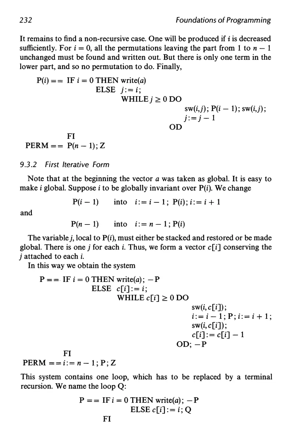
9.3.2 First Iterative Form
232
9.3.3 Second Iterative Form
235
Contents
XI
9.4 The Towers of Hanoi 242
9.4.1 Recursive Procedure 242
9.4.2 The First Form 243
9.5 A General Result 250
9.5.1 The Stack 251
9.5.2 Recomputing the Arguments 251
9.6 The Towers of Hanoi—Second Form 252
9.7 Remarks on the Two Solutions of the Towers of Hanoi 255
Exercises 258
Bibliography 261
Index 263
Preface
Informatics (or computer science or information processing) is too young
a science to have become the subject of many historical studies or philosoph¬
ical analyses. To me, however, its history seems quite exceptional. It is
normal for a science to be bom out of the observation of nature. When a
sufficient number of duly observed facts have been recorded, the outline of a
model can be sketched, and this in its turn allows the prediction of new
patterns of behaviour which are then subject to experimental verification.
Technology comes later, the model being confirmed, to a certain degree of
precision, by experiment, possible applications are conceived and come to
birth. The discovery of electricity is typical of such an evolution. The electric
motor and incandescent lamp did not appear until well after the develop¬
ment of the first theoretical models of electrostatics and of electromag¬
netism.
Much more rarely, technology has come before science. The steam engine
was built long before the science of thermodynamics enabled its output to be
calculated. In informatics we have an extreme example of this class.
The computer was engendered by the necessity for computation experi¬
enced during the Second World War. It was not the brainchild of some
brilliant dabbler, but the product of a technology founded on a well-estab¬
lished science, electronics, and supported by a no less well-founded mathe¬
matical model, Boolean algebra. There is nothing unusual about this. But it
was followed by wild speculation on the part of industrialists who believed
that such monsters might have applications in everyday life and who engi¬
neered these machines for the market. This theme is to be found developed
in a book by Rene Moreau [MOR].
From then on we have witnessed an incredible development of the means
of computation, requiring the support of numerous technicians—
operators, programmers, .... This in turn led to the need to establish
xiii
XIV
Preface
numerous new educational programmes, which began to be satisfied in
about 1960. But the universities which took responsibility for this realised
very quickly that they were not dealing simply with an application of the
science of electronics aided by a very old branch of mathematics, numerical
analysis. We were face to face with something fundamental, with a very old
activity of the human mind, but one whose significance we were not able to
grasp because there was no technical means of allowing it to take full flight.
In the same way as astronomy began with the telescopes of Galileo, but
was unable fully to develop until better means of observation became tech¬
nically possible, so informatics, the science of information processing, will
not be able to show itself clearly until the proper means are found to exercise
it [AR]. It would not be right to allow the reader to believe that what is said
here is an absolute and proven truth, recognised by universal consensus.
There are very many who believe in the existence of a science of informatics,
as is shown, for example, by academic instances in every country: in all the
great universities there are departments of “computer science”; the French
Academy defines ‘Tinformatique” as a science, and the French Academy of
Sciences has two headings “informatique” in its proceedings. But there are
just as many again who would restrict its scope, and deny it all claim to a
character of its own. In this sense, the position of the Academy of Sciences is
ambiguous: there is not one unique classification for informatics, as would
be the case for a well-established discipline, but rather two, one for theoreti¬
cal information science, a branch of mathematics concerned with the prob¬
lems posed by information processing, and the other at the level of “science
for the engineer.” Many professionals see in informatics nothing more than a
technique, sufficiently complicated to require a specific training, but of
narrow breadth. Bruno Lussato has become a champion of this idea, assert¬
ing that informatics can be learnt in three weeks [LUS].
I believe this to be a consequence of the very peculiar development of the
discipline. As had been said, the technology came first, founded as always on
a science, solid-state physics, but remote from its proper concern, the treat¬
ment of information. Since then we have spent much energy trying to master
techniques for which, the need not having been foreseen, we were never
adequately prepared. There has hardly been time to think. The history of
programming, within the history of informatics, is in this respect very re¬
vealing.
In the beginning there were the first computers, for which we had to write
programs in the only language which they could interpret, their own, the
machine language. This was extremely tedious, with a very high risk of error,
and so machine languages were very soon replaced by assembly languages,
maintaining in their forms the structures of the machine languages, and
offering no more distinct operations than the machines could cope with by
Preface
xv
hardware. It very soon became clear that the fragmentation of thought im¬
posed by the very restricted set of these primitive operations was a handicap,
and the first developed language, Fortran, appeared about 1955. This was a
decisive step. The choice of structures for this language and the manner of
writing of its compiler were to leave a deep mark on the history of program¬
ming.
In fact, the language was conceived fundamentally as an abbreviation of
assembly languages, and maintained two of their principal characteristics:
—the assignment instruction, or modification of the contents of a unit
storage in the computer,
—the idea of the instruction sequence, broken by the GO TO instruction,
conditional or unconditional.
Very many languages developed rapidly from this common origin. The
principal languages still in use today, Algol 60, Cobol, Basic, . . . , ap¬
peared over a period of at most five years. Lisp is of the same period, but it
deserves special mention; it was not constructed on the same universal
primitives, having no concept of assignment, no loop, no instruction se¬
quence, but it was based on the recursive definition of functions.
This language explosion, this modem Babel, has caused much dissipation
of energy in the writing of compilers, and in heated argument over a false
problem—that of the comparative merits of the different languages. Un¬
happily, this game has not yet stopped. Take any assembly, anywhere, of
sleepy computer scientists, and turn the discussion on to a programming
language. They will all wake up and throw themselves into the debate. If you
think about this, it is worrying, indeed deeply disturbing. All these languages
in fact have been built upon the same universal primitives, as has already
been pointed out; and the principal problems flow from this fact. Two of the
chief difficulties in programming practice arise from the assignment instruc¬
tion and the branch instruction. Why such rivalry between such close
cousins?
As long as we work ourselves into such excitement over these languages,
we are apt to forget that they are only a means of expression and that the
essential thing is to have something to say, not how to say it.
Ce que l’on conçoit bien s’énonce clairement et les mots pour le dire
arrivent aisément [BOI].
[“That which is well conceived can be expressed clearly, and the words for
saying it will come easily”—Nicolas Boileau, 1636-1711.]
The means for the construction of programs were rudimentary, indeed
non-existent. The literature of the period abounds in works of the type
“Programming in Basic” or “Programming in Fortran IV.” Teaching was no
XV/
Preface
more than the presentation of a language, a trivial matter for these languages
are remarkably poor. After that, the programming apprentice was left to his
own devices. Consequently, each one became self-taught, and no transmis¬
sion of competence was possible. The programmer of the eighties is no better
off than the programmer of the sixties, and the accumulated mistakes of
twenty years are there to prevent him avoiding the many programming traps
into which he will fall.
All this was done in an entirely empirical fashion. (I hardly know why I use
the past tense. If it is true that a few universities now operate differently and
that a small number of industrial centres have at least understood the signifi¬
cance of new methods and adopted them, how many more practitioners go
on in the same old way! More seriously, how many teachers, not to say recent
authors, remain faithful to what cannot in any way be described by the name
of “method.”) The programmer sketches out the work to be done and makes
a schematic representation of his program, setting out all the branch instruc¬
tions, in the form of a flow-chart. Then he writes out the instructions, and
begins the long grind of program testing. The program is put into the com¬
puter, and a compiler detects the syntactic errors. Some sophisticated com¬
pilers now even detect semantic errors (chiefly errors concerned with data
types). The program is corrected and eventually accepted by the compiler,
but that does not yet mean that it is correct. It still has to be made to run with
test data. If the results appear correct, the program is declared to be correct.
Otherwise, the program is examined for any apparent abnormalities, and
modified to prevent their unfortunate consequences. It is the method called
“trial and error” or, in the professional jargon, “suck it and see.” I have seen
it as practiced by a research worker in biology. His Fortran program was
causing problems, and he had, by program-tracing (printing instructions as
executed, with intermediate values), finally isolated his error. He then told
me with great satisfaction how he had put it right. His program began with
the declaration of two arrays:
DIMENSION A( 1000), B( 1000)
One loop involving the array A was running beyond the array bounds and
was destroying the values of B. I asked him how he had found the error which
caused the bounds to to exceeded, and how he had gone on to correct the
loop. But his reply showed he had done neither. He had simply doubled the
size of A:
DIMENSION A(2000), B( 1000)
How can anyone expect correct results from a program which is manifestly
false? How can he go on to publish a paper, saying “It has been found by
computation that. . .”?
Preface
XVII
It has been all too easy to denounce this lamentable state of the art [BOE].
Statistics-for 1972, dealing with sums of millions of dollars, give the cost of
writing as $75 per instruction, but after program testing $4000 per instruc¬
tion. In its estimates at the beginning of its bid for support for ADA, the
United States Department of Defense declared that if the cost of program¬
ming errors were to be reduced by only 1%, the total saving would be $25
million per annum. . . .
The answer has been sought in languages with tighter constraints. Increase
control by having more data types. I must be permitted to say that I do not
appreciate this line of reasoning. Let us take a comparison. Because certain
reckless drivers take needless risks and so endanger the community of drivers
and passengers, we need to multiply the methods of control and surveillance
— traffic lights, automatic barriers at stop signs, weighing devices at the
approaches to bridges, radar for speed control, . . . .All this translates into
inconvenience for the reasonable driver, penalised for the brutishness of a
few clods. Programming is going the same way. Just because my biologist
does not know how to look after his subscripts and lets them exceed their
declared bounds, at every call of a subscripted variable the run-time system
will make tests to ensure that there is no error, and too bad for me if I have not
made an error. These tests cost computing time, which costs money. I am
paying for fools.
The other cure, the one in which I believe, lies in teaching. The program¬
mer can be taught to work properly, to write correct programs, which he
knows are right, and why.
It is difficult to say who first launched this idea. “Notes on Structured
Programming” of Edsger Dijkstra is, in the view of many, the first important
text in this domain [Dll]. “Testing a program can show only that it contains
errors, never that it is correct. . . .”
Many research workers have addressed themselves to the problem of the
creation of programs, and we shall not attempt here to give an exhaustive
bibliography, being unable to do so and unwilling to risk being unfair. But
two works stand out along the way. In 1968, Donald Knuth began the
publication of a series of books entitled “The Art of Computer Program¬
ming” [KNU]. In 1981, David Gries published “The Science of Program¬
ming” [GRI]. From art to science in ten years! As far as we are concerned, the
most important step has been the introduction of inductive assertions by
R. Floyd [FLO] in 1967, the system axiomatised by Tony Hoare [HOA] in
1969. At first this was regarded as a tool for proving the correctness of
programs. But experience has shown that it can be very difficult to prove a
program written by someone else.
Assertions have been used, therefore, as the basis of a method of program
construction [AR1] [AR2] [GRI]. This method will be recalled in the first
XVIII
Preface
chapter, below. We presented it first in 1977, and again in a book in 1980,
trying to avoid as far as possible all mathematical formulation; that book was
intended primarily for school teachers, some of them certainly literate in the
humanities, and it was essential that its language should discourage none of
them. David Gries, on the other hand, regards it as essential to formulate the
assertions in terms of first-order logic, and discusses the relationship between
this and the logic expressible in natural language with AND and OR. We
shall say a few words here about this point. Because we have no wish to write
a book of mathematics, we shall as far as possible keep to assertions expressed
in natural language.
The program construction method is founded on recurrence. “Suppose
that I have been able to solve the problem up to a certain point. . . .’’If that
is the end, we stop. Otherwise, we move a step nearer the solution by going
back to the recurrence hypothesis. Then we look for a way to begin. In other
words, and in simplified, schematic fashion, suppose I have been able to
compute f(i). If i = n, and/(«) is required, the work is finished. Otherwise, I
compute f(i + 1) in terms of/(/), then I change i + 1 into i and start again.
Finally I compute /(0).
It is remarkable that the same reasoning, with little or no modification,
will produce a recursive procedure. We shall give in the second chapter a
certain number of examples of procedure construction for recursive func¬
tions. They do not use the assignment instruction, and so their programming
style is very different. It is nearer to axiomatic definition than to computing
strategy. It is computed through a very complex execution mechanism, but
also gives the possibility of deduction from the properties of the recursive
definition. We shall give several examples of this, particularly in connection
with the complexity or precision of computations.
If recurrence is the common base of iteration and recursion, we can build it
into a true programming language. It uses recurrent sequences of depth 1,
and the minimisation operator. In this sense, we can say that it is constructed
on the same universal primitives as its contemporary Lucid [ASH], proposed
by Ashcroft and Wadge. But we would not seek to develop a formal system,
and we use numerical indices for the sequences, although in fact we would
call only on the successor function of natural integers. The important thing is
to have a simple means of expressing recurrence, which is at the centre of the
whole of this study. We shall show how a recurrent algorithm can be inter¬
preted and transformed into an iterative program. Our aim is much less to
make of this a true programming language, endowed with good data struc¬
tures, and compilable by a computer, than to be able to write recurrent
algorithms in a recurrent language, and to have a simple method of extract¬
ing iterative programs from them. But why this diversion, when in the first
chapter we have shown how to create the iterative program directly? One of
Preface
XIX
the reasons is that this recurrent language has no assignment insthiction, and
so makes possible substitution, and hence the whole of algebraic manipula¬
tion. This allows a recurrent algorithm to be transformed easily into the form
best adapted for translation into a good iterative program. We shall give
several examples of this.
This language proceeds at the same time from recursion, for like that it is
not founded upon assignment, and from iteration, for like that it shows
sequences of values to be computed to reach a result. It is thus not surprising
that it can serve as an intermediary between recursion and iteration. We shall
show how a recurrent program can be created from a recursive function
definition. This will allow us to expose for examination the execution mech¬
anism of a recursive procedure, to study in depth the concept of the stack, not
laid down a priori, but deduced from the recurrent scheme, and to discuss the
further significance of this. We shall show afterwards how stronger hypothe¬
ses allow simplication of the iterative form, making the stack redundant in
some cases, and often leading finally to the reduction of a program to a single
loop.
Because recursion and iteration are two expressions of the same recur¬
rence, there must exist a simple transition from one form to the other. We
shall show in Chapter 5 how we can pass directly form the recursive defini¬
tion to an iterative program. A generalisation of the recursive definition gives
the recurrence hypothesis on which the iterative program can be con¬
structed. A substitution, a little algebraic manipulation, and then a unifica¬
tion lead to the body of the loop. This method is extremely powerful when it
can be used. Thus it provides a true mechanism for program synthesis.
Beginning with a recursive definition which describes the function, but says
nothing as to how it can be computed, we obtain an iterative program which
exhibits a computing strategy.
This method is valid only for recursively defined functions. For sub-pro¬
grams, other tools are needed. Just as recurrent sequences have played their
part as the hinge between recursion and iteration, so regular actions, pre¬
sented in Chapter 6, take on this double aspect, both iterative and recursive.
They can be interpreted as segments of a program which has branch instruc¬
tions, but also as recursive procedures without formal parameters or local
variables. In particular they are amenable to substitution (the replacement of
a procedure name by the procedure body), to identification (an expanded
form of identity between two actions), and to the transformation of their
terminal recursion into iteration. We show how this can be used to formulate
the program representing an automaton.
It can also be used for program transformations. We give in Chapter 7
three frequently used syntactic transformations, which do not depend on the
program’s semantics and which do not modify the sequence of computa¬
XX
Preface
tions defined by the program. But we may well need transformations acting
on this sequence if we are to modify, principally to shorten, it. We give some
transformations which depend only on local properties. With these tools, we
can build up more complex transformations or operate upon programs, for
example to make their termination become clear or to pass from one strategy
to another.
Regular actions and syntactic or local semantic transformations allow
operations on iterative programs. To operate on recursive sub-programs, we
need a more powerful tool. Thus we introduce generalised actions, and show
how they can be regularised. This allows us to pass from parameterless
recursive procedures to iterative procedures, if necessary through the intro¬
duction of an integer variable. To operate upon procedures with formal
parameters and local variables, we must first make semantic transforma¬
tions replacing the formal parameters and local variables by global variables.
We give a first example in Chapter 8.
But that is concerned with the most powerful tool we have for operating on
programs, and its presentation leads us to develop some examples which are
both longer and apparently more sophisticated. We delve more deeply into
the study of the replacement of formal parameters and local variables by
global variables. We try to spell out the choices which are made during the
transformation process and to demonstrate their importance.
For we end up, in fact, with a new method of programming. We create a
recursive procedure; by semantic transformations we pass to global vari¬
ables; by transformations into regular actions, and their subsequent manipu¬
lation, we obtain an iterative program which often seems to have very little
left in common with the initial procedure. During a meeting of an interna¬
tional working group at the University of Warwick in 1978, where I pre¬
sented this mode of operation, Edsger Dijkstra strongly criticised it, compar¬
ing it with the analytical geometry of Descartes. For him, it is worse than
useless to spend hours in covering pieces of paper with tedious computa¬
tions, just to get in the end a simple program which a little reflective thought
would have revealed directly. He thinks that it is a waste of time for me to
teach methods of computation which apply to programs and that I would do
better to teach people how to think and how to ponder.
I am sensitive to this criticism. It has truly become an obsession with
me—how does one invent a new program? How do you get a simple idea
which turns into a simple program? I have not for the moment any answer,
and I am afraid there may not be one. Human beings have been confronted
with the problem of creativity for thousands of years, and we still have not a
chance of being able deliberately to create anything new. Nonetheless, the
constraints of computer technology have thrust the assignment instruction
on us, and obliged us to invent new forms of reasoning. Recurrence is an old
Preface
XXI
form of reasoning; iteration and recursion are creations of informatics. This
book tries to shed some light on their relationships. Will this result in new
ways in matters of program creation, and thence, in problem solving?
For me, analytical programming is a new path of discovery. From simple
premises, and by computational methods which hardly change from one
example to another, I can obtain a simple program in which what I am
looking for—a simple strategy—is to be found. In his book, David Gries
says that when we have obtained a simple program in this way, we should
forget the twisted path by which we have come, and look for the straight road
which leads directly to it [GRI]. It would indeed be a good thing to have only
a simple way of producing a simple result. But I do not think that this would
necessarily benefit the student or programming apprentice. He may well be
filled with admiration for the master, but is it not a deceit to be made to
believe that the master has an excess of inventive genius when, on the
contrary, it is computation which has been the principal instrument of his
success?
In this book, we should like to illustrate the mechanism for the creation of
programs by computation, that is, “analytical programming.” We have not
hesitated, in developing the working, freely to jump over several clear but
tedious steps from time to time. We immediately ask the reader on each of
these occasions to do the computations himself, if he wishes to make the
most of what is in front of him.
Henri Ledgard [LEI] has recognised good style with his programming
proverbs. He might have included, from Boileau: “Qui ne sut se bomér ne
sut jamais écrire” [“No one who cannot limit himself has ever been able to
write”]. A cruel proverb, and I have suffered a lot here. There are so many
extraordinary examples of program transformations, revealing altogether
unexpected strategies. . . . How to choose the best of them? Where to pub¬
lish the others? I have tried to be content with examples not requiring too
much computation and yet producing spectacular results. I have tried hard
not to reproduce the examples of my previous book, still valid even if I have
abandoned its notation as too unreadable and my methods of computation
rather too sketchy [AR2]. The reader may wish to refer to it if he needs
further examples.
If he learns from this book that recurrence is the foundation of methodical
informatics, that recursion is an excellent method of programming, and that
there are in general simple transitions from recursion to iteration, I shall
already have achieved an important result. But I have been a little more
ambitious: has the reader been convinced that computation is a reliable tool
for the creation of programs?
I am anxious to warn the reader that this book revives my previous work
[AR2], continuing much of its argument in terms which are, it is hoped,
XXII
Preface
more simple. Since it was written I have had much new experience, both in
transforming programs and in teaching students. This new book brings all
these things together. I hope the result is rather more readable. . . .
Finally, exercises have been given, because it is not the result which is
significant, but the way in which it is obtained. This aspect needs to be
developed completely—but to do that I shall have to write another book.
List of Programs Discussed in the Book
(Numbers in parentheses are chapter and section numbers.)
Exponentiation
Computation of xn, x real, n natural integer: An incorrect program (1.1),
discussed (1.4), corrected (1.4). Recursive forms (2.2.2), precision (2.5.2),
complexity (2.5.3). Computation (2.3), transformation to iterative (4.2).
Factorial
Computation of «!: recursive form (2.2.1), aberrant form (2.6.1). Var¬
iously derived iterative forms (4.6.1, 4.6.2).
String reversal
Mirror image of a character string, NOEL giving LEON: Recursive defini¬
tion (2.2.3), its nature (2.4), complexity (2.6.2). Transformation to itera¬
tion (5.3.1), added strategy (5.3.1). Application to the representation of an
integer in binary; conversion of an odd binary integer into the integer
whose binary representation is the image of that of the given number,
recursive and iterative forms (5.5).
Conversion of an integer to base b
Regarded as a character string: recursive definition (2.2.4), property
(2.5.1). Regarded as a decimal number: beginning with n = 5 and 6 = 2,
write 101 (the number one hundred and one, not the string one, zero, one).
Recursive definition (4.8.2), transformation to recurrent (4.8.2), to itera¬
tive (5.3.2).
Fibonacci sequence
Dyadic recursive definition (2.2.5): computation (2.3.2), complexity (2.7),
transformation to monadic recursive procedure (2.7), complexity (2.7),
recurrent form (3.6.3).
Product of two integers
Dyadic recursive form (2.2.6): transformation to monadic (4.8.1), then to
iterative (4.8.1). Other iterative forms (9.2). Recurrent form from another
algorithm (3.6.1), associated iterative form (3.8.2).
XXIII
XXIV
List of Programs Discussed in the Book
Hamming sequence
Sequence, in increasing order of integers with no other prime factors than
2, 3, or 5:
2 3 4 5 6 8 9 10 13 15 16 18 20 24 25
27
Recursive definition (2.7), iterative form (5.7).
“Function 91”
A dyadic recursive definition which computes a constant: Definition,
value, complexity (2.8.1).
Christmas Day
Recurrent algorithm giving the day of the week on which Christmas Day
falls in a given year (3.1).
Perpetual calendar
Gives the day of the week corresponding to a specified date (3.2).
Integral square root
Recurrent algorithm and improved forms, associated iterative forms (3.9).
Iterative form operating in base b by subtraction of successive odd num¬
bers (3.10).
Euclidean division of integers
Recursive form (4.1.1), associated iterative form (4.3).
Addition of integers by successor and predecessor functions only
Recursive and associated iterative forms (4.7.2, 4.7.3).
Longest common left-prefix of two integers in base b
In base b, the two integers are represented by character strings; the longest
common prefix (leftmost part) of the two strings is taken as representing
an integer in base b, the required result (5.4).
Greatest common divisor of two integers
Recursive form based on Euclid’s algorithm and associated iterative form
(5.4), automatic change of strategy (7.9).
Happy numbers
Sequence of integers obtained from a variant of the sieve of Eratosthenes,
by crossing out at each stage only numbers which have not yet been
crossed out. Complete elaboration of an iterative form, improvement, and
comparison with another form (5.6).
Equality of two character strings apart from blanks
Automaton (6.1), change to an iterative program and improvement (6.8).
List of Programs Discussed in the Book
xxv
Search for a sub-string in a given string
Automaton (6.7.2), iterative form (6.7.2), change of form (6.3).
A problem of termination, due to Dijkstra (7.8)
Closing parenthesis associated with an opening parenthesis
Recursive form (8.1.1), assembly language form (8.1.3), iterative form
with counter (8.3).
Permutations of a vector (9.3)
Towers of Hanoi (9.4, 9.6, 9.7)
Notations
These are not intended to be learnt by heart, but only, should the need arise, to be consulted in
cases of doubt.
♦
/
!
t
a[i. . . j]
a[i. . . j] < c
AND, and
OR, or
sbs(c, i, “ ”)
sbs(c, i,j)
sbs(c, /, i)
“< Sequence of
characters not
including a
quotation mark>”
CC 99
pos(c, i, d)
Multiplication sign
Integer quotient (only for natural integers)
Real division
Sign for concatenation of character strings giving
the string resulting from placing the operand
strings end to end
Exponentiation, x T n = xn
Sequence a[i\, a[i + 1],. . . a\j\, empty if j < i
Equivalent to a[i\ < cAND a[i + 1] < cAND. . .
a\j] < c
Forms of the boolean operator giving the value
TRUE if and only if the two operands both have
the value TRUE
Forms of the boolean operator giving the value
FALSE if and only if the two operands both have
the value FALSE
Sub-string taken from the string c beginning at the
character in position i and finishing at the end of c
Sub-string taken from the string c beginning at the
character in position i and comprising j charac¬
ters
Special case of the foregoing: the character of c in
position i
A constant string whose value is the string enclosed
between the quotation marks
Empty constant string
c and d are character strings; the value of this func¬
tion is 0 if d does not occur within c with its
XXVH
XXVIII
Notations
leftmost character at a position > i; otherwise it is
the position (rank) of the beginning of the first
occurrence of d in c beginning at position i
=> Implication sign; P —■* Q is false if and only if P is
false and Q is true
— Definition sign for recursive functions, or, depend¬
ing on the context, syntactic equivalence of se¬
quences of instructions (equivalence maintain¬
ing the history of the computation)
f [a —* b\ Its value is the string of characters representing f in
which every occurrence of a has been replaced by
an occurrence of b (substitution of b for a, or
change of a to b)
FI Closing parenthesis associated with the opening pa¬
renthesis IF; the selection instruction can take
one or other of the two forms
IF t THEN a ELSE b FI
IF t THEN a FI
If t is true, the sequence of instructions a is exe¬
cuted; otherwise b is executed if it exists, or noth¬
ing is done if it does not. The closing parenthesis
FI makes it unnecessary to enclose the sequences
a and b between BEGIN and END
WHILE t DO a OD Is the loop, which can also be represented by
L: IF NOT t THEN GOTO L' FI;
a;
GOTOL
L': continue
REPEAT a UNTIL t Is the loop, which can also be represented by
L: a;
IF NOT t THEN GOTO L FI;
continue
EXIT Instruction causing the immediately enclosing loop
to be left and execution to continue in sequence
with the instruction written immediately after the
loop
EXIT(p) Leave p immediately enclosing nested loops and
continue in sequence. EXIT(l) is the same as (is
abbreviated to) EXIT
Notations
XXIX
EXIT(0)
DO...OD
[[< Predicate >]]
INTEGER
Empty instruction
Parentheses enclosing a loop; OD may be consid¬
ered as an instruction to repeat the execution of
the instructions of the loop, conditionally if the
loop is prefixed by a WHILE clause
Assertion; relation between the variables of the pro¬
gram, true at the point at which it is written
The set of natural integers
Translator's Introduction
No computer programmer of any experience can feel complacent about
the state of his craft. It is, as it has always been, in a mess, and nowhere more
so than in that part of programming practice to which the beginner is nowa¬
days most likely to be first exposed—the software of the more popular
microcomputers, including those provided by beneficent authorities in more
and more of our schools. It seems as if nothing has been learned from the last
thirty or forty years. Future professional programmers are helped neither by
those of their teachers who become obsessed with the messier details of some
assembly language or variation of “Basic” nor, at a “higher” level, by those
who distance themselves as far as possible from actual computers and whose
theories are developed upon pseudo-mathematical wishful thinking.
Professor Arsac’s method is based on the definition and unification of
many techniques known to, and practised by, good programmers over the
years. In the hands of the new programmer who is prepared to work thor¬
oughly and carefully, this book cannot fail to lead to the production of
programs of which he can justly be proud. The teacher who may have
despaired of finding a way of communicating a plain and straightforward
approach to the programmer’s task will find new hope and no little comfort
in these pages. Only the “computer junky” with chronic “terminal disease”
and the self-appointed high priest of fashionable programming theory will
fail to appreciate the value of Arsac’s work.
Good programming is not a mysterious art dependent on inspiration
granted only to the genius, nor is it an automatic product of the use of the
latest commercial system. Arsac shows, with numerous and remarkably
appropriate examples, that it is the result of painstaking thoroughness helped
sometimes by luck.
xxx/
XXXII
Translator's Introduction
Arsac’s book deserves a place on the desk of every programmer and
would-be programmer whose concern for the quality of his work is more
than superficial.
Clevedon F. G. Duncan
1984
Chapter 1
Iterative Programming
1.1 An Incorrect Program
We have remarked already on the poor state of the art of programming—
here is a piece of evidence of this. In the January-February 1979 issue of
Ordinateur Individuel [in English, Personal Computer], Didier Caille [CAI]
published the following program (the language used is LSE, which means very
little here; the semantic intention of the instructions of this little program is
self-evident):
1 * Personal computer
2 * example of arithmetical calculation
3 PRINT “this program calculates x to the power n”
4 PRINT “give me x please; READ x
5 PRINT “give me n please:”; READ n
6 IF n < 0 THEN BEGIN PRINT “n positive, please”; GOTO 5 END
7 a <- x
8 i <-0
9 a<r- a*x
10 i <— i + 1; t <— n — 1
11 IF i < t THEN GOTO 9
12 PRINT a
13 FINISH
From the text printed by line 3, we know the object of this program. From
line 9 we can see that it is meant to work through repeated multiplication by x,
but it is very easy to see that it is incorrect. Let us execute it “by hand” for a
simple pair of input values, x = 2 and n = 1.
7
2
Foundations of Programming
From line 6, n = 2 being greater than 0, the program continues at line 7, where
a takes the value of x; that is, a = 2. In line 8, i = 0. In line 9, a is multiplied by
x:a = 2 * 2 = 4. In line 10, i is increased by 1: i = 1; t takes the value of n — 1;
i = 0. In line 11, i = 1 is not less than t ( = 0), and so the program passes
to line 12, and the result 4 is printed for the value of x = 2 to the power
n = 1—evidently false.
We should be astonished by this. In any other discipline, the publication of a
false result would be considered abnormal, even scandalous. It is admitted in
informatics that the writing of a correct program is exceptional, and thus that
error is normal. As long as this point of view is sustained, no progress will be
possible, but we should not throw stones at the author of this little program.
We can find equally elementary mistakes in many other books.
Many programmers will react by carrying out tests on this program in order
to localise the error, but this is no way out. For even if we arrive at a version of
the program which will pass the tests, what can we infer if we still do not
understand how it works and why it gives the expected results? “Testing a
program allows us to show that it contains errors, never that it is correct”
(Edsger W. Dijkstra [Dll]). We need tools and methods for describing the
functioning of a program.
1.2 The Assignment Instruction
This instruction, which can change the value of a variable, is often a cause of
obscurity in programs which use it. It is denoted by the sign <- in APL and
LSE. More frequently, we use the sign : = , as in ALGOL and PASCAL.
Consider the sequence
x:=x + y; y:=x — y; x:=x — y
It is very difficult to see the effect of this by inspection alone. By its nature, an
assignment instruction realises a transformation; it changes the state of a
variable. To set out the effect of this sequence, we need to describe the set of
states generated by the three instructions. We place the description of a
state—represented by a relation involving the constants and variables of the
program—between the signs [[ and ]]. Thus, if a and b are the initial values of
the variables x and y, we may write
[[x = a y = bj] x : = x + y
We execute the instruction x : = x + y with the values a and b of the variables x
and y; y remains unchanged.
7 Iterative Programming
3
[[x = a y = bj] x: = x + y [[x = a + b y = bj\
The next instruction changes only y:
y: = x — y [[x = a + b y = (a + b) — b = d]~\
The final instruction changes x:
x: = x — y [[x = (a + b) — a = b y = aj]
Thus the final values of x and y are their initial values interchanged. Let us be
quite clear as to what we have done. We have placed between the instructions
comments in the form of predicates describing the state of the variables. The
passage from one state to another is achieved by the execution of the
instruction upon the values of the variables given by the predicates.
The affirmation of a relation holding among the variables of a program at a
given point is called an “assertion”. An instruction effects a transformation
upon a predicate. To say how an instruction modifies the assertion which
precedes it (its “preassertion”) to give that which follows or succeeds it (its
“postassertion”) is to define the semantics of that instruction. We shall
examine more closely the effect of the principal instructions on the assertions.
First, however, we shall look again at the part played by the three instructions
of our example. They are, with their assertions,
[£x = a y = bj]
[[x = a + b y = bj]
[[x = a + b y = a]]
[[* = b y = a]]
Let us suppose that the numbers a and b are “real”, and that b is very small in
comparison with a. The calculations are carried out with a constant number of
significant figures. To the precision of the arithmetic, b is negligible compared
to a, and the addition of b does not change x. So,
[[x = a y = £>]] x: = x + y
[[x = a y = b]] y:= x — y
Again, subtracting b from a has no effect:
[[x = a y = aj] x: = x — y
[[x = 0 y = a]]
The exchange of values does not take place. There is 0 in x and a in y. This
shows how the mechanism of assertions can be a very fine instrument
describing even the way in which calculations are executed in the computer. It
allows a very precise interpretation of the effect of a sequence of instructions.
It is this which enables us to give a meaning to a program.
x:= x + y
y:=x-y
x:= x — y
4
Foundations of Programming
1.3 Assertions and Instructions
1.3.1 Assignment
Consider an assignment instruction modifying the variable x. Two cases
are possible:
x is given a new value independent of its old value. We write for this case
x: = a (constant relative to x).
x is given a value calculated from its old value. We write this as x: = f(x).
These notations say nothing about the possible dependence of a and f(x) on
other variables in the program. The preassertion will be denoted in the form of
a predicate linking x to the other variables of the program; thus P(x, y). This
does not require x to depend on these other variables, symbolised by y, but
implies only that in the most general case, x bears a certain relation to them.
If initially
[CP fry)]} *:=a
the old value of x being destroyed, the relation with the other variables,
represented by P is also destroyed:
[[P(x, y)]] x:= a [[* = a]]
If a is a function of y, we have created a new relation between x and y.
Suppose now x: = f(x). We shall introduce for the sake of clarity a new
intermediate variable x' such that the sequence
x':=f(x); x:=x'
is equivalent overall to x: = f(x).
We now have two assignments of the preceding type:
[[P (x,y)]] X':=f(x) [[P(x,y) and x'= f(x)]]
Giving x the value of x' through x: = x' is the same as replacing x by x'.
Suppose first that f(x) has an inverse f-1 such that x' = f(x) is equivalent to
x = f“ V)- Then,
P(x, y) and x' = f(x)
is equivalent to
P(f_1(x'),y) and x = f-1(x')
If we now give x a new value, its previous value is destroyed, and x appears in
the place of x'. Finally,
[[P(f-1(x'),y) and x = f_1(x')]] x:= x' [[P(f-1(x)> y)]]
1 Iterative Programming
5
If we eliminate the intermediate variable by simplifying the assertions, we are
left with
[[P(x,y)]]x:=f(x) [[Pr1«^)]]
The algebra also comes out neatly if the predicate P(x, y) is itself of the form
Q(f(x),y):
[[<№), y)]] *':= f(*)
We replace f(x) by x'
[[<№), y)]] x':=f(x) [[Q(x',y)]]
x:= x' [[Q(x, y)]]
or, finally,
[[Q(fW,y)]]x:=f(x)[[Q(x,y)]]
Where f has an inverse, the two methods give the same result. If in fact
P(x, y) = Q(f(x), y), then the substitution for x of f-1(x) in P gives
P(f_1(x),y) = Q(f(f-1(x)),y) = Q(x, y).
These results are at first sight surprising. Let us therefore look at their
application to some simple cases.
Suppose we have
[[x > 0]] x: = x + 1
It is clear that increasing x still leaves it positive but does not allow it to be
zero. We must therefore have as postassertion x > 0. With f(x) = x + 1,
f_1(*) = X - 1,
[[x > 0]] x:= X + 1 [[x - 1 > 0]]
The postassertion is equivalent to x > 1 or x > 0. In the same way, for any
preassertion involving x,
[[P(x)]] x: = x + 1 [[P(x - 1)]]
This is one of the most serious difficulties in the explanation of information
processing to those who are not scientifically trained. We can get across the
idea of the situation (state of variables characterised by predicates) being
modified by instructions which act as transformations. But it is not easy to
explain why a situation involving x is transformed into the same situation but
involves x — 1 by the execution of x: = x + 1. Of course, we might say that if
an observer has arrived at x, and if x is advanced, then everything happens as if
the observer had stepped back relative to x, and so sees no more than x — 1. It
is not entirely convincing.
6
Foundations of Programming
We should also note that it is not at all certain in general that f has an
inverse. If we suppose n to be an integer variable
[[P (")]] n:=n:2
we can affirm nothing more, at least not without introducing a new variable r
having the values 0 and 1 for the remainder of the division by 2. Then,
[[P(»)]] n:=n:2 [[P(2*n + r)]]
More precautions are now needed in the development of the assertions.
All this shows the extent to which the assignment instruction is difficult to
manipulate and to interpret. We shall have many occasions to return to these
problems.
1.3.2 Selection
The instruction of selection,
IF condition THEN ELSE FI
(where FI is the closing parenthesis associated with the opening parenthesis
IF) distinguishes in a given situation between two sub-situations, depending
on whether the condition is satisfied or not:
[[P]] IF t THEN [[P and i]] ELSE [[P and not t]] FI
The “test” part of the instruction is not transformational in nature and has no
effect on situations; it serves only to distinguish the two possible cases.
This is why it would be indeed abnormal for the evaluation of the condition
t to modify any variable whatever; for example, as a side effect of a function
procedure. In the general case, it is difficult to say what this means for the
postassertion of a selection. Let f be the set of instructions of the alternative
“true” and g that of the alternative “false”!
[[P]] IF t THEN [[P and t]] f [[P']]
ELSE [[P and not t]] g [[P"]]
FI [[P' or P"]]
However, in many cases the object of this instruction is to attain the same final
situation whatever the initial condition t. We will then have P' = P".
1.3.3 Branching Instruction
The GOTO instruction does not modify any variable of the program and
thus does not operate upon states. If a is a label referring to an instruction and
7
1 Iterative Programming
P the preassertion of the GOTO instruction, then
[[P]] GOTO a [[P]]
that is, [[P]] is also the preassertion of the instruction labelled by a. In other
words, the GOTO instruction links two points in the program characterised
by the same situation.
This remark is of very great importance. It has been said that branching
instructions are dangerous and to be avoided [DI2], [LEI]. They are inimical
to the legibility of the program, the reader having to jump frequently from one
place to another. This has happened as a result of the abuse of these
instructions. Nevertheless, when we are confronted by a situation which has to
be decomposed into two, we are obliged to consider these two one at a time.
The human mind is constrained to consider first one and then the other. The
branching instruction may involve the anticipation of a situation which will be
considered later (GOTO “further down”, “forward jump”) or the recon¬
ciliation with a situation already encountered and dealt with (GOTO “back
up”, “backward jump”).
The greatest danger arises out of the way in which the programmer
considers this instruction. Most often, it is seen as the answer to the question,
“What to do next?”, being read as “go to such a point in the program to do
such an action”. Rather, it must be seen as a reply to the question, “Where are
we now?”. It is absolutely necessary first to think in terms of situations and
then to deduce from these situations what to do. My experience of teaching
extremely diverse groups has convinced me that the backward jump is in
general less dangerous than the forward jump. In the former case, a situation
already encountered is found again. The programmer knows enough about
what he has written to find the right point in the program. The forward jump is
in contrast an anticipation of a situation which is to be dealt with later and
whose details are as yet unknown. The programmer rarely bothers to work
them out there and then, promising himself to deal with them later. When he
does so, he has forgotten some details, and the result is in error. For the sake
of prudence, at every forward jump we should write, as commentary, a
description of the corresponding situation which will have to be matched later
on.
1.3.4 The WHILE Instruction
This instruction is written
WHILE iDOaOD
where t is a test, and a is a set of instructions. It is equivalent to
L : IF t THEN a ; GOTO L FI
8
Foundations of Programming
Let P0 be the situation at the beginning of the execution of this instruction.
The preassertion of a is P0 and t. The execution of a produces a postassertion
Px. The instruction GOTO L links two points of an identical situation so that
either Pt = P0 or at least Px is a particular case of P0 (Pt implies P0). Usually, P0
and Pt will be particular cases of the same general situation P encompassing
all these particular cases, so we will have
[[P]] WHILE £ DO [[P and £]] a [[P]] OD; [[P and not £]]
The assertion P and t is true at each repetition of a and thus invariant over the
execution of the loop. When t becomes false, P is still true so that at the exit
from the WHILE instruction, we have P and not t. As at the entry we already
have P, we can say that the effect of the loop is to obtain the realisation of not t
while conserving P.
7.3.5 The Loop
The loop which we consider most often in this book comprises a list of
instructions forming the body of the loop and including one or several EXIT
instructions, denoted here by f(EXIT), including a sequence of instructions
containing at least one occurrence of an EXIT instruction. The loop is
enclosed in the loop parentheses DO OD:
DO f(EXIT) OD
OD, the closing parenthesis of the loop, can be considered as an instruction
sending one back to the head of the loop. EXIT means “leave the loop and
continue in sequence”. This loop is thus equivalent to
L : f(GOTO L') ; GOTO L ;
L':
As in the case of the WHILE loop, the postassertion of f is the preassertion
of GOTO L and so must imply the preassertion of L. This assertion is thus
invariant through the loop.
If P is the preassertion of the loop and Q that of the EXIT instruction (or
the union of those of the EXIT instructions if there are several such), then
CCP]] DO
[[P]] f([[Q]] EXIT)
OD;
[[Q]]
This loop being rather more general than the WHILE loop, there is not
necessarily a simple relationship between P and Q. This depends on the
1 Iterative Programming
9
structure of the sequence of instructions f. Experience shows, however, that it
is amenable to a systematic analysis. We return to this point later in the
chapter [AR1].
I. 4 The Interpretation of a Program
The idea of assertion was proposed by R. Floyd [FLO], as a means of
giving a meaning to a program, and then formalised by C. A. R. Hoare
[HOA]. We shall use it to study the program by Didier Caille (Section 1.1).
There is a loop from line 9 to line 11, and so we must have at the entry to line
9 an assertion which will be invariant through the loop. It will involve the
variables of the loop, which are a and i. As this program is intended to
compute x", let us suppose, as hypothesis, that a is of the form x\ We arrive for
the first time at line 9 from line 7.
7. a <- x [[a = x]]
8. i«- 0 [[a = x and i = 0]]
A possible assertion here is a = xl+1. Let us see what will lead to this
assertion:
9. [[a = xi=1]] a <- a * x [[a/x = xI+1, that is a = xl+2]]
10. [la = xi+2J] i«- i + 1 [[a = xi+1]]
We note that the assertion a = xi+1 has been re-established with a greater
value of i. We must adjust i by reference to n. As t = n — 1,
II. [[a = xi+1]] IF i < t THEN [[a = x£+1 and i<n- 1]] GOTO 9
12. [[a = xi+1 and i>n— 1]]
If, in 12, the equality is attained, then
a = xi+1 and i = n — 1
giving a = xw, and the program is correct.
We note also that the GOTO instruction of line 11 leads to line 9 with the
assertion
a = xi+1 and i < n — 1
If we use this assertion, we must have for the preassertion of line 10:
10. [[a = xi+2 and i<n— 1 ]]i «- i,+ 1 [[a = xi+1 and i<n — 1]]; t +-
n — 1
11. IF i < t THEN [[a = xi+1 and i < n - 1]] GOTO 9
12. [[a = xi+1 and i = n — 1 thus a = x"]]
7 0 Foundations of Programming
Thus we shall arrive at line 12 with the correct assertion if we can reach line 9
with
a = x‘+1 and i < n — 1
But by the initialisation
a = x and i = 0
We must therefore have 0 < n — lorn>l. We have the result we have been
looking for—the program computes a = x" for n > 1 only.
It is not very easy to correct this. It appears likely that the author has chosen
his terminating condition badly and that he has sought to correct it by
introducing the variable t, computed in line 10, whose value is thereafter
constant. Its computation inside the loop is abnormal.
We have said that situations have primacy over actions. To re-edit the
program, we must first describe a general situation. Suppose that we had done
part of the work and had calculated a = x‘ for a value of i<n (it would be
absurd to suppose i > n, for that would mean that the computation had gone
too far):
9. comment: we have computed a = x‘ and i < n
If i = n, we have finished:
10. IF i = n THEN GOTO 12
If not, we must get nearer to the solution by incrementing i:
11. a<- a*x; i*- i + 1; GOTO 9
It remains to find values of a and i such that hypothesis 9 is verified for all n,
positive and zero. We must take i = 0 and then a = x° = 1. Hence the new,
correct, program:
3 PRINT “this program calculates x to the power n”
4 PRINT “give me x please:”; READ x
5 PRINT “give me n please:”; READ n
6 IF n < 0 THEN BEGIN PRINT “n positive, please”; GOTO 5 END
7
8 a <- 1; i«- 0
9 comment: a = x‘ and i < n
10 IF i = n THEN GOTO 12; comment: a = x‘ and i = n gives x = a"
11 a •«- a * x; i <- i + 1; GOTO 9
12 PRINT a
13 FINISH
1 Iterative Programming
1.5 Recurrent Construction of Iterative Programs
11
The exercise we have just carried out may appear difficult to the reader.
Indeed, there are many who think that the proof a posteriori of a program
already written is a labour at the limit of what is possible. The only way to
arrive at a soundly based program is to construct it on a foundation of its
assertions. We have established, above, a methodology of programming
[AR1], [AR2].
A program describes the set of transformations which must be executed by a
computer for it to pass from the situation of its initial state (the data) to that of
its final state (the results). If the way from one to the other is not direct, we must
mark it by means of intermediate situations.
The iterative solution of a problem rests upon the loop instruction,
characterised by the invariance of its situations. The construction of a loop
depends on the choice of the invariant situation with which it is associated. To
construct a loop, a good method is the following:
-specify a general situation, invariant for the loop, which might be called a
“recurrence hypothesis”;
-see whether it is finished (and if so leave the loop);
-if not, move towards the solution while maintaining the recurrence
hypothesis (or by re-establishing it, for one will in general be obliged
temporarily to discard it);
-begin the process by finding initial values compatible with the problem and
satisfying the recurrence hypothesis.
Rather than remain at a pseudotheoretical level, we shall present this
through a well-known example in order to show how one can choose such a
recurrence hypothesis and the consequences of this choice. Suppose we have
to sort a vector a of n elements a[\... ri]. We wish to find a permutation of this
vector by transposition of its elements such that each element of the resultant
vector is less than or equal to that which follows it (its successor):
a[i] < a[i + 1] for all i such that 1 < i < n
The most usual way to formulate a recurrence hypothesis is to suppose that
we have done part of the work. Suppose that we have sorted by transpositions
part of the vector; that is, a[l...i] has been sorted, where i < n, by
transposition. The work is finished if all of the vector has been sorted; that is, if
i = n. If not, we must extend the sorted part. For this we bring x = a[i + 1] to
its proper place in the sorted part of the array, also by transposition. Hence the
program
12
Foundations of Programming
i:= 1;
DO
[[a[l... i] sorted by transposition]]
IF i = n THEN EXIT FI;
x: = a[i + 1];
put x into its proper place in a[l... i + 1] by transposition;
i:= i + 1;
OD
Any implementation of the action “put x into its proper place in
a[l... i + 1] by transposition” gives a sorting program. One might either
-first find the place for x and then put x into this place by transpositions, or
-realise the operation directly by recurrence.
In the former case, the search can be done linearly or by using dichotomy.
We give here a program based on a linear search:
i:= 1;
DO
[[a[l,..., i] sorted by transposition]]
IF i = n THEN EXIT FI;
x: = a[i + 1];
j:= i + 1;
DO
[[the place for x is at j or below]]
IF; = 1 THEN EXIT FI;
IF a[; - 1] < x THEN EXIT FI;
j- = j~ 1
OD;
k:= i + 1;
DO [[the elements above k have been moved up]]
IF k = j THEN EXIT FI;
a[fc + 1]: = a[fc] ;k: = k — 1
OD;
a[fc] := x;
i: = i + 1
OD
One remark is needed. We have written the assertions in plain language. This
has the effect of simplicity and allows this method of working to be put within
the reach of those without a strong mathematical background. But there are
hidden snags too. Thus, for example, the assertion
[[the place for x is at j or below]]
13
1 Iterative Programming
means that the place for x cannot be above j
-either because j is the highest position which it can take, j = i + 1;
-or because the elements above j belonging to a[l ...i] are greater than x,
all of which can be written as
j < i implies for all j such that j < j' < i, x < a[/]
The reader concerned for rigour will work with such assertions. Our intention
is not to give a course in mathematics. We make use of mathematics here as
physicists and chemists have always done. But it is as well to remain clear, to
know that perhaps these assertions in plain language can become a source of
ambiguity, and not hesitate to have recourse to a more rigorous formalism.
The program we have just written contains two successive loops inside a
larger enclosing loop. The second internal loop causes k to run through the
same values as are taken by j in the first. One may wish to combine these two
loops into one. This is a problem in program transformation, which will be
dealt with in later chapters.
We leave as exercises for the reader the problems of realising the sorting
program (a) through the method of dichotomy, and (b) by putting x at each
stage directly into its place by successive transpositions with preceding
elements.
1.6 Partial Correctness
To resolve a problem there is not in general a unique recurrence hypothesis.
For each hypothesis there is a corresponding program (if the hypothesis is
acceptable!). The effect of the choice of hypothesis on the form of the resultant
program is difficult to predict. We shall develop some other sorting programs
to illustrate this point.
We have taken as a recurrence hypothesis “a[ 1 ...f] has been sorted by
transposition”. Let us.now take a weaker hypothesis. We cannot abandon the
affirmation that we have only made transpositions; that is part of the
statement of the problem. Thus there remains as recurrence hypothesis
[[only transpositions have been made]]
It appears unlikely that we should be able to proceed on such a feeble
hypothesis. But, nonetheless, it is true that we have worked towards the object
of the sorting; that is, we have reduced the disorder of the vector. If we apply
the proposed method strictly, we must now test whether it is finished. In the
absence of precise information on the state of the vector, one cannot decide
14
Foundations of Programming
this by a simple test. To know if it is finished, that is to say if the vector has been
sorted, we return to the definition of the sort: the result is a permutation of the
initial vector (which is assured by the fact that we have only done trans¬
positions) such that for all i less than n
a\i~\ < a[i + 1]
The work is not finished if this condition is false, and there is a value of i less
than n such that a[z] > a[i + 1].
If we find such an i, the sorting is not finished. We must go back to the
recurrence hypothesis (that is to say, that only transpositions are done) to
reduce the disorder of the vector. We know that a pair of consecutive elements
is badly ordered. We transpose these two elements. At the beginning, we take
the vector as it is; having done nothing, we have satisfied the recurrence
hypothesis
DO
[[we have made only transpositions]]
see whether there is a value of i such that a[i] > a[i + 1];
IF none such THEN EXIT FI;
interchange a[z] and a[i + 1]
OD
We shall deal later in detail with the three parts of this program, simple enough
in other respects, which are here suggested in informal language. We have here
a simple program, “partially correct”—and that remark may seem not
particularly interesting. If the program stops, it gives the right result. We can
be sure of this because it will not leave the loop, through EXIT, unless and
until the vector has been sorted. It is this which is meant by “partial
correctness”—a program which gives the right result if it stops, but it is not yet
certain that it does stop.
The program above is meaningless if it does not stop. To prove that it does,
we make use of an integral value which measures in some way how far the
program is from the solution. If we can show that this value decreases at each
step of the loop, then termination is certain. It will not be necessary to believe
that it will always be reached. However, here is a very short program operating
on a natural integer n:
READ n;
WHILE n # 1
DO IF even(n) THEN n: = n/2
ELSE n:=3*n + 1
FI
OD
1 Iterative Programming
15
No one knows whether this always stops. Its termination has been verified by
computer for values of n up to a very large number. It is conjectured that it
does always stop, but this has not been demonstrated.
We return to our sorting program. It is not difficult to show that it stops. In
the following, an “inversion” means any pair of elements a[i] > a[7] with
i < j. The interchange of two adjacent elements initially in inversion reduces
by one the total number of inversions. This does not change the number of
inversions due to elements other than i and i + 1. If there is an inversion
involving i, or i + 1, and another element j other than i and i + 1, it is not
affected by the interchange, for the relative positions of the elements
concerned remain the same.
The number of inversions in the vector is taken as a measure of the
remoteness of the solution. When it is zero, the vector has been sorted. It is
reduced by one at each step of the loop. Therefore the program terminates. We
know, moreover, the cost of this; the number of steps of the loop is equal to the
number of inversions in the original vector. If there are few, the program may
be acceptable. In the worst case, that of a vector in reverse order, there are
n(n — l)/2 inversions (each element is in inversion with respect to every ele¬
ment which follows it). We must expect therefore that the number of steps
of the loop will be of the order of n2. As it contains an inner loop for
seeking an inverse adjacent pair of elements, requiring a number of steps of
order n, this program will be of order n3, which is very bad.
But we have learnt a result of general significance—that any sorting
program which operates by interchange of neighbours is of order n2 (it
removes the inversions one by one).
Let us finish the program. The development of the instructions needs no
explanation:
DO
i:= 1;
DO
[[no inversion of neighbours until i]]
IF i = n THEN EXIT FI;
IF a[i\ > a[i + 1] THEN EXIT FI;
i: = i + 1
OD;
IF i = n THEN EXIT FI;
x: = a[i]; a[i]: = a[i + 1]; a[i + 1] : = x
We notice in this program that one test is repeated. If we leave the inner loop
with i = n, we test again for i = n before leaving the outer loop. In other words,
for i = n we leave two loops. If now we leave the inner loop with i ^ n, the test
76
Foundations of Programming
which follows has no effect. The program can be shortened by the introduction
of an instruction EXIT(2) which leaves two nested loops:
DO
i:= 1;
DO
IF i = n THEN EXIT(2) FI;
IF a[i] > a[i + 1] THEN EXIT FI;
i:=i+ 1
OD;
x: = a[i]; a[i] := a[i + 1]; a[i + 1]: = x
1.7 Strengthening the Recurrence Hypothesis
The programming process is not necessarily complete when a program is
correct. The program must be examined to see if it can be improved. We have
already discussed this. We shall show here how a study of the program can
reveal properties which can be used to save instructions.
In the earlier form of the program, without EXIT(2), the first loop can be
interpreted in a more refined way as:
search for the first inversion of adjacent elements of a.
At the exit from the loop:
-if i = n, the vector has been sorted;
-if i < n, there is an inversion between i and i + I, and this is the first. In
other words, the vector has been sorted up to i.
This gives us a new program identical with the old except that the first loop
has been replaced by an indication of its effect, and we have added the newly
discovered assertion:
DO
i:= 1;
search for the first inversion of neighbours after i;
IF i = n THEN EXIT FI;
[[a sorted up to ¿]]
interchange a[i] and a[i + 1]
OD
The interchange affects the elements i and i + 1 and leaves the lower part of the
vector unchanged. If it is not empty, it remains sorted. There are thus two
1 Iterative Programming
17
possibilities:
-if i = 1, the part 1,2 of a has been sorted;
-if i > 1, the part from 1 to i — 1 has been sorted.
[[a sorted up to ¿]]
interchange a[i] and a[i + 1]
[[a sorted up to if i = 1 then 2 else i — 1]]
This assertion, true before OD, is also true at the beginning of the loop. We
have strengthened the initial assertion. Having started with “only trans¬
positions have been made”, we now have “by transpositions only, a has been
sorted up to if i = 1 then 2 else i — 1”. With such an assertion, the search for
the first inversion of adjacent elements need not begin at 1 but at 2 or i— 1.
We note also that the initialisation must be modified if we wish this
assertion to be true at the entry to the loop. To simplify matters, we shall
change the value “if i = 1 then 2 else i — 1” to i before OD, in order to affirm
that a has been sorted up to i at the entry to the loop and that i is initialised to
1 before the loop. We have again reached the recurrence hypothesis of
Section 1.5, but through a different strategy of progression. The two programs
are not very different. That which we have obtained here is a little less efficient
and involves more comparisons than that of Section 1.5. We leave it as an
exercise to the reader to say why.
i:= 1;
DO
[[by transpositions, a sorted up to and including i]]
DO
IF i = n THEN EXIT FI;
IF a[i] > a[i + 1] THEN EXIT FI;
i: = i + 1
OD;
IF i = n THEN EXIT FI;
x: = a[i]; a[i]: = a[i + 1]; a[i + 1]: = x;
i: = IF i = 1 THEN 2 ELSE i - 1 FI
OD
1.8 The Effect of the Choice of the Recurrence Hypothesis
We have seen that the weakening of the recurrence hypothesis is expressed
in a degradation of the program. The use of a new property has improved the
program but enriched the recurrence hypothesis. Can we see here an
18
Foundations of Programming
indication of a general phenomenon linking the performance of the program
to the richness of the recurrence hypothesis? This is a question that we cannot
always answer in the affirmative, although it appears to be very often so.
Let us enrich the hypothesis of Section 1.5 by supposing that not only is
there a part of the vector already sorted, but that we know also that this part is
in its proper place. For convenience, let us suppose that this place is at the top
of the vector:
a[m + 1... n] is sorted, and in place, by transpositions
It is finished if m = 0, for then a is sorted from 1 to n. But this takes no account
of the affirmation that the upper part is in its proper place. If m = 1, the part
from 2 to m is sorted and in place. Trivially, the first element is also in place.
Sorting is thus finished if m = 1 also. If it is not finished, to reach the solution
we must extend the part which is sorted and in place. To do this, we put the
element m in its proper place. This is necessarily the greatest element in the part
1 to m, whence the program
m:= n\
DO
[[a[m + 1... n] sorted, in place, by transpositions]]
IF m = 1 THEN EXIT FI;
move by transpositions the greatest of l...wtow;
m:= m— 1
OD
The innermost operation
move by transpositions the greatest of 1... m to m
can be effected in either of two ways:
-directly, by recurrence (left as an exercise for the reader), giving the well-
known “bubble sort” with its variants;
-by partition into two—
search for the position k of the greatest of 1... m
interchange the elements a[fc] and a[m]
We give this version in detail without further comment:
m:= n;
DO
[[a[m + 1... n] sorted, in place, by transpositions]]
IF m = 1 THEN EXIT FI;
j:= 1 ;k:= 1;
DO
1 Iterative Programming
19
[№ ...J]<a[fc]]]
IF j = m THEN EXIT FI;
j-=j+ i;
IF a(j] > a[fc] THEN k: = j FI
OD;
x: = a|7c]; a[fc] := a[m]; a[m] := x;
m:= m — 1
OD
This is a very well-known sorting procedure, but one not without interest. The
outer loop is executed n — 1 times. There are thus exactly n — 1 interchanges
in the program. The inner loop is done m — 1 times. There are thus n(n — l)/2
comparisons. But comparisons are cheaper than interchanges.
The program can be improved. We note that in fact the search for the
greatest element in the inner loop is done by selecting elements of the vector of
increasing size. We are sorting into increasing order; we keep only the last
element of the increasing sequence. Let us now try keeping the last but one as
well. When we modify fc, let us keep as p its previous value:
IF a[j] > a[k] THEN p:= k;k: = j FI
At the time of that operation, k was the greatest element in 1.. .j — 1, and so p
is the position of the greatest element in 1... k — 1.
As before, let us enrich the recurrence hypothesis of the inner loop. (It will be
necessary in consequence to modify the initialisation. We shall see this later.)
DO
QX1.../C—l]<a[p] a[l...y]<a[k]]]
IF j = m THEN EXIT FI;
j:=j + 1;
IF fl[j] > a[k] THEN p: = k; k: = j FI
OD;
... k — 1] < o\_p~\ and a\_ 1... wi] < «[*]]]
interchange a[fc] and a[m];
[[a[l...k-l]<a[p]]]
We thus have an assertion at the end of the loop much stronger than that
taken as invariant. We must try to make use of this. It is interesting because the
invariant of the inner loop is k is the position of the greatest element in 1.. .j.
So at the end of a step of the loop we have the information that p is the position
of the greatest element in 1... k — 1. Rather than carrying on with k = 1, the
position of the greatest element of a vector of length 1, we take k = p, the
position of the greatest of k — 1 elements.
But p is not defined unless there exists j such that a\_j~\ > a[fc]. We have to
clarify the assertion. It is of use only if p exists. Let us denote by a recognisable
20
Foundations of Programming
particular value, for example p = 0, the case where p is undefined. {If p is
defined, then p > 0}. Writing -*■ for implication,
P ->• Q stands for
IF P THEN Q ELSE TRUE FI
The above piece of program becomes
DO
[[p * 0-+ a[l...k — 1] < a[p] a[l... f] < a[k]]]
IF j = m THEN EXIT FI;
1;
IF a[j] > a[fc] THEN p:= k; k: = j FI
OD;
[[p ± 0-»a[l ...k — 1] < a[p] a[l...m] < a[fc]]]
interchange a[fc] and a[m];
[[p#0^a[l...fc-l]<a[p]]]
We can take this as a new invariant of the loop, provided that the initialisation
is modified so that this hypothesis is realised at the entry to the loop. It is
sufficient to take p = 0.
Taking account of this invariant, the inner loop can be entered with the
best values when p is non-zero. As, moreover, p < k — 1 and k < m, we have
p < m — 1:
m: = n; p: = 0;
DO
[[a[m + 1... n] sorted, in place, by transpositions
p t6 0 ->• a[l... k — 1 < a[p]]]]
IF m = 1 THEN EXIT FI;
IF p = 0 THEN j:= l;k:= 1
ELSE j: = k— l;fc:=p;p:=0
FI;
DO
[[p ^0->a[l.../c - 1] < a[p] fl[l...j] ^ a[k]]]
IF j = m THEN EXIT FI;
j-=j+ i;
IF a[;] > a[k] THEN p:=k;k: = j FI
OD;
interchange a[/c] and a[m];
m:= m — 1
OD
This program still takes n — 1 steps of the outer loop, but the inner loop has
1 Iterative Programming
21
been accelerated. If p is non-zero, it has fewer than m — 1 steps. We can do
better. Let us suppose that at the end of the inner loop we had fc = m and
p # 0. The interchange of the elements k and m is useless, because k = m.
Moreover, we have the greatest element in 1... m — 1 and we can immediately
do the interchange in the next step of the loop. In other words, we skip one step
of the outer loop by doing
k:= p; m:= m — 1
But then m decreases by two, and we can expect m = 0. We must change the
test m = 1 to m < 1. With this modification, we can never have j — m at the
entry to the inner loop. This is not possible at the first entry, through
the initialisation, if n is greater than 1, which is what we will suppose. If at the/
exit from the inner loop, k — 1 = m — 1, then p must be reset to 0 (we have
made use of the greatest element in 1... m — 1). We cannot then obtain k — m
unless k has been defined in the inner loop, and then p ^ 0. Thus we obtain
a new version where not only the number of comparisons has been reduced,
but even the number of interchanges and of steps of the outer loop. The per¬
formance of this program depends on the data. By tests with vectors whose
elements have been taken at random over an interval with a uniform distri¬
bution of values, we have obtained an improvement of the order of 20 to 30%
over the program not making use of the variable p:
m:= n; p:= 0;
DO
[[a[m + 1... n] sorted, in place, by transpositions
p # 0 -► a[ 1... k — 1] < a[p] and k — 1 < m]]
IF m < 1 THEN EXIT FI;
IF p = 0 THEN j:= 1 ;k:= 1
ELSE j\ = k — 1; fc: = p; p: = 0
FI;
DO
[Dp#0->a[l...fc- 1] < a[p], a[ 1...7] < a[fc]]]
IF j = m THEN EXIT FI;
+1;
IF a[;] > a[fc] THEN p:= k; k: = j FI;
OD;
IF k = m THEN m:=m— 1; k: = p;p:=0FI;
x: = a[fc]; a[fc]: = a[m]; a[m]: = x;
m:= m — 1
OD
It will be noticed that what we have gained in efficiency we have lost in
22
Foundations of Programming
simplicity. This program is much more difficult to explain, and it seems hardly
possible for it to have been written by any other method than that which we
have followed.
I. 9 "Heap Sort"
We can go still further along the path of the enrichment of the recurrence
hypothesis in pursuit of improved performance. There is no question of our
reinventing, through more or less convincing reasoning, the algorithm of
J. W. Williams [WIL]. That is often considered as delicate and difficult of
presentation [WIR]. We wish only to show that it has its place in the set
of sorting algorithms which we have just been studying.
We have progressed by enriching the recurrence hypothesis. Can we do
more? We have supposed the existence of an upper part of the vector sorted
and in its proper place. We can add nothing to that. Rather it is to the lower
part that we must turn our attention. We cannot suppose that to have been
sorted—for the sorting would have been finished. Let us say then that it is
arranged in a way to be defined—not yet sorted, but not entirely in disorder.
This must prepare us for the following action: namely, to find the position of
the greatest element in 1... m. We cannot suppose that this greatest element is
at m, for by recurrence we could then show that the vector has already been
sorted. We must therefore suppose that the greatest element is at 1, the only
other easily accessible place.
The organisation of the first part implies that its greatest element is at its
head. We know from other work—and this is brilliantly presented by
Hopcroft [HOP]—that if an algorithm has a computing time of the order of
n2 and if the problem can be partitioned into two sub-problems of measure
n/2 and of time dependence linear in n, then we can find an algorithm requiring
a time of the order of n log n. The organisation of the lower part of the vector
must thus depend on such a partitioning. The idea of J. W. Williams was to
arrange it as a binary tree with the greatest element as the vertex. Each sub-tree
has the same arrangement. The tree is represented linearly in the vector by the
convention that the sub-trees of the element i have vertices 2i and 2i + 1. We
call a section of the vector organised in this way a “heap”. (The author uses the
French word “epi”, an ear of corn. The word “tas”, heap, hardly conveys the
idea of orderly arrangement; “epi” sounds a little like “heap”, but it also means
the stock from which spring the shoots carrying the grains.)
We shall say that a[j... fc] is a heap when:
-for all i such that j < i and 2i + 1 < fc,
a[i] < a[2i + 1] and a[i] < a[2Q
-there exists an i such that j < i and 2i = fc, a[i] < a[2Q
23
1 Iterative Programming
The recurrence hypothesis is now
[[a[m + 1... n] is sorted, in place, by transpositions
a[l ...m] is a heap]]
The condition at the end of the loop is the same as in Section 1.8. There is no
need to find the position of the greatest element in 1 ...m—that is already
known to be 1. The interchange of the elements at 1 and m extends the part
sorted and in place, but it also disorganises the heap in 1... m. First, this heap
has been shortened, the element m no longer being part of it. Next, its first
element is no longer the greatest. But since only the element 1 has been
modified, the sub-heaps with vertices 2 and 3 are unchanged. We have to
reorganise a heap whose head is “aberrant”.
The initialisation is a problem in itself:
make a heap in 1... n; m: = n;
DO
[[a[m + 1... ri] sorted, in place, by transpositions
a[ 1 ...m] is a heap]]
IF m = 1 THEN EXIT FI;
interchange the elements at 1 and m;m : = m — 1;
reorganise the heap 1... m with aberrant head
OD
Let us assume that we know how to reorganise a heap with aberrant head. The
initial construction of a heap on 1... n can proceed from that. But first we note
that for all the elements of the second half of the vector there are no possible
sub-heaps—for i > n/2 means 2i > n—and these elements are themselves
heaps. It is thus sufficient to go back again from n: 2 (integral part of n/2) to 1,
reorganising those heaps of which only the head is aberrant. The initialisation
is thus
i: = n: 2;
DO
reorganise the heap from i to n with aberrant head;
IF i = 1 THEN EXIT FI;
i:=i- 1
OD
We denote by reorg(ij) the reorganisation of a heap on a\i.. .7]. The heap
sort program is
i: = n: 2;
DO
reorg (i,n);
IF i = 1 THEN EXIT FI;
i:= i — 1;
24
Foundations of Programming
OD;
m:= n;
DO
IF m = 1 THEN EXIT FI;
x: = a[l]; a[l]: = a[m]; a[m]: = x;
m:= m — 1;
reorg(i, m)
OD
It remains for us to reorganise a heap i,j with aberrant head. If the vertex i
has no sub-heaps (2 i > j), there is nothing to do. If it has two sub-heaps
(2i + 1 < j), we must take that one of these which has the larger head (in fact,
the new head must be the greatest element in this heap—the sub-heaps are
correctly organised, and the head of each is its greatest element). Then we
interchange the vertex i with this head, thus putting the right value in i but
disorganising the sub-heap in giving it an aberrant head. We continue with this
heap:
reorg(i,;):
DO
fc: = 2 * i; IF fc > j THEN EXIT FI;
IF k + 1 < j THEN
IF a[k + 1] > a[k] THEN k:= k + I FI
FI;
IF a[i] > a[k] THEN EXIT FI;
x: = a[i]; a[i]: = a[k]; a[fc]: = x;
i:=k
OD
This procedure runs through the elements of a from i to j inclusive, doubling,
at least, the index each time. Its execution time is thus proportional to the
logarithm of the length of the vector. The heap sort thus consists of two parts:
the initialisation and the sort itself, each of which requires an execution time of
the same order proportional to it log n. This algorithm needs to make far fewer
comparisons than that which we have been studying but, in general, more
interchanges.
Exercises
E.1.1 Under what conditions can the two assignments x: = 1; y: = 2 be
permuted to give y : = 2; x : = 1 ? Same question for a[i] : = 1 ; a[j] : = 2.
25
1 Iterative Programming
E.1.2 When may we permute x: = /; y: = q\ Consider the cases
/, g constants with respect to x and y9
dependent on one only of these two variables,
dependent on both variables.
E.1.3 When may we combine x: = 3; x: = 4 into x: = 4? Same question for
a\_i\: = 3; a[i]: = 4; a[a[i]]: = 3; a[a,[ij\: = 4.
E.1.4 When may we combine x: = /; y: = g in each of the cases listed in
Exercise E.1.2?
E.1.5 Double assignment. The notation
x,y‘-=f,9
is to be read as: compute the values of / and g; assign the first of these to x and
the second to y: Thus
x,y: = y,x interchanges the values of x and y;
x,y := x + y,x — y. puts into x, y their sum and difference. How can the
double assignment
x,y:=f,g
be replaced by a sequence of single assignments? Examine all the cases listed in
Exercise E.1.2.
E.1.6 Sorting by insertion with dichotomic search. Go through the sorting
strategy of Section 1.6 again, but find the place of x in a[l...i] by
dichotomy—that is, by partitioning the area of search at each stage into two.
Evaluate the complexity of the algorithm—that is, the number of com¬
parisons and of transpositions.
E.1.7 Use the strategy of paragraph 1.6 for sorting by insertion to achieve
the operation which puts x into its correct place by a single loop. Show the
connection with the program of paragraph 1.6.
E.1.8 Sorting. Compare the program of paragraph 1.7 with that of
paragraph 1.6. Say why it is slower. Can it be improved?
E.1.9 Bubble sort. Use the strategy of paragraph 1.8 to effect in a single
loop the action of moving by transposition the maximum element of 1... m to
position m. Compute the number of comparisons and transpositions in this
program. Investigate the possible improvements to this program.
E.1.10 Write a program to find whether a character string C is an anagram
of given string D (that is, it has the same characters though possibly in a
different order; for example, “paul sernine” is an anagram of “arsene lupin”,
26 Foundations of Programming
the space counting as a character). Repeat for the same problem but with the
spaces ignored.
E.1.11 Write a program which compares two character strings apart from
any spaces.
E.1.12 Given a vector a[ 1... ri] and an integer p, 1 < p < n, write a program
which exchanges the parts l,...p and p + l,...n of the vector a without
making use of an auxiliary vector. Take care that the order of elements within
each of the two parts is maintained.
E.1.13 A vector a[ 1... ri] and a vector defining an ordering of a are given.
The first element has as index in a the value of the variable d. The successor of
the element of rank i in a is the element of rank c[i]. Permute the elements of a
so that they appear in this order in a, without using any auxiliary vector
(apart from a and c).
E.1.14 Make a sorting program taking as recurrence hypothesis that
a[m + 1... n] is in place.
Chapter 2
Recursive Programming
2.1 Recursivity Recalled
In Chapter 1, we have shown how to construct an iterative program; that is
to say one whose underlying computing strategy is based on the use of
recurrence. To avoid vagueness, let us return to a specific example—the
computation of x".
Suppose we have done part of the work and have already computed x\ We
have finished if i = n. Otherwise, by multiplying this result by x, we obtain
xl+1.By changing from i to i + 1, we go back to the initial hypothesis. To start,
we can take i = 1 and xl = x. The recurrence works as follows:
-if I have been able to compute x1,1 can compute xi+19
-and I can compute x1.
Without changing anything in this form of reasoning, we can construct a
“recursive” algorithm. We shall use the symbol ~ as sign of definition. Let
exp(x,n) be the function xn:
exp(x, n) ^ IF n = 1 THEN x ELSE x * exp(x, n — 1) FI
Such a definition embodies precisely the above notion of recurrence: if I can
compute exp(x, n — 1), I can compute
exp(x, n) = x * exp(x,n — 1)
and I can compute exp(x, 1) = x.
We shall discuss later the significance of what we have just done, the
differences between recursive and iterative definitions, the transition from one
to the other. For the moment, we shall consider further examples of recursive
definitions and say a few words on how to find them. Although a recursive
definition may be considerably simpler than an iterative definition, experience
27
28
Foundations of Programming
shows in fact that many programmers do not know how to make use of them,
perhaps because they are too much accustomed to the writing of iterative
programs. Certain school teachers have tried to persuade me that, in a sense,
recursive definition is “more abstract” than the iterative. It could be...
In the writing of the recursive definition of exp(x, n), we have used the well-
known property
xn = x * xn~1
We have been able to use this relation, but at the same time it has obscured
perhaps more profitable relations. We are about to try a method of operation
which is often useful and simple, and which has the advantage of being usable
even by programmers with little knowledge of the properties of the function to
be computed.
2.2 The Construction of Recursive Definitions
2.2.1 The Factorial Function
The function n!, written here as fac(n), is defined by
fac(n) = n*(n — 1)*(n — 2)*... *2* 1
We mark off the right-hand terms
fac(n) = n *
(n — 1) * (n — 2) *... * 2 * 1
The boxed expression is fac(n — 1). We have the required relation
fac(n) = n * fac(n — 1)
We must find a particular case to stop the recurrence. As a working rule we
should first resolve the general case and not look for a specific value for which
there is an explicit definition until later, just as we have done for iteration; the
initialisation is dealt with at the end. We choose the special value to prevent
the recursive definition leading into difficulties. Here, fac(n) is defined in terms
of fac(n — 1), which in turn must be defined. We can stop at fac(l) = 1.
fac(n) - IF n = 1 THEN 1
ELSE n * fac(n — 1)
FI
Some writers propose the extension of the definition to include
fac(0) = 1
This is a pointless convention.
2 Recursive Programming
2.2.2 The Exponential Function
29
We return to the computation of x":
exp(x, n) = x*x*x* ...*x (n factors in this expression)
We mark off the n — 1 right-most factors
exp(n) = x
*
x *x *...* x
(n — 1 factors in the box)
This is the familiar relation
exp(x, n) = x * exp(x, n — 1)
As a special case, we can take exp(x, 1) = x or exp(x,0) = 1 (the latter has the
advantage of extending the definition to the case n = 0):
exp l(x, n) c* IF n = 0 THEN 1 ELSE x * exp l(x, n - 1) FI
The complexity of this will be discussed later. There are other ways of
grouping the factors x in exp(x, n). Suppose n is even. We might partition the
factors in two equal sets
exp(x, n) = (x * x *... * x) * (x * x *... * x)
with n/2 factors in each set. In this case,
exp(x,n) =exp(x,n/2)2
or, by writing y = exp(x,n/2),
exp(x, n) = y*y
If, however, n is odd, we can still do the same thing having first separated one
of the factors
exp(x, n) = (x) * (x * x *... * x) * (x * x *... * x)
We obtain thus a second definition of exp(x, n):
exp2(x, n) * IF n = 0 THEN 1
ELSE IF even(n) THEN y * y
ELSE x * y * y
FI
FI
WHERE(y = exp2(x, n: 2))
In this definition, the clause WHERE(y = exp2(x, n: 2)) gives the meaning of
an intermediate variable introduced for the convenience of the computation.
30
Foundations of Programming
When n is even we can group the factors in another way, by taking them two
at a time:
exp(x, n) = (x * x) * (x * x) * (x * x) *... (x * x)
There are n/2 groups, each of two factors:
exp3(x, n) m IF n = 0 THEN 1
ELSE IF even(n) THEN exp3(x * x, n: 2)
ELSE x * exp3(x *x,n: 2)
FI
FI
It is too early to compare these three versions. They are not equivalent. It is
clear that the second and third forms make n decrease more rapidly and so
must require fewer operations than the first. We shall return to this point later.
2.2.3 Reverse of a String
We wish to define the function which gives the reverse of a string: that is, a
string formed of the same characters but in reverse order. Thus the string
ABCD has as its reverse DCBA. As before we isolate a part of each string:
A(BCD) gives (DCB)A
The string in the result box is the reverse of the string in the initial box. We
have to isolate the first character of c, the given string. The function sbs(c, 1,1)
gives the left-most sub-string of length 1. The rest of the string is given by
sbs(c, 2, “ ”). It remains to decide on the special case. The isolation of a part of
the string in a box is useless if this part is null; thus if the length of the string is
less than 2,
rev(c) a IF length(c) < 2 THEN c
ELSE rev(sbs(c, 2, “ ”))! sbs(c, 1,1)
FI
Clearly, this is not the only way to partition the given string. We could isolate
the right-most character instead of the left-most. That would make little or no
difference. We could cut the string into two pieces at any point:
rev2(c) a IF length(c) < 2 THEN c
ELSE rev2(sbs(c, z + l,“”))!rev2(sbs(c,l,z))
FI
WHERE(z = length(c): 2)
This definition contains two occurrences of the function rev2. It is much more
complex than before. We shall investigate this further.
2 Recursive Programming
2.2.4 Expression of an Integer in Base b
31
Given a natural integer n, and a number base b (natural integer greater than
1), it is required to form the string of characters which represents n in base b.
There is no simple way of setting out the result, unless the generalisation of the
case b = 10 is accepted without demonstration. (This demonstration is quite
easily done.) The figure on the right of the representation of n in base 10 is the
remainder in the division of n by 10. The rest of the figures, to the left, are the
representation of the quotient, n divided by 10.
The only difficulty comes from the requirement not to write non-significant
leading zeros. Only the number 0 is written with 0 as its first figure. We have
said that there is an advantage in beginning with the general case:
rep(n, b) = rep(n :b,b)\ fig(mod(n, b))
where mod(n, b) is the remainder in the division of n by b and fig(x) the
character which represents x in base b (0 < x < b). To avoid having leading
non-significant zeros, we need n: b to be non-zero. Then, by recurrence, it does
not begin with a zero. We have n: b non-zero for n> b. The special case is thus
n<b:
rep(n, b) cn IF n < b THEN fig(n)
ELSE rep(n :b,b)\ fig(mod(n, b))
FI
That rep(n, b) does not begin with 0 if n is not itself 0 can be seen by following
the form of reasoning by recurrence which we have used before.
2.2.5 Fibonacci Numbers
Fibonacci numbers are defined by recurrence by
fib(0) = 1
fib(l) = 1
fib(i) = fib(i - 1) + fib(i - 2)
There is nothing to add to this except the formulation
fib(n) s IF n < 2 THEN 1
ELSE fib(n - 1) + fib(n - 2)
FI
As with the procedure rev2, there are two calls of fib within fib. This gives rise
here to considerable complexity of computation. We shall discuss this point
further.
32
Foundations of Programming
2.2.6 The Product of Two Integers
If n is even, n = 2 * (n: 2). If n is odd, n = (n: 2) + (n: 2 + 1). From this it is
easy to deduce the following definition:
prod(n, a) St IF n = I THEN a
ELSE IF even(n) THEN 2 * prod(n: 2, a)
ELSE prod(n: 2, a) + prod(n: 2 + 1, a)
FI
IF
We have given this procedure, of very limited practical interest, as an example
of a mixed case: if n is even, there is only one recursive call; if it is odd, there are
two. (See Section 4.8.1.)
2.3 Computation of a Recursively Defined Function
2.3.1 Monadic Definition
A definition which contains only one recursive call on the function itself is
called monadic. We take as an example the computation of exp3(2,13).
We have, taking again the notation of Section 2.2.2,
x = 2 n = 13
As n ^ 0 and n is odd,
exp3(2,13) = 2 * exp3(2 * 2,13:2) = 2 * exp3(4,6)
We must now compute exp3(4,6). As 6 is even,
exp3(4,6) = exp3(4 * 4,6:2) = exp3(16,3)
exp3(16,3) = 16 * exp3(16 * 16,3:2) = 16 * exp3(256,1)
exp3(256,1) = 256 * exp3(256 * 256,1:2) = 256*exp3(65536,0)
exp3(65536,0) = 1
for this time, the second argument is zero, and there is no recursion. We can
substitute the result so obtained in the line above:
exp3(256,1) = 256 * 1 = 256
exp3(16,3) = 16 * exp3(256,1) = 16 * 256 = 4096
exp3(4,6) = exp3(16,3) = 4096
exp3(2,13) =2* exp3(4,6) = 2 * 4096 = 8192
This method of computation is complex and very badly suited to execution
2 Recursive Programming
33
“by hand”. That should cause no surprise—a recursive definition is not a
description of a computing strategy. It answers the question “Can that
function be computed?” rather than “How should that function be
computed?”.
The computation above was done in two consecutive parts:
-in the first phase, it passed from one recursive call to another until a value
of n which stopped the recursion was reached (here n = 0),
-in the second phase, results obtained were substituted back to complete the
evaluation of partially computed expressions.
We shall see in a later chapter that it is by this method that a computer
operates in executing a recursive procedure. There are numerous cases where
this method of execution can be simplified.
2.3.2 Dyadic Definition
We shall consider the computation of fib(5) (Section 2.2.5):
fib(5) = fib(4) + fib(3)
fib(4) = fib(3) + fib(2)
fib(3) = fib(2) + fib(l)
fib(2) = fib(l) + fib(0)
fib(l) = 1
fib(0) = 1
From here we can begin the back-substitution. Immediately fib(2) can be
computed:
fib(2) =1 + 1 = 2
We come back to fib(3):
fib(3) = fib(2) + fib(l) = 2 + 1 = 3
For fib(4), we now know fib(3) and fib(2):
fib(4) = fib(3) + fib(2) = 3 + 2 = 5
and, finally,
fib(5) = fib(4) + fib(3) = 5 + 3 = 8
This process does not appear very complicated. It is quite different on a
computer. To compute fib(5), we have used two values previously computed,
which are obviously still there on our sheet of paper. A computer would first
compute fib(4), that is, 5, and store that value; then fib(3), that is, 3, which it
34
Foundations of Programming
would add to the stored value 5. This means that it will have computed fib(3)
twice—first in the computing of fib(4) and second as a term to be added to
fib(4). We shall see that on a computer, this process requires a time which
increases exponentially with n.
2.4 The Nature of a Recursive Definition
As has just been remarked, a recursive definition gives only a very poor
means of computing a function, and yet it offers facilities which are not found
in the computer. On the other hand, the writing of a recursive definition does
not require the use of the assignment instruction. We may note in every one of
the examples presented here the total absence of this instruction. This is not
only a syntactic phenomenon. We might have said that the WHERE clause of
Section 2.2.2 was a kind of pseudo-assignment. It is nothing of the sort. We
insisted in Chapter 1 on the transformational nature of the assignment: it
changes the value of a variable, creating a discontinuity in time. There is the
time before its execution and the time afterwards. They correspond to different
situations.
There is nothing of this in a recursive definition. With every name is
associated a value which does not vary in time.Take for example the function
rev(c) of Section 2.2.3, with c = “abed”!
rev(c) = rev(sbs(c, 2, “ ”))! sbs(c, 1,1)
The first term of the concatenation involves a new call on another value of c.
This is not a change to the value of c. And this must be so because we are about
to use this value in the second term of the concatenation.
A new call of c is in fact a change of context. We no longer work with the
preceding c, which keeps its value, but with a new variable, distinct from the
preceding one. That is what happens in the computer. The variables of the
procedure are local to that procedure. A new activation creates new variables,
which have and keep their values as long as they exist.
This being so, a recursive definition is not by nature transformational. It
describes relations between values. Recursivity allows functions to be defined
and applied to arguments. That is why this form of programming has been
given the name FUNCTIONAL PROGRAMMING or APPLICATIVE
PROGRAMMING according to which aspect has been emphasised—
definition of function or application of a function to its arguments. We have
come right out of the domain of transformational programming based on the
assignment instruction, sometimes called IMPERATIVE PROGRAM¬
MING to insist on the “command” aspect of the instructions.
2 Recursive Programming
35
It provides an axiomatic definition of a function rather than a method of
computation. This results for the moment from the difficulties of computation
which we have stressed. We shall see this in a more precise manner when we
show how to pass from recursivity to iteration, thus adding a computational
strategy to the recursive definition which it contains only implicitly.
Such a difference between iteration and recursivity may appear surprising
when one considers that it is the same reasoning by recurrence which gives rise
to both the one and the other. We have no simple explanation for this
phenomenon.
What has just been said leads on to two questions:
-if recursive definition is truly closer to the axiom than to the method of
computation, it must facilitate the study of the properties of a function;
-is functional programming of practical utility? So far we have presented
only “toy problems”. Can we not go further?
We shall try to answer these questions by example.
2.5 Properties of a Recursively Defined Function
2.5./ A Simple Example
Let us return to the definition of the representation of an integer n in base b
and show that if n ^ 0, the left-most figure of n is different from 0:
rep(n, b) * IF n < b THEN fig(n)
ELSE rep(n : b, b)! figfmod(n, b))
FI
We operate by recurrence on the computation [VUI]. We suppose the
property true for the inner call. We show that it is thus true for the outer call.
We show that finally it is true if there is no recursive call. This implies that it is
always true, because in order to compute the function, either there is no
recursivity and it is proved or the inner call is executed first. In other words, we
make use of the order of computation imposed by the recursive definition.
Suppose then n ± 0. If n is less than b, the result is given by fig(n), formed of
a single figure, different from 0 since n is non-zero. If now n > b, we have
n :b 0; if we suppose the property true for the inner call,
rep(n: b, b) does not begin with 0, and so nor does
rep(n: b, b)! fig(mod(n, b))
We have thus demonstrated the property in which we were interested and
proved the validity of our definition.
36
Foundations of Programming
2.5.2 Computational Precision
We are about to show through an example how a recursive definition allows
us to study the precision of a computation. We shall study the definitions of
the function x", inspired by a study of iterative programs [DUM]. The
recursive definitions contain only operations on the integer n, made without
error, and multiplications, subject to error. We suppose the computations to
be carried out by the computer in “semi-logarithmic” notation (or “scientific”
in the terminology of manufacturers of pocket calculators). The numbers are
expressed with a mantissa having a constant number of significant figures. Let
m be the number of binary digits in each of the mantissae of x and y, the most
significant always being a 1. The product of x and y is a number of 2m — 1 or
2m digits, of which we retain the m most significant. This result has a
reasonably constant relative error. We denote by <5 the mean deviation of a
product, that is to say the mean value of the quantity x * y/xy. It is a number in
the interval
1 < 5 < 1 + 2~m
Let 01(x, n) be the deviation of the function expl(x, n); that is,
01(x,n) = expl(x,n)/x"
We shall modify the definition of expl slightly by taking x1 = x as the special
case in order subsequently to avoid a multiplication by 1, which does not
introduce an error:
expl(x,n) = IF n = 1 THEN x ELSE x * expl(x,n — 1) FI
This gives
01(x,n) = IF n = 1 THEN 1 ELSE (x*expl(x,n - l))/x" FI
We rearrange the second alternative:
(x*expl(x,n — l))/x"
= (x*expl(x, n — l))/(x*expl(x, n — l))(xexpl(x,n — l))/(xx"-1)
= ddl(x,n — 1)
Whence the recursive definition of 01:
01(x,n) = IF n = 1 THEN 1 ELSE <501(x,n - 1) FI
01 does not depend on x. This is true if n = 1. If we suppose it to be true for
n — 1, then it is also true for n. It may be expressed more simply:
01(n) = IF n = 1 THEN 1 ELSE <501(n - 1) FI
37
2 Recursive Programming
It can be verified by recurrence that
01(n) = ¿"-1
This result is quite as expected. The procedure computes x" by n — 1
multiplications. The total deviation is the product of n — 1 elementary
deviations.
Let us do the same for exp2(x, n). Again, to avoid an unnecessary operation
we rewrite exp2:
exp2(x, n) ^ IF n = 1 THEN x
ELSE IF even(n) THEN exp2(x, n:2) * exp2(x, n: 2)
ELSE x * exp2(x, n: 2) * exp2(x, n: 2)
FI
FI
We calculate the deviation in the three cases:
-If n = 1, there is no operation, and 62(x,n) = 1.
-If n is even,
02(x, n) = (exp2(x, n: 2) * exp2(x, n: 2))/(exp2(x, n: 2))2
•(exp2(x, n: 2))2/(x":2)2
or
02(x, n) = <502(x, n: 2)2
-If n is odd,
02(x, n) = (x * exp2(x, n: 2)* exp2(x, n: 2))/(x exp2(x, n: 2)2)
• (x exp2(x, n: 2)2)/(x(xn:2)2)
= ¿202(x,n:2)2
Whence the recursive definition of 62:
62(x, n) = IF n = 1 THEN 1
ELSE IF even(n) THEN 562(x, n: 2f
ELSE ¿202(x, n: 2)2
FI
FI
Here again, 62 is independent of x:
62(n) = IF n = 1 THEN 1
ELSE IF even(n) THEN 562(n: 2)2
ELSE d262(n: 2)2
FI
FI
38 Foundations of Programming
As this definition is rather more complicated, a good way to proceed is to
compute the first few values. We find easily
02(1) = 1 02(2) = 8 02(3) = <52 02(4) = 83
We conjecture that 02(n) = 8”~l. This is verified by recurrence:
02(2n) = S02(n)2 = ¿(¿"-1)2 = S2"-1
02(2 n + 1) = <5202(n)2 = d2^1)2 = 82n
Thus, we obtain what is perhaps rather a surprising result. This procedure,
although giving rise to fewer multiplications, gives the same precision as that
using repeated multiplication.
As an exercise for the reader, we leave the verification of the result for exp3,
which is also the same.
The three procedures give the same precision.
2.5.3 Complexity
We shall count the number of multiplications necessary to compute x". Let
ml(n) be the number of multiplications necessary to compute expl(x,n)
expl(x, n) ~ IF n = 1 THEN 1 ELSE x* exp l(x,n — 1) FI
If n = 1, no operation is necessary, and so ml(l) = 0. Otherwise, we must do
all the multiplications of expl(x,n — 1) plus one:
ml(n) = IF n = 1 THEN 0 ELSE ml(n - 1) + 1 FI
This gives immediately,
ml(n) = n — 1
This result was easily predictable, and it has already been used; expl(x, n)
computes x" by n — 1 multiplications by x.
Now consider exp3(x, n):
exp3(x, n) a; IF n = 1 THEN x
ELSE IF even(n) THEN exp3(x * x, n: 2)
ELSE x * exp3(x *x,n: 2)
FI
FI
Let m3(n) be the number of multiplications necessary. If n = 1, no operation is
necessary and so m3(l) = 0. If n is even, we need one multiplication to
compute x*x, and then we have to do the operations of exp3(x * x, n: 2),
2 Recursive Programming
39
making thus
1 + m3(n: 2)
If, finally, n is odd, there is one multiplication for the multiplication by x, one
for the argument x * x, and then those of exp3.
m3(n) = IF n = 1 THEN 0
ELSE IF even(n) THEN 1 + m3(n: 2)
ELSE 2 + m3(n: 2)
FI
FI
Consider the binary representation of n. The integer n: 2 has one less binary
digit than does n. The division of n by 2 takes one digit from n and increases m3
by (at least) 1. If the digit taken from n is a 0, then m3 is increased by 1. If it is a
1, m3 is increased by 2. We leave it to the reader to verify that
m3(n) = (number of binary digits of n)
+ (number of ones in the binary representation of n)
-2.
Hence we deduce
log2(n) < m3(w) < 21og2(n)
This shows that although exp3 requires far fewer multiplications than expl,
this procedure gives nevertheless the same precision. That is the practical
justification for this procedure—we lose nothing in precision, but we gain in
computing time. We must beware of jumping too hastily to the conclusion
that, because fewer multiplications have been done, the precision is better.
That is clearly false in this case.
2.6 The Choice of a Recursive Form
We have seen that one and the same function can have several different
recursive definitions. The choice of the form can be important.
2.6.1 The Problem of the Termination
We have defined the factorial on the basis of the property
n! = n * (n — 1)!
40
Foundations of Programming
We might have used
n! =(n+ !)!/(« + 1)
giving
facfalse(n) ~IFn= 1 THEN 1
ELSE facfalse(n + l)/(n + 1)
FI
Such a definition is unacceptable, because this procedure cannot stop itself. To
compute 3! it will try 4! and, if it succeeds, 5!, going further away from the
terminating condition instead of getting nearer to it. We have advised the
reader to begin with the general case. The computation of f(x) usually gives
rise to a new call f(b(x)). This in turn gives rise to a sequence of arguments x,
b(x), b(b(x)), b(b... b(x)...) which must tend towards the terminating value
and reach it in a finite number of steps. In other words, there must exist a finite
integer k such that bk(x) satisfies the terminating condition.
2.6.2 Complexity
The number of calculations to be done depends on the speed with which the
terminating condition is reached. We have verified it in the case of the
exponential. The terminating condition was given by n = 0 or n = 1. In exp 1, n
is decreased by 1. In the two other definitions n is divided by 2. They have a
lower order of complexity.
But this is not the only way in which the complexity is affected. A dyadic
definition is likely to be much more complex than a monadic definition. But
the transition from dyadic to monadic form is not always simple.
Let us return to the two definitions of the reverse of a string. The number of
concatenations to be done depends only on the length of the string. Let
n(length(c)) be the number of concatenations implied by the recursive
definition
rev(c) as IF length(c) < 2 THEN c
ELSE rev(sbs(c, 2, “ ”))! sbs (c, 1,1)
FI
n(length(c)) = IF length(c) < 2 THEN 0 ELSE n(length(c) — 1) + 1 FI
which gives n(length(c)) = length(c) — 1. Now take the second definition,
rev2(c) c* IF length(c) < 2 THEN c
ELSE rev2(sbs(c, z + 1, “ ”))! rev2(sbs(c, 1, z))
FI
WHERE (z = length(c): 2)
2 Recursive Programming
41
We now have
n(length(c)) = IF length(c) < 2 THEN 0
ELSE n(length(c) — z) + n(z) + 1
FI
WHERE (z = length(c): 2)
If the length of c is even, say length(c) = 2m, then
z = m length(c) — z = m
and
n(2m) = n(m) + n(m) + 1
If it is odd,
length(c) = 2m + 1 z = m
n(2m + 1) = n(m + 1) + n(m) + 1
Since n(l) = 0, we have as solution n(z) = z — 1, and so this procedure is of
the same complexity as the other. We need to beware of hasty conclusions
as to the number of operations on the sole basis of the monadic or dyadic
forms. We shall treat the case of the Fibonacci numbers in more detail.
2.7 Transformation of Recursive Definitions
First let us evaluate the number of operations necessary to compute a
Fibonacci number starting with the definition
fib(n) - IF n < 2 THEN 1 ELSE fib(n - 1) + fib(n - 2) FI
Let fa(n) be the number of additions or subtractions needed to compute fib(n).
If n is less than 2, there is nothing to do:
fa(l) = 0
Otherwise, two subtractions are needed to compute n — 1 and n — 2, then
what is needed to compute fib(n — 1) and fib(« — 2), and finally one addition
to combine them together:
fa(n) = fa (n — 1) + fa(n — 2) + 3
This is a recurrence relation of the same form as that for the Fibonacci
sequence itself.
Writing fa(n) = x fib(n) + y and substituting in the recurrence relation
x fib(n) + y = x fib (n — 1) + y + x fib(n — 2) + y + 3
which gives y = — 3.
42
Foundations of Programming
We now have
fa(n) = x fib(n) — 3
From fa(0) = fa(l) = 0 and fib(O) = fib(l) = 1 we see that x = 3, and so the
number of additions needed to compute fib(n) is 3 * (fib(n) — 1). Now fib(n)
increases exponentially with n. Therefore the recursive procedure which we
have been considering requires a computation time which increases exponen¬
tially with n. (The reader should, as an exercise, verify that the increase is
exponential.)
We will change the recursive definition. The difficulty here arises because
there are two recursive calls. To avoid that, we shall write a procedure which
computes simultaneously two successive values of fib. Let this be the function
fib2(n) whose value is a pair of integers:
fib2(n) = fib(n), fib(n - 1)
As fib2(0) is undefined, we begin with
fib2(l) = fib(l),fib(0) = 1,1
Now
fib2(n) = fib(n), fib(n - 1) = fib(n - 1) + fib(n - 2), fib(n - 1)
So fib2(n) is expressed in the same terms as
fib2(n - 1) = fib(n - 1), fib(n - 2)
fib2(n) = IF n = 1 THEN 1, 1
ELSE x + y9 x
FI
WHERE (x,y = fib2(n — 1))
This definition is monadic. Its complexity is no longer the same. Let fa2 be the
number of additions and subtractions necessary to compute fib(n). If n = 1, no
operation is necessary. If n # 1, we need one subtraction to compute n — 1
and one addition for x + y:
fa2(n) = IF n = 1 THEN 0 ELSE fa2(n - 1) + 2 FI
from which we see that
fa2(n) = 2(n - 1)
The computation is linear in n.
This is somewhat disturbing. A few modifications, amounting to very little,
in the recursive definition can have considerable effect on the computation
time. How can we generalise this? Are there general rules? With some dyadic
2 Recursive Programming
43
definitions, we can expect multiple computations of the function for one and
the same argument, resulting in an evident loss of efficiency.
But the transformation enabling this to be avoided is not always so simple.
The following example is taken from the book by Dijkstra, A Discipline of
Programming [D13]. It is concerned with numbers whose only prime factors
are 2, 3, and 5; that is to say, with numbers of the form 2p3q5r where p, q, r are
natural integers. The problem posed is to compute these numbers as a
monotonically increasing sequence. The problem is solved if it is known how
to find the successor of a number in the sequence. Let s(x) be the successor of x.
We extend the definition by saying that s(x) is the smallest member of the
sequence greater than x.
A number in the sequence is divisible by 2, or by 3, or by 5, and by at least
one of these numbers. The result of the division has itself no other prime
divisors than 2, 3, or 5. It is thus also a member of the sequence. Suppose s(x) to
be divisible by 2. It is of the form 2 * (a member of the sequence). This number
is itself greater than x: 2. There cannot be a member of the sequence between
x: 2 and s(x): 2, for then its double could be s(x). So, if s(x) is divisible by 2, it is
2 * s(x: 2). Thus, s(x) can only be one of
2 * s(x: 2) 3 * s(x: 3) 5 * s(x: 5)
As the sequence is in increasing order, it is the smallest of these three.
We have to find a simple case not involving recursion. The first few numbers
of the sequence are 2 3 4 5 6:
s(x) - IF x < 6 THEN x + 1
ELSE min(2 * s(x: 2), 3 * s(x: 3), 5 * s(x: 5))
FI
There are three calls on s. Some of these will give rise to repeated
computations. There is no clear way of avoiding these redundant operations
[BER].
2.8 The Proper Use of Recursion
When it is written simply and based on a well-established property of the
function to be computed, a recursive definition presents no problems and can
be very effective. Its execution by computer requires, in general, the use of a
stack (realised by the compiler) and so stack-management time and store
space. If the depth of recursion (number of nested calls) is kept small, this time
and space requirement will be small. To avoid this requirement an iterative
procedure will be needed. But the management of iteration also involves
44
Foundations of Programming
implicit operations which can cost as much as for recursion. We shall see some
examples of this in the case of recursive sub-programs.
It also takes time to construct an iterative form which will be at least as
efficient as the recursive form. How much does that cost? We must reject
absolutely the myth that recursion is always inefficient and should always be
avoided. That is true only to a very variable extent. Only by a careful study in
each case can we say whether recursion ought to be rejected as inefficient. It is
in the analytical stage so much more simple that it must be regarded as a
normal programming tool. That being so, the initial statement of a recursive
definition may conceal some dangerous traps. To the same extent as recourse
to recursion must be a normal aspect of programming, so must prudence in the
face of the uncommented statement of a recursive procedure. Here are some
classic examples of such traps.
2.8.1 Function 91
The following function is due to MacCarthy:
f(n) a IF n > 100 THEN n - 10
ELSE f(f(n+ 11))
FI
For n greater than 100, f(n) = n — 10.
We note that the inner call f(n + 11) does not itself give rise to recursion if
n + 11 > 100; that is if n > 89. For such a value,
f(n + ll) = n + 11 - 10 = n + 1
89 < n < 100 gives f(n) = f(n + 1), which implies that within this interval f is
constant:
f(100) = f(f(l 11)) f(lll) = 101 f(101) = 91
For 89 < n < 100, f(n) = 91.
We can now extend this result. For 78 < n < 89, f(n) = f(f(n -I- 11)) =
f(91) = 91. So step by step we obtain the value of f:
f(n) = IF n > 100 THEN n - 10 ELSE 91 FI
There is no longer recursion or iteration. The recursive definition was dyadic
and complex. Let cf(n) be the number of additions and subtractions needed to
compute f. To compute f(n) with n > 100 requires one subtraction. For other
values of n, one addition is needed for n+ 11, then cf(n +11) operations to
compute f(n + 11), and finally cf(f(n + 11)) operations more:
cf(n) = IF n > 100 THEN 1
ELSE 1 + cf(n + 11) + cf(f(n + 11))
FI
2 Recursive Programming
45
We can replace f(n + 11) by its value:
cf(n) = IF n > 100 THEN 1
ELSE 1 + cf(n + 11) + cf(IF n + 11 > 100 THEN n + 1
ELSE 91 FI)
FI
This distinguishes the case n > 89:
cf(n) = IF n > 100 THEN 1
ELSE IF n > 89 THEN 2 + cf(n + 1)
ELSE cf(n + 11) + cf(91) + 1
FI
FI
For 89 < n < 100,
cf(n) = cf(n + 1) + 2 and cf(100) = 2 + cf(101) = 3
giving cf(n) = 203 — 2n and then cf(91) = 21. For n < 89,
cf(n) = cf(n + 11) + 22
After further calculations, we find cf(n) = 203 — 2n:
cf(n) = IF n > 100 THEN 1 ELSE 203 - 2n FI
Thus, we have a function whose value is simple to compute—we have an
explicit definition for it—but whose recursive definition has the double
inconvenience of not showing clearly this simple value and of demanding
considerable computing time.
The definition of f(n) can be modified to avoid the double call f(f(n + 11)).
We remark that the recursion leads to the nesting of an increasing number of
calls on f. We define a new function:
Thus,
For n < 100,
g(n,i) = fi(n)
g(n,0 = g(f(n),i - 1)
g(n, 1) = f(n)
g(n,i) = g(f(f(n + 11)), i - 1) = g(n + 11, i + 1)
For n > 100, f(n) = n — 10. The result depends on i. We thus obtain
g(n, i) - IF n > 100 THEN IF n = 1 THEN n - 10 ELSE g(n - 10, i - 1) FI
ELSE g(n+ll,i+l)
FI
This hardly changes the complexity of the computation.
46
Foundations of Programming
What do we learn from this example? That a recursive definition can hide a
simple result. Care is needed. To write a recursive definition for computing a
function is in general a simple and reasonably efficient solution, as can often be
demonstrated. To say what a given recursive definition will compute can be
difficult.
2.8.2 Call by Need
Let f(n, p) be the function of two integers n, p defined by
f(n,p) - IF n = 0 THEN 1 ELSE f(n - l,f(n - p,p)) FI
Suppose we wish to compute f(l,0). Since n is non-zero, there is a recursive
call of
f(0,f(l,0))
The first argument being zero, the result does not depend on the second
argument, and it is 1.
Most computers would go about this differently. There is a recursive call of
f. First of all, the arguments of the function are computed, then the function is
called. Here the first argument is a constant and immediately available, but the
second argument is
f(l,0)
which is precisely the final object of the computation.
There is thus an infinite loop, and the computation will not terminate.
The call by value, in which the values of the arguments are computed before
the function is entered, is not safe [MAN]. It can make a correct recursive
definition impossible to compute. The only safe call is the call by need—not
to compute the value of an argument unless and until that is indispensible
to the continuation of the computation. We shall resume this matter in
Chapter 3.
2.9 Functional Programming
The examples developed in this chapter may leave the impression that
recursivity is meant for the definition of elementary functions, not for the
programming of real problems. That is why we shall present here a more
complex example. The reader already convinced may omit this section, at his
own risk.
2 Recursive Programming
47
We shall see in the program transformations an operation of simplification
of nested tests:
IF t THEN IF t THEN a ELSE b FI ELSE c FI
In the THEN branch of the outer structure, t has the value true. It is therefore
pointless to evaluate it again. It is certain, if there are no side effects in the
computation of t, that it will be found true, and so a will be executed. This
instruction thus simplifies to
IF t THEN a ELSE c FI
We shall make a function SIMPL(c), which simplifies the character string c, if c
is such as to allow simplification:
SIMPL(c) a IF t = “ ” THEN c
ELSE
“IF” ! t ! “THEN” ! RED(/, t, TRUE)
! “ELSE” ! RED(0, t, FALSE) ! h
FI
WHERE(f,/,0,fc = DEC(c))
This definition is based on the dissection of c into the parts of a selection
instruction by the function DEC. If c does not begin with a selection
instruction, t is empty, and so c is unchanged. Otherwise, there is the
recomposition of a selection instruction with the reduced forms of the two
alternatives, where t has a known value. The reduction is defined recursively:
RED(c, u, b) t* IF t = “ ” THEN c
ELSE IF r = « THEN
IF b THEN RED(/, u, b) ELSE RED(g, u, b) FI
ELSE
“IF” ! t ! “THEN” ! RED(/, u, b) !
“ELSE” ! RED(0, u,b)\h
WHERE(f, f,g, h = DEC(c))
There is no reduction unless c begins with a selection instruction. Unless this
has the test u, each of the branches is reduced. If it has u, the TRUE or FALSE
branch following b is retained, and then reduced. Note that t and u are
character strings representing the tests. For simplicity, it is considered that
reduction will take place if the strings representing the tests are identical. This
is a sufficient, but not a necessary, condition.
The function DEC(c) puts c into the form
“IF” t “THEN” / “ELSE” gh
48
Foundations of Programming
where h begins with “FI”:
DEC(c) =s IF sbs(c, 1,3) 9* “IF” THEN “ ”, “ ”, “ ”, c
ELSE
sbs(c,3,i — 3),sbs(c,i + 6,7 — i — 6),
sbs(c,; + 6, k—j — 6),sbs(c,fc,“”)
FI
WHERE (i = pos(c, 3,“THEN”),
j = POSLIB(c, i + 6, “ELSE”),
k = POSLIB(c, j + 6, “FI”))
POSLIB(c, i,d) gives the position within c, starting at i, of the sub-string d not
included in a selection instruction within c. Let j be the first occurrence of d
starting at i. If there is no “IF” between i and j, that is the result. Otherwise, j
must be sought after the corresponding FI:
POSLIB(c, i, d) a IF k = 0 OR k > j THEN j
ELSE
POSLIB(c, POSASS(c, k + 3 ),d)
FI
WHERE (j = pos (c,i,d),
k = pos(c, i, “IF”))
The FI associated with IF in i is the first following FI, if there is no IF in the
interval. Otherwise, we must go to the corresponding FI and look for the result
after that:
POSASS(c, i) si IF k = 0 OR k > j THEN j
ELSE POSASS(c, POSASS(c, k + 3))
FI
WHERE {j = pos(c,i,“FI”)
k = pos(c, i, “IF”))
This example gives quite a good idea of the way functional programming
works. The functions are defined and then applied to the arguments. The
program, if it can be called a program, is reduced to the call of a function. The
iterative programming of the same example is far from trivial. We leave it as an
exercise for the reader.
It must be recognised that the example invokes recursion. It deals with a
character string parenthesised by the words IF...FI. The parenthetic
structure is recursive. There is a strong connection between the processed
structure and the form of programming. That is, moreover, why the iterative
form leads either to the management of a stack or to repeated scans.
2 Recursive Programming
Exercises
49
E.2.1 Real division: Let a, b be real positive numbers, 0 < a <b, and d a
precision factor, all given. The quotient q of a,b to precision d satisfies
\q(a,b,d) — a/b\ < d
Give a recursive definition of q(a, 6,d), involving
q{2a, b, 2d) or <?(2a — b, fc, 2d)
E.2.2 Logarithm to base b: Let a,h,d be given real numbers, such that
1 < £>, 1 < a < b, and 0 < d. As in E.2.1, d is a precision factor. Using the
same method, find a recursive definition of
log(£>, u,d) such that |log(fe, a,d) — log5(a)| < d
E.2.3 Euclidean division of integers: Let a and b be natural integers, with b
non-zero. Let q and r be the quotient and remainder of the euclidean division
of a by b
a = b*q + r 0 <r <b
Find the quotient and remainder of the division of q by 2:
q = 2 * q' + q”
and hence deduce a recursive algorithm for integer division.
E.2.4 Error in computing xn: Carry out the computation of the deviation
for exp3(x, n), Section 2.5.2.
E.2.5 Error in computing the logarithm: Following the methods of
Section 2.5.2, evaluate the precision obtained in the computation of the
logarithm to base b, Exercise E.2.2.
E.2.6 Complexity of the computation of the logarithm: Evaluate the
complexity of the recursive definition of the logarithm to base fc,
Exercise E.2.2.
E.2.7 Value of a Roman numeral: Give a recursive definition of the value
of a Roman numeral, taken as a character string of the alphabet of signs
MDCLX VI
E.2.8 Give a recursive algorithm for deciding whether a character string is a
palindrome (is equal to its reverse).
E.2.9 Define recursively a boolean function, true if two character strings are
equal, false otherwise. Do the same for the comparison < or < for the
50
Foundations of Programming
lexicographic ordering of the two strings. Can you write a single recursive
procedure to examine the strings, to be used by three procedures for =, <, <,
so that these three do not make any pass along the strings?
E.2.10 Give a recursive procedure which decides whether one word is an
anagram of another. Note: if the two words are not of the same length, the
answer is already known. But to put this in the recursive definition is in a
certain sense stupid. Why, and what can be done?
Chapter 3
Recurrent Programming
3.1 Direct Algorithms
Consider the following little problem: say on what day of the week
Christmas Day falls in a given year a; as a point of reference, Christmas Day
1900 was a Tuesday. We shall keep a in the interval
1900 < a < 2100
It is a simple problem. Christmas falls one day later in the week (for 1 year is
365 days or 52 weeks and one day) every year except in leap years when it
comes 2 days later in the week than in the year before. The total shift is thus
t = d + b
where d is the number of years between 1900 and a, and b is the number of
these which are leap years:
d = a — 1900
As the date of the reference year, 1900, is a multiple of 4 (it is not itself a leap
year, but that does not matter as Christmas is after 28 February);
b = int(d/4)
Denoting the days of the week by numbers: 0 for Sunday, 1 for Monday, etc.,
and Christmas 1900 being on a Tuesday, the result required is
day i + 2 of the week
which is a day j, where
j = mod(i + 2,7)
mod(a,i>) denoting the remainder when a is divided by b.
51
52
Foundations of Programming
Let us put all this together in the form of an algorithm. The heading gives
the names of the algorithm, the result, and the data:
j = CHRISTMAS(a) a INTEGER 1900 < a < 2100
t = d + b
d = a- 1900
b = int(d/4)
j = mod(i + 2,7)
(Remark: The year 2000 is a leap year, which is necessary to the validity of the
algorithm. But 2100 is not a leap year, which is why 2100 has been excluded
from the domain of validity.)
We have just given a way of computing j given a. But this is not a program
constructed on the basis of the assignment instruction. The several lines of the
algorithm are definitions of variables. There is no change in the value of a
variable. Each variable is defined once and only once in the algorithm (except
for that data). Every definition is explicit; that is, the variable defined does not
appear in the expression defining it.
Let us execute the algorithm for the year 1983:
d = 1983 - 1900 = 83
b = int(d/4) = int(83/4) = 20
t = d + b = 83 + 20 = 103
j = mod(i + 2,7) = mod(105,7) = 0
(Christmas Day 1983 is a Sunday.)
Once a is given, the values of the other variables are known. The order of
computation results not from the will of the writer of the algorithm but from
the fact that, to compute the value of a variable, the values of those variables
on which it depends must be known. In other words, the algorithm is not
changed merely by changing the order of the definitions.
There is no assignment, and so there is nothing essential in the written order
of the definitions of the algorithm. We have insisted on the transformational
nature of assignment instructions; it is that which is responsible for the need to
order these instructions, a sequence of transformations not being in general
commutative. When assignments disappear, the need for ordering disappears
with them.
Because there are no longer any assignments, each name in the algorithm is
associated with a unique value. We can therefore always replace a variable by
its value, for that is uniquely defined. We thus have regained the possibility of
“substitution” in the mathematical sense. An algorithm is not changed if a
variable is replaced by its value (and in consequence the definition of an
unused variable is removed). So, for example, b can be replaced in t by its value
3 Recurrent Programming
and its definition deleted:
53
t = d + int(d/4)
d = а - 1900
j — mod(i + 2,7)
Again, we can take t into j, and delete its definition:
j = CHRISTMAS(a) a INTEGER 1900 < a < 2100
j = mod(d + int(d/4) + 2,7)
d = a- 1900
This algorithm is equivalent to the previous one (in the sense of an equivalence
relation), differing from it only by substitutions and suppression of unused
definitions of variables.
In the most general case, a definition may include conditional expressions.
For example, consider the algorithm that gives Christmas Day up to 2199. The
year 2100 is not a leap year. If, then, a > 2100, the computed number of leap
years must be reduced by 1:
j = CHRISTMAS(a) a INTEGER 1900 < a < 2200
t = d -Ь b
d = a — 1900
b = int(d/4) — IF a > 2100 THEN 1 ELSE 0 FI
j = mod(i + 2,7)
3.2 Construction of Algorithms
In a definition of an algorithm, a value resulting from the execution of
another algorithm may be used. To illustrate this, we shall write an algorithm
to give a perpetual calendar. A date being given by a day of the month d, a
month m (1 < m <, 12), and a year a (1900 < a < 2100), on what day of the
week does it fall?
For this we shall need the number of days between 1st January of year a and
the given date. We may use a table showing the number of days from the
beginning of the year to the first of each month m. The 1st January in year a
falls on the same day of the week as Christmas Day in year a — 1:
r = CALPER(j, m, a) j, m, a DATE 1900 <a< 2100
num = c[m] + j + cor
cor = IF mod(a,4) = 0 AND m > 2 THEN 1 ELSE 0 FI
r = mod(num + p — 1,7)
p = CHRISTMAS(a - 1)
54
Foundations of Programming
c[l] = 0 c[ 2] =31 c[ 3] =59 c[ 4] =90
c[5] = 120 c[6] =151 c[7] =181 c[8] =212
c[9] = 243 c[10] = 273 c[ll] = 304 c[12] = 334
The domain of validity of this algorithm is given in the heading. The year must
be in the interval 1900 to 2100 (exclusive), and j,m,a must constitute a valid
date. The month must be in the range 1 to 12 (inclusive) and the day between 1
and the number of days in that month (inclusive).
The algorithm can be modified to make this clearer. The validity of a and to
is given with reference to an interval and so is easy to verify; that of j is
computed in the algorithm, the result being — 1 for an invalid date.
r = CALPERVa to, a) 1 < to < 12 1900 < a < 2100
v =j < c[m + 1] — c[to] + IF mod(a,4) = 0 AND to = 2 THEN 1
ELSE 0 FI
num = cirri] +j + cor
cor = IF mod(a, 4) = 0 AND to > 2 THEN 1 ELSE 0 FI
r = IF v THEN mod(num + p - 1,7) ELSE -1 FI
p = CHRISTMAS(a - 1)
c[l] = 0 c[2] =31 c[3] =59 c[4] =90
c[5] = 120 c[6] = 151 c[7] = 181 c[8] = 212
c[9] = 243 c[10] = 273 c[ll] = 304 c[12] = 334 c[13] = 365
Intuitively, the call on the algorithm CHRISTMAS gives p the value of the
number for Christmas Day in the year a — 1. We can deal formally with this
call by means of the so-called “copy rule”. The call
p = CHRISTMAS(a - 1)
is replaced by a copy of the body of the algorithm, with the following changes:
-the names of data are replaced by the expressions appearing in the call,
-the name of the result is replaced by that appearing in the call,
-the names of variables of the algorithm which already occur in the calling
algorithm are replaced by new, as yet unused, names.
We obtain thus a new algorithm, equivalent to the preceding one, but no
longer containing a sub-algorithm:
r = CALPERVO, to, a) 1 < to < 12 1900 < a < 2100
v =j < c[m + 1] — elm] + IF mod(a,4) = 0 AND to = 2 THEN 1
ELSE 0 FI
num = c[m] + j + cor
cor = IF mod(a,4) = 0 AND to > 2 THEN 1 ELSE 0 FI
r = IF v THEN mod(num + p - 1,7) ELSE -1 FI
t = d + b
d = (a - 1) - 1900
3 Recurrent Programming
55
b = int(d/4)
p = mod(r + 2,7)
c[l] = 0 c[ 2] =31 c[3] =59 c[ 4] =90
c[5] = 120 c[6] = 151 c[7] = 181 c[8] = 212
c[9] = 243 c[10] = 273 c[ll] = 304 c[12] = 334 c[13] = 265
This new algorithm is no clearer than the previous one. It has been given solely
to illustrate the treatment of the subalgorithm. We shall need this technique
later.
3.3 The Precedence Relation
A precedence relation is defined over the variables of an algorithm. We say
that the variable x precedes the variable y if x occurs at least once in the
definition of y. It follows that the value of y depends on the value of x, and it is
not possible to compute y unless x has already been computed. The relation “x
precedes y” may thus be read as “the computation of x must precede the
computation of y”.
This relation is a partial ordering of the variables of the algorithm. Thus, for
example, in the last algorithm there is no precedence between j, v, and num.
The data (or the constants—the constants c have not been shown in the
accompanying graph associated with the algorithm) are the only entry points
of the graph, the only points without predecessors. The data do not depend on
r
56
Foundations of Programming
any variable, and they are immediately available. Only a result can be an exit
point of the graph, a point without a successor. If an intermediate variable
were without successor, it would not belong to any definition; its value would
not be used, and so its computation would be needless. If a vertex of the graph
is an exit point without being a result, it can be erased from the graph and the
corresponding definition deleted without changing the algorithm. However, a
result need not be an exit point; its value may be used in the computation of
some other result. Note that no circuits are to be found in the graph.
3.4 Transformation into a Program
To obtain a program in the ordinary sense of the term, that is to say with
assignment instructions, the definitions have to be changed into assignments
and put in order. A total ordering of the definitions must be found, compatible
with the partial ordering represented by the precedence relations. It is achieved
by what is called a “topological sort”.
The algorithm is simple:
-take any exit point of the graph, and write the corresponding assignment
at the head of the program being developed;
-erase this vertex from the graph;
-repeat as long as the graph is not yet entirely erased.
At certain stages, several vertices will be exit points; any one of these vertices
may be chosen for the next step.
Let us apply this to the algorithm developed at the end of Section 3.2. There
is only one exit point, r. We write the corresponding assignment and erase r
from the graph. There are now three exit points: p, v. num.
Suppose we take v. There will then be in the program, and in this order,
assignments to v and then r. Removing v from the graph, there remain p and
num as exit points. Take num and then cor. Only p now remains as an exit
point. We take in order p, i,fe, d and obtain the program:
d:=a- 1901;
b: = int(d/4);
i: = d + b;
p: = mod(i + 2,7);
cor: = IF mod(a/4) = 0 AND m > 2 THEN 1 ELSE 0 FI;
num: = c[m] + j + cor;
v:= j < c[m + 1] — c[m] + IF mod(a,4) = 0 AND m = 2 THEN 1
ELSE 0 FI;
r:= IF i; THEN mod(num + p - 1,7) ELSE -1 FI
3 Recurrent Programming
57
This is a correct program, which effectively computes the required result.
There is assignment, but with the choice of names here there is only one
assignment to each variable. There is no case of a change of value of a variable.
Every variable is in one or other of two possible states:
-undefined, because not yet computed;
-defined, with a value which is not going to be changed by any subsequent
assignment.
The difference between assignment and definition is rather subtle. That is
why reference has been made to “single assignment” [CHA][TES][ROU].
Let us return to the topological sort. The first exit point is r, and the last
assignment of the program is thus that to r. After that, there is a choice
between three variables: p, v9 num. We have chosen one of these arbitrarily. In
fact, a choice corresponds to the existence of independent sub-graphs. These
may be computed in any order. They may also be computed in parallel. Let us
try to show this. The program can be represented by
Compute in parallel:
BEGIN d:= a - 1901 ;b:= int(d/4); t := d + b;
p: = mod(t + 2,7)
END,
BEGIN cor : = IF mod(a, 4) = 0 AND m > 2 THEN 1 ELSE 0 FI;
num: = c[m] + j + cor
END,
v: = j < c[m + 1] - c[m] + IF mod(a,4) = 0 AND m = 2 THEN 1
ELSE 0 FI
End of parallel computation;
r: = IF v THEN mod(num + p - 1,7) ELSE -1 FI
It is for the detection of parallelism in computations that the idea of single
assignment has been put forward. Where there is no assignment, there is no
complete ordering of a computation, only a partial ordering. Any complete
ordering compatible with the partial ordering corresponds to a possible
program, but there are then redundancies in this complete ordering. The form
of an algorithm without assignment, or with only single assignment, imposes
no ordering. There is only that associated with the precedence relations.
We must return to the program obtained by the topological sort. Whether
the date is valid or not, it computes p and num. If the date is valid (i? true), the
value associated with num and p is assigned to the variable r. If it is not valid, r
is assigned the value — 1, and the computation has been carried out in vain.
This can be avoided by taking precautions in writing. Let us make a new
algorithm CALPER2, isolating the effective computation in a sub-algorithm
58
Foundations of Programming
CALPEREF:
r = CALPER2(y, m,d) 1 < m < 12 1900 < a < 2100
r = IF v THEN CALPEREF(j, m, a) ELSE -1 FI
v = j < c[m + 1] — c[m] + IF mod(a,4) = 0 AND m = 2 THEN 1
ELSE 0 FI
r = CALPEREF(j, m, a)
num = c[m] + j + cor
cor = IF mod(a, 4) = 0 AND m > 2 THEN 1 ELSE 0 FI
p = mod(t + 2,7)
t = d + b
b = int(d/4)
d = a - 1901
In the first algorithm, r depends only on v. Thus, v will be computed. If it is
false, the result is — 1; otherwise, the second algorithm is executed. But here
one must work delicately; it is the responsibility of the author of the algorithm
to discover that there may be a problem, and consequently to anticipate it by a
cleverly contrived structure. That, however, does not resolve all the difficulties.
3.5 "Lazy" Evaluation
Consider the following algorithm:
x = SQRTABS(t) t REAL
x = IF t > 0 THEN u ELSE v FI
u = SQRT(t)
v = SQRT(-t)
x depends on t, on u, and on v. By topological sorting, we are led to compute
first u and v, and then t:
u: = SQRT(i) ;v:= SQRT( -1);
x:= IF t > 0 THEN u ELSE v FI
For any non-zero t, the program tries to compute the square root of a negative
number and so produces a run-time error; but the algorithm is properly
constructed. For positive t, x has the value of u which is the square root of a
positive number. For negative i, x has the value of v, the square root of a
positive number.
It is all the more unsatisfactory that an equivalent algorithm is obtained by
replacing u and v by their values and suppressing the intermediate variables:
x = SQRTABSP(r)
x = IF t > 0 THEN SQRT(i) ELSE SQRT(-t) FI
3 Recurrent Programming
59
The difficulty is exactly that which we have already met in the case of recursive
procedures. A variable should not be computed unless and until there is need
of it. This algorithm calls only that one of the variables u and v which is
computable. Following a topological sort, to force systematically the com¬
putation of all the variables leads to an error if any of them is not computable.
We must operate the “call by need”; a variable is computed if and only if it is
needed.
We have said that, in view of the uniqueness of definition of each variable,
substitution can be used, that is, the replacement of the name of a variable at
each of its right-hand occurrences by the expression defining that variable.
This is exactly the copy rule for procedures. We are led to consider each
definition as the definition of a procedure. We can rewrite the algorithm
CHRISTMAS:
INTEGER PROCEDURE t;t:=d + b;
INTEGER PROCEDURE d;d:= a- 1900;
INTEGER PROCEDURE b; b: = int(d/4);
INTEGER PROCEDURE j;j:= mod(t + 2,7);
A program reading the value of a and printing the result j is thus
READ a; PRINT;; FINISH
How does it work? It reads a. Suppose it is given 1983. It tries to print j.
That is a function procedure. It enters the body of the procedure and begins
to evaluate mod(r + 2,7). But t is a function procedure. It has to leave the
body of j and enter that of t. It begins to evaluate d + b. But d is a function
procedure. It leaves the body of t to enter that of d. The computation of
d is possible as a is known. It obtains d = 83. It returns to the body of t with
i: = 83 + b. As b is a function procedure, it leaves the body of t again to
execute that of b. It must evaluate int(d/4). As d is a function procedure, it
leaves the body of b to execute d (a second time). As a has not changed, it
recomputes the value 83; it can then achieve the result b = int(83/4) = 20.
Then it computes t
t = 82 + 20 = 102
and j,
j = mod(102 + 2,7) = 6
and finally it prints j = 6.
There is a relation between this mechanism and the topological sort. It is
required to print the result, exit point of the graph. The evaluation depends on
certain variables, which are necessarily predecessors of this vertex in the graph
(variables occurring in the definition are called). The graph is thus retraced to
an entry point (constant or data value), but only necessary branches are traced.
60
Foundations of Programming
For SQRTABS(r), x has to be printed. As t is given, one of u,v is called,
depending on the sign of t; only that which is defined is computed.
As in the case of recursion, only the call by need is safe [HOO].
There is another phenomenon. The value associated with a name in an
algorithm without assignments is unique. Every call of a function procedure
associated with a variable will produce the same value (at least for one given
execution). Thus in the algorithm CHRISTMAS, the two calls of d produce
the same value each time.
We have remarked that the difference between definition and assignment in
this kind of algorithm is subtle. In fact, each variable can be in one of only two
states:
-not yet computed;
-computed, and then its value remains constant.
This leads us to refine the method of computation, following the technique
called “lazy evaluation” [AR2][HOO]. With every variable there is as¬
sociated a boolean state variable, taking the values “defined” or “undefined”.
When the name of a variable is encountered in an expression, there are two
possibilities:
-the variable is in the “defined” state; its value is known and can be used;
-the variable is in the “undefined” state. Its value is computed, from its
definition, and the associated boolean variable is put in the “defined” state.
By this means an efficient method of computation is obtained, which
computes only necessary values. The only extra time required, in comparison
with an ordinary program, is that for the manipulation of the boolean
variables.
We could easily construct an interpreter for a language without assignment
based on the idea of lazy evaluation. But we shall now see the limitations of
this technique when it is seen to be the equivalent of recursion or recurrence.
3.6 Recurrent Algorithm
3.6.1 An Example
We shall develop an algorithm for multiplication based on the same idea as
the exponentiation algorithm of Section 2.2.2. The real a is to be multiplied by
the natural integer b. We represent b in base 2;
b = ftc(j)2-'“1 c(n) = 1 c(j) 6 {0,1}
1
3 Recurrent Programming
The required result r is
61
r = a*b = Yjc(j)*(a2i x)
1
Writing u(i) = a2\ we can define u by recurrence:
(1)
(2)
whence,
u(i) = 2* u(i — 1)
u(0) = a
r = fic(j)*uU - 1)
i
Again, we can define r by recurrence, introducing the variable
(3)
v{i) = fJc(j)*u(j - 1)
1
v(i) = v(i — 1) + c(i) * u(i — 1)
(4) i*0) = 0
The required result is r = v(n), but n is not known:
(5) r = v(n)
We now have to define c(i) and n. The c(i) are successive binary digits of b. It is
known that they can be found by successive division of b by 2. We write
We obtain
w(0 = Z c(j)2J 1 1
i+1
or, finally,
w(i - 1) = 2 * w(i) + c(i)
(6)
(7)
w(i) = w(i - 1): 2
c(i) = w(i — 1) — 2 * w(i)
(8) w(0) = b
Now for all i less than n, w(i) is non-zero, because c(n) = 1. Thus, w(n) is the first
zero term in the sequence of w. In order to be able to use this as a definition of
n, we introduce the operator MU:
(9) n = MUi:w(i) = 0
62
Foundations of Programming
which is read as
n is the smallest positive or zero i such that w(i) = 0
We combine all this into one recurrent algorithm:
r = PROD(a, b) a REAL b INTEGER
u(i) = 2 * u(i — 1)
u(0) = a
v(i) = v(i — 1) + c(i) * u(i — 1)
t>(0) = 0
w(i) = w(i — 1): 2
w(0) = b
c(i) = w(i — 1) — 2 * w(i)
n = MU i: w(i) = 0
r — u(n)
We can improve this algorithm a little by noting that c(i) can take only the
values 0 and 1. Thus
v(i) = v{i — 1) if c(i) = 0; that is, if w(i — 1) = 2 * w(i)
and
v(i) = u(i — 1) + u(i — 1) otherwise
The variable c can be eliminated:
r = PRODA(a, b) a REAL b INTEGER
u(i) = 2 * u(i — 1)
u(0) = a
v(i) = IF w(i - 1) = 2 * w(i) THEN v(i - 1) ELSE v(i - 1) + u(i - 1) FI
t>(0) = 0
w(i) = w(i - 1):2
w(0) = b
n = MU i: w(i) — 0
r = v(n)
Such an algorithm contains several recurrence relations. The first two lines
define an infinite sequence, that of the multiples of a by the powers of 2. The
sequences of v and w move on together, because the computation of v(i) must
make use of w(i). We shall examine later, and in detail, the problem of the
execution of such an algorithm, but we can already suggest one way of
executing it.
Suppose a = 7 and b = 13:
u(0) = 7 v(0) = 0 w(0) = 13
u(l) = 14 t>(l) = 7 w(l) = 6
3 Recurrent Programming
63
u( 2) = 28 i?(2) = 7 w(2) = 3
u(3) = 56 u(3) = 35 w(3) = 1
m(4) =112 v(4) = 91 w(4) = 0
3.6.2 The General Form
In the following, an overbar, such as x, will denote a “tuple” of values; that is
to say, the set of values, possibly of different types, which make up the data and
results of an algorithm. The most general recurrent algorithm is given by
r = A(d) d e 3)
v(i) = R(V(i - l),i, d)
v(0) = 1(d)
k = MU i: t(i)
t(i) = T (v(i)9 Ud)
r = F(v(k), d, k)
where R, I, F, T are algorithms, simple or recurrent, and t is a boolean variable.
The reader should verify that the algorithm PRODA is indeed of this form. It
will be seen that v denotes the triplet (“3-tuple”) m, v, w. The initial algorithm is
w(0), u(0), w(0) = u, 0, h
In PRODA, the algorithms R, I, F, T are all direct. In the most general case,
they may themselves be recurrent. If I or F is recurrent, then we have a system
of successive “loops”. If R or T is recurrent, then we have nested loops. It can
be shown [AR2] that this form allows all the algorithms to be expressed as
Markov algorithms.
In this algorithm, the variable i has a very special role. Unlike the other
variables, i is not defined in the algorithm, and it can be imagined as taking a
succession of values and thus being outside the rule that a unique value is
associated with each name. Another way of presenting this algorithm is to
regard it as an abbreviation for the infinite sequence of computations:
t>(0) = 1(d)
¿7(1) = R(t7(0), M)
v(2) = R(v(l),2,d) _
v(i) = R(v(i - 1 ),i,d)
i(0) = T(i7((W)
i(l) = T(j7(l), l,d)
f( 2) = T(v(2),2,d)
t(i) = T (v(i),i,d)
k is the smallest i for which t(i) has the value TRUE.
The restricted forms of the index of the recurrent variables will be noted:
0 in the definition of the initial values,
1 and * — 1 in R, i in T,
k in the final algorithm F.
64
Foundations of Programming
3.6.3 Deep Recurrences
We have said that this general form allows the expression of all algorithms.
This may, however, appear to be untrue in some simple cases. Consider, for
example, the computation of the Fibonacci numbers, defined by the recur¬
rence relation
f(i) = f(i - 1) + f(i - 2)
We have no means of investigating recurrences of depth 2. We can avoid this
by using a technique comparable to that which is used to replace a second
difference by two first differences.
We define a variable g(i) by
g(0 = f(i - 1)
From this
f(i) = g(i) + g(i - 1)
There is a risk of difficulties in the initialisation. We have
f(l) = 1 f(0) = 1
By the definition of g,
g(0) = f(—1), which is undefined
But by the above relations,
g(l) = f(0) = 1
f(l) = g(l) + g(0) = 1 + g(0) = 1, giving g(0) = 0
Finally,
g(i) = f(i + 1)
f(0 = g(0 + g (i - 1)
g(0) = 0
f(0) = 1
Now we try to write an algorithm to compute f(n). We have to define the final
value of the index by minimisation. It is very simple:
r = FIB(n) n INTEGER
g(0 = f(i - l)
f(0 = 8(0 + g(i - 1)
g(0) = 0
f(0) = 1
r = f(k)
k = MUi:i — n
3 Recurrent Programming
3.7 Execution of a Recurrent Algorithm
65
We have said, in connection with direct algorithms, that only the call by
need is safe. Let us try to use this in computing
PRODA (3,20)
The result is r. Its value
r = v(n)
depends on n. Thus, n must be evaluated. It is given by a minimisation
n — MU i: w(i) = 0
The sequence of w must be computed beginning with i = 0, up to the first zero
value:
w(0) = b = 20
w(l) = w(0):2 = 10
w(2) = w(l):2 = 5
w(3) = w(2): 2 = 2
w(4) = w(3): 2 = 1
w(5) = w(4): 2 = 0
and so n = 5. We now have
r = r(5)
We must compute i>(5):
i>(5) = IF w(4) = 2* w(5) THEN t;(4) ELSE v(4) + u(4) FI
v(5) depends on r(4) which depends on i>(3) and so we have to compute the
sequence of v beginning with d(0):
v(0) = 0
v(l) = IF w(0) = 2* w(l) THEN...
Since w(0) = 2* w(l),
p(1) = p(0) = 0
And since w(l) = 2* w(2),
v(2) = u(l) = 0
Now
o(3) = IF w(2) = 2 * w(3) THEN v(2) ELSE o(2) + u{2) FI
We need first u(2), then u( 1), and the recurrence with u must be restarted at 0.
66
Foundations of Programming
We have here a very heavy-handed mechanism, very difficult to put
effectively to work. It is moreover contrary to the very idea of recurrence; if we
have been able to compute the variables up to the step i — 1, then they can be
computed up to i. That implies the idea of a slope, based on increasing indices
i, up to the critical value which stops the recurrence because a condition is
finally satisfied.
The execution mechanism is thus simplified by forcing the computation of
all the recurrent variables at each step of the algorithm. That is what we have
done in Section 3.6.1. Some undesirable effects can come out of this if certain
values of a recurrent variable are not necessary, or worse, not computable.
There is no simple way of detecting this [HOO], and it may be seen as a severe
restriction on the use of languages without assignment—either the mecha¬
nism of execution is very complicated, and so inefficient, or there is the danger
of errors in execution which are not errors of the algorithm, without this being
decidable.
We should be tempted to say that a “well-constructed” algorithm could not
give rise to such errors; that after all they are no more serious than those which
are generated by the majority of compilers which do not use the call by need
for recursion and so cause errors of execution in well-constructed recursive
procedures. The problem is not of current interest; there is no language of the
type presented here in actual use, perhaps because of these difficulties. It is not
our purpose to promote their use. We wish to show to the programmer means
of expressing algorithms without using the assignment instruction. On the
other hand, it is possible easily to translate an algorithm expressed in this way
into a program with assignments “by hand”. This suggests a programming
method:
first find a recurrent algorithm,
then transform this into an iterative program.
For the general algorithm given in Section 3.6.2, the following schematic
program is obtained:
i: = 0;
DO
f(i):= T (v(i),i,d);
IF t(i) THEN EXIT FI ;
i : = i + 1 ;
v(i):= R(F(i- 1 ),i,d)
OD;
k: = i;
r:= F (v(k),d,k)
3 Recurrent Programming
67
This form shows very clearly the recurrence mechanism, and so the way in
which the recurrent variables are computed. It must be noted that if there are
variables local to the algorithm R, itself not recurrent, then, the call by need
still being used in R, their values are computed only when necessary. This form
reduces the call by value to the control of the recurrence. In fact, this
replacement of the call by need by the call by value is a complex problem
which has not yet been resolved [MYC].
3.8 Transformation into an Iterative Program
3.8.1 The General Case
The form just given ensures an iterative execution of the recurrence. A
control mechanism which organises the computation according to the
increasing values of i is superimposed on the recurrent definition. But it is not
yet an iterative program, for the uniqueness of value for each name is still
maintained. In a language without assignment, this property is not preserved.
The assignment instruction, in its nature, modifies the values of the variables
of the program.
We rely on the fact that the recurrence is always of depth 1 (we have seen
how to achieve this). The computation of v(i) requires only that we know
v(i — 1). Thus at any time we make use of only two values of v, the old and the
new. We obtain the following schematic program:
v:=I (d);
i:= 0;
DO
t:= T (v,i,d);
IF t THEN EXIT FI;
i: = i + 1; rT: = v;
v: = R(v\i, d)
OD;
k: = i;r: = F (v,d,k)
We can save one of the variables i, k. For example, it is enough to change i
into k throughout and to delete the assignment k: = i at the exit from the
loop.
If the final algorithm F does not use the variable fc, and if the algorithms
T and R do not use i, both variables i and k can be suppressed, giving a
68
Foundations of Programming
much simpler form:
v:=I(d);
DO
t:=T(M);
IF t THEN EXIT FI;
v':=v;
v:=R(v',d)
OD;
r: = F(v,d)
There are other possible simplifications, but they cannot be selected and
applied without further examination as to the form of R.
3.8.2 An Example
We take as an example the algorithm PRODA of Section 3.6.1. The
algorithm T which gives the terminating condition reduces to
w(i) = 0
and so does not depend directly on i.
The final algorithm F reduces to
r: = v(ri)
and does not depend directly on n.
It is thus useless to make i and n appear in the program. The recurrent
variables are u, v, w. We shall use first the general scheme:
u:= a; v:= 0; w:= b;
DO
IF w = 0 THEN EXIT FI;
u': = u; v’: = v; w’: = w;
compute u, v, w
OD;
r:= v
The computation of u, v, w remains to be worked out. It follows from the three
definitions
u = 2 * u'
v = IF w' = 2 * w THEN v' ELSE v' + u' FI
w = w':2
The u', v', w' are the data of this algorithm. Since w precedes v (there is an
occurrence of w in v), w must be computed before v. The computation of u can
3 Recurrent Programming
69
be done at any time.Hence the more explicit form
u: = a; v: = 0;w: = b;
DO
IF w = 0 THEN EXIT FI;
u': = u; v': = v; w': = w;
w := w':2;
t? : = IF w' = 2 * w THEN t/ ELSE i?' + «' FI;
u : = 2 *u'
OD;
r:= v
In this form we note that the variables v' and m' are redundant, for v' only
appears in the definition of v and u! in those of u and v. If they are suppressed,
the definition of v becomes
v:= IF w' = 2* w THEN v ELSE v + u FI
which simplifies to
IF w'2 * w THEN v: = v + m FI
We thus obtain a new program:
m:= a;v:= 0; w:= b;
DO
IF w = 0 THEN EXIT FI;
w': = w;
w:= w':2;
IF w' ^ 2 * w THEN v: = v + u FI;
u:= 2*u
OD;
r:= v
3.8.3 The Reduction of the Number of Variables
Let us generalise this. Suppose that in the general form of Section 3.8.1 it is
decided to use only one variable to represent v(i) and v(i — 1).
Let x and y be two recurrent variables. If x(z) occurs in the definition of y(i),
then x(i) must be computed before y(i) and so x precedes y.
The computation of y(i) destroys the value y(i — 1). As long as there is need
of y(i — 1), y(i) must not be computed. The computation of x(i) must precede
that of y(i) if x(z) depends on y(i — 1). There are thus two precedence relations:
x precedes y if
-x(i) occurs in the definition of y(i);
-y(i — 1) occurs in the definition of x(Q.
70 Foundations of Programming
These relations are not necessarily compatible. Thus in the algorithm
PRODA:
w(i) occurs in v(i) and so w precedes v
w(i — 1) occurs in v(i) and so v precedes w
Because of this contradiction, an auxiliary variable w' must be used. As
u(i — 1) occurs in v(i), v precedes u. Hence the order w', w, v, u.
If there is no incompatibility in the precedence relations, a single variable
can be used for each recurrent variable, and the topological sort can be
applied.
3.9 The Use of Recurrence in the Writing of a Program
In a recurrent algorithm, we make use of mathematical substitution. We can
thus transform it by normal algebraic means. We know how to transform a
recurrent algorithm into an iterative program. We thus have a method of
writing a program:
-find a recurrent algorithm,
-improve it algebraically,
-transform it into an iterative program,
-if possible, reduce the number of variables in this program.
It is a powerful method. The example which we give of it is well known.
We shall return to this method in Chapter 4, with some less conventional
examples.
The integral part of the square root of the integer n is the integer r such that
r2 < n < (r + l)2
Note that for all i < r, i2 <r2 <n and (i + l)2 <r2 <n.
Thus r is the smallest integer such that (r + l)2 is greater than n. The
required algorithm reduces to
r = SQRTl(n) n INTEGER
r = MU i: (i + 1 )2>n
This algorithm is that of looking up a table of squares. It seeks to enclose n
between two successives squares in the table, and then it takes the first square
greater than n. The trouble is that if there is no table of squares in the machine,
the table has to be recomputed each time. That makes very heavy going. We
try to reduce the number of squares required. For this, suppose that for each i
we have access to the quantity
t(0 = (i + l)2
3 Recurrent Programming
71
r is then given by
r = MU i: t(0 > n
The i(i) must be computed by recurrence. We form
t(i) — t(i — 1) = (i + l)2 — i2 = 2 * i + 1
Initialisation is simple:
r(0) = l2 = 1
r = SQRT2(n) n INTEGER
f(i) = t(i — 1) + 2 * i + I
r(0) = 1
r = MU i: t(i) > n
There are no more squares but still a lot of computing. Suppose we have
s(i) = 2* i + 1
By recurrence
s(i) - s(i - 1) = 2*i + 1 - 2*(i - 1) - 1 = 2
s(0) = 1
r = SQRT3(n) n INTEGER
f(i) = t(i — 1) + s(i)
s(i) = s(i — 1) + 2
r(0) = 1
s(0) = 1
r = MU i: t(i) > n
This algorithm is somewhat special in that the result is the value of the
minimisation. It requires the computation of i to be iterative. We can avoid
this by noting that
which gives
s(r) = 2 * r + 1
r = (s(r) - 1):2
We thus obtain the algorithm
r = SQRT4(n) n INTEGER
i(i) = t(i — 1) + s(i)
s(i) = s(i - 1) + 2
t(0) = 1
s(0) = 1
k = MU i: t(i) > n
r = (s(k)~ 1):2
72
Foundations of Programming
The transformation of this algorithm into a program is simple. Since s(i)
occurs in t(i), s precedes t. This is the only precedence relation. The variable i is
not used in the recurrence, nor is the variable k used in the computation of the
result. Thus they are not needed in the iterative progam:
t:= 1; s:= 1;
WHILE t < n DO
s:= s + 2;
t: = t + s
OD;
r: = (s — 1): 2
The algorithm we have just written is derived from a linear look-up of the table
of squares (sequential pass through the table), seeking the first square greater
than n. A binary search of the table would have given the result a lot more
quickly. Suppose that at some stage n has been found to lie between two
squares in the table
q(i)2 <n< (q(i) + p(i))2
If p(i) = 1, the required result is q{i); otherwise we divide the interval by 2 and
place n by reference to
(q(i) + (p(i): 2))2
In this way we obtain a recurrent definition of p and q:
P(t) = p(i- 1):2
q(i) = IF (q(i - 1) + p(i))2 < n THEN q(i - 1) + p(i)
ELSE q(i - 1) FI
fc = MU i:p(i)= 1
r = q(k)
There is a problem in starting. We need an interval within which n is known to
lie. We have 0 < n, so q(0) = 0, but we also need p(0) such that
n < p(0)2
Moreover, as p(i) will be divided by 2, it is desirable for it to be even, and so for
p(0) to be a power of 2. Therefore we choose as p(0) the smallest power of 2
whose square is greater than n:
r = SQRTD1 (n) n INTEGER
P(0 = P(i - 1):2
q(i) = IF (q(i - 1) + p(i))2 < n THEN q(i - 1) + p(i)
ELSE q(i - 1) FI
3 Recurrent Programming
73
k = MU i: p(i) = 1
r = q(k)
l = MU j:(2j)2 > n
P( 0) = 2'
q( 0) = 0
We have here an example of an algorithm where the computation of the initial
value of a recurrent variable it itself achieved by recurrence.
This algorithm is awkward for two reasons: the computation of p(0) is based
on raising values to the power j; and the computation of q(i) is based on
squaring. Applying the same technique again, we shall first suppose those
quantities whose computation is long to be known and then define them by
recurrence:
(q(i - 1) + p(i))2 = q(i - l)2 + 2 * p(i) *q(i - 1) + p(i)2
We note that, p(i — 1) being even,
p( i) = p(i — 1): 2 implies p(i — 1) = 2 * p(i)
and thus
(q(i - 1) + p(i))2 = q(i - l)2 + p(i - 1 )*q(i - 1) + p(i)2
Writing,
x(i) = q(i)2 z(i) = p(i) * q(i) c(i) = p(i)2
we have
{q(i - 1) + p(0)2 = x(i - 1) + z(i - 1) + c(i)
whence
q(i) = IF x(i - 1) + z(i - 1) + c(i) < n THEN q(i - 1) + p(i)
ELSE q(i - 1) FI
We must compute x(i) = q(i)2:
x(i) = IF x(i - 1) + z(i - 1) + c(i) < n THEN (q(i - 1) + p(i))2
ELSE q(i - l)2 FI
To simplify the writing, we introduce a new variable:
u(i) = x(i — 1) + z(i — 1) + c(i)
x(i) = IF u(i) < n THEN u(i) ELSE x(i - 1) FI
q(i) = IF u(i) < n THEN q(i - 1) + p(i) ELSE q(i - 1) FI
It remains to compute z(i) = p(i) * q(i):
z(i) = IF u(i) < n THEN (q(i - 1) + p(i}) * p(i) ELSE q(i - 1) * p(i) FI
74
Foundations of Programming
Since p(i) = p(i — 1): 2,
q(i - 1 )*p(i) = q(i - 1 )*p(i - 1):2 = z(i - 1):2
z(i) = IF n(i) < n THEN z(i - 1): 2 + c(i) ELSE z(i - 1): 2 FI
The initial values are
x(0) = 0 z(0) = 0 c(0) = p(0)2
We must compute c(0) in the algorithm which produces p(0). We write
w(7) = V w'(j) = 4j
and obtain, finally,
r = SQRTD2(n) n INTEGER
w(j) = w(j — 1) * 2 w(0) = 1
w'(j) = w'{j - 1) * 4 w'(0) = 1
l = MUj: w'(j) > n
P(0) = w(l)
c(0) = w'(l)
x(0) = 0
z(0) = 0
q(0) = 0
u(i) = x(i — 1) + z(i — 1) + c(i)
c(i) = c(i - 1): 4
p(i) = p(i - 1):2
x(i) = IF u(i) < n THEN u(i) ELSE x(i - 1) FI
q(i) = IF u(i) < n THEN q(i - 1) + p(i) ELSE q(i - 1) FI
z(i) = IF u(i) < n THEN z(i - 1): 2 + c(i) ELSE z(i - 1): 2 FI
fe = MUi:p(i)= 1
r = q(k)
This can be simplified a little. The result is given by q(k), and the variable q is
not used for the computation of any other recurrent variable. If then r could be
deduced from another recurrent variable, the computation of q would not be
needed:
z(k) = p(k) * q(k) and p(k) = 1 give z(k) = q(k)
We note that since c(i) = p(i)2, p(i) = 1 is strictly equivalent to c(i) = 1. The
variable p(i) can thus be suppressed and the minimisation condition replaced
by c(i) = 1:
fc = MUi:c(i)= 1
3 Recurrent Programming
75
Next, p(i) becomes redundant and can be suppressed. This in turn means that
w is no longer used and can disappear. We thus obtain a new algorithm,
simpler than the preceding one and with less work to do:
r = SQRTD3(n) n INTEGER
w'(j) = 4 * w'(j — 1)
/ = MUyrw'O) > n
w'(0) = 1
c(0) = w'(l)
x(0) = 0
z(0) = 0
u(i) = x(i — 1) + z(i — 1) + c(i)
c(i) = c(i— 1): 4
x(i) = IF u(i) < n THEN u(i) ELSE x(i - 1) FI
z(i) = IF u(i) < n THEN z(i - 1): 2 + c(i) ELSE z(i - 1): 2 FI
k = MU i: c(i) = 1
r = z(fc)
This algorithm can be expressed as a program without difficulty. The program
contains two successive loops. The first of these achieves the recurrence on
w'(j); one variable is enough. The final value of w' is passed as initial value to c.
Thus one variable called c is used to represent w' in the first loop and c in the
second.
In the second loop, c(i) must be computed first. The computation of z(i)
requires at every instance that of z(i — 1): 2. There is first the assignment
z:= z:2
after which, if and only if u < n, x and z are modified. Here is the resultant
program:
c:= 1;
WHILE c< «DO c:=4*cOD;
x:=0; z:= 0;
WHILE c * 1 DO
c:=c:4;«:=x + z + c;
z:= z:2;
IF u < n THEN x:=m;z:=z + cFI
OD;
r:= z
The first program obtained is very well known, and there are many ways of
achieving it without the need of recourse to recurrence. This one is much less
familiar. The reader should try to reach it by a more direct method.
76
Foundations of Programming
3.10 Giving a Meaning to a Program
We have remarked that the assignment instruction was a cause of obscurity
in programs. To make a program easier to understand, the replacement of
iteration by recurrence is a good thing to do. We effect the inverse of
compilation by re-establishing the recurrence relations which bind the
successive values of a variable, after having changed the names of the variables
in such a way that distinct names correspond to distinct values.
The example here is not one of the simplest. It illustrates the power of the
system well, and at the same time shows the different phases of the work.
Consider the following program, where n and b are natural integers, with b
greater than 1:
t:= l;b2:= b*b;
WHILE t < n DO t:= t*b2 OD;
s:= 0;
WHILE t ^ 1 DO
t: = t/b2;s: = s/b + t;
WHILE n > s DO
n:= n — s; s:= s + 2*t
OD;
s:= s — t
OD;
result: = s/2
This program is complex, containing three loops. We isolate the inner loop,
calling it A:
n,s: = A (n, s, t)
s:= s -I-1;
WHILE n > s DO
n:= n — s; s:= s + 2*t
OD;
s:= s — t
The second loop of the program becomes
WHILE t * 1 DO
t: = t/b2;s: = s/b;
n,s:= A (n, s, t)
OD
Let us write the function A without assignments. The data n,s must be
distinguished from the results which we denote by np, sp. The variables n, s in
3 Recurrent Programming
77
the loop become recurrent sequences which we denote by n(i),s(i), as no
ambiguity can arise with n, s:
np, sp = A(rt, s, t)
n(i) = n(i — 1) — s(i — 1)
s(i) = s(i — 1) + 2 * t
n(0) = n
s(0) = s + t
np = n(k)
sp = s(k) — t
k = MU i: = n(i) < s(i)
We leave it to the reader to show that
s(i) = (2 * i + 1) * t + s
By summing the relations n(i) = n(i — 1) — s(i — 1) from 1 to k and simplify¬
ing, we obtain
n{k) = n(0) + £s(i - 1)
1
We replace s(i — 1) by its value. After simple computations which are left to the
reader,
n(k) = n(0) - (s + t)k - tk(k - 1)
and, finally,
np = n — ks — k2t
Suppose that at entry 0 < n. The algorithm proceeds as long as n(i) > s(i), and
so does not give any n(i) < 0. Certainly, then, 0 < n(k).
Finally, n(k) < s(k) by the minimisation, and on exit
As for sp, it is
0 <np<sp + t
sp = s(k) — t = (2k + l)t + s — t = 2 kt + s
From this k can be found
k = (sp — s)/(2t)
Substituting this in np,
np = n — k(s + kt) = n — (sp — s)(sp + s)/(4f) — n — sp2/4t + s2/4i
We thus have a simple relation between the data and results of A.
np + sp2/4t = n + s2/4t 0 <np<sp + t
78
Foundations of Programming
Putting this into the second loop:
s:= 0;
WHILE t#lDO
t: = t/b2;s: = s/b;
[[n + s2/4i = a]]
n,s:= A (n, s, t)
[[n + s2/4r = a 0 < n < s + f]]
OD
By the loop mechanism, if one step of the loop has been taken, we have at the
entry to the loop the assertion
[[n + s2/4t = a 0 < n < s + f]]
t:= t/b2;
[[n + s2/4b2t = a]]
s: = s/b;
[[« + s2/4i = a]]
We have an invariant for the loop, if it is true at the first entry to the loop. Now,
after the initialising loop,
t> n s = 0 a = ninitial
which establishes the validity of the invariant for the loop.
At the exit from the second loop, we still have
n + s2/4t = n initial 0 < n < s + t
and besides, t = 1 and r = s/2:
n initial — n + r2 0 < n < 2r + 1
We have thus proved (at least in outline—the reader has been left to fill in the
details) that our program computes the integral part of the square root of n.
The result does not depend on the value of b, which exists only to reduce the
complexity of the computation.
Exercises
E.3.1 Write a recurrent algorithm to compute the value of the polynomial
E aix‘
¡ = 0
where n is a natural integer, a the vector of real coefficients, x real, all given.
3 Recurrent Programming
79
There are two ways of partitioning the sum. These give two algorithms
which should be compared.
E.3.2 Write a recurrent algorithm to compute the greatest common divisor
of two non-zero natural integers by Euclid’s algorithm.
E.3.3 It is required to compute the logarithm to base b (real) of x (real),
verifying that 1 < x < b, to a given precision.
Write a direct algorithm for this, using interpolation in a (little) table.
E.3.4 It is required to compute the logarithm, with the same data as in the
preceding exercise. This logarithm is to be represented in base 2:
log(M) = Z aJT
the number of terms in the sum being chosen to give the required precision.
Give a recurrent algorithm computing the successive at and the corresponding
sum.
E.3.5 The same exercise, for the function arc cos, or arc tan,
E.3.6 Give a natural integer n, a real vector a, and a real x, it is required to
compute the Fourier sum
E apC0S(px)
p — 0
The cosine is to be computed by recurrence
cos (px) = 2* cos ((p — 1) * x) * cos(x) — cos((p — 2) * x)
E.3.7 CAND and COR are non-commutative boolean operators:
aCANDb = IF a THEN b ELSE FALSE FI
a COR b = IF a THEN TRUE ELSE b FI
Given a natural integer n, a real vector a[0...n — 1] and a real x, write a
recurrent algorithm whose result is n if x is not in the vector a, and the position
of the first occurrence of x in a otherwise.
E.3.8 Say whether the vectors a and b are equal.
Chapter 4
From Recursion to Recurrence
4.1 The Recurrent Form Associated with a Recursive Scheme
4.1.1 The Scheme to Be Considered
We shall consider here a monadic recursive scheme generalising the
majority of recursive definitions which we have already met:
f(x) a IF c(x) THEN a(x) ELSE f(b(x)) o d(x) FI
Here x denotes a simple variable or a list of variables; c(x) is a directly
computable function of x with a boolean value; a(x) is a directly computable
function of x and so are b(x) and d(x). The sign ° denotes any binary operation,
whose properties will be defined in due course.
As defined, f(x) may be a single value or a list of values. We suppose that its
definition is well formed and that all the operations invoked have a meaning.
As an example, we construct a recursive definition of the Euclidean division
of two integers a and b. The quotient q and the remainder r are given by
a = b*q + r 0 <r <b a,b,q,r INTEGER
Divide q by 2:
q = 2*q' + q" 0<q"<2
Substituting this in a and rearranging the result,
u = (2 * b) * qf + (b * q" -F r)
As q" can take only the values 0 and 1,
0<b*q" + r = r'<2*b
81
82
Foundations of Programming
and so q\ r' are the quotient and remainder of the division of a by 2b; the value
of q" follows from the inequality given above. If
q" = 0 then r' <b else b <r'
We have a case of direct resolution if a < b; for then q = 0 and r = a are the
quotient and remainder, hence the recursive definition in which DIV(a,b)
has as values the quotient and remainder of the division of a by b:
DIV(a, b) ca IF a < b THEN 0,a
ELSE IF r'<b THEN 2 * q\ r'
ELSE 2*q'+ 1 ,r'-b
FI
FI
WHERE (q\ r' = DIY (a, 2 * b))
In this definition, the variable x is represented by the pair a, b. The function
with boolean value c(x) is represented by a < b:
a(x) is the pair 0, a
b(x) the function transforming a,b into a,2*b
d(x) is the second component of x; that is, b
Finally,
(q\ r') o b = IF r' < b THEN 2 * q\ r' ELSE 2 * q' + 1, r' — b FI
This example shows that the recognition of the scheme in a concrete definition
can be a rather delicate matter. But it also suggests the very general scope of
the scheme. We have already seen in Section 2.7 how dyadic schemes can be
reduced to this form, which widens the scope further.
4.7.2 The Associated Recurrent Form
The computation of f(x) is done in one of the following two ways:
-either c(x) is true and a(x) is computed,
-or c(x) is false, and then a new value f(b(x)) must be computed.
Usually, the computation of f for a certain argument will invoke the
computation of f for a new argument, thus giving rise to a sequence of
arguments until a value for which direct computation is possible is reached.
Let us examine this sequence. Let u(i) be the general term of the sequence, and
y(i) = f(«(0)
the associated value of f.
4 From Recursion to Recurrence
83
We wish to compute f(x). The first term of the sequence is thus
(1) w(0) = x
The required result is f(x); thus f(u(0)) = y(0),
(2) result = y(0)
If c(«(i — 1)) is false, y(i — 1) = f(u(i — 1)) is not directly computable, and there
is a recursive call:
y(i - 1) = f(b(u(i - l)))°d(u(i - 1))
The new argument is
(3) u(i) = b(u(i - 1))
from which f(b(u(i — l))) = f(u(i)) = y(i)
(4) y{i- 1) = y(i) ° d(u(i - 1))
The computation stops for the first argument satisfying c:
(5) k = MU i: c(u(i))
For this value u(k), c being true, f can be calculated directly.
(6) y(k) = a(u(k))
Thus, we have completely defined the computation of f(x)—beginning with
u(0) = x (relation (1)), the successive values of u are computed by the
recurrence (3), as far as that which stops the recurrence (relation (5)).
Having the last argument w(fc), y(k) can be computed by relation (6). This
done, by relation (4), we return to y(0), which is the required result (2).
This method of operation is in perfect accord with that mentioned in
Section 2.3, the first recurrence going from i = 0 up to i = k to reach the value
of the argument which stops the recursion, then the second recurrence going
down, computing the y.
4.1.3 The Iterative Program
To be completely rigorous, it is necessary to put these relations into a rather
different form if we wish to obtain a recurrent algorithm in the canonical form
of Chapter 3. In particular, the indices in relation (4) have to be changed to
give an ascending recurrence, but this can be avoided if we require the
corresponding iterative program.
The question of the recurrent variables u(i) is more serious. They are
generated in ascending order in the first recurrence, and used in descending
84
Foundations of Programming
order in the second. We cannot therefore use the method of Chapter 3, which
associates only two simple variables with each recurrent variable (the previous
and current values). Instead, we have to keep all the values of u in a vector. In
the program, u(i) (recurrent variable) becomes u[i] (vector). Thus we obtain
the following schematic program:
u[0] := x; i:= 0;
WHILE NOT c(w[i]) DO
i: = i + 1; w[i]: = b(u[i — 1])
OD;
y:=a(u[i]);
WHILE i # 0 DO
i:=i- 1; y:= y°d(u[i])
OD;
result := y
This shows clearly the two loops of the corresponding iterative program and
the need to keep the intermediate values in a vector. In fact, the recursive
definition hides a complex computing mechanism, and it is hardly surprising
that its execution is heavy going. In the most general case, we have to
implement an equivalent of what is given here.
4.1.4 Example
In fact, there are few examples justifying such complexity. It is usually
possible to effect simplifications, as will be illustrated below. For a recursive
definition needing such an iterative program, we should have had to fabricate
a special case. Suppose then the function f of the natural integer n to be defined
by
f(n) * IF n = 1 THEN 1 ELSE n - f(INT(SQRT(n))2 FI)
The direct application of what has just been done gives the iterative program:
u[0] := n;i: = 0;
WHILE u[i] # 1 DO
i := i + 1; w[i] := INT(SQRT(m[i - 1]))
OD;
y:=l;
WHILE i # 0 DO
i:= i - 1; y:= u[i] - y*y
OD;
result: = y
4 From Recursion to Recurrence
85
The reader should attempt by some other means to write an iterative program
for computing this function. I should be interested to know whether there is
anything simpler...
4.2 The Stack
We shall look again at the use of the vector u as a means of keeping the
results of the first loop until they are required in the second. We note that the
successive values are placed in the vector u in the sense of increasing i and
removed in the reverse order. The last value placed in u is the first to be taken
out. Such a structure is called a “stack”; it is characterised by the fact that the
last value in is the first value out. The relation of this structure with the
structure of parenthesis is well known; the last parenthesis opened is the first
parenthesis closed.
We shall rewrite the program of Section 4.1.2 to show more clearly the fact
that every entry to u is preceded by an increment in i, while every withdrawal
from u is followed by a decrement in i:
i: = — 1; v: = x;
i: = i + 1; u[i]:= v;
WHILE NOT c(v) DO
v:= b(v); i:= i + 1; ii[i]:= v
OD;
v:= w[i]; i:= i - 1; y:= a(i>);
WHILE i # - IDO
v: = w[i] ;i: = i — 1; y: = y ° d(v)
DO;
result: = y
We give this transformation without justification. The methods to be
developed later demonstrate how it can easily be achieved in an almost
mechanical way. (We remark only that the instruction i:=.i — 1 having been
anticipated before the second loop, the test which controls this loop has
become i ^ — 1.)
We denote by push(i;) the sequence i: = i + 1; u[i]: = v
and by pop(i;) the sequence v: = u[i];i:= i — 1
The initialisation i: = — 1 defines the stack to be empty. The comparison i ^
— 1 tests whether the stack is not empty. This leads to another formulation, in
a sense more “abstract” (it says nothing as to how the stack is implemented).
We denote schematically by
stack: = empty
86
Foundations of Programming
the initialisation of the stack, and by
stack 76 empty
the test verifying that it is not empty.
stack:= empty; v:= x;
push(i>);
WHILE NOT c(v) DO
v: = b(u); push(u)
OD;
pop(t>);y:=a(t>);
WHILE stack # empty DO
pop(u) ;y: = y ° d(i>)
OD;
result: = y
Some redundancy can be seen in this program. The last value of v is pushed,
and so made accessible on the stack, but all the time it is also available as v. To
improve matters we might, instead of pushing each v as soon as it is computed,
decide not to push it until the imminent computation of a new value endangers
the old one. Here again we could carry out a systematic transformation. We
prefer for the moment to keep to a more “semantic” method, trusting our
understanding as to the correct operation:
stack: = empty; v: = x;
WHILE NOT c(i>) DO
push(t;); v: = b(i;)
OD;
y:= a(u);
WHILE stack ^ empty DO
pop(t>)l y:== y°d(t>)
OD;
result: = y
This is the most general form of an iterative program computing the function f
defined in Section 4.1.1. It requires a stack and two loops. We shall examine
the possibilities of simplification later. For the moment we shall go on a little
with the problem of the exchange of values between the two loops. So far we
have operated first by using a vector, then with its abstraction the mechanism
of stack management. It is true that, for most programmers, a stack is
implemented with a vector and a pointer, as we have just done. But this is a
very specific implementation, which can conceal the true nature of the stack
mechanism, and makes it difficult to find more suitable forms when that is
what is required.
4 From Recursion to Recurrence
87
In the specification of abstract types [MEB], the operation “push” is
characterised as an application of the cartesian product to sets of stacks and
of elements in the set of stacks
stack * element -► stack
We can say that one way of keeping the elements u[i] is to group them into a
single value so that they can be retrieved. We rewrite the recurrent system of
Section 4.1.2:
u(0) = x
result = y(0)
u(i) = b (u(i — 1))
y(i~ 1) = y(0 ° d(«(i — 1))
fc = MUi:c(«(i))
№ = »(«(*))
We form a recurrent sequence p(i) by
p(0 = g(p(i - 1), u(i - 1))
choosing g such that g~l exists:
p(i - 1), u(i - 1) = g~l(p(i))
We initialise p with an initial value e such that for all i, p(i) # e:
Pi0) = e
We obtain the new iterative program
p:= e;v:= x;
WHILE NOT c(i>) DO
p:=g(p,v);v:=b(v)
OD;
3/:=a(t>);
WHILE p # e DO
P,v:=g~1(p)',y-=y°<i(v)
OD;
result: = y
It differs from the previous version only in notation. The operation push(r) has
been replaced by an instruction
P'= g (p,v)
with the same significance—the new stack is obtained by combining the
element v and the old stack, this combination being reversible.
88
Foundations of Programming
There is only a change of notation. But this new form suggests other
stacking modes. Thus, in a language with good primitives for the manipulation
of character strings, we might take a character string as a stack. To push v,
concatenate it at the head of the string with a suitable separator. To pop, take
off the head of the string, up to the first separator.
We shall give a different example. But first we note that d(i;) could have been
pushed rather than v> since in fact it is this value which is used in the second
loop. This can be an important point, if the values d(u) are easier to push than
are the values v:
p:= e; v:= x;
WHILE NOT c(i;) DO
P: = g(P> d(»)) ;v: = b(t>)
OD;
y:= a(i>);
WHILEp^e DO
p,w:=g~l(p);y:=yow
OD;
result: = y
To illustrate the interest of this form, we return to the recursive definition of
Section 2.2.2:
exp2(x, n) a IF n = 0 THEN 1
ELSE IF even(n) THEN y*y
ELSE x * y * y
FI
FI
WHERE(y = exp2(x, n: 2))
This is easily translated into the recurrent scheme
u(i) = u(i — 1): 2
u(0) = n
y(i - 1) = IF even(«(i - 1)) THEN y(i)2 ELSE x * y(i)2 FI
k = MU i: u(i) = 0
№ = l
result = y(0)
The second recurrence does not use u(i — 1) but only
even(u(i — 1))
The division of u(i — 1) by 2 produces a remainder which can be interpreted as
giving the parity of u(i — 1). Thus,
u(i), d(i) = div(u(i — 1), 2)
4 From Recursion to Recurrence
89
The d{i) have to be “pushed” to be used in the recurrence on y. Thus a number 0
or 1 has to be combined with p in a way which can be reversed. This number
could be concatenated as rightmost digit in the binary representation of p. We
then take a natural integer for p, and for the function g(p,d)
2*p + d
We obtain the new system
u(i), d(i) = div(u(i - 1),2)
p(i) = 2 *p(i — 1) + d(i) equivalent to p(i — 1 ),d(i) = div(p(i), 2)
y(i - 1) = IF d(i) = 0 THEN y(i)2 ELSE x * y(i)2 FI
u(0) = n
k = MU i: u(i) = 0
y(k) = 1
result = y(0)
We cannot take e = 0 as initial value of p; for then
p(l) = 2*p(0) + ¿(0)
would still be equal to 0 for ¿(0) = 0. Thus we take
P(0) = 1
There is no difficulty in transforming this into an iterative program. A single
variable is enough for each of the recurrent variables:
u:= n; p:= 1;
WHILE m ^ 0 DO
u,d: = di v(m, 2);p:=2*p + d
OD;
y:= 1;
WHILEIDO
p,d:= div(p, 2);
y: = IF d = 0 THEN y * y ELSE x * y * y FI
OD;
result: = y
Make no mistake—in this program the variable p is really a stack. In the first
loop, the rightmost binary digit of u is concatenated to the right of p. This
means that the binary representation of p is obtained by placing a 1 (initial
value of p) at the head (to the left) of the mirror image of the binary
representation of n. Thus for n = 13, represented in binary as 1101, p is
represented by 1 1011 and so has the value 27 at the exit from the first loop.
Thus the first loop has as its only effect that of returning the binary
representation of n.The second loop extracts the binary digits from this, from
90
Foundations of Programming
right to left. We thus have a new interpretation of the program:
y is initialised to the value 1
the successive bits of n are extracted, from left to right for each bit, y is
squared, and multiplied by x if the bit is 1
It is left as an exercise for the reader to write the corresponding program.
There is also the relation between the two definitions exp2 and exp3 of
Section 2.2.2. These are both based on the binary representation of n; but exp2
scans n from left to right, while exp3 scans it from right to left (which is simpler).
It is important to remember that the two definitions give rise to the same
number of multiplications and the same precision. This is why the program we
have just developed is rarely used.
Later we shall meet other examples of the representation of stacks.
4.3 Programs without Stacks
We have several times indicated that the general iterative scheme can often
be simplified. We consider here the case where the stack is not needed, leaving
an iterative program with two loops.
The stack is used to transmit the values u(i) from ascending recurrence to
descending recurrence. This is unnecessary if the values u can be recomputed.
The ascending recurrence is given by
u(0) = x
u(i) = b (u(i — 1))
The recurrence on y arises from
k = MU i: c(u(i))
We need to be able to recomput the values of w, in reverse order beginning with
u(k). This is possible if the function b has an inverse:
u(i - 1) = b-'iuii))
We will then have the following recurrent scheme:
u(0) = x u(i) = b(u(i — 1)) ascending recurrence
k = MU i: c(u(i))
y(k) = a(«(fe))
y(i — 1) = y(i) o d(u(i — 1)) descending recurrence
u(i - 1) = t_1(w(0)
result: = y(0)
4 From Recursion to Recurrence
91
u:= x;
WHILE NOT c(u) DO
u: = b(u)
OD;
y:=a(u);
WHILE u * x DO
u:= b_1(u); y:= y°d(u)
OD;
result: = y
The termination problem of the second loop has been resolved without
recourse to a counter. The first recurrence runs from 0 to k and the second from
k to 0, but we can also say that the first recurrence causes u to run through
the values u(0) = x to u(k). It is certain that, for all i such that 1 < i < k,
u(i) ^ m(0) = x.
If indeed it were otherwise, the sequence u would be periodic, and the exit
condition would never be reached.
The second recurrence causes u to run through the values u(k) to u(0) = x.
The division algorithm given in Section 4.1.1 is of this type. The function b
changes the pair a, b to a, 2 * b. Its inverse changes the pair a, b (where b is even)
to a,b: 2.
The transformation to the recurrent scheme is simple. The pair a,b is
replaced by the recurrent pair u(i), v(i):
u(i) = u(i - 1)
v(i) = v(i — 1) * 2 giving v(i — 1) = tf(i): 2
q(i - 1) = IF r(i) < v(i - 1) THEN 2 * q(i) ELSE 2 * q(i) + 1 FI
r(i - 1) = IF r(i) < v(i - 1) THEN r(i) ELSE r(i) - v(i - 1) FI
k = MU i: u(i) < v(i)
u(0) = a v(0) = b
q(k) = 0 r(k) = u(k)
We have here an additional simplification (which reduces the program
without affecting its complexity—it still involves two recurrences). The
sequence u is constant, equal to a.
The iterative form is easily deduced from this scheme. We have first
computed 2 * q(i) in the second loop, to shorten the text.
v:= b;
WHILE v < a DO v: = 2* v OD;
q:=0;r:=a;
WHILE v # b DO
v:= v:2; q:—2*q;
IF r > v THEN q:= q + 1; r: = r — » FI
OD;
92
Foundations of Programming
This is the well-known algorithm for division in base 2. Operating on the
binary representations, the first loop shifts the divisor to the left to make it
greater than the dividend. The second loop shifts to the right, and, whenever
possible, the divisor is subtracted from what remains of the dividend, and 1 is
added to the right of the quotient; otherwise, 0 is added to the right.
4.4 A Program with Only One Loop
A new simplification is seen in the scheme when the value u(k) which causes
exit is known in advance. If then
c(x) is equivalent to x = x0
the first loop
w:= x;
WHILE u^x0DO
u: = b (u)
OD;
is not needed. Its only effect is to give u the value x0. The value then taken by f
is a(x). But since x = x0 is a constant, a(x0) is also a constant which we denote
simply by a:
f(x) - IF x = x0 THEN a ELSE f(b(x)) o d(x) FI
The associated iterative scheme is
u:= x0;y:= a;
WHILE u^xDO
u: = b_1(w); y: = y ° d(u)
OD;
result: = y
The best known example of this is the factorial:
fac(n) - IF n = 0 THEN 1 ELSE n * fac{n - 1) FI
b(n) = n — 1 has as inverse b_1(n) = n + 1
The corresponding iterative program is
u:= 0 ;y:= 1;
WHILE u^n DO
u\— u + 1; y:= y*u
OD;
result: = y
We shall see some other cases of simplification.
4 From Recursion to Recurrence
93
4.5 Interpretation of the Recursive Scheme
We return to the recurrent form of the recursive scheme:
u(0) = x
result = y(0)
y(i- 1) = y(i) o d(u(i - 1))
«(*) = b(u(i - 1))
k = MU i: c(«(i))
y(k) = a(u(fc))
We can replace y(0) by its value
result = y(l) o d(u(0))
y(l) = y(2)od(u(l))
which gives
result = (y(2) o d(tt(l))) © d(w(0))
Repeating this process,
result = ((.. ,(y(k) o d(u(k - 1))) o d(u(k - 2))) o...) o d(u(0))
To simplify the writing, we shall suppress the parentheses while emphasising
always that the computation is to be done from left to right. Moreover,
y(k) = a(w(fe)), so
result = a (u(k)) o d (u(k — 1)) o... o d(u(0))
We thus have a clear interpretation as to what the recursive scheme considered
here will compute, if in addition we note that
u(i) = b‘(x)
There is “accumulation” of the operation © over the values d(bl(x)). It is a
generalisation of the factorial, which accumulates multiplication over the
successors of 1.
4.6 Other Simplifications
4.6.7 Associativity
First let us suppose that the operation © is associative:
(a © b) © c = a © (b © c)
94
Foundations of Programming
This means that we can reverse the order of computation within an expression,
taking it from right to left. This has an enormous advantage—the values u are
used in the sense of increasing index. We form a recurrent sequence by the
accumulation of operations o from the right:
result = a(u(k)) © d(w(fc — 1)) © d(u(k — 2)) © ...
w(k — 2)
w(fc — 1)
Then,
For i = 1,
w(fc)
result = a (u(k)) © vv(fc)
w(i) = d (u(i — 1)) © w(i — 1)
w(l) = d(w(0)) © w(0)
Now d(w(0)) is the rightmost term of the expression, so w(0) must be defined in
such a way that
d(u(0)) © w(0) = d(w(0))
which implies that w(0) must be the neutral element to the right of the
operation ©.
If so:
the operation is associative
it has an element neutral to the right, denoted by e and such that, for all x,
x°e = x
f is computed by the recurrent scheme:
U(0 = b(u(i - 1))
w(i) = d(u(i — 1)) ° w(i — 1)
u(0) = x
w(0) = e
k = MU i: c(u(i))
result = a (u(k)) o w(k)
The corresponding iterative program is very simple:
WHILE NOT c(u) DO
w: = d(u) o w;
u: = b(u)
OD;
result: = a(w) ° w
4 From Recursion to Recurrence
95
It will be noted that this program differs profoundly from that given
previously. It operates in the sense of “increasing” u [u: = b(w)], and w occurs
as a right operand of © (w: = d(n) ° w in the place of y: = y © d(u)).
Applying this to the factorial,
u:= n;w:= 1;
WHILE u t* 0 DO
w: = m* w;
u:= u — 1
OD;
result: = w
Remark. The initialisation w: = 1 is due to the fact that 1 is the neutral
element for multiplication and not because of the constants appearing in the
recursive definition. The result is given by
result: = a(x) * w
but a(x) = 1 (constant appearing in the definition).
In this program u runs from n to 0, rather than from 0 to n as in the preceding
program. The operation * being commutative, the change from
y: = y*w to w: = u*w
has no effect.
4.6.2 Permutability
Suppose the operation © is “permutable”,
(a © b) © c = (a © c) © b
as in the case of subtraction,
(a — b) — c = (a — c) — b
In the general expression of the result, we can now permute any two terms of
the sequence (except the first)
result = (((...) © d(u(p))) o d(u(p — 1))) ©...
= (((... )od(«(p-l)))od(«(p)))o...
By repeated application of this operation we can effect any desired per¬
mutation of the sequence d(u(k — 1)),..., d(u(0)) and in particular,
result = a(u(/c)) o d(u(0)) °... ° d(u(k — 1))
the computation being done always from left to right. Nothing is gained by this
if a depends in fact on u(k), not known in advance.
96
Foundations of Programming
If a is a constant, then the result can be computed by ascending recurrence:
w'(0) = a
w'(l) = w'(0) o d(u(0))
and more generally,
w'(0 = w'(i* — 1) © d (u(i — 1))
w'( 0) = a
u( 0) = x
u(i) = b(u(i - 1))
k = MU i: c(m(z))
result = w'(fc)
The iterative program is thus
u: = x; w':= a;
WHILE NOT c(u) DO
w': = w' o d(w);
m : = b(u)
OD;
result: = w'
This can be applied to the factorial function, for
(a * b) * c = (a * c) * b
The constant a is 1:
u : = n ; w' := 1;
WHILE u^ODO
w':= w' *u ;
u:= u — 1
OD;
result: = w'
This is the program already obtained, but where this time w' is initialised to
1—not the neutral element of multiplication but a constant in the recursive
definition.
4.7 A Degenerate Form of the Recursive Scheme
4.7.1 The Degenerate Form
We consider now a degenerate case of the recursive scheme where there is no
binary operation
f(b(x))od(x)
4 From Recursion to Recurrence
97
but only a unary function which we denote by h:
f(x) =s IF c(x) THEN a(x) ELSE h(f(b(x))) FI
The writing of the associated recurrent algorithm is very simple. We follow the
same method as above. We obtain
u(i) = b(u{i - 1))
y(i - 1) = h(y(i))
w(0) = x
y(k) = a(«(fc))
k = MUi: c(u(i))
result = y(0)
There are still two recurrences: one ascending for w, the other descending for y.
But the recurrence for y does not use w, and there is no need of a stack. The
ascending recurrence is stopped by the condition c(w). The descending
recurrence for y is not stopped by a condition on y, so a counter i has to be
used. In the most general case, the associated iterative scheme is thus
u:= x; i:= 0;
WHILE NOT c(u) DO
i: = i + 1; u: = b(u)
OD;
y:= a (m);
WHILE i ^ 0 DO
y:=h(y);i:= i - 1
OD;
result: = y
We have no simple example of such a scheme. Two forms of simplification are
often possible.
4.7.2 When a Is Constant
In this case the recurrence on y can be turned around. With
w(i) = y(k - i)
we have
w(0) = y(k) = a
result = y(0) = vv(fc)
We have a new recurrent scheme:
u(i) = b(u(i - 1))
w(i) = h(w(i - 1))
98
Foundations of Programming
u( 0) = x
w(0) = a
k = MU i: c(u(i))
result = w(fc)
and the corresponding simple program:
u:= x; w: = a;
WHILE NOT c(u) DO
u: = b (u);
w: = h(w)
OD;
result: = w
Here is a simple example of this.
We define add(u, b) by
add(a, b) * IF b = 0 THEN a ELSE s(add(a,p(i>))) FI
p is the predecessor function, s the successor function, and a is a constant
through the algorithm. We obtain easily
u:= b;w:= a;
WHILE 0 DO
u:= p(w);
w: = s(w)
OD;
result: = w
This is the well-known algorithm for the addition of integers. The fact that
p(w) = u — 1 s(w) = w + 1
plays no part in it.
4.7.3 When h is the Identity Operation
If h(x) = x, the general scheme simplifies further. The recurrence on y
becomes
y(i - 1) = h(y(i)) = y(i)
that is, the sequence y is constant. We then have
result = y(0) = y(k) = a (w(fc))
4 From Recursion to Recurrence
99
The recurrent scheme associated with the recursive definition
f(x) ¡2 IF c(x) THEN a(x) ELSE f(b(x)) FI
is thus
w(i) = b(u(i - 1))
u(0) = x
k = MUi:c(u(i))
result = a(u(fc))
which gives the following iterative scheme:
u:= x;
WHILE NOT c(u) DO
u: — b(n)
OD;
result: = a(u)
A simple example of this is another form of the recursive definition of
addition:
add(a,b) m IF b = 0 THEN a ELSE add(s(a), p(h)) FI
The iterative program is obtained directly:
u:= a;v:= b;
WHILE »/ODO
u: = s(w) ; v: = p(u)
OD;
result: = u
4.8 Special Cases
We have just identified a certain number of schemes for which there are
simplified forms of iterative program. But this cannot exhaust the cases where
such a simplification is possible. Just as in mathematics, certain forms of
differential equations are known for which there is a general method of
solution (Lagrange, Clairaut,...) without in any way exhausting the cases
where an explicit solution is possible, so here recursive definitions will be
encountered which will allow simplification without falling into any of the
cases treated above. We shall give two examples of this, which it is believed are
representative of numerous other cases.
Foundations of Programming
4.8.1 A Dyadic Scheme
We have already shown how the dyadic scheme for the Fibonacci numbers
can be reduced. Here is an example, apparently more complex, of a definition
comprising one monadic branch and one dyadic. (See Section 2.2.6.)
When I want to do by hand the division of two integers with a large number
of significant figures, I first construct a multiplication table of the divisor with
the first nine non-zero integers. This can be done by succesive addition, but
then the divisor has to be copied out each time to minimise the risk of error,
and this is hardly practical. I operate as follows:
To compute the product by 2k, I double the product by k.
To compute the product by 2k + 1, I add the products by k and k -1-1,
already computed and written in successive lines, thus well placed for addition.
This is a recursive definition of the product:
f(fc,x) ~ IF /c = 1 THEN x
ELSE IF even(fc) THEN 2*f(/c: 2, x)
ELSE f(k: 2, x) + f((k: 2) + 1, x)
FI
FI
As has already been done for the Fibonacci numbers, the functions f are taken
in pairs, writing
g(k,x) = f(k,x),f(k + l,x)
We thus obtain
g(2fc,x) = f(2fc,x),f(2fc + l,x)
= 2*f(fc,x),f(/c,x) + f(k + l,x)
which can be expressed in terms of the components of g(k, x):
g(2 k + l,x) = f(2k + l,x),/(2k + 2,x)
= f (k, x) + t(k + 1, x), 2 * f(k + 1, x)
which again can be expressed in terms of the components of g(k, x), whence the
definition of g, using the fact that f(0,x) = 0:
g(k, x) ^IF/c = 0 THEN 0,x
ELSE IF even(k) THEN 2*u,u + v
ELSE u + v,2*v
FI
FI
WHERE (u, v = g(k: 2, x))
4 From Recursion to Recurrence
101
This is a function whose definition has exactly the same form as that of the
function exp2 considered in Section 4.2. We give the iterative program without
developing the computations:
q:= k;p:= 1;
WHILE 4 # 0 DO
q,d:= diw(q, 2);
p:= 2* p + d
OD;
u:= 1; v:= x;
WHILE p # 1 DO
p,d:= div(p,2);
IF d = 0 THEN v:= u + v;u:= 2*u
ELSE u:= u + v;v:= 2*v
FI
OD
4.8.2 Non-Associativity
Suppose we wish to express a number n in base b, where b < 10. We can form
a character string to represent it, but this string can also be considered as the
representation in base 10 of another integer /(n,fe). We give a recursive
definition of this.
We obtain f(n, b) by writing the figure representing mod(n, b) to the right of
the representation of f(n:b,f>). Now, to write a figure x at the right of the
number y is to form a new number:
10 + x
The recurrence can be stopped by taking n = 0, which has the same
representation in all bases:
f(n, b) c* IF n = 0 THEN 0
ELSE 10 * f (n :b,b) + mod(n, b)
FI
The law y ox = 10*y + xis neither associative nor permutative, and so this
scheme falls into none of the cases which we have studied as giving rise to
simplification. None the less we form the recurrence relations. The base b is a
constant for the algorithm. We denote by u(i) the first argument of f, by y(i) the
associated value of f. We give the recurrence relations without redeveloping
the computations;
y(i — 1) = 10 *y(¿) + mod(u(¿ — 1 ),b)
u(i) = u(i — 1 ):b
102
Foundations of Programming
u(0) = n
k = MU i: u(i) = 0
y(k) = 0
r = y(0)
We cannot apply the methods proposed for the cases where the operation
denoted by ° has specific favourable properties, but we can keep to the general
idea which led to these methods. The result has to be expressed as a function
of the several values appearing in the recurrence; in other words, r = y(0) has
to be computed by accumulation of the recurrence relations:
y(0) = 10 * y(l) + mod(u(0), b)
Replacing y(l) by its value
y(0) = 100*y(2) + 10 * mod(u(l), b) + mod(u(0), b)
If we reiterate this process, 10‘ * y(i) will appear, which suggests the
introduction of a new variable
z(i) = 10' * y(i)
We have then
z(i — 1) = 10i_1 *y(i — 1) = 10‘_1 * (10 * y(i) + mod(u(i — 1), b))
= 10' * y(i) + 10,_1 *mod(u(i — l),h)
and, finally,
z(i — 1) = z(i) + 101_1 *mod(n(i — 1), b)
For the extreme values,
r = y(0) = 10° * y(0) = z(0)
z(k) = 10k * y(k) = 0
and, finally, we have a new system (we write s(i) = 10‘):
z(i — 1) = z(i) + s(i — 1) * mod(u(i — 1), b)
s(i) =10* s(i - 1)
u(i) = u(i — 1): b
u(0) = n
s(0) = 1
k = MU i: u(i) = 0
r = z(0)
z(k) — 0
This time the law in question is addition, and it has all the desired favourable
properties. We can use the results of Section 4.6.1. By adding together the
4 From Recursion to Recurrence
103
relations involving z for i from 1 to k, we obtain
r = z(0) = £ s(i — l)*mod(u(i — 1 \b)
i— 1
The sum is computed by recurrence, giving the new scheme
w(i) = w(i — 1) + s(i — l)*mod(w(z — 1 \b)
w(0) = 0 (neutral element for addition)
u(i) = u(i — 1 ):b
u( 0) = n
s(i) = 10 * s(i — 1)
S( 0) = 1
k = MU i: u(i) = 0
r = w(k)
From this we deduce the required iterative program:
w: = 0; s:= 1; u:= n;
WHILE u=£ 0 DO
u,q:= div(u, &);
w:= w + s*^;
s:= 10*s
OD;
result: = w
We could try to generalise what has just been done and devise a schematic
model. There seems no point, however, in extending the catalogue of schemes
for which there is a simple iterative transformation. When the work is done “by
hand”, the recognition of an abstract scheme in a concrete definition is by no
means easy, and a lot of time can be spent searching through the catalogue for
the applicable scheme. It seems preferable to follow systematically the general
method:
-form the recurrence relations (this is usually done very quickly);
-reorganise them to obtain if possible a single ascending recurrence. To do
this, a good way to proceed is to write the explicit form of the result as a
combination of the recurrence relations, as we have been doing.
“Artificial intelligence” operates otherwise [BD1]. The system of
R. Burstall and J. Darlington indeed searches through a catalogue for a
known, applicable, theoretical scheme. If one is found, the transformation
takes place; otherwise the system is stranded. The function given here leaves
such a system high and dry.
For the human being relying on natural intelligence, recourse to a catalogue
is likely seriously to impede progress (bring it to a full stop if the catalogue is
104
Foundations of Programming
insufficiently rich, or drag it to a crawl if it is too thick). It is much better to
work steadily with a method of general application.
Exercises
E.4.1 Give the recurrent form, then the iterative program, associated with
the recursive definition exp3(x,n), Section 2.2.2.
E.4.2 Give first the recurrent, then the iterative, forms associated with the
recursive definition of the expression of an integer in base b, Section 2.2.4.
E.4.3 The same, for the recursive definition of the real numbers of
Exercise E.2.1.
E.4.4 The same, for the recursive definition of the logarithm, Exercise E.2.2.
E.4.5 Construct an iterative program to compute the value associated with a
Roman numeral using the recursive definition found in Exercise E.2.7.
E.4.6 Construct the iterative programs for comparison of strings by
lexicographic order (Exercise E.2.9).
E.4.7 Exercise E.3.1 asked for the construction of two recurrent algorithms
for the evaluation of a polynomial. Each is the translation of a recursive
definition. What are these definitions?
E.4.8 In Section 2.8.1, a recursive definition of a function was given, of which
it was shown that it computed a very simple function, given in the same
section. We have shown that the dyadic definition can be replaced by a
monadic definition g(n, i).
Form the recurrent algorithm associated with the recursive definition g(n, i).
Show from these recurrences that the value is 91 for n < 100.
Chapter 5
From Recursion to Iteration
5.1 An Example of Direct Transformation
5.1.1 Invariance in a Loop
We have based the writing of an iterative program on the choice of an
invariant situation. We would be able to pass directly from recursion to
iteration if we could deduce this invariant from the recursive definition.
Returning to the general scheme of Chapter 4:
f(x) * IF c(x) THEN a(x) ELSE f(b(x)) o d(x) FI
and supposing that the law of ° is associative, we have a recurrent system
computing f (Section 4.6.1):
u(i) = b(u(i - 1))
w(i) = d(u(i — 1)) o w(i — 1)
«(0) = x
w(0) = e
k = MU i: c(u(i))
result = a(u(/c)) o w(k)
The variables w have been introduced to represent the quantities
w(z) = d(u(i — 1)) o d(w(i — 2)) °... o d(u(0))
We have also
result = y(i) o d(u(i — 1)) o d(w(z — 2)) °... ° d(u(0))
= y(i)oW(i)
Thus, the quantity
y(i)ow(i) = f(u(i))°w(i)
is invariant over i and equal to the required result.
105
106
Foundations of Programming
In the associated iterative program, the recurrent variables u(i) and w(i) are
replaced by the simple variables u and w. We thus have as invariant for the
loop
[[result = f(w) o w]]
5.1.2 Construction of the Iterative Program
From this point, the construction of the program is easy. Following the
method of Chapter 1, we first examine the condition for termination.
Execution finishes if the result is computable, then if f(u) is computed directly,
then if c(u) is true. In that case, f(u) = a(u) and the result is
result = a (u) © w
otherwise, we replace in
result = f(w) © w
the value of f taken from the recursive definition
f(w) = f(b(M))od(w)
We thus have
result = (f(b(w)) © d(w)) o w
The law of © being associative,
result = f(b(u)) o (d(u) o w)
To find the invariant of the loop, the argument of f must be replaced by u and
the second operand of the operation © by w. We then have
WHILE NOT c(u) DO
u,w: = b (w), d (u) © w
OD;
result: = a(u) © w
To begin the loop, we need initial values for u and w such that
f(x) = f(u) o w
We take u — x and w = e, the neutral element to the right for the operation ©.
We then have the program already given:
u:= x; w:= e;
WHILE NOT c(m) DO
w:= d(w)© w;
u: = b (u)
5 From Recursion to Iteration
107
OD;
result: = a (u) © w
(The double assignment to w, w has been replaced by two single assignments in
the correct order.)
5.2 Extension
Let us go through what has been done, pointing out the different stages.
5.2.1 Generalisation
We began with the recursive definition
f(x) = f(b(x))©d(x)
The invariant for the loop was, in the case of associativity,
result = f(u)ot?
The expression to the right of the equal sign can be considered as a
“generalisation” of the recursive definition. It is of the same form, but the
argument of f and the second operand of the operator © are arbitrary
variables, unconstrained by the existence of an x such that
u = b(x) and v = d(x)
The invariant for the loop thus follows from the recursive definition by
generalisation. The form of the definition is preserved, but the several
expressions in it are replaced by variables, the same expression being
consistently replaced by the same variable.
We shall see that this is not critical. A poor generalisation prevents the
realisation of further stages, and the reasons for the stoppage indicate ways of
improving the generalisation. We shall give an example of this.
5.2.2 The Test for Exit
The generalised form contains an occurrence of the recursive function f.
We have reached the end if this can be computed directly, that is, if the
condition for non-recursion in the recursive definition is satisfied.
The test for exit is given by the recursive definition.
108
Foundations of Programming
5.2.3 Progression
The generalised form must contain an occurrence of the recursively defined
function. This is replaced by its value, taken from the recursive definition. This
is a simple substitution in the mathematical sense of the term. Because the
definition is recursive, the replacement re-establishes an occurrence of the
function.
Then the resultant expression is rearranged to give it the form of the
invariant for the loop, to within changes of variables. These changes of
variables, which restore to the expression obtained the form of the invariant,
are sometimes called “unification” (they give the same form to two expressions
or transform one of them into the other).
If the unification is impossible, that is to say if there is no change of
variables mapping one expression onto the other, then either the gen¬
eralisation has been poorly done or there is no iterative program of one loop
which will compute the recursive function.
5.2.4 Initialisation
There is nothing special here. Initial values have to be found which put the
required result f(x) into the form of the invariant for the loop. This is generally
a matter of bringing into play the neutral elements of the operations.
This method, very simple and quick to apply, is not constrained to the case
of an associative law. We shall present a few examples of it.
5.3 Examples
5.3.1 The Reverse of a String
We gave in Section 2.2.3 a recursive definition of the reverse of a character
string:
rev(c) ~ IF length(c) < 2 THEN c
ELSE rev(sbs(c, 2, “ ”))! sbs(c, 1,1)
FI
The recursive definition is
rev(c) = rev(sbs(c, 2, “ ”))! sbs(c, 1,1)
We generalise this, overlooking the relation existing between the argument of
rev and the second operand of the concatenation,
result = rev(w)! v
5 From Recursion to Iteration
109
We thus have a program beginning
DO
[[result = rev(u)! u]]
• ♦ ♦
It is finished when rev(u) can be computed directly, that is, by the recursive
definition when length(u) is less than 2.
DO
[[result = rev(u)! vj]
IF length(u) < 2 THEN EXIT FI;
OD;
[[result = rev(u)! v AND length(u) < 2 gives result = u\vj]
result : = u ! v
We now see the progression; rev(w) is replaced in the invariant for the loop by
its value
rev(sbs(u, 2, “ ”)) ! sbs(u, 1,1)
Thus,
result = rev(sbs(w, 2, “ ”)) ! sbs(w, 1,1) ! v
The operation of conacatenation being associative, this is also
result = rev(sbs(u, 2, ” ”)) ! (sbs(w, 1,1) ! t?)
To return to the form of the invariant, we must take as new m, v,
m, v : = sbs(u, 2, “ ”), sbs(w, 1,1) ! v
We thus have the required program. The double assignment is linearised,
noting that v must be computed first as its value depends on u. Initialisation is
done by putting
rev(c) into the form rev(w) ! v
As there is no concatenation in rev(c), the concatenation to the right in
rev(w) ! v must have no effect, so v must be the neutral element for concatena¬
tion, the empty string:
[[result = rev(u) ! z;]]
IF length(u) < 2 THEN EXIT FI ;
v: = sbs(u, 1, l)!u;
u : = sbs(w, 2, “ ”)
OD;
result :=u\v
110
Foundations of Programming
The presentation of this program can be improved. A “WHILE” loop can
be used. Also, we have chosen to stop the recursion when length(c) becomes
less than 2. We might have asked for c of length zero. That poses no
difficulty. If c is of length 1, sbs(c, 1,1) is identical to c, and sbs(c,2,“”) is
empty. The corresponding recursive definition is
rev(c) ~ IF c = “ ” THEN “ ”
ELSE rev(sbs(c, 2, “ ”))! sbs(c, 1,1)
FI
The generalised form is the same, the recursive form not having changed. The
termination is given by u = “ ”. We have then
result = rev(u)! v
but as u is empty, rev(u) is also empty, and the concatenation reduces to v.
Finally, we have
u: = c;v: =
WHILE u # DO
v: = sbs(u, 1,1)! v;
u: = sbs(u, 2, “ ”)
OD;
result: = v
Several times people have remarked to me that this program cannot be right; a
character is taken from the head of u and placed at the head of v. That is
correct; and that is how the string is reversed. Imagine a queue, which people
leave to form another; whoever is at the head of the first goes to the head of the
second. If you were, at the start, at the head of the first queue, you would be the
first to join the second, and one after another, people arriving later would go in
front of you in the second queue, and you would be the last,....
5.3.2 Expression in Base b
We return to the example of Section 2.8.2, which called for a great deal of
work in the writing of the iterative program:
f(n, b) si IF n = 0 THEN 0
ELSE 10 * f(n: b, b) + mod(n, b)
FI
We must first generalise the form of the recursive definition. This time we shall
5 From Recursion to Iteration
111
deliberately make a bad generalisation. In
10 * f(n: b, b) + mod(n, b)
while retaining the factor 10 multiplying a function f of two arguments, we
shall include the addition of an extra term:
result = 10*f(u,w) + v
We have then the beginning of the program
DO
[[result = 10 * f(u, w) + r]]
IF u = 0 THEN [[result = 10 * f(u, w) + v AND u = 0
gives f(u, w) = 0
gives result = w]]
EXIT
FI
To proceed, we now take the value of f(u, w) from the recursive definition; that
is,
10 * f(u: w, w) + mod(w, w)
into the invariant for the loop
result = 10 * (10 * f(u: w, w) + mod(u, w)) + v
= 100 * f(u: w, vv) + 10 * mod(u, w) + v
This can never be expressed in the form
10*f(...
because of the factor 100 at the beginning. We have generalised badly. From
10 * f we reach 100 * f, which shows that the multiplier of f is not constant.
Conversely, from f(u,w) we reach f(u:w,w), which shows that the second
argument of f is constant. It keeps its initial value, which is b. We thus have a
second form of invariant:
result = s * f(u, b) + v
If f(ti, b) is replaced by its value as given by the recursive definition
10 * f(w :b,b) + mod(u, b)
we obtain
result = s * (10 * f(u: b, b) + mod(u, b)) + v
= (10 * s) * f(u: b, b) + (s * mod(u, b) + t>)
112
Foundations of Programming
Thus we have the new values of s, w, v:
s,u,v:= 10 * s, u: b, s * mod(w, b) + v
Since the computation of v makes use of u and s, it must be done first, after
which the order of computation of u and s is not significant. To start, s, w, v
must be found such that
We take
Finally,
f (n,b) = s*f(u,6) + v
s = 1 (neutral element for multiplication)
v = 0 (neutral element for addition)
u = n
u:= n; v:= 0; s:= 1;
WHILE u#ODO
v: = s* mod (u, h) + v;
s:= 10*s;
u:= u:b
OD;
result: = v
This program can be slightly rearranged, noting that u: b and mod(w, b) are
both needed. It is worthwhile computing them together, using a supplemen¬
tary variable r, in anticipation of the computation of u:
u:= n;v:= 0; s:= 1;
WHILE 0 DO
w,r:= div(u,fc);
u:= s*r + v;
s:= 10*s
OD;
result: = v
This example illustrates two points:
-if the generalisation is badly done, the unification cannot be done, and
study of the reason for this shows which quantity has in error been taken as
constant. Correct it and start again.
-even after such an error and its correction, this method is clearly simpler
than that of Chapter 4 and requires less imagination. Unfortunately, it is
limited; it can only produce an iterative program with one loop (at least within
the framework of what has been done here; see [ARK]).
5 From Recursion to Iteration
113
5 A Program Synthesis
We have insisted in Chapter 2 on the understanding that a recursive
procedure is more a definition, in the limit axiomatic, than the description of a
computing strategy. Now we can pass in a systematic way from this definition
to an iterative procedure which describes the computing strategy. The
example of the reversal of a string is especially typical. The recursive definition
says what the reverse of a string is. The transformation of this definition into
an iterative program shows us that the head of the given string must be taken
and put at the head of the reverse string.
Thus by this transformation we have produced a new result—in this sense,
it is legitimate to present the transformation of recursion into iteration as the
true “synthesis” of a program. In the most general form, synthesising a
program consists of producing a form suitable for the computer from a
specification of the problem. In the present case, the recursive definition is the
specification from which we start in order to produce the iterative program.
All the same, we still have to produce the recursive definition, which can be
complex. The example presented here has something of a history. A team of
research workers had implemented a program for the automatic synthesis of
iterative programs starting from axiomatic specifications. On the basis of
sound axioms, the program had synthesised Euclid’s algorithm. I had written
to them putting forward the following problem.
Two natural integers x and y, and a natural integer b greater than 1, are
given. The integers x and y are written in the base h, each being represented by
a string of characters:
x is written c^c2cz ...cp with cl # 0 if x ^ 0
and similarly,
y is written dxd2d3... dq
We form the longest common prefix (leftmost part) of these two strings. This
prefix is empty if c1 ^ dx.
Otherwise, it is the longest string which is at the same time a leftmost part
(that is to say a substring beginning with ci or dx) of x and y. This string
represents an integer z in base b. We define z to be zero if this string is empty.
As an example, in base b = 10, the integers x = 1357, y = 134 have as longest
common prefix z = 13.
The reply was the following: This problem is presented as one about natural
numbers—given x,y,fe find z. But in fact, it has to do with character strings.
First, the representations of x and y in base b have to be found—this much
can be synthesised from the axioms. Next, the longest common prefix has to be
114
Foundations of Programming
extracted from the two strings. This also can be synthesised. Finally, the
integer represented in base b by this string has to be found.
The decision so to treat the problem was not made by the synthesising system
but by its users. Now, perhaps surprisingly, this problem is indeed a problem
about integers, with a very simple solution. Suppose first that x = y. In this
case, the strings representing them are identical, and their longest common
prefix is identical to these two strings, and thus z = x = y. If however the
numbers are different, one of them is greater than the other. Suppose this is x.
If x is very much greater than y, the string which represents it is longer, the
common prefix is shorter than x, and so the rightmost figure of x is not in the
prefix. It can be removed from x without this affecting the result. Let us call the
required number lcpre(x, y). Taking the rightmost figure from x is the same as
replacing x by x: b. Consequently, if x is “very much greater” than y
lcpre(x, y) = lcpre(x: b, y)
Suppose now that x is greater than y but that the strings representing these
integers have the same length. The longest common prefix cannot include all
the figures of x, because they are not all equal to those of y. There is at least one
figure of x which is not in the longest common prefix, and since by definition
the prefix is at the left, the rightmost figure of x is not in the prefix. Again,
lcpre(x, y) = lcpre(x: b, y)
From this we deduce the recursive definition
lcpre(x,y) ~ IF x = y THEN x
ELSE IF x > y THEN lcpre(x: b, y)
ELSE lcpre(x, y:b)
FI
FI
A recursive definition of the greatest common divisor of two integers x and y is
gcd(x, y) ~ IF x = y THEN x
ELSE IF x > y THEN gcd(x - y,y)
ELSE gcd(x, y — x)
FI
FI
The iterative forms of these two algorithms are easily obtained. We give a few
details of the derivation of the iterative form of lcpre. We have to generalise
the recursive definition, which is either
lcpre(x: b, y) or lcpre(x, y: b)
5 From Recursion to Iteration
115
Suppose it is lcpre(u, v). If the generalisation has gone too far, the fact will be
obvious. At the beginning, it is enough to take u = x, v = y. It is finished if
u = v, and the result is u; otherwise we go to either lcpre(u: b, v) or lcpre(u, v: b)
as the case may be:
u:= x;v:= y;
WHILE u±v DO
[[result = lcpre(u, t>)]]
IF u>v THEN u:=u:b
ELSE v:= v: b
FI
OD;
result: = u
For the greatest common divisor, the same method gives
u:= x; v:= y;
WHILE a#t»DO
[[result = gcd(u, d)]]
IF u > v THEN u:= u — v
ELSE v: = v — u
FI
OD;
result: = u
The moral of this story is not that program synthesis is prone to failure but
rather that it is extremely sensitive to the manner in which the problem to be
solved is specified. The same is true for the construction of iterative programs
starting from recursive definitions. A slight change in the form of a recursive
definition can considerably modify the process of transformation to the
iterative program. For example,
f(x) ~ IF x = 0 THEN 0 ELSE f(f>(x)) ° d(x) FI
is easily transformed into an iterative program if the operation ° is permutable
(Section 4.6.2), while
f(x) ^ IF x = 0 THEN x ELSE f(b(x)) ° d(x) FI
cannot be so transformed. It is this which led Burstall and Darlington, after
they had written their first system for automatic transformation [BD1], to
write a second system to transform one recursive procedure into another, thus
allowing the second, non-transformable, definition above to be changed into
the first, transformable, version. We are a long way from understanding all the
ramifications of this problem [BD2].
776
Foundations of Programming
5.5 A Complex Recursion
It may happen that a very complicated recursive scheme will lead to a very
simple iterative program. Here is an example of this. We are given an odd
natural integer x. In base 2, its representation begins and ends with the bit 1.
We form the sequence of bits obtained by reversing the representation of x.
This too begins and ends with 1 and represents in binary an odd number y. The
problem is, given x, to compute y: another integer problem passing for a
problem with character strings. As above, it must have a direct solution. We go
back to the method which was used for character strings. One bit of x is
detached, for example, the rightmost bit x = 2 * x' + r. The required number is
obtained by writing r to the left of the mirror image of x'. For that we must
know the order of magnitude of x, that is to say the power of 2, say h(x), such
that
h(x) < x < 2*h(x)
If x = 1, h(x) = 1. We thus obtain a pair of recursive definitions:
h(x) as IF x = 1 THEN 1 ELSE 2*h(x : 2) FI
m(x) si IF x = 1 THEN 1
ELSE r * h(x) + m(x')
FI
WHERE (x', r = div(x, 2))
The generalisation of this definition is very difficult. We would have to write
result = u* h(t>) + m(w)
If m(w) is replaced by its value, we have
result = u * h(u) + r * h(w) + m(w')
and we can go no further, because the two functions h cannot be combined. A
relation between v and w is thus needed. We shall therefore change the
recursive definition to make this relation show itself. By the definition of h,
h(x) = 2*h(x:2) = h(x')
This gives for m(x)
2 *r* h(x') + m(x')
To eliminate the leading factor 2, we could also change the definition of h,
taking for this function the smallest power of 2 greater than x; thus,
h(x)/2 < x < h(x)
5 From Recursion to Iteration
117
We also modify the terminating values
h(0) = 1 m(0) = 0
We obtain
h(x) - IF x = 0 THEN 1 ELSE 2*h(x:2) FI
m(x) - IF x = 0 THEN 0
ELSE r * h(x') + m(x')
FI
WHERE (x', r = div(x, 2))
From here on the generalisation is easy:
result = u * h(i>) + m(i?)
It is finished if v = 0, for then h(*;) = 1, m(u) = 0 giving result = u. If it is not
finished, replacing m(i?) by its value
result = u * h(u) + r * h(t/) + m(i/)
h(v) = 2*h(v:2) = 2* h(i/)
result = 2 * u * h(i/) + r * h(i?') + m(t/)
= (2 *u + r)* h(r') + m(i/)
Leaving for a moment the question of initialisation:
WHILE v * 0 DO
v9r:= div(t;,2);
u:= 2*u + r
OD;
result: = u
To start, we must express m(x) in the form u* h(i?) + m(v) and then take
u = 0 and v = x. We obtain finally,
u\— 0; v:= x;
WHILE y^ODO
v, r: = div(i?, 2);
u\— 2 *u + r
OD;
result: = u
This program was expected. The iterative strategy for the reversal of a string
has been explained. The rightmost character of the given string is detached
and placed at the right of the reverse string. The division by 2 removes the
118
Foundations of Programming
rightmost bit r of the given number, and the following instruction con¬
catenates this bit r to the right of the reverse string. Knowing what we do, we
might have written the program directly.
But what is surprising is first, the great complexity of the recursive
definition—it needed the associated function h(x). Next, the simplification
which appeared in the course of the transformation. The function h occurs in
the invariant for the loop but has disappeared from the final program. It is
quite certain that the computation of m(x) by two recursive procedures h and
m is rather worse than direct iterative computation.
Nevertheless, such an example is relatively isolated. We do not know how to
infer any general “law” about the relative complexities of a recursive definition
and the associated iterative form. We shall see cases where a recursive
definition leads to more rapid computation than any associated iterative form.
Finally, we note how easy it was to proceed from the second given recursive
form. The reader will probably not have imagined the first form and will not
have considered its transformation into the iterative form. We have said that
the transformation is very sensitive to the recursive form from which it begins.
We have deliberately shown here how to operate when a recursive form has
been chosen which could not have been foreseen as not lending itself to the
transformation. There again, the transformation mechanism itself gives some
indications as to possible corrections.
5.6 Happy Numbers
We shall consider a problem on the fringes of brainteasers and recreational
informatics to illustrate the power of the methods presented here.
Happy numbers are defined, as given below, by a variant of the Sieve of
Eratosthenes. We know that this allows the generation of the sequence of
prime numbers, when at each stage all the multiples of a prime n are deleted;
the numbers remaining are the primes. Here is this variant.
We write down the natural integers starting with 2:
2 3 jt 5 $ 7 $ 9 $ 11 ft 13 ft 15 1$ ...
The first number in the sequence is “happy”: /j[1] = 2. We delete every second
number from the sequence and so obtain the new sequence:
3 5 7 ? 11 13 tf> 17 19 if 23 25 # 29 31 ...
The first number in this sequence is happy: h[2] = 3. We delete every third
number and obtain
5 7 11 13 17 19 23 25 29 31 35 37 41 43 ...
5 From Recursion to Iteration
119
Each time, the first number x in the sequence is happy, and every xth number is
deleted to give the next sequence.
If we know the happy numbers from 1 to i — 1, can h[i] be computed? For
that, the different sequences must be defined correctly. We are not (yet) writing
the program; we are looking for a recurrence rule to enable the happy numbers
to be generated. Let g(j, i) be the jth sequence, its terms being numbered from
i = 0:
g(l, 0) = 2
8(1,1) = 3
8(1,2) = 4
g(l,0 = i + 2
8(2,0) = 3
8(2,1) = 5
8(2,2) = 7
g(2, i) = 2 * i + 3
8(3,0) = 5
8(3,1) = 7
8(2,2) =11
...
It is already difficult to give a rule for the sequence. It may be better to look for
a way of passing from the sequence g(J — 1,) to the sequence g(;',).
By the definition of happy numbers, the first term in each sequence is happy,
and so h[ j] = gO',0).
In passing from the sequence g(J — 1,) to the sequence g(j,), the numbers
whose ranks are multiples of x in g(j — 1,) are deleted, where
x = h{J - i] = gO' - 1,0)
The elements
g (j - 1, X) g O' - 1,2x) ... g O' - 1 ,kx) ...
are thus not copied into gO'):
g0,0:x - 2) = g(; - 1,1 :x - 1)
(the elements of g(j,) from 0 to x — 2 are those of g(j — 1,) from 1 to x — 1).
The next group of elements of g(j,) comes from x — 1 elements of g(j — 1,),
x itself being skipped:
g0\x - 1:2x - 3) = g(j - l,x + 1:2x - 1)
and more generally,
g(./>9*(* - 1):* - 2 + q*(x - 1)) = g(j - 1,1 + q*x:(x - 1) + q*x)
We can now look at each term of g:
SihQ*(x - 1) + r) = g(j - 1 ,q*x + r + 1) 0 < r < x — 1
We thus have a rule permitting the construction of the sequence g(j, i) start¬
ing from g(j — 1, i). Since the first sequence g(l, i) is given by an explicit rule,
g(l,i) = i + 2, we can compute all of the g sequence. It remains for g(j,i) to
be expressed in the form above, that is, to express i in the form
i = q*(x — 1) + r 0 < r < x — 1
720
Foundations of Programming
This shows that
q = i: (x — 1) and r = mod(i, x — 1)
Then,
q*x + r + l = q*(x — 1) + r + 1 + 4 = i + 1 + i: (x — 1)
We thus have the recursive definition of the function g:
g(;, i) m IF; = 1 THEN i + 2
ELSE g(j - l,i + 1 + (i:(h[j - 1] - 1)))
FI
h\jl = g(/,0)
Knowing the previous values of h, we can now begin the computation of 7t[k],
By the definition above,
/i[/c] =g(/c,0)
We have been brought back to the computation of a recursively defined
function. We generalise the recursive definition. The required result is a
function g of two arguments. We take as recurrence hypothesis
*[*] = g(j, i)
It is finished if the first argument has the value 1:
IF; = 1 THEN [[7i[fc] = g(l,i) = i + 2]]
If not, the recursive definition gives the new values of i and
i:=i + l + (i:(h[;-l]-l));
1
At the start, j = k and i = 0, from the definition of h.
We thus have a first form of the program which computes h[k] (eventually
this piece of program will have to be placed in a loop over k, but this is not
urgent):
j:= fe; / := 0;
WHILE;V IDO
¿:=*' +1 + amj -1] - d);
j'=j — i
OD;
fc[fc]:=i + 2
When such a program has been obtained, before anything else its
functioning must be examined to see whether any simplification is possible. As
we have already indicated, we have not developed a computing strategy;
5 From Recursion to Iteration
121
rather, we have deduced it from the recursive definition, and we do not yet
know altogether what it is.
The loop above operates in the sense of decreasing j, thus of decreasing
h\_j~\. In contrast, i increases. For the first values, i is less than h\_j — 1] — 1, the
integer division giving a zero quotient, and the loop can be simplified. We shall
therefore cut the loop into two:
-in a first loop, all the values for which there is no need to carry out the
division will be dealt with.
-the second loop will deal with those remaining to be computed. This will be
based upon the following equivalence (which will be demonstrated later, but
which will be assumed for the moment):
WHILE tDOflOD^
WHILE t AND u DO a OD;
WHILE t DO a OD
(The first loop of the second form computes a while t and u are both true; it
stops
-either because t has become false, when every case has been dealt with, u
being true for all—here the second loop does nothing because at its entry t is
false;
-or because although t is still true, u has become false; not all cases having
been dealt with, the second loop completes the work.)
Applying this here, a new program is obtained:
j:= k; i:= 0;
WHILE j * 1 AND i < h\_j - 1] - 1 DO
i:=i+l+(i:(fc[j-l]-l));
j- = j~ 1
OD;
WHILE j* IDO
i:=i+l+(i:(fc[;-l]-l));
1
OD;
The first loop simplifies because the quotient in it is zero:
j:=k;i: = 0;
WHILE j * 1 AND i < - 1] - 1 DO
i:=i + 1;
OD;
122
Foundations of Programming
The sum i + j is invariant through this loop. By the initialisation, its value is k.
Thus the computation of i in the loop can be avoided by changing i into k—j
in the test and assigning the value of this expression to i at the exit from the
loop:
j-=k;
WHILE j # 1 AND k -j < h[j - 1] - 1 DO
j-=j- 1
OD;
i:=k-j;
The test of the loop can be rearranged:
j • — •
WHILE j * 1 AND k < h\_j - 1] + j - 1 DO
)■ = )- 1
OD;
i:= k — j;
h[ß increases with j, and so also does h\_ß + j; the effect of this loop is thus to
find j such that
hlj - 1] +j - 1 < k < hiß +j
Suppose we initialise the program by setting h[l] = 2 and h[2] = 3; k is then
greater than or equal to 3. For j = 2,
hlj - 1] +; - 1 = h[l] + 1 = 3 < k
We are thus certain that the loop will stop before reaching 7=1, and the
corresponding test can be omitted. In this way, we have a new piece of
program, much more efficient than the previous version (it saves a good
number of divisions):
j • — fa •
WHILE k < h[j - 1] +7 - 1 DO j:=j - 1 OD;
i • — j •
WHILE j ± 1 DO
i:=i + 1 + (i-(h[j — 1] — 1));
j'-—j — 1
OD;
h[fe]:=i + 2
If we now take the complete program for computing the sequence of happy
numbers, we shall find a new type of simplification. We replace the first loop by
5 From Recursion to Iteration
123
a phrase describing its effect:
h[l]: = 2; fc[2]: = 3; k: = 3;
WHILE k < m DO
find the smallest j such that fc[y] +j>k;
i:=j - k;
WHILE j* IDO
i:=i+l + (i:(h[;-l]-l));
j- = j~ 1
OD;
/i[fc]:=i + 2
fc: = k + 1
OD
Let us give a name p to the smallest j computed at the beginning of the loop. At
the entry to the loop, its value is 2:
fc[l]: = 2; fc[2]: = 3;k: = 3;p:=2;
WHILE k < m DO
[[p is the smallest j such that h[_j] + j > k]]
j:=p;i: = j - k;
/i[fc] := i + 2;
[[p is the smallest j such that k[j] +j> k]]
fc:=fc+ 1
We are no longer certain that p is the correct j, for fc has been increased. If in
fact k reaches the value k[p] + p (it increases in steps of 1, so it cannot pass this
value), then p + 1 and not p is the required smallest value. Thus we obtain the
final program:
k[I] := 2; h[2] := 3;k:=3;p:=2;
WHILE k < m DO
j:=p;i:=k-p;
WHILE j # IDO
i:=i+I+(i:(fc[y-l]-l));
y=j-1
OD;
k[k]: = i + 2
k:= k + 1
IF k = h[p] + p THEN p:= p + 1 FI
OD
In several courses for varied groups, I have asked the participants to solve
this problem. I have never been offered this solution, which seems unob¬
tainable by any other method. In contrast, I have obtained a different solution,
7 24 Foundations of Programming
given below without justification (remember that EXIT(2) means exit from
two nested loops):
7i[l]:=2;7t[2]:=3;fc:=3;n:=3;
WHILE k < m DO
DO
n:= n + 2; j: = 2; z: = (n — 1):2;
DO
IF z < hiß THEN EXIT(2) FI;
q,r:= div(z - 1 ,h[;']);
IF r = 0 THEN EXIT FI;
z:= z-q - 1 ;j: = j + 1
OD
OD;
h[_k]:=n
OD
This program, incidentally, generates the function g. We leave it as an exercise
for the reader to show that n = g(j, z — 1); but note that here j increases and so
the recurrence between the g must be slightly modified.
This program is a lot more complex, requires an EXIT(2), and takes more
computing time than the other one. Instead of operating directly in computing
the next happy number, it sees whether the next odd number can be a happy
one. We have compared the execution times of these two programs under the
same conditions on the same microcomputer. The computation of the first 500
happy numbers took 78 seconds with the first program and 195 seconds with
the second. Here again the problem of the inventor is shown up clearly. The
first program cannot be devised directly; it can only be deduced from a good
recursive definition.
The importance of the work of simplification of the raw form obtained by
the transformation from recursive to iterative must be emphasised. We did not
show this raw form in the fc-loop; here it is:
A[l]: = 2; A[2]: = 3; k: = 3;
WHILE k < m DO
j:=k;i:= 0;
WHILE ; # IDO
i:=i+l+(i:(ÄD--l]-l));
1
OD;
7i[fc]:=i + 2;
k:=k + 1
OD
5 From Recursion to Iteration
125
It differs from the better program only in the initialisation of j and i in the loop
and in the manipulation of p. But on the same microcomputer, to compute the
first 500 happy numbers, instead of 78 seconds it takes 475.
5.7 The Haming Sequence
From all of the foregoing there emerges a good method of working: given a
problem to solve, first look for a recursive solution; then transform this into an
iterative solution. The question is to know whether there is not a risk of a
fruitless digression and whether it might not have been better to have gone
immediately to the iterative solution. There is no simple answer to such a
question. Some people are suspicious of recursion; perhaps because they have
for too long used a language which makes it hardly practicable, their first
thought is for iteration. Such was my own case, having begun programming in
Fortran. If good results come from this, perhaps there is no need to look
further. But there are, all the same, cases which, it seems to me, are much more
quickly solved by means of recursion. The example of the happy numbers is
one of those where I can hardly see how the solution can be achieved without
the use of recursion. The following example is on the borderline; it has an
easily obtained iterative solution [DI3] [GRI], and its recursive form is
particularly unfavourable. Nevertheless, this form is instructive, and the work
done in deriving it is about the same as that which gives the iterative form.
There is no question of wasted time or useless work....
The sequence attributed to Haming is that of those numbers which have no
prime factors other than 2,3, and 5, arranged in increasing order. The sequence
might also be defined as follows:
It is required to place the first n elements of ft into an array ft[ 1: n].
If we suppose the array filled up to i — 1, we are left with the problem of
computing the next element of ft. We give an outline of the program. First we
form the beginning of the sequence:
ft[ 1] = 1 hi 2] = 2 hi 3] = 3 ... ft[6] = 6 hi 7] = 8
hi 1] = 1
ftp] <hp + 1]
2*/ip]
and for all i:
3 * ftp] 5 * ftp] are elements of ft
i:= i;
WHILE i < 6 DO ftp] := i; i:= i + 1 OD;
WHILE i < n DO
OD
/26 Foundations of Programming
The function s(x) is that which gives the number immediately following x in the
sequence:
x < s(x)
s(x) belongs to h
there is no element of h between x and s(x)
The function s(x) has been defined in Section 2.7:
s(x) ^ IF x < 6 THEN x + 1
ELSE min(2 * s(x: 2), 3 * s(x: 3), 5 * s(x: 5))
FI
To take this into the program above would lead to excessive computing times,
the same operations being repeated over and over again. In fact, we replace s in
the second loop of the program by its value:
WHILE I < n DO
x: = min(2 * s(h[i — 1]: 2), 3 * s (h[i — 1]: 3), 5 * s (h[i — 1]: 5));
h[i]:=x;
i: = i + 1
OD
As before, we pretend to know the quantities that are difficult or tiresome to
compute; these are s(h[i — 1]: 2) and the two other s(...). We define then three
indices ¿2, ¿3, ¿5 such that
s(h[i — 1]: 2) = h[i2] and similarly for 3 and 5:
WHILE i < n DO
[№>] = s№ - 1]: P) for p = 2,3,5]]
x: = min(2 * h[i2~\, 3 * h[f3], 5 * h[i5]);
h\j]: = x;
i:=i+ 1
OD
Having reached this point, we do not meet the invariant for the loop again; i
has been modified, and the ip give the successors of h[i — 2]: p. We note that
by the definition of x itself, using the function min,
x < p*h[ip~\
If x < hiip] * p, then x: p < fc[ip] and so ip still denotes the successor of x: p.
Conversely, if x = p * h[ip], then
h[ip] = x:p
and the successor of x: p is now the next term in the sequence, ip + 1.
At the start, we need to give the ip for i = 7, which is simple. Thus we have a
5 From Recursion to Iteration
127
first program:
i:=l;
WHILE i < 6 DO Jt[i] : = i; i:=i + 1 OD;
i2: = 4; 13: = 3; ¿5: = 2;
WHILE i < n DO
x: = min(2 * h[i2], 3 * fc[i3], 5 * Ji[i5]);
h\j]:= x;
IF x = 2 * /i[i2] THEN ¿2: = ¿2 + 1 FI;
IF x = 3 * Ji[i3] THEN i3: = ¿3 + 1 FI;
IF x = 5 * fc[i5] THEN ¿5: = ¿5 + 1 FI;
i: = i + 1
OD
There are too many expressions of the form p * h[ip]. Here again, we suppose
them to be known, and we place their computation at an opportune point in
the program (at initialisation and at each modification of ip). We thus obtain
the final program, which differs from others already published only in the
method by which it was obtained:
i:= 1;
WHILE i < 6 DO fc[i] := i; i:= i + 1 OD;
i2:= 4; c2:= 8;
i3: = 3; c3:= 9;
/5:= 2; c5:= 10;
WHILE i < n DO
x: = min(c2, c3, c5); h[i] : = x;
IF x = c2 THEN i2:= i2 + 1; c2: = 2*fe[i2] FI;
IF x = c3 THEN ¿3 := i3 + 1; c3 : = 3 * fc[i3] FI;
IF x = c5 THEN ¿5 := ¿5 + 1; c5 : = 5 * Iz[i5] FI;
i: = i + 1
OD
The examples presented here offer considerable variety of situations while
by no means exhausting all possibilities. As we have already remarked, the
important thing is not to have a list of program schemes which we know how
to handle but to have a general method which can be adapted to each
particular case. The examples given have no other purpose than to stimulate
the imagination.
Exercises
E.5.1 By the method developed in this chapter, construct the iterative
algorithm associated with the following recursive definitions (Section 2.2.2):
128
Foundations of Programming
-expl(x, n),
-exp2(x, n),
-exp3(x, n).
E.5.2 Permutations by exchange of adjacent elements: Given a vector of n
elements, of which no two are the same, it is required to construct the sequence
of permutations of this vector in such a way that in passing from one
permutation to the next only one pair of adjacent elements is interchanged.
Give a recursive definition of the function s(i), which gives the rank of the
element which is interchanged with its successor in order to pass from the
permutation of rank i to that of rank i + 1. Hence, deduce an iterative
program which prints all the permutations of a by exchange of adjacent
elements.
E.5.3 Write the iterative program computing an approximation to the
logarithm of x to the base b, starting from the recursive definition of
Exercise E.2.2.
E.5.4 The same exercise for the division of reals, Exercise E.2.1.
E.5.5 Write three procedures for the comparison of character strings
according to lexicographic order, for the operators =,<,<. They are to call a
single procedure for examining the strings (see Exercise E.2.9).
E.5.6 Write an iterative procedure which decides whether one word is an
anagram of another, following Exercise E.2.10.
E.5.7 Write directly an iterative procedure to print the character string
which represents an integer n in base b. Note that the number zero is printed 0,
and this is the only case where the representation begins with the figure 0.
Work out the iterative procedure which follows from the recursive
definition in Section 2.2.4.
Chapter 6
Regular Actions
6.1 Intuitive Presentation of the Idea of an Action
It was said in Chapter 1 that a program describes the sequence of
transformations needed to pass from the given initial situation to the fi¬
nal situation through a series of intermediate situations. Situations have
been described in terms of predicates connecting the variables of the
program.
The program may be broken down into elementary actions each of which
serves to take it from one given situation to the next, or, more generally, to each
of its immediate successors. Then we can isolate those situations to be
considered as the “pivots” of the program and say how the program passes
from one of these to another. It is more usual to speak of “states” than of
situations, but that is only a matter of terminology. We use either word
indifferently.
Consider an example. Given two character strings a and b each terminating
with the character $. It is required to determine whether they are equal “apart
from blanks” (the “space” character being regarded as non-significant). This
problem is not at all as innocent as it appears at first sight; I have set it as an
exercise to many different groups. I have been given many complicated
answers and as many false solutions; only the school teachers to whom I was
presenting programming methods have given me the elegant solution which
appears below. It is understood that no intermediate strings are to be
generated (otherwise, one solution would be to copy a to a', suppressing the
blanks, and then do the same for b, copied to b\ and finally to see whether
a' = b').
Suppose part of the work has been done and that
sbs(a, 1,0 — sbs(f>, 1J)
129
130
Foundations of Programming
(the symbol a* here denotes equality apart from blanks). Let us call this state
G. We now look at the next character of a. If it is a space, there is still equality
apart from blanks, and we are still in state G. Otherwise, if it is the symbol $, we
have reached the end of the string a and are in a state which we call FA.
Finally, if it is some other symbol, we have a significant character of a. We call
this state CA. We have thus,
[[sbs(a, 1, i) ^ sbs(h, 1 j)]]
G == i: = i + 1;
IF sbs(a, i,l) = “ ” THEN G
ELSE IF sbs(a, i, 1) = “$” THEN FA
ELSE CA
FI
FI
In the state CA (there is a significant character in position i of the string a), we
look at the next character of b. If this is a blank, we stay in the same state; if it is
a $, a is not exhausted, but b is exhausted, the strings are not equal, and so the
result is FALSE, state F. If, finally, there is a significant character in b, then
either this is different from that of a, and we have reached state F, or we are
again in state G:
[[sbs(a, 1, i — 1) — sbs(i>, l,j) and sbs(a, 1, i) is significant]]
CA == j: = j + 1;
IF sbs(b,j, 1) = “ ” THEN CA
ELSE IF sbs(b,j, 1) = THEN F
ELSE
IF sbs(u, i, 1) * sbs(b,j, 1) THEN F ELSE G FI
FI
FI
Consider now the state FA. The string a has been examined completely. We
must look at the next character of b. If it is a blank we are in the same state; $
gives equality of the two complete strings, apart from blanks—result TRUE,
state T; any other character gives the result FALSE, state F:
[[a ^ sbs(b, 1,»]]
FA ==;: = ; + 1;
IF sbs(b,j, 1) = THEN FA
ELSE IF sbs(b,j, 1) = “$” THEN T ELSE F FI
FI
It remains to initiate the process. At the beginning of the program, nothing
is known of the two strings, so we can take i = 0 and j = 0. We call the
6 Regular Actions
program P:
131
F == i:= 0; j: = 0; G
F == result := FALSE; Z
T = = result : = TRUE ; Z (Z is the action stopping the program)
The system comprising the six actions P, G, CA, FA, F, T completely defines
the program.
6.2 Systems of Regular Actions
An action is a named sequence of instructions. The name of the sequence is
itself an instruction. Thus the action named P is defined by a sequence of three
instructions:
P = = i: = 0; 7: = 0; G
the third of which is represented by G, the name of an action.
With each action name is associated a state, denoted by the same name; this
is the preassertion of its sequence of instructions. The preassertion must be
true before any call of the corresponding action.
An action is called regular if the two following conditions are satisfied:
-Every execution of the action ends with a call of an action; thus for
example an execution of FA ends with a call of FA or of T or of F, and there is
no other possibility. (This is why the action Z has been introduced to terminate
the program. An action name has to occupy the last position of the program.)
-Every call of an action in the body of the definition is in a terminal
position; that is to say that it is not followed by any instruction in the body of
the action.
We denote
by a, a', a",.-- a.sequence of instructions not containing any calls of
actions;
by f, f', f ",... the bodies of regular actions
by X, X', X",... names of actions
by t, t', t",... predicates
There is no other possible form for the body of an action than
f = a; X
f = a ; IF t THEN f ' ELSE f " FI
Later, this framework will be enlarged to admit the introduction of iterations.
By this definition, it appears that the terminal position of a sequence of
instructions is that of the last instruction of the sequence and that the terminal
positions of a selection are those of each of its alternatives.
132
Foundations of Programming
It should be noted also that this definition does not allow the use of a
selection whose second alternative is empty. We cannot have
IF t THEN f FI
This is because the body of an action cannot be empty; it contains at least a call
of an action. In practice, particular attention must be paid to this point. In an
earlier book [AR2], the second alternative was carefully and systematically
written in every case; the effect on the programs was somewhat fattening, and
what had been gained in security (there was no risk of forgetting the second
alternative) was lost in legibility...
Let us consider an action which involves only one action name A. We show
that such an action can always be expressed in the form
a; A
If A occurs only once, it is true by the definition given above, because there is
no other possible form than
a; A
Otherwise, we proceed by recurrence on the number of selections. If the
definition depends only on A and includes at least one selection, then it is of the
form
f(A) = a; IF t THEN f'(A) ELSE f"(A) FI
f' and f" having one less selection than f. If f'(A) and f"(A) can be expressed in
the form
f (A) = a'; A and f"(A) = a"; A
then
f(A) = a; IF t THEN a'; A ELSE a"; A FI
We can extract from the selection the common termination of the two
alternatives
f(A) = a; IF t THEN a' ELSE a" FI; A
which establishes the proposition.
It is interesting to see how this last form is obtained. The call of A is
suppressed in f(A), and A is concatenated to the end of the resultant form. We
denote the empty instruction by EXIT(O). This is justified by the following
considerations:
EXIT(p) means: exit from p loops and continue in sequence
(see EXIT(2) in Chapter 1).
EXIT(O) means, therefore, exit from no loops and continue in sequence,
6 Regular Actions
133
thus do nothing and continue in sequence—it is the empty, or null,
instruction.
To suppress A in f(A) is to replace A by the empty instruction, that is, by
EXIT(O):
f(A) = f(EXIT(0)); A
The significance of this result must be understood. Because every action X in
the body of a regular action is in a terminal position, the replacement of X by
EXIT(O) has the effect of making the program leave the body of the action and
continue in sequence.
This cannot be used when the body of the action contains calls of several
different actions. Suppose for example we have an action body
f(A,B)
If A is replaced by the empty instruction EXIT(O), an execution of f
terminating with a call of A will give rise to an exit from f before the
continuation in sequence. To retrieve the call of A, it will be necessary to
concatenate A to the end of f, as was done above. But as calls of B remain in f, B
will no longer be in a terminal position.
The converse of the above relation (which is a particular case of simple
expansion—see below) must be handled very carefully. At the present state of
the discussion, a sequence
a; A
can be replaced by an expression of the form f(A) only if it contains no
iteration. All the terminal positions of the sequence a must be filled with A. In
particular,
IF t THEN a FI; A
has two terminal positions—that following a in the TRUE alternative of the
selection and the empty instruction in the implicit FALSE alternative:
IF t THEN a FI; A = IF t THEN a; A ELSE A FI
6.3 Interpretation of a System of Regular Actions
6.3.1 Interpretation as Label
The definition of an action may be considered as a sequence of instructions
marked by a label, the name of the action. An action name used as an
instruction in the body of an action is interpreted as a branch to the
134
Foundations of Programming
corresponding label. Thus the action FA will be interpreted as
FA:
j-=j+ 1;
IF sbs (b,j, 1)
FI
THEN GOTO FA
ELSE IF sbs{b,j, 1) = “$” THEN GOTO T
ELSE GOTO F
FI
One of these actions is designated as the program, and its name is then the
entry point of the program. The transcription of the system of actions of
Section 6.1 into programs is then easy. The starting point is indicated by a
suitable ordering of the sequence of actions. Thus for example we begin with
P, which is the name of the program. As P calls only G, we write G after P:
P:i:=0;;:=0;GOTOG
G:i:= i + 1 ;
IF sbs(a, i, 1) = THEN GOTO G
ELSE IF sbs(a, i, 1) = “$” THEN GOTO FA
ELSE GOTOCA
FI
FI
The writing can clearly be simplified. If the action G is written immediately
after P, then GOTO G is an empty instruction and can be omitted. Moreover,
the conditional instructions can be unpacked since
IF t THEN a; GOTO X
ELSE b
FI
is equivalent to
IF t THEN a ; GOTO X FI ;
b
Using these two simplifications we obtain the following program:
P : i : = 0 ; j:= 0;
G : i : = i + 1 ;
IF sbs(a, U) = “ ” THEN GOTO G FI ;
IF sbs(a, i, 1) = THEN GOTO FA FI ;
CA :j: = j + 1 ;
IF sbs(b,7,1) = “ ” THEN GOTO CA FI ;
IF sbs(bj, 1) = THEN GOTO F FI ;
IF sbs(a, i, 1) ф sbs(bj, 1) THEN GOTO F FI ;
GOTO G ;
6 Regular Actions
135
FA:j: = j + 1;
IF sbs(b,j, 1) = “ ” THEN GOTO FA FI;
IF sbs(bj, 1) = “$” THEN GOTO T FI;
F: result: = FALSE; GOTO Z;
T: result: = TRUE;
Z: continuation of program
We may well doubt the qualities of style evident in this program with all its
GOTO statements, but it is only a first attempt. The interest of actions lies
precisely in the possibilities for manipulation which they provide; this
program will be tidied up in due course. For the moment, we have sought only
to give a more concrete sense to the idea of an action.
We have said that attached to each action there is a preassertion or a state
which characterises it. We come across these preassertions again here; each of
them is true at the entry to the corresponding labelled sequence of
instructions.
6.3.2 Decomposition of a Program into Actions
We now consider, conversely, a program with branching instructions. We
suppose all the loops to have been broken down and replaced by sequences of
instructions with tests and branches. If necessary, the first line will have been
supplied with a label.
An action is associated with each label of the program. If a and b are
sequences of instructions, and L a label, the sequence
a; L:b
is replaced by
a; GOTO L; L:b
The program can then be cut up into labelled sequences of instructions, each
such sequence having only one label declaration (at its beginning). In the body
of each sequence, the instruction GOTO L is replaced more simply by L. A
sequence
IF t THEN GOTO L FI; b
where b represents the end of the action is replaced by
IF t THEN L ELSE b FI
These are the inverse transformations of those which were implemented in
Section 6.3.1.
From this it follows that any program can be decomposed into a set of
regular actions. Note that by the last transformation, L comes into a terminal
136
Foundations of Programming
position whatever the sequence b. Because a GOTO L is eventually added into
the end of the action, the last instruction of every action is a GOTO, so that
every terminal position becomes occupied by a a call of an action.
This also shows how every program can be reduced to an automaton whose
states are the situations associated with the labels of the program.
This reduction might be seen as having a “de-structuring” effect. The loops
are broken down, and the program turns into a quite intricate system of
elementary actions. But this is too hasty a judgment. The same operation also
“structures” the program by bringing out the important situations and the way
these are interconnected. As, moreover, the actions are easy to handle, we have
here an absolutely essential tool for the creation and transformation of
programs.
6.3.3 Actions as Procedures without Parameters
An action may also be considered as a subroutine without either formal
parameters or local variables. Each action works on the set of variables which
are global to the system. To execute the program, the procedure whose name is
the name of the program is called.
We take as self-evident the semantic equivalence of the two interpretations.
An attempt to justify this might be made as follows. Consider an action as
P == i:= 0; j:= 0; G
The execution of P is as follows:
-initialisation of P by executing the instructions i: = 0; j: = 0;
-call of G
-initialisation of G
-execution of G
-termination of G
-termination of P
If, then, G is executed correctly in this interpretation, the same will be true
for P. By induction, the required equivalence can be deduced. It will be noted
that this interpretation differs from the preceding one only in the existence of
the termination of actions at the end of their execution. This is so because all
the actions are in terminal positions.
It may appear strange, from the point of view of style, to base a method of
programming on the use of procedures without either parameters or local
variables, and so working systematically with side-effects. But first note that
this is not entirely true. The side effects are inherent in the functions, for the
reason that they introduce an order of computation into expressions which
6 Regular Actions
137
normally have none. They are not otherwise troublesome, as regards sub¬
programs, unless they are unforeseen. There is no question of that here,
everything taking place precisely by action on the global variables. This is no
more troublesome than the type of modification effected by assignment
instructions.
We have associated a preassertion, or state, with each action. This
preassertion is that of the parameterless procedure; how to associate a
preassertion with a procedure is well known. There is no need to be concerned
here with postassertions; every action terminating with a call of another
action, its postassertion is the preassertion of this new action.
6.4 The Graph of a System of Actions
Consider a program defined by a system of regular actions. One of these
actions is designated as the program. There is one particular action (which we
usually denote by Z) which is the exit from the program and does not have to
be defined in the system. Apart from this exit (or stopping) action, every action
is defined once and once only in the system.
There is no ordering in the writing of the actions within the system; this is
interpreted easily in the double framework presented in Section 6.3.3.
-as regards labelled sequences, each sequence nominates its successor explic¬
itly, wherever it is written;
-as regards parameterless procedures, these are all defined at the same level
(as in Algol 60, and not hierarchically as in Pascal) and without ordering
among themselves.
We define a precedence relation between actions. Let X and Y be two
actions. We say that X precedes Y if the execution of X calls Y or if Y has an
occurrence in X. The graph of this relation has a unique entry point, which is
the action whose name is that of the program, and a unique exit point, which is
the exit action Z. The graph may contain circuits which correspond to the
loops of the program.
We give in the figure on the next page the graph of the program of
Section 6.1. The vertices G, CA, and FA are looped, corresponding to three
loops in the program. There is also a loop from G to CA to G. Such a structure
is apparent in the form of Section 6.2.2.
This graph is also the flowchart of the program with boxes and lozenges
replaced by points, and so shows no more than the links between the labels.
We shall use this graph occasionally as a guide to the structuring of a
program given as a system of regular actions.
138
Foundations of Programming
6.5 Substitution
6.5.1 The Copy Rule
Actions being parameterless procedures, we can apply the copy rule to
them. There is no need of special precautions—because they have no formal
parameters, the problem of parameters defined by name, reference, or value
does not arise; and because there are no local variables, no conflict of names is
possible. The copy rule for them can be stated thus:
The call of an action can always be replaced in a sequence of instructions by
the body of that action.
This is quite simply the replacement of the name of an action by the definition
of that action, which is known in mathematics as substitution—the name is
replaced by the value.
As an example of this, in the action FA of Section 6.1, we replace V and F by
their values
FA == j: = j + 1;
IF sbs(fcj, 1)
FI
“ ” THEN FA
ELSE
IF sbs(fcj, 1) = THEN result:= TRUE; Z
ELSE result: = FALSE; Z
FI
This can be rearranged. In anticipation of a semantic point which will be
considered later,
IF sbs(i>,;, 1) = “$” THEN result:= TRUE; Z
ELSE result: = FALSE; Z
FI
6 Regular Actions
139
is equivalent to
IF sbs(bj, 1) = “$” THEN result := TRUE
ELSE result: = FALSE
FI; Z
(Z, the common end of each alternative, has been removed from the selection).
As each alternative is an assignment to result, this is
result: = IF sbs(b,j, 1) = “$” THEN TRUE ELSE FALSE FI; Z
or, finally,
result: = sbs(b,j, 1) = ; Z
Substituting this in FA, we obtain a new form
FA == j' — j “I- 1*
IF sbs(b,j, 1) = THEN FA
ELSE result: = sbs(6,;, 1) = “$”; Z
FI
Substitution will be used principally for two forms of simplification:
-Substitution allows two actions to be brought together, their common
features and interdependence considered, and thus any possible simplification
realised. We shall see several examples of this.
-A vertex of a graph with only one predecessor and only one successor is
called a “transmitter”. If a transmitter is copied into its predecessor, there is no
longer a call on it, and it can be removed from the system. Moreover, as the
transmitter has only one successor, this does not change the complexity of the
system; one action name has been replaced by a sequence of instructions
comprising one single name.
6.5.2 The Inverse Transformation
The inverse transformation is to remove a sequence of instructions from an
action, give this sequence a name, and replace it in the sequence from which it
has been taken by its new name. A new action has been created by the
association of the sequence with the name given to it.
It is always necessary for the name which replaces the sequence to be in a
terminal position. It comes to the same thing to say that the removed sequence
must have been terminal or in a terminal position.
For example, in the action FA we can call the second alternative of the
selection X
FA = = j : = j + 1 ; IF sbs (bj, 1) = “ ” THEN FA ELSE X FI
X = = IF sbs (bj, 1) = “$” THEN T ELSE F FI
140
Foundations of Programming
Similarly for CA:
CA = = j: = j + 1; IF sbs(b, j, 1) = “ ” THEN CA ELSE Y FI
Y = = IF sbs(b,j, 1) = “$” THEN F ELSE U FI
U = = IF sbs(a, i, 1) ¥= sbs(bj, 1) THEN F ELSE G FI
The interest of this transformation lies in the simplification because the same
sequence of instructions occurring at several places afterwards occurs at only
one place in the system; in a more fragmented form other comparisons are
possible.
6.6 Transformation from Terminal Recursion to Iteration
6.6.7 A Particular Case
First, let us consider a regular recursive action, in the body of which only
one other action is involved. This can be expressed simply by
A = = f(A, B)
The action is recursive because A occurs in the body of the action, and the only
other action whose name appears in the body of A is B. The recursion is called
terminal because, the action being regular, all the occurrences of A are in
terminal positions. Since there are two occurrences of actions in the body of A,
there must be at least two terminal positions, and so at least one selection.
We shall explain this action in terms of branch instructions:
A:
IF... THEN
GOTO A
GOTO В
ELSE
GOTO A
GOTO B
FI
The instructions GOTO A make this sequence of instructions into a program
loop (indicated by the loop on A in the associated graph). The instructions
6 Regular Actions
141
GOTO B cause exit from the loop in order to proceed with B. We could say
that they effect the EXIT instruction from the loop which is followed by a
branch to B.
We write the sequence of instructions in a (formal) loop:
DO f(...) OD ; GOTO B
The instruction GOTO A must be replaced by an instruction causing the
looping, an instruction leading to OD. Now we have seen that the replacement
of an action name by the empty instruction EXIT(O) causes execution to
continue in sequence after f, in this case therefore to pass to OD. We have thus
the following equivalence (for greater clarity, f where A is replaced by EXIT(0)
and B by EXIT is denoted by f[A -► EXIT(O); B EXIT]):
A == f(A, B) =
A == DO
f [A -> EXIT(0), B - EXIT]
OD;
B
Thus a recursive action on A has been replaced by an iterative action. This is
an absolutely fundamental operation, at the heart of the problem of the
elimination of branch instructions, which can always be replaced by calls of
recursive procedures [FLK], By way of example, we apply this result to the
definition of CA (Section 6.1). This action contains a terminal recursive call of
C A, and calls of F and G. Thus, apparently we have not the desired conditions.
But all these latter calls are in one and the same alternative. Let us call this X;
by the inverse of substitution,
CA == j' — j + 1 ;
IF sbs(b,j, 1) = “ ” THEN CA ELSE X FI
X = = IF sbs(b,j, 1) = THEN F
ELSE IF sbs(a, i, 1) ^ sbs(b,j, 1) THEN F
ELSE G
FI
FI
Now CA satisfies the hypotheses considered here. We replace CA by EXIT(0)
and X by EXIT, obtaining
CA == DO
j '■=j + 1 ;
IF sbs(b,j, 1) = THEN EXIT(0) ELSE EXIT FI
OD;
X
142
Foundations of Programming
We can now reverse the selection by negating the test condition interchanging
the alternatives, and then replacing EXIT(O), the empty instruction, by
nothing:
DO
j-=j + 1;
IF sbs{b,j, 1) # THEN EXIT ELSE FI
OD
We suppress the ELSE with its empty clause:
CA == DO
j'-—j+ 1;
IF sbs(b,j, 1) # THEN EXIT FI
OD;
X
We shall often use this transformation.
6.6.2 The General Case
Suppose now that the definition of A contains calls of several actions with
different names. The recursive call is again an iteration because it is in a
terminal position. If in
A == f(A, B,..., X)
A is replaced by EXIT(O), there will be continuation in sequence after f and
iteration if f is enclosed in the parentheses DO... OD.
But it is no longer possible to replace any of B,..., X by EXIT, for all will
continue in sequence after the loop and not go to B,..., X. We shall make use
of a conventional notation. In the loop we shall denote by B + 1 a call of B
modified to represent: exit from one loop and go to B. More generally,
B + p signifies: exit from p loops and go to B
(or call B, according to the interpretation).
With this notation,
A == f(A, B,..., X) =
A == DO
f[A^EXIT(O), B-B + 1,...,X->X + 1]
OD
6 Regular Actions
143
This requires the definition of regular actions to be generalised. Thus we say
that if
A == f(A, B,..., X)
is a regular action, then
A == DO f(EXIT(0),B + 1,...,X + l)OD
is also a regular action.
Substitution must be generalised. Consider the replacement of X by its
value
X == g(A, B,...)
in an occurrence X + p.
The notation X + p can be interpreted either as “exit from p loops and
execute X” or as “execute X and exit from p loops”. In this second
interpretation, X is executed at the level at which it is placed, and each of its
exits must be associated with the leaving of p loops. In other words, each of the
exits must be incremented by p:
g(A, B,...) + p = g(A + p,B + p,...)
In a regular action, any iteration is at a terminal position. This is a
consequence of the mechanism for the introduction of iterations. When a
recursive action is made iterative, the body is formed of a single iteration in
terminal position since there is no instruction after the iteration. (This result is
apparently contradicted by the form of Section 6.6.1; it is a matter of
absorption, a point to which we shall return.) To introduce an iteration into an
action, we might also operate by substitution, replacing an action name by the
action body. But the substitution takes place at a terminal position, thus
confirming the result.
Let us take an example. Suppose the system has two regular actions A and B,
where A is the name of the program and Z the exit action, and that A, B, Z
occur in both f and g:
A == f(A, B, Z)
B == g(A,B,Z)
We make B iterative:
B == DO g(A + 1,EXIT(0),Z + 1) OD
Replacing B in A,
A = =■• f(A, DO g(A + 1,EXIT(0),Z + 1) OD, Z)
144
Foundations of Programming
To make A iterative, A must be replaced by EXIT(O). But A has an occurrence
A + 1. Thus some meaning must be given to EXIT(0) + 1. We have seen that
to make A iterative, the calls of A have to be changed into instructions
continuing in sequence after f. For A in terminal position, the replacement by
the empty instruction EXIT(O) is enough. But A + 1 is in an iteration and in
terminal position. To leave f, it is sufficient to leave the iteration and continue
in sequence. Thus A + 1 must be replaced by EXIT. More generally, A + p is
in p loops of which the outermost is in terminal position. It is sufficient to exit
from the p loops. Thus A + p is replaced by EXIT(p). We can express this by
the rule
EXIT(O) + p = EXIT(p)
With this, the iterative form of A is
A == DO f(EXIT(0), DO g(EXIT, EXIT(O), Z + 2) OD, Z + 1) OD
This action depends only on Z. We can replace Z by EXIT(0), giving EXIT for
Z + 1 and EXIT(2) for Z + 2, and then copy Z in sequence at the end
(Section 6.2):
A = = DO f(EXIT(0), DO g(EXIT, EXIT(O), EXIT(2)) OD, EXIT) OD; Z
We now have an action comprising one iteration, which no longer has calls of
actions, followed by the call of the final action Z. We can suppress Z and call
this the “resolved form” of the program, a form which no longer has calls of
actions.
6.7 The Structure of a System of Regular Actions
6.7.7 The General Case
Consider a program XI given by a system of regular actions XI, X2,..., Xn,
which we represent symbolically in the most general form:
Xi == f;(Xl,X2,...,Xn,Z)
It may be that one of the actions Xj other than XI (which is the program itself
and so cannot be eliminated from the system) contains no call of Xj, or, in
other words, is not recursive. In this case, fj can be copied in the place of Xj in
the bodies of the other actions, and so Xj will be eliminated as no calls of it
remain. This will reduce the depth of the system.
6 Regular Actions
145
If now all the actions are recursive, then any one of them, say Xi, can be
chosen arbitrarily and made iterative:
Xi = = DO fj[Xi -► EXIT(O), Xj -► Xj + 1] OD
Now Xi no longer contains calls of Xi. Thus, Xi can be substituted in the other
actions and its definition suppressed. In this way and in every case, the depth
of the system is reduced, and after a finite number of steps it will be reduced to
a single action
XI == f'(Z)
By the expansion of Section 6.2, this becomes
XI == f'(EXIT(0));Z
Z being the action which stops the program. In f ' there are no calls of actions
but only instructions of the language. We have a structured form of the
program equivalent to the system of regular actions. Thus, the required
program is
f'(EXIT(0))
Here is a very powerful tool. Given a program with branch instructions, we
can transform it into a system of regular actions (Section 6.3.2) and then
resolve this system into a program comprising only selections, iterations, and
loop exits, but no GOTO instructions. The form of the program depends on
the order of the transformations effected, but the history of the computation
(sequence of assignments and tests) is not in any way affected by that order.
This structural process has been amply studied in the literature [LE2] [KOS].
Programs written only with these instructions are called REn, the index p of
the EXIT(p) instructions being limited to n. The reader is referred to the cited
articles and to the present author’s previous work [AR2] for the study of these
questions. Here we have no need of anything more than RE2.
6.7.2 Example: Finding a Substring of a String
We are given the function pos(a, 1, b) whose value is 0 if the string b does not
occur as a substring in a, and i if
sbs(a,z,length(&)) = b 1 < i < length(a) — length(6) + 1
We shall write the piece of program which computes pos(a, 1, b).
146
Foundations of Programming
We begin with the following general state. The first j characters of b have
been found in a substring of a beginning at i:
[[sbs(a, i,j) = sbs (b, 1,7')]]
G == IF j = length(b) THEN Z
ELSE j : = j + 1 ;
IF sbs(a, i+j— 1,1) = sbs(b,j, 1) THEN G
ELSE F
FI
FI
F == i:=i+ 1;
IF i > length(a) - length(b) + 1 THEN i:= 0; Z
ELSE 7 := 0 ; G
FI
P == i: = 0; F
F corresponds to the state: there is no occurrence of b beginning in sbs(a, 1, i).
The graph of this program shows that there is one loop on G, included in a
loop on F.
We begin by making G iterative. Z and F are incremented by 1; G is replaced
by EXIT(0). The first alternative of the second selection becomes empty; some
simplification is gained by inverting the selection by negating the test
condition.
G == DO
IF 7 = length(b) THEN Z + 1
ELSE j : = j + 1 ;
IF sbs(a,i +7—1,1)# sbs(f>,7,1)
THEN F + 1
FI
FI
OD
6 Regular Actions
147
We can now take G into F:
F == i:= i + 1;
IF i > length(a) — length(b) + 1
THEN i:= 0; Z
ELSE j: = 0;
DO
IF j = length(fe)
THEN Z + I
ELSE j:=j + 1;
IF sbs(a,i + j — 1,1) ^ sbs(b,j, 1)
THEN F + 1
FI
FI
OD
FI
Only F and Z occur in F. The replacement of F by EXIT(0) causes the
appearance of EXIT(l) = EXIT; Z + 1 becomes Z + 2. Now we can take the
iterative F into P:
P ==i: = 0;
DO
i: = i + 1;
IF i > length(a) — length(b) + 1
THEN i: = 0; Z + 1
ELSE j: = 0;
DO
IF; = length(f>)
THEN Z + 2
ELSE 1;
IF sbs(a, i +j - 1,1) # sbs(b,j, I)
THEN EXIT
FI
FI
OD
FI
OD
Now we have an action P = = f(Z). We replace Z by EXIT(O); this causes
EXIT to appear in the place of Z + 1 and EXIT(2) in the place of Z + 2.
The instruction
IF t THEN a; EXIT(p) ELSE b FI
148
Foundations of Programming
can be rewritten as
IF t THEN a; EXIT(p) FI; b
to reduce nesting of the selection instructions. We thus obtain a first form of
the program:
»':= 0;
DO
i:=i+ 1;
IF i > length(a) - length(h) + 1 THEN i: = 0; EXIT FI;
;:= 0;
DO
IF j = length(b) THEN EXIT(2) FI;
j-=j+ 1;
IF sbs(a, i+j- 1,1) * sbs (b,j, 1) THEN EXIT FI
OD
OD
We have here a program with no surprises; in the outer loop, i runs from 1 to
length(a) — length(b) + 1, and for each i the inner loop determines whether the
successive characters of a and b coincide.
But we can resolve the system in another way. The action F is not recursive.
Thus it can be eliminated by writing it out in P and in G. First see what
happens to P:
P
i:= 0;
i: = i + 1;
IF i > length(a) — length(b) 4- 1 THEN i
ELSE j
FI
0; Z
0; G
The sequence i: = 0; i: = i + 1 can be simplified to i: = 1. With this value of
* (*' = })>
IF i > length(a) — length(b) + 1
becomes
IF 1 > length(a) — length(fc) +1 or IF length(fe) > length(a)
To simplify things, we suppose that b is not longer than a. Then this condition
is false, and the selection is not needed, only the second of its alternatives being
accessible. (For these semantic transformations, see below.)
There remains only
P == i:= 1; j: = 0; G
We shall now see what becomes of G after substitution of F. As above, we
invert the test on the comparison of characters:
149
6 Regular Actions
G
IF j = length(h) THEN Z
ELSE j: = j+ 1 ;
IF sbs(a,i + j — 1,1) ^ sbs(b,j, 1)
THEN i: = i + 1;
IF i > length(a) — length(h) + 1
THEN i : = 0 ; Z
ELSE j:= 0;G
FI
ELSE G
FI
FI
We make G iterative, replacing G by EXIT(0), the empty instruction, and Z by
Z + 1. We then copy G into P:
P
= i:= 1;;:= 0;
DO
IF j = length(h) THEN Z + 1
ELSE j: = j+ 1:
IF sbs(a, i +j — 1,1) ^ sbs(b,j, 1)
THEN i: = i + 1;
IF i > length(a) — length(h) + 1
THEN i : = 0 ; Z + 1
ELSE j:=0;
FI
ELSE EXIT(O)
FI
FI
OD
Now, P depends only on Z. We can replace Z by EXIT(O) and then Z + 1 by
EXIT. We can unpack the selections by the transformation already
mentioned:
i:= 1 ;j:= 0;
DO
IF j = length(b) THEN EXIT FI ;
+ 1;
IF sbs(a, i +j — 1,1) ^ sbs(b,j, 1)
THEN i : = i + 1 ;
IF i > length(a) - length(h) + 1 THEN i
;:= 0
FI
0; EXIT FI;
OD
150
Foundations of Programming
We have a new program equivalent to the preceding one (when the string a
is at least as long as the string b\ but unlike the preceding program it contains
only a single loop. This difference of structure is remarkable, and it should be
considered carefully by the reader. It does not correspond with a change of
strategy. The two programs give rise to the same sequence of operations (apart
from the initial test on i). It is simply that they are not organised in the same
way. This means that the structure of a program (number of loops and nesting
of loops) is not an essential characteristic. We have strongly insisted on this in
the previous book [AR2], because at that time it was a new phenomenon
which deserved comment. We believe that today the question does not arise.
There is hardly any reason to prefer one form to the other. If the complexity of
a program is measured by the number of its loops, the second program is
preferable to the first. But its strategy is less clear, and the first is easier to
present in terms of simple actions (as has been done above).
The most important conclusion is that the best form is that which does not
raise problems, that is to say the form of the system of actions. This is the most
primitive of these forms, and the others can be deduced from it. It is the
clearest, for it shows up the automaton underlying the program, with its three
associated states as preassertions to the actions P, G, F.
6.8 Identification
Consider two regular actions:
XI == fl(Xl,X2,...,Xn,Z)
X2== f2(Xl,X2,...,Xn,Z)
which differ only in the occurrences of the actions XI and X2. They contain the
same instructions and the same tests; they have the same calls of actions other
than XI and X2. Their executions are the same except that some calls of XI in
one are calls of X2 in the other and vice versa.
More precisely, the two actions are the same if X2 is changed to XI
throughout:
f 1 [X2 -► XI] = f2[X2 -» XI]
The effects of the two actions cannot be distinguished. Any call of either XI or
X2 causes the execution of the same sequence of instructions and tests, with
the same exits to the outside or the same call of their common sequence. We
regard these two actions as identical.
We replace X2 by XI in every call in the system (and not only in XI), then we
suppress the action X2. We thus obtain a new system which is equivalent to the
6 Regular Actions
151
preceding one. This can modify the preassertion of XI:
[[PI]] XI == fl(Xl,X2,...)
[[P2]]X2 == f2(Xl,X2,...)
After changing X2 into XI and identifying X2 with XI, we have
[[PI or P2]] XI == fl(Xl,Xl,...)
This transformation is very important for the simplification of programs,
but it can in general be used only after semantic transformations (see
Chapter 7).
We shall apply it to the problem dealt with at the beginning of the present
chapter, the comparison of strings apart from blanks. The actions CA and FA
look somewhat alike. We shall enhance their resemblance and then make them
identical. First we shall rewrite CA, dividing it into two actions as was done in
Section 6.6.1:
CA == j: = j + 1;
IF sbs(b,j, 1) = “ ” THEN CA ELSE X FI
X == IF sbs(b,j, 1) = “$” THEN F
ELSE IF sbs(a, i, 1) sbs(b,j, 1) THEN F
ELSE G
FI
FI
Similarly for FA:
FA == j: = j + 1;
IF sbs(b,j, 1) = “ ” THEN FA ELSE Y FI
Y== IF sbs(b,j, 1) = “$” THEN T ELSE F FI
A preassertion of CA is
For FA
sbs(a, i, 1) # “$”
sbs(a, i, 1) = “$”
We define a new action:
W = = IF sbs(a, i, 1) = THEN Y ELSE X FI
As the leading instructions of CA and FA act only on j and do not modify i, we
can write
[[sbs(a,U) #“$”]]
C A = = j \z= j -j- j •
IF sbs(b,j, 1) = THEN CA
ELSE [[sbs(a, i, 1) # “$”]] X FI
152
Foundations of Programming
With this assertion, X can be replaced by W:
[[sbs(a,i, 1) “$”]] W == IF sbs(o,i, 1) = THEN Y ELSE X FI
This in fact reduces to X. Similarly, Y can be replaced by W. We obtain thus
CA == j: = j + 1;
IF sbs(b,j, 1) = “ ” THEN CA ELSE W FI
FA == j:=j + 1;
IF sbs(b,j, 1) = “ ” THEN FA ELSE W FI
W == IF sbs(a, i, 1) = THEN Y ELSE X FI
If in FA we change FA into CA, the bodies of the two actions become identical.
We can thus identify both actions with CA and suppress FA. The new
preassertion of CA is
sbs(a, i, 1) = or sbs(a, i, 1) * “$”
which is always true. We replace FA by CA in G:
G =— i: = z + 1;
IF sbs(a, i, 1) = “ ” THEN G
ELSE IF sbs(a, i, 1) = THEN CA ELSE CA FI
FI
After simplification we obtain the new program
G = = i: = i + 1;
IF sbs(a, i, 1) = “ ” THEN G ELSE CA FI
CA == j: = j + 1;
IF sbs(bj, 1) = THEN CA ELSE W FI
W == IF sbs(a,i, 1) = “$” THEN Y ELSE X FI
X == IF sbs(bj, 1) = “$”THEN F
ELSE IF sbs(a, i, 1) # sbs(b,j, 1) THEN F
ELSE G
FI
FI
Y == IF sbs(b,j, 1) = “$” THEN T ELSE F FI
P == i: = 0; j:= 0; G
F == result := FALSE; Z
T = = result : = TRUE ; Z
We make G iterative:
G == DO
i:= i + 1;
IF sbs(a, i, 1) * “ ” THEN EXIT FI
OD;
CA
6 Regular Actions
153
That is,
G == REPEAT i:=i+ 1 UNTIL sbs(a,i, 1) # CA
Similarly,
CA == REPEAT j: = j + 1 UNTIL sbs(b,j, 1) # W
We take CA into G and suppress its definition:
G == REPEAT i: = i + 1 UNTIL sbs(a,i, 1) # “”;
REPEAT1 UNTIL sbs(b,j, 1) ^
W
Thus G has a symmetrical form of two similar actions, one acting on a, the
other on b. This is not surprising; the problem as set gave identical roles to the
two strings. We shall have to maintain this symmetry in W. We take X and Y
into W:
W = = IF sbs(a, i, 1) = “$” THEN IF sbs{b,j, 1) = “$” THEN T ELSE F FI
ELSE IF sbs{b,j, 1) = “$” THEN F
ELSE
IF sbs(a, i, 1) =A sbs(b,j, 1) THEN F ELSE G FI
FI
FI
We shall regroup the tests, after listing the possible cases:
sbs(a, i, 1) =
sbs(a, i, 1) = “$”
sbs(a, i, 1) # “$”
sbs(a,i,l)*“$”
sbs(b,j,1) =
sbs(bj, 1) / “$”
sbs (b,j, 1) =
sbs (bj, 1) #
T
F
F
comparison
Thus we can rewrite W:
W = = IF sbs(a, i, 1) = AND sbs(b,j, 1) = “$”
THENT
ELSE IF sbs(a, i, 1) = “$” OR sbs (bj, 1) = “$”
THEN F
ELSE IF sbs(a, i, 1) ^ sbs(b,j, 1)
THEN F ELSE G FI
FI
It is now easy to proceed. We replace F and T by their values, which brings in Z
as the only variable other than G in W. We take W into G and eliminate this
154
Foundations of Programming
action, which is no longer called. The action G is recursive; it is made iterative:
G == DO
REPEAT i: = i + 1 UNTIL sbs(a, i, 1) * “ ”;
REPEAT j: = j+ 1 UNTIL sbs(b,j, 1)
IF sbs(a, i, 1) = “$” AND sbs{bj, 1) = “$”
THEN result: = TRUE; Z + 1
ELSE IF sbs(a, i, 1) = OR sbs(b,j, 1) =
THEN result: = FALSE; Z + 1
Else if sbs(a, t, i) ^ sbs(b,j, i)
THEN result:= FALSE; Z + 1
FI
FI
FI
OD
We copy G into P, replace Z by EXIT(O), and then Z + 1 by EXIT; we unpack
the selections. We obtain the final program:
i:= 0;j:= 0;
DO
REPEAT i:= i + 1 UNTIL sbs(a,i, I) *
REPEAT;: = ; + 1 UNTIL sbs(b,j, 1) ¥=
IF sbs(a, i, 1) = “$” AND sbs (bj, 1) =
THEN result: = TRUE; EXIT FI;
IF sbs(a, i, 1) = “$” OR sbs(b,j, 1) =
THEN result: = FALSE; EXIT FI;
IF sbs(a,i, 1) / sbs(b,j, 1)
THEN result:= FALSE; EXIT FI
OD
This form is the most symmetrical possible, it being understood that within the
framework considered here we have no means of placing the two passes
through a and b of the REPEAT loops in parallel.
In most cases, those who are asked to write this program begin effectively
enough by searching for the next non-space in a (the first REPEAT loop). But
then they test the character so found immediately (as we have done in the
system of actions). If it is the symbol $, the string a has been exhausted,
but not perhaps b. They leave the loop to execute a complementary pass
through b.
The following form, which I obtained while recycling the work of
155
6 Regular Actions
professional programmers, is subtly false:
i:= 0;;:= 0;
G: search for the next non-blank in a;
IF this is “$” THEN GOTO FA;
search for the next non-blank in b;
IF this is THEN GOTO FB;
IF the characters are equal THEN GOTO G ELSE GOTO F FI;
FA: search for the next non-blank in b;
IF this is “$” THEN GOTO T ELSE GOTO F FI;
FB: search for the next non-blank in a;
IF this is THEN GOTO T ELSE GOTO F FI;
T: result: = TRUE; GOTO Z;
F: result := FALSE;
Z:
This program is at least symmetrical in its form. The general idea is that if one
string is exhausted, but not the other, then the result has the value FALSE.
But suppose that the program has stopped in a at the last non-blank
character before the $. It does not go into FA, but it looks for the next non¬
blank in b; suppose this is none other but the symbol $. The string b is
exhausted, but not a, and so the result is FALSE. As the symbol $ in b has been
reached, the program goes into FB, where it looks for the next non-blank in a.
So the last character of a is not examined, and as the non-blank which follows
is $, the result TRUE is given.
What has happened here is that the concern of the authors to preserve
symmetry, or perhaps their instinct as to what is symmetry, has led them
towards a false form. If it is true that when a is exhausted, b must be run
through by FB, conversely, if FB is entered it is because a is not exhausted
(otherwise FA would have been entered) and b is exhausted. Thus FB is to be
replaced by F.
This shows the danger of not starting with the assertions of a program. The
use of the result of the pass of a before the pass through b destroys the
symmetry, which then becomes a trap into which these professional pro¬
grammers have fallen. It goes without saying that this program had passed its
tests (the very particular case discussed here had not been tested) and had been
presented to me as correct. I must say that it was not until after the end of this
stage that I discovered the error.
The other matter for reflection, or, to be more precise, for perplexity, is the
fact that only rarely are programmers capable of imagining the correct,
perfectly symmetrical, form given here. I have not found it myself, even by
using program transformations. It was the school teachers who gave it to me.
756
Foundations of Programming
This poses brutally and cruelly the problem of creative invention in
programming. Correct programs can be obtained by sound methods of
reasoning. The “good” program which solves the problem not only correctly
but even elegantly can be passed by if one has not the imagination to see the
end to be reached. The example given here is not the only case of discomfiture.
One suggestion, even a wrong one, is enough to light the spark which will show
the right direction and lead to the desired result. Once the teachers had told me
that the two strings should be operated on symmetrically—two passes, tests
grouped with AND and OR, program transformations, these soon gave the
result from the starting point of the actions which I had previously written
down, following the method set out in detail here.
For a teacher as I am, the crucial question remains—how do I get good
ideas, and how do I teach students how to get good ideas?
Exercises
E.6.1 It is required to remove the redundant blanks from a text, that is to say:
-those at the beginning, preceding the first non-blank,
-those at the end, following the last non-blank,
-those beyond the first, between consecutive words.
Construct an automaton to do this; give the corresponding system of
actions; and derive the iterative programs.
E.6.2 Here is a program in the style of Fortan:
1 i= root
4 IF (son(i) # 0) GO TO 5
2 write i
IF (brother(i) # 0) GO TO 3
IF (i = root) GO TO 9
i = father(i)
GO TO 2
3 i = brother(i)
GO TO 4
5 i = son(i)
GO TO 4
9 continuation of program
Write the system of regular actions associated with this program. Resolve
this into a structured program.
757
6 Regular Actions
E.6.3 Using the operations on actions, how can the instruction
REPEAT a UNTIL t
be written with the aid of the WHILE loop?
E.6.4 Make an automaton for the so-called “plateau” problem [GRI].
Given a vector of n integer elements, in non-decreasing order, it is required to
find the length of the longest constant sub-sequence of the vector.
E.6.5 Given the instruction
WHILE t DO a;
WHILE uDObOD
OD
where a and b are sequences of instructions not containing EXIT, (for example
sequences of assignments and tests) and t and u are tests, find an equivalent
system of regular actions and then resolve this into a program with one single
DO loop containing a single non-indexed EXIT.
E.6.6 The same exercise for the loop
REPEAT a;
REPEAT b
UNTIL u
UNTIL t
Chapter 7
Program Transformations
7.1 Definitions and Notations
We shall give here a number of definitions without which it would be
impossible to describe the principal syntactic transformations. This will be
done without demonstration or proof, as that would require the use of a
weighty formal apparatus with which we would not wish to burden the reader.
For those who are interested in rigour, the proofs can be found in the work of
Guy Cousineau [C01][C02]. In our earlier work [AR2], an attempt was
made at justifying the results, but this has lost all interest now that there are
better means of demonstration.
Terminal Instruction of a Sequence. Let f be a sequence of instructions and
s an instruction of this sequence. We say that s is terminal for f if the successor
of s is not in f. This is denoted by s = ti(f).
Terminal Value. We say that the terminal value of s = ti(f) in f is null, or
empty, if the instruction s means “leave f and continue in sequence after f ”. We
say that it is p > 0 if it means “exit from p loops enclosing f and continue in
sequence”. We denote the terminal value of s in f by t(s, f).
Depth of s in f. This is the number of iterations enclosing s and contained
in f. It is denoted by <5(s, f).
Terminal Position. This concept has already been defined in connection
with regular actions.
Reducible Sequence. A terminal instruction of value 0 makes the program
continue in sequence and leave f; thus it is necessarily in terminal position if its
depth is 0. If its depth is 5, it makes the program leave 5 loops before
159
7 60 Foundations of Programming
continuing in sequence after f, and so the outermost of the iterations which
contain it is in terminal position.
A terminal instruction of non-empty value is not necessarily in terminal
position. We say that the sequence of instructions is reducible if all its terminal
instructions are in terminal positions. Thus,
f = IF t THEN EXIT FI ; b ; EXIT(O)
has two terminal instructions, both at depth 0. EXIT(O), of empty value, is in
terminal position. EXIT, of value 1, is not. This sequence is not reducible. By
contrast, the sequence
f = IF t THEN EXIT ELSE b; EXIT(O) FI
is reducible, as EXIT, as well as EXIT(O), is in terminal position.
Proper Sequence. The sequence f of instructions is said to be proper if all
its terminal instructions are of empty value.
Notation. By the preceding definitions any instruction can be terminal. In
the sequence
i:=0;j:=0
the terminal instruction is j:= 0. To avoid the need to consider such
possibilities and to simplify the notation, it is understood that there is inserted
an (additional) empty instruction EXIT(O) immediately after every basic
instruction in terminal position so that every terminal instruction is now of the
form EXIT(p), where p > 0.
In this way, the terminal selection
IF t THEN a FI
will be changed into
IF t THEN a ELSE EXIT(O) FI
showing explicitly its empty second alternative, so that its terminal in¬
structions are those of a and the EXIT(O) of the second alternative.
Incrementation. Let p be a natural integer. We define f + p
f + p = f [s -► s + p]
which is to be read as “f + p is obtained by incrementing each of the terminal
instructions of f by p”.
These are all of the form EXIT(g) with q > 0. The incrementation of an
EXIT instruction has already been defined:
EXIT (q) + p = EXIT (q + p)
7 Program Transformations
161
The principal syntactic transformations will now be described. These are
transformations which do not change the computational process—that is, the
sequence of tests and assignments—and therefore are always valid, even in the
presence of side-effects.
7.2 Simple Absorption and Simple Expansion
Let f and g be two sequences of instructions. Simple absorption is defined by
the following equivalence, where ^ denotes the fact that two sequences of
instructions describe the same computational sequence:
f;g - f[s:t(s,f) = 0->g + <5(s,f)]
Intuitively, this can be expressed as follows. A terminal instruction of f with
value 0 leads in sequence to what is after f, that is, to g. In the equivalent form,
instead of the program leaving f to go to g, g is executed inside f. If the terminal
instruction is contained within <5 iterations, the execution of g must include the
leaving of these <5 iterations before it can leave g; this ensures the in¬
crementation of Ô.
Let us examine some particular cases.
Let f = EXIT(O). The only terminal instruction of f is the EXIT(O) itself at
depth 0. As <5 is null, EXIT(O) is replaced by g:
EXIT(O) ; g - g
EXIT(O) is the neutral element for concatenation; this is consistent with the
definition of EXIT(O) as the empty instruction.
Similarly,
f ; EXIT(O) a f[s : t(s, f) = 0 - EXIT(O) + <5(s, f)]
= f [s : t(s, f) = 0 EXIT(<5(s, f))]
Now a terminal instruction of value 0 at depth <5 can only be EXIT(<5). Its effect
is to leave ô loops and continue in sequence. This, then, leaves s unchanged:
f ; EXIT(O) ~ f
Let f = EXIT(p) with p # 0. The only terminal instruction of f is EXIT(p), at
depth 0, of non-empty value p. There is no terminal instruction of empty value,
and so the simple absorption requires no modification to f. As for g:
EXIT(p);g~EXIT(p) p# 0
Let us now take
f = IF t THEN f ELSE f" FI
162
Foundations of Programming
From what we have just seen, this is
f = IF t THEN f' ; EXIT(0) ELSE f" ; EXIT(O) FI
Note that in this form f" can be empty, corresponding to
IF t THEN V FI
The only terminal instructions of value 0 are the two EXIT(0) instructions
terminating the two alternatives. (It should be noted that this form of f is not
reducible; there may be terminal instructions of non-empty value in non¬
terminal positions in f' and f".) These instructions are at depth 0. They are
replaced by g:
IF t THEN f ELSE f" FI ; g
a IF t THEN f' ; g ELSE f" ; g FI
This is a fundamental transformation and one that we have already used. It
takes a special form when
f ' = a ; EXIT and f" is empty
f ' = a ; EXIT cannot have terminal instructions of value 0 (those of a are not in
terminal positions and so are not terminal for f'). Thus,
f ; g = a; EXIT; g ~ a; EXIT
IF t THEN a; EXIT FI; g
~ IF t THEN a ; EXIT ELSE g FI
This is the transformation which was frequently used in Chapter 6 to unpack
the selections in a loop.
Simple Expansion. Simple expansion is the inverse of simple absorption.
Let f be a sequence of instructions. If there are two sequences f ' and g such that
f is the result of the simple absorption of g in f', then
f ~f';g
if f = f'[s : t(s, f') = 0 -► g + <5(s, f')]
A direct characterisation of f can be given in terms of f [AR2] but that
would require the introduction of complex notations and needlessly obscure
the exposition. In simple terms, we replace in f the terminal occurrences of g by
EXIT(O) and so obtain a possible f. In the latter, if the application of simple
absorption leads back to the original f, then the expansion has been realised; if
it does not, then the expansion is not possible.
In Section 6.2.1, a particular equivalence was given—if f(A) is a regular
action in which only the action name A occurs,
f(A)~f(EXIT(0)); A
7 Program Transformations
163
All the terminal positions of f(A) are occupied by an action name. As there is
no other name than A, they are all occupied by A. By the construction of
regular actions, A appears in the form A + p if it is inside exactly p loops and as
A if it is inside no loop. The replacement of A by EXIT(O) thus gives rise to a
terminal instruction, in terminal position and of value 0, and besides these
there is no other terminal instruction so generated. This means above all that
f(EXIT(0)) is a proper sequence. The replacement in f(EXIT(0)) of the terminal
instructions of value 0 by A incremented by the depth yields A for an
instruction at depth 0 and A + p for an instruction inside p loops, and thus
reconstructs f(A). This equivalence is thus an immediate application of simple
expansion.
7.3 Double Iteration and Loop Absorption
Let f be a reducible sequence and
DO DOfOD OD
be a double iteration.
A terminal instruction of f of value 0 makes the program go in sequence to
what is after f, the inner OD, and hence again to the beginning of f.
A terminal instruction of value 1 makes the program leave the inner loop, go
in sequence to the outer OD, and then begin f again. It has the same effect as a
terminal instruction of value 0. The computation is not changed if a terminal
instruction of value 1 of f is replaced by a terminal instruction of value 0, or, in
other words, if this terminal instruction is decremented by 1. This instruction
must always remain terminal after the transformation and be in terminal
position; this is assured if f is reducible (f has all its terminal instructions in
terminal positions). A terminal instruction of value p > 1 makes the program
leave p loops enclosing f, including the two in which it is immediately enclosed.
An equivalent sequence having no more than one iteration is obtained by
replacing the instructions of value 1 by instructions of value 0, and reducing by
1 the instructions originally of value greater than 1. This amounts to reducing
by 1 all the instructions originally of non-null value:
DO DO f OD OD
- DO f[s : t(s, f) > 0 -> s — 1] OD
if and only if f is reducible
This transformation can be used in two cases. In resolving a system of
actions it is possible inadvertently to generate a double iteration. Rather than
starting again, one can eliminate it by this transformation. The loop
1 64 Foundations of Programming
absorption follows from the combination of the simple absorption and the
double iteration.
Suppose the sequence of instructions is
DO
DOfOD;
g
OD
Here g can be absorbed in its preceding instruction. In
DOfOD
the terminal instructions of value 0 must be replaced by g + ô. But these
instructions, which lead to g, are those of f which cause the inner loop to be left
and followed in sequence; that is, they are those of value 1 in f. Their depth in
DO f OD is their depth in f increased by 1. Absorption in
DOfOD
thus replaces s : t(s, f) = 1 by g + <5(s, f) + 1
DO DO f OD; g OD
c* DO DO f [s : t(s, f) = 1 ^g + <5(s,f) + 1] OD OD
This has caused a double iteration to appear, which we shall eliminate. All the
terminal instructions of non-null value must be decremented by 1, and those
of value 1 must remain terminal. (This is enough, for those of value greater
than 1 may not be in terminal position.) Now these terminal instructions are
either those of f of value greater than 1, or those of g + ô -b 1. Those of value 1
come from those of g of value 0 and in terminal position. So we obtain
DO DO f OD ; g OD
~ DO
f[s:t(s,f) = 1 -*g + ¿(s,f),s:t(s,f) > 1 —>s — 1]
OD
if and only if f is reducible
Remark. The equivalences just derived are valid only for reducible
sequences; this is a constraint, not a restriction. If a sequence is not reducible,
that is because there is in it a terminal instruction of non-null value in a non¬
terminal position. Let this sequence be f. The terminal instruction s in non¬
terminal position belongs to a sub-sequence f of f in which it is in terminal
position, and f' is followed by a certain g, so that
f = f';g
s being terminal for f and f and in terminal position in f.
7 Program Transformations
165
By simple absorption, g can be put into f', giving an equivalent sequence in
which s is in terminal position (for s, being of non-null value in f', is not
modified by the absorption).
It follows from this that absorption can always be applied to a loop or to a
double iteration, provided that first simple absorptions are applied to bring
the terminal instructions of value 1 into terminal positions.
The Importance of Loop Absorption. It must be noted that, at the cost of
some simple absorptions, any system of nested loops with adjacent entries can
be replaced by a single loop.
The expansion of the loop is the inverse transformation. As with simple
expansion, no direct characterisation will be given. But we shall make use of
the transformation as it is the only way that we have of generating loops with
adjacent entries. It has been pointed out already that the manipulation of
regular actions can make one loop appear inside another, though always in
terminal position. The interest in loop expansion is that it can clarify the
operation of a complex loop.
Example. As an example, we shall consider again the problem of finding a
substring within a string, as in Section 6.7.2. With the same notation, the
action G
G = = IF j = length(h) THEN Z
ELSE j:=j+ 1;
IF sbs(a,i + j — 1,1) = sbs(b,j, 1) THEN G
ELSE F
FI
FI
is cut into two by naming H all that follows j: = j+ 1:
G = = IF j = length(b) THEN Z ELSE j: = j + 1; H FI
H = = IF sbs(a, i+j- 1,1) = sbs (b,j, 1) THEN G ELSE F FI
For the rest, we use the form of P valid for length (a) > length(b):
P == i:= 1 ;j:= 0; G
F = = i: = i + 1;
IF i > length(a) - length(b) + 1 THEN i: = 0; Z
ELSE j:= 0;G
FI
Substituting for G in P,
P == i:= 1; 0; IF j = length(h) THEN Z ELSE j: = j + 1; H FI
Suppose further that b is non-empty; that is, length(b) # 0. Then in P the test
766
Foundations of Programming
has the value “FALSE”, and it can be suppressed:
p == ¿:= 0;;:= 0; j': = ; + 1;H
which simplifies to
P
The same can be done in F:
0 ;j
l;H
F
i + 1 ;
IF i > length(a) — length(b) + 1 THEN i
ELSE j
FI
0;Z
1;H
Substituting this in H, and so making H iterative,
H == DO
IF sbs(a,i + j — 1,1) = sbs (b,j, 1)
THEN IF j = length(h) THEN EXIT
ELSE ; + 1 FI
ELSE i:= i + 1;
IF i > length(a) — length(b) + 1
THEN i:=0; EXIT
ELSE I
FI
FI
OD
(Z has been replaced by EXIT(0) as if H had been copied into P.)
It can be verified, by applying the loop absorption to the final form of the
program, that the loop expansion takes effect after both the sequence of
instructions contained in the innermost loop and the sequence between the
two OD instructions have been made reducible by simple absorption:
i:= i + 1 1;
DO
DO
IF sbs(a, i+j- 1) = sbs (b,j, 1) THEN EXIT FI ;
i : = / + 1
IF i > length(a) - length(h) + 1 THEN i: = 0; EXIT(2) FI;
;:=1
OD;
IF j = length(b) THEN EXIT FI ;
j- = j + 1
OD
7 Program Transformations
167
This program is usable only if b is non-empty and if a is at least as long as b.
But in this case, we have three equally valid programs:
-the first (Section 6.7.2, first form) consists of two loops; the inner loop
increments j and the outer loop increments i;
-the second (Section 6.7.2) has only a single loop;
-the third (given here) again consists of two loops, but the inner loop
increments i, while j is incremented in the outer loop.
Not only can we change the number of loops, but here we can even transfer
an operation from the inner loop to the outer loop. This points to the need for
extreme caution with regard to a priori statements as to the structure of a
program. The structure of a program is quite flexible...
7.4 Proper Inversion
We shall establish this equivalence formula for a particular case. The
generalisation has been established elsewhere [AR2].
Consider the regular action
A == a; f(A, B)
where a is a sequence of instructions containing no calls of actions and such
that a has only one successor, which is f(A, B). This is a proper sequence in the
sense of Section 7.1.
If we make A iterative, we obtain
A = = DO a; f(EXIT(0), EXIT) OD; B
We introduce a new action C:
We substitute for A in C:
A == a; C
C == f (A, B)
C = = f(a;C,B)
We make C iterative:
C == DO f(a; EXIT(O), EXIT) OD; B
which simplifies, since a; EXIT(O) ~ a, to
C = = DO f (a, EXIT) OD ; B
Now we try to get a out of f by simple expansion. We replace a by EXIT(O).
168
Foundations of Programming
Consider
f(EXIT(0),EXIT); a
The only terminal instructions of value 0 in f(EXIT(0), EXIT) are those which
arise from the replacement of A by EXIT(O); it was said in Section 6.6.1 that A
is changed into EXIT(O) to make the program continue in sequence after f at
the OD instruction, and this is indeed the effect of a terminal instruction of
value 0. If then a is absorbed into f, every EXIT(O) coming from the
replacement of A is changed into a, giving f(a, EXIT).
Thus,
C = = DO f(EXIT(0), EXIT) ; a OD ; B
Substituting for C in A,
A = = a ; DO f (EXIT(O), EXIT); a OD ; B
Compare this with the initial form:
A = = DO a ; f(EXIT(0), EXIT) OD ; B
The order of the two sequences a and f in the loop has been inverted, a having
being pushed out in front of the loop. It has been shown [AR2] that this result
can be generalised for any sequence
DO a; fOD
s a;DOf;aOD
if and only if a is proper
In most cases, this transformation will not have been used in this way, recourse
to it having been avoided by the processing of a system of actions (although it
is, by the way, through such a system that it has been introduced here).
However, it is very important to be aware of it as it can be very useful.
Here is a well-known example. We have a sequential file, which must be
processed record by record, until it is exhausted. The manipulation of the file is
achieved by means of the two instructions:
-OPEN, which prepares the file for access to its first record;
-NEXT RECORD, which accesses the next record. This instruction acts
upon a boolean variable END OF FILE, global to the system, and having the
value TRUE when access is attempted to a record beyond the last. The
program has the following form:
P == OPEN file; T
T == NEXT RECORD ;
IF END OF FILE THEN Z
ELSE process the record ; T
FI
7 Program Transformations
169
The resolution of this system is simple—T is made iterative and copied into P;
then Z is replaced by EXIT(O). We obtain
OPEN file;
DO
NEXT RECORD;
IF END OF FILE THEN EXIT FI;
process the record
OD
By proper inversion or by some other manipulation of the system (the
selection in T is named U; T is replaced throughout by its value; this action is
eliminated; and the system is resolved), we find
OPEN file;
NEXT RECORD;
DO
IF END OF FILE THEN EXIT FI;
process the record;
NEXT RECORD
OD
This program is of interest because it can be rewritten more simply with a
WHILE loop:
OPEN file;
NEXT RECORD;
WHILE NOT END OF FILE DO
process the record;
NEXT RECORD
OD
This is often used in a language such as Pascal, whose principal loop
structure is the WHILE loop. From my point of view, what we have here is a
programming trick which allows one to get around the constraint introduced
by the WHILE (a single exit test at the head of the loop). Now teachers of
information processing are not fond of the use of tricks. In fact, several
experiences with different audiences have convinced me that systematic
recourse to the WHILE loop does not help the construction of correct loops
by the students. They begin by writing WHILE and then try to find the exit
condition. Following the method presented at the beginning of this book (and
in my earlier works [AR1] [AR2]) and which is also to be found in The Science
of Programming [GR1] by David Gries, the work begins with the invariant for
the loop, then with conditions implying that the computation has been
finished and the loop can be left. It may be that a simple test is enough, in which
170
Foundations of Programming
case a WHILE instruction will do it. Equally, it may be that a certain
evaluation, or a succession of evaluations and tests, is needed before the exit
condition can be determined. That is not to say that the WHILE loop is
unusable. We think that it is better first to construct the program with
convenient control structures (essentially EXIT, or systems of actions), and
then by appropriate transformations put it into the required form. That is
what program transformations are there for.
7.5 Repetition
Suppose we have a regular action
A == f (A, B)
We make it iterative:
A = = DO f(EXIT(0), EXIT) OD; B
By substitution, we first substitute for A in f,
A == f(f(A, B), B)
and make that iterative:
A = = DO f(f(EXIT(0), EXIT), EXIT) OD; B
Going back to what has been done for proper inversion, we can make use of
the simple expansion:
f(f( EXIT(O), EXIT), EXIT) - f(EXIT(0), EXIT); f(EXIT(0), EXIT)
We can show that this can be generalised to any sequence of instructions:
DO f OD ^ DO f; f OD
This form can be generalised further, but we have no need of any more
powerful result.
7.6 Local Semantic Transformations
7.6. 1 Assignments
By semantic we mean a transformation which changes the course of a
computation. In general, such a transformation is possible only after the
demonstration or verification of a condition of validity. In particular, careful
7 Program Transformations
171
attention must be paid to side-effects. We shall assume that no side-effect due
to the presence of a function modifying a variable of the program will occur.
A semantic transformation will be called local if its validity can be decided
solely on the basis of those instructions which are executed (except, perhaps, as
far as side-effects are concerned—it is certain that there are no side-effects if
there are no functions calls, but that is too strong a condition).
Permutation of Two Assignments
Consider the sequence of two assignments
xl := fl(xl,x2); x2:= f2(xl,x2)
In general these instructions cannot be permuted. Let us suppose that the
initial values of xl and x2 are al and a2:
[[xl = al x2 = a2]] xl := fl(xl,x2);
[[xl = fl(al,a2) x2 = a2]] x2:= f2(xl,x2)
[[xl = fl(al,a2) x2 = f2(fl(al,a2),a2)]]
If the assignments are permuted, the postassertion becomes
[[xl = fl(al,f2(al,a2)) x2 = f2(al,a2)]]
It can be said, schematically, that as the first instruction destroys x 1 it cannot
be displaced without care; but its effect could first be copied in f2. However, in
its turn f2 modifies x2, and fl cannot be computed after x2. If, on the other
hand, fl does not depend on x2, the permutation is possible:
xl := fl(xl); x2:= f2(xl,x2)
is semantically equivalent to
x2:= f2(xl ->fl(xl),x2);xl: = fl(xl)
Let us be clear: the course of the computation has been changed (fl is now
computed twice). The condition for validity is (apart from side-effects) given by
the non-occurrence of x2 in fl. But we must be more careful. We have
implicitly assumed that the variables xl and x2 are different. Suppose that xl
does not occur in f2:
xl := fl(xl); x2:= f2(x2)
is semantically equivalent to
x2:= f2(x2); xl := fl(xl)
In particular, this is the case if fl and f2 are constants. Suppose then
a[i]:=l;a[;]:=2
772
Foundations of Programming
We make the permutation
aU']:= 2; a [i]:= 1
The two sequences are equivalent only if i ^ j; for if i = j, the first sequence
gives the common variable the value 2, the second the value 1. Therefore we
must add a supplementary condition for validity: the variables x 1 and x2 have
to be distinct. This condition may perhaps not be decidable locally; in the
foregoing example it has to be shown that i # j, a result dependent on the rest
of the program. Nevertheless, only the variables i and j matter. We shall keep
the name “local semantic transformation”, it being understood that it might
happen in certain locally recognisable cases that the verification of the validity
of application cannot be local:
xl := fl(xl); x2:= f2(xl,x2)
is semantically equivalent to
x2:= f2(xl ->fl(xl),x2); xl := fl(xl)
if and only if xl and x2 are distinct
The Merging of Two Assignments
Suppose there are two successive assignments to the same variable:
x:=fl(x);x:=f2(x)
Assuming the initial value of x, we can write the assertions for this sequence:
[[* = a]] X: = fl(x); [[x = fl(a)]] x: = f2(x) [[x = f2(fl(a))]]
This can be written
x: = fl(x); x: = f2(x)
is semantically equivalent to
x:=f2(fl(x))
if and only if there is no side-effect on the name x
The restriction can be explained by means of an example. Let i = 3, a[3] = 3,
and suppose the sequence is
alalQ] :=l;a[a[i]]:= 2
With the values given above, the first assignment gives a[3] the value 1; the
second gives a[ 1] the value 2. But the result of the merging of the two is
a[a[i]]:= 2
and this gives a[3] the value 2. The validity of the transformation can usually
be decided locally.
7 Program Transformations
173
It must be noted how the use of subscripted variables can introduce side-
effects which may be very difficult to fathom. Extreme care is needed when
there are assignments to subscripted variables.
7.6.2 Selection Instructions
Ineffective Selections
Consider the selection
IF t THEN f ELSE g FI
Suppose it can be affirmed that t is true (or false). This implies that we have an
assertion concerning i, which is not local. The selection can thus be suppressed
and only one of the alternatives, true (or false), retained. Certainly this is not
valid unless there are no side effects in t; if there are, to suppress the
computation of t might change the context of f or g:
[[i]] IF t THEN f ELSE g FI
is semantically equivalent to
f
[[NOT i]] IF t THEN f ELSE g FI
is semantically equivalent to
g
Redundant Selections
In the previous example, suppose that f began with a test on t. As f is in the
“true” alternative of the selection, t is known to be true and simplification is
possible:
IF t THEN IF t THEN V ELSE f" FI ELSE g FI
is semantically equivalent to
IF t THEN f' ELSE g FI
Similar simplification occurs if the selection is in the “false” alternative, t
then being known to have the value FALSE. The result is still valid if the
selection on t is more deeply embedded in the considered alternative; it is
necessary and sufficient that there be no computation after the first evaluation
of t which can modify the value of this predicate.
This is an extremely common transformation in the processing of programs.
174
Foundations of Programming
Tautology
We shall call a selection whose two alternatives are identical a tautology:
IF t THEN f ELSE f FI
is semantically equivalent to
f
Appearances to the contrary, this transformation is useful. Tautologies are
rarely found written in programs, but a succession of transformations can
make a tautology appear, and the usual way of introducing a test is by the
creation of a tautology.
As an example, consider the inversion of the order of two tests:
IF t THEN IF u THEN f' ELSE g' FI
ELSE IF u THEN f" ELSE g" FI
FI
We wish to begin with the test on u. One way is to use a decision table. We
want a test on u on the outside; we introduce it by tautology:
IF u THEN IF t THEN IF u THEN f' ELSE g' FI
ELSE IF u THEN f" ELSE g" FI
FI
ELSE IF t THEN IF u THEN f' ELSE g' FI
ELSE IF u THEN f" ELSE g" FI
FI
FI
All the interior tests on u are redundant and can be suppressed. In the first
alternative, u is true, and only f' and f" remain; in the second, u is false and only
g' and g" remain.
IF u THEN IF t THEN f' ELSE f" FI
ELSE IF t THEN g' ELSE g" FI
FI
Left Absorption
Consider the sequence
x : = f(x) ; IF t(x) THEN g ELSE h FI
We can move the assignment instruction into the selection if we make
7 Program Transformations 175
consequential changes to the test:
x: = f(x); IF t(x) THEN g ELSE h FI
is semantically equivalent to
IF f(f(x)) THEN x: = f(x); g ELSE x: = f(x); h FI
It is perhaps not a good idea to generalise this transformation further. It
requires considerable care in use. A better plan is to reconstruct it each time on
the basis of assertions.
The primitive transformations just described are sufficient for a great
variety of applications, of which only a hint can be given here through the
examples which follow.
7.7 The Development of More Complex Transformations
7.7.1 WHILE Loops
In Section 5.6, the following sequence was considered:
WHILE t AND uDOaOD;
WHILE t DO a OD
We shall try to simplify it. For this, we first replace the iterations by terminal
recursive actions. The program is named, and the program is made to
terminate with the terminal action Z. The WHILE instructions are replaced by
loops with EXIT instructions:
A = = DO
IF t AND u THEN a ELSE EXIT FI
OD;
DO
IF t THEN a ELSE EXIT FI
OD;
Z
Calling the second loop B, a system of two regular actions is obtained:
A = = DO
IF t AND u THEN a ELSE EXIT FI
OD; B
B = = DO
IF t THEN a ELSE EXIT FI
OD; Z
/76
Foundations of Programming
B is absorbed into the first loop. The only terminal instruction of null value
belonging to this loop is EXIT, at depth 1. EXIT is replaced by B incremented
by 1. The same is done for Z in B:
A == DO
IF t AND u THEN a ELSE B + 1 FI
OD
B == DO
IF t THEN a ELSE Z + 1 FI
OD
By the inverse operation to that of Section 6.6, these actions are made terminal
and recursive. The loop parentheses DO... OD are removed. The terminal
instructions of null value in the iterating part are replaced by the name of the
loop, and the others are decremented by 1:
A == IF t AND u THEN a; A ELSE B FI
B == IF t THEN a; B ELSE Z FI
To replace the conjunction AND in A by a nest of tests, we enclose the
selection in a tautology on t:
A == IF t THEN IF t AND u THEN a; A ELSE B FI
ELSE IF t AND « THEN a; A ELSE B FI
FI
In the first alternative, t being true, t AND u is equivalent to u. In the second, t
being false, t AND u is false:
A IF t THEN IF u THEN a; A ELSE B FI
ELSE B
FI
We take B into A:
A == IF t THEN IF k THEN a; A
ELSE IF t THEN a; B ELSE Z FI
FI
ELSE IF t THEN a; B ELSE Z FI
FI
The internal tests are redundant (they are separated from the test on t only by
the computation of u, assumed not to have side effects):
A == IF t THEN IF u THEN a; A ELSE a;B FI
ELSE Z
FI
B == IF t THEN a; B ELSE Z FI
7 Program Transformations
177
We try to make B more like A. For this, we enclose the first alternative of B in a
tautology on u, thus obtaining two actions which have the same test structure:
B == IF t THEN IF u THEN a; B ELSE a; B FI
ELSE Z
FI
If throughout B is changed into A, B becomes identical to A. The two actions
can then be identified, and the system reduces to
A == IF t THEN IF u THEN a; A ELSE a; A FI
ELSE Z
FI
The selection on u is a tautology and can be suppressed:
A == IF £ THEN a; A ELSE Z FI
This action is made iterative:
A = = DO IF t THEN a ELSE EXIT FI OD; Z
which reduces to
WHILE t DO a OD
We have thus established the semantic equivalence
WHILE t AND u DO a OD;
WHILE t DO a OD
is equivalent to
WHILE t DO a OD
7.7.2 A Transformation due to Suzan Cerhardt [GER]
Consider the following loop:
WHILE t DO
WHILE t AND iiDOaOD;
WHILE t AND NOT u DO b OD
OD
We try to simplify this. As before, we make it a regular action and call it S after
the name of its author and concatenate with it the terminal action Z:
S == WHILE t DO
WHILE t AND u DO a OD;
WHILE t AND NOT u DO b OD
OD; Z
178
Foundations of Programming
We replace the WHILE instructions by loops with EXIT:
S == DO
IF t THEN DO IF t AND u THEN a ELSE EXIT FI OD;
DO IF t AND NOT u THEN b ELSE EXIT FI OD
ELSE EXIT
FI
OD; Z
Z is absorbed into the loop, where, incremented by 1, it replaces the last EXIT:
S = = DO
IF t THEN DO IF t AND u THEN a ELSE EXIT FI OD;
DO IF t AND NOT « THEN b ELSE EXIT FI OD
ELSE Z +1
IF
OD
To make S recursive, S is added to the end of the first alternative, and Z + 1
becomes Z again:
S = = IF t THEN DO IF t AND u THEN a ELSE EXIT FI OD;
DO IF t AND NOT u THEN b ELSE EXIT FI OD;
S
ELSE Z
FI
To be able to replace the loops by recursions, they must first be named. We call
them X and Y:
S == IF t THEN X ELSE Z FI
X == DO IF t AND u THEN a ELSE EXIT FI OD; Y
Y == DO IF t AND NOT u THEN b ELSE EXIT FI OD; S
Y is absorbed into the X loop, S into the Y loop:
S == IF t THEN X ELSE Z FI
X == DO IF t AND u THEN a ELSE Y + 1 FI OD
Y == DO IF t AND NOT u THEN b ELSE S + 1 FI OD
These actions are made recursive:
S == IF t THEN X ELSE Z FI
X == IF t AND u THEN a; X ELSE Y FI
Y == IF t AND NOT u THEN b; Y ELSE S FI
We now have a regular system on which we can set to work.
7 Program Transformations
179
We decompose the tests with AND into nested tests, as in the foregoing
Section. The details will not be repeated:
S == IF t THEN X ELSE Z FI
X == IF t THEN IF u THEN a; X ELSE Y FI
ELSE Y FI
Y = = IF t THEN IF NOT u THEN b; Y ELSE S FI
ELSE S FI
We take S into Y, having inverted the selection on NOT u:
Y = = IF t THEN IF u THEN IF t THEN X ELSE Z FI
ELSE b; Y
FI
ELSE IF t THEN X ELSE Z FI
FI
The internal selections on t are redundant. Simplifying,
Y == IF t THEN IF u THEN X
ELSE b; Y
FI
ELSE Z
FI
Notice that by suppressing the tests which were required in the first form we
have changed the order of the computation and reduced the computing time.
We take X into Y :
Y = = IF t THEN IF u THEN IF t THEN IF u THEN a ; X ELSE Y FI
ELSE Y
FI
ELSE b; Y
FI
ELSE Z
FI
In the first line, the second test on u is redundant, and the selection reduces to
a; X. Similarly, the second test on t is redundant, and the selection reduces
again to a; X. Once more we have suppression of tests and reduction of
computing time:
Y == IF t THEN IF « THEN a; X
ELSE b;Y
FI
ELSE Z
FI
180
Foundations of Programming
We take Y into X:
X == IF t THEN IF u THEN a; X
ELSE IF t THEN IF u THEN a; X ELSE b; Y FI
ELSE Z
FI
FI
ELSE IF t THEN IF u THEN a; X ELSE b; Y FI
ELSE Z
FI
FI
We suppress all the redundant tests:
X == IF i THEN IF u THEN a; X ELSE b; Y FI
ELSE Z
FI
From this it follows that X and Y are identical. We suppress Y by replacing it
throughout by X:
S == IF t THEN X ELSE Z FI
X == IF t THEN IF u THEN a; X ELSE b; X FI
ELSE Z
FI
Taking X into S,
S == IF t THEN IF i THEN IF u THEN a; X ELSE b; X FI
ELSE Z
FI
ELSE Z
FI
Simplifying, to remove the redundant second test on t,
S == IF t THEN IF u THEN a; X ELSE b; X FI
ELSE Z
FI
X and S are identical apart from their names. Replacing X by S, we obtain two
identical actions. So X is identified with S, and there remains
S == IF t THEN IF u THEN a; S ELSE b; S FI
ELSE Z
FI
7 Program Transformations
181
This is resolved into
DO
IF t THEN IF u THEN a ELSE b FI
ELSE EXIT
FI
OD
and finally,
WHILE t DO
IF u THEN a ELSE b FI
OD
We have thus obtained the following equivalence:
WHILE t DO
WHILE t AND «DOaOD;
WHILE t AND NOT u DO b OD
OD
is equivalent to
WHILE i DO
IF u THEN a ELSE b FI
OD
7.7.3 Remark on the AND Operator
The two transformations which have just been described work through the
replacement of a selection
IF t AND u THEN f ELSE g FI
by nested selections:
IF t THEN IF u THEN f ELSE g FI
ELSE g
FI
This is always possible. The inverse transformation is a delicate one; we must
be certain that the test on u is defined when t has the value FALSE. A typical
example is provided by the linear table look-up:
DO
IF i<n THEN IF a[i] * x THEN i:=i+ 1 ELSE EXIT FI
ELSE EXIT
FI
OD
182
Foundations of Programming
The tests cannot be rearranged with AND because a[i] = x can only be
computed if i < n. This is a condition for the validity of the foregoing
transformations, in the direction which introduces AND.
7.8 Application to a Problem of Termination
Consider the following program:
READ n;
WHILE IDO
IF even(n) THEN n: = n: 2
ELSE n: = n + 1
FI
OD
For a given natural integer n, the problem is to determine whether the
execution of this program terminates. We can in general decide whether a
program stops if we can find a function of natural integer value, zero for the
solution, and decreasing at each step of the loop. If we can, we are certain to
reach the solution in a finite number of steps. Here there is a single variable n.
The solution is characterised by n = 1, so perhaps n — 1 can be taken as the
distance function. But n — 1 will be decreased only when n is even. There is no
obvious way of finding a function f(n) which will always decrease. Another
approach is to modify the program so that we can show that it will always stop
for any natural integer n.
As a start, we rewrite it in the form of regular actions. The program is named
D (after Dijkstra, who set this problem during a meeting of the IFIP Working
Group 2.3 on Programming Methodology at St. Pierre de Chartreuse in 1976).
The loop is named E and the exit Z:
D = = READ n ; E
E = = WHILE n#lDO
IF even(n) THEN n:=n:2
ELSE n : = n + 1
FI
OD;
Z
We replace the WHILE loop by a loop with EXIT:
E == DO
IF n ^ 1 THEN IF even(n) THEN n: = n: 2 ELSE n: = n + 1 FI
ELSE EXIT
FI
OD;
Z
7 Program Transformations
Then Z is absorbed into the loop:
183
E == DO
IF n ^ 1 THEN IF even(n) THEN n: = n: 2 ELSE n: = n + 1 FI
ELSE Z + 1
FI
OD
The action can now be made recursive:
E == IF n * 1 THEN IF even(n) THEN n:= n:2
ELSE n: = n + 1
FI; E
ELSE Z
FI
The difficulty arises because, in certain cases, n increases. Let us try to see
what happens on the next step of the loop. We must examine the sequence
n: = n 4- 1; E. We shall make it appear explicitly. Absorbing E in the selection
which precedes it,
E == IF n * 1 THEN IF even(n) THEN n:= n:2; E
ELSE n:=n + 1; E
FI
ELSE Z
FI
We replace E by its value after n:=n+ 1 and write a few assertions drawn
directly from the tests:
E == IF n # 1 THEN [[n > 1]]
IF even(n)
THEN n: = n:2; E
ELSE [[n odd > 1]]
n:=n + 1;
[[n even > 2]]
IF n # 1 THEN IF even(n)
THEN n: = n: 2; E
ELSE n:=n+ 1; E
FI
ELSE Z
FI
FI
ELSE Z
FI
184
Foundations of Programming
Immediately under the assertion n > 2, and therefore n # 1, the selection is
unnecessary and can be suppressed. At the same point n is even, and so the
inner selection, on even(n) is unnecessary and can be suppressed. There
remains
E == IF n ^ 1 THEN IF even(n) THEN n:=n: 2; E
ELSE n: = n + 1; n: = n:2; E
FI
ELSE Z
FI
The two successive assignments to n are merged:
n:=n + 1; n: = w: 2 becomes n: = (n + 1): 2
It is very easy to resolve this system of actions. We obtain thus the new
program, semantically equivalent to its predecessor:
READ n;
WHILE n # IDO
IF even(n) THEN n:=n:2
ELSE n:=(n+ 1):2
FI
OD
In this form, n decreases at each step of the loop, and so the program must stop.
But suppose that instead of n: = n + 1, we had been given n:=3*n + 1. In
that case we should have found
n: = (3*n + 1):2
which is greater than n, and so nothing would have been proved about the
termination of that program. In fact, the termination of the program
READ n;
WHILE n/1 DO
IF even(n) THEN n: = n: 2
ELSE n: = (3*n + 1):2
FI
OD
has still not been demonstrated...
7.9 Change of Strategy
We shall now apply transformations to a very well-known program. This is
Euclid’s algorithm for computing the greatest common divisor of two non¬
7 Program Transformations
185
zero natural integers a and b. Here is Euclid’s algorithm:
READ a, b;
DO
r: = mod(a, b);
IF r = 0 THEN EXIT FI;
a:= b;b:= r
OD;
write(fc)
We call this program E, the final action Z, and the loop F. We introduce an
action Y for the exit from the loop:
E == READ a,b; F
F == DO
r: = mod(a, b);
IF r = 0 THEN EXIT FI;
a:= b;b:= r
OD;
Y
Y == write(fe); Z
The action E is made recursive:
E == READ a,b; F
F == r:= mod (a, b);
IF r = 0 THEN Y ELSE a: = b;b: = r; F FI
Y == write(b); Z
We shall develop the computation of the remainder of the division of a by b by
using the method of successive subtraction:
r: = mod(<z, b)
is computed as
r:= a;
WHILE r>b DO r:=r — b OD
We call the WHILE loop G and rewrite it with an EXIT:
F == r:= a; G
G == DO
IF r < b THEN EXIT FI;
r := r — b
OD;
H
H == IF r = 0 THEN Y ELSE a:= b;b:= r;F FI
186
Foundations of Programming
We make G recursive:
F == r:= a;G
G == IF r < b THEN H ELSE r:= r — b; G FI
H == IF r = 0 THEN Y ELSE a:= b;b:= r;F FI
So far we have taken only one initiative—that of computing mod(a, b) by
successive subtraction of b. The rest is only computing, and always in the same
direction, which is to make the actions recursive. We have used several actions
in order to keep their bodies simple.
We must now do something new. We have one idea in mind. There exists an
algorithm, which we should like to find, which subtracts the smaller number
from the larger until they have become equal. But, for the moment, there is no
sign of it. Some writers say that the transformations should be directed
towards an objective [WEG]. This is a point of view which we dispute
strongly, with our practical experience of transformations. Quite often, as
here, the objective pursued is of no help at all in choosing the next
transformation. We have to trust our senses and not be afraid of taking a step
which turns out to be fruitless. We try something, and if this does not help, we
leave that and try something else. This costs writing paper, but no great mental
effort.
The action F has a body reduced to one instruction and an action call. Let us
see if eliminating can help:
E == READ a,b; r: = a; G
G == IF r < THEN H ELSE r:= r — b; G FI
H == IF r = 0 THEN Y
ELSE a:= b;b:= r;r: = a; G
FI
Y == write(h); Z
It has produced something altogether surprising—the appearance in H of a
sequence
a:= b;b:= r;r:= a
which can be identified with swap(f>, r) as a serves only as a temporary store.
But this is possible only if a is otherwise unused. Now a occurs only in E. We
can therefore make this modification:
H = = IF r = 0 THEN Y ELSE swap(6, r); G FI
G == IF r <b THEN H ELSE r: = r — f>; G FI
Let us be clear: Euclid’s algorithm defines new values for a and b. Here, a has
disappeared, and what was a definition of a and b has become a swap between
7 Program Transformations
187
b and r. We have not intended this. We have simply tried a transformation and
obtained this effect. Now let us see where this leads us. Even without having
the algorithm of subtractions at the beginning, we have here a system which
has increased the symmetry between the roles of b and r. Also, the termination
by comparison of r with 0 is undesirable. We need termination by comparison
of b with r.
At the beginning, in E, we have a ^ 0, b # 0 (by hypothesis), and then b # 0
AND r # 0 is a preassertion of G.
In G, the subtraction r:=r — b does not affect b but can make r zero. This is
not the case unless, before this subtraction, r = b. It is a symmetrical test on b
and r. We shall try to bring this out. To find the effect of this modification on
the program as a whole, we first take H into G:
G == IF r < b THEN IF r = 0 THEN Y
ELSE swap(b, r); G
FI
ELSE r: = r — b; G
FI
We enclose all this in a tautology on r = b:
G == IF r = b THEN IF r < b THEN IF r = 0 THEN Y
ELSE swap(b, r); G
FI
ELSE r: = r — b; G
FI
ELSE IF r<b THEN IF r = 0 THEN Y
ELSE swap(b, r); G
FI
ELSE r:=r-b;G
FI
FI
In the first alternative, r < b is false. Simplifying,
G == IF r =
b THEN r:= r — b;G
ELSE IF r < b THEN IF r = 0 THEN Y
ELSE swap(b, r); G
FI
ELSE r:= r — b;G
FI
FI
In the first line, [[r = b]] r: = r — b; [[r = 0]] G. By the hypothesis r = 0, G
188
Foundations of Programming
reduces to Y, for b is non-zero and thus r cannot be equal to b:
G = = IF r = b THEN r:= r - b; Y
ELSE...
Y uses only b. We can thus omit the modification to r and simplify to
G == IF r = b THEN Y
ELSE IF r < b THEN IF r = 0 THEN Y
ELSE swap(£>, r) ; G
FI
ELSE r : = r — b ; G
FI
FI
We have said that at the entry to the program b =£ 0 AND r j= 0 is a
preassertion of G. If we suppose this to be true before G, it will remain true
through the above action. We cannot in fact leave it through G unless r # b,
either by swap of b and r, which preserves this assertion, or by the subtraction
of b from r (greater than b), which also preserves it. Thus, r # 0 AND b ^ 0 is
the preassertion of G, and r = 0 cannot be true in G, which now simplifies:
G == IF r = b THEN Y
ELSE IF r < b THEN swap(M; G
ELSE r : = r — b ; G
FI
FI
E == READ a,b; r := a; G
Y == write(b); Z
We have a new program which is worth spending a little more time on. Its
resolution is very simple and is left as an exercise for the reader:
READ a,b,r : = a;
WHILE r * b DO
IF r < b THEN swap(b, r) ELSE r: = r — b FI
OD;
write(b)
We can use the transformation of Section 7.7.2 on the WHILE loop. It
becomes
WHILE r*b DO
WHILE r * b AND r < b DO swap(i>, r) OD ;
WHILE r * b AND r > b DO r:= r — b OD
7 Program Transformations
189
The first inner loop can be simplified:
r < b implies r # b
Thus, it reduces to
WHILE r <b DO swap(fc,r) OD
Call this loop U, its exit V, and rewrite it with an EXIT:
U == DO IF r< b THEN swap(b,r)
ELSE EXIT
FI
Make U recursive:
OD; V
U = = IF r < b THEN swap(b, r); U ELSE V FI
We rewrite U in U, adding some assertions taken from the tests and from the
semantics of the swap:
U == IF r < b THEN [[r < b]] swap(M; [|> > bj]
IF r<b THEN swap(b, r) ELSE V FI
ELSE V
FI
In the first alternative, we can suppress the test on r < b, whose value is
FALSE:
U == IF r < b THEN swap(b,r); V ELSE V FI
or finally, by simple expansion,
U = = IF r < b THEN swap(b, r) FI; V
This selection replaces the WHILE loop. The new program is
WHILE r # b DO
IF r<b THEN swap(b, r) FI;
WHILE r > b AND r # b DO r:= r — b OD
The expression r > b AND r =£ b simplifies to r > b:
READ a, b; r: = a;
WHILE r ^b DO
IF r < b THEN swap(b, r) FI;
WHILE r > b DO r:= r - b OD
OD;
write(b)
790
Foundations of Programming
The strategy of this program is remarkably different:
-we begin with a and b;
-if the first number in this pair is not greater than or equal to the second,
they are swapped;
-if possible, the second is subtracted from the first; if this results in the
equality of the two numbers, the program has finished; if not, the numbers are
permuted and we begin again.
We are already a long way from Euclid’s strategy. But we could perhaps
expect more of symmetry in the parts played by b and r.
We return to the system of actions. We replace G by its value after the swap
of b and r, because some possibility of simplification must appear, all the tests
on b, r having known values:
G == IF r = h THEN Y
ELSE IFr<b
THEN swap(b, r);
IF r = h THEN Y
ELSE IF r<b THEN swap(b, r); G
ELSE r: = r — b; G
FI
FI
ELSE r:= r — b; G
FI
FI
After r < b and swap(6, r),b <r is true. Thus there remains
G =
IF r = b THEN Y
ELSE IF r < h THEN swap(h, r);r:= r — b;G
ELSE r: = r — b; G
FI
FI
By a local semantic transformation, we can replace
swap(h, r);r: = r — b
by
b: = b — r; swap(b,r)
7 Program Transformations
191
We introduce a new action L:
L = = swap(i>, r); G
G == IF r = b THEN Y
ELSE IF r < b THEN b: = b-r ; L
ELSE r:= r — b,G
FI
FI
To make the symmetry complete, we must have L = = G. Let us try to verify
this. We take G into L:
L =
swap(b, r) ;
IF r = b THEN Y
ELSE IF r < b THEN b:= b — r;L
ELSE r:=r — b;G
FI
FI
We advance the instruction swap(b, r) into the selections which follow it. This
has no effect on the test b = r.
After this test, if it has the value TRUE, we find
swap(f>, r); Y
But if b = r, the swap produces nothing and the instruction can be suppressed.
The test r < b is changed into b < r:
becomes
swap(b,r);b:= b — r; L
r:=r — b; swap(b,r); L
We replace L by its value:
r:=r — b; swap(b,r); swap(b,r); G
The sequence of two swap instructions has no effect. There remains
r:= r — b;G
Then
swap(b, r) ; r : = r — b ; G
becomes
b:—b — r; swap(b,r); G or b: = b — r; L
192
Foundations of Programming
Finally,
L == IF r =
b THEN Y
ELSE IF b <r THEN r:=r-b;G
ELSE b:=b-r; L
FI
FI
This form is identical to that of G, except that the test on r <b has been turned
around and the alternatives permuted. It follows that L = = G, and we obtain
a new program:
E = = READ a, b; r: = a; G
G == IF r - b THEN Y
ELSE IF r < b THEN b: = b — r;G
ELSE r: = r — b; G
FI
FI
Y == write(b); Z
The solution of this is quite clear, and so we obtain the required program:
READ a,b;r: = a;
WHILE r ^b DO
IF r < b THEN b:= b — r ELSE r:=r-b FI
OD;
write(b)
Its strategy is plain; as long as the two numbers are distinct, the smaller is
subtracted from the larger. We have done enough manipulation of this
program and will not find yet another form for it. But we must emphasise the
result obtained here.
It is fashionable to say that a program is constructed on the basis of the
properties of the entities manipulated and of the desired objective. The axioms
of theorems concerning the function to be computed are used. Along these
lines, it is said that Euclid’s algorithm is founded on the following theorem:
Let a and b be two non-zero natural integers and q and r the quotient and
remainder of the division of a by b. Then,
a = b*q + r 0 <r <b
and either r is zero, and b is the required greatest common divisor, or r is non¬
zero, and any number which divides a and b also divides r, so that the required
number is also the greatest common divisor of b and r.
7 Program Transformations
193
This is seen clearly in the first version of the program. The last algorithm is
based on another property:
Any number which divides a and b also divides either a — b (if a > b) or
b — a (if b > a).
This is what is seen in the last algorithm. What is rather surprising for us is that
we have passed from one program to the other without any axiomatic change
and without any appeal to any property of the greatest common divisor. This
is by no means an isolated phenomenon; we have several examples of the same
kind.
What should we conclude from this? I do not know how to reply, if not to
say that programming offers new paths of research and new ways to construct
algorithms of which we should both take account and give account. I ignore
completely how they relate to the ways of mathematics.
Exercises
E.7.1 Apply the transformation due to S. Gerhardt (Section 7.7.2) to the
program of Section 7.8; then simplify it and comment on it.
E.7.2 Here is a program, n being an odd natural integer:
WHILE n # IDO
n:= n + 1;
WHILE even(n) DO n:=3*n:2 OD;
n:= n — 1;
WHILE even(n) DO n:=n:2 OD
How is it related to
WHILE n # IDO
IF even(n) THEN n:= n:2 ELSE n: = 3*n + 1 FI
OD
E.7.3 The plateau problem was presented in Exercise E.6.4. It can be given in
three iterative forms, based on the following recurrence hypotheses:
-we have gone through the vector as far as a certain point, which is the end
of a plateau, and we know the length of the longest plateau so far;
-we have gone through the vector as far as a certain point, whose position in
a plateau is arbitrary, and we know the length of the longest plateau so far; we
know in addition the position of the beginning of the plateau in which that
194
Foundations of Programming
certain point is;
-we have gone through the vector as far as a certain point, whose position in
a plateau is arbitrary; we know the length of the longest plateau so far, but the
positions of the beginnings of the plateaus have not been recorded.
Write these three forms. Relate them to the automaton of Exercise E.6.4.
How can one pass from one form to another?
E.7.4 Write a sorting program for the following method:
-the vector a is supposed sorted from 1 to i. If the sorting is not finished, we
take the element i + 1 to its place in the sorted part, exchanging it step by step
with its predecessors as long as it is smaller than each one.
This will give rise to a loop containing an operation which swaps neigh¬
bouring elements
swap(a[j + l],fl[j])
Making this operation explicit can be done in two ways:
x:= a[;];a[;]:=a[; + l];a[; + l]:=x
and
x\=a\_j+ l];a[; + 1] := a[;]; a[;] := x
In one of these forms, it happens that x has a value constant over the loop,
which allows some simplification and leads to a change of strategy. Show
evidence for this, and set out the new strategy.
E.7.5 Consider again the sorting program of Section 1.7. Find a trans¬
formation which allows it to be changed into the program of Exercise E.7.4.
This requires a careful treatment of assertions.
Chapter 8
The Transformation of Sub-Programs
from Recursive to Iterative
8.1 Generalised Actions
8.1.1 Intuitive Presentation
Let a be a non-empty, correctly parenthesised, string of characters and i a
pointer directed at a character of the string which is either an opening
parenthesis or a character of a substring of i enclosed within a pair of
parentheses. We wish to find an action AACP which will advance i to point at
the associated closing parenthesis (associated, that is, either with the opening
parenthesis at i or with the sub-string containing the character at i).
Advance to the next character. If this is a closing parenthesis, we have
reached the goal. If it is not a parenthesis, we are still with the conditions of
the problem as they were, the character i being between the same pair of
parentheses, and we are again faced with the same problem. If, finally, it is an
opening parenthesis, we have to jump to its associated closing parenthesis (by
the action AACP itself) and then continue to advance towards the parenthesis
sought for, having returned to the original parenthetic level:
AACP = = i: = i + 1;
IF sbs(a,i, 1) = “)” THEN finished
ELSE IF sbs(a, i, 1) # “(”
THEN AACP
ELSE AACP; AACP
The action AACP is not regular; it has a non-terminal call. Experience has
shown that many readers are put off by such a procedure. In the sequence
195
796
Foundations of Programming
AACP; AACP, the first call makes the pointer jump to the closing parenthesis
associated with the opening parenthesis which has just been found, and the
second causes resumption of the scanning:
We shall discuss later what is most suitable to put in place of the word
“finished”, whose significance here is clear—we have satisfied the postasser¬
tion assigned to the action, and so the action is complete. This implies nothing
about what is to happen afterwards; that will be discussed now.
8.1.2 Definition
By defining new actions as they are needed, a system of actions containing a
generalised action can be put into such a form that it contains
-regular actions;
-a generalised action X having n + 1 non-terminal occurrences in the noted
This implies that the system for concatenating actions should be gen¬
eralised. A regular action designates its successors explicitly. Every terminal
position being occupied by an action name, every execution terminates by
calling an explicitly named action.
Here, two mechanisms for concatenation are put to work:
-X may, in some executions, terminate with the explicit designation of a
successor; this is the case for every terminal position occupied by an action
name. For example, in AACP, the fact of reaching some character other than a
parenthesis causes AACP, the explicitly designated successor, to be called.
-X, in every other execution, does not designate its successor, but the
execution continues in sequence after X. The successor is therefore the action
which follows X in a non-terminal call.
If, for example, the execution of X in
is followed in sequence, then the successor of X is Yi. It is defined by the
context, not in the body of X.
( -( )- ). '
AACP
actions
Ui == X; Yi
8 The Transformation of Recursive Sub-Programs
197
This means that not all the terminal positions of X are occupied by action
names, but certain of them lead in sequence to what is after X. An instruction
leading in sequence to what is after a sequence of instructions has been called
“a terminal instruction of empty value”. In other words, a terminal position of
a generalised action is occupied
-either by an action name,
-or by a terminal instruction of value 0.
In AACP, the word “finished” designates, therefore, a terminal instruction
of value 0. As it is not enclosed in any iteration, it must be the the instruction
EXIT(O) (the empty instruction). For simplicity, we shall attach to every
generalised action X an empty action, denoted by —X, to represent this
terminal instruction of value 0 and so to maintain in a conventional way the
fact that every terminal position is occupied by an action name. But one of
these names is empty, is not defined in the system, and only marks the route of
continuation in sequence. With this convention, AACP becomes
AACP = = i:=i + 1;
IF sbs(a, i,1) = T THEN - AACP
ELSE IF sbs(<z, i, 1) ^ “(”
THEN AACP
ELSE AACP; AACP
8.1.3 Interpretation
From what we have just seen, the action —X represents exit in sequence
from X, and it leads to one of the Yi, depending on the context. So —X stands
for one of the Yi, and it has no defined syntactic value.
We cannot, then, replace the action calls syntactically by branchings. The
only possible interpretation is to consider the actions as procedures without
parameters.
We shall expand the precedence relation defined over a regular system
(Section 6.4) in the following way:
-a being an action distinct from the Ui and /? an action having one terminal
occurrence in a, a precedes /?,
-Ui precedes X (for all i),
— X precedes each of the Yi.
If there is only one non-terminal call,
U0 = = X; Y0
198
Foundations of Programming
the only possible value for — X is YO. We can then directly replace UO by X and
— X by YO, so obtaining a regular system. This is a degenerate case which we
do not need to consider further.
The power of expression of generalised actions is considerable [HEN]. We
shall not consider all the possible situations. We shall confine ourselves to the
case where X represents a “procedure” in the usual sense of the term; it is
entered by X, and it is left by — X. We translate this by saying that, in the graph
of actions, there exists a sub-graph having as unique entry point X and as
unique exit point —X.
To be precise, all the successors of X belong to the sub-graph; all the
predecessors of — X are in the sub-graph; no arc penetrates into the sub-graph
other than through X, and no arc leaves the sub-graph other than by —X.
There are two extreme cases. First there is the case where none of the Ui
belongs to the sub-graph. Here the sub-graph is that of a regular system of
actions, having X as entry point and —X for exit point. This system can be
resolved into
X == a; -X
where a is a proper sequence.
We can substitute this resolved form into each of the calls
Ui == X; Yi
which then becomes
Ui == a; -X; Yi
Here the value of —X is defined explicitly, and this sequence is equivalent,
more simply, to
Ui == a; Yi
The system is now regular. In fact, we have resolved the procedure X into a
body a, and then, by the copy rule, we have replaced each call of X by a copy of
the body of the procedure. This case is simple, and no more will be said of it.
The other extreme case is that where all the Ui except one, UO say, belong to
the sub-graph X. There is then one single arc entering the sub-graph, the arc
from UO to X, and one arc leaving it, that from —X to YO. We shall term the
call of X in UO the initial call, or the first activated call. The other calls of X in
the Ui are recursive calls of X in the body of the procedure. This is the case we
shall consider below. If there are several U at the outside of the graph, we are
again dealing with a recursive procedure, several non-recursive calls of which
8 The Transformation of Recursive Sub-Programs
199
exist outside the procedure. We shall not examine this case; in practice X will
first be transformed into an iterative procedure, of the form
X == a; -X
by techniques which will be set out; after this a is substituted for X in the
different calls.
The procedure AACP given above does not have the canonical form which
we are considering. Its initial call has not been marked. It should be
P = = AACP; Z the initial call
U = = AACP; AACP is the recursive call
AACP = = i: = i + 1;
IF sbs(a,i,l) = T
THEN - AACP
ELSE IF sbs(a, i, 1) ^ T THEN AACP ELSE U FI
FI
In the accompanying associated graph, U belongs to the sub-graph AACP,
and this procedure is thus truly recursive. It has been used in this form on a
microprocessor in assembly language. A description is given here in plain
language, each line corresponding to one machine instruction. The micropro¬
cessor has two ordinary registers and an index register. The subroutine calls
can be recursive, the computer stacking the return addresses at the moment of
call and ünstacking them at exit:
p
assign to register 1
assign to register 2
assign to the index register
i
AACP
increment the index register
compare register 1 to
a, index
branch if equal to
-AACP
compare register 2 to
a, index
branch if not equal to
AACP
U
call subroutine
AACP
branch to
AACP
-AACP
return
200
Foundations of Programming
The terminal calls have been translated into branchings. The non-terminal
call has been translated into a recursive call of the procedure. This is a
particularly eifective form to which we shall return.
8.2 Régularisation
8.2.1 The General Case
Non-terminal calls have to be eliminated, and this is only possible if we use
the one mechanism of explicit concatenation by terminal calls. This is a matter
of replacing —X by its value, which is one of the Yi:
-X == f(Y0,Yl,...,Yn)
If we can find explicitly this sequence f, then each call
Ui = = X; Yi will be replaceable by Ui == X
The whole problem is to construct f, an operation which is semantic in nature.
8.2.2 The Use of Predicates
Let us suppose that n + 1 mutually exclusive predicates iO, tl,...,fn,
preassertions for the Yi, can be determined. They can be used to define —X:
—X == IF tO THEN YO
ELSE IF tl THEN YI
ELSE
FI
FI
These predicates will be obtained usually as the result of a careful study of the
assertions of the program. We shall give some examples because, when it is
possible, it is the best solution. When such predicates are not available, they
have to be created by means of a global variable.
8.2.3 The Property of Invariance
We shall go on with the same recursive procedure X, with an initial call
UO == X; YO
201
8 The Transformation of Recursive Sub-Programs
and the recursive calls, all in the body of X:
Ui==X;Yi l<i<n
We shall add to the system a global variable k (necessarily global, for all the
variables of the system are global), distinct from all other variables. Because of
this, k is not affected by any of the actions of the system.
We wish to have k invariant over X. If then fcO is the value of k before the call
of X, we require
Ilk = fcO]] X Hk = fcO]]
To ensure the invariance of k over X, we operate by recurrence. We suppose
that k is modified only in the Ui, i ^ 0. Since k is a variable added to the system
and modified only in the Ui, its value is invariant if X is left through — X
without any intervening recursive call.
We set out the modifications of k in Ui:
Ui == k:= fj(fc); X; fc: = g£(fc); Yi
By recurrence, we suppose k invariant over the inner call:
[[* = *0]] Ui == ilk = *o]] k: = «*) [[* = Ukom;
x; [[* = mm
*:=&(*)[[* = &K(W))]];Yi
We can keep k invariant only if this last assertion guarantees k = fcO; and if
this is so, then k is invariant over each sequence Ui. As it is not modified
anywhere else, it is invariant over X.
This result is obtained if f£ has an inverse and g£ = ff1:
Ui == k^fWiXik^frHQlYi
We can then initialise k in U0.
U0 == fc:=fc0;X;[[fc = fc0]]Y0
8.2.4 The Activation Counter
We consider first the case where there is only one recursive call: n = 1.
There are two non-terminal calls:
-the initial call U0 = = X; Y0
- the recursive call U1 = = X; Y1
An activation counter, giving the depth of recursion attained, is sufficient to
distinguish them. The counter is initialised in U0, for example, to the value 0,
202
Foundations of Programming
and then incremented before the recursive call of X:
UO = = fc:=0;X;[[fc = 0]]Y0
In Ul, fx(x) is x + 1 and fj^M is x — 1:
U1 = = fc:=fc + 1; X; [[k ^ 0]] fc: = fc — 1; Y1
To make things clearer, we can introduce here a new action YIP:
Ul = = k:=k+ l;X;[[k^0]]YlP
YIP = = k:= k — 1; Y1
It is then easy to define —X because we have a predicate k = 0 characterising
the first activation. We obtain the regular system
UO == fc:= 0; X
Ul == k:=k + 1;X
— X == IF k = 0 THEN Y0 ELSE YIP FI
The action YIP can now be eliminated:
UO == fc:= 0; X
Ul == fc:=fc + 1;X
-X == IF fc = 0 THEN Y0 ELSE fc: = fc — 1; Y1 FI
8.2.5 The n-ary Counter
We can now consider the general case n > 1. The initial call has to be
distinguished from the recursive calls, and each recursive call from the others.
One way would be to stack before each recursive call an integral value proper
to that call, for example, its serial number:
Ui = = push(z); X; pop(z); Yi
This ensures the global invariance of the stack, initialised to the empty state in
UO. In —X, an empty stack characterises the initial call, a non-empty stack a
recursive call. By removing the integer from the top of the stack, one obtains
the serial number of the call.
But this stack contains only integers in the range 1: n. It can thus be
considered as the representation of an integer in some convenient base.
The base n + 1 could be used, but the number 0 is not used. It would appear
more economical then to stack not i but i — 1, an integer in the range 0: n — 1.
The stack then represents an integer in base n. The difficulty will be in
distinguishing between the empty stack and a stack containing only zeros, and
so read as the integer 0. We might overcome this by, for example, starting at the
203
8 The Transformation of Recursive Sub-Programs
number 1 for the n-ary counter. We would then have
UO == k: = l;X;[[k = 1]] YO
Ui = = k: = n * k + i — 1; X;
Hk > 1 AND mod(k, n) = i - 1]]
k,r:= div(k,n); Yi
The assignment k, r: = div(k, n) placed between X and Yi effects the inverse of
the modification made before the call of X. The variable r is another
supplementary variable introduced here for convenience, but which is needed
only in the tests distinguishing the values of —X.
There is no point in having supplementary actions representing what
follows X in the Ui. All the assignments k, r: = div(fc, n) are regrouped in — X.
Thus the system
UO == X; YO
Ui == X; Yi l<i<n
is regularised to
UO = = fc: = 1; X
\Ji==k:=n*k + i— 1;X 1 < i < n
— X = = IF k = 1 THEN YO
ELSE k, r: = div(k, n);
IF r = 0 THEN Y1
ELSE IF r = 1 THEN Y2
This does not of course prejudice any simplifications which may be possible in
each particular case.
This solution is by no means unique. Any way of marking the calls Ui so
that their exits Yi will be distinguished, thus ensuring a definition of —X, is
acceptable. We shall see other examples of this.
8.3 Example
Let us apply this to AACP. We can symbolise the program calling AACP by
P = = f; AACP; Y
We isolate the non-terminal call
Q= = AACP; AACP
204
Foundations of Programming
We have then the system
p == f ; AACP; Y
Q == AACP; AACP
AACP = = z : = z + 1 ;
IF sbs(a, i, 1) = “)” THEN - AACP
ELSE IF sbs(a, z, 1) # “(” THEN AACP
ELSE Q
FI
FI
We have no information which would enable us to distinguish between the
initial call and the recursive calls. There are only two non-terminal calls. An
activation counter is enough:
P
Q
-AACP
AACP
f;fc:=0; AACP
k: = k + 1 ; AACP
IF k = 0 THEN Y
ELSE k: = k — 1 ; AACP
FI
i : = z + 1 ;
IF sbs(zz, z, 1) = T THEN - AACP
ELSE IF sbs(a, z, 1) # “(” THEN AACP
ELSE Q
FI
FI
We leave the resolution of this regular system to the reader, giving only the
resolved form:
f;k:=0;
DO
z : = z + 1 ;
IF sbs(a, z, 1) = “)” THEN IF k = 0 THEN EXIT
ELSE k : = k — 1
FI
ELSE IF sbs(a,z, 1) = “(” THEN k:=k + 1 FI
FI
OD;
Y
This is the traditional form of a procedure for finding the associated closing
parenthesis. A counter k is incremented by 1 at each opening parenthesis and
decremented at each closing parenthesis, the process terminating with the
closing parenthesis associated with level 0. A “physical” interpretation might
be given of k—it is the number of opening parentheses which have not yet
been balanced by their corresponding closing parentheses.
8 The Transformation of Recursive Sub-Programs
205
This form is not very efficient on a microprocessor because it requires the
manipulation of a supplementary variable. We could ask ourselves how the
first procedure was found. In fact, the call of procedure involves the stacking of
the return address (that of the preceding line, — AACP in the program of
Section 8.1.3). At each recursive call, the height of the stack increases by 1.
When a closing parenthesis is detected, the procedure is left, and so the height
of the stack reduces by 1. It is thus the height which plays the part of the
counter.
I find it remarkable that I had never found the efficient form of Section 8.1.3
before I did this work on actions and recursion. However, this form does not
depend on any special knowledge; it is no more than an application of
recursive thinking. On the contrary, once this procedure has been found and
well understood, a new style of programming becomes apparent, which uses
systematically the recursion of sub-programs without formal parameters or
local variables. In this way I have written a system LSE for a microprocessor.
It achieves very interesting performance figures with regard to computing time
and storage requirements.
8.4 The Schemes of Irlik
Jacek Irlik has put forward [IRL] a number of models of recursive
procedures and has given for each one an equivalent iterative scheme on the
basis of a semantic interpretation. We shall study the most complex of these
schemes to show how the method proposed here takes account of it and to
compare our result with that of Irlik.
The procedure considered by Irlik is
X== IF p THEN a; -X
ELSE f0; X; fx;...; X; f„; -X
FI
By the creation of new actions, we put it into the canonical form, and we add
the action Q which calls X and represents the initial call and whose exit is Z (Q
is written for UO).
Q == X; Z
X == IF p THEN a; -X
ELSE f0;Ul
FI
Ui == X; Yi for i = 1 to n — 1
Yi = = ft ; Uf with 7 = 2+ 1
Yn == fn; —X
206
Foundations of Programming
We can apply the results of Section 8.3 directly:
Q == k:= 1; X
X == IF p THEN a; -X ELSE f0; U1 FI
U1 == k:=n*k;X
Ui = = k: = n*k + i — 1; X
Un = = k:= n* k + n — 1; X
Y1 == ft; U2
Yi == fj; Uj with j = i + 1
Yn = = f„; —X
Finally,
—X == IFfc= 1 THENZ
ELSE k,r: = div(fc,n);
IF r = 0 THEN Y1
ELSE IF r= 1
THEN Y2
ELSE IF r = n - 2
THEN Yn - 1
ELSE Yn
FI
FI
If we replace Yi by its value
FI
FI
Yi == fj; Ur
and then Uj by its value
Yi = = ; k : = n * k + j — 1 ; X
we see that all the exits from the alternatives are through X except the first,
which is through Z, and the last, by way of Yn:
Yn == f„; —X
through — X.
8 The Transformation of Recursive Sub-Programs
207
We shall modify the numbering of the exits so that Yn comes with the case
r = 0, and in such a way that the first exit is through Z, the second through
—X, and all the others through X.
We thus change Ui to
U i == k:= n*k + n — i;X
giving for U1
Ul = = k: = n*k + n — 1; X
We thus obtain, with the Yi replaced by their values,
X = = IF p THEN a; -X ELSEf0; k:= n*k + n — 1; X FI
—X = = IF fc = 1 THENZ
ELSE k,r:= div(k,n);
IF r = 0 THEN f„; -X
ELSE IF r = 1 THEN f„_j; fc: = n * fc; X
ELSE
ELSE IF r = n — 2 THEN f2;k:= n*k + n — 3;X
ELSE ft;k: = n*k + n — 2;X
FI
We can now reorganise the tests on k. We note that k = 1 gives mod{k, n) # 0:
-X == IF mod(fc,n) = 0 THEN k:= k:n; f„; -X ELSE R FI
R == IF k = 1 THEN Z ELSE S FI
S - k, r: = div(fc, n);
IF r = 1 THEN fn_j; fc: = n * fe; X
ELSE....
FI
Let k0 = n*k' + i be the value of k at the entry to S. The values of k and r
are obtained from k, r: = div(/c, n); they are k = k' and r = i.
Next,
f¡-1;k:=n*k + i— 1; X
is executed. The final value of k is
n * id + i — 1 = fc0 — 1
independent of the value of i. Over the sequence S, k decreases by 1 which¬
ever branch is followed. We can “factorise” this operation out, and the
208
Foundations of Programming
computation of k' is now unnecessary:
S = = r: = mod(/c, n);
IF r = 1 THEN fB_!
ELSE IF r = 2 THEN f„_2
ELSE IF
ELSE fx
FI
FI
FI;
k:= k — 1;X
If the function which executes f„_f when r has the value i is called sf(r),
S = = r:= mod(fc,n); sf(r); k: = k — 1; X
We can now write the iterative procedure Q equivalent to X. The resolution of
the system is easy and is left as an exercise for the reader. We have introduced
the action R to make a WHILE loop appear in —X:
Q == k:= 1;
DO
WHILE NOT p DO
f0; k: = n*k + n — 1
OD;
a;
WHILE mod(fc, n) = 0 DO
f„; k: = k: n
OD;
IF k = I THEN EXIT FI;
sf(mod(k, n));
k:= k — 1
OD;
Z
There are other possible simplifications, but they are of interest only when we
have further information. In particular, the first WHILE loop accumulates the
operations
k: = n*k + n — 1
If we define a variable k' by k! — k + 1,
k! : = n*k + n = n*(k + 1) = n*k.’
If then the loop is done q times, k' is simply multiplied by n, q times,
k':=k'*nq
8 The Transformation of Recursive Sub-Programs
209
so finally,
k: = (k + l)*n* — 1
is the effect of the loop on k.
We shall make use of this from time to time.
We shall now compare our solution to that of Irlik. Irlik uses n
supplementary variables d,ju...
The initial call defines these variables:
Q = = A := 0; 0;d: = 1;X;Z
X == IF p THEN a; -X
ELSE ji. = ji + d,... yjn—i .= jn—i d, d2*d,i0,
X;
ji- = ji -d:2; ft;X;
jn-i • jn—i d.2, f„_1, X,
d:=d:2;fn; -X
FI
The ji and d are invariant over X. This can be demonstrated by recurrence; if
it is true for each of the inner calls, it is true for the outer call. It is true if there is
no recursion. This being so, we have the required predicates:
in Q, before Z, d = I
In X, after the first X, > d : 2 for all i:
After ff: X we have jk < d: 2 for k < i, the others being greater than d: 2.
By developing these computations, we obtain the procedure put forward by
Irlik:
Q = = ji := jn—i *= 0, d. 1,
DO
WHILE NOT p
DO
ji- = ji + d-,...\jn_i: = jn.l + d;d:= 2*d;f0
OD;
a;
DO
IF d = 1 THEN EXIT(2) FI;
IFy'i > d: 2 THEN A: = ;‘x — d: 2 ;/t; EXIT FI;
IFj.-! > d: 2 THEN;*-!: = : 2; U; EXIT FI;
d:=d: 2
OD
OD;
Z
210
Foundations of Programming
Simplifications are possible here also. The relative merits of the two solutions
cannot be discussed in absolute terms—they depend on what simplifications
can be made. If none is possible, the first solution is better, as it requires only
one variable k to control it; but it requires arithmetic in base n. Here the j are
binary variables, each one attached to an occurrence of X.
What does appear interesting is that the method we have put forward allows
due account to be taken of Irlik’s transformation, if the supplementary
variables are well chosen as recognising the several exits through —X. But it
also allows others to be put forward. That is yet again the difference between a
general method which can be adapted to particular cases and a catalogue of
outline schemes which have very little chance to cope with the very wide
variety of possible situations.
8.5 Formal Parameters and Global Variables
8.5.1 Local Variables
Let X be a procedure with local variables whose reach extends beyond a
recursive call. The values of these variables must be globally invariant over a
call of X. As they are local to X, this new call is in danger of redefining them.
This leads us either to store them in a stack before the call of X and fetch them
back at the exit:
Ui == push(local variables); X;
pop(local variables); Yi;
or to make them global by binding their names to different activations of X, for
example, by putting them into a table indexed on the level of activation of X.
Some examples of this will be given.
8.5.2 Formal Parameters
Formal result parameters may, in general, be taken directly as global
variables. Their values are effectively fixed by the execution of the procedure.
Their values at entry are destroyed. There are no difficulties arising out of
these parameters.
On the other hand, parameters serving as data for the procedure (param¬
eters called, or passed, by value) can pose very delicate semantic problems.
To fix our ideas, we denote by t the n-tuple of formal parameters serving as
8 The Transformation of Recursive Sub-Programs
211
data. We write X(i) for the procedure with its parameters. The initial call is
UO == X(i0); YO
The recursive calls are
Ui==X(fl(i));Yi
We make t global. The effect of the call by value is given by a preassignment
to t:
UO t: — toj X;...
Ui == t:= f4(t); X;...
The problem is due to the fact that, in general, the value of t at.the entry to Ui is
used in Yi; t must be restored before Yi.
Suppose first that
-t is globally invariant over X:
[[i = i']]X[[i = i']]
-each f\ has an inverse.
We can then define Ui:
Ui == r: = f£(r); X; i: = frx(0; Yi
meaning that t is effectively globally invariant over X provided only that it is
not modified in the other branches of X.
If any f, does not possess an inverse, recourse to the stack is necessary.
We shall see also that the invariance of t over X is a condition that can be too
much of a constraint. We shall give cases where this condition can be relaxed.
Rather than treating these points formally, we shall present some examples
illustrating the different ways of replacing the formal parameters and global
variables by local variables.
8.6 A Known Recursive Scheme
We shall first restate the recursive function definition of Section 4.1.1:
f(x) - IF c(x) THEN a(x) ELSE f(b(x)) o d(x) FI
This scheme has already been studied at length, which should allow attention
to be focussed on its manner of operation rather than on the perfectly
understood result.
The first thing to do is to replace the function definition by a recursive sub¬
program assigning the value of the result to a formal parameter. Let us call
272
Foundations of Programming
this r:
F(x, r) is the procedure which effects r: = f(x)
We thus have a procedure body which, as a first approach, can be written
F(x, r) == IF c(x) THEN r: = a(x)
ELSE r:=f(b(x))od(x)
FI
We must make F appear on the right, and for this f must be isolated in the
right-hand side of the assignment:
F(x, r) = = IF c(x) THEN r: = a(x)
ELSE r: = f(b(x));r:=r»d(x)
FI
Now the second alternative is written with F:
F(x, r) = = IF c(x) THEN r: = a(x)
ELSE F(b(x),r);r:=r°d(x)
FI
A very free style of writing has been used here, giving formal parameters to
something which looks like an action. We shall refine the presentation in order
to have something which is properly an action, or rather a system of actions.
First, the exit action — F has to be made to appear explicitly, and then — F
has to replace the terminal actions of value 0. There is one of these, in the form
of an empty instruction, at the end of each alternative:
F(x, r) = = IF c(x) THEN r: = a(x); - F
ELSE F(b(x), r): = r o d(x); - F
FI
The initial call of F has to be revealed. For this, we make a program which calls
F, applied to a given d, and exits through Z:
P = = F(d, r); result: = r; Z
Now the formal parameters must be replaced by global variables. As it is a
result, r is taken as global. For the given parameter there must be a pre¬
assignment to the global variable x:
P = = x: = d ; F; result: = r; Z
In F, the call F(b(x), r) becomes
x: = b(x); F
8 The Transformation of Recursive Sub-Programs
213
but x is used in the form d(x) after the call of F. It must therefore be either saved
or recomputed.
In the former case, we have again two possibilities:
F == IF c(x) THEN r:= a(x); -F
ELSE save(x); x: = b(x); F;
restore(x); r: = r ° d(x);
-F
FI
But we can also save the value d(x):
F == IF c(x) THEN r:= a(x); -F
ELSE save(d(x)); x: = b(x); F;
res to re (y); r\ — r°y;
-F
FI
The most general way of saving x is to use a global variable p (which could be
an array, a character string, or any other structure considered adequate). We
assume p to be globally invariant over F. For this, p has to be left unchanged by
the non-recursive branch of F.
The saving of x is achieved by a combination of x and p, giving a new p and
having an inverse:
F == IF c(x) THEN r:= a(x); -F
ELSE p: = g(p,x);x: = b(x); F;
P, x: = g_1(p); r: = r ° d(x);
FI
If p is invariant over the inner call F, it is also invariant over the outer call, and
this assures us of the (global) invariance of p and thus of the safety of x.
The stack is only one way of achieving this.
We shall develop the iterative program associated with this recursive form.
We must add to P an initialisation of p (which, by extension, we may call the
stack):
P == p: = p0; x:= d; F; result: = r; Z
Z = = IF c(x) THEN r:= a(x); —F
ELSE p: = g(p, x); x: = b(x); U
FI
U == F; Y
Y == p,x:=g_1(p);r:=r°d(x); -F
We have a predicate for the first activation—p = p0 is true in P, but not in U.
214
Foundations of Programming
Thus we have the regularised system:
p == p:= Po;x:= d; F
F == IFc(x)THENr:= a(x); -F
ELSE p: = g(p, x); x: = b(x); F
FI
— F = = IF p = pQ THEN result: = r; Z
ELSE Y
FI
Y = = p,x:= g_1(x); r:= rod(x); -F
P
The resolution of this system is simple. We copy Y into — F. Then F and — F
are made iterative, which can be done with WHILE instructions. The details
of the computations are without difficulty or interest:
p:= p0;x:= d;
WHILE NOT c(x) DO
p:=g(p,x);X:=b(x)
OD;
v *= a(x) *
WHILE p * p0 DO
p,x: = g_1(x);
r: = r o d(x)
OD;
result: = r
This is exactly the same program as that of Section 4.2. That is not surprising;
the interesting point is that it has been obtained by a very different method.
We have seen one of the ways of saving x; d(x) can be saved in the same way.
Now let us consider the case where the recomputation of x is possible. We have
F(b(x),r)
8 The Transformation of Recursive Sub-Programs
215
We change this call to
x : = b(x) ; F(x, r) ; x : = b_1(x)
assuming that b has an inverse. If we suppose x to be globally invariant over F,
then it is globally invariant over this sequence also. We replace F(x,r) by
F == IF c(x) THEN r:= a(x); -F
ELSE x: = b(x); F ; x : = b-1(x) ; r : = r °d(x); — F
FI
This gives the system
P = = x : = d ; F ; result : = r ; Z
F == IF c(x) THEN r:= a(x); -F
ELSE x : = b(x) ; F ; Y
FI
Y = = x : = b-1(x) ; r : = r ° d(x) ; — F
There is a predicate on x:
x = d
true in P after F (because x is globally invariant over F) and false after F in F
(because if for some x in F we had x — d, then the sequence of the x would be
periodic and F would not stop).
It is now easy to regularise the system:
p == x:=d; F
F == IFc(x)THENr:= a(x); -F
ELSE x : = b(x) ; F
FI
Y = = x : = b-1(x) ; r : = r ° d(x) ; — F
-F == IF x = d THEN result : = r ; Z
ELSE Y
FI
Here again, régularisation is simple:
x:= d;
WHILE NOT c(x) DO x : = b(x) OD ;
r:= a(x);
WHILE x # d DO x : = b-1(x) ; r : = r « d(x) OD;
result : = r
This is the program of Section 4.3.
It requires a little imagination to obtain a program with a single loop. The
recursive procedure contains the operation
f(b(x))od(x)
2 i 6 Foundations of Programming
Instead of F computing r, let us take F', combining the value of f operating
on r:
F'(x,r) effects r:=f(x)®r
We proceed as above, giving first a form for F' with formal parameters:
F'(x, r) = = IF c(x) THEN r: = a(x)°r
ELSE r:=f(b(x))°d(x)°r
FI
If the operator °is associative, we can compute the second operation first:
F'(x, r) = = IF c(x) THEN r: = a(x) o r
ELSE r:=d(x)°r;r:=f(b(x))°r
FI
We can make F' appear on the right-hand side:
F'(x, r) = = IF c(x) THEN r: = a(x) o r
ELSE r: = d(x) ° r; F'(b(x), r)
FI
It is interesting that this time F' is in terminal position. If we can keep it in
this position while the formal parameters are being replaced by global
variables, we shall have a simpler, degenerate, case.
We form first the initial call. We wish to obtain
result := f(d)
by means of an operation f(d) ° r. We take as r the right-hand neutral element
P == r:= e; F'(d,r); result:= r; Z
The parameter r is immediately made global. In F', x is not used after the call
F'(b(x), r). There is no point in saving it.
P == r:= e;x:= d; F'; result:= r; Z
F' == IFc(x)THENr:= a(x)°r; -F'
ELSE r:= d(x)°r; x:= b(x); F'
FI
As there is only one non-terminal call, we have directly
—F' == result: = r; Z
P ==/•:= e; x:= d; F'
F' = = IFc(x)THENr: = a(x)or; -F'
ELSE r:= d(x)»r;x:= b(x);F'
FI
8 The Transformation of Recursive Sub-Programs
217
and after resolution,
r:= e; x:= d;
WHILE NOT c(x) DO
r: = d(x)or;
x: = b(x)
OD;
result: = a(x) © r
This is the program of Section 4.6.1.
We have, then, a considerable armoury of weapons for converting
recursively defined functions into iterative procedures:
-by way of equivalent recurrent sequences, which are re-ordered and
transformed into programs;
-by going directly to the iterative form and generalising the recursive form
under the recurrence hypothesis;
-by writing a sub-program to compute the program, transforming this into
regular actions, and resolving.
The preference of the programmer may fall on one or other of these
according to the case in hand, but also according to his own aptitudes and
tastes. We shall see, nevertheless, in Chapter 9 that the manipulation of
actions tends to greater flexibility for the transformation of the program; as we
saw in Chapter 7, actions provide an excellent means of transformation.
Exercises
E.8.1 Given a binary tree, that is, a tree each vertex of which may have only
0,1 or 2 sub-trees (sons), the symmetric list of this tree is given by the procedure
SYM(r) == IF r = null THEN
ELSE SYM(leftson(r)) ;
write(r) ;
SYM(rightson(r))
FI
(null signifies an empty tree). Transform this into an iterative procedure.
E.8.2 The recursive procedure of the previous exercise can be modified so as
not to look at a (sub-)tree unless it is not empty. Effect this modification, then
transform the modified procedure into an iterative procedure, and compare
the result with the solution of Exercise E.8.1.
218
Foundations of Programming
E.8.3 The traversal in postfix order is given, with the same notation, by
POST(r) == IF r = null THEN
ELSE POST(leftson(r));
POST(rightson(r));
writ e(r)
FI
Transform this into iterative form.
E.8.4 A tree (not necessarily binary; a vertex can have any number of sons) is
given such that there are for each vertex the functions
son(i) points to the leftmost son of vertex(z)
brother(z) points to the brother to the immediate right of i
father(z)
When a vertex has no son or no brother, the corresponding function is null.
Write a recursive procedure for traversing this tree in postfix order (it
contains a loop in which there is a recursive call), then transform it into an
iterative procedure.
E.8.5 The eight queens problem is well known—place eight queens on a
chess board in such a way that none attacks another. A queen attacks another
if the two are on the same row, the same column, or the same diagonal.
A recursive solution of the problem can be given by creating a procedure
HR(fc), which finds all the solutions with the queens in rows 1 to k — 1
fixed;then this can be transformed into an iterative procedure.
Can the search for all the solutions be reduced by taking account of the
symmetrical properties of the chessboard (a square array of eight rows and
eight columns)?
E.8.6 Permutations in lexicographic order. Given: a sequence of n numbers,
which can be taken equal to the integers from 0 to n — 1 and considered as the
digits in base n. A permutation of this sequence can be read as an integer in
base n (of n digits, all different). Generate all the permutations for which the
corresponding integers are in ascending order.
Write first a recursive procedure, then transform this into an iterative
procedure, and, finally, discuss the strategies involved.
E.8.7 To factorise an odd natural integer n, we might proceed as follows:
n is expressed in the form n = x * y where x, y are both odd; a being a given
even integer, x and y are divided by a:
x = <z * u + c 0 < c < a c odd
y = a*v + b 0 <b < a b odd
219
8 The Transformation of Recursive Sub-Programs
whence it can be deduced, with a new variable p:
p = a*u*v + b*u + c*v
n = a*p + b*c
If p is even, u and v are of the same parity, whereas if p is odd, they are of
opposite parity.
Expressing u in the form 2*wor2*M + 1, and similarly for v, we again find
relations of the same form. If pea, the product u*v must be zero, and the
only possible solutions are of the form
u = 0 v = p:c
or
v = 0 u = p:b
and they are acceptable if and only if the divisions have zero remainder.
Write a recursive procedure based on this idea.
Using the recursive procedure and beginning with the above relations, show
that the only divisions carried out are of quantities p, &, c less than the square
root of n.
Discuss the initial call of this procedure for an integer n. Put this procedure
into iterative form. Discuss the efficiency of the iterative and recursive forms.
Chapter 9
Analytical Programming
9.1 Analytical Programming
We shall present by means of examples a new and still rather controversial
method of programming. We have a problem to solve. We find a recursive
solution. We transform the formal parameters and local variables into global
variables. We thus obtain a system of generalised actions. We make this
system regular.
From this point we can resolve the regular system and obtain a first iterative
program.
But we might also examine the system for opportunities of simplification.
By manipulation of the system, we simplify it, and we obtain a new iterative
program whose merits are there to be considered.
Throughout this process, there are decisions to be taken and things to be
done. It has to be borne in mind that the choice of one solution is the rejection
of another. But at the moment of choice one is not necessarily in possession of
all the information which might influence that choice. It is therefore
recommended that the programmer should not hesitate to develop solutions
corresponding to different choices, and to decide only afterwards which is the
form best adapted to the purpose. This may appear to be a heavy-handed
approach, above all to the reader who only sees the exercise of transformation
practised by others. But when one has mastered a little of this computational
technique it is only a matter of writing, requiring little thought, and for which
after all the computer can be usefully employed.
So, instead of a program being created by necessarily inventive effort, it is
obtained by computation. This has been compared to the case of Euclidean
geometry. Suppose, for example, it is required to construct a square whose four
sides, produced if necessary, pass through four given points of the plane. One
could perhaps, with a lot of imagination, find the straight line to draw which
222
Foundations of Programming
solves the problem. That would depend only on very rudimentary knowledge
of plane geometry. Alternatively, one might express the four lines by means of
linear equations, taking account of those pairs which are parallel and those
pairs which are perpendicular to each other. One would then express that the
segments bounded on these lines by their points of intersection are equal. The
resolution of the system gives the required answer. Invention has been
replaced by computation. And it seems to me to be much easier to become
good at computation (it only needs training, and the computer is there to help)
than to acquire a sound creative imagination.
This comparison is due to Edsger Dijkstra. While I was presenting my ideas
on program transformation at a meeting of the IFIP (International Federa¬
tion for Information Processing) working group on programming meth¬
odology, he reproached me for committing “the error of my compatriot
Descartes”, which was, in my view, praise altogether too high. Dijkstra thinks
that instead of spending time and energy processing a program, I would do
better to reflect and obtain an elegant program by elegant means. But, again
from his formulary, “there is no royal road to geometry”, nor is there to
programming. Faced with a problem, I can wait months for inspiration. At the
very least, analytical programming does not leave me helpless.
It is true, however, that its domain of application is limited; it is designed to
solve those problems where the chief difficulty is in the discovery of an
algorithm. It would hardly help to write a payroll program. It would not be
much better for parallel programming, at least in the present state of affairs.
But in its own field it is effective, and it would be wrong to believe that this field
is empty. I have proved in practice, by enquiries and surveys, that professional
programmers in management find themselves sooner or later face to face with
a problem in the organisation and manipulation of data for which they have
no known algorithm. What they do in this situation is, to say the least,
astonishing, and it is not done to enhance the brand image of programming...
We shall not construct a theory of “analytical programming” (so called by
analogy with analytical geometry); we shall present applications of it. That
makes sense only if the reader will work in the following way:
-read the statement of the problem;
-close the book, and try to solve the problem. If the solution comes directly,
good for the reader—perhaps he has no need of analytical programming; the
book can stay shut.
If he arrives at a solution by a transformational method, then perhaps he
may like to open the book again to see whether I can compute as well as he...
If he does not find a solution, then perhaps he will search in this book for a
possible starting point and try his luck again. But I ask him to do the
9 Analytical Programming
223
computations himself. He will not otherwise begin to acquire that facility of
technique without which analytical programming will be of no use to him.
9.2 An Old Friend
In Section 4.8.1, we considered the function defined recursively as follows:
f(k, x) as IF k = 1 THEN x
ELSE IF even(fc) THEN 2 * f(/c: 2, x)
ELSE f(k: 2, x) + f((/c: 2) + 1, x)
FI
FI
We have associated with this scheme a simpler, monadic, scheme:
g(k, x) ~ IF fc = 0 THEN 0, x
ELSE IF even(fc) THEN 2*u,u + v
ELSE u + v, 2 * v
FI
FI
WHERE («, v = g(k: 2, x))
the result f(k,x) being the first component of the doublet g(k,x)—remember
that
g(fe,x) = f(fc, x), f(k + l,x)
9.2.7 Creation of the Recursive Sub-Program
The function g produces two results. We shall therefore take two result
variables in F. The variable x is constant over g, and it can immediately be
taken as global. Thus we can make use of a sub-program F(k, u, v) computing
u,v:= g(k,x)
Using this in g,
F(k, u,i;) = = IF k = 0 THEN u, u: = 0, x
ELSE F(fc:2,M;
IF even(k) THEN u,v:= 2*u,u + v
ELSE u,v: = u + v,2*v
FI
FI
224
Foundations of Programming
The program computing f(n, b) is
P == x:= b; F(n,u,v); result:= u; Z
It will be necessary to add an exit action at the end of the alternatives in F. This
is not a problem. But k,u,v have to be made global. For u and v this can be
done immediately as they are the result parameters. For k, the call F(fc: 2, m, v)
is changed to
k: = k:2; F(k,u,v)
But k is destroyed and cannot be recovered, since the operation k: 2 has no
inverse; and we need k after this call in
IF even(fc) THEN
Therefore we have to save either k itself or mod(fc, 2) from which even(fc) can be
computed, it being the same as mod(fc, 2) = 0. So we replace
F(k: 2, u, v); IF even(fc) THEN ...
by
push(mod(fc, 2)); fc: = fc: 2; f; pop(i);
IF t = 0 THEN ...
We now have the system of actions:
P == x:= b;k:= n; stack:= empty; F; result:= u; Z
F = = IF fc = 0 THEN u:= 0;v:= x; -F
ELSE push(mod(fc, 2)); fc: = fc: 2; U
FI
U .== F;
Y == pop(i);
IF t = 0THEN v:= u + v;u:= 2*u
ELSE u:= u + v;v:= 2*v
FI;
-F
Up to now we have had no choices to make. The first decision was to replace a
procedure with two calls of f in cascade by a monadic procedure. This is a
classic transformation which imposes itself—see what has been said about this
in connection with the Fibonacci sequence, in Section 2.7. The second has
been to save not fc but mod(fc, 2). There again there is no real choice, for the
simple reason of quantity of information—mod(fc, 2) costs one bit against
however many bits there are in fc.
9 Analytical Programming
225
We shall for the moment leave the operations push and pop without
detailed definition.
We regularise the system and then resolve it.
9.2.2 Régularisation
We have to define — F. This is easy, because we have an obvious predicate to
characterise the first activation. In P, and only in P, the stack is empty after F.
By régularisation, U becomes
U == F
Thus we replace U by F in F. We obtain
P —= x:= b; k:= n; stack : = empty ; F ;
F = = IF k = 0 THEN u:= 0;v:= x; -F
ELSE push(mod(k, 2)) ; k : = k : 2 ; F
FI
Y == pop(r);
IF t = 0 THEN v: = u + v;u:= 2*u
ELSE u: = u + v;v : = 2* v
FI;
-F
— F = = IF stack = empty THEN result : = u ; Z
ELSE Y
FI
The resolution of this system is simple. We make F iterative, which can be
done with a WHILE instruction (one test only, at the beginning). We take Y
into — F, so making — F recursive. We can then go on to iteration, here again
with a WHILE instruction. We obtain, after detailed working:
x: = b;k: = n; stack : = empty ;
WHILE k # 0 DO
push(mod(k, 2)) ; k : = k : 2
OD;
u:= 0; v:= x;
WHILE stack # empty DO
pop(t);
IF t = 0 THEN v:=u + v;u:=2*u
ELSE u:= u + v;v:=2*v
FI
OD;
result : = u
226 Foundations of Programming
We now have to choose an implementation for the stack, taking account of the
fact that it is a stack of bits.
9.2.3 First Realisation of the Stack
First we take the classic implementation of the stack as an integer variable
in base 2. Let p be this integer:
stack: = empty becomes p: = 1
push(w) p: = 2 * p + u
pop (u) P,u: = div(p, 2)
stack = empty p = 1
(It was explained in Section B.2.5 why p has to be initialised to 1.) From this we
have immediately a first form for the program:
x:= b; k:= n; p:= 1;
WHILE k # 0 DO
k,r: = div(k,2); p: = 2*p + r
OD;
u: = 0; v:= x;
WHILE p # 1 DO
p,t: = div(p, 2);
IF t = 0THEN v : = u + v;u: = 2*u
ELSE u:= u + v;v:= 2*v
FI
OD;
result: = u
This is the program which was given, without detailed working, in Sec¬
tion 4.8.1. We may have forgotten what it does—p is closely bound to the
integer whose binary representation is the mirror image of the binary
representation of k. This is clear because the first loop removes the rightmost
bit of k and concatenates it to the right of p.
9.2.4 Second Implementation of the Stack
The stack of bits is again considered as an integer represented in base 2 but
is read in the opposite sense. Instead of stacking by concatenation to the right
of the representation of p, we concatenate to the left. But in order to do this, we
need access to a pointer which shows where to put the next binary digit. We use
9 Analytical Programming
an integer h whose values are powers of 2:
227
push(t) t = 0 or 1 p:= h*t + p; h:= 2*h
pop (t) h:=h:2;
IF p > fc THEN t: = l;p:=p-fc
ELSE t:= 0
FI
This ensures that “pop” is indeed the inverse operation to “push”. Initialisa¬
tion remains to be done. The height of the stack being given by fc, a stack is
empty if fc has reverted to its initial value. We do not have here the problem of
distinguishing between a stack containing only elements of value 0 and an
empty stack:
stack: = empty p: = 0; fc: = 1
The stack is empty when h = 1.
Putting this directly into the program,
x: = b;k: = n;p:=0;h:= 1;
WHILE fc # 0 DO
fc, r: = div(fc, 2);
IF r # 0 THEN p: = p + fc FI;
fc: = 2*h
OD;
u:= 0; v:= x;
WHILE IDO
h:= h:2;
IF p > h THEN u: = u + v;v :=2*v;p: = p — h
ELSE v:= u + v;u:= 2*u
FI
OD;
result: = u
We have made one simplification—the operation “pop” defines t as 0 or
1 according to the relation between p and k, and then t is compared with 1 to
select the operations on u and v. The two tests have been combined into one.
The first loop removes the rightmost bit of k and adds it to the left of p. Thus
it must reconstitute k in p. More precisely, the bits which are no longer in fc are
in p and in such a way that the concatenations of the representations of fc and p
must give n:
n = p + h*k
Let us validate this assertion. It is true immediately after initialisation, when
228
Foundations of Programming
p = 0, h = 1, k = n. Suppose it is also true after the first DO:
DO [\_p + h*k = n]]
k,r:= div(/c, 2)
[[p + h*(2*k + r) = n AND (r = 0 OR r = 1)]]
IF r # OTHEN [[p + 2*h*k + h = n]]
p:=p + h
[[p + 2 *h*k = n]]
FI;
[[p + 2*h*k = n]]
h:=2*h
[[p + h * k = «]]
This establishes the property. At the exit from the loop
p + h*k = n AND k = 0 giving p = n
This allows us to avoid the computation of p in the loop. But then we may ask
ourselves what is the use of the variable k. If we can replace the test on k by a
test on h, then the computation of k also is pointless. Now, by the assertion
p + h*k = n
h is less than n, while k is different from 0. We also have p <h. This is true after
initialisation, and it remains true throughout the body of the loop.
(Demonstration is left to the reader.) We can now affirm that
p + h*k = n<h*(k+ 1)
for k > 1, h < n
for k = 1, h < n
for k = 0, n < h
From this we deduce a new program:
x:= b;h:= 1;
WHILEh < «DOh:=2*hOD;
u:= 0; d:= x; p:= n;
WHILEh* IDO
h:=h: 2;
IF p ^ h THEN u:= u + v;v:= 2*v; p:= p — h
ELSE v:= u + v;u:= 2*u
FI
OD;
result: = u
9 Analytical Programming
22 9
There are no surprises in this version, and it could have been derived directly
from the first. Here in effect the binary representation of n is turned around
before the different digits are taken from the right. This means that the digits of
n itself are used in order from left to right. This program first looks for the
leftmost digit (first loop) and then extracts the successive digits from left to
right. In other words, the problem here was to discover that it is necessary to
operate by extracting the binary digits from left to right; this done, the rest is
easy. A point of great importance should always be noted.
We formed first a program containing the operations “push”, “pop”, etc.,
without saying anything as to how these were to be implemented. This is
consistent with the trend in current programming research on abstract types (a
simplified description is to be found in [MEB]). Certain languages, and
notably ADA, allow the use of a type, and its definition, to be isolated
completely by a set of procedures sharing the use of variables to which the user
may not have access. For example, in the case of a stack, the user does not
know how the stack is implemented, and if it happens to be implemented by an
array and a pointer, he has no access to either of these variables. With this
method we should be obliged to remain with the first version of our program.
Everything we have obtained beyond this has come from a study of the
properties of the stack, whose particular implementation we have then
decided is best adapted to our problem. Then we have interpreted this
implementation by looking for a “physical” meaning for the variables used
and the operations carried out.
This is not a condemnation of the work which has been done on types or the
choices taken in ADA. It is a question asked of those who do the research in
this subject. For me it is an extremely disquieting point, and I must admit that I
am a long way from understanding all its implications. That is why I am very
careful when I speak of data types, so much so that I can be accused of not
giving this essential aspect of programming sufficient emphasis in my
teaching. But to do more would require my mastery of the subject. How can I
teach what I understand so inadequately?
9.2.5 Variations
We shall carry on with the foregoing implementation of the stack, except
that the operation “pop(i)” will be realised in a different way. We know that t is
the most significant bit of p and that its weight is h: 2. As for the new stack, it is
p deprived of this digit. Thus, “pop(t)” can now be realised by
h: = h: 2; t, p: = div(p, h)
This affects only the second loop of the program. We have then without
230
Foundations of Programming
further computation:
x: = ft; ft: = 1;
WHILE h<n DO ft: = 2 *ft OD;
u: = 0; v: = x; p: = n;
WHILE ft ^ 1 DO
ft: = ft: 2; i, p: = div(p, 2);
IF t = 0 THEN i?:=w + i;;m:=2*w
ELSE u:= u + v;v:= 2*v
FI
OD;
result: = u
We know that this program, in the second loop, makes use of the successive
binary digits of n and that t is the digit of weight ft in n. Instead of breaking
down p, initialised to n, we can consult n directly. The digit t of weight ft is the
units (least significant) digit of n: ft. Its value is 0 if this number is even. Whence
a new version
x: = b; ft: = 1;
WHILE ft < n DO ft := 2 * ft OD;
u:= 0;v:= x;
WHILE ft t* 1 DO
ft: = ft: 2;
IF even(n: ft) THEN i;:=m + i;;m:=2*w
ELSE u:=w-|-t?;i;:=2*i?
FI
OD;
result: = u
The possible variations have not been exhausted. We leave it as an exercise for
the reader to construct others. Perhaps he will have forgotten, after all this
work, that the five programs which have been presented all compute
result :=n*b
I must admit that I had myself lost sight of this point and so have taken the
trouble to put one of these programs on a computer to “see” the result: “E pur
si muove”, to parody Galileo; yet it does work.
9.3 A Problem of Permutations
9.3./ The Recursive Procedure
Here is an example with a local variable. We are given a vector a[0... n — 1]
of n elements. Warning: the first choice, as usual, was a[l...n], but in the
course of the work some properties appeared which allowed some simplifica¬
tion with 0 rather than 1 as origin of indices. In the first study, 1 was taken as
9 Analytical Programming
231
origin; this possibility of simplification was revealed, the origin was changed,
and the computations were repeated. One iteration of them is omitted here so
as not to weary the reader. But make no mistake. There was no brilliant flash
of genius to show that this problem needed 0 as origin of indices. No, 1 was
taken as usual, it was seen that it was not the best choice, and the work was
begun again (see the last proverb of Ledgard [LEI]).
We require a program which will write out all the permutations of the vector
a (whose elements are supposed all different, to avoid the problem of dealing
with repetitions). We work recursively. Suppose that we have a procedure
which writes out all the permutations of a which leave unchanged the part
from i + 1 to n — 1, and, moreover, that at the exit from this procedure, a has
the same value as at entry.
The vector a being given
a0 ax a2 ... <zn-i
we execute P(n — 2). This gives all the permutations ending with an_i. It leaves
at the end
a0 d\ &2 • • • an-1
We can now, by the simple interchange of two elements, move into the last
position, one after the other, all the elements of the sequence, and so obtain all
the permutations. Denoting by sw(ij) the interchange operation of the two
elements a[i\ a\_j\ what has to be done is
P (n — 1) sw(n — l,n — 2) P(n — 1)
But it does not end up with the initial vector; it leaves an_2 in the last position.
We put dn-i in its place:
P (n — 1) sw(n — 1, n — 2) P(n — 1) sw(n — 1, n — 2)
We can continue:
sw(n — l,n — 3) P(n — 1) sw(n — l,w — 3)
sw(n — 1,0) P(n — 1) sw(n — 1,0)
All the permutations have been written, and the vector a has resumed its initial
value. The first call does not have the general form. Observing that
sw (n — l,n — 1)
is an empty operation, we write the first call as
sw(n — l,n — 1) P (n — 1) sw(n — l,n — 1)
We now have the essential part of the recursive procedure for effecting P(i):
j'=il
WHILE j > 0 DO
sw(ij); P(z — 1); sw(ij);
OD
232
Foundations of Programming
It remains to find a non-recursive case. One will be produced if i is decreased
sufficiently. For i = 0, all the permutations leaving the part from 1 to n — 1
unchanged must be found and written out. But there is only one term in the
lower part, and so no permutation to do. Finally,
P(i) == IF i = 0 THEN write(a)
ELSE j: = i;
WHILEj > 0 DO
sw(ij'); P(i — 1); sw(ij);
j- = j ~ 1
OD
FI
PERM == P(n- 1);Z
9.3.2 First Iterative Form
Note that at the beginning the vector a was taken as global. It is easy to
make i global. Suppose i to be globally invariant over P(i). We change
and
P(i — 1) into i:= i — 1; P(i);i: = i + 1
P(n — 1) into i:=n— 1; P(i)
The variable j, local to P(i), must either be stacked and restored or be made
global. There is one j for each i. Thus, we form a vector c[i] conserving the
j attached to each i.
In this way we obtain the system
P = = IF i = 0 THEN write(a); - P
ELSE c[i]:=i;
WHILE c[i] > 0 DO
sw(i,c[i]);
i:= i — 1; P; i:= i + 1;
sw(i,c[i]);
c[i]:=c[/]-l
OD; -P
FI
PERM = = i : = n — 1; P; Z
This system contains one loop, which has to be replaced by a terminal
recursion. We name the loop Q:
P == IF i = 0 THEN write(a); — P
ELSE c[i]:= i; Q
FI
9 Analytical Programming
Q == DO
233
IF c[i] < 0 THEN EXIT FI ;
sw(i,c[i]);
i: = i— 1 ; P ; i : = i + 1 ;
sw(i,c[i]);
c[i]:= c[j] - 1
OD;
-P
The loop is replaced by a terminal recursion. We obtain the system
P = = IF i = 0 THEN write(a) ; — P
ELSE c[i]:=i;Q
FI
Q == IF c[i] < 0 THEN -P
ELSE sw(i, c[i]) ; i : = i — 1 ; U
FI
U == P; Y
Y == i: = i + 1 ; sw(i,c[i]); c[i] := c[i] — 1 ; Q
PERM == i: = n — 1 ; P; Z
Now i is globally invariant over P. We thus have a predicate for the first
activation; i = n — 1 only between P and Z in PERM, for i is decremented
before every call of P by U in Q. Régularisation is then simple.
P == IF i = 0 THEN write(a) ; -P
ELSE c[i]:= i; Q
FI
Q == IF c[i] <0 THEN -P
ELSE sw(i,c[i]);i: = i — 1 ; P
FI
Y = = i:=i + 1 ; sw(i,c[i]); c[i] := c[i] — 1 ; Q
-P == IF i = n - 1 THEN Z ELSE Y FI
PERM == i : = n — 1 ;
To resolve this system, we first take Q into P to make the loop over P
appear:
P == IF i = 0 THEN write(a); -P
ELSE c[i]:=i;
IF c[i] < 0 THEN - P
ELSE sw(i, c[i]) ; i : = i — 1 ; P
FI
FI
234
Foundations of Programming
Simplification is possible. In the ELSE branch of the first test, i is non-zero;
thus, so is c[i]; as P is called with i non-negative, c[i] is strictly positive, and
the subsequent test is not needed. There remains only the sequence
sw(i,c[i]); i: = i — 1 ; P
But since i = c[i], sw(i,c[i]) is an empty instruction (interchange of elements
with the same index), and can be suppressed. This is quite a remarkable
phenomenon. For convenience, two instructions sw (i,j) with no effect were
introduced before and after the first call of P, and now one has been eliminated.
What should we make of this? There remains for P:
P == IF i = 0 THEN write(a) ; -P
ELSE c[i] : = i ; i : = i — 1 ; P
FI
which is quickly transformed into
p == WHILE i * 0 DO
c[i] := i;i:=i — 1
OD;
write(n); — P
The resolution is now simple. We take Y into — P, then Q into — P. We make
— P iterative; it has two exits, Z and P. We take it into P, which in turn we
make iterative:
P == DO
WHILE i # 0 DO
c[f] : = i;i:=i — 1
OD;
write(a) ;
DO
IF i = n - 1 THEN Z + 2
ELSE i : = i + 1 ; sw(i, c[i]) ;
c[i]:= c[i] - 1;
IF c[i] < 0 THEN
ELSE sw(i,c[i]);
i:=i — 1 ; EXIT
FI
FI
OD
OD
To improve the structure of the loop, we reverse the test c[i] < 0. The
sequence of instructions
sw(i, c[i]) ; i : = i — 1 ; EXIT
9 Analytical Programming
235
is pushed by the expansion out of the loop. We thus obtain the first “good”
version of our program:
i: = n — 1;
DO
WHILE z # 0 DO
c[z] := i;i: = i — 1
OD;
write(a);
DO
IF z = n - 1 THEN EXIT(2) FI;
i: = i + 1; sw(z,c[z]);
c[i]:=c[i]-l;
IF c[z] > 0 THEN EXIT FI
OD;
sw(z,c[z]); i:=i— 1
OD
This program is right because the recursive procedure which we have left
behind was correct and because we have carried out only correct trans¬
formations. It none the less poses a serious problem. We should be able to
show directly why it writes all the permutations of a. I have not been able to do
this. I presented this example during the course of a panel discussion in the
World Congress of Information Processing held at Melbourne in 1980.1 have
received a letter from Australia informing me that research carried out in an
Australian university has met with no more success.
9.3.3 Second Iterative Form
Starting with the recursive form, we have tried to find a form without
parameters or local variables. We took the decision to attach j to i by means of
the array c. The other solution is to save j in a stack. The instruction P(z — 1) is
changed to
push(;); i: = i - 1; P; i: = i + 1; pop(;)
We thus obtain the generalised system:
PERM = = i: = n — 1; stack: = empty; P; Z
P = = IF i = 0 THEN write(a); - P
ELSE j: = i; Q
FI
Q == IF j <0 THEN -P
ELSE sw(z', j); push(y); i: = i — 1; P; Y
FI
Y == i:=i + 1; popO); sw(ij); j: = j - 1; Q
236
Foundations of Programming
The definition of — P has not been modified:
-p == IF i = n — 1 THEN Z ELSE Y FI
Thus, we need only concern ourselves with the stack. From the form of the
recursive procedure, the variable j associated with i takes its values from the
sequence of natural integers from 0 to i. We represent the stack by an integer k:
push(y') k: = k*(i + 1) + j
pop (;) k,j: = div(k,i + 1)
As we do not make any test as to the emptiness of the stack, this property need
not be characterised. The initialisation
can be realised by
stack: = empty
k:= 0
We thus have the regularised version:
PERM == i: = n— 1; k: = 0; P
P == IF i = 0 THEN write(a); - P
ELSE j:= i;Q
FI
Q == IF j < 0 THEN-P
ELSE sw(i,j); k:= k*(i + 1) + j;
i: = i — 1; P
FI
Y = = i: = i + 1; kj : = div(k,i + 1); sw (i,j);
j: = j-l;Q
-P== IF i = n - 1 THEN Z ELSE Y FI
In this form, the program shows hardly any advantages over its predecessor.
We have replaced the stack, represented by the vector c, by a stack represented
by the integer k. This is of interest only if the arithmetic properties of k come
into play. We have said that the first loop of an iterative program associated
with a recursive program can often be simplified. Let us then form the loop P.
We take Q into P:
P = = IF i = 0 THEN write(a); -P
ELSE j:=i;
IF j < 0 THEN -P
ELSE sw(i,j);k:=k*(i+ 1) + j;
i:=i — 1; P
FI
FI
9 Analytical Programming
237
As in the previous case, j cannot be negative, and sw(ij) is an empty
instruction because we have just effected the assignment
j:= i
Whence the new form,
P = = IF i = 0 THEN write(a) ; - P
ELSE j:= i; k:= k*(i + 1) + i ; i : = i — 1 ; P
FI
Writing k' = k + 1 (see Section 8.4), the assignment to k becomes
k':=/c*(i + l) + i+ 1 = (jfc + 1 )*(i+ l) = fc'*(i + 1)
Now the loop is based on decreasing values of i, the last-used value of i being
i = 1. Thus k' becomes multiplied by (i + 1)! which we denote by fac(i + 1).
At the exit from the loop, i is zero. The value of j is of no consequence, for
P is followed by — P, which does not use j9 and — P exits either through Z
where j is of no concern or through Y where j is redefined before being used.
We can thus express P in the following form (where k has been reinstated
using k = kf — 1):
P == k:= (k + l)*fac(i + 1) — 1; i:= 0; write(a); —P
So the first loop has disappeared to be replaced by a sequence of assignments.
But this is an illusory advantage unless further possibilities for simplification
appear, because it now requires a loop to compute fac(i +1).
Now let us look at — P. We take Q into Y, and then Y into — P to construct
the loop around — P:
— P= = IF i = n—1 THEN Z
ELSE i: = i + 1 ;kj: = div(fc, i + 1); sw (ij);
j-=j-U
IF j <0 THEN -P
ELSE sw(i,j); k:= k*(i + 1) + j;
i: = i — 1; P
FI
FI
Here k is divided by the increasing i + 1 each time the previous division has
had zero remainder. The first time, — P is entered from P, and thus with i = 0.
Then k is divided by a factorial. More precisely, suppose that at the entry
k = (q * (m + 2) + r) * fac(m + 1)
We know i = 0.
238
Foundations of Programming
In the first step of the loop, in — P, i becomes 1, and k is divided by 2 giving
j = 0, sw(l,0). Then — P is re-entered with
t = (^*(m + 2) + r)*fac(m + l)/2 AND i = 1
We take then as invariant for the loop
[[/c = (q * (m + 2) + r) * fac(m + l)/fac(i + 1) AND i<m< nj]
-P== IF i = n- 1 THEN Z
ELSE i: = i 4- 1;
[[/c = (^*(m + 2) + r)* fac(m + l)/fac(i)
AND i <m< n]]
k,j:= div(k, i + 1);
[[/c = (q * (m + 2) + r) * fac(m + l)/fac(i 4- 1)
AND i <m <n AND j = 0]]
sw (ij);j: = j- 1;
Here sw(i,0) is executed and j becomes — 1, causing the loop over — P.
The loop will not be left until either i = n — 1 or a division has produced a
non-zero remainder. Consider first the case where i = m in — P:
Hk = q * (m + 2) + r AND i = m < n — 1]]
— P== IFi = n— 1
THENZ
ELSE i: = i + 1;
Hk = g*(m + 2) + r AND i = m + 1]]
kj: = div(k,i + 1);
[[* = 9 AND j = r]]
sw(i,; - 1;
[[; = r — 1 > 0]]
IF j <0 THEN — P
ELSE sw(i,j);
k:= k*(i + 1)
[£k = q*{m + 2) + r — 1]]
i: = i — 1;
[[fc = q*(m + 2) + r - 1 AND i = m]]
k: = (k + 1) * fac(i + 1) — 1;
[[fc = (q*(m + 2) + r)* fac(m + 1) — 1
AND i = m]]
i: = 0; write(a); — P
FI
FI
9 Analytical Programming
239
We re-enter — P, having written a, with a value of k, which is the preceding
value decremented by 1. We can thus shorten the computations on k in the
following way:
After writing a and before calling — P, save k in kp.
When — P is left with non-negative j, give k the saved value kp decreased by 1:
— P= = IF i = n — 1 THEN Z
ELSE i: = i + 1;
k,j: = div(fc,i + 1);
sw (i,j);j: = j- 1;
IF ; < 0 THEN -P
ELSE sw{Uj);
k:= kp — 1;
i: = 0;
kp:= k;
write(a); — P
Now we can take P into PERM:
PERM == i:= n — l;fc:=0;
k: = (k 4- 1) * fac(i + 1) — 1; i: = 0; kp: = k; write(a); — P
The two assignments to k can be merged:
PERM == i:= n - 1;
k: = fac(i + 1) — 1; i: = 0; kp: = k; write(a); — P
The first assignment to i can be absorbed in the two assignments which
follow it:
PERM == k:= fac(n) — 1; i: = 0; kp: = k; write(a); — P
As the last part of this sequence occurs twice, we give it a name:
PERM = = k: = fac(n) — 1; R
R = = i: = 0; kp: = k; write(a); — P
— P==IFi' = n— 1 THEN Z
ELSE i: = i + 1;
Kj:= div(k, i + 1);
svj(i,j);j: = j - 1;
IF j < 0 THEN — P
ELSE sw(i,j) ;
k:= kp — 1; R
FI
FI
240
Foundations of Programming
Now we try to find a condition such that fc, taken in the interval of natural
integers less than fac(n) (this comes from the initialisation and from the
decrementation by steps of 1), will make — P terminate with Z. Any integer
fc can be written uniquely in the form
k = (q*(m + 2) + r)*fac(m +1) r # 0
With i = m, the assertion at entry to — P is
k = q*(m + 2) + r r/0 i = m
If i = n — 1, then since r is non-zero, k is at least equal to 1. Now q — 0 and
r = 1 are the lowest possible values. They give, for fc, k = fac(m + 1) and
m = n — 1; that is, k = fac(n), a value outside the interval. The only other value
which will give zero j for all i is the value k = 0.
We should remark that there is no surprise in this; when k = 0, the stack
which k represents is empty. But we do not have the reciprocal property—
fc = 0 is equivalent to stack = empty.
To make the test k = 0 appear in the program, we enclose — P in a tautology
on k = 0. To reduce the amout of writing, we apply the hypotheses fc = 0 and
k t* 0 to the simplification of each alternative, that is, in each case to the body
of -P.
When k = 0, any division of fc gives fc = 0, j = 0. When decremented by
1, j becomes negative. Thus we have
PI == IF i = n — 1 THEN Z
ELSE i:= i + 1; sw(i,0); — P
In the case where k # 0, i = n — 1 is always false. Call this alternative P2:
P2 == i: = i + 1; kj: = div(fc, i + 1);
sw (i,j);j:=j- l;
IF j < 0 THEN — P
ELSE sw(i,j);k: = kp — 1; R
FI
Finally,
— P==IF/c = 0 THEN PI ELSE P2 FI
We now take — P into PI:
PI == IF i = n — 1 THEN Z
ELSE i:=i + 1; sw(i,0);
IF fc = 0 THEN PI ELSE P2 FI
FI
As PI does not alter k,k = 0 remains true, and so this reduces to
9 Analytical Programming
241
PI ==IF i = n- 1 THEN Z
FI
ELSE i:
i + 1; sw(i,0); PI
or, finally,
PI == WHILE i # n — 1 DO i:= i+ 1; sw(i,0) OD; Z
Similarly, in P2 we look for possible simplifications. We have obtained as
preassertion for — P:
k = (q * (m + 2) + r) * fac(m + l)/fac(i +1) r # 0
which cannot give fc = 0, even with i = m. But, for i = m, the division gives
k = q and j = r, and causes the loop on — P to be left through R. Thus in P2,
k remains non-zero, and — P can be replaced by P2, whence a new system:
PERM == k:= fac(n) — 1; R
R == i:=0;kp:= k; write(a); —P
-p == IF k = 0 THEN PI ELSE P2 FI
PI == WHILE i # n - 1 DO i:= i + 1; sw(i,0) OD; Z
P2 == i:= i + 1; k,j: = div(/c,i + 1);
sw(i, j);j: = j- 1;
IF j < 0 THEN P2
ELSE sw(i, j); k: = kp — 1; R
FI
Resolution of the system gives the following form directly:
k: = fac(n) — 1;
DO
i: = 0; kp: = k; write(a);
IF k = 0 THEN EXIT FI;
DO
i:= i + 1; k,j:= div(k,i + 1);
sw(i, j);j:=j- 1;
IF; > 0 THEN sw(i, j);k:=kp- 1; EXIT FI
OD
OD;
WHILE i * n — 1 DO i:= i + 1; sw(i,0) OD
This program can still be improved slightly. The little loop which ends it does
not write any permutations; it only restores the vector to its initial state. If that
was not part of the statement of the problem, the final loop can be omitted.
Consequently, the assignment i: = 0 in the main loop, written to initialise both
this outer loop and the second inner loop, can be postponed until after the test
IF k = 0..., and similarly, for the initialisation of kp. We use a simple
242
Foundations of Programming
expansion:
k: = fac(n) — 1;
DO
write(a);
IF k = 0 THEN EXIT FI;
i:= 0; kp: = k;
DO
i:= i + 1; k,j:= di v(k,i + 1);
sw(/,j);j:=y- 1;
IF j > 0 THEN EXIT FI
OD;
sw (i,j);k:=kp- 1;
OD
In this form, the method is very clear; k is initialised to fac(n) — 1, then
decreased in steps of 1 to 0, and so the number of permutations produced is
fac(n). For each value of k, a permutation is constructed based on the
arithmetic properties of k, which have not been spelt out and which have not
been made use of in the writing of the program. Here again, we have made
small transformations, chiefly on the variable k. We have demostrated some
assertions concerning k, but these are directly bound to the form of the
program rather than to the properties of the permutations. It is very
remarkable that with such crude implements we have been able to produce a
program whose direct construction would require no little mathematics.
9.4 The Towers of Hanoi
9.4.1 Recursive Procedure
The puzzle of the Towers of Hanoi is well known. Three vertical rods
(numbered here 0,1,2) are mounted vertically on a baseboard. Circular discs,
pierced at their centres, can be threaded on the rods. Initially, all the discs form
a “tower” on rod 0. Their diameters are all different, decreasing towards the
top; the largest disc is at the base and the smallest at the top. We take the
diameter of the smallest disc as unity. We shall call this smallest disc “disc 1”,
and number the discs with successive integers; we can say that the diameter of
disc p is p. The object of the puzzle is to rebuild the tower on rod 1; but only
one disc may be moved at a time, and at no stage may any disc be placed
on a smaller disc.
The solution is very simple. We write H (p,d,a) for the procedure which
transports discs p to 1 from the “departure” rod d (where they are assumed to
9 Analytical Programming
243
be, in proper order) to the “arrival” rod a. We note that, because we are
concerned with the p smallest discs, this procedure can be carried out whatever
the disposition of the remaining larger discs.
H(p, d, a) involves rods d and a, but we can also make use of the third rod,
x say, as an intermediary. Suppose we move the p — 1 smallest discs from
d to x. This is H(p — 1, d, x).
The disc p is now at the top of the tower on rod d, and a is either empty or has
only discs larger than p. We may thus take disc p from d and place it on a. To
finish, we have to move the p — 1 smallest discs from x to a.
It is easy to compute x as a function of d and a, for the sum of the numbers of
the three rods is 0 + 1 + 2 = 3, and so x = 3 — a — d. Finally, when p = 1,
H(p,d,a) reduces simply to moving disc 1 from d to a; that is always possible,
since disc 1 is the smallest:
H(p, d, a) == IF p = 1 THEN m(l ,d,a)
ELSE H(p- \,d,3-a-d);
m (p,d,a);
H(p- 1,3 -a-d,d)
FI
where m(p, d, a) might reduce to PRINT p, “is moved from”, d, “to”, a. The
program calling H is
H(n, 0,1)
9.4.2 The First Form
The formal parameters have to be made global. We can assume that the
global variables p, d, a are globally invariant over H. A call such as
H(p- l,d,3-a-d)
will thus be changed into
p:= p — l; a:= 3 — a — d;H; a:= 3 — a — d; p:= p + l
We obtain
H == IFp = 1 THENm(l,d,a); -H
ELSE p:= p — 1;a: = 3 — a — d;H;
a:= 3 — a — d; p:= p + 1;
m (p,d,a);
p: = p — 1; d: = 3 — a — d;H;
d: = 3 — a — d; p:= p + 1;
-H
FI
244
Foundations of Programming
The most inconvenient feature of this is that the second call of H, which was
terminal, no longer is because of the assignments restoring the values of the
two variables p, d. We put the system into canonical form by the creation of
new actions and by the definition of the program:
HANOI == p:= n;d:=0; a:= 1; H;Z
H = = IF p = 1 THEN m(l,d,a); -H
ELSE p:= p — 1 ;a:= 3 — a — d; U1
FI
Y1 == a: = 3 — a — d;p: = p + 1;
m (p,d,a);
p: = p — l;d: = 3 — a — d; U2
U1 == H; Y1
U2 == H; Y2
Y2 = = d:= 3 — a — d; p:= p + 1; —H
We have three non-terminal calls. The initial call in HANOI can easily be
recognised, as it is the only one which leaves p = n (before each of the two
other calls there is p: = p — 1).
There is no obvious property which can be used to distinguish between the
two other calls. A binary counter k must be introduced in order to mark them
and so enable each to be recognised.
We have described this technique in Section 8.2.5. But the counter can also
be for the recognition of the initial call. We have two possible tests for this. The
previous example suggests that it may be worthwhile to use the same variable
for all the tests; we had a test for exit, i = n — 1, which we replaced by a test on
k. So here we take the same variable k to test for the initial call and to
distinguish between the recursive calls. We take k as globally invariant over H,
and we modify HANOI, Ul, and U2:
HANOI == p:= n;d:=0;a:= 1; fc:= 1;H;Z
Ul== fc:=2*fc+l;H;fc:=fc-l;Yl
U2 == H;k:=k:2;Y2
Now k is not modified in the non-recursive branch of H; it is incremented in
Ul and then decremented by 1 between H and Yl; it is finally restored to its
initial value between H and Y2; thus, it is globally invariant over H. We can
define — H:
—H = = IF /c = 1 THEN Z
ELSE IF even(fc) THEN k:= k:2; Y2
ELSE k:= k- 1;Yl
FI
FI
9 Analytical Programming
245
H = = IF p = 1 THEN m(l,d,a); -H
ELSE p: = p — l ;a: = 3 — a — d;k: = 2*k + 1; H
FI
Y1 == a:= 3 — a — d; p\= p + l;m(p,d,a);
p: = p — 1; d: = 3 — a — d;¥L
Y2 == d:= 3 - a - d; p:= p + 1; -H
We have here a form which is easy to resolve, and thence an iterative
program. It must be simplified. We first examine the loop on H, in which we
can expect simplification.
The iterative form of H is
H = = WHILE p # 1 DO
p:=p — 1; a: = 3 — a — d; k:= 2*k + 1
OD;
m(l ,d,a); — H
The body of the loop is executed p — 1 times. The final value of p is 1. Let a0 be
the initial value of a. At the end of the execution of the first step of the loop, a is
3 — a0 — d, and after the second, it is 3 — (3 — a0 — d) — d = a0.
The final value of a is thus a0 if p — 1 is even; otherwise, 3 — a0 — d. There
remains k. We observe, as in the previous section, that fc + 1 is changed to
2*fc+l + l= 2*(fc+l), that is, multiplied by 2, in each step of the loop. We
can thus replace H by the resolved form:
H == IF odd(p - 1) THEN a: = 3 - a - d FI;
k:=(k+ 1)*2P_1 — 1; p:= l;m(l,<U); -H
which in turn simplifies to
H = = IF even (p) THEN a: = 3 — a — dFl ;
k: = (k 4- 1)*2P_1 — 1; p:= 1; m(l,d,a); — H
Note that if p = 1, k,p,a remain unchanged. This is consistent with the fact
that the body of the loop is not executed.
Now we consider — H. The action Y2 ends with — H, Y1 with H. There is
thus only one branch of — H to cause an iteration, and it would be interesting
to isolate it in the first alternatives of the selections. The iteration occurs for
even fc, and in this case k cannot have the value 1.
The simplest way is to enclose — H in a tautology on even(fc) and then to
simplify the result by removing all the redundant tests. That is left as an
exercise for the reader:
-H == IF even(fc) THEN k:= k:2;d:=3 — a — d;p:= p + 1; -H
ELSE R
FI
R = = IF fc = 1 THEN Z
ELSE k:=k - 1; Y1
FI
246
Foundations of Programming
We put — H into iterative form:
—H == WHILE even(fc) DO
k:
R
OD;
k:2; d:= 3 — a
d;p:=p+ 1
This works in a manner similar to that of H. Let q be the number of steps of the
loop. At each step of the loop k is divided by 2, which has the effect of removing
a zero from the right-hand end of its binary representation. The loop stops
when k is odd, that is, when every zero at the right of k has been removed. We
denote by nzr(fc) the number of zero bits at the right of the binary
representation of k:
q = nzr(k)
The effect of — H is thus
-H == q:= nzr(k); IF odd(q) THEN d: = 3 — a — d FI;
p:= p + q\ fc: = k:29; R
Before continuing, we note that — H is called by H, with p = 1. We can
therefore simplify
p.= p + q
p:=q+l
This being so, q can be replaced by p — 1:
-H == p: = nzr(fc) + 1; IF even(p) THEN d: = 3-a-dFl;
k:= k:2p~1;R
We now take R into — H, after the necessary substitutions. We simplify in Y1:
p:= p + 1; m(p,d,a); p:= p — 1 becoming m(p + l,d,a)
— H == p:= nzr(k) + 1; IF even(p) THEN d: = 3 - a - d FI;
k:=k:2p~1;
IF k = 1 THEN Z
ELSE fc: = k — 1;
a: = 3 — a — d; m(p + l,d,a); d: = 3 — a — d;
IF even(p) THEN a:=3 — a — dFI;
k:=(k + 1)*2P_1 — 1; p:= 1; m(l,d,a); — H
FI
247
9 Analytical Programming
We move the assignment k : = k— 1 down to merge it with
k:=(k+ 1)*2P-1 - 1
Then we move the assignment k:=k:2p~l to merge with the previously
merged assignment; the result is k: = k — 1. This modifies the test
k = 1 into k — 2P~1
-H == p: = nzr(fc) + 1; IF even(p) THEN d: = 3 — a — d FI;
IF fc = 2P_1 THEN Z
ELSE a: = 3 — a — d; m(p 4- 1, d, a); d: = 3 — a — d;
IF even(p) THEN a:= 3 - a - d FI;
k:=k — 1 ; p: = 1; m(l, d, a); — H
FI
We have a new form of the program in which H no longer appears. To
eliminate this action, we take it into HANOI:
HANOI ==p.= n;d:=0;a:= l;fc:= 1;
IF even(p) THEN a:= 3 - a - d FI;
k:=(k + 1)*2P-1 — 1;p:= l;m(l,d,a); -H
All the evident simplifications are made:
HANOI == d:= 0; IF even(n) THEN a:= 2 ELSE a: = 1 FI;
k: = 2" — 1; p: = 1; m(l, d, a); — H
The sequence
p:= l;m(l,d,a); —H
occurs twice; let us call it G. As p is redefined in — H, there is no point in
making the assignment to p. There remains
HANOI == d:= 0; IF even(n) THEN a:= 2 ELSE a:= 1 FI;
k:=2n — 1; G
G == m(l,d,a); -H
— H == p:= nzr(fc) + 1; IF even(p) THEN d:= 3 — a — d FI;
IF k = 2P_1 THENZ
ELSE a:= 3 — a — d; m(p + l,d,a);
d:= 3 — a — d;
IF even(p) THEN a:=3 — a — d FI;
k:= k— 1; G
FI
Note first the change of status of the variable k. It was introduced as a binary
counter to distinguish the calls of H. Now it is decremented by 1 at each step of
the loop, and its value serves to determine which disc is to be moved.
248
Foundations of Programming
In fact, k begins at 2" — 1 and is decreased in steps of 1 until the next lower
power of 2 is encountered, which is 2B_ *. Let us try to change this interval of
variation to 2" -1... 0. We put k into the form k = 2”~1 + k'.
For all non-zero k', nzr(fc) = nzr(fc'), and so k can be replaced by k'. When
k’ is zero, nzr(fc) cannot be computed. It will therefore be necessary in — H to
anticipate the test k' = 0, which ensures that the modification to d does not
take place. This is once again what we have seen already in the permutation
program. The program in its present form re-establishes the variables p, d, a
with their initial values. If we anticipate the test on k, this will not happen, but
it does not matter. We have then a new form:
HANOI == d:= 0; a:= IF even(n) THEN 2 ELSE 1 FI;
k: = 2" — 1; G
G == m(l,d,a);
IF k = 0 THEN Z
ELSE p: = nzr(k) + 1;
IF even(p) THEN d: = 3 — a — d FI;
a:= 3 — a — d;m(p + 1 ,d,a);
d:=3-a-d;
IF even(p) THEN a:= 3 - a - d FI;
k:= k — 1;G
FI
We shall now try to follow the values of d and a. Let d0,a0, and x0 be the values
of d, a, and x at the entry to G:
G == m(l,d,a);
IF k = 0 THEN Z
ELSE p: = nzr(k) + 1;
[[a = a0 d = d0
x = x0]]
IF even(p) THEN d:
= 3 — a — d FI;
[[even(p) ->a = a0
d = x0 x = d0
odd(p) -*• a = a0
i—i
i—i
©
II
X
©
II
a:= 3 — a — d;
[[even(p) ->a = d0
d = x0 x = a0
odd(p) -*• a = x0
d = d0 x = Aq]]
m(p+ 1 ,d,a);
d:= 3 — a — d;
[[even(p) ->a = d0
d = a0 x = x0
odd(p) -* a = x0
i—i
rn
©
II
X
©
II
^3
IF even(p) THEN a:
= 3 — a — d FI;
[[even(p) -»• a = x0
©
^3
II
©
II
odd(p) ->a = x0
1—1
1—1
©
^3
II
©
II
k:=k- 1;G
FI
9 Analytical Programming
249
The effect of G is now clear. The move m(p + 1, d, a) takes disc p + 1 from x0
to d0 if p is even and from d0 to x0 if p is odd. We note that this takes place after
m(l, d, a), which has put disc 1 on a0. As no other disc can be placed on top of
disc 1, and because this move is not a move of disc 1, it must necessarily be a
move between the two other towers d0 and x0 and affects the smaller of the
discs on top of these two towers. The parity of p provides the necessary
information.
Taking account of the assertions above, we simplify G to
G == m(l ,d,a);
IF k = 0 THEN Z
ELSE x:=3 — a — d; p:= nzr(fc) + 1;
IF even(p) THEN m(p + l,x,d)
ELSE m(p + 1 ,d,x)
FI;
d:= a;a:= x;
k:= k — 1; G
FI
The work is finished, and we can now give the final program:
d:= 0;a:= IF even(n) THEN 2 ELSE 1 FI;
k:= 2n_1 - 1;
DO
m(l ,d,a);
IF fc = 0 THEN EXIT FI;
x:=3 — a — d;p: = nzr(fc) + 1;
IF even(p) THEN m(p + l,x,d) ELSE m(p + 1 ,d,x) FI;
d:= a; a:= x;
k:= k — 1
OD
At the risk of repetitiveness, we must insist that we have not been looking for
this particular program. We started with an undoubted, well-known, recursive
procedure. We made one choice; for H to save its arguments, which implied
that the second call did not stay terminal, and thus that there were three non¬
terminal calls. We applied a general technique to distinguish the calls by means
of a binary counter. Then, in the resultant program, we identified certain
actions on the counter, in terms not of a strategy for the Towers of Hanoi, but
of local properties. We considered in detail the assignments to the variables
a and d and made consequent simplifications. All that done, we found the
following strategy:
move the smallest disc from d to a,
move the next smallest disc,
make a cyclic permutation of the three towers.
250
Foundations of Programming
In other words, the smallest disc takes part in every alternate move and always
in the same (cyclic) direction. The next move is completely determined each
time.
We have thus found a remarkably simple strategy for the Towers of Hanoi
without, we repeat, having sought it directly. This strategy is the simplest
possible.
Had we been asked directly to write an iterative program for the Towers of
Hanoi based on the serial numbering of the moves (the variable k), would we
have been able to find this strategy? I regard it as unimportant among the
results of the program that
the number of moves is 2" — 1
This result can, in fact, easily be obtained from the recursive procedure, but
that would require a deliberate effort. Here it has appeared without being
asked for.
The development of this program is a good illustration of what we call
“analytical programming”. We begin with a “raw”, axiomatic form and with
no apparent strategy. We operate on the program, following general methods,
always trying to make good use of whatever may come to light.
This, then, is “analytical programming”. The operations are carried
out on the basis of the possible simplifications, not directed towards an
unknown goal. The result is often a program which one had not dared to
hope for...
9.5 A General Result
We made a choice, and we underlined this choice: the second call of H was
not kept terminal, because with the formal parameters becoming global, it was
an easy matter to arrange for the exit. To keep H terminal, it would have been
necessary to know how H modified the global variables which replaced the
formal parameters.
Consider a recursive procedure
F(x) == IF t THEN a ELSE p; F(h(x)) FI
where x represents the n-tuple of formal parameters, a is a sequence of
instructions not containing any call of F, and /? a sequence which does contain
one or more calls of F. We suppose moreover that a does not modify x.
We have considered the solution obtained by supposing that F globally
preserves x, a global variable:
9 Analytical Programming
251
F == IF i THEN a; -F
ELSE /3[F(g(x)) - x: = g(x); F; x: = g"‘(x)];
x:= h(x); F; x:= h x(x); — F
FI
If the inverse functions do not exist, this is impossible. It is the same if we
wish to keep the second call terminal. Two solutions are then usable.
9.5.1 The Stack
We can save x in a stack:
F == IF t THEN a; -F
ELSE 0[F(g(x)) -»■ push(x); x: = g(x); F; pop(x)];
x: = h(x); F
FI
The last call of F remains terminal and does not have to be regularised. This is
an advantage paid for by the price of stack manipulation. If, for example, this
were to be used without other precautions in the case of the Towers of Hanoi,
it would be necessary to stack p, d, a at every call—something we would wish
to avoid.
9.5.2 Recomputing the Arguments
If the procedure F does not save its arguments, it modifies them in a way
that we can try to determine. Let 5 be the transformation which F imposes on
the global variables representing the formal parameters:
[[x = x0]] F [[x = <5(x0)]]
Note that the effect of 5 depends on the value of t: when t is true, a, which is
supposed not to modify x, is executed. For this case, 5 is thus the identity
function. If on the other hand t is false, /? is executed, and j6 is supposed to
preserve x (otherwise the call F(h(x)) would pose problems...):
[[x = x0]] F = = IF t THEN a[[x = x0 = <5(x0)]]
ELSE j8;
[[* = *oH
x:=h(x); [[x = h(x0)]]
F[[x = <5(h(x0))]]
FI [[x = <5(x0)]]
252
Foundations of Programming
We deduce from this a recursive definition of the function <5:
<5(x) ~ IF t THEN x
ELSE <5(h(x))
FI
With <5, and provided that all the inverse functions exist, we have a new form
for F:
F == IF t THEN a; -F
ELSE /?[F(g(x)) -* x: = g(x); F; x: = g~l(8~ L(x))];
x: = h(x); F
FI
This form is interesting because it keeps F terminal and avoids the need for a
stack.
In certain cases, it may be necessary to have recourse to a compromise
between the two techniques. This is what we are about to see with the Towers
of Hanoi.
9.6 The Towers of Hanoi—Second Form
We return to the recursive form of Section 9.4.1. This gives directly the
recursive definition of 5:
5(p,d,a) ^ IFp = 1 THENp,d,a
ELSE d(p — 1,3 — a — d, a)
FI
We have to find the explicit form of this recursive (or implicit) definition. In
every case, the third argument is unchanged; that is, preserved by 5. At exit
from 5, p is necessarily equal to 1:
8(p,d,a)= l,...,a
After every two calls, d takes its original value. We may then conjecture
that
5 (p,d,a) = 1, IF even(p) THEN 3 - a-d ELSE d FI, a
Show by means of recurrence that this is so. It is true for p = 1. If it is assumed
true for the inner call, it is also true for the outer call (left as an exercise for the
reader).
9 Analytical Programming
253
Because it is invariant through F, a can easily be recomputed. If the value of
p after F is known, d can be recomputed. But p cannot be recomputed since all
initial values give the same final value 1.
Thus, we have to stack p. After F, the stack gives p; a has kept its value; and d
is unchanged if p is odd, otherwise 3 — a — d. As it is p — 1 rather than p which
is needed, we shall stack p — 1. We return to the form of generalised actions
defining H, and add to it some assertions about p,d,a, using the notation
x = 3 — a — d:
UP = Po d = d0 a = a0 x = x0]]
H = = IFp = 1 THENm(l,d,a); -H
ELSE p: = p — 1; a: = 3 — a — d; push(p);
UP = top = Po - 1 d = d0 a = x0
x - a0]]
H;
Up =1 top = Po - 1 a = x0
d = IF even(top) THEN a0 ELSE d0 FI]]
c the variables p, d, a can be recovered c
FI
pop(p);
Up = Po - 1
even(p) a = x0
d — do
o
II
odd(p) -> a = x0
d = d0
x = a0]]
x:= a;
IF even(p) THEN a: =
d; d:= 3 — a — x
ELSE a:= 3 — d — x
FI
We obtain a new generalised system, without formal parameters:
H = = IF p = 1 THEN m(l,d,a); -H
ELSE p:=p — l;a:=3 — a — d; push(p); H; K
FI
K == pop(p); x: = a;
IF even(p) THEN a:= d; d:= 3 — a — x
ELSE a: = 3 — d — x
FI;
m(p + 1 ,d,a);
d:=3-a-d;
H
HANOI = = p: = n; d: = 0; a: = 1; stack: = empty; H; Z
254 Foundations of Programming
There are only two non-terminal calls, and the initial call in Z is characterised
by stack = empty. Régularisation is immediate:
H == IFp = 1 THEN m(l,d,a); -H
ELSE p : = p — l;a:=3 — a — d; push(p) ; H
FI
K == pop(p); x: = a;
IF even(p) THEN a:= d;d:= 3 — a — x
ELSE a : = 3 — d — x
FI;
m(p + 1, d, a) ; d : = 3 — a — d ; H
HANOI = = p:=n;d:=0;a:= 1; stack : = empty ; H
- H = = IF stack = empty THEN Z ELSE K FI
Operations procédé as before. The loop in H cannot be suppressed, because of
its successive stackings, but its effect on a can be synthesized.
H == IF even(p) THEN a:= 3 - a - d FI;
WHILE p ¥= 1 DO p:= p — 1 ; push (p) OD;
m(l,d,a); — H
Let us now follow the effect of K on the variables a, d, x. Let a', d', x' be the
respective values of these three variables at the point of entry into K:
[[a',d',x']]
K = = pop(p); x: = a; [[a',d',a']]
IF even(p) THEN a : = d ; [[d', d\ a']]
d:= 3 — a — x [[d',x\a']]
ELSE a : = 3 - d - x [[x', d', a']]
FI;
m(p + l,d,a);
d:= 3 — a — d; [[even(p) ->• d',a',a'
odd(p) x',a',a']]
H
But H begins by modifying a if p is even:
H = = IF even(p) THEN a : = 3 - a - d [[x', a', a']] FI ;
WHILE...
We isolate this loop:
H == IF even(p) THEN a:=3-a-dFI;S
S == WHILE...OD;m(l,d,a); —H
We take H into — H and into HANOI, and simplify where possible. The details
9 Analytical Programming
are omitted here:
255
HANOI == p: = n;d:= 0; stack:= empty;
a: = IF even(n) THEN 2 ELSE 1 FI;
S
S == WHILE p * 1 DO p: = p - 1; push(p) OD;
m(l ,d,d); — H
-H = = IF stack = empty THEN Z ELSE K FI
We write K in terms of a', d', x':
K = = pop(p);
IF even(p) THEN m(p + 1, x', d') ELSE m(p + 1, d', x') FI;
d:= a'; a: = x'; S
It is sufficient to compute x to obtain the required form:
K = = pop(p); x: = 3 — a — d;
IF even(p) THEN m(p + l,x,d) ELSE m(p + 1 ,d,x) FI;
d:= a;a:= x; S
Here is the program:
p:= n;d:= 0; stack:= empty; a:= IFeven(n) THEN 2 ELSE 1 FI;
DO
WHILE p -A 1 DO p: = p — 1; push(p) OD;
m(l ,d,a);
IF stack = empty THEN EXIT FI;
pop(p); x: = 3 — a — d;
IF even(p) THEN m(p + 1 ,x,d) ELSE m(p + 1 ,d,x) FI;
d:= a; a:= x;
OD
This program strongly resembles the previous one, in particular in its
treatment of a, d, x. The choice of the move
m(p+l,if,x) or m(p+l,x,d)
is decided by the stack and not by k.
9.7 Remarks on the Two Solutions of the Towers of Hanoi
The two solutions which we have achieved resemble each other, and that
should not surprise us. They have one essential point in common; they do not
make use of any representation of the puzzle. That is a surprising fact.
A “conventional” approach to this program, with the aim of finding an
iterative solution, would have been to define the types of the data of the
256
Foundations of Programming
problem and to consider ways of representing these data in a program. Two
solutions come to mind:
-represent each of the towers by a vector or a list;
-attach to each disc the number of the tower in which it is.
It is also necessary to unearth an iterative strategy. At a given point in the
solution of the puzzle, there are only two movable discs:
-the smallest one at the top of a tower, which can go to either of the two
others;
-the smaller of the two discs at the tops of the other towers, which can go to
the tower which does not have the smallest disc.
It is easy to see that the smallest disc takes part in every second move.
Suppose it has just been moved. At the next move, if the smallest disc is moved
again, that move will be annulled. We have to take the only move possible—
there is no choice. The smaller of the two other top discs has to go onto the
larger. After that, there are again only two discs which can be moved—that
which is not the smallest, being the one which has just been moved. Suppose it
is disc p which has just been moved. There is now at the top of the tower it has
left a disc larger than p, and p is still the smaller of the discs other than disc 1.
The puzzle of the Towers of Hanoi is thus strongly determinate. We must
move alternately the smallest disc and the only other movable disc. The only
choice to make thus concerns the movement of the smallest disc; it has two
possible moves at each stage.
What the foregoing programs have shown us is that the smallest disc must
always move in the same (cyclic) direction. (We can imagine a cyclic
permutation of the three towers.)
Another way to obtain this result is by experimentation. We can write out
the recursive procedure and run it on a computer. We would then find out
that the smallest disc takes part in alternate moves, and that the smallest
disc moves always in the same (cyclic) direction.
This demonstration is insufficient for a valid construction, but it provides a
starting point. We might show, by recurrence, that these properties are true.
After that, the construction of an iterative program becomes simple:
find the direction of movement of the smallest disc;
DO
move the smallest disc in this direction;
IF all the pieces are in tower 1 THEN EXIT FI;
move the only possible disc other than the smallest
OD
9 Analytical Programming
257
But we should need to know where the smallest disc is—a variable y would
suffice. It would then be necessary to have a representation of the puzzle in
mind so as to be able to tell which disc is at the top of each tower, and hence
what moves are possible.
We could represent the puzzle by a vector r[l... n].
t[i] is the number of the tower containing disc i.
To move disc 1 in the direction s, add s to i[i] modulo 3. The only other
movable disc is the smallest of those which are not under disc 1. We run
through the array t looking for the first element different from t[i]. We give
without further development the following program:
t[l...n]:= 0; t[n + 1]:= 3;
s: = IF even(n) THEN 2 ELSE 1 FI;
DO
<1'-— i[1] + s; IF q > 2 THEN q: = q — 3 FI;
p-= i;
WHILE tip] = q DO p: = p + 1 OD;
IF p > n THEN EXIT FI;
x: = 3 - q - tip]; m(p,tip],x);t[p]: = x
OD
We leave it to the reader to decide carefully which program of those put
forward appears to him to be the best. Remember that the last one given would
not have been found if we had not first “computed” the others.
A final point remains to be cleared up. We have obtained simple programs
by computation. There must be a simple way of deriving them. Now, if we can
indeed find the means to clear up some points, others will remain obscure.
Thus, why go by the number of zeros on the right of the serial number of the
move, and by the parity of this number?
Even granted that this point can be resolved [AR2], what can be done to
make those properties which have first to be established—theorems to be
proved, say—appear naturally? If it is true that I can, after the event, justify
the program which I have computed, which is a way of verifying that I have
not made any computing errors, I have no simple way of bringing the solution
to the reader.
We are still in the state of analytical geometry.
Two types of transformations have been presented:
-semantic transformations based on assertions;
-syntactic or strongly local semantic transformations. These latter can be
realised by a computer with an adequate program. I have written two
258
Foundations of Programming
experimental systems of this type, one in SNOBOL for an IBM370/68, the
other in LSE, first for a MITRA15CII, then for a THEMIS EFCIS-
THOMSON (a microcomputer with 64K store and discs, based on the
MOTOROLA 6800 microprocessor).
These systems are an interesting aid, because they produce the rewritten
programs while avoiding errors in copying and transliteration. But make no
mistake—they do not “think”; they can neither take the initiative nor make
suggestions. It is for the user to say what transformation he wants to be done
and where. For that he has to be able to anticipate the effect of each
transformation; and the result of the transformation as it appears on the
screen has to be in such a form as to be not entirely unfamiliar to him. In other
words, he must have had much practice doing the work by hand for the
machine to be of any real use.
This is a serious handicap. Many people reel before the prospect of
“analytical programming” because it requires a thorough apprenticeship,
which, I am ready to admit, can be tedious. And there is not any interactive
system which can ease this apprenticeship, at least not in the form in which we
have written such systems—perhaps a system more inspired by the methods
of computer-assisted learning?
The purpose of this book has been to show the reader that there are
important tools for the creation of programs. Perhaps he is still unconvinced
that programming with these tools is worth all the trouble, all the “gymnastic
exercises”, and all the tiresome computation. But he should know that some
others have succeeded with this method and that in my view there is only one
other possibility—to develop one’s imagination, one’s creativity, and the
rigour of one’s thought... I do not know which of these two ways will appear
the more attractive to him. This book states clearly what has been my own
choice.
Exercises
E.9.1 One way of sorting a vector consists of sorting its upper and lower
halves and then merging these two sorted segments. Normally, the two halves
are merged into another vector; this allows a form of merging whose execution
time is linear in n. But the two sorted vectors could be merged in their own
space. We shall confine ourselves, for simplicity, to the case of the merging of
two parts of a vector whose length is a power of 2.
Let a be a vector. Let i and j be two indices in the domain of a, and l a power
of 2 such that j > i + Z. The merging operation F(iJ, Z) produces in the two
parts of a, of equal length Z, and beginning at i and j, the sorted sequence
9 Analytical Programming
259
resulting from the merging of the sorted sequences of length l which were
initially in a in the segments beginning at i and j:
F(iJ, l) = = IF l = 1 THEN csw(ij)
ELSE F(iJ,/:2);
F(i + /:2j + /:2,Z:2);
F(i + /:2j,/:2)
FI
The operation csw (ij) is a conditional interchange of the elements of ranks
i and j; it is defined here, but, to avoid tedious computations, it should not
be written explicitly in F:
csw (ij) = = IF a[i] > a |j] THEN x: = a[i]; a[i]: = a[j]; a[ j]: = x FI
There are several ways of transforming F into an iterative procedure.
E.9.1.1 Suppose that F conserves the global variables ¿j, Z. Use an arithmetic
variable in base 3 to distinguish the calls.
E.9.1.2 Same hypothesis. Use two counters in base 2.
E.9.1.3 Same hypothesis. Do not use counters, but make use of the
properties of i and j to distinguish the calls. Supposing that the initial call is
F(0,2n,2")
discuss the peculiarities of the binary representations of ij.
E.9.1.4 Keep the third call terminal.
E.9.2 “Le Baguenaudier”*: This is a patience game represented by a
rectangular board divided into squares, which can be regarded as a vector
a[l...n]. There are n pieces which can be placed in or removed from the
squares. The rules of the game are these: at each move, one may play only
-on the first square, or
-on the square following the first occupied square,
“playing on a square” meaning that one may place a piece on the square if it is
empty or remove the piece from the square if it is occupied.
There are two possible games:
ON(n) The board is completely empty; put the n pieces on it.
OFF(n) The board is fully occupied by the n pieces. Take them all off.
* This game may be more familiar to the reader in the form of “The Chinese Rings”
[Translator].
260
Foundations of Programming
E.9.3 Ackerman’s function is defined by
A(ro,n) a IF m = 0 THEN n + 1
ELSE IF n < 0 THEN 1
ELSE A(m — 1, A(m, n — 1))
FI
FI
Transform this into a recursive sub-program. (The only recursive call occurs in
a loop.)
Further transform it into an iterative procedure using a stack to save one of
the arguments (say why the other argument does not have to be saved).
Consider the structure of the stack, and show that it can be replaced by a
vector giving the number of times that each integer in a certain interval occurs
in stack.
E.9.4 Consider again the recursive sub-program for merging, of Exer¬
cise E.9.1. The first two calls could be made in parallel, or their sequence could
be reversed. Write a new recursive procedure PF (i,j, l, k) which implements the
k calls:
F(i + x*k,j + x*k,l) for x = 0,l,...,fc — 1
Beginning with F, define it and then make it iterative. Take this investigation
as far as you can. There will appear some altogether unexpected properties of
the binary representations of i and j.
E.9.5 To sort a vector a of n elements, we may proceed thus:
T(p) == IF p > n: 2 THEN
ELSE T(2 * p); T(3 * p); run(p)
FI
The sort is given by T(l).
The idea is this: T(p) is the sorting process at step p, meaning that for all
i such that the indices concerned are in the interval of validity 1... n:
a[i] < a[i — p]
The operation run(p) is given by
run(p) == i:= 1;
WHILE i + p < n DO csw(i, i + p) OD
csw being the conditional interchange defined in Exercise E.9.1.
Write an iterative procedure beginning with this recursive procedure.
Work systematically through your first version.
The detailed behaviour of this procedure should be carefully studied; it will
show that certain steps in the sorting process are repeated unnecessarily
[BER],
Bibliography
[AR1] J. ARSAC, Premières leçons de programmation, Nathan (Paris, 1980).
[AR2] J. ARSAC, La construction de programmes structurés, Dunod (Paris, 1977).
[AR3] J. ARSAC, La science informatique, Dunod (Paris, 1970).
[ARK] J. ARSAC and Y. KODRATOFF, Some techniques for recursion removal from
recursive functions, ACM Transactions on Programming Languages, Vol. 4, No. 2 (April
1982).
[ASH] E. A. ASHCROFT and W. W. WADGE, Lucid, a non procedural language with
iteration, Comm. ACM 20, 7 (July 1977), pp. 519-526.
[BAR] D. W. BARRON, Recursive Techniques in Programming, Macdonald (London, 1969).
[BD1] R. M. BURSTALL and J. DARLINGTON, A system which automatically improves
programs, Acta Informática 6 (1976), pp. 41-60.
[BD2] R. M. BURSTALL and J. DARLINGTON, A transformation system for developing
recursive programs, J ACM 24, 1 (January 1977), pp. 44-61.
[BER] P. BERLIOUX, Application des propriétés de composition séquentielle et parallèle des
instructions à la transformation de programmes récursifs. Dans B. ROBINET, Transforma¬
tion de programmes, Actes du 3e Coll, international sur la programmation, Dunod (Paris,
1978), pp. 187-202.
[BOE] B. W. BOEHM, The High Cost of Software, Proc, of a symposium SRI, Menlo Park
(Monterey, 1973).
[BOI] N. BOILEAU, VArt poétique, 1674 (Paris, 1894).
[BUR] A. W. BURGE, Recursive Programming Techniques, Addison Wesley (Reading,
Massachusetts., 1976).
[CAI] D. CAILLE, Le langage LSE, Vordinateur individuel (January-February 1979),
pp. 50-52.
[CHA] D. D. CHAMBERLAIN, The single assignment approach to parallel processing,
AFIPS Conf. FJCC, Vol. 79 (1971), pp. 263-269.
[COI] G. COUSINEAU, Thèse d’Etat, Institut de programmation (Paris, 1978): Un système
formel complet pour Véquivalence de schémas itératifs.
[C02] G. COUSINEAU, Transformation de programmes itératifs dans programmation,
Actes du 2e Coll, international, Dunod (Paris, 1976), pp. 53-74.
[DI1] O. J. DAHL, E. W. DIJKSTRA, and C. A. R. HOARE, Structural Programming,
Academie Press (London, 1972).
[DI2] E. W. DIJKSTRA, Go To statements considered as harmful, Comm. ACM, Vol. 11,
No. 3 (March 1968).
267
262
Foundations of Programming
[DI3] E. W. DIJKSTRA, A Discipline of Programming, Prentice Hall (1976).
[DUM] J. DUMONTET, Etude de la preuve de programmes numériques: contrôle, précision et
minimisation des erreurs de calcul, Thèse d’Etat, Institut de programmation (Paris, 1979).
[FLK] R. W. FLOYD and D. E. KNUTH, Notes on avoiding Go To statements, Information
Processing Letters, Vol. 1 (1979), pp. 23-31.
[FLO] R. W. FLOYD, Assigning Meaning to Programs, Proc, of a symp. in applied math.,
Vol. 19, Math, aspects of computer science (Providence, Rhode Island, 1967).
[GER] S. GERHARDT, Proof theory of partial correctness verification systems, SIAM
Journal of Computing, Vol. 5, No. 3 (1976), pp. 355-377.
[GRI] D. GRIES, The Science of Programming, Springer-Verlag (1981).
[HEN] C. HENRY, Structures de contrôle et puissance d’expression, 4e Coll, international,
Springer-Verlag, Lecture notes in comp. sei. No. 83, pp. 147-162.
[HO A] C. A. R. HO ARE, An axiomatic basis for computer programming, Comm. ACM,
Vol. 12(1969), pp. 576-583.
[HOO] P. HOOGVORST, Thèse d’Etat, Ecole normale supérieure (Paris, 1982).
[HOP] J. E. HOPCROFT, Complexity of Computer Computations, Proc, of the IFIP
conference Stockholm, North-Holland (Amsterdam, August 1974), p. 620.
[IRL] J. IRLIK, Translating some recursive procedures into iterative schemas, Programma¬
tion, 2e Coll., Dunod (Paris, 1978), pp. 39-52.
'[KNU] D. E. KNUTH, The Art of Computer Programming, Vol. 1, Addison Wesley (Reading,
1968).
[KOS] R. KOSARAJU, Analysis of structured programs, Journal of Computer and Systems
Science, Vol. 9 (December 1974), pp. 232-255.
[LEI] H. F. LEDGARD, Proverbs de programmation, French translation by J. ARSAC,
Dunod (Paris, 1978).
[LE2] H. F. LEDGARD and M. MARCOTTY, A genealogy of control structures, Comm.
ACM, Vol. 18 (November 1975).
[LUS] B. LUSSATO, Chronique Journal Le Monde, 8 July 1981.
[MAN] Z. MANNA, Mathematical Theory of Computation, McGraw-Hill (New York, 1974).
[MEB] B. MEYER and C. BAUDOIN, Méthodes de programmation, Eyrolles (Paris, 1978).
[MOR] R. MOREAU, Ainsi naquit /’informatique, Dunod (Paris, 1981).
[MYC] A. MYCROFT, The Theory and Practice of Transforming Call by Need into Call by
Value, 4C Coll, intern., Springer-Verlag, Lecture notes in comp, sei., Vol. 83 (1980), pp. 269-
281.
[ROH] J. S. ROHL, Recursion via Pascal. In Sophisters and Calculators (Australia, 1984).
[ROU] G. ROUCAIROL, Transformation de programmes séquentiels en programmes par¬
allèles, 1er Coll, intern., Springer-Verlag, Lecture notes in comp, sei., Vol. 19 (1974), pp. 327-
349.
[TES] L. G. TESLER and M. J. ENEA, A language design for concurrent programming,
Proc.SJCC (1968).
[VUI] J. VUILLEMIN, Proof Techniques for Recursive Programs, Comp. Sei. Dept.,
Standard University (October 1973).
[WEG] B. WEGBREIT, Goal directed program transformations, IEEE Trans, on Software
Engineering, SE 2, 2 (1976), pp. 69-80.
[WIL] J. W. WILLIAMS, Heap sort, Comm. ACM, Vol. 7, No. 6 (June 1964), p. 232.
[WIR] N. WIRTH, Algorithms + Data Structure = Programs, Prentice Hall (Englewood
Cliffs, New Jersey, 1976).
Index
Note. Certain words appear many times in the text. There is no point in listing all their
occurrences. Only the most significant are given here.
A
Absorption, 161, 163, 165, 174
Action, 129, 135, 212, 224
generalised, 195, 221
regular, 131, 133, 135, 143, 150, 217, 221
Addition (recursive definitions), 98, 99
Algorithm, 51
recurrent, 60
Artificial intelligence, 103
Assertion, 2,12,152,171,173,175,184,189,
227, 238, 240, 248, 253
Assignment, 2,4, 34, 52, 56, 57, 60, 75, 137,
170, 249
Associativity, 93, 101, 105, 106, 107, 216
Automaton, 136, 150
Axiom, 35, 113, 193, 250
B
Branch instruction, 6,133,135,140,145,199
C
Calendar, perpetual, 53
Call by need, 46, 65, 66, 67
value, 46, 67
Catalogue, 103, 210
Choice, 13, 39, 221, 224,226, 231, 249, 250,
256
Complexity, 38, 40, 41, 42, 118
Construction, 11, 28, 70, 136, 156, 193, 222,
223, 256
of algorithms, 53
Copy, 54, 59, 138, 144, 198, 214, 258
Correctness, partial, 13
Counter, 201, 204, 244, 249
Creation, see Construction
D
Depth, of an instruction, 159
Depth, of recursion, 43, 201
“De-structuring”, 136
Division, 88
Dyadic, 33, 40, 41, 100
E
Efficiency, 43, 46, 186, 205, 222
Eratosthenes, 118
Execution, 65, 84, 150
Exit, 8, 14, 132, 142, 144, 145
Expansion, 133,145,161,162, 165,235,242
Exponential, 1, 27, 29, 36
F
Factorial, 92, 237
Fibonacci, 31, 41, 64, 100, 224
File, sequential, 168
Formal parameter, 136, 138, 210, 212, 216,
221,243, 253
Functional programming, 34, 46
G
Generalisation, 103, 107, 117, 120
Graph, precedence, 55,59,137,146,198,199
263
264
Index
H
Hamming sequence, 43, 125
Hanoi, Towers of, 242, 252
Happy numbers, 118
Hypothesis, recurrence, 11, 13, 14, 16, 120,
193,217
I
Identification, 150, 180
Indexed variable, 172, 230
Instruction, terminal, 159, 162, 163, 196
Intelligence, artificial, 103
Interpretation, 9, 76, 93, 133, 136, 142, 143,
197, 229
Invariance, invariant, 8, 11, 105, 107, 169,
200, 202, 210, 211, 213, 215, 232, 243,
244
Invention, 156, 186, 222, 229
Inverse, 211,213, 224, 227, 251
Inversion
proper, 167
of selections, 174
Iteration, 11,76,141,143,145,175,213,217,
221,225, 256
L
Label, 6, 133, 135
“Lazy” evaluation, 58
Loop, see Iteration
M
Merging, of two assignments, 172, 247
Method, 103, 125, 127, 210, 217, 221, 222,
229, 250, 257
Monadic, 32, 40, 42, 80, 100, 223, 224
N
Need, call by, 46, 59
Neutral element, 94, 95, 161, 216
Numbers
happy, 118
prime, 118
O
Objective, 186, 192, 250
P
Parallel, 57, 222
Parameter, formal, 136, 138, 210, 212, 216,
221,243, 253
Parenthesis, 48, 85, 195, 204
Permutability, 95
Permutation, 11, 95, 128, 171, 230
Position, terminal, 131, 133, 135, 136, 139,
143, 196,216
Preassertion, 3, 8, 131, 137, 151, 187, 188,
200, 240
Precedence, 55, 137, 197
Precision, 36
Predicate, 3, 131, 200, 202, 209, 213, 215,
225, 233
Prefix, 113
Prime numbers, 118
Procedure, 59, 136, 197, 199
Product, 32, 60, 100
Program synthesis, 113, 254
Programming
analytical, 221
applicative, 34
functional, 34, 46
imperative, 34
Proper inversion, 167
Proper sequence, 160, 167, 198
Property, 35, 230, 240, 244, 249, 257
R
Recurrence, 11,27,31,35,37,60,64,76,119,
132, 209,217, 252, 256
Recurrence hypothesis, 11, 13, 14, 16, 120,
217
Recursion, 27, 32, 34, 35, 43, 125, 140, 221,
223, 230, 249
Reducibility, 159, 162, 163, 166
Redundant selection, 173, 176, 180, 245
Regular action, 131, 133, 135, 143, 150,217,
221
Régularisation, 200, 214, 215, 221, 225, 233
Repetition, 170
Resolution, 144,181,192,214,217,221,225,
234, 241
Reverse of a string, 30, 108, 113
Root, square, 70
S
Scheme, 205, 210, 211, 223
Selection, 6, 131, 145, 173
redundant, 173, 176, 180, 245
Semantics, 3, 138, 200, 210
Sequence, 61, 62, 63, 82, 217
proper, 160, 167, 198
reducible, 159
Index
265
Side-effect, 6, 47, 136, 171, 173
Situation, see also State, 5, 7, 11, 129, 136
Sorting, 11
topological, 56
Specification, 113, 115
Square root, 70
Stack, 43,85,89,202,205,210,211,213,224,
225, 226, 229, 235, 251
State, 2, 57, 60, 129
Strategy, 33,35,113,117,120,150,184,190,
192, 249, 256
String, 30, 88, 113, 114, 129, 145, 165, 195
Structure, 145
Substitution, 52, 59, 108, 138, 143, 198
Synthesis, of a program, 113, 254
T
Tautology, 174, 176, 177, 187, 240, 245
Terminal instruction, 159, 161, 196
Terminal position, 131, 133, 135, 136, 139,
143, 196,216
Terminal recursion, 140, 176, 232,244,249,
252
Terminal value, 159, 212
Termination, 14, 28, 39, 107, 136, 182, 215
Tests, of programs, 2
Transformation
semantic, 138, 148, 151, 170, 190, 257
syntactic, 159, 175, 257
Transformation of definitions
recurrent, 70
recursive, 41
Transformation of predicate, 3
Transformation of program, 13, 67, 85, 106,
113, 135, 140, 170, 186, 217, 221, 242,
257
Transformation of situation, 5, 11, 34
Transmitter, 139
Tricks in programming, 169
Type, of data, 229, 255
U
Unification, 108
V
Value
call by, 46
final, 245
terminal, 159, 212
Variable
global, 200, 210, 212, 216, 221, 223, 232,
243, 250
indexed, 171, 230
local, 136,210, 221,230
W
WHILE, 7, 169, 175, 177, 214, 225
A.P.I.C. Studies in Data Processing
General Editors: Fraser Duncan and M. J. R. Shave
1. Some Commercial Autocodes. A Comparative Study*
E. L. Willey, A. d’Agapeyeff, Marion Tribe, B. J. Gibbens and
Michelle Clarke
2. A Primer of ALGOL 60 Programming
E. W. Dijkstra
3. Input Language for Automatic Programming*
A. P. Yershov, G. I. Kozhukhin and U. Voloshin
4. Introduction to System Programming*
Edited by Peter Wegner
5. ALGOL 60 Implementation. The Translation and Use of ALGOL 60
Programs on a Computer
B. Randell and L. J. Russell
6. Dictionary for Computer Languages*
Hans Breuer
7. The Alpha Automatic Programming System*
Edited by A. P. Yershov
8. Structured Programming
O.-J. Dahl, E. W. Dijkstra and C. A. R. Hoare
9. Operating Systems Techniques
Edited by C. A. R. Hoare and R. H. Perrott
10. ALGOL 60. Compilation and Assessment
B. A. Wichmann
11. Definition of Programming Languages by Interpreting Automata
Alexander Ollongren
12. Principles of Program Design
M. A. Jackson
13. Studies in Operating Systems
R. M. McKeag and R. Wilson
14. Software Engineering
R. J. Perrott
15. Computer Architecture: A Structured Approach
R. W. Doran
* Out of print.
16.
Logic Programming
Edited by K. L. Clark and S.-A. Tâmlund
17. Fortran Optimization
Michael Metcalf
18. Multi-microprocessor Systems
Y. Paker
19. Introduction to the Graphical Kernel System—GKS
F. R. A. Hopgood, D. A. Duce, J. R. Gallop and
D. C. Sutcliffe
20. Distributed Computing
Edited by Fred B. Chambers, David A. Duce
and Gillian P. Jones
21. Introduction to Logic Programming
Christopher John Hogger
22. Lucid, the Dataflow Programming Language
William W. Wadge and Edward A. Ashcroft
23. Foundations of Programming
Jacques Arsac
24. Prolog for Programmers
Feliks Kluzniak and StanisTaw Szpakowicz
THE FOUNDATIONS OF PROGRAMMING
by JACQUES ARSAC
This book will prove useful, interesting and provoking not only to all practising
and aspiring programmers, but also to those with an interest in programming tech¬
niques and methodology.
Recurrence, recursion and reiteration are the key words. The author studies the
relationship among these three basic tools, and shows how to use them to construct
clear, correct and efficient programs. He takes as his starting point the premise that to
construct a program to solve a problem efficiently one must first correctly formulate
the problem.
In illustrating the mechanism for the creation of programs by computation, that
is, "analytical programming", the author argues that the programmer can learn to
write correct programs, easily verified and understandable, without wasting effort and
expense in lengthy testing and correction and without the need for deep creative or in¬
tuitive skills.
!
Academie Press
(Harcourt Brace Jovanovich, Publishers)
LONDON ORLANDO SAN DIEGO NEW YORK
TORONTO MONTREAL SYDNEY
Academic Press Inc. (London) L
24/28 Oval Road, London NW1 7DX,
TOKYO
td.
England
Academie Press, Inc., Orlando, Florida 32887
Academie Press Canada
55 Barber Greene Road, Don Mills, Ontario M3C 2Al, Canada
Academie Press Australia
P.O. Box 300, North Ryde, N.S.W. 2113
I, Australia
Academic Press Japan, Inc.
. lidabashi Hokoku Bldg., 3-11-13, lidabashi, Chiyoda-ku, Tokyo 102,
c
O
a.
O
—>
4*.,
•
L*-
ISBN: 0-12-064460-6