/


Автор: Krichever I.M. Braden H.W.
Теги: mathematics programming computer science university of dublin the seiberg and witten equations
Год: 2000


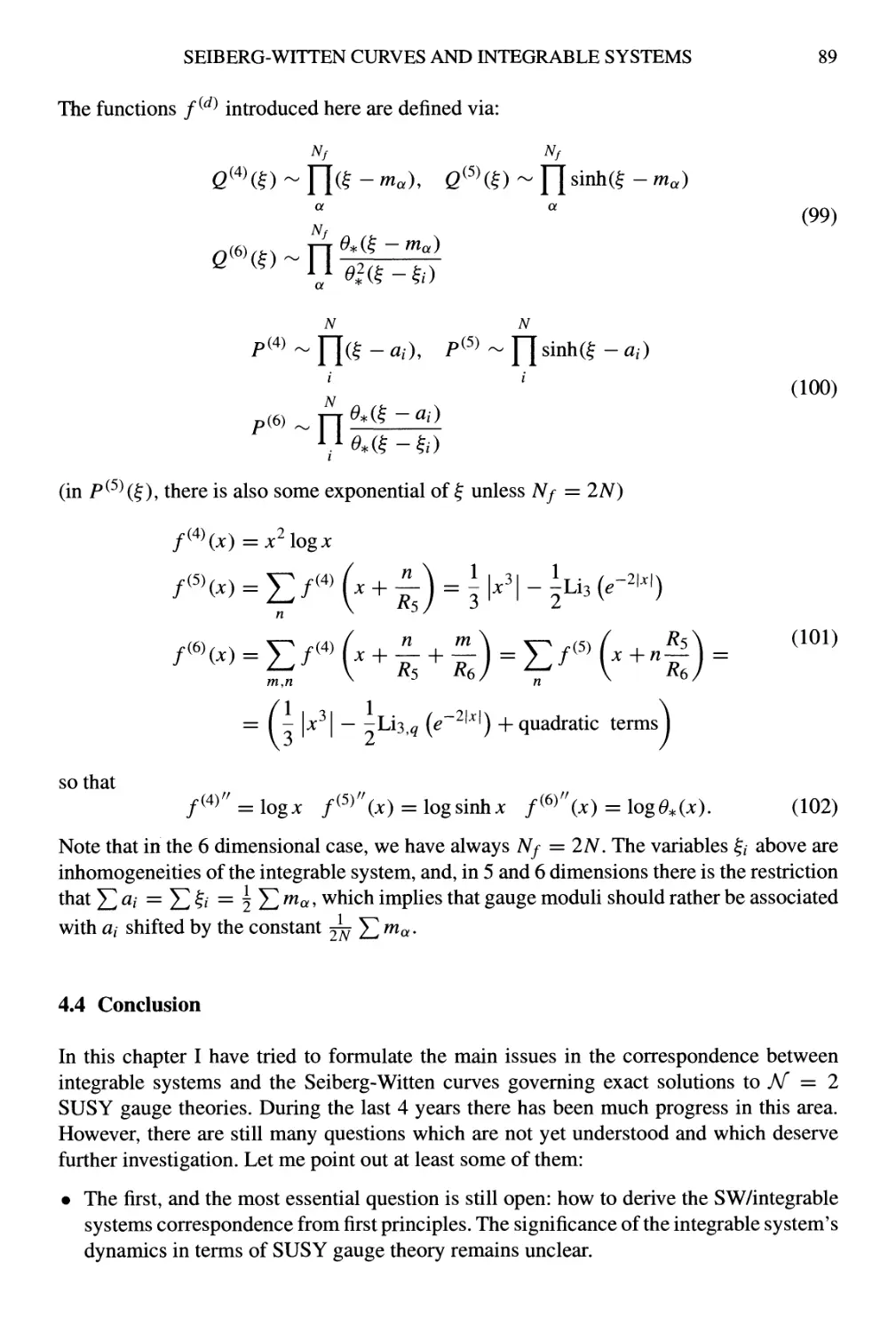
Текст
Integrability:
The Seiberg-Witten and Whitham Equations
Edited by
H.W. Braden
University of Edinburgh, Scotland
and
I.M. Krichever
L,D. Landau Institute of Theoretical Physics
Moscow, Russia
GORDON AND BREACH SCIENCE PUBLISHERS
Australia • Canada • France • Germany • India • Japan
Luxembourg • Malaysia • The Netherlands • Russia
Singapore • Switzerland
Copyright © 2000 OPA (Overseas Publishers Association) N.V. Published by license under
the Gordon and Breach Science Publishers imprint.
All rights reserved.
No part of this book may be reproduced or utilized in any form or by any means, electronic
or mechanical, including photocopying and recording, or by any information storage or
retrieval system, without permission in writing from the pubHsher. Printed in Singapore.
Amsteldijk 166
1st Floor
1079 LH Amsterdam
The Netherlands
British Library Cataloguing in Publication Data
ISBN: 90-5699-281-3
Contents
Preface vii
1 Baker-Akhiezer Functions and Integrable Systems 1
I.M. Krichever
2 Algebraic Geometry, Integrable Systems, and Seiberg-Witten Theory 23
E. Markman
3 Seiberg-Witten Theory and Integrable Systems 43
E. D 'Hoker and D.H. Phong
4 Seiberg-Witten Curves and Integrable Systems 69
A. Marshakov
5 Integrability in Seiberg-Witten Theory 93
A. Morozov
6 WDVV Equations and Seiberg-Witten Theory 103
A. Mironov
1 On Geometry of a Special Class of Solutions to Generalised WDVV Equations 125
A.P. Veselov
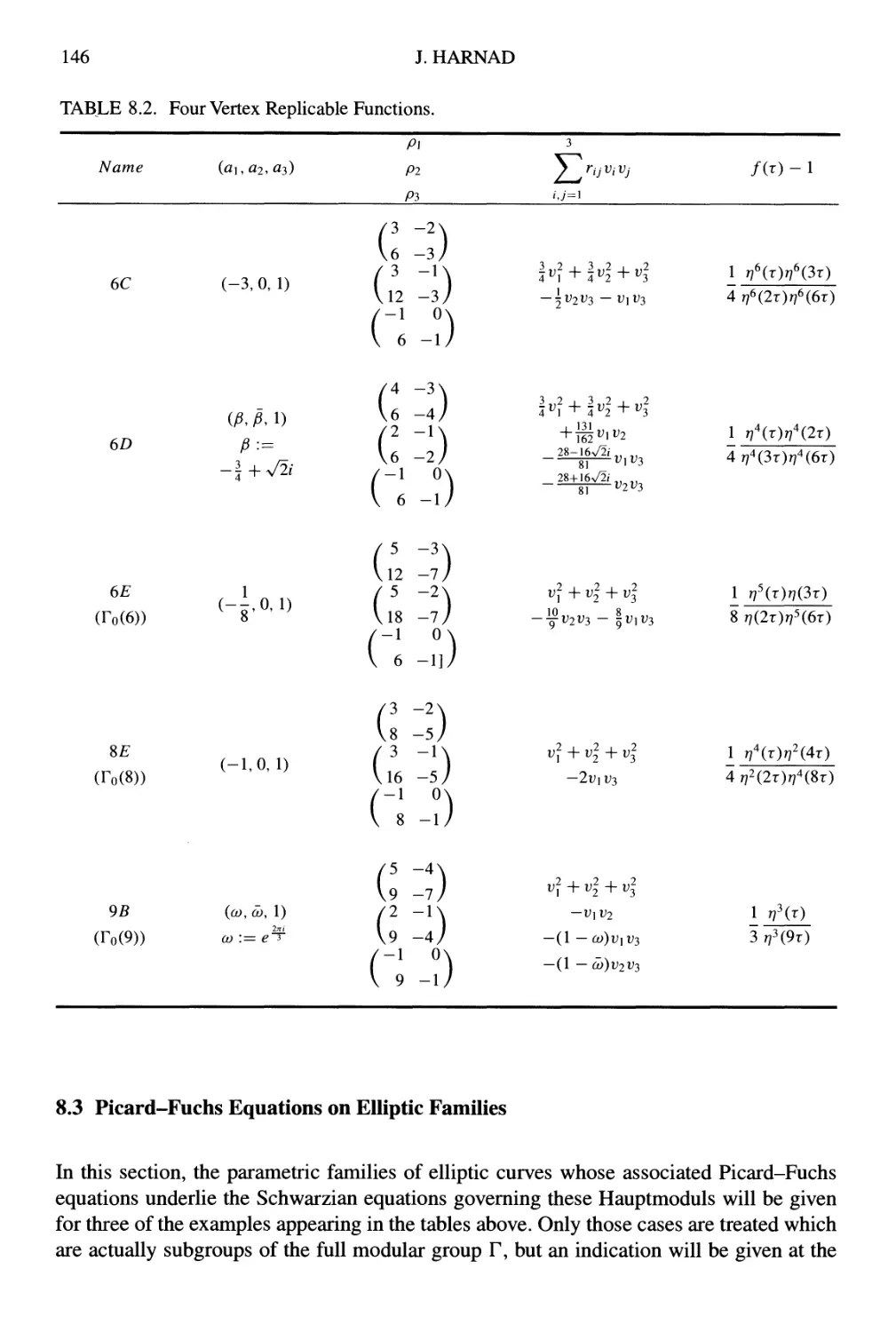
8 Picard-Fuchs Equations, Hauptmoduls and Integrable Systems 137
J. Hamad
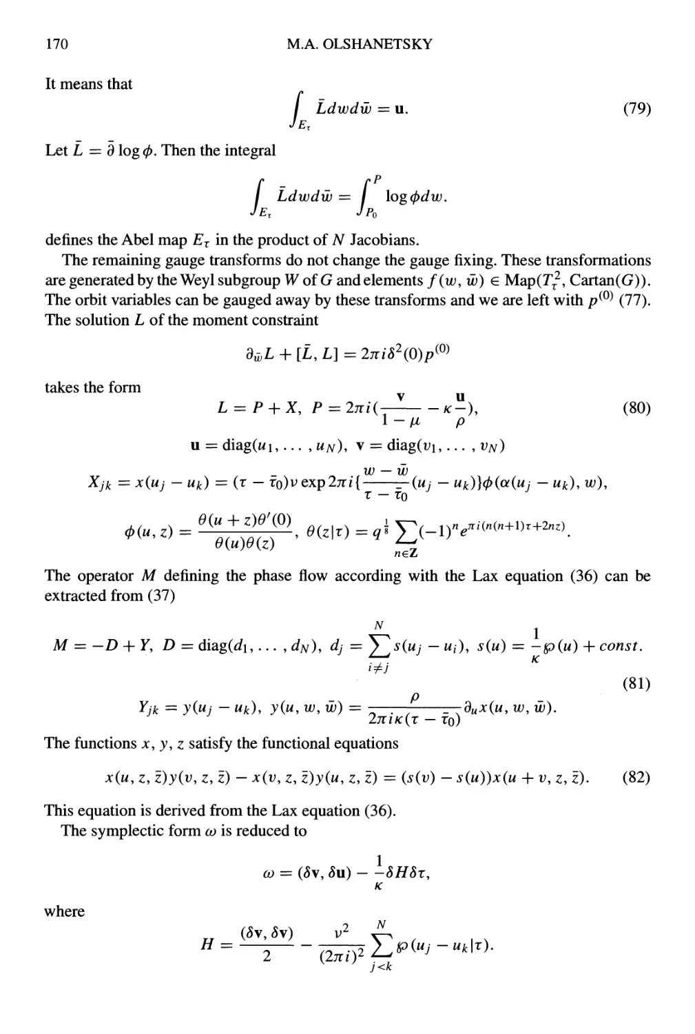
9 Painleve Type Equations and Hitchin Systems 153
MA. Olshanetsky
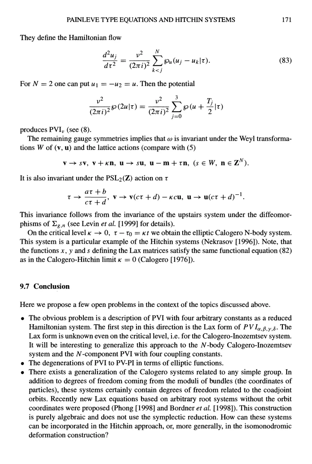
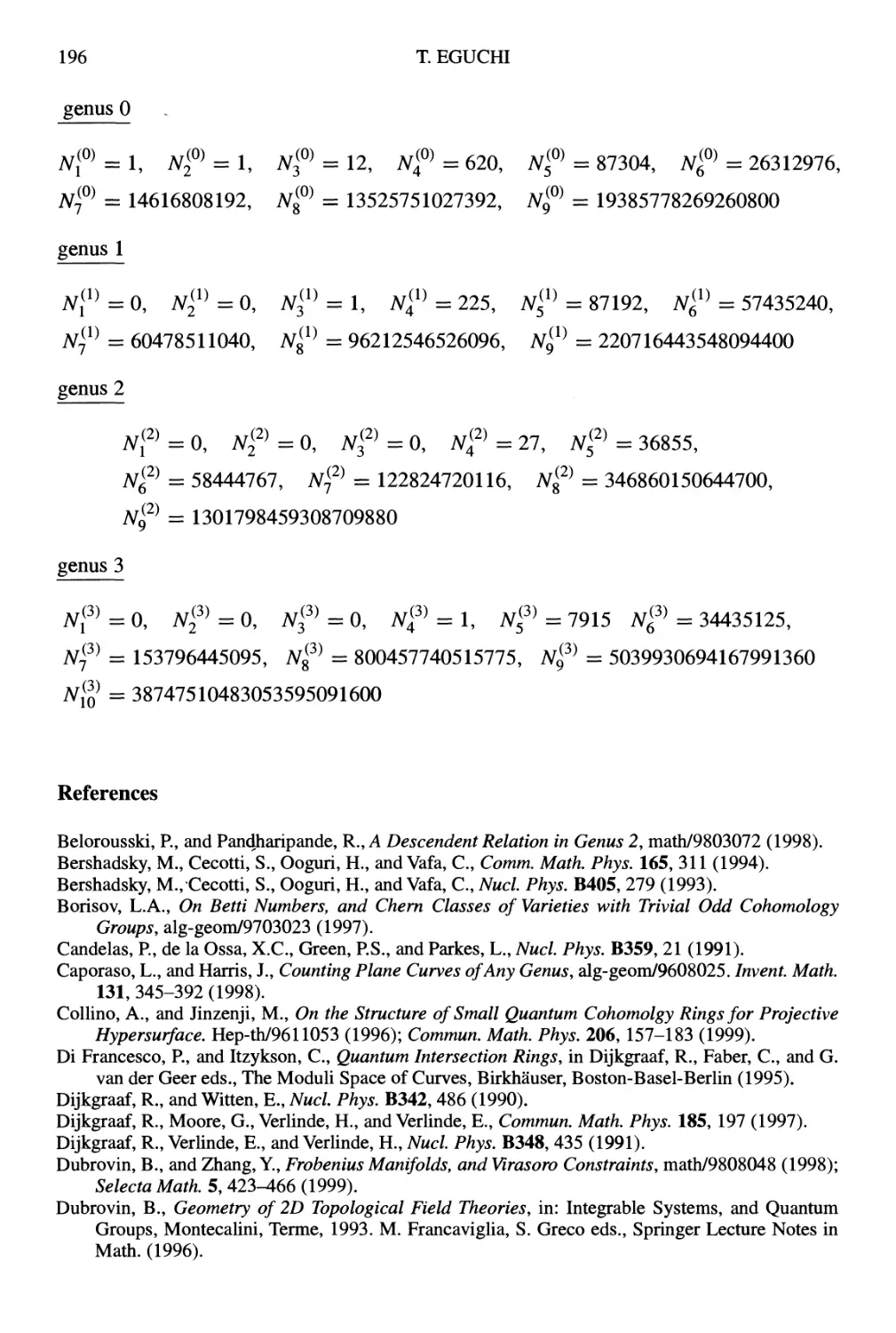
10 World-sheet Instantons and Virasoro Algebra 175
T Eguchi
vi CONTENTS
11 Dispersionless Integrable Systems and their Solutions 199
Y. Kodama
12 A^-Component Integrable Systems and Geometric Asymptotics 213
M.S. Alter
13 Systems of Hydrodynamic Type from Poisson Commuting Hamiltonians 229
A.P. Fordy
14 Integrability of Equations of Hydrodynamic Type from the End of the
19th to the End of the 20th Century 251
S.P. Tsarev
Appendix: List of Participants 267
Index 275
Preface
Integrable systems, like invariant theory, has had a somewhat chequered history. The
nineteenth century saw many aspects of geometry and analysis, particularly the development
of Abelian functions, drawn together in the study of integrable systems. The works of
Jacobi, Abel, Riemann and Weierstrass enabled a number of important integrable problems
of mechanics and physics to be solved, including the problem of geodesic motion on a
tri-axial ellipsoid (Jacobi), the motion of a heavy body around a fixed point (Kowalevski),
the motion of a rigid body in a liquid (Kirchoff, Clebsch and Steklov) and the motion of
a material point on a sphere under the influence of a quadratic potential (Neumann).
Geometric aspects of integrable systems were developed by Darboux, Levi-Civita and
Stackel. The turn of the twentieth century however saw a change in attitude towards
integrable systems. After the results of Poincare and de Bruns, integrable systems lacking
any 'obvious' group symmetry were perceived as something exotic, and ideas about the
structure of nontrivial integrable systems did not exert any real influence on the development
of physics for much of that century.
This situation changed drastically with the discovery of soliton theory. Nonlinear
phenomena could now be treated, and the ever-growing interest in this theory is connected
with the fact that it is applicable to equations which (as became clear in the mid-sixties)
possess remarkable universality properties. They arise in the description of the most diverse
phenomena in plasma physics, the theory of elementary particles, the theory of
superconductivity and in nonlinear optics. Among the equations referred to are the Korteweg-
de Vries equation, the nonlinear Schrodinger equation, the Sine-Gordon equation and many
others. Perhaps surprisingly, finite-dimensional integrable systems again appear in this new
setting, now (for example) describing the evolution of exact solutions of the partial differential
equations. Thus many classical integrable systems, together with several families discovered
at this time (such as the Toda and Calogero-Moser systems), can be viewed as either
describing particular soliton solutions, or as finite-dimensional systems their own rights.
There is a rich interplay between the Inverse Scattering techniques developed to study
the integrable partial differential equations of soliton theory and the techniques of integrable
systems. This ubiquity of integrable systems together with the beautiful structures that
viii PREFACE
underly them has led to a renewed interest in the area. Geometry and algebraic geometry,
functional equations and special functions, Lie algebras and groups all come together in
their study. The most recent burst of interest is due to the unexpected connections of these
systems to N=2 supersymmetric gauge theories.
In 1994 Seiberg and Witten suggested a new way to deal with four-dimensional N=2
supersymmetric gauge theories, both for pure gauge theories and those with matter
hypermultiplets. The consequences of this work are still being assimilated. The low energy
effective actions of such supersymmetric theories are described by a function, the prepotential
^and depends on a finite dimensional moduli space. This moduli space characterises the
vacuum of the theory. Seiberg and Witten introduced an ansatz identifying this moduli space
with the moduli space of a certain family of algebraic curves. The prepotential F which
encodes the effective quantum theory is derived from a (Seiberg-Witten) one-form on this
moduli space.
At this stage there was no a priori reason to expect the appearance of integrable systems.
The first hint of a connection was the observation by Gorsky that the Seiberg-Witten curve
corresponding to the pure A^ = 2 SUSY gauge theory with gauge group SU (N^) could be
identified with the family of spectral curves of the A^^-periodic Toda lattice. Subsequently,
integrable systems were associated to the spectral curves arising from A^ = 2 gauge models
coupled to matter hypermultiplets in varying representations. (A fuller list of models and
references will appear in the text.)
The connection between the Seiberg-Witten ansatz and integrable systems was further
strengthened by the identification of the Seiberg-Witten one-form with that one-form central
to the Whitham equations. The Whitham equations in view here are those that arise when
applying Whitham averaging to finite-gap solutions of soli ton bearing equations. Whitham
averaging is essentially the WKB method applied to nonlinear equations. (The Whitham
equations are the first order equations of an asymptotic expansion in the parameter describing
the slow variation.) In the context of finite-gap solitons (which depend on a finite number
of parameters or moduli) exact results are possible, and as these moduli slowly vary
Whitham averaging describes the evolution of the solitons. The equations themselves are
a quasi-linear, first order system of equations of hydrodynamic type. Remarkably, this one-
form, central to both Whitham theory and Seiberg-Witten theory, is the generator of a
canonical transformation to action-angle variables in the Hamiltonian setting of the soliton
theory.
Yet although many connections now exist between Seiberg-Witten theory and integrable
systems, the correspondence remains poorly understood. The present volume arose from
a meeting devoted to the further elucidation of these connections. The chapters of this book
consist (in most part) of surveys given by plenary speakers at this meeting, and cover
various areas impinging on the subject. Overviews are seldom easy, and we are very grateful
to the contributing authors for holding so strictly to their remit. We hope that this book
will provide an excellent introduction to the ideas and methods surrounding these exciting
theories.
An overview of the book is as follows. The first chapter sets the theme, introducing
many of the main characters that will be developed further in the book. The Baker-Akhiezer
functions central to finite-gap integration, the Whitham equations, topological and Seiberg-
Witten theories are all introduced. Following this are three detailed chapters on various
PREFACE ix
aspects of Seiberg-Witten theory. Markman overviews the special and algebraic geometry.
D'Hoker and Phong survey the physical background to Seiberg-Witten theory and focus
on connections with the Calogero-Moser family of integrable systems. Marshakov describes
the construction of Seiberg-Witten curves associated with a wide range of integrable
systems. Morozov's contribution then tackles the fundamental connection between Seiberg-
Witten and integrability: why should integrability appear at all? Connections with matrix
models, x-functions and the Kontsevich model amongst other things are touched upon.
The next two chapters deal with the WDVV equations. Both the Seiberg-Witten
prepotential and the Whitham equations give rise to solutions of the WDVV equations that
characterise two-dimensional topological theories. These equations describe relations between
various third derivatives of the prepotential. They define an associative algebra known as
a Frobenius algebra; the geometrical data defines a Frobenius manifold. Mironov surveys
the connections between these equations and Seiberg-Witten theory, while Veselov describes
a special class of solutions related to deformations of Calogero-Moser systems. Both
Hamad and Olshanetsky describe particular classes of equations associated with surfaces
and integrable systems, the former that of Picard-Fuchs equations and the latter, Painleve
equations and Hitchin systems. Eguchi's contribution returns to the topological field theoretic
aspects touched upon in several of the earlier chapters, notably in connection with the
WDVV equations. In particular, the Virasoro conjecture on quantum cohomology is reviewed.
Topological theories are related to integrable systems of hydrodynamic type, and Kodama
describes this connection together with those of dispersionless hierarchies and Frobenius
manifolds. Alber's contribution deals with geometric asymptotics which further relates
solutions of partial differential equations with integrable systems. The final two chapters
focus on equations of hydrodynamic type. Fordy surveys the connection between such
systems and the equations arising by requiring two (quadratic) Hamiltonian vector fields
to Poisson commute. Tsarev concludes with an extensive overview of equations of
hydrodynamic type, with particular emphasis on the connections with classical geometric
problems such as the existence of orthogonal curvi-linear coordinates and many others.
Each chapter can be read alone, yet together they convey something of the rich flavour
of present day integrable systems.
It remains our pleasure to thank various individuals and organisations. The meeting
'Integrability: The Seiberg-Witten and Whitham Equations' which took place in Edinburgh
in 1998 and from which this book stems, was largely funded by EPSRC. We are grateful
to them for this support. The meeting was organised under the auspices of the International
Centre for Mathematical Sciences, Edinburgh, and we wish to thank Tracey Dart and her
assistants for their organisational skills and hard work. We are also grateful to our co-
organisers David Fairlie and Ian Strachan for their substantial efforts. Finally we thank all
of those who attended the meeting. (The list of participants is given as an appendix.) Their
informal discussions and the shorter research presentations given at this time were deemed
very helpful by many, and we were delighted to see several research collaborations ensue
from the meeting.
H.W. Braden
I.M. Krichever
1 Baker-Akhiezer Functions and Integrable
Systems
I.M. KRICHEVER
Columbia University, 2990 Broadway, New York, NY 10027, USA and Landau Institute for
Theoretical Physics, Kosygina str 2, 117940 Moscow, Russia;
e-mail: krichev @ math. Columbia, edu.
Key ideas of the algebra-geometric methods in the theory of solitons are presented. Unexpected Hnks between
various theories in which the same objects emerge repeatedly, albeit under different names, like r-function in the
Whitham theory, partition function in topological filed theories, and prepotential in Seiberg-Witten theory mainly
are discussed.
1.1 Introduction
The main goal of this chapter is to present key ideas which unify the algebro-geometric
methods in the theory of soliton equations and recent developments in the theory of N = 2
super symmetric gauge models.
Solitons arose originally in the study of shallow water waves. Since then, the notion of
soliton equations has widened considerably. It embraces now a wide class of non-linear
partial differential equations, which all share the characteristic feature of being expressible
as a compatibility condition for an auxiliary pair of linear differential equations. A variety of
methods have been developed over the years to construct exact solutions for these equations.
Since the middle seventies algebraic geometry has become one of the most powerful tools
among them.
In the next section we outline basic elements of the, so-called, finite-gap theory which
were originated in (Novikov [1994]; Dubrovin et al. [1976], Lax [1975], McKean et al.
[1975]) in the framework of the Floquet spectral theory of periodic Schrodinger operators
combined with a theory of completely integrable Hamiltonian systems. Analytical properties
2 L KRICHEVER
of Bloch solutions of finite-gap Schrodinger operators with respect to an auxiliary spectral
parameter, established in this remarkable series of papers, were a starting point in a
definition of the Baker-Akhiezer functions which are the core of a general algebro-geometric
construction of exact periodic and almost periodic solutions to soliton equations proposed
in (Krichever [1976, 1977a, 1977b]).
Section 3 is devoted to brief description of the Whitham method which is a generalization
to the case of partial differential equation of the classical Bogolyubov-Krylov averaging
method. It turns out that differential equations describing a slow modulation of integrals of
finite-gap solutions of soliton equations, called Whitham equations, are deeply connected
with a theory of deformations of topological quantum field models. This connection between
Whitham theory and the, so-called, Witten-Dijgraaf-Verlinde-Verlinde (WDVV) equations
is discussed in Section 4.
In the last section we show that the Seiberg-Witten theory ofN = 2 supersymmetric
gauge theories can be considered on one hand as a part of the Whitham theory and at the
same time leads to a new general approach to Hamiltonian theory of soliton equations
proposed in (Krichever ^r fl/. [1977, 1999]).
Our discussion of unexpected links between various theories in which the same objects
emerge repeatedly, albeit under different names, like r-function in the Whitham theory,
partition function in topological field theories, and prepotential in Seiberg-Witten theory
mainly follows Krichever et ah [1999]), where more details can be found.
1.2 Finite-gap Solutions of Integrable Systems
The finite-gap or algebro-geometric integration method is uniformly applicable to all soliton
equations. In the case of spatial one-dimensional evolution equations it is instructive enough
to consider as a basic example equations that have Lax representation
dtL = [A,L], (1)
where the unknown functions {m, (x, y, 0}/^Jo ^ {^7 (-^^ y^ ^'^)T=o ^^ ^^^ coefficients of the
ordinary differential operators
n—2 m—2
/=0 7=0
A preliminary classification of equations of the form (1) is by the orders n, m of the operators
L and A.
In the case n = 2 the operator L is just the usual Schrodinger operator L = —d^-\-u(x,t),
and for A = d^ — 3/2udx — 3/4ux equation (1) is equivalent to the KdV equation
4Ut - 6uUx + Uxxx = 0.
From (1) it follows that certain spectral quantities of the operator L are integrals of
motion. In the framework of the finite-gap theory these integrals are organized in the form
of the so-called spectral curve. In all the cases, i.e. finite-dimensional integrable systems,
spatial one- or two-dimensional evolution equations, the spectral curve is defined by a
characteristic equation
R(w, E) = det(M; - T(t, E)) = 0, (3)
BAKER-AKHIEZER FUNCTIONS AND INTEGRABLE SYSTEMS 3
where T(t, E) is a, finite-dimensional matrix depending on a spectral parameter E.
In the case of finite-dimensional (or (0+1)) integrable systems, which have the Lax
representation Lt(t, E) = [A(t, E), L(t, £")], where L and A are finite-dimensional
matrices depending on the spectral parameter, the matrix T(t, E) defining the spectral
curve is the Lax matrix L by itself, i.e. T(t, E) = L(t, E).
In the infinite-dimensional case the spectral curve can be defined for special classes of
solutions, only. For spatial one-dimensional systems these classes are singled out by the
constraint that there exists an additional operator T which commutes with L and (dt — A).
For example, if the coefficients of the operator L of the form (2) are periodic functions of
the variable x with period T, then the operator L commutes with the shift operator
f : y(x) h^ y(x + T). (4)
Therefore, the finite-dimensional linear space C(E) of the solutions of the ordinary
differential equation
y(x) e C(E) : Ly = Ey (5)
is invariant with respect to T. Restriction of the shift operator onto C defines a finite-
dimensional linear operator
T(E) = f\ciE)^ (6)
A point Q of the spectral curve F is just a pair Q = (E,w) of complex numbers that satisfy
(3). They parametrize Bloch eigenfunctions of the operator L, i.e. common eigenfunctions
of L and the monodromy operator
LV^(x, Q) = Eif(x, 2), if(x -\-T,Q) = wif(x, Q). (7)
In a generic case the corresponding Riemann surface is a smooth surface of infinite genus. If
its genus is finite then the corresponding operators are called finite-gap or algebro-geometric
operators. It should be emphasized that in such a case the Riemann surface defined by the
characteristic equation is a singular surface. After resolving the singularities we get a finite
genus smooth Riemann surface, i.e. an algebraic curve. For example, let L = — 9^ + u(x)
be the Schrodinger operator with a periodic potential u(x) = u(x -\-T). Then equation (3)
has the form
w^ - 2Q(E)w + 1=0, 2Q(E) = Tr T(E). (8)
The roots 6, of the equation Q^(E) = 1 are points of the periodic or anti-periodic spectrum
of the Schrodinger operator. Equation (8) can be rewritten in the form
oo
y^ = Y[(E-ei), y = w-Q(E). (9)
i=i
If all of the edges 6, are distinct then (9) defines smooth infinite genus hyperelliptic Riemann
surface. The finite-gap operators correspond to the degenerate case when all but a finite
number of eigenvalues of periodic or anti-periodic spectral problem for L are multiple. Let
£"1 < • • • < £"2^+1 be the simple eigenvalues. Then a finite genus smooth algebraic curve
of the Bloch functions is defined by
2g-\-l
4 I. KRICHEVER
Note that Ei are the edges of the spectrum bands of L, being considered as an operator in
the space of square integrable functions on the whole Une.
The finite-gap theory was initiated by the work (Novikov [1974]), where the spectral
theory of periodic operators was combined with an approach based on a use of the KdV
hierarchy. The KdV equation (as well as any soliton equation) is compatible with an infinite
hierarchy of commuting flows. They have the Lax representation
diL = [Ai,L], di = ^. (11)
where A, is an ordinary differential operator of order 2/ + 1. Consider stationary solutions
of a linear combination of these flows, i.e. solutions of the ordinary differential equation
g
[L,A]=0, A = Y^CiAi, (12)
i=\
As it was shown in (Novikov [1974]), equation (12) is a completely integrable Hamiltonian
system. Therefore, its general solution is a quasi-periodic function of x. Periodic solutions
are finite-gap potentials.
Let A{E) be the restriction of the operator A commuting with L onto C{E). The
matrix elements of A(£') are polynomial functions of the spectral parameter. Therefore,
the characteristic equation det(A(£') — iti) = 0 defines an algebraic curve P. It turns out
that this curve coincides with the spectral curve (10).
Note that the operator equation (12) is a particular case of the more general problem of
the classification of commuting ordinary differential operators L„ and L^ of orders n and
m, respectively. As a purely algebraic problem it was considered and partly solved in the
remarkable works of Burchnall and Chaundy (Burchall et al [1922, 1928]) in the 1920s.
They proved that for any pair of such operators there exists a polynomial R(X, /jl) in two
variables such that R(Ln, Lm) = 0. If the orders n and m of these operators are co-prime,
(n,m) = 1, then for each point Q = (X, /jl) of the curve F defined in C^ by the equation
R(X, /jl) = 0 there corresponds a unique (up to a constant factor) common eigenfunction
V^(jc, Q) of Ln and Lm
Ln-^ix, Q) = X\lf{x, Q)\ Lmif(x, Q) = fiir(x, Q).
The logarithmic derivative V^^ V^~^ is a meromorphic function on P. In the general position
(when r is smooth) it has g poles yi(jc),... , y^(jc) in the affine part of the curve, where
g is the genus of P. The commuting operators L„ and Lm (in this case of co-prime orders)
are uniquely defined by the polynomial R and by a set of g points yi(jco),... , y^(^o)
on P.
In such a form, the solution of the problem is one of pure classification: one set is
equivalent to the other. Even the attempt to obtain exact formulae for the coefficients of
commuting operators had not been made. Baker proposed making the program effective
by pointing out that the eigenfunction -[jr has analytical properties that were introduced
by Clebsch, Gordan and himself as a proper generalization of the notion of exponential
BAKER-AKHIEZER FUNCTIONS AND INTEGRABLE SYSTEMS 5
functions on Riemann surfaces. The Baker program was rejected by the authors of (Burchnall
et al. [1922, 1928]) consciously (see the postscript of Baker's paper [1928]) and all these
results were forgotten for a long time. This program was realized only in (Krichever [1976,
1977a]) (though at that time the author was not aware of the remarkable results of Burchnal,
Chaundy and Baker) where the commuting pairs of ordinary differential operators were
considered in connection with the problem of constructing solutions to the KP equation.
Spatial two-dimensional integrable systems of the KP type have an analogue of the Lax
representation of the form
[dy-L,dt -A] = 0, (13)
where, as before, L and A are ordinary differential operators of the form (2) but now with
the coefficients depending on the variables x,y,tAn two dimensions in order to single out
special classes of solutions for which a spectral curve can be defined one needs to impose
two constraints. For example, that can be done if we assume that in addition to (13) there
exist two ordinary differential operators of orders n and m such that
[a^-L,L,] = 0, [a^-L,L^] = 0. (14)
Such operators commute with each other, and commute with the operator (9? — A). The
corresponding spectral curve is a spectral curve of commuting operators L„, L^. It does
not depend on {x,y,t). (Classification of commuting operators of arbitrary orders was
completed in Krichever [1978]).
The common eigenfunction of commuting operators is a particular case of the general
definition of the scalar multi-point multi-variable Baker-Akhiezer function. Let F be a
non-singular algebraic curve of genus g with A^ punctures Pa and fixed local parameters
k~^{Q)m neighbourhoods of these punctures. For any set of points yi,... , y^ in general
position, there exists a unique (up to constant factor c{toi,i)) function ij/it, Q), t = (taj).
Of = 1,... , A^ ; / = 1,... , such that:
(i) the function i// (as a function of the variable Q e F) is meromorphic everywhere
except for the points Pa and it has at most simple poles at the points yi,... , y^ (if all
of them are distinct).
(ii) in a neighbourhood of the point Pa the function i// has the form
oo oo
V^(r, Q) =txp{J2taA){J2^sAt)ka').ka =ka(Q). (15)
i = l s=0
The Baker-Akhiezer function i// depends on the variables t = [tij,... , t^j} as on external
parameters.
From the uniqueness of the Baker-Akhiezer function it follows that for each pair (a, n)
there exists a unique operator La,n of the form
n-l
7 = 1
6 I. KRICHEVER
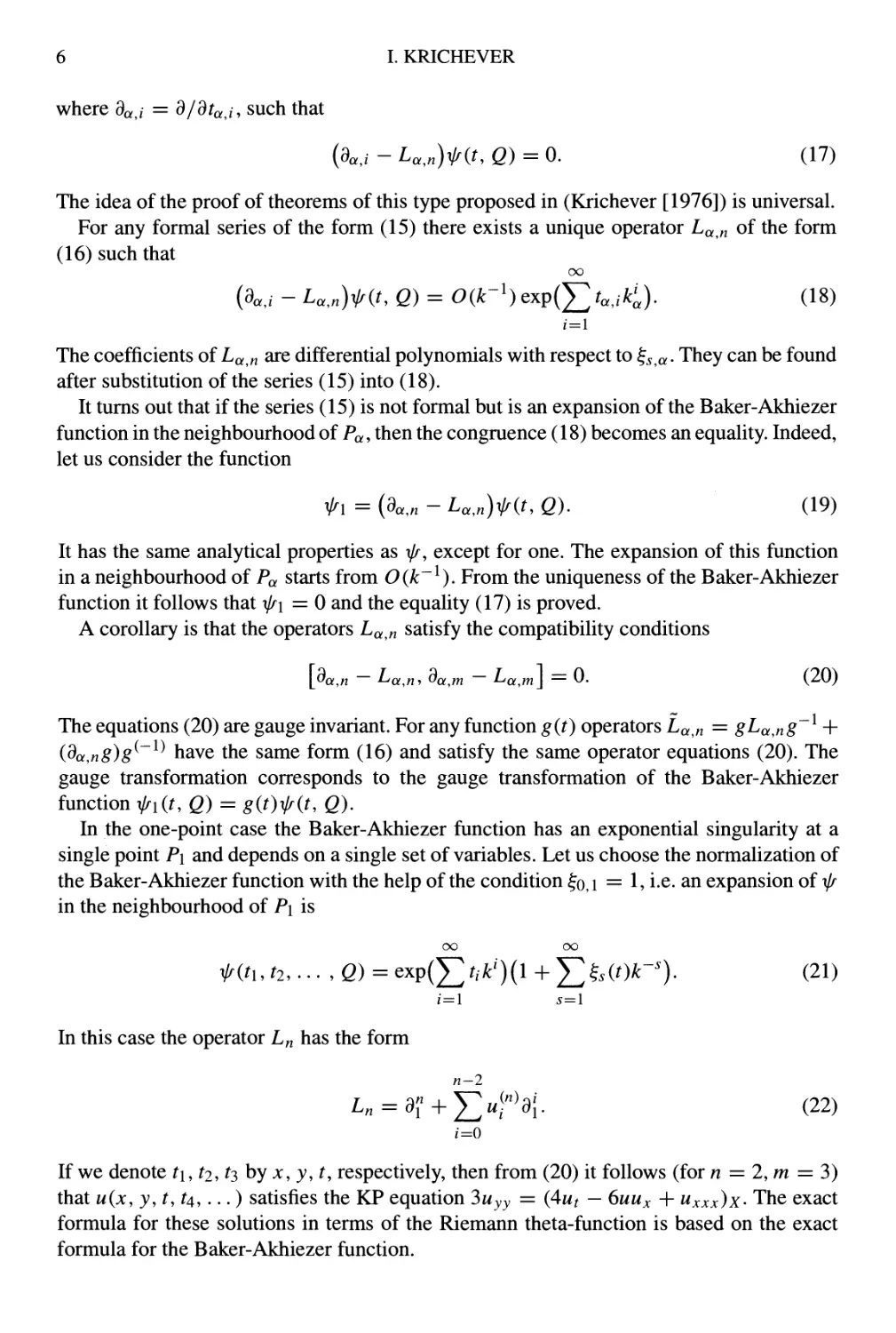
where daj = 9/9^a,i, such that
{da,i-La,n)^(t,Q)=0. (17)
The idea of the proof of theorems of this type proposed in (Krichever [1976]) is universal.
For any formal series of the form (15) there exists a unique operator La,n of the form
(16) such that
oo
i = l
The coefficients of Lc^^„ are differential polynomials with respect to ^^ c^. They can be found
after substitution of the series (15) into (18).
It turns out that if the series (15) is not formal but is an expansion of the Baker-Akhiezer
function in the neighbourhood of Pa, then the congruence (18) becomes an equality. Indeed,
let us consider the function
iri={da,n-La,n)if(t,Q). (19)
It has the same analytical properties as V^, except for one. The expansion of this function
in a neighbourhood of Pa starts from 0(k~^). From the uniqueness of the Baker-Akhiezer
function it follows that t/^i = 0 and the equality (17) is proved.
A corollary is that the operators La,n satisfy the compatibility conditions
The equations (20) are gauge invariant. For any function g(t) operators La,n = gLa,ng~^ +
(^a,ng)g^~^^ have the same form (16) and satisfy the same operator equations (20). The
gauge transformation corresponds to the gauge transformation of the Baker-Akhiezer
function V^i(r, Q) = g(t)\l/(t, Q).
In the one-point case the Baker-Akhiezer function has an exponential singularity at a
single point Pi and depends on a single set of variables. Let us choose the normalization of
the Baker-Akhiezer function with the help of the condition §o, i = 1, i-^- an expansion of i//
in the neighbourhood of Pi is
oo oo
ir(tut2, ... , 2) = exp(^r,/:')(l +J^^,(t)k-'). (21)
i=l s=l
In this case the operator L„ has the form
n-2
L, = af + ^t.f>a|. (22)
If we denote ^i, ^2, t^ by jc, y, t, respectively, then from (20) it follows (for n = 2, m = 3)
that u(x, y, r, ^4,...) satisfies the KP equation 3uyy = (4ut — 6uux + Uxxx)x- The exact
formula for these solutions in terms of the Riemann theta-function is based on the exact
formula for the Baker-Akhiezer function.
BAKER-AKHIEZER FUNCTIONS AND INTEGRABLE SYSTEMS 7
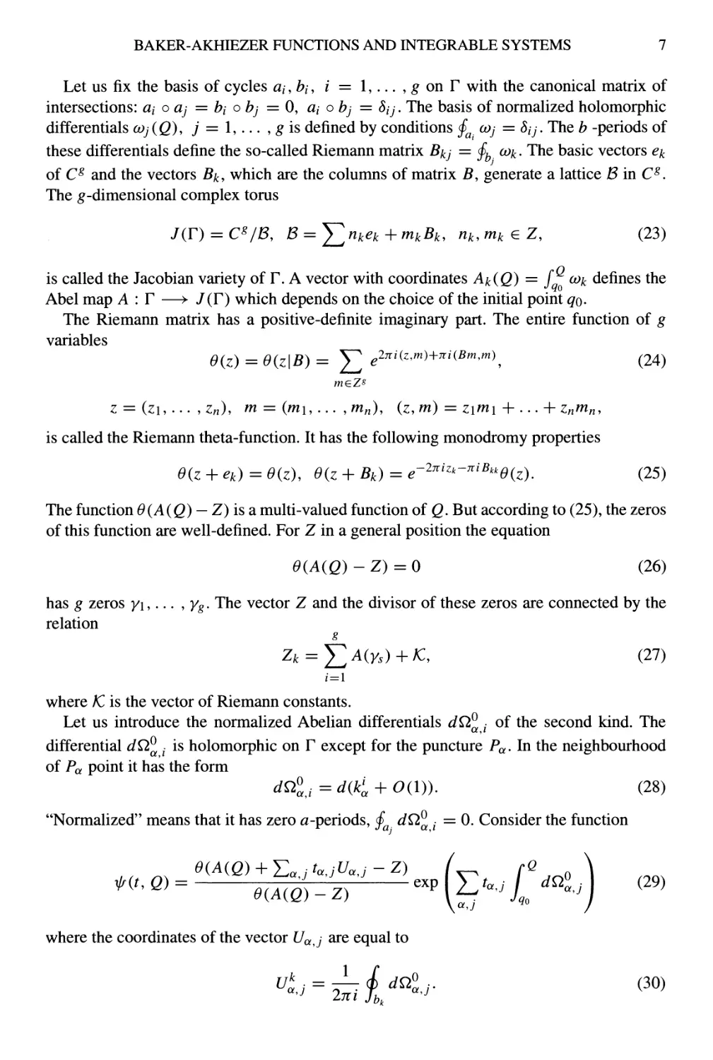
Let us fix the basis of cycles a,, Z?,, i = 1,... , ^ on F with the canonical matrix of
intersections: at o aj = bi o bj = 0, at o bj = 8ij. The basis of normalized holomorphic
differentials coj(Q), j = I,..., g is defined by conditions ^^ coj = 8ij. The b -periods of
these differentials define the so-called Riemann matrix Bkj = fi^.^k- The basic vectors Ck
of C^ and the vectors Bk, which are the columns of matrix B, generate a lattice BinC^.
The ^-dimensional complex torus
J(T) = C^/B, B = J2^kek+mkBk, rik.mkeZ, (23)
is called the Jacobian variety of F. A vector with coordinates Ak(Q) = / cok defines the
Abel map A : F —> /(F) which depends on the choice of the initial point qo.
The Riemann matrix has a positive-definite imaginary part. The entire function of g
variables
0(z) = 0(z\B) = J2 ^2^'^^'^>+^'^^^'^>, (24)
meZs
z = (zi,... , Zn). m = (mi,... , rUn), (z, m) = z\m\ + ... + z„m„,
is called the Riemann theta-function. It has the following monodromy properties
e{z + ck) = 0(z). 0(z + Bk) = ^-2^'^^-^'^^^^(^). (25)
The function 0(A(Q) — Z) is a multi-valued function of Q. But according to (25), the zeros
of this function are well-defined. For Z in a general position the equation
0(A(Q) - Z) = 0 (26)
has g zeros yi,... , y^. The vector Z and the divisor of these zeros are connected by the
relation
g
Zk = J^A(ys)+IC, (27)
i=i
where /C is the vector of Riemann constants.
Let us introduce the normalized Abelian differentials dQ^ • of the second kind. The
differential dQ^ ■ is holomorphic on F except for the puncture Pa. In the neighbourhood
of Pa point it has the form
J<, =J(4 + 0(1)). (28)
"Normalized" means that it has zero a-periods, f^ dQ^ ■ = 0. Consider the function
0(A(Q)-\-J2ai^ccjUaj-Z) /-_, rQ „\
ir(t, Q) = ^^aj_i—J / \Ytai dOP^ . (29)
^''"^^ e{A{Q)-Z) \t7 4 '7
where the coordinates of the vector Uaj are equal to
8 I. KRICHEVER
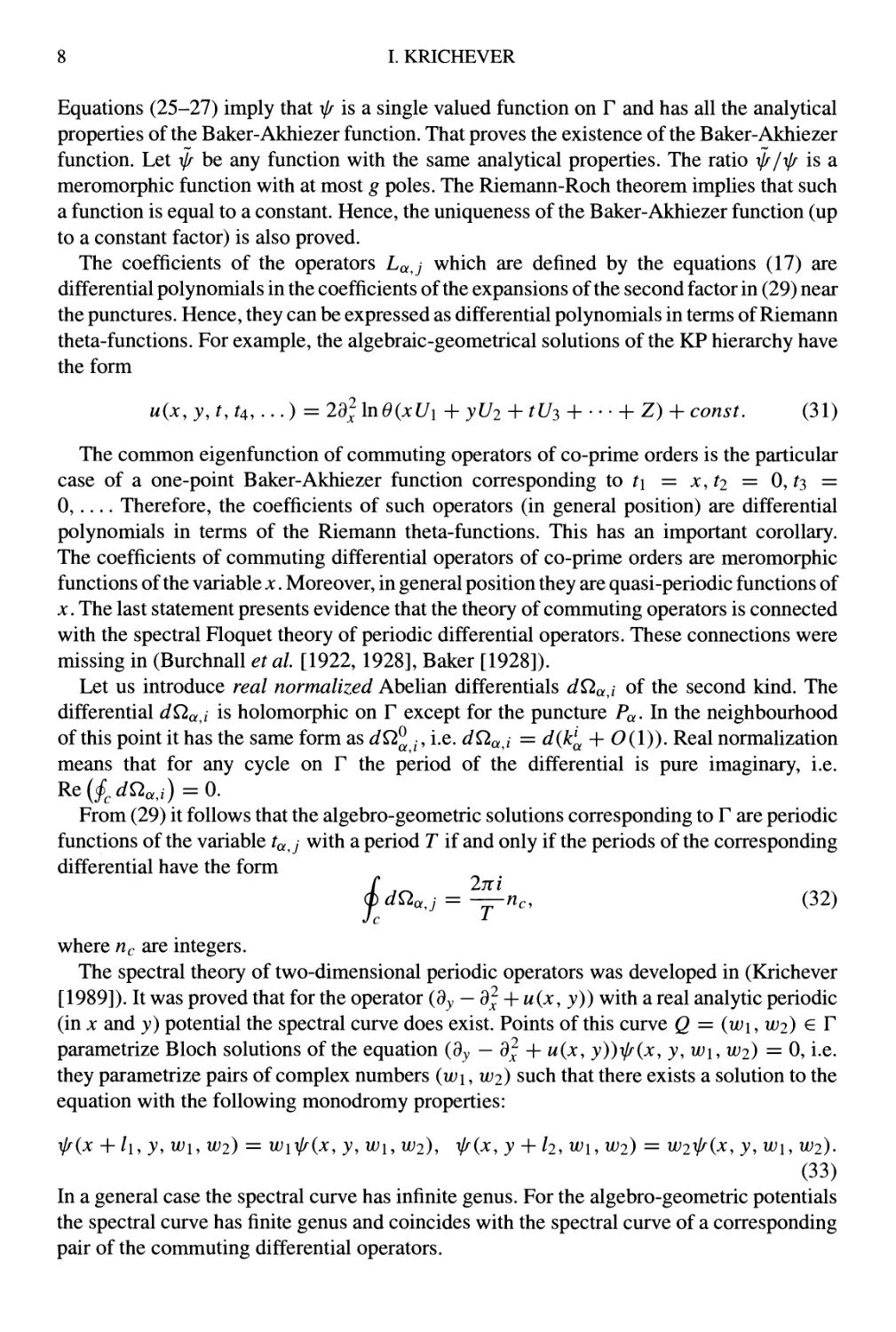
Equations (25-27) imply that t/^ is a single valued function on F and has all the analytical
properties of the Baker-Akhiezer function. That proves the existence of the Baker-Akhiezer
function. Let ^jr be any function with the same analytical properties. The ratio -ilr/1// is a
meromorphic function with at most g poles. The Riemann-Roch theorem implies that such
a function is equal to a constant. Hence, the uniqueness of the Baker-Akhiezer function (up
to a constant factor) is also proved.
The coefficients of the operators Laj which are defined by the equations (17) are
differential polynomials in the coefficients of the expansions of the second factor in (29) near
the punctures. Hence, they can be expressed as differential polynomials in terms of Riemann
theta-functions. For example, the algebraic-geometrical solutions of the KP hierarchy have
the form
m(jc,>;, ^,^4,...) = 2d^lnO(xUi -\-yU2-\-tU3 H + Z)-\-const. (31)
The common eigenfunction of commuting operators of co-prime orders is the particular
case of a one-point Baker-Akhiezer function corresponding to ^i = jc, ^2 = 0, ^3 =
0, Therefore, the coefficients of such operators (in general position) are differential
polynomials in terms of the Riemann theta-f unctions. This has an important corollary.
The coefficients of commuting differential operators of co-prime orders are meromorphic
functions of the variable x. Moreover, in general position they are quasi-periodic functions of
X. The last statement presents evidence that the theory of commuting operators is connected
with the spectral Floquet theory of periodic differential operators. These connections were
missing in (Burchnall et al [1922, 1928], Baker [1928]).
Let us introduce real normalized Abelian differentials dQ.a,i of the second kind. The
differential dQ.oi,i is holomorphic on F except for the puncture Pa. In the neighbourhood
of this point it has the same form as dOP^ ., i.e. dO^aj = d{¥^ + 0(1)). Real normalization
means that for any cycle on F the period of the differential is pure imaginary, i.e.
Kt{§^dQ.oc,i)=0.
From (29) it follows that the algebro-geometric solutions corresponding to F are periodic
functions of the variable taj with a period T if and only if the periods of the corresponding
differential have the form
Ini
i
dQaj = -zrnc, (32)
T
where nc SiTQ integers.
The spectral theory of two-dimensional periodic operators was developed in (Krichever
[1989]). It was proved that for the operator (dy — 9^ + m(jc, y)) with a real analytic periodic
(in X and y) potential the spectral curve does exist. Points of this curve Q = (wi, W2) G F
parametrize Bloch solutions of the equation (dy — 9^ + u(x, }?))V^(jc, y, ifi, W2) = 0, i.e.
they parametrize pairs of complex numbers (wi,W2) such that there exists a solution to the
equation with the following monodromy properties:
'\lf(x-\-luy,wuW2) = wi'\lf(x,y,wuW2), i^ix, y-\-l2,wuW2) = W2ilf(x, y,wuW2).
(33)
In a general case the spectral curve has infinite genus. For the algebro-geometric potentials
the spectral curve has finite genus and coincides with the spectral curve of a corresponding
pair of the commuting differential operators.
BAKER-AKHIEZER FUNCTIONS AND INTEGRABLE SYSTEMS 9
The space of algebro-geometric data defining solutions of the full hierarchy of spatially
two-dimensional KP type systems is infinite dimensional because it contains a choice of
the local coordinates near the punctures. At the same time the space of algebro-geometric
solutions of a single equation of the zero-curvature form (13) is finite-dimensional. If L and
A are operators of orders n and m with scalar coefficients, then this space can be described
as follows (see details in (Krichever et al [1997])).
Let Mg{n, m) be the space (F, E, Q) of pairs of Abelian integrals on a smooth genus g
algebraic curve F, where E and Q have poles of orders n and m, respectively, at a puncture
Po • Then we define a local coordinate k~^ near the puncture by the equality k^ = E. This
choice of the local coordinate corresponds to the identification of the variable y with a basic
time variable y = tn.
In the presence of a second Abelian integral Q, we can select a second time t, by writing
the singular part Q-{-(k) of 2 ^s a polynomial in k and setting
Q^(k) = aik-\ h flm^"", ti = ait, 1 <i <m. (34)
This means that we consider the Baker-Akhiezer function -{//(x, y,t; k) with the essential
singularity exp(kx -\-k^y -\- Q^(k)t), and construct the operators L and A by requiring that
(dy - L)\lr = (dt — A)\lr = 0. The pair (L, A) provides then a solution of the zero-curvature
equation. By rescaling t, we can assume that A is monic.
The proper interpretation of the full geometric data (F, £", 2; yi, • • • y^) is as a point in
the bundle J\fg(n, m) over Mg{n, m), whose fiber is the ^-th symmetric power S^{T) of
the curve:
Ml(n,m)^^ Mg(n,m) (35)
The ^-th symmetric power can be identified with the Jacobian of F via the Abel map.
More generally, we can construct the bundles Afg(n, m) with fiber S^{T) over the bases
Mg(n,m). Thus the bundle J\f^^^(n, m) =Mg{n, m) is the analogue in our context of the
universal curve.
1.3 Whitham Equations
We have seen that soliton equations exhibit a unique wealth of exact solutions. Nevertheless,
it is desirable to enlarge the class of solutions further, to encompass broader data than just
rapidly decreasing or quasi-periodic functions. Typical situations arising in practice can
involve Heaviside-like boundary conditions in the spatial variable jc, or slowly modulated
waves which are not exact solutions, but can appear as such over a small scale in both space
and time.
The non-linear WKB method (or, as it is now also called, the Whitham method of
averaging) is a generalization to the case of partial differential equations of the classical
Bogolyubov-Krylov method of averaging. This method is applicable to nonlinear equations
which have a moduli space of exact solutions of the form uo(Ux + Wt + Z\I). Here
uoizi,... ,Zg\I) is a periodic function of the variables Zi\ U = (f/i,... , Ug), W =
(Wi, ... , W^) are vectors which like u itself, depend on the parameters / = (/i,... , /yv).
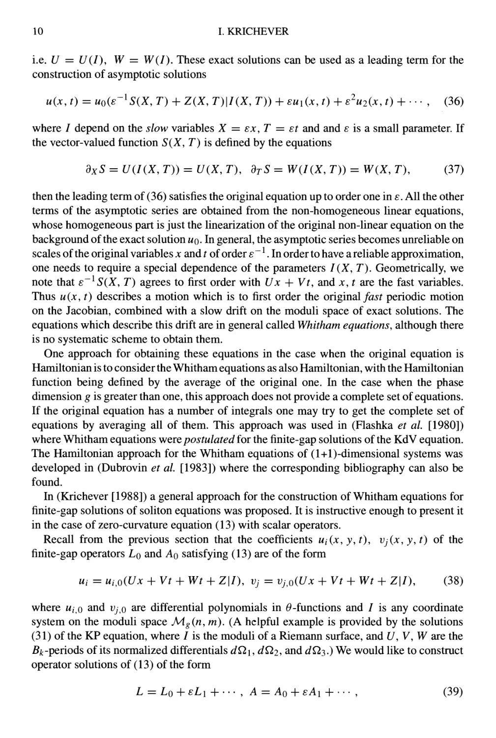
10 I. KRICHEVER
i.e. U = U(I), W = W(I). These exact solutions can be used as a leading term for the
construction of asymptotic solutions
m(jc, t) = uo(6~^S(X, T) + Z(X, r)|/(X, T)) + suiix, t) + s'^U2{x, t) + - • • , (36)
where / depend on the slow variables X = sx.T = st and and £ is a small parameter. If
the vector-valued function S{X, T) is defined by the equations
dxS = U(I(X,T)) = U(X,T), dTS=W(I(X,T)) = W(X,T), (37)
then the leading term of (36) satisfies the original equation up to order one in s. All the other
terms of the asymptotic series are obtained from the non-homogeneous linear equations,
whose homogeneous part is just the linearization of the original non-linear equation on the
background of the exact solution mq- In general, the asymptotic series becomes unreliable on
scales of the original variables x and t of order 6~^.ln order to have a reliable approximation,
one needs to require a special dependence of the parameters /(X, T). Geometrically, we
note that 6~^S(X, T) agrees to first order with Ux + Vt, and jc, ^ are the fast variables.
Thus u{x,t) describes a motion which is to first order the ongmdX fast periodic motion
on the Jacobian, combined with a slow drift on the moduli space of exact solutions. The
equations which describe this drift are in general called Whitham equations, although there
is no systematic scheme to obtain them.
One approach for obtaining these equations in the case when the original equation is
Hamiltonian is to consider the Whitham equations as also Hamiltonian, with the Hamiltonian
function being defined by the average of the original one. In the case when the phase
dimension g is greater than one, this approach does not provide a complete set of equations.
If the original equation has a number of integrals one may try to get the complete set of
equations by averaging all of them. This approach was used in (Flashka et al. [1980])
where Whitham equations wqyq postulated for the finite-gap solutions of the KdV equation.
The Hamiltonian approach for the Whitham equations of (l+l)-dimensional systems was
developed in (Dubrovin et al. [1983]) where the corresponding bibliography can also be
found.
In (Krichever [1988]) a general approach for the construction of Whitham equations for
finite-gap solutions of soliton equations was proposed. It is instructive enough to present it
in the case of zero-curvature equation (13) with scalar operators.
Recall from the previous section that the coefficients m,(jc, y, t), Vj{x, y, t) of the
finite-gap operators Lq and Aq satisfying (13) are of the form
Ui = Ui^oiUx -\-Vt-\-Wt-\- Z\I), Vj = Vj^oiUx -\-Vt-\-Wt-\- Z\I), (38)
where m,,o and Vj^o are differential polynomials in ^-functions and / is any coordinate
system on the moduli space Mg(n, m). (A helpful example is provided by the solutions
(31) of the KP equation, where / is the moduli of a Riemann surface, and U, V, W are the
i5)t-periods of its normalized differentials J^i, ^^2, and ^^3.) We would like to construct
operator solutions of (13) of the form
L = Lo + £Li + • • • , A = Ao + £Ai + ... , (39)
BAKER-AKHIEZER FUNCTIONS AND INTEGRABLE SYSTEMS 11
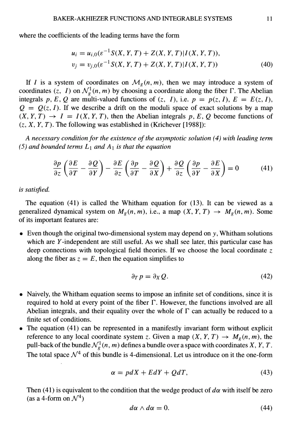
where the coefficients of the leading terms have the form
ui = ui^o{8-^s{x, y, T) + z(x, y, r)|/(x, y, r)),
vj = vj,o{8-^s{x, y, T) + z(x, y, r)|/(x, y, r)) (40)
If / is a system of coordinates on M.g(n,m), then we may introduce a system of
coordinates (z, /) on Afg(n, m) by choosing a coordinate along the fiber P. The Abelian
integrals p, E, Q arc multi-valued functions of (z, /), i.e. p = p(z, I), E = E(z, I),
Q = (2(z, /). If we describe a drift on the moduli space of exact solutions by a map
(X, y, D ^ / = /(X, y, r), then the Abelian integrals p, E, Q become functions of
(z, X, y, r). The following was established in (Krichever [1988]):
A necessary condition for the existence of the asymptotic solution (4) with leading term
(5) and bounded terms L\ and A\ is that the equation
\dT dY J dz \dT dx) dz \dY dX)
dp (dE
Vz
is satisfied.
The equation (41) is called the Whitham equation for (13). It can be viewed as a
generalized dynamical system on Mg(n, m), i.e., a map (X, y, T) -^ Mg(n,m). Some
of its important features are:
• Even though the original two-dimensional system may depend on y, Whitham solutions
which are y-independent are still useful. As we shall see later, this particular case has
deep connections with topological field theories. If we choose the local coordinate z
along the fiber as z = £", then the equation simplifies to
dTP = dxQ. (42)
• Naively, the Whitham equation seems to impose an infinite set of conditions, since it is
required to hold at every point of the fiber P. However, the functions involved are all
Abelian integrals, and their equality over the whole of P can actually be reduced to a
finite set of conditions.
• The equation (41) can be represented in a manifestly invariant form without explicit
reference to any local coordinate system z. Given a map (X, y, T) -^ Mg{n, m), the
pull-back of the bundle A/'^H'^, m) defines a bundle over a space with coordinates X, y, T.
The total space M^ of this bundle is 4-dimensional. Let us introduce on it the one-form
a = pdX + EdY + QdT, (43)
Then (41) is equivalent to the condition that the wedge product of da with itself be zero
(as a 4-form on J\f^)
da Ada = 0. (44)
12 I. KRICHEVER
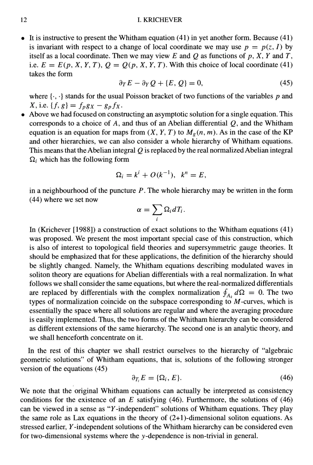
• It is instructive to present the Whitham equation (41) in yet another form. Because (41)
is invariant with respect to a change of local coordinate we may use p = p(z, I) by
itself as a local coordinate. Then we may view E and Q as functions of p, X,Y and T,
i.e. E = E(p, X, y, r), Q = Q(p, X, F, T). With this choice of local coordinate (41)
takes the form
dTE-dYQ + [E,Q} = 0, (45)
where {•, •} stands for the usual Poisson bracket of two functions of the variables p and
X, i.e. {/,^} = fpgx -gpfx^
• Above we had focused on constructing an asymptotic solution for a single equation. This
corresponds to a choice of A, and thus of an Abelian differential Q, and the Whitham
equation is an equation for maps from (X, Y, T) to Mg(n, m). As in the case of the KP
and other hierarchies, we can also consider a whole hierarchy of Whitham equations.
This means that the Abelian integral Q is replaced by the real normalized Abelian integral
Q^i which has the following form
Q^i =k' -\-0(k-^), r = E,
in a neighbourhood of the puncture P. The whole hierarchy may be written in the form
(44) where we set now
i
In (Krichever [1988]) a construction of exact solutions to the Whitham equations (41)
was proposed. We present the most important special case of this construction, which
is also of interest to topological field theories and supersymmetric gauge theories. It
should be emphasized that for these applications, the definition of the hierarchy should
be slightly changed. Namely, the Whitham equations describing modulated waves in
soliton theory are equations for Abelian differentials with a real normalization. In what
follows we shall consider the same equations, but where the real-normalized differentials
are replaced by differentials with the complex normalization §^ dQ = 0. The two
types of normalization coincide on the subspace corresponding to M-curves, which is
essentially the space where all solutions are regular and where the averaging procedure
is easily implemented. Thus, the two forms of the Whitham hierarchy can be considered
as different extensions of the same hierarchy. The second one is an analytic theory, and
we shall henceforth concentrate on it.
In the rest of this chapter we shall restrict ourselves to the hierarchy of "algebraic
geometric solutions" of Whitham equations, that is, solutions of the following stronger
version of the equations (45)
dT,E = {Qi,E]. (46)
We note that the original Whitham equations can actually be interpreted as consistency
conditions for the existence of an £" satisfying (46). Furthermore, the solutions of (46)
can be viewed in a sense as 'T-independent" solutions of Whitham equations. They play
the same role as Lax equations in the theory of (2+l)-dimensional soliton equations. As
stressed earlier, F-independent solutions of the Whitham hierarchy can be considered even
for two-dimensional systems where the };-dependence is non-trivial in general.
BAKER-AKHIEZER FUNCTIONS AND INTEGRABLE SYSTEMS 13
Equations (46) define a system of commuting flows on the moduli space of Abelian
integrals. For the one puncture case this space is a union of the spaces Mg(n) of Abelian
integrals with the pole of order n at the puncture. The complex dimension of Mg(n) is
equal to dim A4g(n) = 4g -\-n — I. Let us describe a special system of coordinates for it.
The first 2g coordinates are still the periods of dE,
Ta,,e = <p dE, Tb,,e = <p dE.
(47)
The differential dE has 2g -\- n — 1 zeros (counting multiplicities). When all the zeroes
are simple, we can supplement (47) by the 2^ + n — 1 critical values Es of the Abelian
differential £", i.e.
Es = E{qs). dE(qs) =0, 5 = 1, ... , 2^ + n - 1. (48)
Let V^ be the open set in Mg(n) where the zero divisors of dE and dp, namely the sets
{z\dE(z) = 0} and {z\dp(z) = 0}, do not intersect and where all zeros of dE are simple.
As shown in Krichever et al [1997], the set (Ta^^e, Tb^^e, Es) define a local coordinate
system on
The Whitham equations (46) define a system of commuting meromorphic vector fields
(flows) on A4g(n) which are holomorphic on V C M.g(n) and have the form
a a do^i
— Ta^,e=0, —Tb^^e=0, dT^Es = -^(qs)dxEs. (49)
aTj aTj ^ dp
An important consequence of (49) is that the space Mg(n) admits a natural foliation by
the joint level sets of the functions 7a.,£, T^^. £. The leaves of the foliation are smooth
(2g -\-n — 1)-dimensional submanifolds, and are invariant under the flows of the Whitham
hierarchy (46).
A special case of the construction of exact solutions to (46) in [Krichever [1988]) may
now be described as follows: the moduli space Mg{n,m) provides the solutions of the first
n + m-flows of (46) parametrized by 3^ constants, which are the set
^Ai,Q = (p dQ, Tb,,q = (p dQ, at = (h QdE.
JAi JBi JAi
Let us consider the joint level set of functions (47, 50). Then the functions
(50)
Ti = -Resp,{E-''''QdE) (51)
define coordinates on its open set V^ where the zero divisors of dE and dQdiO not intersect.
The projection
Mgin, m) -^ Mgin) : (F, E, Q) h^ (F, E) (52)
defines (F, £") as a function of the coordinates onMg{n,m). For each fixed set of parameters
TAi,E^ TBi,E,TAi,Q,TAi,Q, «/, the map (7^))^i~^^ -^ Mg(n) satisfies the Whitham
equations (46).
14 I. KRICHEVER
For the proof of this statement it is enough to note that if we use E(z) as a local
coordinate on F, then as we saw earlier, the equations (46) are equivalent to the equations
dTiP(E, T) = dx^i(E, T). These are the compatibility conditions for the existence of a
generating function for all the Abelian differentials dO^i. In fact, if we set
dS = QdE, (53)
then it turns out that
dT,dS = dQi, dxdS = dQ, (54)
(For the proof of (54), it is enough to check that the right and the left hand sides of it have
the same analytical properties.)
Consider now the second Abelian integral 2 as a function of the same parameters Tt,
1 < / < n -\-m. Then Q(p, T) satisfies the same equations as £", i.e.
dT,Q = {ni,Q}. (55)
Furthermore,
{E.Q} = L (56)
We note that (56) can be viewed as a Whitham version of the so-called string equation (or
Virasoro constraints) in a non-perturbative theory of 2-d gravity (Douglas [1990], Witten
[1991]).
The solution of the Whitham hierarchy can be summarized in a single r-function defined
as follows. The Icey underlying idea is that suitable submanifolds of Mg(n,m) can be
parametrized by Whitham times Ta, to each of which is associated a "dual" time Tda^ and
an Abelian differential J^a, which generates with the help of equation (46) the Ta-Aow.
Recall that the coefficients of the pole of dS determine n-\-m Whitham times (51). Their
dual variables are
TDj = Resp{z-JdS), (57)
and the associated Abelian differentials are the familiar dO^i of (28) (complex normalized).
When ^ > 0, the moduli space Mg (n, m) has in addition 5^ more parameters. We consider
only the foliations for which 3^ parameters 7a,,£, T'^.,^, and Ta^^q (defined by (47, 50) are
fixed.
Thus the case ^ > 0 leads to two more sets of g Whitham times, namely each ak and
TBk,Q- Their dual variables are
aok = -:^^ <p dS, T^j^ =—^ (p EdS.
In I Jb, '"' 2ni Ja~
(58)
(Because EdS has a jump on the cycle, one has to be careful in choosing a side of integration.
The superscript A^ here means the left hand side of the cut with respect to the natural
orientation.) The corresponding Abelian differentials are respectively the holomorphic
differentials dcok and the differentials dQ^, defined to be holomorphic everywhere on
r except along the Aj cycles, where they have discontinuities
J^f + - dQ^~ = SjkdE. (59)
BAKER-AKHIEZER FUNCTIONS AND INTEGRABLE SYSTEMS 15
We denote the collection of all 2g -\- n -\-m times by Ta = (Tj.ak, T^ = Tb^^q).
We can now define the r-function of the Whitham hierarchy by
1 1 ^
inr(r) = nr) = ^Y.^^^^^ + -r-'Y.''^^k E^^knBk). (60)
where Ak H Bk is the point of intersection of the Ak and Bk cycles. Note that the definition
of the r-function for a general case of the universal Whitham hierarchy (for which a
corresponding moduli space is the space of curves with fixed pair of Abelian integrals
with several poles) is given by the same formula. The only difference is that there are more
times and more corresponding differentials (see (Krichever et al [1997, 1999]).
As shown in Krichever [ 1994] the derivatives of T with respect to the 2^+n+m Whitham
times Ta are given by
1 ^
^T.J" =TDA + -;—y\ Sa,,AT^E{Ak n Bk).
dl,A^ = ^ hiAk n Bk)8^E,k),A - i d^A , (61)
ai,c^=E''-..r-^^^jii^j
These formulae show that the r-functions encodes the whole hierarchy, because the
coefficients of expansions of the differentials at the puncture, as well as their periods
are given by derivatives of r. (Note that formulae (61) require some modifications in the
multi-puncture case for differentials with nonzero residues (see D'Holcer et al. [1997]).)
1.4 Topological Landau-Ginzburg Models on Riemann Surfaces
In general, a two-dimensional quantum field theory is specified by the correlation functions
< 0(zi) • • • 0(z7v) >^ of its local physical observables (pi (z) on any surface F of genus g.
Here 0/ (z) are operator-valued tensors on P. The operators act on a Hilbert space of states
with a designated vacuum state |^ >. Topological field theories are theories where the
correlation functions are actually independent of the insertion points Zi. Thus they depend
only on the labels of the fields 0, and the genus ^ of P. This independence implies that
for all practical purposes, the operator product (l)i{zi)(j)j{zj) can be replaced by the formal
operator algebra
k
16 I. KRICHEVER
The associativity of operator compositions translates into the associativity of the operator
algebra (62). Furthermore, the operator algebra is commutative.
As shown in (Dijkgraaf et al. [1990,1991a, 1991b], the partition function J^(xi,... , jc„)
for the marginal deformations of a topological field theory with n primary fields 0i,... , 0^
satisfies an overdetermined system of equations which are equivalent to the condition that
the commutative algebra with generators (pk and the structure constants defined by the third
derivatives of J^:
CklmM = -J -1 , (63)
cl>kcl>i = c^iix) (l>m\ c^i = cm rf"^'. mrl"^ = K^ (64)
is an associative algebra, i.e.
c\.{x)c[^{x) = c]^{x)c\^{x) (65)
In addition, it is required that there exist constants r^ such that the constant metric r] in (64)
is equal to
mi =r'^ckim(x). (66)
In terms of J^ the conditions (65) become a system of non-linear equations called the
Witten-Dijkgraaf-Verlinde-Verlinde (WDVV) equations. In recent years these equations
have become a key element of the theory of Gromov-Witten invariants and have been
applied for solving various problems of enumerative geometry.
In the original work (Dijkgraaf et al. [1991a,b]) a solution to WDVV equations for
some topological Landau-Ginzburg theories was found. In Krichever [1992], it was noted
that the calculation of Dijkgraaf [1991], are similar to the construction of solutions to the
dispersionless Lax equations which are the zero genus case of the Whitham hierarchy. The
results of Krichever [1992] were generalized for higher genus Whitham hierarchies for Lax
equations in Dubrovin [1992]. The general case of the universal Whitham hierarchy was
considered in Krichever [1994].
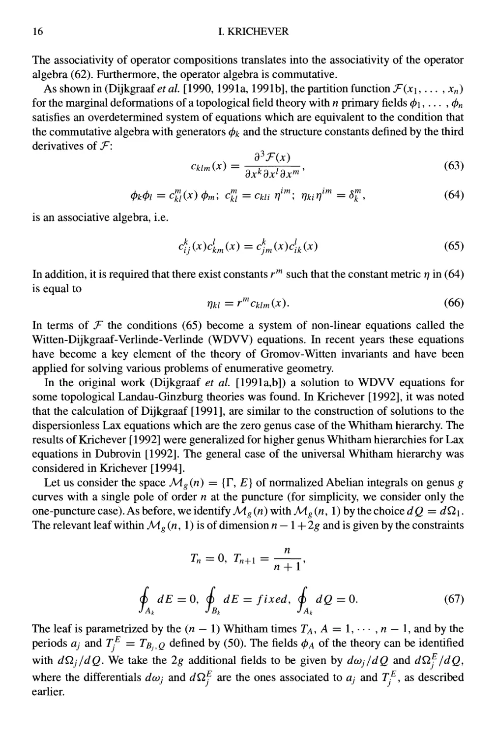
Let us consider the space Mg (n) = {F, E] of normalized Abelian integrals on genus g
curves with a single pole of order n at the puncture (for simplicity, we consider only the
one-puncture case). As before, we identify Mg(n) with Mg(n, 1) by the choice dQ = dQi.
The relevant leaf within Mg(n, 1) is of dimension n — l-\-2g and is given by the constraints
n
Tn = 0, r„+i =
AZ + 1
(f) dE =0, (f) dE = fixed, (f) dQ=0. (67)
The leaf is parametrized by the {n — \) Whitham times rA,A = l,•••,« — 1, and by the
periods Uj and T^ = Tbj,q defined by (50). The fields 0a of the theory can be identified
with dQj/dQ. We take the 2g additional fields to be given by dcoj/dQ and dO^J/dQ,
where the differentials dcoj and J^^ are the ones associated to aj and T^, as described
earlier.
BAKER-AKHIEZER FUNCTIONS AND INTEGRABLE SYSTEMS 17
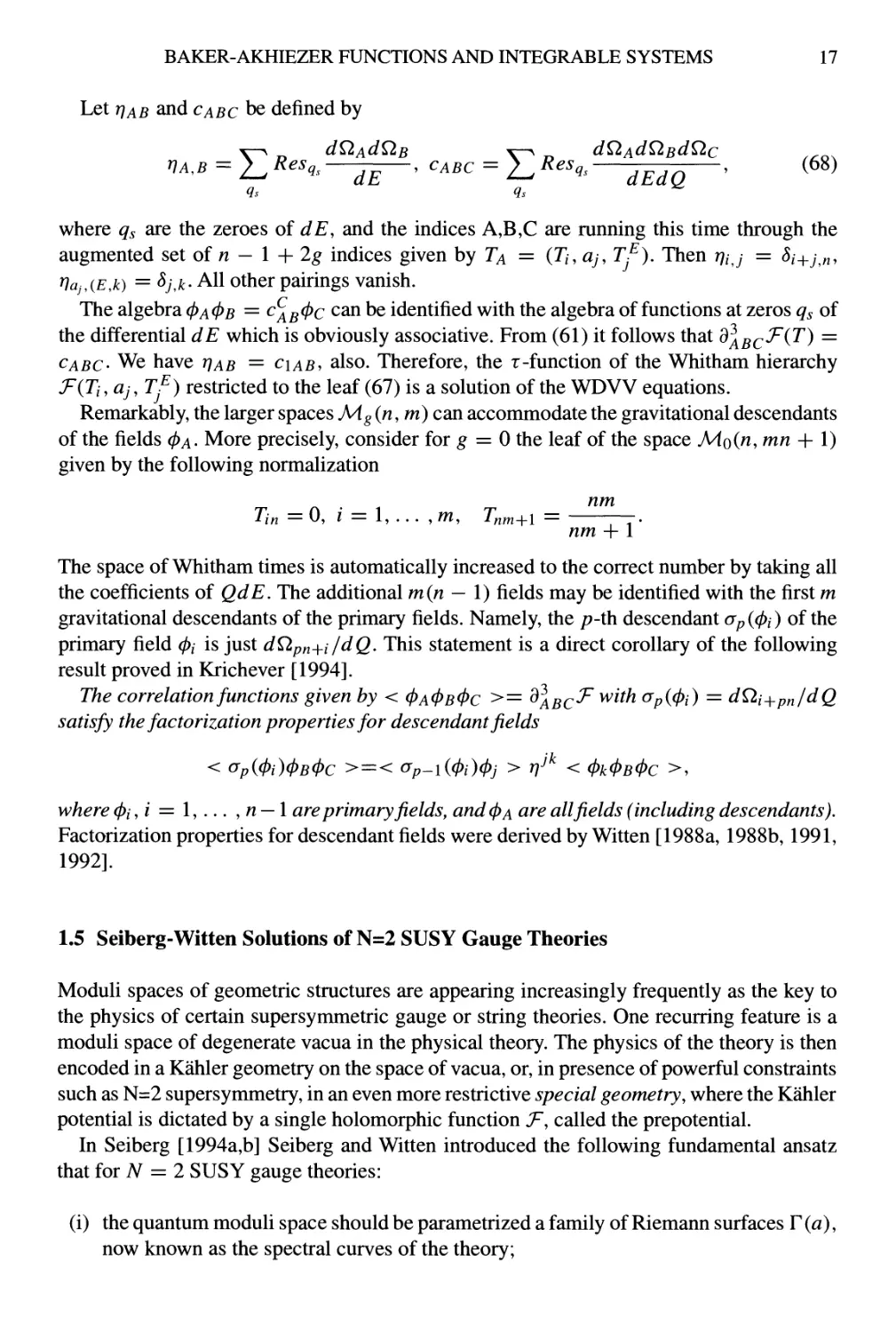
Let rjAB and cabc be defined by
E dQAdQB \-^ „ dQAdQBdQc .^ox
'''''''-^^' '^'^ -L^^^.^ dEdQ ' ^^^^
where ^^ are the zeroes of dE, and the indices A,B,C are running this time through the
augmented set of n — 1 + 2g indices given by Ta = (Tt, aj, T^). Then r]ij = Sj-^j^n^
Vaj,iE,k) = ^j,k' AH Other pairings vanish.
The algebra 0a 05 = ^a^^c can be identified with the algebra of functions at zeros qs of
the differential dE which is obviously associative. From (61) it follows that ^AfiC-^^^) ~
CABC' We have tjab = ciab, also. Therefore, the r-function of the Whitham hierarchy
J^(Ti, aj, Tf) restricted to the leaf (67) is a solution of the WDVV equations.
Remarkably, the larger spaces Mg(n,m) can accommodate the gravitational descendants
of the fields 0a. More precisely, consider for ^ = 0 the leaf of the space Mo(n, mn + 1)
given by the following normalization
^^
Tin =0, / = !,..., m, r^m+i =
nm + 1
The space of Whitham times is automatically increased to the correct number by taking all
the coefficients of QdE. The additional m(n — I) fields may be identified with the first m
gravitational descendants of the primary fields. Namely, the p-ih descendant <yp{(j)i) of the
primary field 0/ is just dQpn-{-i/dQ. This statement is a direct corollary of the following
result proved in Krichever [1994].
The correlation functions given by < (I)a(I>b(I>c >= ^abc^ ^^^^ cfp((j)i) = dQt-^pn/dQ
satisfy the factorization properties for descendant fields
< ap((j)i)(l)B(l)c > = < cfp-\{(l)i)(l)j > rjJ^ < (l)k(l>B(l>c >,
where (l)i,i = 1, ... , n — 1 are primary fields, and(l)A are all fields (including descendants).
Factorization properties for descendant fields were derived by Witten [1988a, 1988b, 1991,
1992].
1.5 Seiberg-Witten Solutions of N=2 SUSY Gauge Theories
Moduli spaces of geometric structures are appearing increasingly frequently as the key to
the physics of certain supersymmetric gauge or string theories. One recurring feature is a
moduli space of degenerate vacua in the physical theory. The physics of the theory is then
encoded in a Kahler geometry on the space of vacua, or, in presence of powerful constraints
such as N=2 supersymmetry, in an even more restrictive special geometry, where the Kahler
potential is dictated by a single holomorphic function ^, called the prepotential.
In Seiberg [1994a,b] Seiberg and Witten introduced the following fundamental ansatz
that for A^ = 2 SUSY gauge theories:
(i) the quantum moduli space should be parametrized a family of Riemann surfaces F (a),
now known as the spectral curves of the theory;
18 I. KRICHEVER
(ii) on each r(fl), there is a meromorphic one-form dX, such that its derivatives along the
moduli space are meromorphic differentials;
(iii) J^ is determined by the periods of dX
ak = Q) dX, aD,k = z-r Q) dX, -— = aD,k-
JAk 271 i Jb, dak
(69)
In Gorsky et ah [1995], it was noticed that the moduli space of curves for SU(N) theories
can be identified with spectral curves of the A/^-periodic Toda lattice. It was also noted
that the generating differential dX coincides with the generating differential dS (c.f. 53) of
the Whitham hierarchy. A general approach for solution of the Seiberg-Witten ansatz was
developed in Krichever et al [1997]. We present here Icey elements of this approach.
Let now n = iria), m = {nia), a = 1,... , N, be multi-indices, and Mg(n, m) be the
moduli space (F, £", Q) of pairs of Abelian differentials on F with poles of orders ria and
rua at punctures Pa. The dimension of this space is equal to
dimMgin, m) = 5g - 3-\-3N -\- Y^(na + m^). (70)
The Whitham coordinates on this space can be introduced in a similar way to the one
puncture case. The Abelian integral E defines a coordinate system Za near each Pa by
E=Za''"-\-R^logZa.
(for simplicity we assume that ria is strictly positive). Then the formulae
Taj = --Resp^{z'aQdE), Ta,o = Resp^(QdE), (71)
I
define I]^^i(AXa -\- rUa) -\- N - I parameters (X!a Ta,o = 0).
The remaining parameters needed to parametrize Mg (n,m) consist of the 2N—2 residues
of dE and dQ
R^ = RespJE, R^ = RespJQ, of = 2, • • • , A^, (72)
and 5^ parameters which are the periods of dE, dQ and a-periods of dS = qdE given by
(47, 50).
In Krichever et al [1997], it was shown that the joint level sets of all parameters except
ak = §j^ dS define a smooth foliation of the open seiV^ of Mg(n,m), which is independent
of the choices made to define the coordinates themselves. This intrinsic foliation is central
to the Seiberg-Witten theory and the Hamiltonian theory of soliton equations. We shall refer
to it as the canonical foliation.
Our goal is to construct now a symplectic form co on the complex 2^-dimensional space
obtained by restricting the fibration J\fg(n, m) to a ^-dimensional leaf M of the canonical
foliation of M.g{n,m).
BAKER-AKHIEZER FUNCTIONS AND INTEGRABLE SYSTEMS 19
Let us consider the Abelian integrals E and Q as multi-valued functions on the fibration.
Despite their multivaluedness, their differentials along any leaf of the canonical fibration are
well-defined. In fact, E and Q are well-defined in a small neighbourhood of the puncture Pi.
The ambiguities in their values anywhere on each Riemann surface consist only of integer
combinations of their residues or periods along closed cycles. Thus these ambiguities are
constant along any leaf of the canonical foliation, and disappear upon differentiation. The
differentials along the fibrations obtained this way will be denoted hy 8E and 8Q. Restricted
to vectors tangent to the fiber, they reduce to the differentials dE and dQ. These arguments
show that (Krichever et al. [1997])
the following two-form on the fibration M^in, m) restricted to a leaf M. of the canonical
foliation of M.g{n,m)
g g
COM = MI] 2(K/M^(n)) = I]5e(n) A dEin) (73)
defines a holomorphic symplectic form which is equal to
g
COM = /_] ^^i ^ ^^i' ^'^^^
i = l
where (pk are canonical coordinates on the Jacobian of the curve.
Note that the first set of formulae (61) implies that the restriction of the logarithm of the
r-function of the Whitham hierarchy on a leaf of the canonical foliation satisfies relations
(69) for the prepotential, and therefore, the function J^(T) given by (60) is a solution of the
Seiberg-Witten ansatz. Although the results presented above suggest deep relations between
N=2 gauge theories, soliton equations, their Whitham theory, and Landau-Ginzburg type
models, such relations are still not fully understood at the present time. Nevertheless, the
parallels between these fields allows us to apply to the study of the prepotential J^ of gauge
theories the methods developed in the theory of solitons. In D'Hoker et al. [1997], with
the help of these methods, the renormalization group equation for the prepotential J^ for
SU(A^c) gauge theories with Nf < 2Nc hypermultiplets of masses my in the fundamental
representation was derived. It was shown that this equation is powerful enough to generate
explicit expressions for the contributions of instanton processes to any order.
We conclude this chapter by a discussion of connections of the symplectic form (73) with
the Hamiltonian theory of soliton equations. The Hamiltonian theory of finite-dimensional
and spatial one-dimensional soliton equations is a rich subject which has been developed
extensively over the years (see Faddeev et al. [1987], Diclcey [1991]). However, until
recently much less was known about the 2D case. In Krichever et al. [1997, 1999], a new
algebro-geometric approach to the Hamiltonian theory of soliton equations was developed.
This approach is uniformly applicable for all integrable systems: finite-dimensional, spatial
one- or two-dimensional evolution equations. Its universality is based on a universal
symplectic form which can be defined on a space of operators in terms of operators and
their eigenfunctions, only. For simplicity we consider here the Lax equations (1) for the
operators (2) with scalar coefficients.
20 I. KRICHEVER
Let V^ (jc, /:) be a formal solution of the form
V.(x, k) = /^(l + ^§,(x)/:-0 (75)
to the equation Li// = k^i/r, normalized by the condition ijfiO.k) = 1. The coefficients hi
of the expansion
oo
dAnjlf = k-\-J2hsk~' (76)
s=l
are differential polynomials in the coefficients m, of L, i.e hi = hi(u). They are densities
of integrals of motions Hs = J hi(u)dx of the Lax equation (1). Let us introduce the dual
formal solution
oo
r=e-^'(\ + Y.^t{x)k-') (71)
s=l
of the formal adjoint equation V^*L = /:"t/^*, normalized by the condition / V^* t/^Jjc = 1.
The main ingredients are the one-forms 8L and S^o- The one-form 5L is given by
n-2
8L = J2^^iK^
i=0
and can be viewed as an operator-valued one-form on the space of operators L. Similarly,
the coefficients of the series i// are explicit integro-differential polynomials in m,. Thus Si//
can be viewed as a one-form on the space of operators with values in the space of formal
series.
Consider the following two-form on the space of operators L
( f(if''8LA8ilf)dxjdp,
CO = Resoo ( / (V^*5L A 8ilf)dx j dp, (78)
where p = k -\- ^^ Hsk~^. In Krichever et al. [1999] it was shown that on the subspaces
of the operators L defined by the constrains {Hi = const, / = 1,... , n — 1} the form co
(i) defines a symplectic structure, i.e, a closed non-degenerate two-form;
(ii) the form co is actually independent of the normalization point {x = 0) for the formal
Bloch solution i/rix, k);
(iii) the flows (1) are Hamiltonian with respect to this form, with the Hamiltonians
InHm+niu).
Consider now the leaves A^^ of the canonical foliation on M.g{n, 1) corresponding
to zero values of variables § dE = 0. These leaves correspond to spectral curves of
one-dimensional finite-gap Lax operators, i.e. we have a geometric map of the Jacobian
bundle A/^ over M^ to the space of operators
g:Af^ ^ (L).
BAKER-AKHIEZER FUNCTIONS AND INTEGRABLE SYSTEMS 21
A connection of the Hamiltonian theory of soliton equations with the previous construction
of algebro-symplectic structures associated with the Seiberg-Witten theory was established
in Krichever [1997]. Namely, it was proved that
(iv) the restriction of the symplectic form co given by (78) via the geometric map to the leaf
M^ of the canonical foliation is holomorphic symplectic form equals
g
The results presented above are a particular case of more general settings. It turns out the the
algebro-geometric symplectic structure (73) on the general leaves of the canonical foliation
on Mg (n, 1) is a restriction of the basic symplectic structure for 2D soliton equations. The
symplectic structure on leaves of the foliation for Mg (n, m) for m > 1 is the restriction of
higher symplectic forms for soliton equations. It is necessary to emphasize that the same
soliton equations are Hamiltonian flows with respect to all these structures but generated by
different Hamiltonians. A variety of examples which show the universality of our approach
can be found in Krichever et al. [1997, 1999].
Acknowledgement
Research supported in part by National Science Foundation under the grant DMS-98-02577
and by the grant RFFI-98-01-01161.
References
Baker, H.F, Note on the foregoing paper "Commutative ordinary differential operators", Proc. Royal
Soc. London 118, 584-593 (1928).
Burchnall, J.L., and Chaundy, T.W., Commutative ordinary differential operators. I, Proc. London
Math Soc. 21, 420-440 (1922).
Burchnall, J.L., and Chaundy, TW., Commutative ordinary differential operators. II, Proc. Royal Soc.
London 118, 557-583 (1928).
D'Hoker, E., Krichever, I., and Phong, D.H., The renormalization group equation for N=2
supersymmetric gauge theories, Nucl. Phys. B494, 89-104, hep-th/9610156 (1997).
Dickey, L.A., Soliton equations and Hamiltonian systems. Advanced Series in Mathematical Physics,
Vol. 12 (1991) World Scientific, Singapore.
Dijkgraaf, R., and Witten, E., Mean field theory, topological field theory, and multi-matrix models,
Nucl. Phys. B 342, 486-522 (1990).
Dijkgraaf, R., Verlinde, E., and Verlinde, H., Topological strings in ^ < 1, Nucl. Phys. B 352, 59-86
(1991).
Dijkgraaf, R., Verlinde, E., and Verlinde, H., Notes on topological string theory and 2D quantum
gravity, in "String theory and quantum gravity". Proceedings of the Trieste Spring School 1990,
M. Green (ed), World-Scientific, 1991.
Douglas, M., and Shenker, S., Strings in less than one dimension, Nucl Phys. B 335, 635-654 (1990).
Dubrovin, B., and Novikov, S., The Hamiltonian formalism of one-dimensional systems of the
hydrodynamic type, and the Bogoliubov-Whitham averaging method, Sov. Math. Doklady 27,
665-669 (1983).
22 I. KRICHEVER
Dubrovin, B., Hamiltonian formalism of Whitham-type hierarchies and topological Landau-Ginzburg
models, Comm. Math, Phys. 145, 195-207 (1992).
Dubrovin, B., Matveev, V., Novikov, S., Non-linear equations of Korteweg-de Vries type, finite zone
linear operators and Abelian varieties, Uspekhi Mat. Nauk 31(1), 55-136 (1976).
Faddeev, L., and Takhtajan, L., "Hamiltonian methods in the theory of soliton". Springer-Verlag,
1987.
Flaschka, H., Forrest, M., and McLaughlin, D., Multiphase averaging and the inverse spectral solution
of the Korteweg-de Vries equation, Comm. PureAppl. Math. 33, 739-784 (1980).
Gorsky, A., Krichever, I., Marshakov, A., Mironov, A., and Morozov, A., Phys. Lett. B 355, 466-474
(1995).
Krichever, I., and Phong, D.H., On the integrable geometry of soliton equations and N = 2
supersymmetric gauge theories, J. Differential Geometry 45, 349-389 (1997).
Krichever, I., and Phong, D.H., Symplectic forms in the theory of solitons. Surveys in Differential
Geometry: Integral Systems, vol. 4, 239-313. International Press, Boston (1999).
Krichever, I., Averaging method for two-dimensional integrable equations, Funct. Anal. Appl. 22,
37-52 (1988).
Krichever, I., Methods of algebraic geometry in the theory of non-linear equations, Russian Math
Surveys 32, 185-213 (1977a).
Krichever, I., Spectral theory of two-dimensional periodic operators and its applications, Uspekhi
Mat. Nauk 44(2), 121-184 (1989).
Krichever, I., The r-function of the universal Whitham hierarchy, matrix models, and topological field
theories, Comm. PureAppl. Math. 47, 437^75 (1994).
Krichever, I., The algebraic-geometric construction of Zakharov-Shabat equations and their solutions,
Doklady Akad. Nauk USSR 227, 291-294 (1976).
Krichever, I., The commutative rings of ordinary differential operators. Funk. anal, ipril. 12(3), 20-31
(1978).
Krichever, I., The dispersionless Lax equations and topological minimal models, Comm. Math. Phys.
143(2), 415^29 (1992).
Krichever, L, The integration of non-linear equations with the help of algebro-geometric methods.
Funk. anal, ipril. 11(1), 15-31 (1977b).
Lax, P., Periodic solutions of Korteweg'de Vries equation, Comm. Pure and Appl. Math. 28, 141-188
(1975).
McKean, H., and van Moerbeke, P., The spectrum of Hill's equation. Invent. Math. 30, 217-274
(1975).
Novikov, S., Periodic Problem for the Korteweg-de Vries equation, Funct. anal, i pril. 8(3), 54-66
(1974).
Seiberg, N., and Witten, E., Electric-magnetic duality, Monopole Condensation, and Confinement in
N = 2 Supersymmetric Yang-Mills Theory, Nucl. Phys. B 426, 1952, hep-th/9407087 (1994).
Seiberg, N., and Witten, E., Monopoles, Duality and Chiral Symmetry Breaking in N = 2
Supersymmetric QCD, Nucl. Phys. B 431, 484-550, hep-th/9410167 (1994).
Witten, E., Topological Quantum Field Theory, Comm. Math. Phys. Ill, 353-386 (1988).
Witten, E., Topological sigma models, Comm. Math. Phys. 118, 411^49 (1988).
Witten, E., Two-dimensional gravity and intersection theory on moduli space. Surveys in Differential
Geometry 1, 281-332 (1991).
Witten, E., Mirror manifolds and topological field theory, in "Essays on Mirror Manifolds", ed. by
S.T. Yau, International Press (1992), Hong-Kong, 120-159.
Algebraic Geometry, Integrable Systems, and
Seiberg-Witten Theory
EYAL MARKMAN
Department of Mathematics and Statistics, University of Massachusetts Amherst, MA, USA
e-mail: emarkman @ math, umass.edu
This survey chapter reviews the relationship between integrable systems and the moduli spaces of A^ = 2
supersymmetric Yang-Mills theories in 4 dimensions. Our starting point is the special Kahler structure on these
moduli spaces. We then review the geometry of the generalized Hitchin systems. Donagi and Witten conjectured
that a particular Hitchin system produces a special Kahler structure equal to the one coming from the moduli of
the supersymmetric Yang-Mills theory when the gauge group is SU(n). We conclude with a closer look at this
particular Hitchin system.
2.1 Introduction
Physical arguments imply that the moduli space B of N = 2 supersymmetric Yang-Mills
theories in 4 dimensions is a finite dimensional Kahler manifold endowed with an extra
structure called a special Kahler structure. The mysterious connection between these
Yang-Mills theories and integrable systems is formally explained by
Theorem 2.1 (see Donagi and Witten [1996], Donagi [1997] and Freed [1999], Theorem
3.4) The following data are equivalent:
L the data given by an integral special Kahler structure on a complex manifold B, and
2. the data given by an algebraically completely integrable hamiltonian system A^- B,
Algebraic integrable systems are defined in section 2.2. The definition of a special Kahler
structure and the derivation of Data 2 from Data 1 is sketched in Section 2.3. In Section 2.4
we will briefly explain how a special Kahler structure is defined on the base of every
algebraic integrable system. In view of the above equivalence, it is natural to look for a
23
24 E. MARKMAN
known integrable system A ^^ B, which special Kahler structure on B is the one coming
from supersymmetric Yang-Mills theory. Such an identification enables one to compute the
real-world observables of the N = 2 supersymmetric Yang-Mills theories ("the low energy
effective Lagrangian") in terms of periods of a family of abelian varieties. Donagi and
Witten conjecture that the integrable system for the SU(n) theory is a generalized Hitchin
system [1996]. In Sections 2.5 we review the general construction of these systems and their
Poisson structure. In Section 2.6 we describe the complete integrability of the symplectic
leaves of the generalized Hitchin systems. Section 2.7 is devoted to the geometry of the
particular Hitchin system considered by Donagi and Witten: the moduli space of KP elliptic
solitons of order Az.
The moduli space of KP elliptic solitons fits also in a family of integrable systems
associated to root systems; the Calogero-Moser systems with elliptic parameter. The
Calogero-Moser systems are conjectured to provide the identification of the special Kahler
structure of the supersymmetric Yang-Mills theories for all simple groups. Lax pairs for
these systems are described in Bordner et ah [1999] and Hoker and Phong [1998]. An
interpretation of the Calogero-Moser systems as Hitchin systems is worked out in Hurtubise
and Markman [1999].
Most of the material below is contained in the excellent survey of Donagi [1997]. One
exception is a sufficient condition for the generic fiber of the Hitchin map in a given
symplectic leaf to be smooth and compact (Proposition 2.10 and Corollaries 2.11 and 2.13).
We include this more detailed discussion in response to questions asked at the workshop.
2.2 Algebraically Completely Integrable Systems
An algebraically completely integrable Hamiltonian system is a complex algebraic variety
M (the phase space) with a holomorphic symplectic structure a (a (2, 0)-form) and a
lagrangian fibration tt : M ^^ B. Given a function / on M, the symplectic structure
translates the 1-form df to a (Hamiltonian) vector field. The algebra of functions on the
base B gives rise to a maximal sub-algebra of commuting vector fields on M. Classically,
such systems were discovered in the study of differential equations. A classical example is
the geodesic flow on ellipsoids. In that context, one starts with a hamiltonian (function) on
M (e.g. the kinetic energy in the case of geodesic flow) and the coordinates of the lagrangian
fibration n correspond to a complete set of conserved quantities. Compact smooth lagrangian
fibers are tori by Liouville's Theorem. The integral curves of the Hamiltonian vector field are
"straight lines" in the lagrangian fibers. When these tori are abelian varieties, one uses theta
functions to obtain explicit formulas for the solution of the ordinary differential equation
given by the Hamiltonian vector field.
Recall, that an n-dimensional compact complex torus A is an abelian variety, if it admits
an embedding as a subvariety of the complex projective space. Integration
/
//i(A,Z) ^ //^'^(A)* (1)
embeds the first homology as a full lattice in the complex vector space dual to the
space of global holomorphic one-forms. As a complex torus A is naturally the quotient
SEIBERG-WITTEN THEORY 25
//^'^(A)*///i(A, Z). An embedding of A into projective space is determined by a
positive line-bundle whose first Chem class is an integral Kahler (1, l)-form co (the
polarization). We can choose a symplectic basis yi,..., y^; y^+i,..., y2n for //i(A, Z)
so that span[y\,...,]/«} and span{yn-\-i, -. - ^yin) are isotropic with respect to a> and
co(yi, yn-\-j) = ^i • ^ij' The non-zero integers 5i,..., 5„ are called the divisors of the
polarization and the polarization in principal if they are all equal to 1. As elements in
//^'^(A)* we can express the last n elements y„+i,..., y2n in terms of yi,..., y„
n
Yn+i = E^O?- (2)
The two conditions (i) a> is a (1, l)-form and (ii) co is Kahler, translate to Riemann's two
bilinear conditions: (i) then x n matrix r is symmetric and (ii) its imaginary part Im(z) is
positive definite (Griffiths and Harris [1978]). Consequently, any polarized abelian variety
(A, co) is obtained as the quotient of C" by the lattice generated by the columns of an n x 2n
matrix (A5; r) where A5 is a diagonal matrix with integral entries 8i and r is a point in the
Siegel upper half space
Mn := {n X n symmetric matrices with a positive definite imaginary part}.
Changing the choice of a symplectic basis yi,..., y^; y^+i,.. •, y2n introduces an action
of an integral subgroup Fs of Sp(2n, R) on H^. If the polarization is principal, the modular
group r is Sp(2n, Z). Two points in M^ correspond to the same polarized abelian variety
if and only if they belong to the same orbit of Vs.
2.3 Integral Special Kahler Geometry
Let G be a complex reductive group of rank r, T a maximal torus, g, t, their Lie algebras,
and W the Weyl group. The moduli space ofN = 2 supersymmetric Yang-Mills theory in
4 dimensions is the vector space B := i/W.liis equipped with an integral special Kahler
structure. Locally, this special Kahler structure consists of the following data:
1. Electric charges ai,... , a^ thought off as holomorphic coordinates on B.
2. A holomorphic function J-'(ai,... ,ar) on B (the prepotential) expressing the relations
between the electric and magnetic charges.
The goal, which was achieved in Serberg and Witten [1994] for SL(2, C), is to compute
the functions at and the prepotential J^ in terms of the natural coordinates ut on the vector
space t/ W. The coordinates ut are those obtained by a choice of generators for the algebra
of W-invariant polynomials on t.
The magnetic charges are given by
af := f (3)
and are thought off as dual coordinates on B. Clearly, the electric and magnetic charges
determine the prepotential up to an additive constant. We get also a symmetric matrix
r(a)ij := -^ (4)
dai auj
26 E. MARKMAN
whose imaginary part is required to be positive definite (a point in the Siegel upper half-space
Mr). It follows that
ds^ := Im{xdada) = Im(da^dd),
K{a,a) := -Im ( ^S^a^di j , and
tj
are a Kahler metric, its Kahler potential, and its Kahler form.
Analytic continuation of the local holomorphic functions {at, aj^] globally on B (away
from a bad codimension 1 locus) forces multi-valuedness. The electric-magnetic "duahty"
is the statement that a finite index subgroup of the integral symplectic group Sp(2r, Z) is
a symmetry group for the data {at, «,^}. More precisely, any other local branch [bj, bj^] is
related to {at, aP] by an affine integral symplectic monodromy transformation
Above, R is an integral symplectic matrix, the constants m, are the masses and nt.nf are
integral vectors. Consequently, the differential one-forms transform via R
(db^\ ^ j,(da^\
\db ) \da )
In particular, in the absence of masses, the electric and magnetic charges can be interchanged
(up to sign) by the involution R = \ j f\Y
The fact that R is symplectic implies that the Kahler form co is global (single-valued).
The integrality of R implies that [dai^da^] is a local symplectic basis of a global family
A := Uh^B^b consisting of a rank 2r integral lattice A^ in each holomorphic cotangent
space T^ B. Consequently, we get a family A:= {T'^B)/A of abelian varieties (away from a
bad locus of codimension 1 in i5). Moreover, the natural symplectic form on r*i5 descends
to A because, locally, the lattice A is generated by closed 1-forms. We see that an integral
special Kahler structure gives rise to an integrable system A ^^ B whose lagrangian fibers
are principally polarized abelian varieties.
One can formalize the above discussion and define an integral special Kahler structure
on a Kahler manifold M via the above local data and subject to the above integral symplectic
gluing transformations. An equivalent coordinate-free definition was found by Freed [1999].
Definition 2.2 A special Kahler structure on a Kahler manifold M is a real flat torsion-free
symplectic connection v on the tangent bundle of M with respect to which, the complex
structure I satisfies dyl =0. The special Kahler structure is integral if there is a lattice
A* C TM, flat with respect to v» whose dual A C T'^M is a complex lagrangian
submanifold.
SEIBERG-WITTEN THEORY 27
In case G is SL(2, C), the moduli space i5 is a complex line, r in (4) is a point in the
upper half plane M and A ^^ B isa family of complex elliptic curves. Seiberg and Witten
used physical arguments to show that, in the absence of mass, the monodromy group is the
level-2 congruence subgroup r(2) of SL(2, Z) generated by
(-2 ?) ^'^ (o^ -l)-
This is precisely the monodromy of the family of elliptic curves Eu given by the equation
/ = (jc + l)(jc - l)(jc - m), m g C \ {1, -1}.
2.4 The Special Kahler Structure of an Integrable System
We sketch in this section the construction of a special Kahler structure on the base i9 of an
algebraically integrable system n : A ^^ B with a section s : B ^^ A. We assume that all
fibers are smooth polarized abelian varieties. In particular, the local system of integral first
homologies R\^nJ^ corresponds to a representation 7i\{B, bo) ^^ F^ of the fundamental
group of the base in the integral modular subgroup Fs of Sp(2n, R) (see Section 2.2).
We may assume also that the section s is lagrangian (otherwise, replace the symplectic
structure a by the difference a — {sonYa). Since tt is a lagrangian fibration, the symplectic
structure induces an isomorphism between the tangent bundle and the conormal bundle of
each fiber A^. Both are trivial bundles modelled after the vector spaces //^'^(A^,)* and T^B
respectively. We get an isomorphism
i : (H^^^y ^ T*B (6)
of vector bundles over the base B. Composing l with a relative version of the integration
homomorphism (1) we get an embedding of the local system of integral first homologies
Ri^j^^Z eis a, holomorphic family A C r*i5 of full lattices in the cotangent bundle of the
base. It follows that the phase space A is canonically isomorphic to the quotient T*B/A.
The section s of A pulls back to A C T*B. Hence, A is lagrangian with respect to the
puUback or of (7 to r*i5. In particular, the zero section of r*i5 is lagrangian, which implies
that a is the standard symplectic structure on r*i5. It follows that local sections of A are
closed holomorphic 1-forms.
We can choose a symplectic basis of local sections of A
Jzi,..., Jz„; dzi ,... ,dzn
corresponding to a symplectic basis of local sections of Rx^-^JL. Being closed, we can lift
the local basis to a set of holomorphic functions {zi. ^f }• The equations defining the period
matrix (2) translate to the system of linear equations
^.? = E'.f •
28 E. MARKMAN
The symmetry of Zij implies that the 1-form
dT:^y:zr-^
is closed. Hence, locally on the base, we get a holomorphic function J^ satisfying
oZi
Setting ai := |- and aP := zf we get the local data of a special Kahler structure.
Remark 2.3
1. (Donagi and Markman [1996a]) While the local sections dT and Yl,ij dlfa^^i ^ ^^J
of r*i5 and Sym^{T''B) depend on the choice of a symplectic basis, the cubic tensor
obtained locally as the third derivative of ^ is a global section c of Sym^(T'^B). Under
the identification of r*i5 with the Hodge bundle H^'^ via (6) and the polarization, c
is mapped to the differential of the classifying map B -^ M^/ F^, which is a global
section of Hom(TB, Sym^H^i).
2. The special Kahler structure we get, locally on the base, is the one coming from the
family A ^^ B of principally polarized abelian varieties, where A^ is obtained from the
quotient of A^ by the subgroup of order YYi=i ^i
spanzi-—, • • •. -r~} I spanzidzu • • •, dzn)
01 On
of torsion points. In general, there does not exist a canonical choice of such a subgroup.
Thus, the global analogue A, of the lattice span[dai, da^} defining the special Kahler
structure, would be constructed on a finite cover B ^^ B parametrizing such choices.
2.4.1 Seiberg- Witten Differentials
The special Kahler structure on the moduli space B of supersymmetric Yang-Mills theories
involves the electric and magnetic charges rather than their differentials. In other words,
it includes a global lift of the lattice of closed 1-forms A C r*i5 via a homomorphism
J : A ^^ Ob into the sheaf of holomorphic functions. The lift is subject to the symplectic
affine monodromy transformations (5). In the case when all the masses m, vanish (and
the transformations are symplectic), such lifts I are in one-to-one correspondence with
equivalence classes of holomorphic 1-forms XonA satisfying
a = dX. (7)
In particular, the symplectic form a on >l is exact. Two such 1-forms Xi, X2 give rise to the
same left / if and only if Xi — X2 is the pulback of a 1-form on B. Indeed, given such a 1-form
X and a local section y of A, we consider y as a section of the lattice of first homologies
Ri,Tr^Z and define the value of I(y) at Z? g i5 to be the y-period of the restriction of X to
Ah. Conversely, given such a lift I, the local vector field J^t ^i j^. patches to a global vector
field V on B. Let /x^ be the corresponding function on 7*5 and a the tautological (action)
1-form on r*i5. Then the 1-form X := ot — dfjCy on r*i5 is invariant under translations
by local sections of A and descends to a 1-form X on A satisfying (7). (See Lemma 2 in
Donagi and Markman [1996a] for more details).
SEIBERG-WITTEN THEORY 29
In the general case, when the masses m, do not vanish, a lift I: A ^- Ob satisfying (5)
is provided by a meromorphic 1-form X satisfying (7) and having poles along A^ divisors
with residue m, along the i-ih divisor.
2.5 Yang-Mills Theory and Algebraic Geometry
The special Kahler structure on the r-dimensional moduli space ofN = 2 supersymmetric
Yang-Mills theories in 4 dimensions (with one hypermultiplet of mass in the adjoint
representation) is known to depend on the (complexified) gauge group G of rank r, one mass
parameter m, and an ^L (2, Z) orbit of a point Xd in the upper half plane. We are thus looking
for a known family of 2r dimensional integrable systems depending on these parameters. A
natural first guess would be to consider integrable systems arising from classical Yang-Mills
theory.
We describe in this section a family of integrable systems, the generalizedHitchin systems,
depending canonically on gauge theoretic data
('E,G,C,DARp]peD)
where S is a Riemann surface, G a complex reductive group, c the topological type of a
principal G-bundle (the first Chem class in the case of GL{n)), D an effective divisor on
S, and Rp is a marking of each point /? g D by a non-zero coadjoint orbit Rp in g* (or,
possibly, in the dual of the positive half of the loop algebra) (see Hitchin [1987a], Bottacin
[1995] and Markman [1994]). The phase space of this integrable system is the moduli space
M := M(i;, G, c, D, [Rp}p^D) of Higgs pairs defined below.
If G is 5 L(r +1) and we choose S to be the elliptic curve determined by r^/, then the
dimension of M (if non empty) is equal to the dimension of YipeD ^p- ^^^ ^^^y choices
(D, YipeD Rp^ resulting in a 2r dimensional system are: (i) D empty, in which case we
get the Hitchin system, (ii) D consists of the zero point po of the elliptic curve and Rp^
is the minimal non-zero nilpotent orbit, in which case we get another birational model of
the Hitchin system, or (iii) D consists of the zero point po and Rp^ = mR, where R is the
minimal non-zero semi-simple coadjoint orbit of
/-I 0 ... 0\
0 -1
' (8)
-1 0
\ 0 ... 0 rj
Donagi and Witten performed a sequence of (quite involved) tests verifying that the geometry
of this family of integrable systems agrees with the physical predictions [1996]. We will
come back to this system in Section 2.7. The dimension of non-zero coadjoint orbits of other
simple groups is larger than 2r. Hence, non-trivial choices of data (D, YipeD ^/?) ^^^^ ^^
integrable systems of too large a dimension. The Calogero-Moser systems are conjectured
to be the correct choice for more general groups (see Bordner et al [1999], D'Hoker and
Phong [1998], and Hurtubise and Markman [1999]).
30 E. MARKMAN
Definition 2.4 A (holomorphic) Higgs pair (P,(p) over S consists of a principal G bundle
P and a holomorphic section cp of the twist ad(P) (8) Kj: of its adjoint Lie algebra bundle
by the canonical line bundle. The pair (P,(p) is a meromorphic Higgs pair if instead,
(p is a meromorphic section of ad(P) (g) Kj:. The Higgs pair is stable (semi-stable) if
every ad (P)-invariant subbundle p C ad(P) of parabolic subalgebras has negative (resp.
non-positive) degree.
When G is GL{n), then P is the frame bundle of a vector bundle E and cp G EndC^") (g) K^,
is a 1-form with values in the endomorphism bundle of E. The moduli space M(i;, G, c)
parametrizes isomorphism classes of (stable) holomorphic Higgs pairs of topological type
c (where c is a class in 7ri(G)). If the principal bundle P is itself stable, then standard
deformation theory identifies the space H^{Ti, ad{P)) with the tangent space to the moduli
space of principal bundles. Using Serre's duality we get that the space //^(S, ad(P) (8) ^e ),
of Higgs fields with a fixed bundle P, is the cotangent space to moduli. Hence, the cotangent
bundle of the moduli space of principal bundles is an open set of M(i;, G, c). M(i;, G, c)
is the phase space of the Hitchin system.
Remark 2.5 The stability condition is significant for two reasons: It enables one to
construct the moduli space as an algebraic (quasi-projective) variety (see Faltings [1993],
Hitchin [1987a], Nitsure [1991] and Simpson [1994, 1995]). There is also a real-analytic
isomorphism between M(i;, G, c) and the moduli space of irreducible representations
of the fundamental group of S (or of a central extension of 7ri(i;)). In that context,
stability of the Higgs pair corresponds to irreducibility of the representation. There is also a
relationship between meromorphic Higgs pairs (possibly with additional parabolic data) and
representations of the fundamental group of the complement of the polar divisor (Hitchin
[1987a] and Simpson [1990]).
Denote by M(i;, G, c, D) the moduli space of (stable) meromorphic Higgs pairs whose
polar divisor is contained in a fixed effective divisor D. We will denote it also by M(D)
for short. M(D) is smooth if the group is GL(n) or SL(n), but it may have quotient
singularities in general (in which case the moduli stack is smooth) (see Faltings [1993]).
Some insight into the geometry of M(D) is gained by its realization "as" the quotient of
a symplectic variety by a finite dimensional Hamiltonian group action. We will obtain a
rough description of a Zariski open subset of M(D) as a bundle of Hitchin systems over
the dual g^ of a Lie algebra (or a reduction of g^ if S is rational or elliptic). In particular,
when the Hitchin system (of holomorphic Higgs pairs) is a single point, the moduli space
of meromorphic Higgs pairs admits a group theoretic description. This happens when S is
rational (Example 2.6) or elliptic (Example 2.8).
Example 2.6 (Alder and van Moerbeke [1980], Adams et al. [1990], Beauville [1990]
and Reiman and Semenov-Tian-Shansky [1994]) Let us describe this open subset of M(D)
when S is rational, c is the trivial topological type and D is a collection of distinct points
D = pi-\-p2-\ \-pd^ d > 3. An open subset of M(D) consists of Higgs pairs with a trivial
G-bundle P. Hence, it consists of conjugacy classes of sections cp of //^(P^, g* (8)c K(D))
by the group G (considered as the group of global automorphisms of P). By the residue
SEIBERG-WITTEN THEORY 31
theorem, H^(F^, g* (8)c K(D)) embeds as the kernel of
(01,...0j) h> ^0,-
1 = 1
where /x is the moment map for the diagonal conjugation action. Hence, an open subset of
M(D) is the reduction of the dual §^ of the Lie algebra of the group Gd of maps from D to
G. In particular, M(D) has a Poisson structure. When D contains a point with multiplicity,
the above statements holds if Gd is the group of jets of maps.
2.5.7 The Poisson Structure
The moduli space of holomorphic Higgs pairs is a partial compactification of the cotangent
bundle of the moduli space of principal bundles. Hence, it has an algebraic symplectic
structure (even a hyperkahler structure). The moduli space M(D) of meromorphic Higgs
bundles has a natural Poisson structure. A canonical global formula for this Poisson structure
is obtained via cohomological techniques once the tangent and cotangent spaces to moduli
at a Higgs pair (P, ^) are identified with the first hyper-cohomology of the complexes
r(p,^)M(D) = H\ad{P) ^ ad{P) 0 K^{D)]
T^^P^^^M(D) = H\ad{P){-D) ^ ad{P) 0 K^] (9)
The contraction with the Poisson structure T^p .M(D) -^ T(p^(p)M(D) is induced by
the natural homomorphism of complexes (Bottacin [1995], Markman [1994] and Faltings
[1993]).
A geometric description of the Poisson structure on a Zariski open subset of M(D)
was given in Markman [1994]. Recall that when a group G is acting symplectically on
a symplectic variety X with a moment map /x : X ^- g*, then a "nice" quotient X/G
has a natural Poisson structure. Given a coadjoint orbit R C Q*, the symplectic reduction
fji~^(R)//G (when connected) is a symplectic leaf of X/G. For example, the standard
Poisson structure on the dual of a Lie algebra g* can be recovered via the above construction
if we consider g* as the quotient of the cotangent bundle r*G via the lifted action of G.
Let V{Ti,G,c, D) be the moduli space of framed principal bundles. We denote it by
V{D) for short. A point in V{D) is a pair (P, vj) consisting off a principal bundle P and a
lift
T] \ D ^^ P
of the divisor D to an embedding in the total space of P. When G is GL(az), P is the
frame bundle of a vector bundle £", and D consists of distinct points, then r] corresponds
to a choice of a frame in each fiber of E over D. Standard deformation theory identifies
the tangent bundle of V{D) at (P, vi) with //^(S, ad(P)(-D)). Serre's duality identifies
the cotangent space with H^(i:,ad(P) (g) K(D)). Hence, the cotangent bundle T^'ViD)
paramQinzQs framed Higgs pairs. A point in T*V(D) is a triple (P,(p,r]) where (P, ^) is
a Higgs pair and ?; is a framing of P along D.
32 E. MARKMAN
Note that the data of a framing t] is equivalent to a trivialization of the restriction of the
bundle P to D. The group Go of maps from D to G acts naturally on V(D) by changing
the framing data rj. Hence, it act symplectically on its cotangent bundle. The quotient space
"is" the moduli space of Higgs pairs (over open sets where the various stability notions
agree). The action of Go factors through its quotient Go •= Gd/Z(G) by the diagonal
embedding of the center of G (because the center Z(G) embeds in the automorphism group
of P). The moment map
(P^cp,ri)^((pi^r (10)
conjugates the restriction (p\^ via the trivialization rj into q (S>c (K(D))\^. The latter space
is naturally identified with g^ via the trace-residue pairing. We get that a coadjoint orbit
R = YipeD ^p ^^ 5d determines a symplectic leaf M(R) in the moduli space M(D) of
Higgs pairs. Coadjoint orbits of g^ embed via the inclusion g^ ^-> g^ as those coadjoint
orbits of 0^ which central summand satisfies the constraint imposed by the global residue
theorem.
Example 2.7 In the setup of Example 2.6, the quotient Gd/G is the open subset in the
moduli space of (stable) framed bundles V(F^, G, c, D) consisting of isomorphism classes
of pairs (P, rj) with P trivial. The action of Go on Gd/G lifts to the cotangent bundle
T'^iGo/G). The moment map is Gd -equivariant. In particular, it is equivariant with respect
to the stabilizing group G/Z(G). As the action of Go on Gd/G is transitive, we get that
the quotient map
T\Gd/G) -^ M(D)
factors through the moment map as the composition
T*{GdIG) ^ qI ^ Ql/G.
This is precisely the birational embedding of M{D) in 02)/G described in Example 2.6.
Example 2.8 (The elliptic Gaudin system (Reiman and Semenov-Tian-Shansky [1994])
and (Markman [1994]) Section 9.2). A second example of a rigid bundle is obtained when
the curve S is elliptic, the group G is GL{n) but we fix the determinant line bundle of
the vector bundle det(£') = L and require its first Chem class c to be relatively prime to
the rank n. Atiyah proved that there exists a unique such stable vector bundle E (Atiyah
[1957]). The moduli space V(L, D) of framed bundles contains, as a Zariski open subset,
a copy of SL(n)D' The moduli space M(L, D) of traceless Higgs pairs (F, cp) with fixed
determinant line bundle L contains the vector space //^(S, End(£')o <S>K(D))2is the Zariski
open subset in which F is stable (and hence isomorphic to E). An argument analogous to
the one in Example 7 provides an isomorphism between this open subset of M(L, D) and
the quotient (slnTo ^f T'^[SL(n)D] by SL(n)D' This isomorphism is compatible with the
poisson structures because the quotient map is the moment map. In particular, we get that
coadjoint orbits of the Lie algebra (5/^)^ are completely integrable systems!
SEIBERG-WITTEN THEORY 33
2.6 Complete Integrability
Hitchin made the remarkable observation that the moduli space of holomorphic Higgs
pairs is a completely integrable system [1987]. The lagrangian fibration is given by
the characteristic polynomial map (also known as the Hitchin map). The analogous
construction induces a lagrangian fibration on the symplectic leaves M(R) of the moduli
space of meromorphic Higgs pairs. Let ai,... a^ be generators of the algebra of invariant
polynomials on g, dt the degree of at and set
Char(D) := e^^i/Z^S,/^(D)®^0-
Since a, is invariant, it can be evaluated at the section cp of ad(P) (g) K(D) to give a global
section of //^(S, K{D)®^'). We get the characteristic polynomial map
char : M{D) -^ Char(D). (11)
It is easy to check that the dimension of the generic fiber of char is equal to half the
dimension of the maximal dimensional symplectic leaves M(R) corresponding to regular
(of maximal dimension) coadjoint orbits R of g^ (See Markman [1994], Proposition 7.17).
Moreover, the algebra of polynomials on Char(D) pulls back to a Poisson involutive algebra
on M(D).
The generic fiber of char is a smooth compact abelian variety contained in a unique
symplectic leaf M(R) of maximal dimension (here we need to assume that the derived
subgroup of G is simply connected to assure that the fiber is connected). This abelian
variety is the Jacobian of a branched (spectral) cover of S if the group is GL(n) (see
Beauville et al [1989]). In that case, we choose the invariant polynomials at on g/„ to
be the coefficients of the characteristic polynomial. Given a section Z? := (Z?i,..., Z?„) of
Char(D), we get a morphism of complex surfaces pb : K{D) -^ K(D)®^ which sends a
section y of K(D) to the section y"" + biy""-^ + • • • + Z?« of KiD)®"". The spectral curve
Cb is the inverse image in K(D) of the zero section of K{D)®^. If b is the characteristic
polynomial of a Higgs pair (E,(p : E ^^ E (S) K(D)), then the spectral curve parametrizes
eigenvalues of cp. The puUback of E to Cb contains a canonical eigenline-sub-bundle. This
defines a map from the fiber of char over b to the group PIcq of line bundles on Cb.
The inverse PIcq -^ char~^ (b) of the above map is obtained as follows (up to a shift by
the ramification line-bundle): The pushforward tt^L of a line-bundle L on Cb to S is a rank
n vector bundle £" on S. The fiber of E over a point jc G S is the direct sum of the fibers
of L at the points of Cb over x (if a point ic is a ramification point of tt : C^? ^- S, then the
space of jets of sections of L at ic of appropriate height is taken as a direct summand). L
determines also a Higgs field (p \ E ^^ E^ K(D). Observe first that the pullback 7t''K{D)
of the line bundle K{D) to its total space has a canonical section y. Away from the fibers
over D, the surface is the cotangent bundle of S and y is the action 1-form on the surface.
It extends to the whole surface as a meromorphic 1-form with poles along 7r~^(D). We
get a homomorphism <^yb \ L ^> L ^ n'^K(D) where yb is the restriction of y to Cb-
The Higgs field cp is the pushforward of (Siyb- The meromorphic 1-form y provides the
Seiberg-Witten differential needed to derive a special Kahler structure from the Hitchin
systems (see Section 2.4.1).
34 E. MARKMAN
For a general reductive group G, the generic fiber of char is described in terms of a curve
in the twisted Cartan bundle t (8)c K(D). One observes that the vector bundle ^^■^■^KiD)'^^'
is the quotient of the total space of t (8)c K(D) by the natural action of the Weyl group
A point b in Char(D) is a section of the quotient bundle. The inverse image Cb := q~^(b)
is a curve embedded in t (S>c K{D). We call Cb the cameral cover. It is a Galois W-cover
of S. Denote by A the weight lattice Hom(T, C^). The data of a principal T-bundle C on
Cb is equivalent to the data given by the homomorphism
sending a weight of T to the associated principal C^ bundle, i.e., to a line-bundle on Cb.
Hence, the moduli space of principal 7-bundles on Cb is Horn (A, Pic^ ), whose connected
component is the cartesian product of r copies of the Jacobian /^ . The Weyl group acts
on A and J^ and the generalized Prym is the connected component of the subgroup of
W-equi variant homomorphisms
Prynib := Homw(A, J'^)^.
The fiber of char over a characteristic polynomial b with a smooth cameral cover Cb is
isogenous to Prynib (and is isomorphic to Prynib if the derived subgroup [G, G] is simply
connected) (see Donagi [1995], Faltings [1993] and Scognamillo [1998]).
Example 2.9 Let us compare the two descriptions of the fiber of the Hitchin map when the
group G is GL(az). The Weyl group W is the symmetric group. Cb is an n! sheeted branched
cover of S, while the n sheeted spectral cover Cb is the quotient of Cb by the stabilizer
Synn-i of the highest weight of the standard representation of GL(n), If ^i,..., ^„ is the
standard basis of A* and W^. is the stabilizer of ei, then
, w
Prymb:=(Jc,^zA^r={ H ^cJ = (^f'><'••>< ^f")
We ~
The invariant subvariety /~ ' is isomorphic to the Jacobian of the quotient Cb/We- which is
Cb '
Cb. Thus, the right hand side is the diagonal embedding of the Jacobian /c^ of the spectral
cover in the r-th cartesian product of the Jacobian of the cameral cover. Hence, Prynib is
isomorphic to /q .
It is also easy to describe the map from the fiber of char in M(D), over a generic
characteristic polynomial b, to a coset of Prynib in the moduli space of principal T-bundles
on Cb. Fix a Borel subgroup B C G and a maximal torus T C B. One observes that the
cameral cover Cb parametrizes pairs (x, fi) of a point jc in S and a Borel subalgebra fi in
ad(P)x containing the centralizer of cpx. Over Cb, the puUback of P admits a canonical
reduction to a principal B bundle. Using the natural homomorphism B ^' T v/q associate to
the i5-bundle a principal T-bundle on C^?. The main effort in Donagi [1995] and Scognamillo
[1998] is devoted to the proof that this map is invertible (under suitable conditions on G
and the cameral cover).
SEIBERG-WITTEN THEORY 35
2.6.1 Smooth Compact Hitchin Fibers in a Symplectic LeafM(R)
Consider now the fibers of the restriction of the Hitchin map (11) to a symplectic leaf
charR : M(R) —> Char(R) C Char(D) (12)
for a general coadjoint orbit /? in g^. Understanding the geometry of these fibers could be
quite complicated. The difficulty arises from singularities which a general R could impose
upon the spectral (and cameral) curves (see Hurtubise and Markman [1998], Section 6.4).
When the cameral cover Cb is singular over points in the divisor D C S, the fiber of (11)
over b may intersect several symplectic leaves M(R) in M(D). Two simplifying technical
assumptions are: (i) R is regular, or (ii) R is closed in g^. The regularity assumption
fits well with the results of (Donagi [1995]) and helps to describe the generic fiber of
(12) as a generalized Prym of the cameral cover, even if the latter is singular over points
in D. Condition (ii) holds, for example, if each Rp is a semi-simple coadjoint orbit of
0*. The closedness of R helps to prove that the generic fiber of chavR is an abelian
variety (Corollary 2.11). A further relaxation of the closedness condition leads to the same
conclusion (Corollary 2.13).
Proposition 2.10 Let (P, cp) be a Higgspair with poles along D and polar tail in R. If the
characteristic polynomial b := char(P, cp) determines a reduced and irreducible spectral
(or cameral) cover, then M(R) is non-empty. If, in addition, R is a closed orbit in g^, then
the generic fiber of (12) is a (smooth compact) lagrangian abelian variety.
Sketch of proof: M(R) is non-empty because the pair (P, cp) is necessarily stable. The
moduli space M(D) of stable Higgs pairs is contained in its partial compactification
M(Dy^\ the moduli space of semi-stable Higgs pairs. The morphism char extends to
a proper morphism from M(Dy^ to Char(D). The condition on the spectral curve implies
that every Higgs pair with characteristic polynomial b is stable and its automorphism group
is minimal (equal to the center Z(G)). Hence, the compact fiber in M(Dy^ is contained in
the smooth locus of M(D).
Next we show that if R is closed, M(R) is a closed subset of M(D). We conclude that
the fiber of (12) over b is compact. Consider the moduli space M(D) of triples (P, ^, rj)
consisting of a stable Higgs pair (P,(p) and a framing rj along D. M(D) is similar to the
cotangent bundle in (10) except that we require the Higgs pair (rather than the framed
bundle) to be stable. The morphism /x given by (10) extends to M(D). The morphism
7T : M(D) -^ M(D) is surjective and an open map in the complex topology (it is even a
principal Go bundle over the locus of Higgs pairs with automorphism group Z(G)). Thus,
M(R) is closed if and only if 7T~^(M(R)) is closed. The latter is closed because we have
the equality 7T-\M(R)) = jn'^R).
Since M(R) is a finite union of symplectic leaves, its intersection with the smooth locus of
M(D) is smooth. Hence, the generic fiber of (12) is smooth. It remains to prove that the fiber
of (12) over b is lagrangian. It would follow that a compact smooth fiber is an abelian variety
by Liouville's Theorem. We already know that the polynomial algebra on Char(D) pulls
back to a Poisson involutive algebra on M(D) (and in particular on M(R)). Hence, the fiber is
involutive. Showing that the fiber is isotropic amounts to a formal cohomological calculation
36 E. MARKMAN
using the identification (9) of the Poisson structure. One proceeds as in the proof of Theorem
II.5 in Faltings [1993]. It is easier to carry out the cohomological calculation on the level of
stacks. This enables us to drop the stability assumption and to use functorial operations, such
as pull-back to a finite cover of S, reduction to a Borel bundle, induction to a torus bundle,
pushforward via a faithful representation of G, and decomposition into rank 1-bundles.
These operations reduces the calculation to the case of Higgs line bundles in which the
Higgs field ^ is a meromorphic 1-formon S andM(/?) isthecoset [^ + //^(i;, K)] xPic^
of the cotangent bundle of Pic^ in //^(S, K(D)) x Pic^. □
As a corollary of the Proposition we get:
Corollary 2.11 If the genus of S is > 2, then M(R) is non-empty for every orbit R of
0^. If /? is closed then the generic fiber of (12) is a (smooth compact) lagrangian abelian
variety.
Note: A partial analogue for the genus 1 case is provided in Remark 2.15. Whether M(R)
is empty or not is a delicate question in the genus 0 case (see Simpson [1991]).
Proof of Corollary 2.11 Let P be a stable principal bundle on S. Then H^(ad(P)) and
H^(ad(P) (8) K) are the center 3 of g and its dual 3*. As the evaluation homomorphism
from H^(ad(P) 0 K(D)) to ker[ad(P) (g) K(D)i^ -^ H\ad(P) (g) K)] is surjective, the
moment map homomorphism from H^(ad(P) (8) K(D)) to g^ is also surjective. Choose cp
in H^(ad(P) (g) K(D)) mapping to R. The whole coset cp + H^(ad(P) (g) K) is contained in
M(R). Moreover, if P is generic (more precisely, very stable) the characteristic polynomial
map from the vector space of holomorphic Higgs fields
H^(ad(P)(S}K) -^ ^'i^^H^iK®"^^)
is surjective (see Kouvidakis and Pantev [1995] Lemma 1.4; their proof for GL(n) works for
a general reductive G as the cited theorem of Laumon holds in general). Since the generic
cameral cover in t (8) ^ of the Hitchin system is smooth and irreducible (Faltings [1993]),
the generic cameral cover in t (g) K(D) of Higgs fields in the coset cp + H^(ad(P) (g) K) is
reduced and irreducible. The Corollary follows from Proposition 2.10. D
Remark 2.12 Note that if R is closed but not regular, then the spectral and cameral covers
of every Higgs pair in M(R) are necessarily singular. In that case, when the group is
GL(az), the generic fiber of (12) in Proposition 2.10 is the Jacobian of the normalization of
the singular spectral curve.
Proposition 2.10 can be extended to more general coadjoint orbits R of g^ which are not
closed but which admit a "lift" to a closed orbit once we consider higher jets. In this case,
the symplectic leaf M{R) is not closed but the morphism (12) factors through a coarser
foliation of M(R) whose generic leaf is closed in M(D). The following simple example
illustrates this situation. Let D = Ip consist of a single point p and R be the coadjoint orbit
SEIBERG-WITTEN THEORY 37
in s/(2)* of the regular nilpotent orbit of the zero order germ (p\^ of the Higgs field
\cz -az ) z
Clearly R is not a closed orbit. If we consider however iht first order germ (p\^^ and c 7^ 0,
then we get a closed orbit of SL(2)2p. On the other hand, the orbit R^ in formula (6.9) in
Hurtubise and Markman [1998], Section 6.4 does not admit a lift to a closed orbit. Moreover,
none of the fibers of M{R') -^ Char{R') is compact.
Corollary 2.13 \fG\sGL{n)oxSL{n), the genus of S is > 2, and D consists of distinct
points, then the generic fiber of (12) is a lagrangian abelian variety for every orbit R of g^
whose generic lift ^ is a closed orbit of G2d- This abelian variety is the Jacobian or prym
of a smooth compact irreducible curve.
Sketch of Proof (GL(n) case) We need to prove that the germ (pi^^ of the generic Higgs
field (p : E ^^ E (S) K(D) in M(R) belongs to a closed orbit R of G2d- The argument
used in the proof of Proposition 2.10 would then imply that the generic fiber of (12) is an
abelian variety. The orbit R is closed if and only if each factor Rp, p e D, is closed. Thus,
it suffices to prove that for a generic stable vector bundle £", the evaluation homomorphism
H^(End(E) (S> K) ^^ [End(£') (g) K]\^ is surjective. For a stable £", End(£') is semi-stable
and the evaluation homomorphism fails to surject if and only if End(£') has a line subbundle
of the form O^iiq — p), q 7^ P- The corresponding section / of End(£')(/7) must be an
isomorphism E ^^ E(p — q). Hence, Oj^iq — /?) is a line-bundle of order dividing n and
£" is a fixed point of the automorphism £" i-> £" (g) O^ (q — p). If the genus of S is > 2, the
generic stable vector bundle is not fixed by any of the n^^ — I such automorphisms.
It is known, that if the spectral curve Cb is reduced and irreducible, then the fiber
char~^(b) in M(D) is the compactification of its Jacobian via the moduli space of rank 1
torsion free sheaves of a fixed Euler characteristic (Simpson [1994, 1995]). The Jacobian
J^ acts on this compactification. The fiber of (12) over bis a, union of orbits of J^ . Every
such orbit is a bundle over the Jacobian of the normalization of Cb with rational fibers.
Being an abelian variety, the generic fiber can not contain any orbit other than the Jacobian
of the normalization of C^,. D
Coadjoint orbits as germs of maps: The results of Section 2.6.1 admit the following
algebro-geometric interpretation when the group is GL(n). Simpson introduced a dictionary
under which (1) meromorphic Higgs pairs with poles along D correspond to (2) sheaves
on the total space S of K(D) (Simpson [1994, 1995]). The infinitesimal version of this
correspondence associates to a coadjoint orbit R in 0/(n)^ an O^-module Fr of length
n ' deg(D). The generic fiber of (12) is the Jacobian of a smooth curve, if and only if
this module Fr is the germ of a morphism y : C ^- C C 5 of degree 1 from a smooth
irreducible curve C onto a curve C in the linear system of n sheeted spectral covers in S.
By a germ of a morphism we mean that Fr is isomorphic to v^[Oc/Oc(—7T~^D)].
38 E. MARKMAN
There are infinitesimal as well as global obstructions for an O^-module Fr to be the
germ of such a map. The results of Section 2.6.1 give criteria for Fr to be such a germ. We
also prove that if Fr is the germ of such a map, then the generic such C is smooth away
from the fibers over D, Moreover, the singularity over D is "as mild as it could be" in the
following sense: the difference between the arithmetic and geometric genus of C is equal
to half the difference between the maximal dimension of coadjoint orbits of Ql(nYj^ and the
dimension of R.
2.7 KP Elliptic Solitons
Donagi and Witten conjectured that the generalized Hitchin system M{11, SL(n), po.mR)
provides the special Kahler structure on the moduli space of N = 2 supersymmetric
Yang-Mills with adjoint matter when S is an elliptic curve, po its origin, and the coadjoint
orbit R in s/* is given by (8). We describe in this section the geometry of this system.
A Higgs pair (E, cp) in M(R) consists of a rank n vector bundle E with a trivial determinant
line bundle and a homomorphism cp \ E ^^ E ^ Kj: (po)- The generic (semi-stable) vector
bundle E is represented by the direct sum ofn line bundles Oj: (pi—po) 0 • • • 0 Os (Pn—po)
with ^ Pi in the linear system \n - po\. We get a rational morphism from M(R) to P"~^
The differential of the i-ih invariant polynomial a, on s/* vanishes along R to order
/ — 2. Thus, the characteristic polynomials (Z?2, - • • ,bn) of Higgs pairs in M{R) are
sections of //^(S, 0^^2^s iPo)®^) in a fixed coset Br of the n — 1 dimensional subspace
//^(S, 0^^2^?')- If '^ > 2, the generic spectral curve Cb in Ky:(po) is singular. It is
convenient to identify the fiber of Kj: (po) over po with C via the residue map. Cb has one
smooth point po passing through the point m(n — l) over po and n — 1 branches through the
point —m meeting pairwise transversally. Separating these n — l branches of a generic Cb
we get a smooth curve Cb of genus n (see Remark 2.15 for a proof).
The spectral curves described above are the celebrated tangential covers (Krichever
[1980], Treibich and Verdier [1989, 1990]) (see also Donagi and Markman [1996b] Section
6.3.5). They have the property that the Abel-Jacobi image of Cb in /q (sending a point p
to p — po)is tangent at po to the image of /^ in /q . In fact, they are characterized by this
property. If the Abel-Jacobi image of a curve C is tangent at po to an elliptic curve S, then C
admits a morphism to S. Moreover, the morphism factors through a curve C in the total space
of Ky: (po) intersecting the fiber over po transversally at po and at one additional point with
multiplicity n — l (where n is the degree of the morphism). Krichever constructed solutions
of the KP hierarchy from algebro-geometric data. Krichever's construction identifies M(R)
as a moduli space of finite dimensional solutions in which the orbit of the first KP equation
is S.
Again we have a group theoretic description of a Zariski open subset of M(R):
Lemma 2.14 The moduli space M(R) is naturally birational to the coadjoint orbit R. The
orbit R is isomorphic to the unique non-trivial affine bundle over P'^"! with a principal
r*P"-i structure.
Proof There is a one-to-one correspondence between line bundles on the (normalized)
SEIBERG-WITTEN THEORY 39
spectral curves Cb and Higgs fields in M(i;, GL(n), c, R), with arbitrary first Chem class
c (see Remark 2.12). Under this correspondence L <—> (£", cp), the vector bundle E is the
push-forward of L. In particular, the Euler characteristic h^(L) — h^(L) of the line bundle
is equal to that of the vector bundle E. Riemann-Roch on S and Cb implies that a line
bundle of degree n — \-\- c corresponds to a vector bundle of degree c. The condition that
E has trivial determinant implies that L varies in an abelian subvariety Prym^~^ of J^~^
of codimension 1.
M(R) is naturally the relative prym of degree r of the family of tangential covers (the
union Prym^~^ ''=^beBR Prym^~^ of their Pry ms). The point ^o with residue m(Az—l) over
po is a marked smooth point on each spectral curve Cb- Hence, we have a natural birational
isomorphism between Prym^~^ and Prym^~^ (isomorphism along the locus with reduced
and irreducible spectral curves). The latter is the moduli space M{Oy. (—po), R) of Higgs
pairs with a fixed determinant line-bundle O^ (—po)- This is precisely a symplectic leaf of
the elliptic Gaudin system of Example 2.8 and we saw that it contains the coadjoint orbit
/? as a Zariski open subset.
There is a unique non-trivial extension 0^-r*P"~^^-y^- Opn-i ^- 0 of the trivial
line bundle by r*P"-i. If P^-^ = P(//), then a concrete model of V is obtained by choosing
the fiber of V over a line € in // to be the subspace of End(H) of traceless endomorphisms
leaving £ invariant and whose image in End(H/£) is a multiple of the identity. The section
— 1 of Opn-i determines an affine subbundle of V which maps isomorphically onto the orbit
RinEnd(H). D
Let us describe one of the tests performed in Donagi and Witten [1996] to check the
compatibility of the geometry of this integrable system charR : M(R) -^ Br with the
physical predictions. Let A C i^^? be the discriminant divisor parametrizing singular
tangential covers. The most singular locus of A parametrizes the most singular covers,
those with geometric genus 1. It is a zero dimensional locus and t'Hooft predicted that
there is a one-to-one correspondence between points in this locus and index n subgroups of
Z/n X Z/n.
There is indeed a one-to-one correspondence between degrees genus 1 covers y : F ^- S
and index n subgroups of the group of line bundles of order n on S. We send such a cover to
the kernel of y* : Pic^ -^ PiCp. It remains to show that any such y admits a factorization
y : r ^- f C K(po) (unique up to deck transformations of y) as an n-sheeted spectral
cover f intersecting the fiber over po with residues (—1,...,—1,az — 1). Pulling back the
tautological meromorphic 1-form y on K(po), we would get a 1-form (p := v'^y onF with
simple poles along n points y~^(po) with residue n — 1 along one point po and residue — 1
along the others—1 points. We may choose po arbitrarily, as any two choices are related by
a deck transformation of the covering. Conversely, any such 1-form (p would give rise to a
factorization v : F ^^ K(po) whose image is the spectral curve of the Higgs field obtained
by pushing forward (8)0 : L ^^ L(S}K(y~^ po) where L is any line bundle on F (see Section
2.6). The existence of a unique such 1-form 0 follows from the residue theorem.
Remark 2.15 Note that the above argument provides a construction of a reduced and
irreducible n-sheeted spectral cover with Higgs fields in M{R') for every non-zero orbit
40 E. MARKMAN
R' = YipeD ^p of 5/(az)^ where D consists of distinct points and each R^ is semi-simple. In
particular, Proposition 2.10 applies and the generic fiber of (12) is an abelian variety which
is the prym of the normalization of a spectral curve. One needs to place the residues of (p at
points in y~^(D) in an arrangement, which is not invariant with respect to any non-trivial
subgroup of Gal(T/Ti). This is always possible, though it may impose some restrictions
on the choice of GaliT/H) (a cyclic group will do). Such an arrangement assures that
y : r ^- f is of degree 1.
Acknowledgements
I would like to thank the organizers for the invitation to participate in the conference and
Ron Donagi for pleasant and helpful conversations.
This work was partially supported by NSF grant number DMS-9802532.
References
Adams, M.R., J. Hamad, J., and Hurtubise, J., Isospectral Hamiltonian flows in finite and infinite
dimensions, 11. Integration of flows. Commun. Math. Phys. 134, 555-585 (1990).
Adler, M., and van Moerbeke, R, Completely integrable systems, Euclidean Lie algebras, and curves.
Advances in Math. 38, 267-379 (1980).
Atiyah, M., Vector bundles over an elliptic curve. Proc. Lond. Math. Soc. 7, 414-452 (1957).
Beauville, A., Jacobiennes des courbes spectrales et systemes hamiltoniens completement integrables.
Acta Math. 164, 211-235 (1990).
Beauville, A., Narasimhan, M.S., and Ramanan, S., Spectral curves and the generalized theta divisor.
J. ReineAngew. Math. 398, 169-179 (1989).
Bordner, A.J., Sasaki, R., and Takasaki, K., Calogero-Moser models II: Symmetries and Foldings,
Progr. Theoret. Phys., 101(3), 487-518 (1999).
Bottacin, R, Symplectic geometry on moduli spaces of stable pairs. Ann. Sci. Ecole Norm. Sup. 4,
28(4), 391^33 (1995).
D'Hoker, E., and Phong, D.H., Calogero-Moser Lax pairs with spectral parameter for general Lie
algebras, Nucl. Phys. B 530(3), 537-610, hep-th/9804124 (1998).
Donagi, R., and Markman, E., Cubics, integrable systems, and Calabi-Yau threefolds, Israel Math.
Conference Proceedings 9 (alg-geom eprint no. 9408004) (1996a).
Donagi, R., and Markman, E., Spectral covers, algebraically completely integrable Hamiltonian
systems, and moduli of bundles. Springer Lecture Notes in Math. 1620, 1-119 (1996b).
Donagi, R., and Witten, E., Supersymmetric Yang-Mills theory and integrable systems, Nucl. Phys B
460, 299 (1996). HepTh, 9510101.
Donagi, R., Principal bundles on elliptic fibrations. Asian J. Math. 1, 214-223 (alg-geom eprint no.
9702002) (1997).
Donagi, R., Seiberg-Witten integrable systems. Algebraic geometry-Santa Cruz 1995, 3^3, Proc.
Sympos. Pure Math., 62, Part 2, Amer. Math. Soc, Providence, RI (1997). (alg-geom eprint no.
9705008).
Donagi, R., Spectral covers, in: Current topics in complex algebraic geometry. Math. Sci. Res. Inst.
Publ. 28, 65-86 (Berkeley, CA 1992/93) (alg-geom eprint no. 9505009) (1995).
Faltings, G., Stable G-bundles and Projective Connections, Jour. Alg. Geo. 2, 507-568 (1993).
Freed, D., Special Kahler Manifolds, Comm. Math. Phys., 203(1), 31-52 (1999).
Griffiths, P.A., and Harris, J., Principles of algebraic geometry. Pure and Applied Mathematics.
Wiley-Interscience 1978.
SEIBERG-WITTEN THEORY 41
Hitchin, N.J., Stable bundles and integrable systems. Duke Math. J. 54(1), 91-114 (1987).
Hitchin, N.J., The self-duality equations on a Riemann surface. Proc. Lond. Math. Soc. 55, 59-126
(1987a).
Hurtubise, J., and Markman, E., Rank 2 Integrable Systems of Prym Varieties. Adv. Theor. Math. Phys.
2, 633-695 (1998).
Hurtubise, J., and Markman, E., Calogero-Moser systems and Hitchin systems. Math. AG/9912161
(1999).
Hurtubise, J., Integrable systems and Algebraic Surfaces, Duke Math. J. 83(1), 19-50 (1996), and
Erratum:, Duke Math. J. 84(3), 815 (1996).
I.M. Krichever, Elliptic solutions of the K-P equation and integrable systems of particles. Funct. Anal
14,45-54(1980).
Kouvidakis, A., and Pantev, T., Automorphisms of the moduli spaces of stable bundles on a curve.
Math. Ann. 302(2), 225-268 (1995).
Markman, E., Spectral curves and integrable systems, Compositio Math. 93, 255-290, (1994).
Nitsure, N., ModuU space of semistable pairs on a curve, Proc. London Math. Soc. 3(62), 275-300
(1991).
Reiman, A.G., and Semenov-Tian-Shansky, M.A., Integrable Systems II, chap. 2, in Dynamical
Systems VII, Encyclopaedia of Mathematical Sciences, vol 16., V.I. Arnold and S.P Novikov,
eds.. Springer-Verlag, Berlin, 1994.
Scognamillo, R., An elementary approach to the abelianization of the Hitchin system for arbitrary
reductive groups. Compositio Math. 110(1), 17-37 (1998).
Seiberg, N., and Witten, E., Monopoles, duaUty and chiral symmetry breaking in N = 2
supersymmetric QCD, Nucl. Phys. B 431, 484-550 (1994).
Simpson, C, Harmonic bundles on non-compact curves, J. ofAMS, 3(3), (1990).
Simpson, C, Higgs bundles and local systems. Inst. Hautes Etudes Sci. Publ. Math. IS, 5-95 (1992).
Simpson, C, Moduli of representations of the fundamental group of a smooth projective variety. I, II,
Inst. Hautes Etudes Sci. Publ. Math. 79, 47-129 (1994), and No. 80 (1994), 5-79 (1995).
Simpson, C, Products of matrices. Differential geometry, global analysis, and topology (Halifax, NS,
1990), 157-185, CMS Conf. Proc, 12, Amer. Math. Soc, Providence, RI, 1991.
Treibich, A., and Verdier, J.-L., Solitons elliptiques. The Grothendieck Festschrift, III, 437^80,
Birkhauser Boston, 1990.
Treibich, A., and Verdier, J.-L., Varietes de Kritchever des solitons elliptiques de KP. Proceedings of
the Indo-French Conference on Geometry (Bombay, 1989), 187-232, 1993.
3 Seiberg-Witten Theory and Integrable Systems
ERIC D'HOKERi and D.H. PHONG^
^Department of Physics, University of California^ Los Angeles, CA 90095, USA
^Department of Mathematics, Columbia University, New York, NY 10027, USA
We summarize recent results on the resolution of two intimately related problems, one physical, the other
mathematical. The first deals with the resolution of the non-perturbative low energy dynamics of certain J\f = 2
supersymmetric Yang-Mills theories. We concentrate on the theories with one massive hypermultiplet in the adjoint
representation of an arbitrary gauge algebra Q. The second deals with the construction of Lax pairs with spectral
parameter for certain classical mechanics "Calogero-Moser" integrable systems associated with an arbitrary Lie
algebra Q. We review the solution to both of these problems as well as their interrelation.
3.1 Introduction
Some of the most important physical problems of contemporary theoretical physics concern
the behaviour of gauge theories and string theory at strong coupling. For gauge theories,
these include the problems of confinement of colour, of dynamical chiral symmetry
breaking, of the strong coupling behaviour of chiral gauge theories, and of the dynamical
breaking of supersymmetry. In each of these areas, major advances have been achieved over
the past few years, and a useful resolution of some of these difficult problems appears to be
within sight. For string theory, these include the problems of dynamical compactification of
the 10-dimensional theory to string vacua with 4 dimensions and of supersymmetry breaking
at low energies. Already, it has become clear that, at strong coupling, the string spectrum is
radically altered and effectively derives from the unique 11-dimensional M-theory.
This rapid progress was driven in large part by the Seiberg-Witten solution of J\f = 2
supersymmetric Yang-Mills theory for SU(2) gauge group (see Seiberg and Witten [1994])
and by the discovery of D-branes in string theory. Some of the key ingredients underlying
these developments are:
43
44 E. D'HOKER and D.H. PHONG
(1) Restriction to solving for the low energy behaviour of the non-perturbative dynamics,
summarized by the low energy effective action of the theory.
(2) High degrees of supersymmetry. This has the effect of imposing certain holomorphicity
constraints on parts of the low energy effective action, and thus of restricting its form
considerably. For gauge theories in 4-dimensions, we distinguish the following degrees
of supersymmetry.
• J\f = I supersymmetry supports chiral fermions and is the starting point for the
Minimal Supersymmetric Standard Model, the simplest extension of the Standard
Model to include supersymmetric partners.
9 J\f = 2 supersymmetry only supports non-chiral fermions and is thus less realistic
as a particle physics model, but appears better "solvable". This is where the
Seiberg-Witten solution was constructed.
• J\f = 4 is the maximal amount of supersymmetry, and a special case of Af = 2
supersymmetry with only non-chiral fermions and vanishing renormalization group
)S-function. Dynamically, the latter theory is the simplest amongst 4-dimensional
gauge theories, and offers the best hopes for admitting an exact solution.
(3) Electric-magnetic and Montonen-Olive duality. The free^Maxwell equations are
invariant under electric-magnetic duality when E ^^ B and B -^ — £". In the presence
of matter, duality will require the presence of both electric charge e and magnetic
monopole charge g whose magnitude is related by Dirac quantization e • g ^ h. Thus,
weak electric coupling is related to large magnetic coupling. Conversely, problems of
large electric coupling (such as confinement of the colour electric charge of quarks)
are mapped by duality into problems of weak magnetic charge. It was conjectured
by Montonen and Olive that the A/* = 4 supersymmetric Yang-Mills theory for any
gauge algebra Q is mapped under the interchange of electric and magnetic charges,
i.e. under e <^ l/e into the theory with dual gauge algebra Q^. When combined with
the shift-invariance of the instanton angle 0 this symmetry is augmented to the duality
group SL(2, Z), or a subgroup thereof.
(4) Finally, the Maldacena equivalence between Type IIB superstring theory on AdSs x S^
and 4-dimensional J\f = 4 superconformal Yang-Mills theory is conjectured to hold
at strong coupling. The AdS/SCFT correspondence thus establishes a link between
certain non-perturbative phenomena in string theory and in gauge theory.
Of central interest to many of these exciting developments is the 4-dimensional
supersymmetric Yang-Mills theory with maximal supersymmetry, J\f = 4, and with arbitrary
gauge algebra Q. Here, we shall consider a generalization of this theory, in which a mass
term is added for part of ihcj\f = 4 gauge multiplet, softly breaking ihej\f = 4 symmetry
to A/^ = 2. As an A/^ = 2 supersymmetric theory, the theory has a ^-gauge multiplet, and a
hypermultiplet in the adjoint representation of Q with mass m.
This generalized theory enjoys many of the same properties as the A^ = 4 theory: it
has the same field contents; it is ultra-violet finite; it has vanishing renormalization group
y^-function, and it is expected to have Montonen-Olive duality symmetry. For vanishing
hypermultiplet mass m = 0, the A/* = 4 theory is recovered. For m -^ oo, it is possible
to choose dependences of the gauge coupling and of the gauge scalar expectation values
so that the limiting theory is one of many interesting M — 2 supersymmetric Yang-Mills
SEIBERG-WITTEN THEORY AND INTEGRABLE SYSTEMS 45
theories. Amongst these possibihties for Q = SU(N) for example, are the theories with any
number of hypermultiplets in the fundamental representation of SU(N), or with product
gauge algebras SU(Ni) x SU(N2) x • • • x SU(Np), and hypermultiplets in fundamental
and bi-fundamental representations of these product algebras.
Remarkably, the Seiberg-Witten theory for A/^ = 2 supersymmetric Yang-Mills theory
for arbitrary gauge algebra Q appears to be intimately related with the existence of certain
classical mechanics integrable systems. This relation was first suspected on the basis of the
similarity between the Seiberg-Witten curves and the spectral curves of certain integrable
models (see Gorsky et aL [1995]). Then, arguments were developed that Seiberg-Witten
theory naturally produces integrable structures (see Donagi and Witten [1996]). But a
connection derived from first principles between Seiberg-Witten theory and integrable
models still seems to be lacking.
For the Af = 2 supersymmetric Yang-Mills theory with massive hypermultiplet,
the relevant integrable system appears to be the elliptic Calogero-Moser system. For
SU(N) gauge group, Donagi and Witten [1996] proposed that the spectral curves of the
SU(N) Hitchin system should play the role of the Seiberg-Witten curves. Krichever (in
unpublished work), Gorsky and Nekrasov [1996], and Martinec [1996] recognized that
the SU(N) Hitchin system spectral curves are identical to those of the SU(N) elliptic
Calogero-Moser integrable system. That the SU(N) elliptic Calogero-Moser curves (and
associated Seiberg-Witten differential) do indeed provide the Seiberg-Witten solution for
the J\f = 2 theory with one massive hypermultiplet was fully established by D'Hoker and
Phong [1998], where it was shown that:
(1) the resulting effective prepotential J^ (and thus the low energy effective action)
reproduces correctly the logarithmic singularities predicted by perturbation theory;
(2) J^ satisfies a renormalization group type equation which determines explicitly and
efficiently instanton contributions to any order;
(3) the prepotential in the limit of large hypermultiplet mass m (as well as large gauge scalar
expectation value and small gauge coupling) correctly reproduces the prepotentials for
Af = 2 super Yang Mills theory with any number of hypermultiplets in the fundamental
representation of the gauge group.
The fundamental problem in Seiberg-Witten theory is to determine the Seiberg-Witten
curves and differentials, corresponding to an A/^ = 2 supersymmetric gauge theory with
arbitrary gauge algebra Q, and a massive hypermultiplet in an arbitrary representation
R of G, subject to the constraint of asymptotic freedom or conformal invariance. With
the correspondence between Seiberg-Witten curves and the spectral curves of classical
mechanics integrable systems (see Donagi and Witten [1996]), this problem is equivalent
to determining a general integrable system, associated with the Lie algebra Q and the
representation R.
The Af = 2 theory for arbitrary gauge algebra Q and with one massive hypermultiplet in
the adjoint representation was one such outstanding case when Q ^ SU(N). Actually, as
discussed previously, upon taking suitable limits, this theory contains a very large number
of models with smaller hypermultiplet representations R, and in this sense has a universal
aspect. It appeared difficult to generalize directly the Donagi-Witten construction of Hitchin
systems to arbitrary Q, and it was thus natural to seek this generalization directly amongst the
46 E. D'HOKER and D.H. PHONG
elliptic Calogero-Moser integrable systems. It has been known now for a long time, thanks
to the work of Olshanetsky and Perelomov [1976, 1981], that Calogero-Moser systems can
be defined for any simple Lie algebra. Olshanetsky and Perelomov also showed that the
Calogero-Moser systems for classical Lie algebras were integrable, although the existence
of a spectral curve (or Lax pair with spectral parameter) as well as the case of exceptional
Lie algebras remained open. Thus several immediate questions are:
• Does the elliptic Calogero-Moser system for general Lie algebra Q admit a Lax pair with
spectral parameter?
• Does it correspond to the J\f = 2 supersymmetric gauge theory with gauge algebra Q
and a hypermultiplet in the adjoint representation?
• Can this correspondence be verified in the limiting cases when the mass m tends to 0 with
the theory acquiring Af = 4 supersymmetry and when m ^- oo, with the hypermultiplet
decoupling in part to smaller representations of ^?
The purpose of this chapter is to review the solution to these questions, which were obtained
in D'Hoker and Phong [1998a,b,c]. In summary, the answers can be stated succinctly as
follows.
• The elliptic Calogero-Moser systems defined by an arbitrary simple Lie algebra G do
admit Lax pairs with spectral parameters.
• The correspondence between elliptic Q Calogero-Moser systems and Af = 2
supersymmetric Q gauge theories with matter in the adjoint representation holds directly when
the Lie algebra Q is simply-laced. When Q is not simply-laced, the correspondence is
with new integrable models, the twisted elliptic Calogero-Moser systems introduced in
D'Hoker and Phong [1998a,b].
• The new twisted elliptic Calogero-Moser systems also admit a Lax pair with spectral
parameter (see D'Hoker and Phong [1998a]).
• In the scaling limit m = Mq ^ -^ oo, M fixed, the twisted (respectively untwisted)
elliptic Q Calogero-Moser systems tend to the Toda system for {Q^^^Y (respectively
Q^^"^) for 8 = i^T (respectively 8 = ~). Here hg and h^ are the Coxeter and the dual
Coxeter numbers of Q (see D'Hoker and Phong [1998b]).
The remainder of this chapter is organized as follows. In section 3.2, we briefly review
supersymmetric gauge theories, the set-up and basic constructions of Seiberg-Witten theory.
In section 3.3, we discuss the elliptic Calogero-Moser systems introduced by Olshanetsky
and Perelomov long ago, and present the new twisted elliptic Calogero-Moser systems
introduced in D'Hoker and Phong [1998a,b]. In section 3.4, we show how these systems
tend to the Toda systems in certain limits and discuss their integrability properties and Lax
pairs with spectral parameter in section 3.5. Finally, in sections 3.6 and 3.7, we discuss the
Seiberg-Witten solution for the A/^ = 2 supersymmetric Yang-Mills theories and a massive
hypermultiplet in the adjoint representation of the gauge algebra for Q = SU(N) and for
arbitrary Q respectively.
SEIBERG-WITTEN THEORY AND INTEGRABLE SYSTEMS 47
3.2 Seiberg-Witten Theory
Supersymmetric Yang-Mills theories are ordinary field theories of scalar, spin 1/2 fermions
and gauge fields, with field contents fitting into representations of the supersymmetry algebra
and with certain special relations between the gauge, Yukawa and Higgs self-couplings. For
each of A/* = 1, 2, 4, there is a gauge multiplet (g) in the adjoint representation of the gauge
algebra Q and foYj\f= 1, 2 there are matter multiplets (m) in an arbitrary representation
Rofg.
3.2.1 Supersymmetry Multiplets
(1) For M = 1, we have
(g) the gauge multiplet (A^, X) containing a gauge field A^ and a Majorana fermion X;
(m) the chiral multiplet ((p^i/r) containing a complex scalar (p and a chiral fermion i//.
(2) For A/" = 2, we have
(g) the gauge multiplet (A^, X±, 0) containing a gauge field A^, a Dirac fermion X±
and a complex scalar 0, which we shall often refer to as the gauge scalar. Under
an A/^ = 1 supersymmetry subalgebra, the A^ = 2 gauge multiplet is the direct
sum of the A/* = 1 gauge multiplet and an A/* = 1 chiral multiplet in the adjoint
representation of ^.
(m) the hypermultiplet (V^±, H±) contains a Dirac fermion \l/± and two complex
scalars H±. Under an A/* = 1 subalgebra, this multiplet is the sum of one left
and one right M = \ chiral multiplets.
(3) For A/^ = 4, we have
(g) the gauge multiplet (A^, Xa, (l>i), containing a gauge field A^, four Majorana
spinors X^, a = 1, • • • , 4 and six real scalars 0/, / = 1, • • • , 6. Under an A/^ = 2
subalgebra, the multiplet is the sum of an A/^ = 2 gauge multiplet and an A/^ = 2
hypermultiplet in the adjoint representation of the gauge algebra Q.
(m) there is no matter multiplet for J\f = 4.
3.2.2 Supersymmetric Lagrangians
For the study of Seiberg-Witten theory, we shall need both the A/^ = 2 supersymmetric
microscopic (renormalizable) Lagrangian as well as A/* = 2 supersymmetric effective
Lagrangians. Both types may be viewed as general Lagrangians involving the multiplets
given above, but with the restriction that only terms are retained with at most two derivatives
on any term involving boson fields, and one derivative on any term involving fermion fields.
This is the usual approximation made when dealing with effective low energy theories, and
also happens to be one of the criteria for renormalizability. These effective Lagrangians
are always polynomial in the gauge and fermion fields, but depend upon the various scalar
fields through possibly general functions. Supersymmetry imposes certain holomorphicity
conditions on some of these functions, a property fundamental in the Seiberg-Witten
analysis. Henceforth, we restrict to considering only such Lagrangians.
48 E. D'HOKER and D.H. PHONG
For M = I supersymmetric theories with gauge multiplet (A^, X^), a = 1, • • • , dim Q
and chiral multiplets {(p\'\lf^),i = 1, • • • , A^/, the key parts of the most general Lagrangian
are given by the kinetic terms type and potential terms for the fields (all other terms such
as Yukawa couplings are omitted, as we shall not need their form)
£ = - ,,.;[D,^'dV + ifh^D^r] - 1 ,7^^
^ o(p d(pJ /i\
- \Tabi<p)[{^F^^.F'^^' - ^F^^.F^"' + X"a^D^x'] + c.c. + ■■■
Here g-j = 3idjK((p, cp) is the Kahler metric oti the scalar fields, D^ are suitable covariaivt
derivatives with respect to the gauge field (and the Kahler connection for D^ on fermions),
and F^y is the field strength of A^. The superpotential W((p) and the gauge coupling field
Tab((p) are constrained by AA = 1 supersymmetry to be complex analytic functions of (p.
For M = I supersymmetric theories, it is very convenient to derive the above results from
an A/^ = 1 superfield formulation, in which the complex analyticity of W and Xab emerges
from the fact that these functions arise in F-terms, while the Kahler potential comes from a
D-term. In F-terms, only superfields of one chirality enter; since a chiral fermion is in the
same multiplet as the complex scalar field cp, but not ip, all ^-dependence emerging from
F-terms is inherently complex analytic. With a generalization io J\f = 2 and A/* = 4 in
mind, where no convenient off-shell superfield formulation is available, we prefer here to
use component language throughout.
For M = 2 supersymmetric theories, the gauge multiplet consists of an A^ = 1 gauge
multiplet and an A/^ = 1 chiral multiplet in the adjoint representation of the gauge algebra.
Thus, part of the components of the chiral field (^', V^') are in the adjoint representation,
and we shall denote that part by (0^, t/^^), with the index a running through the adjoint
representation. (The remaining components make up hypermultiplets.) Since the adjoint
representation is real, there is no distinction between a and a. We shall concentrate on that
part of the Lagrangian (1) which involves only the A/* = 2 vector multiplet fields.
Enforcing M = 2 supersymmetry on the A/* = 1 Lagrangian (1) for the vector multiplet
is not so easy. However, it is straightforward to enforce some necessary conditions. The
M = 2 supersymmetry algebra is invariant under an SU(2)r group which rotates the two
independent supercharges into one another, and thus rotates the two spinors in the J\f = 2
gauge multiplet into one another as well. In the A/* = 1 language used in (1), these two
spinors are V^^ and X^.Af = 2 supersymmetry requires invariance under SU(2)r, and thus
invariance of the Lagrangian under this symmetry. Invariance of the kinetic terms for X and
t//" in (1) immediately yields a relation between the Kahler metric and the gauge coupling
function
Since Tab((p) is a complex analytic function of 0, the partial derivative of (2) with respect
to (p^ is complex analytic, and thus
SEIBERG-WITTEN THEORY AND INTEGRABLE SYSTEMS 49
for some complex analytic function Tabc of (j). The most general solution to (3) is very
easily obtained by integrating up twice, and may be expressed in terms of a single complex
analytic function T, called the superpotential. In terms of T, the quantities r and K are
given by
This restricted form of the A/^ = 2 effective action is closely related with special geometry.
Imposing SU(2)r -symmetry on the Yukawa couplings requires that the superpotential for
the gauge scalars be similarly restricted. The resulting expressions are rather complicated,
and we shall give below only the special cases needed for our analysis. Analogous conditions
are required upon inclusion of hypermultiplets, but we shall not give those here. Once these
necessary conditions arising from SU(2)r invariance have been imposed, it may in fact be
shown that the Lagrangian obtained in this way is indeed J\f = 2 supersymmetric (see de
Wit and van Proeyen [1984]).
3.2.3 The Set- Up for Seiberg- Witten Theory
The starting point for Seiberg-Witten theory is an A/* = 2 supersymmetric Yang-Mills theory
with gauge algebra Q and hypermultiplets in a representation RofQ with masses my. The
microscopic Lagrangian is completely fixed by J\f = 2 supersymmetry in terms of the gauge
coupling g and the instanton angle 0, and is given by
£ = ^^Mv^"" + sl^^Mv^"" + D^4>D''<I> + m, <A]2 + •.. (5)
where we have neglected hypermultiplet and fermion terms.
The low energy effective theory corresponding to this model can be analyzed by studying
first the structure of the vacuum. Af = 2 supersymmetric vacuum states can occur whenever
the vacuum energy is exactly zero. Since the energy is always positive in a supersymmetric
theory, we are guaranteed that any zero energy solution is a vacuum. This is the case here
for vanishing gauge fields and constant gauge scalar fields cp for which the potential energy
term also vanishes. The potential energy vanishes if and only if [0, 0] = 0, a condition
equivalent to the vacuum expectation value of 0 being a linear combination of the Cartan
generators of the gauge algebra Q,
n
< (j) >= 2_]ajhj, n = rank Q. (6)
7 = 1
Here, the complex parameters aj are usually referred to as the quantum moduli, or also as
the quantum order parameters of the A/* = 2 vacua.
50 E. D'HOKER and D.H. PHONG
For generic values of the parameters aj, the ^-gauge symmetry will be broken down to
f/(l)"/Weyl(^), and the low energy theory is that ofn different Coulomb fields, up to global
identifications by Weyl(^). Since A/^ = 2 supersymmetry is unbroken in any of these vacua,
the low energy effective Lagrangian will have to be invariant under Af = 2 supersymmetry.
But, we have already given a description of all such effective actions before, in terms of
a complex analytic superpotential ^(0). In the case of n different U(l) gauge fields, this
effective Lagrangian is particularly simple, and we have
>Ceffective = -Im(r,y) F^,F^^^' + -Re(r,7)F;,F^^^' + d^^^d^cl^Dj + fermions (7)
Here, the dual gauge scalar 0d and the gauge coupling function r,y are both given in terms
of the prepotential T
(pBi = T// = (8)
^^ d(j)j '^ d(j)id(j)j ^ ^
The form of the effective Lagrangian (7) is the same for any of the values of the complex
moduli of J\f = 2 vacua, with the understanding that the fields 0y take on the expectation
value < (pj >= aj. Since the prepotential J-'icp) is a function of the fields 0 only, but not of
derivatives of 0, the prepotential will be completely determined by its values on the vacuum
expectation values of the field, namely by its values on the quantum order parameters aj.
3.2.4 The Seiberg-Witten Solution
The object of Seiberg-Witten theory is the determination of the prepotential T{aj), from
which the entire low energy effective action will be known. This is achieved by exploiting
the physical conditions satisfied by T (see Seiberg and Witten [1994]),
(1) !F{aj) is complex analytic in aj in view of J\f = 2 supersymmetry, as shown in b)
above.
(2) The matrix Im r,y = Im9,9y^ is positive definite, since by (7), it coincides with the
metric on the kinetic terms for the gauge fields Aj.
(3) The large aj behaviour is known from perturbative quantum field theory calculations
and asymptotic freedom, and is given by J^(a) ^ (at — aj)^ ln(ai — aj)^.
More precisely, for gauge algebra Q and hypermultiplets in the representation R of Q,
T{a) is of the form
__[ ^ (o,.a)in—^^- Y^ (X.a+m)ln -^ ].
871/
SEIBERG-WITTEN THEORY AND INTEGRABLE SYSTEMS 51
Here A is a dynamically generated scale introduced by renormalization, /i^ is the
quadratic Casimir of Q (equal to the dual Coxeter number), I(R) is the Dynkin index
of the representation R, and 7Z(Q) and W(R) denote respectively the roots of Q and
the weights of the representation R. The terms on the right hand side of (9) represent
respectively the classical prepotential, the one-loop perturbative corrections (higher loops
do not contribute in view of non-renormalization theorems), and the instanton corrections
jr{d) _ jr^^{2h^-i{R))d ^^ ^^X orders d. In general, it is prohibitively difficult to determine
the coefficients Td from field theory methods. For conformally invariant theories, the
expansion (9) is replaced by a similar one where the dynamical scale A is replaced by
a modular invariant q = ^^^'^ (see e.g. (49) and (54-56) below).
As a result of the requirements points 1 and 2 above, it follows immediately that !F
cannot be a single-valued function of the aj. For if it were, S r/y would be both harmonic
and bounded from below, which would imply that it must be independent of aj. But, from
point 3, we know that xtj is not constant at large aj. And indeed, from point 3 again, it is
clear that neither T nor zij are single valued functions of the aj.
As is clear from the large aj behaviour r/y (a) ~ In (a, — fly), one of the ways in which
Xij (a) is multiple valued is by shifts of any of the matrix elements by an integer. This
ambiguity does not affect the physics of the low energy effective action (7), because the
constant shifts in Re(r/y) are like the shifts of the instanton angle 0 by In times an integer
and not observable. A more complicated multiple-valuedness consists in taking r -^ — r ~ ^
and corresponds to electric-magnetic duality, as shown by Seiberg and Witten [1994]. The
combination of these two types of transformations produces the full duality group SL (2n, Z)
of monodromies of r.
A natural setting in which the above monodromy problem may be solved is provided
by families of Riemann surfaces, called the Seiberg-Witten curves, denoted by P. Indeed,
letting the quantum moduli ay correspond to moduli of the Riemann surfaces, there is
automatically a complex analytic period matrix, whose imaginary part is positive definite,
and whose monodromy group corresponds to the modular group of the surface. For
g = SU{2) gauge group and no hypermultiplets for example, the Seiberg-Witten curve
is a of genus 1, and may be represented as a double sheeted cover of the complex plane,
r(M) = {(x, y)\ y^ = {x — A)(x + A){x — u)}. Here m is an auxiliary parameter, which
will be related to the quantum modulus a, and A is the renormalization scale. We shall
choose the branch cut between the points jc = ibA. The quantum modulus and prepotential
are then given by
1 / dx dT(a) 1 / dx
a(u) = —^ (p (x - u)— aoiu) = —- = —^ (p (x - u)— (10)
Ini J A y da Ini Jb y
where the A-cycle may be chosen around the branch cut between ibA and the 5-cycle
between the branch points +A and u.Asu -^ ±A, the elliptic curve produces a singularity
which physically is interpreted as caused by the vanishing of the mass of a magnetic
monopole or dyon.
Starting from the Seiberg-Witten solution for gauge group Q = SU(2), one may abstract
the general set-up of the Seiberg-Witten solution, expected for arbitrary gauge algebra Q
with rank n and general hypermultiplet representation. The ingredients are
52 E. D'HOKER and D.H. PHONG
(1) The Seiberg-Witten curve is a family of Riemann surfaces r(Mi, • • • , m„) dependent
on n auxiliary complex parameters Uj, which are related to the quantum moduli aj.
The Seiberg-Witten curve will also depend upon the gauge coupling g and ^-angle
and on the hypermultiplet masses ruk.
(2) The Seiberg-Witten meromorphic differential 1-form dX on F, whose residues are
linear in the hypermultiplet masses nik. Since the hypermultiplet masses receive no
quantum corrections as aj varies, the derivatives d(dX)/daj are holomorphic 1-forms.
(3) The quantum moduli and the prepotential are given by
1 / dJ=' I r
aj = -—7 (b dX, aoj = t— = t—: (p dX. (11)
27TI /a, 9fly 27TI Jb-
Shortly after the initial work of Seiberg and Witten, the curves and differentials for general
SU(N), with and without hypermultiplets in the fundamental representation were proposed,
as well as generalizations to the gauge groups.^'OCA^) and Sp(N) (see Lerche [1996,1997],
Krichever and Phong [1997], Donagi [1997] and Marshakov [1997] for reviews). Use was
made of the /?-charge assignments of the fields, the singularity structure of the degenerations
of the Seiberg-Witten curve, and much educated guess work.
3.3 Twisted and Untwisted Calogero-Moser Systems
3,3,1 The SU(N) Elliptic Calogero-Moser System
The original elliptic Calogero-Moser system is the system defined by the Hamiltonian
1 1
H(x,p) =-Y^pf --m^Y^pixi-Xj) (12)
Here m is a mass parameter, and p (z) is the Weierstrass p-function, defined on a torus
C/(2coiZ + 2co2Z). As usual, we denote by r = C02/CO1 the moduli of the torus, and set
q = ^^TTir jYic well-known trigonometric and rational limits with respective potentials
--m^y^ ^ ^ ^ and - :::^^ Y^ : ^
2 ^4sh2(^) 2 ^.(Xi-Xj)^
arise in the limits coi = —in, C02 ^^ 00 and co\,cl>2 -^ 00. All these systems have been
shown to be completely integrable in the sense of Liouville, i.e. they all admit a complete
set of integrals of motion which are in involution (see Calogero [1975], Moser [1975] and
Braden [1998]). For a recent review of some applications of these models see Polychronakos
[1999].
SEIBERG-WITTEN THEORY AND INTEGRABLE SYSTEMS 53
Our considerations require however a notion of integrability which is in some sense more
stringent, namely the existence of a Lax pair L(z), M(z) with spectral parameter z. Such a
Lax pair was obtained by Krichever [1980] in 1980. He showed that the Hamiltonian system
(12) is equivalent to the Lax equation L(z) = [L(z), M(z)], with L(z) and M(z) given by
the following N x N matrices
Lijiz) = PiSij - m(\ - 8ij)<^(xi - Xj,z)
Mijiz) = mSij Y^p(xi - Xk) - m{\ - 8ij)^\xi - Xj, z). (13)
The function 0(x, z) is defined by
C|>(;C,z) = ^^^.-^(^>, (14)
a(z)cr(x)
where (7 (z), ^(z) are the usual Weierstrass a and ^ functions on the torus C/(2co[Z-\-2co2Z).
The function 0(jc, z) satisfies the key functional equation
<t>(x,zW(y,z) - <^(y,zW(x,z) = (p(x) - p(y))<^(x + y,z). (15)
It is well-known that functional equations of this form are required for the Hamilton
equations of motion to be equivalent to the Lax equation L(z) = [L(z), M(z)] with a Lax
pair of the form (13). Often, solutions had been obtained under additional parity assumptions
in X (and >^), which prevent the existence of a spectral parameter. The solution 0(jc, z) with
spectral parameter z is obtained by dropping such parity assumptions for general z. It is a
relatively recent result of Braden and Buchstaber [1997] that, conversely, general functional
equations of the form (15) essentially determine 0(jc, z).
3.3.2 Calogero-Moser Systems defined by Lie Algebras
As Olshanetsky and Perelomov [1976,1981] realized very early on, the Hamiltonian system
(12) is only one example of a whole series of Hamiltonian systems associated with each
simple Lie algebra. More precisely, given any simple Lie algebra Q, Olshanetsky and
Perelomov [1976, 1981] introduced the system with Hamiltonian
1 ' 1
i=l aeniG)
where r is the rank of Q, 71{G) denotes the set of roots of Q, and the m |c^| are mass parameters.
To preserve the invariance of the Hamiltonian (16) under the Weyl group, the parameters
m\a\ depend only on the orbit |Qf | of the root a, and not on the root a itself. In the case of
Atv-i = ^^/(A^),it is common practice to use A^ pairs of dynamical variables(jc/, /?,),since
the roots of Ayv-i lie conveniently on a hyperplane in C^. The dynamics of the system
are unaffected if we shift all Xi by a constant, and the number of degrees of freedom is
effectively N — I = r. Now the roots of SU(N) are given by a = et — ej,l < /, j < A,
/ ^ j. Thus we recognize the original elliptic Calogero-Moser system as the special case of
(16) corresponding to A^-i. As in the original case, the elliptic systems (16) admit rational
and trigonometric limits. Olshanetsky and Perelomov succeeded in constructing a Lax pair
for all these systems in the case of classical Lie algebras, albeit without spectral parameter
[1976, 1981].
54 E. D'HOKER and D.H. PHONG
3.3.3 Twisted Calogero-Moser Systems defined by Lie Algebras
It turns out that the Hamiltonian systems (16) are not the only natural extensions of the
basic elliptic Calogero-Moser system. A subtlety arises for simple Lie algebras Q which
are not simply-laced, i.e., algebras which admit roots of uneven length. This is the case for
the algebras i5„, C„, G2, and F4 in Cartan's classification. For these algebras, the following
twisted elliptic Calogero-Moser systems were introduced by D'Hoker and Phong [1998a,b]
^twisted ^1 ^^2 _1 ^ ml^^^^.,{a.x). (17)
i=\ aen{G)
Here the function v(a) depends only on the length of the root a. If ^ is simply-laced, we
set y(Qf) = 1 identically. Otherwise, for Q non simply-laced, we set y(Qf) = 1 when a is a
long root, v(a) =2 when a is a short root and Q is one of the algebras i5„, C„, or F4, and
v(a) = 3 when a is a short root and ^ = G2. The twisted Weierstrass function Pv(z) is
defined by
y-l
Pv(z) = y2p(z-\-2cOa-), (18)
where coa is any of the half-periods a>i, a>2, or coi + a>2- Thus the twisted and untwisted
Calogero-Moser systems coincide for Q simply laced. The original motivation for twisted
Calogero-Moser systems was based on their scaling limits (which will be discussed in
the next section) (see D'Hoker and Phong [1998a,b]). Another motivation based on the
symmetries of Dynkin diagrams was proposed subsequently by Bordner, Sasaki, and
Takasaki [1998].
3.4 Scaling Limits of Calogero-Moser Systems
3.4.1 Results of Inozemtsev for An-i
For the standard elliptic Calogero-Moser systems corresponding to A^-i, Inozemtsev
[1989a,b] has shown in the 1980s that in the scaling limit
i_
m = Mq 2A^, ^ ^- 0 (19)
Xi = Xi - 2a>2 —, 1 < / < A^ (20)
where M is kept fixed, the elliptic A^-i Calogero-Moser Hamiltonian tends to the following
Hamiltonian
^ TV N-l
The roots et — et^i, I < i < N — I, and e^ — ei can be recognized as the simple roots
of the affine algebra aJ^_j. (For basic facts on affine algebras, we refer to Goddard and
Olive [1986]). Thus (21) can be recognized as the Hamiltonian of the Toda system defined
SEIBERG-WITTEN THEORY AND INTEGRABLE SYSTEMS 55
3.4.2 Scaling Limits based on the Coxeter Number
The key feature of the above scaling limit is the collapse of the sum over the entire root
lattice of A TV-1 in the Calogero-Moser Hamiltonian to the sum over only simple roots in the
Toda Hamiltonian for the Kac-Moody algebra A)^_j. Our task is to extend this mechanism
to general Lie algebras. For this, we consider the following generalization of the preceding
scaling limit
m = Mq-2\ (22)
X = X - 2co28p'', (23)
Here x = (xt), X = (X,) and p^ are r-dimensional vectors. The vector x is the dynamical
variable of the Calogero-Moser system. The parameters 8 and p^ depend on the algebra
Q and are yet to be chosen. As for M and X, they have the same interpretation as earlier,
namely as respectively the mass parameter and the dynamical variables of the limiting
system. Setting coi = —in, the contribution of each root a to the Calogero-Moser potential
can be expressed as
m^p(ax) = -M^ ^ — -—. (24)
2 ^—^ ch(Qf • X — 2nco2) — 1
n=-oo ^ ^
It suffices to consider positive roots a. We shall also assume that 0 < 5 a • p^ < 1. The
contributions of the n = 0 and n = —\ summands in (24) are proportional to ^2ft>2(5-5a p"^)
and ^2ft>2(5-i+5a p"^) respectively. Thus the existence of a finite scaling limit requires that
5 <5Qf •p'' < 1-5. (25)
Let Of,, 1 < f < r be a basis of simple roots for ^. If we want all simple roots a, to survive
in the limit, we must require that
Gti p"" = 1, 1 <^' <r. (26)
This condition characterizes the vector p^ as the level vector. Next, the second condition
in (18) can be rewritten as 5{1 + maxa (ot • p^)} < 1. But
hg = 1 + max (Of -p^) (27)
a
is precisely the Coxeter number of Q, and we must have 8 < -^. Thus when 8 < ^, the
contributions of all the roots except for the simple roots of Q tend to 0. On the other hand,
when 8 = 7;^, the highest root ofo realizing the maximum over a in (27) survives. Since
ng
—Qfo is the additional simple root for the affine Lie algebra Q^^\ we arrive in this way at the
following theorem, which was proved in D'Hoker and Phong [1998b].
56 E. D'HOKER and D.H. PHONG
Theorem 3.1 Under the limit (22-23), with 8 = -^, and p^ given by the level vector, the
Hamiltonian of the elliptic Calogero-Moser system for the simple Lie algebra Q tends to
the Hamiltonian of the Toda system for the affine Lie algebra Q^^\
3.4.3 Scaling Limit based on the Dual Coxeter Number
If the Seiberg-Witten spectral curve of the A/* = 2 supersymmetric gauge theory with a
hypermultiplet in the adjoint representation is to be realized as the spectral curve for a
Calogero-Moser system, the parameter m in the Calogero-Moser system should correspond
to the mass of the hypermultiplet. In the gauge theory, the dependence of the coupling
constant on the mass m is given by
i v/ m ~^
X = —/iXln —y ^=> m = Mq ''q (28)
ATT M^
where /i^ is the quadratic Casimir of the Lie algebra Q. This shows that the correct physical
limit, expressing the decoupling of the hypermultiplet as it becomes infinitely massive, is
given by (22), but with 5 = tV . To establish a closer parallel with our preceding discussion,
we recall that the quadratic Casimir h^ coincides with the dual Coxeter number of Q, defined
by
/j^ z^l+maxCa^'-p), (29)
where a^ = ^ is the coroot associated to a, and P = ^ l^a>o ^ ^^ ^^^ well-known Weyl
vector.
For simply laced Lie algebras Q (ADE algebras), we have hg = h^, and the preceding
scaling limits apply. However, for non simply-laced algebras (Bn, Cn, G2, F4), we have
hg > ^g, and our earlier considerations show that the untwisted elliptic Calogero-Moser
Hamiltonians do not tend to a finite limit under (28), ^ ^- 0, M is kept fixed. This is
why the twisted Hamiltonian systems (17) have to be introduced. The twisting produces
precisely to an improvement in the asymptotic behaviour of the potential which allows a
finite, non-trivial limit. More precisely, we can write
2 ^^ 2
m'pAx) = - Y. T-; 1 TT- (^^>
2 ^—^ chv(x — 2nco2) — 1
Setting X = X — 2co28^p, we obtain the following asymptotics
= v^mA
2 2 21 -^ 2a>2(ra-p-«-)-«-.X^^-2<«2(l-^-«--p-r)+a-.X^ ifaislong;
" ^ ' ' e-2'»2(^"« p-^ )-a^-x if a is short.
(31)
This leads to the following theorem (see D'Hoker and Phong [1998b]).
SEIBERG-WITTEN THEORY AND INTEGRABLE SYSTEMS 57
]_
Theorem 3.2 Under the limit x = X -\- 2co2T7-p, m = Mq ^^Q , with p the Weyl vector
and q ^^ 0, the Hamiltonian of the twisted elliptic Calogero-Moser system for the simple
Lie algebra Q tends to the Hamiltonian of the Toda system for the affine Lie algebra (Q^^^Y.
So far we have discussed only the scaling limits of the Hamiltonians. However, similar
arguments show that the Lax pairs constructed below also have finite, non-trivial scaling
limits whenever this is the case for the Hamiltonians. The spectral parameter z should scale
as ^^ = Z^ 2, with Z fixed. The parameter Z can be identified with the loop group parameter
for the resulting affine Toda system.
3.5 Lax Pairs for Calogero-Moser Systems
3.5.1 The General Ansatz
Let the rank of ^ be n, and d be its dimension. Let A be a representation of Q of dimension A^,
of weights Xi, I < I < N. Let uj e C^ be the weights of the fundamental representation
of GL(N, C). Project orthogonally the m/'s onto the X/'s as
sui = Xi -\-vi, Xi A.VJ. (32)
It is easily verified that 5"^ is the second Dynkin index. Then
ocij =Xi -Xj (33)
is a weight of A (g) A* associated to the root uj —uj of GL(N, C). The Lax pairs for both
untwisted and twisted Calogero-Moser systems will be of the form
L = P-\-X, M = D + X, (34)
where the matrices P,X,D, and Y are given by
^ = Y. ^iJ^iJ^'^JJ^ ^)Eij, Y = J2 Cij<^u(aij, z)Eij (35)
and by
P = ph, D=d'(h®h)-\-A. (36)
Here /i is in a Cartan subalgebra Hq for Q,h is in the Cartan-Killing orthogonal complement
of Hq inside a Cartan subalgebra H for GL(N, C), and A is in the centraHzer of Hq in
GL(N, C). The functions <^ij(x, z) and the coefficients Cjj are yet to be determined. We
begin by stating the necessary and sufficient conditions for the pair L(z), M(z) of (34) to be
a Lax pair for the (twisted or untwisted) Calogero-Moser systems. For this, it is convenient
to introduce the following notation
Pu = ^uiocij • X, zWjii-ocij -x.z)- ^ij(-aij • X, zWjiiajj • x, z). (37)
58 E. D'HOKER and D.H. PHONG
Then the Lax equation L(z) = [L(z), M(z)] implies the Calogero-Moser system if and
only if the following three identities are satisfied
^ CljCjip'jjOCij =S^ Yl ^]a\Pv{ot){OL ' X) (38)
/// aeniG)
J2 CijCjip'iji^i -vj) = 0 (39)
Y CikCkj{^ik^'kj-^'iK^Kj)=sCij^ijd'{vi-vj)+ Y^ A ijCkj^kj
Ki^I,J Ki^IJ
- Y. CiK^iK^KJ (40)
The following theorem was established in D'Hoker and Phong [1998a]:
Theorem 3.3 A representation A, functions <^ij, and coefficients Cjj with a spectral
parameter z satisfying (38^0) can be found for all twisted and untwisted elliptic Calogero-
Moser systems associated with a simple Lie algebra Q, except possibly in the case of twisted
G2' In the case of Es, we have to assume the existence of a ±1 cocycle.
3.5.2 Lax Pairs for Untwisted Calogero-Moser Systems
We now describe some important features of the Lax pairs we obtain in this manner.
• In the case of the untwisted Calogero-Moser systems, we can choose ^ij{x,z) =
0(x, z), pij(x) = p(x) for all g.
• A = 0 for all ^, except for E^.
• For An, the Lax pair (13-14) corresponds to the choice of the fundamental representation
for A. A different Lax pair can be found by taking A to be the antisymmetric
representation.
• For the BCn system, the Lax pair is obtained by imbedding Bn in GL(N, C) with
N = 2n -\- I. When z = coa (half-period), the Lax pair obtained this way reduces to the
Lax pair obtained by Olshanetsky and Perelomov [1976, 1981].
• For the B^ and D„ systems, additional Lax pairs with spectral parameter can be found
by taking A to be the spinor representation.
• For G2, a first Lax pair with spectral parameter can be obtained by the above construction
with A chosen to be the 7 of G2. A second Lax pair with spectral parameter can be
obtained by restricting the 8 of Bt, to the 7 0 1 of G2.
• For F4, a Lax pair can be obtained by taking A to be the 26 0 1 of F4, viewed as the
restriction of the 27 of Ee to its F4 subalgebra.
• For £"6, A is the 27 representation.
• For F7, A is the 56 representation.
SEIBERG-WITTEN THEORY AND INTEGRABLE SYSTEMS 59
• For £"8, a Lax pair with spectral parameter can be constructed with A given by the 248
representation, if coefficients c/j = ±1 exist with the following cocycle conditions
c(A,, X — 8)c(X — 8, fji) = c(X, /x + 5)c(/x + 5, /x)
when 8 • X = —8 ' fji = I, X - fjt = 0
c(X, fji)c(X — 8, fji) = c(X, X — 8)
when 8 ' X = X • fji = I, 8 - fjt = 0
c{X, fji)c(X, X — fji) = — c(X — fji, —fji)
whenX • /x = 1. (41)
The matrix A in the Lax pair is then the 8 x 8 matrix given by
Aab = Yl '^{c(fia.S)c(8, fib) + Cifia, Pa " ^)c{pa " 5, Pb))p{^ ' x)
- ^ —{c{fia.^)c{8,fib)+c{fia.Pa-^)c{Pa-^.Pb))p{^'X)
Aaa= Yl ^2p(8 ' X) -\-2m2p(Pa ' X), (42)
where y^a, 1 < fl < 8, is a maximal set of 8 mutually orthogonal roots.
• Explicit expressions for the constants Cjj and the functions d(x), and thus for the Lax
pair are particularly simple when the representation A consists of only a single Weyl
orbit of weights. This is the case when A is either
(1) the defining representation of A„, C„ or D„;
(2) any rank p totally anti-symmetric representation of A„;
(3) an irreducible fundamental spinor representation of Bn or D„;
(4) the27of £6;the56of £7.
The, the weights X and /x of A provide unique labels instead of / and /, and the values
of C/7 = Cxi^ are given by a simple formula
Cxi^ =
\a\ when a = X — fji is a root
0 otherwise
The expression for the vector d may be summarized by
sd'Ux= ^ mi8\p(8'x)
),-8=l; 8^=2
(For Cfi, the last equation has an additional term, as given in D'Hoker and Phong [1998a].)
In each case, the number of independent couplings m\a\ equals the number of different root
lengths.
60 E. D'HOKER and D.H. PHONG
3.5.3 Lax Pairs for Twisted Calogero-Moser Systems
Recall that the twisted and untwisted Calogero-Moser systems differ only for non-simply
laced Lie algebras, namely i5„, C„, G2 and F4. These are the only algebras we discuss in this
paragraph. The construction (38-^0) gives then Lax pairs for all of them, with the possible
exception of twisted G2. Unlike the case of untwisted Lie algebras however, the functions
O/7 have to be chosen with care, and differ for each algebra. More specifically,
• For Bn, the Lax pair is of dimension N = 2n, admits two independent couplings m 1 and
m2, and
f 0(jc,z), ifI-J^O,±n
0/j(jc,z)= . (43)
1 02(^Jc,z), ifI-J = ±n
Here a new function O2 (x, z) is defined by
^2(-x, z) = —^ ., (44)
2 "^(couz)
• For Cn, the Lax pair is of dimension N = 2n-\-2, admits one independent coupling m2,
and
0/j(x,z) = 02(x+a>/7,z),
where cou are given by
coij
0, if / 7^ / = 1,2, ••• ,2az + 1;
0)2. if 1 < / < 2az, J = 2n + 2; (45)
-0)2, if 1 < / < 2az, I = 2n + 2.
• For F4, the Lax pair is of dimension N = 24, two independent couplings mi and m2,
f 0(x,z), if X/x = 0;
^Xf^(x,z)= \ ^i(x,z), ifX/x=^; (46)
[ <^2(^x,z), ifX'fji = -1.
where the function Oi (jc, z) is defined by
Oi(jc, z) = 0(jc, z) - ^^'^^^>+^^^0(jc + a>i, z) (47)
Here it is more convenient to label the entries of the Lax pair directly by the weights
X = Xi and fjt = Xj instead of / and /.
• For G2, candidate Lax pairs can be defined in the 6 and 8 representations of G2, but
it is still unknown whether elliptic functions <^ij(x, z) exist which satisfy the required
identities.
We note that recently Lax pairs of root type have been considered (see Bordner etal. [1998,
1998] and Bordner and Sasaki [1998]) which correspond, in the above Ansatz (34-36), to
A equal to the adjoint representation of Q and the coefficients Cjj vanishing for / or /
associated with zero weights. This choice yields another Lax pair for the case of Fg.
SEIBERG-WITTEN THEORY AND INTEGRABLE SYSTEMS 61
3.6 Calogero-Moser and Seiberg-Witten Theory for SU(N)
The correspondence between Seiberg-Witten theory for J\f = 2 super-Yang-Mills theory
with one hypermultiplet in the adjoint representation of the gauge algebra, and the elliptic
Calogero-Moser systems was first established in D'Hoker and Phong [1998d], for the gauge
algebra Q = SU(N). We describe it here in some detail.
All that we shall need here of the elliptic Calogero-Moser system is its Lax operator L(z),
whose N X N matrix elements are given by
Lijiz) = PiSij - m(l - 8ij)<t>(xi - Xj, z) (48)
Notice that the Hamiltonian is simply given in terms of L by //(jc, /?) = ^trL(z)^ + Cp (z)
withC = -^m^A^CA^ - 1).
3.6.1 Correspondence of Data
The correspondence between the data of the elliptic Calogero-Moser system and those of
the Seiberg-Witten theory is as follows.
(1) The parameter m in (48) is the hypermultiplet mass;
(2) The gauge coupling g and the ^-angle are related to the modulus of the torus
£ =C/(2a>iZ + 2a>2Z)by
0)2 0 Ani ^^^^
T = — = — + -^ ; (49)
(0\ ATT g^
(3) The Seiberg-Witten curve F is the spectral curve of the elliptic Calogero-Moser model,
defined by
r = {(k, z) G C X E, dQi{kI - L(z)) = 0} (50)
and the Seiberg-Witten 1-form is dX = k dz. T is invariant under the Weyl group of
SU(N).
(4) Using the Lax equation L = [L, M], it is clear that the spectral curve is independent of
time, and can be dependent only upon the constants of motion of the Calogero-Moser
system, of which there are only A^. These integrals of motion may be viewed as
parametrized by the quantum moduli of the Seiberg-Witten system.
(5) Finally, dX = kdz is meromorphic, with a simple pole on each of the A^ sheets above
the point z = 0on the base torus. The residue at each of these poles is proportional to
m, as required by the general set-up of Seiberg-Witten theory, explained in section 3.2.
3.6.2 Four Fundamental Theorems
While the above mappings of the Seiberg-Witten data onto the Calogero-Moser data is
certainly natural, there is no direct proof of it, and it is important to check that the results
inferred from it agree with known facts from quantum field theory. To establish this, as
well as a series of further predictions from the correspondence, we give four theorems (the
proofs may be found in D'Hoker and Phong [1998d] for the first three theorems, and in
D'Hoker and Phong [1998] for the last one).
62 E. D'HOKER and D.H. PHONG
Theorem 3.4 The spectral curve equation det(/:/ — L{z)) = 0 is equivalent to
^1 f ^a - m^)\z\H(k) = 0 (51)
where H(k) is a monic polynomial in k of degree N, whose zeros (or equivalently whose
coefficients) correspond to the moduli of the gauge theory. If H(k) = Y[i=i(k — h), then
1
^^0 27ii Jj^. ' 2
lim i) kdz = ki m.
^ '^TTi J A,
Here, i^i is the Jacobi ?^-function, which admits a simple series expansion in powers of
the instanton factor q = e^^^^, so that the curve equation may also be rewritten as a series
expansion
Y^(-Yq-2^^^-^^e^'H(k - Az . m) = 0 (52)
neZ
where we have set coi = —in without loss of generality. The series expansion (52) is
superconvergent and sparse in the sense that it receives contributions only at integers that
growlike Az^.
Theorem 3.5 The prepotential of the Seiberg-Witten theory obeys a renormalization
group-type equation that simply relates T to the Calogero-Moser Hamiltonian, expressed
in terms of the quantum order parameters aj
^^ 2ni J A
= H{x,p) = UxL{zf + Cp{z) (53)
Furthermore, in an expansion in powers of the instanton factor q = e^^^^, the quantum
order parameters aj may be computed by residue methods in terms of the zeros of H{k).
The proof of (53) requires Riemann surface deformation theory (see D'Hoker and Phong
[1998d]). The fact that the quantum order parameters may be evaluated by residue methods
arises from the fact that Ay-cycles may be chosen on the spectral curve T in such a way that
they will shrink to zero as ^ ^- 0. As a result, contour integrals around full-fledged branch
cuts Aj reduce to contour integrals around poles at single points, which may be calculated
by residue methods only. These methods were originally developed in D'Hoker et ah
[1997a,b]). Knowing the quantum order parameters in terms of the zeros kj of H{k) =0
is a relation that may be inverted and used in (53) to obtain a differential relation for all
order instanton corrections. It is now only necessary to evaluate explicitly the r-independent
contribution to T, which in field theory arises from perturbation theory. This may be done
easily by retaining only the n = 0 and n = \ terms in the expansion of the curve (52), so
that z = lnH(k) —In H(k — m). The results of the calculations to two instanton order may
be summarized in the following theorem (see D'Hoker and Phong [1998d]).
SEIBERG-WITTEN THEORY AND INTEGRABLE SYSTEMS 63
Theorem 3.6. Theprepotential, to 2 instanton order is given by T = ^^P^^^ -\-!F^^^ -\-T^^.
The perturbative contribution is given by
2 ^-^ ' Sni ^
(a,- —aj) In (a; —Oj) — (at —Oj —m)^ ln(a; —aj —m)^
' '-J
while all instanton corrections are expressed in terms of a single function
(54)
as follows
q
I
^-^ ^ {at - ajY {at - aj - my
jr(2) _ _^ Tv^ cv.Ai^2c./.A I A V^ Si{ai)Sj{aj) Si(ai)Sj(aj)
Sni
i^j
(56)
The perturbative corrections to the prepotential of (54) indeed precisely agree with the
predictions of asymptotic freedom. The formulas (56) for the instanton corrections ^^^^ and
are new, as they have not yet been computed by direct field theory methods. Perturbative
expansions of the prepotential in powers of m have also been obtained in Minahan et ah
[1997].
The moduli /:/, 1 < / < N,of the gauge theory are evidently integrals of motion of the
system. To identify these integrals of motion, denote by S be any subset of {1, • • , A^}, and
let 5* = {1, • • • , A^} \ 5, p(S) = p(xi — Xj) when S = {/, j). Let also ps denote the
subset of momenta pt with i e S. We have (see D'Hoker and Phong [1998]
Theorem 3.7 For any K,0 < K < NJetcrK(ki, - - - ,kN) = cfRik) be the K-th symmetric
polynomial of {k\, • • • , k^), defined by H(u) = X1a:=o(~)^^^(^)"^~^- ^^^'^
[K/2] I
CTKik) = CTKip) + ^ m^^ J2 ""K-lliPiul^S^y) Y[^P(Si) + ^] (57)
1=1 \SinSj\=28ij ' i = l ^1
3.6.3 Partial Decoupling of the Hypermultiplet and Product Gauge Groups
The spectral curves of certain gauge theories can be easily derived from the Calogero-Moser
curves by a partial decoupling of the hypermultiplet. Indeed,
• the masses of the gauge multiplet and hypermultiplet are \ai — aj \ and \ai — aj + m\. In
suitable limits, some of these masses become 00, and states with infinite mass decouple.
The remaining gauge group is a subgroup of SU(N).
64 E. D'HOKER and D.H. PHONG
• When the effective coupling of a gauge subgroup is 0, the dynamics freeze and the gauge
states become non-interacting.
Non-trivial decoupling limits arise when r ^- oo and m ^- oo. When all at are finite, we
obtain the pure Yang-Mills theory. When some hypermultiplets masses remain finite, the
U(l) factors freeze, the gauge group SU(N) is broken down to SU(Ni) x • • • x SU(Np),
and the remaining hypermultiplets are in e.g. fundamental or bifundamental representations.
For example, let A^ = 2Ni be even, and set
ki = vi-\- Xi, kNi-\-j = V2-\- yj, 1 < /, j < Nu
^ith J^fli ^i = Jlfli yj = ^' (The term i; = fi — i;2 is associated to the U(l) factor of
the gauge group). In the limit m ^- oo, ^ ^- 0, with xt, yj, fi = v — m and A = mq^
kept fixed, the theory reduces to a SU(Ni) x SU(Ni) gauge theory, with a hypermultiplet
in the bifundamental (M, A^i) 0 (A^i, A^i), and spectral curve
A(x) - t(-)^'B(x) - 2^'A^'(- - t^) = 0, (58)
where A(x) = Ylf^liix - jc/), B(x) = Y[f=i(^ + M - yj)^ t = e^. This agrees with the
curve found by Witten [1997] using M Theory, and by Katz et ah [1998] using geometric
engineering.
The prepotential of the S U (Ni )xSU (Ni) theory can be also read off the Calogero-Moser
prepotential. It is convenient to introduce x\ \ I = 1,2, by jc^. = jc/, x^ ^ = >;/,
1 < / < A^i.Set
Al=Y[(x-xP), B\x)= Y\{^Ji±{x-xf')), 5/(x) = ^^,
where the ib sign in B^ (jc) is the same as the sign of J — I. Then the the first two orders of
instanton corrections to the prepotential for the SU(Ni) x SU(Ni) theory are given by
(1) _(-2A)^ y. Y^^i. (IK
^^^ 7=1,2 /G/
^SU(N,.SU(N,- 8^, ^2^^Z.^(^.- ) 3^(/)2 +Z. (^(/)_ (/))2 •
(59)
We note that an alternative derivation of (51) was recently presented in Vaninslcy [1998].
3.7 Calogero-Moser and Seiberg-Witten Theory for General Q
We consider now the A/* = 2 supersymmetric gauge theory for a general simple gauge
algebra Q and a hypermultiplet of mass m in the adjoint representation. Then (see D'Hoker
and Phong [1998]):
SEIBERG-WITTEN THEORY AND INTEGRABLE SYSTEMS 65
the Seiberg-Witten curve of the theory is given by the spectral curve F = {(k, z) G
C X S; dci(kl — L(z)) = 0} of the twisted elliptic Calogero-Moser system associated
to the Lie algebra Q. The Seiberg-Witten differential dX is given by dX = kdz.
The function R{k, z) = det(/:/ — L(z)) is polynomial in k and meromorphic in z. The
spectral curve F is invariant under the Weyl group of ^. It depends on n complex moduli,
which can be thought of as independent integrals of motion of the Calogero-Moser
system.
The differential dX = kdz is meromorphic on F, with simple poles. The position and
residues of the poles are independent of the moduli. The residues are linear in the
hypermultiplet mass m. (Unlike the case of SU(N), their exact values are difficult to
determine for general G-)
In the m ^- 0 limit, the Calogero-Moser system reduces to a free system, the spectral
curve F is just the producer of several unglued copies of the base torus S, indexed by the
constant eigenvalues of L(z) = p - h. Let kt, I < i < n,bcn independent eigenvalues,
and Ai, Bt be the A and B cycles lifted to the corresponding sheets. For each /, we
readily obtain
cii = T— (p dX = -— (b dz = -r-^ki,
ciDi = :z— <p dX= -— (p dz= :r-^rki.
2ni Jsi 2711 Jb 27TI
Thus the prepotential J^ is given by ^ = | Yl^=i ^f- This is the classical prepotential
and hence the correct answer, since in the m ^- 0 limit, the theory acquires an A/^ = 4
super symmetry, and receives no quantum corrections.
The m ^- 00 limit is the crucial consistency check, which motivated the introduction of
the fw/5'^^ J Calogero-Moser systems in the first place (see D'Hoker and Phong [1998a,b]).
In view of Theorem 3.2 and subsequent comments, in the limit m ^- oo, ^ ^- 0, with
!_
X = X-\-2co2 A-p,m = Mq ^^^ with X and M kept fixed, the Hamiltonian and spectral
curve for the twisted elliptic Calogero-Moser system with Lie algebra Q reduce to the
Hamiltonian and spectral curve for the Toda system for the affine Lie algebra (^^^^)^. This
is the correct answer. Indeed, in this limit, the gauge theory with adjoint hypermultiplet
reduces to the pure Yang-Mills theory, and the Seiberg-Witten spectral curves for pure
Yang-Mills with gauge algebra Q have been shown by Martinec and Warner [1996] to
be the spectral curves of the Toda system for (^^^^)^.
The effective prepotential can be evaluated explicitly in the case of ^ = D„ forn < 5.
Its logarithmic singularity does reproduce the logarithmic singularities expected from
field theory considerations.
As in the known correspondences between Seiberg-Witten theory and integrable models
(D'Hoker and Phong [1998d] and D'Hoker et al [1997a]), we expect the following
equation
^-f^Hf''^{x,p\ (60)
ax
to hold. Note that the left hand side can be interpreted in the gauge theory as a
renormalization group equation.
66 E. D'HOKER and D.H. PHONG
• For simply laced Q, the curves R(k,z) = 0 are modular invariant. Physically, the gauge
theories for these Lie algebras are self-dual. For non simply-laced Q, the modular group
is broken to the congruence subgroup To(2) for Q = Bn.Cn, F4, and to To(3) for G2.
The Hamiltonians of the twisted Calogero-Moser systems for non-simply laced Q are
also transformed under Landen transformations into the Hamiltonians of the twisted
Calogero-Moser system for the dual algebra Q^. It would be interesting to determine
whether such transformations exist for the spectral curves or the corresponding gauge
theories themselves.
Spectral curves for certain gauge theories with classical gauge algebras and matter in
the adjoint representation have also been proposed in Uranga [1998] and Yokano [1998],
based on branes and M-theory. Relations with integrable systems were discussed in Gorsky
[1997], Gorsky et al [1995] and Cherkis and Kapustin [1997].
Acknowledgements
We are happy to acknowledge invitations to lecture on the material presented in this paper
by Harry Braden and Igor Krichever at the workshop "Integrability, the Seiberg-Witten and
Whitham Equations" at Edinburgh, Sepember 1998, by Ryu Sasaki and Takeo Inami at the
"Workshop on Gauge Theory and Integrable Models" at Kyoto, January 1999, and by Tohru
Eguchi and Norisuke Sakai at "Supersymmetry and Unified Theory of Elementary Particles"
at Kyoto, February 1999. We wish to thank these organizers for their warm hospitality and
generous support.
This research was supported in part by the National Science Foundation under grants
PHY-95-31023 and DMS-98-00783.
References
Bordner, A., and Sasaki, R., "Calogero-Moser systems III: Elliptic potentials and twisting", hep-
th/9812232. Prog. Theor. Phys. 101, 799-829 (1999b).
Bordner, A., Corrigan, E., and Sasaki, R., "Calogero-Moser systems: a new formulation", hep-
th/9805106. Prog. Theor Phys. 100, 1107-1129 (1998).
Bordner, A., Sasaki, R., and Takasaki, K., "Calogero-Moser systems II: symmetries and foldings",
hep-th/9809068. Prog. Theor Phys. 101, 487-518 (1999a).
Braden, H.W., and Buchstaber, V.M., "The general analytic solution of a functional equation of
addition type", Siam J. Math. Anal. 28, 903-923 (1997).
Braden, H.W., "A conjectured R-matrix", J. Phys. A 31 (1998) 1733-1741.
Calogero, E, "Exactly solvable one-dimensional many-body problems", Lett. Nuovo Cim. 13,411^16
(1975).
Carroll, R., "Prepotentials, and Riemann surfaces", hep-th/9802130.
Cherkis, A., and Kapustin, A., "Singular monopoles and supersymmetric gauge theories in three
dimensions", hep-th/9711145. Nucl. Phys. B525, 215-234 (1998).
D'Hoker, E., and Phong, D.H., "Calogero-Moser Lax pairs with spectral parameter for general Lie
algebras", Nucl. Phys. B 530, 537-610, hep-th/9804124 (1998a).
D'Hoker, E., and Phong, D.H., "Calogero-Moser systems in SU(N) Seiberg-Witten theory", Nucl.
Phys. B 513, 405^44, hep-th/9709053 (1998d).
SEIBERG-WITTEN THEORY AND INTEGRABLE SYSTEMS 67
D'Hoker, E., and Phong, D.H., "Calogero-Moser, and Toda systems for twisted, and untwisted affine
Lie algebras", Nucl Phys. B 530, 611-640, hep-th/9804125 (1998b).
D'Hoker, E., and Phong, D.H., "Order parameters, free fermions, and conservation laws for
Calogero-Moser systems", hep-th/9808156, to appear in Asian J. Math. (1998d).
D'Hoker, E., and Phong, D.H., "Spectral curves for super Yang-Mills with adjoint hypermultiplet for
general Lie algebras", Nucl Phys. B 534, 697-719, hep-th/9804126 (1998c).
D'Hoker, E., Krichever, LM., and Phong, D.H., "The effective prepotential for A/" = 2 supersymmetric
SU{Nc) gauge theories", Nucl. Phys. B489, 179, hep-th/9609041 (1997b).
D'Hoker, E., Krichever, LM., and Phong, D.H., "The renormalization group equation for AT = 2
supersymmetric gauge theories", Nucl. Phys. B 494, 89-104, hep-th/9610156 (1997a).
de Wit, B., and Van Proeyen, A., Nucl. Phys. B245, 89 (1984).
Donagi, R., and Witten, E., "Supersymmetric Yang-Mills, and integrable systems", Nucl. Phys. B 460,
288-334, hep-th/9510101 (1996).
Donagi, R., "Seiberg-Witten integrable models", in: Surv. Differ. Geom. IV, International Press, M.A.
(1998). alg-geom/9705010.
Goddard, P., and Olive, D., "Kac-Moody, and Virasoro algebras in relation to quantum physics",
InternationalJ. Mod. Phys. A, I, 303^14 (1986).
Gorsky, A., and Nekrasov, N., "Elliptic Calogero-Moser System from two-dimensional current
algebra", hep-th/9401021.
Gorsky, A., Gukov, S., Mironov, A., "SUSY field theories, integrable systems, and their stringy brane
origin", Nucl. Phys. B1518, 689-713 (1998), hep-th/9710239.
Gorsky, A., Krichever, LM., Marshakov, A., Mironov, A., and Morozov, A., "Integrability and
Seiberg-Witten exact solution", Phys. Lett. B355, 466, hep-th/9505035 (1995).
Gorsky, A., "Branes, and IntegrabiUty in the AT = 2 SUSY YM theory". Int. J. Mod. Phys. A12,1243,
hep-th/9612238 (1997).
Inozemtsev, L, "Lax representation with spectral parameter on a torus for integrable particle systems",
Lett. Math. Phys. 17, 11-17 (1989a).
Inozemtsev, L, "The finite Toda lettices", Comm. Math. Phys. 121, 628-638 (1989b).
Katz, S., Mayr, P., and Vafa, C, "Mirror symmetry, and exact solutions of 4D A/" = 2 gauge theories".
Adv. Theor. Math. Phys. 1, 53, hep-th/9706110 (1998).
Krichever, LM., and Phong, D.H., "Symplectic forms in the theory of solitons", hep-th/9708170.
Surveys in Differential Geometry, Vol. IV, 239-313, International Press, M.A. (1998).
Krichever, I.M., "Elliptic solutions of the Kadomtsev-Petviashvili equation, and integrable systems
of particles", Funct. Anal. Appl 14, 282-290 (1980).
Lerche, W, hep-th/9611190, Nucl. Phys. Proc. Suppl. B55, 83 (1997).
Lerche, W., "Introduction to Seiberg-Witten theory, and its stringy origins". Proceedings of the Spring
School, and Workshop on String Theory, ICTP, Trieste (1996).
Marshakov, A., "On integrable systems, and supersymmetric gauge theories", Theor Math. Phys. 112,
791-826, hep-th/9702083 (1997).
Martinec, E., and Warner, N., "Integrable systems, and supersymmetric gauge theories", Nucl. Phys.
B 459, 97-112, hep-th/9509161 (1996).
Martinec, E., "Integrable structures in supersymmetric gauge, and string theory", hep-th/9510204.
Minahan, L, Nemeschansky, D., and Warner, N., "Instanton expansions for mass deformed J\f = 4
super Yang-Mills theory", hep-th/9710146. Nucl. Phys. B528, 109-132 (1998).
Moser, L, "Three integrable Hamiltonian systems connected with isospectral deformations", A(iv«nc^5
Math. 16, 197 (1975).
Nekrasov, N., "Holomorphic bundles, and many-body systems", Comm. Math. Phys. 180,587 (1996).
Olshanetsky, M.A., and Perelomov, A.M., "Completely integrable Hamiltonian systems connected
with semisimple Lie algebras", Inventiones Math. 37, 93-108 (1976); "Classical integrable
finite-dimensional systems related to Lie algebras", Phys. Rep. 71 C, 313^00 (1981).
Polychronakos, A.P., "GeneraUzed Statistics in one dimension", hep-th/9902157. Les Houches
Lectures 1998.
Seiberg, N., and Witten, E., "Electro-magnetic duahty, monopole condensation, and confinement in
M = 2 supersymmetric Yang-Mills theory", Nucl. Phys. B 426, 19-53, hep-th/9407087 (1994).
68 E. D'HOKER and D.H. PHONG
Uranga, A.M., "Towards mass deformed M = A SO(N), and Sp(K) gauge theories from brane
configurations", NucL Phys. B 526, 241-277, hep-th/9803054 (1998).
Vaninsky, K., "On explicit parametrization of spectral curves for Moser-Calogero particles, and its
applications", Intemat. Math. Res. Notices, pp. 509-529 (1999).
Witten, E., "Solutions of four-dimensional field theories via M-Theory", Nucl. Phys. B 500, 3,
hep-th/9703166(1997).
Yokono, T., "Orientifold four plane in brane configurations, and Af = 4 USpilN), and SO (IN)
theory", Nucl. Phys. B 532, 210-226, hep-th/9803123 (1998).
4 Seiberg-Witten Curves and Integrable Systems
A. MARSHAKOV
Theory Department, Lebedev Physics Institute, Moscow 117924, and ITEP, Moscow
117259, Russia
E-mail address: mars@lpi.ru, andrei@heron.itep.ru
This chapter gives an introduction into the subject of Seiberg-Witten curves and their relation to integrable systems.
We discuss some motivations and origins of this relation and consider the explicit construction of various families
of Seiberg-Witten curves in terms of corresponding integrable models.
4.1 Introduction
Some time has already passed since the observation of Gorsky et al. [1995] that the effective
theories for A/* = 2 vector supermultiplets (Seiberg and Witten [1994a,b] and Klemm et al.
[1995]) can be reformulated in terms of integrable systems. This connection, though still not
clearly understood, has become a beautiful example of the appearance of hidden integrable
structures in (multi-dimensional) quantum gauge theories. Accordingly it has become quite
a popular topic at many different conferences. In this chapter I was asked to review basic
facts known of this relationship, to explain briefly the constituents of this correspondence,
and to present a list of problems which deserve further investigation.
The formulation of the Seiberg-Witten (SW) solution (Seiberg and Witten [1994a,b]) itself
is very simple: the (Coulomb branch) low-energy effective action for the 4D A/* = 2 SUSY
Yang-Mills vector multiplets can be described in terms of an auxiliary Riemann surface
(complex curve) S equipped with meromorphic 1-differential dS. The complex structures
arise here because supersymmetry requires the metric on the moduli space of massless
complex scalars from M = 2 vector supermultiplets to be of "special Kahler form". The
the Kahler potential ^(a, a) = Im ^- a, |^ is expressed through a holomorphic function
T = ^(a) , the prepotential. This setup possesses several peculiar properties:
69
70 A. MARSHAKOV
• The number of "live" moduli (of the complex structure) of S is strongly restricted
(roughly "3 times" less than for a generic Riemann surface). The genus of S for SU(N)
gauge theories is exactly equal^ to the rank of gauge group — i.e. to the number of
independent moduli.
• The variation of generating 1 -form dS over these moduli gives holomorphic differentials.
• The periods of the generating 1-form
=/.
dS
A
&j) — <t dS
give the set of "dual" masses — the W-bosons and the monopoles — while the period
matrix TijiH) provides the set of couplings in the low-energy effective theory. The
prepotential is a function of half of the variables (1), say T = .f (a), and
Tij =
8fl^ _ d^j^ ^^^
daj dai daj
This data means that the effective SW theory is formulated in terms of a classical finite-gap
integrable system (see, for example, (Dubrovin et al [1985]) and references therein) and
their Whitham deformations (Gorsky etal [1995]). The corresponding integrable models are
well-known members of the KP/Toda family — for example, pure gauge theory corresponds
to a periodic Toda chain (Gorsky et al [1985] and Martinec and Warner [1996]), the theories
with broken J\f = 4 SUSY by an adjoint mass can be formulated in terms of the elliptic
Calogero-Moser models (Donagi and Witten [1996]), the theories with extra compact
dimensions (or Kaluza-Klein modes) give rise to appearance of relativistic integrable
systems (Nekrasov [1998], Braden etal. [1998, 1999]).
The aim of this chapter is rather modest, to give some arguments in favour of the
appearance of complex curves S in the context of SUSY gauge theories and to present
in a clear way how the form of these curves can be explicitly found in by means of Lax
representations of well-known finite-dimensional integrable systems. I should stress that
the curves S (and corresponding integrable systems) are auxiliary from a physical point
of view since the quantities (1), (2) describing the effective theories depend only on the
moduli of the SW curve, that is only on half of the variables of the classical integrable
system. This dependence is governed by integrable systems which are, in a sense, derivative
from those we are going to consider below — the hierarchies of Whitham and (generalized)
associativity equations. Both these subjects are, however, beyond the scope of these notes
and are described elsewhere in the volume.
^ For generic gauge groups one should speak instead of genus — the dimension of the Jacobian of a spectral curve
— about the dimension of the Prym variety. In practice this means that for other than A a^-type gauge theories one
should consider spectral curves with involution and only invariants under the involution possess physical meaning.
We consider in detail only the A^ theories, the generalization to the other gauge groups is straightforward: for
example, instead of periodic Toda chains (Toda [1981]), corresponding to A^ theories (Gorsky et al. [1995]),
one has to consider the "generalized" Toda chains (Martinec and Warner [1996]), first introduced for different
Lie-algebraic series (B, C, D, E, F and G) in (Bogoyavlensky [1981]).
SEIBERG-WITTEN CURVES AND INTEGRABLE SYSTEMS 71
4.2 Motivations and Origins
Despite the absence of any consistent or complete explanation at the moment of why the
SW curves are identical to the curves of integrable systems, let us start from some physical
motivations. We consider, first, the perturbative limit of Af = 2 SUSY gauge theories
and show that (degenerate) spectral curves and corresponding integrable systems already
appear at this level. The situation is much more complicated for the non-perturbative picture
and an explanation of the origin of the full SW curve exists only in the framework of
non-perturbative string theory or M-theory. In the second part of this section we shall
briefly discuss how the Lax representations of the SW spectral curves arise in this context.
4.2,1 Perturbative Spectral Curves
Amazingly enough the relation between SW theories and integrable systems can already be
discussed at the perturbative level, where J\f = 2 SUSY effective actions are completely
defined by the 1-loop contributions (see Seiberg and Witten [1994a] and references therein).
The scalar field 4> = ||0/^ || of the A/^ = 2 vector supermultiplet acquires nonzero VEV
4> = diag(0i,..., 07v) and the masses of "particles" — W-bosons and their superpartners
are proportional to 0/y = 0/ — 0y due to the Higgs term [A^, 4>],^ = A^ (0, — 0^) in the
SUSY Yang-Mills action. These masses can be written altogether in terms of the generating
polynomial
w = Pn(X) = det(X -<!>) = Yl(^ - (t>i) (3)
(4> — the adjoint complex scalar, Tr4> = 0) via the residue formula
rriij ^ (p Xdlogw = (p XdlogPN(X), (4)
which for a particular "oo-like" contour Cij around the roots X = (j)i and X = (j)j gives rise to
the Higgs masses. The contour integral (4) is defined on a complex plane (the X-plane with
the A^ roots of the polynomial (3) points), a degenerate Riemann surface. The masses of the
monopoles are naively infinite in this limit, since the corresponding contours (dual to Cij)
start and end in the points where dS has pole singularities. This means that the monopole
masses, proportional to the squared inverse coupling, are renormalized in perturbation theory
and defined naively up to the masses of particle states times some divergent constants.
The effective action (the prepotential) T, or the set of effective charges Tij (2), are
defined in A/* = 2 perturbation theory by 1-loop diagrams which give rise to the logarithmic
contribution
(si2nr\ rj. v-^ 1 (mass)2 (0. _0.)2
(5 T).. = Tij ^ }^ log —j^ = log p . (5)
masses
Here A = Aqcd and the last equality is written only for pure gauge theories, since
the only masses we have in this are the Higgs masses (4). That is all one has in the
perturbative weak-coupling limit of the SW construction, when the instanton contributions
to the prepotential being proportional to the powers of A^^ (or q^^ = ^^ttitTV ^^ uV-finite
theories with bare coupling r) are (exponentially) suppressed, consequently one keeps
72 A. MARSHAKOV
only those terms proportional to r or log A. We shall list several more examples below
and demonstrate that these degenerate rational spectral curves are related to the family
of trigonometric Ruijsenaars-Schneider and Calogero-Moser-Sutherland systems and the
open Toda chain or Toda molecule.
We start with the original case of SU(2) pure gauge theory. Eq. (3) turns into
w = X^ —u, (6)
with u = ^Tr4>^. In the parameterization of (Seibeg and Witten [1994a]) X = w = e^ =
}? — M, Y — wX, and the same equation can be written as
Y^ = X^(X-\-u). (7)
The masses (4) are now defined by the contour integrals of
X^dX XdX XdX , dX
dS = Xdlog w = 2- = + -—- = VX + M —. (8)
X^ — u X — y/u X + ^u X
One notices that Eqs. (6)-(8) may be interpreted as the integration of the open SL(2)
(the Liouville) Toda chain with the co-ordinate X = w = e^, momentum p = X and
Hamiltonian (energy) u. The integration of the generating differential dS = pdq over the
trajectories of the particles gives rise, in fact, to the monopole masses in the SW theory.
This is actually a general rule, the perturbative J\f = 2 theories of the "SW family"
give rise to the "open" or trigonometric families of integrable systems such as the open
Toda chain, the trigonometric Calogero-Moser or Ruijsenaars-Schneider systems. This may
easily be established at the level of the spectrum (4) and the effective couplings (5). For
the A^-particle Toda chain case the corresponding (rational) curves are given by (3) and (4),
while for the the trigonometric Calogero-Moser-Sutherland model we have
dS = X—. (9)
For the trigonometric Ruijsenaars-Schneider system we have
Plf^\^) dw
yo= .4 . . ds = \ogx—. (10)
It is easy to see that the (perturbative) spectra are given by general formula (see Braden
etal [1999])
nn e + nn
^^ /? R (11)
n eZ.
and contain, in addition to the Higgs part 0,;, the Kaluza-Klein (KK) modes ^ and the
KK modes for fields with "shifted" (by e) boundary conditions. The e parameter here can
be treated as a Wilson loop of a gauge field along the compact dimension — a different (or
dual) kind of moduli in the theory and in a subclass of models plays the role of the mass of
the adjoint matter multiplet.
SEIBERG-WITTEN CURVES AND INTEGRABLE SYSTEMS 73
4,2,2' Nonperturbative SW Curves, M-Theory and the d-Equation
As an example, let us again consider the case of pure SU(2) J\f = 2 gauge theory (Seiberg
and Witten [1994a]). The gauge group has rank 1 and from the "integrable" point of view
the situation is trivial, since the corresponding integrable model is "one-dimensional" (that
is, the phase space is two dimensional) and this case can be always solved explicitly. The
full ("blown-up") spectral curve has the form
A^ 7 7
w-\- — = 2A^ coshz = X^ -u = P2(X) (12)
(cf. with (3)) and coincides with the equation relating the Hamiltonian (energy) u with the
co-ordinate z = iq (or z = q) and momentum X = p of a particle moving in the SL(2)
Toda-chain potential. This is the well-known physical pendulum (rather than the previously
considered "Liouville wall"^.) There are two other (hyper)elliptic parameterizations of the
SU{2) SW curve: the first one was proposed in Seiberg and Witten [1994a]
Y^ = (X2-4A^)(X + m)
X = P2{X) = X^-u Y = Xy
with ^5 = (X + /i)^, Jr = ^, and another one used in Seiberg and Witten [1996]
y2 = yo^ -\-hw^ + A^w
w = A e^ y = Xw
endowed with dS = y^ = ^^'+^^~+^^^^ and dt = ^. Since any 1-dimensional system
with conserved energy is integrable, (12) gives
Jr = ^ = ^=2^, (15)
p X y
where
y^ = (X^ - uf - 4A^ = 4A^ sinh^ z. (16)
Then
rdx ^ rdx
is the Abel map for (13) or (12). The (normalized) action integrals in the two different ("sine
and sinh-Gordon") phases are the periods
(a,aD)=(p dS = d) pdq = d) dqJu-\-A^ cos q, (18)
J{A,B) J{A,B) J{A,B)
2>
^Note, that for the SW theory one has to consider both phases — the sine-Gordon and the sinh-Gordon
— of an integrable system together, that is why sometimes people speak in this respect about a complex integrable
system.
74 A. MARSHAKOV
In the "sine phase" if m >> A^ the interaction is inessential and, the main effect for the
integral (18) comes from
a ^ Vm I dq ^ \fu x const (19)
J A
In the other "phase", corresponding to imaginary values of q (q -^ iq + n) the action
integral (18) turns into
a^ = (p pdq = (p dqJu — A^ cosh^ (20)
which in the first approximation is equal to
a^ ^ I dqJu — A^ cosh q ^ ^/u I dq ^ ^/u x q^ = ^/u log—r:. (21)
Jb ^ Jb A^
Here we have denoted by q^ the "turning point" A^e^* = m. It is easy to see that expressions
(19) and (21) give the perturbative values of the W-boson m^ = u and monopole
m\f = (^) masses in the SU(2) SW theory. The prepotential for m >> A^ is thus
This is an obvious perturbative (1-loop) result of J\f = 2 SUSY Yang-Mills theory. The
main hypothesis of Seiberg and Witten [1994a], is that formula (18) (and the prepotential
or the set of coupling constants they define) are valid beyond perturbation theory. In this
case the right hand side of (22) would contain an infinite instanton series (in ^ for the
SU(2) gauge group) but this can be encoded into a relatively simple modification of the
SW curves.
In the construction inspired by M-theory, moduli arise either as the positions of the
D-branes, 0i ^ ^, or as the monodromies of the gauge fields e = § AMdx^ along the
compactified directions (and are related to the positions of branes by T-duality), i.e. they are
given by the set of data (Am, 4>^'^). The perturbative spectral curves (6), (9), (10) correspond
in this picture to the /7-branes (/7-dimensional hypersurfaces with the (p + 1)-dimensional
world volume) with D(p — l)-brane sources (see Witten [1997]). In the particular case when
the configuration can be described by two real (or one complex component) of both kind of
fields (A, 4>) one can define the full (smooth) spectral curves S^ as a cover of some bare
spectral curve So (usually a torus, which can be naturally chosen when one has at least two
compactified dimensions) by generalization of the equation (3)
det(X - 4)(z)) = 0. (23)
Here 4> = 4>(z) is now function (in fact a 1-differential) on the bare curve So and obeys
(see Hitchin [1987] and Gorsky and Nekrasov [1994])
aO + [A, O] = ^ /^"^5^2)(p _ p^^ (24)
SEIBERG-WITTEN CURVES AND INTEGRABLE SYSTEMS 75
i.e. it is holomorphic in the complex structure determined by A. The invariants of A can be
thought of as co-ordinates (one commuting set of variables) while the invariants of O as
hamiltonians (another commuting set of variables) of an integrable system. The M-theory
point of view implies that the VEV 4> becomes a function on some base spectral curve
So (usually a cylinder or torus) appearing as a part of the (compactified) brane world
volume and satisfies a 9-equation. Such holomorphic (or, better, meromorphic) objects
were introduced long ago in Dubrovin et al [1985] as Lax operators for finite-dimensional
integrable systems, holomorphically depending on some spectral parameter.
The (first-order) equation (24) arises from the BPS-like condition (Diaconescu [1996] and
Marshakov et al. [1998]) of the type Qi/r = FmDm^ + ^mn^mn = 0 which determines
the form of the Lax operator O and, thus, the shape of the curve (23). On torus with p
marked points zi,..., z^ we obtain (/, 7 = 1,..., A^)
94>o- + {qi - qj)<i>ij = Y, 4f^(z - Za). (25)
a=l
The solution has the form {qij = qi — qj)^
'^ijiz) = Sij I Pi + J2 4"'9 log^*(2 - 2«|-^)) +
(26)
^ "^ V '' o.{z-zoc)e*e^qij)
The exponential (nonholomorphic) part can be removed by a gauge transformation
<^ij{z)^iU-'<^U)ij{z) (27)
with Uij = e^'^Sij. The additional conditions to the matrices J^j
E^.f-O (28)
imply that the sum of all the residues of the function O,, vanish. Setting
Tr/^"^ = ma (29)
with m-a = const, the m^ are parameters ("masses") of the theory. The spectral curve
equation becomes
TV
V(X; z) ^ det (X - <l>(z)) = X^ + Vx^'V^a) = 0 (30)
NxN *•—'
'''ks, usual, we denote by ^*(z|t) = ^n (z|t) the (only on a torus) odd theta-function ^*(0|t) =0.
76 A. MARSHAKOV
where fk{z) are some functions (in general with k poles) on elliptic curve. If, however, the
J {a) ^^ further restricted by
rank/^"^</, / < A^, (31)
the functions fk{z) will have poles at zi,..., z^ of order not greater than /. The generating
differential, as usual, should be
dS = Xdz (32)
and its residues at the marked points (z^, )^^^\za)) (different i correspond to the choice of
different sheets of the covering surface) are related to the mass parameters (29) by
TV
rua = YCSz^Xdz = y^jcs^-\ ^^X^^\z)dz = res^^Tr4>Jz. (33)
We shall see that general form of the curve (30) coincides with the general curves arising
in the SW theory (in many important cases the torus should degenerate into a cylinder).
For example, the /? = 1, / = 1 case gives rise to the elliptic Calogero-Moser model (see
eq. (56) below).
Thus, in the M-theory picture, it becomes clear that the full non-perturbative SW curves
are smooth analogues of their degenerate perturbative cousins. This blowing up corresponds
to the "massive" deformation of the previous family of integrable systems, or, more
strictly, the non-perturbative SW curves correspond to the family of periodic Toda chains
(Toda [1981]) and Calogero-Moser (Calogero [1969], Krichever [1980], Ruijsenaars and
Schneider [1986] and Ruijsenaars [1987]) integrable models.
4.3 The Zoo of Curves and Integrable Systems
Now let us turn to the question of the zoo of SW integrable systems, that is some classification
of relations between the SUSY YM theories and corresponding integrable models. We shall
consider the cases of broken A/* = 4 SUSY theories, or J\f = 2 SUSY Yang-Mills with extra
adjoint matter multiplets, theories with soft Kaluza-Klein (KK) modes or with an extra 5th
compact dimension and, as a separate question, theories with fundamental matter (all for a
SU(N) gauge group). The last case has been less investigated yet and there still exist some
open problems, mostly related with the "conformal" case Nf = IN. The first two classes
can be formulated in a uniform manner since there exists a "unifying" integrable system, the
elliptic Ruijsenaars-Schneider model (Ruijsenaars and Schneider [1986] and Ruijsenaars
[1987]) (with bare coupling r, "relativistic" parameter R—the radius of compact dimension
and an extra parameter e — see (11)), and this gives rise to all known models of these two
classes in its various degenerations (Braden et ah [1999]):
• If /? ^- 0 (with finite e) the mass spectrum (11) reduces to a single point M = 0, i.e. all
masses arise only due to the Higgs effect. This is the standard four dimensional M = 2
SUSY YM model associated with the periodic Toda chain. In this situation J\f = 2 SUSY
in four dimensions is insufficient to ensure UV-finiteness, thus bare coupling diverges
r -^ /00, but the dimensional transmutation substitutes the dimensionless r by the new
dimensionful (andfinite) parameter A^ = e^^^^(e/R)^.
SEIBERG-WITTEN CURVES AND INTEGRABLE SYSTEMS 77
If R ^^ 0 and e ^ mR fox finite m, then UV finiteness is preserved. The mass spectrum
reduces to the two points M = 0 and M = m. This is the four dimensional YM model
with A/* = 4 SUSY softly broken to J\f = 2. The associated finite-dimensional integrable
system (Donagi and Witten [1996]) is the elliptic Calogero-Moser model (Calogero
[1969] and Krichever [1980]). The previous case is then obtained by Inosemtsev's [1989]
double scaling limit when m ^- 0, r ^- /oo and A^ = m^e^^^^ is fixed.
If /? 7^ 0 but 6 ^- /oo the mass spectrum reduces to a single Kaluza-Klein tower,
M = Ttn/R, n e Z. This compactification of the five dimensional model has N = I
SUSY and is not UV-finite. Here z ^^ ioo and e -^ ioo, such that Inz — Ne remains
finite. The corresponding integrable system (Nekrasov [1998]) is the relativistic Toda
chain (Ruijsenaars [1990]).
Finally, when R ^ 0 and e and r are both finite one distinguished case still remains:
6 = 7r/2.'^Here only periodic and antiperiodic boundary conditions occur in the compact
dimension. This is the case analyzed in Braden et al [1998, 1999] and interested reader
can find all details there.
4.3,1 Toda chain
This is the most well-known example of SU(N) pure gauge theory (see Klemn etal [1995]).
The spectral curve is
u) (34)
Pn(X) = det(X -^) = X^ -J2^k^^
and the generating 1-form dS = X^ satisfies
<^moduli"*^ — <^moduli"*^ lu;=const ^ v'^moduli'^)
W
(35)
J2 ^^^Uk dw ^c-A X^dX
; = > 8uk = holomorphic
where
dPN
dx
The spectral curve (34) corresponds to the periodic A^-particle Toda chain (Date and Tanaka
[1976] and Krichever [1978]). Let us now recall how this can be derived via the language of
integrable systems. We will use two different forms of the Lax representation with spectral
parameter for the periodic Toda chain.
"^The case e = 0 of fully unbroken five dimensional N = 2 supersymmetry is of course also distinguished,
but trivial: there is no evolution of effective couplings (renormalisation group flows) and the integrable system is
just that of A^ non-interacting (free) particles.
78 A. MARSHAKOV
The Toda chain system (Toda [1981], see also Ueno and Takashi [1984]) is a system of
particles with nearest neighbour, pairwise exponential interactions. The equations of motion
are^
^-^=Pi ^ = e^'-^-^' - e^'-^'-\ (37)
dt ^ dt ^
where one assumes (for the periodic problem with the "period" A^) that qi^^ = qt and
Pi_^j^ = pi. It is an integrable system, with A^ Poisson-commuting Hamiltonians, hi =
^ Pi = P, /i2 = ^{^pj + e^'~^'-^) = E, etc. Starting naively from an infinite-dimensional
system of particles (37), the periodic problem can be formulated in terms of (the eigenvalues
and the eigenfunctions of) two commuting operators: the Lax operator C (or the auxiliary
linear problem for (37)^)
and a second operator T. In the case of periodic boundary conditions T is chosen to be a
monodromy or shift operator in a discrete variable (the number of a particle):
Tqn = qn^-N Tpn = Pn-{-N T^n = ^n-{-N - (40)
The existence of common spectrum of these two operators^
C^ = X^ T^ = w^ [£, r] = 0 (41)
means that there is a relation between them V(C, T) = 0. This can be expressed in terms
of a spectral curve (see Krichever [1977]) S: V(X, w) = 0. Here there is an important
difference with the perturbative case considered above, where only one (Lax) operator was
really defined and there was no analogue of the second T-operator. The generating function
for the integrals of motion, the Toda chain Hamiltonians, can be written in terms of both
the C and T operators and Toda chains possess two different (though, of course, equivalent)
formulations of this kind.
^For simplicity in this section we consider a periodic Toda chain with coupling constant equal to unity. It is
easy to restore it in all the equations; then it becomes clear that it should be identified with A = Aqcd - the scale
parameter of pure M = 2 SUSY Yang-Mills theory.
^Equation (39) is a second-order difference equation and it has two independent solutions which we shall
often denote below as ^"^ and ^~. In more general framework of the Toda lattice hierarchy these two solutions
correspond to the two possible choices of sign in the time-dependent form of the Lax equation (39)
^Let us point out that we consider a periodic problem for the Toda chain when only the BA function can
acquire a nontrivial factor under the action of the shift operator while the coordinates and momenta themselves are
periodic. The ^M«5/periodicity of coordinates and momenta — when they acquire a nonzero shift — corresponds
to a change of the coupling constant in the Toda chain Hamiltonians.
SEIBERG-WITTEN CURVES AND INTEGRABLE SYSTEMS
79
In this first description the Lax operator (39) when re-written in the basis of the T-operator
eigenfunctions and becomes ih^ N x N matrix,
simple a
-ao + ive
(
e^
P\
{qi-qx)
0
1 ^^
^2
\Le\^q\-qN) q
0
(qs-qi)
P3
0
0
0
(42)
PN
I
It explicitly depends on the spectral parameter w, the eigenvalue of the shift operator (40),
and is defined on a cylinder. The matrix (42) is almost tri-diagonal, the only extra nonzero
elements appear in the off-diagonal comers are due to the periodic conditions (40) which in
this naive way reduce the infinite-dimensional constant matrix (39) to a finite-dimensional
one, but depending on spectral parameter w. The eigenvalues of the Lax operator (42) are
defined from the spectral equation
P(X, w) = det (C^^iw) -X)=0.
NxN
Substituting the explicit expression (42) into (43), one gets:
V(X, w)
1
w-\- Pn(X)
w
0
(43)
(44)
i.e. eq. (34), where Pn(^) is a polynomial of degree A^, with the mutually Poisson-
commuting coefficients:
p^(X) =X^ -^ hiX^-^ + ^(/i2 - hl)X^-^ + ...
(45)
(hk = J2iLi pf + " ')y parameterizing (a subspace) in the moduli space of the complex
structures of the hyperelliptic curves S^^ of genus N — I = rank SU(N).
An alternative description of the same system arises when one (before imposing
the periodic conditions!) solves explicitly the auxiliary linear problem (39) which is a
second-order difference equation. To solve it one rewrites (39) as
^l,i^, = (X - pi)^i - e^
■^/-i
(46)
or, since the space of solutions is 2-dimensional^, it can be rewritten as ^z+i = L/(X)^/
where ^/ is a set of two-vectors and L/ — a chain of 2 x 2 Lax matrices. After a simple
gauge" transformation Li -^ f//+iL,f/. ^ where Ut = diag(^2^s e 2^'-') (and replacing
be written in the f
Pi -^ —Pi) these matrices can be written in the form (Faddeev and Takhtadjan [1986])
'X + Pi ""'
l,...,N
(47)
^The initial condition for the recursion relation (46) consists of two arbitrary functions, say, ^j and ^2,
which are, of course, linear combinations of ^+ and ^~ from (38).
80 A. MARSHAKOV
The matrices (47) obey quadratic r-matrix Poisson bracket relations: the canonical Poisson
brackets of the co-ordinates and momenta of the Toda chain particles [qi, Pj} — ^ij can be
rewritten equivalently in the "commutator" form
{Li(X)^LjiX^)] = 8ij [r(X - V), Li(X) 0 Ly(X')] . (48)
Here the (/-independent!) numerical rational r-matrix r(X) = ^ Xla=i ^a^cr^ satisfies the
classical Yang-Baxter equation. As a consequence, the transfer matrix
N>i>l
satisfies the same Poisson-bracket relation
{TN(X)nN(^')} = [r(X - XO, Tn(X) 0 Tn(X')] (50)
and the integrals of motion of the Toda chain are generated by another representation of the
spectral equation
det (Tn(X) -w) = w^ - wTyTn(X) + det Tn(X)
2x2
= w^ -wTyTn(X)-\-1 =0.
(51)
Here we have that det2x2 L(X) = 1 leading to det2x2 T]si(X) = 1. Thus
V(X, w) = w-\- TyTn(X) = w-\- Pn(X) = 0, (52)
w w
which coincides with (44). The polynomial PNiX) = TyTn(X) in (52) is of degree A^, its
coefficients are the integrals of motion since
{TrTM(X\ TrlMiX')} = Tr {Tn(X)nNi^')} = Tr [r(X - V), Tn(X) 0 Tn(X')] = 0. (53)
Finally, let us note that the Toda chain N x N Lax operator (42) can be brought by gauge
transformation to another familiar form
y simple a J \ simple a
0 |;^5(^3-^2) ^3 0
\le-2^q^-qN) 0 0 PN /
Uij = v'Sij w = v^. (54)
SEIBERG-WITTEN CURVES AND INTEGRABLE SYSTEMS 81
Formally this corresponds to change of gradation of the Toda chain Lax operator. The
form (54) is especially natural and relates the Toda chain Lax operator with the sl(N)
Kac-Moody algebra. In the form (54) the periodic Toda chain can be thought of as a special
"double-scaling" limit of the SL(N) Hitchin system on a torus with a marked point —
the Calogero-Moser model (see below). It is clear that the Lax operator (54) satisfies the
9-equation (24) on a cylinder with trivial gauge connection (see Marshakov [1999]).
simple a I
' . (55)
e-"°*£„„+ Y. «"*£-„ j 5(Poo)
simple OL J
and this can be easily solved giving rise to (54).
432 Broken N=^4 SUSY and the Elliptic Calogero-Moser Model
Now let us turn to the observation that ih^ N x N matrix Lax operator (42) can be thought
of as a "degenerate" case of the Lax operator for the A^-particle Calogero-Moser system
(see Krichever [1980]).
C'^^(z) = h H + J^Fiq a\z)EA =
Pi F(qi-q2\z) ... F(qi-qN\z)\ (56)
F(q2-qi\z) P2 ... F(q2-qN\z)
.F(qN-qi\z) F(qN-q2\z) ... Pn
The matrix elements F(q\z) = ^aiq)aiz)^^^^^^ ^^ expressed in terms of the Weierstrass
sigma-functions so that the Lax operator C{z) is defined on an elliptic curve E{x)
y^ = {x - e\){x - e2)(x - ^3),
1 , (57)
x = p(z) y = :^p(z),
or a complex torus with modulus r and one marked point z = 0,jc = 00, y = 00.
The Lax operator (56) corresponds to a completely integrable system with Hamiltonians
h\ = Yli Pi = P^ ^2 = Zl, p} + ^^ Hi<j P(^i ~ ^7)' ^t^- The coupling constant m
in the 4 dimensional interpretation plays the role of the mass of adjoint matter J\f = 2
hypermultiplet breaking J\f = 4 SUSY down ioAf = 2 (see Donagi and Witten [1996]).
From the Lax representation (56) it follows that the spectral curve S ^^ for the A/^-particle
Calogero-Moser system
det (C^^(z) -X)=0 (58)
NxN
82 A. MARSHAKOV
covers N times the elliptic curve (57) with canonical holomorphic 1-differential
dz = ^. (59)
The SW BPS masses a and sld are now the periods of the generating 1-differential
dS^^ = 2Xdz = X— (60)
y
along the non-contractable contours on S^^^.
In order to recover the Toda-chain system, one has to take the double-scaling limit (see
Inozemtsev [1989]), when m and —it both go to infinity and
qt -qj ^ 2 [^^ ~ -^^ ^^^^ "^ ^^' ~ ^J^^ ^^^^
such that the dimensionless coupling r gets substituted by a dimensionful parameter
A"^ ~ m^e^^'^. The idea is to separate the pairwise interacting particles far away from
each other and to adjust the coupling constant simultaneously in such a way, that only the
interaction of neighbouring particles survives (and turns out to be exponential). In this limit,
the elliptic curve degenerates into a cylinder with co-ordinate w = e^e^^'^ so that
^5^^ -> dS^"^ = k—. (62)
w
The Lax operator of the Calogero system turns into that of the A^-periodic Toda chain (42):
C^^iz)dz^C^'^iw)— (63)
w
and the spectral curve acquires the form (43). In the simplest example ofN = 2 the spectral
curve S^^ has genus 2. Indeed, in this particular case, Eq. (58) turns into
V(X;x,y) = X^ -\-u-m^x =0. (64)
This equation says that with any value of jc one associates two points of S^^
X = ±iy/u — mP-x (65)
i.e. it describes S^^ as a double covering of an elliptic curve ramified at the points x = -^
and JC = 00. In fact, x = -^ corresponds to a pair of points on E(t) distinguished by the
sign of y. This would be true for jc = oo as well, but x = oo is one of the branch points,
thus, two cuts between x = -^ and jc = oo on every sheet of E(z) touching at the common
end at JC = 00 become effectively a single cut between (-^, +) and (-%,—). Therefore, we
can consider the spectral curve S^^ as two tori E(t) glued along one cut, i.e. I1^^2 ^^^
genus 2. It turns out to be a hyperelliptic curve (for N = 2 only!) after substituting in (64)
JC from the second equation to the first one.
^Let us point out that the curve (58) has genus g = N (while in general the genus of the curve defined by
N X N matrix grows as A^^). However, the integrable system is still 2(A^ — 1)-dimensional since the sum of the
periods of (60) vanishes due to specific properties of Xdz and there are only A^ — 1 = g — I independent integrals
of motion.
SEIBERG-WITTEN CURVES AND INTEGRABLE SYSTEMS 83
Two holomorphic 1-differentials on S^^ (^ = A^ = 2) can be chosen to be
dx XdX dz dx dX
dv^ =dz = — = , dv- = — = —- = —, (66)
2y y A Lyk y
so that
dx dx
and
dS = 2Xdz = X— = —y/u -m^jc, (67)
y y
ddS ^ dx
--- = —- =dv-. (68)
au 2yX
The fact that only one of two holomorphic 1-differentials (66) appears on the right hand
side of (68) is related to their different parity with respect to the Z2 (8) Z2 symmetry of S ^^:
y -^ —y,X -^ —Xanddv± -^ ibJi;±. Since J5 has a definite (positive) parity, its integrals
along two of the four elementary non-contractable cycles on S^^ automatically vanish
leaving only two non-vanishing quantities a and ao, as necessary for the 4 dimensional
interpretation. Moreover, the two remaining nonzero periods can be defined in terms of the
"reduced" curve of genus ^ = 1
3
y2 = -(yXf = {u- m^x) Y\(x - ea), (69)
a=l
equipped with J5 = (u — m^x) ^^^. Since for this curve jc = 00 is no longer a ramification
point, dS has simple poles when x = 00 (on both sheets of 5]^^^^^^) with the residues ±m.
The opposite limit of the Calogero-Moser system with vanishing coupling constant
m^ ^- 0 corresponds to the J\f = 4 SUSY Yang-Mills theory with identically vanishing
yS-function. The corresponding integrable system is a collection of free particles and the
generating differential dS = y/u • dz is just a holomorphic differential on E(t).
4.3.3 Relativistic Toda Chain and the Ruijsenaars-Schneider Model
So far we have considered theories with only Higgs and adjoint matter contributions to the
spectrum (11). If, however, one also adds soft KK modes (Nekrasov [1998]), the resulting
integrable systems would correspond to the Ruijsenaars-Schneider family (Ruijsenaars and
Schneider [1986], Ruijsenaars [1987, 1990]), which is often described as a relativistic
integrable model. The 1-loop contributions to the effective charge (5) are now of the form
Tij - ^ log (aij + -^ j ^ log ]^ [R^aij + m) - log sinh {Rsaij) (71)
^^This curve can be obtained by simple integration of the equations of motion since we again here deal with
the only degree of freedom in our integrable system. The concerning energy u = p^ +m^p{q) gives
J Jh -m^piq) J J{x
y/h -m^piq) J y/{x - ei)ix - e2)(x - e^){u - m^x)
i.e. exactly the Abel map on the reduced curve (69)
(70)
84 A. MARSHAKOV
i.e. in going from 4 dimensions up to 5 dimensions one should make a trigonometric
substitution a -^ sinhfl/?5, at least, in the formulas for the perturbative prepotential.
A similar change of variables corresponds to relativization of integrable systems, which
implies a sort of "Lie group generalization" of the "ordinary" integrable systems related
rather to Lie algebras. The relativization of an integrable system replaces the momenta
of particles by their exponentials and it results in period matrices or effective charges of
the form (71). For example, in the case of SU(2) pure gauge theory it gives instead of
Hamiltonian of the Toda chain (12)
cosh z = cosh p — h. (72)
The net result in the case of relativistic Toda chain is that the spectral curve is a minor
modification of (52),
+ - = (A5X)-^/2p(X),
u; + - = (A5X)-^^/^P(X), (73)
w
which can be again rewritten as a hyperelliptic curve in terms of the new variable
Y^ = P^{X)-AaI^X^ . (74)
Here X = fu? = e^^, where § can be chosen as a spectral parameter of the relativistic Toda
chain and A 5 is its coupling constant.
The most general picture in these terms corresponds to the "unifying" elliptic Ruijsenaars-
Schneider model (Nekrasov [1998] and Braden et al [1999]). The Lax operator for the
elliptic Ruijsenaars model is (Ruijsenaars [1987])
'J a{qij+e)a{z)
e^' = eP' Y[VP(^)-P(m)^
(75)
and in the trigonometric limit it turns into
^TR _ ^p, sinh(^,^ + z) sinh(6)
"'^ sinh(^/^ + e) sinh(z)
^^' = eP^
sinh^6
k^i T sinh2(^,^)
n>
(76)
Introducing v, = e^*, f = e^z ^ud q = e^^ one finds that
'■' qvi — Vj 1 — ^ f^oo "' 'q
— Ht)
p, _ n, T-T ^/qvi-vj^/vi-qvj
ki-i
(77)
SEIBERG-WITTEN CURVES AND INTEGRABLE SYSTEMS
85
Only the leading term in (77) is usually taken as an expression for the Lax operator of
trigonometric Ruijsenaars system. The elliptic Ruijsenaars spectral curve acquires the form
(Ruijsenaars [1987] and Braden et al. [1999])
det(X-£^a)) = ^(-X)^-
where^^
k=0
E(-^)
N-k
k=0
^^^^1^^ = ^-^ ' a^(z)a^(^-i)(.) ■
(Do(z\e) = 1 and Di(z\e) = 1.) The generating differential is
dS = log Xdz.
In the simplest case of 1 degree of freedom (A^ = 2) Eq. (78) reads
Dk(z\e)Hk=0
(78)
(79)
(80)
X^-uX + D2(z\e) = X^-uX- ^(^ .Z?"^,^^!^^ = X^-uX-\-p(z) - p(e) =0 (81)
cr'^(z)(y'^(e)
and one gets a spectral curve identical to (64). The same sort of arguments as for the elliptic
Calogero-Moser model shows that its full genus is ^ = 2 while the SL(2) integrable
system lives effectively on a reduced spectral curve of genus one. In the trigonometric limit
(76), (77) the spectral curve (78) turns into (10). The interested reader can find the details
concerning various limits of the Ruijsenaars-Schneider model in Braden et al [1999].
4.3.4 Fundamental Matter
Let us finally turn to the case of SUSY QCD, those SW theories with matter multiplets in
the lowest dimensional representations of the gauge group. According to Seiberg and Witten
[1994b] and Hanany and Oz [1995] the spectral curves for J\f = 2 SQCD with gauge group
SU(N) and any number of matter multiplets Nf < 2N have the form
/ = p2(X)-4A2^-^/P;v,(A)
/=1
Pm(X) ^ pI^\x) + Rn-i(X) ^ Y\(X - Xi(<t>, m)),
P^^(X)^Y[(X-ma).
(82)
a=l
''in Braden et al. [1999] we have used for technical reasons a slightly different form of the Ruijsenaars
spectral curve, which can be obtained from Eq, (78) substituting X -^ Ac(z) (or D^(z|e) -^ D^(z|e)c*^(z)) with
some (independent of Hamiltonians and e) function c{z). Such substitution does not change the "symplectic form"
^ Adz and utilising this function some particular formulas can be brought to more simple form.
86 A. MARSHAKOV
Here P^^ (X) and Rn-i(X) are "moduli independent" polynomials of X (i.e. they depend only
on "external" masses of matter hypermultiplets (see Hanany and Oz [1995]) and the spectral
curves are still described by hyperelliptic equation. In contrast to a pure gauge theory one
immediately runs into a problem of parameter counting: there are A^ — 1 moduli ^Tr4>^
together with Nf masses rua give N -\- Nf — I parameters and this is more than the number
of hyperelliptic moduli 2g — 2 = 2N — 4 of the equation (82) for Nf > N — 3. In other
words, the moduli space of Eq. (82) is too small to be parameterized by all the parameters
of the theory. That is why there are some complications in retranslating these models into
the language of integrable systems^^. However, the form (82) immediately implies (see
Marshakov [1996]) that for A/^ = 2 SQCD there should exist a 2 x 2 representation of the
kind (51) with monodromy matrix r/v(X), whose invariants have the form
Tr Tm(X) = Pn(^),
dtiTN(X) = PM,(X),
A natural proposal then is (see Gorsky [1996]) to use a generalization of the 2x2 Toda chain
Lax representation, i.e. to deform the Lax matrix (47) preserving the Poisson brackets (48)
and (50). The monodromy matrix T(X) is again constructed by multiplication of L,(X)'s
(satisfying (48)) at different sites giving rise to the spectral curve equation
dQi(TN(X)-w) = 0 (84)
where from T-matrix one has to require (83). A wide class of such systems is given by
the family of spin chains. To get the most general form of the transfer matrix one should
consider the inhomogeneous spin chain ^^
Tn(X)= n ^i(^-^i) (85)
N>i>l
If the Lax matrices L, (X) were of size p x p, equation (84) would have the form of p-ih
degree polynomial in w. When /? = 2 it is exactly the general case of (82)^"^
w + ^^^ = TxTn(X), (86)
^^In particular, there are different ideas of interpretation of the equation (82) (at least in the case of small
Nf < N) in the context of integrable models. Some of these can be found in Marshakov [1996], Ahn and Nam
[1996] and Krichever and Phong [1997]. We shall consider below, following (see Gorsky et al [1996a] and Gorsky
et al. [1996]) only one such option, which seems at present to be the most attractive, since it leads to a family of
integrable systems which admits, for examples in the case of adjoint matter, inclusion of a KK sector, and natural
relativistic generalizations.
^^For the Toda chain the inhomogeneity parameters /, are not independent variables — they can be reabsorbed
into the definition of momenta.
^"^We introduce a new variable W = . ^ in order to make analytic representation of the spectral
curve more symmetric. In the picture of M-theory these redefinitions are related with different brane pictures of
the theories where presence of fundamental matter multiplets are caused by extra semi-infinite branes.
SEIBERG-WITTEN CURVES AND INTEGRABLE SYSTEMS 87
or
W-\- — = , ^' ^ = /' . (87)
w vdetryvw y?;;^
As in the Toda chain case, TyTn (A.) has degree A^ but now det Tn (A.) is not longer unity but
some general polynomial of degree Nf < 2N. The generating 1-form, according to general
rules, becomes
dS = X^, (88)
Vr
The right hand side of the equations (86), (87) contain the dynamical variables of the
spin system only in special combinations of the Hamiltonians (which are all in involution or
mutually Poisson-commuting) and the inhomogeneities which commute with all dynamical
variables. The 2x2 Lax matrix for the simplest 5"/(2) rational XXX chain is
3
L(X) = X-l-\-J2Sa ■cr'' (89)
a=l
and the Poisson brackets on the space of the dynamical variables Sa,a = 1, 2, 3 are implied
by quadratic r-matrix relations (48) with the same rational r-matrix as for the Toda chain
(see Sklyanin [1989]).
The r-matrix relations (48) for the Lax matrix (89) are equivalent to the well-known 5"/(2)
commutation (Poisson bracket) relations
{Sa,Sb} = ieabcSc; (90)
the vector [Sa) plays the role of angular momentum ("classical spin") variables giving the
name "spin-chains" to the whole class of systems. The algebra (90) has an obvious Casimir
operator (an invariant Poisson commuting with all generators Sa),
3
K^=S^ = J2SaSa. (91)
Thus
a=l
dciL(X) = X^ - K^,
2x2
dtiTN(X)= n dti Li(X-li)= n {(X-lif-Kf)
2x2 ^ ^ 2x2 1 1 V ' ^ /QO)
1</<7V l<i<N ^^ ^
= n i^ + rn^K^ + mr).
l<i<N
We have assumed that the values of spin K can be different at different nodes of the chain,
and set^^
mf = -liTKi. (93)
^^Eq. (93) implies that the Hmit of vanishing masses (all mf = 0) is associated with the homogeneous chain
(all /, = 0) and vanishing spins at each site (all Ki = 0).
88 A. MARSHAKOV
The determinant of the monodromy matrix (92) depends on the dynamical variables only
through the Casimirs Kt of the Poisson algebra, and the trace Pn(^) = \^^2x2Tn(^)
generates the Hamiltonians or integrals of motion. In the case of 5"/(2) XXX spin chains,
the spectral equation acquires precisely the form (86) or (87) where the number of matter
multiplets, Nf < IN (which determines the degree of polynomials in (83)) depends on the
particular "degeneracy" of the full chain.
In this picture the rational si (2) XXX spin chain literally corresponds to Nf < 2N J\f = 2
SUSY QCD. Things are not so simple in the "conformal" Nf = IN case when an additional
dimensionless parameter appears. A naive toric generalization of the XXX-picture leads
to the XyZ chain with Hamiltonian structure given by the elliptic Sklyanin algebra (see
Sklyanin [1989]). This model was proposed in Gorsky et al. [1996] as a candidate for
the integrable system behind the Nf = 2N theory, and, as it was discussed later (see,
for example, Marshakov and Mironov [1998] and references therein), it should rather be
interpreted as a 4 dimensional theory with two extra compact dimensions (or a compactified
6 dimensional theory).^^ The condition Nf = 2N which can be easily broken in 4 and 5
dimensions situations is very strict in 6 dimensions and one may think of the corresponding
theory as of blowing up all possible compactified dimensions in the Nf = 2N 4 dimensional
theory with vanishing )^-function.
In general, one finds, that the spectral curves for SUSY QCD with Nf fundamental
multiplets (and prepotentials) in the 4, 5 and 6 dimensional cases are described by similar
formulae (see Marshakov and Mironov [1998]). The spectral curves in all cases can be
written in the form
w + -—^ = 2P^^H§), (95)
w
or
1 2P(^>(§) w
W + —= -7===, W= . (96)
The generating differentials are
dS = ^dlogW (97)
and the perturbative part of the prepotential is always of the form
^^Indeed, in the 6 dimensional theory with two extra compactified dimensions of radii R^ and R^ one should
naively expect
m,n
~ log ]~[ (^«5au + m + «^^ ~ loge (RiOij Uj-)
(94)
i.e. coming from 4 dimensions or 5 dimensions to 6 dimensions one should replace the rational (trigonometric)
expressions by the elliptic functions, at least, in the formulas for the perturbative prepotential, the (imaginary part
of) modular parameter being identified with the ratio of the compactification radii R5/Re-
SEIBERG-WITTEN CURVES AND INTEGRABLE SYSTEMS 89
TTie functions /^^^ introduced here are defined via:
2(4)(^) ^ Yl(^ _ ^^)^ 0(5)(^) - ]^sinh(§ - mj
a a
TV TV
p(4) ^ Y[{^ _ ^.), p(5) ^ Yl sinhd - a,)
(99)
>(6)
T-nr6'*(^ -a,)
(100)
0*(§-^,)
(in P*^*(§), there is also some exponential of § unless iV/ = 2N)
/W(x) = x2logx
m,n ^ ^ ^ "^ n ^ "^
= ( - |x^| - -Li3,^ (^~^'^') + quadratic terms J
(101)
so that
/^^^'' = logJc /^^^''(jc) = logsinhjc f^^^\x) = logO^(x), (102)
Note that in the 6 dimensional case, we have always Nf = IN. The variables §, above are
inhomogeneities of the integrable system, and, in 5 and 6 dimensions there is the restriction
that ^at =YlHi = \Yl^oi^ which implies that gauge moduli should rather be associated
with at shifted by the constant 577 XI ^«-
4.4 Conclusion
In this chapter I have tried to formulate the main issues in the correspondence between
integrable systems and the Seiberg-Witten curves governing exact solutions to A/* = 2
SUSY gauge theories. During the last 4 years there has been much progress in this area.
However, there are still many questions which are not yet understood and which deserve
further investigation. Let me point out at least some of them:
• The first, and the most essential question is still open: how to derive the SW/integrable
systems correspondence from first principles. The significance of the integrable system's
dynamics in terms of SUSY gauge theory remains unclear.
90 A. MARSHAKOV
• It does appear clear that the SW construction itself is much more transparent from the
point of view of non-perturbative string theory or M-theory. However, there are still
many open questions in this direction. For example, what is the M-theory picture of
the Ruijsenaars-Schneider model and double-elliptic systems, etc. It is clear that the
Ruijsenaars Lax operator (75) satisfies an equation similar to the 9-equation (24), but
there is no clear interpretation of this equation in terms of D-brane constructions.
• I have already mentioned some general problems with fundamental matter. Of particular
interest is the conformal Nf = IN case, which should be clearly related, on one hand,
with double-elliptic systems and, on the other hand, with the K3 and elliptic Calabi-Yau
compactifications of string and M-theory.
• In this chapter only the SU(N) gauge theories were considered in detail. I did not touch
at all on the many problems related to the generalizations to the other gauge groups and
representations. From the point of view of integrable systems this is a question, in part,
about different representations of the Lax pairs for integrable systems and overlaps, for
example, with the problem of different Lax pairs for the Calogero-Moser systems found
recently in Bordner et al [1998] and D'Hoker and Phong [1998].
Acknowledgements
I am grateful to H.W. Braden, I. Krichever, A. Mironov and A. Morozov for illuminating
discussions and to the organisers of the conference for the nice time in Edinburgh. The work
was partially supported by the RFBR grant 98-01-00344 and the INTAS grant 96-482.
References
A. Hanany, and Oz, Y, Nucl Phys. B452, 283, hep-th/ 9505075 (1995).
Ahn, C, and Nam, S., Phys. Lett B387, 304, hep-th/ 9603028 (1996).
Bogoyavlensky, O., Toppling Solitons. Nonlinear Integrable Equations, Moscow, Nauka, 1981.
Bordner, A., Corrigan, E., and Sasaki, R., Prog. Theor. Phys. 100, 1107 (1998), hep-th/9805106.
Braden, H., Marshakov, A., Mironov, A., and Morozov, A., Nucl. Phys. B558, 371-390 (1999b),
hep-th/9902205.
Braden, H., Marshakov, A., Mironov, A., and Morozov, A., Phys. Lett. B448, 195-202 (1999a),
hepth/9812078.
Calogero, R, J. Math. Phys. 10, 2191, 2197 (1969).
D'Hoker, E., and D. Phong, Nucl. Phys. B530, 537 (1998), hep-th/9804124.
Date, E., and Tanaka, S., Prog. Theor. Phys. 55, 457 (1976).
Diaconescu, D.-E., Nucl. Phys. B503, 220 (1997), hep-th/ 9608163.
Donagi, R., and Witten, E., Nucl. Phys. B460, 299, hep-th/9510101 (1996).
Dubrovin, B., Krichever, I., and Novikov, S., Integrable systems — /, Sovremennye problemy
matematiki (VINITI), Dynamical systems - 4, 179 (1985).
Faddeev, L., and Takhtadjan, L., Hamiltonian Approach to the Theory of Solitons, Moscow, Nauka,
1986.
Gorsky, A., and Nekrasov, N., hep-th/ 9401021 (1994).
Gorsky, A., Krichever, I., Marshakov, A., Mironov, A., and Morozov, A., Phys. Lett. B355, 466,
hep-th/9505035 (1995).
SEIBERG-WITTEN CURVES AND INTEGRABLE SYSTEMS 91
Gorsky, A., Marshakov, A., Mironov, A., and Morozov, A., in Problems in Modem Theoretical Physics,
Dubna 1996, 44, hep-th/ 9604078.
Gorsky, A., Marshakov, A., Mironov, A., and Morozov, A., Phys. Lett. B380, 75, hep-th/ 9603140
(1996).
Hitchin, N., Duke. Math. Journ. 54, 91 (1987).
Inozemtsev, v., Comm. Math. Phys. 121, 629 (1989).
Klemm, A., Lerche, W., Theisen, S., and Yankielowicz, S., Phys. Lett. 344B, 169; (1995) hep-th/
9411048; hep-th/9412158.
Krichever, L, and Phong, D., J. Diff. Geom. 45 349, hep-th/ 9604199 (1997).
Krichever, L, Func. Anal. & Appl. 14, 282 (1980).
Krichever, I., Func. Anal. & Apps. 11, 15 (1977).
Krichever, I., Soviet. Math. Surveys 33, N4 215 (1978).
Marshakov, A., and Mironov, A., Nucl. Phys. B518 59, hep-th/ 9711156 (1998).
Marshakov, A., in New Developments in Quantum Field Theory, Plenum Press 1999, NATO ASI
Series B: Physics 366 (Eds. PH. Damgaard, and J. Jurkiewicz), 279; hep-th/ 9709001.
Marshakov, A., in Proceedings of 10th International Conference "Problems of Quantum Field
Theory", Dubna 1996, hep-th/ 9607159.
Marshakov, A., MartelUni, M., and Morozov, A., Phys. Lett. B418 294; hep-th/ 9706050 (1998).
Marshakov, A., Mod. Phys. Lett. All, 1169; hep-th/ 9602005 (1996).
Martinec, E., and Warner, N., Nucl. Phys. 459, 97-112, hep-th/9509161 (1996).
Nekrasov, N., Nucl. Phys. B531, 323, hepth/9609219 (1998).
Ruijsenaars, S., and Schneider, U.,Ann. Phys. (NY.) 170, 370 (1986).
Ruijsenaars, S., Comm. Math. Phys. 110 191 (1987).
Ruijsenaars, S., Comm. Math. Phys. 133, 217 (1990).
Seiberg, N., and Witten, E., hep-th/9607163 (1996).
Seiberg, N., and Witten, E., Nucl. Phys. B426,19, hep-th/9407087 (1994a).
Seiberg, N., and Witten, E., Nucl. Phys. B431 484, hep-th/9408099 (1994b).
Sklyanin, E., J. Sov Math. 47 2473 (1989).
Toda, M., Theory of Nonlinear Lattices, Springer-Verlag, 1981.
Ueno, K., and Takasaki, K., Adv. Studies in Pure Math. 4, 1 (1984).
Witten, E., Nucl. Phys. B500, 3^2 (1997), hep-th/ 9703166.
5 Integrability in Seiberg-Witten Theory
A. MOROZOV
777259, ITEP, Moscow, Russia
A review is given of the theory of effective actions and the hypothetical origins of integrabihty in Seiberg-Witten
theory.
This conference has emphasised the remarkable links between the recently discovered
Seiberg-Witten ansatz (Seiberg et al [1994]) for the low-energy effective action of N = 2
supersymmetric Yang-Mills theories in 4 and 5 space-time dimensions and the old theory of
classical (0+l)-dimensional integrable systems, based on the notions of Lax representations
and spectral Riemann surfaces. The basic question about this whole subject is why
integrability properties should arise at all in the study of high-dimensional models, and it
remains obscure and not even addressed in most publications. Still, in Gorsky et al [1995]
integrability has been deliberately searched for — and found — as the hidden structure
behind the Seiberg-Witten ansatz. It is the goal of this brief presentation to collect the
implicit arguments in favour of the a priori existence of a hidden integrable structure. These
arguments are non-convincing and somewhat non-constructive, yet they deserve being kept
in mind in the study of Seiberg-Witten theory and its predecessors (like matrix models) and
possible generalizations.
5.1 Why Integrability?
The question about the origins of integrability in Seiberg-Witten theory is in fact a part of
broader question: what is the role of integrability in physics? Different people would give
93
94 A. MOROZOV
different answers to this question, and most of them would choose between the following
options:
• Integrable models provide funny examples.
• These exactly solvable examples can be (and actually are) used as the starting points for
perturbative expansions describing approximately the really relevant physical models.
• Whatever is solvable is integrable, i.e. if anybody succeeded in providing an exact solution
to some physical model, there should be a (hidden) integrable structure in this model,
responsible for the very possibility to solve it. This a posteriori integrability principle,
while certainly true, is not very interesting: we would prefer to know about the existence
of integrable structures in advance.
• Integrability theory is rather a branch of mathematics (group theory), and can be of little
physical significance.
What we are going to advocate in the present notes is a less obvious hypothesis'.
integrability is the general property of effective actions.
However, in order to understand this hypothesis it is important to have an adequately
adjusted (and broad enough) notion of integrability.
5.2. What is Integrability? (Morozov [1992,1994])
Effective actions are functional integrals like
ZU|0o}^ I Dcl>e'^'\^K (1)
These quantities depend on two types of variables: on the shape of the "bare action" 5(0)
and on the boundary conditions 0o for the integration variables (fields) 0. In "physical
language" these are (respectively) dependencies on the "coupling constants" t and on the
choice of "vacuum" 0o.
Obviously, being a result of integration, an (exponentiated) effective action Z exhibits
peculiar features, unfamiliar from the studies of other classes of objects in quantum field
theory and mathematical physics. Identification of such features should be the key to
characterization of the new class of special functions, which will be used to represent
the answers to any questions in non-perturbative quantum field (string) theory.
Among those already discovered, the most important are (Morozov [1994]): (i) covariance
of Z under variation of the coupling constants (the shape of 5(0)), reflecting invariance of an
integral under a change of integration variables (fields) 0; and (ii) certain relations between
the dependencies of Z on the shape 5(0) and on the choice of the vacuum (boundary
conditions) 0o, reflecting dependence of vacuum states on the shape of the action.
The first feature turns out to imply that effective actions exhibit a (hidden) integrable
structure and hypothetically effective actions are (always?) the (generalized) r-functions
of integrable hierarchies.
So far, we have a restricted set of examples where this hypothesis is explicitly formulated
and checked:
INTEGRABILITY IN SEIBERG-WITTEN THEORY 95
• Ordinary matrix models. Here one can straightforwardly study the r-dependence of
matrix integrals and find the links to the simplest KP/Toda-like r-functions.
• Character formulas and Chem-Simons theory. Here the dependence on boundary
conditions can be investigated and again the links with KP/Toda r-functions are easily
established. This result can be less expected than the previous one, yet still it is true.
• Generalized Kontsevich Model (GKM). The GKM theory allows us to study the interplay
between the t- and 00-dependencies.
• Seiberg-Witten conjecture and Donaldson N=4 SUSY 4d Yang-Mills model (the
topological 4d Yang-Mills theory). In this context the quasiclassical (Whitham) r-functions
enter the game.
All these examples are distinguished by the property that the relevant r-functions belong
to the well studied KP/Toda family (i.e. are associated with the simplest Kac-Moody algebra
U{\)]^=\). New examples are likely to be discovered after further advances in the theory
of geometric quantization, when the notion of r -functions for other groups becomes more
familiar.
5.3 Ordinary Matrix Model (Ambjom et ah [1990], Gerasimov et al [1991], Mironov
etal [1990], Itoyama etal [1991], Morozov [1992])
In this case the role of the functional integral is played by an ordinary integral over N x N
Hermitean matrices 0:
Z{t] = fd""'^ exp (f^tkTvcpn (2)
Invariance of the integral under arbitrary change of integration variable 0 ^- /(0) leads
to covariance of Z[t} under the change of its arguments: the coupling constants tk. Namely
(Mironov et al [1990], Ambjom et al [1990], Itoyama et al [1991]), if 50 = 60"+^ then
the action S((p) = Tr J^k ^^^^ changes by 8S = Tr6 J^k ^^^0^^"^ ^^^ — if 6 is a number,
not a matrix - this variation can be reinterpreted as the result of the change of r-variables:
8tk-{-n = ^ktk. This implies a relation like Z[t] ^ Z{t -\- 8t]. Such a relation would imply
that Z{t} is actually independent of r. In fact, one should also take into account the change of
the measure dcp under the variation of 0, and an exact statement, expressing the covariance
of ZU), is:
LnZ = 0 forn > -1,
This covariance still implies that Z{r} is essentially independent of its arguments tk, but a
more precise statement is that a dependence exists, but is of a very peculiar form:
Z[t} = ZKp{t\Go}. (4)
i.e. Z[t} is a KP r-function at some special point Go of the universal Grassmannian (a
particular group element of L^(l)^^i). This statement can be checked by explicit evaluation
of the matrix integral (Gerasimov etaL[\99\\) in the formalism of orthogonal polynomials.
96 A. MOROZOV
Thus, the dependence of an effective action on the coupling constants can be represented
in terms of the t-functions.
5.4 Generalized t-Functions and Dependence on the Boundary Conditions
The generalized t-function (Gerasimov et al. [1995]) is a generating function for all the
matrix elements of a given group element G in a given representation R\
ZR{t\G) = {0\e''^'G\0)R (5)
Here t^ are parameters of the generating function and J^ are generators of the Lie algebra
under consideration.
As already mentioned, the conventional KP/Toda-like t functions are associated with
the free fermion realization of the simplest affine algebra U{\)]^=i\ J(z) = V^V^(z),
S = f^-^di//. Here C is a Riemann surface (complex curve), which can be used instead
of the group element G = expXlm,n ^mn'^m'^n in the definition of t for affine (1-loop)
algebras. Also, in this case it is convenient to parametrize the set of f-variables by a single
function A:
TKP(A\C) = {cxpU AJhc (6)
The standard form of the KP tau-fiinction is a particular case of this one, associated with
The same KP t-function can alternatively be represented in terms of a topological
f/ir^^-dimensional field theory: abelian Chem-Simons model (Morozov [1998b]) (this is
a simple example of the "AdS/CFT-correspondence" (Maldacena et al [1998], Gubser et
al [1998], Witten [1998])). Here
TKP(A\C)= f VAoxpScs, (7)
where
(8)
Scs == I Ad A -i-cb AA
Jm JdM
and M is the "filled Riemann surface C" — the 3 dimensional manifold with boundary C.
This identity illustrates the important hypothesis: the boundary conditions dependence
of the functional integral (that of the Chem-Simons theory in this particular example) can
also be (like that of the coupling constants) represented in terms of t-functions. This may
not be too surprising since the dependence on coupling constants and boundary conditions
are in fact deeply interrelated.
INTEGRABILITY IN SEffiERG-WITTEN THEORY 97
5.5 Generalized Kontsevich Model (Kharchev et ah [1992,1993], Morozov [1994])
This interrelation can be illustrated with the example of the Generalized Kontsevich Model
(GKM), defined as the matrix integral over n x n Hermitean matrices Z,
Zgkm[L\Vp^x} = C j d"""
^^tr(-y^+i(X)+XL)^ ^9^
Here L is a n x n Hermitean matrix and Vp+i (jc) is a polynomial of degree /?+1, its derivative
Wp{x) = y' J (jc) is a polynomial of degree p. In GKM theory one introduces two sets of
"time-variables" to parametrize the dependence on L and on the shape of V^+i (jc):
Tk^^TrA-^, f;t^^TrA-^ L = Wp(A) = AP, (10)
and (Krichever [1992])
tk = ^^^^res^W;-^/^(/x)J/x. (11)
In (9) C is a prefactor used to cancel the quasiclassical contribution to the integral around
the saddle point X = A,
C = exp (try^+i(A) - trAy;+i(A)) dci^^^ddVp^iiA). (12)
The central result of the GKM theory is that (Kharchev et al [1993])
ZGKM{L\Vp+i} = e-''^^^^\'^\p{fk+tk) (13)
where Zp is a t-function of the "/7-reduced KP hierarchy", and the shape of Zp as a function
of time-variables (i.e. the associated group element of U{\)) depends only on degree p and
not on the shape of the polynomial Wp{x). The exponential factor in (13) contains
J'pifkVk) = -Y^Aij{t){fi+ti){fj+tj),
^ ij (14)
Aij =reSoo W'^P(X)dwl^^(X)
which is a "quasiclassical (Whitham) r-function".
At first glance this GKM example does not seem very close to (1): neither of the
two types of variables in (9) — the shape of V^+i and the matrix L — is obviously
interpreted as a boundary condition or vacuum. Instead the whole expression (9) looks
very much like a (matrix) Fourier transform, and the interrelation (13) between the L- and
Vp+i-dependencies, which puts them essentially on equal footing, is not too surprising:
usually the dependence of the Fourier transform (Z) on its argument (L) contains entire
information about the shape of transformed function (e~^p+^^^^). However, the GKM
example is not irrelevant to our considerations. As shown in Gorsky et al. [1998], the
GKM partition function (9) can be a natural member (the oversimplified case, associated
with the genus-zero spectral curve) of the family of the Seiberg-Witten prepotentials, which
are clearly quantities of the type (1).
98 A. MOROZOV
5.6 The Low Energy Effective Actions
Low energy effective actions describe the effective dynamics of light modes, arising after
all the heavy modes have been integrated away. In the case of the Seiberg-Witten theory
the light modes are abelian supermultiplets (their lowest components parametrize the
valleys in the potential, i.e. the moduli space of vacua) and the Chem-Simons degree of
freedom (not a field!) K = f d^xTr(AdA + f A^), peculiar to Yang-Mills theories in
four dimensions with the property that the (non-perturbative) effective potential is always
a periodic function of ^. It remains an unresolved problem to derive the low-energy
effective action for the fluctuations along the valleys in interaction with the dynamics in
^-direction — which should be just a (0+l)-dimensional problem — directly from the
non-perturbative N = 2 SUSY Yang-Mills theory. Still one can attempt to guess what the
transition to the low-energy effective actions should mean from the point of view of the
T-functions.
Normally, in higher-dimensional field theories the functional integrals depend on an
additional parameter: the normalization point /x, which is the IR cutoff in the integration over
fluctuations with different momenta. Effective actions with a given /x describes the effective
dynamics of excitations with wavelengths exceeding /x~^ The low-energy effective action
arises in the limit /x -> 0, when only finite number of excitations (the zero-modes of
the massless fields) remain relevant. Of course, different theories can possess the same
low-energy action (e.g. in all the theories without massless particles there are no degrees of
freedom, surviving in the low-energy approximation, and the low-energy effective action
is just zero for all of them): these actions are pertinent for universality classes rather
than for particular field theory models. As usual in the study of universality classes it is
instructive to look for the simplest representative of the given class. The matrix integrals,
which are (0+0)-dimensional models are such simple representatives of the class which
also contains the 2d topological sigma-models interacting with 2d gravity. Similarly, the
Seiberg-Witten conjecture can be interpreted so that N = 2 SUSY Yang-Mills models
belong to universality class, of which the simplest representatives are the (0+l)-dimensional
integrable systems.
The natural hypothesis (suggested in Gorsky et al. [1995]) about interpretation of the
low-energy effective actions in terms of the t-functions states that:
• The low-energy effective actions are quasiclassical (Whitham) t-functions.
• The proper coordinates (the flat structure) on the moduli space of vacua are provided by
the adiabatic mvariauts {ac = ^^ pdq).
• TYve lime-variables, associated with the low-energy correlators (i.e. renormalized
coupling constants) are Whitham times (the deformations of symplectic structure).
Seiberg-Witten theory provides us with two kinds of pieces of evidence in support of this
hypothesis:
• Dynamics of branes seems to imply the shapes of the spectral curves and their period
matrices (Witten [1997], Marshakov et al [1998] and Kapustin et al [1998], Kapustin
[1998]).
INTEGRABILITY IN SEIBERG-WITTEN THEORY 99
• The correlation functions in Donaldson theory seem to be indeed described in terms of
the relevant Whitham fc^w-functions (Losev et al. [1998] and Gorsky et al [1998]).
5.7 Dynamics of 5-Branes (Gorsky [1997], Witten [1997], Marshakov et al [1998],
Kapustin et al [1998], Kapustin [1998]).
The fundamental object associated with the J = 11 supergravity — and thus, presumably,
with the entire M-theory — is a membrane, i.e. a 2-brane. Its dual — which should be equally
fundamental — is a 5-brane with a 6-dimensional world volume. In the first-quantized
approach the dynamics of a 5-brane is described in terms of some 6d field theory, which
— as a first choice - can be either a non-abelian super-Yang-Mills model or that of abelian
self-dual 2-forms. If the topology of the world volume is /^"^ x C one gets a family of Ad
Yang-Mills models, parametrized by the choice of vacua, labelled by Riemann surfaces C.
The possible choice of C is restricted by the equations of motion of the 6d theory. According
to Marshakov et al [1998], these equations for 6d super-Yang-Mills model, provide C in
the form of the spectral curve,
C: det(L($)-A) =0 (15)
with the flat coordinates on the moduli space of such curves defined as c^c = fc^- ^^ ^^^
further considers the theory of abelian 2-forms on such curves, one immediately gets (Witten
[1997]) the Seiberg-Witten prepotential (the N = 2 SUSY substitute of the low-energy
effective action) J^(aA), of which the second derivative is the period matrix of the spectral
curve C: as = dJ^/daA, T = das/da a-
Eq. (15) is in fact the equation of motion for scalar fields O/y in the 6d super-Yang-Mills
theories:
D^<t> = fermionic v.e.v. (16)
For the topology R^xT with 2 dimensional torus T (the bare spectral curve) and the 5-brane
wrapped around the torus, this equation becomes (in the gauge A =0 and Aij = diag(^/))
(d + A)(aO) = source. (17)
If there is no source at the right hand side, O/y = const — this is the case of unbroken N =4
supersymmetry in four dimensions. Breakdown of supersymmetry (down to A^ = 2 as result,
say, of non-trivial boundary conditions imposed along T on some fields) somehow produces
a non-vanishing source on the right hand side If, for example, the source is a 5-function,
m(l - 8ij)8^^H^ - ^o)Ahcn
( ^(§-§0 + ^(^/-^7))\
Lij = d^ij ^ d^ USij + m(l - 6ij) ^' 0(^-^0) I ' ^^^^
This is the Lax operator of elliptic Calogero model.
In the double-scaling (Inosemtsev's) limit m -^ oo, z -^ ioo, A^^ = w?-^e^^^'^ the
spectral equation
det (l{z) - i) = 0 (19)
100 A. MOROZOV
turns into familiar equation for the Toda-chain system:
z + - = W{X), i = X— (20)
z z
where W(X) is a polynomial of degree A^ and z ~ e^^^^.
Thus we see, that the brane dynamics forces the brane, wrapped around the bare spectral
curve (with some SUSY breaking boundary conditions), to split its A^ sheets in such a way
as to form thQ full spectral curve.
5.8 Correlation Functions for A^ = 2 SUSY YM in 4d
The main observables in Donaldson theory are made from the scalar fields 0: the lowest
components of the supermultiplets. With Ok = tr 0^ we are interested in the quantities
Ck,...k, = (Ok,...OkJ. (21)
The ordinary anomalies in Yang-Mills theory, like
^ ^ ' (22)
imply that
A^Ck„„k„=PC2k,...k,, (23)
in particular
A^(0k)=P(020k) (24)
dA
In Losev et al [1998] the correlation functions {020k) were explicitly evaluated by
methods of Donaldson theory as functions of the moduli. In Gorsky et al. [1998] it was
shown that these answers are indeed consistent with an interpretation in terms of Whitham
T-functions, which implies that
(Uk, ...OkJ = — —— (25)
dTk, ...dTk„
The prepotential (Whitham t-function) J^ and the Whitham times T are introduced by the
following construction (Krichever [1992], Dubrovin [1992], Itoyama etal. [1997], Nakatsu
et al. [1996], and Gorsky et al. [1998]). The differential dS = X which is the eigenvalue of
the Lax matrix 1-form L/y = 30/^ has the property that
ddS
holomorphic differential on C. (26)
Omoduli
INTEGRABILITY IN SEIBERG-WITTEN THEORY 101
If one allows C to have punctures, then "holomorphic" means that the first-order poles
are allowed at punctures. If punctures collide, then higher order poles are allowed. The
differential dS can be now deformed:
dS = X + Yl TkdQk (27)
where dQk has a pole of degree ^ +1 at a given point. One can now include the cycles going
around the punctures into the set of A-cycles and those going between the punctures into
the set of 5-cycles. The enlarged period matrix Tkl can be used to define the prepotential:
TkL = TlK = ^rr r,rr (28)
The prepotential itself is given by the sum over the enlarged set of A and B cycles:
Presumably it should satisfy the generalized WDVV equations (Marshakov et al [1996,
1997], Morozov [1998a], Mironov et al [1998]).
In the case of the Toda chain one can explicitly evaluate the period matrix (Gorsky et al.
[1988]):
dTmoTn 27X1 \ mn da^ aaJ ^ / .^r.^
mn
This result is in agreement with the calculation of (Losev et al. [1998]). On the other hand,
it is obviously a direct generalization of Eq. (14) in the case of GKM.
Acknowledgements
It is a pleasure to thank H.W. Braden and other organizers of the meeting.
My work is partly supported by the Russian President's grant 96-15-96939 and RFBR
grant 98-02-16575.
References
Ambjom, J., Jurkiewicz, and Makeenko, Yu., Phys. Lett. B251, 517 (1990).
Dubrovin, B., Nucl Phys. B379, 627 (1992).
Gerasimov, A., Khoroshkin, S., Lebedev, D., Mironov, A., and Morozov, A., Int. J. Mod. Phys. AlO,
2589, hepth-9405011 (1995).
102 A. MOROZOV
Gerasimov, A., Marshakov, A., Mironov, A., Morozov, A., and Orlov, A., Nucl Phys. B357, 565
(1991).
Gorsky, A., Krichever, I., Marshakov, A., Mironov, A., and Morozov, A., Phys. Lett. B355, 466,
hepth-9505035 (1995).
Gorsky, A., Marshakov, A., Mironov, A., and Morozov, A., Nucl. Phys. 527B, 690, hepth-9802007
(1998).
Gorsky, A., Phys. Lett. B410, 22, hepth-9612238 (1997).
Gubser, S., Klebanov L, and Polyakov, A., Phys. Lett. 428B, 105, hepth-9802109 (1998).
Itoyama H., and Matsuo, Y., Phys. Lett. B255, 202 (1991).
Itoyama H., and Morozov, A., Nucl. Phys. B491, 529, hepth-9512161 (1997).
Kapustin, A., and Sethi, S., Adv. Theor. Math. Phys. 2, 571 (1998).
Kapustin, A., Nucl Phys. B534, 531 (1998).
Kharchev, S., Marshakov, A., Mironov, A., and Morozov, A., Mod. Phys. Lett. A8, 1047; hepth-
9208046 (1993).
Kharchev, S., Marshakov, A., Mironov, A., Zabrodin, A., et al., Phys. Lett. 275B, 311, hepth-9111037
(1992); Nucl. Phys. B380, 181, hepth-9201013 (1992).
Krichever, I., Comm. Math. Phys. 143, 415, hepth-9205110 (1992).
Losev, A., Nekrasov, N., and Shatashvili, S., Nucl. Phys. B534, 549, hepth-9711108 (1998).
Maldacena, J., Int. J. Theor. Phys. 38, 1113 (1999), hepth-9711200.
Marshakov, A., Martellini, M., and Morozov, A., Phys. Lett. B418, 294, hepth-9706050 (1998).
Marshakov, A., Mironov, A., and Morozov, A., Phys. Lett B389, 43, hepth-9607109 (1996); Mod.
Phys. Lett. Ml, 113, hepth-9701014; hepth-9701123 (1997).
Mironov, A., and Morozov, A., Phys. Lett. B252, 47 (1990).
Mironov, A., and Morozov, A., Phys. Lett. B424, 48, hepth-9712177 (1998).
Morozov, A., hepth-9810031 (1998b).
Morozov, A., Phys. Lett. B427, 93, hepth-9711194 (1998).
Morozov, A., Russian Physics Uspekhi 35, 671 (1992) (162 #8 (1992) 84 in Russian edition).
Morozov, A., Russian Physics Uspekhi 37,1 (1994) (164 (1994) 3 in Russian edition), hepth-9303139;
hepth-9502091.
Nakatsu T., and Takasaki, K., Mod. Phys. Lett. 11, 417, hepth-9509162 (1996).
Seiberg, N., and Witten, E., Nucl. Phys. B426, 19, hepth-9407087 (1994); Nucl. Phys. B431, 484,
hepth-9408099 (1994).
Witten, E., Adv. Theor. Math. Phys. 2, 253 (1998), hepth-9802150.
Witten, E., Nucl. Phys. B500, 3, hepth-9703166 (1997).
6 WDVV Equations and Seiberg-Witten Theory
A. MIRONOV
Theory Department, Lebedev Physics Institute, Moscow 117924, and ITEP, Moscow
117259, Russia
E-mail: mironov@lpi.ru & mironov@itep.ru
We present a review of the results on the associativity algebras and WDVV equations associated with the
Seiberg-Witten solutions of N = 2 SUSY gauge theories. It is mostly based on the integrable treatment of these
solutions. We consider various examples of the Seiberg-Witten solutions and corresponding integrable systems
and discuss when the WDVV equations hold. We also discuss a covariance of the general WDVV equations.
6.1 What is WDVV
More than two years ago N. Seiberg and E. Witten [1994] proposed a new way to deal with
the low-energy effective actions ofN = 2 four-dimensional supersymmetric gauge theories,
both pure gauge theories (i.e. containing only vector supermultiplet) and those with matter
hypermultiplets. Among other things, they have shown that the low-energy effective actions
(the end-points of the renormalization group flows) fit into universality classes depending on
the vacuum of the theory. If the moduli space of these vacua is a finite-dimensional variety,
the effective actions can be essentially described in terms of a system with^n/f^-dimensional
phase space (# of degrees of freedom is equal to the rank of the gauge group), although the
original theory lives in a many-dimensional space-time. These effective theories turn out
to be integrable. Integrable structures behind the Seiberg-Witten (SW) approach have been
found in Gorsky et al. [1995] and later examined in detail for different theories in Martinec
etal. [1996], Gorsky etal. [1996a], [1996b], [1998], [1999], Nakatsu etal. [1996], Donagi
etai [1996], Nekrasov [1998], Braden^f^/. [1999a],Marshakov^f^/. 1998],Itoyama^f^/.
[1996].
103
(Fi)jk = ^.. ^.. ^.. ^ ij,k = l,...,n (2)
104 A. MIRONOV
The second important property of the SW framework which merits the adjective
"topological" has been more recently revealed in the series of papers (Marshakov et al.
[1996], [1997a], [1997b], Morozov [1998], Mirozov et al. [1998], Braden et al [1999b])
and has much to do with the associative algebras. Namely, it turns out that the prepotential of
SW theory satisfies a set of Witten-Dijkgraaf-Verlinde-Verlinde (WDVV) equations. These
equations have been originally presented in Witten et al. [1991], Dijkgraff et al. [1991] (in
a different form, see below)
FiFr'Fk = FkFr'Fi (1)
where F/ 's are matrices with the matrix elements that are the third derivatives of the unique
function F of many variables ai 's (prepotential in the SW theory) parameterizing a moduli
space:
d^F
dai daj dak'
Although generally there are a lot of solutions to the matrix equations (1), it is an extremely
non-trivial task to express all the matrix elements through the only function F. In fact, until
recently only two different classes of non-trivial solutions to the WDVV equations were
known, both being intimately related to the two-dimensional topological theories of type A
(quantum cohomologies (Manin [1996], Kontsevich et al. [1994])) and of type B (A^ = 2
SUSY Landau-Ginzburg (LG) theories that were investigated in a variety of papers, see, for
example, Krichever [1994], Dubrovin [1992], and references therein). Thus, the existence of
a new class of solutions connected with the four-dimensional theories looks quite striking.
It is worth noting that both two-dimensional topological theories and SW theories reveal
integrability structures related to the WDVV equations. Namely, the function F plays the
role of the (quasiclassical) t-function of some Whitham type hierarchy (Krichever [1992,
1994], Gorsky^f^/. [1995]).
In this brief review, we will describe the results of papers (Marshakov et al. [1996,
1997a, 1997b], Morozov [1998], Mironov and Morozov [1998] and Braden etal [1999b])
that deal with the structure and origin of the WDVV equations in the SW theories and, to
some extent, with their general properties ^ To give some insight of the general structure of
the WDVV equations, let us consider the simplest non-trivial examples ofn = 3 WDVV
equations in topological theories. The first example is the A^ = 2 SUSY LG theory with the
superpotential W\X) = X^ — q (Krichever [1994]). In this case, the prepotential reads as
F = -aial + -aja3 + -^2^3 (3)
and the matrices Ft (the third derivatives of the prepotential) are
/O 0 1\ /O 1 0\ /I 0 0\
Fi = ( 0 1 0 ) , F2 = I 1 0 0 ) , F3 = I 0 0 ^ ) . (4)
\1 0 0/ \0 0 q/ \0 q 0/
One can easily check that these matrices do really satisfy the WDVV equations (1).
^We tried to make this review self-consistent. Some related points can be found in other talks presented at
the Workshop, in particular, delivered by A. Marshakov and A. Morozov.
WDVV EQUATIONS AND SEIBERG-WITTEN THEORY 105
The second example is the quantum cohomologies of CP^. In this case, the prepotential
is given by the formula (Manin [1996])
1 1 '^ AT ^3A:-1
where the coefficients A^;^ (describing the rational Gromov-Witten classes) counts the
number of the rational curves in CP^ and are to be calculated. Since the matrices F have
the form
/O 0 1\ /O 1 0 \ /I 0 0 \
Fi = ( 0 1 0 ) , F2 = ( 1 F222 ^^223 I , F3 = ( 0 F223 F233 I (6)
\1 0 0/ \0 F223 /^233/ \0 F233 /^333/
the WDVV equations are equivalent to the identity
^333 — ^223 ~ ^m^ll>l> 0)
which, in turn, results into the recurrent relation defining the coefficients A^;^:
A^;^ Y- a^b(3b - l)b(2a - b) ^^
= > NnNh. (8)
(3k-4)\ V, (3a - l)\(3b - l)\ '^
a-\-b=k
The crucial feature of the presented examples is that, in both cases, there exists a constant
matrix F\. Following Krichever [1994], one can consider it as a flat metric on the moduli
space. In fact, in its original version, the WDVV equations have been written in a slightly
different form, that is, as the associativity condition of some algebra. We will discuss this
later, and now just remark that, having a distinguished (constant) metric r] = F\, one can
naturally rewrite (1) as the equations
CiCj=CjCi (9)
for the matrices C/ = r]~^Fi, i.e. (C/);[ = rjj^Fnk. Formula (9) is equivalent to (1) with
j = I. Moreover, this particular relation is already sufficient (Marshakov et al. [1997a,
1997b] to reproduce the whole set of the WDVV equations (1). Indeed, since Ft = FiQ,
we obtain
FiFr'Fk = F,(CiCj;'Cj) (10)
which is obviously symmetric under the permutation / ^^ j. Let us also note that, although
the WDVV equations can be fulfilled only for some specific choices of the coordinates at on
the moduli space, they still admit any linear transformation. This defines the flat structures
on the moduli space, and we often call at "flat coordinates".
In fact, the existence of the flat metric is not necessary for (1) to be true, as we explain
below. Moreover, the SW theories give an example of just this case where there is no
distinguished constant matrix. This matrix can be found in topological theories because of
existence their field theory interpretation where the unity operator is always present.
106 A. MIRONOV
6.2 Perturbative SW Prepotentials
Before going into the discussion of the WDVV equations for the complete SW prepotentials,
let us note that the leading perturbative part of them should by itself satisfy equations (1)
(since the classical quadratic piece does not contribute to the third derivatives). In each
case this can be checked by straightforward calculation. On the other hand, if the WDVV
equations are fulfilled for the perturbative prepotential, it is a necessary condition for them
to hold for the complete prepotential.
The perturbative prepotential can be obtained from the one-loop field theory calculations.
To this end, let us note that there are two origins of masses in A^ = 2 SUSY YM
(SYM) models: first, they can be generated by vacuum values of the scalar 0 from the
gauge supermultiplet. For a supermultiplet in representation R of the gauge group G this
contribution to the prepotential is given by the analog of the Coleman-Weinberg formula
(from now on, we omit the classical part of the prepotential from all expressions):
F/,=±^Tr/,02log0, (11)
and the sign is "+" for vector supermultiplets (normally they are in the adjoint
representation) and "—" for matter hypermultiplets. Second, there are bare masses rriR which should
be added to 0 in (11). As a result, the general expression for the perturbative prepotential is
F = ^ ^TrA(0 + MnUflogicI) + MnU)
vector
mplets
- - ^Tr/?(0 + m/?//?)^log(0 + m/?//?) + /(m)
hyper
mplets
where the term f(m) depending only on masses is not fixed by the (perturbative) field
theory but can be read off from the non-perturbative description, and Ir denotes the unit
matrix in the representation R.
As a concrete example, let us consider the SU(n) gauge group. Here the perturbative
prepotential for the pure gauge theory acquires the form
^v^"" ""jJl (^^ ~ ^jf ^^^ (^^ ~^j)
(13)
This formula establishes that when vacuum expectation values of the scalar fields in the
gauge supermultiplet are non-vanishing (perturbatively ar are eigenvalues of the vacuum
expectation matrix (0)), the fields in the gauge multiplet acquire masses nirr' = ar — ar'
(the pair of indices {r,r') label a field in the adjoint representation of G). In the 5'C/(n)
case, the eigenvalues are subject to the condition ^ • ai — 0. The analogous formula for the
adjoint matter contribution to the prepotential is
^pert ^ _ V^ ^^. _ ^^ _j_ ^^ i^g ^^. _ ^^ _j_ ^^
(14)
WDVV EQUATIONS AND SEIBERG-WITTEN THEORY
while the contribution of the fundamental matter reads as
107
(15)
Similar formulae can be obtained for the other groups. The eigenvalues of (0) in the first
fundamental representation of the classical series of the Lie groups are
Bn{S0{2n + \))
Cn (Spin))
Dn {S0{2n))
{a\, ..., Qn, 0, —a\,..., —an}\
(16)
while the eigenvalues in the adjoint representation have the form
Bn
Cn
Dn
{^aj\ ±aj ± ak), j <k <n\
[^2aj\ ±aj :^ak}, j < k < n;
{±aj ± ak), j < k <n.
(17)
Analogous formulae can be written for the exceptional groups too. The prepotential in the
pure gauge theory can be read off from the formula (17) and has the form
Bn
Cn
Dn
i,i i
Fo = - ^ ((^/ - ajf log {ai - aj) + {at + ajf log {at + aj)j + 2 ^^f log^,;
Fo = - ^ [{ai - aj) log [at - aj) + [at + aj) log [at + aj)j
i,i
(18)
The perturbative prepotentials are discussed in detail in Marshakov et al. [1997a]. In that
paper is also contained the proof of the WDVV equations for these prepotentials. Here we
just list some results of Marshakov et al. [1997a] adding some new statements recently
obtained.
i) The WDVV equations always hold for the pure gauge theories F^^^ = Fy^^ (including
the exceptional groups)^. In fact, in Marshakov et al. [1997a] it has been proved that, if one
starts with the general prepotential of the form
F = -Y2[0(- {at - ajf log {at - aj)-\r a+ {at + ajf log [at + ^7)) + ^ XI ^^ ^^g at
i,i i
(19)
^The rank of the group should be bigger than 2 for the WDVV equations not to be empty, thus for example
in the pure gauge G2-model they are satisfied trivially. It have been checked in Marshakov et al. [1997a, 1998]
(using the MAPLE package) that the WDVV equations hold for the perturbative prepotentials of the pure gauge
F4, Ee and Ej models. Note that the corresponding non-perturbative SW curves are not obviously hyperelliptic.
108 A. MIRONOV
the WDVV hold iff a+ = a_ or a-^ =0,r] being arbitrary. A new result due to A. Veselov
[1999] shows that this form can be further generalized by adding boundary terms. For this
latter case, however, we do not know the non-perturbative extension.
ii) If one considers the gauge supermultiplets interacting with the n/ matter hypermulti-
plets in the first fundamental representation with masses m^
^pert ^ ^pert ^ ^^pert ^ ^y^(^) (20)
(where r and K are some undetermined coefficients), the WDVV equations do not hold
unless K = r^/4, the masses are regarded as moduli (i.e. the equations (1) contain the
derivatives with respect to masses) and
for the SU(n) gauge group and
"'^ (22)
+ ^^ 2^w„logw„
for other classical groups, 5^ = 2 for the orthogonal groups and s = —2 for the symplectic
ones.
Note that at value r = —2 the prepotential (20) can be considered as that in the pure
gauge theory with the gauge group of the higher rank = rankG + n/. At the same time, at
the value r = 2 with like at's lying in an irrep of G, the masses m^'s can be regarded as
lying in an irrep of some G. If G = A„, C„, D„ then G = An, Dn.Cn- (This is nothing
but the notorious (gauge group <—> flavor group) duality, see, e.g. Argyres et al [1996].)
These correspondences "explain" the form of the mass term in the prepotential /(m).
iii) The set of the perturbative prepotentials satisfying the WDVV equations can be further
extended. Namely, one can consider higher dimensional SUSY gauge theories (Nekrasov
[1998], Gorsky et al [1996b], Braden et al [1999a] and Marshakov et al [1998]), in
particular, 5d theories compactified onto the circle of radius R, so that in four-dimensions
it can be seen as a gauge theory of infinitely many vector supermultiplets with masses
Mk = Tzk/R. Then, the perturbative prepotentials in the pure SU(n) gauge theory of such
type reads as
^"" - I E {\4 + ^i3 (e-'-'O) -jZ-f (23)
ij ^ ^ i>j>k
where aij = at — aj and Li3(jc) is the standard tri-logarithm function. The first sum in this
expression tends to the usual logarithmic prepotential F^^^ as /? ^- 0, while the second
one vanishes. It warrants mentioning that the cubic terms do not come from any field
theory calculation, but correspond to the Chem-Simons term Tr (A A F A F) in the field
theory Lagrangian (Seiberg et al [1996]. It is similar to the C/^-terms of the perturbative
WDVV EQUATIONS AND SEIBERG-WITTEN THEORY 109
prepotential F^^^ of the heterotic string (Harvey etal. [1996]). The presence of these terms
turns to be absolutely crucial for the WDVV equations to hold. Further details on this
case, and on the prepotential with fundamental hypermultiplets included can be found in
Marshakov ^f ^/. [1998].
One can also consider other classical groups. Then, the perturbative prepotentials acquire
the form (18) with all jc^ log jc substituted by ^x^ + ^Lis (e~^^^^). One can easily check,
along the line of Marshakov et al. [1998] that these prepotentials satisfy the WDVV
equations.
iv) If in the four dimensional theory adjoint matter hypermultiplets are present, i.e.
^pert ^ ^pert ^ ^pert ^ y^(^) ^^e WDVV equations never hold. At the same time,
the WDVV equations are fulfilled for the theory with matter hypermultiplets in the
symmetric/antisymmetric square of the fundamental representation^ if and only if the
masses of these hypermultiplets are equal to zero.
v) Our last example (Braden et al. [1999a,b]) has the most unclear status, at the moment.
It corresponds to the pure gauge 5d theory with higher, N = 2 SUSY in five dimensions.
Starting with such a five dimensional model one may obtain four dimensional N = 2 SUSY
models (with fields only in the adjoint representation of the gauge group) by imposing
non-trivial boundary conditions on half of the fields:
(l>(x5-\-R)=e^^'(l>(x5). (25)
If 6 = 0 one obtains N = 4 SUSY in four dimensions, but when e ^ 2iin this is explicitly
broken to N = 2. The low-energy mass spectrum of the four dimensional theory this time
contains two towers of Kaluza-Klein modes:
Tin € -\- Tin
M = — andM = --^^ , N e Z. (26)
R R
The prepotential for the group SU(n) (i = I.. .n) should be
i,j n=~oo I
- {Raij -\-7Tn- ef log {Raij -\-7Tn-€)\ = - Y^' fiatj)
i ij
with
f(a) = Lis (^-''■'^") - Lis (^-2^(^-+0^ (28)
^These hypermultiplets contribute to the prepotential
Fs=- - 2J(^' + ^j + '")^ log(^' + ^j + '^)
Fas = -- 2_^(^/ + ^j + ffi)^ log(^/ + ^j + f^)
{Raij + Tin) log {Raij + nn)
(27)
no A. MIRONOV
The prepotential (27) satisfies the WDVV equations if and only if e = tz (Braden et al.
[1997b]). Moreover, it gives the most general solution for a general class of perturbative
prepotentials Fpen assuming the functional form
F = J2f(aa), (29)
where the sum is over the root system O of a Lie algebra. The mystery about this prepotential
is that, on the one hand, it never satisfies the WDVV equations unless e = tt and we do
not know if the corresponding complete non-perturbative prepotential satisfies the WDVV
even for 6 = tt. On the other hand, in the limit R -^ 0 and e ^ mR for finite m, (when the
mass spectrum (26) reduces to the two points M = 0 and M = m), the theory is the four
dimensional YM model with N = 4 SUSY softly broken to N = 2, i.e. includes the adjoint
matter hypermultiplet. This corresponds to item iv) when the WDVV always do fail. For
all these reasons, this exceptional case deserves further investigation.
From the above consideration of the WDVV equations for the perturbative prepotentials,
one can learn the following lessons:
• masses'are to be regarded as moduli
• as an empirical rule, one may say that the WDVV equations are satisfied by perturbative
prepotentials which depend only on the pairwise sums of the type (at -^bj), where moduli
at and bj are either periods or masses'^. This is the case for the models that contain either
massive matter hypermultiplets in the first fundamental representation (or its dual), or
massless matter in the square product of those. Troubles arise in all other situations
because of the terms with ai±bj ±Ck± (The converse statement is false - there are
some exceptions when the WDVV equations hold in spite of the presence of such terms
- e.g., for the exceptional groups.)
Note that for the non-UV-finite theories with perturbative prepotential satisfying the
WDVV equations, one can add one more parameter to the set of moduli - the parameter
A that enters all the logarithmic terms as jc^ log jc/A. Then, some properly defined WDVV
equations still remain correct despite the matrices F.~ no longer existing (one just needs
to consider instead of them the matrices of the proper minors) (Bertoldi et al. [1998]) —
see footnote 9 in section 6.6.
6.3 Associativity Conditions
In the context of the two-dimensional LG topological theories, the WDVV equations arose as
associativity condition of some polynomial algebra. We will prove below that the equations
in the S W theories have the same origin. Here we briefly recall the main ingredients of this
approach in the standard case of the LG theories.
In this case, one deals with the chiral ring formed by a set of polynomials {0/ (X)} and two
co-prime (i.e. without common zeroes) fixed polynomials Q(X) and P(X). The polynomials
"^This general rule can be easily interpreted in D-brane terms, since the interaction of branes is caused by strings
between them. The pairwise structure (a, ± bj) exactly reflects this fact, a, and bj should be identified with the
ends of string.
WDVV EQUATIONS AND SEIBERG-WITTEN THEORY 111
O form the associative algebra with the structure constants C^- given with respect to the
product defined by modulo P':
<t>i<t>j = C^j<t>kQ' + (*)P' -^ C^j^kQ' (30)
the associativity condition being
(cD,c|>.)cD;^ = cD. (cD-cD;^), (31)
i.e. CiCj=CjCi. (Q)i=cik (32)
Now, in order to get from these conditions the WDVV equations, one needs to properly
choose the flat moduli (Krichever [1994]):
—res (P'/" J(2), n = ord(P) (33)
at =
i(n — i)
Then, there exists the prepotential whose third derivatives are given by the residue formula
On the other hand, from the associativity condition (32) and the residue formula (34), one
obtains that
Fijk = (Qyj FQUk, i.e. Ci=FiF-}. (35)
Substituting this formula for C/ into (32), one finally obtains the WDVV equations in the
form
FiG-^Fj = FjG-^Fi,
^ ^ (36)
G^Fq.
The choice Q' = O/ gives the standard equations (1). In two-dimensional topological
theories, there is always the unity operator corresponding to Q' = 1, and this leads to the
constant metric Fq' .
Thus, from this short study of the WDVV equations in the LG theories, we can get three
main ingredients necessary for these equations to hold. These are:
• associative algebra;
• flat moduli (coordinates); and
• residue formula.
We will show that in the S W theories only the first ingredient requires a non-trivial check,
while the other two are automatically present because of appropriate integrable structures.
6.4 SW Theories and Integrable Systems
Now we turn to the WDVV equations emerging within the context of the SW construction
(Seiberg and Witten [1994]) and show how they are related to integrable system underlying
the corresponding SW theory. The most important result of (Seiberg and Witten [1994]),
112 A. MIRONOV
from this point of view, is that the moduli space of vacua and low energy effective action
in SYM theories are completely given by the following input data:
• Riemann surface C;
• moduli space M. (of the curves C; and)
• meromorphic 1-form dS on C.
As pointed out in Gorsky et al. [1995, 1996] and Marshakov et al. [1997a], this input
can naturally be described in the framework of some underlying integrable system. Let us
consider a concrete example — thQ SU(n) pure gauge SYM theory that is associated with
the periodic Toda chain with n sites. This integrable system is encoded by the Lax operator
/ pi ^^'-^2 m;^^«-^i\
L(w) =
e^^-^2 p^
(37)
X^-e^^-^^ ... pn J
The Riemann surface C of the SW data is nothing but the spectral curve of the integrable
system, which is given by the equation
dct(L(w)-X) =0. (38)
Taking into account (37), one can get from this formula the equation
1 "
1 = 1 i
where the ramification points A/ are Hamiltonians (integrals of motion) parameterizing the
moduli space M of the spectral curves. The substitution Y = w — \/w transforms the curve
(39) into the standard hyperelliptic form Y^ — P^ — 4, the genus of the curve being n — \.
The same integrable system, i.e. the periodic Toda chain may be alternatively rewritten
in terms of 2 x 2 Lax matrices Li each associated with the site of the chain:
The Lax operator Li can be considered as an "infinitesimal" transfer matrix that shifts from
the /-th to the / + 1-th site of the chain
f:i(X)^i{\) = ^i^x{X) (41)
where ^/ (A) is the two-component Baker-Akhiezer function.
One also needs to consider proper boundary conditions. In the SU(n) case, they
are periodic. The periodic boundary conditions are easily formulated in terms of the
Baker-Akhiezer function and read as
^i^n(^) = w^i(X) (42)
WDVV EQUATIONS AND SEIBERG-WITTEN THEORY 113
where w; is a free parameter (diagonal matrix). The Toda chain with these boundary
conditions can be naturally associated with the Dynkin diagram of the group aJ^^j.
One can also introduce the transfer matrix shifting / to i -\-n
T(X)=Cn(X)...Ci(X), (43)
Now the periodic boundary conditions are encapsulated in the spectral curve equation
dct(T(X) - w;. 1) = 0, (44)
or
w^ - TtT(X)w + det r(A) = 0. (45)
This curve coincides with (39), since det T(X) = I for the Toda Lax operators (40).
The last important ingredient of the construction is the meromorphic 1-form dS =
X^ = X^. From the point of view of the Toda chain, it is just the action ''pdq'' along the
non-contractible contours on the Hamiltonian tori. Its defining property is that the derivatives
of dS with respect to the moduli (ramification points) are holomorphic differentials on the
spectral curve.
After this concrete example, we are ready to describe how the SW data emerge within
a more general integrable framework and then discuss more on the concrete examples of
the SW construction. As before, we start with the theories without matter hypermultiplets.
First, we introduce a bare spectral curve E (that is the torus j^ = jc^ + g2X^ + g3 for the
UV finite SYM theories) with the associated holomorphic 1-form dco = dx/y. This bare
spectral curve degenerates into the double-punctured sphere (annulus) for asymptotically
free theories: x -^ w-\- \/w, y -^ w — \/w, dco = dw/w. On this bare curve we are further
given either a matrix-valued Lax operator L(x,y) (if one considers an extension of the (37)
Lax representation), or another matrix Lax operator Ci (x,y) associated with an extension of
the representation (40) and defining the transfer matrix T(x,y). The corresponding dressed
spectral curve is defined either from the formula det(L — A) = 0, or from det(r — w)=0.
This spectral curve is a ramified covering of E given by the equation
V(X;x,y)=0. (46)
In the case of the gauge group G = SU(n), the function P is a polynomial of degree n in
X.
Thus, the moduli space M of the spectral curve is given just by coefficients of V. The
generating 1-form dS = Xdco is meromorphic on C ("=" denotes the equality modulo total
derivatives).
The prepotential and other "physical" quantities are defined in terms of the cohomology
class of dS:
ai = (p dS,
(47)
dS,
Ai oBj =8ij.
114
A. MIRONOV
The first identity defines here the appropriate flat moduli while the second one defines the
prepotential. The defining property of the generating differential dS is that its derivatives
with respect to moduli give holomorphic 1-differentials. In particular,
ddS
dai
= dcoi
(48)
and, therefore, the second derivative of the prepotential with respect to ai 's is the period
matrix of the curve C:
dai daj
(49)
The latter formula allows one to identify the prepotential with the logarithm of the t-function
of the Whitham hierarchy (Krichever ^f ^/. [1992, 1994]): F = logr.
So far we reckoned without matter hypermultiplets. In order to include them, one just
needs to consider the surface C with punctures. Then, the masses are proportional to residues
of dS at the punctures, and the moduli space has to be extended to include these mass
moduli. All other formulas remain in essence the same (see Marshakov et al. [1997a] for
more details).
The known correspondences between SYM theories and integrable systems associated
with the SW construction are collected in the table^.
TABLE 6.1. SUSY gauge theories ^^=^ integrable systems correspondence.
SUSY
physical
theory
4d
5d
6d
Comments
Pure gauge
SYM theory,
gauge group G
Toda chain
for the dual
affine G^
Relativistic
Toda
chain
There are
two Lax
representations
SYM theory
with fund.
matter
XXX
spin
chain
XXZ
spin
chain
XYZ
spin
chain
Spherical
bare
curve
SYM theory
with adj.
matter
Calogero-Moser
system
Ruijsenaars-
Schneider
model^
Elliptic
bare
curve
^In Table 6.1 we considered only the classical groups.
^This case is better associated with the specific boundary conditions imposed on the fields in the fifth
dimension (see Braden et al. [1999a,b] and section 6.2) than with the adjoint matter added Nekrasov [1998].
WDVV EQUATIONS AND SEIBERG-WITTEN THEORY 115
The table reflects the several possible generalizations of the periodic Toda chain. First of
all, one can extend the representation in terms of the "large" Lax matrices (37). It naturally
leads to the system whose potential is a doubly-periodic function of the coordinates. This
system is the Calogero-Moser system. It is associated with an elliptic bare spectral curve
and generating 1-form dS = Xd^, § being the coordinate on the bare torus. On the physical
side, this system corresponds to including the adjoint matter hypermultiplets (Donagi et al.
[1996]).
The second possible extension is to generalize the 2 x 2 Lax representation of the Toda
chain (40). This leads to the XXX spin chain with a cylindrical bare spectral curve and the
same generating 1-form dS = Xdw/w. Physically, this system describes the inclusion of
fundamental matter hypermultiplets (Gorsky et al. [1996, 1998]).
Now, each of these systems can be further generalized to higher dimensional (5d and
6d) SYM gauge theories (Gorsky et al. [1996b], Braden et al. [1999a], Marshakov et al.
[1998]), with the target space (the fifth and sixth dimension) being accordingly a cylinder
or a torus. Within the integrable framework, this means putting the momenta of the
system onto the cylinder (Hamiltonians periodic in momenta) and the torus (Hamiltonians
doubly-periodic in momenta) respectively. In the generating 1-form one needs simply to
substitute respectively X -^ log A in 5 dimensions and A ^- f in 6 dimensions, f being the
coordinate on the target space torus. At the same time, the bare spectral curve associated
with coordinate dependence is unchanged in this extension.
In a word, adding adjoint matter makes the coordinate dependence (and the bare spectral
curve) elliptic, while going to higher dimensions provides trigonometric and elliptic
momentum dependence (and the corresponding target space).
Let us discuss a little the dressed spectral curves. In the adjoint matter case, the spectral
curve is non-hyperelliptic, since the bare curve is elliptic. Therefore, it can be described
as some covering of the hyperelliptic curve. We will not go into further details here, just
referring to Marshakov et al. [1997a] and Braden et al. [1999a], since the WDVV equations
do not hold, at least, in the standard form (1), with the elliptic bare curve (see below).
Instead, we will describe in more explicit terms the dressed spectral curves for the 4
dimensional theories without adjoint matter and with classical gauge group. Let us note that
in all these cases the curves are hyperelliptic, since all of them follow from some 2x2 Lax
representation and are, therefore, the spectral curves of the form (45).
More concretely, for the SYM gauge theory with the gauge group G, one should consider
the integrable system given by this 2x2 Lax representation on the Dynkin diagram for the
corresponding dual affine algebra G^ (Gorsky and Mironov [1999]).
The spectral curves can be described by the general formula
Q(X)
V(X, w) = 2P(X) -w- ^^ (50)
w
Here P(X) is the characteristic polynomial of the algebra G itself for all G 7^ C„, i.e.
P(X) = det(G - XI) = Y\(^ - ^i) (51)
116 A.MIRONOV
where the determinant is taken in the first fundamental representation and the A/'s are the
eigenvalues of the algebraic element G. For the pure gauge theories of the classical groups
(Martinec etal. [1996]), Q(X) = X^' and'^
An-i : P(X) = Y[(X-Xi), s=0;
i=\
n
'=' (52)
« 2
Cn: P(X) = Y\(X^-Xf)--^, s = -2;
Dni P(X) = Y[(^^-^h ^ = 2
/=1
For the exceptional groups, the curves arising from the characteristic polynomials of the
dual affine algebras do not acquire this hyperelliptic form, although the WDVV equations
still seem to be fulfilled.
In order to include np massive hypermultiplets in the first fundamental representation
one can simply change X^^ for Q(X) = X^^ n"=i(^ ~ ^i) if G = A„ and for Q{X) =
X^' n"li(^^ - ^?) ifG = BnXn,Dn (Gorsl^ and Mironov [1999], Argyres and Sharpere
[1996], Hanany [1996]).
Note that the 5 dimensional theories can be also described by the same curves but with
different 1-forms dS (Marshakov et al [1998]).
6.5 WDVV Equations in SW Theories
As we already already discussed, in order to derive the WDVV equations along the line used
in the context of the LG theories, we need three crucial ingredients: flat moduli, a residue
formula and an associative algebra. The first two of these are however always contained in
the SW construction provided the underlying integrable system is known. Indeed, one can
derive (see Marshakov et al. [1997a]) the following residue formula
Fijk = res —-—^- , (53)
da)=o dcodX
where the proper flat moduli ai 's are given by formula (47). Thus, the only point to be
checked is the existence of the associative algebra. The residue formula (53) hints that
this algebra is to be the algebra Q^ of the holomorphic differentials dcoi. In the following
discussion we restrict ourselves to the case of pure gauge theory, the general case being
treated in complete analogy.
^In the symplectic case, the curve can be easily recast in the form with polynomial F(A) and 5=0.
WDVV EQUATIONS AND SEIBERG-WITTEN THEORY 117
Let us consider the algebra Q^ and fix three differentials dQ, dco, dX e Q^. The product
in this algebra is given by the expansion
dcoidcoj = C^jdcokdQ + (^)dco + (*)JA (54)
that should be factorized over the ideal spanned by the differentials dco and dX. This product
belongs to the space of quadratic holomorphic differentials:
Q^ -Q^ eQ^ = Q^ ■ (dQ 0 Jo; 0 dX) (55)
Since the dimension of the space of quadratic holomorphic differentials is equal to 3g — 3,
the left hand side of (54) with arbitrary dcot's is a vector space of dimension 3g — 3.
At the same time, on the right hand side of (54) there are g arbitrary coefficients Cf in
the first term (since there are exactly this many holomorphic 1-differentials that span the
arbitrary holomorphic 1-differential Cf-dcok), g — 1 arbitrary holomorphic differentials in
the second term (one differential should be subtracted to avoid the double counting) and
g — 2 holomorphic 1-differentials in the third one. Thus, in total, we get that the right hand
side of (54) is spanned also by the basis of dimension g -\- (g — I) -\- (g — 2) = 3g — 3.
This means that the algebra exists in the general case of the SW construction. However,
this algebra is generally not associative. This is because, unlike the LG case, when it was
the algebra of polynomials and, therefore, the product of the two belonged to the same
space (of polynomials), the product in the algebra of holomorphic 1-differentials no longer
belongs to the same space but to the space of quadratic holomorphic differentials. Indeed,
to check associativity, one needs to consider the triple product of ^^:
Q^ 'Q^ 'Q^ eQ^ = Q^' (dQf e Q^' dco e Q^■ dX (56)
Now let us repeat our calculation: the dimension of the left hand side of this expression is
5g — 5, that is the dimension of the space of holomorphic 3-differentials. The dimension
of the first space in expansion of the right hand side, is g, the second one is 3g — 4 and the
third one is 2g — 4. Since g + (3g — 4) + (2g — 4) = 6g — 8 is greater than 5g — 5 (unless
g S 3), formula (56) does not define the unique expansion of the triple product of Q^ and,
therefore, the associativity fails.
The situation can be improved if one considers the curves with additional involutions.
As an example, let us consider the family of hyperelliptic curves: y'^ = Pol2gj^2{X). In this
case, there is the involution, a : y -^ —y and Q} is spanned by the a-odd holomorphic
1-differentials ^' ^^, / = 1,..., g. Let us also note that both dQ and dco are a-odd, while
dX is a-even. This means that dX can only be meromorphic on a surface without punctures
(which is, indeed, the case in the absence of mass hypermultiplets). Thus, dX drops from
formula (54) which thus acquires the form
Qi^ = Q}_'dQ®Q}_' dco, (57)
where we expanded the space of holomorphic 2-differentials into the parts with definite
a-parity: Q^ — ^^ 0 ^?^, which are manifestly given by the differentials ^' ^^^ ,
/ = 1,..., 2g — 1 and -—y^, i = 1,..., g — 2 respectively. Now it is easy to understand
that the dimensions of the left hand side and right hand side of (57) coincide and are equal
to2g-l.
118 A. MIRONOV
Analogously, in this case, one can check the associativity. It is given by the expansion
qI=qI- (dQf eQl'dco (58)
where both the left hand side and right hand side have the same dimension: 3g — 2 =
g + (2g — 2). Thus, the algebra of holomorphic 1-differentials on hyperelliptic curve really
is associative. This completes the proof of the WDVV equations in this case.
Now let us briefly look at the cases when there exists an associative algebra arising from
the spectral curves discussed in the previous section. First of all, it exists in the theories
with gauge group A„, both in the pure gauge 4 dimensional and 5 dimensional theories and
in the theories with fundamental matter, since, in accordance with the previous section, the
corresponding spectral curves are hyperelliptic of genus n.
The theories with the gauge groups SO(n) or Sp(n) are also described by the hyperelliptic
curves. The curves, however, are of higher genus 2n — I. This would naively destroy all
the reasoning of this section. The arguments, however, can be restored by noting that the
corresponding curves (see (52)) have yet another involution, p : X -^ —X. This allows
one to expand further the space of holomorphic differentials into the pieces with definite
p-parity: ^L = ^L_ 0 ^L_^ etc. so that the proper algebra is generated by the differentials
from ^L_. One can easily check that it leads again to an associative algebra.
Similar considerations are even more tricky for the exceptional groups, when the
corresponding curves appear non-hyperelliptic. However, additional symmetries should
allow one to obtain associative algebras in these cases too.
There are more cases when an associative algebra exists. First of all, there are 5
dimensional theories, with and without fundamental matter (Marshakov et al. [1997a]).
One can also consider the SYM theories with gauge groups being the product of several
factors, with matter in the bi-fundamental representation (Witten [1997]). These theories are
described by SL(p) spin chains (Gorsky et al. [1998]) and the existence of an associative
algebra in this case has been checked in Isidro [1999].
The situation is completely different in the adjoint matter case. In four dimensions, the
theory is described by the Calogero-Moser integrable system. Since, in this case, the curve
is non-hyperelliptic and lacks enough additional symmetries, one needs to include into the
considerations both the differentials do) and dX for algebra to exist. However, under these
circumstances, the algebra is no longer associative, as was demonstrated above. This can
also be verified by direct calculation for the first values of n (see Marshakov et al. [1997a]).
This also explains the lack of the perturbative WDVV equations in this case (see section
6.2).
6.6 Covariance of the WDVV Equations
Having discussed the role of the (generalized) WDVV equations in SYM gauge theories
of the Seiberg-Witten type, let us briefly describe the general structure of the equations
themselves. We look at them now just as at some over-defined set of non-linear equations
WDVV EQUATIONS AND SEIBERG-WITTEN THEORY 119
for a function (prepotential) of r variables^ (times), F(f'), / = 1,... , r, which can be
written in the form (36)
FiG-^Fj = FjG-^Fi,
k=\
Fi being r xr matrices (Fi)jk = Fjjk = d/dt^t'' ^^^ ^^^ "metric" matrix G is an arbitrary
Hnear combination of F^'s, with coefficients r]^(t) that can be time-dependent.^
The WDVV equations imply consistency of the following system of differential equations
(Morozov [1998]):
fFjjk^-Fjji^^r(t)=0, ^iJ^k (60)
Contracting with the vector r]^(t), one can also rewrite it as
-JL.=Cj^Dr, yij (61)
where
Ck=G-^Fk, G = n'Fi, D^n'di (62)
^We deliberately chose different notations for these variables, t instead of a in the gauge theories, in order
to point out the more general status of the discussion.
^We already discussed in section 6.2 that one can add to the set of times (moduli) in the WDVV equations
the parameter A (Bertoldi and Matone [1996]). In this case, the prepotential that depends on one extra variable
r^ = A can be naturally considered as a homogeneous function of degree 2:
see Krichever et al. [ 1992] for the general theory. As explained in Bertoldi and Matone [ 1996], the WDVV equations
(59) for F(t') can be also rewritten in terms of T(t^):
TiQ-'Tj=TjQ-'Ti, V/,7 = 0, 1,... ,r;{r?^(0}
where this time Ti are (r + 1) x (r + 1) matrices of the third derivatives of ^ and
Q = Y^^''TK. g-i=(detg)g-
/t=0
Note that the homogeneity of T implies that r^-derivatives are expressed through those with respect to f, e.g.
t ^,oij = —^jjkt , t ^,ooi = ^jkit t , t JFooo = —^,kimt t t'" etc.
Thus, all the "metrics" Q are degenerate, but Q~^ are non-degenerate. One can easily reformulate the entire
present section in terms of ^.Then, e.g., the Baker-Akhiezer vector-function \l/(t) should be just substituted by
the manifestly homogeneous (of degree 0) function \l/(t' /t^). The extra variable t^ should not be mixed with the
distinguished "zero-time" associated with the constant metric in the 2d topological theories which generically
does not exist (when it does, see comment 6.2.3 below, we identify it with t'').
120 A. MIRONOV
(note that the matrices Q and the differential D depend on choice of {r)\t)}, i.e. on choice
of the metric G) and (59) can be rewritten as
[Q,C,]=0, V/,; (63)
As we already discussed, the set of the WDVV equations (1) is invariant under linear
change of the time variables with the prepotential unchanged (Marshakov et al. [1997a]).
According to the second paper of Krichever et al. [1994] and especially to Losev [1997],
there can also exist non-linear transformations which preserve the WDVV structure, but
they generically change the prepotential. In Mironov et al. [1998], it is shown that such
transformations are naturally induced by solutions of the linear system (60):
(64)
t' -^
F(t) -^
ins intact:
7 . . —
''•^ dt^dtJ
p = r(t).
F(t),
dPdtJ ^^J
(65)
Now let us make some comments.
1. As explained in Morozov [1998], the linear system (60) has infinitely many solutions.
The "original" time-variables are among them: x//^ (t) = t^.
2. Condition (65) guarantees that the transformation (64) changes the linear system (60)
only by a (matrix) multiplicative factor, i.e. the set of solutions {i/^(t)} is invariant
of (64). Among other things this implies that successively applying (64) one does not
produce new sets of time-variables.
3. We already discussed that, in the case of 2d topological models (Manin et al [1996],
Krichever et al [1994] and Losev [1997]), there is a distinguished time-variable, say,
t^, such that all Fjjk are independent of t^:
— Fijk=0 V/,y,^ = l,...,r (66)
(equivalently, -^Frjk = 0 V/, j, k). Then, one can make the Fourier transform of (60)
with respect to t^ and substitute it by the system
±jfl=zCi,fl ^ij (67)
where f^it^,... ,t''~^) — Jf^{t'^,... , t''^^, fje^''df. In this case, the set of
transformations (64) can be substituted by a family, labeled by a single variable z:
f -^ P= xkUt) (68)
WDVV EQUATIONS AND SEIBERG-WITTEN THEORY 121
In the limit z -^ 0 and for the particular choice of the metric, G = Fr, one obtains the
particular transformation
a7^
= C'jj^hl", hi" = const, (69)
discovered in Losev [1997]. (Since C/ = 3/C, one can also write Ci = C[h^,
4. Parameterizations like (69) can be used in the generic situation (64) as well (i.e. without
distinguished f'^-variable and for the whole family (64)), the only change is that h^ is
no longer a constant, but a solution to
{dj-DCj)[h^=0 (70)
(h^ = Di//^ is always a solution, provided i//^ satisfies (61)).
Note also that, although we have described a set of non-trivial non-linear transformations
which preserve the structure of the WDVV equations (59), the consideration above does
not prove that all such transformations are of the form (64), (65). Still, (64) is already
unexpectedly large, because (59) is an over-defined system and it could seem to be very
restrictive, if to have any solutions at all.
6.7 Concluding Remarks
To conclude this short review, let us emphasize that a lot of problems have to be solved
before we get any real understanding of what the WDVV structure means. We already
mentioned the problem of lack of the WDVV equations for the Calogero-Moser system.
The way to resolve this problem might be to construct higher associativity conditions as has
been done by E.Getzler in the elliptic case (Caporaso et al. [1996]) (that is to say, for the
elliptic Gromov-Witten classes). The other kind of problem is that the WDVV equations for
the type A topological theories themselves still await an explanation in terms of associative
algebras.
All these problems are to be resolved in order to establish to what extent there is a really
deep reason for the WDVV equations to emerge in topological and Seiberg-Witten theories.
Note that the latter two are connected through the Whitham hierarchies (see, e.g., Moore
et al. [1997], the second paper in Krichever et al [1992] and the review by A. Morozov
at the Workshop) and there are also tight connections of the Whitham hierarchies with the
WDVV equations (Krichever [1992]).
The other problem is more on the structure of the WDVV equations themselves: at present
we do not understand what the class of solutions to the equations is, how wide it is, only
having some particular examples in hands. Perhaps even more obscure are the origins and
implications of the covariance of the WDVV equations.
Finally we still have no clear understanding of the connections between the WDVV and
integrable structures. Rather what we have is a set of random observations.
122 A. MIRONOV
All these problems call for better understanding before the associative algebras and
WDVV equations can be put on any solid footing.
Acknowledgement
I am grateful to H.W. Braden, A. Gorsky, A. Marshakov and A. Morozov for useful
discussions and to H.W. Braden for strongly encouraging me to write this review. I also
acknowledge the hospitality of University of Edinburgh and the Royal Society for support
under a joint project.
The research is partly supported by the RFBR grant 98-01-00328, INTAS grant 96-482
and the program for support of the scientific schools 96-15-96798.
References
Ahn, C, and Nam, S., Phys, Lett. B387, 304, hep-th/9603028 (1996).
Argyres, R, and Shapere, A., Nucl. Phys. B461, 437, hep-th/9509175 (1996).
Bertoldi, G., and Matone, M., Phys. Rev. D57, 6483-6485; hep-th/9712109 (1998).
Braden, H.W., Marshakov, A., Mironov, A., and Morozov, A., hep-th/9812078; Phys. Lett. B448,195
(1999).
Braden, H.W., Marshakov, A., Mironov, A., and Morozov, A., hep-th/9902205; Nucl. Phys. B558,371
(1999).
Brandhuber, A., and Landsteiner, K., Phys. Lett. B358, 73, hep-th/9507008 (1995).
Caporaso, L., Harris, J., Invent. Math. 131, 345-392 (1998) alg-geom/9608025.
Carroll, R., hep-th/9712110.
Danielsson, U., and Sundborg, B., Phys. Lett. B358, 273, hep-th/9504102 (1995).
Dijkgraaf, R., Verlinde, E., Verlinde, H., Nucl. Phys. B352, 59 (1991).
Donagi, R., Surv. Differ. Geom. IV, Int. Press, Boston, MA, 1998, alg-geom/9705010.
Donagi, R., and Witten, E., Nucl. Phys. B460, 299, hep-th/9510101 (1996).
Dubrovin, B., Nucl. Phys. B379, 627; hep-th/9407018 (1992).
Eguchi, T., and Yang, S.K., Mod. Phys. Lett. All, 131—138, hep-th/9510183 (1996).
For reviews see: Itoyama H., and Morozov, A., "Frontiers in quantum field theory", 301-324, World
Sci., NJ, 1996, hep-th/9601168.
Getzler, E., J. Amer. Math. Soc. 10, 973-998 (1997) alg-geom/9612004; for the latest review, and
further references, see: Getzler, E., Contemp. Math. 241, Amer. Math. Soc, 1999, math/9812026.
Gomez, C, and Hernandez, R., hep-th/9711102.
Gorsky, A., and Marshakov, A., Phys. Lett. B375, 127, hep-th/9510224 (1996).
Gorsky, A., and Mironov, A., hep-th/9902030; to appear in Nuclear Physics B550, 513 (1999).
Gorsky, A., Gukov, S., and Mironov, A., Nucl. Phys. B517, 409, hep-th/9707120 (1998).
Gorsky, A., Gukov, S., and Mironov, A., Nucl. Phys. B518, 689, hep-th/9710239 (1998).
Gorsky, A., Krichever, I., Marshakov, A., Mironov, A., and Morozov, A., Phys. Lett. B355, 466,
hep-th/9505035 (1995).
Gorsky, A., Marshakov, A., Mironov, A., and Morozov, A., Nucl. Phys. B550, 513, hep-th/9604078
(1999).
Gorsky, A., Marshakov, A., Mironov, A., and Morozov, A., Phys. Lett. B380, 75, hep-th/9603140
(1996).
Gorsky, A., Marshakov, A., Mironov, A., Morozov, A., Nucl. Phys. B527, 690-716, hep-th/9802007
(1998).
Hanany, A., Nucl. Phys. 466, 85 (1996), hep-th/9509176.
Harvey, J., and Moore, G., Nucl. Phys. B463, 315-368; hep-th/9510182 (1996).
WDVV EQUATIONS AND SEIBERG-WITTEN THEORY 123
Intriligator, K., Morrison, D.R., and Seiberg, N., Nucl. Phys. B497, 56 (1997); hep-th/9702198.
Isidro, J.M., NucL Phys. B539, 379^02, hep-th/9805051 (1999).
Ito, K., and Yang, S.-K., Phys. Lett. B433, 56-62 (1998).
Itoyama H., and Morozov, A., Nucl. Phys. B477, 855, hep-th/9511125; hep-th/9512161 (1996).
Ketov, S., hep-th/9710085.
Klemm, A., hep-th/9705131.
Kontsevich, M., Manin, Yu., Comm. Math. Phys. 164, 525 (1994).
Krichever, I., and Phong, D., Surv. Differ. Geom. TV, Int. Press, Boston, MA, 1998, hep-th/9708170.
Krichever, I., Comm. Math. Phys. 143, 415, hep-th/9205110 (1992).
Krichever, I., Comm. Pure Appl. Math. 47, 437 (1994).
Losev, A., Nekrasov, N., and Shatashvili, S., Nucl. Phys. B534, 549-611, hep-th/9711108; hep-
th/9801061 (1998).
Losev, A., JETP Lett. 65, 374 (1997).
Manin, Yu., Frobenius manifolds, quantum cohomology, and moduli spaces, Amer Math Soc.
Colloquium Publications 47, Amer Math. Soc. (1999).
Marshakov, A., and Mironov, A., NucL Phys. B518, 59-91, hep-th/9711156 (1998).
Marshakov, A., Mironov, A., and Morozov, A., hep-th/9701123.
Marshakov, A„ Mironov, A., and Morozov, A., Mod. Phys. Lett. All, 773, hep-th/9701014 (1997).
Marshakov, A., Mironov, A., and Morozov, A., Phys. Lett. B389, 43, hep-th/9607109 (1996).
Marshakov, A., Int. J. Mod. Phys. All, 1607, hep-th/9610242 (1997); Theor & Math. Phys. Ill, 791,
hep-th/9702083 (1997).
Martinec, E., and Warner, N., hep-th/9511052; Marshakov, A., Mod. Phys. Lett. All, 1169, hep-
th/9602005 (1996).
Martinec, E., and Warner, N., Nucl Phys. B459, 97-112, hep-th/9509161 (1996).
Martinec, E., Phys. Lett. B367, 91, hep-th/9510204 (1996).
Mironov, A., and Morozov, A., Phys. Lett. B424,48-52, hep-th/9712177 (1998).
Mironov, A., Nucl. Phys. B. Suppl. 61A, 177-185 (1998), hep-th/9704205.
Mironov, A., hep-th/9801149.
Moore, G., and Marino, M., Nucl. Phys. Prod. Suppl. 68, 336-347, hep-th/9712062 (1998).
Moore, G., and Witten, ^.,Adv. Theor Math. Phys. 1, 298-387 (1997), hep-th/9709193.
Morozov, A., Phys. Lett. B427, 93-96, hep-th/9711194 (1998).
Nakatsu T., and Takasaki, K., Mod. Phys. Lett. 11, 417, hep-th/9509162 (1996).
Nekrasov, N., Nucl. Phys. B531, 323, hep-th/9609219 (1998).
Seiberg, N., and Morrison, D., Nucl. Phys. B483, 229; hep-th/9609070 (1997).
Seiberg, N., and Witten, E., Nucl. Phys. B426, 19, hep-th/9407087 (1994); Nucl Phys., B431, 484,
hep-th/9408099 (1994).
Seiberg, N., Phys. Lett. B388, 753; hep-th/9608111 (1996).
Takasaki, K., Asian J. Math. 1, 1049-1078 (1998), solv-int/9704004; Lett. Math. Phys. 43, 123-135
(1998), solv-int/9705016.
Veselov, A., Phys. Lett. A261, 297-302 (1999), hep-th/9902142.
Witten, E., Nucl Phys. B500, 3, hep-th/9703166 (1997).
Witten, E., Surv. Diff. Geom. 1, 243 (1991).
7 On Geometry of a Special Class of
Solutions to Generalized WDVV Equations
A.R VESELOV
Department of Mathematical Sciences, Loughborough University, Loughborough,
Leicestershire, LE 11 3TU, UK
Landau Institute for Theoretical Physics, Kosygina 2, Moscow, 117940, Russia
E-mail: A.RVeselov@lboro.ac.uk
A special class of solutions to the generalized WDVV equations related to a finite set of covectors is considered.
We describe the geometric conditions (v-conditions) on such a set which are necessary and sufficient for the
corresponding function to satisfy the generalized WDVV equations. These conditions are satisfied for all Coxeter
systems but there are also other examples discovered in the theory of the generalized Calogero-Moser systems.
As a result some new solutions for the generalized WDVV equations are found.
7.1 Introduction
The WDVV (Witten-Dijgraaf-Verlinde-Verlinde) equations have been introduced first in
topological field theory as some associativity conditions (see Witten [1991] and Dijkgraaf
et al. [1991]). Dubrovin has found an elegant geometric axiomatization of the these
equations introducing a notion of Frobenius manifold (see Dubrovin [1992]).
What we will discuss in this paper are their generalized versions that appeared in
the Seiberg-Witten theory (see Seiberg [1994] and Marshakov [1996]). The generalized
WDVV equations are the following overdetermined system of nonlinear partial differential
equations:
FiF-^Fj=FjF^^Fi, /,i,^ = l,...,n, (1)
where Fm is the n x n matrix constructed from the third partial derivatives of the unknown
125
126 A.R VESELOV
function F = F(jc\ ... , jc"):
_ d^ F
In this form these equations have been presented by A. Marshakov, A. Mironov and
A. Morozov, who showed that the Seiberg-Witten prepotential in A^ = 2 four-dimensional
supersymmetric gauge theories satisfies this system [1996].
We will consider the following special class of the solutions to (1):
F^ = ^(a,Jc)2log(a,Jc)^ (3)
where 21 be a finite set of noncoUinear vectors a in R". It is known to be a solution of
the generalized WDVV equations in case when 21 is a root system (see Marshakov et al.
[1997b] for the classical root systems and Martini [1999] for the general case). In the paper
by Veselov [1999] it was observed that the same is true for any Coxeter configuration where
the general geometric conditions on 21 have been found which guarantee that (3) satisfies the
generalized WDVV equations (the so-called v-conditions). We describe these conditions
in the first section below.
It turned out (see Veselov [1999]) that these conditions are satisfied not only for the root
systems but also for their deformations discovered by O. Chalykh, M. Feigin and the author
in the theory of the generalized Calogero-Moser systems (Veselov et al. [1996], Chalykh
et al. [1998] and Chalykh et al. [1999]).
The corresponding families of the solutions to WDVV equations have the form
n 1 "
F ^ ^(x,- -;c;)2logte -xy)2 + - J^xflogxf (4)
KJ 1 = 1
with an arbitrary real value of the parameter m and
n
F=kJ2 [(^i + ^jf log (xi + Xjf + (xi - Xjflog (xi - Xjf] +
i<j
n
+ Yl i^^i "^ ^n+l)^l0g (Xi + Xn-\-\f + (Xi - X„+i)^log (Xi - Xn-\-\f] + (5)
n
+ 4m ^ xf logxf + 4/x^_^i log x^_^i,
where the real parameters k,mj satisfy the only relation
^2/ + l) :=2m + l. (6)
GENERALIZED WDV V EQUATIONS 127
When m = 1 the formula (4) gives the well-known solution to WDVV equations,
corresponding to the leading perturbative approximation to the exact Seiberg-Witten
prepotential for the gauge group SU(n + 1) (see Marshakov et al. [1996]). For the general
m it corresponds to the deformation A„ (m) of the root system An related to the Lie algebra
su(n + 1) (see Veselov et al. [1996] and below). The corresponding solution (4) was first
found in Marshakov et al. [1997b] (see the formula (3.15) and the calculations after that)
although the fact that it is related to the configurations with non-Coxeter geometry seems
only to have been realized in Veselov [1999].
The second family of the solutions to WDVV equations (5) was found in Veselov [1999].
When k = m = I = I they correspond to the root system C„+i; in the general case, to its
deformation C„+i (m, /) (see Chalykh et al. [1999] and below).
In this paper, which is an extended version of Veselov [1999], we present also a
new family of solutions which is related to a configuration discovered in the theory of
integrable Schrodinger operators by Yu. Berest and M. Yakimov [1997]. It has a form
F(xu ...,x^, ji, ...J/),
k I
F = X^fe - ^jf log i^i - xjf + J2 ^^^^yp - y^^^ ^^s ^yp - y^^^-^
(7)
k I ^ ^
+ Yl Yl^^^^' ~ yp^^ ^^^ ^^^'" ~ yp^^'
for any integer k and / and arbitrary parameter /x.
The fact that all the families of the configurations discovered so far in the theory of
multidimensional integrable Schrodinger operators satisfy the v-conditions seems to be
remarkable and calls for better understanding.
7.2 v-Systems and a Particular Class of Solutions to WDVV Equations
It is known (see Marshakov etal [1996,1997]) that WDVV equations (1), (2) are equivalent
to the equations
FiG-^Fj=FjG-^Fi, /,; = l,...,n, (8)
n
where G = ^ r]^Fk i^ any particular invertible linear combination of Ft with the
k=\
coefficients, which may depend on jc. Introducing the matrices F/ = G~^Fi one can rewrite
(8) as the commutativity relations
[f,,F,]=0, /,; = l,...,n. (9)
We will consider the following particular class of the solutions to these equations.
Let y be a real linear vector space of dimension n, V* be its dual space consisting of the
linear functions on V (covectors), 21 be a finite set of noncoUinear covectors a G V*.
128 A.R VESELOV
Consider the following function on V:
F^ = ^(a,jc)2log(a,Jc)^ (10)
where (a, x) = a(x) is the value of covector a e V* on a vector x e V. For any basis
^1,... ,en we have the corresponding coordinates jc\ ... , jc" in V and the matrices Ft
defined according to (2). In a more invariant form for any vector a e V one can define the
matrix
Fa = J2'''^i'
i=\
By a straightforward calculation one can check that Fa is the matrix of the following bilinear
form on V
^ (a, jc)
where a 0 P(u, v) = a(u)P(v) for any u,v e V and a, fi e V*.
Another simple check shows that G^ which is defined as as F^, i.e.
is actually the matrix of the bilinear form
G^ = ^a0a, (11)
which does not depend on jc.
We will assume that the covectors a g 21 generate V*, in this case the form G^ is
non-degenerate. This means that the natural linear mapping (p^ : V -^ V* defined by the
formula
((^2i(w), v) = G^{u, v), u,v e V
is invertible. We will denote (p^^(a), a G V* as a^. By definition
Y^a"" (S>a = Id
as an operator in V* or equivalently
(a,i;) = ^(a,r)(y^,^)- (12)
)6g21
for any a e V*,v e V. Now according to (9) the WDVV equations (1,2) for the function
(10) can be rewritten as
[e^f]-0 (13)
GENERALIZED WDV V EQUATIONS 129
for any a,b e V, where the operators F^ are defined as
A simple calculation shows that (15) can be rewritten as
1^ } \ra \ aA/3 = 0, (15)
^^/rr^.9f (a,x)(y6,x)
where
and
a A P =a(Si P - P(SiOi
Ba,fi(a, b)=aA P(a, b) = a(a)P(b) - a(b)P(a).
Thus the WDVV equations for the function (10) are equivalent to the conditions (15) to be
satisfied for any x,a,b e V.
Notice that WDVV equations (1,2) and, therefore, the conditions (15) are obviously
satisfied for any two-dimensional configuration 21. This fact and the structure of the relation
(15) motivate the following notion of the v-systems (Veselov [1999]).
Recall first that for a pair of bilinear forms F and G on the vector space V one can define
an eigenvector e as the kernel of the bilinear form F — AG for a proper X:
(F -XG)(v,x) =0
for any v e V. When G is non-degenerate e is the eigenvector of the corresponding operator
F = G-^F:
F(e) = G-^F(e) =Xe.
Now let 21 be as above any finite set of non-coUinear covectors a e V^, G = G^ be the
corresponding bilinear form (11), which is assumed to be non-degenerate, a^ are defined
by (12). Define now for any two-dimensional plane IT c V* a form
Definition. We will say that 21 satisfies the v-conditions if for any plane U g V^ the
vectors a^, a G O U 21 are the eigenvectors of the pair of the forms G^ and G^. In this
case we will call ^ a V-system.
The V-conditions can be written explicitly as
J2 P{cc^)^^^Xa\ (17)
for any a g O fl 21 and some A, which may depend on IT and a.
130 A.RVESELOV
If the plane 11 contains no more that one vector from 21 then this condition is obviously
satisfied, so the v-conditions should be checked only for a finite number of planes 11.
If the plane 11 contains only two covectors a and ^ from 21 then the condition (17) means
that a^ and y^^ are orthogonal with respect to the form G^:
^(a^)=G^(a^,y6^)=0.
If the plane 11 contains more that two covectors from 21 this condition means that G^
and G^ restricted to the plane 11^ c V are proportional:
G^ln.-Mn)G^|nv (18)
Theorem 7.1. A function (10) satisfies the WDW equations (1) if and only if the
configuration 21 is a V-system
Proof We have shown above that the function (10) satisfies the generalized WDW
equation if and only if the relations (15) are satisfied. Rewriting these relations as
^ G'^(a\nBa,^(a,b)
2^ 7^-T oi A Pka,x)=o = 0
for any a g 21 it is easy to see that they are equivalent to
^ G^(a^,r)^.,^(^,^) ,.,
for any a G 21 and any two-dimensional plane 11 containing a (cf. Chalykh et al. [1999]).
The last conditions are equivalent to
J2 G^(a^,r)5c.,M^,^)=0 (19)
for any a g 21 and 11 such that a g 11.
We would like to show that these relations are actually equivalent to the v-conditions. If
n contains only two covectors a and P from 21 then it is obvious since in this case both of
these relations are simply saying that G^(a^, fi^) =0.
Assume now that 11 contains more than two covectors. We should show that in this case
G^ is proportional Gpj after the restriction to 11^. First of all the relations (19) are obviously
satisfied if we replace G^ by Gp|:
J2 Gl(a'',p'')Ba,p(a,b)=0 (20)
GENERALIZED WDVV EQUATIONS 131
for any a G 21 and any plane 11 containing oc. This follows for example from the fact that in
two dimensions any function satisfies the generalized WDVV equations, but can be easily
checked in a straightforward way as well. In particular this immediately implies that the
V-conditions are sufficient for (10) to satisfy the generalized WDVV equations.
To prove that they are also necessary for this let us suppose that this is not the case, i.e.
G^ is not proportional GpJ on 11^. Then we can find such a constant c that the restriction
of the form G^ - cG"^ onto n^ has a rank 1:
G^ - cG^llnv = 6)/ 0 Kinv, 6 = +1 or - 1.
for some y g V*. Without loss of generality we can assume that (y, a.^) > 0 for all a G 21.
Let a^ be "the very right" vector from 21^ in the half-plane (y, i;) > 0, f G n^ such that
^ao,)S(^' b) = ocq A P(a, b) has the same sign for all y6 G 21. Now put in the relations (19)
and (20) a = ao and subtract from the first relation the second one multiplied by c:
J2 (G'^-cGlXa^, P'')BaoM^, b) = £(>/, c^o^) ^ (y, ,6^)5,„^(^, b)=0
;6/ao,)SGnn2l )6/ao,)8Gnn2l
Since due to the choice of y and ocq all the summands have the same sign this is possible
only if all of them are zero, i.e. (y, fi^) = 0 for all y6 G n PI 21 different from ao- But this
contradicts to the assumption that we have more than two noncoUinear covectors from 21
belonging to n. This completes the proof of the Theorem 7.1.
7.3 Examples of v-Systems and New Solutions to Generalized WDVV Equations
Let V be now Euclidean vector space with a scalar product (, ), and G be any irreducible
finite group generated by orthogonal reflections with respect to some hyperplanes (Coxeter
groups, see Bourbaki [1981]). Let 7^ be a set of normal vectors to the reflection hyperplanes
of G. We will not fix the length of the normals but assume that IZ is invariant under the
natural action of G and contains exactly two normal vectors for any such hyperplane. Let
us choose from each such pair of vectors one of them and form the system 7^+:
7^ = 7^+u(-7^+).
Usually 7^+ is chosen simply by taking from IZ vectors which are positive with respect to
some linear form on V. We will call a system 7^+ a Coxeter system and the vectors from
7^+ as roots.
Theorem 7.2. Any Coxeter system 7^+ is a y-system.
The proof is very simple. First of all the form (11) in this case is proportional to the
euclidean structure on V because it is invariant under G and G is irreducible. By the same
reason this is true for the form G n (16) if the plane 11 contains more than two roots from 7^+.
When n contains only two roots they must be orthogonal and therefore satisfy v-conditions.
132 A.RVESELOV
Corollary. For any Coxeter system 7^+ the function
F = J2 (oi,xf\og(a,xf (21)
aen+
satisfies WDVV equations (1), (2).
When the Coxeter system is a root system of some semisimple Lie algebra this result has
been proven in Marshakov et al. [1997b] and Martini [1999]. Notice that even when G is
a Weyl group our formula (21) in general gives more solutions since we have not fixed the
length of the roots.
It is remarkable that the v-conditions are also satisfied for the following deformations
of the root systems discovered in the theory of the generalized Calogero-Moser systems in
Veselov etal [1996], Chalykh etal. [1998, 1999] and Berest [1997].
To show this let us first make the following remark. One can consider the class of functions
related to a formally more general situation when the covectors a have also some prescribed
multiplicities /jta
/r(2i,M) ^ J2 f^a(a, xf log (a, xf. (22)
But it is easy to see that this actually will give no new solutions because F^^'^^ = F^-\-
quadratic terms, where 21 consists of covectors y/JI^a.
The following configurations An(m) and C„+i(m, /) have been introduced in Veselov
et al. [1996], Chalykh et al [1998, 1999]. They consist of the following vectors in R"+i:
\ _ f ^/ ~ ^7' 1 < « < y < w, with multiplicity m,
" ~ \ei — y/men-\-\, / = 1, ... , n with multiplicity 1,
and
Iei ±ej, 1 < « < 7 < w, with multiplicity k,
let, / = 1, ... , n with multiplicity m,
et ± ^fken+i, / = 1,... , n with multiplicity 1,
2\/^^„+i with multiplicity /,
whereJb = ^.
When all the multiplicities are integer the corresponding generalization of Calogero-
Moser system is algebraically integrable, but usual integrability holds for any value of
multiplicities (see Veselov ^f^/. [1996], Chalykh ^f^/. [1998, 1999]).
Notice that when m = 1 the first configuration coincides with the classical root system of
type An and when ^ = m = / = 1 the second configuration is the root system of type C„+i.
So these families can be considered as the special deformations of these roots systems.
One can easily check that the corresponding sets
{^{et - ej), I <i < j <n,
et - v^^„+i, / = 1,... ,n
GENERALIZED WDVV EQUATIONS
133
and
Cn-\-\(mJ)
I y/kei ± y/kej, I < i < j < n
2y/mei, / = 1, ... , n
ei ± V^^„+i, / = 1, ... ,n
[ 2^/lden-\-\,
with k = ^j^ satisfy the v-conditions. To write down the corresponding solution in a
more simple form it is suitable to make the following linear transformation:
An(m) =
et — ej, I < i < j < n,
1
et, / = 1,... , n
and
C„+i(m,/)
f Vk(ei ± ej), I < i < j < n,
2y/mei, / = 1, ... , n
et ±^„+i, / = 1, ... ,n
where again k = ^^•
Now the corresponding functions F have the form (4), (5) written in the Introduction.
The third family of solutions (7) is related to the configuration which I would denote as
Ak^Ai(fM)
Ak^Aiifi)
Ci -ej.
I <i < j <k.
Kfp - fq). I < P <q <l.
y f^et - fp, i = 1,... ,k, p = l,,
where et and fp are the basic vectors in R^ and R^ correspondingly. This configuration
has been discovered by Yu. Berest and M. Yakimov [1997] who were looking for a special
"isomonodromial deformation" of the Calogero-Moser problem related to a direct sum of
the root systems of types Ak and A/. When the parameter /x = 1 it coincides with the
standard Ak-{-i-\-i root system. Again the fact that this family of configurations satisfies the
v-conditions can be checked in a straightforward way.
As a corollary we have the following
Theorem 7.3. The functions F given by the formulas (4), (5), (7) satisfy the generalized
WDW equations.
134 A.P.VESELOV
It is easy to see that these solutions are really different, i.e. they are not equivalent under a
linear change of variables, which is a symmetry of the generalized WDVV equations. Indeed
the bilinear form G^ is determined by the configuration 21 in an invariant way and thus
induces an invariant Euclidean structure on V and V*. In particular, all the angles between
the covectors of the configuration are invariant under any linear transformation applied to
the configuration. A simple calculation shows that these angles depend on the parameters of
the families and the only case when these configurations have the same geometry is when
m = 1 in the first family and /x = ±1 in the third one. In this case we have simply the root
system of type A^^.
7.4 Concluding Remarks
At the moment there are no satisfactory explanations why the deformed root systems arisen
in the theory of the generalized Calogero-Moser problems turned out to be v-systems. It
may be that it is a common geometrical property of all the so-called locus configurations
(see Chalykh et al. [1999]). In this connection I would like to mention that v-systems can be
naturally defined in a complex vector space. Their classification seems to be very interesting
and important problem.
Another very interesting problem is the investigation of the corresponding almost
Frobenius structures related to these systems (see Dubrovin [1992, 1993]). Dubrovin
discovered some very interesting duality in the Coxeter case with the Frobenius structures
on the spaces of orbits of Coxeter groups (Dubrovin [1993, 1999]). The natural question
is whether this can be generalized for the non-Coxeter v-systems and what are the
corresponding dual Frobenius structures.
Acknowledgements
I am grateful to M. Feigin for the useful comments on the preliminary version of this paper,
to Yu. Berest for the suggestion to look at the configurations he discovered with M. Yakimov
and to B. Dubrovin for the inspiring discussions at MSRI, Berkeley in February 1999. I
am grateful also to A. Marshakov who attracted my attention to a very important paper by
Marshakov et al. [1997b] where in particular one of the families of our solutions (4) has
been first discovered.
References
Berest, Yu., and Yakimov, M., Private communication (October 1997).
Bourbaki, N., Groupes et algebres de Lie. Chap. VI, Masson, 1981.
Chalykh, O.A., Feigin, M.V., and Veselov, A.P., Multidimensional Baker-Akhiezer Functions and
Huygens' Principle. Commun. Math. Physics, 206, 533-566 (1999).
Chalykh, O.A., Feigin, M.V., and Veselov, A.P, New integrable generalizations of Calogero-Moser
quantum problem. J. Math. Phys. 39(2), 695-703 (1998).
GENERALIZED WDVV EQUATIONS 135
Dijkgraaf, R., Verlinde, E., and Verlinde, H., Notes on topological string theory and 2D quantum
gravity. Nucl Phys. B 352, 59 (1991).
Dubrovin, B., Geometry of 2D topological field theories. In: Springer Lecture Notes in Math. 1620,
120-348 (1996).
Dubrovin, B., Private communication (February 1999).
Dubrovin, B., Differential Geometry of the space of orbits of a Coxeter group, hep-th/9303152 (1993).
Marshakov, A., Mironov, A., and Morozov, A., More evidence for the WDVV equations in N=2 SUSY
Yang-Mills theories, hep-th/9701123 (1997).
Marshakov, A., Mironov, A., and Morozov, A., WDVV equations from algebra of forms. Mod. Phys.
Lett. All, 773, hep-th/9701014 (1997a).
Marshakov, A., Mironov, A., and Morozov, A., WDVV-like equations in A^ == 2 SUSY Yang-Mills
theory. Phys. Lett. B 389, 43-52, hep-th/9607109 (1996).
Martini, R., and Gragert, RK.H., Solutions of WDVV equations in Seiberg-Witten theory from root
systems. J. of Nonlinear Math. Physics 6(1), 1-4 (1999).
Seiberg, N., and Witten, E., Electro-magnetic duality, monopole condensation, and confinement in
A^ = 2 supersymmetric Yang-Mills theory. Nucl. Phys. B 426, 19-53 (1994).
Veselov, A.R, Deformations of the root systems and new solutions to generalized WDVV equations.
Phys. Lett. A. 261, 297-302 (1999).
Veselov, A.R, Feigin, M.V., and Chalykh, O.A., New integrable deformations of quantum Calogero-
Moser problem. Usp. Mat. Nauk 51(3), 185-186 (1996).
Witten, E., Two-dimensional gravity and intersection theory on moduli space. Surv. Diff. Geom. 1,
243-210(1991).
8 Picard-Fuchs Equations, Hauptmoduls and
Integrable Systems
J. HARNAD
Department of Mathematics and Statistics, Concordia University, 7141 Sherbrooke W.,
Montreal, Que., Canada H4B 1R6,
Centre de recherches mathematiques, Universite de Montreal, C P. 6128, succ. centre ville,
Montreal, Que., Canada H3C 3J7,
E-mail: hamad@ crm. umontreal. ca
The Schwarzian equations satisfied by certain Hauptmoduls (i.e., uniformizing functions for Riemann surfaces of
genus zero) are derived from the Picard-Fuchs equations for families of elliptic curves and associated surfaces.
The inhomogeneous Picard-Fuchs equations associated to elliptic integrals with varying endpoints are derived
and used to determine solutions of equations that are algebraically related to a class of Painleve VI equations.
8.1 Differential Equations for Modular Functions
There are a number of differential systems whose general solutions may be expressed
in terms of modular functions. An example is the Darboux-Halphen system (see Halpen
[1881a,b,c]),
w[ = W\(W2 + W^) — W2W3
w'2 = W2{Wi -\r W3) - W\W3 (1)
w;3 = W3(wi + W2) - W1W2,
which was already thoroughly studied in the last century, but recently has recurred in several
applications in mathematical physics (see Gibbons and Pope [1979], Atiyah and Hitchen
[1988], Chakravarty et al. [1990], Tod [1994], Hitchin [1995] and Dubrovin [1996]). Its
137
138 J. HARNAD
symmetrization under the symmetric group in three variables ^3 gives the Chazy equation
[1910]
W'" = VNW" - ?>W'^, (2)
whose solutions are related to those of (1) by
W = 2{wi+W2 + w^). (3)
The physical contexts in which these equations have appeared include:
1. the dynamics of magnetic monopoles pairs (Atiyah and Hitchin [1988]).
2. homogeneous, 50(3) invariant solutions of self-dual Einstein equations (Gibbons and
Pope [1979], Tod [1994] and Kitchen [1995]).
3. solutions of the WDVV equations in topological field theory (Dubrovin [1996]).
The general solution to (1) was determined in 1881 by Halphen [1881a,b,c] and Brioschi
[1881] in terms of the elliptic modular function
X{z) = k^T), (4)
where ^(t) is the elliptic modulus, viewed as a function of the ratio t of the elliptic periods.
A particular solution to (1) is given by
1 d X' \ d ^ X'
w\\=-—-m—, w;2 •=--;—In
2dz X' 2dz {X-\y
\ d ^ X' ^^
wx := In .
2dz X{X-\)
The general solution is obtained by composing this with a general Mobius transformation
(-)
Similarly, a particular solution to (2) is given by
T:x-^ ?7T^ = ^^''^' I " ^ I ^ "^^(2, C). (6)
^^=^-'-^i^"7^(7!^IF' ^'^
where / denotes Klein's /-function
_ 4(^2 - A + 1)3
27X2(A, - 1)2 '
(8)
and the general solution is again obtained by composing / with a Mobius transformation
(6).
PICARD-FUCHS EQUATIONS, HAUPTMODULS AND INTEGRABLE SYSTEMS 139
The key element in deriving these solutions is to first note that the period integrals, when
viewed as functions of A, are hypergeometric functions
/■
Jo
f
Jo
dt IT
(9)
, dt in
iK2 = / , = ^Fa,{; 1; 1 - A),
and hence satisfy the hypergeometric equation of Legendre type
d^y dy 1
Since X(t) is the inverse of the function t(X) given by the ratio of the periods, it follows
that it satisfies the Schwarzian equation
A A -[- 1 ,2
where
is the Schwarzian derivative (see Gerretson and Sansone [1969]). This implies that (5)
defines a solution of (1) and, by the SL(2, C) invariance of the system, composition with the
Mobius transformations (6) gives the general solution. Similarly, the fact that (7) determines
the general solution to (2) follows from the Schwarzian equation satisfied by /
which is obtained from (11) by composing with (8). This latter Schwarzian equation equation
is analogously related to the hypergeometric equation
J(l-jA^C--lj)^-^y = 0. (14)
Thus / is the inverse of the function obtained by taking the ratio of two linearly independent
solutions of (14).
The hypergeometric equations (10) and (14) may both be viewed as examples of
Picard-Fuchs equations for elliptic pencils; that is, as Fuchsian differential equations
determining the variation of elliptic integrals over an affine parametric family of elliptic
curves. In each of these cases, the relevant inverse function is a modular function.
This follows from the fact that the projectivized monodromy groups for the associated
hypergeometric equations (10) and (14) are both commensurable with the modular group
r := PSL(2, Z). For the case (10), this gives the principal congruence subgroup r(2),
which is the automorphism group of the modular functions A(t), while for (14), it is the
full modular group, the automorphism group of /(r).
140 J. HARNAD
There is another sense in which Picard-Fuchs equations may be related to nonlinear
equations of interest in mathematical physics; namely, the class of isomonodromic
deformation equations, such as the family of Painleve equations Py/(a, P, y, 8)
X(X-i)(X-t) / pt^ y(t-i) 8t(t-i)\
(15)
It was shown in the work of Hitchin [1995], Dubrovin [1996] and Mazzocco [1998] that
solutions to particular cases of (15) with special values of the parameters (a, fi, y, 8) could
be given in terms of solutions to (1). For example, for the case Pyi{oc = 2, fi = 0,y =
0, 5 = 5). we have the one-parameter family of Chazy solutions given by
(W2W3 - WiW2 - WiWsf
^ ^ —;; ~r ^—' (i^>^
4w\W2U}3{'W\ — W3)
where the independent parameter is taken as
w\ — W3
t:=— -=X, (17)
W2 — W3
and (w;i, W2, W3) is a general solution to (1). (Only one of the three SL(2, C) parameters
introduced by (6) is effective.) More generally, a sequence of Chazy-type solutions for
parameter values a = \{2^i — 1)^, M + 5 G Z\l are derived in Mazzocco [1998] by
application of discrete symmetry transformations.
Another class of solutions to (15) for the case (a = 0, y6 = 0, y = 0, 5 = ^) was already
known to Picard [1889], who expressed them in terms of elliptic integrals with variable
end-points. This allows us to relate this case to an inhomogeneous Picard-Fuchs equation.
Namely, consider the 1-parameter family of elliptic curves
/ ^ 4;^(;^ _ l)(;^ _ X) , (18)
and corresponding period integrals:
/oo y '
If the elliptic integral with varying (A-dependent) endpoints
.{X{k),Y{k)) j^
y
^1 = / —, K2 =
Joo y Joo
g (A.-depe
Joo
(19)
(20)
is required to satisfy the same hypergeometric equation as do the period integrals Ki, K2,
i.e., if it is set equal to a linear combination
K = AKi + BK2, (21)
PICARD-FUCHS EQUATIONS, HAUPTMODULS AND INTEGRABLE SYSTEMS 141
it follows that X = X(X) satisfies Pvi(oi = 0, fi = 0,y = 0, 5 = ^), providing a
2-parameter family of solutions. More generally, Fuchs [1907] showed that Pyi (a, P, K, 5)
is equivalent to the inhomogeneous Picard-Fuchs equation
d^K dK 1
Ml-X)^+ (1-2.)---/.
X{X
Y ( , px' , yQ--1) , /, i\Mi-x)\
(A more recent perspective on such equations and their algebro-geometric meaning may
be found in Manin [1998]).
In the following sections a number of further examples of modular functions having
similar properties will be considered. These all provide solutions to certain associated
systems of nonlinear differential equations whose origins may be traced to Picard-Fuchs
equations for families of elliptic curves. In each case, an associated inhomogeneous
Picard-Fuchs equation may also be determined, and shown equivalent to an equation that
is algebraically related to the Picard case of Pyi.
8.2 Generalized Halphen Equations
8.2.1 Triangular Cases
Halphen [1881a,b,c] also considered generalizations of the system (1) related to the general
hypergeometric equation
d^y dy
f(^-f)-7^-^(c-(a-^b-^ l)f)^ - aby = 0. (23)
Assuming the inverse function of the ratio of two linearly independent solutions of (23) to
exist (which by no means is always the case in a global sense, in view of the infinite-valued
multiplicity of the solutions of (23) due to monodromy), it also satisfies a Schwarzian
equation of the form
{/,r} + 2/?(/)/2 = 0, (24)
where
with the parameters (A, /x, y) defined by
A := 1 — c, iJi\=c — a — b, v:—b — a. (26)
The generalized Halphen-Brioschi variables
W\ \— In —, W2 := In
2dT /' " 2dz (/-I)'
1 d f
W3:= In -^
(27)
2dT /(/-I)
142 J. HARNAD
then satisfy the general Halphen system:
W[ = Wi(W2 + W3) - W2W3 + X
W2 = W2(Wi + W3) -WiW3-^X
W; = W3(Wi + W2) -WiW2-\- X, (28)
+ 0} - /x^ - v^W3W\ + (/x^ -1} - y^)W2W3.
A sufficient condition for having a well-defined inverse function /(t) is that the
projectivized monodromy group of the hypergeometric equation (23) be a Fuchsian group
of the first kind. This essentially means that it acts properly discontinuously and there is a
tesselation of the image space by fundamental domains with a finite number of vertices. In
the present case, the domains are necessarily triangular (with circular arcs as sides), since
the vertices must map to the three regular singular points (0, 1, 00). (The more general case,
with n singular points is considered in the next subsection.) The projectivized image of the
monodromy representation is just the automorphism group of the function. The parameters
(A, /x, y) are the fractions of tt giving the angles at the vertices of the fundamental domain.
In general, the automorphism group 0/ of a function / (t) (under Mobius transformations
(6)) is said to be commensurable with the modular group F if it is a subgroup of PGL(2, Q)
whose intersection with F is of finite index in both F and 0/. Such a function and its
automorphism group will be referred to as modular. By a HauptmoduU we understand a
uniformizing function for a genus zero Riemann surface; that is, the quotient H/0/ of the
upper half r-plane by the automorphism group defines a genus zero Riemann surface. The
fact that such a function is the sole generator of the field of meromorphic functions on the
Riemann surface implies that / must satisfy a Schwarzian equation of the type (24) for
some rational function R{f). A special class of such Hauptmoduls, referred to as replicable
functions (due to their replication properties under the action of generalized Hecke operators
(see Conway and Norton [1979])), have the additional property of containing a finite index
subgroup of the type
-l(:2)
Fo(A^) := { ,\ eSL{2,Z), c = OmodN\, (29)
(Such functions arise in connection with "modular moonshine", either as character
generators for the Monster sporadic group, or in relation to these through the generalized
Hecke averaging procedure (see Conway and Norton [1979] and Ford et al. [1994])). Each
such function, of which there are only a finite number, is analytic in the upper half-plane,
has a finite number of vertices in its fundamental domains, a cusp at 00 and admits, up to
an affine transformation, an expansion as a normalized McKay-Thompson ^-series
1 "^
F(q) = af(T) + P = - +Yanq\ q := ^''^^ (30)
n=\
convergent in the upper half-plane. (For the cases considered here, we also have an G Z.)
PICARD-FUCHS EQUATIONS, HAUPTMODULS AND INTEGRABLE SYSTEMS 143
TABLE 8.1. Triangular Replicable Functions.
Name (a,b,c) (k,(ji,v) Po /(i")
r Vl2'12'3/ V3'2' / Vl -1/ SAi^^i^^i^l
Vl2' 12' 3/ \3' 2'7 VI -1/
al^) ni,o) r-')
V8' 8'4/ V4 2' / V2 -2/
/I 1 5\ /I 1 \ /O -IX (,^^(r)+27,^^(3r))^
\6'6'6/ V6'2' / \3 -3/ 108r;i2(T)r;i2(3T)
'ro(2) V4'4'2j V2' ' / \2 -l) ^ (<(r)+z^:(r))
^ro(3) V3'3'3/ V3' / \3 -l) 2l\r){3x)f
^ro(4) V2 2 ; V4 -,) =l^Um)
2a (- i ?^ ("i i 0^ ("^ "^^ x/3/(^--'/3^3^(2t)-i>,^(2t))'
4a (- - l\ (- ^ 0] ("^ ~^\ i {^li2T) + i^li2T)y
V4'4'47 V4'4' / VS -8/ 82>4(2t)2>32(2t)2>2(2t)
/I 1 5\ /^^ ^ \ { ^ ~'^ \ V3i{r]H2T)-\-3V3ir]H6T)f
^^ V3'3'6/ V6'6' / V12 -12/ 36r]^(2T)r]^{6T)
The table above (which is taken from Hamad and Mackay [1998]) contains a complete list,
up to equivalence under affine transformations in the t variable, of the replicable functions
of triangular type (i.e., those for which the fundamental domain has three vertices). These
coincide with the arithmetic triangular functions of noncompact type (see Takeuchi [1977]).
Through formulae (27), they provide solutions to the general Halphen systems (28).
In this table, the first column gives the labelling according to the notation of Conway
and Norton [1979] and Ford et al. [1994], consistent with the finite group atlas. The second
and third columns give the hypergeometric parameters (a,b,c) and (A, /x, y). The fourth
column contains the generator of the automorphism group which stabilizes a vertex mapping
to 0. The corresponding generator stabilizing the cusp at 00 is
Poo = (q j), (31)
144 J. HARNAD
and the third generator p\, stabiHzing a vertex mapping to 1 is determined by the relation
PooP\Po=l' (32)
The last column in Table 8.1 gives explicit expressions for the Hauptmoduls in terms of null
theta functions ?^2(^), ?^3(^), ?^4(^) or the Dedekind eta-function rjir).
In section 8.3, it will be shown how the corresponding hypergeometric equations, which
imply the Schwarzian equation (24), and hence provide solutions to the generalized Halphen
equations for the triangular cases, may be derived as Picard-Fuchs equations for families
of elliptic curves. But first we consider some further generalizations of the Halphen system
(1) corresponding to second order Fuchsian equations with more than three regular singular
points. Such generalized systems were introduced by Ohyama [1997].
8.2.2 Generalized Halphen Systems with n Singular Points
Consider second order Fuchsian equations of the form
d2_y
df
-^ + RU)y = 0, (33)
where /?(/) is a rational fiinction of the form
A^(/)
(£>(/))2'
^(^> = 7^' o(/) = !!(/-«'•). (34)
/ = 1
and A^(/) is a polynomial of degree < 2n — 2. (Any second order Fuchsian equation is
projectively equivalent to one of this form; i.e., it may be transformed to this form, with no
first derivative term, by multiplication of the solutions by a suitably chosen function.) Let
t(/) again denote the ratio
r(/) :- - (35)
of two linearly independent solutions of (33), and suppose again that the inverse function
/ = /(t) is well-defined. It then satisfies the Schwarzian differential equation
{/,r} + 2/?(/)/2^0, (36)
and conversely, at least locally, all solutions of the Fuchsian equation (33) are expressible
as:
(A + ^r(/))
y = \ • (37)
{TV
The image of the monodromy representation
M : 7ri(P- {a\, ...an,
M::^i(P-{ai,...a„,oo}) -^ GL(2,C)
a b\ (38)
PICARD-FUCHS EQUATIONS, HAUPTMODULS AND INTEGRABLE SYSTEMS 145
defined up to global conjugation by
K:(Ji,J2)I/o = (ji,J2)I/oM^, (39)
determines a subgroup 0/ C GL(2, C) that acts on t by Mobius transformations (6),
leaving /(t) invariant. Introducing the new variables (see Ohyama [1996] and Hamad and
Mckay [1998])
u:=Xo = -'—. Vi:=-(Xo-Xi) = --!—, (40)
2 f 2 2 f -at
these satisfy the set of quadratic constraints
(at - aj)viVj + (aj - ak)vjVk + (ak - ai)vkVi = 0, (41)
and the differential equations:
V- = -2vf + 2uvi, / = 1,... n (42)
n
u' = U^ — 2_. ^ij'^i'^j^ (43)
where the quadratic form Yl^ j=\ ^ij'^i'^j appearing (43) is determined by expressing of the
rational function /?(/) in the form
1 "
4 .^j (f - ai)(f - aj)
(There is a nonuniqueness in such expressions for /?(/), but this just corresponds to the
freedom of adding any linear combination of the vanishing quadratic forms (41) to the
right hand side of Eq. (43) In this case, if the automorphism group of / is again Fuchsian,
the angles {a/7r}/=i „ at the finite vertices of the fundamental polygon are related to the
diagonal part of the quadratic form by
rii = l-af. (45)
Table 8.2 below, which is a shortened version of one appearing in Hamad and Mckay
[1998], again contains a list of Hauptmoduls that are replicable functions. But in these
cases, their fundamental domains have four vertices, and hence there are four generalized
Halphen variables (w, v\, V2, fs) appearing in Eqs. (42), (43).
The first column again identifies the functions and their groups according to the notation
of Conway and Norton [1979] and Ford etal [1994], the second gives the values of /(t) at
the finite vertices (i.e., the location of the poles of R(f)), and the third lists the generators
of the automorphism group of / corresponding to these vertices (i.e., the projectivized
monodromy group generators). The fourth column gives the quadratic form appearing in
(43), and serves to define the rational function R(f) through (44). The last colunm lists
explicit formulae for /(t) in terms of the Dedekind ?;-function. This table contains all the
geometrical and group theoretical data characterizing the Hauptmoduls listed. A similar set
of data may be determined for all the replicable functions appearing in Conway and Norton
[1979] and Ford et al. [1994], and from this the corresponding Schwarzian equations and
generalized Halphen equations may be deduced. (It should be noted that the number of
vertices for the corresponding fundamental domains never exceeds 26, and that there are
algebraic relations interlinking all these various cases.)
146 J. HARNAD
TABLE 8.2. Four Vertex Replicable Functions.
Name
P\
{ax ,^2,^3) p2 2_^ ^'J^'^J /(^) - 1
P3 iJ=^
6C (-3,0,1)
6D
(ro(8))
-I+V2-
6E 1
(ro(6)) ' 8'
(-1,0,1)
95 {o),^,l)
(ro(9)) co-e"^
(I
a
{-:
c
ii
(1
(,',
(«
{-:
ii
c
(-1
ii
ii
{-',
ID
:0
-n
:n
:D
-:)
:?)
:?)
-,°)
:D
:;)
-:)
::)
::)
.:)
Iv^ + lvl + vj
-\V2VJ -V,V3
Iv^ + lvj + vj
-mMVky,y^
v\ + v\ + v\
v\^v\^ v\
-V\V2
— (1 — (i>)V\V^
— (1 — (JL>)V2V'i,
1 r;6(T)r;6(3T)
4 ?;6(2t)?;6(6t)
1 r;4(T)r;4(2T)
4 ^\^x)^\(,x)
1 ^'(T)r7(3T)
8 r;(2T)r;5(6T)
1 r]\x)^^{^x)
4 r;2(2T)r;4(8T)
1 r]\x)
3 ?;3(9t:)
8.3 Picard-Fuchs Equations on Elliptic Families
In this section, the parametric families of elliptic curves whose associated Picard-Fuchs
equations underlie the Schwarzian equations governing these Hauptmoduls will be given
for three of the examples appearing in the tables above. Only those cases are treated which
are actually subgroups of the full modular group F, but an indication will be given at the
PICARD-FUCHS EQUATIONS, HAUPTMODULS AND INTEGRABLE SYSTEMS 147
end of this section how the other cases may be similarly derived. (A more complete version
of these results will appear elsewhere Hamad [1999].)
8.3.1 Arithmetic Triangular Subgroups of F
Four of the cases appearing in Table 8.1 involve automorphism groups that are contained
in the full modular group; these are: lA -> T, 25 -- ro(2), 3B -> ro(3) and 4C ->
To (4) ~ r(2). For each of these, it is possible to find a 1-parameter family of elliptic
curves for which the associated Picard-Fuchs equation gives the required hypergeometric
equation. We illustrate this below for the two cases: lA ~ F and 2B ~ ro(2). The first
of these leads to the hypergeometric equation (14) associated with the /-function. (The
case 4C ~ To (4) ~ r(2) gives the corresponding Legendre hypergeometric equation (10)
associated with A, and hence the original Halphen system.)
1. Hauptmodul I A. The associated family of elliptic curves is given by the elliptic pencil
j2 = 4(^ _ i);^3 _2ax-a (a = J). (46)
Denote by K and L the elliptic integrals of the first and second kind.
Joo y Joo
(47)
where we allow the endpoints to depend upon the parameter a. Differentiating these with
respect to a, taking the endpoint contributions into account, we deduce the inhomogeneous
Gauss-Manin system
^, (5^ - 2)K _ ^ ^ a + {2 + a)X + 2{\-a)X^ r
12^(^ - 1) 6a 6a(a - 1)Y Y
K + {Ua + 4)L _ -^ - ^X + (4 + 2a)X^ XX'
^ 24a(a - 1) 12^(^ - l)Y "^ ~1^*
(Usually, the term "Gauss-Manin system" refers to the equations satisfied by the
corresponding differential cohomology classes, but here we consider integrals along a
suitable path, with varying endpoints.) If instead of taking variable endpoints, we integrate
around a cycle, the right hand sides of Eqs. (48), (49) vanishes, and we have the more usual
homogeneous Gauss-Manin system. Eliminating the L integral from this system gives the
inhomogeneous Picard-Fuchs equation
„ (2a - 1) , (36a^ - Ala - A) 1 . „ . ,9 . , .
(50)
148 J. HARNAD
where
^.(X):='^<-'>f-^'- ,51,
+ (60^ - Sla^)X^ + (16 - 140^ + 124^2)X^^ (53)
Y^ := 4(a - 1)X^ - 3aX - a. (54)
Taking the path defining ^ to be a cycle, the right hand side of (50) disappears and we
obtain the homogeneous Picard-Fuchs equation, which is projectively equivalent to the
hypergeometric equation (14) under the identification a = J. (More precisely, the function
a^(a — 1)4^, taken over a generating pair of cycles gives a basis of solutions of (14).)
Setting the integral K with variable endpoints equal to a linear combination
K = AKi + BK2, (55)
where Ki and K2 denote the values of the integral taken over a basis of cycles, amounts
to choosing X(a) as an elliptic function, defined as the inverse of the elliptic integral K,
with its argument taken as AK\ + BK2. This implies that the right hand side of of (50)
disappears, giving an equation for X(a) of the same type as Picard's case of Pyi- (In fact,
the two are algebraically related through through (8).)
2. Hauptmodul 2B. The associated family of elliptic curves in this case is given by the
elliptic pencil
y^ = 4x^ - 3(1 + 3a)x + 9^-1. (56)
(To be precise, the Hauptmodul f2B normalized as in Table 8.1 corresponds to the inverse
^ of the parameter appearing in (56).) Denoting again by K and L the elliptic integrals of
the first and second kind, respectively, defined as in (47), and differentiating with respect
to the parameter, we obtain the corresponding inhomogeneous Gauss-Manin system:
, (3a -\)K-2L 1 + 3^ + (1 - 3a)X - 2X^ X'
T^' I _i 1 2 _L. rs7^
12^(^ - 1) 6a(a - l)Y Y ^ ^
, (l + 3^)^ + (2-6^)L _ 1 - 9^ + (1 + 3^)X - (2 - 6^)X2 XX'
"^ 24^(^ - 1) ~ 12^(^ - 1)F "^ ~Y~ .^g.
and the resulting inhomogeneous Picard-Fuchs equation of type 2B
^" + ^7^^' + 77-7^^ = ^ i^" - -42(X)X'2 - AiiX)X' - Ao(X)),
a{a — 1) l6a{a — 1) Y ^ '
(59)
PICARD-FUCHS EQUATIONS, HAUPTMODULS AND INTEGRABLE SYSTEMS 149
where
1 2 4- 4X
-^^^^ •= 8a(a-l)(l-9a + 4X+4X2)- ^^^^
Again, if the integrals are taken over cycles, the right hand side of (59) vanishes, and the
independent variable transformation a -^ ^ gives an equation that is projectively equivalent
to the hy pergeometric equation satisfied by F{\, \, \\ ^). Choosing K once again to equal a
linear combination of the period integrals as in (55); i.e., expressing X{a) again as an elliptic
function of this argument, this defines a 2-parameter family of solutions to the equation
obtained by equating the right hand side of (59) to zero. (This again is algebraically related
to the Picard type solutions of Py/.)
A further class of examples is provided by the 4-vertex cases listed in Table 8.2 that
correspond to subgroups of P. Up to projective equivalence, these are 6E ~ To(6),
^E' - ro(8)' - ri(4) n r(2), and 9B' - ro(9)' - r(3). (The primes ' in this
notation just denote composition with transformations of the type t -^ t/2 or t ^- t/3,
which do not affect the resulting Schwarzian equations.) These are all cases of elliptic
pencils corresponding to Beauville's elliptic surfaces (see Beauville [1982]). The only
case of Beauville's surfaces that does not appear in Table 8.2 is the one corresponding
to Fi (5), which does not give a replicable function since this contains no Tq{N) subgroup.
Nevertheless, it can be can similarly dealt with.
As an illustration, here are the details in the case of the Hauptmodul with automorphism
group To (8). The elliptic pencil is defined by
x^ + 2xy + a{x^ - j^) + jc = 0. (63)
In this case, the elliptic integrals of first and second kinds are
_ r^-') dx r^^''> xdx
Joo x-ay Joo X -ay'
(64)
The inhomogeneous Gauss-Manin system is
aK + L _ (l+a^)X + 2aX2 X'
^ a^-\ a{a^-\){X-aY)^ X-aY ^ '
^ aK-^L 2aX + (l+a^)X^ XX'
a{a^-V)~ a{cfi-l){X-aY) X-aY'
and the inhomogeneous Picard-Fuchs equation is
(3a2 - 1) , 1 _ 1
a(a2 - 1) ^ "*" (a2-l)^"" X-aF
^" + f,!',!!^' + 712^^ = ^F^ i^" - ■42(X)X'2 - ^,(X)X' - AoiX)),
(67)
150 J. HARNAD
where
A .v^ a + 2(l+a2)X + 3flX^
^'^^^ '-^ 2(aX3 + (l+a2)X2+aX) ^^^^
_ 2a3-(l-4a2-a4)x + 2a3x2
•^'^^•~ a(a2-l)(aX2 + (l+a2)X + a) ^ ^
X(X^ — 1)
2a{aX^ + (1 + ^ )a + a)
The associated Fuchsian equation for this case is the corresponding homogeneous Picard-
Fuchs equation, and the result of choosing the argument of the elHptic function defining
X(ci) as in (55) again defines a Picard type solution of an equation algebraically related to
We conclude with the following remarks.
1. The nonlinear monodromy (Dubrovin [1996] and Mazzocco [1998]) of the Picard-type
solutions of these Py/-like equations coincides in each case with the monodromy
of the associated homogeneous Picard-Fuchs equation, since it just involves a linear
transformation of the coefficients in the linear combination (55), giving the argument
of the elliptic function that defines the solution X{a).
2. The Fuchsian and associated Schwarzian equations governing the other cases of
Hauptmoduls, which do not involve subgroups of F, may also be derived from Picard-
Fuchs equations, since they are obtained by taking extensions of the automorphism
groups by Atkin-Lehner involutions (Conway and Norton [1979] and Ford etal [1994]).
Instead of considering families of elliptic curves, however, one must consider families
of surfaces obtained essentially by taking the topological products of the pairs curves
involved. (Further details will be provided in Hamad [1999].)
3. The various Py/-like equations that arise are all related by the same algebraic
transformations that connect the corresponding homogeneous Picard-Fuchs (and
Schwarzian) equations (see Hamad and Mckay [1998]).
From the viewpoint of generalizations and applications of integrable dynamical systems
involving such modular functions, it seems natural to try to extend these considerations
to families of higher genus curves, and also to determine whether analogs of the Chazy
solutions exist, which might provide new cases of Frobenius manifolds.
Acknowledgements
I would like to thank J. McKay, J. Hurtubise and C. Doran for helpful discussions relating
to this material. The results quoted in Section 8.2, in particular the contents of Tables 8.1
and 8.2, are taken from Hamad and Mckay [1998], where the associated dynamical systems
and the algebraic relations between the cases are developed in greater detail. This research
was supported in part by the Natural Sciences and Engineering Research Council of Canada
and the Fonds FCAR du Quebec.
PICARD-FUCHS EQUATIONS, HAUPTMODULS AND INTEGRABLE SYSTEMS 151
References
Atiyah, M.F., and Hitchin, NJ., The Geometry and Dynamics of Magnetic Monopoles, Princeton
University Press, Princeton (1988).
Beauville, A., "Les families stables de courbes elliptiques sur P' admettant quatre fibres singulieres,
C R. Acad. Sci. Paris 294, 657-660 (1982).
Brioschi, M., "Sur un systeme d'equations differentielles", C.R. Acad. Sci. Paris 92, 1389-1393
(1881).
Chakravarty, S., Ablowitz, M.J., and Clarkson, PA., "Reductions of Self-Dual Yang-Mills Fields and
Classical Systems", Phys. Rev. Let. 65, 1085-1087 (1990).
Chazy, J,, "Sur les equations differentielles dont I'integrale generale possede une coupure essentielle
mobile", C. R. Acad. Sc. Paris, 150, 456-^58 (1910).
Conway, J., and Norton, S.P, "Monstrous moonshine". Bull. Land. Math. Soc. 11, 308-339 (1979).
Dubrovin, B.A., "Geometry of 2D topological field theories". Lecture Notes in Math. 1620,
Springer-Verlag, Berlin, Heidelberg, New York (1996).
Ford, D., McKay, J., and Norton, S., "More on replicable functions" Comm. in Algebra 22,5175-5193
(1994).
Fuchs, R., "Uber lineare homogene Differentialgleichungen zweiter Ordnung mit im endlich gelegene
wesentlich singularen Stellen." Math. Ann. 63, 301-321 (1907).
Gerretson, J., and Sansone, G., Lectures on the Theory of Functions of a Complex Variable. II.
Geometric Theory. Walters-Noordhoff, Groningen (1969).
Gibbons, G.W,, and Pope, S.N., "The Positive Action Conjecture and Asymptotically Euclidean
Metrics in Quantum Gravity", Commun. Math. Phys. 66, 267-290 (1979).
Halphen, G.-H., "Sur des fonctions qui proviennent de I'equation de Gauss", C.R. Acad. Sci. Paris 92,
856-858 (1881a); "Sur un systeme d'equations differentielles", ibid. 92, 1101-1103 (1881b);
"Sur certains systemes d'equations differentielles", ibid. 92, 1404—1406 (1881c).
Hamad, J., and McKay, J., "Modular Solutions to Equations of Generalized Halphen Type", to appear
Proc. Roy. Soc, preprint CRM-2536 (1998), solv-int/98054006
Hamad, J., "Picard-Fuchs equations for elliptic families and Schwarzian equations for Hauptmoduls",
(CRM preprint (1999), in preparation).
Hitchin, N., "Twistor Spaces, Einstein metrics and isomondromic deformations", J. Diff. Geom. 42,
30-112(1995).
Manin, Y., "Sixth Painleve equations, universal elliptic curve and mirror of P^", Bonn preprint (1998),
alg-geom/9605010.
Mazzocco, M., "Picard and Chazy Solutions to the Painleve VI Equation", preprint SISSA 89/98
(1998).
Ohyama, Y, "Systems of nonlinear differential equations related to second order linear equations",
Osaka J. Math. 33, 927-949 (1996);"Differential equations for modular forms with level three",
Osaka Univ. preprint (1997).
Picard, E., Memoire sur la Theorie des Functions Algebriques de deux Varables, Journal de Liouville
5, 135-319(1889).
Takeuchi, K., "Arithmetic triangle groups", J. Math. Soc. Japan 29, 91-106 (1977).
Tod, K.P, "Self-dual Einstein metrics from the Painleve VI equation", Phys. Lett. A190, 3-4 (1994).
9 Painleve Type Equations and Hitchin Systems
M.A. OLSHANETSKY
Max-Plank-Institut fur Matematiky Bonn, Institut of Theoretical and Experimental Physics,
Moscow, Russia
E-mail: olshanet@ mpim-bonn. mpg. de; olshanet@ heron, itep. ru
In this survey we present the interpretation of isomondromy preserving equations on Riemann surfaces with marked
points as reduced Hamiltonian systems. The upstairs space is the space of smooth connections of GL(N) bundles
with simple poles at the marked points. We discuss relations of these equations with the Whitham quantization
of the Hitchin systems and with the classical limit of the Knizhnik-Zamolodchikov-Bemard equations. The main
example is the one-parameter family of Painleve VI equation and its multicomponent generalization.
9.1 Introduction
The famous Painleve VI equation depends on four free parameters (PVIa,p,y,s) and has
the form
d^X
dt^
1/1 1 1 \ fdxy n 1 1 \ dx
2\x^ x-\ ^ x-t) ydTJ ~ V ^ r-i "^ x-t) ~dt^
, X{X-\){X-t) ( ^.t t-\ t(t-\)\
(1)
It was discovered by B. Gambier [ 1910] in 1906. He accomplished the Painleve classification
program of the second order differential equations whose solutions have no movable critical
points. This equation and its degenerations PV — PI have a lot of applications in classical
and quantum integrable systems (see, for example NATO [1990]), topological field theories
(Dubrovin [1992]), general relativity (Hitchin [1995] and Korotkin et al. [1998]), and in
the Seiberg-Witten theory (D'Hoker et al. [1998]). In this paper we discuss two important
and interrelated aspects of PVI:
153
154 M.A. OLSHANETSKY
• PVI and isomonodromic deformations of linear differential equations;
• The Hamiltonian structure of PVI.
The derivation of the PVI equation as the monodromy preserving condition was
given by Fuchs [1907], while the Hamiltonian structure of PVI was introduced by
Malmquist [1992-3].
We incorporate the one-parameter family PVI^ _yL )^ ^_yL =PVIy in a wide class of
4 ' 4 ' 4 ' 2 4
nonlinear equations. They preserve monodromies of systems of linear equations on Riemann
curves with marked points when the complex structures of curves are changed. These
systems come from the flatness condition of vector bundles over the curves. We restrict
ourself by considerations of smooth connections with simple poles only, and therefore
don't include the Stokes phenomena. In such general form the isomondromy preserving
equations were considered in Iwasaki [1992]. Our investigation of these systems is inspired
by methods developed in classical and quantum integrable systems. In general all the systems
can be derived using three different constructions:
1. The symplectic reduction procedure from free infinite dimensional theory. This approach
is very similar to the derivation of the Hitchin integrable systems (Hitchin [1987]);
2. The Whitham quantization of the Hitchin systems (Krichever [1994]);
3. Classical limit of the Knizhnik-Zamolodchikov-Bemard (KZB) equations (Knizhnik
etal [1984] and Bernard [1988]).
We discuss these constructions separately and then demonstrate their application on
the multicomponent generalization of PVIy. The presentation is based for the most part
on a previously published paper (Levin et al. [1999]). First, in Section 9.2 we consider
the elliptic form of PVI. In this form the relations of PVI with the Hitchin systems
and KZB equations become transparent. Then we discuss these three approaches to the
isomonodromic deformations. In Section 9.6 the multicomponent generalization of PVI is
described. Finally, we discuss some open problems related to PVI and its generalizations.
9.2 Elliptic Form of PVI
9.2.1 Elliptization Procedure
Soon after discovering of PVI (1) by Gambier, Painleve presented it in terms of the
Weierstrass elliptic functions (Painleve [1906]). This paper was almost forgotten for ninety
years and the elliptic form was rediscovered recently in Manin [1998] and Babich et al
[1997]. We follow the derivation presented in Manin [1998], where the Hamiltonian form
and symmetries of PVI in terms of elliptic functions are treated.
Consider the family of elliptic curves
Er = C/(Z + Zt) (2)
where r e H = {Imr > 0}. Let p(m|t) be the Weierstrass function
.(M|r) = ^ + J2 {-TT ^-Z ^ - 7 T ^2) ' (^ = ")•
u^ ^-^ \{u-\-mu)\-\-nuyi) (mcoi + nc02) / m
(3)
PAINLEVE TYPE EQUATIONS AND HITCHIN SYSTEMS 155
In the most part of the paper we put a;i = landp(M|T) = p(m|1, a;2). p(m|t) uniformize
the elHptic curve
Pu(u\t) = 4(p(m|t) - ei(T))(p(u\T) - e2(r))(p(u\T) - ^sC^^)), (4)
ei = P (j\r) , (To,... , Ts) = (0, 1, r, 1 + r).
We consider two kind of transformations. The first one is the lattice action
u -^ u -\-m -\-nr, r -^ z. (5)
It leaves p(u\t) and Pu(u\t) invariant. The second is the modular transformation by
PSL2(Z)
/ u ar-\-b\ ,^o / u az-\-b\ ^
P( —-I —- =(cT-\-drp(u\T), Pu —-I -— ={cZ+dyPu{u\T),
\cx-\-d cT-\-dJ \cT-\-d cT-\-dJ
(6)
Now consider another family of elliptic curves Et -^ B, Y^ = X(X — l)(X — t)
parameterized by B = {t e P^ \ (0, 1, oo)}. There exists the morphism [Er] -^ {Et}
defined as
(u,t) -^ [X = , Y = , t = . (7)
Theorem 9.1 In terms of(u, r) Pyia,p,y,8 takes the form
TT(u\
U \U \
(ao.
r),
U(u\
."3)
T) =
-(«:
1
(271 i
.-/S,
3
\2 Z^">^
y,\-s).
The proof of the equivalence of (1) and (8) is based on the Picard-Fuchs equation on
elliptic curves. The Picard-Fuchs operator
acting on the holomorphic differential co = (dE/Bx)/y yields the exact differential
\dE/B (x-t)^' T^^ Picard-Fuchs equation just means that periods of dE/sx/y are annihilated
by Lt. Using the Picard-Fuchs operator Fuchs proved that PVI (1) is equivalent to the
following equation
f^ ( t t-\ \ t(t-\)\
(9)
156 M.A. OLSHANETSKY
The equivalence of (1) and (9) follows from the following equality
., .r f^ , , ^t{t-\)Y (fX \(\ 1 1 \{dX\^
(7-7^-x^)f' (^^-(-^)(-
0).
The proof is straightforward.
Thus, PVI can be written in the form of the so-called /x-equation (Manin [1998])
Joo
muLt j CO = S(a,fi,y,8)(X), (10)
Joo
where the right hand side is a special section of the bundle Ef. It can be fixed by the
symmetries of the equation.
Under the morphism (7) the holomorphic differential dE/HZ on Er is transformed into
dE/Bx/y, and jp into Lf. More exactly, the left hand side of (10) takes the form
dz.
(ei - e2){e\ - ^3)(^2 - ^i)^ ^^^
Taking into account that
/
Jo
Y = -{e2-ex)-^'^Pu{u,T)
we come finally to (8).
9.2.2 Hamiltonian Structure
The Hamiltonian form of (8) is defined by the standard symplectic form
co^^'>=8v8u, (11)
and the Hamiltonian
H = --U(u\T). (12)
Consider the bundle V over the moduli space M. = if/PSL2(Z) with the symplectic fibers
parameterized by the local coordinates (v, u). It plays the role of the extended phase space
for the non-autonomous Hamiltonian system (11), (12). The equation of motion (8) can be
derived from the action J^ onV
8J^ = v8u-H8t. (13)
The symmetries of the non-autonomous Hamiltonian systems are determined by the
invariance of the two-form co on V
CO = 0)^^^ - 8H8t = 8v8u - 8H8t. (14)
PAINLEVE TYPE EQUATIONS AND HITCHIN SYSTEMS 157
It follows from (3) and (6) that the symmetry group is the semi-direct product of Z + Zt
and the group r(2) c PSL2(Z). We consider a simplified version of this action in Section
9.7 in detail.
9.2.3 Calogero-Inozemtsev Equation and PVI
Let us introduce the new parameter k and instead of (14) consider
1
CO = coo 8H8t. (15)
K
It can be achieved by the rescaling the dynamical variables (f, u) and periods a)i,(02 by
V -^ K~2^ u -^ K^, coi -^ K2, C02 -^ K2. Then, (8) takes the form
^^t4 = -^uU(u\t). (16)
Put T = To-\- Kt^ and consider the system in the limit k -^ 0. We come to the equation
Jdi^
^-duU{u\To) (17)
corresponding to the autonomous Hamiltonian system with the time-independent potential
U{u\zo). It is just the rank one elliptic Calogero-Inozemtsev equation (CIa,^,y,8) (Calogero
[1976] and Inozemtsev [1989]). The potential U(u\to) was considered first by Darboux
[1882]. It arises also in the soliton theory (Treibich [1990]). Thus, we have in this limit
PVIa,fi,y,s"-^CIa,^,y,S. (18)
There is the inverse procedure (Whitham quantization) that allows one to construct
approximations of non-autonomous systems starting from integrable autonomous systems.
It will be discussed in Section 9.4.
Inozemtsev considered degenerations of C/(m |to) playing with the coupling constants, the
periods, and u. In this way he obtained trigonometric, rational and exponential interactions.
Presumably, they describe the degenerations of PVI to PV-PI in terms of degenerations of
elliptic functions. Here is one of his potentials:
1 1
ao ^ f-ai ^ f-a2expM -\-a3Qxp2u.
sinh^ u sinh^ 2m
In what follows we consider only the subfamily PVIy corresponding to aj = v^.
158 M.A. OLSHANETSKY
9.3 Isomonodromic Deformations
Here we describe the monodromy preserving equations as reduced Hamiltonian systems.
The original phase space is infinite-dimensional and almost all degrees of freedom are
killed by the symplectic reduction. Our approach differs from Hamad [1996], where PI-PVI
equations are treated as a result of symplectic reduction of a finite-dimensional space.
9.3.1 Hamiltonian Approach
Let Tig be a Riemann curve of genus g. Consider the space FBun^^G of flat vector bundle
Vg, where G = SL(N, C) with smooth connection A. The flatness means that its curvature
vanishes
FA=dA-^-[AA]=0. (19)
Let us fix the complex structure on S^. Then for ^ = (A, A) we have locally a consistent
system of matrix differential equations
(a + A)vI/=0,
(a + A)vI/ =0.
We modify this system in the following way. First, introduce formally a parameter k eR
(the level) and consider the operator k d instead of d in the first equation. Let /x be a Beltrami
differential on S^ (/x G ^ ^~ ^'^^(S^)). It means that in local coordinates/x = /x(z, z)^<^dz.
It allows us to deform the complex structure on S^ such that the new complex coordinates
are
3^(z, z)
w = z- e(z, z), w = z, i^(z, z)
l-d€(z,z)'
The holomorphic operator dw = 3 + /x3 annihilates the one-form dw likewise d annihilates
dZ' We do not touch the anti-holomorphic operator Kd.ln the new coordinates (19) takes
the form
F^ = (a + a/x)A - KdA + [A, A] = 0. (20)
Thus, we come to the system
(Aca + A)vl/= 0, (21)
(a + /xa + A)vI/=0. (22)
Represent the Beltrami differential as /x = J2a=i ^^ M^' where /x p ... , /x|^ is the basis in the
tangent space to the moduli space Mg of complex structures on S^, (/ = dim Mg = 3g — 3,
for g > 0). In other words, t = (t\,... , f/) are coordinates of a tangent vector to Aig.
To fix a fundamental solution of (21), (22), impose the following normalization for some
reference point (zo, ^o) ^ Tg
^(zo,zo) = /.
PAINLEVE TYPE EQUATIONS AND HITCHIN SYSTEMS 159
Let y be a homotopically nontrivial cycle in S^ such that (zo, ^o) ^ Y and y is the
corresponding monodromy transformation
y(y) = ^(zo, zo)\y = Pexp * A.
The set of matrices {y(y)} generates a representation of the fundamental group tti (E^, zo)
in SL(A^, C). Independence of the monodromy y on the deformations of the complex
structure means that the linear equations
day = 0, (a = h...J)(da=dO (23)
are consistent with (21), (22).
Proposition 9.1 Equations (23) are consistent with (21), (22) iff
daA=0, (« = l,... ,/), (24)
daA = -Atxl (a = l,...J). (25)
K
The proof is straightforward.
Proposition 9.2 Equations of motion (24), (25) are Hamiltonian.
Endow the space FBun^^c with the symplectic form
L
(0^^^ = / <SA, SA >, (<, >= tr), (26)
and the set of Hamiltonians
< A,A>/if, (a = l,...,Z). (27)
""IL
Then (24), (25) are Hamiltonian equations with respect to co^^^ and Ha.
Consider the bundle V over the moduli space Mg with FBun^^c as the fibers. The
triple (A, A, t) can be considered as the local coordinates of the total space of the bundle.
It is useful to consider V as the extended phase space (Arnold [1978]). There is a closed
two-form on V
r..-rJ^)--\^SHa8ta. (28)
K
a
Though CO is degenerate on V it produces the equations of motion (24), (25), since the form
co^^^ is non-degenerate along the fibers.
The gauge transformations in the deformed complex structure take the form
A ^ f-'Kdf + f-'Af, A -^ f-\d + ^l^)f + f-'Af. (29)
160 M.A. OLSHANETSKY
The form co is invariant under these transformations, though its constituents co^^"^ and Ha
separately are not invariant.
Introduce a new pair of connection components A = {A, A'), where A' = A — ^f^A. In
terms of (A, AO the form co (28) takes the canonical form
= f <8A,8A' > .
0)= <8A,8A' > . (30)
9.3.2 Symplectic Reduction
Gauge fixing along with the flatness condition (20) is nothing but symplectic reduction from
the space of smooth connections Sm^^c in the bundle Vg to the reduced space
FBun^^G = FBun^^c/G = Sm^^of/G'
The double slashes means that we impose the moment constraints (20) and fix the gauge.
FB wn E, G is the moduli space of flat connections of the bundle Vg • In terms of the symplectic
reduction procedure the flatness condition is called the moment constraint equation.
Let us fix the gauge in a such way that the A component of A becomes anti-holomorphic
dL =0, (L = f-\d + ^l^)f + f-'Af). (31)
We can do this because the antiholomorphity of /~^(3 + /x3)/ + f~^Af amounts to the
classical equations of motion for the Wess-Zumino-Witten functional Swzwif^ A) for the
gauge field / in the external field A. Denote the gauge transformed field A as L
L = f-'Kdf + f-'Af.
Then (20) takes the form
(a + a/x)L + [L, L] = 0. (32)
Thus, the moduli space of flat connections FB un^^c^^ characterized by the set of solutions
of the linear differential equation (32) along with the condition (31). The moduli space
FBun^^G is a finite-dimensional space
dim F^n^^G = 2(N^ - l)(g - 1), g > 1.
After gauge fixing we come to the bundle V over Mg with FBun^^G as the fibers. The
system of linear differential equations (21), (22) and (23) after gauge fixing takes the form
(Aca + L)vI/=0, (33)
(a + /xa + L)vI/=0, (34)
(Kds-\-Ms)^=0, (35)
PAINLEVE TYPE EQUATIONS AND HITCHIN SYSTEMS 161
where we replaced ^ by f~^^ and Ms = —Kdsff~^.
The gauge transformations do not spoil the consistency of the system. The consistency
of (33) and (34) is provided by (32) and (31). In fact, the consistency (35) with (33) and
(34) leads to the Lax form of the equations of isomonodromic deformations
dsL - KdM + [M, L] = 0, (36)
KdsL - /x^L = (a + fMd)Ms - [Ms, L]. (37)
They play the role of (24), (25) correspondingly. The last equation allows us to find Ms in
terms of dynamical variables L, L.
The symplectic form co on the reduced phase space V is
= f <8L,8L>—y^SHsSts,
0)=^ <8LJL>—> SHsSts, (38)
Hs = l f <L,L>fMfK (39)
Introduce the local coordinates (v, u) in FBun^c-
L = L(v, u, t), L = L(v, u, t),
V = (fi, . . . , i;(A^2_i)(^_i)), U = (mi, . . . , M(A^2_i)(^_i)).
Assume for simplicity that this parameterization leads to the canonical form on FBun^^c
.(0)
-i
< 8L(\, u, t), 8L(\, u, t) >= ((5v, (5u), (40)
5].
where the pairing in the right hand side is induced by the trace. The form on the extended
phase space is
o) = (5v, 8u) - - Y^Ks(\, u, t)8ts, (41)
s
and the variations of the Hamiltonians Ks in the new variables take the form
8Ks = I [< L,8L> /xf ^ + k(< 8L, dsL > - < dsL, 8L >)]. (42)
Now, due to (32), the Hamiltonians depend explicitly on times. Consider the one-form (the
integral invariant of Poincare-Cartan)
= 8-^CO = (v, (5u) - - V ^,(v, u, t)8ts
1^- ^—'
162 M.A. OLSHANETSKY
There exists a 3g — 3 = dim Al^-dimensional space of vector fields Vs that annihilate 0
Vs=Kds-\-{Hs,'l (s = h,..J), (43)
It can be checked that V^ satisfy the following conditions
KdsHr - KdrHs + {/f„ /f,L(0) = 0. (44)
Thereby, they define a flat connection in the bundle V. These conditions are called the
Whitham hierarchy (WH). The equations for any function /(v, u, t) on V take the form
!ffi^=«^^%^ + (H„/, (45,
dts dts
They are called the hierarchy of isomonodromic deformations (HID).
Both hierarchies can be derived from variations of the prepotential T. It is defined as the
integral over the classical trajectories in the extended phase space V
/»U,t
J^(u, t) = J^(uo, to) + / Csdts. (46)
•>'Uo,to
where Cs{dsVL, u, t) = (v, O^u) — ^^(v, u, t), {dsVL = ^) is the Lagrangian. T satisfies
the set of the Hamilton-Jacobi equations
^a,^+/f,(^,u,t)=0. (47)
The logarithm of T is called the tau-function of HID.
9.3,3 Singular Curves
Singular curves are important for applications since they produce nontrivial systems for
curves of low genus (g = 0, 1). In these cases explicit calculations of hamiltonians are
available.
Consider a curve I)^,„ of genus g with n marked points (jci,... , jc„). The number of
times is equal to dimension of the moduli space Al^,^. We extend the space of connections
FBun^^G = {A^ ^} by adding the coadjoint orbits of G = GL(N, C) at the marked points
(Oi,...,a), ot = {pb = gp^g-'},
where p^ fixes the conjugacy class of Ob- We allow the A component of the connection to
have simple poles at the marked points, while the Beltrami differentials vanish there. The
Hamiltonian formalism is provided by the modified symplectic form
/ < 8A, 8A > -\r27ii ^ < 8(pbg^^), Sgb
w*"* = / < <5A, <5A > +2ni ^ < SipbSh'), Sgb > ■ (48)
b=l
PAINLEVE TYPE EQUATIONS AND HITCHIN SYSTEMS 163
Finally, we come to the same linear system (33)-(35), but due to the singularities of A
the following relation between L and L holds
(d + a/x)L + [L, L] = 0, L\,^,, - 27zi-^^ (49)
Z- Xb
As before, the linear equations are equivalent to the equations of motion of HID coming
from the symplectic form
1 ^
CO = co^^\y, u, p) - - J2^^s(y, u, p, t)8ts, (I = dim(Mg,n), (50)
'^ 5 = 1
where p = (pi,... , Pn),coo is determined by the reduction from (48)
J^"^ = < 8L(\, u, p), (5L(v, u, p) > +27r/ ^ < 8(pbg^^), Sgt >, (51)
•^^^^ b=i
and Ks (42).
9.4 Hitchin Systems and Their Whitham Deformations
9.4.1 Hitchin Systems
Consider the moduli space 1Zg^M of stable holomorphic SL(N, C) vector bundles V over
Tig. It is a smooth variety of dimension
dimng,M =g = (N^- l)(g - 1). (52)
Let T^lZg^M be the cotangent bundle to Tlg^M with the standard symplectic form on it.
Hitchin [1987] defined a completely integrable system on T*lZg m-
The space T*7lg^M can be obtained by symplectic reduction from the space T*7Z^ ^ =
(O, A), where A is a smooth connection of the stable bundle corresponding to 3 + A and
O is the Higgsfield O G OPiTg, EndV 0 K) (K is the canonical bundle of Tg). There is
the well defined symplectic form on this space
-L
a;(0) ^ j < 50, (5A > . (53)
This form is invariant with respect to the gauge group Q = C^MapiTig, SL(N, C) action
^ -^ /"'^/, A -^ /-la/ + f-'Af. (54)
In particular, 1Zg^M = ^^,a^/^- Let p^j^ = ps,k^z~^ ^ ^^ ^^ ^^^ (~^ + ^' 1)-differentials
(Ps^k ^ H^(Tig, r^-i)), and s enumerates the basis in H^(Tig, r^~^), (ps,2 = f^s)- E>ue to
the Riemann-Roch theorem
dim//i(S„r^-i) = (2^-l)(g-l).
164 M.A. OLSHANETSKY
These differentials allow us to define the gauge invariant Hamiltonians
Hs,k = \ I <<^^> Ps,k, (k = h...,N, s = h...,(2k- l)(g - 1)). (55)
The Hamiltonian equations take the form
da<^=0, (da = ^,a = (s,k)), (56)
Ota
daA = <l>''-^Ps,k (57)
The gauge action produces the moment map /x : T*1Z^ -^ Lie*(SL(N, C)). It follows
from (53),(54) that /x = 30 + [A, O]. The reduced phase space is the cotangent bundle we
started with
The Hitchin hierarchy (HH) is the set of Hamiltonian equations with Hs^k (55) on the
reduced phase space T^lZg^M- Hitchin observed that the number of integrals Hs,k
J2(2k-l)(g-l) = (N^-l)(g-l)
k=2
which coincides with dimension g of the coordinate space TZg^M (52). Since they are
independent and Poisson-commute, HH is the set of completely integrable Hamiltonian
systems.
Let us fix the gauge of the field A
A = fdf-' + fLf-\
Then
L = f-'<t>f.
is a solution of the moment constraint equation
dL + [L, L] = 0. (58)
The space of solutions of this equation is isomorphic to//^(S^, End y0^) -the cotangent
space to the moduli space Tlg^M-
The gauge transformation / defines the element Ma in Lie(SL(A^, C) Ma = daff~^.
Proposition 9.3 The system of linear equations
(A + L)F=0, (59)
(a -\-J2x^-hs,kPs,k + L)Y = 0, (60)
s,k
(da-^Ma)Y=0 (61)
is consistent and defines the equations of motion for HH.
PAINLEVE TYPE EQUATIONS AND HITCHIN SYSTEMS 165
Proof The consistency of (59) and (60) follows from (58). In terms of L the equations of
motion (56), (57) take the form
daL + [Ma, L] = 0 (the Lax equation), (62)
dal - dMa + [Ma, L] = L^-'Ps,k, (a = (s, k)). (63)
The Lax equation provides the consistency of (60) and (61), while the second equation
of motion (63) plays the same role for the pair (60) and (61). This equation allows us to
determine Ma from L and L.
The bundles over singular curves can be incorporated in this approach as well (Nekrasov
[1996]). The Higgs field has simple poles at the marked points and (58) is replaced by
n
dL + [L, L] = 2jTiJ2^^(^b)Pb^ (64)
b=i
The form a;^^> on T^Ug^N
o)^^^ = / <8LJL> -\-27Ti Y < 8(ptg^^), Sgb > (65)
J^^ b=x
Note that the space T*lZg^M and the space of flat bundles FBun^^c have the same
dimensions. Moreover, it follows from the comparison the moment constraints (49), (64)
and the symplectic forms (51), (65) that they are isomorphic as symplectic manifolds.
9.4.2 Spectral Description
Due to the Liouville theorem the phase flows of HH are restricted to the Abelian varieties,
corresponding to a level set of the Hamiltonians Hs,k = Cs,k' The phase flow takes a simple
form in terms of action-angle coordinates. They are defined in a such way that the angle type
coordinates are angular coordinates on the Abelian variety, and the Hamiltonians depend
on the action coordinates only. To describe them consider the characteristic polynomial of
the matrix L
P(A, z) = det(A + L) = A^ + ... + bjX^-J + ... + Z?a^, (66)
bj = 22 ^i^j^ (Mirij — principle minors of order j, b^ = det L).
The spectral curve C c T* S^ is defined as the zero set of P
C = {P(X,z)=0}.
It is a well defined object, because the coefficients bj are gauge invariant.
166 M.A. OLSHANETSKY
Since L G H^i^g, End V 0 K), the coefficients bj g H^i^g, KJ) and we obtain the
map
p : T*ng,N -^ B = ejL2^^^^' ^^')- (67)
The space B can be considered as the moduH space of the family of spectral curves
parameterized by the Hamiltonians Hs^k- The fibers of p are Lagrangian subvarieties of
T^lZg^N' The spectral curve C is the A^-fold covering of the basis curve Tig^M
TC \ C -^ ^g,N'
There is a line bundle C with an eigenspace of L(z) corresponding to the eigenvalue X as a
fiber over a generic point (X, z)
CckcT(X-^L) C7r*(y).
It defines a point of the Jacobian Jac(C), the Liouvillean variety of dimension g = dimB.
Conversely, if z g S^ is not a branch point one can reconstruct V for a given line bundle
onC as
Let (Oj, j = I.., ,g be the canonical holomorphic one-differentials on C such that for
the cycles ai,... , a^; y^i,... ,Pg, ocfOCj = fit • fij = 0, a/ • fij = 8ij, /^. coj = (5/y. Then
the symplectic form co^^^ (53) can be written in the form
f <8L,8L >=T] f ^h^^j-
Here ^j are the diagonal elements of sLs ^ where s diagonalizes L, sLs ^
diag(Ai,... , Aa^). Then we obtain
«(«> = f sxs^.
Because A is a holomorphic one-form on C, it can be decomposed as A = X!f=i ^j^j-
Thereby
a;^^>
7 = 1
The action variables can be identify with
f
Xj, (j = l...,g), (68)
To define the angle variables, put locally ^ = d log x//. If (/7^) is a divisor of i/^ then
/ ^7^? = y] / ^7 log V^ = %•
PAINLEVE TYPE EQUATIONS AND HITCHIN SYSTEMS 167
Thus (pj are linear coordinates on Jac(C) and
g
9.4.3 Scaling Limit
Consider HID in the limit k -^ 0. The value ac = 0 is called critical. We prove that on the
critical level HID coincide with part of HH relating to the quadratic Hamiltonians (55).
Note first, that in this limit the A-connection is transformed in the Higgs field O: A —> O,
and therefore
FBun^^G —> T*1Zg^M'
But the form co on the extended phase V appears to be singular (see (28), (38)). To get
around this we rescale the times
t = T + Act^, (69)
where t^ are the fast (Hitchin) times and T are the slow times. Assume that only fast times
are dynamical. This means that
5/x(t):=^^/xf5ff, (/Xf =an,).
s
After this rescaling the forms (28), (38) become regular. The rescaling procedure means that
we blow up a vicinity of the fixed point /x^ ^ in Mg^n and the whole dynamic is developed
in this vicinity. This fixed point is defined by the complex coordinates
wo = z-Y^ Ts€s(z, z), u'o = z- (70)
s
Now compare the Baker-Akhiezer function of HID vj/ (33), (34),(35) with the Baker-
Akhiezer function of HH Y (59), (60), (61). Using the WKB approximation, assume that
c(0)
vI/ = Oexp( +5^^^), (71)
K
where O is a group valued function and S^^\ S^^^ are diagonal matrices. Let us substitute
(71) in the linear system (33), (34), (35). If
dwo dt^
there are no terms of order ac ~ ^ It follows from the definition of the fixed point in the moduli
of complex structures (70) that
5(0) ^ s^O)^j^^ ^^^^Ti\z-Y, Ts^siz, z)). (72)
168 M.A. OLSHANETSKY
We take also S^^^ = dS^^^ J2s ts"^s(z, z). In the quasi-classical limit we put
dS^^^ = X. (73)
In the zero order approximation we come to the linear system of HH (33), (34), (35),
defining by the Hamiltonians Hk,s^ k = 2. The Baker-Akhiezer function Y takes the form
\^ fH _d_ o(0)
Y = ^e^^ ^^ 9^^ ^ . (74)
Our goal is the inverse problem. We need to reconstruct the dependence on the slow times
T starting from solutions of HH. Since T is a vector in the tangent space to the moduli of
curves Aig^n, it defines a deformation of the spectral curve in the space B (see (55), (67)).
Solutions Y of the linear systems (59), (60), (61) take the form Y = <^e^^ ^' ^\ v/here Qs
are diagonal matrices. Their entries are primitive functions of meromorphic differentials
with singularities matching the corresponding poles of L. Then according with (74) we can
assume that
dS = dQs-
dTs
These equation define the approximation to the phase of ^ in the linear problems (33), (34),
(35) of HID along with
do — coj.
daj ^
The differential dS plays the role of the Seiberg-Witten differential. The important point
is that only part of the spectral moduli, that connected with Hk^s^ k = 2, is deformed.
As a result there is no matching between the action parameters of the spectral curve
aj, j = 1,... , g (68) and deformed Hamiltonians. A detailed analysis of this situation
in the rational case is undertaken in Takasaki [1997].
Another object of the Whitham quantization is the prepotential J^ (46). It depends on the
action variables aj . This dependence is compatible with the Hamilton-Jacobi equation (47)
with slow times Ts as the independent variables. These equations are discussed in Takasaki
[1997] and Itoyama et al [1997].
9.5 Classical Limit of the Knizhnik-Zamolodchikov-Bemard Equations
The Knizhnik-Zamolodchikov-Bemard equations (KZB) are the system of differential
equations having the form of the non-stationary Schrodinger equations with the times
coming from Mg^n (see, for example, Ivanov [1996]).
They arise in the geometric quantization of the moduli of flat bundles FBun^G (Axelrod
et al. [1991] and Hitchin [1990]). Let V = Vi x • • 0 y„ be the tensor product
of finite-dimensional irreducible representations associated with the marked points. The
Hilbert space of the quantum system is a space of sections of the bundle f y,/c««««' (S^,n) over
FBun^G depending on non-negative number /c^"^"^ with the V-fibers. It is the space of
conformal blocks of the WZW theory on S^,„.
PAINLEVE TYPE EQUATIONS AND HITCHIN SYSTEMS 169
The Hitchin systems are the classical limit of the KZB equations on the critical level
(Nekrasov [1996] and Ivanov [1996]). The classical limit means that one replaces operators
by their symbols and generators of finite-dimensional representations in the vertex operator
acting in the spaces Vj by the corresponding elements of coadjoint orbits. To pass to the
classical limit in the KZB equations
(K^^'''''ds-^Hs)F = 0, (75)
we replace the conformal block by its quasi-classical expression
F=exp|, (76)
where h = (/c^"««^)-i. Consider the classical limit /c^"^"^ -^ oo and assume that values
of the Casimirs Q, (/ = !,..., rankG, a = 1,... ,n) corresponding to the irreducible
representations defining the vertex operators also go to infinity. Let all values lim ^^^ be
finite. This allows us to fix the coadjoint orbits at the marked points. In the classical limit
(75) is transformed to the Hamilton-Jacobi equation for the action ^ = log t (47) of HID.
The integral representations of conformal blocks are known for WZW theories over
rational and elliptic curves (Schechtman et al [1991], Falceto et al. [1996], Etingof et al.
[1994] and Felder et al. [1996]). Then (76) allows us to extract the prepotential JT of HID.
The KZB operators (75) play the role of flat connections in the bundle p^"^"^ over the
moduli of curves Mg,n with the fibers 5y,/c««««'(^^,n) (Hitchin [1995] and Felder [1995])
[K^^^^^ds + Hs, /t^"^"'a, + Hr] = 0.
These equations are the quantum counterpart of the Whitham hierarchy (44).
9.6 Multicomponent Generalization of PVIy
Consider FBun^^c over the family of elliptic curves with a one marked point Ali,i. The
space M\,\ is one-dimensional, because the position of one point on a torus is irrelevant.
Thus, we have only one time t and Mi,i ~ Er (2). In this case the Beltrami differential
takes the form
T - TO
M = ^•
T - To
Consider the most degenerate orbit O = (gp^g~^) of SL(N, C) sitting at the marked
point z =0 with
p^ = v[(h^_^f 0(1,...,!)- Id], (11)
N N
For stable bundles the gauge transforms allow us to put the A component in diagonal form
27zi
L = ^u, u = diag(Mi,... , um) eH — Cartan algebra. (78)
T — To
170 M.A. OLSHANETSKY
It means that
/ Ldwdw = u. (79)
Let L = d log 0. Then the integral
j Ldwdw = I logcpdw.
JEr JPo
defines the Abel map E^ in the product of A^ Jacobians.
The remaining gauge transforms do not change the gauge fixing. These transformations
are generated by the Weyl subgroup W of G and elements f(w,w) G Map(r^^, Cartan(G)).
The orbit variables can be gauged away by these transforms and we are left with/7(^> (77).
The solution L of the moment constraint
d^L + [L, L] = 27zi8^(0)p^^^
takes the form
L = P + X, P = 2jTi(— AC-), (80)
1 -/x p
u = diag(Mi,... , un), V = diag(i;i,... ,vn)
w — w
Xjk = x(uj - Uk) = (t - ro)vexp27r/{ —{uj - Uk)}(t>{oc{uj - Uk). w),
T — To
e(u)e(z) ^
The operator M defining the phase flow according with the Lax equation (36) can be
extracted from (37)
M = —D -\-Y, D = diag(Ji,... , d^), dj = ^^^(^j ~ "/)' ^(^) = -p(w) +
(81)
Yjk = y(uj - Uk), y(u, w, w) = . :—dux(u, w, w).
2niK{z — ro)
The functions x,y,z satisfy the functional equations
x{u, z, z)y{v, z, z) - x{v, z, z)y{u, z, z) = {s{v) - s(u))x(u + v, z, z). (82)
This equation is derived from the Lax equation (36).
The symplectic form co is reduced to
(o = ((5v, Su) SHSr,
K
where
2 ^
(8\,8\) y-
j<k
PAINLEVE TYPE EQUATIONS AND HITCHIN SYSTEMS 171
They define the Hamiltonian flow
$ = (^E«^«(«-«^l^)- (83)
k<j
For N = 2 one can put u\ = —U2 = u. Then the potential
y2 y2 3
^p(2w|r) = ——2X^p(w + ^|r)
produces PVIy (see (8).
The remaining gauge symmetries implies that co is invariant under the Weyl
transformations W of (\, u) and the lattice actions (compare with (5)
V -^ 5V, V + Acn, u -^ 5U, u — m + rn, (s e W, n e Z^).
It is also invariant under the PSL2(Z) action on t
nr 4- h
V -^ V(CT -\- d) — KCU, U -^ U(CT + J)
This invariance follows from the invariance of the upstairs system under the diffeomor-
phisms of J^g^n (see Levin et al. [1999] for details).
On the critical level ac -^ 0, r — tq = KtwQ obtain the elliptic Calogero N-body system.
This system is a particular example of the Hitchin systems (Nekrasov [1996]). Note, that
the functions jc, y and s defining the Lax matrices satisfy the same functional equation (82)
as in the Calogero-Hitchin limit k =0 (Calogero [1976]).
9.7 Conclusion
Here we propose a few open problems in the context of the topics discussed above.
• The obvious problem is a description of PVI with four arbitrary constants as a reduced
Hamiltonian system. The first step in this direction is the Lax form of PVIa,^,y,8' The
Lax form is unknown even on the critical level, i.e. for the Calogero-Inozemtsev system.
It will be interesting to generalize this approach to the A^-body Calogero-Inozemtsev
system and the A^-component PVI with four coupling constants.
• The degenerations of PVI to PV-PI in terms of elliptic functions.
• There exists a generalization of the Calogero systems related to any simple group. In
addition to degrees of freedom coming from the moduli of bundles (the coordinates of
particles), these systems certainly contain degrees of freedom related to the coadjoint
orbits. Recently new Lax equations based on arbitrary root systems without the orbit
coordinates were proposed (Phong [1998] and Bordner et al. [1998]). This construction
is purely algebraic and does not use the symplectic reduction. How can these systems
can be incorporated in the Hitchin approach, or, more generally, in the isomonodromic
deformation construction?
172 M.A. OLSHANETSKY
• Gonsider the A^ = 2 elliptic Calogero system. The solution u(t), corresponding to the
fixed value /i2 of the Hamiltonian
2 2
H = — -\- —^p(2u\to) = /i2,
2 47r^
is implicitly described by the elliptic integral of the first kind
1 f^^dx , r ^
where y = 4(x — e\ (tq)) (jc — ^2 (^0)) (^ — ^3 (^0)) • As was mentioned at the end of Section
9.6 this can serve for calculating solutions to PVIy. This procedure may be accomplished
by the Krichever averaging method (Krichever [1998]). It will be interesting to compare
this approximation with explicit solutions presented recently in Deift et al. [1998] and
Kitaev et al. [1998] for some particular value of the coupling constant v.
As suggested in Section 9.5 another way of approximation comes from the classical limit
of conformal blocks for SL2(C) theory on elliptic curves with one marked point (Etingof
et al. [1994] and Felder et al. [1995]). Which method gives the better approximation?
We considered deformations with respect to the moduli of complex structures of curves.
They describe only part of the moduli of the spectral curves C. The remaining moduli
of C come from p^j^, k > 2. They correspond to the so-called W-geometry of the basic
curve ^g,n' This geometry is poorly understood. On the other side, there are no examples
of isomonodromic deformation equations with respect to these moduli spaces, as well
as the corresponding higher order KZB equations. Any progress in understanding of one
of these subjects will shed light on another.
Acknowledgements
The work is supported in part by grants RFFI-96-02-18046INTAS 96-518 and 96-15-96455
for support of scientific schools. I am grateful to the Max-Planck-Institut fiir Mathemamatik
in Bonn for the hospitality, where this chapter was prepared.
References
Arnold, V.I., Mathematical methods of classical mechanics. Springer-Verlag, NY (1978).
Axelrod, S., Delia Pietra, S., and Witten, E., Geometric quantization of the Chem-Simons gauge
theory, Joum. Diffi Geom. 33, 787-902 (1991).
Babich, A., and Bordag, L., The elliptic form of the sixth Painleve equation. Preprint NTZ 25/1997.
Bernard, D., On the Wess-Zumino-Witten models on the torus, Nucl. Phys. B303, 77 (1988); On the
Wess-Zumino-Witten models on the Riemann surfaces, Nucl. Phys. 309, 145 (1988).
Bordner, A.J., Corrigan, E., and Sasaki, R., Calogero-Moser Models: A New Formulation, hep-
th/9805106. Prog. Theor Phys. 100, 1107-1129 (1998).
Calogero, F, Exactly solvable one-dimensional many-body problems, Lett. Nuovo Cim. 13,411^17
(1976),
PAINLEVE TYPE EQUATIONS AND HITCHIN SYSTEMS 173
D'Hoker, E., and Phong, D.H., Calogero-Moser Systems in SU(N) Seiberg-Witten Theory, Nucl
Phys. B513, 405-444 (1998).
Darboux, M.G., Sur une equation lineare, Comptes Rendues de VAcademie de Science de Paris
XCIV(N25), 1645-1648 (1882).
Deift, P., Its, A., Kapaev, A,, and Zhou, X., On the algebro-geometric integration of the Schlesinger
equations, and on elliptic solutions of the Painleve VI equation. Preprint lUPUI 98-2 (1998).
Dubrovin, B., Integrable systems in topological field theories, Nucl. Phys. B 379, 627-689 (1992).
Etingof, P., and Kirillov, A., Representations of affine Lie algebras, parabolic differential equations,
and Lame functions, Duke Math. J. 74, 585-614 (1994).
Falceto, F, and Gawedzky, K., Elliptic Wess-Zumino-Witten model from elliptic Chem-simons theory,
hep-th/9502161, Lett. Math. Phys. 38, 155 (1996).
Felder, G., and Varchenko, A., Integral representation of solutions of the elliptic Knizhnik-
Zamolodchikov-Bemard equations, hep-th/9502165. Int. Math. Res. Notices 221-233 (1995).
Felder, G., andWeiczerkovski, C, Conformal blocks on elliptic curves, and Knizhnik-Zamolodchikov-
Bemard equations, hep-th/9411004, Comm. Math. Phys. 176, 113 (1996).
Felder, G., The KZB equations on Riemann surfaces, hep-th/9609153, to appear in the Proceedings
of the 1995 les Houches Summer School.
Fuchs, R., Uber lineare homogene Differentialgleichungen zweiter ordnung mit im endlich gelegne
wesentlich singularen Stellen, Math. Annalen, 63, 301-323 (1907).
Gambler, B., Sur les equations differentielles du second ordre et du premier degre dont Tintegral
generale a ses points critiques fixes. Acta Math. Ann 33, 1-55 (1910).
Hamad, J., Dual Isomonodromic Deformations, and Moment Maps to Loop Algebras, Commun. Math.
Phys. 166, 337-366 (1994); Hamad, J., and M.-A. Wisse, Loop Algebra Moment Maps, and
Hamiltonian Models for the Painleve Transcendants, Fields Inst. Commun. 7, 155-169 (1996).
Hitchin, N., Flat connections, and geometric quantization, Comm. Math. Phys. 131, 347-380 (1990).
Hitchin, N., Stable bundles, and Integrable Systems, Duke Math. Joum. 54, 91-114 (1987).
Hitchin, N., Twistors spaces, Einstein metrics, and isomonodromic deformations, Joum. Diff. Geom.
3, 52-134 (1995).
Inozemtsev, V., Lax Representation with spectral parameter on a toms for integrable particle systems,
Utt. Math. Phys. 17, 11-17 (1989).
ItoyamaH., andMorozov, A., Prepotential, and the Seiberg-Witten Theory, A^mc/. Phys. B491,529-573
(1997).
Ivanov, D., KZB eqs. as a quantization of nonstationary Hitchin systems, hep-th/9610207 (1996).
Iwasaki, K., Fuchsian moduli on a Riemann surface — its Poisson stmcture, and Poincare-Lefschetz
duality. Pacific J. Math. 155, 319-340 (1992).
Kitaev, A., and Korotkin, D., On solutions of the Schlesinger Equations in Terms of S-Functions,
math-ph/9810007. Intemat. Math. Res. Notices 17, 877-905 (1998).
Knizhnik V., and Zamolodchikov, A., Current algebra, and Wess-Zumino model in two dimensions,
Nucl. Phys. B247, 83 (1984).
Korotkin, D., and Matveev, V., On solutions of the Schlesinger system, and Ernst equation in terms
oftheta-functions. Preprint AEI-087, 1998.
Krichever, I., Method of averaging for two-dimensional "integrable" equations, Func. Anal. Appl. 22,
200-213 (1988).
Krichever, I., The tau-function of the universal Whitham hierarchy, matrix models, and topological
field theories, Comm. on Pure, and Appl. Math. XLVII, 437-475 (1994).
Levin, A., and Olshanetsky, M., Isomonodromic deformations, and Hitchin systems, Amer. Math. Soc.
Transl. 2, 191 (1999).
Malmquist, J., Sur les euations differentielles du second odre dont Tintegrale generale a ses points
critiques fixes, ArA:. Mat. Astr Fys. 17, 1-89 (1922/23),
Manin, Yu.L, Sixth Painleve equation, universal elliptic curve, and mirror of P^, alg-geomi/9605010,
Amer. Math. Soc. Transl. 2(186), 131-151 (1998).
Nekrasov, N., Holomorphic bundles, and many-body systems, Comm. Math. Phys. 180, 587-604;
hep-th/9503157(1996).
174 M.A. OLSHANETSKY
Painleve, Sur les equations differentielles du second odre a points critics fixes, CRAS, 143, 111 1-1117
(1906).
Phong, D.H., Talk given at this conference; D'Hoker, E., and Phong, D.H., Calogero-Moser Lax Pairs
with Spectral Parameter for General Lie Algebras, Nucl. Phys. B530, 537-610 (1998).
Schechtman V., and Varchenko, A., Arrangements of hyperplanes, and Lie algebra homology, /nv.
Math. 106, 139-194 (1991).
Takasaki, K., Spectral Curves, and Whitham Equations in the Isomonodromic Problems of Schlesinger
Type, A5/«/i/. Math. 2, 1049-1078 (1998), solv-int/9704004 (1997).
Treibich, A., and Verdier, J.-L., Revetements tangentiels et sommes de 4 nombres triangulaires, C.R.
Ac. Sci. Paris, sen Math., 311, 51-54 (1990).
Workshop on Painleve Transcedents, Their asymptotics, and Physical Applications, NATO ASI Sen
B: Physics Vol. 278 (1990) Sainte Adele, Quebec, ed. by D. Levi, and P. Wintemitz.
10 World-sheet Instantons and Virasoro Algebra
TOHRU EGUCHI
Department of Physicsy Faculty of Science, University of Tokyo, Tokyo 113, Japan
In this chapter I would Hke to review our recent results on the structure of the topological string theory and in
particular the so-called Virasoro conjecture on quantum cohomology theory: a certain infinite set of differential
operators forming a Virasoro algebra annihilate the partition function of the string theory and determine the number
of world-sheet instantons at arbitrary genus.
I start from an elementary introduction to a topological a model coupled to topological gravity and then discuss
the case of the CP^ model, which describes holomorphic maps from the Riemann surface onto CP^ A present
the Virasoro operators which annihilate the partition function of the CP^ model and show that they reproduce the
known results on the number of holomorphic curves in C P^. I then present the operators in the case of an arbitrary
Kahler manifold M which form a Virasoro algebra with a central charge c = x i^) (X is the Euler number). It
is pointed out that these Virasoro operators possess a free-field realization with a free bosonic (fermionic) field
corresponding'to each even (odd) homology cycle of the target manifold M. Thus the "quantum geometry" of a
Kahler manifold M is described by means of a 2-dimensional conformal field theory with a central charge x i^)-
10.1 Introduction
The approach of topological field theory may play a fundamental role in our attempts at
understanding the geometrical principles behind string theory. String theory exposes its
geometrical structures in a most transparent manner in its topological formulation and we
may gain geometrical insights from the study of the topological version of string theories.
When a string is compactified on a Kahler manifold M, the theory is described by an A^ = 2
supersymmetric non-linear a-model. By twisting N = 2 theory we obtain a topological
field theory, the topological a-model (A-model).
It is well-known that the amplitude of the topological a-model is given by the sum
over holomorphic maps (world-sheet instantons) from the Riemann surface onto the target
manifold M (see Witten [1998]). a-model correlation functions are interpreted as the
intersection numbers among various homology cycles on the manifold M (Gromov-Witten
175
176 T. EGUCHI
invariants) and the world-sheet instantons describe the quantum deformations of classical
geometry (quantum cohomology). Evaluating the instanton amplitudes amounts to counting
the number of holomorphic curves of M.
When the target space Af is a Calabi-Yau manifold, the first Chem class vanishes
ci (Af) = 0 and the dimensions of the moduli space of instantons do not depend on their
degrees. In the case of a Calabi-Yau 3-fold the (virtual) dimension of the moduli space
vanishes and the instantons are all isolated. It is well-known that the mirror symmetry has
been used to count the number of genus=0 instantons (see Yau [1992]). The prediction of
the number of rational curves of arbitrary degrees in the quintic Calabi-Yau manifold was a
spectacular success of mirror symmetry (see Candelas etal. [1991]). The A-model partition
function at genus ^ = 1 may also be determined by using the holomorphic anomaly (see
Bershadsky ^f^/. [1993, 1994]).
It is well-known that the one-loop beta function of the supersymmetric a-model is
proportional to the (negative of) 1st Chem class of Af. Thus the Calabi-Yau condition
c\ (Af) = 0 corresponds to the scale invariance of the theory. On the other hand, in the
case of manifolds with ci (Af) > 0 (Fano varieties), the theory is asymptotically free and
develops a mass gap due to dimensional transmutation. Thus the theory resembles QCD.
Examples of Fano varieties are given by complex projective spaces CP^, Grassmannians,
hypersurfaces of lower-degree in projective spaces etc.. (It seems that there is an interesting
subtlety. In the case of a degree-^ hypersurface in projective space CP^ there is an
anomaly at the "weakest" Fano variety k = N. In this case the theory does not seem
to have a mass gap although the beta function is still negative. This anomalous behaviour
is detected by a shift in the relation of quantum cohomology (see Givental [1996] and
Jinzenji [1996].)
The situation of world-sheet instantons changes very much in the case of Fano varieties.
Holomorphic curves now have moduli and are able to move inside the target manifold. The
dimension of the moduli space increases with the degree of the curve. In order to count
the number of curves one imposes an extra condition that the curve pass through a certain
number of fixed points. This condition corresponds to an insertion of extra operators into
the or-model Correlation functions.
Recently an algorithm based on the associativity of the quantum cohomology ring was
developed and used to determine recursively the number of rational curves in various Fano
varieties (see Kontsevich and Manin [1994], Itzykson [1994] and Jinzenji and Sun [1996]).
The associativity approach is equivalent to the use of the WDVV equation in 2-dimensional
topological field theories (see Dubrovin [1996]). The machinery is powerful, however, it
is essentially limited to the case of lower genera (for the case of genus-1 Gromov-Witten
invariants see Getzler [1996]).
Thus far our knowledge of Gromov-Witten invariants is limited to the case of low
genus curves. Instead of studying the theory perturbatively, genus by genus, however,
we would like to develop an approach which enables us to study the theory as a whole
non-perturbatively.
In our previous communications (see Eguchi et al. [1997b, 1998] and Eguchi and Xiong
[1998]) we have proposed a new approach to quantum cohomology theory: we consider the
case of the topological cr-model coupled to the 2-dimensional gravity (gravitational quantum
cohomology) so that we introduce Riemann surfaces of arbitrary genus and incorporate
WORLD-SHEET INSTANTONS AND VIRASORO ALGEBRA 177
gravitational descendants. We control the structure of the gravitational quantum cohomology
at an arbitrary genus by an infinite set of differential operators which form a Virasoro
algebra. We have shown that the Virasoro conditions (Virasoro operators annihilating the
partition function of the theory) together with topological recursion relations reproduce
exactly the known Gromov-Witten invariants of various Fano manifolds at lower genus
(see Kontsevich and Manin [1994], Vainsencher [1993], Itzykson [1994], Jinzenji and Sun
[1996], Caporaso and Harris [1996] and Getzler [1996]). Our "Virasoro conjecture" has
now been proved rigorously in the case of ^ = 0 and 1 (see Liu and Tian [1998], Getzler
[1998] and Dubrovin and Zhang [1998]).
In the following we first discuss some basic materials of topological a-model coupled to
2-dimensional gravity. We then propose Virasoro generators in the case of CP^ manifolds
and show that the Virasoro conditions correctly reproduce the results on instanton numbers
of projective spaces. Next we present the general form of the Virasoro operators for an
arbitrary Kahler manifold. We then construct a free field description of Virasoro operators
and quantum cohomology. We shall show that to each even (odd) homology class of a Kahler
manifold we have a free bosonic (fermionic) field and Virasoro operators are given by a
simple bilinear form of these fields. It turns out that the central charge of the Virasoro algebra
equals the Euler characteristic of the manifold M. Finally we discuss topological recursion
relations which are auxiliary equations converting correlation functions of gravitational
descendants to those of primaries.
10.2 Basics
10.2.1 Lagrangian
It is well-known that when the target manifold of a supersymmetric non-linear a model
is Kahler, a new supersymmetry generator can be constructed from the complex structure
of the manifold and the theory acquires an extended N = 2 supersymmetry. When a
theory has an A^ = 2 supersymmetry it is possible to twist the theory by redefining its
spinor quantum numbers and convert it into a topological field theory. After twisting, the
spinor fields are turned into ghost fields, i.e. anti-commuting fields with integer spins. The
topological a model is obtained from twisting the A^ = 2 supersymmetric non-linear a
model. The Lagrangian of the topological theory is obtained from the standard Lagrangian
of non-linear a model with spinor fields being replaced by ghosts p, x and the Dirac operator
being replaced by a suitable covariant derivative operator
= it I d^z{Q,V)-itxd,
V = \8ij{/4^-z<l>' + Pi9z<^), d = i j gij{d,<l>'d-,<l>J - di4>'d,(t>^). (1)
178 T. EGUCHI
Here d is the degree of the map 0 : E -^ Af. 2 is the BRST operator given by the scalar
component of the twisted N = 2 supercharge operator. BRST transformations of the fields
are given by
8(1)' =/6x', S(t>' =i€x\
8x'=0, 8x'=0,
8pi = -ed,<p^-iex^r)^p^, (2)
The BRST variation 8 is nilpotent, 8^ = 0, up to equations of motion. Thus the Lagrangian
of the topological a model is given by a BRST commutator (modulo a term proportional
to the degree of the maps)
Lagrangian = [Q, V], (3)
When the Lagrangian is a BRST commutator, the WKB approximation of the path-integral
becomes exact and there are no higher-order corrections beyond the one-loop Gaussian
fluctuations. In the case of the topological a model, the saddle point of the action is found
by saturating the inequality
gi]{dz(t>'dict>^ + d-,ct>'d,ct>^) + gij{ - d,ct>'dict>^ + 3^0^'3^00 = 2g,jd-,ct>'d,ct>^ > 0. (4)
It is given by the holomorphic maps
^z<P' = 3z0^ = 0. (5)
Eq. (4) is analogous to the inequality in non-Abelian gauge theories
TrF^ + TrFF* = -Tr(F + F*f > 0 (6)
which is saturated by the instantons, i.e. the anti-self-dual gauge fields. Due to this analogy
the holomorphic maps (5) are called as world-sheet instantons. Thus the path-integral of
topological a model reduces to a sum over world-sheet instantons.
10.2.2 Instantons
For the sake of simplicity let us now consider instantons from a genus 0 Riemann surface,
i.e. CP\ onto the target space which is also CP^ If we use local coordinates z and w for
the world-sheet and target space CP\ respectively, a degree-J instanton is described as
w =■ J J—-. . (7)
The number of parameters of this map is given by
2(d-\-l)-l=2d-\-l (8)
WORLD-SHEET INSTANTONS AND VIRASORO ALGEBRA 179
where one parameter was subtracted since only the ratio matters in (7). When the system
is coupled to gravity, we have to divide by the automorphism group SL(2, C) of the sphere
and hence the number of parameters reduces to
2d - 2. (9)
We can write the above result more formally as
dimMo,o(CP^; d)=2d-2 (10)
where M.g,s (A^; d) denotes the moduli space of degree-J instantons from genus g Riemann
surfaces with s punctures onto a manifold M. A general formula is known for the
dimensionality of the (virtual) moduli space of holomorphic maps
dimA^^,,(M; d) = ci(M)d + (1 - ^)(dimM - 3) + ^ (11)
where ci(Af) is the first Chem class of the manifold M. Note that ci(CP^) = 2 and we
recover (10).
10.2.3 Observables
Physical observables in the topological a-model come from the de Rham cohomology
classes of the target manifold. In fact, given a closed differential p-form coa =
(Ji^ciii i (<l>)d<f)^^ A" 'd(l>^p € /f^(Af; R) on Af we can construct a BRST invariant operator
a '
Woe = 0. (12)
using the BRST transformation law (2). In the case of C P^ there are two de Rham classes 1
(identity) and co (Kahler class) and the corresponding physical observables O are denoted as
P and (2. In the case of CP^ there are three de Rham classes, \,a),co^ and the corresponding
physical operators are denoted as P, Q, R, respectively. These operators are fields on
the world-sheet and depend on z, z, however, coordinates are usually suppressed since
correlation functions are position independent in topological field theories.
10.2.4 Ghost-Number Conservation
The ghost number of an observable Oa is given by 1/2 of the degree of its corresponding
differential form
ghost number (Oa) = ^^ = - degree of form coa- (13)
Thus qp =0,qQ = I in the CP^ model and qp = 0, ^g = 1, ^/? = 2 in the CP^ model,
etc. We introduce parameters [t^} in order to describe the coupling of the fields [C7^]. The
derivative of the free energy with respect to t" gives the expectation value of the operator
^ = (O.). (14)
180 T.EGUCHI
When gravity is coupled to the topological a model, new BRST observables, gravitational
descendants cfniOa) (n = 0, 1,2, •••) appear for each primary field Oa- The 0-th
descendants croiOa) are identified as the primary fields Oa themselves. Descendants or„ (Oa)
carry a ghost number
ghost number (cfniOa)) =n-\-qa. (15)
The coupling parameters of the descendants OniOa) are denoted as t^ {t^ = t^). When
only the primary couplings t^ are non-vanishing, the theory is said to be in the small phase
space. On the other hand, when descendant couplings are turned on, the theory is in the
large phase space.
Now the ghost number conservation law reads as
s s
([\cfn,{Oa,))g,s 7^ 0 4=> Y.{ni^qcc,) = dinLM^,,(M; d)
i=\ i=\
= cx{M)d + (1 - ^)(dimM - 3) + ^. (16)
The above formula implies that the correlation function (n/=i ^n, {Oai))g,s is non-zero and
receives degree-^ instanton contributions if one can solve the equation ^\=\{ni 4- qat) —
c\(M)d 4- (1 — ^)(dimAf — 3) + 5- for a non-negative integer d given the values of
{w/}, {c^i}» ^, •$■ and ci(Af). We note the crucial difference between the case of Calabi-Yau
manifolds with c\ (M) = 0 and the cases of Fano varieties ci (Af) > 0. In the former case
the degree d does not enter in the right-hand-side of (16) and non-vanishing correlation
functions receive contributions from instantons of all degrees. On the other hand, in the
latter case, contributions come from instantons of a definite degree. Instantons carry a
weight proportional to c\ (M) which is the coefficient of the 1-loop beta function.
10,2.5 Metric
A metric in the space of primary fields {C>a} in the matter theory is given by the two-point
functions on the sphere,
riafi = {OaOp)s=o. (17)
When gravity is coupled, the sphere with two-punctures becomes unstable and we should
instead consider a three-point function
rja^ = {POaOp)g=o. (18)
Ghost number conservation (16) reads (only the "classical" piece d = 0 contributes to the
metric)
qcti + qctj = dimM (19)
and thus the metric corresponds to the classical intersection pairing /^ Oa aO^ = rja^.
In the case of the CP^ model the only non-vanishing element of the metric is given by
{PPQ) = 1. Thus the classical piece ofthe genus 0 free energy has the form, Fq^ = ^tj,tQ.
In the case of CP^ , {PQQ) = ^, (PPR) = 1 while others vanish. Here the classical
free energy is given by Fq^ = ^tptQ-\- jtptR.
WORLD-SHEET INSTANTONS AND VIRASORO ALGEBRA 181
10.2.6 Instant on Contributions
Let us next evaluate the instanton contributions to the genus 0 free energy in the small phase
space. If we consider the case of C P ^ and correlation functions of the type {P - " P Q - - - Q)
wheren P'sandm 2's appear, the ghost number conservation law reads m = 2J—24-n4-m.
Hence n has to vanish for J > 0 and correlation functions with P insertion receive no
contributions from instantons. On the other hand correlation functions of the type (Q - " Q)
with any number of Q's receive a unique degree-1 instanton contribution and we obtain
{Q- " Q) = exp(fg). Thus we find the genus 0 free energy of the CP^ model to be
Fo = F^'-hF^'' = ^tltQ-he'^. (20)
In the case of CP^ the situation becomes more complex. If we consider correlation functions
of the type {P • " P Q " - QR - " R) inihQ small phase space with n P's,m Q's and i /?'s,
ghost number conservation gives m-\-2l = 3d — l-\-n-\-m-\-i. When n = 0, there exist
non-vanishing correlation functions for all d with I = 3d — l. Thus the genus 0 free energy
has an expansion
Fo = F^^ + Fo^" = ^tptl + ^tltR + f(tQ, tR),
.3d-l
/(^e,^/e) = E<^5^.'"^. (21)
A^^ is the number of genus-0 degree-J instantons which pass through 3d — I fixed points
on C P^. It can be computed recursively in the following manner (see Kontsevich and Manin
[1994]).
Let us introduce a basic set of two-point functions at genus 0
u = (PP)o, V = {PQ)o, w = {PR)o. (22)
•)o denotes the genus-0 correlation function. In the small phase space they are give
i3d-l)\
by u = tR, V = tQ, w = tp. Then we have {QQ)o = tp + E (^^ryy^'^ ^^"^^^
w 4- d^f(u, v)/dv^ where
,j3d-\
/(«'^)-E<'(^^''"- (23)
Similarly we find (QR) = du^vf, (RR) = 9h/ in the small phase space. These are the
so-called constitutive relations of the CP^ model. By making use of topological recursion
relations it is possible to show that these relations actually hold in the large phase space
(see Dijkgraff and Witten [1990]). Thus we obtain formulas
{QQ)o = w + U, {QR)o = fuv, {RR)o = fuu. (24)
Now consider the operator-product-expansion (OPE) relations
QQ = {QQPhR + {QQQhQ + {QQR)oP = R + fvvvQ + fuw,
QR = (QRP)oR + (QRQ)oQ + {QRRhP = fuwQ + fuuv,
RR = {RRP)oR + {RRQ)qQ + {RRR)oP
= fuuvQ + fuuu. (25)
182 T.EGUCHI
By imposing the associativity of OPE, {QfR = Q(QR), Q(RR) = R(QR), we find the
basic relation
Juvv ^^ Juuu "T Jvvvjuuv' \^^)
This leads to a recursion formula for the expansion coefficients A^^
<'=E<'<'^4'(^:2)-<3':0^
k+i=d
(27)
10.2.7 Gravitational Quantum Cohomology
In the following we are going to analyze topological a-models coupled to 2-dimensional
gravity. Thus we study the theory in the presence of gravitational descendants (in the large
phase space) and at arbitrary genus of Riemann surface. Such a system may be called
gravitational quantum cohomology (see Eguchi et al. [1997a]).
Some authors, however, are reluctant to introduce gravitational descendants and prefer to
work within the small phase space. The introduction of infinitely many extra variables t^ may
appear an unnecessary complications. We would like to stress, however, that these additional
variables actually simplify the problem: in some sense they linearize the system so that we
can write down a universal formula for differential operators which are bilinear in these
variables and annihilate the partition function of the theory. We can then study the system by
using the representation theory of Virasoro algebra. These constructions are universal and
equally apply to arbitrary Kahler manifolds. If we wish, we may eliminate the descendant
variables by making use of topological recursion relations. (Topological recursion relations
(TRR's) were available only at genus 0 and 1 (see Witten [1990]). Recently, however,
TRR has been obtained at genus 2 (see Getzler [1998] and Belorousski and Pandharipande
[1998]) and conjectured at all genus (see Eguchi and Xiong [1998]).) This is exactly what
we do when we compare predictions of Virasoro conditions with the known numbers of
holomorphic curves. Contrary to our construction, the conventional quantum cohomology
theory appears to be a difficult non-linear problem where each manifold has to be studied
individually.
10.3 CP^ Model
10.3.1 Virasoro Operators
Virasoro conditions take the form
LnZ = 0, n = -l,0,1,2, ••• (28)
where Z is the partition function related to the free energy of the theory as
Z=exp(^x2«-2F^). (29)
g=0
WORLD-SHEET INSTANTONS AND VIRASORO ALGEBRA 183
X is the genus expansion parameter. Operators L„ form the Virasoro algebra [L„, L^] =
(n -m)Ln+m'
The cohomology classes of the complex projective space M = CP^ are given by
{1, (W, <w^, • • • , o)^} where co is the Kahler class. The corresponding fields are denoted
as {Oa, a = 0,1, 2, • • • , A^} and their coupling parameters are given by [t^]. Gravitational
descendants of Oa are denoted as OniOa), n = 1, 2, • • • and their parameters by [t^],
Virasoro operators for CP^ are then defined by
A^ oo 1 ^
a=Om=l a=0
A^ oo A^—1 oo
^tm^m-l,a-\-l
a=Om=0 a=0 m=0
1 ^"^ 1
oo A^ N—a
^n = E E E (^ + D^C^-''^'", n)f«9„+„-^,„+,- n > 1
m=Oa=0;=0 (32)
.2 N N-an-j-l
+ y E E E (^ + l)''0«)(m, n)dZdn-m-J-l,a+j
a=0;=0 m=0
+ :4 E (N + ir+h"t„+„+u
a=0
where
C^j\m, n) = (be, + m)(bcc + m + 1) • • • (^a + m + n)
X
m<^i<€2<
and
Dy>(m,n) = b'^ib'' + 1).. • (b''-hm)ba(ba + 1) • • • (Z.^ +n - m - 1)
-\<ii<i2<-<ii<n-m-\ ^i=\ ^ ' ^/
}; iMi-^^)- (34)
-m-l<€i<€2<
Here dn,a = 9/9f" and Z?^ is related to the degree q^ of the cohomology class coa as
ba^qa- \(N - 1), coa € /f2^«(M). (35)
184 T. EGUCHI
The indices are raised and lowered as usual by the metric
^"^=5a+^,^. (36)
Thus q^ =N - qcc, ba-\-b"" = 1.
Note that the factor A^ + 1 which appears in the right-hand-side of Eqs. (31), (32) is the
magnitude of the first Chem class of CP^, ci (CP^) = (N-\- l)co. Thus the terms jt = 0
represent the broken scale invariance of the a-model with the target manifold M which
is a Fano variety. If one considers a fictitious manifold with a vanishing first Chem class
with a fractional dimension N/N + 2, then it turns out that the above Virasoro operators
reduce to the well-known expressions in the theory of KP hierarchy and the two-dimensional
gravity coupled to minimal models (see Dijkgraaf ^f al. [1991]). Thus Eqs. (30-32) may be
regarded as the generalization of Virasoro conditions of 2-dimensional gravity to the case
of a well-defined target space. We also note that when A^ = 1 the above expressions reduce
to those already obtained in the case of CP^ model (see Eguchi and Yang [1994]).
The Virasoro algebra
[Ln,Lm] = (n-m)Ln-\-m, n,m>-l, (37)
may be verified by making use of identities as
i
J2 Ct'^k, n)C'^Jl_j{k + n-i+j, m)
= {ba+k + n)C^\k, n+m) + C^'^Hk, n + m), (38)
i
J2 Dt'\K n)C^Jli_j(n -k-i-hj-hm)
j=0
= (ba+n-k- l)D^J\k, n + m) + D^-^\k, n + m). (39)
Our original derivation of the Virasoro conditions (28) uses the algebraic recursion
relations for genus-0 correlation functions derived in Eguchi et al. [1997a]. See Eguchi
et al [1997b] and Getzler [1996] for details.
10.3.2 Number of Rational Curves
We have made an extensive check of the Virasoro conditions Eq. (28). For the sake of
illustration we consider the case of CP^ and the equation LiZ = 0. We denote the three
primary fields corresponding to the cohomology classes l,a),a)^ as P, Q, R and denote
their couplings ast^,t^,t^. The genus-0 free energy is given by (21). In the small phase
space with ^" = 0 for all a and n > I except for fj^ = — 1, the LiZ = 0 equation reads as
- l(cr2(P))o + ^t^(cTi(R))o + lt^(cri(Q))o - ^t""{ai(P))o - 6{ai(Q))o
4 4 4 4
+ 6tQ(R)o - 9{R)o - l{P)o(R)o + ^(2)0(2)0 + ^(^'')' = 0. (40)
WORLD-SHEET INSTANTONS AND VIRASORO ALGEBRA 185
We take the second derivative of (40) in f*2 and set f ^ =t^ =0. We obtain
- \{02{P)QQh + ^t^{oi{R)QQ)o + \{cr\{Q)Q)o - 6{ai(Q)QQ)o (41)
+ U{RQ)o - 9{RQQ)o - ^{PQQ)o{R)o - l{PQh{RQ)o - l{Ph{QQR)o
+ \{QQh{QQh + \{QQQh{Qh = 0.
In order to eliminate descendant fields in (41) we use the topological recursion relation
(TRR) at genus-0 (see Witten [1990]),
{an{Occ)XY)o = {cfn-x{0„)Op)o{OPXY)o (42)
(X, Y are arbitrary fields) and also the "flow equations"
(ori(P)P)0 = ««; + -V^ (ori(P)e)o = VW - f^ + ufuv + u/vt, (43)
{ai(P)R)o = -u;2 + «/„„ + vfuv - fu, {cri{Q)Q)o = vfuv + ^(w + Uf.
Flow equations are derived using TRR. Then Eq. (41) is rewritten as
3t''{RR}o + 6(QR}o - 9{QQR)o + {QhiQQQh + ^t^{QRUQQQh
-^{QQ)o{QQQ)o + i{QQ)of = 0. (44)
By using the expansion of the free energy (21) we can convert (44) into a relation for the
instanton numbers. After some algebra we recover the result of Kontsevich and Manin (27)
nP = (3^-4)! J]^^^-i^^^^|—^^2^[3H+£-2^]. (45)
10,3.3 Number of Elliptic Curves
We may also consider the genus-1 instanton numbers and check against the recent results
of Getzler [1996] and Caporaso and Harris [1996]. The genus-1 free energy of CP^ has an
expansion
—fQ ffR\^d
We again consider the equation L\Z = 0 for simplicity. This time we use the TRR at
genus-1 (see Witten [1990])
{crn(Oa))i = ^{crn-i(Oa)O^Oho + {crn-i(0^)0^)o{Ohi (47)
186 T.EGUCHI
and the flow equation Eq. (43). After some algebra we find
(2)0(01 + 3f^(e/?>o(e>i + It^'iQQRh - liQQQh
8 4
- 6{QQ)o(Q)i + ^(22)0 - 9(/?>i = 0 (48)
where (• • •)! denotes genus-1 correlators. Using the free-energy expansion (46) we find
1 A^^^^ A^^^^ I
<^ = ^Pj^did - Did - 2) + ^ (3J - l)!-_^_|^-(3^2 - 2k), (49)
The above equation has a form somewhat different from the one of Getzler [1996], yet
nonetheless predicts identical instanton numbers (see Pandharipande [1997]). We can also
check that the genus-1 instanton numbers of CP^ are correctly reproduced by the Virasoro
conditions.
10.3.4 Virasoro Operators for the Negative Branch
It is interesting to see if we can construct the negative branch L_„, n > 2 of Virasoro
operators and compute the central charge of the algebra. It turns out that in the case of CP^
with A^ =even it is possible to construct {L_„}. They are given by
oo
L-^Yl E^^ + iyAiJ\m,n)C+„+jdm.a+j
m=0 a,j
+ y E E (^ + ^yB^J\m, n)t^_^^j_,tm,a-,j, n>l. (50)
a,j m=0
The coefficients are defined by
A<J\m,n) = {-iy ^-
iba+m + j + l)(ba + m + j+2)'
^ £,..., (n^:^^;^^)- "■>
■■■(ba+m+j + n-1) j^^_^^
and
Bi^\m,n) = (-1^77^ .,,,„ ^ , r^ -ttttt \ :
{b" - j){b"+ \-j)---{b"+m-\-J
i„ + j)ibce + \+j)---{bcc+n-m-2 + J\<i,<i,h<ej<n-2 \U ba+j-m + ii)
(52)
WORLD-SHEET INSTANTONS AND VIRASORO ALGEBRA 187
We can check the entire algebra and find that the central charge is given by
c = A^4-l. (53)
This suggests that there exists a realization of the algebra by means of A^ + 1 free scalar
fields. In the case of A^ =odd some factors in the denominators of A^ \m, n), B^ (m, n)
vanish and the above expressions become singular. We do not understand the origin of this
disparity between even and odd values of A^.
10.4 General Kahler Manifolds
We now turn to discussion of the case of general Kahler manifolds M. We first note that the
L_i operator of (30) is universal and does not depend on the data of the manifold M. The
L_ 1Z = 0 gives the well-known string equation. The Lq operator of (31), on the other hand,
is a formula of Hori [1995] adapted for the case of CP^. In the case of general manifolds
Hori's equation reads as
m=0 ^^m m=l K-l ^^
1 /3-dimM f \
+ ^( ^ xiM)- J^ci(M)cdimM-i(M)\ (54)
where x(^) is the Euler characteristic of M and C denotes the matrix of the first Chem
class of M defined by
(CI
a^= I Ci(M) ACOcc A COp. (55)
JM
(54) may be derived using the intersection theory on the moduli space of Riemann surfaces.
The form of Virasoro operators in CP^ now suggests a natural generalization for a
general Fano manifold. We consider
OO
Ln = Y.llY. <^a-''*('"' ")(^ ')JC^m+n-j,P « > 1 (56)
m=0 a,p j
+ y E E E ^«'('»' «)(^ ^')/a^9n-m-;-M + ^2 T,(c "+')Jt%,
a,p j m=0 ap
OO
L-n = Y.mi ^«''('"' «)(^ ')JC^n+j^m,p, « > 1 (57)
m=0 a,p j
+ y E E E ««■'■'('"' «)(^ ^')/C.+;-l'm,^.
ci,p j m=0
(dimM-1) 1
bc( = qa , Qa — - degree of differential form co^ e H (M)
188 T.EGUCHI
where C ^ is the 7-th power of the matrix C and a, fi run over the cohomology classes of
M. Equations (56, 57) reduce to (32, 50) in the case of CP^.
10.4.1 Equation for Betti Numbers
The operators (56), (57) (together with Lq of (54)) satisfy the Virasoro algebra if and only
if the following condition is obeyed
-^T.^^- = Ya\ 2 X(M)-y^ci(M)AcdiinM-iW)- (58)
(This follows from [Li, L_i] = 2Lo).
Equation (58) is an interesting relation depending only on the geometrical data of M. It
is easy to check that the formula holds in various Kahler manifolds, i.e. projective spaces,
rational surfaces, Grassmannians etc. In fact there is a theorem (see Libgober and Wood
[1990]) that (58) holds if and only if the manifold has only analytic classes (i.e. classes
of the type H^'P in the Hodge decomposition) as in the case of projective spaces. In the
general case when "off-diagonal" classes if ^'^, pt = q arQ present, one has instead
> E(»-^-^)(^-^)'.''(->)-'=hm^L-'-L'"^'-')- <''>
(n is the dimension of M).
Comparison of (59) with (58) suggests that one should define the factor ba in the Virasoro
operators asba = p — (n — l)/2 for a cohomology class coa € HP'^(M)(p ^ q). One may
as well define ba = q — {n — \)/2 since h^'^ is symmetric in /?, q and the left hand side of
the above equation remains invariant under /?, q interchange. Let us call these values of ba
as the holomorphic and anti-holomorphic dimensions.
Based on the above observation S. Katz [1997] has proposed to define holomorphic
(anti-holomorphic) Virasoro operators where the factors ba are given by the holomorphic
(anti-holomorphic) dimensions. The sign factor (—1)^+^ in (59) is taken care by the Fermi
statistics in the case of cohomology classes with p + ^=odd which are described by
anti-commuting variables.
Predictions of the holomorphic (anti-holomorphic) Virasoro conditions have not been
studied yet in detail. In Eguchi et al. [1998] we made a sample calculation in the case of a
cubic hypersurface in CP^ and reproduced known instanton numbers up to genus 0 and 1.
10.5 Free Field Representation
Let us next come to a free-field realization of the Virasoro operators. We may assemble
variables [t^} into field operators {O"} and rewrite Virasoro operators as their bilinear
form. It turns out that we have a free bosonic field for each even cohomology class W^^^
and a free fermionic (ghost) field for each odd cohomology class H^^^. Together they form
a conformal field theory (CFT) of central charge c — x^M).
WORLD-SHEET INSTANTONS AND VIRASORO ALGEBRA 189
10.5.1 Bosonic Fields
We first consider cohomology classes coa € if ^'^ with /?+^=even so that the corresponding
parameters [t^} are ordinary commuting numbers. By assembling these into Fourier series
we obtain a basic set of bosonic fields 0",
_ V^ I (g> +n) Q^ j^_iyci a _ r.01 01 _ f i\n^a », ^ n (f^CW
= -Z^ p.^c^x ^n^ ' ^n=%^ ^_n-l = (-1) ^n' " ^^- (^O)
Here z is an arbitrary complex variable (not to confused with the local coordinate of the
Riemann surface in section 10.2).
It is easy to see that the scalar fields {0"} have a canonical OPE. In terms of the currents,
j^(z) = az0"(z) it is given by
ja(z)j^(w) ^ " (61)
(z — wY
As usual the stress tensor is defined as the generating function of the Virasoro operators
For convenience we introduce a generalization of the currents j"(z) by an additional
parameter e
•a. . . Y^ r(Z7^+n + l-6) ^ ^„_^«_i+.
(63)
We then find that the stress tensor can be represented as
IbosonKZ)
N
a
N
a,i6=0 m,£ ^
riba-m-l + e)
(=0
+ ^(E^"^«)z-^ (65)
190 T. EGUCHI
Derivatives in e of the ratio of gamma functions in (65) reproduce the coefficient functions
A, B,C, D of Virasoro operators.
Since the stress tensor involves derivatives in 6, the basic currents j"(z) themselves do
not have a good conformal property. Instead we consider new operators defined by
«(-ir+ir(Z7« + 6)
6=0
a
= ^(expCa,)
^=0 ^ r(bp-m-l-\-€)
<. (66)
6=0
After some algebra we find the following OPE
Ja(z)J^(w) is regular for a > fi. These currents /« are primary fields with respect to the
stress tensor
Tboson(z)r(w) ^ --^r(w) + —L-^du^r(w), (68)
(z - wY (z - w)
The stress tensor itself is expressed as a bilinear form in terms of /«
Ttosoniz) = \J2'' G"^J-(z)Mz) : + J(^ b,b-)z-\ G"^ = rj-^ - C"^. (69)
Thus we have a standard Sugawara form for the stress tensor (if necessary, we may further
rotate the currents /« and bring G"^ to the unit matrix). We should note, however, the
operators Ja(z) contain powers of logarithms of z and are not single valued. Logarithms
come from the derivative in e hitting the exponent of z in (66).
We may define currents /« which are single valued as (these operators were denoted as
/« in Eguchi ^f ^/. [1998].)
"(-ir+^nb^+e)
p=o ^ T{bp-m-\-\-e)
aP,z-'"-^'-\ (70)
€=0
Then the currents Jaiz) have a modified OPE and conformal property as
Uz)P{w)^(-^—\ ( ^ +^"^"~^^^ ly p>a, (71)
\l-CJ„ \(z-wy 2{z-w) wj
Tiz)riw) « -J—^/«(„;) + —1— id^J"(w) + J2 (t^) " b/-^
(z-wY (z-w)l ^\\-CJp '^ w
(72)
WORLD-SHEET INSTANTONS AND VIRASORO ALGEBRA 191
The stress tensor itself, however, is expressed in exactly the same manner as /«
1
2
Tbosoniz) = IJ2'' G"^Jc.(z)Mz) : A(J2b^b'')z-\ (73)
Thus our stress tensor Thoson is somewhat different from that of standard CFT: primary
fields are multiple-valued while single-valued fields are not exactly primary. This is due to
the mixing of the variables {t^} in Virasoro operators caused by the non-vanishing of the
1st Chem class of M. When ci(M) vanishes as in the case of K3 surface or Calabi-Yau
manifolds, mixing disappears and the basic fields 0" themselves become primary fields.
10.5.1 Ghost Fields
Now we consider odd cohomology classes coa € if ^'^ with p + ^=odd. In this case the
parameters coupled to co^ are anti-commuting numbers 0^. Odd classes always occur in
pairs as coa € if ^'^ and co^ € H^'P. We thus obtain a pair of anti-commuting variables
{Oa,n}, {On) for ^ach odd class. By collecting these variables together we construct ghost
fields
„ror(^"+« + i) +4^ r(M 30n,/ ' ^'^^
Here ba denotes the holomorphic dimension pa — (dim M — l)/2 of (W^. OPE's are given
by
bAz)cHw) = S^-^(^r ^ 8t (—^ + -) . (76)
z — w w \{z — w) w J
The stress tensor of the be system is defined as
T,host{z) = Y,:d,b^{z)c''{z)'.-]^{Y,b^b^)z-^. (11)
a a
The total stress-tensor is given by the sum of (69) and (77). As is well-known, a free boson
contributes 1 to the central charge of the Virasoro algebra. On the other hand, a pair of be
ghosts (of spin 0 and 1) contributes —2 to the central charge. Hence the odd-dimensional
cohomologies contribute — (number of odd classes) in total. Thus the Virasoro central
charge equals
c — number of even classes — number of odd classes = x (M) (78)
for a general manifold M where x(M) is its Euler characteristic.
10.6 Topological Recursion Relations
In order to test the predictions Virasoro conditions against the data on the number of
holomorphic curves we need TRR's which convert descendant correlation functions into
192 T. EGUCHI
those of primaries as we have seen in section 10.3. (It seems unlikely that the descendant
correlation functions are evaluated directly by geometrical methods.) At the time of our
proposal of Virasoro conditions TRR's were available only at genus 0 and 1. Recently,
however, genus-2 TRR was obtained by Getzler [1998] and further discussed in Belorousski
and Pandharipande [1998]. Its derivation is based on the analysis on the linear dependence
among homology cycles in the moduli space of stable maps.
In Eguchi and Xiong [1998] we proposed a somewhat different form of TRR at higher
genera starting from a simple assumption on the dependence of higher-genus free energies
on genus=0 primary correlation functions. Our recursion relation at genus g involves
gravitational descendants of degree n,n — I,-- ,n — 3g -\- 1. In the case of genus 2
descendants of degree n,n — I,-- ,n —5 appear and thus our relation is weaker than
that of Getzler's which involves descendants of degree n,n — l,n —2. Nevertheless, these
TRR's can be used together with the Virasoro conditions in order to completely determine
the number of holomorphic curves of arbitrary degree and genus. In the case of CP^ at
genus g = 2, 3 we explicitly verify that our TRR and Virasoro conditions reproduce the
known results of Vainsencher [1993], Itzykson [1994] and Caporaso and Harris [1996].
10.6,1 TRR at Higher Genus
Our basic assumption is that the genus-g free energy of topological string theory is a
function depending only on the primary multi-point functions of genus g = 0. Let us
consider the case of a theory with primary fields {Oa}(o( — 0, 1 • • • , A^) coupled to the
perturbation parameters {f"}. Gravitational descendants and their couplings are denoted as
{<yn(Pa)\ and {f"} (n = 0,1, 2, • • •), respectively. We define genus=0 correlation functions
as Maia2..«; = (^^ai^a2 * * * ^a^ )o where P denotes the puncture operator C>o. Then our
assumption is that the genus-g free energy Fg is a function only of the genus=0 correlation
functions Uoi,,Ua,a2. • • , Ua.a^-oi^.-x
Fg(t) = Fg{Ua,{t), Ua^ajO)^ '" ^ Wda^-ag.-i (0), ^ > 1- (79)
Here t stands for all the couplings [t^] of the large phase space. Note that the dependence
on the parameters t of the free energy Fg occurs only through the functions Ua^aj-.a (J —
l,2,...,3g-l).
Equation (79) is known to hold in the 2-dimensional pure gravity theory. For instance,
the genus 1,2 and 3 free energies are given by Dijkgraaf and Witten [1900] and Itzykson
and Zuber [1992]
Fi = -l0g., ^^ = ^^^4-J^^^^-[Y^2^ (80)
5u''^ 59u''\^^^ 83w''^w(3)2 ^^^(3)3 83^//3^(4) X213u'u^^^u^^^
f^ — 1 1 1
648m'^ 3024m'^ 7168m'^ 64512m'^ 15120m'^ 322560m'^
__103w^ 35?>U''\^'^ 531.(3)^(5) ^^.^(6) ^(7)
483840m'4 322560m'^ 161280m'^ 46080m'^ 82944m'3
WORLD-SHEET INSTANTONS AND VIRASORO ALGEBRA 193
where M = {PP)o and ' denotes the f^-derivative. Eq. (79) is also known to hold in some
cases of the 2-dimensional gravity coupled to minimal matter at lower genera (see Eguchi
et al. [1995]). It is also valid in the case of CP^ model (Eguchi and Yang [1994]). Eq. (79)
means that higher genus amplitudes are expressed in terms of the genus=0 data and suggests
a possible reinterpretation of the world-sheet topological theory as a field theory on the target
space (see Itzykson and Zuber [1992] and Eguchi et al, [1995]). We now assume that (79)
is a universal feature of 2-dimensional topological field theories coupled to gravity.
It is then easy to derive our TRR's. Let us first consider for simplicity the case of genus=l.
Genus-1 free energy depends on {ua} and {m^^}. We then have
dF, du^ dF, du^, dF, dF, d{an(Oa)O.P)o dF,
At n = 0 Eq. (82) becomes
(a>i = {OccO^P)o^ + {OccO^O,P)o^. (83)
We use the genus=0 TRR
{an{Oa)AB)o = {Gn-xOyUO^ AB)o (84)
to rewrite (82) as
dFx
{crn(Oa))l = (crn-l(Oa)0^)o(O^O^P)o
du^
+ ((crn-i(Oa)0^)o{0^0^0,P)o + (crn-i(Oa)0^0^)o(0^0,P)o) ^^'
dujj^v
(85)
Putting n = 1 in (85) gives
dFi
du^
+ ({0^0^)o{0^0^0,P)o + {O^O^Op)o{0^0,P)o)^
= {OceOpUOhi + {OaO^Ofi)o{Of'0,P)o^ (86)
where (83) has been used. By making use of (83) and (86). Eq. (85) is then reexpressed as
(or„(0„)>i = (a„-i(a)O^)0(O^>i + {cr„-2(0„)0y)o({<ri(0y))i - {OWpUOl'h).
(87)
Eq. (87) is our TRR at genus=l. It appears somewhat different from the standard TRR (see
Witten [1910]
{On{Ooc))x = j^{(rn-i(0„)OfiOf)o + {<r„-i(Oc)Op)o{Of)i. (88)
194 T. EGUCHI
However, when one uses the structure of the genus=l free energy
Fi = — log dti(uap) + /i (ua) (89)
one may easily check (87) and (88) are equivalent.
By repeating the same procedure as above we can derive the TRR at genus=2
+ {crn^i(Oa)0^)oA^^ + {an(Oa)Op)oA^^ (90)
where
A^o ^ {0^2 (91)
A^,^(ai(0^))2-(O^Oy)oAl (92)
A^ ^ {a2(0^))2 - {cri(0^)Oy)oAl - {O^Oy)o • A\ (93)
A^ ^ (or3(C^^)>2 - {a2(0^)Oy)oAl - {ai(0^)Oy)o • A\ - {O^Oyh • A^ (94)
A^ = (or4(C^^)>2 - {cr3(0^)Oy)oAl - {a2(0^)0y)o • A[ - {ai(0^)Oy)o • A^
-(C^^C^^>o-A3^ (95)
Thus all the descendants {(JniOa), n > 5} may be eliminated in favour of {cri(Oa), i —
1, 2, 3, 4} at genus g = 2.
Similarly TRR's at arbitrary genus (g > 1) are given by
3^-2
(0r„+3^_l(a)>^ = Y. (^n+3^-2-;(aC^^))0A^^ (96)
;=o
aI ^ {Oh,. (97)
A^. = {a^iPh), - Y.{a^(PhOh^A]_^_^, (98)
. k=^
Thus the descendant degrees are reduced to n < 3g — 2 at genus g. These TRR are not
quite as efficient as the standard TRR at genus 0 and 1 which reduce the descendant degrees
all the way to zero. However, they are powerful enough to determine instanton numbers
of arbitrary genera when combined together with the Virasoro conditions. We present the
result of the calculation of instanton numbers in CP^ up to genus 3 in the Appendix.
10.7 Discussion
Recently, by assuming the Virasoro conjecture for constant maps Getzler and Pandharipande
[1998] obtained strong results on the intersection theory of the Hodge bundle on Mg^n
which in part reproduce previously conjectured results (see Faber [1997]). Dubrovin and
Zhang, on the other hand, proposed a generalization of the Virasoro conjecture for general
2-dimensional topological field theories (Dubrovin and Zhang [1998]). It seems that there is
now strong empirical evidence for the Virasoro conjecture of quantum cohomology although
its complete mathematical proof may not become available for some time.
WORLD-SHEET INSTANTONS AND VIRASORO ALGEBRA 195
Finally I would like to draw attention to a striking analogy between our result and the
formula for the Betti numbers of the Hilbert schemes of points which featured in recent
studies on string duality. The well-known formula of Gottshe [1990] for the generating
function for the Poincare polynomial of the Hilbert scheme of points reads as
Here M is a smooth projective surface and bii — 0, • • • 4 are Betti numbers of M. mS^^
denotes the Hilbert scheme parameterizing n points in M and Pt{M^^^) is its Poincare
polynomial, Pt(M^^^) = X!/ t^hi(M\^^). If one puts ^ = 1, one obtains the sum over the
number of cohomology classes of M^^^
E^-£M"")= "-■,"_;ytll- 000)
We recognize that the system is described by Z?o + ^2 + ^4 = beven free bosons and
b\ + Z?3 = bodd free fermions. On the other hand, if we set f = —1, we obtain
WTien t is set to —1, fermions are converted into ghosts and we have a partition function
of a CFT with a central charge=x(M). Thus we find an identical CFT as ours with beven
bosons and bodd ghosts describing the cohomology of M^^^ (formula (101) also holds for
higher-dimensional manifolds if one uses the orbifold Euler number (see Dijkgraaf et al.
[1997]). Therefore an isomorphic CFT describes both (i) holomorphic curves in M and
(ii) cohomology of the symmetric products of M. This is an extremely curious coincidence
worth further study: it may possibly be explained by some kind of duality relating the moduli
space of curves in M with that of vector bundles on M.
Acknowledgement
I would like to thank K. Hori, C.S. Xiong and M. Jinzenji for their collaborations. This
work is supported in part by the Grant-in-Aid for Scientific Research on Priority Area 707
"Supersymmetry and Unified Theory of Elementary Particles", Japan Ministry of Education.
10.8 Appendix
Instanton Numbers ofCP^
N^ denotes the numbers of degree d and genus g curves
196
T. EGUCHI
genus 0
A^.
(0)
= 1, A^f ^ = 1, A^f ^ = 12, A^f ^ = 620, A^f ^ = 87304, A^f ^ = 26312976,
A^^^^^ = 14616808192, A^g^^^ = 13525751027392, A^^^^^ = 19385778269260800
genus 1
A^{^^ = 0, A^2^^^ = 0, A^3^^^ = 1, A^^^^ = 225, A^5^^^ = 87192, A^^^^ = 57435240,
.(1)
,(1)
.(1)
A^)^^ = 60478511040, N^'^ = 96212546526096, A^9''' = 220716443548094400
genus 2
A^P> = 0, A^f ^ = 0, A^f ^ = 0, A^f ^ = 27, A^f ^ = 36855,
N^^^ = 58444767, A^f ^ = 122824720116, N^^^ = 346860150644700,
N^^^ = 1301798459308709880
genus 3
A^P> = 0, A^f ^ = 0, A^f ^ = 0, A^f ^ = 1, A^f ^ = 7915 A^f ^ = 34435125,
A^f ^ = 153796445095, N^^^ = 800457740515775, A^9^^^ = 5039930694167991360
N^^^ = 38747510483053595091600
References
Belorousski, P., and Pandharipande, R., A Descendent Relation in Genus 2, math/9803072 (1998).
Bershadsky, M., Cecotti,'s., Ooguri, H., and Vafa, C, Comm. Math, Phys, 165, 311 (1994).
Bershadsky, M.,Cecotti, S., Ooguri, H., and Vafa, C, Nucl Phys, B405, 279 (1993).
Borisov, L.A., On Betti Numbers, and Chem Classes of Varieties with Trivial Odd Cohomology
Groups, alg-geom/9703023 (1997).
Candelas, P, de la Ossa, X.C, Green, PS., and Parkes, L., Nucl, Phys, B359, 21 (1991).
Caporaso, L., and Harris, J., Counting Plane Curves of Any Genus, alg-geom/9608025. Invent. Math.
131, 345-392 (1998).
Collino, A., and Jinzenji, M., On the Structure of Small Quantum Cohomolgy Rings for Projective
Hypersurface, Hep-th/9611053 (1996); Commun, Math. Phys, 206, 157-183 (1999).
Di Francesco, P., and Itzykson, C, Quantum Intersection Rings, in Dijkgraaf, R., Faber, C, and G.
van der Geer eds.. The ModuU Space of Curves, Birkhauser, Boston-Basel-Berlin (1995).
Dijkgraaf, R., and Witten, E., Nucl Phys. B342, 486 (1990).
Dijkgraaf, R., Moore, G., Verlinde, H., and Verlinde, E., Commun, Math. Phys. 185, 197 (1997).
Dijkgraaf, R., Verlinde, E., and Verlinde, H., Nucl. Phys, B348, 435 (1991).
Dubrovin, B., and Zhang, Y., Frobenius Manifolds, and Virasoro Constraints, math/9808048 (1998);
Selecta Math. 5, 423-466 (1999).
Dubrovin, B., Geometry of 2D Topological Field Theories, in: Integrable Systems, and Quantum
Groups, Montecalini, Terme, 1993. M. Francaviglia, S. Greco eds.. Springer Lecture Notes in
Math. (1996).
WORLD-SHEET INSTANTONS AND VIRASORO ALGEBRA 197
Eguchi, T., and Xiong, C.S., Adv. Theor Math. Phys. 2, 219 (1998).
Eguchi, T., Hori, K., and Yang, S.-K., Int. J. Mod. Phys. AlO, 4203 (1995).
Eguchi, T., and Yang, S.-K., Mod. Phys. Lett. A9, 2893 (1994).
Eguchi, T., Hori, K., and Xiong, C.S., Int. J. Mod. Phys. All, 1743 (1997a).
Eguchi, T., Hori, K., and Xiong, C.S., Phys. Lett. B402, 71 (1997b).
Eguchi, T., Jinzenji, M., and Xiong, C.S., Nucl. Phys. B510 [PM], 608 (1998).
Eguchi, T., Yamada, Y, and Yang, S.-K., Rev, Math. Phys. 7, 279 (1995).
Essays on Mirror Manifolds, ed. S.-T. Yau, International Press (1992).
Faber, C, A Conjectured Description of the Tautological Ring of the Moduli Space of Curves,
math/9711218. Aspects Math. E33, Vieweg, Braunschwerg (1997).
Fukuma, M., Kawai, H., and Nakayama, R., Int. J. Mod. Phys. A6, 1385 (1991).
Getzler, E., and Pandharipande, R., Virasoro constraints, and the Chem classes of the Hodge bundle,
math/9805114. Nucl Phys. B530, 701-714 (1998a).
Getzler, E., Intersection Theory on M\,4, and Elliptic Gromov-Witten Invariants, alg-geom/9612004.
J. Amer Math. Soc. 10, 973-998 (1997).
Getzler, E., Topological recursion relations in genus 2, math/9801003 (1998). In "Inetgrable Systems,
and Algebraic Geometry", World Scientific (NJ) (1998b).
Givental, A.B., A Mirror Theorem for Toric Complete Intersections, alg-geom/9701016 (1997); Prog.
Math. 160, Birkauser, Boston MA (1998).
Givental, A.B., Equivariant Gromov-Witten Invariants, alg-geom/9603021. Intemat. Math. Res,
Notices 13, 613-663 (1996).
Givental, A.B., Stationary Phase Integrals, Quantum Toda Lattices, Flag Manifolds, and the Mirror
Conjecture, alg-geom/9612001 (1996).
Gottsche, L., Math. Ann. 286, 193 (1990).
Hori, K., Nucl Phys. B439, 395 (1995).
Itzykson, C, and Zuber, J.-B., Int. J. Mod. Phys. AT, 5661 (1992).
Itzykson, C, Int. J. Mod. Phys. B8, 3703 (1994).
Jinzenji, M., and Sun, Yi., Int. J. Mod. Phys. All, 171 (1996).
Jinzenji, M., On Quantum Cohomology Rings for Hypersurfaces in CP^~\ hep-th/9511206. J. Math.
Phys. 38, 6613-6638 (1995).
Katz, S., unpublished, March 1997.
Kontsevich, M., and Manin, Yu., Comm. Math. Phys. 164, 525 (1994).
Libgober, A.S., and Wood, J.W, J. Diff. Geom. 32, 139 (1990).
Liu, X., andTian, G., Virasoro Constraints For Quantum Cohomology, math/9806028. J. Differential
Geom. 50, 537-590 (1998).
Pandharipande, R., A geometric construction of Getzler's relation, alg-geom/9705016. Math. Ann.
313,715-729(1999).
Vainsencher, I., Enumeration of n-fold Tangent Hyperplanes to a Surface, alg-geom/9312012. J.
Algebraic. Geom. 4, 503-526 (1995).
Witten, E., Commun. Math. Phys. 118, 411 (1988).
Witten, E., Nucl Phys. B340, 281 (1990).
11 Dispersionless Integrable Systems and their
Solutions
YUJI KODAMA
Department of Mathematics, Ohio State University, 231 West 18th Avenue, Columbus, OH
43210, USA
E-mail: kodama @ math, ohio-state, edu
This chapter concerns the general properties of dispersionless integrable systems in their connections to topological
field theory. We consider the dispersionless KP hierachy as a prototype example of the system. A solution to the
hierarchy determines a Frobenius manifold in a parameterization with the flows of the hierarchy. We also discuss
an example of a degenrate Frobenius submanifold.
11.1 Introduction
In this chapter, we summarize a basic method to find expHcit solutions of dispersionless
integrable systems, and discuss their fundamental connections to topological field theory
(TFT). We will pay particular attention to the dispersionless KP (dKP) hierarchy with certain
finite dimensional reductions such as the A^-component vector nonlinear Schrodinger (NLS)
equation. Most of the basic results presented here can be found in the papers (Kodama
and Gibbons [1990] and Aoyama and Kodama [1996]). We also discuss an embedding
of a degenerate Frobenius manifold recently discussed by Strachan [1999], and suggest a
possible stratification of the Frobenius manifold based on the zeros of the t-function (or
the singularity of the free energy).
This chapter is organized as follows:
In Section 11.2, we begin with a summary of the general properties of integrable systems
of hydrodynamic type (Dubrovin and Novikov [1989]) which are a special class of 1st order
quasi-linear system of pdes. The integrability is then defined as the existence of infinitely
many symmetries which are expressed as commuting flows of the system. Then the solution
199
200 Y. KODAMA
method based on the decomposition of the higher commuting flows is presented, and the
basic properties connecting this to TFT are summarized. The symmetry parameters in the
commuting flows then give the coupling constants in the TFT, and finding a particular
solution of the dKP hierarchy determines a Frobenius manifold which characterizes the
theory.
In Section 11.3, we give a brief summary of the KP theory placing particular emphasis on
the T-function (Date et al. [1983]), and then formulate the dKP hierarchy as a quasi-classical
limit of the KP hierarchy. The main feature of the dKP theory is that the spectral problem
of the Lax operator of the KP hierarchy provides a genus zero algebraic curve giving
an invariant level set of the dKP hierarchy. The dKP hierarchy is an integrable system
of hydrodynamic type, and as a consequence of the quasi-linearity one can treat all the
symmetry parameters on an equal basis. This unifies two of the main dispersionless
hierarchy, the dKP and dispersionless (or continuous limit of) Toda hierarchy (Kodama
[1990] and Aoyama and Kodama [1996]).
In Section 11.4, the main concern here is to discuss an example of a degenerate Frobenius
manifold recently discussed by Strachan [1999]. The degeneracy in this example can be
obtained by a singular reduction of a nondegenerate higher dimensional Frobenius manifold.
The nondegenerate example discussed here is given by the dispersionless N-component NLS
equation (Zakharov [1980] and Gibbons [1981]). We also expect a nested structure of the
Frobenius manifold similar to the case of the Birkhoff strata of the Grassmannian for the
KP hierarchy (Pressley and Segal [1986] and Adler and van Moerbeke [1994]).
11.2 Integrable Systems of Hydrodynamic Type
Let y be a vector valued function of (jc, t) on C^ which satisfies the following equation of
hydrodynamic type,
^^A^ (1)
: dt dx
where A € Mnxn(C) is a function of V only. The symmetry of the system (1) plays an
essential role in the method of solution, and it is defined by
dv dv
Definition 11.1 A quasi-linear system — = B— with B e Mnxn(C) is a symmetry
ds dx
of the system (1), if it commutes with (1), that is,
— = —• (2)
dtds dsdt
Here the variable s represents the symmetry parameter
Since A does not depend on the coordinates x explicitly, we have jc-translational invariance,
i.e. with B = I,ihc N X N identity matrix,
^ = ^ (3)
3fO dx ^ '
DISPERSIONLESS INTEGRABLE SYSTEMS 201
In this chapter, we consider a system having an infinite number of symmetries, which
we call an integrable system of hydrodynamic type. We write the system in the form of
symmetry,
dv dv
— =An — , forn =0,1,2,..., (4)
dt^ dx
in which the first N coefficient matrices {A„}^~ are assumed to form a basis of all
commuting matrices with Ai = A (we also assign Aq = I,i^^NxN identity matrix). Note
here that the commutativity of the matrices A„ is necessary but not sufficient for the flow
with An being a symmetry. Then by means of the Cay ley-Hamilton theorem, the commuting
matrices A„ can be also expressed as the polynomials of the reference matrix A in (1), i.e.
N-l
A„:=0„(A) = ^4"\A)^ (5)
k=0
where aj^ are scalar functions of V. Thus we have a commutative ring of polynomials,
where Ca(0 is the characteristic polynomial, Ca(0 = det(f / — A).
The commutative matrix algebra having the basis {A„}^~^ forms a Frobenius algebra
with a nondegenerate inner product given by the trace of the matrices,
(A,A,>:=tr(A,A,). (7)
In the generic case of diagonalizable matrices, one can write
N
where f„ are the eigenvalues of At. With the polynomial expression of A„ in (5), we have
the residue formula,
' 27TiT^=^ Ca(0 c,in=o\ Ca(0 J
In terms of the TFT, each matrix A„ in the basis gives a primary field representing the
matter fields, and the algebra of the fields
N-l
AnAm = Y^C^nmAkAo, (10)
k=0
gives a fusion rule with the structure constants c^^. Taking the inner product, we have
N-l
Cnml := {AnAmAi) = ^ C^^ (Ai^A/Ao). (11)
k=0
202 Y. KODAMA
which ^ive the 3-point functions of the TFT. In particular the 3-point function ckio
defines a metric rjki providing a matrix of lowering the indices (the inverse of the matrix
('nki)~^ •= (^^0 then provides the matrix of raising the indices), i.e.
rjki := (AkAiAo). (12)
These variables Cnmi, Vki are the functions of the coupling constants tn through the variable
y, that is, we have a deformation of the Frobenius algebra by an integrable system (4).
In particular, if the metric r]ki is constant, the deformation defines a Frobenius manifold
introduced by Dubrovin [1996]. An explicit solution V can be obtained as follows: Through
the higher order symmetries, we have:
Theorem 11.1 Kodama and Gibbons [1989] A solution of the systems (4) can be obtained
in the following implicit form (hodograph type),
t-^Y^CkUl^ (13)
k=0
where Ck are arbitrary constants, and fx^ are the coefficients in the expansion of the matrix
Af^^k if^ the primaries {A„}q ~ ,
N-l
n=0
Remark 11.1 The solution formula (13) is identified as the string equation of the
corresponding TFT, and the expansion (14) gives the so-called topological recursion relation
(see Dijkgraaf and Witten [1990] and Aoyama and Kodama [1996]). We will give a more
precise connection of these relations in the case of Landau-Ginzburg model associated with
the dispersionless KP hierarchy in the next section.
Remark 11.2 A formula equivalent to (14) was obtained by Tsarev [1985] in somewhat
different way which is called the generalized hodograph method. His formula is
x-\-^j^t = Vk, forA: =!,••• ,N, (15)
where ^k and Vk are respectively the eigenvalues of the matrices A of the flow (1) and
B of its symmetry (both flows are assumed to be diagonalizable hamiltonian systems of
hydrodynamic type).
11.3 The Dispersionless KP Hierarchy
Here we present the basic structure of the dKP theory as a quasi-classical limit of the KP
theory. Let us begin with a brief summary of the KP theory.
DISPERSIONLESS INTEGRABLE SYSTEMS 203
113.1. The KP Theory
Let L be a formal pseudo-differential operator given by
L = 8 + ^f/^8-(^+i\ (16)
/=o
where U^ = U^ (X, Ti,T2,'"), the symbol d implies the derivative with respect to X, and
d~^d = dd~^ = I. The operation with d^ is given by the generalized Leibnitz rule,
''^■=§0
^^^rd'-J' , i gZ. (17)
5" = —^[L"+^]+ . (19)
7=0
The KP hierarchy is then defined by the so-called Lax formula,
IL = IB\L]:= B'^L - LB\ n=0,h'' (18)
where the differential operator 5" is given by the differential part of L^~^^/(n H-1), denoted
by
1
The commutativity of those flows is just a direct consequence of the definition of B^ in (19)
(Date etal. [1983]).
The Lax equation (18) with (16) gives a system with an infinite number of the variables
{U^}q^. There are several finite dimensional reductions of the equation (18) to 1 -h 1
soliton equations. For example, the N-KdV equation can be derived by the condition
(Gelfand-Dickey reduction [1975]),
[L^+i]+ = L^+i = 8^+1 + vid""-' -^'--^VN, (20)
(when N = 1 this corresponds to the KdV equation while N = 2 yields the Boussinesq
equation). The reduced L given by
N
L = D-\-Y^ VPk(^ - Uk)~^^, with D = id (21)
k=i
provides the A^-component NLS equation for the vector valued function q = (qi,-- - ,qN)^
with qk = y/^exp(i f^ UkdX),
where q^ = (qi,- - , qN) (see for example Kodama [1999]).
204
Y. KODAMA
The hierarchy (18) is also given by the compatibility conditions of the following linear
equationsforthewavefunction^(ro, Ti, • • OwithJo = X and the iso-spectrality condition
— -0-
dTn
= 5"^.
(23)
(24)
The wave function ^ with prescribed asymptotic condition is called the Baker-Akhiezer
function and is given by Date et al. [1983],
^(T,X) =
T(T)
where exp ^(J, X) is the free space solution with
oo .
^(T,X) = T—-X-^'Tn,
Here t(T) is the tau-function of the KP hierarchy, and
r(T - [X-i]) :=r(To-^,Ti-^,^>\
= exp
k=0
x^+i dTk
r(7b,ri,---).
(25)
(26)
(27)
11.3.2. The Dispersionless KP Theory
The dKP hierarchy is defined as the "quasi-classical" limit of the KP theory (see for example
Kodama [1988]). Let /i be a small parameter, and introduce the variables.
tn := hTn, for n = 0,1, • • ,
u' =u'(to,tu'"):=U'(To,Tu"'), for / = 0,1,
(28)
(29)
which lead to the replacement -^ = h-^. Then writing the wave function ^ in the WKB
form,
(30)
^(To,Tu'" ;X)= exp -5(^0,^1,... ; X) [,
where the function S is called the action, and it plays a fundamental role in the dKP theory
in the framework of the Hamilton-Jacobi theory (Kodama and Gibbons [1990] and Guha
Takasaki [1998]). The expression of the action S can be found from the Baker-Akhiezer
DISPERSIONLESS INTEGRABLE SYSTEMS 205
function (25) in the dispersionless limit,
^(T, X) = — exp[^(r, X)] = —r exp -^(t, X)
t(T) t(0 L^ J
^exp^-ga,X)+log .^^^ J
= exp r^^a, X) + (e-^T.^ii; _ l^ iogf(01
= exp \^^(t, X) - ^ -l^i-(/^iogf(0) + Oih^)] (31)
from which we can write
oo . oo .
s(t, x) = y -^x-^'tn - y TTZT—^t),
(32)
The function T{t) is the free energy (see for example Takasaki and Takebe [1995] and
Carroll and Kodama [1995]),
T{t) = lim h^logf(0 = lim h^logr (-] := logZdKP, (33)
where the raw-function t^kp plays the role of the partition function of the TFT. The free
energy can be also directly derived from the dKP hierarchy. The following argument for the
derivation of the free energy is particularly important and necessary for the case of rational
reduction of the dKP hierarchy (Aoyama and Kodama [1996]): With (25), the quasi-classical
limit leads to, for / € Z,
^-^^-!L=K-^^-^ -^ p\ as h -^ 0. (34)
where p is the quasi-momentum defined by
dS
P = ^' (35)
ax
Using (34), Eqs. (23) and (24) become
X = p-\- — -\--r-\-''' , (36)
p p^
dp 82"
— = , (Hamilton-Jacobi equation). (37)
dtn dx
where the Hamiltonian 2" given by lim [5„^/^] is the polynomial part of X""^V('^ + 1)
in p. Thus Q^ can be expressed by
oo
Q- = -—[X-^^]^ = -—X-^' - T G'\ (38)
206 Y. KODAMA
where the coefficient G^" can be calculated by the residue form,
G^" = - res [X^ff^dX] = —!— res \x^^^—dp\ (39)
k=oo k -\- 1 P=oo |_ dp ]
which also shows the symmetric property G^" = G"^. Equation (36) for the spectral
parameter of the Lax operator gives an algebraic constraint of a level set of the dKP hierarchy.
Equation (37) can be expressed in terms of the conservation laws as the compatibility
conditions,
(40)
- X. This implies the integrability of G"'" as expn
in terms of the free energy in (32),
Note in particular Q^ = p and to = x. This implies the integrability of G"'" as expressed
G^^ = ——J^^ (41)
dtn dtm
which defines the constitutive equations G"'" as 2-point functions (Dijkgraaf and Witten
[1990] and Aoyama and Kodama [1996]). In the present formulation of the dKP hierarchy,
X is considered to be a constant given by the spectral parameter of L. However with Eq. (36)
one can treat /? as a constant instead of X (recall that Eq. (36) gives an algebraic constraint,
i.e. F(X, p, x) = 0). This formulation then leads directly to the quasi-classical limit of the
Lax equation (18),
^.{2«,,^.^^_^^. (42)
dtn dp dx dx dp
These formulations can be put into the differential three-form,
oo
dQ:=J2dQ'' A dtn AdX = 0, (43)
; n=o
from which we have also the general form of the Lax equation,
{G^M" = {G^M'"•.= f^^-f^^. (44)
dp dtm atm dp
This equation (44) indicates the democracy of the coupling constants tn, the symmetry
parameters, and there is no particular significance of the variable x, unlike the original
KP theory. This observation also connects the relation between the continuous limit (or
dispersionless) of Toda hierarchy and the dKP hierarchy (Kodama [1990] and Aoyama and
Kodama [1996]). In the case of the dispersionless Toda hierarchy similar to the example
discussed in the next section, we have a log-function for some of the Hamiltonian 2"; e.g.
Q~^ = logip — s) then introducing a new momentum P = p — s,ihc Lax equation (44)
with m = — 1 is expressed in the pair (P, r_i) as
dx
~dt,
^^p(dQ;^^_dg^dX\
V dP dt-i dt-i dPj'
DISPERSIONLESS INTEGRABLE SYSTEMS 207
which shows the Poisson bracket for the dispersionless Toda hierarchy as commonly used
(Takasaki and Takebe [1991]).
11.4 Example of Degenerate Frobenius Manifold
Let us now consider the example of the dispersionless limit of the N- component vector
NLS equation (32) (Zakharov [1980] and Gibbons [1981]). We then construct a degenerate
Frobenius manifold as a singular reduction of the manifold associated with this example.
We start by presenting the general structure of the dispersionless vector NLS equation.
11.4.1. The Dispersionless Vector NLS Equation
The spectral parameter of the equation is given by the dispersionless limit of (21),
N
The generating functions 2" of the symmetry flow are then given by Krichever [1994] and
Aoyama and Kodama [1996],
QiO,n) _ _!_[;^n+l] for n = 0, 1, 2, • • • ,
n -\-1
= log(p-Uk), forA: = l,. • ,iV (47)
[/x^-^]_, forA: = l," ,A/^, n = 2,3, ••• .
Q{k-n)
n-\
Here /Xjt are the local coordinates near p = Uk having the asymptotic forms,
Pk
/Xjt = + 0(1), near p = Uk, (48)
p-Uk
which also satisfy the global relations /xi = • • • = /x^^ = ^, and [/x^~^]_ represents the
part of /x^~^ containing the negative powers of {p — Uk). The Lax equations with 2" in
(47) are given by (42), i.e.
^={Q\^\ (49)
ata
and they are shown to be all commute (Aoyama and Kodama [1996]). In the variable
V = (pi, Ml, • • • , pN, unV, the flows (49) gives an integrable system of hydrodynamic
dV ^dV
type, — = A — with x = ^(o,0)- The matrix A" can be expressed by
dtct dx
A" = -^:=cj>", (50)
dp
208 Y. KODAMA
with p in the rational function 0"(/?) substituted for the matrix A^^'^\ Since A" is a matrix
with the size IN x IN, we have a 2A/'-dimensional basis such as
B =
.".. j.».-.j;^,.j.».-j;:;]. (5i)
Because of (50), this basis can be also expressed by the rational functions 0" defined in
(50), the primary fields, and the space spanned by the basis forms a rational ring given by
A
where the ideal of the ring is given by
X' = |^ = l-E-^=0. (53)
Equation (53) gives
k=\
which is the expansion of the function 0^^'"^^ in terms of the primaries in the basis B. The
rational functions 0" which are not in the basis B are called the gravitational descendants of
the primary fields, generating the higher symmetry flows of the dispersionless vector NLS
equation, and we denote them as
ctm{(I>''), for M > 1, a € a. (55)
where A is the set of primary indices. These are given by the rational functions defined in
(50) with (47) except those of the primaries 0^^'"^^ which are expressed as
8 /rx^ 1 \u^
aM(0^^'-'^) := — ( I ]t7i(log^ - cm) I - ^(log/^it - cm)
(56)
where cm = T^ - (Eguchi and Yang [1994] and Aoyama and Kodama [1996]). Despite
the appearance of the log-terms in (53), trM(0(^'~^^) is a rational function in C[/7, {p —
u\)~^,' " , {p — un)~^] (see Aoyama and Kodama [1996] for the detailed calculations
having the log terms). Then with the ideal (53) they can be decomposed into the primary
fields with the coefficients determined completely by the constitutive equations, the 2-point
functions. This is precisely the topological recursion relation on the TFT (Dijkgraaf and
Witten [1990]) (see Eq. (14)), and one can state:
DISPERSIONLESS INTEGRABLE SYSTEMS 209
Lemma 11.1 Aoyama and Kodama [ 1996] For each primary 0", the topological recursion
relation can be written as
cTMir) = ^(trM-i(0")0^>0^ (mod X'). (57)
forM>\ andaoicj)'') = 0".
Note here that the 2-point function (crM-i((t>^)(t>^) can be expressed as the 3-point
function, that is, using the relation J^y ^ay^^^ = ^a,
(crM(r)(l>^(t>^^^^^) = (aM-i(0")0^>. (58)
The 3-point functions {(p^(p^(j)'^) is then expressed by the residue formula (Dubrovin [1996]
and Aoyama and Kodama [1996]),
(0 0^0>^) = res [ -— dp . (59)
In terms of those n-point functions, the dispersionless vector NLS equation is just the
integrability relations,
7^(0^0^) = 7^(0"0n = (0"0^0^> (60)
ota Ot^
which implies that the 3-point functions are indeed the derivatives of the free energy J^
i^r<t>^V) = ^~-^T. (61)
oiqi^ at^ aty
To find an explicit form of !F, we first note Theorem 11.1, which we can restate in terms of
the 2-point functions in Lemma 11.1,
Proposition 11.1 Aoyama and Kodama [1996] A solution of the system (49) can be
obtained in the hodograph form,
^"=X^(^m-i(0^)0">Cm,^, (62)
M>1
/36A
where Cm,^ cire arbitrary constants.
In particular, if we take Cm,^ = ^M,i8p,^o with an arbitrary choice of the primary index
Po, the solution leads to a flat metric rj"^ = (0"0^0(^'^^) = constant, which is called the
flat solution and determines a Frobenius manifold of the corresponding TFT. Note here that
one can construct 2N different flat solutions in this model (Aoyama and Kodama [1996]).
210
Y. KODAMA
11.4.2 Degenerate Frobenius Manifold
We now give an explicit solution of the system having a degenerate metric as a singular
reduction of the dispersionless 2-component NLS equation. To find the flat solution, we
first give the 2-point functions (0"0^) as the 4x4 symmetric matrix,
/P1+P2 Wi
Ml log Pi
((0"0^» =
Pi
\W2
Ml -
P2
Pi
Ml -
Pi -
P2
M2 — Ml
PlP2
M2 \
log(M2 - Wl)
Pi
M2—Ml (W2—Mi)2 M2—Ml
Pi
l0g(M2 -Ml) log p2
M2 — Ml
(63)
/
where we have ordered the indices as [(0, 0), (1, —1), (1, —2), (2, —1)]. In finding (63),
we have used the residue formulae similar to (39). The dispersionless 2-component NLS
equation is explicitly expressed with those 2-point functions as (60). In particular, one
should note from the form log P2 that the equation has a particular solution P2 = 0 which
reduces the equation into the single dispersionless NLS equation. This observation is a key
to a singular reduction of the Frobenius manifold.
Using Proposition 11.1, a flat solution is obtained by setting Cm,^ = 5m,i5^,(2,-i), that
is,
t- = (0(2'-iV">, (64)
from which the corresponding (nondegenerate) flat metric is given by
(n"h^
0 1 0 1\
10 10
0 10 0
.10 0 0/
The free energy can be computed by integrating (63), and we obtain
jr ^ ,0,1,2 _ 1,1(^2)2 + 1 (,2)2 ^i„g,2 _ 3^ _ ^2^,
(65)
(66)
where *' for j" = 0, • • • , 3 are defined by
,0 _ ,(0,0)^ ,1 _ jd.-l)^ ,2 ._ ,(1.-2)^ ,3 _ ,(2,-1)
(67)
Now we consider the singular limit t^ -> —oo which corresponds to the case p2 -> 0. In
this limit, the ideal X' = 0 leads to a further constraint on the primaries,
X'
P2=0
^ 0(0.0) _ ^(1,-2)^0
(68)
DISPERSIONLESS INTEGRABLE SYSTEMS 211
from which we have, for any primaries 0" and 0^,
(0«0^V) = ± ((0^0<«-«)} - {0^0<'--2>}) = 0. (69)
Then from (63) with p2 = 0, one finds a nontrivial Casimir C,
= U2-\- —^— =t^ - t^. (70)
U2 — U\
Note also C = X(p = m2, P2 = 0) (Strachan [1999]). Then the free energy constrained on
the level surface C =constant and p2 =0 turns out to be a system with a degenerate metric
for {t^.t^j^) having the form,
/O 1 0\
(tJ"^) =10 1. (71)
\0 1 0/
In the free energy J^ in (66) on the constraint C =constant, the r^-variable appears as a
linear term except the e^ (= P2) term. Thus the terms containing t^ in ^ do not influence
the theory of the reduced system. Then the corresponding free energy can be written as
i(.¥(.og,^-2)-,
^= V(rV + ^(^')Mlog^' - ^ ) - ^V\ (72)
which has been obtained by Strachan [1999] as an example of a degenerate Frobenius
manifold. Namely his degenerate example can be considered as a singular reduction of the
higher dimensional nondegenerate system. It is also interesting to note that this singular
reduction can be viewed as a constraint on the zero set of r-function TdKP = exp J^ in (33).
Namely the degenerate system lives on the constraint given by t^j^p (^^, • • • , ^^) = 0, and
it gives a possible stratification of the Frobenius manifold. This may relate to a recent study
on the Birkhoff strata of the Grassmannian based on the zeros of the KP r-function (Adler
and van Moerbeke [1994]). This problem is currently under investigation.
Acknowledgement
I would like to thank S. Aoyama for a general discussion on the topological field theory and
I. A. B. Strachan for explaining to me his example of the degenerate Frobenius manifold.
My work is partially supported by NSF grant DMS9403597.
References
Adler, M., and van Moerbeke, P., Birkoff Strata, Backlund Transformations, and Limits of Isospectral
Operators, A^v. Math. 108, 140-204 (1994).
212 Y. KODAMA
Aoyama, S., and Kodama, Y., Topological Landau-Ginzburg theory with a rational potential, and the
dispersionless KP hierarchy Comm. Math. Phys. 182, 185-219 (1996).
Carroll, R., and Kodama, Y, Solutions of the dispersionless Hirota equations. J. Phys. A: Math. Gen.
28, 6373-6387 (1995).
Date, E., Jimbo, M., Kashiwara, M., and Miwa, T., Transformation Groups for Soliton Equations in
Nonlinear Integrable Systems — Classical, and Quantum Theory, Eds. Jimbo, M., and Miwa,
T., Proc. RIMSSymp. (World Scientific, Singapore, 1983) 39-119.
Dijkgraaf, R., and Witten, E., Mean field theory, topological field theory and multi-matrix models.
Nucl. Phys. B342, 486-522 (1990).
Dubrovin, B., and Novikov, S.R, Hydrodynamics of weakly deformed soliton lattices. Differential
geometry, and Hamiltonian theory, Russian Math. Surveys 44(6), 35-124 (1989).
Dubrovin, B., Geometry of 2D topological field theories, in "Integrable Systems, and Quantum
Groups" Montecalini 1993, Eds. M. Francaviglia, and S. Greco, Springer lecture notes in
mathematics 1620, 120-348 (1996).
Eguchi, T., and Yang, S., The topological CP^ model, and the large A^ matrix integral. Mod. Phys.
Lett. A9, 2893-2902 (1994).
Gel'fand, I.M., and Dikii, L.A., Asymptotic behavior of the resolvent of the Sturm-Liouville equation,
and the Algebra of the Korteweg-de Vries equation, Russ. Math. Surv. 30, 67-100 (1975).
Gibbons, J., CoUisionless Boltzmann equations, and integrable moment equations, Physica D 3D,
503-513(1981).
Guha, P., and Takasaki, K., Dispersionless hierarchies, Hamilton-Jacobi theory, and twistor
correspondences, J. Geom. Phys. 25, 326-340 (1998).
Kodama, Y, A solution method for the dispersionless KP equation. Prog. Theor Phys. Suppl. 94,
184-194(1988).
Kodama, Y, and Gibbons, J., A method for solving the dispersionless KP hierarchy, and its exact
solutions n. Phys. Lett. 135, 167-170 (1989).
Kodama, Y, and Gibbons, J., Integrability of the dispersionless KP hierarchy, in Proc. of Workshop
"Nonlinear, and Turbulent Processes in Physics" (NonUnear World) Kiev 1989, (World Scientific,
1990) 160-180.
Kodama, Y, Solutions of the dispersionless Toda equation, Phys. Lett. 147A, 477-482 (1990).
Kodama, Y, The Whitham equations for optical communications: mathematical theory of NRZ, Sept.
1997, SIAMJ. ofAppl Math., 59, 2162-2192 (1999).
Krichever, I., The raw-function of the universal Whitham hierarchy, matrix models, and topological
field theories. Comm. PureAppl. Math. 47, 437-475 (1994).
Pressley, A., and Segal, G., Loop Groups (Oxford University Press, Oxford, 1986).
Strachan, I.A.B., Degenerate Frobenius manifolds, and the bi-Hamiltonian structure of rational Lax
equations, J. Math. Phys. 40, 5058-5079 (1999).
Takasaki, K., and Takebe, T., Integrable hierarchies, and dispersionless limit. Rev. Math. Phys., 7,
743-808 (1995).
Takasaki, K., and Takebe, T, SDiff(2) Toda equation — hierarchy, tau function, and symmetries, Lett.
Math. Phys. 23, 205-214 (1991).
Tsarev, S.R, On Poisson brackets, and one dimensional hamiltonian systems of hydrodynamic type.
Sov. Math. Dokl 31, 488-491 (1985).
Zakharov, V.E., Benney equation, and quasi-classical approximation in the inverse transform model,
Funct. Anal. Appl 14, 15-24 (1980).
12 A/^-Component Integrable Systems and Geometric
Asymptotics
MARK S. ALBER
Department of Mathematics, University of Notre Dame, Notre Dame, IN 46556, USA
E-mail: Mark. S.Alberl@ nd. edu
A method of complex geometric asymptotics for the Hamihonian systems on Riemann surfaces is reviewed. Then
a connection between integrable billiards and weak piecewise solutions of nonlinear evolution equations including
shallow water equation, Dym type equations and a class of N-component systems is described.
12.1 Introduction
The method of geometric asymptotics was introduced to investigate semiclassical
asymptotic solutions of the wave and Schrodinger equations in the presence of caustics (that is,
focal surfaces of the corresponding geodesic flow). For example, this was done in Keller and
Rubinow [1960] to explain the whispering gallery phenomenon of acoustics. This method
was developed into one of the areas of research in geometric analysis by Leray, Hormander,
Guillemin and Sternberg, Kostant, Weinstein, Arnold, Maslov, Duistermaat, Souriau and
many others. (For details see Guillemin and Sternberg [1977].) Maslov also developed
complex WKB method (see Maslov [1994] and Mishchenko et al. [1990]).
There have been many important developments in which the methods of complex and
algebraic geometry have been used to investigate the eigenfunctions of Hill's operator in
the context of integrable equations. For example, Bloch eigenfunctions of Hill's operators,
which are meromorphic on the associated spectral curves play an important role in the inverse
scattering transform method for nonlinear soliton equations. For details see amongst others,
Ablowitz and Segur [1981] and Dubrovin, Krichever and Novikov [1985].
213
214 M.S.ALBER
Algebraic-geometric methods also yield construction of action-angle variables for the
Hamiltonian systems on Riemann surfaces. In particular, action-angle variables were used
in Krichever and Phong [1997] to introduce the notion of the symplectic form on Jacobian
fibrations in terms of the Kadomtsev-Petviashvili (KP) Lax operator and the associated KP
Baker-Akhiezer wave-function and its conjugate.
Action-angle variables play a central role in the techniques for establishing a link
between mechanical systems and their quantum mechanical counterparts (see Arnold
[1978], Veselov and Novikov [1982] and Lazutkin [1993]). One such technique uses the
WKB method to analyze asymptotic limits of eigenfunctions and thereby establish the
corresponding semiclassical solutions (modes). This technique can be used to establish
certain semiclassical limits of the spatial flows related to integrable nonlinear evolution
equations. In this way a connection is established between special classes of solutions
of nonlinear equations and mechanical systems, to form a semiclassical theory for these
nonlinear equations. For example the Jacobi problem of geodesies on n-dimensional
quadrics and billiards in domains bounded by quadrics is related to the Dym equation and
the C. Neumann problem for the motion of particles on an n-dimensional sphere in the field
of a quadratic potential has the KdV flow associated with it. Recently the Camassa-Holm
shallow water equation was linked to the geodesic motion in the presence of a potential on
an n-dimensional ellipsoid (see Alber et al. [1999a,b]).
For the C. Neumann problem, the spectral parameter appears linearly in the potential
of the corresponding Schrodinger equation: V = u — X. In contrast, Antonowicz and
Fordy [1987, 1988, 1989] investigated potentials with poles in the spectral parameter
for what they refer to as energy dependent Schrodinger operators connected to certain
systems of evolution equations. Specifically, they obtained multi-Hamiltonian structures
for A/'-component integrable systems. The presence of a pole in the potential was shown in
Alber et al. [1994, 1995] to be essential for the existence of weak billiard solutions of the
nonlinear equations including the Dym equation and equations in its hierarchy. These weak
billiard solutions can be obtained for large classes of the A/'-component systems.
In this chapter we giye a review of a method of complex geometric asymptotics for the
Hamiltonian systems on Riemann surfaces and illustrate it by constructing semiclassical
modes for the families of geodesies in domains outside of n-dimensional quadrics in the
context of problems of diffraction and for the n-dimensional complex spherical pendulum
in the context of semiclassical monodromy.
Then we describe a connection between integrable billiards and weak billiard solutions
of nonlinear equations, including shallow water and Dym type equations. Notice that weak
billiard solutions can be obtained for the whole class of N-component systems.
12.2 N-component Systems
The hierarchy of an N-component systems of nonlinear equations is obtained as the
compatibility condition for the eigenfunction of the linear system of equations
LV^ = 0, (1)
xlrt=Axlr, (2)
A/^-COMPONENT INTEGRABLE SYSTEMS AND GEOMETRIC ASYMPTOTICS 215
The time flow is produced by the Unear differential operator
where B(x,t, E) is a specified rational function. The operator L is assumed to be of the
energy dependent Schrodinger type,
J2
L = -
with the potential in the form
L = —^-hV(x,t,E), (4)
V(x,t,E) = ^=^^^^^^-—— (5)
where rj are constants and the Vj (jc, 0 are functions of the variable jc, the parameter t and
the spectral parameter E is complex.
In particular, the potential is chosen as
E
and
U(x, t)
V(E) = -^+4 (7)
E
to obtain the Dym type (HD) equation
U^^t + 2U^U^^ + UU^^^ - 2kU^ = 0 (8)
and the (SW) equation, derived from the Euler equations of hydrodynamics in Camassa and
Holm [1993],
Ut + 3UU^ = U^^t + 2U^U^^ + UU^^^ - 2kU^ (9)
respectively. Stationary flow of the system determined by (6) coincides with the geodesic
flow on quadrics. Mechanical systems associated with the potential (7) were studied in
Braden [1982].
One chooses
V{E) = kE^ -h m(jc, t)E -h v(x, t) , (10)
to recover the cKdV system
ut = v' - ^uu' -\-Kiu' , (11)
vt = \u''' - vu' - \uv' -\-Kiv\ (12)
or
V(E) = m(jc, t)-\-KE-\- -^ , (13)
216 M.S.ALBER
to recover the cDym system
Ut = \ujcxx - \UU^ +V^+ KlUx (14)
Vt = -UjcV - \uvj, + KxVj, , (15)
The compatibility condition of (l)-(2) leads to the Lax operator equation
L, = [L,A]. (16)
Using the definition for the Schrodinger operator and the differential operator A in (3) and
(1) in this Lax equation yields
dV _ \d^B dB dV
dt 2 dx^ dx dx
which is a generating equation for the coefficients of the differential operator A. By taking
B to be the rational function,
m n
B(x, t,E)=J2 ^'"-^(^' ^) ^^ = ^"' n^^ - ^^(^' ^» ' (1^>
k=-r k=l
substituting it into the generating equation (17) and equating like powers of £", a recurrence
chain of equations for the coefficients bj is obtained.
Assuming that Vt = 0 in (17) and integrating gives the stationary generating equation
which has the form
-B^^B -h \{B^f + 2B^V = C(E) , (19)
where the choice of B(E) ensures that C (E) is a rational function with constant coefficients.
These coefficients are the first integrals and parameters of the N-component system of
equations.
The time evolution of B is obtained using a dynamic generating equation (17). At each
instant, that is for each value of the parameter ^, 5 is a solution of the the stationary
generating equation (19). bifferentiating (19) with respect to t and requiring consistency
of Vt with (17) yields,
B.^B'„B^-BiB., i.e, |(^) = ^ (|) , (20)
where Bi = J2j=z0^j^^~^ i^ ^ solution of the dynamical generating equation (17). The
order n is calculated using the number of roots of the spectral polynomial. These may be
endpoints of gaps or isolated poles corresponding to solitons. Thus, n is the dimension of
the solution space and / labels the equation in the hierarchy.
To show how the generating equations yield the quasiperiodic n-phase solutions of
evolution equations, one introduces the roots /xy, of B. Substituting X = /xy, y = 1,..., n
one by one into (19) one obtains a system of ordinary differential equations for the spatial
flow of the /x-variables:
/^) = ™—^ ^J^(t^j) ' 7 = 1,...,«. (21)
A/^-COMPONENT INTEGRABLE SYSTEMS AND GEOMETRIC ASYMPTOTICS 217
The motion in t is produced by substituting X = fXj with B this time in (20) so that,
Solutions of this system of equations for /Xy (jc, 0 can be related to the Vj(x, t) to obtain
solutions of the original hierarchies of evolution equations generated by (17). Basic facts
about these systems are therefore of great interest. The systems (21) and (22) have a
Hamiltonian structure with
"'g n;;.a.,-.,) ■ ' = ' "■ '^''
where D(fXj) = 1 and D(fXj) = Bi (/Xy) in the stationary and dynamical cases, respectively.
We think of C^" as being the cotangent bundle of C", with configuration variables
/xi,... , /x„ and with canonically conjugate momenta Pi,... , P„. The two Hamiltonians
(23) on C^" both have the form
^=^^'"'>/ + V(/xi,.../x„), (24)
where gJJ is a Riemannian metric on C". The two Hamiltonians are distinguished by
different choices of the diagonal metric. They have the same set of first integrals, which are
of the form
P? = C(/x,), y = !,...,«,
where C is a rational function of fXj. Thus, we get two commuting flows on the symmetric
product of n copies of the Riemann surface R defined by
P' = C(/x).
These Riemann surfaces can be regarded as complex Lagrangian submanifolds of C^". We
call this the ^i-representation of the problem. Recall that a Hamiltonian system is linearized
when written in action-angle variables on the complex Jacobian.
For details about integrating the /x — representation by reducing to the Jacobi inversion
problem and using Riemann ^-functions in case of the KdV equation see Dubrovin [1981]
and Ercolani and McKean [1990] and for details about the generating equations see J. Alber
[1981] and Alber ^r a/. [1997].
12.3 Complex Semiclassical Modes
An important part of geometric asymptotics is the establishment of a link between the
Schrodinger equation (using the Laplace-Beltrami operator in its kinetic part plus a potential
part, in the usual way) and certain integrable nonlinear Hamiltonian systems. One does this
by considering a class of solutions of the Schrodinger equation of the form
U = ^Ait(/xi,... ,/x„)exp(/w;5it(/xi,... ,/x„)), (25)
218 M.S.ALBER
where the /x variables evolve according to the phase flow of an associated Hamiltonian
system
—- = [W, HI W = (All,... , /x„, Pi,... , Pn). (26)
ax
Here {,} are the standard canonical Poisson brackets and H is a. Hamiltonian function
of the form kinetic plus potential energy corresponding to the quantum Hamiltonian; this
Hamiltonian determines a flow on the phase space that we denote by
g, : M^" -^ M^\ (27)
which is a 1-parameter group of diffeomorphisms of the phase space, complex 2n-
dimensional manifold M^".
The function Ak is the so-called amplitude, which contains all the information about
caustics (that is, the set of focal or conjugate points of the extremal, or geodesic, field)
The function Sk is called the phase function and one can show that it is the generating
function of the Lagrangian submanifold of the phase space obtained by transporting an
initial Lagrangian submanifold by the Hamiltonian flow.
Here w; is a parameter, and in WKB theory, one normally takes w = 1/h where h is
Planck's constant. Semiclassical solutions (modes) are constructed in the form of functions
of several complex variables on the moduli of Jacobian varieties of compact multisheeted
Riemann surfaces.
This method enables one to use, in the neighborhood of a caustic, a circuit in the complex
plane. By gluing together different pieces of the solution in this fashion, one can obtain
global geometric asymptotics. Quantum conditions are defined as conditions of finiteness
on the number of sheets of the Riemann surface. This procedure, together with the transport
theorem for integrable problems on Riemannian manifolds, facilitates the construction of
geometric asymptotics for a whole class of quasiperiodic solutions of integrable systems
on hyperelliptic Jacobi varieties.
For every spatial (stationary) Hamiltonian (24) there is a corresponding stationary
Schrodinger equation which has the form
W^WjU -h w^(E - V)U = 0. (28)
Here w; is a parameter as before, and V^ and Vy are covariant and contravariant derivatives
defined by the metric tensor g^^:
g''
J=ly/Ul=l\8ll\^^^^ n1/=1
We consider geometric asymptotics to be solutions of equation (28) of the form (25) defined
on the covering of the Jacobi variety in the phase space of the integrable problem.
Substituting (25) into (28) and equating coefficients for different orders of w results in
the following system
V^ (AlWj Sk) = 0 (transport equation), (30)
VJ'Sk'^jSk -V = -E (eikonal equation). (31)
A/^-COMPONENT INTEGRABLE SYSTEMS AND GEOMETRIC ASYMPTOTICS 219
We can interpret the eikonal equation as the Hamilton-Jacobi equation of the corresponding
classical problem. Solutions can be constructed using symmetry properties of the Riemann
metric, which in turn determines the quantum equation.
Then modes of the form (25) are constructed which link the Schrodinger operators
on Riemannian manifolds with integrable systems corresponding to the class of metrics
mentioned above.
12.4 Complex Diffracted Modes
In this section we describe geometric asymptotics for billiards outside of a quadric in
connection with the problem of diffraction by an n-dimensional ellipsoid.
The main idea of the collapsing construction can be described as follows. One first
considers the geodesic flow on a quadric in M""^^. Associated with this flow is some
underlying complex geometry, first integrals of the motion, and a complex Hamiltonian.
We fix the value of the first integrals and let a„+i, the shortest semiaxis (in the case of an
ellipsoid and the semiaxis with the smallest absolute value in the case of a hyperboloid),
tend to zero. This yields corresponding first integrals and Hamiltonians for the geodesic
flow in a domain in W bounded by a quadric. In the hyperbolic case, the trajectories may
be regarded as complex billiards. We will use complexification of the problem to resolve
the singularities at caustics and to extend the semiclassical mode into the shadow domain.
(For details see Alber [1991] and Alber and Marsden [1994].)
We apply the above construction to the geodesic flow on hyperboloids. The first integrals
and Hamiltonian for geodesies in the domain outside the (n — 1)-dimensional ellipsoid,
after applying the collapsing construction, have the form
Pj = ±
and
n d2 T n2n
2n-l
LoY[(f^j-^k), j = l,...,n (32)
The quantities fXj = t^j(x) are functions of the variable x and the diagonal metric tensor
has the expression
g" = f^—7^ T (34)
and the potential energy is given by
220 M.S. ALBER
Now let (/Xy, 7 = 1,... , n — 1) vary along cycles on the Riemann surface
over the cuts with end points at m^ and let /x„ vary over an infinite cut from m2n-i to —oo.
We call domains on the real axis other than cuts of the Riemann surface shadow domains.
For example, after collapsing the hyperboloid by means of the limiting process (a^ =
W3) -> 0, and making the choice of parameters and first integrals given by
m4 < m3 < 0 < m2 < mi,
one obtains the interval ]m4, 0[ as one of the shadow domains.
Applying the method of geometric asymptotics, as described above, one obtains a
diffracted mode that has the following form:
[n+l n -1-1/4
n n^^y-'^/) (36)
X exp I /— — i — Do — wD\ -\- iwD2 1. (37)
The mode (36) can be constructed independently in each domain. Here Do is a vector of
Maslov indices, Di is given by
Di = (-lY^Tn(mn,f^n)-\-knTn(mn,0); Tn(a,b) = f PndfXrt,
Ja
and D2 is the real part of the phase function S.
We keep track of the number of reflections on the boundary of the quadric and number
of tangent points with caustics by introducing indices k and Maslov indices r.
12.5 Semiclassical Monodromy
Cushman and Duistermaat [1988] considered the semiclassical spherical pendulum and
by studying Bohr-Sommerfeld quantum conditions numerically, detected monodromy in
the semiclassical spectrum of the Schrodinger operator. They suggested that semiclassical
solutions could be used for the asymptotic description of the eigenfunctions of the
Schrodinger operator obtained as a result of quantization of the spherical pendulum. They
also pointed out that the main difficulty is related to the construction of action-angle
variables at the singular points. Guillemin and Uribe [1989] suggested that one should
relate monodromy to Maslov effects.
In this section complex modes are constructed for the n-dimensional spherical pendulum
to demonstrate complex monodromy.
A/^-COMPONENT INTEGRABLE SYSTEMS AND GEOMETRIC ASYMPTOTICS 221
The Hamiltonian of the n-dimensional spherical pendulum in Cartesian coordinates Qj
and their conjugate momenta Pj has the form:-
(38)
Here the acceleration due to gravity is taken to be unity. We also constrain the length of Q to
be one. The same Hamiltonian in the n-dimensional spherical coordinates can be expressed
in the following "nested" form
1 " / " 1 \
H= :^y^Po\ n T I -h/?COSl9„.
2^'pr H,i/^i (sin^,)V
(39)
The change of coordinates
Zj = (cos Oj)^,
Pl(l-zj)zj = Pi. j = h
Zn =COS0n,
Pl(l-zl) = Pl,
results in the Hamiltonian
n-l
,n-h
(40)
^7 = 1 ^k=j-^l ^^^ ^"
The nested structure of the Hamiltonian (39) shows that one has the following first integrals
for the n-dimensional pendulum:
r P^
^l
Pi +
^l
(sin6i2)^
PL +
«2
r'n-
(sin0„_i)2
-Pi
2 - /q2
(42)
K''^+si?) ^'""■=*
2V ^" (sin i9„
Here ^j are constants along solutions of the corresponding Hamiltonian system. Let
Kj(z) = fif(l-z)-fif_,, 7=2,...,n-l,
and
Kn(z) = 2(p^^-z)(l-z^)-P^_,.
222
M.S. ALBER
In what follows we extend our system into the complex domain by considering fij to be
complex numbers and let the variables Zj be defined on the associated Riemann surfaces:
Ri : Wf =
Pi
z\{\ -zxY
^ Z2(l-Z2)^
P . W2 Kn-l(Zn-l)
(43)
Rn : W^ =
Zn-l(l -Zn-l)^'
KniZn)
(^-zl)
2\2-
We call the Hamiltonian system with Hamiltonian (41) and first integrals (42) on the
Riemann surfaces (43) a complex n-dimensional spherical pendulum.
To make things concrete, we shall apply the general construction of geometric asymptotics
to the case of the 2-dimensional spherical pendulum. In this case the action function S can
be represented in terms of angle variables {a\, 0^2) as follows:
S = -^ia\ - ^la2 -if
^^ zidzi
;? VMfe)
(44)
The last two terms correspond to the holomorphic and meromorphic parts of the action
function. The holomorphic part is proportional to the angle variable of the classical problem.
The amplitude A can be found after calculating D and /. We find that
1
^ = \/gng22 =
and
det/-' =
dUi
dzj
V(l -^1)^1
2)^2
"VM(z2)zi(l-zi)*
This results in the following form of the function U:
U= Yl AoVl^2(M(z2)r'^^cxp\iwJ2SkAzj)\ (45)
where
and
*.(^.)=_(:/^
Zl)Z]
dz\ +k\Tx
Sk2(Z2)
-L
1/ T, 2T2 ^^^2 + k2T2 + ^r-,
(46)
(47)
A^-COMPONENT INTEGRABLE SYSTEMS AND GEOMETRIC ASYMPTOTICS 223
where r2 is the Maslov index and
(48)
4 VMfe) "^^ 4 (1 -
dz2
Quantum conditions of Bohr-Sommerfeld-Keller type can be imposed as conditions on the
number of sheets of the covering space of the corresponding Riemann surface for each
coordinate Zj:
Iwk\Tx =27tNu
TT ^ (49)
-r2 + wk2T2 = 2nN2.
Here Ni, N2 are integer quantum numbers. The quantum conditions (49) include a
monodromy part after transport along a closed loop in the space of parameters (fii and
P2)' This semiclassical monodromy consists of a classical part as well as a contribution
from complex monodromy and the Maslov phase. (For details about monodromy see Alber
et al [1997] and Bates and Zou [1993] and about Maslov's phases see Littlejohn [1988].)
Quantum numbers Nj are considered in the form of continuous functions of the
parameters. It is justified by Berry's idea of fast switching quantum conditions passing
rational winding numbers through the dense sets of ratios. (See Berry [1985] and Littlejohn
[1988].) Only integer shifts of Nj are considered after transporting the system along a closed
curve in the space of parameters as allowed. It means that the changing of parameters could
lead to a changing of quantum state.
12.6 Quasiperiodic Solutions of (HD) and (SW) Equations
In this section we describe Jacobi problems of inversion associated with the equations (8)
and (9). Let us substitute (18) into (19) and (20) and set £" = /xi,..., /x„ subsequently.
This results in the following two systems of equations
/^f = ^— = Sign(/x/, m2/-i, m2M st)——p- (50)
and
f^i = -T7 = Sign(/x,,m2/-i,m2M^0—pz^r-^ 7'
/ = !,...,«, D = /xi H h /Xn,
in X and t, where R(fM) = —Lq/x Y[r=i (/^ ~ ^r) and R(fM) = /x Yir^ (/^ ~ ^r) in the case
of equations (8) and (9) respectively. By rearranging and summing equations (50) and (51)
and integrating on particular branches of hyperelliptic Riemann surface F, one obtains the
following nonstandard Jacobi inversion problem
n k-\ . f^ A: =!,...,«-2,
224 M.S. ALBER
which contains (n — I) holomorphic differentials and one meromorphic differential on F.
Thus, the number of holomorphic differentials is less than genus of the Riemann surface,
which implies that the corresponding inversion problem cannot be solved in terms of
meromorphic functions of jc and t.
Stationary case: t = to. To transform (52) to a standard inversion problem, let us introduce
a new space variable 5'i defined as follows
r
= / /^i
^0
'fXn/Lodsi (53)
Then, using the well-known Jacobi identities
/^f
n]M^i-f^j)
0 k = 0,,,.,n-2,
1 k = n-l, (54)
D k = n,
we rearrange the equations of (50), obtaining the following system
k-i
EfM. dfMi \ dsi k = 1,
. , ly^RQlO ~ i 0 k = 2,...,n-l.
(55)
/=i
The map can be inverted, resulting in expressions for algebraic symmetric functions of
/x-variables in terms of theta-functions of n arguments depending linearly on 5-1 and to.
Then, by using the trace formula, one can obtain a quasi-periodic stationary solution (profile)
U(si, to) of equations (HD) or (SW).
In addition, by substituting the theta-functional expression for the product fxi - - - fXn into
(53), we obtain a quadrature. Taking it, one finds x as a meromorphic fiinction of s\
depending on to as on a parameter.
Dynamical case: To study time-dependent solutions, we introduce a new variable ^i defined
by
^o(mi H + /^«)
This results in the following canonical Abel-Jacobi mapping
'*-! dix
m-
^, 2^/ROl)
\ si-\-ti-\-(pi k= 1,
(t>k k = 2,...,n-h (57)
t -\-(t>n k = n.
where 0i,..., 0„ are constant phases.
To describe the relation between ti,t and 5-1, we take the expressions for the symmetric
functions /xi, • • • , /x„, /xi H h /x„ and substitute them into (56).
As a result, in contrast to the quadrature (53) relating x and 5-1, now we get a differential
equation of the form
dt
-— = F(t,tusi),
at\
A^-COMPONENT INTEGRABLE SYSTEMS AND GEOMETRIC ASYMPTOTICS 225
where F is a transcendental function of ^ ^i involving 5'i as a parameter. It can be shown
that the equation has a transcendental integral.
It follows that, in contrast to the s\-flow considered above, the flow generated by (51)
(t-flow) gives rise to a nonlinear flow on the Jacobi variety Jac(T). From the point of view
of algebraic geometry, this constitutes the main difference between, say, the KdV equation
and equations (HD) or (SW).
For detailed formulae in terms of ^-functions see Alber et al. [1999a,b, 2000].
12.7 Billiard Dynamical Systems and Billiard Solutions of PDE's
In this section a link is described between certain integrable billiards and weak billiard
solutions of nonlinear integrable equations. (For details see Alber et al. [1999a,b, 2000].)
We start by considering a family of confocal quadrics in W~^^ = (jci,..., jc„+i)
Q(s) = \ —^i— -h ... -h ^"""^^ = 1 [, s eR, 0 < a„+i < ai < • • • < a„.
yai-s an-\-i-s j
These define elliptic coordinates /xi,..., /x„+i in IR"+^ in a standard way:
^/ = (a,-c) P/r'^"^'^,. y = l,...,« + l. (58)
Uk=i,k^j(^j-^k)
It is well-lmown that the problem of geodesies on the ellipsoid Q = Q(0) is completely
integrable. Moreover, as shown by many authors (see e.g. Ranch-Wojciechowski [1995]),
there exists an infinite hierarchy of integrable generalizations of the problem describing a
motion on Q in the force field of certain polynomial potentials Vp(xi,,.,, jc„+i), /? € N.
The simplest integrable potential is a Hooke potential or the potential of an elastic string
joining the center of the ellipsoid Q to the point mass on it:
Vi = 2^^"^^ "^ "^ -^n+i)' ^ = ^^^st.
In this case, under the substitution (58) the total energy (Hamiltonian) takes the Stackel
form:
''^sX:—^(i^^—(^j ^2^.^-
a>(/x) = (/x - ai) • • • (/x - a„+i).
Geodesic motion and motion in the field of a Hooke potential on a quadric are closely
related to the quasi-periodic stationary solutions of equations (HD) and (SW), respectively.
Namely, we have
n n n
U(si ,to) = J2 f^J = J2 ^/<*i. z) + X^ «.•. (59)
j=l y=l ,=1
226 M.S. ALBER
Now suppose that a„+i -> 0. In the limit, Q passes into the interior of the {N — 1)
-dimensional ellipsoid
Q = {x\lax -h • • '^xllan = 1} € M", M" = (jci, JC2 ..., Jc„).
The motion on Q transforms to billiard motion inside the ellipsoid Q.The motion on Q
under the Hooke force passes to the motion inside Q under the action of the Hooke force
with the potential V = a{xl -\- • • • -\- x^)/2 and again with elastic reflections along Q,
Thus, we have "a generalized ellipsoidal billiard with potential**.
Under the limit a„+1 -> 0, the Jacobi inversion problem (55) can be written in the following
integral form
= (pi = const, I = I,... ,n — I,
I 1 JUc
IfM^/RQl)
k=l -^^0
R(f^) = -(/^ - ai) • • (/x - a„)[(/x - ci) • • • (/x - Cn-i) - or/x"], (60)
which contain n — 1 holomorphic differentials on the Riemann surface of genus g =n — 1
and one differential of the third kind having a pair of simple poles Q_, Q+ on C with
/x(Q±) = 0.
Billiard solutions of PDE's: In the above limit the system (52) is formally reduced to the
Abel-Jacobi mapping.
The profiles of billiard weak solutions of the (SW) and (HD) equations are associated
with the solutions of the Jacobi inversion problem by using the trace formula at time ^ = ^o-
For or = 0 we get ;
U(x,to) = Y.^tMj = Y^^at -x" -^^^ , (61)
while for a ^ 0 we get
lu .^ ^ ^ g"^[A](zo + q/2) + e-'e[A]izo - q/2)
where
zo = (zio, • • • , Zgo)^ (63)
is a vector of constant phases and U € C^ is a vector of ^-periods of the normalized
differential of the second kind on C with a double pole at the infinite point and ^'s are the
standard theta-functions. (For details see Alber et al. [1999a,b], [2000].)
iV-COMPONENT INTEGRABLE SYSTEMS AND GEOMETRIC ASYMPTOTICS 227
Solitary peakon solutions: Collapsing pairwise roots of the spectral polynomial R(E)
yields solitary type billiard solutions. We demonstrate this approach by deforming spectral
polynomial of the genus 2 quasi-periodic solution. This results in the following inversion
problem
dui , dLi2 dX
h-T^ 7 + h , 7 = «2 = a2Y (64)
J/xi J/X2 dX
h—; -+h—; r = «i = axY (65)
/Xl(/Xl - a2) /X2(/^2 - (12) /X1/X2
We consider three different cases: {l\ = 1, /2 = 1), {l\ = 1, /2 = —1) and {l\ = —1, h =
— 1). In each case we integrate and invert the integrals to calculate symmetric polynomials
of /x's. After substituting these expressions in the trace formula for the solution, this results
in three different parts of the profile of the solution defined on different subintervals on the
real line. The union of these subintervals covers the whole line. On the last step these three
parts are glued together to obtain a wave profile with two peaks. The dynamics of the two
peakon solutions is described by using the same approach. (For details see Alber and Miller
[2000].)
Acknowledgement
Research partially supported by NSF grant DMS 9626672 and NATO grant CRG 950897.
References
Ablowitz, M.J., and Segur, H., Solitons, and the Inverse Scattering Transform, Philadelphia: SIAM
(1981).
Alber, M.S., Camassa, R., Fedorov, Y., Holm, D.D., and Marsden, I.E., On Billiard Solutions of
Nonlinear PDE's, Phys. Lett A 264, 171-178 (1999a).
Alber, M.S., Camassa, R., Fedorov, Y., Holm, D.D., and Marsden, I.E., The geometry of new classes
of weak billiard solutions of nonlinear pde's (subm.) (1999b).
Alber, M.S., Camassa, R., Holm, D.D., and Marsden, I.E., On Umbilic Geodesies, and Soliton
Solutions of Nonlinear PDE's, Proc. Roy. Soc, London Ser A 450, 677-692 (1995).
Alber, M.S., Camassa, R., Holm, D.D., and Marsden, I.E., The geometry of peaked solitons, and
billiard solutions of a class of integrable pde's, Lett. Math. Phys. 32, 137-151 (1994).
Alber, M.S., and Miller, C, On Peakon Solutions of the Shallow Water Equations, Appl. Math. Lett.
(to appear) (2000).
Alber, M.S., and Fedorov, Yu.N., Geometric Solutions for Nonlinear Evolution Equations and Flows
on the NonUnear Subvarieties of Jacobians, 7. Phys. A: Math. Gen. (to appear) (2000).
Alber, M.S., Hyperbolic Geometric Asympiotics, Asymptotic Anal. 5, 161-172 (1991).
Alber, M.S., Luther, G.G., and Marsden, I.E., Energy Dependent Schrodinger Operators, and Complex
Hamiltonian Systems on Riemann Surfaces, Nonlinearity 10, 223-242 (1997).
Alber, M.S., and Marsden, I.E., Complex Geometric Asymtotics for Nonlinear Systems on Complex
Varieties, TopoL Methods Nonlinear Anal. 4, 237-251 (1994).
Alber, S.J., On stationary problems for equations of Korteweg-de Vries type. Comm. Pure Appl. Math.
2, 259-272 (1981).
228 M.S. ALBER
Antonowicz, M., and Fordy, A.P., Coupled Harry Dym equations with multi-Hamiltonian structures,
J. Phys. A 21, L269-L275 (1988).
Antonowicz, M., and Fordy, A.P., Coupled KdV equations with multi-Hamiltonian structures, Physica
Z) 28, 345-357 (1987).
Antonowicz, M., and Fordy, A.P., Factorisation of energy dependent Schrodinger operators: Miura
maps, and modified systems, Comm. Math. Phys. 124, 465-486 (1989).
Arnold, V.I., Mathematical Methods of Classical Mechanics, Springer-Verlag: New York, Heidelberg,
Berlin (1978).
Bates, L., and Zou, M., Degeneration of Hamiltonian monodromy cycles, Nonlinearity 6, 313-335
(1993).
Berry, M.V., Classical adiabatic angles, and quantal adiabatic phase, J. Phys. A: Math. Gen. 18, 15
(1985).
Braden, H.W., A completely integrable mechanical system, Lett. Math. Phys. 6, 449-452 (1982).
Camassa, R., and Holm, D.D., An integrable shallow water equation with peaked solitons. Phys. Rev.
Lett. 71, 1661-1664 (1993).
Cushman, R., and Duistermaat, J.J., The Quantum Spherical Pendulum, Bull. Amer. Math. Soc. (new
series) 19, 475-479 (1988).
Dubrovin, B.A., Krichever, I.M., andNovikov, S.P., Integrable systems. I. (Russian) Current problems
in mathematics. Fundamental directions, 4, 179-284, 291 (1985); Itogi Nauki i Tekhniki, Akad.
Nauk SSSR, Vsesoyuz. Inst. Nauchn. i Tekhn. Inform., Moscow (1985).
Dubrovin, B.A., Theta-functions, and nonlinear equations. With an appendix by I.M. Krichever. Russ.
Math. Surveys 36, n{\9U).
Ercolani, N., and McKean, H., Geometry of KdV(4): Abel sums, Jacobi variety, and theta function in
the scattering case. Invent. Math 99, 483-544 (1990).
Guillemin, V., and Sternberg, S., Geometric Asymptotics, Math. Surveys 14, Amer. Math. Soc,
Providence, Rhode Island (1977).
Guillemin, V., and Uribe, A., Monodromy in the Quantum Spherical Pendulum, Commun. Math. Phys.
122,563-574(1989).
Keller, J.B., and Rubinow, S.I., Asymptotic solution of eigenvalue problems, Ann. Phys. 9, 24 (1960).
Krichever, I.M., and Phong, D.H., On the integrable geometry of soliton equations and N = 2
supersymmetric gauge theories, J. Differential Geom. 45(2), 349-389 (1997).
Lazutkin, V.F., KAM theory, and semiclassical approximations to eigenfunctions. With an addendum
by A.I. Shnirel'man. Ergebnisse der Mathematik und ihrer Grenzgebiete (3) [Results in
Mathematics, and Related Areas (3), 24. Springer-Verlag, Berlin (1993).
Littlejohn, R.G., Cyclic:Bvolution in Quantum Mechanics, and the Phases of Bohr-Sommerfeld, and
Maslov, Phys. Rev Lett. 61, 2159 (1988).
Maslov, V.P., The complex WKB method for nonlinear equations. I. Linear theory. Progress in Physics,
16. Birkhuser Verlag, Basel (1994).
Mishchenko, A.S., Shatalov, V.E., and Stemin, B.Yu., Lagrangian manifolds, and the Maslov operator.
Springer Series in Soviet Mathematics. Springer-Verlag, Berlin (1994).
Rauch-Wojciechowski, S., Mechanical systems related to the Schrodinger spectral problem. Chaos,
Solitons, and Fractals 5, 12, 2235-2259 (1995).
Veselov, A.P, and Novikov, S.P, Poisson brackets that are compatible with the algebraic geometry,
and the dynamics of the Korteweg-de Vries equation on the set of finite-gap potentials. Sov
Math. Doklady 26, 357 (1982).
13 Systems of Hydrodynamic Type from Poisson
Commuting Hamiltonians
A.R FORDY
Department of Applied Mathematics and Centre for Nonlinear Studies^ University of Leeds,
Leeds LS2 9JT, UK
E-mail: allan @ amsta. leeds. ac. uk
In this chapter we discuss systems of hydrodynamic type (PDEs) which arise through the commutativity of two
functions on a finite dimensional phase space (each of which is associated with a system of ODEs (the corresponding
Hamiltonian flow)). These functions should be quadratic in the momenta, but may contain first degree terms, in
which case the resulting hydrodynamic system is of "non-homogeneous" type.
Not all systems of hydrodynamic type can be obtained in this way, so one of our tasks is to identify and (if
possible) classify those that can. Another question concerns the integrability of the resulting hydrodynamic type
systems. The answer is simple only for the 'homogeneous' systems. A number of interesting open questions remain
for the non-homogeneous case. We give an alternative derivation of the non-homogeneous system, which may
help to answer some of these questions in the future.
This paper essentially constitutes a review of the papers (Ferapontov et al [1997a,b, 1999]).
13.1 Introduction
Many wave phenomena in gas dynamics and hydrodynamics (not to mention traffic flow,
chromatography and many other applications) are modelled by first order, quasi-linear
hyperbolic systems. There is a rich body of knowledge on how to handle such equations,
masterfully summarized by Whitham [1974], in which there is much emphasis on the close
connection between dispersive and hyperbolic wave equations, which is the origin of the
"Whitham Equations" of the title of this meeting.
This connection was exploited in the context of equations of Korteweg-de Vries type in
Flaschka et al [1980] and Dubrovin et al [1983]. In Dubrovin et al [1984], Dubrovin and
Novikov developed the theory of Poisson brackets of hydrodynamic type, the coefficients
229
230 A.R FORDY
of which take particular geometric significance as a result of the Jacobi identities. For both
these aspects see the review (Dubrovin et al. [1989]). This theory was further developed
in Tsarev [1985], in which it is shown that a "semi-Hamiltonian", diagonal system (see
below) possesses an infinite number of first integrals of "hydrodynamic type", which are
in involution with respect to the hydrodynamic Poisson bracket. It was further shown that
these generate an infinite number of commuting flows of hydrodynamic type and that these
can be solved by the generalized hodograph method (see the review Tsarev [1991] and also
in this volume (Tsarev [1999])). There is a large literature on such systems, more recently
reviewed in Ferapontov [1994].
In the present chapter we do not use this Hamiltonian property of hydrodynamic type
systems. The Poisson bracket mentioned in the title is the canonical one acting on a
finite dimensional phase space, with coordinates q\ pt. Furthermore, the inverse metric
coefficients ^" which occur in this chapter are not those of the Dubrovin-Novikov bracket,
but those which describe the kinetic energy of our finite dimensional Hamiltonians.
Any two Poisson commuting functions H, F on this phase space generate commuting
Hamiltonian flows, which we suppose to be respectively parameterised by x and t. The
commutativity means that we may consider a 2—dimensional surface in phase space,
parameterised by x and t. On this surface we have:
i ^H , dF
opi dpi
from which (in principle) we can eliminate pt to obtain a system of first order PDEs for
q'{x,t):
qi = K'[q\'",q\ql"',q:i (1)
This system is not usually quasi-linear, but is when the functions H and F are quadratic in
momenta, which is the case considered in this chapter. There is no guarantee that this system
of PDEs is in any sense integrable, but any functions q^(x,t), obtained by solving the two
systems of ODEs, will giVe a solution of (1). When H generates a completely integrable
Hamiltonian system (always the case in 2 degrees of freedom), then integrating this finite
dimensional system gives a 2n—parameter family of solutions of our PDEs. Remarkably,
there is a class of such PDEs whose general solution can be obtained by these "finite
dimensional" methods (see section 13.3).
By eliminating some of the variables in the system (1) it is possible to generate higher
order (in jc—derivatives) PDEs which are sometimes integrable (but sometimes not!). For
instance, choosing the pair of functions:
H=^(pi-^pl)-^h(q\q\
F = q^pxP2-q^pl + f{q\q^),
then the system (1) is of hydrodynamic type:
1 2 2 2 2 1 o 1 2
(It =^ ^x^ ^t =^ ^x-^^ ^x^
POISSON COMMUTING HAMILTONIANS 231
whose diagonal form is the linearly degenerate system (16). In this calculation, h and /
play no role (but are respectively conserved density and flux for the hydrodynamic system).
To eliminate one of the q^ we need the particular form of h. The functions h for which H
and F commute belong to the Stackel class for parabolic coordinates. The Henon-Heiles
potential h = {q^)^ -\-\q^ {q^)^ leads to the KdV equation for ^ ^ whilst the quartic potential
h = 16(^1)4 -h 12(^1)2(^2)2 _^ (^2)4 generates:
^' 48 dx
iA(^,«(,v),
which is not integrable (a//the integrable cases of such equations are listed in canonical form
in Mikhailov et al. [1991]). We currently have no way of knowing in advance whether or
not the resulting system will be integrable, although some progress has been made recently
(Blaszak etal. [1999]).
The rest of this chapter is concerned with systems of hydrodynamic type which arise in
this way. In section 13.2 we derive the general equations which result from commuting two
quadratic (diagonal) Hamiltonians. In section 13.3 we consider the homogeneous case and
show how the separation of variables for ihQ finite dimensional Hamiltonian system leads to
the general solution for the corresponding homogeneous system of hydrodynamic type. The
simplest non-homogeneous examples, associated with Killing vectors of the given metric,
are presented in section 13.4. The general case (in 2 dimensions) is considered in section
13.5. When the homogeneous version is just linear, the corresponding non-homogeneous
terms are derivatives of Weierstrass elliptic functions. Otherwise, we obtain a finite sequence
of specific functions (see Figure 13.1), but have no proof that these are the only solutions.
In section 13.6 we present a duality between pairs of our metrics, enabling new solutions
to be constructed from old. In section 13.7 we present an alternative way of constructing
(some of) our solutions, involving the extension of Noether constants to non-homogeneous
form. Some open problems are identified in the conclusions (section 13.8).
13.2 Commuting Quadratic Hamiltonians
In Ferapontov et al. [1997b] we considered Poisson commuting, quadratic Hamiltonians
with electromagnetic term. We mainly considered diagonalised Hamiltonians H and F of
the form:
1 "
H=-Y,g'\pi-Aif-hh, (2)
^ n n
F = :^J2s"^'(Pi - ^')^ + J2'^'iPi - Ai) + f. (3)
^ ,=1 ,=1
Such diagonalization is always possible in two degrees of freedom, provided the metric gtj
has Euclidean signature, but generally is a restriction. In this diagonal case the commutativity
232 A.P. FORDY
conditions can be written in the form:
diV^ = 0 for any i = 1,- ,n, (4)
djln(g'') =-^^ for any / # y, (5)
11/ — lit
yJ — v^
n
(6)
1
9<<o' - -gii Y^ (p'^dkg" for any i = 1, ■ • ■ , n,
^ k=i
(v''-v')(diAk-dkAi)=gudk(p'+gkkdi(p'' for any i jl: k, (7)
n
dif-v^dih-\-J2^^(^kAi-diAk)=0 forany / = !,...,«, (8)
it=i
^/8it/i = 0. (9)
k=i
In this case the system (1) takes the guise of a non-homogeneous system of hydrodynamic
type in Riemann invariant form:
ql = v'qi-\-(p', i = l,",n. (10)
Condition (4) means that our system (10) is linearly degenerate. Cross differentiation of (5)
gives:
9*(^) = 'J (^) '^'^y '• ^> ^M'•• (11)
This means, that the "homogeneous" part ql = v^q^^ of system (10) is semi-Hamiltonian,
thus possessing an infinite number of first integrals of hydrodynamic type, together with
the corresponding commuting flows (Tsarev [1985, 1991]). In fact, the homogeneous
equation can be solved exactly either by a reciprocal transformation (Ferapontov [1991])
or by separating the variables of the associated finite dimensional Hamiltonian system
(Ferapontov et al. [1997a]). The latter approach is briefly described in section 13.3.
With nontrivial At and (p^, we provide a natural way to add nontrivial right hand sides
to homogeneous, linearly degenerate systems, but generally destroying integrability. For
instance, the semi-Hamiltonian property no longer guarantees the existence of an infinite
number of first integrals. In Ferapontov et al. [1997b] we presented the simplest solutions
of equations (4)-(9), for which Af = 0. In this case (p^ are the components of a Killing
vector of the diagonal metric ga. This includes some interesting examples, such as the
Gibbons-Tsarev equation (Gibbons et al. [1996]). These results were extended in Ferapontov
et al. [1999], where we presented examples for which both At and (p^ are nontrivial. For the
case of 2 degrees of freedom it is possible to completely solve equations (4)-(8), subject
only to the constraint (9). For higher degrees of freedom the situation is more complicated,
but some progress can be made (Aujla [1999] and Aujla et al. [1999]).
POISSON COMMUTING HAMILTONIANS 233
Thequestion of the integrability of our non-homogeneous systems is an open problem. In
Ferapontov et al. [ 1997b] we present both integrable and non-mtegrable examples. However,
the non-homogeneous hydrodynamic systems obtained by our construction are very special,
possessing a higher order conservation law dtC = dxJ^, where:
^ n n
with the density C a quadratic expression in the first derivatives q]^. However, they seem to
possess only finitely many symmetries in general.
13.3 The Homogeneous Case
We briefly describe homogeneous, linearly degenerate, semi-Hamiltonian systems:
ql=v'{q)qi,, / = l,...,n, (13)
with the eigenvalues v^ satisfying the equations (4) and (11). Ferapontov [1991] has given
the general solution of this system. For any particular solution we can solve (5) for ^", the
compatibility of which is guaranteed by (11). The resulting functions v^ and ^" are, in fact,
solutions regardless of whether or not we are in the homogeneous or non-homogeneous
case, so can be used later. Since the q^ derivative of ^" is not given, this metric coefficient
is only determined up to an arbitrary function /^(^^) of a single variable. Therefore, the
general solution of (5) (for given v^) contains n arbitrary functions, each of one variable.
In the case (p^ = 0, equations (7) imply diAk — dkAt = 0, so that Ak is a gradient
(Ak = dkA) and we can set Ak = 0 by performing the canonical transformation
Pk 1-^ pk -\- dkA. Thus in the homogeneous case, Hamiltonians H and F contain no
first degree (in pt) terms. The remaining equation (8) reduces to:
dif = v'dih for any / = 1, ••-,«, (14)
which means that h(q) is a conserved density of the system (13) with the corresponding
flux/:
dt dx
The integrability conditions dt dj f = 9/ di f give a system of^n(n — l) second order, linear
equations for h, which take the form:
didj((v' - vJ)h) = 0, for / # y, (15)
234 A.P. FORDY
after using the linear degeneracy condition (4). Taken with the semi-Hamiltonian property,
this leads to h being parameterised by n arbitrary functions of 1 variable (Tsarev [1991]).
Therefore, any semi-Hamiltonian system in Riemann invariants possesses infinitely many
integrals of hydrodynamic type.
Thus, in the homogeneous case, our Hamiltonians H and F depend on 2n arbitrary
functions of 1 variable. This gives the possibility of integrating all linearly degenerate semi-
Hamiltonian systems through the Hamilton-Jacobi approach, applied to the corresponding
Hamiltonian flows for H and F (Ferapontov et al. [1997a]). In fact, we have too many
arbitrary functions, so can set n of them to zero and still obtain the general solution of the
hydrodynamic system. The resulting formulae coincide with those obtained previously in
Ferapontov [1991] within a different approach.
Example 13.3.1 (2-Component System) There is essentially only one possibility for the
2 component linearly degenerate system for which neither of v^ is constant:
Then
1 2 1 2 12
q^ — q"^ q"^ — q^
t\q')-f^{q^) . f\qW-
h = 7 9 , / = r-
(16)
(17)
where /', \{r' are arbitrary functions. The corresponding Hamiltonians H and F assume
the form:
^ {f\q')pi - f\q^)P2 + ^\q') - ir\q^)) ,
{f\qWp\ - fHqWpl + f\qW - i^HqW) ■
11
F
=
q'
q'
-q^
1
-q^
This is easily extended to n-components.
Example 13.3.2 (n-Component System). This extension takes the form:
qi=v\q)qi, v'=J2^'-q\ (18)
with corresponding Hamiltonians H and F:
„ ^^f(q')pf + r(q') , ^ A if'(q')pf + r(q')
H=y — ; , and F= > v — ; ,
^ Uk^iiq^ - q^) ^ ^k^M' - q^)
which is of Stackel type.
POISSON COMMUTING HAMILTONIANS 235
To obtain the general solution of (18) we can set \/r\q^) = 0. Since the metric is of
Stackel type, the Hamilton-Jacobi equation for the generating function S(q,a):
A/'(^')(^)'
1 V^ X-. ,
- > — r—— = const. (19)
is separable, meaning that S(q, a) = Si(q^, a) -\- • - • -\- Sn(q^, a). It is an easy matter to
show that the numerators in (19) must be the same function of their respective variables and
that this must be polynomial:
where we introduce the notation r(^) = ai -\- ^2? H h «n?"~^- Hence
In the new canonical variables at, b^ = dS/dat the Hamiltonians H and F become
an an-i
which generate trivial linear (in jc and f) flows. With fo" = |+const., b"~^ — —j+const.
and b' = const, otherwise, S(q, a) generates the canonical transformation:
which constitutes an implicit solution for (18), containing n arbitrary functions of a single
variable. When n = 2 we recover the solution of (16). By selecting some particular
form for P{q^) and allowing the functions V^^{q^) to be arbitrary, we obtain a different,
but equivalent, solution of the hydrodynamic equation (Ferapontov et al. [1997a]). These
solutions were obtained in a different way (using reciprocal transformations) in Ferapontov
[1991].
13.4 The Killing Vector Case
After the homogeneous case the next simplest is that for which dtAk — dkAt = 0, but
(p^ ^ 0. In this case (6) and (7) are respectively the diagonal and off-diagonal components
of Killing's equations for the metric gu (best seen in the general non-diagonal case, written
in terms of the covariant derivative (Ferapontov et al. [1997b])), so that (p^ are just the
components of a Killing vector (infinitesimal symmetry) of this metric. Equation (8) again
corresponds to a local conservation law and the integrability conditions again lead to an
overdetermined system of linear wave equations for the function h. However, in this case,
h must satisfy the constraint (9), so only very special potential energy functions (conserved
densities for our non-homogeneous hydrodynamic systems) are allowed.
236 A.P. FORDY
We have no classification of those of our metrics which possess Killing vectors, but
can write down several classes of flat and constant curvature metrics, each of which
therefore possesses the maximal number of symmetries for the corresponding dimension.
In 2 dimensions (with v^ as in (16)) the metric is given by (17), and this is of constant
curvature R = —1«3 when the functions take the same cubic form:
f{q') = ao-^aiq'-\-a2(q'f-\-a3(q'f.
This includes the flat case when a^ = 0. Here we just give some examples.
Example 13.4.1 [f = 1] The flat metric
M 1 ^22 1
S 1 9 » 6 9 1
has 3 Killing vectors, with:
(cp\(p^) = (-^^,^^), ((p\(p^) = (q^-^3q\3q^-hq^), and ((p\(p^) = (1, 1)
q^ -q^ q^-q^
This gives rise to the 3—parameter family of non-homogeneous systems:
ql = qVx + -T^ + ^(^^ + 3^^) + ^'
q^ -q^
qf = q^ql + ^^ + ^(3^^ + q^) + c,
H H
where a, b and c are constants. This includes the Gibbons-Tsarev system, corresponding
to ^ = c = 0.
Example 13.4.2 {f = {q'f) The metric:
11 iq'? 22 (^')'
^ ~ -1 _9 ' ^ ~
1 9 » 6 9 1
has constant curvature (= — i). The 3 Killing vectors have the form:
, 1 2, , 1 2, , 1 2, (iq'rr -q\q'Y\
, 1 2, /v±i! ii+v\
giving rise to the 3—parameter family of systems:
ql = q^ql + ««' + ^'"1 ' ''2 + ^
(q^)^q^ , 3q^+q^
q^-q^ ' 3^2 '
qf^qq,+aq +b-^^—^+c ^^, ,
where a, ^ and c are constants.
POISSON COMMUTING HAMILTONIANS 237
These examples can be extended to A/'—components. For instance, the Gibbons-Tsarev
equation is extended to:
Here H and F are of the form
N 2 N i 2 ,
f. _ V Pf p_x- v'pf + pi
trn*#,(9'-?')' ttWk^M' -<!")'
13.5 Systems with Nontrivial At in 2 Degrees of Freedom
In 2 degrees of freedom v^ is either constant or an arbitrary (non-constant) function of ^^~^.
In Ferapontov et al. [1997b] we gave the general solution of (4)-(9) in the case when
v^ = d were constants. In this case:
with
q} = c'ql + d2rlr\q\ qf = c^ql + 91^^^^),
8iVl = a{f^f + M^ + Yx, dlf^ = -ccif^f + M^ + Yi.
where a, p^i and yi are constants. Thus V^^ are Weierstrass elliptic functions. All the other
quantities can be written in terms of V^^. For instance:
Al = n 5-' ^2 = ^5 r.
The details can be found in Ferapontov et al, [1997b].
We now consider the system of equations (4)-(9) for the case when neither of v^ is
constant. In this case we can re-define q^ so that:
,1_.2 2_ 1 11 _ /H^^) 22 _ /'(^')
for arbitrary functions /^ (^^). Equation (6) for / = 1 takes the form:
2(q' - q^)di<p' = Uq' - q^)^ - l) cp'-^ <p\
with the i = 2 equation obtained by the interchange 1 <^ 2. In Ferapontov et al. [1999] we
derived the formulae:
9'=y[F7^^2^. H>^ = {P~P^\^. (22)
238 A.P. FORDY
where the function \/r(q^, q^) satisfies:
-2(q^ - q^)did2if -\- diif - d2if = 0, (23)
for all functions /^ /^. I repeat, for emphasis, that this equation is independent of the
particular metric. This equation is discussed in the appendix, where a number of useful
solutions are listed.
With these forms for (p^, equation (7) for vector potential Ai takes the form:
d2Ai - diA2 = di I Jj^dix/r I - 82 JjYd2^ I • (24)
If the right hand side of this is zero, then we may choose a gauge (performing a canonical
transformation) in which At = 0, returning us to the Killing vector case. Otherwise, up to
the usual gauge freedom, (7) has solution:
IP P
JI^2ir, A2 = -Jj,
^i = -i/Tr^2V^, A2 = - j^dixlr. (25)
We are left with equation (8) for di f:
dif = q^dih - dix/r (Jpdl (/pdlA " /ph LfpdlA) , (26)
and similarly for 82/ by the interchange 1 <^ 2. The integrability conditions give an
equation for/i:
did2((q'-q^)h) = ^182 {f{d2ff - f\diff) + ^82 {dixlf {2 f dlxjf + d2fd2ir))
- ^di {d2f(2pdlf + dipdiif)) , (27)
which is a nonhomogeneous form of the wave equation (36) (see the appendix), with
a = —I. The wave operator on the left of (27) will be called L_i in what follows. We
can explicitly integrate this equation to obtain the general solution:
^ = 2( l^_ 2) (^(^') + ^(^') + / (2/'92V + hfhir) dix/rdq'
- j (2/l8iV + ai/^aiV^) ^lirdq^ + fOl^rf - fHdix/rA , (28)
where a (^ ^) and ^(^^) are arbitrary functions, representing the kernel of the wave operator.
This solution must satisfy the constraint (9), now taking the form:
d2\lrdih-\-dix/rd2h=0. (29)
POISSON COMMUTING HAMILTONIANS 239
Handling this constraint in general seems to be difficult. For a given metric, what are the
consistent choices of solution \/r of (23)? Alternatively, given the function \/r, what are the
consistent choices of functions /^ ? These are just two different formulations of the same
problem, but the second has the advantage that the unknown functions are each of just one
variable. For given ^/z the integrals / 91 V^9i V^J^^ etc., can be explicitly evaluated, since
the coefficients /^ etc., are independent of the integration variable. In this situation it is
possible to separate variables and fully determine /^.
Once we have determined h, xjr and /^, it is straightforward to integrate equations (26)
to find /.
Particular choices of ^ give, for (^^,^^), Killing vectors for the flat and constant
curvature metrics. In the following table (Figure 13.1) these are denoted by a •. Consistent
(but "non-Killing") solutions are denoted by o. A x denotes a verified "no solution" case.
The functions Pi, etc., are defined in the appendix.
Qi Q\ Go tnh Ig Pi P2 P^ Pa f(q)
X
X
•
•
o
o
•
•
•
o
•
•
•
o
o
•
•
o
o
X
•
o
o
X
o
o
X
X
o
I
q
q'
q'
q'
FIGURE 13.1. The pattern of solutions
13.5.1 Examples
We now briefly illustrate the above procedure with a few examples. We only list those for
which curl A 7^ 0. Examples corresponding to Killing vectors can be found in Ferapontov
et al [1997b]. We only need give the single component (p^, since all our solutions have a
symmetry 1 <^ 2.
The first examples are listed against specific metrics as in Figure 13.1, ordered from left to
right. Then we give an alternative form of the calculation, in which we specify the function
V^ and determine the viable metrics.
In the next section we show that there is a "duality relation" between certain metrics,
which enables us to map corresponding solutions onto each other.
13.5.1.1 Metric with f^q) = 1
With this metric we have the following solutions for which A is not a gradient field:
240 A.P. FORDY
1. V^ = tnh-^ y' = . ^/, ■ , Ai=-<p\
The function h satisfies the usual homogeneous equation L-\h = 0, giving (after the
constraint):
, C2 . -1 C2{q^+q^)
^ = ^1 TT' f = TT^ n •
q^q"^ Sq^q"^ q^q^^
2. V^ = P3 -^ ^l=3((^l)2 +2^1^2^5(^2)2)^ Ai=-(p\
The function h satisfies the usual homogeneous equation L_i/i = 0, so can choose
/i = 0, leading to:
/ = -6(15(^1)4 - m.q'fq' - 6(q'f(q^f - I2q\q^f + 15(^2)^).
3. xlf = P4 =^ (p^=4(5(q^)^-\-9(q^f(q^)-\-l5q\q^f-\-35(q^)^). At =-(p\
The function h satisfies L-ih = 12288(^1 - q^)P3, giving:
h = 1024(^1 - ^2)2(^1 + q^XKq^f + 2q^q^ + Kq^f),
f = -256((q' - q'fOS^q')^ + 60(^1)^^2 ^ 66(^1^2)2 ^ 60^1(^^)3 ^ 35(^2)4)^
13.5.1.2 Metric with f{q) = q^
With this metric we have the following solutions for which A is not a gradient field:
1. V^ = Pl ^ ^1=^2 ^^1^2^ Al=-f^. ^2 = -fi,
and h just satisfies (36) with a = — 1. The constraint forces /i to be a constant, so we
take:
/, = 0 and / =-1(^1-^2)2
and h satisfies L-\h = 96 (^i — q^) Pi. We take /i to be the particular integral:
h = \6{q'+q'){q'-q^f,
f = -18 {(q'f + (q^) + 8^1^2 ((^1)2 ^ (^2)2>| ^ 20(^1^^)2
13.5.1.3 The Solution when \/r is Specified
Previously we calculated the solutions x// which are consistent with a given metric function
/^(q^). In our diagram, this corresponds to moving in a horizontal line. We now consider
which metric functions /^ (q^) are consistent with a given function \/r. In our diagram, this
corresponds to moving in a vertical line.
POISSON COMMimNG HAMILTONIANS 241
We find L_i/i = ^OiV^ - a|/^), giving:
The constraint (29) leads to:
q^d^f' - q'dlf = 2(dia + 82^) + q'd^.f' - q'dlf.
giving:
f
1
/2 = a(^ V + )S2(^¥ + m^ + 52,
a=ao--()Sl+)S2)(^')'-«(^')^
^ = -«o + ^(Pi-hP2KqY-^a(q^)\
1 . 1 . t .. 1
1 I ^2n , ^_/^l ^2x2
/^ = ^(n + y2) + -(A +)S2)(^^ +r) + ^ctiq-q'T'
13.6 A Duality Between Metrics
The notation used in the definition of H and F suggests that the Hamiltonian vector field
of H describes the motion of a particle on a manifold with metric gtj, electromagnetic
potential A and scalar potential h. However, since F is also quadratic in momenta, we can,
instead, regard the quadratic part of F as defining a metric. A simple change of coordinates
will transform F into "Stackel form" and H into a form analogous to the current F.
We define the canonical coordinates:
G^=i, Pi = -(q'fpi, / = 1,2,
q'
and define dual functions H^ and F^ by:
1 1 ^
H"^ = F(-, -Q^P) = - J2s''(Pi - Aif + h
1 1 2 2
F"" = H(-, -Q^P) = - Y,rv\Pi - Aif ^Y.^\Pi - Ai) + /,
where f)^ = 2^ ^nd:
(GMVUtf)
^^^ = -
)i -n2
242 A.P. FORDY
22' 22^
f^-h
with similar formulae after making the change 1 <^ 2. It can be seen that this transformation
gives a duality between metric, with /^ = {q^Y and /^ = (2^)^"- For instance, there is
such a duality between a flat {n = 2) and constant curvature {n = 3) metric. The functions
\lr and ^, corresponding to cp^ and ^^ are:
x/r Qo tnh /^ Pi P2
^ Pi /^ tnh Qo Qx
Thus, for the metric with f^(q) = q^we can immediately construct five solutions, two of
which have curl A 7^ 0:
1. ^ = lg =^ <P^^-^i^, M--j^,
with:
2. ir = Pi ^ <p'=<p2 = (q'q^)y\ Ai = - (|^)^^^ ,
Notice that the transformation does not respect the Killing property. Indeed, the duality
between n = 0 and n = 5 cannot respect the Killing property, since when n = 5 there are
no Killing vectors.
Remark 13.6.1 The formula for 0^ is easily constructed by using (10) to calculate
expressions for Q]:
POISSON COMMUTING HAMILTONIANS 243
leading to:
which corresponds to reversing the roles of x and t. The nonhomogeneous term is just (p^,
given above.
Example 13.6.2 (The duality between n = 6 and n = —1) Here we just give one example.
For the metric with f^(q^) = (q^)^ we have:
q^-q'' (q')Hq'-q^)'
and
h = ci-^C2(q'-hq^)-h\(q'-hq^)\ f = C2q'q'-\{q'+q'f{{q'f-q'q" ^{q'f).
Under the above transformation, we reach the solution with yjr = — 2tnh for the metric
with/(^^) = (^^)-i:
q^(q^-q^)
(l-\-2c2q^q^) ^ C2(q^-\-q^) q^-\-q^
h = ^.,1 9x9 > f = -c\-
2(^1^2)2 ' ^ qlql (^1^2)2'
13.7 An Alternative Way to Isolate our Solutions
We have solved (4-9) in terms of a function \lr{q^,q^), which satisfies (23). We were left
with the constraint (9), which contains the metric functions f^(q^). This is complicated
constraint on \/r, p (q^) and upon the two functions a(q^), b{q^).
However, it turns out that (for some metrics) these particular choices of xjr can be isolated
by postulating the existence of a first degree (in pi) constant of the motion. We have already
seen that since the flat and constant curvature metrics have an algebra of Killing vectors,
the second degree (in pi) part of H has a corresponding algebra of Noether constants of
the form ki = ^l p\ -\- ^fpi- Our non-homogeneous solutions for H sometimes possess a
non-homogeneous form of these Noether constants (with ^/ and ^f unchanged):
ki=^lpX+Hfp2+Hl
Whilst ^? can be gauged to zero, it is fixed by our choice of gauge in the definition (25).
This accounts for our rows of 5 solutions (both • and o), but not for the 'odd' case '^ = tnh
for f^(q^) = 1. This case corresponds to a conformal Killing vector, satisfying:
[k, H] = aH, a a constant. (30)
244 A.P. FORDY
Our choices of At (equivalently \/r) correspond to the absence of pt dependence in [k, H] (or
in [k, H] — aH). However, with \/r fixed by this simple calculation, the remaining equations
in [F, H] = 0 arc straightforward to solve (when compatible), after which we can check
the precise form of [k, H}. This can vanish, but in some cases k satisfies:
[k, [k, [k, H}}} = 0.
Not all of these calculations have yet been carried out. I present below only the case of the
simplest metric with f^(q^) = 1.
13.7.1 The Metric with f(q') = l
In example 13.4.1 we listed the 3 Killing vectors. Consider the 3 non-homogeneous
extensions of the corresponding Noether constants:
ki = ^\^-^^f, k2 = px+P2+Hh h = {q'+^q')pi+0q'+q^)P2+Hl
We consider H with (as yet) undetermined At and h. Since the "homogeneous" part of kt
is Noether for the "kinetic" part of H, the quadratic parts of {k, H] vanish. Requiring
the degree 1 parts of [k, H] to vanish gives us a formula for the partial derivatives
dj^f, whose integrability conditions lead to a restriction on the gauge invariant quantity
Bn = diA2 -92^1.
For ki, the explicit formulae are:
ai^f = (q^ - q^KdiAi - diAi) -\-Ai - A2,
92?? = (q^ - q^)(dlA2 - d2A2) + A2 - Ai,
whose integrability condition can be written as:
M^'5i2 = r^^Oi - 92) - , 1 ^ 2m] ^12 = 0' (31)
Iq^-q^ (^1-^2)2 J
which leads to
B12 = (q^ - q^)y\q^ + ^^), Y an arbitrary function. (32)
Introducing the derivative y^ rather than y is convenient at the next step. The operator M^^
has a simple formula in terms of the function \/r^^ = Log (q^ — q^) , used to build the
homogeneous part of A:i (?/ = 82^^^^, ^l = 9iV^^0-
M^' = d2xlr^'di-\-dixlr^'d2-\-2did2xlr^'. (33)
For each k we have formula (33) and equation (31) in terms of the corresponding V^^.
Having fixed the form of Bn (up to a function of 1 variable), (24) gives us an equation
for \/r, which, in the present case, is:
Ol - d^Oi^ = Bn, (34)
POISSON COMMUTING HAMILTONIANS 245
whose general solution contains arbitrary functions ofq^-\-q^ and q^ —q^. These are fixed
by requiring V^ to be a solution of (23). When B\2 has the form (32), equation (34) can be
solved explicitly:
f = -\iq'-q'fY+ci{q' + q')+ b{q'- q"). (35)
Equation (23) then gives:
' - - ■■ ^' ^a" + -y.
8 q q
where the primes denote derivatives with respect to appropriate arguments. The only
non-separated part of this equation is that containing y^\ giving us that y'' = 2c2, a constant.
The remaining equation separates, so can be integrated:
Y=cx{q^+q^)+C2{q^+q^f,
a = a,{q'+q^)+a2{q'+q^f - |(^^ +^V - |(^' +^V,
b = b, logiq' - q') + |(^1 - q'f - '^(q' - q')\
The parts of \/r corresponding to ai, a2 and bi give rise to the 3 Killing vector cases
(denoted by • in Figure 13.1). The coefficients of ci and C2 respectively give P3 and P4.
The o corresponding to "tnh" is not obtained in this way.
For each \/r arising in this way, the remaining part of the calculation of [F, H] = 0
proceeds as before. We give the two cases Ci ^ 0.
The case ci 7^ 0: V^ = P3 Here we have:
o
h = 0, f = -^(qi - q2f(5(q'f + eq'q"" + 5(^^)2)
With the compatibility conditions satisfied, we can integrate the equations for ^f to obtain
^f = —\c\{q^ -h q^). Indeed, since this Bn satisfies M^'Bu = 0 for / = 1, 2, 3, we can
extend all 3 of the Noether constants:
The resulting kt satisfy:
[k\,k2} = -2c\, {kx^k^} = 4ki, {fe, k3} = -4k2,
with Casimir function:
1 ci
H = -k\k2 + —k^.
246 A.P. FORDY
In terms of ki,F = ^ikiks — k^). The Hamiltonian H with the 2 first integrals ki, k2 (for
instance) is a super-integrable system, which can therefore be solved (non-parametrically)
by fixing the values of these constants.
The case C2 ^Oixjr = P4 In this case:
Ai = -cp' = ^(^(^'f + 9(^')V + l5q\qY + 35(^^)3)^
Bn = C2((q'f-(qY),
h = j^(q' - q^fCKq'f + 9(q'fq'' + 9q\qY + l(q^f),
j/o
Only the compatibility conditions for ki are satisfied, and ^f = — j^C2(3^ ^ -\-q^)(q ^ +3^^).
The function ki is not a constant of the motion, but satisfies:
[kuH} = --^P3 and hence [ku [ku {ku H}}} = 0,
where P3 is defined in the appendix.
13.7.1.1 The Conformal Killing Vector Case
We now seek a function w = w^pi-\-w^p2-\-w^, satisfying (30). We can no longer appeal
to our previous knowledge of Killing vectors, but the calculation follows the same pattern.
The quadratic (in pi) part of (30) gives:
-2(q^-q^)diw^-\-w^-w^ =a(q^-q^),
2(q^ - q^)diw^ -\-w^ -w^ = a(q^ - q^),
diw^-d2W^=0.
Adding the first two of these leads to w;^ = 82^^^, w^ = 9iV^^, where x//^ satisfies a
non-homogeneous form of (23), together with the linear wave equation:
-2(^1 - q^)did2r + ^ir - ^iV = ct{q^ - q^).
of - di)r = 0.
Choosing the solution x//^ = q^q^ (having a = —3) leads to an equation of the form (31)
with operator (33) defined in terms of V^^, with solution:
We solve (23) and (34) in terms of a function of the single variable q^/q^. We obtain the
function "tnh" of the appendix, giving our 'extra' solution of Figure 13.1. With this choice
we find that w;^ = 0.
POISSON COMMUTING HAMILTONIANS 247
13.8 Conclusions
In this chapter we have seen a connection between systems of hydrodynamic type
(both homogeneous and non-homogeneous) and commuting quadratic integrals with
terms linear in momenta. We have presented various classes of such systems. The
simplest are associated with Killing vectors of the corresponding metric. Both these and
solutions with nontrivial "electro-magnetic" term At are associated with solutions of the
(linear) Euler-Poisson-Darboux equation (23) and fit nicely into the pattern depicted in
Figure 13.1. Most of these results were presented in the 2 degrees of freedom (2 dimensional
hydrodynamic system) context, but can be extended to higher dimensions.
For higher dimensional flat and constant curvature metrics we can immediately write
down the Killing vector solutions, such as the extension of the Gibbons-Tsarev equation
given after example 13.4.2. In 2 dimensions there is a unique (up to coordinate change)
semi-Hamiltonian, linearly degenerate system (equation (16)). In higher dimensions
Ferapontov has given a general formula for such v^, involving n(n — I) arbitrary functions
of a single variable (n — 1 functions of q^ for each /) (Ferapontov [1994]), the simplest
being v^ = Xlj^i q^ — q\ which arose in the extension of the Gibbons-Tsarev equation.
For such examples it is possible to find a system of equations analogous to (23) and a
pattern of solutions analogous (but much larger than) Figure 13.1 (see Aujla [1999] and
Aujla et al. [2000] for the 3 dimensional case), but once again no way of classifying all
solutions. In higher dimensions, not all of our finite dimensional Hamiltonian systems
are completely integrable, since our construction deals with first integrals of H and not
involutivity.
We are left with a number of open problems:
1. can we classify all non-homogeneities (p^ which arise in our scheme?;
2. can the "non-homogeneous Noether constant" approach of section 7 be applied in all
cases?;
3. can we find a criterion for the integrability of our hydrodynamic systems?; and
4. for the integrable cases can we find a unified way of solving them or must we tackle
each equation individually?
We have discussed the first of these above. Regarding the second problem, the "duality"
of section 13.6 may help, since the Poisson algebra of functions is invariant under canonical
transformations. One interpretation of these "non-homogeneous Noether constants" is as
usual Noether constants for a metric in an extended space. We may consider the linear terms
in our functions H and F as derived from quadratic terms piP2, in a 3 degrees of freedom
system with ignorable coordinate q^. This places the expression —g^^Ai in the (/, 3) slot
of the 3 dimensional metric.
The third and fourth questions are undoubtedly the most pressing, but also the most
difficult. It is certainly true that there exist non-integrable cases, but all of our systems
have special properties and some are integrable (sometimes in a trivial way). Gibbons and
Tsarev have recently (Gibbons et al. [1999]) given a construction of the solutions of their
equation (see example (13.4.1)). This is much more complicated than either the generalised
hodograph method of Tsarev (see his article in this volume) or the inverse spectral transform.
248 A.P. FORDY
Acknowledgements
Most of the results presented in this chapter were obtained in collaboration with E.V.
Ferapontov.
References
Aujla, K.S., and Fordy, A.P., Three component non-homogeneous systems of hydrodynamic type and
commuting Hamiltonians. Preprint, 2000.
Aujla, K.S., Hamiltonian systems and related equations of hydrodynamic type. PhD thesis. University
of Leeds, 1999.
Dubrovin, B.A., and Novikov, S.P, Hydrodynamics of weakly deformed soliton lattices, differential
geometry and Hamiltonian theory. Russ. Math. Surveys 44, 35-124 (1989).
Dubrovin, B.A., and Novikov, S.P., On Poisson brackets of hydrodynamic type. Sov. Math. Dokl 30,
651-4(1984).
Dubrovin, B.A., and Novikov, S.P, Hamiltonian formalism of one-dimensional systems of
hydrodynamic type and bogolyubov-whitham averaging method. Sov. Math. Dokl 27, 665-9 (1983).
Ferapontov, E.V., and Fordy, A.P, Commuting quadratic Hamiltonians with velocity dependent
potentials. Rep. Math. Phys., 44, 71-80 (1999).
Ferapontov, E.V., and Fordy, A.P, Nonhomogeneous systems of hydrodynamic type, related to
quadratic Hamiltonians with electromagnetic term. Physica D 108, 350-64 (1997).
Ferapontov, E.V., and Fordy, A.P, Separable Hamiltonians and integrable systems of hydrodynamic
type. J. Geom. andPhys. 21, 169-82 (1997).
Ferapontov, E.V., Hydrodynamic-type systems. In N.H. Ibragimov, editor, CRC Handbook of Lie
Group Analysis of Differential Equations, volume 1, chapter 14, pages 303-31. CRC Press,
USA, 1994.
Ferapontov, E.V., Integration of weakly nonlinear hydrodynamic systems in Riemann invariants. Phys.
i>to. A 158, 112-8(1991).
Flaschka, H., Forest, M.G., and McLoughlin, D.W., Multiphase averaging and the inverse spectral
solution of the Korteweg-de Vries equation. Comm. PureAppl. Math. 33, 739-84 (1980).
Gibbons, J., and Tsarev, S.P, Conformal maps and reductions of the Benney equations. Phys. Lett. A
258, 263-71 (1999).
Gibbons, J., and Tsarev, S.P, Reductions of the Benney equations. Phys. Lett. A 211, 19-24 (1996).
Blaszak, M., and Fordy, A.P, Solvable nonUnear evolution equations from integrable mechanical
systems. In preparation, 1999.
Mikhailov, A.V., Shabat, A.B., and Sokolov, V.V., The symmetry approach to classification of
integrable systems. In Zakharov, V.E., editor. What is Integrability, pages 115-84. Springer-
Verlag, Berlin, 1991.
Tsarev, S.P, On Poisson brackets and one-dimensional Hamiltonian systems of hydrodynamic type.
Sov. Math. Dokl. 31, 488-91, (1985).
Tsarev, S.P, The geometry of Hamiltonian systems of hydrodynamic type, the generaUsed hodograph
transform. USSRIzv. 37, 397-419 (1991).
Tsarev, S.P, Integrability of equations of hydrodynamic type, from the end of the 19th to the end of the
20th century. In Braden, H.W., editor, Integrability, the Seiberg-Witten and Whitham Equations.
Gordon and Breach/Harwood, New York, 1999.
Whitham, G.B., Linear and Nonlinear Waves. Wiley, New York, 1974.
POISSON COMMUTING HAMILTONIANS 249
13.9 Appendix: The Euler-Poisson-Darboux Equation
The Euler-Poisson-Darboux equation:
Laf{x, y) = a{x - y)\lrxy -\-i^x - i^y =0, (36)
occurs frequently in mathematical physics and is satisfied by circularly symmetric solutions
of the standard linear wave equation in two spatial dimensions. It is important in several
contexts related to this chapter. It arose in the calculation of non-homogeneities, with
a = —2 (see equation (23)), and then as the governing equation for the potential function
h (equation (27)), in which case the general solution can be written down:
,, , a(x)-\-b(y)
h(x,y) = .
x-y
In the case a = 2 it is the equation satisfied by the flat coordinates for our flat metrics.
It has a sequence of polynomial solutions, generated by the solution:
T/r^ = (l-^jc)l/^(l-^3;)l/^
for arbitrary b. There exist "raising" and "lowering" operators:
ra = -a(x^d^-\-y^dy)-\-x-\-y, l^ =-(d^c-\-dy),
which shift us up and down this sequence. The Kernel of r^ is:
for arbitrary function of one variable A (^). Choosing A (^) = ^ ~ ^ /^, we obtain the particular
member:
' Go = (^j)'/'.
Operating on Qo with la generates a sequence of non-polynomial solutions of (36), labelled
Gn.
For a = —2 some of these are:
Po = 1, Pi=x-\-y, P2 = 3x^ -h 2xy -h 3/, P3 = 5jc^ -h 3x^y -h 3jc/ -h 5y^,
P4 = 35jc^ -h 20x^y -\- ISjc^/ -h 20xy^ -\- 35/,
eo = ^,en = (^,lg = Log(.-,).tnh = tanh-(yf).
These functions satisfy the recursion relations:
r(P„)(xP„+i, l{P„)(xP„.i, riQ„)(xQ„-i, l(Q„) oc Q„+u
with:
'•(20) = 0, /(tnh)aeo, /(lg) = 0.
14 Integrability of Equations of Hydrodynamic Type
From the End of the 19th to the End of the
20th Century
SERGUEI P. TSAREV
Krasnoyarsk State Pedagogical University^ Lebedevoi 89, 660049 Krasnoyarsk, Russia
tsarev @ edk. krasnoyarsk. su
A remarkable parallelism between the theory of integrable systems of first-order quasilinear PDEs and some
old results in the differential geometry of orthogonal curvilinear coordinates, conjugate nets, Laplace equations
and their Bianchi-Backlund transformations is exposed. The applications of these results range from models in
topological field theories to the celebrated Bieberbach Conjecture in the theory of conformal univalent mappings.
14.1 Introduction
The modem theory of integrable systems of hydrodynamic type — i.e. quasilinear systems
of first-order PDEs
'"/\ /v\(u) '" vj^iu)^ /"^
.v-,(u) ... <(m)
(1)
where u^ = u^(x,t),i = l,-- - ,n are the dependent variables (unknown functions), x and
t are one-dimensional space and time variables — started with the paper by Dubrovin and
Novikov [1983] where a general hamiltonian formalism for such systems was proposed.
Physical examples of (1) with a "natural" Hamiltonian structure are numerous, see e.g. (Bao
et al. [1985], Dzyaloshinskii and Volovick [1980], Holm and Kupershmidt [1983, 1988],
Holm [1985, 1986a, 1986b], Katz and Lebedev [1985] and Novikov [1982]) for physical
examples of systems with Hamiltonian structures originating from infinite-dimensional
Lie algebras naturally related to the respective systems; such Hamiltonian structures are a
251
252 S.P. TSAREV
particular case (when the coefficients g^J (u) are linear in u^, and b^j^ are constant — see (9),
(10) in the next section) of the more general structure described by Dubrovin and Novikov.
Their generalization allows us to cast into Hamiltonian form another vast class of systems
(1), derived from integrable nonlinear equations via the so called "averaging" procedure,
which gives a system (usually of type (1)) describing slowly varying ("modulated")
quasiperiodic solutions of the respective initial nonlinear equation — see Witham [1974],
Avilov etal [1987], Chierchia [1987], Dubrovin and Novikov [1989], Lax [1957], Lax and
Levermore [1979, 1983]). It is the Hamiltonian structure of Dubrovin and Novikov which
made possible integration of such physically interesting systems of hydrodynamic type as
the Whitham equations and many other systems originating from different models of gas or
liquid motion. Some particular cases of this Hamiltonian structure for averaged equations
were studied in Hayes [1973].
The simplest system (1) known to be integrable (via the classical hodograph
transformation) since the end of the 19th century is the Euler system describing 1-dimensional perfect
barothropic gas motions:
Pt + (pu)x = 0
Ut -h UUx -h Px/P =0, p = p(p),
where p(x,t) is the gas density, u(x,t) is the gas velocity. The classical hodograph
transformation (see for example Rozhdestvenski and Yanenko [1983]) interchanges the
dependent (p, u) and independent (jc, t) variables producing a linear 2x2 first-order
system for the new unknown functions x(p,u), t(p,u); this system should be further
integrated (for special barothropic laws p{p)) using different methods specific for
linear systems of hyperbolic PDEs. Hereafter we will accept a "weak" definition of
integrability: if the problem of solution of a nonlinear system is transformed to a linear
problem, we will consider the initial nonlinear system "integrated". Fortunately for many
integrable systems of hydrodynamic type the respective linear problem may be solved,
this will be described below for the Whitham and Benney equation as well as ideal
chromatography/electrophoresis equations.
The classical hodograph method is limited to systems (1) with n = 2. Some physical
examples of (1) such as the aforementioned Whitham equations (the averaged 1-phase KdV
equation) (see Whitham [1974]):
u^ = v^ (u)u^ v^ (u) - ^'+^'+^' - 2(^^-^^)/s:(5)
Uj —V\\U)U^, V\\U) — 3 ?,{K{s)-E{s))'
(here s^ — (u^ — u^)/{u^ — m'); E{s), K(s) are the complete elliptic integrals), Zakharov
reduction of the Benney system (see Benney [1973] and Zakharov [1980]):
hi+(q'h%=0, i^l,...,N,
qi+q'qi+S^=0, S = h^ + ...+h^.
or ideal chromatography equations (see Rozhdestvenski and Yanento [1983]):
c-4 + (a'(m)+«'■), =0, i = l,...,N,
a' = atkiu'/V, V = 1 + J2"=i ksu\
INTEGRABILITY OF EQUATIONS OF HYDRODYNAMIC TYPE 253
(where a/, kt and c are constants, u^ and a^ are concentrations of the non-absorbed and
the absorbed i-ih component respectively) as well as equivalent to (5) isotachophoresis
equations (see Babskii et ai [1988]) have n > 2. The integrability of these equations
was established in Tsarev [1985, 1991] where a generalized hodograph method suitable
for reducing the problem of solution of the above systems to a linear problem was
given. Independently a partial result was obtained in Serre [1983]. This method may be
applied to a wide range of "averaged" integrable equations which possess alongside with
Dubrovin-Novikov Hamiltonian structure the remarkable property of diagonalizability:
after a suitable change of the dependent variables u^ in (1) one obtains a system
mJ = Vi(u)u^^, / = !,...,«, (6)
(no summation over repeated indices hereafter!) with diagonal matrix Vi(u)8j. These new
variables u^ are called Riemann invariants. For n = 2 every hyperbolic system (1) may
be diagonalized; for n > 2 this is not true in general, and a special criterion (see Haantjes
[1955]) shall be applied to check diagonalizability of (1).
On the other hand the methods of Tsarev [1985, 1991] lead to an unexpected link
between the theory of Hamiltonian diagonalizable hydrodynamic type systems and a
classical object of local differential geometry intensively studied at the end of 19th and
beginning of 20th century — orthogonal curvilinear coordinates in flat Euclidean space
R^. Practically all "physical" entities (conservation laws, symmetries etc.) have their
counterparts in the theory of orthogonal curvilinear coordinates; amazingly enough the basic
formulae relating conservation laws, symmetries and the Hamiltonian structure of integrable
systems of hydrodynamic type may be found in Darboux [1910]! Further investigation
discovered a deep relation between other types of integrable nonlinear systems studied in the
modem theory of integrable physical equations and classical problems studied in Darboux
[1887-1896, 1910], Bianchi [1955], Guichard [1905, 1935, 1936] and other papers at the
turn of this century.
Differential-geometric methods of integration for (6) were later extended to some classes
of non-homogeneous systems
as well as some (2+l)-dimensional homogeneous systems
'w\(u) ■■■ w^„(u)
(7)
(8)
In fact one may say that the integrability of systems (7), (8) describing different local
geometric objects was estabUshed by Darboux, Bianchi, Tzitz6ica et al. some 80 years ago.
254 S.P. TSAREV
This review is devoted to (an inevitably brief) exposition of this remarkable link as well as
some recently discovered deeper relations between the classical differential geometry that
flourished at the end of the 19th century and the modem theory of integrable nonlinear PDEs
appearing in different applications to mathematical physics. Applications of this theory to
topological quantum field theory given for the first time in Dubrovin [1991] and Krichever
[1994] are described in more detail in other reviews. The bibliography given in the end
of the review is certainly very incomplete; a better review of different branches of current
research undertaken in the theory of integrable systems of hydrodynamic type even in the
past decade would require a separate volume; tracing all links of this theory to the results
in differential geometry would enlarge it by an order of magnitude. The author apologies
for all inevitable omissions and expects that a reader interested in a particular topic will be
able to find further papers of the authors given.
14.2 Diagonal Systems of Hydrodynamic Type and Orthogonal Curvilinear
Coordinate Systems in R^
Let us recall briefly the main results of Dubrovin and Novikov [1983], Tsarev [1985,1991]. A
(generally nondiagonal) system (1): u\ = Yl]=i ^j (^Wx is caUed Hamiltonian if there exist
a Hamiltonian — a functional of the following form: H = f h(u)dx — and a Hamiltonian
operator,
A'J =g'\u)^-hl/j^\u)4 (9)
which define a skew-symmetric Poisson bracket on functionals
r 81 ^ 8J
J dU^(x) duJ{x)
This bracket should satisfy the Jacobi identity and generate the system
u\(x) = {u'(x), H] = J^Aij-^ = J2^g'Jdkdjh-^l/j/djh)4 = ^4(m)w^, (10)
j "^^ ^^^ j,k k
where ds = d/du^. B.A. Dubrovin and S.P. Novikov [1983] proved that necessary and
sufficient conditions for Atj to be a Hamiltonian operator in the case of a non-degenerate
matrix g^J are:
(a) g^J = gj^, i.e. the inverse matrix g~^ defines a Riemannian metric.
(b) b^j^ = ~S^^^ik ^^^ ^^ standard Christoffel symbols F^^ generated by gij:
'j ^ 2 \ dui duJ du^ J '
(c) the metric gij has identically vanishing curvature tensor: RW^ = 0.
In this case we have Vj(u) = V^Vjh = g^^VsVjh with the covariant derivatives defined
by^/y.
INTEGRABILITY OF EQUATIONS OF HYDRODYNAMIC TYPE 255
Lemma 14.1 (Tsarev [1985]). In order that a matrix vUu) be a matrix of a Hamiltonian
system (1) with a nondegenerate metric in A^^ it is necessary and sufficient that there exists
a nondegenerate zero curvature metric gij (u) such that
(a) gikv^ = gjkv^ and
(b) Vyi;[ = Vjtuj, where V is the covariant differentiation generated by the metric gij.
For a diagonal matrix v^. (u) = Vj (M)3y this implies that gij (u) is also diagonal and
Ji^!!^ = rli = ldi\ngkk, di = d/du^ (11)
Vi -Vk 2
(we recall that we do not imply the summation on repeated indices!). From (11) we deduce
dj-^^ = di-^^^, i^jj^k. (12)
Vi - Vk Vj - Vk
From a differential geometric point of view, giving a zero curvature nondegenerate
diagonal metric is equivalent to giving an orthogonal curvilinear coordinate system on
a flat (possibly pseudo-Euclidean) space (see Darboux [1910]). Locally these coordinate
systems are determined by n(n — l)/2 functions of two variables (see Bianchi [1955]). A
striking fact can be discovered: formula (11) was found in Darboux [1910] (p. 353)! This
formula is crucial for the integrability property of diagonal Hamiltonian systems (6): if
we interpret it as an overdetermined (compatible in view of the zero curvature property of
g) system on n unknown functions Vj(u) (ga given) we can generate from every solution
Wj(u) a symmetry (commuting flow)
u\ = Wi{u)u\, i = 1,..., n,
of (6) and a solution of (6) (the generalized hodograph method):
Theorem 14.1 (T«arev [1985, 1991]). Any smooth solution u^ (jc, t) of a semihamiltonian
system (6) in a neighbourhood of a generic point (jcq, ^o) (where m^ are non-zero for all i)
can be found as the solution of the system
Wk(u) = Vk(u)t-\-X, / = l,...,n, (13)
where Wk(u) are solutions of the linear system
diWk = r^,(M) • (^i - Wk), i # k,
rli = diVk/(vi - Vk) = l/2di \ngkk.
One can prove (see Tsarev [1991]) the completeness property for this class of symmetries
and solutions parameterized by n functions of 1 variable, the generic Cauchy data for our
diagonal system (6).
The corresponding geometric notion used in the theory of orthogonal curvilinear
coordinate systems corresponding to (11) is the so called Combescure transformation (see
Darboux [1910]).
256 S.P. TSAREV
Definition. ^ Two orthogonal curvilinear coordinate systems x^ = jc^(m^ ... , m") and
jc^ = jc^(m^ ... , m") m the same flat (pseudo)Euclidean space R^ = {(x^ ... , x")} are
said to be related with a Combescure transformation (or simply parallel) if and only if their
tangent frames ei = dx/du^ andet = dx/du^ are parallel in points corresponding to the
same values of curvilinear coordinates u\
Let us take the quantities Hi (u) = |2f | = y^, Hi (u) = \ei \ (Lame coefficients).
Lemma 14.2 The quantities Wi(u) = Hi(u)/Hi(u) satisfy (11) with V^- = diHk/Hk,
the connection coefficients for the metric gu = Hf. Conversely^ for any solution Wi of
(11) gu = (wiHi)^ will give an orthogonal curvilinear coordinate system related to the
coordinate system with the metric gu = Hf by a Combescure transformation.
The theory of Combescure transformations coincides with the theory of integrable
diagonal systems of hydrodynamic type.
Physical examples of such systems (Whitham equations, Benney equations) have
Hamiltonian structures (9), (10) with diagonal metrics gu possessing the so called Egorov
property: digkk = \gii' As we have demonstrated earlier (Tsarev [1991]) this is a
consequence of Galilei invariance of the original systems. See also Dubrovin [1990] for
the algebro-geometric background of this property for averaged integrable systems. Using
this property and homogeneity of coefficients one can find explicit formulas for solutions
of (11) for the systems in question (see Tsarev [1994], Kudashev and Sharapov [1991a,b]
and Tian [1994]).
The class of Egorov orthogonal curvilinear coordinate systems is interesting in itself and
merits our special attention.
14.3 Egorov Coordinate Systems; Nonhomogeneous and (2+l)-dimensional
Integrable Systems of Hydrodynamic Type
Introducing Pik{u) =^diHk/Hi, i 7^ k, Puiu) = 0 (rotation coefficients of a given
orthogonal curvilinear coordinate system with gu = Hf) one can easily check the following:
(a) the vanishing of the curvature tensor is equivalent to
dj^ik = fiijfijk, i+i+ K (15)
s^i,k
(b) the Egorov property digkk = hga reduces to
Pik = Pki^ (17)
In the Egorov case condition (16) is equivalent to r^S/it =0,T = di-\-.. .-|-9„. Consequently
the problem of classification of Egorov coordinate systems is reduced to description of all
off-diagonal symmetric matrices (fiik) satisfying (15) and Tfiik = 0.
B.A. Dubrovin [1990] had observed that this problem coincides with the purely imaginary
reduction of the well-known integrable system describing resonant A/'-wave interactions.
INTEGRABILITY OF EQUATIONS OF HYDRODYNAMIC TYPE 257
Namely, restriction of ^ik on any (jc, t) plane u^ = a^x -\-b^t gives (compare, for example,
Nowikow etal. [1984])
[A, r,] - [B, rj = [[A, n, [5, r]],
A = diag(a\ ... , a"), 5 = diag(b^,... , ^"), T = (Ptk) with additional reduction
Im r = 0, r^ = r. For the case A/^ = 3 this reduces to
b}-\-cibl =Kb^b^,
bj-\-C2bl =Kb^b^, (18)
b^-\-C3bl =Kb^b^.
This is a system of type (7), integrable by the 1ST method (see Novikov et al. [1984]).
Now we can compare the progress achieved in the modem integrability theory for (18)
and the results obtained more than 90 years ago in the theory of Egorov coordinate systems
initiated by G. Darboux in 1866 and continued by D.Th. Egorov in 1901 in his thesis
([1970]). It was Darboux [1910] who proposed to call this special type of coordinate
systems Egorov type systems. From the point of view of integrability properties remarkable
progress was achieved by L. Bianchi in 1915 ([1955]). He found a Backlund transformation
for this problem and established the permutability property as well as the superposition
formula for it. We also note that the pioneering results on Backlund transformations and
their permutability in the well-known theory of constant curvature surfaces in R^ are due to
Bianchi as well. For an exposition of this theory see Tsarev [1992] and Ganzha and Tsarev
[1996].
One can enjoy reading (Case and Chiu [1977] and Kaup [1981]) where these formulas
were rediscovered in the context of the 3-wave system. So the basic integrability results
for (18) were established long ago by Darboux, Egorov and Bianchi certainly with the
exception of the 1ST transformation.
An unexpected result (hidden in Darboux [1910]) consists of the existence of a
homogeneous system (1) of three equations related to (18) by a nonlocal transformation.
Geometrically this is trivial: given an orthogonal curvilinear coordinate system in R^ we
have in each its point P(jco, jo, ^o) the orthogonal 3-frame of tangent planes
Z = Pk(x - xo) -h qk(y - yo) + zo, k = 1, 2, 3. (19)
Let us parameterize it by 3 functions A (jc, y, z), B(x,y, z),C(x,y, z), with the coefficients
Pk, qk of the tangent planes being the three solutions of
pq+Ap + Bq= 0,
p^-q^+ 2(Cp -h Hq) = 0, 2(BC - AH) + 1=0,
different from the trivial solution p = q = 0 (see Bouligand [1953]). Then the Frobenius
compatibility conditions for these three families of distributions (19) gives a system of three
homogeneous first-order equations of type (8):
2(AQ - CAz) = 2Cy -\-By-Ajc
2(BHz - HBz) = 2H^ + By - A^ (20)
AH, - HA, + BC, - CB, = Ay - B,
where H = (2BC - 1)/2A .
258 S.R TSAREV
For this, system one can reformulate the Backlund-like transformation given in Bianchi
[1955] in terms of Pik(u). A number of different transformations producing (with
quadratures) solutions of (20) parameterized by arbitrary many functions of one variable
may be found in Darboux [1910]. Thus (20) is integrable.
If we search for solutions of (20) which do not depend on z then a remarkable
nondiagonalizable integrable system (1) with three equations appears. Since one can easily
prove the equivalence of z-independence in (20) and the Egorov property (17) we have
found a homogeneous system related to (18) by a nonlocal change of variables. In the Euler
(p, x//, 0 parameterization of orthogonal 3-frames it reads
' V^A / — cos^ (p — sin ^ cos (p/ sin 0
^^1 = 1 — sin ^ sin ^ cos ^ — sin^^ 0 ) ( ^;c | (21)
,(Pt / \ —cos^(l-hcos^^) — sin^cos^cos^/sin^ 1>
This nonlocal change does not affect the existence of higher order conserved densities.
Recently Ferapontov [1993] has proved the uniqueness result for such 3x3 homogeneous
systems possessing higher-order conserved densities: they may be transformed to (21) by
reciprocal and point transformations. Also another nonlocal transition from (18) to (21) was
given there.
The matrix of (21) has constant eigenvalues — 1, 0, -h 1 but its eigenvector fields (properly
normalized) form a so(3) Lie algebra, consequently (21) is a non-diagonalizable (1)
integrable system.
The complete system (21) certainly may be called a (2+l)-dimensional generalization of
the (l+l)-dimensional 3-wave system (18). Orthogonal curvilinear coordinate systems in
R^ also provide only a (2-\-1 )-dimensional generalization of the (l+l)-dimensional N-wave
system since they are parameterized hyn(n — l)/2 functions of two variables (L. Bianchi).
14.4 Semihamiltonian Diagonal Systems and Coordinate Systems with Conjugate
Lines
The class of integrable diagonal systems (6) is wider than the class of Hamiltonian systems
of this type. Namely, the property (12) which is a weaker consequence of the hamiltonian
property is sufficient (Tsarev [1991]). Let us call a diagonal system semihamiltonian if
n = 2 or if n > 2 and vt (u) satisfy (12). As a physical example of a semihamiltonian (but
non-hamiltonian for n > 3) system one can mention the ideal Langmuir chromatography
and electrophoresis systems (Tsarev [1991]).
To every semihamiltonian system we can relate a diagonal metric ga (u) via 8/ In gkkf^ =
^i^kli'^i — Vk)- This metric is not flat in general though some coefficients of the curvature
tensorvanishasaconsequenceof(12).Namelyintroducing/fi = y/gii ,fiikM = dtHk/Ht,
we can find out that (12) is equivalent to the set (15) of equations on Pik. Solutions of (15)
may be parameterized by n(n — 1) functions of 2 variables. This system coincides with the
compatibility conditions for a linear system
^ifk = Pikfi. ii^k.
INTEGRABILITY OF EQUATIONS OF HYDRODYNAMIC TYPE 259
Restricting (15) on 3-dimensional planes u^ = a^ x-\-b^ y-\-c^ z iTi R^ we obtain (for general
nonvanishing constants a\b\d)2i (2+1 )-dimensional nonhomogeneous system on n (n — 1)
quantities ^ik{x, j, z).
As we have seen earlier the theory of Hamiltonian diagonal systems (6) is closely
related to the theory of orthogonal curvilinear coordinate systems in R^. The geometric
background for the theory of semihamiltonian systems is given by the theory of coordinate
systems with conjugate coordinate lines (see Darboux [1910], 1887-1896], t. 4, ch. 12).
A general (non-orthogonal) coordinate system x{u\,U2,m)in R^ is called a system with
conjugate coordinate lines (or simply a conjugate coordinate system) if on every coordinate
surface St^ = [uq = const} at every point P(jco, jo, ^o) the lines of intersection of this
surface with two other coordinate surfaces belonging to other one-parameter families of
coordinate surfaces and containing P(jco, jo, ^o) are conjugate on St^ (with respect to its
second fundamental form); this is equivalent to the equations (22) below. Every orthogonal
curvilinear coordinate system is conjugate due to Dupin's theorem mentioned above. The
theory of conjugate coordinate systems was developed by Darboux and others and borrowed
many results from the classical theory of conjugate coordinate nets on surfaces inR^ (known
as "nets" or "reseaux", see Eisenhart [1962], Guichard [1905, 1935, 1936] and Tzitzecia
[1924]. A number of Backlund-like transformations for these coordinate systems was given
with permutability properties.
Every conjugate coordinate system x^ = Jc^(M^ ... , m") in /?" = {(jc^ ... , jc") is
characterized by the conditions of conjugacy of coordinate lines:
didkx = rli(u)dkx -h rij^(u)dix, i # k. (22)
This system of equations coincides with the system describing hydrodynamic type conserved
quantities of a semihamiltonian system (seeTsarev [1991]). The quantities F^- in (22) satisfy
the compatibility conditions
which are equivalent to the semihamiltonian property (12). Introducing Hi(u) as solutions
of diHk(u) = r^-Hk(u) and fitk = diHk/Hi, i ^ k, we obtain a set of fiik satisfying
(15). The converse is also true: given a solution fitk of (15) one can find (a number of)
semihamiltonian systems related to it. Any semihamiltonian system also may be related to
a Combescure transformation of conjugate coordinate systems (see Darboux [1910]).
This geometric interpretation provides another example of an integrable system (8).
Namely, given a conjugate coordinate system in R^ one can take the field of its (non-
orthogonal) tangent 3-frames (?i, ?2, ^s) and parameterize it by 6 independent functions
e[(x,y,z),i = 1, 2, A: = 1, 2, 3 (the coefficients el may be set to 1 due to normalization).
Then the Frobenius compatibility conditions give 3 homogeneous first-order PDE's on
e[(x,y,z)J = 1, 2, A: = 1, 2, 3. Another 3 equations are given by the conjugacy condition
det((?/ • V)2jt, 2/, ek) = OJ < k. This system of 6 equations is a homogeneous system
(8) in question. Its z-independent solutions satisfy a system of type (1) enjoying properties
analogous to those of (21): it has constant eigenvalues —1, 0, -hi (all doubly degenerate) and
6 linearly independent fields of eigenvectors forming (if properly normalized) a nontrivial
Lie algebra. This remarkable system was studied in many recent publications (see papers
260 S.R TSAREV
by E.V. Ferapontov, E.V. Zakharov, M. Manas, A. Doliwa). A generalization of the classical
Laplace transformations of hyperbolic equations Zxy = «(jc, y)zx + b{x, y)zy -h c(jc, y)
(see Darboux [1887-1896], t. II for the detailed exposition of Laplace transformations —
which have nothing to do with the Laplace transforml) to the case of systems (22) was given
in Darboux [1887-1896], t. IV; see also Ferapontov [1987] and references therein.
14.5 Further Topics
In the past 15 years a lot of progress has been achieved in the study of Hamiltonian
structures of more general type than that of Dubrovin and Novikov. A nonlocal formalism
was developed in Ferapontov [1991], Mokhov and Ferapontov [1991], Mokhov [1992a,b];
this formalism is capable of encompassing virtually all semi-hamiltonian diagonal systems
as well as many others. All known physical examples of integrable systems of hydrodynamic
type (6) (including Whitham and Benney systems) have multi-hamiltonian structure:
see Tsarev [1991] and subsequent publications by M.V. Pavlov, E.V. Ferapontov and
O.I. Mokhov.
Weakly nonlinear semihamiltonian systems (i.e. systems (6) with dtVi = 0 — no
summation on / — such systems are also called "linearly degenerate") were studied in
Ferapontov [1990] and Serre [1989]. The theory of such systems is connected to the theory
of n-webs on Euclidean plane, Dupin eyelids and Stackel metrics (E.V. Ferapontov). Among
the results are: quasiperiodic behaviour of their solutions (Serre [1989], complete description
of such systems and complete sets of their hydrodynamic symmetries (Ferapontov [1990]).
E.V. Ferapontov communicated to the author the following fact: any n-phase (n-zone)
quasiperiodic (or a n-soliton) solution of the KdV equation can be represented by a
solutionof a weakly nonlinear semihamiltonian system/?J = (Jlk^i R^)Rx,i = I, .. ,n.
These results may be compared with Curro and Fusco's results [1987] in the soliton-like
interactions of Riemann simple waves for some 2x2 systems.
Temple type systems (Temple [1983]) were studied in Agafanov and Ferapontov [1996]
and recent publications by D. Serre.
As proved in Tsarev [1991], the Whitham and Benney equations possess in addition
to conservation laws and symmetries of hydrodynamic type studied here other higher
order symmetries and recursion operators. Many physical 2x2 systems in fact have these
properties, see Sheftel [1986, 1993], Teshukov [1989], Pavlov and Tsarev [1991] and Serre
[1983].
IST-like methods were developed in Geogdzhaev [1987], Kodama and Gibbons [1989,
1991] for some diagonal Hamiltonian systems of physical importance. Certainly this
approach should be related to our geometric methods.
An important and rapidly growing field is the theory of discretizaton of continuous
geometric objects studied in this review; see e.g. Bobenko and Hertrich-Jeromin [1997]
and papers by A. Doliwa, M. Manas, P. Santini (some of them are obtainable from
solv-int@xxx.lanl.gov). The important relation of Backlund transformations and the
discretized systems deserves detailed study.
Investigation of finite-parametric reductions of the initial (infinite) Benney moment
INTEGRABILITY OF EQUATIONS OF HYDRODYNAMIC TYPE 261
equations
A^l + A^+i + nA^'-^Al =0, n = 0, 1,... , oo, (23)
has resulted in a classification theory of such reductions (the mentioned above Zakharov
reduction (4) is a particular example of such reduction of (23) to a finite system (1)) bearing a
close resemblance to the Loewner method which was used by de Branges in his final proof
of the celebrated Bieberbach Conjecture in the theory of univalent conformal mappings
(see an exposition of the history of this Conjecture in Fomenko and Kuz'mina [1986], and
Gibbons and Tsarev [1986, 1989] for the details).
Acknowledgements
The author enjoys the occasion to express his gratitude to the organizers of the Workshop
"Integrability: the Seiberg-Witten and Whitham equations" (Edinburgh, September 14th-
19th, 1998) for their hospitality; my participation in the Workshop was supported by a grant
from EPSRC.
This work was partially supported by INTAS grant 96-0770 and Russian Presidential
grant 96-15-96834.
References
Agafonov, S.L, and Ferapontov, E.V., Systems of conservation laws from the point of view of projective
theory of congruences, hvestia RAN (Math.) 60, 1-30 (1996).
Avilov, V.V., Krichever, I.M., Novikov, S.P., Evolution of the Whitham zone in Korteweg-de Vries
theory, Soviet Phys. Doklady 32 (1987).
Babskii, V.G., Zhukov, M. Yu., and Yudovich, V.I., Mathematical theory of electrophoresis. Kiev, 1983;
Plenum Press, N.Y., 1988.
Bao, D., Marsden, J., Walton, R., The Hamiltonian structure of general relativistic perfect fluid, Comm.
Math. Phys. 99, 319-345 (1985).
Benney, D.J., Some properties of long nonlinear waves. Stud. Appl. Math. 52, 45-50 (1973).
Bianchi, L., Opere 3: Sisteme tripli ortogonali, Ed., Cremonese, Roma (1955).
Bikbaev, R.F., and Novokshenov, V.Yu., Self-similar solutions of the Whitham equations and the
Korteweg-de Vries equation with finite-gap boundary condition, Proc. 3 Intern. Workshop
"Nonlinear and turbulent processes in physics", Kiev, v.l, p.32 (1987).
Bobenko, A., Hertrich-Jeromin, U., On discrete triply orthogonal systems and Clifford algebras.
Preprint SFB-288, Berlin, 1997.
Bouligand, G., Une forme donnee a la recherche des systemes triples orthogonaux, C.R. Acad. Sci.
Paris 236, 2462-2463 (1953).
Case, K.M., and Chiu, S.C, Backlund transformation for the resonant three-wave process, Phys.
Fluids 20, 76S (1977).
Chierchia, L., Ercolani, N., and D.W McLauhglin, On the weak limit of rapidly oscillating waves,
Duke Math. J. 55, 759-764. (1987).
Curro, C, and Fusco, D., On a class of quasilinear hyperbolic reducible systems allowing for special
wave interactions, Zeitschr Angew. Math. andPhysik 38, 580 (1987).
Darboux, G., Legons sur la theorie generale des surfaces et les applications geometriques du calcul
infinitesimal t. 1-4, Paris (1887-1896).
Darboux, G., Legons sur les systemes orthogonaux et les coordonnees curvilignes, Paris (1910).
262 S.R TSAREV
Demoulin, A., Recherches sur les systemes triples orthogonaux. Memoirs Soc. Roy. Sciences Liege
11, 98 (1921).
Dubrovin, B.A., and Novikov, S.R, Hydrodynamical formalism of one-dimensional systems of
hydrodynamic type and the Bogolyubov-Whitham averaging method, Soviet Math. Doklady
27, 665-669 (1983).
Dubrovin, B.A., and Novikov, S.R, Hydrodynamics of weakly deformed soliton lattices. Differential
geometry and Hamiltonian theory, Russ. Math. Surveys 44, 29-98 (1989).
Dubrovin, B. A., Differential geometry of moduU spaces and its applications to soliton equations and to
topological conformal field theory. Preprint n.l 17, Scuola Normale Superiore, Risa, November,
p.31 (1991).
Dubrovin, B.A., Geometry and integrability of topological-antitopological fusion. Commun. Math.
Phys. 152, 539-564 (1993).
Dubrovin, B.A., Geometry of 2D topological field theories. In: Springer Lecture Notes in Math. 1620,
120-348 (1996).
Dubrovin, B.A., Hamiltonian formalism of Whitham-type hierarchies and topological Landau —
Ginsburg models. Commun. Math. Phys. 145, 195-207 (1992).
Dubrovin, B.A., Integrable systems in topological field theory, Nucl. Physics B 379,627-689 (1992).
Dubrovin, B.A., On the differential geometry of strongly integrable systems of hydrodynamic type.
Funk. Anal 24, 280-285 (1990).
Dubrovin, B.A., The differential geometry of moduli space and its applications to soUton equations
and to the topological conformal field theory, Surv. Differ Geom. TV, 213-238, Int. Press, Boston
MA, (1998).
Dubrovin, B.A., Weakly perturbed sohton lattices. Nucl. Phys. B (Proc. Suppl.) 18A, 23 (1990).
Dzyaloshinskii, I.E., and Volovick, G.E., Roisson brackets in condensed matter physics, Ann. of
Phys.125, 67-97 (19S0).
Egorov, D.Th., Collected papers on differential geometry, Nauka, Moscow (1970) (in Russian).
Eisenhart, L.R, Transformations of surfaces, Princeton (1923), 2nd ed., Chelsea (1962).
Ercolani, N., et al., Hamiltonian structure for the modulation equations of a sine-Gordon wavetrain,
Duke Math. J. 55, 949-983 (1987)
Ferapontov, E.V., and Fordy, A.R, Separable Hamiltonians and integrable systems of hydrodynamic
type, J. of Geometry and Physics 21, 169-182 (1997).
Ferapontov, E.V., and Mokhov, O.I., The equations of associativity as hydrodynamic type systems:
Hamiltonian representation and the integrability. In Proc. NEEDS-95, Lecce, Italy.
Ferapontov, E.V., Differential geometry of nonlocal Hamiltonian operators of hydrodynamic type,
Func. Anal. itsAppl'.lS (1991).
Ferapontov, E.V., Dupin hypersurfaces and integrable Hamiltonian systems of hydrodynamic type,
which do not possess Riemann invariants. Diff. Geometry and its Appl. 5, 121-152 (1995).
Ferapontov, E.V., Integrability of weakly nonlinear hydrodynamic systems in Riemann invariants,
Phys. Letters A 158, 112-118 (1991).
Ferapontov, E.V., Integration of the weakly nonlinear semihamiltonian systems of hydrodynamic type
with the web theory methods. Mat. Sbomik 181, 1220 (1990).
Ferapontov, E.V., Isoparametric hypersurfaces in spheres, integrable nondiagonalizable systems of
hydrodynamic type, and A^-wave systems. Diff. Geometry and Appl, 1995.
Ferapontov, E.V., Laplace transformations of hydrodynamic-type systems in Riemann invariants:
Periodic sequences, J. Phys A; Math. Gen. 30, 6861-6878 (1997).
Ferapontov, E.V., On the integrability of 3 x 3 semihamiltonian hydrodynamic type systems which do
not possess Riemann invariants, Physica D 63, 50-70 (1993).
Ferapontov, E.V., On the matrix Hopf equation and integrable Hamiltonian systems of hydrodynamic
type, which do not possess Riemann invariants. Physics Letters A 179, 391-397 (1993).
Raschka, H., Forest, M.G., and McLaughlin, D.W., Multiphase averaging and the inverse spectral
solution of the Korteweg-de Vries equation, Comm. Pure Appl Math. 33, 739 (1980).
Fomenko, O.M., and Kuz'mina, G.V., The last 100 days of the Bieberbach conjecture. Math.
Intelligencer 8( 1), 40-47 (1986).
INTEGRABILITY OF EQUATIONS OF HYDRODYNAMIC TYPE 263
Ganzha, E.L, and Tsarev, S.P., An algebraic formula for superposition and the completeness of the
Backlund transformations of (2+l)-dimensional integrable systems, Russian Math. Surveys 51
(1996) No 6, 1200-1202. also solv-int@xyz,lanl.gov, 1996, No 9606003.
Geogdzhaev, V.V., Solutions of Benney equations by the method of the inverse scattering problem,
Theor Math. Phys. 73, 255 (1987).
Gibbons, J., and Tsarev, S.P., Conformal maps and reductions of the Benney equations. Physics Letters
A, 1999.
Gibbons, J., and Tsarev, S.P., Reductions of the Benney equations. Physics Letters A 211, 19-24
(1986).
Grinevich, RG., Nonisospectral symmetries of the KdV equation and the corresponding symmetries
of the Whitham equations, NATO Adv. Sci. Inst. Ser B. Phys. 320, Plenum NY (1984).
Guichard, C, Sur les systemes triplement indetermines et les systemes triples orthogonaux. Collection
Scientia, no. 25, Paris, 95 p. (1905).
Guichard, C, Theorie des reseaux. Memorial Sci. Math. 74, Paris (1935).
Guichard, C, Theorie generale des reseaux, appUcations, Memorial Sci. Math. 77, Paris (1936).
Gumral, H., and Nutku, Y, Hamiltonian structure of equations of hydrodynamic type, J. Math. Phys.
31, 2606 (1990).
Haantjes, J., On X„_i-forming sets of eigenvectors, Proc. Konink. Nederl. Akad. Wet. 58(2);
Indagationes Mathematicae, 17(2), 158-162 (1955).
Hayes, W.D., Group velocity and nonlinear wave propagation, Proc. Roy. Soc. (London) Ser. A 332,
199-221 (1973).
Holm, D.D., and Kupershmidt, B. A., Hamiltonian formulation of ferromagnetic hydrodynamics, Phys.
Letters A 129, 93-100 (1988).
Holm, D.D., and Kupershmidt, B.A., Poison brackets and Clebsch representation for magnetohydro-
dynamics, multifluid plasmas, and electricity, Physica Z), 6, 347-363 (1983).
Holm, D.D., Hamiltonian formulation for Alfven wave turbulence equations, Phys. Letters A 108,
445-447 (1985).
Holm, D.D., Hamiltonian formulation of a charged fluid, including electro- and magnetodynamics,
Phys. Letters A 114, 137-141 (1986b).
Holm, D.D., Hamiltonian formulation of baroclinic quasigeostrophic fluid equations, Phys. Fluids
29, 7-8 (1986a).
Katz, E.L, and Lebedev, V., Nonlinear dynamics of smectic liquid chrystals with orientational ordering
in the layer, Soviet Phys. JETP 61 (1985).
Kaup, D.J., The lump solutions and Backlund transformation for the 3-dimensional 3-wave resonant
interaction, J. Math. Phys. 22(6), 1176-1181 (1981).
Kodama, Y, and Gibbons, J., Integrability of the dispersionless KP hierarchy, in: Proc. Intern.
Workshop "Nonlinear and turbulent processes in physics", Kiev, 1989.
Kodama, Y, and Gibbons, J., Solving dispersionless Lax equations, Proc. NATO ARW "Singular
Limits and Dispersive Waves", Lyon, France, 8-12 July, 1991.
Krichever, I., The t-function of the universal Whitham hierarchy, matrix models and topological field
theories, Commun. Pure and Applied Math. 47, 437-475 (1994).
Krichever, I.M., Averaging method for two-dimensional "integrable" equations. Functional Anal.
Appl. 22 (1988).
Kudashev, V.R., and Sharapov, S.E., Hydrodynamic symmetries for the Whitham equations for the
nonlinear Schrodinger equation (NSE), Phys. Lett. A, 154, 445 (1991b).
Kudashev, V.R., and Sharapov, S.E., The inheritance of KdV symmetries under Whitham averaging
and hydrodynamic symmetries for the Whitham equations, Theor Math. Phys. 87, 40 (1991a).
Lax PD, Hyperbolic systems of conservation laws II. Comm. in Pure and Appl. Math. 10, 537-566
(1957).
Lax, P.D., and Levermore, CD., The Small Dispersion Limit for the Korteweg-de Vries Equation I,
II, III, Comm. Pure Appl. Math. 36, 253-290, 571-593, 809-830 (1983).
Lax, P.D., and Levermore, CD., The Zero Dispersion Limit for the Korteweg-de Vries Equation,
Proc. Nat. Acad. Sci. USA 76(8), 3602-3606 (1979).
264 S.R TSAREV
Lax, P.D., Hyperbolic systems of conservation laws 11. Comm. in Pure andAppl. Math. 10, 537-566
(1957).
Mokhov, O.I., and Ferapontov, E.V., On the nonlocal Hamiltonian operators of hydrodynamic type
connected with constant-curvature metrics, Russian Math. Surveys, 45 (1991).
Mokhov, O.I., Differential equations of associativity in 2D topological field theories and geometry
of nondiagonalizable systems of hydrodynamic type. In: Abstracts of Intemat. Conference on
Integrable Systems "Nonlinearity and Integrability: from Mathematics to Physics", February
21-24, 1995, Montpellier, France (1995).
Mokhov, O.I., Hamiltonian systems of hydrodynamic type and constant curvature metrics. Phys.
Letters A, 166, 215-216 (1992).
Mokhov, O.I., Symplectic and Poisson geometry on loop spaces of manifolds and nonlinear equations.
Trans. Amer Math. Soc. ser. 2. v.170. 121-151 (1995).
Mokhov, O.I., Symplectic and Poisson geometry on loop spaces of manifolds and nonlinear equations.
Advances in Soviet Mathematics. S.P Novikov seminar. Ed. S.P Novikov. 22, AMS, Providence,
USA (1995).
Novikov, S.P, Hamiltonian formalism and a muti-valued analogue of Morse theory. Russian Math.
Surveys 37 (1982); Theory ofSolitons, eds. S.R Novikov et al.. Plenum Press, N.Y., 1984.
Pavlov, M.V., andTsarev, S.R, On the conservation laws for Benney equations, Russian Math. Surveys,
45 (1991).
Rozhdestvenski, B.L., and Yanenko, N.N., Systems of quasilinear equations and their appUcations to
gas dynamics, AMS, 1983.
Schief, W.K., Rogers, C.S., and Tsarev, S.R, On a 2+1-Dimensional Darboux System — Integrable
and Geometric Connections, Chaos, Solitons & Fractals 5(12), 2357-2366 (1995).
Serre, D., Int'egrabiUt'e d'une classe de systemes de lois de conservation. Forum Math 4, 607-623
(1992).
Serre, D., Invariants du premier ordre des systemes hyperboliques semi-Uneares. J. ofDiff. Eq. 49,
270-280 (1983).
Serre, D., Systemes d'EDO invariants sous Taction de systemes hyperboliques d'EDP, Ann. Inst.
FoMr/er39, 953 (1989).
Sheftel, M.B., Higher integrals and symmetries of semi-Hamiltonian systems, Dijf. Equations 29(10),
1782-1795 (1993).
Sheftel, M.B., Integration of Hamiltonian systems of hydrodynamic type with two dependent variables
with the aid of the Lie-Backlund group, Func. Anal Appl. 20, 227-235 (1986).
Sheftel, M.B., On the infinite-dimensional noncommutative Lie-Backlund algebra associated with the
equations of one-dimensional gas dynamics, Theor Math. Phys. 56, 878-891 (1983).
Sheftel, M.B., On the integration of the Hamiltonian systems of hydrodynamic type with two
dependent variables with the help of a Lie-Backlund groups. Funk. Anal. 20 (1986).
Sheftel, M.B., On the Lie-Backlund groups admissible by the equations of one-dimensional gas
dynamics, Vestnik of Leningrad State Univ. No. 7, 37-41 (1982) (in Russian).
Temple, B., Systems of conservations laws with invariant submanifolds. Transactions of the American
Mathematical Society 280(2), 781-795 (1983).
Teshukov, V.M., HyperboUc systems admitting a nontrivial Lie-Backlund group. Preprint LEAN,
Leningrad, 1989.
Tian, F.R., On the InitialValue Problem of the Whitham Averaged System, Proc. NATO ARW "Singular
Limits and Dispersive Waves", Lyon, France, 8-12 July, 1991. N.M. Ercolani, (ed.) et al.. New
York, NY: Plenum, NATO ASI Ser., Ser. B, Phys. (1994).
Tsarev, S.R, Classical differential geometry and integrabiUty of systems of hydrodynamic type, in:
Proc. NATO ARW "Applications of analytic and geometric methods to nonlinear differential
equations", Exeter, UK, NATO ASI Series C 413, (ed. RA.Clarkson), Kluwer Publ, 241-249,
14-19 July, 1992.
Tsarev, S.R, On Poisson brackets and one-dimensional Hamiltonian systems of hydrodynamic type,
Dokl. Akad. NaukSSSR 282, 534-537 (1985); {Sov. Math. Dokl. 31, 488-491 (1985)).
INTEGRABILITY OF EQUATIONS OF HYDRODYNAMIC TYPE 265
Tsarev, S.P., On the integrability of the averaged KdV and Benney equations, Proc. NATO ARW
"Singular Limits and Dispersive Waves", Lyon, France, 8-12 July, 1991. Ercolani, N.M. (ed.) et
al.. New York, NY: Plenum, NATO ASI Ser., Ser. B, Phys. 320, 143-155 (1994).
Tsarev, S.P, The geometry of Hamiltonian systems of hydrodynamic type. The generalised hodograph
method. Math, USSR Izv. 37, 397-419 (1991).
Tzitzeica, G., Sur une nouvelle classe de surfaces, C.R, Acad. Sci. Paris 150, 955-956, 1227-1229
(1910).
Tzitzeica, G., Geometrie differentielle projective des reseaux, Paris-Bucarest, 1924.
Verosky, J., Higher-order symmetries of the compressible one-dimensional isentropic fluid equations,
J, Math. Phys. 25, 884 (1984).
Whitham, G.B., Linear and nonlinear waves, N.Y, John Wiley (1974).
Zakharov, V.E., Benney equations and the quasiclassical approximation in the inverse spectral problem
method. Funk. Anal 14 (1980).
Zakharov, V.E., Description of the n-Orthogonal Curvilinear Coordinate Systems and Hamiltonian
Integrable Systems of Hydrodynamic lype. Part 1. Integration of the Lame Equations. Duke
Math. J. 94, 103-139 (1998).
List of Participants
ALBER, Mark
University of Notre Dame, Mathematics Department, Room 370, CCMB, Notre Dame,
Indiana 46556-5683, USA
Email: mark.s.alber. 1 @nd.edu
ATHORNE, Chris
Glasgow University, Department of Mathematics, 15 University Gardens, Glasgow, G12
8QW, UK
Email: c.athome@maths.gla.ac.uk
BEGGS, Edwin J.
University of Wales Swansea, Department of Mathematics, Singleton Park, Swansea, SA2
8PP, UK
Email: e.j.beggs@swansea.ac.uk
BELOKOLOS, Eugene
Institute of Magnetism, Vemadsky Str. 36, Kiev-142, 252142, Kiev, Ukraine
Email: bel@im.imag.kiev.ua
BIELAWSKI, Roger
The University of Edinburgh, Dept. of Mathematics and Statistics, The James ClerkMaxwell
Building, King's Buildings, Mayfield Road, Edinburgh EH9 3JZ, UK
Fax: 0131 650 6553
BOALCH, Phillip
Oxford University, Mathematical Institute, 24-29 St Giles, Oxford, OXl 3LB, UK
Email: boalch@maths.ox.ac.uk
267
268 LIST OF PARTICIPANTS
BRADEN, Harry
University of Edinburgh, Department of Mathematics, James Clerk Maxwell Building,
Mayfield Road, Edinburgh, EH9 3JZ, UK
Email: hwb@maths.ed.ac.uk
BUCHSTABER, Victor M.
Steklov Mathematical Institute, Dept. of Mathematics and Mechanics, Moscow State
University, Moscow 119899, Russia
Email: buchstbe@nw.math.msu
BYATT-SMITH, John
The University of Edinburgh, Department of Mathematics, James Clerk Maxwell Building,
King's Buildings, Mayfield Road, Edinburgh EH9 3JZ, UK
Email: byatt@maths.ed.ac.uk
CARROLL, Robert
Univ. of Illinois at Urbana-Champaign, Mathematics Department, 1409 W Green Street,
Urbana,IL 61801, USA
Email: rcarroll@math.uiuc.edu
CHALYKH, Oleg
Loughborough University, Loughborough, Leicestershire LEll 3TU, UK and
MSU, Russia
Email: 0.Chalykh@lboro.ac.uk
CORRIGAN, Edward E
University of Durham, Dept. of Mathematical Sciences, Science Laboratories, South Road,
Durham DHl 3LE, UK
Email: edward.corrigan@durham.ac.uk
DUBROVIN, Boris
SISSA, Via Beirut, 2-4,1-34013, Trieste, Italy
Email: dubrovin@sissa.it
DUNAJSKI, Maciej
Oxford University, Mathematics Institute, 24-29 St Giles, Oxford OXl 3LB, UK
Email: dunajski@maths.ox.ac.uk
EDELSTEIN, Jose D.
University of Santiago de Compostela, Department of Particle Physics, Faculty of Physics,
E-15706, Santiago de Compostela, Spain
Email: edels@fpaxpl.usc.es
LIST OF PARTICIPANTS 269
EGUCHI, Tohru
The University of Tokyo, Department of Physics, Faculty of Science, Bunkyo-ku, Tokyo,
Japan 113
Email: eguchi@ siren.phys.s.u-tokyo.ac.jp
FAIRLIE, David B.
University of Durham, Dept. of Mathematical Sciences, Science Laboratories, South Road,
Durham DHl 3LE, UK
Email: david.fairlie@durham.ac.uk
FELDER, Giovanni
ETH Zentrum, Dept. of Mathematics, CH-8092 Zurich, Switzerland
Email: felder@math.ethz.ch
FLUME, Rainald
Universitat Bonn, Mathematics Institute, Rheinische Friedrich-Wilhelms, D-53115 Bonn,
Germany
Email: unp06d@ibm.rhz.uni.bonn.de
FORDY, Alan R
University of Leeds, Dept. of Applied Mathematics, Leeds, LS2 9JT, UK
Email: allan@amsta.leeds.ac.uk
FREEMAN, Mike
King's College London, Department of Mathematics, Strand , London, WC2R 2LS, UK
Email: mfreeman@ mth.kcl.ac.uk
GANZHA, Elena
Krasnoyask State Pedagogical University, Maths. Dept., Lebedevoi, 89, Krasnoyarsk
660089, Russia
Email: ganzha@edk.kraznoyarsk.su
GIBBONS, John
Imperial College, Dept. of Mathematics, Huxley Building, 180 Queens Gate, SW7 2BZ,
UK
Email: j.gibbons@ic.ac.uk
GILSON, Claire
University of Glasgow, Department of Mathematics, Glasgow, G12 8QW, UK
Email: claire@maths.gla.ac.uk
GRANT, James D.E.
University of Hull, Department of Mathematics, Cottingham Road, Hull, HU6 7RX, UK
Email: j.d.grant@maths.hull.ac.uk
270 LIST OF PARTICIPANTS
HARNAD.John
Concordia University, Department of Mathematics, 7141 Sherbrooke St. W., Montreal, QC,
Canada H4B 1R6
Email: hamad@crm.umontreal.ca
HASSNER, Martin
IBM Research Division, Almaden Research Division, Almaden Research Centre, 650 Harry
Road, San Jose, CA 95120-6099, USA
Email: hassner@almaden.ibm.com
HAWKSLEY, Ruth
The University of Edinburgh, Dept. of Mathematics, James Clerk Maxwell Building, King's
Buildings, Mayfield Road, EH9 3JZ, UK
Email: ruthh@maths.ed.ac.uk
HITCHIN, Nigel
Oxford University, Department of Mathematics, 24-29 St Giles, Oxford, OXl 3LB, UK
Email: hitchin@maths.ox.ac.uk
HOUGHTON, Conor J.
University of Cambridge, Dept. of Applied Maths & Th. Physics, Silver Street, Cambridge,
CBS 9EW, UK
Email: c.j.houghton@damtp.cam.ac.uk
JOHNSON, Peter
Max-Plank Institut fiir Gravitationsphysik, Albert-Einstein-Institut, Schlaatzwegi 1„ D-
14473 Potsdam, Germany
Email: johnson@aei-potsdam.mpg.de
JOHNSTON, Des
Heriot-Watt University, Dept. of Mathematics, Riccarton Campus, Edinburgh, EH14 4AS,
UK
Email: des@ma.hw.ac.uk
KODAMA,Yuji
Ohio State University, Department of Mathematics, Ohio State University, 231 West, 18th
Avenue, Columbus, OH 43210, USA
Email: kodama@math.ohio-state.edu
ROSTOV, Nikolay
Bulgarian Academy of Science, Institute of Electronics, Boul. Trakia 72, BG-Sofia, 1784
Bulgaria
Email: n_a_kostov@yahoo.com
LIST OF PARTICIPANTS 271
KMCHEVER, Igor
Columbia University, Department of Mathematics, 2990 Broadway, mcode 4406, New York,
NY 10027, USA
Email: igor@landau.ac.ru
LEYKIN, Dmitry V.
Institute of Magnetism NASU, Vemadsky Str. 36, Kiev-142, 252142, Kiev, Ukraine
Email: dile@d24.imp.kiev.ua
MANTON, Nick S.
University of Cambridge, Department of Applied Mathematics, Silver Street, Cambridge,
CBS 9EW, UK
Email: n.s.manton@damtp.cam.ac.uk
MARKMAN, Eyal
University of Massachusetts, Department of Maths and & Statistics, LGRT, Box 34515,
Amherst, MA 01003-4515, USA
Email: markman@math.umass.edu
MARSHAKOV, Andrei
FIAN, Leninsky pr., 53, 117924, Moscow, Russia
Email: mars@td.lpi.ac.ru
MASON, Lionel
St Peter's College, Oxford, 0X1 2DL, UK
Email: lmason@maths.ox.ac.uk
MCKAY, John
Concordia University, Dept. of Maths and Computer Sci., Sir George Williams Campus,
1455 De Maisonneuve Blvd. West, LB 903 15, Montreal, QC Canada H3G IM*
Email: mckay@cs.concordia.ca
MIKHAILOV, Sasha
University of Leeds, Dept. of Applied Mathematical Studies, Leeds, LS2 9JT, UK
Email: sashamik@lpm.univ-montp2.fr
MIRAMONTES, J. Luis
University of Santiago, Dept. De Fisica De Particulas, Facultad De Fisca, Santiago De
Compostela, E-15706, Spain
Email: niiramont@fpaxpl.usc.es
MIRONOV, Andrei
ITEP, B. Cheremushinskaya, 25-117259, Moscow, Russia
Email: niironov@heron.itep.ru
272 LIST OF PARTICIPANTS
MOKHOV, Oleg I.
Centre for Nonlinear Studies, Landau Institute for Theoretical Physics, Kosygina 2, Moscow,
GSP-1, 117940, Russia
Email: mokhov@mi.ras.ru
MOROZOV, Alexei
Inst, of Theoretical and Experi. Physics, B. Cheremushinskaya 25,117259, Moscow, Russia
Email: morozov@vitep5.itep.ru
NIJHOFF, Frank W.
University of Leeds, Department of Applied Mathematical Studies, Leeds, LS2 9JT, UK
Email: frank@amsta.leeds.ac.uk
NIMMO, John C.
University of Glasgow, Department of Mathematics, 15 University Gardens, Glasgow, G12
8QW, UK
Email: j.nimmo@maths.gla.ac.uk
OLIVE, David
University of Wales Swansea, Department of Mathematics, Singleton Park, Swansea, SA2
8PP, UK
Email: d.I.olive@swansea.ac.uk
OLSHANETSKY, Misha
ITEP, B. Cheremushinskaya 25, 117259, Moscow, Russia
Email: olshanet@heron.itep.ru
PHONG, Duong H.
Columbia University, Department of Mathematics, 2990 Broadway, 4406, New York, NY
10027, USA
Email: phong@math.columbia.edu
RAMANAN, S.
TATA Institute, School of Mathematics, Tata Institute of Fundamental Research, Colaba,
Mumbai 400 005, India
Email: ramanan@math.res.in
ROBBERS, Jonathan
BRIMS, Hewlett-Packard Laboratories, Filton Road, Stoke Gifford, BS12 6QZ, UK
Email: j.robbins@bristol.ac.uk
LIST OF PARTICIPANTS 273
SANCHEZ-GUILLEN, Joaquin
University of Santiago, Dept. De Fisica De Particulas, Facultad De Fisca, Santiago De
Compostela, E-15706, Spain
Email: joaquin@gaes.usc.es
SASAKI, Ryu
Yukawa Institute for Theoretical Physics, Kyoto University, Kyoto, 606-8502 Japan
Email: ryu@yukawa.kyoto-u.ac.jp
SCHROERS, Bemd
University of Amsterdam, ITEP, Valckenier Straat 65, 1018 XE Amsterdam, The
Netherlands
Email: schroers @phys.uva.nl
SINGER, Michael
The University of Edinburgh, Dept. of Mathematics and Statistics, The James ClerkMaxwell
Building, King's Buildings, Mayfield Road, Edinburgh EH9 3JZ, UK
Email: michael@maths.ed.ac.uk
STRACHAN,IanA.B.
University of Hull, Department of Applied Mathematics, Cottingham Road , Hull, HU6
7RX,UK
Email: i.a.strachan@maths.hull.ac.uk
SUTCLIFFE, Paul M.
University of Kent, Institute of Mathematics, Canterbury, Kent, CT2 7NF, UK
Email: p.m.sutcliffe@ukc.ac.uk
TAKASAKI, Kanehisa
Kyoto University, Department of Fundamental Sciences, Sakyo, Kyoto, 606-8501 Japan
Email: takasaki@yukawa.kyoto-u.ac.jp
TSAREV, Serguei
Krasnoyarsk State Pedagogical University, Maths. Dept., Lebedevoi, 89, Krasnoyarsk,
660089 Russia
Email: tsarev@edk.krasnoyarsk.su
VAN DE LEUR, Johan
University of Twente, Faculty of Mathematical Sciences, PO Box 217,7500 AE Enschede,
The Netherlands
Email: vdleur@math.utwente.nl
VANINSKY, Kirill
Kansas State University, Department of Mathematics, Manhatten, Kansas, 66506 USA
Email: vanisky@math.ksu.edu
274 LIST OF PARTICIPANTS
VARELA, Victor
Edinburgh University, Dept. of Mathematics and Statistics, James Clerk Maxwell Building,
King's Buildings, Mayfield Road, Edinburgh EH9 3JZ, UK
Email: varela@maths.ed.ac.uk
VESELOV, Sasha
Loughborough University, Department of Mathematical Sciences, Loughborough,
Leicestershire, LE11 3TU, UK
Email: a.p.veselov@lboro.ac.uk
Index
algebraically completely integrable 23,
24, 27,
associativity 105, 110, 117, 121, 176,
182
B
Baker-Akhiezer function (BA) 5, 6, 8,
78, 112, 167, 204, 214
billiards 219, 225
billiard solutions 214, 226
BPS 75, 82 ;
Burchnall and Chaundy 4
Calogero-Moser 24, 29, 45, 46, 52, 54,
56, 57, 65, 70, 72, 76, 81, 99, 114,
118, 126, 177
Camassa-Holm (SW) 214, 215
cameral cover 34, 35
Chem-Simons 95, 98
Combescure 257, 258
D
diagonalizable 233, 255, 257, 258, 261
dispersionless 16, 206
dispersionless KP 199, 202, 204
E
Egorov property 258-260
Fano varieties 176, 180, 187
Frobenius manifold 125, 150, 199, 201,
202, 207, 209-211
T function 14, 15, 17, 19, 95, 96, 114,
211
G
Gaudin system 32, 39
geometric asymptotics 214, 217
Gibbons-Tsarev 238, 239, 249
Gromov-Witten invariants 16, 105, 175,
176, 177
H
Hamilton-Jacobi 204, 205, 219, 236, 237
Hauptmodul 142, 144, 150
Harry Dym equation (HD) 214, 215, 223
Hitchin map 35,
system 24, 29, 30, 33, 38, 45, 81,
154, 163, 169, 171
hodograph 202, 209, 254, 257
holomorphicity 44, 47
hydrodynamic 199, 200, 207, 232, 234,
253, 255, 261
275
276
INDEX
isomonodromic deformations 158, 162, 172
Ruijsenaars-Schneider 72, 76, 83, 84, 114
Jacobi 214, 224
Jacobian 9, 19, 20, 33, 34, 36, 166, 218,
224
K
Killing vector 234, 237, 241, 245, 248
Knizhnik-Zamolodchikov-Bemard
equations (KZB) 168
linearly degenerate 233-235, 249
M
Maslov indices 220, 223
matrix models 95
moduli 51, 61, 169
moduli space 11, 13, 17, 30-33, 37, 38,
98, 104, 112, 156, 159, 160, 163, 192
monodromy 220, 223
N
Neumann 214
nondiagonalizable 260
Painleve VI equations 140, 153
partition function 16, 176, 182
peakon 227
Picard-Fuchs equation 139, 140, 144,
146, 149, 155
prepotential (^) 19, 25, 45, 50-52,
62-65, 69, 71, 74, 88, 99, 101, 106,
108, 109, 127, 168
Prym 34, 37, 39, 70
Seiberg-Witten curves 45, 51, 52, 61, 65
differential 28, 33, 52, 61, 65, 168
semi-Hamiltonian 234, 235, 249, 257,
260-262
special geometry 17, 49
special Kahler 23, 25-29, 33, 38, 69
spectral cover 33, 38, 45, 56
spectral curve 2, 8, 18, 36, 45, 56, 62,
66, 74, 75, 77, 82, 100, 113, 165
spin chains 86, 88, 114, 115, 118
string equation 14, 202
supersymmetry 47, 48-50, 177
Shallow Water equation (SW) 223
tau-function (t) 14, 15, 94, 96-98, 162,
204, 211
Toda systems 46, 54-56, 70, 72, 73, 76,
77, 83, 99, 101, 112, 114, 206
topological field theory (TFT) 12, 15,
16, 96, 104, 105, 138, 175, 193, 194,
199, 200, 201, 205, 208
topological recursion relations (TRR) 177,
181, 182, 191, 192, 202, 208, 209
topological Sigma model 98, 175, 178
two-dimensional gravity (2d gravity) 14,
98, 184
V
Virasoro
condition 177, 182, 184, 186, 188,
192, 194
conjecture 177, 194
operators 182, 186, 188, 190, 191
v-conditions 129
quantum cohomologies 104, 105, 176,
182, 194
reciprocal transformation 234, 237
Riemann invariants 255
W
WDW equations 16, 17, 101, 104, 107-
109, 116, 119, 121, 125, 130, 132,
133, 138
Whitham equations (hierarchy) 9-13,
114, 162, 169, 231, 254, 258, 262
times 14-17, 98, 100