/


Текст
QUANTITATIVE
SEISMOLOGY
SECOND EDITION
Keiiti AKI / Paul G. RICHARDS
QUANTITATIVE
SEISMOLOGY
SECOND EDITION
Keiiti Aki
Observatoire Volcanologique du Piton de la Fournaise
Paul G. Richards
Lamont-Doherty Earth Observatory of Columbia University
University Science Books
Sausalito, California
University Science Books
55D Gate Five Road
Sausalito, CA 94965
itnt'H'. uscibooks, com
Order information:
Phone(703)661-1572
Fax (703) 661-1501
Editor: Jane Ellis
Production Manager: Ann Knight
Manuscript Editor: Lee A. Young
Designer: Robert Ishi
Compositor: Windfall Software
Illustrators: John and Judy Walter
Printer and Binder: Maple-Vail Book Manufacturing Group
This book is printed on acid-free paper.
Copyright © 2002 by University Science Books
Reproduction or translation of any part of this work beyond that permitted
by Section 107 or 108 of the 1976 United States Copyright Act without
the permission of the copyright owner is unlawful. Requests for permission
or further information should be addressed to the Permissions Department,
University Science Books.
Library of Congress Cataloging-in-Publicalion Data
Aki. Keiiti. 1930-
Quantitative Seismology / Keiiti Aki, Paul G. Richards.—2nd ed.
p. cm.
Includes bibliographical references and index.
ISBN 0-935702-96-2 (alk. paper)
I. Seismology—Mathematics. 1. Richards, Paul G.. 1943- 11. Title.
QE539.2.M37 A45 2002
551.22—dc21 2002071360
Printed in the United Slates of America
10 9876 5 4321
Contents
Preface to the Second Edition 13
Preface to the First Edition 17
1. INTRODUCTION 1
Suggestions for Further Reading 6
2. BASIC THEOREMS IN DYNAMIC ELASTICITY 11
BOX 2.1 Examples of representation theorems 12
2.1 Formulation 12
BOX 2.2 Notation 14
BOX 2.3 Euler or Lagrange? 19
2.2 Stress-Strain Relations and the Strain-Energy Function 20
2.3 Theorems of Uniqueness and Reciprocity 24
2.3.1 Uniqueness theorem 24
2.3.2 Reciprocity theorems 24
BOX 2.4 Use of the term "homogeneous" as applied to equations and boundary
conditions 25
BOX 2.5 Parallels 26
2.4 Introducing Green's Function for Elastodynamics 27
2.5 Representation Theorems 28
2.6 Strain-Displacement Relations and Displacement-Stress Relations in General
Orthogonal Curvilinear Coordinates 30
BOX 2.6 General properties of orthogonal curvilinear coordinates 31
Suggestions for Further Reading 34
Problems 35
3. REPRESENTATION OF SEISMIC SOURCES 37
3.1 Representation Theorems for an Internal Surface; Body-Force Equivalents for
Discontinuities in Traction and Displacement 38
3.1.1 Body-force equivalents 39 v
CONTENTS
BOX 3.1 On the use of effective slip and effective elastic moduli in
the source region 41
3.2 A Simple Example of Slip on a Buried Fault 42
3.3 General Analysis of Displacement Discontinuities across
an Internal Surface £ 49
BOX 3.2 On uses of the word "moment" in seismic source theory 53
3.4 Volume Sources: Outline of the Theory and Some Simple Examples 53
BOX 3.3 Body-force equivalents and the seismic moment tensor 54
BOX 3.4 Tlie strain energy released by earthquake faulting 55
Suggestions for Further Reading 58
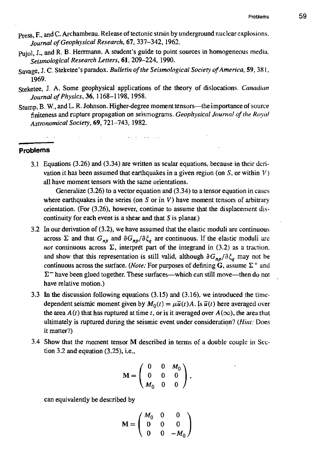
Problems 59
4. ELASTIC WAVES FROM A POINT DISLOCATION SOURCE 63
4.1 Formulation: Introduction of Potentials 63
BOX 4.1 On the outgoing solution of'g = &(x)8(t) + c2V2g with zero initial
conditions 65
4.1.1 Lame's theorem 67
4.2 Solution for the Elastodynamic Green Function in a Homogeneous, Isotropic.
Unbounded Medium 68
BOX 4.2 On potentials 69
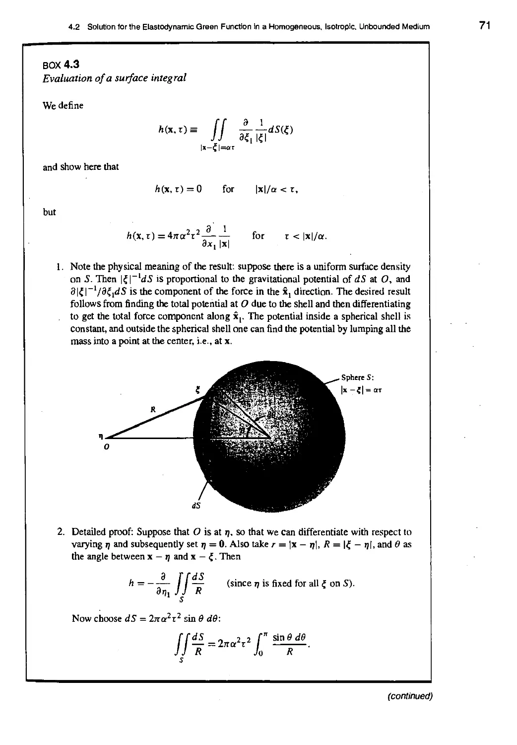
BOX 4.3 Evaluation of a surface integral 71
4.2.1 Properties of the far-field P-wave 73
4.2.2 Properties of the far-field S-wave 73
4.2.3 Properties of the near-field term 74
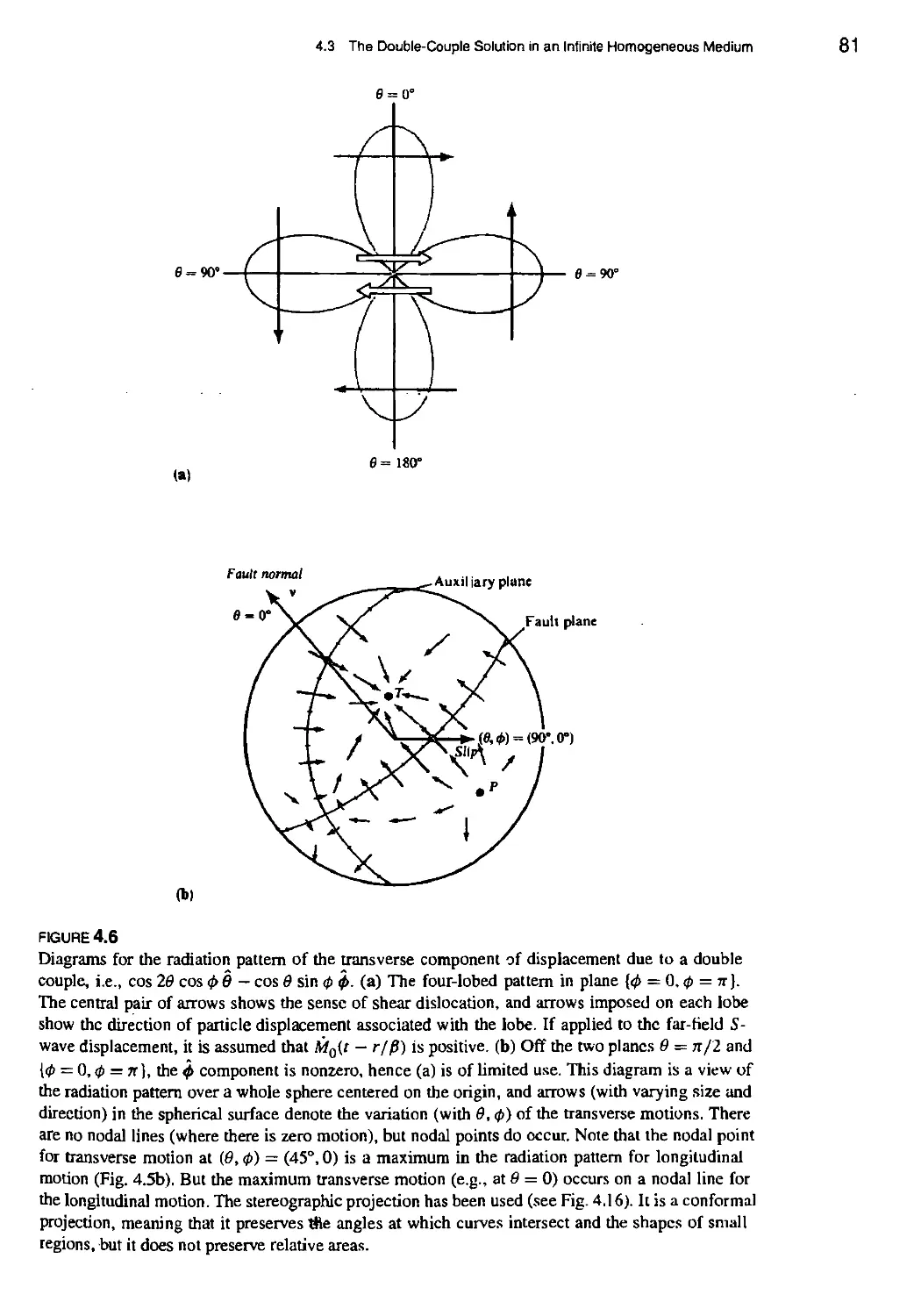
4.3 The Double-Couple Solution in an Infinite Homogeneous Medium 76
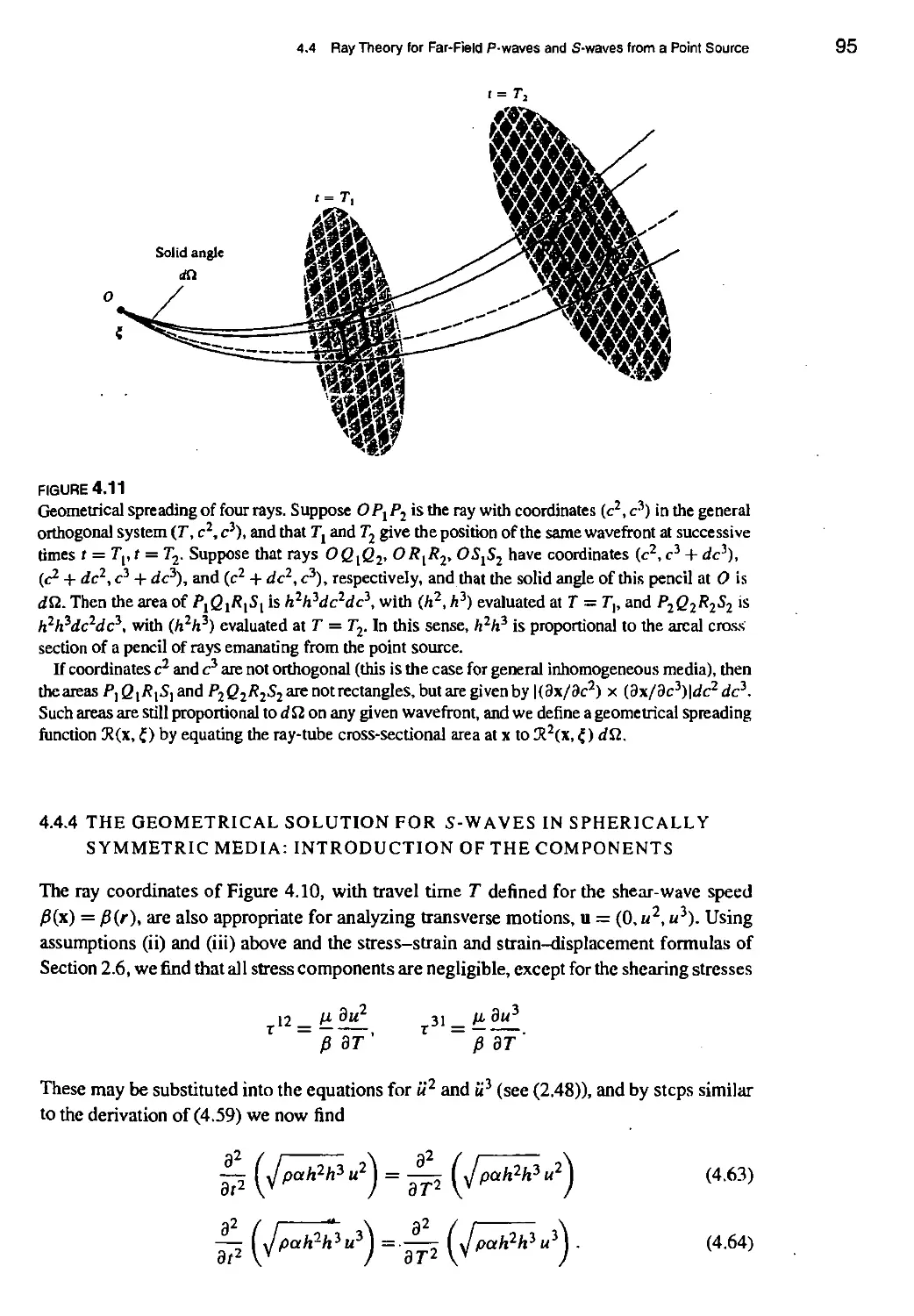
4.4 Ray Theory for Far-Field P-waves and S-waves from a Point Source 82
4.4.1 Properties of the travel-time function 7"(x) associated with
velocity field r(x) 87
4.4.2 Ray coordinates 90
4.4.3 The geometrical solution for P-waves in spherically symmetric
media 92
4.4.4 The geometrical solution for S-waves in spherically symmetric media:
Introduction of the components 95
4.4.5 The geometrical ray solutions in general Inhomogeneous media 96
4.5 The Radiation Pattern of Body Waves in the Far Field for a Point Shear
Dislocation of Arbitrary Orientation in a Spherically Symmetric Medium 101
4.5.1 A method for obtaining the fault-plane orientation of an earthquake and
the direction of slip using teleseismic body-wave observations 102
4.5.2 Arbitrary orientation of the double couple in a homogeneous
medium 106
4.5.3 Adapting the radiation pattern to the case of a spherically symmetric
medium 110
BOX 4.4 Cartesian components of the moment tensor for a shear dislocation of
arbitrary orientation 112
Suggestions for Further Reading 113
Problems 114
CONTENTS VII
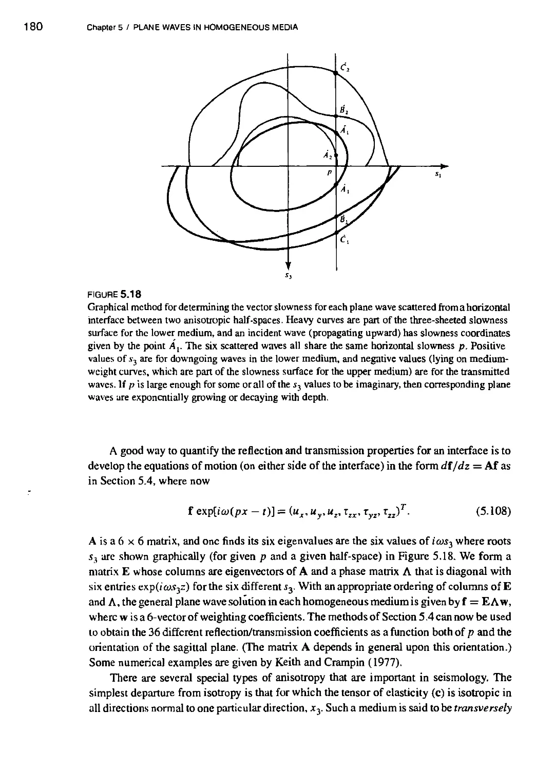
5. PLANE WAVES IN HOMOGENEOUS MEDIA AND THEIR REFLECTION
AND TRANSMISSION AT A PLANE BOUNDARY 119
5.1 Basic Properties of Plane Waves in Elastic Media 120
BOX 5.1 Notation 121
5.1.1 Potentials for plane waves 123
5.1.2 Separation of variables; steady-state plane waves 124
BOX 5.2 The sign convention for Fourier transforms used in solving
wave-propagation problems 125
5.2 Elementary Formulas for Reflection/Conversion/Transmission Coefficients 128
5.2.1 Boundary conditions 128
BOX 5.3 The distinction between kinematics and dynamics 129
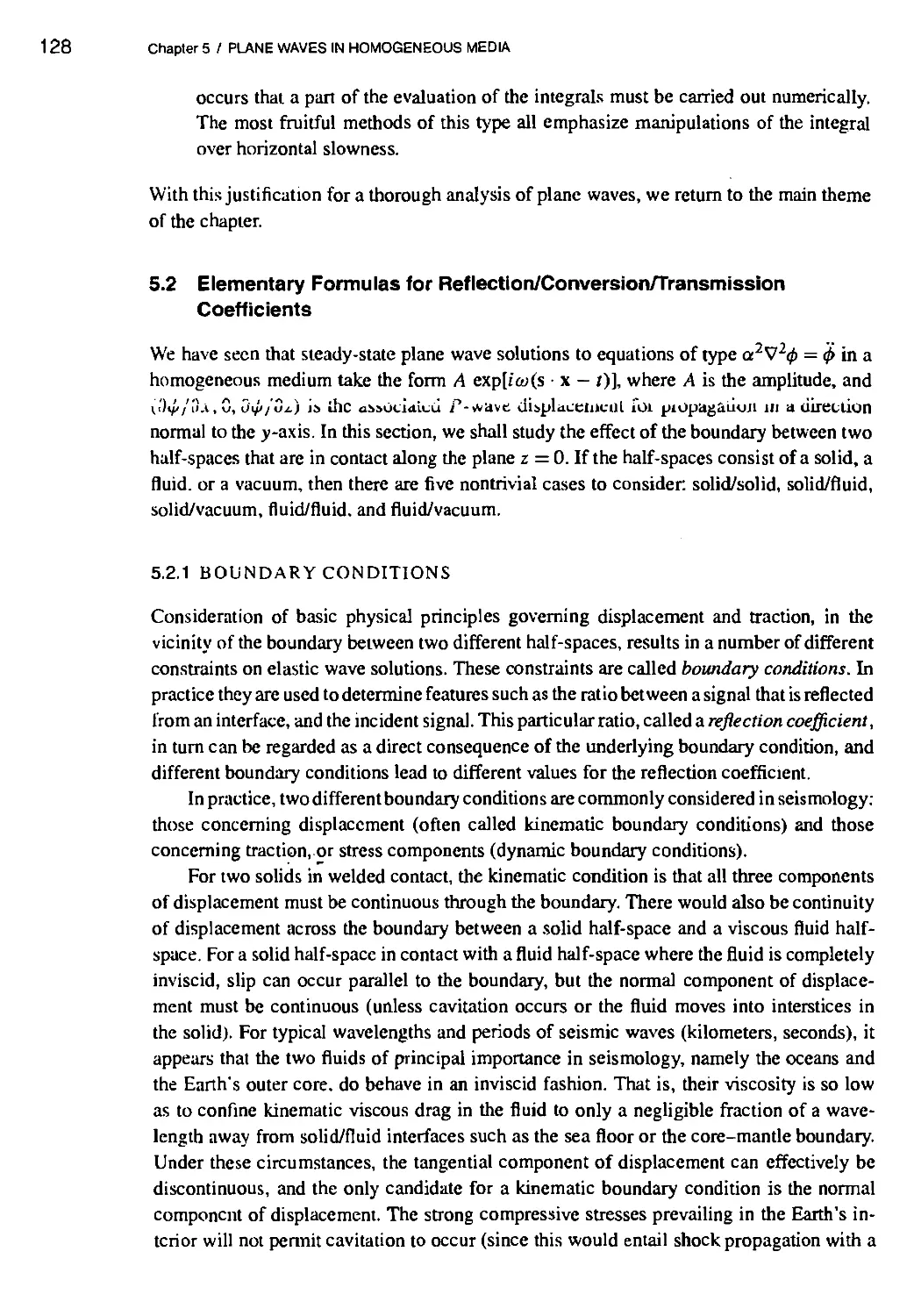
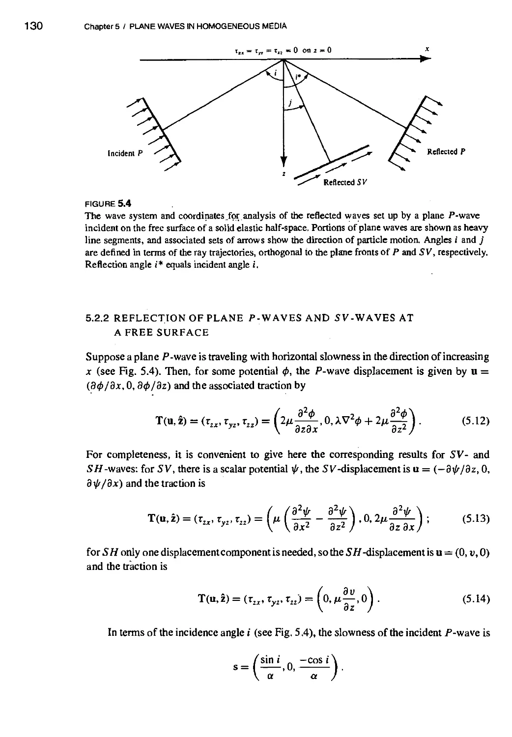
5.2.2 Reflection of plane P -waves and sv -waves at a free surface 130
BOX5.4 Impedance 132
5.2.3 Reflection and transmission of SH-waves 136
5.2.4 Reflection and transmission of P-SV across a solid-solid interface 139
5.2.5 Energy flux 145
5.2.6 A useful approximation for reflection/transmission coefficients between
two similar half-spaces 147
5.2.7 Frequency independence of plane-wave reflection/transmission
coefficients 149
5.3 Inhomogeneous Waves, Phase Shifts, and Interface Waves 149
BOX 5.5 Phase shifts: phase delay and phase advance 151
BOX 5.6 The Hilbert transform and the frequency-independent phase advance 152
5.4 A Matrix Method for Analyzing Plane Waves in Homogeneous Media 157
5.5 Wave Propagation in an Attenuating Medium: Basic Theory for
Plane Waves 161
BOX 5.7 Different definitions of Q 162
5.5.1 The necessity for material dispersion in an attenuating medium 163
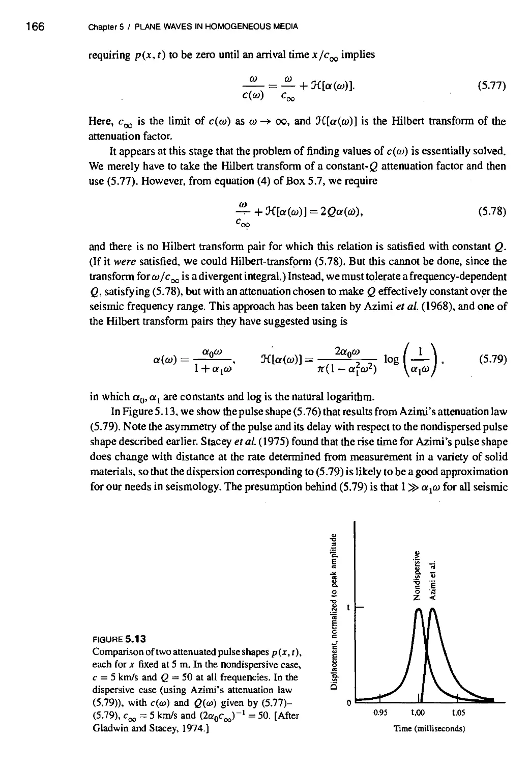
5.5.2 Some suggested values for material dispersion in an attenuating
medium 165
BOX 5.8 Relations between the amplitude spectrum and phase spectrum of a causal
propagating pulse shape 167
5.6 Wave Propagation in an Elastic Anisotropic Medium: Basic Theory for
Plane Waves 177
BOX 5.9 Shear-wave splitting due to anisotropy 181
Suggestions for Further Reading 183
Problems 183
6. REFLECTION AND REFRACTION OF SPHERICAL WAVES; LAMB'S
PROBLEM 189
6.1 Spherical Waves as a Superposition of Plane Waves and Conical Waves 190
BOX 6.1 Fundamental significance of Weyl and Somtnerfeld integrals 193
6.2 Reflection of Spherical Waves at a Plane Boundary: Acoustic Waves 195
BOX 6.2 Determining the branch cuts «/\/or~- — p1 = {, in the complex p-plane,
so that Im <f > Ofor a whole plane. 197
CONTENTS
BOX6.3 Tlie evaluation of /(.v) =/c F{Oexp[.r/(t)]</< by the method of
steepest descents 200
BOX 6.4 Outstanding features of head waves 205
6.3 Spherical Waves in an Elastic Half-Space: The Rayleigh Pole 209
BOX 6.5 Independence of P-SM and SH motions for piecewise homogeneous
media in which the material discontinuities are horizontal 210
BOX 6.6 On cylindrical coordinates 213
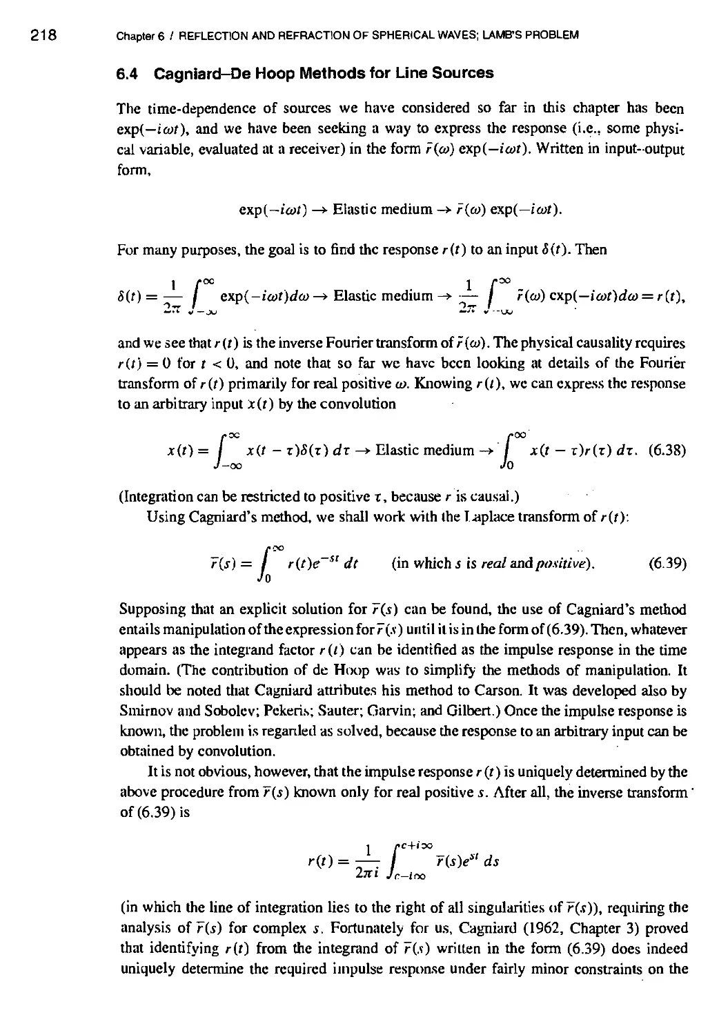
BOX 6.7 Outstanding features of Rayleigh wives from a buried point source 217
6.4 Cagniard-De Hoop Methods for Line Sources 218
BOX 6.8 An example of Jordan's U'mma 224
BOX 6.9 On writing down the multitransfonned solution. (6.64) 229
6.5 Cagniard-De Hoop Methods for Point Sources 235
BOX 6.10 Horizontal transforms for functions symmetric about a vertical axis 240
6.6 Summary of Main Results and Comparison between Different Methods 244
Suggestions for Further Reading 245
Problems 247
7. SURFACE WAVES IN A VERTICALLY HETEROGENEOUS MEDIUM 249
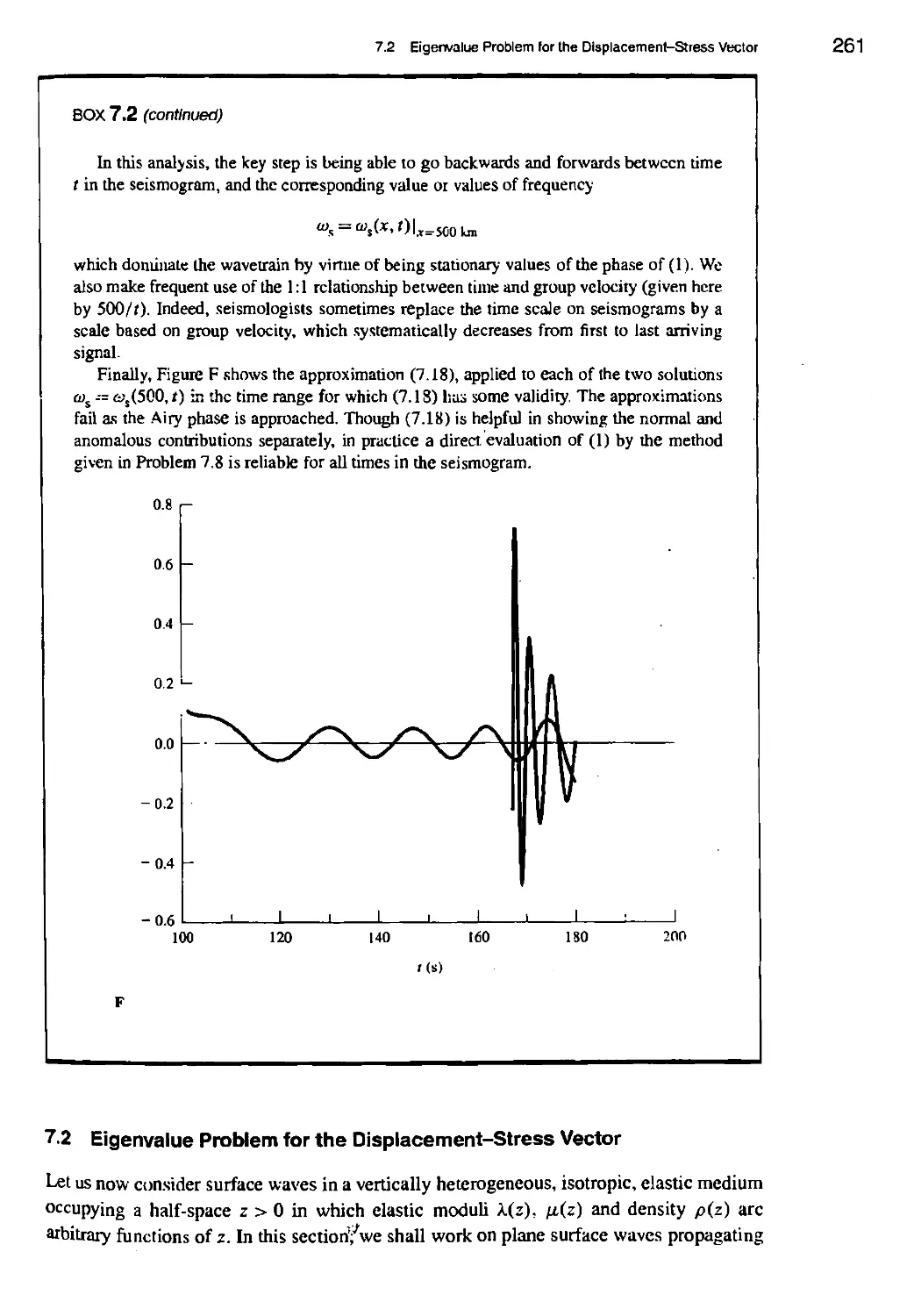
7.1 Basic Properties of Surface Waves 249
BOX 7.1 Initial assumptions 250
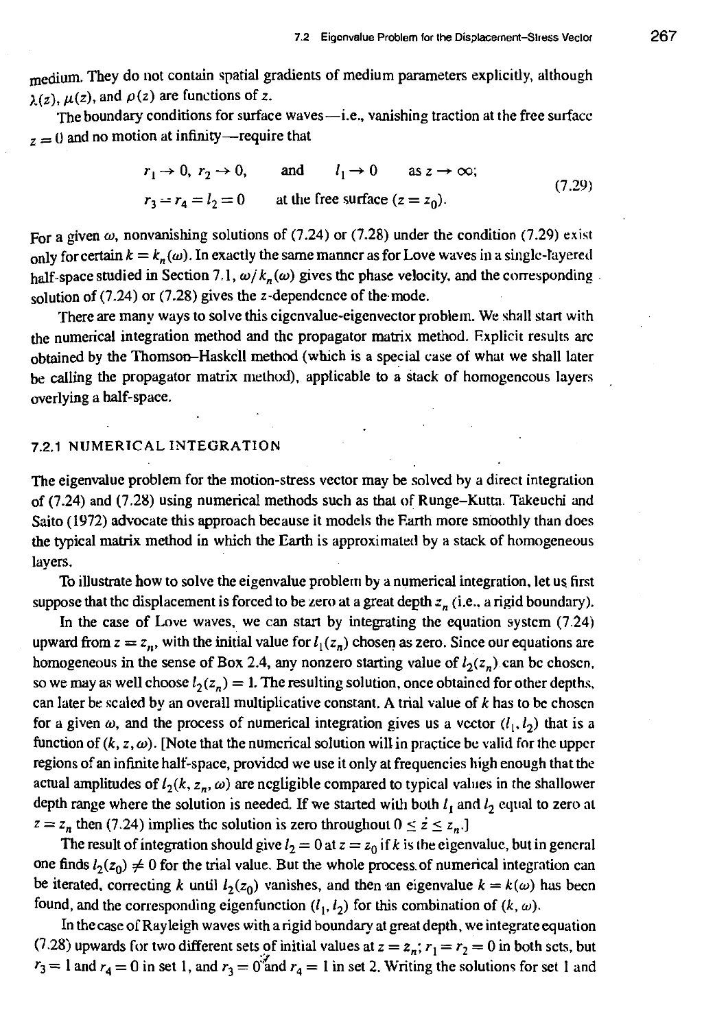
BOX 7.2 Analysis of a simple surface-wave seistnogram 257
7.2 Eigenvalue Problem for the Displacement-Stress Vector 261
BOX 7.3 Measurement of surface wave phase velocity 264
7.2.1 Numerical Integration 267
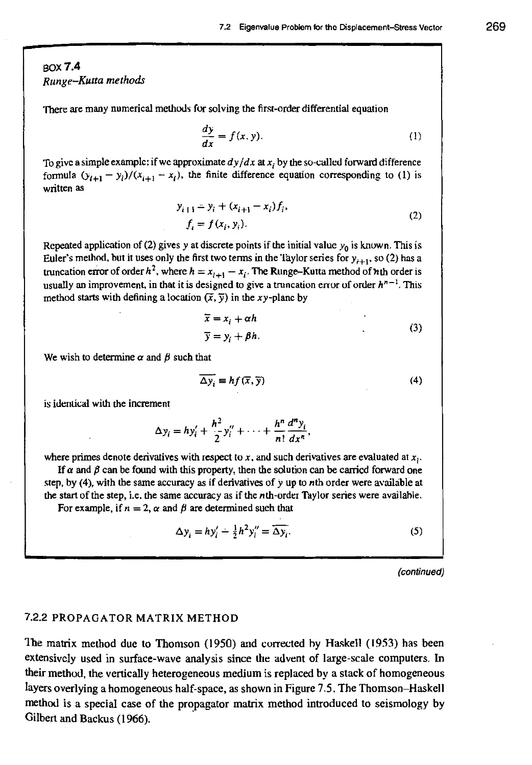
BOX 7.4 Runge-Kutta methods 269
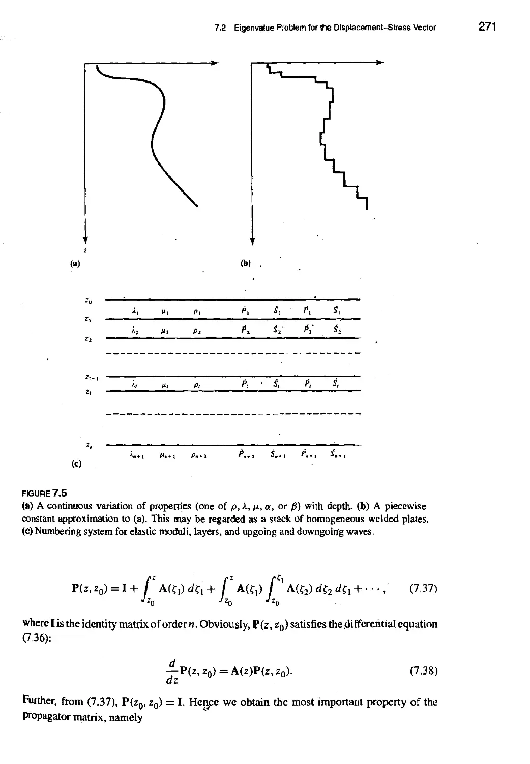
7.2.2 Propagator matrix method 269
BOX 7.5 On avoiding potentials 275
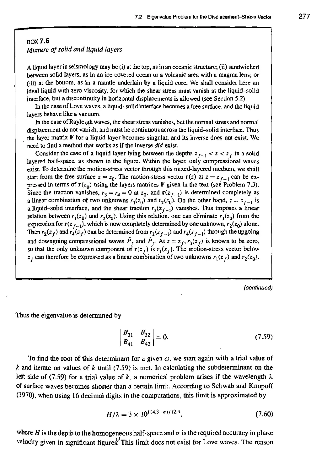
BOX 7.6 Mixture of solid and liquid layers 277
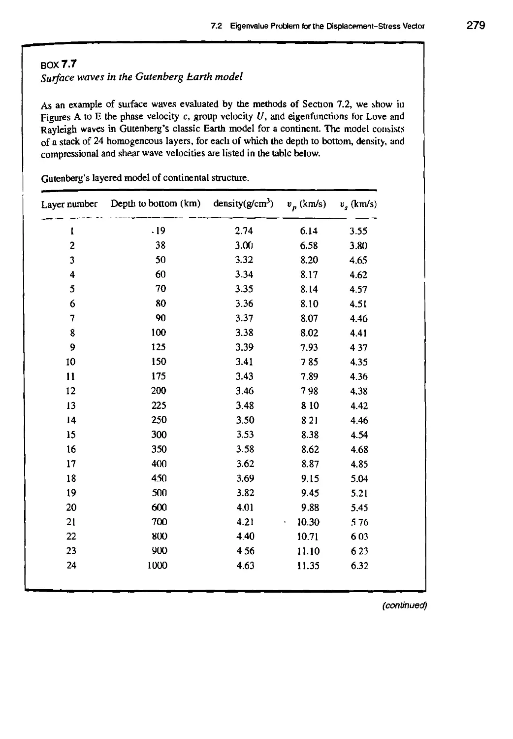
BOX 7.7 Surface waves in the Gutenberg Earth model 279
7.3 Variational Principle for Love and Rayleigh Waves 283
7.3.1 Love waves 283
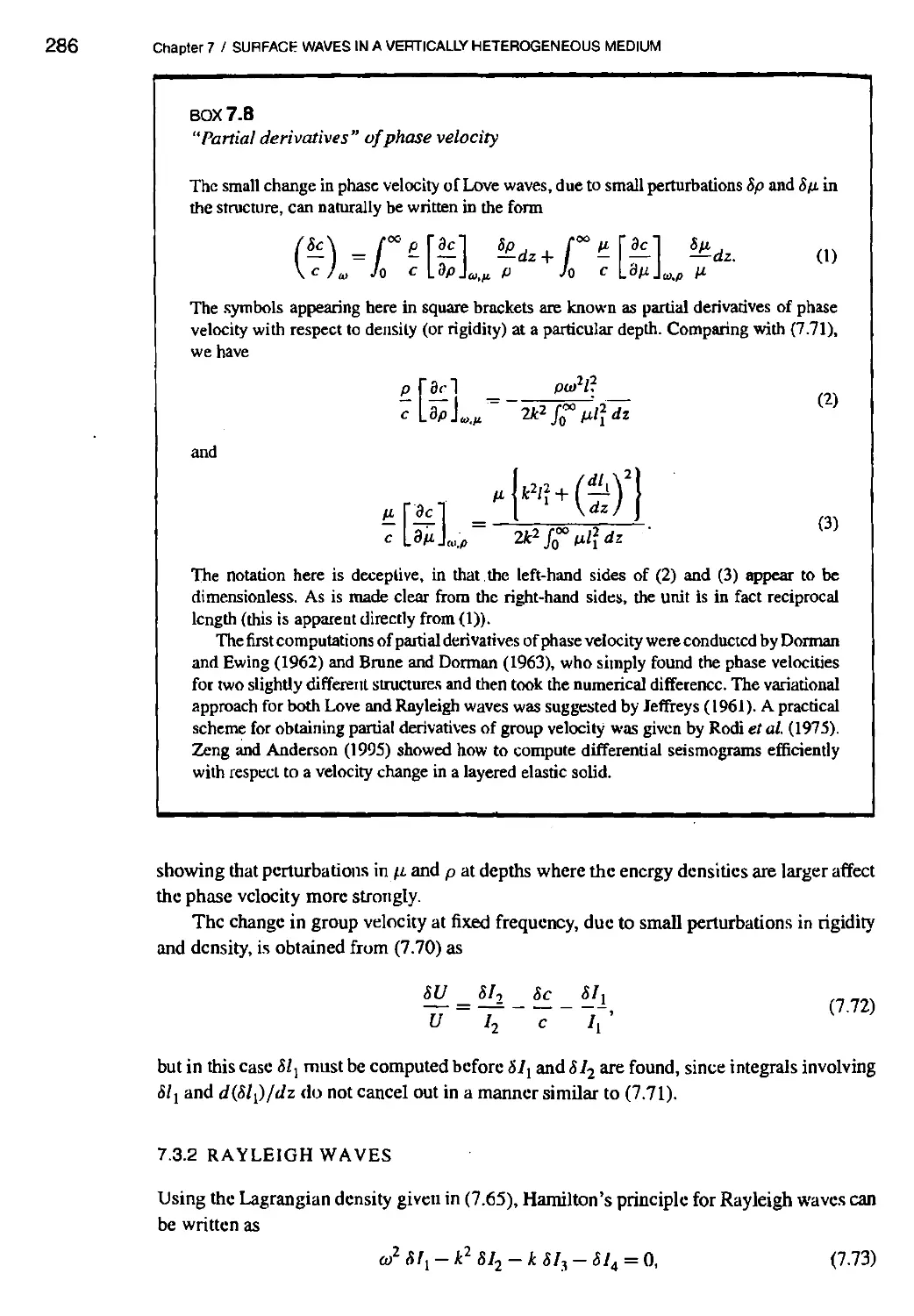
BOX 7.8 "Partial derivatives" of phase velocity 286
7.3.2 Rayleigh waves 286
7.3.3 Rayleigh-RHz method 288
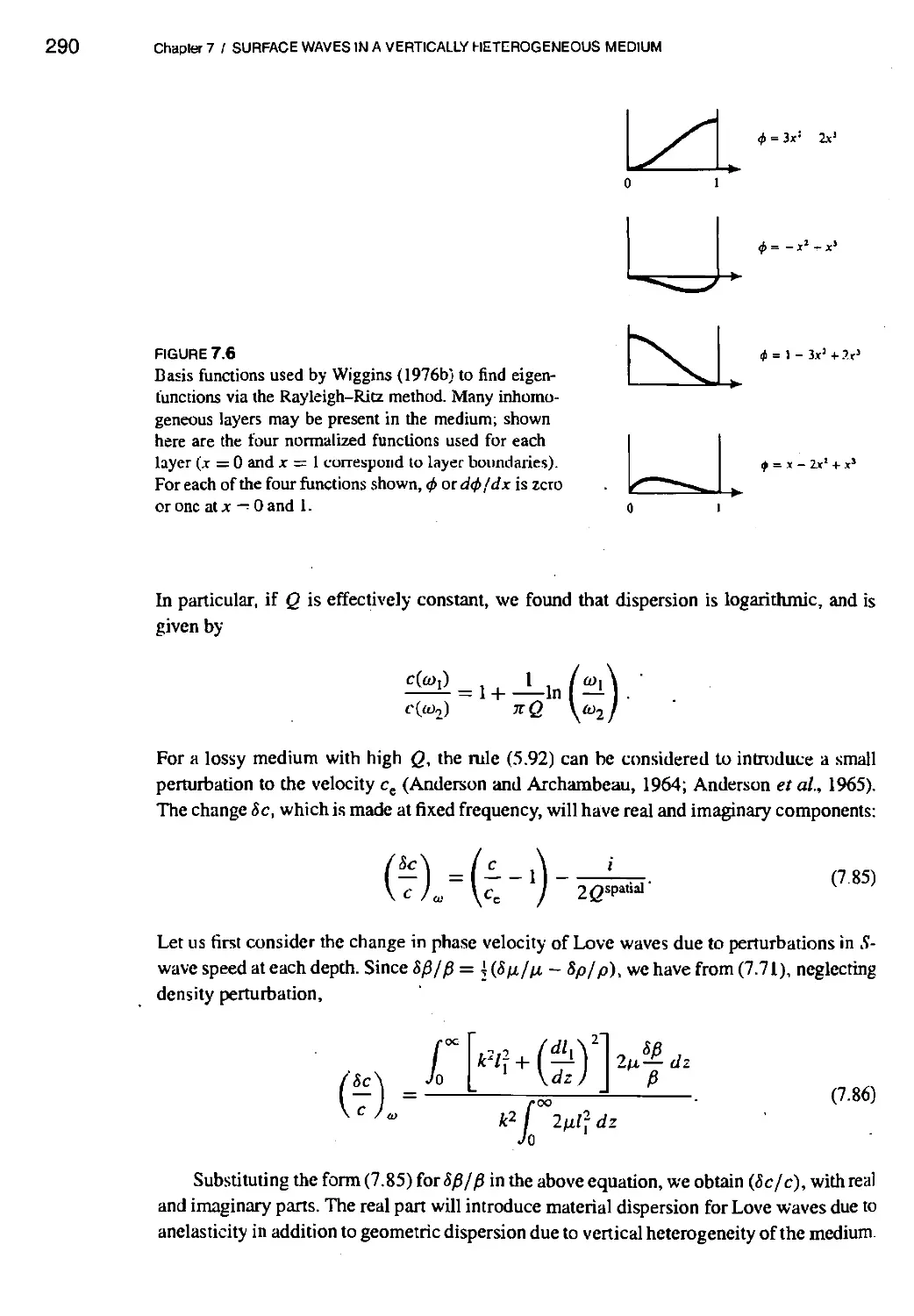
7.3.4 Attenuation of surface waves 289
BOX 7.9 Some effects ofanisotropy 292
7.4 Surface-Wave Terms of Green's Function for a Vertically Heterogeneous
Medium 293
7.4.1 Two-dimensional case 294
BOX 7.10 Sign convention on vertical motion 298
7.4.2 Three-dimensional case 298
BOX 7,11 On horizontal wave functions 302
7.5 Love and Rayleigh Waves from a Point Source with Arbitrary Seismic
Moment 308
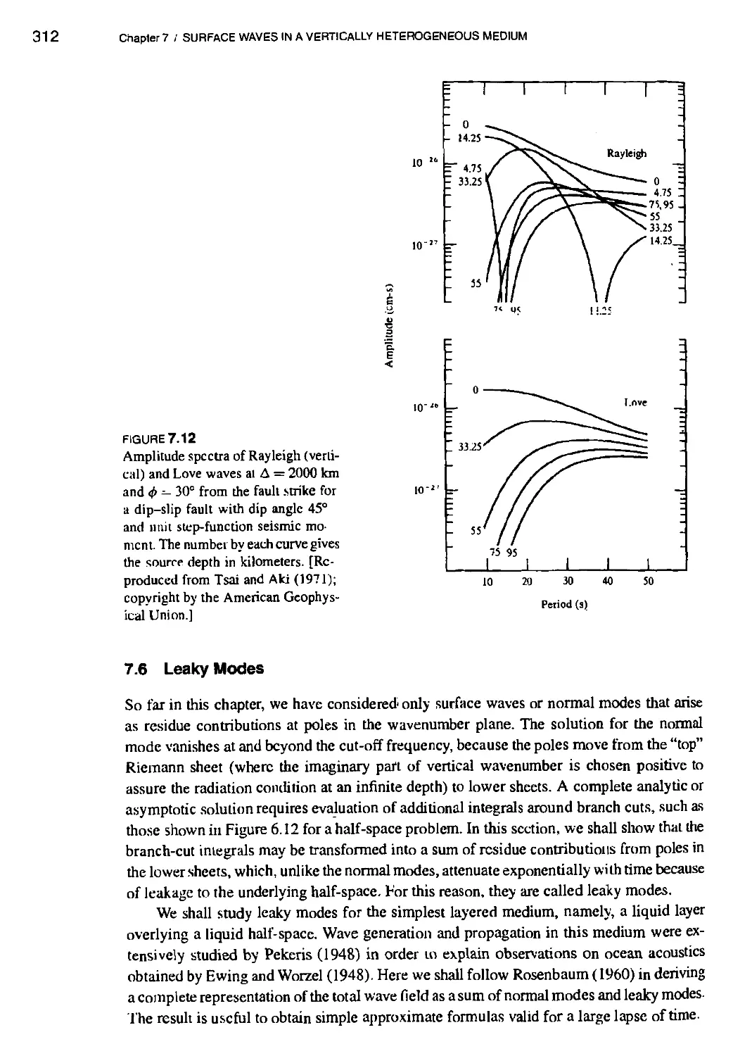
7.6 Leaky Modes 312
7.6.1 Organ-pipe mode 321
7.6.2 Phase velocity and attenuation 322
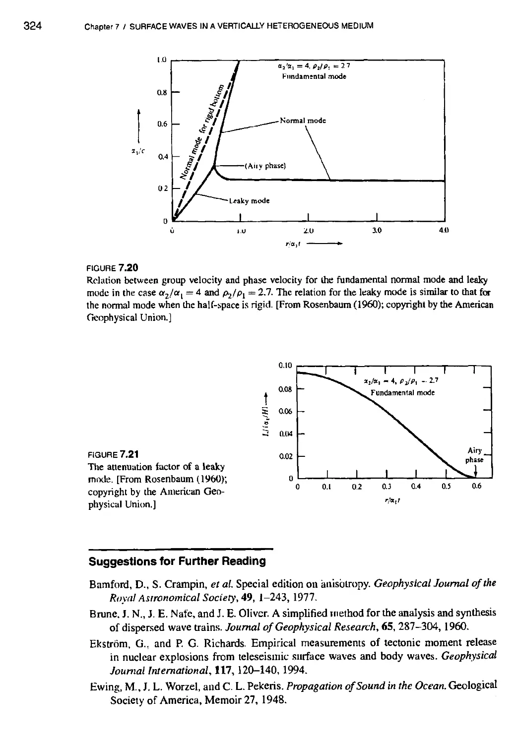
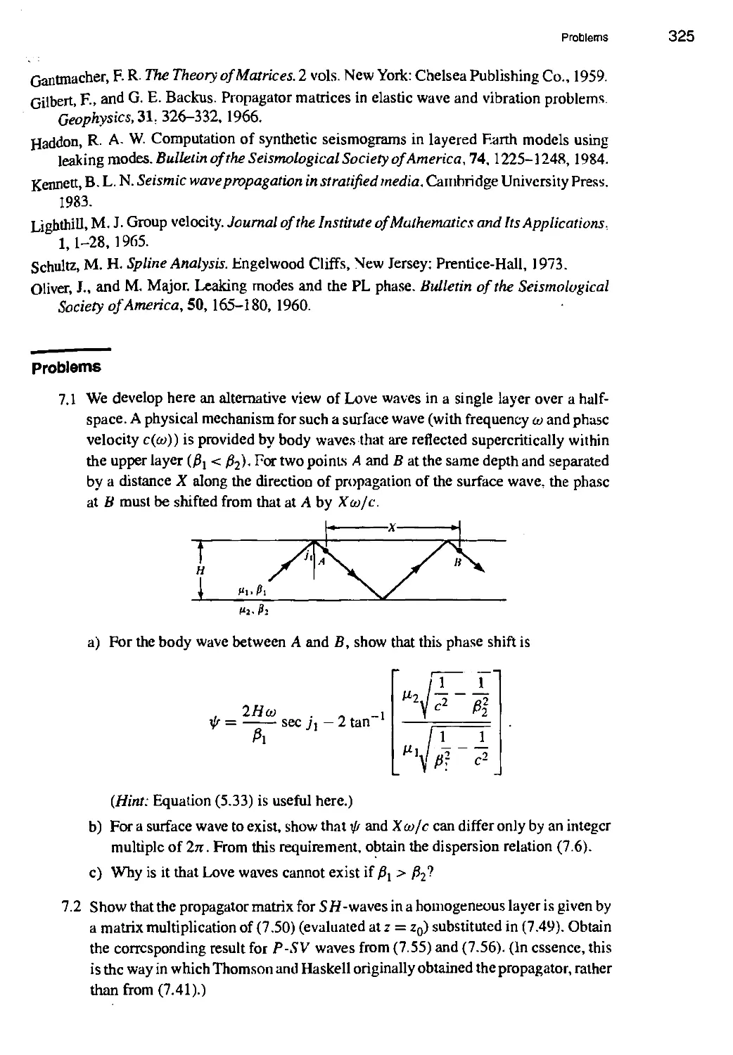
Suggestions (or Further Reading 324
Problems 325
8. FREE OSCILLATIONS OF THE EARTH 331
8.1 Free Oscillations of a Homogeneous Liquid Sphere 332
BOX8.1 Spherical surface harmonies 334
8.2 Excitation of Free Oscillations by a Point Source 342
BOX 8.2 Identification of free-oscillation peaks when the earthquake source
mechanism is known 349
8.3 Surface Waves on the Spherical Earth 351
BOX 8.3 An example of the Poisson sum formula 352
BOX 8.4 Different Legendre functions and their asymptotic approximations 354
8.4 Free Oscillations of a Self-Gravitating Earth 357
8.5 The Centroid Moment Tensor 366
BOX 8.5 Consideration of initial stress 367
8.6 Splitting of Normal Modes Due to the Earth's Rotation 370
8.7 Spectral Splitting of Free Oscillations Due to Lateral Inhomogeneity of
the Earth's Structure 374
BOX 8.6 Quasi-degeneracy 377
Suggestions for Further Reading 381
Problems 381
9. BODY WAVES IN MEDIA WITH DEPTH-DEPENDENT PROPERTIES 385
9.1 Cagniard's Method for a Medium with Many Plane Layers: Analysis of
a Generalized Ray 388
9.2 The Reflectivity Method for a Medium with Many Plane Layers 393
BOX 9.1 Propagator matrices for SH and for P-SV problems 397
BOX 9.2 Earth-flattening transformation and approximations 403
9.3 Classical Ray Theory in Seismology 407
9.4 Inversion of Travel-Time Data to Infer Earth Structure 413
9.4.1 The Herglotz-Wiechert formula 414
BOX 9.3 Abel's problem 417
9.4.2 Travel-time inversion for structures including low-velocity layers 423
BOX 9.4 Measurement of r(p) 426
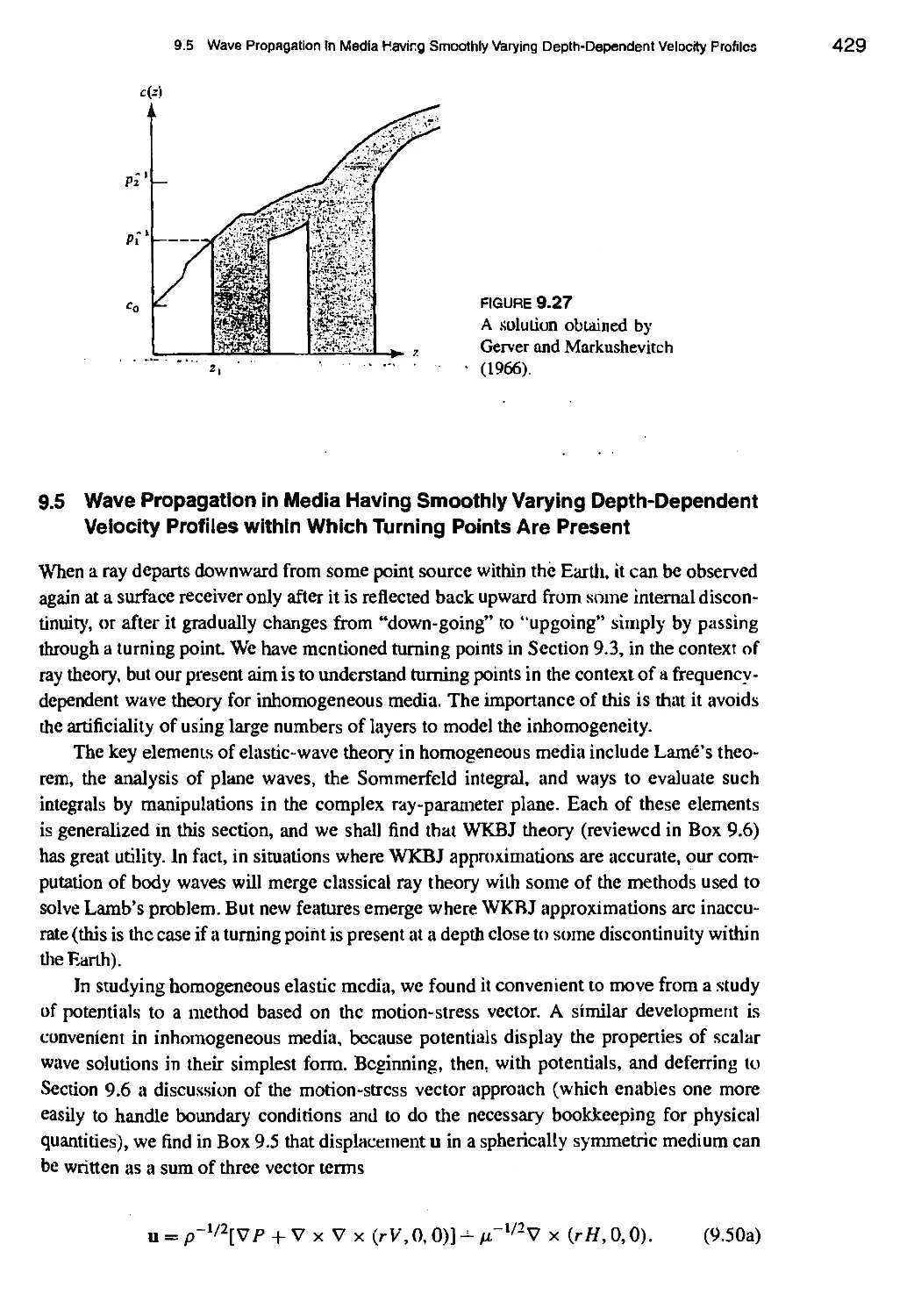
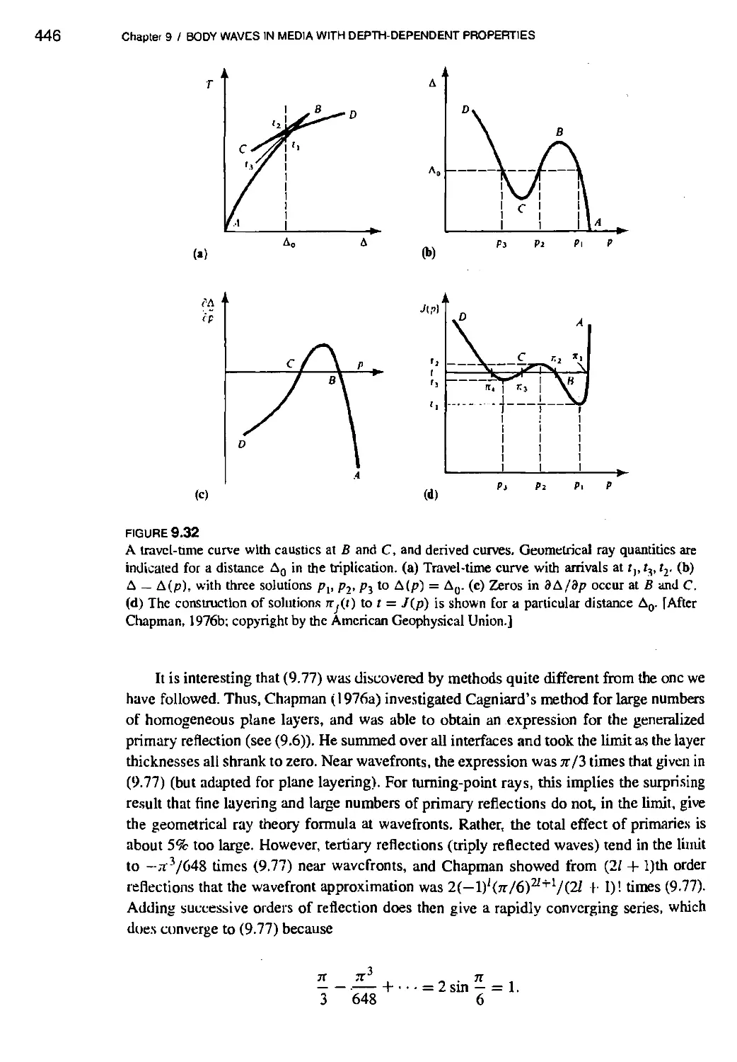
9.5 Wave Propagation in Media Having Smoothly Varying Depth-Dependent Velocity
Profiles within Which Turning Points Are Present 429
BOX 9.5 Scalar potentials for P-, SV-, and SH-waves in spherically symmetric
media 431
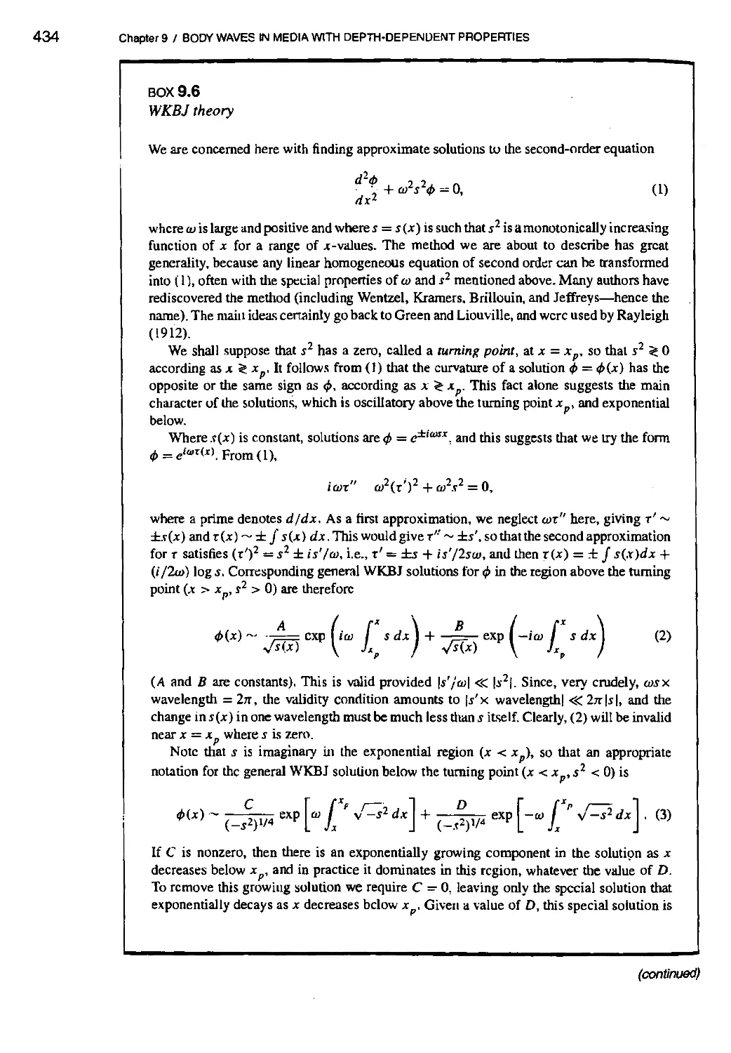
BOX 9.6 WKBJtheory 434
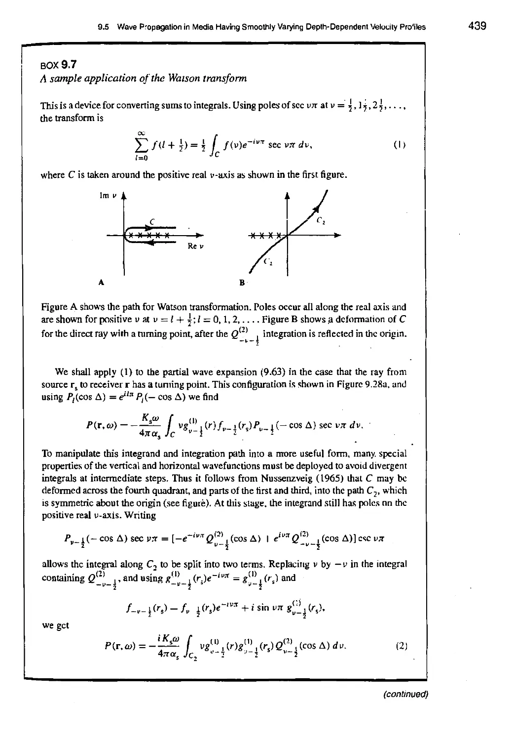
BOX 9.7 A sample application of the Watson transform 439
BOX 9.8 Useful transform pairs 445
9.6 Body-Wave Problems for Spherically Symmetric Earth Models in Which
Discontinuities are Present between Inhomogeneous Layers 447
X
CONTENTS
BOX 9.9 Generalized scattering/mm a stack of inhomogeneous layers: and
the special example of one spherical interface between two radially
inhomogeneous layers 451
BOX 9.10 A uniformly asymptotic approximation for vertical wavefunctions 459
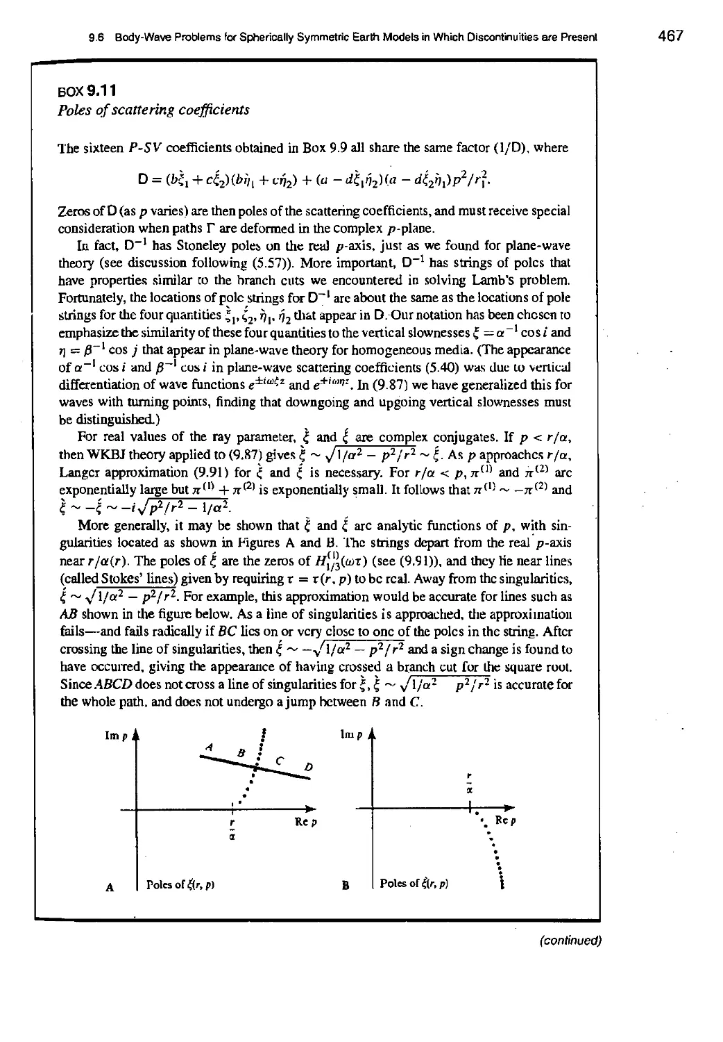
BOX 9.11 Poles of scattering coefficients 467
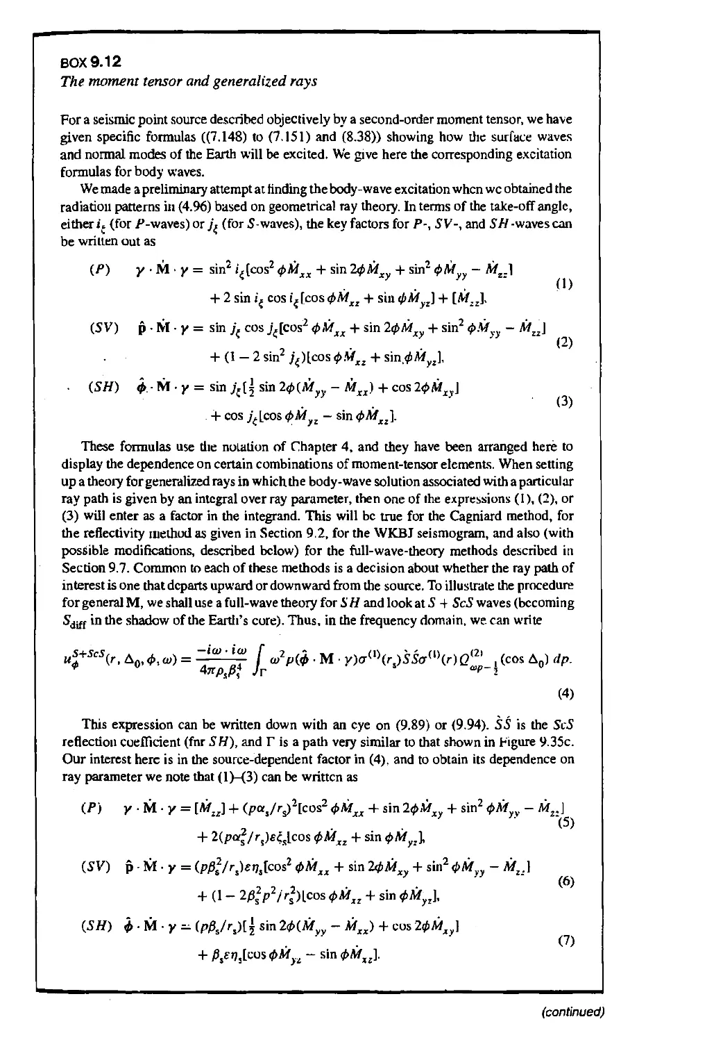
BOX 9.12 The moment tensor and generalized rays 471
9.7 Comparison between Different Methods 481
Suggestions for Further Reading 483
Problems 484
10. THE SEISMIC SOURCE: KINEMATICS 491
10.1 Kinematics of an Earthquake as Seen at Far Field 492
10.1.1 Far-field displacement waveforms observed in a homogeneous,
isotropic, unbounded medium 492
10.1.2 Far-field displacement waveforms for inhomogeneous isotropic media,
using the geometrical-spreading approximation 494
10.1.3 General properties of displacement waveforms in the far field 495
10.1.4 Behavior of the seismic spectrum at low frequencies 497
10.1.5 A fault model with unidirectional propagation 498
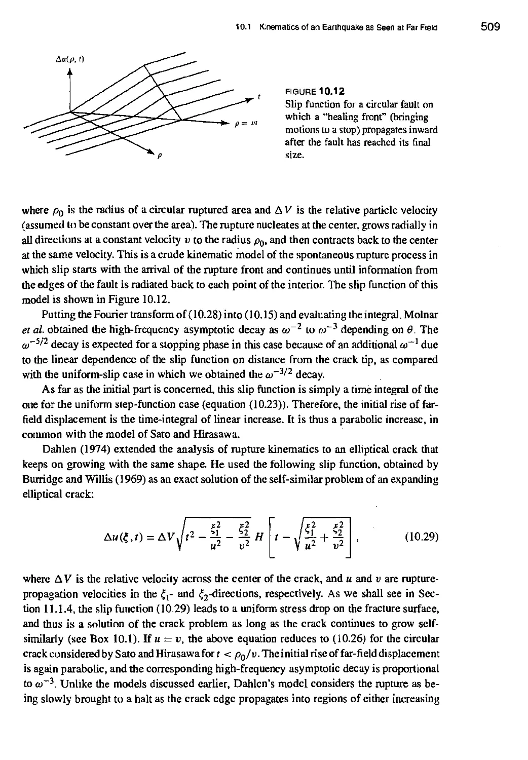
10.1.6 Nucteat'ton, spreading, and stopping of rupture 503
BOX 10.1 On the concept of "self-similarity " 510
10.1.7 Corner frequency and the high-frequency asymptote 511
BOX 10.2 Allowance for finite faulting in calculating far-field body waves within
depth-dependent structures 514
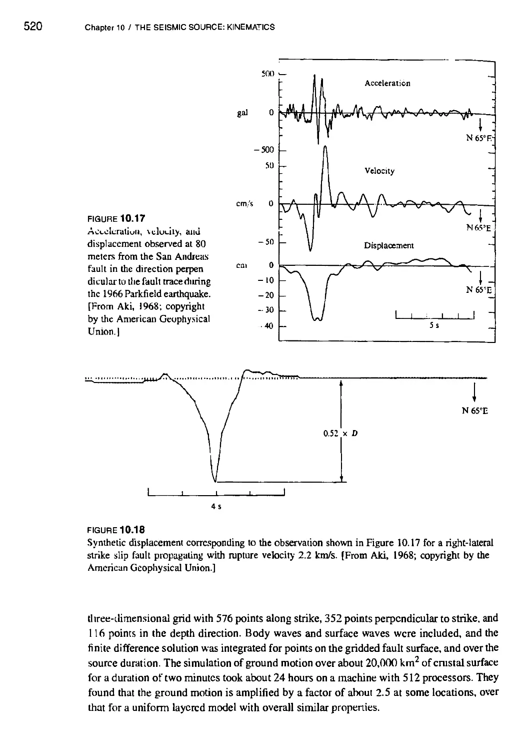
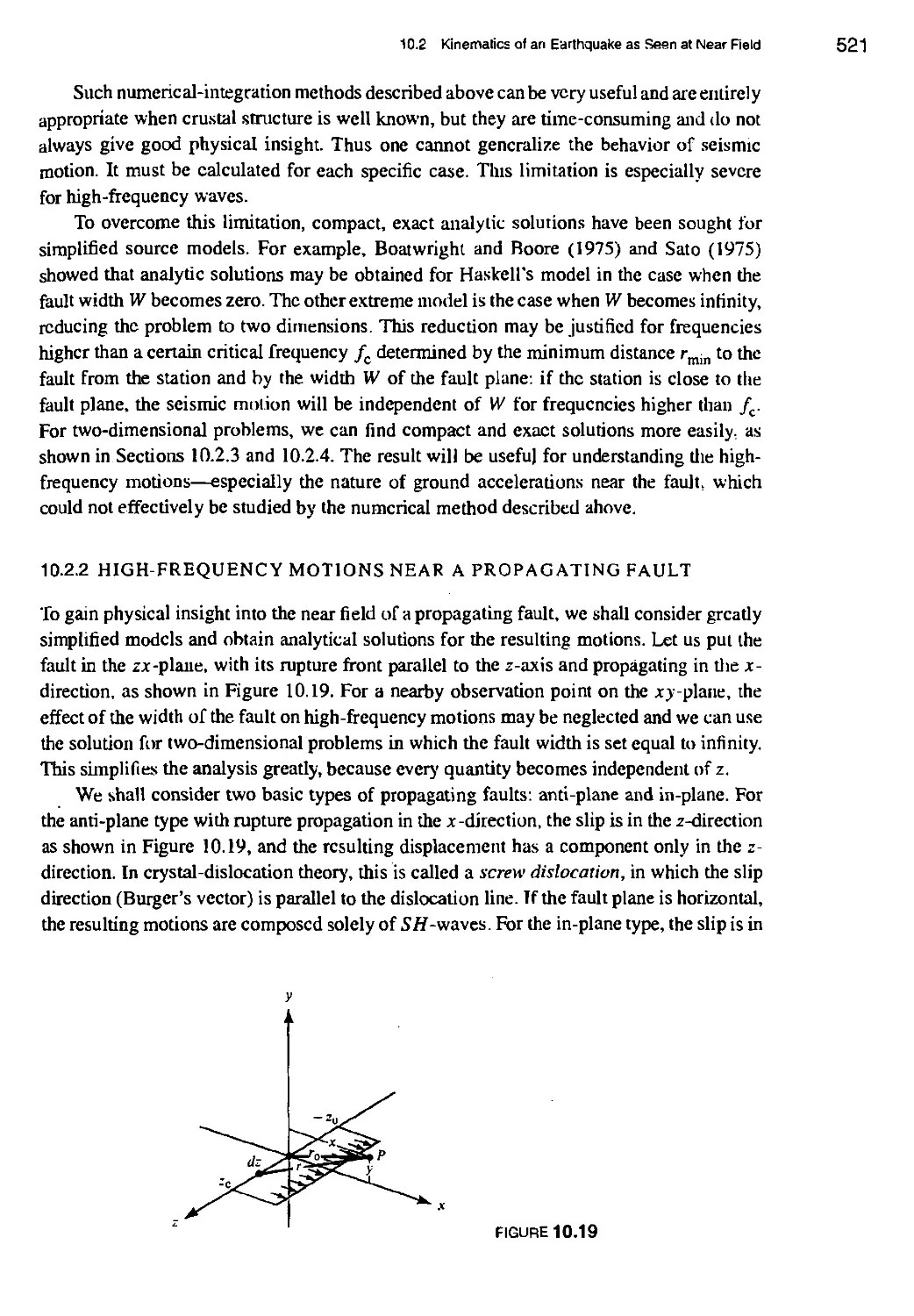
10.2 Kinematics of an Earthquake as Seen at Near Field 516
10.2.1 Synthesis of near-field seismograms for a finite dislocation 517
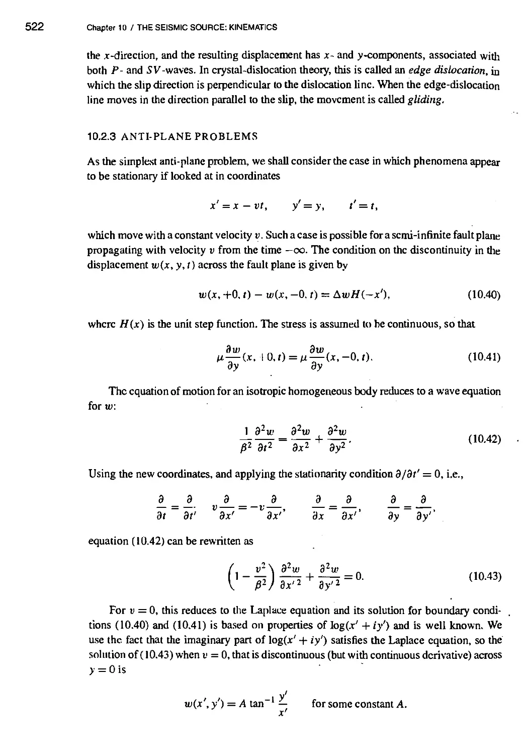
10.2.2 High-frequency motions near a propagating fault 521
10.2.3 Anti-plane problems 522
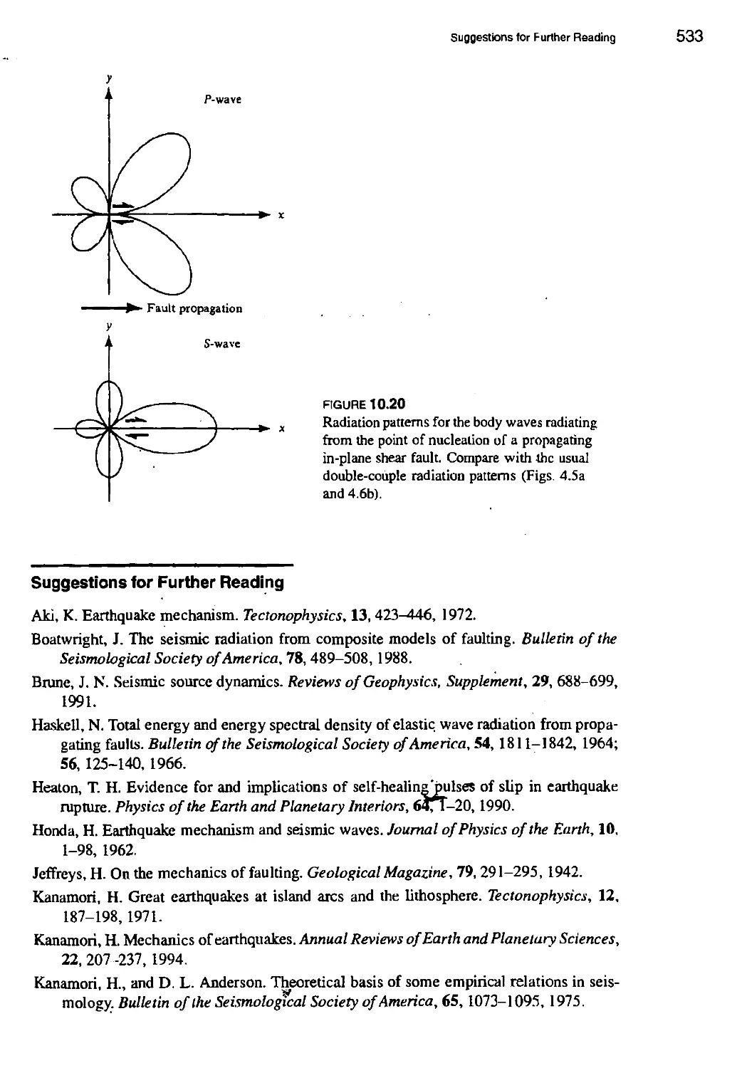
10.2.4 In-plane problems 526
Suggestions for Further Reading 533
Problems 534
11. THE SEISMIC SOURCE: DYNAMICS 537
11.1 Dynamics of a Crack Propagating with Prescribed Velocity 539
11.1.1 Relations between stress and slip for a propagating crack 539
BOX 11.1 Stress singularities for static, in-plane, and anti-plane shear cracks of
finite width 2a. 542
11.1.2 Energetics at the crack tip 545
11.1.3 Cohesive force 548
BOX 11.2 Fracture criteria 549
11.1.4 Near field of a growing elliptical crack 552
11.1.5 The far-field spectrum for a circular crack that stops 560
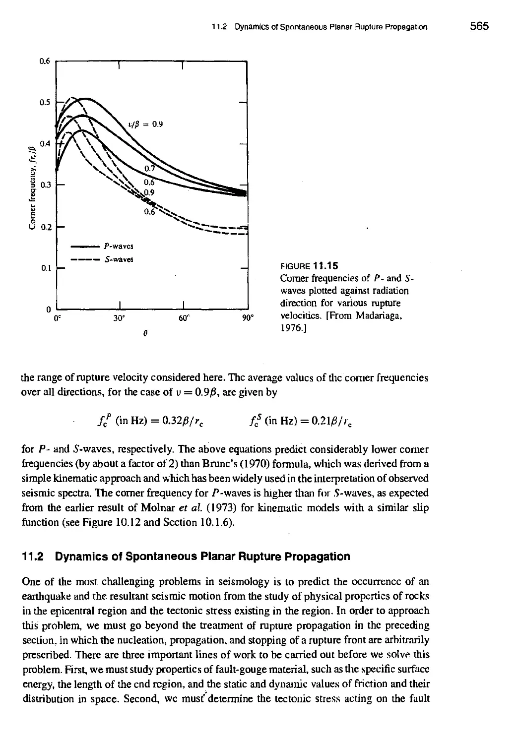
11.2 Dynamics of Spontaneous Planar Rupture Propagation 565
11.2.1 Spontaneous propagation of an anti-plane crack: general theory 566
11.2.2 Examples of spontaneous anti-plane crack propagation 572
BOX 11.3 The stress-intensity factor associated with cohesive force alone 573
11.2.3 Spontaneous propagation of an in-plane shear crack 582
11.3 Rupture Propagation Associated with Changes in Normal Stress 590
Suggestions tor Further Reading 592
Problems 593
12. PRINCIPLES OF SEISMOMETRY 595
12.1 Basic Instrumentation 598
12.1.1 Basic inertial seismometer 598
12.1.2 Stable long-period vertical suspension 602
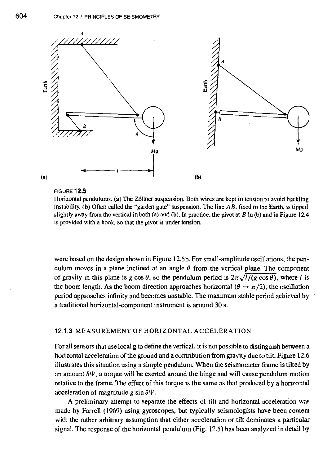
12.1.3 Measurement of horizontal acceleration 604
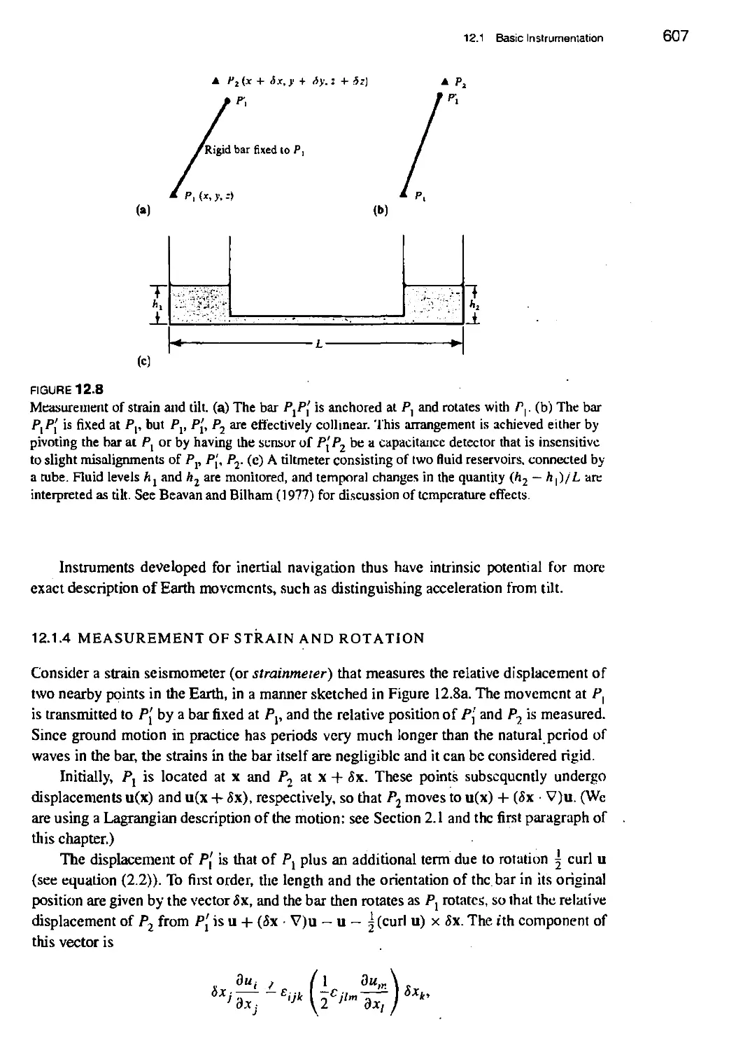
12.1.4 Measurement of strain and rotation 607
12.2 Frequency and Dynamic Range of Seismic Signals and Noise 609
12.2.1 Surface waves with periods around 20 seconds 611
BOX 12.1 Terminology associated with large ranges in wide 612
BOX 12.2 Recording media 613
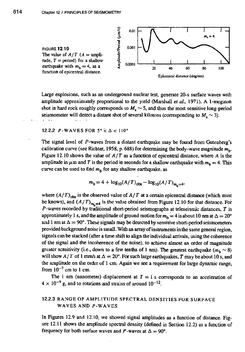
12.2.2 P-waves for5" < A < 110° 614
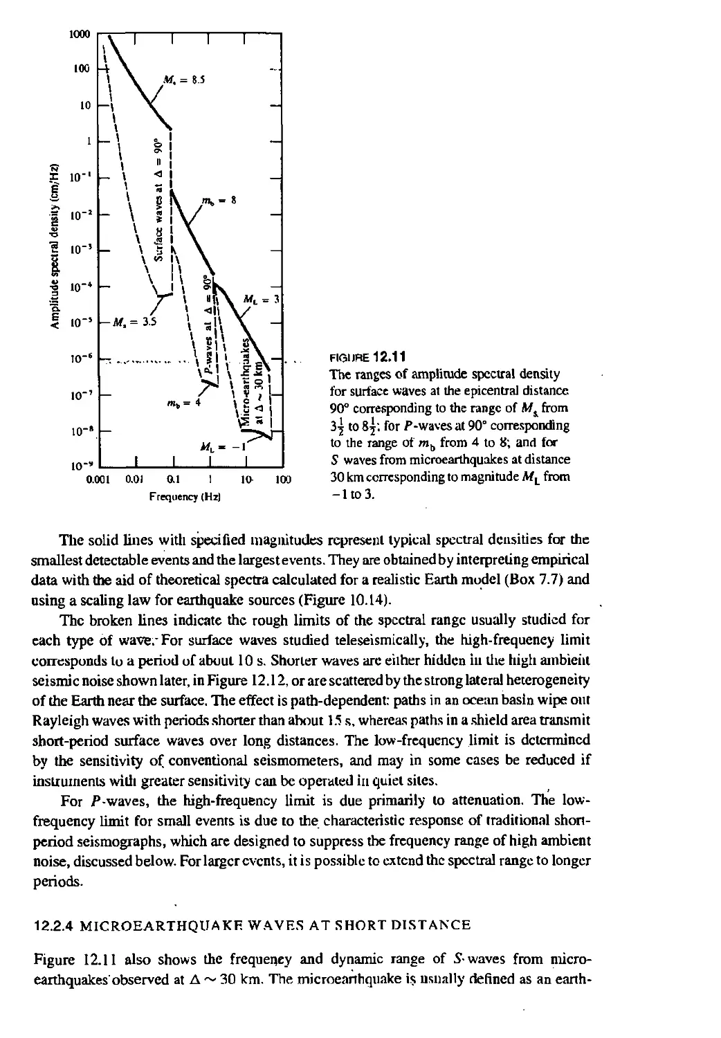
12.2.3 Range of amplitude spectral densities for surface waves and
P-waves 614
12.2.4 Microearthquake waves at short distance 615
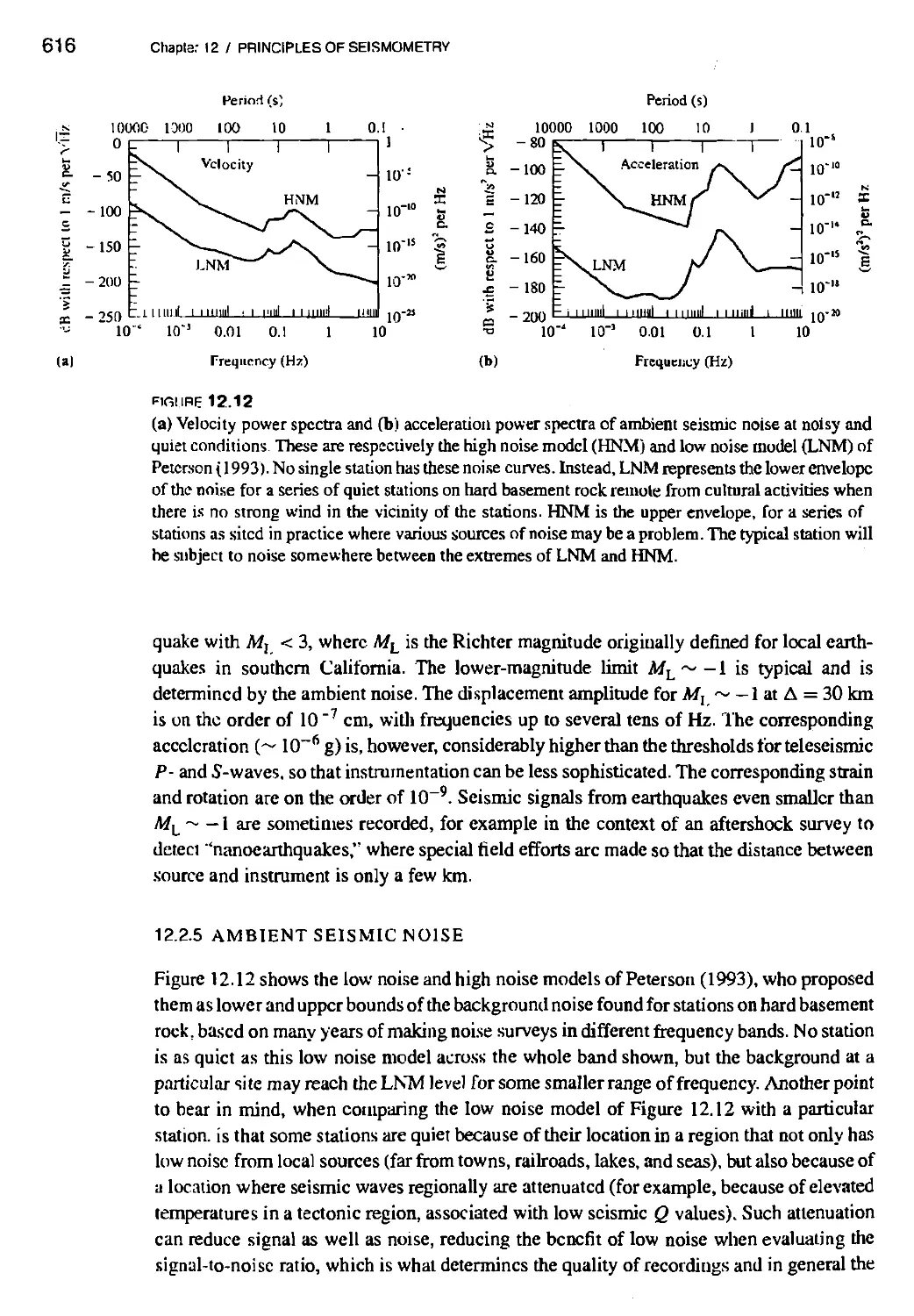
12.2.5 Ambient seismic noise 616
12.2.6 Amplitude of free oscillations 617
12.2.7 Amplitudes of solid Earth tide, Chandler wobble, plate motion, and
moonquakes 618
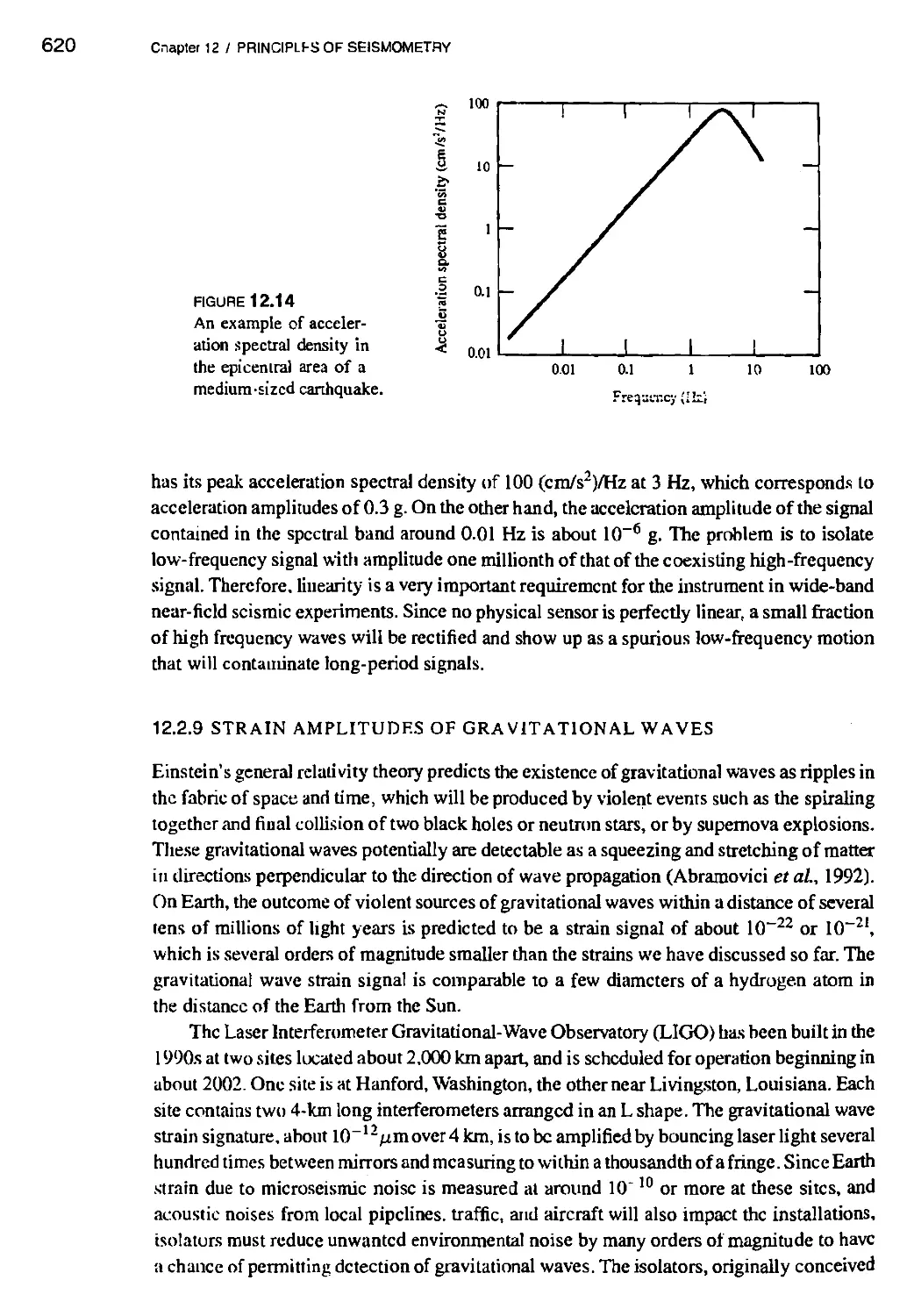
12.2.8 Seismic motion in the epicentral area 618
12.2.9 Strain amplitudes of gravitational waves 620
BOX 12.3 Engineering response spectra 621
12.3 Detection of Signal 623
12.3.1 Brownian motion of a seismometer pendulum 623
12.3.2 Electromagnetic velocity sensor 625
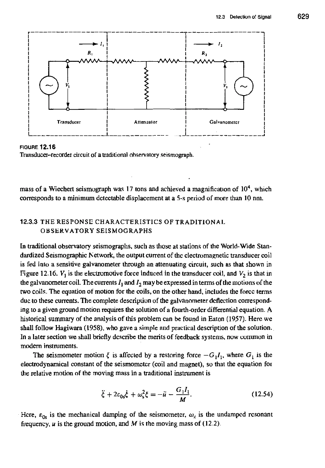
12.3.3 The response characteristics of traditional observatory
seismographs 629
12.3.4 High sensitivity at long periods 632
BOX 12.4 General features of the response of a traditional electromagnetic
seismograph 634
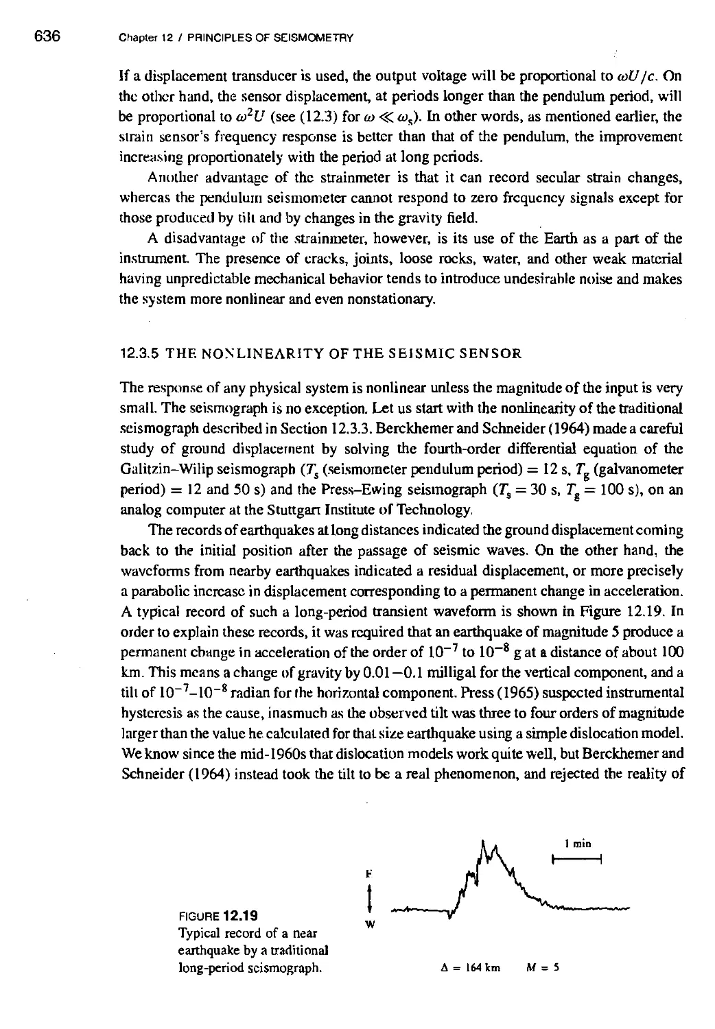
12.3.5 The nonlinearity of the seismic sensor 636
BOX 12.5 Poles and zeros 637
12.3.6 Feedback seismometers 639
Suggestions for Further Reading 642
Problems 643
Appendix 1: Glossary of Waves 647
Appendix 2: Definition of Magnitudes 655
Bibliography 657
Index 687
Preface
TO THE SECOND EDITION
In 1975 I received a surprising letter from Kei Aki, beginning "I wonder if you would be
interested in coauthoring a text book on theoretical seismology with me ... "
We had both taught advanced seismology courses at our respective institutions, the
Massachusetts Institute of Technology and Columbia University. But his were informed
by many years as a leading researcher. He had worked on everything from the practical
study of noise to theoretical frameworks for interpreting free oscillation signals. I was in
my fourth year as an assistant professor, knew nothing about vast areas of seismology, and
had focussed on some details in source theory and wave propagation that he knew a great
deal more about than I did. But I said yes to his invitation, and thus began a wonderful four-
year period of being forced to learn about seismology well enough to write explanations of
the underlying theory.
At that time, in the mid to late 1970s, the concept of quantifying seismic sources
with a moment tensor had just begun to take hold. Film chips of analog data from (he
Worldwide Standardized Scismographic Network were the best source of seismograms for
most gcophysicists in academia. but their narrow band and limited dynamic range were
problematic (the seismograms, not the geophysicists). Broadband instruments and digital
methods of recording were only beginning to show their potential.
Kei sent me 300 pages of his teaching notes. Wc quickly drafted a sequence of chapter
titles and began writing. In 1978 wc sent our first draft to the publisher. It was promptly
rejected as being three times longer than planned, and unmarketable. I was devastated. But
Kei calmly responded with the suggestion that we could do a little re-organization and offer
the material as two volumes. The original publishers agreed, and after two more years of
editing and figure preparation the first edition appeared in February 1980.
The IRIS Consortium and the Federation of Digital Scismographic Networks emerged
in the 1980s to meet growing needs for high-quality broadband seismic data. Global,
national, regional, and local networks of broadband seismometers have since been deployed
at thousands of locations, and quantitative seismology is conducted today on a scale that
could hardly be imagined in the 1970s and 1980s. Every generation of seismologists
correctly knows that it is working at new levels of excellence. As always, the rationale for
support to seismology is multi-faceted: to study the Earth's internal structure, to conduct
research in the physics of earthquakes, to quantify and mitigate earthquake hazard, and xiii
XIV PREFACE TO THE SECOND EDITION
to monitor explosions both to evaluate the weapons development programs of a potential
adversary and to support initiatives in nuclear arms control.
These different applications of seismology are illustrated by our own careers. In 1984
Kei Aki moved from MIT to the University of Southern California, and promoted
integration of scientific information about earthquakes and its public transfer as the founding
science director of the Southern California Earthquake Center. At the Center, for example,
input from earthquake geologists was used together with the fault model of quantitative
seismology, to generate output useful for earthquake engineers. In this work, the concept of
seismic moment was central to unifying information from plate tectonics, geology, geodesy,
and historical and instrumental seismology. The public transfer of the integrated
information was made in the form of probabilistic estimates of earthquake hazards. The Center is
still alive and well, long after Kei left for an on-site prediction of volcanic eruptions using
seismic signals from an active volcano (Reunion) in the Indian Ocean. In the mid-1980s,
I also changed my interests to applied aspects of seismology and began work on practical
problems of monitoring compliance with nuclear test ban treaties. At first the main issue
was estimating the size of the largest underground nuclear explosions, in the context of
assessing compliance with the 150 kiloton limit of the Threshold Test Ban Treaty. Later
the focus changed (o a series of technical issues in detection, location, and identification
of small explosions, in the context of verification of the Comprehensive Nuclear-Test-Ban
Treaty. This latter treaty became a reality in 1996. and is now associated with an
International Data Centre in Vienna and an International Monitoring System currently being built
at hundreds of new sites around the world. In early 1996, Xiaodong Song and I working at
Columbia's Lamont-Doherty Earth Observatory discovered small changes in the travel time
with which seismic waves traverse the Earth's inner core—evidence that we interpreted as
due to inner core motion with respect to the rest of the solid Earth.
These developments in understanding earthquake hazard, explosion monitoring, and
Earth's internal structure and processes, directly show that people do seismology for utterly
different reasons. The common thread is interpretation of seismograms. The quality of
data and ease of data access have greatly improved since 1980. but the fundamentals of
seismogram interpretation arc little changed. Progress in applications of seismology relics
upon sophisticated methods of analysis, often incorporated into software that students must
leam to use soon after beginning graduate school. The purpose of this book is to provide
students and other researchers with the underlying theory essential to understanding these
methods—and their pitfalls, and possibilities for improvement.
We received numerous requests to keep the 1980edition in print, and it would have been
easy to accept invitations simply to republish. But I decided in late 1994 to rewrite rather
than republish, because the emergence of new methods for detecting and recording seismic
motions meant that much of the instrumentation chapter would have to be completely
reworked, and rewriting could accommodate new problems, up-to-date references, and
thousands of small changes as well as major revision of some sections. The new publisher.
University Science Books, working with Windfall Software, enabled this second edition
with modem methods of design and typesetting.
Dropped from the first edition are chapters on inverse theory, methods of data analysis,
and seismic wave propagation in media with general heterogeneity. (Note that whole books
have been published since 1980 on these subjects.) Parts of our discarded chapters have
PREFACE TO THE SECOND EDITION
been reworked into Ihe chapters that remain. Numerous sections elsewhere are brought
up-to-date (for example, an explanation of the centroid moment tensor). The revised and
rewritten material emphasizes basic methods (hat have turned out to be most important in
practice.
To facilitate commentary on the second edition, and to provide supplementary material
as it may accumulate in future years, a website is maintained at http://www.LDEO.columbia
.cdu/-richards/ Aki_Richards.html
Books like this are more than scaled-up versions of research papers—teams of people
have to work together for years to turn concepts into reality. I thank Jane Ellis, my editor
at University Science Books, for encouragement, tact, patience, help, and stamina since we
began this project in 1994. The help of the first edition publisher. W. H. Freeman and Co.. in
allowing us to use original figures where possible, is gratefully acknowledged, i thank Paul
Anagnostopoulos of Windfall Software who introduced me to ZzTgX and solved electronic
design and typesetting problems on this second edition for seven years; Kathy Falato and
Violeta Tomsa who took care of my office at Lamont; and Kathy Falato, Elizabeth Jackson.
MaryEllen Oliver, and Gillian Richards for entering text and equations to recreate something
like the original edition electronically, thus giving me an entity that could be revised. (How
else could piles of notes for revision be merged with a text generated in the 1970s with IBM
Selectrics?)
I received support during the rewriting from Los Alamos National Laboratory in 1997.
and from several federal agencies back at Lamont: the Air Force Office of Scientific
Research, the Department of Energy, the Defense Threat Reduction Agency, and the National
Science Foundation. Many people helped with comments on the first edition, with
suggestions for new material, critical reading, supplying references and figures, and checking
the new problems. It is a pleasure here to acknowledge such contributions to the second
edition from Duncan Agnew, Joe Andrews, Yehuda Ben-Zion, Phil Cummins, Steve Day,
Tony Dahlen. Wen-xuan Du. Goran Ekstrom, Karen Fischer, Steve Grand, John Granville,
David Harkrider, Klaus Jacob. Bruce Julian, Richard Katz. Vitaly Khalturin. Dcbi Kilb.
Won-Young Kim (who selected the broadband seismogram shown in red on the cover, and
the filtered versions with all their different character as shown also in Figure 12.1). Boris
Kostrov, Anyi Li. Wcnyi Li, Gerhard Miiller, Jeffrey Park, Mike Ritzwoller, Peter Shearer,
Jinghua Shi. Bob Smith, Stan Whitcomb. Riidi Widmcr. Bob Woodward, and Jian Zhang.
Jody Richards has stayed with all this, and with me. since the very beginning. I owe her
more than thanks. And now it's done, maybe there is more time to dance together. 1 hope so.
Paul G. Ricitanls
June 2002
Preface
TO THE FIRST EDITION
In the past decade, seismology has matured as a quantitative science through an
extensive interplay between theoretical and experimental workers. Several specialized journals
recorded this progress in thousands of pages of research papers, yet such a forum does
not bring out key concepts systematically. Because many graduate students have expressed
their need for a textbook on this subject and because many methods of seismogram analysis
now used almost routinely by small groups of seismologists have never been adequately
explained to the wider audience of scientists and engineers who work in the peripheral
areas of seismology, we have here attempted to give a unified treatment of those methods of
seismology which are currently used in interpreting actual data.
We develop the theory of seismic wave propagation in realistic Earth models. We study
specialized theories of fracture and rupture propagation as models of an earthquake, and we
supplement these theoretical subjects with practical descriptions of how seismographs work
and how data are analyzed and inverted.
Our text is arranged in two volumes. Volume I gives a systematic development of the
theory' of seismic-wave propagation in classical Earth models, in which material properties
vary only with depth. It concludes with a chapter on seismometry. This volume is intended
to be used as a textbook in basic courses for advanced students of seismology. Volume II
summarizes progress made in the major frontiers of seismology during the past decade. It
covers a wide range of special subjects, including chapters on data analysis and inversion,
on successful methods for quantifying wave propagation in media varying laterally (as well
as with depth), and on the kinematic and dynamic aspects of motions near a fault plane
undergoing rupture. The second volume may be used as a textbook in graduate courses on
tectonophysics, earthquake mechanics, inverse problems in geophysics, and geophysical
data processing.
Many people have helped us. Armando Cistcmas worked on the original plan for the
book, suggesting part of the sequence of subjects wc eventually adopted. Frank Press's
encouragement was a major factor in getting this project started. Chapter 12. on inverse
problems, grew out of a course given at MIT by one of the authors and Theodore R.
Madden, to whom we are grateful for many helpful discussions. Our students' Ph.D. theses
have taught us much of what wc know, and have been freely raided. Wc drew upon the
explicit ideas and results of several hundred people, many of them colleagues, and hope xvii
XVJii PREFACE TO THE FIRST EDITION
their contributions are correctly acknowledged in the text. Here, wc express our sincere
thanks.
Critical readings of all or part of the manuscript were undertaken by Roger Bilham, Jack
Boaiwright, David Boorc. Roger Borchcrdl. Michel Bouchon. Arthur Cheng, Tom Chen,
Wang-Ping Chen, Bernard Chouet. George Choy. Vernon Cormier, Allan Cox, Shamita Das,
Jim Dewey, Bill Ellsworth. Mike Fehler. Neil Frazcr, Freeman Gilbert, Neal Goins. Anton
Hales. David Harkrider, Lane Johnson, Bruce Julian, Colum Keith, Gerry LaTorraca, Wook
Lee, Dale Morgan, Bill Menke, Gerhard Miillcr. Albert Ng. Howard Patton, Steve Roecker,
Tony Shakal, Euan Smith, Tcng-Fong Wong. Mai Yang, and George Zandt. Wc appreciate
their attention, their advice, and their encouragement.
About fifteen different secretaries typed for us over the four years during which we
prepared this text. Linda Murphy at Lamont-Doherty carried the major burden, helping us
to salvage some self-respect in the way wc handled deadlines. We also thank our manuscript
editor. Dick Johnson, for his sustained efforts and skill in clarifying the original typescript.
Wc acknowledge support from the Alfred P. Sloan Foundation and the John Simon
Guggenheim Memorial Foundation (P.G.R.). This book could not have been written without
the support given to our research projects over the years by several funding agencies: The
U.S. Geological Survey and the Department of Energy (K.A.); the Advanced Research
Projects Agency, monitored through the Air Force Office of Scientific Research (K.A. and
P.G.R.); and the National Science Foundation (K.A. and P.G.R.).
Keiili Aki
Paul G. Richards
June 1979
CHAPTER
Introduction
Seismology is the scientific study of mechanical vibrations of the Earth. Quantitative
seismology is based on data called seismograms, which arc recordings of the vibrations,
which in turn may be caused artificially by man-made explosions, or caused naturally by
earthquakes and volcanic eruptions. Such phenomena have strongly attracted the attention
of humankind for centuries, even today arousing feelings of fear and mystery as well as our
intellectual curiosity.
The great progress made in seismology since the 1880s—when instruments called
seismometers were first deployed that could record the vibrations (seismic waves) generated
by an earthquake on the other side of the world—has been stimulated principally by the
availability of better and better data, which can still be expected to improve in future
decades. The major steps in this progress have been initiated by scientists well grounded in
the methods of mathematical physics.
Each generation of seismologists has worked toward quantitative results, with barriers
to computation pushed back first by mechanical hand calculators and later by advances in
digital microprocessing. Since the 1960s, combined improvements in instrumentation, our
understanding of the Earth and the theory of seismic waves, and compulation have become
effective to handle a large fraction of the information contained in seismograms. These
improvements extend even to the interpretation of the detailed shape of waveforms recorded
in seismograms, as well as their limes of arrival. The quantitative picture of seismology
today involves a massive interplay between high-quality data, detailed models of seismic
source mechanisms, models of the Earth's internal structure, theories of wave propagation
and theories of data inversion, and the largest modem computers.
Today seismology is used in mineral prospecting and exploration for oil and natural
gas. and in structural engineering to aid in the design of earthquake-resistant buildings.
Other uses arise generally in far-ranging political, economic, and social problems associated
with the reduction of seismic hazards, and in the detection of nuclear explosions. Thus,
since the 1970s there have been great efforts to mitigate earthquake hazards by improving
probabilistic estimates of the location and timing of damaging earthquakes. There is great
pressure on seismologists to pursue this aspect of their subject, as can be seen by noting that
earthquakes from 1985 to 2001 have killed about 200.000 people, injured about 500,000,
made about 2.5 million homeless, and have caused more than $330 billion in economic 1
1
2 Chapter 1 I INTRODUCTION
losses. The next great earthquake in a major metropolitan region could cause damage at the
multi-trillion dollar level. Figures such as these make accurate assessment of earthquake
hazards, hazard mitigation, and the general goal of earthquake prediction all so important
that seismology is likely to continue to change and grow, just as it grew in the 1960s
in response to the need to monitor nuclear explosions, then occurring on average a few
times a week. (The first global network of calibrated seismographs as well as several large-
aperture arrays was set up initially to improve the capability of seismology to detect and
identify underground nuclear tests.) The Comprehensive Test Ban Treaty of 19% will drive
many improvements in global seismic monitoring. Even though this treaty has yet to enter
into force—the United States Senate in October 1999 denied its advice and consent to
ratification, and certain key countries had not signed this treaty as of late 2001—there is
still the need for global programs of nuclear explosion monitoring. The reading list at the
end of this chapter includes books and papers that cover this wide range of applications of
modern scismological techniques.
Seismology is at an extreme of the whole spectrum of Earth sciences. First, it is
concerned only with mechanical properties and dynamics of the Earth. Second, it offers a
means by which investigation of the Earth's interior can be carried out to the greatest depths,
with resolution and accuracy higher than arc attainable in any other branch of geophysics.
Resolution and accuracy arc good because seismic waves have the shortest wavelength of
any wave that can be observed after modulation by passing through structures inside the
Earth. Seismic waves undergo the least distortion in waveform and/or the least attenuation
in amplitude, as compared with other geophysical observablcs. such as heat flow, static
displacement, strain, gravity, or electromagnetic phenomena.
A third unique characteristic of seismology is that it contributes to our knowledge of
only the present state of the Earth's interior. Because of its emphasis on current tectonic
activity, seismology attracts a rather direct public interest.
The methods of seismology, like other geophysical methods, are applicable to
tremendous ranges of scale. These ranges may be classified according to the size of the seismic
source (both man-made and natural) and according to the size of the seismograph network
and to the signals it may record. The explosive charges used in scismological investigations
range in size from less than a gram to more than a megaton (a factor greater than I012).
From the smallest detectable microearthquakc to such great events as the Chilean
earthquake of 1960 May 22, the range of natural earthquakes is even greater, amounting to a
factor of about I0,R in terms of the equivalent point-source strength (seismic moment). The
linear dimensions of seismograph networks range from tens of meters for an engineering
foundation survey to 10.000 km for the global array of seismological observatories, or a
factor of IO6. The signals of ground displacement range down to I0~10 m (comparable to
the diameter of a hydrogen atom), detectable in good conditions, and up to tens of meters
for the slip on a major fault during a great earthquake. It became routine in the 1990s for
seismometers to use 24-bit recording (amplitude ranging over lens of millions), but still it
is necessary to use different sensors to span the range from the smallest detectable signal
in the presence of Earth noise up to the largest reported signals.
The interpretation of seismograms has progressed in the usual scientific manner,
starling with an initial guess that is later supported or corrected after testing its consequences
against new data. We simplify the problem of interpreting seismograms by artificially sep-
Introduction
uniting (he effect of the source from the effect of the medium. Historically, our knowledge
of the seismic source and our knowledge of the Earth medium have advanced in a see-saw
fashion. For example, at one stage the source may be better known than the medium, in
which case new data arc used to improve the knowledge of the medium, assuming that the
source is known. In the next stage, new data are combined with the improved knowledge
of the medium to revise our knowledge of the source.
Many of the concepts developed by geophysicists to interpret seismograms are now
being applied, not to the study of the Earth, but rather to the study of the Sun and other stars
(helioseismology. asteroseismology). to medical imaging (sonography), and to
nondestructive testing of factory-made objects both large and small (aircraft wings, semiconductor
chips). In these nongeophysical fields, one finds the basic phenomena of body waves and
surface waves being used to explore depth-dependent and three-dimensional structures, and
to search for cracks and other defects.
As in all other branches of geophysics, the effects of source and medium arc strongly
coupled in seismology. Double errors, one in the source and another in the medium,
can produce a prediction consistent with observation. A deep understanding of physical
principles is required to avoid being lured by an apparent consistency. A fascinating story
of such double errors concerns the identification of P- and S-wavcs. In the early days of
seismology, it was controversial whether the main motion of a local earthquake is due to
congressional waves or shear waves. The main motion was called the i'-phase because it was
the secondary arrival, preceded by the smaller /'-phase, so called because it was the primary,
i.e.. first, arrival. In 1906. F. Omori. the founder of seismology in Japan, investigated this
problem using the seismograms of an earthquake observed at what was then the world's best
local station network. Using his own formula relating the time between S and P arrivals to
the distance between seismometer and earthquake epicenter, and using also the relative
arrival times at several stations, he located the epicenter at about 500 km south of the
coast of Honshu. Then he found that the panicle motion of the S'-phase is mainly in the
north-south direction—that is. the S-phasc is apparently longitudinally polarized. If, at this
point, he had insisted that the 5-phase should be shear waves, having a particle motion
perpendicular to the direction of wave propagation, then he could have correctly put the
focal depth of the earthquake about 500 km beneath Honshu to resolve the inconsistency.
Instead, he erroneously concluded that the S-phase does not consist of shear waves. This
double error was actually in harmony with then dominating ideas about earthquake foci
and seismic waves. At that time, the concept of isoslasy was already well known to explain
gravity observations, and nobody dreamed of earthquake foci deep in what was then thought
to be a ductile part of the Earth. The conclusion about the S-phase was also in harmony with
the so-called Mallet's doctrine, which held that the main motion in the epicentral area is
due to longitudinal waves. Robert Mallet, who was also the first person to measure seismic
velocity in the field using explosives, arrived at this doctrine from the first scientific field
study of earthquake-damaged structures, which he examined in the epicentral area of the
Neapolitan earthquake of 1857.
In 1906. the existence of compressional waves and shear waves in solids was well
known. Since the discovery of Hooke's law in 1660, major advances in elasticity theory
were made by Navier's study in 1821 on the general equation of equilibrium and
vibration, as well as by Young's and Fresncl's interpretations showing that light consists of
4 Chapter 1 / INTRODUCTION
transversely polarized waves. Before these interpretations, it was generally considered that
only longitudinal waves could propagate through an unbounded continuum. Progress in the
theory of clastic wave propagation continued with Cauchy (who by 1822 had developed
the concept of six independent components of stress, and six of strain) and with Poisson
(who used a Newtonian concept of intcrmolecular forces within a solid, so that the force
between any pair of molecules is assumed to be proportional to the distance away from
their equilibrium separation). Poisson found theoretically the two types of waves we now
know as P and S, and concluded for his restricted model that the P-wavc speed is >/3 times
the S-wavc speed. A firmer foundation for the theory was given by Green, who invoked
the existence of a strain-energy function with 21 independent coefficients for an arbitrary
anisotropic body. The number of coefficients reduces to two for an isotropic body.
Love gave an excellent historical sketch of the development of elasticity theory in
the introduction to his classic textbook (Love, 1892; reprinted 1944). The early history
of observational seismology is well described by Dewey and Bycrly (1969).
The explanation of Rayleigh waves (Raylcigh. 1887). which can propagate over the
free surface of an elastic body, postdated the first recording of earthquake waves. The first
theoretical seismogram was constructed by Lamb (1904) for a point impulsive source buried
in a homogeneous half-space. The resultant seismogram at the surface consists of a sequence
of three pulses corresponding to P-. S-, and Raylcigh waves—much too simple as compared
with observed records.
When the first earthquake seismogram was recorded in the early 1880s, seismologists
were puzzled why the oscillations lasted so long. We shall find that Raylcigh waves can be
dispersed (meaning that waves having different frequencies travel at different speeds), and
this is one reason for long-lasting oscillation. But there arc also oscillations after the arrival
of P- and S-wavcs and before the arrival of surface (e.g.. Rayleigh) waves. Jeffreys (1931)
examined and rejected a host of explanations, concluding that "the only suggestion which
survives is that (he oscillations are due to reflexions of the original pulse within the surface
layers." When the first seismogram for the Moon was obtained in 1969, seismologists
were again puzzled by the great length of time for which oscillations continued. Again,
the explanation appears to lie in the scattering of waves by heterogeneities.
The application of Lamb's methods to actual earthquakes and explosions in the Earth
had to be postponed to about I960, when high-quality data on long-period seismic waves
became available through the efforts of Hugo Benioff, Maurice Ewing. Frank Press, and
others. Long-period waves average out tlie small-scale heterogeneity of the Earth, and the
Earth then behaves as if it were an equivalent homogeneous body. The process at the
earthquake source is also simpler at long periods. For this reason, the extremely simple
model of Lamb's problem can be of practical use in the interpretation of long-period
seismograms.
The Earth models considered in this book arc very simple. In most cases, the medium
is homogeneous or heterogeneous only in one direction, such as the layered half-space or
sphere, in which material properties change only vertically or radially.
Models in seismology are mathematical frameworks within which observed
seismograms are related to the Earth's interior via model parameters. For example, if a
homogeneous, unbounded, isotropic elastic body is used as the model of the Earth in interpreting
seismograms, the parameters obtainable from such interpretations arc. at best, Lame"s
Introduction
moduli. X and //. and a constant density, p. On the other hand, when the model is
vertically heterogeneous, we can determine k. /u. and p as functions or depth z. Of course, a
three-dimensionally heterogeneous and arbitrarily anisotropic medium is the most
desirable model, but the numerical effort to deal with it on a large scale becomes too great to be
practical. Also it has more parameters than we can expect to elucidate from data presently
available. Despite progress made in three-dimensional tomographic studies as well as in
scattering studies using random media models, the most productive model so far in
seismology has been a vertically heterogeneous half-space or sphere. The heart of this book
is devoted to surface waves (Chapter 7). free oscillations (Chapter 8), and body waves
(Chapter 9) in such models.
To prepare the reader for these chapters, we start with basic and practically useful
theorems applicable to general problems of elastodynamics, such as the reciprocity theorem
and a representation theorem (Chapter 2). In Chapter 3 we formulate the representation
of localized internal seismic sources as the starting point for developing the theory of
seismic motions in the Earth. The most productive source representation for an earthquake
has been the displacement discontinuity across an internal surface, called the dislocation
model. In Chapter 3 we also consider a volume source in which transformational strain is
prescribed within a volume. Additional aspects of seismic source mechanisms are postponed
to Chapters 10 and II.
A complete description of seismic motion from a point dislocation source in a
homogeneous medium is given in Chaptcr4. The analysis is extended to a smoothly varying medium,
using curvilinear coordinates fixed by the geometrical ray paths. This chapter, among other
things, offers the basis for determining the fault plane solution of an earthquake from body
waves.
The properties of plane waves, such as reflections and transmissions at a plane interface,
phase shifts, inhomogeneous (evanescent) waves, attenuation, and physical dispersion, arc
extensively studied in Chapter 5. In Chapter 6 we solve Lamb's problem, in which a spherical
wave from a point source interacts with a plane surface. Three major types of waves emerge
from this interaction: waves that arc directly reflected from, or transmitted through, the
boundary; waves that travel from source to receiver along the boundary (head waves);
and waves of the Rayleigh. or Stoncley type, with amplitude decaying exponentially with
distance from the interface. We study these waves using the Cagniard method, as well as
Fourier transform methods, to prepare the ground for Chapters 7 through 9, giving practical
methods for calculating seismograms in vertically heterogeneous structures.
The ordering of the three chapters on vertically heterogeneous media (surface waves.
free oscillations, and body waves) reflects the historical development of wave-theoretical
analysis of seismograms, as well as the degree of difficulty of the analysis. The
fundamental modes of Love and Rayleigh waves are the first waves whose entire records were
understood quantitatively in terms of the parameters of realistic models of the Earth and
earthquakes. The analysis of body waves is more difficult, partly because we cannot set up
the seismograph station at any desired position along the wave path, but only at its endpoint.
A complete analysis of free oscillations is also more difficult than that of surface waves, but
in this case the reason is the work involved in manipulating the long records, which can
contain thousands of modes. The methods of calculating seismograms for onc-dimensionally
heterogeneous Earth models described in Chapters 7 through 9 arc now well established.
6 Chaplor 1 / INTRODUCTION
The models in seismology are essentially mathematical. The physics involved is usually
rather simple, mostly contained in the equation of motion. Hooke's law. and a few other
constitutive relations. The challenge to the seismologist is in reducing the observed complex
vector-wave phenomenon in three space dimensions with wiggly temporal variation in
an orderly manner to a description of the wave source and the propagation medium. It
is therefore very important to have an adequate model of the source of seismic waves.
Chapters 10 and 11 are devoted, respectively, to the kinematic and dynamic models of
an earthquake fault. In the kinematic model, we study the relation between the fault-slip
function and seismic radiation in the far field and near held. We find that sources of finite
spatial extent can in practice have seismic radiation differing from that emanating from a
point source, even for receivers at great distances from the source. In the dynamic model, the
slip function is derived from the initial condition of tectonic stress and from frictional and
cohesive properties of the fault zone. These models are important for the study of earthquake
source mechanisms and current tectonic activities in the Earth. They arc also useful for the
practical purpose of predicting earthquake strong motions for an active fault.
Our final subject is the problem of how seismic data may be acquired. Thus, in
Chapter 12, we describe principles of seismometry, together with a survey of seismic signals
and noises for a wide range of frequencies, sources, and source-receiver distances to help in
designing instrumentation for a given experiment. This concluding chapter is accessible to
anyone with some knowledge of classical physics (properties of pendulums and elementary
electronic circuit theory).
This book is intended to be a self-contained description of the basic elements of modern
seismology. Additional material, usually more specialized, is covered in a number of books
and monographs listed below, that complement our coverage of quantitative seismology.
Suggestions for Further Reading
EARTHQUAKE ENGINEERING
Chopra. A. K. Dynamics of Structures: Theory and Applications to Earthquake Engineering.
Englewood Cliffs. New Jersey: Prentice-Hall, 1995.
Kanai. K. Engineering Seismology. University of Tokyo Press. 1983.
Paz. M. International Handbook of Earthquake Engineering: Codes, Programs, and
Examples. London/New York: Chapman & Hall. 1994.
Priestley. M. J. N.. F. Seible, and G. M. Calvi. Seismic Design and Retrofit of Bridges. New
York: John Wiley & Sons, 1996.
SEISMIC PROSPECTING
Sheriff. R. E.. and L. P. Geldart. Exploration Seismology. 2nd ed. Cambridge University
Press, 1995.
Telford. W. M.. L. P. Geldart, R. E. Sheriff, and D. A. Keys. Applied Geophysics. 2nd ed.
Cambridge University Press. 1990.
Yilmaz, O. Seismic Data Processing. Tulsa: Society of Exploration Geophysicists. 1987.
Suggestions lor Further Reading 7
SEISMIC DETECTION AND DISCRIMINATION OF NUCLEAR
EXPLOSIONS
Dull. B. A. Nuclear Explosions and Earthquakes: Tlie Parted Veil. San Francisco: W. H.
Freeman. 1976.
Dahlman. O.. and H. Israelson. Monitoring UndergroundNuclear Explosions. Amsterdam:
Elsevier Scientific Publishing Co.. 1977.
Husebyc. E. S.. and A. M. Dainiy. eds. Monitoring a Onnpwhensire Test Ban Treaty.
Dordrecht: Kluwer. 1996.
National Academy of Sciences. Technical Issues Related to Ratification of the
Comprehensive Nurlear-Te.it-Ban Treaty. Washington. D.C.: National Academy Press, 2002.
Panel of the Committee on Seismology, National Research Council. Research Required
to Support Comprehensive Nuclear Test Ban Treaty Monitoring. Washington. D.C.:
National Academy Press, 1997.
Kichards. P. C and W.-Y. Kim. Testing the nuclear test-ban treaty. Nature. 389.781-782.
1997.
Thirlaway. H. 1. S. Forensic seismology. Quarterly Journal of the Royal Astronomical
Society. 14.297- 310. 1973.
U.S. Congress, Office of Technology Assessment. Seismic Verification of Nuclear Testing
Treaties. OTA-ISC-361. Washington. D.C.: U.S. Government Printing Office. 1988.
EARTHQUAKE PREDICTION AND HAZARD REDUCTION
Andrew. C, and R. J. S. Spcncc. Earthquake Protection. New York: John Wiley & Sons.
1992.
Hanks. T. C. Imperfect science: Uncertainly, diversity, and experts. EOS. Transactions.
American Geophysical Union. 78,369, 373 & 377. 1997.
Lomniiz. C. Fundamentals of Earthquake Prediction. New York: John Wiley & Sons. 1994.
Paper:; from Colloquium on Earthquake Prediction: The Scientific Challenge. Proceedings
ofthe National Academy ofSciences,93, 3719-3837.19%.
Reitcr. L. Earthquake Hazard Analysis: Issnes and Insights. New York: Columbia
University Press. 1991.
Scawthorn. C. Seismic Risk: Analysis and Mitigation. New York: John Wiley & Sons. 1998.
Simpson. D. W.. and P. G. Richards, eds. Earthquake Prediction, an International Review.
Maurice Ewing Series, vol. 4. Washington. D.C.: American Geophysical Union. 1981.
U.S. Congress. Office of Technology Assessment. Reducing Earthquake Imsrs. OTA-ET1-
623. Washington. D.C.: U.S. Government Printing Office. 1995.
Wyss. M.. and R. Dmowska. eds. Earthquake Prediction—Stale of the An. Basel:
Birkliauver. 1997.
SEISMOLOGY AND EARTHQUAKE FAULTING
Bcn-Menaltcm. A. and S. J. Singh. Seismic Waves and Sources. New York: Springer- Verlag.
1980.
Bullcn. K. E.. and B. A. Bolt. An IntnHlvction to the Theory of Seismology. Cambridge
University Press. 1985.
Cftgrtor 1 '' INTRODUCTION
Dahlcn. F. A., and J. Tromp. Theoretical Global Seismology. Princeton. New Jersey:
Princeton University Press. 1998.
Das. $.. J. Boatwright. and C. H. Scholz. Earthquake Source Mechanics. Maurice Ewing
Series, vol. 6. Washington. D.C.: American Geophysical Union. 1986.
Hudson. J. A. The Excitation and Propagation of Elastic Waves. Cambridge University
Press, 1980.
Kenncit. B. L. N. Seismic Wave Propagation in Stratified Media. Cambridge University
Press, I9K3.
Kostrov. B. V., ami S. Das. Principles of Earthquake Source Mechanics. Cambridge
University Press. 1988.
I .ay. T.. and T. C. Wallace. Modern Global Seismology. San Diego: Academic Press. 1995.
Scherbaum. F. Of Poles and Zeros: Fundamentals of Digital Seismology. Modern
Approaches in Geophysics, vol. 15. Kluwcr Academic. 1995.
Sato. H.. and M. C Fehler Seismic Wave Propagation and Scattering in the Heterogeneous
Earth. Mew York: Springer-Verlag. 1997.
Scholz. C. H. The Mechanics of Earthquakes and Faulting. 2nd cd. Cambridge University
Press. 2002.
Shearer. P.M. Introduction to Seismology. Cambridge University Press, 1999.
Yeats. R. S.. K. Sich, and C. R. Allen. The Geology of Earthquakes. Cambridge University
Press. 1996.
OTHER APPLICATIONS OF SEISMOLOGY AND OF
SEISMOLOG1CAL METHODS
Bertagne. A., el al. Special section on Borehole Seismology. Leading Edge. 17.925-959.
1998.
Gibowicz, S. J., and A. Kijko. An Introduction to Mining Seismology. San Diego: Academic
Press. 1994.
Gubbins, I). Portable broadband seismology: Results from an experiment in New Zealand.
In Seismic Modelling of Earth Structure, edited by F„ Boschi. G. Ekstrbm. am! A.
Morclli. Istituto Nazionalc di Gcofisica. Kditrice Compositori. 305-398.1996.
Gubbins. IX Seismology and Plate Tectonics. Cambridge University Press, 1990.
Gupta. H. K.. and R. K. Chadha. eds. Induced Seismiciry. Birkhauscr. 1995.
Hcbcnstreit, C».,ed. Perspectives on Tsunami Hazard Reduction: Observations. Theory and
Planning. Advances in Natural ami Technological Hazards Research, vol. 9. Kluwcr
Academic. 1997.
Iyer. H. M.. and K. Hirahara. eds. Seismic Tomography: Theory and Practice. New York:
Chapman & Hall. 1993.
Neuberg. J.. R. Luckctt. M. Ripcpe. and T. Braun. Highlights from a seismic broadband
array on Stromboli volcano. Geophysical Research Letters. 21.749-752. 1994.
Oliver. J. Shocks and Rocks: Seismology in the Plate Tectonics Revolution. Washington.
IXC: American Geophysical Union. 1996.
Provost. J., and F.-X. Schmidcr. eds. Sounding Solar and Stellar Interiors. International
Astronomical Union Symposia, vol. 81, Kluwcr Academic. 1997.
SUJSCMWS tor Furlhef n«»drt} 9
Sanders. R. C. and N. S. Miner, eds. Clinical Sonography: A Practical Guide. Lippincoit-
Raven. 1998.
Webb. S. C. Broadband seismology and noise under the ocean. Reviews ofGeoplnsics. 36.
105-142. 1998.
ADDRESSES FOR INFORMATION ON SEISMOLOGY AVAILABLE
ELECTRONICALLY
Surfing the net for schmological information.
http://www.gcophy$.washington.cdu/seismosurring.hlml
International Seismological Centre. http://www.isc.ac.uk
The GEOSCOPE Data Center. Fiance,
http://geoscone.ipgp.jussieu.fr
Compnelien*ivc Nuclear-Text-Dun Treaty OigwiizufU"! (Vienna).
htlp://w\vw.cibto.org/ http:/Avww.pidc.org
ORFEUS Data Center (Royal Netherlands Meteorological Institute).
http://orfcu.s.knmi.nl
Swiss Seismological Service, http://seismo.ethz.ch
British Geological Survey, Global Seismology Reseairh Group,
liltp://www.gs rg.nmh.3C.uk/gsrg.html
Earthquake Research Institute at the University of Tokyo,
http://www.cri .u-tok yo.ac.jp
US Geological Survey National Earthquake Information Center (NEIC),
http://wwwneic.cr.usgs.gov
US Geological Survey, Menlo Park (Northern California),
http^/quakc. wr.usgs.gov
US Geological Survey, Albuquerque Seismological Laboratory, examples of current seismic
data.
http://aslwww.cr.usgs.gov/Seismic_Data
Treaty Monitoring by the US Air Force.
http://www.it.ai_ic.gov
General tsunami information and resources.
http://www.geophys.washington.edu/lsunami/intro.html
The IRIS Consortium, http://www.iris.edu
IDA/IRIS programs at the University of California at San Diego.
http://quakcinfo.uc.Nd.cdu/idaweb
Southern California Earthquake Center.
http://www.scecdc.sccc.org
Seismological Laboratory of the California Institute ofTechnology.
http://www.gps.caltcch.cdu/seismo/seiMiti>.p;igc.html
University of California. Berkeley. Seismograph Stations.
http://www.scismo.berkeley.edu/ittismo/Homcpagc.html
Lamont-Doherty Forth Observatory of Columbia University,
http://www.ldco.cotombia.edu/LCSN
10 Chapter I / INTRODUCTION
Earth Resources hihoraiory of the Massachusetts Institute of Technology.
hilp://eaps.mU.cdu/crl
International Association of Seismology and Physics of the Earth's Interior.
hltp:/Avww. iaspoi.org
Scisutoloyical Society of America. htlpr/Avww.seismosoc.org
American Geophysical Union. hllp:'Avww.a$u.org/
Earthquake Engineering Resean-h Institute (EERI). hltp.7/ww\v.eeri.oiy
CHAPTER
Basic Theorems in Dynamic Elasticity
An analytical framework for studying seismic motions in the Earth must incorporate, at the
very least, the following three components: a description of .seismic sources, equations
for the motions that can propagate once motion has somewhere been initiated, and a
theory coupling the source description into the particular solution sought for the equations
of motion. It will he useful if the theory can be simplified by taking full advantage of
our conjectures about seismic motion (though such a theory may mislead the user if the
conjectures are invalid). For example, there is the conjecture that two sets of small motions
may be superimposed without interfering with each other. Another conjecture is that the
seismic motions set up by sonic physical source should be uniquely determined by the
combined properties of that source and the medium in which the waves propagate. These
conjectures, and many others that are generally assumed by seismologists to be true, arc
properties of infinitesimal motion in classical continuum mechanics for an clastic medium
with a linear stress-strain relation: such a theory will provide the mathematical framework
for almost all of this text.
Seismology is largely an observational science, so the ability to interpret seismograms
is fundamental to progress. For this reason, there is a need to know what information about
the motion in one part of a medium is enough to determine uniquely the motion that may be
observed in another pan. As a practical example, we often need to know how to characterize
a seismic source (an explosion ora spontaneous fault motion) and how to allow for boundary
conditions at the Earth's free surface in order to determine the resulting motion at a network
of receivers, l-brtunately. for a linear elastic medium, this problem has a delinite solution,
in that prescribed source conditions (in terms of body forces) and boundary conditions
can readily be stated in forms that do enforce uniqueness for the resulting motions. After
giving a formulation of the problem (i.e.. establishing notation; defining displacement,
strain, traction, body lorce. and stress: and stating constraints on the motion), we prove
the two fundamental theorems of uniqueness and recipn>ciiy. Reciprocity is used together
with a Green function to obtain a representation of motion al a general point in the medium
in terms of body forces and information on boundaries. This method of representation in
clasiodyiiaiuics is due to KnopoiT( 1956) atnl dc Hoop (1958). It has many familiar parallels
in complex number theory, in potential theory, and in the theory of the scalar wave cqwftwn
for a homogeneous medium. 11
2
12 Chaptet 2 i BASIC THEOREMS IN OYNAMIC ELASTICITY
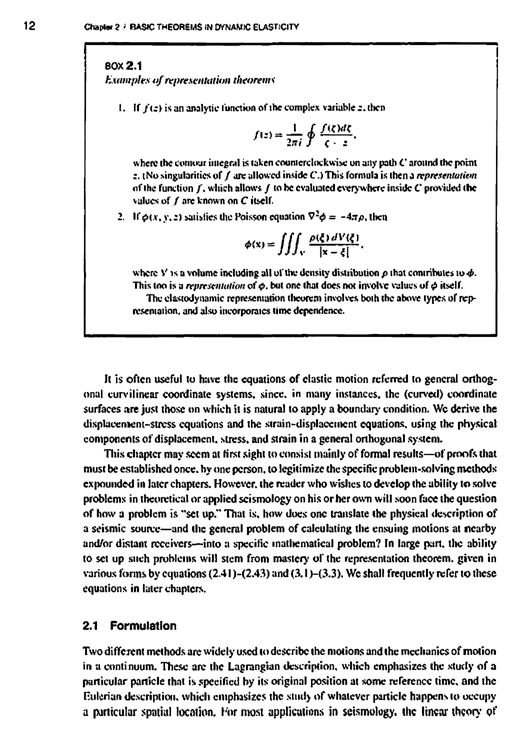
BOX 2.1
Examples of representation theorems
1. If /tr> is an analytic function of the complex variable r. then
2tii J < - z
where the contour integral is taken counterclockwise on any pad) C around the point
r. i No singularities of / arc allowed inside OThis formula is then a representation
of the function /. which allows / to be evaluated everywhere inside C provided the
values of / arc known on C itself.
2. ll*^(A, v.;)^alisliesthel'oissoncquaiion V^= -4.7/>.tltcn
where V is a volume including all of the density distribution p that contributes io<t>.
This loo is a representation of c>. but one that does not involve values of $ itself.
The el&stodynamic representation theorem involves both the above types of
representation, and also incorporates time dependence.
It is often useful to have the equations of clastic motion referred to general
orthogonal curvilinear coordinate systems, since, in many instances, the (curved) coordinate
surfaces are just those on which it is natural to apply a boundary condition. Wc derive the
displacement-stress equations and the strain-displacement equations, using the physical
components of displacement, stress, and strain in a general orthogonal system.
This chapter may seem at first sight to consist mainly of formal results—of proofs that
must be established once, by one person, to legitimize the specific problem-solving methods
ex|X)unde<l in later chapters. However, the reader who wishes to develop the ability to solve
problems in theoretical or applied seismology on his or her own will soon face the question
of how a problem is "set up." That is. how does one translate the physical description of
a seismic source—and the general problem of calculating the ensuing motions at nearby
and/or distant receivers—into u specific mathematical problem? In large part, the ability
to set up such problems will stem from master)' of the representation theorem, given in
various forms by equations (2.41)-(2.43) and (3. l>-(3.3). Wc shall frequently refer to these
equations in later chapters.
2.1 Formulation
Two different methods are widely used to describe the motions and the mechanics of motion
in a conti nuum. These arc the Lagrangian description, which emphasizes the study of a
particular particle that is specified by its original position at some reference time, and the
[uilcrian description, which emphasizes the study of whatever particle happens to occupy
a particular spatial location, lor most applications in seismology, the linear theory of
2.1 Formation 13
elasticity is conceptually simpler to develop with the Lagrangian description, and this is the
framework wc shall almost always adopt. Note that a seismogram is the record of motion of
a particular pari of the Harth (namely, the particles to which the seismometer was attached
during installation), so it is directly a record of Lagrangian motion.
We shall work in this chapter with a Cartesian coordinate system (.v,. x2. v,). and all
tensors here are Cartesian tensors. We use che term displacement regarded as a function
of space and time, ami written as u = u(x. /). to denote the vector distance of a particle at
time r from the position x that it occupies at some reference lime i0. often taken as / = 0.
Since x does not change with lime, it follows that \\\c purticle velocity is 8u/0/ and that the
(Ktithle acceleration is 0*u/3/-.
To analyze the distortion of a medium, whether it be solid or fluid, clastic or inelastic,
we use the strain tensor. If a particle initially at position x is moved to position x + u. then
the relation u = u(x) is used to describe the displacement field. To examine the distortion
of the part of the medium that was initially in the vicinity of x. wc need to know the new
position of the particle that was initially at x + Sx. This new position is x + Sx — u(x + fix).
Any distortion is liable to change the relative position of the ends of the line-element Sx.
If this change is &u. then Sx + Su is the new vector linc-clcmcm. and by writing down the
difference between its end points we obtain
Sx -r Su = x + Sx + u(x I Sx) - (x + u(x)).
Since |5x| is arbitrarily small, we can expand u(x + Sx) asu + {Sx • V)u plus negligible
terms of order |<Sx|2. It follows that Su is related to gradients of u and to the original line-
element <5x via
$u = tfx-V)u. or $11; = —Sx:. (2.1)
' Hjcj '
However, wc do not need all of the nine independent components of the tensor u-j to
specify true distortion in the vicinity of x. since part of the motion is due merely to an
infinitesimal rigid-body rotation of the neighborhood of x. This can be seen from the identity
(m, j - itjj)SXj = £ij^jiMumjSxk (sec Box 2.2 and Problem 2.2). so that equation (2.1) can
be rewritten as
Sttj = \(u,_j + uJi,)&xj -\ J(curl u x Sx),.. (2.2)
and the rigid-body rotation is of amount jcurl u.The interpretation of the last term in (2.2) as
a rigid-body rotation is valid if \i<;-«& I. ll'displiicvinvnt gradient* were not "infinitesimal"
in the sense of this inequality, then we should instead have to analyze the contribution to <5u
from a finite rotation - a much more difficult matter, since finite rotations do not commute
and cannot be expressed as vectors.
In terms of the infinitesimal strain tensor, defined to have components
r,;« UttitJ-rufl).
(2.?)
14
Cn*pM* 2 ,' BASIC THEOREMS IN DYNAMIC ELASTICITY
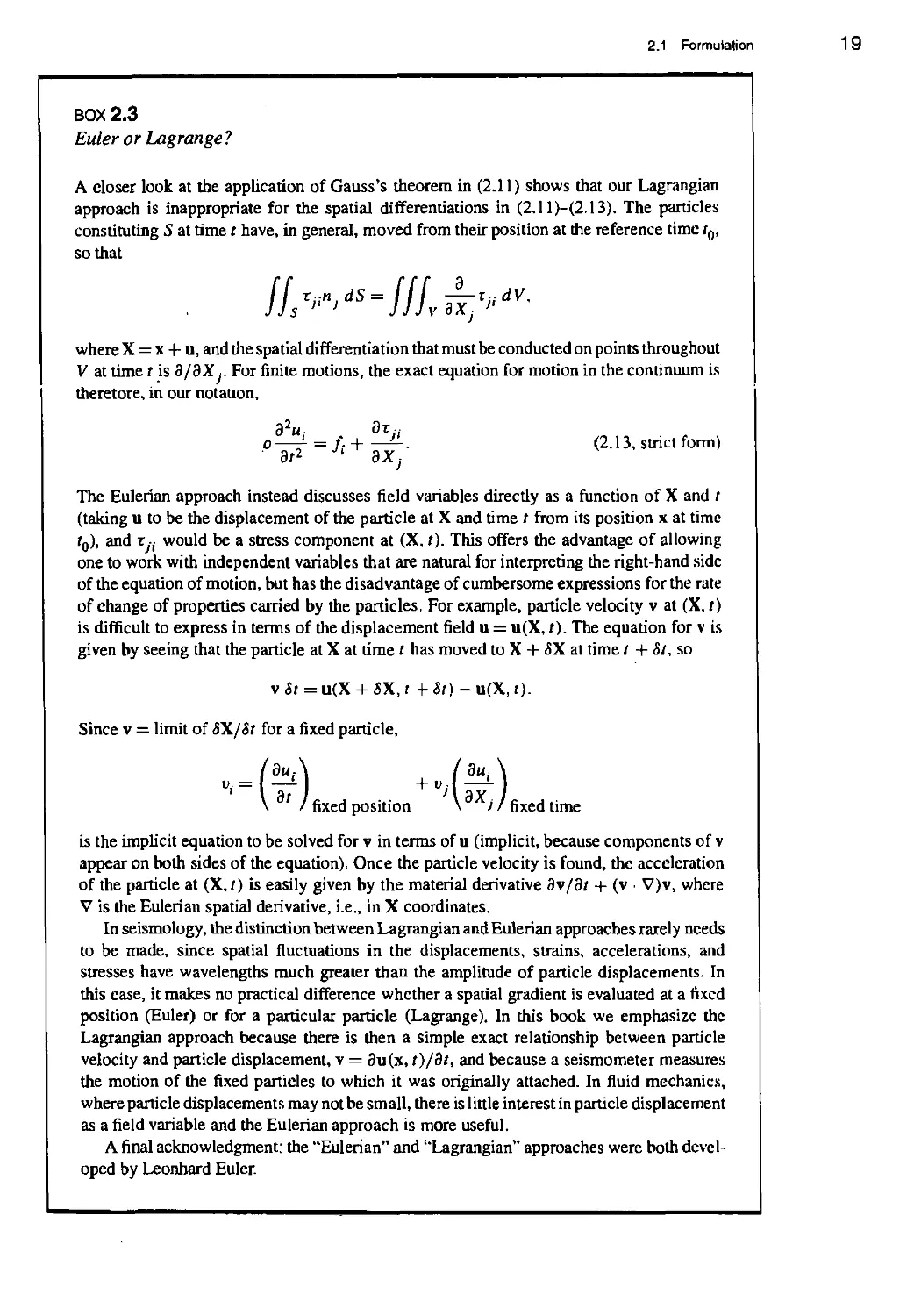
00X2.2
Monition
We stall use boldface symbols (e.j;.. u. r t lor \cctor and tensor fields, and subscripts (e.g..
rr-. r;i) lu designate \ccior and tensor components in a Cartesian coordinate system. Useful
references for the piopcnics of Caiicsiuii tensors are Jeffreys t W65) and Chapter 3 of
Jeffreys and Jeffreys < l«72>.
For unit vectors (oilier than v. I. n. bi. the circumllex is used (e.g.. x>. Scalar products
are written as a • b. and vector products are written ;v> a x b.
Ovcrdots are used to indicate lime derivatives (e.g.. ii = itufdi, ii = H'U/iit-1. and a
comma between subscripts is used for spatial derivatives (e.g.. n, t - Hujfl.x ).
Hie summation convention lor repeated subscripts is followed throughout (e.g.. atl\ —
(/,/», I aJu I <;x/>i = o • b). and frequent use is made of the Kroneckcr symbol HtJ and the
aliemaline tensor with components a-,;<:
& — 0 for »}ty. and *•• — I for i =■ j:
ym = ° •' any of i.j.kjK equal.
otlierwise
The most important properties of these symbols are then
«, = »,,</j. »;,<«A = lax hi,:
and they arc linked by the properties
'*„ *,; ««|
f„kt»m=hit6»w.-ijJiU anJ *ijt'ln» = *im *im 6kr* '
• *i» */« ^iir
The second-order tensor 1 is symmetric if and only if tiitiit m 0.
the effect of true distortion on any line-clement Sxf is to change the relative position of
its end (mints by <*;/*;. Rotation docs not affect the length of the element, and the new
length is
Sx + 6u| = y/Sx • «Sx - 25u • Sx {neglecting o'u ■ «Su)
= Js.x,S.x, ~ 2eijS.XiS.xj (from t2.2>. and using (curl u x Sx) •■ Sx = 0)
r= ,5x| (I 4 f^i'jV)) (to lirsl order. \t\c,: |« I).
where v is the unit vector Sx/ [Sx\. It follows that the cxtcnsional strain of a line-element
originally in the v direction is r;,i:;i>y.
To analyze (he internal forces acting mutually between adjacent particles within a
continuum, wc use the concepts of tntelhm and stress tensor. Traction is a vector, being the
2.1 Formulation
15
■;/Jfc
FIGURE 2.1
The definition of traction T act i up at a
point across the internal surface S with
normal n. The choice of sign is such that
traction is a pulling force. Pushing is in ihc
opposite direction, so for a fluid medium,
the pressure would he —n • T.
force acting per unit area across an internal surface within the continuum, and quantities
the contact force (per unit area) with which particles on one side of the surface act upon
particles on the other side. For a given point of the internal surface, traction is defined (see
Fig. 2.1) by considering the infinitesimal force SF acting across an infinitesimal area AS of
the surface, and taking the limit ofbF/fiS as SS -* 0. With a unit normal n to Ihc surface
S. the convention is adopted that <5F has the direction of force due to material on the side to
which n points and acting upon material on the side from which it is pointing: the resulting
traction is denoted as T(n>. If 6F acts in the direction shown in Fig. 2.1. traction is a pulling
force, opposite to a pushing force such as pressure. Titus, in a fluid, the (scalar) pressure is
n • T(n). For a solid, shearing forces can act across internal surfaces, and soT need not be
parallel to n. Furthermore, the magnitude and direction of traction depend on live orientation
ol'lhe surface element SS across which contact forces are taken (whereas pressure at a point
in a fluid is the same in all directions), 'lb ap|Meciatc this orientation-dependence of traction
at a point, consider a point P. us shown in Figure 2.2. on Ihc exterior surface of a house.
For an clement of area on the surface or the wall at P. the traction T(n() is zero (neglecting
atmospheric pressure and winds): but for a horizontal element of area within the wall at P.
the miction T(n2) may be large (and negative).
The forces acting upon panicles in a solid or fluid medium consist not only of the
contact forces between adjacent particles, hut also of (i) forces between particles that are
FIGURE 2.2
T(ii,)*T(n.>.
16 Chapter 2 / BASIC THEOREMS IN DYNAMIC ELASTICITY
FIGURE 2.3
A material volume V of the
continuum, with surface S.
not adjacent, and (li) forces due to the application of physical processes external to the
medium itself. An example of type (i) would be the mutual gravitational forces acting
between particles of the Earth. Type (ii) is illustrated by the forces on buried particles of
iron when a magnet is moved around outside the medium in which the iron is contained.
To these noncontact forces, we give the name body forces, and use the notation f (x, r)
to denote the body force acting per unit volume on the particle originally at position x
at some reference time. It will often be useful to consider the special case of a force
applied impulsively to one particular particle at x = £ and time t = r. If this force is in
the direction of the xn-axis, it follows that ft (x, t) is proportional to the three-dimensional
Dirac delta function S(x — £), specifying the spatial location; to the one-dimensional Dirac
delta function 5(f — r), specifying the timing of the impulse; and to the Kronecker delta
function 8in, signifying the directional property that /< = 0 for i ± n. Thus the body-force
distribution in this case is given by
/I(x,0 = A5(x-O5(r-T)S,.„, , (2.4)
where A is a constant giving the strength of the impulse. Note that the dimensions of /,,
<5(x - {), and 8(t — t) are, respectively, force per unit volume, 1/unit volume, and 1/unit
time. The Kronecker delta is dimensionless, so A does have the correct physical dimension
for an impulse (force x time).
We are now in a position to place a constraint on the accelerations, body forces, and
tractions acting throughout a volume V with surface S (see Fig. 2.3). By equating the rate
of change of momentum of particles constituting V to the forces acting on these particles,
we find
7,fI(/^dv=lfL",v+fLna)ds a5)
This relation is based on a Lagrangian description, and V and S move with the particles.
The left-hand side can thus be written as JJfv p(32u/3r2) d V, since the particle mass p dV
is constant in time.
Our first use of (2.5) is to obtain an explicit form for the functional relationship
T = T(n) and to introduce the stress tensor. Consider a particle P within the medium for
which the acceleration, the body force, and the tractions are all nonsingular. Surround this
particle by a small volume A V, and consider the relative magnitude of the three terms in
2.1 Formulation
17
T(-»)
FIGURE 2.4
A small disc within a
stressed medium.
(2.5) as A V shrinks down onto P. The volume integrals will be of order A V, but the surface
integral is of order ffs dS taken over the surface of A V. In general such integrals arc of order
(AV)2/3, tending to zero more slowly than A V. After dividing (2.5) through by ffs dS, it
follows that
]-^— ^ = 0(AV1/3)->O as AV->0. (2.6)
SJdS
Now suppose that A V is a disc, with opposite faces having outward normals n and —n (see
Fig. 2.4) and the edge having insignificant area. Equation (2.6) then implies the result
T(-n) = -T(n). (2.7)
Next, take A V to be a small tetrahedron, with three of its faces in the coordinate planes (see
Fig. 2.5) and the fourth having n as its outward normal. Equation (2.6) then implies
T(n) ABC + Tj-xJOBC + T(.-x2)OCA + T(-x3)OAB
ABC + OBC+OCA + OAB "*"
as A V -*■ 0. Here, the symbols ABC etc. denote areas of triangles, and one can show
geometrically that the components of n are given by (wj, n2,n3) = (OBC, OCA, OAB)/ABC.
Then (2.8) and (2.7) yield
T(n) = T{xj)nr (2.9)
which is a specific and important relationship between traction T(n) and n in terms of three
tractions acting across coordinate planes. The properties (2.7) and (2.9) are trivial for a static
medium, but we have shown them to be true even during acceleration.
The stress tensor is introduced by defining the nine quantities
so that xkl is the Ith component of the traction acting across the plane normal to the fcth axis
due to material with greater xk acting upon material with lesser xk. Thus
Ti = xjinj. (2.10)
18 Chapter 2 / BASIC THEOREMS IN DYNAMIC ELASTICITY
FIGURE 2.5
The small tetrahedron
OABC has three of its faces
in the coordinate planes,
with outward normals
-\j(j = 1,2,3), and the
fourth face has normal n.
T(-S,)
T(-*2)
Our second use of (2.5) is to obtain the equation of motion of a general particle.
Applying (2.10) and Gauss's divergence theorem to give
we find for a general volume V that
Jffv(pui-fi-rjiJ)dV = 0.
(2.11)
(2.12)
This integrand must be zero wherever it is continuous, otherwise a volume V could be found
that violates (2.12), hence
P><i = fi + Tji,j>
(2.13)
which is our first form for the equation of motion.
Another constraint upon the mechanics of motion is given by equating the rate of change
of angular momentum about the origin of coordinates to the moment of forces acting on the
particles in V. Thus
±///vX*,*dV-///vXxMV+//xxM& (2.14)
where X = x + u. Since dx/dt, u x u, and d(p dV)/dt are all zero, the left-hand side
here is fffv X x pii dV. Using the strict interpretation of (2.13) developed in Box 2.3,
2.1 Formulation
BOX 2.3
Euler or Lagrange ?
A closer look at the application of Gauss's theorem in (2.11) shows that our Lagrangian
approach is inappropriate for the spatial differentiations in (2.11)—<2.13). The particles
constituting 5 at time r have, in general, moved from their position at the reference time t0,
so that
Ik^-IIL-sT*"-
where X = x 4- u, and the spatial differentiation that must be conducted on points throughout
V at time r is 3/dX . For finite motions, the exact equation for motion in the continuum is
therefore, in our notation,
o -^ = /, + —£-. (2.13, strict form)
9r2 ' dXj
The Eulerian approach instead discusses field variables directly as a function of X and t
(taking u to be the displacement of the particle at X and time / from its position x at time
r0), and r.,- would be a stress component at (X, t). This offers the advantage of allowing
one to work with independent variables that are natural for interpreting the right-hand side
of the equation of motion, but has the disadvantage of cumbersome expressions for the rate
of change of properties carried by the particles. For example, particle velocity v at (X, t)
is difficult to express in terms of the displacement field u = u(X, /)■ The equation for v is
given by seeing that the particle at X at time t has moved to X + <5X at time t + St, so
v St = u(X + SX, t + St) - u(X, r).
Since v = limit of S\/St for a fixed particle,
\ dt /fixedposition \dXJ/
fixed position \ J / fixed time
is the implicit equation to be solved for v in terms of u (implicit, because components of v
appear on both sides of the equation). Once the particle velocity is found, the acceleration
of the particle at (X, t) is easily given by the material derivative 3v/3f + (v • V)v, where
V is the Eulerian spatial derivative, i.e., in X coordinates.
In seismology, the distinction between Lagrangian and Eulerian approaches rarely needs
to be made, since spatial fluctuations in the displacements, strains, accelerations, and
stresses have wavelengths much greater than the amplitude of particle displacements. In
this case, it makes no practical difference whether a spatial gradient is evaluated at a fixed
position (Euler) or for a particular particle (Lagrange). In this book we emphasize the
Lagrangian approach because there is then a simple exact relationship between particle
velocity and particle displacement, v = 9u(x, t)/dt, and because a seismometer measures
the motion of the fixed particles to which it was originally attached. In fluid mechanics,
where particle displacements may not be small, there is little interest in particle displacement
as a field variable and the Eulerian approach is more useful.
A final acknowledgment: the "Eulerian" and "Lagrangian" approaches were both
developed by Leonhard Euler.
Chapter 2 / BASIC THEOREMS IN DYNAMIC ELASTICITY
it follows that
IIL E'ikX>kXik dv=Iflv 'vw* -h) dv
= JfsijkXjTkdS (from (2.14))
= // eijkXjXlkn,dS (from (2.10)).
Applying the divergence theorem to this surface integral and using dXj/BXt = S 7, one
obtains
£iikrjk dV = 0 f°r any volume V,
implying £jjkTjk = 0 everywhere, and hence that the stress tensor is symmetric:
*kj = Tjk- (2-'5)
With this fundamental result, we can finally state the formula for traction components
as
Ti = Tijnj (2.16)
and the equation of motion as
pu, = fi+T,jj. (2.17)
The spatial derivative here should be carried out with respect to Xj, but (as discussed
in Box 2.3) differentiation with respect to x- is usually adequate in seismology, and will
henceforth be assumed.
2.2 Stress-Strain Relations and the Strain-Energy Function
A medium is said to be elastic if it possesses a natural state (in which strains and stresses
are zero) to which it will revert when applied forces are removed. Under the influence of
applied loads, stress and strain will change together, and the relation between them, called
the constitutive relation, is an important characteristic of the medium. That there is such a
relation we prove below by thermodynamic arguments. The relation itself is a proper subject
for experimental determination, and Robert Hooke's measurements of "springy bodies" led
him, over 300 years ago, to the conclusion that stress is proportional to strain. His statements
on this matter were somewhat enigmatic, as today's concepts of traction and tensor were then
unavailable. Augustin Cauchy, in the early nineteenth century, was the first to develop many
of our modern ideas of traction, and it is clear that he understood many results that today are
more easily communicated in terms of tensors, which did not come into general use until
the twentieth century The modern generalization of Hooke's law is that each component
///
2.2 Stress-Strain Relations and the Strain-Energy Function 21
of the stress tensor is a linear combination of all components of the strain tensor, i.e., that
there exist constants ci;i/ such that
T,-; = <W=w (2.18)
A body that obeys the constitutive relation (2.18) is said to be linearly elastic. The
quantities c, w are components of a fourth-order tensor, and have the symmetries
ciiPq = cijp<, (due to r7(. = t,7) (2.19)
and
f;;* = p* Muetoew = *M). (2.20)
It is also true from a thermodynamic argument that c t ■ = ctj■ , as we now shall show.
Suppose that an elastic body occupies the volume V with surface S. The first law of
thermodynamics states that the body possesses an internal (or, intrinsic) energy, which may
change with deformations of the body, and the energy balance for work done on the body
is:
Rate of doing mechanical work + Rate of heating
= Rate of increase of (kinetic + internal energies). (2.21)
Let us analyze each of these terms separately.
(1) The rate of mechanical work is given by
IfL,idv+f(slidS
-III
fi&j + (r,;ij) • dV (from (2.16) and Gauss's divergence theorem)
V (2.22)
= fjf (/>","; + TfjUij) dV (from (2.17))
= — III -pUjitj dV + HI *,•:«,■• dV (symmetry of z^ and definition of ci;).
(2) Let h(x, t) be the heat flux, such that h • n is the rate at which heat is transmitted
(per unit area) in the n direction across area elements normal to n. Let Q(x, f) be the heat
per unit volume due to input through the boundary, so that the rate of heating is given by
rJfLadv=-ffsh*dS- <225)
Then clearly Q = — V • h.
(3) The rate of increase of kinetic energy is given by
^ 111 -pw.u,
if JJJvl ' '
-pitjU: dV. (2.24)
22 Chapter 2 / BASIC THEOREMS IN DYNAMIC ELASTICITY
(4) Let U be the internal energy per unit volume. Then from (2.21 )-(2.24) we conclude
that
U = -hu+TiJeiJ, or U = Q + zijiij. (2.25)
[f IX, Q, and et: are measured as small perturbations away from a state of
thermodynamic equilibrium, then (2.25) is equivalent to
dU = dQ + ztj dei}
= 7 dS + Ttj de^ (for reversible processes), (2.26)
in which S is the entropy per unit volume and T is the absolute temperature. Equation (2.26)
implies that entropy and strain components are the state variables in terms of which internal
energy is completely and uniquely specified. In particular, internal energy does not depend
on the time history of strain.
It is often useful to work with a function W of the strain components that allows the
stresses to be generated via
*u = r—• 0-21)
dei}
A function with this property is called a strain-energy function.
Note from (2.26) the formal result
*~{%\-
(2.28)
If the processes of deformation are adiabatic, so that h = 0 and Q = 0, then the actual
changes in IX associated with changes in strain do occur at constant entropy, and we can
choose W = It and use (2.28). This is the situation in seismology, since the time constant
of thermal diffusion in rock ((distance)2/diffusivity) is very much longer than the period of
seismic waves (wavelength/velocity).
It is also true that r,-. = (33r/3e,y)T, where J = U — 7S is the free energy per unit
volume (for which d7 — -S d7 + r,7 de^). For deformation processes that take place so
slowly as to be isothermal, as in some tectonic processes, it is then natural to form tj;- from
changes in the free energy, and one would choose W = 7.
For all deformations such that the strain-energy function exists, we may combine its
properties with Hooke's law and find
aw
= hi=cit9aeoa, (2.29)
which implies
'"•-"» rm s^rr-s-sr'- <230)
;)
2.2 Stress-Strain Relations and the Strain-Energy Function 23
Since all the first derivatives of W are homogeneous (of order one) in strain components,
and W can be taken as zero in the natural state, W itself must be homogeneous (of order
two) in the form
W = d-- e e P31)
"ijpq'-ij^pq- \—'>J
This quadratic is the same as j (diipq + dpqij)ei}epq, but differentiation of (2.31) to give TtJ
shows that (d,,_. + ^pqij) — cijpq' hence the strain-energy function is, explicitly.
w = \ci}kietjeki = 3 t^. (2.32)
Under adiabatic or isothermal conditions, the stTain-energy function is positive except for
the natural state (where W = 0), so that \cijkleijekl is a positive definite quadratic form.
(W > 0, because we assume the natural state is stable.)
The CijM are independent of strain, which is why they are sometimes called "elastic-
constants," although they are varying functions of position in the Earth. The elasticity theory
used in seismology is to a large extent characterized by a preoccupation with inhomogeneous
media, particularly with a spherically symmetric medium that is everywhere isotropic.
In general, the symmetries (2.19), (2.20), and (2.30) reduce the number of independent
components in C; i; from 81 to 21. There is considerable simplification in the case of an
isotropic medium, since c must be isotropic. It can be shown (Jeffreys and Jeffreys, 1972)
that the most general isotropic fourth-order tensor, having the symmetries of c, has the form
cUki = kSijhi + M(My/ + susjk)- <2-33)
This involves only two independent constants, k and (i, known as the Lame moduli.
Note that the results we have obtained in the present section are specialized to the case
of small perturbations away from a reference state in which strain and stress are both zero. In
the Earth's interior, self-gravitation is responsible for pressures of up to around 1 megabar.
Even if one postulates a state of zero stress and strain for Earth materials, it is clear that
the results of this section cannot directly be applied in seismology, since strains due to such
pressures are not small. Using such a reference state, one must work with a theory of finite
strain, in which the stress-strain relation is nonlinear. Alternatively, one can choose the
static equilibrium configuration of the Earth, prior to an earthquake, as a reference state.
This is the usual procedure in seismology. By definition, the reference state is one of zero
strain, but now the initial stress is nonzero, and seismic motions are studied in terms of a
linear relationship between strains and incremental stresses. Thus the stress is <7° at zero
strain, and is cr° + x at nonzero strain, where r, — cijkiekh ^^ components ct?- can be of
the same order as components c(- w (~ 1 megabar).
For the present, we shall continue to neglect the effects of initial stress or0. This
simplification is justified in Chapter 8, where initial stresses are correctly taken into account
and where a brief review is given of those aspects of the theory that need revision (Box 8.5).
To quantify the effects of self-gravitation, we shall in Chapter 8 adopt an Eulerian approach.
24 Chapter 2 / BASIC THEOREMS IN DYNAMIC ELASTICITY
2.3 Theorems of Uniqueness and Reciprocity
It is natural to introduce the discussion of uniqueness (for the displacement field u
throughout a body with volume V and surface S) with some general remarks concerning the ways
in which motion can be set up. Because the displacement is constrained to satisfy (2.17)
throughout V, the application of body forces will generate a displacement field, as will the
application of tractions on the surface S. We shall show that specification of the body forces
throughout V, and tractions over all of 5, is enough to determine uniquely the displacement
field that will develop throughout V from given initial conditions. An alternative way to
specify the influence of S on the displacement field is to give a boundary condition (on S)
for the displacement itself, instead of for the traction. For example, S might be rigid. It might
seem at first that the traction on S and the displacement on 5 are independent properties
of the displacement field throughout V. This is not so, however, and it is important for an
intuitive understanding of Sections 2.3-2.5 to appreciate that traction over S determines the
displacement over 5\ and vice versa.
2.3.1 UNIQUENESS THEOREM
The displacement u = u(x,/) throughout the volume V with surface S is uniquely
determined after time /0 by the initial values of displacement and particle velocity at /0 throughout
V; and by values at all times t > tQ of (i) the body forces f and the heat Q supplied throughout
V; (ii) the tractions T over any part Sl of S; and (hi) the displacement over the remainder
S2 of 5, with 81 + 82 = S- (Either of 5! or S2 can be the whole of S.)
PROOF
Suppose U] and u2 arc any solutions for u that satisfy the same initial conditions and are
set up by the same values for (i)-(iii). Then, using linearity, the difference U = u] — u2 is
a displacement field having zero initial conditions, and is set up by zero body forces, zero
heating, zero traction on S,, and U = 0 on S2. It remains to prove that U = 0 throughout V
for f > f0.
From (2.22), the rate of doing mechanical work in the displacement field U is clearly
zero throughout V and S, and S2 for t > r0. The last equality in (2.22) can be integrated
from /0 to ?, and, together with the zero initial conditions and the use of a strain-energy
function (U involves adiabatic changes), it follows that
Both the kinetic and strain energies are positive definite, so that Ut = 0 for t > t0. But Vi = 0
at / = /0. and hence U = 0 throughout V for t > f0.
2.3.2 RECIPROCITY THEOREMS
We shall state and prove several general relationships between a pair of solutions for the
displacement throughout an elastic body V.
2.3 Theorems of Uniqueness and Reciprocity 25
BOX 2.4
Use of the term "homogeneous " as applied to equations and boundary conditions
The equation for elastic displacement is L(u) = f, where L is the vector differential operator
defined on the components of u by
If body forces are absent, then the equation L(u) = 0 for u is said to be homogeneous. A
homogeneous boundary condition on the surface S is one for which either the displacement
or the traction vanishes at every point of the surface. If a solution to the homogeneous
equation is multiplied by a constant, the result is still a solution (unlike the outcome of
multiplying a solution to the inhomogeneous equation. L(u) = f with f ^ 0, by a constant).
This terminology is reminiscent of linear algebra, for which a system of n equations
in n unknowns, in the form Ax = 0, is also said to be homogeneous. Here, x is a column
vector and A is some n x n matrix. It is well known that nontrivial solutions (x ■£ 0) can
exist, but only if A has a special property (namely, a zero determinant). The corresponding
result in dynamic elasticity is that motions can occur throughout a finite elastic volume V
without any body forces and with a homogeneous boundary condition over the surface of
V. These are the free oscillations or normal modes of the body, which can occur only at
certain frequencies. See Chapter 8.
Suppose that u = u(x, r) is one of these displacement fields, and that u is due to body
forces f and boundary conditions on S and initial conditions at time f = 0. Let v = v(x, /)
be another displacement field due to body forces g and to boundary conditions and initial
conditions (at t = 0) which in general are different from the conditions for u. To distinguish
the tractions on surfaces normal to n in these two cases, wc shall use the notation T(u, n)
for the traction due to the displacement u and, similarly, T(v, n) for the traction due
to v.
The first reciprocal relation to note between u and v is
fff (t-pu)-vdV+ ff T(u,n) \dS
= III (g-p\)-udV + jf T(v,n)-urfS.
(2.34)
This result is due to Betti. It can easily be proved by substitution from (2.17) and (2.16)
and then applying the divergence theorem to reduce the left side to fffv cijUvi;UkJ dV.
Similarly, the right-hand side reduces to fffv ci:klui jVkt dV, and (2.34) follows from the
symmetry ciJU = cUij.
Note that Betti's theorem does not involve initial conditions for u or v. Furthermore,
it remains true even if the quantities u, ii, T(u,n), and f are evaluated at time tx but
v, V, T(v, n), and g are evaluated aTa different time t2- If we choose t{ = t and t2 — r - t
26 Chapter 2 / BASIC THEOREMS IN DYNAMIC ELASTICITY
BOX 2.5
Parallels
A rearrangement of Betti's relation (2.34) gives
fff {^tju^Aj ~ "fajuVkJj) dv = jjs{v^u'n) - "i7!^")) ds-
This is a vector theorem for the second-order spatial derivatives occurring in the wave
equation of elasticity, which is analogous to Green's theorem
///^-^""-//.(♦s-'t)"
for scalars and the Laplacian operator. Green's theorem is a working tool for studying
inhomogeneous equations, such as V20 = — 4itp, and we shall use Betti's theorem for the
elastic wave equation, in which the inhomogeneity is the body-force term.
There are many further analogies between Dirichlet problems (for potentials that are
zero on 5) and elasticity problems with rigid boundaries; and between Neumann problems
(d<j>/dn = 0 on S) and traction-free boundaries.
and integrate (2.34) over the temporal range 0 to r, then the acceleration terms reduce to
terms that depend only on the initial and final values, since
/ p{fi(0-v(r-r)-u(0-v(T-»)}<*'
Jo
= p f |-{u(f) • v(r - t) + n(0 ■ y(t - t)} dt
JO at
= p (u(t) • v(0) - u(0) • v(r) + u(r) ■ v(0) - u(0) • v(t)} .
If there is some time r0 before which u and v are everywhere zero throughout V (and
hence u = v = 0 for r < z0), then it follows that the convolution
/ p{ii(t)-\(T-t)-u(t)-\(r-t)}dt
J -oc
is zero. We deduce from Betti's theorem the important result, for displacement fields with
a quiescent past, that
/ d' Iff Wx'r>-8<*.T-0-v(x,r-0-f(x,0}dV'
(2.35)
= I dt U {v(x, r - t) ■ T(u(x, t), n) - u(x, r) ■ T(v(x, t - t), n)} dS.
2.4 Introducing Green's Function (or Elastodynamics 27
2.4 Introducing Green's Function for Elastodynamics
A major aim of this chapter and the next is the development of a representation for the
displacements that typically occur in seismology. The representation will be a formula
for the displacement (at a general point in space and time) in terms of the quantities that
originated the motion, and we have seen (in the uniqueness theorem) that these arc body
forces and applied tractions or displacements over the surface of the clastic body under
discussion. For earthquake faulting, the seismic source is complicated in that it extends
over a finite fault plane (or a finite volume) and over a finite amount of time, and in general
involves motions (at the source) that have varying direction and magnitude. We shall find
that the representation theorem is really nothing but a bookkeeping device by which the
displacement from realistic source models is synthesized from the displacement produced
by the simplest of sources—namely, the unidirectional unit impulse, which is localized
precisely in both space and time.
The displacement field from such a simple source is the elastodynamic Green function.
If the unit impulse is applied at x — £ and t = r and in the ^-direction (see (2.4), taking
A = unit constant with dimensions of impulse), then we denote the ith component of
displacement at general (x, f) by Gin(x,t; £, r). Clearly, this Green function is a tensor
(we shall work throughout with Cartesian tensors, and therefore do not distinguish between
tensors and dyadics). It depends on both receiver and source coordinates, and satisfies the
equation
f>^2Gin=sin^-OHt-r) + ^- icukl~^Gkn\ (2.36)
throughout V. We shall invariably use the initial conditions that G(x, f;ij,r) and
3{G(x, /; f, r)}/3/ are zero for / < t and x ^ £. To specify G uniquely it remains to state
the boundary conditions on 5, and we shall use a variety of different boundary conditions
in different applications.
If the boundary conditions are independent of time (e.g., S always rigid), then the time
origin can be shifted at will, and we see from (2.36) that G depends on; and r only via the
combination t — r. Hence
G(x,f;f,r) = G(x,/ - r;,J,0) = G(x.-r;£.-/). (2.37)
which is a reciprocal relation for source and receiver times.
If G satisfies homogeneous boundary conditions on S, then (2.35) can be used to
obtain an important reciprocal relation for source and receiver positions. One takes f to
be a unit impulse applied in the m-direction at x = <J | and time t = r,, and g to be a unit
impulse applied in the ^-direction at x = f2 and time / = —t2. Then «, — G,m(x, t; £,. r,)
and Vj = Gin(x, t; £2, —t2), so that (2.35) directly yields
GBM«2, t + r2*?„ r,) = Gmn(£„ r - t,^2, -r2). (2.38)
28 Chapter 2 / BASIC THEOREMS IN DYNAMIC ELASTICITY
Choosing rt — t2 = 0, this becomes
G„m«2.T;€1,0)~GmBtf1,T;<;2,0), (2.39)
which specifies a purely spatial reciprocity. Choosing t = 0 in (2.38) gives
Cbiii«2.T2;Ci.t1) = Gmii({„-t1;{2,-t2). (2.40)
which specifies a space-time reciprocity.
The actual computation of an elastodynamic Green function can itself be a complicated
problem. We shall take up this subject in later chapters, beginning in Chapter 4 with the
simplest of elastic solids (homogeneous, isotropic, infinite) and moving on to the case of
large separation between source and receiver in inhomogeneous media.
2.5 Representation Theorems
If the integrated form of Betti's theorem, our equation (2.35), is used with a Green function
for one of the displacement fields, then a representation for the other displacement field
becomes available.
Specifically, suppose we are interested in finding an expression for the displacement u
due both to body forces f throughout V and to boundary conditions on S. We substitute into
(2.35) the body force g,(x, r) = Sin <5(x — £) S(t), for which the corresponding solution is
vi(x,t) = G,n(x,/;£,0), and find
Hn«.*>=£ dt fff /,(x,OG,„(x,r-f;<J,0)</V
+ f ^yj{Gin(x,r-/;$,0)ri(u(x,0,n)
- ut(x, t)cijklnjGknJ(.\, x-t;i,0)} dS.
Before giving a physical interpretation of this equation, it is helpful to interchange the
symbols x and d; and the symbols t and r. This permits (x, t) to be the general position and
time at which a displacement is to be evaluated, regarded as an integral over volume and
surface elements at varying £ with a temporal convolution. The result is
un{x,t)= J dxjjj fi(t,T)GiHG,t-T;x,0)dV{t)
+ j dz jj {G,-n(«,r - T;x,0)7}(u(f,r),n)
(2.41)
This is our first representation theorem. It states a way in which the displacement u
at a certain point is made up from contributions due to the force f throughout V, plus
2.5 Representation Theorems 29
contributions due to the traction T(u, n) and to the displacement u itself on 5. However,
the way in which each of these three contributions is weighted is unsatisfactory, since each
involves a Green function with source at x and observation point at £. (Note that the last
term in (2.41) involves differentiation with respect to f,.) We want x to be the observation
point, so that the total displacement obtained there can be regarded as the sum (integral)
of contributing displacements at x due to each volume element and surface element. The
reciprocal theorem for G must be invoked, but this will require extra conditions on Green's
function itself, since the equation Gin(£,t - r; x, 0) = G„,(x, t - t; £, 0) (see (2.39)) was
proved only if G satisfies homogeneous boundary conditions on S, whereas (2.41) is valid
for any Green function set up by an impulsive force in the n-direction at £ = x and r = t.
We shall examine two different cases. Suppose, first, that Green's function is
determined with S as a rigid boundary. We write Gngld for this function and G"n6L (<J,f - t;x,0) =
0 for £ in S. Then (2.41) becomes
«„(x. t)=y~ dt fffv m, T)Gnrifd(x,
t-r;i,0)dV
~ /^ dt jfs «,-«, z)cijklnj^-Gnnf(x, f - t; £,0)} dS.
(2.42)
Alternatively, we can use Gfree as Green's function, so that the traction
cijkinj(d/d&G%e<.Z> r - r; x, 0) is zero for £, in S, finding
«„(x,r) = j dt jfjv /j«,t)G^(x,/ - r;£,0) dV
+ f dt [f G£e(x,f-r;,J,0)7}(u(£,r),n)</S.
J-oo JJs
(2.43)
Equations (2.41)-(2.43) are all different forms of the representation theorem and each
has its special uses. Taken together, they seem to imply a contradiction to the question of
whether u(x, t) depends upon displacement on 5 (see (2.42)) or traction (see (2.43)) or both
(see (2.41)). But since traction and displacement cannot be specified independently on the
surface of an elastic medium, there is no contradiction. In (2.41), the Green function is not
completely defined.
The surface on which values of traction (or displacement) are explicitly required has
been taken, in this chapter, as external to the volume V. It is often useful instead to take
this surface to include two adjacent internal surfaces, being the opposite faces of a buried
fault. Specialized forms of the representation theorem can then be developed, which enable
one to analyze the earthquakes set up by activity on a buried fault. This subject is central to
earthquake source theory, taken up in Chapter 3 and developed much further in Chapters 10
and 11.
So far, we have considered only Cartesian coordinate systems. In practice, the
seismologist is often required to use non-Cartesian coordinates that allow the physical relationship
between components of displacement, stress, and strain to be simplified for the geometry of
30 Chapter 2 / BASIC THEOREMS IN DYNAMIC ELASTICITY
a particular problem. We do this because it is often found that a boundary condition must be
applied on a surface on which a general curvilinear coordinate is constant. Many texts derive
formulas in general orthogonal coordinates for vector operations such as grad, div, curl, and
V2, but rather more is needed to analyze the vector operations required in elasticity, as we
next discuss.
2.6 Strain-Displacement Relations and Displacement-Stress Relations
in General Orthogonal Curvilinear Coordinates
Continuing with the notation developed in Box 2.6, we shall first obtain relations between
strain components epq and displacement components ur that generalize the usual
Cartesian result etj = \{dut/dXj + diij/dxi). By epq, we merely mean the components of the
Cartesian second-order tensor e, referred to rotated Cartesian axes, which are defined (at
the point of interest) to lie along the directions n\ n2, n3. Thus we emphasize the physical
components of strain, rather than the general tensor components (which may not even have
the dimensions of strain). Our problem is to express epq in terms of derivatives (with respect
to c1, c2, c3) of the physical components of displacement also resolved along n1, n2, n3: the
difficulties that arise are due (a) to spatial changes in the scaling functions hi, h1, h3, and
(b) to spatial changes in the directions n1, n2, n3.
Direction cosines of the rotated Cartesian axis along np are (np,nP,nP), referred
to the Cartesian axes ij, x2, i3 (which are in the same fixed direction at every point).
Therefore, from the fundamental transformation property of Cartesian vector and tensor
components.
(summation is retained for repeated subscripts) (2.44)
1 dx
hphi dcp
1
2hPhq
1
2hq
pdcq2 \dxj dx;)
f dxt dut dXj 9«, \
ydcPdc*! drfdcp)
(from (3) in Box 2.6; no summation over superscripts)
(reversing the chain rule in the previous line)
_dcq\hpdcp) 'dcq\hpdcpJj
+ — \— (^^l) _ u J_ (±^l\\
2hp [dcp \hq BdJ ' dcp \hq dd J\
1 dup 1 duq l [ l 3 p I 3 <,i
= — + -u:\ nP + nf (from (3) in Box 2.6, and (2.44))
2hq dcq 2hp dcP 2 ' lh* 3<* ' hp 3cp ' J
~~ lhq 3c<? 2hp dcp 2° \_hq dc* hp dcp\ '
2.6 Strain-Displacement Relations and Displacement-Stress Relations 31
box 2.6
General properties of orthogonal curvilinear coordinates
Consider a point at the vector position x to be specified by three parameters, c1, c2. c3. That
is, each of the three components of x (in some Cartesian coordinate system) is a scalar
function of thee'':
xt = x,V,c2,c3) (f=l,2.3).
We suppose that these functions xi have continuous derivatives and that there are inverse
functions
CP =cp(xl,x1,x3) (/>= 1,2,3) or c" = cp(x),
so that the equation cp = constant can be thought of as a coordinate surface for each p.
and these three surfaces intersect in pairs on lines along which only one of the c\ c2. c3 is
varying. We use superscripts for quantities identified with the general curvilinear system.
Let np be the unit normal to the coordinate surface cp = constant, and suppose x and
x + dx both lie in this surface. Then cp(x) = cp(x + dx), and hence dx ■ Vcp = 0, using the
Taylor expansion of cp(x + dx). Since dx is any line element within the surface, it follows
that Vcp is normal to cp = constant, and Vcp must be parallel to np.
Let the length of vector Vcp be l/hp (a scaling factor). Then
ap = hpVcp. (1)
(We drop the summation convention for superscripts, but retain it for subscripts, these being
related to the original Cartesian system.)
We shall assume that c1, c2, c3 form a right-handed orthogonal system, i.e.. that
npn'l = 8'"> (the Kronecker delta), (2)
and that n3 = n1 x n2.
Using np for the ith Cartesian component of np . we can now obtain an important relation
between ap and dx/dcp, as follows:
„ p- p 3x v^ » 3x 3c' ,, , .
nr=n;X,=n; — = > nt (the chain rule)
i q i
= Ynfl^- (from(l)) =V^lil (fr0m(2))
« 1
and hence
o'=-Lii. (3)
hP dcP
A small change dx in position is associated with a small change in each of coordinates
c1, c2, c3 by dx = £p(dx/dcP)dcp, and the magnitude of this change is given by
{ds)1 = dx-dx = Y —dcP ■ Y —dc"
P 1
= (hl dc1)2 + (h2 dc2)2 + (A3 dc*)2 (from (3) and (21). (4)
(continued)
Chapter 2 / BASIC THEOREMS IN DYNAMIC ELASTICITY
BOX 2.6 (continued)
This result leads to one of the quickest ways of actually finding the scaling functions:
the Euclidean distance associated with increment dcl along n1 is h{dcl; and similarly for
h2 and h\
In Section 2.6, we need formulas for derivatives of the type dnp/dc* in terms of the
undifferentiated normals. From (2) and (3), the equations to be satisfied are
3n9 dnp
np ■ 1- aq • =0 (18 different scalar equations)
3C Be'
(hpT\p) = (hqaq) (3 nontrivial vector equations).
del dcp H
The above are 27 different scalar equations tor the 27 scalar unknowns in 3u"/'3c'', and
hence are exactly enough to determine the solution. In vector form, this solution is
3np
9c?
hp dcP W 9c1 h2 dc2 ft3 3c3 J' K)
as may be verified by direct substitution back into (5).
Pi
In this form, we can use the final equation of Box 2.6 to obtain
~2lhidc0 \hp) + hPdcP \hi)\ h* W 3^' + /*29c2 +A3ac3_r ('
in which all reference to the Cartesian system (*,, x2, x3) has at last been eliminated. Only
the first square bracket is required for the off-diagonal components (p^q), but for a typical
diagonal component (2.45) reduces to, e.g.,
£ ~ V del + h\h2 9c2 + /,3/jl 9c3- ( • }
To obtain the displacement-stress relations for general orthogonal components of u
and t, we follow steps similar to the derivation of /?«,- = r^j given in Section 2.1 for fixed
Cartesian directions. The principal difficulty lies in interpreting ffs T dS, the integral of
traction acting across the surface S with volume V. With v as the outward normal on dS,
Ti{v)dS = ziJvjdS
= Y^ ^pqnpinqj VjdS (transformation to components in rotated Cartesians)
p.i
= £Tp<yV dS,
where vq is the component of the normal to dS, resolved along nq.
2.6 Strain-Displacement Relations and Displacement-Stress Relations 33
. c' = constant
dS-
7
<</S
W
FIGURE 2.6
The projection of dS onto the surface <fl = constant. The resulting area on the coordinate surface is
vq dS. (a) Shown here is dS as part of the surface of V. (b) The projection of dS, in broken outline,
onto the coordinate surface c9 = constant.
Now vq dS is the projection of dS onto the surface cq = constant (see Fig. 2.6), so that
v1 dS = h2h3 dc2 dc3; similarly for v2 dS and v3 dS. It follows that
ff TtdS = J2 U [rp'nfh2h3 dc2 dc3 + x^nfhW dc3 dc1
+ r"3nf hxh2 dcx dc2}
-i:///v[sr<"V*w> + £<''V*J*,>
+ ±.(TP\Ph'h2)\dc}dc2dc3.
3c3 J
But the physical volume element dV is hlh2h3 dc] dc2 dc3, so from steps parallel to the
derivation of the equation of motion given in Section 2.1, we find here that
dt2 tfh2h3 *-* 3c? \ hi )
Chapter 2 / BASIC THEOREMS IN DYNAMIC ELASTICITY
Again, the derivative dnp/dc^ is needed (see (6) in Box 2.6), and by resolving (2.47) along
direction n' we find
aV
a*2
= /' + l
r12 dh
■±.iznhV) + ±yW) + ^
1 r31 dh1 r22 dh2 r33 3*3
r +TTrrT-r rr^—r r~r—r
(2.48)
hlh2 3c2 A3*1 3c3 hlh2 3c1 A3*1 3c1'
Similar results for pit2 and pii3 can be found from a permutation of superscripts in (2.48).
The stress-strain relation, r,-. = c^^e^, becomes
in isotropic media. We have used (2.33) here: A. and /a are (in general) functions of position,
and ekk = en + e2i + e^ is the volumetric strain. Equation (2.49) is expressed in terms
of components in the fixed-direction Cartesian system, but the corresponding result for
physical components in the general orthogonal system has the same form. It is
rpi = wq ^ err + 2fiePi, (2.50)
r
since isotropy of the medium implies cpqrs = cpqrs, and we can again use (2.33). The only
difference in the form of (2.49) and (2.50) is due to our using a summation convention for
subscripts but not for superscripts.
Applications of (2.46), (2.48), and (2.50) are common in spherical polars (r,8,<t>), for
which the scaling functions hl,h2,h3 become, respectively, 1, r,r sin 6; and, in cylindrical
polars, (r, <p, z) with scaling functions 1, r, 1. In Chapter 4 we shall use orthogonal
curvilinear coordinates associated with the wavefronts and rays that emanate from a point source
in an inhomogeneous isotropic medium. Our convention of superscripts is convenient for
the derivation of (2.45)-(2.50), but in applications the superscripts are usually replaced
by subscripts that directly indicate the coordinate of interest. Thus, if (c1, c2, c3) are the
spherical polars (r, 6, <f>), one refers to ei2 as er9, to u3 as u^, and to n2 as 6.
Suggestions for Further Reading
Achenbach, J. D. Wave Propagation in Elastic Solids. Amsterdam: North-Holland, 1973.
Fung, Y. C. Foundations of Solid Mechanics. Englewood Cliffs, New Jersey: Prentice-Hall,
1965.
Jeffreys, H. Cartesian Tensors. Cambridge University Press, 1965.
Love, A. E. H. A Treatise on the Mathematical Theory of Elasticity. New York: Dover
Publications, 1944.
Malvern, L. E. Introduction to the Mechanics of a Continuous Medium. Englewood Cliffs,
New Jersey: Prentice-Hall, 1969.
Problems
35
Problems
2.1 Show that the displacement equation for infinitesimal motion in an elastic
anisotropic medium is
P»i=fi + (cijkiuk,i\j-
If the medium is homogeneous and isotropic, show that this displacement equation
becomes
P'di = fi + (* + M)"/,/; + MM,-,//-
The above two equations are the ith Cartesian component of a vector equation.
Show that this vector equation, for the homogeneous isotropic medium, is
pii = f + (A. + 2/i)V(V -n)-/iVx(Vx u).
2.2 From the expression for ei:keimn in Box 2.2, show that
EijkEilm = SjlSkm-SjmSkl md EijkEjlm = 5im&kl ~ SilSkm-
2.3 For an isotropic elastic solid in which the stress-strain relation is zv = kekkSjj +
2fiet , show that the strain-stress relation is
2.4 What happens to the stress in a body if temperature is raised at fixed strain? Does
the stress obey Hooke's law (2.18) or must this be modified in some way? (Recall
that seismological applications of (2.18) are usually for adiabatic loading.)
2.5 We have shown how the displacement field u(x, f) for an elastic body is given
uniquely (e.g., by applied body forces and tractions). Show that body forces and
tractions are given uniquely once u(x, t) is known everywhere. (A proof "by
construction" is very quick and simple.)
2.6 Do the relations (2.21)—(2.25) change if stress depends on strain rate (e.g., for a
viscous medium)?
2.7 Obtain the traction due to displacement field u acting on area elements normal to
n, in the form
)n + n (2— +n
\ on
T(u, n) = A.(V • u)n + n ( 2— + n x (V x u)
Here
du
— = (n • V)u.
8n
36 Chapter 2 / BASIC THEOREMS IN DYNAMIC ELASTICITY
2.8 The traction T in the previous question is a function of position x, in the sense that
T = T(u(x).n).
a) Modify our derivation of (2.7) to show that traction is a continuous function of
position, in the sense that
T(x + 5x) - T(x) -► 0 as Sx -»■ 0,
provided <5x is taken parallel to the direction n that defines the orientation of
area elements on which traction is evaluated.
b) Consider a book resting on a flat table. Is it true that traction is a continuous
function of position on the surface of the table?
c) Check that your answers to a) and b) are not in conflict.
d) Show that ryz, x2X, tz, are continuous functions of z in any medium, but that
rZ2 need not be continuous in the x- or y-directions; and that t^, r , and xxy
need not be continuous in the z-direction.
2.9 For a point at pressure P in a fluid, the stress tensor is isotropic and has components
r, • = - PSjj. To emphasize the differences between stresses that are possible in a
solid and those that are present in a fluid, it is convenient to define deviatoric
stresses x'.. by r,-• = \xkkhV] + x'-- and deviatoric strains by eiy- = \ekkS(j H-e'-.
Show then that the strain energy U in an isotropic elastic medium is given by
U=\[{X+\n.)eiiekk+2ne'ije\j\
Show that eu is the change in volume per unit volume (i.e., the volumetric strain).
Hence U can be regarded as a sum of dilatational energy, j(A. + \n)eHekk, and
shear strain energy /*e| V.. Why must X + |/x (often called the bulk modulus,
denoted by k ) and u be positive? Is it natural to call k the compressibility or the
incompressib ility?
2.10 Consider two points, x and ^, in an elastic medium, and let the unit vectors n
and v specify particular directions at x and f, respectively. Show first that a unit
impulse in the v direction at £ leads to a displacement at x whose component in
the n direction is given by n,G,_(x, t; {, 0)v . Then show that this displacement
component equals the displacement component in the v direction at £ caused by a
unit impulse in the n direction at x. (This result generalizes the reciprocity result
given in (2.39), which was for an impulse taken along one of the coordinate axes
and a displacement component also along a coordinate axis. The reciprocity is true
for arbitrary directions n and v.)
CHAPTER
Representation of Seismic Sources
Seismic waves are set up by winds, ocean waves, meteorite impacts, rocket launchings, and
atmospheric explosions—even by people walking around in the vicinity of seismometers.
These, however, are examples of sources external to the solid Earth, and they can usually
be analyzed within the simple framework of time-varying tractions applied to the Earth's
surface. Other sources that, for many practical purposes, are also external, include volcanic
eruptions, vented explosions, and spalling (free fall of a surface layer thrown upward by
an underground explosion). For internal sources, such as earthquakes and underground
explosions, the analytical framework is more difficult to develop, because the equations
governing elastic motion (2.17)-(2.18) do not hold throughout the solid Earth. This chapter
is about internal sources, and we shall distinguish two different categories: faulting sources
and volume sources.
A faulting source is an event associated with an internal surface, such as slip across
a fracture plane. A volume source is an event associated with an internal volume, such as
a sudden (explosive) expansion throughout a volumetric source region. We shall find that
a unified treatment of both source types is possible, the common link being the concept of
an internal surface across which discontinuities can occur in displacement (for the faulting
source) or in strain (for the volume source).
The mathematical description of internal seismic sources has classically been pursued
along two different lines: first, in terms of a body force applied to certain elements of the
medium containing the source; and second, by some discontinuity in displacement or strain
(e.g., across a rupturing fault surface or across the surface of a volume source). The second
approach can usefully be incorporated into the first if we can find body-force equivalents
to discontinuities in displacement and strain. We begin our analysis by developing body-
force equivalents in some detail for simple shearing across a fault surface, showing that
radically different systems of forces can be equivalent to exactly the same displacement
discontinuity. We then develop the general theory for faulting sources, following Burridge
and Knopoff (1964), and finally we outline the theory for a volume source.
The motions recorded in a seismogram are a result both of propagation effects and
of source effects. Thus a major reason for seeking a better understanding of the source
mechanism has been to isolate the propagation effects, since these bear information on the
Earth's internal structure. Since tht pioneering work of Sykes (1967), earthquake source 37
3
38 Chapter 3 / REPRESENTATION OF SEISMIC SOURCES
mechanisms have been studied to chart the motions of tectonic plates. Source theory can
elucidate physical processes such as those taking place in volcanoes. It continues to be
developed with a view to predicting earthquake hazards at engineering sites, on the basis
of geological and geophysical data on the properties of nearby faults and the distribution of
regional stresses.
3.1 Representation Theorems for an Internal Surface; Body-Force
Equivalents for Discontinuities in Traction and Displacement
The representation theorems obtained in Chapter 2 can be a powerful aid in seismic source
theory if the surface 5 is chosen to include two adjacent surfaces internal to the volume V.
The motivation here comes from the work of H. F. Reid, whose study of the San Andreas
fault before and after the 1906 San Francisco earthquake led to general recognition that
earthquake motion is due to waves radiated from spontaneous slippage on active geological
faults. We shall discuss this source mechanism in more detail in Sections 3.2 and 3.3, and the
dynamical processes involved (and other source mechanisms) in Chapter 11. Our present
concern is simply to show how the process of slip on a buried fault, and the waves radiated
from it, can naturally be analyzed by our representation theorems.
For applications of (2.41 )-(2.43), we shall take the surface of V to consist of an external
surface labeled S (see Fig. 3.1) and two adjacent internal surfaces, labeled E+ and E~,
which are opposite faces of the fault. If slip occurs across E, then the displacement field is
discontinuous there and the equation of motion is no longer satisfied throughout the interior
of S. However, it is satisfied throughout the "interior" of the surface S + E+ + E~, and to
this we can apply our previous representation results.
The surface S is no longer of direct interest (it may be the surface of the Earth), and we
shall assume that both u and G satisfy the same homogeneous boundary conditions on
FIGURE 3.1
A finite elastic body, with volume V and external surface S, and an internal surface E (modeling
a buried fault) across which discontinuities may arise. That is, displacements on the E ~ side of E
may differ from displacements on the E+ side of E. The normal to E is v (pointing from E~ to
E+), and the displacement discontinuity is denoted by [u(§, r)] for £ on E, with square brackets
referring to the difference u({, t)|e+ — u({, r)|j-_. In general, a similar difference may be formed
for the tractions (due to external applied forces on E), but for spontaneous rupture the tractions must
be continuous, and then [T(u, v)] = 0.
3.1 Representation Theorems for an Internal Surface 39
5 though not on E (see below). Then from (2.41), using (2.39) and renaming some
variables and indices,
"„(x, r) = j™ dx Jjjv fp(n, r)Gnp(x, t - t; r,, 0) «/V(i,)
-[Gn/,(x,r-r;<,0)T/,(u(^,T),v)]j rfl. (3.1)
This formula uses jj as the general position within V, and <J as the general position on E.
Square brackets are used for the difference between values on E+ and E ~ (see caption for
Fig. 3.1).
As yet, nothing has been assumed for the boundary conditions on Z. Although the
choice for u must conform to actual properties of displacement and traction across a
rupturing fault surface, the choice for G can be made in any fashion that turns out to be
useful. Thus, for u, the slip on a fault leads to a nonzero value for [u], but the continuity
of traction (see the proof of (2.7), and Problem 2.8) implies [T(u, v)] = 0. The simplest
and most commonly used way to establish a defining property of G on E is to take E as an
artificial surface across which G and its derivatives are continuous, so that G satisfies the
equation of motion (2.36) even on E. This is by far the easiest Green function to compute
for the volume V, and (in the absence of body forces for u) it gives the representation
It is not surprising that displacement on the fault is enough to determine displacement
everywhere: this feature of (3.2) might have been expected from the uniqueness theorem.
Nevertheless, it is at first sight surprising that no boundary conditions on E are needed for
the Green function that describes waves propagating from the source. One might expect that
motions occurring on the fault would set up waves that are themselves diffracted in some
fashion by the fault surface. But although this interaction complicates the determination of
the slip function [u(£, r)], it does not enter into the determination of the Green function used
in (3.2), and many seismologists have used this formula to compute the motions set up by
some assumed model of the slip function. We shall describe examples of such integrations
in Chapter 10.
3.1.1 BODY-FORCE EQUIVALENTS
The earthquake model we have just described does not directly involve any body forces,
though the representation (3.2) does give displacement at (x, /) as an integral over
contributing Green functions, each of which is the same as if it had been set up by a body force.
Thus there must be some sense in which an active fault surface can be regarded as a surface
distribution of body forces.
40
Chapter 3 / REPRESENTATION OF SEISMIC SOURCES
To determine this body-force equivalent, we start with (3.1) and assume still that £ is
transparent to G. Making no assumptions about [u] and [T(u, n)] across £ (so that sources
of traction are also allowed), we find
«„(*,/)= j dz jjj /p(ij,T)GJip(x.r-T;ij.O)rfV(i?)
+ JX dx jj ([«,.({, r)] cijpqVjGnM(x, t - t; {,0)
- [r,(u«, r), v)] Gnp(x, f - r;«, 0)) rfS«). (3.3)
The discontinuities on £ can be localized within V by using the dciuifuiiUionj(i} - £)•
For example, [T] rf£(<J) has the dimensions of force, and its body-force distribution (i.e.,
force/unit volume) is [t] S(r) - £)d£ as J) varies throughout V. The traction discontinuity
in (3.3) therefore contributes the displacement
J-* dT IIL I" fh [r'(u({'T)'V)] ^ ~ ° dT\ G«p(x'' " T;"'0) dV-
Since this expression has precisely the form of a body-force contribution (see the first term
in the right-hand side of (3.3)), the body-force equivalent of a traction discontinuity on £
is given by f[T^, where
fm(i|1t) = - jj [T(u(S,T),v)]8(r,-OdX{0. (3.4)
The displacement discontinuity is harder to interpret, displacement being less simply
related to force than is traction. We use the delta-function derivative dS(rf - O/^lq t0
localize points of £ within V. This function has the property
J-GHp(.x,t-v,t,0) = -JJj j-S(r,-OGnp(x,t-r;r,,0)dV(,,),
so that the displacement discontinuity in (3.3) contributes the displacement
II" III, I - IL 1"*',1'*,'i,('-!liJ
GnD(x,t-r;T),0)dV
np
at position x and time t. The body-force equivalent flu] of a displacement discontinuity on
£ can now be recognized from this expression as
/p'u](?, t) = - fj [«,-«. z)] cijpqVj ^-S(„ - O d-L. (3.5)
3.1 Representation Theorems tor an Internal Surface 41
BOX 3.1
On the use of effective slip and effective elastic moduli in the source region
We are using the words "fault plane" and "fault surface," symbolized by E, as mathematical
entities that have no thickness. Yet there are many places in the world where Earth scientists
have direct access to fault regions, and one often finds there a zone of crushed and deformed
rock, perhaps several meters thick, so that geologists often speak of "fault gouge" and a
"fault zone." What, then, is meant by our claim that body-force equivalents depend only on
elastic moduli at the fault surface?
The fault zone itself may be as wide as 200 meters, which for most but not all
purposes is far less than the wavelengths of detectable seismic radiation, in which case it is the
displacement change across the whole fault zone that is the apparent displacement
discontinuity, initiating waves which propagate out of the source region. Therefore, in almost all
practical cases, the elastic moduli for equations (3.2), (3.3), and (3.5) are the constants
appropriate for the competent (unaltered) rock adjoining the fault zone. Exceptions may arise
with fault zone effects that may be significant for seismic wave excitation at frequencies of
interest to strong motion seismology (Aki, 1996).
Although the integrand here involves 27 terms (summation over i, j,q), which are
different for each p, we shall find important examples in which only two or three terms
are nonzero. The body-force equivalents (3.4) and (3.5) hold for a general inhomogeneous
anisotropic medium, and they are remarkable in their dependence on properties of the elastic
medium only at the fault surface itself.
Since faulting within the volume V is an internal process, the total momentum and total
angular momentum must be conserved. It follows that the total force due to f[u', and the
total moment of f M about any fixed point, must be zero. Thus
///,
•[uj,
flul(n,T)dV(»j)=0 for all r, (3.6)
v
and
]lf(ri-ii0)xflv'1(ri,i)dV(Ti) = 0 for all r and any fixed n0. (3.7)
To verify (3.6), note that the p-component of the left-hand side is
~ Ik [ui]cijPqvj (///v^Oj-O/Sv^J dUtf). The volume integral here is
lis ^0? ~ Onq ^S(ij), which vanishes because r/ on S can never equal <J (S and S having
no common point).
42 Chapter 3 / REPRESENTATION OF SEISMIC SOURCES
To verify (3.7), write the m-component of the left-hand side as
fffv*~vlrin-*OH>f}u]dV
= " IL C'ipqVj M IIIv £mnp{r)n ~ %n)~kKri ~ ° dV dE (fr°m (3'5))
= + Ih Em'lpCii'"}Vj ^ d* (usins a7(r?n ~ '?0b) = s"q)
= 0 (using the symmetry cijpq = cijqp).
As a simple example of a body force that is equivalent to a field discontinuity, consider
the case of a body force applied at just one point, and in a particular direction (e.g., the body
force for a Green function, given by (2.4)). This can instead be regarded as a discontinuity in
a component of stress. To obtain the equivalence, take x3 as the depth direction and consider
a vertical point force, with magnitude F, applied at (0,0, h) and time r = 0 and held steady.
Then
f(ij, r) = (0,0, F)i(.ni)*(jl2)t(.Tl3 ~ h)H(r)- (3.8)
This source can instead be regarded as a discontinuity in traction across one point of the
plane £3 = A, with
[TC^)]£«|;£I-i = -(0.0,F)««1)i«2)H(T). (3.9)
i.e., rt3, t23 are continuous, and the jump is in r^. The equivalence of (3-8) and (3.9) can
be shown by a straightforward application of (3.4).
The most important example of a body-force equivalent in seismology is found in shear
faulting, and we next take up this subject in some detail.
3.2 A Simple Example of Slip on a Buried Fault
The seismic waves set up by fault slip are the same as those set up by a distribution on
the fault of certain forces with canceling moment. The distribution (for given fault slip) is
not unique, but in an isotropic medium it can always be chosen as a surface distribution of
double couples. Thi s conclusion was unexpected, in view of arguments used in a long-lasting
debate on the question of whether earthquakes should be modeled by a single couple or by a
double couple. Those who advocated the single-couple theory did believe that earthquakes
were due to slip on a fault, but they intuitively thought for many years that such slip was
equivalent to a single couple (composed of two forces corresponding to the motions on
opposite sides of the fault). An intuitive approach is often dangerous in elastodynamics.
On the other hand, some of those who advocated the double-couple theory thought that an
earthquake must be voluminal collapse under pre-existing shear stress. The fault theory of
earthquake sources (now recognized as the equivalent of a double couple) has gained strong
3.2 A Simple Example of Slip on a Buried Fault 43
'j, f -, t ,S ..r ,r—f .■-" .■- .1 , , .. ,. ,
S^S?
*•?■
£±:
■ — y->V"0
FIGURE 3.2
A fault surface Z within an isotropic medium is shown lying In the 53 = 0 plane. Slip is presumed to
take place in the ^-direction across H, as shown by the heavy arrows. Motion on the side E"* (i.c .
C3 = 0+) is along the direction of £, increasing, and on the side S" is along ^ decreasing.
support from increasing amounts of data obtained very close to the source region, as well
as support from the radiation patterns observed at great distances.
As shown in Figure 3.2, we shall take the fault E to lie in the plane £3 = 0, so that
vj = v2 = 0. For the case that we are calling "fault slip", [u] is parallel to £ and so [u] has
no component in the ^-direction. Let {, be the direction of slip, so that [h2] = [n3] = 0.
Then the body-force equivalent, from (3.5), reduces to
/,(»). *) = - jf^ [«,(€. t)] c13M—*0j -«) rfc, «/&.
In isotropic (though still possibly inhomogeneous) media, we can find from (2.33) that all
c13p<? vanish, except c13I3 = cmi = M. Hence
/lOl. t) = - // M(0 [«,({, r)] 5(n, - 4,)5(«2 - fc)/-a(»?3) d£, d&.
3?J3
/2(7.T)=0,
(3.10)
/3<*. r) = - fj^ p [„,] !«(,, - W„2 _ ^(^ d,t ^
First, let us look at /,, which we shall find represents a system of single couples (forces
in indirection, arm along ^-direction, moment along n2-direction) distributed over E.
The integral above yields
A(n, t) = -/*(!,) [„,(,,, T)l —0^3).
9^3
(3.11)
As shown in Figure 3.3, this component may be thought of as point forces distributed over
the plane n3 = 0+ and opposed forces distributed over the plane t/3 = (T.
44 Chapter 3 / REPRESENTATION OF SEISMIC SOURCES
i.fl
(b)
1i
,. li
(»)
fli
FIGURE 3.3
Interpretive diagrams for the first component, /,, of the body-force equivalent to fault slip of the
type shown in Figure 3.2. (a) The spike (-«(t)3),0,0) is plotted against n3. (That is, a spike in
the -redirection, acting at r/3 = 0.) (b) The derivative ((-3/3J7j)<5(r/3),O,0) is plotted against j)y
The body force (/,, 0,0) is proportional to this quantity (see equation (3.11)). (c) Heavy arrows show
the distribution of /, over the £+ side of T. and over the E" side (broken arrows). This is the body-
force component that would intuitively be expected in any body-force model of the motions shown
in Figure 3.2.
The total force due to /, vanishes (see discussion of (3.6)), but the moment of this force
component alone does not. The total moment about the r^-axis is
ffj ^fldV = -fff ^["il^fos^M^S*//^ [«!«'*)] dH.
If slip is averaged over E to define the quantity
_, _ //s MS *)]</£
A
where A = ffz dY, is the fault area, and if the fault region is homogeneous (so that fj. is
constant), then the total moment about the r/2-axis due to /,(£, r) is simply ixu A along the
direction of rj2 increasing.
3.2 A Simple Example of Slip on a Buried Fault 45
[«.]
M
1i
FIGURE 3.4
Interpretive diagrams for the third
component, /3, of the body-force equivalent
to fault slip [«,] . (a) An assumed
variation of slip [u,] with i},, at fixed ij2
and r. (b) The corresponding
derivative d[ul]/dr]l. (c) The distribution of
single forces /3 with varying j?( (see
equation (3.12)). This distribution will
clearly yield a net couple, with moment
in the -(^-direction.
The body-force equivalent, given in (3,10), also involves /3, and we shall find that this
represents a system of single forces. Taking the ^-derivative outside the integration, we
find
(3.12)
Although this component is not itself a couple at each point on E, in the sense that we have
shown fx to be a couple, the whole distribution of /3 across £ does have a net moment.
Figure 3.4 shows how f3 can reverse direction at different points of £. The total moment
about the r/2-axis is
JJJ e2\^\fi dV = / / / r>,— [n [«,]} S(ij3) dr)x dr,2 d^
= ffz £,^-{/4«,]} dii di2 = - fj rtux]dhd£2.
(This last equality follows from an integration by parts, using a fault surface E defined to
have [u] = 0 around its perimeter.) In a homogeneous source region, it follows that the total
moment due to /3 is — fiuA, which is equal in magnitude to the total moment of f{, but acts
in the opposite direction. We obtained this result in more general form in (3.7), but have
found here the two canceling contributions that arise.
46 Chapter 3 / REPRESENTATION OF SEISMIC SOURCES
We have now shown that fault slip is equivalent to a distribution of single couples (/[),
plus a distribution of single forces (/3) that have the net effect of an opposing couple. Yet
the classical force equivalent for fault slip is a double-couple distribution over E, as was
first shown for a finite fault by Mamyama in 1963. The fact is that force equivalents to a
given fault slip are not unique. A direct way to see this, and to obtain the double-couple
density as well as the single-couple/single-force density, is to write out representation (3.2)
for the fault slip described in Figure 3.2. The result is
**'>-£>//l'H*l+*!l'E-
The first term here in curly brackets, ?Grti(x. t — r: (. Q)/d£j, is the limit of
Gtll(x,f-T;{+fi|3,0)-G<,1(x,f-T;{-g{3vO)
2s
as e -*■ 0. (We take |( as a unit vector in the ^,-direction.) This is the single-couple
distribution shown in Figure 3.5a. The second terra in (3.13) involves the limit of
G„3(x, % - t; ( + e| „ 0) - G„3(x, / - r; j - e\ x, 0)
2e
and this single-couple distribution is shown in Figure 3.5b. These two systems form a
double-couple distribution, and we must ask why the earlier set of body-force equivalents
we derived, (3.10), made up a single couple plus a single force. The answer can be seen if
one term in (3.13) is integrated by parts, giving
^"-/>/A'(w^,-fe]°-)"- a,4)
This force system is illustrated in Figure 3.6; clearly it is the same as the system we found
first of all, shown in Figures 3.3 and 3.4. There is always a single couple (/4, Figs. 3.3,
3.5a, and 3.6a) made up of forces in the same direction as fault-surface displacements
(Fig. 3.2). But a complete equivalent to fault slip has another part, which may be regarded
as a distribution of single forces (/3, Figs. 3.4 and 3.6b), a distribution of single couples
(Fig. 3.5b), or an appropriate linear combination of these alternative extremes. For a given
element of area «/E on the fault, these force systems are physically quite different: from the
integrand in representation (3.13), there appears to be no force or moment acting on dE;
but from (3.14), there does appear to be both force and moment acting on d E, although we
showed earlier that /, and /3 integrate to give zero net force and zero net moment on the
whole of E.
We have brought out these results in some detail, because they show the limited utility of
force equivalents for studying the actual forces occurring in dynamic processes of fault slip.
Whereas the body-force equivalent to fault slip is unique (see Box 3.3), force equivalents in
the sense of this section are not unique (force equivalents in this case being force/unit area
on a finite fault). It is the whole fault surface that is radiating seismic waves, and we cannot
3.2 A Simple Example of Slip on a Buried Fault
(a)
\
i
S3
k
1
■
k
1
k
1
k
{■
FIGURE 3.5
The radiation from these two
distributions is the same as
the radiation from slip on a
fault. In this sense, these two
single-couple distributions,
taken together, are equivalent
to fault slip. Note that there
is no net couple, and no net
force, acting on any element of
area in the fault plane (£, = 0).
assess from (3.13) or (3.14) the actual contribution made to the radiation by individual
elements of fault area. This makes sense in physical terms, because individual elements
of fault area do not move dynamically in isolation from neighboring parts of the source
region. Force equivalents (usually chosen as the double-couple distribution) find their main
use only when the slip function [u(cj, t)] has been determined (or guessed), and then they are
important because they enable one to compute the radiation by weighting Green functions.
At great distance from a rupturing fault, it often occurs that the only waves observed
are those with wavelengths much greater than linear dimensions of E, the causative fault.
W
f»*
1
(b)
T
FIGURE 3.6
Another force system that is
equivalent to fault slip (compare
with Fig. 3.5). (a) and (b) here
constitute a single-couple plus
single-force system, which has
zero total couple and zero total
force for the whole fault surface.
But individual elements of area
are acted on by a couple and a
force.
48 Chapter 3 / REPRESENTATION OF SEISMIC SOURCES
(Higher frequency components are relatively weak even at the source—see Chapter 11—
and are more effectively attenuated during propagation.) In such cases S acts as a point
source, and if we also assume that the only waves observed have periods much longer than
the source duration then the slip is localized by replacing [u(<!;j, £2, r)] by the concentrated
distribution uAS(^,)5(^2)W(t). Then /3, as well as /j, becomes a single couple, and the
double-couple point source equivalent to fault slip is
/,(>}, r) = -M0S(J?1)a(7?2)-^-5(^)W(T)
/20».r) = 0 (315)
3»?i
where
Ma = fjiuA = \i x average slip x fault area. (3.16)
We call M0 the seismic moment. It is perhaps the most fundamental parameter we
can use to measure the strength of an earthquake caused by fault slip. Measured values of
M0 range from about 1030 dyn-cm (1960 Chilean earthquake, 1964 Alaskan earthquake)
down to around 1012 dyn-cm for microearthquakes, and 105 dyn-cm for microfractures in
laboratory experiments on loaded rock samples. Even for geophysics, twenty-five orders
of magnitude is an exceptionally large range to be spanned by a single physical variable.
The first person to obtain the double-couple equivalence for an effective point source of slip
was Vvedenskaya (1956). The first estimate of seismic moment was made by Aki (1966)
for the Niigata earthquake of 1964, using long-period Love waves observed by the World-
Wide Standard Seismograph Network. Moment estimates are now made routinely within
hours, or even minutes, after the occurrence of significant earthquakes. The limiting factors
are the time taken for seismic waves to travel through the Earth's interior to the stations
whose data are used; and the time taken for the recorded waveform data to be passed to the
processing site where the estimate is made.
Kanamori (1977) introduced the concept of moment magnitude to seismology. This is
simply a magnitude scale based on the seismic moment of an earthquake, which must first
be estimated. His definition of the moment magnitude, denoted as Mw, is
log M0=1.5MW+ 16.1 (3.17)
in which the constants were chosen so that Mw is approximately the same as the surface
wave magnitude (see Appendix 2) for a certain class of earthquakes. Magnitude scales in
seismology have traditionally been defined empirically, usually as some type of distance-
corrected measure of the strength of ground shaking. However, the moment magnitude,
being derived from a physical characteristic of the source (namely, M0), is fundamentally
different from these empirical magnitudes.
3.3 General Analysis of Displacement Discontinuities across an Internal Surface £ 49
We have defined M0 as a constant, but for some purposes it is useful to evaluate the
seismic moment as a function of time, given by iAu(t)A, in which u is averaged at time t. In
these cases, M0H(x) in (3.15) is replaced by M0(x), and (in the terminology of Chapter 10)
we speak of the "rise time" being different from zero.
Note that there is a fundamental ambiguity in identifying the fault plane associated with
the point-source double couple (3.15). We have worked in this section with a fault surface
normal to the jc3-direction and slip parallel to the *,-direction. If the fault surface instead
is taken normal to the .Xj-direction and slip is taken parallel to the j^-direction in a faulting
episode with the same moment, then the equivalent body force is again (3.15) It follows
that there can be no information in the seismic radiation or static displacement field from
an effective point-source of slip that will enable one to distinguish between the fault plane
and its auxiliary p!ir>e (i.e., the plane perpendicular to both the fault and the slip).
3.3 General Analysis of Displacement Discontinuities across
an Internal Surface E
In this section we introduce the seismic moment tensor, M. This is a quantity that depends on
source strength and fault orientation, and it characterizes all the information about the source
that can be learned from observing waves whose wavelengths are much longer than the linear
dimensions of S. In this case, the source is effectively a point source with an associated
radiation pattern, and the moment tensor can often be estimated in practice for a given
earthquake by using long-period teleseismic data. In practice, seismologists usually use
moment tensors that are confined to sources having a body-force equivalent given by pairs
of forces alone (couples, vector dipoles). Such sources include geologic faults (shearing)
and explosions (expansion), with M as a second-order tensor. For forces differentiated more
than once, sources can be characterized by higher order moment tensors (see Julian et ai,
1998).
For sources of finite extent, we shall introduce the seismic moment density tensor, m,
which can often be thought of as dM/d'E, or as dM/dV for a volume source.
There are two ways in which this section generalizes Section 3.2. First, the coordinate
axes are not taken in directions related to directionalities of the source. (This generality
is important, because the direction of slip and the orientation of the fault plane are not
usually known a priori, but must be deduced from the radiated seismic waves.) Second,
discontinuities are to be allowed in the displacement component normal to the fault plane,
so that expansions or contractions can be simulated.
Our starting point for the general analysis of displacement discontinuities is the
representation (3.2), but using now the convolution symbol * so that
"n(x> °=fL ^ vj°ijM * ~kGnp dE' (318)
Note that / * g = /„' f{x)g(f -x)dx = /„' f(t - x)g{x) dx = /f^ f(x)g(i - x) dx if
/(/) and g{t) are zero for t < 0. If X0 is the amplitude of a force applied in the p-direction
at £ with general time variation, th^n the convolution X0 * Gnp gives the ^-component
of displacement at (x, /) due to the varying point force at £. More generally, if the force
Chapter 3 / REPRESENTATION OF SEISMIC SOURCES
(1.2)
(1.3)
A- A-
(2,1)
(2.2)
(2.3)
(3,1)
FIGURE 3.7
The nine possible couples that are required to obtain equivalent forces for a generally oriented
displacement discontinuity in anisotropic media.
applied at £ is F(£, t), then we can sum over p and write Fp * Gnp for the n-component
of displacement at (x, t). For displacement discontinuities as in (3.18), there are instead
derivatives of Gnp with respect to the source coordinates f . Such a derivative, we saw in
Section 3.2, can be thought of physically as the equivalent of having a single couple (with
arm in the £, -direction) on S at £. The sum over q in (3.18) is then telling us that each
displacement component at x is equivalent to the effect of a sum of couples distributed
over Z.
For three components of force and three possible arm directions, there are nine
generalized couples, as shown in Figure 3.7. Thus the equivalent surface force corresponding to an
infinitesimal surface element rfS(«J) can be represented as a combination of nine couples.
In general, we need "couples" with force and arm in the same direction (cases (1,1), (2,2),
(3, 3) of Fig. 3.7), and these are sometimes called vector dipoles.
Since [«,-] VyCyM * dGnp/d^q in (3.18) is the n-component of the field at x due to
couples at £, it follows that [w(] VjCtjpq is the strength of the (p, q) couple. The dimensions
of [w,] VjCjjpq are moment per unit area, and this makes sense because the contribution
from £ has to be a surface density, weighted by the infinitesimal area element dT. to give a
moment contribution. We define
3.3 General Analysis of Displacement Discontinuities across an Internal Surface E 51
mpq = [Ui]VjCijpq <3-19>
to be the components of the moment density tensor, m. In terms of this symmetric tensor,
which is time dependent, the representation theorem for displacement at x due to general
displacement discontinuity [u(f, t)] across Z is
un(x,t) = ff mpq*GnpqdZ. (3.20)
When we have learned more about the Green function (in Chapter 4), we shall find that the
time dependence of the integrand in (3.20) is quite simple, because if x is many wavelengths
away from £, then convolution with G gives a field at (x, t) that depends on what occurs at
£ only at "retarded time," i.e., t minus some propagation time between £ and x
For an isotropic body, it follows from (2.33) and (3.19) that
mpq = ^k [«*(«. *)] &„ + M (v„ [«,«. t)] + vq [«„«, t)]) . (3.21)
Further, if the displacement discontinuity (or slip) is parallel to E at d;, the scalar product
v • [u] is zero and
mpq = n(vp[uq] + Vq[up]). (3.22)
In the case of E lying in the plane £3 =± 0, with slip only in the ^,-direction, we have
the source model considered in Section 3.2, and for this the moment density tensor is
/ 0 0 M[«i«,r)]\
m= ° 0 ° I '
\/*[«,«. r)] oo/
which is the now familiar double couple.
In the case of a tension crack in the £3 = 0 plane, only the slip component [m3] is
nonzero, and from (3.21) we find
/X[ii3«,t)] 0 0 \
m= 0 X[«3(«,r)] 0
V 0 0 (A + 2/t) [i/3«. r)] /
Thus a tension crack is equivalent to a superposition of three vector dipoles with magnitudes
in the ratio 1:1: (k + 2fi)/X (see Fig. 3.8).
The above results have been developed for a fault plane E of finite extent, but in practice
the seismologist often has data that are good only at periods for which the whole of £ is
effectively a point source. For these waves, the contributions from different surface elements
dT. are all approximately in phase, and the whole surface S can be considered as a system
of couples located at a point, say the center of E, with moment tensor equal to the integral
of moment density over I. Thus, for an effective point source,
«„$, /) = M * G
(3.23)
52 Chapter 3 / REPRESENTATION OF SEISMIC SOURCES
FIGURE 3.8
The body-iorce equivalent iOi a. tcr.sicr. crsck in np inotropic medium.
where the moment tensor components are
»»-liS~d*~HzM»l
cUPq dT..
i.e.,
mpq =
_dM£1
dH
(3.24)
In (3.23) we have one of the most important equations of this chapter. Later in this book,
we shall evaluate the Green function and the different waves it contains. Thus in Chapter 4
we shall use ray theory for G and interpret (3.23) in terms of body waves excited by given
M (equation (4.96)). In Chapter 7, we shall find the surface waves excited by M (equations
(7.148H7.151)), and in Chapter 8 the normal modes of the whole Earth (8.38).
In terms of seismic moment M0, and with the choice of coordinate axes made in
Section 3.2, the moment tensor for an effective point source of slip is
M =
0
0
M0
0
0
0
M0
0
0
(3.25)
Equations (3.24) justify the name "moment tensor density" for m. In the case of a
finite source, we can now interpret the representation (3.20) as an areal distribution of point
sources, each point having the moment tensor m dE.
We conclude this section with an interesting use of "seismic moment," suggested
by Brune (1968), involving the kinematic motions of tectonic plates. Such motions lead
frequently to a type of regional seismicity in which many different earthquakes share the
same fault plane (although any one event will involve slip over only a part of the whole
fault area). If M^ is the seismic moment of the ith earthquake in a series of N earthquakes
in time interval A7\ it follows from the definition of Mq that the total slip due to the whole
series is
At/ =
N
1=1
MS '
(3.26)
3.4 Volume Sources: Outline of the Theory and Some Simple Examples
BOX 3.2
On uses of the word "moment" in seismic source theory
In rotational mechanics, it is often enough to speak of a couple possessing the qualities
of magnitude and a single direction. The magnitude of a couple is then a scalar quantity
called the moment. In our study of displacement discontinuities, however, and body-force
equivalents, we imply more directional qualities behind the word "couple" than is the case
in rigid-body rotational mechanics. For us, "couple" involves the directions of both force
and lever arm. A result of this is that the quantity "moment" jumps up from scalar to tensor.
Second-order Cartesian tensors in mathematical physics are usually quantities that relate
one physical vector to another. One example is given by equation (2.16), in which the stress
tensor is a device for obtaining traction from the vector orientation of an area element.
Another example is the inertia tensor I, which gives angular momentum h from angular
velocity a> viah- — I{ <Oy In seismic source theory, however, the moment tensor is an input
rather than a filter, and it is operated on by a third-order tensor to yield vector displacement
(see (3.20) and (3.23)).
where S is the total area broken in the series. AU is averaged over all of 5, and all the terms in
the right-hand side of (3.26) can be estimated. If all the plate motion occurs seismically, and
if the seismicity during AT is representative of the activity on that plate margin for longer
time scales, then AU/AT is an estimate of the relative velocity of the plates, regarded as
slow-moving rigid bodies, and it can be obtained from seismic data alone.
3.4 Volume Sources: Outline of the Theory and Some Simple Examples
In order to develop equations for seismic waves from buried explosions or from rapid
phase transformations, it is necessary to introduce the concept of a volume source. We
shall describe such a source in terms of a transformational (or stress-free) strain introduced
in the source volume, and shall develop properties of an associated seismic moment tensor.
Let us illustrate this concept by a set of imaginary cutting, straining, and welding
operations described by Eshelby (1957). First, we separate the source material by cutting
along a closed surface E that surrounds the source, and we remove the source volume (the
"inclusion") from its surroundings (the "matrix"). We suppose that the material removed
is held in its original shape by tractions having the same value over S as the tractions
imposed across £ by the matrix before the cutting operation. Second, we let the source
material undergo transformational strain Aers. By this, we mean that Aers occurs without
changing the stress within the inclusion, hence the name "stress-free strain." It is this
strain that characterizes the seismic source. Processes that can be described by stress-free
strain include phase transformation, thermal expansion, and some plastic deformations.
Stress-free strain is a static concept. Third, we apply extra surface tractions that will
restore the source volume to its original shape: this will result in an additional stress field
-cpqrs Aers = ~Axpq throughout the inclusion, and the additional tractions applied on its
surface £ are -c s Aersv wher#u is the outward normal on E. Since Arpq is a static
field, Az'p = 0. The stress in the matrix is still unchanged, being held at its original value
54
Chapter 3 / REPRESENTATION OF SEISMIC SOURCES
BOX 3.3
Body-force equivalents and the seismic moment tensor
For a general displacement discontinuity across E, it follows from (3.5) that
where, by & (£), we mean a one-dimensional spatial Dirac delta function that is zero off £.
Thus, if S lies in the plane ^3 = 0, S(E) = <S(rj3) for points (ijj, r)2) on T.
It must be emphasized that f is a force per unit volume, and it is unique. (Once [u(.] is
given on S, then u is determined everywhere, and f = L(u), where L is given in Box 2.4.)
The ambiguities mentioned in Section 3.2 ari«e only when equivalent surface forces are
sought. Thus the above formula for / does not give a distribution of couples and dipoles.
Such a distribution arises only after the displacement representation fffv G {/} d V has
been integrated by parts and the q3 integration completed to give (3.18), which may then
be interpreted in terms of equivalent surface forces. These are nonunique—see (3.13) and
(3.14)—but a surface distribution of couples and vector dipoles is always possible.
We have introduced the seismic moment tensor in the form M = ffj. [uj] VjC^ dH,
but from the above formula for body force it is easy to show that
M
py
-Hi
fpv, rfV(if).
This result can be used to extend the definition of M, since it can be used for any body-force
distribution, and not just for the body-force equivalent to a displacement discontinuity. With
this definition, the moment (in the ordinary sense of rotational mechanics) of body-forces
f about the j'th axis is fffv e,-:ji) j/j dV = e■ t AfA •, which is zero whenever the moment
tensor is symmetric (e.g., in (3.24)).
by tractions imposed across the internal surface S, and having the same value as tractions
imposed on the matrix by the inclusion before it was cut out. Fourth, we put the inclusion
back in its hole (which is exactly the correct shape) and weld the material across the cut.
The traction on £~ is now an amount —c Ae„v greater than that on 2+, leading
to a traction discontinuity (in the v-direction) of amount +c Aersv . This traction is
due to applied surface forces that are external to the source and which act on the inclusion
to maintain its correct shape. Fifth, we release the applied surface forces over E_. Since
traction is actually continuous across E, this amounts to imposing an apparent traction
discontinuity of —{cpqrs Aers)vq. The elastic field produced in the matrix by the whole
process is that due to the apparent traction discontinuity across S.
The above procedure can be extended to a dynamic case of seismic wave generation,
since, at any given time, a transformational strain Aers can be defined for the unrestrained
material. For each instant, it is still true that ArD(IO = 0 because stress-free strain (and
the stress derived from it) is a static concept. The seismic displacement generated by the
3.4 Volume Sources: Outline of the Theory and Some Simple Examples
BOX 3.4
The strain energy released by earthquake faulting
Within a medium that initially has a static stress field a0, we suppose that a displacement
discontinuity develops across an internal surface S. This leads to a displacement field
u(x, t), measured with reference to the initial configuration, and from u we can determine
the additional time-dependent strain and the additional stress t. Then the total stress is
a = <jr° -+■ t, and after all motions have died down the new static stress field is <j'. If AC
is denned as the change in strain energy throughout the medium, from its initial static
configuration to its final static configuration, it can be shown that
AE^-lj^tf+a^VjdT, (1)
where [u] is the final offset. (See Fig. 3.1 for definitions of [ ] and v.) Equation (1) is
known as the Volterra Telation (Stcketee, 1958; Savage, 1969a).
This result (which we derive below) can be simply restated in terms of work apparently
done by tractions on the fault surface. We can say from (1) that the drop in strain energy
throughout the medium, — A E, is the positive quantity obtained by imagining a quasi-static
growth of traction that is linear with offset:
T = T"+(Tl -T0)— for 0<U<[u] (2)
[«]
(for each component of traction T and displacement II). Integrating from 0 to [u] to get the
total work done on £ then gives (1).
Several points now need to be made about this relation between A£ and the average
stress.
The liberated energy, —A£, supplies the work actually done on the two faces E + and
£~ as they grind past each other, plus the work done in initiating the process of fracture.
We discuss these two types of work in Chapter 11. Moreover, - A£ supplies the seismic
energy £s that is radiated away from the source region. It is natural to introduce the seismic
efficiency, n, as the ratio Es/(—A£). Then
£s = -n A£ = \r, f [u,] (a° + o-,>, rfL. (3)
If the average of the two static tractions does not vary strongly over E, then for the type of
tangential slip shown in Figure 3.2 we see that (3) can be expressed in terms of the moment
M0 — h fL [u,] <f E. This gives
£s = nM0a/p., (4)
where a = j(of3 + o-j3).
From estimates that can be made of £s, M0, and n, it thus becomes possible from (4) to
estimate the product rjcf, called the apparent stress by Wyss and Brune (1968, 1971). The
reason for this name is that r\a would be the stress that appears to be acting on the fault,
if we make the assumption that the observed radiated energy is equal to the liberated strain
energy. (The assumption here is not a good one. The seismic efficiency is at most a few
percent, so that only a small fraction of the liberated energy is radiated as seismic waves.)
(continued)
56
Chapter 3 / REPRESENTATION OF SEISMIC SOURCES
BOX 3.4 (continued)
Since the slip function [u(f,/)] in (3.18) determines all displacements (and hence strain
and stress increments) throughout the medium, it also determines the stress drop, or0 — al.
But there is no way one can work purely from observations of the radiated field u(x, t) and
leam anything about the absolute level of stress in the source region. Putting this another
way, and using (1), one can make the following statement. If the same slip function [u({, t) ]
occurs on S in two different faulting events with different initial stresses, then all the seismic
displacements will be the same for the two events: but the strain energies liberated for the
two events may be quite different.
It remains, then, to prove our main result (1). This is a formula of great generality, and a
correct derivation can be given by considering the quasi-static deformation we described in
(2). We r.hal! give ?n ait;->!io'« proof for the special case in which the internal strain energy
U is given by a strain-energy function W (see Section 2.2). Further, we assume there is an
accessible reference state of zero stress and zero strain. The initial stresses and strains just
prior to faulting are ctP. and «9., and u is measured from this state.
From (2.32) applied to the total stresses and strains, we get
W = \(af} + T,7)(e°- + ",,_,) (using symmetry of ai})
= Wu+H"lV + K/"*./
(using (2.30)).
Thus the increase in internal energy in the new static configuration is
A£ = J (W1 - W°) dV = \ j{p}j + o*)uu dV,
(5)
where V is the whole elastic volume containing E (see Fig. 3.1). Since a9. and o^- are static
stress fields, (2.17) implies a°. ■ = a\ , = 0 (we assume there are no body forces). From
(5), we obtain
AE=lfv{(v?j+crlj)ui}JdV,
to which we can apply Gauss's divergence theorem, regarding V as the interior of S + £ + +
£ ~. This does give (1) if S is a rigid surface, or if, like the surface of the Earth, it is free.
discontinuity in traction was given by (3.3). Putting [Tp\ = —(cpqrs &ers)va *n (3-3), we
get
«„(*•') = £* dxjj cpqrs Ae„vqGnp(x,t - r;{,0)dE«). (3.27)
If the integrand and its derivatives with respect to f are continuous, we can apply the Gauss
theorem to obtain
«„(x, t) = j™ dz fff ±- [cpqrs AersGnp(x, / - t; £,0)} dV(£) (3.28)
3.4 Volume Sources: Outline of the Theory and Some Simple Examples 57
(V here refers only to the volume of the inclusion, i.e., the source volume). Using
3(c „ A<?„)/3<^9 = Arpq,q = °« we can rewrite (3.28) and obtain
"n(X' ° = jjfv C<">rs A'" * ~JT dV' (3'29)
Comparing this volume integral with the surface integral in (3.18), one sees that it is natural
to introduce a moment-density tensor
-jf- = cpqrs^rs (3-30)
with the dimensions of moment per unit volume (compare also with (3.24)). Then
rrr dMna 3G„„
"■*"-///,-if *if'v- <""
Note that &rpq = dMpq/dV is not the stress drop (the difference between the initial
equilibrium stress and the final equilibrium stress in the source region), as is clear from its
definition. The stress drop is not limited to the source volume, but Ar vanishes outside
the source volume. Krpq is called the "stress glut" by Backus and Mulcahy (1976).
For long waves, for which the whole of V is effectively a point source, the whole
volume V can be considered a system of couples located at a point, say the center of V,
with moment tensor equal to the integral of moment density over V. Thus, for an effective
point source, (3.23) applies, with the moment tensor components
-///,
1
M = 2mV
1
f °
0
^A«?l3
0
0
0
A«„
0
0
Mpq = ]JjvCpqrs^rsdV. (3.32)
For example, if a shear collapse occurs in a homogeneous isotropic body of volume
V with the nonzero transformational strain components Ae13 = Ae31, say, the moment
tensor is
(3.33)
The seismic radiation is identical to the point source equivalent to a fault slip, except that
the seismic moment MQ is given by 2/x Ae)3V. For a group of earthquakes in an intraplate
seismic zone, a cumulative strain may be more meaningful than a cumulative slip given
by (3.26). Kostrov (1974) suggested summing moments for a group of earthquakes sharing
the same source mechanism in a given volume to find the total strain in the volume. From
(3.33), the total strain A£]3 may be estimated as
N
em;
AE.3^. (3.34,
where M'Q is the moment of the t'th earthquake.
Chapter 3 / REPRESENTATION OF SEISMIC SOURCES
Finally, let us consider a spherical volume with radius a undergoing a transformational
expansion. The stress-free strain components in this case are Ae12 = Ae13 = Ae^ = 0 and
Aeu = Ae22 = Ae33 = 5 AV/ V, where AV/V is the fractional change in volume and
V = \na}. For this expansion in an isotropic medium, cpqrs Aen = (A + \v.)&pq AV/V
and from (3.32) we have
/(k + \n)AV 0 0 \
M= [ 0 (k+]iJ.)AV 0 J . (3.35)
\ 0 0 (A. + |/*)AV/
Thus a spherical source with transformational volume expansion is equivalent to three
mutually perpendicular dipoles, as shown in Figure 3.7. In the above equation, AV is the
stress-free volume change and should not be confused with the volume change S V of a
confined source region, as discussed in Problem 3.8.
Suggestions for Further Reading
Backus, G., and M. Mulcahy. Moment tensors and other phenomenological descriptions
of seismic sources—I. Continuous displacements. Geophysical Journal of the Royal
Astronomical Society, 46, 341-361, 1976.
Backus, G., and M. Mulcahy. Moment tensors and other phenomenological descriptions of
seismic sources—II. Discontinuous displacements. Geophysical Journal of the Royal
Astronomical Society, 47,301-329, 1976.
Bowers, D., and J. A. Hudson. Defining the scalar moment of a seismic source with ageneral
moment tensor. Bulletin of the Seismological Society of America, 89,1390-1394,1999.
Burridge, R., and L. Knopoff. Body force equivalents for seismic dislocations. Bulletin of
the Seismological Society of America, 54, 1875-1888, 1964.
Ekstrom, G. Anomalous earthquakes on volcano ring-fault structures. Earth and Planetary
Science Letters, 128,707-712, 1994.
Eshelby, J. D. The determination of the elastic field of an ellipsoidal inclusion and related
problems. Proceedings of the Royal Society, A241, 376-396,1957.
Heaton, T. H., and R. E. Heaton. Static deformations from point forces and force couples
located in welded elastic Poissonian half-spaces: Implications for seismic moment
tensors. Bulletin of the Seismological Society of America, 79,813-841, 1989.
Jost, M., and R. B. Herrmann. A student's guide to and review of moment tensors.
Seismological Research Letters, 60, 37-57,1989.
Julian, B. R., A. D. Miller, and G. R. Foulger. Non-double-couple earthquakes 1. Theory.
Reviews of Geophysics, 36, 525-549,1998.
Kostrov, B. V. Seismic moment and energy of earthquakes and seismic flow of rock. Izvestia,
Physics of the Solid Earth, 13-21, January 1974.
Kostrov, B. V., and S. Das. Principles of earthquake source mechanics. New York:
Cambridge University Press, 1988.
Maruyama, T. On force equivalents of dynamic elastic dislocations with reference to the
earthquake mechanism. Bulletin of the Earthquake Research Institute, Tokyo Uni ver-
«*y, 41, 467-486, 1963.
Problems
Press F., and C. Archambeau. Release of tectonic strain by underground nuclear explosions.
Journal of Geophysical Research, 67, 337-342, 1962.
Pujol, J., and R. B. Herrmann. A student's guide to point sources in homogeneous media.
Seismological Research Letters, 61, 209-224, 1990.
Savage, J. C. Steketee's paradox. Bulletin of the Seismological Society of America, 59, 381,
1969.
Steketee, J. A. Some geophysical applications of the theory of dislocations. Canadian
Journal of Physics, 36, 1168-1198, 1958.
Stump, B. W., and L. R. Johnson. Higher-degree moment tensors—the importance of source
fmiteness and rupture propagation on seismograms. Geophysical Journal of the Royal
Astronomical Society, 69, 721-743, 1982.
Problems
3.1 Equations (3.26) and (3.34) are written as scalar equations, because in their
derivation it has been assumed that earthquakes in a given region (on S, or within V)
all have moment tensors with the same orientations.
Generalize (3.26) to a vector equation and (3.34) to a tensor equation in cases
where earthquakes in the series (on S or in V) have moment tensors of arbitrary
orientation. (For (3.26), however, continue to assume that the displacement
discontinuity for each event is a shear and that S is planar.)
3.2 In our derivation of (3.2), we have assumed that the elastic moduli are continuous
across L and that Gnp and dGnp/d^ are continuous. If the elastic moduli arc
not continuous across S, interpret part of the integrand in (3.2) as a traction.
and show that this representation is still valid, although 9Grt/>/9<L may not be
continuous across the surface. {Note: For purposes of denning G, assume S + and
E~ have been glued together. These surfaces—which can still move—then do not
have relative motion.)
3.3 In the discussion following equations (3.15) and (3.16). we introduced the time-
dependent seismic moment given by M0(t) — (j,u(t)A. Is u(t) here averaged over
the area A(t) that has ruptured at time r, or is it averaged over A(oo), the area that
ultimately is ruptured during the seismic event under consideration? (Hint: Does
it matter?)
3.4 Show that the moment tensor M described in terms of a double couple in
Section 3.2 and equation (3.25), i.e.,
(0 0 M0
0 0 0
M0 0 0
can equivalently be described by
(MQ 0 0 \
M = I 0 0 0
V o o -mJ
Chapter 3 / REPRESENTATION OF SEISMIC SOURCES
where components of M are now referred to the principal axes of M as coordinate
axes. (By definition, the principal axes of a symmetric tensor are such that the
off-diagonal components of the tensor, referred to these axes, are all zero.)
In terms of body-force, equivalents, this result is illustrated by the following
diagram:
i>
a
t\
This shows that a double couple is equivalent to a pair of vector dipoles, equal in
magnitude but opposite in sign.
3.5 Show that a seismic point source described by a symmetric second-order moment
tensor M can be thought of as an isotropic point source Mj plus two double couples.
Is this a unique decomposition of such a point source?
Show that M can also be written in the form
/0 0 0'
M = M1 + (M,-A/2) 0 -1 o|+A/CLVD
\0 0 1
1
2
0
0
0
_ 1
2
0
0
0
1
in which Mt («' = 1,2,3) are the principal moments. The last term here is called a
"compensated linear vector dipole," having axial symmetry and no volume change.
If M[ — M2 is the largest difference between principal moments, then MCLVD
quantifies the extent to which the deviatoric part of the moment tensor differs from
a pure double couple.
3.6 Show that the body-force equivalent to a point source at { with moment tensor
Mpq is given by
fJx,t) = -MpJt)—8(x-S).
dx„
3.7 Consider a spherical cavity with radius a inside a homogeneous isotropic body.
When a uniform step in pressure, 8pH(t), is applied at the surface of the cavity,
spherically symmetric waves will be generated, which have displacement only in
the radial direction. After the waves have passed, displacement everywhere tends
to its final static value, which characterizes the final outward expansion due to the
applied pressure in the cavity.
a) Use the vector wave equation of Problem 2.1 to show that this static
displacement satisfies V(V u) = 0.
Problems
61
b) Hence, in this problem with spherical symmetry, show that the radial
displacement is proportional to l/r2 (for a < r, so that this is a so-called external
solution).
c) Show from equations (2.50) and (2.46) that for this problem the radial stress is
given by
,. n dur 2A.
rrr = (A + 2M)—- + - ur.
dr r
d) The walls of the cavity will oscillate at first, after the constant step in pressure
is applied, but will eventually be displaced outward a constant amount. Let this
final static displacement be 5a. Show that
Sp = 4/u. —.
a
3.8 Suppose that a spherical volume with radius a, inside a homogeneous isotropic
unbounded medium, undergoes expansion with stress-free volumetric strain given
by AV/V where V = |7ra3. The moment tensor is given by equation (3.35), but
now we shall consider the effects of the rest of the medium, which prevents the
actual strain from attaining its stress-free value.
The confinement of the source region means that instead of radius a expanding
to a + Aa (where A V is given to first order by 4na2 Aa), and being subjected to
zero pressure, the final static radius is given by a + Sa, subjected to pressure Sp.
We can build upon the results of Problem 3.7 to obtain relationships between the
stress-free changes characterized by Aa and AV (see equation (3.35)) and the
actual final static changes, Sa and 5 V.
a) Use the method of Problem 3.7 to show that within the source region the final
static radial displacement is proportional to r. (This is the so-called internal
solution.) If A is the constant of proportionality such that the static radial
displacement is Ar, show that the associated radial stress zrr is a constant and
the final static value of pressure throughout the source region is
8p = -(3k + 2fi)A.
b) For this problem we can evaluate key steps in the series of cutting and welding
operations first described by Eshelby and covered in Section 3.4. The static
displacement of the surface of the source region, due to the effects of confinement,
is from Aa to 5a as pressure changes from the stress-free value (which is zero,
by definition) to the final actual static value, Sp. Show then that
3A. + 2u .
Sp = (Aa - 5a)
a
and hence, from a relationship given in Problem 3.7, that
Aa = Sa.
X+\p
62 Chapter 3 / REPRESENTATION OF SEISMIC SOURCES
c) As indicated in equation (3.35), the moment tensor is isotropic. In general
M = MQ(t)8 is a function of time that depends on details of the process
by which the source region undergoes its change in properties. The final static
value from (3.35) is given by
M0(oc) = (k+l(i)AV
where A V is the final value of the stress-free volume change. Show that it is
also given in terms of the actual final (static) volume change SV by
M0{oo) = (.k + 2(i)SV.
d) Show that the actual volume change SV is independent of a, in the sense
that having proved A/0(oo) = (A. + 2/^)5 V as above for some small value of
a, we can choose a larger value of a and evaluate the outward actual static
displacement for this new surface. But 5V is unchanged in value. {Hint: Use
the exterior solution, mentioned in Problem 3.7.)
[We shall find in later chapters that the time-dependent moment is an
important property of the seismic source, which can often be obtained from
seismograms, and that the final value M0(oo) is related simply to the long-
period spectrum of observed signals. Our equations relating moment to AV
and 8 V enable measurements of M0(oo) to be interpreted in terms of volume
change at the source, for isotropic sources. We see that the actual volume change
of a source that wants to expand, 8 V in the present problem, is approximately
half the size of the stress-free volume change (since (X + 2/i)/(k + \ii) ~ 2),
as noted by Miiller (2001). Earlier, Miiller (1973b) showed that for isotropic
sources the scalar moment is (A. + 2p.) x area x outward displacement. In the
notation used here, area x outward displacement = Ana2 x 8a = 8V.
Explosive sources are sometimes quantified by this volume change. We are free to
take the value of a large enough to confine all nonelastic processes to the
interior region, and as noted above the actual volume increment 8 V has meaning
independent of any value of a. The actual volume increment 8V represents
the expansion that the nonlinear source region applies to the external linearly
elastic region. Miiller* s 1973 result complements the fact that for shear
faulting the double couple is based on a scalar moment given by fi x area x slip.
This too can be thought of as the output from the nonlinear region, where rocks
are fracturing and shearing, applied to the external elastic region. The product
given by area x slip is called the potency. Heaton and Heaton (1989) and Ben-
Zion (2001) recommend that the potency be used to quantify earthquake (shear
dislocation) sources, instead of the seismic moment (ix x potency). Like SV,
potency has the dimensions of volume change. The potency, 5 V, and seismic
moment all provide ways to characterize quantitative attributes of the nonlinear
source, which are needed to interpret measurements made in the linearly elastic
region.]
CHAPTER
Elastic Waves from
a Point Dislocation Source
We now begin a series of six chapters that develop the basic features of seismic wave
propagation. So far, in Chapters 2 and 3, we have found that seismic motions can be
represented by an integration over the spatial and temporal region within which the seismic
source is acting. The integration (e.g., equation (3.2)) is a synthesis from the displacement
field of a certain Green function, introduced in Section 2.4. In this first chapter on wave
propagation we are concerned with properties of Green's function itself, and we shall
derive a specific formula (4.23) for the displacement within a homogeneous, isotropic,
unbounded medium due to a unidirectional force acting with general time-varying strength
at a particular point of the medium. The formula is obtained by using the device of potentials
for elastic displacement, and P-waves and 5-waves are identified.
For many purposes, a body force acting at a point is an adequate source model for
the seismic displacements observed from an earthquake. But, for fault slip, the point body
force itself is a double couple (see (3.15)) rather than a unidirectional force. Wc obtain the
displacement field for a double couple in (4.32) and discuss its radiation pattern at large
distances (the "far field") and at small distances (the "near field") from the source point.
In order to adapt these exact results for practical applications, a method is needed to
assess the focusing and defocusing of seismic waves by systematic inhomogeneities in the
Earth. Classical ray theory can be used to obtain an approximate solution to this problem
in the far field, and the chapter concludes with some general results for the amplitude and
radiation patterns (both P and S) due to a double couple that models slip in a specified
direction on a fault surface with specified strike and dip.
4.1 Formulation: Introduction of Potentials
The first major problem before us is to solve for the displacement u(x, /) set up by a
unidirectional point body force acting with time-varying magnitude at a fixed point O in a
homogeneous, unbounded, isotropic, elastic medium. Without loss of generality, we take
0 as the origin of Cartesian coordinates and the xraxis as the body-force direction. The
equation to be solved for u is given in Problem 2.1, for any body force, as
put = ff+ (A. + n)u}Ji + put-jj 63
4
64 Chapter 4 / ELASTIC WAVES FROM A POINT DISLOCATION SOURCE
or
pii = f + (A + 2ju)V(V • u) - nV x (V x u). (4.1)
In the present case, the body force f is given by fi = X0(r)5(x)5,-,, and we have the initial
conditions u(x, 0) = 0 and u(x, 0) = 0 for x ^ 0.
In the notation of earlier chapters, this displacement field has components
inH the problem has every appearance of being complicated by details of directionality at
the source (x, at O) and receiver (u at x). What, then, is a similar scalar problem—Dm
without such distracting complications—in whose terms we can begin to study the general
properties of waves propagating in three dimensions away from a point source? To avoid
directionality at the source, the scalar problem must be spherically symmetric, hence the
problem that suggests itself is to find g = g(x, t) such that
g = <5(x)5(r) + t-2V2g, (4.2)
with zero initial conditions.
The solution of (4.2) is
g(x,„ ■ «L^£>. ,4.3,
4ttc2 |x|
This amazingly simple result, proved in Box 4.1, is very informative as to the nature
of three-dimensional waves, and from it we shall construct a hierarchy of ever-more-useful
Green functions for elastodynamic problems. Solution (4.3) is the first explicit wave solution
we have given in this book, and three major properties should be remembered for future use.
First, the solution is the product of one factor (the delta function) whose spatial fluctuation
is rapid and another factor (the reciprocal distance function) whose fluctuation is relatively
slow, at least away from the source. In general, there would be a radiation-pattern factor,
dependent on the direction of x from the source, but that factor is constant in this case
because of the spherical symmetry. Second, the rapidly varying function depends, at any
given |x|, only on time relative to an "arrival time," here |x|/c, at which motion begins.
Clearly, c is the velocity of wave propagation. Third, the wave shape is the same in time
(at any fixed receiver) as the time history of the inhomogeneous term in (4.2). This turns
out to be true only for cases in which the spatial singularity at the source is like <5(x) (and
not, for example, a dipole), but the elastodynamic problem (4.1) is just such a case and
we shall find there too that particle displacements are often dominated by the same pulse
shape as is present in the applied body force. A related property for (4.2) and (4.3) is that g
returns to zero at a given receiver after the wave (in this case, with shape 5(f — |x|/c)) has
gone by.
4.1 Formulation: Introduction of Potentials
BOX 4.1
Proof that
4;rc-d|x| \ c J
is the outgoing solution of'g = 8{x)8(t) + c2V2g with zero initial conditions
By symmetry, the spatial dependence of the solution can be only on the di stance r = | x | from
the source, so we seek the functional form of g = g(r, t). Expressing V2 as a differential
operator in spherical polar coordinates, it follows that
rl dr \ tir / r drl
Therefore, everywhere except at r = 0, rg satisfies the one-dimensional wave equation
(rg)" = rg/c2 (a prime here denoting d/dr), and this has the well-known general solution
rg — f(t — r/c) + h(t + r/c). We know that h = 0 because the required solution is
outgoing, hence it remains to prove that /(r) = 5(r)/(4jrc2), i.e., that 47rc2/(r) has the same
properties as fi(r) when integrated over ranges of time.
We can establish this required result by investigating the function
rr/c+e2 4 2 rc2
F(r,eve2) = Anc2 g(r,t)dt = / f(z)dz.
Jr/c-ei r J-cx
Operating with V2 on F, we have to differentiate the limits and the integrand g with respect
to r, finding
V2F = 4n c
2g'(r,0 + -s(r,t)A.S.(r,t)\ + 4jrc2 / V2g(r,t)dt.
r c Ji=r/c-e. Jr/e-el
Substituting c2V2g = g — 8(x)S(t), one can carry out the above integral of g to give
another term in g/c in the square bracket above. All these terms then cancel out, since
rS = /(' — r/c) implies g' = —g/r - g/c, which leaves
V-F = -4;r<5(x) / 5(f) dt.
7,
When the right-hand side is integrated over any volume V, whether the origin is in V
or not, it yields the same result as the volume integral of — 4:rr<5(x) f_\ S(i) dt. Using the
property V2(l/r) = -4:rS(x), it follows that
r's^=Ul
F(r,£1,e,)=- / S(t)dt.
r J-fl
(F does not involve an additional harmonic function, since such a function would either
add another singularity at r = 0 or violate the property F -* 0 as r -* co.) From the second
equality given in the definition of F, we can now see that 4wc2 f..\ /(r) dt — f_\ S(t) di
for all (e,, e2), and hence f(z) is the required delta function.
66
Chapter 4 / ELASTIC WAVES FROM A POINT DISLOCATION SOURCE
FIGURE 4.1
In its simplest form, a wave is a
propagating quantity that is a function only of
a particular linear combination of spatial
coordinates and time, (a) For some
purposes, we are interested in the wave as a
function of time at a fixed distance |x — {|
from the source at <J. This is the case in a
seismogram. (b) For other purposes, we
are interested in the wave as a function of
position at fixed time. This is the case in a
photograph.
t '{-*?)
Fixed x
t '(-^!)
Fixed t
(b)
At this stage, the following three problems can be stated and solved (zero initial
conditions are assumed throughout):
(i) If g, = 5(x — £)8(t — r) + c2V2gx then a shift of the origin used in the previous
solution gives here
gl(x,0:
. '(--fc7fl)
Anc2
|x-£i
(ii) If g\ = 5(x - £)f0) + c2V2g2, we note that /(f) = /f^ /(r)<5(r - t) dx so that
we can use a superposition of solutions gx above to get the following exact result
/oo
/(T)g,(x, t) dz =
-oo Aitc1
. '('-^)
|x-£l
(4.4)
We shall later find solutions in a form similar to (4.4), but for wave propagation in
inhomogeneous media. These, however, will be only approximations, accurate only
at great distance from the point source.
(iii) If the source is extended throughout a volume V as well as in time, say
4.1 Formulation: Introduction of Potentials
67
d2d> <I>(x. t) , ,
—r = -L—Z+or2VV (4.5)
dt2 p
(using <£ now rather than g3, to anticipate future needs), then the source is
<S>(x,t) = j dx jjj <P(Z,T)5(.x-OHt-T)dV(£).
From superposition of g2 solutions, the solution of (4.5) is
4na2p J J J v |x-{|
rfV, (4.6)
which has the important property that the field at (x, f) is sensitive to source activity in the
element S V (at £) only at the so-called retarded time, t - |x - <J |/or. With this understood,
it should again be emphasized that the solution (4.6) is remarkably simple, in view of the
equation that it solves, (4.5). This equation is a second-order partial differential equation in
four variables (three of space, one of time), and has a general inhomogeneous term.
The equation
V'*—^ (4.7)
aLp
is a special example of (4.5), called a Poisson equation, and it has no time dependence.
From (4.6), we see that it has the time-independent solution
A7ta2p J J J v |x - £
The problem now facing us is to find a way of breaking up the elastodynamic equation
(4.1) into soluble equations of the type (4.5). In what follows, we shall state a way in which
this breakup can be achieved (Lame's theorem), and in Box 4.2 we give some perspective
on what is actually a rather subtle result.
4.1.1 LAME'S THEOREM
If the displacement field u = u(x, r) satisfies
pii = f + (X + 2/u)V(V - u) - /xV x (V x u), (4.1 again)
and if the body force and initial values of u and u are expressed in terms of Helmholtz
potentials via
f = Vd> + V x W; u(x,0) = VA + V x B; u(x,0) = VC + V x D, (4.9)
with
V*, VB, VD all zero,
(4.10)
68 Chapter 4 / ELASTIC WAVES FROM A POINT DISLOCATION SOURCE
then there exist potentials 0 and \jr for u with all of the following four properties:
(i)
U = V0 + Vx^r (4.11)
(ii)
(iii)
V-V=0, (4.12)
4> = - + ot2V2<j> I with a2 = CLLZtL \ % (4.5 agajn)
P \ P )
(iv)
Hs)
f = — +P2V2,lr (with0z = -) (4.13)
(V0 and V x iff are called the P-wave and S-wave components of u, respectively).
The proof entails constructing <p and ^r by integrations of 4> and xfr as follows:
</>(x, /) = p "' f (f - r){<t>(x, r) + (X + 2m)V • u(x, r)} dr+tA + C (4.14)
./o
, /) = p~x [ (t - t){*(x, r) - mV x u(x, r)} dx + *B + D, (4.15)
*(x.
and verifying that all the properties (i)-(iv) are indeed satisfied if we use (4.14) and (4.15)
to define (p and ^. Properties (i) and (ii) are easy to verify. To obtain (iii), note from (4.14)
that the left-hand side of (iii) is {<& + (>. + 2/u.)V • u} /p. This does equal the right-hand
side of (iii), because from (i) it follows that V2<p = V • u. The final property (iv) follows in
a similar fashion, making repeated use of the vector identities
V2V = V(V-V)-V x (V x V), Vx(V<J>)=0, V(VxV)=0.
Now that we have found the solution for the scalar wave equation and have found how
to turn the elastic wave equation into simpler equations for potentials, we can return to the
main theme of this chapter.
4.2 Solution for the Elastodynamic Green Function in
a Homogeneous, Isotropic, Unbounded Medium
Recall that we are seeking to solve for the displacement u(x, t) that satisfies the elastic-
wave equation (4.1) with a body force f, which is X0(f) applied in the x,-direction (i.e., x,)
at the origin.
4.2 Solution for the Elastodynamic Green Function in a Homogeneous, Isotropic, Unbounded Medium
BOX 4.2
On potentials
Helmholtz potentials for the vector field Z = Z(x) are fields X, Y such that Z = VX 4- V x
Y, with V • Y = 0. To construct X and Y (given Z), it is enough to solve the vector Poisson
equation V2W = Z, since then the identity V2W =? V(V • W) - V x (V x W) tells us that
we can choose potentials X = V • W and Y = —V x W. The solution for the vector Poisson
equation is a simple extension of (4.8) and (4.7), giving here
Why, then, do we not define elastic potentials <t> and x/r to be Helmholtz potentials for
u / The itasoii i» that a substitution of (4.11) and (4.12) into the clastic v/avi: equation (1.!)
yields a third-order partial differential equation in <p and y\t. This has to be operated on with
V • ( ) and V x ( ) to give separated equations for the potentials, which then satisfy
fourth-order wave equations,
V2W - * - (X + 2m)V20} = 0, V2{p# - * - nvV) = 0.
Lame's theorem gives us a much better result, to the effect that we need seek potentials
satisfying only second-order wave equations.
Finally, two remarkable facts: Lamp's theorem was conjectured and used for almost 100
years before a proof such as the one here, based on equations (4.14) and (4.15), was ever
given; and the theorem remains true even for static fields u = u(x). In this case, <j> and iff
are still functions of (x, f), and they still satisfy wave equations. The static displacement is
still the sum of the P-wave and the S-wave, although the time dependence cancels out for
the combination W<p + V x ^r.
The first step is to find body-force potentials <t> and 4* such that
X0(t)S(x)x]=t = V<t> + Vx* and V-*=0. (4.16)
This is a problem of the type solved in Box 4.2, since <1> and *P are Helmholtz potentials
for f (x, t) at each fixed moment of time. One first constructs
4n JJJv |x-f| 4tt|x|
which then gives
4tt 8jc, |x|
*(x,o = -vx^ = ^(o,f-L
47T V dXj |x|
(4.
70 Chapter 4 / ELASTIC WAVES FROM A POINT DISLOCATION SOURCE
At first sight, it is somewhat surprising that our spatially concentrated body force
(proportional to S(x)) has potentials (4.17) that are nonzero outside the source region. This
often happens in elasticity, and it brings out the artificiality of the potential method.
The second step in finding displacements is to solve wave equations for the Lame
potentials <j> and &. From (4.5), (4.13), and (4.17), we get
(£ = _M2J-J_+a2V2</) (4ig)
Anp dx{ |x|
and
\ 'dx3|x| 3*2 1x1,
f-^-^-L 0, — . )+0*V'1r. (4.19)
4np "■■ '"' n- '■■'
The solution of (4.18) follows by comparison with (4.5) and (4.6), so that here
1_ fff X°V~"V") 3 1
dV(£). (4.20)
Fortunately, this integral can be simplified by integrating over the volume V via the
system of concentric spherical shells centered on x. If a r is the radius of a typical shell S,
so that |x — £ | = art and the shell thickness is a dx, then
(4>ra)Wo t \JJsKi\Z\ )
In Box 4.3, it is shown that the integral over S is a simple explicit function of x and r, and
it follows that
i / a i \ r|xl/a
*<x,0 = --— — — / xX0U-r)dx. (4.21)
4np \dXi\x\J Jq
Similarly, for the vector Lame potential, one finds
1 / 3 1 3 1 \ rwp
*(x.,) = __0.——,-——/ xX0U-r)dr. (4.22)
47rp y 3x3 |x| 9je2|x|/ Jo
The third and final step in obtaining the displacement due to body force X0(t) applied in
the jr,-direction at the origin is to form V0 + V x \fr from (4.21) and (4.22). Using r = |x|,
this gives
1 / 92 l\ ['IP
«;(x.0 = —- — / xX0(t-x)dx
4np ydx^x^ J Jr/a
p~^r \dx~idx~t) X° V~«) + 4~^pr \n ~ S^afJ *° (' " j)
4-itpa2
4.2 Solution tor the Elastodynamic Green Function in a Homogeneous, Isotropic, Unbounded Medium
BOX 4.3
Evaluation of a surface integral
We define
and show here that
but
h™~ // ktid™
x—£|=ar
h(\, r)=0 for |x|/a < r,
/i(x, r) =47razr
2^2 9
1
3x, |x|
for r < |x|/a.
1. Note the physical meaning of the result: suppose there is a uniform surface density
on S. Then \£\~]dS is proportional to the gravitational potential of dS at O, and
d\Z\~i/d£idS is me component of the force in the x{ direction. The desired result
follows from finding the total potential at O due to the shell and then differentiating
to get the total force component along x;. The potential inside a spherical shell is
constant, and outside the spherical shell one can find the potential by lumping all the
mass into a point at the center, i.e., at x.
Sphere S:
2. Detailed proof: Suppose that O is at rj, so that we can differentiate with respect to
varying ij and subsequently set ij = 0. Also take r = |x - ?j|, R = |<j; — ij|, and 0 as
the angle between x — ij and x — £. Then
h=-
(since ij is fixed for all { on S).
= d_ Tfdl
dij, J J R
s
Now choose dS = 2na2r2 sin 6 d9:
JJR Jo R
(continued)
72
Chapter 4 / ELASTIC WAVES FROM A POINT DISLOCATION SOURCE
BOX 4.3 (continued)
But R2 = r2 4- a V - 2rar cos 0, so that 2R dR =-■ 2rax sin 9 d9, and
J J S R r jR{e=0) r J\ax-r\
Anar if O is inside S (r/a < r)
4jra r
if 0 is outside S (r < r/a).
Hence, if 0 is inside S,
h = 47rorr = 0 (r/a < t).
and if O is outside S,
h =
8 4,T«2r2
dr\.
= 47rorr —
2T2
a i
dx{ r
(r < r/a).
If we change the subscript 1 to j throughout this formula, the result corresponds to the
displacement set up by a point force in the x - direction. Using direction cosines yi for the
vector x, so that yi = jc,/r = dr/dXj, we can write
92 1 _ tyYj - Sjj
dXj dxj r r3
Then for a point force X0(t) in the xy-direction at the origin, we have
«, (x, t) = X0 * Gtj (in the notation of Chapter 3)
r/P
1 / \1 fr/p
(4.23)
4npa2
This is the formula we wanted to find; an equivalent version was first given by Stokes
in 1849. It is one of the most important solutions in elastic wave radiation, and we next
examine its main properties.
The relative magnitude of different terms in the Green function depends upon the
source-receiver distance r. Note that r~3 ffj£ rX0(t — r) dx behaves like r-2 for sources
in which X0 is nonzero for times that are short compared to r/fi — r/a (e.g., for the impulsive
source of Green's function itself, with X0(f) = c5(0)- The remaining terms in (4.23) behave
like r "', becoming dominant (over r-2) as r ->• oo. The terms including r_1X0(r — r/a) and
r ~' X0{t - rjfi) are therefore called/ar-/jeW terms. But since r"2 dominates r~l as r -*■ 0,
the term including r-3 / rX0(t - r) dz is called a near-field term. Almost all seismic data
used in geophysics are collected in the far field (i.e., at a distance at which far-field terms
in (4.23) are dominant). There are important exceptions, however, such as observations of
the final static offset due to faulting, which is a near-field effect. The seismic data used in
4.2 Solution for the Elastodynamic Green Function in a Homogeneous, Isotropic, Unbounded Medium 73
earthquake engineering are occasionally collected in the near field. But when one takes up
in more detail the question of where the near field ends and where the far field begins, it
becomes apparent that far-field terms also can be big enough to cause earthquake damage
to engineering structures. (See Problem 4.1.)
4.2.1 PROPERTIES OF THE FAR-FIELD P-WAVE
We introduce here the far-field P-wave, which for (4.23) has the displacement up given by
uf (x,r) = —L-YiYj-Xo 0-L) (4-24)
Aiipaz 'r \ a/
As in (4 v*). this is for a point force X0(t) in the r -direction at the origin. Along a given
direction y from the source, it follows from (4.24) that this wave
(i) attenuates as r_1;
(ii) has a waveform that depends on the time-space combination t — r/a, and therefore
propagates with speed a (recall that or2 = (k + 2/x)/p);
(iii) has a displacement waveform that is proportional to the applied force at retarded time;
and
(iv) has a direction of displacement at x that is parallel to the direction y from the source.
This follows from the property uf oc y( (see (4.24)). The far-field P-wave is therefore
longitudinal (sometimes called radial) in that its direction of particle motion is the
same as the direction of propagation. If / = 0 is chosen as the time at which X0(/)
first becomes nonzero, then r/a is the arrival time of the P-wave at r.
4.2.2 PROPERTIES OF THE FAR-FIELD S-WAVE
The far-field S-wave in (4.23) has displacement us given by
"f(X'l)-4^(^-}'^)Xo('"^)' ^^
As in (4.23), this is for a point force X0(t) in the xy-direction at the origin. Recall that y
is the unit vector directed from the source to the receiver. Along a given direction y, this
wave
(i) attenuates as r-1;
(ii) propagates with speed /J and has arrival time r/fi at x;
(iii) has a displacement waveform that is proportional to the applied force at retarded time;
and
(iv) has a direction of displacement us at x that is perpendicular to the direction y from
the source. (From (4.25) it is easy to show that u5 • y = 0.) The far-field S-wave is
therefore a transverse wave, because its direction of particle motion is normal to the
direction of propagation.
Radiation patterns for up and us are given in Figure 4.2.
Chapter 4 / ELASTIC WAVES FROM A POINT DISLOCATION SOURCE
\
\
Far-field f>
\t /
/
/
(a)
Xj-direction
Far-field S
/
/
1
\
\
\
<■>)
\
A"
i
/
/
FIGURE 4.2
Radiation patterns showing the amplitude and direction of P and S motions in the far field, for a
point force 0 in the x -direction within an infinite homogeneous isotropic medium. Directions for
P and S arc given by properties (iv) for each wave (see text), the particular choice of transverse
direction y' for S being determined by requiring axial symmetry, (a) The magnitude of up is given
by up • y ocYj, where y- is the cosine of the angle between the force direction and the direction of
up. (b) The magnitude of us is given by us • y' oc y', where y' is the cosine of the angle between the
force direction and the direction of us.
4.2.3 PROPERTIES OF THE NEAR-FIELD TERM
We define the near-field displacement u" in (4.23) by
1 1 frfP
nf (x, t) = —QYiYj ~ Su)- / rX0(f - r) dr. (4.26)
Anp J r3 Jr/a
As in (4.23), this is for a point force X0(t) in the jc -direction at the origin.
In our derivation (see above) of this near-field component, we see that there are
contributions both from the gradient of the P-wave potential (0) and from the curl of the 5-
wave potential (^r). In this sense, u" is composed of both P-wave and 5-wave motions. It is
neither irrotational (i.e., having zero curl), nor solenoidal (i.e., having zero divergence), and
this indicates that it is not always fruitful to decompose an elastic displacement field into
its P-wave and 5-wave components. Furthermore, uN has both longitudinal and transverse
motions, since the longitudinal component is
v 1 (m
Ijipr* Jr/a
and the transverse component is
i r'v
u y'=-vk 3/ rX0(t-x)dx
' 4npr3 Jrict
(see Fig. 4.2 for definitions of y and y').
4.2 Solution for the Elastodynamic Green Function in a Homogeneous, Isotropic, Unbounded Medium
75
X„U)
(a)
X„(/-r)l
(b)
(c)
FIGURE 4.3
Diagrams to interpret the "arrival time" and "duration" of the near-field motion. uv. (a) Body-force
time function, nonzero only for t between 0 and T. (b) Variation of XQ(t — r) against t for fixed
t. This function is nonzero for r in the range r/a to r/fi only if / lies between r/a and r//3 + T.
(c) Variation of f'ff rX0(r - r)dr with time. At great distance, r/a 2> T, XQ(t — r) in the integrand
for u" is effectively a delta function, and uN has nonzero values only between r/a and r/P, with
height proportional to time. At such distances, however, u,v is usually negligible compared to the
far-field terms.
For the near-field displacement, it is not possible to identify the simple properties
corresponding to (i)-(iv) found for the far field. Nevertheless we can identify the arrival
time and the duration of displacement uN at a fixed receiver If / = 0 is chosen as the time
when X0(t) first becomes nonzero, let us suppose that X0(t) returns again to zero for all
times t > T. A function of this type is shown in Figure 4.3a, and X^t - t) is shown (against
t) in Figure 4.3b. It then follows from (4.26) that uN is a motion that arrives at x at the P-
wave arrival time (r/a) and which is active until the time r/fi + T, so that it has duration
(/■//} — r/a) + T. If X0(t) never does return permanently to zero (i.e., if T is not finite), then
the near-field term persists indefinitely. Several further properties of X0 * G are brought out
in Problems 4.1 and 4.2.
We have seen in Chapters 2 and 3 that in seismology the Green function is more
appropriately studied in the form Gnp ., with an active couple at the source, rather than
a single force. We now develop s6*me special properties of this more directly relevant
displacement field.
76 Chapter 4 / ELASTIC WAVES FROM A POINT DISLOCATION SOURCE
4.3 The Double-Couple Solution in
an Infinite Homogeneous Medium
This section describes one more step in the sequence of wave solutions that we initiated
in Box 4.1 with a scalar wave, spreading in spherically symmetric fashion from a point
source. We have seen how to synthesize vector waves and second-order tensor fields Gi.:.
Now we wish to study the third-order tensor field Gnpq so that we may understand the
radiation pattern (in both near field and far field) for the waves set up by a displacement
discontinuity (see (3.18), or, for a point source, (3.23)). We shall conclude with remarkably
straightforward formulas (4.32)-(4.33) for the displacement due to a moment tensor M
corresponding to a point shear dislocation. These formulas describe the far-field radiation
pattern that has actually been observed in many thousands of earthquakes. Since this double-
coupie suuilc is yji audi p.iutieul interest, '' might he thought that we should restrict our
analysis to a particular combination such as Af0 * (dGni/d^) + M0 * (9Gn3/9^l) (see
(3.23) and (3.25)). Instead, with less effort and using the summation convention we shall
work with the fully general nine couples in Mpq * Gnpq.
Our principal findings will be mat far-field displacements still attenuate as r~' and are
proportional to particle velocity at the source; that certain remarkable similarities are found
between far-field and near-field radiation patterns; and that the final static displacement,
set up throughout the medium by a displacement dislocation that eventually reaches a final
fixed offset, attenuates as r~ 2.
We start with an application of Stokes' solution, (4.23), to obtain the n-component of
displacement due to a body-force distribution f(x, /) = F(t)S(x — f), i.e., the force F(f)
applied at <!;. This displacement, at (x, r), is
in which r = |x — f | is the source-receiver distance and direction cosines y{ = (xi - <H,)/r
are referred to a source at £. Formula (4.27) has the same apparent form as (4.23), but
now a summation over p is present, since F in general is not along a particular coordinate
direction.
In order to obtain the total effect of nine couples, of the type shown in Figure 3.7, we
can evaluate (4.27) for ¥(i) applied at f -I- Al (where Al? is a small distance in the
(indirection) and subtract the value of (4.27) for F(/) applied at f. This difference gives the
displacement field (at x) due to a couple with the moment | A/J |F|, and it is a difference
which, to first order in A/ , is given directly by the calculus operation A/ (3/3^ ). (This
is a dimensionless operation, so the result is still a displacement. The sum over q gives
the outcome for all of the three possible "arm" directions.) The final step is to equate the
product A/ F (f), in which A/ -> 0 and Fp --* oo such that the product remains finite,
with the moment tensor component M At).
4.3 The Double-Couple Solution in an Infinite Homogeneous Medium 77
+
The above procedure is expressed by the equality
Mpq*G„M= limit AlqFp*^-Gnp. (4.28)
The summation is over both p and q. The operation given in (4.28) is straightforward to
apply to (4.27), using the two rules
dr dyj YjYq-8jq
— = -y„ and —L = -^—* J-±,
Kq Yq Hq
and the outcome is a displacement field (see (3.23)) having the nth component
M" * G»" " \ i^ ) 7 L xM»«u -T) dx
(f>ynyPYq - ynspq - yPKq - yqsnp\ i /_i\
\ 4npai J r* * \ a)
(6ynyPYq - Yn*„ - yPKq - 2Yq&np\ 1 / r_\
The near-field terms in this displacement field, radiated by a general second-order
symmetric moment tensor (point source), are proportional to r ~4 f'j£ rMpq(t — x) dx, and
the far-field terms are proportional to r~lM q{t — r/a) (P-waves) or to r~xMpM — r/pi)
(S-waves). Recall from Chapter 3 (equation (3.23)) that M * Gnpq is the n-component
of displacement, at x, from a displacement discontinuity over a fault plane with linear
dimensions much smaller than the wavelength of radiated waves of interest at the receiver,
so that components of the moment tensor M are proportional to particle displacements
averaged over the fault plane. It follows that Mpq{jt — r/a) and M (t — r/fi), giving the
pulse shape of displacement in the far field, are proportional to particle velocities at the
source, averaged over the fault plane.
Present in (4.29) are some terms proportional to r~2Mpq{t — r/a) and r'7Mpq(t -
r/P). Since their asymptotic properties, at small and large values of r, are intermediate to
the asymptotic properties of the near-field and far-field displacements, we can naturally call
these the intermediate-field terms. This is, however, a slightly misleading name, since there
is no intermediate range of distances in which these terms dominate, so it is common to
include them with the near-field terms. Vidale etal. (1995) pointed out an unusual example
where an effect of these intermediate terms is observable at great distance from a very large
deep earthquake (see also Problem 4.11).
78 Chapter 4 / ELASTIC WAVES FROM A POINT DISLOCATION SOURCE
From the generality of formula (4.29), which gives the radiation from any moment
tensor M, we shall often specialize to cases where M arises from a shear dislocation.
The averaged displacement discontinuity, u, is then parallel to the fault surface: u • v = 0,
where v is normal to the fault surface. And from (3.24) and (3.21), we see that Mpq =
M"pvq + uqvp)A f°r a fault with area A. Then
(^YnYpyqvq-6vnyp-6SnpYqvq\ ^ ['/P
"hi
4 i*— i tii (r-r)dr
/P/vvii — 2v. v -2Sryv,\ / r\
+ 'n'fv i -■ f -t^J i \ lxAu i j _ _ i
\ 4irpa2r2 I p \ a J
\ Anppr2 )" p\ p)
«V p\ ot) \ 47ip03r j p\ PJ
^YnYpYqV,
(4.30)
Our next goal is to turn this expression, for the displacement field radiated by a shear
dislocation, from its Cartesian form into a form that naturally brings out the radial and
transverse components of motion. This goal can be accomplished by choosing axes so that
the fault lies in the (*,, x2) plane, i.e., v = (0,0,1), with <* = 0, and introducing spherical
polar coordinates r, 9, and <j> centered on the source. We measure 8 from the x3-direction
(see Fig. 4.4); choose the *j-axis to be the direction of slip, so that u = (u, 0,0); and take
<t> = 0 as the plane containing v and u. Unit vectors f, 6, $ are in the directions oir,9,<f>
increasing (respectively) so that the "radial" direction is along f, and 9 and # are both
"transverse" directions.
We seek to express the displacement vector at x, for which the nth Cartesian component
is given in (4.30), as a sum of vectors in the three directions f, 9, and if>. Fortunately, (4.30)
is composed of vectors of only three types—namely, ynypupyqvq, vnypup, and Snpupyqvq.
These three types can be recognized, respectively, as follows:
2ynypupyqvq is the nth component of u sin 29 cos <f> f,
2vn ypup is the nth component of u sin 28 cos <f> f - u 2 sin2 9 cos <j> 9,
_ (431)
2&npupyqvq is the nth component of u sin 20 cos tf> f + u 2 cos2 6 cos <j> 9
— h 2 cos 8 sin <j> #.
These results follow from relations f = y = (sin 8 cos <j>, sin 9 sin #, cos 8), 8 = (cos 9
cos </>, cos 9 sin <p, — sin 9), and <j> = (- sin 0, cos <j>, 0).
4.3 The Double-Couple Solution in an Infinite Homogeneous Medium
Area A
FIGURE 4.4
Cartesian and spherical polar
coordinates for analysis of
radial and transverse components
uf uiapUcemenL radiated by a
shear dislocation of area A and
average slip u. See (4.31).
With the identification of vector components in (4.31), it now becomes possible to write
our displacement field un = Mpq * Gnp in a concise vector form, using the time-dependent
seismic moment M0(f) = iiii(t)A. We find
i i rr/p
u(x,0 = —-AN- / rMQ(t-r)dx
+ T±-2AlPl2MoO-L) + ~2^'Sl^oO-i) W.32)
4npa2 r2 u\ <*/ 4npfi r2 u\ 0J
r °V a J AitpfP r °\ p)
Anpa2
in which the near-field, the intermediate-field P and S, and the far-field P and 5 have
radiation patterns given, respectively, by
AN = 9 sin 29 cos <j> r - 6(cos 19 cos <f> 6 - cos 0 sin <j> 4>)
A = 4 sin 20 cos <j> r - 2(cos 20 cos <t> 6 - cos 9 sin<j>4>)
AIS = —3 sin 29 cos # f + 3(cos 29 cos 0 0 — cos 9 sin 0 0)
AfP = sin 29 cos 0 f
cos 29 cos 0 9 — cos <9 sin </> 0.
(4.33)
Aw =
These radiation patterns explicitly display a radial component, proportional to sin 29
cos <p f, and a transverse component, proportional to (cos 29 cos <j> 9 — cos 9 sin <£ #). The
important property brought out by (4.33) is that these are the only two radiation patterns
needed to obtain a complete picture of all the different terms in the displacement field
radiated from a shear dislocation Rouble couple). Figure 4.5 shows the way in which
80 Chapter 4 / ELASTIC WAVES FROM A POINT DISLOCATION SOURCE
8 = 0"
FIGURE 4.5
Diagrams for the radiation
pattern of the radial
component of displacement due
to a double couple, i.e..
sin 20 cos 4> r. (a) The lobes e = W
arc a locus of points having a
distance from the origin that
is proportional to sin 26. The
Hii<ir«m is for :i plane of
constant azimuth, and the pair of
arrows at the center denotes
the shear dislocation. Note
the alternating quadrants of
inward and outward
directs)
tions. In terms of far-field l '
P-wave displacement, plus
signs denote outward
displacement (if MQ(t - r/a)
is positive), and minus signs
denote inward displacement,
(b) View of the radiation
pattern over a sphere centered
on the origin. Plus and minus
signs of various sizes denote
variation (with 6, <p) of
outward and inward motions.
The fault plane and the
auxiliary plane are nodal lines
(on which sin 26 cos <p = 0).
An equal-area projection has
been used (see Fig. 4.17).
Point P marks the pressure
axis, and T the tension axis. (fc)
6 = 90"
6= 180°
Auxiliary plane
Fault plane
the radial component varies in magnitude for different directions (9, </>), and Figure 4.6
shows how the transverse component varies in both magnitude and direction. Only the
radial component is present for the far-field P-wave, and only the transverse component
is present for the far-field 5-wave. However, the intermediate-field displacements, both P
and S, involve both radial and transverse components, as does the near-field displacement.
The surprisingly simple dependence on (9, (j>), which we have found in (4.32) and (4.33)
and shown in Figures 4.5 and 4.6, prompts one to ask if a more direct method can be used in
the derivation. Indeed this is the case, vector surface harmonics (see Chapter 8) providing the
necessary analytical framework and demonstrating the simple dependence on {6, <f>) from
the outset, but the associated algebraic manipulations for this more sophisticated method are
4.3 The Double-Couple Solution in an Infinite Homogeneous Medium
8 = 0°
6 = 90'
= 90°
(a)
e= 180°
81
Auxil iary plane
Fault plane
•»re.« = (9O',0°)
(bl
FIGURE 4.6
Diagrams for the radiation pattern of the transverse component of displacement due to a double
couple, i.e., cos 20 cos </> 8 — cos 9 sin <j> <j>. (a) The four-lobed pattern in plane {<j> — 0, # = n}.
The central pair of arrows shows the sense of shear dislocation, and arrows imposed on each lobe
show the direction of particle displacement associated with the lobe. If applied to the far-field S-
wave displacement, it is assumed that MQ(t — r/P) is positive, (b) Off the two planes 9 = n/2 and
W> = 0, <j> = n), the ^ component is nonzero, hence (a) is of Limited use. This diagram is a view of
the radiation pattern over a whole sphere centered on the origin, and arrows (with varying size and
direction) in the spherical surface denote the variation (with 9, <p) of the transverse motions. There
are no nodal lines (where there is zero motion), but nodal points do occur. Note that the nodal point
for transverse motion at (6,<f>) = (45°, 0) is a maximum in the radiation pattern for longitudinal
motion (Fig. 4.5b). But the maximum transverse motion (e.g., at 9 = 0) occurs on a nodal line for
the longitudinal motion. The stereographic projection has been used (see Fig. 4.16). It is a conformal
projection, meaning that it preserves tfte angles at which curves intersect and the shapes of small
regions, but it does not preserve relative areas.
82 Chapter 4 / ELASTIC WAVES FROM A POINT DISLOCATION SOURCE
(in our opinion) as laborious as the Cartesian analysis we have chosen to use. In Section 4.4,
we shall develop properties of the far-field displacement for a medium that, like the Earth,
is inhomogeneous. In Section 4.5 we shall reexamine the radiation patterns (4.33), showing
how they may be used in practice to obtain (from seismic data) the fault-plane orientation
and the direction of slip.
To conclude the present section, we obtain from (4.32) the final static displacement
field for a shear dislocation of strength M0. This involves taking the limit of M0(t — r),
MQ(t — r), and f'jf rM0(t — r) dx as / -» oo, assuming that the seismic moment itself
has a final constant value, M0(oc). The result is
x M0(oo) r „ / 1 1 \ A'p A/5]
47ipr- i \2£2 2a-/ a- & J
= —-—t - I -^ z I sin 20 cos d> r
Anpr2 L2 \P2 a2/
H—r (cos 29 cos <j> 6 — cos 0 sin # 4>)
a1
which attenuates (along any given direction {9,4>)) as r-2.
4.4 Ray Theory for Far-Field P-waves and S-waves
from a Point Source
Books and papers on the theory of elastic wave propagation are for the most part concerned
with homogeneous media. Seismologists often require a good grasp of the properties of
waves in such simple media and of the exact solutions that may be obtained (e.g., Chapters 5
and 6). However, the practical analysis of seismograms requires also a good grasp of
approximate solutions for the waves that propagate in inhomogeneous media. Not only does
the Earth have material boundaries across which the elastic properties are discontinuous,
but also it contains vast regions within which there is a systematic and continuous change
of bulk modulus, rigidity, and density. Thus P-wave and S-wave velocities both increase by
a factor of about two from the top to the bottom of the mantle, and this is enough to distort
beyond recognition the radiation patterns we have described above, unless the effects of
inhomogeneity are accounted for. In this section and the next, we show how to remove the
distortion, and demonstrate how amplitudes of body waves can be substantially changed
by focusing or defocusing effects of the type exhibited by light propagating in media of
varying refractive index. The approximate solution we shall obtain, called the geometric
ray solution, provides a guide to more sophisticated methods, should they be necessary.
Ray theory can perhaps best be remembered as a collection of verifiable intuitive ideas
and approximations. Thus body waves travel with a local propagation speed along "ray
paths" determined by Snell's law, arriving (as a "wavefront") with an amplitude determined
by the geometrical spreading of rays from the source to the receiver. These are statements
that we shall prove, but intuition enters strongly at the initial stage of setting up a trial form
for the solution.
•
4.4 Ray Theory for Far-Field P-waves and S-waves from a Point Source
83
r /
(a) 0>) (c)
FIGURE 4.7
A hierarchy of discontinuous functions, with formulas for their associated high-frequency spectra.
The ramp values are given by R(t) = tH{i).
Our approach will be to generalize the form of the far-field solution we have already
found for P- and S-waves, and to use a system of coordinates that provides a natural way to
describe the spreading of a wavefront due to a point source in an isotropic inhomogeneous
medium. For spherically symmetric media, orthogonal coordinates based on the rays have
the property that P and two different components of 5 (known as 5 V and SH) are separated
out. These three different motions are parallel to three different coordinate directions.
A wavefront is a propagating discontinuity in some dependent variable of physical
interest (such as the particle acceleration). In this context, the word "discontinuity" is taken
to mean "discontinuity in the variable or one of its derivatives." Thus the ramp shown in
Figure 4.7a is actually continuous at t = T, but such a function is an eligible candidate for
describing the behavior near a wavefront, since the ramp has a discontinuous derivative.
Where necessary, one speaks of a function whose (n — l)th derivative is discontinuous
at t = T (but with all lower-order derivatives continuous there) as having an nth order
discontinuity at t = T. A review of the Green function solution (4.23) will show that a
(temporal) discontinuity in the body force X0(t) leads to a propagating discontinuity in the
far-field terms which has the same order as that occurring in the body force. That is, X0(t)
acting at r = 0 leads to displacement pulse shapes X0(t — r/a) and X0(t - r/fi) at large
r. (There has to be a discontinuity of some order at the source, otherwise X0(t) and all its
derivatives are zero for all time and no waves are generated.) There is also a propagating
discontinuity in the near-field terms, j*j£ rX0(t - r) dz, but it is less severe. For example,
if X0(t) oc H(t) (the Heaviside step function, which has a first-order discontinuity), then
propagating steps in displacement are radiated to the far field, but the near-field terms carry
second-order discontinuities, since ff!£ t H (t - r) dx is continuous at t = r/a and t = r/fi
but has discontinuous first derivatives there (see Fig. 4.8).
This observation, that the strongest discontinuities are carried by what we have called
the far-field terms, is of fundamental importance. In fact, it is sometimes better to use it as
the defining property of these terms, since the commonly used labels "far-field" and "near-
field" can be misleading. At any fixed distance r, whether large or small, the behavior of
the radiated wave at times sufficiently near r/a and r/fi will be dominated by the strongest
discontinuity (strongest wavefront)Arriving at these times, and in general this is contained in
H(t-z)
SO-
Chapter 4 / ELASTIC WAVES FROM A POINT DISLOCATION SOURCE
X0{i - T)
+
(a)
FIGURE 4.8
Comparison of far-field and near-field displacement pulse shapes for the Green function convolved
wuii a0\i) m. it (i). (*»; Tiic foi ficM: Acre Is a first order disccnf'n"'*y "<r rinv» t =r T. where T is either
r/a or r/fi. (b) The near field: the displacement is continuous at all times and grows parabolically
between times r/a and r/fi, but particle velocity is discontinuous at both these wavefronts.
a far-field term. At large enough r, there are therefore two reasons for the far-field terms to
dominate: strength of discontinuity and relatively weak attenuation (geometrically) with
distance. At fixed small r, however, the far-field terms will dominate or not dominate
according as the strength of their discontinuity is more or less important than the weakness
of the singularity in r~l.
Fortunately, by turning to the frequency domain, a simpler way can be found to compare
the displacements that we have labeled as near-field and far-field. Throughout this book, we
shall use the notation and conventions
fi.cS)
J-0
f(t)e+i»'dt.
fit)
-JL[a
~ In J-o
f((o)e-la}ld(a
for a Fourier transform on functions of time and frequency, letting the context
determine whether / is evaluated in the time or frequency domain. (See Box 5.2 for our
reasons in choosing this convention.) Then XQit — r/a) transforms to e+lwrlaXQ(co), and
t) dr can be seen as the convolution of X0(r) with a function shaped like
C **o<'
n
in which the sloping part would pass through the origin at time t = 0 if it were projected
back to earlier times. The convolution therefore transforms to the product
rr/fi r /r 1 \ e+ioir/a /-. i \ e+it»r/fi-
X0M / te+'«dt = X0<») - - - - ) — + (- ~ ~ ) —
Jr/a L \a 1(0/ '(0 \P '(0/ U0
and from (4.23) we obtain the Fourier transform of X0(t) * G, (f) as
4.4 Ray Theory for Far-Field F-waves and S-waves from a Point Source 85
Y,Yj + (3X,X, - V (- ^) + (3y,y, - 6tJ) ( ~£)^
toYj ~ V + (3*y, - 5,) (-£) + (3yiYj - 5,) (-£-)^ .
(4.35)
The dimensionless terms within the square brackets of (4.35) give relative magnitudes
of different far-field and near-field displacements. Of importance here are the dimensionless
ratios cor fa, cor IP and we note that
cor fa = 2jt x (number of wavelengths, for a P-wave of frequency co,
between source and receiver), and
cor IP = 2n x (number of wavelengths, for an S-wave of frequency co,
between source and receiver).
With this interpretation, we can at last get a clear picture of where different terms of the
Green function dominate. The far field is simply "all positions that are more than a few
wavelengths away from the source," and the near field is "all positions within a small
fraction of a wavelength from the source." At near and intermediate distances, one must
assess the relative magnitude of each term in (4.35), perhaps concluding that no single term
is dominant (see Problem 4.1).
Our above discussion of the discontinuities that can propagate in the time domain
translates formally to properties of the high-frequency spectra. If g(t) has a unit jump at the
origin, then the spectrum g(co) has a term behaving asymptotically like (—ico)~' as co -*■ oc
(Bracewell, 1965). Integrating this result repeatedly and applying the shift theorem,
g(t -T)-> g{co)eiwT,
we obtain the following: if f(t) has an nth-order discontinuity at t = T, such that
dn~lf(t)\<=T+
^—— = A (where A is a constant),
gfn-l \I=T-
then the Fourier transform f(co) behaves asymptotically like A(—ico)~"e+""T asw-> oo.
This does enable us to see how the different terms in (4.35) arc associated correctly with
different discontinuities in the time domain, but it can be a misleading result, since the
behavior of/(w) may be like that of A(-ico)~"e+"°T only at frequencies much higher than
can be observed. Putting it in another way: the observed trend of a physical variable f(co)
at high frequencies may not be indicative of the properties of any underlying wavefront,
since the latter might require kilohertz or megahertz frequencies to be observed; and these
frequencies are usually unavailable in seismology. We can separate near-field and far-field
terms, even at seismic frequencies, on the basis of the different frequency dependencies
shown in (4.35), although the abstract qualities "wavefront" and "strength of discontinuity"
may be unobservable.
XQ(fi»Gij(.a>) =
X0(co)e+iur'a
XnpoP-r
X0(<o)e+ia>r^
4npP2r
86 Chapter 4 / ELASTIC WAVES FROM A POINT DISLOCATION SOURCE
These results are brought out in some detail because formal texts on ray theory tend
to emphasize the analysis of different levels of discontinuity, and we cannot appeal to
this method in seismology. Rather, we shall adopt a less rigorous approach, though with
clearly stated assumptions, in which the derivative X0(t — r/a) is presumed to dominate
over (a/r)X0(t — r/a), because this would be true at the high frequencies we commonly
observe in far-field body waves (i.e., wr/a » 1).
An elegant way to study the longitudinal and two transverse components of body-
wave displacement is to set up a system of curvilinear coordinates in which these three
components lie either along a coordinate axis or within a coordinate plane. Suppose a point
source at position £ becomes active at a time chosen to be the origin, t = 0. In a
homogeneous medium, wavcfronts emanate from the source as ever-expanding spheres, with radii
at (for P-waves) and fit (for S), arriving at the general position x at times r/a and r/fi,
where r = |x — <J |. We generalize this for inhomogeneous media by introducing 7"(x, £) as
the position-dependent travel time required for the wavefront to reach x from £. If more
than one wavefront can exist for the particular source in question, as will be the case if both
longitudinal and transverse waves are present, then more than one travel-time function will
be needed. Often, however, it is enough to refer to T(x) and let the context indicate which
wavefront and which point source are of interest.
Our first ansatz (i.e., trial form of solution) for displacement in the vicinity of a
wavefront is therefore
u(x,f) = /(x)U(/-r), (4.36)
in which U is the vector waveform (pulse shape) in the vicinity of the wavefront, and /
gives the spatial variability of the amplitude of this waveform. We shall examine (4.36)
as an approximate solution for the wave equation piii = Tn , (valid everywhere except at
the source singularity x = £). The stress-displacement relations for a general anisotropic
inhomogeneous medium are Tiy = c(-yW(x)ufc<;(x, t), and direct substitution yields
pVif = kijuWkf)Aj- (4-37)
Near a wavefront, we assume that U is fluctuating much more rapidly than / or c,. -H;
and that the successive derivatives U and U are fluctuating still more rapidly. Equation (4.37)
contains both temporal and spatial derivatives of Uk, but the dependence of U on the space-
time combination (f — 7"(x)) makes possible such relations as
'J dX[ dXj BxfiXj
so that the second derivatives in (4.37) can be gathered together as
if** ~ Cijki|f j£\ 0kf = £,(U/), (4.38)
where E includes merely (i) first-order derivatives of U, (ii) U itself, and (iii) the
elastic moduli and amplitude function /(x) and gradients of these. Thus E must be
4.4 Ray Theory for Far-Field P-waves and S-waves from a Point Source 87
much smaller than U, so we conclude that the matrix of coefficients of Ukf must be
singular:
det\pSik-cijkl^^-\=0. (4.39)
I J OX.- dxt'
It is this equation which determines the possible wavefronts in an elastic medium, since it
gives a constraint on the function T(x).
In an inhomogeneous isotropic medium, the special form of ctjkl (see (2.33)) allows
(4.39) to be factorized in the form
(vTVT — ) ( V7- Vr- - ) =0. (4.40)
V k + 2iij\ /J
That is, T satisfies the eikonal equation
{VT)2 = \, (4.41)
cl
where c is either the local P-wave speed y/(X(x) + 2/u.(x))/p(x) = a (x), or the local 5-wave
speed, yjtt(x)//t)(x) = 0(x).
We next develop the consequences of T satisfying an eikonal equation with velocity c\
and derive an equation from which rays can be introduced.
4.4.1 PROPERTIES OF THE TRAVEL-TIME FUNCTION T(x)
ASSOCIATED WITH VELOCITY FIELD c(x)
Suppose that a wavefront S is given by t = T{\) and that 5 reaches the point x -I- dx at a
time dt later than it reaches the point x. Then t +dt = T(x + dx), so that dt = VT ■ dx. If
V is the velocity of the advancing wavefront, in the direction dx, it follows that V = dx/dt.
and V7" • V = 1. Hence
V2>-~^=c2 (using (4.41)),
with equality only when vectors V and V7" are parallel, i.e., when dx is perpendicular to S.
It follows that c is the velocity of S, normal (perpendicular) to itself.
For a given wavefront 5, we introduce rays as the normals to 5 as the wavefront
propagates. If a ray is parameterized in the form x = x(f), with f changing monotonically
along the ray, it follows ih&tdx/dr = g(x)VT is the equation of the ray, where g, a scalar
function relating parallel vectors, is determined by the particular choice one makes for C,.
For example, choosing
— = c2V7 = (cV7> (4.42)
and noting that cVT is the unit normal to S and that c is the velocity of S normal to itself,
it follows that f has the interpretation of travel time along the ray. As S propagates normal
88 Chapter 4 / ELASTIC WAVES FROM A POINT DISLOCATION SOURCE
to a particular ray R, the intersection of S and R will occur at different values of T. To
examine the relation between this T and the f of (4.42), we note that
— = VT • — = Vr • (c2VT) = 1,
dt; d;
and hence T and £ increase in precisely the same manner along the ray direction. The ray
itself may thus be parameterized by T, and T has the physical interpretation of travel time
along the ray.
In working with the equation of the ray path, it is sometimes convenient to use as a
parameter the distance s, measured along the ray from some reference point. It follows that
dx
— =cV7 (4.43)
ds
(since dx/ds and V7 are parallel, but the left-hand side of (4.43) is a unit vector).
The rays themselves are fixed curves in space, and so to examine their geometrical
properties we often need to eliminate the time quantity T in (4.43), in this way obtaining
an equation for x = x(s) that involves only c(x). Several stages are needed in such an
elimination (which uses the eikonal equation), and step by step we have
d_
ds
^d£j = ±VT = g . v) vr = (cvr - v)vr
= icV[(V^]= lev (!) = -!Vc.
The differential equation for a ray, in spatial coordinates only, is thus
d_
ds
(£)-'(;)■
This equation is conceptually simple to solve by finite differences, to obtain the path of a
ray whose starting point and initial direction are known in a medium for which c and V( 1/c)
may be computed at each point. In a homogeneous region, (4.44) reduces to d2x/ds2 = 0,
with the general solution x = ys + £ (y and f here are vector constants), which is a straight
line in the y direction, and passing through the point x = £.
In a medium where c depends only on depth z (in a Cartesian coordinate system), the
quantity
1 dx
zx =Q (4.45a)
c ds
is constant along a ray, since
dQ . d
— = zx —
ds ds
(£)-*»'G)-
(z being parallel to V(l/c)). It follows that rays are confined to planes parallel to the z-axis
and that |Q| = sin i(z)/c(z) = p is constant along a ray, where i is the angle between the
4.4 Ray Theory for Far-Field P-waves and S-waves from a Point Source
FIGURE 4.9
(a) A ray path in a medium
where velocity depends only
on depth: sin i(z)/c(z) is
constant, and the ray is confined
to a vertical plane, (b) A ray
path in a spherically
symmetric medium where velocity
depends only on the distance
r from the center of
symmetry: r sin i(r)/c(r) is constant,
and the ray stays in a vertical
plane. The angle i evaluated
at the source is known as the
take-off angle.
increasing z-direction and the ray (see Fig. 4.9a). This is Snell's law, and p is known as the
ray parameter.
In a spherically symmetric medium, c = c(r), it is the quantity
rx--=Q (4.45b)
c ds
that is constant along a ray. (Here we are using r = (r, 6, <p) and spherical polars with origin
at the center of symmetry.) This result again uses (4.44), as
dQ dr Idr d (1 dr\ A „ /1\ A
—- = — x +rx- =0 + rxV-=0.
ds ds c ds ds \cdsj \cj
Rays stay in a vertical plane, and now the quantity r sin i (r)/c(r) = p (still called the ray
parameter) is constant along a ray path (see Fig. 4.9b). This is Snell's law for spherically
symmetric media. We shall make frequent use of the quantity p in later chapters, often
treating it as a variable, with different values corresponding to different rays from a point
source. Note that p has a different physical dimension in depth-dependent media (4.45a)
than is the case in spherically symmetric media (4.45b).
There is one more general property of rays to be brought out before returning to
the study of amplitudes of radiated particle displacement. This result is known as Fer-
mat's Principle, which states that for two points A and Bona ray /?, the ray itself is
a path along which, in the velocity field c(\), the travel time from A to B is
stationary. We can prove this by using further properties of the parameter t in the ray equation
dx/dr = g(x)VT = g(i;)V7 (recall that we have already used f for travel time and for
Point source
(a)
«
90 Chapter 4 / ELASTIC WAVES FROM A POINT DISLOCATION SOURCE
distance). The quantities g(f) and f are constrained by the eikonal equation (4.41), which
implies
dx dx
d^'dC
"(f)
Given f, we then require for the associated g that
( dx dx\
1/2
(4.46)
In general <i/^j = (c/g) d/dt;, hence from (4.44) we have the ray equation for any choice
off as
gd$
gd>;\ \c)
This form can be identified with the Euler equations of variational calculus by first
eliminating g via (4.46) to obtain
d_
d;
1
*1
dS
c(x) /dx dx\
Uc'dt
1/2
-oi-sr^)-
This in turn can be written as three scalar equations (i = 1,2,3):
d_
m
These are the Euler equations we seek, since they tell us the travel time is stationary for a
ray path. In other words,
JA c(x) JA c(x) Vdi; dj
(4.47)
is an integral that, for all possible paths connecting A and B, is stationary if and only if
x = x(f) is a ray path.
4.4.2 RAY COORDINATES
The wavefront 5 is orthogonal to its associated rays, and we have shown how points along
a ray are parameterized by values of T. We now introduce (c2, c3) as some coordinate
system within the wavefront itself (or, equivalently, recognize that rays associated with a
point source form a two-parameter family), and then each point reached by rays in the
velocity field c(x) (c = or or fi) is described by values in a ray coordinate system (T, c2, c3).
4.4 Ray Theory for Far-Field P-waves and S-waves from a Point Source 91
Our notation for curvilinear coordinates is introduced in Box 2.6. The 7-direction (which
is along the ray) is orthogonal to the c2 and c3 directions at every point, but in general
inhomogeneous media it is not possible to choose coordinates so that the c2 and c3
directions are always orthogonal. Fortunately, the special case of a spherically symmetric medium
does permit a choice for orthogonal c2 and c3, allowing us then to apply directly the results
for general orthogonal systems developed in Chapter 2. Note here that the scale factor
hT = h1 = c, since a distance increment ds along the ray is cdT.
In homogeneous media, we found that far-field P-waves are longitudinal and 5-waves
are transverse. The same holds true for general inhomogeneous (but still isotropic) media,
as may be seen from taking the vector product and the scalar product of equation (4.38)
with V7. In isotropic media, the results are
[jO-/xVr-Vr]tJx V7 = E(U) x VT (4.48)
and
[p - (A + 2/x)V7 • VT] U • VT = E(U) • VT. ■ (4.49)
Since |E| is of order |U|, and terms of order (U| are much greater than terms of order |U|,
it follows that either
UxVT = », in which case (VT)2 = —^— = —!—. (4.50)
X + 2/j. a(x)2
or
UVT = 0, in which case (VT)2 = ^ = —^. (4.51)
H /3(x)2
The ray direction is given by VT, so that equation (4.50) describes a longitudinal wave
propagating along rays defined by the local P-wave speed, and (4.51) describes a transverse
wave propagating along rays defined by the local S-wave speed.
Our next goal is to find the amplitude variation of P- and S-waves as they propagate
along rays in an inhomogeneous medium. From our results (4.50) and (4.51), we shall
assume that
(i) if (T, c2, c3) are defined in terms of the P-wave speed a(x), then the equations of
motion have solutions in which u1 is dominant and can be factorized into a pulse
shape times an amplitude factor. This is the longitudinal solution, with ansatz
u(x, t) = («'(x, 0,0,0) + (0, A«2, Aw3) (4.52)
and
M1(x,/) = /'(x)(71(f-r), (4.53)
in which jm'| » | Aw2| and |«'f» | Ak3|, and the pulse shape t/1 stays the same along
the ray, merely being shifted in time by the amount T(x) at position x, i.e., by the
92 Chapter 4 / ELASTIC WAVES FROM A POINT DISLOCATION SOURCE
travel time along the ray. Within this framework, we want to find the explicit form of
the amplitude factor /'(x). Examples of /' are obtained in Section 4.4.3.
For the transverse solutions (S-waves), we assume that
(ii) if (7", c2, c3) are defined in terms of the 5-wave speed /6(x), then the displacements
u7 and u3 are dominant. This is the transverse solution, with ansatz
u(x, t) = (o, «2(x, t), w3(x, o) + (Ak \ 0,0) (4.54)
and
u"(x, i) = j-(X)Uzv - i), k:ix, t) = j2(x)U2(t - l), (.4.53)
in which \u2\ » |A«'| and |k3| » | Aul\, and we want to find the explicit forms of
the amplitude factors f2 and /3.
We shall first examine the special case of a spherically symmetric medium, this being a
good approximation to the Earth's structure. For this case, described in Section 4.4.4, c2 and
c3 are chosen as the orthogonal coordinates p and <j> described in Figure 4.10. We shall find
that the amplitude functions fl, f2, and /3 of (4.53) and (4.55) can be obtained quickly,
and two independent components of the 5-wave are identified. A more general solution is
given in Section 4.4.5.
4.4.3 THE GEOMETRICAL SOLUTION FOR P-WAVES IN
SPHERICALLY SYMMETRIC MEDIA
The exact equation satisfied by ul(x, t) is now
(4.56)
r^_Ba_ r31 da z2Z dh2 r33 8/t3
+ ah2"dc2 + hia3ci ah2 dT h3a dT
(see (2.48) and Figure 4.10), except at the source x = £. The right-hand-side terms in (4.56)
are of different magnitude, depending on how many derivatives of the wavefunction in the
T-direction they contain. We can simplify this scalar wave equation by assuming that
(iii) wavefunction derivatives perpendicular to the wavefront are much greater than
derivatives parallel to the wavefront.
Our approach is to apply the formulas (2.50), (2.45), and (2.46) relating stress to strain and
thence to displacement derivatives. We shall retain in (4.56) only the strongest terms such
as u1 and d2ul/dT2, together with terms at the next level such as du^/dT. We ignore terms
of order u] which are two levels smaller than the main terms.
4.4 Ray Theory for Far-Field P-waves and S-waves from a Point Source
93
North Pole
FIGURE 4.10
Genera) orthogonal ray coordinates for a spherically symmetric medium. We choose (c1, c2, c3) =
(T, p, <t>), where T is the travel time taken for a wavefront to go from { to x along the ray path, p
is the ray parameter r sin i(r)/c(r) (which is constant along a given ray), and <t> is the geographical
azimuth angle. Thus, assigning a value to the pair (p, <t>) specifies a particular ray leaving the source,
and T specifies a particular point along the ray. Associated normals at x are n1 (along the ray), n2
(transverse and in a vertical plane), and n3 (transverse and horizontal). We use the symbols 1, p, <£ for
these respective unit normals.
Another possible choice for c2 is i,., often called the take-off angle: in this case i« and <p would be
the angles for a system of spherical polar coordinates centered on the source, with direction i. = 0
taken downward and the direction <fr = 0 being due North from the source. The reason for taking
L = 0 as the downward vertical is that a right-handed coordinated system is then obtained with <p
measured clockwise round from North, which is the usual way to specify azimuth angles.
Contributing strains are
adT
22 _U^_dh? 33 _ K1 3/t3
(4.57)
leading to stresses
u_k + 2fidul A.M1 / 1 dh2 , 1 dh^
a dT
+ a \h2 dT + PdT)
r22 _ r33
A du[
r" = r"= . (4.58)
a dT
Shear strains and shear stresses are not needed since they contribute to (4.56) only at the u'
level, not at the m1 or li1 levels. Substituting from (4.58) into (4.56) gives the approximate
form
^-MH^^m
94 Chapter 4 / ELASTIC WAVES FROM A POINT DISLOCATION SOURCE
To the same order of approximation (i.e., retaining strongest terms such as it1 and
d2u*/dT2, and terms at the next level such as 8ul/dT), this is equivalent to
£ (V&W) = Jl (V^fcW) , (4.59)
which is merely a one-dimensional wave equation for a wave propagating along the direction
of varying T. The general solution for -Jpah2h? ux is therefore a function of t — T plus
a function of / -f- T. The P-wave solution for longitudinal motion that propagates in the
direction of increasing T must therefore be of the form
up(x, /) - (u\ 0,0) -= /—lj-j Jp(c2, c3) (lfl(t - T(x)) 0.o) , (4.60)
and at last we have obtained an explicit form of the amplitude function appearing in (4.53).
The factors in the right-hand side of this expression have several of the properties that
were noted in Section 4.1 (following (4.3)) for the elementary solution of a wave spreading
from a point source in a homogeneous medium. The quantity Qi2h3)~l/2 describes the
attenuation of the wave due to geometrical spreading (see Fig. 4.11); the factor 3rP (c2, c3)
describes the radiation pattern of P-waves emanating in different directions (c2, c3) from
the source; and we can expect that the function U\t - T(x)), giving the displacement pulse
shape in the longitudinal direction, must be related to the time function of the operative body
force at the source.
The most cryptic factor in (4.60) is (A2/i3)- ^2, which in Figure 4.11 we have associated
with geometrical spreading, and which in homogeneous media is simply l/|x - £|. The
geometrical spreading factor in inhomogeneous media is of great practical importance, since
it describes the focusing and defocusing of rays. We therefore introduce a new function,
$.p(x, {), described in the following specific way: the pencil of P-wave rays spreading
from the source £ within solid angle d£2 has, on the wavefront coinciding with x, the area
dA given by [Jip(x, Of dQ. It follows that
(4.61)
If the rays are straight lines, then 3LP (x, {) = |x - £ |. But in the more general case of curved
rays shown in Figure 4.11, with x varying along a particular ray tube, CRp(x, <J) a (h2h3)l/2.
The constant of proportionality here can depend only on £ and on the ray direction at {
specified by (c2, c3). Since it is merely a scale factor, it can be absorbed within 3rP and Ul
to give
u/>(x' ° = J < w i n>p/ ^ y'(c2'c3) (Ul(t ~ rP(X'^))' °'°) (462)
Y p(x)a(x) Rp(x,Z) V )
for the geometrical ray solution of P-wave displacement. A superscript is also used here
for the travel time, and Tp(x, «J) s= /| \ds\/a, in which the integral (see (4.47)) is taken
along the ray. In Section 4.5 we shall evaluate ^(c2, c3) and U\t) explicitly for a point
shear dislocation of arbitrary orientation.
4.4 Ray Theory for Far-Field P-waves and S-waves from a Point Source
FIGURE 4.11
Geometrical spreading of four rays. Suppose OPlP2 is the ray with coordinates (c2, c*) in the general
orthogonal system (7\ c2, c3), and that Tj and T2 give the position of the same wavefront at successive
times t = Tv t = T2. Suppose that rays OQxQ2, OR{R2, OS^ have coordinates (c2, c3 4- dcJ),
(<?■ + dc2, c3 + dc3), and (c2 -f- dc2, c3), respectively, and that the solid angle of this pencil at 0 is
JQ. Then the area of PlQlRlSl is h2hzdcldc', with (h2, *3) evaluated at T = 7",, and P2Q2R2S2 is
h2h^dc1dci, with (/i2/i3) evaluated at T = 7*2. In this sense, ft2/t3 is proportional to the area! cross
section of a pencil of rays emanating from the point source.
If coordinates c2 and c3 are not orthogonal (this is the case for general inhomogeneous media), then
the areas P, Q [/^S, and P2Q2R2S2 are not rectangles, but are given by |(3x/3c2) x (6x/ac3)|<ic2dc3.
Such areas are still proportional to dSl on any given wavefront, and we define a geometrical spreading
function 3?(x, {) by equating the ray-tube cross-sectional area at x to 3£2(x, £) dtt.
4.4.4 THE GEOMETRICAL SOLUTION FOR S-WAVES IN SPHERICALLY
SYMMETRIC MEDIA: INTRODUCTION OF THE COMPONENTS
The ray coordinates of Figure 4.10, with travel time 7 denned for the shear-wave speed
/}(x) = /}(r), are also appropriate for analyzing transverse motions, u = (0, u2, m3). Using
assumptions (ii) and (iii) above and the stress-strain and strain-displacement formulas of
Section 2.6, we find that all stress components are negligible, except for the shearing stresses
12 _ VlQ*L 31 _ f- ^"3
~ £ 37"' ~ jf3 37 '
These may be substituted into the equations for w2 and a3 (see (2.48)), and by steps similar
to the derivation of (4.59) we now find
96 Chapter 4 / ELASTIC WAVES FROM A POINT DISLOCATION SOURCE
Again, these are one-dimensional wave equations for which we know the general solution;
equations (4.63) and (4.64) also tell us that w2 and u3 propagate independently. Referring
to Figure 4.10, we see that w3 is a motion in the horizontal direction at x, hence it is called
the SH -component in seismology. The motion u2 is also transverse to the ray, but is in the
vertical plane, hence it is called the SV-component. Note that in general the SV -component
is not in the vertical direction.
The geometrical 5-wave solutions in spherically symmetric media can now be stated as
uSV(x-f) = i/-7TSr*- ^s7-TT ^V*) (O'^' ~ ^(x.O),o) (4.65)
\ p(x)P(x) #s(x,f) V /
u™(x,0 = /-—L— —]— 3SH(p,4>) (o,0,[/3(r-T5(x,£))) . (4.66)
Y P(x)/3(x) X-Hx.O v 1
Although the radiation patterns ?5V and 3rSH may be different, the two components of
S in an isotropic medium share the same geometrical spreading factor 0is(\y {) and the
same travel-time function Ts. The pulse shapes U2 and £/3 may, in general, be different,
although we shall find in the next section that they are the same for far-field S-waves from
a point shear dislocation. The relative amount of motion partitioned into SV and SH is
known as the polarization of the S-wave, and it does not change along a given ray in a
continuously varying medium; this is a property of great importance in interpreting body-
wave scismograms.
4.4.5 THE GEOMETRICAL RAY SOLUTIONS IN
GENERAL INHOMOGENEOUS MEDIA
The precision of modem seismology makes apparent the fact that the Earth's internal
structure is not quite spherically symmetric. Thus travel-time curves (plots of the time
T against distance over the Earth's surface) for body waves from a surface source show
systematic differences in different regions. Part of the departure from symmetry is due
to the Earth's ellipticity, but corrections for this are now well understood (Bullen, 1937;
Kennett and Gudmundsson, 1996). In studies such as that by Dziewonski (1984), significant
differences of a few tenths of a second (in travel times amounting to several minutes),
remaining after corrections for ellipticity, have been used to estimate the departure from
homogeneity in the deep mantle. Van der Hilst et al. (1997) used travel-time anomalies
for paths in the upper and lower mantle to identify major laterally varying structures such
as descending slabs of lithosphere, some of which appear to reach all the way down to
the Earth's core. For inhomogeneous media, there are effects on body waves that may
sometimes be interpreted in terms of reflection and refraction at oblique (i.e., nonhorizontal)
boundaries, but our present concern is with ray theory for media that vary smoothly, i.e.,
without discontinuities in the structure.
If the assumption of spherical symmetry is dropped, then the principal complication is
that a given ray is no longer confined to lie in a plane. At worst, it may twist around like a
4.4 Ray Theory lor Far-Field P-waves and S-waves from a Point Source 97
bent corkscrew, and it is therefore surprising that the results (4.62), (4.65), (4.66), already
obtained for spherical symmetry, require very little adaptation to the general case. In fact,
the geometrical ray solution (4.62) for P-waves is unchanged in general isotropic media.
For S-waves, the displacement amplitude still changes like l/[^/p/3'Rs{x,£)] (cf. (4.65),
(4.66)), and there is still a sense in which the polarization is unchanged along the ray path.
But because it is no longer possible to find coordinates (c2, c3) that are orthogonal in every
wavefront, the results we have just stated require a different and more intricate method of
proof.
Thus, for P-waves, we can try the ansatz
up(x, t) = fix) U(t - T(x)) q-VJ-, (4.67)
which is suggested by (4.50). Here aVT is a unit vector in the direction of longitudinal
particle motion, and to find /(x) we substitute (4.67) into the general displacement equation
for inhomogeneous isotropic media,
P-^T = ^-tH,"*.* + /*(«ij + «;,;)]• (4-68)
obtained from (2.17), (2.49), and (2.3). The terms of order 0 all cancel, because (VF)2 =
1/a2, and if we require the terms of order U also to vanish, we do indeed obtain an equation
for the P-wave amplitude function, /(x). Taking the scalar product with VT (cf. (4.49)),
this equation is obtained after some manipulation in the form
(A. + 2n)[2VT ■ V(or/) + 2a3fTkTikTi + <*/V2T] + or/V(A. + 2/x) - V7" = 0. (4.69)
Most of these terms can immediately be converted to spatial derivatives with respect to
distances along the ray, since a(3r/3jr,)(3/3j:i) = 3/3.5. For example,
T.kl
_ dT 1 3 dT _ 1 3 I ST dT\_ 1 3 / 1 \
' '' dxk a ds dxk 2a ds \dxkdxkJ 2a ds \a2 J
The effect of geometrical spreading is present in (4.69) in the term V2T. This is the
divergence of V7", and using an elementary volume with corners at T ± \8T, c2 ±. \Sc2, r3 ±
j5c3, we see that the flux of V7" out of the volume is nonzero only for the two sides with
area3i2(x, f) dQ. (See Fig. 4.11 and its legend.) It follows from the fundamental definition
of divergence (flux per unit volume) that
^2^ I 9 /3£2(x,£)rfa\ ^ 1 3 f$.2\ ,Anns
V2r= — —y-±L— 57- _ _ — (4 70)
$.2(x,Z)dQa8TdT \ a ) 3?2 ds \ a )
and (4.69) reduces to
1 Bf I dp 1 da 1 33?
—J~ + -zr— + — — + -=0. (4.71)
/ ds Tp ds 2a ds 31 ds
98 Chapter 4 / ELASTIC WAVES FROM A POINT DISLOCATION SOURCE
This integrates to give /(x) oc l/[V/o(x)or(x) 3£(x, £)], in which the constant of
proportionality depends on the particular ray, i.e., on (c2,c3). The ansatz (4.67) therefore leads to
exactly the same geometrical solution for P-waves, as we found in (4.62) for spherically
symmetric media.
For 5-waves, we know from (4.51) that particle displacement is still, in general,
transverse to the ray, but there is now a phenomenon that cannot be quantified from experience
in the study of homogeneous or spherically symmetric media. The new phenomenon is
that the direction of particle motion may rotate around the ray as the wavefront
propagates.
Our ansatz for 5-wave motion is
us(x,0-/(x)t/(r-r(x))w(x), . (4.72)
where /(x) is the amplitude, U(t) the pulse shape, and unit vector v is the direction of
(transverse) particle motion, so that v • VT = 0. Again, we substitute our ansatz into the
displacement equation (4.68), but this time form the vector product with VT. The largest
terms in 0 cancel in view of the property (VT)2 = l//?2, and by requiring the terms in U
to vanish we obtain
fj,[2(Vf • V7> x V7 + 2/((V7" • V)u) x VT + /(V27> x V7']
+ /(V^- V7> x VT=0.
Using the Tu\efi(3T/dxi)(d/dxi) = d/ds to convert to derivatives with respect to distance s
along the ray, and also V2T = (l/3i2)(3/3s)(3?2/£), where 31 is the geometrical spreading
factor for 5-waves (cf. (4.70)), (4.73) becomes
\fds 2pds 20 ds Olds J \ds )
However, the two vector directions here, v x VT and dv/ds x V7\ are orthogonal. (This
follows from the mutual orthogonality of VT, v, and v x VT; and from the fact that
0 = d/ds(v ■ v) = 2v • dv/ds, so that dv/ds lies in the plane of VT and v x VT.) Hence
the amplitude function / is constrained by
iV + _L3p + _LM + l^=0 (475)
/ ds 2p ds 20 ds 31 3*
and also
dv/ds xVT=0, (4.76)
implying that dv/ds must be along the longitudinal direction,_VT.
From (4.75) we see that /(x) oc 1/[Vp(x)/6(x) 3l(x, f) ], and the amplitude has the same
property previously found for both the SV- and 5//-components in spherically symmetric
media (cf. (4.65), (4.66)).
From (4.76) we can show that there is a sense in which the 5-wave retains the same
polarization at different points along the ray, even in general inhomogeneous media. This
4.4 Ray Theory for Far-Field P-waves and S-waves from a Point Source
99
FIGURE 4.12
The system of three mutually orthogonal unit vectors at point P, intrinsic to the geometry of a twisting
ray: 1 is along the ray; n is normal to the ray and lies in the plane in which the ray is changing direction
(dl/ds). (This is the osculating plane, defined as the limiting plane containing points OPQ lying
on the curved ray, as O and Q tend to P.) The unit binormal b is taken in the direction that makes
(I, n', b) a right-handed triple. If the ray does not twist, but nierelj cui vus in a plane, then b is normal
to that plane.
effect may be analyzed using the intrinsic system of unit vectors associated with each point
along a ray. These are the unit tangent 1 = pVT, the unit normal n = (dl'/ds-)/\d\/ds\, and
the unit binormal b = lxn. The local curvature of the ray, k(s), measures the tendency to
change direction, and is simply \d\/ds\. Note that this direction change, which is normal to
1, is related to n by
d\
— = *r(s)n. (4.77)
ds
For each point on the ray, the vectors 1 and n determine a plane known as the osculating
plane (see Fig. 4.12), which coincides with the plane of the ray in cases where the ray is
confined to one plane (e.g., rays in a spherically symmetric Earth). More generally, the
osculating plane (which is normal to b) changes direction along the ray, and the derivative
db/ds gives a measure of the tendency of the ray to "twist" out of the osculating plane.
Writing db/ds = ql + c2n + c3b, it is simple to show from the fixed length of b that
c3 = 0, and from the definitions of b and n that q = 0. Thus db/ds is in direction n, and
the local torsion T of the ray, or second curvature, is defined by
- = -7n. (4.78)
ds
This equation means that the axes (n, b) rotate around the ray in a right-handed fashion at
rate T per unit distance.
Since n = b x 1, it follows that
— = -k 1 + 7 b. (4.79)
ds
Equations (4.77)-(4.79) are known as the Frenet formulas, and we now return to the
problem of finding out how the direction of transverse motion changes during propagation.
1 00 Chapter 4 / ELASTIC WAVES FROM A POINT DISLOCATION SOURCE
At distance s along the ray, suppose that the transverse direction v of S-wave motion
makes an angle y with the local normal:
v = cos y n + sin y b. (4.80)
Then, from (4.78) and (4.79).
dv (dy \
— = -k cos y 1 — I — + 7 I (sin y n — cos y b). (4.81)
3s \ds J
But we already concluded from (4.76) that dv/ds is directed along V7\ i.e., along I,
hence the coefficients of n and b in (4.81) must vanish, and
— = -7. (4.82)
ds
This means that the .S-wave motion u5, as referred to the (n, b) directions, rotates around the
ray at exactly the same rate 7 as the axes themselves rotate (see (4.78)), but in the opposite
direction. Because of this cancellation, the S-wave may be said to retain its polarization
in isotropic media. (This contrasts with the behavior of S-waves in anisotropic media,
where splitting can occur due to differences in propagation speed associated with different
polarizations. See Box 5.9.) Though it might appear that spatial gradients of the S-wave
speed in inhomogeneous isotropic media often vary (both vertically and horizontally) in
such a way as to require full 3-D ray tracing for the analysis of travel times and radiation
patterns from a particular point source, it is difficult to accumulate much of a change in
practice in the SH : SV ratio for 3-D structures (see Cormier, 1984). A change begins to
accumulate in high gradient zones, but the ray will quickly turn out of such zones.
These results conclude our present development of geometrical ray theory in isotropic
media. In Chapter 5, we shall relate the above results to the conservation of energy in ray
tubes; and in Chapter 9 we shall develop further properties of rays in a spherically symmetric
medium (finding for caustics, where 3i(x, O = 0, and for shadows that the results of this
section must be modified).
The methods of this section have been carried much further by V. M. Babich and by
J. B. Keller and their colleagues, using trial solutions such as
oo
u(x, to) = exp(i(oT) J2 An(x)(i6>)~". (4.83)
Recursion relations between the A„ can be found that make it possible to find as many terms
in the infinite series as may be required (Karal and Keller, 1959). Our work above is for Aq,
which dominates at sufficiently high frequencies. Occasionally, A] is useful. (For example,
if material boundaries are present, and the source-receiver geometry is such as to permit
head waves, then their dominant effect is contained within Aj.) More commonly, it may be
said that where A0 alone is inadequate, then one must either take many more terms in the
series (4.83) (which is impractical), or use a different form of trial solution. (In the time
domain. An in (4.83) weights a term proportional to (/ — T(x))n~\ so that this solution
"blows up" away from wavefronts; see Okal and Mechler, 1973.)
4.5 Body Waves in the Far Field for a Point Shear Dislocation
4.5 The Radiation Pattern of Body Waves in the Far Field
for a Point Shear Dislocation of Arbitrary Orientation
in a Spherically Symmetric Medium
A thorough understanding of this subject title has played a major role in the discovery and
measurement of lithospheric plate motions (Sykes, 1967; Isacks, Oliver, and Sykes, 1968).
This radiation pattern, once it has been recognized and its orientation obtained for a given
earthquake, gives information about the direction of block motions caused by episodes of
faulting.
We have already given a description of the radiation pattern in source coordinates in
Section 4.3 (see Figs. 4.5b, 4.6b). For P-waves, there are two nodal planes. These are
orthogonal, and one of them is the fault plane. This source-coordinate system, however, is
unavailable to us until we have learned the orientation of the causative fault and the direction
of the slip on that fault. Fault orientation is specified by strike and dip, and then either the
rake or the plunge is used to specify the direction of slip (see Fig. 4.13). A fault has two
surfaces, and the one illustrated is the surface of the foot wall. The other surface is known
as the. hanging wall. The strike direction is that one of the two horizontal directions in the
fault plane for which the block containing the hanging wall is on the right, as viewed by an
observer looking along strike. Slip u is taken as the direction of the hanging wall, relative
to the foot wall. Rake A. is the angle between strike direction and slip: — n < k < it. If h is
neither 0 nor n/2 and A. is within the range (0, x), the fault is termed a reverse fault or a
thrust fault. However, if A. is within the range (—n, 0), the fault is termed a normal fault.
Instead of the rake (which is measured within the fault plane), some authors use the
plunge, which is measured in the vertical plane. Measuring the plunge from the horizontal
down to the direction of u, we find the sine of the plunge is equal to —sin A. sin 6.
A strike-slip fault is one for which the slip is horizontal (A. = 0 or n). For a vertical
strike-slip fault (5 = n/2 in addition to A. = 0 or n), there are two possible choices of
FIGURE 4.13
Definition of the fault-orientation parameters (strike <pr dip 8) and the slip-direction parameter
(rake A.). <ps is measured clockwise round from North, with the fault dipping down to the right of the
strike direction: 0 < </>5 < 2n. The dip angle 8 is measured down from the horizontal: 0 < 5 < n/2
The slip direction is specified by the rake X, measured in the fault plane as the angle between the
directions of strike and slip.
102 Chapter 4 / ELASTIC WAVES FROM A POINT DISLOCATION SOURCE
strike direction and the one we choose determines which of the two fault surfaces is the
hanging wall (it is the fault surface of the block on the right, when looking in the along-
strike direction). Then right-lateral and left-lateral strike-slip faults can immediately be
distinguished by X values alone. (A right-lateral fault is one for which an observer standing
on one block sees the other block as having moved to the right.) X = 0 is a left-lateral
strike-slip fault and X = n is right-lateral.
A dip-slip fault is one for which slip is perpendicular to the strike direction (A. = n/2 or
-7r/2). For a vertical dip-slip fault (5 = n/7), again there is ambiguity in strike direction.
We take the foot wall to lie in the down-dropped block, and the strike direction as again
that for which the hanging wall is on the right, when looking in the strike direction. Then a
vertical dip-slip fault always has X = n/2.
In this section, we introduce the focal sphere (see Fig. 4.14) as a surface on which to
describe the radiation pattern, and shall show how nodal planes are obtained from global
observation of far-field body waves. We augment this descriptive approach by deriving
specific formulas for the radiation pattern of P-, SV-, and S A/-waves as a function of general
strike, dip, and rake, and also as a function of ray parameter p and azimuth <p from source
to receiver. Such formulas are required for an accurate estimation (from body waves) of
seismic moment M0.
4.5.1 A METHOD FOR OBTAINING THE FAULT-PLANE ORIENTATION
OF AN EARTHQUAKE AND THE DIRECTION OF SLIP USING
TELESEISMIC BODY-WAVE OBSERVATIONS
The radiation pattern of a shear dislocation is characterized, for P-waves (see Fig. 4.5), by a
quadrantal distribution. This feature is most commonly studied in terms of the first motion
of P-wave displacement. For a given receiver, the longitudinal particle motion is either
toward or away from the source: the first-arriving waves at a seismometer often provide the
most unambiguous and most easily interpreted part of the record of ground displacement.
The radiation pattern can conveniently be understood in terms of the focal sphere, defined
in Figure 4.14. Thus, for a given observation of a P-wave at x, we trace the ray back to the
source at f, transferring information obtained at x onto the corresponding point on the focal
sphere (i.e., the point with coordinates (««, <£)).
To illustrate the distortion such a mapping can make, Figure 4.15 shows an outline of
the maj or continents as mapped by P-waves on the lower half of a focal sphere centered on
a point 42 km below the Kurile Islands (a part of the North Pacific). Because the P-wave
speed increases with depth throughout the mantle (in the Earth model used to obtain this
figure), very strong areal distortion occurs in mapping the Earth's surface onto the focal
sphere.
Note that another mapping is required to show the focal sphere on a plane surface
(such as the printed page). The two most commonly used are the stereographic projection
(Fig. 4.16) and the zenithal equal-area projection (sometimes called the Schmidt-Lambert
equal-area projection; see Fig. 4.17).
The process of obtaining a fault-plane solution from P-wave motions involves (a)
marking particular positions on the focal sphere that correspond to P-wave rays for which one
has data, using a different symbol depending on whether the longitudinal motion, trav-
4.5 Body Waves in the Far Field for a Point Shear Dislocation
103
FIGURE 4.14
The focal sphere for a seismic point source is a sphere centered on the source and having arbitrarily
small radius. It is a convenient device for displaying radiation patterns, since information recorded
by seismometers (distributed over the Earth's surface) may be transferred to the focal sphere; this
involves tracing the ray back from each receiver to the source and seeing where the ray intersects the
focal sphere. Equivalently, one may specify a point on the focal sphere by angular ray coordinates
(if, 0), used now in a spherical polar system centered on the source, (i. = 0 is the downward vertical;
<t> is azimuth round from North. The radius of the focal sphere is then immaterial, and usually taken
as unity.) The radiation patterns of Figures 4.5b and 4.6b are shown as patterns on the focal sphere.
Since the focal sphere lies within the near field of the source, it is not obvious that far-field radiation
patterns mapped onto the focal sphere would directly indicate the displacements actually occurring in
the source region. However, for a shear dislocation with final offset in the same direction as averaged
particle velocity, confusion does not occur. This is because the far-field radiation pattern (the terms
AFP and Af 5 in (4.32) and (4.33)) is then the same as the radiation pattern for static displacements
(4.34) at all distances from the source (and, in particular, on the focal sphere).
figure 4.15
The focal sphere is shown, in equal
area projection, for a point beneath
the Kurile Islands (43°26'N, 147°03'E,
depth 42 km). For seismological
purposes, eastern Russia could contribute
more information than all other
continental areas combined. The lack of
coverage in the Pacific Ocean would
make it very difficult to obtain a fault-
plane solution. [Adapted from Davies
and McKenzie, 1969.]
104 Chapter 4 / ELASTIC WAVES FROM A POINT DISLOCATION SOURCE
FIGURE 4.16
The stereograpliic projection of the focal sphere maps point P on the lower hemisphere to the point P'
as shown in the horizontal plane that separates upper and lower halves of the focal sphere, (a) Shown
here is a vertical plane through the center of the focal sphere and the point P. (b) A plan view of the
horizontal plane viewed on edge in (a). This is the plane of the projection, and point P' is at distance
tan ji, from the point O. The figure shows projection only of the lower half of the focal sphere, but
by projecting from B instead of A, the upper half of the focal sphere can also be mapped inside a
circle of unit radius.
Since this projection preserves the shapes of small regions, the scale is locally the same in all
directions at position P'. However, this scale at P' is proportional to sec2 jir, so that area elements at
P arc scaled at P' by a factor sec4 ji.. This is highly undesirable, since it gives a large amplification
of areas for points on the focal sphere that are not near A and B. The effect appears in (b) mainly as
a relative compression of the area associated with downgoing rays (i.e., with small i^).
The stereographic projection is used in association with a Wulff net, which provides a template for
drawing in (b) the possible curves that in (a) represent the intersection of the focal sphere with fault
planes of arbitrary orientation.
eling along the ray from the focal sphere to the recording station, is outward or inward;
and (b) partitioning the focal sphere by two perpendicular great circles, with each
quadrant having either all outward or all inward arrivals. An example is given in Figure 4.18.
(Instead of characterizing the P-wave motion as outward or inward, the alternative terms
compressional and dilatational are often used. Demonstrating the linkage between these
descriptions is set as Problem 5.9.)
There are two principal points to note. The first is the ambiguity in choosing which
of two nodal planes is the fault plane. This difficulty was foreseen in Section 3.2, from
the symmetry between the two components of the double-couple body-force equivalent
(3.15). For the event shown in Figure 4.18, a surface break was observed whose strike
differed by only 8° from that of one of the two nodal planes, hence the choice <p% = 301°,
5 = 67° can be made with confidence. The second is that a so-called pressure axis is
located in the center of the dilatational quadrant and a tension axis in the center of the
compressional quadrant (outward motions). These are principal axes of the moment tensor
(sec Problem 4.3), and are also principal stress axes if the fault plane is a plane of maximum
shear. The fault plane for a given earthquake, however, is established by tectonic processes
extending back into geologic time. Rather than a plane of maximum shear stress, it is often
4.5 Body Waves in the Far Field for a Point Shear Dislocation 105
(a) B (b)
FIGURE 4.17
The zenithal equal-area projection of the focal sphere maps point P to the point P". The azimuthal
angle 4> is unchanged (this is a property of all zenithal projections), and distance OP" is sin(jir).
(a) Shown here is a vertical plane through the center of the focal sphere and the point P. (b) A plan
view of the horizontal plane that is viewed on edge in (a). If the area element sin i, di* d<p at P is
mapped into an element at P", its new area is
sin(|i{) <ty[sin(|i£ + jdi^) — sin(ji'i)]= | sin i. di* d</>,
i.e., a reduction by the constant factor \. The whole focal sphere (area 4n) maps into the unit circle
(area n), but it is conventional to plot the upper half (projected from B, i.e., using sin(|jr - j/,))
separately from the lower half in order to avoid the large angle-distortions of the upper focal sphere
that would otherwise occur. Again, a system of templates is needed to draw possible fault-plane
positions in (b). Differences between the equal-angle and the equal-area projections are apparent
in Figures 4.5b and 4.6b, which show the fault plane and the auxiliary plane (for the same focal
mechanism) in the two different ways.
a pre-existing fault plane that is reactivated in a given earthquake. Even for new fractures,
the angle between the greatest compressive stress and the fault plane is typically about 30°,
not 45°. McKenzie (1969) showed in general that the only restriction on the direction of
greatest compressive stress is that it must lie in a dilatational (inward) quadrant of the focal
sphere.
The use of 5-wave radiation patterns entails considerably greater effort than for P-
waves, since more than one instrument must be used at each receiving station to obtain the
polarization; moreover, a correction must be made for the effect of observation at the Earth's
free surface (see Problem 5.6). The principal features of S-wave radiation are shown in the
example of Figure 4.19: particle motion diverges from the pressure axis, converges on the
tension axis, and is perpendicular to the P-wave nodal planes.
Once the strike, dip, and rake have been determined, it is possible to set up the system
of spherical polar (source) coordinates used in Figures 4.5 and 4.6 to analyze amplitude
dependence within the radiation pattern in detail. However, in i* and <f> (Figs. 4.10 and 4.14)
we already have a system of spherical polar angles at the source. Furthermore, these are the
natural source coordinates to use since we know their properties also as ray coordinates
for SV- and SH-waves (see Section 4.4). Our next goal is therefore to obtain the radiation
106
Chapter 4 / ELASTIC WAVES FROM A POINT DISLOCATION SOURCE
<fc = 293° /
^-y
North
-^-~^T
/*>> = 301°
' 6 = 67°
•
o
X ^^
* '*\
/
<*. = 43°
.S = 62°
FIGURE 4.18
P-wave first motions obtained by McKenzie for the shock of 1966 August 19 in eastern Turkey.
The diagram is an equal-area projection of the lower hemisphere of the focal sphere. Solid circles
represent compressions, open circles dilatations; crosses indicate stations near a nodal plane. <£s and
S are the strike and dip of the nodal planes, and arrows indicate the sense of motion. The broken
line shows the strike of the major right-lateral surface break that accompanied the earthquake. [From
McKenzie, 1969.]
pattern of P-, SV-, and SH-waves as a function of i^ and <p, and also as afunction of general
strike, dip, and rake.
Two different steps may be distinguished in achieving this goal. The first step is to
identify P, SV, and SH in the far field for a source within a homogeneous medium. The
second step is to adapt this result to the case of a spherically symmetric medium, like the
Earth.
4.5.2 ARBITRARY ORIENTATION OF THE DOUBLE COUPLE
IN A HOMOGENEOUS MEDIUM
From the Cartesian components of displacement given in (4.30) for an effective point source
with moment tensor M appropriate for a shear dislocation, we can identify the far-field
P-wave in vector form as
2(y v)(y-u)/iAy
ur(x,r) =
4npa3r
(4.84)
Here y is the longitudinal direction from the source at £ to the receiver at x; v is the fault
normal; u is the particle velocity at the source, averaged over fault area A and evaluated
at retarded time t — r/a; and r is the distance |x — £|. The corresponding result for the
far-field 5-wave is
[(y • v)u + (y ■ u)v - 2(y • v){y ■ u)y]y.A
Anppr
u5(x,f):
(4.85)
in which u is evaluated at t — r/fi.
4.5 Body Waves in the Far Field lor a Point Shear Dislocation 107
1966, May 15, 14 hr 46 min 06 sec
1966, June 2, 03 hr 27 min 53 sec
1966, July 4, 18 hr 33 min 36 sec
FIGURE 4.19
Individual focal mechanism diagrams are shown, using the equal-area projection. In the P-wave
diagrams (the left figure of each pair) the triangles represent dilatational first motions, circles represent
compressions, and crosses represent f-wave arrivals that appear to be near nodal lines. (Such arrivals
are identified by their emergent nature.) Symbols P, T, B are the axes of the moment tensor, and
X and Y are the poles of the nodal planes. 5-wave diagrams are on the right. [From Stauder, 1968;
copyright by American Geophysical Union,]
Chapter 4 / ELASTIC WAVES FROM A POINT DISLOCATION SOURCE
Since y is a unit vector at the source, directed along the ray to x, the problem of
obtaining the radiation pattern of the P-wave is simply a matter of expressing y • v and
y u in terms of strike 0S, dip 5, rake A., take-off angle i«, and source-receiver azimuth (j>.
The radiation patterns for S V and SH are slightly more complicated because the separation
into SV and SH is not immediately apparent in (4.85). Clearly, this formula does indicate
that us is a transverse motion, because us • y = 0. It follows that SV and SH motions,
which are (respectively) in the directions p and 0 of Figure 4.10, are given by
and
u^(X, i> = (us ■ p) p = Krv)(5'P) + (r^-pMp (4 86)
uw(x,f)«(u'-»)»=[(y-y)qi-») + (y ■■><*•»>]<"*». (4.87)
4npp3r
To obtain all three radiation patterns in terms of (<j>s, S,k,iiy <j>), we introduce Cartesian
coordinate directions x, y, z at the epicenter. Our choice is x = North, y = East, and z =
vertically downward, as shown in Figure 4.20. In terms of these three unit vectors,
slip u = u (cos k cos <£s + cos 8 sin k sin <ps) x
+ u (cos k sin 0S - cos S sin k cos <f>s) y
— u sin k sin 5 i,
fault normal u = — sin S sin <£s x + sin 5 cos <ps y — cos S i, (4.88)
P-wave direction 1 = y = sin i^ cos <p x ■+- sin ii sin $ y 4- cos i{ z,
S V-wave direction p = cos /^ cos <j> x -I- cos i'{ sin 0 y — sin i£ z,
SW-wave direction 0 = — sin <p x + cos <p y.
Six different scalar products are needed in the radiation pattern formulas (4.84), (4.86),
(4.87). and these can readily be obtained from (4.88). In dimensionless form, the radiation
patterns 7P, 3rSV, and JSH are given by
Jp = 2(yv)(yW)/il
= cos k sin S sin" i. sin 2(# •- 4>s) — cos k cos 5 sin 2j'= cos(# — <£s)
(4.89)
+ sin k sin 2<S(cos2 i^ - sin2 i^ sin2(tf> — <£s))
sin A. cos 25 sin 2i\ sin(<£ — <£s),
4.5 Body Waves in the Far Field for a Point Shear Dislocation 109
North
FIGURE 4.20
Definition of Cartesian coordinates (x, y, z) used to obtain the explicit dependence of P, SV, and
SH radiation patterns on (<ps, S, X, i,, <j>). The origin is taken at the epicenter (the point of the Earth's
surface vertically above the seismic source of interest). Advantages of this coordinate system are
that z follows convention in being the depth direction, and azimuthal angles <j>, measured clockwise
round from North (the x-axis), follow the geographical convention. The horizontal components of
u can easily be resolved into u cos X (along strike) and u cos S sin X (in the negative dip direction).
Components given in the text (4.88) are for North (a:) and East (y). This is a natural coordinate
system in which to give components of a moment tensor (Box 4.4). The take-off angle i * can be used
interchangeably with ray parameter p as a ray coordinate. Since 1 is the longitudinal direction along
the ray, 1 = y for a homogeneous medium.
3rSV = [(y-v)(u-p) + (y-S)(i>-p)]/ff
= sin X cos 25 cos 2i^ sin (<p — 4>s) — cos X cos 5 cos 2^ cos(0 — <f>s)
+ 5 cos X sin S sin 2i« sin 2(<p — <ps)
- | sin X sin 25 sin 2j'j(1 + sin2(0 — <ps)),
JSH = [<y-v)(fi.£) + (yn)<w.£)]/S
= cos X cos 5 cos i{ sin (<p — 4>s) + cos X sin 5 sin i^ cos 2(<p — 0,)
+ sin X cos 25 cos i'{ cos(0 — r/>s)
- j sin X sin 25 sift it sin 1{<p — 0S).
(4.90)
(4.91)
110 Chapter 4 / ELASTIC WAVES FROM A POINT DISLOCATION SOURCE
Associated far-field displacements are then
up(x,r) = . , « (t--)l.
uSV(x'°=3^('-^ (4-92)
4.5.3 ADAPT1NU THb RADIATION PATTERN TO THE CASH
OF A SPHERICALLY SYMMETRIC MEDIUM
We have taken care to obtain P, S V, and SH displacements (4.92) in a form comparable with
the geometric ray solutions derived in Section 4.4 (see (4.62), (4.65), (4.66)). To complete
the comparison for P-waves, it remains only to identify and generalize r/a as the ray travel
time Tp, \/r as the geometrical spreading factor \/"Rp{\, {), and /j./(pa3) as the factor
^(0/[a/p(£) POO «(£) a(x) a2(ij)]. This last result follows from generalizing /u./(/>a3)
to a term proportional to l/Jp(x)a(x) (as required by (4.62)), in which the constant of
proportionality can depend only on properties at the source. Then
u'(x, 0 = 7>M)Ai«-T')l
4w>/p({)p(«)««)«(x)a2«)3i|,(x,{)
and similarly
4* XO /»(x) 0(0 /S(x) PHO Xs(*,0
«-(x, 0 = g™M«Mg(,-Tf)j
4jVp({)p(x)^«)^(x)^) tts(x,0
The radiation patterns here are exactly the same as for a homogeneous medium, and
are given in (4.89)-(4.91). The only noteworthy symmetry is a reversal in sign of 1P, Jsv,
JSH if the rake is changed by 180°. Particularly, one should note that there is no symmetry
to changes of 180° in strike <ps, or takeoff azimuth <£, so that care must be taken to follow the
definitions given in Figures 4.13 and 4.20, in which these angles increase clockwise round
from North.
The principal use of our final formulas (4.93)-{4.95) lies in estimating the seismic
moment. From a far-field observation of the displacement, one can obtain fj.Au(t — T) after
correction for the radiation pattern, geometrical spreading, and scaling factors at source and
receiver. (In practice, correction is typically required also for the effects of transmission
across material boundaries, attenuation, and instrument response.) It often occurs that the
4.5 Body Waves in the Far Field for a Point Shear Dislocation 111
duration of faulting is much shorter than the periods at which body waves are observed,
yet these periods are still short enough to use ray theory. In this case, the averaged particle
displacement u at the source is effectively a step function, MQ(t) = M0(oo) Hit), hence the
spectrum of the observed displacement pulse shape, /x({) Au, is just M0(oo) at long periods.
Section 10.1 goes into the effects on far-field waveforms when the duration of faulting is
comparable to, or longer than, the periods in the observed waveform.
For point sources specified by a general moment tensor (i.e., nine couples with
symmetry M„„ = M' ), the far-field body waves are given in terms of the six independent
components of M by generalizing (4.84) and (4.86)-(4.87). We use the far-field terms in
(4.29), and for homogeneous media it follows that
uF(x,t) =
u5V(x,0 =
us//(x,r) =
yM(r-^ V
' p-M
V
V
4yrpP3r
Anpa^r
Y
/
*,
(4.96)
which are easily adapted to inhomogeneous media by using ray theory. First, the
denominators in (4.96) are replaced by those of (4.93)-(4.95). Second, we must be careful to
distinguish where the unit vectors p and 0 are evaluated—whether at the source (at <*) or
at the receiver (at x). In (4.96) the contraction of the transverse directions p and 4> with M
takes place at the source, whereas p and 4> at the receiver are the appropriate directions
for identifying SV- and Sff-components in the radiated particle motion. The adaptation to
inhomogeneous media is then
uF(x, r) = r K ' r 1,
\4n y/p(&) p(x) «({) a(x) a2(£) Xp(x. 0/
p«f)-M(f-7s)-y \
~ ~ T ~ P(x).
HZ)Xsi*.t)J
usv(x,t) =
usw(x,f) =
k4ti Jp(Opfr)P(t)p(x)p
f 4>{Z)-M(t-Ts)y
K4it >(£) p(x) p(0 £(x) PMXHx. t),
(4.97)
112
Chapter 4 / ELASTIC WAVES FROM A POINT DISLOCATION SOURCE
BOX 4.4
Cartesian components of the moment tensor for a shear
dislocation of arbitrary orientation
In our final formulas tor the body-wave radiation pattern from a shear dislocation, we have
combined properties of the moment tensor with properties of the Green function. If it is
surface waves we wish to study, or free oscillations in a more complicated medium, then
we must develop further theories of wave propagation to evaluate the appropriate Green
function. But the moment tensor is unchanged, even if the medium is inhomogeneous and
anisotropic. We here obtain the Cartesian components of M for a shear fault described by
strike <£s, rake X, dip 5, and moment M0.
Referring to Figure 4.20, in which the ^-direction is taken as North, the Cartesian
components of fault slip u and fault normal v have already been given in (4.88). Recall
from Chapter 3 that the moment M0 of a shear dislocation is fj.Au, where \l is the rigidity
in the source region (Box 3.1) and A is the area over which the displacement discontinuity
has been averaged. From (2.21) and (2.23), it follows that M = fiA(u v + u v ), and
hence the Cartesian components of moment tensor M are
Mxx = — Af0(sin 5 cos X sin 2</>s + sin 25 sin X sin2 ^s),
Mxv = + A/0(sin 5 cos X cos 20s + j sin 25 sin X sin 20s) = M ,
Mxz = — M0(cos 5 cos X cos <j>s + cos 25 sin X sin 0S) — Mzx,
M = + Af0(sin 5 cos X sin 20s — sin 25 sin X cos2 <t>s),
Myz = - Af0(cos 5 cos X sin <j>i - cos 25 sin X cos 0S) = M ,
MZi = + M0 sin 25 sin X.
This general result can be recognized as a weighted sum of four elementary moment
tensors,
M = cos 5 cos X M(1> + sin 5 cos X M(2) - cos 25 sin X M0) + sin 25 sin X MC4) (2)
(1)
where
M(3) = iV/0
M(2) = M0
M(4) = M0
Each of M''' (i = 1,2,3,4) has eigenvalues M0, — Af0, and zero, so that each is the moment
tensor for a shear dislocation. In fact (from (2)), M(1) is given by M in the case of 5 = 0,
X = 0, so M(1) is appropriate for a horizontal fault plane, with slip direction defining the
strike. Similarly, M(2) is the moment tensor for a pure strike-slip fault (5 = 7r/2, X = 0),
M'3) is for a pure dip-slip fault (5 = ,t/2, X = tt/2) and M(4) is for a thrust fault dipping at
45° with slip being purely up-dip (5 — n/4, X = n/2).
(continued)
Suggestions for Further Reading 113
BOX 4.4 (continued)
Although our formulas for the Green function may involve some approximations, the
decomposition of the radiation field implied by (2) is exact. That is, the waves radiated
from a shear dislocation of arbitrary orientation can always be written as the sum of waves
radiated from four different elementary shear dislocations, all sharing the same strike. Only
three elementary shear dislocations need be studied, if one drops the requirement that they
share a common strike. This follows by replacing M(1) in (2) by M(3) evaluated at strike
*,-*/2.
In the above presentation, we have taken coordinates (x, >, z) at the source as (North,
East, Down). Another convention, more natural in the context of normal-mode studies for
the whole Earth, is based on coordinates (r, A, <f>), where A measures epicentral distance
and 4> is the epicentral longitude (<j> = 0 is South). Cartesian components of the moment
tensor are then Mrr, MrCi, etc., where these components are referred to a Cartesian system
at the source with directions (Up, South, East). It follows that components of M in the two
systems are related by
(4)
Note, in this normal-mode convention, that the source-receiver azimuth becomes n — <p.
Kr
M*r
M0r
Ka
^AA
*v
KA
MA*) =
M*J
( Mzz
\ Mxl
V-Mvz
*„
Mxx
~M„
-««,
-MXJ
MyY
Suggestions for Further Reading
Cerveny, V., and F. Hron. The ray series method and dynamic ray tracing system for three-
dimensional inhomogeneous media. Bulletin of the Seismological Society of America,
70,47-77, 1980.
Cerveny, V, I. A. Molotkov, and I. Psencik. The Ray Method in Seismology. Prague: Charles
University Press, 1978.
Julian, B. R., A. D. Miller, and G. R. Foulger. Non-double couple earthquakes 1. Theory.
Reviews of Geophysics, 36, 525-549, 1998.
Kravtsov, Y., and Y. Orlov. Geometrical Optics of Inhomogeneous Media. New York:
Springer-Verlag, 1990.
Love, A. E. H. A Treatise on the Mathematical Theory of Elasticity. New York: Dover
Publications, 1944.
Morse, P. M., and H. Feshbach. Methods of Theoretical Physics (Chap. 13 for Green's
functions in elasticity). New York: McGraw-Hill, 1953.
Moser, T. Shortest path calculation of seismic rays. Geophysics, 56, 59-67, 1991.
Pulliam, J., and R. Snieder. Ray perturbation theory, dynamic ray tracing and the
determination of Fresnel zones. Geophysical Journal International, 135,463-469, 1998.
Steinberg, E. On the integration of the equations of motion in the classical theory of
elasticity. Archive for RationaVMechanics and Analysis, 6, 34-50, 1960.
114 Chapter 4 / ELASTIC WAVES FROM A POINT DISLOCATION SOURCE
Problems
4.1 Sketch the "seismogram" for Green's function G/y- itself. That is, draw the relative
positions and pulse shapes of the three different terms in (4.23) when X0 is an
impulse. Then show that the area under each one of the three pulses has a distance
dependence proportional to 1/r. The area under a pulse is equal to the limit (as
a) -» 0) of the Fourier transform of the pulse, and from the frequency dependence
of (4.35) it therefore appears that the area is unbounded. Show that in fact there
is a cancellation of the terms in l/(o>2r3), l/(cor2) in (4.35), and that the distance
dependence as u> -> 0 is indeed like 1/r.
For a seismometer that is sensitive only to periods much longer than the S — P
time, i.e., (r//8 - r/a), note then that the near-field term of the Green function is
effectively an impulse, as well as the far-field terms. To study near-field effects
(such as the strong ground motion near a rupturing fault), it also follows that the
so-called "far-field" and "near-field" terms are equally important in the near field,
in the sense that the source time function X0 will be nonzero for times that are long
compared to (r//J - r/a), so the first term in (4.23) is also of order 1/r.
To summarize: "far-field" terms dominate in the far field, but "near-field" and
"far-field" terms are of equal importance in the near field after they have been
convolved with a source time function.
4.2 If a constant force XQ is applied in the y-direction at the origin within an infinite
homogeneous isotropic medium, show from (4.23) that the static solution for the
/-component of displacement at x is
(This expression is sometimes known as the Somigliana tensor.)
4.3 Which of the principal axes £[, £3 of the moment tensor shown in Problem 3.4
marks the pressure axis (P), and which the tension axis (7)?
Note from Figures 4.5 and 4.6 that the P and T axes correspond to directions of
maximum radiated P-wave amplitude out of the focal sphere—and to zero radiated
S-wavcs. Which of these axes corresponds to maximum outward particle motion
(motion away from the source) in the radiated waves, and which to maximum
inward motion (motion toward the source)?
4.4 To evaluate the geometrical spreading function Ji(\, £) between two points £ and
x in a spherically symmetric Earth, consider two rays departing from £ with the
same azimuth and with takeoff angles i^ and i^ + Si? (see Figure 4.10, and take
x = 0 as the center of the Earth).
Consider also two rays obtained from the previous two by making an azimuth
increment 8<p0. The solid angle made at £ by the four rays is sin ^ 8i^ 8<t>0. Show
that the cross-sectional area of the ray tube at x is - |x|2 cos ix sin A 8 A S0O. Then
use ray parameter
Problems 115
|glsint{ _ ixlsini,
P~ c(0 ~ c(x)
(see (4.45b)) to obtain
[cos L
cos i^ sin A
9A
dp
1I/2
Because of the symmetry of the right-hand side, we immediately find the
reciprocity 3£(x, £)c(£) = %■(£■• x)c(x), proved here for spherically symmetric media
only.
4.5 Obtain the ray theory solution
/((x)/,«) *(/-r(x,{))
4^pV2(x)pl/2(^)a3/2(^)al/2(x)3i(;X) £)
for the far-field P-wave contribution to Gi;(x, t; f, 0). (Use the solution given for
(4.71), (4.62), and the far-field P-wave term in (4.23).) Then apply the reciprocity
theorem (2.39) to prove that
3(x,$)a«) = 3i({Ix)or(x)
in general inhomogeneous isotropic media. [This reciprocity for geometrical
spreading is a remarkable result in the differential geometry of rays. A direct
proof is given by Richards (1971).]
4.6 Show that the root-mean-square value for the radiation pattern of far-field P-wave
amplitudes from a point source of fault slip, averaged over the focal sphere, is
y/^; for S-waves, show that the corresponding result is y/\. (Hint: Start from the
radiation patterns defined in (4.33).)
Show from these results, and the discussion of energy in Section 5.1. that the
energy in a homogeneous whole space radiated seismically from a double-couple
point source as P -waves is EP and as S-waves is Es where
fi°[Af0tdt fQ~lM0]2dt
Ep — t— and £?= ;—,
F \5npas s I0irpfis
and M0(t) is the moment as a function of time. (Since p5/a5 <K 1. note that Er is
only a few percent the size of Es.)
Discuss whether these are "far-field" results, or simply statements about the
source. How are the formulas changed if the source MQ(t) acts as a double couple
in an inhomogeneous medium?
4.7 For the spherical polar coordinates used in (4.31 )-(4.33) to describe the radiation
pattern for a double couple, show that the far-field components of /■"• * G( are
1
47rpi
~lTFi {*■ a) + ^pJ2 r ' V " p)
1 1 6 Chapter 4 / ELASTIC WAVES FROM A POINT DISLOCATION SOURCE
(This gives the (-component of displacement at (r, 9, (f>) in terms of the Cartesian
components of unit vectors f, 6, 4> for a force F(f) applied at the origin.)
4.8 Show that the problem of solving for the path of a ray in an inhomogeneous
medium with wavespeed c = c(x) is equivalent to solving for the motion of a
particle moving in a force field with potential proportional to 1/c2. (flint: Choose
a scalar variable a to define position along a ray, with a having the property that
dx/do = VT.)
4.9 For parts of an isotropic medium within which the body-wave speed c is a linear
function of depth z, show that ray paths are arcs of circles. Specifically, for a region
within which c(z) ~az + b for some constants a and b, show that the path with ray
parameter p is a circular arc whose center lies at the depth z = — b/a and whose
radius is (pu)
For a spherically symmetric medium in which the body-wave speed c depends
only on the radius r from the center of symmetry, show that ray paths are circular
arcs in regions for which c(r) = a — br2.
4.10 In terms of the unit tangent 1 along a ray in an isotropic medium (see Figure 4.12),
the gradient of the body-wave travel time is VT = 1/c, where c = c(x) is the body-
wave speed in an inhomogeneous medium (see (4.43)). Show then that
0,
a)Vx(I)=,
b) Vxl = clxv[-)= (") x1'
d\
c) (V x 1) x 1 = — where 5 is distance along the ray from a fixed point,
ds
d) — = cV (-\ - \c\ • V (- J11 = [1 V(log c)] I - V(log c).
e) This last result is useful in setting up a finite difference computation for ray
paths in an inhomogeneous medium. Starting at position x0 where s is set to
zero, and choosing an initial take-off direction Iq at Xq, show that the ray position
at discrete points measured by Aj,2Ai, 3As,... along the ray is given by
X],, x2, x3 etc., where
•m + l^m + A* —
= lm + As [(lm • ejl„ - gj where gm = V(log c)|x=x
form =0.1,2,3,...
f) Show that 1 does not change direction along the ray, at points where it is
parallel to the gradient of the body-wave velocity; and that the directions of
1 for which the ray changes direction at the maximum rate, are those for which
1 is perpendicular to the gradient of c.
Problems 117
4.11 Show that for times near the />-wave arrival, the /'-wave in the far field of a shear
dislocation with time-dependent scalar moment M0(t) has a displacement pulse
shape proportional to
MQif - Tp) + ^M0(t - Tp)
in a homogeneous medium. [For a sufficiently large dislocation, the additional
term here, (4/Tp)M0(t - Tp), can be seen even in the far field (see Vidale et al.,
1995)].
4.12 Using a homogeneous sphere as a model, find rays whose travel times are
stationary, but not minima.
4.13 This set of questions ii> based upon use of a Cartesian coordinate system with x-,
y-, and r-directions in the North, East, and Down directions, respectively.
a) Give the orientation of the fault plane, and direction of slip, for an example of
shear faulting that is modeled by a moment tensor M in which all components
are zero except Mzx = Mxz ^ 0.
b) What is a different example of shear faulting that has the same moment tensor
as a)?
c) If M{j = 0 except for Mzx = Mxz ^ 0 and Mzv = Myz ■£ 0, what then are the
orientations of faulting, and directions of slip, represented by M, that generalize
a) and b)? (Hint: Define an angle by <f> = tan-l(Mzy/Mzx.)
d) Using Hooke's Law for an isotropic solid elastic medium, what can be said
about the shear strains ezx and e at the surface z = 0, if this surface is taken
as the stress-free surface of the Earth?
4.14 With the notation of Box 4.4, show that the elementary matrices M(2) and M(4)
are related by
n o o \
|M(2) = M<4) + M0 0 \ 0
\0 0 -1/
if the strike of the M(4) dislocation is jt/4 greater than the strike of the M(2)
dislocation. Hence show that the SH waves due to a vertical strike-slip fault in
a spherically symmetric Earth are the same (at all azimuths and all distances) as
the SH waves from a thrust fault dipping at 45° with pure up-dip slip, but having a
strike angle that is 45° greater and a seismic moment that is a factor of two smaller,
than the strike and moment of the strike-slip fault.
Is this result unchanged if the sources are in an isotropic but laterally inhomo
geneous Earth?
CHAPTER
Plane Waves in Homogeneous Media and
Their Reflection and Transmission
at a Plane Boundary
So far, we have investigated the details of seismic wave generation by various point sources
in a homogeneous, infinite, isotropic, elastic medium, and we have begun to look at
transmission problems by developing geometrical ray theory for smoothly varying inhomoge-
neous media. We now continue to develop the theory of wave transmission, looking at basic
problems involving a discontinuity of elastic properties in the medium within which waves
are propagating. We analyze here only the simplest type of discontinuity, in which two
homogeneous isotropic elastic media are in welded contact on a plane boundary. Details of
the seismic source are avoided by considering only the case of a plane wave incident on the
boundary.
The first analysis of such problems is due to George Green (1839); it appeared in the
same classic paper that introduced a strain-energy function. Green was attempting to explain
reflection and refraction of light in terms of elastic waves, and his work is similar in some
detail to a modern analysis of P, S V, and SH plane waves. He did not, however, complete all
the algebra necessary for the case in which the two half-spaces have entirely different elastic
constants (moduli) and densities. This generalization was obtained by Knott (in 1899), using
potentials, and independently by Zoeppritz (in 1907).
The assumption of an incident plane wave may be quite good in practice for
investigating waves at great distances from their source (see Fig. 5. la). But if the reflection and
refraction take place near the source (Fig. 5.1b), phenomena are observed that cannot be
explained directly by Knott's theory. An outstanding example is the /^-wavc, discovered
by Mohorovicic in 1909. Although this wave is of a type that can propagate in a medium
composed of two welded homogeneous half-spaces (see Box 6.4), it involves a point source
radiating spherical waves. We mention this point in order to bring out an important indirect
application of Knott's theory: a method of studying spherical waves is to decompose them
into a sum (or integral) of plane waves, then to apply Knott's theory to each plane wave; and
finally to synthesize the required result by superimposing the results for each plane wave.
In this chapter, we shall summarize the basic properties of plane waves, which are
required in many of the following chapters. After showing how to set up P, SV, SH
problems with three scalar potentials, we obtain specific formulas for reflection/conversion/
transmission coefficients, and relate these to unitary scattering matrices. We describe in-
homogeneous waves and the associated phase shift of scattering coefficients. 119
5
Chapter 5 / PLANE WAVES IN HOMOGENEOUS MEDIA
(a)
lb)
FIGURE 5.1
(a) If the point P on some boundary within the Earth is sufficiently far from the localized source
of waves under study, then wavefronls arriving at P may effectively be treated as incoming plane
waves, (b) If Q is sufficiently close to the source, then curvature of the wavefronts at Q may have
to be taken into account (see Chapter 6). Note that by "sufficiently far" and "sufficiently close" we
refer to the number of wavelengths between die point of interest (P or Q) and the source. Thus, even
for the source/receiver geometry in (b), it may be possible to use plane wave theory for the very high
frequencies
The Earth is an imperfect elastic medium, in the sense that small particle motions
initiated by a propagating wave lead to irreversible loss uf energy from the wave due to
a wide variety of dissipative mechanisms. From the point of view of the effect on the
propagating wave, such attenuation is summarized conveniently by the parameter Q. We
continue the chapter with a brief description of the effect on the pulse shape of propagation in
an attenuating medium like the Earth, in which Q is nearly constant over the frequency range
of observed seismic waves. Finally, we outline the basic theory for plane-wave propagation
in anisotropic media.
5.1 Basic Properties of Plane Waves in Elastic Media
A physical quantity (such as particle acceleration or a stress component) propagates as a
plane wave in direction 1 with speed c if
(i) at a fixed time, the quantity is spatially unchanged over each plane normal to the unit
vector 1, and if
(ii) the plane associated with a particular value of the quantity moves with speed c in
direction 1.
5.1 Basic Properties of Plane Waves in Elastic Media 121
FIGURE 5.2
For a quantity propagating with speed c in the 1 direction, the heavy oblique line marks a plane on
which values oi the qudii'uty aic all equal. CiinvcfiUo;i<iily in seismology Vvt iuk\, positive ^ a> Uic
depth direction and define the x-axis to be the direction that lies along the horizontal component
of 1. We often use the angle i, between the z-axis and direction 1, to specify the direction of wave
propagation. Then the apparent speed of propagation along the x-axis is c/sin /', which exceeds r if
0 < i < 90°. This apparent speed is often measured in seismology by using instruments arrayed over
part of the Earth's surface. Its reciprocal is the horizontal slowness, or ray parameter.
It follows that physical quantities propagating with these two properties must have
a functional dependence on space and time only via the combination t — (1 • x)/c. We
call 1/c the slowness vector s. An advantage of using slowness (rather than velocity) to
summarize the speed and direction of propagation of a wave is that slownesses may be
added vectorially (but velocities, in this context, may not). Thus, using Cartesian coordinates
(jc, y, z), the slowness of a given wave is the vectorial sum of its components sx,sy, sz along
each coordinate direction: s = srx + j y + szi and the slowness in direction n is simply
s • n. In contrast, the velocity with which a plane wave advances in a particular direction is,
in general, faster than its velocity in the direction of propagation (sec Fig. 5.2).
BOX 5.1
Notation
The advantage of using subscripts to denote vector and tensor components is considerably
reduced if one is interested in the detailed properties of a particular component. In this
chapter, we shall often use the notation u = (u, v, w) for the three Cartesian components
of displacement, with x = (x, y, z) as the coordinates. We shall find that P- and SK-waves
are coupled by boundary conditions on horizontal planes and that P and SV plane waves
can each be analyzed in terms of displacement components u = w(x, z, t), w — w(x,z,t).
SH plane waves involve u = u(x, z, r), and they do not couple to P or SV.
Where the subscript notation is still convenient (equations (5.1), (5.2), (5.5)), we
retain it with the obvious interpretations, e.g., e22 = j(d"2/°x3 + ^/dx^) — |(3u/0z +
dw/dy)=ev,.
1 22 Chapter 5 / PLANE WAVES IN HOMOGENEOUS MEDIA
The two basic types of plane waves in a homogeneous isotropic medium are easily
distinguished by substituting the general form u — u(r — s • x) for displacement into the
elastic displacement equation,
piii = (k + n)ujjj + V-"ijj, (5-1)
to give
[p8ik - (k + risfy - HSjSj&i^ uk = 0. (5.2)
Forming the vector product and scalar product of (5.2) with s, and using s2 = 1/c2, we
obtain
(p c"2)iixs = 0, (p_^ + ^)u.s = 0. (5.3)
Therefore, either [ii x s = 0 and c} = (A 4- 2(j.)/p], or [ii • s = 0 and c2 = /u./p]. It
follows that the plane wave is either a P-wave, with longitudinal motion (parallel to s) and
speed y (a 4- 2/u.)//o = or, or an S-wave with transverse motion and speed s/fi/p = 0. Our
analysis here is similar to that of equations (4.48)-(4.51), the difference being now that we
dt> not have to make approximations. The longitudinal or transverse nature of P or S motion
is exact, at all frequencies, for plane waves in homogeneous isotropic media.
To describe the energy associated with elastic motion, we developed in Chapter 2 the
concept of an elastic strain-energy density. The strain energy of a medium is its capacity to
do work by virtue of its configuration, and in (2.32) we found the strain-energy density to
be ^rt e-. For a plane wave ui = ut(t — s • x), the strain tensor is ev = — j[«i*, + UjSt],
and from the stress-strain relations for an isotropic medium (2.49) it is easy to show that
bijeij = 3K* - /*)(» • «)2 + M(« • u)(s ■ s)]. (5.4)
In the case of either a P-wave (for which s is parallel to ii, and |s] — a-1) or an S-wave (s
perpendicular to u, and |s| = £_1), it follows from (5.4) that
iVir>2- (5-5)
i.e., that the strain-energy density equals the kinetic-energy density. The quantities in (5.5)
are all real, and the energy densities depend on t and x only via the combination t — s • x.
Hence the speed of energy propagation is no different from the speed with which a pulse
shape in particle displacement is propagated: either a for P-waves or /3 for S-waves.
It follows that the flux rate of energy transmission in a plane wave (i.e., the amount of
energy transmitted per unit time across unit area normal to the direction of propagation) is
pail2 for P-waves and pfiu2 for S-waves. We have proved this result only for plane waves
in homogeneous media, and it is a "local" property, depending on material properties and
on the planar nature of the wave only at the point at which the flux rate is evaluated. We can
therefore expect that flux rates arc still given approximately by pu2 times the propagation
velocity for the case of slightly curved wavefronts in a medium with some spatial fluctuation
5.1 Basic Properties of Plane Waves in Elastc Media
123
FIGURE 5.3
Parameters for a ray tube originating on a point source at <!;. The eruy>-seclional areas of the turw
at x, and x2 arc given by 8At = &Q K2(Xj, {)(/ = 1,2), where 8Q is the solid angle at the source.
According to geometrical ray theory, the energy crossing 8 A: in unit time is the same as the energy
crossing SA2 in unit time, after allowing for the time delay in propagation between x: and x2.
in material properties. It follows that there is a physical interpretation of the results of
geometrical ray theory for displacement amplitude, which we obtained in Chapter 4. Thus.
for P-waves spreading from a point source in an inhomogeneous medium, (4.62) indicates
(for a particular ray) that v'p(x)a(x) up is dependent on receiver position x pnly via the
geometrical factor l/Jlp(x, f) and the travel time T p(x, (,). Hence the flux rate is controlled
only by the ray geometry. Referring to Figure 5.3, the rate at which energy crosses SAi is
equal to p(x])o((x1)u2 8AV But since SA, oc [CRp(x,, £)12, it follows from (4.62) that the rate
at which energy crosses 8 A, at time Tl is equal to the rate at which it crosses 8 A2 at time 7\
(T2 - Tx being the time taken for the wave to advance from x, to x2). In this sense we learn
from geometrical ray theory that propagating seismic energy is confined within ray tubes.
This is only an approximation, becoming accurate at sufficiently high frequencies.
5.1.1 POTENTIALS FOR PLANE WAVES
We saw in Chapter 4 that potentials for elastic displacement can be used to separate
P- and S-components, and that this is useful because wave equations for the separate
potentials are much simpler (involving only one wave speed) than the wave equation for
elastic displacement. The advantages of using potentials (<j> and ^r) appear to be offset
by the fact that <j> and ifr involve four unknown functions, whereas the physical quantity
we are often interested in, clastic displacement, is a vector with only three unknown
components. The extra unknown is constrained by an extra equation, usually V • ^r = 0.
In homogeneous isotropic media we find we can work with only three scalar potential
functions, corresponding separately to the P-, SV-, and 5//-components of motion.
We shall prove this general result in Box 6.5, but our present interest is in plane waves,
and for these there is a special form for the two scalar S-wave potentials. Thus an .S'-wave
in general has displacement. V x ^r. If the wave is a plane wave and Cartesian coordinates
are chosen as in Figure 5.2, with the x-axis taken in the direction of the horizontal slowness
component, then i/r depends only on j, z, and /. It follows from the constraint V* • ^r = 0
that
^ + ^=0. (5.6)
dx dz
124 Chapter 5 / PLANE WAVES IN HOMOGENEOUS MEDIA
If the wave is polarized purely as SV, then the ^-component of displacement is zero, and
J£i--ii=0. (5.7)
dz 3x
In the context of the theory of functions of a complex variable, (5.6) and (5.7) are Cauchy-
Ricmann equations. It follows that i/rz + i\j/x is an analytic function of the variable x + iz.
By Liouvillc's theorem, a function that is everywhere analytic and bounded is constant.
For a plane wave, \/rz + ityx is certainly bounded. Furthermore, if the S V-wave is given by
V x rfr only in a restricted depth range, one can conceptually extend this displacement to
all depths, so that ^2 + i }frx is analytic everywhere. It follows that \l/z 4- i tyx is a constant;
and since only gradients of i/rx and \jsz are of any physical concern, the constant can be
taken as zero. We therefore conclude thai the most general plane S V wave, propagating in a
vertical plane containing the x-axis, can be expressed in terms of the potential ifr = (0, xjr, 0)
with displacement V x \/r = (—di/r/dz, 0, d\jr/dx). The vector wave equation reduces to the
scalar form p2V2ij/ = \j/.
For a plane SH-wave the use of a vector potential is unnecessary, since the horizontal
displacement component is itself a satisfactory scalar function with which to work. For
coordinates chosen as in Figure 5.2, the displacement u = (u, v, w) reduces for SH to
u = (0, v, 0), with v = v(x, z, t) for a plane wave. Already the constraint V • u = 0 for a
shear wave is satisfied, and it is easy to show that the elastic displacement equation reduces
to p2V2v = v.
For P-waves, displacement is V0 with <j> satisfying a2V2<j> = ij>. The special case of
a plane P-wave propagating as in Figure 5.2 leads to a zero component of displacement
in the ^-direction, and <p = <f>(x, z, /) (independent of the y-coordinate). Thus the P-wave
displacement may be analyzed via (d<p/dx, 0,90/9z).
5.1.2 SEPARATION OF VARIABLES; STEADY-STATE PLANE WAVES
We shall show briefly that solving the wave equation
a2V20 = 0 (5.8)
by the method of separation of variables in a Cartesian coordinate system is equivalent to
analyzing a type of plane-wave solution.
Thus we shall seek solutions of (5.8) in the form X(x)Y(y)Z{2)T(t), each factor being
a function of only one variable. It follows from (5.8) that
a2d2X a2d2Y a^d^Z _ \_dh[_
X dx2+ Y dy2 + Z dz2 ~ T dt2
implying that (1/ 7") d2T/dt2 is constant (differentiate (5.9) with respect to t in order to see
this). For example,
d2T
—r- 4- a>2T = 0, and thus T a exp(±/wf).
dt2
5.1 Basic Properties of Plane Waves in Elastic Media
125
BOX 5.2
The sign convention for Fourier transforms used in solving wave-propagation
problems
Using a Cartesian coordinate system in which z increases with depth, we shall often carry
out Fourier transforms of the two horizontal variables, x transforming to kx, and y to Jtv.
Our convention for spatial transforms here is
CO
J—oo
and similarly for functions of y. Note that we shall usually avoid special symbols (such as /
or / or F) to denote that / has been transformed. Whenever it is not clear from the context
whether / denotes fix) or the transformed function, we shall write / with its specific
argument, fix) or fikx).
We shall also be transforming the time dependence, either with a Laplace transform from
/ to s and the convention
f
Jo
/<0-►/(*)=/ fit)e-s'dt
JO
or with a Fourier transform from t to a>. Although these transforms are essentially the same,
if the transform variable assumes complex values, it is still useful to distinguish between
them, since some methods of analysis work with real a), so that Fourier transformation is
appropriate, whereas some methods work with real s (i.e., imaginary co), in which case the
Laplace transform is more convenient.
For Fourier transformation of time dependence, our sign convention for the exponent is
fit) -> fico) = J f(t)e\pi+iut) dt.
J-<x
Note that this differs from the convention adopted above in this Box for spatial Fourier
transformations. Of course, one would like to avoid using a mixed convention, but there arc
three good reasons why it is appropriate in solving wave-propagation problems relevant to
seismology.
First, it permits a convenient interpretation of the inverse Fourier transforms. If
fix, y, z, /) is some propagating physical variable of interest, it is often possible to obtain
the triply transformed function f{kx, k , z, a>). Then the required solution is
i fCO rOQ r<X>
fix,y,z,t) = — / dkx f dk j deof(kJI,krz,Qj)e\p[iikxx + ky-iot)l
o3t J—oo J—oo J-oo
For our choice of sign convention, this integrand can be interpreted in the case of positive
kx, ky, and en, as a wave propagating in the directions of increasing x and y.
Second, if fix,y, z, t) satisfies a wave equation of type c2V2/ = /, then fikx, k , z, o>)
satisfies
%-(*+*-$'■
(continued)
126
Chapter 5 / PLANE WAVES IN HOMOGENEOUS MEDIA
BOX 5.2 (continued)
If the medium is homogeneous (i.e., c is constant), then
f(kx,ky,z,(o)(xe
-tico^z
(1)
where wi, = (a)2/c2 — k2 — k2)1'2. The choice of sign in (1) indicates whether / is a
downgoing wave (+) or an upcoming wave (—). However, if w2/c2 < k2 + k2, we shall
find almost always that we wish to work with the positive imaginary value of co£, for then
the wave g+""^ attenuates correctly with depth (z -> oo) if w > 0, and the wave e~"°^z
attenuates correctly with height (z -»■ — oc).
Third, anticipating our need in later chapters to use Haiikel functions, we use what
physicists have almost universally adopted, i.e., the convention that Hankel functions
of type 1 represent outgoing waves and those of type 2 represent incoming waves. As
propagating (steady-state) waves, these must then be associated with the factor e~""'.
Integration (with respect to a>) over terms with this factor constitutes the inverse Fourier
transform back to the time domain, and hence our sign convention is indeed correct for the
standard Hankel function convention.
Similarly,
^4 + klx = °> *"• x<x exp(±«'Jt.jc)
dx2
d2L
dy2 • ~r
^r+k2Y = Q,
and Y oc exp(±ik y)
for some constants kx, k . The z-dependence, however, is constrained in that
d2Z
—r- 4- k*Z = 0 (with solutions Z oc exp{±ikzz))
dzr
where the separation constant is given by
a-
(5.10)
so that the solution is characterized by only three independent numbers (&>. kx, k ), not four.
Separated solutions are therefore of the type
exp[j(k • x — a>t)\
in which k = (kx, ky, kz), and |k| = \a>/a\. Clearly, this is a plane wave with a particularly
simple time dependence, a steady oscillation at a fixed frequency <y. The vector k, of
three separation constraints, is known as the wavenumber vector, and it is just co times
the slowness.
5.1 Basic Properties of Plane Waves in Elastic Media 127
General solutions of (5.8) are obtained by superposition of the separated solutions, and
/CC rOO TOO
dw / dkx / dkyQ{kx,ky,to)
-co J-oo J-oc
(5.)I)
x exp
kxx + kyy + J — - k% - kj z - cot
a2
Here, <t>(kx, ky, to) is acting merely as some weighting function, giving the amount of plane
wave characterized by (kx ,ky,(o) that is present in the superposition for the required solution
4<x,t).
The result we have obtained in (5.11) is essentially the same as that stated by using
inverse Fourier transforms in Box 5.2. Here we have used Cartesian coordinates, but for
other coordinate systems it is also true that a solution given by inverse transforms can be
thought of as a superposition of separated solutions.
Plane waves are directly of importance in seismology, because body waves from
a distant source will often behave locally like plane waves. Representation (5.11) also
indicates the indirect importance of steady-state plane waves, showing that they are a basis
for synthesizing more general solutions. The details of this synthesis have been extensively
studied, and they form the subject of Chapter 6 and parts of 7 and 9. Since these details
determine the properties of plane waves that we shall need to develop, it is useful to list
here the following comments on representation (5.11).
(i) Because of the dependence on kx, k , it will be important to study plane waves as a
function of their horizontal wavenumber—or, often more conveniently, as a function
of their horizontal slowness.
(ii) Part of the process of solving a wave-propagation problem via (5.11) will be the
determination of the function <t> (kx, jfc, co) that is appropriate for the particular source
under study. In the context of an integration over elements dco dkx dky, <t> can be
thought of as a density Junction in (tu, kx, k ) space. In the context of Fourier transform
theory, it is related to the triple transform of <j> with respect to t, x, and v. In the context
of superposition, it is the excitation function, indicating how much of a particular plane
wave is excited by the source under study.
(iii) It is often useful to study waves propagating invonly two spatial dimensions, x and z,
in which case the y-dependence and the ky integral are absent in (5.11).
(iv) A decision must be made as to the sign of a square root appearing in the integrand
in (5.11). Also, if the horizontal wavenumber is great enough, the square root of a
negative number must be taken, and exponential growth or decay will occur in the
2-direction. We take up this subject in Section 5.3.
(v) Once the various factors appearing in the integrand of (5.11) have all been obtained, a
method is required for evaluating the triple integral. We shall find that many different
methods are in use, and that they often involve making approximations. In a few
cases, the integrals can be inverted exactly to give a closed-form expression for <f>.
For the elastic media that are studied in problems relevant to seismology, it often
128 Chapter 5 / PLANE WAVES IN HOMOGENEOUS MEDIA
occurs that a pan of the evaluation of the integrals must be carried out numerically.
The most fruitful methods of this type all emphasize manipulations of the integral
over horizontal slowness.
With this justification for a thorough analysis of plane waves, we return to the main theme
of the chapter.
5.2 Elementary Formulas for Reflection/Conversion/Transmission
Coefficients
We have seen that steady-state plane wave solutions to equations of type a2 V20 = lj> in a
homogeneous medium take the form A exp[/w(s x — /)], where A is the amplitude, and
vi')«/>/i).i, 0, G'i///Ci.) is the aisucid/u-u /""-wave dUplaceinciil foi piopagaikm in a direction
normal to the y-axis. In this section, we shall study the effect of the boundary between two
half-spaces that are in contact along the plane z — 0. If the half-spaces consist of a solid, a
fluid, or a vacuum, then there are five nontrivial cases to consider: solid/solid, solid/fluid,
solid/vacuum, fluid/fluid, and fluid/vacuum.
5.2.1 BOUNDARY CONDITIONS
Consideration of basic physical principles governing displacement and traction, in the
vicinity of the boundary between two different half-spaces, results in a number of different
constraints on elastic wave solutions. These constraints are called boundary conditions. In
practice they are used to determine features such as the ratio between a signal that is reflected
from an interface, and the incident signal. This particular ratio, called a reflection coefficient,
in turn can be regarded as a direct consequence of the underlying boundary condition, and
different boundary conditions lead to different values for the reflection coefficient.
In practice, two different boundary conditions are commonly considered in seismology:
those concerning displacement (often called kinematic boundary conditions) and those
concerning traction, or stress components (dynamic boundary conditions).
For two solids in welded contact, the kinematic condition is that all three components
of displacement must be continuous through the boundary. There would also be continuity
of displacement across the boundary between a solid half-space and a viscous fluid half-
space. For a solid half-space in contact with a fluid half-space where the fluid is completely
inviscid, slip can occur parallel to the boundary, but the normal component of
displacement must be continuous (unless cavitation occurs or the fluid moves into interstices in
the solid). For typical wavelengths and periods of seismic waves (kilometers, seconds), it
appears that the two fluids of principal importance in seismology, namely the oceans and
the Earth's outer core, do behave in an inviscid fashion. That is, their viscosity is so low
as to confine kinematic viscous drag in the fluid to only a negligible fraction of a
wavelength away from solid/fluid interfaces such as the sea floor or the core-mantle boundary.
Under these circumstances, the tangential component of displacement can effectively be
discontinuous, and the only candidate for a kinematic boundary condition is the normal
component of displacement. The strong compressive stresses prevailing in the Earth's
interior will not permit cavitation to occur (since this would entail shock propagation with a
5.2 Elementary Formulas for Reflection/Conversion/Transmission Coefficients
BOX 5.3
The distinction between kinematics and dynamics
Kinematics is the branch of mechanics that deals purely with motion, without analyzing
the underlying forces that cause or participate in the motion. Dynamics is the branch of
mechanics that deals directly with force systems, and with the energy balance that governs
motion. From these fundamental definitions, two useful conventions have developed for
applying the words "kinematic" and "dynamic."
First, in the analysis of displacements alone, kinematic properties are those that may be
derived from the eikonal equation (4.41), whereas dynamic properties are those related to
displacement amplitudes. Thus the existence of particular wavefronts and ray paths i.s part
of the kinematics of the problem in hand. As an example of a dynamic problem, we might
ask if a certain approximation is adequate for the displacements obc»r red at a giver, rccciv ci
at some given distance from a localized source.
Second, in those problems for which we have a direct interest in both the displacement
and the associated system of stresses, then kinematic properties are properties of the
displacement field and dynamic properties are related to the stresses. For example, if the
relative displacement between opposite faces of a fault surface is known as a function of
space and time, we say that we have a kinematic description of the fault motion. If the
stresses (i.e., traction components) are known on the fault surface, we have a dynamic
description. As another example, one refers to boundary conditions as being kinematic or
dynamic, in the sense developed in the present section.
stress discontinuity many orders of magnitude greater than the strength of rocks). Moreover,
any significant diffusion of fluid into solid would require a time far greater than the period
of seismic waves. It is therefore appropriate in seismology to take the kinematic boundary
condition for a solid/fluid interface as continuity of normal displacement only.
The dynamic boundary condition is continuity of traction across the interface. This
result can be proved along the lines of our discussion of Figure 2.4. The tractions acting
across a small thin disc, with its two flat faces in different media, are equal in magnitude
but opposite in direction (see (2.7)). Reversing the direction of one of the outward normals
of the disc, the traction T(n) is the same for each face of the disc, and hence is continuous
through the interface (see also Problem 2.8). Since traction is a vector, this appears to give
three scalar constraints. One or two of these, however, may be satisfied trivially, since a
propagating plane wave does not necessarily excite all three components of traction. Note
that these traction components, for our choice of the interface as a plane normal to the z-axis,
are the stress tensor components tzx, x xzz. At an interface with a vacuum, these three stress
components are all zero, and this is effectively the case also for the surface of the Earth or
the oceans, since the elastic moduli for the atmosphere are several orders of magnitude less
than the elastic moduli of rock or the bulk modulus of sea water. (Exceptions can occur for
air-coupled surface waves, as described in Appendix 1.) The case (tzx, rzy, t:z) = (0,0,0)
on z = 0 is referred to as the "free-surface boundary condition" on z = 0, and this is the first
reflection problem we shall examine in detail.
130 Chapter 5 / PLANE WAVES IN HOMOGENEOUS MEDIA
FIGURE 5.4
The wave system and coordinates _for analysis of the reflected waves set up by a plane P-wave
incident on the free surface of a solid elastic half-space. Portions of plane waves are shown as heavy
line segments, and associated sets of arrows show the direction of particle motion. Angles i and j
are defined in terms of the ray trajectories, orthogonal to the plane fronts of P and SV, respectively.
Reflection angle i* equals incident angle i.
5.2.2 REFLECTION OF PLANE P-WAVESAND SV-WAVES AT
A FREE SURFACE
Suppose a plane P-wave is traveling with horizontal slowness in the direction of increasing
x (see Fig. 5.4). Then, for some potential <j>, the P-wave displacement is given by u =
(d<p/dx, 0,8tp/dz) and the associated traction by
T(u, z) - <r„, V t„) = (2/^. 0, AV2* + 2M0) • (5.12)
For completeness, it is convenient to give here the corresponding results for SV- and
Sff-waves: for SV, there is a scalar potential \jr, the SV-displacement is u = (-di/r/3z, 0,
d\j//dx) and the traction is
T(u, z) - (T„. v rzz) = (M (0 - g) . 0,2^) ; (5,3)
for SH only one displacement component is needed, so the SH-displacement is u = (0, v, 0)
and the traction is
T(u,z) = (r„, Tyz, t„) = (0, m^, 0) . (5.14)
In terms of the incidence angle i (see Fig. 5.4), the slowness of the incident P-wave is
(sin 1* n -cos i \
5.2 Elementary Formulas for Reflection/Conversion/Transmission Coefficients 131
Since no ryz component is excited by this wave (see (5.12)), no SH-component is excited
(see (5.14)), and the only candidates for reflected waves are P and SV, with respective
slownesses
(¥•»•¥) •(^sjLy
Thus the total (p potential is made up from an incident component 4>inc, and reflected
component 0refl, with
tine . j.refl
<t> = (j)wc + (t)nn, (5.15)
,inr . T. /sini cost \1 .. , ..
<pm-±z A exp Yico I x-- z-fl , 13.1b)
.rcfl ,, . /sin i cos i \\ ,-..„.
0refl = Bexp \io)l x-\ z~t) ■ (517)
The amplitudes A and B are constant in each wave, and the total 5V-wave is given by
rlf = x/rna (5.18)
where
rea = C exp L (™±x + C-^±z - A] . (5.19)
There are no kinematic boundary conditions to concern us, since it is meaningless to
speak of displacements above the free surface, and the displacement of the free surface of
the solid is not constrained. The nontrivial dynamic boundary conditions are zzx — zzz=Q
on z = 0, and from equations (5.12), (5.13), (5.15)—<5.19) we find that each of tzx, rz, is a
sum of three contributions involving factors of the type
f. /sini \1 / sin i \ [. /sin j \1
exp ho> I x — t I or exp ia> I x — t j or exp tw I x~'f -
The boundary conditions hold on z = 0 for all x and t, so that these factors, which control
the horizontal propagation of the wave system, must all be the same, for all (x. t). Hence
•» j sir" sin/ __,.
i* = i and ■ = —-. (5.20)
The angles of reflected and incident P are equal, but, perhaps even more basic, the horizontal
slowness of the incident wave is preserved on reflection, and is preserved also on conversion
to SV. If there were transmission into an upper half-space, the horizontal slowness
component would again be preserved. These results are all consistent with Snell's law, which wc
have already proved (see (4.45a)) for media with smoothly varying depth-dependence of
132
Chapter 5 / PLANE WAVES IN HOMOGENEOUS MEDIA
BOX 5.4
Impedance
The impedance that a given medium presents to a given motion is a measure of the amount
of resistance to particle motion. Specifically, impedance in elasticity is a ratio of stress
to particle velocity, so that for a given applied stress, the particle velocity is inversely
proportional to impedance
Impedance properties of different wave types can vary considerably, as we now discuss
by looking at specific examples.
First, consider an SW-wave with displacement v =■ u0 exp{icv[px + (£_1 cos j)z - /]}.
Then, for horizontal planes (z = constant), the tangential stress is r = i/xa>(/3-1 cos j)v
and the tangential particle velocity is v = -icov, so that the impedance is ry,/i =
riP'1 '-"'■!■ j) " -pP '""'■ .'• For th" Faith's rrust. representative values of density and
shear velocity are p = 2.8 g/cm3 and $ = 3.5 km/s, so that the impedance is of order 106 cgs
units. A stress wave with amplitude 100 bars (= 108 cgs units) therefore corresponds to a
ground velocity of about 100cm/s.For.SH waves, however, note that impedance rv2/u —»■ 0
as j —> 7t/2 (grazing incidence).
Second, consider an acoustic wave (i.e., a P-wave in a fluid) in which the pressure is
given by P = P0 exp {i<o[px + (a~x cos i)z - t]). Then, since pii — —VP, the vertical
particle velocity is given by -iu)pu2 — -8P/dz, and the impedance is P/u2 = (por)/cos i.
Note now that the impedance approaches infinity as i -*■ x/2 (grazing incidence), in contrast
to the behavior of SH- waves.
velocity. We are developing here the important concept that the whole system of waves, set
up by reflection and transmission of plane waves in plane-layered media, is characterized
by the value of their common horizontal slowness. Often we shall call this value the ray
parameter, although the name is inadequate since (sin i)/a — (sin j)/P = p is a parameter
of a whol e system of rays, not just of one ray.
Simplifying the equations (5.12), (5.13) giving physical variables as a function of
potentials <p and \jf and writing them now in terms of p, <p, \/r, d<p/dz, and dty/dz, we
find
for P
for SV
displacement = I icop<f>, 0, — )
V dz/
traction = ( 2pP2icop—,0, -p(l - 2P2p2)w2<p\
( ^ \
displacement = I ,0,ia>p\jf )
\ dz )
traction = (/0(1 - 2p2p2)a)2\Jr,0,2pP2icop — \ .
(5.21)
(5-22)
Our immediate goal is to obtain formulas for the ratios B/A and C/A, giving the amplitude
of the potentials for reflected and converted waves as a fraction of the amplitude of the
potential for the incident wave. The two equations to determine these ratios are
5.2 Elementary Formulas for Reflection/Conversior/Transmission Coefficients 1 33
r„ = -P(l - 2p2p2)u>2(<l>inc + tf>refl) + 2pP2icop-?— = 0
Substituting from (5.16), (5.17), (5.19), these become
2pB2p^^-(A -B)fp(l- 202p2)C = 0 (5.23)
or
/o(l-20V)(A + fl) + 2p£2/>^C = O (5.24)
with solutions
B _ a p
a 0
_4^p^ii(l-2^V)
^ _ a
A 4^V— ^+0-2/JW
a /3
(5.25)
(5.26)
Using trigonometrical identities and relations between elastic moduli, a large number of
different but equivalent forms have been derived for the above two expressions. Note,
for example, that (1 - 2/32/?2) is cos 2j. We have chosen to work with p, a~x cos /', and
/3_1 cos j because these are the components of the slowness vector and in Chapter 9 we
shall show that the reflection coefficients (5.25) and (5.26) can then be easily generalized,
using horizontal and vertical slownesses, to study media that are vertically heterogeneous.
We have called the ratios B/A and C/A "reflection coefficients," but actually these
ratios are amplitude ratios only for potentials. In practice, we are usually interested in
amplitude ratios for displacements (and, occasionally, for energy). For a propagating steady-
state P-wave, the displacement amplitude is (ox(potential amplitude)/a, and similarly for
SV displacement the amplitude is a>x(potential amplitude)/)?. (5.25) and (5.26) may be
adapted to give displacement reflection coefficients, though we still need to establish a sign
convention for reflection coefficients. Our choice is described in Figure 5.5.
Many, many different notations have been proposed for
reflection/conversion/transmission coefficients. Fortunately, the problems one needs to solve turn out usually to require
only a small number (one or two) of particular coefficients. In these cases, a comprehensive
notation is unnecessary, since it may be clear from its context that a symbol such as RPP
or P P is a reflection coefficient, with no ambiguity as to which particular combination of
reflected wave/incident wave is intended. Such is the case in the present problem of a solid
half-space with a free surface; only one type of incident P-wave is present, and only one
P-wave is derived from it. Nevertheless, we shall shortly have to deal with the solid/solid
interface, for which P-waves (and S-waves) can be incident from above and below. Each
of the four possible types of incident P-SV waves (P or SV, from above or below) can
Chapter 5 / PLANE WAVES IN HOMOGENEOUS MEDIA
Incident P
PP / \ it
PS <^ ^ ss
Incident SV
(a) (b)
FIGURE 5.5
Notation and sign convention for coefficients of reflection and transmission due to P or 5 V incidence
on a free surface. A motion is taken as positive if its component to the right (i.e., in the horizontal
direction of propagation) has the same phase as the propagation factor, exp[i w(px — /)].
generate all four types of outgoing P-SV waves, hence 16 coefficients are involved for a
complete analysis of just this one interface. In the present problem, therefore, it will be
convenient to adopt a notation that can easily be extended to more complicated interfaces. We
shall take P P as the P -> P reflection coefficient for Figure 5.5a and PS as the P -»■ S
conversion coefficient. In Figure 5.5b, the S -*■ P conversion is given by S P, and S -> S
reflection by SS. This use of acute and grave accents indicates directly the intended sequence of
incident wave -*■ derived wave, since all waves are moving from left to right. Thus an acute
accent (e.g., P) indicates an upcoming wave, and agrave accent (e.g., S) a downgoing wave.
Combining this notation with the sign convention of Figure 5.5, we specify in Table 5.1 the
exact vector form of motions corresponding to the two possible types of incident wave.
Our notation with grave and acute accents has been introduced for displacement
amplitude ratios. It can also be applied for particle-velocity amplitude ratios and for particle-
acceleration amplitude ratios (since these incident and scattered waves are scaled by the
same power of frequency). However, coefficients are different for ratios of potentials, or
energy fluxes. Where such different ratios are needed (e.g., Box 6.6, and equation (5.43)), we
shall retain accented symbols for displacement amplitude ratios, and multiply by appropriate
scaling corrections.
It follows from Table 5.1 and equations (5.25M5.26) that
At. \P2 ) « P
PP = —^ —2 e—, (5.27)
/ 1 _ ,\ . , cos i cos j
B a \B2 )
PS = £ j-^ - . (5.28)
I 1j77«*»cos;
(*-*)
a B
In the case of an SV-wave incident on the free surface, we can expect a reflected
P-wave (SP) and a reflected SV-wave {SS). For the vector displacements in Table 5.1,
TABLE 5.1
Explicit expressions for the vector displacements involved in P-SV plane-wave problems of the type shown in Figure 5.5. In this Table we use S to
denote the amplitude of the incident wave. This amplitude can be thought of in two ways: either as the displacement amplitude of a steady-state wave;
or as the amplitude of the Fourier transform of particle velocity, in the case that the incident wave is a step S in displacement.
Type
Incident wave
Displacement
Type
Scattered waves
Displacement
~ T /sitii cosi \~|
Upgoing P S(sin i, 0, —cos i) exp ia> I x z — t II
Upgoing SV S(cos j',0, sin ;') exp ico I x —-z — t I I
^ „ „,.'.« ->^a T. /sin i cosi \1
Downgoing P S(sini,0,cos i)PP exp iw I x -\ z -t I
Downgoing SV S(cos j.0,.-sin j)PS exp ico ( ^J-x + ^J.z - t J
~ . „. • • „ ,^^ T. /sin/' cosi M
Downgoing P S(sin i,0,cos i)SP exp io> I —-* H z - ' I
Downgoing SV S(cos j,0, -sin yJA'S exp iw f ^^-x + 5^iZz - /)
136 Chapter 5 / PLANE WAVES IN HOMOGENEOUS MEDIA
we find that the condition tzx = 0 on z — 0 reduces to the equation
-2/>a/3 —SP + (1 - 2ySV)(i - SS) =0, (5.29)
a
and the condition xzz = 0 on z = 0 reduces to
-(1 - 2p2p2)SP + 2^P COS ;'(1 + SS) = 0. (5.30)
Solving (5.29) and (5.30), we obtain
aP-pc-211(.
SP = -7—^ f 2^ , (5-31)
, _cos i cos ;
a 0
2
„ ,COS I COS J
4pz -
SS = -^ ^ ^-. (5.32)
. , COS I COS J
a fi
In this simple example of reflection from the free surface of a solid half-space, we have
now obtained specific formulas for each component of the matrix
(V St)
\PS SS J
This matrix, summarizing all possible reflection coefficients for the problem at hand, is
an example of a scattering matrix. Each of its components is plotted against slowness in
Figure 5.6, and even for this very simple interface, the components are found to vary quite
strongly. Only the range 0 < p < 1/a is shown. For slowness in the range 0.14 to 0.195 s/km,
note that the reflected motion is almost all opposite in type from the incident motion. That
is, incident P is converted almost totally to reflected SV, and incident SV to reflected P.
Far more complicated behavior can occur in other interface problems (solid/fluid, etc.),
and seismologists often have to analyze this behavior in great detail in order to interpret a
particular piece of data. For convenience, therefore, we shall give the coefficient formulas
for two other interfaces of importance in seismology. Unfortunately, there is a long history
of published misprints in these formulas (see Hales and Roberts, 1974, or Young and Braile,
1976, for a review). In order for an individual to have confidence in his or her evaluation
of a particular coefficient, we conclude Section 5.2.5 with a useful check to verify that the
formulas have been correctly transcribed.
5.2.3 REFLECTION AND TRANSMISSION OF SH-WAVES
To consider the scattering of a plane SW-wave at the interface between two solid half-
spaces we use the notation of Figure 5.7 and Table 5.2. Stress components r and zzz
5.2 Elementary Formulas for Reflectton/Conversion/Transmission Coefficients 137
5r
I
5r
a = 5km/s
0 = 3km/b
SP
0.05 0.10 0.15 0.20
Slowness p (s/km)
0.25
(a)
0.190
(b)
0.195 0.200
Slowness p (s/km)
FIGURE 5.6
The four possible P-SV reflection/conversion coefficients (displacement amplitude ratios) for a
free surface are shown against horizontal slowness p. See Figure 5.5. In this case, a = 5 km/s and
P = 3 km/s, and we restrict p to lie in the range 0 < p < 1/or so that incidence angle / is always real.
For i = 90°, SP is quite large (~ 4.1). The left panel shows the whole range of p. The right panel
shows an expanded view of the range just less than p = 1/a.
O.205
Incident SH
Pi P>
r = 0
Pi Pi
Incident SH
FIGURE 5.7
Notation for the four possible reflection/transmission coefficients arising for problems of incident
SH -waves.
TABLE 5.2
Vector displacements for the SH plane wave problems shown in Figure 5.7.
Type
Incident wave
Displacement
Type
Scattered waves
Displacement
Downgoing SH (0, 5,0) exp
icolp
. , cos;',
ico\px+ ——z-t
UpgoingS/f (0, 5,0) exp
/ cos j2 \
to I px
UpgoingSff (0,5,0)55 exp
Downgoing SH (0,5,0)55 exp
Upgoing SH (0, 5,0)55 exp
Downgoing SH (0, 5,0) 5 5 exp
ipx-
-z-t
(cos j2 \
( cos j1
10) I
cos /',
z
m
I
I
O
2
O
o
m
z
m
o
c
tn
2
m
g
>
5.2 Elementary Formulas for Reflediori/Conversion/Transmission Coefficients 139
are not excited by any of the incident/reflected/transmitted SH displacements, so that
the only nontrivial dynamic boundary condition is continuity of r across z = 0. The y-
component of displacement is also continuous, and we find from (5.14) that the elements
of the scattering matrix
(SS SS\
\SS ss)
are
v , _ Piffi cos jt - P2P2 cos h (,$ _ 2p2j82 cos j2
SS =
2p1/3I cos jt
(5.33)
SS = -SS,
where
A = PiPi cos ;, + p2p2 cos j2.
5.2.4 REFLECTION AND TRANSMISSION OF P-SV ACROSS
A SOLID-SOLID INTERFACE
The scattering matrix now is
(PP SP PP SP\
PS SS PS SS
PP SP PP SP
\ PS SS PS SS)
and it may be obtained from continuity of the x- and z-components of both displacement
and traction. Each column of the scattering matrix represents the four waves scattered away
from the interface by a particular type of incident wave. Hence, to evaluate all columns, it
appears that we must set up four systems of four equations in four unknowns to solve for
scattered waves from all the different incident waves shown in Figure 5.8 and described
in Table 5.3. Unless some care is taken to use all available symmetries in the problem, a
complete statement of all 16 coefficients can involve extensive algebraic manipulation. This
manipulation is minimized in the method we now describe, which is based on the work of
Nafe (1957).
We shall assume that all four possible incident waves are present together and have the
same horizontal slowness, as shown in Figure 5.9, with respective displacement amplitudes
* * y ./
P[, Sy, P2, S2. Subscripts are now necessary in order to identify the medium in which the
wave is traveling. The four scattered waves have displacement amplitudes Px, 5,, P2, S2.
140
Chapter 5 / PLANE WAVES IN HOMOGENEOUS MEDIA
Incident P
Incident SI
(a)
(b)
Incident P
(c)
Incident 5 V
(<J)
FIGURE 5.8
Notation for the sixteen possible reflection/transmission coefficients arising for problems of P-SV
waves at the welded interface between two different solid half-spaces. Short arrows show the direction
, of particle motion.
From continuity of ux, uz, t„, tz., we obtain the four equations
sin «!(/>, + P,) + cos ^(Si + 5,) = sin i2(P2 + P2) + cos j2(S2 + S2),
cos /[(P, - P{) - sin 7,(S, - Sx) = cos i2{P2 - P2) - sin j2(S2 - S2),
2p]fip cos (,(/>, - Px) + p,^(l - 2p\p2)Csx - 5,)
= 2p2plp cos i2(P2 - P2) + p2$2{\ - 2pjp2)Cs2 - S2),
pxax{\ - 2p2p2)(Px + P~x) - 2px£\p cos 7,(5, + Sx)
(5.34)
= p2ct2{\ - 2plp2)(P2 + P2) - 2p2p2p cos ;2(52 + S2),
5.2 Elementary Formulas for Reflection/Conversion/Transmission Coefficients
141
Pi *2
FIGURE 5.9
The complete system oi incident ana scatteied piarie P-s V waves, in terms of which the scattering
matrix can quickly be found. Short arrows show the direction of particle motion; long arrows show
the direction of propagation.
respectively. Rearranging these equations so that scattered waves are all on the left-hand
side and incident waves all on the right, we find
M
/M
= N
\SJ
/M
w
(5.35)
in which the coefficient matrices are
M =
HP
COS I
2/0,/3?-
jPfpCOSlj
V-/o1al(l-2j8fp2)
-cos /',
-hp
p,/91(l-2j92p2)
2P]fip cos ji
N =
COSl
*\P cos h
-PiP
/o^i(l - 2ftp2)
2/Jfp2) -2pxp\p cos ;,
2plfi2p cos jj
a2p
cos i2
2p2p2p cos i2
p2a2(l-2p2p2)
-a2p
cos z2
2p$\p cos i2
-p2«2(l - 2plp2)
cos y2
~P\P
p2/J2(l - 2fl2p2)
-2p2P2p cos j2
(5.36)
—cos j2
-fop
p2p2{\- 2fi2p2)
2p2p$pcosj2
(5.37)
In the case that P} = I and S} = P2 = S2 = 0, the first column of the scattering matrix
becomes simply (P,, 5,, jP2, S2)t, i.e., the first column of M~ 'N. There are similar results for
TABLE 5.3
Vector displacements for the P-SV plane wave problems shown in Figure 5.8 (solid over solid).
Type
Incident wave
Displacement
Type
Scattered waves
Displacement
Downgoing P S(sin i,,0, cos /,) exp
ten
(cos i, \
I COS 7, \
Downgoing SV 5(cos jv0, -sin j,)exp io) I px -\ -z-t]
L \ ft /
Upgoing P S(sin i(,0, -cos /,)/>/> exp
Upgoing SV S(cos _/',, 0,sin j^PS exp
Downgoing P S(siii i2,0, cos L) P P exp
Downgoing SV S(cos /2,0, —sir- j2)PS exp
Upgoing P S(sin /,, 0, -cos i})SP exp
im I /7^
cos»', \
iz-/)
°i /.
■ / cos A ,\
(COS 1, \
px + ———z — / 1
«2 /_
(cos y2 \
!ft> I px
Downgoing P S(sin i2,0, cos i ^S/1 exp
Downgoing SV S(cos ;2,0, -sin j2)SS exp
cos I,
p* ■+■ ■——-z - /
or2
):
cos i, \
L2_,J
«i /
/ cosy, \\
Upgoing SV S(co$ j{, 0, sin jt)SS exp /'o> I px -z — i)\
L \ ft /J
IQjf
COS 7,
ia> \ px + —-±z - f
)"
TABLE 5.3
Continued
Type
Incident wave
Displacement
Type
Scattered waves
Displacement
Upgoing P SXsin i2,0, -cos i2) exp
(cos L \
Upgoing .S V 5(cos j2,0, sin j2) exp
1(0
( cos j, \
Upgoing P S(sin /,, 0, -cos iJPP exp
Upgoing SV 5(cos _/,, 0, sin /,)PS exp
Downgoing P 5(sin /2,0,cos i2)PP exp
Downgoing SV S(cos y*2» 0. _s<n j2>PS exp
Upgoing P 5(sin i (, 0, —cos i'j) SP exp
Upgoing SV
Downgoing P S(sin i3,0, cos /
Downgoing SV S{cos j-,, 0, —sin j\)SS exp 11"
cosi, i
iu> ( px -2 — t
«i
( cos y"i A
(cos /', \
(cos j2 \
(COSI, \
[/ COS /', \
iw I px -z — t J
[/ cos f, \
i<o lpx-\ -z-t j
144 Chapter 5 / PLANE WAVES IN HOMOGENEOUS MEDIA
the other three columns, and it follows that the complete scattering matrix is given directly
by
(PP SP PP SP\
PS SS PS ss
PP SP PP SP
\ PS SS PS ss)
= M-1N.
(5.38)
Fortunately, the many similarities between matrices M and N lead to quite simple
formulas for each component of the scattering matrix. In detail, these formulas make
repeated use of the variables
a = p2{ 1 - 2plp2) - p,(l - 2p2p2), b = p2{\- Wlp1) + 2Plj32p2,
c = p,(l - 2p\p2) + 2p2p2p\ d = 2{p2fi2 - prf),
and repeated use also of the cosine-dependent terms
. cos /, cos U , cos /', cos ;',
E=b ]-+c 2-, F = b ±±+c ^,
a, a2 fa fa
„ cos /,cos/-> „ ,cosj\cos/,
G=a-d i H, H=a-d ^ -±,
«i fa «2 fa
D = EF + GHp2 = (det IVD/Ca,^^).
The main formulas are
-. - /cos/, cos/2\ „ / ,cos/, cos /2\ „ j /
PP= \b l--c i ]F-[a+d — ) Hp2 / D,
A «i «2 / \ «i fa ) ]/
- ' cos/, / , cos/? cos U\
PS=- 2—^ lab + cd—±—^ ) parftfp),
a2 P2
• - COS li
PP = 2Pl *Fa,/(a2D),
[i
COS 11
PS = 2P] x-HpaJ(fiP),
a,
>.A ~cos Jl / , ,cos j2 cos ;2
SP= -2—^i [ab + cd ? -1
fa
a2 fa
kj^/^D),
(5.39)
SS=- L
fecos j} ^cos j2 \ E_ I dcosi2cosj1
■1 C fa \ «2 fa
W /d,
5.2 Elementary Formulas for Reflectiori/Conversion/Transmission Coefficients 145
v <■ COS /i
SP = -2Pl—^Gp/3,/(a2D),
Pi
COS 7i
SS = 2p1—±Ef}l/(P2D\
h
PP=2p2
COS h
■Fa2/(ap),
, , COS l->
PS= -2p2 lGpa2/(pt2D),
PP= -
a2
f , COS J i COS J7 \
\b i-c H ^ +
<*2
^ cos^cos^X 21 /
{ «i fix I jl
PS = 2
cosi, / , ,cos /', cos /'A , „ ^
a2 \ o, 0, /
- ' COS 7t
SP = 2p2—^Hpp2/(aiD),
COS /i
SS = 2p2—£Ep\/(fi1D),
h
~cos /? / , COS
SP=2—-^ [ac + bd
h
SS =
\ <*\ Pi /
For two different solids that meet at a planar interface, but are not in welded contact,
then traction is still continuous but by implication sliding can take place. Chaisri and Krebes
(2000) consider displacement discontinuities on z = 0 such that
LZZ\
ux2~ux\ — cxTzx'
uz2~uzl = czrzz-
(5.41)
where cx and cz are constants and subscripts 1 and 2 refer to the upper and lower media.
They obtained 16 coefficients of the same general form as (5.40). But in their more general
case (i.e., with cx and cz not equal to zero), there is an explicit dependence on frequency,
absent in (5.40).
5.2.5 ENERGY FLUX
For a steady-state plane wave incident on the boundary between two homogeneous half-
spaces, there is no possibility of trapping energy at the interface (otherwise amplitudes
146 Chapter 5 / PLANE WAVES IN HOMOGENEOUS MEDIA
would increase indefinitely). Hence the flux of energy leaving the boundary must equal that
in the incident wave.
For a steady-state displacement P-wave having amplitude S and propagation factor
exp[/o>(s • x — f)J, the actual (real) displacement amplitude is 5 cos[co(s ; x — /)]. Then
paS2o)2 s'm2[co(s • x — t)] is the rate of energy transmission across unit area of wave-
front (see Section 5.1). One must multiply this result by cos i to obtain the energy flux
across unit area of a horizontal boundary upon which the wave is incident at angle /,
since only cos i of wavefront area is involved. Similarly, for S-waves the energy flux is
pfl cos j S2a>2 sin2[tu(s • x — f)]. Since the reflection/transmission coefficients we have
found above were for displacements, it follows that the equality of incoming and outgoing
energy flux will give, for example,
p^ocj cos il = pjCK, cos i^PP) ■+- P\P\ cos JxiPS)
+ p2u2 cos i2(PP)2 + fhh cos h^Sf
(5.42)
for the scattered wave system shown in Figure 5.8a.
Equation (5.42) is a constraint on the first column of the scattering matrix for a
solid/solid interface. It can be simplified by working with new dependent variables: namely,
displacement x ^density x wave speed x cosine of angle of incidence. In terms of these
scaled displacements (which are proportional to the square root of energy flux), the
scattering matrix S is a unitary Hermitian matrix. This property can be shown from equations
given by Frasier (1970), and has been extensively studied by Kennett et al. (1978).
For example, the new reflection coefficient corresponding to the previous PS is
displacement amplitude of downgoing SV-wave x ypj^cos j2
displacement amplitude of incident upgoing />-wave x y/p2a2cos i2
(see Figure 5.8c), which is PS^/(P2 cos Ji)/(a2 cos '2)- The complete form of this
scattering matrix is
S =
/ Pp $f /gicosi'i ^p plaicosi1 — / PjOCi cos r, \
V p2a2 cos i2 \ p2P2 cos j2
p£ Pjcosjt ^ ^. jpipicosjl 6. jplplco&jl
ai cos jj Y p2a2 cos i2 y p2fi2 cos j2
pp /P2"2C0S'2 §p P2<*2cosi2 pp £i, l<X2c0Si2
PjaL cos ij Y P\Pi cos j\ V ^2cos H
PS P2P2cosj2 ^ p2p2 cos j2 ^ 02 cos j2 .£
Y P]0cx cos ix Y P\Picos J\ V a2 cos '2 ^
(5.43)
5.2 Elementary Formulas for Reflecfion/Conversion/Transmission Coefficients 147
and
S = SW=S~~1. (5.44)
(By SH we mean the complex conjugate of the transpose of S.)
Once the 16 coefficients PP, PS, etc. have been obtained from (5.38) or (5.40), they
can be checked by verifying that S satisfies (5.44). In fact, provided that the slowness is low
enough for all the angles iv, j{, i2, j2 to be real, the entries of S (as we have defined them)
are all real, so that the transpose of S is also the inverse of S. As a specific example, we find
that
(0.1065 -0.1766 0.9701 -0.1277
-0.1766 -0.0807 0.1326 0.9720
0.9701 0.1326 -0.0567 0.1950
-0.1277 0.9720 0.1950 0.0309,
in the case (p,, a{, 0V p2, a2, f}2, p) = (3, 6, 3.5, 4, 7, 4.2, 0.1), and this particular matrix
does indeed have the properties S = Sr = S-1.
A matrix S with complex entries would be obtained if, in forming the 16 coefficients,
reference levels z t < 0 in the upper half-space and z2 > 0 in the lower half-space were used.
Extra phase factors must then be introduced to account for the shift in vertical reference. In
this case, it is the complex conjugate transpose of S (i.e., Sw), which is also the inverse
of S. Finally, we remark that if there is some more complicated transition zone in the
range zt < z < z2 (e.g., a continuous variation of elastic properties or a stack of welded
homogeneous layers having different elastic moduli), but with the regions above z, and
below z2 still homogeneous, then a scattering matrix S can still be defined for the whole
transition zone, and S is still Hermitian and unitary. These properties are a consequence of
energy conservation, reciprocity, and causality.
5.2.6 A USEFUL APPROXIMATION FOR REFLECTION/TRANSMISSION
COEFFICIENTS BETWEEN TWO SIMILAR HALF-SPACES
If the two half-spaces under consideration have similar properties, then one may expect that
transmission coefficients will be large for waves that retain the same mode of propagation
(e.g., PP, in which the mode of both the incident and the transmitted wave is downgoing
P), but all other types of scattering coefficient will be small. Thus, if there is a jump
in properties amounting to Ap = p2 — P\< Aa = a2 — alz Ayf3 = fi2 — P\, and the ratios
Ap/p, Aa/or, Ap7/3 have magnitudes much less than one (where p, a, fi are the mean
values of density and velocities for the two half-spaces), we may expect that quantities
such as SP, PS will be small, but that transmissions PP and SS will be of order one. We
shall here derive the first-order effect of small jumps in density and velocities for the PS V
problem of two solid half-spaces, since the resulting approximate formulas (5.46) are often
remarkably accurate. They give some insight into the separate contributions made by Ap,
Aa, A/S. Chapman (1976a), Stolt and Weglein (1985), and many others have shown that
these formulas are important in the analysis of waves in inhomogeneous media.
148 Chapter 5 / PLANE WAVES IN HOMOGENEOUS MEDIA
Wc shall assume that all angles ix. i2, _/',, j2 are real and that none of these angles is near
90°. Then from Snell's law relating i] and i2, j\ and j2, it follows that
Ai = i2 - i, = tan i(Aa/a), Aj = j2 - Ji = tan /'(A/3//3) (5.45)
(correct to first order in the velocity jumps). After expanding the terms defined in (5.39),
correct to first order in the jumps Ap, Act, A/3, we can substitute into (5.40), finding that
p 2 cos2 j a 0
- ' — pa
PS =
/. -,„•>•> _ ,-»cos i cos / \ Ap .,->(-> cos i cos A A/3~|
l - 20-p" + 2/r -^ ) —<- -4/3* I p~ ^ I —i- ,
2 cos j
p Vzcosm / or
M = ""
jK'-^-^T^f^^^i1)^
2 cos
sp = <?LLJ-ps, (5.46)
« cos I
p \2cos2; / 0
- - —cos /' /J
SP = J--^-PS,
a cos j
2 p \2cos2;' / £
The remaining eight coefficients arc easily deduced from the eight given above, merely by
making a change in sign in the jumps Ap, Aor, Ap\ A generalization of (5.46) to handle
weakly anisotropic media is given by Vavrycuk and Psencik (1998).
There is a tendency for the coefficients of Afi/P in (5.46) to be larger than the
coefficients of Ap/p and Aa/a, implying that fluctuations in shear velocity are relatively
more efficient in scattering elastic waves. It is interesting that all of the conversions between
P and S (PS, SP, etc.) are insensitive to first-order changes in the P-wave speed.
The approximate formulas (5.46) will fail if angles i (or /") are near 90°, since then
only a small jump in velocity can lead to a large change in i (or j). It can even happen that
the wave undergoes total internal reflection. Uses of the first-order approximations (5.46)
are given by Bortfeld (1961) and Richards and Frasier (1976). The approximations are
important for interpreting "amplitude variation with offset" (known as AVO in geophysical
exploration), i.e., the variability of reflection amplitudes with source-receiver distance, as
noted in Problem 5.8 and discussed by Russell (1993). Chapman (1976a), in a major study
of the waves set up by a point source in media with depth-dependent properties, showed
how to handle the singularities in (5.46) at / = 90° and j = 90°.
5.3 Inhomogeneous Waves, Phase Shifts, and Interface Waves 149
5.2.7 FREQUENCY INDEPENDENCE OF PLANE-WAVE
REFLECTION/TRANSMISSION COEFFICIENTS
So far in this section, we have analyzed only steady-state plane waves with frequency cd
(see Tables 5.1-5.3), so that reflection and transmission coefficients have been obtained
in the frequency domain. But in formulas for the coefficients (e.g., (5.27), (5.33), (5.40)),
there does not appear to be any frequency dependence. We phrase this cautiously, using
the word "appear," because in Section 5.3 we shall find that there can be a type of
frequency dependence (involving sign-dependent phase shifts) in the coefficients wc have
obtained. However, the coefficients are frequency independent when the angles of
incidence (referred to above variously as i, j, j{, j2, ij, i2) are all real. In this case, p~\ the
horizontal phase velocity, is greater than propagation speeds a and p of P- and S-waves.
The reflection/transmission coefficients are then all real, and the fact that they are
independent of frequency means that waves leaving the boundary must have the same pulse shape
(but with different amplitudes) as the incident wave. This is a very special property, and it
is not true in general if the boundary is not plane or if the waves are not plane waves. One
of the important phenomena we shall describe later is the way in which the pulse shape of
a reflected or transmitted wave can differ from that of an incident wave when the incident
wavefront is curved (Chapter 6) or if the boundary is slightly curved (Chapter 9).
5.3 Inhomogeneous Waves, Phase Shifts, and Interface Waves
For the plane waves we have described so far, it has been implied that the direction I of
propagation is a vector (parallel to slowness s) that has real Cartesian components. In this
section, we investigate the consequences of allowing the components of 1 (or s) in the depth
direction to be imaginary. We shall find that waves of this type are possible, and that their
amplitude grows or decays exponentially with depth. They are examples of inhomogeneous
waves (formally defined, following (5.98)), and again we shall use their horizontal slowness
p as an independent variable to study their properties.
Previously, we found for P-waves that
s = (a-1 sin /', 0, ±a_1 cos i) = (p, 0, ±yjl/ct2 - p2).
If the depth component of s is imaginary, then p > 1/a. That is, the horizontal phase velocity,
p~l, is less than the propagation speed of P-waves. The quantity we have previously called
"sin i", equal to or/?, is still real but is now greater than unity, so that angle / is no longer
real. If p is even greater, so that p > l/ft > l/a, then the associated 5-wave is also an
inhomogeneous wave, its slowness s being (p,0, ±y/\/f$2 - p2). Previously, we studied
steady-state plane waves with phase factor exp[j'w(s • x — t)], it being understood that the
actual fluctuation of the wave, in space and time, is given by the real part of this phase
factor, i.e., cos[oj(s • x - r)]. Now, however, with imaginary sz, the actual fluctuation of the
wave is expressed by a factor like exp(ia«2z) cos[co(px — t)], in which the real quantity
exp(i(oszz) gives exponential growth or decay with depth, according as tosz is negative
or positive imaginary. Previously, we found that the requirement of satisfying a wave
150 Chapter 5 / PLANE WAVES IN HOMOGENEOUS MEDIA
equation reduced to the requirement that s2 = 1/c2, where c = a = j(k + 1\i)jp for P-
waves and c = /5 = \fpjf) for S. This requirement still holds for inhomogeneous waves, and
since now p = sx > l/c and s2 = s2 + s2 = l/c2, we see that the wave equation provides
the fundamental reason for haying an imaginary vertical slowness component when the
horizontal component of slowness is sufficiently large.
Before going into further detail, let us step back and see that the physically distinctive
features of inhomogeneous waves are (i) that their phase velocity is slower than the
underlying body-wave speed, and (ii) that they have amplitudes that grow or decay exponentially
in directions of constant phase. These two properties are linked, because the wave equation
shows that exponentially growing amplitudes are associated with low phase velocities, and
vice versa. The slower the phase (below the body-wave velocity), the greater the
exponential rate of change of amplitude with distance. For an inhomogeneous wave in an elastic
isotropic medium, the surfaces of constant phase are perpendicular to surfaces of constant
amplitude.
As an example of the need for considering inhomogeneous waves in seismology,
consider again the problem shown in Figure 5.5b of a plane SV-wave incident upon a
free surface. We obtained formulas in (5.31) and (5.32) for conversion coefficient SP
and reflection coefficient SS and showed values of these in Figure 5.6 as functions of p
in the range 0 < p < 1/a. But what happens when 1/a < p7 If p becomes so great that
1//J < p, then even the S V -wave is inhomogeneous and it is not clear what we mean by
an "incident wave." However in the range 1/a < p < 1//5, the SV-wave does have a real
angle of incidence j = s'm~i(fip). In this range, we must regard cos./' as real and positive,
but a-1 cos i = \j\/a2 - p2 is pure imaginary. Since the entry in Table 5.1 involving SP
gives the P-wave displacement as
„, - ■ « ■, a~ (. cos i \ r. /sin i \1
5(sini,0, cos Q SP exp I ico z\ exp \ia> I x—1\ \, (5.47)
and since we cannot allow the .P-wave to grow exponentially with depth, it follows that
:osj /*! F
= ±t J p r, according as co ^ 0.
a V a2
cos, ,.,., . .. _ (54g)
Thus, for positive frequencies, we find that (5.47) becomes
S (ap, 0, iy/a2p2 - l\ SP exp I -co Jp2 ~\A exp [i co (px - /)]. (5.49)
The steps taken in (5.29)-(5.32) to derive SP and SS are unchanged, provided we interpret
"cos i" as an imaginary quantity given by (5.48), so that now the coefficients SP and SS
are no longer real. Consequently, when the real part is taken of the vector components in
(5.49) to obtain the physical displacement, we find there is a phase shift of amount <£, where
<j> = phase (SP) for the horizontal component and 4> = njl + phase (SP) for the vertical.
At fixed p, the phase shift is the same for all positive frequencies, and it is easy to see that
the shift is in the opposite direction for all negative frequencies.
5.3 Inhomogeneous Waves, Phase Shifts, and Interlace Waves
151
BOX 5.5
Phase shifts: phase delay and phase advance
Phase shifts in a propagating wave are caused by a variety of mechanisms. Thus, in the phase
factor exp[io)(s • x — /)], we can define a phase shift due to propagation as <t>(<o) = a>s • x.
Such a shift is termed & phase delay, since it is the equivalent of evaluating the basic time
variation exp(—itot) at a time delayed by s - x, i.e., as exp[—ia>(t — s ■ x)].
Another example of a phase shift occurs in equation (5.49), showing that the downward
vertical component of motion in an inhomogeneous P-wave has a phase that is n/2 greater
than the phase of the horizontal component in the direction of propagation. This too is an
example of phase delay: the maximum downward displacement is-delayed a time n/{2io)
with respect to the maximum horizontal component (in the direction of propagation). The
time delay is a quarter of a period, leading to prograde particle motion (see Problem 5.4).
In contrast, the phase shift occurring in SS, due to an 5 V-wave incident on a free surface
at angle j greater than sin_1(^/or), is a phase advance. This can be seen from (5.32) with
cos i having a positive imaginary part, so that the phase of SS is negative (see also Fig. 5.10),
corresponding to an evaluation of exp(—i'<wr) at an earlier time.
Our overall point here is that the sign of a phase shift can depend on the sign of
frequency (see (5.48)) and on our convention of signs in the Fourier time transform, but the
designations "phase delay" and "phase advance" are more fundamental, and give a better
indication of the physical significance of the phenomenon causing the phase shift. Thus, in
Section 5.5, we shall discuss the phase delay due to attenuation, and in'Chapter 9 we shall
find that a phase advance occurs when a body wave touches a caustic.
Although the derived P-wave (5.49) is an inhomogeneous wave, the reflected S-wavc
does not decay with depth. From Table 5.1, with cos j real and equal to y/\ - fi2p2, the
reflected S-wave displacement is
Ul - P2p2,0, -pP\ SS exp \ico I px + l~ - p2 z - t j
(5.50)
But because of the phase shift in SS, it is no longer true that the pulse shape of the reflected
5-wave is the same as that of the incident wave. From the argument in Box 5.6, the reflected
pulse shape is a linear combination of the incident shape and its Hilbert transform.
In Figure 5.10, we show SP and SS as functions of p in the range 0 < p < l/p, giving
both amplitude and phase.
As another example of the need for using inhomogeneous waves, consider the reflection
and transmission of Stf-waves, as described in Figure 5.7 and equations (5.33).
Inhomogeneous waves will be present in the upper medium if l/£, < p, and then this wave attenuates
away from the interface, provided that we again choose
cos 7,
P
= +i
(in the case w > 0),
(5.51)
152
Chapter 5 / PLANE WAVES IN HOMOGENEOUS MEDIA
BOX 5.6
The Hilbert transform and the frequency-independent phase advance
If the Fourier components of a function / = /(f) are all advanced in phase by n/2, then
the resulting phase-distorted function in the time domain is
1 fx
— / f(co)exp
in J-oo
dco
(1)
-iw('+N).
= — / f(a>) exp (-i— sgn(<u)) exp(-iwr) dio
i r00
= — / (-isgn(a)))/((w)exp(-£'(ur)^
where sgn(w) = ±1 according as to ^ 0. Substituting f(a>) = f^ /(r) exp(i<wr) dx in
(I), we obtain the equivalent formula
i r *, r
71 JO J-o
f(x) sin[o>(r -t)]dx,
(2)
sometimes called the allied Junction of /(f). Integrating over w in (2), one finds also the
form
I f°° nil
n J-cc x - t
dx.
(3)
in which the singularity at t = t is handled by taking the principal value of the integral, i.e.,
by cancelling out the singular contributions from x just greater and just less than f.
The form (3) is one common definition of the Hilbert transform of /(f), which we
symbolize by "K[f(t)\ It can also be seen as a convolution (denoted by *), so that the final
equivalent form for the distorted signal is
f(t)*(-\/nt).
(4)
Wc shall loosely refer to any one of the versions (l)-(4) as the Hilbert transform of /(f).
In practice, when this transform is to be computed, the original form (1) is the most
straightforward: one Fourier transform gives /(cu), and the 7r/2 phase advance reduces
to an interchange of real and imaginary parts of f(a>) (with a sign change in the resulting
imaginary part). An inverse Fourier transform then returns the required 9t[/(r)].
Note that
M[f(t)]=- I dco j f(x)sin[a>(x-t)]dx,
n Jo J-oc
whereas
t TOO />OC
/(f) = - / dco / /(r) cosMr - f)] dx.
n Jo y-oo
If the Hilbert transform pair, /(f) and "K[f{t)], is itself Hilbert-transformed, the resulting
pair is 0i{f(t)) and -/(f). This polarity reversal is simply a result of two n/2 phase
advances.
(continued)
5.3 Inhomogeneous Waves, Phase Shifts, and Interlace Waves 153
BOX 5.6 (continued)
Arons and Yennie (1950) pointed out that if a function f(t) undergoes a phase advance
£, then the resulting function may be calculated from a linear combination of /(f) and its
Hilbert transform. The large class of seismological examples of such phase shifts includes
all plane waves that are supercritically reflected or transmitted at a discontinuity such as
the Earth's free surface, ocean bottom, crust-mantle boundary, or core-mantle boundary.
Choy and Richards (1975) pointed out several examples in seismograms of SH-waves and
SV-waves. Constants in the linear combination may be derived as follows:
±f
In J-
f{a)) exp[—ie sgn(o))] exp(-icot) d<o
oo
1 Z"00 (5)
— — / /(a>)[cos f - (" sgn(a,'> sin e] exp(—\<ot) d<e
2jt J-oc
= cos s f(t) + sin e :K[/(f)].
The most important Hilbert transform is that of the Dirac delta function £(/); which is
(— ]/nt). A box function that is unity for 0 < t < T and zero elsewhere has the Hilbert
transform (- l/jr)(log |r| - log \t - T|). If / <K T, the box function approaches the Heaviside
function H(t), and its Hilbert transform approaches (—1/jt) log \t/T\.
Note that a Hilbert-transformed function has the same Fourier amplitude spectrum as
the original function.
for then exp[—ico (/3-1 cos j)z] -> 0 as z -»• —oo, when l/£ < p. The phenomenon of total
internal reflection can occur if the lower medium (velocity fi2)nas slower 5-waves than the
upper medium (i.e., fi2 < P\), and an S W-wave is incident upward from below. For slowness
in the range l//3j < p < l//82. the incident wave is an ordinary traveling plane wave, and the
scattered waves are still correctly given by Table 5.2 and formulas (5.33), provided that cos
/', is interpreted by (5.51). In particular, note that \SS\ = 1, but there is a phase shift in the
reflection. (See J.A. Hudson (1962) for an analysis of energy flux in this problem.) Since
the behavior for p in the range 0 < p < l/fi^ is so different, it is natural to refer to p — \ffiy
as a critical value and j2 = sin_1(/J2/j3|) as the critical angle of incidence. We shall refer
to a wave whose slowness components are all real as a homogeneous wave, so that in this
SH example, the transmitted wave is homogeneous or inhomogeneous according as p is
less than or greater than a critical value.
As a general rule, all the reflection/transmission coefficients associated with a particular
interface will become complex if at least one of the waves set up at the interface by an
incident wave is an inhomogeneous wave. So far, we have looked at examples in which the
incident wave is homogeneous, in which case at least one of the scattered waves must also
be a homogeneous wave; the overall picture is still one of energy propagating toward the
boundary, then interacting with the other half-space and finally propagating away from the
interface.
The next possibility we must consider is that all the plane waves interacting with the
boundary are inhomogeneous wave"?. Thus, for inhomogeneous plane P- and 5V-waves
at the free surface of a half-space (Fig. 5.5, Table 5.1), we consider slowness in the range
154 Chapter 5 / PLANE WAVES IN HOMOGENEOUS MEDIA
E
<_
*2_ 0
tv
It
8 -
a 2
w
«>
M
«
-C
a.
to
2
-n
i i
i i i
0.1 0.2 0.3
Slowness, p
0.1 0.2
Slowness, p
— +-.
0.3
FIGURE 5.10
The amplitude and phase of two reflection coefficients are shown as a function of p, the horizontal
slowness. The coefficients are SP and SS for an SV-wave incident on the free surface, and we have
taken or = 5 km/s, 0 = 3 km/s, so that these coefficients have already been shown in Figure 5.6 for the
range 0 < p < 1/a. Here we extend the range to 0 < p < 1//8, so that an inhomogeneous P-wave is
present for the range 1/a < p < \/fi. We have chosen to emphasize phase advance rather than phase
shift, since the former is independent of the sign of frequency and independent of our Fourier sign
convention. The phases actually plotted are those of SP and SS as determined by (5.31) and (5.32).
Note that zeros in the coefficients are now associated with jumps of amount ?r in phase.
1/a < l/p < p. In this case, we have a very different overall picture from that considered
so far, since now the energy is no longer transmitted toward the boundary and scattered
from it. Rather, it can be channelled only along the boundary itself. For a half-space we
cannot permit unbounded waves, so that the only permissible wave types are those which
exponentially decay with distance from the surface:
P (ap, 0,1,/a V - 1J exp I -coJp2 - \ z j exp[/a>(px - t)] (5.52)
for the inhomogeneous P-wave, and
S (ijpp2 - 1,0, -fip\ exp l-o>Jp2 - j% zj exp[/a>(px - r)] (5.53)
5.3 Inhomogeneous Waves, Phase Shifts, and Interface Waves 155
for the inhomogeneous S V-wave. In each of (5.52) and (5.53), the first factor (P or S) gives
the displacement amplitude at z = 0. The second factor is a unit vector (in the sense that
i1 +I2 = 1 implies 1 is a unit vector, even though lx > I). The third factor gives the amplitude
decay with depth (which is different for P- and S-waves), and the final factor gives the
phase due to horizontal propagation and time. These two waves are coupled by boundary
conditions (z2X = x2Z = 0 on z = 0), and, just as we found previously for homogeneous
waves, the amplitude ratio of these two inhomogeneous waves is determined by these two
conditions. The difference this time is that we have not identified a specific incident wave
in the coupled system, so that there is one less amplitude ratio to be determined, with
no reduction in the number of boundary conditions. The free surface boundary condition
requires that
Ipapiyjp2 - 1/a2 P + (1 - 2,8 V) 5 = 0 (from r„ = 0 on z = 0) (5.54)
and
(1 - 2/?V) P - 2(P*p/a)iy/p2 - \/p2 5 = 0 (from r„ = 0 on z = 0). (5.55)
Since these are two equations for the same amplitude ratio (S/P), the determinant of
coefficients must vanish and p must satisfy R(/>) = 0, where
(5.56)
/ 1 „ 2\ . 2cos I cos /
This function of p2 has just one zero (for positive imaginary "cosines"), which is real and
positive. Since the corresponding positive value of p is slightly (4—14%) greater than l/p
for all elastic solids, it is indeed possible for a coupled pair of inhomogeneous waves, P
and SV, to propagate along the surface of a half-space. The surface wave is named for
Rayleigh, who described its properties in 1886, and R(p) defined in (5.56) is known as the
Rayleigh function. Note that the Rayleigh function is just the denominator of the plane-wave
coefficients given in (5.27), (5.28), (5.31), (5.32). Rayleigh waves are widely observed in
seismology, and as a surface wave for a homogeneous half-space we note the following
main properties:
(i) their propagation speed cR, where R(l/cR) = 0, is a few percent less than the shear-
wave speed;
(ii) cR is independent of frequency, hence the wave does not disperse (this property arises
physically because there is no intrinsic length scale in a homogeneous half-space,
though we shall find in Chapter 7 that surface waves in media with depth-dependent
properties are necessarily dispersed);
(iii) the particles move in an elliptical trajectory (see Fig. 5.11) that is retrograde at the free
surface (this result, developed in Problems 5.4 and 5.5, is remarkable in that for each
156
Chapter 5 / PLANE WAVES IN HOMOGENEOUS MEDIA
Direction of propagation
FIGURE 5.11
The sense of particle motion in a Rayleigh wave as a
function of depth. The convention for distinguishing
between prograde and retrograde motion can be
remembered in terms of a ball rolling along the top of
the half-space from source to receiver. The sense of
rotation of the ball is prograde, which is the direction
of iii>>:iun fc-i inhomogencous P ind SV -waves,
and also for the Rayleigh wave at sufficient depth.
However, the particle motion for the Rayleigh wave
at the surface is retrograde.
Rolling ball
Q
10
■5
10
of the component inhomogeneous waves, P and SV, the particle motion is prograde
elliptical);
(iv) below a certain depth, which depends on frequency, the particle motion in a Rayleigh
wave is dominated by the SV-component, and hence becomes prograde elliptical.
Once the above theory for Rayleigh waves is thoroughly grasped, the generalization to
interface waves (P - S V) for two homogeneous half-spaces can be readily obtained. Such
a wave is composed of inhomogeneous waves decaying upward in the upper medium and
decaying downward in the lower medium, so that particle motions are effectively confined
to the vicinity of the interface. In terms of the "scattered" waves listed in Table 5.3, we
therefore make the following interpretations (for positive frequency):
cos i,
M
COS In
«2
+'■>
+j
2 _
at
*2-
ax
COS Jj
cos j2
IT
+'->2-75-
+/
Pi
,2_-L
K
(5.57)
(compare with (5.51) and (5.48)), and the possible values of horizontal slowness p are
determined by the requirement that D(p) = 0, where D is defined in (5.39). Of course, we are
interested only in real roots, for which ^ is greater than the largest of (\/av \/fiv l/a2. l//32).
so that all the "cosines" in (5.57) are pure imaginary. It was shown by Scholte (1947) that
D(p) = 0 always has four roots (i.e., two values of p2, with four roots for p), but that these
are real and appropriately large only when the ratios p,/p2 and Px/fa lie in certain ranges.
These waves are named for Stoneley, who discovered their main properties in 1924. As a
special case, Stoneley waves can always exist at the interface between a fluid and a solid.
5.4 A Matrix Method for Analyzing Plane Waves in Homogeneous Media 157
Note that frequency does not enter the definition of D, so Stoneley waves, like Raylcigh
waves, are not dispersive (for homogeneous half-spaces).
In this section, we have chosen to emphasize the differences between homogeneous
and inhomogeneous waves, although we have unified the theory by studying these waves
as a function of their horizontal slowness. In later work, we shall refer to both these wave
types as "plane waves," finding that both types are required to synthesize the wave system
set up by a localized source. We shall find in Chapter 6 how the Hilbert transform arises
in wide-angle reflections, and in Chapter 7 how surface waves are associated with poles of
reflection coefficients. To prepare for these later chapters, it is helpful now to introduce a
systematic matrix method for working with the fundamental (plane wave) solutions.
5.4 A Matrix Method for Analyzing Plane Waves in Homogeneous Media
For all the plane waves that were considered in Section 5.3, the equations of motion and the
constitutive relation can be combined in such a way that only first-order depth derivatives
of stress and displacement are needed. By this statement, we mean that plane waves in
homogeneous media can be studied in terms of an equation of the type
— = Af, (5.58)
dz
in which f = f (z) is a column-vector giving the depth dependence of particle displacement
and stress. A is a constant matrix (i.e., independent of z), with entries depending on elastic
properties of the (homogeneous) medium and on horizontal slowness p and frequency u>.
For example, the SW-waves considered in Table 5.2 are all a result of analyzing the
displacement uy = v = v(x, z, t) in which the dependence on (x, t) is only via a factor
exp[io>(px — f)]. The equation of motion is pv = t + xyx x, and the constitutive relation
(2.18) becomes merely z = ndv/dz, zyx = (idv/dx. It follows that such SH problems
can be discussed in terms of the vector f given by
-•»-(;)•
f(z)exp[ia»(pjc-t)]= , (5.59)
and the depth dependence of f is given by solving the standard equation (5.58) with
coefficient matrix
A=( . °, ^ fl~l). (5.60)
\a>\lip--p) 0 J
For acoustic waves (see Box 5.4), with pressure P and vertical particle displacement
u,, we take
f(z)exp[to(/w-f)]=[ "Dr ) and A=| ° p per2 | . (5.61)
pco2 0
"('J
1 58 Chapter 5 / PLANE WAVES IN HOMOGENEOUS MEDIA
For P-SV waves, we take
f(z) exp[ito(px — t)] —
A =
(X
"z
Z1X
and
V
o
—icjpk
X + 2p
4ftj2/72/u(A. + p.) 2
par
X+2p
0
—icop
0
0
—pco2
p
0
0
-icop
0
1
k + 2p
—icopk
X + 2/z
0
/
(5.62)
A great deal is known about the solutions of coupled first-order differential equations
like di/dz = Af (see, e.g., Coddington and Levinson, 1955; Gantmacher, 1959), and we
shall make extensive use of this theory in Chapters 7-9 to study wave propagation in
inhomogeneous media. Our present discussion, however, concerns homogeneous media,
for which A is independent of z.
The first property to notice is that, if va is an eigenvector of A and A." is the associated
eigenvalue, a solution to (5.58) is given by
f = vaexp[A.a(z-zref)]
(5.63)
(no summation over superscript a), where zref is a reference level for the exponential.
Now let F be the matrix whose columns consist of different solutions of type (5.63).
Thus, if A is an n x n matrix, we can find n eigenvalues and n linearly independent
eigenvectors (a — 1,..., n), so that F is also an n x n matrix, with the ath column given by
v° exp[A."(z - zref)]. It follows that the most general solution f to the equation df/dz = Af
is some linear combination of the columns of F, i.e.,
f = Fw,
(5.64)
where w is a vector of constants, weighting the columns of F that appear in solution f.
The reason why an analysis of plane waves in terms of such eigenvalues and
eigenvectors can be powerful lies in the physical interpretation of (5.63) and (5.64). Thus consider the
case of Stf-waves, for which df/dz = Af, with f and A given in (5.59) and (5.60). The two
eigenvalues of A are ±ioj,/l/{32 - p2 = ±itofi~l cos j, which are merely i times the
vertical wavenumbers for downward and upward traveling SH-waves. The quantity /J-1cosy
is the vertical slowness for S waves, and we introduce the notation
(5.65)
5.4 A Matrix Method for Analyzing Plane Waves in Homogeneous Media 159
Corresponding to eigenvalues ±icor) are the eigenvectors
( ' )
Hence, following (5.63), the basic solutions for SH motion are either of type
\io>M )
e\p[icoT)(z - zref)]
or of type
( ) exp[-ict)»?(2 - zrcf)].
Clearly, the first of these gives particle displacement and shearing stress for a downgoing
5//-wave, and the second is for an upgoing wave. The most general type of plane S//-wave
is a linear combination of these, so that the interpretation of vector w (appearing in (5.64))
is that its first component gives the amount of downgoing wave, and its second component
gives the amount of upgoing wave, present in the total wave system f.
Note that the matrix F for SH -waves can be explicitly stated as
-(■' ' )(
ia) fir]
= EA,
'exptfa>n(z-zref)|
0
exp[-ia>ij(z - zrcf)] J (5.66)
and F itself has been factored into a matrix E, made up from eigenvectors of A, times a
diagonal matrix A containing the vertical phase factors, which have been referred to the
level zref. F is known as the solution matrix, or (within the context in which it has been
most used in seismology) the layer matrix. The inverse of F for S H-waves is
exp[-jcw^(z-zref)|
0
\
— l«r—1
F-^A-'E"1-
2 2(1>ILT)
1
0 exp[i^(z-zref)]/ \2 i^
1
. (5.67)
For P-SV waves, the four eigenvalues of A are ±ico£, where
£ =
cos /
(5.68)
160 Chapter 5 / PLANE WAVES IN HOMOGENEOUS MEDIA
E =
A =
and ±i(x)f], where r\ is given by (5.65). The general solution oidi/dz = Af (with f, A given
in (5.62)) is again f = Fw, with F factored into EA, and
/ <*P Pi <*P Pv \
a£ -0p -ac, Pp
2iu>pafl2pt icopP(l-2p2p2) -2icopaP2p^ -icopP(l - 2p2p2)
\iu)pa{\ - 2p2p2) —liwpP^pj) iwpa(\ —2p2p2) —licapP^pt] /
(5.69)
'exp[i^(z-zref)] 0 0 0 ^
0 exp[/w»j(z - zref)] 0 0
0 0 exp[-/&;f(z - zrcf)] 0
0 0 0 exp[-/^(z-zref)]/
Note that components of f are just those physical quantities that are continuous across
a welded interface. Thus, for P — SV problems, we have seen that ux, uz, rzx, tzz are
continuous across a horizontal boundary (z = 0, say) between two different half- spaces.
Hence, from (5.62), f is continuous, although A is not.
The matrix method we are developing plays a major role in the study of plane waves
propagating in a stack of homogeneous layers. As a very simple example, we shall indicate
a derivation of formulas (5.33) that gives all reflection/transmission coefficients for SH-
waves incident on the boundary between two half-spaces.
Going back to Figure 5.7, we have f = Fj(z)w, in the upper medium (z < 0), where Fj
is given by (5.66) with values of p, /3, j appropriate to the upper medium, and w, is a vector
giving the amounts of downgoing and upgoing wave in the upper medium. Similarly, in the
lower medium (z > 0), f = F2(z)w2. Then
F1(0)w, = F2(0)w2, (5.70)
since f is continuous across z = 0, giving a general relation between the upgoing and
downgoing wave systems in the two media, whatever these systems may be.
To solve for SS, etc., we apply (5.70) to the two cases shown in Figure 5.7. Thus, for
SH incident from above, we have
w1 = (A) and *2=(S°)-
Substitution of these into (5.70) gives two scalar equations in the two unknowns SS and
55. For SH incident from below, we have
w
"(ii) and W2=(SiS)'
which again we can substitute into (5.70), to obtain two scalar equations for SS and SS.
In practice, it is often worthwhile to normalize the eigenvectors v" so that the associated
particle displacement has unit amplitude. We did this above, for our discussion both of SH
and P — 5 V. In order to keep frequency as a common factor for all terms in E, some authors
5.5 Wave Propagation in an Attenuating Medium: Basic Theory for Plane Waves 161
use components of particle velocity and traction to define the solution vector f, rather than
components of displacement and traction as we have done in (5.59) and (5.62).
As we shall find in Chapters 7 and 9, a major reason why these matrix methods
are important is that they permit computation of the waves that interact with numerous
homogeneous layers and with the interfaces between them. Computations are facilitated by
the fact that the matrix F(z) has an inverse F~' = A_1E_1 that can be stated in closed form.
For example, for P - S V waves the matrix E of (5.69) has inverse
E- =
/ EL
a
P2p
a
2„2
i - Wp
20/7
1 ~ 21V
-Pp
-(1-20V)
2or£
Pp
-ip
2copa£
—i
2copP
'P
loopac,
i
—i
2copa
ip
2o)pPrj
—i
2a>pa
IP
2copfi 2(oppr]
(5.71)
5.5 Wave Propagation in an Attenuating Medium:
Basic Theory for Plane Waves
For the adiabatic wave propagation we have so far been describing, wave motion will
continue indefinitely, once it has been initiated by some specific source. Thus the wave
motion may be spatially attenuated, as waves spread away from a localized source region,
but the total energy of particle motion (i.e., the volume integral of kinetic energy and
elastic strain energy throughout the medium) has been held constant. This follows from
the discussion in Section 2.2. In contrast to such idealized behavior, however, it is common
experience that as a wave is propagated through real materials, wave amplitudes attenuate
as a result of a variety of processes, which we can summarize macroscopically as "internal
friction."
To give but two examples: the strains and stresses occurring within a propagating wave
can lead to irreversible changes in the crystal defect structures of the medium, and work
may also be done on grain boundaries within the medium if adjacent material grains are not
elastically bonded. Such media are said to be anelastic, since the configuration of material
particles is to some extent dependent on the history of applied stress. The gross effect of
internal friction is summarized by the dimensionless quantity Q, defined in various ways
(for slightly anelastic media) in Box 5.7.
The general subject of wave attenuation by internal friction (sometimes called intrinsic
attenuation) is very large, as can be seen from identifying three different aspects:
(i) As a branch of materials science, studies are made of the fundamental (microscopic)
processes that cause attenuation. The effects of a variety of crystal defects, grain-
boundary processes, and some thermoelastic processes have been reviewed by Mason
(1958), Jackson and Anderson (1970), and Nowick and Berry (1972).
(ii) The frequency dependence of Q is studied as a macroscopic phenomenon in a variety
of materials. From observationlfof the frequency dependence of Q in seismic waves
162
Chapter 5 / PLANE WAVES IN HOMOGENEOUS MEDIA
BOX 5.7
Different definitions ofQ
If a volume of material is cycled in stress at a frequency w, then a dimensionless measure
of the internal friction (or the anelasticity) is given by
1
QUo)
A£
(1)
where £ is the peak strain energy stored in the volume and — A E is the energy lost in each
cycle because of imperfections in the elasticity of the material.
The definition is rarely of direct use, since only in special experiments is it possible to
drive a material element with stress waves of unchanging amplitude and period. More
commonly, one observes either (i) the temporal decay of amplitude in a standing wave at fixed
wavenumber or (ii) the spatial decay of amplitude in a propagating wave at fixed frequency.
The commonest situation in seismology involves attenuation of a signal composed of arange
of frequencies, and we shall make the strong assumption (which must be checked later) that
attenuation is a linear phenomenon, in the sense that a wave may be resolved into its Fourier
components, each of which can be studied in terms of (i) or (ii), and that subsequent Fourier
synthesis gives the correct effect of attenuation on actual seismic signals.
In the case of either (i) or (ii), for a medium with linear stress-strain relation, wave
amplitude A is proportional to E1?-. (For example, A may represent a maximum particle
velocity, or a stress component in the wave. We assume also that Q » 1, so that successive
peaks have almost the same strain energy.) Hence
1
CM
1 AA
ji A '
(2)
from which we can obtain the amplitude fluctuations due to attenuation.
Thus, in case (i), we ask: What is A = A(f), given that initially A = AQ and A decreases
a fraction jz/Q at successive times 2n/co, 4n/a>,..., Irni/co ...? Clearly,
A(f) = A0(l-7i/Q)n (iort = 2nn/co).
Thus, using the definition exp(jc) = limit (1 + x/n)",
n-t-oo
T cot T r afl
A(t) = A0 1 — -»■ A0 exp (for large n; i.e., for large times).
L 2gnJ L 2QJ
(3)
From observations of exponentially decaying values of A(/), we use (3) to define the value
of a temporal Q. It is this value that is used in describing the attenuation of the Earth's free
oscillations (see Chapter 8).
We were forced to obtain the above result (3) by using discrete times, since this is the
nature of experiments based on case (i). For case (ii), however, the derivation of the form
A = A(x) for distance x is easier, since a particular wave peak can be followed along a
distance dx, and the gradual spatial decay of A can be observed. (We assume here that
the direction of maximum attenuation is along the *-axis, which is also the direction of
propagation.) Then AA = (dA/dx)\, where X is the wavelength given in terms of a> and
(continued)
5.5 Wave Propagation in an Attenuating Medium: Basic Theory for Plane Waves
163
BOX 5.7 (continued)
phase velocity c by A. = 2ttc/co. Equation (2) becomes dA/dx = — (u)/2cQ)A, with the
exponentially decaying solution
A(jc) = Ao«p[~
(4)
From observations of exponentially decaying values of A(x), we use (4) to define the value
of a spatial Q. Of course, any spatial decay due to geometrical spreading effects must
be studied too. In Section 5.5, we shall avoid this problem by confining our attention
to plane waves propagating in homogeneous media. Such simple problems also avoid
the complication of geometric dispersion due to material heterogeneity, which involves
differences between Q measured via (3) and Q measured by (4). These additional effects of
dispersion (which are present even in perfectly elastic media) are taken up in Section 7.3.4,
in connection with surface waves.
Note that to obtain the effect of attenuation on a wave solution such as etikx~""\
an experiment to measure temporal Q can be thought of as replacing a; by a complex-
valued frequency, and an experiment to measure spatial Q can be thought of as
replacing k by a complex-valued wavenumber. In the first case, w acquires an imaginary part,
-ia)/2Qtemporal; in the second case, k acquires an imaginary part, iA/2gspat'al.
(Archambeau et ai, 1969; Solomon, 1972, 1973), one may then constrain the
possibilities for Earth composition. Solomon used this method to estimate the extent of
partial melting in the upper mantle.
(iii) Many authors have developed macroscopic stress-strain relations to replace Hooke*s
law.and hence (with/OM, = t(- -j)have obtained equations of motion for materials with
some particular Q = Q(co). Critical here is the use of a causality constraint, which
leads to the phenomenon of dispersion for an attenuating medium.
In the remainder of this chapter, we shall cover some of the ground mentioned in (iii),
since pulse shapes observed in seismology are certainly influenced by internal friction. The
principal result is that, if Q is effectively constant over the range of frequencies observed in
seismology, then wave propagation in the attenuating Earth can be studied by considering
body-wave velocity (a and/or /3, which we have hitherto regarded as real and independent of
frequency) as the complex-valued and frequency-dependent quantity defined in (5.94). But
if Q varies significantly with frequency in the seismic range, then (5.94) may be inadequate.
5.5.1 THE NECESSITY FOR MATERIAL DISPERSION IN
AN ATTENUATING MEDIUM
Consider a plane wave having the impulsive shape <5(? - x/c), propagating with speed <■
along the positive a:-direction in a perfectly elastic homogeneous medium. As we have
164 Chapter 5 / PLANE WAVES IN HOMOGENEOUS MEDIA
shown in earlier sections of this chapter, such a wave retains its shape exactly, and all
frequency components travel coherently with the same velocity c.
Now consider such a wave as the input at x = 0 to an attenuating medium. Knopoff
(1964a) has summarized the experimental measurements of attenuation by concluding that
Q{co) a a)-1 for a variety of fluids, but that Q is approximately constant for the frequency
range of observation in solids. It is this type of behavior with which we are most concerned
in seismology: Q is taken to be constant, or only weakly dependent on frequency.
Each Fourier component of the impulse,
/:
<$(/ - x/c)e'wt dt = exp\icox/c],
will now be attenuated by a factor exp[— ry(/,))x] and from equation (4) of Box 51 we find
that this attenuation rate is or = co/(2cQ).
At distance x, what will be the pulse shape p(x, t) (say) of the attenuated wave? As a
first attempt at an answer, let us suppose that no dispersion is present, so that the pulse is a
synthesis from its Fourier components, all having the same speed c. Then
Pi
-°-u
exp
-cox
1
2cgJ
exp
[-(!-)]
dco
(5.72)
(here x > 0, and Q is interpreted as an odd function of co in order to evaluate attenuation
for negative frequencies: see Problem 5.12). If Q is constant (for co > 0), the integral here
is easily shown to be
P(x,t) =
1
2c Q
\2cQj
+
Cf-OJ
(5.73)
and this pulse shape is plotted against time at fixed distance x in Figure 5.12.
Unfortunately, Figure 5.12 shows this pulse shape to have several unacceptable features.
It shows a (small) arrival at positions x > 0 even before time t = 0, which violates our
most elementary notions of causality. It shows a rise time (see figure caption) that is too
large (Stacey el al, 1975, report that the measured rate of increase of r with distance is
FIGURE 5.12
The pulse shape p(x,t) given by
(5.73) is shown against time at
a fixed distance. The rise time
r, defined by extrapolating the
tangent to p(x, t) at the point
with maximum gradient, can be
found in terms of x, c, Q as r =
4x/{iScQ) for this pulse
whereas the experimental rise
time is found to be considerably
shorter.
5.5 Wave Propagation in an Attenuating Medium: Basic Theory tor Plane Waves 165
only (2cQ)~l, but Fig. 5.12 and equation (5.73) imply about 1.5 times this rate); and the
symmetrical shape of the pulse also disagrees with experiments, which show an asymmetric
shape having a decay time much greater than the rise time.
In questioning the three assumptions that went into our derivation of this pulse shape
(5.73), i.e., linearity, constant Q, and no dispersion, it is natural to try to retain the first two
and relax the third. (The indirect evidence for retaining linearity is simply that it has led to
self-consistent results in so many careful analyses of seismic data. Nowhere is this more
clear than in studies of the Earth's normal modes, which are excited to observational levels
by hundreds of earthquakes each year, with periods of oscillation that, to a high degree
of precision, are found to be unchanged for different sources and different seismographs.)
Although we shall shortly drop the assumption of constant Q, one of our points here is that
we must permit some dispersion, since the symmetry of an attenuated impulse is otherwise
unavoidable (Problem 5.12).
5.5.2 SOME SUGGESTED VALUES FOR MATERIAL DISPERSION IN
AN ATTENUATING MEDIUM
Our first attempts at quantifying material dispersion will invoke the concept of a wavefront
for anelastic media. We shall assume that a plane wave u(x, t) propagates in the direction
of increasing x and that the wavefront first arrives at position x = 0 at time / = 0. Thus
m(0, 0 = 0 for t < 0. (5.74)
At x > 0, each Fourier component of u can be factored as
u(x, co) = k(0, co) cxp(iKx),
where the complex wavenumber K is now given in terms of phase velocity c(co) and
attenuation factor a(a>) by
K = — + ia(w). (5.75)
With the assumption of linear superposition, the wave at (*, t) is
1 f°°
u(x,t) = — / m(0,o>) exp[i(Kx - a)t)]du,
which is equivalent to the convolution of «(0,0 with
1 f°°
p(x,t) = — / cxp[i(Kx-cot)]d(o, (5.76)
27T J-oq
p(x, t) being the attenuated response to an impulse that was described earlier in (5.72).
Now, however, we are allowing c to Be frequency dependent, and in Box 5.8 wc show that
166
Chapter 5 / PLANE WAVES IN HOMOGENEOUS MEDIA
requiring p(x, t) to be zero until an arrival time x/c^ implies
c(a>) c„
(5.77)
Here, c^ is the limit of c(a>) as (o -*■ oo, and 3K[a(w)] is the Hilbert transform of the
attenuation factor.
It appears at this stage that the problem of finding values of c(a>) is essentially solved.
We merely have to take the Hilbert transform of a constant- Q attenuation factor and then
use (5.77). However, from equation (4) of Box 5.7, we require
^ + Oi[a{o>)] = 2Qa(0),
(5.78)
and there is no Hilbert transform pair for which this relation is satisfied with constant Q.
(If it were satisfied, we could Hilbert-transform (5.78). But this cannot be done, since the
transform for w/c^ is a divergent integral.) Instead, we must tolerate a frequency-dependent
Q, satisfying (5.78), but with an attenuation chosen to make Q effectively constant over the
seismic frequency range. This approach has been taken by Azimi et al. (1968), and one of
the Hilbert transform pairs they have suggested using is
a(a>) =
1 + alco'
Oila(o>)] =
2a0&>
3T(l-afw2)
(5.79)
in which or0, al are constants and log is the natural logarithm.
In Figure 5.13, we show the pulse shape (5.76) that results from Azimi's attenuation law
(5.79). Note the asymmetry of the pulse and its delay with respect to the nondispersed pulse
shape described earlier. Stacey et al. (1975) found that the rise time for Azimi's pulse shape
does change with distance at the rate determined from measurement in a variety of solid
materials, so that the dispersion corresponding to (5.79) is likely to be a good approximation
for our needs in seismology. The presumption behind (5.79) is that 13> ctyco for all seismic
figure 5.13
Comparison of two attenuated pulse shapes p(x,t),
each for x fixed at 5 m. In the nondispcrsive case,
c = 5 km/s and Q = 50 at all frequencies. In the
dispersive case (using Azimi's attenuation law
(5.79)), with c(w) and Q{<o) given by (5.77)-
(5.79), Coo = 5 km/s and (2a0coo)-1 = 50. [After
Gladwin and Stacey, 1974.]
c
E
8.
o
0.95 1.00 1.05
Time (milliseconds)
5.S Wave Propagation in an Attenuating Medium: Basic Theory for Plane Waves
167
BOX 5.8
Relations between the amplitude spectrum and phase spectrum
of a causal propagating pulse shape
We assume that the propagating pulse shape p(x, t) has the Fourier transform e'Kx with
real and imaginary parts of K given by
0)
K=——+ia{a>). (I)
c((o)
Then if
we shall show that
p(x, 0=0 for t < x/cx, (2)
' -TT = — + «[«(«)]• (3)
c(*>) coc
First, we note that the causality described in (2) is completely equivalent to the statement
that
F(co), defined by F(<w) = exp[i(K - w/cx)x], is analytic
in the upper half-plane (i.e., for Im co > 0).
For, if (2) is true, then
rOC
F(m) = p{x, co) expC-Zo)*/^) = / p(.r, t) exp[i<o(/ - x/c^)} dt, (5)
J*/cx
which, by Jordan's Lemma (see Box 6.8), does indeed converge in the upper half-plane. F
and all its derivatives exist, hence (4) is obtained. On the other hand, if (4) is true, we write
1 fx
p(x, 0 = — / F{io) exp[-i'<y(/ - x/cx)] dco (6)
lit J-x,
and add a semicircular path at infinity in the upper half-plane (from which there is no
contribution if t < x/c^, since the exponential vanishes). The integrand in (6) is then
analytic everywhere inside a closed contour, and so (2) is obtained.
Second, we show also that log F(a>) is analytic in the upper half-plane. To prove this,
we need show only that F{co) has no zeros for which co has a nonnegative imaginary part.
Suppose, in fact, that F(<w0) = 0 for 1m cb0 > 0. Then F(co) = (co — ojQ)kf(w) for some
A > 0 and some / with f(a>0) j^ 0. However, if x is increased to x -f- Ax, it follows from
(4) that
(co - to0)W+*J'/x)f(a>)[+iix/'
is analytic in the upper half-plane—which is impossible, because in this form it is seen to
have a branch point at to0.
(continued)
168
Chapter 5 / PLANE WAVES IN HOMOGENEOUS MEDIA
BOX 5.8 (continued)
Third, we note a special form of Cauchy's theorem: if g(z) is analytic on and inside a
closed circuit C, then for a point x onC itself, we have
,Was.L,/£<£>*
m Jc z—x
(7)
(where P indicates the process of taking Cauchy's principal value).
Finally, we apply (7) to the analytic function
log F(co) = \og\ F(co)\ + i phase F(co)
— —a(w).r + i
(.1 _±)
\c(co) Coo)
(8)
using for C the infinite semicircle encompassing the upper half of the complex co plane,
with diameter as the real co-axis. We find for a real value of co that
log
1 f°° \o°
F(co) = —P !2»
F(0 «*?
■co
(9)
(unless there is a contribution from the arc of the semicircle; see below). Substituting from
(8) into (9), and separating real and imaginary parts, we find
Jr J-oc \c{S) c^/S-cd \_ \c(co) cx)_
(10)
and
(±.i)=ipr^=X[8(B)li
\c{co) c^J n y_oc t,-co
(3) again
which is the required result. A result equivalent to (3) in electromagnetic theory is known
as the Kramers-Kronig relation.
It can happen that log F(&>) for large |oi| does not behave in a fashion that permits (9)
to be valid, because of a contribution from the semicircular arc (see e.g., Problem 5.14).
However, one can modify the above analysis by applying (7) to the function log F(u)/co.
The same infinite semicircle is used, leading now to two semiresidues; at f = 0 and f = w,
log F(0) log F(co)
f(<q) = i p r
co iti j-o
logf(C)
-CO CO 111 J-oo <(? — co)
[There is no contribution from the large arc if, for example,
log F(co) = 0(log co) as |eo| —> oc.
d(.
(11)
(12)
An nth order discontinuity of p(x, t) at the wavefront t = x/c^ will lead to F(co) =
0(<o-"). and hence to (12) and (11).]
(continued)
5.5 Wave Propagation in an Attenuating Medium: Basic Theory for Plane Waves
169
BOX 5.8 (continued)
It follows from (11) and (8) that
_L=±+Wr^i and «
c(w) c^ L 0) J
(») - «(0)
= -W
1
c(<u)
(13)
This is a simple example of a more general result called a dispersion relation with one
subtraction, and a(0) is called the subtraction constant (Nussenzveig, 1972)..
There are circumstances in which it may be known that a function /(/) is such that
/(/) = 0 for f < 0, and hence that f(a>) is analytic in the upper half-plane, but nothing
else is known about /(&»). (In the special problem above, a specific formula given in (4) is
available for the function in the frequency domain.) In the general case, we cannot reject
the possibility that f(co) iias zeros.
Suppose, then, that f(co) has zeros at a> = a>,- (i = 1,2,..., n) in the upper half-plane.
We construct a function /0(a>) via
/M = /o(»)fl'
i=i
Since f0(co) has no zeros, its amplitude and phase 0o(w) are related by
(14)
(15)
(proved by steps parallel to the derivation of (3) above; note that / and /0 have the same
amplitude spectra). But, from (14), the phase 0(oi) of f(co) is related to <t>0(a>) by
E. / Im o>; \
2 tan"1 ( —=— ]
,=i VB-Reo,»/
Now, given the various possible pulse shapes in the time domain that have the same
amplitude spectrum \f(a>)\, the pulse shape associated with the phase spectrum #0(o>) is
known as the minimum-delay pulse shape, because the group delay due to the zeros,
d x~\ Im u>,
— [4>(co) - 4>a(cS)) = +2 > -.
deo ° ^{(Imw^-Kw-Rew,.)2}
is always positive (since Im <ot > 0).
The special pulse shape considered above, in equation (6), which is due to attenuation
after propagation a distance x, is therefore a minimum-delay pulse shape after the arrival
time x/cx.
frequencies, so that the departure of attenuation from a law a(co) oc w is not apparent until co
is very large. We can then neglect a\w2 in the expression for 5C[«(<u)l, finding from (5.77)
that the phase velocity is given effectively by
C((0)
1 2a0,
= — + —- log
Cv, Tt
(-)■
(5.80)
170 Chapter 5 / PLANE WAVES IN HOMOGENEOUS MEDIA
From (5.78) and (5.79), Q has approximately the value (2cooa0) l> enabling as to obtain
from (5.80) the ratio of phase velocities at two different seismic frequencies <u, and co2:
M = 1+ 1 tegfeY (5.81)
(o>2> *Q \a>2/
This is an important result, since it appears to be a good approximation for a variety of
attenuation laws in which Q is effectively constant over the seismic frequency range (see
Problem 5.13 for other examples). However, specific attenuation laws have been proposed
that do have an effectively constant Q, but for which the dispersion is not given accurately
by (5.81) (see, e.g., Stride, 1970, and Problem 5.14). To see how this can happen, note
from (5.77) that the phase delay at frequency a>, i.e., x/c(co), is x/c^ plus an amount
jto)-1 0i[a(co)]. Thus the phase delay at a specific frequency depends on an integral (the
Hilbert transform) of the attenuation spectrum over all frequencies. If the asymptotic
behavior of a (w) as to -*■ 0 and to -*■ oo is chosen so that the integral converges slowly, a
very large phase delay can occur at seismic frequencies. In this circumstance, it is advisable
for us to constrain the attenuation factor a {to) at very high and very low frequencies by
returning to a discussion of the physical nature of anelasticity.
Suppose that a step-function stress a = aQH(t) is applied to a solid that is initially in
a state of zero stress and zero strain. For a linear medium, the resulting strain e'(t) can be
written as
MveU) = <r0[l + 4>(.t)l (5.82)
where Mu is an elastic modulus and <j){t) is known as the creep function for this modulus.
(We shall discuss (5.82) as a relation between scalars, since in this section we are interested
only in one-dimensional wave propagation.) For an isotropic elastic medium, <j> = 0 with
A/u = \l for transverse waves, and Mv = A. + 2/i for longitudinal waves. For anelastic
materials, there is an instantaneous strain a0/Mv in response to the applied stress (note
that <t>(t) = 0 for t < 0). This is the reason for our use of a subscript U on the modulus:
U stands for unrelaxed in the sense that My gives the proportionality between stress and
strain as soon as the stress has been applied, before the material has started to relax (via
creep) to some new configuration.
The stress-strain relation (5.82) is easily generalized to the case of general loading
a —a{t), to give
Mve(t) = o{t)+ I or(T)0fc-T)dr ,
as shown by Boltzmann in 1876. Since 0(;) = 0 for r < 0, the above can conveniently be
written as a convolution,
Afu£(r)=ff(r)+ir(O*0(r). (5.83)
Consider now the situation in which o and e are due to a plane wave propagating with
fixed frequency co in the x-direction: a =a0 exp i(Kx — cot), with complex wavenumber K
5.5 Wave Propagation in an Attenuating Medium: Basic Theory tor Plane Waves
171
related to the phase velocity c(a>) and the attenuation factora(w) by (5.75). The stress-strain
relation then becomes
Mve(t)
"<4+jf
0(r) exp(z'uJT) dx
(5.84)
(using the special form of o(t) oc exp(—icot) and <p(t) — 0 for t < 0). It follows that stress
is proportional to strain via a complex modulus M(a>), where
M(eo) = Ml}/ \l+ I </>(r) exp(j'ujr) dx
(5.85)
The continuity of <j> at the origin implies that the integral here tends to zero as o> —» oc.
showing that M {pi) -*■ Mv as cu —>• oc.
From the equation of motion p'u — dcr/dx = Md2u/dx2, we obtain par = K2M<u>).
from which follow the relations
+ ia(w) = (o /—-— = — 1 + / 0(f) exp(icot) dt
V M(a>) Cocl Jo ,
1 2c(<u)a(tt>) ImM(a)) Im {f0°° <j>0) exp(/a>f) dt}
c(a>)
1/2
(5.86)
Q(co)
CO
ReM(cv) 1 + Re {/0°°0(r) exp(«'&>T) dt)'
We have here identified a velocity cx in terms of the unrelaxed modulus via r,x = ^fhi^/p.
and (5.86) is now in a form that permits us to translate various creep laws into laws of
attenuation and dispersion.
Thus Lomnitz (1956, 1957) summarized his laboratory observations of creep in rocks
by the logarithmic law
Ht)
0 t <0
^logd + ar) />0
in which the fundamental frequency a may be as high as the vibration frequency of a vacancy
in the crystal lattice (i.e., of the order of 1010Hz; see Savage and O'Neill. 1975).The Fourier
transform of 4> is then
aq
h l + i-
■at
y + l0g{f)~if]e'ia''a (58?)
for w«a, where y = 0.577 ... is Euler's constant. Since q <JC 1, we find from (5.86) and
(5.87) that
(O . CD
h iqt(uj) = —
1-i
Y +l°g
©] + ^l
(5.88)
(correct to first order). The imaginary part of this expression yields
2 c^ 2
tzQc(w) ttQ
1 72 Chapter 5 / PLANE WAVES IN HOMOGENEOUS MEDIA
for one of Lomnitz' constants. From this result and the real part of (5.88), the frequency
dependence of c is found via
1
c(e>)
^Q L
Y + log
©]
which is in agreement with the relation
= ! H—rlog
c(<a2)
Tfi
a).
(5.81 again)
established above for Azimi's attenuation law.
Wc have now obtained logarithmic dispersion in the form (5.81) for media with almost
constant Q, via two completely different methods—namely, from an attenuation law (5.79),
and from laboratory observations of creep. Further support for logarithmic dispersion
is provided, as we show next, by Boltzmann's approach using a creep function that is
synthesized from well-understood mechanisms so as to give an effectively constant Q over
seismic frequencies (Liu et al., 1976). Thus, from what follows, a physical basis for (5.81)
is available directly from the observation of constant Q.
The assumption made by Liu et al. is that attenuation is due to a superposition of
different relaxation phenomena, each one of which (if it acted alone) would be represented
by the stress-strain relation
a + xcb — MR(e + r£e).
(5.89)
(Many of the physical mechanisms proposed to explain attenuation appeal to satisfy this
relation, which is the stress-strain law for a standard linear solid, first studied in detail by
Zener, 1948.) Here r£ is the characteristic relaxation time of strain under an applied step
in stress, and ra is the relaxation time for stress corresponding to a step change in strain.
MR is an elastic modulus, and (5.89) can be solved for the response to a step-function load
<r(0 =<70H(t) to give
£(/) =
M„
KH
(5.90)
Comparing this with (5.82) and giving special consideration to the instantaneous response
at / = 0, we can identify
MR = Mv-±
and
<P(0
■a-)
(i - e-"*o.
(5.91)
5.5 Wave Propagation in an Attenuating Medium: Basic Theory for Plane Waves 173
Mr
p
I
1 J
<2<cu) /
■^1
\ 1
^ [cfo)]2 \
1 1
—
M»
P
FIGURE 5.14
The internal friction, g_1, and the square of
the phase velocity, [c(u>)]2, as a function of
frequency in a standard linear solid (i.e., a
solid with a single relaxation mechanism).
[After Liu et ai, 1976.]
MR is known as the relaxed modulus, since (from (5.90)) it gives the ratio of stress to strain
in the limit as / —>• oo. The transform
f
Jo
<p{t) exp(t'o)r) dt
is needed in (5.86) to obtain Q values and the dispersion, and it is simple to show from the
creep function (5.91) that
J__ <o(tc - rg)
Q~ l + «u2Tffr,
and
[c(c)]2 = ^
P
1 +
\MR j 1
1
-i-l
+ a>2r2
These two quantities are plotted in Figure 5.14, and note that attenuation is concentrated
near the frequency (ja re)~^2, with g-1 behaving like co for frequencies below this central
peak and like <o~l for frequencies above it. Moreover, the phase velocity c(cu) increases
monotonically with frequency, the lower limit at co = 0 being y/MR/p.
In order to reproduce the effectively constant Q values observed at seismic frequencies,
Liu et al. (1976) used a discrete superposition of twelve relaxation peaks of the type shown in
Figure 5.14, all sharing the same relaxed modulus MR. They chose the 24 available anelastic
parameters (re and r0 for each mechanism) to give Q~* and phase velocity as shown in
Figure 5.15. Over the range 0.0001-10 Hz, note that Q~x is effectively constant within 1 %
and that phase velocity has a linear dependence on log co. Carrying the analysis one stage
further, they considered a continuous superposition of relaxations, specified by a density
function, and again found the linear dependence of c(a>) on log co to be like that shown in
Figure 5.15. In fact, they found the gradient of c(<w) analytically, and showed that the ratio
cito^/dwj) has the now-familiar value from (5.81), namely 1 -f- (n Q)~l log(a>,/aj2).
This logarithmic dispersion now has ample justification for materials in which Q is
observed to be constant, so that it is clear how to solve problems of wave propagation in
174
Chapter 5 / PLANE WAVES IN HOMOGENEOUS MEDIA
FIGURE 5.15
Top. Internal friction values. Bottom.
Phase velocities obtained (via (5.86))
from a superposition of 12 different
relaxation peaks. [After Liu et a/.,
1976.1
10
0.01
0.005
'•
1
io-
1
' 1
1
7
Q-1O0
1
10°
1
\
\
1
1C
•
v;
10"* 10°
Frequency (Hz)
10*
anelastic media once the parallel problem for an elastic medium has been solved. We have
seen that the propagation factor
exp[i(fc* - cot)] — exp[ia>(x/c - t)]
for elastic media is to be replaced by
exp i(Kx - at) = exp exp ico ( ——- - r) .
V \.2c{co)Q{co)\ FL \c{fi>) )\
Although c appears as a frequency-independent constant in the elastic solution, c = ce, that
solution will be an analytic function of ce. It then follows by analytic continuation that the
anelastic solution is given by replacing ce via the rule
ce cM V 2Q(to)J
which is equivalent, to first order, to
ce-^c(co) (1 —).
(5.92)
(5.93)
If Q is effectively constant, then we can expect to be able to use the logarithmic
dispersion law (5.81) relating values of c at two different frequencies, in order to evaluate the
frequency-dependence of c appearing in (5.93). We need here to fix a reference frequency—
say, coG—against which dispersion can be recognized. For example, a frequency of 1 Hz
5.5 Wave Propagation in an Attenuating Medium: Basic Theory tor Plane Waves 175
corresponds to co0 = 2n. Then the elastic wave speed ce is replaced via the rule
l+-L,og(^)--i-l (5.94)
(correct to first order in Q), where the constant c(co0) is the body-wave phase velocity at
the reference frequency &>0.
Throughout this section, we have so far assumed that the attenuating plane wave
of interest is a one-dimensional wave. Thus, for a propagating wave described by
exp(— ax) cxp[ica{x/c(ca) — t)], the direction of maximum attenuation is also the direction
of increasing phase delay. For plane waves in general, these two directions arc different.
In what follows, we shall explore the way in which phase velocity depends on Q. for two-
dimensional wave propagation, showing that it is still fruitful to analyze plane waves in
terms of their horizontal slowness, even when the wave is attenuating.
We consider solutions to
VV + K"V = 0. (5.95)
where K2 = co2p/n is complex because the shear modulus \i is complex. In general, the
steady-state plane wave solution to (5.95) is a constant times
exp(-A ■ x) exp [i(P • x - cat)], (5.96)
where A and P are vectors with real Cartesian components. A is the direction of maximum
attenuation, and P is the direction of wave propagation (i.e., of increasing phase delay).
Substituting (5.96) into (5.95) yields
P2 - A2 = Re{K2), (5.97)
PA cos y = i lm{/:2}, (5.98)
where P and A are the amplitudes of P and A, and y is the angle between P and A. The
wave is said to be homogeneous or inhomogeneous according to whether y = 0 or y ^ 0.
We met these terms before in Section 5.3 in the context of elastic media. As shown by
Buchen (1971) and Borcherdt (1973), for elastic media one must either have A — 0 or
Y = jt/2. This follows from (5.98), with Im [K2] = 0. But, for anelastic media, necessarily
A^O and y ^ tt/2. Previously in this section, we have considered only A ^ 0 and y = 0,
which is a homogeneous attenuating wave. But to handle the effect of an interface between
anelastic half-spaces, we must consider inhomogeneous plane waves, with 0 < y < n/2.
Fortunately, these more general plane waves can still be studied as a function of the
independent variable p, because
exp
iwpif +
i Jk2 - o>2p2 z - ion (5.99)
176 Chapter 5 / PLANE WAVES IN HOMOGENEOUS MEDIA
is also a general plane-wave solution to the wave equation. Solutions (5.99) and (5.96) are
equivalent, with the y-axis perpendicular to P and A. The Cartesian components of P and
A are
P=(Re{^},0,Re{yK2-wV)V
A = (lm{ap),0,ha UK2 -c^pA ] .
(5.100)
These expressions allow for the possibility that p might be complex, and this we shall
find is desirable in Chapieis 6-9. The (physical) horizontal slowness is Re{/?}.
Buchen (1971), Borcherdt (1973,1977), and Richards (1984) have extensively studied
the properties of plane waves in terms of the vectors P and A. Physical properties of
individual plane waves are then easy to identify. For example, the angle of incidence to
the vertical is simply 9, where
Pz = Pcos0. (5.101)
The phase velocity is a)/P, and it follows from K2 = co2p//j, and (5.97)-(5.98) that
this velocity is exactly
feigj/ 2;1 + ^ . (5.102)
P Y l + Vl + sec2)/(2-2
Note that (5.102) is based onag defined by Q~] = -Im^/Ref//}; see (5.86). This
is probably the best of several different definitions that scientists have used for Q (see
O'Connell and Budiansky, 1978). In Box 5.7, we noted several properties, derived when
Q»l, that can be used as the definition of Q. But these definitions will disagree with each
other if they are applied for strongly attenuating media.
Because two angles (9 and y) are now needed to characterize a plane wave incident
upon an interface, Snell's law takes an extremely complicated form in terms of physical
quantities such as P and A for each wave at the interface (Borcherdt, 1977). But in terms of
plane waves expressed via (5.99), with K taking different (complex) values on either side of
the interface, Snell 's law reduces to the familiar rule that parameter p is the same for all plane
waves coupled by the interface. This allows us very quickly to generalize all the formulas
we previously obtained for reflection/conversion/transmission coefficients in elastic media,
making them applicable in the anelastic case. Thus, to obtain the SS transmission coefficient
for .SW-waves crossing between two anelastic half-spaces (see Fig. 5.7a), we must first
interpret the angles jl and j2 in terms of the independent parameter p:
5.6 Wave Propagation in an Elastic Anisotropic Medium: Basic Theory tor Plane Waves 177
(5.103)
The incident wave here is proportional to exp[ia)(px + r\xz — /)], and the algebra that led
to (5.33) gives us here
SS = ' ' ' = ^ . (5.104)
Care must be taken in working out the angles of incidence and emergence of the transmitted
wave SS exp[ico(px + j]2z —1)\ For this we must use (5.100) and the angle 9 in (5.101).
determined for each individual plane wave. Note in general that the angles of incidence
and emergence will not be jl and j2, since these angles have meaning only via (5.103),
and we have chosen to use p as the independent variable (rather than, say, j{). Richards
(1984) showed that the square roots in (5.103) may need to be chosen such that amplitude
increases with distance from the interface (though decreasing along the direction P of wave
propagation).
Inspection will show that our coefficient 55 in (5.104) depends directly upon complex
body-wave velocities f)l and /J2 (or upon /x( and /i2) an<^ P- F°r example, p*\ and fi2 must
be evaluated via rules such as (5.93) (or (5.94) if Q is nearly independent of frequency).
Our earlier description of attenuation was limited to one-dimensional homogeneous waves.
It is satisfying that the complex elastic moduli we introduced for these simple waves are
all that we need to evaluate two-dimensional plane waves, even though the latter may be
inhomogeneous waves. Thus reflection/transmission/conversion coefficients for an interface
in attenuating media may be obtained from the analogue in elastic media (e.g., (5.33))
merely by substituting complex elastic moduli, provided we are careful to interpret such
concepts as "angle of incidence" and "angle of emergence."
5.6 Wave Propagation in an Elastic Anisotropic Medium:
Basic Theory for Plane Waves
Steady-state plane waves in a homogeneous anisotropic medium can propagate with
constant slowness s, provided that the displacement u = U exp[ -ico (t — s • x) ] satisfies the wave
equation, piii = ctj u . U is a constant, the polarization vector, giving the direction of
particle motion. Therefore we require that
CyrffrU^pUi. (5.105)
178 Chapter 5 / PLANE WAVES IN HOMOGENEOUS MEDIA
Wc need to understand the conditions under which values of the slowness and
polarization vectors can be found, that satisfy this equation.
By denning M = c^ LI where I is the unit vector in the slowness direction (so that
s = |s|l), we find that (5.105) becomes
M,pUp = (p/\s\2)Ut. (5.106)
Since M is symmetric, it follows from (5.106) that in general there are three mutually
orthogonal eigenvectors for the polarization U, each one of them associated with an eigenvalue.
The equation for the three eigenvalues is
detlM-(p/|s|2)I] = 0, equivalent to det\p8ip-cijpqsjs<j\ = 0. (5.107)
In isotropic media, (5.107) factors into three separate equations for slowness
amplitudes, namely |s|2 = p/(A + 2/x), |s|2 = p/ix, and |s|2 = p/p. again, corresponding to
P-waves and two types of S-wave (see (4.36)-(4.39) and (5.2)). It is the nature of an
isotropic medium that these slowness amplitudes are independent of the slowness
direction. But for the general anisotropic case it is not possible to solve analytically for slowness
amplitudes, and furthermore the three different values for |s|2 are dependent on 1.
In practice the three separate types of body waves in an anisotropic medium have
properties that are often strongly similar to those of body waves in an isotropic medium.
For example, a wave typically exists with particle motion that is dominantly longitudinal
and that is much faster than the other two waves—which are dominantly transverse. In such
cases it is common to refer to the quasi P-wave, or the quasi shear waves.
A useful aid in visualizing the allowed slowness of wavefronts is the slowness surface,
S. Using Cartesian axes (s j, s2, ^3) for points in slowness space, 5 is composed of points that
satisfy (5.107). For isotropic media, 5" consists of three concentric spheres: one with radius
y/p/(X + 2^t); and two, which are coincident, with radius yjpjfi. But for an anisotropic
medium, 5 has three sheets that are separate and nonspherical. For a given unit direction 1
of slowness, there are three different values of the magnitude |s| that make s = |s|I lie on
the slowness surface (see Fig. 5.16). They correspond to three different body waves with
mutually perpendicular particle motions, and the magnitudes of their slowness are found
by solving the eigenvalue problem (5.107).
From the slowness surface, it is possible to construct another three-sheeted surface,
W(r), for the position (at a given time f) of the wavefronts associated with a point source.
Clearly, W is related to the solutions (x,, x2, *3) that satisfy t = s • x. The problem here is
that, for each x in the wavefront, there will be a different s on the slowness surface. We define
W to be the envelope of planes t = s • x, as s varies over the slowness surface. Geometrical
relationships between a point s on S and the corresponding point x on W are described by
Musgrave (1970). The normal to S at s is parallel to x. From this a graphical construction of
W can be devised (since the direction of x is now known, and |x| is determined by t = s • x).
The reciprocal relation also holds, and perhaps this is more important from the seismological
point of view: the normal to W at x is parallel to s. The simplest observable quality of a
wavefront is likely to be the direction (normal to itself) in which it advances, and this is
5.6 Wave Propagation in an Elastic Anisotropic Medium: Basic Theory tor Plane Waves 179
FIGURE 5.16
The three-sheeted slowness
surface 5. There are three possible
slownesses in the 1 direction, with
magnitudes OPv OP2,*nd OPy
Normals to 5 at Py P2, P} give
the directions of energy
propagation (rays) for each of the throe
slownesses.
given by s. However, as described by Vlaar (1968), the ray direction, which is the direction
of energy transport, is not in general along s, but lies along the normal to the slowness
surface at s. A general method for computing the geometrical spreading for wavefronts in
anisotropic inhomogeneous media is given by Cerveny (1972).
To analyze the effects of horizontal interfaces between homogeneous half-spaces, we
have previously (i.e., for isotropic media) taken an *2-direction so that s = (p, 0, .v3). Snell's
law for interfaces normal to x3 reduces to 5j = p, s2 = 0 for all plane waves coupled at the
interface, and s3 is different for each wave. The same approach is helpful in anisotropic
media, and Figure 5.18 gives a construction for the s3-components for plane waves on ei thcr
side of a horizontal interface between two half-spaces. The plane portrayed in Figure 5.18,
containing all the coupled slowness vectors, is known as the sagittal plane. This also is the
plane of incidence, and if it is varied then one may rotate the (x (, x2) axes to keep s2 = 0. The
penalty for this is that Cartesian components of c must be transformed to the new coordinate
system.
>/'
FIGURE 5.17
For a plane wavefront, the ray direction (given by the energy
flux) is not, in general, perpendicular to the wavefront. nor
does it necessarily lie in the sagittal plane.
1 80 Chapter 5 / PLANE WAVES IN HOMOGENEOUS MEDIA
FIGURE 5.18
Graphical method for determining the vector slowness for each plane wave scattered from a horizontal
interface between two anisotropic half-spaces. Heavy curves are part of the three-sheeted slowness
surface for the lower medium, and an incident wave (propagating upward) has slowness coordinates
given by the point Av The six scattered waves all share the same horizontal slowness p. Positive
values of .v3 are for downgoing waves in the lower medium, and negative values (lying on medium-
weight curves, which are part of the slowness surface for the upper medium) are for the transmitted
waves. If p is large enough for some or all of the s2 values to be imaginary, then corresponding plane
waves are exponentially growing or decaying with depth.
A good way to quantify the reflection and transmission properties for an interface is to
develop the equations of motion (on either side of the interface) in the form dt/dz = Af as
in Section 5.4, where now
f e\p[ia)(px - t)] = (ux, uy, uz, zzx, ryz, r„)r. (5.108)
A is a 6 x 6 matrix, and one finds its six eigenvalues are the six values of icos^ where roots
s3 are shown graphically (for given p and a given half-space) in Figure 5.18. We form a
matrix E whose columns are eigenvectors of A and a phase matrix A that is diagonal with
six entries expO'ca^z) for the six different Sy With an appropriate ordering of columns of E
and A, the general plane wave solution in each homogeneous medium is given by f = E A w,
where w i s a 6-vector of weighting coefficients. The methods of Section 5.4 can now be used
to obtain the 36 different reflection/transmission coefficients as a function both of p and the
orientation of the sagittal plane. (The matrix A depends in general upon this orientation.)
Some numerical examples are given by Keith and Crampin (1977).
There are several special types of anisotropy that are important in seismology. The
simplest departure from isotropy is that for which the tensor of elasticity (c) is isotropic in
all directions normal to one particular direction, x3. Such a medium is said to be transversely
5.6 Wave Propagation in an Elastic Anisotropic Medium: Basic Theory lor Plane Waves 181
BOX 5.9
Shear-wave splitting due to anisotropy
In a weakly anisotropic medium, elastic waves can propagate with properties similar to
the P- and S-waves of isotropic media. But certain distinctive differences, between wave
properties in anisotropic and isotropic media, provide information on the extent of the
anisotropy. The best example is that of the so-called quasi shear wave in an anisotropic
medium, which can show features associated with the fact that the two components of the
particle motion, resolved in the directions of fastest and slowest propagation, will become
spatially separated because they propagate with different speeds. Such shear-wave splitting
is measurable, and has been widely used to quantify the departure from isotropy.
In the simplest example of such a phenomenon, suppose that a quasi shear wave is
propagating in the z direction, with particle motion U in the (x, y) plane; and that the a-axis
is taken as the direction of particle motion for which such shear waves propagate fastest.
From the discussion of (5.107), the y-axis will then be the direction of particle motion
associated with the slowest propagation. Suppose the velocity of propagation is fi for shear
waves with particle motion polarized purely along the y-axis, and is /3 + A/J for the jr-axis.
Now consider a plane quasi shear wave in this anisotropic medium, propagating in the z-
direction with general polarization. Let P be a spatial reference point which is passed by the
wave, and let the pulse shape be /(() at P. If the particle displacements of this transverse
wave make an angle <j> with the x-axis at P, then the (x, y) components of the wave at
P are
U(P, *) = (/(/) cos *./(i) sin *).
What then are the components of the wave after it has propagated to the point Q, a
distance z away from P? The (jr, y) components will be
The component of this wave at Q in the original direction of polarized particle motion is
then
to first order. This particle motion differs from what would be observed in an isotropic
medium by only a small amount—the last term, above.
More interesting is the component of the wave at Q in the direction perpendicular to the
original direction of polarized particle motion at P. This component is
/ (t I - / I' ) cos <b sin <b = — • — - - • cos <p sin <p
'-?
to first order. In an isotropic medium, A/J = 0 and this component would be zero. But for
the anisotropic case, we see that the "perpendicular" component has a pulse shape that
is proportional to the derivative, df/dt, of the dominant pulse shape in the main direction
(continued)
182 Chapter 5 / PLANE WAVES IN HOMOGENEOUS MEDIA
BOX 5.9 (continued)
of polarization. By comparing the shape and amplitude of the "perpendicular" component
with the time derivative of the dominant pulse shape in the main direction, and seeing how
this comparison changes for waves coming in with different initial polarities at P, it is
possible to estimate both the fast direction (4> = 0) and the time AT = ^f- ■ 4 by which the
component in the slow direction is delayed.
The basic idea of shear-wave splitting, first described in the geophysical context by
Kosarev et al. (1979), has been widely applied (Vinnik etal., 1989; Silver and Chan, 1991).
The values of A7", obtained from seismic data, indicate the amount of anisotropy present
along the path of propagation. One of the most important examples of shear wave splitting
in the Earth that appears to be quantified approximately by the above model of anisotropy, is
the neai-vertital propagation uiSKS waves. 5-waves, when they leave the source, in general
consisting of mixed SH and 5 V, are converted to P-waves in the core, and are then polarized
as S V at the point on the core-mantle boundary that begins their upward path through the
mantle. But observations of SKS at the Earth's surface often show an 5-wave signal, in
the horizontal direction perpendicular to SV, with pulse shape that is approximately the
derivative of the S V pulse shape.
Anisotropy can also be studied with observations of SH -waves that have been converted
from P, as described by Kosarev et al. (1984) and Vinnik and Montagner (1996).
isotropic, and it is characterized by five independent moduli. The coefficient matrix for
dl/dz = Af in transversely isotropic material has been extensively analyzed by Takeuchi
and Saito (1972) with the anomalous direction *3 taken as vertical. In this case there is
remarkably little difference from isotropic media. SH decouples from quasi P and quasi
SV, which are often written qP and qSV, and the symmetry about a vertical axis means
that wave solutions do not depend upon the orientation of the sagittal plane. This major
simplification is not possible for any other type of anisotropy.
Where anisotropy is weak but otherwise quite general, Backus (1965) has shown that
the velocity of body waves propagating within a particular plane has a simple dependence
upon direction of propagation within that plane. For example, qP waves propagating
in the (x{,x2) plane with slowness (cos <f>, sin 0,0)/or have phase velocity a(0) given
approximately by
pa2 = A + B cos 20 + C sin 20 + D cos 40 + E sin 40. (5.109)
Backus's discovery of this form for a = a(0) was prompted by Hess's (1964) observation
from published data that P-waves refracted along the underside of the Moho beneath oceans
appeared to have several percent velocity anisotropy. In turn, the specific form (5.109) has
stimulated attempts (e.g., Crampin and Bamford, 1977) to invert observations of a in terms
of five other elastic parameters (the coefficients A, B,C, D,E, which themselves are linear
combinations of components of c).
Problems 183
Suggestions for Further Reading
Auld, B. A. Acoustic Fields and Waves in Solids. 2 vols. 2nd ed. Malabon, Florida: Kricger
Pub. Co., 1990.
Babuska, V., and M. Cara. Seismic Anisotropy in the Earth. Boston: Kluwer Academic,
1991.
Coddington, E. A., and N. Levinson. Theory of Ordinary Differential Equations (Chap. 6).
New York: McGraw-Hill, 1955.
Gantmacher, F. R. The Theory of Matrices. 2 vols. New York: Chelsea Publishing Co., 1959.
Liu, H.-P, D. L. Anderson, and H. Kanamori. Velocity dispersion due to anclasticity;
implications for seismology and mantle composition. Geophysical Journal of the Royal
Astronomical Society, 47,41-58,1976.
Randall, M. J. Attenuative dispersion and frequency shifts of the earth's free oscillations.
Physics of the Earth and Planetary Interiors, 12, 1-4, 1976.
Silver, P. G. Seismic Anisotropy. Annual Reviews of Earth and Planetary Sciences, 24,
38-432, 1996.
Silver, P. G., and M. L. Savage. The interpretation of shear-wave splitting parameters in the
presence of two anisotropic layers. Geophysical Journal International, 119, 949-963.
1994.
Tsvankin, I.D. Seismic Signatures and Analysis of Reflection Data in Anisotropic Media.
Amsterdam; New York: Pergamon, 2001.
Problems
5.1 If the surface of a solid elastic half-space is traction-free, we found that there can
exist a surface wave of displacement (the Rayleigh wave). If the surface is rigid,
show that there can be no corresponding surface wave of tractions. {Hint: Find a
determinant that does not vanish for appropriate values of p.)
5.2 Why can there be no interface S//-wave at the boundary between two
homogeneous half-spaces?
5.3 For a solid half-space z > 0 (see Fig. 5.5 and Table 5.1), obtain the P-SV scattering
matrices
(*> *h
\PS SS J
when the boundary condition on z = 0 is given (a) by m, = 0 and t,x = 0, and
(b) by ux = 0 and t.„ = 0. (You can reduce the algebra by working from equations
(5.34).)
If a combination of P-wave and SV-wave energy is propagating toward
the surface z = 0, show that by adding the reflections derived from boundary
conditions (a) to the reflections corresponding to (b) all downward reflections are
eliminated. (Smith, 1974, 1975, showed that this is a useful way to eliminate
184 Chapter 5 / PLANE WAVES IN HOMOGENEOUS MEDIA
unwanted reflections from grid boundaries in numerical work with the Finite
Element and Finite Difference methods.)
5.4 This problem concerns the particle motion in Rayleigh waves (see Fig. 5.11).
a) Show briefly that the inhomogeneous /"-wave (5.52) and the inhomogeneous
SV-wave (5.53) each haveprograde elliptical particle motion.
b) From (5.52)-(5.56), show for Rayleigh waves that the particle displacement
vector at the free surface (z = 0) is proportional to the vector
c) Show then that particle motion for the free surface is retrograde elliptical.
d) Give a brief argument to show that particle motion at sufficient depth is again
prograde elliptical.
5.5 Show that it is the horizontal (and not the vertical) component of the Rayleigh
wave that goes through zero as depth increases, as shown in Figure 5.11.
5.6 Since seismometers are often placed on (or very near to) the traction-free surface
of the Earth, it is of interest to obtain the total displacement of the free surface
of a half-space due to a P, SV, or SH plane wave incident from below. Using
the notation of Table 5.1 and Figure 5.5, show that this total displacement at the
surface is
4ap cos i cos j —2a cos
?&-*).
exp[i<w(p* — f)]
(*-**)
, , cos I cos J
for a P-wave (of amplitude P) incident from below; and is
' T 2 cos / / 1 „ 2\ _ 4p cos i cos / "I r. ,
G^-2)
. o cos i cos /
+ 4p «
a 0
for an 5 V-wave (of amplitude S) incident from below. (In the range 1/a < p <
1//S, this last formula can be used with the positive imaginary value or-1 cos i =
i yjp2 - 1/c*2 to give the phase shift in the surface displacement when SV is
incident at a supercritical angle j > jc = sin_1(jf3/a).)
For incident SH, show that particle motion in the free surface is simply double
the particle motion in the incident wave.
5.7 Suppose that we have accurate three-component recordings (Z(f), N(t), £(/)) of
the free-surface motions described in Problem 5.6 for the incident 5 V-wave, which
comes in to the recording station from azimuth </> with pulse shape S(t) in the
Problems 185
time domain. Then the horizontal particle motion R(t) is given from the data by
combining the North and East components via R(t) = -N(t) cos <f> - £(;) sin <j>.
The data R and Z record the total free-surface motion (noting that Z is measured
as positive upward, though depth is positive downward—see Box 7.10).
Show then that we can estimate the incident waveform from the data via
kt) = ^L. ■ R(t) - sin ; • Z(0 = ' ~ 2^"f • /?(/) - ffp ■ Z{t)
2 cos; 2y/l-p2p2
provided we can estimate the horizontal slowness p and the shear-wave speed p.
This formula in a sense provides a "free-surface correction," enabling the
effects of reflected waves, present in the recorded data, to be removed. See House
and Boatwright (1980), Kennett (1991), and Kim el al. (1997).
For the case of a P-wave incident as in Problem 5.6, with pulse shape P{jt)
and slowness p, show that P can be recovered from the data via
Pit) = ?£L ■ Z(Q + I sin j ■ *(,) = ' 7 2^f? • ZQ) + £g ■ *(,)
2 cos j a 2y/l — a2p2 a
and that a Hilbert transform of the Z-component is needed here if p > l/a.
5.8 Show that the P P coefficient of Section 5.2.6 has (to first order) the form PP0 +
B sin2 i, where PP0 is the reflection coefficient at normal incidence (i = 0), and
B is a constant. (This formula for PP is important because it indicates how
to estimate 5-wave properties and changes in rigidity, from knowledge of the
variability of P-wave reflection amplitudes as a function of the angle of incidence.
See Shuey, 1985, and Russell, 1993.)
5.9 Show that the longitudinal first motion of a compressional P-wave is outward, and
that for a dilatational P-wave is inward.
5.10 Given the form of f defined in (5.62), show that indeed df/dz = Af for P-SV
waves, provided that A has the form given in (5.62). Show that A still has this
form when p, k, and p, are functions of z, but that (5.63) does not then in general
solve (5.58).
5.11 Consider the P-wave potential <f> = A exp[/w (px + £z - t)], which, for a
homogeneous medium, satisfies a2V2<j> — <j> provided that £ = ^a~2 — p2. Show that
ux, uz, rzx, zzz constructed from this potential forms essentially the first column of
F = EA, given in (5.69). (The difference is due only to a different normalization
of this downgoing P-wave.)
Repeat the discussion for SV-potential B exp[i<w(px + nz - /)] (with rj —
y/B~2- p2), P-potential C exp[ico(px - £,z - f)], and SV-potential
D e\p[iw(px -r\z- t)\ (The point here is that different columns of F in (5.69)
are downgoing and upgoing P- and SV-wavcs in which the displacement and
stress components are given explicitly for each wave.)
186 Chapter 5 / PLANE WAVES IN HOMOGENEOUS MEDIA
Show that these four waves, described by potentials, are equivalent to the wave
system f = Fw, in which w is the column vector
(iwA icoB icoC icoD\
5.12 Show that Q is in general an odd function of co (i.e., Q{— co) = — Q(co)). Then
show that the attenuated impulse described by (5.72) is always symmetric about
t = x/c if there is no dispersion.
5.13 Obtain the approximation (5.81) in the cases
(XnCO
a) a{co) = and
1 f a2col
b) a(co) =a0to{H(co — cot) — H(co — o^)}
(o>, and ct^ being low- and high-frequency cutoffs and H the Heaviside step
function); use 0 < co{ «; co «. co^ in deriving (5.81). Hilbert transforms of the
above two attenuation functions will be needed. Definitions above are for co > 0.
Corresponding "K[a(co)] are then
00 a -log I ^j I for (a)
it 1 -I- a7co2
and
\a2co2J
5.14 Azimi etal. (1968) and Stfick (1970) examined the attenuation law a(co) = a0\co\s
for s just less than one. This can give an effectively linear dependence of a(co) on
co over observed frequencies (i.e., Q = constant). From relation (13) of Box 5.8
and the Hilbert transform IK[sgn co|a>|y—'] = M*-1 tan sn/2, show here that
1 I CC(C0) S7T
= — + -^tan—.
c(w) c^ \co\
Show then that relative dispersion between different frequency components
over the seismic frequency range might be small, and hence hard to detect, though
absolute dispersion (with respect to the phase velocity c^) may be large for s only
just less than one. (This curious result is due to the slow convergence of the Hilbert
transform integral. The amplitude spectrum at megahertz frequencies and higher
is controlling the phase delay at seismic frequencies. This implausible behavior
here is associated with a medium for which Q -»• co as co -> oo. Real materials
have finite Q as co —> oo.)
5.15 If Q~] <§: 1 and (5.102) is expanded by thebinomial theorem, we find that the phase
velocity in general for an attenuating plane S-wave is ^/Ref/xJ/p x (1 + term of
Problems 187
order I/O1). Does this violate an important conclusion of Section 5.5; namely,
that attenuation in a causal medium has an effect on velocity that introduces a
correction of order 1/Q?
5.16 An attenuating medium that has all its losses confined to shear and none to pure
compression can be characterized as having a complex rigidity, but a bulk modulus
that is purely real. Show for such a medium that the ratio of Q for P -waves to Q for
S-waves is 3a2/{£f)2), where a and /8 are the two wave speeds (assume Q S> 1).
If there are losses also in pure compression, show more generally that
_L = J_ + *£! (J L\
Qr QK ^2\Qs QJ'
where - QK is the ratio of the real and imaginary parts of the bulk modulus.
5.17 Fortimes t such that \t — T\ <5C T, show that one can regard the Heaviside function
t -T
H(t — T) as having the Hilbert transform (—1/tt) log .
CHAPTER
Reflection and Refraction of
Spherical Waves; Lamb's Problem
The elementary theory needed to explain seismic data usually falls into one or the other
of two categories: one studies either the asymptotic approximations for the waves that
propagate in realistic models of the Earth, or the exact form of waves that propagate in
highly idealized media. Thus the first category includes geometric ray theory (Chapter 4),
and the second includes all of our work in Chapter 5 on plane waves and homogeneous half-
spaces. As we develop more sophisticated methods, these two categories gradually merge,
in the sense that we shall aim to calculate quite accurately the waves that propagate in fairly
realistic Earth models.
The present chapter is mainly a contribution to the second category of theoretical
development referred to above, for we shall be concerned with the calculation of waves
emanating from a point source in a medium consisting of only two homogeneous half-
spaces. In 1904, Horace Lamb gave the exact solution for a problem of this type, in which
the source acted as an impulse applied normal to a point on the free surface of a solid half-
space. However, since his paper contained so much more, the term "Lamb's problem" has
come to refer to more general source/medium geometries with a single interface, in which
one is principally interested in the exact calculation (in the time domain) of waves emanating
from an impulsive line source or point source.
We introduce this subject by expressing the spherical wave emanating from a point
source as a superposition of plane waves (the Wcyl integral) and then as a superposition of
conical waves (the Sommerfeld integral). When the spherical wave interacts with a plane
boundary between two different half-spaces, the resulting wave systems can naturally be
divided into three major types: (i) waves that are directly reflected from or transmitted
through the boundary; (ii) waves that travel from source to receiver via a path involving
refraction along the boundary at a body-wave speed (head waves); and (iii) waves of
Rayleigh or Stoneley type, with amplitude decaying exponentially with distance from the
interface. These results are derived by manipulation of integration paths in the complex
ray-parameter plane. After giving a general outline of the three major wave types, using the
frequency domain, we develop exact methods of solution based on the work of Cagniard
and de Hoop. These methods employ the Laplace transform of time, although final solutions
are stated in the time domain. The tfasic division into three different wave types is again 189
6
1 90 Chapter 6 / REFLECTION AND REFRACTION OF SPHERICAL WAVES; LAMB'S PROBLEM
apparent, together with minor contributions from a leaking mode (another type of interface
wave).
At the outset, we must emphasize that the best way to solve Lamb's problem is
yia Laplace transformation and the inversion methods of Cagniard. The discussion of
integration paths in the complex ray-parameter plane is then relatively simple; and the
actual inversion of the Laplace transform, to obtain pulse shapes in the time domain, is
made trivial. A self-contained description of these methods is given here in Sections 6.4
and 6.5. We introduce this material, however, with a Fourier transform. In part, this is
an acknowledgment to the vast literature on the subject, including books by Ewing et al.
(1957). Rrekhovskikh (1960), arid Cerveny and Ravindra (1971), and many hundreds of
papers. Rut the major reason for developing Fourier-transform methods in connection with
Lamb's problem is to prepare the ground for Chapter 9, which gives practical methods
for calculating seismograms in realistic structures. We shall find there that Llie reflectivity
method for layered media and powerful solution methods for problems of grazing incidence
are based on numerical work with the Fourier transform rather than analytic inversion of
the Laplace transform.
6.1 Spherical Waves as a Superposition of Plane Waves and Conical Waves
Consider an inhomogeneous wave equation with source at the origin and time dependence
cxp(—imt):
~ - c2V20 = 4ttc25(x) exp(-io)r). (6.1)
The solution of this equation (in an infinite homogeneous space) is obtained from (4.4) as
0(x.r) = -exp ia>f--/J . (6.2)
where R — jx1 + y2 + z2.
Equation (6.1) can also be solved by recognizing the time dependence of </> (x, t) as the
steady oscillation exp(—icot) and then using Fourier-transform methods to derive the spatial
dependence. From transformation of (6.1) we find that
0(k, 0 = [4nc2/(k2c2 - (o2)] exp(-icot),
where k2 = k\ + k2 + k\. Then from (6.2) and the triple inverse transform of <f>(k, t),
1 I". (R \\ cxp(-icot) [ff™ exptfk-xK, _,, _,,
- exP ^ (- - ,) j = -JL_ jj]_^ ~^r<ikx dky dkl. (6.3)
k
c2
The left-hand side of (6.3) is a spherical wave propagating from the origin with speed c.
Its amplitude is a function only of radial distance and has no directional variation. The
right-hand side of (6.3) is a superposition of plane waves exp[r(k • x — cot)] over the entire
range of k.x, ky, k., weighted by \2jt\k2 - o)2/c)2]-1. It therefore appears that we have
6.1 Spherical Waves as a Superposition of Plane Waves and Conical Waves 191
ImJL
Pole locations'
(■)
Imk, k
Kek,
Elastic
Anclasuc
FI6UHE 6.1
Pole locations in the complex kz-plane for different real values of kx, k , and fixed a> > 0. (a) Elastic
medium, (b) Attenuating medium.
already accomplished our aim of representing the spherical wave by superposing plane
waves. However, a closer look at the plane waves in (6.3) shows that they have arbitrary
velocity (= co/k), from —oo to oo, so that they do not yet have the form of plane waves in
a medium with given velocity c.
In order to obtain the Weyl integral (see Box 6.1), we must carry out an integration with
respect to one of the wavenumber components. We shall do this for kz, so that the integrals
that remain will be over horizontal wavenumbers.
The integration over k2 in (6.3) is simple if we extend k7 to complex values and apply
residue theory. For given kx and ky, the integrand has poles at k, = ±Mo)2/c2) - k~ - k2,
and the only difficulty is that (for a certain range of values of kx and k ) these poles lie
on the real £2-axis, interfering with the integration path (see Fig. 6.1a). For convenience,
we introduce a small attenuation by making 1/c complex. As wc have seen in Chapter 5
(equations (5.92), (5.94)), the proper way of doing this is to regard 1/c as the sum of a certain
reference value, plus a small complex correction that has a positive imaginary part. Thus
Im{l/c} = s and £ > 0 (for w > 0). The immediate result is to change the pole locations into
the first and third quadrants (sec Fig. 6.1b), removing the interference with the integration
path.
We define the location of the pole in the first quadrant as
ks = iY = +J(v2/c2 - k2 - k).
Then the position of the other pole (third quadrant) is
__ f
K = -iY = -jo?/c2-k2-k2.
In both cases, we find that Re{y} is positive and Im(y 1 is negative.
192
Chapter 6 / REFLECTION AND REFRACTION OF SPHERICAL WAVES; LAMB'S PROBLEM
FIGURE 6.2
Paths of integration in the complex kz-plane for obtaining the Weyl integral, (a) The path when z > 0.
(b) z < 0.
The residue evaluation is now straightforward. For z > 0 the factor exp(iifczz) suppresses
the integrand in (6.3) if it is taken around a sufficiently large semicircle in the upper half-
plane (see Fig. 6.2a). Adding this semicircle to the integration path along the real axis,
we have a closed path going in the positive direction around a pole at k. = iy in the first
quadrant, so that
4> = 27ii x residue =
exp(-ifa>Q
In
/£
expO'^* 4- ikyy - yz)
dkx dky.
For z < 0, we add a sufficiently large semicircle in the lower half-plane (Fig. 6.2b) to obtain
a closed path in the negative (i.e., clockwise) direction, which picks up a pole at kz — —iy
in the third quadrant:
<p = -lizi x residue =
exp(
-hot) cr
rr J J-o
exp(ikxx + ikyy + yz)
In J j-oc y
Combining these results for z •> 0 and z < 0, we obtain the Weyl integral
'-30 expO'^jr + ikyy - y\z\)
dkx dky.
£ctpK)=£/£
dk dk ,
(6.4)
where y = /&; + k\. - co2/c2 and the sign of y is chosen so that Re y > 0. In the limiting
case of zero attenuation, this becomes Re y > 0.
In the above expression, the plane waves in the integrand do satisfy the wave equation
with velocity c, so that the spherical wave is indeed represented by a superposition of
such plane waves. Note that for some parts of the (kx, ky) integration, the plane waves
are inhomogeneous. This occurs for a>2/c2 < k\ 4- k\, so that y becomes positive real
6.1 Spherical Waves as a Superoosition of Plane Waves and Conical Waves 193
BOX 6.1
Fundamental significance of Weyl and Sommerfeld integrals
The locality of solutions to a wave equation with particular homogeneous boundary
conditions is a vector space, and for various coordinate systems one may establish a basis of
vectors to span this space. The Weyl integral uses plane waves as a basis, summing them
to give the solution for a point source. The Sommerfeld integral is the analogous result for
conical waves. Often we refer to the basis vectors as eigenvectors or eigenfunctions,
appropriate for a particular coordinate system. Plane waves and conical waves are seen to be
eigenfunctions, in the context of studying solutions to the wave equation by the method of
separation of variables (e.g., see Chapter 5, equations (5.9) and (5.10)).
These ideas will recur repeatedly in later chapters, where the eigenfunctions may be
surface wave modes of vector displacement, where the source may have a complicated
radiation partem, where the coordinate system may involve spherical polars with origin at
the center of the Earth, and where a discrete sum over eigenfunctions may be appropriate,
rather than the integrations over horizontal wavenumber that we have used here.
The problem of finding the particular integral (or sum) of eigenfunctions appropriate for a
particular source is then the problem of finding the coefficient of each (suitably normalized)
eigenfunction in the expansion. This coefficient is a measure of the degree to which a
particular eigenfunction has been excited.
A property common to all these source expansions, true for the Weyl integral as well
as the more complicated expressions for surface waves and normal modes described in
Chapters 7 and 8, is that the integrand (or each term in the sum) can be factored into
a vertical eigenfunction evaluated at the source, a vertical eigenfunction evaluated at the
receiver, and a transverse wavefunction that is dependent on the horizontal separation of
source and receiver. (In our case, e.g., (6.4) and (6.9), vertical eigenfunctions at source and
receiver are waves traveling in opposite directions, so that only the difference phase appears,
proportional to the vertical separation.) The independent variable describing different terms
in the integral is essentially the horizontal slowness, and a function of this variable provides
a weighting factor for the integrand.
and the corresponding inhomogeneous waves propagate parallel to the x v-planc, changing
amplitude most rapidly in the z-direction.
As suggested above, a different wavenumber component could have been used for
the integration instead of kz. If we had used kx, we should find inhomogeneous waves
propagating parallel to the vz-plane, equally representing the spherical wave. We chose to
work with the depth component of wavenumber, for then the result (6.4) is appropriate for
analyzing boundary conditions on horizontal surfaces.
To obtain the Sommerfeld integral (see Box 6.1), we change integration variables from
(fcx,*y) to (*,,*') via
kx = kr cos (j)', ky = kr sin <j>'. (6.5)
Thus i y = yfar/c1 — k}, and the area element dkx dky is replaced by the element krdkr d<j>',
with the whole horizontal wavenumber plane (-co < kx < oo; —oo < ky < oo) being
covered by the ranges 0 < kr < oo, (?< <£' < In. The integral (6.4) becomes
1 94 Chapter 6 / REFLECTION AND REFRACTION OF SPHERICAL WAVES; LAMB'S PROBLEM
1 / R\ 1 f00 f k
— exp (ico— ) = — / dkr I d4>'~ t\p[ikrr cos(<£ — <t>') — y\z\], (6.6)
R \ c J 2jt Jo Jq Y
where we have introduced (r, <t>) as the polar coordinates related to (x, y) via x = r cos tj>,
y — r sin <j>. We often call r the offset or the horizontal range, or simply the range, and <f> is
the azimuthal coordinate of cylindrical or spherical polars. Since z is measured downward,
note that cp increases clockwise when the horizontal plane is viewed from above.
The integral over <p' in (6.6) can be given explicitly, using the relation 2xJQ(krr) =
f0 T e\p(ikrr cos <I>) d<t> to obtain the Sommerfeld integral
1 /. R\ rkrJ0(krr)txV(~YU\) JU
— exp I ico— I = I — dkr (6.7)
R V cj Jo Y
where i y — y/aP/c2 - k1 and Re{y} > 0. The integrand here is a new kind of fundamental
wave, the conical wave (with symmetry about a vertical axis). The dependence on r and on
z appears via separate factors.
In Chapter 5, we found it convenient to analyze plane waves by choosing a y-axis
normal to the direction of propagation, and then identifying kx with ray parameter p via
kx = co sin i/c = <op (e.g., equation (5.16)). Now, however, for a point source, the system
of plane waves departing from the. source involves all possible horizontal directions of
propagation, as shown directly in (6.6) by the integration over <f>'. The relation between
horizontal wavenumber and ray parameter therefore becomes
kx=co sin / cos <p'/c = cop cos <p', k =co sin i sin cp'/c = cop sin <j>'.
By comparison with (6.5) we see thai
kr = cop. (6.8)
Hence, from (6.7), we can express the spherical wave as an integral over all ray parameters
in the form
1 / R\ f°° n
— exp I ico— J = ico I ^JQ(copr) exp(/w,J |z|) dp. (6.9)
Here wc have taken iy = cot]. Recall too that Re{y} > 0. Hence
Vr2 P'
(6.10)
and wc must choose the branch Im{<j) > 0,which becomes Im{<5) > 0 for perfectly elastic
media. With this definition of the square root, the vertical wave function in (6.9) can readily
be identified with the formulas of Chapter 5: it is exp[/tu(c_1 cos i)|z|], with (r._1 cos j) =
y/c~2 - p- - £ being positive imaginary if l/c < p. Note that (, is the vertical slowness
(compare with (5.65)) and iy the corresponding vertical wavenumber, whereas p is the
horizontal slowness.
6.2 Reflection of Spherical Waves at a Plane Boundary: Acoustic Waves 195
In terms of slownesses sx, sv, I related to wavenumber components by kx = w.vt.
k = a>sy, cot; =iy, the Weyl integral (6.4) can be written as
in which the integrand is particularly easy to recognize as a plane wave. The horizontal
slowness is Js2 + s2 = p, and c, is given by (6.10).
For a solid medium, we shall use £ for the P-wave vertical slowness so that c2 I p2 ■=
\,'ct2. For S-waves, we shall use rj as the vertical slowness (as in (5.65)) and iv for the
vertical wavenumber. Thus rf + p2 = 1/p"2. Because this chapter is predominantly about
body waves and nondispersive surface waves, it is convenient in practice to work with
slownesses p, §, t). Therefore, we shall consistently work here with (6.9) rather than (6.7).
For the surface waves described in Chapter 7, when strong dispersion can be present and the
vertical wavenumber is imaginary, we shall revert to using variables such as kr,y, and v.
6.2 Reflection of Spherical Waves at a Plane Boundary:
Acoustic Waves
In this section and the next, we shall examine the basic phenomena that arise when a curved
wavefront is incident upon the boundary between two different media. For this initial work
we shall use waves at fixed frequency, since so many of the observations in seismology can
be physically interpreted as a synthesis (the inverse Fourier transform) of such waves. In
later work, to obtain exact wave solutions in the time domain, we shall turn to a method that
is more conveniently developed via the Laplace transform.
The first problem we shall solve (see Fig. 6.3) involves acoustic waves in a body
consisting of two different homogeneous semi-infinite liquids in contact along the plane
z = 0. The source is in medium 1 (density /o,, velocity aj) at depth z0.< 0, and we shall also
take the observation point (x, y, z) in medium 1. The source-receiver distance is given by
/? = v'jr2 + y2 + (z-20)2,
and wc shall assume that the source generates waves of pressure P in the form
P = P™ = A~
R
""(„"-)_
for some constant A.
196
Chapter S / REFLECTION AND REFRACTION OF SPHERICAL WAVES; LAMB'S PROBLEM
Direct wavefronts
FIGURE 6.3
Configuration of source and receiver in a fluid half-space z < 0 with density P) and velocity or,.
A diffcient fluid half-space (p2<a2^ occupies z > 0, and pressure and vertical displacement are
continuous across the interface. It is because of the complexity of wavefront systems that we shall
usually use rays alone.
Using the results of Section 6.1, we shall express />1DC as a superposition of conical
waves. Then we apply the theory of Chapter 5 to find reflected and transmitted plane waves,
which must again be superposed. Thus
P"K = - exp
R
= iiv cxp(
-iwt) j —J0(a>pr) exp0"axj,|z - zQ\) dp
(6.12)
where £, = orj"' cos /, = Ja['2 — p2 is positive imaginary if 1/a, < p. Seeing the integrand
here as an azimuthal integral over plane waves (compare with equation (6.6)), it is natural
to attempt a solution for the reflection and transmission fields as
/•oo u
Prcfl = /ajexp(—i(ot) I —J0(u)pr)exp[-ico^(z + z0)]dp inz<0 (6.13)
and
ftrans = iaiexp(-i"wO
(w/>r)exp(—<wc;1z0 + iw£2z) dp in z > 0. (6.14)
6.2 Reflection of Spherical Waves at a Plane Boundary: Acoustic Waves
197
BOX 6.2
Determining the branch cuts of^/a~2 — p2 = £ in the complex p-plane,
so that Im £ > Ofor a whole plane.
We wish to make <f a single-valued analytic function of p, and the ambiguity of sign for a
square root requires us to consider two p-plancs (Ricmann sheets) to describe < completely.
We speak of a top sheet and a bottom sheet, according as Im £ > 0 and Im ^ < 0, connected
along lines (branch cuts) determined by Im c = 0. Clearly the cuts include points where
£ — 0 (branch points), and these are p — ±l/a. We shall need to understand how to take
closed padis around a branch point in such a way that £ varies smoothly with p for the
whole path.
Since branch cuts are determined by Im £ — 0, it follows that ot~z — p2 is real and
nonneeative on the cut itself, and hence that
1/a2 - (Re p)2 + (Im p)2 - 2/(Re p)(lm p) > 0. (1)
But since Im (1/a2) is (small and) positive, the requirement that the left-hand side of (1) is
real implies
(Rep)(lmp) = e for some e = ^Im(l/a2) > 0, with e -* 0
in the limiting case of perfect elasticity. Hence the branch cuts lie on a hyperbola in the first
and third quadrants. A further restriction, from (1), is lhat (Im p)2 > (Re p)7 - Re (1/a2),
limiting the branch cuts to positions shown schematically in Figure 6.4.
In order to see how the devices of branch cuts and Riemann sheets make a single-valued
analytic function out of what ordinarily is considered a double-valued function c = £(.!')•
consider the three circuits shown below:
Starting from point A, the closed circuit r{ is drawn entirely on the same sheet: £ is single
valued, but is discontinuous on crossing the branch cut at B. For the circuit r2, £ is analytic
at B, requiring T2 to go on to a different sheet (broken line); but then F2 does not return
C to die same value at A as it had initially. Finally, r3 shows a path going twice around
the branch point, with £ varying analytically all the way and returning to its original value
at A.
198 Chapter 6 .' REFLECTION AND REFRACTION OF SPHERICAL WAVES; LAMB'S PROBLEM
Continuity of pressure across z = 0 requires that A + B = C. From Box 5.4,
continuity of vertical displacement across z = 0 leads lo continuity of (l/p)3P/3z. Hence
(si/Pi)(^ — B) = (&/Pi)C> and we now nave two equations determining plane-wave
reflection/transmission coefficients, solved as
cos lo COSIi
P\ '-Pi
b _ P1C2 - p%i\ _ <*2 ^i_
a~ p&-p2Z1~ pc_2lh + ft£2lil
(6.15)
and
C 2p2£,
2P2^
A P& + Pzti ^£0812 + ^cos^i
a2 a.
Note also tliat u^! cosi2 — £2 = y aJ2 — P2 is positive imaginary if l/a2 < p, to ensure
exponential decay of (6.14) with depth.
In the remainder of this section, we shall concentrate on an approximate evaluation
of the reflected wave (6.13), using the standard method of saddle-point integration and
beginning with the case that al > a2.
The first step is to rewrite (6.13) using the Hankel function flj, instead of J0. Since
J0(x) = \[H?\x) + //0(2,(x)j and #0(2)(;0 = -.H^( x), we find
/>«"»= —
/3C p
— Hq (copr) cxp[—i(o£i(z + z0)l dp (6.16)
-00 £1
(using the fact that B is even in p)
Secondly, let us assume that the range r is many wavelengths, so that pr is large and
we can approximate H^ ((opr) by its asymptotic expansion
1 _
H^(copr) = /-?- exp[/(o»/>r - tt/4)] [l - -?— + O ( —i— ) | . (6.17)
y rccopr L 8ci)pr Xar'P^r^J \
(The above expansion is inaccurate for p-valucs near zero, but we shall later distort the
integration path in a way that avoids p = 0. It would be more correct to substitute from
(6.17) after the distortion.) The approximate result is now
prell _
/ Z"30 B f~5
= ,/-— cxp[-i(cot - n/4)] / —-— exp[iw{pr - £xz - ^,z0)l dp, (6.18)
V 2nr J-oc (f,
in which terms of order \/u> have been neglected in the integrand; and B = B(p), involving
both Ci and £2. is given in (6.15).
The location of branch cuts for fj and <?2 is described in Box 6.2, and the cuts for PieS
are shown in Figure 6.4. Our goal now is lo di stort the path of integration in such a way that
6.2 Reflection of Spherical Waves at a Plane Boundary: Acoustic Waves 199
Imp k
-1
<*i
FIGURE 6.4
Branch cuts for q, t;,, and v/p
in the complex p-plane. The cuts
are given by Ini ^ = 0, Im <j;: = 0,
Re , and Re Jp = 0 (this being the cut
assumed in (6.17); in fact, it is
directly a branch cut for Hu ){u>pr)).
The integration path for Pnn (see
(6.18)) lies nn the negative real axis
just above three cuts, and lies on the
positive real axis just below two cuts.
only a limited range of p-values makes any significant contribution, and then to cvuluaie
the integral itself. To this end, we use standard methods of saddle-point analysis to obtain
an asymptotic approximation to Prefl, valid for sufficiently large frequencies.
Following the notation of Box 6.3, with x — w, f — /?, we see that
f(p) = i(pr + 4x\z + z0|) (recall z < 0, z0 < 0),
f\p) = i(r-p\z + z0\/l;l),
f»(p) = -i\z + z0\/(a2iSt),
(6.19)
indicating a saddle point p = rJs such that rcj = p\z + z0|. In terms of an angle, ps =
-l
cvj~ sin is. Then £t = aj~ cos is, so that r cos /'5 = \z + zQ\ sin i's. From Figure 6.5 it is now
apparent that the saddle occurs precisely for that value of p which gives the reflected ray
between source and receiver. Following through with the approximation (1) of Box 6.3, a
little algebra and trigonometry give the asymptotic result
as w
oc,
(6.20)
Source
Receiver
FIGURE 6.5
Geometry for the ray reflected
at the interface between source
and receiver. It has the special
ray parameter /;,. = o/j"1 sin /'s.
/?0 is the distance between
image source (at z — — zn) and
receiver. Note the trigonometrical
relationships r = R^p^ct^ pr +
aj~ cos ijz + r0| = Ru/at, and
r cos i = 2 + z,.\ sin i'.
200 Chaptsr 6 I REFLECTION AND REFRACTION OF SPHERICAL WAVES. LAMB'S PROBLEM
BOX 6.3
The evaluation of I(x) = fc F(f) expl;r/(f)] di; by the method of
steepest descents
We presume the reader has some acquaintance with this method (see, e.g., Jeffreys and
Jeffreys, 1972). Our purpose here is to state notation and review the main concepts. F and
f are complex functions of £, and x is large and positive.
To begin, suppose f(() has a saddle point at ? = f0. Where / is analytic, contours of
Re / = constant and contours of Im / = constant are orthogonal to each other. Near f0,
these contours are hyperbolas, as shown in the figure here. (The angle x is shown having a
value about —30°. In general, it can lie anywhere in the range — tt/2 < x < t/2.)
The designations "valley" and "ridge" and the directions of rising and falling describe
topography of the surface with height given by Re /, evaluated near £0. The integrand for
/ (.r) is primarily controlled (in magnitude) by cxp(x Re /); therefore, since x is large and
positive, the terras "valley" and "ridge" apply a fortiori to this integrand. By taking the
integration path up one valley, across the ridge at its lowest point, and down the opposite
valley, one often achieves the desirable goal of minimizing the range of integration that
is significant for evaluation of /(.»). Details of how contour C is deformed—in order to
cross the saddle from valley to valley—will depend on singularities and branch cuts of the
integrand and on rhe end points of C. We shall assume that C has been deformed to the path
of ascent and descent as described above, the path making an angle x with the positive real
f-axis Making a Taylor series expansion of/(£) about f0, it is easy to show that f"(r0)e2ix
is real and negative if the integrand is to behave like a gaussian function near f0. If /'' has
phase (f>, then x = \ (n — <t>) or i (-.t - 0). By ignoring 0[(f - ?0)3] in the expansion for
/(C). one finds that the contribution to I(x) from the saddle is asymptotically
F(r0)eix expU/(C0)] as x -»co. (1)
(continued)
provided only that the real path of integration in (6.18) can be deformed onto the steepest
descents path over p = ps, without picking up any further contributions from singularities
or branch cuts of the integrand. The saddle itself lies on two branch cuts, so that at first
sight it does not seem possible to use the steepest descents path. Indeed, it is not possible
if the path is confined only to the Riemann sheet with Im q > 0, Im f2 > 0. But, by using
(in the first quadrant) the sheet with Im f ( < 0, Im d;2 < 0, the path F shown in Figure 6.6
is obtained with the following properties:
(i) the quantity i{pr — £,|z + z0|) is an analytic function, taking the value i/?0/ai at *e
saddle point;
(ii) elsewhere on f\ i{pr + ^|z + z0|) — i/?n/<*i is a negative real number;
(iii) the asymptotes of V are lines, as shown in Figure 6.6, making angles i's with the
negative and positive real p-axis.
\^
| 2t
These three properties arise from the solution of i(pr + £||z + z0|) = - X~ + i^0/ai ^or
p as a function of the real number X. We shall give further details of such solutions later
6.2 Reflection of Spherical Waves at a Plane Boundary: Acoustic Waves
BOX 6.3 (continued)
This formula, however, is only of passing interest in seismology, since we shall find that
it gives nothing more than the answer we would obtain by using geometrical ray theory.
More important are the numerical methods of integrating over the saddle without making
crude approximations to /(C). Often we shall follow the "valleys" of Re / out to some
distance from the saddle itself (see, e.g., Fig. 6.6), in which case the trend of the valleys
(in the legend of Fig. 6.12c, and also for related paths in the context of Cagniard theory).
The remaining point to make here is that when al > a2, there is no difficulty in deforming
from the real-axis path of (6.18) to the path T of Figure 6.6. Connecting arcs C, and C2 are
required in the first and second quadrants, hut on these the integrand vanishes exponentially.
At point B, the path I" must leave the top Riemann sheet if it is to avoid discontinuities in the
integrand. On reaching the top of the saddle, T reappears on the top sheet, where it remains
for the rest of the path. Having satisfied ourselves that branch cuts and singularities make
no contribution, we return to a discussion of the asymptotic solution (6.20).
We note first that the geometrical spreading factor for the reflected wave would be just
l/R0, and its travel time would be Rq/ocv The expectation from geometrical ray theory
would then be that /,refl ~ A(l/K0)'exp[i<o(K0/al - f )J multiplied by a factor representing
the ratio of reflected/incident pressures for the interface. We have obtained such ratios in
202 Chapter 6 / REFLECTION AND REFRACTION OF SPHERICAL WAVES, LAMB'S PROBLEM
In. pi
FIGURE 6.6
The steepest descents path T in the complex ray-parameter plane for obtaining Prefl (see (6.18)), when
ai > a,. We have indicated the exact path for its whole length, using the rule that cof(p) — cof(ps) is
negative real, so that exp[w/(/>)] decays exponentially away from the saddle point. Near the saddle
point itself, ridges and valleys are as shown in Box 6.3, with x — - jt/4. The dotted path is on a lower
Riemann sheet, for which 1m £t and Im £2 are negative.
Chapter 5 for plane waves, but here the incident wave has a spherical wavefront.
Nevertheless, the plane-wave reflection coefficient B/A given in (6.15) will be adequate if the
radius of curvature is sufficiently large, provided that B = B(p) is evaluated at the ray-
parameter value ps (corresponding to the actual angle of reflection, is). It is satisfying that
we have now given a physical interpretation of the solution (6.20) in terms of geometrical
ray theory and plane-wave reflection coefficients. We shall find that such explanations are
still available as we advance our theoretical methods to handle ever more realistic Earth
models. However, if these were all we could achieve with integrations in the complex ray-
parameter plane, the effort would hardly be worthwhile. Going over the derivation of (6.20),
we see that several different approximations were made, beginning with the neglect of
higher-order terms in (6.17) and continuing in Box 6.3 with the approximation of /(/?)
by fi.Pi) + 4 (p — Ps)2/"(/'s)- This last approximation is particularly poor, since it is valid
only in the vicinity of the saddle, yet is applied for the whole p-plane. As we shall find later
in this chapter and also in Chapter 9, modem methods of quantitative seismology often
make the approximation (6.17), keeping only the first term, and then finding a numerical
way to obtain the steepest descents path I\ evaluating f{p) exactly on this path.
By keeping additional terms in the approximations used to derive (6.20), it can formally
be shown for ckj > a2 that
prcB = A<ft)
-JN=)"H'-(H
(6.21)
as co -> oo, in which the constants a^aj, ■ ■ ■ depend on source-receiver geometry. In the
time domain, Prefl becomes
6.2 Reflection of Spherical Waves a? a Plane Boundary: Acoustic Waves
203
*-""' -"Receiver '~
Source ?».< «jJ^-wjCts*— ^** »-"j
Image source
FIGURE 6.7
For receivers in the light gray region, the reflected ray has angle of incidence i'4 < i^. as shown. We
define «'c = sin" l(al/a2), so that, by Snell's law, rays incident at this angle emerge in the lower half-
space with i2 = it ft. i.e., in the horizontal direction. Receivers in the dark gray region would have
is > j'c, so that ps = aj~l sin i's > l/ur2- Tlien plane waves in the lower medium with this ray parameter
would be inhomogencous waves. It is for receivers in the dark gray region that head waves may be
observed.
«.+<*HH(-=.)2 + -];
(6.22)
as t -*■ /?0/ai' ^ mat *e reflected wave has a longer tail than the incident wave in the
time domain (Pmc = (A/R)8(t - /?/a,)). The equivalent expressions in (6.21) and (6.22)
are wavefront expansions. As we indicated in Chapter 4 (following (4.83)), their use in
seismology is limited, although the first term can be of interest in giving geometrical ray
theory.
To continue our analysis of acoustic waves in two different half-spaces, we next discuss
the case a, < a2, which permits head waves (see Box 6.4) to exist. Equation (6.18) is still
valid, and the branch cuts axe as we found them in Figure 6.4 but with 1 /a) now to the right of
l/or2. As before, there is a saddle point ps = a j"1 sin is, wliich must lie between 0 and 1/or,.
but now there is the possibility that ps lies to the right of \/a2- In Figure 6.7, a critical angle
ic = sin-1(of i/a2) is defined, and the spatial regions corresponding to ps = a j"' sin is < 1/or,
and p% = a^1 sin j's > l/a2, are identified.
First, we shall consider the case of a receiver in the light gray region of Figure 6.7, i.e.,
ps < l/a2. Then the reflected wave />refl can be analyzed in detail by exactly the same typo
of steepest descents path T as we found earlier. The path is shown in Figure 6.8, and again
it must be taken on to the sheet Im q < 0, Im^ < 0 in the first quadrant. Our discussion
above of the geometrical ray solution (6.20) is unchanged.
Second, we consider the case of a receiver in the dark gray region of Figure 6.7, i.e..
ps > l/or2. Although ps is still a saddle point of i(pr 4- ^\z + z0'), the problem now is thai
the valley of approach in the first quadrant lies on the sheet Im £; < 0, Im c2 > 0. From this
sheet, how is it possible to circumvent branch cuts and cross from one sheet to another with
a path that begins (as required) in the second quadrant on the sheet Im ^ > 0, Im c,2 > ^'•'
A solution is shown in detail in Figure 6.9.
'KHK
204 Chapter 6 / REFLECTION AND REFRACTION OF SPHERICAL WAVES; LAMB'S PROBLEM
Imp A
FIGURE 6.8
The steepesi descents path r in the complex ray parameter plane for obtaining ?"* (see (6.18)),
when a, < a2 but pB < l/a2. The path is similar to that of Figure 6.6.
Ini {, > 0, Im ti > 0
Im i, > 0, Irn Z, < 0
-— — •— •—• Im Ci < 0, Im 42 > 0
FIGURE 6.9
The integration path T in the complex ray-parameter for obtaining Prefl (see (6.18)) when a, < a2
but p< > I/a,. Note that three Rieifiann sheets are needed as shown at the upper right. Starting at
point A, there is no contribution from arc AB. For BC, C to l/a2. and around the cut lm i,2 — 0, the
path stays on the top sheet to D, which is some point sufficiently far up to give a negligible integrand.
Crossing the cut at D, the path must descend to Im ^ > 0, Im £> < 0 in order to keep the integrand
analytic. From E to the saddle point and on to G is exactly the path of steepest descents; at F, the
parh crosses to Im i;, < 0, Im £2 > 0, and crosses back to the top sheet at saddle. A large arc GH
contributes nothing.
6.2 Reflection of Spherical Waves at a Plane Boundary: Acoustic Waves
BOX 6.4
Outstanding features of head waves
1. Amplitude attenuates with distance as r~l'2L~"3/2, which will be approximately
r~2 for r » \z + z0\, so that the attenuation is much stronger than for the incident
spherical wave Pinc or for the wide-angle reflection.
2. The factor ifu> corresponds to an integration in the time domain, making the wave
form smoother, with a more emergent onset and longer tail as compared to the
waveform of Pmc.
3. Near the critical distance at which head waves formally can exist, L is small (sec
Fig. 6.10), and our approximate formula (6.26) blows up as L -» 0, i.e., as i, —>■ i'c
from above. A corresponding failure can be shown for the reflection formula (6.21),
is that;:, --> o; as t", - :'c from below, so that our asymptotic formulas will fail
completely at the critical distance. Different asymptotic formulas can be developed
that apply specifically in the critical range iy ~ <c (Brckhovskikh, 1960. para. 22),
but for practical purposes it is imperative to develop numerical methods applicable
for all distance ranges.
Head waves are also known in the seismological literature as "conical waves" or "lateral
waves," and their propagation path was first recognized by Mohorovicic during his studies of
the arrival time of certain waves from a European earthquake of 1909. These waves, which
we now call Pn, are refracted along the top of the mantle. They have a linear relationship
between arrival time and horizontal range, unlike the travel-time curve for a reflected or
direct arrival, as shown in Figures A and B. At sufficient distance, the head wave is the first-
arriving wave (see receiver A4), but this is offset by the amplitude decay noted above in
item 1. Jeffreys (1926) originated the theory of head waves as recognizably distinct arrivals.
The method we have used in Section 6.2 has been extended by Berry and West (1966) for
an elastic layered medium, and applied by them to interpret the waves P , Pn, P*, PMP,
Pj P that had earlier been recorded on the Colorado Plateau by the M.S. Geological Survey.
Figure C gives propagation paths for these waves: P , P* and Pn are head waves; rtP and
PM P are reflections. Observations are shown in Figure D, and there is general agreement
with amplitudes calculated for a particular crustal model, shown in Figure F. [Figures D
and E here are taken from Berry and West (1966), copyright by American Geophysical
Union.] The low amplitude of head waves makes them difficult to detect, except when they
arrive ahead of all reflected waves. The major discrepancy is in reflected wave amplitudes,
which are observed to be much smaller than those calculated. The effect is attributed by
Berry and West to roughness of the Conrad and Moho discontinuities.
A better flat-layered approximation to Earth's crustal structure and upper mantle may
require consideration of layers in which there are velocity gradients, rather than
homogeneous layers as described here. Any velocity gradient whether positive or negative, will
destroy the pure head wave, since the refracted wave on the faster side of the interface can
not continue to propagate horizontally unless the material is homogeneous. A seismic wave
with essentially the travel-time curve of Pn is often still observed (a straight line), even
when there is a velocity gradient in the mantle just below the Moho, but this "P„" wave
may have an amplitude very different from that predicted by our theory here for head waves
at an interface between homogeneous layers. We return to this subject in Chapter 9.
(continued)
206
Chapter 6 / REFLECTION AND REFRACTION OF SPHERICAL WAVES; LAMB'S PROBLEM
BOX 6.4 (continued)
Source
A «■>
S, i
!opc —
T i
:
^^^"^^ ^^
^f""" 1 1
*^ Head wave
(Slope 1)
--""Slope —
1 ►
<<i
At r
Shot
Receiver
discontinuity
6.2 Reflection of Spherical Waves at a Plane Boundary: Acoustic Waves 207
BOX 6.4 (continued)
too
10
e
w
c-
1
O
u
.2 ic
o.
6
<
0 1
0.02
\* Ax
~ \ \
<v A
i t i i i
50 100 150 200 250
Distance from shot point (km)
D
io-3
units)
3
Amplitude (arbitrary
S
10"J
J
300
E
= Vr' \
— \ p"v'p"
30 kx
V,'
u,»^>
\y-
2 km ^V \
—Ulu/i ^>^^
27 km ^s^^
—€ 8 km,'5 ^^fe>
42 km „„ j 1 i^^
i 7 8 km,s 1 1 ^
50 100 150 200 250
Distance from source (km)
.100
In considering the complicated path of integration shown in Figure 6.9, note that the
integrand is exponentially small, and hence negligible, for all points except those near the
real axis. Integration over the saddle again gives a term that is approximately
exp
10) \ t
\ ce, i
(6.23)
although now the reflection coefficient has a phase shift due to inhomogeneous waves in
the lower medium associated with l/a2 < ps. For reasons that are apparent in Figure 6.7,
the wave approximated by (6.23) is known in seismology as a wide-angle reflection (note
Js > rc). Because of the phase shift in B(ps), the reflected pulse shape is distorted in a fashion
described in Section 5.3 and Box 5.6.
The other contribution from path T of Figure 6.9 comes from integration around the
branch cut of g2- On the positive real axis just below this cut, £2 IS positive real, equal to
208
Chapter 6 / REFLECTION AND REFRACTION OF SPHERICAL WAVES; LAMB'S PROBLEM
a2 ' cos i2; just above the cut, £2 = - a, ' cos i2. Itfollows from (6.18) and (6.15) that this
contribution is
l,/^ exp[-i(w/ - jt/4)] ( / + / ' ) ^^ exp[^/(/7)]
Y 2,-rr yioo Jo J cosi!
—/SjGi cos i2 + /02a2 cos!, +Pi«i cos i2 + p2a2 cos ij
H-p^! cos j2 + /o2a2 cos i, -p\<*\ cos/2 4- p2a2 cos il
(6.24)
rf/>,
where the exponent function f(p) is given in (6.19). Between p — 0 and /? = l/a2, f(p)
is imaginary, so that the integrand in (6.24) has rapid oscillations. The main contributions
come iiOm jz-valucsfor which lm[f'(p)} is smallest, 2nd from (6.19) one finds this smallest
value occurs right atp= l/a2. Hence, toobtain an approximation forthe branch-cut integral
(6.24), we can make a Taylor expansion that is valid near the right-hand end of the branch
cut, namely
f(p) = /(l/a2) + (p- \/a2)f'0/a2).
We evaluate cos i, and Jp zXp — l/a2, and take cos i2 = v/2a2(l/a2 — p). From (6.19) and
the trigonometry of Figure 6.10, we find /(l/a2) = i\, where th=\z + z0\/(al cos ic) +
L/a2 is tlie arrival time of head waves and f'(l/'a2) — iL. The approximation for (6.24)
then becomes
-4A
(1
TTT-, / J pexp u»L\p
dp. (6.25)
Source
Receiver (r. r)
FIGURE 6.10
Head waves have a travel time ;h corresponding to a leg of length |z0| sec ic in the upper medium, a
leg of length L in the lower medium (traveling horizontally), and a leg of length |z| sec ic back in the
upper medium. Thus
fh = (a,-1 sec ic)|2 + z0| -t ot^L,
which can be shown to equal r/a7 + (aj"1 cos ic)\z + zlt\. Distance L is clearly r — \z + z„| tan i'£.
6.3 Spherical Waves in an Elastic Half-Space: The Rayleigh Pole 209
Putting (p - 1/ck2) = iy2 and using /0°° y2e~"f dy — (\/A)^/n/ai,'z, wc finally get the
asymptotic approximation
2i P\Ctr 1
~A 7, 1, 2^ r-rrin eXP[^(rh ~ ')] »S Q> ->■ CO. (6.26)
(O P2a2(l ~ al'a2' V"^ '"
Identification of the whole branch-cut integral (6.24) as head waves (see Box 6.4) is
made on the basis of the approximate result we have just obtained. Again, we emphasize
that numerical methods (without approximating the integrand) give more accurate results.
6.3 Spherical Waves in an Elastic Half-Space: The Rayleigh Pole
In Section 5.2, we saw that a free surface can lead to very strong interactions between
P and 5 plane waves. For example, at some angles of incidence for an incident /*-wave,
the reflected system consists entirely of S-waves (see Fig. 5.6). With spherical waves now
recognized as an integral over plane waves, it may thus be expected that a detailed discussion
of elastic waves from a point source in a half-space will require a careful study of coupling
between P and 5 at the boundary.
This problem was first solved by Lamb (1904), and subsequently re-examined by many
others. We shall here follow Lapwood (1949) in decomposing the elastic wave field into
several component waves, each with a simple physical interpretation. In particular, we
shall study the generation of Rayleigh waves, wliich are the dominant part of seismograms
written at a distant observation point on the free surface. Later we shall solve the problem
by Cagniard-de Hoop methods, giving the exact solution for the total field.
We assume that a homogeneous, isotropic, elastic body, with body-wave velocities a
and /6 and density p, occupies the half-space z > 0. A point source is located at z = h, x =
y = 0. We shall work through a PSV problem (see Box 6.5) that has been simplified in
that axial symmetry is imposed about the vertical line through the source. In this sense the
problem is two-dimensional, with solutions dependent only on {r,z), where r = -Jx2 + y2.
We shall use both Cartesian and cylindrical coordinates, (x, y, z) and (r, 0, z), sharing the
same depth direction. Thus displacement is represented as
u = Vtf> + V x V x (0,0, \f/),
with P-potential <p satisfying
$ = -+ o2V20, (6-27)
P
and SV-potential V satisfying
' P
210
Chapters / Rtr-LECTION AND REFRACTION OF SPHERICAL WAVES; LAMB'S PROBLEM
box 6.5
Independence ofP-SV and SH motions for piecewise homogeneous media in
which the material discontinuities are horizontal
A piecewise homogeneous medium is one composed of different regions, each of which is
homogeneous. We have already seen in Chapter 5 that a horizontal plane interface between
two homogeneous media leads to coupling between P and SV plane waves, and that SH
waves propagate independently. Here, we generalize this result.
Beginning with Lame's theorem (Section 4.1), we note that wave equations
are satisfied by potentials related to displacement u and body force f via
u = S/(j> + V x i//, t = V4> + V x *, with V • ^ = 0, V • * = 0.
The wave equations (1) are equivalent to three scalar equations
4> = */p + Qf2V2^,
(1)
d2
1
»2v72,
3-5(V x f)z = -(V x vjf), + 0'vzL(V x f )J,
at* p
(2)
In the absence of body forces, it is clear from (2) that any motion can be decomposed into
three kinds of motion; namely, those in which two out of the three functions </>, (V x t(r)z, \/rz,
vanish everywhere.
1. Motions of the first kind, with (V x y{r)z and ijr, being zero, are clearly P-waves.
They are characterized by nonzero V • u, but V x u = 0.
2. Motions of the second kind involve 0 = 0 and ifr2 = 0. Since also V • ij/ =0, we know
di[rx/dj. + dyiy/dy = 0. This is the condition for existence of some function M such
that fx = dM/dy, iry = -dM/Bx, i.e., f - V x (0,0, M). We can choose to write
M as the scalar ijr. Then
u = V x V x (0,0, \j/)-.
Bx ' Bz dy
dx2
B_
3y
PI
For these motions, V • u and (V x u)z are zero, hence SV waves fall into this
category.
3. Motions of the third kind involve 0 = 0 and (V x i/r)z — 0. Then V • u = 0 and
m. — 0, so that displacement here is like i/r in item 2: there exists a function x
such tliaL u = V x (0,0, x)- This motion is clearly like SH, being characterized
by (Vxu)2/0,«.=O,V.n = 0.
Similarly, the three types of body force in (2) can each be described by a scalar
potential, and f = V<J> fVxVx (0,0, *) + V x (0,0,X), withP-.ST-.SH-wavc
equations being, respectively,
ij> = <t>/fi + orV*4>,
^ = *f/p+£3vV,
X=X/p + fi*V2X. (3)
(continued)
6.3 Spherical Waves in an Elastic Half-Space: The Rayleigh Pole
211
BOX 6.5 (continued)
For a horizontal discontinuity in material properties, the three scalar conditions of
continuity of components of u can be differentiated in horizontal directions. The three
conditions are then equivalent to continuity of
dx
dux
3.v
dur
a«v
+ —-
dx 9v
i.e., continuity of
(V x u)z, V - u - dujdz.
Similarly, continuity of traction implies continuity of
d
02
M
dz
d2u, ,
A.V • u + 2m
3«,
a7
(4)
(5)
For an Stf-wave, with (V x u)z fi 0 but uz = 0 and V • u = 0, it follows that four of the
six continuity conditions in (4) and (5) are satisfied trivially, and that uz and V • u remain
zero after interaction with the boundary, so that SH-waves remain SH.
Similarly, for an incident wave with (V x u)2 = 0 but with nonzero u, and V ■ n, ihere
is no coupling to SH at a boundary. However, the coupling between uz and V • u implies
that P and S V are coupled.
In media whose density and Lame parameters are depth-dependent, there is again
decoupling between SH and P + SV motions: the coupling between P and SV is directly
apparent in the wave equations, which do not separate into the form (2). Instead, one finds
two equations, each involving <j> and (V x ijr)..
where <t> and * are potentials for the body force f via
f = pii - (X + 2/i)V(V • u) + /nV x (V x u) = V* + V x V x (0,0, *). (6.28,)
We shall consider a point source of P -waves, as shown in Figure 6.11. (The figure also
describes a simple point source of 5 V. Point sources that are more relevant for seismology
are described in terms of cylindrical coordinates in the next chapter. A line source of SV is
described in Section 6.4.) Thus we take here
4> = A4:tpa2 S(x) &(y) S(z - h) exp(-iwf); * = 0.
(6.29)
Via the wave equation (6.27) for poteutial, this source generates a spherical wave
(*inc(x, t) = - exp \ia> (- - A with R = ,/c2 + >'2 + <z - h)\ (6.30)
212
Chapter 6 / REFLECTION AND REFRACTION OF SPHERICAL WAVES; LAMBS PROBLEM
Free surface
z-Q
r = ft
I
V
)
P wave source
SV-wavc source
(a)
(b)
(<:)
FIGURE 6.11
Two different point sources are shown at depth h in an elastic half-space, (a) The /'-wave source,
leading to the spherical wave <p,nc — {A/R) exp ico(R/a — t), where R is the straight-line source-
receiver distance. This source is a simple model of an explosion, (b) The 5 V-wave source, leading to
Tj/'rx = (A/R) exp ia>{R/f) — t). (c) To visualize this SV source, consider a small torus (doughnut)
with its axis vertical and an axisymmetric motion in which particles of the torus "roll," as shown
by the arrows, so that particle motions are confined to vertical planes. It is clear that SV-waves are.
radiated by such a torus, and it can be shown that a source of this type, in the limit as the torus tends
to a point, does have a spherically symmetric \jf'nc as given above.
which then is incident on the free surface at z — 0. The total potentials are
f°° P
# = Ai(oexp{-iot) I — J0(copr) exp[i<w<!;|z h\]dp (incident wave)
Jo K
I ' v P
' PP — J0(a)pr)exp[ia)l;(z + h)]dp
o i
(generalized PP reflection),
Cx ( 1 P -A P
\j/ = Aim exp(-i(ut) / I PS I — J0(a>pr) exp[/cyHh + tjz)] dp
Jo \iu>pa / £
(6.31)
(6.32)
(generalized PS reflection)
(see Box 6.6), in which P P and PS are the p-dependent coefficients described for the free
surface in Chapter 5 (equations (5.27) and (5.28)).
We focus attention on the generalized P P reflection in (6.31), showing how it separates
out into three different types of P-waves as range r is increased.
First wc split J0 into its traveling-wave components to obtain the generalized P P
reflection:
— exp(-jo>0 / PPP^H^\(opr)exp\io>^z+h)] dp
- J -oc C
~ AJ^e-^" "/4) (°° PP^ exp [iaipr - Zz + £/i)] dp
(6.33)
asai ■-> oc (compare with the derivation of (6.16) and (6.18)). Recall that Im^ >0, lmr;> 0.
6.3 Spherical Waves ir. an Elastic Half-Space: The Rayleigh Pole
213
BOX 6.6
On cylindrical coordinates
Formulas (6.31) and (6.32) can be obtained using the theory of plane waves in Cartesian
coordinates, the Wcyl integral (6.4), and subsequent conversion to cylindrical coordinates,
parallel to our derivation of (6.9). Much quicker, however, is the following method due to
Lamb (1904), using cylindrical geometry tliruughout.
Axisymmetric solutions of the homogeneous wave equations for potentials are
JQ(mpr) exp(+iax;z — icot) for tf> and /0(cupr)exp(±i<yjjz - icot) for x//,
where 4' = y/a~2 — p2 and r] = -JB-1 - p2. Suppose an incident upgoing P-wavc and its
reflections are expressed by the total fields
q> = J0{fiipr)[Ae-'"*z + fle'^J cxp(- icot),
t/r = J0{copr)Ceia""- cxp(-ja>f).
Then, from u = V</> + V x V x (0,0, f) and dJ0(x)/dx - -J^x), we find
d<p 32Vf
ur = —+
dr dr dz
= -(opJ^copryiAe-^2 + Beia*z + iionCeia},]z\ exp(-i^f),
w - £* _ 1A (r^) = JQ(a>pr)[-ia>$Ae-ia,lz + ia>~Beia>^ + co2p2Ceia"r-\t\p( icot).
dz r Or \ dr /
From Section 2.6, with axisynunetry,
/3w, 3«,\
(i)
= im2Jl(copr){2pR2pcl(A - B) + p(l - 282p2)(-icopC)]exp(--ia:t) on z = 0,
du
T„ = A.divu + 2^-* =
dz
w
4 +2/x
dz
(2)
= -to2J0(copr)\p(l - 28-p-)(A + B) + 2pB2pi)(-iwpC)] exp(-i'w/) on z = 0.
Equating (I) and (2) above to zero (the free-surface boundary conditions), we find equations
that differ from those obtained in our study of plane waves only in the substitution of -iwpC
for the C appearing in (5.23) and (5.24). It follows that
B=APP and C = —^PS.
icop a
(3)
where PP and PS are the reflection/conversion coefficients for displacement given in (5.27)
and (5.28). Formulas (6.31) and (6.32) follow immediately from the Sonmierfeld integral
for the incident wave and from superposition of reflections.
Second, we inspect the branch cuts and steepest descents paths of the exponent in
(6.33). On the top Riemann sheet (Im £ > 0, Im r\ > 0), as shown in Figure 6.12, there is
a saddle point at ps = or-1 sin is antra pole where p = l/cR (cR being the Rayleigh wave
speed and a zero of the denominator of PP). If wc compare the steepest descents path T
214 Chapter 6 / REFLECTION AND REFRACTION OF SPHERICAL WAVES; LAMB'S PROBLEM
of Figure 6.12c with the singularities of Figure 6.12b, we see that there is little interference
from singularities, provided the reflection angle is small. This is the case in Figure 6.12d,
and the saddle point contribution alone is important However, if /, becomes large (i.e., if
r»z + /i),a strong interference takes place, as shown in Figure 6.12e, leading to three
identifiable contributions: (i) from ra, the main contribution is still from the saddle point,
and can be interpreted as the surface P reflection shown in Figure 6.12a; (ii) from IV the
main contribution comes from the vicinity of the branch point p = 1/fi. This propagation
path is identifiable as an inhomogeneous P-wave decaying upward from the source to the
free surface, followed by horizontal propagation along the free surface as an SV-wave and
ending as an inhomogeneous P-wave decaying downward from free surface to receiver. It
is called the surface S-wave. Finally, (iii) from TR, the f-wave component of the Rayleigh
wave is obtained, with amplitude given simply by the residue of the integrand (6.33). Since
PP~-
1 \ ^-"-V'-R2-/5-2
cRR'(l/cR)
as p ->■ l/cK, where R(p) = 4/>2<; q + (1//92 - 2p2)2 and R' = dR/dp, we find from (6.33)
that the Rayleigh wave has F-wave component
♦,~-U.fe=.M
exp
n r,
(6-34)
as co -> cc. An estimate of the distance range at which this residue is not picked up is given
by seeing when the steepest descents path T (Fig. 6.12c) still lies below the Rayleigh pole.
Roughly, this occurs where
1 1
> —
or, equivalently, for
tan i. =
s z + h
J.
(6.35)
a'
The inequality (6.35) was first obtained by Nakano, and interpreted as the distance range
for which Rayleigh waves have not yet built up. If
z + h
»
v^-4
■0.6,
then the pole contribution is well isolated from branch cuts and the steepest descents path,
and (6.34) will be significant.
6.3 Spherical Waves in an Elastic Half Space: The Rayleigh Pole 215
We can analyze the .SV-wave (6.32) along similar lines, generalizing PS and finding
that an ordinary downgoing S-wave is reflected from the incident spherical P-wave. Also
present, at sufficient range, is a wave with horizontal slowness l/'fi. Known as the secondary
S-wave, this leaves the source as an inhomogeneous P-wave, decaying upward and then
propagating horizontally as S to the receiver. A Rayleigh pole is again present, and the
residue gives
t[/r ~ A A
2itco
J*/4
x exp
1
Y rcR &>R'(l/cR) \PZ c\
/•(H.
(6.36)
exp
-co
V
±-±>
-R
az
.. -V CR
1
as o) —*■ oo.
Corresponding displacements can be calculated from
d<p d2ifr
u — ur — 1- ,
dr or dz
w =u,
_ld_ (rdxlr\
rdr\dr)
(We adhere to the common convention of u for horizontal displacement, though now
meaning the radral component rather than the horizontal Cartesian component in the r-
dircction.) The Rayleigh wave displacement at the surface (z = 0) is men
uR~-2iFein'4
wR ~ -2Fe""A
_2_ M 1_
exp
'. tr \i r n r
ICO I t\ exp -CO ^r -
4 f>\
exp
ico
exp
ci a-
(6.37)
where
F = A
2n
CO (1)
rcK ^R'(l/cR)
Although the pole at p = l/cR is a predominant feature of half-space problems, we
shall find in the next section that other zeros of the Rayleigh function, occurring on
different Riemann sheets, can also be significant. The main properties of Rayleigh waves
are summarized in Box 6.7.
In our analysis of spherical waves incident on plane boundaries, we have now seen two
phenomena, head waves and Rayleigh waves, that are not manifested when the incident
wavefront is plane. Our asymptotic formulas that evaluate these phenomena have enabled
us quickly to assess many of their properties, but now we turn to an alternative approach
that, for Lamb's problem, can be maae exact.
216 Chapter 6 / HbFLECTION AND REFRACTION OF SPHERICAL WAVES; LAMB'S PROBLEM
:*0
Source
Reccivet (r, ;1
(»)
6.3 Spherical Waves in an Elastic Half-Space: The Rayleigh Pole 217
FIGURE 6.12
Diagrams for interpretation of the generalized reflection for a point source in an elastic half-
space, (a) The source-receiver geometry and a reflected P-wave defining the reflection angle i's.
(b) Branch cuts for t. and r; in the complex p-plane, together with a pole at p = l/'cR. (Note:
For attenuating media, the branch cuts and pole on the positive real axis move up into die first
quadrant.) (c) The steepest descents path r for the exponent in (6.33), this being the path such that
pi r{H V* = R<s/a + positive imaginary quantity = /?„/« + iX2. One may solve for p to find
Rip = rJiX2 + RQ/a ± fi* - 2iX2R0/ct (z t h)
on T, crossing the real axis at p = ps = a-1 sin is and also at p = l/(a sin i's). (d) Tor small i's. the
steepest descents path can be taken (going on to the sheet Im £ < 0, Im rj < 0 in the first quadrant, as
in Fig. 6.8). (e) For large i5, the integration path (wholly on the top Riemann sheet) can be thought
of as a sum of two branch-cut integrals, r„ and Ve, plus a circuit TR picking up the residue from the
Rayleigh pole.
BOX 6.7
Outstanding features of Rayleigh waves from a buried point source
1. Attenuation behaves like r-1/2 with distance, as compared with body waves (~- r~')
and head waves (r-2). so that Rayleigh waves must dominate the ground motion
at sufficient range. Note that the ratio between horizontal and vertical motions in
the cylindrical Rayleigh wave (6.37) is just that found for a plane Rayleigh wave in
Problem 5.4b.
2. Phase delay is given by &»7cr. and is independent of depth h, so that the travel time
curve is a straight line.
3. Amplitude is an exponentially decaying function of h and ox
exp[—o>y'cR2 — or-2 h] ~ exp[—\/03a)h/fi].
For an 5-wave source, this becomes
exp[-cjy cR2 - $~2 h] ~ exp[- V02 wh/fi].
4. Particle motion is retrograde elliptical («.' has a phase shift of — n/2 with respect to
h, and hence a phase advance of +tc/2\ see Box 5.5). and the ellipticity is the same
as for the free Rayleigh waves described in Section 5.3.
5. From items 2 and 3 above, the slope of the phase spectrum is a function of range but
not of depth, and the shape of the amplitude spectrum is a function of depth but not
of range. Therefore, the amplitude and phase are independent of each other. This is a
common feature of what we generally call normal modes, to be investigated in more
detail for a layered medium in Chapter 7. This independence, of course, violates
causality (see Box 5.8), hence it is meaningless to speak of the "first motion" of
Rayleigh waves or individual normal modes.
218 Chapter 6 / REFLECTION AND REFRACTION OF SPHERICAL WAVES; LAMB'S PROBLEM
6.4 Cagniard-De Hoop Methods for Line Sources
The time-dependence of sources we have considered so far in this chapter has been
exp(—iwt), and we have been seeking a way to express the response (i.e., some
physical variable, evaluated at a receiver) in the form r(co) exp(-icot). Written in input-output
form,
exp(-icot) -*■ Elastic medium -> f{w) enp(—i<ot).
For many purposes, the goal is to find the response r(t) to an input S(t). Then
i r00 i r°°
S(t) =— / exp(-ia>t)dw —> Elastic medium -*■— I r(«) cxp(—icot)do> = r(t),
*J7Z ^ — jy —./► v --JU
and we see that r (t) is the inverse Fourier transform of r(aS). The physical causality requires
r(t) = 0 for t < 0, and note that so far wc have been looking at details of the Fourier
transform of r(t) primarily for real positive to. Knowing r(i), we can express the response
to an arbitrary input x (t) by the convolution
/cc roo
x(t -r)S(z)dT ->-Elastic medium-?- / x(t - r)r(r) dz. (6.38)
-oo ^0
(Integration can be restricted to positive t, because r is causal.)
Using Cagniard's method, we shall work with the T.aplace transform of r(r):
-i
CO
-St
r(s)— I r{t)e dt (in which s is real and positive). (6.39)
JO
Supposing that an explicit solution for 7(s) can be found, the use of Cagniard's method
entails manipulation of the expression for 7(x) until it is in the form of (6.39). Then, whatever
appears as the integrand factor r(i) can be identified as the impulse response in the time
domain. (The contribution of de Hoop was to simplify the methods of manipulation. It
should be noted that Cagniard attributes his method to Carson. It was developed also by
Smirnov and Sobolev; Pekeris; Sauter; Garvin; and Gilbert.) Once the impulse response is
known, the problem is regarded as solved, because the response to an arbitrary input can be
obtained by convolution.
It is not obvious, however, that the impulse response r (r) is uniquely determined by the
above procedure from 7(s) known only for real positive s. After all, the inverse transform
of (6.39) is
i rc+ioo
r(f) = — / r(s)e" ds
27TI Jc-ino
(in which the line of integration lies to the right of all singularities of F(.t)), requiring the
analysis of r(s) for complex s. Fortunately for us, Cagniard (1962, Chapter 3) proved
that identifying r{t) from the integrand of r(x) written in the form (6.39) does indeed
uniquely determine the required impulse response under fairly minor constraints on the
6.4 Cagniard-De Hoop Methods lor Line Sources 219
differentiability and boundedness of r{t). This is known as Lerch's lemma (or theorem).
The proof is intricate and long, and is omitted here.
It is clear that 7{s) can be obtained from formal substitution of a> — is in the
expressions for r(w) in our Sections 6.1-6.3. It is convenient, however, to derive 7(a) directly
from Laplace transformation of the output when the source is S(t). For example, in two-
dimensional problems involving propagation normal to the Cartesian v-dircction, we seek
to obtain the functional form of r — r(x, z, f). With an input &(t), we shall find it convenient
to take a spatial Fourier transform over x and a Laplace transform over t, obtaining an
algebraic expression for the double transform 7 = r(kx: z. s). The inverse Fourier transform
is then
1 fx -
^n J -oo
r(x,z,s) = — / r(kx,z,s)cxp(ikxx)dkx.
Since kx here is the horizontal component of wavenumber, we extract a factor is and identify
kxj{is) = p as the ray parameter. Then
is fioc -
7(*,z,j) = / r(isp,z,s)e-spx dp. (6.40)
2jT ./-/oo
Regarding p here as a dummy variable of integration, it remains to manipulate (6.40) into the
form of the integral in (6.39). The resulting integrand then permits /-(.r, z, t) to be recognized
immediately, without ever having to carry out an integration.
The surprising and most important feature of Cagniard's method is that by obtaining
and then manipulating an explicit expression 7 for the doubly transformed solution, wc can
end up with the solution r(x, z,t) where we want it, namely in the space-time domain.
without actually having to carry out either one of the two inverse transform integrals.
Note that s appears in the integral (6.39) in only one position, as a factor of the exponent.
The manipulation of (6.40) often leads to a form
JO
*(/)«-" A. (6.41)
in which case the impulse response can be calculated from
dn
dt"
in which g(t) is known explicitly. Alternatively, taking as input a delta function that has
been integrated n times, the response is directly recognized as g(t).
In the remainder of this section we shall invesugate the above method for line sources
of S//-waves, and for a line source of PS V waves in an elastic half-space. We shall find the
medium response can be given exactly by algebraic expressions. Extension of the method
to point sources is given in the next section, and we conclude the chapter with some overall
comparisons between the Cagniard-de Hoop approach, and the Fourier transform methods
discussed in Section 6.1-6.3.
We begin with a simple SH problem. Using Cartesians (x, y. z), we suppose that a line
source in an infinite elastic medium dfcts along the y-axis and consists of a body force acting
220 Chapter 6 / REFLECTION AND REFRACTION OF SPHERICAL WAVES; LAMB S PROBLEM
impulsively in the y-direction. Thus the body force is
f = (0,A6(x)S(z)S(t),0),
where A is a constant having the dimensions of impulse per unit length. Only the
v-component of displacement is excited by this source, so that displacement u is
(0, v(x, 2, f), 0). The equation for v is
pv = A S(x) 8{z) 8(t) + nV2v, (6.42)
and both v and v are zero for t < 0.
later ti
Box 4.1 and integrate for sources all along the y-axis:
where /?, — y/x2 + y2 -f z2. Since dy/R} = dR3/y and J?3 is even in y,
2jtPP2 Jr y \ p) 3
0 for t < -,
P
-£-z * forr>--, (6.43)
V ^2
where # = V*2 + z2 is the distance function for two-dimensional problems.
Let us now derive (6.43) again, using the Cagniard-de Hoop approach.
Taking the double transform
exv(-ikxx)dx / e~s' dt.
we find
*--v(kx,z,s) = --^-8(z) + n2v(kx,z,s), where n2 = *2-r ir. (6.44)
ozL pp'- pz
Thus everywhere except at z — 0, we know d2v/dz* — n2v, with solutions
v{kx, z, 5) = aen~ + be~nz (fixing the choice of root by n > 0)
for some constants a and b. Considering separately the two regions z ^ 0 and requiring v to
be bounded as z -*■ ±oo, we see that a = 0 for z > 0 and b = 0 for z < 0. But (6.44) implies
6.4 Cagniard-De Hoop Methods tor Line Sources 221
that v is continuous across z = 0, and dv/dz has a step jump down of amount A/pft2. It
follows that v oc <?-n|zi, and knowing the magnitude of the step in dv/dz we finally find
w(Jkjr,z,*) = -4r-«-"W. (6.45)
(Alternatively, we can obtain (6.45) by transforming the z-dependence in (6.44) and using
poles in the kz plane, just as we did in deriving the Weyl integral, (6.4).) In (6.45), we have
obtained the necessary explicit form of the double-transformed solution, needed as part of
ihe Cagniard method.
The Laplace transform of the space-time solution we seek is now
/_:
expO'Jfcj* — n\z\)
v(x,z.s) = t / r x —</*, (6.46t
4XPP1- J-eo n
with Re n = + s2/fi2) > 0. generalized from the previous n > 0 to allow discussion
of complex values. Observe in (6.46) that kx is a dummy variable of integration, and write
it instead as kx = isp. Then
v(x, z, s) = -—- / dp (6.47)
where q = V j)~2 — p2, and Re r\ > 0.
Already we have isolated s to just one position in the integrand (6.47); we now continue
the manipulations to force (6.47) into the form of a forward Laplace transform. To this end,
wc write the real and imaginary parts of (l//y)e-i(/ur+,',*') as E(p) and O(p), respectively,
noting that E is even and O is odd for imaginary values of p. Then
/iao /woo f /-ioo
-i(E + iO)dp = -2i I Edp = 21m\l (E + iO)dp
ioo Jo yJo
and hence
A [ fio° e^O"-"!!*!)
V{X'Z'S)=2^lm{l dp
\Jo n
(6.48)
Titchmarsh (1939) gives a result similar to our derivation of (6.48) from (6.47), and calls
it "the principle of reflection." The branch cuts for rj are determined now by Re r} > 0, and
are shown in Figure 6.13. (To analyze Fourier transforms, note that we chose Im rj > 0, for
which branch cuts were much more complicated, involving parts of the real and imaginary
p-axes.)
If we are to force (6.48) into the form of a forward Laplace transform, we must
investigate the path C in the complex />-plane for which the quantity px + r)\z\ is real.
It is natural to label this quantity as t, so that the exponential in (6.48) becomes e~", and
then we shall use
t = px + ti\z\ (6.49)
222
Chapter 6 / REFLECTION AND REFRACTION OF SPHERICAL WAVES; LAMB'S PROBLEM
Imp
FIGURE 6.13
Branch cuts and integration path
in the complex /»-plane for the
Laplace transform (6.48).
. Integration path
'Branch cuts oft)
Re?
as an independent variable of integration, instead of p. We call the path C, given by p = p(t)
where t is real and positive, the Cagniard path. Our next step is to find how this path is
parameterized by real values of t increasing from zero to infinity.
Solving (6.49) for p as a function of t merely requires solving a quadratic equation,
and one of the roots is
P =
R2
R2
R*
R
for t < —
~ 0
forr>£.
P
(6.50)
In Figure 6.14, we show the path p = p{t) given by (6.50) in the complex p-plane for
different real values of/. We have taken x > 0. If x < 0, the mirror image
can be used for C.
The next stage is to see if the integral (6.48) up the positive imaginary p-axis can instead
be taken over the Cagniard path, on which t increases from zero to infinity. If we can do
this, then v(x, z, s) will look like an explicit Laplace transform from whose integrand we
can identify our desired solution in the space-time domain. In fact, there is no contribution
from the integrand in (6.48) along that part of C between / = 0 and t = R/fi, since the
integrand and the small increments dp are purely real. Neither is there a contribution from
the large arc C in the first quadrant (see Box 6.8). Since there are no singularities between
C and the positive imaginary p-axis, we conclude that
d(x,
s) = r Im
2npP2
\L
e-s(px+n\z\)
dp
(6.51)
6.4 Cagniard-De Hoop Methods for Line Sources
223
Imp
Source
(b)
Receiver
FIGURE 6.14
(a) The Cagniard path C given by
(6.50) is shown in the complex
p-plane, beginning at I = 0 on
the negative real /j-axis. turning
on to a branch of a hyperbola
at t — R/fi, and continuing into
the first quadrant along a path
with asymptote making the angle
j = tan-1 xj\z\ with the positive
imaginary p-axis. Note that on the
real />-axis, C cannot lie on the
branch cuts. Also shown is part
of a large arc in the first quadrant,
connecting the imaginary p-axis
and C. (b) Angle j is identified as
the angle of incidence of the ray
from source to receiver.
It remains only to convert to using t as the variable of integration. From (6*.49) and
(6.50), one can show that
dp
dt
in
V'r2 - R2/p2
onC, for/ > R/ft,
which gives
v(x,z,s) =
roc e-„
JK/fi Jt2 - R2/
-.dt.
2npp Jr/p Jt2 - R2/02
From this expression we can at last identify the time-domain solution as
A H{t - R/0)
(6.52)
v(x,z,t) —
2np02 y/t2 - R2/02
(6.43 again)
This concludes ourrederivation of the delta-function response. Note that the pulse shape
(6.43) has the arrival time t = RIP, which we should expect. There is a singularity in v at
' = Rift, but it is integrable, so that there is no difficulty in obtaining by convolution the
response to a body force f with general time dependence.
224
Chapter 6 / REFLECTION AND REFRACTION OF SPHERICAL WAVES; LAMB'S PROBLEM
BOX 6.8
An example of Jordan's J^rnma
We shall show thai
L
e-s{px-^\z\)
dp >0
as the radius of large arc C, (shown in Fig. 6.14) tends to oo.
On C{, p = Le'e for some large L, and 0 < n/2 - j <6 < n[2. Then rj ~ —ip (since
Re ii > 0). and i} ■" L sin 0 - iL cos 9, hence
1
r*/2
: / 2 exp[-y(L cos 9x + L sin 9\z\)) d6
(1)
(provided L is large enough; the "2" is inserted to ensure correctness of <). If neither x
nor z is zero, the exponent here is vanishingly small for all 6. If x is zero, then j = 0 and
the Cagniard path is just the imaginary axis, so there is nothing to prove. But if z is zero,
then j = jt/2 and wc must check that the integral in (1) still tends to zero for large L,
even though the integrand in (1) does not tend to zero as 9 -*■ n/7. We use the inequality
1 - 29/n < cos6 for 0 < 6 < Jt/2. Then from (1), with |z| = 0,
L *f
2e-°LV-16/n)xd9 = —(1 - e~sLx) ■-> 0
sLx
as L
00.
More generally, it is true that fr r~Xp f {p)dp —* 0 as L —* oo, where A. is real and
positive, T is the semicircle p — Le'e(—n/2 < 9 < n/2), and \f(p)\ -*■ 0 as \p\ —* oo on
T. This general result is Jordan's Lemma, often stated for negative imaginary X, and with
T as the upper semicircle with 0 < 8 < n.
Next we examine a simple SH problem in which head waves can arise. We suppose
that a line source given by f = (0, A 8(x) 5(z — z0) S(i), 0) acts in a homogeneous half-
space z < 0, so that z0 < 0, with another half-space in z > 0 and welded contact along z = 0.
Density and shear speed are />, and /?, for the upper medium, p^ and p\ f°r the lower (see
Figure 6.15). Taking the double transform (x, t) -+ (Jfc^, s), it follows from (6.45) that the
incident wave in the upper medium is
Hkx,z,s) =
2pjj3fjn
exp(-5^1|z - z0|),
(6.53)
where r;, = Jlffi* — p2- Continuity of v and ryz = p. dv/dz across z = 0 determines
reflection and transmission coefficients 55 and 55, and from (5.33) these are
55-
/*!>?) ~ M2*?2
55 =
2Mi>?i
Ml>?, + fi27?2
The total fields arc then
6.4 Cagniard-De Hoop Methods tor Line Soutes
225
Source
Receiver (r, 71
Image source
(aj
Imp
fi
7\^
Rep
W
FIGURE 6.15
(a) Parameters for a line source
of SH at x = 0, z — z0 < 0, in a
medium consisting of two half-
spaces in welded contact along
2 = 0. R0 = jx2 + (z + z0)2
is the distance of the receiver
from an image source in the
lower medium. We presume
ft-, > ft{, and the critical angle
ir - sin-'(/?,//?,'). The wide-
angle reflection has an angle
of incidence js, and 7, > j .
(b) Features of the complex ray-
parameter plane for evaluation
of the generalized reflection
(6.56) at a receiver beyond the
critical distance, so that js > jc
(see (a)), and head waves can
occur beginning at t = th.
inz<0, v{kx,z,s) = - {cxp(-srj,|z - z0\) + 5Jexp[-i7/,|z -f-z0|]}, (6.54)
in z > 0, v(k , z, s)
2fi\sr)\
SSexp[-s(ti2z-\ jjJzqI)].
(6.55)
These are the algebraic expressions needed to start the Cagniard de Hoop inversion. Wc
have already examined the first term in (6.54). We shall now examine the second term,
which we can call vna, giving the generalized reflection response in the upper medium.
Following the steps that led to (6.48), we know that
..refl
vnn(x,z,s) =
2nplf)
5lm j r - l^-^A eM-s(px + „|z + z0|)]dp]
(6.56)
involving branches defined by Re r/j > 0, Re tj2 > 0.
The Cagniard path C for the reflection is a solution p = p(t) of
' ijr PX + >li\z + z0\,
(6.57)
226 Chapter 6 / REFLECTION AND REFRACTION OF SPHERICAL WAVES; LAMB'S PROBLEM
that is.
p =
'—i. + «l/|-.>
"I
i R2
I *o2
*0
t < —
*0
~ h
(6.57a)
(6.57b)
where J?0 = y/x2 + (z + z0)2 is the distance between receiver and image source (see
Fig. 6.15b). It is interesting to compare this Cagniard path with the steepest descents path
of integration for (6.56). To find this latter path, we adopt the terminology of Box 6.3
with x = s, t = p, and / = — (px + r\^z + z0|). A saddle point p = ps must be such that
f'(ps) = 0, i.e., x cos js = \z + z0\ sin js, where ps = 0,-1 sin ys, so that pR is just the ray
parameter for the reflected ray between source and receiver, having js as the angle of
incidence in the upper medium (Fig. 6.15a). Note that some close parallels with Section 6.2
are beginning to emerge (see (6.19)). In that section, we analyzed a P-waYC problem, used
a Fourier transform, and considered a point source. Yet here we find essentially the same
saddle-point position. A difference now is that the steepest descents path is perpendicular to
the real p-axis; i.e., angle x — ?r/2 (see Box 6.3), whereas previously we found x = —TtfA.
In fact, where the Cagniard path lies on the real axis (6.57a), it lies on a "ridge" of the
integrand, the ridge descending to a saddle point at ps = x/(^?0j8[) = p~x sin y's as t increases to
R0/Py There the Cagniard path turns through jt/2 and follows a "valley" of the integrand,
which is the ordinary steepest descents path for t increasing from Rq/P^ (see (6.57b)).
If the receiver is in a position such that x/R0 < fljfc, then the point of departure of the
Cagniard path from the real />-axis lies to the left of branch cuts emanating from p = l//3(
and p = 1//S2. (The inequality implies that x is less than the critical distance at which head
waves begin to be observable.) No interference with the branch cuts can occur, and since
dp/dt = im/jt7 - Rl/P\ on C (for t > jyft),
it follows that
vK\x, z, /) =
27rp |/3
i^i
Re
Mtfi+z^
^ - Rltfi'
(6.58)
(There is no contribution for t < Rq/P\, since then p(t) is real (see (6.57a)), and the
integrand (6.56) has zero imaginary part.) This algebraic formula (6.58) is exact, and
is evaluated for / > RQ/fil by first using (6.57b) to obtain a corresponding point on the
Cagniard path, then finding n( = Jfif2 — p2) (i = 1,2); and finally, substituting into (6.58).
This an example of what we can naturally call a narrow-angle reflection.
If the receiver is beyond (he critical distance, so that PJp\ <x/R0< 1 and we expect a
wide-angle reflection (see discussion of (6.23)), then the Cagniard path departs from the real
p-axis at a point p = ps between l/p2 an^ V£i- as shown in Figure 6.15b. The deformation
6.4 Cagniard-De Hcop Methods for Line Sources 227
from the positive imaginary p-axis (6.56) to the Cagniard path proceeds just as before, but
now there can be a contribution from that part of the path which lies on the real p-axis. This
is the head-wave contribution, which arises in the evaluation of (6.56) along the Cagniard
palli for real ^-values between l//52 and /3~l sin j.; then r)2 is pure imaginary, so that the
integrand has a nonzero imaginary part. Corresponding values of time arc found from (6.57):
2 '
at p = l//32, t = th = x/p2 + \z + 2CIN/^, 2 j6:
lh being the arrival time at (a, z) of head waves from (0, z0);
at p = ff~l sin js, t = flo/0,,
the arrival time of the wide-angle reflection. Between times /h and Rq/P\, y? *s a negative
pure imaginary quantity. It follows that an exact formula for the generalized reflection is
urefl(jr,z,f) = .Im
(J-\1l - h.2t]2 | Hjt - fh) - H(r - V/3,)
vm + vzIi) jRiifi - r-
+ _A Rc f^^i-^^j H{t-R0l
lnp$\ [^i^i + ^^l 1,2 _ R-i/p
2
I
(6.59)
The last term here evaluales the shape of the wide-angle reflection at time t > R^/P^
However, there is a phase shift, because associated waves in the lower medium are inhomo-
geneous (p > I//J2)- As we showed in Box 5.6 and in Section 6.2, the pulse shape of the
wide-angle reflection is a linear sum of the incident pulse shape and its Hilbcrt transform.
The latter involves motions often called the head-wave term. In this sense, one can speak
of the wide-angle reflection as "emerging from the tail of the head wave." Note, however,
that the attempt to separate the head-wave and reflection contributions will fail whenever
there is a breakdown of the approximate (asymptotic) theory for each contribution (e.g..
(6.26), if the receiver is near the critical distance, so that L is very small). Although this is
a breakdown of terminology, (6.59) continues to give the exact total effect of "head wave"
plus "reflection" even when L is small.
The final problem we shall consider in this section on the exact impulse response for
two-dimensional problems is thai ofa line source of P-SV waves in a half-space taken as the
region z < 0, with a free surface at z = 0 so that a Rayleigh wave is generated. We closely
follow Chapman (1972), obtaining exact results that have many points of similarity with
Section 6.3 above. One new idea is introduced: the concept ofa "leaking mode," associated
with zeros of the Rayleigh function lying in the Riemann sheet {Re £ < 0; Re r) > 0).
We shall consider PSV motions with displacement only in the x- and z-direclions.
Then, from an argument given in Section 5.1, it is sufficient to work with scalar potentials
4> and \lf related to displacement via
u = V0 + V x (0, f, 0)"= (d(j>/dx - drfr/dz, 0, d<j>/dz + df/dx). (6.60)
228 Chapter 6 / REFLECT ION AND REFRACTION OF SPHERICAL WAVES; LAMB'S PROBLEM
The source of such motions is a body force f, which (without loss of generality) is given hy
f = Vd> + V x (0, *, 0). From Lame's theorem, potentials satisfy
<p = a2V2<p f $/p and \(r = p"2V2i/r -r */p, (6.61)
and to specialize to a line source at depth /i, we take
$>(x, z. t) = LQ(t) S(x) <5(z - h) (P-wave source),
1>{x, z, t) = M0(t) S(x) &{z - h) (SVr-wave source).
(6.62)
Each of these two sources generaies a wave incident on the free surface, and after the
transformation (x, t) -» (kx, s) we see hy comparison with (6.53) that the incident waves
have potentials
**»,.»>-^.-*-«. ^.^^f;;'"-". <6.63,
2pa2s£, 2pP2sx)
As usual, we have here used c, = (a~2 - p2Y/2, tj = (fi~2 - p2)l/1 and chosen the roots
Re c, > 0, Re t) > 0 to satisfy radiation conditions. When waves (6.63) reach the free
surface, they will generate P and S reflections with amplitude determined by satisfaction of
boundary conditions r2J — xzz = 0 on z = 0. By transforming to the {kx, z, s) domain, we
have essentially reduced the calculation of reflections to a problem in plane-wave theory,
so that the total potentials are just
4>(kx, z,s) = -^L{exp(-^|z -h\) + PP exp[-i£(z + /«)]}
Mn(s) a ' •
+ T^L-^Pexp[-s(^ + nh)l
2p02si] 0
2pa2sl; a
(6.64)
f(kx,z,s)= - „ u, r-PS cxp[-s(r,z + g/t)]
+ ^-5V~{exp(-*9'2 - A|) - SS exp[-ST)(z + h)]},
2ppLsr\
where reflection/conversion coefficients (see (5.27)-(5.28); (5.31)—(5.32)) are
Pp = 4p2$n-(p-2-2p2)2 $p = WpiW2 -2p2)/a
R(P) R(P)
-2-2p2)/P ^ = -4p2Zr, + (fi
R(|0 ' R(P)
^ = 4af>gtf-2-2p2)/^ ~ = -4p2c»? + ^-2 -2p2)2
(6.65)
and
R(/>) = 4/>2£r, + (/T2 - 2/>2)2 (6.66)
is the Rayleigh function.
6.4 Cagniard-De Hoop Methods for Line Sources
229
BOX 6.9
On writing down the multitransformed solution, (6.64)
The only difficulty that prevents one from immediately writing down the formulas (6.64)
concerns the detail of our sign convention and normalization of reflection/conversion
coefficients. Beginning in Chapter 5, we adopted the convention of writing these coefficients for
displacement-amplitude ratios, with a positive sign for motion in the increasing .v-direction
(see Fig. 5.5). Since (6.64) is for potentials, minus signs are introduced for PS and SS; and
factors a/0 and p/u for SP and PS, respectively.
In practice, one does not carry out the inversion of potentials to the time domain
and then use (6.60) for displacement components. Rather, one obtains the transformed
displacement components equivalent to (6.64), inverting these directly to the time domain.
Using u = (u, 0, w) and recognizing that operation d/dx becomes multiplication by (— sp)
In tbe Tansf("-mf:<l domain, it follows from (6.60) that for 0 < z < h.
(:«:.»>) - £§ Kr )-*«■ - •»+» (uh-«H
ggp(:j)«*-.«"*»
+Wh [(~-p) expi"<2 _ *n+" (~p) ™rt""(i+*"] •
Since the vectors
(7) - (-I)
+
+
(i)
have amplitude \/a and 1//3, respectively, a factor a/f) precedes SP (and fi/oc precedes
PS) in order for conversion coefficients to retain their standard definition in terms of
displacement-amplitude ratios.
In the remainder of this section, to establish some general methods and obtain specific
results, we shall restrict ourselves to the inversion of just one wave to the time domain.
(A total of six waves is indicated by (6.64), but two of these are incident waves, which
are trivial to evaluate.) We choose to evaluate the generalized SS reflection in the case that
Af0(r) — M0H(t) (i.e., a step of constant height M0 for which the Laplace transform is
MQ/s). From the last term in (1) of Box 6.9, the horizontal component of displacement in
this wave is uss, where
uss(kx,z,s) = -
Mn
2pph
SSexp[-sr)(z + h)].
(6.67)
230 Chapter 6 / REFLECTION AND REFRACTION OF SPHERICAL WAVES; LAMB'S PROBLEM
Since SS is even in p, the inverse ^-transform can be written as
uss(x,z,s) =
Afn
rim
/•lOO
/ SS
Jo
SS(p) exp[-spx - sr){z + h)] dp \ (6.68)
2npp2
(recall that kx = isp). Defining a Cagniard path by / = px + r){z + h), i.e.,
P(0 =
xt - (z - h)
2-A)./- 2 t
V P
• v 02
*0
(6.69)
^./^
with #u = v'jc- + (z + ft)2 as the distance between receiver and image source, we obtain
uss{x,z,s) =
Mn
rim
(r
27rp/S2
and hence the exact solution in the time domain is
M0
°° SS(p)e-^dt\
dt
uss(x,z,t) =
Ixpp
-lm
{«wi)
M,
0
lm
4p^n-(p-1-2piydp
2npp2~" 14/?2^ + (P~2 -2p2)2 dt
(6.70)
p=p(')
In this expression.
d±-.
dt
\RA-t2
\jp2
in
i»-3
P
*-
P2
so thai an inlegrable singularity is present in (6.70) at the ray arrival time of reflected waves,
t = RQ/p.
Despite the simplicity of the exact solution (6.70) it is worthwhile to go further,
since insight is acquired by identifying various features in the associated complex p-plane
(Fig. 6.16b) and the approximate properties of waves that are controlled by these features.
Thus, the first arrival at the receiver (if it is sufficiently distant from the source) is a head
wave, having ray parameter 1/a and arrival time rh = x/a 4- (z + h)jp~2 — a~2. Its pulse
shape is determined by evaluation of (6.70) in the vicinity oit = th,p— 1/a, values for
which the Cagniard path lies on a branch cut beginning at p = 1/a. Another major arrival
is the reflection associated with a saddle point of (6.68). This occurs on the Cagniard path
6.4 Cagniard-De Hoop Methods for Line Sources
231
FIGURE 6.16
The generalized 55 reflection
for a line source buried in a
homogeneous half-space, (a) The
source-receiver geometry in
the case j > jc, showing both
reflection and head-wave paths.
(b) The complex p-plane, with
Cagniard palli oil llic Ricinaiiu
sheet {Re c, > 0; Re >> > 0}. The
Rayleigh pole at p — l/cR now
lies on two branch cuts.
at / = Rq/P and has properties similar to those we investigated in (6.58) and (6.59). The
two new phenomena that occur are due to poles of the integrand in (6.68), i.e., zeros of the
Rayleigh function
R(p)=4/>\E»j + (0 2-2/>2)2-
From Section 5.3, we know that R(p) has zeros at p = ±l/cR near p = ±l/fi on the
sheet {Re £ >0;Re 77 >0}, where % and r\ are in fact pure imaginary. R(p) = 0 also has zeros
near p = ±l/a on the sheet {Re £ < 0; Re 77 > 0}. Such a sheet is often called "forbidden"
or "unphysical," in the sense that an integrand evaluated at a point on this sheet would tend
to infinity as z -»■ oo, in violation of the radiation condition. However, we shall rind that
poles of SS at zeros of R(p) that are on a forbidden sheet can yet make an identifiable
contribution on a seismogram.
We shall assess first the effect of the Rayleigh pole at p = l/cR. As the source-receiver
distance increases, the angle ji increases (Fig. 6.16a) and the Cagniard-path asymptote
becomes closer to the real /;-axis (Fig. 6.16b). The Cagniard path itself therefore passes
closer to the Rayleigh pole. If one were to contour the magnitude of SS(p) in the vicinity
of p = l/cR, as shown in Figure 6.17, it is apparent that the large values of SS{p) in the
vicinity of the pole would lead to an identifiable Rayleigh wave, provided the Cagniard
path lies sufficiently close to p = l/cR. To get an estimate of when the Rayleigh pulse is
well developed, we can see if, at its "arrival time." */cR, the Cagniard path lies closer to
the Rayleigh pole than does the next-nearest feature of SS and dpjdt that might influence
uss in (6.70). Since this next-nearest feature is a branch point at p = 1//3, it follows that
the Rayleigh wave is likely to be well developed if
ip(-V<-4 «>•■>■)
I \cr/ cr fi
5K-wave source
Receiver
w
Imp
232
Chapter 6 / REFLECTION AND REFRACTION OF SPHERICAL WAVES; LAMB'S PROBLEM
Rep
FIGURE 6.17
Tiic iiiagiiiiuiic of SS(p) is ci.iiiiouieJ in ihc complex p-pimic i"«ji values near the Rayieigh puk.
Then SS(p) oc (p - l/cR)_l, so that contours are essentially a system of concentric circles centered
on the pole. The numbers shown are in the ratio l:j:j:j:j:..., which is appropriate for equal
increments of radius. For a large value of /s (see Fig. 6.16ab), the Cagniard path C is shown cutting
across the contours close to the pole: associated values of uss given by (6.70) will clearly be large at
these times. Such values constitute the Rayleigh-wave pulse shape (i.e., its shear wave component).
There is another contribution from generalized 5 P, giving the P-wave component
since then the p-value gives a point on the Cagniard path whose distance to the pole is less
than the distance from the pole to the branch point, and the effect of the pole will be likely
to dominate for that point on C. In tliis inequality, we can evaluate p at time x/cR from
(6.69) and find that a completely equivalent inequality is the geometrical relation
tan
/ 2cR
(6.72)
In practice, this result appears to be rather better than Nakano's inequality (6.35), which
we developed for a P-wave source (the inequality there being reversed, since it designated
the range for which Rayieigh waves had not developed). Since cR ~ 0.92/8 for many rocks,
we conclude from (6.72) that the range must be at least five times greater than the source +
receiver depths in order for the Rayieigh pulse to be developed as an identifiable feature in
the scismogram.
Gilbert and Laster (1962) labeled the pole at p = l/rR the 5-pole, and the associated
" Rayieigh wave as the S-pulse. This label was chosen because, in general terms, the Rayieigh
wave is a phenomenon of diffraction associated with a nearby 5-wave wavefront, which
interacts with the free surface. Similarly, there is an effect associated with poles of R(/>)
which usually lie near p = 1/a, moving away from this branch point only for values of
Poisson's ratio greater than about 0.4. These poles, called P-poles by Gilbert and Laster,
do not lie on the physical Riemann sheet. Introducing the notation of Phinncy (1961), we
designate the physical sheet {Re i, > 0; Re t) > 0) as the (-H-) sheet, and similarly for the
three unphysical sheets: (H—); (—h), and (- ). Whereas the Rayieigh pole (5) lies on the
(++) sheet, P-poles lie on the (—1-) sheet.
6.4 Cagmard-De Hoop Methods for Line Sources 233
FIGURE 6.18
Contours showing the magnitude of SS(p) in the vicinity of a P-pole p = p0 lying on an "unphysical"
Riemann sheet. This is the (-+) sheet, and R(p0) — 0. where still R(p) = 4p2£rj + (f)~2 - 2/?2)2.
AJthmifh fhe contours close to prj are concentric circles lying entirely in the fourth quadrant of
the (—h) sheet, contours with larger radius must run into the branch cut running to the right from
p = 1/a. Such contours will then extend on to the first quadrant of the physical Riemann sheet, since
this is the way SS(p) is kept analytic across a branch cut (see Box 6.2). On the (—K> sheet, contours
are shown as broken lines. The extension of contours onto the (++) sheet is shown by solid lines.
Note that the Cagniard path lies on the real p-axis for part of the segment between 1/a and 1/p.
It might reasonably be thought that poles of SS(p) lying on unphysical sheets cannot
influence the generalized reflection uss in (6.70), since the Cagniard path lies entirely on
the (++) sheet. Shown schematically in Figure 6.18, however, is a system of contours of
SS in the vicinity of a P-polc. Since we are interested in values of SS in the first quadrant
of the (—-(-) sheet (this is the region in which our Cagniard path lies), it is just this sheet
that is contoured for the first quadrant in Figure 6.18. Analytic continuation of SS into the
fourth quadrant (i.e., across the real p-axis for I/or < p) diet) requires going on tn a different
Riemann sheet, the fourth quadrant of the (—h) sheet, and in this region there is a pole of
SS. The pole shown is in fact in the appropriate location for a Poisson's ratio of around 0.4,
and the important point is that contours associated with this pole do appear on the physical
sheet. For a receiver at sufficient range, so that the Cagniard path lies on or close to the real
p-axis, these solid-line contours of Figure 6.18 will be crossed in the evaluation of (6.70),
and a rather broad pulse shape will be the result. This is the /"-pulse described in detail
by Gilbert, Laster, Backus, and Schell (1962). It occurs for ray parameters lying between
1/a and l/jf3, and its place in the seismogram is between the head-wave arrival and the
wide-angle reflection. An example is shown in Figure 6.19a.
Values of Poisson's ratio up around 0.4 are abnormal. For values decreasing from 0.4
to around 0.263 (which is physically more plausible). P-poles migrate to the real p-axis
just to the left of p — 1/a (but still on the (—h) sheet). As Poisson's ratio decreases still
further, from 0.263 to zero. P-poles remain on the real p-axis, one pole actually tending to
the branch point itself, at p = 1/a (see Problem 6.4). The presence of a pole near that point
of die Cagniard path at which head waves originate (also at p — 1/a, but on the (++) sheet)
has the effect of distorting the head-wave arrival from its usual shape. In Figure 6.19b, we
show an example of uss for an ordinary value of Poisson's ratio (0.25), and in Figure 6.19c
we show the theoretical seismogram" tor a very low Poisson's ratio (0.1).
234 Chapter 6 / REFLECTION AND REFRACTION OF SPHERICAL WAVES; LAMB'S PROBLEM
-01
(a I
FIGURE 6.19
The horizontal component of the generalized SS reflection given by (6.70) is shown as a function
of time for three different values of Poisson's ratio. We use dimensionless time, ta/R0, where R0 is
the distance between receiver and image source: (h, x, z) = (1,20,0.1) units. Since the head wave is
traveling at the P-wave speed for most of its path, it arrives just after ta/Rn = 1. Time scales have
been chosen so that head-wave and reflection times are aligned on the three traces. To bring out the
detailed pulse shapes between head-wave and reflection arrival times, a tenfold increase in amplitude
scale is also used for this part of the seismogram (shown in gray), (a) Poisson's ratio = £. There is
a P pole away from the real p-axis, of the type shown in Figure 6.18, leading to a P-wave between
the head-wave arrival time and the wide-angle reflection, (b) Poisson's ratio = j. The head-wave and
the wide-angle reflection are clearly separated pulses, (c) Poisson's ratio = |^. A f-pole lies on the
real p-axh, close to the branch point p = l/o, although not on the (++) sheet. Its principal effect
is to influence the shape of the head wave, giving here an impulsive arrival. There is an integrable
singularity at the reflection arrival time, but there is insignificant area under this part of the pulse for
all three cases shown, since x » h + z.
6 5 Cagniard-Ue Hoop Methods for Point Sources 235
The P-pulse is a simple example of a leaking mode. The adjective "leaking" is
appropriate, because, for that part of the Cagniard path which is influenced by the P-pole, rj is
either purely real or, for times just after the reflection arrival, has only a small imaginary
part. This implies that energy is radiated downward, away from the free surface, as SV
motion. Such a radiation leakage of energy does not occur for S, for which both £ and rt are
imaginary. We shall look further at leaking modes in Chapter 7.
6.5 Cagniard-De Hoop Methods for Point Sources
The attractive feature of Cagniard-de Hoop analysis for two-dimensional problems (line
sources) was found above to be that exact algebraic solutions are possible. For three-
dimensional problems, we shall find here that exact solutions in the time domain cannot
usually be stated as algebraic expressions, but rather as single integrals. It is common
to manipulate these integrals so that they are carried out over a finite segment of the
Cagniard path itself. For many three-dimensional problems of practical interest, an adequate
approximate form of solution can be found (see (6.95), (6.96)), in which the integral is
readily computed because it is a convolution.
Wc begin again with a simple SH problem, using both Cartesian coordinates (a, v. z)
and related cylindrical coordinates (r, 4>, z). Wc suppose that a point source in an infinite
elastic medium acts as a point torque at the origin, so that the body force is
f = V x (0,0, X) (6.73)
in which the body-force potential X is axisymmetric, so that X = X(/\ z, /), independent
of (f>. Only the azimuthal component of displacement u is excited by this source, and it is
independent of 0. Thus, in cylindrical coordinates,
u=Vx(0,0,x) = (0,-3x/9r,O), (6.74)
and the equation of motion reduces to
PX=X + lxV2x. (6.75)
For a point source at the origin, with a step-like time dependence,
X = N0H(t)S{x)8{y)S{z) = N0H(t)^P-S(z) (6.76)
for some constant N$, and from (4.4) it is clear that the solution for 5//-potential x is exactly
4jt pfi1 R
using R = |x|.
Lei us now derive this result again, using instead the Cagniard-de Hoop approach for
three-dimensional problems.
236 Chapter 6 / REFLECTION AND REFRACTION OF SPHERICAL WAVES; LAMB'S PROBLEM
We start by taking the triple transform
/OC rOC /-OC
exp(-ikxx) dx I exp(-ikyy) dy I exp(-st) dt
-OC J— 00 J — oo
operating on (6.75) and (6.76):
—;Xtkx,k,z,s) = ---£-8(z) + n2x(.kx,k,z,s),
oz~ PP s
where n2 = £; + ky 4- s2/fi2. Comparing with (6.44) and (6.45): it follows that
X(kx,ky,z.s) = z-^—e-nU\ (6.78)
choosing the root of n2 for which Re n > 0.
The I .aplace transform of the desired solution is given by two inverse Fourier transform
of (6.78):
N nx /-oo Cxp(ikxx + ikyy-n\z\)
x(x'5) = rrV/ dk* dky-^—^ y- , (6.79)
and our goal is to rearrange this into the form of a forward Laplace transform, from which
the integrand can be recognized as / in the time domain.
To this end, we investigate the (kx, *v)-plane by using new variables (w, q) denned by
kx =s(w cos </>-q sin <p), kv = s(w sin <£ + <y cos #). (6.80)
This is the de Hoop transformation (de Hoop, 1960): it involves the azimuthal coordinate
4>, and consists of a rotation and stretch of the whole horizontal-wavenumber plane. Since
x = r cos <j>, y = r sin <t>, and the area element dkx dky is replaced by s2dw dq, we find
from (6.79) that
/ x ^0 f°° _, f°° , e\p{iswr - sri\z\)
BnipP2 J_oo ./-no T)
where t] = \fp~~1 + q2 + w2 and Re j] > 0.
One standard method of inverting (6.81) to the time domain is to convert the ^-integral
to a forward Laplace transform of the tu-integral. This approach is often taken in the applied
mechanics literature, and is used for a solution quoted in our Chapter 11 (see equations
(11.31) and (11.32), in which an extra factor 1/a has been removed from q and w to make
these variables dimensionless). The resulting solution for x (x. 0 is an integral over a finite
range of w.'-values.
Another method of inverting (6.81) is to exploit the similarities with line-souxce
problems. To bring the integrand (6.81) into a form familiar in the two-dimensional case (e.g.,
see (6.47)). we change the w-variable via p = iw, giving
6.5 Cagniaro-De Hoop Methods for Point Sources
237
Nn f00 T /"'
exp(-s{pr + r]\z)))
dp
(6.82)
where T) = y/p)1 -r q2 - p2. (To obtain (6.82) from (6.81), wc also used half-ranges of
integration and properties of evenness in q\ and evenness and oddness in w for the real
and imaginary parts of the integrand.)
Strong similarities are now apparent between the integrands of (6.48) and (6.82). Note
here that the horizontal variable is r, rather than x, and l/fi2 + q2 replaces 1//32 in the
definition of tj. Previously, we found that
Ln [ f° «*-'(*» + >mdp] (with , = fi-2 _7)
is the Laplace transform of
and this enables us now to write (6.82) as
xM=_s_ r „ r .w-*/f*j?].-„, (f,83)
Here we are using fl = ^jc2 f y2 + z2 = Vr2 + z2 as the three-dimensional distance
function. If we integrate with respect to q first, and then with respect to t, we find
x(x,5) = _^ rdte" H(t--) f
V'2/«2-i//?2
rff
V'f2-/f2(/?-2-f^)
(6.84)
(as explained in Fig. 6.20). But now from this integrand we can recognize the required
solution as
2n2p02 V 0JJo
R^ ,J<llR2-\/(P
dq
Jt2 - R2(f}~2 + q2)
(6.85)
This is essentially the method of de Hoop (1960). and we list the following comments
on (6.85):
(i) The solution has the typical form for point-source problems, in that the exact solution
is a single finite integral.
238
Chapter 6 / REFLECTION AND REFRACTION OF SPHERICAL WAVES; LAMB'S PROBLEM
(a)
FIGURE 6.20
Diagrams to explain equivalent
integrations in the t — q plane, (a) The t-
integration at fixed q is conducted first, as
in (6.83). with die lower limit as a
function of q. (b) The ^-integration at fixed
r is conducted first, as in (6.84), with the
upper limit as a function of t.
1 I
(b)
(ii) In our particular case, the integral in (6.85) is easy to evaluate analytically. The
substitution q — y/2//?2 - 1/jf?2 sin 9 immediately gives n/(2R) for the integral,
and solution (6.77) is recovered.
(iii) Going back to (6.84), we find x (x, s) - (N0e~sR/p)/(4npP2sR). For a general time
dependence N0(t), rather than the step function we have so far assumed,
R/P)
*npP2R AnpftR
The physical displacement, from (6.74), is
u ra n0q-r/p)-\
* [dr AnpfflR J"
(iv) When an interface is present, with its attendant head waves and interface waves, the
above method is changed only in that die /-integral of (6.83) is more complicated
(again, it can be written down from prior study of the corresponding two-dimensional
problem).
Although the above method of solution is a brilliantly conceived and successful
approach, it does not fully exploit the properties of ray parameter and of integration in the
complex ray-parameter plane, which educated our intuition in Section 6.4. Therefore, modern
6.5 Cagniaro-De Hoop Methods tor Point Sources 239
methods of solving Lamb's problem for a point source have often taken the approach
initiated by Strick (1959), and later extended by Helmberger (1968) and Gilbert and Helmberger
(1972), in which the complex ray-paramctcr plane again plays a central role. These methods
require familiarity with the Hankcl transform and related results for modified Bessel
functions, which arc reviewed in Box 6.10. By way of illustration, we again turn to the problem
(6.75)-(6.76), operating this time with the double transform Jq30 r/0(Ar) dr J™ e~sl dt
to Gnd
ii
dz1
X(k,z,s) = —^-5(z) + (5— -X2) x(a,z,5).
The doubly transformed solution is therefore (compare (6.45) and (6.44))
X{\,z.s)= N° e-"M. (6.86)
^npfPs2^
where t) = >/l/^2 — X2/s2 and Re n > 0. Using A = sp (a factorization we have now done
several times in one form or another) and the inverse transform (Box 6.10, equation (4)),
we see that
X(r,z,s) = —^r f00 ^k0(spr)e-s^dp, (6.87)
\n-pph J-ice n
in which tj = {P~2 — p1)^2 and s, r, r\ are all real and positive.
Noting that KQ(%*) = [K0(^)]* where * denotes taking a complex conjugate, we can
see that (6.87) gives
*M = ^T>M
C'°° n 1
/ £-KQ(spr)e-"Milp\. (6.88)
JO T)
In view of the asymptotic result
JW">-^'"w'(,+0(^)) <689)
for large argument, (6.88) bears a very strong similarity to the line-source formula (6.48).
Roth integrands involve the complex ray-parameter plane, but now r replaces x as the
horizontal variable. We define
t'=pr + t)\z\
and then solve for a Cagniard path p — p(t') in the first quadrant (see Fig. 6.21). Deforming
the path of integration in (6.88) to the Cagniard path gives
X(*.*) = —!r^Im / ^K0(spr)e-S^dp, (6.90)
and at last we are in a position to invert to the time domain.
240
Chapter 6 / REFLECTION AND REFRACTION OF SPHERICAL WAVES; LAMB'S PROBLEM
BOX 6.10
Horizontal transforms for functions symmetric about a vertical axis
Consider a function / = fix, y) in which the dependence is really only on y/x2 + y2 = r.
The transformed function,
/(*,, ky) = jf f(x, y) c*p\-i(kxx + kyy)] dx dy,
may be evaluated in terms of fcr, and <j>', just as we did in (6.5) to develop the Sommerfeld
integral. Following the method that led to (6.7), we find now that
/•OO
f(kx,ky) = ln J rf(r)J0(krr)dr.
which is a function only of kr, and not tp'. It is conventional to use fir) = fix, y), but
f(kr) = /(fex, ky)j2-x. We then find from the above and a similar treatment of the inverse
transform tlial
/(*,) = I rf(r)J0ikrr) dr
Jo
fir) = fXkrf(kr)J0(krr) dkr
Jo
which is the Hankel transform
pair of order zero.
(1)
More generally it can be shown that there is a Hankel transform pair of order n:
/•OC
f^ikr)= / rfir)Jn(krr)dr
Jo
(•OO
/(/■)= / krfin\kr)Jnikrr)dkr.
Jo '
(2)
(We use the superscript (n) when it is necessary to emphasize the order of the Bessel function
used in the transform. The proof of (2) entails showing that if the general result is true for
some integer n > 0, it is true for the integer n + 1. But it is true for n = 0, and hence must
be true in general.)
The order of Hankel transform to choose in any particular wave problem is the one for
which, in the wave equation under discussion, operations with the variable r are reduced
to scalar multiplication in the transform domain. For example, the derivatives in (6.75) are
written
\_r dr V dr )
d2X
3z2
PX=X-1
Here it is appropriate to use the zero-order Hankel transform, since
jPEHt*)]**"*"*^*
(continued)
6.5 Cagniard-De Hoop Methods for Point Sources
BOX 6.10 (continued)
(This equality follows from integrating by parts twice, then using the differential equation
satisfied by 70.) However, the wave equation satisfied by u. = -3x/3r is
p"V = U + ^(y2u>* = U + V- (v2"0 - ;i) •
(3)
and the extra last term here indicates that the zero-order Hankel transform would be
unsuccessful. Instead, the first-order transform is the one that reduces all operations with r
and f)/3r in (3) to scalar multiplication in the kr-domain. In P-SV problems with a point
source on r = 0, use of the zero-order transform is appropriate for uz and t2;. The first-
order transform is needed for ur and rzr. These results are apparent from Box 6.6, which
uvuio ««» in the wavciuunbei- frequency domain.
In solving two-dimensional problems via the Cagniard-de Hoop method, wc made early
use of a relation kx — isp between horizontal wavenumber and ray parameter (see (6.40)).
For point-source problems, this relation clearly becomes kr = isp (compare with (6.8) for
the Fourier time transform), hence it will be important to examine (2) for pure imaginary
values of A,.. We shall use kt = ik and then (2) can be rewritten as
/<"•(*)
/(O
JO
nt I
J 10
rf{r)I(kr) dr
kpn<(k)Kn(kr)dk.
(4)
Here, /„ and Kn are modified Besscl functions. The transform pair (4) bears the same
relationship to (2) as the Laplace transform does to the Fourier transform.
Source
(b)
Receiver
FIGURE 6.21
The complex ray-paraineler plane
and features for the evaluation of
(6.90M6.92). Note the similarity
to Figure 6.14.
Chapter 6 / REFLECTION AND REFRACTION OF SPHERICAL WAVES; LAMB'S PROBLEM
From tables, we know that /?0(jCT]) is the Laplace transform of
H«-o{)/Jt*-trl
and hence K0{scr,) e~sai is the Laplace transform of
H{t - ox - o2)/Jo - <r2)2 - o-,2.
Therefore, (6.90) implies
nfpp- JPw) n y/(t - n\z\¥ - p2r2
The contribution to this integral comes only from values R/f} <t'<t (at the lower limit,
the integrand begins to have an imaginary part: the upper limit is the cutoff from the step
function), so that
^^Ah, /' £ / —±rir' (6.92)
in which
P = pU) = ^ ,
-£ = —="7 and /;= /— - p2 with Re r/> 0.
df ^-Ryp2 v 0
Although it is not obvious that the imaginary part of the integral in (6.92) reduces to
nj(2R), the integral is simple to evaluate numerically after taking account of integrable
singularities at both upper and lower limits. So the result is (6.77) again.
Once the derivation of (6.92) has been mastered, almost all the features of practical
Cagniard-de Hoop applications arc relatively simple. Thus, suppose two half-spaces are
in welded contact along z = 0, as shown in Figure 6.15, with a point source of S//-waves
acting at z0 < 0 in the upper medium. The SH-potential in the upper medium is just the
incident wave
xiPc(Xif)=_^*('-*/l,)
4*/),$ R
using R = •v/r^+lz^-z^)7 (see (6.77)), together with a generalized reflection potential. By
analogy with the line-source problem and (6.92), the reflection is exactly
^Vf):
2jt2plp- Jo i]\
Mill ~ V2r)2
1 dp-dt' (6.93)
■s/t - t'Jt -t' + 2pr dt
6.5 Cagniard-De Hoop Methods for Point Sources 243
in which p(t') is given by (6.57), bulnowofcour.se with r in place of x and t' in place off.
The integral in (6.93) is extended down to zero to pick up possible head waves in the case
that fc > py
We have made no approximations in deriving (6.93), but for many practical purposes
an important approximation can often be made that vastly reduces the computational
effort, with little sacrifice in accuracy. Thus, suppose \pr\ » t - t' throughout the range of
integration. Then we can make the approximation
y/t - /' + 2pr
(6.94)
and recognize (6.92) and (6.93) as convolutions of a function of time with l/V?- That is,
if we wish to calculate yrefl from (6.93} for the whole interval 0 < t < T. we first calculate
the function
W) =
1
2tt2p,^
rim
Pit)
1i
1 dp
y/2pr dt
(6.95)
forO<f < 7.Then
X(*,t) = N0 f J^2=A'= #«,*(,) *-L- (6.96)
Jo -Jt - t' -Jt
and the theoretical seismngram for 0 < t < T can be generated in just one convolution
operation—a very efficient and fast computational process. By comparison, the exact result
(6.93) requires a different numerical integration for each single point in the desired time
series.
Note that the approximation (6.94) is good for large ranges, but fails even then for
sufficiently long times. It is equivalent to using ^'ir/{2spr)e~spr for K0{spr) in (6.88),
and hence is the same approximation we made at (6.18) in Section 6.2 for a point-source
problem discussed in the frequency domain. Further terms can be kept in the expansion for
Ka, and are equivalent to approximating \jyjt — t' — 2pr by the binomial expansion
yJ2pr [ Apr + 32 I pr )
+
Provided \2pr\ > t — t', these further terms may be expected to give improved accuracy,
though the effort is rarely worthwhile. Since they depend on t only via factors of type
(f — /')", they loo yield simple convolutions (Helmberger and Harkrider, 1978).
The solutions (6.92) and (6.93) are for the case of a step-function time dependence of
the force. Other time dependences can clearly be obtained by convolution, but there is one
time dependence that in effect "cancels out" the convolution (6.96). Suppose, for example,
that
X(r,r.f) = Aro(r)^(z)
znr
with N0(t) =
H(t)
244 Chapter 6 / REFLECTION AND REFHACTICN OF SPHERICAL WAVES; LAMB'S PROBLEM
Then it is an elementary e\ercise in convolutions to show that
d\t 1 1
X(X, ») = -—*—= * = l/r(f),
dt y/t Tty/t
and in this sense we can actually get a useful algebraic expression for the seismogram,
given by (6.95).
The approximation (6.94) and the resulting convolution (6.96) are now very much a
part of modern seismology, as we shall find in Chapter 9 when looking at the effects of
multiple layering.
6.6 Summary of Main Results and Comparison between Different Methods
We have described two methods lor solving problems of a spherical wave interacting
with a plane boundary. The first method (Sections 6.1-6.3) uses the Fourier transform
of time dependence, and leads to solutions for displacement, pressure, etc. as a function
of frequency. The second method (Sections 6.4-6.5) uses a Laplace transform, but (by
manipulations due to Cagniard, de Hoop, and others) leads to solutions directly in the time
domain. In this section we list some similarities and differences between the two methods
and briefly discuss their merits and disadvantages.
First, we list the similarities. Both the Fourier method and the Cagniard method
entail integrations in the complex ray-parameter plane: ray paths in the physical problem
correspond to saddle points in the integrand under consideration; head waves correspond
to branch cuts; interface waves (e.g., Rayleigh, Stoneley) correspond to poles; and leaking
modes (e.g., P) correspond to poles on Riemann sheets other than that on which the radiation
condition is satisfied.
Second, there are several superficial differences, (i) To obtain results in the time
domain via the Fourier method, a numerical inverse transform is required. But, in practice,
the Cagniard solution must be convolved with a source function and with the instrument
response, and these operations are essentially equivalent to numerical Fourier
transformations, (ii) We characterized the Cagniard methods as being exact, whereas early in the
development of the Fourier method, we made an approximation to certain Hankel
functions (see (6.16)-(7.17)). In practice, an equivalent approximation (6.94) is often made
in the Cagniard approach, (iii) Branch cuts in the Cagniard method were chosen to make
{Re t, > 0; Re r) > 0}, and it was found possible to keep the path of integration on this same
physical Riemann sheet, without crossing branch cuts. However, we developed the Fourier
theory with branch cuts fixed by (Im £ > 0; Im r\ > 0}, in which case we found it
necessary to develop complicated paths of integration (e.g., Fig. 6.9) that had segments on non-
physical sheets. Many authors have taken this approach, and a correct discussion of the
effect of leaking modes can be highly involved. Fortunately, the choice of branch cuts is
quite flexible in the Fourier method, and a path of integration can in fact be chosen that does
lie close to the steepest descents path, yet also stays on the same Riemann sheet. The main
constraint, the radiation condition, requires that the integrand (e.g., (6.33)) tend to zero as
\z\ -*■ 0 only for values of p on the original path of integration. Thus, in (6.33), we really
require Im ^ > 0 only for p-values on the real p-axis, and do not need to use branch cuts
Suggestions tor F jrthei Reading
for which Im f > 0 on the whole plane. In Figure 6.22 are shown some different choices
for branch cuts, which enable one to take integration paths that are more successful for
numerical applications of the Fourier method.
Finally, we point out some of the differences between our two methods in order to
show the appropriateness of each for certain circumstances, (i) The Cagniard path must be
found exactly for each generalized ray, but the path of integration in the Fourier method
need only approximately follow a steepest descents path: as we shall see in Chapter 9,
two or three straight-line segments are often adequate. This difference between the two
methods is particularly important when theoretical seismograms are required for a large
suite of source depths or source-receiver distances. Then, in the Fourier method, the same
integration path can be used several rimes to generate different seismograms by changing
only one factor (e.g., e"°Pr, to look at different ranges). The various Cagniard paths we
have described have all been obtained by solving a quadratic equation, but in practice the
equation to be solved is often of higher order. For example, the SF reflection (6.64) entails
solving t = px + nz +£h, which is a quartic in p. Fortunately, as Helmberger (1968) has
shown, there is no difficulty in determining a numerical solution, even for multilaycrcd
media, (ii) The success of the Cagniard method depends on a certain property of the Laplace
transform of the required solution—namely, that it can be written as a function of x times
a factor in the form /0°° g(t)e~" dt (sec (6.41)). Unfortunately, this property is quite easily
destroyed. For example, if attenuation is introduced, then, as we saw in Chapter 5, the body-
wave velocity becomes frequency dependent. The Laplace transform of the response takes
a form /0°° g(s, t)e~sr dt, and it is not possible to factor g in a way that permits the lime-
domain solution to be identified directly. The same difficulty arises for media in which
elastic properties vary continuously with depth, but with occasional discontinuities, as we
shall see in Chapter 9. (Tf WKBJ theory—see Box 9.6—can be applied to obtain the depth-
dependence of the solution in the transform domain, then Cagniard-de Hoop methods may
be suitable for the inversion back to time and space: see Verweij and de Hoop, 1990.)
In summary, it is clear that the Cagniard-de Hoop solution has great advantages for
solving Lamb's problem with a point source or a line source. The impulse response is
obtained directly and with a minimum of computational effort- The Fourier method also has
merit, giving some complementary insight in that the behavior of different frequency
components is studied directly and being more flexible than the Cagniard method in applications
beyond Lamb's problem.
Suggestions for Further Reading
Brekhovskikh, L. M. Waves in Layered Media. New York: Academic Press, 1960.
Cerveny, V., and R. Ravindra. Theory of Seismic Head Waves. University of Toronto Press,
1971.
Chapman, C. H. Lamb's problem and comments on the paper 'On leaking modes' by Usha
Gupta. Pure and Applied Geophysics, 94, 233-247, 1972.
de Hoop, A. T. Modification of Cagniard's method for solving seismic pulse problems.
Applied Science Research, B8, 349-356, 1960.
246 Chapter 6 /' REFLECTION AND REFRACTION OF SPHERICAL WAVES: LAMB S PROBLEM
Im p
*1 »!
1 1
r ' R'
(a)
Problems 247
FIGURE 6.22
Various branch cuts and integration paths in the complex p-plane, showing the flexibility of choice.
(a)-(d) are relevant to the problem solved in Section 6.2 of a point source of pressure in a medium
consisting of two fluid half-spaces, (a) Branch cuts are chosen so that Im £, > 0, Im ft > 0 for
the whole plane. T lies on the real axis, just above cuts in the third quadrant, and below cuts
in the first. Compare with Figure 6.4. (b) For die same problem, we have changed branch cuts to
Re f i > 0. Re £» > 0- The solution is unchanged, because I" is unchanged and the value of an integrand
(e.g.. (6.18)) at any point on r is unchanged from (a), (c) T is distorted from the position shown in
(b) to lie on a steepest descents path in a case where head waves arc possible. The path around the
cut is now much simpler than that shown in Figure 6.9, although there is still a problem in that the
steepest descents path runs into the cuts at p = 1/(0!] sin i's), hence V is subsequently drawn below the
cut. I'd) For cuts like those shown here, there is no difficulty in keeping Y everywhere on the steepest
descents path (except around the branch point at p = 1/or2)- To see that these cuts are possible, note
ihat they can be moved from the position shown in (a) before T is distorted from the real axis. In
subsequent distortion of T to the path shown here, Im 11 and lm <2 do become negative in the first
quadrant to the left of the cuts shown. This is allowed because no singularities are present between this
part of r and a path (shown as a broken line) on which Im ^ and Im £2 are positive, (e) This shows the
p-plane for a solid half-space problem, e.g., for evaluating the generalized P P reflection (see Fig. 6.12
for comparison). Branch cuts are drawn upward into the first quadrant, and a path r favorahle for
computations is made up from straight-line segments and a semicircle around p = l/cR. Branch cuts
of this type have properties similar to the lines of poles found in Chapter 9 in generating theoretical
seismograms when the Earth's spherical geometry is taken into account.
Gilbert, F., and L. Knopoff. The directivity problem for a buried line source. Geophysics,
26,626-634,1961.
Johnson, L. R. Green's function for Lamb's problem. Geophysical Journal of ihe Royal
Astronomical Society, 37. 99-131, 1974.
Lamb, H. On the propagation of tremors over the surface of an elastic solid. Philosophical
Transactions of the Royal Society of London, A203, 1-42, 1904.
Lapwood, E. R. The disturbance due to a line source in a semi-infinite elastic medium.
Philosophical Transactions of the Royal Society of London, A242, 63-100, 1949.
Pekeris, C. L. The seismic buried pulse. Proceedings of the National Academy of Sciences,
41, 629-639, 1955.
Richards, F. G. Elementary solutions to Lamb's problem for a point source and their
relevance to three-dimensional studies of spontaneous crack propagation. Bulletin of
the Seismological Society of America, 69,947-956, 1979.
Verweij, M. D. Reflection of transient acoustic waves by a continuously layered halfspacc
with depth-dependent attenuation. Journal of Computational Acoustics, 5, 265 -276,
1997.
Wilson, C. R. The Abel-Fourier method of Hankel transformation: Applications to seismic
data. Geophysical Prospecting, 34, 545-568, 1986.
Problems
6.1 When head waves can occur in the solution (6.93), arriving at time fh, show that
(6.94) is equivalent to requiring
P2
248 Chapter 6 / REFLECTION AND REFRACTION OF SPHERICAL WAVES; LAMB'S PROBLEM
When f}2 < P\- show that (6.94) is equivalent to requiring
r2 R0
»f -.
KqP\ Pi
The above constraints on the applicability of our convolution solution (6.96) might
at first sight make it seem that (6.96) is nothing more than a wavefront.
approximation (e.g., (6.22)). In fact, (6.96) is much more powerful than a wavefront
approximation. Show briefly that this is so by considering expressions for the seis-
inograms at distances near critical, where the head wave and wide-angle reflection
are superimposed.
6.2 Use a body-force equivalent like (3.8) of Chapter 3 to show that the discontinuity
in tiv/'dz, used to obtain (6.43), is pnysically due to a discontinuity in stress.
6.3 Show from (6.14) that the transmitted wave in Figure 6.3 is given approximately
by
V 27rr J_oo fj
Find an equation for the value of p at which this integrand is stationary, and show
that the stationary point is given by the horizontal slowness corresponding to the
transmitted ray from source to receiver.
6.4 Show that the zero crossings of PP and SS in Figure 5.6 occur precisely at values
of p for which the Rayleigh function has zeros on nonphysical Riemann sheets.
(It is the right-most zero crossing of Fig. 5.6, near p = 1/a, that can affect the
head-wave arrival contained in expression (6.70), evaluated in Fig. 6.18.)
6.5 Give an algebraic solution for the classical Lamb problem with a line source. That
is, give the surface displacements (m, iv) when a line source along the y-axis acts
on the surface of an elastic half-space, so that there is an impulse / (per unit length)
applied downward at the origin (x = 0, t = 0) on the free surface z = 0. Obtain a
simple approximation for the shape of the Rayleigh wave.
6.6 In setting up P-SV problems with the method of potentials, note that in general
the S V-displacement is represented by V x V x (0,0, \Jr). See Box 6.5. Reconcile
this with a conclusion reached in Section 5.1, in which the S V-displacement was
represented by V x (0, V, 0) for plane waves. (By a synthesis from such waves,
V x (0, ^> 0) is appropriate for SV in all problems with fields independent of the
v-coordinate.)
6.7 In Figure 6.9, is the result of integrating along the total path r (as shown) any
different from using the path A -*• B -> C -*■ (around l/a2) -*■ F' -*■ (saddle) ->
G -> HI (That is, omitting F' -» D -*■ E -*■ F'.)
6.8 Show that the motion uss obtained in (6.70), and illustrated in Figure 6.19, diverges
to infinity as / -*■ oc. Show (without developing full algebraic details) that this
behavior is cancelled out by a similar divergent expression arising from the P-
wave component of particle motion (generalized SP).
CHAPTER
Surface Waves in a Vertically
Heterogeneous Medium
Surface waves are propagated in directions parallel to the surface of the Earth. Their
amplitude distribution over depth is stationary with horizontal position (apart from an overall
multiplicative factor describing the horizontal spreading). Therefore, the geometrical spreading
effect is much less for surface waves than for body waves (for which the energy spreads
both horizontally and vertically down into the Earth's interior). In fact, surface waves are
usually the dominant feature of seismograms in the period range 10-200 s, and much of
the reliable information on the long-period part of seismic source spectra is obtained from
surface waves. Surface-wave phase velocities, group velocities, and attenuation
characteristics have been useful in delineating the structure of the crust and upper mantle in various
regions of the Earth. Surface-wave source spectra and radiation patterns have contributed to
determination of seismic moments, focal mechanisms, and focal depths of remote events.
Surface waves also supply crucial data for distinguishing earthquakes from underground
explosions.
The main purpose of this chapter is to describe the basic properties of surface waves
in a vertically heterogeneous medium bounded by a free surface, and to derive formulas
for their amplitude and phase spectra due to arbitrary point sources. In the final section, to
complete the modal approach, we shall represent the total wave field as a sum of normal
modes and leaky modes.
7.1 Basic Properties of Surface Waves
Let the z-axis be vertical, with the positive direction downward. Our vertically heteroge
neous medium occupies the lower half-space, z > 0. As we saw in Sections 5.1 and 5.2, it
is worthwhile to consider waves in which the dependence on spatial coordinates and time
is given by the method of separation of variables. Thus, beginning with the simplest of
problems, we shall consider Cartesian coordinates and a surface wave propagating in the
horizontal direction of increasing x, with frequency a>:
u{x, y, z,id = Z(z) exp [i(kx - wt)]. (7.1) 249
7
250
Chapter 7 / SURFACE WAVES IN A VERTICALLY HETEROGENEOUS MEDIUM
BOX 7.1
Initial assumptions
As we begin to discuss surface waves, note that a double meaning is attached to the very
first equation here, (7.1). In the main icxl, litis basic wave is introduced as a steady-state
wave, having fixed horizontal wavenumber. (For brevity, we shall use k where in previous
chapters we used kx otkr.) This permits a clear physical picture of the wave, and obviously
d
—u(a, z, r) = —ia>u(x. z, t),
dt
—uU,z,r) = iku(x,z,t).
'6x
bul trie surface waves in .seismology aie actually a synthesis of such od.iic wiven, SO ii
is appropriate for us to think of the displacement field as a function of (k, z, co), being
the double Fourier transform (over x and r) of the nonseparable surface wave u(x, r).
In this context, the double transforms of r)u(x, t)/!)t and flu(x, t)/!ix are, respectively,
—ia>u(k, z, co) and +ifcu(fe, z, a>). By two different but related approaches, we have thus
reduced partial derivatives (with respect to x and r) to scalar multiplications.
The all-important consequences of this equation are that only z-derivatives remain in the
wave equation and boundary conditions, and such one-dimensional problems are relatively
simple to solve.
In fact, the problem is to evaluate (7.1) under three general conditions. These waves
must satisfy the free surface condition at z = 0, where the traction vanishes. At the other
boundary, z = oo, their amplitude must vanish because no energy is supplied at infinity.
In addition, they must, of course, satisfy the equation of motion. Under such restrictive
conditions, a nontrivial solution of the form (7.1) does not exist for arbitrary values of both
frequency cu and wavenumber k. It can exist, however, if w is given an arbitrary value, and
k takes a special value that depends on to. We write the special value as kn(a>). This is an
eigenvalue problem, and we use a subscript n because it can often happen that more than one
value of k provides a surface wave (7.1) with given co. Here kn(a)) is an eigenvalue, and the
corresponding solution u„(z) is the eigenfunction. Thus, for a given frequency <w, surface
waves (if they exist) have uniquely determined wavenumbers k0(co), k{(co), k2((o) .... The
largest eigenvalue is designated as A0, with others ordered as Jt0 > Jfc, > Jfc2 . . . . Then phase
velocities c„ = <o/kn must also take discrete values at any fixed co, and c0<c{<c2....
The z-dependence of the eigenfunction is fixed, independent of the horizontal location.
To illustrate these general concepts, we shall first study the simplest case of plane Love
waves in a single homogeneous layer overlying a homogeneous half-space (Fig. 7.1). Putting
the rigidities of the layer and half-space as /i,, fx2 and their densities as px, p2 respectively,
the y-component of displacement (i.) satisfies the wave equation
dt2 ~ p, \dx2 + dz2)
in the layer 0 < z < H
7.1 Basic Properties of Surface Waves 251
:-0
: = "
FIGURE 7.1
A homogeneous layer over a homogeneous half-
space, the simplest medium in which Love waves
can be generated.
and
92v ix2 fd2v , d2v\ . . . ,,
—- = — I —- H in the half-space H < z.
3r2 p2 \3x2 dz2J V
Using trial solutions of the form (7.1), we find
v = \sxe-v\2 + Sxev\2 exp[i(*jc-wO] 0 < z < H
and
where
■ = [V~v + V V] exp [i {k.x -cot)] H < z, (7.2)
v, = Jk2 - <o2/p?, Rei»,>0, and £ = y^"
for i' = l and 2. Then Im vt < 0 (cf. properties of y in (6.4)). S{, S\, S2, and S, are constants,
as yet unknown.
We shall assume that the velocity /Jj of the layer is lower than the velocity f)2 of the half-
space. From the boundary conditions as z -»• oo, we know (if the wave is homogeneous,
i.e., if v2 is negative imaginary) that there can be no upcoming wave, so that S2 = 0, and
it is also just this wave that must vanish if v2 is positive real, to avoid exponential growth
with depth. (The sign of the root for v, and v2 gives ivj and iv2 the property of vertical
wavenumber, having real and imaginary parts that are either positive or zero if k, <o, and
/J, are real-valued.) Since the free surface condition is satisfied if dv/dz = 0 at z = 0, wc
must have i'j = Sv Thus we are left with two unknowns, S] and S2, which must satisfy the
following equations, required for continuity of displacement and traction across z = H:
2S1cos(iu1//) = .V 2
v,H
2i/i.1u1Sysin(iv1//) = (i2v2S2e 2
u,H
(7.3)
252 Chapter 7 / SURFACE WAVES IN A VERTICALLY HETEROGENEOUS MEDIUM
or
$2 2cos(ivxH) li/XjVj sinO'Uj/f)
e-HH
H2v2e'
-v.H
(7.4)
This gives wavenumber eigenvalues kn as the solutions of F(k) — 0, where
F(*) = tan0-p,f/)-^^-,
or phase-velocity eigenvalues c„ = co/kn as the solutions of
(7.5)
/T
/:
„ / 1 1 M2 V c p2
tanw// /— - —= £2 \
V >8f c2 **i /J__J_
(7.6)
The corresponding eigenfunctions v„ are obtained by putting (7.4), S] = Slt and S2 = 0
into (7.2):
vn(x,z,t) =25[COS
M 1
exp[i (Jfc„;c - cot)] for 0 < 2 < //
= 25, cos
exp
-a>l±-±(z-H)
< ft
(7.7)
x exp[i{knx - cot)] for H <z,
which shows a sinusoidal oscillation with depth in the layer and an exponential decay with
depth in the half-space.
Solutions to (7.6) may be shown graphically, to illustrate properties of the phase-
velocity values. Figure 7.2 shows the right side of (7.6) as a broken line and the left side as
a solid line, both as functions of (H/fi{)J\ — /J2/c2 = X, say, so that the right-hand side
of (7.6) is proportional to ^constant)2 - X2/X. The roots are given by line intersections.
From the figure, it is clear thai the real roots for c are limited to lie between /Jj and /J2
(we assumed fil < /?2). We see that there are only a finite number of real roots for a given
frequency eo. When w = 0 there is only one root, which is a point on the fundamental mode
that corresponds to the extreme left branch of the tangent curves. If we increase co, the
tangent curve marked as n = 1 enters the range from the right. It enters when n/w is equal
to (////Jj)./l — fi\lfi\. If we further increase co, more tangent curves will enter the range
from the right. The nth curve enters there when co is equal to
0>r
' M IV ft
(7.8)
7.1 Basic Properties o1 Surface Waves 253
FIGURE 7.2
Graphic solution of equation (1.6)
for the dispersion of Love waves in
a single layer over a half-space.
c
FIGURE 7.3
Schematic diagram of phase velocities for the
fundamental mode (n = 0) and the next three
higher modes, plotted against frequency.
which is called the cut-off frequency of the nth higher mode, because, as shown in Figure 7.3,
the nth mode exists only for w > oim. For example, in the case of a typical crust-mantle
structure in a continent, taking H = 35 km, f$x = 3.5 km/s, and j82 = 4.5 km/s, the cut-off
frequency of the first higher mode is 0.08 Hz (a period of 13 s).
Thus the nth-higher mode appears at (o = co^, and exists for frequencies higher than
w^. At the cut-off frequency, all the modes have a phase velocity of c = p2- As co -*■ oo,
the phase velocity approaches /5j for all modes. We can draw schematic phase-velocity
curves as shown in Figure 7.3. It is now clear that for a given frequency co, there are only a
finite number of modes. The eigenfunction corresponding to each mode can be calculated
by (7-7)» once the phase velocity is determined.
The relative excitation of different modes depends on the depth and nature of the
seismic source. For example, long-period waves from a shallow source are in general
predominantly of the fundamental mode, which we have designated as n = 0. One way
of separating different modes is to record them at a great distance, where they arrive at
different times due to propagation with different group velocities. The group velocity for a
given frequency cvQ is the velocity of transport of a wave packet consisting of contributions
from a band of frequencies around a>0. The peaks, troughs, and zeros of the wave packet
are propagated at the phase velocity, 'fthich is in general different from the group velocity.
*■ g-jT-pW
0 &>„ wcl <uc.
254 Chapter 7 / SURFACE WAVES IN A VERTICALLY HETEROGENEOUS MEDIUM
Since the group velocity is a concept attached to a wave packet having a continuous spectrum
instead of a discrete line spectrum, it is best explained by constructing a waveform in the
time domain from integrating the single-mode solution (with unit amplitude and zero initial
phase) over a finite frequency band around a given frequency coQ. Using a cosine transform,
this construction for the nth mode is
1 /,f,,o+'/2 Af"
/0(x, 0 = - / cos[<ot - kn{<a)x\ da). (7.9)
7T Jwn-1/2 Aw
1 /,f,,o+'/2 Af"
/cDq— 1/2 A<u
For small Aw, we can expand kn{ca) in a Taylor series,
M«»)=*»H) + r^J (o>-ob) + --.. (7.10)
Neglecting terms higher than (co — co0), we put (7.10) into (7.9) and integrate to obtain
Mx, t) ^— cosier - M«><j)*]. (7.11)
where
'■^[-(S).4
The waveform (7.11) is a sinusoidal oscillation of frequency <u0 modulated by an
envelope sin Y/Y, which is peaked at Y = 0 or x = (da>/dkn)0t. For fixed x, this peak
arrives at a particular time. We therefore see that the envelope is transported with the group
velocity (d<o/dkn)0, and the phase (marked by apeak, trough, or zero of the cosine function)
is moving with the phase velocity o»0/ kn (a)0).
A wave packet with a given spectral density |F(uj)| and initial phase </)(ti>) composed
of a single mode may be expressed as
1 fx
f(x,t) = — \F(o))\exp[-icot+iknx + i<l>((D)] da>. (7.12)
2tt J-oo
This integral may be evaluated by dividing the w-axis into consecutive sections of width
Aw, and summing up the approximate solutions, such as (7.11). See Problem 7.8 to find
how the effect of d\F(a>)\/d<o is included for all the sections.
When a surface wave is nondispersivc, such as Rayleigh waves in a half-space, the
waveform does not change with propagation, because cn does not change with frequency
and so
f{x, t) = — / F(co) exp [-ico(t - x/c„)] da>
= f(t-x/cn). (7.13)
7.1 Basic Properties of Surface Waves 255
When a surface wave is strongly dispersive, we can use the stationary phase method
to approximate the waveform. Similar to the steepest descents method, integration by the
stationary phase method also exploits behavior of an integrand near its saddle point. In
the steepest descent (see Box 6.3), integration is taken along a path for which the phase
is constant and the amplitude has the most rapid change. In the stationary phase method
applied to (7.12), the path is along the real axis of co, along which the phase (—cot + knx)
varies most rapidly. Then for large x and/or /, the real and imaginary parts of the integrand
in general arc very rapidly oscillating functions of co, with a self-canceling effect on the
integral. Only at and near the saddle point, where the phase is stationary or varies slowly
with co, will diere be an appreciable contribution to the integral. The saddle point, or the
point of stationary phase, is given by the frequency value for which
—(-<ar + knx)=0
dco
or
- = £■' (7M)
t dk„
This equation determines the frequency a>s = cos(x, t) that can be expected to dominate at
time / for a given distance x; and cos is the frequency for which the group velocity is equal to
x/t.As discussed with a particular example in Box 7.2, there may be zero or 1 or 2 co% values
that satisfy (7.14) for given values of x and t. The practical details of how many cus(x, t)
values there are, as t varies for fixed x, determine the overall character of a surface-wave
seismogram at position x.
Expanding the phase as a Taylor series in the vicinity of the point of stationary phase
and neglecting terms of order higher than (co - cos)2, we have
x d2k
-cot + knx ~ -co,/ + A„K)* + z tt(» - tos>2- <7-15>
2 aa/
For large x, a small departure of co from a>s will generate a rapid oscillation of the integrand,
leading to a self-canceling effect. Therefore, the integration limit can be extended beyond
the limit for Taylor expansion. Taking twice the real contribution from positive frequencies
only, to account for a contribution from negative frequencies, we then have
/(*. 0 = —2Re cxp[-icost + ikn(cos)x]\F(cos)\ J cxp
&*-J
dco\ .
(7.16)
256
Chapter 7 .' SURFACE WAVES IN A VERTICALLY HETEROGENEOUS MEDIUM
Fourier component
FIGURE 7.4
The misalignment (by 7/8) between a peak with period T in a dispersed wave train and the peak of
the corresponding Fourier component. This example is for normal dispersion, in which the longer
periods have greater velocity and hence arrive earlier. The opposite phenomenon, in which longer
periods travel slower, is called anomalous dispersion.
Since integral tables give
/ sin ( -aco' ) dco = I cos | -aar ) da = -/—, (7.17)
Jo V2 / Jo \2 ) IS a ^ '
we have
f(x,t)
\F(cos)\
n
\
In
X
d%
do?
cos
-<usr +kn(a)s)x ± —
(7.18)
in which ± corresponds to d2kn/deo2 § 0, respectively. For a given x and t, &>s is obtained
by solving (7.14). The above formula gives the waveform of dispersive surface waves when
the phase velocity cn = <o/kn, group velocity Un = dco/dk„, and dU~1/da> are known. The
sign of a phase shift by ti/4 (a time shift by j of a period) implies a delay when the group
velocity increases with period. A visual Fourier analysis of waves with such a dispersive
property, called normal dispersion and shown in Fig. 7.4, gives an intuitive explanation of
the apparent phase delay for f(x,t) relative to the Fourier component (Brune ex cd„ I960).
As shown in Box 7.2, there may be two different points of stationary phase for some values
of x and t, in which case the seismogram is approximated by summing two applications
of (7.18), one for each value of a>s.
When Lhe group velocity is stationary with respect to frequency, the denominator in
(7.18) vanishes and this formula is no longer valid. Inclusion of higher-order terms in the
Taylor expansion of phase gives a result in terms of the Airy function (see Savage, 1969b).
For this reason, the arrivals associated with the group velocity maxima and minima are
called Airy phases. The evaluation of an Airy phase is also easily done by a straightforward
numerical integration of (7.12), because the group velocity is slowly varying and the total
duration of the phase is short.
7.1 Basic Properties of Surface Waves 257
BOX 7.2
Analysis of a simple surface-wave seismogram
The best way to appreciate the concepts of dispersion relation, group velocity, and Airy
phase—and to see how surface waves begin and end in a seismogram—is to work through
the details of a particular example. Here, we examine the fundamental Love wave in the
single layer over a half-space with parameters as given in Figure A.
10 tm
Pi-2.8
ft = 3.0
P2 = 3.2
/3. = 5.0
The structure used here to analyse fundamental Love waves.
5.00
Phase velocity (t) and group velocity (£/) as a function of frequency.
Figure B shows the phase velocity dispersion relation, c = c(co), of the fundamental
mode. It is obtained by finding the lowest value of c that solves (7.6), at 41 frequencies
from 0 to 0.4 Hz. From c — c(co) = <o/k we can obtain the horizontal wavenumber k at
different frequencies. Figure B also shows values of the group velocity U as a function of
frequency, obtained from finite differences as the ratio AcofAk.
(continued)
258
Chapter 7 / SURFACE WAVES IN A VERTICALLY HETEROGENEOUS MEDIUM
BOX 7.2 (continued)
Let us now use these values of c and I/ to analyse the seismogram at a particular distance
x = 500 km, assuming it is given by
/(500, r)
2n J-<
exp[i(kx ~(ot)\dai.
(1)
This assumes a unit amplitude spectrum, and all frequencies leave the source at x = 0 with
the same zero initial phase.
250 r
200
150 -
t^ZOs
100 s
120 s
140 s
160 s
180 s
200 s
1.0 1.5
to (radians's)
2.0
2.5
The phase of (1) at seven different times, giving examples where to, lias 0,1, or 2 values.
Figure C shows the phase of (1), plotted as a function of <o at 20 s increments from
/ = 80 to 200 s. It can be seen that the phase at times I = 80 and 200 s does not have
stationary values—that is, there is no solution of d(kx — eot)/da = 0 for (jc, t) = (500,80)
or (500,200). For / = 100,120, and 160 s there is only one stationary value, a solution cos
of equation (7.14). And for f = 180 s, there are two solutions to .
7.1 Basic Properties of Surface Waves 259
BOX 7.2 (continued)
It is apparent from Figure B that double solutions occur at times just after / = 500/3 =
166.67 s, since this time corresponds to the arrival, at x = 500 km, of the signal with group
velocity 3 km/s, appropriate for infinite frequency. For each group velocity in the range from
about 2.748 to 3 km/s, i.e., for each time from about 166.67 to 182 s, there are two values
a at which the phase of (1) is stationary. Further detail is given in Figure D, showing the
phase of (1) at4 s increments from/ = 166 to 190 s. At time/ = 166 s there is one stationary
value—i.e., one solution ws; at / = 170,174, and 178 s there are two solutions &>s; and at
/ = 182 s there is an inflection corresponding to the minimum in the group velocity curve
atfrequencyaboutO.il Hz. At / = 186 and 190 s there are no stationary values.
o> (radians/s)
D
Further examples of the phase of (1) at different times, including the inflection at 0.11 Hz
corresponding to the Airy phase.
(continued)
260 Chapter 7 / SURFACE WAVES IN A VERTICALLY HETEROGENEOUS MEDIUM
BOX 7.2 (continued)
—
1 1 , 1 l 1 l !
1k-
i'ii
80 100 120 140 160 180 200
r(s)
The seismogram obtained from (1) by summing contributions such as (7.11) from frequency
intervals of width 0.01 Hz, from 0 to 1 Hz.
These results allow us to interpret in general terms the seismogram given in (1). It is
shown in Figure R, obtained by the procedure described following (7.12). At times less
than 100 s there is no stationary value of frequency and the seismogram begins gradually
with a long period component (id is near zero in Figure B for group velocity near 5 km/s,
corresponding to r = 100 s at x = 500 km). As time in the seismogram increases from 100 s,
the group velocity decreases from 5 km/s and there is just one frequency (<ws) for which the
phase is stationary. This frequency increases as time increases (normal dispersion), until
time f — 166.67 s is reached. At this point, corresponding to U = 3 km/s, and shortly
thereafter, a wide range of high frequencies arrive—leading to the appearance of a quite
sharp pulse, followed by signal with anomalous dispersion superimposed upon the normally
dispersed wavetrain. The normal and anomalous wavetrains, where they are superimposed,
correspond to the two <us values. Where they merge, at around r = 182 s, there is an Airy
phase. It corresponds to the minimum in the group velocity at about 0.11 Hz, and very
shortly thereafter the surface wave seismogram ends (i.e., returns to negligible amplitude).
7.2 Eigenvalue Problem for the Displacement-Stress Vector 261
BOX 7.2 (continued)
In this analysis, the key step is being able to go backwards and forwards between time
tin the seismogram, and the corresponding value or values of frequency
<W5 = «S(JC,/)U^soo Ion
which dominate the wavetrain by virtue of being stationary values of the phase of (1). We
also make frequent use of the 1:1 relationship between time and group velocity (given here
by 500/r). Indeed, seismologists sometimes replace the time scale on seismograms by a
scale based on group velocity, which systematically decreases from first to last arriving
signal.
Finally, Figure F shows the approximation (7.18), applied to each of the two solutions
<ws ~ <ys(500, r) in the time range for which (7.18) has some validity. The approximations
fail as the Airy phase is approached. Though (7.18) is helpful in showing the normal and
anomalous contributions separately, in practice a direct evaluation of (1) by the method
given in Problem 7.8 is reliable for all times in the seismogram.
0.8 r-
200
7.2 Eigenvalue Problem for the Displacement-Stress Vector
Let us now consider surface waves in a vertically heterogeneous, isotropic, elastic medium
occupying a half-space z > 0 in which elastic moduli k{z), /x(z) and density p(z) arc
arbitrary functions of z. In this sectiorif we shall work on plane surface waves propagating
262 Chapter 7 / SURFACE WAVES IN A VERTICALLY HETEROGENEOUS MEDIUM
in the *-direction. It will be shown later that their z-dependcncc is the same as that of
cylindrical surface waves spreading from a point.
In some aspects, this section duplicates parts of an earlieT discussion of body waves,
Section 5.4. However, our notation here is more suited to surface waves in thai n/2
phase shifts between various displacement and stress components are recognized explicitly.
Moreover, because of dispersion, the frequency dependence of horizontal wavenumber it
is here more complicated, so that k is left as an explicit symbol and is not factored into
a) x horizontal slowness.
For Love waves, we shall seek a solution for the equation of motion (2.13) of the form
«=0
v - lx(k,z,to) exp [i(kx - tot)], (7.19)
w=0.
The stress components associated with the above displacement are
*jcx *yy Tzz *zx ^'
dl,
V = li-r exP [*(** - oa)]. (7-20)
'" dz
Txy = ikiillexp[i(kx — tot)].
If we substitute (7.19) and (7.20) into (2.13), wc obtain the equation of motion for
h(k,z,to):
-wzp{z)l, = L L(2)^l ~ *V(*)J|- C7.2D
As described in the preceding section, such Love waves are a solution of the equation of
motion that satisfies the source-free condition everywhere (no body force). The traction
must vanish at the free surface z = 0, and no source exists at infinity. In addition to these
conditions, the displacement and traction must be continuous at any interfaces where the
elastic moduli have a discontinuity, because otherwise the discontinuities in displacement
and traction would act as a seismic source (Section 3.1). Since in this chapter we arc
considering media for which discontinuities occur only across horizontal planes, the stress
component zyz is required to be continuous for Love waves. Here we shall introduce a new
function to describe the z-dependence of xy, by
zyz = l2(k, z, w) exp [i(kx - wt)]. (7.22)
7.2 Eigenvalue Problem tor the Displacement-Stress Vector 263
Then (7.20) and (7.21) can be rewritten as a set of first-order ordinary differential equations.
dly l2
dz n(z)
^ = (fc2/i(z)-o)2p(z))/1,
(7.23)
or in a matrix form,
\l2)-\kMz)-<o2pU) "o ){lj- (?24)
It is often a convenience to write the column vector in (7.24) as the transpose of a row
vector, (/j, l2)T, where (.. .)T is used to denote a transpose. We shall refer to the vector in
(7.24) as the motion-stress vector for Love waves and note (Box 7.1) that it is also the double
transform of the (x, t) dependence of (uy, ryz)T for general SH particle motion along the
y-direction.
The motion-stress vector for Rayleigh waves can be obtained in a similar manner. We
start with the following form for the displacements:
u = r^k, z, co) exp [i(kx — cot)],
v = 0, (7.25)
w = ir2(k, z, w) exp [i(kx — tot)].
(For real positive rt and r2, the above combination of u, w represents a prograde motion.
In practice rl and r2 may have different signs, giving a retrograde motion.) The stress
components corresponding to (7.25) are given by
zxx = i k— + k(k + 2n)ri exp [i(kx - wt)],
( dr-> \
yy = i I ^~r + k*-ri) exP t' (kx ~ w,)l' ,-) 26^
exp [i[kx — cat)],
tzx = fi l—j - kr2\ exp [i(kx - cot)].
The stress components zzx and r are continuous in z. We write them as
zyy
,^i\ (A.-f-2ju)-j^ +k\rl
dz
Tzx = r3(*> z> w) eXP [' (kx " ** )J.
Zzz = 'r4(*' Z' w) eXP U(kx - ^O] ■
(7.27)
264 Chapter 7 / SURFACE WAVES IN A VERTICALLY HETEROGENEOUS MEDIUM
BOX 7.3
Measurement of surface wave pfiase velocity
The measurement of phase velocity conventionally presupposes that the wave group under
consideration consists purely of a single surface-wave mode, possessing a propagation
velocity determined only by frequency. In other words, we assume that the wave group
propagating along the x-axis can be expressed as
f(x, t) = — I ]f(x,a>)\ exp -iw (i - -j— J + i4>{<») dcu, (1)
where \fix, io)\ is the amplitude spectral density, </>(«) is the phase term due to factors
other than propagation, and c(a>) is the phase velocity. The phase delay cujc/c(o>) due to
propagation can be obtained by Fourier analysis of the seismngram. The Fourier transform
of the above equation can be written as
/f(x,i)c\p(ia)i)dt = \fix,a>)\ exp \i<p{o)) + i—— .
•dc L e(riO J
By measuring the difference in phase spectra between two stations at distance a, and x2,
which is [cu/c(a>)](xl — x2) ± 2ht, we can obtain the phase velocity ciw). The unknown
integer n can be determined by an approximate apriori knowledge of c(a>), by measurement
at more than two stations, or by eval uating c as a continuous function of frequency, beginning
at low frequencies (for which n is usually unambiguous) and choosing n so that c is
continuous as frequency increases.
To consider the effect of noise on the accuracy of phase-velocity measurement, suppose
that the seismogram d(t) consists of signal sit) and noise «(/). Then
<*(!) = *(r) + «(!).
Let us write the Fourier transform of sit) as \s(a>)\ txp[i<j>s(.<o)) and thai of n(r) (for
the duration IT of signal) as \nria>)\ exp[iipni(o)]. The Fourier transform d{a>) of the
seismogram can be written as
\d{a>)\ exp[i^(w)l = \s(o>)\ exp[i'^(o;)] + \nTia>)\ exp[/0„(w)].
For small \nT(a>)\/\sia>)\, we can write
|nr(co)|
(pdko) ~ 0,(0)) + ' sin[4>nM - <$>,ia>)\
|S(0))1
The second term is the fluctuation of phase due to the noise. If n[t) is uncorrelated with
sQ), and <f>n — <(>s is randomly and uniformly disuibuted from 0 to 2n, the RMS fluctuation
of 4>d(a>) will be equal to
. . _ 1 \nT(o>)\
(continued)
7.2 Eigenvalue Problem for the Displacement-Stress Vector 265
BOX 7.3 (continued)
The RMS error of the phase difference between two stations that share the same signal
and noise level will be |nr(w)|/|s(a))|. Therefore, the RMS error of the phase-velocity
measurement will be
Acrms= * IM">1 * (7)
c 2n |.y(o>)| Ax'
where A. is the wavelength and Ax is the distance over which the phase difference is
measured. The error in measurement of the phase velocity decreases inversely in proportion
to the signal-to-noise ratio.
Equation (2) indicates two ways to improve the measurement of surface-wave phase
velocity: either the signal-to-noise ratio must be increased, or the wavelength relative to the
distance between stations must be decreased.
The most straightforward way of improving the accuracy may seem to be to increase the
signal amplitude by studying larger seismic sources. However, the noise may also increase
with the strength of the source. [As mentioned above, we presume that the signal is a single
surface-wave mode. Therefore, if other waves from the same source coexist in the data,
they must be considered noise. If our signal is the fundamental mode of Raylcigh waves,
then all the higher modes of Rayleigh waves, body waves, and even the fundamental-mode
Rayleigh waves which approach from different propagation directions because of lateral
heterogeneity must be considered as noise. Obviously such noise increases with the source
strength. Therefore, if the main pari of the noise consists of such signal-generated noise,
no further improvement in accuracy in possible by studying larger sources.! Note also that
larger sources lend to have a finite spatial extent rather than radiating in effect from a point,
indicating that measurement of phase velocity may actually become more inaccurate as the
size of the source increases.
Further improvement of the signal-to-noise ratio is possible by increasing the number
of measurements for an appropriate arrangement of sources and receivers. If the signal-
generated noise can be made uncorrected among these measurements, the error of the
velocity measurement will decrease inversely in proportion to the square root of the number
of measurements.
The phase-velocity method was first applied to the California area by Press (1956), using
a large earthquake in Samoa with the path to California lying entirely in the deep ocean and
showing little evidence of multipath interference effects. He used a tripartite method, in
which phase-delay times measured at three stations are combined to give the phase velocity
and azimuth of wave approach. Although the ratio of wavelength to the distance between
sensors was small, around 1, a good signal-to-noise ratio allowed an accuracy of about 1%.
Talcing advantage of what, for its time, was a dense network of scismogTaphic stations,
operating in Japan, Aki (1961) found a significant variation of phase velocity within Japan.
About 50 stations were divided into several geographic groups. A large number of stations
made possible an accuracy of about 1.5% for each group, although the wavelength was
comparable to or greater than the station distance.
The accuracy of velocity measurement may be improved by increasing the travel
distance Ax at the expense of the spatial resolution. For a relatively uniform area, such as shield
and deep ocean floor, a long travel distance has been effectively used to attain an accurate
average phase-velocity measurement. For example. Brune and Dorman (1963) obtained
(continued)
Chapter 7 /' SURFACE WAVES IN A VERTICALLY HETEROGENEOUS MEDIUM
BOX 7.3 (continued)
a good result for the Canadian shield using the two-station method, in which the phase
velocity was obtained from the records of earthquakes whose epicenters lie within 4° of the
great-circle path connecting two receivers. The wavelength A ranged from 80 to 300 km,
and the station distance, Ajc, was about 3000 km. Thus the ratio A./A* ranged from 1/40
to 1/10. Equation (2) gives the corresponding range of velocity error:
— = ' T ' (0.004 - 0.015). (3)
c |.5(<t)) |
From the scatter of measured phase velocities about a mean smooth curve, Bruno and
Dorman estimated an RMS error of about 0.5%, roughly independent of wavelength. From
(3). we find for this phase-velocity error that the signal-to-noisc ratio must have been about
1 for the shortest waves and about 3 for the longest waves.
In a tripartite measurement of the phase velocity, if the propagation direction is parallel
to one leg of the tripartite net. the magnitude of phase velocity is determined by the time
difference between the two stations of the leg, and is unaffected by a small fluctuation in
the measured lime at the third station. Recognizing this fact, Knopoff et al. (1967) showed
experimentally that the two-station method does a better job of minimizing errors in phase
shifts in the presence of lateral inhomogeneity than does the tripartite method. Theoretical
support for this result comes from Chernov (1960), who showed that the phase fluctuation
of waves propagating in a random medium has much greater correlation distance (smoother
variation) in the direction parallel to the propagation path, than perpendicular to it.
In some cases, the single-station method gives even better results than the two-station
method. The single-station method is applicable to earthquakes with known source
parameters needed for calculating the term <p((o) in equation (1). This term essentially is governed
by the phase of the surface wave as it leaves the source, and it can be obtained from
formulas we derive in Section 7.4. The single-station method has been successfully applied
to many earthquakes in numerous regions. For example, Weidner (1974) showed that the
phase velocities across the Atlantic Ocean determined by the two-station method using a
Greek earthquake and a Nicaraguan earthquake agree well with those by the single-station
method using a mid-Atlantic ridge earthquake recorded at both sides of the ocean, but the
former showed a somewhat greater interference effect than the latter.
The differential equations for the motion-stress vector (r^ r2, r3, r4)T are then obtained from
(7.26) and (2.13) as
0 k /x~'(z) 0
-/U(z)[A(z) + 2M(z)r' 0 0 [k(z)+2(i(z)]-v
k2S(z)-ti?p(z) 0 0 k\(z) \k(z) + 2ix(z)]-1
0 -<o2p(z) -k 0
where {(*) = 4/*(z) [>-(z) + //.(z)] / [k(z) + 2fj.(z)]. The matrices in (7.24) and (7.28) look
very simple, and in essence are the same as those obtained in Section 5.4 for a homogeneous
7.2 Eigenvalue Problem for the Displacement-Stress Vector 267
medium- They do not contain spatial gradients of medium parameters explicitly, although
;.(z), M2)-an^ p(z) are functi°ns of z-
The boundary' conditions for surface waves—i.e., vanishing traction at the free surface
z s 0 and no motion at infinity—require that
r{ -*■ 0, r2 -> 0, and /t -»■ 0 as z -»• oo;
(7.29)
r3 — r4 = l2 = 0 at the free surface (z = z0).
For a given co, nonvanishing solutions of (7.24) or (7.28) under the condition (7.29) exist
only for certain k = kn (co). In exactly the same manner as for Love waves in a single-layered
half-space studied in Section 7.l,co/kn(co) gives the phase velocity, and the corresponding
solution of (7.24) or (7.28) gives the z-dependence of the mode.
There are many ways to solve this eigenvalue-eigenvector problem. We shall start with
the numerical integration method and the propagator matrix method. Fxplicit results arc
obtained by the Thomson-Haskcll method (which is a special case of what we shall later
be calling the propagator matrix method),, applicable to a stack of homogeneous layers
overlying a half-space.
7.2.1 NUMERICAL INTEGRATION
The eigenvalue problem for the motion-stress vector may be solved by a direct integration
of (7.24) and (7.28) using numerical methods such as that of Runge-Kutta. Takeuchi and
Saito (1972) advocate this approach because it models the Earth more smoothly than does
the typical matrix method in which the Earth is approximated by a stack of homogeneous
layers.
To illustrate how to solve the eigenvalue problem by a numerical integration, let us. first
suppose that the displacement is forced to be zero at a great depth zn (i.e., a rigid boundary).
In the case of Love waves, we can start by integrating the equation system (7.24)
upward from z = z„, with the initial value for lx (z„) chosen as zero. Since our equations are
homogeneous in the sense of Box 2.4, any nonzero starting value of Z2(z„) can be chosen,
so we may as well choose /2(z/:) = *• The resulting solution, once obtained for other depths,
can later be scaled by an overall multiplicative constant. A trial value of k has to be chosen
for a given co, and the process of numerical integration gives us a vector (/,, l2) that is a
function of (k, z, co). [Note that the numerical solution will in practice be valid for the upper
regions of an infinite half-space, provided we use it only at frequencies high enough that the
actual amplitudes of l2{k, zn, co) are negligible compared to typical values in the shallower
depth range where the solution is needed. If we started with both /, and l2 equal to zero at
z = z„ then (7.24) implies the solution is zero throughout 0 < z < z„.]
The result of integration should give l2 — 0 at z = z0 if k is the eigenvalue, but in general
one finds l2(za) ^ 0 for the trial value. But the whole process, of numerical integration can
be iterated, correcting k until i2(zo) vanishes, and then an eigenvalue k = k(u>) has been
found, and the corresponding eigenfunction (f j, /2) for this combination of (k, co).
In the case of Rayleigh waves with a rigid boundary at great depth, we integrate equation
(7.28) upwards for two different sets of initial values at z = z„; r j = r2 = 0 in both sets, but
^3 = 1 and r4 = 0 in set 1, and r3 — O'and r4 = 1 in set 2. Writing the solutions for set 1 and
268 Chapter 7 / SURFACE WAVES 'N A VERTICALLY HETEROGENEOUS MEDIUM
set 2 as r(1) and r(2), respectively, a general solution of (7.28) can be expressed as
r=Ar(1) + Br(2). (7.30)
If r is an eigenvector, its stress components r-x(z0) and r4(z0) must vanish, i.e.,
Ar(3i\z0) + B/f\z0) = 0,
(7.31)
Ar?\z0)-Br™(z0)=0.
Thus a nontrivial solution of (7.30) is possible only when
= 0. (7.32)
r(,'Vz 1 r(2)(- \
The eigenvalue is searched for by trial and correction until (7.32) is met. Once the eigenvalue
is found, A / B can be determined from (7.31), and then the eigenvector from (7.30).
A better approximation of the lower boundary condition than infinite rigidity is to
replace the Earth below zn by a homogeneous half-space. The solutions in the homogeneous
half-space that involve exponential decay with depth are well known. For Love waves, we
use the following initial values:
'i(zn)-exp(-»;„_,2„),
dl, (7-33)
h^n) = ^n+ij; = -v„+,M„+) exp(-un+12„),
where vn+1 = Jk2 - co2/82+v chosen so that Re un+) > 0 (and hence Im vn+1 < 0). The
subscript n + 1 applies to the properties of the lower half-space. For Raylcigh waves, the
required two sets of initial values may be calculated using potentials given by
for the first set and
0 = exp(-yn+1z), V'=0 (7.34)
| = 0, V = exp(-v„+]z) (7.35)
for the second set, where y„+\ = W^2 — w/a2+i and vn+1 = Jk2 - ct>2//?2+1. The
corresponding motion-stress vectors r(1^(z) and r*2)(z) throughout z0<z < z„ can be calculated
by putting (7.34) and (7.35) into (6.60) to get starting values at z = zn, then using (7.25) and
(7.28). The upward numerical integration is carried out for each of the two sets of initial
values r(1)(z„) and r(2)(z„), and the result is iterated over Jk-valucs until (7.32) is satisfied
to find the eigenvalue. For small a>/k, the two sets of initial values become numerically
indistinguishable. In such cases, the sum and difference of the two solutions may be used
as the initial values.
7.2 Eigenvalue Problem for the Displacement-Stress Vector
269
BOX 7.4
Runge-Kutta methods
There are many numerical methods for solving the first-order differential equation
dx
(1)
To give a simple example: if wc approximate dy/dx at xi by the so-called forward difference
formula (y(^ — ;y,)/(.xi+1 - *,), the finite difference equation corresponding to (1) is
written as
(2)
Repeated application of (2) gives y at discrete points if the initial value y0 is known. This is
Euler's method, but it uses only the first two terms in the Taylor series for yh+l, so (2) has a
truncation error of order h2, where h = xi+l — xr The Runge-Kutta method of >ith order is
usually an improvement, in that it is designed to give a truncation error of order h"~[. This
method starts with defining a location (3c, y) in the xy-planc by
x = Xj + ah
J = yi+Ph.
We wish to determine a and fi such that
Avi =hf(x,y)
(3)
(4)
is identical with the increment
, , h1 „ hndnyl
Av, = /,yi.+ 2-y,.' + ... + --^,
where primes denote derivatives with respect to x, and such derivatives are evaluated at x(.
If a and /? can be found with this property, then the solution can be carried forward one
step, by (4), with the same accuracy as if derivatives of y up to nth order were available at
the start of the step, i.e. the same accuracy as if the nth-order TayloT series were available.
For example, if n = 2, a and ft are determined such that
Ay. = ft));_'^v;' = A>.
(5)
(continued)
7.2.2 PROPAGATOR MATRIX METHOD
The matrix method due to Thomson (1950) and corrected by Haskell (1953) has been
extensively used in surface-wave analysis since the advent of large-scale computers. In
their method, the vertically heterogeneous medium is replaced by a stack of homogeneous
layers overlying a homogeneous half-space, as shown in Figure 7.5. The Thomson-Haskell
method is a special case of the propagator matrix method introduced to seismology by
Gilbert and Backus (1966).
270
Chapter 7 / SURFACE WAVES IN A VERTICALLY HETEROGENEOUS MEDIUM
BOX 7.4 (continued)
Expanding (4) around (*;, y(), we have
^-/Cx1+«*.,i + W-A~[/l+«A(g)| + /I*(^
On the other hand, since
dx dx dy dx
we obtain
*>.'+^'^+K(s),+(E4
Putting (6) and (7) iuto (5), we find (5) is satisfied if we choose a = j and /6
x=xt+\h, y=yl + {hfi.
Thus, in the second-order Runge-Kutta method, the solution is given by
yt+i = yi +Ayi*
*y~ = hf(x, y) = A/Cx, + \h, y. + \hft).
In the case of simultaneous equations
— ~f{x,y,z), -■ = g{x. y,z),
the solution by the second-order Runge-Kutta method is given by
yi+i=y,+~£yr
zi+1=z; + ~KTi,
Ay~ = hf(x; + £A, y,- + \hfi.zi + \hgt).
~Krt = hg{Xi + {h, y, + {lift, z, + \hgt).
h. (6)
(7)
= \fi><*
(8)
(9)
(10)
(U)
We first generalize the differential equations (7.24) and (7.28) for the motion-stress
vector to a matrix form.
df(z)
dz
= A(z)f(z).
(7.36)
where f (z) is an n x 1 column vector and A(z) is an n x n matrix; n = 2 for Love waves,
and n = 4 for Rayleigh waves.
The propagator matrix (sometimes called the matrizant) is defined as
7.2 Eigenvalue Problem for the Displacement-Stress Vector
271
<■)
0»
0 ~~
1 —
'-1
A;
Ci
Mj
/>■
P2
P,
P>
s,
*«■
f'.
>Y
*.
s2
:-l ""
'■i
^.
Pi
P;
■ 4
fit
s,
If
(c)
•».»l /'.■•I />«»l
P.., S.*i /*... C
FIGURE 7.5
(a) A continuous variation of properties (one of p, >., fi, a, or /?) with depth, (b) A piecewise
constant approximation to (a). This may be regarded as a stack of homogeneous welded plates,
(c) Numbering system for elastic moduli, layers, and upgoing and downgoing waves.
P(2, z0) = l+ f A(d) d{, + r A({,) f ' A(C2) dt2 dd + • • • / (7.37)
where I is the identity matrix of order n. Obviously, P(z, 20) satisfies the differential equation
(7.36):
dz
P(z,z0) = A(z)P(z,2n).
(7.38)
Further, from (7.37), P(z0, z0) = I. Hence we obtain the most important property of the
propagator matrix, namely
272 Chapter 7 / SURFACE WAVES IN A VERTICALLY HETEROGENEOUS MEDIUM
f(z) = P(z,z0)f(z0), (7.39)
since the right-hand side here satisfies the differential equation (7.36) and does give f (z0)
at z — z0. Thus P(z, z0) generates the motion-stress vector at z by operating on the vector
atz0.
An interesting property of P(z, zu) can be found by observing that
f(z2)=P(z2>z,)f(z1)
= P(z2lz1)P(z1,z0)f(z0).
Choosing z2 = z0 and applying the above chain rule for any f (z0), it follows that
I=P(z0,z1)P(z1,z0), (7.40)
so that the inverse of P(zj, z0) is P(z0, z,).
When A(z) is constant (i.e., is independent of z), as assumed within a given layer by
Thomson and Haskell, the propagator matrix takes a simple form. From (7.37)
P(z, z0) = I - (z - z„)A + \{z - z0)2AA + • • ■
(7.41)
= exp [(z - z0)A].
For a square matrix A with distinct eigenvalues Xk (k = 1,2,... n), a function of the matrix
A can be expanded by Sylvester's formula (e.g., Hildebrand, 1952):
n(A-M)
It is this relation that assigns meaning to the last part of (7.41). For Love waves, A is given
in (7.24). To find eigenvalues, we set
|A-;.i| =
-A A*"1
k2 \jl — <a2p —A.
= 0
and obtain A = ±y/k2 — oP/fi'1 = ±v. Putting these results into (7.42), we find
P(z,z0) = cxp[(z-zo)A] = ( "^(x-zo) (vMr'sinhvtz-z^
u L " J \ vfi smh v(z - z0) cosh v(z - z0) )
This matrix generates the motion-stress vector l(z) by operating on l(z0) when both z and z0
are in the same layer. For a layered medium as shown in Figure 7.5, the propagator matrix
P(z, z0) lor zA_, < z < zk is found from
f (z) = P(z, zk .!)P(zt ,, zk_2) ■ ■ ■ P(Zl. z0)f (z0) = P(z, z0)f(z0),
and hence
7.2 Eigenvalue Problem for the Displacement-Stress Vector
273
Jt-i
P(z, z0) = exp [(z - r4_,)Aj Y[ exp [(z, - z,_,)A,].
(7.44)
Similarly, the layer matrix for Rayleigh waves can be obtained by putting A given
in (7.28) into (7.41). Tn this case, the eigenvalues of A are ±y = ±^k2 - co2/a2 and
_j-u = ±y/k2 — a)2/ft2. The resulting elements of P(z, z0) are given below (with z and z0 in
the same layer):
Pu = P» = ! + ^ [2*2 sinh' 1^ • <** + v*> rinh' *^2>] ,
Pl2 = _p43 = J*. Lp + ^^yfr-'o) 2u sinh v(z _ 2o)l,
co^p L Y J
"-it*2
sinh y(z-z0)
— usinh
v(z - zn)
D 2* f . .2 y(z-20) .,2v<2_zo)l
**—'fe^r" ~~2—smh —2-\r
P21 = -Pm = if [(** + ^)SinhU(Z-^} - 2K sinh ,(z - z0)l,
p22=^=1+^^sinh2^^_(fc2+,2)sWri£p)ji
(7.45)
^24 — ~~2
orp L
P --£-
2sinh i»(z-z0) . 1
fc2 — - y sinh Kz - z0) -
t , , ,sinh v(z — zn)~\
4k2y sinh y(z - z0) - (k2 + v2)2 %■ ,
P32 = -P41 = 2^(fcz + i/)P14,
,2
p42 = £_ ]^v sinh v(2 _ 2o) _ (Jk2 + wV**rCz-*6>j
Equations (7.43), (7.44), and (7.45) give the propagator matrix in the Thomson-Haskell
method.
The propagator matrix can also be used to solve the system with a source term,
dtjz)
dz
= A(z)f(z)+g(z),
(7.46)
where g(z) is a known nxl matrix function of z. The solution is
f(z)=P(z,z0)
jT'p-'tt.^BKWC+ffeb)
L*-o
(7.47)
To verify this result, we use (7.38) to get
274 Chapter 7 / SURFACE WAVES IN A VERTICALLY HETEROGENEOUS MEDIUM
df _dP
dz dz
JZp-\t,z0)gU)d;+f(z0)
+ P(Z,Z0)P \z,ZQ) g(z)
= A(z)P(z, zo)?"1^, z0)f(z) + g(z)
= A(z)f(z) + g(z).
Thus (7.47) satisfies (7.46). From (7.40), P(z, z0)P-1^, z0) = P(z, z0)P(z0, f) = P(z, f),
so the solution (7.47) simplifies to
'(z) = T P(
f(7) = / P(z, O g(f) ^C + P(z, z0)f(z0). (7.48)
Let us now discuss some of the practical problems encountered in the application
of Thomson-Haskell methods. One problem is that the radiation condition is imposed
by suppressing certain waves at infinity, rather than by a constraint on the motion-stress
vector directly, so we need to relate the motion-stress vector to the presence (or absence) of
upgoing and downgoing wave types in the bottom half-space. Of course, for large enough k,
these wave types become respectively growing or decaying exponentially with depth. From
(5.64) and (5.66), with vertical wavenumber i v replacing cor), the relation for S//-waves in
a homogeneous body is
or 1 = Fw, where v = y/k2 — aP-jf!1 and fi = V/^/P- S and S are constants giving the
displacement amplitudes of downgoing and upgoing waves, respectively. The inverse of
the relationship in (7.49) is
orw = F"'l.
Applying this latter relation to the motion-stress vector at z = z„, the amplitudes of
upgoing and downgoing waves in the lower half-space are expressed in terms of the motion-
stress vector at the free surface z = z0:
"Wl = KlW2n> *o)K2o> = BHZ0)- (7-5D
7.2 Eigenvalue Problem for the Displacement-Stress vector 275
BOX 7.5
On avoiding potentials
In contrast to the methods of Haskell (1953, 1960, 1962) for wave propagation in layered
media, we have minimized the use of potentials for P, SV, and 5H-waves in this chapter.
Although it is true ihat potentials can clarify certain steps in the theory of elastic waves in
homogeneous isotropic media, matrix methods for discussing solutions to 3f /3z = A(z)f
are usually far more powerful. Potentials are of no direct interest, and are awkward to use
in imposing boundary conditions, whereas f is made up from the components of particle
motion and stress, which are the physical quantities for which we wish to solve.
The reader may note that the first reflection coefficient discussed in Chapter 5 was
derived by using potentials, but that we quickly turned to work with displacements directly.
Potentials recur in Chapter 6, because their scalar wave equations appeal- simpler than vector
equations containing P- and 5-motions, since we had not then put wave equations into the
form 3f/3z = Af. However, in Box 6.9 we did discuss the first two entries of the motion-
stress vector f for PS V waves, and did develop a result that equates f to a sum of the basic
waves possible, i.e., f = Fw (in the notation of this chapter).
Radiation conditions are easy to impose by setting appropriate components of w equal
to zero.
To summarize: understanding elastic wave potentials, and solving for them, is an
important learning process. But it is better to move on to the use of matrix methods for solving the
relevant wave equations. We shall occasionally use potentials in the pages that follow, but for'
the most part we shall emphasize an understanding off(z) =P(z,Z(j)f(z0) andf(z) = F(z)-w.
A connection between potentials and the layer matrix F is developed in Problem 5.11.
Since in+1 = 0 and ^(^o) = 0 from the radiation/boundary conditions, we have
(VMS wen
For a nontrivial solution 1, we sec from the above equation that J321 must vanish. Thus
the eigenvalue is determined by
B2l = 0. (7.53.)
To find the root of this equation for a given a), we start with a trial value of k. For known
o> and k, one can calculate the value of B2l by the matrix multiplication (7.51), using the
layer parameters of the medium. Then it is changed slighdy, and the resulting change in B2[
is monitored. Once the eigenvalue is found, the eigenfunction can be calculated via (7.44).
The above method is easily extended to Rayleigh waves by finding a relation between
the motion-stress vector (rj, r2- r3, r4) and the numbers (P, 5, P, S) describing how much of
each of the four possible wave types is present in each layer. Just as we developed f = Fw to
solve 3f /dz = Af in Section 5.4, with.f factored into a matrix made up from eigenvectors
276 Chapter 7 / SURFACE WAVES IN A VERTICALLY HETEROGENEOUS MEDIUM
of A times a diagonal matrix containing the vertical phase factors (see (5.69)), so here we
have
/ri'
'2 _
= Fw - F
S
P
(7.54)
The matrix F is factored as
F = aT
ak
ay
-2a fiky
V -un(k2 + v2)
0
0
V o
0
,-vz
0
0
0
0
eyz
0
0V
?k
-0IA(k2 + V2)
—2Bjj,kv
0 \
0
0
ak
—ay
2a fiky
-a/zOfc- 4- v2)
j6v
-fik
y3M(*2 + v2)
-2Pixkv
\
(7.55)
I
We are free to choose any suitable normalization for the eigenvectors of the coefficient
matrix appearing in (7.28), and for the specific forms of (7.54) and (7.55) wc have been
guided by two requirements. The first is that the four component waves contained in Fw
do have displacement amplitudes given by (P, S, P, S) for homogeneous waves (i.e., when
Y and v are negative imaginary). The second is that for surface waves (when y and v are
positive real I, the entries in F are all real numbers.
A specific inverse can be written down for each of the matrix factors of F in (7.55), and
F-' =
0
0
V o
0
0
0
0
0
0
0
0
0
,-vz
p
2a/iyV(o
2pnkyv
—a/j.y{k2 + v2)
2fiiikyv
—any(k2 + v2)
J
-filLV(k2 + V2)
2a /iky v
Pliv(k2 -<- v2)
—2a fxkyv
-fikv 0yv \
uyv —aky
0kv Pyv
—ayv —aky/
(7.56)
Each of w, F, F ' is layer dependent, and we can relate the amplitude of different wave-
types in the lowermost half-space to the motion-stress vector at the free surface:
w«+1 = F;+ip(^. *o)r(*o) = Br(z0).
Corresponding to our treatment of Love waves, (7.51)-(7.52), we find here that
(7.57)
Vl\
V. _
0 "
o /
(Bu
B21
B3I
U4<
fi12 B13 B14^
22 ^*2^ 24
Bi2 £33 B34
B42 fl43 644 /
( r\^0>
r2(zo)
0
1 0
(7.58)
7.2 Eigenvalue Problem fcr the Displacement-Stress Vector 277
BOX 7.6
Mixture of solid and liquid layers
A liquid layer in seismology may be (i) at die top, as in an oceanic structure; (ii) sandwiched
between solid layers, as in an ice-covered ocean or a volcanic area with a magma lens; or
(iii) at the bottom, as in a mantle underlain by a liquid core. We shall consider here an
ideal liquid with zero viscosity, for which the shear stress must vanish at the liquid-solid
interface, but a discontinuity in horizontal displacements is allowed (see Section 5.2).
In the case of Love waves, a liquid-solid interface becomes a free surface, and the liquid
layers behave like a vacuum.
In the case of Rayleigh waves, the shear stress vanishes, but the normal stress and normal
displacement do not vanish, and must be continuous across the liquid-solid interface. Thus
the layer matrix F for a liquid layer becomes singular, and its inverse does not exist. We
need to find a method that works as if the inverse did exist.
Consider the case of a liquid layer lying between the depths z,l < z < i, in a solid
layered half-space, as shown in the figure. Within the layer, only compressional waves
exist. To determine the motion-stress vector through this mixed-layered medium, we shall
start from the free surface z = z0. The motion-stress vector r(z) at z — z, , can be
expressed in terms of r(z0) using tie layers matrices F given in the text (sec Problem 7.3).
Since the traction vanishes, r3 = r4 = 0 at z0, and r(z^_,) is determined completely as
a linear combination of two unknowns /■](z0) and r2(z0). On the other hand, z = z,_, is
a liquid-solid interface, and the shear traction r3(zy_1) vanishes. This imposes a linear
relation between r^z0) and r2(z0). Using this relation, one can eliminate rx(z0) from the
expression for rfe,.,), which is now completely determined by one unknown, r2(z0) alone.
Then r2{zA and rA(z,) can be determined from r2(z,_l) and r^z,^ through the upgoing
and downgoing compressioual waves Pr and Pf. At z = Zy, r3(Zj.) is known to be zero,
so that the only unknown component of r(zj) is r,(z,). The motion-stress vector below
z f can therefore be expressed as a linear combination of two unknowns rx(zA and r2(z0).
(continued)
Thus the eigenvalue is determined by
B31 B32
e41 b42
^ 0. (7.59)
'lb find the root of this determinant for a given ci, we start again with a trial value of
k and iterate on values of k until (7.59) is met. In calculating the subdeterminant on the
left side of (7.59) for a trial value of k, a numerical problem arises if the wavelength k
of surface waves becomes shorter than a certain limit. According to Schwab and Knopoff
(1970), when using 16 decimal digits in the computations, this limit is approximated by
///a = 3x io<14-3-^/12-4, (7.60)
where H is the depth to the homogeneous half-space and c is the required accuracy in phase
velocity given in significant figures': This limit docs not exist for Love waves. The reason
278
Chapter 7 / SURFACE WAVES IN A VERTICALLY HETEROGENEOUS MEDIUM
BOX 7.6 (continued)
It follows that the radiation condition on waves in the half-space leads to an equation similar
to (7.58), where r^) is replaced by rx(z^), and r2(z0) by r2(zf).
S,
Fluid layer
f.M
S..i
In the case of a liquid layer overlying a solid medium, the unknown component of r(z0)
will be only r,(z0) to start with, and therefore the steps to be taken are identical to the
preceding case in which overlying solid layers are eliminated. In the case of a liquid half-
space, the condition of vanishing r^ij will replace that of vanishing Sn+V
Although, as wc have shown above, a mix of solid and fluid layers can still be handled
by matrix methods, the necessary matrices arc not easily obtained simply by taking the limit
for solid/solid layers as the rigidity for one layer tends to zero, because the underlying 4x4
system becomes singular. Gilbert (1998) has given two approximate methods that remove
the singularity.
why it exists for Rayleigh waves is due to the following matrix At(z), present in the layer
matrix (7.55):
A,(z) =
/exp(-y,z) 0 0 0 \
0 exp(-vzz) 0 f)
0 0 exp(j/,z) 0
\ 0 0 0 exp(v,z)/
(7.61)
When H/X is large, some of the diagonal elements of A, will be very large. Lumping the
matrix products in B before and after A/ as L and R, we write
B = LA,R
(7.62)
The subdeterminant of B corresponding to (7.59) will contain terms like
exp(2j/1z)(/3_-,r3,/43r32 - /43r3i^3r32)'
7.2 Eigenvalue Problem for the Displacement-Stress Vector
279
BOX 7.7
Surface waves in the Gutenberg Earth model
As an example of surface waves evaluated by the methods of Section 7.2, we show in
Figures A to E the phase velocity c, group velocity U, and eigenfunctions for Love and
Rayleigh waves in Gutenberg's classic Earth model for a continent. The model consists
of a stack of 24 homogeneous layers, for each of which the depth to bottom, density, and
compressional and shear wave velocities are listed in the tabic below.
Gutenberg's layered model of continental structure.
Layer number Depth to bottom (km) density(g/cm3) v (km/s) vs (km/s)
I
2
3
4
5
6
7
8
9
10
11
12
13
14
15
16
17
18
19
20
21
22
23
24
• 19
38
50
60
70
80
90
100
125
150
175
200
225
250
300
350
400
450
500
600
700
800
900
1000
2.74
3.00
3.32
3.34
3.35
3.36
3.37
3.38
3.39
3.41
3.43
3.46
3.48
3.50
3.53
3.58
3.62
3.69
3.82
4.01
4.21
4.40
4 56
4.63
6.14
6.58
8.20
8.17
8.14
8.10
8.07
8.02
7.93
7 85
7.89
7 98
8 10
821
8.38
8.62
8.87
9.15
9.45
9.88
• 10.30
10.71
11.10
11.35
3.55
3.80
4.65
4.62
4.57
4.51
4.46
4.41
4 37
4.35
4.36
4.38
4.42
4.46
4.54
4.68
4.85
5.04
5.21
5.45
5 76
6 03
6 23
6.32
(continued)
280
Chapter 7 / SURFACE WAVES IN A VERTICALLY HETEROGENEOUS MEDIUM
BOX 7.7 (continued)
47
4.6
i 5
4J
1? 4-3
= 4.0
2 3.9
(X
3.7
3.6
3.5
>—
• o °
i— ° Love waves
o
— O I
o
o
o
1 « 1 1 1 1 1 1
20 30 40 50 60 70 80 90 !(X)
A Psriod (s)
Phase and group velocity of the fundamental-mode Love waves for the Gutenberg Earth
model.
(continued)
which is identically ?ero, but which will be obtained as a difference of two large numbers
in the process of computation if exp(y,z) is large, causing a loss of significant figures. This
problem was pointed out by Dunkin (1965) and remedied by him and Knopoff (1964b) by
the use of Laplace's development by minors. It can be remedied also by the layer-reduction
method (Schwab and Knopoff, 1970), in which the lower part of the medium is replaced
by a homogeneous half-space at increasingly shallower depths for waves of shorter period.
The layer-reduction method, however, should be avoided for cases with deep wave guides
and be used only at depths for wliich all the layers below contain only inhomogeneous
P- and SV-waves. Another approach is to use propagator-matrix methods for the second-
order minors from solutions r(1) and r(2) (see (7.30)). These six minors are:
p _r(»-<2)
R -r(1V(2)
K5 ~ r2 r4
. (1) (2)
r2 rl >
- r(1V(2)
r4 r2 '
*2~rl r3
/? _r0)_(2>
a4 — r, r3
R -r(1)r(2)
«6~r3 r4
- r(1V2)
r3 r\
r(l)r<2)
— r3 r2
_(1)_C2)
Takcuchi and Saito (1972) showed that f = (/?j, R2, a"3, /?4, R5, R6)T satisfies an equation
of type df/dz = CT.. which we have already shown how to solve. This time, however, the
dispersion relation (7.32) reduces to requiring one scalar component of f (namely, /?6) to
vanish at the free surface z = z0.
7 2 Sgenvalue Problem for the Displacement-Stress Vector
281
BOX 7.7 (continued)
Displacement
Men. A„.")
The eigenfuncbons for the fundamental-mode Love waves foi various periods. The
amplitude is normalized to the displacement at z = 0.
I^4
■£
t
?
x
T,
>
41
40
39
JS
37
36
3^
34
33
32
31
<
30
r— m
•
hT
■
0
— 0
—c
JL
~
o
0
o
o
c
F
1 1 1
Ruylcigh wjvcs
I i i
20 30 40 50 Ml 70 80 9C 100
Period (s;
Phase and group velocity of the fundamental-mode Rayleigh waves for the Gutenberg Earth
model.
(continued)
BOX 7.7 (continued)
I lorizontal displacement Shear stress
The horizontal eigenfunctions for the fundamental-mode Rayleigh waves for various
periods. The amplitude is normalized to the vertical displacement r2 at z = 0.
Vertical displacement Normal stress
The vertical eigenfunctions for the fundamental-mode Rayleigh waves for various periods.
Again, the amplitude is normalized to the vertical displacement r~, at z = 0.
7.3 Variational Principle for Love and Rayleigh Waves 283
7.3 Variational Principle for Love and Rayleigh Waves
We show here that the cigcnvaluc-cigcnfunction problem discussed above can be solved
bv the Raylcigh-Ritz method. We shall also use variational techniques for finding several
important formulas to calculate group velocity, attenuation, and partial derivatives of phase
velocity with respect to medium parameters.
Let us find expressions for the Lagrangian densities L for Love and Rayleigh waves in
isotropic vertically inhomogeneous media. For a linear elastic body, the Lagrangian density
is the kinetic energy minus the elastic strain energy (2.32). For an isotropic body,
L = \pu,ut - \\k{ekkf + M^;^] . (7.63)
In the case of plane Love waves given by (7.19), since et- = j(u,-,- +«,,), we have
(L) = \pa>2l2 - |M
(2)1
*2'?+(=rl I- (7.M)
The brackets ( ) here denote an averaging process, so that terms like cos2(Ajc - a>t) and
sio2(kx — cot), present in (7.63), have been replaced by 5 in the derivation of (7.64).
In the case of plane Rayleigh waves given by (7 25),
(L) = \pa>\r2 + r2)- I k (kr, + ^ Y + * (j£ - *r2)
(7.65)
4- l\ikLr\ 4- 1\i
7.3.1 LOVE WAVES
For these surface waves we define the energy integrals
roo eoc y-oc / jf \2
h=\ \ f>i\ <*z. I2 = { vl\dz, h = i fl[~) (lz- (766)
When there are no body forces and no surface tractions, Hamilton's principle tells us
that the integral of {/-} must be stationary for any first-order perturbation of/] about the
actual molion. To verify this, we examine the perturbation in the integral of (L), which is
just one-half of
co2 SI{ - k2 Sl2 - 5/3
f'x Z"00 f °° dl d SI
-(o2 / plxMxdz-k2 I fxl.hl.dz- \ m— ]-dz
JO JO Jo dz dz
284 Chapter 7 / SURFACE WAVES IN A VERTICALLY HETEROGENEOUS MEDIUM
If (i) the equation of motion (7.21), (ii) the free surface condition dly'dz = 0 at z = 0,
(iii) vanishing Sl^ at z = oc and (iv) continuity of/j and n dljdz (which was used above,
in the integration by pans) are all satisfied, we do indeed find that
&>2 57, — it2 S72 — 5/3 = 0. (7.67)
The /, that satisfies these four conditions is nothing but an eigenfunction. Thus we have
verified that a;2/] — k~I2 — /3 is stationary for perturbation of /j around an eigenfunction.
Furthermore, we can show that the Lagrangian integral w2/] - k2I2 - /3 vanishes at its
stationary point by multiplying the equation of motion (7.21) by l± and integrating it with
respect to z from 0 to 00:
M r (7-68)
= 2a;2/, - 2k2I2 - 2/3 + /,**—M ,
dz\0
and when /, is an eigenfunction, /, = 0 at z = 00 and \xd\xjdz = 0 at z = 0, so that the last
term in (7.68) vanishes. Thus, for an eigenfunction,
w2/,=/fc2/2 + /3. (7.69)
In other words, averaged over a cycle, the total elastic energy contained in a normal mode
is equal to the total kinetic energy.
There are three particularly important applications of the two relations u? 81^ =
k2 5/2 + 5/3 and w2/, = k2I2 + /3 for us to examine. Different quantities are perturbed
in each application, and the subtlety and power of variational methods are well illustrated
by the fact that three such different results all stem from the same root.
First, we shall suppose that in a numerical attempt to evaluate a true eigenfunction /,(z),
wc have made errors and have in fact obtained lx + 81 v From this, wc would numerically
obtain /, + 5/,, l2 + 8l2, and /3 -r 5/3 by using /, + 5/! in (7.66). However, addition of the
two relations (7.67) and (7.69) tells us that a? is related to k2 via
i2_o1V1-8!l)-(I3 + 8rj
12 + 8I2
It follows that k can be determined accurately as a function of co if the lx arc approximately
known, since first-order errors in lx do not lead to first-order errors in the eigenvalue.
Second, we shall obtain a useful formula for group velocity U without having to
perform a numerical derivative. We suppose that /,(&, co) and /, + 8l{ — l\(k + 8k,<o + 8(d)
are both eigenfunctions. Using this /, + 5/( to evaluate energy integrals, it follows from
(7.69) that
(co + 5«)2(/, + 5/,) = (k + ik)\l2 + &I2) + (/, + 8/,).
Subtracting (7.69), wc find, to first order, that
co2 5/, + 2a> Scoly = k2 8J2 + 2/fc Skl2 +• 5/3.
7.3 Variational Principle tor Love and Rayleigh Waves 285
However, using this /j + 671 does constitute a perturbation to lx for which (7.67) applies.
Therefore 2a 8coIx = 2k Skl2, and
U=SJH = !L!l = X (7.70)
8k a) /] c/i
This exact formula gives the group velocity in terms of integrals, and the result is numerically
more stable than differentiation.
Third, wc shall evaluate the changes in phase velocity and group velocity that arise
(at fixed frequency) when small perturbations in rigidity (j. and density p are made in the
structure. Suppose that lx(k, a>) is the eigenfunction in structure (p(z), fx(z)). We write this
as ij = lx(p, \i., k, ft>) and consider a perturbation /, 4- <5'i = l\{p + 8p, p,+ Sn,k + Sk, w)
that is also an eigenfunction, but in a slightly different structure. Applying (7.69) to the new
eigenfunction gives
0)
oc
2
f (p + 8p)(ll+8ll)2dz = (k + 8k)2 f (/i + «/u)(/, + */,)2rfz
Jo Jo
-/ (M + a/i) —</, + «/]) dz,
Jo \.az
and subtracting (7.69) for the original eigenfunction gives (to first order)
/■OC /"OO rOC
co2 / (/J 8p + 2plx «,) dz = k2 / (Zf S(i + 2fxlx 5/,) dz + 2k8k / fil2 dz
Jo Jo Jo
f°° (dli\2 f* dlxdSlx
Jo \dz / Jo dz dz
But from (7.67) we can cancel out all integrals here that contain the terms in <$/, and
d(8lx)/dz. We are left with a relation between 8k and integrals over 8p and S/u. It remains
to relate 8c and 8k, and the final result is
r fc2/2+W) Slldz.. r^tupdz
(*l\ Sk JO j \dzj Jo
JO
(7.71)
2fc2 / /4/f dz
This formula shows a linear relation between the fractional change 8c/c in phase velocity
and the perturbation in model parameters, and it plays a central role in the inversion of
phase-velocity data. (In the language of inversion theory, (7.71) solves the forward problem
of seeing how phase velocity is changed by perturbation of the model. The inverse problem,
is to find the model that makes the phase velocity fit a particular data set. The procedure
for inverting commonly uses a trial model, for which the forward problem is solved, and
then finds the model perturbation needed to make a change in the derived data from the
trial model, so that the perturbed model fits the observed phase velocity data. The change
is given by (7.71). Because (7.71) is correct only to first order, iteration is generally needed
to achieve an accurate fit to observations.) The weight, or kernel, function for (8/j.//x) is
proportional to the strain-energy density and that for (Sp/p) to the kinetic-energy density,
286 Chapter 7 / SURFACE WAVES IN A VERTICALLY HETEROGENEOUS MEDIUM
BOX 7.B
"Partial derivatives" of phase velocity
The small change in phase velocity of Love waves, due to small perturbations Sp and Sp. in
the structure, can naturally be written in the form
\c /u Jo c 1.3/0 .L,^ P he LdM-Up M
The symbols appearing here in square brackets are known as partial derivatives of phase
velocity with respect to density (or rigidity) at a particular depth. Comparing with (7.71),
we have
and
f[
Bel po>2/?
(3)
2k2f™txl\dz
The notation here is deceptive, in that the left-hand sides of (2) and (3) appear to be
dimensionless. As is made clear from the right-hand sides, the unit is in fact reciprocal
length (this is apparent directly from (1)).
The first computations of partial derivatives of phase velocity were conducted by Dorman
and Ewing (1962) and Brune and Dorman (1963), who simply found the phase velocities
for two slightly different structures and then took the numerical difference. The variational
approach for both Love and Rayleigh waves was suggested by Jeffreys (1961). A practical
scheme for obtaining partial derivatives of group velocity was given by Rodi et al. (1975).
Zeng and Anderson (1995) showed how to compute differential seismograms efficiently
with respect to a velocity change in a layered elastic solid.
showing that perturbations in (.l and p at depths where the energy densities are larger affect
the phase velocity more strongly.
The change in group velocity at fixed frequency, due to small perturbations in rigidity
and density, is obtained from (7.70) as
U ~ I2 c /7'
(7.72)
but in this case 5/] must be computed before &lx and SI2 are found, since integrals involving
<5/, and diSl^/dz do not cancel out in a manner similar to (7.71).
7.3.2 RAYLEIGH WAVES
Using the Lagrangian density given in (7.65), Hamilton's principle for Rayleigh waves can
be written as
a^Sr1-k2SI2-k5I3-SIA = 0, (7.73)
7.3 Variational Principle for Love and Rayleigh Waves
287
where
roc roc _ -.
/,s|l /)</? + r2) dz, /, = J / | (a + 2/i)rf - M'fJ <*z.
(7.74)
dz.
It can be shown that (7.73) is equivalent to the equation of motion (7.28), boundary
conditions (7.29), and continuity of r,, r2, r3, and r4. Since rvr2, which satisfy these
conditions, are eigenfunctions for Rayleigh waves, (7.73) shows that the integral ar/t —
k2I2 - klj - U is stationary for perturbation of eigenfunctions. As is true for Love waves,
wc find that this integral vanishes at the stationary point:
a>2/1-*2/2-*/3-/4 = 0.
(7.75)
So this equation can be used as a check on the eigenvalue and eigenfunction calculations
for Rayleigh waves, using the methods discussed earlier for Love waves.
By perturbing k and co in (7.75) and using (7.73), we find that
/, 8{co2) = I2 8{k2) + l3 8k
and hence the formula for group velocity is
h
, I2 +
8k clx
(7.76)
where c is the phase velocity.
The change in phase velocity due to small perturbations in )., ix, and p can also be
obtained from (7.75). For a given co, again using (7.73), we have
8 ft dr.
Sk(2kl2 + 73) - \ I co2(r2 + r2) 8p dz - \ I lkr} + —^\ 8k d
-irh+'@)>-£)'
The corresponding fractional change in phase velocity can be written as
Vc/„ Jt Ak?Ucl. [Jo \ ' dz) h
+ 2 f^Y + (kr2 - ^j\ Sn dz - f^ o>\r2 + r2) Sp dz
(7.77)
2*2r?
(7.78)
where (7.76) was used in simplifying the denominator on the right-hand side. The weighi
function for 8pjp is again the kinetic energy, and that for <5A. is proportional to the dilatational
288 Chapter 7 / SURFACE WAVES IN A VERTICALLY HETEROGENEOUS MEDIUM
strain energy. By rewriting (7.78) in terms of 8(\ + |/u.) and Sn, we would find weight
functions proportional to dilatational- and shear-strain energies (see Problem 2.9; note that
A. + \ti is the bulk modulus).
7.3.3 RAYLEIGH-R1TZ METHOD
The variational principle, such as given in (7.67) and (7.73) for Love and Rayleigh waves, is
used in the Rayleigh-Ritz method to find eigenvalues and eigenfunctions. In this approach,
we approximate the cigenfunction by a linear combination of basis functions 0;(z),
n
/,(*) = £ c&iz), (7.79)
i=l
which are chosen usually to satisfy boundary conditions at z = 0 and z = oo. If we substitute
this form into the energy integrals in (7.66), we find
/, = crA,c, /2 = crA2c, /3 = crA3c, (7.80)
where c = (c{, c2 cn)T and the symmetric matrices A^ A2, and A3 have elements
A\ij = \ / P<Pi<t>jdz,
JO
/»oc
Alij -■ 2 / Mi4>j dz, (7.81)
JO
The coefficient vector c that minimizes the Lagrangian integral <d2/[ — k2I2 — /3 is
obtained by setting the derivative of the integral with respect to c,(i = 1,2,..., n) equal to
zero. The result is given by
(<y2A, - A:2A2 - A3)c = 0. (7.82)
This equation defines an eigenvalue-eigenvector problem for c. Nonrrivial solutions c exist
only when k is an eigenvalue that satisfies
ia>2A,-fc2A2-A3| = 0 (7.83)
for a given a>. Once an eigenvalue is determined, the corresponding eigenvector is obtained
by solving (7.82).
Since the eigenvalue is stationary with respect to any perturbation in the eigenfunction,
the approximate eigenvector determined by solving (7.82) can be used to find a more
accurate eigenvalue using (7.69).
7.3 Variational Principle for Love and Raylcich Waves 289
Takeuchi and Kobayashi (1959) used exponentially decaying functions as the basis
functions and determined the Love-wave dispersion in a half-space in which rigidity
increases linearly with depth. They demonstrated the power of Rayleigh-Ritz methods by
obtaining essentially the same results as the numerical integration method of Sato (1959),
but with far less computational effort. Wiggins (1976b) used cubic polynomials, as shown
in Figure 7.6, for the basis functions. Their values and derivatives are unity or vanish at the
end points, which is convenient for constructing a trial eigenfunction satisfying prescribed
boundary conditions. Wiggins concluded that the Rayleigh-Ritz method using these
basis functions is competitive with the most efficient propagator matrix method. A similar
approach was taken also by Buland and Gilbert (1976).
In the early 1990s, a series of papers by Robert Gcller and colleagues developed
elastodynamic solutions with a source term (Geller et al, 1990a, b; Hara et al., 1991:
Cummins et al. 1994a, b). For general (k, co) and using our present notation, these solutions
satisfy
(o^Aj - *2A2 - A3)c = g (7.84)
where g(k, co) is a source term, known explicitly for a given moment tensor. The solution
in the time domain is obtained by numerically solving (7.84) for c = c(k, co) and then
numerically carrying out the inverse transforms over (k, co)- -a process of summation.
Various different basis functions have been tried, including the following system of linear
splines as the basis functions:
(Z - ZI_,)/(Z,- - Z,_,) 2,-_i < Z < Z,-
0,(Z) = (Z, + 1 - Z)/(Z, + , - Z,) Zj<Z< zH ,
0 otherwise.
Note that the matrix co2Al — k2A2 — A3 in (7.84) is singular at (k, co) values corresponding
to a surface-wave eigenvalue. But such singularities are avoided in attenuating media using
real (k, co). We return to some of these issues in Section 7.4.2 (obtaining surface waves
for a given source, using integration over continuous real k) and Section 9.2 (obtaining the
complete seismogram in the time domain, again by summation over (k, co) contributions).
7.3.4 ATTENUATION OF SURFACE WAVES
In Chapter 5, we introduced spatial Q(co) to describe the attenuation of plane body waves
with increasing travel distance and discussed the associated dispersion. Wc found that
the propagation factor exp [i(kx - cot)] = exp [ico(x/c - t)] for elastic media is to be
replaced by
exp [i(Kx — cot)] = exp exp {iu> t \\ .
l2c(co)Q(co) \ v\ [c(co) J J
When the solution of an elastic-wave problem is given in terms of c = cc, the corresponding
anelastic solution is given by replacing ce via the rule
- -»■ — (1 + ——) . (5.92 again)
ce c(«) V 2Q(co)J
290 Chapter 7 / SURFACE WAVES IN A VERTICALLY HETEROGENEOUS MEDIUM
<t> = 3x: 2x>
FIGURE 7.6
Basis functions used by Wiggins (1976b) to find eigen-
l'unctions via the Rayleigh-Ritz method. Many inhomo-
geneous layers may be present in the medium; shown
here are the four normalized functions used for each
layer (x = 0 and x = 1 correspond to layer boundaries).
For each of the four functions shown, <f> or d<j>/dx is zero
or one at* — Oand 1.
* = 1 -3x] +5rJ
9 = x - 2x! 4- x'
In particular, if Q is effectively constant, we found that dispersion is logarithmic, and is
given by
c(co2) n Q \m2/
For a lossy medium with high Q, the rule (5.92) can he considered to introduce a small
perturbation to the velocity ce (Anderson and Archambeau, 1964; Anderson et al., 1965).
The change Sc, which is made at fixed frequency, will have real and imaginary components:
\c)w \cc l) 20*
2 £)spatial'
(785)
Let us first consider the change in phase velocity of Love waves due to perturbations in S-
wave speed at each depth. Since 8/J/^ = \{&n/n - Sp/p), we have from (7.71), neglecting
density perturbation,
(t).-
fH£)2B
dz
i
(7.86)
Jfc2 / 1\d\ dz
Substituting the form (7.85) for &fS/f} in the above equation, we obtain (<5c/c), with real
and imaginary parts. The real pan will introduce material dispersion for Love waves due to
anelasticity in addition to geometric dispersion due to vertical heterogeneity of the medium
7.3 Variational Principle fur Love and Rayleigh Waves
The imaginary part will cause attenuation of Love-wave amplitudes, and from (7.85) wc
define the spatial QL of Love waves by
spatial Q~l = -21"1 (<5cAV
puttirg Im (80/P) = -l/(2Qfl) in (7.86), we obtain
(7.87)
spatial GL =
VQp'dz
Jo
(7.88)
/t2 / nl* dz
This formula shows that Q^ for Love waves is expressed as an integral of 07' for shear
waves, weighted by the strain-energy density of the particular mode.
For Rayleigh waves, the perturbations in X and p, are replaced by those in a and ft, and
recognizing the term 5(X -I- 2p,)({\ +. 2p.) = 25a/a + Sp/p in (7.78), we obtain
(7.89)
Denning the spatial Gr ot" Rayleigh waves in a manner similar to that of (7.87), we put
Im(<5a/c0 = -1/(2GU)- From (7.89), we then get
spuiaI e*~'=jpkr; [1°° ("■+S)! (i+2")2e»' *
♦jO-*)'-**'
-l
2fiQpdz
(7.90)
Again. Gr for Rayleigh waves is expressed as an integral of Q~] for P- and 5-wavcs with
appropriate weight functions.
So far, we have considered the spatial Q defined for attenuation with travel distance
(Box 5.7). This definition is suitable for measurement on propagating waves. However, there
are several cases of seismic measurements in which the temporal Q is directly observed.
The most important case is the attenuation of a particular free oscillation of the whole Earth.
In this case k is fixed, whereas in a propagating-wave experiment co is fixed. The change of
phase velocity due to model-parameter perturbation is different between experiments with
fixed o) and fixed k. Thus the phase function exp[i(kx — cot)\ is replaced by
exp [i (kx — £lt)\ = exp
Ml
2Q(a>).
exp [ik(x — ct)].
292
Chapter 7 / SURFACE WAVES IN A VERTICALLY HETEROGENEOUS MEDIUM
BOX 7.9
Some effects of anisotropy
The general theory of surface-wave propagation in anisotropic media with vertical inho-
mogeneity is conceptually a simple extension of the propagator matrix techniques given in
Section 7.2. The displacement-stress vector (see (7.36)) is now of length 6, and in general
wc cuiinut speak of Love and Rayleigh waves as separate families of surface waves. Rather,
there exists one generalized family of surface waves, which, in weakly anisotropic media,
can be broken down into quasi-Love and quasi-Rayleigh motions.
If anisotropy is weak, then the phase velocity c of surface waves can be shown to have
dependence on the azimuthal direction 0 of propagation via
r((t>,co) = A((o) + S(co) cos 20 H C(a>) sin 20 + E(u>)cos40+ F(a>)sin40 (1)
(Smith and Dahlen, 1973; detailed discussion is given by Auld, 1990). This formula is
approximate, and is similar to the body-wave result (5.109). Forsyth (1975) applied (1) to
surface-wave data for the Pacific, though he did not include the 40 terms because in practice
(with his data) their effect was minor.
For an anisotropic half-space composed of a welded stack of homogeneous layers, a
detailed discussion of surface-wave dispersion has been given by Crampin (1970, 1971),
1975, 1977). If anisotropy is present in the Earth because of some preferential alignment of
anisotropic crystals (e.g., of olivine) that originally solidified near a spreading center such
as a midoccanic ridge, then horizontal planes through the anisotropy are likely to be planes
of symmetry. Taking *_, as the depth direction, Love (1944) showed that there is symmetry
about horizontal planes if and only if cijkl = 0 when either one or three of the subscript;
is the number 3. Crampin (1975) described a surface-wave particle motion characteristic
of this type of anistropy. Called Inclined-Rayleigh motion, it consists of elliptical particle
motion with vertical and horizontal axes, but the plane of the ellipse is inclined to the sagittal
plane (see Section 5.6). Thus particle motion has a component transverse to the slowness
direction in which the wave is propagating. The horizontal components are in phase, but are
±7r/2 out of phase with the vertical component. Crampin and King (1977) described several
observations of this particle motion at an array of seismometers in Norway (NORSAR), for
surface waves that have travelled across Eurasia.
The replacement of an elastic velocity ce is now made via the rule
that is,
e \ 2(?temP°,a'/ '
2 £) temporal
(7.91)
Since both (o>, k + 8k) and (to + Sm, k) are pairs of eigenvalues for the perturbed medium,
the slope of the line connecting the two points in an co-k diagram will give group velocity
U for the perturbed medium:
to — (o> + Sco) _ Sco
(k+&k)-k ~~lk'
(7.92)
7 4 Siirlace-Wave Terms of Green's Function for a Vertically Heterogeneous Medium 293
But in the one case we have * + 8k = K = k(\ + i/2j2spal,al), and in the other we have
£, + So) = ft = a>(l - i/2(2temP°raI). From these we construct -Sw/Sk and obtain the
general rule
temporal Q~l = — x spatial Q~\ (7.93)
c
These two kinds of Q were first distinguished by Brune (1962) in a study of surface waves.
The above formula is important when we compare Q of dispersive waves determined by
a standing-wave experiment and by a propagating-wave experiment. For nondispersive
waves, c=U and there is no distinction between the two Q's.
Equation (7.93) can be easily understood if we measure the attenuation of dispersed
waves using the stationary-phase approximation (7.18). At a given x and t, the frequency
to that dominates the record is given by the solution to x/t - U(a>). Since the wave with
frequency to has existed in the medium over the time period r = x/(U(w)), it must have
been attenuated by a factor
-]=ex?b
-cot \ —MX
exp[
(7.94)
.2 temporal Q(co) J \_W(to) temporal Q(to)
Since, by definition, this is equal to
\_2c(io) spatial Q(co) J
we again obtain (7.93).
7.4 Surface-Wave Terms of Green's Function for
a Vertically Heterogeneous Medium
In this section, we shall obtain a simple compact solution for surface waves generated by a
point force with time dependence e~,u" buried in a vertically heterogeneous medium. We
shall first express the general solution for the equations of motion in cylindrical coordinates
(r, (p, z), using the motion-stress vector introduced in previous sections and a set of vectors
that are functions of r, <j> alone to describe the horizontal propagation. A stress discontinuity
equivalent to a point source is expanded in a series of these horizontally varying vector
functions. We then find a solution with the prescribed discontinuity that also satisfies the
boundary conditions at the free surface and at infinite depth. This approach was used by
Haskell (1964), Harkrider (1964), Ben-Menahem et al. (1970), and Hudson (1969a). A
compact result is obtained by applying the variational principle to the residue evaluated
at poles in the k-plane. This last step was taken by Keilis-Borok and Yanovskaya (1962),
Harkrider and Anderson (1966), Vlaar (1966) and Saito (1967).
We shall first describe a simple method that works for two-dimensional cases, using a
reciprocal theorem of Herrera (1964) that, unfortunately, docs not apply in tluee dimensions.
We shall then follow Saito (1967) to find the solution in three dimensions.
294
Chapter 7 / SURFACE WAVES IN A VERTICALLY HETEROGENEOUS MEDIUM
FIGURE 7.7
Integration in (7.95) is taken over the surface 5
enclosing the shaded slab.
7.4.1 TWO-DIMENSIONAL CASH
Let us first find orthogonality relations for eigenfunctions of Love and Rayleigh waves by
the use of our reciprocal theorem (2.35). Neglecting body forces, the Fourier transform of
(2.35) becomes
0 = I I [v(x, co) ■ T (u(x, to), n) - u(x, co) ■ T (v(x, co).. n)} dS (7.95)
(in which the original convolution has become a product of transforms). This equation holds
for any pair of solutions u and v of the equation of motion for a given medium without body
forces. We take two different modes of Love waves propagating in the x-direction as u and
v and define S as the surface enclosing the shaded slab with corners at (a, 0), (b, 0), (a, D),
and (b, D). as shown in Figure 7.7.
For Love waves, the traction T vanishes at the free surface z = 0, and the displacement
vanishes at z = oo. The displacement and traction components along the vertical plane are
for the first solution and
vy = 'l(*m' 2> *0 eXp(ifcmA)
Ty = iknfxli exp(ikmx)
(7.96)
(7.97)
for the second. Other components do not contribute to the integral (7.95). Substituting (7.96)
and (7.97) in (7.95), we find as D -> oo that
/•OC
exp [/(*„ + kja] / i(k„ - km)ii{z)lx{Jim, z, ©)/,(*„, z, co) dz
Jo
/•OC
= exp fi(*„ + kjb] / i(k„ - tm)/i(z)/,(*ml z, &>)/,(*„. z, co) dz.
Jo
7.4 Surface-Wave Terms of Green's Function tor a Vertically Heterogeneous Medium 295
This equality holds for arbitrary a and b, if and only if
/•OC
/ li(z)ll{km,z,co)l](k„,z,co)dz = 0 fock„£kn. (7.98)
Jo
The eigenfunctions of different modes of Love waves, for fixed co, are therefore orthogonal
to each other with the rigidity ix(z) as a weight function.
For Rayleigh waves, wc similarly take the nth mode as u, and displacement and traction
components along the vertical plane are then
ux = ri(fen' z> <") txp{ikHx),
u. = ir2(kn,z, co) exp{iknx),
txx = / 7,(&„, z, co) exp(iknx) = i IX-J^ + (X. + 2^)*,/, exp(/A„.t), (7-99)
I dz \
Tu - T2{kn,z,co) txp{ik„x) = I n—l- - ixknr2 J exp(iknx).
Those for v arc obtained by replacing kn by km. The orthogonality relation for Rayleigh
waves is then obtained as
2 /-oo
Ej[, [ri(kn,z,a>)Tt(km,z,io) - r^k^z^T^.z.to)] dz = 0
or
/ I (A -f 2n)(km - A„)/-i(fc„, z, co)r{(km, z, co) - //(*,„ - kK)r2{kn, z, co)r,{km. z, co)
[dr7(k„,z.co) dr-,(k„,z,co)~\
rfa.z.to) 2Kmd\ -f|(t,,,i,«) 1K nd/ 1 (7.100)
[dr,(km,z,co) dr,(km,z,co)l\
r2{kn, z, co) XKmdy - r2(*m, z, co) —lV ^ M \dz = 0.
With these orthogonality relations in hand, we shall proceed to find surface-wave terms
of Green's function, using the reciprocal theurem again. We use the same solution for u as
defined in (7.96) and (7.99) for Love and Rayleigh waves, respectively, but for v we use a
two-dimensional Green function Gk exp(—/«r), taken here to be the response to a line force
with time dependence exp(—itot) having unit strength per unit distance in the ^-direction,
and located at x = 0, z = h. The line is parallel to the y-axis (i.e., the jr2-axis), and the force
acts in the .^-direction (i.e., x or y or z), so that
-pa>2Gik(x,z;0Ji;co).s= -^-r,..(Gt) + 6ik&(x) &{z - h). (7.101)
dXj
296
Chapler 7 / SURFACE WAVES IN A VERTICALLY HETEROGENEOUS MEDIUM
Following the same steps as taken from (2.35) to the representation theorem (2.41), we find
that
uk(Q.h) = I {Gik(x,z;0,h;o>)T;(u,n) - «i(A:,z)ri(G]t,n)} dS. (7.
102)
Now we choose again the same integration surface S as shown in Figure 7.7, but this
time make not only D -»• oc, but also a -> —oo and b -> +oc. Since surface waves from
a line source suffer no geometric spreading but body waves do, we expect that the Green
function at a large distance will consist entirely of surface waves propagating outward from
the source. Thus for a large x, the y-component of Green's function is given by a sum of
Love waves,
Gx)(x,z;0,h;co)
Y bl2{h)l^km,z,co) e\v(ik...x) * » 0
m
T.bm2Wh(-km^z'a>) C\p(-ikmx) X « 0.
(7.103)
The x- and z-components are composed of Rayleigh waves,
£ <7m*C,)ri(*m> 2»*>> exp(ik„x) .* » 0
m
T, amk(h)ri(km> z> °>) exp{-ikmx) x « 0,
Gxk(x,z;0,h;a)) ~
G,k(x,z:0,h;w)'
T, iamk^r2(^ z' *>) exp(i*mx) x » 0
m
£ ia~k(h)r2(km,z,<o) exp(-ikmx) X«0.
(7.104)
Substituting (7.103) and (7.96) into (7.102), we find the ^-component of displacement
is given by
V0' h)~~ 11 bn,2^ f '<*« ~ *«)/*W/i(*».2- «)'i(*«.2-*>) «p [i(kn + kjb] dz
m
~Ylhml(h^ f Kkn+km)fi{z)lx(k„,z,to)ll{kmtz,a))eKp[i{km-kn)a] dz.
m
Using the orthogonality relation (7.98), this reduces to
uv(0, h) = /,(*„,h,a>) = ~2iknb-2(ft) [ ti{z)l\{kn,z,w)dz
JO
or
h(kn,h,to)
b^) =
-MknI2
(7.105)
where l2 was defined in (7.66). Similarly, using u = /j exp(—iknx) instead of (7.96), we
obtain
KiW = bn2^-
(7.106)
7.4 Surface-Wave Terms of Green's Function for a Vertically Heterogeneous Medium 297
Putting (7.105) and (7.106) into (7.103), we obtain the Love-wave terms of Green's function
due to a line force oriented in the y-direction,
107)
El,(k„,h,u>)L(k„,z,co) I n\
A , exP(i^ + ^ *»0< (7.
n 4*n '2 \ 2 /
or using (7.70),
OyvU.z;0,A;a>)~£-J ^-^ exp(rts* + i-j x»0.
where Ix and I2 are given in (7.66).
The above equation shows the remarkable simplicity of Love-wave terms of Green's
function. The effect of source depth A, receiver depth z, travel distance x, and medium
properties expressed by c, U, and Ix are separated for each mode. Once the eigenvalue
eigenfunction problem is solved, the calculation of the Love-wave amplitude generated by
a line force is extremely simple. We shall show later that this formula with only minor
modification applies to Love waves from a point force.
The Rayleigh-wave terms of Green's function can be obtained similarly by substituting
(7.104) and (7.99) into (7.102) and applying ihe orthogonal relation (7.100). For example,
putting subscript k = 1 (the jc-direction) in (7.102), we obtain
«,«),*) = !■,(*„, A,«)
= - ia~!(fc) / \2ka [<1 + 2ji)if (*„,z, a)) + (irj(k„, z. a,)]
T dr-,(k„,z,o) drAk„,z,a>)
or
fl7iW =
dz
#-,(*„, A, ftj)
dz
dz
-»4*„ /, +
/•)(*„, A, ft))
(7.108)
where 71( /2, f3 are given in (7.74). Again, wc have a^(h) = u~{(h). Substituting them into
(7.104), we. obtain Rayleigh-wave terms of Green's function due to a line force acting in
the ^-direction:
G„(x,2;0,/z;(w)~52
>>!(&„, A, aOrjffcn.z.a*)
4k„cUI
cxp Iiknx M^J
x»0.
r- t n , s V* rx(kn,h,<D)r2(kn,z,(a) _
G„(jc,z;0,A;<w) ~ > -!—2 =—2 exp(i /:„.«■ + cr) ;» 0,
(7.109)
4*„<*"l
298
Chapter 7 / SURFACE WAVES IN A VERTICALLY HETEROGENEOUS MEDIUM
BOX 7.10
Sign convention on vertical motion
Since jt3, or the z-axis, is directed downward, one might expect that the positive direction
for the vertical displacement would be chosen as downward. But practice has not usually
followed this logic. Seismologists have naturally considered the depth to be positive
downward, but have then inconsistently chosen the vertical component of seismic motion to be
positive upward. In this book, we have chosen that the z-axis be positive downward for both
displacement and depth wherever we develop results with (x, y, z) or {r, <p, z) coordinates.
Whenever we make explicit reference to the seismologist's "Z-component of motion", i.e.,
in the upward vertical direction, as in Problem 5.7, a sign change must then be introduced.
Of course, in spherical polars, with r = 0 at the center of the Earth and r as a vertical
coordinate, the vertically upward direction is naturally positive, as we shall assume in Chapter 8
and relevant parts of Chapter 9.
Again, this is an extremely simple form that separates the source, receiver, and path effects.
Green's function for a line force oriented in the z-direction can be obtained likewise as
C„(x. r. 0. A; a,) ~ £ ^K' \?'£" *' »> «p(« V) * » 0, (7.110)
Er-,(k-,h,to)r->(k„,z,w) / jt\
\u ,r eXP 'V + « T7 ) * » 0' <7-! U>
4krcbL \ 2/
Note that the phase shifts appearing in Gxx, GyY, and G.. are all \n phase delay.
A cursory glance at the form of these solutions, with kn in the denominator, suggests
the amplitude spectrum behaves like <u_1. However, Ix (with normalized r, and rz) depends
on co in such a way that knIx is only a weakly varying function of co. See Problem 7.7.
7.4.2 THREE-DIMENSIONAL CASE
A natural framework in which to study Green's function for a point source is the cylindrical
system (r, 0, z) defined in Figure 7.8. Let us go back to Box 6.5 and start with the three scalar
potentials 0, \jr, x representing P-, SV-, and SH-waves, respectively. (Our use of standard
symbols unfortunately leads us here to a double use of cj>—to represent both azimuth angle
and F-wave potential. But the context in each use makes clear which of these very different
quantities is symbolized by <j>.) We showed in Box 6.5 that the elastic displacement in a
homogeneous body can be expressed as
u = V<H-Vx V x (0,0, V0 + V x (0,0, x).
(7.112)
7.4 Surface-Wave Terms of Green's Function for a Vertically Heterogeneous Med.um 299
FIGURE 7.8
Orientations of Cartesian and cylindrical polar
coordinates used to analyze waves from a poim
z source in a vertically heterogeneous medium.
the potentials here satisfying wave equations (3) of Box 6.5. It follows by the methods of
separation of variables that general solutions can be obtained by a superposition of the
busiest )Iutions
(p(x,co)
\(f(X,(t))
X(x.w)
where Jm(kr) is the mth-order Bessel function; m is an integer; A, R, C, D., E, F are
constants; and y = yfk2 - qj2 fa2, v = y/k2 - ar/fi2. (Compare (7.113) with the axisymmetric
solutions in Box 6.6.) We shall find it useful to lump together the r, <f> dependence as
Y?{r,+) = Jm{kr)e""+, (7.114)
a scalar expression that can naturally be called the basic horizontal wavefunctfnn, since it
alone characteri7.es the horizontal propagation for potentials.
An apparent barrier to our continuing with the method of potentials lies in the fact that
our present interest is in vertically heterogeneous media, whereas the solutions (7.113)
require homogeneity. Potentials can, however, help sort out the different horizontal wave
functions that are appropriate for different physical variables, since this aspect of the problem
is unchanged by vertical heterogeneity. Continuing, then, with a homogeneous medium,
we can construct (ur, u^, uz) from potentials via (7.112). The P-wave component, V<j>. is
easily obtained, and for 5 V and SH we have.
sv_/aty i aV _id_ ( w\ i o2^\
~\drdz' ~r dz d<j>' r Br \ dr ) r1 d<p2) '
(7.115j
\r d4> dr )
In Section 2.6 we found the stress-displacement relations for general orthogonal
curvilinear coordinates, and from (2.50) and (2.45) we can give the traction acting on horizontal
planes in terms of displacement components:
(Bu. dur\ /YBu. d«j>\ „ „ 9«-
Jm{kr)e"n't'(Ae-YZ + Beyi) exp(-i<ar).
./Jll(*iVm*(C«~M + Devz) exp(-iojf). (7.113)
Jm(kr)eim+(Ee-'a + Fevz) exp(-iwi).
300 Chapter 7 / SURFACE WAVES :N A VERTICALLY HETEROGENEOUS MEDIUM
If we substitute potentials (7.113) into (7.112) and (7.116), we find that the displacement u
and the traction T acting on the horizontal plane at depth z have the following form:
u = [/,(*, z, <a)Tj*(r, <t>) + rx(k, z, a>)S£(r. <p) + r,(Jt, z, co)R%(r, <f>)] exp(-itot),
(7.117)
T=[/2(ft,2.«)Tj,(r,^) + /-3(*,z,cu)SJ,(r,0) + r4(Jk,z,a>)Rj,(r10)]exp(-i<uO.
in which, to describe the r, <j> dependence of u and T, we have introduced three orthogonal
vector functions defined by
m
kr aq> k or
k Or kr r)</>
R?(r,<P) = -Y?(r,<l>)z,
where f, 0, and z are unit vectors in directions r, 0, z. The z-dependence of u and T
is described by six scalar functions /,, l2, rx, r2, r3, and r4. It can be verified that these
functions (derived here from z-dependent terms in the potentials (7.113)) do satisfy the
familiar equation 3f /dz = Af discussed in Section 7.2, first with f = (lx, l2)T to give (7.24),
and then f = (r:, r2, r3, rA)* to give (7.28).
This result for homogeneous media motivates us to start with the form (7.117). even in
vertically heterogeneous media, substituting it into the equations of motion and the stress-
strain relation. By this route we arrive directly at the first-order simultaneous differential
equations (7.24) and (7.28), finding that the z-dependence for the motion-stress vector in
cylindrical waves is exactly the same as the z-dependence in plane-wave problems.
We have just given a precise reason why cylindrical waves and plane waves share a
common z-dependence. The result becomes intuitively reasonable if we make r large in the
vector functions (7.118). First, we replace Jm(kr) by \[HJ^{kr) + H%\kr)], as we did in
(6.16), and use the asymptotic expansion for outgoing waves
We also neglect terms attenuating with distance more rapidly than 1/Vr. Then
• rwn, ^ . / ~ (■, .2m + l . A 5
outgoingT™(r,<£) 1 J——-exp I ikr -i—-—it + im<j> I 0,
outgoing ST(r,4>) ~ +i I exp (ikr - i it + im<j> ) f, (7.119)
V 27r*r V 4 /
outgoing R™(r,<t>) J exp f ikr - i n + im<f> J i,
showi ng that at a large distance, these waves do behave locally like plane Love and Rayleigh
waves with appropriate polarization. Therefore, their z-dependence can be obtained by
7.4 Surface-Wave Terms of Green's Function for a Vertically Heterogeneous Medium
studying plane waves. To solve the cylindrical wave problem, we can use all the results
obtained previously on motion-stress vectors for plane waves.
Let us now consider surface waves generated by a point force F exp(—icot) in a
vertically heterogeneous medium. Taking the point of application as r = 0, z = h, the
corresponding body force (force per unit volume) is Fexp(—i©f)[5(r)/(2jrr)]S(z - h).
In the following we shall make frequent use of Cartesian coordinates (x, y, z), related to
(r, <p, z) via X = r cos <p, y = r sin <p, and note then that S(r)/(2^r) = 8(x)8(y) (since
each side of this equality has the same effect when integrated over horizontal planes).
By equation (3.4), the applied body force is equivalent to a discontinuity in traction on
horizontal planes at z = h, given by
T(/i + 0) - T(/i - 0) = -F exp(-io>r) 8(x) S(y). (7.120)
Our method of solution will be (i) to decompose this discontinuity into its (jfc, m)
components; (ii) to solve the equation 3f/3z = Af for each (k, m), where f is the z-
dependent motion-stress vector with known discontinuity across z = h; and then (iii) to
construct the solution as a function of (r, <j>, z) by superposition of its (k, m) components.
Thus, we first want to obtain the coefficients fT, fs, fR in
-Fexp(-/a>0 S{x) 8(y) = ^Z^l J] (°° k [fT(k,m)T?
2n m Jo (7.121)
+fs(k.m)Sl, + fR(k,m)R™] dk.
We use the fact that T^1, S£, and R£* are mutually orthogonal, and also that each of these
three types of horizontal wavefunction satisfies an orthogonality relation (for different k
and to) in the form
f2* /-oo „ 2rrS ,S(k - it')
/ / TT(r,0).fe'(r,^)l rdrd<t>=-dmm*}l *\ (7.122)
Jo Jo L J \'kk'
where * indicates the complex conjugate. It follows that the expansion coeffi cients in (7.121)
are given by
fT(k, m) = - / * J F [T£(r, <f>)]* S(x) S(v)r dr d<P, (7.123)
with similar results for fs and fR.
Evaluation of the double integral in (7.123) is simplified by using Cartesians, recog-
nizing f£* /0°°( )r dr d<f> = /^ /!^( ) dx dy and the useful property
Tjftr, W= k~lV x (0,0. Y^). (7.124)
302
Chapter 7 / SURFACE WAVES IN A VERTICALLY HETEROGENEOUS MEDIUM
BOX 7.11
On horizontal wave functions
The horizontal wavefunciion for plane waves described in Chapters 6 and 7 is e'kx. It is
a unique feature of plane waves that this same phase factor is common to all the physical
field variables of interest (such as displacement, dilatation, strain, and stress). For non-
Cartesian coordinates, there is first the problem that separable solutions may not even exist.
However, separable solutions do exist for cylindrical and spherical polars, which are the
most important cases to examine for wave propagation in geophysics.
The second problem is that horizontal wavefunctions in (for example) cylindrical
coordinates may differ from one physical variahle to another. We saw a simple example of this
in Box 6.6, where for ux and r.2 it was JQ but for ur and xzr it was Jx, in an example where
potentials were axisymmetric {m = 0). To handle the general axisymmetric case, there is a
dependence on azimuthal order number m as well as on k, and in (7.117) and (7.118) the
solution we found was to work with three different horizontal wavefunctions, each of which
is a vector.
With the plane-wave horizontal wavefunction, it is possible to synthesize functions of
the horizontal spatial variable x by the Fourier inverse transform.
fix)
2n J-0
f(k)e
,+i'fcx
dk.
(1)
In Box 6.10 we developed similar results (the inverse Hankel transform) for the horizontal
phase function Jm. It is then possible to combine these with the Fourier series
(2)
1 °°
m=—oc
f(m)= [ /(0)e-,m* d<t>
Jo
to obtain an expansion for vector functions of (r, </>). This expansion is
f(r,*) = -L JT r[fr(k,m)r?(r,<t>)+fs(k,m)$£(r,<l>) + fll(k,m)R'£(r,<j>)]kdk,
2lt m=-oo Jo
0)
in which T™,S™,R™ are the horizontal wavefunctions given in (7.118). For the
Cartesian case, scalar horizontal wavefunctions have an orthogonality expressed as 5(Jt — if) =
\/(2jt) f^exp[i(k — k')x] dx. Our vector horizontal wavefunctions are orthogonal too,
and an example for T£ is stated in (7.122). It follows that the coefficients in (3) are
given by
/•2JT /-00
fT(k,m)= / i(r,(t>).[V£(r,4>j\*rdrd<t>,
Jo Jo
fin /-oo
fslk, m) = / / f (r, 0) • [SJV, 0)1* r dr d</>, (4)
Jo Jo
fR{k,m) = J I t(r,*)-[*Z(r,9)]mrdrdt.
7.4 Surface-Wave Terms of Green s Function for a Vertically Heterogeneous Medium 303
Interpreting (7.124) in Cartesians, we find from (7.123) that
/°° Cx 1 / dY~m dY~m\
/ j Fx-r~ - Fy-^r- 5« *<>)dx d>'
-co J-co k \ dy ' dx J
'-^""'"W^^
(7.125)
>=0 o(k.x) |v_o
Since Jm has a zero derivative at the origin except for m = ± 1, fT(k, m)=0 unless m — ± 1.
And (dldOJ±\i£) = ±j at f =- 0, so that
(7.126)
(7.128)
/r(*, !) = £(/■■, +if,),
A similar method works for /^(fc, wi), using
S?(r,tf>)=* ^"(r.*) (7.127)
and working in Cartesians to find fs(k, m) = 0 unless m = ±1, and then
fs(k,l) = ^(-Fx+iFy), ■
fs{k,-l)=frFx + iFy).
For fx(k, m) we work directly in cylindrical coordinates:
/„(*,«) =[* I" F—e-^J^kr) r dr d<p,
Jo Jo 27rr
so that /j,(£, »i) = 0 unless »j = 0, and then
fR(k,0) = J0(0)Fz = Fz. (7.129)
All the expansion coefficients for our traction discontinuity have now been found, the
only contributing terms being those with m = 0, m = ± 1.
Our next step is to find the motion-stress vector (/lt l2. rx, r2, '3, r4) that has prescribed
discontinuities fT, fs, fR in traction components Z2, r3. r4 (respectively). Of course, our
solution must satisfy the equations of motion and the free.surface condition
/.2 = r3=r4 = 0 onz = 0. (7.130)
It must also satisfy the radiation condition, requiring that /(, r,, and r2 must contain
only downward-traveling waves as z -* oo, or, if the wavenumber is large enough so that
y = y/k1 - uP-ja2 and v = v/jfc2 - w2/P2 become real (positive), then all of
'i» r\< i~2 —► 0 as z —> oo.
(7.131)
304 Chapte- 7 / SURFACE WAVES IN A VERTICALLY HETEROGENEOUS MEDIUM
When ihe surface-wave eigenvalue problem was introduced in Section 7.2, we found that a
continuous solution of the equations of motion did not satisfy the homogeneous boundary
conditions (7.130) and (7.131) unless, for given <o, k took on special discrete values. It is
therefore interesting to find that when a traction discontinuity at the source depth is added to
the problem, it becomes possible to find a solution for every value of k. We give this solution
below, noting here that once the motion-stress vector problem is solved as a function of
(k, m, z, <o) it becomes possible to write the steady-state displacement due to point force
F exp(—icot) in the form
(7.132)
u(r,<j>,z,t)= exp(-icot)— V" / k [l[{k,m,z,(v)T£(r,<i>)
+r.(*,jK,.-,aOS?(r,^} [ rz(k,,;i,z,cj)RZ(r,<p)} dk.
Let us first find the solution l}(k, m, z, <o), recapitulating that
31 / 0 u_1\
T = \ 2 _L.t2 n M- (7.24 again)
dz y-w'p + k'n 0 )
satisfies
with l2 = 0 on z = 0. As z -> oo we have a radiation condition, which is that:
either 1 becomes a downgoing wave (a homogeneous body wave)
or 1 -*■ 0 (an inhomogeneous wave),
depending on the value of k/co (the horizontal slowness). Finally
(7.133)
1
-1
,-A- \Mk,m)J
We shall construct a discontinuous solution 1' that satisfies (7.134) and then construct a
continuous solution 1" such that a linear combination
1 = 1' I—?— (7.135)
A(fc)
satisfies all the required conditions. Both 1' and 1'' solve the equation of motion, and
boundary conditions are
/', = 0 and l'2 = 0 for all z> h,
(7.136)
/'1 = U and l'2 = -fj atz = /i-0,
I'l -*■ downgoing or I'! —»• 0 as z —> oo,
(7.137)
l'2'=-A(k)l'2 at 2 = 0.
7.4 Sur'ace-Wave Terms of Green's Function 'or a Vertically Heterogeneous Medium 305
It can readily be verified that 1 given by (7.135), with 1' and I" as defined above, does satisfy
all the required conditions (7.133) and (7.134). The radiation condition for /" in (7.137),
as z -* oc, takes two forms, depending on the value of the horizontal slowness k/a>. If
this value is small enough, then I" at great depth is a homogeneous downward-traveling
body wave. But if (k/co) > hmz_i.00(l/fi(z)), then I" is an inhomogeneous wave tending
to zero as z -> oo. The function A(k) is defined so that the surface shear stress in the
discontinuous solution 1', when multiplied by — A(k), exactly equals the surface shear stress
in the continuous solution. But if k happens to be a surface-wave eigenvalue, the surface
stress vanishes in the continuous solution 1". It follows that A(Jt) must be zero when k is
an eigenvalue and 1" is a surface-wave eigenfunction. No downgoing wave (as z -* oo)
is allowed in this case, since 1" satisfies a wave equation with homogeneous boundary
conditions and no source term F.igenvaliies of k must therefore be large enough t>u dial
/" -*■ 0 as z -> oo, to prevent the downward loss of energy that would be carried by a body
wave.
In Figure 7.9 we give more detail on obtaining 1' and 1". Constructing 1 via (7.135), we
can now use (7.132) to synthesize displacement as
1 f °°
u(r, (f>, z,f) = exp(—ift>/)—Y^ / *
2n '-'Jo
I"
1 A(Jt)
T?(r,<j>)dk. (7.138)
This solution includes the body waves, head waves, etc., as well as the surface waves—
in fact, it is the complete synthetic seismogram for a point source F exp(—/cut). For a
point source F(r) in the time domain we can then obtain the time domain displacement
by summing the solution (7.138) over frequency. This is the overall approach adopted in
the "Direct Solution Method" of Geller and others (Cummins et aL 1994a, b), who obtain
the integrand factor [...] of (7.138) by use of basis functions whose coefficients (see (7.79))
arc determined by an equation of the type (7.84). But it is instructive to identify the surface-
wave contributions in the complete displacement (7.138), since they turn out to have a simple
form, and this will be our next goal. Recall from (7.125) that contributions come only from
m = ±1 if the source is a point force,
The integrand in (7.138) has poles at A(/fc) = 0. Since we have chosen for A a function
that vanishes when k is an eigenvalue, the contribution from these poles will give the normal
modes, or Love waves in this case. Our evaluation of the integral will follow some of
the steps taken in the discussion of (6.12)-(6.16) and (6.31). Thus wc replace Jm(kr) by
\[H^(kr) + Hm\kr)l converting the integral of H^ over positive k to an integral of
H„' over negative k so that (7.138) becomes an integral over the whole real fc-axis. We
write T™ with Jm replaced by \ //„) as T™(1\ and then the pole contributions will be
n"*8 = «*(-<«*) £ £ *K l%^r^Ki)(r' «• (7139)
\dk)k^n
where kn(n = 0,1,2,. ..) are the positive real roots of &{k) = 0. (Negative real roots do not
contribute, by an argument based on the effect of slight anelasticity. Poles on the negative
real axis move down into the third quadrant, and are outside a closed contour formed
306 Chapter 7 / SURFACE WAVES IN A VERTICALLY HETEROGENEOUS MEDIUM
Traction free Ax l\
Radiation condition Radiation condition
ia| (b) (c)
^—^——^— Traction
——««. — Displacement
FIGURE 7.9
(a) Diagrammatic representation of properties of the SH-wave with a traction discontinuity at z — h.
This wave is 1, satisfying homogeneous conditions at z = 0 and z = oo. (b) The solution 1' is zero
below z = h. For given k, V can be obtained above the source by taking initial values
and integrating dl'/dz — Al' upward to z = 0. However, for surface-wave excitation, we shall find
that 1' does not actually have to be evaluated, (c) The solution 1" is continuous. It can be found (for
given k) by taking a solution that satisfies the radiation condition at great depth and integrating the
equation of motion upward to z = 0. This solution is multiplied (at all depths) by a scalar constant,
chosen so that the surface traction becomes — Afjfc) x surface traction in 1' = —A(k)l'2.
Note thatl = 1' + A-Il" is defined for all choices of k. For small enough wavenumbers, downward
radiation of energy is possible (body waves). With large enough wavenumber, however, there is
exponential decay of 1 (and I") with depth. It is this situation that is shown in the figure.
in the upper half plane, whereas poles on the positive real it-axis move up into the first
quadrant, and their residues are picked up. We shall discuss these integration paths further,
and associated branch cuts and body waves, in Sections 7.6 and 9.3.)
The evaluation of (d&/tik)k=k can be done very simply by using the variational
principles of Section 7.3. From (7.68), we find for a continuous solution 1" of the equations
of motion that
7.4 Surface-Wave Terms of Green's Function for a Vertically Heterogeneous Medium 307
Then, from boundary conditions (7.137),
l- A(*)(/2/;%=0 = -a;2/, + k2l2 + ly
If k is nearly an eigenvalue, then 1" is nearly an eigenfunction. Because of the statioiuiriiy
of (—''>2Ii + kzI2 + I}) for slight departures of 1" from a true eigenfunction (see (7.67)). it
follows that the change in A due to a perturbation in k can be written as
where c and U are the phase and-group velocity corresponding to to and kn (sec (7.70)).
We can even eliminate 1'2 at z = 0 from the above equation, because it is easy to show from
the equations of motion that (d/dz) {l\l'2 - l"I'7) = 0. Evaluating the constant l\l2 - l"l\ :\\
2 ■=■ 0 and z = h — 0, and using (7.136) and (7.137), we find
'"'2U=o = -/"r<*»: (7I4,)
Assembling (7.139M7.141), we now find
uLOVB = _,. exp(_iwr) ^ E M^mW J,
m n I
The sum over m is easy to carry' out, because fT = 0 unless m = ±1 (see (7.126)). Since
I" in (7.142) is merely a particular Love-wave mode, we shall drop the primes and use /,:
i.e., we revert to our original notation for individual modes. Wc also replace Tj" ) by the
asymptotic form given in (7.119). Our final result, giving the excitation of Love modes by
a point force F exp(—i<uf) applied at r = 0, z = h, is then
love , • v- {Fy cos *•" F* ixn W**-h-w)
, (7-143)
/ 2
^-l-[il(*I|...^]exp[/(v + j)].
where I\ = \ j^ p [li(kn, z, &>)] dz and /, (A„, z, w) is a continuous eigenfunction.
For Rayleigh waves, following similar steps, the final result is
jRayleigh _ ex , . v y» F^kK.h,a) + i(Fx cos<£ + Fy sin 0)r,(fc/l, h, «.)
8cJ7/i
x ,/4- fri(*B,z.<u)e-'-T/4f + r,(k„,z,t0)ei'''4i\ exp(iknr),
V * V L J
(7.144)
308 Chapter 7 / SURFACE WAVES IN A VERTICALLY HETEROGENEOUS MEDIUM
The compact result, i.e., the pole residue in terms of \/(cUI{) in equations (7.143)
and (7.144), was given for Love waves by Keilis Borok and Yanovskaya (1962). The
corresponding result for Rayleigh waves was guessed at by Harkrider and Anderson (1966)
and verified by them numerically. Saito (1967) was the first to obtain the same compact
form for the excitation of free oscillations of the whole Earth by a point source (a subject
we take up in the next chapter).
Comparison with the line-source solutions given in (7.107), (7.109), and (7.110) shows
a remarkable similarity between the two- and three-dimensional solutions. The solution for
a point source is advanced in phase by k/4 and contains more high frequencies by a factor
proportional to o>1/2, as compared to the line source. This is easily understood because a
line source may be considered as a superposition (and hence spatial smoothing) of the point
source. The basic simplicity of the solutions, i.e., the separation of source, medium, and
receiver tactors, appiies to Doth cases (see also Box 6.1).
To coordinate these results for steady-state displacements with our notation for the
Green function, note that we can drop an exp(—ioif) factor in (7.143) and (7.144), and then
regard the left-hand side as displacement in the frequency domain due to a point force F(o>)
acting at <J — (0,0, h). It follows that
«,(x. w) = FJio)Gj (x;£;a>).
(7.145)
By G(x; £: cv) we mean the Fourier transform of the /-dependent G(x, r; f, r), with x
fixed at zero. Convolutions equivalent to (7.145) appeared frequently in Chapters 3 and 4.
Comparisons with (7.143) and (7.144) now show that surface-wave excitation is described
by Love and Rayleigh wave terms in the Green function. Specifically, these are
.LOVE
=E
/.(z)*i(ft)
8cUL
sin20
sin <f> cos 4>
0
sin 4> cos <f>
cos2 <l>
0
°)Se4M)]
(7.146)
G
and
RAYLEIGH
=E
n I
r^r^h) cos2 <f>
rl(z)rl(h) sin <f> cos #
. ir2{z)r^{h) cos <t>
\"kn>
exp
'(^n)
rj(z)r[(/i) cos q> sin r/>
r\{z)rx(h) sin2 0
ir2(z)r)(h) sin 0
- /r,(z)r2(/j) cos0
—irl(z)r2(h) sin<j>
r2(z)r2(h)
(7.147)
7.5 Love and Rayleigh Waves from a Point Source with
Arbitrary Seismic Moment
If surface waves are excited by a point source described only by its moment tensor M, then
one way to study the excitation is in terms of the equivalent body force, for which we can
use the methods of the previous section. This is Saito's (1967) approach, and the (k,m)
expansion of the traction discontinuity (7.121) is now found to have nonzero terms from
7.5 Love and Rayleigh Waves trom a Point Source with Arbitrary Seismic Moment 309
m — ±2. However, we have already obtained the Love and Rayleigh components of Green's
function, so that a quicker route is simply to use the formula
ii,-(x, w) = Mpg(co) — Gip(x; £; eo).
d<»9
(3.23 again)
In differentiating GLOVE and GRAYLEIGH, wc shall retain only the largest terms, namely,
those that involve depth derivatives of the vertical eigenfunctions or horizontal derivatives
of expO'£„r)- Using dr/d^ = cos <j>, 9/-/9e2 = - sin <j>, we find, for example, that
^OVE(x,o;)= -J3 sin 0
ii(z)
ScUIrf nknr
exp
[<(v+f)]
x|ift„JiWrw„si
sin 4> cos 4> - Myx cos" <p + Mxy sin'' <j> (7.148)
— M sin 0 cos <t>]
dz
[MX2 sin <j> - Myz cos 0]
The derivation of (7.148) is similar to our derivation of (4.29) via (4.28), although wc are
now keeping only the far-field terms. A similar expression can be found for m^'e, and it
is clear that u\ovv = 0, sn ihat a vector formula can be given as
u^x, a,) = T -^- /-^ exp [,■ (knr + *)
{ }*. (7.149)
where { } is the same as the bracket { } of (7.148).
For Rayleigh waves, we find from the last row of components in (7.147) that
,RAYLEIGH
-?^^'4(^+j)]xH)[i'«~?*-
+ (Af.v + Mvr) sin <j> cos <p + Afvv sin2 0] + i—-
■' ' '• dz
[Afx,cos# (7.150)
dr-y
K,\
-rMyz sin 0] - ik„r2(h)[Mlx cos 0 + Mzy sin 0] + —*
For the radial (i.e., horizontal) component of Rayleigh-wave motion, one finds
where { } is the same as the bracket { } of (7.150). It follows from the phase shift between
(7.150) and (7.151), and accounting for the different signs of rx(z) and r2(z) at shallow
310 Chapter 7 / SURFACE WAVES IN A VERTICALLY HETEROGENEOUS MEDIUM
depths (see Box 7.7), that the Rayleigh wave here has retrograde particle motion, as we
expect.
Note that these formulas for surface-wave excitation in terms of the moment tensor are
appropriate not only for small dislocation sources, but also for small volume sources. To see
this, consider a volume source with moment density m = dM JdV. This is the moment
density per unit volume described in Section 3.4, and we start with an equation equivalent
to (3.31) for the jc,-component of displacement:
r a
u,(x,&>) = / m Jt],co)-~— G;Jx;r);co)dV{ri).
Jv VH Brjq
If the moment density is concentrated at a point £, then
mpq(T),co) = Mpq(ui) S(r} - £)
as if varies within V, and the above representation does indeed give ut = MpqGipq again.
As an example, let us first consider the case of an explosive source. Regarded as a point
source, the moment tensor for this isotropic source is a diagonal matrix with equal elements
Mxx = Mvy = Mzz = M,. In this case it is apparent that Love waves are not excited. Rayleigh
waves are azimuthally isotropic, and the vertical displacement is given by (7.150) as
■.<*->-?i^/5(=0«p[<(<"-;)] H + £| j a.m
where we have assumed that M{(t) is a unit-valued step with the physical units of moment
(often taken as dyn-cm), so that M^co) = -l/ion.
Using the phase velocity, group velocity, and eigenfunctions obtained earlier for
Gutenberg's continental Earth model (see Box 7.7), it is a simple matter to compute the amplitude
of fundamental Rayleigh waves from an explosive source buried at various depths. Only
the first term (i.e., n = 0) is taken in (7.152), which has units of cm-s if MT(/) = H(t) dyn-
cm. Numerical results at an epicentral distance of 2000 km are shown in Figure 7.10, and
it is clear that Rayleigh-wave excitation from an explosive source decreases smoothly with
depth.
On the other hand, an earthquake source with the moment tensor of double-couple
symmetry (3.20) generates a Rayleigh-wave spectrum with complicated dependences on
source mechanism and focal depth. The case of pure strike-slip motion on a vertical fault
and the case of a pure dip-slip motion along a fault plane with dip angle 45° are shown in
Figures 7.11 and 7.12, respectively. In both cases, the receiver is located at an epicentral
distance of 2000 km and azimuth 30° from the fault strike, and a steplike change of double-
couple moment by 1 dyn-cm is assumed for both Rayleigh and Love waves. The Cartesian
components of M, needed in (7.149M7.150), are obtained from Box 4.4. Although the
Love-wave spectrum decreases with focal depth smoothly in both cases, the Rayleigh-wave
spectrum shows strong dependence on both the source mechanism and the focal depth,
offering a powerful method for determining these source parameters.
io-" -
Z 14.25
10" '7 =-
10"
i r
"33.25
10 20 30 40 50
Period (s!
FIGURE 7.10
Amplitude spectra of Raylcigh
waves (vertical displacement) at
A = 2000 km for an underground
explosion with unit seismic moment
(each diagonal element). The
number attached to each curve represents
the source depth in kilometers.
[Reproduced from Tsai and Aki (1971);
copyright by"the American Geophysi-
. cal Union.]
IO"" -
10"
E ! 1
- ° —
^"^v
_ 14.25 ^v"" ■
- 475/\"\
" 3325 V«-\<
~ / \fl *
- 1 1 Al
~ 1 1 f\
L 55 75 95 14.25
1
33.25
I.I :
-
Raylcigh
" '— 475 :
"^5^95
>C 75
\^ :
^55 Z
.
10"»
10"
33.25
75 95
_L
I
10 20 30 40
Period (s)
50
FIGURE 7.11
Amplitude spectra of Rayleigh
(vertical) and Love waves at A = 2000 km
and <t> = 30° from the fault strike
for a vertical strike-slip earthquake
with unit step-function seismic
moment. The number attached to each
curve represents the source depth in
kilometers. [Reproduced ifrom Tsai
and Aki (1971); copyright by the
American Geophysical Union. |
312
Chapter 7 / SURFACE WAVES IN A VERTICALLY HETEROGENEOUS MEDIUM
10 " =-
lO"17 =-
E 1 1
- o ~^^
- 14.25-^^,^
=~ 4-75 J >
\ 33.25 \ J^-
— I fS*0
\ iff
l 1 If •
=~ h If
- 35 ill
nil
1 1 I E
;
-
S»N^ Rayleigh
^\^***^^ -r
VTN. —-— o :
"X2ST- 475 :
V **5~-75,95 -
'\ ^v^55
\ ^ 33.25 "
\ S14 25-
V -
I /
[ [25
FIGURE 7.12
Amplitude spectra of Rayleigh
(vertical) and Love waves at A = 2000 km
and 4> — 30° from the fault strike for
a dip-slip fault with dip angle 45°
and unit step-function seismic
moment. The number by each curve gives
the source depth in kilometers.
[Reproduced from Tsai and Aki (1971);
copyright by the American
Geophysical Union.]
I
_ 33.25
10'
75 95
1
10 20 30 40
Period (a)
50
7.6 Leaky Modes
So far in this chapter, we have considered' only surface waves or normal modes that arise
as residue contributions at poles in the wavenumber plane. The solution for the normal
mode vanishes at and beyond the cut-off frequency, because the poles move from the "top"
Riemann sheet (where the imaginary part of vertical wavenumber is chosen positive to
assure the radiation condition at an infinite depth) to lower sheets. A complete analytic or
asymptotic solution requires evaluation of additional integrals around branch cuts, such as
those shown in Figure 6.12 for a half-space problem. In this section, we shall show that the
branch-cut integrals may be transformed into a sum of residue contributions from poles in
the lower sheets, which, unlike the normal modes, attenuate exponentially with time because
of leakage to the underlying half-space. For this reason, they are called leaky modes.
We shall study leaky modes for the simplest layered medium, namely, a liquid layer
overlying a liquid half-space. Wave generation and propagation in this medium were
extensively studied by Pekcris (1948) in order to explain observations on ocean acoustics
obtained by Ewing and Worzel (1948). Here we shall follow Rosenbaum (1960) in deriving
a complete representation of the total wave field as a sum of normal modes and leaky modes.
The result is useful to obtain simple approximate formulas valid for a large lapse of time.
7.6 Leaky Modes
313
FIGURE 7.13
Parameters for a point source at Q in a fluid layer
over a fluid half-space.
Consider a liquid b.yer with thickness //, density pv and acou»ti«. wave velocity u,
overlying a liquid half-space with density p^ and velocity a2 (Fig. 7.13). We shall assume
a spherical pressure source located at a depth h within the layer. We shall use the same
coordinates and start with the same source expressions as in the problem of two liquid half-
spaces in contact, studied in Section 6.2. We shall first write the primary pressure waves in
the form (6.12),
Pmc = - exp
HH.-
(7.153)
where R is the distance between the source point Q and the receiver point P. Wc use a trial
form of solution similar to (6.13) and (6.14), with additional terms representing waves going
both ways in the layer, and determine the unknown factor in integrands to meet the boundary
conditions. The boundary conditions are (i) vanishing pressure at z = 0, (ii) continuity of
pressure and vertical displacement across the interface at z = H, and (iii) no waves coming
from z = +cc. Then (for 0 < z < h) the total pressure field in the layer can be written as
where
Fx{k,a>) = A
roo
2exp(—icot) I J0{kr
JO
p2Yi cosh [y,(# - h)] + pxy2 sinh [y^H - h)]
p2Yi cosh^tf) + p,y2 sinh(}/,tf)
(7.154)
(7.155)
Here yi = Jk2 — co2/af, and the signs of yx and y2 are chosen so that Re vj > 0, Re y2 > 0.
A convenient rule to remember is that iy2 has real and imaginary parts that are positive or
zero if the radiation condition is satisfied.
In order to derive the modal solution for frequencies below the cut-off frequency, it is
necessary to consider a transient source with a continuous spectrum. Let us consider primary
pressure waves of the form
Pinc(i) = - exp
R
ico
(H
R
t> —,
(7.156)
= 0,
/ <
R
314 Chapter 7 / SURFACE WAVES IN A VERTICALLY HETEROGENEOUS MEDIUM
Since the above source can be expressed as a Fourier inverse integral via
Pwc(t)
2nR J-
exp
oo
• / R
—10> I /
a — ia>
da), (7.157)
the corresponding total pressure field can be obtained by an integral of (7.154) with respect
tow:
,»ul(,) = ! r^z!^ld(0 rjo(kr)k^^m,a>)dk. (7.158)
71 J-oo O - id) Jo Y\
Since PloW(t) is real, its Fourier transforms for ±u> are cuinplex conjugate, and we can
rewrite (7.158) as
P-(0 = ^Re T ^£L±^ da> r /o0fcr)Jfc™t2V Fl(Jfc, „) <f*. (7.159)
TV Jo ^ — JCO Jo Y\
Now let us change the order of integration and first evaluate the integral with respect
to &> by deforming the path of integration in the complex <w-plane. Since the integrand is
an even function of y,, a> = ±axk is not a branch point, and the only branch cuts in the
prohlem are those associated with y2. The branch cuts around co — ±a2k are made along
Re y2 = 0, which corresponds to that part of the real w-axis for which |Re w\ > a2k, as
shown in Figure 7.14.
Because of the radiation condition, our original integration path lies on the top sheet,
for which Re y2 > 0. We next show that only a finite number of real roots of
fi(k, (d) = p2Y\ cosh Y\H + pxy2 sinh yxH = 0 (7.160)
exist on the top sheet. Putting
'ViH =/>i + i9,, iY2H = P2 + '<lv
where px, p2, qx, q2 are real, substituting them into fx(eo, k), and taking its imaginary part,
we find that
sinh ft cosh g, ( P2 P\Pi + Wi _ Q (? 161)
cos2 px cosh2 qx + sin2 p, sinh2 qx px P2 + q2
if (7.160) holds. Since y2 — y\ — a?la\ - w2/a2 is real, pxqx — p2q2. Therefore,
P\P2+4\<l2 _1\ Pl + 4z
Pi+vl 12 P2 + V2
Substituting this into (7.161), we see that the first and second terms of (7.161) have
the same sign if q2 > 0. Thus the root of fx((v, k) cannot exist on the top sheet, where
7.6 Leaky Modes 315
Red>
FIGURE 7.14
Poles (closed circles) and branch points
(crosses) in the a>-plane.
q2 = Re YzH > 0. except when qi = ReylH = 0. When Re y{ = 0, the roots are real and
the corresponding phase velocity c is given by the formula
tan o)H
Pi
IT-
\t a
OCX
(7.162)
V c a2
This is similar to the dispersion equation (7.6) for Love waves hut with an important
difference. Because of the negative sign on the right side, the zeroth-order tangent curve
does not contribute a root (see Fig. 7.2). Thus all the modes in a layered acoustic medium
have finite cut-off frequencies, and we shall take n = 1 as the lowest mode (rather than
n = 0). The cut-off frequency cocn for the nth mode is given by setting c = a2 in (7.162):
(7.163)
The corresponding cut-off wavenumber is given by
k -^SS.
"en —
(7.164)
For a given k, there are only a finite number of roots with itcn < k that appear on the top
sheet, as shown in Figure 7.14. In addition to these poles on the real axis, another pole due
to the source-time function exists at —io on the negative imaginary axis.
31 6 Chapter 7 / SURFACE WAVES IN A VERTICALLY HETEROGENEOUS MEDIUM
Now let us deform the initial integration path OC into ODABC, as shown in Figure 7.14,
in such a way that
/ = / -r / + / — 2ni Yj residues at poles.
Joe JOD Jda J ABC
For a large t, because of the factor exp(—ion), the integrand of (7.159) vanishes on DA as
the radius of the arc approaches infinity. On the other hand, along the path OD, the integrand
is purely imaginary except along the small semicircle around - ia, and its only contribution
is minus half the residue at — ia times 2ni. We shall write this as
PL=( = 2e-°< r /0(*rU^LZL^>£ F,(k, -ia) dk (7.165)
Jon Jo . y-Ja)
where Y\(a) = J&2/a\ + ^2. This represents nonoscillatory motion with time dependence
identical to the source function. Although this expression violates the notion of causality
associated with solutions to the acoustic equation (motion starts before the arrival of primary
waves), the result is valid for the large, times t in which we arc primarily interested.
The normal-mode solution is a sum of residues from poles on the real axis, given by
PN = —2ti YJ residues
„n/_:v M (7.166)
= 4 Re y / J0(kr)k sinh(y,z) —^—^ F2(k, co.) dk,
- Jk.. o>„ + ia
where
F2(*><Un)=—ArinhW, • (7.167)
sinh(y1/f)
3^ Jffl=a
Here con are the roots of /,(&, a>n) = 0, and fccn is the cut-off wavenumber defined in (7.164).
The integration limit is imposed because, for k < kcn, the nth pole does not exist on the top
sheet.
We are now left with the integral along the path ABC. If the integrand is continuous
across the real axis between AS and BC, this integral of course vanishes. It does not vanish,
because y2 is discontinuous, having opposite signs across the branch cut. In fact, Im y2
is negative along BC and positive along AB. To show this, using rx, r2,6}, 62 denned in
Figure 7.15, we write
. r~j TTy . . / e^+62 . . 0, + 92\
a2y2 = —i Jo — oc2kA = —i ^/r^r2 I cos — 1- * sin — I .
The first quadrant may be defined by 0 < 6) + 82 < n. Thus, on the top sheet, where
Re yz > 0, Im y2 is negative. Likewise, we can show that Im y2 is positive in the fourth
7.6 Leaky Modes 317
[mm ''
FIGURE 7.15
Definition of the root chosen for y2 in Figure 7.14.
Use 0 < 0[ < 2;r. -7i <82< n, and
a2y2 - V'Vi exP['(6| + f2 - t)/2].
quadrant of the top sheet of the w-plane. (On the bottom sheet, the first quadrant is defined
by2.T <6l + 92<2it.)
With the sign of y2 clearly defined, we can rewrite the integral along ABC as
/ -/ -/
JABC JHC JBA
7T Jo Ja.
(7.168)
a2k (O + IC
sinh j/jzF3(£, <w) </«,
where
/=j(*. w) =
&P\PiYi sinh yift
(^2y! cosh /tF 4- P\Y2 sinh y1W)(p2>/icosn Xi" _ /"iy2 sinn ^i")
(7.169)
To evaluate the above integral, we further deform the integration path from BC to BC',
as shown in Figure 7.16. This time we shall keep the integrand of (7.168) analytic. It follows
that we are forced to lake the path into the fourth quadrant, where Re y2 < 0; i .e., we descend
to a lower Riemann sheet. The integral along a quarter-circle CC vanishes as the radius
tends to infinity. This deformation replaces the branch-line integral partially by the residue
contribution from poles located in the area swept by the deformation. Thus
/
JABC
= Pm + P,
Bl
B2
where
Bl
4 r°° r
= -Im / J0(kr)k dk /
n Jo Ja.
a2 inoexp( ,fttf)sinhyi2F3(<;|a>)rfft> (7.i70)
k co + ia
318 Chapter 7 / SURFACE WAVES IN A VERTICALLY HETEROGENEOUS MEDIUM
and
PB2 = -2ni 2~) residues
/ J0(kr)k dk-^ ^ sinh yxz F2(k; con) dk.
.Jo <>>„ + icr
(7.171)
In evaluating the residues, note that all the poles of F3 encountered in the lower sheet are
the roots of
p2Y[ cosh Y\H + p\Y2 sinh Y\H = 0,
i.e , of fx(k, co) —0 This follows from our discussion of (7.160), which implies here that
p2yx cosh YyH — pxy2 sinh ytH cannot have complex roots if Re y2 < 0. The expression
(7.171) is identical to the normal-mode solution (7.166) except for the integration limits.
These limits arise because the poles exist in the area on the right of BC' only for 0 < k < k0n.
To explain this result, wc shall trace the movement of poles in the co-plane as k increases
from zero to infinity.
Thus, let us pretend that k represents time. At k = 0, iyj = co/ax, iy2 = co/a2> and the
roots of /^O, co) = 0 are given by
o>„ -
H
2H a2p2 + «iPi
(7.172)
The poles are located in the lower sheet of the co-plane, as shown in Figure 7.16 (we assume
p2oc2 > ctiPf). At k = 0, initial velocity and acceleration in the co-plane are, respectively,
dcon
dk
d*a>n
dk2
= 0,
= -!- \ + i
. ft«2 (l °l\ /A^V
p2conH \ «|// \ pfa2,/_
(7.173)
FIGURE 7.16
Poles on the lower Riemann sheet (Re y2 < 0) of the
complex 6>plane.
Im
•
<n
.
•
B
■ •
c
c
*-
RcaJ
•
7.6 Leaky Modes 319
FIGUHt7.17
Initial position (i.e., at k = 0) of poles on the
lower Rietnann sheet Arrows show the direction
and relative magnitude of "acceleration" of pole
positions.
Examining the real and imaginary parts of acceleration, we find that the poles are accelerated
in the direction shown by arrows in Figure 7.17. The lowest order pole is accelerated most.
• At k = 0, on the other hand, the integration path BC' is located on the negative imaginary
axis. The path BC' moves to the right at a constant velocity or2, which is higher than that of
the poles in the initial stage. Thus BC' passes poles one by one as k increases. The integration
limit k0„ introduced in (7.171) is the value of k at the instant when the «th pole is caught
up by BC'. For fe < k^, the nth pole is on the right of BC', hence the residue contribution.
The location w^ of the nth pole at k = k0n satisfies the following equation:
Reco0n=a2k0n. (7.174)
After being passed by BC, a pole proceeds to the right and upward to the real (u-axis.
At the real axis, it meets the other pole coming from the first quadrant (double roots). Then
one of the roots moves to the left, the other to the right, both along the real axis. The root
that moves to the right is now accelerated and catches up with BC' again at k = kcn, where
the pole jumps up to the top sheet at the cut-off frequency wcn = cc2kcn. Thereafter, it slows
down to reach or,/: as k goes to infinity.
We must now evaluate the integral PB] along path BC' given in (7.170). To do this, we
shall change the order of integration again and return to the /c-plane. At the same time, we
change the variable co to q by
q=i(co-a2k). (7.175)
Rewriting (7.170), we have
PBl = -Im / e-V dq / J0(kr)k = sinh y.z F3(k,o>) dk. (7.176)
it Jo Jo q ■ <r + ia2k
Since y2 = s/iq/a2j2k — iq/a7, the branch point is located at k = i(q/2a2), as shown in
Figure 7.18. The cut is made from the branch point to — Zoo. This choice of branch cut and
the original integration path BC' lying on the lower sheet (Fig. 7.16) give the signs of real
and imaginary parts of y2, as indicated in Figure 7.18.
We change the integration path from the positive real Jt-axis to the negative imaginary
axis so that the factor e~"*ik! in the integrand will attenuate rapidly along the latter path. By
*• Re<o
/ / i i J
n=l 2 3 4 5
320 Chapter 7 / SURFACE WAVES IN A VERTICALLY HETEROGENEOUS MEDIUM
FIGURE 7.18
A pole (closed circle) and a branch point
(cross) in the fe-plane.
imt
;.
2a2
Refc
Re •/, < 0
lm>, <.0
this deformation, we pick up contributions from the complex poles in the fourth quadrant.
Since Re y2 < 0 there, p2y, cosh yxH - p{y2 sinh yxII = 0 cannot have complex roots.
Therefore, the poles are the roots of p2Y\ cosh y^H + pxy2 sinh y^fi = 0. Thus we have
pn i — Pbl + P\
B3
PBI = -Im / *~" </$ / Jc
jt Jo Jo
(kr)k
e-ia2kt (7.177)
sinh y]Z F3(k, cS) dk
q — a \ ia2k
and
PHi = -27ri Tj residues
= 4 Re V f °" e-<" JQ(knr)kn "^""^ sinh y,2 F4<*,*) <*<?,
(7.178)
where
F4(*.-«) =
Ap2 sinh )/]/i
sinh yxH
— (p2yi cosh ytH + p{y2
dk
sinh j/jH)
Jh-k_
(7.179)
The integral with respect to fc in (7.177) vanishes if a < q, because the pole i(q a)/a2
will not be on the integration path. Therefore, the integration range for q is 0 < q < o-
Hence PBL vanishes if a = 0 (i.e., a step-function source), and it cannot be an important
term to us.
The integration limit #0n for Pfi3 requires an explanation. As mentioned before, forreal
positive k there are only two values of k, namely k0n and kcn, at which the real part of o)
becomes equal to a2k. In other words, for real positive k and real positive q, theTe are two
roots of /,(*, w) - 0 that have the form
a) = ct2k — iq.
(7.180)
7.6 Leaky Modes
321
lm k
A<U
-»- R« k
FIGURE 7.19
Path of a pole in the A-plane.
One root corresponds to kcn, at which q = 0, and the other root corresponds to k0n at which
q — qQn. For real positive q, there arc no other roots of /,(&, a>) = 0 on the real positive
fc-axis.
Now, near q = 0, it can be shown that lm(dk/dq)j _0 < 0. Therefore, a pole moves
to the fourth quadrant as q increases from zero, as shown in Figure 7.19. Since the pole
crosses the real £-axis only once more at q — q0n, it will not exist in the fourth quadrant for
q>q0„. For this reason, the integration limits tor PBi are 0 < q < q0n.
Finally, we change the integration variable from q to A. by the following relation:
Then
/,(*, q) = p2yl cosh yxH L ply2 sinh yxH = 0.
=const =const.
=cons!.
Substituting this into (7.178), we have
PBi = 4 Re
u
kc J0(kr)kexp(-ia>nt)
- — - sinh yxz F2(k,con) dk, (7.181)
co„ + ia
which has the integrand identical to PN and PB2 in (7.166) and (7.171). Putting all the terms
together, we finally have
/>'-' = 4 Re T fX •/0("r)'eXP("'a,"° sinh yxz F2(k. a>n) dk, (7.182)
where nonoscillatory terms PL and PBL are neglected. The integration path deviates from
the real fc-axis between k0n and kcn, as shown in Figure 7.19.
7.6.1 ORGAN-PIPE MODE
We first consider the case in which the receiver is located above the source, at r — 0, as may
be encountered in a reflection survey. The integral (7.182) then takes a form considered
in Box 6.3, with the exponent — ia>„t, and the integral may be evaluated by the steepest
322 Chapter 7 / SURFACE WAVES IN A VERTICALLY HETEROGENEOUS MEDIUM
descents method for large;. Since, as shown in (7.173), dcon/dk = 0 at k = 0, the saddle
point is located at lc = 0 in this case. Assuming the main contribution to come from the
vicinity of k = 0, we expand the integrand phase factor exp(—icont) as a power series in k,
keeping only the first two terms. Values of con and d2ayjdk2 at k = 0 are given in (7.172)
and (7.173), respectively. The steepest descents path is determined by
--<(0)*2 = -i-A-2
2 " 2
d2o>n
dk2
= -x2
Jfc=0
where x is real. Changing the variable from k to x by the above equation, we obtain
/>«*"■ = _4 Re £
F2(°> w«) sin{(0nZ/a]) cxp(-f<u„(0)O-^
<Wn(0)+i<7
<(0)»
f
ce * dx.
Substituting F2(0, m„), g)„(0) from (7.167) and (7.172), and recognizing that
/0°° jc^-* d* = 2, the above formula can be rewritten as
j total
= 4A-5-y^
sin(<o„/i/a,) sin(wnz/a,)
Jt=0
I \-*,'/^" r ,
-=-= L-- 1 cos —H« — \)nt ~ y\f ,
yoc2p2+axpxJ IH J
(7.183)
where ^ is the phase angle of the quantity inside the absolute value symbol.
The above formula shows a damped oscillation, with period AH/ [(2n — l)aj. The
lowest order mode (n = 1) has wavelength equal to four times the layer thickness H: a
quarter-wavelength oscillator. The damping is such that the corresponding temporal Q
(Box 5.7) is given by
e =
(« - 5)T
'■(
a2p2 + alp1
ct2p2-axpx
(7.184)
If the impedance contrast is large, i.e., cc2p2 ~^> aip], the logarithm approaches 0 and Q
becomes large, resulting in a long-lasting reverberation. This type of reverberation is called
an organ-pipe mode, because it is essentially a one-dimensional oscillation in the vertical
direction.
7.6.2 PHASE VELOCITY AND ATTENUATION
Let us consider the case in which the receiver is located far from the source, so that we can
use the asymptotic expansion of the Bessel function 70(fer). Substituting (6.17) into (7.182)
and retaining only the leading term, we have
■jtotal
nr V J-<
V*
exp (—icont + ikr — in/4)
wn+ia
F2(k,con)dk. (7.185)
7.6 Leaky Modes 323
In this case, the saddle point is determined by
d(-iu>nt + ikr)
~dk
= 0
or
d-^ = r-. (7.186)
dk t
Since rjt is real, we see that the group velocity dcojdk is real at the saddle point. To
locate the saddle point, we must find the (kn,a>n) that satisfies (7.186) and f](kn,con) — 0
(7.160) simultaneously. Once we find the saddle point, say k^, and the corresponding cosn,
the steepest descents path is determined by
-icont + ikr ~ -icosnt + ikmr - £«'a&(* - kM)2t
= -ia)mi + ik^r - x2
with real x. Carrying out the integration along the steepest descents path, we obtain
^total _ 4 Y |g | exp(-V) cos(Ke *>„/ - Re*snr + *), (7.187)
where Ln = —Im cosn + Im k^rjt,
Qn =
(iws„ + a)y/af^
and i^ is the phase angle of Qn. These formulas give the phase velocity and attenuation
associated with each leaky mode.
Rosenbaum (1960) gives some numerical results. For example, Figure 7.20 shows the
relation between group velocity dayjdk = r/t and phase velocity Re(aJsn)/Rc(/:s„) = c
for the lowest mode (n = 1) in the case o^/ati — 4 and P2/P1 = 2-7. Figure 7.21 shows the
corresponding attenuation factor L. The acoustic leaking mode has lower group velocity for
higher phase velocity, and its group velocity is always lower than that of the normal mode.
The relation between group and phase velocity for a normal mode in a layer overlying
a rigid surface is shown by a broken line in Figure 7.20. For an elastic body, on the other
hand, leaky modes arriving earlier than normal modes do exist. A decaying oscillatory long-
period motion following P-waves, called the PL-wave, is often observed at short distances.
Such motions are interpreted as leaky modes by Oliver and Major (1960). Haddon (1984)
gives leaking mode theory for solid-layered models, showing that leaking mode poles are
simply analytic extensions of Rayleigh mode poles and can be used naturally to include
all of the various body-wave phases 4*hich result from wave/boundary interactions in the
model.
324 Chapter 7 / SURFACE WAVES IN A VERTICALLY HETEROGENEOUS MEDIUM
a2'a, = 4, pj/p. =27
Fundamental mode
Normal mode
(Aiiy phase)
1
2.U
3.0
4.0
FIGURE 7.20
Relation between group velocity and phase velocity for the fundamental normal mode and leaky
mode in the case a2/ul = 4 and /0,/Pi = 2.7. The relation for the leaky mode is similar to that for
the normal mode when the half-space is rigid. [From Rosenbaum (1960); copyright by the American
Geophysical Union.]
FIGURE 7.21
The attenuation factor of a leaky
mode. [From Rosenbaum (I960);
copyright by the American
Geophysical Union.]
t
15
.2
0.10
0.08
0.06
0.04
0.02
0
I
-
1
1 1 1 1
>. aj/a, - 4, fii/p, - 2.7
^N^ Fundamental mode
1 1 1 1
1
—
—
Airy _
phase
0.1
0.2
0.J
0.4
0.5
0.6
Suggestions for Further Reading
Bamford, D., S. Crampin, ct al. Special edition on anisblropy. Geophysical Journal of the
Royal Astronomical Society, 49, 1-243, 1977.
Brune. J. N., J. E. Nate, and J. E. Oliver. A simplified method for the analysis and synthesis
of dispersed wave trains. Journal of Geophysical Research, 65, 287-304,1960.
Ekstrom, G., and P. G. Richards. Empirical measurements of tectonic moment release
in nuclear explosions from teleseismic surface waves and body waves. Geophysical
Journal International, 117, 120-140, 1994.
Ewing, M, J. L. Worzel, and C. L. Pekeris. Propagation of Sound in the Ocean. Geological
Society of America, Memoir 27, 1948.
Problems 325
Gantmacher, F. R. The Theory of Matrices. 2 vols. New York: Chelsea Publishing Co., 1959.
Gilbert, E, and G. E. Backus. Propagator matrices in elastic wave and vibration problems
Geophysics, 31, 326-332,1966.
Haddon, RAW. Computation of synthetic seismograms in layered Farth models using
leaking modes. Bulletin of the Seismological Society of America, 74,1225-1248,1984.
Kennett, B. L. N. Seismic wave propagation in stratified media. Cambridge University Press,
1983.
LighthiU, M.J. Group velocity. Journal of the Institute of Mathematics and Its Applications,
1,1-28,1965.
Schultz, M. H. Spline Analysis. Engelwood Cliffs, New Jersey: Prentice-Hall, 1973.
Oliver, J., and M. Major. Leaking modes and the PL phase. Bulletin of the Seismological
Society of America, 50,165-180, 1960.
Problems
7.1 We develop here an alternative view of Love waves in a single layer over a half-
space. A physical mechanism for such a surface wave (with frequency ai and phase
velocity c{co)) is provided by body waves that are reflected supercritically within
the upper layer (/5j < /52)- For two points A and B at the same depth and separated
by a distance X along the direction of propagation of the surface wave, the phase
at B must be shifted from that at A by Xa>/c.
1
H
to-Pi
a) For the body wave between A and fi, show that this phase shift is
(Hint: Equation (5.33) is useful here.)
b) For a surface wave to exist, show that if and Xo)/c can differ only by an integer
multiple of 2n. From this requirement, obtain the dispersion relation (7.6).
c) Why is it that Love waves cannot exist if Px > fi2^
7.2 Show that the propagator matrix for SH-waves in a homogeneous layer is given by
a matrix multiplication of (7.50) (evaluated at z = z0) substituted in (7.49). Obtain
the corresponding result for P-SV waves from (7.55) and (7.56). (In essence, this
is the way in which Thomson and Haskell originally obtained the propagator, rather
than from (7.41).)
, 2Hco . . _,
yr = sec _/] — 2 tan
Pi
326 Chapter 7 / SURFACE WAVES IN A VERTICALLY HETEROGENEOUS MEDIUM
7.3 Generalize the idea expressed in the previous question by relating both f (zz) and
f U/_i) to w, and then showing that
f(z,)=F;(2/)F,-1(^_l)f(z/_,).
Hence show that the propagator from z0 to zk is
P(z„z0) = [f^F^z,,,)] [Yk_x(zk_x)V-k\x(zk 2)] - • ■ [F^z^F-^Zo)] .
(Note: These results arc still true if the medium consists of a stack of inhomoge-
neous layers, provided F;(z) is a matrix whose columns are linearly independent
solutions of 3f/3z = A(z)f in the /th layer.)
7.4 In Sections 5.4 and 7.2, we showed that Fw can be thought of as a sum of all
the possible wave types that solve df/Oz = Af; that each of the columns of F is
separately a basic solution of 9f/3z = Af; and that w is a vector of constants that
give the weight of each basic solution present in the sum Fw. Consider the first
column of F in (7.55) when k > <»/«, and show that the corresponding wave in the
sum Fw of (7.54) is an inhomogeneous P-wave with displacement amplitude
Pe-Yzy/a2k2/oj2 - sin2(/b: - cot).
7.5 Show by redefining the origin that one way to construct Gnp(0,0,h;x, y,z;o>)
is by making the switches (r —»■ r; <p -» <p + it; z -» h; h -*■ z) in formulas for
Gnp(x, y, z; 0,0, h,cv). Use this approach to verify that the reciprocity
Gnp(0,0, h; x, y, z; a) = Gpn(x, y, z; 0,0, h; co)
is satisfied for surface-wave components (7.146) and (7.147).
7.6 Show that the change in phase velocity of Love waves at fixed wavenumber, which
will result from a perturbation (8p, Sju) in the structure, is
r k2i2+(^) f>n dz - r co2rr sP dz
/Sc\ Jo J \dz) Jo '
2co2 / plf dz
k
1.1 Show that the Rayleigh-wavc eigenfunction for a half-space with Poisson's ratio
0.25 is given by
ri=e-0.8475^_05773e-0.3933i2;
r2 = 0.8475 e-°M75kz - 1.4679 e-°my",
and that the energy integral /] is equal to 0.6205p/k (k is the horizontal
wavenumber and p is the density). Then, using (7.150), obtain an explicit formula for
Problems 327
Rayleigh waves due to a point source with arbitrary moment tensor located at
depth h.
7.8 The waveform of a dispersed wave train given by
/(f) = — ["' \F(<o)\e-,M+i*u) da>
1 fx
= — I \F(coY cos \<ot - <p(fi>)] du>
n Jo
can be computed easily and accurately if the group delay time / — d(p/da> and
d\F(&>)|/</o> are known at discrete frequencies to,. Show that
— / |F(o>)|cos(wr -<t>((o))dw
/a.—A«>./2
n
sin [(A<u,-/2)(f - /_,)]
|F(«,)| cos w,(i - /.,)- ■ £_i
' ' p' (Afl>,-/2)(f-fg|.)
d|F(ay)| sin w,.(f - rp|.) [ sin [(A<u,/2)U - fgl)] _ ( __(
" V 'o;)
dco t-toi (Aw,/2)(f-/ .)
- COS I
L 2
where r = <p(u>i)/a>i is the phase delay time at to,.
7.9 Determine the phase velocity as a function of frequency for surface waves that are
observed with all of the following properties:
a) their group velocity is 4.4 km/s independent of frequency;
b) their wave shape changes with the travel distance, but comes back to the same
shape every 8800 km (and not at shorter distances);
c) their phase velocity increases with period.
(Note: Long-period Love waves in the period range 40-200 s are characterized
approximately by the above properties. They show an impulsive form because
of the frequency-independent group velocity, and are sometimes called G waves,
honoring Beno Gutenberg.)
7.10 Show that the phase velocity of a Love-wave mode, at a particular frequency,
exceeds the group velocity at the same frequency. (Hint:Try eliminating /, between
(7.69) and (7.70).)
7.11 In structures that support surface wave higher modes as well as the fundamental
mode, show that the rate of decay of amplitude with depth is greater for the
fundamental mode than for the higher modes. (Show that this result is true, cither
if frequency o> is fixed and different modes are specified with different horizontal
wavenumbers k; or if Jt is fixed and different modes are specified with different at.)
328 Chapter 7 / SURFACE WAVES IN A VERTICALLY HETEROGENEOUS MEDIUM
7.12 This problem explores some practical issues associated with surface waves from
sources that are shallow—including the case of underground nuclear explosions.
Though such explosions may be approximated by an isotropic moment tensor
with components Mi■■ = MjS^, it has been widely observed that explosions often
generate Love waves and that occasionally the polarity of explosion-generated
Rayleigh waves is reversed. The part of the seismic radiation that is not directly due
to the explosive source is generally thought to be due to a release of tectonic stress,
which can often be modeled by slip on a fault. Therefore, in addition to M^,,-, there
are moment tensor components given by the first equations of Box 4.4, for faulting
specified by the double couple moment M0, and the strike, dip, and rake angles
<t>s,&, k. We shall find the special form of the surface wave radiation patterns for
shallow sources, and explore constraints on the five parameters (Mf, M0, (j>s,X, A.)
if the radiation patterns arc known from observations.
The formulas (7.149) and (7.151) for excitation of Love waves and Rayleigh
waves by a source with symmetric moment tensor M can be simplified if the source
is very shallow (or, equivalently, at very long wavelength), since then
dz
= 0, r3(h) = n (p - kr2) = 0,
and
/■4(A) = 0 implies ^1 = (^ - l) fcr,
dz \h \ a2 )
W).
With this background:
a) show for a shallow source specified by M that
u,OVF(x,a>) = GL [U2sin 7x}> - I/3cos2<j>] and
uRAYLHGH(x, to) = GR [£/, + U2 cos 20 -I- U3 sin 2<pl
where the vectors GL and GR are given by
<**»••» = E i$?/J-» [' (v - j)]'.« * -
«^*.-)-i:^g«p['(v-f)]ir.(«)»+.^)a
and the radiation pattern coefficients (t/j, U2, t/3) are given by
tfi = JW„ + Myy) - (1 - 2p2/a2)M22,
U2=±{MXX -Myy),
U3 = Mxy.
PtoUems 329
b) Show that long-period surface waves are not excited by a shallow vertical dip-
slip fault (dip S = 90°, rake A = 0°).
Note the implication, that Mxz and Myz components of the moment tensor
cannot be estimated from surface waves alone if the source is very shallow.
c) Given an explosion with isotropic moment Afj and an associated tectonic release
characterized by M0,4>s, S, A, show that
aL or
U2 = DScos 2<ps - 55 sin 2<j>s,
U3 = SS cos 2<j>s + DS sin 2$s
where
55 = M0 sin S cos A. and DS = \ M0 sin 2S sin A
and hence that the surface wave excitation is
GL [DS sin 2(0 - <f>s) - SS cos 2(<j> - 4>s)] and
GR [(202/a2)M, - (3 - 4p2/a2)DS
+ DS cos 2(<p - <t>s) V SS sin 2(<p - ip,)l
We can think of 55 as the strength of the strike-slip component of the
double couple, and DS as the strength of the dip- slip component. (If 5 = 90"
and A = 0 then 55 = M0 and DS = 0; if 5 = 45° and A = 90°, then 55 = 0 and
D5='M0.)
d) Suppose that surface waves from a nuclear explosion are observed with enough
detail, and that GL and GR are sufficiendy well known, that we can estimate
the three coefficients Ui% U2, t/3 of the radiation.
If it turns out that U2 and t/3 are much smaller than I/,, then SS ~ 0 and
DS ~ 0. The Love waves are small, the Rayleigh waves have an isotropic
pattern with standard polarity, and the isotropic moment (and hence the explosion
yield) can be estimated from U{. But if the explosion generates significant Love
waves and the Rayleigh waves are not isotropic, the tectonic release is
presumably significant and yield estimation based upon surface waves is problematic.
Show that if the tectonic release is associated with thrusting, then DS is
positive and the estimate of Ml (based on measurement of U{) must increase
as estimates of DS increase.
e) If 55 = 0, how big does DS have to be, for the Rayleigh wave to have reverse
polarity at some azimuths? How big must DS be, for reverse Rayleigh polarity
at all azimuths?
f) Suppose an explosion (M} > 0) occurs with tectonic release specified by values
of DS, SS, and <ps. (Note that the same values of DS and 55 can result from
different values of M0,8, A J Show in general that the Love waves and Rayleigh
ulove
.rayleigh
330 Chapter 7 / SURFACE WAVES IN A VERTICALLY HETEROGENEOUS MEDIUM
waves are the same as those resulting from either (i) an explosion of different
Mx (Mj , say, which may be negative in which case this would be an
implosion), and tectonic release that is purely left-lateral strike slip with strength
SS(l) = WDS2 + SS2 on a fault with strike &(1) = 0, - \ taH_1(Z)S/SS); or
(ii) an explosion of different Mr (A/j , say), and tectonic release that is purely
dip slip thrusting with strength DS = +*/DS2 4- SS2 on a fault with strike
<Ps2) = «, + J tan-l(SS/DS) = 0<0 + 45°.
Show further that the same Love waves and Rayleigh waves are generated,
either if the strike slip described in (i) is replaced by right-lateral strike slip
SSa) = - y/DSz + SS2 and the strike angle is increased 90°, or if the thrusting
in (ii) is replaced by normal faulting Z35(2) = -JDS2 + SS2 with the strike
increased from that in (ii) by 90°. In the latter case, show that the isotropic
moment must be given yet another value, Mj ' (say), to obtain the same
observations of surface waves.
Since different types of tectonic release, associated with different isotropic
moments, can fit the same surface wave radiation patterns, it follows in general
that additional information (for example, the orientation of local faulting) is
needed to determine the parameters of the tectonic release in order to use surface
waves to estimate the isotropic moment—and hence the yield—of nuclear
explosions.
CHAPTER
Free Oscillations of the Earth
Long-period surface waves generated by a large earthquake may be recorded several times
at a given station as they continue to travel around the world. The flat Earth model studied in
Chapter 7 is obviously inadequate for analyzing these long-period waves. Even for periods
as short as 20 s, the effect of the Earth's curvature on surface-wave dispersion cannot be
ignored, especially when a pronounced low-velocity layer in the upper mantle traps a large
part of the energy and effectively reduces the travel distance. Furthermore, the dispersion
can be so strong thai long-period surface waves that have traveled N + 1 times around the
Earth can interfere with slower, short-period waves that have traveled N times around and
with waves that have traveled in the opposite direction. It is therefore important, just to
complete the surface-wave analysis, that we study the spherical Earth model. But our main
goal in this chapter is to understand that surface waves and body waves (and head waves
and leaking modes) are phenomena that can be expressed in terms of more basic motions,
the Earth's free oscillations.
Because the Earth is a body of finite size, it can resonate as a whole i>nly al certain
discrete frequencies. Let us first understand why this must be so.
In the previous chapter, wave systems were characterized by their horizontal wavenum-
ber (k) and frequency (w). Because these waves were propagating in media that extend
indefinitely in the lateral (horizontal) direction, k in that case was a continuous variable.
We emphasized an approach in which, for each co, only certain wavenumbers k = kn{a>)
(n = 0,1,2,...) are possible. But we could instead have taken k as the independent
variable, finding that only a certain number of eigenfrequencies a> = n(o{k) are possible for
surface wave modes—though, for each n, n<o(k) varies continuously as a function of k. It
is this latter form of the dispersion relation that connects naturally to a discussion of free
oscillations in the spherical Earth. This follows because in spherical geometry the
"horizontal wavenumber" is fixed at certain discrete values by the finite lateral extent of the medium
(0 < A < 2tt, where A, shown in Fig. 8.1. is the standard variable used in seismology to
measure horizontal distance over a spherical Earth). Because the horizontal wavenumber
takes discrete values, n<o must take discrete values at fixed n. In fact, we shall work with
horizontal angular wavenumber I, instead oik, and find in Box 8.1 thai / must be zero or
a positive integer. Rather than „»(/), we wrile na)lt and one of our first goals must be to
obtain the possible eigenfrequencies1^w; (n = 0,1,2,...) for given /. 331
8
332 Chapter 8 / FREE OSCILLATIONS OF THE EARTH
FIGURE B.1
Spherical polar coordinates (/-, A, tp), with origin at the center
of the Earth. The line A = 0 is often taken to pass through a
seismic source, in which case (r, A, 0) are known as epicentral
coordinates.
We shall start this analysis with a discussion of the "dispersion relation" co = ^u,
for a homogeneous liquid sphere—that is, we need to know how co depends on / for
the fundamental (« = 0) and overtones (n > 0) in such a medium. We shall neglect self-
gravitation, so that we shall be working with an unrealistic but simple model that is very
useful for introducing many of the concepts (such as horizontal and radial wave functions)
that are needed in the analysis of any spherical model. We shall then describe the excitation
of free oscillations by a point source with emphasis on the effect of the Earth's sphericity
on the propagation of surface waves. For waves with periods longer than about 500 s, the
effect of gravity becomes important, and we shall show how self-gravitation can be taken
into account. We shall describe how the normal mode framework is used to interpret body-
wave and surface-wave observations in terms of a moment tensor, now routinely estimated
for several hundreds of earthquakes each year. Finally, we shall discuss the splitting of
spectral lines due to the Earth's rotation, and analyze the splitting due to lateral variation of
structure in the Earth.
8.1 Free Oscillations of a Homogeneous Liquid Sphere
Perhaps the simplest of all free-oscillation systems that shares some major aspects with
free oscillations of the Earth is the "violin-string" problem. The transverse motion of the
string, as a function of position x and time t, satisfies a one-dimensional wave equation
c2d2y/dx2 = d2y/'dt2, and y(x, t) = 0 at x = 0 and x = L. We shall expect the reader to
have some familiarity with the associated Sturm-Liou ville theory. The most important result
is that any solution y (x, t) satisfying the above wave equation and boundary conditions can
be expanded as
y = £"„>'«(*> o>
71
where the an arc constants and the yn are free oscillations; yn = sin(naj*/c) cos{ncot) with
eigenfrequencies na> = (n + l)nc/L.
To develop some, familiarity with the special properties of a spherical medium, we
shall imagine a homogeneous compressible fluid sphere of radius r0, with elastic properties
specified by bulk modulus k and density p. No body forces will be allowed to act within
8.1 Free Oscillations of a Homogeneous Liquid Sphere 333
this medium, and we shall examine the free oscillations of small pressure perturbations P
about the equilibrium pressure field. The usual equation of motion (2.17) simplifies to
pii = -VP, (8 1)
because stress rfJ is merely —PS^; and Ilooke's law (2.18) reduces to
P = -kV-u. (8.2)
Therefore, since p and k are constants,
c2V2/> = a2/»/3f2. (8.^)
where c2 = </p.
We shall assume a "stress free" boundary condition—namely, that F(x, r) = 0 on the
surface with radius rQ—and shall obtain solutions to the homogeneous wave equation (8.3).
Choosing spherical polar coordinates (r, A, <£), as in Figure 8.1. it is natural to try to find
special solutions in which the dependence upon (r. A, 0, t) is separated into four different
factors: P = rt(r)©(A)<J>(#)7'(0- Our discussion of (5.8) indicates that T = e\p(±io)t)
for some constant o>, and in order to separate spatial dependences we need to use the explicit
form of V2 in spherical polars, which is
„2„ 1 9 ( 2dP\ 1 9 /. ap\ 1 d2p
V2P = — — [r2— \ + -n I sin A—) + — ; ^. (8.4)
r23rV Br/ i-2sinA3A\ 3A/ r2 sin2 A d<fi2
In Box 8.1, wc find that
®(A)*(*) = 17"(A,0) - (-l)m [2/J+1i!~W!;1 T(cos A)eimt (8.5)
L 4tt (/ + m)!J
where / and m are integers, — / < m < I, and P™ (cos A) is the associated Legendre function.
Although the A and <f> dependences have been separated, it is common practice to write
y/"(A,^) for the product 0* in (8.5).
Next we must examine the radial wave function R — R(r), and this must satisfy
\_d_ ( 2dR\ IV _
r*dr V dr) L2
W + Dl
R = 0. (8.6)
Since c here is constant, (8.6) is a standard equation that is known to have spherical Hankel
functions as its solutions. Furthermore, since we arc interested in solutions that have no
singularity in pressure anywhere in the range 0 < r < r0, the solution of (8.6) must be
^0") oc Ji(cor/c), where j, is the spherical Bessel function of order /. Because / is an integer,
we can take advantage of the relation
334
Chapter 8 / FREE OSCILLATIONS OF THE EARTH
BOX 8.1
Spherical surface harmonics
A long list of important properties can be derived for the special functions <s>( A)4>(4>) that
separate the horizontal variation of solutions to c2V2P = d7P/di2 in spherical geometry.
We here outline the formal derivation of some of these properties, which arc needed
frequently in geophysics because of the need to define continuous bounded functions over
spherical surfaces within the Earth.
Trying a solution P(x, l) = /?(r)0(A)<l>(0) exp(-i'<or), we find from (8.3) and (8.4)
that
sin2 A d
R Tr
( 2dR\ sin A d
\ ~dr~)+ © dA
I sin A — I
V dAj
o>2r2 . « 1 d24>
H =-sin2A = -.
c2 d> d(j>2
The left-hand side is independent of <j>, hence {\/<f>)(d2<t>/d<j>2) is a constant. Solving
for * and noting that <&(4>) must be periodic with period 2n if P(x, t) is to be a single-
valued function of position, we find that the eigenfunctions associated with the azimuthal
coordinate are
<t> = e>
im*
/n=0,±l,±2,±3,.
(1)
The equation in (r. A) for R and © is now
R dr V dr ) c2
mr
1
sin2 A 6 sin A dA
sin A I ,
where it has been arranged that the left-hand side depends only on r and the right-hand side
only on A. The equation can thus be satisfied for all (r, A) only if there is some constant
K for which
and
d_
dA
JrK^Y\— -K)R=°
(sinAfW-^-*WinA
V dA) \sin2A /
(2)
(3)
We continue with an analysis of the 0-equation, beginning with:
TIIECASEro=0
The function <t>(0) is constant, and the solution P{x, t) has axial symmetry. 0 satisfies
djdAism A dQ/dA) = -KQ sin A, and it is convenient to get away from the angle A
and use instead the variable x = cos A, since then the trigonometric terms in the ©-equation
are suppressed. We find
(1-
dx2
dx
(4)
known as the Legendre equation. For general values of the constant K, the solutions have
singularities at the end points of the range -1 < x < 1. This is the range corresponding to
0 < A < 7r, which is needed to describe position in the Earth. But for certain special values
of K, there are nonsingular solutions © that turn out to be polynomials in x.
(continued)
8.1 Free Oscillations of a Homogeneous Liquid Sphere
335
BOX 8.1 (continued)
To prove these statements, one assumes a power series solution exists in the form
oo
0« =**£>,*< (*0?fcO). (5)
>=0
Substituting (5) into (4) and equating the coefficient of each power of x to zero, we find
b0k(k - 1) = 0, (6)
A,(*+l)* = 0, (7)
and, in general,
1+2 ' L(* + i.+ l)(* + i+2)J
From (8) we see in general that |t,+2/^il -» 1 as i > oo. Thus, by comparison with a
geometric series, there is convergence of (5) provided — 1 < x < 1. But what happens at
x = ±1 (A = 0 or .t)? It can be shown, for such x values, that the infinite series for Q(x)
will diverge, unless one of the even-suffix b( is zero and one of the odd-suffix fc. is zero.
(For then all further bt are zero, so that the infinite series is reduced to a polynomial, which
clearly does "converge" for all values including the special values x = ±1.)
Given that b0 =£ 0, (6) requires k = 0 or 1.
Looking at (8) with k = 0, wc sec that the only way to stop the even power series from
having an infinite number of terms is if K — i (i + 1) for some even integer i. Then bt ^ 0 but
fy+2 = ^i+4 = • • • — 0- The only way to stop the odd power series is to require that bl — 0,
which via (8) means that all coefficients of odd powers vanish, and also (7) is satisfied.
Looking at (8) with k = 1, we see that the power series for 0 starts with the term bQx.
The only way to stop the odd power series is to require that K = (i + l)(i + 2) for some
even integer i. If k = 1, then (7) requires that fc, = 0, and it follows from (8) that there are
no even terms.
We have obtained the important result that the constant K, which was introduced to
separate the radial equation from the O-equation, must in general be the product of two
successive integers. Otherwise, the 9-cquation does not have a solution valid throughout
the range 0 < A <jt.
Furthermore, if K = 1(1 + 1) and / is even, then it is the even powers of x that make up
the solution. Similarly, if K = /(/ + 1) and I is odd, then the solution consists only of odd
powers of x. In either case, the solution for © is a polynomial of order I, with other terms
of order / 2, / — 4,..., with a lowest order term of order 1 (if / is odd) or 0 (if / is even).
The customary choice for bQ is made by requiring
0(jt) = l fbrx = l. (9)
The polynomials that result are the Legendre polynomials. Writing them out as a sum
of descending powers, a great deal of manipulation gives, for / either even or odd, the
expression
' 2'(/!)2 L 2(2/-1) 2-4(2/-l)(2/-3) J
(continued)
336 Chapter 8 / FREE OSCILLATIONS OF THE EARTH
BCX 8.1 (continued)
stopping at either x or l (times a constant) as the last term. The first few Legendre
polynomials are
/><,(.*)-1. />,(*)=*■ P2=i(3x2-1),
Fax) = ±(5jc 1 - 3.r), />4(x) = {(35.x4 - 30,x2 + 3),
and. in general,
/>.(*)= -r^—Ax1- 1)',
which is known as Rodrigues' formula.
Th** f?ci»rp shnM'^ snm? ey.?.rnrt^e? o^I.c^cndrc fi!iKticiii' pl'iticd lis ''I^r^ scule axinilv
symmetric) topography on a sphere, /^(cos A) has / oscillations around the circumference.
Note from the figure (e.g., with / = 5,10,14) thai these oscillations are not quite evenly
spaced, there is an increase in wavelength and amplitude for the peaks (or troughs) at A = 0
and A = n.
r = I - Oil'.(cosfli r = l + O.^cdsft)
- —- —— r = 1 -O.2P,(cos0; _____ r = i + O2P,(cos0)
r = ] -O.'/^uosSl j- = 1 + 0.2P,0(cim«)
r = 1 - ().2/>,<cos0) r = 1 + 0.2/>.,(c.ose)
THE CASES m £ 0
We shall initially assume the integer m is positive. Then with x = cos A in (3), we find
z^-'^rr--*8- (11)
We might attempt a power-series solution like (5). However, this approach becomes
difficult because the formula for bi+2 turns out to involve not just bt (as it did before for B
(continued)
8.1 Free Oscillations of a Homogeneous Liquid Sphere
BOX 8.1 (continued)
with m = 0), but also bi+l, and the general solution of such a three-term recursion relation is
quite complicated. To guess at an alternative approach, wc recall that for m = 0 the properties
of © near x = ±1 are important. They may also he expected to be important for m > 0, by
inspection of the coefficients in (11). We thus turn to a brief examination of © near x = ± 1.
With s = x = 1 and e small, (11) is approximately
d2® d© m29 n
e—- + =0,
de1 de Ae
which has solutions © = em" ande-m/'2. The second solution is not well-behaved at e = 0,
and can be rejected. It seems then that 0 should have zeros of order m/2 at .r = ± I. They
run hr»th h? ^octor^d c.'t by writiri"
@{x) = (l-x2)m'"2A(xh
and we can hope lo study Q by studying A(x).
This approach turns out to he fruitful, because A satisfies the ordinary differential
equation
(1 - *2)^4 - Km + l)x—+[K- m(m + 1)]A = 0, (12)
dx1 dx
which does have just a two-term recursion formula for the coefficients in an expansion of
the form A(x)=xk V^1Q ctx'. The recursion formula turns out to be
[(i+m){i+m + l)-K]
C: , •, — C:.
,+i (i + l)(/+2)
In general, this formula will generate two series solutions for A(x) (one of even powers
ofjc, and one of odd powers). If these scries were not terminated at some power xr, they
would behave like (1 — x2)~m. The requirement that 0 have no singularities in -1 < x < 1
(0 < A < .t) thus leads to the result cr^ 2 = 0 for some r. The series ends with the power
xr. It begins with the power *0 (i.e., a constant) if r is even, and with the power x if r is
odd. Thus
(r +m)(r + m + 1) = K,
and K has eigenvalues that again (i.e., as for m = 0) are the product of consecutive integers;
r > 0, m > 0, hence we lake K =1(1 + 1) for some integer / > 0. Since r > 0, we find also
the important result m < I.
Since A' takes the same eigenvalues if m — 0 or m > 0, the radial function K(r),
determined from (2), is unchanged by dropping the requirement of axial symmetry. So
the radial functions are independent of m.
Wc have shown thai &(x) = (1 - x2)m/1A(x) where A is now a polynomial in x. There,
is no difficulty in finding the coefficients of this polynomial However, a quick way to get an
explicit formula for A is available, since, if the equation satisfied by Legcndre polynomial
P, (see (4)) is differentiated m times, the result is
rfin+l rfm+1 d"
dxm+2 dxm+1 dx'r
(continued)
338
Chapter 8 / FREE OSCILLATIONS OF THE EARTH
BOX 8.1 (continued)
Comparing this with the equation (12) satisfied by A(x), we see that a solution for A is
A(x) = dmPl(x)ldxm. Since Pt(x) is a polynomial involving nonnegative powers of x,
there is no danger of A(x) blowing up anywhere in — 1 < x < 1.
The product (1 - x2)m/2dmPt(x)/dxm is therefore a solution for the angular function
0(.r). It is called the associated LegendreJunction, denoted by P™{x).
The equation (11) for 0 depends upon m only via m2. Therefore, if m < 0, the nonsin-
M,
gular solution must be proportional to P\ '(cos A). We adopt the convention
Prm(x) = (-\)
mil-mV.
Jfto.
in which the constant of proportionality has been chosen so that
P,m(x) =
(X_x2yn/2 J+m
2'/! dx'^
■M* - i)'
(13)
(14)
applies for all (l,m) such that -/ <m<l.
Several books have been written on properties of P{ and Pf (e.g., Robin 1957; Hobson,
1955), and Wiggins and Saito (1971) and Masters and Richards-Dinger (1998) showed
how to compute these functions efficiently. Summarizing the most important formulas, it is
known that
1 °°.
— =y>'/>,(u>sA) 0<r<l
r2 _. 1rm< All/2 Z-f 'v
f=0
(1 \ r2 - 2rcosA)V2
(/ - m + l)P,m+l{x) - (2/ + \)xPin(x) + (/ + m)P£l(x) = 0
(1 - x2)j-P,m(x) = (J. + l)xP!"(x) -d-m + 1)P£,U).
It is convenient to define fully normalized surface harmonics
K,m(A,,/1) = (-ir r^-L!(*~m)!l p«(cos A)eim*
for integers / > 0 and integers m such that —l<m<l. Then
y,-m(A»=( ir[}7(A,^)r,
the * denoting a complex conjugate.
The Legendre functions are orthogonal, as are the azimuthal functions e'm*, and the
normalizing factor in (18) has been chosen so that the orthogonality of the iy"(A,0) takes
a simple form, namely
(15)
(16)
(17)
(18)
(•2T /•."]
/ d<p
Jo Jo
[K™(A, 4>)TYp (A, 4>) sin AdA = &v,&„
(19)
{Note: This is an integration over the surface of a sphere of unit radius.)
If t/r is the angle between the two directions out from the center of coordinates to the
points specified by (A, <*>) and (A', <p') in spherical polars, then cos f = cos A cos A' 4-
sin A sin A' cos(# — <p'). and
P,(cos^)=^- Y, »/"CA.*)[ir(A'.^l*- <20>
(continued)
8.1 Free Oscillations of a Homogeneous Liquid Sphere 339
BOX 8.1 (continued)
In the theory for excitation of normal modes by a point source, we need values of y™
and some of its derivatives at A = 0. A key result is
P?(cos A) -»•■ —— (/ + m)! Am as A ->• 0, for m > 0.
' 2mm\(.l-m)l
Finally, wc comment that surface harmonics provide the horizontal wavefunctions
needed to study wave propagation in spherical coordinates, and in this sense play roles
similar to those of cos^x + k y) and Jm{kr)e,""t' in earlier chapters for Cartesian and
cylindrical coordinates.
so that, for / = 0,
R(r) oc — sin — ; (8.8)
for I = 1,
and for / = 2,
c (<i>r\
K(r)a^sin(-WCos(^V (8.9)
a>-rz \ c / cor \ c )
R(r) ex (^ - S.) si„ (-) _ *1 C0S (™) . (8.10)
\coiri wrj \ c ) o>lr- \ c J
It remains to take account of the "free" boundary condition on r — r0, which requires
R(r0) = 0. It is this condition that gives the permissible cigenfrequencies n<y;. Thus, from
(8.8), we find for I = 0 that sm(<or0/c) = 0. It follows that
^0=^±il££ („= 0,1.2,...). (8.1D
n =0 gives the fundamental mode, and n > 1 constitute the overtones, or higher modes.
Motions with / = 0 arc purely radial modes, because the associated ha and u^ are zero. In
the case that r0 = 6000 km and c — 5 km/s, the periods (in seconds) corresponding to (8.11)
are 2jr/n&;0 = (2400)/(n + I), with the fundamental (« = 0) being 40 min. For / = 2, the
first zero of jt (jc ) occurs where x ~ 1.8 n, hence the period for the mode with n = 0 and / = 2
isabout22rnin. In Figure 8.2 we show the eigenfunctionsni?0c<;'0(n<w0r/c) torn =0,1,2;
and „ R2 oc j^ti^r/c) for n = 0,1,2.
Important properties of the free oscillations of our homogeneous fluid sphere arc their
orthogonality, and their degeneracy with respect to azimuthal order number m. Thus, for the
vector space of steady-state [exp(-;&>r)]solutionstoc2V2f> = dzP/0t2 within |x| < /-0. and
340 Chapter 8 / FREE OSCIL-ATIONS OF THE EARTH
FIGURE 8.2
Eigcnfunctions nRt of pressure within a fluid sphere of radius 6000 km are shown as a function of
radius, (a) nRC:(r) for n = 0,1,2. (b) „ J?2(r) for n = 0,1, 2.
satisfying P(\, t) = 0 for |x| = r0, we define an inner product. If f and g are two members
of this vector space, we define
if.g) = ffjpf*gdV. (8.12)
|X|<r0
Suppose further that / and g are normal modes, with cigcnfrcqucncies a> t and to
respectively. Then some algebra yields
[to]- (fc>})2]|/,£}=0.
Putting / — g here, it follows that a?, must be real. Since equilibrium is stable and motion
does not grow exponentially, the eigenfrequencies themselves are real. With f ^ g and
ujf ^ w it also follows that / and g are orthogvnul in the sense that {/, g} — 0. Thus, in
our present problem,
{;/(na>;7-/e)r'(m(A, tf>), j,,(„.(»t.r/c)rf(&. <t>)} = 0 (8.13)
unless / = /' and m = m' and n = n'. Previously, we have seen orthogonality resulis for
vertical wavefunctions (for example, (7.98) or (7.100)), or for horizonral wavefunctions
(for example, 8{k - k') = l/(27r) /f^[exp(/itx)][exp(ijfc'jc)r dx, or (7.122), or equation
(19) of Box 8.1). The result given in (8.13) is a compact statement of the orthogonality of
wavefunctions in all three dimensions.
8.1 Free Oscillations of a Homogeneous Liquid Sphere 341
For each choice of integers I > 0, n > 0, there are. (21 + 1) free oscillations sharing the
same eigenfrcquency ncol and the same radial eigenfunctions j/(nw/r/c). This degeneracy
arises because the one-dimensional wave equation (8.6) is independent of m. and each
m in the range —l<m<l provides a different normal mode, via pressure — „P["(x, t) =
JtinUf/cWfiA, <f>) exp(-i>;0-
It is pnssible to extend the analysis of free oscillations to spherical media that arc
considerably better models of Earth than our homogeneous fluid sphere, and still retain
the same features of orthogonality and degeneracy and the same numbering scheme for
the modes in terms of (l,m,n). A significant improvement over the fluid model is the
homogeneous elastic solid sphere, which in 1882 was thoroughly studied by Horace Lamb.
This is the simplest compressible medium that exhibits two independent families of modes,
spheroidal and toroidal, which differ in their properties precisely in the way that we have
found P-SV motions to differ from SH in a flat Earth model (Chapter 7). Just as we
introduced vector surface harmonics for cylindrical geometry (7.118), so now we can
introduce such vectors for spherical geometry. We define
Rf(A,0) = y/"r,
S"(A,rf>)= —L- A + —d>\ ,
' Wi y/l(l +1) V 3A sin A d<t> *7 (8.14)
i / i ay,w . ay™ A
T"(A, </>) = , —— - -'-A '- 4> \ ,
1 V/(/ + 1) Vsin A 3<j> 3A /
where Ytm(A, <t>) is the fully normalized surface harmonic defined in (8.5) and f, A, <j> are
unit vectors in directions r, A,<f>, respectively (Fig. 8.1). It is easy to see that R, S, and J'
are perpendicular to each other. Because Y™ (A, t}>) is fully normalized, the vector functions
satisfy the following orthogonal relations:
r sin A dA f d$ Rj" • R/7' = Smm,Sir,
JO Jo
f sin A dA J'' d<t> Sr • Sf = Smm,Su„
Jo Jo
f sin A dA f * dtp TT • T? = <WV
Jo Jo
A spheroidal motion is one for which die radial component of V x u is zero; and
a toroidal motion has both ur = 0 and V • u = 0. The homogeneous fluid sphere clearly
can support only spheroidal motions. If a normal mode in this medium has the pressure
field proportional to }l(ncolrfc)YTt{A, <j>) exp(-/nw/r), then, from (8.1), the corresponding
displacement field is proportional to
\(f) RT(A.*) + 4ZM j, sr(A,*)} ^th^l. (8.15)
It is apparent from this result, and' directly from (8.14), that RJ" and S'/' are required to
describe vector fields associated with spheroidal motion, and T" for toroidal motion.
342 Chapter 8 / FREE OSCILLATIONS OF THE EARTH
Provided we consider Earth models that are spherically symmetric and that do not
rotate, we shall find it possible to describe spheroidal modes by generalizing the radial
functions appearing in (8.15). But the modes will still display the same horizontal wave
functions, the same degeneracy, and an orthogonality similar to that of (8.13). The symbol
nS, is often used to identify a spheroidal mode, and nTt a toroidal mode.
In a sense, the spherical Earth model is easier to investigate than a flat Earth model,
because any motion within a sphere can be expressed by a superposition of normal modes.
The leaky mode, for which we allocated considerable space in Chapter 7, does not exist for
a sphere. As shown in the next section, the formulas for excitation of free oscillations by a
point source can be derived more simply than those for surface waves.
8.2 Excitation of Free Oscillations by a Point Source
Since a sphere is a finite body, any disturbance can be expressed as superposition of normal
modes. Following Gilbert (1971), we shall go back to the nineteenth century and start with
the vibration of a system of N particles as studied by Rayleigh and Routh.
Consider N particles initially in stable equilibrium. A set of external forces is then
applied with fa(t) acting on the ath particle (or = 1,..., N), putting all the particles in
motion. Let the mass of the ath particle be ma and the displacement of the orth particle from
its equilibrium position be ua. For small displacements, we may assume that the change in
internal force between particles is a linear sum of displacements. The equation of motion
for the ath particle can then be written as
d2 ( \ N
w«-r^-Ec«^(t) = faW r>0(o = l,2 N), (8.16)
tt=\
where the initial conditions are
u„(0) = 0 and 4U«(°) = °
at
and c is symmetric and positive definite since equilibrium is stable (cf. (2.32)).
The normal modes of the system are given by nontrivial solutions of (8.16) for fa = 0.
Early on, we noted similarities between normal modes and solutions to linear homogeneous
algebraic equations (see Box 2.4). Since there are now three scalar equations for each
particle, there are 3.Y eigenfrequencies <ot and 3Ar eigenvectors (normal modes) for the total
system. The normal modes are denoted by ;Ua exp(—ioj), this being the displacement of
the ath particle in the ith normal mode. (The use of "i" here, to denote the mode index,
is not to be confused with use of the same symbol for V—1) For each index i, the motion
of all the particles (u = 1,..., N) is needed to describe the mode. The motion of the ath
particle in the ith normal mode is obtained by solving
-cofm^uj + £ ca/,(,V = 0 (a - 1 N). (8.17)
P
8.2 Excitation of Free Oscillations by a Point Source
343
By forming 0;ua • (8.17 for mode i) - (8.17 for mode ;')* • ,uj and using c.pa — ca/3, we
a
can show that the eigenvectors ,ua are orthogonal, in the sense that
X>„(,u:)(,ua)=o
a
unless i = j, but their amplitudes are not determined by (8.17). We choose to normalize
them by
y£,m«(ja*a)Uua)=Sij- (8-18)
Taking the scalar product of (8.16) with -u*, summing over a, and using (8.18), we obtain
afi
(8.19)
Returning to the problem of solving the inhomogeneous equarion (8.16), we write the
solution as a superposition of normal modes. We then need to find the coefficients ai in the
expansion
U«W = XIa'(«u«)exp(-ia>,-0 (r > 0).
(8.20)
(It is the real part of (8.20) that we use in practice for real u„(/) •) We work with the Laplace
transform, ua(f) -» ua{s), finding from (8.20) that
°"W-?JT^'»-
(8.21)
To find the coefficients at, we substitute from (8.21) into the Laplace transform of (8.16):
(8.22)
■VE^.vE^E^.-.-w-
From (8.18), (8.19), and (8.22), it is then easy to show that
a. Y,j<-W
s + ico:
s2 -I- O)2-
so that from (8.21) we have
"» = £
T>£ ■*,»<*)■
to;
,ua>
(8.23)
which is simple to invert to the time domain. Assuming that the forces vary as a temporal
step function, fa(t) =FaH(t), we fincKthat tp(s) = s~lFfi in (8.23). The Laplace inverse
Chapters / FREC OSCILLATIONS OF THE EARTH
FIGURE 8.3
Record of ground motion in a given
norma] mode due to a source that acts
as a step function in time at t = 0.
of [sis2 +a>2)]~1 is H{t){\ - cos co^jo^, so that for t > Owe obtain
r-,/^ * „ I 1 - COS 6J.7
u^)-LlE.'JPFpj.ua ^ ' • <8.24)
When the medium is dissipative, we find, using the temporal Q (Box 5.7), that
MO^E fc-i-'») l^'--*-<-^fl')1~-". (us,
The structure of this solution has some very interesting properties. First, we note that
the static displacement u„(l -*■ oo) is easily obtained from (8.25) as a sum of the normal
modes. In fact, (8.25) indicates that the motion in each mode can be thought of as a decaying
oscillation about a new reference level, this new level being initiated at / = 0, as shown
in Figure 8.3. Second, the form of the normal mode summation (8.25) tells us what can
be learned about the source from observations of the displacement of just one particle.
Suppose we know all the normal modes of the system. If we observe the ath particle and
its displacement ua(t), we can hope to infer the excitation coefficients
for j — 1,2,.... 3A/. (This is not possible for those modes that have a node at the ath
particle. In these cases, tua = 0, and the excitation coefficient of the ith mode cannot be
determined from knowledge of ua(r) because the mode is not observed there. The process
of obtaining the excitation coefficients involves looking at the Fourier spectrum of ua(f)
and measuring the height of spectral peaks centered on each o>,. Again, there is di fficulty in
determining excitation coefficients for two modes that have nearly the same frequency.) It
is interesting that, by observing just one particle and obtaining the excitation coefficients,
it is then possible to use (8.25) with different a and predict the motion of all other particles
in the system. Even if some of the excitation coefficients are not determined (for reasons
noted above), it may still be possible to predict major parts of the spectrum of ua(f) for
alia.
We have made these comments on the solution (8.25) because it can easily be modified
to apply to the Earth. We consider increasing the number of particles so that they approach a
continuum. In the limit, a sum over particles such as £%=i ,u^ • F» is replaced by a volume
8.2 Exc tation of Free Oscillations by a Point Source 345
integral such as ft u*(£) • f(£) dV(£), where f(<J) is now the body force per unit volume.
We shall continue to assume that this body force acts as a step function in time. From (8.25)
we immediately obtain
„(x,,) = £ (/y ,«*«> • f«) «v) ,u(x)1 - "Pt-W^j]c°s ",'.. (g.^
Our use of i here denotes theith normal mode of the whole Earth. That is, each i corresponds
to some value for the triplet of integers (/, m, n) that wc found in Section 8.1 were necessary
for characterizing individual modes. The sum in (8.25) is thus an infinite sum, but, as shown
by Rayleigh in his classic text 'The Theory of Sound" (reprinted 1945, paragraph 101), it
does converge because of the factor w(" . The normal modes in (8.26) have been normalized
(cf. (8.18)) by
X
p(£),u*«)-,u«)dV = «,.,, (8.27)
v
where p(0 is the density, and the volume integrals above are taken over the whole Earth.
We shall now find the vibration of a spherical Earth model due to a point source that
is specified by a moment tensor. Using a result that was previously given as an exercise
(Problem 3.6), the body force becomes
/„«;, t) = -A* (0~a«; - xs). (8.28)
We shall assume that M acts as a step function in time at xs, so that the body force is also a
step function, and (8.26) is directly applicable. The ith excitation coefficient is now
[ ,u"«) •*«) dV= - Mpq f .u;«)-^« - x,)rfV«)
Jv pqJv Kq (8.29)
where te is the (pq) strain component in the ith normal mode. To obtain the last equality
in (8.28), we used the symmetry Mpq = \fqp. Putting (8.29) inlo (8.26), we finally obtain
the displacement for an arbitrary point source MH(t) acting at x^
u(x, 0 = 2>„<V"„] ..uw'-^^f^-''. (8.30)
Thus, once the normal modes (u of the Earth are known, it is conceptually a simple matter
to calculate the response of the Earth to a point source with arbitrary moment tensor.
To find explicit forms for the normal modes, we must be more specific about the Earth
model. We shall consider here a nonrotating spherically symmetric Earth in which the
density p and I.amd parameters X and /.t depend only on the distance r from the center
of symmetry. The equations of motion (2.47)-(2.50) for this model can fruitfully be studied
by the motion-stress vector approach that we adopted in Chapter 7. In spherical polar
Chapter 8 / FREE OSCILLATIONS OF THE EAFITH
coordinates, trie appropriate ansatz for displacement in the mode (/, m, n) is
mOORfCA.*) ^nV,(r)Sp (A,*) +nW,(r)T7!(A,^)]exp(-I>/f). (8.31)
The associated traction working on spherical surfaces r = constant is
[n^(r)R;n(A, <j>) + „^(r)S^(A, 0) + Jt(r)Tf (A, 0)] exp(-,>,f) (8.32)
and we can write the equations for the radial function in the following separate forms:
\ (v\
U
(V\ (
V
s
l
V/a+i)
xjiy H)
r(X-i2h)
mi+DliV-ti) _ 2 _ 2n _ 2;t(.U+2)j.)>/<(;+l)
r-(>.-2^ P6J 7^" r'i(Xl2A)
2m(3X+2m)V'<(/+1)
r2U+2*t)
0
0
1
A+2*t
" r(A+2.u)
2 , *<*(3A+2g) yZ/q+l) 4M
(8.33)
and
d_
dr
W
H(l - !)(/ + 2)
/3CW
(8.34)
(We have dropped subscripts / and n from the dependent variables and from a>. Note that
m does not enter the matrix equations.)
Thus the vibrations of a spherically symmetric Earth without rotation can be separated
into two type of modes. One is the spheroidal mode with horizontal wave functions R{™ and
S™ and radial wayefunctions determined by (8.33). The other is the toroidal or torsional
mode with horizontal wavefunction T" and radial wavefunctions determined by (8.34).
It is clear from a comparison of matrices in (8.33) and (7.28) that the spheroidal modes
include Rayleigh waves. Comparing (8.34) and (7.24), we see that the toroidal modes
include Love waves. Such comparisons require that the horizontal wave number k of surface
waves be identified with -^1(1 + \)/r for free oscillations. We shall present a more detailed
comparison of surface waves and free oscillations in the next section.
To find the normal modes, we must solve the eigenvalue-eigenvector problems (8.33)
and (8.34) under the boundary conditions that the solutions are regular at r — 0 and the
tractions vanish at the Earth's surface (r = rffl). The numerical method and the Rayleigh-
Ritz method described in Chapter 7 can be adapted to solve these problems. One method
of handling the condition at r = 0 (Takeuchi and Saito, 1972) is to assume that the Earth is
uniform in r < rx and solve the differential equations in powers of r. The power series are
then evaluated at r — rx, and numerical integration is initiated from these values and taken
upward. For each integer I, there are eigenvalues n(ot(n = 0,1,2,...) that make the stress
wavefunctions (/?,, S,, 7}) all zero at r — re, and for each na). there is an eigenfunction for
the motion-stress vector. Again we note a degeneracy, in that eigenfrequency and radial
eigenfunction are independent of m.
8.2 Excitation of F.-ee Oscillations by a Point Source 347
The normalization formula (8.27) for normal modes together with that for horizontal
wave functions leads to the following normalization for radial functions:
/
Jo
ۥ
i2 , r i//_m2i_2
p{r)[[nL\{r)t -»- [„ V,(r)ttrz dr = 1 (8.35)
and
Jo
p(r)[nW,(r)Yridr = \, (8.36)
where re is the radius of the Earth.
With the normal-mode solution thus completely defined, our next step toward
computing the point-source response is to evaluate the strain tensor for the normal-mode
displacement at the source point, since this is needed in (8.30). For the spherical coordinates
(r, A, (j>), we obtain the strain components from (2.45) by.putting hr — l,/iA = r, and
h^ = r sin A:
e =^
6rr dr •
iA"r8A + r'
1 9m0 Ma a ",
eH = —T17 + — cot A + -
yv r sin A 30 r r
eA(j>
V
** 2 [r \8A * ) r sin A 90 J
= i r i du 3m» «»i
'" 2 |_r sin A 3</> 3r r J '
ffk-^ + i^l, (8J7)
3r r r9Aj
1
where ur, uA, and m^ are the r, A, 0 components of the displacement given in (8.31).
Following Gilbert and Dziewonski (1975), we shall put the source point at the pole
(A = 0) and evaluate normal-mode strain components as limA >0 e(A). We then find that
all the components vanish for \m \ > 2. The strain components for a spheroidal mode are
shown in Table 8.1. Corresponding results for a toroidal mode are shown in Table 8.2. The
constant bQ appearing in these tables is y/{U + l)/4n. Evaluating the strain components at
the source level r = rs and substituting them into (8.30), we find the response of the Earth
lo a point source with an arbitrary moment tensor that varies as a step function in time. For
general time dependence we can use Mpq(t) = /f^, Mpq{x)H(t — r) dz. Interpreting this
integrand as a step-function source acting at t — r, we find from (8.30) that
u(x,,) = D. W4(<>] *,«« (' eXP(-^)c°S"■') . (8.38)
348
Chapter 8 / FREE OSCILLATIONS OF THE EARTH
TABLE 8.1
Strain components for a spheroidal mode.
er,
«AA
2<Va
2<V,
r
[U
m=0
hdU
b»17
0
0
0
-bcm
2
m = ±l
0
0
0
0
V"
m = ±2
0
fc0V(/+2)(/-l) v
4 r
_eAA
0
0
"»«aa
TABLE 8.2
Strain components for a toroidal mode.
err
'AA
*O>0
2', a
2<*
2'aO
r?!=0
0
0
0
0
0
0
ib0
2
btfn
2
m = ±l
0
0
0
TdW
[dr
[dr
0
t]
t]
m=±2
0
"7 >/(/ + «(/ 1)H
8 r
■«aa
0
0
2 r
The asterisk in (8.38) following M indicates convolution, and (8.38) indicates that
the point source is naturally characterized by its moment-rate tensor, M(f )•
In this section we have followed the simple and straightforward steps due to Gilbert
(1971) and Gilbert and Dziewonski (1975) in deriving the formula for excitation of free
oscillations. Earlier. Saito (1967) solved the same problem using a method similar to the one
we described for surface-wave excitation in Chapter 7, and he obtained a formula equivalent
to (8.30). Figure 8.4 shows a comparison between observed and calculated spectral peaks
at several WWSSN stations for a large deep earthquake in Colombia. The continuous
lines indicate the observed radial displacement spectrum, and the vertical bars show the
theoretical amplitudes of free oscillations calculated by Mendiguren (1973) using Saito's
formula and a focal mechanism determined from the observed 7*-wave first-motion pattern.
Saito's results were used by Mendiguren (1973) in devising a stacking technique for high-
resolution identification of spectral peaks, as described in Box 8.2.
GRM
UME
WIN
1ST
COP
A
(degrees)
97
93
89
100
88
<P
124
26
112
49
34
CO I. 85 -24
TRI 88 44
ATU 96 52
JER 106 57
BUL 100 II
JuOajJuMmM^^
v^MlliUrtM^
Frequency (mH/.)
FIGURE 8.4
Continuous lines indicate the observe radial displacement spectrum. Vertical bars are the theoretical
spectral lines for the fundamental spheroidal mode. A is the epiccntral distance. i> is die azimuth at
the epicenter measured clockwise from North. [From Mendiguren. 1973a.]
BOX 8.2
Identification of free-oscillation peaks when the earthquake source mechanism is
known
When seismic motions are excited in a spherically symmetric nonrotating Earth by an
earthquake, we have found that the oscillation consists of normal modes with distinct
frequencies, expressed by spherical harmonics as different angular (/) and azimuthal (m)
order numbers and depth-dependent eigenfunctions specified by another order number (n).
If we know the epicenter, focal depth, and suurce mechanism of the earthquake, we can
calculate the motion due to a normal mode of a given frequency by methods developed in
this chapter. Assuming apoint source of slipon a fault, the shape of the time function for each
mode will be common at all the stations on the Earth, but the amplitude and sign will change
from one station to another, as determined by the value of the excitation coefficient. For
example, if the source is the moment tensor M(r) = MH(t) acting at xs, then the excitation
coefficient for the ith mode, from (8.30), is given by ^(i,)!/ .
(continued)
350 Chapter 8 / FREE OSCILLATIONS OF THE EARTH
BOX 8.2 (continued)
Suppose thai we collect many seismograms from a good global network for an
earthquake with known source parameters, and correct the sign according to the theoretical
prediction for a particular mode based on the source parameters. (If the theoretical sign
is plus, the record is unchanged. But if it is minus, the sign of the record is reversed.) We
then sum all these corrected seismograms algebraically with no time shift. The result will
enhance the signal (see Figure 8.3) associated with the particular mode for which we worked
out the signs, and will tend to reduce the other modes. The Fourier transform of the stacked
record will more clearly show the spectral peak of the wanted mode. The same result is
obtained by first making Fourier transforms of the records, correcting the phase by n for a
minus sign, and then stacking them.
This method was first applied by Mendiguren (1973b) to global data for a large deep-
focus earthquake in Columbia. The method not only improved the resolution of spectral'
analysis, but also made possible a unique, unambiguous identification of many overtones.
As shown in the Figure here, the method enhances the mode with given order number and
suppresses neighboring modes. Subsequently, many hundreds of new modes were identified
by Gilbert and Dziewonski (1975) using a similar stacking technique.
%aAMamAAa
A
A/VH/VM/W
A jS1(
^VWvv
AMwW
A *^2'
,r" /WWvAjw
/w-'v/vluwi^r
,T,
' Mt
JvhA*
.r,
jVwjpJy*K/
" wJ%hjy
,1":
vA^wArL
if,
JvA>^Wv
0.004 0.0045
0.004
0.005
Frequency (Hz)
Spectral peaks of free oscillation for (on the left) the third higher spheroidal modes jS
derived from the horizontal ground motion, and (on the right) the first higher torsional
modes XT derived from the transverse horizontal ground motion. The spectra at the top are
the sum of the absolute amplitudes of the spectra at all stations. The remaining spectra are
the result of stacking with sign correction. [From Mendiguren, 1973b, copyright by the
American Association for the Advancement of Science.]
8.3 Surface Waves on the Spherical Ear.h 351
8.3 Surface Waves on the Spherical Earth
In the preceding section, we found that the coefficient matrix for free oscillations ((8.33) or
(8.34)) approaches that for surface waves as r tends to infinity provided thai the wavenumber
k of surface waves is replaced by <Jl(l + l)/r for free oscillations. Fur most purposes here,
</T(l + 1) ~ / + |, and we can identify surface wave k as (/ + |)/r. (In fact, k <-> (/ -t- \)/r
is more appropriate than k ++ -Jl(l + [)/r, as shown in Rox 9.6.) Since the wavelength
A is 2n/k, >. is equal to 2xr/(l + i), implying that the circumference is not exactly an
integer multiple of this wavelength; it appears that there is an extra half wavelength. In other
words, the distance between neighboring nodes of a free oscillation cannot be equal to half
a wavelength everywhere. To examine this more closely, we shall consider the simple case
of spheroidal modes generated by an explosive point source Mrr = MAA = M^ = A/0,
with MA4> = Mj,r = MrA = 0. Substituting from Table 8.1 into (8.30), we find that the
r-component of displacement is the spheroidal mode sum
ur(x,0 = 2]^n/i//'/(cosA)[l-exp(-n^r/2ne/)cosnw;4 (8.39)
where
21 I 1
.A,=
' 4^(nW/)2
d rr2nu, y/q + i) ■
TnUl + n Vt
dr r r
HU,(r), (8.40)
and we have assumed that M0(t) is a step with unit amplitude (e.g., 1 dyn-cm). In (8.39)
we are using x = (r, A, ^>); and the sum over all modes i has been written as a sum over the
fundamental and overtones n and order numbers I. Only m — 0 contributes. Thus, (8.39)
shows a superposition of standing-wave patterns called zonal harmonics, determined by
Pj (cos A). Since Pi (cos A) has exactly / nodes in the interval 0 < A < it , there are / cycles of
oscillation around the great circle. On the other hand, the asymptotic expansion of /^(cos A),
which is valid for large / except near A = 0 or A = n, is (see Boxes 8.4 and 9.6)
P,(cosA)~(- 2 , ) cos[(/ + i)A-7r/4]. (8.41)
\(Z +i)7rsin Ay
This shows again that the wavelength is approximately 2nrj(l 4- \) except near A = 0 or
A = n. Taking I cycles of such waves, we get 2nrl/(l + \) instead of 2nr. This means
that the distance between neighboring nodes in the vicinity of A = 0 or n is longer than
elsewhere (see the figure in Box 8.1), and therefore that the apparent phase velocity is faster
in these special regions.
In measuring surface-wave phase velocity, the above effect causes an apparent phase
advance amounting to nj2 at each polar passage, which must be allowed for if the path
contains the epicenter or its antipode. (The phase shift .t/4 in (8.41) is doubled for entrance
tn and exit from the pole.) This is known as the polar phase shift, introduced in modern
seismology by Brune et al. (1961), who showed that it resolved what previously had been
inconsistent results for the phase velocities measured over minor arcs, major arcs, and full
great circles.
352
Chapter 8 / FREE OSCILLATIONS OF THE EARTH
BOX 8.3
An example of the Poisson sum formula
Given a function g = g(i>), we shall first prove that
30 OU -oo
_ . „ J—oo
(1)
i=-oc
Then, applying (1) to the function /(v), where / = g for v > 0 and / = 0 for v < 0, it
follows that
°® °° /-CO
J=0 j=-oo Jo
dv.
(2)
To prove (1), define 5 = S(x) by Six) - £^_00 g(/ + i + x). Then S is periodic with
period 1. We can write out the Fourier series expansion for S(x) as
S{x)= Y S,e-2,n", where S, = / 5(y)«aa
Taking x = 0 and substituting for S, and S(y), we get
00 -J oc
'dy.
.5(0)
-Si E
SC + l+y)*2""^?,
and note that i'(0) equals the left-hand side of (1). Moreover,
because s and / are integers. Thus
oc ^i JO
jr g(i+1) = f; c-ir f E *<*+s+y)^-c+l/^i ^
/=-oo j=-oo •'0 ;=-oc
oc
00 />/+3/2
which equals the right-hand side of (1).
g(v)e2in*vdv,
For a more quantitative comparison of free oscillations and surface waves, we shall use
the Poisson sum formula for each overtone in (8.39). From equation (2) of Box 8.3, we then
obtain
roo °°
u,(x,r) = £/ dv £ (-1)'(iiA1).|/2)P1,„1/2(oosA)C(vii)<
,2ixsv
where
C(v,t) = H(t)[l - cos(ncov_y2t) ■ exp(-„or„_1/2r)]
and a is related to the temporal Q via a = co/2Q.
ell**\ (8.42)
(8.43)
8.3 Surface Waves on the Spherical Earth 353
Following Gilbert (1976), we rewrite the sum over s in (8.42) using Legendre functions
of the second kind, denoted by £>;(cos A) (see Box 8.4). Then
/■CO °°
wr(x,r) = £ / „Au_1/2£ RN(v,A)C(v,t)dv,
(8.44)
where, for N odd,
RN = (-rtN-l)'2{Pv_l/2{cos A) cos[(N - D^vl
71
(8.45)
and for N even,
RN = (-l)N>'2 j P„_1/2(cos A) cos(Nnv) - - (2v_i/2(cos A) sin(Nkv) J . (8.46)
The equivalence of (8.42) and (8.44) follows from
R1 + R2 + R3 + /?4 • • •
— Pv^i/2^ ~ cos2jtv — cos 2jtv + cos 4ttv + cos Anv — cos 6;rv — - • )
+ — Gv_i/2^ + sm ^nv — sin 2^ v - sin 4jtv + sin Anv 4- sin 6;r v — ■ • •)
CO
= E (-D^v-t/2'2'™
The reason for introducing the RN is that they arc the appropriate horizontal wave
functions for the Nth orbit of waves around the Earth. The orbit numbering is shown in
Figure 8.5. Note, however, that each RN as defined in (8.45)-(8.46) is still a standing wave,
rather than a traveling wave. This is demonstrated in Box 8.4, and our point here is that for
purposes of comparison with surface waves we should expect, for each N, to have horizontal
Source
Observation point
FIGURE 8.5
Orbit numbering for waves
traveling around the Earth. N = I is
the minor arc; N = 2 the major
arc; N > 3 involves at least one
great-circle path.
354
Chapters / FREE OSCILLATIONS OF THE EARTH
BOX 8.4
Different Legendre functions and their asymptotic approximations
In Box 8.1 we examined Legendre polynomials ^(cos A). Although these are the only
solutions that are physically allowed near A = 0 and A = 180°, it is often worthwhile to
work with different solutions to the Legendre equation, since these may locally be suitable
for representing seismic motions at distances away from A = 0 and A = 180°.
Quoting from Nussenzveig (1965),
^(C0S A) = vS^ h (v A" 5)+ isrsin (VA" J)+° (£)](1)
for 0 < e < A < zt - e, \v\ ;» 1, and |v|e » 1. This solution, behaving like
(sin A)~l/2 cos(vA - \x),
suggests that a linearly independent solution might exist with asymptotic behavior like
(sin A)_1/2sin(vA — |7r). By summing and subtracting these solutions,one can thusobtain
traveling waves. In fact, there are Legendre solutions g"'(i = 1,2) with the following
properties:
Q?%(cosA)=e
</2n v sin A .
, , . cot A
1±»—— +
8u
•(*)]
(2)
forO <s < A < k — £,|m| S> 1, |v|s» 1, and(v— {) not near the negative integers, where
Qv-\<2 nas P°'es- These poles cancel in the sum
The formal definition of Q\0 is
(3)
where Ql is the Legendre function of the second kind, but the major properties of Qp arc
those that follow from (2).
(continued)
phase functions that, for positive wavenumbcr, are standing waves. This follows because in
Chapters 6 and 7 we frequently found solutions
/•OO
u(X,a>) = I f(k,o)J0{kX)dk
Jo
(8.47)
for flat Earth models. Here we have introduced X as the horizontal distance (the range); k is
horizontal wavenumber, and J0 is the zero-order Bessel function. The integrand of (8.47) is a
standing wave, and to obtain a traveling-wave representation we used /(-it, <o) = - f(k, a>)
and
8.3 Surface Waves on the Spherical Earth 355
BOX 8.4 (continued)
Two further solution!) of Legendre's equation are given by the combinations (8.45) and
(8.46). Writing these in terms of gfI) and Ql2>, one obtains, for iV odd,
~ (-i)(y-i)/2 J. 2 cos U(.V - l)g + A] "1, (4)
V 7T v sin A I 4 J
and for N even,
*„ = (-i)Ni2[Q(;ll/2(oos A)^""" + ei,^l/2(cos Ay**"]
~<.-n"/Z]—^-7C0s(u[A'W-A]+^|. (5)
V jtv sin A I 4 J
From (4) and (5), it is clear that each RN is a standing-wave pattern.
A uniformly asymptotic approximation for ^*lF_|,2» wn'cn works even near A = 0, is
P„_l/2(cos A) - ^ [,0(vA) + i(A cot A - 1)^ + O (£)] .
The effort to identify body waves and surface waves, in some expression that includes
these as well as other waves, is primarily an exercise in manipulating the six Legcndre
functions P, Q, Qa\ Q<-2\ R^N even). RN(N odd). This problem will recur in Chapter 9,
where we choose to use a Watson transformation rather than a Poisson sum.
/oo
f{k,o))H^\kX)dk (8.48)
•00
(see, e.g., (6.16)). It is interesting that the traveling wave functions H0 and H^ for a
flat Earth have a branch cut on the negative real-wavenumber axis (k < 0), and that the
analogous wave functions for a spherical Earth, Qv_ip and Qv_l/2, have poles on the
negative real wavenumber axis (v < 0). In Chapter 9 we shall find several further examples
of strings of poles that, in many ways, behave like branch cuts.
Working only with the first-arriving waves from (8.44). N = 1, we write I + | = v = kr,
where r = |x| is the radial position of the receiver (usually r = re, the Earth's radius). Then
ur(x, r) = /-A- V) P r nA(k) Jn(kX) C(kr, t) dk, (8.49)
V sin A ~ Jo
where we have used
Rt(y, A) = Pv_}/2{cos A) ~ J-^-J0(kX). (8.50)
' \ sin A
X is the horizontal range r A, so that* A = kX; and „A{k) = nAv_{/2.
356 Cliaaler 8 .' FREE OSCILLATIONS OF THE EAFITH
I'm it
FIGURE 8.6
Features in the complex
wavenumber plane, used to
evaluate the surface waves
present in (8.51).
Branch cut
Surface
wave
poles
Refc
Ignoring the static offset term in C(kr, t), we note that the Fourier transform «r(x, co)
is given by substituting
1
1
i[co + „a(k)] - „«<*) i["> - „«>(*)] - na(k)_
for C in (8.49). The coefficient of J0(kX) in (8.49) is odd in it, hence
dk
ur(x,co) = 1J-At £ r r "Mk) Ho^k^-(
4 V sin A . J-oo i[a>-
[»-„»(*)]-„«(*)
(8.51)
The other term, involving w + nw(k), has been dropped, since it generates a pole in the
lower half of the complex A-plane, and our intention is to complete a closed path in the
upper half-plane. To locate the pole of the above integrand and evaluate its residue, we can
obtain the Taylor series for na)(k) as k varies near that value kn(co) which is the eigenvalue
for the nth surface-wave mode. Thus
na>(k) = co + (.k-kn)Un(w) + ---,
where Un((o) = deo/dk = the group velocity. Almost always the group velocity is
positive, so that the pole of (8.51) lies in the first quadrant of the complex £-plane, at k =
kn{u>) -f iaJUn{u>). Here an is based on a temporal Q, so that if we shift to a
description of attenuation based on spatial Q we must replace anj Un = o>/2Q„ mpo Un by
w/lQT^Cn = U2QTiM (see ((7.93)). Using the integration path shown in Figure 8.6,
with the far-field approximation to H™, we can evaluate the residue from the poles in the
first quadrant (one pole for each n; n = 0,1,2,...), and obtain
■'«*•-> - ' WS ? ^ ^=b "p [' ('-*+*)] °*«-m)-
(8.52)
8.4 Free Oscillations of a Selt-Gravitating Earth 357
Here we are writing A(kn) for nA{k) evaluated at £ = kn(cu), and we have assumed that
factors in (8.51) are slowly varying functions of k near each pole, except for the phase
function e'kX. Equation (8.52) gives a representation of surface waves due to an explosive
unit step-function source in a spherical Earth.
In order to compare (8.52) with the corresponding formula (7.152) for Rayleigh waves
in a plane-stratified medium, we must allow for the differences in normalization of
radial/vertical eigenfunctions. In fact, r „£//(r) corresponds to r2{z)/y/lT^, rd(nU,(r))/dr to
-(dr2{z)/dz)/y/2ri; and r nV ft) to rfe)! Jlf^ Thus rA{kn) in (8.52) is replaced to first
order by
-J^to + ^ll aw
2n(o2 \_dz J \wmct level 2/,
Noting that (8.52) is for upward motion, but (7.152) is for the downward component (see
Box 7.10), it follows that the two formulas arc virtually identical. The only differences lie in
the spatial attenuation factor, which we have explicitly included in (8.52), and in the factor
VA/ sin A, which accounts for the azimuthal geometrical spreading over the surface of a
sphere as opposed to the spreading over a flat surface.
In summary, the effect of the Earth's sphericity can be taken into account by the use of
geometrical spreading factor proportional to 1/Vsin A and by appropriate eigenfunctions
obtained by solving (8.33) and/or (8.34) for the motion-stress vector in the spherical Earth
model.
8.4 Free Oscillations of a Self-Gravitating Earth
Gravity does not affect the torsional modes of free oscillation, because these have no
radial component of displacement and are divergence-free, so that the density distribution
is unchanged. Bui vertical motions and density perturbations do occur in spheroidal
motions. Since gravity is effectively abody force, its time dependence will influence the overall
motion. Self-gravitation cannot be neglected for accurate study of spheroidal modes with
periods longer than about 500 seconds, and before giving the necessary theory it is interesting
to look at the historical background.
From the theory of free oscillations of a homogeneous solid elastic sphere, published
by Lamb in 1882, it is apparent that the mode with the greatest period is 052. Bromwich
(1898) studied the period equation numerically, and was able to incorporate the effect of self-
gravitation in the case of an incompressible medium. He showed that for an incompressible
sphere having the same size and mass as the Earth, and with rigidity that of steel, the period
of 052 is decreased from about 65 minutes to about 55 minutes by including self-gravitation.
Love (1911, reprinted 1967) was able to allow for self-gravitation even in a compressible
medium, and by taking Poisson's ratio equal to \ in an Earth model that was otherwise
the same as that considered by Bromwich, he found the period of 0S2 would be very close
to one hour. Clearly, if this mode were to be observed, instruments would be needed thai
had sensitivity at periods very much longer than the periods of seismic motion then being
routinely recorded.
358 Chapter 8 ' FREE OSCILLATIONS OF THE EARTH
In the 1940s and 1950s, it became apparent that observed seismic surface waves had
properties that to a large extent could be understood in terms of the theory for surface
waves within a stack of homogeneous fiat-lying plates welded together at the interfaces.
The theory for such a medium was extensively studied (Haskell, 1953; Ewing et al, 1957),
and in particular the dispersion for such an elastic medium could be calculated. There was
clearly a need to design seismometers that were useful at longer and longer periods, because
the observed surface-wave dispersion could then be used to infer Earth structure deeper and
deeper within the mantle. Hugo Benioff, at the California Institute of Technology, was
a leader in instrument design, and for the Kamchatka earthquake of 1952 November 4
his quartz-rod strain seismometer recorded a 57-min oscillation that "may represent free
oscillations of the Earth as a whole" (Benioff et al, 1954). Many different individuals were
stimulated by this result to develop better seismometers for very long periods, and also
to undertake the theoretical and numerical efforts needed to predict the free oscillations
of realistic Earth models. Thus Alterman et al (1959) published the theoretical value for
the 052-period in Earth models that had earlier been proposed by Bullen and Bullard: in
different models, with and without an inner solid core, the values were always around 53.5-
53.7 min. Concurrent improvements in instrumentation had been made, but observational
confirmation had to await a large enough earthquake. In 1960 May 22, one of the greatest
earthquakes of modern times occurred in Chile. (The magnitude was greater than 8, but this
event was so big that it saturated conventional magnitude scales. See Kanamori, 1977.)
Amid great excitement, three different groups of investigators reported at the IASPEI
(International Association of Seismology and Physics of the Earth's Interior) meeting, held
in the summer of 1960 in Helsinki, that they had observed a wide range of normal modes
of the whole Earth (Benioff et al, 1961; Ness el al, 1961; Alsop et al, 1961a). Clearly, a
whole new branch of seismology had been opened.
In this section we give the theory for spheroidal modes in an Earth model that is
spherically symmetric, nonrotating, self-gravitating and elastic, and has an isotropic stress-
strain relation and an isotropic initial stress.
The equations of elastic motion that we developed in Chapter 2 were for the most part
based upon a Lagrangian formulation in which the particle x at time /0 was assumed to
move to x -r u = X at time t, and we studied u as the function u = u(x, 0. Unfortunately,
the Lagrangian formulation does not easily handle variations of density and the consequent
effects of a fluctuating gravity field, so we shall here take an Eulerian approach: x, X, and
u are defined as above, but we study quantities such as u and p as functions of (X, r).
Let us then consider a spherical Earth model that is in hydrostatic equilibrium under
the self-gravitation. The equilibrium state is described by its density p$(r), pressure P0(r),
and gravitational potential V0(r), all of which are functions only ofr. Since V0 is due to the
density distribution p0, we can apply Poisson's equation
V2VQ^-4nyp0, (8.53)
where y is the gravitational constant (~ 6.674 x 10'~n m3kg-1s~2). The equation of
equilibrium is given by matching the body force to the pressure gradient. Then
8.4 Free Oscillations of a Self-Gravitating Earth 359
where gn = 8a(r)> which is positive, is the magnitude of the unperturhed gravitational force
per unit mass.
Superimposed on this initial stale, we consider a small displacement perturbation
u(X) exp(—icot). We shall describe the density and gravitational potential in the perturbed
state by p(X, t) and V0 + K(X) exp(—if»r), respectively, taking here an Eulerian approach.
From conservation of mass, the increase in mass within a volume V (fixed in space) is
equal to the influx of mass through the surface 5 enclosing V", so that
/ pdV= J f)0dV - I p0uexp(-iwt)-ndS, (8.55)
where n is the outward unit normal for the surface element dS. (Equaiion (8.55) is an
approximation, in that the density of material crossing S is actually changing with time. We
have taken it as p0, which is adequate for a first-order approximation because u is small.)
Changing the surface integral to a volume integral by Gauss's theorem, we obtain
p(K, t) = p0 - V • (p0u exp(-icur)).
Since p0 is a function only of r, we can rewrite the above equation as
p = p0-(ur-j£ + p0V ■ uj exp(-ia>/). (8.56)
The gravitational potential in the perturbed state satisfies the Poisson equation
V2[V0 + K exp(-icot)] = -4nyp,
which with (8.53) and (8.56) can be used to show diat
V2K =Ajzy (h^+PoVuV (8.57)
To obtain the equation of motion, we use Cartesian coordinates (Xj, X2, Xj) and begin
with the relation between rate of change of momentum, body force (gravity), and stress
gradient:
—po)~ui exp(—icot) = p[V0 + K cxp(—ia>r)],,- —<*ijj- (8.58)
(To be exact, the left-hand side here should contain the material acceleration, which is
exp(-io>r)/Z)/2. But u and the particle velocity are small, so thai the acceleration is
—&)2U exp(—icot) to first order.) The stress cr, (X, t) is evaluated in the perturbed state. Since
the particle at X at time t was initially at u = X — u exp(-i<uf), the stress at X is the initial
sffess at X - u exp( iwt) together w*tth an additional effect due to the distortion of the
360 Cnapter 8 / FREE OSCILLATIONS OF THE EARTH
region around the x-partide, i.e., due to the strains associated with u. For an isotropic bodv
with Lame's constants A. and /i., we therefore have
au(X, t) = - P^j \x_aeXp(-ia>,) I- stress due to u
(8.59)
dP 1
= - /»0(r)5,7 +
Substituting the above form into (8.58) and retaining first-order terms, it follows that
-p0o>2u = ("r-^+ /°ov • »J gQr + P0VK- V(p0urg0) + Uk + 2ai)VV • u
(8.60)
- ixV x (Vxu) + — (V-u)r + 2— — + — f x (V x
dr dr dr dr
-]■
The term [ ] here is merely the vector having its ith Cartesian component given by {XV •
uSjj + n.{ui j -t-Myi)}y,assumingthatXand //depend only on radius j\ The remaining terms
on the right-hand side of (8.60) quantify the effect of self-gravitation. When p0(r), A.(r),
and /*(/•) are known, it is possible to find g0(r) and then solve (8.57) and (8.60) for K and u
under appropriate initial and boundary conditions. Note that (8.60) is valid also for toroidal
modes, although most of the terms in this equation are then zero.
Wc have previously found that equations of motion are conveniently bandied if they
are transformed into df/dr = Af, with f continuous across discontinuities in the coefficient
matrix A = \(r,co). This result motivates the following discussion.
When there is a discontinuous jump in some medium property (e.g., p0, A., or (j.) at a
certain radius rd, then displacement and traction components are continuous across rd and
so is the gravitational potential perturbation K. But dK/dr is discontinuous if there is a
density jump. We therefore seek a quantity related to dK/dr, which is continuous.
Rewriting (8.57) as V • (VK - 4tt yp0u) = 0, we apply Gauss's theorem to any volume
V with surface S and find fs(VK - 4jryp0u) • n dS = 0. Choosing V as the thin disc with
one flat face just above the interface rd and one just below, it follows that dK/dr — bnyp$ir
must be the same on either side of the interface. Thus we might choose the continuous
quantity dK/dr — 4:ryp0ur as one of the dependent variables.
For a spheroidal mode, we have already seen that the displacement and traction in the
mode (/, m, ri) are given by
r n t\ i • <?>> A ^/(/ + 2) aA 1> ^/(/ + 1) sin A 3</>
(8.61)
r - RW* r - "S,{r) ^ r - nSfr) 1 3*7
where {xrr, rrA, trt!)) is the traction derived from u. The gravitational potential can also be
separated as
K=„Kl(r)Y["(A,<l>), (8.62)
8.4 Free Oscillations of a Sell-Gravttating Earth
and following Takeuchi and Saito (1972) wc introduce
nGt(r) = $&■- 4;ryp0(nC//) + —n*i- (8-63)
dr r
We have already pointed out that (dK/dr — 4jr yp0ur) and K are continuous across density
jumps, so that nG{ is continuous. The additional virtue of nGt is that „G/(r®) — 0 (i.e., at
the Earth's surface), a result that follows from K satisfying Laplace's equation in r > re
and hence „K[(r) =nKj(r^)(re/r)l+l outside the Earth.
Substituting (8.61)-(8-63) into (8.57) and (8.60), we arrive at a set of six first-order
linear differential equations for the radial functions:
dU 1
dr k + 2fj-
Ir-^HU -v'/(/ + l)V]),
+^±Rs-Po(G-L±iK+'jouy
^- = -s + -[v-v/WTT)U),
dr V- r (8.64)
dA = _ jPoV _ k-MTT)d-± - ±±^i2jwTT)u - id +1)v)
dr r dr rc
+ 2^yri(i TT)u -v]--s- ^y/i(i + D(a: - gou),
r* r r
d£ = G+4nyPoU-l-±±K,
dr r
dG l-\
dr r
(G -) AtiyPqU) + ^^[2U - v//(/+l)n
where we have dropped the subscripts n and /. The equations (8.64) can be written as
dljdr = Af with f continuous and A = A(r, to). The existence of a solution for f that is
regular at r = 0, and for which nRt(rB), „S/(re), and „C/(re) are zero, requires that m
be an eigenvalue. Because the numerical effort to solve (8.64) for the eigenvalues no)t and
eigenvectors f = („ V[, „Ut, „S,, „Rl>nK,, „G[)T is very similar to the. effort described in
Section 7.2 for surface waves, wc shall not give further details. For toroidal modes, (8.60)
gives the coupled system (8.34), since gravity has no direct influence.
The variational methods of Section 7.3 also apply to normal modes, with only notational
changes. Perturbation in phase velocity (due to small changes in structure) is replaced by
perturbation in eigenfrequency. For example, for a toroidal mode (see (8.34) and (8.36)),
and using p now for the original density distribution (rather that p0),
(S
Ufto » + £(»!!) WL,. (8.65,
Chapters / FREE OSCILLATIONS OF THE EARTH
where
(e^l) = JL \^pr2W2 + dH + « _ m + 2)l,wA
and
\w3j3/,iP ft)2 L M J
Partial derivatives for toroidal and spheroidal modes in a transversely isotropic Earth
model were given by Takeuchi and Saito (1972), and Woodhouse (1976) showed how the
perturbation of internal boundaries affects the eigenfrequencies.
We have now given a fairly complete account of normal-mode theory in a
spherically symmetric nonrotating Earth model. About 40 different eigenfrequencies were
distinguished in 1960 following the Chilean earthquake, and the initial effort of various
investigators was simply to identify these modes of oscillation correctly. The data provided
by eigenfrequencies were quite clearly of a different nature from travel-time data of body
waves, since it was known how to construct Earth models having a given travel-time curve,
but it was not clear how normal-mode eigenfrequencies could be used to infer Earth
structure other than by trial and error. The importance of this problem was a stimulus to develop
new methods of inverting geophysical data, and Backus and Gilbert (1967, 1968, 1970)
developed inversion theory using normal-mode data as an example.
It has been possible in recent decades to observe and identify individual normal modes
from earthquakes with magnitude (Afs) as low as 6.5 (Block et al, 1970). To determine
which normal modes will be favorably excited by a given earthquake, we see from (8.38)
that the crucial quantity is the strain in the mode, evaluated at the source. Thus shallow
earthquakes favorably excite the fundamental modes (05, and 07} for different /), whereas
deep earthquakes are best for observing overtones. Using the spectra of 211 WWSSN
seismograms from two deep earthquakes, Gilbert and Dziewonski (1975) were able to report
812 eigenfrequencies. The great majority were overtones. Errors were estimated to be as
low as 0.05% for many modes, and generally were less than 0.1%.
Figure 8.7 shows 1203 torsional mode frequencies in the band from 0 to 18 mHz for
/ ranging from 0 to 100. Each mode indicated in the figure is a multiplet (ranging over
—m <l<m) that degenerates to a unique frequency (independent of m) for a nonrotating
spherically symmetric isotropic Earth. The figure also shows 380 of these modes (plotted
with a larger symbol) that have been identified in seismic data. From the relation / + 5 = kr,
wc can identify the apparent velocity of a given mode, measured at the Earth's surface as
wr0/(l + \) (in km/s). The seismic body wave ScS (the A'-wave reflected upward from the
core-mantle boundary) has apparent velocities greater than a certain minimum value
determined by the apparent velocity of the ScS wave that just grazes the core-mantle boundary.
This minimum slope of &>/(/ + £) is indicated by the oblique line in Figure 8.7. The
information about the Earth that is contained in ScS data (polarized as SH) can be expected to
be similar to the information in toroidal modes with the same horizontal phase velocity as
ScS, i.e., modes to the left of the line. Modes to the right have lower apparent velocity, and
correspond to Stf-waves in the mantle that do not travel steeply enough to hit the core.
Figure 8.8, for spheroidal modes, is far more complicated because it is equivalent
to P-SV phenomena, including Rayleigh and Sloneley waves. This figure shows 2099
8.4 Free Oscillations cf a Self-Gravitating Earth 363
SiS S(SH)
0 20 40 60 80 100
Annular order number, I
FIGURE 8.7
Toroidal modes nW[ plolled against / for different branches 0 < n < 17. The larger symbols indicate
380 observed modes that have been separately identified using data from the Global Seismographic
Network. Smaller symbols are theoretical values for nu)t. [Figure based on information supplied by
RudiWidmer,1997.]
degenerate spheroidal eigenfrequencies, with n running from 0 to 50, together with 760
mode frequencies (larger plotting symbol) that have been observed and separately identified
in seismic data. Problem 8.4 shows an enlarged version of part of Figure 8.8.
Figures 8.7 and 8.8 show generally good agreement between calculated and identified
normal modes at periods greater than about 60 s. The possibility therefore arises of summing
all the modes according to (8.38), using some particular model of an earthquake (i.e.,
its moment rate tensor) and seeing if the resulting theoretical seismograms agree with
those actually observed—that is, to make comparisons in the time domain, rather than the
frequency domain. Sato et al. (1962) were the first to compute seismograms by summing
normal modes. A summary of early work in this field is given by Landisman et al (1970),
who compared various features of the normal-mode summation (e.g., the amplitude of a
particular body wave) with corresponding features in seismic data. The first comparisons in
the time domain—whole wave trains (including body waves) from observed seismograms
and from normal-mode summation—were done by Luh and Dziewonski (1975) for the
deep Colombian earthquake of 1970. Using a previously determined moment rate tensor-
for this event and a particular Earth model, these authors computed 75 seismograms by
superimposing more than a thousand modes in the period range 100-1000 s. Their results
arc shown in Figure 8.9. Straight lines across the record sections indicate Raylcigh waves.
PKiKP
PKP
PKP P
SKS ScS .S(S1'I
I
3
20
40 60
Angular order number, /
80
100
FIGURE 8.8
Spheroidal modes nol plotted against / for different branches n. Modes can correspond to marked body-wave phases only if they lie to the left of the appropriate
phase-velocity line. The larger symbols indicate 760 observed modes that have been identified in seismic data. [Figure based on information supplied by Riidi Widmcr,
1997.J
CO
CD
3)
m
rn
O
to
O
</>
O
-n
3
m
m
>
x
Theoretical vertical components
(a) Time (hr)
Observed vertical components
(b) Time (hi)
FIGURE 8.9
Vertical-component seismograms for the deep Colombian earthquake of 31 July 1970. (a) Theoretical
records for 34 WWSSN stations, with each seismogram plotted at its correct distance A from the
epicenter. (This method of display is known as a record section.) Computation is via (8.38), using
modes in the period range 100-1000 s and the source model and Earth model 1066A of Gilbert
and Dziewonski (1975). (b) Observed vertical ground motion for the same stations and the same
earthquake as (a). (These seismograms have been corrected for instrument response and filtered to
pass the same frequency range as that u^ed in computing (a).) [From Luh and Dziewonski (1975).]
366 Chapter 8 / FREE OSCILLATIONS OF THE EARTH
/?,, R2, etc., which are prominent at these periods, even for such a deep event (depth
assigned as 651 km). Prominent also are body-wave phases in which P- and S-waves
traversing the mantle have multiple legs, e.g., PSPSPS, the conversion between P and
S taking place on reflection at the Earth's surface. The example we have just given is
denoted PS3 and several PSn are marked on the figure. General characteristics of the data
are reproduced by the theoretical record section, and where there is disagreement, Luh and
Dziewonski suggest that the inadequacy can be traced to the assumed moment-rate tensor
and/or the Q-model. Clearly, this method of interpreting seismograms has great potential.
In execution, the principal difficulties lie in adequate computation and storage of the large
number of "short-period" normal modes (periods down to about 5 s) that are observed but
arc not separately identifiable on "broadband" digital seismograms. For toroidal modes, a
transformation is known (Box 9.2) that converts the spherical geometry of the Earth to a
plane-layered problem. In this case, highly efficient programs have been written that permit
modal computations down to periods of about 1 s (Nakanishi etai, 1977; Mantovani etai,
1977). For spheroidal modes, Rayleigh-Ritz methods have been implemented that allow
computation of all modes down to periods of about 45 s (Buland and Gilbert, 1976, 1984).
At even shorter periods, an accurate asymptotic theory has been developed for each mode
(Woodhouse, 1978; Zhao and Dahlen, 1993, 1995a,b). Therefore, it is to be expected that
(8.38) may be used to generate comparisons like those shown in Figure 8.9a,b, but for
broadband signals, without the drastic filtering of the data.
8.5 The Centroid Moment Tensor
In the early 1980s, a series of developments in theoretical understanding and data
acquisition combined to permit components of the moment tensor to be estimated routinely for
numerous seismic sources. Thus, moment tensors have been routinely estimated by Adam
Dziewonski and colleagues from global network data for an average of about two
earthquakes per day. About 15,000 earthquakes had been so analysed by 1998, going back to 1977.
The basis of this work is equation (8.38) in which the source is approximated by a
moment tensor acting at a point. Using a moment rate tensor Mpq(t) — Mpq8(t — ts) acting at
x = Xj and the (Up, South, East) convention for Cartesian components of M (see Box 4.4,
equation (4)), our goal is to estimate the six quantities (Mrr, Mr9, Mr<)), Mee, Md<j>, M^)
which for convenience can be labelled respectively as Mk, fc = 1,2 6. The Jth
component of (8.30) or (8.38) then becomes
6
ii; (x, /) = £ GJk{x, xs, t - ts)Mk (8.67)
*=i
in which
and
where
Gjk(x, xs, t) = mode sum for (J, k) if Jk = 1,4,6
Gjk(x, xs, r) = 2 x mode sum for (j, k) ifk = 2,3,5,
mode sum for tf. ft) - £ ,^(xs) ,.„« | h ' ^(-^Qi) cos coA (g ^
8.5 The Centroid Moment Tensor 367
BOX 8.5
Consideration of initial stress
Stresses within the Earth can reach values of the order of megabars. Since the elastic moduli
in Hooke's law are also of this order, it follows that strains of order one may be present in the
Earth, even in the simple situation where there is a reference state in which strain and stress
are both zero, such that the Faith's present configuration can be obtained from this state by
linear stress-strain theory. But wc have no reason to suppose there is such a reference state;
and even if there were, it would not be a suitable reference for studying seismic waves,
as wave-propagation theory for finite strains is nonlinear. Instead, we need to work with a
theory for small incremental stresses, using as reference an initial state in which the stress
may be large but strains are defined to be zero.
In seismology, it is natural to take as the initial state the Earth's configuration just before
an earthquake. Because the initial stress is predominantly isotropic (being due at any given
depth to the gravity field acting on the overburden of material), it turns out that there are
virtually no complications introduced in all the formulas we have so far obtained, which
altogether ignore the initial stress field. However, the formal development of the theory of
elasticity is very much more complicated. The work necessary to check whether formulas
based on classical elasticity need modification for Earth models with high initial stress has
largely been carried out by Dahlen (1972,1973,1976a, 1977).
Some of the complications of working with a general initial stress lie in the fact that
incremental stress at a material particle consists of two parts: one depending on local
strains, and familiar from the theory given in Chapter 2; the other depending on local
rotations, which act to rotate the initial stress field. Thus total stresses in general depend
upon e(J- = I (utj + Ujt) and w^ = jO^.y — Uj^). In order to describe the stress and strain
fields, Dahlen (1973) advocates a Lagrangian approach. Furthermore, in-order to refer
boundary conditions (such as a description of faulting) back to the initial configuration, the
Cauchy stress tensor used in Chapter 2 is inappropriate. The area elements (in magnitude
and orientation) across which traction acts are in the deformed state for definition of
the Cauchy stress. Instead, Dahlen (1972, 1973) recommends the use of area elements
in the initial state to describe subsequent tractions. Suppose an element of material area
centered on x has, in the initial state, magnitude dS(x) and orientation n(x). At some
later time r, the particle originally at x has moved to X = x + u and the area element
of material has magnitude dS(\, r) and orientation n(X, /). The Cauchy stress tensor ac
has Cartesian components such that the j\ii component of the traction across the material
element is n((X, f)o-/j(X, t) dS(X, t). This traction is equated to n,(;t)o-PK(x, t) dS{x) to
define Cartesian components of the Pinla-Kirchhoff stress tensor, a tensor that can thus
quantify time dependent tractions per unit original area of a deforming surface. Accounting
for the initial stress <r°, the incremental Piola-Kirchhoff stress tensor f and the incremental
Cauchy stress r are given by
a?K = <T°+i and <7C^<r° + r. (1)
Dahlen (1972) and Malvern (1969) point out that the Piola-JCirchhorT stress tensor is not
symmetric. The relation between incremental stress tensors is (to first order in initial stresses
and subsequent strains)
f r -U^O""* „° dU>
,J ,J ,J8xk Jkdxk
(continued)
368 Chapter 8 / FREE OSCILLATIONS OF THE EARTH
BOX 8.5 (continued)
reducing to
duk 3m,-
for an isotropic initial stress, of, = —/>($;'•
For an Earth model that is rotating, sell-gravitating, and isotropically elastic for stresses
and strains about an isotropically stressed initial state, Dahlen (1972) showed that the body-
force equivalent for a shear dislocation (which we derived in Chapters 2 and 3) is still a
distribution of double couples. If the initial state has shearing stresses too, then the body-
force equivalent for shearing consists of double couples plus extra terms, of order [(initial
shearing stresses) +■ (in situ elastic moduli)]. These extra terms are very small, since rocks
typically cannot support shear stresses greater than one or two kilobars. For shear faulting
in the jr3-plane, Dahlen (1976a) found still the continuity [r3I] = [r32] = [r33] = 0 for the
incremental Cauchy stress tensor, and still the formula
AE = -±J [h,(x. oo)](ct° + afrvj dS
(2)
(sec Box 3.4) for the changes in strain energy throughout a medium due to faulting across
E. Formulas for frictional work on E, and work needed to create new fault surface, are
also unchanged by the presence of an isotropic initial stress. Dahlen (1977) studied the
balance of energy in earthquake faulting, taking into account the changes in the Earth's
rotation rate and changes in the gravitational field that can occur for a spontaneous internal
source in a rotating planet. He showed that (2) still expresses the energy of faulting in a
presiiessed Earth model (i.e., the sum of changes in rotational energy, gravitational energy,
and internal shear-strain energy), even though individual terms in this sum can range up to
four orders of magnitude greater than the right-hand side of (2). Chao and Gross (1995)
used normal modes to evaluate changes in the Earth's inertia tensor associated with each
of more than 11,000 earthquakes from 1977 to 1993, and concluded that earthquakes occur
with orientations thai tend to increase the Earth's spin energy. Chao et al (1995) showed
that the same set of earthquakes has tended to decrease the Earth's gravitational energy.
They point out that earthquakes act to transfer energy, in amounts much larger than (2),
between the energies associated with the Earth's rotation, elastic field, gravitational field,
and internal heat; and they argue that earthquakes may make a significant contribution to
global heat flow by converting gravitational energy.
for all j = r,6,<j> and all k = 1,2,..., 6. The quantity G;t(x, Xj., t — ts) is essentially a
Green function, being the jJh component of displacement at (x, t) for a step in moment
values applied at (xs, fs), and associated with sources described by the special tensors
for k — 1,2,..., 6 respectively.
8.5 The Centroid Moment Tensor 369
In application of (8.67), the Gjk(x, xs, t — tj may be computed from (8.68) at each
(x? t) where there is data, provided (xs, rb) are specified and we have an adequate Earth
model. The values of Mk—which are components of the general moment tensor M—are
then obtained as the coefficients which best fit the right-hand side of (8.67) to the data on
the left.
The process of inversion begins with solving for the six coefficients that best fit (8.67)
for some initial choice of (xs, zs). This step is based usually upon hypocentral coordinates
that are estimated from /'-wave arrival times. The outcome is an initial estimate, M^°\ of
the moment tensor components.
At this stage, it is appropriate to reconsider the choice of (xs, fs). Such reconsideration
is an essential feature of estimating what is now known as the centroid moment tensor, or
CMT. The underlying issue is that the location of the point source which best fits long-period
seismograms may differ from an initial choice of (x^ rs) determined from short-period body-
wave arrival times. It is clear from representations such as equation (3.2), discussed further
in Chapter 10, that it is the whole fault surface which radiates seismic waves, whereas the
first-arriving F-waves presumably originate from the point of fault nuclcation.
To investigate the possibility of improving the fit to long-period data with a better source
location and better origin time, the CMT method is developed as an iterative procedure based
upon the first order difference between
k
uj(x,t) = J2 Gjki*,^ + Axs,/ - r« - A/s) (M*0 + AMk) .
k
This difference is
Uj - uf = bjArs + CjA8S + djA<f>s + ejAl, + £ G% AMk (8.69)
where u\ = ^lk Gjk Mk is the theoretical displacement for the ith estimate of the source
coordinates and the moment tensor, and the coefficients (b , c., d:,e) are the partial
derivatives with respect to perturbation of each hypoccnter coordinate about its /lh estimate.
Expressions for such derivatives may be obtained via differentiation of (8.68), and (8.69)
is used to estimate the refinements AXj = (Ars, Af?s, A0S) and AM for each iteration. The
process is started with / = 0 and ended when the long-period data are fit according to some
appropriate criterion (and/or there is no further improvement in the fit).
The procedure as given above is quite general. The CMT method was introduced by
Dziewonski, Chou, and Woodhouse (1981) as a practical way of explaining (modeling,
fitting) the long-period body-wave train, with maximum spectral energy in the period range
from 50 to 60 s, in a window from the P-wave until the arrival of the fundamental-mode
surface waves. They found the lower limit for which the CMT could be estimated from such
data was about magnitude 5.5, using a cut-off period of 45 s (for which the number of modes
in the summation (8.68) is about 5000). Dziewonski and Woodhouse (1983) extended the
CMT method by applying it also i6 overtones and fundamental modes with period longer
than 135 s, finding that such "mantle wave" data were a useful addition (to long-period
370 Chapter 8 / FREE OSCILLATIONS OF THE EAFSTH
body waves) because the signals propagating along minor and major arcs could be used, in
effect doubling the network coverage. Another advantage of going to longer period, such
as mantle waves, is that the "point source" approximation is even more appropriate. The
dominant frequency of mantle wave observations is less than the corner frequency of the
source for all but the largest earthquakes, so there is less sensitivity to source finiteness (see
Section 10.1.7). In addition to the possible complications of source finiteness, estimation
of the CMT using surface wave data at periods shorter than mantle waves requires taking
the strong effects of lateral heterogeneity into account. The theory for such effects has been
developed (for example by Woodhouse and Dziewonski, 1984—note that (8.68) does not
require spherical symmetry of structure), but practical application for the period range where
surface waves are strongest (permitting the study of smaller sources, well below magnitude
5.5) must await better knowledge of actual Earth structure and its lateral variability.
The above presentation of the CMT method is based on Uj = £t Gjk * Mk with
Mk(t) — MkH(t — rs) and hence Mk — MkS(t - fs). More generally, Mk may have finite
duration and thus may differ from a ^-function. Then Mk = Mk(t) and
uj{x, co) = J2 GJk{x, xs, a>)eia"<Mk{co). (8.70)
k
The solution here can be obtained for a number of frequency intervals, within each of which
Mk(&>) can be modeled as appropriate. Thus, if Mk (r) is a box function with duration 2T, the
excitation functions would be multiplied by {\/(oT) sin coT in computing synthetics. For
spatially propagating sources, a variety of different assumptions can be modeled as outlined
in Problem 10.7.
For double-couple sources, Ml + M2 + A/3 = 0. This relation can be added as a
constraint in fitting data via (8.67), thus reducing the number of unknowns from six to five. The
resulting moment tensor can then be analysed to see how well its principal values conform
to those expected of a double couple, namely ± A/0 and zero. The disadvantage of adopting
M\ + M2 + Af3 — 0 as a constraint is that it prevents learning from the data if any volume
change is present in the source.
For shallow sources, the dip-slip components of M, corresponding to k =2 and 3, are
inefficient in exciting seismic waves. This result, developed further in Problems 7.12 and
8.6, is apparent from (8.68), noting that the free surface boundary condition and Hooke's
law imply ere = er$ = 0 at r = re. It follows that the Mr6 and Mr<t> components of M may be
poorly estimated in some cases where other components are well fit. Nevertheless, the ability
to estimate centroid moment tensors routinely and promptly from long-period data, for
numerous earthquakes, is well established and has provided one of the strongest rationales
for deployment of stations in a global network.
8.6 Splitting of Normal Modes Due to the Earth's Rotation
The worst features of the Earth models we discussed in Section 8.4 are that they did not
rotate and were spherically symmetric. Wc consider here the effect of rotation, and allow
for lateral heterogeneity in Section 8.7.
The Earth's daily rotation can be expected to produce quantitative effects upon normal
modes that are roughly in the dimcnsionless ratio (normal mode period)/(24 hours). Clearly,
8.6 Splitting of Normal Modes Due to the Earth's Rotation
this can amount to a few percent for low-order fundamental modes, and should be
observable. Observations of the 1960 Chilean earthquake indeed indicated that modes such as 0S2
did not have a single spectral peak, but were composed of at least Lwo lines with periods of
54.7 and 53.1 minutes (Denioff et al., 1961). The effect was recognized to be
mathematically similar to the Zeeman effect (the splitting of degenerate energy levels of a hydrogen
atom in a magnetic field). For each /, we found previously that there exist 2/ + 1 modes, i.e.,
—I < m < /, with the same eigenfrequency and radial eigenfunction. Rut rotation removes
this degeneracy, and instead of a single eigenfrequency ncol, we must speak of the multiplet
(ofi—l <m 51'), each having a different radial eigenfunction. Before giving the relevant
theory, it is useful to note some of the practical problems that the Earth's rotation imposes
on normal-mode observations.
First, there is the problem of determining the temporal Q of a given mode. A standard
method for measuring the decay rate of a given frequency component in a time series is to
compute the spectrum and measure the width of the spectral peak at its. half-power level.
Thus, for a time function /(f) = H(t)\e~'"o'/2<i cos <w0f], the amplitude spectrum neara^ is
When (o = <wn ± co0/2Qy the amplitude is down by a factor of 1/V2 from its peak value,
and the associated power spectrum | f(a>) |2 is down by a factor of 4. Measuring the width
Acd of the peak at its half-power level, it follows that £)_1 = Aa>/a>0. Clearly, this standard
method of finding Q will not work, if spectral peaks within a given multiplet overlap. Then
individual modes are not resolved, and (8.71) is an inadequate model of the spectrum near
(ou. Alsop et al. (1961b) found that another common method of measuring Q could still be
made to work. Their approach was to interpret Lhe relative amplitude of spectra determined
from carefully chosen time windows (of equal length) along the original seismogram, one
spectrum for each window.
The second problem associated with multiplet splitting by rotation is that it obscures
the multiplet splitting caused by the Earth's departure from spherical symmetry. Dahlen
(1968, 1969) showed that rotation effects to both first and second order must be removed if
the lateral heterogeneity of the Earth is to be studied by its splitting effect on normal modes.
With this background, we can now give the first-order perturbation theory for rotational
splitting.
Consider a toroidal mode of oscillation, which from (8.60) satisfies
This describes small motions away from a nonrotating equilibrium state in which a fixed
inertial coordinate system can be identified. But the Earth has a daily rotation, and it is
therefore appropriate to modify (8.72) so that u describes small motions away from a rotating
equilibrium state. To do this, we use a coordinate system rotating with constant angular
velocity £2 = £2z, where ft is 2/r per 24 hours (actually, per sidereal day) and z is a unit
((O co0f +
(s)!
-I-1/.I
(8.71)
372 Chapter 8 / FREE OSCILLATIONS OF THE EARTH
vector along the Earth's rotation axis. In this noninertial system, particle velocity is given
by 3u/3r + ft x u and panicle acceleration by 32u/3f2 + 2J2 x 3u/3/ + Q x (Q, x u).
Since fi is so small (relative to normal-mode frequencies), we shall neglect terms of order
ft2, and (8.72) becomes
32u 3u
p0— + 2p0£2x — = X, (8.73)
where X, = [/a(«,-,; + ";,/)],;•
We shall assume that (8.73) without the Coriolis acceleration 2ft x 3u/3< has a
degenerate eigenvalue
-u -■ n^i-
(8-74)
The toroidal solution u of (8.73) that we wish to investigate has spatial dependence
dominated by nWt(r)Tf(A, <f>) and an eigenfrequency a> = no™ that is slightly perturbed from
(8.74). It can be shown (Backus and Gilbert, 1961) that u is analytic in ft for small ft, so
that we may use power series in the form
vv 2 V^o/
co , I ft \ / ft \
— = 1+ct,( — )+a7[ — ) +■
<»0
u = u0 + u, ( — J +
(8.75)
where &> is the eigenvalue of (8.73) (i.e., n oc exp(—ia>t)). Substituting £2 = ftz and (8.75)
into (8.73) and equating powers of (ft/w0), we find
-Ptfifao = Xq (8.76)
-/OqW^u, - 2/o0a>2)[ff1ii0 + ii x u0] = X,. (8.77)
Our goal now is to obtain the first-order perturbation av Clearly, Uj must be linearly
independent of u0, so that by redefining u0 if necessary, we can assume Uj and Ur, are
orthogonal. Pekeris et al. (1961) have also shown that Xj is orthogonal to Uq, hence from
(8.77),
/
p0l<7,u0 • ug + iuj • (z x u0)] dV = 0.
This is an equation for ox, and can be rewritten (using (8.36)) as
al = -ii- I p0u0 x u^dV. (8.78)
8.6 Splitting of Norma! Modes Due to the Earth's Rotation 373
Since Uq = nWl(r)TJ'{A, <t>) expl-z'^f ], the integral in (8.78) gives
—m
<*. = • (8.79)
1 /(ill) V '
This result is disappointing from a geophysical viewpoint, for it tells us that the first-order
splitting of toroidal modes is independent of Earth structure. The perturbed eigenfrequencies
are, from (8.75),
nco? = nco, -—£2 for - / < m < /, (8.80)
and the degeneracy has been removed.
Remarkably, equation (8.78) stili holds for spheroidal modes, where u0 = [„k'/R"' +
V(Sj"j exp[—infH[t], and the normalization (8.35) is enforced. Again, <r, can be evaluated,
giving
„< = „*>,-m ft „/*„ (8.8!)
where
""' Jo 1(1 + 1) Jo y/IU + T)
The values of n/3j(J2/na>,) have been computed by Dahlen (1968), and are largest for the
modes ,5r and 0S2, amounting to about 0.015.
Perhaps the main use of the theory of rotational splitting lies in modeling part of an
observed spectral peak in terms of closely spaced components of a split multiplet so that a
method of data analysis can be designed to estimate Q. Stein and Geller (1978) advocate
a synthesis of ground motion in the time domain—that is, obtaining the excitation for
each mode within the multiplet —l<m<l associated with a given («,/). They sum the
modes within the multiplet and compare this synthetic record with the data. (Both synthetics
and data are narrow-band filtered to isolate the multiplet of interest.) Figure 8.10 gives an
example for 0S2 observed after the great Chilean earthquake of 1960, and the 150-hour
length of the record shows interference between different modes within the multiplet.
In this section we have outlined only the simplest aspects of rotational splitting. Dahlen
and Smith (1975) have given an extended treatment, showing that normal modes for a
rotating Earth are no longer orthogonal. When part of the Earth model is fluid (e.g., the
outer core), a whole new range of theoretical problems is opened up, even wilhout the
complications of rotation, because suites of normal modes with very long periods can exist.
They can have periods of many hours, and have been called undertones (Pekeris and Accad,
1972).
There are many influences acting upon the Earth with time scales that are long compared
to the period of 0S2. It might be hoped that a quasistatic treatment of deformation could be
given, but unfortunately this is not simple, due to the presence of the fluid core. Longman
(1963) pointed out that equations (8.64) become mutually inconsistent in the limit as n > 0,
and a> -» 0, and many authors have suggested ways to resolve the paradox (Crossley and
Gubbins, 1975; and see Box 7.6). In the context of normal modes and Earth rotation, the
374
Chapter 8 / FREE OSCILLATIONS OF THE EARTH
„S2 T = 53.8 mir.
FIGURE 8.10
Comparison between observations
of 052 in tlie time domain and
a synthesis of this record using
methods that include and exclude
the effect of rotational splitting.
[From Stein and Geller (1978).]
theory of the Chandler wobble is complicated by Longman's paradox. Smith (1977) has
avoided a quasistatic treatment, and showed how the dynamic equations for a rotating
Earth (with fluid core but without oceans) have the Chandler wobble as a normal mode.
He calculated die period to be 405.19 sidereal days for an Earth model with a stably
stratified fluid core. The observed period is 434.14 ± 1.02 sidereal days (Currie, 1974), but
-Dahlen (1976b) and Smith and Dahlen (1981) showed that the world's oceans would act to
increase the Chandler period for an Earth model such as Smith's (1977), giving satisfactory
agreement between observed and predicted Chandler periods.
8.7 Spectral Splitting of Free Oscillations Due to Lateral Inhomogeneity
of the Earth's Structure
Large-scale inhomogeneities are present all around the Earth, such as oceans, continents,
mid-ocean ridges, trenches, and mountain ranges. Consider then what happens to surface
I i ■ ■ ' ' ■ ■—I I I l l l—i—I
0 50 100 15"
Time (hr)
8.7 Spectral Splitting of Freo Oscillations Due to Lateral Inhomogeneity of the Earth's Structure 375
waves generated by an earthquake. These waves spread out, sweep the Earth's surface,
and converge on the antipode. During this sweep, all the inhomogeneities act as secondary
sources and generate scattered waves. These scattered waves will interfere with each other
and with the original surface waves making a return trip from the antipode to the epicenter,
as well as with scattered waves generated by the returning surface waves. If the Earth were
a lossless medium, the above process would go on for ever, and the result would be a very
complex, completely coupled pattern of surface waves propagating around the Earth.
What would happen to the free oscillation periods?
To answer this question, we shall introduce small perturbations to the parameters of the
laterally homogeneous Earth model, and shall see what is the effect on the free-oscillation
solutions obtained earlier in this chapter. We start with the basic equations for an arbitrarily
heterogeneous, hydrostatically prestressed medium and follow the steps taken by Madai iaga
(1972). If the initial stress field is —PSU, the equation of motion can be obtained from
(8.55)-(8.60) and (8.73) in the form
-pat\ - 2ipai(-Q x u),. = (XeuS;> + 2/^),,- +■ p(V;ju;),,- - Ptiehk + p K, (8.82)
where u exp(—iwt) is the displacement of a small elastic vibration about its equilibrium
state, A' exp(-i'a>/) is the variation of gravitational potential about its equilibrium value V,
and we are now using p rather than p0 to denote the original density distribution (i.e., prior
to the occurrence of seismic motion). The second term on the left-hand side is the Coriolis
force due to the Earth's rotation £2. k and \i are the Lame elastic moduli, e>(- • is the strain
component associated with u, and ekk = ukk is dilatation. The gravitational potential K
satisfies
V2K=Any(pui)i (8.83)
where y is the gravitational constant.
Using the spherical coordinates (r,0.<p), we shall separate the elastic constants and
density into a spherically symmetric part and a small arbitrarily inhomogeneous part:
p(r,0.4>)=p0(r) + 8p(r.O,<t>),
A.(r,6>,0) = Xo(r) +3X(r,6>,0), (8.84)
H(r,9,<p) = n0(r) + 8v(r,6,<p).
Putting (8.84) into (8.82) and (8.83) and keeping only first-order terms of the
perturbation, we have the following equations for u and K:
//,(u, K) = W0,(u, K) + SHjiu, K) = -ptfJu,,
(8.85)
£(u, K) = £0(u, K) + 6\C(u, K) = 0,
where
«0,(u. K) = (/.0ea5,7 + 2/x0e,;) ,- - p0VQr ekkSir + p0(V0r ur)A I pQK ;, (8.86)
£,,(u, K) = -5-V2A' - (poW,.)., (8.87)
376 Chapter 8 / FREE OSCILLATIONS CF THE EARTH
so that H0i and £0 are operators for the radially symmetric problem, with V = V0 + SV;
and
8HAu, K) = 8pco2ut + 2ip0w(C2 x u),- + (Skc^S;: + 28y,eu) f
(8.88)
+ 8p[(VQ<r ur\t - V0_r 8riekk] + p0[(8Vj Uj\t - SVj ekk] + 8p KJt
8L(u,K) = -(8pui\i. (8.89)
Here, 8 V is the perturbation of the gravity field due to the density perturbation. 8 V satisfies
Poisson's equation:
. V28V = -4xy8p.
Equations (8.85), together with the appropriate homogeneous boundary conditions,
define an eigenvalue problem that gives the free-oscillation periods for a laterally inho-
mogeneous Earth. We shall assume that the eigenfunction of the laterally inhomogeneous
Earth can be expressed as a linear combination of the eigenfunctions (sharing the same order
numbers («, /)) of the spherically symmetric Earth.
Let us consider a spheroidal mode „ S, or a torsional mode „ 7} in a spherically symmetric
Earth. We take the eigenfunctions corresponding to „Sl as
nufm = tf (r)Rf (9,<f>) + V(r)Sf(9,4>).
(8.90)
and those corresponding to „ 7] as
llu/or-, = W(r)T7,(0,«, (8.91)
using the vector surface harmonics introduced in (8.14). For fixed I and n, all 21 + 1
spheroidal modes „S" (-/ < m < I) for a spherically symmetric nonrotating Earth have the
same angular eigenfrequency ncof, and all 2/ + 1 torsional modes „ T™ have the same angular
eigenfrequency nu>J. The lateral inhomogeneities will, in general, remove this degeneracy
and split each unperturbed frequency into 21 + 1 frequencies, which we write as
nw?' = „a>f + 8no? and Haf' = n(oJ + S^f* (-/ < i < /). (8.92)
To approximate the corresponding eigenfunctions, we use the following ansatz:
m m
and
X' = ED-u?rm (-/<«■</)■ (8'94>
m
8.7 Spectral Splitting of Free Oscillations Due to Lateral Inhomogeneity of the Garth's Structure
377
BOX 8.6
Quasi-degeneracy
The use of the linear combination of unperturbed eigenfunctions with fixed («, /) as a trial
function for the eigenfunction for a perturbed medium, see (8.93) and (8.94), may be allowed
if the degenerate eigenfrequencies of multiplets of the unperturbed problem are sufficiently
different from each other, so that no coupling occurs to modes with different («,/). On
Hie other hand, if the degenerate eigenvalues of multiplets of the unperturbed problem arc
so close to each other that the first-order corrections within any single mulriplet due to
perturbation are larger than the separation of different multiplets, then the above form of
trial function is no longer appropriate. This is the case of quasi-degeneracy, which was
studied by Dahlen (1969) for a rotating, elliptical Earth and by Luh (1973) for a laterally
inhomogeneous Earth.
Putting the above ansatz into (8.85) and omitting the labels 5,1, and n, we find for
spheroidal modes that
£ c\n[HQJ(u0m, K0m) + SHjfr0™, K0m)] = -Po^)2 ]T d, uf.
m m
£ 4[£n(u0m, K0n) + cXfu0", K0m)] = 0.
m
The eigenfunctions (u0m, K0m) for the unperturbed medium satisfy the equations
HOi(u°,K°) = -p0w2u,>,
£0(u°, K°) = 0.
Subtracting (8.96) from (8.95), we obtain
£ cj, SHj(u0m, AT0"1) = -p, B(at)2 £ Jm uf,
m m
52ciI^0(u°"',/i:0'")=o.
(8.95)
(8.96)
(8.97)
Taking the inner product of (8.97) with each eigenfunction for the unperturbed medium, we
find
£4 *««-,,=*(«>'">2<,< (-^«-</)
m=-l
(8.98)
where
- Uu(]m"SHi(u0m, K0m) + K0m"8L(u0m, K°'")]dV
A„lW ' (8'99)
378 Chapter 8 / TREE OSCILLATIONS OF THE EARTH
The system of linear equations (8.98) defines an eigenvalue problem. For nonvanishing
c' , 8(a>')2 must be the eigenvalue of matrix 8Hmim. Once the eigenvalue is determined, the
corresponding eigenfunction can be obtained by putting the solution clm of (8.98) into (8.93).
For toroidal oscillations, for example, the frequency perturbation is the eigenvalue of
matrix <5H with elements
L u1m'\2 Stuff) : dV + u? fv Spu<>m'*u°m dV
8H„,m = --?—^ '-L-d -——1 '- , (8.100)
fvPdluMpdV
where 8H is known explicitly in terms of Sfi and Sp, as given in (8.88); the effect of the
Earth's rotation, discussed in the previous section, is neglected. One can show, by using
Gauss's theorem and the traction-free condition on the Earth's surface, that the matrix SHm,m
is Hermitian:
*»«m = *»L,>- (8.101)
Hence the eigenvalues 8(w')2 ~ 2co ScJ of (8.98) will be real.
In order to evaluate SHm,m, one must know cigenfunctions «?m for the unperturbed
medium. Since their dependences on (6, $) arc given by Yj"(6, <f>) as in (8.90) and (8.91), it
is natural also to expand the medium perturbations 8k, 8(i, and Sp by spherical harmonics:
00 4
8k(r.$,4>) = J2 £ *A.i(r)I'/(6>,*),
5=1 l — S
OO 1
8n{r,9,4>) = J2 ]T 8^(r)Y^e,4>), (8.102)
5=1 t=-s
OO s
Sp(r,9,<P) = ^2 Yl 8P's{r)Yl(6,<j>).
5 = 1 t = -S
Writing the volume element as dV = r2 dr ■ dSl, the terms in (8.100) can be separated into
radial and angular integrals. The radial part must be evaluated numerically. The angular part
is reduced to the integral of products of three spherical harmonics:
/=/ dQY^'\d,ip)Y^e.(p)Yln(B,(j}), (8.103)
where £20 is the surface of a sphere of unit radius. The above integral may be expressed in
terms of Clebsch-Gordon coefficients, extensively used in the quantum theory of angular
momentum (Edmonds, 1960),
l^-(stlm\sllm')(sOlO\sllQ). (8.104)
An
The bracketed terms are the Clebsch-Gordon coefficients. They can each be expanded in
an integer series whose sum is easily computed.
8.7 Spectral Splitting of Free Oscillations Due to Lateral Inhomogeneity of the Earth's Structure 379
The angular integral / is different from zero only if
(i) s is even,
(ii) s<2l, (8.105)
and (iii) m — t + m.
These three relations between the degree and order of the spherical harmonics are called
selection rules. They have important and interesting implications on the effect of lateral
heterogeneity on the free-oscillation periods.
Rule (i) shows that the lateral inhomogeneity expressed by spherical harmonics of
odd order number docs not show an observable effect on free-oscillation periods.
Obviously, then, wc cannot uncover the odd harmonics of lateral inhomogeneity from observed
free-oscillation periods. This is true, however, only when the assumptions used in the
perturbation methods are valid. They may break down if two different modes of the unperturbed
medium have very close frequencies. In such a case, the method of quasi-degeneracy is
applicable (Box 8.6).
Rule (ii) shows that free oscillations of order I are affected only by the lateral
inhomogeneity harmonics of orders lower than 21. In other words, those inhomogerieities whose
scale length is shorter than half the wavelength of the free oscillation do not affect tlie eigen-
frequency. This is a remarkable insensitivity to the effect of.shorter wavelength scalierers.
Rule (iii) shows that the coupling between the unperturbed eigenfunctions nu™ and
nu" occurs only through inhomogeneity harmonics whose azimuthal order number t is
equal to m' — m. This is interesting in the context of known properties of scattering in
inhomogeneous media. In general, the wavenumber spectra of incident waves, scattered
waves, and inhomogeneity in laterally inhomogeneous media arc related by a convolution
in it-space. If the inhomogeneity and the incident waves had single wavenumbers ka and k,,
respectively, the convolution would give 5 (k -kQ)*8(k -k^) —5 (k — k0 — k ^.Therefore,
the scattered wave will have the single wavenumber jfc0 +- A',. This is essentially rule (iii).
From rule (iii), it follows that the diagonal element SHmm contains only Y®(9, </>), and
the sum of the diagonal elements will have a factor of the form
Then the addition theorem for spherical harmonics (see equation (20) of Box 8.1) gives
n=-l
An ' 4jt
and since
wchave
/
Jsi0
r0
dSl 17(0, <t>). = 0 provided s > 0,
i
*£ Stfmm=0. (8.106)
m=-l
380
Chapte- 8 / FREE OSCILLATIONS OF THE EARTH
Recause of the invariance of the trace of a matrix, we find that the sum of eigenvalues
<5nwj is also zero:
£ m-0-
(8.107)
i=-/
Tins i s called the diagonal sum rule. It was first applied to the perturbation of free oscillations
by Gilbert (1971a). Because of this rule, we can be sure that the average of frequencies in a
multiplet split by lateral heterogeneity is equal to the frequency for the unperturbed,
spherically symmetric Earth model. If we work with observations of tree-oscillation frequencies
that are averages of the frequencies split by lateral heterogeneity, then these observations
are relevant to a spherically symmetric Earth modei obtained from the actual Earth by lateral
averaging.
Calculations of Sco' were made by Madariaga (1972) for torsional oscillations, and by
Luh (1973) for spheroidal oscillations. Figure 8.11 shows an example of the extent of the
splitting, for six different torsional multiplets.
FIGURE 8.11
Spectral splitting of toroidal modes for several different order numbers for the ocean-continent
heterogeneity with the model CANSD under continents (Brune and Dorman, 1963) and 8099
under oceans (Dorman el al, 1960). [From Madariaga and Aki, 1972; copyright by the American
Geophysical Union.]
Problems
Suggestions for Further Reading
Biot, M. A. Mechanics of Incremental Deformations. New York: Wiley, 1965.
Brune, J. N., and F. Gilbert. Torsional overtone dispersion from correlations of S waves to
SS waves. Bulletin of the Seismological Society of America, 64, 313-320,1974.
Cummins, P. R., N. Takeuchi, and R. J. Geller. Computation of complete synthetic seismo-
grams for laterally heterogeneous models using die Direct Solution Method.
Geophysical Journal International, 130, 1-16, 1997.
Dahlcn, F. A., and J. Tromp. Theoretical Global Seismology. Princeton, New Jersey:
Princeton University Press, 1998.
Dziewonski, A. M., and J. H. Woodhouse. Studies of the seismic source using normal-mode
theory. In Proceedings of the International School of Physics, "Enrico Fermi," Course
LXXXV, Earthquakes: Observation, Theory and Interpretation, 45-137', 1983.
Friederich, W., and J. Dalkolmo. Complete synthetic seismograms for a spherically
symmetric Earth by a numerical computation of the Green's function in the frequency domain.
Geophysical Journal International, 122, 537-550, 1995.
Gilbert, F., and A. M. Dziewonski. An application of normal mode theory to the retrieval
of structural parameters and source mechanisms from seismic spectra. Philosophical
Transactions of the Royal Society (Lond.), A278, 187-269, 1975.
Kanamori, H. Shaking without quaking. Science, 279,2063-2064, 1998.
Love, A. E. H. Some Problems ofGeodynamics. New York: Dover Publications, 1967.
Rayleigh, Baron. Theory of Sound (Chapter 5). New York: Dover Publications, 1945.
Sato, Y., T. Usami, and M. Landisman. Theoretical seismograms of spheroidal type on the
surface of a gravitating elastic sphere—Tl. Case of Gutenberg-Bullen A' earth models.
Bulletin of the Earthquake Research Institute, Tokyo Univ., 45, 601-624,1967.
Takeuchi, H., and M. Saito. Seisnuc surface waves. In Seismology: Surface Waves and
Earth Oscillations. Methods in Computational Physics, vol. 11, edited by B. A. Bolt,
217-295. New York: Academic Press, 1972.
Woodhouse, J. H. Long period seismology and the Earth's free oscillations. In Seismic
Modelling of Earth Structure, edited by E. Boschi, G. Ekstrom, and A. Morelli. Istituto
Nazionale di Geofisica, Editrice Compositori, 31-80, 1996.
Problems
8.1 Give the normal-mode theory for torsional oscillations of a homogeneous elastic
solid sphere, and find the two longest periods. What generally is the most favorable
depth for exciting 0T2 by (a) a single horizontal force, and (b) by a couple with
moment about a vertical axis?
8.2 Show that the temporal Q of a torsional mode is related to the Qp(r) of body waves
at radius r by
the partial derivative here being given in (8.66).
382 Chapter 8 / FREE OSCILLATIONS OF THE EARTH
8.3 What is wrong with the following argument? The Earth's daily rotation is not
excited by external forces, and is therefore a free oscillation of the Earth. It must
be a torsional oscillation, and corresponds to I = 1. For an Earth that is spherically
symmetric, it follows that rotation can have no effect on any of the other modes
(toroidal and spheroidal), since orthogonal modes in such a model do not interact.
8.4 The figure here is an expanded version of part of Figure 8.8. Use both figures
to assign I and n for the identified (i.e., large symbol) spheroidal modes with
frequency between 13 and 14 mHz that are associated with PKP but not with
PKIKP.
Angular order number. I
8.5 Consider a sequence of G-waves, Gl, G2,... ,Gn, arriving at a given station after
a large earthquake (see Appendix 1). Taking into account the polar phase shift,
derive a formula for determining the phase velocity over the great circle from the
Fourier transforms of Gn and Gm.
The formula does not include the initial phase due to any source effects if n
and m differ by an even number. Otherwise, it requires knowledge of the difference
between the initial phases at opposite radiation azimuths. Is there any simple rule
relating the initial phases at opposite azimuths from a point source (7.149) that can
be used to simplify the formula for the latter case?
Consider the same problem for mantle Rayleigh waves using (7.150).
8.6 This question is based on the concepts and notation presented in equations (8.30)
and (8.38), and ihe answers to Problem 4.13.
a) What is the value of
if the source position xs is taken very close to a stress-free surface?
b) Show that a dip-slip earthquake (vertical fault, vertical slip) becomes very
inefficient in exciting normal modes if the hypocenter is very shallow.
c) At a fixed depth h, give arguments to show that the strain tensor associated with
seismic motion is essentially the same as the strain tensor at the free surface,
provided the period of the seismic motion is long enough.
Problems 383
d) For a dip-slip earthquake in the crust, the body waves observed teleseismically
include P followed by two near-source surface reflections, pP and sP (sec
figure); and S followed by two near-source reflections, pS and sS. What can
be said about the sum of amplitudes in the P-wave group, and the sum of
amplitudes in the S-wave group?
| SP f ,v
pP
s
[This figure shows "stick seismograms" for the teleseismic P and S arrivals,
each followed by their near-source reflections (i.e., the source acts as an
impulse, and the Earth is taken as elastic, with no attenuation). The figure is
schematically the same for each of the three components of motion—vertical
and two horizontals. In this problem, take the source to be shallow enough that
the arrivals within these two groups blend together, at long period.]
e) In general, how many of the components A/, of a moment teasor are
independent? Suppose a large shallow earthquake is well-recorded at long period
all around the world, and the effort is made (using an interpretation based on
normal modes, or Rayleigh and Love waves, or long-period body waves) to
analyze these signals to infer independent components of the moment tensor.
Point out an intrinsic problem of nonuniqueness, in procedures to determine
some of these components.
f) Do your answers to all previous parts of thi s question depend upon assumptions
about whether the Earth is laterally homogeneous?
CHAPTER
Body Waves in Media with
Depth-Dependent Properties
The most successful single method for using seismic waves to investigate the Earth's
internal structure has historically been the application of ray-theory formulas (Section 4.4)
to interpret short-period body waves. For example, just from observations of the travel-
time function T(\, £) for varying receiver position x and varying source position £. Beno
Gutenberg in 1913 accurately estimated the depth to the core-mantle boundary as 2900 km.
Also on the basis of travel times and interpreting picked arrivals in terms of an appropriate
path of propagation through the Earth, accurate estimates of crustal thickness began with
Mohorovidic" in 1909, and the existence of an inner core was recognized by Inge Lehmann
in 1936. By 1939, the independent efforts of Gutenberg and Harold Jeffreys.in applying ray
theory had led to velocity models of the whole Earth which differ from each other by only
a few percent. They used the Herglotz-Wiechert formula (given here as equation (9.36)) to
infer Earth structure from ray travel times. In the depth range 800-2800 km, there is less
than 1% difference between the P-wave velocities in Jeffreys' and Gutenberg's models,
and also less than 1% between Jeffreys' model and the more recent Earth model iasp91
of Kennett and Engdahl (1991). However, these early results of Gutenberg and Jeffreys,
achieved with ray theory, are not enough to resolve many questions about the composition
and state of materials at great depth within the Earth. For example, in the upper mantle
there are two depth ranges (around 410 km and 660 km) within which the velocity gradient
(da/dz) is anomalously large. The cause is likely to be either a compositional gradient or
a transition between different solid phases of the same mineral, or both, and any generally
acceptable resolution of this difficult question will depend heavily on seismologists being
able to give very accurate estimates of da/dz and dfr/dz with depth. Similarly, to understand
the energetics of a dynamo in the Earth's fluid core, it is important to know if the velocity
gradient there has values that will cither inhibit or promote convection.
It has therefore turned out that one of the most classical aspects of seismology is still an
active research field: namely, the deduction of the Earth's internal structure, but now with
emphasis on fine detail, such as velocity gradients within restricted depth ranges and the
estimation of jumps in properties across recognized discontinuities such as the Moho.
Body waves here have an important role to play, since their relatively short period, and
the possibility of isolating them in time from other waves on a seismogram, permit their use
in studying highly localized regions within the Earth. One such use is found in the methods 385
9
386 Chapter 9 / BODY WAVES IN MEDIA WITH DEPTH-DEPENDENT PROPERTIES
of seismic tomography, in which travel times are analyzed for many different ray paths that
to be effective must thoroughly sample a volume of interest. Seismic tomography is widely
used today to study three-dimensional structure, and has enabled major discoveries such
as the presence of deeply subducted slabs of former lithosphere, which penetrate almost
to the core mantle boundary (van der Hilst et al., 1998). Another use of body-wave travel
times has been to study time-varying changes of the Earth's seismic velocity structure. Such
temporal changes are seen in exploration geophysics in the context of extraction of oil (He
et al., 1998), and in studies of foreshock and aftershock signals associated with shallow
earthquakes that may induce changes in crack distribution, and changes in fluid saturation
(Schaff, 2001). Changes in travel time have also been used to study features of the Earth's
inner core, in particular the possibility that it is rotating at a slightly different speed from the
mantle and crust. (Because the inner core is slightly anisotropic and inhomogeneous, the
travel time of the phase PKIKP as documented at a fixed station will be slightly different
from earthquakes at the same place but at different times, if the inner core is rotating or
undergoing some other type of internal deformation. See Song. 2000, and Richards, 2000.)
Attempts to use ray theory for the amplitude of seismic body-wave arrivals have been
summarized by Julian and Anderson (1968), Wesson (1970), Shimshoni and Ben-Menahem
(1970), Chapman (1971) and Okal (1992). The geometrical spreading function CR(x, f) in
the notation of Chapter 4) can be an exceedingly sensitive function of velocity gradients,
which is a desirable feature for purposes of inverting for Earth structure. However, it is at
this stage that one can clearly recognize some limitations in applying classical ray theory
to the interpretation of data. The problem is a breakdown of the theory itself, for in body-
wave data can be seen a variety of frequency-dependent effects that geometrical ray theory
cannot quantify. Body waves are seen in "shadow zones" (which could not be penetrated
according to Snell's law); they are seen near caustics (a surface that is a weak type of
focus, on which !R(x, f) = 0), with frequency-dependent amplitudes that do not have the
singularity predicted by the geometrical spreading function; and they are seen in situations
where a variety of rays between source and receiver all have similar arrival times, so that
complicated interference effects are observed. To go beyond the framework of geometrical
ray theory in order to model these observations, we need extensions of the methods used in
Chapter 6 to solve Lamb's problem, and extensions of the systematic procedures described
in Chapter 7 for handling waves in layered media. In fact, we shall distinguish three rather
different theoretical methods for successfully studying body waves. Although the methods
of calculation are substantially different, each theory is now used in the same way—namely,
to generate synthetic seismograms in some given Earth model with a given seismic source.
A comparison is then made between theory and observations. Because whole waveforms
present in the data are used to judge whether particular models of the Earth and source
are successful or not, synthetic seismograms are a major advance over the use merely of
ray-theoretical travel-time curves and polarity of first motions.
In this chapter, the concluding one of three that address seismic waves in depth-
dependent (one dimensional) structures, a major goal is to develop an understanding of the
way in which body waves have their waveforms affected by departures from the predictions
of geometrical ray theory—for example, by the presence of caustics, by various types of
diffraction, and by tunneling.
The first of the theoretical methods we shall describe is an extension of Cagniard's
approach (Section 6.5), used in practice to handle the case of a medium composed of
Body Waves in Media with Depth-Dependent Properties
387
very many (possibly several hundred) homogeneous plane layers. As shown by Helmberger
(1968), the key here is a numerical approach for obtaining the Cagniard path in the complex
ray-parameter plane (rather than an evaluation of simple hyperbolas, such as that given
following (6.91)). The second theoretical approach, originated by Fuchs (1968,1970,1971)
and often called the "reflectivity method," again is directed toward the computation of waves
within a medium composed of very many homogeneous layers. Based on the matrix methods
developed in seismology by Haskell (see Chapter 7), Fuchs' method entails numerical
integration over a limited range of real ray parameters, followed by a numerical inverse
Fourier transform over frequency to obtain the synthetic seismogram.
The Earth, of course, is not composed of a stack of homogeneous plane layers;
therefore, to apply the above two methods to the interpretation of scismograms, it is necessary to
note two important results. One, due to a theorem given by Voltcrra(scc Gilbert and Backus,
1966), is that the wave systems in a medium with continuous spatial variations of density
and wave speeds can indeed be studied by solving for the waves in a discrete medium
composed of many homogeneous parts. By taking the wave solution for the discrete medium (in
the limit as the number of homogeneous regions tends to infinity in such a way as to give
the density and wave speeds of the continuous medium), this solution does tend to the wave
solution for the continuous medium. In practice, for a medium in which p, a, fi depend
only on depth (i.e., on the Cartesian coordinate z), it is therefore permissible to model a
continuous profile with a large number of homogeneous plane layers. Such an approach has
been widely adopted, though Chapman (1976a) has extended the Cagniard method to allow
a solution directly, for continuously varying p(z), <x(z), f}(z).
The second result needed to apply Cagniard's and Fuchs' methods in seismology
involves a consideration of the Earth's spherical geometry. (Throughout this chapter, we
shall be concerned only with media in which p, a, 0 are functions of r in a spherical
polar coordinate system or functions of depth z with z belonging to either a Cartesian
system or a cylindrical system with vertical axis of symmetry.) The question, then, is how
to transform a wave-propagation problem posed for a medium with spherical symmetry
(i.e., radial heterogeneity) into a problem posed for a plane-stratified medium, in which our
first two methods of solution are directly applicable. By using such an "Earth-flattening
transformation" (see Box 9.2 for details), Andrianova et al. (1967) and Biswas and Knopoff
(1970) showed that, for S/7-waves, it is possible to obtain exact wave solutions in spherical
media from the corresponding solution in plane media. Chapman (1973) showed thai an
exact transform for P-SV problems does not appear possible, but he obtained Earth-
flattening transformations that are useful approximations to P-SV problems in spherical
media.
The third method of solution we shall describe is one in which the Earth model is
composed of radially inhomogeneous layers. The seismic motions (as a function of time,
at different positions in the Earth) are broken up into signals arriving within different time
windows, each signal corresponding basically to some particular type of body-wave ray
path. Instead of geometrical ray theory, one uses a more accurate solution for the signal of
interest by considering an integral that is conducted over both frequency and ray parameter.
Within this general procedure, several different methods have been proposed for executing
the double integration. Either the frequency integral or the ray-parameter integral can be
done first. The ray-parameter integral can be carried out over real values or over complex
values. Many different scientists have contributed toward the underlying theory. A major
388 Chapter 9 / BODY WAVES IN MEDIA WITH DEPTH-DEPENDENT PROPERTIES
contribution was made by Scholte (1956), who used well-established methods for summing
partial wave expansions in spherical geometry and showed in some detail how the solution
in the frequency domain for specific seismic rays could be identified. The solution involves
an integral in the complex plane using a variable that (essentially) is the ray parameter,
and Phinney and Alexander (1966) and Phinncy and Cathles (1969) showed that this
integral can easily be obtained numerically. Taking the approach of complex integration
over ray parameter, followed by a real integration over frequency, we shall show some
practical applications to several seismic waves that have interacted with the Earth's solid
and fluid cores. Chapman (1978a, b) has described several alternative approaches. One that
is often very effective entails first an integration over real frequencies (in many cases, this
is possible analytically rather than numerically), followed by a fairly simple inversion of
the ray parameter integral. This approach, an application of asymptotic methods based on
W'KBJ theory, is approximate but computationally very fast. Chapman and Orcutt (1985)
evaluated such WKBJ synthetics, in comparison to a more accurate but computationally
more intensive approach based on Earth flattening and the reflectivity method.
9.1 Cagniard's Method for a Medium with Many Plane Layers:
Analysis of a Generalized Ray
This section is a natural extension of Section 6.5, in which we showed how to evaluate the
generalized reflection from the interface between two half-spaces. Supposing that the reader
is familiar with a derivation of (6.91), and the steps detailed in (6.92)-(6.95), we follow
Hclmbcrger (1968) in describing how to evaluate the generalized primary reflection shown
in Figure 9.1. Helmberger's original application of this method was to the interpretation
of hydrophone records due to a point source of pressure (a charge of TNT, tired at depth
dx below the surface of the Bering Sea). With a receiver at depth d^, a major goal was to
interpret the response at ranges r of about 30-70 km in terms of the head wave and reflection
at the Moho. Therefore, the theory required extensions to handle layering in the crust and
possible interference between the head wave and the reflection.
Taking z0 as the ocean-air interface, and layer 1 as the ocean itself, the source is
specified by an incident pressure field in layer 1:
i-fr.M)-,. "' .J,-ag±£zarJigy (,,>
v'r2+.(---*0-<'l>2 V "1 /
That is, the initial pressure pulse has shape P0(t — Rs/a{) at a standard (fixed) distance Rs
from the source. It follows from our analysis of pressure sources in Chapter 6 that we can
immediately write down the Laplace transform for the generalized P-wave primary shown
in Figure 9.1b. It is
IMOO
P(r,z,s) = —RsP0(s)lm[' P
n Jo
Z\ (9-2)
x K0(spr)[PRODUCT(p)]p\p{-s[Sim(p)]}dp,
9.1 Cagnlard's Method for a Medium with Many Plane Layers: Analysis of a Generalized Ray
389
™,
Th,
Po
l>\
Pi
«o
i
2,
/So
/>.
/i;
n.
p. <*, A.
Pn*l ".-.I P"*>
(■)
Source a ?„ + <J,
-M2 • Receiver
(b)
FIGURE 9.1
(a) Notation for the density (p)
and two wave speeds (or, /)) in
a stack of homogeneous layers.
The boundary between layers
n and n + 1 is at depth zn, and
the thickness of the nth layer
is7hn=zn - z„_ i-fl>) Ray
interpretation fur the two main
contributions to the generalized
P-wave reflection associated
with the nth boundary; source
and receiver are in layer 1. We
have assumed an+1 > an, so that
a head wave (involving
horizontal propagation at the top of
the (« + l)th layer) can exist,
together with a wide-angle
reflection, as shown. Because this
generalized reflection is
associated with only one interface, it
is known as & primary reflection.
No mode conversions (from P to
SV) are shown. In practice, for
a P-wave source, it is often true
that the total P-wave response at
the receiver is given quite
accurately by summing such primary
reflections, one for each
interface (i.e., by ignoring multiple
internal reflections and
conversions from P to SV and back
to/5).
where K0 is a modified Bessel function and
PRODUCT^) = (/>/>), • {PP)2 (/'/')„_! • (PP)„
•{PP)n-i {PP)2{Phy
SUM(/;) = (Thy - </,)<;, + 77*2£2 + • ■ • + 77^,,
+ 7V„ + • • • + 77i2§2 + (Tfc, - rf2)4i-
(9.3)
(9.4)
Here, £, = Ju~2 — p1 with branch cuts chosen by Re £■, > 0> and (PP)„_i (etc.) is
a transmission coefficient for the (n - l)th boundary. The product in (9.3), involving
plane-wave transmission and reflection coefficients, is easily written down with an eye on
Figure 9.1b, following the generalized-ray across interfaces. (Although our physical variable
390
Chapter 9 / BODY WAVES IN MEDIA WITH DEPTH-DEPENDENT PROPERTIES
Imp
FIGURE 9.2
The first quadrant of the complex />-plane, showing many branch points on the real axis (with cuts
extending to the right), and a Cagniard path solving (9.5) (i.e., for the generalized ray of Figure 9.1).
The head-wave contribution arises near p = 1/an+l, and the reflection arises near the departure of
the Cagniard path from the real p-axis.
is pressure, we have used displacement coefficients in this case because source and receiver
are in the same layer, and pressure coefficients would give the same product.) Similarly, the
sum in (9.4) is the accumulated vertical phase delay along the generalized ray.
The Cagniard path for inversion of (9.2) is now the solution p =■ p(t') of
t' = pr + SUM(p),
(9.5)
where t' is real and positive. Although this step must be accomplished numerically, a solution
for p as a function of t' can readily be found that has many of Ihe features described for
the generalized reflection in Figure 6.15. Wc show the solution for a multilayered case in
Figure 9.2, assuming that P-wave speeds ofj, ct2,..., aK+1 increase with depth and that r
is great enough so that a head wave from the (n + l)th layer is indeed present.
If the source pulse Pq(0 is a UI,'t step at distance Rs, then the time-domain response
for the generalized primary is exactly
■K.Im
I"L (dA
Jo df, \dt'J
PRODUCT(p) dt'
s/t - t'y/t -1' + 2pr
(9.6)
(compare with (6.92)). In practice, it is often adequate to replace s/t — t' + 2pr in this
denominator by -Jlpr, so that the step function response (9.6) becomes a convolution.
2 , , /I
n V i
where f(t) = R Im
y/p dp PRODUCT^ (r))
fi dt
■JTr
(9.7)
To compare this response with the recorded hydrophone signal, we can differentiate it
to obtain the impulse response, and then convolve it with what we may call a transfer
function, 7"(/), that includes all the steps remaining in the derivation of the desired synthetic
hydrophone record. The transfer function is itself the convolution of a realistic source pulse
9.1 CagniarcTs Method for a Medium with Many Plane Layers: Analysis of a Generalized Ray
391
FIGURE 9.3
The effect of surface reflections, for a near-surface source and receiver, is to add three extra generalized
rays to the original ray shown in Figure 9.1b. Thus, for the near-source reflection, a time delay 2d J a;
is introduced (the ocean sound speed being so much slower than an+1 means that for Moho refraction
the ray paths in the ocean are nearly vertical). Since dl<£Thl and d.t <K r, this time delay is the only
important effect (apart from a sign change on reflection), the remainder of the ray being essentially
the same as for the original generalized ray.
P0(t), the instrument response / (r), and a term that allows for near-source and near-receiver
reflections. These effects together are summarized by
T(t) = P0(t)*l(t)*
V a\) V ai / ■ \ a\ a\}.
. (9.8)
The assumptions behind this choice of three extra delta functions to represent surface
reflections are described in Figure 9.3, and Figure 9.4 shows the way in which Helmberger
(1968) developed 7"(/) from its components. The synthetic hydrophone record is then
d dT 2
T{t) * —[step-function response given in (9.6)] = — * — ^(f) * .,
dt dt n V t
/I
(9.9)
in which the time derivative has been transferred from ifr to T. In practice the derivative can
be applied to P0 or /.
Recall that only the generalized P-wave primary reflection from the interface at z„
has been considered here. For the oceanic crustal model shown in Figure 9.5, there are P-
wave primaries to be considered from four other interfaces above the Moho at depth 19 km.
However, these can easily be included by summing the appropriate ^-functions defined
in (9.7), each with a different Cagniard path, and then carrying out the two convolutions
expressed in (9.9). The result is shown in Figure 9.6, a comparison of synthetic and observed
waveforms given by Helmberger (1968) for a refraction experiment conducted in the Bering
Sea, about 500 km north of Adak. The figure does show remarkably good agreement
between synthetic and observed pulse shapes, although some discrepancies in relative
amplitude remain, due possibly to errors in calibration of the source. Further details of
the Cagniard path, and the wavefront expansion for head wave and reflection, are described
in Problems 9. land 9.2.
The ease with which the contribution from each generalized ray can be computed makes
it feasible to consider cases in which several hundred generalized rays are summed together.
392 Chapter 9 / BODY WAVES IN MEDIA WITH DEPTH-DEPCNDENT PROPERTIES
FIGURE 9.4
Construction of the transfer function, (a) Typical
source function P0(i) for a charge of TNT fired at
a depih of 160 feet. An oscillating gas bubble is
responsible for the later pulses, (b) The instrument
function (hydrophone plus recording system),
which is the response that would be recorded for a
delta-function pressure wave passing the receiver,
(c) Convolution of (a) and (b). (d) The transfer
function itself, after a typical convolution to
describe near-source and near-receiver reflections
(see (9.8)). [After Fig. 6 of Helmberger, 1968.]
(a)
1
P<£')
1
0
1
0.1
1 1
0.2 01
1
0.4
|
0.
riGURE 9.5
A model of the oceanic crust
beneath the Northern Aleutian
Basin. Moho at depth 19 km,
water layer 3.75 km. [After
Fig. 10 of Helmberger, 1968.1
P-velocity
S-velocity
_____ Density
10 12 14
Depth (km)
18 20
A large number of interesting geophysical problems have therefore yielded to analyses
based on this extension to Cagniard's theory. Mellman and Helmberger (1974) showed
how a thin high-velocity layer can cause attenuation of high-frequency waves; Vared and
Ben-Menahem (1974) and Langston and Helmberger (1975) showed how to analyze shear
dislocation sources; Helmberger and Malone (1975) matched synthetics and observations
of SH waves fo show how crustal layering can severely distort the waveforms due to local
9.2 The Reflectivity Method for a Medium with Many Plane Layers
FIGURE 9.6
Comparison of observed ami
synthetic hydrophone records
for the head wave and wide-
angle reflection from the Moho
beneath the Northern Aleutian
Basin. The reflection is relatively
quite strong. Synthetics were
computed from the generalized
P-wave primary reflections in
the model of Figure 9.5. [After
Fig. 11 of Helmberger. 1968.]
earthquakes; and Spudich and Helmberger (1979) examined the sedimentary structures that
may be expected at the ocean floor, evaluating the practical effect of leaking modes like the
P wave we have described in Chapter 6 for a half-space. Richards e.t al. (1991) showed that
the concept of generalized rays based on (9.3) and (9.4) in plane-layered media could be
extended to media with planar but non-parallel interfaces.
Often, however, the number of generalized rays that must be considered is prohibitively
large. This will occur for structures having strong velocity gradients and/or synthetics that
are to be evaluated for extended times. Because of the importance of such problems, we
turn now to an alternative method of computation, in which all the multiples are retained.
9.2 The Reflectivity Method for a Medium with Many Plane Layers
In Chapters 6 and 7, we showed how to obtain doubly transformed solutions as a function
of (k, z, cS), where k is the horizontal wavenumber. These chapters emphasized
manipulations in the complex fc-plane (or p-plane, with k = cop), in order to evaluate an inverse
transform giving the solution as a function of (r, z, <o). Fuchs (1968) initiated direct
numerical evaluation of this inverse transform, by integrating over real values of k, and
then also integrating over real values of co to obtain the desired solution as a function of
(r, z, t). For example, in describing the excitation of Love waves (Section 7.4) we obtained
a formula for the multitransformed solution. This can be computed by using the known
form of the propagator for SH -waves in a stack of homogeneous layers. The integral over
real k is carried out at a sequence of different frequencies, and then a discrete form of
(l/?i) Re f£° s(r, z, co) exp(-/'tt>0 da is used to obtain the synthetic seismogram in the
time domain.
A difficulty in execution of the above program is caused by poles in the
multitransformed solution that correspond to surface-waves modes. These lie on the real fc-axis itself,
and hence on the path of integration. The difficulty can be removed by adding a small
complex part to the velocity in each layer, accounting for anelasticity (see (5.94)), which moves
surface-wave poles off the positive real £-axis and up into the first quadrant of the fc-plane.
However, Fuchs' approach is often usgd in body-wave studies to get the response, at the
Observed
Synthetic
Observed
Synthetic
394 Chapter 9 / BODY WAVES IN MEDIA WITH DEPTH-DEPENDENT PROPERTIES
« + l
Transmitting
2, f inteifaces
Reflecting
and
transmitting
interfaces
FIGURE 9.7
The reflectivity method. A point source at depth h is located in layer s. It is desired to synthesize the
displacement at range r on the free surface for body waves that have interacted with structure in the
medium between depths zm and z„ . Since the propagator matrix is used between these two depths,
all multiples occurring within the strucnire of interest are retained. For example, a P head wave and
5-waves are shown in layer n. Only those waves that depart downward from the source as P-waves
and up to the receiver as P-waves are described in the text. The effect of structure above the source
is concepmally simple to include.
free surface, of a stack of homogeneous plane layers within which a point source is active.
If interest is restricted to body waves, then integration over k can often be limited to a part
of the real fc-axis that has no surface-wave poles. We now discuss a particular example of
this numerical approach, which has come to be known as the reflectivity method.
Referring to Figure 9.7, suppose a point source at depth h generates waves that, at
the receiver, appear to be reflected from structure between depths zm and z„. For example,
in the Earth this might be a region of high velocity gradient, modeled here by many thin
homogeneous layers.
Using the motion-stress vector approach, we have seen that the source is handled by a
discontinuity in f {k, z, <o) at i = A, where components off are multitransformed components
of displacement and traction. If the source has azimuthal (<£) dependence, then we have seen
that a transform from <j> to m is necessary; that the solution for each m component is obtained;
and that f (fc, <f>, z, a>) contains a sum over m. However, only a few terms are necessary in
practice, since — 2 < m < 2 for sources described by a second-order moment tensor such as
a double couple. The discontinuity in f, for a shear dislocation of general orientation, has
been described by Hudson (1969a,b).
If the source were in an infinite homogeneous whole space with the same elastic
parameters as layers, it would not be difficult to obtain the downgoing motion-stress vector
below the source. We shall consider only a P-SV problem, with an interest in the P-wave
9.2 The Reflectivity Method for a Medium wi;h Many Plane Layers 395
mode of propagation in the region above the reflecting structure. Recall in our notation
f = Fw that F = F(z) is the layer matrix, defined in each layer (sec (5.69)) and that w is a
vector that weights the columns of F. The four components of w are constant in general in
each layer, and give the amplitude of downgoing P, downgoing SV, upgoing P, upgoing
SV (respectively) in the layer. The source layer differs from all others in that wv takes two
values, one appropriate for z < h (there are exlra upgoing waves from the source), and
one appropriate for z > h (with extra downgoing waves). It follows from (5.69) that the
motion stress for downgoing P-waves from the source alone is given by the first column of
the matrix E, times phase factor exp[/w^s(z - h)], times a scalar Pmc that is related to the
discontinuity in f at h. It is this vector, f mcP, that we need to start the propagation part of
the problem, and it is
/
• iacP .
= f'mcP(k,m,z,a>) = P"
2iwpsasl$;pis
\icopsas(l-2fi}p2)J
exp[io^,(z - A)J. (9.10)
The source spectrum, and any azimuthal effects, are. contained within the scalar Pmc.
Since our main interest is in displacement, we shall not continue to write out the last two
components of the motion-stress vector.
Carrying the wave on to a downgoing />-wave at the bottom of layer m, we multiply
the downgoing wave by transmission coefficients and vertical phase factors, obtaining
ico
(IH
Pmc exp[i<<(zs -h)]
for the motion that is incident on the stack of layers between zm and zn in which wc are
interested.
Let the P-P reflection coefficient for this stack of layers be denoted by [PP}n with
similar notation for converted (P -> S) and transmitted phases. To obtain this coefficient,
we work with the propagator matrix P(zm, zn) which is known explicitly (see Box 9.1) for
homogeneous layers. Recalling the property
f(zm) = P(zm,z„)f(zJ,
(9.11)
we substitute
f(z,„)=Em
0
\{PS\mJ
and f (z„) = E,
({ph:\
n+\
V
{PS)n
0
0
(9.12)
The reference level for phase is here taken as zm for reflections and zn for transmission
coefficients, so it is the matrices E that appear in (9.12) (because Em = Fm(znj) and
En+1 = Fn+1(z„), from (5.69)). The first of equations (9.12) contains our assumption that
the only wave incident on the stack is'downgoing P; and the second of (9.12) has no upgoing
396 Chapter 9 / BODY WAVES IN MEDIA WITH DEPTH-DEPENDENT PROPERTIES
waves in the half-space below zn. Since these forms for the motion-stress vector, substituted
in (9.U), give four scalar equations in four unknowns, we can solve for the particular
unknown of interest, namely [PP}n . Detailed discussion is given by Cerven^ (1974) and
Kind (1976) (see also Box 9.9). The. upgoing P-wave at the bottom of layer m is
(-rJ m».
m-l
exp
Pinc{PpXexp[J<(zs-/0].
Next, we carry this motion up to the free surface as a P-wave, obtaining
a,/?. ) (PRODUCT) a ^v[lw(SUM)]{PP}"p^, (9.13)
(
-«i£i,
where
(3 "')-(§"')■
PRODUCT = Ml PP, x U PPi , and
(9.14)
SUM=(E tjThj\ + lEZjnj)+Uz*-»-
The. displacement (9.13) must be corrected for the effect of a free surface by adding the
downward-reflected P- and S-waves at z = 0 to the upcoming P-wave. The correction is
given in Problem 5.6, and at last we can state the displacement components of the motion-
stress vector at the receiver. They are
(ur(k,m,0,«>)\ = / 4alJ8]2Klrh \
V uz(k, m, 0,«) ; V -2a,«i(l - ipfp1) J
m (9-15)
PRODUCT x exp[ia) SUMJ x{PP)„ xPg
X d-2/J^)2 + 4/J^1ffl '
This is the multitransformed solution, which is to be summed over m (Pmc is
m-dependent. in general) and integrated over k. and co. Thus, working from (7.132), we
find that in the frequency domain the solution is
u(r,<p,0,a>) = — V / k[ur{k,m.0,a>)S? -iuz(k,m,0,a>)R^]dk.
2n „- «■ Jo
Al body-wave values oik, and with some horizontal separation between source and receiver,
the 4> component of S™ (see (7.118)) is often negligible, hence (9.15) is integrated via
9.2 The Reflectivity Method for a Medium with Many Plane Layers
397
BOX 9.1
Propagator matrices for SH and for PSV problems
We introduced propagator matrices in the context of I ,ove and Rayleigh waves (Section 7.2).
We noted that particle motion decays with depth, so it was convenient to work with e±y!,
e±vz, in which y and v were usually real. Moreover, for P-SV, a 7z/2 phase shift was
explicitly recognized between vertical and horizontal components of displacement and
traction (see (7.25)-(7.27)), so that rv r2, ry r4 were real. Although the resulting equations
are correct for body waves too, the notation y. v is inconvenient because y and v become
negative imaginary. Note also that (for homogeneous waves) there is no phase shift between
displacement components or between traction components, so that r,, r2, rv r4 cannot all be
real. In short, it is better to work with the motion-stress vectors introduced (for plane waves)
in Section 5.4 and to work with slownesses p,i,r] rather than horizontal wavenumber k and
decay constants y and v.
For Sfl-waves in the far field, we use
T = Uk.m,z.a>) = Uwp,m,z,o» = (U*(™,''m-Z-CO\) (la)
for cylindrical coordinates (r, <p, z). The underlying horizontal wavefunction is
eim4> J [/m(fcr)] /dr. This representation is an approximation, since it neglects a horizontal
component of motion perpendicular to the ^-direction. An exact approach can be based on
displacement a = U(k,m, z, a>)Tg{r, 4>) and traction = Tik, m, z, co)T£(r, 0), where T£
is the vector surface harmonic defined in (7.118). In the exact representation, valid in the
near field and for long times, we take
f = ( u(aP'm>z'<°)\
\ T(op,m,z,(o) J '
(lb)
In either (la) or (lb), the associated equations f = Fw, F = EA are described in Section 5.4,
and layer matrix F and its inverse are given explicitly in (5.66M567). The propagator is
-l,. ., _ i cosltvriiz - z0)]
P(Z,Zo)=F(z)F-*(2o)
■(
sin[GHj(z —
CO fit]
WILT) SUl[c07(z — Zq)] COS[ti)T)(.Z
(2)
provided z and z0 arc in the same (homogeneous) layer. If these depths are in different layers
of a structure composed of homogeneous welded layers, we can use (7.44).
For P-SV in the far field, we use ur, uz, rrz, xzz for the components of f. Then F is
found from (5.69) and its inverse from (5.71). The propagator (for z and z0 in the same
homogeneous layer) is then
I oc /«oo
u(r,4>,0,&>) = — Y\ / o>2p
2n m= ^ JO
r d(copr)
Jm(vpr)r + iuzJm(<opr)i
(continued)
eim*dp.
(9.16)
followed by a numerical integral over co to recover u(r, <p, 0, t).
398
Chapter 9 / BODY WAVES IN MEDIA WITH DEPTH-DEPENDENT PROPERTIES
BOX 9.1 (continued)
P(z. z0) =
2p2p2Cf + {l-2fi2p2)Cq
2ip2piSi-^(l-2ft2p2)S.
-4u>tf Ve S. - ^ (1 20 V )25
2ia>pP2p(l - 2p2p2)[Ci - C„]
(l-2^V)C£ + 2/9Vc,
2ia>pp2p(l - 2j8V)rC4 - C„]
-^(l-2i6V2)254-4^VVn
OplJ ' <W/0
~^[Q-c„]
\
(3)
cup
cop
topri
'P.
2p-2p2C{ + (1 - 2/J V)C, Hfp^ - ■■'■- (1 - 20 V)$,
-f (i - 2^v2)^ - 2'"^2/"j^ (i - 20 v>c<+2/jyc, y
where columns 1 and 2 are written above columns 3 and 4, C< = cos[<u£(z — z0)], C^ =
cos[cof)(z - z0)], .«?, = sin[a^(z - z0)], and Sv = sin[<orj{z - z0)).
Note the checkerboard pattern of real and imaginary entries in (3). A product of such
matrices has the same pattern, so that it is easy to program the required manipulations of
the propagator (e.g., (7.44)) using only real variables if p is real and the medium is elastic.
Some of the entries in (2) and (3) are 0(w), and some are O(o)~l). It is sometimes desirable
to remove this frequency dependence algebraically, for example to reduce the number of
multiplications when looping over to. The removal can be done by working with particle
velocities and tractions rather than particle displacements and tractions.
In practice, only a finite range of p-values is used in (9.16), and Fuchs and Miillcr
(1971) recommend 0 < p < l/a,^, where amzx is the fastest /'-wave speed in the layers
above the reflecting region. It follows that SUM is always real, and inhomogeneous waves
are avoided above the reflecting region.
— x " OT
The reflecting region itself appears in the computation only via {PP)n and we shall
shortly look at a simple example that shows how all the multireflected rays within the
depth range zm to z„ are automatically accounted for. But first we show a record section of
synthetic scismograms obtained by the reflectivity method for an explosive source acting at
the surface of a particular crustal structure. The structure is shown in Figure 9.8a, and Fuchs
and Miillcr (1971) have obtained the synthetics shown in Figure 9.8c, using as reflector the
lower boundary of the low-velocity channel and the layers below this channel. A guide in
the interpretation is given by the reduced travel-time curve. Figure 9.8b. (If t were plotted
against r instead of the reduced time t — r/6 against r, the vertical scale would spread over
about 26 s instead of the 6 s shown, and much detail of the temporal separation between
arrivals would be lost.) The travel-time curve is a guide to the range of /^-values needed
in the integration (9.16). since the ray parameter at which prominent waves will arrive at
the receiver is the gradient of time against distance (see Problem 9.2(i)). Since this gradient
ranges from about 1/8.15 to 1/6, the range of p-values used in the integration for Figure 9.8c
was 1/8.15 < p < 1/6. The most time-consuming part of the computation is the evaluation
9.2 The Reflectivity Method tor a Medium with Many Plane Layers
399
20 —
40
1
—
1
1—Jl I I
\ tO layers
I I 1 A
(•)
5 7
a(km/s)
120 140
r(km)
2 —
- 0 —
-2
1
"~~~
1
*-
1
• ■
.
.
J
■
1
-
1
-Head wave
Multiple
(0
80 100 12(1 140
r (km)
160 180
FIGURE 9.8
An application of the reflectivity method, (a) A model of cnistal structure. Only the P-wave speed is
shown. The linear increase in the lower crust (down to the Mono at depth 27 km) is in fact modeled
by 10 homogeneous layers, and a thin linear region below the Mono by 3 layers, (b) A reduced
travel-time curve for />-waves in (a) that have slowness less than 1/6 s/km. (c) Synthetic seismograms
(vertical component of displacement) corresponding to (b), obtained via the reflectivity method.
Most prominent are the wave that has been turned around once within the velocity gradient in the
lowermost crust and the wide-angle reflection at the Moho. Pn is small, but its early arrival beyond
120 km would permit its identification in the Earth if this cnistal structure is accurate. In the range
150-180 km is seen a prominent multiple at reduced travel time 1 s that may be identified as a wave
turned around twice within the lowermost crust, having also been reflected once from below the low-
velocity zone. The "head wave" from just below the lower boundary of the low velocity zone is very
weak beyond about 140 km because of the positive velocity gradient. Latest of all to arrive is a phase
with slowness equal to 1/8.15 (like the main head wave, Pn). This is an artifact of truncating the
integration in (9.16) to a finite range of p. [After Fig. 7 of Fuchs and Miiller 1971.]
400 Chapt9r 9 / BODY WAVES IN MEDIA WITH DEPTH-DEPENDENT PROPERTIES
(»)
(b)
ead wave
Multiple
Reflectivity
method
Cagniard
method
Transmission
losses
I neglected
(O
120 140
r(km|
FIGURE 9.9
A comparison between the reflectivity method and the Cagniard method for crustal structure given
in Figure 9.8a. (a) Selected seismograms from Figure 9.8c plotted to show detailed pulse shapes
obtained by the reflectivity method. Reduced travel time here is based on a slowness of 1/7 s/km.
(b) The calculation in (a) is repeated, using (9.9) for each of the primary interactions in the stack of
layers, (c) The calculation in (h) is repeated, equating all transmission factors (down to and up from
each reflecting interface) to unity. That is, the term PRODUCT in (9.2) and (9.3) is approximated by
(PP)„ only. Also included in calculations (b) and (c) are reflections from the upper crust that have
been ignored in (a), which explains some differences in pulse shapes for earlier times, out to about
120 km. Other discrepancies between (a) and (b) are also apparent, particularly at 100 km and 110 km
for reduced time around 4 s. This part of the seismogTam is controlled mosdy by cruslal structure just
below the low-velocity zone. The increase of velocity with depth in this region causes multiples that
have been ignored in (b) but are automatically retained in (a). At greater distances, 140-180 km, the
head wave and multiple marked in (a) are quite different in amplitude from the computation shown
in (b) (see also Fig. 9.8c). [After Fig. 8 of Fuchs and Miiller, 1971.]
of (P P )n at different values of p and w. However, it is a step that needs to be done only
once since this term is independent of r. A fast program was first given by Kind (1976).
The pulse shapes are shown in somewhat more detail in Figure 9.9, using a different
time scale. A comparison is given between the reflectivity method and the Cagniard
procedure described in Section 9.1, and some differences are apparent. These differences would
disappear if enough generalized rays were picked for subsequent Cagniard inversion.
Computation times for parts (a), (b), (c) of the figure were found by Fuchs and Miiller (1971) to
be in the ratio 20 to 5 to 1, so that the reflectivity method can be significantly longer than a
method that retains only the primary interactions with each boundary in the stack of layers.
9.2 The Re'lectivity Method for a Medium with Many Plane Layers
A I -ft-r
Th2 h
ti
«
Ih
1)
m
FIGURE 9.10
The infinite family of generalized
SH rays that are equivalent to the
reflection/transmission obtained
for a single layer between two
boundaries via the propagator
matrix, (a) Parameters for the
layer. The complete reflection is
- - l
contained within [SS}2. (b) The
family of generalized rays, shown
in the text to be equivalent to (a).
To conclude this account of the reflectivity method, let us establish the fact that a term
like {PP}„ includes all multiples between the levels zm and zn. Although a demonstration
in general can be extremely lengthy, the main idea can be seen with a simple example foi
..W-waves.
Thus, in Figure 9.10, we show a single layer between two half-spaces. The mouon-
stress vector for SH is (see Box 9.1)
and equations corresponding to (9.12) for this SH -problem are
m,)=(.
1
1
i<oixlT)1
)(tik)- ""'-(J
a>ju3?j3
1
JWM37?3
)(*?)
402 Chapter 9 / BODY WAVES IN MEDIA WITH DEPTH-DEPENDENT PROPERTIES
Substituting these into f {zx) = P(Z], z2)f (z2) and using the SH propagator matrix (Box 9.1,
*■ ■* 1 "* " 1
equation (2)), we obtain two equations for the two unknowns {SS}2 and {55}2. The reflection
solution is
/ _ tM37?3S\ _ (i±£hc _ t>272-y\
[SS}2 = -J =4 3 K (9.17)
where C — co$((DT)27h2),an(* ^ = sin(ft)77277t2).
Shown in Figure 9.10b is the system of multiples that may be expected from a causal
approach to the problem. That is, a reflection 55; is expected from the top of the layers-
followed by a wave once-reflected from the bottom of the layer, 5S, • SS2 • si,*2""^7^,
etc. The phase factor allows for vertical propagation, and the total of reflections should be
given as
{SS}2 = ssx + ss{
SSl (9.18)
1 - SS2 • 55, • e7"Miini
This is the key stage. An infinite geometrical series has been replaced by a single exact
expression for the sum. Individual terms of (9.18) correspond to particular rays, and the
whole infinite family of multiples is clearly contained in (9.19). To evaluate (9.19), we can
use (5.33) for individual reflections/transmissions, finding
2/a^ n2ii2-y,3Tb 2n2t)2 c2icov21hz
(55}2=f^'-^
Htfl + Wl ^2^2 + ^^h_ /^l»3l + M2»?2
M2»?2 + ^3^3 /^l + M2»?2
which does reduce (after some algebraic manipulation) exactly to (9.17). In this way we
have shown that the propagator-derived reflection for the double interface can be written as
an infinite set of generalized rays.
If more than two interfaces are present, and with the complication of conversion
between P and SV, it is clear that an immensely involved system of generalized rays
may be present in the propagator-derived reflection, e.g., in [PP}„ ■ Spencer (I960, 1965)
pointed out the main virtue of working with generalized rays—namely, that each term in the
infinite series has an extremely simple dependence on frequency or on the Laplace transform
variable s. For example, in (9.18) we note that o>/j2 = 6>Ji//B2 — pz = is J \jfi\ - p1,
and s enters each generalized ray only via the exponent function. A Cagniard method can
therefore be used to get the contribution (in the time domain) of each generalized ray. The
^-dependence of (9.15) and (9.17) is far more complicated, and Cagniard methods do not
9.2 The Reflectivity Method tor a Medium with Mary Plane Layers 403
BOX 9.2
Earth-flattening transformation and approximations
In Section 7.2 and Box 9.1. we showed how to obtain and use the motion-stress vector
(5)
that solves
dz V W V *V(z) - <»2P (z) 0 )\ r0z) K
This is the Stf-wave equation, and matrix methods for its solution are highly developed,
particularly when the medium is approximated by large numbers of homogeneous plane
layers. For example, the reflectivity method makes this approximation.
Our present interest, however, lies in spherically symmetric media and, from (8.34),
nJ rtf-ff,+2). o1* ~)U' (2)
which is the equivalent of (1) in spherical geometry. An outline of the derivation of (2)
is also given in (9.79W9.82). We are interested in the corresponding P-SV equations,
too. Fortunately, Andrianova et al (1967) and Biswas and Knopoff (1970) have found a
transformation of (2) that gives, exactly, the equation (1). Therefore, the reflectivity-method
can be applied in spherical geometry for SH problems with no approximations (other than
the replacement of depth-dependent p(z), n(z) by many thin layers and the truncation
of integration ranges /0°° dk /0°° da>). For P-SV problems, Kiselev et al. (1997) have
shown that an exact Earth-flattening transformation can still be made between spherical
and plane coordinates, but it entails the use of nonlinear equations. The transformation
between the linear wave equation using spherical coordinates and the linear wave equation
using Cartesians cannot be made exact for P-SV problems, and new approximations arc
introduced.
(continued)
apply directly to the sum of the whole system of multiples. Hron (1971, 1972) showed
how subfamilies of generalized rays could be found that all used the same Cagniard path,
and Cistemas et al. (1973) gave a systematic method for finding out the generalized rays
contained within the exact (i.e., propagator-derived) solution.
The reflectivity method was developed by Fuchs and his colleagues for crustal studies.
Orcutt et al. (1976) applied the method to study the structure of the East Pacific Rise. By
using a flat Earth model that has the same travel times as a spherical Earth model (Box 9.2),
Miillcr (1973) used the reflectivity method to interpret long-period body waves that pass
through the Earth's core, and Mtiller and Kind (1976) analyzed long-period body-wave
seismograms for the whole Earth. The reflectivity method for spherical problems was given
a careful evaluation by Chapman and Orcutt (1985), and it has become a standard technique
for obtaining synthetics.
404
Chapter 9 / BODY WAVES IN MEDIA WITH DEPTH-DEPENDENT PROPERTIES
BOX 9.2 (continued)
First we shall describe the SH transformation. It is convenient to use a subscript s for
quantities relevant to the spherical medium, such as ixs,ps,pv and a subscript f for quantities
in the flat-layered (i.e., z-dependent) medium. Given profiles /is, ps, and an order number
/, we want to transform the equation (2) for
into the equation (1) for
(?)
The new depth variable z is defined by
,"*/«= i.
(3)
where a is any convenient radius (usually taken as the radius of the whole Earth). New
velocity profiles are defined by
«f(z) = "«,(!•), P({Z) = "&(/).
New dependent variables and density are defined by
to.
and it is possible now to show from (2) that
0
o - mi + 2)
.**.,
ix(-a?p{ 0 }
(4)
(5)
(6)
VW
Clearly, the transformation to (1) is complete if the new horizontal wavenumber is defined
to be
kz = (2 - l)(i + 1)1 a1.
(7)
A satisfying feature of (3) and (4) is that travel time along a ray in the spherical medium
is equal to the travel time in the corresponding flat problem. Thus, from (9.21),
T.
I
dr
(where ps —
r sin i (r) \
0.o-> )
-I-T
/'
W'
(from (3) and (4)).
(8)
(continued)
9.2 The Reflectivity Method for a Medium with Many Plane Layers 405
BOX 9.2 (continued)
But, from (9.20),
dz w
=== (using k = cop{ and (7)).
(/-l)(/ + 2)#
aP-a2
It follows that (8) and (9) are identical if the ray parameter in the spherical case is given by
o?p\ = (/ + 2)(/ — 1). The transformations (3) and (4) preserve the kinematic, qualities of
wave propagation. The transformation (5) exactly preserves the dynamic qualities of wave
propagation in the two media. Since (/ + 2)(/ — 1) = (/ + i)2 - 2J, t.op% is approximately
/ + £. A better approximation here is a>p% * (/ + \) - 9/[8(Z + {)l In Sections 9.5 and 9.6
we shall frequently equate cop and / + i in the development of asymptotic theories for wave
propagation in spherical geometry.
Moving on to the PSV problem, we should like to be able to transform (9.81) exactly
into (5.62). Clearly, one uses the same transformations (3) and (4) that worked for SH,
because these still preserve the kinematic properties for PSV waves. However, Chapman
(1973,1974) showed it is impossible to get a transform for dependent variables and density
that will exactly preserve the dynamic properties of PSV. He described the effect of
a variety of transformations like (5), and found the asymptotic properties of errors thai
will arise if the wave solutions for the resulting z-dependent medium are used to generate
solutions in the r-dependent medium. In general, these errors arc of order o>-1.
Once the kinematic transformations (3) and (4) have been made, Cagniard's and Fuchs'
methods replace the z-dependent profiles by a stack of homogeneous layers. It is interesting
to see how tills layering appears once it has been transformed back into spherical geometry.
For the P-wave profile, wc find from (4) that
as(r)=raf/a, (10)
hence as is proportional to r in each layer (a, is piecewise constant). An example is shown
in the figure here, and observe that even where the original velocity profile is homogeneous
(e.g., near 1500 km radius), fine layers are still needed in the transformed medium. In fact,
the velocity gradient for (10) is precisely that for which the angle between a ray and the
local vertical is unchanged. That is, di/dr = 0, as can be seen from (9.24) with the special
velocity profile (10). The rays will have the same angle to the local vertical throughout
any given layer. This is the kinematic quality we might have expected, for it is true also
in a stack of homogeneous plane layers. It follows that no turning point is present along
rays in the inhomogeneous layering of the figure. All the phenomena which, in Section 9.6,
we associate with the properties of wavefunctions near their turning point, must arise in
Cagniard's and Fuchs* methods by interference between different rays within the stack of
inhomogeneous layers.
/w
(continued)
406 Cnapter 9 / BODY WAVES IN MEDIA WITH DEPTH-DEPENDENT PROPERTIES
BOX 9.2 (continued)
2000 —
1500
1000 —
500 —
\
—
-
V Mc
del M2
\ (MUller 1973)
<^-
»-«3
^
1
Back transformation from
flat to spherical structure
9-^3^*
»~^TC.~"-*
o-«=t~ —o
1 !
10 II
P velocity (krn/s)
12
Solid line gives /'-velocity near the inner-core/outer-core boundary in the spherical model
M2 of Miiller (1973). The broken line gives a back-transformed structure that is equivalent
to a stack of plane homogeneous layers. [After Mtiller, 1977; copyright by American
Geophysical Union.]
Our description of wave propagation in a stack of homogeneous layers has led us so far
to two different numerical procedures. However, whether Cagniard's method is adopted (for
many generalized rays) or Fuchs* methixi (with its double integration), there is one skill that
turns out again and again to be useful in acquiring some insight into the waves that propagate
within a given structure—namely, the ability to recognize the way in which particular waves
in the elastic medium are related to properties of certain wavefunctions in the complex ray-
parameter plane. For example, we have examined saddle points, branch cuts, and poles
in the p-plane, and have related them to ray paths, head waves, and surface waves. For a
stack of homogeneous layers, the analysis of a particular generalized ray is fairly simple
in the />-plane. This is largely because the horizontal distance to which a particular ray can
propagate is always an increasing function of ray parameter (see Problem 9.2). However,
in the remainder of this chapter, we shall be looking at waves in media for which there
can be a continuous change in seismic velocities and density within each layer. This can
lead, first, to the phenomenon of a ray being completely turned around within a given layer.
An example is shown in Figure 9.11. Second, we shall find that the horizontal distance
reached by a particular ray (propagating in a stack of inhomogeneous layers) is very often
9.3 Classical Ray Theory in Seismology 407
FIGURE 9.11
A ray is shown that turns around within an
inhomogeneous layer. The point at which the
ray is traveling horizontally is said to be the
turning point. Sncll's law, (sin i)/v — p (a
constant), applies along the ray. Since i = 90°
for a turning point, the equation l/v(z) = p is
satisfied if z is the depth of a turning point.
a decreasing function of ray parameter. The distance can also increase with p, and (for a
given distance A) there can exist rays of both types (i.e., some with dA/dp < 0, others with
dA/dp > 0).
These complications will lead us, in Section 9.5, to develop mathematical methods that
explore phenomena not present for waves in homogeneous layers. However, properties of
wavefunctions in the complex ray-parameter plane will still be of paramount importance.
We prepare for this material in the next section, which reviews some elementary ray theory.
Section 9.4 describes how elementary ray methods are used in the analysis of travel times
to infer Earth structure, and in later sections we return to the main theme of this chapter,
which is the development of body-wave propagation theory when geometrical ray theory
may be inadequate.
9.3 Classical Ray Theory In Seismology
In Chapter 4 we derived the ray-theory solutions for displacement for high-frequency waves
radiated into the far field from a point source. The key concepts of geometrical spreading
and travel time along a ray path were well understood by Christiaan Huygens and Pierre de
Fermat about 300 years ago. Our interest is in the particular properties of the rays, as receiver
position varies, for a medium that is laterally homogeneous. For example, if travel time T
is plotted against distance for a particular observed body wave, how might we conclude that
the wave is a reflection from some internal discontinuity within the Harth? Or how might
we find evidence for a low-velocity zone?
We begin in Figure 9.12 with a look at the 5-wave rays that are present for a surface
source in a model of the upper mantle. Clearly, several rays might arrive at a given receiver,
and the travel-time function (Figure 9.12c) is multivalued for a certain range of distances.
However, each point along the travel-time curve has a unique slope, the value decreasing
from A to B, B to C, etc. This suggests a useful independent variable. It follows from
Figure 5.2 that this slope, dT/dA, which is the horizontal slowness for an obliquely propagating
wave, is nothing but the ray parameter p. (Horizontal distance is A in dimensionless units
and is r A in units of length.)
Tims consider how the distance function depends on p. From Figure 9.12c it is clear that
distance and slope decrease together for the branch BC, but along A B and CD distance is
increasing while slope decreases. This is shown explicitly in Figure 9.13, and some special
significance is attached to the points B and C. Note that dA/dp changes sign at these points,
and it can happen that dA/dp remains continuous, so that dA/dp = 0 at C or at B and C. Since
the geometrical spreading function jt-1 is proportional to 1/VdA/dp (see Problem 4.4),
408 Oapter 9 / BODY WAVES IN MEDIA Wl l"H DEPTH-DEPENDENT PROPERTIES
0
200
400
?
S- 600
C
800
1000
3456 0 10 203040
(„) V, (km/s) q. A (degrees)
Model C1T 11 OB S-waves
FIGURE 9.12
(a) The 5-wave velocity for the upper mantle, taken from model CIT 11 GB. (b) Corresponding S-
wave rays for a point source at the surface, calculated for take-off angles increasing from 28° to 50° in
5 increments. Note that distance between source and receiver in the Earth is measured by the angle
A subtended at the Earth's center, (c) Corresponding reduced travel-time curve. Point C is clearly
identified with strong focusing of rays in (b) at A near 14°, and amplitudes there will be large. Lines
AB. BC, and CD together constitute a triplication, as do the lines CD, DE, and EF, and each of
these two triplications is associated with a major velocity increase (with depth) in the Earth model.
[After Julian and Anderson, 1968.]
ray theory predicts a singular amplitude for the displacement. This is the phenomenon of a
caustic, and an example is shown in Figure 9.12 at the distance 14°. A caustic is the envelope
of a system of rays, and for the source and Earth model of Figure 9.12 the envelope in
three dimensional space is a surface inside the Earth, which intersects the Earth's surface
at a circle centered on the seismic source. Of course, the prediction of ray theory here is
incorrect: there is no singularity at finite frequencies, although amplitudes may be large in
the vicinity of a caustic (as shown by the focusing of rays in Figure 9.12b).
In practice, the sensitivity of amplitudes (calculated by ray theory) to the quantity dA/dp
leads to some difficulties in computation. The problem is that Earth models are ordinarily
specified by giving the values of density (p) and P- and 5-wave speeds (a and /?) at several
different radii. But different methods of interpolation between such discrete values can
_
-
-
-
L—
"■
_
l-.i~,
/
1
\
1
1
1 1
^
Model
ICIT 11 GB-
l
N
S-waves
1
\ -
i
i
i -
V "
\
1
1
r
i i \
I
180
140 -
100 -
60 -
50
-
-
-
-
1 1 ' 1
c<
Model C1T 11 GB
S-waves
, 1 . 1
1
'A
'
/'
,
-
-
-
£
F
9.3 Classical Ray Theory in Seismology
409
(•)
Source
Receiver
M
(c)
m
(O
FIGURE 9.13
The behavior of T, A, and p for a velocity
increase with depth, (a) Nomenclature for a
typical triplication, (b) Three rays are shown, ail
having the same A. The velocity is assumed to
be increasing with depth, and at the level r, an
anomalous increase of velocity with depth also
occurs. The uppermost ray here may be called the
direct ray (branch AB); then there is a
reflectionlike ray (branch BC); and finally a head-wave-like
ray (branch CD). The degree of continuity in the
velocity profile across r( determines whether rays
actually change direction when they reach this
level or have high curvature, (c) A(/>) is shown
for a discontinuous velocity increase across rv
Note that dA/dp is discontinuous at B and C. and
may never be small. (The quantity (dA/dp)~S2 is a
controlling factor in the wave amplitude predicted
by ray theory.) (d) A(p) is shown for a continuous
velocity profile in which the velocity gradient is
discontinuous across r,. Then dA/dp = 0 at C,
giving a caustic, (e) A(p) is shown when both
velocity and velocity gradient are continuous. Both
B and C are caustics.
410 Chapter 9 / BODY WAVES IN MEDIA WITH DEPTH-DEPENDENT PROPERTIES
often lead to completely different estimates for the geometrical spreading. Chapman (1971)
recommends a cubic spline for the velocity interpolation, since the second derivative of
velocity with respect to depth can then be made continuous with depth, and this degree of
continuity is needed if dA/dp is to be continuous. Bullen (1960) gives some examples of how
dA/dp can change character for different kinds of velocity increase with depth, as shown
here in Figure 9.13. The effect of caustics is widely observed in seismic waves, and wave-
theoretical methods of calculation of amplitudes in the vicinity of caustics are described in
Section 9.5.
In Sections 9.1 and 9.2, we have emphasized plane-stratified media in which the ray
parameter p is sin i/a (both i and velocity or being depth dependent). There is frequently
a need to express travel time and distance as a function of p (see Problem 9.2). The results
for P-waves are
f dz f dz
•lTME(p) = / — = / —,
J a(z) cos i(z) J a%
DISTANCE(p) = f tan i dz = / £ dz,
(9.20)
in which
Z=Z(p,z) = J-^--p2 = —
,z) v«2(z)
and the integration is carried out over the range of depths traversed by the ray. However,
much of this chapter is devoted to spherically stratified media, in which the ray parameter
p is (r sin /)/«. since it is for such media that ray theory in seismology is most extensively
applied.
The specific formulas for travel time T and distance A, as a function of p, are easily
derived in spherically symmetric media if we note that an element of ray length ds is related
to a change dr in radius by cos i ds = dr, where i is the angle between local vertical and
the ray direction. Thus, for the P-wavc velocity a — a(r),
„2„2\-'/2
np) =[* = [ dr = f(i_o!V ^ = Mi
J a J <*(r)cos/(r) J \ r2 ) a J a2<*'
(9.21)
where we have used p = (r sin i)/a from (4.45b), and i, = I(r) = y^l/a2 — p2/r2 =
cos i/a for vertical slowness. The integration is carried out over the range of radii traversed
by the ray, so atuming point will often appear as one of the limits in the integration. Using rp
as the turning-point radius corresponding to ray parameter p, it follows that p — r /a(rp),
and hence that the integrands in (9.21) can have singularities.
A quantity formed from T and A that does not have a singular integrand at a turning
point is
9.3 Classical Ray Theory in Seismology 411
r = r(p) = T-pA^ f ^lLdr= hdr. (9.22)
We shall find that z(p) has a surprising number of uses. It appears in inverse theories
(Johnson and Gilbert, 1972; Bessonova et al., 1976) and in theories of wave propagation.
However, even in the restricted context of ray theory it has remarkable properties due to the
relation
^ = -A(/>) (9.23)
dp
(which is proved by differentiating / £ dr aOUmiparing with A in (9.21)). It follows that
r is a monotonically decreasing function of p. unlike A(p), so that it is an even better
function than A(p) for unfolding triplications in travel-time curves. Note that SUM(p) of
(9.4) is effectively the new variable r (p) that we have just defined in (9.22), and a Cagniard
path p = p{t) is the set of points p such that t = pr + x(p) where t is real and positive.
We have seen in Figures 9.12 and 9.13 that triplications are associated with velocity
increasing with depth. If velocity decreases sufficiently rapidly with depth (i.e., da/dr is
positive and sufficiently large), then another characteristicfeature appears in the travel-time
curve. This is the phenomenon of a shadow zone, illustrated in Figure 9.14. Within the low-
velocity zone, there is a range of depths in which no turning point is present. When a turning
point is present at the bottom of a ray, it is achieved by the angle i (between ray and vertical)
being an increasing function of decreasing radius along the ray. Thus a shadow zone occurs
whenever die velocity gradient in the low-velocity zone is such as to make di/dr > 0, for
then i can never increase to the turning-point value (90°) as r is decreased. Since (r sin i)/a
is constant, we find that
r%- = -[1 - f (r)] tan i, (9.24)
dr
where f is the normalized velocity gradient (r/a)(da/dr). The condition di/dr > 0, under
which a shadow is generated, therefore translates to f (r) > 1, or da/dr > a/r. Comparing
Figures 9.14c and 9.14d, note that there are two or one or no values of A corresponding to
a given value of p, whereas r = T - - pA has just one value almost everywhere.
To conclude this brief review of ray theory, a few remarks are needed to augment our
Chapter 4 formulas for pulse shapes. Recall that we found (e.g., (4.57)) that amplitudes
at x are controlled by the factor l/3l(x, f) for a point source at f. However, in the course
of propagation along the ray from £ to x. there arc several effects that can introduce a
frequency-independent phase advance to the waves received in the far field, thus introducing
a distortion into the pulse shape that can often be seen in seismic data. One example is that
of a wave incident upon a discontinuity in the Earth at an angle of incidence great enough to
excite an inhomogeneous wave. As described in Chapter 5, the resulting phase shift leads
to a change in the incident pulse shape that can be calculated via the Hilbert transform.
Another example is that of a ray between £ and x that, though stationary, is not a minimum
time path. Some of the rays most important to seismology in which this arises are direct
P- and 5-waves that depart downwaro^from the source and are received on a branch of the
•ravel-time curator which d2T/dA2 = \/(dA/dp) > 0; PP and SS; and SKKS. Thus SS has
£ ah*,
Source
(»)
(b)
A, A
L\
(c)
'\
(d)
FIGURE 9.14
The behavior of T, A, and p for a velocity decrease with depth, (a) A low-velocity 7ane (within
which da/dr > a/r and there are no turning points) is shown shaded, and a shadow within which
no rays are received is observed at the surface, (b) The travel-time curve. The upper boundary of
the low-velocity zone is the turning point for the ray emerging at point E. Point F has the same ray
parameter, but lies on a ray going through the low-velocity zone itself. As ray parameter decreases
slightly from its value at F, distance A decreases until a caustic Is reached at Aj. (c) The values of
A = A(/j). These show that the further boundary of the shadow is in fact a caustic, (d) Upper and
lower boundaries of the low-velocity zone are turning points for rays that differ infinitesimally in
their ray parameter. The turning-point radius is therefore a discontinuous function of p. This is also
a discontinuity in r (p) = T — p A and in the gradient dz/dp = - A(p).
9.4 Inversion of Travel-Time Data to Infer Earth Structure
413
ss
Bounce point
FIGURE 9.15
An S-wave departing downward
from the source and reflected once at
the Earth's surface between source
and receiver is known as SS, whereas
sS departs upward from the source
and is reflected near the source.
4 min
FIGURE 9.16
(a) Original EW seismogram (orientation is for SH-waves) of a deep earthquake (608 km) below the
Sea of Japan on 1960 October 8. Recorded at PAL. A = 96.3°. (b) The Hilbert transform of (a). For
convenience, the four main phases are still labeled with the original names. One arrow indicates that
SS in (a) is the same shape as the Hilbert transform of sS, shown in (b). The second arrow indicates
that sS in (a) is the same shape (after a polarity reversal) as the Hilbert transform of SS, shown in (b).
[After Choy and Richards. 1975.]
a minimax time path (see Fig. 9.15), because a perturbation of the " bounce point" to points
on the Earth's surface in the same plane as the source and receiver will actually decrease the
travel time (and perturbation perpendicular to this direction will increase the travel time).
On the other hand, sS is a true minimum time path, and Choy and Richards (1975) showed
observations of SS that were quite accurately the Hilbert transform of sS (see Fig. 9.16).
Although we have emphasized spherically symmetric media in this section, all the ideas
and formulas have analogues in plane-stratified media provided the two types of structure are
related by the Earth-flattening transformation (see Box 9.2). We call upon this result when
developing the Earth-flattening approximation to apply Cagniard's and Fuchs' methods to
telcseismic waves in the Earth.
9.4 Inversion of Travel-Time Data to Infer Earth Structure
Most of this chapter is about wave propagation, and we shall go on in Sections 9.5-9.7 to
improve upon the classical ray theory nBsults of Section 9.3. But here we take a break from
414 Chapter 9 / BODY WAVES IN MEDIA WITH DEPTH-DEPENDENT PROPERTIES
wave propagation theory, and show how to infer the variation of seismic velocities with
depth inside the Earth, if travel-time data are interpreted in terms of ray theory.
One of the main objectives of seismology is to determine the Earth's interior structure
from data obtained at the Earth's surface. Ultimately we want to find a method that will give
structure and source parameters by processing all the information in seismograms—that is,
by processing whole waveforms. Mostly in this book, we concentrate on developing
solutions to the "forward problem." That is, for specific models of Earth structure and seismic
source we find out how to compute properties of seismic motion that are observable, such as
travel times, dispersion curves, spectra of near-field strong ground motion, free-oscillation
periods, far-field seismograms, and complete seismograms. The "inverse problem" is to
start with one or more of these observables and to derive information about Earth structure
and seismic sources. Whenever the solution to the forward problem is known, then trial and
error provides one method of inversion: the parameters of a model are readjusted on some
ad hoc basis until some acceptable agreement between observables and data is discovered.
Such an approach immediately brings out the main features we must consider in any inverse
method: Is the model adequate to explain the data? Is it uniquel And, if not unique, what
knowledge about the model do we gain from a particular data set? Books by Menke (1984),
Tarantola (1987) and Parker (1994) address these three questions, and describe methods
and applications of modern inverse theory in geophysics. Here, we shall consider the
classic problem of travel-time inversion for body waves propagated through an Earth model in
which the seismic velocity depends only on depth or distance from the Earth's center. In this
case, the velocity distribution with depth can be uniquely determined by the formula due to
Hcrglotz (1907) and Wiechert (1910) in the absence of a low-velocity layer. It is unusual
for a dataset to permit construction of a unique inverse—but such a desirable objective is
attainable within the framework of ray theory. We shall also derive formulas applying to
structures that include low-velocity layers, following Gerver and Markushevitch (1966).
This section, then, is a self-contained presentation of classical results, some of them
more than a hundred years old, that are a major reason why seismology has been the most
successful geophysical technique for learning about the Earth's deep interior.
9-4.1 THE HERGLOTZ-WIECHERT FORMULA
Travel-time data in seismology arc derived from sets of arrival times giving the onset of
body-wave signals as a function of distance X between the seismic source and receiver,
with X measured along the Earth's surface. The travel-time data T = T(X) are obtained
by subtracting origin time from arrival time. Our results will apply to both P- and S-wave
data. To obtain fundamental results we first consider the case of a flat Earth in which the
generic body-wave velocity r(z) varies only with depth z. From (4.45a), we know that the
ray parameter p defined by
P = ^{ (9-25)
c(z)
is a constant along a given ray path (/ is the angle between the ray path and the vertical (see
Figure 9.17)). The maximum depth Z(p) penetrated by the ray with parameter p is given
by c(Z(p)) = l/p, because /' = tt/2 at the deepest point. The horizontal distance X(p) that
9.4 Inversion of Travel-Time Data to Infer Earth Structure
415
*->'
FIGURE 9.17
Ray path in a flat Earth
model.
the ray with parameter p travels before coming back up to the surface (see Figure 9.17) is
eivenby
X(p)
- 2 / tan i dz = 2 / dz = 2 I —
Jo Jo cos; Jo J
p dz
(c(z))-
(9.26)
where we have used (9.25). Likewise, the travel time T(p) for the ray with parameter p is
given by
JO y/(c(z))-2 - L
(9.27)
SincsdT/dX = sin i0/c(0), where c(O) and/0 are the values of r(z) and f, respectively,
at the surface, the ray parameter p can be determined directly from the travel-time data
T(X) as
dT
(9.28)
Thus the relationships X = X(p) and T = T(p) are observable quantities al (he Earth's
surface. The travel-time inverse problem is to find c(z) from observed X(p) or T(p).
In the case of a spherically symmetric Earth, the ray parameter is no longer relaicd
to the horizontal phase velocity but to the angular velocity. As shown in (4.45b), the ray
parameter p defined by
r sin i
(9.29)
is constant along a ray path for a spherically symmetric Earth, where i is the angle between
the ray path and the radial direction from the Earth's center (Fig. 9.18). For both the source
and the receiver on the surface, the angular distance A(p) can be written as
A(p) = 2 / tan/— =2 /
dr
7(r/C)2 - p2 t '
(9.30)
where rffi is the Earth's radius and rp is the radial distance to the deepest point of the ray
(Fig. 9.18). The corresponding travel rime T{p) is given by
41 6 Chapter 9 / BODY WAVES IN MEDIA WITH DEPTH-DEPENDENT PROPERTIES
■Mp)-
FIGURE9.18
Ray path in a spherical
Earth model.
[r*> (r/c)2 dr
Tip) -2/ —±L=£===---. (9.31)
J', VTr/c)2 - P2 r
Corresponding to the relation (9.28) for flat-lying structures, we have
dA
for the spherical Earth.
The above equations, (9.29) through (9.32) for the spherical Earth, can be obtained
from the corresponding ones (9.25) to (9.28) for the flat Earth simply by replacing X(p) by
rffi A(p), depth z by rG ln(r0/r), c(z) by c(r)rB/r, and the ray parameter p by p/r9 (see
Box 9.2, equations (3) and (4)). It therefore suffices to solve the inverse problem for the flat
Earth. The solution for spherical Earth problems can be obtained immediately by the above
changes of variables.
The formulas expressing the travel distance in terms of the velocily-depth function,
(9.26) and (9.30), can be reduced to the form of Abel's integral equation, for which the
inverse problem has been solved (sec Box 9.3).
We shall first xcwrite equation (9.26) using (c(z))~2 as the integration variable:
X(P)
2p
CC(P) dz fp dz/d(c~z) ->
= / — - / , -d(c-), (9.33)
Jo y/(c(z))-2 - p2 L? V^^P2
where c0 is the velocity at z = 0. The upper limit of integration c.~2 = p1 follows from
the fact that Zip) is the depth of a ray's deepest point, at which the velocity c is the
reciprocal of ray parameter p. Equation (9.33) is identical to (9) of Box 9.3 if we replace
X (p)/2p by t(x), p1 by x, and (c(z))~2 by £. Therefore, the solution of the inverse problem
corresponding to equation (10) of Box 9.3 can be rewritten as
. _.. f' 2^^ . _i f «fi^. (9.34,
X h~- vV - C-2 * h? yjp2 - C-2
where we have dropped the derivative with respect to c~2 from both sides. Equation (9.34)
gives the depth for a given velocity c from observed travel-time data X = X{p). It can be
9.4 Inversion of Travel-Time Data to Infer Earth Structure 417
BOX 9.3
AbeVs problem
The classical problem solved by Abel in 1826 was to determine the shape of a hill when the
time taken by a particle to go up and return is known as a function of the particle's initial
velocity. The particle is constrained to slide over the surface of the hill without friction and
moves under the force of gravity.
From conservation of energy, the maximum height x it reaches with the initial velocity
u0 is given by gx = \vq. Consider the movement along a path from the point of maximum
height P(x, y) down to the starting point O, as shown in Figure A. The potential energy
of the particle at height if is equal to — mg(x — £), and the kinetic energy is \m(ds/dt)7-,
where m is the particle mass and s is the distance measured along the path. Since there is
no frictional loss, we have
(£)'■
2*c* - a
Taking the square root of both sides and integrating, we have
rx ds/dt,
t(x)
Jo
v/2s(* - {)
d<-
(1)
(2)
*• y
Rewriting this in the standard form of Abel's integral equation,
*(*)
Jo
'o >/(*-§)
=d<.
(3)
our inverse problem is to find /(<;) when t(x) is known.
The solution is obtained by the following steps. First, multiply both sides of (3) by
dx/y/r) — x and integrate with respect to x from 0 to r)\
I" t(x) dx = f dx f1 /(»
JO Vl ~ x JO y/1) — X JO y/x - l
Jo J{ Jrj-Xy/x - t,
(4)
(continued)
41 8 Chapter 9 / BODY WAVES IN MEDIA WITH DEPTH-DEPENDENT PROPERTIES
BOX 9.3 (continued)
by changing the order of integration. The integration limits are also changed to cover the
shaded area (Figure C), which is the original area of integration (Figure B), but made up of
strips with different orientation. The iniegral with respect to x in (4) is seen to be a constant
by making the variable change x = £ cos2 0 + n sin2 6, giving
f dx f'l2 ,
h V7 - *"/x - $ JO
2d9 = jt.
(5)
,.
/
r I
i = x
/
X
X
A x = i
^
Y
/
i..
c o
Then equation (4) can be written as
•n
Ja y/1-X Jo
Differentiating (6) with respect to rj, we obtain
d_
dr\ Jo V'J? - x
d f t(x) dx
Jo JT]
(6)
(7)
(continued)
9.4 Inversion of Travel-Time Data to Infer Earth Structure 419
BOX 9.3 (continued)
Replacing rj by <;, we have the standard form
,«, = !* /<£«*£ (8)
7T (IS JQ V£ - Jf
as the solution of Abel's integral equation (3).
According to Bocher (1909), the necessary and sufficient conditions that Abel's integral
equation (3) has the continuous solution (8) are the following:
1. t (x) must be continuous,
2. r(0) = 0, and
3. t (jr) has a derivative that is finite with at most a finite number of discontinuities.
The most serious restriction is the exclusion of a discontinuity in t{x), to avoid having
two different return times for a given velocity at O. This happens if the hill is undulating
with peaks and troughs—corresponding to the presence of low-velocity channels, in the
case of travel-time inversion.
Finally, changing the variables in (3) and (8) such that I —> a — c, and x —* a - x. wc
obtain formulas more suited to our problem of travel-time inversion:
t{x)= f -4^=dl (9)
Jx VC - x
and
m = -l±r<-p±. do)
rewritten in the following forms by integration by parts:
i r° i rx<-c~])
s(c) = / X(p)d(co&-l(pc)) = - / cosh-](pc)dX
where we have used X(cc ') = 0. The result for a spherical Earth is obtained from (9.35)
by variable changes mentioned earlier, giving
i r&(r/c)
log[#-Q/r(c)] = - / cosh'\pc/r)dA. (9.36)
n Jo
In applications, a particular value of the ratio r/c{r) is selected. Via the A = A(/>)
curve, the upper limit of integration in (9.36) is then known, and the integral itself is carried
out (using general values p > r/c) to give a value of log(r$/r). Hence r is known for a
value of r/c{r), leading to the determination of one point in the velocity profile c = c(r).
Equations (9.34) through (9.36) arc called Hcrglotz-Wicchcrt formulas.
420 Chapter 9 / BODY WAVES IN MEDIA WITH DEPTH-DEPENDENT PROPERTIES
The conditions for the validity of Herglotz-Wiechert formulas may be obtained from
Bocher's conditions, discussed in Box 9.3. Translating them for the travel-time problem,
we find that the formulas are applicable to cases in which the derivative of X(p) is
discontinuous, but not to cases in which X {p) itself is discontinuous. Cases of the latter
type occur when velocity decreases with depth (for a spherical Earth, an increase in c(r)/r
with r). Thus the Herglotz-Wiechert method of inversion cannot be used in cases involving
low-velocity channels. It can be applied, however, to die case of a rapid velocity increase
that causes a triplication in the travel-time curve.
Figure 9.19 shows an example of the triplication. For ray paths bottoming above the
zone of rapid velocity increase, the rays penetrating deeper usually emerge farther away
from the source point (i.e., dX/dp < 0). However, the strong refraction by a transition zone
can cause the ray to emerge closer to the source, as depicted in Figure 9.19 for some of
the rays arriving between X, and X2 ydXjdp > 0). If die ray bottoms below the transition
zone, the behavior of the travel-time curve returns to normal. The travel time T{X) and
ray parameter p = dT/dX are also shown schematically as functions of X. The travel-time
curve is downward concave on the normal branches, but upward concave along the receding
branch because d2T/dX2 = dpIdX > 0 there. As shown at the bottom of Figure 9.19, X(p)
is a single-valued continuous function of p, and therefore the Herglotz-Wiechert formula
(9.34) is applicable in this case.
Let us apply the formula to an extreme example due to Slichter (1932), consisting
of a homogeneous layer overlying a homogeneous half-space, in which velocity increases
discontinuously as shown in Figure 9.20. The direct waves traveling with velocity c0 in the
upper layer are designated as P. The refracted and reflected waves from the half-space are
designated as Pn and PMP, respectively. The corresponding travel-time branches meet at a
distance where the total reflection first shows up at the critical angle in, which satisfies
sin in = c0/cy The corresponding relationship between p and X is shown at the bottom of
the figure.
Since the travel time T(X) for the reflection branch PM P is given by
™-kh(if-
we can easily obtain the explicit form of X(p) as
Oh n
J\Jc2-p2 l °
for that branch. Inserting this result into the inversion formula (9.34), we find that
2hp dp
z(c.)
* Jc-1 I.
o Vc02-P2vV-c-2 (9.37)
Thus the correct depth h is recovered for all velocities in the range from c0 to Cj.
For a successful inversion of travel-time data with a triplication, it is necessary to
identify the normal and receding branches correctly. This requires the correct identification
+~ X
Zone of rapid
T velocity increase
+-X
*~x
FIGURE 9.19
Triplication of the travel-time curve
due to a rapid increase in velocity
with depth. X = X(p) is single
valued.
P = dTjdX
Co
-*-X
FIGURE 9.20
Ray paths and travel times for a
homogeneous layer over a half-
space.
422 Chapter 9 / BODY WAVES IN MEDIA WITH DEPTH-DEPENDENT PROPERTIES
FIGURE 9.21
Travel times of the first arrival are
known as shown here, but those
of later arrivals are unknown.
The nonuniqueness problem
in this case is demonstrated in
Figure 9.22.
#-x
of not only the first arrivals but also later arrivals. In practice, correct readings of arrival times
of later phases are often difficult because of interference from the coda of earlier arrivals.
In this situation the use of an array can be helpful, for then the relationship between X and
p = dT/'dX can be measured directly for different branches having the same arrival time T.
Suppose that only the first arrival is correctly identified, and is found to consist of two
line segments, as shown in Figure 9.21. Then there are an infinite number of structures that
will give the same first arrival. In a study of crustal structure along the coast of California,
Healy (1963) considered n-layered structures, for various n, which give the identical first
arrival, while forcing all the arrivals from "masked layers" to pass through the intersection
of the two first-arrival lines. The result is reproduced for n = 1,2, and 50 in Figure 9.22. The
50-layercase approaches the formula c(z) = c0 cosh .tz/ Xc, obtained by Slichter (1932) for
a continuous structure for which all rays emerge at the intersection point (Xc is the horizontal
distance to this point). Thus Figure 9.22 illustrates the nonuniqueness of interpreting the
travel-time data when only the first arrivals are known.
FIGURh 9.22
Velocity distributions that give the
same first-arrival times as shown
in Figure 9.21 (n is the number of
layers). [After Healy, 1963.]
*- c(z)
9.4 Inversion of Travel-Time Data to Infer Carth Structure 423
FIGURE 9.23
Ray paths and travel times
for an Earth model
containing a low-velocity layer.
9.4.2 TRAVEL-TIME INVERSION FOR STRUCTURES INCLUDING
LOW-VELOCITY LAYERS
If the velocity c(z) starts decreasing with depth 2 at a certain depth zl in the fiat Earth model
(or if the ratio of velocity to radius, c(r)/r, starts to decrease with decreasing r in the case
of the spherical Earth model), then ho ray can have its deepest point below this depth until
the velocity comes back to the value it had at zt, as illustrated in Figures 9.23 and 9.14.
In this case, a shadow zone occurs with a gap in the travel-time curve, and a discontinuity
appears in the X — X (p) relation, violating a condition for applicability of the Herglotz-
Wiechert inversion method. In such cases, what can we learn about the Earth's structure
from discontinuous travel-time curves?
Slichter (1932) analysed this problem and drew several interesting conclusions. Since
there arc no rays bottoming within the low-velocity zune (LV7), the velocity distribution
throughout the LVZ affects the travel time, which is always integrated over this zone.
Suppose we simulate the velocity distribution in the I.VZ by a stack of playing cards. The
cards may be shuffled without changing the integrated travel time. Thus, the ordering of the
cards cannot be determined from the travel-time data.
However, Slichter found an upper hound for the thickness of the LVZ from observed
gaps AX and AT in the travel-time curve (see Fig. 9.24). Defining upper and lower
boundaries of the LVZ as shown in Figure 9.23, we find
h
tanidz (9.38)
1
and
A7" f*i dz f':i p, dz AX y1'
— = / = / -£1 = p.— -f- p. / cot i dz, (9.39)
2 Jzt c(z)cost Jz sini cosi 2 y=1
where p^ is the ray parameter of the ray that grazes both the upper and lower boundaries of
the LVZ, so that px = c~l(z{) — c~[(z{). For given A7 and AX, the integrals of both tan i
and cot 1 over the range Zj < z < 2, are fixed. If the. LVZ has a uniform velocity, i will be
constant and the integrals will become ah and h/a, where a = tan i. On the other hand,
if the LVZ consists of a stack of homogeneous layers, the corresponding integrals will be
Y,anhn and Hhn/an, where hn is the thickness and an is tan i for the nth layer. For a given
AT and AX, these integrals are given and their product is therefore the same for the two
cases,
ah ■ h/a-Lh2 = {■Lhn/an){'Lanhny
424 Chapter 9 / BODY WAVES !N MEDIA WITH DEPTH-DEPENDENT PROPERTIES
Shadow zone
p = dT',dX
Co"'
FIGURE 9.24
Ray paths and travel times
for a structure including a
low-velocity layer.
Since the right-hand side is greater than (£ft„)2 unless the layers all have the same value an,
we conclude that the thickness of the LVZ is maximum for a uniform velocity. This bound
on the LVZ thickness can be obtained by putting c{z) = cL, for zl < z < zv in (9.38) and
(9.39):
AX _ pi(z] -2i)roax
2 (cL2-/>t)1/2
(9.40)
.AT _ cL-(fi-Zi)max
2 (c-2 - />2)l/2 '
By eliminating ct from the above equations, we can find the maximum estimate of the
thickness of the LVZ from observed gaps in the travel-time curve.
A more general and complete analysis of low-velocity layer problems was made
by Gervcr and Markushevitch (1966), whose approach made use of the function x{p)
denned by
T{p) = T(p)-pX(p), (9.41)
-+~x
9.4 Inversion of Travel-Time Data to Infer Earth Structure
425
100
1000 I— V SKS
8 ° ° = n B X
ScS ° a I-
500
8 12
p = £T/dtt. (s/dcg)
16
1000
N.
500
100
PKP
PcP *"*>
I--11M..J
10
p = rfr/aA (s/deg)
FIGURE 9.25
Top: r(p) for &', 6X3, and ScS. Bottom: zip) for P, /"A:/*, and PcP. [From Johnson and Gilbert,
1972.]
which was introduced (for spherical Earth problems) in (9.22). The physical meaning of
T(p) is clear: z(p) is the intercept with X =0 of the tangent to the travel-time curve
T = T(X), since p is the slope of that line. From (9.26) and (9.27), we have
T(P)
/•Z(p) ,
= 2/o V'
c"2(z)-p2Jz,
(9.42)
which monotonically increases with Z{p) and decreases with p. The observed r (p) for P-
and S-waves in the Earth are shown in Figure 9.25.
The jump in r(p) due to a low-velocity layer can be written as
Ar = AT-p, AX.
(9.43)
426 Chapter 9 / BODY WAVES IN MEDIA WITH DEPTH-DEPENDENT PROPERTIES
BOX 9.4
Measurement ofr(p)
Bessonova ei at. (1974) used a simple and reliable method of obtaining x(p) from a set of
travel-time data (7j, X;). The method is based on an extremum property of T (p0) — p X (p0)
as p0 is varied with p fixed.
First, wc note that [T(p0) - pX(p0)] at pn = p is just r(p). Second, note that
d/'dPoW'W ~ Px(Pq)1 = CPo _ P)dx/dPo<so that [T(.p0) - pX(p0)] has an extremum
at p0 = p.
The method of Bessonova et al. proceeds as follows. For a given set of travel-time data
(7"(, Xt), plot T: — pXt for a fixed p as a function of X{, as shown in the figure. It will take
an extreme value at X(p), and the extreme value of T, — pXt is equal to x(p).
IOC' km / 200 km
X(p = 0.16)
The inversion formulas based upon data in the form X = X(p) can be rewritten to
apply to data in the form t = t(p), by using the relation dx = —X dp. For example,
equation (9.34) becomes simply
Z(p)
n Jo
dx
v/f2(T)
where v(x) and r(p) are mutually inverse functions and z(c) = Z(p)| , ,c.
Note that Tip) alone contains all the information available: fnim the travel-time data. Since
dT/dX = p,
dx dT dX
T = 7--P—-X(p) = -X(p).
dp dp dp
(9.44)
We can therefore solve the forward problems of determining X = X(p), and then T = T(p),
if r = r(/>) alone is known (note that T(p) — r(p) + pX(p)). The gaps AT and AX in
the travel-time curve due to a LVZ can also be found if r (p) alone is known, because the
9.-1 Inversion of Travel-Time Data lo Infer Earth Structure
427
FIGURE 9.26
Area of integration for
(9.45).
difference indx/dp between p, - 0 and pt + 0 gives AX. Then AT can be determined by
putting known AX and At into (9.43).
Let us now turn to the inversion problems associated with a velocity-depth distribution
that includes low-velocity zones. We shall start with the following identity:
Z(p) = dz-
(cOOl -
dig2)
N/[c(z)-2 - f2](?2 _ p2)-
(9.45)
This is easily verified by substituting q1 = p2 cos2 6 + c~2 sin2 0.
The area of the above integration is shown by a shaded region in the q = q(z) diagram
in Figure 9.26. The integral is taken for a fixed z with respect to q from p lo 1/f (z), and
then the result is integrated with respect to z from 0 to Zip). The lah low-velocity zone
is specified by the ray parameter pk at two depths zk and zk, corresponding to the top and
bottom of the zone, respectively.
Since Z(p) is the depth at which a ray with ray parameter p bottoms and p is equal
to the reciprocal velocity at the bottom, Z{p) as a function of p is equivalent to \/c(z) as
a function of z except within the low-velocity zone, where there are no turning points. For
the A:th low-velocity zone, we shall assume that the curve Z(p) is a straight line connecting
the two points ipk, zk) and (pk, zk). By this definition, Z(p) does not increase with p.
Changing the order of integration, we can rewrite (9.45) as
Z(p)
_ 2 f1/c» qdq r2^
dz
Up),
where I{p) is the integral over the densely shaded area in Figure 9.26. From (9.26)
f2(q)
70
(9.46)
Xiq)
q dz
V[i/cu)]-<r
428 Chapter 9 / BODY WAVES IN MEDIA WITH DEPTH-DEPENDENT PROPERTIES
so we can rewrite (9.46):
Z(rt= A /""« + ,<„>. ,9.47,
The first term of the right-hand side of the above equation is nothing but the Herglotz-
Wiechert formula, and is determined uniquely from the observed travel-time data. The
contribution / (p) from the low-velocity layers can be obtained as
qdq
* 2 fi, fl/eM
= V-/ tan-1
c(z)]2 - <?2 vV - P2
_ (9.48)
[\/c(z)f-pj
2 5 dZ f°r P* > P > P*+»*
/>f - P
The above equations (9.47) and (9.48), obtained by Gervcr and Markushevitch (1966),
represent the extension of the Herglobt-Wiechert formula to include low-velocity layers.
For p > pj,l (p) = 0. Therefore, the Herglotz-Wiechert term gives die solution Z(p),
which gives the velocity -depth function uniquely for z < zv
For p < P\, the Herglotz-Wiechert term is determined from the observed travel-time
data. However, through the second term / (p), an arbitrary velocity-depth function v(z) may
be assigned to the low-velocity layer subject to some constraints described below. Except
for the upper boundary of the first low-velocity layer, the boundary depths zk, z, are also
unknown
The first constraint from observations, on c{z), zk, and zk, is given by the discontinuity
inr(p):
^*
= 2 r ,][l/c(z)f - pi dz. (9.49)
The second is, by definition, that the calculated Z(p) should not increase with p. The third
is that Z(pk + 0) and Z(pk — 0) must agree, respectively, with the depths of the lower
and upper boundaries, zk and zk, of the kth layer. As shown in Figure 9.27, Gerver and
Markushevitch gave a "giraffe-like" area in which the plots of all possible solutions c(z)
must lie for the case of two low-velocity layers. The upper bound for c(z) corresponds to
the Herglotz-Wiechert term. Figure 9.27 also shows the existence of an upper bound for
the thickness of the l.VZ given earlier by (9.40).
The special methods we have described in this section, for inverting travel-time data, are
closely associated with the special properties of the Abel integral equation. These methods
are unusual in that a method of construction is known for obtaining the inverse. More general
methods of inversion, applied to travel times, are described by Johnson and Gilbert (1972).
9.5 Wave Propagation In Media Having Smoothly varying Depth-Dependent Velocity Profiles
FIGURE 9.27
A solution obtained by
Gerver and Markushevitch
(1966).
9.5 Wave Propagation in Media Having Smoothly Varying Depth-Dependent
Velocity Profiles within Which Turning Points Are Present
When a ray departs downward from some point source within the Earth, it can be observed
again at a surface receiver only after it is reflected back upward from some internal
discontinuity, or after it gradually changes from "down-going" to "upgoing" simply by passing
through a turning point We have mentioned turning points in Section 9.3, in the context of
ray theory, but our present aim is to understand turning points in the context of a frequency-
dependent wave theory for inhomogeneous media. The importance of this is that it avoids
the artificiality of using large numbers of layers to model the inhomogeneity.
The key elements of elastic-wave theory in homogeneous media include Lame's
theorem, the analysis of plane waves, the Sommerfeld integral, and ways to evaluate such
integrals by manipulations in the complex ray-parameter plane. Each of these elements
is generalized in this section, and we shall find that WKBJ theory (reviewed in Box 9.6)
has great utility. In fact, in situations where WKBJ approximations are accurate, our
computation of body waves will merge classical ray theory wiLli some of the methods used to
solve Lamb's problem. But new features emerge where WKRJ approximations arc
inaccurate (this is the case if a turning point is present at a depth close to some discontinuity within
the Earth).
In studying homogeneous elastic media, we found it convenient to move from a study
of potentials to a method based on the motion-stress vector. A similar development is
convenient in inhomogeneous media, because potentials display the properties of scalar
wave solutions in their simplest form. Beginning, then, with potentials, and deferring to
Section 9.6 a discussion of the motion-stress vector approach (which enables one more
easily to handle boundary conditions and to do the necessary bookkeeping for physical
quantities), we find in Box 9.5 that displacement u in a spherically symmetric medium can
be written as a sum of three vector terms
u = p"1/2[VP + VxV x (rV\0,0)]-M~1/2V x {rH,0,0). (9.50a)
430 Chapter 9 / BODY WAVES IN MEDIA WITH DEPTH-DEPENDENT FROPEHTIES
Here, the three vectors on the right-hand side are, respectively, the P-, SV-, and SH-
componcnts of displacement, with scalar potentials P, V, H satisfying (in the frequency
domain) the decoupled wave equations
v2p + — r=o,
V2H + ^H=0. (9.50b i
In (9.50a) and (9.5flb), the quantities p, /z, a, and p are each functions only of radius r
in the spherical polar system (r, A, (j)). Thus each of the wayftjejjuations has the form of a
Helmholtz equation with radially varying wavenumber.
Suppose next thai a point, souice is introduced into the medium. Wc first obtain a
representation of the source that plays a role similar to the Sommerfeld integral for waves
in homogeneous media. The simplest source to consider is a delta function introduced into
the wave equation for P(r, a):
V2P +
aHr)
P = K,S{r-rJ,
(9.51)
where the source is at rs and Ks is a constant (subscript s refers throughout this discussion
to constants determined by the source).
The solution of (9.51) for an outgoing wave in an infinite homogeneous medium is
P(r,co) =
Ks exp(Mr - r5l/ocs)
4*|r-rs|
(9.52)
which has a well-known partial wave expansion in terms of spherical Hankel functions and
Lcgendre polynomials:
«>.- J%p+w$[r(*y*(*l
P,(cosA) (9.53)
(for r > rs), where as is the P-wave velocity, constant throughout the medium as well as
being the value at the source in this case.
Tliis last expansion must be generalized if we are to progress in our study of inhomo-
geneous media. Fortunately, the method of separation of variables shows that horizontal
wave functions are still Legendre polynomials, and all the complications are confined to the
vertical (now, radial) wavefunction. Thus we shall try to solve (9.51) by a sum of separated
solutions in the form
P(r,co) = y^2 a(r,l)P,(cosA).
(9.54)
/=o
Then a(r, I) = {I + ^) /„"■ P{r,o))P,icos A) sin A dA, and substitution of (9.54) in
the wave equation gives
dr2
[ra{r,l)] +
CO
W+1)
a-(r)
r1-
ra<s,V) = KMr-r^—-. (9.55)
4;rr
9.5 Wave Propagation in Media Having Smoothly Varying Depth-Dependent Velocity Profiles 431
BOX 9.5
Scalar potentials for P-, SV-, and Sfl-waves in spherically symmetric media
We now use spherical coordinates i>, A, <f>) in which r = 0 is the center of symmetry in
the medium and the direction A = 0 is taken to lie on some point source. A second-order
vector wave equation for displacement u = {ur,u^,uA can then be obtained from relations
between acceleration and stress (2.47), stress and strain (2.50), and strain and displacement
(2.45). The equation is
para = - (X + 2^)VV u + ^V x (V x u) - X'(V • u. 0.0)
— 2/u. ^ + />. (0, Cdri^u, -curlAu) f.
Here, and below, a prime denotes radial differentiation, and curlau is the a-coordinate of
vxuja-r, A, <b). We shall here consider free solutions, i.e.. taking the body force f equal
to 0.
In deriving potentials for u, we shall follow in outline the same method used in
Section 4.1. (Further details for the present problem are given by Richards, 1974.) Thus we
seek to turn (1) directly into the required representation by giving a specific construction
for the potentials.
This construction is
P1'
pV-to- I A + MV/0 A.-t-2/i/ J
(2)
After dividing (1) through by par, the equation of motion can be written in the form
u = p 1/2{VP - V x S) + terms of order |u|/u>. (3)
For the body waves we shall be studying, these last terms are negligible. They are typically
of order (/J'/co) |u|, which reaches about 2% of |u| for 20-s waves in the upper mantle of
Earth models with a fairly high shear-velocity gradient (0.005 km/s per km).
The definitions (2) are now to be turned into wave equations, substituting for u from (3).
In this way, it is found that
V*P -)• — P = terms ot order --,
a + 2u a>
(«;
V*S +^S = terms of order H,
But each separate term on the left-hand side in (4) is of order co|u , so that terms on the
right-hand side are negligible for most purposes, being two orders lower in frequency.
It remains only to find scalar potentials separately for SV and SH. This entails an
inversion of the Beltrami operator D, where
1 3 ( ■ . 9/ \ 1 a2/
Bf=- — sinA-M-h J
sin A 3A V 3A/ sin2 A d(j>2
(continued)
432
Chapte' 9 / BODY WAVES IN MEDIA WITH DEPTH-DEPENDENT PROPERTIES
BOX 9-5 (continued)
Note that B contains the horizontal derivatives present in the Laplacian operator, so that
B Y" — —1(1 + 1) K™ for any surface harmonic Y"'. The inverse B ~1 of B has been discussed
by Backus (1958): if g ~g(r, A, <p) can be expressed as a sum g = JJZy £m=-/ sTi?)?™,
then we invert Bf = g to obtain / = B^g = - ££t J?mm_,U{l + VT^Y?.
SV-POTENTLAJL
For spheroidal motion, curl,u = 0. and then Sr = 0 and V • S = 0 both follow from (2).
Thus 3(sin ASA)/d A + dS^/d^ = 0, which is a condition that there exists a function V
such that SA = (1/ sin A) dV/d<t>, S^ = -3 V/3A. Hence
S = V x (r V, 0,0) for S V waves.
(5)
To construct V, we form cur^S and note that — r curlrS = BV, an operator we have already
found how to invert. Richards (1974) shows that
V2V + ?2- V ^ terms of order ^4.
M
co2
(6)
SH-POTENTIAL
For toroidal morion, ur = 0 and V ■ u = 0. We can therefore follow the same stages as
discussed above for S, introducing a potential H0 via H0 = —B~l(r curLu). To get the
canonical form of the wave equation for S//-potential, it is convenient to work with
H = M'/2//0.Then
and
u = ii~U1V x (rtf, 0,0) for SH-waves,
•> POj 111
VJ H + -— = terms of order —-.
Ii u>
(7)
Equations (9.50a) and (9.50b) are obtained by ignoring small terms in (3)-(7). (All these
terms are zero in homogeneous media.)
Following Seckler and Keller (1959) and Friedman (1951), we introduce three
particular solutions of the homogeneous equation related to (9.55). Let ft(r) be that solution for
(r, /) which is regular at the central point r = 0. For very large values of r, the wave equation
becomes roughly d2a/dr2 = -<o2a/a2. By analogy with the solutions e±lQ,r^a when a is
constant, we expect that two independent solutions of our wave equation can be chosen, one
with a phase that increases with r, and another with a phase that decreases. We label these
solutions g| (r) and g\ (r), respectively. In association widi the factor exp(-ia)t), gw is
an outgoing wave and g(2) is ingoing. Apart from a normalization, the three solutions are
completely defined and we may lake
for 0 < r < rs.
(9.56)
9.5 Wave Propagation in Media Having Smoothly Varying Depth-Dependent Velocity Profiles 433
The constants cx and c2 arc determined by noting that (9.55) implies continuity of
a(r,l) as r increases through rs, and also implies a step of height Ks(2l + l)/(<\jtr7) in
d{a(r,l))/dr. It follows that
c. = -
Ks(2l + 1) /t(rt)
4.-rr2 W(rS
<«/
c2 = —
£s(2/ + 1) gK,'(rs)
4xr2 W(rs)
(9.57)
where W(r) = g^^dfi/dr - /;(r) rfg;0)/<*r is the Wronskian of g/(1) and /). But W(r)
is propoitional to 1/r2, since the wave equations satisfied by gj and /; can be used to
show d(r2W)/dr = 0. The constant of proportionality depends on the normalization of our
wave functions, and at this stage we appeal to WKBJ theory. From Box 9.6 (equation 11),
it follows for large co that
CO
(1)
KM
ar2(r) \ cor I
exp
Jrf >J ctHr') \ cor' J
dr'
, (9.58)
where K^ and K^ are constants and r is that radius at which the integrand vanishes.
Taking
CO
we have
P =
«(rp)
(9.59)
Since the ray parameter in spherical geometry is (r sin i)/a, it follows that rp has a phy sical
interpretation as the radius to the turning point along the ray with ray parameter p.
Our normalization for g, is made after comparison with the Debye approximation
to spherical Hankel functions (see discussion in Box 9.6). This is appropriate, for we
shall assume g/(J) actually equals h^) {cor/a^ if the medium is homogeneous with constant
velocity ors. K^ and AT(2) are now determined, and
0)
„T'T/4
cor
r_i__£!i
U2(r) r2J
1/4
exp
±ico
lp V c*Hr) (r')2
dr'
in the region for which r/a(r) > p (i.e., above the depth of deepest penetration of the
ray with parameter p). Pursuing this link with ray theory even further, we recognize
y/\/a2 — p2/r2 as a-1 cos i, which is the P-wave vertical slowness we have previously
labeled as J. Thus
±ico
f Ur')dr'
(9.60)
434
Chapter 9 / BODY WAVES IN MEDIA WITH DEPTH-DEPENDENT PROPERTIES
BOX 9.6
WKBJ theory
We are concerned here with finding approximate solutions to ihe second-order equation
d2<b
dx2
+ co's^ = 0,
(1)
where <v is large and positive and where s = s (x ) is such that s2 is a monotonically increasing
function of x for a range of jc-values. The method we are about to describe has great
generality, because any linear homogeneous equation of second order can be transformed
into (1), often with the special properties of a> and s1 mentioned above. Many authors have
rediscovered the method (including Wentzel, Kramers, Brillouin, and Jeffreys—hence the
name). The main ideas certainly go back to Green and Liouville, and were used by Rayleigh
(1912).
We shall suppose that s2 has a zero, called a turning point, at x = x , so thai s2 ^ 0
according as x S x . It follows from (1) that the curvature of a solution 4> = <p(x) has the
opposite or the same sign as <j>, according as x ^ x . This fact alone suggests the main
character of the solutions, which is oscillatory above the turning point x , and exponential
below.
Where s(x) is constant, solutions are <f> = e±,eusx, and this suggests that we try the form
<j> = e(wxu) .From(l),
ion" 0>2(O2 + a?s2 = 0,
where a prime denotes d/dx. As a first approximation, we neglect <ur" here, giving t' ~
±.s(x) and r (jc) ~ ± / s(x) dx. This would give r" ~ ±s', so that the second approximation
for t satisfies (t')2 = s2 ± is'/oa, i.e., x' = ±s + is'/2su>, and then t(jc) = ± J s(x)dx +
(i/2a>) log s. Corresponding general WKBJ solutions for <f> in the region above the turning
point (,ic
• x , s2 > 0) are therefore
*(*)■
/n*)
cxp
I ico I s dx 1 H—r==^- exp ( — ico I
s dx
(2)
(A and B are constants). This is valid provided \s'/co\ «: |s2|. Since, very crudely, cosx
wavelength = 2n, die validity condition amounts to \s'y. wavelengthl <3C 2it\s\, and the
change in s {x) in one wavelength must be much less titan s itself. Clearly, (2) will be invalid
near x = x where s is zero.
Note that s is imaginary in the exponential region (x < x ), so that an appropriate
notation for the general WKBJ solution below the turning point {x < x , s
<0)is
*w ~ ^J^f exP [<° I'vC*2 dx] + jI^iT* exP [-<" / "vC^ dx] ■ (3)
If C is nonzero, then there is an exponentially growing component in the solution as x
decreases below xp, and in practice it dominates in this region, whatever the value of D.
To remove this growing solution we require C — 0. leaving only the special solution that
exponentially decays as x decreases below x . Given a value of D, this special solution is
(continued)
9.5 Wave Propagation in Media Having Smoothly Varying Depth-Dependent velocity Profiles
435
BOX 9.6 (continued)
defined by (1) in all ranges of x, and we seek to find its asymptotic expression in the form (2)
for the region above the turning point. What then are the special values of A and B, in terms
of D, for the special solution such that C = 0 below the turning point? We cannot simply
carry (3) up to the turning point, equate it there to (2), and then continue upward, because
both these formulas arc invalid near the turning point, having singularities &\x=xp that arc
absent from the actual solution <b(x). Instead we have to find the connection between the
exponentially decaying solution and the two propagating solutions summed in (2), using a
method that avoids use of (2) and (3) near the turning point itself. We shall use the method
suggested by Rayleigh (1912), based on Airy functions.
We note that Ai (—>•) is a solution oid2w/dy2 + y w — 0. which is a special example of
our equation (1). The following results are known (Abramowitz and Stegun, 1964, formulas
10.4.59-60):
Ai{--y) ~ ;r_1/2y-1/4 cos[|y3/2 - jc/4]
as y
Ai(-y) ~ ^-l'H-y)-l/4e*p{-](-y)i/2] as y ■
oc,
— 00.
(4)
Thus Ai (—y) is the special solution that has exponential decay below the turning point
Near' x = x , wc approximate s2(x) by s2 = K(x — x ). where k = ds2/dx at Jt = x
Then the decaying solution in (3) is
D
P'
kV\xp-x)V*
txji[-h,>Xin{x. -jt)3/:]
for very large w and x just below x . Comparing with the second of (4), this is
2£>;r1/2(«A)1/6 Ai(-«2/3XI/3(* - xp)).
(5)
But now we can use the first of (4) to find how this solution behaves just above the turning
point. It must be like
2D
»3/2.
3^——cost^X^-V--^].
(6)
However, in this region, it is given by (2) as
1
V1/4
A.«/*(x
Comparing (6) and (7), we conclude that
A = De-'"*.
{A exp[i?|W*,/2<jc - xp)3'2] + B exp[-i \a>\x^{x - Jt„)3/2]}. (7)
B = De
+<*;*
(8)
and we have finally found the asymptotic behavior above the turning point for the solution
that decays below.
Actually, the equation to which we wish to apply this method is
£(rB) + (^_«LM)rfl = „. <cf.9.5,)
dr- \otL f )
(9)
(continued)
436
Chapter 9 / BODY WAVES IN MEDIA WITH DEPTH-DEPENDENT PROPERTIES
BOX 9.6 (continued)
There is a singularity at r = 0 that we remove by working with x via r — rQex/xo (the Earth-
flattening transformation again; r0 and x0 arc constants). Then -Jra{r, l)=4> satisfies
dH
+ Vr/*°
dx1 x%
whicli is in the form (1). Terms like a J* s dx become
tf=0,
i\±-<&)
dr',
and the exponeniially decaying solution fora(r, /) is approximately given by
D
ra(rj) = \/r<t>
\ wr I a1
1/4
exp
Jr y\\ or1 j a2
(10)
in the region r < r . This same solution a(r, /) is given, above the turning point (r > r1,
by
ra(r. 1) = J7<\> ■
or y wr I
-£— 2 -T7J [exP ('"T - 'f ) + e*P (-'^ +' J)] ■
where
(ID
Several of ihe special functions used in applied mathematics have widely used
approximations that are particular examples of (2) and (3). An example has already been given in (4)
for the Airy function. Others include spherical Hankel functions h] (cor/a) and ht (ear fa)
(in which or is constant), for which the corresponding WKBJ formula (10), known in this
case as the Debye approximation to h, 4- h\'\ has the normalization D = */a/to. Since a
in this case is constant, t in (11) can be integrated to
N
-r + — sin
'(/+$)«'
The spherical Bessel function jt(cor/a) is approximated by (10), with D = ^/a/2w when
r < r = pa.
(continued)
9.5 Wavg Propagation in Media Having Smoothly Varying Depth-Dependent Velocity Profiles 437
BOX 9.6 (continued)
The WKBJ approximation to Legendre's equation gives
^cosA)^/^^|expH/ + ^A + T]-exp[+i(' + ^^T]l- (12)
and in this case the "turning point" (where (12) breaks down) occurs for sin A = 0, e.g.,
A = 0 and n. Note that (12) is a standing wave, proportional to cos[(i' + j) A - jt/4],
although it has been written in traveling-wave components (cf. (9.64)).
Similarly, from WKBJ theory, wc have
|_r2 a2 J
-co
Jr V (r')2 «V)
(9.61)
in the region for which r/a(r) < p, (i.e., r < r ), so that ft(r) is exponentially decaying
with depth below die turning point. The normalization implied by (9.61) is such as to make
/,(r) = ji(wr/as) (the spherical Bessel function) in a homogeneous medium.
The three functions /,, gt , g, are solutions in all ranges of radius, and it is important
to obtain and to understand the connection formula between them. From Box 9.6, we find
it is the same relation as that for spherical Bessel/Hankel functions, i.e., the connection
formula is simply
Mr) = i[g?\r) + gj2)(r)]. (9.62)
The physical interpretation is that amplitudes decay below the turning point. But above,
there is a standing wave composed of downgoing and upgoing components, just as the ray
first goes down to the turning point and then up. Below the turning point, each of gj and
g\ will grow exponentially with depth.
With the normalization above, it is now possible to evaluate the Wronskian. We find
W{r) = -ias/(a>r2) exactly. Thus, from (9.54), (9.56), (9.57), and (9.62) we finally obtain
P(r,a>) = -—^- £(/ + ^{Vjkf'Vj + sfVjWcos A) (9.63)
47Tt*s ;=o
where r> = greater of (r, rs), and r< = lessor of (r, rs).
It is often useful to split the Legendre function into its traveling-wave components,
,n m v {J*i exp{Ti[(/+5)A-.T/4]}
P, = Q\ ° + Q\-\ where t/2' (cos A) - -^-V—l (9.64)
\'27Tl sin A
438 Chapter 9 / BODY WAVES IN MEDIA WITH DEPTH-DEPENDENT PROPERTIES
FIGURE 9.28
(a) Parameters for a ray-
departing downward from
source to receiver. A
turning point is present, (b)
Associated integration path
T. See equation (9.65).
[From Richards, 1973a]
for large / (provided that / is not near a negative integer and that A is not near 0 or 180°).
Recall for Cartesian coordinates that the horizontal wavefunction is e"°px, in which p is the
horizontal slowness/ray parameter. Similarly, from (9.64), we can recognize (/ 4- \)/a> as
the ray parameter in spherical geometry, as indicated already in (9.59).
The result (9.63) is conceptually similar to the Sommerfeld integral, in the sense that it
shows how the waves from a simple point source can be expanded in vertical and horizontal
wavefunctions appropriate to the coordinate system in which boundary conditions can
easily be analyzed. However, although the partial wave expansion (9.63) is a convergent
series, the individual terms do not significantly decrease until / is large enough to make
g. (r<) + g[ (/-<) exponentially decaying. This requires / greater than cor< -=- a(r<).
Since r< is usually several thousand kilometers and a (r<) is about 10 km/s, several thousand
terms in (9.63) would have to be summed to study short-period (1- or 2-s) body waves!
Such numerical difficulty is effectively avoided by converting the summation over / into an
integral (the Watson or Poisson transform), and then direct integration is simple to carry out
after a suitable contour is found in the (complex) order plane. A rigorous derivation of the
suitable contour is not easy (Nussenzveig, 1965; Ansell, 1978), since (9.63) is essentially a
sum of four different types of waves. Each is of typegj\ (r<)Q\ \ withy = lor 2, k = lor
2, and can be recognized in terms of downward or upward departure from r< to r> and of
arrival toward or away from the source. But if the series (9.63) is separated into four series,
one for each wave type, each series diverges. Some intricate manipulations of the scries and
integration paths are needed to avoid the divergence, and in Box 9.7 we give an example for
the most important case, that illustrated in Figure 9.28, in which a turning point is present.
Although the rigorous manipulation of partial wave expansions is laborious, the results
make sense in that the physical traveling wave of interest can still be identified in the partial
wave expansion. The effect of using complex integration paths is twofold: to eliminate
all unwanted traveling waves: and to obtain a computationally attractive integral for the
remainder. Thus, for source and receiver as shown in Figure 9.28a, the result (2) of Box 9.7
identifies precisely the traveling wave une should expect. We obtain
P(r-w)=^£r i<-i(<l-^K--^°sA)dp' (9-65)
in which p is ray parameter (v = / + \ = wp), and 1\ shown in Figure 9.28b. can be
deformed to cross any convenient point or points of the positive real p-axis.
Imp ik
(a)
9.5 Wave Propagation in Media Having Smoothly Varying Depth-Dependent Velocity Pro'iles
439
BOX 9.7
A sample application of the Watson transform
This is a device for converting sums to integrals. Using poles of sec vn at v — \, 1 ^, 2 j,.
the transform is
T /(/ + j) = J / /(v)e-,UT sec wr d«.
(I)
where C is taken around the positive real v-axis as shown in the first figure,
lm v A
•£
*-x-
X X X X,
u
Rev
Figure A shows the path for Watson transformation. Poles occur all along the real axis and
are shown for positive v at v = I + I; I = 0,1,2,.... Figure B shows a deformation of C
for the direct ray with a turning point, after the Q , integration is reflected in the origin.
— I— 5
We shall apply (1) to the partial wave expansion (9.63) in the case that the ray from
source rs to receiver r has a turning point. This configuration is shown in Figure 9.28a, and
using P^cos A) = e'1" Pt{— cos A) we find
P(v,o)-—r^- I vj(1)1(r)/ir_1(r1)/»„_.(-cosA)secvT«/v.
4;ras Jc l~i - -
To manipulate this integrand and integration path into a more useful form, many, special
properties of the vertical and horizontal wavefunctions must be deployed to avoid divergent
integrals at intermediate steps. Thus it follows from Nussenzveig (1965) that C may be
deformed across the fourth quadrant, and parts of the first and third, into the path C2, which
is symmetric about the origin (see figure). At this stage, the integrand still has poles on the
positive real v-axis. Writing
^„_l(- cos A) sec vji = [-<.-""(2(2), (cos A) I eiv*Q(2) , (cos A)] esc vn
2 V-j -v-j
allows the integral along C2 to be split into two terms. Replacing v by — v in the integral
containing (2(2) ,, and using/?'0 Ar.)e~ivn = g[l) .(O and
„('.)
we get
/_„_ l (r.) - /„ i(rs)e-'VT + i sin vn g" , (,-,)
2 2 2
P{t,g») =
4n
— f vgi,\(r)g[]\(.ri)Q(;\(cosA)dv.
(continued)
440 Chapter 9 / BODY WAVES IN MEDIA WITH DEPTH-DEPENDENT PROPERTIES
BOX 9.7 (continued)
We note that (i) the final integral here can be identified with just one of the four traveling-
wave terms present in the partial wave expansion (9.63); (ii) the factor (r ', (cos A) in (2)
has poles only on the negative real axis, so that C2 can now be distorted to cross the positive
real f-axis wherever convenient; (iii) if there is no turning point present between rs and r,
e.g., if the ray is everywhere going upward, then the expected traveling-wave term in (9.63)
isg,(;V)s;2Vs)2;2,((;osA).
The effect of discontinuities in the Earth, such as the core-mantle boundary, is
examined in the next section. We shall find it necessary to include reflection and transmission
coefficients in the integrand of (9.65). However, the effect of multipathing between source
and receiver, of the type shown in Figure 9.12b,c, is already included in (9.65). Implicit in
our definition of g\ is the assumption that just one turning point r solves p = r/a(r),
hence low-velocity zones have been excluded. (WKBJ expressions may be modified to
permit a relaxation of this assumption.) Because the T — A curve has no gaps, the branches of
the travel-time curve are such as to give one ray, three rays, or, in general, some odd number
of rays between source and receiver.
The uses made of (9.65) have included the computation of the vertical wavefunctions
directly (by integration of the equations of motion), followed by integration as in (9.65) over
a path 1' chosen near a steepest descents path (Chapman and Phinney, 1972). However,
approximations for the wavefunctions are often adequate, and this permits much more
rapid computation. We shall first discuss WKBJ approximations, applied to the radial
displacement derived from (9.65) for a receiver at distance A0 from the source. Then, from
(9.50a), (9.60), and (9.64),
^.^■/Xg-^-"'"""-L. [ S^W, (9.66)
0 \p(r)dr v/2,TP(r) sin A04wrr, Jr Y «r,)
where the phase-delay integral is
J = J(p) = pA0 + J' £dr + j $dr.
'p rp
As pointed out in (9.22), / £ dr is related to the travel-time and distance integrals, so
that
/ - pA0 + T{p) - p A(p) = pA0 + r(p), (9.67)
where T(p) and A(/>) are the time and distance at which the ray with ray parameter p_
arrives at radius r from the source at level rs. Since 8 J/dp = A0 — A(/>) (see (923)), it
follows that the integrand for ur has saddle points at values of p such that A(/>) = A0, i.e.,
at just the ray parameters for which there is a ray between source and receiver. Near such a
9 5 Wave Propagation in Media Having Smoothly Varying Depth-Dependent veccity Profiles 441
saddle point p0 (say), Taylor series expansion gives
J(P) = T(p(l) + \{p- p0)2(-dA/dp). (9.68)
If there is just one real ray between r and rs, then dA/dp is negative (the AB branch
in Fig- 9.13), and the saddle is oriented favorably for T to be taken as the path of steepest
descent, leading to the approximation of (9.66) by
, . ^ ~iKsM r^7eia)T fcosi" sinA0 / 3A\
ur(r,A0.a>)~—-^-J^- ' ■(~t)
4t V P« rrs p0 cos i \ op /
gia>T
pa rrs
Identifying the geometrical spreading via
"1-1/2
o/sD£(r, rs) = rr$y/cos i cos j's sin A0|3A/3p|/p0 (9.69)
(see Problem 4.4), we have
, t v -i*> eiwT
«f(r,A0,«)~- -= — -cosi(r). (9.70)
47r,/pa«;:R(r,r,.)
We have described the source strength by Kv If the P-wave source is described instead by its
moment tensor Mtj(t) = M^f )S,- ■, then the body force is f^x, t) = -Af](f) 35(x - rj/dxj.
To relate Ks and Ml when gradients of material properties in the source region are small,
note that dominant terms in the vector wave equation (Box 9.5. equation (1)) become
p<w2u + V(yoa2V • u) = V[AfI(cu)6(x - rs)], and with u = p~1'2 VP this gives (comparing
with (9.51)) Ks — MI(cj)/(v/pscK2). In the time domain we therefore find from (9.70) that
i a ^ cosi(r)^r(r-r)
ur(r,A0,r)~ =j— , (9.71)
Anyjp{.r)psa{r)ai 3l(r, rs)
which is exactly what geometrical ray theory would predict.
A more complex configuration is shown m Figure 9.29, where for the distance Au
there are five ray parameters that solve the equation A(p) = A0. The second derivative of
the phase integral, -co dA/dp, is alternately positive and negative, giving saddles with the
orientation shown in Figure 9.29b. I" may be chosen to cross each saddle by the steepest
descents path to give approximations of the type (9.71) for the first, third, and fifth saddles.
For the second and fourth, the approximation is of type (9.71) times (—«'). i.e., with a n/2
phase advance. Inverting to the time domain, arrivals corresponding to even-numbered
saddles have pulse shapes that arc the Hilbcrt transform of those for odd numbers. The
phenomenon of a caustic occurs at special distances Ac for which the equation Ac = A(p)
has a double root (at pc, say), so that dA/dp is zero at p = pc. Figure 9.30 describes
wavefunction properties in this case, and the point to emphasize is that (9.66) is still quite
easily evaluated numerically, after generalizing programs to compute T and A for complex
ray parameter. In this way, Richards (1973a) described the effect of the caustic in PKKP on
amplitudes near 240°.
442
Chapter 9 / BODY WAVES IN MEDIA WITH DEPTH-DEPENDENT PROPERTIES
Im p
-H-*
/K/vl
(b)
FIGURE 9.29
(a) A reduced iravel-lime curve, with two overlapping triplications, (b) Integration path in the
complex ray-parameter plane crossing five saddles, each at a value of p satisfying A(r, p) = a.
[From Richards, 1973a.]
Chapman (1976b) has described how representations like (9.66) can be written in the
time domain as a sum of convolutions. The result is important, because it leads to perhaps
the simplest useful method of synthesizing seismograms when multiple arrivals and caustics
can be present. Remarkably, the method has close links to the Cagniard technique, although
it works even when turning points are present. We begin with (9.66), but using an isotropic
moment tensor M,- • — Ml{o>)8ij so that
-icoM^co) g-'*/V/2
ur(r,AQ,w) = - --'7" -—- I B(p)e"aJ^ dp,
^2npps sin A0 4xr rrsa£ Jr
(9.72)
where
-=/iF^-r/(H)
1/4
In the time domain, this becomes (see Box 9.8)
ur(r, A0, r) =
M,
— ■ jfc -^==
v/2?r pps sin A0 4xrrsaj dt y/nt
* -Re f f B{p)eiwU-t)dp do.
n Jo Jr
(9.73)
But the last of the three functions of time convolved here, given as an inverse Fourier integral,
can be recognized in the time domain as f(t) with
/(')
= Re/r
B(p)8[J(p)-t]dp.
(9.74)
Therefore, the integrand makes a contribution precisely from /^-values for which J(p)
is equal to t. Such /^-values are parameterized by real t, and are, in part, identical to
values on a Cagniard path. To see this, we consider first a simple case where just one
ray parameter pQ solves A(p) = A0, with travel time t0 between rs and r (Fig. 9.28). The
9.5 V/avc Propagation in Media Having Smoothly Varying Depth-Dependent Velocity Profiles 443
r,,
Imp i
Ac
(a)
A
(b)
A, < A„
Re/;
A»< A,
(0
(d)
FIGURE 9.30
Behavior of saddle points near a caustic, (a) Two branches of T = 7"(A) touch at the distance Ac.
where there is a caustic, (b) Tor distances A0 just greater than Ac, two real solutions of A(p) = A0
are present, each giving a saddle point on the real p-axis. As A0 moves through Ac, these two saddles
merge at pc, and then (c) for distances A0 just less than Ac, two complex conjugate solutions of
A(p) = A0 are Present, one parallel to and below the real p-axis, and the latter solution gives the
steepest descents path, (d) Two straight-line segments are shown, which are adequate for numerical
evaluation of (9.66) in both cases A0 S? Ac. [After Richards, 1973a.]
quantity J(p) = p A0 + T(p) - pA(p) is shown in Figure 9.31a, and its slope A0 - A(p)
is zero at p0, where J (/?) = f0. For times greater than r0, the equation
t = J(p)
(9.75)
has two roots, which Chapman (1976b) Labels n^t) and n2{t). In fact, equation (9.75) is just
like an equation for a Cagnianl path, r = pA0 + r(p). Previously, we have had an interest
in just one root, and we have followed it off the real p-axis for times later than some ray-
arrival time. Here we shall keep both roots and hold r only to the real p-axis (in the vicinity
of p0) so that complex ray-parameter values are avoided. The paths n{(t) and ;r2(f), shown
in Figure 9.3 lb, have real values only for t > t0. Note that the direction taken along 7T, (f) as
t increases is opposite to the direction familiar from Chapter 6 and Section 9.1. The reason
is that 8 A /dp is now negative at p0, and values along n} (t) near p0 are given via the Taylor
expansion
t = h + 2(*j - />o)2^r = <o - iOA/a^i^TT; - p0)2
(9.76)
444
Chapter 9 / BODY WAVES IN MEDIA WITH DEPTH-DEPENDENT PROPERTIES
r
'o
l\
I V
1 X
1
r
1
I
"X^^^
i
I
I
i
- —i
1
1
(a)
*:(')
Po *2<0
FIGURE 9.31
(a) The function J(p) is obtained from
i ip) (Kg 9.14d) by adding a linear term
pAg. A minimum at p0 corresponds to
time t0 = J(p0). (b) The paths p = 7ij(t)
of solutions to t = J(p), which lie on ihe
real p-axis for / > U-
Im p
W
P - .t,(0
<* I -■»■
Once the real solutions 7ij = .t;- (0 of (9.75) are known, we can approximate the delta-
function argument in (9.74) by
J(p)-t = (p-*j)
dp
= (p- nj)[A0 - A(.t,.)1
near each Kj (r). There is no basis for including higher order terms here, since the expression
being approximated is itself the outcome of a WKBJ approximation. Thus, (9.73) becomes
ur(r,A0,t) =
Mt
d H(t)
y/2pps sin A0 4^2rrsas2 dt Ji ^ |A0 - A(7Tj)|
r*£
B(jt})
(9.77)
To work with, this result is similar to our earlier Cagniard-derived solutions, but without
the complex arithmetic. To be reassured that geometrical ray theory is contained in (9.77),
we expand A0 - A(?r7) near p0 as (-9 A/9p)p (itj - p0) and then use (9.76) to write
a0 - At*,.) ~ j-2dA/dP\Pz y/rn^.
(9.78)
From convolutions in (9.77) and Box 9.8, it follows that each of the two terms (J = 1.2)
contributes just half the geometrical approximation (9.71).
9.5 Wave Propagation ir Media Having Smoothly Varying Cepin-Uependent Velocity Profiles 445
BOX 9.8
Useful transform pairs
Because our time series are real, their Fourier transforms have real parts that are even in
frequency and imaginary parts that are odd. With this understood, we write formulas only
tor positive real frequencies: f(t) = (1/.t) Rc f£° /(so) exp(— iu)t) dco. The connections
between convolutions with r-1''2 and multiplication by o>~ V2 are then based on the following
transform pairs:
Frequency Time
,„/4 fW H(-i)
dt Jt
d_H{-^
dt V-r '
into —
The Hilbert transform of H(t)j~fi is Hi— t)/-J—r, and a basic transform to remember is
H(J) H{t-T\
St JT
= rcH(.t-T).
Convolutions that contain the Hilbert transform operator and the operator djdt can be
written in many different forms by using commutative properties and associating these
operators with different functions. Thus
dt Vr «/f - J dt
and
,,K T d tt(-t) H(T-t)l ( df\ , rr/ „,^ . , „,
To get geometrical ray theory out of (9.77) (9.78), wc use
d H(t) Hit -t0)
dt y/i Jt -1„
The main virtue of (9.77) is that multipathing and caustics are handled
straightforwardly. Thus, in Figure 9.32 is shown a more complicated travel-time curve, with three
solutions />j, p2, P3 to A(/>) = A0. There are four solutions to / = J(p), and it is fairly
clear how to apply (9.77). The caustics at B and C are inflections in J = /(/?), and if A„ is
a caustic then the corresponding inflection in Figure 9.32d is horizontal. Instead of (9.78)
one now finds that A0 — A(;r•) oc (r — tQ)2^, which gives strong amplitudes via (9.77).
446 Chapter 9 / BODY WAVES IN MEDIA WITH DEPTH-DEPENDENT PROPERTIES
(a)
FIGURE 9.32
A travel-time curve with caustics at B and C, and derived curves. Geometrical ray quantities are
indicated for a distance A0 in the triplication, (a) Travel-time curve with arrivals at r,,rv f2. (b)
A — A(p), with three solutions px, p2, p-$ to A(p) = Au. (c) Zeros in 3A/3p occur at B and C.
(d) The construction of solutions jt ■(;) to t = 7(p) is shown for a particular distance A0. [After
Chapman, 1976b; copyright by the American Geophysical Union.]
It is interesting that (9.77) was discovered by methods quite different from the one we
have followed. Thus, Chapman (1976a) investigated Cagniard's method for large numbers
of homogeneous plane layers, and was able to obtain an expression for the generalized
primary reflection (see (9.6)). He summed over all interfaces and took the limit as the layer
thicknesses all shrank to zero. Near wavefronts, the expression was ti/3 times that given in
(9.77) (but adapted for plane layering). For turning-point rays, this implies the surprising
result that fine layering and large numbers of primary reflections do not, in the limit, give
the geometrical ray theory formula at wavefronts. Rather, the total effect of primaries is
about 5% too large. However, tertiary reflections (triply reflected waves) tend in the limit
to -,t3/648 times (9.77) near wavefronts, and Chapman showed from (2/ 4- l)th order
reflections that the wavefront approximation was 2(— l)'(7r/6)2i+1/(2/ 1- 1)! times (9.77).
Adding successive orders of reflection does then give a rapidly converging series, which
does converge to (9.77) because
7T
7f
648
= 2 sin - = 1.
6
9.6 Body-Wave Problems for Spherically Symmetric Earth Models in WSifch Discontinuities are Present 447
Wiggins (1976a) formulated another approach, identi Tying J(p) as the arrival time at A0 of
a wavefront (or "disc") with slowness p. By picking equal time increments along the J(p)
curve, he obtained a discrete version of (9.77) and called this disc-ray theory. Chapman
(1978a) suggested that an appropriate name for the solution (9.77) is the WKBJseismogram.
This is appropriate, because it is an expression in the space/time domain that is equivalent
to WKBJ approximations in the ray-parameter/frequency domain. The WKBJ seismogram
js quickly computed, and in many cases it is probably the method that should be ^wferred
for investigating waveforms. We have obtained it as a special example of what Chapman
(I978a,b) has called the slowness method, i.e., intermediate results (after the frequency
integration) are obtained in the slowness (ray parameter) domain. However, in the next
section we shall find that there arc important examples in which WKBJ approximations are
inaccurate, so that alternatives to (9.77) must be explored.
Throughout this section we have assumed a smoothly varying velocity profile. If
discontinuities are to be allowed for, such as the Earth's free surface, then the associated
reflections and transmission coefficients must be introduced. For the WKBJ seismogram,
it turns out that these are simply plane-wave coefficients. Going beyond WKBJ theory, the
principal techniques are well known (Scholte, 1956) for simple Earth models consisting
of a few homogeneous shells, since in these the vertical wavefunctions are made up from
spherical Hankel functions. It is found in such models that the wave path of interest (for
example, SKKP) can be analyzed by isolating its partial wave series in an expression for the
total response. This is conceptually the same exercise as identifying a particular generalized
ray within an expression that quantifies an infinite family of rays (see Fig. 9.10). A Watson
transform can still be used, but any path deformation in the complex ^-plane must now
take account of poles in the reflection/transmission coefficients for the ray path of interest.
Most of these poles are located by studying properties of the WKBJ approximation to
spherical Hankel functions, hence in more realistic Earth models, with radial variation of
elastic properties between depths of discontinuity, we may still expect to locate relevant
poles by using WKBJ formulas (9.60)-(9.61) for the generalized vertical wavefunctions
gJ_i- The rigorous analysis of path deformations needed to change the Watson path into
paths such as T (Fig. 9.28) is a formidable project for realistic Earth models. However,
several different canonical problems in wave propagation can be identified, and these are
now well understood. In what follows, we shall emphasize spectral methods, in which
intermediate results are obtained in the frequency domain (after an integration over complex
ray parameter).
9.6 Body-Wave Problems for Spherically Symmetric Earth Models in
Which Discontinuities are Present between Inhomogeneous Layers
A systematic treatment of the reflections and transmissions at discontinuities within the
Earth is simplified if we develop an approach based on the motion-stress vector. Without
this device, an ad hoc approach based (usually) on potentials must be used, and detailed
algebraic manipulation must be carried out for each particular application. In this section,
we shall develop the motion-stress vector for PSV motion in spherically symmetric media,
using a notation similar to that we have developed for homogeneous plane layers. The
scattering matrix is easy to write down, and we shall go on to study several different body
Chapte' 9 / BODY WAVES IN MEDIA WITH DEPTH-DEPENDENT PROPERTIES
u
s
waves including three canonical problems that illustrate the most important examples of
departures from geometrical ray theory.
The appropriate horizontal wavefunctions to use are the vector surface harmonics
introduced in Chapter 8. Our notation is based on the fully normalized surface harmonic
r/"(A,4>)(see(8.5)), and
R?(A.4>) = Ylmr,
1 W" - 1 317" «\
' Vl(l - 1) V 9A sin A d<p )
(9.79)
' V/(/ - 1) \sin A d<p 3A /
With these we make the expansions
u = u(r, A, <t>, to) = {ur, uA. ut) = J^ ]£ [U'inRT + VrS? + WTTTl (9-80)
30 /
»=0 m=-f
and
30 /
CI
/=0 m=-l
traction vector - (rrr, rrV t^) = ^ £ [*'mR'm + S?S? + 7i""IT].
We wish to solve for the six quantities U™, V!", Wj", /?;m, S[", 7"/". Each is a function of
(r, I, m, a>), and in tliis sense is the triple transform of a solution in the domain (r, A, <p, t),
in which we are interested. For each inhomogeneoiis layer, only radial derivatives remain in
the multitransformed equations of motion (2.47)-(2.50), and these separate into two groups,
namely
y/Hl+D
Xyftfl + 1)
r{k+2n)
2X
4/(/ + l)/t(X+/t)
-(*?-=*
-lttOi.~lll.)y/W~\)
r(i.+2u.)
2m(.U+2/).)n//j/-H)
r'Hi. I 2/0
0
1
A+l/t
and
...2 , 4/K3A+2/D V/(/+D
"^ + ri(A-2M) '
1
^(/-l)(/ + 2) 2 3
po/ -
" r(i+2/i)
/•(X+2/t)
1/
w
(9.81)
(9.82)
We have dropped subscript / and superscript m from the dependent variables. Note that m
does not even enter the equations, but we must remember that an ra-dependence is present,
9.6 Body-Wave Problems for Spherically Symmetric Earth Models in Which Discontinuities are Present 449
in general, because of ihe m-dependence of die source expansion. In Chapter 8, we also
associated an overione number, n, with the radial functions. Overtones do not arise in our
present approach, because we do not now seek the special solutions subject to regularity ai
r = 0 and zero traction at r = rB (the Earth's surface). Rather, we shall work with a complete
set of linearly independent solutions without (yet) imposing boundary conditions.
Clearly, (9.81) describes P-SV motion (cf. (5.62)), and (9.82) describes SH (cf.
(5.60)), and these two groups of equations are in the standard form dijdr = A(r)f. Our
next goal is to find how f can be written as f = Fw = EAw, where the layer matrix F has
been factored into a term E describing the amplitude of displacement aud stress components
for waves in each layer and a term A (a diagonal matrix) giving vertical wavefunctions for
downgoing and upgoing P and SV. The simplest way to generate F and its factors E and
A is via the potentials (9.50a) appropriate to spherical geometry, since each column of F
is derivable from an identifiable verticalwavefunction (Problem 5.11). Another way is to
invert transformations given by Chapman (1973, 1974). The final result is quite remarkably
similar to plane-wave theory (5.69). For P-SV problems, it is
f(r) =
U
s
= EAw, where A =
0
0
00
(9.83)
and
E =
-at &■ at,
-2upap2fZ -wpfi(\-2p-£) 2topap2^ cop? (l - 2/B2£)
\icvpa{\-2fi2^ -2i<up/93f») icopa (l - 202^) -2iwpP*£n )
(9.84)
The wavefunctions tt^' are for P-waves, and are related to our previous gt} via
en
IPs «j
V p a
in
*<*(r.p.a»mj* *g»~e#*>*^^~. «i exp
±i<D
ftAr')dr'
. (9.85)
pa cos / wr
Wavefunctions a^ for SV are defined from the shear-velocity profile jf3(r), and similarly
a m (r, j», a>) ~ e=i*>A I P^* — exp ±iw f t](r')dr'
y pfi cos j a>r Jr
(9.86)
(r here is the S-wave turning point, where t] = \'\/ft2 — p2/r'2 = ft _1 cos j is zero).
Accented vertical slownesses in (9.84) are defined by
1 dxm t 1 dnw . 1 do™ , i doW
s> =
i =
v =
n = ~
—i(on(r> dr ' i'oot(1) dr ' -iwrP' dr ' iaxyW> dr
, (9.87)
450 Chapter 9 / BODY WAVES IN MEDIA WITH DEPTH-DEPENDENT PROPERTIES
and to first order it follows from WKBJ theory that, above the turning points, £ ~
£ ~ a-1 cos i and fj ~ r\ ~ /3-1 cos j. However, below the turning points, \ ~ —< ~
—iy/p2/r2 - \/a2 and j; '—17 i-Jp2/r2 ~ VP2- Our use °f *e accents, as £ and
(,, is intended to bring out the origin of £ (read as "xi-down") from a downgoing wave and
c, ("xi-up") from an upgoing wave.
The sequence of columns in F, E, and A is taken in the order downgoing P, downgoing
SV, upgoing P, upgoing SV, and the amount in which each wave is present is controlled
by w. These three matrices are defined for each inhomogeneous layer in the Earth, but in
applications there is a major difference in the way they are used compared with those for
homogeneous layers, simply because so few "layers" are now needed. For example, it is
often adequate to use just one layer for the inner core, one layer for the fluid core, and one
layer for the lower mantle from a depth around 650 km all the way down to the core-mantle
boundary.
Because the method of potentials as given in (9.50a)-(9.50b) is only approximate,
it must be recognized that the formulas we give for A and its wavefunctions are only
approximate. However, we shall be able to improve upon the WKBJ approximations.
The formula (9.84) for E is also approximate, even in a homogeneous spherical layer.
Nevertheless, errors are only of order a /cor and /S/Vur for most depth ranges, and at worst are
of order {a/<or)2^ and (ft/cor)2/*, which are still insignificant at body-wave frequencies.
Although we have developed a motion-stress vector approach containing nothing that
was not already implied by potentials, recall that our purpose was to get a systematic method
of bookkeeping when boundary conditions at a discontinuity are encountered. We use the
layer numbering shown in Figure 9.33. A scattering matrix like that given in (5.38) can be
set up for each interface. For reference purposes, we give specific formulas in Box 9.9 for
all sixteen P-SV reflection/conversion/transmission coefficients for an interface at rt.
At last we are in a position to apply our theory to some problems of seismic body-
waves. For our first canonical problem we shall investigate the basic properties of P, PcP,
and P^ waves associated with the core-mantle boundary. The faster medium lies above
Layern
1 1 r'
\ I Layer 2
RGURF 9.33 \ I
Layer/boundary numbering in spherical geometry. I 7 '
Since each layer may be inhomogeneous, only a few \ / L (
layers (about 10) are needed to investigate long-period \ /
body waves in the whole Earth. V
9.6 Body-Wave Problems for Spherically Symmetric Earth Models in Which Discontinuities are Present 451
BOX 9.9
Generalized scattering from a stack ofinhomogeneous layers; and the special
example of one spherical interface between two radially inhomogeneous layers
We suppose that for a slack of inhomogeneous layers it is desired to find the scattering from
all interfaces between the M\h and (N +- l)th layers. The interfaces themselves lie at radii
rM, rM+l, rM+1 rN_{, rv, and layer N + 1 is above rv.
In the Mth layer, the system of upgoing and downgoing P-SV waves is described by the
vector of constants
w.w — C«' ^.W ^iW' ^itf) •
and. from f = Fw in each laver.
wAf = F«V«>fW/)-
Thus,
wM=FM1('M>FM+|('.w)wM+l
= (Fi,(rJI)FM4.,(ril#)} {FtfVw^ff+iMKv+i
= Hw
.V+l'
where H is a matrix product.
It follows that
^M' ^W ^V' $») — H(P/v + l' Sft + V ^N + l' &N+0 •
(I)
(2)
and H can be obtained explicitly if all the layer matrices F and their inverses F~' are known.
For many applications, F in a radially inhomogeneous layer is given by (9.83H984), with
inverse
2P<
F»rt
F«f$
-pAirt
-wft3
Furt
FiZ/fi Fulfil J
-F2v'°.
-fM
F?irt
(3)
Subscript s here refers to properties at some reference level (see (9.60)). This formula for
F 1 in terms of elements of F is aconsequence of properties of the Wronskian for (7r(l)
andtfrW.ff'2*).
rC2)
)
C/V+I.-V-Mi F
u^SM) — S(P/V,_|,5A,+1
•>VSm)T. (4)
where
( PP SP PP SP\
S =
PS SS PS SS
PP SP PP SP
(5)
V PS SS PS SS)
(Compare with (5.35M5.38) for one interface between two homogeneous half-spaces. The
left-hand side of (4) represents the scattered waves, and S operates on the incident waves.)
(continued)
452
Chapter 9 / BODY WAVES IN MEDIA WITH DEPTH-DEPENDENT PROPERTIES
BOX 9.9 (continued)
Entries in S now refer to generalized scattering coefficients, so that, for example, PS denotes
the phase and amplitude of an SV-wave transmitted downward in inhomogeneous layer
number M due to downward P in layer N + 1. Thus PS contains all the multiples within
the stack of layers between interfaces M and N. To obtain S explicitly in terms of entries
of H, manipulate (2) into the form (4) to find
(Hu H
S =
H-
14
23
«,.
34
-1 0 \
0 -1
0 0
0 0
Hn H]
H23 H-
\ W43 #44
/0 0
0 0
D 0
\0 D //24//43 - tf^
*21
J3l
#41 ff.
-W44
W14W43 ~ W13W44
32
42
H:
0
0
-1
0
34
W23W34 - #24 #33
#,
H,
32
Ht
42
0
0
-1
0
0 \
0
0
-1/
(6)
where D = Hl3Hu - W34H43
Multiplying out the two matrices in (6), one can find any desired entry in S. The method
wc have given here is due to Cerveny' (1974), who also showed how to avoid numerical
difficulties by working with the 6 x 6 matrix of 2 x 2 minors of H (the so-called delta
matrix). The delta matrix method, reduced to manipulations with 5x5 matrices, has been
described in detail by Kind (1976) for homogeneous layers.
It is often important to obtain S in the special case of a single interface between two
inhomogeneous layers. Matrix H is then obtained from (1). The method in (5.35)-(5.37)
leads us to define
»2„2. 2..
«2„I
a = p2(\ - 2ftp'/r{) - p,(l - 2|8fpVi). b = p2{\ - Iftp'/rf) + Ip^fp'/rf,
«2„2
a2„2
c^pjl-ipfp'/rfl + lptftp'/rf, d = 2(p2fi2i-plp{), E = b^ + d2,
F = bfil-t-cfi2, G^a-dlxr]2, H = a-dl2hv and D= EF + GHp2/r],
where subscript 1 is for the lower layer and subscript 2 for the upper. The interface itself is
at r., and the P-SV coefficients themselves are
PP = - {[(*£, - c£2)F J- (a + d&JGpt/rf] /d| (jrf/jrf).
PS = J ({2 + Z2)(ac + M^ijjJpoj/O-^D) j in^/a^),
PS
P
P = (/>2«2 + €2)f«2/(a,D)j ix^/n™).
PS=- [pj<& + \2)Gpa2l(rxfip)\ (^2)/<x,®).
SP = (('n, + T,2)(ac -r W^^/Cr^D)) {a™/n\\
SS = [[(*&, - cn2)£ + (a + </$,*2)«p2/if] /DJ (o™/a<\
SP = {^2CV2 t *}2)tf092/(riaiD)} (o^/Jrf21).
S5 = {p2(^2 + ^)£^/(^,D)} (rT2ro/a,(2)).
(continued)
9.6 Body-Wave Problems for Spherically Symmetric Earth Models in Which Discontinuities are Present 453
BOX 9.9 (continued)
PP = [pA + £,)Pa,/(a2D)) (tt'Vz0).
PS= [?,«, +41)Hpcr,/(r1/J2D)) (jr,(V20)).
PP=[[(4-4)F- {a | dixn2)Hp2/r2] /d) (n\l)/x\\
PS = -{(£, +Z1)(ab + cdZ2ri2)pal/(rlplD)) (wJVf2*).
5P = - {Pi(7/, + ^GW^0)} (a}0/*™).
S5 = {p,ft, + i},)^/^)} <rr< V2a)),
SP - - (tf, + »?,)(«& + crf&^pft/^D) J (ofV^2').
SS = - j[(fcrji - cij7)E - (a + d&jGp2/^] /DJ (ofVcf).
The last factor in each coefficient, a ratio of wavefunctions, is evaluated at /-,.
Our sign convention here is geared to the dependent variables in (9.83). For example, if
w2 = (o, l.SP.SSJ then wl = (sP, SS, 0, (V) .
If one of the two layers is a fluid, then only nine of the sixteen coefficients have meaning.
They can easily be found from those given here by a limiting procedure. For example, if
layer 1 is the fluid core, use fix -•> 0, r/l -* oo, and be — adp2jr\ = />|P2. ^n ^is way,
coefficients PP, PP, PS defined above are used for the core-mantle boundary to derive
PK, KK,KS, respectively, using the traditional notation for a P-wave in the fluid core, in
which P is replaced by K (derived from the German word "Kern," meaning "core").
Corresponding results for SH and a single interface are
SS = [{ji2r,2 - mAVD] a,(2)/a2(n, 55 = [(/i2(r)2 + n2))/D] crf/of*,
SS = [</!,.«, I fl,))/D] ff^/of, SS = [0t,i}, - tx2ri2)/D] cr^/a(2),
where D = fi1f)1-i- //.2rj2 and /i,, fi2 are, respectively, the rigidities below and above the
interface.
the slower medium, and the travel-time curves are illustrated generically by rays 1,2, and
3 in Figure 9.34. Our interest is in the distance range around X = Xlt where interference
phenomena for X < Xl change to diffraction phenomena for X, < X.
Using the spherical coordinates appropriate for discussion of the core-mantle boundary,
and starting with an explosive source M^ = M^OS^ located at rs, we note from (9.65)-
(9.71) that
u?\r,A0,co) = ^f^ Lo?p^HO[a(r)ar)^\r))Q(2l ,(coSA0)^.
(9.88)
454 Chapter 9 / BODY WAVES IN MEDIA WITH DEPTH-DEPENDENT PROPERTIES
Velocity
(a)
(b)
X<X,
X<X,
Xt<X
(c)
Tunneling
W)
FIGURE 9.34
Canonical problems of rays and a single interface, when velocity just above the interface is greater
than velocity below: (a) the profile; (h) the travel-time curves, and numbered rays; (c) three rays that
stay in the upper layer; (d) three rays that are transmitted into the lower layer. Grazing incidence is
associated with rays that emerge near the distances X, and X2. The critical ray parameter is the slope
of curves 1,2,3,4,6 at X — X, and at X — X2. There is a caustic between these two distances, where
rays 4 and 5 merge. Ray 3 is diffracted along the upper side of the interface. Ray 6 entails "tunneling"
through the high velocities at the bottom of the upper layer. From Richards (1988). If the interface
is the core-mantle boundary and these are P-waves, then rays 1, 2, and 3 arc respectively P, PcP,
and /jjiy, and distance X, is the shadow boundary of the Earth's core, at around 95°; rays 4 and 5 are
PKP waves, merging in a caustic at around 144°.
9.6 Body-Wave Problems for Spherically Symmetric Earth Models in Which Discontinuities are Present 455
This is just the direct wave, departing downward from rs to r at (r, A0), shown in Figure 9.28.
For present purposes, we assume smoothly varying profiles for p and a, all the way
down from source and receiver depths to the core-mantle boundary. It is this profile that
is used to define wavefunctions jt(1), and to distinguish core profiles and mantle profiles
we shall use subscripts c and m where necessary. We refer to (9.88) as uf°, because it is
an incident wave of precisely tliis type that interacts with the core-mantle boundary. Note
that the r-dependence in (9.88) is due entirely to the integrand factor [a(r)^{r)n^{r)\.
Just this term appears as an entry in the expected row and column of F (radial displacement
component of an upward-arriving P-wave at r). This illustrates the satisfactory bookkeeping
qualities of our new notation for vertical wave functions. It also confirms the fact that
the reflection/transmission coefficients developed in Box 9.9 for columns of F are directly
applicable to the integrand in (9.88).
The generalized reflection at the core mantle boundary is obtained in full by
introducing the factor PP into (9.88):
P+PcP, A x -io)My{(o)ico
(9.89)
x [ (o2pn^{rs)PP[oi{r)Ur)n(X\r))Qa) ,(cosA0)dp,
where path r and associated features of the complex ray-parameter plane are shown in
Figure 9.35. PP is given in Box 9.9, with core and mantle taken as layers 1 and 2,
respectively. Although a rigorous derivation of (9.89) is intricate (Nussenzveig, 1965,
describes a related canonical problem), the result makes sense when simple properties of
this integrand are identified and understood. Thus, at distances A0 such that P and PcP are
received (Figure 9.35a), the integrand has two saddle points. That for the direct P-wave
has ray parameter p, greater than pd, where pd = rCMB/o!m(rCMB) is appropriate for a ray
just touching the core-mantle boundary. Subscript m refers to a property of the mantle.
If P > Pi' men £m ~ "mo' ^ i1 IS readily shown that PP ~ 1. The saddle for direct P in
(9.89) is then just the same as that we examined earlier in (9.66). If p < pd, the phase of
the integrand in (9.89) is derived from factors
^1)('-s)[^2)(r™„)/^1)(rCMB)]7r<11)(r)(22_,(cosA0). .
WKBJ theory for this phase turns out to give exp[j'w(pA0 + T - pA)], where T[p) and
A(p) are appropriate to the PcP ray. We have previously described how such phase factors
give saddle points. In this case dA/dp is positive, giving the saddle orientation shown
in Figure 9.35c. Furthermore, using WKBJ theory in the range p < pd, the amplitude of
PP turns out to be equal to the plane-wave reflection coefficient (still a function of p).
Going on to make the saddle-point approximation for the integral over this PcP saddle
(Box 6.3), we should merely recover classical ray theory for this phase (i.e., geometrical
spreading together with a plane-wave reflection coefficient to describe the scattering at the
core-mantle boundary).
This preliminary discussion of PcP.brings out a special example of a general rule: if a
real ray is present between source and receiver, then a combination of two approximations
456 Chapter 9 / BODY WAVES IN MEDIA WITH DEPTH-DEPENDENT PROPERTIES
Source Source
(c)
FIGURE 9.35
(a) Rays for direct P and PcP. (b) Beyond Ad lies a shadow zone into which />-waves are diffracted,
(c) The associated complex p-plane. For distances A0 < Ad, two saddles are present. Diffraction
poles stringing upward from pd are always present, but we can always evaluate (9.89) by integrating
along a contour such as the broken line, rather than making saddle-point approximations or evaluating
individual residues. Pole locations are described in Box 9.11. Note that one path is adequate for a
range of distances Ac on either side of Ad. Compare with the path shown in Figure 6.22e.
(WKBJ theory and saddle-point approximation) applied to the integral representation for
the generalized ray (cf. (9.89)) will merely yield geometrical ray theory. We first obtained
a result of this nature in our derivation of (6.19) for homogeneous media. Seckler and
Keller (1959) gave many examples for inhomogeneous media. Of course, our interest is
in improving upon classical ray theory. We shall give several examples of the improvement
that results when neither the WKBJ approximations nor the saddle-point approximation is
used.
Returning to Figure 9.35, observe that, as A0 increases, rays for direct P and PcP
move closer together until they merge at the special distance Ad. Taking a phrase from
optics, it is natural to call Ad the shadow boundary, because it marks the edge of a region
Ad < A0 within which neither direct P nor PcP can arrive. As shown in Figure 9.35b, rays
arriving within the shadow must creep around the base of the mantle. This arrival is often
observed, and is known as a diffracted P-wave (written Paif{). It is similar in geometry
9.6 Body-Wave Problems for Spher cally Syr-metric Earth Models in Which Discontinuities are Present 457
to the diffraction of radio waves over the Earth's curved surface, a problem for which
Watson originally developed the transformation that now bears his name. At A0 = Ad,
the two saddles have merged at p = pd. Within the shadow, the line integral (9.89) can
be evaluated as a rapidly converging series of residues from a string of poles (zeros of the
denominator of PP, described in Box 9.11) that stretches up into the first quadrant from
the first pole just above pd. If the receiver is well into the shadow, so that A0 is considerably
greater than Ad, only the first residue is significant. It is located at /Jd]tf. close to pd, in that
Pas = Pd + A.e'jr/3a>_*''3, where A. is a positive constant having a magnitude of the same
order as p[ . Well into the shadow, it follows that the amplitude of the diffracted wave PdiS
is proportional to
exp [-(omX sin(7r/3)(A0 - Ad)] .
Amplitudes in P^ are thus more attenuated at higher frequencies and at greater distances
into the shadow.
All Lhese properties of (9.89) were described by Scholte (1956). Phinney and Cathles
(1969) pointed out that a numerical evaluation of the line integral (9.89) has many
advantages. A suitable path is the two broken line segments shown in Figure 9.35c, and the result
of an integration at two different frequencies is shown in Figure 9.36.
In the remainder of this section, we shall be describing the results of numerical
integration along paths consisting of straight-line segments in the complex ray-parameter plane.
105 110 115 120 125
A(degrees)
FIGURE 9.36
Vertical component of P-wavc displacement amplitude due to an explosive source for which Af,(/)
is a step function. Computation is via (9.89) at two different frequencies, and the path of integration
(linear segments) is shown in the previous figure. The shadow boundary Ai is at 113.54° in this crude
Earth model. For A„ < Ad there is interference of P and PcP. The broken line gives ray theory for
direct P only. Although there is no sharp shadow boundary, the amplitudes at 1 Hz do decay quite
rapidly with distance in the vicinity of Ad. The longer-period waves would be observable far into the
shadow.
458 Chapter 9 / BODY WAVES IN MEDIA WITH DEPTH-DEPENDENT PROPERTIES
But one new element is needed in the theory. We find there is frequently the need to evaluate
wavefunctions like n^ (rCMB, p, co) as p varies near values for which the radial argument is
a turning point. Such is the case, for example, near pd in Figure. 9.35c, and note that almost
all the energy in PAS has this ray parameter. The problem is that WKBJ approximations
break down in precisely this turning-point region, as described in Box 9.6. (The
computation in Figure 9.36 presented no problem, because "mantle" and "core" were homogeneous,
so that vertical wavefunctions it^ and a^ were exactly given by spherical Hankel
functions.) Fortunately, for many cases of radial inhomogeneity, there is a uniformly asymptotic
approximation for n^ and cr^ that is satisfactory. A brief review is given in Box 9.10, and
we state results here as the Langer approximation
7t m(r, p, co) ~ /-^S-i • -S /— • tf$<a>r). (9.90)
V 2pa cor y a<.
where r = T - pA = fr £(r') dr' and <J = £(r) = v/l/a2(r) - p2/r2. Tlie associated
p
vertical slownesses are
- /~i ~P* iT/fiffa?3<»r) - h ? . ..ff2(!>(o>r)
V <*2 r2 . Hljl(coT) V «2 r2 tfg(o>r)
Analogous expressions for <x^\ 7, and r\ are based on f)(.r) and the shear-wave turning
point.
In the remainder of this section, we shall draw upon examples of body waves in
seismology having properties that are readily quantified by using line integrals like (9.89)
in the complex ray-parameter plane, but with the Langer approximation for the vertical
wavefunctions.
Thus for our second canonical problem in this section we look now at P-waves that
have been transmitted into the Earth's fluid core, these being an excellent example of what
can happen when waves interact with a discontinuity in which the slower medium (in this
case, the fluid core) lies below the interface. Specializing to the example of P4KP (see
Fig. 9.37a), which has been observed following large nuclear explosions (Adams, 1972,
Buchbinder, 1972) and deep earthquakes, our theory allows us to write down the radial
displacement at distance A0 as
P4KP, A , -icoM^ico
< (**, A0, co) = — —
-'■ — - -y*
-X
4np.a*
S (9.92)
co2P7tV\rs)pk ■ (KK)* ■ (KP)[a(r)c:(r)n(l\r)]Ql2)p_.(cos A0) dp.
We are here using K as the /'-wave in the fluid core, so that PK is a transmission coefficient
(readily obtained from the general PP given in Box 9.9), ft K is the internal reflection, and
KP is another transmission coefficient. The ray-theoretical travel-time curve for PAKP is
shown in Figure 9.37b, and it is curious that observations of the phase (which arc plentiful
at short-period, so that the frequency content is high enough for one to expect classical
9.6 Body-Wave Problems for Spherically Symmetric Earth Models in Which Discontinuities are Present 459
BOX 9.10
A uniformly asymptotic approximation for vertical wavefunctions
In our early discussions of vertical wavefunctions (g(1), g(2), /, jtii), 7t<2\ a(l), ct(2)), the
main emphasis was on the equations of motion that these functions satisfy, hence we
regarded them principally as functions of r. But to evaluate the waves set up by a point
source, we usually work with vertical wavefunctions at fixed r (a source or receiver position
or a level on which some boundary condition is imposed) and varying p and co.
After an appropriate normalization has been determined, the WKBJ approximation
(9.60)-(9.61), (9.85) is often suitable, evaluating wavefunctions as p and a> vary for large
a). However, this is a nonuniform approximation, being poor or grossly wrong for p-values
near that particular p-value pr which makes the radial argument r a turning point. To obtain
a uniform approximation, we shall again revert to the equation of motion.
In what follows, we shall study gm and g(i\ introduced as the outgoing and ingoing
solutions of
£[.«(,WW [4--^u,o=o. . (i)
Early attempts to solve (1) as r varies near r hinged on developing a Taylor series
expansion for the coefficient of the term ra(r,l), i.e., expanding this term as a series in
powers of r — r . In the turning-point region itself, this leads to Airy-function solutions
with argument proportional to (r — r ) (e.g., see the derivation of equation (5), Box 9.6).
However, this again is a nonuniform approximation, because it works only in the turning-
point region.
The uniformly asymptotic solution we shall use is based on work of Langer (1951) and
Olver (1954a,b). Effectively, the method uses a new depth variable, derived from r and a(r),
in terms of which the equation (1) is close to being an Airy equation at all depths, including
Ihe turning-point level. We shall merely state the results, referring the reader to Richards
(1976b) for more details.
Thus, working from r = t (r, p) = fTr t,dr as defined for the WKBJ approximation, we
p
introduce the new depth variable f = (jcur )2^. It is assumed here that the velocity profile is
an analytic function of radius, so that r is an analytic function of p. It follows that <J, t, and
f are analytic functions of p, and so are £(1> and g(2). If the velocity profile is not analytic
(e.g., it might be made up from many layers, in each of which the velocity is given by arh
with a and b constant—such a dependence on radius is known as a MohoroviSic layer), then
r is not an analytic function of p, and neither are g(1> and g(2-'. See Fra/er (1983). F.ven
so, g(1) and g(2) may vary sufficiently smoothly with p so as to be treated for our purposes
as analytic functions in die complex plane.
In terms of ?, (I) can be written in the form
d2 \ fdT . '
+ <■„.-.... (2)
= terms two orders lower in frequency.
For large a>, the right-hand side is uniformly negligible (i.e., for all depths). It follows that
rjdr/dr a(r,l) has solutions made up from a linear combination of Airy functions
Ai(-f), Ai(-eZin,3r), Ai(-^2iff/3f). (3)
(continued)
460
Chapter 9 / BODY WAVES IN MEDIA WITH DEPTH-DEPENDENT PROPERTIES
BOX 9.10 (continued)
We have now obtained the desired uniformly asymptotic solutions for a(r,l), and it
remains only to identify the particular linear combination of (3) for each of the special
solutions £(l) (outgoing) and ga> (ingoing). This is most easily done by comparing the
WKBJ approximations for the three functions in (3) with WKBJ approximations for g()
and g<2). The comparison tells us that
cor \ c,
(4)
WKBJ theory was used only to obtain the normalization above, and (4) gives the
uniformly asyiripiuik approximation* we requite. They aie iiule more difficult to evaluate
than WKBJ approximations. Both require z = z(r,p). and then (4) works with Airy
functions, whereas WKBJ approximations use exponentials.
The Langer approximations quoted in the text (9.90) are based upon (4) above, (9.85),
and standard formulas relating Airy functions to Hankcl functions of order g. Various branch
cuts needed for individual factors in (4) and (9.90) are chosen so that the product of factors,
the Langer approximation itself, is an entire function (single valued and analytic), bounded
everywhere in the p-plane for finite p. Zeros of g(I) lie in the first and third quadrants of
this plane, and zeros of #(2' lie in the second and fourth quadrants (see Box 9.11).
ray theory to apply) are associated only with the later branch. Even more curious, the
observations are predominantly at distances beyond the "end" of this later branch, i.e.,
beyond the cut-off point A, so that although they are short-period, they are seen at distances
"forbidden" by ray theory. The explanation of these observations can best be appreciated by
examining PK • (KK)* ■ KP at values of p in the vicinity of saddle points corresponding
to the two ray arrivals (i.e., travel-time branches) shown in Figure 9.37b. This product of
coefficients is plotted in Figure 9.37c for frequencies \ Hz, 2 Hz, and for the limiting
case as frequency tends to infinity. A critical ray-parameter value at 254.6 s is apparent,
beyond which the amplitude is zero in the limiting case. The critical value is the parameter
pd for a mantle ray that just grazes the core. However, at finite frequencies, energy can
be transmitted along this generalized ray. even for p > pd. This phenomenon is known as
tunneling (after a phenomenon in quantum mechanics for which there is a similar theory),
and is described further in Figure 9.37d. In terms of the canonical problems illustrated in
Figure 9.34 we are discussing the transition between rays 4 and 6, in the distance range
near X = X-,. In the present example of waves tunneling into the fluid core, PK becomes
small as p increases beyond pa because of the factor (£m + Z^nja (rCMB). Using (9.87)
and the Wronskian for (tt(1\ tt(2)), this factor is of order [jt^Vcmb)]-1- Both ,t(,) and
;r(21 grow exponentially below the turning point, so that the factor we are examining must
decay exponentially. Numerically, KP also behaves like [jt^ i/cmB)]~1. However, A'A'
is of order 1. It just happens that, for this case of the core-mantle boundary, KK has a
zero very near to p = 240 s (i.e., to the left of pd), and A'A' grows rapidly from zero as p
increases near pd. It is the cube of this reflection coefficient that we must evaluate in the case
of P4 KP, and the rapid growth of (K K )3 outweighs the decay in P K ■ K P for a short part
9.6 Body-Wave Problems for Spherically Symmetric Earth Models in Which Discontinuities are Present 461
of the range pd < p, giving the broken and gray curves in Figure 9.37c, which actually have
their maxima in the tunneling region. The choice of f for a computation of (9.92) can be
taken as shown in Figure 9.37e. More simply, it can be taken as the real axis from p ~ 240 s
to p ~ 265 s (because the zero in KK gives a natural tapering on the left, and there is
exponential tapering to the right, as shown in Figure 9.37c). Finally, shown in Figure 9.37f
is the result of evaluating our line integral (9.92) for PAKP at different distances. Indeed,
this does show that the strongest arrivals, in the period range j — 2 s, do lie beyond the
ray-theoretical cutoff" point A. The effect is not small, because arrivals are seen, and are
explained by the theory, at distances 20° (i.e., around 2000 km) into the "forbidden" region.
Fuchs and Schulz (1976) have shown that tunneling also can be significant for body waves
in crustal structures within which there, is a high-velocity layer.
We next examine the wave SKS, and related multiples SKKS, SKKKS, etc., denoted
in brief as SmKS for various integers m. These SV-waves are an excellent example of the
third canonical problem, namely, what can happen when waves interact with a discontinuity
in which the faster medium lies below the interface. (The S'-wave speed at the base of the
mantle is less than the P-wave speed at the top of the core.) Choy (1977) has used the
Langer approximation for these phases, integrating over complex p and also over real a> to
give synthetic seismograms in the time domain. The travel-time curves for this problem are
illustrated generically by rays 1, 2, and 3 of Figure 9.38. These rays provide the standard
"triplication" associated with this type of discontinuity, but our interest now is in the distance
ranges near Xt and X2 where one or more of the rays is at a near-grazing angle to the
interface, and also in the possibility of multiple underside reflections and the interference
between them.
For S V-waves, we must first look at a source other than the isotropic P-wave source we
have so far considered in this chapter. A useful source for which to obtain explicit results
is the shear dislocation with strike 0S, rake X, dip 5, and strength (i.e., moment) fiAu =
M0(co). We obtained the radiation pattern for such a source, as well as the geometrical
spreading formula, in (4.85) and (4.89). Our present goal is therefore to improve upon that
approximation, for which the horizontal component is
sv, A , x 3*v(-fa>M0(q>))(- cos j) exp{icoTs)
u°Ar(r,A0,<f),(o)' . =—- . (9.93)
(A factor - cos j (r) appears here, because (4.89) gives amplitude in the p-direction and
we want the horizontal component in the direction of A increasing.) From nur previous
experience with P -waves, wc know that
^ ( wV(Vs)Mr)c'(r)7r(1)(r)]Q(2) ,(cosA0)d/»
expO'wT ).
}j p{r)ala(r)Xp(r,rs)
Cfiapter 9 / BODY WAVES IN MEDIA WITH DEPTH-DEPENDENT PROPERTIES
Source
(a)
W
40 50 60 70 80
A (degrees)
i> (sAlegree)
4.4 4.5
BT 0.1 —
-i<;
•*
0.01
0.001 —
(c)
255 260
p (s/radian)
(<U
Source
Pn
J*
Sadd:es
A \
^
I''
p»
r
240 s
255 s
Rep
(e)
9.6 Body-Wave Problems far Spherically Symmetric Earth Models in Which Discontinuities are Present 463
I Observations
(Buchbinder, 1972;
I . Adams, 1972)
'■■ ' "■ — ___
-23
-24
f
-25
-26
40 60 XO
A(degrees)
FIGURE 9.37
Waves that travel as P in the mantle, and which have been internally reflected below the Earth's
core-mantle boundary, are known as PmKP, with m an integer specifying the number of legs within
the fluid core, (a) The ray path for P4KP. The ray parameter shown is exactly the core-grazing ray
parameter pd. For this special ray parameter, the point of emergence of P4KP at the Earth's surface is
designated as A. On the basis of classical ray theory, it may be expected that P4KP is observed only
for ray parameters less than or equal to p& Such, however, is not the case, (b) The travel-time curve for
PAKP in the Jeffjreys-Bullen Earth model is shown as a solid line. From the maximum ray parameter
at A, where the curve begins, there is a decrease to a minimum (in A = Mp)) at B where there is
a caustic. Continued decrease of ray parameter is then on a branch for which 3 A/'dp > 0. Shown as
crosses are some travel times observed for nuclear explosions in Novaya Zemlya, recorded at North
American stations, (c) The product of reflection and transmission coefficients relevant to P4KP is
shown against ray parameter for two finite frequencies. The limiting case, as frequency tends to
infinity, is also shown (it is zero for pd < p, and is merely a product of plane-wave coefficients (5.40)
for p < pd). [After Richards, 1973a.] (d) The ray drawn heaviest is the core-grazing ray, emerging
at A. There is exponential decay of energy below a turning point. Thus, for a ray with ray parameter
slightly greater than pd, the core-mantle boundary has energy leaking down from above. Below
the boundary, energy can propagate along real rays. The high-velocity region just below the turning
point therefore acts as a barrier, through which, at finite frequencies, some energy can pass into the
low-velocity zone (the core in this case). For clarity, we here show only PKP, but this tunneling
phenomenon occurs for all PmKP. Energy can also tunnel back out into the mantle. Tunneling will
spread energy over a range of distances, and this range extends well beyond the point .4. (e) Features
in the complex p-plane, for the integrand in (9.92). Saddles on either side of p = pB behave similarly
to those shown in Figure 9.30b,c. At p = p0, there is a zero of KK. (f) The amplitudes of P4KP at
two frequencies are shown against distance, as computed from (9.92) using the Earth model Bl of
Jordan and Anderson (1974). Points A and B for this model are marked, and note that the maximum
amplitudes occur beyond the point A. P4KP is observed typically with period about 1 s, and in die
top half of the figure is shown a histogram based on observations reported by Buchbinder (1972)
and Adams (1972). Maxima in the computed curves do occur at distances where observations are
relatively plentiful.
o
2
Calculation
(Model Dl)
2 s
V
Chapter 9 / BODY WAVES IN MEDIA WITH DEPTH-DEPENDENT PROPERTIES
Distance, X
(a) (b)
(d)
RGUHb 9.38
The canonical problem of rays and a single interface, when velocity just above is slower than velocity
just below: (a) the profile; (bj the travel-time curves, and numbered rays; (c) the most important
three rays, which together form a "triplication," i.e.. they are all three present between distances Xl
and X-, (ray 2, shown here as a wide-angle reflection, also exists as a narrow-angle reflection all
the way back to X = 0); (d) examples of rays that are reflected back downward below the interface.
The sequence of rays 3, 4, 5, ... all merge to the same ray as distance X tends down to X- from
above. From Richards (1988}. If the interface is the core-mantle boundary and rays above/below the
interface are for S-waves//"-waves, then rays 1 to 4 are 5, ScS, SKS, and SKKS. If the interface is the
outer core/inner core boundary and these are all P-waves, then rays 1 to 4 are PKP, PKiKP, PKIKP,
and PKI1KP.
9.6 Body-Wave Problems for Spherically Symmetric Earth Models in Which Discontinuities are Present 465
Therefore, the corresponding result for SV allows us to write
4;rp,#
(9.94)
(r,Ao,0,a>) = a_.oa
x I w2p3svow{h)[P(r)ri(r)o{X\r)]Qa) , (cos A0) dp.
This represents an SV-wave that is downgoing at the source and is received at (r, A0) as
an upgoing SV-wave. From this description alone, we could have written down most of the
integrand factors in (9.94). The remaining factors simply give the normalization, and for
this we can use classical ray theory since the turning point radius is far below the source
depth. Thus 3SV in (9.94) is given as a function of (p, <p) from (4.85):
'J (P, 4>) ~ [sin X cos 25 sin(# - <ps) - cos X cos S cos(0 - 0S)](1 - 2p*plfr£)
-(9.95)
B2D 1
+ [cos ). sin 8 sin 2(<j> - (f)s) - sin A. sin 23(1 + sin2(tf - 0 ))]£££ / — - £-.
rs V ft rl
Since (9.95) originates from ray theory, it is only approximate. However, it is highly accurate
for body waves when the turning point for the ray is well below the source level, and this of
course is always the case for the core phases. Although (9.95) substituted into (9.94) gives
two different integrands, 7sv(p, <j>) may vary so slowly with p along those parts of r from
which there is a numerically significant integrand that 1SV is effectively constant and can
be taken outside the integration (see also Box 9.12).
If the wavelength of waves radiated from the source is not very much greater than
the spatial dimensions of the rupture surface of the fault, then the finite extent of faulting
can have a significant effect on seismic waves in the far field. This subject is covered in
Chapter 10, and the necessary correction to our present theory is given in Box 10.2.
Tn (9.94), we have obtained the representation of the "incident wave" from which SmKS
waves are derived. Thus, for SKS,
uA {r,AQ,<p,<o) = a
Jt-
4np&
(9.96)
[p7svam{r%)Sk ■ KS h{r)ri(r)o™(r)\ Q^Acos A0) dp,
where T is shown in Figure 9.39b. Choy (1977) studied (9.96) using the Earth model 1066B
of Gilbert and D/.iewonski (1975). For large enough A0, the saddle point on the real p-
axis, corresponding to SKS, can move to the left of the line of diffraction poles emanating
from p = pd. The effect of integrating along T is then to pick up the contribution from
diffraction poles, as well as from the saddle. Thus (9.96) automatically contains the phase
SPiiffKS described in Figure 9.39a. Choy also carried out the ^-integration of (9.96), and
some of his results are shown in Figure 9.39c. Clearly, the diffraction as P along the base
of the mantle (contained within SKS) can be significant, as recorded by short-period and
long-period seismometers. Gamero and Helmberger (1996) studied such signals for paths
466
Chapter 9 / BODY WAVES IN MEDIA WITH DEPTH-DEPENDENT PROPERTIES
Source
Mantle
Station
SKS
Core
W
Imp u
#
SKS
saddle,
T
255 s
Rep
0»
A SKS
(degrees) Displacement
Instrument
100
103
106
109
112
116
120
123
-X-
-X-
-JL-
<*)
20 s
FIGURE 9.39
If SKS is observed at distances beyond 100° then the ray is incident upon the core-mantle boundary
with a slowness that allows some coupling to a P-wave diffracted around the base of the mantle. We
label this phase as SP(MKS, shown in (a). The diffracted pan of the path can occur at either end of the
K-\eg. In (b) is shown the path of integration for (9.96), and the effect of SPmKS will be apparent
whenever the saddle for SKS lies to the left of diffraction poles emanating from pA. (c) Left. The
impulse response computed from (9.96) in Earth model 1066B of Gilbert and Dziewonski (1975).
Right. The impulse response, after convolution with a long-period WWSSN instrument (15-100)
(7"s = 15 s, Tg = 100 s; see Section 12.3.3). An arrow marks the emergence of SP^KS, and a strong
effect of this phase can be seen in the coda of SKS beyond 112°. [After Choy, 1977.]
9.6 Body-Wave Problems for Spherically Symmetric Earth Models in Which Discontinuities are Present 467
BOX 9.11
Poles of scattering coefficients
The sixteen P-SV coefficients obtained in Box 9.9 all share the same factor (1/D), where
D = O^! + c4)(J»/i + (.-jj2) + (a - dt^ia - d^h^P2/'}.
Zeros of D (as p varies) are then poles of the scattering coefficients, and must receive special
consideration when paths T are deformed in the complex /j-plane.
In fact, D_1 has Stoneley poles on the real p-axis, just as we found for plane-wave
theory (see discussion following (5.57)). More important, D_1 has strings of poles that
have properties similar to the branch cuts we encountered in solving Lamb's problem.
Fortunately, the locations of pole strings for D_1 arc about the same as the locations of pole
strings for the four quantities \v t,2, ?),, r)2 that appear in D. Our notation has been chesen to
emphasize the similarity of these four quantities to the vertical slownesses { = a ~' cos i and
?! = p~l cos j that appear in plane-wave theory for homogeneous media. (The appearance
of a-1 cos i and /3-1 cos i in plane-wave scattering coefficients (5.40) was due to vertical
differentiation of wave functions e±la!iz and e*'""':. In (9.87) we have generalized this for
waves with turning points, finding that downgoing and upgoing vertical slownesses must
be distinguished.)
For real values of the ray parameter, £ and j are complex conjugates. If p < r/a,
then WKBJ theory applied to (9.87) gives £ ~ yj\/a2 — p2/r2 ~ f. As p approaches r/a,
Langcr approximation (9.91) for £ and £ is necessary. For r/a < p, jrfl) and ;rt2) arc
exponentially large but 7r(1* 4- :r(2) is exponentially small. It follows that ;r(1' jt(2) and
\~-l~ -iy/p2/r2 - 1/a2.
More generally, it may be shown that f and £ are analytic functions of p, with
singularities located as shown in Figures A and B. The strings depart from the real p-axis
near r/a{r). The poles of f are the zeros of H^Xiutx) (see (9.91)), and they He near lines
(called Stokes' lines) given by requiring x = r(r, p) to be real. Away from the singularities,
i ~ -v/l/a2 — p2/r2. For example, this approximation would be accurate for lines such as
AB shown in die figure below. As a line of singularities is approached, the approximation
fails—and fails radically if BC lies on or very close to one of the poles in the string. After
crossing the line of singularities, then £ ~ —,/l/a2 — p2/r2 and a sign change is found to
have occurred, giving the appearance of having crossed a branch cut for the square root.
Since ABCD does not cross a line of singularities for \, £ ~ ■J\Ja2 p2/r2 is accurate for
the whole path, and does not undergo a jump between R and C.
Imp ii
Poles of &,p)
Imp h
Rep
Rep
Poles of i(r,p)
(continued)
468
Chapter 9 / BODY WAVES IN MEDIA WITH DEPTH-DEPENDENT PROPERTIES
BOX 9.11 (continued)
There are also poles for (, in the third quadrant, and poles for <* in the second quadrant,
obtained from Uiose shown here by reflection in the origin (£ and \ are even in p).
Interlaced with the first-quadrant poles of q are zeros of f. Because both zeros and poles
of £ lie along the same general line, c undergoes a rapid variation in amplitude along Uiis
line. A rational function of £, will therefore also have poles and zeros along the same line
in the first quadrant. Scattering coefficients in seismology are typically rational functions
of several vertical slownesses, each based on a different velocity profile (£, r), etc.).
For the core- mantle boundary, am = a2 > ac = ur, > fim = /82 and /?, = 0. Then the
denominator D becomes b2^c + bc£m — d(a — ^c'7m)^m''2/rCMB- P°^es of D_1 are located
near yoio of vjc, £m, and r)m, 25 shown in Figure C.
ln> p 11
rPMB
a.
Rep
P»
i
Poles for the scattering coefficients PK, K K, SK, etc., associated with the core-mantle
boundary. Since D is even in p, there are also poles in the second and third quadrants,
which are obtained from those shown here by reflection in the origin.
in the South Pacific and concluded for part of such paths that the P-wave velocity at the
base of the mantle is anomalously low.
The representation for SmKS(m = 2,3... ) is modified from (9.96) merely by the
insertion of (K K)m ~' to account for the (w — 1) internal reflections. Shown in Figure 9.40
are several such rays and an appropriate path of integration. A problem is apparent, in
that S(m + l)KS arrives in the coda of SmKS, hence the pulse shape observed on a
seismogram is composed on many superimposed multiples. Choy (1977) found that the
convergence of SKKS 4- SKKKS + SKKKKS + ■ • ■ is very slow, even at distances several
thousand kilometers beyond the critical distance (~ 62c) at which SKS originates. It is,
however, an important system of multiples to study, since it is sensitive to velocities in
the outermost fluid core. Choy found that the velocities of 1066B required some slight
modification in this region, and Figure 9.41 shows his comparison between observations
and synthetic seismograms for an Earth model like 1066B, but with an adiabatic velocity
gradient in the outermost 200 km of the core.
The problem of a slowly converging series of multiples, like SmKS, will always arise
when a faster medium lies below a discontinuity (provided the velocity does not decrease
with depth so fast that turning points are absent in the lower medium). This is very often
9.6 Body-Wave Problems for Spherically Symmetric Earth Models in Which Discontinuities are Present 469
SmKS
(»)
Imp
SmKS
saddle , "35 s
'- I
S*7
' 480 s
Rep
\\
FIGURE 9.40
In the coda of SKS lie SKKS,
SKKKS, etc. (a) Note that such
multiples have ever higher turning
points as the number of K-
legs is increased. By inserting
a factor {kkr~] in (9.96),
the representation of SmKS is
obtained, (b) The integration
path shown is affected' by poles
stringing down from about p =
435 s (associated with a P-wave
turning point at the top of the
fluid core) and by poles stringing
up from about p = 480 s (the .S-
wave turning point at the base of
the mantle).
(b)
the case for interfaces within the Earth, and the wave composed of all the multiples taken
together is known as the interference head wave (Cerveriy and Ravindra, 1971). The ray
system is shown in Figure 9.42, and examples abound in oceanic sediments, in crustal
layering (Hill, 1971a,b), possibly in the upper mantle, and certainly in core phases. A
medium that supports such rays is known classically as a whispering gallery (Raylcigh,
1910). Convergence of the system of multiples can be particularly poor if the receiver
position is taken close to the critical distance.
Cormier and Richards (1977) have shown that a good way to avoid the difficulty is
to work directly with an expression that accounts for all the multiples taken together. The
geophysical problem they studied was actually that of P-waves that have traversed both the
outer fluid core and the inner solid core of the Earth, and the interference head wave here
arises at the inner-core/outer-core interface (having radius r}). In Figure 9.43a is shown
the travel-time curve for PKP, also with branch CD for PKiKP (the reflection from r,);
branch DF for PKIKP (with a single transrriission leg below r,); and a branch for PKUKP.
A natural notation for the reflection coefficient in PKiKP is KK, with similar notation
470 Chapter 9 / BODY WAVES IN MEDIA WITH DEPTH-DEPENDENT PROPERTIES
A
(degrees)
103.1
SHA
105.7
BOG
114.5
CAR
116.5
OGD
121.8
QUE
SKS SmKS
1] j\^~~^- Synthetic (1066B')
- i iv-
-ftA-: ^r—
20 s
FIGURE 9.41
Comparison between synthetic seismograms (computed in model 1066B, but modified by replacing
the outermost 200 km of the fluid core with the velocity given by Jeffreys) and observed seismograms
for a deep Fijian earthquake on July 21 1973. Note the change of SKS pulse shape with distance, due
(presumably) to SP^KS. Note too the satisfactory agreement between synthetics and observation for
the interfering multiples in SmKS. Choy summed from m = 2 to m = 15 to obtain these synthetics,
and found that an adiabatic outer core (like that of Jeffreys) was required by the SmKS data. [From
Choy, 1977.]
Source
FIGURE 9.42
An interface between two media, with the faster medium lying below. At a receiver placed beyond
the critical ray, an infinity of ray paths connect the source and receiver. The wave set up by this family
of multiples is the interference head wave. The reflected ray is also shown. As the receiver is moved
toward the critical ray, travel times for all ray paths will tend to a common limit. We have shown
here a curved interface and straight rays. However, an interference head wave can be set up at the
interface between inhomogeneous media (with curved rays), e.g.. by superimposing rays shown in
Figure 9.40a. The uppermost part of the faster medium is here acting as a wave guide, and the effect
is similar to that found in a "whispering gallery.*'
BOX 9.12
The moment tensor and generalized rays
For a seismic point source described objectively by a second-order moment tensor, we have
given specific formulas ((7.148) to (7.151) and (8.38)) showing how the surface waves
and normal modes of the Earth will be excited. We give here the corresponding excitation
formulas for body waves.
We made a preliminary attempt at finding the body-wave excitation when wc obtained the
radiation patterns in (4.96) based on geometrical ray theory. In terms of the take-off angle,
either i* (for /'-waves) or j* (for S-waves), the key factors for P-, SV-, and SH -waves can
be written out as
(/>) y-My
(SV) p M y
■ (SH) 0.-M-X
These formulas use die notation of Chapter 4, and they have been arranged here to
display the dependence on certain combinations of moment-tensor elements. When setting
up a theory for generalized rays in which the body-wave solution associated with a particular
ray path is given by an integral over ray parameter, then one of the expressions (1), (2), or
(3) will enter as a factor in the integrand. This will be true for the Cagniard method, for
the reflectivity method as given in Section 9.2, for the WKBJ seismogram, and also (with
possible modifications, described below) for the full-wave-theory methods described in
Section 9.7. Common to each of these methods is a decision about whether the ray path of
interest is one that departs upward or downward from the source. To illustrate the procedure
for general M, we shall use a full-wave theory for SH and look at S + ScS waves (becoming
Sdiff in the shadow of the Earth's core). Thus, in the frequency domain, we can write
u*+ScS(r, A0, <*>, <o) = """ •'" [ w2p(j> ■ M • x)or(V5)5£<r(1)(r) £?<2' , (cos A0) dp.
(4)
This expression can be written down with an eye on (9.89) or (9.94). SS is the ScS
reflection coefficient (for SH), and r is a path very similar to that shown in Figure 9.35c.
Our interest here is in the source-dependent factor in (4), and to obtain its dependence on
ray parameter we note that (l)-(3) can be written as
(P) y ■ M • y = [MJ + (pajr/lcos2 4>MXX + sin 2</>Mxy + sin2 <f>Myy - Mz.\
+ 2(pof2/rs)ecslcos <f>Mxz + sin <t>Myz\
(SV) p ■ M ■ y = (p/32/rs)ens[cos2 4>MXX + sin 74M + sin2 <j>Mv1 - Mz.\
(6)
+ (1 - 2fip2/r*)lcos<pMxz + sin <f,Myll
(SH) ~<t> ■ M • y - (P0g/r,)[$ sin 2<p(Myy - Mxx) + cos 20M 1
(7)
+ 05e»7s[cos0M>v, - sin $Mxl\.
sin* i^cos2<j>Mxx + sin 2<pMxy + sin2<j>Myy - Mzz\
+ 2 sin if cos i*fcos<pMxz + sin <J>M ] + [Af.J.
sin j( cos j^cos1 </>Mxx + sin 2(pMxy + sin2 $Myy - Mzz\
+ (1 - 2 sin2 ji)[cos<j>Mxz + sin.^My2],
siny,[i sin2<p(Myy - Mxx) + cos24>Mxy\
+ cos jf[cos <t>M — sin <pMxz].
472
Chapter 9 / BODY WAVES IN MEDIA WITH DEPTH-DEPENDENT PROPERTIES
BOX 9.12 (continued)
The symbols £s, rjs denote vertical slowness (e.g., <; = a-1 cos i = y/a 2 — p2/r*)
evaluated at the source, and s is +1 or — 1 according as the ray is downgoing or upgoing at
the source. Substituting from (7) into (4), wc find that die following scheme is convenient
for computation:
Compute and store two fundamental solutions.
5#,(A0,a>) = / sin ./',,/(/?,&>) dp,
SH2(\, co) = I cos j^f{p, to) dp.
(8)
where lor our present problem f(p,w) = iQ)(4npiP*) 'cd^pa^ir^SSa^iryx
Q , (cos A0), sin /, = pPJrs, and cos j^ = fisns. To generate the record section, given
any moment rate tensor M, we can multiply the spectrum of [| sin 2tp(Myy — Mxx) -f-
cos 2<j>Mx ] by 5//,(A0, co), and the spectrum of [cos pM — sin 4>MX,] by SH2(A0, to),
add, and invert to the time domain by integrating over real frequencies. This exercise can
be done very quickly. Wc can set up an even simpler numerical procedure if we decide in
advance that M is appropriate for a shear dislocation with a certain strike, dip, and rake,
and a certain time function for M0(t) = pATi. In this case we form Af0(r) * SH^Aq, t) and
A/0(f) * Stf2(A0, t). These two record sections are shown below after a recursive filter has
been applied to give die effect of a typical long-period seismometer. The virtue of this
approach is that the seismogram for a given distance (A0) is given for any source mechanism
(and any azimuth) in terms a linear sum of the two seismograms for a given distance in the
figure. Coefficients in the linear sum are a function of strike, dip, rake, and azimuth (#) from
source to receiver, so that it is easy to test for the effect of a variety of fault-plane solutions.
The two coefficients are given in detail by [\ sin 2<f>(M — Mxx) + cos 24>Mxy]/M0 and
[cos 4>MV, — sin <j>Mxz)/M0, with components for M as in Box 4.4.
If, instead of SH, we consider a P-wave departing from the source, then it is necessary
to store three fundamental types of solution:
Px{\,to) = J f{p,to)dp,
P2(A0.o))= / sin2 ij/(/>,w) dp,
P3(A0, o>) - / 2 sin ii cos i,f(p, to) dp,
If the source Ls an explosion, only the Px solution is needed. For an 5 V-wave leaving the
source, we must in general work with two fundamental solutions,
SV,(A0,w) = / sin j( cos j^f (p. co) dp,
SV2(A0, m) = f (1 - 2 sin2 j4)/(p, co) dp.
Underlying the discussion we have just given is the implicit assumption that WKBJ
approximations are accurate for vertical wavefunctions evaluated at the source level, rs.
This assumption would have been plain if, for example, we had given a formal derivation
(continued)
9.6 Body-Wave Problems for Spherically Symmetric Earth Models in Which Discontinuities are Present
473
BOX 9A2 (continued)
of (4). This would entail the usual procedure of writing the source equivalent to M in
terms of a discontinuity in displacement and traction components (J. A. Hudson, 1969a)
and evaluating the excitation of radiated waves via transforms over frequency, horizontal
distance, and azimuth (Section 7.4). Where vertical differentiation is necessary at rs, the
result in the transform plane will (if WKBJ methods apply) be like multiplication by plus
or minus ito£s for P and iaij^ for 5. This arises because vertical wavefunctions have phase
factors such as exp(±«'co / c, dr). Clearly, then, we took a major shortcut when we avoided
the rigorous derivation of (4) and instead wrote this expression using the form that WKBJ
theory would give us if it also were to reproduce the radiation patterns we derived in
Chapter 4.
smi
A(degrees)
60
70
80
9U
100
110
120
130
I I
60s
\r~
cos /
Two record sections for S + ScS waves (polarized as SH). Computation is for the PEM-C
Earth model (Dziewonski et at, 1975), with allowance for a 15-100 long-period
seismometer and a moment M0 acting as a linear ramp of 4-s duration. The record section at the left
uses a dependence on sin y. for the integrand; on the right the dependence is on cos y,. Note
that the ScS/S amplitude ratio is larger for cos y. dependence than for sin y*. The reason
for this is that the saddle for ScS occurs at a significantly lower ray parameter than does the
saddle for 5". Though cos u is quite insensitive to saddle-point position (note that j, is a
small angle for both rays), sin u is proportional to p and will be significantly different at
the two saddle-point positions.
Although WKBJ theory will be accurate for waves departing steeply downward or
upward from the source, it is necessary to use a more accurate method for rays departing
nearly horizontally. For such rays, two different problems are present together. First, the
WKBJ approximation for &JS (or erj&) in (5)-(7) may be inaccurate. Second, the choice of
integration path in the complex p-plane is complicated by the need to consider
wavefunctions for both upward- and downward-departing rays. The first problem is easily solved
by using a uniformly asymptotic approximation such as (9.91). (Note that downgoing rays
require ti,% = £s, since £s has a phase that increases if rs is increased above the turning
point, and upgoing rays require e{, = —£s.) For the second problem, the solution is to
break up the computation into three different line integrals in a way that is very similar to
that used in solving the whispering-gallery proWerri (see Fig. 9.43b,c,d). The critical ray
(continued)
BOX 9.12 (continued)
parameter, at which the source level itself is the turning point, is p% = rjcts. To the left of
this point in the complex ray-parameter plane, as shown in the figure below, we compute
downward-departing waves via a path r2 with £s = £sjtsv in the integrand, and use rl (with
<JS = —£sjts ) for upward-departing waves. Both integrands are combined at a point near
ps. Then, to the right, on r3, the integrand decays exponentially, quantifying the effect of
energy tunneling upward from the source level rs to the turning-point level in the source
layer, from which level it can further propagate upward, but with relatively small loss.
Rep
The complex ray-parameter plane, with path T, for the ray departing upward from the
source, path r2 for the ray departing downward, and path r3 for the combined integrand,
quantifying tunneling upward from the source depth. Associated with each path is shown
the appropriate wavefunction and generalized vertical slowness for the source level rs.
Finally, we note that just five different linear combinations of My components are needed
in the representation of body waves set up by a system of couples. (From (1) and (2), we
see that just three different combinations of moment-tensor elements are needed for P and
SV, and two further combinations are apparent in (3) for SH.) The far-field surface-wave
formulas we obtained in Chapter 7, (7.148)-(7.151), can also be written in terms of these
same five linear combinations of A/-. Therefore, at each azimuth from the source, one can
hope at best to obtain (from far-field data) only five linear constraints on the six independent
components of M.
FIGURE 9.43
Generalized PKP. (a) The travel-time curve for PKP and associated reflections and transmissions at
the inner-core/outer-core boundary. The numerical integration in (9.102) is handled by separating the
PKiKP contribution from a single term describing the interference wave. Thus, K (I)K in (9.102) is
broken into two terms via (9.101). (b) With KK in (9.102), the integration is conducted over the path
r,. (c) With (K l ■ IK)/(l - II) in (9.102), the integration is conducted over T2. In each case, there
are poles trending down into the fourth quadrant (pc is the critical ray parameter, corresponding to
rays with turning point at the top of the solid core; p, is the ray parameter for the grazing ray, with
turning point at the bottom of the fluid core), (d) For the remainder of the path, the two integrands arc
combined together into one term proportional to K (I)K. Poles associated with £j have been replaced
by poles associated with {,. To the right of pc, K{i)K tends to +1, hence (9.102) quantifies tiaeAB
and BC branches of PKP.
9.6 Body-Wave Problems for Spherically Symmetric Earth Models In Which Discontinuities are Present 475
920
910
900
890
880
- 1
—
—
D
—
—
1
1 1 1
PKPt
PKiKP J ,.
B 7>
PKIIKP /
PKIKP1
1 1 1
Aj
—
—
F_
no 120
130 140
A (degree)
150
; Poles
Rep
Imp
»)
V'
' Poles
• PKP.,
Poles v . . • ,
%H H^A
'Poles
PKPA. .
Pc P,
476 Chapter 9 / BODY WAVES IN MEDIA WITH DEPTH-DEPENDENT PROPERTIES
for transmissions across r,. The whole family of rays shown in Figure 9.42 is therefore
described by
kk + ki ■ ik + ki ■ 11 ■ Ik + ki ■ uh2 ik+-=kk + KI '[*. (9 97^
1-// ' '
The summation of this geometric series is similar to a problem of multiples we described
earlier in plane-wave theory, (9.18)—(9.19).
In the derivation of each of KK, KI, IK, II, it has been assumed that the energy
scattered into the lower medium is only downgoing energy. In fact, from Box 9.9 with a
liquid layer 2 above solid layer 1,
KK =
[p,(I - 2Pjp2/rfri2 - P2i) +4Pi/^(P?/'?)C2'/iCi
[p,(l - 2P\p2lr\)H2 + p2c', +4Pl#(p2/r?)&^i] n™'
.«)
(9.98)
The T-wave wavefunctions for the solid inner core appear here only via £j, and indeed this is
the appropriate vertical slowness for a downgoing wave. But, as can be seen in Figure 9.42,
this downgoing wave (n\ ) is soon turned around to an upgoing wave 0r("), because the
turning point is not far below the interface. Therefore, for a P-wave incident downward
from the fluid core, it is appropriate instead to use x\ + tt, for the wavefunction in the
lower medium, since this is the wavefunction that correctly describes amplitudes throughout
the solid core. The reflection coefficient kk is modified if this new wavefunction in the
solid core is used, and a natural notation is k{I)k. Satisfying boundary conditions at the
interface, we find
s v , \px0 -2^p2/r2x)%- p2il+4Pl^(p2/r^2f,A
K(I)K=l
where
(2)
(1)'
(9.99)
*' s ~ (i) WT&y + 7ri2>)- (9-100)
Our new reflection coefficient, k(I)k, has two important properties. First, it can be shown
after some algebra that
- v , „ , ki ik
K(I)K = KK + - —, (9.101)
1-/7
and hence this single coefficient accounts for all the rays present in Figure 9.42. The
expansion of k(I)k into the left-hand terms of (9.97) is an example of the rainbow expansion
(sometimes called the Debye expansion), so named because of a similar expansion arising
in the theory of the rainbow. (The refractive index of water in air is similar to that of the core
relative to the mantle, and the seismological analog of the primary rainbow is the caustic in
PKKP.) Il is usually appropriate to make the rainbow expansion when the medium below the
9.6 Body-Wave Problems for Spherically Symmetric Earth Models in Which Discontinuities are Present 477
interface is slower than that above, because the multiples then set up in the lower medium
will not interfere with each other. An example is that of PcP + PKP + PKKP + • • •, and
each of the transmitted waves can be studied separately. However, it is often inappropriate
to make the expansion when the medium below is faster, because the multiples can interfere
with each other, and we need to account tor all of them in combination.
The second important property of K (/) K concerns the position of poles in the complex
p-plane. Previously, for KK, there was a system of poles associated with £,, and therefore
trending down into the fourth quadrant (Box 9.11). But the new ratio defining \x has poles
and zeros stringing just above the real p-axis, between 0 and j-j/a^/-]), and it is here that
poles of K (I)K are found.
The representation of P-waves originating from a point shear dislocation with moment
A/0(a>) and transmitted through the inner core can now be written as
PKP, a j. \ -ia>M0(co)io>
;A/>,A0,tf>,<w) = — —
(9.102)
f a>2p5pn(l)(rs)Pk ■ k(I)K ■ KP [u(r),*(r)jr(l)(r)] Q®_, (cos A0) dp.
x
The radiation pattern here is derived from (4.89), and 3P depends upon the strike <j>s, dip 5,
and rake X via
3rH = sin A. sin 28 + [cos A. sin S sin 2(</> - <ps) - sin k sin 25(1 + sin2(<£ - <t>s))]cx;p2/r2
a2p 1 pT (9-103)
+ 2[sin A cos 25 sin(0 — <t>*) — cos A cos<5cos(4> — <&.)]-*— /—r r.
's Vas2 r*
It is correct to designate (9.102) as the generalized />A7>-wave, because it accounts
for all the compressional phases generated by a P-wave transmitted downward once and
upward once at the core-mantle interface. For p such that the wave has a turning point well
above the inner core, the factor k(l)K in (9.102) is approximately +1, and the effect of
the inner core is negligible. Even the caustic in PKP near 142° is accounted for. At lower
values of p, the interference head wave is correctly quantified, provided the integrand is
broken up into two pans and integrated along separate paths, as shown in Figure 9.43b,c,d.
Using a representation equivalent to (9.102), Cormier and Richards (1977) have
computed PKP in the parameterized Earth model of Dziewonski et al. (1975). Their results are
shown in Figure 9.44 and compared with observations in Figure 9.45.
It is clear that integrands like (9.102) can be built up for more and more complicated
body waves. Even the effect of crustal and upper mantle layering can be accounted for,
because the propagator matrix corresponding to (9.83)-(9.84) can be written in closed
form. In this way, it is possible to compute leaking modes, together with other phases
that arrive within the same time window. Consider, for example, what happens when an
SV-wave is incident from below upon the crust-mantle interface at a ray parameter in the
vicinity of 770 s/radian. This is near the critical value at which P is propagating horizontally
just beneath the Moho, and a variety of possible ray arrivals for a receiver on the surface
478 Chapter 9 / BODY WAVES IN MEDIA WITH DEPTH-DEPENDENT PROPERTIES
l) 1 2
0 1 2
0 1 2
132
134
136
138
140
142
144
146
148
150
152
W
— 72
— 93
74
74
— ■ — 77 —y-
A—
^—
— 86
— 49:
4-
+-
108 4[_-
L
— 98
— 103
— 10!
2h2
329 -\-
309 -4-
273
V
— 573
— 190
~f
-J/—
ir
I- 271 \-
4-
— 127 -V—
— 437 -ir-
293 -4/-
0 12 0 1
Time (min)
FIGURE 9.44
Left in (a) and (b). Impulse response for PKP, computed via (9.102) in the parameterized Earth
model (PEM) of Dziewonski et al. (1975). Right in (a) and (b). Impulse response convolved with the
response of a 15-100 (long-period) WWSSN vertical instrument. Numbers at the left of responses
indicate relative amplitude in a sequence of increasing distances. Note that the waveform does not
change across the critical point near 120°. The position of the critical point merely affects amplitudes.
A long-period procursive phase is apparent in 134-140°, and is associated with the caustic in PKP
(point B, Fig. 9.43a) at 143°. This phase lies on the side of the caustic for which ray theory predicts
no arrivals. The complicated pulses in 138-152° are a result of interference between all the arrivals
shown in Figure 9.43a. [After Cormier and Richards, 1977.]
9.6 Body-Wave Problems for Spherically Symmetric Earth Models in Which Discontinuities arc Present
479
132
134 -
r
i,
140
142
— 15
— 74
27 Akf^-
\^~
V
i
0 1 16:58 59
Time (mini
FIGURE 9.45
Comparison between synthetic seismograms (shown at left), and observed (shown at right) for an
earthquake on 1964 July 9. [After Cormier and Richards, 1977.1
are shown in Figure 9.46, including a whispering-gallery effect. It is also known that the
crust can support leaking modes, called PL-modes, in which the P-wave energy below
the Moho decays exponentially with depth but S V'-wave energy is radiated downward. The
corresponding phase slowness (ray parameter) of the fundamental is only slightly greater
than that of SP^g (see Fig. 9.46e), so that this leaking mode can also be excited by the
incident S V-wave of Figure 9.46. It has been labeled as shear-coupled PL by Oliver (1961),
and prominent examples of this phase, together with a discussion of how it may be excited
efficiently, are given by Chandcr et al. (1968) and Poupinet and Wright (1972). Frazer (1977)
has shown how a single integrand can be developed to describe all the phases of Figure 9.46,
plus multiples in the crust and shear-coupled PL-waves, and he has integrated over real p
and real u> to obtain synthetic record sections, such as the one given in Figure 9.47. To handle
the waves scattered into the mantle from a boundary condition imposed at the Moho, he used
the wavefunction a(2) for downgoing S V, but n(l) + n(2) for P. This is similar to the way in
which a whispering gallery phenomenon was handled in Figures 9.42-9.45. He allowed for
reverberations in the crust by using the propagator matrix between Moho and surface, and
imposed free surface boundary conditions. Frazer was able to show that prominent shear-
coupled PL-waves require a favorably oriented source and a mantle with anomalously high
shear-velocity gradient near 650 km depth.
480 Chapter 9 / BODY WAVES IN MFDIA WITH DEPTH-DEPENDENT PROPERTIES
Direct S Sp
Incident S S
(») (b>
FIGURE 9.46
Ray paths associated with SV incident upon the Mohp at an angle close to that which generates
horizontally propagating P at the top of the mantle, (a) The direct S-wave (SV in the crust),
(b) Traveling as P in the crust, this arrival is denoted by Sp. It arrives a little earlier than the
direct S-wave, and has been described in detail by Jordan and Frazer (1975). (c) A single leg as P
in the mantle is included (the crustal path could be P or S). (d) Three mantle P-wave legs, (e) The
number of mantle P-wave legs can be increased indefinitely, until in the limit (at a critical value of
ray parameter) the ray path is horizontal. Frazer (1977) labels the associated arrival at the surface
SP^if. It contains superposed P- and S-rays through the crust and, in practice, includes the whole
family of rays such as (c) and (d), forming an interference head wave. For a given point source and
a given receiver, all the ray paths (a)-(e) may be present together with reverberations in the crust,
though each particular ray will in general have a slightly different ray parameter.
9.7 Comparison between Different Methods 481
FIGURE 9.47
A record section showing component phases
that make up the complex SV-arrival for
a receiver on the free upper surface of a
crustal layer. The main SV-path in the mantle
has a single turning point between source
and receiver. The P-vclocity is taken as
constant just below the Moho, generating a
very effective whispering gallery, as seen by
the large SPdiff arrival. It is the horizontal
component of motion that is computed here,
and the traces at different distances A have
been time-shifted to align the first arrival.
[After Frazer. 1977.]
9.7 Comparison between Different Methods
It is only since the late 1960s that the effort to compute accurate body-wave pulse shapes
in realistic structures has been more successful in practice than classical ray theory. We
have found it convenient to distinguish three computational methods: (i) Cagniard inversion
of generalized rays that do not have turning points, (ii) double integration (over real
slowness and real frequency) retaining all multiples, and (iii) double integration (over real or
complex slowness and real frequency) for generalized rays (possibly with turning points) in
inhornogeneous layers. The second method includes the so-called "reflectivity" approach of
Section 9.2 originated by Fuchs, and the "Direct Solution Method" discussed in Section 7.4.
From the third method we have derived the WKBJ seismogram, which in practice shares
some of the features of Cagniard inversion. Where this third method improves upon WKBJ
approximations, it is sometimes referred to as a "full-wave theory." These methods can all
be compared with (iv) the direct sum of normal modes (as described in Chapter 8).
First, we note that the methods of Cagniard and Fuchs have been developed for plane
homogeneous layers. Their application in a spherical Earth requires some preliminary
discussion, given in Box 9.2. A trade-off must be addressed in the way that a given
inhornogeneous Earth model is approximated by a layered model. Coarser layering can
substantially decrease computation costs, but at the expense of accuracy. The decision here,
of what layer thickness is appropriate, will of course depend upon the frequency range for
which accurate results are required.
(degrees)
20
30
40
50
60
70
80
90
100
I I L
S*dH1
J I
S min
482 Chapter 9 / BODY WAVES IN MEDIA WITH DEPTH-OEPENDENT PROPERTIES
For broad-band pulse shapes, Cagniard's method and the WKBJ seismogram have
inherent advantages because the response (apart from convolutions) is calculated in the time
domain. When the pulse amplitude is rapidly changing with time, details of this change can
easily be studied by sampling along the Cagniard path at points that are closely spaced.
If pulse shapes are to be computed at many distances, then methods (ii) through (iv) have
an inherent advantage, since the same range of integration or summation can serve for many
distances, whereas the Cagniard path (and the equivalent path for the WKBJ seismogram)
must be newly determined for each distance. It should be recognized that, by "Cagniard's
method" we are referring to a technique that has benefitted from (lie contributions of many
individuals. Computational details are given, for example, by Wiggins and Helmberger
(1974). Fuch's reflectivity method also has been extended from its original formulation. For
example. Kind (1978) modified the method to allow it to handle reverberations in layers both
above and below the source. He was also able to incorporate the effects of attenuation, and
surface waves and leaking modes. By using the solution (9.83) and Box 9.9, it is possible
to extend Fuch's method further to handle all multiples within inhomogeneous layers. By
"full-wave theory" we are loosely referring to the whole range of methods summarized in
Section 9.6, based on complex ray-parameter and real-frequency integration.
If attenuation is strong, in the sense that Q 3> 1 but waves are attenuated by propagating
over many wavelengths, then the theory for methods (ii) and (iii) is virtually unchanged. The
velocity profile itself is defined to be complex (see (5.94)). However, Cagniard's method
and the WKBJ seismogram cannot readily accommodate causal attenuation, except by ad
hoc methods based on classical ray theory.
The various methods differ most strongly in their treatment of problems in which the
wave to be synthesized has been influenced by Earth structure in the vicinity of a turning
point. Just this kind of body wave can be of great geophysical interest, because anomalous
features in a velocity profile are likely to have their strongest effect on body waves with
ray paths that bottom near the anomalous structure. To put this another way: the waves that
contain maximum information about some velocity anomaly are the waves that spend the
longest time in the vicinity of the anomaly. They will therefore be the waves that travel
horizontally at the depth of the anomaly (i.e., have their turning point there). Cagniard's
and Fuchs' methods differ for these problems, because the first is based on generalized rays
(and it is impractical to retain more than a few hundred), whereas the second contains all
multiples within a prescribed range of depths and within a prescribed range of slowness
(dT/dA). These methods arc compared in Figure 9.9.
With full-wave theory, turning-point computations are treated no differently from
problems of narrow-angle reflection. However, it is important to be able to compute vertical
wavefunctions accurately. It is this fact that renders the WKBJ seismogram inaccurate for
problems on grazing incidence. Whether the Langer approximation is used or a numerical
integration of the equations of motion, the precise way in which velocities are interpolated
(in the Earth model) must have some influence on the computed pulse shapes. Earth
models are most commonly tabulated as values of density and P- and S-wave speeds
at different depths, and geophysicists have no convention about how to obtain values at
intermediate levels. Linear interpolation is common, but so are various types of splines.
The Earth-flattening transformation, together with the stack of homogeneous plane layers
used in Cagniard's and Fuchs' methods, is another form of interpolation (see the figure in
Suggestions for Further Reading
483
Box 9.2). It will probably be impossible to decide which of the methods of computing body-
wave seismograms is most appropriate for a particular problem until the effect of different
interpolation laws in the underlying Earth model is thoroughly quantified.
Because the Earth is such a complicated medium (even when assumed to be spherically
symmetric), it is necessary in practice to make approximations in all of the different solution
methods we have described. It is therefore fortunate that there are several methods, since it
often appears that the accuracy of any one method (and, more important, the geophysical
conclusions that may be drawn from its application) can be verified only by a comparison
against other methods. The different methods have some unique and some overlappi ng areas
of applicability.
Suggestions for Further Reading
Ammon, C. J. The isolation of receiver effects from teleseismic P waveforms. Bulletin of
the Seismological Society q^merica, 81, 2504-2510, 1991.
Bouchon, M. A simple method to calculate Green's functions for elastic layered media.
Bulletin of the Seismological Society of America, 71,959-971, 1981.
Budden, K. G. The Propagation of Radio Waves: The Theory of Radio Waves of Low Power
in the Ionosphere and Magnetosphere. Cambridge University Press, 1988.
Bullen, K. E. and B. A. Bolt. An Introduction to the Theory of Seismology. 4th ed. (Chaps. 7
and 8 for ray theory). Cambridge University Press, 1985.
Cerveny, V. Seismic Ray Theory, Cambridge: Cambridge University Press, 2001.
Chapman, C. H., and R. A. Phinney. Diffracted seismic signals and their numerical solution.
In Seismology: Body Waves and Sources, edited by B. A. Bolt. Methods of
Computational Physics, Vol. 12. New York: Academic Press, 1972.
Chapman, C. II., and J. A. Orcutt. The computation of body wave synthetic seismograms
in laterally homogeneous media. Reviews of Geophysics, 23, 105-163, 1985.
Coddington, R. A., and R. Carlson. Linear Ordinary Differential Equations. Society for
Industrial and Applied Mathematics, 1997.
Cormier, V. R, and P. G. Richards. Spectral synthesis of body waves in earth models
specified by vertically varying layers. In Seismological Algorithms, edited by D. Doombos,
3-45. Academic Press, 1988.
Dey-Sarkar, S. K., and C. H. Chapman. A simple method for the computation of body-wave
seismogTams. Bulletin of the Seismological Society of America, 68, 1577-1593, 1978.
Hmery, V., V. Maupin, and H.-C. Nataf. Scattering of S waves diffracted at the core-
mantle boundary: Forward modelling. Geophysical Journal International, 139, 325-
344, 1999.
Fuchs, K. The reflection of spherical waves from transition zones with arbitrary depth-
dependent elastic moduli and density. Journal of the Physics of the Earth, 16, special
issue, 27-41, 1968.
Fuchs, K., and G. Miiller. Computation of synthetic seismograms with the reflectivity
method and comparison of observations. Geophysical Journal of the Royal
Astronomical Society, 23,417^133, 1971.
Helmberger, D. V., and S. D. Malone.^odeling local earthquakes as shear dislocations in
a layered half-space. Journal of Geophysical Research, 80, 4881-4888, J 975.
484 Chapter 9 / BODY WAVES IN MEDIA WITH DEPTH-DEPENDENT PROPERTIES
Miiller, G. The reflectivity method: A tutorial. Journal of Geophysics, 58, 153-J74, 1985.
Nussenzveig, H. M. High-frequency scattering by an impenetrable sphere. Annals of Physics
(New York), 34, 23-95, 1965.
Okal, E. A. A student's guide to teleseismic body wave amplitudes. Seismological Research
l*tters,63,169-179, 1992.
Virieux, J. Seismic ray tracing. In Seismic Modelling of Earth Structure, edited by E. Boschi,
G. Ekstrom, and A. Morelli. Istituto Nazionale di Geofisica, Editrice Compositori, 223-
304, 1996.
Wasow, W. Asymptotic Expansions for Ordinary Differential Equations. Pure and Applied
Mathematics, vol. 14. New York: Interscience, 1965.
Wiggins, R. A., and D. V. Helmberger. Synthetic seismogram computation by expansion in
generalized rays. Geophysical Journal of the Royal Astronomical Society, 37, 73-90,
1974.
Problems
9.1 Given the generalized ray described in Figures 9.1 and 9.2 and the Cagniard path
p = pit') that solves (9.5),
a) show that the distance L traveled by the head wave in layer (n + 1) is
b) Show that, for points on the Cagniard path near and to the right of p = l/a„^,
2
£«+i = -'\/7 C'-'hX
where /,, is the head-wave arrival time.
'h = —+ sum(-M
From (5.39) and (5.40), it can be shown that
PP„ =
where
^'+ £„+!*'
A = A(p) = bFZn - a(a + d^r,n+i)p2,
B=cF- dTjn{a + dinr,n^)p\
A' = bFSn+aGp2,
B' = cF- dnnGp2,
Problems 485
and a, b, c, d. F, G are taken from (5.39) with subscripts n and n + 1 now used
for quantities evaluated just above and just below the boundary, respectively.
Note that A, B, A\ B' are real for p on the Cagniard path near l/orn+1.
c) Obtain the function yj/(t) (see (9.7)) near t — rh. Then use
-^7= * [v^^ - 'h)l = (' - 'h)«(' ~ 'h>
JCy/t L J
(a ramp function) to show that the head-wave pressure response for a source
that is a unit step in pressure at distance Rs is approximately
n+l
AB' + A'B > '
x (r - th)H{t - - fh).
-lp=i/«„+1
This is an asymptotic result, valid as t -> /h, and is an example of the first term
of a wavefront expansion. The onset of the head wave here has the typical pulse
shape we should expect from Chapter 6, i.e., it is the time integral of the pulse
radiated from the source.
9.2 For a particular ray path in a stratified medium, two functions of ray parameter that
are often useful for evaluating pulse shapes associated with the ray are TIMF.(/>)
and DISTANCE(p). We define TTME(p) as the travel time taken along the ray
from source to receiver as the receiver position varies (but with fixed depth), and
DISTANCE(/>) is simply the distance measured horizontally between source and
receiver (i.e., the horizontal range for plane stratification; and angle A for spherical
geometry). Thus, for the wide-angle reflection in Figure 9.1b,
TTME(p) = —! - + — + - • • + — + —!
O] COS!j Of2COSI2 CCn COS i„ CUjCOSlj
and
DISTANCE^) =
(rAj - d{) tan i, + 277i2 tan i2 + • • • + 277i„ tan i„ + (77t, - d£ tan f,.
a) As the receiver position is varied (at fixed depth), show that
d(TTME)
P =
d(DISTANCE)
(i.e., ray parameter is the gradient of the travel-time curve),
b) Show that the Cagniard path (9.5) is given by
t' = pr + TlME(p) - p DISTANCE(p).
486 Chapter 9 / BODY WAVES IN MEDIA WITH DEPTH-DEPENDENT PROPERTIES
We next ask some questions about an approximate evaluation of the wide-angle
reflection and about associated features in the ray parameter plane:
c) Show that dt'/dp = r - DISTANCE(p).
Note then that dt'/dp = 0 for ray parameter p0, provided this is the value
for the actual ray that connects source and receiver (i.e., the solution of
DISTANCE(p) = r).
d) Show that dh'/dp2 = -d(D\STANCE(p))/dp, and hence that dh'/dp2 is
always negative for primary reflections in plane-stratified media.
e) From
where freQ is the ray-arrival time of the wide-angle reflection, show that indeed
the Cagniard path p = p{t') must leave the real p-axis at right angles at p = p0
as real t' increases through rrefl.
f) For times near rrefi, show that
dp 1
d<'~ yfc^7? f~d
2—DISTANCE
V dP
t' < '««>
y/P-t,
refl
V dp
DISTANCE
' >'iefl-
g) In an approximate evaluation of the step response (2/n) /0f $((')/</t - *' dt'
(see (9.7)) for times near /refl, it is sufficient to replace all slowly varying factors
of if/ (t') by their values at t' = rrefl, and to convolve 1/V? with the only rapidly
varying factor, which is dp/dt'.
It follows from (f) that 1/vT * dp/dt, for times near rrefl, is
\
2—DISTANCE
dp
inmt-tn,)~\ogi^-^\
Problems 487
Use this result to obtain the step-function response for the wide-angle reflection
as
*s
~d (PPO ■ ■ ■ {PP)n^P)n-y ■ ■ ■ (PP)l
r —DISTANCE
L \l dp
P=P0
Re(PP,,«(,-,„1,-!l^iai„g(!i
~'refll\
(Recall that Rt is the distance at which the incident wave from the source is.
a unit step in pressure. It is presumed thai Rs is not large enough to place the
calibrating receiver outside layer one.)
h) The geometrical ray theory of Chapter 5 would indicate that the unit step-
function response is given by
o
H(t — T(x, £)) x factor to account for loss of energy at interfaces,
*(x,0
where T(\, £) is the travel time between source at £ and receiver at x and
%(x, £) is the geometrical spreading function. Clearly, 7"(x, £) = frefl. Use the
method of Problem 4.4 to show that
ft(x, 0 = 6/-—DISTANCE.
y pdp
{Note: Source and receiver are both in layer one.)
i) Since transmission coefficients for our generalized ray arc real, and only P Pn
is complex, use the results of (h) and of Problem 5.17 to give an alternative
derivation of the approximate step-function response, which we obtained in (g)
by approximation of Cagniard's method.
9.3 Show that the entries in the propagator matrix P(zm,zn) (for 5/f-waves, or for P-
S V, in a medium composed of homogeneous plane layers, with zm and zn possibly
being separated by several different layers) do not have branch cuts in <£m, »jm, or
in any other vertical slowness.
Outline, in the form (9.16), an exact expression for the Fourier transform of the
total pressure at point (r, z0 -f d2) shown in Figure 9.1b (that is, with all multiples
included and with the source (9.1)). Show that the only branch cuts of the integrand
in the p-plane are those associated with £„., t, rjn+l, and JQ(o)pr). (This result
greatly facilitates a discussion of path deformation. Note that the corresponding
integrand for the gencralizedprimary Moho reflection alone, given by (9.2) for the
Laplace transform, has many more branch cuts.)
488 Chapter 9 / BODY WAVES IN MEDIA WITH DEPTH-DEPENDENT PROPERTIES
9.4 This problem addresses a difficulty with the standard geometrical spreading
formula.
a) For a deep source in a spherically symmetric medium, show that the ray
departing horizontally is the ray with maximum ray parameter. Show that
this ray corresponds to an inflection on the travel-time curve T ~ 7*(A), and
hence corresponds to a zero value for dp/dA, so that the usual expression for
geometrical spreading (9.69) cannot be used.
b) Consider a point source S at radius rs in a spherically symmetric Earth model
with velocity profile a(r). Suppose that a ray departing horizontally from S
is received at P (radius r, distance A from S). Show in this case that the
geometrical spreading at P is given by
V [i-fwi
where f (r) is the normalized velocity gradient, r/a(r)(da/dr). (Hints: What
is R2(S, P) in terms of SrJSi(/■)? How can rs/a(rs) = p give 8rJ8i(ry>)
9.5 The phase of a vertical wavefunction is given, in WKBJ theory, by identifying
coa~l cos/ as the vertical wavenumber and integrating this quantity over the
vertical distance traveled from some reference depth. In this context, interpret the
sumofwavesgi \r) + gn )(r)atalevelr >rp in terms ofan incident wave £„ *and
reflected wave g„ ', and show that a .t/2 phase advance occurs in the "reflection"
from the turning point.
9.6 If WKBJ approximations are used for
^•">=C-i(r)Q2-4(cosA)
in the depth range r > rp, show that the phase of P varies most rapidly along paths
on which r(sin i)/a(r) = p.
9.7 In association with the WKBJ approximation for R(° and Sj*, show that n^ and
ct(/) approximated by (9.85) and (9.86) have the property of conserving the flux
rate of energy across horizontal levels in cones with solid angle sin A <5A &<j> at
the center of the Earth.
9.8 Suppose that the ray path between two points A and B is known in a medium
with velocity c = c(x). Suppose now that a slight velocity perturbation Sc(x) is
introduced into the medium. Then the original travel time between A and B,
fB ds
T = J (where ds is an element of path length)
Ja c(x)
Proaiems 489
is affected in two ways. One, the integrand becomes l/(c + 8c); two, the ray path
itself is slightly changed. Give a statement of Fermat's principle, and show that the
effect of the velocity perturbation on r is given to first order by
fB8cds
ST=~L —•
where the path of integration is the original ray path, so that no new ray tracing is
needed to evaluate 57". TThis result is key to the application of most tomographic
methods. It can also be used to obtain travel-time corrections for the Earth's
ellipticity of figure and other departures from spherical symmetry. Concise results
are given by Dziewonski and Gilbert, 1976; and Kennett and Gudmundsson, 1996.]
9.9 Show that the group velocity for body waves with travel time T at distance A on
a spherical Earth is A/T. Show that, as A ->• 0 for the body-wave reflection ScS,
the group velocity tends to zero but the phase velocity (d>\/dT) tends to infinity.
9.10 In general terms, what are likely to be the typical frequency-dependent and
distance-dependent properties of seismic waves near a caustic?
CHAPTER
10
The Seismic Source: Kinematics
In Section 2.5 and Chapter 3, we studied seismic sources so that we could begin to
determine what aspects of the theory of wave propagation are needed in seismology. Having
completed a study of wave propagation in Chapters 4-9, we return here to a more thorough
examination of seismic sources. Of all the various types of source that can generate seismic
waves (explosions, rapid phase transformations, etc.), the principal source we shall study
is that involving a surface (the fault plane) across which shearing motions develop. In
Section 3.1, we showed that if the displacement discontinuity across a fault surface is a
known function of time and position on the fault, then motions throughout the medium are
completely determined. This result provides the basis of the present chapter, in which we
shall characterize what may be learned from far-field and near-field observations about the
kinematics of motion at an earthquake source.
To understand the physical processes actually occurring in the source region, one
must study stress-dependent material properties such as the way in which material failure
nucleates and spreads (e.g., over a fault plane), rapidly relieving stresses that had slowly
risen (due to long-term tectonic processes) to exceed the strength of material in the source
region. This is a dynamic problem, and a very difficult one, which we take up in the next
chapter. As we develop now the simpler problem of fault kinematics, wc are guided to some
extent by the constraint that faulting is a process of failure in shear.
Our starting point is the representation theorem (equation (3.2)) of Chapter 3.
Neglecting body forces and stress discontinuities, recall that the elastic displacement u csiuscd by
a displacement discontinuity |u(<J, t)] across an internal surface E has the components
ut{x,t) = j_ dx fj [uy«,r)leMCiM(i,i;{1r)VidS({), (10.1)
where Cjk are the elastic moduli defined in equation (2.18); G,-p(x, t: £, t) is the Green
function defined in Section 2.4; v is the normal to E as shown in Figure 3.1; and Gip (x, /:
<5, r) is the derivative of Gip with respect/to <L. In a homogeneous, isotropic, unbounded 491
492 Chapter 10 / THE SEISMIC SOURCE; KINEMATICS
medium, the Green function can be stated explicitly. Thus, using (2.37) and (4.23), with
body force taken as a unit impulse, it follows that
Gip{x.t;t.T)=.-}-(3yiyp-8ip)\ f t' S(t - r - t') dt'
F 4xp F F r3 Jr/a
when* y is the unit vector from the source point £ to the receiver point x, and r = |x — £|
is the distance between those two points.
10.1 Kinematics of an Earthquake as Seen at Far Field
We shall obtain formulas for the displacement waveforms of P- and S-waves in the far field
for faulting in a homogeneous medium. After outlining some general properties of these
waveforms, we shall look in particular at their low-frequency component. Specializing next
to the case of unidirectional propagation, we shall study waveforms due to a source
characterized by five parameters: the fault length; the fault width; the rupture velocity; the final
offset; and the "rise time," which characterizes the time taken for the offset, at a particular
point on the fault, to reach its final value. This simple five-parameter characterization is
often adequate to interpret the waves leaving a finite source. Where a more detailed
description of the fault motions is required, we can separately study different stages of the
faulting process such as nucleation of motion, the spreading of rupture, and the stopping
of motion. We describe several examples of these stages and conclude the analysis of far-
field waveforms with an examination of their intermediate-frequency and high-frequency
content.
10.1.1 FAR-FIELD DISPLACEMENT WAVEFORMS OBSERVED IN A
HOMOGENEOUS, ISOTROPIC, UNBOUNDED MEDIUM
We choose to work with a homogeneous, isotropic, unbounded medium in order to minimize
the complication of path effects.
If the receiver position x is sufficiently far from all points f on the fault surface E,
then only the far-field terms in the Green function (10.2) are significant. From (10.1), after
carrying out the integral with respect to r, we obtain the far-field displacement
(10.3)
4npp
10.1 Kinematics of an Earthquake as Seen at Far Field 493
in which we have used the relation 3/3^ = -d/dxq, valid for operations on quantities such
as y ^ r> which are dependent only on the difference between x and £. Carrying out the
differentiation with respect to xq, noting that dr/dxq is merely yq, and ignoring all terms
that attenuate with distance more rapidly than r-1, we obtain
,a,Md of „,(*,« = //£ Jfc£w, [., (<., - I)] ^ «
(10.4)
Obviously, the first term corresponds to /'-waves and the second to S-waves.
If the station is far enough away, as compared to the linear dimension of fault surface £,
we can safely assume that the distance r and direction cosine yt are approximately constant,
independent of £, and that such slowly varying factors can be taken outside the integral. For
simplicity, we shall further assume that the fault surface £ is a plane and that the direction
of the displacement discontinuity is the same everywhere on the fault. We write
[";(£, 0] = n,-Aiz(<J,r), (10.5)
where Ah is a scalar function, which we shall call the "source function," or the "slip
function" in the case of a shear fault. Under these assumptions, equation (10.4) reduces
to
far-field of „,(,, r) = ^^ • cJkpqy,y,Vtnj ■ /£ Au («., - l) <f £
_ (10.6)
In general, Au can vary rapidly with time and space—so the retarded times in the integrands
of (10.6) must include the variation of r with £. The overall amplitude factor r$l is based
on the distance r0 to the receiver from a reference point on the fault.
The above equation permits a remarkably simple exposition of far-field displacement
due to P - and S-waves from an earthquake source. Since yt y, = 1 and yi (Sip — yt yp) — 0, wc
see immediately that the particle motion of P-waves is parallel to y, and that of S-waves
is perpendicular to y. Wave amplitudes attenuate with distance as r~', and are inversely
proportional to the cube of their propagation velocities. Since other.factors are comparable
between them, the S-wave amplitude is roughly a3//*3 (~ 5) times larger than the P-wave
amplitude.
The factor (cjkpqypyqvkn -) represents the radiation pattern of P-waves, determined by
the orientation of the fault plane (vk), the direction of the displacement discontinuity (ny),
and the direction to the station (yp) from the fault. Similarly, taking y' and y" as orthogonal
unit vectors in the plane perpendicular to y, the radiation of S-waves is described by their
amplitude (.Cjkpqypyqvknj) in the y'-flirection and (.Cjkpqypyqvknj) in the ^''-direction.
494 Chapter 10 / THE SEISMIC SOURCE: KINEMATICS
Relative amplitudes between the two directions determine the polarization angle for 5-
waves, which is sometimes used (in addition to the first motion for P-waves) for determining
fault-plane solutions.
Finally, the shapes of the displacement waveforms of P- and S-waves in equation (10.6)
are described by the only terms exhibiting a time dependence. These waveform shapes are
therefore simple integrals of the form
n(x,t) = jj±u(f,t-l±^\dV{t). (10.7)
where c is the velocity of wave propagation (either a or /J).
10.1.2 FAR-FIELD DISPLACEMENT WAVEFORMS FOR INHOMOGENEOUS
ISOTROPIC MEDIA, USING THE GEOMETRICAL-SPREADING
APPROXIMATION
In Chapter 4, equations (4.84)-(4.86), we obtained the far-field displacement at x under
the assumption that the whole fault (with area A) was acting effectively as a point source.
This is the case when wavelengths of interest are much longer than the fault dimensions,
but are much shorter than the distance from source region to receiver. But throughout all of
this Section 10.1 we are interested in the more general case in which wavelengths may
be comparable with (and possibly less than) the fault dimensions, so that there can be
interference between waves radiated from different parts of the fault surface. Making an
analogy with electromagnetic wave generation, we are thinking here of the waves from a
finite antenna, whose linear dimensions may be longer than the radiated wavelength.
Note that an alternative way to obtain the far-field displacement waveform (10.4) is to
integrate the effect of each area element <2E regarded as a point source, using (4.84) for the
/•-waves and (4.85) for 5-waves, but making allowance for different travel times to x from
different parts of the fault surface. For example, for P-waves, using [u] d Z now instead of
uA, we find from (4.84) that
far-field P-wave of ui (x, t)
which is just the same as the P-wave component in (10.4), since Cjkpq[Uj)yqvk =
2nyj[uj]ykvk for slip in isotropic media.
The virtue of this latter approach is that it can so easily be extended to inhomogeneous
media, since in Chapter 4 we identified the far-field approximation with the geometrical-
spreading approximation, and in equations (4.93M4.95) we gave what can be regarded as
10.1 Kinematics of an Earthquake as Seen at Far Field 495
the integrand of the integral we now need for a finite fault surface. For inhomogeneous
media, then, the equation that generalizes the P-wave component of (10.6) is
far-field P-wave of u(x, t)
4xy/p(to)p(x)c*tf0)a(x) aHtoXP<*Zo>
-— ff Au(Z,t-Tp(.x,Z))di:,
; f o) J J e
(10.9)
in which 1 (the direction at x of the ray from the fault), 'Jp (the radiation pattern), and Rp
(the geometrical spreading factor) are evaluated for some reference point <J0 on E. Formulas
similar to (10.9) but for the waveforms of SV and SH can immediately be written down
from (4.94) and (4.95).
10.1.3 GENERAL PROPERTIES OF DISPLACEMENT WAVEFORMS IN
THE FAR FIELD
For convenience in presentation, we shall continue to use homogenous media for
development of the theory, giving in Box 10.2 an example of how our source theory can be merged
with wave-propagation theory for realistic media.
Taking the origin of coordinates at a reference point on the fault, the distance r between
the surface element dY, and the receiver point x can be written as
r = |x - l
-*M
l£ I2 2«.j/)
= ro
,+ 2
If I2 2«-y)"
rl ro
l
8
-
2
= ro-({.y) + i^-<Lz!i + .
2 r0
2/n
(10.10)
where r0 is the distance to the receiver from the origin. r0 = |x|, y is the unit vector pointing
to the receiver, and ^ is the location vector of dT, measured from the origin (Fig. 10.1).
For r0 large compared with the linear dimension of E, we may approximate
equation (10.10) by
r~r0-(£ -y).
(10.11)
The error Br in path length due to this approximation may be estimated by the largest
terms neglected in the series expansion in equation (10.10):
Sr = ~[\^7 - ^ ■ yfl
2r0
496 Chapter 10 / THE SEISMIC SOURCE: KINEMATICS
x.P
FIGURE 10.1
The origin of coordinates
is taken on a finite fault
surface.
It" this error is equal to or greater than a quarter wavelength, A./4, a serious error will be
introduced in the result of integration. Therefore, the approximation by equation (10.11) is
justified only for
1
±Utt-«.yfi]«±
or, conservatively,
Lr « |/.r0,
(10.12)
where L is the maximum of |£ | on E. This is the same as the condition to be satisfied for
the region of Fraunhofer diffraction in optics. For comparison, note that the condition we
assumed in Chapter 4, in which the whole fault was regarded as a point source, amounted
to L «; y i which is a much more restrictive condition on the applicable frequency range
than (10.12). Under condition (10.12), we can rewrite the displacement waveform given in
equation (10.7) as
fi(x,r) = n(y,0= ff Aiiti
r0-«-y)'
dZ.
(10.13)
Note that the far-field pulse shape depends more directly on y than on x, since it is position
on the focal sphere which governs this pulse shape, and many positions x have the same
value of y
Taking the Fourier transform of the above equation with respect to t, we get
Q(x, a>) = Q (y, a) = ff A««, <o) exp J "T0 *"
cfZ
(10.14)
10.1 Kinematics of an Earthquake as Seen at Far Field 497
This shows that the Fourier transform £2 (y, co) of the observed displacement waveform with
phase correction for the delay (orQ/c: due to propagation can be expressed as a superposition
of plane waves of the type exp[—/&>(£ • y )/<?]. Specifically,
n(.y,a)e-itt*o,c= ff A«({,a) exp[-i<u(<J • y)/c] dH. (10.15)
This right-hand side has the form of a double Fourier transform in space. It is given
by jfz Am(^, co) exp[-j(<j; • k)] dE = /(k). If the transform were known for all k in
wavenumber space, we could invert the double integral and determine Am (£, co) completely,
as a function of £, from far-field observations. Unfortunately, (10.15) shows that the two-
dimensional transform is known not for all k, but only for the projection of toy/c on E (we
are assuming that E is flat, so that £ lies in the plane of E). The range of k we can recover
from far-field observations is therefore restricted to k parallel to E, and, since y is a unit
vector, |k| < co/c. It follows that we cannot find details of the seismic source with scale
lengths shorter than the shortest wavelength observed. The phase velocity along the plane
E of the plane waves in (10.15) is <a>/|k|, and c < <o/\k\. So the underlying reason for not
being able to elucidate short wavelength features of the source is that the only waves which
can radiate to the far field are those whose phase velocity (along the plane E) is greater than
the medium velocity c. The waves with phase velocity smaller than c are inhomogeneous
waves trapped near E, and we investigate them further in Sections 10.2.3 and 10.2.4. Here,
we note that for a complete recovery of the source function Ak(£ , t), we need observations
at near field.
10.1.4 BEHAVIOR OF THE SBISMIC SPECTRUM AT LOW FREQUENCIES
As the frequency co approaches zero, the Fourier transform £2 (x, co) of the far-field
displacement waveform, given in (10.14), approaches a constant value:
n(x,(t>->0)= If A«(^,c<j-»0)rfE.
Since
Aii(£,a>) =nr*Au(<J,r) exp(icot) dt
and also
Au(S,co^-0)= J &u(Z,t)dl = Au(Z,t -»oo),
we have
Q(x,w->0) = II Au(£,r-*oo)dZ. (10.16)
498
Chapter 10 / THE SEISMIC SOURCE: KINEMATICS
Thus Q(x,w -»■ 0) in the limit is the integral of the final slip over the fault area—
which is independent of y, since the effect of the radiation pattern has been accounted for
in a separate factor (see (10.6)). In other words, the spectrum (absolute value of Fourier
transform) of the far-field displacement waveform tends to a constant at low frequencies,
whose height is proportional to the seismic moment defined in equation (3.16). We leave
it as Problem 10.5 to show that the spectrum is flat at the origin. This result is true for
any Au(£,t) provided the final offset is the same, and the spectrum at low frequencies is
independent of details of the process by which the final offset is acquired on the fault plane.
If we make an additional assumption that the fault-slip velocity never reverses its
direction (i.e., that Am does not change sign during an earthquake—a reasonable assumption
if there is significant friction still operating on the fault plane at the time when Aii returns
to zero, so that no further slip takes place), then, from equation (10.13), we find that Q(x, t)
will have the same sign for all t. In that case, the Fourier transform Si (x, a>) is not only flat
hut takes its maximum value at co = 0, and we say the source spectrum has no overshoot.
This result, which is again independent of the details of faulting, has been pointed out by
Savage (1972), Molnar, Jacob, and McCamy (1973), and Randall (1973) in a controversy
triggered by Archambeau (1968) on the low-frequency behavior of the seismic spectrum of
earthquake faulting. In contrast, the source spectrum of an explosion can have a prominent
overshoot.
If the area of fault surface Y. is infinitesimally small and if the slip A«(f, t) varies as a
step function in time, then we find from (10.13) or (4.84) that the far-field waveform is a delta
function and hence that the spectrum is flat for the whole frequency range. Therefore, we
may say that for low frequencies where the spectrum is flat, the seismic source is equivalent
to a point source with a step-function slip. This simple source has been extensively used
in the single-station method of determining phase velocities for Love and Rayleigh waves
from relatively small earthquakes. Weidner (1972) compared the results obtained by the
single-station method with those by the two-station method for North Atlantic paths and
found that the step-function assumption was correct within a phase error of less than about
0.02-0 1 cycle for periods of 20-80 s and for earthquakes with magnitude 6 or less. The
same assumption was also used successfully in the determination of the focal depth of
earthquakes with magnitude less than about 6, using the amplitude (Tsai and AM, 1971)
and the phase (Weidner and Aki, 1973) of Rayleigh waves. The step-function assumption
using free-oscillation data in the period range 150-1200 s is supported by Mendiguren
(1972) and Russakof ct a?. (1997) for a deep earthquake in 1970 in Colombia. A summary
of measurements on seismic moment and fault area was given by Kanamori and Anderson
(1975) for many earthquakes of various magnitudes.
10.1.5 A FAULT MODEL WITH UNIDIRECTIONAL PROPAGATION
As shown in the preceding section, observed waveforms in the far field alone cannot
uniquely determine the source function AwOj;, t). It is therefore, useful to establish a
minimum set of source parameters that can adequately describe the source function. Limited
observations in the far field can then be effectively used to determine these parameters.
Let us first describe the faull plane as a rectangle with length L and width W. The
rupture initiates at one end of the fault and propagates along the length L with velocity v.
10.1 Kinematics ot an Earthquake as Seer at Far Field 499
i
1
W'
0
2
I
L
(■)
• Si
(b)
FIGURE 10.2
Unidirectional faulting on a rectangular
fault, (a) The fault plane, (b) Direction
B = 0 is normal to the fault plane,
and 4* = 0 is the direction of rupture
propagation.
Setting the coordinate system (<Jj, £2) parallel to the length and width of the fault plane as
shown in Figure 10.2, we specify the rupture propagation by
Au(f,/) = /(f-<!;,/u) ifO <c,<Z, and 0 < ^ < W,
= 0 if 4i < 0 or ^ > /., or £2 < 0 or <", > W.
Putting this into equation (10.13), we get
(10.17)
Q(x,0 = (" I" f (, - 2» - «1 + «!* + &*.) *, <*<2. (10.1
Jo Jo \ c v c /
8)
Assuming that W and ^K? are small, and taking * as the angle between the direction to
the receiver and the direction of rupture propagation, we can rewrite equation (10.18) as
ofc„-w(14,-a-{1(i-2=*\
Jo I c \v c )
*ii
(10.19)
Since this integrand ranges from fit — r0/c) to fit — r0/c - L[l/v - (cos *)/r]), S2(x, t)
given by (10.19) is proportional to a moving average of /(/ — r0/r) i ;iken over a time interval
500 Chapter" 0 / THE SEISMIC SOURCE: KINEMATICS
FIGURE 10.3
The factor |X-1 sin X\ in the spectrum of an observed pulse shape can be thought of in the
time domain as convolution with a box function of temporal duration L(\/v — c~l cos *) =
Z.[l/n — r_1(sm 9 cos $)]. This is the apparent duration of rupture, as detected by receivers along
the direction (0,<j>), for rupture speed v and wave-propagation speed c.
with duration L\l/v - (cos *)/c]. Noting that f{t — r0/c) is the far-field displacement
waveform expected for an innnitesimally small fault, we see that rupture propagation over
a finite fault length has a smoothing effect on the waveform.
To find this effect on the spectrum, we take the Fourier transform of (10.7). Writing the
Fourier transform of f(t) as f(a>), we get
«(x,a») = -ia>Wf{a>)eUor*/c / exp \iwc,x (- - S2L^X\ d^
= „/{a,)WL5^«p[i(^-|+x)].
(10.20)
where X = (wL/2)[l/t (cos «l/)/cJ. The effect of the hniteness of the fault on the
amplitude spectrum is expressed by X-1 sin X, which is depicted in Figure 10.3. This effect,
first discussed by Ben-Menahem (1961), produces nodes at X = n, lie The first node
corresponds to the period 2n/a> = L[\/v — (cos V)/c\ An example of observed spectral
nodes is shown in Figure 10.4 for Love waves from the Parkfield earthquake of 1966 June,
observed at Berkeley, Califonua (Filson and McEvilly, 1967). The first node at T = 22.5 s
is explained by (he rupture velocity of 2.2 km/s, the fault length of about 30 km, and cos *
of about 1.
For higher frequencies, the envelope of X ~ 1 sin X is proportional to of'. This
smoothing effect is weakest in the direction of rupture propagation (* = 0) and strongest in the
opposite direction (* = n). As a result, we observe more high-frequency waves at * = 0
than at * =,t.
Two additional source parameters are needed to complete the unidirectional rectangular
fault model. They are the final slip D and the rise time T characterizing the slip function
/(f). Haskell (1964) used a ramp function
/(/) = 0 / < 0.
= Dt/T 0<t<T,
= D T <t,
(10.21)
10.1 Kinematics ol an Earthquake as Seen at Far Field 501
103
102
r
Magnitude
5.5
60 100
J_l_
20 40 SO
Period (s)
FIGURE 10.4
Amplitude spectra of Love waves
from a series of earthquakes in
Parkfield, California, recorded at
Berkeley, California, at a distance
of 270 km. The main shock, with
local magnitude 5.5 (Af5 = 6.4),
shows nodes at 22.5, 9.8, and
7.6 s. The last node is probably a
path effect, because it shows up
for all earthquakes, independent
of magnitude. [From Filson and
McEvilly, 1967.]
fif)i i
FIGURE 1D.5
Definition of rise time T.
as shown in Figure 10.5. Taking the Fourier transform of f(r) and putting it into (10.20),
we obtain
\Cl(x,to)\ = WLD
sin X
l-e
ico'f
uT
(10.22)
The effect of a finite rise time T therefore introduces additional smoothing of the waveform:
for high frequencies, it attenuates the spectrum proportional to co~l. Thus the finite length
of the fault over which the rupture is propagated, together with the finite time needed
to complete the slip at a point on the fault, make the spectrum attenuate as u>~2 at high
frequencies.
So far, we have introduced the following five source parameters:
(i) Fault length L.
(ii) Fault width W.
502 Chapter 10 / THE SEISMIC SOURCE: KINEMATICS
(iii) Rupture velocity v.
(iv) Permanent slip D.
(v) Rise time T.
The corresponding far-field displacement spectrum is given by (10.22). The spectrum is
flat near o> = 0, and the height of the flat part is proportional to DWL, or seismic moment.
For frequencies higher than the reciprocals of apparent rupture time L[l/v — (cos *)/c]
and rise time T, the spectrum decays with frequency as a>~2. If the effect of finite width
is also taken into account, as done by Hirasawa and Stauder (1965), a spectral decay of
tw-3 should be expected. Another extension of the model often used in practice is to assume
that the rupture propagates from a point in the fault plane to positive and negative directions
along its length. This is called bilateral faulting and the corresponding seismic spectrum can
be easily obtained by appropriately superposing the results for two unilateral fault motions
propagating in opposite directions.
The seismic energy, spectral density, and near-field effects of the above five-parameter
model were studied in detail by Haskell (1964,1966,1969), and it is often called Haskell's
model. For many earthquakes, reliable estimates of the product of L, IV, and D have
been made-—and hence of the seismic moment (by assuming a value of the rigidity). The
measurement of L is easier than that of W or D, because its effect can be studied using
longer waves, which suffer less from complex path effects. The reliable estimation of D
and 7" require near-field data, which are usually difficult to obtain. Types of fault slip more
general than those of the Haskell model are considered in Problem 10.7, showing that the far
field spectrum can still be regarded as the product of two factors, the first being associated
with an equivalent point source (and having spectral decay due to the finite rise time), the
second being due to the finiteness of faulting (and having spectral decay due to spatial
interference).
Once the fault area and fault slip are determined, one can make a rough estimate of
stress drop associated with the faulting, by referring to a crack problem of similar geometry.
With some exceptions we can summarize results roughly as the statement that for most
earthquakes the stress drop lies in the range from 10 to 100 bars, independent of magnitude.
The slip velocity (D/T) across the fault also appears to lie in a limited range: from 10 to
100 cm/s. According to Abe's (1975) summary, the stress drop Act and the slip velocity
{D/T) appear to be related via Act = 0p(D/T), where the coefficient of proportionality,
ftp (= shear wave speed x density), is just the impedance for plane shear waves (sec Box 5.4
with angle j = 0).
Equations such as (10.7), (10.16), (10.22) and extensions of them such as discussed in
Problem 10.7 provide the kinematic framework for interpretation of earthquake phenomena
across a range of different geometries and stress drops. Thus, equation (10.7) indicates
that if the slip velocity is constant, then the seismic radiation scales directly with the
size of the rupture. The simplest scaling is one in which slip velocity is constant; and
fault width, rise time, and final offset are all proportional to fault length. The stress drop
is then constant, independent of moment, and M0 oc Lr. Abercrombie and Leary (1993)
reported low-magnitude seismic data from a deep borehole in Southern California, and
data from several other regions, in support of such a simple scaling law across a moment
range spanning 20 orders of magnitude. Other seismologists who have drawn upon data
10.1 Kinematics of an Earthquake as Seen at Far Field 503
across a smaller but still significant magnitude range, for events all from the same region,
have in some cases reported a different result, namely that stress drop appears to increase
monotonically with increasing moment for events below a critical size, becoming constant
for events larger than critical (e.g., Shi et a/.. 1998). Heaton (1990) pointed out numerous
earthquakes with fault length much greater than width, for which the rise time was likely
to be independent of fault length, resulting in a different scaling law.
An extensive study of source parameters of major earthquakes in and near Japan was
made by Kanamori and his colleagues using the Haskell model. The result, as summarized
by Kanamori (1973), showed that the amount of slip and the extent of the fault area obtained
by the seismic method are in good agreement with those obtained by a static method,
using geodetic measurements for earthquakes caused by "brittle elastic" rebound. On the
other hand, for earthquakes attributed to "visco-elastic" rebound, the slip and fault area
were found to be significandy greater by the static method than by the seismic method,
indicating that the seismic event does not totally represent tectonic processes associated
with an earthquake. The completion of the Global Positioning Satellite system in the 1990s
permits subcentimeter determination of absolute locations of points nearly anywhere on
Earth, and Heki et al. (1997) made such a measurement of ground displacements at 16
stations in the vicinity of a magnitude 7.8 subduction zone earthquake that occurred on 1994
December 28, off the Sanriku coast of northeastern Japan. During the ensuing 12 months,
the displacement of 15 of these sites grew to exceed the displacement that had occurred at the
time of the earthquake at these same sites. These authors and DeMets (1997) interpreted the
observations as evidence for afterslip, somewhere on the fault plane that ruptured in the main
shock, rather than as an effect of viscosity in a lower layer. The motion between tectonic
plates is apparently accommodated by a continuum of processes, including slow-rupture
earthquakes, aseismic creep, and afterslip, as well as by more conventional earthquakes.
10.1.6 NUCLEATION, SPREADING, AND STOPPING OF RUPTURE
The unidirectional propagation of rupture in Haskell's source model is an oversimplification
of faulting when wc look closer at the nucleation of the rupture process. To make the model
more realistic, it is desirable to allow rupture to initiate at a point (rather than simultaneously
everywhere along a line segment) and then spread out radially (rather than propagate in a
single direction), until it covers an arbitrary two-dimensional surface on the fault plane. Far-
field waveforms from this type of source model, using a uniform rupture velocity, were first
studied by Savage (1966) using equation (10.13).
As shown in Figure 10.6, we shall place the fault in the plane jc3 — 0 and assume that
rupture propagates from the origin in all directions with uniform velocity v and stops at the
perimeter of the fault plane E. Initially the rupture front is a circle described by p — t?/,
but the final fault will have a perimeter given by p = ^(0'), where (p, tj>') are cylindrical
coordinates in the fault plane.
Savage (1966) assumed the displacement discontinuity was a step function in time with
final value AU{p, <j>'). In our notation and using Heaviside step functions, the model can
be expressed as
Autf,t) = AU{p,%')H(t-p/v)[(l-H(p-pb)). (10.23)
504
Chapter 10 / THE SEISMIC SOURCE: KINEMATICS
FIGURE 10.6
The rupture starts from the origin
and spreads in the xlx2-p\ane with
a constant velocity v. Initially, the
rupture front is a circle p — vt, but the
final fault plane has a perimeter given
by p = pbW>'). P is the observation
point, and an element d£ of the fault
is shown at (p, </>')■
xi.4i
Putting this into (10.13). we find
n<*.f)= fj^ Au (g.r-f°-jf-y)) ««)
x [1 -//(/>- Pt,)],o dp <ty\
(10.24)
where we used the spherical coordinates shown in Figure 10.6 for expressing (f • y). Since
/ f(x) &{ax — b) dx = f(b/a)/a, the integration with respect to p gives
/s (' ~ 7 ~ if) ^U(p'<t'')[l ~ H{P ~ ^)]P dp
t -
r0
forO<
9c/v
t -
= 0
for0<
flc/«
<pb
> Pb>
where qc = 1 - (t'/c) sin 6 cos(0 - 0') is assumed positive everywhere; in other words.
« < c and the rupture is subsonic. [If v > c, waves would arrive before r0/c in the directions
(d.tp) for which qc is negative, because AC/[(f - r0/c)/(qjv),<t>')] will be nonvanishing
for / < r0/c.]
10.1 Kinematics of an Earthquake as Seen at Far Field 505
FIGURE 10.7
Slip function for a circular
fault with uniform slip.
For subsonic rupture propagation, (10.24) can be written as
°<—2 H) *(-?)/-
where the integral is taken over the range of <p' for which [(/ — r0/c)/(q(./v)v] < p,,.
Suppose that the final slip AU is uniform except near the fault perimeter, and suppose
that we look at the beginning of the far-field displacement waveform, when t - r0/c is small
and the range of integration for <p' covers 0 to In. In that case, we see from (10.25) that
the displacement waveform is a linear function of time (a ramp function). The linearity will
hold until the rupture front reaches the perimeter of the prescribed fault surface.
Thus a subsonically spreading rupture with a uniform step-function slip generates a far-
field displacement waveform (t — r0/c)H(t — r0/c) until the stopping signal arrives from
the perimeter of the fault. The corresponding particle-velocity waveform due to this type
of nucleation is a step function with a discontinuity at / = r0/c. The acceleration is a 8-
function, reaching infinity at I = rQ/c. The spectral density of acceleration, velocity, and
displacement are therefore constant, and proportional to w_1 and a>~2, respectively.
In order to see what happens when the rupture stops propagating, let us consider
the case of a circular fault with uniform slip, in which pb = p0 (constant), AU(p, <p') =
AU0 (constant). Then Au(£,t) is a function of p and t, as shown in Figure 10.7. The
simplest result is obtained in the direction normal to the fault plane. For 0 = 0, qc = 1 and
equation (10.25) shows that the integral with respect to (j>r is constant for v(t — r0fc) < p0
and vanishes for v(t — r0/c) > p0. In other words, the far-field displacement waveform
£l(x, t) for 9 = 0, which grows like a ramp function beginning at t = rQ/c, subsequently
has a jump discontinuity at / = r0/c + p0/v, when J2(x, t) suddenly becomes zero. This
jump discontinuity gives infinite particle velocity and acceleration. The spectral density of
displacement, in the high-frequency limit, will decay in proportion to w~i. A seismic signal
associated with the stopping of rupture was named a "stopping phase" by Savage.
For0 ^O,0C = 1 — (v/c) sin 6 cos(# — <j>') is a function of^>', taking its minimum value
in the azimuth 4>' = <l> to the station and its maximum in the opposite azimuth 4>' = 4> + n.
Since AU(p, <p') is constant and qc is a smooth function, the integral in equation (10.25)
is proportional to the range of 4>' for which [v(t — r0/c)]/qc < p0. As long as the locus of
p = [u(f — r0/r)]/^c is contained inside the circle p = p0, the integration range of 0' is 2tt .
P3M
J ±t / i r\ *\£-v
506 Chapter 10 / THE SEISMIC SOURCE: KINEMATICS
P - Po
FIGURE 10.8
FIGURE 10.9
Since the minimum of £c is at 0' = 0, the locus of p = [v{t — r0/c)]/qc will touch the circle
p = p0 first at 4>' = <P> as shown in Figure 10.8. The growth Aip' of the portion of $' for
which \v(t — ra/c)\/qc > p0 can be found from the geometry shown in Figure 10.9.
Expressing pl as the radius of curvature of p = \v{t — r0/c)]/qc at the point of contact,
and taking into account the relation
APo = Po~ y/Pa ~ G°oA0')2
(/>0/2)(Atf>')2
and a similar relation for Apj, we get
&p = Apj - Ap0 ■
(fL-eo\
\2P, 2 J
(A<£')2
Since Ap is proportional to the time At after the two curves make contact, the
integration range A<£' will be proportional to -/Af, and the far-field displacement Q(x, t) will
10.1 Kinematics of an Earthquake as Seen at Far Field
507
FIGURE 10.10
Slip function for a circular fault on
which the shear stress is constant.
therefore have a sudden change proportional to VXt. The corresponding spectral density
for displacement will have a high-frequency asymptotic limit decaying as to'*'-. Both the
particle velocity and acceleration will be infinite at the arrival of this stopping phase. Thus
die stopping phase (oc w~i/7) dominates the nucleation phase (a a>~2) at high frequencies
in this model. For the special direction 9 = 0 the stopping phase is even stronger (ex &>"'),
as would be expected since the stopping of rupture becomes apparent, in retarded time, at
the same instant from all points on the perimeter of this circular fault as rupture ceases.
As can be seen from the derivation given above, the &>-3/2 frequency dependence (for
9^0) applies not only to the stopping of a circular crack front but to that of any smoothly
curved crack front.
There are some unrealistic aspects about the above model as an example of shear
fracture. First, the slip is not consistent with the known static solution; and second, the
stopping of slip in the interior of the fault occurs everywhere instantaneously and therefore
has no causal relationship with the stopping of the rupture front. The first point was partially
taken into account by Savage (1966) but was more fully considered by Sato and Hirasawa
(1973), who assumed the following slip function:
Au(p
, f) = K^{vt)2~Pz H(t - pjv)[\ - H(p p0\] for vt < p0
= K,]pl - p^ [i _ H(p - p0)]
(10.26)
for vt > p(),
where
*-(£)(?
This model is constructed by assuming that Eshelby's (1957) static solution holds at every
successive instant of rupture formation for a circular crack under uniform shear stress (see
►Fig. 10.10). Putting equation (10.26) into equation (10.13) it is possible to carry out the
integration exactly, and Sato and Hirasawa obtained the following compact result:
2x2.2
ft(X, f) = 2Kvp$[7C/(l - JtT]*
f or 0 < x < 1 - k
:4<Jl
-2i
(10.27)
= 2Kvp$(jz/4)[l/k -■/(x'L/k){l + k)~'] for 1 - k < x < 1 - k
508
Chapter 10 / THE SEISMIC SOURCE: KINEMATICS
P-waves
S-waves
FIGURE 10.11
Far-held wave forms
according to equation
(10.27); d is defined in
Figure 10.6. |From Sato
and Hirasawa, 1973.]
*- K/Po
where k = (v/c) sin 9 and x = v(t — r0/c)/p0. An example of S2(x, t) is shown in
Figure 10.11. The initial rise of the far-field displacement is now proportional to (z — r0/c)2
instead of (r - r0/c) as in the previous case of uniform step-function slip. The spectral
density corresponding to this rising part will have high-frequency asymptotic decay
proportional to eu-3. The spectral density for the total waveform, however, shows a high-frequency
asymptotic decay of co~2. indicating once again that the stopping phase dominates the nu-
cleation phase, at high frequencies. The w~2 decay is expected for this case because of an
additional w~1'2 due to the square root dependence of the slip function on distance from the
crack tip, as compared with the uniform-slip case in which we obtained the aT^i2 decay.
A defect of Sato and Hirasawa's model is that particle motions cease at the same instant,
everywhere over the fault plane. Let us now look at another kinematic model of circular
rupture, proposed by Molnar, Tucker, and Brune (1973). The slip-velocity function for this
model is given by
&u{p,t) = AV
H(t^E+eo)_H(t+P_^\] H(Pq _ p)> (10.28)
V v V / \ V V ,/J
10.1 ICnematics of an Earthquake as Seen at Far Field 509
FIGURE 10.12
Slip function for a circular fault on
which a "healing front" (bringing
motions to a stop) propagates inward
after the fault has reached its final
size.
where p0 is the radius of a circular ruptured area and A V is the relative particle velocity
(assumed to be constant over the area). The rupture nucleates at the center, grows radially in
all directions at a constant velocity v to the radius p0, and then contracts back to the center
at the same velocity. This is a crude kinematic model of the spontaneous rupture process in
which slip starts with the arrival of the rupture front and continues until information from
the edges of the fault is radiated back to each point of the interior. The slip function of this
model is shown in Figure 10.12.
Putting the Fourier transform of (10.28) into (10.15) and evaluating the integral, Molnar
et al. obtained the high-frequency asymptotic decay as w~2 to «~3 depending on 6. The
oT5/2 decay is expected for a stopping phase in this case because of an additional a>_1 due
to the linear dependence of the slip function on distance from the crack tip, as compared
with the uniform-slip case in which we obtained the <o~3/2 decay.
As far as the initial part is concerned, this slip function is simply a time integral of the
one for the uniform step-function case (equation (10.23)). Therefore, the initial rise of far-
field displacement is the time-integral of linear increase. It is thus a parabolic increase, in
common with the model of Sato and Hirasawa.
Dahlen (1974) extended the analysis of rupture kinematics to an elliptical crack that
keeps on growing with the same shape. He used the following slip function, obtained by
Burridge and Willis (1969) as an exact solution of the self-similar problem of an expanding
elliptical crack:
/ *2 I2
*■ ■> ~ -.7
V*
(10.29)
where A V is the relative velocity across the center of the crack, and u and v are rupture-
propagation velocities in the £r and ^-directions, respectively. As we shall see in
Section 11.1.4, the slip function (10.29) leads to a uniform stress drop on the fracture surface,
and thus is a solution of the crack problem as long as the crack continues to grow self-
similarly (see Box 10.1). If u = v, the above equation reduces to (10.26) for the circular
crack considered by Sato and Hirasawa for t < p0/v. The initial rise of far-field displacement
is again parabolic, and the corresponding high-frequency asymptotic decay is proportional
to w~3. Unlike the models discussed earlier, Dahlcn's model considers the rupture as
being slowly brought to a halt as the crack edge propagates into regions of either increasing
510
Chapter 10 .' THE SEISMIC SOURCE: KINEMATICS
BOX 10.1
On the concept of "self-similarity "
A self-similar wave-propagation phenomenon is one for which there is no intrinsic length
scale or time scale, so that the phenomenon appears the same at all scales of space and time.
Commonly, there is a resulting simplicity in the space-time dependence of the propagating
wave thai can allow an exact solution of the displacements and stresses, for all (x, t).
For example, the solution to Lamb's problem (the waves set up throughout a
homogeneous clastic half-space by an impulse applied to its surface) is self-similar. If distances
from the source are doubled in a fixed direction from the source, the shape of the exact
waveform at the second distance—the complete waveform in this case is made up from the
/>-wave, i'-wave, and Rayleigh wave—is derived from the first waveform by doubling the
time scale. But if the impulse is applied at a fixed depth rather than at the surface, this depth
provides a scale length and the resulting wave solution is not self-similar.
The waves set up in an elastic whole space by the slip function given in (10.29) are
self-similar, as is apparent from inspection of the solution for this problem presented in
Section 11.1.4. Note that we can write this slip function in terms of a dimensionless time
coordinate r7 = t/T and dimensionless space coordinates £! = i-JLi (i = 1 or 2), for our
choice of constants T. Lv L2. The resulting expression is
AU({,r)=AV.T^--L--2-tf
[7a la
where u' — (T/LJu and v' = (l'/L2)v are dimensionless parameters related to rupture
velocities. The ability to represent key variables in dimensionless form is another feature
of self-similar solutions.
friction or decreasing tectonic stress. For such a slow stopping process he concluded that
the nucleation phase would dominate the stopping phase at high frequencies.
If we neglect the contribution from the stopping phase, the high-frequency limits of
the far-field spectrum can be obtained by putting the Fourier transform of (10.29) into
equation (10.15). The result is given by
|n(x,«)| =
H
4nuv AV<i) 3
v1
sin2 9 cos2 <j> sin2 6 sin3
c-
*)'
(10.30)
where 9 and $ ate defined in Figure 11.7. Since (10.30) does not contain parameters
involving the final size of the crack, this model predicts a high-frequency behavior that
is independent of earthquake sire. On the other hand, if the stopping phase dominaLes at
high frequencies, the size of the earthquake will be a factor, and the high-frequency values
of \Q\ for larger earthquakes will be larger than for small ones. We shall come back to this
point later in the discussion of scaling laws for seismic spectra.
10 I Kinematics of an Earthquake as Seen at Far Field 511
10.1.7 CORNF.R FREQUENCY AND THE HIGH-FREQUENCY ASYMPTOTE
As shown in preceding sections, the far-field displacement due to any reasonable kinematic
model of an earthquake is expected to have a spectrum with a constant value at low
frequencies and proportional to a negative power of frequency at high frequencies. Following Biutic
(1970), we shall define a corner frequency as the frequency at the intersection of the low-
and high-frequency asymptotes in the spectrum. The far-field spectrum is then roughly
characterized by three parameters: (i) the low-frequency level, which is proportional to seismic
moment; (ii) the corner frequency; and (iii) the power of the high-frequency asymptote.
Let us find the corner frequency as a function of source parameters for some of
die kinematic models discussed earlier. We shall find that a major disagreement arises
among various models concerning the relative magnitude of the P-wave and S-wavc comer
frequencies.
Savage (1972) calculated the comer frequencies for P- and S-waves assuming bilateral
faulting with rupture velocity v and final fault length L:
Aii({./) = Z>0G(f-£,/!;) Q<^<L/7
^D0G(t+4i/v) -L/2<ti<0 (10.11)
= 0 otherwise,
where
G(.')=0 ?<0
= l-exp(-//7") 0</.
Assuming that the rise time T is equal to the travel time of the rupture front over half a fault
width, i.e.. T = W/2v, Savage obtained the corner frequency as a geometric mean of two
corner frequencies associated with the finite rupture propagation ancfthe rise time. In this
case, the high-frequency asymptote is proportional to co~z. Assuming further that t = 0.9/9,
the comer frequency averaged over all directions is obtained as
2n(fP) = VZ9 ■ ot/JTw (10.32)
for P -waves and
2n ifs) = ^/l4!8 • 0/JLW (10.33)
for S-waves. For a normal Poisson's ratio, the above formula shows for this model of fault
slip thai the P-wave comer frequency is lower than the 5-wave comer frequency.
However, Furuya (1969) observed that the predominant period of S-waves is 1.3 to
1.5 times greater than that of P-waves for a given magnitude, implying that {fP) is higher
than {/$), and he pointed out that the simple propagating fault model cannot explain such
observations. The majority of subsequent observational studies of corner frequency support
(fP)>{fs)-
The circular-crack model of Sato and Hirasawa also gives an asymptote like ui~ 2, as
discussed in the. preceding section, but predicts higher comer frequency for P-waves than
512
Chapter 10 / THE SEISMIC SOURCE: KINEMATICS
TABLE 10.1
Table of Cp and Cs values
appearing in (10.34) and (10.35)
v/P
05
0.6
0.7
0.8
0.9
CP
1.11
1.25
1.32
1.43
1.53
Cs
1.53
1.70
1.72
1.76
1.85
for S-waves, in accordance with observations. Their comer frequencies averaged over all
directions are
2n(fP) = CPa/R (10.34)
for P-waves and
2x{h) = CsMR (10.35)
for S-waves, where R is the radius of the crack and CP and Cs are functions of rupture
velocity, as shown in Tabic 10.1.
In this case, {fP) is higher than </s), and their ratio varies from 1.26 to 1.43 as v/0
increases from 0.5 to 0.9. Sato and Hirasawa attribute the inadequacy of fault models of the
type considered by Haskell to the restrictive form of Au(£, t) given in (10.17) or (10.31).
where the time-dependence is assumed to be common to all the points on the fault. This
assumption may be approximately valid for a long thin fault in which the slip function is
determined by the width alone, but it is poor for an equidimensional fault in which the
rupture nucleates at a point and spreads out to all directions on the fault plane. Both their
model and the model of Molnar et al. (described in Section 10.1.6), which also predicts
ifj,) > {fs), are free from this restriction. As we shall discuss in Section 11.1.5, some of
the important features of the solution to a dynamic problem of finite circular crack formation
are contained in the models of Sato and Hirasawa, and of Molnar et al.
On the other hand, formula (10.30) for a self-similar elliptical crack predicts lower
comer-frequency for P -waves than for S-waves. The formula is based on the assumption
that the nucleation phase dominates the stopping phase at high frequencies. The high-
frequency asymptote given in (10.30) is determined by the rupture velocities and the particle
velocity. Since the rupture velocities are given as material constants and the particle velocity
is determined by rupture velocities and the initial stress, the asymptote in this case is
determined independent of the size of the final ruptured area: at a given travel distance the
far-field seismic waves would have the same absolute spectrum for frequencies higher than
10.1 Kinematics ol an Earthquake an Seen at Far Field 513
the corner frequency, independent of earthquake magnitude, if formula (10.30) is correct.
This result appears to contradict observations on the scale effect on seismic spectra, as
discussed below.
An observed seismic spectrum is a function of source, path, and receiver. The simplest
way of eliminating the path and receiver effects is to compare seismograms obtained by
the same seismograph at the same station from two earthquakes with the same epicenter.
Berckhemer (1962) was able to collect six such earthquake pairs recorded at the Stuttgart
station for the period 1931-1951, and found a strong frequency dependence of amplitude
ratios between the pair. These data were interpreted by Aki (1967) using two kinematic
models: the w-square and w-cube models. The w-enbe model is a special case of the
earthquake model suggested by Haskell (1966) and has the exact property described in
the previous paragraph (a high-frequency spectrum that is independent of earthquake size).
The far-field displacement spectrum for the co-cube model is expressed as
5(w) = 5(0) _,„, (10.36)
[l+(Wc"o)2]3/2
where 5(0) is proportional to seismic moment. The value of w0 is effectively the corner
frequency, though in practice it may differ somewhat from the definition given previously
in terms of the intersection between high- and low-frequency asymptotes (see Shi e.t at.,
1998). As discussed in Section 10.1.5, if we assume similarity between large and small
earthquakes the seismic moment will be proportional to I?. The corner frequency will be
proportional to TV-1, so we have
S(0) = const, x o)q3. (10.37)
Once the above constant is fixed, a family of spectral curves is determined that wilt describe
the scaling law of seismic spectra. Neighboring curves shown in Figure 10.13 are separated
by a constant factor at frequency 0.05 Hz, so that the curves are designated by a uniform
scale of M% defined by Gutenberg and Richter (Appendix 2) using the amplitude of surface
waves at a period of 20 s. If the Afs of one curve is fixed, then M& is determined for the
rest. One can then find the amplitude ratio between two earthquakes of any magnitude
as a function of frequency. By trial and error, Aki (1967) found the family of spectral
curves, shown in Figure 10.13, which best fit Berckhemer's observed amplitude ratio. These
spectral curves share the same high-frequency asymptote in the absolute sense, independent
of earthquake magnitude. This feature is expected when the nucleation is responsible for the
high-frequency asymptote as in Dahlen's model: the effect may be observed for the initial
portion of the seismogram in which the effect of stopping has not appeared. In fact, the
body-wave magnitude mb (Appendix 2), defined by the amplitude of short-period (about
1 s) P-waves in the first 5 s, reaches^ maximum value at around ma = 6 and does not
increase with earthquake size (Geller, 1976). This is in agreement with the spectral curves
of Figure 10.13, which show that the spectral density at frequencies of 1 Hz and higher is
the same for all Ms greater than 5.5.
Chapter 10 / THE SEISMIC SOURCE: KINEMATICS
BOX 10.2
Allowance for finite faulting in calculating far-field body waves within
depth-dependent structures
In all our chapters on wave propagation in heterogeneous media, we have used very simple
sources, usually a point source. But to explain seismic data it is necessary to merge the
theories of wave propagation with the source theory we are developing in this chapter and
the next. Provided we can make the Fraunhofer approximation, based on (10.12), all that
is needed for purposes of computing the radiation from finite faulting is to know the slip
function [u({, t)] over the fault S, and the Green function G(x, t; £, r).
Thus, in the far-field it is often adequate to make the approximation
(x,/;<J,T)~G(x.r;0,r-^)
G(x,/;<J,T)~Gfx.r;0,r-2-i:j (l)
for that part of the wave field at x associated with waves having velocity c({) in the source
region. Here y is a unit vector ai the origin of coordinates (taken on E); and y is in the
direction of waves departing from E.
x
(
The approximation (1) above is equivalent to approximation (10.11), which was used
in deriving (10.13). When the Green function is integrated over S, wc need only make
an allowance for the far-field phase correction (i.e., the travel-time difference) between {
and O. This is appropriate for far-field body waves and surface waves in depth-varying and
laterally-varying media.
For example, in Chapter 9 we obtained integrals over ray parameter p that gave far-
field body-wave pulse shapes in depth-varying media. Point sources were used, and often
the source was characterized by Af0(w), together with some strike, dip, and rake (see, e.g.,
(9.96) and (9.102)). To generalize these results in order to allow for finite faulting, it is clear
that one must replace
M0(co) by // ft Am({,&>) exp
c«) J
(assuming slip in the same direction everywhere over E).
Note that y itself is dependent on ray parameter, so that the expression (2) should appear
within the integration over p which characterized much of our numerical work in Chapter 9.
However, for many practical purposes it is adequate to evaluate (2) at one representative
value of y for each x.
10.1 Kinematics of an Earthquake as Seen at Far Field 515
Period (s)
5000 1000 500 200100 50 20 10 5 1 1 0.5
103(
1021
102
10*'
10,:
10''
t~i—rnn—m—rr
M, — 8* \ cj-cuhe model
M, defined
-8.0-
-7.5-
-7.0-
-6.5-
-6.0-
-5.5-
-5.0-
-4.5-
-4.0-
3.5>
0.002 0.01 0.05 0.2
II I I I nc
0.0005 0.005 0.02 0.1 0.5 2.0
Frequency (Hz)
FIGURE 10.13
Spectra of far-field body-wave
displacement observed at a fixed distance from
earthquakes with different M%. The
vertical coordinate shows the corresponding
seismic moment. All curves share the .
common shape of equation (10.36), and
similarity between large and small
earthquakes is assumed. The broken line is the
locus of the comer frequency o>0. [From
Aki, 1967; copyright by the American
Geophysical Union.]
The curves in Figure 10.13, however, do not seem to apply to the total seismogram. The
duration of seismic signal is longer for larger earthquakes, so if the spectral density is
independent of magnitude, it follows that larger earthquakes should show smaller amplitudes
for frequencies higher than 1 Hz. This clearly contradicts the observation on peak
accelerations for 6 < M < 8, as shuwn later in Figure 12.13. Peak accelerations observed at short
distances are at frequencies higher than 1 Hz, and they arc greater for larger earthquakes at
a given distance.
Fortunately, Aki's &>-square model gives more satisfactory results. This model has the
far-field spectrum given by
S(a>) =
S(0)
[l + (o>/H)2]'
(10.38)
The corresponding family of spectral curves fitting the Beickhemer data is shown in
Figure 10.14. In this case, the spectral amplitude increases with magnitude Ms for all
frequencies, in agreement with observation.
516 Chapter 10 / THE SEISMIC SOURCE: KINEMATICS
Period (s)
1000 200 50 20 10 5 2 1 0.5 0.2 0.1
1050
10"
1028
10"
FIGUHE 10.14
Same as Figure 10.13 except that the
spectra share the common shape of
equation (10.38). The broken line is the locus
of ai0. rFroin Aki, 1967; copyright by the
American Geophysical Union.]
That the high-frequency spectrum for the aj-square model should increase with
magnitude without ceiling was expected because the a)~2 asymptote indicates the dominance of
a stopping phase at high frequencies, and the number of stopping points (or the length of
stopping loop) increases with the ruptured area. There was a ceiling for the o>-cube model,
because the nucleation point is a single point for any earthquake.
10.2 Kinematics of an Earthquake as Seen at Near Field
In the preceding section, wc studied seismic waves observed in the far field, for which a
simple relation (10.13) exists between the waveform and the fault slip function. There arc,
however, two major drawbacks to the study of seismic sources from far-field observation.
First, as shown by (10.15), the far-field waves carry information about the source function
only for that part of the space-time spectrum for which \eo/k\ > c, where co is the frequency,
k is the wavenumber component in the fault plane, aud r is the wave-propagation velocity.
A complete determination of the slip function requires observation near the seismic source.
Second, the waves recorded in the far field had to travel a long distance from the source.
0.002 0.01 0.05 0.2 0.5 1 2 5 10
Frequency (Hz)
10.2 Kinematics ol an Earthquake as Scon at Near Field 517
During the propagation, waves will suffer from attenuation, scattering, spreading, focusing,
multipath interference, and other complex path effects. One way of minimizing the path
effects is to make observations at a short distance from the seismic source, again leaning
upon the near-field data for more complete study of the source mechanism.
Ideally, we wish to measure the slip function An(£, t) at various points if directly on
die fault plane. Since such a measurement is almost impossible in practice, we must find
out how the seismic motion close to but at some distance from the fault is related to the slip
on the fault. This relation is complicated because the seismograms at short distances are
composed of far-field and near-field terms of P- and S-waves coming from each element of
the fault, as discussed in Section 4.2. These different terms cannot be isolated on the records,
and therefore the total scismogram must be computed for comparison with observations.
Such a computation is useful also for predicting seismic effects at the site of an engineering
structure, due to a nearby earthquake fault on which the kinematic motions have been
prescribed.
10.2.1 SYNTHESIS OF NEAR-FIELD SEISMOGRAMS FOR
A FINITE DISLOCATION
The near-field seismic motion for a finite dislocation source buried in a homogeneous,
isotropic, unbounded medium can be calculated by integrating the solution obtained in
Section 4.2 for seismic displacement due to an infinitesimal fault dH across which the
slip is given as [u({, /)]. The solution for an arbitrary slip function over a finite fault surface
S(f) can be obtained using equation (4.30), or equations (10.1) and (10.2), as
■^"l//[(%",w';7'"<",*|
«('H)-'BM'(":B>B)).
/ l2YinpYpYqvq - 2vinpYp - 2niYqvq \ ^ / ^ _ r\
\ 4npa2r2 I \ a J
' l2YinpYpYqvg - 3v,npYp - 3^^ A..fct_L)
+
\ 4npa*rz I \ a)
(10.39)
4:ipP2r2
2YinpYpYqv9 ~ VjnpYp - /t.-r, V
47rpaJr
Axppr
Afi^.f-0 <*S«),
where F(t) = /0' dt' /0' Am(£,/") dt", n Ak(£ , f) = [u], v is the fault normal, r =
|x - <J |, and Y = (x - O/r. Eac* of the terms under the surface integral has a simple form
identifiable as waves propagating either as P or S, attenuating as a certain negative power
518 Chapter 10 / THE SEISMIC SOURCE: KINEMATICS
I
FIGURE 10.15
of distance from the source. The waveform of each term can be easily calculated for a given
slip function Aw(f, t). It is difficult, however, to make a general statement on the total
displacement because, at short distances, those terms arrive almost simultaneously, often
canceling each other because they are of comparable size, so that the behavior of the sum
of all the terms is quite unpredictable from separate consideration of individual terms. This
is especially true for motion close to the fault, because each term tends to infinity as r -* 0,
although physically we expect the sum of all the terms to be finite (see Problem 4.1).
Early work on evaluating the near field of finite faulting was based mostly on the direct
numerical integration of (10.39) with respect to £. For a numerical integration of (10.39),
we replace the integral by a summation over grid points, assuming that the integrand varies
smoothly in the grid interval. Each term of the integrand in (10.39) contains two dislinct
factors: one is a negative power of r = |x — £ |, and the other is a function directly derivable
from Aw(<{;, t - r/c), where c is the wave velocity. Subsequent work on the evaluation of
(10.39) has entailed making an efficient choice of grid size, and associated approximations,
as we next discuss.
For r~" to be smooth over (r0, r0 + /), nl/r0 must be negligible as compared to 1.
Therefore, the grid interval / must be taken to be much smaller than r^^n, where rmm is
the minimum distance from the observation point x to the fault plane £(f).
The smoothness of the other factor is determined by the slip-time function. Since
Am (£, t — r/c) contains t — r/c in place of the time variable of the slip function, it varies
rapidly as a function of f over a distance / if the slip function varies rapidly over a time
interval l/c. For this factor to be smooth over the grid interval /, l/c must be much smaller
than the minimum period T^n contained in the slip function. For example, if the slip function
is characterized by the rise lime T, then I must be much smaller than cT. The choice oil is
restricted by the above two conditions to the shaded region of Figure 10.15, where A.inin is
the wavelength corresponding to Tmin, and e and e' are small fractions.
For a relatively large rmin, we can relax the above restriction on I to some degree by the
same approximate method used for the far-field calculation in Section 10.1.3. Lf/2 is much
less than r^n • Amin, then from (10.11) applied to each grid interval we can put
r = r0-(y-{),
where y is the unit vector directed from a grid point to the observation point. Then we can
get a compact result for the integral over each grid interval, assuming that the factor r ~" is
constant. For example, if we set the time dependence of A«(f, t) as exp(—icot), the integral
10.2 Kinematics of an Earthquake as Seen at Near Field 519
FIGURE 10.16
over the grid interval will have a factor (x~: sin x)e'x, where x = col/2(l/v - c"1 cos vj/),as
defined in Section 10.1.5. Wc can then sum these integrated terms over all the grid points.
The time-domain solution for a given slip function can be synthesized for the solutions
for various a>. The appropriate choice of / for this method will be in the shaded region of
Figure 10.16, which allows a coarser grid (larger /) for much of the spatial region than is
the case in Figure 10.15.
Both methods have been used in interpreting the records of strong-motion (or low-
magnification) seismographs located at short distances from earthquakes, and several
interesting results have been obtained from comparison with observations. For example, for a
Haskell-type moving dislocation (10.21) with slip motion parallel to the direction of rupture
propagation, it was predicted that the displacement near the fault in the direction
perpendicular to the fault plane should have an impulsive form with amplitude being a significant
fraction of the amount of slip and with width being nearly equal to the rise time. Such
an impulsive displacement with the expected sense of motion was actually observed by a
strong-motion seismograph located only 80 meters from the San Andreas fault during the
Parkfield earthquake of 1966 June 28. Figure 10.17 shows the perpendicular component of
the acceleration, velocity, and displacement. A slightly different displacement record was
published by Housner and Trifunac (1967), who used an integration technique different
from the one used to obtain Figure 10.17. Figure 10.18 shows the theoretical displacement
scismogram synthesized for a unilaterally propagating fault. The rise time and slip for the
models that fit the observation are about 0.4-0.9 s and 60-100 cm, respectively. Although
these estimates of source parameters had to be revised by later work of Bouchon (1979).
who also included the effect of a low-velocity sedimentary layer, the successful comparison
between the theoretical and experimental results encouraged seismologists to pursue further
the synthesis of strong motion near an earthquake fault.
Numerical integration methods were also used by Anderson and Richards (1975) in
a comparative study of the near-field motion for Haskell's model with that calculated for
several different kinematic models of faulting. They found that it is often difficult in practice
to determine the slip function from kinematic modeling, even when several records of
ground motion are available within one fault length from the source region.
In order to simulate ground motion in Southern California associated with a
hypothetical large earthquake on the San Andreas fault, Olsen et al. (1995) modeled a strike slip
source kincmatically with Ait taken to have a gaussian shape, moving along strike with
a rupture velocity equal to 85% of the local 5-wave speed. They used finite differencing
to solve for the wave propagation in an inhomogeneous crustal structure described by a
520
Chapter 10 / THE SEISMIC SOURCE: KINEMATICS
500
FIGURE 10.17
Acceleration, \elucily, ana
displacement observed at 80
meters from the Sao Andreas
fault in the direction perpen
dicul ar to the faul t trace during
the 1966 Parkfield earthquake.
[From Aki, 1968; copyright
by the American Geophysical
Union. |
Acceleration
N 65°F.
4s
N65°E
0.52 x D
FIGURE 10.18
Synthetic displacement corresponding to the observation shown in Figure 10.17 for a right-lateral
strike slip fault propagating with rupture velocity 2.2 km/s. [From Aki, 1968; copyright by the
American Geophysical Union.]
three-dimensional grid with 576 points along strike, 352 points perpendicular to strike, and
116 points in the depth direction. Body waves and surface waves were included, and the
finite difference solution was integrated for points on the gridded fault surface, and over the
source duration. The simulation of ground motion over about 20,000 km2 of cmstal surface
for a duration of two minutes took about 24 hours on a machine with 512 processors. They
found that the ground motion is amplified by a factor of about 2.5 at some locations, over
that for a uniform layered model with overall similar properties.
10.2 Kinematics of an Earthquake as Seen at Near Field
Such numerical-integration methods described above can be very useful and are entirely
appropriate when crustal structure is well known, but they are time-consuming and do not
always give good physical insight. Thus one cannot generalize the behavior of seismic
motion. It must be calculated for each specific case. This limitation is especially severe
for high-frequency waves.
To overcome this limitation, compact, exact analytic solutions have been sought for
simplified source models. For example, Boatwright and Roore (1975) and Sato (1975)
showed that analytic solutions may be obtained for Haskell's model in the case when the
fault width W becomes zero. The other extreme model is the case when W becomes infinity,
reducing the problem to two dimensions. This reduction may be justified for frequencies
higher than a certain critical frequency fc determined by the minimum distance rmin to the
fault from the station and by the width W of the fault plane: if the station is close to the
fault plane, the seismic motion will be independent of W for frequencies higher than /c.
For two-dimensional problems, we can find compact and exact solutions more easily, as
shown in Sections 10.2.3 and 10.2.4. The result will be useful for understanding the high-
frequency motions—especially the nature of ground accelerations near the fault, which
could not effectively be studied by the numerical method described above.
10.2.2 HIGH-FREQUENCY MOTIONS NEAR A PROPAGATING FAULT
To gain physical insight into the near field of a propagating fault, we shall consider greatly
simplified models and obtain analytical solutions for the resulting motions. Let us put the
fault in the zx-plane, with its rupture front parallel to the r-axis and propagating in the x-
direction, as shown in Figure 10.19. For a nearby observation point on the xy-plane, the
effect of the width of the fault on high-frequency motions may be neglected and we can use
the solution for two-dimensional problems in which the fault width is set equal to infinity.
This simplifies the analysis greatly, because every quantity becomes independent of z.
We shall consider two basic types of propagating faults: anti-plane and in-plane. For
the anti-plane type with rupture propagation in the x -direction, the slip is in the z-direction
as shown in Figure 10.19, and the resulting displacement has a component only in the z-
direction. In crystal-dislocation theory, this is called a screw dislocation, in which the slip
direction (Burger's vector) is parallel to the dislocation line. If the fault plane is horizontal,
the resulting motions are composed solely of S#-waves. For the in-plane type, the slip is in
y
FIGURE 10.19
522 Chapter 10 / THE SEISMIC SOURCE: KINEMATICS
the x-direction, and the resulting displacement has x- and y-components, associated with
both P- and S V-waves. In crystal-dislocation theory, this is called an edge dislocation, in
which the slip direction is perpendicular to the dislocation line. When the edge-dislocation
line moves in the direction parallel to the slip, the movement is called gliding.
10.2.3 ANTI-PLANE PROBLEMS
As the simplest anti-plane problem, we shall consider the case in which phenomena appear
to be stationary if looked at in coordinates
x'=x-vt, / = >', t' = t,
which move with a constant velocity v. Such a case is possible for a semi-infinite fault plane
propagating with velocity v from the time -oo. The condition on the discontinuity in the
displacement w(x, y, /) across the fault plane is given by
w(x, +0, t) - w(x, -0, /) = bwH(-x'), (10.40)
where H(x) is the unit step function. The stress is assumed to be continuous, so that
H^(.x, \0,t) = n^(x,-0,t). (10.41)
ay dy
The equation of motion for an isotropic homogeneous body reduces to a wave equation
for id:
1 82w d2w 82w „„,„,
+ -r-7- (10.42)
P dt1 dx2 dy2
Using the new coordinates, and applying the slationarity condition d/dt' = 0, i.e.,
3__j> _9 _9_ A-JL A-JL
dt ~ dt' Vdx' ~ % dxr dx ~ dx'' dy ~ dy''
equation (10.42) can be rewritten as
/ v2\ d2w d2w
( 1 1 r + -^r = 0. (10.43)
V P2/ dx'2 dy'2
For i) — 0, this reduces to the Laplace equation and its solution for boundary
conditions (10.40) and (10.41) is based on properties of log(.r' + iy') and is well known. We
use the. fact that the imaginary part of log(jc' + iy') satisfies the Laplace equation, so the
solution of (10.43) when t1 = 0, that is discontinuous (but with continuous derivative) across
>■ = 0 is
v'
w(x\ y') = A tan-1 — for some constant A.
x'
10.2 Kinematics of an Earthquake as Seen at Near Field 523
The function tan-1 here is taken to lie in the range (—n, n). Since w(x\ y') is a solution
of the Laplace equation, w(x'/y/\ - v2/P2, y') will be a solution of (10.43). Here wc have
assumed subsonic rupture propagation, v < p. Our solution of (10.42) is therefore given by
x Alt' _, Vv/l - v2/B2
w(x, y, t) = tan l — — (10.44)
lit x — vt
where the constant A has been assigned the value Au.'/(2tt). This satisfies the boundary
conditions (10.40), requiring the continuity of u> everywhere except at y =0, x < vt,
because (10.44) does correctly give
vu(x,y,t) =
=
=
dents are
y. Ai
2,T
/z Aiu
xy~ o„ ,
0
Aid
~2~
Ait
2
V
<*-
v/1
at y = 0, x
at y = +0,
at y =± -0,
v/1" «2/^2
v/)2 + (l-i
- v2/B2 (x -
i\2i/| „2
> IT
jc < vr
a: < t;/.
<2/02)y2
w)
/«2^„2'
(10.45)
r , vanishes at y = 0, and the condition (10.41) is satisfied at y = 0, where
dW _ Aw-y/l-t'2/jg2
3y 2jt x — ut
V^^r^^T: „—rr^'- '(' °-46>
The stress t>z on the plane y = 0 is an odd function of x — vt, and becomes —oo behind
the tip and +oo ahead of the tip. Note that r vanishes when the rupture velocity is ft.
Equation (10.44) was obtained by Frank (1949), Liebfried and Dietze (1949), and bshelby
(1949).
The particle velocity is obtained from (10.44) as
9w = Au; yvJT^- v2/B2 (10471
3/ In (x-vt)2 + y2{l-v2/62)'
The peak velocity occurs at x — vt, and the peak value is (Awj/2jr) • [v/iy^/l- v2/B2)\.
The peak value tends to infinity as the rupture velocity approaches /8 for this semi-infinite
crack. It decays as the inverse of distance from the fault.
The acceleration can be obtained from (10.47) as
32u> Au; 2y(x-vt)v2y/i-v2/B2
dt1 2n J(x-vt)2 + y2{\-v2/B2)]r
524 Chapter 10 / THE SEISMIC SOURCE: KINEMATICS
The peak acceleration occurs at x — vt = (>'/>/3)-\A — v2/f}2, and is
Aw 9 i»2
2n 8v1y2(l- v2/jS2)'
The peak acceleration also tends to infinity as the rupture velocity approaches $. It decays
as the inverse square of distance from the fault.
The nature of motions in the near field of a propagating dislocation may be better
interpreted from their spectrum. The Fourier transform ofdw/dt at x — 0 can be obtained
by residue evaluation at poles t = ±iyv 1 — v2/p2/v, and is equal to
Aw
exp
(-1.-1.1.,.^).
This shows an exponential decay with both >• and a>, indicating that they are composed
of inhomogeneous plane waves trapped near the fault plane. Thus, for a subsonic rupture
propagation with uniform velocity that starts at time -oo and continues to time +oo, the
near-field motion decays quickly with the distance y from the fault plane; the peak velocity
decays as y ', and the peak acceleration as y-2. The spectrum decays exponentially with
increasing frequency, as expected for inhomogeneous plane waves. .
Next let us introduce simple models of starting and stopping in the fault propagation,
and see what will happen in the near field. To study the effect of starting, we shall replace
(10.40) with the following boundary condition:
>{x, +0,/) - w{x. -0, t) = Ait HU- ~\ H(x),
(10.48)
which corresponds to a step-function slip starting from x = 0 at t = 0 and propagating
in the +x-direction with velocity v, as shown in Figure 10.19. Since the motion is not
stationary in the moving coordinates, equation (10.43) no longer applies. Expressing the
1 .aplace transform of w(x, y, t) as
w(x,y,s)= I w(x,y,t)e~s'dt,
we rewrite the equation of motion (10.42) as
d2w dhju
fi2 'ax2 + dy
Taking the Laplace transform of the boundary condition (10.48), we have
—w = - — + —-. (10.49)
al = -2 a,,2
Aid • e~sx'v
xv(x, +0,5) - w{x, -0,5) = H(x). (10.50)
Since
~2ttJ-
e sx/vH(x) = — / dk,
-oo i{k - is/v)
10.2 Kinematics of an Earthquake as Seen at Near Field 525
wliich can be obtained easily by residue evaluation of the pole at k — is/v, the boundary
condition (10.50) can be rewritten as
Aw f°° elkx
w(x,+0,s) = -w(x,-0,s) = —- / : dk, (10.51)
4ns J oo i(k — is/v)
where we have used the antisymmetry with respect to y: w(x, —y, t) = w(x, y, t).
To meet the above boundary condition, we assume the solution of (10.49) has the form
w(x,y,s)= f Q(k)eik*-vy dk,
J—oc
where vz = k2 + s2/f}2. Q(k)\s determined by putting y = ±0 and comparing with (10.51).
The result is
Aw f0" eikx-"y
w(x,y,s) = -— / — ——dk, y>0
4ns J-oo i(k — is/v)
(10.52)
Aw f°° e'kx+v:i
= / —- dk, ><0.
4ns J-oo i(k — is/v)
The stress fi(dw/dy) is continuous at y = 0.
Equation (10.52) has a familiar form to which the Cagniard method is applicable (Mitra,
1966; Boore and Zoback, 1974). Transforming the variable k to r by the relation
-sr = ikx - yfk2 + s2/02 y,
(10.52) is reduced to
v/Y2 - r2/fi2 cos 9 - it sin 8
wi~
Alt' f°°n /l
2n Jo y/r2 -
r2/02 sin 9 + i (r cos 9 - r/u)
•Jx2 - r*-lp s
dz,
where x = r cos 9 and y = r sin 9. Since the above equation now has the form of the Laplace
transform for sw(x, y, s), the corresponding time-domain solution 3w(x, y, t)/dt can be
identified as
dw(x, y, t) _ Aw (f2 - r2/fl2) sin 6 cos 9 - t sin 9{t cos 0 - rlv)
3/ ~~ ~2n {t2^ r2/p2) sin2 9 + (t cos 9 - r/v)2
(10.53)
„ H{t-r/P)
X J*-r2/p
This equation reduces to (10.47) for the dislocation propagating from / = -oo if wc
make $ small and x -*■ vt. In other words, the near-field motion at the time of arrival of a
rupture front is approximately explained by the simple solution given in equation (10.47).
526 Chapter 10 ,' THE SEISMIC SOURCE: KINEMATICS
The new solution, however, contains an additional sharp waveform originating from
the starting points at t = 0 and propagating with the velocity of shear waves. The particle
velocity is unbounded at t = r/fi, where it has a square-root singularity. Near / = r/fi,
(10.53) becomes approximately
dw _Aw sing 1 Hjt-r!p)
dt In {filv-cos 6) */5fll Jt-r/0 '
This wave attenuates with distance as \I-Jr, representing a cylindrical wave that originates
at the starting point of the fault propagation, and shows a radiation pattern given by
sin d/(P/v - cos 9). For example, the x-direction along which the fault is propagating
is a node. The spectrum of particle velocity dw/dt given in (10.54) has a high-frequency
asymptote of l/y/aj.
The acceleration associated with this "starting phase" has a singularity of the form
(; — r/P)~V2H(t — r//3) near the shear-wave arrival, and the corresponding spectrum has
a high-frequency asymptote of .^/co.
If the slip function is a ramp function (equation (10.21)) instead of a step function,
the peak, particle velocity will be finite, but the peak acceleration will have a square-root
singularity at t = r/0.
The effect of stopping can be studied by superposition of another moving dislocation
starting at, say, x = L at / = L/v, propagating with the same velocity v, but with opposite
sign of slip. This will annihilate the fault ahead of x = L, and gives the solution for a
finite fault that started at x = 0 and stopped at x = L. We then obtain another singularity
propagating from the stopping point as cylindrical waves. The nature of this "stopping"
phase is nothing but the "starting" phase of the superposed second fault. The equivalence
here of stopping and starting is due to the unidirectional nature of fault propagation. If the
rupture starts from a point and grows over an expanding area, the two effects will be quite
different, as discussed in Section 10.1.6 for the far field.
Note that all the two-dimensional anti-plane faults in this section generate SH -waves
alone.
10.2.4 IN-PLANE PROBLEMS
The simplest in-plane problem (Fig. 10.19) is the semi-infinite fault plane moving with a
constant velocity v from time —oc, and it generates both i>-waves and S V-waves. We shall
consider the case of a step-function slip, in which the boundary condition is written as
u(x, +0, t) - u(x, -0, t) = Ah • H(-x'), (10.55)
where x' — x — vt. The v-component of displacement, v(x, y, t), and the traction on the
fault plane, are continuous across y = 0.
The displacement components that satisfy the equation of motion in the in-plane
problem can be written in terms of two scalar potentials as
u{x, y, t) = -f - -f, v{x, y, t) = •-'- } -f- (10.56)
dx dy dy dx
10.2 Kinematics of an Earthquake as Seen at Near Field
527
(see Section 5.1 for development of two scalar potentials for two-dimensional P — SV
problems). The potentials <f> and \jr satisfy the following wave equations:
j_a2£_324>_ 9^ j_a^_aV 9V
or2 dt2 ~ dx2 + By2' P2 Bt2 ~ Bx2 + Jy*'
where a = V/(X + 2fi.)/p and /5 = yj\xjp are P and 5 velocities, respectively. Using the
moving-coordinate system (compare with the development of (10.43)), the wave equations
can be rewritten as
V aVflx'2 3y2 ' V P2) Bx'2 ay2
We consider here only subsonic motion, i.e., v < a and v < p.
The above equations have solutions of the form
exp(ikx' ± -y/1 - u2/a2 ky) for </>, and exp(ikx' ± y 1 - v7/p2 ky) for ^r.
Since there are no sources of waves at infinity, we require that <j> and \}/ propagate away
from y — 0. For y > 0, then, we introduce coefficients 4> and ^ in terms of which
<p = <f> expQkx' - yj\ - v2/a2 \k\y), f = i cxp{ikx - JI - v2/P2 \k\y), (10.57)
and similarly for y < 0,
<t> = 4> cxp(ikx' + y/l - v2/ce2 \k\y), V = ^ exp(ikx' + JI - v2jp \k\y\
As usual, we express the displacement u, v in terms of <j>, V', 4>, and ijr using (10.56).
The stress components xx and ryy are related to displacement by
, (Bu dv\ „ Bv IBu Bv\ >,«-„.
r-=xU + W+2/V r»=*&*)- (10-58)
The condition of discontinuity for u (see (10.55)) and the condition of continuity for v, r ,
Tyy give four equations to determine four unknowns <p, i//, 0, and iff. The continuity of t>
and xxy imposes the following constraint on (0 + <j>) and {f - \j/):
-jl-v2;a2(4> + j>) + w -fo = o,
2i,/l - v2/a2(<j> + 0) + (2 - v2lp2)W -xjr) = 0.
The determinant of coefficients here is
528 Chapter 10 / THE SEISMIC SOUHCF: KINEMATICS
and it docs not vanish as long as v ^ at, so we must have
From this, we find that u(x, y, t) and t (x, y, t) are odd functions of y, and v(x, y, t) and
tav(,\, y, [) are even functions of y. Since the function rvy must be continuous at y = 0, it
must vanish at v = 0:
ryy =0 aty = 0. (10.59)
Since u is an odd function, the discontinuity condition (10.55) can be rewritten as
Au Au /,co+'£ oikx'
«(jr.+0.r) = -«(x,-0,r) = —#(-*')= — / dk, (10.60)
2 An J-oc+ie ik
where e is a small positive number.
From the conditions (10.59) and (10.60), we can determine <j> and ^ for each k and
express u and v as an integral of (10.57) with respect to k. The result for y > 0 is
«(*,>./) = - ^ J+^U [^ exP ("V1 - *V«2 l*|y)
exp^l-i^/*2!*!?)]*'"4''-^.
ifi1 ~ vz/2)
v2
v[x. y,t) = - ^ j+™ [^y/l - v2/a2 «P ^-v/l-i/2/«2 l*ly)
- fr^ «P f-^W l*ly)l i -8n(Re *) ^ "
v2y/l-v2/P2 \ . /] ik
where sign(Re k) means the sign of the real part of k. Putting y = 0+, we get the desired value
u(x,0,t) — (Au/2) • H(-x'). The integrand decays exponentially with k and y, showing
that they are superpositions of inhomogeneous plane waves, as in the anti-plane case. We
expect, therefore, that they are trapped near the fault plane and attenuate quickly with
distance from the fault. Boih components show a similar amplitude spectrum, but there
is a k/2 phase shift between the two components indicated by the factor i in the integrand
for v(x. y, t). If u(x, y, r) is antisymmetric with respect to x' = 0, then v(x, y, r) will be
symmetric. Wc shall see shortly that for the step-function slip, the transverse component
displacement v(x, y, t) shows an impulsive form with a logarithmic singularity at x' = 0.
To avoid the singularity at£ = 0, we shall first evaluate the particle velocities Bu/dt and
Dv/dt. Since d/'dt introduces a factor -ikv in the integrand that removes the singularity.
10.2 Kinematics ol an Earthquake as Seen at Near Field
529
we can put s = 0. Then the integrals will be either of the form
f exp (ikx' - y]\ - v2/a2 \k\y ) dk
= I exp (ikx' -y]\- v2/a2 kyj dk + I cxp Iikx' -f- jl- v2/a2 ky J dk
(10.61)
2/1 - v2/a2y
~ x'2 + (l-v2/a2)y2
or of the form
r00 / / \ .
I i sign(fc) exp I ikx' - y 1 v2/a2 \k\y \ dk
= I i exp f i*x' - y/l - u2/a2 *y ) dJfc - A i exp h**' + ^/l - v2/a2 &y) <i£
-2x'
x'2 + (\-v2/a2)y2
(10.62)
We can also recognize that (10.61) is the derivative of -2 tan ' (y/l — v2/a2 y/x'\ and
that (10.62) is the derivative of log[x'2 + (I - v2/a2)y2\ with respect to x''. Using these
relations, we obtain the particle velocity for y > 0 as
du(x,y,t) _ 3u(x,y,t) _ v Am
bt
dx'
p2 /r^/a2 • y
u2x'2 + (1-f2/a2)y2
(02 - t,2/2) v'l - v2lfi2 ■ y
v2 x'2 + (l-v2/p2)y
dv(x.y.t) _ 3i;(x, y,_t) _ i> A«
3r
dx'
7T
Pfr^2 fL- _
v2V ' x'2 + (l-t;2/a2
(10.63)
(1 - w7az)y*
Q3--.//2) *'
' «Vl - v2/^2" *'2 + 0 - v2/02)y2
and the displacement for y > 0 as
u(x,y,t) = —
^——^——_— — — lall
^tan
»(*. >. 0 = ^ I £jl~v2/<*2 log (*'2 + (1 - v2/«2)y2)
271 I tr * v '
-^-^■logr^+a-^v)).
(10.64)
530 Chapter 10 / THE SEISMIC SOURCE: KINEMATICS
The above formula was first obtained by Hshelby (1949), and turns out to be valid for
y < 0 as well as for y > 0. Values of tan""' lie in the range (—jr, 7r), so that there is a
step discontinuity in u of amount Aw across y = 0 for x' < 0. This is the fault plane, and
(10.64) correctly reproduces the discontinuity (10.60). The transverse component v(x, y, t)
shows an impulsive symmetric form with a logarithmic singularity log \x'\ at x' = 0 or
x — vt. This result qualitatively agrees with the result of the numerical solution discussed
in Section 10.2.1 in relation to the record of the Parkfield earthquake.
The stress components may be obtained from (10.63) and (10.57) as
(t)2/«2 - u2/2)3Vl - v2/u2 y (\-v1/2p2)>/l-v2/p2y~
x'2 + (1 - u2/a2)y2 x'2 + (1 - v2/02)y2
(l-v2/2p2)y/\-v2/a2y (1 - u2/2^2)/i - v2/p2y~
x'2 + (1 - u2/a2)y2 ' x'2 + (1 - v2/02)y2
V'l-v2/a2x' (1 - t2//*2)V "
x'2 + (1 - v2/a2)y2 v'l - v2/p2 [x' 2 + (1 - v2/p2)y2} "
As imposed by the boundary condition (10.59), ryy = 0 on the fault plane y = 0, and xx is
continuous across y = 0, wheTe
vxy = 2j^ [fi^2 - (1 - vVlff/fi^/fi2] . (10.65)
Thus, r has an Or')-1 singularity at the crack tip, reaching -co behind the tip and
+oo ahead of the tip. Comparing the bracket [ ] of (10.65) with the expression given
in equation (5.56) for determining the phase velocity of Rayleigh waves in a homogeneous
half-space, we see that the in-plane shear stress across the fault plane vanishes when the
crack tip propagates with the Rayleigh wave velocity.
For the particle velocity, the spectral contents and attenuation with distance are quite
similar to those obtained earlier for the anti-plane problem. For example, the peak velocity
decays inversely in proportion to the distance from the fault for both components. On the
fault, the particle velocity is a S -function for the parallel component and proportional to
(jc — vt) l for the transverse component. Both functions have the same constant spectral
density, but they differ by n/2 in phase for all frequencies. Off the fault, the high-frequency
asymptote has an exponential decay, as expected for inhomogeneous plane waves.
Let us now consider the effect of a sudden start to the in-plane faulting, by solving a
problem similar to the one studied in the anti-plane case (equation (10.48)). The faulting
starts at x = 0 and propagates in the x-direction with velocity v. The boundary conditions
arc
u(x, +0, t) - u(x, -0,0 = Am • H{t - x/v)H(x), (10.66)
with continuity for v, rxy, and xyy as before. Again u and x are odd functions of y, and v
and xxy are even functions. It then follows that r must vanish at y = 0, as in the case of the
fault propagated from t — —oc (see Problem 14.2, for a general result in three dimensions).
2fi AuP2
rtv2
ryy =
2(i AuP2
TH'
rxy
2(1 Ak/32
7tV2
10.2 Kinematics of an Earthquake as Seen at Near Field
Working with potentials (10.56) and the Laplace transform, e.g., <f>(x, y, s) =
j 4>(x, y, t)e~sc dt, the equation of motion is satisfied if the potentials satisfy the following
wave equations:
32<j> d2(f> s2 ± d2ifr 32f s2 ,
dx2 8 y2 a2*' dx* By2 f-
The solutions of these equations are of the forms e'kx±yy and e'kx±vy, where
Y2 = k2 -r s2/a2, and v2 = kz + s2/fl7.
The boundary condition for u{x, -| 0, s) can be obtained by taking the Laplace transform of
(10.66):
u(x, +0,s) — -u{x,—0,s) =
Am e~ix/"
2 s
4ns J_or- ilk
00 eik* dk
47ij /-ex i(k - isfv)
(10.67)
This condition and the vanishing r at v = 0 determine the solution for y > 0 as
oo / al
. . A« ["> \p2..
f-k2 _vv 202k2 +
i->)
eikx dk
ry _
2s2 ) i(k - is/v)
(2/S2k2 + s2).
2vs2
-ike-vy
"I eikx dk
J i(k — is/v)
To each term of the above integral, we can apply Cagniard's method. By transforming
the variable k to either
t = -(—ikx + yy) or r = (-ikx + i>v)
j s
and identifying the resulting integral as a Laplace transform, we obtain
du(x,y, t) 02Aw
dt
-Im
n
Im
p\ (t sin 0 + i cos 6y/t2 - r2/a2\
i/v - px
(p2 + 1/202) (t sin 6 + i cos dyjl1 - r2/02)
dv(x,y,t) £2Au
Re
3/ tt I
(p2+l/2/32)p2
-Re
i/v - p2
«'A - Pi
(p2 + l/«2) j>,
i/v - p,
Hjt-r/p)
V<2-r2/f>2
H(t- r/a)
rjt2 _ r2/a2
«<f - r/0)
r^f2 - r2/^2
(10.68)
#(r - r/«)
v/«2 - r2/«2
532 Chapter 10 / THE SEISMIC SOURCE: KINEMATICS
where (jf, v) = r(cos 6, sin 0), and
/TTr*.:..«.,'<, . _1 /!
1 / r2 t 1 / r2 t
pl--',t1 sin 9 + i - cos 9, P2~~Jt2 5 sin0+ i-cos0.
r
.11- t sin o + 1 - cos v, p2~ -.11 - ——
V az r r]j p
The above formulas were obtained by Ang and Williams (1959) and were used by Boore
and Zoback (1974) in the interpretation of accelerograms recorded at Pacoirna Dam during
the San Fernando earthquake of 1971 February 9.
For points that are distant from where the faulting originates, the motion near the fault
should look like the one obtained earlier in equations (10.63). Actually, if wc make both
v/r (= sin 9) and r - vt small, equations (10.68) reduce to (10.63). That is, the near-field
motion at the time of arrival of the rupture front is approximately explained by the simple
forms given in (10.63).
Equation (10.68) contains additional arrivals propagating as P- and S-waves from the
starting point of rupture. Making / — rfa small, we find /'-waves of the form
— cos0
3f = C°S ,; AuP2 sin2g mt-r/a) _
9i> . Q x a2 2(a/v - cos 9) Jt - r/ay/2rja'
dt
and making t — r/fi small, we find S-waves of the form
dt = Sm .. A» cos2° W-rIP) (107())
— cosd * w/"-c™e)jr=7/p*j2F7p-
dt
As shown schematically in Figure 10.20, the radiation patterns of these waves have adouble-
couple symmetry modified by the factor {a/v — cos 9)_1 for P and {fi/v — cos f?)-1 tor 5.
They are cylindrical waves, attenuating as \I-Jr. As in the case of the anti-plane solution,
the particle velocity has a square-root singularity at the onset. The accelerations associated
with these "starting phases" are also unbounded at the onset, where they have 3/2 power
singularities. If the slip function is a ramp function, the peak particle velocity will be finite,
but the peak acceleration will have a square-root singularity at the onset.
As discussed in the preceding section, the effect from stopping of the fault propagation
can be obtained by superposing another moving dislocation. The stopping phases are similar
to the starting phases in the case of unidirectional fault propagation.
For the Haskell model with a uniform slip function over a rectangular fault, Madariaga
(1978) obtained an exact analytic solution for motions at any point in an unbounded, elastic,
homogeneous medium. The solution consists of (i) cylindrical waves from the suddenly
appearing initial dislocation line of length W and from the sudden arrest of rupture, and (ii)
spherical waves radiated from the comers of the rectangular fault. The cylindrical waves
dominate in the regions of a slab normal to the dislocation line containing the fault plane,
and have the same characteristics as the cylindrical waves from the moving dislocation line
given in equations (10.54), (10.69), and (10.70).
Suggestions for Further Reading 533
i
0
0
P-wave
► Fault propagation
y
11 S-wave
FIGURE 10.20
Radiation patterns for the body waves radiating
from the point of nucleatiou of a propagating
in-plane shear fault. Compare with the usual
double-couple radiation patterns (Figs. 4.5a
and 4.6b).
Suggestions for Further Reading
Aki, K. Earthquake mechanism. Tectonophysics, 13,423-446, 1972.
Boatwright, J. The seismic radiation from composite models of faulting. Bulletin of the
Seismological Society of America, 78,489-508, 1988.
Brune, J. N. Seismic source dynamics. Reviews of Geophysics, Supplement, 29, 688-699,
1991.
Haskell, N. Total energy and energy spectral density of elastic wave radiation from
propagating faults. Bulletin of the Seismological Society of America, 54, 1811-1842, 1964;
56,125-140, 1966.
Heaton, T. H. Evidence for and implications of self-healing 'pulses of slip in earthquake
rupture. Physics of the Earth and Planetary Interiors, 64TT-20,1990.
Honda, H. Earthquake mechanism and seismic waves. Journal of Physics of the Earth, 10,
1-98, 1962.
Jeffreys, H. On the mechanics of faulting. Geological Magazine, 79,291-295, 1942.
Kanamori, H. Great earthquakes at island arcs and the lithosphere. Tectonophysics, 12,
187-198, 1971.
Kanamori, H. Mechanics of earthquakes. Annual Reviews of Earth and Planetary Sciences,
22,207-237, 1994.
Kanamori, H., and D. L. Anderson. Theoretical basis of some empirical relations in
seismology. Bulletin of the Seismological Society of America, 65,1073-1095, 1975.
Chapter 10 / THE SEISMIC SOURCE: KINEMATICS
Mansinha, L-, D. E. Smylie, and A. E. Beck, eds. Earthquake Displacement Fields and the
Rotation of the Earth. New York: Springer- Verlag, 1970.
Olsen, K. B., and R. J. Archuleta. Three-dimensional simulation of earthquakes on the Los
Angeles fault system. Bulletin of the Seismological Society of America, 86, 575-596,
1996.
Savage, J. C. Corner frequency and fault dimensions. Journal of Geophysical Research, TJ,
3788-3795,1972.
Scholz, C. H. The Mechanics of Earthquakes and Faulting. Cambridge University Press,
1990.
Sato, T. Seismic radiation from circular cracks growing at variable rupture velocity. Bulletin
of the Seismological Society of America, 84,1199-1215,1994.
Stevens, J. L., and S. M. Day. The physical basis of mh: Ms and variable frequency
magnitude methods for earthquake/explosion discrimination. Journal of Geophysical
Research, 90, 3009-3020,1985.
Trifunac, M. D. A three-dimensional dislocation model for the San Fernando, California,
earthquake of February 9, 1971. Bulletin of the Seismological Society of America, 64,
149-172. 1974.
Weertman, J. Dislocations in uniform motion on slip or climb planes having periodic force
laws. In Mathematical Theory of Dislocations, edited by T. Mura. New York: American
Society of Mechanical Engineers, 1969.
Problems
10.1 One of the most powerful methods for discriminating an underground nuclear
explosion from an earthquake is based on the excitation of short-period P-waves
relative to long-period surface waves. If we take an explosion and a shallow
earthquake that generate comparable P-waves with period around 1 s, it is observed
that the Rayleigh waves generated by the explosion are an order of magnitude
smaller (with period around 20 s) than those generated by the earthquake. Assume
a double-couple point source for the earthquake and a point source with isotropic
moment tensor for the explosion, both buried in a homogeneous half-space. Find
out if the difference in source type and focal depth (the depth of an explosion cannot
be greater than a few kilometers) can cause an order of magnitude difference in
Rayleigh vs. P-wave excitation. If not, what other effects can account for this
observation?
10.2 Some important symmetry properties for the radiation from general shear faulting
on a plane surface within an infinite, homogeneous, isotropic medium can be
inferred from (10.39). For shear faulting in the plane x3 = 0, show that displacement
components parallel to the fault plane are odd functions of distance at3 from the
fault and that the displacement normal to the fault is an even function of x3. Hence,
for traction on planes parallel to £ at distance xit show that the normal component
is an odd function of x3 and that the shear components are even. Finally, show that
the normal component of traction on a planar fault (in an infinite, homogeneous,
isotropic medium) cannot be changed by any shearing event on the fault.
Problems 535
10.3 Equation (10.41) amounts to a dynamic boundary condition for tractions on the
fault plane. Where do we take this condition into account in setting up a
representation of the solution, such as (10.39)? Verify that this representation of the radiated
field does indeed have continuity of shear stress across the fault (use results of
Problem 10.2).
10.4 The opening of a crack may be represented by a displacement discontinuity [u] that
is parallel to v, the fault normal. Obtain the equivalent body force in an isotropic
el aslic body, and find the far-field body waves (P and S) in an infinite homogeneous
medium (cf. equation (10.6)).
10.5 Show that the source spectrum for a faulting episode, derived from the far-field
displacement as discussed in Section 10.1.4 in the limit of low frequencies, is flat
at the origin (co = 0). (This result is true, whether die spectrum has a maximum at
the origin, or whether there is overshoot.)
10.6 Under the assumptions of shear faulting on a plane, and slip everywhere in the same
direction, we have seen that the far-field pulse shape is given by (10.13) provided
fault length L, wavelength A., and source-receiver distance r0 satisfy the constraint
L2 4C jrXr0. Far-field pulse shapes for P -waves and S-waves radiate out to every
direction on the focal sphere. Suppose that the pulse shape ft (r) is radiated as an
5-wave in some direction ys.
a) Show that it is always possible to find a direction yP in which this same pulse
shape ft(/) is radiated as a P-wave (though the arrival time will be different,
and note that we are neglecting the effects of different attenuation between P-
and S-waves).
b) What is the relationship between yP and ys1
c) Given a P-wave pulse shape observed in direction yP, show that it is not always
possible to find a direction in which this same pulse shape is observed as an
5-wave.
10.7 The "finiteness factor" X ~' sin X that appears in equations (10.20H 10.22) is very
simple, because (i) the rupture is unilateral (i.e., it proceeds from one end of the
fault to the other); (ii) it has constant rupture velocity; (iii) the fault width W is
very small; and (iv) the slip function at each point of the fault plane is the same,
apart from a delay due to the time taken for rupture to initiate.
a) Suppose that we drop assumptions (i), (ii), and (iii), but retain (iv). Show that
the far-field pulse shape is then given by
ft (x, <u) = ft0(x, co) F(y, at),
where ft0(x, co) is the pulse shape radiated by a point shear dislocation of
strength A x Au(co), and the finiteness factor in this more general case is
F(y,co)~-^- If exp ia>
r«) - ^
</E.
536 Chapter 10 / THE SEISMIC SOURCE: KINEMATICS
Here A is the fault area, r (f) is the time taken for the rupture to reach { on the
fault plane, and y is the ray direction from source to receiver.
b) In the time domain, show that £2(x, t) is given by convolving S20(x, t) with a
pulse shape having unit "area," i.e., show that J^ F(y, t) dt — 1.
c) Now drop assumption (iv) also, and show that the corresponding finiteness
factor is
M0(co) JJt L c J
where M0(co) = ff (j.(£)&u{£,a>) dY.. Show that this more general finiteness
factor also has unit area in the time domain.
CHAPTER
The Seismic Source: Dynamics
Seismic waves propagate in ways that are largely governed by the relationship /ou, = r ;
between acceleration and stress gradient, and by the relationship between stress and strain
known as Hooke's law (2.18). But in the source region of a particular earthquake. Hooke's
law fails. If we arc to reach a quantitative understanding of the ground motions that result
from that earthquake, we need to replace Hooke's law by some other relationship that
accurately determines stress as a' function of the deformation of materials within the source
region—or, that determines deformation as a function of stress.
So far we have suppressed the difficulties of this problem, because to interpret the
seismograms from one particular earthquake in detail, within the framework of Green
functions weighted by a displacement discontinuity across a fault surface, we saw in
Section 2.5 and Chapter 3 that we all we need to know is the fault slip as a function
of space and time on the fault. See equation (3.2), with which we started Chapter 10
on source kinematics, allowing us to study the seismic motion at near and far field for a
propagating dislocation in cases where the slip function has already been specified—or at
least parameterized in a particular way. The form of the slip function was adopted intuitively
to simulate geologic faulting with the least number of parameters, preferably ones that could
be determined from analysis of the resulting seismic radiation. But unfortunately, some of
the slip functions analyzed in Chapter 10 tum out to have consequences that are physically
unacceptable.
Take the simplest case of an anti-plane problem in which a semi-infinite fault is
propagating with uniform velocity (Section 10.2.3). When the slip occurs as a step function,
the shear stress acting on the fault plane is given by equation (10.46),
Au,yT^W (puttingy =,_,,). • (1U)
J 2.T x
We expect that the fault plane, once ruptured, cannot sustain stress greater than the frictional
stress. But according to (11.1), the shear stress has nonzero values inside the fault plane
(jc' < 0), becoming larger and larger without limit on the fault plane as the crack tip is
approached (i.e., as x' -> 0 from below). Obviously, then, the assumption of step-function
slip leads to a gross violation of physical expectation. In this chapter wc shall develop a 537
11
Chaptfir 11 / THE SEISMIC SOURCE: DYNAMICS
variety of better alternatives to step-function slip, with the principal aim of finding fault
motions that not only are kinematically satisfactory for shear failure, but are also associated
with plausible stresses on the fault plane.
In considering the failure of Hooke's law for a particular earthquake, we can regard
the fault plane—which will eventually rupture—as a surface of weakness. For example, as
stress slowly rises in the source region due to tectonic processes, we may assume that the
capacity of frictional stress to resist the growing shearing stress is eventually exceeded. It
is the pre-existing fault surface that fails rather than another surface, precisely because the
fault is relatively weak. But how does the failure actually take place? As stress rises during
the tectonic loading process over a period of perhaps decades, does strain generally stay
proportional to stress, or is there a tendency for some ductility (in which strain rate would
be nonzero at fixed high stress, even if the stress were constant)? Even if there is no ductility,
does strain stay proportional to stress right up to the instant of failure, or do materials in the
source region exhibit a nucleation process in which strain departs slightly from the linearity
predicted by Hooke's law, just prior to failure? If there is a nucleation process, then what is
its time scale and its dependence on stress relative to a critical stress?If failure occurs and
stress levels on the fauU surface drop from their static frictional values as fault slip begins,
then how quickly do they drop, what is the value of frictional resistance during the actual
process of fault slip, and how do stress levels continue to change as fault slip comes to a
halt?
These questions on material properties have long been the subject of laboratory
experiment. Many observations are summarized by Coulomb's law of friction, stating that
frictional resistance to one object sliding over another is proportional to the net force
bringing the two objects into contact. The expression of Coulomb's law in seismology is that
the frictional shearing stress between the two faces of a fault surface is proportional to the
normal stress. As reviewed by Scholz (1998), in the standard model of stick-slip friction it
is assumed that sliding begins when the ratio of shear stress to normal stress reaches a value
fxs, called the static friction coefficient. Once sliding begins, frictional resistance falls to a
lower value so that the coefficient of dynamic friction, nd, is less than /xs. An instability
can result, leading to slip propagation and all the phenomena of fault rupture and associated
radiation of seismic waves.
It has been found experimentally that fis is greater the longer the fault surfaces have
been in contact without sliding. Furthermore, the value of ^d depends on the relative velocity
with which the fault surface slides. The general subject of fault constitutive laws has been
developed extensively by Dieterich and others (see Dieterich, 1981; Ruina, 1983; Sleep,
1987, Marone, 1998; and Dieterich and Kilgore, 1996). As we shall see in considering
particular examples, there is often a question as to whether the details of some particular
relationship between fault slip and fault stress can be inferred from properties of the resulting
seismic waves, or whether these details entail time scales and length scales too short to
measure from the radiated signals. In the latter case, progress will more likely come from
extrapolation of phenomena measured in the laboratory—over scales on the order of a meter
or much less—up to scales on the order of a kilometer or much more, as needed in application
to earthquakes of significant size.
This chapter studies simple models of dynamic faulting in two main sections, followed
by a shorter section that outline features of more complicated models. Thus in Section 11.1
we shall suppose that the rupture velocity has been prescribed (usually, we shall assume
11.1 Dynamics of a Crack Propagating wiUi Prescribed Velocity 539
it has some constant value). We obtain a simple relation between slip and shear stress on
a fault plane for anti-plane problems. Then we describe the energy balance at the rupture
front for anti-plane and in-plane faulting, and introduce the concept of cohesive force. As a
useful illustration of rupture propagation that originates from a point (and therefore i nvol ves
both anti-plane and in-plane motions), we look at the case of a growing elliptical fault, for
which the radiated motions are known in detail. As an example of a fault thai grows steadily
(from a point) and then suddenly stops, we describe a growing circular fault with known
final radius and use an important numerical procedure to obtain the far-field motions. In the
second main section, we recognize that shear failure is a spontaneous process and that the
velocity of rupture is itself an unknown and probably varying quantity, to be determined
as part of the solution to the problem in hand. The rupture-velocity history is known for
a variety of anti-plane problems and for certain in-plane problems. Our intent in these
Sections 11.1 and 11.2 is to develop analytical methods that provide ways to explore a
variety of relationships between fault stress and fault slip or slip velocity.
In consideration of the dynamics of a particular earthquake, it is vastly simplifying to
restrict attention to situations in which normal stress is unchanged by the faulting process.
But as we point out in Section 11.3, there are a number of important situations in which
normal stress is itself changed by faulting.
11.1 Dynamics of a Crack Propagating with Prescribed Velocity
11.1.1 RELATIONS BETWEEN STRESS AND SLIP FOR
A PROPAGATING CRACK
In order to find an appropriate slip function for a crack propagating with a constant velocity
v, we shall first find a relationship between the stress and slip on the fault plane for a
propagating anti-plane dislocation.
I «t the slip function Auj(.t') be an arbitrary function. We shall express Aw(x') by a
superposition of step functions, as shown in Figure 11.1. An arbitrary A w(x') can be written as
, f° d Aw f° d Aw
Aw{x') = - 0-^rdi = -\ —±H(£-x')dq. (11.2)
Jx' H J-ao d£
The step-function slip //(£ — x') with tip at x' = ^ will generate a stress component
t>z according to equation (11.1) given by
yz{ '<} In x'-Z " '
Multiplying by the step height -(3 Aw/d£) dt, and integrating over < from -oc to 0, we
find that the stress due to the slip function Aw(x') is
' 27T V J-oc X' - < 27T V J-oc c - x'
(11.3)
where Aw is the slip velocity.
540
Chapter 11 / THE SEISMIC SOURCE: DYNAMICS
FIGURE 11.1 II~"I"I~f_3v.
Approximating an arbi- _k,
trary slip function Aw(.t') \
by a superposition of step "" \j . _
functions. 0
For the in-plane problem, a similar relation is found between the shear stress r on the
fault plane and slip velocity Ait1. Applying the same superposition to equation (10.65), we
get
l vv ' -1
jiV
Jl-v-ia1 . / — d£. (11.4)
V %/l - v*/p J-oct-x' '
In both (11.3) and (11.4), we see that the shear stress on the fault plane is a constant times
the Hilbert transform of slip velocity.
A function and its Hilbert transform are very closely related. From Box 5.6, we see that
if #(.*) is the Hilbert transform of a function f(x), then these two function share a common
amplitude spectral density, and their spectral phases differ by n/2.
Thus the shear stress and the slip velocity on the plane y = 0 must share a common
amplitude spectral density apart from a constant factor, with a phase difference of x/2.
Furthermore, the slip velocity must be zero outside the crack (because no slip occurs there
yet), and the shear stress must be zero inside the crack (assuming no frictional stress for
simplicity). In other words, we want to find a pair of functions f(x) and g(x) that satisfy
/(-v)-O ifx>0, £00 = 0 if <0, and g(x) = -[ -^-dZ,.
n J-oo i - x
(11.5)
From tables of Hilbert transforms, we find that the following choices of f(x) and g(x)
satisfy these three conditions:
f(x)=—F=r- and g(x) = —.
yf—X y/X
It is easy to show that they satisfy the integral in equation (11.5) by extending £ to a complex
plane and making a branch cut along the negative real axis (Fig. 11.2). The integral along
AO will be equal to the one along OB because of the opposite signs of %/—? on the two
paths. For x > 0, the residue evaluation of £ = x gives g(x) = l/^/x, and for x < 0 the
integral vanishes because the pole is outside the contour.
Thus we find for our mechanics problem that the boundary conditions for a moving
crack are satisfied by a square-root singularity in stress ahead of the crack tip, and another
square-root singularity in slip velocity behind the crack tip. The square-root singularity in
stress is well known for a static crack.
11.1 Dyramics of a Crack Propagating with Prescribed Velocity 541
+~ Re<
FIGURE 11.2
Integration path for (11.5)
when /«) = W'(-OvR.
By integrating the slip velocity, we find that the slip itself is proportional to J-x' for
x' < 0. We can now summarize results for the anti-plane case as
Aw = AV— x'H(-x'), Aw =
where
Av
■-H(-x'), and
Tyz" ^/£F3
://(*'),
(11.6)
K = V2w
liAjl - v2/p2
and the in-plane case as
Au = A'V^x~'H(-x')<
Au = A"H(-x'), and
where
(11.7)
K' = Jhz
pA'fP [/l - i>2/«2 - (1 - »2/2^)2/vl-i'2/P2]
The coefficients K and K"' are called stress-intensity factors in fracture mechanics.
Note that K is zero for u = /S. And since
K' = -{^nA'p2v2R(\/v)/jl - v20\
where R is the Raylcigh function introduced in (5.56), we find that the stress singularity
ahead of the in-plane crack is zero for rupture speed v = cR, the Rayleigli wave speed.
In the preceding chapter, we studied seismic motion from a propagating dislocation
with step-function slip. Now that we ha\e found a more appropriate slip function for the
542
Chapter 11 / THE SEISMIC SOURCE: DYNAMICS
BOX 11.1
Stress singularities for static, in-plane, and anti-plane shear cracks of finite
width la.
The equilibrium equation for the anti-plane displacement w(x, y) is given by
d2w d2w n
For a crack plane defined by \x < a, y = 0, and a uniform stress rM acting at x —* oo
y -> oo, the boundary conditions for a stress-free crack are
^=0 |*|<a,y-0.
and
u>-»—y as *,)>->• oo.
(1)
and
(2)
(3)
(The reference state for displacement is here taken as the stress-free state, in contrast with
many of the dynamic solutions in this chapter and the previous one, where the reference
state is the static strained slate just prior to crack growth.)
Equation (1) can be satisfied by the real or imaginary part of an analytic function of
z = x + iy. It is easy to show that the imaginary part of
f(x+iy) = ^J(x+iy)2-a2
M v
satisfies equations (1), (2), and (3). So
w = Im f(x I iy)
= ^Im{[(;c2 - y1 - a2)2 + ^V]"4*"/1}.
where sin 9 = 2xy 1 \f{x2 — Y
- a2)2 + 4x2y2. We then have
w= -^vV -x2 y = +0, |x|<a
— '
°*y/a2-x2 y=-0,U|<a.
The stress on the plane y = 0, but outside of the crack, is
dw
dy
x
= T \x\ "> (I
, J> v* -"a
Here we find the square-root singularity of stress at both ends of the crack x = a.
(4)
(5)
(6)
(7)
The
stress intensity factor is i^^na, and grows in proportion to the square root of the crack
(continued)
11.1 Dynamics of a Crack Propagating with Prescribed Velocity 543
BOX 11.1 (continued)
length a. The above solution was given by Knopoff (1958). A solution for an in-plane shear
crack was given by Starr (1928), with the following results:
2 m(X + m)
rDe * + 2/u r^
(8)
2 fiU + fj.)
V a2 - x2 y = — 0, \x | < a
and
V = T~;z^! y-o.ixi>fl. (9)
crack in the form v;—Jt' H(-x') (instead of H(—x')), we shall re-examine the motion in the
vicinity of the fault. Using equation (11.2), we can express the slip function for the moving
crack as a superposition of step functions:
, A /•" i
aV^Ph{-x') = -- /. —=mt-x')dt.
Since our system is linear, if the seismic motion corresponding to unit step-function slip
H(-x') was /(*', >■), then the motion g(x', y) for the moving crack will be
Using this relation, we can obtain the motion and stress around the tip of the anti-
plane crack from the results previously obtained for a step-function dislocation. Putting
equations (10.47) and (10.45) into fix', y) of equation (11.8), the particle velocity w and
stress component xyz for the moving crack can be written as
4n J-oo V=f (x' - i)2 + Y2y2 ' 4* J-oo V=Z (x' - I)2 f y2y2
where y = y^l — v2/f}2. Both integrals can be evaluated easily by using the contour shown
in Figure 11.2. Now poles arc located at £ = x' ± iyy, and the evaluation of residues at
these poles gives
. Av ( 1 I \ Av 4JX'2 + Y2y2-X' ,ttn.
U'=— ( . , ) = 7=- , —-, (11.9.1
4 \2ijx'-iyy lijx' + iyyj Ajl Jx'2 + yhz
y- 4 \2Jx' + iyy 2jx'- iyy/ 4V2 Jx'* + y2y2
544
Chapter 11 / THE SEISMIC SOURCE: DYNAMICS
FIGURE 11.3
Particle velocity and
displacement normal
to the fault plane for
a shear crack and for
a step-function shear
dislocation.
Particle
velocity of
transverse
component
Displacement
of
transverse
component
In-plane
shear crack
1 1
II(x)
Jx'Hix) ~ const.
Step-function
dislocation
log|x'|
In contrast to the case of a step-function dislocation, the peak amplitude of particle velocity
decays with distance from the fault as 1/^/y. The motion for the crack is smoother than for
a dislocation. Before discussing the difference in their spectra, we shall point out a drastic
difference in the transverse component of particle motion between the in-plane crack and
the in-plane step-function dislocation ("transverse" here means "perpendicular to the fault
plane").
The transverse component of particle velocity for the in-plane step-function dislocation
(corresponding to i>(x, 0, r) in (10.63)) is of the form f(x\ y) = ]/x' along y = 0. Using
(11.8), the corresponding solution for the crack is (see Fig. 11.3)
g(x,Q) — - I , = — x >0
2 /-oc V3? x' - i 2 V?
= 0
x' <0,
which has the same form as the shear stress xxy of the in-plane crack obtained earlier.
Remarkably, the transverse component of particle velocity is zero inside the crack. The
corresponding displacement will then be constant inside the crack, and of the form
ahead of the crack. In the case of step-function slip, the transverse component of
displacement shows a symmetric impulsive form (~ log \x'\), as can be seen in Figure 11.3, which
qualitatively agrees wiLh the observed form for the Parkfield earthquake, as discussed in
Section 10.2.1. The solution for the crack, on the other hand, does not show the
symmetric impulsive form, but an asymmetric step-like form, Vx7 H(xf) + constant, as shown in
Figure 11.3.
11.1 Dynamics of a Crack Propagating with Prescribed Velocity 545
Equation (11.8) shows that g(x, y) is the convolution of f(x, y) with \H{-x)lyf^x.
For k — cop > 0, the Fourier transform of the latter function can be obtained as
1 [° _l_e-ikx dx = l f° _L.e-ikxdx (changing the path to the
2 J-oo V-I 2 J_loo J^x ' negative imaginary or-axis)
= ±ei7l/4 [ —<T*>- dy (putting x = -fy)
Jo Jy
Jo
~kz di (putting y = z2)
I HLj*/*—- i n r>">4
2V it 2Y
e-
cup
In the frequency domain, therefore, g{x, y) (the seismic motion caused by a propagating
semi-infinite crack) has an amplitude spectrum proportional to 1/y/co times the spectrum of
f(x, y) (the seismic motion caused by a propagating dislocation with step-function slip),
and the phase is shifted by jt/4. This phase shift in the jc-coordinate corresponds to a delay of
7r/4 in the time axis. Because the l/\/w factor will attenuate higher frequencies, the motion
caused by the propagating crack is smoother than the motion caused by the propagating
dislocation with step-function slip.
11.1.2 F.NF.RGETICS AT THE CRACK TIP
As the crack tip propagates, slip occurs across the fault plane. Neglecting friction, the
traction on the fault plane is zero over the part where slip is occurring. It seems, therefore,
that there is no work done on a crack except for the work against friction. A closer look,
however, reveals that a finite amount of work is indeed done at the crack tip per unit distance
of its propagation. Since the crack tip is moving, it is not obvious how to calculate this work.
Let us first derive a general formula for two-dimensional cracks following Freund (1972).
To obtain compact equations we shall use xt (i = 1,2,3) coordinates, put the crack plane
at x2 — 0, and let its tip propagate toward the +Jti-direction wilh velocity v. As shown in
Figure 11.4, wc consider an external surface 5e fixed to the solid body, with the crack surface
Sc already formed and an internal surface 5, enclosing and traveling with the crack tip.
In the volume V bounded by these three surfaces, the body obeys the equation of
motion, Hooke's law, and strain-displacement relations:
/>».• = ru.r rij= cijktekh 01-11)
e,,. = A(Ml.;+«.,.), (11.12)
where c,- fc;, r( , el,-, andw, are the elastic moduli and components of stress, strain, and
displacement. We assume that body forces are absent.
On the surfaces 5e and Sv traction 7] is given as Tt = r(,« . where n- is the outward
normal of the surface of V.
546 Chapter 11 / THE SEISMIC SOURCE: DYNAMICS
+~x,
FIGURE 11.4
The rate of work of the tractions on Se, and the rates of increase of kinetic energy and
strain energy in V, are, respectively.
W = jf r;«, dS. K = jt fv \pufr dV, U = jt fv \xueti dV. (11.
13)
The energy flow g into the crack tip can now be obtained as a limit of the flow into the inside
ofSt:
g = W - lim [K + U\
s,-*o
Since St is moving along with the crack tip, the region V in equation (11.13) is time-
dependent Thus both K and U consist of the change in energy occurring inside V and the
flux of energy through the boundary St. These contributions are
K = J pufi, dV + J \pu,u,vn dS,
"-} Tij"i.jdv + J 2Ttjuijv*ds (using ri; = t;i),
where vB is the normal component of velocity of a point on S:. Replacing the first integrand
for U by (r^-w^j - ^jju, and applying the divergence theorem to Jv (Tj;«i{) ■ dV, we find
8= ]s Ttut dS - Urn j (p^u,- - r^-ii,) dV -\ J z^n^ dS
I j (xijnjut + fajUijVt + ipuiu^) dS (ll-W)
= - J™, J (v1;"* + 2ri>"ijuD + iP".-"(«n) dS>
11.1 Dynamics of a Crack Propagating with Prescribed Velocity 547
-5
+ e
+ i
>> ►- .x' = x -v.
FIGURE 11.5
where we used (11.11) and (11.12). The contribution from SQ is zero because i/n — 0 and
because the crack surface is traction-free: (As mentioned in the beginning of this section,
we chose to neglect the effect of friction here.)
Now, coming back to the coordinate frame (*', y) moving with the tip, we shall choose
a rectangular surface shown in Figure 11.5 as St. The side lengths of the rectangle are 25 in
the x-direction and 2e in the y-direction. If we shrink the width e to zero, the contribution
from the sides x — ±8 is zero. Since vn is zero on the sides > = ±e, equation (11.14) is
simplified to
g = lim I T(;t',0) • \u(x', -f-0) - u(jc', -0)] dx'.
Thus, by putting equation (11.6) into the above integral, the rate of work for the anti-
plane case is obtained as
2^ *^o J_,
H(-x') H(x')
dx'
-i v-r
and, using equation (117) for the in-plane case, as
rS H(-x') H(x')
g
A'vK' ,. r
— —-z= hm /
2-fbt « >o /_
/> v -x
V7>
dx'.
The integrand in the above formulas is zero except at x = 0, yet the integration gives a
finite result because the integrand behaves like a Dirac delta function. To show this, let us
consider the following integral:
f°° H(x')H(x-x') , , fx dx' „, v ,'„„.,
/ \ ■ v —dx'= I =ttH(x) (see Box 9.3).
J-oo VxWx — x' Jo Vjt'Vx - x'
It then follows that
f.
V*V* — X
K HOc') H(-x') , n
—— , dx = n H (0) = —.
x Vx1 -f^x1 ' 2
548 Chapter 11 /THE SEISMIC SOURCE: DYNAMICS
Thus, for the anti-plane crack, the rate of work done at the crack tip is
fWAvK vK2 I r v*
8=h-—=wr^ CIU5)
and for the in-plane crack
vv2K'2
i =
8 ^
+-$<>-&)/H
2 \2 if „2
2
(11-16)
The above result may be obtained without using a value of H(x) at x = 0. From equations
(11})) and (11.12) for stress and particle velocity of the anli-plane crack, the first term of
the integrand of (11.14) is given by
2r (*', y)w(x', y) = - , "* * 2 2 ,
' 2n(j.(x'z + Y y)
where K is the stress-intensity factor defined earlier and y = y/\ - v2/fi2. Putting y = ±e
into the above formula and integrating from x' = —S to x' = +8, we get
g = lim Km i£l tan"1 (—) = —, (11.17)
«-»0 5- Oxfiy \Sy / 2/i.y
which confirms the result given in (11.15).
In the case of the anti-plane crack, the energy flow at the tip is zero when K = 0,
i.e., when the mpture velocity is equal to the shear velocity. In the case of the in-plane
crack, it is zero when the rupture velocity is equal to the Rayleigh-wave velocity. Thus,
at these velocities, energy needed for creating new surfaces of the crack cannot be
supplied to the crack tip. In this sense, they are the terminal velocities of crack propagation.
Equation (11.16) shows that if the rupture velocity exceeds the Rayleigh-wave velocity, g
becomes negative. In other words, the crack tip becomes a source of energy flow instead
of a sink. This is physically unacceptable, and it appears that the speed of the in-plane
shear crack cannot exceed the Rayleigh-wave velocity. This conclusion, however, will be
modified in Section 11.2.3, where we discuss rupture propagation in a medium with finite
cohesive force.
11.1.3 COHESIVE FORCE
The solutions for stress and particle velocity around the propagating crack tip obtained rn
Section 11.1.1 are still not realistic, because they both become infinite at the crack tip. All
materials have a finite strength and cannot withstand stress beyond some limit. The way to
eliminate the singularities is found by using the concept of cohesive force, introduced by
Barenblatt (1959). This force is distributed inside the crack near the tip, and it opposes the
external stress.
11.1 Dynamics ol a Crack Propagating with Prescribed Velocity 549
BOX11.2
Fracture criteria
Since most materials fracture when stressed beyond some critical level, it is natural to
describe the condition for fracture by a critical applied stress, or strength of material. It
practice, however, it has long been known that the fracture strength of a given material
varies greatly. The theories built around the concept of strength as a material constant were
for a long time incapable of accounting for observed diversity in fracture behavior.
A breakthrough was made by A. A. Griffith in 1920. He assumed the existence of flaws in
material in the form of cracks. Creating new crack surfaces requires an increase of the free
surface energy. This energy must be supplied from the surrounding medium for the crack
to extend. Griffith's fracture criterion is based on the balance of consumed surface energy
and the supply of mechanical energy for an infinitesimal virtual increase in crack length.
In this section, we have just calculated the rate of supply of mechanical energy to the crack
tip when the crack tip moves at a constant speed ((11.15) and (11.16)). In Section 11.2.1,
we shall use the Griffith concept of energy balance in deriving the equation of motion for a
crack tip, equation (11.34).
An alternative approach to fracture mechanics was formulated around the concept of
stress-intensity factor by G. R. Irwin and his associates in about 1950. It was found that the
Griffith fracture criterion is equivalent to the existence of a critical stress-intensity factor.
If the stress-intensity factor exceedsthe critical value, the crack will extend. Wc shall call
this the Irwin criterion.
In equation (11.15) and (11.16), we have shown that the energy flow into the crack tip
is determined by the stress-intensity factor K or A", and the rupture-propagation velocity
v. Therefore, at the initiation of crack extension, when v = 0, the energy flow and stress-
intensity factor are uniquely related, demonstrating the equivalence of Griffith and Irwin
criteria. The equivalence relation is shown explicitly in (11.22), setting v = 0 there for an
anti-plane crack and also in (11.82) for an in-plane crack.
For a finite rupture velocity v, both the Griffith surface energy and the critical stress-
intensity factor may depend on v. In Sections 11.2.2 and 11.2.3, we shall consider two
fracture criteria. In the Griffith criterion, we assume that the surface energy does not depend
on v; in the Irwin criterion, we assume that the critical stress intensity factor is independent
of v. Figure 11.21 compares the motion of the crack tip obtained by the two criteria.
Let us consider the case of an anti-plane crack, and put the total traction on the ruptured
surface (x' < 0) as
<7yz{x',0)=o$z + ac(x'). ■ (11.18)
Here a* is due to dynamic friction and acts all over the crack, but the cohesive force (per
unit area) <rc(x') is nonzero only in —d < x' < 0, where d is the length of the end region, as
shown in Figure 11.6. The distribution of the cohesive force will generate a concentration
of Tyz ahead of the crack tip, with the stress-intensity factor given by
550
Chapter 11 /THE SEISMIC SOURCE: DYNAMICS
-d
FIGURE 11.6
-+- x" = x - vt
This result is derived later in Box 11.3, in a discussion of equation (11.55). The original
stress singularity due to the external stress may be eliminated if we choose the cohesive
force ac(£) that satisfies the condition
[2 f°
V K J-c
cM)
dt.
(11.20)
With this choice of <xc(<!;)>tne stress component a (x', 0) will be finite and continuous at
the crack tip. Since the slip velocity Aii; is the Hilbert transform of the shear stress times
a constant, as shown in equation (11.3), the singularity of &w is also removed if the shear
stress becomes continuous there.
If J is small, the elastic field due to the cohesive force is limited near the crack tip and
does not affect the field outside the immediate vicinity of the crack tip. Then the energy
flow into the crack tip through the external surface will be the same as given in (11.15) for
the case of no cohesive force. This energy flow is absorbed to create a new surface of the
crack. Expressing the surface energy per unit area as G, we have
g=2Gv,
(11.21)
where the factor 2 accounts for both faces of the crack. From (11.15) and (11.21), we find
= *i//T
V" 02
(11.22)
(A similar relation may be obtained for an in-plane shear crack using (11.16).)
In order to get a rough estimate of the highest frequencies involved in seismic motion
caused by propagation of a crack, we shall assume that the cohesive force is uniformly
distributed over the end region. The corresponding stress-intensity factous.
V Jt J-d y/-£ y/lX
(11.23)
11.1 Dynamics of a Crack Propagating with Prescribed Velocity
where ac is the cohesive force per unit area. Putting (11.23) into (11.22), we find
C = ^//^4. (I1.24,
This is a relationship between important quantities that determine the seismic motion around
the crack tip, about which we know very little. In general, G, ct£, and d may depend on the
rupture velocity.
Since d is the measure of distance over which slip is resisted, the larger d is: the
slower the slip at the initial stage of faulting. Contrarily. we expect higher slip velocity
and acceleration as d gets shorter. The characteristic time constant fd may be given by d/v:
„-«.-""*-;&&. HUB)
/d is the time constant that controls the high end of the seismic spectrum. Static experiments
on rock samples in the laboratory give G on the order of 103 erg/cm2 and ac on the order of
109 dyn/cm2. For a rough estimate, we shall assume that their order of magnitude remains
the same in the dynamic case, so that for fi = 3.5 km/s, v = 3 km/s, and /i = 3 x 10"
dyn/cm2, we get
fd = lO-'s.
Thus we expect radiation of seismic waves with frequency up to a gigahertz if the laboratory
values are applicable.
In the actual field situation, G may increase with crack length. The stress around the
crack tip increases as the crack length increases. (As shown in Box 11.1, the static stress-
intensity factor increases for larger cracks.) Consequently, the volume of the region of
microcracks and plastic deformation will increase. This region will absorb energy, making
the apparent value of G greater for larger earthquakes.
The highest frequency contained in usual earthquake records is on the order of 100 Hz.
Assuming that the cohesive stress <xc in the actual fault gouge is on the order of 108 dyn/cm2,
the value of G corresponding to tA = 0.01 s will be around 108 erg/cm2 from (11.25), which
is many orders of magnitude greater than the laboratory values.
The physical meaning of cohesive force becomes clearer if we write it, instead of
equation (11.18), in the form of constitutive equations, such as
cjyz{x',0) = a$z + oc[&w(x')] x'<0 (11.26)
or
ayz(x',0) = a% + ac[F.(x')] x' < 0, (11.27)
where £ is the plastic strain in the fault gouge and A w is the equivalent slip between the fault
surfaces corresponding to the plastic strain. If the thickness of the fault gouge is b, wc may
take Aw = be. The specific surface energy G can be expressed as G = | f£° ac(D) dD,
552 Chapter 11 / THE SEISMIC SOURCE: DYNAMICS
where the factor j accounts for the two surfaces of the crack. Relation (11.27) may be
determined by laboratory experiments on the stress-strain relation of rock samples and
field studies of gouge thickness, and it may be appropriate to allow ac to depend on Au>
as well as on Au;. Once the relation is known, the slip function can be calculated by an
iterative method. We start with an initial guess of the slip function Atu(jr') and obtain the
corresponding cohesive force from (11.26) or (11.27). Then we can calculate the stress-
intensity factor K from (11.20). At a distance, sufficiently far from the tip compared with
the scale of the end region, the cohesive force no longer governs the slip function, which
is determined instead by macroscopic crack parameters such as the shape, length, and
stress drop. Knowing ct for -co < x' < oo, the slip velocity can be obtained by the
Hilbert transform (see equation (11.3)). The resulting slip function can be used as the
second trial function for revising the cohesive force. The iteration proceeds until the slip
function converges to a final solution. Ida (1972, 1973) used this method to calculate the
slip function and its time derivatives for various cases of the cohesive force diagram (a
as a function of slip [AiuJ), assuming a semi-infinite crack with constant stress drop as
the macroscopic model, and discussed the maximum acceleration and velocity in terms of
this material property. Andrews (1976) extended Ida's work and incorporated the cohesive
force in a finite-difference calculation of crack propagation (discussed in Section 11.2.3 and
Fig. 11.26), combining numerical analysis of rupture propagation with laboratory results
on rock mechanics.
11.1.4 NEAR FIELD OF A GROWING ELLIPTICAL CRACK
In Section 10.1.6, we studied the far-field body waves from an elliptical crack growing with
constant velocity and keeping the same shape. Neglecting the stopping phase, wc found
that the initial rise of far-field displacement grows parabolically, being proportional to the
square of time measured from the onset. The corresponding acceleration showed a finite
discontinuity at the onset. In this section, we shall consider seismic motion in the near field
of the growing elliptical crack, for which a Cagniard solution is available.
Let us assume initially a state of uniform stress a° and suppose that a plane shear
crack nucleates at the origin at time t = 0. The fault surface 5(f) is defined in Cartesian
coordinates by the ellipse
S{t) = Jjc3 = 0: x\/u2 + xl/v1 < r2) ,
which (see Figure 11.7)) has axes growing steadily at speeds u and v, each less than (or
equal to) the shear-wave speed /J. The shear stresses across plane x3 = 0 are influenced by
waves emanating from the point of nucleation, but after arrival of the rupture they drop to
new values prescribed over S(t).
To describe the problem further, let u be displacement from the initial (prestresscd,
static) position, with r as the stress tensor due to u (so that <r° 4- t is the total stress).
Within an infinite homogeneous medium, u and z have certain symmetric properties with
respect to the crack plane x2 = 0 (see Problem 10.2): from equation (10.39) or an argument
similar to the one used in the in-plane problem (Section 10.2.4), we find that t33, uv and
u2 arc odd functions of x-x when the discontinuity across the crack plane is restricted to
11.1 Dynamics of a Crack Propagating with Prescribed Velocity
553
>-x,
FIGURE 11.7
shearing. These quantities must therefore be zero at *3 — 0 wherever they are continuous
there. Thus we have the following boundary conditions:
and
r33 = 0 everywhere on x3 = 0
m, = m2 = 0 on jt3 = 0 but off 5(0-
(11.28)
(11.29)
Burridge and Willis (1969) found the following simple solution for the slip function
across a growing elliptical shear crack:
= (0) onx3 = +0butoff5(r).
(11.30)
The elastic field generated by this slip function under the conditions (11.28) and (11.29)
indeed gives a shear-stress jump (r13, j23) that is constant in time and space on 5(f); t13 is
proportional to a and r23 is proportional to b, where a and b are particle-velocity components
554 Chapter 11 / THE SEISMIC SOURCE: DYNAMICS
at the center of the crack, as can be seen from (11.30). For simplicity, we shall take the
Xj-axis in the direction of maximum initial shear, so that no drop occurs in the stress
component r23. In this case, b = 0 and the slip component u2 disappears. On the moving
part of the fault, t13 is constant, and we can think of the total shear stress nrj^ + r13 as being
proportional to a^ via a dynamic coefficient of friction according to the Coulomb law of
friction.
Following Richards (1973b, 1976a), wc shall take the following steps for computing
the elastic field radiated from the growing crack:
(i) Fourier transformation for *, and *2; Laplace transformation for t:
f(xv x2, xv t) -»■ f(kt, k7, &?, s)
where / is any dependent variable (such as a displacement component) of interest.
Boundary conditions on jc3 = 0 are thus transformed to
Anauv
(s2 + k2u* + fy2)2'
HJLUUU
(ii) Transformation of the wave equation and use of potentials to derive algebraic
expressions for u(ifc[, k2, Xy .*)• The double Fourier inverse transform is taken, yielding the
forward Laplace transform as an explicit double integral over the whole (kv k2) plane.
A rotation and stretch of the {kl3 k^) plane to variables (id, q) is carried out via the de
Hoop transformation
*i = (s/a)(q cos (j> — w sin <f>),
k2 = {s/a)(q sin 4> + w cos <£),
where or is the P-wave speed. The Laplace-transformed P-wave component of
displacement at position x then has the form
u/>(x,s) = (1/j2) f dw f dqF{q,w,<P)e-", (11.31)
J ft J -oo
where F is known, t =t(q,w,d)s\ —iq sin 8 — *J\ + q2 -\- w2 cos 9 {R/a), and
the spherical polars (/?, 9, <i>) for x are shown in Figure 11.7. It can be shown that
only the positive real ^-axis is needed for the integration in (11.31). There is a similar
expression for the 5-wave component.
(iii) Application of Cagniard's method, turning the ^-integral into the Laplace transform
of the to-integral, so that displacement in the time domain is recognized as a single
integral over w. A complication arises because of singularities of the integrand F, as
shown in Figure 11.8. This is a diagram of the complex g-plane, and it shows that
between the real-axis path of integration needed in (11.31) and the Cagniard path (on
which the exponent t(q, w,6) in (11.31) is real), the integrand has a pole. It turns
11.1 Dynamics of a Crack Propagating with Prescribed Velocity 555
Imfl
FIGURE 11.8
There is a pole at qnv near the Cagmard path for
Ke q evaluating (11.31). [From Richards. 1976a.]
out to be a second-order pole, denoted by quv, and is due to the moving nature of the
source. It is necessary to pick up residues in converting to the Cagniard path, giving
the form
s- Jo Jo dt
+ / dwR(quv,w,(l>,s)e-"(quv,w,8),
Jo
(11.32)
From the first term on the right-hand side here, one can invert to the time domain in
the usual fashion (i.e., by reversing the order of integration and recognizing the result
as a forward Laplace transform), obtaining a single integral over w. The second term
on the right-hand side of (11.3) is already in the form suitable for recognition as the
Laplace transform of a function of time. This term therefore results in an algebraic
closed-form expression. This overall method, an algebraic expression resulting from
an integral of residues, was first developed by Gakenheimer and Miklowitz (1969)
for solving Lamb's problem with a moving source.
As usual for Cagniard inversion of three-dimensional problems (see Section 6.5), the
complete seismograin can be calculated only numerically, an integration being necessary
for each point in the time series. Figure 11.9 shows theoretical record sections for xt- and
x3-components of acceleration near a left-lateral strike-slip fault. The coordinates for the
four stations are (1, 1.5, 0.5), (4, 1.5, 0.5), (7, 1.5, 0.5), and (10, 1.5, 0.5). The density
of the medium is 2.7 gm/cm3, the P-wave velocity is 5.2 km/s, and the S-wave velocity is
3 km/s. The rupture speed in the x, -direction is 90% of the Rayleigh-wave velocity, and that
in the .^-direction is 90% of the 5-wave velocity. We see, in this case, small P-waves, sharp
step-like 5-waves arriving from the nucleation point, and large acceleration associated with
the passage of the crack tip. The amplitude of waves from the nucleation point decreases
with distance, whereas the acceleration associated with passage of the crack tip increases
because the stress-intensity factor increases with increasing crack length.
The corresponding displacement records are shown in Figure 11.10. As discussed
in Section 11.1.1, the transverse component shows a step-like waveform rather than a
556
Chapter 11 / THE SEISMIC SOURCE: DYNAMICS
ib
©
(S
&
-tV—
s\/
/ \
Fault
'\
-*—
"(D
"3
6
i*i
«i
*i
Q ©
C I I
1/
T
p
>-(
FIGURE 11.9
Synthetic seismograms for x- and xycomponents of acceleration at stations shown at the top. [From
Richards, 1976a.]
symmetric, impulsive form. The parallel components show a very slow rise beginning at
the arrival of P -waves from the nucleation point, and do not show any clear feature that
can be associated with passage of the rupture front. This shows the difficulty of accurately
estimating rupture velocity from displacement measurements at points off the crack plane.
Compact formulas can be obtained for approximate waveforms corresponding to the
arrivals of P- and S-waves from the nucleation point. At the arrival time t = R/a, we find
that the acceleration has a jump discontinuity:
../> 4nv/r cosflsinfl 1 H{t
u = — . „ ; a cos q>
a3(l- Dsin20)2
*/«)*
R
where D = (u2 cos2 <p + v2 sin2 <p)/ct2. (R, 9, <p) are the spherical coordinates shown in
Figure 11.7. The vector ii/> points to the radial (i.e. longitudinal) direction from the nucleation
point, given by the unit vector R. The acceleration due to shear waves from the nucleation
point shows a jump discontinuity at / — R/f):
11.1 Dynamics of a Crack Propagating with Prescribed Velocity 557
-*- *,
0 0 0 0
>-'
FIGURE 11.10
Synthetic seismograms for xr and x3-components of displacement at stations shown at the top. [From
Richards, 1976a.]
[fif,tif,Mf] = -
2u v
(1 - Da2 sin2 6>/j82)2
[cos 9 (a, 0,0)
—a sin 6 cos (p (sin 26 cos (j>, sin 20 sin <j>, cos 20)]
H(* - R/0)
The high-frequency asymptote of the acceleration is therefore proportional to o>_1, and
the corresponding displacement spectrum has a high-frequency asymptote like w-3, in
agreement with previous results (equation (10.30)). The radiation pattern of these waves
shows a double-couple symmetry modified by the factors (1 — D sin2 0)~2 for /'-waves
and (1 - Doe2 sin2 9/02)~2 for S-wavcs.
Another compact form of approximate solution can be obtained for singularities of
particle velocity and traction components near the crack tip. Let us denote the arrival time
of the crack lip at (jtj, x2,0) as ic, so that
: = VJ?/*
2 + x2/v\
The particle velocity iti on the plane x3 = 0 is given by boundary conditions (11.29) and
(11.30) as
u]~ay/ij2int-te)/jr=Te.
(11.33)
558
Chapter 11 / THE SEISMIC SOURCE: DYNAMICS
FIGUHE 11.11
Local Cartesian
coordinates in the normal (n)
and tangent (/) directions.
[From Richards, 1976a.]
*-*!
Singularities in u2 and r33 are absent on xy ■— 0, since these quantities are zero throughout
the plane. Singularities in the remaining velocity and traction components on jc3 = 0 are
2B2Vacos<p [i 2
-^* U.ai/f + si _ BpBs] / _L £^z
Ua2Bs I2 S P Siy2F Jt~=
tc H(tc-0
7
4fj.B2a
13" IpSfT i{Bp ~ Bs) BsVl cos2 * +' (V*B'F ~ y2 cos2 *) (ff2/^)]
5 (11.34)
y.y/tJ2H(tc t)/Jte -1,
AfxB2a cos <t> sin <f>
a3FB,
[B5BP -Bj-i (a2/B2)} J
<c H(fc ~ 0
where ^t is the rigidity and all capital letter symbols arc dimensionless quantities given by
U = u/a, V = v/a, F = U2 sin2 0 + V2 cos2 <t>,
B2+l^B2+S^.^U4 Sin2^+ V* cos2 <t>
02
U2V2F
Since the singularities (11.33) and (11.34) describe local properties of the motion at
points near the crack tip, it is instructive to work with a coordinate system related naturally
to the local geometry. Figure 11.11 shows such a system, using directions of the normal,
the tangent, and the binormal (i.e., the JCj-axis). Tensor components are rotated to
T3« = T3! COS X + T23 Sin X. T,3 = -*3i Sin X + % COS /.
Letting vn be the velocity of rupture in direction n, we find that
r
V"~ a\j U4 sin2 <j> + Vs- cos2 4>"
wluch is simply related to BP and Bs.
11.1 Dynamics of a Crack Propagating with Prescribed Velocity 559
We can now resolve the local motion into in-plane components (m„ and xzn) and anti
plane components («, and zit). Then the singularities for the in-plane components are
. _ avnVcos<p /V //(. - tc)
aU V 2F JT=TC '
_ -ajxB2vnVRQ./vn) cos<j> fl^ H(tc - t)
Xyx~ BSU V2F jt^=l '
where R(l/v„) = [(a2/62)(v2/B2) - ABSBP + 4B2]/(a2v2), so that R is the Rayleigh
function of (5.56),
"W" (? -2"2)2 - W^7^2 - £• <■■ 35»
and singularities for the anti-plane components are
-avnU sin </) / fc //(r - t.)
' aV V IF Jf-Te '
-aixUvnBssin<f> [~^~ H(tc - /)
T,3~ a2V \2F ^f-rj '
In agreement with results obtained in Section 11.1.1, the in-plane stress singularity
will vanish wherever the rupture velocity is the Rayleigh-wave velocity, and the anti-plane
singularity will be zero wherever the rupture velocity is the shear velocity (then, Bs — 0).
The energy flow into the crack tip per unit length of rupture front can be obtained in the same
way as for the two-dimensional crack. Integrating the work rate over the area enclosing the
crack tip and moving with it, we find the rate of energy flow into the crack tip as
g = limit / (t3„ Aii„ + T,3 Aii,) dn
i-->0
- n^2v" -a\ [b2 (vJB)2 U< sin2 <t> - R (\fv„) a2v2n V4 cos2 rf"
(11.36)
4a*U2V2BsF
For t>„ less than the Rayleigh-wave speed cR, R(l/v„) is negative and the crack tip is an
energy sink of both anti-plane and in-plane motions. But for v„ > cR, R(l/u„) is positive
and the crack tip becomes the apparent energy source for in-plane motion. This is unrealistic
for a pure in-plane crack, but may be possible if the energy flow supplied by the anti-plane
component (positive for vn < 8) can compensate for it (Andrews. 1994). The motion at
<p = 0 is purely in-plane, and the terminal velocity of the crack tip will be the Rayleigh-
wave velocity cR. The motion at 0 — 90° is purely anti-plane, with its terminal velocity
being the shear-wave velocity 8. For arbitrary </>, setting g = 0 in (11.36) will give the
terminal velocity. The resultant terminal crack will be approximately elliptical, with major
and minor axes growing at speeds 5 and <f^.
ChaptGr 11 / THE SEISMIC SOURCE: DYNAMICS
The above discussion of terminal velocity is based only on the rates of energy balance
at the crack tip. In the case of an in-plane shear crack, it is possible that the stress associated
with P- and 5-waves running ahead of the crack tip can overcome the cohesive force (if
finite), and the rupture velocity will exceed the Raylcigh-wave velocity, eventually reaching
the P-wave velocity. We shall come back to this point in Section 11.2.3.
11.1.5 THE FAR-FIELD SPECTRUM FOR A CIRCULAR CRACK THAT STOPS
So far we have considered only cases in which the crack grows with a constant velocity.
The results gave us some insight into the slip function expected for a shear crack and also
some understanding of its elastic near field. But to understand its far field, we must solve a
more difficult problem in which the growth of the crack is stopped.
Let us consider a circular crack that nucleates at its center at time t = 0, expands with a
constant velocity u, and suddenly stops at a radius rc. Up to the time of stopping, t = rjv,
the problem is self-similar and the slip function given in (11.30) for u = v gives the exact
solution. If we freeze the motion at this instant, we get the kinematic model depicted in
Figure 10.10, for which the compact far-field solution of Sato and Hirasawa (1973) is given
in equation (10.27). This freezing of motion is unrealistic, because it violates causality. At
the instant of stopping, the points inside the crack have not yet sensed the termination of
crack growth. The slip function of another kinematic model, proposed by Molnar et al.
(1973) and shown in Figure 10.12, is more plausible; and the ramp-function slip at the
crack center is quite appropriate, although the slip function at other points should have a
square-root rise, as proposed by Boatwright (1980).
The high-frequency asymptote of the far-field displacement spectrum was determined
by the form of the slip function in space near the crack tip, as discussed in Section 10.1.6.
For the step-function rise, the asymptote is expected to be a>~3/2, and for the square-root
rise, co~2. As discussed in Section 11.1.3, the cohesive force smooths these singularities
over the length of the end region. The rupture velocity divided by this length will give the
upper limit of frequency to which the asymptote is applicable.
Because of the difficulty in dealing with multiple diffraction at the edges of the crack,
no analytic solution is available for the elastic field of a growing crack that stops. Bur-
ridge (1969) used a numerical solution of the integral-equation representation of the
problem to solve some finite in-plane and anti-plane cracks. A similar method, originated by
Hamano (1974), has been used by Das and Aki (1977a). Finite-difference or finite-element
methods have also been used for similar problems by Hanson et al. (1971), Dieterich
(1973), and Andrews (1975). Here we shall outline the work of Madariaga (1976), who
used a finite-difference method to calculate the far-field seismic spectrum from a
growing circular crack that stops. As we shall see in his results, the finite mesh size and some
smoothing procedures introduce an artificial end region similar to that due to cohesive
force.
We shall use the same notation and coordinate system as for the elliptical crack in
Section 11.1.4 (Fig 11.7). Wc shall again assume that the stress drop on the crack occurs
only in the r13 component. Similarly, t33 is zero on the plane ;c3 = 0, and u x and u2 are zero
outside the crack on the plane x3 = 0. The boundary conditions on x3 = 0 are therefore
11.1 Dynamics of a Crack Propagating with Prescribed Velocity
r13 = - Po ]
T23 = 0 j
forr < mixi(vt,rr),
Ul = u2 = 0 forr > min(uf, rc), and
r33 = 0 for all r
(pa is the stress drop, as discussed in more detail in Section 11.2).
The circular shape of the crack, which has a final radius of rc, suggests cylindrical
coordinates (r, <j>, z) as the most convenient system to study the problem. We can rewrite
the boundary conditions (11.37) as
Zri = ~Po COS 0.] , . . .
" . . \ forr <mm(vt,rc),
^, = Posm<t> I
ur = u<p = 0 for r > min(u/, rc), and
xZ! = 0 for all r.
These boundary conditions have a simple sinusoidal a?imuthal dependence.
Consequently, we find that the 0-dependence of displacement components is either sin <j> or cos <p.
They can be written as
uT = u(r,z, t)cos<j>, m^~ v(r,z,t) sin<f>, uz = w(r,z,t)cos<f>.
The corresponding stress components can also be written in the same form:
rrr^-Err(r,z,Ocos0, r00 = Sw(r,2,t) cos>. rz, = E22(r,z,0costf>,
r„ = Erz(r,z,f)cos0, zrij) = Er^(r,z,f) sin<t>, t20 = E20(r,z,/) sin<£.
Three components of particle velocity, ii, v, w, and six stress components make up nine
unknowns, for which we have a system of nine first-order differential equations: three
equations of motion and six equations from Hooke's law (the stress-strain relation). Denoting
partial derivatives by a comma followed by the variable with respect to which the finite
difference derivative is taken, the nine equations can be written as
pa, = -(rErr),r + -(E,# - E^) + £r2,z,
pitt = J(rEr,)>r + p(£^ - E^) + E^2.
pwt = -(r E„) + -E^ I- E22>2,
r r
Err>, = (/.+■ 2jLi)«jr + A(w + v)/r + \wz,
E„-f = A.iiir + a(m + i))/r + (A. 4- 2/x)?i; z,
E^,f = Xi, -f- (A 4- 2m)(m + w)/r + kw^
E,^>r = /*£,. - /*(« + u)/r, E^, = fiv2 - fiw/r, E2,_, = nu\r + M«,2.
562
Chapter 11 / THE SEISMIC SOURCE: DYNAMICS
< *
FIGURE 11.12
Grid-point assignment for each
of nine stress/particle-velocity
components.
Tot"
-Ar-
u
I .
v
where k, /* arc the Lame constants and p is the density. We have to solve these equations
subject to the following boundary conditions on z = 0:
£„ = -T.^ = -p0 for r < mim>f, rc),
u = v = 0 for r < min(u/,rt), and
E„ = 0 for all r.
The slip components Am j and Am2 in the original coordinates can be written in terms
of m and v at z = 0:
AW[ = 2m cos2 <j> - 2v sin2 0, Aw2 = (« -r v) sin 20.
In the case of self-similar cracks studied in the preceding section, Aw2 vanishes. In the
present case Au2 does not necessarily vanish but is found to be practically negligible; i.e.,
w—v, so that
Au, = 2u — —2v.
(11.38)
Interestingly, Au^ is independent of </>.
Madariaga (1976) solved the above problem by the finite-difference method using a
so-called staggered grid in which the velocities are defined at discrete times k At and the
stresses at times (k + \) At, for integer values of it, where At is Hie time-grid interval. The
spatial grid-point assignment for each of the nine stress-particle velocity components is
shown in Figure 11.12.
Figure 11.13 shows the slip function Aw(r, t) = u(r, +0, t) — u(r, —0, t) at several
points on the crack. The rupture starts at t = 0 and expands with velocity 0.9£, where j)
is the shear velocity. The slip is measured with p0rc//i as the unit. The time t and radial
distance r' are normalized to rjet and rc, respectively, where a is the P-velocity. The
slip function in time is shown at the center (r = 0) and at four other points at intervals of
0.2 rc. At each position for which the slip history is shown, an arrow indicates the time of
arrival of /'-waves, originating from the perimeter of the crack at the instant the rupture
11.1 Dynamics of a Crack Propagating with Prescribed Velocity
563
1.5
l'°
0.5 —
0.0
—
1
atr = 0
' .J\ In 4
1
A i
/I 1
1
+ -s-
'>To.k
"^ 0.4/-e
- 0.6,c
0.8r«
v = 0.90
1
—
0.0
1.0
2.0
Time iatlrj
3.0
4.0
FIGURE 11.13
Slip function at several
distances from the center on the
circular crack plotted against
time. Sec text for explanation
of symbols. [From Madariaga,
1976.1
stops. Figure 11.13 also shows the static slip expected at the center, r = 0. This level is
low compared to the dynamic solutions for r < 0.4 rc, indicating a significant overshoot of
dynamic slip. When the dynamic slip reaches a maximum and its velocity becomes zero, the
slip is held fixed. (This would actually occur if static friction were large enough.) A closed
circle indicates the time of slip arrest at each point. The broken curve at the initial rise shows
the square-root function expected for the analytic solution. The numerical solution shows a
less sharp rise because of the smoothing. This is an example of the effect of the artificially
introduced end region discussed earlier.
The far-field displacement waveform corresponding to the slip function Au, was given
by equation (10.13), which in our present notation is
where y is the unit vector pointing to the receiver, { is the position vector of dH, and c is
the speed of P- or 5-wavcs. Writing the Fourier transform of A'Ki({, /) as A«i (£, oi), the
far-field displacement spectrum can be obtained from equation (10.15) as
Q(x, a) = eiivR/c f Autf.co) exp[-iw(£ • y)/c]dl,.
In our case, since dT, = r dr d<p and &ui is independent of 4>, as shown in (11.38), we get
n{x,co)=eitoR/c I ' rdr A«,(r,w) f
exp
■cor ■ a rj.
i— sin0cos(0
c
-tfb>]
d<i>.
where we have used £ ■ y = r sin d cos(0 - <j>Q). Using the property of a Bcsscl function
given prior to (6.7), we find
Sl{x,o) = 2neiwRlc f ' r dr Aw,(r,w)/0 (r- sin 0 J . (11.39)
564 Chapter 11 / THE SEISMIC SOURCE: DYNAMICS
FIGURE 11.14
Far-field spectra |£2(x, a>)\ for
P- and 5-waves in the case of
rupture velocity i> = 0.9,5. [From
Madariaga, 1976.]
10"
I
•5 10"
0 = 0=
e = 45
io-4
10-
J_
10"
10"' 1
Corner frequency, frc/P
10
This equation shows that the far-field displacement spectrum is a Hankel transform of
Am ,(r, a)). As discussed for a more general case in Section 10.1.3, the far-field spectrum
can recover the slip function only for wavenumbers less than cd/c, because | sin#| < 1 for
real 8.
The numerical solutions for Aii^r,/) are Fourier-transformed in t and Hankel-
transformed in r to find the far-field spectrum £2(x,&>) by (11.39). Figure 11.14 shows
the resulting spectra, S2(x, a>)\ for P- and 5-waves at three receiver directions from a
circular crack with rupture velocity t; = 0.9/5 (0 = 0 corresponds to the normal to the crack
plane). The spectra are fiat at low frequencies and decay roughly as w~2. If the nucleation
phase determines the high-frequency asymptote, we should have obtained a>-3. We must,
therefore, conclude that the stopping phase dominates the high-frequency spectrum, and
the power of asymptotic decay is more like 2 (rather than like 3) in the case of a circular
crack that suddenly stops.
The comer frequencies of the spectra were determined by the intersection of the low-
frequency level and the high-frequency asymptote. They are indicated in Figure 11.14 by
a closed circle for S-waves and a square for P -waves. The results for comer frequencies
for various directions 0 and rupture velocities are summarized in Figure 11.15. The corner
frequencies are given in units of f}/ rc for rupture velocities 0.6/5,0.7/5, and 0.9/5. Although
the comer frequency increases with the rupture velocity, the variation is not very strong for
11.2 Dynamics of Spontaneous Planar Rupture Propagation 565
FIGURE .11.15
Corner frequencies of P- and S-
waves plotted against radiation
direction for various rupture
0= 30= 6C 90° velocities. [From Madariaga,
1976.]
the range of rupture velocity considered here. The average values of the'comer frequencies
over all directions, for the case of v = 0.9)3, arc given by
// (in Hz) = 0.320/re // (in Hz) = 0.21,3/7,
for P- and 5-waves, respectively. The above equations predict considerably lower comer
frequencies (by about a factor of 2) than Brunc's (1970) formula, which was derived from a
simple kinematic approach and which has been widely used in the interpretation of observed
seismic spectra. The comer frequency for /'-waves is higher than for .S-waves, as expected
from the earlier result of Molnar et al. (1973) for kinematic models with a similar slip
function (see Figure 10.12 and Section 10.1.6).
11.2 Dynamics of Spontaneous Planar Rupture Propagation
One of the most challenging problems in seismology is to predict the occurrence of an
earthquake and the resultant seismic motion from the study of physical properties of rocks
in the epicentral region and the tectonic stress existing in the region. In order to approach
this problem, we must go beyond the treatment of rupture propagation in the preceding
section, in which the nucleation, propagation, and stopping of a rupture front are arbitrarily
prescribed. There are three important lines of work to be carried out before we solve this
problem. First, we must study properties of fault-gouge material, such as the specific surface
energy, the length of the end region, and the static and dynamic values of friction and their
distribution in space. Second, wc must* determine die tectonic stress acting on the fault
566 Chapter 11 / THE SEISMIC SOURCE: DYNAMICS
zone. Third, we must be able to predict the entire rupture phenomena from beginning to
end solely on the basis of the initial stress condition and material properties of the fault
zone. In this section, we shall consider the last aspect of the problem for an idealized case.
We shall concentrate on how the stress distribution and the fracture criterion determine
the movement of a crack lip, and (consequently) the slip function. For simplicity we shall
confine our attention to planar shear cracks in an infinite homogeneous medium (so that the
normal stress is unchanged by the rupture process—see Problem 10.2). We start with the
case of an anti-plane crack, following the pioneering work of Kostrov (1966).
11.2.1 SPONTANEOUS PROPAGATION OF AN ANTI-PLANE CRACK:
GENERAL THEORY
Usiim the (x, >', z) coordinates shown in Figure 10 19, we define the crack as
xj < x < x2, —oo <: z < oo, and y = 0.
For an anti-plane case (Section 10.2.3), only the z-componcnt of displacement w{x, >■', t) is
nonzero, and the onlvnonvanishing elements of the stress tensor are x2X = (i(dw/dx) and
xyx = M(d W>')- The problem is two-dimensional, with no dependence on z. The equation
of motion in this case reduces to the wave equation
1 32w d2w dzw
JlW=l& + ^ aL40)
where j8 = ^/JC/p is the shear velocity.
Suppose that initially the crack is absent and the body is in equilibrium with an initial
state of stress or0. We shall take this initial stale as the reference state and measure the
displacement relative to this state. The total stress is then a = <r° + r, where the incremental
stress t is derived from u by Hooke's law. Initial conditions are that w and dw/dt are zero
for t = 0. When the crack is formed (i.e., when a displacement discontinuity develops across
the crack), the traction on the crack drops to the dynamic frictional stress. The only changing
component of traction on the crack (y = 0) is avz, and it changes from its original value a!?,
toancw value, say OyZ. We shall equate the stress drop <7°z(x,0) - cr^2(;e,0,f) to/?(*,/)• The
appropriate boundary condition for traction on the crack for the above choice of reference
stale is then given by
rV2 = -p(x,t) for Jtj < x < x2, y = 0. (11.41)
In order to find the boundary condition outside of (x1( x2) on y = 0, we first need to
establish that w(x, y, f) is an odd function of y. This is done by writing the solution of
equation (11.40) as
w
= 11 w(co, k) exp(—icat + ikx — vy) dco dk y > 0
= / / w(a>, k) exp(-ia)f + ikx + vy) dcodk y < 0,
11.2 Dynamics of Spontaneous Planar Rupture Propagation
567
where v = y/k2 — co2lfS2 and Re v > 0 because of the radiation condition. Continuity of
traction r across y — 0 then gives
w(<o, k) = —w(w,k),
so w(x, y, t) must indeed be an odd function of >•. Secondly we note that an odd function
of y must be zero at y = 0 if it is continuous there. Since w is continuous at y = 0 outside
the crack, it follows that
w(x,y,t)-0 x <x{.x2 < x,y = 0. (II.42)
Equations (11.41) and (11.42) together give what is called a mixed boundary condition
on y = 0. Because of the symmetry, it is sufficient to obtain a solution only in the half-space
y < 0.
To solve this boundary-value problem, let us start with the representation theorem
(2.43), using the Green function that satisfies the stress-free condition on the surface y = 0.
Since displacements and stresses are independent of z, the relevant form of (2.43) is
/OO rOC
di / Gf^(xQ,y0,t0,x,0,t)T^x,0,t)dx (11.43)
-oc J —no
where C33 is the displacement at (x0, y0, r0) in the direction perpendicular to (*0, y0) for a
line source at (x, 0, t) in the direction perpendicular to (x, y).
Such a Green function, entailing only Sff-waves, can be obtained by first finding the
Green function G for a full space corresponding to a line body-force impulse located at
(*,0,r):
a2G a2G a2G ,, ,,,,«.,
P-r^r ~ V—, ~ M—t = <$(*o - *) s(yo) s('o ~ 0-
9'o dxo ^o
Apart from differences in notation, this is the equation (6.42) that is solved by (6.43), and
for our present purposes we obtain the full space solution as
n [('o - 0 - v^o-^ + Jo//*]
G^y0,t0;X,0,» = -± — J.
where R2 = (r0 - t)2 — \(x0 - x)2 + y2,]//}2 and H[ ] is the unit step function. Since the
full-space Green function G, with a source on y — 0, satisfies the stress-free condition at
y0 = 0, the Green function C^ for a source on the free surface y0 — 0 is merely 2G, where
the effect of reflection is taken care of by doubling the amplitude. That is,
Gf£e(x0,y0,t0;x,0,t)=2G(xo,y0,to-x,O,t). (11.44)
Another way to obtain (11.44) is to use reciprocity and the result given in Problem 5.6 for
S//-waves recorded on a free surface.
568 Chapter 11 / THE SEISMIC SOURCE: DYNAMICS
FIGURE 11.16
All points within S0 can
influence the displacement
at (.r0. rc).
r - i3 = -u - xo)/0
*-x
In terms of the traction 7*3 = t = x(x, t), say, for all x on y = 0, we can write the
solution for displacement w by putting 2G(.r0, <0; *, t) into the representation (11.43) as
»>U<y, y0< h) = — // ^' dx dt y0<0,
TTfJ, JJs R
where S is that part of the xt -plane which lies inside the cone
02(ro-O2-(*o-*)2-}o>O 0</<f0.
(11.45)
For ),, =0 , we obtain
nfj.JJs0 y/U0 - t)2 - (xQ - xY/p
(11.46)
where S0, shown as tlie shaded area in Figure 11.16, is the triangle
02(to -t)2-(x0-x)2>0 0<t< t0.
Since we do not yet know x{x, t) for the whole area of S0, equation (11.46) does not
immediately give the solution. To find r we can use (11.42), to obtain the following equation
for x0 < x, and *0 > x2-
JL
r{x,t) dx dt
= =0.
W('o-Os-(*0-i)2//}2
r(jc, f) is known in some parts of the above integration region S0, shown in Figure 11.17,
where the loci of crack tips are indicated by Jf,(/) and x2(t). The subregion Sx lies inside
the crack, and x(x. t) is known there from (11.41). We also know that x(x,t) is zero in
the subregion S0 Sx — S2, for which x > x2(0) 4- fit, because any disturbances from the
crack have not yet reached this subregion. The value of r (jc, t) in subregion S2 is unknown.
11.2 Dynamics ot Spontaneous Planar Rupture Propagation
569
x2(0) + fit
*i(0)
*2(0)
>- x
FIGURE 11.17
t(jc, r) is known in 5,, but
unknown in S2. It is zero
in S0 — S; — 52.
Thus, as long as Su does not intersect x^t) (when the disturbances from the left crack tip
have not yet reached the observation point), for x0 < xx and x0 > x2 we have
If r(xt)dxdt =rr P(x.t)dxdt
JJs2 J(t0-t)2-(x0-x?/p JJs, v/(/0 - 02 - (x0 - *)2/02'
To solve this integral equation for t (x, t) in 52, we make the following transformation:
f = (/3f - x)/V2, ti = iflt+x)/>/2. (11.48)
Then (11.47) can be rewritten as
""K)p«,i?)«/>?
/•'o dl t% x{i,r))dr\ f'o dj r
J-x2(Q)/j2 y/Zv-t, Jn2«) \/rl0 - *l J-x,(0)/V2 v/^0 ~ f ^-'
■« Vto - n
(11.49)
where j/2(0 is the solution of
n2 - * = V2.
*2
V V2ys;-
which defines the position of the right crack tip in terms of <^ and r\. The integration limits
for (, and r\ can be found from Figure 11.18, and (11.49) will be satisfied if
dn
V^o-7?
(11.50)
Equation (11.50) is in the form of Abel's integral equation for t(£, jj). The solution is
described in Box 9.3, and in our case we find
1 d f'o
it dnn J„if,
dm r^] ,_ , dn
Chapter 11 / THE SEISMIC SOURCE; DYNAMICS
FIGURE 11.18
Change of integral
variables from (jr, r) to (£, r)).
n = 1c
-£
-♦-x
Since
P ^ =sin-'(
1 +
»
the above equation reduces to
*(£o-»to) =
1
^v'Jo-^^o) J-io
'Jo-'?
rfq. (11.51)
The path of integration is along (, = <^0, which corresponds to the path l — l0 — (x — x0)/ft
in jrr-coordinates. Transforming back to jef-eoordinates, and referring to Figures 11.17 and
11.18, we obtain
*<*o<'o) =
1
/ ;,[*,, +(X_X^/0]V-Jli dx (11.52)
Jr__fli_ Xn — X
°' °' / 7TT f
for *0 > x2(t0), where r2 is the solution of
fltQ-x0 = pt2-x2(t2).
In other words, t2 is the time at which the crack-tip locus x2(t) intersects the integration
path. The above expression is valid for the time interval 0 < r0 < [x0 — *,(0)]//3. A similar
result may be obtained for the region x0 < x, for the time interval 0 < t0 < [x2{0) — xny(}.
To determine r(x0, t0) for later periods, additional subregions of 50 with unknown r(x, t)
appear, corresponding to repeated diffraction of the waves at the crack boundary.
Equation (11.52) shows that the stress r(x0, t0) becomes infinite when the crack tip
arrives at the receiver, so that x0 = x2(t0). At any given time tQ prior to arrival, the distance
between the crack tip and the receiver is x0 — x2(t0). Using the stress-intensity factor K
defined in Section 11.1.1, T(x0,t0) near and ahead of the crack tip can be written as
r(x0, tQ) ■
J2n[x0 - x2(t0)]
(11.53)
11.2 Dynamics of Spontaneous Planar Rupture Propagation
»-.x
x2Uo) _ 0'o
FIGURE 11.19
Integration path for
(11.55).
On the other hand, as can be seen from Figure 11.19,
jc0 - jc2(i2) = /S(/0 - t2),
*2('o) - *i(h) ~ *2('o)('o - '2).
and therefore
Xq — X2\t2)
Comparing (11.52), (11.53), and (11.54), we find that
„ v/i-i2Cb)//8 r-^
fx-J'o>
Jx2(t0)-fitQ '
d.x
(11.54)
* = " 1==— / P\x, ta - [x2(t0) ~ x]/(}}-]=
In 17 Jx,(tn)-f>,n jx2(t0)-x
(11.55)
near the crack, tip, where j0 ~ x2U2) ~ *2('o)- The integration path is a straight line, shown
connecting [t0, x2(t0)] and [0, x2(t0) - fit0] in Figure 11.19.
In Section 11.1.2, we showed that the tip of an anti-plane crack moving with a subsonic
velocity v absorbs energy at a rate given by
vK2 I I «2
(11.15 again)
Expressing the surface energy required to create a new unit area as G, we have
2v W V P
Combining this equation with (11.55) (and dropping the subscript 0 from /0), wc obtain
K=2jI5v-v2/p2)V*
]-y/\ - v/0 f 2 p[x, t-(x2- x)/0]
dx
-J*l-x
572 Chapter 11 / THE SEISMIC SOURCE: DYNAMICS
or
f ** dx , /1 + v/3 \1/4
/ p[x.t-(x2- x)/p\ = y/lfuiG ( -t- '£) , (11.56)
where v = i20). This equation, first derived by Kostrov (1966), gives the velocity of the
crack tip for given p(x, t) and G. Equation (11.56) holds only when
/
'* dx ,
p[x, t - (x2 - x)/p]~—=z- > J2fixG.
2~f>l *JX1 ~x
Otherwise, the crack tip does not move.
Once the locus x2(t) of the crack tip is determined, rU0, f0) can be calculated by
equation (11.51). Then we can use (11.45) to determine the displacement at any point. In
fact, the displacement inside the crack can be determined using only the stress drop p(x, t)
inside the crack. To see this, we transform the variables (x,t) to (£.n) by equation (11.48),
and rewrite (11.46) as
u.,«o.»Jo) = — //'r f f / onv=0.
Next, we divide the area of integration into four parts, as shown in Figure 11.20. In 5, and
Sy —t(£, rj) is given as the stress drop p(£, ij). In S2, t(£, tj) is unknown but is determined
by equation (11.51) using />(£, rj). In the remaining parts of SQ, r(c;, jj) vanishes.
From equation (11.50), for a point (£t, n{) close to the crack-tip locus but outside the
crack, we have
p x(^r,)dr) _ C*i
Jr,2(i} V?i ~ '/ J-ii
"i«> p(tvri)dn =Q
V?i-i
Our integral with respect to /; for the areas 5j and S2 is exactly of the above form, with
jj0 = i;,. Thus the contributions from Sx and &' are zero. The only contribution comes from
S3, so that the displacement on >• = 0_ is
»<Co. 1o) = -5— / n / i (1157)
where £ = ^(17) is the locus of the crack tip in the (£, n) plane. The above equation, giving
the fault slip (2m;) as a function of stress drop />(£, r)) and crack-tip location £2(r)), was used
by Ida (1973) in a study of spontaneous rupture propagation that is one of the examples we
take up in the next section.
11.2.2 EXAMPLES OF SPONTANEOUS ANTI-PLANE CRACK PROPAGATION
Let us find how the equation of crack tip motion, (11.56), is solved for some simple
examples.
BOX 11.3
The stress-intensity factor associated with cohesive force alone
Here we shall show that equation (11.55) can be used to derive (] 1.19) for the case of a
crack tip moving at constant velocity.
Let the coordinate in the x -direction in a frame moving with the crack tip at a velocity
u be x'. Then x = x — x2(t), where x2Q) — constant + vi.
We have previously defined p as the stress drop rr°z — a^z. But if a cohesive force is
considered, as in (11.18), the stress on the fault plane becomes a* 4- o\, so that the stress
drop is o°, - a*z - <rc, i.e., it is augmented by an amount -cjc. The effect of the cohesive
force is therefore to add a stress concentration, with the stress intensity factor derived from
(11.55) by replacing p with -a.. The integration is limited to the region -d < xf < 0 in
which <7C ^ 0, and all this range is included in the integration limits of (11.55).
As can easily be seen from the figure,
*2<'o> - * = -—(-*') «•»! dx = -£- dx'.
p — v p — V
Therefore, equation (11.55) is transformed to
«, /i/V>-£,
Y n J-d y/—x
which is the result used earlier in (11.19). Note that K is independent of v in this case.
Ki.fi)
574 Chapter 11 /THE SEISMIC SOURCE: DYNAMICS
A SEMI-INFINITE CRACK
Consider an unbounded body under a uniform shear stress OyZ. A crack appears
instantaneously at t = 0 over the half-plane y = 0, x < 0. Assuming that the dynamic friction is
zero, a stress drop of a° occurs instantaneously for y = 0, x < 0. We shall find the position
x2(t) of the crack tip I > 0 using the equation of crack-tip motion. Since
p(x, 0 = OyZ for x < jc2(0,
we have from equation (11.56)
(- 4^_,6S5(!±Mr. diss)
The left-hand side here is equal to 2o®y/fii. The above equation cannot be satisfied for t
smaller than tc given by
2er°gy/pTe = j2nxG, (11.59)
and the crack tip does not propagate until time re. Once this time is passed, the crack-tip
motion is governed by equation (11.58), i.e.,
1/4
[7 /l+y/A'
pc \\-x2ip)
Solving for x2 and integrating with respect to f from tc to t, we find
x2(t) = Pt-0tc 1 + 2 tan""1
The crack tip starts moving at t = tc with zero initial velocity, rapidly reaching a terminal
velocity £. Figure 11.21 shows the motion of the crack tip for different tc. The solid lines
correspond to the Irwin criterion in which the critical stress-intensity factor is assumed to
be a material constant, independent of rupture velocity (see Problem 11.3). The step-like
curves are obtained by a numerical method that is discussed later.
A SEMI-INFINITE CRACK THAT STOPS
The above classic example given by Kostrov (1966) was extended by Husseini et al. (1975)
to include the stopping of crack-tip motion. The crack-tip motion can be stopped by placing
a barrier of high surface energy along the fault plane or by limiting the prestressed region
to a finite size. In either case, the following condition is imposed on the stress drop p(x, t)
over the initial semi-infinite crack:
p(x,t)=0 for x < — a and t > 0,
= p0 for - a < x < x2(t) and t > 0,
11.2 Dynamics of Spontaneous Planar Rupture Propagation
20
15
x
§ 10
u
Instantaneous semi-infinite
anti-plane shear crack
—— Analytical solution
(Irwin criterion)
Analytical solution
(Griffith criterion)
Numerical solution
(AT/A.Y
Tt = 23.0
T, = 35.0
FIGURE 11.21
The crack-tip location x2 as a function of rime for various values of Tc, where Tc = atjd, a is the
compressional wave velocity, tc is the rupture starting time defined in (11.59), and d is the grid length
used in the numerical solution described in Section II.2.3. S is the parameter of a fracture criterion
used in the numerical solution, and 1 + S — Sc/(a" — ojL), where 5C is the critical stress difference
defined in (11.78). Broken curves correspond to the criterion of constant surface energy, and solid
curves to the criterion of constant critical stress-intensity factor. [From Das and Aki, 1977a.]
where p0 is a constant This is intended to simulate a finite crack without introducing
complex multiple diffractions at crack edges. For a given p0 and specific surface energy
C0 at x = 0, a must be greater than j8rc so that the rupture can be initiated. From (11.59),
the condition is
a >
2P0 '
The rupture can be stopped by making G increase with x. For example, consider a linearly
increasing surface energy
G(x) = (l + mx)G0.
From equation (11.56), we get
f2 - r?(l + mx2)2
<x2 + a)2/fi2-t?(\ + mx2f
¥ (x2 + a)2/p +**(! + mx2y-
(11.60)
576 Chapter 11 /THE SEISMIC SOURCE: DYNAMICS
The stopping position of the crack tip, *s, may be obtained from the second equation in
(11.60) by setting x2(t) = 0. Then
a-fite
x — ^
s m0lc - 1
Since the solution jts must be positive, the rate m of increase in specific energy must be
greater than (0?c)-1 for the crack tip to stop. The motion of the crack tip can be obtained
by solving the differential equation (11.60).
Another simple case of a barrier is a step-like increase in G:
G = G0 0 < x < b,
G = G0 + AG b < x.
In this case, for x2{t) > b, we have
• Jx2 + aJ1/fi2-t*[l + (±G/GQ)t m,n
and setting x2 = 0 we can solve for the stopping position of the tip,
xs = ptc[] + (AG/G0)]-a.
Since xs > b, an inequality has to be satisfied for the stopping to occur:
/ AG\ iw(Gn+ AG)
frc 1 + — = ° 2 ->(a + b). (11.62)
\ G0) 2p0
If we put this condition into equation (11.61), we find x2 to be zero or negative. Since x2
cannot be negative physically, i2 must vanish and the equality holds in (11.62). The equality
means that x^ = b, or that the crack tip stops immediately at b if condition (11.62) holds.
If not, the tip will propagate indefinitely beyond b. For example, if G0 = 104 erg/cm2,
{a + b) = 1 km, p0 = 10 bar, and /i = 3x 10" dyn/cm2, then AG must be about
107 erg/cm2 or greater for the rupture to stop. Furthermore, the larger the length or the
larger the stress drop, the greater AG must be to stop the rupture.
An alternative way of stopping a rupture is to limit the size of the prestressed region.
For example, consider the case in which, for t > 0,
p{x,t) = 0 for x < -a
= p0 — a <x < x2(t) < b
= 0 b<x.
The equation of motion (11.56) gives the crack-tip velocity as
= [f(x2,t)f-phZ
*2 [f(x2>»? + P2t?'
11.7. Dynamics of Spontaneous Planar R jpture Propagation 577
where
f{x2, f) = y/Jt x2 <b,x?- fit> -a
= y/x2 +a x2~ fit < -a
— Jfit — Jx2 - b x2 > b, x2 - fit > —a
— y/x2 +a - \/xt b x2 — fit < -a.
From the final equation, the stopping position may be obtained by setting x7 = 0. Then
(a I b)2 b-a fitc
4/3/c 2 4
For example, if h ~ a ~ /5rt, then xs ~ b{\ 4- j); but if b » a ~ ^/c, then x5 ~ b( 1 I fe/4a).
Thus, if the length b of the prestressed region is much greater than fitc — fj.7tG0/2pl, there
will be a considerable overshoot of crack extension into the initially unstressed region. For
typical values of the surface energy G measured in the laboratory (~ 104 ergs/cm2), and
r0 = 10 bar, fitc is only 50 cm. However, as mentioned in Section 11.1.3, the real value of
G for earthquakes may be around 108 erg/cm2, which corresponds to values of fiic around
5 km. Since G is expected to increase with earthquake magnitude because of increase in
the zone of microcrack formation and plastic deformation, overshoot may not play a very
important role in practice.
Slip-rate-dependent boundary condition on the fault
If there should be any constitutive relation between the stress and slip, or between stress and
slip rate, it can be incorporated into our equation of rupture propagation. For example, Ida
(1973) assumed that the stress <xyz on the fault is related to the slip rate Aw by the following
equation (see Fig. 11.22):
a =y Ait: for Aw < vc
. (11.63)
= <r°, for Ait; > vc,
where ayz is total stress acting on the fault plane, i.e., the sum of the initial stress o®z and
the stress increment ryz due to crack formation. The slip rate Ad" is equal to — 2w for w
evaluated on y = 0~ (which is the side of the fault for which we have studied displacement;
see, e.g., (11.45)). Although the above constitutive relation is not very realistic, it does
display a transition from ductile to brittle behavior. This may grossly simulate the behavior
of an earthquake fault on which creep and dynamic failure arc both occurring.
Suppose we start with an initially unstressed fault. As the tectonic stress increases,
slow creep may occur across the fault, and the slip rate may increase in proportion to the
stress. When the slip rate reaches a certain yield limit vc, the stress may suddenly drop to
the dynamic friction level oyz, creating.an earthquake.
578 Chapter 11 .' THE SEISMIC SOURCE: DYNAMICS
FIGURE 11.22
Constitutive relation between the stress across the fault
plane and slip rate given by (11.63). [From Ida, 1973,
copyright by the American Geophysical Union.]
e* -/
v. Slip rale, A w
To incorporate the above constitutive relation into the equation of nipture propagation,
wc make use of
u-'^O' '?o) =
-1
•Jinn
% p(Z,n)dt)
i v"?o - n
(11.57 again)
from which we can find the slip Au> = — 2iu inside The crack in terms of the stress drop p
inside the crack.
Let us assume, as before, that a semi-infinite crack suddenly appears for x < 0 at
t = 0. Since, for t < -x/fl or r\ < 0, we expect no disturbance from the crack tip, the
slip will be uniform under a uniform initial stress <r®2. The slip for r) < 0 can be expressed
by equation (11.57) in terms of a uniform stress drop p0, which is to be determined by the
constitutive relation (11.63). Since the integration region is bounded by i = 0, £2(") — —1
fur n < 0. Then equation (11.57) can easily be integrated to give
foot
on y = 0 ,
where (11.48) has been used. From equation (11.63), we have
<V = <Ty2~ Po = y A™ = -2yw = lyfipjp. for fit < -x. (11.64)
This equation determines the stress drop p0 occurring for fit < —x in terms of the initial
stress and the material constants, i.e.,
Po =
'yz
1 + lyfi/p:
For fit > — x or rj > 0, we can determine the stress drop p(£, >j) in essentially the same
way as the above by solving (11.57) and (11.63) simultaneously. We must, however, use
numerical methods to solve the integral equation (11.57). Since the integration range is
limited to 53, shown in Figure 11.20, the discretized integral equation can be solved in
steps, in each of which the unknowns are p(£„, i/n) and w($n, r)n) at one discretized point
11.2 Dynamics Of Spontaneous Planar Rupture Propagation 579
(n, m). Since p(£„, r/n) and Ad1 = -2w(<Jn, rln) must be related by equation (11.63), the
two equations can determine both p and Aw at the point.
In solving (11.57), the crack-tip location f2(J?) must be known. Recognizing that
q — [Bt - x2(t)]/\/2 and .7 - [0t + x2U)]/V2 on the crack-tip locus, we have
d^ _ d&Jdt _ p - .T2(f)
dr\ drj/dt )3 + x2(t)'
Then the equation (11.56) for the motion of the crack tip can be rewritten as
dc2 _ (27ifi.G)2
~d^~
/ p[x,t -(x2-x
Jx-,-0'
(11.65)
>//*]- <1X
The above equation is valid only when
f 2 p[x, t - (jc, - x)/fi\ dx > V/2^C. (11.66)
Jx2-Pl y/X2 ~ X
otherwise the crack tip does not move and x2(t) = 0. In that case,
^ = 1. (11.67)
dr,
The condition (11.66) can be checked by a numerical integration of discrctized
p(*n,r)n)- Then, either (11.65) or (11.67) is used to determine the locus of the crack
tip by
dr]
where Ar) is the grid spacing in r\.
Ida (1973) made numerical calculations for various choices of the parameters ut. y,
and <jyZ, and found two distinctly different types of rupture propagation, depending on the
parameter values. One type is a smooth rupture propagation in which, once the rupture
starts, the crack tip accelerates smoothly and approaches the shear velocity. An example
of smooth propagation is shown in Figure 11.23. Here the time t is measured in units of
tc = 7TfiG/2fipQ. This is the delay time given in (11.59), which corresponds to the stress
drop given in (11.64). We discussed the magnitude of rc in earthquakes in the previous
example of a scmi-infinitc crack that stops. The distance x is measured in units of 0tc, and
the numbers in Figure 11.23 represent oyz(x, /) in units of p0. The parameters are chosen
as y = 2fx/P, vc = 2.1 x (ySp0//i), and a^. = 0. In the case of smooth rupture propagation,
the cracked region (for which ay: = 0 in this case of a* = 0) extends in both directions.
For a slightly different choice of parameters, themode of rupture propagation can be
quite different. The result is shown in Figure 11.24 for y = 2/.1 /fi, t't = 2.6 x (fip0//.i), and
OyZ = 0. The rupture propagation is quite irregular; the crack tip moves for a short distance,
then stops, restarts, and repeats the process. The fault, once cracked, can be quickly healed.
580
Dhaptern I THE SEISMIC SOURCE: DYNAMICS
0.24
0.22
. 1 r
3\0 oounoooooooo.o
3 3\0 00000000000u
3 3\0 00000000000„
0 0 0
0 0
0 0
T
0 - „ „
0 0 0 TO^iPTV* s o o on/°
SOOOOMPJOpOOo/
3\C 0 0 (P-H^O 0 0 0/
3\0 0000000/
3 CXO 0 0 0 00 0/
3 3\0 0 0 0 0 0 0'
3 3 3\0 0 0 0 0 0/
3 3 3X0 0 0 0 0/
2 3 3
2 2^5 3
3 2 2 2 i& TT2» 2 3
— 222 P*-i-- 2 2
3222222334
222222233
3222222234
3 2 2 2 2 2 2
3222222234
3 22222???
3^22222224
3 222 22 222
3322222223
3 2 2 2 2 2 2 2 1
3322222221
I I
0 0 0
0 0 Oy
0 0 0
3X 0 0 .0
3
3
3 4
„V/ INTACT
0 0/
•:/
0 0
-0.04
-0.02
0.02
FIGURE 11.23
Plot of <rv.(r, t) in units of p0. A smooth propagation occurs in this case. [From Ida, 1973; copyright
by the American Geophysical Union.]
because the slip rate drops below vc. Thus the healing front follows the crack tip with a
similar speed, making the effective crack length always roughly constant.
As discussed in Chapter 10, the high-frequency spectrum of seismic waves in the far
field consists primarily of contributions from rupture nucleation and stopping points. We
therefore anticipate a long duration of complex high-frequency waves from an irregular
rupture process such as shown in Figure 11.24. On the other hand, a smooth earthquake
like the one shown in Figure 11.23 will generate large long-period waves, with distinct
short-period phases associated with the initial start and the final stopping points.
Ida's result indicates that the smooth type of rupture occurs when fi/P (the impedance
associated with plane shear waves—see Box 5.4) is only a small multiple of Pq/vc. Thus,
roughly speaking, the smooth type of fault propagation occurs when the impedance in the
creep region is higher than in the elastic region. For a given value of vc, the smooth type of
rupture occurs at lower frictional stress a*
COHESIONLESS CRACK
Burridge and Halliday (1971) considered an anti-plane crack that nucleates along a line
at a constant depth in a homogeneous half-space. The crack propagates vertically both
upward and downward. Their fracture criterion is a special case of (11.56), in which the
• 1.? Dynamics of Spontaneous Planar Rupture Propagation
581
0.28
0.26
0.24
0.22
3 3 3 3 3 3 3 3
3 3 2 3 3 3 3 3
3 3 2 3 3 3 3 3
3 3 3 2 3 3 3 3
|— 3 332 3333
3 3 3 3 2 2 3 3
3 3 3 3 2 2 3 3
3 2 2 3 2 2 2 3
3 2 2 3 2 2 2 3
3 3 2 2 3 2 2 3
32223222
3 3 2 2 2 3 2 2
■22222332
22222233
2 222 2233
V2^W?33
2 2 2 2 KiJp'2 2
2 2 2 2 '-'Y^l 2 2
3 ?. 2 2 2 2 2 2
— 2222 2222
32222 222
22222223
32222 222
3 2 2 2 2 2 2 2
3 2 2 2 2 2 2 2
3 2 2 2 2 2 2 2
32222222
— 3 222 2222
33222222
3 2 2 2 2 2 2 2
3 3 2 2 2 2 2 2
BRITTLE
SLIP
INTACT
-0.C4
-0.02
002
FIGURE 11.24
•Plot of ay,(x,t) in units of /y A case of irregular propagation. [From Ida, 1973; copyright by the
American Geophysical Union.]
specific surface energy G is set to zero. Horn (11.56), the condition that G = 0 can be met
either by
or by
v = 0
/ p[x,t-(x2-x)/0]—
J*7-P' V x2 ~ x
= 0.
(11.68)
Equation (11.68) is possible only if p(x, i) changes sign along the above integration path.
If (11.68) is not met, the crack tip must propagate with the shear velocity j3. To slow down
a propagating crack, therefore, one must postulate a negative stress drop. Taking the jr-axis
vDrtically downward, Burridge and Halliday considered the stress drop given by
p(x,l) = p00-x2/b2),
(11.69)
where p0 is a constant. The crack, tip propagates downward and past the depth h with
the velocity fi until the contribution from negative p matches that from positive p to
satisfy equation (11.68). Then the crackr'tip moves deeper with a velocity determined by
582 Chapter 11 /THE SEISMIC SOURCE: DYNAMICS
equation (11.68). Thus the stress along the fault plane above the depth b drops to a lower
value, but that below b jumps to a higher value. We shall come back to the cohesionless
fracture in the discussion of in-plane cracks in the next section.
11.2.3 SPONTANEOUS PROPAGATION OF AN IN-PLANE SHEAR CRACK
Let us now consider spontaneous propagation of an in-plane shear crack. As in the anti-plane
case, the crack lies on the plane v = 0, extending to infinity in the 2-direction but confined
in the *-direction between xx(t) and x2{t) at time t. For the in-plane case, the nonvanishing
displacement components are u(x, y, t) and v(x, y, t) (see Section 10.2.4). As in the anti-
plane case studied in Section 11.2.1, we assume that initially the crack is absent and that
the body is in equilibrium with an initial state of stress ff°. We shall take this initial state
as the reference state and measure the displacement relative to it. The initial conditions arc
then given by
u = v = 0 and — — — =0 for i < 0.
3/ at
The total stress is then a = ct° + t. When the crack is formed, a on the crack drops from
<7°y to the dynamic factional stress aj! . Putting the stress drop o®y - o\J? = p(x, r), the
boundary condition for incremental stress on the crack appropriate for the above choice of
reference state is given by
rxy = -p{x,t) x,(t)<x <x2(t),y=0. (11.70)
As shown in Section 10.2.4, the continuity of v(x, y\ I) and xxy(x, y, /) across y = 0
leads to symmetries such that u (x, y, t) and ryy(x, y, t) are odd functions of >• and v(x, y, t)
and rxy(x, y, t) are even functions of y. Since t is continuous across y = 0,
ry>.=0 y = 0. (11.71)
Wc need another condition on y = 0 outside the crack. This is given by the continuity of u.
Since a continuous odd function of y must vanish at y = 0, we have
«=0 x<xl(t),x2(t) <jc,>=0. (11.72)
(11.70) and (11.72) taken together are a mixed boundary condition on y = 0, and (11.71)
gives the other boundary condition for all x on y = 0. Because of the symmetry, it is sufficient
to obtain a solution only in the half-space y < 0.
We shall define the two-dimensional Green functions gxf{x, y, t; £, y, t) and
gv^{x, >, t; {, y, r), for a homogeneous half-space y < 0 with free surface at y = 0, as
the displacement components u and v observed at (x, y, t) due to a line-impulsive force
applied at (<^,y, r) in the <J-direction. Then, from the representation theorem (2.43),
11.2 Dynamics ol Spontaneous Planar Rupture Propagation 583
since our gx,, gyi satisfy the stress-free boundary condition, and since tvv = 0 on y — 0,
we have
u(x, y, t) = ff zxy(£, r)gxi(x, y, t; {. 0, t) di, dz,
v(x,y,t) = I Txy(q,T)gyi(x,y,t;Z,0,T)dZ dr.
The region of integration S is, from causality, that region of the ({, v) plane for which
u2(l-x)2-(x-O2-y7'>0 f>T>0,
where a is the P-wave velocity. The above representation is valid also for displacements
on the crack plane y = 0~, in which wc arc particularly interested. In this case, the region
of integration is a triangle S0 in the (c, t) plane given by
a2(r-t)2-(;c-£)2>0 />r>0.
and we write
u{x, 0,0 = J J rsy(Z, r)gxi(x -Z,0,t- t) d£ dz,
(11.73)
v(x,0,t)= II rxy(Z,T)gyi(x -£,0,i-T)dcdz.
This notation for the Green function refers to the case of a homogeneous half-space when
source (c, »7, r) and receiver (x, y, t) are both on the free surface. Explicit formulas for gxt
and gy[ are easily derived by Cagniard's method (Section 6.4), and they are particularly
simple when y = r\ = 0. The result for this case is
4c2 {a2 - p~2Wo2 - a~2 I 1
f>r(jr,0. t) — — <a< —
xi 7znP2x R(<t)R*(ct) a 0
1 Vct2 - P~7 1
-<cr- (11.74)
7TflP2X R(CT) fi
: - p-2Wa2 - a~\rp*Z
. « , KiA *\ 2cr (2ff2
R(or)R*(<r)
584 Chapter 11 / THE SEISMIC SOURCE: DYNAMICS
where a = t/x, fi is the velocity of shear waves, R is The Rayleigh function
R(ct) = (7o2 - p~2)2 ~ 4nWa2 - a~\fa2 - p~2,
R* and K} are denned by
R*(ct) = (2n2 - /S"2)2 + 4a2y/a2 - a~2Jc2 - p~2,
(2fl2/cl - I)3
K,=
and rR is the velocity of Rayleigh waves (R(c^l) — 0). Equation (11.74) was first derived
by Lamb (1904).
If t (4,0 were known on the whole x axis, equation (11.73) would give the solution of
the problem. From the boundary condition (11.70), however, the stress component (11.72)
is known only on the crack surface. Outside the crack, the boundary condition (11.72) is
a constraint on the displacement component u. Separating the region of integration S0 in
(11.7 3) into a part S1 inside the crack [xj (r) < x < x2(r)]. for which r^ is known by (11.70),
and a part 52, we can rewrite the condition (11.72) as
ff p(Z,t)g^x-S,0,t-T)ciqdT (11.75)
four < JT](f)
=/!'««•
c or:t2(0 < x.
Kosirov (1975) obtained an analytic solution of the above equation. The result, however, is
much more involved than in the case of an anti-plane crack. For example, the stress-intensity
factor given by only one integration in the anti-plane case (equation (11.55)) now requires
five integrations and one differentiation. Besides, the result is valid only for a crack-tip
velocity less than the Rayleigh-wave velocity. It therefore appears that a numerical approach
may be more satisfactory.
A sophisticated method of discretizing the integral equations (11.73) and (11.75) was
described by Burridgc (1969). However, a more conventional method, such as the one used
by Hamano (1974), reproduces Burridge's result quite closely. In Hamano's method, the
x-axis is divided into segments of equal interval d, and each segment is presumed to take
the average value of stress and displacement over the segment. Then it is natural to replace
the point-to-point Green function g(x — £, 0, / - r) by a segment-to-segment Green
function g(xt — £j, 0, / — t), which is the averaged displacement over the i'th segment due tn
the force distributed over the jth segment:
1 r*,+VW riMd/2)
8(x,-$„0.r-T) = -5 / dx / s(x -{,0,r -T)d{. (11.76)
az Jxr(d/2) Jij-l.d/2)
11.2 Dynamicsof Spontaneous Planar Rupture Propagation 585
For gx,{,x,0,t) given in (11.74), gxx(x,0,t) can be obtained in a compact form, as given
iii Das and Aki (1977a). Using the averaged Green function, the integral equation (11.75)
can be discretized as
j '
in Sy
(11-77)
*—' *-< x> J ' *» ' ' ' or JS (/.) < AT;.
in S2
The order of solving the above set of equations in Hamanu's method can be arranged so that
there is only one unknown, Txy (£,-, t,), when each equation is solved. Once rxv is determined
for the whole region, the displacement can be calculated by the discretized equation (11.73).
So far, we have been proceeding as if the locations of crack rips *](/) and .x2(f) were
known. But these locations are determined by some fracture criterion. The simplest criterion
that can be easily incorporated in the discretized formulation (11.77) is to monitor the stress
difference between the neighboring grid points that bracket the position of the crack tip The
total stress at the point inside the crack is known to be <r£y, and that outside is determined as
°xy "■" zxy by solving (11.77) for the incremental stress zxv. Thus the excess of stress outside
the crack over that inside is r + oxy — o£y = t + p. As soon as this stress difference
exceeds a certain limit Sc, i.e.,
rt,-crxdy+o&>Sc. ("-78)
we presume that rupture takes place. The crack tip advances beyond the point at which
the stress difference had been exceeded, and the stress at the point is set to o*v. The stress
difference across the crack tip may be considered as a smeared-out stress concentration. Wc
know from equation (11.7) that the stress concentration lakes the form
a = -*=//(*•),
•Jlitx'
where x' = x — vt is the distance measured from the crack tip and K' is the stress-intensity
factor for in-plane cracks. Suppose that the crack tip lies halfway between two grid points
as shown in Figure 11.25. Then the average stress over the grid immediately outside the tip
will be
dJo
K' A ' 0 K'
ax —7
*J2xx'
In Box 11.2, we introduced Irwin's fracture criterion, which is based on the critical
intensity factor Kc. The critical average stress <f over the grid immediately outside the tip
corresponding to Kc may be written as
V=2-^L_. (11.79)
586 Chapter 11 / THE SEISMIC SOUHCb: DYNAMICS
FIGURE 11.25
Grid points are shown by
X symbols.
Das and Aki (1977 a) compared a numerical solution based on the criterion for Sc and
an analytic solution based on the criterion for Kc for the case of a semi-infinite, anti-
plane crack. Figure 11.21 shows the analytic solution as solid curves and the numerical
solution as step-like curves. The symbol Tc attached to the analytic solution is the rupture
starting time rc defined in (11.59), normalized to a/d as Tc = ottjd. For an anti-plane
crack the critical stress intensity factor Kc may be obtained by setting v = 0 in (11.22),
i.e., AT2 =4//.G. Then, from (11.59), we have fitc = (jt/2)K*/(2o^)2. The parameter
S, used to specify the numerical solution, is related to Sc by 1 + S = SJ(p®., — crfy. If
our assumed relation (11.79) is correct, we should find the relation between Tc and 5 is
rc = (7r/4)2(a/jS)(l + S)2 ~ 1.07 (1 + S)2, where we take into account the assumption
OyZ = 0 made in deriving (11.59). Figure 11.21 shows that equation (11.79) gives a good
approximation to the actual value for large S. For small S, the constant factor in (11.79)
must be slightly larger than 2. For the range of S from 0.5 to 5, the appropriate value of the
constant varies from 2.10 to 2.53. For a given Sc, S can be increased by making the grid
length smaller.
Thus the fracture criterion for the critical stress difference Sc may be approximately
the same as the fracture criterion for the critical intensity factor, which we called Irwin's
criterion in Box 11.2. As discussed in the Box, the Irwin and Griffith criteria are equivalent
as far as the initiation of crack extension is concerned. However, for a finite rupture velocity,
the two criteria are different, and the fracture criterion by Sc is not exactly the same as the
Griffith criterion, resulting in different crack-rip motions as shown in Figure 11.21.
Das (1980) extended Hamano's discretization method to determine Ihe slip function
for general three-dimensional motion—that is, for slip in two dimensions on a fault plane
within a homogeneous whole space, radiating a mix of anti-plane and in-plane motions into
three dimensions. In some respects the problem is simpler than the analysis of shear stress
by (11.77), and the subsequent determination of fault slip, because for the three-dimensional
problem the basic Green functions corresponding to (11.74) are simpler. These 3D Green
functions, the solutions to Lamb's problem for a point source when both source and receiver
lie in the surface of a homogeneous half-space, become zero once the Rayleigh waves have
passed. This results in a great reduction of the memory needed to store the Green functions,
unlike the two-dimensional problem with a line source where the disturbance never ceases.
The two-dimensional problem is of course simpler in physical terms because of the reduced
number of relationships between stress and strain.
11.2 Dynamics of Spontaneous Planar Rupture Propagation 587
>- An
FIGURE 11.26
Relation between shear stress and slip used by Ida
(1972) and Andrews (1976). The static friction is
rrs: at this upper level of friction, instability begins
and weakening occurs. For slip greater than D, stress
drops to the dynamic friction level, aA. The shaded
area corresponds to surface energy, i.e., the work
done against the cohesive force (sec Section 11.1.3).
[After Andrews, 1976; copyright by the American
Geophysical Union]
Andrews (1976) used Ida's description of cohesive force to introduce the Griffith
criterion (Section 11.1.3) into a finite-difference calculation of the in-plane shear-crack
propagation. He assumed that traction across die fault plane is related to the slip Am by the
following formulas (see Figure 11.26):
<t(Am) = as - (<rs — oj) Au/D Aw < D,
o-(Am) = ad Am > D.
(11.80)
where rrs is the static friction, ad is the dynamic friction, and D is the slip required for stress
to drop to erd. This is an example of what has come to be called a "slip-weakening" law.
More specifically, it is a slip-weakening law with a constant weakening rate. The inelastic
work done at the rupture front in excess of the work done against the dynamic frictional
stress crd is identified as the specific surface energy (for each unit surface of newly created
crack),
G = k<r%-cr,)D.
(11.81)
The boundary condition on the fault plane must next be described. When the crack is
not slipping,
3 Am
0/
= 0
and
W% + rxy'<a(Au):
and during slip,
3 Am
dt
^0
and
■TJC¥ = or(An)sign
m
With this boundary condition, the propagation of a crack expands symmetrically in both the
+x and —x directions. The results are discussed in terms of two nondimensional numbers:
LJL and (<rs — ct0)/(<7o — °<i)' wnere &$ is the initial stress <r° and Lc is the critical
half-length of an in-plane Griffith crack, which can be obtained from equation (11.16).
588 Chapter 11 /THE SEISMIC SOURCE: DYNAMICS
Taking the limit as v -*■ 0, the critical stress intensity factor Kc will satisfy the following
equation:
2i>
i*? to -
(11.82)
8/U. X-k-fx'
From equation (.9) oi box 11.1, the stiess-inieiisity factoi K' is related to the crack half-
length L by K' = (<r0 — o^s/nL. Therefore, the critical half-length Lc is given by
7i(X. + 2u,)(a0-crd)2
Lc= .a"T:_ ,2- (11.83)
Das and Aki (1977a) solved the same problem using Hamano's method, with the
fracture criterion based on Sc, discussed earlier. In their case, Lc can be calculated by putting
the value of Kc obtained from (11.79) into K = (o0 - a^y/nL to find
Lc = d-( S° . (11.84)
The other parameter, (cts - crQ)/(,0o — ad), is nothing but the parameter S used in the
discussion of Figure 11.21:
S= c- 1 = -S i_i = _! °. (H.85)
a0 ~ CTd ^0 " ai °U ~ °i
The results of calculation by the two methods agTee in general, and only Andrew's result
is reproduced in Figure 11.27. There are two distinct styles of rupture propagation. If the
parameter S is greater than about 1.63, the velocity of rupture propagation is always less than
the Rayleigh-wave velocity cR> and the velocity approaches cR as the crack length increases.
On the other hand, if 5 is less than 1.63, the rupture starts with sub-Raylcigh velocity.
But as the crack length exceeds a certain limit (which depends on S), the rupture velocity
exceeds the shear velocity and approaches the P-wave velocity as the crack length increases.
The critical value of S = 1.63 was obtained by Burridge (1973), using the cohesionless
fracture criterion discussed in the example of anti-plane crack propagation (see the last
part of Section 11.2.2). The cohesionless crack cannot propagate at velocities lower than
the Rayleigh-wave velocity because of its inability to sustain any stress singularity. It can
propagate with the Rayleigh velocity, at which speed the stress-intensity factor is zero.
Burridge, however, showed that even at the Rayleigh velocity, the stress ahead of the crack
at the 5-wave front may exceed the static friction if 5 is less than 1.63. In that case, the
admissible speed of the crack tip is the P-wave velocity. In Section 11.1.2, we concluded
from the study of energetics at the crack tip that the speed of an in-plane crack cannot
112 Dynamics of Spontaneous Planar Rupture Propagation
FIGURE 11.27
Showing separate regions in
which rupture propagates with
sub-Rayleigh velocity, and with
super-shear velocity. [After
Andrews, 1976; copyright by the
American Geophysical Union.]
exceed the Rayleigh-wave velocity. Fur a cohesionless crack, the stress-intensity factor is
always zero and there is no energy flow through the crack tip. Therefore, the conclusion
from the energetics does not apply to a cohesionless crack. A more difficult question is why
the numerical solutions, which apparently involve a finite energy flow through the crack tip
(as demonstrated by the agreement with analytic solutions for such cases), show rupture-
propagation velocities exceeding that of Rayleigh waves. The answer lies in their fracture
criterion, in which the initiation of fault slip does not require an infinite stress but only a finite
stress, Thus, the stress associated with F- and S-waves propagating ahead of a crack tip can
cause the fault slip. Hence we may say that the super-Rayleigh-wave velocity propagation
is a consequence of finite cohesive forces.
The finite cohesive force has another important consequence on what happens when
the rupture propagates along a fault plane with obstacles or barriers. These barriers may be
expressed by a localised high value of Sc defined in (11.78). Das and Aki (1977b) found
that three different situations can occur when a crack tip passes such a barrier, depending
on the relative magnitude of harrier strength to initial stress:
(i) If the initial stress is relatively high, the barrier is broken immediately.
(ii) If the initial stress Is relatively low. the crack tip proceeds beyond the barrier, leaving
behind an unbroken barrier.
(iii) If the initial stress is intermediate, the barrier is not broken at the initial passage of
the crack tip, but eventually breaks due to a later increase in stress.
If the barrier encounter of type (i) occurs throughout the fault plane, rupture propagation
is smooth, generates a simple impulsive seismic signal, and results in a high average
stress drop. On the other hand, if the type (ii) encounter occurs at many barriers, rupture
propagation becomes rough, generates a long sequence of high-frequency waves, and ends
up with a low average stress drop. Type (iii) propagation generates seismograms with ripples
superimposed on long-period motion. The seismic radiation becomes less dependent on
direction of rupture propagation than others, because the slip on the central part of the crack
occurs more or less simultaneously, resulting in an effectively symmetric source. Similar
results were obtained by Mikumo and Miyatake (1978), who studied rupture propagation
over a fault plane with a two-dimensional nonuniform distribution of static friction.
U..T
0.4
t 0.3
L
02
0.1
—
Super- \
shear >
Rupture propagation
slower than
Kayleigh velocity
1^ 1
1 1.63 2
590 Chapter 11 / THE SEISMIC SOURCE: DYNAMICS
Thus, a variety of rupture processes can be generated by distributing a number of
barriers with different strengths on the fault plane to serve as more complex models of
actual earthquakes. The fault model with barriers is particularly important for the study
of short-period motions from a large earthquake, because it is associated with strong ground
motion in the frequency band that is most damaging to man-made structures.
Our numerical methods of solving for fault slip in this chapter have included both
finite difference methods as in Section 11.1.5, in which seismic motions are propagated
throughout a volume, and so-called boundary integral methods such as those of the present
Section 11.2.3, in which calculations of displacement and stress are confined only to the
plane of the fault itself (via (11.73) and (11.75)). Bizzani et al. (2001) have thoroughly
studied the slip distribution for two-dimensional in-plane shear rupture governed by the slip-
weakening law shown in Figure 11.26, and also by more general rate- and state-dependent
friction laws proposed by Dieterich and Ruina. They find the two numerical methods of
solving for fault slip lead to identical solutions if care is taken to ensure numerical stability
and adequate resolution. Their boundary integral method, developed by Andrews (1985),
was faster than their finite difference method.
11.3 Rupture Propagation Associated with Changes in Normal Stress
Many times in the solutions discussed above we have made use of the fact that shear
discontinuities on a planar fault surface, in a homogeneous isotropic elastic whole space,
cannot change the normal stress on the fault. See Problem 10.2. (This constancy of normal
stress does not mean that the original planar fault surface stays flat. In practice it warps
during slip in a fashion that keeps the normal stress unchanged.) The constancy of normal
stress simplifies the discussion of shearing stresses on the fault plane, since in practice we
can relate shearing stress via a coefficient of friction to the normal stress. Because the normal
stress cannot change, changes in the coefficient of friction are directly reflected as changes
in the shear stress. But this simplification is lost if the fault surface is nonplanar, or if the
fault surface is itself a material discontinuity between media with different elastic moduli,
or if the fault is shallow. In the latter case, seismic motions will be reflected from the Earth's
free surface, back down into the source region. If the reflections reach the fault while it is
still in the process of slipping, then the normal stress on the fault will be changed in ways
that can influence the process of slip. In this section, we briefly review each of these three
possibilities for changing the normal stress.
If the fault surface is bumpy, then resistance to slip may be greater due to the possibilities
of indentation of material on one side of the fault into the other. Conceptually such a fault
can lock, and a new plane of weakness can develop nearby. Models of such an asperity can
be developed in terms of a spatially varying coefficient of friction applied over a planar fault,
so that greater shear stress is needed to accomplish slip near the location of the indentation.
But such an approach does not reproduce the fact that normal stress across the fault will
change as an asperity begins to slip. Bouchon and Streiff (1997) considered a generalized
version of the spontaneous rupture model discussed above in Section 11.2. They allowed
for nonplanar faulting by assuming that shear stress at the time of nucleation drops from its
initial static level to the value given by a dynamic coefficient of friction times the original
normal stress. For a fault with a bend, their boundary integral method allows for friction
11.3 Rupture Propagation Associated with Changes in Normal Stress
591
that varies as the dynamic normal stress changes continuously. But Tada and Yamashita
(1996) have pointed out fundamental differences in behavior for in-plane shear cracks diat
are nonplanar, between cracks that change their orientation smoothly from point to point,
and cracks with an abrupt kink (discontinuous change in fault normal). They found that the
normal stress along a smoothly curved crack di ffers from that along a chain of line segments
connected at abrupt kinks (the chain being a discrete version of the smooth variation).
Faults that have endured numerous earthquakes over millions of years can accumulate
many kilometers of offset, bringing rocks of quite different composition—and different
elastic properties—into contact. When a new episode of slip occurs across a surface that
is also a material discontinuity, the resulting wavefields are significantly more complicated
than the usual P and S body waves. For example, head waves can propagate along the
faster side of the interface, delivering energy into the slower (more compliant) medium by
refraction at a critical angle. This energy arrives earlier and from a different direction than
would be the case if slip occurred only within a homogeneous block of the slower medium.
Ben-Zion and Malin (1991) showed for the San Andreas fault, in central California, that such
head waves have sometimes been misinterpreted as body waves arriving directly from an
earthquake hypocenter, leading to erroneous estimates of the hypocenter location. Weertman
(1980) showed that for a dislocation moving along a material interface at constant speed,
the change in normal stress increases with increasing dislocation velocity up to the speed
of the S-wave in the slower medium. Andrews and Ben-Zion (1997) used a finite difference
method for two-dimensional plane strain to study slip between materials that had a 20%
contrast in elastic wave speeds, and found features similar to those predicted by Weertman.
They showed that a self-sustaining and spatially narrow pulse of slip, associated with a
tensile change of normal stress, could propagate at about the velocity of the slower i'-wave
speed. The direction of propagation is always the same as the direction of slip in the slower
medium.
The phenomenon of tensile changes in normal stress has also been found for slip on
planar faults in homogenous media. These tensile changes, which can be large enough to
cause separation of the two surfaces of the fault, arise in laboratory experiments conducted
by Brune and coworkers. They used foam rubber blocks in a geometry that simulated
shallow-angle thrust faulting. Mora and Place (1994) modeled the geometry of the foam
block experiments using a numerical lattice model, and also found interface waves
associated with tensile changes in normal stress that tended to separate the fault surfaces. The
reason for such changes in normal stress is presumably the interaction between fault
motions on the shallow fault and motions reflected from the free surface, which cause tensile
changes on the fault plane. Brune et al. (1993) found that the observed particle motions
show several features very different from those commonly found for planar dislocations
within a whole space. Interface waves associated with fault opening propagate updip along
the thrusting fault plane, and temporarily decouple the hanging wall from the foot wall.
Seismic energy becomes trapped in the overlying wedge, and consequently the particle
motions are asymmetrical, being far greater in the hanging wall than the foot wall. The
energy becomes increasingly concentrated toward the tip of the upper wedge—the toe of
the hanging wall—leading to what these experimenters call spectacular breakout phases
when the rupture reaches the free surface. Their results suggest that the seismic hazard of
great subduction zone thrust earthquakes, and continental shallow angle thrust faults, may
Chapter 11 / THE SEISMIC SOURCE: DVNAMICS
be significantly greater than would he predicted by standard dislocation models that do not
take into account the interactions of fauli rupture with a nearby free surface.
Throughout our chapters on source theory, we have focused on models that apply to
individual earthquakes. For each such model we have sought to explain how its associated
fault slip and radiated motions can be analyzed. We have, avoided the obvious fact that
earthquakes occur in the setting provided by previous earthquakes. But each earthquake
changes the stress environment in which it was triggered, dropping the stress over length
scales comparable to the width and length of the fault-ruptured area. Each new earthquake,
whether large or small, occurs in the inhomogeneous initial stress established by all its
predecessors, though typically increased by tectonic loading. It is therefore of interest to
determine how the balance is maintained between large earthquakes, which presumably
tend to reduce stresses over wide regions, and small earthquakes, which introduce short
wavelength inhomogeneities into the stress field. These underlying characteristics of the
environment in which individual earthquake occur will determine the size of each new
earthquake in a sequence. The overall relationship between earthquakes of different sizes
may be governed by the principles of self-organized criticality. Earthquakes show properties
that we still do not understand. It is a challenge to bring the wide range of observed
earthquake phenomena into a complete and satisfactory framework established on basic
physical principles.
Suggestions for Further Reading
Achenbach, J. D. On dynamic effects in brittle fracture. In Mechanics Today, vol. 1, edited
by S. Nemat-Nasser, New York: Pergamon Press, 1974.
Andrews. D. J. Dynamic plane-strain shear rupture with a slip-weakening friction law
calculated by a boundary integral method. Bulletin of the Seismological Society of
America, 75, 1-21, 1985.
Ben-Zion, Y., and D. J. Andrews. Properties and implications of dynamic rupture along a
material interface. Bulletin of the Seismological Society of America, 88, 1085-1094,
1998.
Bizzarri, A., M. Cocco, D. J. Andrews, and E. Boschi. Solving the dynamic rupture
problem with different numerical approaches and constitutive laws. Geophysical Journal
International, 144, 656-678, 2001.
Bouchon, M., and D. Streiff. Propagation of a shear crack on a non-planar fault: A method
of calculation. Bulletin, of the Seismological Society of America, 87,61-66, 1997.
Cochard. A., and R. Madariaga. Dynamic faulting under rate-dependent friction. Pure and
Applied Geophysics, 142. 419-445, 1994.
Das, S., J. Boatwright, and C. H. Scholz, eds. Earthquake Source Mechanics. Geophysical
Monograph 37, Maurice Ewing Series, vol. 6. Washington, D.C.: American
Geophysical Union, 1986.
Dieterich, J. H. A model for the nucleation of earthquake slip. In Earthquake Source
Mechanics,edi.ted by S. Das, J. Boatwright, andC. H. Scholz. Geophysical Monograph
37, Maurice Ewing Series, vol. 6, 37-47. Washington, D.C.: American Geophysical
Union. 1986.
Probletis
593
Ellsworth, W. L., and G. C. Beroza. Seismic evidence for an earthquake nucleation phase.
Science, 268, 851-855, 1995.
Freund, L. B. Crack propagation in an elastic solid subject to general loading. II.
Nonuniform rate of extension. Journal of Mechanics and Physics of Solids, 20, 141-152,
1972.
Freund, L. B. The mechanics of dynamic shear crack propagation. Journal of Geophysical
Research, 84,2199-2209, 1979.
Geubelle, P., and I. R. Rice. A spectral method for 3D elastodynamic fracture problems.
Journal of Mechanics and Physics of Solids, 43, 1791-1824, 1995.
Liebowiu, H., ed. A Treatise on Fracture, vol. 2. New York: Academic Press, 1968.
Kostrov, B. V., and S. Das. Principles of Earthquake Source Mechanics. Cambridge
University Press, 1988.
Madaiiaga, R. High frequency radiation from crack (stress drop) models of earthquake
faulting. Geophysical Journal of the Royal Astronomical Society, 51, 625-651, 1977.
Marone, C. Laboratory-derived friction laws and their applications to seismic faulting,
Annual Reviews of Earth and Planetary Sciences, 26, 634-696, 1998.
Orowan, E. Mechanism of seismic faulting. In Rock Deformation, edited by D. Griggs and
J. Handin, Ch. 12. Geological Society of America, 1960.
Rice, J. R. A path independent integral and the approximate analysis of strain concentration
by cracks and notches. Journal of Applied Mechanics, 35, 379-386, 1968.
Rice, J. R., Y. Ben-Zion, and K. S. Kim.Three-dimensional perturbation solution for a
dynamic planar crack moving unsteadily in a model clastic solid. Journal of Mechanics
and Physics of Solids, 42, 813-843,1994.
Scholz, C. H. Earthquakes and friction laws. Nature, 391, 37-42,1998.
Zheng, G., and J. R. Rice. Conditions under which velocity-weakening friction allows a
self-healing versus crack-like mode of rupture. Bulletin of the Seismological Society of
America, 88, 1466-1483, 1998.
Problems
11.1 If slip across a fault surface E is known as a function of position and time, is this
enough to determine completely the motions throughout the medium within which
the fault is situated (assuming no other source is active)? If your answer is "yes,"
then explain why this result is only of limited use in earthquake source theory. If
your answer is "no," then describe what else must be known about the source in
order to determine the motions that it radiates.
Suppose that, instead of the slip, wc know the traction at all times on the part of
the fault surface that is undergoing slip (i.c, on E(0)- Is this enough to determine
the motion radiated away from the fault? Comment on your answer here (yes or
no) in the same fashion requested above.
11.2 For the self-similar elliptical crack described in Sections 10.1.6 and 11.1.4, show
that
a) the fault area grows like t2,
b) the average slip grows like*,
11 i THE SEISMIC SOURCE: DYNAMICS
c) the seismic moment grows like t3, and hence that
d) the far-field velocity seismogram is proportional to (t - tP)H(f — tP) near the
arrival time/ = tP.
3 For a semi-infinite crack described as an example in Section 11.2.2, the stress-
intensity factor K is given by
(l-i2//8)'/2 f2 dx
VT/2 J^-Bi
2{\-xJP)V\
JJt.
In that example, we derived the crack-tip motion assuming that the surface energy
G is independent of rupture velocity. Show that if instead the critical stress intensity
factor is constant (i.e., instead of G), then the crack-tip motion is given by
x2(t) = 0(t-te)-fitclogt/tc.
This curve is shown in Figure 11.21 together with the curves corresponding to
constant G.
4 For an in-plane tensile crack, the rupture propagation always has velocities lower
than the Rayleigh velocity, even in the case of finite cohesive force. Confirm this
conclusion by investigating the sense of stress associated with the P- and S-wave
part of the Green function appropriate for a tensile crack.
CHAPTER
Principles of Seismometry
The data on which seismology depends are records of ground motion. To define ground
motion carefully, we begin with a statement of what we mean by ground displacement.
Consider a particle within the ground thai, at time r0, is located at x = (r, y, z) with
respect to Cartesian axes that are fixed in an inertia! reference frame. At time /, this
particle has coordinates u + x = (u + x, v + v, w + z) with respect to the same axes. The
displacement u = u(x, r) is the ground displacement. In Chapter 2 we called this formulation
the I.agrangian description of motion. An instrument that is attached at t0 to the ground at x
and which responds to the time-dependence of u is a seismometer. If the instrument makes
a record of the ground motion, we shall often refer to it as a seismograph.
It is possible to measure Earth motions by a sensor fixed to an inerTial reference frame.
An example is the use of the radio signal from a quasar to measure ground motions by long-
baseline interferometry; this has become an important tool in geodetic measurement. But all
existing seismometers and seismographs arc fixed to the Earth, not to an incrtial reference
frame. The receiver of seismic waves is moving with the object within which the waves are
traveling. Furthermore, the reference frame with respect to which most seismic motions are
conventionally reported is not in fact, an inertial frame, but one that rotates steadily once
every 24 hours. The fact that the observer is moving with the object during an earthquake
makes the experimental aspects of seismometry distinctly different from those of most other
branches of physical science.
The challenge with any seismograph is to make recordings that are a linear and time-
invariant response to ground motion. Seismic signals and noises cover wide ranges of
frequency and amplitude, which for most of the 1900s led to the use of numerous different
types of seismographs, typically with analog recording, that faithfully measured ground
motion in narrow ranges of frequency and amplitude. For example, special instruments,
many of them still in use, were designed with very low sensitivity to record (without going
off scale) the strong ground motion found near the epicenter of damaging earthquakes. At the
other extreme, highly sensitive seismographs capable of amplifying ground displacement by
a factor of about 106 at around 1 Hz were used at quiet sites for detecting weak signals from
distant earthquakes and explosions. In Section 12.2.5 we shall describe the noise spectrum
of ground motion, which includes power in the range 0.07 to 0.4 Hz due to ocean waves that
couple their energy into the solid Earth. For several decades it was traditional in seismology 595
12
Chapter 12 / PRINCIP.ES OF SEISMOWETRY
to design most instruments to operate either in the frequency band below this range (so-
called "long-period" seismometers, most useful for the study of teleseismic surface waves
and normal modes), or in the band above ocean wave noise ("short-period" seismometers,
used for studying the arriva] times and waveforms of teleseismic body waves, and regional
waves such as Pn and Lg). But two major developments changed these tradidonal practices.
First, beginning in the 1960s, digital recording began to replace analog. This had the
immediate advantage that more sophisticated data processing became possible. Signals
could be automatically detected, and they could be filtered and stacked to enhance signal-
to-noise ratios. A later advantage, as sensors and digital recorders improved, was that weak
and strong signals could both be faithfully recorded from the same sensor. The second
major development, beginning in the 1970s, was the successful construction of sensors
that maintained sensitivity across broad bands of frequency, permitting the acquisition, in
one seismogram, of all the information that had previously required long-period and short-
period instrumentation.
As an example cfu.Twdcrr. broadband digital recording, Figure !?.l shows the vertical
ground motion at a station in China from an underground nuclear explosion in Kazakhstan
at a distance of about 1000 km. The signal is very different in different frequency bands.
In this chapter we shall describe basic instrumentation (Section 12.1), the frequency
and dynamic range of seismic signals and noises (Section 12.2), and the main features
of classical and modern seismometers (Section 12.3). We still need to understand (he
older types of instrumentation, because they provided almost all the recordings we have
of earthquakes prior to about 1980, and because they are still operating and acquiring
useful data in many locations. As examples of classical or traditional instruments, we
have in mind the short-period and long period seismometers used with analog recording
for the World-Wide Standardized Seismographic Network from about 1962 to the late
1980s. These instruments, and many like them in previous decades, featured an incrtial
sensor with a velocity transducer sending current into a galvanometer, whose output was
recorded optically on paper. Modern instruments, as deployed by the Federation of Digital
Seismographic Networks, including the IRIS Consortium and die U.S. Geological Survey,
feature incrtial sensors with feedback to improve linearity and increase bandwidth, and
signals recorded digitally after being filtered to achieve a desired response (for example,
flat to velocity).
F1CURE12.1
Broadband vertical-component seismogram of ground velocity recorded at station WMQ in China,
for an underground nuclear explosion on 1989 July 8 in Kazakhstan at a distance of about 955 km,
together with the results of filtering the original data with six different pass bands. The time scale
begins at the source origin time. The peak signal strength is shown for each trace. Note that different
seismic waves (Pn. L , surface waves) appear in different frequency bands, which would have
required different instruments using traditional seismometry available prior to about 1980. A long
period signal (0.01-0.05 Hz) can be clearly seen, about a hundred times smaller than the dominant
signal (1-5 Hz). [Figure, courtesy of Won Young Kim.]
Principles of Sei3mometry 597
L'nfiltered
US9 nm/s
U.01-0.05 »7
V nm/s "v-
Surfacc waves
m0^^^!!-'&
i\htHw
yWV-
-- "V
I- J I ',
0.05-0.1 Hz^
107 nm/s
V 'J I !l
ll
0.1-0.5 H2
708 nm/s
/»1Mi^'**>>NfWWVi''V*fHW^
' '' il'iiiil
0.5-1 Hz
773 t>m/s
1-5 Hz
1384 nm/s
5-10 Hz
190 MIL'S
I i i i i i I i i i i I ii 'I I i i i i i I i i i i i I i i i i i '■ i i i i I i i i ■; I I
60 120 180 S40 300 360 420 480 540 MX) 660
Time (s)
598 Chapter 12 / PRINCIPLES OF SEISMOMETRY
12.1 Basic Instrumentation
There are two basic types of measurement used routinely today to quantify seismic motion.
The one most commonly used is based on the principle of inertia, and the pendulum
seismometer is an example of an inertial sensor. The other type is based on the deformation
of a small part of the Earth, and the strainmeier, or strain seismometer, is the sensor. This
chapter is mostly about these two methods of measuring ground motion, and in this section
we describe the two basic types of sensor. We shall later describe traditional inertial sensors
introduced in the early 1900s, in which the relative velocity of the mass and its supporting
frame is detected electromagnctically. We also describe modern inertial sensors, introduced
in the 1970s, that incorporate feedback. And wc describe a variety of strain sensors. At long
period, the techniques of strain and displacement measurement, needed by seismologists,
merge with the techmques of geodesy.
In principle a third type of measurement is needed in seismology and geodesy, namely
the measurement of rotation, to study changes in Earth rotation associated for example with
the Chandler wobble and with tidal frkl ion, and the rotation of tectonic plates as well as the
rotation carried by S-waves (Takeo and Iio, 1997). Methods of rotation measurement could
be based on the conservation of angular momentum, which can find application in numerous
types of sensor. In the absence, of external torque, the direction of the angular momentum of
a gyroscope would stay the same in an inertial reference frame, allowing the measurement
of rotation of the Earth-fixed gimbal system. Another useful property of the gyroscope is
its precession under the action of torque, which also could be used for detecting rotation.
Such devices are commonly used in inertial navigation and are beginning to be used in
geophysics for more complete descriptions of Earth motion. The motions within a torus of
superfluid helium are reported by Schwab et al. (1997) as a way to measure Earth rotation
(~ 15°/hour) with a precision of around two parts in 105 after one hour. Their approach
differs from one based on conservation of angular momentum in providing an estimate of
absolute rotation. Ring laser rotational seismograms are described by McLeod et al. (1998),
who conclude that although these instruments are far too expensive and bulky for practical
field deployments, foreseeable developments may eventually permit practical applications.
Pancha et ul. (2000) report ring laser detection of rotations from teleseismic waves caused
by two earthquakes (magnitudes 7.0 and 7.3).
12.1.1 BASIC INERTIAL SEISMOMETER
An inertial seismometer consists of a mass M attached to a point of the Earth through a
parallel arrangement of a spring and a dashpot, as shown in Figure 12.2. Assuming that
all motion is restricted to the x-direction, we denote the motion of the Earth in the inertial
reference frame as u{t) and the motion of mass M relative to the Earth as I{i). The spring
will exert a force proportional to its elongation t - l0 from its zero-tension length Z0, and
the dashpot will exert a force proportional to the relative velocity £0) between the mass
and the Earth. Represeniing these constants of proportionality as k and D, the equation of
motion is given by
12.1 Basic Instrumentation 599
Earth
////////////////
FIGURE 12.2
A seismometer based on an inenial sensor is
essentially a mass suspended by a parallel arrangement
of spring and dashpot. If the initial length of the
spring (with no tension) is /0, then the equilibrium
length <j;0 for a vertical sensor is related to the spring
modulus (<:), to the mass (M), and to the strength
of the gravitational field (g) by £(<;0 - /0) = Mg
(used to eliminate Mg and /0 in equation (12.1)).
Rewriting the displacement £ (/) — <^0 relative to the equilibrium position £0 as £(/), we have
£ + 2e£ + a>tZ = -ii
(122)
where 2? = D/M and a% = kjM.
The inertia sensor responds only to ii, and equation (12.2) shows that we can reproduce
the acceleration of Earth motion by a linear and measurable combination of i(t) and its
lime derivatives. For very rapid Earth motion, the first term of the left hand side of (12.2)
dominates, and \ becomes nearly equal to ii. In other words, the record £(<) reproduces
the Earth's displacement — u (t) if the movement is rapid. For very low frequency motion,
in which the third term dominates, the term o2i; becomes nearly equal to —it. It follows
that the record £(t) reproduces the acceleration ii(t) if the motion is slow. The sensitivity
in this case is proportional to Ts2, where Ts — 2ji/(o& is the undamped period of the sensor
and &js is the corresponding undamped angular frequency.
The response of such a seismometer to sinusoidal ground displacement u(t) = Ue~,a"
can be written as UX(co)e~'°" where U is the (constant) amplitude of the input sinusoid.
X (co) is called (he frequency-response function, and it completely describes the performance
of the sensor. In general, the input spectrum m(o>) and output spectrum I (&>) are related by
£(a>) = u(w)X(a>), and equation (12.2) gives
X(a>) =
co2 + 2ieco — co1
(12.3)
Defining the amplitude response | AT (co) | and fat phase delay <f>{a>) by
X{a))t=\X(c0)\emu>\
600 Chapter 1? ' PRINCIPLES OF SEISVOMETRY
3,
tt>0/(U
FIGURE 12.3
Amplitude response |X(k>)| and
phase delay <p(co) of an inertial
seismometer according to (12.4).
h is the dimensionless damping
constant, e/w .
1
^■h = 0
^~+
u*o/u
we find
|X(i.»)| =
<u
y/(w2 - a>2)2 -f 4f2w2
and 0(6)) = —tan
-l
2eo)
+ n. (J 2.4)
For w » u>s, |A'(o))| —► 1 and 0(«) -»• ;r. In other words, the sensor displacement i,
records the ground displacement faithfully at low frequencies, but with reversed sign. The
sign difference is usually eliminated by indicating the direction of ground motion properly
on the record. Figure 12.3 shows 'X(a>)| and <p(a>) without the Tt term in (12.4). The curves
arc shown with h = e/cos as a parameter; h is the damping constant, equal to half the
reciprocal of die Q-va\\ie (the quality factor of a damped oscillator).
The performance of an inertial seismometer can also be completely described by its
response f(t) to a unit impulsive acceleration u(t) =S(t), the Dirac S-function Fn>m
equation (12.2), /(f) satisfies
f + 2ef + w2sf = -8{t).
Taking the Fourier transform of both sides of (12.5) and putting
f°° f(t)eiMl dt = /(»),
J- oc
(12.5)
(12.6)
12.1 Basic Instrumentation
wc have
/(«») = ^—^ r. (12.7)
—<x>L — 2lE0) + (Of
Since f(w) = —X(co)/o)2, the frequency-response function can be obtained from the
impulse-response function by the Fourier transform, and vice versa. From the inverse
transform of (12.6),
/W.-Lf '-"-■"' ±f l!^h , (12.8)
2vT J-oo a>z + 2ieco — <of In J-oo (<!>-&>] + ie)(co + &>] + is)
where a>? = cot ~ £~- If we extend u> to the complex w-plane, we find that poles of the
integrand always lie in the lower half-plane because e > 0. Then, for t < 0, the integral
along the real axis can be replaced by one around the infinite semicircle in the upper half-
plane, which vanishes because of the factor | exp(—ia>t) = exp( I lm[a>t}). Thus
/(r) = 0, /<0. (12.9)
For t > 0, the residue contribution from the poles gives, in the case <os > e,
/(/) = — e~e' sinajjf, (12.10)
and in the case cos < e,
m - v?b h [- (■ - J*1*)'] -" [- (s+J^*) •] I •
(12.11)
In the limiting case of o>s — s, both formulas give
f(t) = -te-e'y ,>o. (12.12)
If the seismometer is underdamped (wa» e), the impulse response will show
undesirable ringing. On the other hand, if it is overdamped (cos <& s), one of the exponential decay
constants in equation (12.11), £ - v/e2 - &>j, is nearly \{o)\je) and hence very small, and
the response will be delayed longer for greater damping. For these reasons, the best practical
result is usually obtained near the critical damping cos = e.
The response %(t) of the seismometer to an arbitrary ground acceleration «(/) can be
obtained by a convolution with the acceleration impulse response /(f):
{(*)=/" «(f-T)/(T)rft, (12.13)
Jo
and this is the general solution of (12.2):
602 Chapter 12 / PRINCIPLES of seismometry
12.1.2 STABLE LONG-PERIOD VERTTCAL SUSPENSION
The response of an inertial sensor at low frequency {co <SC cos) is found from (12.3) to be
X (&>) ~ u>2/a>i. which in turn is proportional to the square of the sensor's free period.
Therefore, finding a stable, long-period sensor was the most important problem of instrumental
seismology for many years, until LaCoste invented the "zero-initial-lcngth" spring in 1935.
LaCoste's spring can theoretically achieve an infinite period without instability.
Usually, when a spring is stretched, the applied load F is proportional, via a modulus
k, to the elongation / - /0, where / is the actual length and /0 is known as the initial length.
Thus a zcro-initial-length spring is one in which the tension is proportional to the actual
length. The zero-initial-length spring must be wound with a twist applied to the wire as it is
coiled, and it has a residual tension even when no load is applied because of the finite size, of
the coils. When loaded slightly, the residual tension will keep the spring length unchanged
until the load increases to a certain limit Then the coils begin to separate and the spring
length / will increase proportionally with the load, F = W.
An easy but accurate test for checking whether a given spring has zero initial length is
as follows: suspend the spring vertically with a load that extends it to some new equilibrium
length I. Let it oscillate vertically about this equilibrium position, and measure the period
T. We leave it as an exercise (Problem 12.2) to show that T = In y/(,l — l0)/g for any spring
that obeys Hooke's law, and from this formula one can obtain / —10. Then, if / - Z0 is equal
to the directly measured vjjjie of /, the spring has zero initial length.
Figure 12.4 illustrates how the spring is used to measure the vertical component of
ground motion. Mass M is fixed to a boom that rotates around a hinge point B. One end of
the zero-initial-lcngth spring is connected to a point A through a short flexible wire, and the
other end is similarly connected to a point on the boom near mass M. Point A is vertically
above point B, and both are fixed to the Earth.
Let us consider the equilibrium of the pendulum under no Earth movement. The torque
around point B due to the gravitational force exerted on M is equal to Mghl sin (f>, where
h, is the boom length and <p is the angle between the boom and the vertical. Because of the
zero initial length, the torque due to the spring is equal to klh2 sin 0, where I is the spring
length, k is the spring constant, h2 is the distance between A and B, and 6 is the angle
between the spring and vertical. At the equilibrium position, the two torques balance each
other:
Mgh, sin <j> — klh2 sin 9.
But from the sine rule we see that / sin 9 = h\ sin cf>, where h\ is the distance along the boom
from B to the point of spring attachment. Therefore, the equilibrium condition is given by
Mgh ( sin 4> = kh\h2 sin <t>, or
Mgh{ = kh'xh2. (12.14)
Surprisingly, this balance condition is independent of 0. Tn other words, once the lengths and
mass are properly chosen, there is no restoring force. Any mass position is in equilibrium,
so the pendulum has an infinite period.
12.1 Basic Instrumentation 603
Mg
FIGURE 12.4
Vertical (LaCoste) pendulum, with a zero-initial-length spring. Since the boom will also respond to
a change in gravity, this instrument is sometimes called a gravimeteK
There are many conceptual ways of suspending mass and spring other than the one
shown in Figure 12.4 to achieve an infinite period. In practice infinite period is unattainable,
because of inexact spring length, hinge positions at not quite the right locations, finite
restoring force of the hinge, variations in spring constant k due to temperature change,
variations in gravity, and other disturbances. Traditional long-period seismometers based
on the zero-initial-length spring are usually operated at periods of 15 to 30 s, though periods
up to 80 s have been attained in routine operation.
As mentioned above, the sensitivity of a sensor to long-period acceleration is
proportional to the square of the sensor's free period. From (12.2), for a gradual change in
acceleration by an amount —Aa, we have
Aa Aa „-,
^ col (2*)2 ' •
For example, if Ts ~ 60 s, ^ ~ A« • 102 s2. The pendulum mass will move by 1 mm when
the acceleration changes by 1 milligal (= 10 3 cm/s2).
Stable long-period pendulums for a horizontal-component seismometer have been
known for more than a hundred years. The long-period horizontal pendulum of the
traditional seismograph—for example, for the World Wide Standardized Seismographic
Network that dominated global seismology studies from about 1902 to 1982-—is shown
schematically in Figure 12.5a. The top and bottom wires supporting the mass and boom
are kept in tension by the weight. This method of suspension, originally due to Zbllner
(1869), eliminated friction at the pivots that hampered earlier horizontal pendulums, which
604 Chapter 12 / PRINCIPLES OF SEISMOMETRY
<W
FIGURE 12.5
I lorizontal pendulums, (a) The Zollner suspension. Both wires are kept in tension to avoid buckling
instability, (b) Often called the "garden gate" suspension. The line A R, fixed to the Earth, is tipped
slightly away from the vertical in both (a) and (b). In practice, the pivot at B in (b) and in Figure 12.4
is provided with a hook, so that the pivot is under tension.
were based on the design shown in Figure 12.5b. For small-amplitude oscillations, the
pendulum moves in a plane inclined at an angle 0 from the vertical plane. The component
of gravity in this plane is g cos 9, so the pendulum period is 2it y/l/(g cos 0), where / is
the boom length. As the boom direction approaches horizontal (0 —*■ n/2), the oscillation
period approaches infinity and becomes unstable. The maximum stable period achieved by
a traditional horizontal-component instrument is around 30 s.
12.1.3 MEASUREMENT OF HORIZONTAL ACCELERATION
For all sensors that use local g to define the vertical, it is not possible to distinguish between a
horizontal acceleration of the ground and a contribution from gravity due to tilt. Figure 12.6
illustrates this situation using a simple pendulum. When the seismometer frame is tilted by
an amount 8 *, a torque will be exerted around the hinge and will cause pendulum motion
relative to the frame. The effect of this torque is the same as that produced by a horizontal
acceleration of magnitude g sin 5V.
A preliminary attempt to separate the effects of tilt and horizontal acceleration was
made by Farrell (1969) using gyroscopes, but typically seismologists have been content
with the rather arbitrary assumption that either acceleration or tilt dominates a particular
signal. The response of the horizontal pendulum (Fig. 12.5) has been analyzed in detail by
12.1 Basic Instrurrentat'on
605
FIGURE 12.6
T Tilt causes apparent horizontal
Mg acceleration of a suspended mass.
Rodgers (1968), who described another problem with this design, apart from the ambiguity
between tilt and horizontal acceleration. Although the instrument is sensitive primarily to
horizontal accelerations (and their tilt equivalent) perpendicular to the boom, its response is
affected also by along-the-boom accelerations and by tilt components that change the angle
6 (see Fig. 12.5). Rodgers called these "parametric effects," because they act to change the
free period of the instrument.
It has been customary to consider the motion of a seismometer pendulum in Cartesian
coordinates, where the gravitational force is directed parallel to the z-axis. Actually, the
gravitational force is directed to a point, the center of the Earth. A design that takes
this into account is the Schuler pendulum, used in inertia! navigation. This design is
shown in Figure 12.7; the pendulum is hinged at P, and for simplicity in the derivation
below, we shall consider a motion restricted to the jrv-plane. The equation of pendulum
motion is
Jp^ = M(hxg)2-M(hx^\ , (12.15)
where J is the moment of inertia of the pendulum around P, 9 is the rotation of the
pendulum measured from the jr-axis, M is the mass of the pendulum; h is the position
of the mass relative to P-, g is the gravitational acceleration, and r is the position of P
relative to the center of the Earth.
Let us consider the motion of the pendulum when P moves horizontally, i.e.,
perpendicular to the direction toward the center of the Earth. In this case, the coinponenls of the
acceleration vector d2r/dt2 are (—r# sin 6, rii cos B, 0), where i? is the angle between
606 Chapter 12 / PRINCIPLES OF SEISMOMETRY
FIGURE 12.7
The motion of a pendulum
subjected to a gravitational
force directed toward
the center of the Earth.
Cartesian axes here have
directions fixed in inertial
space.
Motion of P
r and the x-axis. The components of other vectors are h = (—h cos 6, —h sin 9,0) and
g = (—g cos #, —g sin i?,0). Equation (12.15) becomes
d2B
Ja— = Mhg sin(# - 6>) + Mhr'6.
dt2
(12.16)
Since the angle i/r of deflection of the pendulum from the vertical is equal to 9 — d, we can
rewrite the above equation as
Jp(^ + Yp\+Mghsinx!r = Mhri) (12.17)
or
J„ (j£\ + Mhg sin it = -{Jp - Mhr)i).
The pendulum period T0 for small rjr, for which sin \\t ~ t^, is given by
(12.18)
In
V
Mgh
(12.19)
The force due to horizontal acceleration vanishes when ./ = Mhr. This condition is
equivalent to
2jt _ I Mgh _ lg_
T0 ~ V Mhr ~ V r'
(12.20)
which is the period of a simple pendulum with length equal to the Earth's radius. The
corresponding period is 84 min. A pendulum with this period is called a Schuler pendulum.
A Schuler pendulum carried by aircraft will always point to the center of the Earth, and
will be unaffected by horizontal acceleration. If we mount an accelerometer on the Schuler
pendulum, measure the horizontal acceleration during a flight from one point to another on
the Earth, and then integrate that acceleration twice with respect to time, we can measure
the distance between the two points.
12.1 Basic Instrumentation
w
A H2{x + Sx.y + Ay. z + $7)
'Rigid bar fixed to P,
,(*,>',-->
W
1
"- •
■ *. •-■-,■
"■■-:' ■ -, ':--■
■ -*"■■■*' ' '• ,*
♦
*i
T
(c)
FIGURE 12.8
Measurement of strain and tilt, (a) The bar P^P[ is anchored at P, and rotates witli P,. (b) The bar
PXP[ is fixed at P,, but Pv P[, P2 are effectively collinear. This arrangement is achieved either by
pivoting the bar at Pl or by having the sensor of Pj'P2 be a capacitance detector that is insensitive
to slight misalignments of P,, Pf, P2. (c) A tiltmeter consisting of two fluid reservoirs, connected by
a tube. Fluid levels hl and h2 are monitored, and temporal changes in the quantity (h2 — ht)/L are
interpreted as tilt. See Beavan and Bilham (1977) for discussion of temperature effects.
Instruments developed for inertial navigation thus have intrinsic potential for more
exact description of Earth movements, such as distinguishing acceleration from tilt.
12.1.4 MEASUREMENT OF STRAIN AND ROTATION
Consider a strain seismometer (or strainmeter) that measures the relative displacement of
two nearby points in the Earth, in a manner sketched in Figure 12.8a. The movement at P,
is transmitted to P[ by a bar fixed at P,, and the relative position of Pj and P7 is measured.
Since ground motion in practice has periods very much longer than the natural period of
waves in the bar, the strains in the bar itself are negligible and it can be considered rigid.
Initially, Pl is located at x and P2 at x + 8x. These points subsequently undergo
displacements u(x) and u(x 4- fix), respectively, so that P2 moves to u(x) + (<5x • V)u. (We
are using a Lagrangian description of the motion: see Section 2.1 and the first paragraph of
this chapter.)
The displacement of P[ is that of P, plus an additional term due to rotation | curl u
(see equation (2.2)). To first order, the length and the orientation of the bar in its original
position are given by the vector Sx, and the bar then rotates as P, rotates, so that the relative
displacement of P2 from P[ is u + (Sx ■ V)u - u - j(curl u) x Sx. The ith component of
this vector is
x dui / /l du,r
Sx
k'
Chapter 12 / PRINCIPLES OF 5EISM0MET3Y
which can be rewritten as eu Sxj, with e,j as the Cartesian components of the strain tensor:
'"=2 [^+1£) ■
This result shows that the strainmeter, based on a bar that is anchored at one end, is indeed
sensitive to strain components, but not to the rotation.
But in practice, it is the scalar difference between />■,/', and P\P^ that is measured, not
the vector e^ Sxjt so that Py need provide only a pivot for the bar and the "bar" can just as
well be a wire. Rotation is not considered, and P2 P, and P[P^ are aligned as in Figure 12.8b.
As shown following equation (2.3). the length |5x + 5u| - \6x\ of P2P[ is ei jVjvASx],
where v is a unit vector along the bar. In order to determine six components of strain, we
need in general six different strainmeters, each oriented along a different direction v. For
a measurement made near the Earth's free surface, the condition of zero traction imposes
three linear constraints on the stress components, so tnai oni,y ih
needed to determine the strain tensor completely. A variety of site effects can contaminate
the local (measured) strain field, making it different from the strain field of geophysical
interest In particular, there can be a significant effect from the cavity within which the
instrument is emplaced (Harrison, 1976a; Agnew, 1986) and from topography near the
instrument site.
A rotation sensor may be constructed by suspending a mass at its center of mass and
coupling it to (lie Earth through a spring and a dashpot, This approach has been attempted
but the sensitivity has been inadequate for producing a useful result. The use of gyroscopes
and ring lasers to measure rotation is briefly mentioned near the beginning of Section 12.1.
Takeo and Ito (1997) note the utility of measuring rotation near a rupturing fault plane (to
improve estimates of the distribution of slip on that fault surface), but as of this writing
seismology still awaits a suitable instrument for making such measurements.
As a special case, rotation about a hori7.ontal axis is known in geophysics as tilt.
Small rotations can be represented veclorially with three components, and tilt is concerned
with the two horizontal components. We have remarked already that the principles upon
which tiltmeters and horizontal accelerotneters are presently designed do not in any way
permit a separation of the two effects. Pendulum tiltmeters have been used extensively
for measuring solid Earth tides, as described in detail by Melchior (1966). Apart from
pendulums, most common in geophysics is the use of two fluid-filled reservoirs connected
by a tube (Fig. 12.8c): measurement is made of the differential level in the reservoirs. Spatial
fluctuations in temperature within the working fluid can give a spurious signal, which is
reduced if the connection between the reservoirs is an open half-filled channel rather than
a closed tube. Using a tiltmeter of Qiis design, with 500 feet between reservoirs and with
interferometers to measure water height, Michelson and Gale in 1919 were able to measure
tidal tilting.
Tilt can be measured over a short baseline via an air bubble that is free to move within
the working fluid trapped under a slightly curved horizontal plate (Agnew, 1986). The
bubble position is monitored continuously, so that, if tilt occurs, a signal is generated that
is proportional to the bubble displacement. Harrison (1976b) has described the operation of
a similar instrument, using a bubble trapped under an optical flat. If tilt occurs, the plate is
12.2 Frequency and Dynamic Range of Seismi,-: Signals and Noise 609
re-leveled to maintain the bubble position. Using this feedback as the output signal, Harrison
was able to measure the M2 tide to about0.5% after 3 months of observation. However, short-
base tiltmeters are inherently susceptible to very local site effects, which are hard to quantify.
If nearby rock units are heterogeneous, then an applied overall strain can cause local tilling,
which partly explains why closely spaced short-baseline tillmeters do not always give the
same signal.
12.2 Frequency and Dynamic Range of Seismic Signals and Noise
Most of the signals studied in seismology are transient, i.e., they have in practice a finite
duration, such as seismograms from explosions and earthquakes. For such a transient signal
fit), the Fourier transform /(<w) exists with the definition
/(«)=/ f(t)eiu"dt, and /(0 = / f(a>)e-io:'~, (12.21)
in which I is the time and a> is the angular frequency. We shall define the amplitude spectral
density as the absolute value of /(<m), and the phase-delay spectrum <I>(cj), by
/M = |/(ai)|/*(";. (12.22)
Our reason for calling 0 the phase delay is given in Box 5.5. Since fit) is real.
/V) = /(-">)• \fio>) = \f(-co)\, and 4>ia>) =-<Pi-u>), (12.23)
where the asterisk indicates the complex conjugate.
The unit of |/(a>)| is the unit of /(/) divided by the unit of frequency ico/2n). For
example, if fit) represents the ground displacement in cm, then the unit of \f(w)\ is cm
per Hz—which explains why |/(w)| is called the amplitude spectral density (though the
abbreviation "amplitude spectrum" is common). The most commonly used units of <p ia>)
are die radian or the circle (i.e., 27i radians).
There are three other distinct types of signal for which the ordinary Fourier transform
does not exist One is the superposition of sinusoidal oscillations with frequencies <un, such
as the tidal Earth-strain caused by the gravitational attraction of the Sun and the Moon. For
this, we define amplitude An and phase delay 4>n in the following manner
/(/) = Yl K exp(-'*V + ''*„)• (12.24)
n
where An has the same physical dimension as fit).
Another type of signal we shall consider is the stationary stochastic process, such
as ambient seismic ground noise caused by the atmosphere, the oceans, some volcanic
processes, industrial activities, and traffic. These signals cannot be expressed either by
(12.21) or by (12.24). We first introduce the autocorrelation function P(r), denned as
P(t) = if it) fit r- x)>,
(12.25)
610 Chapter 12 / PRINCIPLES OF SEISMOMETRY
where the symbols (> indicate averaging over time r. We then introduce the power spectral
density, P(io), which is the Fourier transform of P(r):
-L
P(w) = P{x)elu"dz. (12.26)
The unit of P (o>) is the square of the unit of /(/), divided by the unit of frequency {<o(2n).
For displacement /(:) measured in cm, the unit of P(w) is cm2/Hz. Note that P(a>) does
not contain information about the phase.
The final type of signal we consider that lacks an ordinary Fourier transform is non-
stationary, nonsinusoidal, and has unknown behavior outside the finite length of our record.
We shall refer to signals of this type as "drift." Approximating them as some overall time-
dependent change, these signals may be characterized by the total change and the rise time.
They may be approximated by a linear trend, in which case the rate of change will be the
key parameter.
When a signal has an approximately sinusoidal form with a certain frequency, the
amplitude may be measured from the record. If the bandwidth of the signal is known, then
one can estimate the amplitude or power spectral density. Likewise, if the spectral densities
and the signal bandwidth arc known, one can estimate the signal amplitude.
For a rough approximation, the amplitude of a wavelet is the product of amplitude
spectral density and bandwidth of the wavelet For example, if |/(<o)| = F (a constant) for
—a>0 < ax a)0, | f(<o), = 0 otherwise, and <p (&>) = 0 for all co, men the corresponding signal
fit) is
/(') = —/ Fe-'°"dw=2.Ff0.
sin (o0t
-Oio 0>ot
where /„ = o>0/2n .The maximum amplitude is at t — 0, and is equal to F • 2/0 (i.e., spectral
amplitude x bandwidth) because x~l sin x ->■ 1 as x -» 0. Likewise, for a band-passed
signal with l/(co)| = F for w0 < |cd| < ft>t, |/(a))| = 0 otherwise, and <}>{<i>) = 0, we obtain
/(0 = 2F/1 L-2Ff0 2\
<!>\t co0t
where fx = w,/2,t. The maximum amplitude occurs at t = 0, and is
/(0.,_o = F • 2(/i - /0), (12.27)
which again is the product of the amplitude spectral density and the bandwidth.
For the power spectral density P(co) defined for noise, we obtain
1 t°°
P(t) = — / P(o)e'uat du, (12.28)
2;r J-x
which is the inverse transform of (12.26). Thas
1 f30
P(i) =— / P(<o)da>.
r=0 2tt ,/_oo
12.2 Frequency and Dynamic Range of Seismic Signals and Noise
On the other hand, by definition,
P{*)\ ~ i/Ht))-
'r-G
Therefore, we have
-!- f P(<o)da>=(f\t)). (12.29)
For example, if P[to) = P for <ob < \a>\ < a^, and P(w) = 0 otherwise, then we have
</2<r)} =/> • 2(/, -/„). (12.30)
Thus, for a rough approximation, the mean square amplitude of noise in the time domain is
equal to the product of the power spectral density and the bandwidth.
By using (12.27) and (12.30), and knowing the bandwidth of the signal, we can
approximately relate the amplitude spectral density to the amplitude, and the power spectral
density to the mean square amplitude.
With this background we can now make a survey of seismic signals and explore the
frequency and dynamic range covered by various observations. In each case, we shall
characterize the observations in terms of one of the four types of signal wc have considered
above.
12.2.1 SURFACE WAVES WITH PERIODS AROUND 20 SECONDS
The most prominent signals recorded by a traditional long-period seismograph for a distant
shallow earthquake are surface waves with a period around 20 s. Body waves show smaller
amplitude because of stronger geometrical spreading than surface waves. The surface waves
with periods less than about 10 or 15 s suffer from scattering due to shallow heterogeneities,
and those with periods longer than 25 s begin to lose energy into the asthenosphere. Besides,
the magnification of traditional seismographs decreases with periods of more than 20 s. It
was quite natural, therefore, that a magnitude scale ,Vfs was introduced by Gutenberg and
Richter (1936) based on the surface wave amplitude at a period of 20 s (see Appendix 2).
Figure 12.9 shows the amplitude of surface waves from a shallow earthquake with
magnitude A/s = 3 as a function of epicentral distance. The curve is obtained from a table
given by Richter (1958, p. 346). Sensitive long-period seismometers can detect a distant
i o.oi - ^•v^^
< 0.03,1 1 1 J L
0 40 80 120 160
Epicentral distance (degrees)
FIGURE 12.9
Amplitude of surface waves from a shallow
earthquake with magnitude Ms = 3 as a
function of epicentral distance.
612 Chaster 12 / PRINCIPLES OF SEISMOMETRY
BOX 12.1
Terminology associated with large ranges in value
In astronomy, acoustics, seismology, and other physical sciences, and in electrical
engineering, there is often the need to measure physical fields whose values range over many
orders of magnitude. It is natural to report such values on specialized logarithmic scales,
such as those underlying astronomical and seismic magnitudes. But there is also a standard
terminology for measurement over large ranges, which is widely applied across all of these
different physical subjects.
For example, whether the measurement is pressure, displacement, acceleration, volts or
electrical current, the so-called dynamic range, R, of the measuring system is commonly
taken to be the ratio of the amplitudes of the largesi signal to the smallest signal. The
limitation at the low end comes from system sensitivity, and at the high end typically comes
from requiring system linearity. (Signals that are too big will "clip" or "go off scale.")
The ratio R is commonly reported in decibels (abbreviated as dB), derived from R by
the formula 20 log,0 R. For example, if R is amillion. the dynamic range would he 120 dB.
(Tin- uciiix:! iiiiu i> haseii oil a puwei rat.u, ami conventionally the ^uAicu original signal
is referred to as a power signal regardless of whether it is displacement2 or acceleration2,
or a true physical power signal such as volts x current The dynamic range in bels is given
as log10 R7, which is 2 log10 R and hence equal to 20 log10 R in decibels.)
It is also common to state the amplitude of a particular measurement, of signal or
background noise, in units of decibels above or below a standard signal level. For example,
Figure 12.12 shows noise levels in the frequency domain using measurements of power
spectral density, which are referenced to the standard levels of 1(m/s)2perHz(Fig 12.12a)
and I(m/s2)2perHz(Fig 12.12b). Because these reference values and the right-hand vertical
axes of Fig 12.12ab are already in power units, their logarithms are in bels and the dB values
as shown arc simply 10 log 10 (power).
The output of a digital recording system is typically a stream of integer numbers,
sometimes called counts, representing a physical signal that has been sampled at different times.
Ihe instrument response to various inputs is then in units of "counts per input unit." For
example, an instrument designed to be "flat to velocity" between two specified frequencies
would respond to input ground velocity with an approximately constant output value of
counts per m/s, for input with frequency lying between the two specified frequencies. A
common convention is to change this definition slightly so that two specified frequencies
are given, say /1(wer and f^^a, such that the signal amplitude is a few dB (often 3 dB) down
from its maximum value between /Iower and /oppcr.
Early digitizers used in seismology were applied to sensors that had dynamic ranges of a
few hundred or in some cases up to about a thousand. Since 1000 ~ 2J0, and the underlying
physical signal could have positive and negative values, only 11 binary bits were needed to
record the full range of signals, large and small. Early digitizers were usually 8-bit or 10-
bit, though the Soviet Union developed an 11-bit digitizing system used for example at the
Borovoye Geophysical Observatory in Northern Kazakhstan, when it began digital seismic
recording in 1966. Improved sensors became widely available in the 1970s and 1980s with
much larger dynamic range, requiring more bits for faithful recording. Western scientists had
access to 12-bit systems at fairly low cost in the mid-1970s, then 16-bit digitizers became
standard for a few years, only to be superceded by 24-bit systems, which are appropriate:
for signals ranging from ±1 up to ±8 million (dynamic range of about 140 dB). It should
be noted that in practice the bottom few bits are used to record background noise levels.
Since the lowest signal level will be comparable to such noise, the number of bits of signal
will be less than 24 for a 24-bit recording system, and in this sense the dynamic range will
be less than 140 dB.
12.2 Frequency and Dynamic Range of Seismic Signals and Noise
613
BOX 12.2
Recording media
Digital recording is superior to analog recording, both in dynamic range and in ease of
processing on computers. For a few decades it had the drawback of relatively low density
of information per unit area of recorded medium, which for many years placed inconvenient
restrictions on the amount of data that could be recorded in the field. But beginning in the
1970s, VCR technology for increasing the information density on tapes became available,
which used helical scanning for analog recording, and which was further developed in the
1980s to solve the practical problem of recording large amounts of easily usable digital
information.
Cheap mass storage can preserve die enormous volume of digital data produced by
modem instruments, for temporary field deployments as well as for fixed stations. It became
common in the mid- 1990s to use hard disks in the field with a capacity of 1 Gbyte, backed
up on cheap tapes holding several Gbytes each. At data centers, mass storage in the late
1990s was still based largely upon tape rather than optical technology, with tape libraries of
a tnousand Or more cartridges accessed vi a robot, and methods ot Helical scanning that place
lip to 50 Gbytes of data on a single cartridge. It can be expected that major improvements in
recording technology will continue, driven largely by the entertainment industry (including
digital television).
Note that seismological data centers differ from mass storage systems where data is kept
in large blocks, in that seismologists often want access to numerous short time segments of
the data, corresponding to the arrival times (at different stations) of particular waveforms,
none of which may have long duration.
earthquake with Ms ~ 3, which will show an amplitude of 100 nm (10-5 cm) at A = 20°
and 10 nm at A = 80°. On the other hand, the largest earthquake (Afs = 8^) will show an
amplitude of several cm at A = 20° and several mm at 80°. The large dynamic range of
these signals (from 10-6 cm to 1 cm) imposes heavy demands on seismic instrumentation
and recording media (see Box 12.2).
As described in Section 12.1, three different types of sensor are needed in seismology:
the inertial sensor, which is sensitive to acceleration; the strainmeter, which measures strain
in the Earth beneath it; and various sensors for measuring rotation. It is instructive to give
the value of acceleration a, strain e, and rotation 9 associated with the 20-s surface waves
from a small earthquake, say M% ~ 3. For plane Rayleigh waves with period 20 s, phase
velocity 3.5 km/s, and displacement amplitude 0.1 ^m (appropriate for Ms ~ 3 at distances
of a few tens of degrees), we have
a~ \^-\ 10-5cm/s2~10 6gal=10-9g,
2*
•10_s~10-u.
3.5 x 105 x 20
9 ~ e = 10_n ~f x 10 6 arc-s.
614 Chapter 12 / PRINCIPLES OF SEISMOMETRY
FIGURE 12.10
The value of A/ T (A =
amplitude, T = period) for a shallow
earthquake with mb = 4, as a
function of epicentral distance.
Large explosions, such as an underground nuclear test, generate 20-s surface waves with
amplitude approximately proportional to the yield (Marshall et al„ 1971). A I-megaton
shot in hard rock roughly corresponds to M% ~ 5, and thus the most sensitive long-period
seismometer will detect a distant shot of several kiloions (corresponding to Afs ~ 3).
12.2.2 P-WAVES FOR 5° < A < 110°
The signal level of P-waves from a distant earthquake may be found from Gutenberg's
calibration curve (see Richter, 1958, p. 688) for determining the body-wave magnitude mb.
Figure 12.10 shows the value of A/T as a function of epicentral distance, where A is the
amplitude in jim and T is the period in seconds for a shallow earthquake with mb = 4. This
curve can be used to find mb for any shallow earthquake, as
m„ = 4 + log10(A/Dobs - logl0M/ T) 4,
D
where (A/ r)obs is the observed value of A/ T at a certain epicentral distance (which must
be known), and (A/ D„. =4 is the value obtained from Figure 12.10 for that distance. For
P -waves recorded by traditional short-period seismographs at teleseismic distances, T is
approximately 1 s, and the amplitude of ground motion for mb = 4 is about 10 nm at A = 20°
and 1 nm at A = 90°. These signals may be detected by sensitive short-period seismometers
provided background noise is small. With an array of instruments in the same general region,
signals can be stacked (after a time shift to align the individual arrivals, using the coherence
of the signal and the incoherence of the noise), to achieve almost an order of magnitude
greater sensitivity (i.e., down to a few tenths of 1 nm). The greatest earthquake (mb ~ 8)
will show A J T of 1 mm/s at A = 20°. For such large earthquakes, T may be about 10 s, and
the amplitude on the order of 1 cm. Again we see a requirement for large dynamic range,
from 10-7 cm to 1 cm.
The 1 nm (nanometer) displacement at 7 = 1 s corresponds to an acceleration of
4 x 10~9 g, and to rotations and strains of around 10~12.
12.2.3 RANGE OF AMPLITUDE SPF.CTRAL DENSITIES FOR SURFACE
WAVES AND y-WAVES
In Figures 12.9 and 12.10, we showed signal amplitudes as a function of distance.
Figure 12.11 shows the amplitude spectral density (defined in Section 12.2) as a function of
frequency for both surface waves and P -waves at A = 90°.
20 40 60 80
Epitcntral distance (degieta)
100
E 10"' -
!
•?3
I
AfL = 3
0.001 0.01
Frequency (Hz)
FIGURE 12.11
The ranges of amplitude spectral density
for surface waves at the epicentral distance
90° corresponding to the range of M^ from
3| to 8|: for P-wavesat 90° corresponding
to the range of mb from 4 to 8; and for
S waves from microearthquakes at distance
30 km corresponding to magnitude ML from
-lto3.
The solid lines with specified magnitudes represent typical spectral densities for the
smallest detectable events and the largest events. They are obtained by interpreting empirical
data with the aid of theoretical spectra calculated for a realistic Earth model (Box 7.7) and
using a scaling law for earthquake sources (Figure 10.14).
The broken lines indicate the rough limits of the spectral range usually studied for
each type of wave.- For surface waves studied teleseismically, the high-frequeney limit
corresponds lo a period of about 10 s. Shorter waves are either hidden in the high ambient
seismic noise shown later, in Figure 12.12, or are scattered by the strong lateral heterogeneity
of the Earth near the surface. The effect is path-dependent: paths in an ocean basin wipe out
Rayleigh waves with periods shorter than about 15 s, whereas paths in a shield area transmit
short-period surface waves over long distances. The low-frequency limit is determined
by the sensitivity of conventional seismometers, and may in some cases be reduced if
instruments with greater sensitivity can be operated in quiet sites.
For /'-waves, the high-frequency limit is due primarily to attenuation. The low-
frequency limit for small events is due to the characteristic response of traditional short-
period seismographs, which are designed to suppress the frequency range of high ambient
noise, discussed below. For larger events, it is possible to extend the spectral range to longer
periods.
12.2.4 MICROEARTHQUAKE WAVES AT SHORT DISTANCE
Figure 12.11 also shows the frequency and dynamic range of S waves from micro-
earthquakes observed at A ~ 30 km. The microeartriqiiake is usually defined as an earth-
616 Chapla: 12 / PRINCIPLES OF SEISMOMETRY
10000
0 F-
•250
10"'
(a)
i'mil nil
10"' 0.01
ll 11 lllll'l
0.!
Frequency (Hz)
1
10
1
10 -
10 1U
ID"15
10""
io-a
M
X
ha
c.
?
3=
s
u
y
r
B
I
10000 1000
-80
Period (s)
100 10
(b)
0.01 0.1 1
Frequency (Hz)
PlfillRE 12.12
(a) Velocity power spectra and (b) acceleration power spectra of ambient seismic noise at noisy and
quiet conditions These are respectively the high noise model (HNM) and low noise model (LNM) of
Peterson (1993). No single station has these noise curves. Instead, LNM represents the lower envelope
of the noise for a series of quiet stations on hard basement rock remote from cultural activities when
there is no strong wind in the vicinity of the stations. HNM is the upper envelope, for a series of
stations as sited in practice where various sources of noise may be a problem. The typical station will
he subject to noise somewhere between the extremes of LNM and HNM.
quake with Mx < 3, where AfL is the Richter magnitude originally defined for local
earthquakes in southern California. The lower-magnitude limit ML ~ -1 is typical and is
determined by the ambient noise. The displacement amplitude for M, ~ — 1 at A = 30 km
is on the order of 10 ~7 cm, with frequencies up to several tens of Hz. The corresponding
acceleration (~ 10~6 g) is, however, considerably higher than the thresholds for teleseismic
P- and S-waves, so that instrumentation can be less sophisticated. The corresponding strain
and rotation arc on die order of 10-9. Seismic signals from earthquakes even smaller than
A/L ~ — 1 are sometimes recorded, for example in the context of an aftershock survey to
detect "nanoearthquakes," where special field efforts arc made so that the distance between
source and instrument is only a few km.
12.2.5 AMBIENT SEISMIC NOISE
Figure 12.12 shows the low noise and high noise models of Peterson (1993), who proposed
them as lower and upper bounds of the background noise found for stations on hard basement
rock, based on many years of making noise surveys in different frequency bands. No station
is as quiet as this low noise model across the whole band shown, but the background at a
particular site may reach the LNM level for some smaller range of frequency. Another point
to bear in mind, when comparing the low noise model of Figure 12.12 with a particular
station, is that some stations are quiet because of their location in a region that not only has
low noise from local sources (far from towns, railroads, lakes, and seas), but also because of
a location where seismic waves regionally are attenuated (for example, because of elevated
temperatures in a tectonic region, associated with low seismic Q values). Such attenuation
can reduce signal as well as noise, reducing the benefit of low noise when evaluating the
signal-to-noisc ratio, which is what determines the quality of recordings and in general the
12.2 Frequency and Dynamic Range of Seismic Signals and Noise
utility of the station. The best stations for global studies are located in regions with low
noise from local sources, and with high seismic Q values for waves propagating in both
crust and upper mantle.
The main features of the noise spectra commonly found at a particular station are two
peaks, usually at about 0.2 Hz and about 0.07 Hz. Both peaks are due to ocean waves. The
smaller peak occurs at the primary frequency at which most ocean waves are observed and is
considered to be due to the action of ocean waves on coasts, as proposed first by Wiechert in
1904. Part of the main peak was explained by Longuet-Higgins in 1950 as due to the pressure
from standing ocean waves, which may be formed by waves traveling in opposite directions
in the source region of a storm or near the coast. This mechanism generates seismic waves
with a frequency twice that of ocean waves. Hasselman (1963) showed that both theories
quantitatively explain seismic and ocean-wave observations. The minimum in noise power
beginning at long periods of around 40 s was first reported by Savino et al. (1972), who used
records of the first global network of so-called high-gain long-period (HGLP) seismographs
developed by Pomeroy et al. (1969) and installed at eight stations around the world.
The level of noise recorded on vertical-component seismographs housed in an airtight
casing on competent rock is independent of local meteorological conditions and of the
depth of overburden. On the other hand, horizontal-component long-period seismographs
are affected by the noise due to local meteorological conditions if the vault is shallow. This
effect attenuates quickly with depth. The noise level in power can be reduced to 10% of the
level at the surface by placing the seismograph at a depth of 100 meters. This substantial
decay was correctly predicted by Sorrells (1971), who modeled the noise source by a wind-
induced pressure field propagating as a plane wave with ground-level wind velocities (see
Problem 12.3).
The power spectra in Figure 12.12b are for ground acceleration. Showing the
information in these units is preferred for some purposes, because the two curves (LNM, HNM)
then span a smaller vertical range than for the velocity spectra.
12.2.6 AMPLITUDE OF FREE OSCILLATIONS
The amplitude of free oscillations excited by an earthquake attenuates with time (see
Figure 8.3). The initial amplitude corrected for attenuation was obtained for the great
Chilean earthquake of 1960 by Bcnioff et al. (1961). This measurement was made by
a strainmeter, and the initial strain amplitudes for the fundamental-mode spheroidal free
oscillations, 052 (7" = 54 min), 0S5 (20 min), and 0519 (6 min) were 2 x 10-11, 8 x 10_u,
and 2 x 10⁻⁹ respectively.
Free oscillations from the same earthquake were also observed by the LaCoste-
Romberg tidal gravimeler. Power spectral analysis by Ness et al. (1961) revealed spectral
peaks with amplitude about 0.1 - 1 x (10_9g)2/cph (cycles per hour) and bandwidth a
small fraction of 1 cph. The vertical acceleration amplitude of these oscillations, therefore,
was a fraction of 10-9 g.
An estimate for the initial displacement amplitude was given by Abe (1970) for the
Kurile Islands earthquake of 1963 October 13 (Ms = 8], seismic moment = 7.5 x 1028
dyn-cm) and for the great Alaska earthquake of 1964 March 28 (Ms = 8.3, seismic moment
= 7.6 x 1029 dyn-cm). The initial amplitudes were about 10" 2 cm for 0510 through 05I4
for the Alaskan earthquake.
618 Chapter 12 / PRINCIPLES OF SEISMOMETRY
Free-oscillation peaks from individual earthquakes as small as Ms = 6.5 can now be
routinely delected. The signal level of these peaks in the frequency range 10 to 20 cph (25
to 60 mHz) is about 10-21 g2/cph, that is, about 3.5 x 1CT16 {m2/sAyih..
12.2.7 AMPLITUDES OF SOLID EARTH TIDE, CHANDLER WOBBLE,
PLATE MOTION, AND MOONQUAKES
The semi-diurnal and diurnal Earth tides arc the largest signals in the frequency range lower
than 1 cph. Their acceleration peak-to-peak amplitude is about 3 x 10~7 g, and their strain
amplitude is about 10 7.
The variation of latitude due to free nutation was predicted by Euler in 1765, and was
named after Chandler, a merchant in Cambridge, Massachusetts, who discovered the wobble
period of 428 days. The amplitude of the wobble is about 0.2 arc-s, or 10-6 radian.
The fastest relative rotation of lithospheric plates is that of the Pacific plate relative to
the Antarctic plate at the rate of 10~6 degree/year (LePichon, 1968) or2 x 10~8 radian/year.
Plates have relative motion typical amounting to a few cm/year, which can accumulate as
strain (eventually relieved by earthquakes) over distances on the order of 100 km near plate
boundaries. Faithful measurement of the resulting strain rates (10~l4 s~') requires extremely
high instrumental stability.
Natural moonquakes (category A, Latham et al., 1971) were recorded with amplitudes
in the range 10-8 — 10_/ cm with periods around 1 s. The noise spectra (Fig. 12.12) for
the Earth show that they could not be detected tclcseismically on the Earth. A challenge
in building the seismometers used on the Moon in the 1960s and 1970s, was that these
instruments had to be designed to operate in an environment quieter than anywhere on
Earth.
12.2.8 SEISMIC MOTION IN THE EPICENTRAL AREA
Figure 12.13a shows the peak horizontal ground acceleration (in units of gravitational
acceleration) as a function of distance to the closest surface trace of fault slip for three ranges of
earthquake magnitude summarized by Page et al. (1975). The largest value is 1.25 g recorded
on a rock ridge 3 km from the fault plane during the 1971 San Fernando, California,
earthquake (magnitude 6.6). The 1992 Petrolia earthquake and the 1994 Northridge earthquake,
both in Cali fomia, also led to recordings of peak acceleration in excess of 1 g. Figure 12.13b
shows Campbell's (1997) summary fit to strong motion data, giving the variation of peak
acceleration with distance and magnitude.
A curve for the typical acceleration spectral density is given in Figure 12.14 for a station
at a distance of 8 km from the fault break of a medium-sized earthquake (Temblor station
record during the Parkfield, California, earthquake 1966 June 28; Ms = 6.3, ML = 5.5,
seismic moment — 1.4 x 1025 dyn-cm). The curve was obtained from the actual record
for periods shorter than 1 s and by an exirapolation for periods longer than 1 s using an
appropriate dislocation model.
For a complete description of the source mechanism of an earthquake, it is necessary
to obtain a wide spectral range such as that shown in Figure 12.14. This requirement poses
a difficult problem in seismic instrumentation. As Figure 12.14 shows, the main signal
12.2 Frequency and Dynamic Range of Seismic Signals and Noise
619
I
1.0
0.1
0.0!
irwii
1
Z A
—
_
z
-
-
-
■
—L
1 1 1 Mil
•
* " A
•
A
A
Magnitude
a 5.0-5.9
• 6.0-6.9
a 7.0-7.9
i 1
i
**'
A
4A
.
1 1 1llllj 1 II
•• 0
•• „
1"
•»
A A»" *•
• •• •
• ««•
4 ^<».n
A m ,
s *' &
A A A
• CD
A tt ••
1 1 1 lllll 1 II
1 1
~
-
—
_
_
-
-
"
~
"
"
"
1 1
(a)
10 100
Distance (km)
_ 0.1
0.01
.-_.
\
*""■ h
\
1
' Horizot
— — — Vcnica
1
^^s,
"i \
\ >
\
«al \
1
M
7\.
\
O
\
\
\
= 5
•
. .i" .
>
,_j
\
V
S
g.0
\
6.5
•
(b)
1 10 100
Distance to seismogenic rupture (km)
FIGURE 12.13
(a) Peak horizontal ground acceleration (in units of gravitational acceleration) as a function of distance
to the closest surface trace of fault slip. Different symbols arc used for different magnitude ranges.
[After Page et al., 1975; copyright by the American Association for the Advancement of Science.]
(b) Scaling of peak acceleration with magnitude and distance, for horizontal and vertical components,
obtained as a fit to strong motion data. [From Campbell, 1997; published by the Seismological Society
of America.]
620 Cnapter 12 / PRINCIPLES OF SEISMOMETHY
100
FIGURE 12.14
An example cf
acceleration spectral density in
the epiceniral area of a
medium-sized earthquake.
I
t
£
<U
■o
1
8
&
1
•s
1
10
1
0.1
0.01
has its peak acceleration spectral density of 100 (cm/s2)/Hz at 3 Hz, which corresponds lo
acceleration amplitudes of 0.3 g. On the other hand, the acceleration amplitude of the signal
contained in the spectral band around 0.01 Hz is about 10-6 g. The problem is to isolate
low-frequency signal with amplitude one millionth of that of the coexisting high-frequency
signal. Therefore, linearity is a very important requirement for the instrument in wide-band
near-field seismic experiments. Since no physical sensor is perfectly linear, a small fraction
of high frequency waves will be rectified and show up as a spurious low-frequency motion
that will contaminate long-period signals.
12.2.9 STRAIN AMPLITUDES OF GRAVITATIONAL WAVES
Einstein's general relativity theory predicts the existence of gravitational waves as ripples in
the fabric of space and time, which will be produced by violent events such as the spiraling
together and final collision of two black holes or neutron stars, or by supernova explosions.
These gravitational waves potentially are detectable as a squeezing and stretching of matter
in directions perpendicular to the direction of wave propagation (Abramovici et al, 1992).
On Earth, the outcome of violent sources of gravitational waves within a distance of several
tens of millions of light years is predicted to be a strain signal of about 10-22 or 10-21,
which is several orders of magnitude smaller than the strains we have discussed so far. The
gravitational wave strain signal is comparable to a few diameters of a hydrogen atom in
the distance of the Earth from the Sun.
The Laser Interferometer Gravitational-Wave Observatory (LIGO) has been built in the
1990s at two sites located about 2,000 km apart, and is scheduled for operation beginning in
about 2002. One site is at Hanford, Washington, the other near Livingston, Louisiana. Each
site contains two 4-km long interferometers arranged in an L shape. The gravitational wave
strain signature, about 10_1 Vm over 4 km, is to be amplified by bouncing laser light several
hundred times between mirrors and measuring to within a thousandth of a fringe. Since Earth
strain due to microseismic noise is measured al around 10"10 or more at these sites, and
acoustic noises from local pipelines, traffic, and aircraft will also impact the installations,
isolators must reduce unwanted environmental noise by many orders of magnitude to have
a chance of permitting detection of gravitational waves. The isolators, originally conceived
12.2 Frequency and Dynamic Range ol SeisTiic Signals and Noise
BOX 12.3
Engineering response spectra
The concept of a response spectrum was introduced in Section 12.1.1 as the output spectrum
of a seismometer divided by the input spectrum of ground motion. The instrument output
is then the product or convolution of the input and the response, depending on whether we
are using me frequency domain ot the time domain. These are basic ideas in linear filter
theory.
In the terminology of engineering seismology, a "response spectrum" means something
quite different. Engineers are interested in the response of buildings, rather than
seismometers, and we begin this discussion with the equation for displacement f (f) of a building mass
M thai is exposed to ground motion via structure with stiffness k and damping D, so that
Ml + DZ, + k£ = Mil. In this way the building is treated as a one-degree-of-freedom
system, with an equation that can be rewritten as
I + 2ej + u>2Z = -ii, (1)
in which the natural frequency co = \fk'M and 2e = D/M. Critical damping corresponds
to e = co.
Equation (1) here, for motion in a building, is the same as (12.2) for the motion of a
pendulum used as a seismic sensor. Following the steps from (12.2) to (12.13), we can
show thai the solution of (1), if co > s, is the convolution
I —- sin co.t I
\ wi /
£(f, a>, e) = —ii(t) * ( —- sin co.t J where co, = \loP- — e2. (2)
If ii is known, £(t, co, s) can be computed from (2) for different values of (co, f). The
engineering response spectrum, SD, is then defined to be the maximum value of ;£ (f, co, e)\
for all values of /. This definition has three major differences from response spectra of
seismometers. First, the engineering response spectrum is based on time-domain motions
driven by « and hence is different for every earthquake. Second, it is a function of the natural
frequency and damping of the responding objects—which we can think of as a double series
of different buildings, rather than a particular seismometer subjected to a series of different
frequencies. Third, it is derived from the maximum value of |£(r, co, e)|, not from an rms
value or a mean, and not from a spectral ratio.
We have defined SD = SD(a>, s) as the engineering displacement response spectrum,
and in a similar way we could define SV and SA based on maximum values of |£(r,co, e)|
and \i(t,co. e)\ as t varies. But instead it is common to work with the so-called pseudo
velocity spectrum PSV and the pseudo acceleration spectrum PSA, defined as PSV = aiSD
and PSA = co2SD. Hudson (1962) showed SV ~ PSV and SA ~ PSA over most of the usual
frequency and damping ranges of relevance in engineering seismology.
(continued)
as alternating layers of rubber and steel, are now more elaborate. Seismic noise is expected
to be the dominant noise below about 70 Hz, because vibration isolation systems work less
effectively at lower frequencies. The range from about 70 to about 300 Hz appears to be
the best detection band for the first operational LIGO system. Detections will be needed at
both sites to build confidence that gravitational waves are indeed observed.
622 Chapter 12 / PRINCIPLES OF SEISMOMETRY
BOX 12.3 (continued)
An advantage of the two pseudo spectra is that values of SD, PSV, and PSA can all be
read off a single figure of the type shown below.
400
200
100
80
60
40
20
8 10
1 8
J 6
2
0.8
0.6
0.4
0.2
0.1
.04 .06 OX .1 0.2 0.4 0.6 0.8 1 2 4 6 8 10 20
Period (s)
Typical earthquake response spectra, shown as a tripartite logarithmic plot. Damping values
arc 0,2,5,10, and 20% of critical (the smoothest curve correspond to the greatest damping).
These spectra are based on an accelerogram record of ground motion ii for the 1940 Imperial
Valley, California, earthquake. For 30 years this recording was famous as providing one of
the very few examples of near-field strong ground motion. As indicated by Figures 12.13ab,
many such near-field records are now available. From D. F.. Hudson (1979).
Basically this figure is a plot of log PSV vs. log T where period T = 2n/<o, and a factor
of 10 has the same length on the vertical and horizontal axes. It follows that values of
SD (= PSV/co) and PSA (= PSV x w) can be read off axes rotated -f45° from the PSV
axis.
12.3 Detection of Signal 623
12.3 Detection of Signal
Now that we have reviewed the frequency and dynamic range of various seismic signals,
let us consider more practical aspects of seismic sensors. First, of course, the seismometer
must be sensitive enough to detect the signal. The sensitivity of a sensor is ultimately limited
hy the thermal noise generated in its dissipative elements.
12.3.1 BROWNIAN MOTION OF A SEISMOMETER PENDULUM
A pendulum with one degree of freedom (i.e., with movement restricted to one direction)
has mean kinetic energy given by \kT (k = Bollzmamf s constant) when it is in thermal
equilibrium with the surrounding air at the absolute temperature T (degrees Kelvin). If it
had more energy, it would warm the air by accelerating the motion of air molecules. If it
had less energy, the collision of air molecules would accelerate the pendulum motion.
Referring back to Figure 12.2 and equations (12.1) and (12.2), the motion of the
pendulum due to the force e(t) exerted by the collision of air molecules is the solution
of the equation
M't + DZ+kZ = e(t). (12.31)
The solution is given by the convolution of e(t) with the impulse response f(t) obtained
earlier in equation (12.10):
W> = 17 f e{t')f(t-t')dt'. (12.32)
Since the motions of individual molecules are independent and uncorrelated, the
autocorrelation of e(t) should have the form
{e(t)e(t'))=a2S(t-t\ (12.33)
where a2 is determined by the condition that the mean kinetic energy of the pendulum is
equal to \kT. From (12.32), we have
M<<2<'» = 17 f /<' " f'> dt' f <«('>«"»/(' ~ '"> dt"
M J-oo J-oC
M J-oo M Jo
Then, using equations (12.9) and (12.10), we have
a2 1
M(i2(t)) = — • — =kT (12.34)
M 4e
or
a2 = \MskT.
624 Chapter 12 / PRINCIFLES OF SEISMOMETFY
Since the pendulum mass is moving with velocity <j(r) under the force e(f). the power
received is
<£(f)c(0) = TJ [ [e(t)eit'))j(t-t')dt'
M J-oo
(12.35)
2
= ^-/(0)=4e*r.
This shows that there is no thermal noise power if e = 0. In other words, if there is no lossy
element, energy cannot flow into the system, because the outflow and inflow must halance at
equilibrium. Only the dashpot can convert its kinetic energy into heat; the mass and spring
cannot.
In order to sec the noise generation of the dashpot more directly, we can remove the
spring and then compute the power:
^/w/))=<£^2l = -ii(0). (12.36)
2eM 2sM
The power is infinite! Bui die power spectral density defined in (12.26) is finite. Since
S(t) — 1/(2tt) /^ exp(-ia)f) da>, we can write
<l(t)e(») = —^ = — — / da>= 4kT df, (12.37)
2eM 2jc 2sM J-oo JO
where / = o)/(2t). In other words, the available thermal power of the dashpot in the
frequency band of width A/ is ikTAf. This form of thermal power is independent of
c, and is applicable not only to any mechanical dissipative system but also to an electrical
dissipative system. For example, the bandwidth of our pendulum system is about s, and the
total noise power is AekT according to equation (12.35), giving the power density AkT. The
noise power from an electric resistance R may be expressed as {V2)/R, where V is voltage.
Equating this power to AkTAf, we obtain the well-known formula for Johnson noise:
{V2) = 4RkTAf. (12.38)
Let us now consider the ground acceleration a (t) that would generate pendulum motion
equal to its Brownian motion. Since the acceleration produces the force Ma (t), the available
noise power of the dashpot is
M{£(tMl)) = f (a(r)a(O) = 4kTAf
2e
or
{a2(l)l = !£*?>/. (12.39)
M
12.3 Detection of Sigral 625
This gives a ground acceleration equivalent to the Brownian motion of the pendulum. Using
Q-1 = 2t/ct)3, where tojln = Ts is the undamped pendulum period, (12.39) is rewritten as
&k = ^L (P40)
A/ MQX
Thus the instrumental acceleration-noise power-density is inversely proportional to the
product of mass, instrument Q. and pendulum period.
For comparison with the ground-noise spectra given in figure 12.12, it is interesting to
note that the Low Noise Model ground-noise spectrum is approximately flat in acceleration
for frequencies in the range 0.002 to 0.03 Hz, and also for frequencies greater than about
1.5 Hz. In order to estimate the instrument parameters required for the thermal noise to
be kept below the ground noise, we can therefore fit (12.40) to the observed LNM ground
noise spectra, shown in Figure 12.12b, at long periods and short periods separately. From
the figure, we would want
— < 10_l7(m/s)2/Hz at frequencies below 0.03 Hz.
< 10-19(m/s)2/Hz at frequencies above 1.5 Hz.
Putting kT ~ 4 x 10~14 erg, we therefore find that the requirement for thermal noise
to be below the ground noise is given approximately by
Afg7s>lkg-s for long periods (12.41)
and
MQT%> 0.01 kg-s for short periods. (12.42)
The traditional long-period seismograph has about a 10 kg mass and a period of 15-30 s,
easily satisfying (12.41) with near-critical damping {Q = \). One. of the first instruments to
satisfy the long-period requirement (12.41) with much smaller mass was an accelerometer
described by Block and Moore (1970). This instrument had M about 10 grams and a
relatively short period of 1 s, and it achieved low thermal noise by making the pendulum Q
high (200) and using capacitive sensing and electrostatic feedback—techniques we discuss
further in Section 12.3.6.
Many simple short-period seismometers still in common use have pendulum periods of
0.1 to 1 s. The mass required to overcome the thermal noise is then only 10 to 100 grams. The
pendulum mass traditionally used in the short-period sensor of the Worldwide Standardized
Seismographic System is much larger. The sensing device of these instruments (a moving
coil in a magnet gap) requires a larger pendulum mass for greater signal power, as shown
in the next section.
12.3.2 ELECTROMAGNETIC VELOCITY SENSOR
The motion of a pendulum relative to'the seismometer frame was for decades measured
most commonly in seismology by the electromagnetic velocity sensor shown schematically
Chapter 12 / PRINCIPLES OF SEISMOMETRY
FIGURE 12.15
When a coil attached to the mass
moves through the magnetic
field, the voltage across the coil
terminals is proportional to the
relative velocity between mass
and magnet.
in Figure 12.15. A voltage V(r) is generated across the terminals of a coil that is fixed to the
mass M and is moving with velocity £(r) through a magnetic field. The terminal is shunted
by resistance R, representing the int ernal resistance of the recorder. Let I represent the length
of coil wire within the magnetic field of flux density B, and assume that the directions of
coil movement, magnetic field, and electric current in the coil are perpendicular to each
other.
Consider first the mechanical work done by the mass moving through the magnetic
field. The force F encountered is, by the Biot-Savart law:
F = IIB, (12.43)
where / is the current in the coil. The mechanical power consumed is
F'i = HBt (12.44)
This power must be consumed by the resistance R + R0(R for the shunt and R0 for the
coil), since these are the only dissipative elements of the system. Thus we have VI = IIB£
or
V = lBt- (12.45)
If we write G for IB, we find the interesting result that V = G£ and F = GI, which is a
special case of Onsagcr's reciprocal theorem on irreversible thermodynamics.
Earth
# ////////////////////
12.3 Detection of Signal 627
It follows that
/ = G<» (12.46)
Ko + R
and
f= c2<
R0 + R
With this force F acting on the mass, the equation of motion of the pendulum is
C2 h
I + co2£ = -u - —. (12.47)
s K0 i R M
Comparing (12.47) with the equation for a pendulum with dashpot (12.2), we find
G2
2e = - . (12.48)
(R0 + R)M
In general, if the pendulum's mechanical attenuation is not zero but e0, the total damping
is given by
G2
E = £0-r . (12.49)
0 2(/?0 + R)M
The electric power generated in the shunt resistance by the pendulum motion <j (/) is, from
(12.46),
(VI) = R{I2)= D.,(£2(0)- (12.50)
(K0 + K)-
In order to make the sensor powerful, G2/(/?0 + R) must be large—which, from (12.49),
tends to increase the attenuation e, potentially making the pendulum response insensitive to
ground motion. In order to keep e small, we have to increase M. This is the reason a large
mass is needed for a sensitive instrument without an electronic amplifier.
Neglecting e0, critical damping is achieved for
cos 2(R0 + J?)Mo>s
or
= 1 (12.51)
RQ+R
Putting (12.52) into (12.50), the power is given by
= 2A/<ys. (12.52)
{VI)=,—^~-2M<o^2). (12.53)
628 Chapter 12 / PRINCIPLES OF 3EISMOME7RY
The power is proportional to mass and inversely proportional to pendulum period. The
internal resistance of the coil cannot be much larger than the shunt resistance for effective
operation. For a traditional seismometer with mass 5 kg and period 1 s, (12.53) gives
(V/)~5x 103x2jt x <<*2).
The highest ground-noise level, such as caused by traffic in a city built on soft sediment,
may amount to \{£2) — 10-2 cm/s. Then
{VI) ~ 1 erg/s = 10~7 W,
showing the impracticality of generating electricity from traffic noise using a seismometer.
The electromagnetic sensor was introduced to seismology by Galitzin in 1914. He
treated seismometry with the exact methods of experimental physics, and cleared up the
question of identification of I'- and i'-waves once and loi ail foi iclescismic events.
Galitzin used a galvanometer to measure the voltage generated by the electromagnetic
sensor. A galvanometer is a coil suspended by a thin fiber at its center of mass in a magnetic
field, so that electric current passing through the coil will exert a torque around the fiber. A
mirror is attached to the coil, and the deflection of the mirror is optically recorded. For
several decades this design provided the most common seismographic system at many
observatories, and it is still widely in use.
The power sensitivity of such a system is proportional to the pendulum mass, as shown
by (12.53). If the mass is large, it is difficult to damp its oscillation electromagnetically
as shown in equation (12.48). We need a high G-value to obtain a high-gain seismometer.
Before 1939, the quality of magnets was poor and the available magnetic flux B was limited;
the only way to increase G was to increase the length / of the coil. Benioff' s (1932) variable
reluctance seismograph achieved this by using a magnet as the pendulum mass, which moves
between two armatures fixed to the seismometer frame and wound with a long wire. He was
able to damp critically a pendulum mass of 100 kg at periods of about 1 s. His seismograph
supplied valuable data on short-period body waves at teleseismic distances.
Rihn (1969) gives an estimate for the volume V of magnet necessary to provide
critical damping for a pendulum with mass M and period T: for the ALN1CO V magnet,
V(ciuJ) = 50Af (kg)/r<s).
With the improved quality of modern magnets, we no longer need a 100-kg mass to gain
the required sensitivity at short periods. Willmore (1960) summarized the later development
of electromagnetic sensors and concluded that a pendulum mass of 5 kg is just right for a
system directly coupled to a galvanometer. He also showed that, for pendulum periods
longer than I s, one can minimize the total instrument weight by using the magnet as the
pendulum mass.
One can further reduce the mass by using an amplifier or by using a displacement
transducer. The Block-Moore accelerometer widi a mass of 10 gm can sense a displacement
of l_nm at 5-s periods. Broadband Guralp and Streckeisen feedback instruments introduced
in the 1980s have masses of a few tens of grams. The classic pendulum seismograph of
Wiechert had to overcome the fricdon of the pen running over smoked paper. The largest
12.3 Detection o' Signal
629
■+-'.
O—-AAA/V—|-v\AA\*
Transducer
MVA-i—«VvVA-
Ailenjalor
-*- I,
Galvanometer
FIGURE 12.16
Transducer-recorder circuit of a traditional observatory seismograph.
mass of a Wiechert seismograph was 17 tons and achieved a magnification of 104, which
corresponds to a minimum detectable displacement at a 5-s period of more than 10 nm.
12.3.3 THE RESPONSE CHARACTERISTICS OF TRADITIONAL
OBSERVATORY SEISMOGRAPHS
In traditional observatory seismographs, such as those at stations of the World-Wide
Standardized Seismographic Network, the output current of the electromagnetic transducer coil
is fed into a sensitive galvanometer through an attenuating circuit, such as that shown in
Figure 12.16. V, is the electromotive force induced in the transducer coil, and V2 is that in
the galvanometer coil. The currents 7, and I2 may be expressed in terms of die motions of the
two coils. The equation of motion for the coils, on the other hand, includes the force terms
due to these currents. The complete description of the galvanometer deflection
corresponding to a given ground motion requires the solution of a fourth-order differential equation. A
historical summary of the analysis of this problem can be found in Eaton (1957). Here we
shall follow Hagiwara (1958), who gave a simple and practical description of the solution.
In a later section we shall briefly describe the merits of feedback systems, now common in
modem instruments.
The seismometer motion f is affected by a restoring force — Gj/j, where. Gj is the
electrodynamical constant of the seismometer (coil and magnet), so that the equation for
the relative motion of the moving mass in a traditional instrument is
£+2e0sr| + a&=-«-
M "
(12.54)
Here, e0s is the mechanical damping of the seismometer, cox is the undamped resonant
frequency, u is the ground motion, and M is the moving mass of (12.2)
630 Chapter 12 / PRINCIPLES OF SblSMOMETRY
The current /2 in the galvanometer leads to a couple, G2I2, which acts to rotate the
galvanometer mirror through an angle <P. Here, G2 is the electrodynamical constant of the
galvanometer, and
G»l
4> + 2e0g«-rfl^*= K
2A1
(12.55)
where fc0 is the mechanical damping of the galvanometer, a>g is its undamped resonant
frequency, and K is the moment of inertia of the galvanometer coil and mirror.
We can regard the current /; as the sum of currents due to two separate voltage sources:
/, = (current through R\ with V2 = 0) + (current through /?, with V, = 0)
= /,
+ /,
v2=o
(12.56)
v1=o
/?! here is the resistance of the seismometer coil. V2 can be maintained at zero if the
galvanometer coil is physically restrained from moving; such a coil is said lo be clamped.
Similarly, /J v ^ is given by clamping the seismometer coil. From (12.46) we have
/,
7 ?'
V2-0 ''1
'11
with the impedance Zj, here being the ratio of Vj to I{ when the galvanometer is clamped.
Similarly,
v,=o
G2 d<$
Z22 dt
, with Z27 as the impedance v2//2 with a clamped seismometer. This last current flows partly
through the attenuator circuit and partly through the seismometer coil, so that
_ p2G2 </4>
v1=o
Z22 dt
where ^ = (/1//2)|^=0 is an attenuation factor. From (12.56) we conclude that
H2G2 d 4>
and similarly
h =
Zll
V\G]- G2 d<&
'22
dt
(12.57)
willi n
■ft)
(12.58)
v,=o
When (12.57) is substituted into the seismometer equation (12.54), we see that an extra
damping term is present, and
1?3 Detection of Sgnal 631
{ + 2e£ + cole, = -u + ^T-hr-r- (12-59)
/.^-iM at
es now is the total seismometer damping, s0s + jG^/iZi lM) (cf. (12.49)). The reaction of
the galvanometer on the seismometer motions is quantified by the last term in (12.59).
When (12.58) is substituted into the galvanometer equation (12.55), we find
<t> + 2e * + *?<b = A' ' 2l (12.60)
in which eg is the total galvanometer damping, e'Qg + ^GyiZ-^K).
The seismograph response <l>(f), for a given input«(/), can be obtained by solving the
fourth-order equation that results when £. is eliminated between (12.59) and (12.60). Wc
find that
& -t- 2(es + eg)<t> + [wl + a>l + 4escg(l - ct2)]$
G G (12.61)
+2^ + e ^2)* + o>s2o>^ = - ^-^,
where
a2 =
M#2G1G2 ^lMl^s-^^g-t'Og)
4ZuZ22WA:£s£g £s£g
The quantity a2 is a dimensionless measure of the coupling between seismometer and
galvanometer. The coupling is small when the attenuation is strong, and the electromagnetic
damping is small relative to the mechanical damping. The effect ofcoupbog. on the shape of
the seismograph response is strongest when the periods of pendulum and galvanometer are
equal. Even then, according to Hagiwara (1958), ifwetakeo2 < |. the maximum deviation
from the zero-coupling response is about 20% in amplitude and about 15° in phase. If the
coupling is neglected (a2 = 0), the reaction term (oc d<3>/dt) in (12.59) is taken as zero, and
the response function of the seismograph can be easily calculated. Taking u = U exp(—t'a>/),
the solution of (12.59) is ^ = co2U exp(—i<ot)/[—u)2 - He^co + a>2]. From this as input to
(12.60) we find
? MiQ.gi<-'«> "2V'-iM (1262)
T.uK{~aP- - 2iegco + co2] [- oj2 - 2ie%u> + co;]
For large co, we have
For small co, we have
4>^£l£i£(rJ_W.-« (12.63)
ZUK \icoJ
ZUK \iufct)
632 Cnapter 12 / PRINCIPLES OF SEISMOMETRY
The above equations show that the amplitude response peaks at frequencies between <os and
w , decreases with increasing frequency as a>'-1 for higher frequencies, and decreases with
increasing period as 7' J for longer periods.
The absolute value of seismograph sensitivity is determined by a product of constants,
lj]GlG2/ZuK, which is easily measured. For example, if we put a constant current 70
through the galvanometer coil, the deflection 4> is given by (12.55) as
from which G2/ K can be calculated. Other quantities arc discussed earlier.
The phase response can also be calculated easily using (12.62). Putting 4> =
|ct>| exp[—icot + Kp{co)i,<p(o>) represents the imiiumuiLu phase delay. A email problem
here is the choice of sign in (12.62) or a phase uncertainty by n. The choice depends on
how the instrument is calibrated. Suppose we are calibrating a vertical-component
seismograph and we apply a downward impulse on the pendulum mass. The galvanometer
deflection trace will swing to one direction, which will be marked as "up" because the
downward mass movement corresponds to an upward ground movement. For an impulsive
movement, the seismograph will respond according to the high-frequency asymptotic
characteristics (12.63). With the choice of sign given in (12.62)-(12.64), the response would
be like a negative step, because this is the time-domain signal corresponding to (1/i<w) as
w -*■ oo. But since we now designate the direction of galvanometer swing as "up" when
the ground moves impulsively "up", we change the sign of (12.63) so that
d> ~ Ml ' '2u . - exp{-ic>t + j'jt/2) as a> ->• oo.
ZUK o>
The signs for (12.62) and (12.64) must also be reversed. The phase delay is +;r/2 for infinite
frequency, decreases monotonically with decreasing frequency, and reaches —3tt/2 at zero
frequency (see Box 12.4).
The phase values shown in Hagiwara's original figures must be corrected by adding x
in order to be consistent with this conventional method of marking the direction of Earth
movement on the record. Corrected phase delays as well as the amplitude response curves
are shown in Figure 12.17 for various coupling constants a2, in the case of o>Jo>g = 6
and es/o)s = ejo = 1, which roughly apply to the long-period seismographs of WWSSN
stations. (Such seismographs are often referred to as "15-100 instruments." The numbers
here, 15 and 100, are, respectively, the seismometer free period and the galvanometer free
period, both in seconds. Also common are 30-100 instruments. A widely used WWSSN
short-period seismograph has the configuration 1-0.75.)
12.3.4 HIGH SENSITIVITY AT LONG PERIODS
The frequency response of the traditional velocity-transducer-galvanometer system
attenuates inversely proportional to the cube of period at long periods, as shown in (12.64). By
increasing the pendulum period, the highly attenuating range can be pushed further toward
longer periods. In Section 12.1 we mentioned LaCoste's pendulum, which operates stably
at periods of several tens of seconds.
12.3 Detection of Signal
633
100
5 io F
^
-
-
-
Sa1 =0.25
2L'-L-6
co, 7,
t, = tU, £, = OJ,
i i i i mil i
._—-<j2 = l
sft- a' = 0.75
^fjr- <H = 0.5
i i i i nil \ i I
;
-
:
-
i i i i ii
I
—
1
0^ = 0
i i i mil
^O* = 1
^^ct1 -- 0.5
' 1 '
—
Tri i t-H
0.1 1 10
Ground motion period/Pendulum period
(co,/col
100
FIGURE 12.17
Amplitude and phase-delay
response for various coupling
constants a2. [After Hagi-
wara, 1968.]
Two basically different ways of improving high sensitivity at long periods are the use of
(1) a displacement transducer instead of a velocity transducer and (2) a strain sensor instead
of an inertial sensor. Either way, the low-frequency response is improved proportionately
with the period. Both improvements were combined in Benioff's cxtensometer (1959),
which successfully recorded the Earth's free oscillations during the great Chilean earthquake
of 1960.
The displacement transducer developed by Benioff used a capacitor plate attached to
the moving part of the seismometer and sandwiched between two plates fixed to the frame.
But the circuitry had inherent nonlinearities for large displacement. Later displacement
transducers use a different circuitry, though also based on capacitors. For the circuit shown
in Figure 12.18, a fixed-frequency oscillator (16 kHz in Block and Moore. 1966; 3 kHz in
Stacey et al, 1969; and 500 kHz. in Buck et al, 1971) supplies equal and opposite voltage
Amplifier
FIGURE 12.18
Displacement transducer. The plate P0 is attached to the moving part of the seismometer, and the
other two plates are attached to the frame. With this? design, response is linear over a wide range of
input ground motions.
634
Cnapter12 / PRINCIPLES OF SEISMOMETRY
box 12.4
General features of the response of a traditional electromagnetic seismograph
We have seen how an instrument that records seismic motions can usefully be thought of
in terms of several components. It is informative to look at the frequency response, of each
component, using an approximate theory if necessary to get a simple result. We shall find
responses that are proportional to different powers of frequency, so that graphical display
is best done with log-log plots.
As examples of the basic inertial sensor, we have considered masses on both springs
and pendulums. For these devices, the output (, (Fig. 12.2) has an amplitude response
| X (/■!)) | given by (12.4). | X (co) I is just the ratio between output and input amplitude spectra,
\i,((o)\/\u(o>)\. It tends to a constant at high frequencies, and is proportional to or at low
frequencies, so that the behavior is roughly as shown in Figure A below.
*+0
-- 0
-0
The main features of the sensor's displacement response are its constant amplitude at
frequencies above cos and its rapid falloff (12 db per octave) below co%. In Figure B, the coil
response is proportional to frequency at all frequencies. In Figure C, the galvanometer
response is constant below its natural frequency (co) and falls off rapidly at higher
frequencies. Summing the first three log (response) curves, in the case co < <ys, we see in
Figure D an extremely rapid falloff at low frequencies. If, instead, cos < co , the shape of the
total response is unchanged. Note that double differentiation to get acceleration response
(i.e., response to ground acceleration) corresponds to multiplying (a) by <o~2, so that it will
be flat below a>s and decay according to to-2 at higher frequencies.
(continued)
12.3 Detection of Signal 635
BOX 12.4 (continued)
The next component may be a coil, for which £(w) is the input and current I(co) is the
output. From (12.46) we see that the amplitude-response spectrum of this component is
proportional to co (Figure B), because £(<w) = — im^(a>).
The final component may be a galvanometer, for which / (eo) is the input and the minor
angle <t>to), perhaps multiplied by some frequency-independent constant, is the output.
We have made the simplifying assumptions that the current in the galvanometer is directly
related (proportional) to the current in the seismometer coil and that neither current has
a feedback effect (coupling) on the pendulum motion. From (12.55), it follows that the
galvanometer response, <t>(w)//(co), has an amplitude that is constant at low frequencies
and behaves like a>~2 at high frequencies (Figure C).
The total response is a product of the component responses, becoming a summation when
studied with log (response) plots. Typically, one finds for the so-called "velocity pickup"
(i.e., the coil), that the total response is as shown in Figure D. If the inertial sensor has its
displacement output (instead of its velocity output) directly converted to an electrical signal,
then the final response is merely the sum of Figures A and C. In modern instruments, the
seismometer output (inertial sensor plus coil) may become the input, to a variety of electronic
amplifiers with different frequency characteristics, in which case curves in Figures A and B
must be added to the amplifier response.
The phase-delay spectrum is approximated, for the inertial sensor, by a step jump from
—r to 0 as a; increases through <ws. (It is assumed that the direction of ground motion has
been properly marked, as discussed following equation (12.4).) For the coil, the phase delay
is constant at —it/2, and for the galvanometer the phase delay is a step jump from 0 to n
as a> increases through a> . These delays are shown in gray in the figures.
on die capacitor plates P, and P2 by use of a transformer with a split secondary. The center
up of the secondary is grounded. When the plate P0 is in the mid position, the voltage of P0
relative to the ground is zero. Since the capacitance of a pair of parallel plates is inversely
proportional to the distance between the plates, the voltage of P0 is directly proportional
to the displacement of P0 from the midpoint. This voltage can be measured very precisely
by the tuned amplifier—either a lock-in amplifier or a synchronous detector—because the
signal frequency is precisely known. An important point about the lock-in method used
with a capacitive sensor is that the the signal is being measured at a high frequency, thus
lowering the noise (since most electronic devices have much increased noise at a few Hz
and below).
The strain seismometer has a certain advantage over the inertial seismometer as a sensor
of long-period waves. Consider a simple harmonic wave with velocity c propagating in the
x-direction. Let the displacement u in the ^-direction be
u = Ue-iM0-x,e\
Then the extensional strain in the jc-direction is
^L = iJHue-ita('-x/c).
dx c
636
Chapter 12 / PRINCIPLES OF SDSMOMETRY
If a displacement transducer is used, the output voltage will be proportional to toU/c. On
the other hand, the sensor displacement, at periods longer than the pendulum period, will
be proportional to co2U (see (12.3) for <o <£ <us). In other words, as mentioned earlier, the
strain sensor's frequency response is better than that of the pendulum, the improvement
increasing proportionately with the period at long periods.
Another advantage of the strainmeter is that it can record secular strain changes,
whereas the pendulum seismometer cannot respond to zero frequency signals except for
those produced by till and by changes in the gravity field.
A disadvantage of the strainmeter, however, is its use of the Earth as a part of the
instrument. The presence of cracks, joints, loose rocks, water, and other weak material
having unpredictable mechanical behavior tends to introduce undesirable noise and makes
the system more nonlinear and even nonstationary.
12.3.5 THE NONLINEARITY OF THE SEISMIC SENSOR
The response of any physical system is nonlinear unless the magnitude of the input is very
small. The seismograph is no exception. Let us start with the nonlincarity of the traditional
seismograph described in Section 12.3.3. Berckhemer and Schneider (1964) made a careful
study of ground displacement by solving the fourth-order differential equation of the
Galitzin-Wilip seismograph (7S (seismometer pendulum period) = 12 s, T„ (galvanometer
period) = 12 and 50 s) and the Press-Ewing seismograph (Ts = 30 s, T —100 s), on an
analog computer at the Stuttgart Institute of Technology.
The records of earthquakes at long distances indicated the ground displacement coming
back to the initial position after the passage of seismic waves. On the other hand, the
waveforms from nearby earthquakes indicated a residual displacement, or more precisely
a parabolic increase in displacement corresponding to a permanent change in acceleration.
A typical record of such a long-period transient waveform is shown in Figure 12.19. In
order to explain these records, it was required that an earthquake of magnitude 5 produce a
permanent change in acceleration of the order of 10-7 to 10-8 g at a distance of about 100
km. This means a change of gravity by 0.01 —0.1 milligal for the vertical component, and a
tilt of 10_7-10-8 radian for (he horizontal component. Press (1965) suspected instrumental
hysteresis as the cause, inasmuch as the observed tilt was three to four orders of magnitude
larger than the value he calculated for thaL size earthquake using a simple dislocation model.
We know since the mid-1960s that dislocation models work quite well, but Berckhemer and
Schneider (1964) instead took the tilt to be a real phenomenon, and rejected the reality of
1 min
W
FIGURE 12.19
Typical record of a near
earthquake by a traditional
long-period seismograph. A = 164 km M
BOX 12.5
Poles and zeros
A succinct convention has been developed in many fields of physical science for quantifying
the response function of a causal linear time-invariant system such as a seismometer. The
response is simply given by specifying the location of poles and zeros of the transformed
impulse response. This could be done using the Fourier transform—for example by
specifying the poles and zeros of expressions such as (12.3) and (12.7)—but conventionally for
decades the specification has been based on the Laplace transform, f(s) = j^ f{t)e~"dt,
rather than the Fourier transform.
Linearity means that the principle of superposition applies. If the inputs «,(;) and u2(t)
separately produce outputs £,x(t) and <2(f) respectively, then for any constants A and B the
input Au{(t) + Bu2(t) produces the response A£,(r) + B<;2(f )• Time invariance means that
the response does not change with time—for example, because of changes in temperature,
or aging of materials. The response of any linear time-invariant system to the steady-
state ur.it input e~'"" contains oiiTy uic SukuC steady-state variation c'~""', multiplied by
a frequency-dependent factor f(<o) which we have called the frequency response. Because
the input u(t) is the sum of its frequency components, linearity tells us that the output is .
SO = ST SZ= "(fi>)fiw)e-ia'dw = «(t) * /(r).
All the sensors of seismic motion described in this chapter have idealized outputs
that satisfy ordinary differential equations with constant coefficients. This is true for the
simplest pendulums as well as for compound instruments involving various magnets, coils,
capacitors, electronic filters, and feedback loops. Such instruments have a relationship
between input ground motion u(t) and output ^(r) in the form
d"£ d"~li dmu dm~lu
" dt" "~1din-1 ° mdtm "■-'rffn-i ° w
See, for example, the relationship (12.61) for the traditional seismograph.
An input u (») that fust becomes nonzero at time t = 0 has an output {(i) that also is zero
prior to t = 0, and by Laplace-transforming (1) wc obtain the response
(is) b^s" + bm_.sm'1-\ hbn
uis) ans" + ar_,5"-1 + • ■ ■ + a0
Since the numerator and denominator here are both polynomials, we can factor them and
express (2) in terms of their roots:
m
f(s) = K'=] . (3)
nc-p/)
where K = b„/a„. The roots of the numerator, z,,z^,...zm, are called the zeros and
those of the denominator, pv p2,... pn, are called the poles of the response. Since the
two polynomials in (2) have real coefficients, the poles and zeros are themselves either real,
or else occur in complex conjugate pairs. Since (he response is causal, the singularities of (3)
must all lie in the left half-plane (i.e., Re(p ■) < 0). The traditional seismograph response,
derived from (12.61), has three zeros and four poles. The instrument used in the Global
Seismographic Network, operated by the IRIS Consortium and the U.S. Geological Survey,
has a response described in detail by Fels and Berger (1994). It has five zeros, all of them
real, and 14 poles, four of them real and ten that occur as five pairs of conjugate complex
values.
The response / is easily obtained in the time domain by expressing (3) as a sum of
partial fractions and inverting them one by one.
638 Chapter 12 / PRINCIPLES OF SEISMOMETRY
FIGURE 12.20
Bow-stringing of a helical
spring.
gravity change. They attributed it to a nonlinearity of the vertical-component seismograph,
which they were able to explain in a qualitative way.
The nonlinearity they considered is due to the bow-stringing effect of a helical spring.
A strong earthquake at a short distance will shake the seismograph strongly and may cause
an oscillation of the spring, as depicted in Figure 12.20. Assuming a sinusoidal fundamental
mode of oscillation with the amplitude a at the center, the spring length will be
-Ch®h
where
' = a sin I — 1 .
vw
For small values of (a/l^) this gives
/~/n
m
The angle SO will be
80=^
dx
an
:=0
The torque exerted by the spring is
(T + ST) h sin(0 + 86) ~ Th sin 6 + 8T h sin 6 + Th cos 0 89-Th sin 6»
(SO)2
where T is ihe tensional force exened by the spring to maintain itself at length ln, and 57"
is the change in T due to the bow-stringing effect.
12.3 Detection of Signal 639
For the zero-initial-length spring with spring constant k, we can go on to find that
2
Then the torque exerted by the spring is
(T + ST) h sin(0 + 86) = Th sin 6
<€
+ Th cose se.
Since SO is a rapidly oscillating term due to bow-stringing, it vanishes on the average. Thus
the effect of bow-stringing averaged over time is always to reduce the torque in the spring
and hence to lower the mass position. This effect transforms a high-frequency disturbance
into a low-frequency spurious signal. For the LaCoste-type vertical seismometer, this effect
will always look like a step increase of gravity.
Nonlinearity was also a serious problem for early designs of strain seismometer.
Sacks et al. (1971) specifically designed a strainmeter free from the effects of nonlinearity
and hysteresis, and installed three of them at Matsushiro, Japan, close to a quartz-tube
strainmeter. Their instrument consists of a liquid-filled resilient tube, which is buried in
a borehole and held in tight contact with the rock wall. The coupling between the wall
and the tube is made by the use of expanding cement. The tube is designed to follow
the minute distortion of the borehole down to 10~6 /u.m. The instrument measures only
the dilatational strain. Their principal observation was that a number of strain changes
associated with near earthquakes had been recorded by the quartz extensomcter, but not
by the borehole strainmeter. Their result suggests that many strain changes observed by
the quartz extensometer may be spurious and probably due to nonlinearity. Agustsson et al.
(1999) describe volumetric strain changes measured with the borehole instrument, which are
reliably associated with an earthquake in Iceland that was possibly triggered by magmatic
intrusion.
12.3.6 FEEDBACK SEISMOMETERS
We have seen that a traditional seismometer is based upon measurement of ground motion
against an inertial reference, such as a pendulum or a mass on a spring. The best modem
seismometers sense ground motion using the same inertial principle, but add an additional
electromagnetic or electrostatic restoring force in a direction such that the inertial mass
closely follows the motion of the ground. Such a system provides negative feedback.
Because relative motion between the mass and its surroundings (moving with the ground)
is greatly reduced, this type of system can avoid the parametric effects mentioned in
Section 12.1.3, and the nonlinearities associated with excursions from what (without the
feedback) would be the equilibrium position. The electric voltage or current that generates
the restoring force is nearly proportional to ground acceleration, and is used as the output
signal. Such an approach, based on an electronic network without moving elements, can
have linearity and dynamic range that are greatly superior to those of mechanical systems
640 Chapter 12 / PRINCIPLES OF SEISMOMETRY
Inpui
Total
force
X u-x
J *
Inertia! sensor
I
.«' + Its + 01;
{
Coil
sK
Negative
force
Pruduces force
= P x input vuliage
.n vc
SA
Voltage ~ {
Voltage = KAs2i
Feedback sjstem
Second
differentiator
Output
FIGURE 12.21
Schematic for an acceleration feedback seismometer. The seismometer mass is made to appear very
large. Adapted from Usher etai. (iy/V).
with relative motion between their components. Because feedback affects signal and ground
noise equally, it docs not affect detection capability.
As an example of a simple acceleration feedback system, we follow Usher et al. (1979)
and show ground motion ii in Figure 12.21 as an input to the inertial sensor with free period
ws = *Jk/M and damping e = D/M. The sensor output is detected by a coil, which in
1 he traditional instrument delivers current to a galvanometer. But in Figure 12.21 the coil
output goes to a second differentiator with output voltage V(j) = KAs2£(s). A feedback
system then delivers an acceleration Jff(\), proportional to V, which is applied as a negative
acceleration to the inertial sensor.
The equations governing this system are
•"total — U-Xf,
V =
KAs2
52+2f5+wrto,aI' f
*iota!' xf — fiV
so that the overall response is
KAs1
s2{\ + K Ap) + 2es + o>\
(12.65)
In effect, the original mass M has been increased to A/(l + KAp), and the natural frequency
has been decreased to cos/^/l + KAfi.
A simple displacement feedback system is shown in Figure 12.22. Here, the inertial
sensor is monitored with a displacement transducer, which is then amplified to provide an
output voltage V(s) = rA£(s). In this case the feedback system delivers an acceleration
rApV, applied in the negative direction to the inertial sensor. The governing equations are
■*lol;il — u - xf,
rA
s2 + 2es + w2
1 total'
x{ = rA0V
12.3 Detection of Signal
Input
Negative
force
Total
force
.. ..
) "'X't
) *
Inertial sensor
.
s'- + 2cs + <<v
z
Displacem
tr
ansduce
r
Produces force
- fi X input voltage
Voltage = r£
Amplifier
Voltage = rAZ
feedback system
Output
FIGURE 12.22
Schematic for a displacement feedback seismometer. The seismometer spring is effectively made to
appear very stiff. Adapted from Usher et al. (1979V
and the overall response is
rA
s2 + 2es + (<d2 + rAfi)'
(12.66)
Here, the original stiffness of the sensor has effectively been increased. The response is flat
to acceleration from low frequencies up to near the new natural frequency, y/to2 + rAfi.
We saw in (12.41) and (12.42) that the requirement for thermal noise to lie below
ground noise can be met with instruments of low mass (a few tens of grams) and period
around 1 s, provided the instrument Q is large enough (on the order of 100). An advantage
of seismometers with low values of M and 7"s is that, unlike traditional electromagnetic
seismographs, they can be made small enough for borehole deployments. A borehole can
provide a temperature-stable environment, as well as the ground-noise reduction needed for
good recordings of weak horizontal-component seismic signals.
The importance of operating sensitive long-period and broadband seismometers under
rigid environmental control is recognized as a key step in the series of improvements
that lie between Galitzin's instruments of the early 1900s, and the modern observatory
instrument. The high-gain long-period system of Pomeroy et al. (1969) was the first to place
seismometers in an airtight chamber with controls to maintain near-constant temperature.
(Slight temperature changes of air at normal pressure would change the buoyancy force
acting on the inertial mass.) Wielandt and Streckeisen (1982) describe a compact feedback
instrument that is placed in a chamber with air evacuated down to a pressure around
10 mbar. With careful attention to the design of springs and circuit elements, such broadband
instruments are operated with internal noise less than ground noise over a band ranging at
least from 0.3 to 300 s period and typically from 0.1 to 3000 s, and have a dynamic range
of 140 dB. The key to the compact design is replacement of the traditional zero-initial-
length spring with a leaf spring, made of a rectangular piece of metal. Wielandt achieved
details of the design shown in Figure 12.23 by trial and error with the help of computer
simulation, and it can be constructed with a long natural period of oscillation. Wielandt and
Steim (1986) describe a modification to the feedback circuit of these instruments, giving
642
Chapter 12 / PRINCIPLES OF SEISMOMETRY
FIGURE 12.23
Spring geometry of a vertical component seismometer, in which the inertial mass is supported by
a leaf spring. The spring is bent over into an arch, with its left-hand end fixed to the frame. The
right-hand end is fixed to the boom to which the inertial mass is attached. This type of spring is stiff
compared to the traditional spring (which can bow-string as shown in Figure 12.20), and its lowest
resonance is at 80 Hz. Adapted from Wielandt and Streckeisen (1982).
them an output flat to ground velocity from 0.2 to 360 s period. This wide band is well
suited to the study of normal modes, surface waves, and most teleseismic body waves,
but it does not extend sufficiently far at the short period end to record the information
carried by regional waves such as Pg, Pn, Sn and Lg, which may include ground motion at
frequencies above 20 Hz. Short-period signals are particularly important in discriminating
between earthquakes and explosions. For such work, the instrument used for the records in
Figure 12.1 is more suitable.
We conclude by noting that much progress has been made to develop seismometers
capable of recording across wide bands of frequency and amplitude. But for the great variety
of signals to be observed, it is still not possible to record ground motions faithfully by use
of a single instrument.
Suggestions for Further Reading
Agnew, D. C. Strainmeters and tiltmeters. Reviews of Geophysics, 24, 579-624,1986.
Beauchamp, K. G., ed. Exploitation of Seismograph Networks. Leiden, Noordhoff:
International Publishing, 1975.
Problems
643
Fels, J.-F., and J. Bergcr. Parametric analysis and calibration of the STS-1 seismometer of
the IRIS/IDA seismographic network. Bulletin of the Seismological Society nfAmerica,
84, 1580-1592, 1994.
Kanamori, H. Importance of historical seismograms for geophysical research. In Historical
Seismograms and Earthquakes of the World, edited by W. H. K. Lee, H. Meyers, and
K. Shimazaki, 16-33. 1988.
LaCoste, L. C. Measurement of gravity at sea and in the air. Reviews of Geophysics. 5,
477-526, 1967.
McLeod, D. P., G. E. Stcdman, T. H. Webb, and U. Schreiber. Comparison of standard and
ring laser rotational seismograms. Bulletin of the Seismological Society of America, 88,
1495-1503, 1998.
Melton, B. S. The sensitivity and dynamic range of inertial seismographs. Reviews of
Geophysics and Space Physics, 14, 93-116,1976.
Murphy, A., J. Savino, J. Rynn, G. Choy. and K. McCamy. Observations of long-period
(10 s-100 s) seismic noise at several worldwide locations. Journal of Geophysical
Research, 77, 5042-5049, 1972.
Riedesel. M. A., R. D. Moore, and J. A. Orcutt. Limits of sensitivity of inertial
seismometers with velocity transducers and electronic amplifiers. Bulletin of the Seismological
Society of America, 80,1725-1752,1990.
Rodgers, P. W. The response of the horizontal pendulum seismometer to Rayleigh and lane
waves, tilt, and free oscillations of the earth. Bulletin of the Seismological Society of
America, 58, 1384-1406, 1968.
Sax, L. R. Stationarity of seismic noise. Geophysics, 33, 668-674, 1968.
Scales, J. A., and R. Snieder. What is noise? Geophysics, 63, 1122-1124, 1998.
Scherbaum, F. Of Poles and Zeroes: Fundamentals of Digital Seismology. Hingham, Mass.:
Kluwer Academic Publishers, 1996.
Usher, M. J., R. F. Burch, and C. Guralp. Wide-band feedback seismometers. Physics of the
Earth and Planetary Interiors, 18, 38-50, 1979.
Wielandt, E., and G. Streckeisen. The leaf-spring seismometer: Design and performance.
Bulletin of the Seismological Society of America, 72,2349-2367, 1982.
Wielandt, E., and J. Steim. A digital very-broad-band seismograph. Annates Geophysicae,
Series B, 4, 227-232,1986.
Problems
12.1 Show that the convolution (12.13) can also be written in the form
/<OC
i(t)= I u(t-T)f(T)dT.
Jo
12.2 Show that the period T of a mass suspended vertically by a spring is equal to
T = 2jt J(l - l0)/g, where / is the equilibrium length of the spring (under its
gravitational load) and /0 is the initial length (under no tension).
644 Chapter 12 / PRINCIPLES OF SEISMOMETHY
12.3 This problem is motivated by the need to know how much ground motion is caused
by atmospheric disturbances, and how much this motion (which is noise, for most
studies) can be reduced by burying seismometers at some depth (Sorrells, 1971).
Consider a homogeneous half-space with its surface at z — 0. Suppose that a
moving pressure is applied to the surface, and is modeled by boundary conditions
Tzx = Tyz = 0» Xiz = ~P exp[l'0>(x/c - /)].
a) Show that P-SV motion in the half-space is given by the motion-stress vector
f = Fw, where f and F are given by (5.60) and (5.65), and
w —
ip
(opP2R(p)
(y^)z
\
-2p£
0
0
/
where p = c l, R(p) is the Rayleigh function (5.54), and £ = s/l/oi1 — p2.
b) If c «; P and cozc/lfi1 «; 1 show that the horizontal and vertical components
of displacement are, respectively,
x cop?2 U2 P c ] V L Vc )\
and
'■-$yh+7]*~~>MH]-
c) If P is a few millibars, and co is a frequency corresponding to periods of a
few minutes, how deeply should long-period seismometers be buried,
according to the above equations, to ensure that seismic noise due to atmospheric
disturbances is at most a few nanometers'?
12.4 Show thai the coil response, in part (b) of the figure in Box 12.4, can be
characterized as "rising at 6 dB per octave." (Note: An octave represents a factor of
2 in frequency.) What is the corresponding number of dB per octave for the low
frequency response {co < a> ) in part (d) of the same figure?
12.5 From the outputs of a pendulum and a strainmeter at the same site, how could you
obtain the surface-wave dispersion? (That is, how could you study the frequency
dependence of phase velocity c{co), where c is given in terms of frequency and
horizontal wavenumber by c = co/k'l)
12.6 Give a schematic (similar to Figures 12.21 and 12.22) for a velocity feedback
seismometer, and show that with an appropriate choice of parameters it can make
the damping very high.
Problems 645
12.7 With reference to Box 12.3, suppose that a building (treated as a one-degree-of-
freedom system) is subjected to ground acceleration 2(f) = A sin QiH(t). If e = 0
(no damping), show that the resulting building displacement is
sin(Acot) sin(w + Aa>f) ,A '
cos(o> + Aa»)/ cos(Awf)
Aw to + Aw
where Ao> = i(l2 — co). In the limit as fi -*■ co, show that
t = —-(cot cos<ot — sin of).
2a>-
IThese two solutions indicate that displacements can grow with time to large and
thus hazardous values, if a building is subjected to ground motion close to, or at,
its resonant frequency. The growth continues indefinitely in this case, because the
input shaking has no end]
If the ground motion has finite duration at a fixed frequency, so that it =
A sin £ltH(t)H(T — t), show that the undamped engineering displacement
response spectrum SD(<i>,£)|e_0 is approximately AT/(2<o) if |(S2 — <i))T\ <§: 1 and
(t)T > 1. [This result makes clear the importance of the duration of shaking at
frequencies close to resonance, since the undamped response spectrum near these
frequencies has amplitude proportional to 7.]
APPENDIX
Glossary of Waves
Air waves Audible sounds are sometimes generated by earthquakes: a local earthquake
may sound like distant thunder. Instrumental measurements show that these sounds
arrive simultaneously with the first P-waves (Hill ei «/., 1976). Long-period (minutes
to hours) acoustic-gravity waves are also excited by great earthquakes, as well as by
volcanic explosions, meteorite falls, and nuclear blasts in the atmosphere (Harkridcr,
1964).
Air-coupled surface waves Despite the great density contrast between air and ground,
atmospheric pressure disturbances traveling over the Earth's surface can amplify
surface waves if the phase velocity is equal to the acoustic velocity in the air. Such
a coupling with air has been observed for flexural waves in ice sheets floating on the
ocean and for Raylcigh waves in ground with low-velocity surface layers (Press et a/.,
1951). A simultaneous arrival of air waves and tidal disturbances was observed after
the famous explosion of the volcano Krakatoa in 1883.
Airy phase Portions of dispersed wavctrains associated with the maxima or minima of the
group velocity (as a function of frequency). The stationary phase approximation blows
up for them, but the method we describe in Problem 7.8 is still accurate. Alternatively,
an Airy function can be used for an approximate calculation of the waveform (Savage,
1969b). Examples are continental Rayleigh waves at periods around 15 s and mantle
Rayleigh waves at periods of 200 to 250 s.
Body waves Waves that propagate through an unbounded continuum are called body
waves, as opposed to surface waves, which propagate along the boundary surface.
c This symbol is used to indicate the reflection at the core-mantle boundary for waves
incident from the mantle. For example, incident S-waves arc designated ScS. A major
study of PcP is described by Frasier and Chowdury (1974).
Coda waves of a local earthquake The scismograms of a local earthquake usually show
some vibrations long after the passage of body waves and surface waves. This portion
of the seismogram to its end is called the coda. They arc believed to be back-scattering
waves due to lateral inhomogeneity distributed throughout the Earth's crust and upper
mantle (Aki and Chouct, 1975). Coda has been successfully used to obtain source
spectra (Rautian and Khalturin, 1978), and can be made the basis of a regional
magnitude scale that has excellent properties of stability and precision. 647
1
Appendix I I GLOSSARY OF WAVES
Converted waves Conversion of P to S and S to P occurs at a discontinuity for non-
normal incidence. These converted waves sometimes show distinct arrivals on the
scismogram between the P and S arrivals, and may be used to determine the location
of the discontinuity.
Crary waves Crary waves are a train of sinusoidal waves with nearly constant frequency
observed on a floating ice sheet. They are multi-reflected SV-wavcs with horizontal
phase velocity near the speed of compressional waves in ice.
Depth phases (pP,pS, sP, sS) The symbol p P has been used for /'-waves propagated
upward from the hypocenter, turned into downward propagating P-waves by reflection
at the free surface, and observed at teleseismic distances. sS, sP, and pS have
analogous meanings. For example, .vP corresponds to a phase that ascends from the focus
to the surface as 5-waves and then, after reflection, travels as />-waves to the
recording station. These phases are useful for an accurate determination of focal depth. See
Figure 9.15 for sS.
Diffracted P The P-wavc ray path from a surface focus that grazes the Earth's core
emerges at an epicentral distance of about 100°. Although geometrical optics predicts
no direct arrivals of P-wavcs in the shadow zone beyond this distance, we continue
to observe P-waves, especially of long period, up to distances of at least 130°. They
are diffracted around the core boundary. See Figure 9.35b.
Flexural waves A normal mode in an infinite plate in vacuum with motion antisymmetric
with respect to the median plane of the plate. Examples in nature are the waves in
floating ice. (For short waves, the period equation for a normal mode reduces to that
for flexural waves in a plate modified slightly by the presence of water. For long waves,
however, the gravity term in the period equation dominates, and the mode approaches
that of gravity waves in water.)
Frozen waves In the epicentral area of a great earthquake, walls, embankments, and the
like are sometimes left in the form of a wave. These "frozen waves" are attributed to
cracking open of the ground at the crests of the waves, sometimes with the emission
of sand and water. Frozen waves are also seen on the surface of the Moon, concentric
with very large impact craters.
Gravity waves Normal modes in a surface layer with very low shear velocity, such as
unconsolidated sediments, may be affected significantly by gravity at long periods
(Gilbert. 1967). Waves similar to the gravity waves in a fluid layer are possible in
addition to the shortening of wavelength of normal modes by gravity. So-called "visible
waves" with large amplitude and relatively long periods observed in the epicentral
area of a great earthquake have been suggested to be gravity waves (Lomnitz. 1970).
Ground roll A term used in exploration seismology to refer to surface waves generated
from explosions. They are characterized by low velocity, low frequency, and high
amplitude, and arc observed in regions where the near-surface-layering consists of
poorly consolidated, low-velocity sediments overlying more competent beds with
higher velocity. Thus ground roll usually consists of Rayleigh waves.
Guided waves Guided waves arc trapped in a waveguide by total reflections or bending of
rays at the top and bottom boundaries. An outstanding example is the acoustic waves
in the SOFAR channel, a low-velocity channel in the ocean. Since the absorption
coefficient for sound in seawatcr is quite small for frequencies on the order of
a few hundred cycles per second, transoceanic transmission is easily achieved. If
Glossary ot Waves
wc consider the Earth's surface as the top of a waveguide, surface waves, such as
Rayleigh. Love, and their higher modes, are guided waves. The waves associated
with a low-velocity channel in the crust or mantle may be interpreted as normal modes
with concentration of energy in the channel. Where they can exist, guided waves may
propagate to considerable distances, because they are effectively spreading in only
two spatial dimensions.
G-waves (Gri) Another name for long-period Love waves. Because the group velocity
of Love waves in the Earth is nearly constant (4.4 km/s) over the period range from
about 40 to 300 s, their waveform is rather impulsive, and they have received this
additional name. They are called G-waves after Gutenberg. It takes about 2\ hours
for G-waves to make a round trip of the Earth. After a large earthquake, a sequence of
G-waves may be observed. They are named G1, G2 Gn. according to the arrival
time. The odd numbers refer to G-waves traveling in the direction from epicenter to
station, and the even numbers to those leaving the epicenter in the opposite direction
and approaching the station from the antipodc of the epicenter. See Problem 7.9 and
Figure 8.5.
Head waves Head waves are observed in a half-space that is in welded contact with
another half-space with higher velocity when the seismic source is located in the
lower-velocity medium. The ray path of head waves is along the interface, and the
wavefronl in the lower-velocity half-space is a part of the surface of an expanding
cone. For this reason, head waves are sometimes called "conical waves."
/, i The symbol / is used to indicate that part of a ray path has traversed the Earth's inner
core as a /J-wavc. For example. PKIKP refers to P-waves that have penetrated to the
interior of the inner core and returned to the surface without conversion to S-wavcs
throughout the entire path. On the other hand. / is used to indicate reflection at the
boundary between outer and inner core (for example, PKiKP) in the same manner
that c is used for reflection at the core-mantle boundary.
Inhomogenous plane waves Plane waves with amplitudes varying in a direction different
from the direction of propagation. The velocity of propagation is lower than that of
the regular plane waves. They are also called "evanescent waves."
J The symbol J is used to indicate that part of a ray path has traversed the Earth's
inner core as an 5-wavc. Unambiguous observations of waves such as PKJKP and
SKJKP have not yet been achieved, but they may be possible with suitable sources
and instrument responses.
K P-waves in the outer core arc designated as K (the German word for core is Kern). For
example, S-wavcs traveling steeply downward in the mantle, converted to /'-waves
at the core boundary, propagated through the outer core as P-waves. and converted
back to 5-waves at re-entry to the mantle are designated as SKS. Just as PP. PPP. etc.
are used to designate surface reflections. KK, KKK. etc. arc used for P-wavcs in the
core reflected at the core-mantle interface from below.
L (LQ, LR) The symbol L is used to designate long-period surface waves. When the
type of surface wave is known. LQ and LR are used for Love and Rayleigh waves,
respectively.
Leaking modes Normal modes in a layered half-space, in general, have cutoff frequencies
below which the phase velocity exceeds the P- and/or .5-vclocitics of the half-space.
Appendix 1 / GLOSSARY OF WAVfcSS
and the energy leaks through the half-space as body waves. Because of the leakage,
the amplitude of leaky modes attenuates exponentially with distance.
Lg-waves Short-period (1-6 s) large amplitude arrivals with predominantly transverse
motion (Press and Ewing, 1952). Lg-wavcs propagate along the surface with
velocities close to the average shear velocity in the upper part of the continental crust (Herrin
and Richmond. 1960). The waves are observed only when the wave path is entirely
continental. As little as 2° of intervening ocean is sufficient to eliminate the waves.
When Lg-waves arrive in two distinct groups, they are called Lg I and Lg2.
£t-waves These arc similar to Lg-waves, but their existence is not as widely accepted as
that of Lg. The velocity of L/-waves is 3.8 km/s (as compared to 3.5 km/s for Lg)
and may be associated with the lower continental crust (Bath, 1954, 1957).
Longitudinal waves Displacement associated with far-field P-wavcs in a homogeneous
isotropic solid is parallel to the direction of propagation. For this reason. P-waves arc
also called "longitudinal waves."
Love waves Stf-waves having their largest amplitudes confined near the surface of an
clastic body. Their existence was first predicted (by A. E. H. Love) for a homogeneous
layer overlying a homogeneous half-space with an S-wave velocity greater than that
of the layer. They can exist, in general, in a vertically heterogeneous medium. They
cannot, however, exist in a homogeneous half-space as long as the surface is plane.
Mantle Rayleigh waves Just as long-period Love waves are given another name, "G-
waves." long-period Rayleigh waves are sometimes called mantle Rayleigh waves.
Microseisms Continuous ground motion constituting background noise for any seismic
experiment. Microseisms with frequencies higher than about 1 Hz arc usually caused
by artificial sources, such as traffic and machinery, and are sometimes called mi-
crotremors. to be distinguished from longer-period microseisms due to natural
disturbances. At a typical station in the interior of a continent, the microseisms have
predominant periods of about 6 s. They are caused by the pressure from standing
ocean waves, which may be formed by waves traveling in opposite directions in the
source region of a storm or near the coast (Longuet-Higgins. 1950).
Normal modes Normal modes were originally defined as free vibrations of a system
with a finite number of degrees of freedom, such as a finite number of particles
connected by a massless spring. Each mode is a simple harmonic vibration at a certain
frequency called an cigcnfrcqucncy. There are as many independent modes as the
number of degrees of freedom. An arbitrary motion of the system can be expressed as a
superposition of normal modes. Free vibrations of a finite continuum body, such as the
Earth, are also called normal modes. In this case, there arc an infinite number of normal
modes, and an arbitrary motion of the body can be expressed by their superposition.
The concept of normal modes has been extended to waveguides in which free waves
with a certain phase velocity can exist without external force. Examples arc Rayleigh
waves in a half-space and Love waves in a layered half-space. In these cases, however,
one cannot express an arbitrary motion by superposing normal modes.
P* Designates P-waves refracted through an intermediate layer in the Earth's crust with
a velocity near 6.5 km/s. The upper boundary of this layer has been called the Conrad
discontinuity. See Box 6.4.
P' Another symbol for PKP.
Glossary ol Waves
P coda The portion of P-waves after the arrival of the primary waves. They may be due
to P to S conversions at interfaces or to multiple reflections in layers or to scattering
by three-dimensional inhomogeneities.
PdP otPdP This wave is like the surface reflection PP, except that the reflection occurs at
an interface at depth d (expressed in kilometers, e.g., Pf^P) instead of at the surface.
Pd, Pu, Pr The travel time for P-waves near A = 20° shows a triplication due to a sharp
velocity increase in the upper mantle below the low-velocity layer. Three branches
are designated in the order of decreasing dt/dA as Pd (direct). Pu (upper), and Pr
(refracted).
Plate waves The period equation for normal modes in an infinite plate in a vacuum can
be split into two. One of the equations governs the mode with motion symmetric with
respect to the median of the plate, and the other governs the mode with
antisymmetric motion. The former is sometimes called the M 1-wave, and the latter A/2. For
example, A/11 and M12 arc the fundamental and first higher modes of the M1 wave,
respectively. For very short waves, both M11 and A/21 approach Rayleigh waves in
an clastic half-space made of the plate material. For wavelengths that are long
compared with plate thickness, A/21 arc called flcxural waves. They are dispersive, with
phase velocities decreasing to zero with increasing wavelength (Sato. 1951).
PL-waves A train of long-period waves (30 to 50 s) observed in the interval between P-
and S-waves for distances less than about 30°. They show normal dispersion (longer
periods arriving earlier). They are explained as a leaking mode of the crust-mantle
waveguide (Oliver and Major, 1960; Su and Dorman. 1965).
P„ or Pn Beyond a certain critical distance, generally in the range from 100 to 200 km, the
first arrival from seismic sources in the crust corresponds to waves refracted from the
top of the mantle. Called Pn, these waves are relatively small, with long-period motion
followed by larger and sharper waves of shorter period called P. which are propagated
through the crust. The P„-wave has long been interpreted as a head (conical) wave
along the interface of two homogeneous media—namely, crust and mantle. The
observed amplitude, however, is usually greater than that predicted for head waves,
implying that the velocity change is not exactly step-like but has a finite gradient at
or below the transition zone. The designation Pn has been applied to short-period P-
waves that propagate over considerable distances (even up to 20°) with horizontal
phase velocities in the range 7.8-8.3 km/s. Thus Herrin (1969) defines P„ as "the
first arrival of seismic energy in the range from a few degrees to a distance where the
travel-time function begins to show appreciable curvature." An interpretation in terms
of head waves at the Moho is here unsatisfactory (although the horizontal velocity
and travel times would be explained), because head waves must decay rapidly with
distance. More likely is an explanation in terms of guided waves, within a high-Q
layer several tens of kilometers in thickness at the top of the mantle. Sec description
of the related wave S„.
P (Pg) Travel-time curves at short distances (up to a few hundred km) for seismic sources
in the Earth's crust usually consist of two intersecting straight lines: one with velocity
about 6 km/s at shorter distances and the other about 8 km/s at greater distances. The
former is attributed to direct P-waves propagating through the crust and is designated
as P or Pg, which stands for granitic layer. The latter is Pn.
Appendix 1 / GLOSSARY OF WAVES
P-waves Comprcssional elastic waves are called P-waves in seismology. P standing for
"primary." In a homogeneous isotropic body, the velocity of P-waves is equal to
J(k + \n)}p. where*, //. and p are bulk modulus, rigidity, and density, respectively.
The particle displacement associated with P-waves is often parallel to the direction of
wave propagation. For this reason. P-waves arc sometimes called longitudinal waves.
Raylcigh waves The most fundamental of the surface waves, with strongest amplitudes
in the neighborhood of the free surface of a planar clastic body. For the case of a
homogeneous body, the velocity of propagation is0.88 to 0.95 times the shear velocity,
depending on Poisson's ratio. Rayleigh waves in a vertically heterogeneous half-space
have frequency-dependent phase and group velocities. Higher modes can exist in the
vertically heterogeneous half-space.
Rg Short-period, fundamental-mode Rayleigh waves (in the range 8 to 12 s) observed for
continental paths arc sometimes designated as Rg (Press and Ewing. 1952).
5-waves Elastic shear waves are called 5-waves in seismology. 5 standing for
"secondary." In a homogeneous isotropic body, the velocity of 5-waves is equal to Jul p.
where ft and p are rigidity and density, respectively. The particle displacement
associated with 5-waves is perpendicular to the direction of wave propagation if the
medium is isotropic. For this reason. 5-wavcs arc sometimes called transverse waves.
S (Sg) 5-wavcs propagating through the crust like P or Pg. These waves are seen with
simple impulsive onsets at short distances (up to a few tens of km). At greater
distances, onset may not be impulsive (due to multiple paths all trapped in the crust)
and Sg then is an alternate name for the wave also called Lg.
Sa-wavcs 5«-waves typically have periods of 10 to 30 s and a group velocity of 4.4 to
4.5 km/s measured along the surface. They can have both SV- and 5//-components
of motion. Their waveforms arc usually complex and vary from station to station in
an irregular manner (Brune. 1965).
Seiche A free oscillation (resonance) of the surface of an enclosed body of water, such as a
lake, pond, or bay with a narrow entrance. They arc sometimes excited by earthquakes
and by tsunamis. The period of oscillation ranges from a few minutes to a few hours,
and the oscillation may last for several hours to one or two days.
Shear-coupled PL-waves This is a long-period wavclrain that follows 5 for distances up
to about 80°. It has been explained as being due to the coupling of 5-waves with a
leaking mode of the crust-mantle waveguide, i.e.. PL-waves. The coupling of PL-
waves with SS and SSS has also been observed (Chander el«/., 1968; Poupinel and
Wright, 1972).
SH-wavc 5-waves with displacement only in the horizontal direction. For a vertically
heterogeneous medium. 5//-waves do not interact with P-wavcs and arc simpler
than 5 V -waves.
S„ or Sn Early use of the designation 5„ was in reference to short-period 5-waves that were
presumed to propagate as head waves along the top of the mantle. Quite commonly,
(he term is also now applied to a prominent arrival of short-period shear waves that
may be observed (with a straight-line travel-time curve) at epicentral distances as
great as 40° (Molnar and Oliver. 1969). Stephens and Isacks (1977) suggest that these
waves travel in a waveguide at the top of the mantle. Propagation for shorter periods is
more efficient, because longer-period waves have a substantial fraction of their energy
Glossary ol waves
within lovvcr-<2 material, at greater depth, and hence arc filtered out. Examples of S„
at great distances are given by Walker et al. (1978).
Stoneley waves These are interface waves with the largest amplitudes confined to the
neighborhood of a plane interface of two elastic media. They arc always possible at
a solid-fluid interface, but can exist at a solid-solid interface only in restrictive cases
where the shear-wave velocities in the two media arc nearly equal.
Surface P-waves The ray path of surface P consists of two segments: an S-wave path
from the source to the free surface with an apparent horizontal velocity equal to the P-
wave velocity, and a P-wave path along the free surface to the receiver. The surface
/'-waves appear at the critical distance and can be a sharper arrival than the direct
S-waves, although they attenuate very rapidly with distance. In some respects they
behave like head waves.
Surface reflections (PP, 55, SP, PS, PPPy 555) P-waves that have undergone one
reflection at the surface before arriving at the recording station are denoted as PP
if the wave initially left the hypocentcr in the downward direction (in contrast lo pP.
which leaves in an upward direction). Those reflected twice at the surface are denoted
as PPP. Likewise, PS is a once-rcllected wave arriving at the station as an S-wave
after conversion by reflection from P-waves. See Figure 9.15.
5 V-wave For an isotropic homogeneous body, the displacement associated with far-field
S-waves is restricted to a plane perpendicular to the direction of the propagating ray.
The particle motion in the plane can be described by two orthogonal vectors, one in
the horizontal direction and the other perpendicular to it. The latter component is the
SV-wavc. SV-waves interact with P-waves in a vertically heterogeneous medium.
T-phasc, T-waves The letter T here stands for tertiary, following the interpretation of P
as primary and S as secondary. T-waves are late-arriving phases with period less than
1 s. observed at stations on islands or in coastal regions for earthquakes in which the
path of propagation is mostly oceanic. T-wavcs (ravel the oceanic part of the path
within the ocean itself, in the SOFAR channel (SOund Fixing And Ranging). They
arrive late compared to P and S. because the speed of sound in water is so slow
compared to the speed of longitudinal and transverse waves in rocks (Linehan, 1940:
Ewing etaL 1952).
Tsunami, or ''tidal wave" Gravity waves set up on the surface of the sea by disturbances
in the sea bed. This disturbance may be an upheaval or subsidence due to a submarine
earthquake, submarine landslide, or volcanic explosion. Because their wavelength
(hundreds of km) is so much greater than ocean depths, their behavior is governed by
the theory of waves in shallow water.
Tube waves in a borehole In an empty cylindrical hole, a kind of surface wave can
propagate along the axis of the hole with energy confined to the vicinity of the hole.
Such waves exhibit dispersion with phase velocity increasing with the wavelength.
At wavelengths much shorter than the hole radius, they approach Rayleigh waves.
The phase velocity reaches the shear velocity at wavelengths of about three times
the radius. Beyond this cutoff wavelength, they attenuate quickly by radiating S-
waves. In a fluid-filled cylindrical hole, in addition to a series of multi-reflected conical
waves propagating in the fluid, tube waves exist without a cutoff for the entire period
range. At short wavelengths, they approach Stoneley waves for the plane liquid-solid
interface. For wavelengths longer than about 10 times the hole radius, the velocity of
tube waves becomes constant, given in terms of the bulk modulus k of the fluid and
654 Appendix 1 / GLOSSARY OF WAVES
the rigidity n of the solid, by v = cf-J\ + k//i, where c is the acoustic velocity in the
fluid (Biot. 1952; White, 1965).
Visible earthquake waves Slow waves with long period and short wavelengths reported
by eyewitnesses in the epicentral area of a great earthquake (Lomnitz, 1970).
Volcanic tremor The seismic signals generated by volcanic activity are quite variable in
character, ranging from those indistinguishable from tectonic earthquakes to
continuous vibrations with sharply peaked spectra. The continuous vibrations are known as
volcanic, or harmonic, tremor (Minakami, 1974; Aki et a/., 1977).
APPENDIX
Definition of Magnitudes
An earthquake magnitude was originally defined by Richtcr (1933) as (he logarithm (to
the base 10) of maximum amplitude measured in microns on the record of a standard
torsion seismograph with a pendulum period of 0.8 s, magnification of 2800. and dampling
factor 0.8. located at a distance of 100 km from the epicenter. This standard instrument,
known after its designers as the Wood-Anderson seismometer, consists of a small copper
cylinder (with mass less than I gram and with its axis vertical) attached to a vertical metal
fiber. The restoring force is supplied by tension in the fiber. The instrument as a whole is
sensitive to horizontal motions, which are detected via light reflected from a small mirror
in the cylinder. A calibration curve was constructed to reduce the amplitude observed at an
arbitrary epicentral distance to that expected at 100 km. This magnitude scale is now referred
to as local magnitude Mt. In practice the scale requires different calibration curves for
regions such as stable continental interiors, as compared to the Southern California region
for which the scale was originally defined, because the attenuation of seismic waves with
distance is very different for different geological/geophysical provinces. A local magnitude
scale for Eastern North America is described by Kim (1998).
A magnitude scale based on tclcscismic surface waves was described by Gutenberg
and Richter (1936) and developed more extensively by Gutenberg (1945). For shallow
earthquakes at distances 15° < A < 130°. he found the formula
M% = log A + 1.656 log A + 1.818, (A.l)
where A is the horizontal component of the maximum ground displacement (in microns)
due to surface waves with periods of 20 s.
Many formulas for Ws have been proposed since that of Gutenberg. They were
summarized by Vanek el al. (1962), who proposed the formula
A/s = log(/l/ T)mM + 1.66 log A + 3.3 (A.2)
which has been adopted officially by the International Association for Seismology and
Physics of the Earth's Interior (IASPEI). In equation (A.2). (A/T)na% is the maximum of all 655
2
656 Appendix 2 / DEFINITION OF MAGNITUDES
AIT (amplitude/period) values of the wave groups on a record. For T = 20 s, equation (A.2)
becomes nearly identical to (A. I).
Another important magnitude scale is the one based on the amplitude of teleseismic
body waves. It is defined by the formula
/»b = log(,4/r) + 0(A./»). (A3)
where Q is a function of epicentral distance A and focal depth h, empirically determined
by Gutenberg and Richter (1956) for eliminating the path effect from observed amplitude
(see Figure 12.10). A/T is the maximum in the wave group of either P. PP. or SH, with
separate tables and charts of Q for each phase. VanSk et ai (1962) also summarized later
formulas formb and proposed a revised calibration function for Q.
The practice of mh determination used by the U.S. Geological Survey is, however,
significantly different from what was used by Gutenberg and Richter. The most important
difference is in the instrument characteristics used for the determination. Gutenberg and
Richter used broadband instruments that register relatively long-period P-waves (4-10 s) for
major events, but for most of the 1970s and 1980s the U.S. Geological Survey measurements
typically were made using short-period instruments such as those of the WWSSN. which
show P-wavcs with period nearly always about I s. With the gradual replacement of
analog recording (of short-period or long-period sensors) by digital recording of broadband
instruments, beginning in the 1980s and becoming dominant in the 1990s, practical details
of how A and T arc measured (for application of equations (A.1MA.3)) have changed
again. It is common to pass (he broadband signal through (liters that more-or-lcss represent
classical short-period or long-period responses, as appropriate for a particular magnitude
scale, and then to measure A and T.
In practice there are many different magnitude scales, associated with the slightly
different measurement practices of different agencies as well as with choices of the frequency
band in which ground motion is filtered before being measured. With one exception, these
scales arc all empirical. The exception is the moment magnitude scale, discussed briefly in
Section 3.2. The moment magnitude has the great merit of being based on a physical model.
The more traditional empirical scales, with all their defects (the same earthquake can result
in a sometimes bewildering set of different magnitude values), arc still widely used.
Perhaps this is because the empirical scales arc all based on measurements of A (albeit with
corrections for distance and source depth), and so they arc more directly related to what for
many people is the most important characteristic of a particular earthquake, namely, "How
strongly did the ground shake?"
The fact that a seismic event may have different magnitudes on different scales (for
example, mb and A/s), is in practice the basis for methods of identifying the event (perhaps
as an earthquake, or an explosion). Thus, rather than seeing different magnitude scales as
an inconvenience, they can be viewed as a useful means for characterizing the great variety
of different sources of seismic signals.
Bibliography
Abe, K. Determination of seismic moment and energy from (he Earth's free oscillation.
Physics of the Earth and Planetary Interiors, 4,49-61, 1970.
. Static and dynamic fault parameters of the Saitaina earthquake of July I. 1968.
Tectonophysics, 27.223-238. 1975.
Abercrombic. R.. and P. Leary. Source parameters of small earthquakes recorded at 2.5 km
depth. Cajon Pass, Southern California: implications for earthquake scaling.
Geophysical Research Letters, 20. 1511-1514. 1993.
Abramovici, A., and 13 co-authors. LIGO: The Laser Interferometer Gravitational-Wave
Observatory. Science. 256. 323-333, 1992.
Abramowitz. M., and I. A. Stcgun. Handbook of Mathematical Functions. U.S. National
Bureau of Standards. 1964.
Adams. R. D. Multiple inner core reflections from a Novaya Zemlya explosion. Bulletin of
the Seismologicat Society of America. 62. 1063-1071. 1972.
Agncw. D. C. Strainmeters and tiltmctcrs. Reviews of Geophysics. 24. 579-624. 1986.
Agnew, D., J. Bcrgcr. R. Buland, W. Farrell. and F. Gilbert. International deployment of
accelcrometcrs: A network for very long period seismology. EOS.. Transactions of the
American Geophysical Union. 51, 180-188, 1976.
Aguslsson. K.. A. T. Linde, R. Stcfansson and S. Sacks. Strain changes for the 1987
Vatnafjoll earthquake in south Iceland and possible magmalic triggering. Journal of
Geophysical Research. 104. 1151-1161, 1999.
Aki, K. Crustal structure in Japan from the phase velocity of Rayleigh waves. Bulletin of
the Earthquake Research Institute, Tokyo University. 39. 255-283, 1961.
. Generation and propagation of G waves from the Niigata earthquake of June 16.
1964. 2. Estimation of earthquake movement, released energy, and stress-strain drop
from G wave spectrum. Bulletin of the Earthquake Research Institute. Tokyo University.
44, 23-88. 1966.
. Scaling law of seismic spectrum. Journal ofGeophysical Research, 72.1217-1231.
1967.
. Seismic displacements near a fault. Journal ofGeophysical Research. 73. 5359-
5376. 1968. 657
BIBLIOGRAPHY
. Scale dependence in earthquake phenomena and its relevance to earthquake
prediction. Proceedings of the National Academy of Sciences, USA, 93,3740-3747,19%.
Aki, K., and L. B. Chouet. Origin and coda waves: Source, attenuation, and scattering
effects. Journal of Geophysical Research. 80. 3322-3342, 1975.
Aki, K., M. Fehler, and S. Das. Source mechanism of volcanic tremor; fluid-driven crack
models and their application to the 1973 Kilauca eruption. Journal of Vocanology and
Geothermal Research, 2,259-287, 1977.
Alekseyev, A. S., and B. G. Mikhaylcnko. Solution of Lamb's problem for a vertically
inhomogeneous elastic half space. Izvestiya, Physics of the Solid Earth, 11-25, 1976.
Alsop, L. E., G. H. Sutton, and M. Ewing. Free oscillations of the Earth observed on strain
and pendulum seismographs. Journal of Geophysical Research. 66,631-641, 1961a.
. Measurement of Q for very long period free oscillations. Journal of Geophysical
Research, 66,2911 -2915. 1961 b.
Attcnnan, Z.. H. Jarosch, and C. L. Pckeris. Oscillations of the Earth. Proceedings of the
Royal Society of London. A252. 80-95, 1959.
Anderson. D. L.. and C. B. Archambeau. The anelasticity of the Earth. Journal of
Geophysical Research. 69, 2071-2084. 1964.
Anderson, D. L., A. Bcn-Menahmen. and C. B. Archambeau. Attenuation of seismic energy
in the upper mantle. Journal of Geophysical Research, 70, 1441-1448, 1965.
Anderson. J. G., and P. G. Richards. Comparison of strong ground motion from several
dislocation models. Geophysical Journal of the Royal Astronomical Society, 42, 347-
373, 1975.
Andrews, D. J. From anti-moment to moment: Plane strain models of earthquakes that stop.
Bulletin of the Seisnwlogical Society of America. 65, 163-182, 1975.
. Rupture velocity of plane-strain shear cracks. Journal of Geophysical Research,
81.5679-5687.1976.
. Dynamic plane-strain shear rupture with a slip-weakening friction law calculated
by a boundary integral method. Bulletin of the Seisnwlogical Society of America, 75,
1-21, 1985.
. Dynamic growth of mixed-mode shear cracks. Bulletin of the Seisnwlogical Society
of America. 84, 1184-1198. 1994.
Andrews, D. J., and Y. Bcn-Zion. Wrinkle-like slip pulse on a fault between different
materials. Journal of Geophysical Research. 102.553-571, 1997.
Andrianova, Z. S.. V. I. Keilis-Borok, A. L. Lcvshin, and M. G. Nciganz. Seismic Love
Waves. New York: Consultants Bureau, 1967.
Ang, D. D„ and M. L. Williams. The dynamic stress field due to an cxtcnsional
dislocation. Proceedings of the Fourth Midwestern Conference on Solid Mechanics. Austin:
University of Texas Press, 1959.
Ansell, J. H. On the scattering of SH waves from a point source by a sphere. Geophysical
Journal of the Royal Astronomical Society, 54. 359-387, 1978.
Archambeau, C. B. General theory of elasto-dynamic source fields. Reviews of Geophysics,
16.241-288,1968.
BIBLIOGRAPHY
Archambeau, C. B., E. A. Flinn, and D. G. Lambert. Fine structure of the upper mantle.
Journal of Geophysical Research, 74, 5825-5865. 1969.
Arons. A. B.. and D. R. Yennie. Phase distortion of acoustic pulses obliquely reflected from
a medium of higher sound velocity. Journal of the Acoustical Society of America. 22,
231-327, 1950.
Auld, B. A. Acoustic Fields and Waves in Solids, 2 vols., 2nd. ed. Malabon, Florida: Krieger
Publishing Co., 1990.
Azimi. Sh. A., A. V. Kalinin, V. V. Kalinin, and B. L. Pivovarov. Impulse and transient
characteristics of media with linear and quadratic absorption laws. Izvestiya, Physics
of the Solid Earth, 88-93. 1968.
Backus. G. A class of self-sustaining dissipative spherical dynamos. Annals of Physics
(N.Y.), 4, 372-447. 1958.
. Possible forms of seismic anisotropy in the uppermost mantle under oceans.
Journal of Geophysical Research. 70. 3429-3439. 1965.
Backus. G., and F. Gilbert. The rotational splitting of the free oscillations of the Earth.
Proceedings of the National Academy of Sciences. 47.362-371, 1 % 1.
. Numerical applications of a formalism for geophysical inverse problems.
Geophysical Journal of the Royal Astronomical Society, 13,247-276, 1967.
. The resolving power of gross Earth data. Geophysical Journal of the Royal
Astronomical Society. 16. 169-205, 1968.
. Uniqueness in the inversion of inaccurate gross Earth data. Philosophical
Transactions of the Royal Society of London, A266, 123-192, 1970.
Backus, G.. and M. Mulcahy. Moment tensors and other phcnomcnological descriptions
of seismic sources. I. Continuous displacements. Geophysical Journal of the Royal
Astronomical SiKiety, 46.341-361, 1976a.
. Moment tensors and other phcnomological descriptions of seismic sources. II.
Discontinious displacements. Geophysical Journal of the Royal Astronomical Society,
47.301-329. 1976b.
Barcnblatt, G. I. The formation of equilibrium cracks during brittle fracture. General ideas
and hypotheses. Journal of Applied Mathematics and Mechanics, 23,622-636, 1959.
Bath. M. The clastic waves Lg and Rg along Eurasiatic paths. Arkiv Geophysik, 2,295-342.
1954.
. A continental channel wave guided by the intermediate layer in the crust. Geofisica
pura e applicata, 38, 19-31. 1957.
Bcavan, J., and R. Bilham. Thermally induced errors in fluid tube tiltmeters. Journal of
Geophysical Research, 82, 5699-6704, 1977.
BeniolT. H. A new vertical seismograph. Bulletin of the Seismological Society of America,
22. 155-169, 1932.
. Long waves observed in the Kamchatka earthquake November 4. 1952. Journal of
Geophysical Research, 63. 589-593. 1958.
. Fuscd-quartz cxtcnsomctcr for secular, tidal, and seismic strain. Bulletin of the
Geological Society of America, 70, 1019-1032, 1959.
BIBLIOGRAPHY
Benioff, H., B. Gutenberg, and C. F. Richter. Progress report. Transactions of the American
Geophysical Union, 35.979-987. 1954.
Benioff, H., F. Press, and S. W. Smith. Excitation of the free oscillations of the Earth by
earthquakes. Journal of Geophysical Research. 66.605-620.1961.
Ben-Menahcm, A. Radiation of seismic surface waves from finite moving sources. Bulletin
of the Seismological Society of America, 51,401 -435, 1961.
Ben-Menahem. A.. M. Rosenman, and D. G. Harkrider. Fast evaluation of source parameters
from isolated surface-wave signals. I. Universal tables. Bulletin of the Seismological
Society ofAmerica, 60, 1337-1387, 1970.
Ben-Menahem. A., S. W. Smith, and T.-L. Tcng. A procedure for source studies from
spectrums of long-period seismic body waves. Bulletin of the Seismological Society
ofAmerica, 55.203-235. 1965.
Ben-Menahem. A., and M. N. Toksbz, Source mechanism from spectra of long period
surface waves. Journal of Geophysical Research. 68, 5207-5222, 1963.
Ben-Zion, Y. On quantification of the earthquake source. Seismological Research Letters,
72. 151-152.2001.
Ben-Zion, Y.. and P. Malin. San Andreas fault zone head waves near Parkfield. California,
Science, 251, 1592-1594, 1991.
Berckhemer, H. Die ausdehnung dcr Bruchfliiche im Erdbcbcn herd und ihr Einlluss auf
das scismischc Wcllcn spcktnnn. Gerlancls. Beitr. Geophys., 71, 5-26. 1962.
Berckhemer, H.. and G. Schneider. Near earthquakes recorded with long-period
seismographs. Bulletin of Seismological Society of America. 54, 973-985, 1964.
Berry. M. J., and G. G. West. Reflected and head wave amplitudes in a medium of several
layers. In The Earth Beneath Continents, Geophysical Monograph 10. Washington,
D.C.: American Geophysical Union, 1966.
Bessonova, E. N., V. M. Fishman. V. Z. Ryaboy. and G. A. Sitnakova. The tau method for
inversion of travel times. I. Deep seismic sounding data. Geophysical Journal of the
Royal Astronomical Society, 36,377-398, 1974.
Bessonova, E. N., V. M. Fishman, M. G. Shnirman, G. A. Sitnikova, and L. R. Johnson.
The tau method for inversion of travel times. II. Earthquake data. Geophysical Journal
of the Royal Astronomical Society, 46, 87-108, 1976.
Biot, M. A. Propagation of elastic waves in a cylindrical bore containing a fluid. Journal
Applied Physics. 23,997-1005. 1952.
Biswas. N. N.. and L. Knopoff. Exact earth-flattening calculation for Love waves. Bulletin
of the Seismological Society of America, 60. 1123-1137. 1970.
Bizzarri, A., M. Cocco, D. J. Andrews, and E. Boschi. Solving the dynamic rupture
problem with different numerical approaches and constitutive laws. Geophysical Journal
International, 144,656-678.2001.
Block, B., J. Dratlcr, and R. D. Moore. Earth and normal modes from a 6.5 magnitude
earthquake. Nature. 226. 343-344. 1970.
Block, B„ and R. D. Moore. Measurements in the earth mode frequency range by an
electrostatic sensing and feedback gravimctcr. Journal of Geophysical Research. 71.
4361-4375, 1966.
BIBLIOGRAPHY
. Tidal to seismic frequency investigations with a quart/, accclcromctcr of new
geometry. Journal of Geophysical Research, 75, 1493-1506, 1970.
Boatwright. J. A spectral theory for circular seismic sources: simple estimates of source
dimension, dynamic stress drop, and radiated seismic energy. Bulletin of the
Seismological Society of America, 70, 1-27, 1980.
Boatwright, J., and D. M. Boorc. A simplification in the calculation of motions near a
propagating dislocation. Bulletin of the Seismological Society of America, 65. 133-
138, 1975.
Bocher, M. An Introduction to the Study of Integral Equations. Cambridge: Cambridge
University Press, p. 9, 1909.
Bolt. B.A. Gutenberg's early PKP observations. Nature, 196. 122-124. 1962.
. The velocity of seismic waves near the Earth's center. Bulletin of the Seismological
Society of America, 67.43-67. 1964.
Boore, D. M., and M. D. Zoback. Near-field motions from kinematic models of propagating
faults. Bulletin of the Seismological Society of America, 64, 321-342, 1974.
Borcherdt, R. D. Energy and plane waves in linear viscoclastic media. Journal of
Geophysical Research, 78,2442-2453, 1973.
. Reflection and refraction of lype-U S waves in elastic and anelastic media. Bulletin
of the Seismological Society of America, 67.43-67, 1977.
Bortfcld. R. Approximation to the reflection and transmission coefficients of plane
longitudinal and transverse waves. Geophysical Prospecting, 9,485-502, 1961.
Bouchon. M. Predictability of ground displacement and velocity near an earthquake fault;
an example, the Parkficld earthquake of 1966. Journal of Geophysical Research, 84,
6149-6156. 1979.
Bouchon, M., and K. Aki. Discrete wave-number representation of seismic-source wave
fields. Bulletin of the Seismological Society of America. 67, 259-277, 1977.
Bouchon, M, and D. Streiff. Propagation of a shear crack on a nonplanar fault: A method
of calculation. Bulletin of the Seismological Society of America, 77, 61 -66, 1997.
Bracewell, R. B. The Fourier Transform and Its Applications. New York: McGraw-Hill,
1965.
Brekhovskikh, L. M. Waves in Layered Media. Chapter 4. New York: Academic Press.
1960.
Bromwich, T. J. PA. On the influence of gravity on elastic waves, and. in particular, on the
vibrations of an clastic globe. Proceedings of the London Mathematical Society, vol.
30. 1898.
Brune, J. N. Attenuation of dispersed wave trains. Bulletin of the Seismological Society of
America. 52. 109-112. 1962.
. The Sa phase from the Hindu Kush earthquake of July 6. 1962. Pure and Applied
Geophysics, 62. 81-95. 1965.
. Seismic moment, seismicity. and rate of slip along major fault zones. Journal of
Geophysical Research, 73. 777-784. 1968.
BIBLIOGRAPHY
. Tectonic stress and the spectra of seismic shear waves from earthquakes. Journal
of Geophysical Research, 75,4997-5009, 1970.
Brune, J. N., and J. Dorman. Seismic waves and Earth structure in the Canadian Shield.
Bulletin of the Seismological Society of America. 53, 167-210, 1963.
Brune, J. N., J. E. Nafe, and L. E. Alsop. The polar phase shift of surface waves on a sphere.
Bulletin of the Seismological Society of America. 51, 247-257, 1961.
Brune, J. N., J. E. Nafe, and J. Oliver. A simplified method for the analysis and synthesis
of dispersed wave trains. Journal of Geophysical Research, 65.287-304. 1960.
Brune, J. N., S. Brown, and P. A. Johnson. Rupture mechanism and interface separation in
foam rubber model of earthquakes: A possible solution to the heat How paradox and
the paradox of large ovcrthmsts. Tectonophysics, 218.59-67. 1993.
Buchbinder, G. G. R. Travel times and velocities in the outer core from PmKP. Earth and
Planetary Science Letters, 14, 161-168, 1972.
Buchen, P. W. Plane waves in linear viscoelastic media. Geophysical Journal of the Royal
Astronomical Society. 23, 531 -542, 1971.
Buck, S. W., F. Press, D. Shepard, M. N. Toksoz, and H. Trantham. Development of a
mercury (iltmctcr for seismic recording. Final Technical Report to the Advanced
Research Projects Agency on Contract No. F44620-69-C-0I26. Massachusetts Institute
of Technology, 1971.
Buland, R. P., and F. Gilbert. The theoretical basis for the rapid and accurate computation of
normal mode eigenfrcqucncics and cigenfunctions. In Retrieving the Seismic Moment
Tensor. Ph.D. thesis of R.P. Buland, University of California, San Diego, 1976.
. Computation of free oscillations of the Earth. Journal of Computational Physics,
54,95-114.1984.
Bullen, K. E. The ellipticity correction to travel-times of P and S earthquake waves. Monthly
Notices of the Royal Astronomical Society, Geophysical Supplement, 4,143-157,1937.
. Notes on cusps in seismic travel-times. Geophysical Journal of the Royal
Astronomical Society, 3,354-359, 1960.
Burridgc. R. The numerical solution of certain integral equations with non-intcgrable
kernels arising in the theory of crack propagation and clastic wave diffraction.
Philosophical Transactions of the Royal Society of London, A265. 353-381, 1969.
. Admissible speeds for plane-strain self-similar shear cracks with friction but
lacking cohesion. Geophysical Journal of the Royal Astronomical Society, 35, 439-
456, 1973.
Burridge. R., and G. S. Halliday. Dynamic shear cracks with friction as models for shallow
focus earthquakes. Geophysical Journal of the Royal Astronomical Society, 25, 261-
283, 1971.
Burridge. R., and L. Knopoff. Body force equivalents for seismic dislocations. Bulletin of
the Seismological Society of America, 54. 1875-1888, 1964.
Burridgc. R.. and J. Willis. The self-similar problem of the expanding elliptical crack in an
anisotropic solid. Proceedings of the Cambridge Philosophical Society. 66, 261-283.
1969.
BIBLIOGRAPHY
Byrne. C. J. Instrument noise in seismometers. Bulletin of the Seismological Society of
America. 51.69-84. 1961.
Cagniard. L. Reflection and Refraction of Progressive Seismic Waves. Trans, by E. A. Flinn
and C. H. Dix. New York: McGraw-Hill. 1962.
Campbell. K. W. Empirical near-source attenuation relationships for horizontal and vertical
components of peak ground acceleration, peak ground velocity, and pseudo-absolute
acceleration response spectra. Seismological Research Letters. 68. 154-179. 1997.
Cerveny, V. Seismic rays and ray intensities in inhomogeneous anisotropic media.
Geophysical Journal of the Royal Astronomical Society. 29. 1-13. 1972.
. Reflection and transmission coefficients for transition layers. Studia Geophysica
et Geodetica. 18,59-68, 1974.
. Seismic Ray Theory. Cambridge. New York: Cambridge University Press. 2001.
Cerveny. V„ and R. Ravindra. Theory of Seismic Head Waves. University of Toronto Press.
1971.
Chaisri, S.. and E. S. Krebes. Exact and approximate formulas for P-SV reflection and
transmission coefficients for a nonweldcd contact interface. Journal of Geophysical
Research, 105,28045-2.054. 2000.
Chander, R., L. E. Alsop. and J. Oliver. On the synthesis of shear-coupled PL waves. Bulletin
of the Seismological Society of America, 58. 1849-1877, 1968.
Chao, B. F., and R. S. Gross. Changes in the Earth's rotational energy induced by
earthquakes. Geophysical Jounral International, 122,776-783. 1995.
Chao, B. F.. R. S. Gross, and D.-N. Dong. Changes in global gravitational energy induced
by earthquakes. Geophysical Jounral International, 122.784-789. 1995.
Chapman, C. H. On the computation of seismic ray travel times and amplitudes. Bulletin of
the Seismological Society of America, 61, 1267-1274, 1971.
. Lamb's problem and comments on the paper, "On Leaking Modes" by Usha Gupta.
Pure and Applied Geophysics, 94, 23-247, 1972.
. The Earth flattening transformation in body wave theory. Geophysical Journal of
the Royal Astronomical Society, 35.55-70, 1973.
. The turning point of elastodynamic waves. Geophysical Journal of the Royal
Astronomical Society. 39,613-621, 1974.
. Exact and approximated generalized ray theory in vertically inhomgeneous media.
Geophysical Journal of the Royal Astronomical Society, 46,201 -233, 1976a.
. A first motion alternative to geometrical ray theory. Geophysical Research Letters,
3. 153-156. 1976b.
. A new method for computing scismograms. Geophysical Journal of the Royal
Astronomical Society, 54.481-518.1978a.
. Body waves in seismology. In Modem Problems in Elastic Wave Propagation.
edited by J. Miklowitz and J. D. Achenbach. 477-498. New York: Wiley. 1978b.
Chapman, C. H., and J. A. Orcutt. The computation of body wave synthetic seismograms
in laterally homogeneous media. Reviews of Geophysics, 23. 105-163. 1985.
BIBLIOGRAPHY
Chapman, C. H., and R. A. Phinney. Diffracted seismic signals and their numerical solution.
In Seismology: Body Waves and Sources, edited by B. A. Bolt. Methods in
Computational Physics, vol.12. New York: Academic Press, 1972.
Chernov, L. A. Wave Propagation in a Random Medium. New York: McGraw-Hill, 1960.
Choy, G. L. Theoretical seismograms of core phases calculated by a frequency-dependent
full wave theory, and their interpretation. Geophysical Journal of the Royal
Astronomical Society. 51, 275-311. 1977.
Choy, G. L., and P. G. Richards. Pulse distortion and Hilbert transformation in multiply
reflected and refracted body waves. Bulletin of the Seismological Society of America.
65.55-70.1975.
Cisternas, A., 0. Betancourt. and A. Leiva. Body waves in a "real Earth." Part I. Bulletin of
the Seismological Society of America. 63. 145-156. 1973.
Coddington. E. A., and N. Lcvinson. Tlieory of'Ordinary Differential Equations. New York:
McGraw-Hill. 1955.
Cormier, V., and P. G. Richards. Full-wave theory applied to a discontinuous velocity
increase: The inner core boundary. Journal of Geophysical Research. 43, 3-31. 1977.
Cormier, V. F. The polarization of S waves in a heterogeneous isotropic Earth model. Journal
of Geophysics. 56, 20-23, 1984.
Crampin. S. The dispersion of surface waves in multi-layered anisotropic media.
Geophysical Journal of the Royal Astronomical Society, 21, 387-402, 1970.
. The propagation of surface waves in anisotropic media. Geophysical Journal of
the Royal Astronomical Society. 25.71 -87. 1971.
. Distinctive particle motion of surface waves as a diagnostic of anisotropic layering.
Geophysical Journal of the Royal Astronomical Society, 40, 177-186, 1975.
. A review of the effects of anisotropic layering on the propagation of seismic waves.
Geophysical Journal of the Royal Astronomical Society. 49. 9-27. 1977.
Crampin, S.. and D. Bamford. Inversion of P-wavc anisotropy. Geophysical Journal of the
Royal Astronomical Society. 49, 123-132. 1977.
Crampin. S., and D. W. King. Evidence for anisotropy in the upper mantle beneath Eurasia
from the polarization of higher mode surface waves. Geophysical Journal of the Royal
Astronomical Society, 49, 59-85, 1977.
Crossley, D. J., and D. Gubbins. Static deformation of the Earth's liquid core. Geophysical
Research Letters. 2, 1-4. 1975.
Cummins. P. R.. R. J. Geller, T. Hatori, and N. Takeuchi. DSM complete synthetic
seismograms; SH. spherically symmetric, case. Geophysical Research Letters. 21, 533-536.
1994a.
Cummins, P. R., R. J. Geller. and N. Takeuchi. DSM complete synthetic seismograms; P-
SV, spherically symmetric, case. Geophysical Research tetters, 21,1633-1666.1994b.
Currie. R. G. Period and Q of the Chandler wobble. Geophysical Journal of the Royal
Astronomical Society, 38, 179-185, 1974.
Dahlen, F. A. The normal modes of a rotating elliptical Earth. Geophysical Journal of the
Royal Astronomical Society. 16, 329-467, 1968.
BIBLIOGRAPHY
. The normal modes of a rotating elliptical Earth. II. Near-resonance multiplct
coupling. Geophysical Journal of the Royal Astronomical Society* 18.397-436. 1969.
. Elastic dislocation for a self-gravitating elastic configuration with an initial static
sirens field. Geophysical Journal ofthe Royal Astronomical'.Sw/Vfy, 28,357-383,1972.
. Elastic dislocation theory for a self-gravitating clastic configuration with an initial
static stress field. II. Energy release. Geophysical Journal of the Royal Astronomical
Society, 31,469-484, 1973.
. On the ratio of /'-wave to S-wavc corner frequencies for shallow earthquake
sources. Bulletin of the Seismological Society of America. 64, 1159-1180, 1974.
. Seismic faulting in the presence of a large compressive stress. Geophysical
Research Letters. 3,245-248. 1976a. (Correction, p. 506.)
. The passive influence of the oceans upon the rotation of the Earth. Geophysical
Journal of the Royal Astronomical Society. 46. 363-406. 1976b.
. The balance of energy in earthquake faulting. Geophysical Journal of the Royal
Astronomical Society. 48.239-261. 1977.
Dahlcn. F. A., and M. L. Smith. The influence of rotation on the free oscillations of the Earth.
Philosophical Transactions of the Royal Society of London, A279,583-629. 1975.
Dahlcn. F. A., and J. Tromp. Theoretical Global Seismology. Princeton. New Jersey:
Princeton University Press, 1998.
Das. S.. and K. Aki. A numerical study of two-dimensional spontaneous rupture
propagation. Geophysical Journal of the Royal Astronomical Society. 50. 643-668, 1977a.
. Fault plane with barriers: A versatile earthquake model. Journal of Geophysical
Research. 82. 5658-5670. 1977b.
Davies, D., and D. P. McKcnzic. Seismic travel-time residuals and plates. Geophysical
Journal of the Royal Astronomical Society, 18,51-63, 1969.
de Hoop. A. T. Representation theorems for the displacement in an elastic solid and their
applications to clastodynamic diffraction theory. D.Sc. Thesis. Tcchnishche Hogeschool,
Delft. 1958.
. A modification of Cagniard's method for solving seismic pulse problems. Applied
Science Research, B8.349-356, I960.
DcMets. C. Afterslip no longer an afterthought. Nature. 386.549. 1997.
Dewey. J., and P. Byerly. The early history of scismomctry (to 1900). Bulletin of the
Seismological Society of America, 18.51-63. 1969.
Dictcrich. J. H. A deterministic near-field source model. Proceedings of the 5th World
Conference of Earthquake Engineers. Rome. 1973.
. Constitutive properties of faults with simulated gouge. In Mechanical
Behavior ofCrustal Rocks, edited by N. L. Carter, M. Friedman, J. M. Logan, and D. W.
Stearns. Geophysical Monograph 24,103-120, Washington. D.C.: American
Geophysical Union, 1986.
Dictcrich. J. H.. and B. Kilgore. Implications of fault constitutive properties for earthquake
prediction. Proceedings of the National Academy of Sciences. U.S.A., 93, 3787-3794.
1996.
BIBLIOGRAPHY
Doornbos, D. J., and E. S. Huscbyc. Array analysis of PKP phases and Iheir precursors.
Physics of the Earth and Planetary Interiors, 5, 387-399, 1972.
Dorman, J., and M. Ewing. Numerical inversion of seismic surface wave dispersion data
and crust mantle structure in the New York-Pennsylvania area. Journal of Geophysical
Research, 67.5227-5241. 1962.
Dunkin, J. W. Computation of modal solutions in layered, elastic media at high frequencies.
Bulletin of the Seismological Society of America, 55.335-358, 1965.
Dzicwonski. A. M. Mapping the lower mantle: determination of lateral heterogeneity in P
velocity up to degree and order 6. Journal of Geophysical Research, 89, 5929-5952,
1984.
Dziewonski, A. M., T.-A. Chou. and J. H. Woodhouse. Determination of earthquake source
parameters from waveform data for studies of global and regional seismicity. Journal
of Geophysical Research, 86.2825-2852, 1981.
Dziewonski. A. M.. and F. Gilbert. The effect of small aspherical perturbations on travel-
times and a re-examination of the corrections for cllipticity. Geophysical Journal of the
Royal Astronomical Society. 44,7-17, 1976.
Dziewonski, A. M., A. L. Hales, and E. R. Lapwood. Parametrically simple Earth models
consistent with geophysical data. Physics of the Earth and Planetary Interiors, 10,
12-48, 1975.
Dziewonski, A. M., and J. H. Woodhouse. An experiment in systematic study of global
seismicity: ccniroid-moment tensor solutions for 201 moderate and large earthquakes
of 1981, Journal of Geophysical Research, 88,3247-3271, 1983.
Eaton, J. P. Theory of the electromagnetic seismograph. Bulletin of the Seismological
Society of America, 74,37-75, 1957.
Edmonds, A. R. Angular Momentum in Quantum Mechanics. Princeton, New Jersey:
Princeton University Press, I960.
Eshclby. J. D. Uniformly moving dislocations. Proceedings of the Physical Society, A62,
307-314.1949.
. The determination of the elastic field of an ellipsoidal inclusion, and related
problems. Proceedings of the Royal Society of London. A241, 376-396. 1957.
Ewing. M., W. Jardetzky, and F. Press. Elastic Waves in Layered Media. New York:
McGraw-Hill, 1957.
Ewing, M.. F. Press, and J. L. Worzel. Further study of the 7"-phase. Bulletin of the
Seismological Soceity of America, 42.37-51, 1952.
Ewing, M„ and J. L. Worzel. Long-range Sound Transmission. Geological Society of
America Memoir 27, 1948.
Farrell, W. E. A gyroscopic seismometer: measurements during the Borrego earthquake.
Bulletin of the Seismological Society of America, 59, 1239-1246, 1969.
Fcls, J.-F., and J. Bcrgcr. Parametric analysis and calibration of the STS-1 seismometer of
the IRIS/IDA seismographic network, Bulletin of the Seismological Society of America.
84, 1580-1592, 1994.
Filson, J., and T. V. McEvilly. Love wave spectra and the mechanism of the 1966 Parkfield
sequence. Bulletin of the Seismological Society of America, 57, 1245-1259, 1967.
BIBLIOGRAPHY
Forsyth. D. W. The early structural evolution and anisotropy of the oceanic upper mantle.
Geophysical Journal of the Royal Astronomical Society, 43, 103-162. 1975.
Frank. F. C. On the equations of motion of crustal dislocations. Proceedings of the Physical
Society, A62. 13l-l34. 1949.
Frasier. C. W. Discrete time solution of plane P-SV waves in a plane layered medium.
Geophysics, 35, 197-219. 1970.
Frasier, C. W.. and D. K.Chowdury. Effect of scattering on PcPIP amplitude ratios at LAS A
from 40° to 84° distance. Journal of Geophysical Research. 79. 5469-5477, 1974.
Frazer, L. N. Synthesis of shear-coupled PL. Ph.D. thesis, Princeton University. 1977.
. Two problems in WKBJ theory: The interpolation of sampled velocity profiles and
the use of frequency-dependent, complex velocities. Geophysical Journal of the Royal
Astronomical Society, 72. 193-211. 1983.
Frcund, L. B. Energy flux into the tip of an extending crack in an elastic solid. Journal of
Elasticity, 2. 341-348. 1972.
Friedman, B. Propagation in a non-homogeneous atmosphere. Communications of Pure and
Applied Mathematics. 4.317-350. 1951.
Fuchs. K. The reflection of spherical waves from transition zones with arbitrary depth-
dependent elastic moduli and density. Journal of Physics of the Earth. Special Issue,
16,27-41, 1968.
. On the determination of velocity depth distributions of elastic waves from the
dynamic characteristics of the reflected wave field. Zeitschriftfiir Geophysik. 36.531—
548. 1970.
. The method of stationary phase applied to the reflection of spherical waves from
transition zones with arbitrary depth-dependent elastic moduli and density. Zeitschrift
fur Geophysik, 37.89-117. 1971.
Fuchs, K, and G. Miillcr. Computation of synthetic seismograms with the reflectivity method
and comparison of observations. Geophysical Journal of the Royal Astronomical So-
ciety. 23.417-433. 1971.
Fuchs, K. and K. Schulz. Tunneling of low-frequency waves through the subcrustal lilho-
sphere. Journal of Geophysics, 42, 175-190. 1976.
Furuya, I. Predominant period and magnitude. Journal of Physics of the Earth, 17.119-126.
1969.
Futterman, W. I. Dispersive body waves. Journal of Geophysical Research. 67.5279-5291.
1962.
Gakenhcimcr. D. C, and J. Miklowitz. Transient excitation of an elastic half-space by a
point load travelling on the surface. Journal of Applied Mechanics (Trans. ASME, Ser.
E), 36.505-515. 1969.
Galitzin. B. Vorlesungen iiber Seismometrie. Leipzig: Tcubncr. 1914.
Gantmacher, R. R. Theory of Matrices (2 vols). New York: Chelsea Publishing Co., 1959.
Garnero. E. J., and D. V. Helmberger. Seismic detection of a thin laterally varying boundary
layer at the base of the mantle beneath the central-Pacific. Geophysical Review Letters,
23, 977-980, 1996.
BIBLIOGRAPHY
Geller, R. J. Scaling relations for earthquake source parameters and magnitudes. Bulletin
of the Seismological Society of America, 66, 1501 -1523, 1976.
Geller, R„ T. Hara. and S. Tsuboi. On the equivalence of two methods for computing partial
derivatives of seismic waveforms. Geophysical Journal International, 100. 153-156,
1990a.
. On the equivalence of two methods for computing partial derivatives of seismic
waveforms—II. Laterally homogeneous initial model. Geophysical Journal
International. 102.499-502. 1990b.
Gcrvcr, M, and V. Markushevitch. Determination of a seismic wave velocity from the travel
time curve. Geophysical Journal of the Royal Astronomical Society, 11,165-173.1966.
. On the characteristic properties of travel lime curves. Geophysical Journal of the
Royal Astronomical Society, 13.241-246. 1967.
Gilbert, F. Gravitationally perturbed elastic waves. Bulletin of the Seismological Society of
America. 57, 783-784. 1967.
. Excitation of the normal modes of the Earth by earthquake sources. Geophysical
Journal of the Royal Astronomical Society, 22, 223-226. 1971.
. The representation of seismic displacements in terms of travelling waves.
Geophysical Journal of the Royal Astronomical Society. 44. 275-280, 1976.
. Elastic waves in a transitional solid with arbitrarily small rigidity. Geophysical
Journal Internationa!. 133.230-232. 1998.
Gilbert, F, and G. Backus. Propagator matrices in elastic wave and vibration problems.
Geophysics. 31. 326-332. 1966.
Gilbert, F, and A. M. Dziewonski. Application of normal mode theory to the retrieval
of structural parameters and source mechanisms from seismic spectra. Philosophical
Transactions of the Royal Society of London, A278. 187-269, 1975.
Gilbert. F, and D. V. Helmberger. Generalized ray theory for a layered sphere. Geophysical
Journal of the Royal Astronomical Society, 2,57-80, 1972.
Gilbert, R. and S. J. Laster. Experimental investigation of PL modes in a single layer.
Bulletin of the Seismological Scciety of America, 52,59-66. 1962.
Gilbert, F„ S. J. Laster. M. M Backus, and R.Schcll. Observations of pulses on an interface.
Bulletin of the Seismological Society of America, 52.847-868. 1962.
Gladwin, M. T„ and F. D. Staccy. Anclastic degradation of acoustic pulses in rock. Physics
of the Earth Planetary Interiors. 8, 332-336. 1974.
Green. G. On the laws of reflexion and refraction of light. Transactions of the Cambridge
Philosophical Society, vol. 7, 1839. (Reprinted in Mathematical Papers of George
Green, pp. 245-269, London, 1871).
Griffith, A. A. The phenomena of rupture and flow in solids. Philosophical Transactions of
the Royal Society of London, A221. 163-198. 1920.
Gutenberg, B. Ober die Konstituion des Erdinncrn. crschlosscn aus Erdbebcnbeobachtun-
gen. ZeitschriftfiirGeophysik, 14. 1217-1218. 1913.
Gutenberg, B., and C. F. Richtcr. Magnitude and energy of eathquakes. Science, 83, 183-
185. 1936.
BIBLIOGRAPHY
. Amplitudes of surface waves and magnitudes of shallow earthquakes. Bulletin of
the Seismological Society of America, 35, 3-12. 1945.
. Earthquake magnitude, intensity, energy, and acceleration. Bulletin of the
Seismological Society of America. 46. 105-145. 1956.
Haddon. R. A. W. Corrugations on the mantle-core boundary or transition layers between
inner and outer cores'? EOS. Tranactions of the American Geophysical Union, 53,600,
1972.
. Computation of synthetic scismograms in layered Earth models using leaking
modes. Bulletin of the Seismological Society of America, 74, 1225-1248, 1984.
Hagiwara. T. A note on the theory of the electromagnetic seismograph. Bulletin of the
Earthquake Research Institute. Tokyo University, 36, 139-164, 1958,
Hales. A. L.. and J. L. Roberts. The Zoeppritz amplitude equations: More errors. Bulletin
of the Seismological Society of America, 64. 285. 1974.
Hamano. Y. Dependence of rupture-time history on the heterogeneous distribution of stress
and strength on the fault plane. EOS, Transactions of the American Geophysical Union,
55. 362. 1974.
Hanson. M. E., A. R. Sanford, and R. J. Shaffer. A source function for a dynamic bilateral
brittle shear failure. Journal of Geophysical Research. 76, 3375-3383. 1971.
Hara. T., S. Tsuboi. and R, J. Geller. Inversion for laterally heterogeneous earth structure
using a laterally heterogeneous starting model: preliminary results. Geophysical Journal
International, 104,523-540. 1991.
Harkrider, D. G. Theoretical and observed acoustic-gravity waves from explosive sources
in the atmosphere, Journal of Geophysical Research. 69, 5295-5321, 1964.
Harkrider. D. G.. and D. L. Anderson. Surface wave energy from point sources in plane
layered Earth models. Journal of Geophysical Research, 71,2967-2980, 1966.
Harrison. J. C. Cavity and topographic effects in tilt and strain measurements. Journal of
Geophysical Research. 81.319-328. 1976a.
. Tilt observations in the Poorman Mine near Boulder, Colorado. Journal of
Geophysical Research. Si, 329-336, 1976b.
Haskell, N. A. The dispersion of surface waves in multilayered media. Bulletin of the
Seismological Society of America. 43. 17-34. 1953.
. Crustal reflections of plane SH waves. Journal ofGeophysical Research, 65,4147-
4150. 1960.
. Crustal reflection of plane P and SV waves. Journal ofGeophysical Research, 67,
4751-4767, 1962.
. Radiation pattern of surface waves from point sources in a multi-layered medium.
Bulletin of the Seismological Society of America, 54. 377-394, 1964.
. Total energy and energy spectral density of clastic wave radiation from propagating
faults. II. Bulletin of the Seismological Society of America. 56. 125-140. 1966.
. Elastic displacements in the near-field of a propagating fault. Bulletin of the
Seismological Society of America. 59. 865-908. 1969.
BIBLIOGRAPHY
Hassclman, K. A statistical analysis of the generation of microseisms. Reviews of
Geophysics, \.\77-2\0, 1963.
Haubrich, R. A. Microseisms. In International Dictionary of Geophysics, edited by S. K.
Runcorn. London: Pcrgamon Press, 1%7.
He, W., G. Guerin, R. N. Anderson, and U. T. Mcllo. Time-dependent reservoir
characterization of the LF sand in the South Eugene Island 330 Field, Gulf of Mexico. The
Leading Edge, 17, 1434-1437. 1998.
Healy, J. H. Crustal structure along the coast of California from seismic-refraction
measurements. Journal of Geophysical Research, 68, 5777-5787. 1963.
Hcaton, T. H. Evidence for and implications of self-healing pulses of slip in earthquake
rupture, Physics of the Earth and Planetary Interiors, 64, 1-20. 1990.
Heaton, T. H., and R. E. Hcaton. Static deformation from point forces and force couples
located in welded elastic Poissonian half-spaces: Implications for seismic moment
tensors. Bulletin of the Seismological Society of America, 79, 813-841, 1989.
Heaton, T. H., and D. V. Helmbergcr. A study of the strong ground motion of the Borrcgo
Mt., California, earthquake. Bulletin of the Seismological Society of America, 57.315-
330, 1977.
Hcki, K.. S. Miyazaki. and H. Tsuji. Silent fault slip following an interplate thrust earthquake
at the Japan Trench. Nature, 386, 595-598, 1997.
Helmbergcr, D. V. The crust-mantle transition in the Bering Sea. Bulletin of the
Seismological Society of America, 58.179-214, 1968.
Helmberger, D. V., and D. A. Harkrider. Modeling carthquaakes with generalized ray theory.
In Modem Problems in Elastic Wave Propagation, edited by J. Miklowitz and J. D.
Achenbach, 499-518. New York: Wiley-Intersciencc, 1978.
Helmbergcr, D. V., and S. D. Malonc. Modeling local earthquakes as shear dislocations in
a layered half space. Journal of Geophysical Research, 80,4881-4888, 1975.
Herglotz, G. Uber das Benndorfsche Problem der Fortpflanzungsgcschwindigkcit dcr Erd-
bebenstrahlen. Zeitschrift fiir Geophysik, 8, 145-147. 1907.
Hcrrera. D. V. A perturbation method for elastic wave propagation. I. Non-parallel
boundaries. Journal of Geophysical Research, 69, 3845-3851. 1964.
Hcrrin, E. Regional variation of P-wave velocity in the upper mantle beneath North
America. In The Earth's Crust and Upper Mantle, edited by P. J. Hart, Geophysical
Monograph 13,242-246. Washington, D.C.: American Geophysical Union, 1969.
Herrin, E., and J. Richmond. On the propagation of the Lg phase. Bulletin of the
Seismological Society of America. 50, 197-210. I960.
Hess, H. Seismic anisotropy of the uppermost mantle under oceans. Nature. 203,629-631.
1964.
Hildebrand, F. B. Methods of Applied Mathematics, 2nd. ed., Englcwood Cliffs. New Jersey:
Prentice-Hall, 1952.
Hill. D. P. Velocity gradients and anelasticity from crustal body wave amplitudes. Journal
of Geophysical Research, 76,3309-3325, 1971a.
BIBLIOGRAPHY
. Velocity gradients in the Earth's crust from head-wave amplitudes. In 'Hie Structure
and Physical Properties of the Earth's Crust, edited by J. G. Heacock, Geophysical
Monograph 14.71-75. Washington. D.C.: American Geophysical Union, 1971b.
Hill, D. P., F. G. Fischer. K. M. Lahr, and J. M. Coakley. Earthquake sounds generated
by body-wave ground motion. Bulletin of the Seismological Society of America, 66.
1159-1172.1976.
Hirasawa. T.. and W. Staudcr. On the seismic body waves from a finite moving source.
Bulletin of the Seismological Society of America. 55. 1811-1842. 1965.
Hobson, E.W. The Theory of Spherical and Ellipsoidal Harmonics. New York: Chelsea
Publishing Co., 1955.
House, L, and J. Boatwright. Investigation of two high stress drop earthquakes in the
Shumagin seismic gap. Alaska. Journal of Geophysical Research, 85, 7151-7165,
1980.
Housncr. G. W.. and M. D. Trifunac. Analysis of accelerograms—Parkfield earthquake.
Bulletin of the Seismological Society of America, 57. 1193-1220. 1967.
Hron. F. Criteria for selection of phases in synthetic scismograms for layered media. Bulletin
of the Seismological Society of America, 61,765-779,1971.
. Numerical methods of ray generation in multilayered media. In Seismology: Body.
Waves and Sources, edited by B. A. Bolt. Methods in Computational Physics, vol. 12.
New York: Academic Press, 1972.
Hudson. D. E. Some problems in the application of spectrum techniques to strong-motion
earthquake analyses. Bulletin of the Seismological Society of America, 52. 417-430,
1962.
. Reading and Interpreting Strong Motion Accelerograms, monograph, Berkeley,
California: Earthquake Engineering Research Institute. 1979.
Hudson, J. A. The total internal reflection of SH waves. Geophysical Journal of the
Astronomical Society, 6. 509-531. 1962.
. A quantitative evaluation of seismic signals at telcseismic distances. I. Radiation
from seismic sources. Geophysical Journal of the Astronomical Society, 18, 233-249,
1969a.
. A quantitative evaluation of seismic signals at teleseismic distances. II. Body waves
and surface waves from an extended source. Geophysical Journal of the Astronomical
Society, 18, 353-370, 1969b.
Husseini, M. I., D. B. Jovanovich. M. J. Randall, and L. B. Freund. The fracture energy
of earthquakes. Geophysical Journal of the Royal Astronomical Society, 43, 367-385.
1975.
Ida. Y. Cohesive force across the tip of a longitudinal shear crack and Griffith's specific
surface energy. Journal of Geophysical Research, 77.3796-3805, 1972.
. Stress concentration and unsteady propagation of longitudinal shear cracks.
Journal of Geophysical Research. 78, 3418-3429. 1973.
Isacks, B., J. Oliver, and L. R. Sykcs. Seismology and the new global tectonics. Journal of
Geophysical Research, 73.5855-5899. 1968.
BIBLIOGRAPHY
Jackson, D. D.. and D. L. Anderson. Physical mechanisms of seismic-wave attenuation.
Review of Geophysics and Space Physics, 8, 1-63, 1970.
Jeffreys, H. On comprcssional waves in two superposed layers. Proceedings of the Cam-
bridge Philosophical Society. 23,472-481, 1926.
. On the cause of oscillatory movement in seismograms. Monthly Notices of the
Royal Astronomical Society. Geophysical Supplement, 2,407-416, 1931.
. Rock creep, tidal frictions and (he Moon's ellipticities. Monthly Notices of the
Royal Astronomical Society. 118. 14-17. 1958.
. Small correction in the theory of surface waves. GeophysicalJoumal of the Royal
Astronomical Society. 6. 115-117. 1961.
. Cartesian Tensors. Cambridge University Press, 1965.
Jeffreys. H.. and B. S. Jeffreys. Methods of Mathematical Physics. 3rd. ed.. Cambridge:
Cambridge University Press, 1972.
Johnson. L. E., and F. Gilbert. Inversion and inference for tclcscismic ray data. In
Seismology: Body Waves and Sources, edited by B. A. Bolt. Methods in Computational
Physics, vol. 12. New York: Academic Press. 1972.
Jordan. T. H.. and D. L. Anderson. Earth structure from free oscillations and travel times.
Geophysical Journal of the Royal Astronomical Society, 26,411 -459. 1974.
Jordan, T. H., and L. N. Fra7.cr. Crustal and upper mantle structure from Sp phases. Journal
of Geophysical Research, SO, 1504-1518. 1975.
Julian, B. R.. and D. L. Anderson. Travel times, apparent velocities and amplitudes of body
waves. Bulletin of the Seismological Society of America. 58, 339-366, 1968.
Julian, B. R.. A. D. Miller, and G. R. Foulgcr. Non-doublc-couplc earthquakes I. Theory.
Reviews of Geophysics, 36.525-549. 1998.
Julian. B. R.. and M. K. Sengupta. Seismic travel time evidence for lateral inhomogencity
in the deep mantle. Nature, 242,443-447. 1973.
Kanamori, H. Mode of strain release associated with major earthquakes in Japan. Annual
Review of Earth and Planetary Sciences. 1. 213-239. 1973.
. Re-examination of the Earth's free oscillations excited by the Kamchatka
earthquake of November 4. 1952. Physics of the Earth and Planetary Interiors, 11,216-226,
1976.
. The energy release in great earthquakes. Journal of Geophysical Research, 82.
2981-2987. 1977.
Kanamori. H.. and D. L. Anderson. Theoretical basis of some empirical relations in
seismology. Bulletin of the Seismological Society of America. 65, 1073-1095. 1975.
Karal, F. C, and J. B. Keller. Elastic wave propagation in homogeneous and inhomogencous
media. Journal of the Acoustical Society of America. 31,694-705. 1959.
Keilis-Borok. V. I., and T. B. Yanovskaya. Dependence of the spectrum of surface waves
on the depth of the focus within the Earth's crust. Bulletin of the Academy of Sciences,
U.S.S.R., Geophysics Series (English translation). 11. 1532-1539. 1962.
BIBLIOGRAPHY
Keith, C, and S. Crampin. Seismic body waves in anisotropic media; reflection and
refraction at a plane interface. Geophysical Journal of the Royal Astronomical Society, 49,
181-208. 1977.
Kennett. B. L .N. The removal of free surface interactions from three-component seismo-
grams. Geophysical Journal of the Royal Astronomical Society, 52. 215-229. 1991.
Kennett. B. L. N.. and E. R. Engdahl. Travel times for global earthquake location and phase
associiition. Geophysical Journal International, 105,429-465. 1991.
Kennett. B. L. N.. and O. Gudmundsson. Ellipticity corrections for seismic phases.
Geophysical Journal International. 127.40-48. 1996.
Kennett, B. L. N.. N. J. Kerry, and J. H. Woodhousc. Symmetries in the reflection and
transmission of elastic waves. Geophysical Journal of the Royal Astronomical Society,
104. 153-163. 1978.
Kim, W.-Y. The jW, scale in Eastern North America. Bulletin of the Seismological Society
of America, 88.' 935-951. 1998.
Kim. W.-Y.. V. Aharonian. A. L. Lerner-Lam, and P. G. Richards. Discrimination of
earthquakes and explosions in Southern Russia using regional high-frequency three-
component data from the IRIS/JSP Caucasus Network. Bulletin of the Seismological
Society of America, 87. 569-588. 1997.
Kind. R. Computation of reflection coefficients for layered media. Journal of Geophysics.
42. 191-200. 1976.
. The reflectivity method for a buried source. Journal of Geophysics, 44.603-612,
1978.
Kiselev, S. G-, A. N. Kuznetsov. and V. M. Markushcvich. The Earth flattening problem:
Genesis, exact solving methods, and expansion into scries. Computational Seismology.
29, 28-43 (in Russian). 1997.
Knopoff. L. Diffraction of elastic waves. Journal of the Acoustical Society of America. 28.
217-229. 1956.
. Energy release in earthquakes. Geophysical Journal of the Royal Astronomical
Society. 1.44-52. 1958.
. Q. Reviews of Geophysics, 2.625-660. 1964a.
. A matrix method for elastic wave problems. Bulletin of the Seismological Society
of America, 54.431-438. 1964b.
Knopoff, L., M. J. Berry, and F .A. Schwab. Tripartite phase velocity observations in
laterally heterogeneous regions. Journal of Geophysical Research. 72. 2595-2601.
1967.
Knott, C. G. Reflection and refraction of clastic waves with seismological applications.
Philosophical Magazine. Series 5.48. 64-97. 1899.
Kosarev. G. L„ L. I. Makeyeva. Ye. F. Savarensky, and Ye. M. Chesnokov. Influence of
anisotropy under a seismograph station on the records of body waves. Izvesliya, Physics
of the Solid Earth, translated by the American Geophysical Union. 15. 102-110. 1979.
Kosarev. G. L.. L. I. Makeyeva. and L. P. Vinnik. Anisotropy of the mantle inferred from
observations of P to S converted waves. Geophysical Journal of the Royal Astronomical
Society. 76.209-220. 1984.
BIBLIOGRAPHY
Kostrov, B. V. Unsteady propagation of longitudinal shear cracks. Journal of Applied
Mathematics and Mechanics, 30. 1241- 1248. 1966.
. Seismic moment and energy of earthquakes, and seismic flow of rock. Izvestiya,
Physics of the Solid Earth, 10, 13-21, 1974.
. On the crack propagation with variable velocity. International Journal of Fracture,
11,47-56,1975.
LaCoslc, L. J. C. A simplification in the conditions for the zero-length-spring seismograph.
Bulletin of the Seismological Society of America, 25, 176-179. 1935.
Lamb, H. On the propagation of tremors over the surface of an elastic solid. Philosophical
Transactions of the Royal Society of London, A203, 1-42, 1904.
Landisman. M., T. Usami. Y. Sato, and R. Masse". Contributions of theoretical seismograms
to the study of modes, rays, and the Earth. Review of Geophysics and Space Physics,
8,533-589. 1970.
Langcr, R. E. Asymptotic solutions of a differential equation in the theory of microwave
propagation. Communications of Pure and Applied Mathematics, 3,427-438, 1951.
Langston, C. A., and D. V. Helmberger. A procedure for modelling shallow dislocation
sources. Geophysical Journal of the Royal Astronomical Society, 42, 117-130, 1975.
Lapwood, E. R. The disturbance to a line source in a semi-infinite elastic medium.
Philosophical Transactions of the Royal Society of London, A242, 63-100, 1949.
Latham. G., M. Ewing, J. Dorman, D. Lammlein, F. Press, N. Toksoz. G. Sutton, F.
Ducnncbicr, and Y. Nakamura. Moonquakes. Science, 174,687-692, 1971.
LcPichon. X. Sea-floor spreading and continental drift. Journal of Geophysical Research,
73,3661-3697.1968.
Licbfricd, G., and H. D. Dietze. ZUr iheorie der Schraufenversetzung. Zeitschrift fiir Geo-
physik, 126,790-808, 1949.
Linehan, D. Earthquakes in the West Indian region. Transactions of the American
Geophysical Union, 21. 229-232. 1940.
Liu, H.-P. D. L. Anderson, and H. Kanamori. Velocity dispersion due to anelasticity;
implications for seismology and mantle composition. Geophysical Journal of the Royal
Astronomical Society, 47 41-58. 1976.
Lomnitz. C. Creep measurements in igneous rocks. Journal of Geology, 64,473-479,1956.
. Linear dissipation in solids. Journal of Applied Physics, 28,201-205. 1957.
. Some observations of gravity waves in the 1960 Chile earthquake. Bulletin of the
Seismological Society of America, 60.669-670, 1970.
Longman, I, M. A Green's function for determining the deformation of the Earth under
surface mass loads. 2. Computations and numerical results. Journal of Geophysical
Research, 68,485^96, 1963.
Longuet-Higgins, M. S. A theory of the origin of microseisms. Philosophical Transactions
ofthe Royal Society of London, A243, 1-35, 1950.
Love, A. E. H. Some Problems ofGeodynamics. Cambridge: Cambridge University Press,
1911 (reprinted. New York: Dover Publications, 1967).
BIBLIOGRAPHY
. A Treatise on the Mathematical Theory of Elasticity. Cambridge: Cambridge
University Press, 1892 (reprinted. New York: Dover Publications. 1944).
Luh. P. C. Free oscillations of the laterally inhomogeneous Earth: Quasi-degenerate
multiple! coupling. Geophysical Journal of the Royal Astronomical Society. 32.203-218,
1973.
Luh. P. C, and A. M. Dzicwonski. Theoretical scismograms for the Colombian earthquake
of 1970 July 31. Geophysical Journal of the Royal Astronomical Society, 43,579-695.
1975.
Madariaga, R. Toroidal free oscillations of the laterally heterogeneous Earth. Geophysical
Journal of the Royal Astronomical Society. 27.81 -100. 1972.
. Dynamics of an expanding circular fault. Bulletin of the Seismological Society of
America, 66,639-666. 1976.
. The dynamic field of Haskell's rectangular dislocation fault model. Bulletin of the
Seismological Society of America, 68,869-888. 1978.
Major. M. W., G. Sutton. J. E. Oliver, and P. Metsger. On elastic strain of the Earth in the
period range 5 seconds to 100 hours. Bulletin of the Seismological Society of America.
54, 295-346. 1964.
Malvern. L. E. Introduction to the Mechanics of a Continuous Medium. Englewood Cliffs,
New Jersey: Prentice-Hall. 1969.
Mantovani, E., F. Schwab, and L. Knopoff. Generation of complete theoretical scismograms
for SH-l I. Geophysical Journal of the Royal Astronomical Society. 48.531 -536,1977.
Marone. C. Laboratory-derived friction laws and their application to seismic faulting.
Annual Reviews of Earth and Planetary Sciences, 26.634-696. 1998.
Marshall. P. D., A. Douglas, and J. A. Hudson. Surface waves from underground explosions.
Nature. 234.8-9. 1971.
Maruyama. T. On the force equivalents of dynamic elastic dislocations with reference
to the earthquake mechanism. Bulletin of the Earthquake Research Institute, Tokyo
University, 41,467-486. 1963.
Mason. W. P. Physical Acoustics and the Properties of Solids. London: D. Van Noslrand.
1958.
Masters. G.. and K. Richards-Dinger. On the efficient calculation of ordinary and
generalized spherical harmonics. Geophysical Journal International, 135, 307-309. 1998.
McLeod, D.P., G.E. Stcdman. T. H. Webb, and U. Schrcibcr. Comparison of standard and
ring laser rotational scismograms. Bulletin of the Seismological Society of America. 88.
1495-1503. 1998.
McHugh. S., and M. J. S. Johnston. Short-period nonseismic tilt perturbations and their
relation to episodic slip. Journal of Geophysical Research, 81,6341-6346. 1976.
McKcnzie. D. P. The relation between fault plane solutions for earthquakes and the
directions of the principal stresses. Bulletin of the Seismological Society of America, 59,
295-346. 1969.
Mclchior, P. The Earth Tides. London: Pergamon Press, 1966.
Mcllman. G. R., and D. V. Hclmberger. High-frequency attenuation by a thin high-velocity
layer. Bulletin of the Seismological Society of America, 64, 1383-1388. 1974.
BIBLIOGRAPHY
Mendigurcn. J. Source mechanism of a deep earthquake from analysis of worldwide
observations of free oscillations. Ph. D. thesis, Massachusetts Institute of Technology,
1972.
. Identification of free oscillation spectral peaks for 1970 July 31. Colombian deep
shock using the excitation criterion. Geophysical Journal of the Royal Astronomical
Society, 33, 281-321, 1973.
Menke W. Geophysical Data Analysis: Discrete Inverse Theory. New York: Academic
Press, 1984.
Michelson, A. A., and H. G. Gale. The rigidity of the Earth. Astrophwsical Journal, 50,
330-345, 1919.
Mikumo. T, and T. Miyatake. Dynamic rupture process on a three-dimensional fault with
non-uniform frictions and near-field seismic waves. Geophysical Journal of the Royal
Astronomical Society. 54.417—438. 1978.
Minakami, T. Seismology of volcanoes in Japan. In Physical Volcanology. edited by L.
Civctta, P. Jasparini. G. Luongo, and A. Rapolla. Amsterdam: Elsevier, 1974.
Mitra, M. Surface displacement produced by an underground fracture. Geophysical Journal
of the Royal Astronomical Society, 31,204-213. 1966.
Molnar, P.. K. H. Jacob, and K. McCamy. Implications of Archambeau's earthquake source
theory forslipon faults. Bulletin of the Seismological Society of America, 63, 101-104,
1973.
Molnar. P.. and J. Oliver. Lateral variations of attenuation in the upper mantle and
discontinuities in the lilhosphere. Journal of Geophysical Research, 74,2648-2682, 1969.
Molnar, P.. B. E. Tucker, and J. N. Brune. Corner frequencies of P and S waves and models
of earthquake sources. Bulletin of the Seismological Society of America. 63. 2091—
2104, 1973.
Mora. P.. and D. Place. Simulation of the frictional stick-slip instability. Pure and Applied
Geophysics. 143.61-87. 1994.
Miiller, G. Amplitude studies of core phases. Journal of Geophysical ResearchJS. 3469-
3490. 1973a.
. Correction. Journal of Geophysical Research. 82.2541-2542. 1977.
. Seismic moment and long-period radiation of underground nuclear explosions.
Bulletin of the Seismological Society of America, 63, 847-857, 19731).
. Volume change of seismic sources from moment tensors. Bulletin of the
Seismological Society of America, 91, 880-884.2001.
Miiller. G.. and R. Kind. Observed and computed scismogram sections for the whole Earth.
Geophysical Journal of the Royal Astronomical Society. 44.699-716, 1976.
Musgrave, M. J. P. Crystal Acoustics, San Francisco: Holdcn-Day. 1970.
Nafc. J. E. Reflection and transmission coefficients at a solid-solid interface of high velocity
contrast. Bulletin of the Seismological Society of America. 47. 205-219. 1957.
Nakanishi. K.. F. Schwab, and L. Knopoff. Generation of complete theoretical scismograms
for SH-\. Geophysical Journal of the Royal Astronomical Society. 48. 525-530. 1977.
BIBLIOGRAPHY
677
Ness. N. F. J. C. Harrison, and L. B. Slichtcr. Observations of the free oscillations of the
Earth. Journal of Geophysical Research, 66.621-629, 1961.
Niazy. A. Elastic displacements caused by a propagating crack in an infinite medium: An
exact solution. Bulletin of the Seismological Society of America, 63, 357-379. 1973.
. An exact solution for a finite, two-dimcnlional moving dislocation in an elastic
hasf-space with application to the San Francisco earthquake of 1971. Bulletin of the
Seismological Society of America, 65, 1797-1826. 1975.
Nowick, A. S., and B. S. Berry. Anelastic Relaxation in Crystalline Solids, New York:
Academic Press, 1972.
Nussenveig, H. M. High-frequency scattering by an impenetrable sphere. Annals of Physics
(N.Y.). 34, 23-95. 1965.
. Causality and Dispersion Relations, Mathematics in Science and Engineering, vol.
95. edited by R. Bellman. New York: Academic Press, 1972.
O'Connell. R. J., and B. Budiansky. Measures of dissipation in viscoelastic media.
Geophysical Research Letters, 5,5-8, 1978.
Okal. E. A. A student's guide to teleseismic body wave amplitudes. Seismological Research
Letters, 63. 169-180. 1992.
Oliver. J. On the long-period character of shear waves. Bulletin of the Seismological Society
of America. 51. 1-12, 1961.
Oliver. J., and M. Major. Leaking modes and the PL phase. Bulletin of the Seismological
Society of America, SO, 165-180. 1960.
Olson. K. B„ R. J. Archuleta, and J. R. Matarcsc. Three-dimensional simulation of a
magnitude 7.75 earthquake on the San Andreas Fault. Science, 270. 1628-1632, 1995.
Olver. F. W. J. The asymptotic solution of linear differential equations of the second order
for large values of a parameter. Philosophical Transactions of the Royal Society of
London. MAI, 307-327, 1954a.
. The asymptotic expansion of Bc&sel functions of large order. Philosophical
Transactions of the Royal Society of London, A247, 328-368. 1954b.
Orcutt. J. A.. B. L. N. Kennett, and L. M. Dorman. Structure of the East Pacific Rise from
an ocean bottom seismometer survey. Geophysical Journal of the Royal Astronomical
Society. 45. 305-320. 1976.
Page. R. A., J. A. Blume. and W. B. Joyner. Earthquake .shaking and damage to buildings.
Science, 189.601-608. 1975.
Pancha. A.. T. H. Webb. G. E. Stedman, D. P. McLeod, and K. U. Schreibcr. Geophysical
Research Utters, 27. 3553-3556.2000.
Parker, R. L. Geophysical Inverse Theory, Princeton. New Jersey: Princeton University
Press. 1994.
Pekeris, C. L. Theory of propagation of explosive sound in shallow water. Geological
Society of America Memoir 27, 1948.
Pekeris, C. L., and Y. Accad. Dynamics of the liquid core of the Earth. Philosophical
Transactions of the Royal Society of London. A273. 237-260. 1972.
678
BIBLIOGRAPHY
Pekeris, C. L., Z. Alterman, and H. Jarosch. Rotational multiplets in the spectrum of the
Earth. Physics Review, 122, 1692-1700, 1961.
Peterson., J. Observations and modeling of seismic background noise. U.S. Geological
Survey Open-File Report. 93-322,95p. 1993.
Peterson. J., H. M. Butler, L. G. Holcomb, and C. R. Hutt. The seismic research observatory.
Bulletin of the Seismological Society of America, 66, 2049-2068, 1976.
Phinney. R. A. Leaking modes in the crustal wave-guide. I. The oceanic PL wave. Journal
of Geophysical Research, 66, 1445-1469, 1961.
Phinney. R. A., and S. Alexander. P wave diffraction theory and the structure of the core
mantle boundary. Journal of Geophysical Research, 71,5943-5958, 1966.
Phinney, R. A., and L. M. Calhlcs. Diffraction of P by the core: A study of long-period
amplitudes near the edge of the shadow. Journal of Geophysical Research, 74, 1556-
1574. 1969.
Pomcroy. P. W.. G. Hade, J. Savino, and R. Chandcr. Preliminary results from high-gain
wide-band long-period electromagnetic seismograph systems. Journal of Geophysical
Research, 74, 3295-3298, 1969.
Poupinct, G., and C. Wright. The generation and propagation of shear-coupled PL waves.
Bulletin of the Seismological Society of America, 62, 1699-1710, 1972.
Press, F. Determination of crustal structure from phase velocity of Raylcigh waves. Part I.
Southern California. Bulletin of the Seismological Society of America. 67. 1647-1658.
1956.
. Displacements, strains, and tilts at tclcscismic distances. Journal of Geophysical
Research. 70, 2395-2412. 1965.
Press, F., A. P. Crary, J. Oliver, and S. Katz. Air-coupled flcxural waves in floating ice.
Transactions of the American Geophysical Union, 32, 166-172. 1951.
Press, F., and M. Ewing. Two slow surface waves across North America. Bulletin of the
Seismological Society of America, 42.219-228. 1952.
Randall, M. J. Spectral peaks and earthquake source dimensions. Journal of Geophysical
Research, 78, 2609-2611,1973.
Rautian, T. G., and V. I. Khalturin. The use of coda for determination of the earthquake
source spectrum. Bulletin of the Seismological Society of America. 68.923-948. 1978.
Rayleigh, J. W. S. On waves propagated along the plane surface of an elastic solid.
Proceedings of the ljondon Mathematical Society, 17,4-11, 1887.
. The problem of the whispering gallery. Philosophical Magazine, 20, 1001-1004,
1910.
. On the propagation of waves through a stratified medium, with special reference
to the question of reflection. Proceedings of a Royal Society of London, A86,207-226.
1912.
. The Theory of Sound, 2 vols. New York: Dover Publications. 1945.
Richards. P. G. An elasticity theorem for heterogeneous media, with an example of body
wave dispersion in the Earth. Geophysical Journal of the Royal Astronomical Society,
22.453-472.1971.
BIBLIOGRAPHY
. Calculation of body waves, for caustics and tunnelling in core phases. Geophysical
Journal of the Royal Astronomical Society. 35. 243-264. 1973a.
. The dynamic field of a growing plane elliptical shear crack. International Journal
of Solids and Structures. 9. 843-861, 1973b.
. Weakly coupled potentials for high-frequency elastic waves in continuously
stratified media. Bulletin of the Seismological Society of America. 64, 1575-1588. 1974.
. Dynamic motions near an earthquake fault: A three-dimensional solution. Bulletin
of the Seismological Society of America. 66, 1-31. 1976a.
. On the adequacy of plane-wave reflection/transmission coefficients in the analysis
of seismic body waves. Bulletin of the Seismological Society of America, 66,701-717.
1976b.
. On wavefronts and interfaces in anelastic media. Bulletin of the Seismological
Society of America, 74. 2157-2165, 1984.
. A short course on theoretical seismology. In Oceanographic and Geophysical
Tomography, edited by Y. Dcsaubics. A. Tarantola. and J. Zinn-Juslin. Session L.
NATO ASL North-Holland: Amsterdam. 1988.
. Earth's inner core—Discoveries and conjectures. Astronomy & Geophysics. The
Journal of the Royal Astronomical Society, 41, 20-24, 2000.
Richards, P. G-, and C. W. Frasicr. Scattering of clastic waves from depth-dependent
inhomogencitics. Geophysics, 41.441-458, 1976.
Richards. P. G.. D. Witte and G. EkstrOm. Generalized ray theory for seismic waves in
structures with planar non-parallel interfaces. Bulletin of the Seismological Society of
America, 81, 1309-1331, 1991.
Richter. C. F. An instrumental earthquake magnitude scale. Bulletin of the Seismological
Society of America. 25, 1-32. 1935.
. Elementary Seismology. San Francisco: W. H. Freeman and Company, 1958.
Rihn. W. J. The design of electromagnetic damping circuits. Bulletin of the Seismological
Society of America. 59,967-972. 1969.
Robin, L. Fonclions Spheriques de Legendre el Fonctions Spheroidales. 3 vols. Paris:
Gauticr-Villars. 1957.
Rodgers. P. W. The response of the horizontal pendulum seismometer to Rayleigh and Love
waves, tilt and free oscillations of the Earth. Bulletin of the Seismological Society of
America, 58. 1384-1406. 1968.
Rodi. W. L., P. Glover, T. M. C. Li, and S. S. Alexander. A fast, accurate method for
computing group-velocity partial derivatives for Rayleigh and Love modes. Bulletin
of the Seismological Society of America, 65. 1105-1114. 1975.
Rosenbaum, J. H. The long-time response of a layered elastic medium to explosive sound.
Journal of Geophysical Research, 65. 1577-1613. I960.
Ruina, A. Slip instability and state variable friction laws. Journal of Geophysical Research.
88. 10359-10370. 1983.
Russakof. D.. G. Ekslrbm, and J. Tromp. A new analysis of the great 1970 Colombia
earthquake and its isotropic component. Journal of Geophysical Research. 102.20423-
20434. 1997.
BIBLIOGRAPHY
Russell. B. (editor). Introduction to AVO, beading Edge. 12. 161-208 and 230-233. 1993.
Sacks. I. S.. S. Suychiro, and D. W. Evcrtson. Sacks-Evcrtson strainmcter, its installation
in Japan and some preliminary results concerning strain steps. Proceedings of the
Japanese Academy. 47. 707-712. 1971.
Saito. M. Excitation of free oscillations and surface waves by a point source in a vertically
heterogeneous Earth. Journal of Geophysical Research. 72. 3689-3699, 1967.
. Synthesis of rotational and dilatational seismograms. Journal of Physics of the
Earth. 16.53-62. 1968.
Sato, R. Fast computation of theoretical seismograms for an infinite medium. Part I.
Rectangular fault. Journal of Physics of the Earth. 23. 323-331. 1975.
Sato, T., and T. Hirasawa. Body wave spectra from propagating shear cracks. Journal of
Physics of the Earth. 21.415-431. 1973.
Sato. Y. Study on surface waves. II. Velocity of surface waves propagated upon elastic plates.
Bulletin of the Earthquake Research Institute, Tokyo University. 29, 223-261, 1951.
. Numerical integration of the equations of motion for surface waves in a medium
with arbitrary variation of material constants. Bulletin of the Scismological Society of
America. 49 57-77. 1959.
Sato, Y., T. Usami. and M. Ewing. Basic study on the oscillation of a homogeneous clastic
sphere. IV. The Geophysical Magazine. 31.237-242. 1962.
Savage. J. C. Radiation from a realistic model of faulting. Bulletin of the Seismological
Society of America. 56.577-592. 1966.
. Steketee's paradox. Bulletin of the Seismological Society of America, 59,381 -384,
1969a.
. A new method of analyzing the dispersion of oceanic Rayleigh waves. Journal of
Geophysical Research, 74, 2608-2617n 1969b.
. Relation of corner frequency to fault dimensions. Journal of Geophysical Research,
27.3788-3795. 1972.
. Anelastic degradation of acoustic pulses in rock—comments. Physics of the Earth
and Planetary Interiors. 11.284-285. 1976.
Savage, J. C. and M. E. O'Neill. The relation between the Lomnitz and Futicrman theories
of internal friction. Journal of Geophysical Research, 80.249-251. 1975.
Savino, J., K. McCamy, and G. Hade. Structures in Earth noise beyond twenty seconds—A
window fortmrthquakas. Bulletin of theSeismological Society of America,62.141-176.
1972.
Schaff. D. 4D high resolution seismology: Repeating events and large scale relocation. Ph.
D. Thesis, Stanford University, California, 2001.
Scholte. J. G. J. The range of existence of Rayleigh and Sloneley waves. Monthly Notices
of the Royal Astronomical Society, Geophysical Supplement. 5. 120-126. 1947.
. On seismic waves in a spherical Earth. Koninkl Ned. Meteorol. Inst. Publ. 65.
1-55, 1956.
Scholz. C. H. Earthquakes and friction laws. Nature, 391, 37-42, 1998.
BIBLIOGRAPHY
Schwab, F.. and L. Knopoff. Surface wave dispersion computations. Bulletin of the Seismo-
logical Society of America. 60. 321-344. 1970.
Schwab. K.. R. Bruckner, and R. E. Packard. Detection of the Earth's rotation using
superfluid phase coherence. Nature, 386,585-587. 1997.
Sccklcr. B. D.. and J. B. Keller. Asymptotic theory of diffraction in inhomogencous media.
Journal of the Acoustical Society of America, 31. 206-216, 1959.
Shi, J., W.-Y. Kim, and P. G. Richards. The corner frequencies and stress drops ofintraplatc
earthquakes in the Northeastern United States. Bulletin of the Seismologicat Society of
America, 88, 531-542, 1998.
Shimshoni. M., and A. Ben-Menahcm. Computation of the divergence coefficient for
seismic phases. Geophysical Journal of the Royal Astronomical Society. 21.285-294.
1970.
Shuey. R.T. A simplification of the Zoeppritz equations. Geophysics. 50.609-614. 1985.
Silver. P. G., and W. W. Chan. Shear wave splitting and subcontinental mantle deformation.
Journal of Geophysical Research. 96, 16429-16454. 1991.
Sleep, N. H. Application of a unified rate and slate friction theory to the mechanics of
fault /.ones with strain localization. Journal of Geophysical Research. 102.2875-2895.
1987.
Slichter, L. B. The theory of the intepretation of seismic travel lime curves in horizontal
structures. Physics, 3, 273-295. 1932.
Smith. M. L. Wobble and nutation of the Earth, Geophysical Journal of the Royal Astii>-
nomical Society, SO. 103-140, 1977.
Smith. M. L.. and F. A. Dahlen. The aziimuhal dependence of Love and Rayleigh wave
propagation in a slightly anisotropic medium. Geophysical Journal of the Royal
Astronomical Society, 78.3321 -3333. 1973.
. The period and Q of the Chandler wobble. Geophysical Journal of the Royal
Astronomical Society. 64, 223-281. 1981.
Smith. W. D. A non-reflecting plane boundary for wave propagation problems. Journal of
Computational Physics. 15.492-503. 1974.
. The application of finite clement analysis to body wave propagation problems.
Geophysical Journal of the Royal Astronomical Society. 42.747-768. 1975.
Solomon. S. C. Seismic-wave attenuation and partial melting in the upper mantle of North
America. Journal of Geophysical Research, 77. 1483-1502. 1972.
. Shear wave attenuation and melting beneath the Mid-Atlantic Ridge. Journal of
Geophysical Research, 78. 6044-6059. 1973.
Song. X. Joint inversion for inner core rotation, inner core anisotropy. and mantle
heterogeneity. Journal of Geophysical Research. 105.7931-7943. 2000.
Sorrclls. G. G. A preliminary investigation into the relationship between long-period seismic
noise and local fluctuations in the atmospheric pressure field. Geophysical Journal of
the Royal Astronomical Society. 26, 71 -82. 1971.
Spencer. T. W. Long-time response predicted by exact elastic ray theory. Geophvsics, 25.
625-641. I960.
BIBLIOGRAPHY
. The method of generalized reflection and transmission coefficients. Geophysics,
30.363-368.1965.
Spudich, P. K. P., and D. V. Hclmberger. Synthetic seismograms from model ocean bottoms.
Journal ofGeophysical Research, 84. 189-204. 1979.
Staccy. F. D.. M. T. Gladwin, B. McKavanagh, A.T. Linde. and L. M. Hastie. Anelastic
damping of acoustic and seismic pulses. Geophysical Sun'ey, 2, 133-157, 1975.
Staccy, F. D.. J. ML Rynn, E. C. Little, and C. Croskell. Displacement and tilt transducers
of 140 db range. Journal of Scientific Instrumentation (Journal of Physics, E), Scries
2.2,945-949, 1969.
Starr. A.T. Slip on a crystal and rupture in a solid due to shear. Proceedings of the Cambridge
Philosophical Society, 24,489-500. 1928.
Staudcr, W. Mechanism of the Rat Island earthquake sequence of February 4, 1965. with
relation to island arcs and sea-floor spreading. Journal of Geophysical Research, 73.
3847-3853, 1968.
Stein, S.. and R. J. Geller. Time domain observation and synthesis of split spheroidal and
torsional free oscillations of the I960 Chilean earthquake: Preliminary results. Bulletin
of the Seismological Society of America, 68. 325-332. 1978.
Stephens, C. and B. L. Isacks. Toward an understanding of S„: Normal modes of Love
waves in an oceanic structure. Bulletin of the Seismological Society of America, 67.
69-78. 1977.
Stolt, R. H., and A .B. Weglein. Migration and inversion of seismic data. Geophysics,
50,2458-2472, 1985.
Strick. E. Propagation of elastic wave motion from an impulsive source along a fluid/solid
interface. II. Theoretical pressure pulse, Philosophical Transactions of the Royal
Society of London, A251.465-523. 1959.
. A predicted pedestal effect for pulse propagation in constant-(? solids. Geophysics,
35.387-403. 1970.
Su, S. S., and J. Dorman. The use of leaking modes in seismogram interpretation and in
studies of crust-mantle structure. Bulletin of the Seismological Society of America, 55.
989-1021.
Su, S. S., and J. Dorman. The use of leaking modes in seismogram interpretation and in
studies of crust-mantle structure. Bulletin of the Seisomological Society of America,
55,989-1021,1967.
Swanger, H. J., and D. M. Boorc. Simulation of strong-motion displacements using surface-
wave modal superposition. Bulletin of the Seismological Society of America, 68,907-
922, 1978.
Sykes, L. R. Mechanism of earthquakes and nature of faulting on the mid-oceanic ridges.
Journal of Geophysical Research. 72, 2131-2153. 1967.
Tada, T.. and T. Yamashita. The paradox of smooth and abrupt bends in two-dimensional in-
plane shear-crack mechanics. Geophysical Journal International, 127,795-800, 1996.
Takeo, M.. and H. M. Ito. What can be learned from rotational motions excited by
earthquakes? Geophysical Journal International, 129, 319-329, 1997.
BIBLIOGRAPHY
Takeuchi. H., and N. Kobayashi. Surface waves propagating along a free surface of a
semi-infinite clastic medium of variable density and elasticity. Part I. Journal of the
Seismological Society of Japan Scries 2.12, 115-121, 1959.
Takeuchi. H.. and M. Saito. Seismic surface waves. In Seismology: Surface Waves and
Earth Oscillations, edited by B. A. Bolt. Methods in Computational Physics, vol. 11,
217-295. New York: Academic Press, 1972.
Tarantola, A. Inverse Problem Tlieory: Methods for Fitting and Model Parameter
Estimation. New York: Elsevier. 1987.
Thomson. W. T. Transmission of clastic waves through a stratified solid. Journal of Applied
Physics, 21,89-93, 1950.
Titchmarsh. E. C. Conjugate trigonometrical integrals. Proceedings of the London
Mathematical Society. Series 2.24. 109-130, 1926.
. The Theory of Functions 2nd. ed. London: Oxford University Press, 1939.
Tsai, Y. B., and K. Aki. Amplitude spectra of surface waves from small earthquakes and
underground nuclear explosions. Journal of Geophysical Research, 76, 3440-3452,
1971.
Usher, M. J.. R. F. Burch, and C. Guralp. Wide-band feedback seismometers. Physics of the
Earth and Planetary Interiors, 18.38-50, 1979.
van der Hilst. R. D.. S. Widiyantoro, and E. R. Engdahl. Evidence for deep mantle circulation
from global tomography. Nature. 386,578-584. 1997.
van der Hilst, R. D.. S. Widiyantoro, K. C. Creager, T. J. McSwecney. Deep subduction and
asphcrical variations in P-wavespeed at the base of Earth's mantle. In The Core-mantle
Boundary Region, edited by M. Gurnis, M. Wysession. E. Knittle, and B. A. Buffett.
Geodynamics Scries 28.5-20. Washington, D.C.: American Geophysical Union. 1998.
Vanek. J.. A. Zapotck. V. Kamik, N. V. Kondorskaya, Yu. V. Rizmichcnko. E. F. Saverensky.
S. L. Solov'yov. and N. V. Shcbalin. Standardization of magnitude scales. Izvestiya
Akad. Nauk S. S. S. /?.. Scr. Geoliz.. 2.153-158. 1962.
Vared, M.. and A. Ben-Menahem. Application of synthetic seismograms to study of low-
magnitude earthquakes and crustal structure in the northern Red Sea region. Bulletin
of the Seismological Society of America, 64, 1221-1237, 1974.
Vavrycuk. V.. and I. PSencik. PP-wavc reflection coefficients in weakly anisotropic elastic
media. Geophysics, 63, 2129-2141, 1998.
Vcrwcij, M. D.. and A. T. de Hoop. Determination of seismic wavcficlds in arbitrarily
continuously layered media using the modified Cagniard method. Geophysical Journal
International. 108. 731-754, 1990.
Vidale, J. E.. S. Goes, and P. G. Richards. Near-field deformation seen on distant broadband
seismograms. Geophysical Research Letters, 22, 1-4, 1995.
Vinnik, L. P., R. Kind, G. L. Kosarev. and L. I. Makeyeva. Azimuthal anisotropy in the litho-
sphcrc from observations of long-period 5-waves. Geophysical Journal International,
99. 549-559.1989.
Vinnik, L. P., and J.-P. Montagner. Shear wave splitting in the mantle Ps phases.
Geophysical Research Letters. 23, 2449-2452. 1996.
BIBLIOGRAPHY
Vlaar, N. J. The field from an SH-pmnl source in a continuously layered inhomogcneous
medium. I. The field in a layer of a finite depth. Bulletin of the Seismological Society
of America. 56,715-724, 1966.
. Ray theory for an anisotropic inhomogcneous elastic medium. Bulletin of the
Seismological Society of America, 58. 2053-2072. 1968.
Vvedenskaya, A. V, The determination of displacement fields by means of dislocation
theory. Izvestiya Akad. Nauk. S.S.S.R.. Ser. Geofiz.. 227-284, 1956.
Walker, D. A., C. C. McCreely, G. H. Sutton, and F. K. Dunncbicr. Spectral analyses of
high frequency Pn and Sn phases observed at great distances in the western Pacific.
Science. 199. 1333-1335. 1978.
Weertman. J. Unstable slippage across a fault that separates elastic media of different clastic
constants. Journal of Geophysical research. 85, 1455-1461, 1980.
Weidner. D. J. Rayleigh waves from mid-ocean ridge earthquakes: Source and path effects.
Ph. D. thesis. Massachusetts Institute of Technology. 1972.
. Rayleigh wave phase velocities in the Atlantic Ocean. Geophysical Journal of the
Royal Astronomical Society. 36. 105-139, 1974.
Weidner, D. J., and K. Aki. Focal depth and mechanism of mid-ocean ridge earthquakes.
Journal of Geophysical Research,78, 1818-1831. 1973.
Wesson. R. L. A time integration method for computation of the intensities of seismic rays.
Bulletin of the Seismological Society of America. 60.307-316. 1970.
White. J. E. Seismic Waves. New York: McGraw Hill, 1965.
Wideman, C. J., and M. W. Major. Strain steps associated with earthquakes. Bulletin of the
Seismological Society of America, 57, 1429-1444, 1967.
Wicchcrt, E. Ein astatischc Pcndcl htiher Empfindlichkeit zur mcchanischcn Rcgislrierung
von Erdbeben. Beitr. Geophys., 6.435-450. 1904.
. Bestimmung des weges der Erdbebenwellen im Erdinncm. I. Thcorctischcs. Phys.
Z. 11,294-304. 1910.
Wielandt. E.. and J. M. Steim. A digital very-broad-band seismograph. In Symposium on
Broad-band and Long-period Seismology in Europe, edited by R. Madariaga and B.
Romanowicz. Annalcs Gcophysicac, Scries B: Terrestrial and Planetary Physics, vol.
4.227-232.1986.
Wielandt, E., and G. Streckciscn. The leaf-spring seismometer: design and performance.
Bulletin of the Seismological Society of America, 72,2349-2367, 1982.
Wiggins. R. A. Body wave amplitude calculations. II. Geophysical Journal of the Royal
Astronomical Society, 46, 1-10. 1976a.
. A fast, new computational algorithm for free oscillations and surface waves.
Geophysical Journal of the Royal Astronomical Society. 47. 135-150. 1976b.
Wiggins. R. A. and D. V. Helmberger. Synthetic seismogram computation by expansion in
generalized rays. Geophysical Journal of the Royal Astronomical Society. 37, 73-90,
1974.
Wiggins. R. A., and M. Saito. Evaluation of computational algorithms for the associated
Legendre polynomials by internal analysis. Bulletin of the Seismological Society of
America, 61, 375-381, 1971.
BIBLIOGRAPHY
Willmore, P. L. The detection of Earth movement. In Methods and Techniques in
Geophysics, edited by S. K. Runcorn, 230-276. New York: lnterscicncc. I960.
Woodhouse. J. H. On Raylcigh's principle. Geophysical Journal of the Royal Astronomical
Society. 46. 11-22. 1976.
. Asymptotic results for elastodynamic propagator matrices in plane stratified and
spherically stratified Earth models. Geophysical Journal of the Royal Astronomical
Society. 54. 263-280. 1978.
Woodhouse. J. H., and A. M. Dzicwonski. Mapping the upper mantle: Three-dimensional
modeling of Earth structure by inversion of seismic waveforms. Journal ofGeophysical
Research. 89. 5953-5986. 1984.
Wyss, M.. and J. N. Brune. Seismic moment, stress and source dimensions for earthquakes
in the California-Nevada region. Journal of Geophysical Research. 73. 4681-4694,
1968.
. Regional variations of source properties in Southern California estimated from
the ratio of short- to long-period amplitudes. Bulletin of the Seismological Society of
America, 61. 1153-1167, 1971.
Young, G. B., and L. W. Brailc. A computer program for the application of Zoeppritz's
amplitude equations and Knott's energy equations. Bulletin of the Seismological Society
of America. 66. 1881 -1885. 1976.
Zcncr, C. M. Elasticity and Anelasticity of Metals. Chicago: The University of Chicago
Press, 1948.
Zcng. Y.. and J. G. Anderson. A method for direct computation of the differential scis-
mogram with respect to the velocity change in a layered elastic solid. Bulletin of the
Seismological Society of America. 85. 300-307, 1995.
Zhao. L. and F. A. Dahlen. Asymptotic eigenfrequencies of the Earth's normal modes.
Geophysical Journal International, 115,729-758, 1993.
. Asymptotic normal modes of the Earth—Part II. Eigcnfunctions. Geophysical
Journal International. 121. 585-626. 1995a.
. Asymptotic normal modes of the Earth—Part 111. Frechet kernel and group velocity.
Geophysical Journal International. 122.299-325. 1995b.
Zollncr. F. Uber cine neuc Mcthodc zur Mcssung anziehender und abstossender Kraftc. Ber.
scichs. Akad. Wis. Math.-nat. Klasse. 21. 280-284. 1869.
Index
Abel's integral equation , 416 , 417 - 419 , 428 ,
569
Abercrombie , R . , 502
Abramovici , A . , 620
Abramovttz , M . , 435
Accad , Y , 373
Achenbach , J . D . , 34 , 592
Acoustic waves , 132 , 195 - 196
Adams , R . D . , 458 , 462
Adiabatic motions , 22
Afterslip , 503
Agnew , D . , 608 , 642
Agtjstsson . K . , 639
Airy functions , 435 , 459
Airy phase , 256 , 259 261
Aki , K . , 41 , 48 , 265 , 311 , 312 , 380 , 498 , 513 ,
515 , 516 , 520 , 533 , 560 , 647 . 654
Alaskan earthquake (1964) , 48 , 617
Alexander , S . , 388
Allen , C . R . , 8
Allied function , 152
Alsop , L . E . , 358 , 371
Alhskman , Z . , 358
Ambient seismic noise . 616 - 617
Ammon , C . J . , 483
Amplitude spectral density , 609
for surface waves and P - waves , 614 - 615
Anderson , D . L . , 161 , 183 , 290 , 293 , 308 ,
386 , 408 , 462 , 498 , 533
Anderson , J . G . , 286 , 519
Andrew , C , 7
Andrews , D . J . , 552 , 559 , 560 , 587 , 589 , 590 ,
591 , 592
Andrianova , Z . S . , 387 , 403
Anelastic media , definition of , 161
Ang , D . D . , 532
Anisotropic media , 177 - 182
shear wave splitting due to , 181 - 182
surface waves in , 292
Anomalous dispersion , 256
Anski . l . J . H . , 438
Anti - plane problems . 522 - 526 . 537 , 539 ,
566 - 582
Anti - plane shear crack
propagation with prescribed rupture velocity ,
537 - 539
spontaneous propagation , 566 - 582
Apparent stress , 55
Archambeau , C . B . , 59 , 163 , 290 , 498
Archuleta , R . J . , 534
Arons , A . B . , 153
Arrival time , 73 , 75
Aseismic creep , 503
Asperity , 590
Associated Legcndre function , 338
Attenuation
of free oscillations , 371 . 381
of plane waves , 161 - 177 , 186 , 187
of surface waves , 289 - 293
Auld . B . A . , 183 , 292
Autocorrelation function , 609 - 611
Auxiliary plane , 49 , 80
Azimi , Sh . A . , 166 , 172 , 186
Babich , V . M . , 100
Babuska , V , 183
Backus , G . E . . 57 , 58 , 182 , 270 , 233 . 325 , 362 ,
372 , 387 , 432
Bamfoku , D . , 182 , 324
Bandwidth , of signal , 610 - 611
Barf . nrlatt , G . I . , 548
Barriers , to fault rupture , 589
688
INDEX
Bath , M„ 650
Bkauchamp , K . G . , 642
Bf . avan , J . , 607
Bi - ch , A . E . , 534
Beltrami operator , 431
Benioff , H . , 4 , 358 , 371 , 617 , 628 , 633
Ben - Menahem , A . , 7 , 293 , 386 , 392 , 500
Bf . n - Zion , Y . , 62 , 591 , 592
Bekckhemer , H . , 513 , 636
Bergf . r , J . , 637 , 643
Bf . ro/ . a . G . C , 593
Berry . B . S . . 161
Berry , M . J . , 205
Beriagnh , A . , 8
Bessonova , E . N . , 426
Betti's theorem , 25 - 26
Uii . ham . R . , 607
Binomial , 99 - 100
Bun , M . A . , 381 , 654
Biot - Savart law , 626
Biswas , N . N . , 387 , 403
Bits . 612
Bizzarri , A . , 590 , 592
Block , B . , 362 , 625 , 633
Boatwright , J . , 8 , 185 , 521 , 533 , 560 , 592
BAcher . M . , 419
Bochcr's conditions , 419
Body forces
definition of , 16
potentials for , 69 , 210 , 211
Body - force equivalents
for general displacement discontinuity ,
39 - 42 ,
for planar shearing , 42 - 48
in relation to moment tensor , 49 - 58
for traction discontinuity , 40
Body waves , see Far - field body waves
Boi . t , B . A . , 7 , 483
Boi . tzmann , I . . , 170 , 172
Bt>ORE , D . M . , 52l , 525 , 532
Bokcherdt , R . , 175 , 176
Borehole instruments , 639 , 641
Borovoye Geophysical Observatory , 612
Bortfeld , R . , 148
Boschi . E . , 8 , 592
Boi . CHON , M . A . , 483 , 519 , 590 , 592
Boundary condition of traction , 36
Boundary conditions , 25
at a free surface , 129 , 155
at an interface , 128 - 129
at a liquid - solid interface , 277 - 278
of traction , 36
Boundary integral methods , 590
Bowers , D . , 58
Bracewell , R . B . , 85
Braile . L . W . , 136
Branch cut integral , 208 , 216 - 217
Branch cuts , 197 , 198 - 199 , 221 , 231 , 244 , 355 ,
467
Braun , T . . 8
Brekhovskikh , L . , 190 , 205 , 245
Brillouin , L . , 434
Broadband seismometers , 639 - 642
Rromwich , T . J . 1 . *A . , 357
Brownian motion , 624
effect on seismometer , 623 - 625
Brunf . , J . N . , 52 , 55 , 256 , 265 , 266 , 286 , 293 ,
324 , 351 , 380 , 381 , 508 , 511 , 533 , 591 ,
652
Bubble pulses , 392
BUCHBINDER , G . G . R . , 458 , 462
Buchen . P . W . , 175 , 176
Buck , S . W„ 633
Budden , K . G . , 483
Budiansky , B . , 176
Buland , R . P . , 289 , 366
Bulk modulus , 36
Bullard , E . , 358
Bullen , K . E . , 7 , 96 , 358 , 410
Burch , R . E , 643
Burger's vector , 521
Burridge , R . , 37 , 58 , 509 , 553 . 560 , 580 , 581 ,
584 , 588
Cagniard path
definition of , 222
for many layers , 390 , 484 - 487
Cagniard , L . , 189 , 218 , 190 , 387 , 405 , 481 .
482
Cagniard - de Hoop methods
for an elliptical crack , 552 - 560
for finite faulting , 525 - 526
for line sources , 218 - 235
for many layers , 388 393
for point sources , 235 - 244
Calvi , G . M . , 6
Campbell , K . W . , 619
Canonical problems , of velocity increase and
decrease , 454 , 464
Cara , M , 183
Carlson , R . , 483
Carson , J . R . , 218
Cathles , L . M . , 388 . 457
Cauchy stress , 367
Cauchy's theorem , 168
Cauchy , A . , 4 , 20
INDEX
Causality , 147 , 163 , 167 - 169
Caustics , 100 , 386 , 408 - 410 , 412 , 441 , 443 ,
445 - 446 , 454 , 476 , 478 , 489
Centroid moment tensor , 366 - 370
Cerveny , V . , 113 , 179 , 190 , 245 , 396 , 452 ,
469 , 483
Chadha , R . K . , 8
Chaisri , S . , 145
Chander , R . , 652
Chandler wobble , 374
amplitude of , 618
Chandler , S . C . , 618
Changer , R . , 479
Chan , W . W . , 182
Chao . B . F . , 368
Chapman , C H . , 147 , 148 , 227 , 245 , 287 , 386 ,
388 , 403 , 405 , 410 , 440 , 442 , 443 , 446 ,
447 , 449 , 483
Chernov , L . A . , 266
Chilean earthquake (1960) , 2 , 48 , 358 , 362 ,
371 , 373 - 374 , 617 , 633
Chopra , A . K , 6
Chou , T . - A . , 369
Choudury , D . K . , 647
Chouet , L . B , 647
Choy , G . L . , 153 , 413 , 463 , 465 , 466 , 468 , 470 ,
643
Cisternas , A . , 403
Classical ray theory , 407 - 413
Clebsch - Gordon coefficients , 378
Cochard , A . , 592
Codoington , E . A . , 158 , 183 , 483
Coefficient of friction , 538 , 590
Cohesionless crack , 580 - 582 , 588 - 589
Cohesive force , 548 - 552 , 587 , 594
Compensated linear vector dipole , 60
Comprehensive Test Ban Treaty , 2
Compressional waves , 104
Conical waves , 193 - 194 (see also Head waves)
Connection formula , 437
Conrad discontinuity , 205 - 206 , 650
Constitutive laws of friction , 538
Conversion coefficients
between P and SV plane waves . 130 - 149
(see also Scattering matrix)
Core mantle boundary , 386
diffraction around , 455 - 457
Coriolis acceleration , 372 , 375
Cormier , V . R , 100 , 469 , 477 , 478 , 479 , 483
Comer frequency , 511 - 516 , 565
Cosso , M . , 592
Coulomb's law of friction , 538 , 554
Counts , 612
Coupling , of pendulum and galvanometer , 631
Crack healing , 579 - 580
Crack tip acceleration , 579
Crack - tip energetics , 545 - 548 , 559 , 588
Crampin , S . , 180 , 182 , 292 , 324
Creep function , 170
Critical angle , 153 , 203 , 225 , 420
Critical damping , 601 , 621 , 627
Crossley . D . J . , 373
Crystal defects , 161
Cubic splines , 410
Cummins , P . R . , 289 , 305 , 381
Cukjwe , R . G . , 374
Curvilinear coordinates , 30 - 34 , 86
(see also Ray coordinates)
Cut - off frequencies , 253 , 315
Cylindrical coordinates , 213
Dahlen . F . A . , 8 , 292 , 366 , 367 , 368 , 371 , 373 ,
374 , 377 , 381 , 509
Dahlman , O . , 7
Dainty , A . , 7
Dalkolmo , J . , 381
Damping constant , of seismometer , 600 - 601 ,
621
Das , S . , 8 , 58 , 560 . 575 , 586 , 588 , 589
Davies , D„ 103
Day . S . M . 534
dB , 612
De Hoop transformation , 236
De Hoop , A . T . , 11 , 189 , 218 , 236 , 237 , 244 ,
245
Debyc approximation , 433 , 436
Debye expansion , 476
Decibels , dB , 612
Degeneracy , of normal modes , 339 - 341 , 346 ,
377
Delta matrix , 452
Demets , C , 503
Detection of signal , 623 - 625
Deviatoric strain , 36
Dey - S . \rkar , S . K . , 483
Diagonal sum rule . 380
Dietrich , J . H . , 538 , 560 , 590 , 592
Dietze , H . D . , 523
Diffraction , 454 , 456 - 457
Diffraction poles , 465 . 467
Digitizers , 612
Dilatational waves , 104
Dip angle (&) , of a fault , 101 - 102
Direct Solution Method , 305 , 481
Direction cosines , 72
Directivity function , see Finitencss factor
690
INDEX
Disc - ray theory , 447
Dislocation source
general displacement discontinuities , 49 - 58 ,
491
simple example of slip , 42 - 49
waves from , 63 117
(see aha Source theory , kinematics)
Dispersed wavctrain , analysis of , 257 - 260
Dispersion , normal and anomalous , 253
of Love waves , 249 - 261 , 280
for normal modes , 331 - 332
of Rayleigh waves , 281 - 282
(see also Material dispersion)
Displacement , definition of , 13
potentials for , 67 - 70 , 123 - 124
Displacement discontinuity , see Dislocation
source
Displacement transducer , 633 - 636
Displacement - stress relations , 30 - 34
Displacement - stress vector , 262 - 280
Dmoska . , R . , 7
Dorman , J . . 265 , 266 , 286 , 380 , 651
Double couple source , 42 - 48
waves from , 76 - 82
Drift . 610
Dunkin , J . W„ 280
Duration of shaking , effects of , 645
Dynamic range , of signals , 609 - 611 , 612 , 613 ,
614
Dziewonski , A . M„ 96 , 347 , 348 , 350 , 362 ,
363 , 365 , 366 , 369 , 370 , 381 , 465 , 466 ,
473 , 477 , 489
Earthquake engineering , 6
engineering response spectra , 621 - 622
Earthquake faults , 7
Earthquake hazard reduction , 7
Earthquake hazards , 1 , 2
Earthquake prediction , 7
Earthquake response spectra , 621 - 622
Earth - flattening transformation , 387 , 403 - 406 ,
413
Eaton , J . P . , 629
Edge dislocation , 522
Edmonds , A . R . , 378
Effective elastic moduli , 41
Eigenfunction expansion
with normal modes , 345 - 348 , 363
with plane waves and conical waves , 193
Eigenvalue/eigcnfunctions
for displacement - stress vector , 262 - 280
for general Love waves , 267 - 268 , 274 - 275
by Rayleigh - Ritz methods , 288 - 289
for Rayleigh waves , 267 - 268 , 275 - 278 ,
281 - 282
for simple Love waves , 250 , 252
for a system of N particles , 342 - 344
by variational methods , 283 - 284 , 287
Eikonal equation , 87
Ekstrom , G - , 8 , 58 , 324
Elastic constants , 23
Electromagnetic sensor , 625 - 629
Elliptical crack , 509 - 510 , 512 - 513 , 552 - 560 ,
593
Ellipticity of the Earth , 96
Ellsworth , W . I . . , 593
Emery , V . , 483
End region , of a crack , 550 - 552 , 560
Energy flux . 122 , 145 - 146
Engdahl , E . R . , 385
Engineering response spectra , 621 - 622
Epicenter , definition of , 109
Epicentral coordinates , 332
Equal - area projection , 80 , 102 , 105
Equation of motion
for a crack tip , 572
in general media , 18 - 20
in homogeneous media , 35
with self gravitation , 357 - 358 , 360
Eshelby's static solution 507
Eshelby , J . D . , 53 , 58 . 523 , 530
Euler equations , 90
Eulerian description of motion , 12 , 19 , 358 - 359
Euler's constant , 171
Euler , L . , 19 , 618
Ewing , E . , 4 , 190 , 286 , 312 , 324 , 358 , 649 ,
652 , 653
Excitation
of body waves , 110 - 111 , 127 , 471 - 474
of free oscillations , 344 - 348
of surface waves , 293 - 312
External sources , 37
Farrell , W . E . , 604
Far - field body waves , 72 - 74 , 79 , 110 - 111
from finite faulting , 492 - 516 , 560 - 565
Far - field , definition of , 63 , 85
Far - field pulse shape , 496 - 497 , 505 , 535 - 536
Far - field spectra , 497 - 516
Fault gouge , 41 , 551 - 552
Fault - plane solution , 102 - 106
Federation of Digital Scismographic Networks ,
596
Feedback instruments , 628 , 639 - 642
Fehler , M . C , 8
Fels , J . - R , 637 , 643
INDEX
691
Fermat's Principle , 89 - 90 , 489
Fermat , P . De , 407
Feshbach , H . , 113
Fii . son , J . , 500 , 501
Finitencss factor , 500 - 501 , 535 - 536
First motion , see Radiation patterns
Foam rubber models of faulting , 591
Focal sphere , 80 - 81 , 102 - 107
Foot wall , 101 - 102 , 591
Forsyth , D . W . , 292
Foulger , G . R . , 58 , 113
Fracture criteria , 549
Frasier , C . W . , 148 , 647
Fraunhoffer diffraction , 496
Frazejr , L . N . , 459 , 479 , 480 , 481
Free oscillations , 25 , 331 - 383
degeneracy of , 339 - 341 , 346
effect of Earth's rotation , 370 - 374
effect of lateral heterogeneity , 374 - 380
effect of the fluid core , 373 - 374
effects of self - gravitation , 357 358 , 360
excitation of , 342 - 348
of homogeneous sphere , 332 - 333 , 339 - 342
observed amplitudes of , 617 - 618
orthogonality of , 339 - 340
overtones of , 331 , 339
of spherical stratified Earth , 357 - 366
stacking for identification of , 349 - 350
summation of , 345 - 348 , 363
Free surface , correction for , 184 — 185
Free - surface boundary condition , 128 , 155
Frequency - response function , 599 , 637
Fresnel , A . , 3
Friedman , B . , 432
Friedrich , W . , 381
Frenet formulas
Fuchs , K . , 387 , 393 , 398 , 399 , 400 , 403 , 405 ,
463 , 481 , 482 , 483
Full - wave theory , 471
Fundamental mode
in Gutenberg's Earth model , 279 - 282
of a homogeneous sphere , 339 - 340
of surface waves , 253 ,
Fung , Y . C , 34
Furuya . I . , 511
Gakenheimer , D . C , 555
Gale , H . G . , 608
Gai . ttzin , B , 628 , 641
Galitzin - Wilip seismograph . 636
Galvanometer , in seismometry , 628 - 632
Gantmacher , F R . , 158 , 183 , 325
Garden gate suspension , 604
Garnero , E . J . , 465
Garvin , W . W . , 218
Geldarv , I . . P . , 6
Geller , R . , 289 , 305 , 373 , 374 . 381 , 513
Generalized ray theory , 388 - 393 , 400 - 403 ,
481 , 484 - 487
Geometrical ray theory , 82 - 111 , 441 , 456
Geometrical spreading , 94 - 95 , 114 - 115 , 123 ,
386 , 407 - 408 , 441
from a deep source , 488 , 494 — 495
reciprocity of , 115
GEOSCOPE , 9
Gerver , M . , 414 , 424 , 428 , 429
Geubelle , P . , 593
GIBOWIC7 - , S . I , 8
Gilbert , F . , 218 , 232 , 233 , 239 . 247 , 270 , 278 ,
289 , 325 , 342 , 347 , 348 , 350 , 353 , 362 ,
365 . 366 , 372 , 380 , 381 , 387 , 411 , 428 ,
465 , 466 , 489 , 648
Gladwin , M . T . , 166
Gliding edge dislocation , 522
Global Positioning Satellite system , 503
Global Seismographic Network (GSN) , 363 ,
637
Gravimeter , 603 , 617
Gravitational energy , 368
Gravitational potential , 358 - 361
Gravitational waves , 620 - 621
Grazing incidence , 132 , 454 , 460 , 462
Green functions , 11
for derivation of the centroid moment tensor ,
366 - 368
far - field formula for , 72 - 74 , 115 - 116
introduction of , 27
ray theory for , 115 , 514
reciprocity of , 27 - 28
scalar solution , 64 - 66
for an SH line source , 567
solution in homogeneous infinite media .
63 - 72 , 114
surface wave terms of , 293 - 310
two - dimensional solution to Lamb's problem ,
583 - 584
(see also Representation theorems)
Green's theorem , 26
Green , G . , 4 , 119 , 434
Griffith criterion for fracture , 549 , 586 , 587
Griffith , A . A . , 549
Gross , R . S . , 368
Group delay , 169 , 327
Group velocity from variational methods ,
284 - 287
Group velocity , 253 - 254 , 257 , 260 - 261 , 489
INDEX
Gubbins , D . J . , 8 , 373
Gudmundsson , O . , 96 , 489
Gupta , II . K . , 8
Guralj' , C , 643
Gutenberg Rarth model , 279
surface waves in , 279 - 282
Gutenberg , B . , 385 , 513 , 611 , 614 , 649 , 655 ,
656
Gyroscope , 598 , 604
G - waves . 327 , 382
Haddon , R . A . , W„ 323 , 325
Hagiwarv T . . 629 , 631 , 632 , 633
Hales , A . L . , 136
Hallway . G . S . . 580 , 581
Hamano , Y . , 560 , 584 , 585
Hamilton's principle , 283 , 286
Hanging wall , 101 - 102 , 591
Hankel transforms , 240 - 241
Hanks , T . C , 7
Hanson , M . E . , 560
Hara . T . S . , 289
Harkrider , D . A . . 243 , 293 , 308 , 647
Harrison , J . C , 608 , 609
Haskell source model , 500 , 503 , 519 . 532
Haskell , N . A . , 269 . 272 , 275 , 293 , 325 . 358 ,
387 . 500 , 502 , 512 , 513 , 533
Hl , W . , 386
Head waves , 5 , 203 - 209 . 225 227 , 230 - 231 ,
244 , 247 - 248 , 388 - 391 , 394 , 484 - 487
on a fault surface , 591
Healy . J . H . , 422
Heat flux , 21
Heaton . R . E . , 58 , 62
Heaton , T . H . , 58 , 62 , 503 , 533
HEBENSTREtT , G . . 8
Heki , K . , 503
Helical scanning . 613
Helmberger , D . V . , 239 , 243 , 245 , 387 , 388 ,
391 , 392 , 393 , 465 , 482 , 483 , 484
Hehnholtz potentials , 67 , 69
Herglotz , G . , 414
Hcrglntz - Wiechert inversion , for velocity ,
414 - 429
Hermitian matrix . 146 - 147
Herrkra , D . V . A . . 293
Herrin , E . , 650 , 651
Herrmann , R . B . . 58 , 59
Hess , II . , 182
Higher modes , of surface waves , 253
Hilberl transform , 152 - 153 , 166 , 167 - 169 ,
185 , 186 , 411 413 , 441 , 445 , 540
Hiiofbrand , F . B . , 272
Hill , D . P . , 469 , 647
Hikahaka , K . , 8
Hirasawa , T . , 502 , 507 , 508 , 509 , 511 , 512 ,
560
Hobson , E . W . , 338
Honda , H . , 533
Hooke's Law , 3 , 20 , 370 , 537 , 602
in anelastic media , 22
failures of , 35 , 538
statement of , 20 - 21
Hooke , R . , 20
Horizontal acceleration , 604 - 607
Horizontal slowness , 121 . 132 , 193
(see also Ray parameter)
Horizontal wavefunction
cylindrical coordinates , 299 - 300 , 302
spherical coordinates , 339 , 341
House , L . , 185
Housner , G . \V . , 519
Hron , P . , 113 , 403
Hudson , D . E . , 293 , 394 , 622
Hudson , J . A . , 8 , 58 , 153 , 473
Husebye , E . S . , 7
Husseini , M . I . , 574
Huygens , C . , 407
Ida , Y , 552 , 578 , 580 , 587
Impedance , 132
Impulse response , 218 - 219 , 601
Incompressibility , 36
Incremental stress , 23 , 367 - 368
Inertia] navigation , 605
Inertial seismometer , 598 - 604 , 635
with feedback , 639 642
Inhomogeneous layers , 447 - 483
Inhomogeneous waves , 149 - 157
Initial stress , 367 - 368 , 375
Inner core , 477
rotation of , 386
Intercept time (r) , 411 , 424 - 425
measurement of , 426
in spherical problems , 440
Interface waves , 149 , 156 - 157
associated with fault opening , 591
Interference head wave , 469—470
Intermediate field , 77 , 79
International Association of Seismology and
Physics of the Earth's Interior (IASPEI) ,
358 , 655
Intrinsic friction , 161
Inverse problems , 285 , 362 , 411 , 414 - - 429
In - plane problems , 526 - 533 , 540
INDEX
In - plane shear crack
propagation with prescribed rupture velocity ,
540 - 541
spontaneous propagation , 582 - 590
IRIS Consortium , 9 , 596 , 637
Irrotational waves , 74
Irwin fracture criterion , 549 , 585 - 586
Irwin , G . R . , 549
Isacks . B . L . , 101 , 652
Isothermal motions , 22
Israelson , H . , 7
Ito , H . M . , 598
Iyer , H . M . , 8
Jackson , D . D . , 161
Jacob , K . H . , 498
Jeffreys , B . S . , 14 , 23 , 200
Jeffreys , H . , 4 , 14 , 23 , 34 , 200 , 286 , 385 , 434 ,
470 , 533
Johnson noise , 624
Johnson , L . E . , 411 , 428
Johnson , L . R . , 59 , 247
Jordan's Lemma , 167 , 224
Jordan , T . H . , 459 , 480
Jost , M . , 58
Julian , B . R . , 49 , 58 , 113 , 386 , 408
Kanai , K . , 6
Kanamori , H . , 48 , 183 , 358 , 381 , 498 , 503 ,
533 , 643
Karal , F . C , 100
Kf . ii . is - Borok , V . I . , 293 , 308
Keith , C , 188
Keller , J . B . , 100 , 432 , 456
Kennett , B . L . N„ 8 , 96 , 185 , 325 , 385 , 489
Keys , D . A . , 6
Khalturin , V I . , 647
Kuko , A . , 8
Ktlgore , B . , 538
Kim , W . - Y . . 7 , 185 . 598 , 655
Kind , R . , 396 , 400 , 403 , 452 , 482
Kinematics of an earthquake source
far - field , 492 - 516
near field , 516 - 533
King , D . W . , 292
Kiselev , S . G . , 403
Kvopoff , I . . , 11 , 37 , 58 , 164 , 247 , 266 . 277 ,
280 , 387 , 403 , 538
Knott , C . G . , 119
Kobayashi , N . , 286
Kosarev , G . L . , 182
Kostrov , B . V , 8 , 57 , 58 , 566 , 572 , 574 , 584 ,
593
Kramers , H . A . , 434
Kramers - Krfinig relation , 168
Kravtsov , Y . , 113
Krebes , E . W . , 145
Lacoste , L . C , 602 , 643
LaCoste - Romberg gravimeter , 617 , 632
Lagrangian description of motion . 12 - 13 , 19 ,
367 , 595 , 607
Lamb's problem , 4 . 189 , 190 , 218 , 245 , 429 ,
555 , 586
Lamb , H . , 4 , 189 , 209 , 213 , 247 , 341 , 357
Lame's moduli , 4 — 5 , 23
Lame's theorem , 67 69 , 210 , 228
Landisman , M , 363 , 381
Longer approximation , 458 , 459 - 460 , 463 , 482
Langer . R . E . , 459
Langston , C . A . , 392
Laplace equation , 522 - 523
Lapwood , E . R . , 209 . 247
Laser Interferometer Gravitational - Wave
Observatory (LIGO) , 620 - 621
Laster , S . J . , 232 , 233
Lateral inhomogeneity , effect on free
oscillations , 374 - 380
Latham , G . , 618
Layer matrix , 159 , 395
for Love waves , 272
for Rayleigh waves , 273
Lay , T . , 8
Leaf spring , 641 - 642
Leaking modes , leaky modes , 235 , 312 - 324 ,
342 , 393 , 477 , 479
Leary , L . , 502
Left - lateral fault , 102
Legendre equation , 334 , 355 , 437
Legendre functions , 338 , 354
polynomials , 335 - 336
of the second kind , 353 , 354 , 437
Lehmann , I . , 385
LePichon , X . , 618
Levinson . N . , 158 , 183
Lg - wave , 596 - 597
Liebfried , J . , 523
LibBOwnz , H . . . 593
Ligiithill , M . J . , 325
T . INFHAN , D . , 653
Liouville , J . , 434
Liquid - solid interface , 277 - 278
I . iu . H . - R , 172 , 173 , 174 , 183
Lomnitz , C , 7 , 171 , 172 , 648 , 654
Longitudinal waves , 73 - 74 , 86 , 91
Longman , I . M . , 373
INDEX
Longman'* paradox , 374
Longuet - Higgins , M . S . , 617 , 650
Love waves , 5
excitation of , 299 - 302 , 307 - 318
in general stratification , 267 , 268 , 270
simplest example of , 249 - 261 , 325
Love , A . E . H . , 4 , 34 , 113 , 292 , 357 , 381 , 650
Low - velocity zone , 411 - 412 , 419 , 423 - 429
upper bound for thickness , 424 , 428 - 429
Luckett , R . , 8
Luh , P . C , 363 , 365 , 366 , 377 , 380
Madariaga , R . , 375 , 380 , 532 , 560 , 562 - 565 ,
592 , 593
Major , M . , 323 , 325 , 651
Malin , P . , 591
Mallet , R . , 3
Malone , S . D . , 392 , 483
Malvern . L . E . , 34 , 367
Manotvani , E . , 366
Mansinha , L . , 534
Markushevich , V . , 414 , 424 , 428 , 429
Marone , C , 538 , 593
Marshall , P . D . , 614
Maruyama , T . , 46 , 58
Mason , W . P . , 161
Mass storage , 613
Masters , G . , 338
Material dispersion , 163 - 175
Matrix methods , 157 - 161 , 261 - 280 , 395 - 398 ,
449
Maupin , V . , 483
McCamy , K . , 498 , 643
McEvilly , T . V , 500 , 501
McKenzdh , D . , 103 , 105 , 106
McLeod , D . P . , 598 , 643
Mechler , P . , 100
Melchiok , P . , 608
Mellman , G . R . , 392
Melton , B . S . , 643
Menuigurin , J . , 348 , 349 . 350 , 498
Menke , W . , 414
M - discontinuity , see Moho
Michelson , A . A . , 608
Microearthquakes , 615 - 616
Microseistns , 616 - 617
Miklowitz , J . , 555
Mikumo , T . , 589
Miller , A . D . , 58 , 113
Minakami , T , 654
Miner , N . S . . 9
Minimax time path , 413
Minimum delay , 169
Mitra , M . , 525
MlYATAKE , T . , 589
Moho discontinuity , 205 , 385 , 388 - 391 , 399 ,
479 - 481
Mohorovicic , A . , 119 , 205 , 385
MohoroviCic layer , 459
Molnar , P . , 498 , 508 , 512 , 560 , 565 , 652
Molotkov , I . A . , 113
Moment magnitude (A/w) , 48
Moment , seismic , 48 - 49 , 59
Moment tensor , 49 , 51 - 54 , 57 - 60
and body waves , 76 - 82 , 111
Cartesian components of , 112 - 113
and free oscillations , 345 - 347
and generalized rays , 471 - 474
and surface waves , 309 - 310
Moment - density tensor , 49 - 52
for surface sources , 51 - 53 , 59 - 60
for volume sources , 53 - 54 , 56 - 59 , 61 - 62
Montagner , J . P . , 182
Moonquakes , amplitude of , 618
Moore , R . D . , 625 , 633 , 643
Mora , P . , 591
Morelli , A . , 8
Morse , P . M . , 113
Mosf . r . T . , 113
Motion - stress vector , 262 - 280 , 394 , 450
Mulcahy , 57 , 58
Multiplet , of normal modes , 362
and quasi - degeneracy , 377
splitting of . 371 , 373
Murphy , A . , 643
Musgrave , M . J . P . , 178
MOller , G . , G2 , 398 , 399 , 400 , 403 , 406 , 484
Nafe . J . E . , 139 . 324
Nakanishi , K . , 366
Nakano , H . , 214
Nanocarthquakes , 616
Narrow - angle reflection , 226 , 464
Nataf , H . - C , 483
National Academy of Sciences , 7
Navier , C . L . M . H . , 3
Near field body waves , 72 - 76 . 79
for an elliptical crack , 552 - 560
for a finite fault , 516 - 521 , 524 - 526
Near field , definition of , 63 , 85
measurement of morions in , 621 - 622
Ness , N . R , 358 . 617
Neuberg , J . , 8
Niigata earthquake (1964) , 48
Nodal lines/nodal planes , 80 - 81 , 101 - 102 , 104 ,
107
INDEX
695
Nodal points , 81
Noise , 612 (see also Seismic noise)
Nonlinearity of traditional seismometers ,
636 - 639
Normal dispersion , 256
Normal fault , 101
Normal modes of surface waves
see Love waves , Rayleigh waves
Normal modes of the whole Earth
see Free oscillations
Normal stress
changed by faulting , 590 - 592
constancy during faulting , 534
Nowick , A . S . , 161
Nussensveig , H . M . , 169 , 354 , 438 , 439 , 455 ,
483
O'CONNELL , R . J . , 176
Okal , E . A . , 100 , 386 , 483
Oliver , J . E . , 8 , 101 , 323 , 324 , 325 , 479 . 651 ,
652
Olsen , K . B . , 519 , 534
Olver . RW . J . , 459
Omori , E , 3
O'Neill , M . E . , 171
Onsager's reciprocal theorem , 626
Orcutt , J . A . , 388 , 403 , 483 , 643
Organ - pipe mode , 321 - 322
Orowan , E . , 593
Orthogonality
of horizontal wavefunctions , 301
of normal modes , 339 - 340
of surface harmonics , 338 , 341
of surface wave eigenfunctions , 294 - 295
Osculating plane , 99
Overshoot , 498
P4KP , 458
Pacoima dam , 532
Page , R . A . , 618
Pancha , A . , 598
Parametric effects , 605 , 639
Parker , R . L . , 414
Partial derivatives , of observables with respect
to a model parameter , 285 - 288 , 326 , 381
Paz , M , 6
Pc/\425 . 454
Peak acceleration , 619 - 620
Pekerts , C . L . , 218 , 247 , 312 , 324 , 372 , 373
Pendulum seismometer , 598 , 602 - 604 ,
604 - 607 , 623 - 625
Peterson , J . , 616
Phase delay , of traditional seismometers ,
632 - 633
Phase - delay spectrum , 609
Phase shifts
delay and advance , 151 , 170 , 217 , 256 , 609
due to reflection , 150 - 154 , 227
relation to Hilbert transform , 152 - 153 , 227
Phase velocity of surface waves
measurement of , 264 - 266
of Love waves , 250 - 253 , 257 , 280
of Rayleigh waves , 267 , 281
Phinney , R . , A . , 388 , 440 , 457 , 483
Piola - Kirchhoff stress tensor , 367 - 368
PKIKP , 386 , 464 , 469
PKKP , 441
PKP , 425 , 454 , 464 , 474 - 479
Place , D„ 591
Plane waves
in anisotropic media , 177 - 182
in attenuating media , 161 - 177
definition of , 120 - 121
inhomogeneous , 149 - 157 , 175 - 176 , 530
reflection/conversion/transmission
coefficients , 128 - 149
Plate motion , amplitude of , 618
Plunge , of a fault , 101
P/ . - wave , 323 , 479
/>/t - wavc , 119 , 420 , 596 - 597
Poisson equation , 12 , 67 , 358 - 359 , 376
Poisson sum formula , transform , 352
Poisson's ratio , 233 , 234 , 357
Poisson , S . D . , 4
Polar phase shift , 351
Polarization angle or polarization vector ,
177 - 178 , 494
Poles , of a response function , 637
Pomeroy , P . W . , 617 , 641
Potency , 62
Potentials
on avoiding , 275
for depth - dependent media , 429 , 431 - 432
for elastic displacement , 63 - 72 , 209 - 211 ,
248
for plane waves , 123 - 124
Poupinet , G . , 479 , 652
Power spectral density , 610 - 611 , 616 , 624
Pressure axis , P - axis , 80 , 104 - 105 , 107
Press , E , 4 , 59 , 265 , 636 , 647 , 649 , 652
Press - Ewing seismograph , 636
Priestley , M . J . N . , 6
Primary reflection , 389 - 390 , 446 - 447
Principal stress axes , 59 - 60 , 104 , 114
Progradc motion , 156 , 184
INDEX
Propagator methods , 267 , 269 - 280 , 394 - 398 ,
487
Provost , J . , 8
PsENflK , I , 113 , 148
Pseudo spectra , 621 - 622
Pujol , J . , 59
Pulliam , J , 1 13
/' - wave , 3 : 4 , 68 , 122
amplitude of , 614
fur - field radiation from faulling , 72 - 74
redefinitions of . 161 , 162 - 163 , 171 . 176
effect on signal strength , 616 - 617
measurement of , temporal . 371
Uc - e aim) Attenuation)
Q of seismometer , 625 , 641
Quasi P - wavc , 178 . 182
Quasi 5 - wavc , 178 , 182
Qmisi - degeneracy . of normal modes , 377 , 379
Radiation patterns , 73 - 74 , 79 - 82 , 94 , 101 - 111 ,
533
average value of , 115
Rainbow expansion , 476
Rake (A) , of a fault , 101
Ramp function , 83
Randall , M . J . , 183 , 498
Rautian . T . C . 647
Ravindra . R . , 190 , 245 , 469
Ray coordinates , 90 - 100
Ray curvature , 99
Ray parameter , 88 - 89 , 102 , 109 , 121 , 132 , 193 ,
219 , 238 . 406 . 407 , 410 , 414 - 415 . 438
Ray theory solutions , 82 - 111 , 407 - 413
Rayleigh function , 155 , 228 , 541 , 559 , 584
Raylcigh waves , 4 , 155 - 157 , 209 - 217
definition of , 155
dispersion of . 281 - 282
excitation of , 307 , 309 - 310
in a half space , 326 - 327
panicle motion of . 156 , 184 , 217
Rayi high , J . W . S . , 4 , 244 , 342 , 345 , 381 , 434 ,
435 . 469 , 381
Raylcigh - Ritz methods , 288 - 289 , 346 , 366
Reciprocity , 11 , 24 - 28 , 36 , 115
Recording media , 613
Reduced travel - lime curve , 398 - 400 , 408
Reflection coefficients , 128 - 149 , 198
approximations for , 147 - 148
for attenuating media , 177
as a function of ray parameter , 228
for a stack of layers , 395 - 398
(see also Scattering matrix)
Reflectivity method , 387 . 393 - 407 , 481 - 482
Reid , H . F , 38
REITER , L . , 7
Relaxation time , 172
Relaxed modulus , 172 - 173
Representation theorems , 11 - 12 , 28 - 29 , 38 - 42 ,
491 , 567 , 582 - 583
Retarded time , 51 , 67
Retrograde motion , 155 - 156 , 184 , 263
Reverse , fault , 101
Rice , J . R . , 593
Richards , P . G . , 7 , 148 , 153 , 176 , 177 , 247 ,
324 , 386 , 393 , 413 , 431 , 438 , 441 , 442 ,
443 , 454 , 459 , 460 . 469 . 477 . 478 . 479 .
483 , 519 , 554 , 555 , 556 , 557 , 558
RlCHARDS - DlNGER , K . , 338
Richmond , J . , 650
Richler magnitude (ML) , 615 - 616 , 655
Riciiter . C . F , 513 , 611 , 614 , 655 , 656
RlEDESEL , M . A . , 643
Riemann sheets , 197 , 202 , 204 , 215 , 217 ,
231 233 , 244
Right - lateral fault , 102
Ruin , W . J . , 628
Ring laser , 598 , 608
Ripepe , M . . 8
Rise time of seismic source , 49 , 492 , 501 - 503
Roberts . J . L . , 136
Robin , L . , 338
Rodgers , P . W . , 605 , 643
Rodi . W . L . . 286
Rodrigues' formula , 336
ROSENBAUM , J . H . , 312
Rotation , infinitesimal , 13
Rotation , measurement of , 607 - 609
Rotational energy , 368
Routh , E . J . , 342
Ruina , A . , 538 , 590
Runge - Kutta methods , 267 , 269 - 270
Rupture velocity , 502 , 538 ; variable , 565 - 592
Russakov , D . , 498
Russell , B . . 148 , 185
Rynn , J . , 643
Sacks , I . S . , 639
Saddle point , 199 , 200 - 201 , 202 , 204 , 443 ,
455 - 456 , 471
Sagittal plane , 179 , 182
Saito , M . , 182 , 267 , 280 , 293 , 308 , 338 , 346 ,
348 , 361 , 362 , 381
San Andreas fault , California , 519 , 591
Sanders , R . C 9
Sato , H . , 8
INDEX
Sato , R . , 521
Sato , T . , 507 , 508 , 509 . 511 , 512 , 534 , 560
Sat6\Y . , 289 , 363 , 381 , 651
Salter , F . , 218
Savage , J . C , 55 , 59 , 171 , 256 , 498 , 503 , 505 ,
507 , 511 , 647
Savage , M . . L . , 183
Savino , J . , 617 , 643
Sax , L . R . , 643
Scales , J . A . , 643
Scaling laws of seismic spectra , 513 - 516
Scattering matrix
for energy flux , 145 - 147
for free surface , 136
generalizations about , 147
P - SV waves , 139 - 145
SH - waves , 136 - 139
between two inhomogeneous layers , 450 ,
451 - - 453
SCAWTHORN , C , 7
Schaff , D . , 386
Schell , R . , 233
Scherbaum , K , 8 , 643
ScHMIDER , F . - X . , 8
Schmidt - Lambert projection , 102 , 105
SCHNEIDER , G , 636
Scholte , J . G . J . , 156 , 388 , 447 , 457
Scholtz , C . H . , 8 , 534 , 538
SCHRE1BER , U . , 643
Schuler pendulum , 605 - 607
Schiii . tz , K . , 463
Schultz , M . J . , 325
Schwab , F . , 277 , 280
Schwab , K . , 598
Screw dislocation , 521
ScS , 362 - 364 , 425
Seckler , B . D„ 432 , 456
Secondary S - wave , 215
Seible , F . , 6
Seismic detection , 7
Seismic discrimination , 7
Seismic efficiency , 55
Seismic moment , 48 - 49 , 59
Seismic noise , 609 - 611 , 612 , 616 - 617 , 620
due to Brownian motion , 623 - 625
minimum in , 617
reduction of , 617 , 644
Seismic prospecting , 6
Seismic spectrum at high frequencies , 511 - 516 ,
521 - 533 , 560 , 564 , 580
Seismic spectrum at low frequencies , 497 - 498
Seismic tomography , 386
Seismology , uses of , 1 , 2 , 8 - 9
Selection rules , for normal mode coupling , 379
Self - similarity , 510 . 552 - 560 , 562 , 593
Separation of variables . 124 - 128 , 193 , 334 , 430
Shadow boundary , 454 , 456 - 457
Shadow zones , 386 , 411 - 412 , 456
Shear dislocation , 42 - 49 , 101 - 113
Shear wave splitting , 181 - 182
Shearer , P . M . , 8
Shear - coupled PL , 479
Sheriff , RE . , 6
Shimshoni , M . , 386
Shi , J . , 513
Shuey . R . T . , 185
S# - wave , 96 , 108 , 124
Sieh , K . , 8
Sign conventions , 25 - 126 , 134 , 229 , 298
Signal detection , 623 - 625
Silver , P . G . , 182 , 183
Simpson , D . W . , 7
Singh , S . J . , 7
Site effects , 608 - 609
SAXS , 413 , 463 , 464 , 468
SKS , 181 - 182 , 425 , 466 , 470
Sleep , N . H . , 538
Slichtek , L . B . , 420 , 422 , 423
Sliding contact , 145
Slip function , 38 53 ,
Slip - weakening law of friction , 587
Slowness methods , 447
Slowness surface , 178
Slowness vector , 126 , 178 ; definition of , 121
Smirnov , V . I . , 218
Smith , M . L . , 292 . 373 . 374
Smith , W . D . , 183
Smylie , D . E . , 534
Snell's law , 82 , 88 - 89 , 131 . 148 . 176 . 179 , 203 ,
407
Snieder , R . , 113 , 643
Sobolev . S . , 218
Solenoidal waves , 74
Solomon , S . C , 163
Solution matrix , 159
Somigliana tensor , 114
Sommerfeld integral , 193 - 194 , 213 , 429 , 430 ,
437
Song , X . , 386
Sorrells , G . G . , 617
Source dynamics , 537 - 594
Source finiteness , 370 , 492 - 535
Source kinematics , 491 - 536
Source nucleation , 503 - 510 , 513 - 516 , 538 ,
555
SPdiffKS , 466
INDEX
Spence , R . J . S . , 7
Spencer , T . W . , 402
Spherical surface harmonics , 334 - 339
addition theorem for , 379
Spheroidal motion , 341 , 346 , 364
Splitting , of normal modes , 370 - 380
Spontaneous rupture , 565 - 592
Spudicii , P . K . P . , 393
, * . S and SS , 413
Stacey . F . D . , 164 . 166 , 633
Staggered grid . 562
Standard linear solid , 172
Starr , A . T . , 543
Static solutions , 69 , 82 , 114
Stationary stochastic process , 609
Stationary - phase method , 255 - 256
Stauder , W . , 107 , 502
Stedman , G . C , 643
Steepest descents , method of , 200 - 201 , 226
Stegun , I . A . , 435
Steim , J . , 643
Steinberg , E . , 113
Stein , S . , 373 , 374
Steketee , J . A . , 55
Stephens , S . . 652
Stereographic projection , 81 , 102 , 104
Stevens , J . L . , 534
Stick - slip friction , 538
Stokes , G . G . , 72 , 76
Stolt , R . H . , 147
Stnneley waves , 5 , 156 - 157
Stopping phase , 507 - 510 , 526 , 564
Strain , measurement of , 607 - 609
Strain components for normal modes , 348
Strain energy , 22 - 23 , 55 - 56 , 122 , 291 , 368 ,
545 - 548
Strain tensor , definition of , 13
deviatoric components of , 36
Strainmeter , 598 , 607 - 609 , 617 , 635 - 636
in a borehole , 639
Strain - displacement relations , 30 - 32
Strain - energy function , 22 - 23 , 56
Streckeisen , G . , 641 , 642 , 643
Streiff . D . , 590 , 592
Stress discontinuity , 248 , 301 , 306
Stress drop , of faulting , 502
Stress - free strain , 53
Stress glut , 57
Stress - intensity factor , 541 , 548 , 549 , 550 , 559 ,
570 571 , 573 , 585 - 588
Stress singularities , 537 , 540 , 542 - 543
Stress - strain relations , 20 - 23
Stress tensor , definition of , 15 - 20
deviatoric components of , 36
symmetry of , 20
Strick , E . , 170 , 186 , 239
Strike (0S) , of a fault , 101 - 102
Strike - slip fault , 101 - 102
Strong ground motion , 618 - 620
Stump , B . W . , 59
Sturm - Liouville theory , 332
Su . S . S . , 651
Subtraction constant , 169
Surface energy , 549 , 550 - 552 , 571 - 572 ,
587 - 588 , 594
linearly increasing , 575
Surface wave
amplitudes , 611 - 614
dispersion , 256 , 257
on die spherical Earth , 331 , 351 - 357
(see also Love waves , Rayleigh waves)
Surface wave magnitude (A/s) , 611 , 613
Surface S - wave , 214
SV point source , 211 - 212
SV - wavc , 96 , 108 , 124 ,
Sykes , L . R . , 37 , 101
. Sylvester's formula , 272
S - wave , 3 , 4 , 68 , 122
far - field , 72 - 74
polarization of , 96 , 99 - 100 . 124
Tada , T . , 591
Taxeo , M . , 598
Tawuchi , N . . 182 , 267 , 280 , 289 , 346 , 361 ,
362 . 381
Take - off angle (i«) , 103 , 108 - 109
Tarantola , A . , 414
Tau function , see Intercept time
Tectonic release , 328 - 330
Telford , W . M , 6
Tension axis , T - axis , 80 , 104 - 105 , 107
Tension cracks , 51 - 52 , 535
Thermodynamics , 20 - 23
Thirlaway , H . I . S . , 7
Thomson , W . T . , 269 , 272 , 325
Thomson - Haskell method , 267 , 269 - 270 ,
272 - 274 . 325
Thrust fault , 101
Tides , of the solid Earth , 608 , 609 , 618
Tilt , tiltmeters , 604 - 609
Titchmarsh , E . C , 221
Tomography , 386
Toroidal motion , 341 , 346 , 363
Torsion , 99
Traction discontinuity , 248 , 301 . 306
INDEX
Traction , definition of , 13 - 20
due to plane waves , 130
Traditional seismometers . 629 - 632 , 634 - 635 ,
637
Transfer function , 390 - 392
Transmission coefficients , 136 - 149
{see also Scattering matrix)
Transverse waves , 73 - 74 , 86 , 91 - 92 , 99 - 100
Transversely isotropic media , 180 , 182
Travel time
inversion of , 414 - 429
for plane - stratified media , 410
for spherically - stratified media , 407
Trifunac , M . D . , 519 , 534
Triplication , of a travel - time curve , 408—409 .
420 - 422 , 442 , 464
Tromp . J . , 8 , 381
Tsai . Y . B . , 311 , 312
TSVANKIN , L D . , 183
Tucker , B . E . , 508
Tunneling , 460 - 463
Turning poini , 407 , 412 , 429 - 447 , 449 ,
459 - 460 , 464
Underground nuclear explosions , 7 , 328 - 330 ,
534 , 596 - 597
Undertones , 373
Unidirectional propagation , of a fault , 498 - 503
Uniform asymptotics , 459
Uniqueness theorem , 11 , 24
Unrelaxed modulus , 170
Usami , T . , 381
Usher , M . J . , 640 , 641 , 643
U . S . Geological Survey , 9 , 596 , 637 , 656
U . S . Congress , 7
Van Der Hilst , R . D . , 96 , 386
Vanek , J . , 655 , 656
Vared , M . , 392
Variational principle , 283 - 293 , 306 - 307 ,
361 - 362
Vavky£uk , V , 148
Vector dipoles , 50 , 60
Vector surface harmonics , 341 , 448
Vertical slowness , 158 , 433 , 449 - 450 , 467 - 468
Verweu , M . D . , 245
Vidale , J . E . , 77 . 117
Vinnik , L . P . , 182
Virieux , J . , 483
Visco - elastic rebound , 503
Vlaar , N . J . , 179 , 293
Voherra relation , 55
Volterra , V , 387
Volume sources , 53 - 58 , 61 - 62 , 370
V'vedenskaya , A . V , 48
Wallace , T . C , 8
Walker , D . A . , 653
Wasow , W . , 483
Watson transform , 438 , 439 - 440 . 447 , 457
Wavefront , definition of , 83
for reflection and transmission , 196
in attenuating media , 165
Wavefront expansions , 100 . 203 , 391
Wavenumber vector , 126
Webb , S . C , 9
Webb , T . H . , 643
Weertman , J . , 534 , 591
Weglein , A . B . , 147
Wehl integral , 192 - 193 : 195 , 213
Weidner , D . J . , 266 , 498
Wentzel , G . , 434
West . G . G . , 205
Whispering gallery , 469
White , J . , E . , 183 , 654
Wide - angle reflection , 205 , 207 , 226 - 227 , 399 ,
464 , 485 - 487
Widmer , R . , 363 , 364
Wiechert seismograph , 629
Wiechert , E . , 414 , 617 , 628
Wielandt , E . , 641 , 642 , 643
WicctNS , R . A . , 289 , 290 , 338 , 447 , 484 , 483
Williams , M . L . , 532
Willis , J . , 509 , 553
Willmore , P . L . , 628
Wilson . C . R . , 247
WKBJ seismogram , 447 , 481 - 482
WKBJ theory , 388 , 429 . 433 . 434 - 437 , 440 ,
444 , 447 , 455 - 456 , 458 , 459 , 471 , 473 ,
488
Wood - Anderson seismometer , 655
Woodhouse , J . H . , 362 , 366 , 369 , 370 , 381
World - Wide Standard Seismograph Network ,
see WWSSN
Wor7 . fx , J . I . . . , 312 , 324
Wright , C , 479 , 652
Wronskian , 433 , 437 , 451
Wulffnet , 104
WWSSN , 48 , 348 - 349 , 362 , 365 , 466 , 478 ,
479 . 596 , 603 , 625 , 632
Wyss , M , 7 , 55
Yamashita , T . , 591
Yanovskaya , T . B . , 293 , 308
Yeats , R . S . , 8
Yennie , D . R . , 153
INDEX
Yilmaz . O . . 6
Young , G . B . , 3 , 136
Zeeman effect , 371
Zener . C , 172
Zeng , Y . , 286
Zeros , of a response function , 637
Zero - initijil - length spring , 602 - 603
Zhao . L . , 366
Zheng , G . , 593
Zoback , M . D . , 525 , 532
Zobppritz , K . , 119
Zonal harmonics , 351
Zollner suspension , 604
Zollner , R , 603
Key Formulas
The ith component of body force for an impulse of strength A applied at (£, r) in the xH
direction is
fl(%,t) = AS(x-i)Hi-r)Sln. (2.4)
% is the Jth component of the traction acting across the plane normal to the Jfcth axis, due
to material with greater xk acting upon material with lesser xk. This leads to
T, = r}in}. (2.10)
The equation of motion, in terms of displacement and stress variables, is
Piii = fi + Ttjj. (2.17)
A spatial reciprocity of the Green function is given by
Cnm«2,T;tl.0) = Gmn<£l,r;i2,0). (2.39)
The stress-strain relation for an isotropic (possibly inhomogeneous) elastic medium is
*y = *V** + 2^tf- (2'49)
Seismic displacement in terms of a causative displacement discontinuity across a fault is
u„{x, t) = r dx [[ [«,({, t)] cywi»;-j-Cnp(x, t-r;i, 0) dZ. (3.2)
J—oo J J Tu v\q
Displacement due to a point source characterized by a second-order moment tensor is
«B(x.r) = Mw*C„M. (3.23)
where the moment tensor components are
Mn=f&*<>*=fJz[uiWu„d*> ■o-**-^1' <324>
The equation of motion in a homogeneous medium, using displacement variables, is
pu = f + (X + 2jt)V(V • u) - fiV x (V x u). (4.1)
Key Formulas
A modern form of Stokes' solution, giving the component of displacement in the jc„ direction
due to the force F(r) applied at position {, is
u„(x, t) = Fp * G„p = ^OYnYP ~ V)3 jT TFp(, - r) dr
+^>^K) (4-27)
The far-field displacement due to a point source dislocation of strength M0(t) is
"<*•'>= 3^A"^ ('- =)+^A";"« B) • (432)
where the far-field radiation patterns are given by
A" = sin 20 cos <£? and AFS = cos 20 cos 4> 9 - cos 0 sin <j> 0. (4.33)
The definition of geometric spreading along a ray tube is
Generalization of far-field displacement (4.32), for a point-source moment tensor, to give
P, SV, and SH components in a spherically symmetric Earth according to geometric ray
theory:
„ / y-M(t-Tp)y \
up(x,/) = [ r v ' T )l,
\47t Jp(Z) yo(x) a(Z) a(x) o*«) Xp(x, {))
*v ( P(0 M(t-Ts)-Y \ .
u5V(x, /) = ( , HVW V V c p(x), (4.97)
™ ( *«) • M (t - Ts) V \ -
uSH(x, t) = . y S V ' r— *(x).
\47r Jp(0p(x)M)/J(x)pit)'RHx.O)
The Rayleigh function R(p), which is zero for p = l/cR, is defined as
R(p) * (± - itf - tfjp^- f^Jr (5.56)
Sections (5.4) and (7.2.2) cover the motion-stress vector equation
^^ = A(z)f(z), solved by f = Fw = EAw.
dz
Continued on rear endpaper
Key Formulas
Formulas for the quality factor, Q, used to characterize attenuation:
= = —. (Box 5.7 and (5.86))
Q(a>) InE R<zM(a>)
The excitation of Love waves by a point-source moment tensor is
n,mR(x.«,)= Er777 J-T-^A1 (k»r + t)1 ((7.149) and (7.148))
^ ScUI^ nknr L V 4/J
x I iknlx(h)[Mxx sin <p cos # - Myx «-os2 <fr r A-/^ sin7 4>
MA
- M sin <(> cos 0]
y> dz
[Mxz sin <f> - M cos <£J \ iff.
h
\
The excitation of Rayleigh waves by a point-source moment tensor has vertical component
given by
■.""— - E ^g-p [' (v+1)] >< |v,w[«,, «*♦
+ (Af,y + Myx) sin tf> cos # + A*,, sin2 </>] + i-p-
XI
h
\Mxlcos<t> (7.150)
+Myz sin 0] - ifc„r2(/i)[A/„ cos <p + Miy sin <p] + -^
dz
Mzz
Seismic displacement as an explicit sum of normal modes excited by a point-source moment
tensor is given by:
»(«.0 -XV„W*„WJ* i-W (1~eXP("^2Q')COS"'f) • (8-39)
The ray parameter is used in Chapters 4, 5, 6, 8, and 9 in several ways, sometimes as a
constant (along a ray), sometimes as a real or a complex variable (to specify different rays
or the angle of incidence at an interface), and also for integration (to evaluate the total field
radiated by a particular source):
r sin i rp dT I +
ray parameter = horizontal slowness = p — ' = —— — — = -.
v v(rp) dA at
A general Cagniard path for a ray that may cross numerous layers is given by solving for
P — pU) where
t = p x horizontal distance + / (vertical slowness) dz. ((9.4) and (9.5))
Jray path
Key Formulas
The Herglotz-Wiechert formula, for inverting perfect travel-time data to obtain body-wave
velocity as a function of depth, is
log[rffl/r(c)] = - / cosh_1(pc/r) dA. (9.36)
n Jo
A general Cagniard path for a ray (in a spherical Earth) that may have a turning point is
given by solving for p = p(t) where
t = />A0 + T{p) - PA(p) = pA0 + x{p). ((9.67) and (9.75))
Uniformly valid expressions for generalized vertical slownesses:
G>,
1 P* ,.-,.*"#<«">
a2 r2
,(2)
H%{a>T)
and <*
/T~7 p*"^
\a2 r2
#,/>*)
(9.91)
The far-field pulse shape, allowing for finite faulting provided L2 <3C iA.r0, is
n(x,t) = n(y,i) = jj A«k,*-r°~(* y>] <*£ (10.13)
The finiteness factor, with unit area in the time domain, is
F(y,<o) =
M0(a>]
j//xM<»
A«(£, co) exp/<u
^]
rf£,
where M0(co) = /Y/4(£)A.«(£, w) d~£. (Box 10.2 and Problem (10.7))
A representation of displacement in terms of a Green function satisfying Lamb's problem
on a planar surface S is used in Section 11.2.3 to develop a 2D boundary integral method
based on (2.43):
ii.O, t) = jj GjjJ*(x, r;Z,0) * r,(u«, f), n) rfS.
The response of an inertial seismometer to an impulsive acceleration is governed by the
equation
which is solved by f(t) — e-4' sin a>[f for ojs > e,
(12.5)
(12.10)
andby/(f) = -—-e
Kl
for ws < e, where <w* = a>2 - e2. (12.11)
GEOLOGY—SEISMOLOGY
Reviewers' Comments:
"For more than twenty years. Aki and Richards' classic has maintained
its position as the most complete and accessible text on theoretical
seismology. Now brought up to date throughout, and with several
completely revised chapters, this book will remain "The Bible" of the
subject for years to come."
—Bruce R. Julian, USGS
"An important renewal of a classic geophysics text."
—Jeffrey Park, Yale University
"Still the preeminent text on analytic theory and methods
in seismology."
—D.J. Andrews. USGS
Kei Aki. left and Paul Richards on the occasion of Kei's
retirement from academia. (Photo courtesy of Tom Henyey
and John McRaney]
The Authors:
Keiiti Aki now resides on Reunion Island in the Indian Ocean after a
distinguished career that included faculty appointments for many years at
the Massachusetts Institute of Technology and the University of Southern
California. He carries out research on volcano seismology and maintains a
vigorous schedule of global travel and lecturing.
Paul Richards has taught and conducted research for many years at
Columbia University's Lamont-Doherty Earth Observatory, where his work
has turned to methods of monitoring earthquakes and underground nuclear
explosions. His current research is focused on improving the accuracy with
which earthquakes and explosions are routinely located around the world.
<!>
University Science Books
55D Gate Five Road
Sausalito.CA 94965
www.uscibooks.com
i-> a '-^i■-':!,' H:, 3
9 7S0v5b .'3296V
9 0 0 0 0