Springer
Berlin
Heidelberg
New York
Hong Kong
London
Milan
Paris
Tokyo

Joseph Pedlosky
Waves
in the Ocean
and Atmosphere
Introduction to Wave Dynamics
With 95 Figures
Springer

Author
Dr. Joseph Pedlosky
Woods Hole Oceanographic Institution
Department of Physical Oceanography
Clark 363 MS 21
Woods Hole, MA 02543
USA
e-mail: jpedlosky@whoi.edu
ISBN 3-540-00340-1 Springer-Verlag Berlin Heidelberg New York
Library of Congress Cataloging-in-Publication Data Applied For
Bibliographic information published by Die Deutsche Bibliothek
Die Deutsche Bibliothek lists this publication in the Deutsche Nationalbibliografie;
detailed bibliographic data is available in the Internet at http://dnb.ddb.de
This work is subject to copyright. All rights are reserved, whether the whole or part of the material
is concerned, specifically the rights of translation, reprinting, reuse of illustrations, recitation, broad-
broadcasting, reproduction on microfilms or in any other way, and storage in data banks. Duplication of
this publication or parts thereof is permitted only under the provisions of the German Copyright
Law of September 9,1965, in its current version, and permission for use must always be obtained from
Springer-Verlag. Violations are liable for prosecution under the German Copyright Law.
Springer-Verlag Berlin Heidelberg New York
a member of BertelsmannSpringer Science+Business Media GmbH
http://www.springer.de
© Springer-Verlag Berlin Heidelberg 2003
Printed in Germany
The use of general descriptive names, registered names, trademarks, etc. in this publication does not
imply, even in the absence of a specific statement, that such names are exempt from the relevant pro-
protective laws and regulations and therefore free for general use.
Cover Design: Erich Kirchner, Heidelberg
Dataconversion: Biiro Stasch, Bayreuth
Printed on acid-free paper - 32/3140 - 5 4 3 2 1 0

Preface
For over twenty years, the Joint Program in Physical Oceanography of MIT and the
Woods Hole Oceanographic Institution has based its education program on a series of
core courses in Geophysical Fluid Dynamics and Physical Oceanography. One of the
central courses in the Core is one on wave theory, tailored to meet the needs of both
physical oceanography and meteorology students. I have had the pleasure of teaching
the course for a number of years, and I have particularly enjoyed the response of the
students to their exposure to the fascination of wave phenomena and theory.
This book is a reworking of course notes that I have prepared for the students, and I
was encouraged by their enthusiastic response to the notes to reach a larger audience
with this material. The emphasis, both in the course and in this text, is twofold: the de-
development of the basic ideas of wave theory and the description of specific types of waves
of special interest to oceanographers and meteorologists. Throughout the course, each
wave type is introduced both for its own intrinsic interest and importance and as a ve-
vehicle for illustrating some general concept in the theory of waves. Topics covered range
from small-scale surface gravity waves to large-scale planetary vorticity waves. Con-
Concepts such as energy transmission, reflection, potential vorticity, the equatorial wave
guide, and normal modes are introduced one step at a time in the context of specific
physical phenomena. Many topics associated with steady flows are also illustrated to
great benefit through a consideration of wave theory and topics such as geostrophic
adjustment, the transformation of scale under reflection, and wave-mean flow interac-
interaction. These are natural links between the material of this course and theories of steady
currents in the atmosphere and oceans.
The subject of wave dynamics is an old one, and so much of the material in this book
can be found in texts, some of them classical, and well-known papers on certain aspects of
the subject. It would be hard to claim originality for the standard ideas and concepts, some
of which, like tidal theory, can be traced back to the nineteenth century. Other more recent
ideas, such as the asymptotic approach to slowly varying wave theory found in texts such
as Whitham's or LighthilPs, have been borrowed and employed to illuminate the subject.
In each case, references at the end of the text for each section indicate the sources that I
found particularly useful. What I have tried to do in the course and in this text is to weave
those ideas together in a way that I personally believe makes the subject as accessible as
possible to first-year graduate students. Indeed, I have tried to retain some of the infor-
informality in the text of the original notes. The text is composed of twenty one "lectures," and
the reader will note from time to time certain questions posed didactically to the student
and certain challenges to the reader to obtain some results independently. A series of prob-
problem sets, which the students found helpful, are placed at the end of the text.

VI Preface
My teaching and research at the Woods Hole Oceanographic Institution has been
generously supported by the Henry L. and Grace Doherty chair in Physical Oceanog-
Oceanography for which I am delighted to express my appreciation. I also am happy to express
my gratitude for years of support from the National Science Foundation, which rec-
recognizes the inextricably linked character of research and teaching.
The waves course has been fun to teach. The fascination of the material seems to
naturally engage the curiosity of the students and it is to them, collectively, that this
book is dedicated.
Joseph Pedlosky
Woods Hole
May 05, 2003

Contents
1	Introduction 	 1
Wave Kinematics 	 2
2	Kinematic Generalization 	 9
3	Equations of Motion; Surface Gravity Waves	19
First Wave Example: Surface Gravity Waves	20
Boundary Conditions 	23
Plane Wave Solutions for Surface Gravity Waves: Free Waves (pa = 0)	26
4	Fields of Motion in Gravity Waves and Energy	33
Energy and Energy Propagation 	35
Addendum to Lecture 	39
5	The Initial Value Problem	41
Discussion	49
6	Discussion of Initial Value Problem (Continued) 	53
7	Internal Gravity Waves	59
Group Velocity for Internal Waves 	65
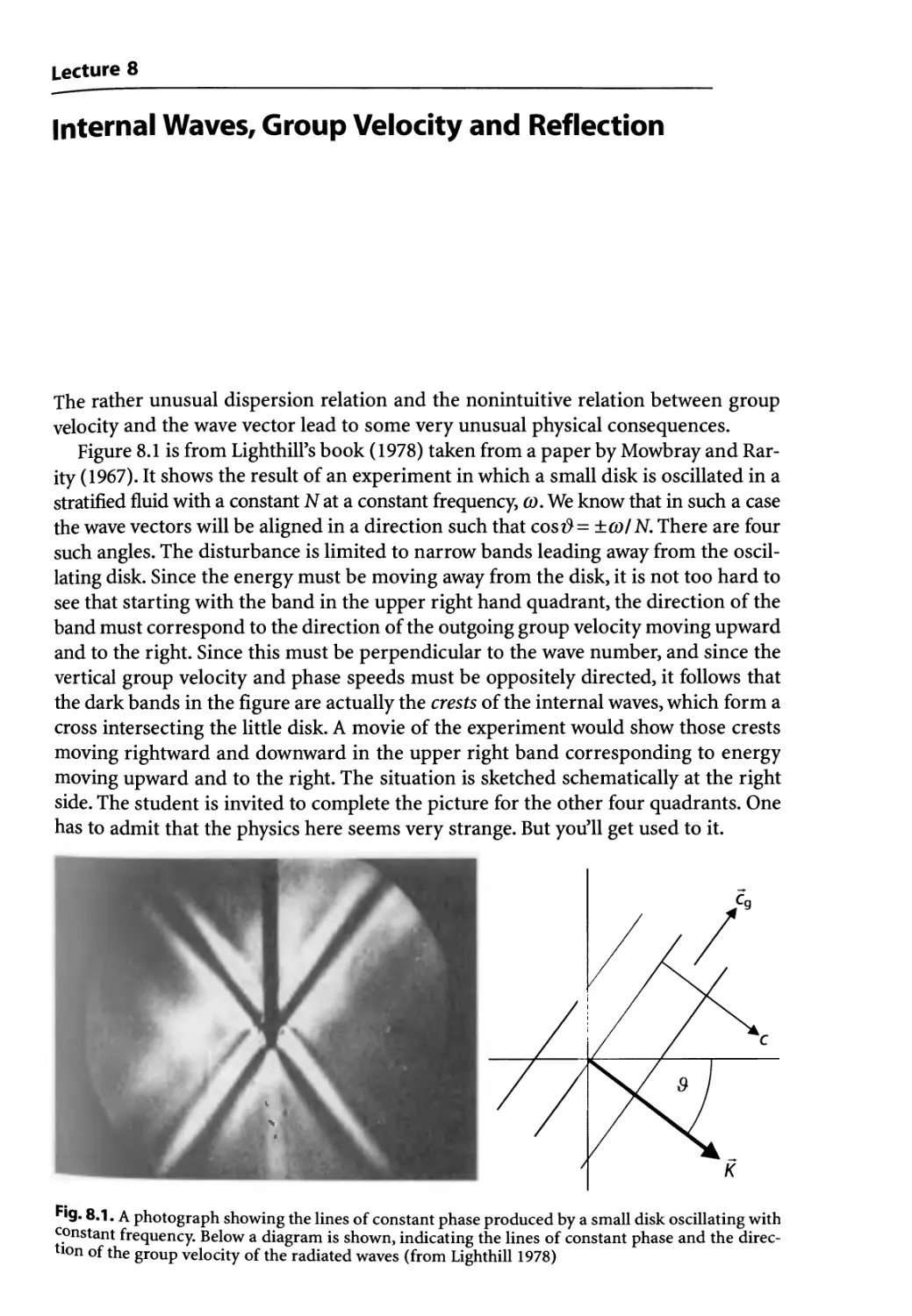
8	Internal Waves, Group Velocity and Reflection 	67
9	WKB Theory for Internal Gravity Waves	75
Normal Modes (Free Oscillations) 	79
10	Vertical Propagation of Waves:
Steady Flow and the Radiation Condition 	91
11	Rotation and Potential Vorticity	107
12	Large-Scale Hydrostatic Motions 	 119
Potential Vorticity: Layer Model 	 120
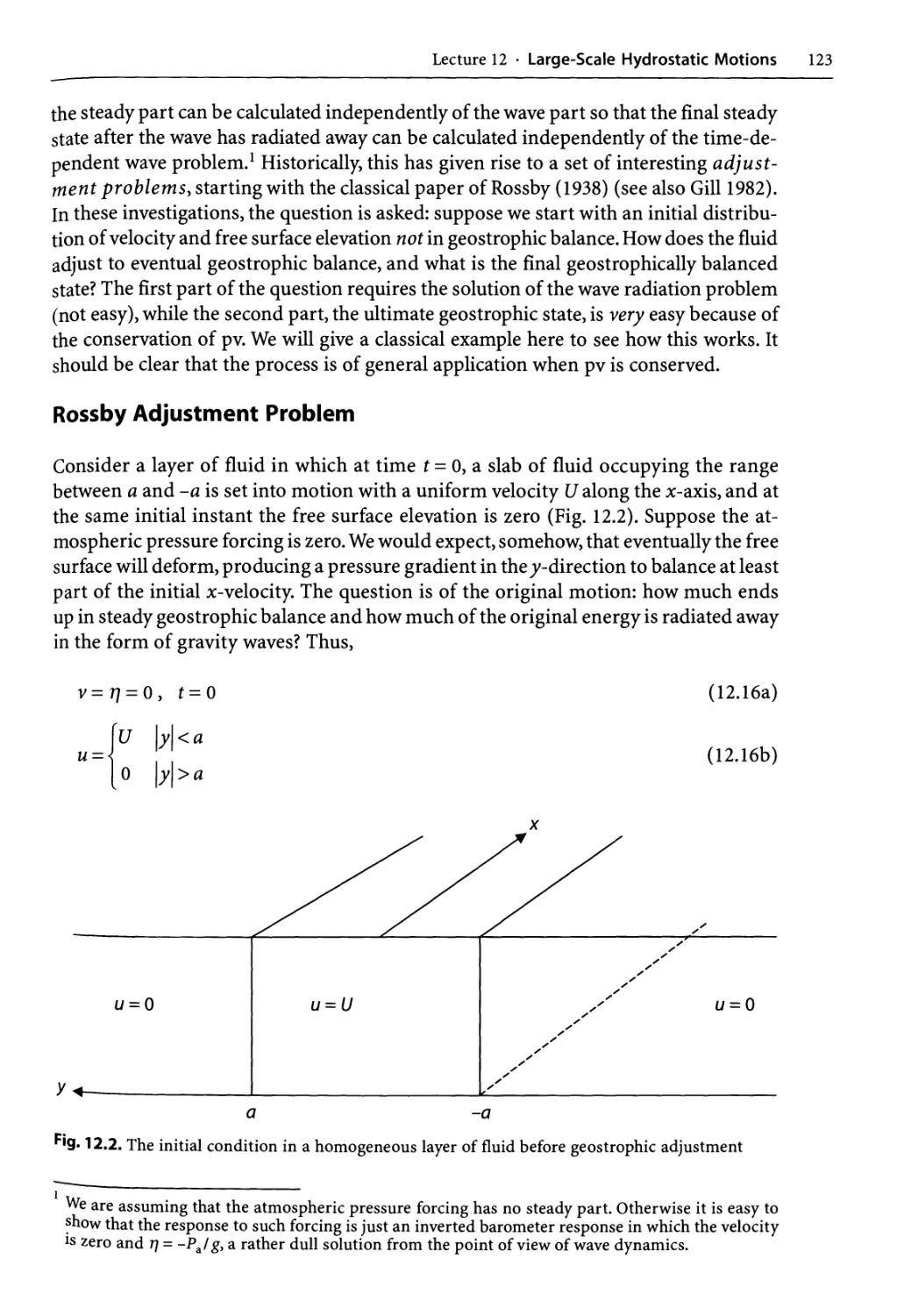
Rossby Adjustment Problem 	 123
Energy 	 129

VIII Contents
13	Shallow Water Waves in a Rotating Fluid;
Poincare and Kelvin Waves 	 133
Channel Modes and the Kelvin Wave	 136
The Kelvin Mode 	 142
14	Rossby Waves	 149
15	Rossby Waves (Continued), Quasi-Geostrophy 	 159
Quasi-Geostrophic Rossby Waves	 169
16	Energy and Energy Flux in Rossby Waves	 173
The Energy Propagation Diagram 	 175
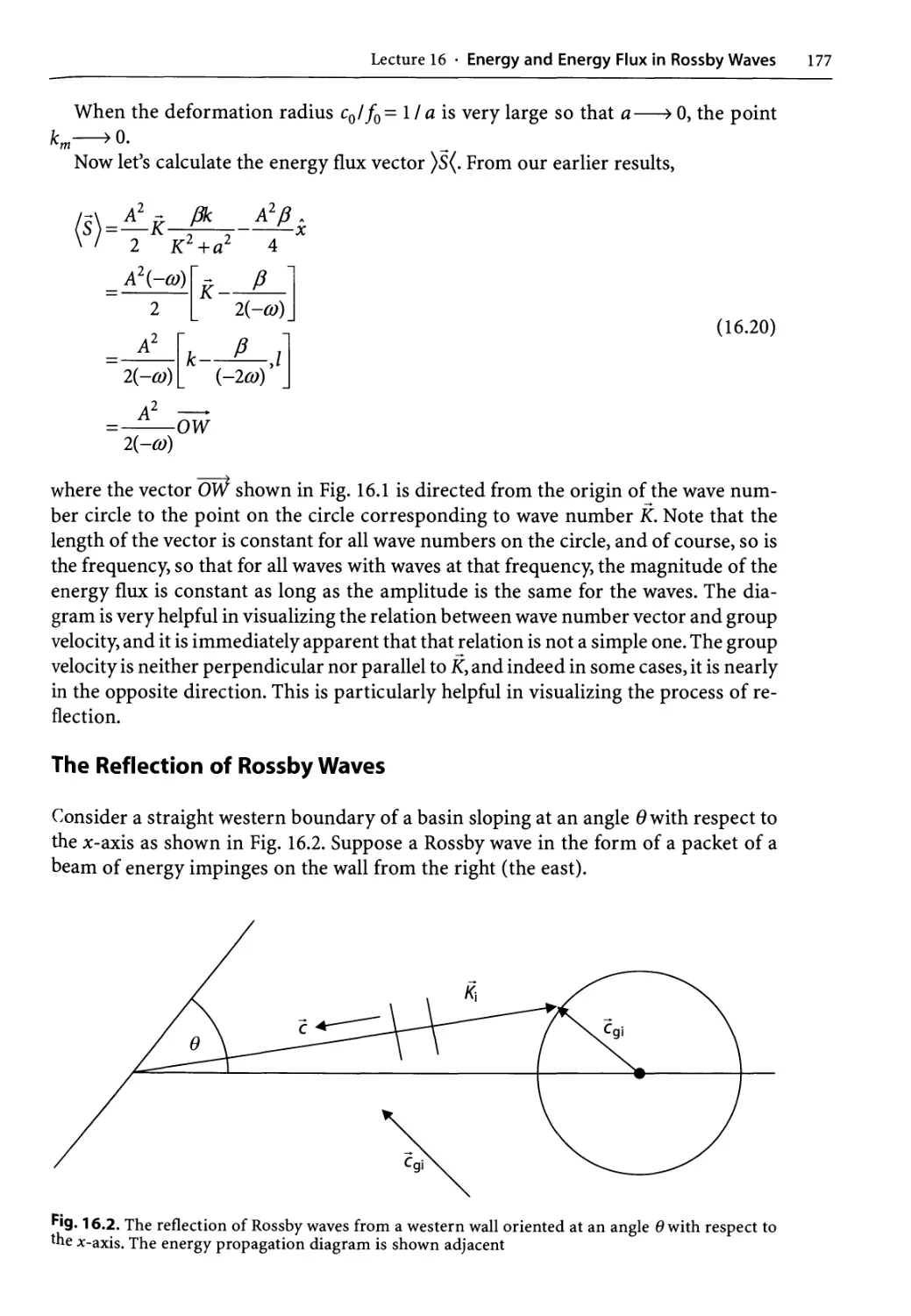
The Reflection of Rossby Waves	 177
The Spin-Down of Rossby Waves 	 180
17	Laplace Tidal Equations and the Vertical Structure Equation 	 183
18	Equatorial Beta-Plane and Equatorial Waves 	 193
The Equatorial Beta-Plane 	 194
19	Stratified Quasi-Geostrophic Motion and Instability Waves		205
Topographic Waves in a Stratified Fluid 		208
Waves in the Presence of a Mean Flow 		209
Boundary Waves in a Stratified Fluid 		211
Baroclinic Instability and the Eady Model 		213
20	Energy Equation and Necessary Conditions for Instability 	 221
General Conditions for Instability	 227
21	Wave-Mean Flow Interaction	231
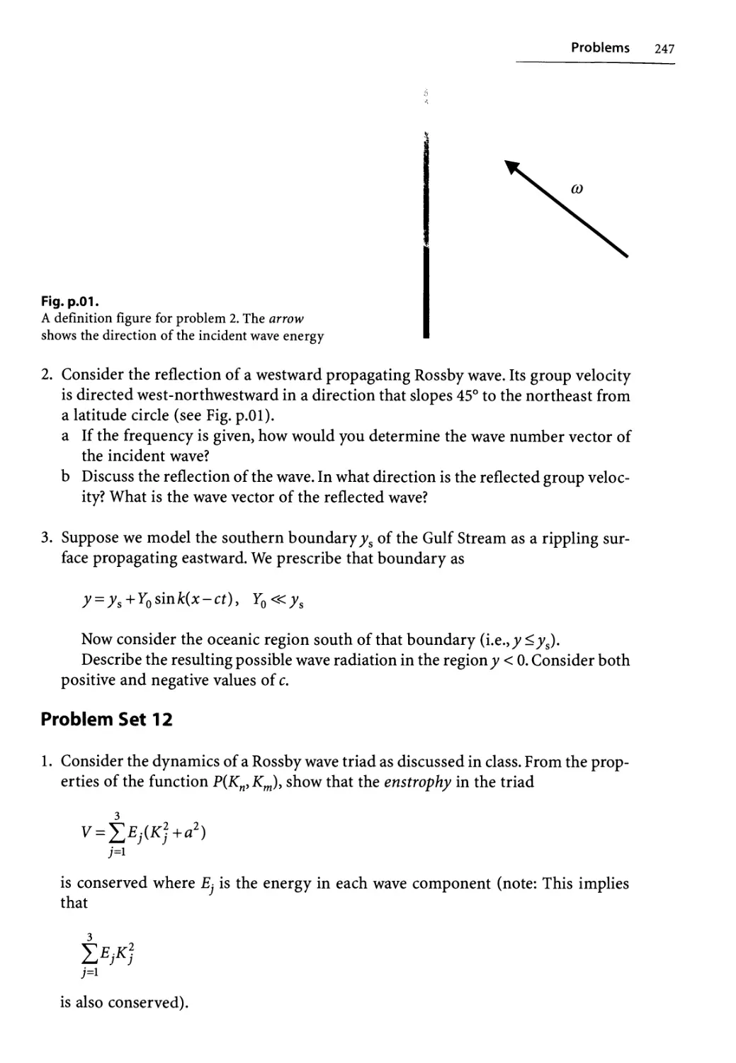
Problems 	 239
References 	 249
Index	 253

Lecture 1
Introduction
A course on wave motions for oceanographers and meteorologists has (at least) two
purposes.
The first is to discuss the important types of waves that occur in the atmosphere
and oceans, in order to understand their properties, behavior, and how to include them
in our overall picture of the ocean and atmosphere. There are a large number of such
waves, each with different physics, and it will be impossible to discuss all of them ex-
exhaustively.
At the same time, a second purpose of the course is to develop the theory and con-
concepts of waves themselves. What are waves? What does it mean for a wave to move?
What does the wave do to the medium in which it propagates, and vice-versa? How do
waves (if they do) interact with one another? How do they arise? All of these are good
and fundamental questions.
In order to deal with both of these goals, the course will describe a series of differ-
different waves and use each wave type to describe a different aspect of basic wave theory.
It will then be up to you to form the necessary connections and generalize the ideas to
all waves, at least on a heuristic basis. This will require you to sometimes retroactively
apply some new ideas developed in the discussion of wave type B, for example, back
to the application of wave type A discussed previously in the course.
In general, the physical ingredients will be stratification and rotation. But first, what
is a wave?
There is no definition of a wave that is simple and general enough to be useful, but
in a rough way we can think of a wave as:
A moving signal, typically moving at a rate distinct from the motion of the
medium.
A good example is the "wave" in a sports stadium. The pattern of the wave moves
rapidly around the park. The signal consists in the cooperative motion of individuals.
The signal moves a much greater distance than the motion of any individual. In fact,
while each person moves only up and down, the signal moves laterally (until it gets to
the costly box seats where it frequently dissipates).
Similarly in a fluid whose signal could be an acoustic pressure pulse, the surface
elevation of the ocean in a gravity wave, the rippling of the 500 mb surface in the tro-
troposphere due to a cyclone wave, or the distortion of the deep isopycnals in the ther-

Lecture 1 • Introduction
modine due to internal gravity waves, the wave moves faster and further than the in-
individual fluid elements. Thus, usually if
¦	u = the characteristic velocity of the fluid element in the wave, and
¦	c = the signal speed of the wave,
-«1	A.1)
c
We shall see that this is also equivalent to the condition for the linearization of the
mathematical description of the wave physics.
Wave Kinematics
Before discussing wave physics, it is useful to establish some basic ideas and notational
definitions about the kinematics of waves. A more complete discussion can be found
in the excellent texts by Lighthill A975) and Whitham A974).
For simple systems and for small amplitude waves (i.e., when we linearize) we of-
often can find solutions to the equations of motion in the form of a plane wave. This
usually requires the medium to be, at least locally on the scale of the wave, homoge-
homogeneous. If 0(xz-,O is a field variable such as pressure,
**"^	A.2)
where
¦	A - the wave amplitude (complex so it includes a constant phase factor),
¦	K = the wave vector,
¦	0) - the wave frequency, and
¦	Re implies that the real part of the following expression is taken.
We can define the variable phase of the wave 6 as
0{x,t) = K-x-ax = kixi-(ut	A.3)
where the summation convention is implied in the second form, that is,
max dim
In the simplest case, A, co and kj are constants.
This begs the question of why we should ever observe a disturbance with a single
K = K and co. To understand that we must do more work later on. But standing on a
beach and looking at the swell approaching it appears often to be the first order de-
description of the wave field and a naturally simple case.
Of course, by Fourier's theorem (look it up now) we can represent any shape by a
superposition of such plane waves.
The function 0we have considered above is constant on the surfaces (planes, hence
the name) on which 6 is constant, i.e.,
kixi-cot = constant	A.5)

Lecture 1 • Introduction
kx + ly- cot = constant
Fig. 1.1. Schematic of wave crest
0 = constant
6 = constant
Fig. 1.2. The plane wave showing the crests and
wave vector and wavelength
In two dimensions, for example, these will be the lines
K-x- cot = klxl + k2x2- cot = kx-\-ly- cot
A.6)
(We will use the notation regularly, kx = k,k2= /, k3 = m, in Cartesian coordinates).
The directions of the lines of constant phase are given by the normal to those lines
of constant 6 (Fig. 1.1, Fig. 1.2), i.e.,
or equivalently
Define
K =
K
i.e., the magnitude of the wave vector. Then
Kx = Ks
A.7)
A.8)
A.9)
A.10)
where s is the scalar distance perpendicular to the line of constant phase, for example
the crests where 0 is a maximum.
The plane wave is a spatially periodic function so that (j)(Ks) = (j)(K[s + X]) where
KX = 2k, since
eKKs)=ei(Ks+2n)
Thus,
K
A.11)

Lecture 1 • Introduction
Fig. 1.3.
The wavelength of a plane wave
Fig. 1.4.
The increase of phase in the direction of the
wave vector
is the wavelength. It is the distance along the wave vector between two points of the
same phase (Fig. 1.3).
At any fixed position, the rate of change of the phase with time is given by
dO
dt
--CO
A.12)
co is therefore the rate of decrease of phase (note: as crests arrive, moving parallel to
the wave vector K, the phase will decrease at a fixed point (see Fig. 1.4).
How long do we have to wait until the same phase appears? The shortest wait occurs
when a time T has passed such that coT= 2k. The time T is called the wave period,
and
CO
What is the speed of movement of the line of constant phase
A.13)
A.14)
Note that as t increases, s must increase to keep the phase constant (Fig. 1.5,1.6).
dOtdt co
dtjg deids K

Lecture 1 • Introduction
Fig. 1.5.
The movement with time of the
line of constant phase in the
direction of the wave vector
0(f>O)
0(t = O)
Fig. 1.6.
A plane wave in perspective view	0^o	k=-\t l = 0.022
Be sure you understand the reason for the appearance of the minus sign:
{At constant 0, d0 = 0 = Kds - codt, so that ds/ dt = col K}
We define the phase speed to be the speed of propagation of phase in the direction
of the wave vector.
phase speed: c- co/K
Note that phase speed is not a vector. For example, in two dimensions the phase
speed in the x-direction would be defined such that at fixed y,
dO=0 = kdx-codt or
CO dOldt
A.16a)
A.16b)

Lecture 1 • Introduction
Note that if the phase speed were a vector directed in the direction of K, its jc-com-
ponent would be
- : co K : *y
cz=	z =-—
K K K2
A.17)
Therefore, it is clear that the phase speed does not act like a vector, and this is a
clue that this speed, by which the pattern of the wave propagates, may have less physi-
physical meaning that we would intuitively want to give to it.
Note that cx is the speed with which the intersection of the moving phase line with
the jc-axis moves along the jc-axis (Fig. 1.7):
cY=-
cosa
and as a goes to 7i/2, cx becomes infinitely large! This makes us suspicious that the
phase may not be the messenger of physical entities like momentum and energy.
In an interval length 5 perpendicular to the surface of constant phase, the increase
in phase divided by 2n gives us the number of crests in the interval. Thus, Fig. 1.8.
Fig. 1.7.
The small arrow shows the intersection point of
the line of constant phase and the x-axis
/CS/2tt = # of crests
0 5 10 15 20 25
Fig. 1.8. A plane wave and the number of crests along the coordinate s
35

Lecture 1 • Introduction 7
Thus also, the increase in phase along the wave vector is
\^\	A.18)
A0\^ds
J ds
The more fundamental definitions have already been given; namely,
K=V0	A.19a)
co = -d4~	A.19b)
dt
The former gives the spatial increase of phase, while the latter gives the temporal
(decrease) of phase.
In all physical wave problems, the dynamics will impose, as we shall see, a relation
between the wave vector and the frequency. This relation is called the dispersion
relation (for reasons that will be made more clear later). The form of the dispersion
relation can be written as:
O) = G(k})	A.20)
Note that each wave vector has its own frequency. Often the frequency depends only
on the magnitude of the wave vector, K, rather than its orientation, but this is not al-
always the case. Up to now, the wave vector, the frequency, the phase speed and the dis-
dispersion relation have all been considered constants, i.e., independent of space and time.

Lecture 2
Kinematic Generalization
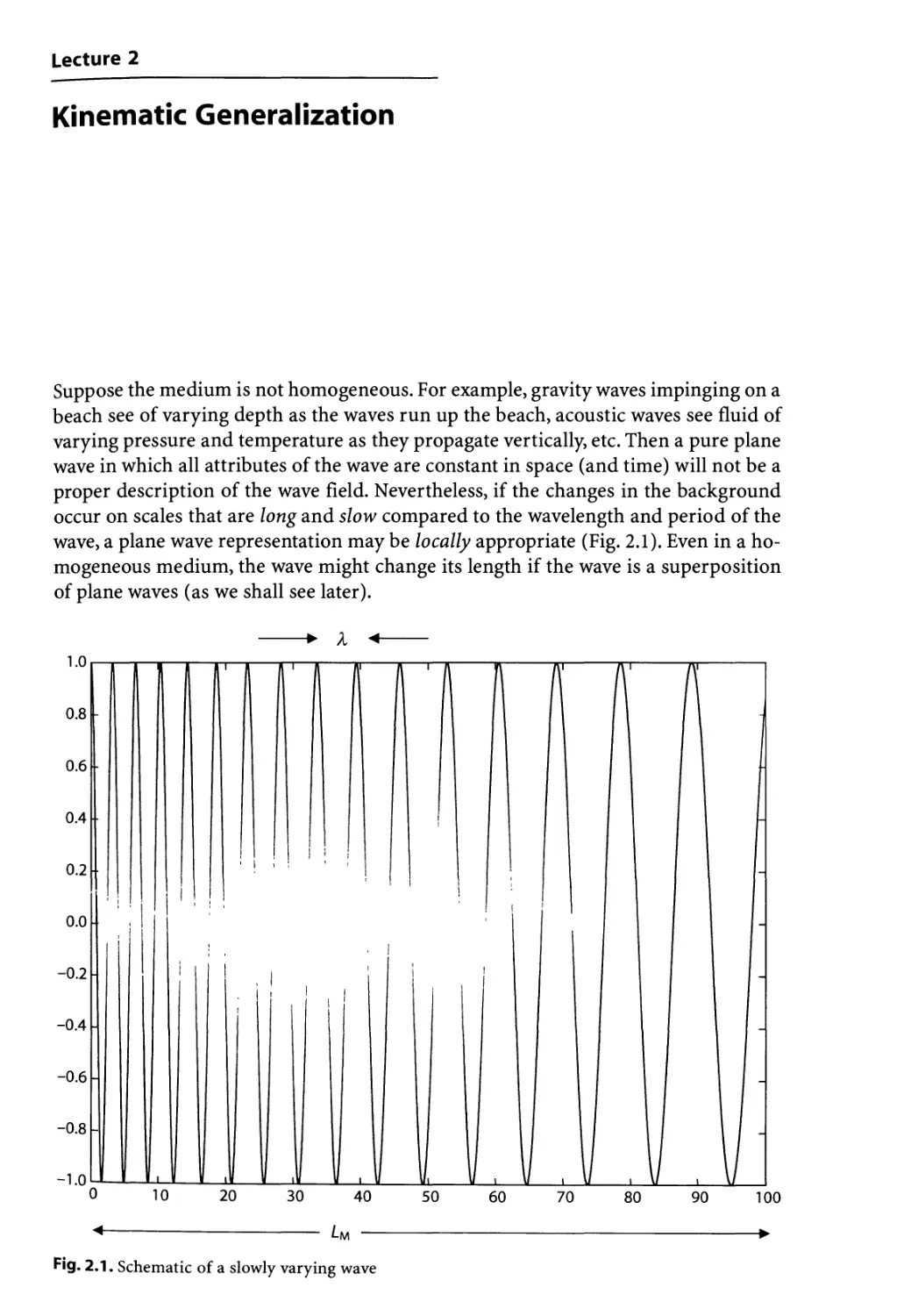
Suppose the medium is not homogeneous. For example, gravity waves impinging on a
beach see of varying depth as the waves run up the beach, acoustic waves see fluid of
varying pressure and temperature as they propagate vertically, etc. Then a pure plane
wave in which all attributes of the wave are constant in space (and time) will not be a
proper description of the wave field. Nevertheless, if the changes in the background
occur on scales that are long and slow compared to the wavelength and period of the
wave, a plane wave representation may be locally appropriate (Fig. 2.1). Even in a ho-
homogeneous medium, the wave might change its length if the wave is a superposition
of plane waves (as we shall see later).
1.0
0.8
0.6
0.4
0.2
o.o
-0.2
-0.4
-0.6
-0.8
-1.0
¦ V W i
0	10 20 30 40 50 60
	 LM
70
80
90
100
Fig. 2.1. Schematic of a slowly varying wave

10 Lecture 2 • Kinematic Generalization
Thus, locally the wave can still look like a plane wave if XILM <$c 1. In that case, we
might expect the wave to be described by the form:
0Cc,f) = A(x,OeI0(x>f) (the real part of the expression is taken for granted), B.1)
where A varies on the scale LM while the phase varies on the scale X. Thus,
1 dA J l ¦	B.2a)
dXj
so that
V</>=Ae'eV0+O —
We define (guided by our experience with the plane wave):
K=W6 local spatial increase of phase
-co = — local increase of phase with time
ot
B.2b)
B.3)
B.4a)
B.4b)
Since the wave vector is defined as the gradient of the scalar phase, it follows auto-
automatically that V x K = 0.
Consider the increase of phase on the curve Cx from point A to point B in Fig. 2.2:
1 B	1
nr =— \k-dx = — \kdx
B.5)
Fig. 2.2.
Counting crests on two paths
AC^ and AC2B
0 = constant

Lecture 2 • Kinematic Generalization
11
Now consider the same increase calculated on curve C2:
i B	i
if— — i f — —
nc -— \K'dx = — iC-dx
2tc jj	2ti CJ
The difference between them is
B.6)
"Cl
_„ = _L f-
Cl In I
2nrJ
^ total
B.7)
A
0
Here we have used Stokes theorem relating the line integral of the tangent compo-
component of K with the area integral of its curl over the area bounded by the closed con-
contour composed of the sum of the two curves Cj and C2. Since the curl is zero, the two
calculations for the increase of phase must be independent of the curve used to do the
calculation.
Note that since
K=V0
B.8a)
co = —
dt
it follows by definition that
B.8b)
dt
B.9)
in those cases where the wave vector and the wave frequency are slowly varying
functions of space and time (i.e., where it is sensible to define wavelength and frequency).
To better understand the consequences of the above equation, consider the fixed
line element AB in Fig. 2.3.
Fig. 2.3.
Conservation of crests along
the line AB

12 Lecture 2 • Kinematic Generalization
Integrate the above conservation equation along the line element from A to B:
3 B B
fjic-dx
B.10)
Using our previous definitions, in particular that Ks 12n is the number of crests in
the interval s, it follows from the above that
B.11)
dnAB _ co(A)
dt 271 271
That is to say, the rate of change of the number of crests in the interval (A,B) is equal
to the rate of inflow of crests at point A minus the outflow of crests at point B, since
the frequency (divided by 2ri) is equal to the number of crests crossing a point at each
moment. E.g.,
co(A) = rate of decrease of phase at point A (see Fig. 2.4)
Phase increasing in space
0	123456789	10
Fig. 2.4. The movement of the phase through the interval AB

Lecture 2 • Kinematic Generalization 13
We may think of this as a statement of the conservation of wave crests. Namely,
the number of wave crests in a smoothly varying function 0 as given above does not
change. The number in any local region increases or decreases solely due to the ar-
arrival of preexisting crests, not to the creation or destruction of existing crests.
Now, let's suppose that we still have a local dispersion relation between frequency
and wave number but that the relationship slowly changes on scales that are long com-
compared with a wavelength or period due to changes, perhaps, in the nature of the me-
medium in which the wave is embedded.
In that case, the natural generalization of the dispersion relation is
co=Q(kj,xi,t)	B.12)
where the wave vector components and the frequency may themselves be functions
of space and time (slowly), and the dispersion relation is explicitly dependent on space
and time.
Thus,
^ = — +^11^.	B.13)
dt dt Jg - dkj dt
where the first term on the right-hand side is due to the explicit dependence of the
dispersion relation on time, as might happen if the temperature of a region through
which an acoustic wave were traveling were increasing with time.
We define the group velocity by the formula for each of its Cartesian components:
for the component of the group velocity in the/h direction, or
cz = VEQ	B.15)
It follows from a fundamental theorem in vector analysis that since the phase
is a scalar and the gradient operator is a vector, the group velocity is a true vector
(distinct from the phase speed). That is, it follows the law of vector decomposi-
decomposition.
Since, by our earlier definitions
B.16)
do)
T-	B.17)
OKj
IT
we thus
dco
~dt~~
do)
j
obtain
dn
~~ dt

14 Lecture 2 • Kinematic Generalization
It therefore follows that
	+ co - Vco =	<= explicit derivative with time	B.18)
dt 8	dt
Again, by similarly using
it follows that
dk{ dn dn dk{
—L+	+	1- = 0 or	B.19a)
dt dxi dkj dXj
^+3?3^_3?	Bj9b)
dt dkj dXj dxi
Since the wave vector has no curl, it follows that
so the above equation can be rewritten:
dK	-
— + (cg * V)K = -Vi2 <= explicit dependence on space	B.20)
Note that the sum of derivatives on the left in the equations for the rate of change
of wave vector and frequency are the rate of change for an observer moving with the
group velocity.
So,
1.	If the medium is independent of time,	> @ propagates with the group velocity;
2.	If the medium is independent of space,	> K propagates with the group velocity.
If both (i) and B) are true, both frequency and wave number propagate with the
group velocity:
dn
This is a vector, and we see here that real wave attributes propagate with this velocity. If
the dispersion relation is a function of space and/or time, the above equations tell us how
the frequency and wave number change as we move with the group velocity following a
wave. Further discussion can be found in Bretherton A971) and Pedlosky A987).

Lecture 2 ¦ Kinematic Generalization 15
Example
We will soon see that free surface gravity waves (short enough so that rotation is
unimportant but long enough so that the wavelength is large) compared to the depth
have a dispersion relation:
O) = l
where His the depth of the fluid and k is the wave number for this one-dimensional
example (Fig. 2.5).
The phase speed and group velocity are equal in this case:
If the depth is a function of x, then following a signal, since the dispersion rela-
relation is independent of time, the frequency will be constant for an observer moving
with the velocity cg= c = (gH)m. For such an observer, with frequency constant,
k = const. / H1/2> which implies that the wave will grow shorter (larger k) as the wave
enters shallow water. (It may become so short that it might break). Note that the
observer, following a particular frequency moving with the group speed will pro-
proceed at a rate:
^W))	B.22)
at
For example, if H(x) is of the form H = H0(l - xl xQ) where x is measured posi-
positive shoreward from some offshore position a distance x0 from the waterline (see
Fig. 2.5), the signal corresponding to a given frequency will proceed onshore such
that at a point x after an elapsed time t, the relationship between the elapsed time
and its onshore progress is
t = 2xo(l-Jl-xIxo)/(gHo)m	B.23)
Fig. 2.5.
Water wave running up a
sloped beach
x Zq	x = Xq
The above kinematic discussion doesn't tell us how the amplitude of the wave propa-
propagates or, equivalently, how the energy in the wave moves. In some simple cases that
are general enough to be of interest, we can actually describe how the amplitude and
hence energy moves.

16 Lecture 2 • Kinematic Generalization
Consider the case of a homogeneous medium in which the governing equation for
the wave function 0 is of the form
B.24)
where II is a polynomial in the partial derivatives with respect to space and time. A
simple example would be the Rossby wave equation:
B.25)
dx2dt dy2dt
so that in this case,
dx{dx) dy\dy
i.e., the polynomial in the partial derivatives are in respect of x,y and t.
Suppose we look for an approximate solution of the form
jo
20 40 60 80 100 120 140 160 180 200
-0.1 -
-0.2
-0.3
-0.4
Fig. 2.6. A wave packet. The wave has wavelength A while its envelope has a scale LN

Lecture 2 • Kinematic Generalization 17
where A, k and co are slowly varying functions of time, i.e., where the solution has the
form of a one-dimensional wave packet (see Fig. 2.6), then
B.26)
dx I
or
i*+^ |A 0	B.27)
dt dxj
Expanding the polynomial using the fact that the time and space derivatives of A
are small compared to co and k,
M^lELfU	,2.28,
The dispersion relation for plane waves comes from the disappearance of the first
term (which is the dominant one), namely
H(-iCQ, ik) - 0	> Linear dispersion relation	B.29)
In the case above, this yields co = -fi/k.
When this dispersion relation is satisfied, the remaining term yields the condition:
o
dt dWdcodx
where the derivatives of IT in the equation occur when FI is evaluated as a function of
frequency and wave number as in Eq. 2.29.
Since
. da,)
~ )
it follows that
dA dA
( '
B'32)
Thus, the amplitude (and we can suppose) energy will propagate with the group
velocity and not the phase speed. Where the envelope (that is A) of the wave goes,
that is where the energy is. There is clearly no energy outside the wave envelope.

18 Lecture 2 • Kinematic Generalization
The reader should calculate the group velocity for this simple case of one-dimensi-
one-dimensional Rossby waves to see that the group and phase velocities are not the same. Similarly,
the argument presented here can be extended to any number of dimensions (try it).
It is also clear that one might be able to use similar ideas for inhomogeneous media.
Once again we see here the physical primacy of the group velocity over the phase
speed for the propagation of physical attributes of the wave.

Lecture 3
Equations of Motion; Surface Gravity Waves
For a rotating stratified fluid, the general equations of motion can be written as:
1.	Momentum equation:
p — + 2Qx u = -Vp+/N2u + *V(V • u) (if ji constant, kis second viscosity) C.1)
\_dt	J
2.	Mass conservation:
^) = 0 ;and	C.2)
+
dt
3. Thermodynamic energy equation:
dt
where s is specific entropy and H is the nonreversible heat addition. This can be re-
rewritten, assuming that s is a thermodynamic function of p and p,
dr_«rdp=<p+_«Lv2r+ 2s^	C3)
F dt p dt p
Here, T is temperature, cp is the specific heat at constant pressure, a is the coeffi-
coefficient of thermal expansion, and 0 is the dissipation function, i.e., the frictional trans-
transformation of mechanical to thermal energy. If T^ is the stress tensor and e^ is the rate
of the strain tensor, 0 = r^e^ (sums implied). Note that
For a perfect gas with a state equation p = pRT, the thermodynamic equation is
usually written in terms of the potential temperature:

20 Lecture 3 • Equations of Motion; Surface Gravity Waves
so that the thermodynamic equation becomes
1 dO H
e?7	C-5)
while for an incompressible liquid we can approximate the thermodynamic equation with
it cp
Here we have used the approximate state equation p = po(l - a(T- To)) to relate
temperature in the thermodynamic equation to density. Be sure to note that when we
make the approximation of incompressibility in the mass equation (V • u ~ O),this does
not imply that dp/ dt = 0 is the governing equation for density. Only if the dissipation H
can be neglected will that be true. That is a separate physical statement about the adia-
batic nature of the motion quite apart from the issue of compressibility. For a com-
compressible fluid, we would have, instead of dpi dt = 0, the statement dsl dt = 0. For a
detailed discussion of the formulation of these equations, especially the thermody-
thermodynamics, see Batchelor A967).
First Wave Example: Surface Gravity Waves
Perhaps the most familiar of waves in the ocean are the waves we see on the surface, either
from a ship or from the beach (or from the air). These are waves on the interface between
the water and the air (Fig. 3.1). The latter is so light compared with the former that we will
approximate the air as having zero density to eliminate any dynamical interaction with
the air to begin with. Theories of wave generation must include that coupling.
Consider a layer of liquid of uniform density and uniform depth. We suppose the
scale of the motion is small enough to be able to ignore the Earth's rotation and the
motion is small enough to be able to linearize this motion. In all such cases, we need
to ask ourselves whether these statements are sensible, and if so, for what range of
parameters? That is, if we ignore rotation, is there a limit, for example on the size of
the wave for which that is appropriate? We might already know, for example, that the
tides, which are a gravity wave response to the sun and the moon, do feel the effects of
the Earth's rotation, but, of course, they are of planetary scale.
1. Can we ignore rotation, friction and nonlinearity?
-	To ignore rotation, compare d/dt with Q	> this implies that we need co » Q.
-	To ignore friction, compare d/dt with /iA:2,where A: is a typical value of wave-
number—> cay> jik2.
Fig. 3.1.
The homogeneous layer of	constant
fluid supporting surface
gravity waves	^_^^____.^__-__
D

Lecture 3 • Equations of Motion; Surface Gravity Waves 21
- To ignore nonlinearity, compare d/dt with respect to ii • V	> co » uk or c » u <=:
this is the condition that the disturbance be wave-like, i.e., that the signal is
carried by the wave rather than the advective motion of the fluid.
2. Can we treat the fluid as incompressible?
Assume we can linearize. Suppose the motion is adiabatic. In general then, we
have
^• = 0, s = s{p,p)	C.7)
at
with the linearization
*=0=*&+*&.	C.8)
dt dp dt dp dt
Thus,
dp _ ds/dp dp _( dp] dp
C.9)
dt ds/dp dt {dp)sdt
From the theory of acoustics we know (or we can easily find out) that the speed of
sound in any medium is in fact given by the adiabatic compressibility of the medium.
That implies that if ca is the speed of sound in a fluid,
(One of the few scientific mistakes Newton made was to imagine that the speed of
sound was this derivative at constant temperature and not entropy).
So we have the estimate for the relation between a perturbation in the density and
the perturbation of the pressure:
Sp = clSp	C.10)
We can, on the other hand, estimate the magnitude of the pressure fluctuation from
the horizontal momentum equation; if
~^j then
from which it follows from the relation between the pressure and density disturbances:
Hz)

22 Lecture 3 • Equations of Motion; Surface Gravity Waves
Thus,
1 dSp _ | UOJ
~~p~lH~ [c*k
We should compare this term, which is the estimate of the size of the local time
derivative in the mass conservation equation with a typical term in the remaining
combination of terms, namely, V • u = O(ku). Their ratio is thus
dSp
V-5
Thus, as long as the phase speed of the wave is small compared to the speed of sound,
we can approximate the wave motion occurring as in an incompressible fluid for
which the equation for mass conservation reduces to the condition
V-m = 0	C.13)
Note again that this does not by itself imply that dp/ dt = 0. A separate consider-
consideration of the thermodynamics and the strength of the dissipation is required for that.
We now have a series of parameter tests we can make after the fact to check to see
whether the approximations of
1.	linear motion
2.	inviscid motion
3.	incompressible motion
4.	nonrotating dynamics
will be valid.
Assuming that these conditions will be met by the waves under consideration here,
the equations of motion reduce to the much simpler set:
p^-=-Vp-pgz	C.14a)
dt
V-m = 0	C.14b)
where z is a unit vector in the direction antiparallel to the direction of the local gravi-
gravitation.
We could have just waved our hands (perhaps appropriately for a course on waves)
and written down these traditional approximate equations. However, it is impor-
important for each new investigation of a wave type to carefully consider a priori the condi-
conditions required to achieve the approximate dynamics used for the physical description
of the wave to make sure that our physical system is no more complicated than
it need be, while at the same time, it should be consistent with the underlying physics
of the fluid.

Lecture 3 • Equations of Motion; Surface Gravity Waves 23
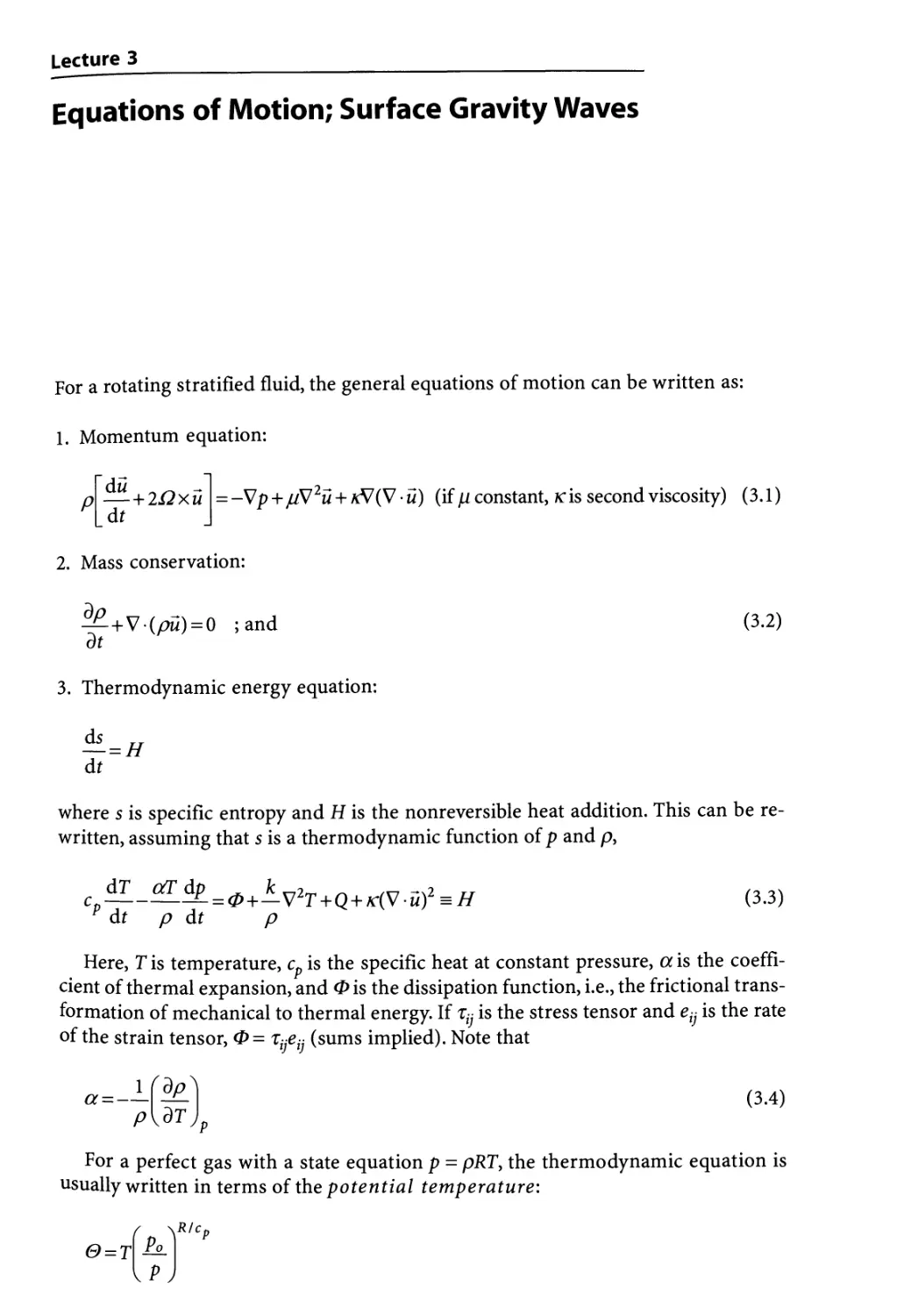
The curl of our momentum equation (recall that we are considering a fluid of con-
constant density; the student is invited to use the thermodynamic equation to find the
condition for the validity of that approximation) yields
0	C.15)
dt
So, if the vorticity is zero initially or at any instant (as it would be for an oscillatory
motion for which each field goes through zero periodically), it follows that it remains
zero for all time. If the curl of the velocity is zero, it follows from a fundamental fact
of vector calculus that the velocity can be represented by a velocity potential, 0,
w = V0	C.16)
Note that only the spatial gradients of the velocity potential carry physical infor-
information. Any arbitrary function of time can be added to 0 without changing the veloc-
velocity field.
Since the motion is incompressible,
V.w = V-(V0)=V20 = O	C.17)
The equation of motion within the fluid thus reduces to the elliptic problem gov-
governed by Laplace's equation:
V20 = O	C.18)
This is an amazing simplification, and it should be a little disconcerting, because
we are looking to describe a wave motion. Laplace's equation, by itself, is certainly not
a wave equation. It describes among other things the electrical potential of static
charges as well as certain static gravitational fields but, alone, no dynamical wave
mechanism. The resolution of this seeming paradox is of course connected to the fact
that we have not yet considered the boundary conditions for our problem. There is no
more illuminating example of the importance of boundary conditions in the specifi-
specification of the problem than this case of surface gravity waves. All the dynamics are in
the boundary conditions. The internal equation, i.e., Laplace's equation merely relates
the horizontal and vertical structure of the motion field.
Boundary Conditions
The obvious boundary condition at the lower horizontal surface is that the normal
velocity vanishes there, i.e., w = 0 at z = -D, or
^- = 0, z = -D	C.19)
The boundary conditions at the upper surface are significantly more interesting. Let's
call the departure of the free surface from its level "rest position" 77 (*,;>, t) (Fig. 3.2),

24 Lecture 3 • Equations of Motion; Surface Gravity Waves
z = r\{x,y,t)
P = Paix.y.t)
Fig. 3.2.
A definition figure for variables
describing the motion in the
surface gravity wave
which must be small (this will presently be made more explicit). Thus, we consider
the rippled free surface to only be slightly in departure from its rest state.
At the free surface, the physical boundary conditions are
1. the dynamic condition:
x,y&t) = p&(x,y,t) z=r\
C.20)
and
2. the kinematic condition:
_d(/> _dr/ dr/
dz dt dt
C.21a)
or
dn
C.21b)
We must now write these conditions completely in terms of the velocity potential, 0.
The linearized momentum equation is
du dVd Vp _
— = —— = ——-qS/z
dt dt p 6
or
C.22a)
C.22b)
The integral of the last equation implies that
C.23)
where F(t) is an arbitrary function only of time. We can always add a function that is
only of time to the velocity potential without changing the physical meaning of that
potential. Let's imagine that we have added such an additional term such that its de-
derivative with respect to time is equal to F(t). This allows us to write this linearized form
of Bernoulli's equation everywhere in the fluid in the form:

Lecture 3 • Equations of Motion; Surface Gravity Waves 25
g 0	C.24)
dt p
Now let's apply this equation to the upper surface where z = T](x,y,t) andp = pa(x,y,t).
Thus,
g] o	C.25)
dt p
A derivative of this equation with respect to time yields, using the kinematic con-
condition on the upper surface,
dt2 dz p dt
Note that each term in this boundary condition is linear.
The condition is applied at the unknown location z = t]. Indeed, the position of the
free surface is, after all, one of the principal unknowns of the problem that we are try-
trying to predict. For the general nonlinear problem, this unknown location of the bound-
boundary, at which the important boundary conditions are applied, is one of the most diffi-
difficult aspects of the problem. However, we are considering only the linear small ampli-
amplitude problem, and it turns out that we can apply the boundary condition at the original
position of the interface, i.e., at z = 0. To see this take any term on the left-hand side of
the above boundary condition, generically call it G(x,jv,r]) and expand it around r\ = 0.
Thus,
r)C
+ higher order terms	C.27)
z=0
The first term on the right-hand side of the above equation is of the order of the
amplitude of the motion, since G is one of the dynamic variables. Note that all the
dynamical variables are linear in the size of the amplitude of the motion.
The second term is of the order of G times the free surface height and is therefore
of the order of the amplitude squared. To be consistent with our linearization, such
quadratic terms must be neglected. That implies that each term in the boundary con-
condition stated above can be applied at z = 0; thus, we have
d <p d0 1 dpa
TT+?^r- =	—> at z = 0	C.28)
dt oz p dt
as the boundary condition on the upper surface, while again at the lower surface,
d<p
-^- = 0, z = -D	C.29)
Note that the upper boundary condition contains two time derivatives. This is the
mathematical source of the wave motion we will be describing. Its physical source is

26 Lecture 3 • Equations of Motion; Surface Gravity Waves
the interplay between the gravitational force at the upper boundary providing a re-
restoring force and the relation between the free surface elevation and the vertical ve-
velocity at the upper surface.
We must also specify boundary conditions on the lateral boundaries. The simplest
problem we will consider will be that of a wave in an infinitely broad layer of fluid.
This is clearly an approximation, and we imagine that such a description will be valid
until the waves to be found propagate and interact with the inevitable lateral bound-
boundaries of the fluid. Until that time, we may provisionally just insist that the solutions
remain finite as x and/ go to infinity. Useful references for formulation of the gravity
wave problem can be found in Kundu A990), Lamb A945) and Stoker A957).
Plane Wave Solutions for Surface Gravity Waves: Free Waves (pa = 0)
In Cartesian coordinates, Laplace's equation can be written as
(,30,
We clearly can't have a f/zree-dimensional plane wave because
1. the operator (the Laplacian) won't allow it, since an attempt to find such a plane
wave would lead to the condition
=
C.31)
which is impossible if all three components of the wave vector are real;
2.	a plane wave won't satisfy the boundary condition 30/ dz = 0 at z = -D;
3.	the boundary conditions of finiteness as x and/ get large imply that the horizontal
components of the wave number are real, and thus the vertical component, k3 or m,
must be purely imaginary.
We can find solutions, however, that are periodic in x,y, and t of the form
^^y-^	C.32)
where again, the real part of the above equation is meant. Substitution into Laplace's
equation yields the ordinary differential equation for R(z),
d2R
—r—K2R = 0	C.33a)
dz
K2=k2+l2	C.33b)
Note that all Laplace's equation will do is determine the structure with depth of
the plane wave solution in x and/.
The solution for R that satisfies the kinematic boundary condition at z = -D, i.e.,
that dR I dz = 0, is

Lecture 3 • Equations of Motion; Surface Gravity Waves 27
R = AcoshK(z + D)	C.34)
When this form is substituted into the boundary condition at z = 0, we obtain as a
condition for a nonzero solution for A
-a?cosh (KD) + gKsinh (KD) = 0	C.35)
or
O) = ±ijgKteinhKD	C.36)
and
There are several important things to note about these results.
1.	For each wave vector amplitude K, there are two waves propagating in opposite
directions, parallel and antiparallel to the wave vector. The frequency and phase
speed depend only on the wavelength, i.e., K and not on the orientation of the wave
vector.
2.	The phase speed is different for different wavelengths in distinction to light waves
or sound waves. A pattern made out of a superposition of plane waves of different
wavelengths will have each component move at a different speed and hence the
pattern will disperse, which is why the relation between frequency and wave num-
number is called the dispersion relation.
3.	There are some important limiting cases to consider.
The maximum phase speed occurs when the wavelength (inverse to K) is long com-
compared to the depth, i.e., when KD <K 1. Then the phase speed approaches (gD)m and is
independent of wavelength in that limit. In that case, when the phase speed is inde-
independent of wavelength, the wave is called nondispersive. In that long wave limit or
for shallow water waves, co=K(gD)m.
On the other hand, when the wavelength is short compared with the depth, i.e., when
KD » l, the dispersion relation becomes independent of depth and CO = (gK)m, while
c = (g/K)m. These deepwater waves are clearly dispersive. We will have to investi-
investigate why the frequency and phase speed become independent of D in this limit.
Now that we have the phase speed, we can check our assumption of incompress-
ibility, that is, is c « ca. Since the maximum phase speed is given by the shallow water
limit for that condition, it will be satisfied if
or
D«c2Jg

28 Lecture 3 • Equations of Motion; Surface Gravity Waves
For water, the sound speed is of the order of 1400 m s. That places a condition
on the depth such that for the incompressibility condition to be valid, we require
D <sc 200 km (pretty safe for oceanography, at least on Earth).
The nature of the dispersion relation is evident in Fig. 3.3 showing the frequency,
phase speed and group velocity as a function of wave number.
The dispersive nature of the waves can be contrasted to that of the standard "wave
equation" (which we will see in this course captures only a small fraction of wave phys-
physics in oceanography and meteorology). For light waves in a vacuum, sound waves and
waves on a thin string, the governing equation in one dimension is of the form
dt2 dx2
whose general solution is known to be
<p = F(x + at) + G(x - at)
C.38)
C.39)
consisting of two pulses traveling with the constant phase speeds ±a. The forms F
and G are determined by initial conditions after which the pulses travel without fur-
co,c and cg versus kD
Fig. 3.3. Curves of frequency, phase speed and group velocity for surface gravity waves

Lecture 3 • Equations of Motion; Surface Gravity Waves 29
ther change of shape. These are the classic nondispersive solutions for waves. In our
case, the waves are highly dispersive and the evolution of the wave shape with time
and unraveling the subsequent propagation of properties in the waves is a problem of
great subtlety and interest. It will eventually, as we might imagine from our earlier
discussion, come to depend on the character of the group velocity. For gravity waves,
with the dispersion relation quoted above
C.40)
Thus, since the frequency is a function only of K, the group velocity is parallel to
the wave vector and hence parallel to the direction of phase propagation.
With a? = gK tank KD,
cosh2KD
C.41a)
or
and
cosh'KD
2KD \
sin2iCDJ
C.41b)
C.41c)
Thus the group velocity coincides with the phase speed for long waves (KD «c 1),
while for short waves the group velocity is 1/2 the phase speed (see Fig. 3.4).
Fig. 3.4.
A wave packet propagating
with the group velocity carries
a plane wave with crest moving
with the phase speed

30 Lecture 3 • Equations of Motion; Surface Gravity Waves
1.0
0.9
0.8
Q 0.7 -
O
c
o
0.5 -
0.4 -
0.3 -
0.2 -¦¦
0.1
1.0
0.9 -
0.8 -
?
b gravit
1
o
(Z
0.7
0.6
0.5
0.4
0.3
0.2 -
0.1 -
0.0
5
KD
V
DI/2
a i i i i i
i
1
i

i

10
\
b
__
i j
	-
5
KD
10
Fig. 3.5. a The group velocity as a function of wave number, b The ratio of the group velocity to
phase speed for surface gravity waves as a function of wave number scaled with fluid depth, i.e., KD

Lecture 3 • Equations of Motion; Surface Gravity Waves 31
Suppose we have a wave packet carrying a short wave, KD «c 1.
The amplitude and K will move with the group velocity, while individual crests will
move with the phase speed. Since cg is half the phase speed for short waves, we will
see individual crests appearing at the rear of the packet and travelling through the
moving packet to disappear at the leading edge of the packet. Where do the crests go?
Well, they are only a feature of the pattern, and they appear and disappear like smiles.
It is the wave envelope moving with the group velocity that has physical content.
The ratio of the group velocity to the phase speed is shown in Fig. 3.5b as a func-
function of wave number. They are equal for the longest waves, while for short waves the
group velocity is half the phase speed.

Lecture 4
Fields of Motion in Gravity Waves and Energy
Now that we have the dispersion relation, i.e., the dependence of frequency on wave
number (we define the magnitude, K, of the wave vector K to be the wave number),
we can ask what the fluid motion is in the wave field.
Our plane wave solution has been written in the form:
0 =AeiiR*-°)t) cosh K(z + D)	D.1)
Using the boundary condition at z = 0,
g?? = -d?z = 0	D.2)
ot
since pa has been taken to be zero for these free waves. We can therefore calculate the
free surface elevation from Eq. 4.1 and Eq. 4.2,
J
and it is understood the real part of each expression is to be taken.
A is an arbitrary amplitude, and it will be useful to consider the amplitude of
the disturbance in terms of the amplitude of the free surface perturbation. So, let's
define
=*' —
%=*' — coshKD
I Z )
and take it to be real (this only defines the zero of the spatial phase, the point where
the free surface elevation is a maximum). This yields
ri=riQcos(kx-CQt)	D.3a)
K sinhKD
From the velocity potential, we can calculate each velocity component, since u = V0.

34 Lecture 4 • Fields of Motion in Gravity Waves and Energy
From the above formula for 0, we calculate the horizontal velocity vector and the
vertical component of velocity:
— \cos(K-x-aX)	.	D.4a)
K J	sinh KD
. ,~ ~ ^sinhK(z + D) drj sinh K(z + D)	...
w = 7]Q0)sm(K - x - cot)	 = —		D.4b)
0	sinh KD dt sinh KD
From the Bernoulli equation
we can calculate the pressure field in the wave. (Note that part of the pressure field has
nothing to do with the wave. That is the first term on the right-hand side; it is present even
in the absence of the disturbance). From the result from the velocity potential we obtain
p = -pgz+pgn0cos(K-x-CQt)
cosh KD
D.5)
coshKXz + D) 1
-z
coshKD
There are some very important qualitative features to note before moving on.
1.	The horizontal velocity, wH, is in the direction of the wave vector and hence in the
direction of the propagation of the wave. This is not surprising for anyone who has
lolled in the surf and felt himself move back and forth in the direction of a wave as
it has passed by;
2.	Each perturbation variable is proportional to the amplitude of the free surface el-
elevation. That is, in this linear problem, the amplitude of every aspect of the motion
is proportional to the free surface elevation. This implies that products of any two
motion variables must be quadratic in the surface elevation (this is what we used to
linearize the surface boundary condition);
3.	In the limit of deep water or equivalently short waves for which KD » 1, the as-
asymptotic forms of the hyperbolic functions imply that
coshK(z + D) eK{z+D) Kz
z<0	4.6a)
sinhKD e
- = eKz	D.6b)
sinh KD eKD
so that all the dynamical variables decrease exponentially from the free surface.
The scale of decrease, as imposed by Laplace's equation, is just the wavelength.
Hence, for waves whose wavelength is short compared to the depth, the motion

Lecture 4 • Fields of Motion in Gravity Waves and Energy 35
decays long before the bottom is reached. The wave field then does not sense the
presence of the bottom. This is why the frequency/wave number relation becomes
independent of D as KD gets large. It's a good rule of thumb to remember for grav-
gravity waves; the depth of influence of the wave is its wavelength.
For very long waves, or equivalently, for shallow water, such that KD	> 0, the
limiting form of the hyperbolic functions yields
KD«l
(z + D)	D.7b)
dt
p = pg(Tj-z)	D.7c)
In this limit, the horizontal velocity is independent of depth. Its magnitude is the ratio
of the free surface elevation to the depth multiplied by the phase speed. Thus, as long as
rjID «: 1, it will follow that uH/ c «: 1, which is the condition for linearization. The verti-
vertical velocity is proportional to the rate of displacement of the free surface, linearly dimin-
diminishing to zero at the bottom, and the pressure field is in hydrostatic balance in this limit.
It is left to the student to show that in the short wave limit, KD «: 1, the condition
for linearization, u<^c, leads directly to the condition r\0K «: 1. That is, the free sur-
surface displacement divided by the wavelength must be small, i.e. the slope of the free
surface must be small.
Energy and Energy Propagation
The kinetic energy in a gravity wave per unit volume is simply
A
2
where the magnitude of the velocity is denoted by the vertical bars. Integrated over
depth we have the kinetic energy per unit horizontal area,
KE= fdz^L	D.8)
-d 2
The potential energy per unit horizontal area is
()	D.9)
-D	2
Note that the term proportional to D2 in the PE is an irrelevant constant. Note, too,
that we have integrated to the free surface elevation r\ in the expression for PE but only
to z = 0 in the expression for KE. The reason for this is that we are calculating the en-
ergy to the second order in the wave amplitude, and to do this for the PE we must in-

36 Lecture 4 • Fields of Motion in Gravity Waves and Energy
elude the free surface displacement. If we were to extend the integral for KE to include r\
in the upper limit, the correction to the expression for KE would be of O(w27]), i.e., of
third order in the small wave amplitude and hence negligible. So the above integrals
as stated are each of order amplitude squared.
Now let's try to develop an equation for the propagation of wave energy. We start
from the governing equation, which is Laplace's equation for the velocity potential.
An excellent discussion of wave energy and its propagation can also be found in Kundu
A990) and Stoker A957).
We multiply that equation by the time derivative of the potential, viz.
dt {dt T) T dt
D.10)
'dt
We recognize that the first term is (minus) the rate of change of kinetic energy per
unit volume.
Let's now integrate the above equation over the depth of the fluid.
d r 2 f i ^0} f ^ i d(bd(p |
	Idz(V^) /2+ I Vtt • \d)— dz+ I —	dz — 0	D.11)
dt_D	_D { dt) _Ddz{dz dt)
Here the symbol VH is the portion of the divergence in the horizontal plane, i.e.,
dx dy
where Q is any vector.
The last term in the equation above can be integrated, and the resulting terms evalu-
evaluated using the boundary conditions. Since 30/ dz = 0 at z = -D, while
^- = -gJl, z = 0	D.12b)
ot
we obtain
~ Jdz(V^J/2+ JVh/v^W^^0 or	D.13a)
dt_JD	_JD { dt)	dt
—[KE + PE] + Vu-3 = 0	D.13b)
dt
3 = - j|^VH^dz	D.13c)

Lecture 4 • Fields of Motion in Gravity Waves and Energy 37
That is, the rate of change, locally, of the total energy per unit horizontal area is bal-
balanced by the horizontal divergence of the flux of wave energy, 3, a horizontal vector.
This horizontal flux can be easily interpreted physically, since
v^ {p pg)n	D.14)
at
and (p + pgz) = p1, which is the part of the pressure field due to the wave activity. There-
Therefore, the energy flux vector is just the rate at which the pressure field in the wave is
doing work on the surrounding fluid. That rate of work yields the energy transfer from
one part of the fluid to another and hence the energy flux. We shall often be looking
for energy balance equations of the above type, i.e.,
r)F	—
—+V • 3 = sources + dissipation
dt
that is, the rate of change of wave energy locally and its flux to other parts of the fluid
balanced by sources and sinks of energy. In the present case of a free, inviscid gravity
wave, both the sources and sinks are zero.
An interesting question arises here. If, as we believe, the important physical at-
attributes in the wave field propagate with the group velocity, can we relate the energy
flux vector to the group velocity?
First, let us calculate the kinetic and potential energy in the field of motion of the
plane wave we have been discussing. To make life easier for ourselves (always a good
idea) let us orient our x-axis to coincide with the direction of the wave vector. Then,
since the horizontal velocity is in the direction of the wave vector as shown above, there
will be only the x-component of the horizontal velocity to deal with along, of course,
with w. In this coordinate frame, K=k.
The potential energy is easy to calculate:
D.15)
This form oscillates between its maximum and zero during a wave period. The signifi-
significant quantity for our purposes is the average over a wave period, denoted by brackets, i.e.,
D.17)
4
For KE we have
o	o
KE= \dzp{u2+w2)l2=
-d	-D
and
2/l x cosh2 A:(z+D)
cos (kx-cot)	j
sinh kD
.2,1 , sinh2 A:(z+D)
+ snr(kx-cot)	^
sinh2 kD
D.18a)

38 Lecture 4 • Fields of Motion in Gravity Waves and Energy
sinh2A:D
Jn 4 sinh kD	8k sinh2 kD
~D	D.18b)
sinh kD cosh kD _ pgrfo
4sinh2A:D ~ 4
In deriving this result, we have first used the averaging of the cosine and sine terms
over a wave period, then the identity relating the square of the cosh and sinh terms to
cosh of twice the argument and then finally the dispersion relation itself to write of
in terms of the wave number.
We note the important fact that averaged over a wave period (or a wavelength if we
were to average in x instead of t)> the kinetic and potential energies are equal; that is,
there is equipartition of energy in the wave field between potential and kinetic en-
energy exactly as in the oscillation of a pendulum.
The total energy averaged over a period is
Now let's calculate the energy flux vector in the x-direction and its average over a
period.
dt dx J
JDdt dx _DA:sinh2A:D
cosh2k(z + D)
fP sinh2A:D"|
2A:sinh2A:DL2 4k J
PTJockD , , f 1 sinh2kD 1
= y /0 9	gtanhA:D -+
2sinh2A:D	\_2 4kD ]
pgr\lck(pn) fl sinh2A:Dl , , ^ . , , ^ *.1T, . L ,m
= Hh ° 	— -+	 (note that 2sinhA:DcoshA:D = sinh2A:D)
sinhA:DcoshA:DL2 4kD j
c\U\
2 |_2 sinhlkDj
2 g
~-(cgE)	D.20)

Lecture 4 • Fields of Motion in Gravity Waves and Energy 39
The important result obtained here is that for a plane gravity wave, the horizontal
flux of energy is equal to the energy itself multiplied by the group velocity. That
is equivalent to saying that the energy in the wave propagates with the group velocity.
That is, the energy equation may be written:
^)+VH.cg(?) = 0	D.21)
In a uniform medium where the frequency and wave number are essentially con-
constant, the group velocity will be independent of position. Thus for a wave packet, whose
averaged energy just depends on the distribution of its envelope of free surface height,
the above equation can be rewritten
D.22)
which states that for an observer moving laterally with the group velocity, the energy
averaged over one phase of the wave is constant. The energy in a slowly varying
packet travels with the group velocity in a homogeneous medium.
We will generalize this result to cases in which the energy is not simply contained
in a compact packet, and we will see that the generalization also allows us to think of
sequences of energy packets, each propagating with a group velocity appropriate for
the wave number of that particular packet, which together with its companions rep-
represents an arbitrary disturbance.
Addendum to Lecture
With the velocity field given by the velocity potential, we can calculate the trajecto-
trajectories of fluid elements in the plane wave. Let ? and ? be the x and z displacements of
the fluid elements around some original position (xo,zo). Then if the displacements
are small, we can linearize the Lagrangian trajectory equations:
D)	D.23a)
cot)\ r^
sinh kD
and similarly
d? , v . /T ,sinh/c(z + D)	tA „ , ,
— = w{x0,z0,t) = OO]0srn{kx-cot)		D.23b)
d?	sinh kD
Integration yields
e . /T .coshk(z + D)
$ = ~% sm(kx - cot)	-	-	D.24a)
sinh kD
D.24b)
sinh kD

40 Lecture 4 • Fields of Motion in Gravity Waves and Energy
It follows that the trajectories are ellipses, i.e.,
cosh/c(z + D)
sinh kD
sinh/c(z + D)
sinh/cD
D'25c)
Thus, the orbits are flat at the bottom of the fluid layer where Lz = 0. For deep wa-
water, the two axes of the ellipse are equal {rioekz)y so the orbits are circularly shrinking
in radius as z becomes more negative. For shallow water, the orbits reduce to essen-
essentially horizontal lines parallel to the bottom. The student is asked to discuss the direc-
direction of motion along the ellipse as the wave passes overhead.

Lecture 5
The Initial Value Problem
It is not easy to see how a uniform or nearly uniform wave train can realistically emerge
from some general initial condition or from a realistic forcing unless the initial condition
or the forcing is periodic. That turns out not to be the case, and the ideas we have so far
developed about group velocity and energy propagation turn out to be invaluable in get-
getting to the heart of the general question of wave signal propagation. Indeed, it is the very
dispersive nature of the wave physics (i.e., the dependence of the phase speed on the wave
number) that is responsible for the emergence of locally nearly periodic solutions. This
can be seen by examining the solution to the general initial value problem. This was first
done by Cauchy in 1816. It was also solved at the same time by Poisson. The problem was
considered so difficult at that time that the solution was in response to a prize offering of
the Paris Academie (French Academy of Sciences). Now it is a classroom exercise.
We will again consider a disturbance that is a function only of x and z (and t of course),
and we will consider the problem unforced by a surface pressure term, i.e.,pa = 0.
The layer is again of depth D and it is initially at rest.
As initial conditions, we will take
ri(x,0) = N(x)	E.1a)
The governing equation for the velocity potential is Laplace's equation, which for
two dimensions is
dx2 dy2
with boundary conditions:
^7 = 0, z = -D	E.3a)
E.3b,c)

42 Lecture 5 • The Initial Value Problem
Since the region is infinitely long in the x-direction (in our approximation of a broad
swath of open water) and the coefficients of the differential equations and boundary
conditions are independent of xy it is appropriate and useful to represent the solution
as a Fourier Integral. You may want to brush up on the Fourier integral by looking at
any one of number of standard mathematical texts, e.g. Morse and Feshbach A953).
Thus, we write the velocity potential as
ftx,z,t) = -l= ~\0(kyzyt)eikxdk	E.4a)
with the dual return relation:
0(kyzyt) = -j= l<f>(xiZit)e-ikxdx	E.4b)
V2JU,
Note that the placement of the factors V2rc is somewhat arbitrary, and different con-
ventions^are used. The only requirement is that the product of the constant before each
integral multiplies to ViK.
Similarly for the free surface elevation,
^We*xd*	E.5a)
E.5b)
What we are doing is representing an arbitrary disturbance by an infinite sum of
plane waves in xy whose wave numbers are a continuous distribution over all ky which
is why an integral is required for the representation.
If the above representation for the potential is put into Laplace's equation, we ob-
obtain as a condition for the solution that at each wave number ky
^-k20 = O	E.6)
dz
while the boundary conditions become
—T+S^- = 0> z = 0	E*7a)
dt dz
^ = 0, z = -D	E.7b)
dz
and the similarity to the plane wave problem should be apparent. Indeed, the solution
for O can be written:
0(kyzyt) = A(kyt)coshk(z + D) I smhkD	E.8)

Lecture 5 • The Initial Value Problem 43
This satisfies the boundary condition at z - -D. Satisfying the boundary condition
on z = 0 requires
+ O)(k)A 0	E.9)
dt2
where
co(kJ = gktanhkD	E.10)
Thus, we can write
A(t) = a(k)ei0){k)t +b(k)e-iti)ik)t	E.11)
so that
^^)COShHz + D)	E.12a)
sinh/cD
E.12b)
The solution for the velocity potential consists of a sum of waves. For each /c, one is
moving to the left (the first term in square brackets) and the other is moving to the
right (the second term). Each one is moving with the frequency associated with the plane
wave at that k and with the vertical structure function of the plane wave at that k. The
total solution is the integral sum of all the plane waves excited by the initial conditions.
Since
E.13a)
z=o
?j(xyt) =	j= Leia* -be-iox]io)eikxcothkDdk	E.13b)
at t = 0 the velocity potential and its derivatives vanish. Thus for all /c,
a(k) = -b(k)	E.14)
and using the dispersion relation w2 = gk tanh kD,
E.15)
= -]Lr °°\N0(k)eikxdk	E.16)
V2tc

44 Lecture 5 • The Initial Value Problem
which implies that
or
2ik
j
V27C _„
E.18)
which has a simple interpretation, namely, that half of the initial condition at each k
propagates to the left and the other half propagates to the right, each with the phase
speed, frequency, and wave number relation of the plane wave of that k. We might have
written down the above equation directly from our knowledge of the plane wave phys-
physics, but it is useful to go through the formal derivation at least once. Incidentally, now
that b(k) is known,
E.19)
This yields the formal solution to the problem, but it doesn't take much to realize
that a solution written as an infinite integral is not very revealing, and our real work
in understanding the physical nature of the initial value problem has just begun.
But first, to simplify things, let's assume that the initial condition on the free sur-
surface height is an even function of x around the origin, namely, 7]0(x) = 7]0(-x). It fol-
follows from this that the Fourier transform of the initial condition, N0(k) is an even func-
function of k. To show this,
V27C _o
\e-ikx?]{x)dx letx = -?, then	E.20a)
No(*)= JeS(-0d? = -i- V
V271 _i	V271 _i
= N0(-k)	E.20b)
where in the last step we have used the evenness of r\(x). Since N0(k) is an even func-
function of k,
?]=-^= \N0(k)cosateikxdk
V271 i
-^=
V271
N0(k) cos cot cos kxdk	E.21)
o

Lecture 5 • The Initial Value Problem 45
Thus, we have succeeded in reducing the interval to the range @,oo) in our k integra-
integration. Using a well-known identity for the product of cosine functions,
7/= ll J
» ft o
ft 0
E.22)
where again we recall that co = (gk tanhkD)m (here we can take the positive root since
we have explicitly included both signs of the solution in the above formulae).
At this point, we are still in the position of having our solution given in terms of an
infinite integral. What can we say about the solution? Will some useful approximation
teach us anything?
For short times, i.e., for a very small t, we could expand the expression for 77 as a power
series in U the first term of which is the known initial condition. That can allow us to ex-
examine the initial evolution of the disturbance. We might rightly object, saying that the ini-
initial evolution will depend very heavily on the arbitrary form of the initial condition. It will
be much more illuminating to ask about the solution after a long time has passed so that
the wave field can evolve to a state that reflects the general properties of the gravity wave
field. Can we say something more useful, then? It turns out we can, using a classical method
of approximating integrals of the type we have above: the method of stationary phase.
Our integrals for the free surface height are of the form
rj= /I]W[e;*«+e^(/c)]dfc	E23a)
' ft 0 ^
E.23b)
y/(k) = k(x/t)-co(k)t	E.23c)
and we would like to evaluate the integrals above for a large t and with the ratio x/t
fixed. This is equivalent to saying that for a large t, we are evaluating the integrals
moving away from the origin at the speed (arbitrary) U = xl t. So, for a large U an
arbitrary x should be chosen, which is also large. That determines U=x/t, and we want
to find the value of the integral at that time and at that point.
The disturbance for x > 0 will be given by the second term in the above integral, so
consider the second integral in the equation for 77. Suppose that the function y/(k) does
not vanish on the semi-infinite k interval. Then we could change the dependent vari-
variable of the integral from k to i//, and obtain
Integration by parts yields
d N
it dys/dk l0 it 0J
E.24)
( '

46
Lecture 5 • The Initial Value Problem
so that the disturbance would decay at least as fast as 1 /1 (in fact it will decrease much
more rapidly, exponentially. See Lighthill, Waves in Fluids A978) Jeffreys and Jeffreys
A962) or Stoker A957).
This rapid decay with time is due to the fact that while NQ(k) is a smooth function
of /c, the sinusoidal behavior of the exponential produces a factor that oscillates very
rapidly when t is large as & function ofk, so that contributions to the integral from
some interval in k are cancelled at k + A/c by a factor of the opposite sign, as shown in
Fig. 5.1.
Thus, as long as y/(k) increases smoothly with /c, the factor ettl^® will oscillate very
rapidly as a function of k for a large t, unless in the neighborhood of some point ksi the
function y/(k) does not increase with /c, i.e.y unless that point is a stationary point at
which
d/c
E.26)
At such points, the phase function i//"will not increase with /c, and there is an op-
opportunity for the integral to accumulate value in that neighborhood.
-0.5
-3	-2	-1	0	1	2	3
Fig. 5.1. The behavior of the exponential factor for a large t showing the interval of stationary phase

Lecture 5 • The Initial Value Problem 47
To find such points of stationary phase:
y/=kU-(o(k)y U = x/t
^- = 0 = U
dk
E.27a)
E.27b)
Thus at a given x and t, or for an observer moving away from the origin at a speed x IU
the wave number of stationary phase, ks is given by that wave number whose group
velocity matches the velocity U=x/t (Fig. 5.2).
We note that for a given xl t, a stationary phase wave number can be found as
long as xl t is less than the maximum value of cg in the whole k interval. Since the
maximum value of the group velocity occurs for the longest wave and this maxi-
maximum is ^[gD, we anticipate that for time U the disturbance will be limited to a region
x < t^gb. Thus, there will be a front moving out from the origin at the speed Vg5>
ahead of which the fluid will be essentially undisturbed and behind which the solu-
solution will be given by the asymptotic approximation to the integral we will now de-
develop (Fig. 5.3).
ca as a function of kD
0.3 -
0.2 -
0.1
123456789	10
kD
¦9- 5.2. The curve of group velocity versus KD. The point of stationary phase corresponds to xl t = c

48 Lecture 5 • The Initial Value Problem
Front
Disturbance limited to this region
Fig. 5.3.
The interval for which the
disturbance can be found
for a large t
Consider the integral:
t f itw ™q\K) -	. .
1 = e T	d/c	(d.zo)
oJ 2
As we have argued, for a large U the major contribution from this integral comes
from the interval in k near the stationary point ks. Near that point, we can write
E.29)
d/r
= 0 by defn.
Thus the integral can be approximated as
E.30)
Note that we have replaced N0(k) by its value at the stationary point. This is valid
since only in this vicinity will the integral have an asymptotic value greater than 1/t
and No is assumed to be a smooth function of k and hence much more slowly varying
than ty/for a large t.
Thus,
j^M!^e^(ks)yt?\ks)(k-ksJ,2dk	E<31)
where the integral really extends over a region centered on ks.
Let
or
\l/2
E.33a)
E.33b)

Lecture 5 • The Initial Value Problem 49
This allows the integral to be written:
T~ ° s e	U^ssnv'iks)^	E.34)
where the extension of the limits to plus and minus infinity follows from the relation
between k and 0for a large t. The remaining integral is a standard one and can be found
in almost all integral tables:
Putting these results together leads us to our final formula for the asymptotic solu-
solution for the initial value problem for x > 0 and for a large t:
^ #(>(*») c*W(fcs)+[ft/4]sgn^(fcs))	E 36a)
KM1'2
^ = -it-©(it)	E.36b)
Discussion
Now let's try to interpret the solution, valid for a large x and t, shown in the boxed
equation above.
We can think of the solution in the vicinity of the point (x,t) as a plane wave with
amplitude:
*dt^	E.37)
and a phase
O{x,t) = ty/ = ksx-co{ks)t	E.38)
Notice that since the wave number ks is a function of x and f through the station-
stationary phase condition
dco
Ik
(ks) = x/t
the dependence of the phase of x and t can be rather complicated.

50 Lecture 5 • The Initial Value Problem
However, consider our generalized definition of wave number:
dO	dks dco dks
— = ks+x—s-	1—-
ax	dx dk dx
^r[xcAk8)t]	E.39)
dx b
Hence, the local variation of phase in x is equal to ksforx/t = cg(ks), i.e., for an ob-
observer moving away from the origin of the disturbance with the group velocity asso-
associated with that wave number. Further, moving at that constant speed, the wave number
remains constant if the observer moves with that group velocity. Similarly,
a)(ks)^[xcg(ks)t}	E.40)
at	ot
so that the frequency will be equal to co(A:s) for an observer moving at the group speed
at the stationary wave number.
Thus, at some point in the wave train, the disturbance will look like a plane wave
with the wave number and frequency (cosy ks) related by the dispersion relation, and these
local parameters will remain constant as the point moves away from the origin with
the group speed. In other words, the wave number and frequency propagate with the
group speed even though the original disturbance need not be anything close to a peri-
periodic form. This is a result valid for a large t. What has happened is that the spectrum of
the disturbance sorts itself out wave number by wave number such that the part of the
disturbance with wave number ks propagates with its group velocity to the position
x = cgt. This happens for each k. The part of the spectrum with the fastest group veloc-
velocity (the long waves in this case) will be found out in front and the slow waves will bring
up the rear. This explains why, although the initial disturbance may be quite different
from a plane wave (e.g., a gaussian in x), the disturbance with time can be locally ap-
approximated by a plane wave, justifying our earlier concentration on the properties of
plane and nearly-plane waves. It is the dependence of the phase speed and group speed
on k that disperses the original signal into a parade of local plane wave perturbations.
At any fixed x, the wave number will change with time as slower, shorter waves ar-
arrive at that x.
Again, let's consider the phase
^] [c(ks)]	E.41)
Thus, if we move in such a way as to keep the wave number constant, x 11 = cg(ks) * c(ks),
then the phase will change for the observer. Such an observer will see individual crests
and troughs moving past at a rate that depends on the difference between the group
and phase velocities. If, on the other hand, one wishes to follow an individual crest, so
that we set xl t = c(k)y then from our above results,

Lecture 5 • The Initial Value Problem
51
dx
ox
E.42)
so that following an individual crest implies that the wavelength associated with that
crest will be changing with time. In this physics, you can always ride the same horse if
you want, but it may be repeatedly changing size if you insist on staying on the same
horse. In order to ride a horse that is always the same size, you will need to constantly
change horses (crests).
We can work this out analytically and explicitly in the limit when the water is so
deep that for all wave numbers possessing any reasonable amount of energy in the
spectrum, kD » 1. In this limit,
co=(gk)]
1/2
1/2
8 2UJ 2
E.43a)
E.43b)
-0.5 -
-1.0
-0.5 -
-1.0
100	150	200
a Free surface as function of x,t= 10
250
300
b Free surface as function of t,x = 100g = 10 m s 2
TV?" 5" ^e uPPer Panel (a) shows the free surface at a fixed time. Note the long waves out in front,
fhe bottom panel (b) shows the surface height field as a function of time at a fixed point. The low
frequency waves (small k) arrive first and the higher frequencies arrive later, since they have slower
group velocities

52 Lecture 5 • The Initial Value Problem
To find what the wave number of stationary phase is at the point x at time t,
c =x/(=-U-	E.44a)
2UJ
E.44b)
E.44c)
c(ks) = 2x/t	E.44d)
Note that at a. fixed position, the wave number increases (waves get shorter) with
time, while the waves with the slower group velocities arrive later. At any given time,
the waves get longer (k gets smaller) as x increases. Note that the phase at any x and t
will change with time according to the ratio gf/x. To ride a particular crest, an ob-
observer must then move so that x oc t2, that is, the observer must accelerate with time to
keep up with a particular phase. To follow a particular wave number, the observer must
move at a constant speed equal to the group velocity for that wave number. Hence, for
dispersive waves, one can not simultaneously keep to the same phase and the same
wavelength, since the phase speeds and group velocities are not the same (Fig. 5.4).

Lecture 6
Discussion of Initial Value Problem (Continued)
We have seen that the initial spectrum of the waves, which is initially localized
in space, gets strung out with time so that at time t, each wave number appears at
x = cg(k)t. We might expect that the energy, if conserved, would also be distributed
by wave number, so that the amount of energy at wave number k in the original
spectrum at wave number k would also be found at the position x = c^(k)t for a large
enough time. This is as if the original disturbance is composed of an infinite number
of packets of constant wave number, each of which moves away from the origin of
the disturbance with its own group velocity. Each satchel of energy moves with
the group velocity (Fig. 6.1).
Let's try to make this more quantitative, and we will at the same time be able to
explain the inverse dependence of the amplitude on the square root of time found
in the last lecture. The energy in the gravity wave field is, as we have seen, propor-
proportional to the square of the free surface displacement. By a fundamental theorem of
Fourier analysis,
E = ^I72dx = ^}N(kfdk	F.1)
—oo	— oo
which only states that we can count the energy in space or with the wave number spec-
spectrum.
Now, following an argument due originally to Rossby A945) consider the energy
in a spatial interval between xs and xs + Ajcs such that the center of this infinitesimal
interval is the place where the wave number ks is found at time t.
Again, x = cg(ks)t.
fcg(k1)	fcg(k2)
k2
-> x
'9' 6.1. A disturbance initiated by an initial source of energy, S, propagates away and is distributed
among "suitcases" of energy, each moving with its group velocity

54 Lecture 6 • Discussion of Initial Value Problem (Continued)
The x interval Axs will, for long times, be related to a wave number interval in the
original spectrum by the relation
Afcs=r—Afcs	F.2)
The energy in that spatial interval from our asymptotic formula for the wave height
will be (assuming No is an even and real function)
F.3)
Averaging over a period and using the above expression for the interval length,
7]2AxsA± °^ s) A/cs (half goes the other direction)	F.4)
The above expression is a function only of ks and so will remain constant for an
observer moving at the group velocity. Thus, the energy in the original spectrum in
the wave number interval A/c is conserved as it propagates outward with the group
velocity. The length of the interval that energy is contained in continuously and lin-
linearly extends with time, because the group velocity is slightly different at the leading
and trailing edges of the interval, since k is a continuous function of x at a given time.
In order to have the energy conserved, the product of the amplitude squared times
the interval length must be constant. Since the latter increase linearly with U the am-
amplitude must decrease like t~m to conserve energy. This explains the square root fac-
factor in the result of the previous lecture. Note that the contribution to the wave ampli-
amplitude for those parts of the integral not near the stationary phase point will decline at
least as fast as lit. Then as time goes on, the stationary phase contribution will be-
become increasingly dominant.
In the sense described above, the energy propagates with the group velocity. That
is, energy present in the original spectrum at a given k finds itself at a position con-
consistent with the group velocity as the propagation speed for energy.
Looking carefully at the result for the amplitude, we note that there is a potential
difficulty with the expression for those values of k corresponding to the maximum (or
minimum, should one exist) of the group velocity. At such values of k,
^?3u0	F.5)
dk2 dk
and a singularity occurs. This, of course, coincides with a particularly interesting po-
position in the wave train corresponding to (in the case of the maximum) the very front
of the wave train where the fastest group can be found. Since the second derivative of
frequency with respect to k vanishes at that k (this would be k = 0 for the gravity wave

Lecture 6 • Discussion of Initial Value Problem {Continued)
55
case), the expansion of ft) as a function of k around ks must be carried to a higher or-
order, i.e., to order (k - /csK. A discussion of the asymptotics can be found in many texts
(e.g., Whitham 1974 or Stoker 1957). As one might imagine, since the group velocity is
changing much more slowly where the derivative of the group velocity is nearly zero,
the x-interval spreads more slowly, and the amplitude decreases more slowly in the
local area near the front, i.e., like t~1/3. Indeed, it is easy to show that for the front of the
gravity wave train, the asymptotic formula previously derived must be replaced by
F.6)
4lK D {c0t/2Dj/3 \D[c0t/2D]1/3
where A{ is the first Airy function that is a solution of the ordinary differential equation
dx2
— xA=0
F.7)
so that it is oscillatory for negative values of its argument but exponentially decreas-
decreasing for positive values of its argument, as shown in Fig. 6.2.
Airy function representation of wave train near leading edge
-0.2 -
-0.4 -
-0.6 -
-0.8
-10 -8
F|g. 6.2. The Airy function describing the behavior of the wave amplitude near the leading edge of
the advancing wave front

56
Lecture 6 • Discussion of Initial Value Problem {Continued)
Wave packet
-20
-15
-10
-5
Fig. 6.3. The wave packet described by Eq. 6.8
Another example that is also illuminating occurs when the initial spatial perturba-
perturbation is nearly a plane wave. Suppose that at time t =0, the spatial distribution of r\ is of
the form (Fig. 6.3)
n _ at p-(*/*oJrn<;A- r	F ft)
The wave packet is shown above. By using standard tables of integrals, it is easy to
show that the Fourier amplitude of the disturbance is
=
V2
F.9)
and is shown in Fig. 6.4.
Notice that the confinement length in x is x0, while the width of the spectrum is of
order 1 / x0. Thus, if the disturbance is broad in x, approximating a plane wave slowly
modulated by the long envelope, the spectrum is very narrow in k space. This, of course,
is the basic content of the quantum mechanical uncertainly principle, where k and x
are the momentum and position coordinates. We do not need to get very fancy here,
but it is important to note that with an N(k) so sharply peaked, the formula we previ-
previously derived for the evolution of the free surface,

Lecture 6 • Discussion of Initial Value Problem {Continued) 57
12
10 -
8 -
4.0	4.5	5.0	5.5	6.0	6.5	7.0	7.5	8.0
Fourier amplitude x0 = 15, /co = 6.2832
Fig. 6.4. The Fourier amplitude of the wave packet of Eq. 6.8
F.10)
can be evaluated using the fact that for k distant from the spectral peak at k = k0 (noth-
(nothing whatever here to do with stationary phase), the integrand is essentially zero.
The integral is a standard one and the result is
x-cg(k0 )tJ /4(AxJ
F.12)
where
F.13)

58 Lecture 6 • Discussion of Initial Value Problem {Continued)
The origin of the Gaussian packet is now centered on the position cg(k0)t, and it
spreads (a little more algebra is needed to put this in real form, but the result is clear)
linearly in time, yielding an amplitude that decays like the inverse of the square root
of t. This is very similar to our stationary phase result for an arbitrary initial condi-
condition and emphasizes that the result we achieved there can be thought of as an infinite
collection of packets of the type described in this idealized example.

Lecture 7
Internal Gravity Waves
In both the atmosphere and the ocean, the fluid is density stratified, i.e., p = p(z) (it is
also a function of horizontal coordinates and time) so that usually dense fluid under-
underlies lighter fluid. This stratification supports a new class of waves called internal waves.
Internal waves are designated as such, because the vertical structure of the waves is
oscillatory in z (contrast with the surface gravity wave) and most of the vertical dis-
displacement occurs within the fluid as opposed to the upper boundary, as in the gravity
wave example we have just studied.
We will consider the problem in the simpler incompressible case appropriate for
the ocean. The generalization to the atmosphere is straightforward if a bit more com-
complicated (see, for example, Gill 1982 and also Lighthill 1978, for the generalization).
For an incompressible, stratified, nonrotating fluid that experiences small pertur-
perturbations about a state of rest, the rest state is characterized by
w = 0, p = po(z), p = po(z)	G.1a-c)
If we examine small perturbations about a state of rest, the equations of motion,
assuming that the motion is frictionless and adiabatic1, are
*T=-?	G-2a)
ot dx
du dv dw ^	. JX
— +—+— = 0	G.2d)
ox dy dz
di+wdit=0	G-2e)
The student is asked to remind him(her) self what is required to make these assumptions in a
consistent fashion.

60 Lecture 7 • Internal Gravity Waves
where we have written the total dynamical fields for density and pressure as
P«Po	G-3*)
P«Po	G.3b)
so that all the non-subscripted variables in the above equations are perturbation
quantities. Be sure to note again that the last equation is the equation for adiabatic
motion, i.e., the energy equation. The condition for incompressibility is expressed
by Eq. 7.2d.
A very simple special case of the above equations occurs when the horizontal ve-
velocities are identically zero, and when the pressure perturbation is also zero and the
vertical velocity is independent ofz. In that case, the first, second and fourth equations
are trivially satisfied, and the combination of the third and fifth equation leads di-
directly to
d2W -¦ 2
—-+N w = 0	G.4a)
dt2
N2=l!.dPo.	G.4b)
For consistency, the quantity N must in this special case be independent of z to al-
allow w to remain independent of z. N is called the buoyancy frequency, or sometimes
the Brunt-Vaisala frequency or simply the Brunt frequency (depending on your na-
national prejudice). Whatever it is called, the simple motion we have examined, columns
of vertical motion rising or falling with no variation in the vertical direction, oscillate
with the frequency AT, which depends on the degree of vertical stratification. It is helpful
to compare this frequency with the frequency of surface gravity waves. For deep wa-
water waves of wave number k for example (these are the relatively slow surface waves),
the ratio of the surface to internal wave frequencies is
I kpQOZ J I PquZ j
G.5)
a/2
Po J
Here we have used the fact that the vertical scale of the surface gravity wave is its
wavelength A, and that scale times the vertical derivative of the density gives an esti-
estimate of the overall change of density on that scale. Since, in the ocean, the density
changes by less than 0.001 over the total depth, the ratio of the frequencies is such that
the internal wave frequencies are always smaller than the surface wave frequencies.
This makes sense, since the gravitational restoring force for surface waves depends on
the difference between the density of air and water, while for the internal waves it de-
depends on the slight difference of density between adjacent strata of fluid.

Lecture 7 • Internal Gravity Waves 61
We can derive a more general equation for the internal wave field. Taking the hori-
horizontal divergence of the horizontal momentum equations yields
Po±Vh-uh=-V2hP = -po^	G.6)
at	dt
with the aid of the continuity equation. In the above equation, the subscript h refers
to the two-dimensional operator in the horizontal plane, z is the vertical coordinate
antiparallel to gravity, and x and/ are the horizontal coordinates.
Thus,
The time derivative of the vertical equation of motion with the aid of the adiabatic
equation yields
^_ + N2w = _±^P_	G.8)
dtz	p0 dtdz
Note that for zero pressure fluctuation, the problem reduces to the case of the os-
oscillation at frequency N.
Eliminating the pressure between the last two equations yields
j_ a( _ dw
A)
vl=h+h	G-9b)
ox ay
Before continuing to find solutions, let's examine the last term in the square bracket
on the left-hand side of the equation. This is
, +N2V2hw = 0	G.9a)
pQ dz{ dz.
The ratio of the two terms on the right-hand side is
dw/dzdpQ/dz d dp0
Pod2w/dz2 A) dz
where d is the vertical scale of the vertical velocity w. Since that scale for internal waves
^ less than the total depth of the ocean (it is usually of the order of the thickness of
the thermocline or less) the ratio is less than the total density change from top to bot-
bottom in the ocean, a term, again, very much less than unity. Thus, in the governing equa-
equation for density, the derivative of the background density with respect to z may be ig-
nored, leading to the simpler governing equation:

62 Lecture 7 • Internal Gravity Waves
T[wJN> 0	G.13)
dt
where the Laplacian following the second time derivative is now the full, three-dimen-
three-dimensional Laplacian. Note that the structure is not spatially isotropic. The term multi-
multiplying N2 involves only horizontal derivatives. In the presence of stratification, hori-
horizontal and vertical directions have dynamically different significance. Note also that
if N is zero, we obtain, again, Laplace's equation for the vertical velocity, i.e., in the
absence of stratification, the flow would be irrotational.
In fact, it is left to the student to show that the three components of the vorticity
equation in this linearized example are
|-(v«-«,)=0	G.14a)
for the z-,x- andjy-components of the vorticity equation (subscripts in the above equa-
equations denote partial differentiation). If the perturbation density is zero, which will occur
if there were no density variation in the basic state, each component of vorticity would
be zero if initially so. Thus for internal gravity waves, we can anticipate that the rela-
relative vorticity will be different from zero.
Let us try to find plane wave solutions in three dimensions, i.e., we write
w = wQcos(k-x-cot)
G.15)
K - x = kx + ly + raz
Inserting this trial solution in the governing partial differential equation yields as
the condition for nontrivial solutions
co2K2 = N2K2h = N2(k2 + I2)	G.16)
or
co = ±N^-	G.17)
Since K2 = k2 + I2 + m2, the frequency can be written:
co = ±Ncos$	G.18)
where tfis the angle between the wave vector K and the horizontal plane (Fig. 7.1).

Lecture 7 • Internal Gravity Waves
Fig. 7.1.
Schematic of wave vector orientation
Fig. 7.2.
The force diagram along
a wave crest
+ 9
The frequency depends only on the orientation of the wave vector and not its mag-
magnitude. The frequency is therefore independent of the wavelength.
To get a better appreciation for the reason for this rather bizarre dispersion rela-
relation, consider a balance of forces along a line of constant phase, for example the crests
of the waves, as shown in Fig. 7.2.
Let ?be the displacement of a fluid element along the line of constant phase. If the
wave vector is tilted to the horizontal at an angle tf, a displacement of an amount ?
along the phase line yields a vertical displacement dz = ?cos A This in turn yields a
buoyancy force in the vertical direction (positive upward) of
The component of this force along the direction of the phase line is just
dz
Since, by definition, there can be no variation of pressure along a phase line (noth-
lng in the wave field varies along a line of constant phase for a plane wave), there is no
pressure force along the phase line and the force balance reduces to

64 Lecture 7 • Internal Gravity Waves
or
G.19a)
dt
G.19b)
which recovers our dispersion relation for frequency of a harmonic oscillation. No-
Notice that when # is 0, we recover the first simple case in which the frequency of oscil-
oscillation is exactly N. To understand the reason for that, note that for a plane wave, such
that all fields are of plane wave type
G.20)
G.21a)
G.21b)
the continuity equation imposes the condition
ku0 + /v0 + mw0 = 0 or
Thus, the fluid velocity in the three-dimensional plane wave is perpendicular to the
wave vector. The fluid velocity is along the crests of the waves, i.e., for internal waves,
the wave motion is transverse; that is, it is perpendicular to the direction of phase
propagation. Thus when the wave vector is horizontal, the motion of fluid elements in
the wave is purely vertical and with no variation of phase in z (m = 0) the vertical
motion will be independent of z. Those were the conditions of our introductory ex-
example, and we see here that this is obtained when the wave vector is horizontal. It also
yields the maximum frequency for internal waves, i.e. ft)max = N.
Note too that the frequency is a constant on a cone in three-dimensional wave
number space (Fig. 7.3) where the elements of the cone make an angle & to the hori-
horizontal. The frequency increases as the cone opens up, i.e., when the elements of the
cone are closer to the horizontal plane. This has important consequences for the di-
direction of the group velocity, since the frequency is a function only of #.
Fig. 7.3.
The cone of constant frequency and the
direction of the group velocity

Lecture 7 • Internal Gravity Waves 65
Group Velocity for Internal Waves
By definition, the three-dimensional group velocity is
G.22)
where i,j, k are the three unit vectors along the x-,y- and z-axes, respectively. Let (j) be
the angle in the x-jy-plane between the horizontal projection of the wave vector and
the x-axis (Fig. 7.4).
Then a simple calculation using
co2=N2-
G.23)
yields
dco^_N_m2__k__N_ .
~dk~ K K2 Kh~ KSU
dco__N_m2_J__N_ .
dl ~ K K2 Kh~ KSU
dco _ Khm _ N
dm
K3
K
In particular, note that
codco
——-
m dm
N2

K2
G.24a)
G.24b)
G.24c)
G.25)
so that the vertical phase velocity is always opposite to the vertical group velocity. Waves
that appear to be propagating their phase upwards will be propagating their energy
downwards, and vice versa. This is evident from examining the dispersion cone in three
dimensions, keeping in mind that the frequency increases in a direction perpendicu-
perpendicular to the elements of the cone as shown in Fig. 7.3.
F'g. 7.4.
The orientation of the wave vector

66 Lecture 7 • Internal Gravity Waves
Fig. 7.5.
The orientation of the group velocity with
respect to the wave vector
Finally, note that
G.26)
so that the group velocity is perpendicular to the wave vector and therefore in
the direction of the fluid velocity. Energy travels along the crests and troughs and
not perpendicular to them. For surface gravity waves, we had to get used to the fact that
the group velocity was not equal in magnitude to the phase speed. Now, for internal
gravity waves, we have to adjust to the remarkable fact that the group velocity is not
even in the same direction as the propagation of phase but at right angles to it (Fig. 7.5).

Lecture 8
Internal Waves, Group Velocity and Reflection
The rather unusual dispersion relation and the nonintuitive relation between group
velocity and the wave vector lead to some very unusual physical consequences.
Figure 8.1 is from LighthilPs book A978) taken from a paper by Mowbray and Rar-
Rarity A967). It shows the result of an experiment in which a small disk is oscillated in a
stratified fluid with a constant AT at a constant frequency, co. We know that in such a case
the wave vectors will be aligned in a direction such that cos$ = ±co/N. There are four
such angles. The disturbance is limited to narrow bands leading away from the oscil-
oscillating disk. Since the energy must be moving away from the disk, it is not too hard to
see that starting with the band in the upper right hand quadrant, the direction of the
band must correspond to the direction of the outgoing group velocity moving upward
and to the right. Since this must be perpendicular to the wave number, and since the
vertical group velocity and phase speeds must be oppositely directed, it follows that
the dark bands in the figure are actually the crests of the internal waves, which form a
cross intersecting the little disk. A movie of the experiment would show those crests
moving rightward and downward in the upper right band corresponding to energy
moving upward and to the right. The situation is sketched schematically at the right
side. The student is invited to complete the picture for the other four quadrants. One
has to admit that the physics here seems very strange. But you'll get used to it.
¦9.8.1. A photograph showing the lines of constant phase produced by a small disk oscillating with
constant frequency. Below a diagram is shown, indicating the lines of constant phase and the direc-
llon of the group velocity of the radiated waves (from Lighthill 1978)

68 Lecture 8 • Internal Waves, Group Velocity and Reflection
Note that since the fluid element velocities are at right angles to the wave vector,
the pressure work term pu is perpendicular to the wave vector. Since we expect the
energy flux to be given by the pressure work term, this explains the perpendicular
orientation of K and cg (Can you derive the energy equation from the momentum and
thermodynamic equations we used at the beginning?).
Something even stranger appears to happen if we ask about the reflection of inter-
internal gravity waves from a solid boundary. Let us suppose we have a lower boundary
sloping upward to the right at an angle /3. We will suppose the incident wave and re-
reflected wave are in the plane of the slope. It is easy to consider the generalization in
Fig. 8.2.
Suppose the incident wave has the representation
W =
(8.1)
where the I subscripts refer to the incident wave field.
For this two dimensional problem (no y wave number), the continuity equation is
simply
dx dz
so that a stream function can be used, where
(8.2)
u = —
dz
(8.3a)
w = -
~dx~
and the incident wave, represented in terms of its stream function is
(8.3b)
1*
) _y,e
(8.4)
The solid boundary at which the reflection takes place satisfies z = xtan/3 so that
the unit vector parallel to the boundary is fB = x cos/3 + z sin/3, where x and z are unit
vectors in the x- and z-direction, respectively.
Now the reflected wave will have x and z wave numbers and a frequency that are
not known a priori. How are they determined?
Fig. 8.2.
A wave packet with wave
number KY is incident on a
sloping surface

Lecture 8 • Internal Waves, Group Velocity and Reflection 69
We can write the reflected wave, generally, as
y/T= ^eWrS+mrZ-ovO	(8.5)
The total wave field during the reflection process is the sum of the two waves,
On the boundary where z = xtan/3, the total stream function must be a constant.
Without loss of generality, let that constant be zero. Thus, on z - xtan/3 we have
This must be true for all t and for all x along the boundary. Clearly a single relation
between the amplitudes of the incoming and reflected waves will be unable to satisfy
Eq. 8.7, unless
0^=0),.	(8.8a)
fcj + ml tan/? =kY+mr tan/? or	(8.8b)
KriB = Kr-iB	(8.8c)
Thus, the frequency and the component of the wave vector parallel to the boundary
are both conserved under reflection. This is a general result for plane waves. What
is special for internal gravity waves is that the conservation of frequency implies that
since (O- AT cos #, the angle of the wave vector with the horizontal must be preserved
under reflection, regardless of the orientation with the boundary. For more familiar
problems where the reflection is specular, the wave vector component perpendicular
to the boundary is preserved. This is not the case here. Thus, under reflection both
the component of wave vector along the boundary and the horizontal component of
the wave vector must be preserved.
We can use a geometrical construction to see how this occurs (see Fig. 8.3).
In the construction, the reflected wave vector is determined by three considerations:
1.	The component along the slope must be the same for both incident and reflected
wave;
2.	The angle of the reflected wave vector to the horizontal must have the same magni-
magnitude as for the incident wave so that the cosine of the angle (frequency) is pre-
preserved under reflection;
3.	The direction of the reflected wave vector must be such that the associated group
velocity is directed away from the slope.
We note that in this example, the magnitude of the reflected wave vector is much
greater than that of the incident wave. Therefore, the wavelength of the wave is not
preserved under reflection; indeed, the wavelength shortens as a consequence of the
reflection process.

70 Lecture 8 • Internal Waves, Group Velocity and Reflection
Fig. 8.3.
A sketch showing the wave
numbers of the incident and
reflected internal gravity waves
from a sloping surface
To determine the result analytically, let the magnitude of the incident wave vector
be Kv Then the component of the incident wave vector along the slope is KY cos( # - /?),
while that of the reflected wave along the slope is Krcos($ + p). Note that we have used
the fact that $ is preserved under reflection. Since these two terms must be equal to
satisfy the condition of no flow through the solid surface of the slope,
(8.9)
Now define
Here a is the angle with respect to the horizontal of the group velocity of the inci-
incident packet and also the angle with respect to the horizontal of the reflected packet
(see Fig. 8.4). Note too that co=Nsin a.
If the definition of a is used in the equation for the equality of the along-slope com-
components of the wave vectors, we obtain
Kr
(8.10)
Note that as the angle of the incident group velocity approaches the angle of the
slope, the magnitude of the reflected wave number becomes infinite. Thus, as the fre-
frequency is lowered, a gets smaller; when it coincides with ft, KT becomes infinite. We
would anticipate that such short scales would be affected by friction and are likely to
be efficiently dissipated. So, p is a critical angle for the incident packet.
There is also a problem when a is less than p according to the above formula; since
neither of the wave number magnitudes can be negative, the left-hand side is always
positive, but the right-hand side becomes negative when a < p. Clearly, the situation

Lecture 8 • Internal Waves, Group Velocity and Reflection 71
Fig. 8.4. A sketch showing the relation of the incident and reflected wave vectors
Fig. 8.5.
The reflection process when
the slope is steep (a < J5)
Fig. 8.6.
The reflection in a shallow
wedge
must be reconsidered in that case. Figure 8.5 shows the geometry of the reflection proc-
process, then (see also Fig. 8.6). We see that when a > /3, as in the previous case, the reflec-
reflection is forward along the slope. Now, when a < /3, the reflection must be backward (and
since a is preserved, forward reflection would put the wave packet inside the slope,
which is an impossibility). The back reflection leads to the relation (try it)
sin(fi-a)
a result one might have guessed.

72 Lecture 8 • Internal Waves, Group Velocity and Reflection
Fig. 8.7.
The reflection in a large, open
wedge
Since the reflection from a horizontal surface will be specular if the bottom slope
forms a wedge-shaped region with an upper horizontal surface, the reflection process
can lead to further surprises. If, for example, a wave packet enters the wedge with a
frequency such that a > /?, the reflection from both the bottom slope and the top sur-
surface will be forward. The wave packet will bounce back and forth, advancing towards
the apex of the wedge, becoming shorter at every bottom reflection, and finally dissi-
dissipating in the apex of the wedge (Fig. 8.7).
If, on the other hand, the bottom slope is strong enough so that /? > a (in the limit
it could be a vertical wall), the reflection from the bottom will be backward, and the
wave wiMeave the region of the wedge (Fig. 8.7).
Recall that all of these bizarre properties are due entirely to the fundamental phys-
physics of the wave that determines its frequency only in terms of the angle the wave vec-
vector makes to the horizontal, and since the frequency must be preserved under reflec-
reflection, this places a terrific constraint on the reflection kinematics.
Up to now we have dealt with fluids in which the buoyancy frequency has been in-
independent of z. In the ocean, N is certainly a function of z. It is large in the thermo-
cline and small in both the mixed layer and in the abyss. Before dealing with that vari-
variation, it is useful to discuss the equation for the energy in the wave field.
Multiplying each momentum equation by the velocity component in that direction,
we obtain
dKE
dp dp dp
d d d
dt dx dy dz	(8.11)
= V-pu-wpg
where
The step between the first and second equations uses the condition of incompress-
ibility, i.e., the divergence of the velocity vanishes. The last term on the right-hand side
of the equation for the kinetic energy is the transformation of potential to kinetic
energy. If heavy fluid sinks (p > 0, w < 0) or light fluid rises (p < 0, w > 0) (where we
recall that p is the density perturbation), then the kinetic energy will increase by the
conversion of gravitational potential energy. This last term can be written in conser-
conservation form using the adiabatic equation, since from that equation it follows that
A) N2 dt 2p0N2
(8.13)

Lecture 8 • Internal Waves, Group Velocity and Reflection 73
Thus,
ot
It is tempting to consider the second term in the square bracket as potential en-
energy. To see that in fact it is, it is useful to use the relationship between the Lagrangian
vertical displacement ? and the vertical velocity. For small displacements,
w = ^f	(8.15)
dt
(Large displacements would require the total derivative in the above equation).
If this is used in the adiabatic equation, we obtain
N2
P = Po	f	(8-16)
g
by a simple integration. We can therefore think of ? as the vertical displacement of
each isopycnal surface, such that the perturbed fluid element remains on its original
density surface. In turn, we can now write the energy equation as
so that the second term in the square bracket has exactly the same form as the poten-
potential energy of an extended spring in which the spring constant per unit mass measur-
measuring the restoring force is the buoyancy frequency squared, i.e., N2.
It will be left for the student to show that for a plane wave, there is equipartition
between kinetic and potential energy and that the energy flux vector
pii = cgE	(8.18)
where E is the sum of the kinetic and potential energy.
Note that for a plane wave in two dimensions, we can always align our coordinate
system for a single plane wave to align the wave vector in the x-z-plane.
Suppose the plane wave has the form
w=wocos0	(8.19a)
O=kx + mz-a>t	(8.19b)
Then from the continuity equation,
^	(8.20)

74 Lecture 8 • Internal Waves, Group Velocity and Reflection
(note that this satisfies the condition that the fluid velocity be perpendicular to the
wave vector). From the relation between w and the vertical displacement ?, (or from
the adiabatic equation),
^	(8.21)
CO
Thus, the kinetic and potential energies averaged over a wave period are
from which it follows that the horizontal and vertical components of the energy flux
are
Note again that the direction of the vertical energy flux is opposite to that of the
vertical phase speed col k. Indeed, the energy flux is perpendicular to the wave vector
as can be immediately verified.

Lecture 9
WKB Theory for Internal Gravity Waves
The buoyancy frequency is never really constant. Indeed, in the ocean there is a
significant variation of AT from top to bottom. Figure 9.1 (next page) from the Levitus
Atlas A982) shows the distribution of N of the zonally averaged global ocean.
By assuming that N is constant in our calculations to this point, we have been say-
saying effectively that over the vertical distance Xz=2k/ m, N2 changes only slightly. Al-
Alternatively, we can state equivalently that Nis a. slowly varying function with respect
to the phase of the wave over which
SN2=—AZ«N2	(9.1)
dz
The major change in N occurs in the vertical; that is, it is a stronger function of z
than of the horizontal coordinates. We already know from our earlier work on waves
in slowly varying media that
^ + ?gVK Vi2	(9.2)
dt 8
where Q is the local dispersion relation. If we consider AT to be a function only of z,
this equation implies that the vertical component m will be the only component
of the wave vector that will alter as the wave traverses a region of variable N. Fur-
Furthermore, if we assume that N is independent of time, the dual equation for the
frequency
shows that the frequency will be independent of time for an observer moving with
the group velocity. Since the wave packet itself will move with the group velocity, this
means that (/c, /, co) will be constant. It remains to be determined how m changes and
how the amplitude will vary in a region of varying N.
The governing equation is again
p- V2w + N2(z)V2hw = 0	(9.4)

76 Lecture 9 • WKB Theory for Internal Gravity Waves
Latitude
EQ
90° N
- 200
Latitude
EQ
90° N

Lecture 9 • WKB Theory for Internal Gravity Waves 77
Let's try to find a solution in the form
(9.5)
and we will assume that the vertical variation of the phase is much larger that the ver-
vertical variation of A; that is, we will assume that N is varying slowly enough in z so that
locally our solution will look like a plane wave.
We define
7)f)
m(z) = —	(9.6)
dz
(Note that for a pure plane wave, 6 would be simply mz).
Inserting the hypothesized solution in the governing equation yields (z subscripts
denote differentiation)
-GJ[-(k2+l2)A+Azz-0*A] -N2(k2 +l2)A-ico2B0zAz+0zzA)=O or (9.7)
0	(9.8)
We have assumed that 6Z is order one while Azzl A «: 1 and that the variation of 6Z
and A are also small (the local plane wave approximation. This implies that the domi-
dominant term in the equation is the curved bracket in the second term. This yields an ex-
expression for m or equivalently,
d
or	(9.9a)
m(z) = — =
dz
^^ Kh	(9.9b)
(O2
or, equivalently, one may think of this relation as the necessary condition that the fre-
frequency both satisfy the plane wave dispersion relation
^	(
m2+K2h
while at the same time be independent of z. This yields for the vertical phase factor
(9.u)
th^'9" UPPer Panek Annual mean global potential density distribution in depth and latitude for
, e world ocean. Lower panel: Annual mean of the buoyancy frequency as a function of latitude and
aePth (reworked after Levitus 1982)

78 Lecture 9 • WKB Theory for Internal Gravity Waves
With the differential equation in the form
we might naively have expected the vertical structure for slowly varying N to look like
but instead it is the integral that enters the phase so that the vertical component of
the wave number vector is given by its local plane wave value.
The imaginary part of the equation for A (or equivalently, the next order term is
the slow variation with z) yields the constraint
i-[Am1/2]=0	(9.13)
dz
or
so that z0 and ra0 are evaluated at some arbitrary constant value of depth. As m gets
larger, i.e., in a region of larger N, the amplitude diminishes. This is easy to understand
physically. As the wave propagates vertically, the flux of energy must remain the same
at each z to avoid the pile up of energy and the local increase of amplitude with time.
We saw in the last lecture that the vertical energy flux could be written
using A instead of w0 for the amplitude. To keep the energy flux independent of z, and
since both frequency and horizontal wave number are independent of z, it follows
that A must go inversely with m1/2, which is the result we have already achieved. Thus
that behavior is simply a consequence of energy conservation.
If the wave propagates to an elevation where the frequency is greater than the local
value of N, the vertical wave number becomes purely imaginary and the disturbance
exponentially decays beyond that location. We can say then that the wave will be
trapped between regions in z where N matches the frequency of the wave.
To find the path of the wave packet in the vicinity of such a region, we can use the
ray equations, which for two dimensions are

Lecture 9 • WKB Theory for Internal Gravity Waves 79
Fig. 9.2.
The ray path near a turning
point where the frequency co Q g2
equals N	'-0.02 -0.015 -0.01 -0.005 0.0 0.005 0.01 0.015 0.02
The path of the ray in the x-z-plane is given by
co
dz
—
dx
In1-co2
(9.16)
Consider the region near the point z* where N(z*) = co. Expanding N2 around z* yields
(9.17a)
co
) = N2(z*)-(z*-z)(N2)+-
dx
z*-z =
or
*-z)
CO
-(**-*)
,2/3
(9.17b)
(9.18)
The ray path has a cusp at the turning point (x*, z*) as shown in Fig. 9.2.
Normal Modes (Free Oscillations)
Consider a fluid bounded below by a flat bottom atz = -D and with a free surface whose
rest position is z = 0 (Fig. 9.3). Again, the fluid is incompressible and stratified. This
situation is a combination of the two problems previously studied. There should be
the possibility of surface gravity waves as well as internal waves due to the stratifica-
hon. The issue here is how they relate to each other and in addition, what the nature
°f the internal waves in this bounded domain is.
Again, the governing equation is
(9.19)
f°r unforced motions.

80
Lecture 9 • WKB Theory for Internal Gravity Waves
z=ri
z=0
\
z = -D
Fig. 9.3. The definition figure for determining the normal modes of a stratified fluid with a free surface
The boundary conditions are
1.	At the bottom,
w = 0,-. z = -D	(9.20)
2.	At the free surface, we have both the kinematic condition
3/7
dt
where r\ is the free surface elevation, and
Since r\ is supposed to be small (linear, small amplitude motions),
az
(9.21a)
(9.21b)
(9.22)
We only want to keep terms that are linear in the amplitude of the motion on the
right-hand side of the above equation, since we are doing a consistent linearization of
the dynamics. Since the linearized form of the vertical momentum equation is
dp
dw
at
(9.23)
each term in the above equation is of the order of the amplitude of the motion and so would
yield a quadratic term when multiplied by r\ in the expansion of the boundary condi-
condition, except the first term on the right-hand side of the equation for the vertical pressure
gradient, which yields dp I dz in the absence of motion. Thus, considering only terms
that are linear in the perturbation amplitude, the pressure condition on the free surface is
x,y,z = 7]) = 0 = p(x, 7,0) - pog7]
(9.24)

Lecture 9 • WKB Theory for Internal Gravity Waves 81
It is important to realize that we are not assuming the motion is hydrostatic; all
we have used is the small amplitude approximation. We did not have to work very
hard in the surface gravity wave problem, because we had the Bernoulli equation
at our disposal to use at the surface. Since the fluid is stratified, the motion is no
longer irrotational and the velocity potential and resulting Bernoulli equation no
longer exist.
Thus at the upper boundary,
p(x)yi0) = p0g7jy z = 0	(9.25a)
^- = w	(9.25b)
dt
Eliminating the free surface elevation between the two conditions,
—p(x,y,O) = pogw, z = 0	(9.26)
ot
We can operate on the above equation with the horizontal Laplacian
^fc	(9-27)
and use the previously derived relation (from the divergence of the horizontal mo-
momentum equations and the continuity equation)
to obtain for the upper boundary condition in terms of w:
= 0' z = 0	(9-29)
We will particularly be interested in the oceanographically relevant case where the
parameter DN2/g «: 1. This parameter can be interpreted in several ways. First of all,
it gives a measure, as we have seen before, of the total density difference over the depth
°f the fluid divided by the mean density. This is very small for the ocean. Second, us-
mg our previous results, it can be seen as the ratio of the (square) of the maximum
internal gravity wave frequency to the surface wave frequency (squared) for a wave
whose wavelength is of the order of the depth of the fluid. We are interested, as noted,
m the case when this ratio is small, i.e., when the surface waves have higher frequency
and phase speeds than the internal waves. This helps separate the two wave types that
are described by the same set of equations given above. There is a hint then that in the
case when DN2/ g<? 1, approximations to the governing equation will be in order if
we want to concentrate on one or the other of the waves.

82 Lecture 9 • WKB Theory for Internal Gravity Waves
Since the fluid is unbounded in the x and^-directions in this simple model, we can
look for plane wave solutions in the horizontal direction. Orienting the x-axis to be in
the direction of the horizontal wave number, this implies that we can look for solu-
solutions of the form
w = W(z)ei{kx-°*)	(9.30)
and insertion in the equation for w and its boundary conditions yields
d2W
+ k
¦2
N
-1 \W = 0	(9.31a)
W = 0, z = -D	(9.31b)
2<W i2tt	n	, „ x
6T	^rW = O, z = 0	(9.31c)
dz
Consider the case where AT is constant and AT2 > of. The solution of the W equation
will be oscillatory in z and the solution that satisfies the boundary condition at z = -D
will be
W = A sinm(z + D)	(9.32a)
^5—1	(9.32b)
*> J
Note that the latter definition implies that were m known, the corresponding fre-
frequency would be
(9.33)
which is a familiar result from our work on plane internal gravity waves. We can ex-
expect the above eigenvalue problem to yield quantized values of m so that the equa-
equation for the frequency in terms of k and m will be as in the plane wave case except that
m will no longer be a continuous variable but quantized.
The upper boundary condition yields the eigenvalue relation:
OJmcosmD = gk2 sinmD	(9.34)
or using the relationship between frequency and wave number written above,
m
k +m2
(9.35)
It is useful to write the above condition in terms of non-dimensional wave num-
numbers.

Let
Lecture 9 • WKB Theory for Internal Gravity Waves 83
(9.36)
Then the eigenvalue relation becomes
N2D
g
ni
- = tanra
(9.37)
The roots of this can be found numerically. A graph of each side of the equation is
helpful in understanding the results (Fig. 9.4).
Figure 9.4 shows both the left- and right-hand sides of the dispersion relation for
the case where the parameter N2DI g is artificially large @.1) and kD = 1. Still, the roots
of the relation corresponding to the intersections of the two curves are very close to
an integral multiple of n. In the above case, the first two are at mD = 3.1562 and 6.2947.
For smaller values of the parameter N2D/ g, it is not possible to distinguish the curve
of the left-hand side of the equation from zero, in which case we can see either graphi-
graphically or analytically from the equation itself that in the limit N2D/ g	> 0, the roots
approach
IGW dispersion relation kD = 1 N2D/g = 0.1
0.5
0.4-
0.3 -
0.2 -
0.1
0.0
-0.1
-0.2-
-0.3 -
-0.4-
-0.5
/
	i_
	1	1	1	 1
/)
2	3	4	5
First two eigenvalues at mD = 3.1562 6.2947
Fi9.9.4. The dispersion relation 9.37

84 Lecture 9 • WKB Theory for Internal Gravity Waves
) = j7l, ; = 1,2,3...	(9.38a)
kN
k2+j2K2ID
In this limit, W(z) is very nearly
kN
= 0)}= ±—	—		(9.38b)
J k2+j2n2/D2
W(z) - AsinMz + D) = A(-l)} sin^-	(9.39)
D	D
so that w vanishes on both the lower and upper surfaces. For these internal gravity wave
modes for which cq<N, the free surface dynamically acts as if it were rigid and the
eigensolutions are the same as if the upper surface were simply a rigid lid on which
w = 0.
Now let's examine if there are solutions of the problem for co > N. If that is the case,
we can still use the same solutions and dispersion relation but we must realize that m
will now be purely imaginary. It might be clearer to just go back and rewrite the solu-
solution in terms of real variables. So for co> N, we write
N2~
-—	(9.40)
or
in terms of which the solution satisfying the lower boundary condition is
w = Asmhq(z + D)	(9.41)
which should look familiar from our surface wave studies. The upper boundary con-
condition now yields
(9.42a)
(9.42b)
(9.42c)
k -q
When the parameter N2D/g is small, the left-hand side will be small except in the
vicinity of q1 = k\ which yields the only eigenvalue for which co> N (see Fig. 9.5).
This is the graph of the two sides of the eigenvalue relation when N< co. There is a
single root for qD which in the case when N2D/g= 0.01 is equal to 0.9884/cD, q is very
nearly k.
This yields a frequency using the upper boundary condition:
co2q cosh qD = gk2 sinh qD	(9.43)
or since q is very nearly A:,

Lecture 9 • WKB Theory for Internal Gravity Waves 85
Dispersion relation for surface IGW mode N2D/g = 0.01
-0.5 -
-1.0
0.0	0.2
Fig. 9.5. The dispersion relation for the external mode
0.4	0.6	0.8
Root at qD = 0.98841
co ~ ±ylgk tanh kD
and the eigenfunction is,
W(z) = sinh k{z + D)
(9.44)
(9.45)
Both the eigenfunction and the eigenvalue in this limit are precisely the values ob-
obtained for the surface gravity wave problem for a homogeneous fluid.
Thus, the full spectrum of oscillatory modes splits into two (unequal) parts. There is
first of all the free surface mode, which, when N2D/ g<? 1, does not even notice the strati-
stratification. This is because the depth of penetration is of the order of the wavelength, and for
small values of N2DI g> the fluid motion in the wave, maximum at the surface and
exponentially decreasing into the fluid, does not encounter the density variation. The sec-
second class of solutions whose frequencies are all less than N consist of internal gravity waves
whose vertical motion at the upper surface is negligible. Compared to w within the fluid,
the vertical velocity at the free surface is negligible and the frequencies of the modes and
their structures are approximately those for a fluid contained within two horizontal rigid
surfaces. It is left to the student to show that for eigenfunctions of the same amplitude, the
free surface displacement of the internal gravity wave compared to that of the free surface
Wave is small, and this smallness is of the ratio of the respective frequencies.

86 Lecture 9 • WKB Theory for Internal Gravity Waves
For the internal gravity wave part of the spectrum using the rigid lid approxima-
approximation,
w = W(z)ei{kx-°*)
where W satisfies
d2W Jn2
W=Oy z = -Dfi
W=0
(9.46)
(9.47a)
(9.47b)
For N constant, the eigensolutions are the sine functions sin (jnz ID) and for the jth
mode,
(9.48)
Note that for large /c, the frequencies of all the modes approach N (the student should
think about the dispersion relation for plane internal gravity wave modes to under-
understand why this is so)(Fig. 9.6).
6	8 10 12 14
(o/N as a function of kD
16
18
20
Fig. 9.6. The dispersion relation showing the frequency as a function of wave number for the first
three internal gravity wave modes

Lecture 9 • WKB Theory for Internal Gravity Waves 87
The normal modes, of course, do not propagate energy vertically. Each mode in z
can be decomposed into two plane waves using each with vertical wave number of
opposite sign so that the eigenfunction can be thought of as the sum of an upward
and downward propagating mode whose energy fluxes vertically cancel.
There is energy propagation in the horizontal direction, and for each vertical mode:
—r=ND-,	J U.J = 1A3...	(9.49)
* (V 22K'2
Note that for very large /cD, the group velocity in the horizontal direction goes to
zero. The maximum group velocity for each mode is cgmax = NDI jn, which occurs for
the long waves, i.e., as kD	> 0.
Since N is a relatively strong function of z in the natural ocean, it is important to
point out that qualitatively the eigenfunctions and eigenvalues of the more general
problem are similar to the case of constant N. There are, however, a few important fea-
features of the solution to consider when N is variable.
Consider again the governing equation for the eigenfunction, W(z):
w = 0	(9.50a)
dzZ [of
W=0, z = -D,0	(9.50b)
It should be clear that the solutions of the above problem satisfying the homoge-
homogeneous boundary conditions on Wmust have frequencies less than the maximum value
of N in the interval -D < z < 0. This follows intuitively from the nature of the equa-
equation, for if the frequency is greater than Nmax, the coefficient in front of the last term
in the equation is always negative and the character of the solutions will be exponen-
exponential rather than wavelike, and it will be impossible to satisfy the two homogeneous
boundary conditions. This also follows from multiplication of the W equation by W,
which with integration by parts and use of the boundary conditions yields
o
-D
, . ... , , -,- - -	(9.51)
az I
If co > N everywhere in the depth interval, both terms in the integral would be nega-
negatively definite, and there would be no way to satisfy the condition that the integral
vanish. Similarly, it follows from the theory of standard Sturm-Liouville problems that
the eigenfunctions corresponding to different eigenvalues are orthogonal:
o
\WjWkN2(z)dz = 0y i*j	(9.52)
-D
In addition, the eigenfunction corresponding to each higher eigenvalue has one
more zero of the function W(z) in the depth interval.
The character of the eigenfunctions are of interest. If
N2min<GJ<N2max	(9.53)

88 Lecture 9 • WKB Theory for Internal Gravity Waves
the character of W will be oscillatory in the depth interval in which N is greater than co
and evanescent outside that interval. We can therefore expect some modes to have their
energy trapped in the region where the stratification is greatest, and these will be the
modes with the highest frequencies. There is a very good discussion of the general
problem in Gill's book, and Fig. 9.7 and 9.8 are taken from that book.
Figure 9.7 shows a characteristic profile of Nin the subtropical North Atlantic. Note
the maximum of N in the region of the thermocline at about 750 meters. Figure 9.8
shows the first two eigenfunctions for that profile.
Potential temperature (°C/dbar) x 101
-0.10 -0.05 0.00 0.05 0.10 0.15 0.20 0.25 0.30
X
Pressure (dbc
Fig. 9.7.
The distribution of N(z) in the
North Atlantic (from Gill 1982)
I
0
25 -
50 -
75 -
100 -
125 -
150 -
175 -
200 -
225 -
250 -
275 -
300 -
325
350 -
375 -
400 -
425 -
450 -
475 I
500 -
i i i i i i i i
Brunt-Vaisala frequency (cph)
1234567891
/
	—
f /
;
-
{
.	I	I
-
-
-
-
-
i i i i i i. j—-

Lecture 9 • WKB Theory for Internal Gravity Waves 89
The figures on the left of the figure are essentially W-. The second figure is essen-
essentially the form of the solution in the long wave limit (more of this will be discussed
later), and the last figure is the shape of the pressure or horizontal velocity in each
mode, really the derivative of the function W. Note, as expected, the n = 1 mode has
no zeros for W (just like shuc z/D), while the second mode has a single zero (like
sin27C z/D). However, the location of the zero and maxima differ from the constant N
case. Note too that at great depth where N is small, the eigenfunctions are not oscilla-
oscillatory in agreement with out qualitative discussion of the governing equation.
Fig. 9.8. Eigenfunctions for the buoyancy profile of Fig. 9.7 (from Gill 1982)

Lecture 10
Vertical Propagation of Waves:
Steady Flow and the Radiation Condition
There are numerous situations in which fluid flows over an obstacle, say a mountain
in the atmosphere, a sea mount, or a ridge in the ocean, and we would imagine that
internal gravity waves, if the fluid is stratified, would be generated. Such situations
are of interest in their own right, but additionally they force us to carefully examine
the radiative properties of the waves, which must be understood, sometimes, to actu-
actually solve the problem.
Consider the case of a stratified, incompressible fluid as studied in the preceding
lectures, except now we will imagine that the background state includes a mean ve-
velocity in the x-direction, which is also a function of depth, z. If the dynamics are
inviscid, such unidirectional flows are themselves exact solutions of the equations of
motion. Indeed, consider the equation of motion in the zonal direction. In the absence
of rotation and friction, and for motion in the x-z-plane,
du du du 1 dp	/,/x ,\
—+w— + w— =	-^	A0.1)
at ox az p ox
Before we start to examine the wave problem, first note that if the flow is periodic
in the x-direction, the x-average denoted by an overbar will yield
To obtain this equation, we have used the continuity equation and the assumption
that the x-average of all terms of the form 3 / 3x[finite] will be zero. The equation above
describes how the mean current can change if there is a convergence of the flux of
^-momentum carried by vertical motion uw. Note that this term can be different from
zero even ifu and w separately have zero x-average. It is therefore possible for the waves
that we will consider to alter the very flow that constitutes the character of the back-
background in which the waves are embedded, but note that the change will be quadratic
in the amplitude of the wave motions (if the flux uw is due to the waves). Thus, in lin-
linear theory for the waves, the background flow can be approximated by its initial value,
but the above equation can be used to consistently calculate the small, second order
changes in the mean due to the waves, and sometimes we are very interested in that
change.

92 Lecture 10 • Vertical Propagation of Waves: Steady Flow and the Radiation Condition
To linearize the equations of motion, we write all variables as a sum of the order
one basic state plus a small perturbation. For our fields, that will be
"total = U(z) + u(x,z,t) + ...	A0.3a)
wtotal = w(x,z,0 + ...	A0.3b)
>0 + ...	A0.3c)
z>0 + ...	A0.3d)
where the lower case variables are the wave fields, and each is the order of the wave
amplitude and hence is small compared with the basic state. Again, the basic state
density and pressure fields, denoted by a subscript 0 satisfy the hydrostatic relation.
The linearized equations of motion, when the above decomposition is inserted into
the equations of motion and only terms that are linear in the wave amplitude are re-
retained,
d TT d 1 dU dp	.
+u\+i	A0-4a)
\W + Pg -^	A0.4b)
dx]	dz
A0.4c)
ao.4d)
dt dx] dz
Once again, we have assumed that the motion is incompressible and adiabatic
(Eq.10.4d). In the continuity equation, we have assumed that the basic state density
changes by a very small amount over the vertical scale of the motion. Except for the
presence of terms proportional to l/(z), this set of equations is identical to the equa-
equations we used to study internal gravity waves. Note that the last equation could be re-
rewritten in the form
—+U— \b-wN2 =0	A0.5a)
dt dx]
A0.5b)
It is convenient to introduce a compact notation for the linearized advective op-
operator, i.e.,
f[7—1	A0.6)
dx\

Lecture 10 • Vertical Propagation of Waves: Steady Flow and the Radiation Condition 93
in terms of which our equations are
po5u + powUz=-px
ux+wz=0
Db=wN2
A0.7a)
A0.7b)
A0.7c)
A0.7d)
where, for ease, subscripts have been used to denote differentiation.
Note that using the linearized Lagrangian relation between vertical displacement
and the vertical velocity
the adiabatic equation yields
A0.8)
A0.9)
Multiplying each momentum equation by its velocity component and the adiabatic
equation by the buoyancy, b, with the aid of the continuity equation, we obtain the
energy equation
2N2
?2N
dz
A0.10)
If the vertical shear of the basic state velocity U is zero, then we obtain the usual
conservation statement for the sum of the kinetic and potential energies. However, when
the shear is different from zero, there is a source term for the perturbation wave energy.
This source is proportional to the shear and its product with the product -pouw, the
Reynolds stress. We are particularly interested in the sign of this term when averaged
over a wave period or wavelength, -pouw. Consider the situation depicted in Fig. 10.1.
U(z)
J"ig. 10.1. Illustrating the flux of momentum in the Reynolds stress. The velocity profile is smoothed
by the transfer of momentum by the waves

94 Lecture 10 • Vertical Propagation of Waves: Steady Flow and the Radiation Condition
Think about a region in which d UI dz > 0. If, on average, the perturbation zonal velo-
velocity u is positive whenever w is negative, the source term will be positive and the energy
of the wave field will tend to increase (of course the energy so produced could be locally
fluxed away). Is that likely? If a fluid element has w < 0 with dU7 dz > 0, then it is coming
from a region where U is larger than where it arrives. If it retains to some degree its origi-
original x-momentum, it will show up at its new location with a perturbation w, which is posi-
positive. Now the "if" of the last sentence is a big one, since there is no guarantee that other fac-
factors, such as the perturbation pressure, might not intervene to alter that simple prediction.
In fact, it often occurs that the Reynolds stress turns out to be zero even in the presence of
shear and perturbations u and w. When that correlation -pouw is different from zero, it
provides a flux of w-momentum from one z-level to another. If that flux, as described above,
is downgradient, i.e., from larger U to smaller U, the perturbation energy will increase.
However, in fluxing mean momentum down the gradient it will tend to locally "flatten"
the profile of mean velocity as shown in the figure. Now from elementary considerations,
this internal mechanism cannot alter the overall mean momentum of the flow; that is,
J[/dz = constant	A0.11)
allz
However, the mean kinetic energy is
\U2p0dz/2
allz
It is easy to see that if the integral of U is fixed and the profile of U is made more
flat, the variance of U, i.e., the kinetic energy of the mean flow will decrease.
This can also be seen directly by considering the momentum equation for the mean
flow in x as written above:
?^	(io-i2>
dt dz
Multiplication by u yields
1	du2 _duw duuw — du	, , „ *
—— = -u—- =	—+uw—- A0.13a)
2	dt	dz dz	dz
or
1	du2 duuw — du	. ,v
	+	= uw— A0.13b)
2	dt dz	dz
The first term in the above equation is the rate of change of the kinetic energy asso-
associated with the mean flow (per unit mass). The second term on the left is a flux term,
which will integrate to zero if the flow is contained between horizontal plates where w
vanishes. The term on the right-hand side is a source or sink of kinetic energy of the
mean. Comparing it to the equation for the perturbation energy we see that if the
Reynolds stresses increase the energy of the perturbation wave field, they must at the

Lecture 10 • Vertical Propagation of Waves: Steady Flow and the Radiation Condition 95
same time be decreasing the energy of the mean flow. (Note in our identification we
are using the fact that to order amplitude squared, u = U.) Thus, this term is an energy
transformation term representing an energy transfer between the mean (over a pe-
period or wavelength) and the perturbations.
The vertical flux of wave energy is again pw. What can we say about it and its rela-
relation to the Reynolds stress? The earliest treatment of the problem can be found in
Eliassen and Palm A960) and the student is referred to it for an fuller understanding
of the historical context.
We are going to be especially interested in steady flows over bumps and the result-
resulting steady wave field generated by the interaction of the flow and the topography.
In the steady state in which there is no secular increase in the wave energy, the en-
energy equation reduces, when averaged in xy to
A0.14)
^{p^+PoWU} PoU^
dz	dz
after a simple integration by parts of the source term.
On the other hand, the steady momentum equation in the x-direction is
!U^ + p]+A)"^r = 0	A0.15)
dx	dz
Since the motion is two-dimensional and nondivergent, we can introduce a stream
function y/ such that
u = -y/z	A0.16a)
w = y/x	A0.16b)
which allows the momentum equation to be rewritten as
Q	AQ17)
dx
If the motion is periodic in x or if it vanishes as x	> infinity, then the quantity
inside the square bracket must itself vanish, so that
= 0	A0.18)
If this equation is multiplied by w,
pouwU + pw = ---?-p0—	A0.19)
2 dx dz
where the relation between i/^and w has been used. An average over a wavelength in x
then yields the important result:
pw + p0Uuw = 0	A0.20)

96 Lecture 10 • Vertical Propagation of Waves: Steady Flow and the Radiation Condition
From this it follows from the energy equation that
duw
dz
- = 0	A0.21)
This implies that even if uw ^ 0, its derivative with z must be zero if the wave field is
steady and there is no dissipation. Returning to the first equation of this lecture for the
mean flow, it also means that the wave field will not, under these circumstances, alter
the mean. This will occur only for that part of the wave field that has its quadratic prop-
properties varying with time, for example at the front of an otherwise steady wave field.
The relationship of the vertical energy flux and the Reynolds stress allows a simple
interpretive tool to characterize the sign of the energy flux. From pw + pouw = 0, it
follows that
= p0Uysxy/z
T	A0*22)
2
If the vertical energy flux is positive, this implies that the slope in the x-z-plane of
the lines of constant y/ (these are the phase lines of the wave) must be negative if U is
positive (Fig. 10.2).
Now let's derive the governing equation for steady perturbations. By taking the
z-derivative of the x-momentum equation and subtracting from that the x-derivative
of the vertical momentum equation, we obtain
PoDWx-uz]-poUzux-powzUz -powUzz=-pobx	A0.23)
which is the equation for the ^-component of vorticity. The term on the right-hand
side represents the baroclinic production of relative vorticity by horizontal density
gradients in the wave (this is the linearized part of Vp x Vp). With the aid of the con-
continuity equation, this becomes
DV2y-yxUzz=-bx	A0.24)
while the adiabatic equation is
Db = N2y/x	A0.25)
/= constant
pw>0
Fig. 10.2.
The orientation of wave crests
to yield upward wave radiation

Lecture 10 • Vertical Propagation of Waves: Steady Flow and the Radiation Condition 97
Eliminating b between the two equations yields the final equation for the stream
function:
b2V2y/+N2y/xx =Dy/xUzz	A0.26)
We note that if U = 0, the equation reduces to the equation for internal gravity waves
we obtained in the last lecture, since now D = d/dtif Uis zero.
However, we are interested in the case where U is not zero but where the flow and
the wave field are steady. In the steady state, D = Ud/ dx, and so the governing equa-
equation for y/can be written in the compact form
it
dx
4
u2 u
= 0	A0.27)
For motion that is periodic in x (or which vanishes at infinity) we can integrate the
above equation twice to obtain
VV+ ^r-— \w = 0	A0.28)
[u2 u |r
For solutions that are periodic in x with wave number /c, we can look for solutions
of the form
ys = <p(z)eikx	A0.29)
where it is understood that we take the real part of the solution.
Thus, 0 satisfies
d2d 9 ,
—?r + (r(z)-k H = O	A0.30a)
dz2
A0.30b)
U2 U '
A particularly illuminating example occurs when we consider the flow over a bumpy
lower boundary, whose elevation is given by the periodic form
h = h()coskx
(which is why we chose k for the wave number of our solution).
The lower boundary condition is
" = -— = [/—	A0.31)
at ox
where the last equality depends on the solution being steady and linear.

98 Lecture 10 • Vertical Propagation of Waves: Steady Flow and the Radiation Condition
We will imagine that the upper boundary is very far away and idealize that by con-
considering that z runs between 0 at the lower boundary and <» for large positive z.
Since w = dy// dxy an integration of the lower boundary condition in x yields
y/=Uh9 z = 0	A0.32a)
or
1** => <p = \J\, z = 0	A0.32b)
A glance at the differential equation for 0 shows that the character of the solution
depends on whether
?2>k2
or
?2<k2
In the former case, the solutions will be oscillatory in z, while in the latter case they
will be exponential in z. For the simple case of constant L7, this change in character has
a simple physical interpretation. In this case, f = N2/ U2. In the frame in which the lower
boundary is fixed and the flow is moving to the right with speed L7, the motion is steady.
Let's put ourselves in a frame moving to the right with the basic flow. Then the unper-
unperturbed fluid appears to be at rest, but it is being disturbed by a lower boundary with a
ripple of wave number k moving to the right at speed U. This will force a response with
the forcing frequency of the boundary disturbance, which is Uk. If that frequency is
greater than the maximum internal gravity wave frequency, N, we clearly can't have a
wavelike response in z. The condition that Uk < N is simply 12 = N2/U2> k2.
Let us first examine the other case where I2 < k2.
In this case, the solution for 0 is
A0.33)
Now, for large positive z, we would like the solution to remain bounded, i.e., as
z	> oo, we want 0 to remain finite. This clearly requires that we choose B - 0. The
remaining constant is determined by the condition at z = 0, namely,
A = UhQ	A0.34)
Thus,
\// = ReUhoe'mzeikx = Uhoe~mz cos kx = Ue'mzh(x)	A0.35)
from which we obtain

Lecture 10 • Vertical Propagation of Waves: Steady Flow and the Radiation Condition 99
w = y/x= -UhQke~mz sin foe	A0.36a)
u = -i//z=-Uh0me'mzcoskx	A0.36b)
y/xi^z=U2h^mke~2mzsinkxcoskx = 0	A0.36c)
Note that the streamlines are in phase with the topography and simply diminish
exponentially with height above the bottom. Furthermore, the last equation tells
us that the Reynolds stress and hence the vertical energy flux are identically zero
when averaged over a wave period. That seems reasonable. In this parameter regime,
no internal gravity wave can be excited (the frequency is too large), and without a wave
response there is no upward radiation of energy. Note also that the vertical displace-
displacement
? = ?. = V~m* cos kx = h(x)e-mz	A0.37)
is exactly in phase with the topography. Where the bottom goes up, the streamline
follows it.
Let's calculate the drag on the mountain by the pressure in the wave field. For a
bottom with a relief h = h(x)>
2n/k -\t
Drag= f p—dx	A0.38)
o dx
That is, the drag is the pressure times the projection of the topography that presents
a face perpendicular to the x-axis. There will be a drag if there is higher pressure
on the face of the slope upstream compared to the pressure on the face downstream.
We can easily calculate the pressure from the steady zonal momentum equation when
dU/dz = 0. In that case,
px=-p0Uux => p = -p0Uu = p0Uy/z	A0.39)
from which it follows in the present case,
p = -p0U2mh(x)e~mz	A0.40)
Note that for this case, the pressure is in phase with the topography. The lowest
pressure (the largest negative anomaly) occurs over the ridge crest, and the pressure
is symmetric about the crest; indeed,
A0.41)
Thus, in this parameter regime there is no wave radiation and no drag on the to-
Pography. The absence of drag is not too surprising. We know that for a homogene-
homogeneous, incompressible, irrotational flow in the absence of friction there is no drag. Clearly,
2n/k
Drag = jp(x,O).
0
2n/k
hxdx = -p0U2m §hhxdx =
0

100 Lecture 10 • Vertical Propagation of Waves: Steady Flow and the Radiation Condition
if Uk is much greater than N, the fluid will respond as if the stratification were zero
and the zero drag result of potential flow is anticipated. It is perhaps a little strange
that this result holds up to the equality (at least) where Uk = N, but as we shall see, the
drag is directly related to the ability of the flow to support a wave, and the threshold
Uk = N is precisely that boundary between wave and no wave.
Now let's consider the more interesting case when Uk < N. This puts the fluid in the
parameter regime in which internal gravity waves can be generated. In this case, we define
m2 =?2-k2 =^r-k2 >0	A0.42)
U2
so that the solution for the wave is
<p(z) = Aeimz + Be~imz	A0.43)
We still have the boundary condition at z = 0 that
0 = UhQ, z = 0	A0.44)
However, the condition that the solution be finite at infinity is no help at all in re-
rejecting either the A or B solution for 0, so that with the boundary condition at z = 0,
we will have one condition (equation) for the two unknowns, A and B. How did we get
into this pickle?
The essence of the difficulty is related to the two infinities we have introduced into
our problem by our simplifications. First, we have assumed that since the upper bound-
boundary is so far away, we may idealize the region as infinite in z. Of course, for waves radi-
radiating upward, that will hold only for a finite time. Second, we have decided to exam-
examine the steady problem after all transients have radiated away and that requires that
in principle, an infinite amount of time has passed so there is clearly a conflict be-
between the two assumptions. Had we solved the initial value problem, i.e., if we had
considered the problem for finite t while the z-domain was infinite, it would be clear
that since the group velocity is finite, for all finite t the disturbance should go to zero
as z goes to infinity. However, in the problem what we have done is to invert this limit.
By examining the steady problem, we let time go to infinity first and then we must ask
how the solution looks for large z. Stated this way, it is clear that we are asking for the
partial solution that is valid within the advancing front that was set up long ago by
the initial disturbance. Inside that front the solution may be steady, but without con-
considering the initial value problem, there seems no way, with the boundary conditions
so far applied, to specify the steady solution (find A and B). Because we have chosen
to solve a simple, physically incomplete problem, we must add some physics to take
the place of the initial value problem we have chosen not to solve (because it would be
so complicated). Indeed, it would be a pity to have to go through the whole initial value
problem just to determine which combination of A and B is correct in the steady state.
The physics that we must add is called the radiation condition. Simply put, it states
that we must decide on the direction of the wave radiation in the steady state that is
physically pertinent for our problem. If we consider the problem as one in which a
disturbance is formed at the topography by its interaction with the current and then

Lecture 10 • Vertical Propagation of Waves: Steady Flow and the Radiation Condition 101
radiates upward, the condition should be that the radiation be outgoing radiation;
that is, the energy flux in the z-direction should be positive.
We have seen before that the vertical energy flux is
where again an overbar denotes an average in x over a wavelength.
With the above solution for 0, we have
A0.45)
A0.46)
The part of the solution with coefficient A has its phase lines tilting upstream (for
U> 0), while the B solution has its phase lines tilting downstream (Fig. 10.3).
We saw earlier that the energy flux would be upward for phase lines tilting upstream
so we would expect the A solution to be the one that gives us the physically acceptable
solution of outgoing radiation. Let's calculate the energy flux explicitly.
With pw - p0Uy/xy/zy we first calculate the energy flux in the A solution. Recall that
we must use the real part of the solution. Thus, using * to denote complex conjugation,
2
so that with 0=kx + mz
-j(kx+mz)
A0.47)
A0.48)
=fp0U\A\2>0
It is important to note that in calculating the quadratic product of pw, we had to
use the real part of y/, which involves both the linear solution and its complex conju-
conjugate. Had we erroneously used only the term proportional to ew, we would have ob-
obtained only terms like e2W from the product, and these have zero average over a wave-
wavelength. The correct answer given above, whose average is different from zero, depends
on using the full real parts to calculate the flux terms.
Fig. 10.3.
The tilt of the wave crests in
the two solutions. The
4 solution has energy
propagating upward; the
? solution has energy
propagating downward
\
\ \
"A" solution
"B" solution

102 Lecture 10 • Vertical Propagation of Waves: Steady Flow and the Radiation Condition
If we were to make the same calculation with the B solution, the result would be
A0.49)
Since by convention both m and k are positive, it is the A solution that represents
outgoing radiation, and the B solution represents incoming radiation from infinity.
Consistent with our physical description, it is the A solution which is appropriate to
our problem, since that is the solution that satisfies the radiation condition of out-
outgoing energy flux. It is important to realize that the B solution is a perfectly fine so-
solution physically. It represents, in the context of the steady problem, wave energy mov-
moving downward from some source far away and above the topography. There may in-
indeed be problems in which that radiation would be appropriate, but our specification
of outward radiation is the additional condition that we must add to render our solu-
solution both unique and appropriate to the physical problem we have in mind.
Using the condition that z = 0 yields A = Uh0 so that
= ReAei{kx+mz) =
A0.50)
this yields, as expected, phase lines tilting upstream (Fig. 10.4).
From the earlier result (Eq. 10.39),
p = -p0Uu = PqUi//z = -p$J\m sin(foc + mz)
A0.51)
Thus on z = 0,p = -poUhom sin kx, which is now 90° out of phase with the topogra-
topography. High pressure now occurs on the upstream face of each ridge (where x is -n 12)
while the downstream face has low pressure. This leads to a net force on the topogra-
topography so that (Fig. 10.5)
U
—>
kx + mz = constant
Fig. 10.4. A schematic of the solution satisfying the radiation condition. The phase lines tilt against
the current

Lecture 10 • Vertical Propagation of Waves: Steady Flow and the Radiation Condition 103
p high
plow
h(x)
Fig. 10.5. The pressure distribution with respect to the topography for the case where waves are radiated
2"f* dkA	rr2, 2 km
Drag= J p—dx = pQuX —
ox	I
ox
A0.52)
Note that for km > 0, the correct choice of the phase orientation, the drag is posi-
positive. This drag has nothing to do with friction; it is simply the response to the wave
energy that is radiated away to infinity by the topography. Indeed, in the case where
there was no wave radiation, there was no drag. Note the relation between the wave
drag on the topography and the flux of energy; using our result for the amplitude A,
. mk
2
A0.53)
so that the rate at which energy is radiated away from the topography is precisely equal
to the rate at which the drag is doing work on the topography and thus is equal to the
rate at which the topography is doing work on the fluid.
There have been other techniques introduced to deal with the apparent indetermi-
indeterminacy of the solution for which we have used the radiation condition. An alternative is
to introduce a small amount of friction, for ease, proportional to the velocity, and re-
recalculate the constant m. With the presence of friction, m will be complex and one
solution will exponentially increase with z, while the other decreases. Choosing the
solution with the exponential decrease and then letting the size of the friction go to
zero reproduces the solution found here by the radiation condition. The student should
think through the physical reason for why this is true, and those with a background
that includes the Laplace transform should also see why it is equivalent to the steady
state chosen by the initial value problem.
We noted above that the choice of solution by the radiation condition is equivalent
to choosing the solution that has the energy flux upwards. Let's spend a moment re-
reviewing how that would enter explicitly in the steady problem.
Let prime variables denote velocities and positions seen by an observer moving to
the right at the speed U. For such an observer, there will be no mean flow and as al-
already mentioned, that observer will see a rippled lower boundary moving to the left
with speed -(/forcing the fluid with a frequency Uk.

104 Lecture 10 • Vertical Propagation of Waves: Steady Flow and the Radiation Condition
To move into the primed frame, we introduce the relations
x = *' + Uf
A0.54)
t=f
so that the phase in the resting frame ei{kx~m) becomes eHM+iku-a]?) in the movmg
frame. We define the intrinsic frequency as the frequency seen in the frame moving
with the mean flow so that it is the frequency with respect to a locally stationary fluid:
OH = co-kU or	A0.55a)
co = Uk + GH	A0.55b)
Thus, in the original frame in which the lower boundary is at rest, the frequency is
the sum of the intrinsic frequency plus the D op pier shift Uk. We know that the in-
intrinsic frequency for internal gravity waves, i.e., in the absence of a mean flow, is
co0=± , ¦• =	A0.56)
In the case under consideration, we are taking into account a disturbance which is
steady in the rest frame so that the frequency co must be zero. This means we must
choose the negative sign in the above equation for the intrinsic frequency so that the
Doppler shift downstream cancels the phase propagation upstream.
The condition of zero frequency chooses the wave number component m such that
m2 =——k2
U2
a result already obtained from our differential equation for 0. Although the frequency
is zero, its derivative with respect to wave number is different from zero. Therefore
the group velocity in the resting frame is
Nkm
+m2
Using the above results for m yields
Uk2
c.x=^	A0.58a)
8 K2
A0.58b)
K2
so that the direction of the group velocity is downstream and upwards even though
the phase lines are tilting upstream.

Lecture 10 • Vertical Propagation of Waves: Steady Flow and the Radiation Condition 105
Thus,
cgx k
A0.59)
so that cg is parallel to the wave vector K. In the frame in which there is no mean flow,
our earlier results (or a recalculation using the intrinsic frequency) yield
cg*o ~ K3/2
Nkm
K
3/2
A0.60a)
A0.60b)
so that in the frame of no mean flow, as previously noted, the group velocity is at right
angles to the wave vector
A0.61)
The relation between the two is illustrated in Fig. 10.6. It is a simple matter to show
that the two group velocities are orthogonal to one another; that is, cg- cg0= 0.
The difference between the two group velocities is precisely equal to the mean flow
in the x-direction U, which carries energy of the wave field downstream. The two wave
vectors and their relation to the mean flow are shown in Fig. 10.7. A very clear discus-
discussion of the relationship is to be found in Lighthill A978).
A final remark is in order about the relation between the drag and the effect on the
mean flow. Since the drag represents a force on the fluid by the topography, one ex-
Cgo
Fig. 10.6.
The wave vector and the
direction of the group velocity
for the steady, radiated internal
gravity wave
Fig. 10.7.
The relationship between the
group velocity vector for the
steady wave and the wave in a
resting medium
UrnW
Uk2/^

106 Lecture 10 • Vertical Propagation of Waves: Steady Flow and the Radiation Condition
pects that the mean flow will decelerate as a consequence. However, we earlier noted
that for steady waves in the absence of dissipation,
duw
= 0 and since
duw
at
where the right-hand side is calculated from the wave field, there is apparently no
deceleration of the mean flow. How is this apparent paradox resolved? (Note: usually
a paradox is a sign of incomplete thought, not an out and out error).
As mentioned above in our discussion of the radiation condition, there will be an out-
outgoing front, ahead of which there is no wave signal, behind which we will have established
the steady wave field of our calculation. At a time t, the front will have moved to a
distance c^t above the topography into the fluid. At the position of the front, the above
momentum1 balance holds. So ahead of the front uw - 0 while behind the front (Fig. 10.8)
2
uw = U
Thus,
duw
<0
and is large at the front. It is at the front that the deceleration occurs, and only there.
Integrating across the front yields a local change in the mean
Note that the change is of the order of the small parameter {h0KJ> which is the
square of the steepness of the topography.
uw = 0
- Front
Fig. 10.8. The waves radiated from the topography and the Reynolds stress developed behind the
advancing front

Lecture 11
Rotation and Potential Vorticity
For motions whose time scales are of the order of a day or greater, or more precisely
when the frequency of the wave motion is of the order of the Coriolis parameter or
less, the effects of the Earth's rotation can no longer be ignored. Such waves are evi-
evident in both oceanic and atmospheric observational spectra. Figure 11.1 taken from
the article of Garrett and Munk A979) shows a power spectrum of vertical displace-
displacement of an isotherm. We see a great deal of variance at frequencies less than AT (as we
might expect) with a peak near the Coriolis frequency/= 2?2sin6.
Some waves, such as gravity waves, are affected by rotation while others are prima-
primarily due to rotation, and of these there are different types with different characteristic
time scales.
Consider first an unbounded fluid. To simplify the analysis, we will start by assum-
assuming that it is incompressible, inviscid and uniformly rotating. We will also assume that
the vertical scale of the motion is much smaller than the scale over which the density
9.1.
A power spectrum of internal
^ave energy (after Cairns and
Williams 1976)
102
101
1
? 10°
10"'
10
A
-
-
-
\ 1
1 1
k"
V
0.01	f 0.1	1.0 N 10
cph

108 Lecture 11 • Rotation and Potential Vorticity
would change by an 0A) amount, i.e., we assume that if m is the vertical wave num-
number of the motion,
—^«m	A1.1)
A> oz
For small perturbations we write, as before,
Aotal=Al + P> P«A>	AL2a)
Ptotal=Po+P. P«Po	(".2b)
Then the linearized equations of motion for a fluid whose rotation axis is anti-par-
anti-parallel to the direction of gravity are
dw dp
¦
fi+|l+^ = 0	A1.3d)
dx ay dz
	wN2=0	A1.3e)
dt
^	(
Po az
Our goal is to derive a single equation for either the pressure or vertical velocity to
serve as our wave equation. To start, we take the x-derivative of thejy-momentum equa-
equation and subtract from that the jy-derivative of the x-momentum equation; that is, we
are taking the curl of the horizontal momentum equations to obtain
Note that the Coriolis parameter in this study is assumed independent of position,
an assumption that will be relaxed later in the course. The component of vorticity
parallel to the z-axis is

Lecture 11 • Rotation and Potential Vorticity 109
It is important to note that in the presence of the background rotation, z-de-
pendent vertical motion will give rise to relative vorticity by stretching the vortex
lines associated with the overall rotation of the fluid. If instead of taking the curl
of the horizontal momentum equations we take the divergence, i.e., the x-derivative
of the x-momentum equation and the /-derivative of the /-momentum equation,
we obtain
A1.6a)
dt	p0
or
p0
If we eliminate w between the vorticity and the divergence equation,
dl.6b)
U..7)
while eliminating the vorticity between the same two equations yields
+ff	,„.»)
dt oz dz p0
If the perturbation is independent of horizontal position, the right-hand side of
the above equation would be identically zero, and that would give rise to a harmonic
oscillation at the Coriolis frequency/. This is analogous to the situation we saw for a
nonrotating fluid in which disturbances independent of z gave rise to oscillations with
frequency N. In the latter case, we discovered N as a limiting frequency of oscillation.
We shall discover the same thing in the presence of rotation for oscillations with
frequency/.
If we take the time derivative of the vertical momentum equation and use the adia-
batic equation to eliminate the buoyancy b,
|?+*WJ-|?	A1.9)
3r	p0 dtdz
so that again, disturbances independent of z will oscillate with frequency N. We now
have two limiting cases to keep an eye on. If we eliminate the pressure between Eq. 11.1
and Eq. 11.2, we obtain a single equation for w (take the horizontal Laplacian of Eq. 11.2
and the vertical derivative of Eq. 11.1):

110 Lecture 11 • Rotation and Potential Vorticity
When/is zero, this recovers the wave equation for internal gravity waves studied
earlier. To derive this equation, we have used repeatedly the approximation that the
vertical derivative of the background density is small with respect to the vertical de-
derivative of w, i.e.,
«±^	AL12)
p0 dz w dz
Before proceeding to the solution of the wave equation for w, it is illuminating to
examine the equations of motion a bit more carefully.
First of all, note that if we knew the pressure, we could easily find the horizontal
velocity uh from the easily derived equation
7p	A1.13)
where z is° the unit vector in the z-direction parallel to the rotation (and anti-parallel
to gravity).
Second, we can find an equation for the pressure by eliminating w between Eq. 11.8
and Eq. 11.9 instead of the other way around. We obtain
A1.14)
This is almost the same equation we obtained for w. There is an extra time deriva-
derivative operating on the whole equation. For motions of nonzero frequency that would
make no difference, but we must be careful. A first integral of the equation yields
',z)	A1.15)
The question is what is Q7. Its existence is connected with the conservation equa-
equation, whose first integral is the above equation. It is also clear that it ought to be de-
determined by initial data since it is independent of time. Clearly, then, it should be re-
related to some quantity that is conserved during the motion.
If we return to the vorticity equation
K = f^L	A1.16)
and use the adiabatic equation to eliminate w, we obtain
dt^	dz
This is, for the simple model we are considering, the form of the conservation of
potential vorticity q, where

Lecture 11 • Rotation and Potential Vorticity 111
this form can be easily interpreted. Let's call (to avoid confusion with the symbol for
vertical relative vorticity) the vertical displacement of a fluid parcel, Z. From the adia-
batic equation,Z=b/N2 so that
If the potential vorticity (pv) is conserved, the spreading apart of density surface,
i.e., dZ/dz > 0 in the presence of background planetary vorticity,/, will give rise to a
corresponding increase in relative vorticity to keep q constant. This should be famil-
familiar from simple layer model treatments of pv.
It seems likely that our conserved quantity ?2 is related to q. Can we show what the
relation is? To simplify the derivation, we will take N constant.
From
fC=—-^zt	(H-20a)
Po
wzt=bzzt/N2	A1.20b)
Po N2 dz dt2 { p0
-+-1T^L+~wzttt	A1.20d)
Po N p0 N
and
-f%IN2=-?r(-pzz-wzt)	A1.21)
%IN2=
it follows that
b 1	1	If2	f2
If	f
-l«'zm+J-TPzzlPo+^zt or A1.22)
N2 j h"y° N2p0 yzz" N2 zm N2 "zz ™ N
PON2\ dt2 dz2

112 Lecture 11 • Rotation and Potential Vorticity
so that comparing with the earlier equation, we have, finally,
2q	A1.24)
Thus, the conserved quantity in the wave equation for the pressure is a simple
multiple of the potential vorticity. This has very important consequences:
1.	Since dq/dt = 0, the initial data that gives the pv is sufficient to determine X2, and it
remains unaltered throughout the motion;
2.	The oscillating part of the wave field has no potential vorticity. This also follows
from the conservation of potential vorticity, since if the motion is periodic, the
conservation equation dq/dt = O becomes simply coq = 0. If the frequency is not
zero, the potential vorticity must be zero.
Therefore, the pressure and velocity field may be divided into two parts. There is a
wave part that carries no potential vorticity and a steady part, which is a steady par-
particular solution of the p Eq. 11.3.
Let's write the total solution for py b and the velocity:
s(xyyyzyt)
\x,y,zyt)	A1.25)
where the g subscripted variables are independent of time and the w subscripts refer
to the wave-like part of the motion.
For the steady, linear part of the motion, the balances are
/ve=——	A1.26a)
8 A) d*
fu =-—-?&-	A1.26b)
A) 37
wg=0	A1.26c)
b^	A1.26d)
8 dz
that is, for the steady part of the solution, the horizontal velocity is in geostrophic and
hydrostatic balance, the vertical velocity is zero and most importantly,
(Note, it is because the geostrophic w is zero that the wave equation for w does not
contain the extra time derivative that the pressure equation does, because there is no
nontrivial steady solution for w).

Lecture 11 • Rotation and Potential Vorticity 113
Thus, if the potential vorticity is determined by the initial conditions, the above
elliptic equation for the geostrophic pressure completely determines the steady part
of the solution, since once the geostrophic pressure is determined, both the steady
density perturbation and the geostrophic horizontal velocities can be calculated from
the geostrophic pressure. Note that the vertical velocity in the steady geostrophic so-
solution is zero as a consequence of the steady form of the adiabatic equation. Thus, the
steady geostrophic part of the solution can be determined independently of the wave
part, in terms of the initial value of the potential vorticity.
Since the wave field carries no pv, the wave part of the pressure field is determined
from the homogeneous part of Eq. 11.3; thus,
= 0	A1.28)
The initial conditions on the wave pressure must satisfy that part of the initial pressure
field, which contains no pv. Thus, if the total initial perturbation pressure is pt'ota] (*>>>> ?> 0),
pw(xiy,zfi) = p'mal(x,yizfi)-pg(x,y,z)	A1.29)
We will see later how to exploit the potential vorticity conservation for the initial
value problem, but now let's return to the wave problem. Let
w = Woei(kx+ly+mz-°x)	A1.30)
substitution in the wave equation yields the dispersion relation,
co2=f2 2 m! + N2 /f 2	A1.31)
?2+/2+m2 fc2+/2+m2
Note that if m were zero, the frequency would be N, while if k and / were zero, the
frequency would be/. Let Kh be the magnitude of the horizontal component of the wave
vector , i.e., Kh = VFT71, such that (see Fig. 11.2)
sin6=m/K	A1.32a)
cos0 = Kh/K	A1.32b)
fc2+/2+m2]1/2	A1.32c)
so that
co1 = f2sin20 + N2cos20	A1.33)
Since
AT2 - co2 = N2 - f2 sin2 6 - N2 cos2 0
= (N2-f2)sin20	A1.34)
co2-f=(N2-f2)cos20

114 Lecture 11 • Rotation and Potential Vorticity
Fig. 11.2. The three-dimen-
three-dimensional wave vector, whose
orientation determines the
frequency of the inertial-
gravity wave
and since almost everywhere in the ocean N»/, it follows that the frequency of the
plane wave will satisfy/< 0)<N, which explains the rapid fall off of the spectrum of
observed internal waves at N. The observed peak at/is related to the geometrical prop-
properties of the forcing. Usually, the horizontal scale is much greater than the vertical scale.
In this case, a convenient way to write the frequency relation is
-o. Au	-7 o Au
so if iCh« m, the excited frequencies will be close to/.
With the dispersion relation for the frequency, the student should check that the pv
in the wave is zero by calculating both the relative vorticity and b> as well as forming q.
Now let us orient the coordinate system so that the wave vector lies in the x-z-plane.
This makes the ^-wave number zero. Note that velocity in the y-direction will be dif-
different from zero, since
if / is zero.
Then
2 rl
M =/
m2+k2
dk
so that
A1.35a)
A1.35b)

Lecture 11 • Rotation and Potential Vorticity 115
—	A1.36a)
OK	K
and similarly,
'*2L = -[n2 - f2 ] *_^-	A1.36b)
dm	K
Thus the components of the group velocity are
(cgx,cgz)=(N^~{ }mk{m,-k)	A1.37)
Once again, the vertical component of the group velocity is opposite to the vertical
phase speed
co
and the group velocity is perpendicular to the wave vector (because, again, with an incom-
incompressible fluid, a three-dimensional plane wave has its fluid velocity orthogonal to the wave
vector, and the group velocity will be in the direction of the energy flux vector pu).
In the limit where fc«m, the dispersion relation is
7.2
OJ=f2+N2^J	A1.38)
and waves with such frequencies are called Poincare waves.
Now that w or the wave pressure is determined, it is easy to calculate each of the other
velocity components and the density perturbation so that the energy in the plane wave
may be found. The student should check whether equipartition between kinetic and
potential energy obtains for the internal gravity waves in the presence of rotation.
If
w = W0 cos(kx + mz-cot)
it follows that
— =	-—Wncosikx + mz-cot)	A1.39a)
u = -—w = -—W0cos(kx + mz-cot)	A1.39b)
k k
dv	f rn
-^- = -fu=>v = J—-Wosin(kx + mz-(Dt)	A1.39c)
ot	co k
b = -(N2/a))W0sin(kx + mz-CDt)	A1.39d)

116 Lecture 11 • Rotation and Potential Vorticity
Hodograph of horizontal velocity
-1.0 -0.8 -0.6 -0.4 -0.2 0.0 0.2 0.4 0.6 0.8 1.0
-0.2 -
-0.4 -
-0.6 -
Fig. 11.3. The ellipse traced out by the position of the horizontal velocity vector during one wave period
Note that the relations for u and v imply that the horizontal velocity vector will rotate
in the horizontal plane clockwise with time for @ > 0 and m > 0, i.e., for downward
energy propagation. Indeed, the horizontal velocity vector traces out an ellipse
(Fig. 11.3)
A1.40)
whose major axis is along the x-axis and whose minor axis, along the^y-axis, is smaller
by a factor// co.
Finally, note that if the fluid is contained between two lateral boundaries a distance D
apart, the equation for the normal modes in that region will be (with the rigid lid ap-
approximation)
kx+ly-ax)	A1.41a)
	-—\-Kh—-	—
dz2 h(co2-f2)
W = 0
A1.41b)
A1.41c)

Lecture 11 • Rotation and Potential Vorticity 117
p(z)
Z(z)-
= O.O3/Vo
2 4-212 -2
i i i i i i I i i
Fig. 11.4. Normal modes for three frequencies. The density distribution and the distribution of N(z)
are shown in the first two panels on the left (redrawn from Garrett and Munk 1976)
The mode shapes will depend on the frequency, and the discussion of the domains
of oscillation and evanescence in z are similar to the nonrotating case. Figure 11.4, taken
from the previously referenced article by Garrett and Munk A976), shows some ex-
examples.

Lecture 12
Large-Scale Hydrostatic Motions
For many motions in both the ocean and the atmosphere, the horizontal scale far ex-
exceeds the vertical scale of the motion. For example, motions in the ocean occurring in
the thermocline will have a vertical scale of a kilometer or less, while the horizontal
scales might be of the order of hundreds of kilometers. Motions in the ocean induced
by traveling meteorological systems will have such large scales. If the motion has such
disparate scales in the vertical and horizontal, we can expect important influences on
the dynamics. First of all, we would expect that the vertical velocity will be small com-
compared with the horizontal velocity, since the motion consists of nearly flat trajecto-
trajectories. That in turn could mean that the vertical acceleration is small. Such dynamical
consequences often allow simplifications to our treatment of the physics, and we are
always looking for such simplifications so that we can make progress with more diffi-
difficult problems; not just make life easier for ourselves.
We need to define clearly what "small" means in a dynamical context. As an example,
let's review the results of the plane internal gravity wave with rotation. As we saw in
the last lecture, if
w = W0cos(kx + mz-G)t)	A2.1)
then the pressure and horizontal velocity is
-L-J^-^W^kx+mz-wt)	A2.2a)
p0 mco
u =	W0cos(kx + mz-G)t)	A2.2b)
k
Therefore, the ratio of the vertical acceleration to the vertical pressure gradient is
while GJ=N2—+f2^ or	A2.3)
R^t_Q\f2HK2-f2)k2iKr
n2+ N2

120 Lecture 12 • Large-Scale Hydrostatic Motions
Now consider the case where the horizontal scale is much larger than the vertical
scale of the motion. This implies that k «c ra, and so K21 m2 ~ 1. Since k/ mis small and
in oceanographic settings // N is small, we see that the vertical acceleration is small
compared to the vertical pressure gradient. Later we will see more directly how this
comes about by scaling the equations of motion, but here we can see it from the solu-
solution of our problem. This implies that to
0
the vertical acceleration in the vertical momentum equation can be ignored compared
with the vertical pressure gradient so that to this order, that equation is replaced by
the hydrostatic approximation
? = -/*	A2.5)
d
for the perturbation as well as the mean resting state. That is, the motion has such a
weak vertical acceleration that although the fluid is in motion, the pressure can be
calculated from the hydrostatic equation as if the fluid were at rest. This is character-
characteristic of motions whose horizontal length scales for the motion are large compared to
the vertical scales of the motion.
However, note that although w is small with respect to w,
()w
— = O(mW0)	A2.6a)
dz
^ O(W0k(m/k)) o{^]	A2.6b)
dx	V d )
so that w cannot be neglected in the continuity equation. The vertical velocity is small
with respect to the horizontal velocity, but the fast derivative in z in comparison with
x compensates.
We will examine such hydrostatic motions and waves starting with a simple ho-
homogeneous model.
Potential Vorticity: Layer Model
Consider a layer of inviscid fluid with, to begin with, a flat bottom and a uniform
density p. The fluid is rotating with a constant angular velocity Q-f/2, whose axis is
opposite to the gravitational force (see Fig. 12.1).
This is meant to be a model for a small segment of the ocean, whose lateral scale,
while being much greater than the depth, is small enough so that the dynamical ef-
effects of the Earth's sphericity can be ignored. We therefore use Cartesian coordinates.
Further, it is convenient to define P = p I p in terms of which the linearized equations
of motion are, when the hydrostatic approximation is used,

Lecture 12 • Large-Scale Hydrostatic Motions 121
Q
z = 0
D
i
Fig. 12.1. A shallow layer of fluid rotating and of constant density
du , dP
z = -D
A2.7a)
dv r dP
+f
A2.7b)
dP
0 = -g-—
dz
du dv dw
— +— +	= 0
dx dy dz
From the hydrostatic equation, it follows that
A2.7c)
A2.7d)
A2.8)
where r\ is the free surface height and Pa is the atmospheric pressure field at the free
surface. Using the result of the calculation of the pressure, the horizontal momentum
equations become (subscripts for derivatives)
ut-fv = -g7]x-Pax	A2.9a)
vt+fu = -g7]y-Pay	A2.9b)
Since the forcing terms on the right-hand side of the momentum equations are in-
independent of z, it is consistent to look for solutions for u and v that are also indepen-
independent of z. This allows us to integrate the continuity equation immediately to obtain
D(ux + vv) + w(h) - w(-D) = 0
Since w is zero at the bottom (z = -D) and is equal to drj I dt at the free surface, the
equation for mass conservation is simply
A2.10)

122 Lecture 12 • Large-Scale Hydrostatic Motions
The horizontal convergence of velocity times D yields the horizontal conver-
convergence of volume. This must be compensated for by an increase in the free surface
elevation r\.
The elimination of the pressure from the horizontal momentum equations leads
to the vorticity equation
? = vx-uy	A2.11a)
K = -f{u +v ) = L^L	A2.llb)
or
which is the state me nt of potential vorticity conservation for the linear, single layer
model when/is constant. We define the pv as
q=C~t?	(i2-i2)
To obtain a wave equation for disturbance, we start by taking the divergence of the
horizontal momentum equations:
f?- = -gV277-V2Pa	A2.13)
which with the continuity equation yields
-	y--/^ = -gV2/7-V2Pa	A2.14)
The vorticity can be eliminated from this equation with the aid of the equation re-
relating the vorticity to the potential vorticity so that
V277~———-—T] = V2PdL/g-—q	A2.15)
c0 dt2 cl	g
where cQ=^[gD is the gravity wave speed for long waves in a nonrotating fluid.
Note that the potential vorticity is, by the conservation statement, independent of
time. Thus, once again we can separate the solution for r\ into a steady part (which will
be in geostrophic balance) and an unsteady part associated with the waves and which
will carry no potential vorticity. The geostrophic part of the field will absorb the con-
consequences of the initial distribution of potential vorticity, while the remainder of the
initial conditions, the part containing no pv, will radiate away as gravity waves. Again,

Lecture 12 • Large-Scale Hydrostatic Motions 123
the steady part can be calculated independently of the wave part so that the final steady
state after the wave has radiated away can be calculated independently of the time-de-
time-dependent wave problem.1 Historically, this has given rise to a set of interesting adjust-
adjustment problems, starting with the classical paper ofRossby A938) (see also Gill 1982).
In these investigations, the question is asked: suppose we start with an initial distribu-
distribution of velocity and free surface elevation not in geostrophic balance. How does the fluid
adjust to eventual geostrophic balance, and what is the final geostrophically balanced
state? The first part of the question requires the solution of the wave radiation problem
(not easy), while the second part, the ultimate geostrophic state, is very easy because of
the conservation of pv. We will give a classical example here to see how this works. It
should be clear that the process is of general application when pv is conserved.
Rossby Adjustment Problem
Consider a layer of fluid in which at time t = 0, a slab of fluid occupying the range
between a and -a is set into motion with a uniform velocity U along the x-axis, and at
the same initial instant the free surface elevation is zero (Fig. 12.2). Suppose the at-
atmospheric pressure forcing is zero. We would expect, somehow, that eventually the free
surface will deform, producing a pressure gradient in the^-direction to balance at least
part of the initial x-velocity. The question is of the original motion: how much ends
up in steady geostrophic balance and how much of the original energy is radiated away
in the form of gravity waves? Thus,
U~
[U \y\
0 \y\
<a
>a
A2.16a)
A2.16b)
u = 0
u = 0
a	-a
F'9« 12.2. The initial condition in a homogeneous layer of fluid before geostrophic adjustment
We are assuming that the atmospheric pressure forcing has no steady part. Otherwise it is easy to
show that the response to such forcing is just an inverted barometer response in which the velocity
is zero and t] = -PJ g, a rather dull solution from the point of view of wave dynamics.

124 Lecture 12 • Large-Scale Hydrostatic Motions
The potential vorticity, q> at t = 0 can be easily calculated. The initial free surface
height is zero, so the only contribution to the potential vorticity comes from the rela-
relative vorticity:
dy
A2.17)
where S(x) is the Dirac delta function. It is zero except where its argument is zero,
where its value is infinite and has the property that its integral over the origin of its
argument is one. It is the derivative of the step function H(x). Since the original zonal
velocity can be written as the sum of two step functions
u = u[H{y + a)-H(y-a)}
(see Fig. 12.3) the result for the vorticity follows directly.
The potential vorticity is thus
0.2 -
0.1 -
0.0
-S{y-a))
A2.18)
f=0
-2 -1.5 -1.0 -0.5
Fig. 12.3. The initial velocity as a function of y showing the two delta functions in the vorticity

Lecture 12 • Large-Scale Hydrostatic Motions 125
In the steady state in which the final adjusted state is to be calculated,
a)]	A2.19)
Co g~ '
Note that the problem is forced entirely by the distribution of pv. Since we expect u
and r\ to be functions only of y in the final state, the equation can be simplified to
f2 Uf
77-^—77 = ——[S(y + a)-S(y-a)]	A2.20)
4 g
which must be solved on the infinites-interval between plus and minus infinity. Since
the delta functions are zero except at the zeros of their arguments, the right-hand side
of the above equation is zero except at the two points ±a. Note that what we are really
doing is finding the Greens function response for r\ to two point sources of pv at the
two points ±a.
The velocity field u is initially even about the origin y = 0, and there is nothing in
the linear problem above that will break that symmetry for u. If u is an even function
of y, 77, whose derivative with respect to y yields the geostrophic w, must be an odd
function of y.
Thus the solution can be written
\y\<a
y>a	A2.21)
-Ae{y+a)Usmh(a/A) y<-a
where A is the deformation radius defined by
A = ^-	A2.22)
The deformation radius is an intrinsic length scale and measures the tendency for
gravity to smooth disturbances out horizontally against the tendency for rotation to
link the fluid together vertically along the rotation axis. If the fluid were stratified,
instead of co, the appropriate speed for defining the deformation radius would be the
internal gravity wave speed for a particular vertical mode. Hence, for a stratified fluid
there will in general be an infinite number of deformation radii. In the present case,
we have only one for the homogeneous layer. Like many other fundamental quantities
in GFD, this one is named after Rossby and is often called the Rossby deformation
radius. We will shortly see why the word deformation is used.
We have used the anticipation of antisymmetry for r\ to write the solution in terms
of a single unknown constant A. We have also chosen the solution so that the free sur-
surface elevation is continuous at the point ±a. Otherwise, since u is proportional to the
^-derivative of 7], we would generate infinite velocities at those points.

126 Lecture 12 • Large-Scale Hydrostatic Motions
To determine the constant A, we return to the differential equation for r\ and
integrate it over a small neighborhood around the pointy = a, i.e., from y = a - e to
y = a + e. We will then let ?	> 0. Carrying out the integration and remembering that
the integral of the delta function is unity when the interval includes the zero of its
argument, we obtain
A2.23)
In the limit where e	> 0, this yields, using the limits of the solutions on each side
of the point y = a,
-—sinMaM)-—cosh(a/A,) = Uf / g
A2*24)
This completes the solution. Collecting our results, we have
\y\<a
y>a
y<-a
A2.25)
from which the geostrophic zonal velocity of the final state can be calculated from
/
u/U =
e-fl//lcosh0>//l) \y\<a
-e7/Asinh(a/;i) y<-a
A2.26)
Note that u is not continuous as the point +a and -a; the jumps in the velocity of
the initial conditions persist to the final steady state that is forced the by delta func-
function sources of potential vorticity at ±a, which give rise to "kinks" in the free surface
elevation at those points where the slope of r\ is discontinuous. Note that v is zero in
the steady state, although it is certainly not zero in the waves whose radiation is es-
essential to reach the steady state.
The solution for the adjusted steady state has some curious and nonintuitive prop-
properties.
Figure 12.4 shows the solution for r\ and u for the case where a = 1 and A is 10, i.e.,
when the deformation radius is large compared to the geometrical scale of the flow.
Note that in the figures the zonal velocity, whose profile is shown coming out of
the paper, is positive.

Lecture 12 • Large-Scale Hydrostatic Motions 127
1.2
1.0-
0.8 -
0.6 -
0.4 -
0.2 -
0.0 -
-0.2
-
u/U
*——
-
i i i i i
"-2.0
-1.5
-1.0 -0.5
U/c0 = 0.2,
0.0	0.5
= co/f=1O/
1.0
1.5
2.0
>y
Fig. 12.4. The free surface height (solid) and the x-velocity (dashed) for the case where the deforma-
deformation radius is ten times the current half width a
The velocity profile has not changed much; it is still nearly the sum of step func-
functions of the initial data, but the free surface elevation that was initially zero has changed.
The fluid, under the influence of the Coriolis force, has slid to the right of the direc-
direction of flow to set up a pressure gradient with high pressure to the right of the current
and low pressure to the left of the current (looking downstream). This final adjusted
state seems intuitively attractive, and indeed is often the example used for illustrative
purposes and close to the one Rossby originally used (note: the free surface height
has been multiplied by 5 for clarity).
The results become a good deal stranger when the deformation radius is as small or
smaller than the geometrical scale, i.e., when A < a. For example, when X is equal to a,
we get the situation shown in Fig. 12.5.
Note that now the reduction of the zonal velocity in the center of the region is much
more evident. The free surface is tilting to support the flow geostrophically, but note the
reverse flow in the region beyond ±a. Also note that the characteristic decay scale for the
deformed free surface is just the deformation radius, hence the name. The really fun-
fundamental role of the potential vorticity is particularly evident when the deformation
radius is small with respect to the scale a. Figure 12.6 shows the case when A is 0.1 a.
In this limit, the final flow consists of two vortex sheets limited to regions of the
order of the deformation radius around each edge where the delta functions of the pv
are maintained. The free surface elevation is symmetric about each delta function, and
the two are nearly nonoverlapping. The structure is very distant from the original pic-

128 Lecture 12 • Large-Scale Hydrostatic Motions
0.6
0.4 -
0.2 -
\
\
\
\
\
\
\
\
\ /
\
^ _ '
1
u/U
y
1 /
1 /
1 /
/
/
-/
i i i
-4
0.0	__^-
-0.2 -
-0.4 -
-0.6
Fig. 12.5.
0.5
0.4
0.3
0.2
0.1
0.0
-0.1
-0.2
-0.3
-0.4
-3-2-10 1 2
l//co = O.2, A=co/f=1, 0 = 1
3 4 5
As in Fig. 12.4, except that the deformation radius equals the current half width
-°-52.0
Fig. 12.6.
width, i.e.;
1
-
-
\
\
\
\
\
\
I
I
I
I
I
I
\ y
\ \
\ u/U '
I (
I (
I (
\ (
\ /
\ /
i \ /
1 1 1
1 1 1 1
0" ¦
/
/
\
\
\
\
\
-1.5
-1.0 -0.5 0.0 0.5
l//co = O.2, A = co/f=O.1f 0=1
1.0
1.5
2.0
As in Fig. 12.4 except that the deformation radius is small with respect to the current half
,0.1

Lecture 12 • Large-Scale Hydrostatic Motions 129
ture of the first figure and emphasizes that the resulting adjusted geostrophic flow is
determined by the distribution of pv, not by the original distribution of momentum.
Given the remarkable difference between the final states and the initial state, it is
important to realize that it is the waves, which are not described, that radiate away that
part of the initial condition that will not move to geostrophic balance. One measure
of the amount of radiation is the difference between the initial energy and the final
energy in the adjusted state.
Energy
By forming the product of the horizontal momentum equations with each velocity
component and the product of the continuity equation with the free surface height, it
is easy to show that the equation for the energy per unit horizontal area is (in the ab-
absence of atmospheric pressure forcing)
dt
+ V-(g7]u)D = 0	A2.27)
Note that the kinetic energy involves only the horizontal velocity. Consistent with
the hydrostatic approximation, the vertical velocity is too small to contribute. The
energy flux term is the horizontal velocity times the pressure, which in this case is given
hydrostatically by the free surface elevation.
In the adjustment problem just discussed, the initial energy is all kinetic energy,
since the initial free surface elevation is zero. That initial total energy is
DU2
A2.28)
We could compute the final energy by using our results for u and r\ and integrating
over the whole jy-interval. There is, though, an easier indirect way to do the calculation.
Starting from the equation relating r\ and the potential vorticity,
jV2v~r?=q	A2.29)
Multiplication by gDr\ //yields
grj^qrj^j-	A2.30)
If the disturbance vanishes at infinity, the divergence term, the first term on the
left- hand side of the equation, will have zero integral over the whole domain. Recog-
Recognizing that the kinetic energy of the geostrophic velocities is given by the second term
(divided by 2), we finally obtain for the geostrophically balanced state

130 Lecture 12 • Large-Scale Hydrostatic Motions
where the integral is over the whole domain. In the case just considered, q is the sum
of two delta functions, so
2 °°
= ~ \ip[S{y-a)-8{y+a)Yy
J —oo
A2.31)
U2D
The ratio of the final energy to the initial energy will give us a measure of how much
is retained in the geostrophic state and how much is radiated away by the gravity waves.
That ratio is
E i p-2«M
initial 2«/^
A2.32)
so that the ratio is a function only of the parameter a I X=fal c0, i.e., the ratio of the
width of the current to the deformation radius. The energy ratio as a function of that
parameter is shown in Fig. 12.7.
^geostrophic / ^initial
0
Fig. 12.7
12 3 4 5 6 7
a/?i = fa/co
The ratio of the final geostrophic energy to the initial energy

Lecture 12 • Large-Scale Hydrostatic Motions 131
The energy ratio is unity when the deformation radius is large, i.e., when the rota-
rotation is negligible. That limit is easy to understand, since if there were no rotation, the
initial state of no free surface elevation and a uniform flow in the region between/ = -\-a
and -a would be an exact steady solution. Nothing would happen, and no energy would
be radiated. At the other extreme, when the deformation radius is small with respect
to a, the motion is limited to a narrow region around the end points at ±a, and the
energy, almost all of which is kinetic, is of the order of U2D*X, i.e., it is of the order
of A. As the deformation radius becomes small, the energy retained in the geostrophic
motion becomes small, and in this limit, most of the energy of the initial state is radi-
radiated away as gravity waves.
The complete problem was studied by Cahn A945), an associate of Rossby's. Cahn
presents the full-time dependent solution showing the evolution to the time indepen-
independent state. The analysis is more complicated than we have space for, but I encourage
you to at least examine the graphical results of his calculation.

Lecture 13
Shallow Water Waves in a Rotating Fluid;
Poincare and Kelvin Waves
We now examine the nature of the waves which serve, among other things, to sculpt
the geostrophic final state from an arbitrary initial state. These waves, as we noted
earlier, have no potential vorticity, because in the simple models we are examining,
the conservation of pv is simply the statement:
f*=0	A3.1.)
dt
q = C-T}^	A3.1b)
Thus, for periodic motion for which the time derivative can be replaced by multi-
multiplication by the frequency, q must vanish. The wave part then satisfies the wave equa-
equation derived in the last lecture:
A3.2)
If there were no rotation, we would get the classical, nondispersive wave equation.
In one dimension that equation would be
A3.3)
Its well-known solution is
A3.4)
where F and G are arbitrary functions of their arguments. The functions can be deter-
determined by initial data. The important thing to note here is that the shape of the distur-
disturbance remains fixed with time, and each function translates F to the right and G to
the left with the speed c0. The unchanging shape is a reflection of the fact that for
nonrotating shallow water, the phase speed is independent of wave number; the wave
is nondispersive, and so no change of shape occurs.
Returning to the case where the rotation is different from zero, we can find plane
wave solutions in the x-jy-plane of the form

134 Lecture 13 • Shallow Water Waves in a Rotating Fluid; Poincare and Kelvin Waves
K = xk+yl	A3.5b)
K = Jk2+l2	A3.5c)
which yields for the frequency the dispersion relation:
A3.6)
It is important to note that the horizontal velocity has a nonzero divergence, since
so the group velocity does not have to be perpendicular to the wave vector. Indeed, we
can tell immediately from the dispersion relation that the group velocity will be in the
direction pf the wave vector.
Note that the frequency has a minimum value of ±/. That is, these waves all have
frequencies greater than the Coriolis parameter. If X is the wavelength, the increase of
the frequency of the wave above/will depend on the ratio of the wavelength to the
deformation radius, co/f. If the wavelength is large compared to the deformation ra-
radius, the frequency will be close to/.
We may easily calculate the two components of the group velocity:
A3.7a)
A3.7b)
Thus, the group velocity is in the direction of the wave vector and in the same direc-
direction as the phase speed. Note that while the group velocity goes to zero as the wave
number goes to zero (large wavelengths), the phase speed becomes infinite in that limit;
this is another indication of the physical irrelevance of the phase speed as a messenger
of real information.
By eliminating v between the two horizontal momentum equations, one obtains a
simple relation between u and 7], i.e.,
to+f^-ggL-Z*!	A3.8)
dt	oxdt dy
similarly for v,
dt2 J * dtdy " dx
This allows us to solve for u and v in terms of r\ unless the operator of the left-hand
side is null, which will happen for oscillations exactly at the inertial frequency, i.e.,
when co = ±f

Lecture 13 • Shallow Water Waves in a Rotating Fluid; Poincare and Kelvin Waves 135
For all other frequencies, we have the relations (after aligning the x-axis with the
wave vector):
] = rj0cos(kx-cot)
rjn co /f x
u = ——cos(kx-cot)
D k
A3.11a)
A3.11b)
D k
A3.11c)
so that again the velocity vector traces out an ellipse in the x-y-plane whose major axis
is in the direction of the wave vector, and its minor axis shorter by an amount co//is at
right angles. For positive frequency and wave number, the velocity vector in the wave
moves clockwise as the wave progresses through a period. Note that the fluid velocity
is smaller than the phase speed by the (small) parameter ri0/ D.
We also note that the maximum group velocity is c0, and this occurs for the short-
shortest waves. The longest waves have the slowest group velocity. Therefore, were we to do
the adjustment problem, we would expect that we would see the short waves speed
away from the adjusting current first, and after a long time, a long swell of waves would
finally move away from the vicinity of the current. This is exactly what Cahn found as
seen in Fig. 13.1 redrawn from his paper.
1.0
0.5
0.0
Q
Q -0.5
-5+0.5
3
§¦ 0.0
-0.5
-1.0
— —
/
<y<
CO)
¦ —
\
—
->
^
^^
\
- -
>0)
f\
1
- —
I—
Horizontal unit = deformation radius c0 / f
F>9.13.1. The free surface height as a function of time showing at first the passage of the fast short
waves and then the longer waves with slower group velocities (after Cahn 1945)

136 Lecture 13 • Shallow Water Waves in a Rotating Fluid; Poincare and Kelvin Waves
Channel Modes and the Kelvin Wave
Up to now, we have not considered waves in a domain bounded horizontally. Normally,
what that does is introduce certain conditions that quantize the horizontal wave num-
number. However, in the case of a rotating fluid, there are some surprises. Consider the
wave motion in a channel of width L (Fig. 13.2).
Again, the equation of motion for the wave is
On the boundaries of the channel, which have been oriented along the x-axis, the
jy-component of the velocity, v, must vanish. Since
at	otdy ox
the boundary condition becomes
0 g^+gf^	(
dtdy dx
7 = 0,L	A3.14b)
The domain is infinite in the x-direction, and so we can look for wave modes of the form
n = ff(y)e{1kx'M)	A3.15)
so that 7] (y) satisfies the ordinary differential equation:
..	03.16.
this is subject to the boundary conditions;
^L+hJ-7f = 0	A3.17a)
dy co
y = O,L	A3.17b)
o°
Fig. 13.2. The channel of width L in plan view in which gravity modes occur

Lecture 13 • Shallow Water Waves in a Rotating Fluid; Poincare and Kelvin Waves 137
Note that if there were no rotation, /= 0, a possible solution would be fj indepen-
independent of y with co = ±kc0. This would be the lowest cross stream mode and the solution
with the lowest frequency. Higher modes of the form cosjny/ L would also be possible
with frequencies
It will be of interest to examine how the rotation alters this simple structure of the
problem (see also Gill 1982 and Pedlosky 1987). The cause of the change will be found
in the mixed boundary condition ?Xy = 0 and L, which mixes the function and its de-
derivative, and which explicitly involves the frequency.
It is useful to define the constant
so that ? is something like a /-wave number. The solution can then be written
rj(y) = Asiniy + Bcosiy	A3.19)
The constants A and B are not both free but must be chosen to satisfy the bound-
boundary conditions. Applying the boundary condition on y - 0 first yields
0 >B A	A3.20)
co	kf
The same boundary condition applied dXy-L yields
0	A3.20)
co
which when combined with the first equation relating A and B yields
sin^L
+
kf co
A3.21)
When the definition of ? is used to evaluate the square bracket in the condition above,
we obtain the final eigenvalue relation for the modes in the rotating channel, i.e.,
1 + k2f2]= sin ?L
A3.22)
"L co

138 Lecture 13 • Shallow Water Waves in a Rotating Fluid; Poincare and Kelvin Waves
There are apparently three possible ways in which this eigenvalue relation, or dis-
dispersion relation linking co and k, can be found.
1.	co=±f
2.	co - ±kc0
3.
The first of these is immediately suspicious, since as we have noted, when the fre-
frequency is exactly equal to/, we can no longer use Eqs. 13.8 and 13.9 that relate the
velocities to the free surface elevation. We will have to examine this case very care-
carefully, and in fact, it will turn out that this is a spurious root.
The second possibility does not look much more promising, since it appears to yield
the frequency relation for ajy-independent mode for a nonrotating fluid. Note that the
boundary conditions
(?L + k^-7j = O, v = 0,L	A3.23)
dy co
do not allow a nontrivial/-independent solution if /is not zero.
With all this doubt in mind, let's start with the term that looks like the most ordi-
ordinary of eigen conditions, namely
0	A3.24)
The solution of this condition is
?L = nny n = 1,2,3...	A3.25)
where we note that we have started with n = 1. The solution corresponding to n = 0
would yield, from the boundary condition at y = 0, B - 0. But if ? =0, the remaining
term proportional to A would be the sine of a zero argument. Hence, the whole solu-
solution becomes trivially zero.
The physical reason why this occurs is related to the relation between r\ and v. If
the free surface height were independent of y, we would have
v= if ***>»	A3.26)
f-co1 dx
which would be nonzero at the boundaries y = 0,L, unless r\ were identically zero ev-
everywhere. Hence, the first nontrivial term must be n = 1.Using the definition
this yields the dispersion relation for co for each n,

Lecture 13 • Shallow Water Waves in a Rotating Fluid; Poincare and Kelvin Waves 139
OJ=f2+c20[k2+n2n2/L2]	A3.28)
This is exactly the dispersion relation for the plane Poincare wave we deduced ear-
earlier, except that the /-wave number is quantized in multiples of n/L with the major
exception that then = 0 mode is not allowed. Now, in the unbounded case, there is such
a /-independent mode. In addition, when/is zero there is such a mode allowed. What
has happened to that lowest mode? Something is missing, since it makes no physical
sense that the addition of the smallest rotation of the system can eliminate the lowest
mode previously allowed. We have a problem here we must be sure to clear up. For
now though, let's go ahead as if we have not noticed this vexing apparent paradox and
examine what the modes that are allowed are like.
Using the relation between A and B and choosing A to measure the elevation of the
free surface,
rj = TjQ\ cos(nny/L)—^— sin(mr//L) \cos(kx-cot)	A3.29)
|_	conn	J
Note that the /-structure depends on the phase speed of the mode; that is, in the
square bracket the relative importance of the sine term with respect to the cosine term
depends on co/k. To keep the equations uncluttered, the subscript n on the frequency
has been suppressed, but the student should recall that for each n, the frequency is
given from the dispersion relation above. Since for each k there are two roots for co
differing in sign, it follows that the cross channel structure will differ for waves going
to the right and waves going to the left. Using the relations between the velocities and
the free surface height
^^	A3.30)
ox Stay
one easily finds that
=-*7o
v=
D amn/L
sin{ /L)sin{kx_0}t)
The /-component of velocity contains only the sine term, since of course it has to
vanish on/ = 0 and L. Similarly, the velocity in the x-direction can be found and is
y \cos(kx-cot)	A3.32)
nn	J
Looking back at the formula for the free surface elevation (Eq. 13.29), we note that r\
will vanish for those values of/ for which
{l+2
kf L {	f

140 Lecture 13 • Shallow Water Waves in a Rotating Fluid; Poincare and Kelvin Waves
1.0
0.9
0.8
0.7
0.6
0.5
0.4
0.3
0.2
0.1
0.0
I I I lllll
i i 11 mi
i i i inn
/ i 111111
/ i 111 in
i i 11111
' //Mil
I I I I l\
/ lllll
/ I I I I
''III
^' < I I I
11,/^-
1 1 1 / s
III// s~
lllll ' ,-
III// / /
Mill 1 1 ,-~
Will1/ /
Mill 1 1 ,
lllll 1 1 1
Mill 1 1 1
\ll\ 1 1 1 1
^ s
\
\
\
\
I
1
V
\
\ I *
\ v'
\ i i1
Mi1
i H
i i i
111111
iiii!
i '	j'" i i' i
» '	i'' 11' i
« i	'I,,ii
' '	'"
"m\»x / / 'I I
11111 \* x^/ / /'III
\\\\\\\ ////i ;;
1M x x ^ -x / /,,
/ / /
III',
N \ \ I
HI-/ / N \ % \
I I ' I /	\ \ \ ' ,"
I I / / / / v. \ \ I ' ,"
Mill/ \ \ I I ' |"
111 I I I \ I I I' I1'
11111 i tin111
..... . . i i, 11 11
in11111 i
11111111 i
1111111 \ \
liiiiii \ \
ii11111 \ \
111111 \ \
1111 \ \ \ \
111 \ \ \ \ v
IIWW ^v
I I \ \ \ x
I \ \ \ x v ¦
I \ \ \ x ^.
\ \ \ N.
\ -.
-2.0 -1.5 -1.0 -0.5	0.0	0.5	1.0
n = 1, ft = 3.1416, cl/PL2=\0, co/f= 14.0852
1.5
2.0
Fig. 13.3. The elevation of the free surface for a low rotation mode, co/f= 14.0852. The gravest mode
corresponding to n = 1 is shown
1.0
0.9
0.8
0.7
0.6
0.5
0.4
0.3
0.2
0.1
0.0
\ \ I 111
\ x "Ml
I x 1111.
I"'".
1 '""l
I ""'l
I ' ""l
/ ' ""l
I I 11 I
lllll
lllll /
lllll I
,11111
ijllll I
i|ii"\
i in'
l"M
, I \ \ \
l.'
ll'
"I"" '
I\,H I I I
Infill »
1,111 I I
I .1.11 ,
I ,11111 ,
i ,mi i ,
i inn ,
i.iiiii
I HIM
1 \ \ \
\ \ \ ^
/
III//
I ' / / / /
miii/
N \ \ \
^ X X \ \ \
— \X\|\
X \ \ \ | |
^ \\h|i
\ \ \ |
X \ \ \ I
" / / / ^ \\HI|
Hill/-	\ \ X \ | I |
I / / / / / / -	\ » \ | I ,
INI// /1\ M ii
-2.0 -1.5 -1.0 -0.5	0.0	0.5	1.0
n = 1, ft = 3.1416f eg/ft2 = 0.1, ©/f= 1.7245
1.5
2.0
Fig. 13.4. The gravest mode for the case of large rotation. co/f= 1.7245 and the deformation radius is
about 1/3 of the channel width

Lecture 13 • Shallow Water Waves in a Rotating Fluid; Poincare and Kelvin Waves 141
When /= 0, these coincide with the infinities of the tangent function, i.e., at y at
odd half multiples of L. So, in the limit as /	> 0, all these modes coincide with the
cosine modes of cross stream wave number nnl L for n > 0. So, once more we are per-
perplexed to find that even though we have an infinite number of modes, we are missing
the lowest mode corresponding to n = 0.
Let's first look at the structure of the modes we have found. First let's look at the mode
for small/or when the deformation radius is much larger than the channel width. For
co/fL = 10, the contours of the free surface height are shown in Fig. 13.3 for an x-wave
number n/ L.
Note that for this case, at low rotation the lowest mode has a node at about the half-
halfway point in y in the channel. On the other hand, when the rotation rate is large so
that the deformation length is about a third (actually 0.316) of the channel width, the
form of the free surface is as shown in Fig. 13.4, and we note that now the zero level is
much closer to the lower boundary.
Both of the cases above are for wave patterns propagating to the right. If the fre-
frequency is negative so that the pattern propagates to the left with the same speed as
the above example, the free surface height instead looks like in Fig. 13.5.
The pattern is essentially the same except that the nodal line in y has shifted to-
towards the boundary at y = L as the pattern propagates to the left.
The student is left to discuss the group velocity in these modes in the x-direction.
Note that there is no energy flux in the ^-direction, and it is left to the student to ex-
explain why that is in terms of individual plane Poincare waves.
1.0
0.9
0.8
0.7
0.6
0.5
0.4
0.3
0.2
0.1
0.0
,,\\W " "
7V.1
' / i
" ' / i i
\ \
II I I \ \ \
I I I \ \ \
I I \ \ \ \
v. I » I
\ \ I
1 / ,
I /
mm
11
11111 /' i''
i u., \ / / /;' ¦ ¦
111\ \ -^s i'i",
~2.0	-1.5	-1.0	-0.5	0.0	0.5	1.0
n = 1, /cL = 3.1416, cl/f2L2= 0.1,©/f=-1.7245
•9.13.5. As in the previous figure but for a wave propagating to the left
1.5
2.0

142 Lecture 13 • Shallow Water Waves in a Rotating Fluid; Poincare and Kelvin Waves
The Kelvin Mode
Let's now examine the second possibility as a solution of the eigenvalue condition,
namely that
O) = ±kc0	A3.34)
As we noted, this is a rather unexpected possibility, since it is the dispersion rela-
relation for /-independent, nonrotating, long surface gravity waves. Our fluid is rotating,
and as we noted above, no solution independent of y is a possible solution in the chan-
channel. So, it is of interest to examine the possibility with some care. Using the definition
we find that for this case,
? = ±if/c0	A3.36)
so that the cross channel wave number is purely imaginary. Let's look at the solution
corresponding to the positive imaginary root (it is left to the student to repeat the analy-
analysis for the negative root to demonstrate that nothing new is discovered; the negative
root only serves to interchange the identity of the two solutions we will shortly find).
Using the relation between A and B from the boundary condition at y = 0,
A? + B^ = 0, =>B = -—A	A3.37)
co	kf
and writing the sine and cosine in their exponential form, we obtain
A3.38)
Here we have redefined A = iri0.
The solution consists of two parts. The first term exponentially decreases from the
lower boundary at/ = 0. The second term exponentially decreases in the -/-direction
from boundary happens at y - L. The scale for the exponential decrease from either
boundary is the deformation radius. Note that this solution can occur only in the pres-
presence of lateral boundaries in order to keep the solution finite for all/.
For the solution propagating to the right for which co = kc0, the second term vanishes,
and the total solution restoring the x- and ^-dependence is the right moving Kelvin
wave:
n=nQ(t-fylc* Cos(kx-cot)	A3.39)
Note that such a solution would be valid for the region y > 0 if only a single wall
were present and the fluid were semi-infinite in the +/-direction. We obtained the
solution using only the boundary condition at y = 0, and we must check that it also

Lecture 13 • Shallow Water Waves in a Rotating Fluid; Poincare and Kelvin Waves 143
satisfies the v = 0 condition at y — L. In fact, let's calculate v for all y in the channel
using the relation
= -gfksin(kx-kcot) + g—kcosin(kx-kcot)	A3.40)
co
= 0\
The cross channel velocity is identically zero for all values oiy in the channel, and
so of course this satisfies the boundary conditions trivially at y = 0 and L. Moreover,
calculating u,
u(f2-co2) = -gfr]y-g7]xt
y
2
co
or
u = -^	A3.42)
fdy
so that the long channel velocity is in geostrophic balance with the pressure field, al-
although the motion is unsteady and the frequency is not small with respect tof
If we choose the other root co = -kc0 so that the wave is traveling to the left, the so-
solution consists of the same wave, now a maximum at the boundary aty = L exponen-
exponentially decreasing in the direction towards the lower boundary at y = 0. Again, as you
can check, the cross channel velocity is exactly zero, and the long channel velocity is
in geostrophic balance. Note that in regions where the free surface elevation and the
w-velocity are in phase and if one is positive, so is the other.
Note that as/	> 0, the mode becomes independent of y and
r/->7]ocos(kx-C0t)
which is the "missing" lowest mode of the nonrotating case. That mode in the pres-
presence of rotation maintains its character of having no cross channel velocity and does
so by introducing a sloping free surface elevation that exactly balances geostrophi-
cally the Coriolis acceleration of u. Indeed, it is illuminating to examine the original
equations using the a priori condition that v is identically zero, i.e.,
fu = -griy	A3.43a)
ut=-g7?x	A3.43b)
TJt=-Dux	A3.43c)

144 Lecture 13 • Shallow Water Waves in a Rotating Fluid; Poincare and Kelvin Waves
Combining the last two of these equations yields
T]tt=c20T]xx	A3.44)
one solution of which is 7] = F(x - cot,y) where F is an arbitrary function. The first
equation determines the/-structure of F. Since from that equation/uf = -gr\yV> we find
that from the second equation -jgv\x = -gr\yt = gctf]yx-> the second equality follows from
the x - cot structure of the function F. This yields the differential equation
!**+{"*=o	(i3-45)
from which the exponential /-structure of the solution follows immediately. An im-
important consequence of this approach is that we see that the form of the Kelvin wave
in x is arbitrary. Any function of the argument x - cot is legitimate for the x-t-stvuc-
ture, and as we could see from its dispersion relation, the form in x is unchanging with
time as the wave propagates, because the frequency relation is nondispersive, i.e., the
frequency is a linear function of k.
While the Poincare waves have a minimum frequency
A3.46)
the Kelvin wave has no minimum. As k	> 0, the frequency will go to zero. So if we
had a rather narrow channel for which the minimum frequency was quite a bit higher
than/, a forcing at or below the inertial frequency would not be possible in the chan-
channel for Poincare waves. The dynamical equations (linear, rotating shallow water) we
have been studying are often called the Laplace Tidal Equations, because they are
exactly those used to discuss the tidal response to solar and lunar forcing. Naturally,
one has to include the effects of sphericity, which we have not done, but qualitatively
we can see there would be difficulty of the tidal forcing at semi-diurnal or diurnal
periods to effective produce a Poincare wave response in a narrow sea. Instead, the
response is more likely to be a Kelvin wave signal propagating around the boundary
of the sea.
To get a feeling what that might look like, consider the superposition of two Kelvin
waves of equal amplitudes propagating on both boundaries of the channel represent-
representing an incoming wave on one boundary balanced by an outgoing wave on the other
boundary. We are neglecting the (difficult) problem of the reflection of the Kelvin wave
at one of the ends of the channel if it is close, but we will assume it is far enough away
to ignore.
The sum of the two Kelvin waves would be
7] = 7]0 [cos(k[x - cot] )e~fy"c° + cos(k[x + cot] )e-(L^)//c° ]	A3.47)
where we have introduced a constant term in the second wave so that each wave has
the same maximum amplitude. Note that the second wave is decreasing as/ diminishes.

Lecture 13 • Shallow Water Waves in a Rotating Fluid; Poincare and Kelvin Waves 145
Note that at y - L12, the channel mid-point, the free surface height is
= 2% cos foe cos kc0te~^/2c°
A3.48)
so that for all t the free surface elevation vanishes and is therefore fixed in time at the
points
= jn/2, j = 1,2,3...
A3.49)
These fixed points for the elevation are called amphidromic points in tidal theory.
Figures 13.6-13.8 show the sum of the two Kelvin waves at several times over a wave
period. The asterisks mark the amphidromic points.
Figure 13.6 shows the case where kL is n and the figure is drawn for the time ?=774
where Tis the wave period 2n/kc0. Figure 13.7 shows the free surface elevation some
time before when t - 0.245 T.
Note that the amphidromic points on the zero contour of free surface height have
remained stationary as the phase of the disturbance rotates around it. Figure 13.8 shows
the situation at the later time t - 2.55T.
Again, note that although the phase lines have altered their tilt considerably, the
amphidromic points remain stationary.
1.0
0.9
0.8
0.7
0.6
0.5
0.4
0.3
0.2
0.1
0.0
- /1...
"i !
/ /
. - ' / /
I \ \ '
\ \ \ , t •
miwx\ x -
Ml 1 \ X
1111 \
M \ X
\\W
\ \ X
\ x \
\ \
x \
\x^ .
\
\ ^ —
\
\ " -
^ _
III/ s —
Will// /
'~*\^\
X X ^
111
"//'/ /~N \ X '
I////// ^ \\\
miiii// ^ \ \ w
\\\i 11 /1 y ~- \\\
-L	I . ^\\
-2.0	-1.5	-1.0	-0.5	0.0	0.5	1.0
/7_ /Co = 0.5, XI period = 0.25, /c/. = 3.1416
1.5
2.0
Fig. 13.6. The superposition of a left and right traveling Kelvin wave of equal amplitude in the chan-
channel. Note the amphidromic points marked by the asterisks. The pattern is shown at a time where the
phase lines in y are vertical

146 Lecture 13 • Shallow Water Waves in a Rotating Fluid; Poincare and Kelvin Waves
0.0
-2.0
-1.5
-1.0 -0.5	0.0	0.5	1.0
fL/.Co = 0.5, tl period = 0.245, kL = 3.1416
Fig. 13.7. As in the previous figure but at a later time. The phase lines have moved but the amphidromic
points are fixed on the phase line
0.0
-2.0
-1.5
-1.0 -0.5	0.0	0.5	1.0
fL /Co = 0.5, tl period = 0.255, /c/. = 3.1416
1.5
Fig. 13.8. The same Kelvin wave superposition at a later time

Lecture 13 • Shallow Water Waves in a Rotating Fluid; Poincare and Kelvin Waves 147
We now turn our attention to the third possibility for an eigen solution, namely
co=±fy and we noticed that in this case it was not possible to solve directly for the ve-
velocity field from the free surface height, since for example
!-	A3.50)
the operator on the left-hand side is trivially zero and would give an infinite ampli-
amplitude for v. We must return to the original equations, i.e.,
vt+fu = -g71y	A3.51a)
ut-fv = -grjx	A3.51b)
Let's examine a solution oscillating like e"^, i.e., with co =/, and see if it is possible.
Then
-ifv + fu = -glfy	A3.52a)
-ifu-jv = -gikff	A3.52b)
Note that the determinant of the coefficients of u and v is zero, but if the second
equation is multiplied by i and subtracted from the first, we obtain
^ + k7f = 0	A3.53a)
dy
so that
7f = Tloe-ky	A3.53b)
At the same time using one of the two momentum equations,
u = _iv+g_kTi	A3.54)
If this is placed in the equation for mass conservation,
Wt+D(ux+vy) = 0	A3.55)
we obtain
-if7]+ikD(iku + vy) = 0	A3.56a)
=0	A3.56b)
\

148 Lecture 13 • Shallow Water Waves in a Rotating Fluid; Poincare and Kelvin Waves
which yields the solution for v:
2Dk
f2
A3.57)
However, v must vanish on^ = 0 and L. We can make v vanish ony = 0 by the proper
choice of A so that
2,2
.=ifih\l cok
k\ f
Dk
sinhky
A3.58)
The only way v can vanish on y - L is if the coefficient in front of the sinh term van-
vanishes, in which case v is identically zero and the exponential decay rate for 77 is e"^/c0,
while the frequency,/, is also kc0. Thus, there is no possible wave solution with fre-
frequency/except at a single wave number at which point the solution is indistinguish-
indistinguishable from a Kelvin wave. We conclude that the full solution of the problem consists of
an infinite ^number of Poincare waves plus the Kelvin wave. The dispersion diagram
for the complete problem is shown in Fig. 13.9.
Note that for very large k, all the modes approach the dispersion curve for the Kelvin
wave. Note that there are two Kelvin modes, one for each boundary.
w/fvs.kL for rotating channel Poincare and Kelvin modes
-8
Fig. 13.9. The full dispersion relation of the Poincare and Kelvin waves

Lecture 14
Rossby Waves
When we consider waves of large enough scale, the sphericity of the Earth can no longer
be ignored. Rossby was the first to point out that the most significant effect of the
Earth's sphericity is that it rendered the Coriolis parameter/^ 2I2sin0, a function of
latitude. Since the large scale motions in the ocean are nearly horizontal, the only com-
component of the Coriolis acceleration that really matters is the one involving the hori-
horizontal velocities, and therefore only the local vertical component of the Coriolis pa-
parameter is dynamically significant. Otherwise, for scales that are large but still sub-
planetary, a Cartesian coordinate system can be used to obtain at least a qualitatively
correct view of the dynamics. Such an approximation in which the variation of the
Coriolis parameter with latitude is treated but in which the geometry is otherwise
Cartesian is called the beta-plane approximation^ and we shall use it without a de-
detailed justification. The student is referred to Pedlosky A987) for a careful derivation.
In this course, we will use the heuristic approach outlined above.
In this way, we take as the governing linear equations of motion
ut-fv = -gVx	A4.1a)
vt+fu = -gVy	A4.1b)
where now
R	A4.2)
K
where 6Q is a mid-latitude point about which we have expanded the Coriolis param-
parameter, and R is the Earth's radius. The relation between latitude and the y-variable fol-
follows from (see Fig. 14.1)
y = R@-0o)y and note that ft = df/dy	A4.3)
If L is a characteristic magnitude of the north-south scale of the motion, then the
change of/compared to its characteristic value is
0Ay/fo=O(L/R)«l	A4.4)
as the principle parameter restriction for the validity of the beta-plane approximation.

150 Lecture 14 • Rossby Waves
Fig. 14.1.
The tangent j3-plane at the
central latitude 00
Fig. 14.2. The homogeneous layer of fluid on the j3-plane
At the same time, we will let the depth of the fluid in the absence of motion, which
we have called D, be a function of position as well (Fig. 14.2). Thus,
= D0-hh(x,y)
A4.5)
Returning to the continuity equation and integrating it over the depth of the fluid,
assuming again that since the pressure gradient is independent of depth, we may take
the horizontal velocities independent of depth:
D(ux + vy) + w(top) - w(bottom) = 0
w(bottom) = u V/zb
A4.6a)
A4.6b)
A4.6c)
The last condition follows from the kinematic condition that at the bottom, the
velocity must be parallel to the bottom so that a horizontal velocity flowing across the

Lecture 14 • Rossby Waves 151
gradient of the bottom depth produces a vertical velocity in order that the total veloc-
velocity is parallel to the bottom. Putting the equations together yields the equation for mass
conservation:
7]t+D(ux + vy) + u-VD = 0	A4.7a)
or
7]t + V-(Dw) = 0	A4.7b)
(note that VD = -Vftb).
Now let's form the vorticity equation by cross-differentiating the momentum equa-
equations to eliminate the pressure term. We obtain, remembering that/is a function of y,
Ct+f{ux+vy) + /}v = 0	A4.8)
and then with the mass conservation equation we can eliminate the horizontal diver-
divergence of velocity:
] /?v=0	A4.9)
or
^-\?-f-] + i-Vf-if-VD/D = O	A4.10a)
dt I Dj
or equivalently,
^	A4.10b)
D]	D
The first term in this equation is the rate of change of the potential vorticity. The
second term is the inner product of the mass flux with the gradient of the ambient
potential vorticity f/D. Up to now, with constant/and constant D that term has been
zero, and the potential vorticity has been constant at each point. However, in the pres-
presence of a gradient of the potential vorticity preexisting in the absence of motion, the
potential vorticity will not be constant at each point, even though it will be conserved
following a fluid element. When the background potential vorticity is not constant,
waves may now possess nonzero potential vorticity.
Let's try to estimate the order of magnitude of the frequency of such a wave in which
the rate of change of pv is produced by motion in the field of varying ambient poten-
potential vorticity. The magnitude of the rate of change of pv can be estimated as:
¦ (oUILy where U is the characteristic fluid velocity in the wave and L is the charac-
characteristic horizontal scale of the wave (so that derivatives in x and y go like 1 /L).The
last term we can estimate as pU, and this yields an estimate of the frequency;

152 Lecture 14 • Rossby Waves
¦	co = 0(/3L), that is, of the order of the gradient of/times the north-south excursion
of the fluid element. The ratio of co to /will then be:
¦	co/f= O(PL/f0) <c 1, if the beta plane approximation holds. That is, these waves, in
distinction to the Poincare waves, will have frequencies less than the Coriolis param-
parameter; they will have time scales long compared to a day and be parametrically separated
from the spectrum of gravity waves. Note, too, that this wave, again in distinction to the
Poincare and Kelvin waves, owes its very existence to the presence of rotation. We need
to discover the relationship between the Rossby wave, as this /3 dependent wave is called,
and the earlier gravity waves we have discussed. We must formulate an equation that
governs both and then see how each wave type emerges from the governing equation.
To do so, it is helpful to introduce the transport variables
U=uD	A4.11a)
V=vD	A4.11b)
where D is the undisturbed depth. In terms of these variables,
Ut~fV = -gD7]x	A4.12a)
Vt+fU = -gD7]y	A4.12b)
rit+Ux + Vy=0	A4.12c)
Cross-differentiating the momentum equations yields
(Vx-Uy)t+f(Ux+Vy) + /3V = -g(Dx?7y-Dy7?x)	A4.13)
The divergence of the momentum equations yields
(Vy+Ux)t-f(Vx-Uy)+/3U = -g{(D7ly)y+(DT}x)x\	A4.14)
We can eliminate the vorticity-like term between the two equations by taking the
time derivative of the divergence equation and adding to it the vorticity equation
multiplied by/to obtain
0	A4.15)
In the above equation, we have introduced two new operators,
A4.16a)
J(ayb) = axby-aybx	A4.16b)
where a and b are arbitrary functions of x,y and t.

Lecture 14 • Rossby Waves 153
The equation for mass conservation allows us to eliminate the divergence of the
transport to obtain
]	A4.17)
Note that were /? = 0, we would have a single equation in 7], and it would in fact be
the equation previously derived for gravity waves in the presence of rotation with the
important exception of the derivatives of D on the right-hand side. To obtain a single
equation in 7], we must work a little harder.
As before, we can derive equations relating U and V to the free surface elevation.
From manipulating the momentum equations we obtain, as before,
= -gDrlxt-gDfTly
A4.18)
= -gDrlyt+gDfTlx
Using these relations, we can eliminate U and V from the previous equation for r\
to finally obtain
JU-^	A4.19)
This is a single equation for the free surface height. It is valid (or should be) for
both Poincare and Rossby waves, but given that the former have frequencies greater
than/and the latter have frequencies less than/, some terms in the equation may be
important for one wave and not for the other.
Let's estimate the various bracketed terms in the above equation for the case of the
waves that have frequencies greater than/. We will estimate each term separately and
then their ratios:
(l) = O(co3c20/L2O1 B) = O(gfco2hb/L2O1
Ca) = O(/fc0V / LO] Cb) = O(/k20fco/LOi Cc) = O(fk20f21 L)tj
Here we have estimated the operator 9t = O(a?) and have used L to estimate hori-
horizontal derivatives.
The ratio B)/(I) is
B)_fgco2hhL2_fhb
A) LWc2 coD	^ ' }
For waves that have frequencies >/ it follows that for such waves the second term
will be small with respect to the first term, since we have assumed hh « D. Similarly,
as a consequence of the beta plane approximation.

154 Lecture 14 • Rossby Waves
It also follows that
A) co1 f
«1
A)
f
A4.23a)
A4.23b)
Thus, for waves whose frequencies exceed /, the governing equation within an er-
error of the order of (/3L//0,/zb/D0) remains the same equation as before; namely,
= 0
A4.24)
so that we will obtain the same Poincare and Kelvin waves as before and the new terms
in the governing equation will give rise, at most, to small corrections to the frequency
and structure (one might be interested in finding those corrections but our main con-
conceptual point here is that they are just corrections to the basic rotational-gravity waves
we have already found).
On the other hand, for ft)<^/, the balance of terms will be quite different. For ex-
example, the operator 91 = Oif2) and each term can be estimated to have the order
(l) = (af2c2/L2)?] B) = (fghh/L2O]
Ca) = (j3c2oJ/LOj Cb) = (/3c20af/LOi Cc) = (j3c2f2 IL)tj
Therefore, for frequencies in the range of the estimated Rossby wave frequency,
A) a> D
A) / /
Cfe) _ PL
A) /
«1
A4.25)
A) (o
so that for low frequency motions, the approximation to the governing equation is
t
=0
or
A4.26a)
A4.26b)

Lecture 14 • Rossby Waves 155
Recalling that/=/0 + Py and that the second term is much smaller than the first,
we have a uniform approximation to the above equation as
A VV^-? \ + }G?,f+fohb/Do) = Q	A4.27)
where we have also used the smallness of hh with respect to Do. Note that in this equa-
equation, supposedly valid for low frequency waves,/and D are considered constants ex-
except in places where they are spatially differentiated. We will have to work a little harder
to justify this heuristic derivation, but the outlines of the scaling justification should
be clear at this point.
Let's look for plane wave solutions, and to make the notation simple to begin
with let's examine the simple case where hh is a function only of y and such that its
derivative with respect to y is constant, i.e., a constant bottom slope. Plane waves of
the form
?? = Aei(kx+ly-ax)	(H>28)
will be a solution of the above equation, if
Bk
co-—-—j-—-—- (Rossby wave dispersion relation).	A4.29)
Here we have defined
j3 = p + fQJhL	A4.30)
dy
as an "effective/?."
There are a number of astonishing properties of the dispersion relation. The dis-
dispersion relation itself is shown in Fig. 14.3.
In Fig. 14.3, the frequency is scaled by /5co/fo and the wave numbers by the defor-
deformation radius co//o, and the/ wave number has been chosen to be/0/c0.
First of all and most striking is that for each positive k there is only one value of ox and
it is always < 0. So, the phase speed of Rossby waves is always towards negative x (in this
case where the bottom slope is in the/-direction and where we assume that $ > 0). The
topographic slope could have the opposite sign, and the wave could have its phase propa-
propagate to positive x, but the important thing is that there is only one value for the phase
speed. Previously, for all the gravity waves we have studied, for each wave propagating
to the right, there was one propagating to the left with a frequency of the same mag-
magnitude. This is not true for the Rossby wave. Space is no longer dynamically isotropic.
The dynamics recognizes, for example, which way north is by the direction of the in-
increase off Once there is a special direction in space picked out for the wave, all its
properties will manifest that non-isotropy.
The phase of the wave propagates in such a way that an observer, riding on the wave
crests and looking in the direction of propagation, would see higher ambient poten-
potential vorticity on his right.

156 Lecture 14 • Rossby Waves
0.00
-0.05
-0.10
-0.15 -
-0.20 -
-0.25 -
-0.30 -
-0.35 -
-0.40
i	i	i	i	i	i	i	i
4	6	8 10 12 14 16 18
Rossby dispersion relation /co/f=1, «min = -0.35355 kco/f
Fig. 14.3. The dispersion relation for Rossby waves
The maximum frequency (numerically) as a function of k will occur when
A4.31a)
J=	A4.31b)
Over both k and /, the maximum frequency will occur when the y wave number is
zero (i.e., when the y wavelength is very much less than the deformation radius) so
that the overall maximum of the Rossby wave frequency and thus the minimum of
the Rossby wave period is
-o)^
L
2/o
A4.32)
Second, it is dynamically impossible at this level of approximation to distinguish
between the effect of the Earth's sphericity and the effect of a uniform bottom slope
on aflat Earth in providing the necessary ambient potential vorticity gradient to sup-
support the Rossby wave. This fact has often been used with profit to construct labora-
laboratory models of oceanic waves or circulations that depend on the effect of /3 by instead
introducing a uniformly sloping bottom.

Lecture 14 • Rossby Waves 157
The fact that the phase speed is always directly to the west (if we think about the
planetary beta factor) seems puzzling. What would happen to wave energy in a basin
if it always moved westward and never had a chance to return eastward? Of course,
we are already alert to the fact that the energy moves with the group velocity and not
the phase speed, so it is important to calculate the group velocity.
From the dispersion relation (and for now we will simply write /? for the effective
ambient pv gradient),
cgx~t
,=p
2kl
A4.33a)
A4.33b)
The group velocity in the x-direction is of two signs, although the phase speed is
always negative. For k2 > I2+/02/ c\, i.e., for waves that are short in the x-direction, the
group velocity component in the x-direction is positive, while for long waves in x> that
is, k2< P+fo/cl, the group velocity is negative, i.e., westward. Long waves have their
energy propagating westward, and short waves have their energy propagating east-
eastward.
Figure 14.4 shows the group velocity in the x-direction as a function of k (scaled
with the deformation radius).
0.2
0.1 -
0.0 -
-0.1 -
-0.2 -
-0.3 -
-0.4 -
-0.5
-	j
!
••¦¦/-(
f i
"^
1—-
ill!;1
¦¦¦¦:•.:¦
: ! i ; ; ;
i i i i i i
! !
	1	1	-
0	2	4	6
F«g. 14.4. The group velocity in the x-direction for the Rossby wave
8	10 12 14
lco/fo='\
16 18 20
kLD	>

158 Lecture 14 • Rossby Waves
The group velocity in the x-direction is, of course, zero when k2 - P+ffi/cQ, and it
has its positive maximum at
That maximum positive group velocity in the x-direction is
while its minimum group velocity, or equivalently, its maximum negative group ve-
velocity occurs at k - 0, the longest waves in x, and is equal to
4 #2>	A4-35)
/o
where we have introduced the notation LD = co//o for the deformation radius. Note that
the maximum speed to the west is eight times greater than the speed to the east. The
westward moving long waves have a much swifter speed of energy propagation than
the shorter waves, whose energy moves eastward.
The group velocity in the j-direction can have either sign, depending on the sign
of the product of k and /. Note that since
cy=-	A4.36a)
2} <0	A4.36b)
the group velocity in the j-direction is oppositely directed to the phase speed in the
/-direction. This is reminiscent of the oppositely opposed phase and group speeds in
the vertical direction for internal gravity waves, and it is left to the student to develop
and complete the analogy.

Lecture 15
Rossby Waves {Continued), Quasi-Geostrophy
For the Poincare wave, 6)>f and so the wave motion is not in geostrophic balance,
while for the Rossby wave,
6><j3Ld=/3c0/f	A5.1)
so that
A5.2)
where L is the scale of the motion. Thus, for Rossby waves, the frequency is less than/
so that in the x-momentum equation, for example,
1 2
^t-fr = -g7Jx	A5.3)
term A) will be less than term B) by the order of co/f. The velocity will be in approxi-
approximate geostrophic balance to that order. This is similar to the hydrostatic approxima-
approximation in which the vertical pressure gradient can be calculated as if the fluid were at
rest, even though it is motion, because the vertical accelerations are very small when
the aspect ratio DlL of the motion is small. Here the horizontal pressure gradient is
given by the Coriolis acceleration as if there were no acceleration of the relative ve-
velocity, i.e., as if the flow were uniform in space and time even though it is not because
that acceleration is very small compared to the Coriolis acceleration.
These simple intuitive ideas form the basis of a formal theory, quasi-geostrophy, that
systematizes that idea (Pedlosky 1987). The reason why we have to be formal is that other-
otherwise (and brutal historical experience shows the foolishness of taking the careless path) it
is not clear how to proceed in the approximation beyond its initial step to arrive at an equa-
equation of motion that is dynamically consistent and conserves in appropriate approximate
form all the conservation principles present in the original, more complex set of equa-
equations. We want the simplified set so that we can penetrate more deeply into the low fre-
frequency limit of the dynamics, which is of special interest in oceanography and meteorol-
meteorology, but we clearly want to do it right. It is always easy to do it wrong.
For example, if the Coriolis parameter varies, where can that variation be ignored
and where must it be maintained? The same question will hold with regard to the varia-
variation of the depth, which we saw in the last lecture acted dynamically similarly to the
^-effect. If the motion is in geostrophic balance at the lowest order, how can we con-

160 Lecture 15 • Rossby Waves {Continued), Quasi-Geostrophy
sistently calculate its evolution in time or its structure in space? Geostrophy only tells
us that if we know the velocity, we can calculate the pressure, or vice-versa, but it does
not tell us how to calculate either of them from initial or boundary data. Our task now
is to take up this question, and our goal is to derive a set of equations for the low fre-
frequency motion of the fluid, in this example a homogeneous layer of fluid, that is sim-
simpler than the initial set but rich enough to allow us to go beyond the investigation of
simple plane wave theory.
To do so, we must bring to the analysis certain physical ideas. Nothing here is, to
begin with, automatic. Based on our experience, we describe a set of consistent pre-
presumptions and find the dynamics consistent with those presumptions. If those a priori
ideas are valid and physically interesting, the resulting equations will give us interest-
interesting results; otherwise, they will not.
We presume, a priori that the time scales of the motions of interest are long com-
compared to 1 //. Or, more formally, if T (think of a wave period) is the time scale of the
motion such that
^ OA/T)	A5.4)
at
then we presume
/T»l, i.e. (ffl//)«l	A5.5)
We also assume that there is a length scale, L, which characterizes the horizontal
scale of the motion such that horizontal derivatives can be estimated by 1 / L. Further,
we assume that there is a scale for the fluid velocity, U, which characterizes the mo-
motion of the fluid. This means that the nonlinear part of the total derivative, i.e., terms
like uvx, will be of the order of U2/L, and this introduces an advective time scale,
Tadvective = LI U. The condition that the advective time scale be long compared to the
rotation period is/Tadvective» 1 or equivalently that
€ = — «!	A5.6)
where e is the Rossby number. Actually, we will define the Rossby number in what
follows in terms of the constant value of/at the reference latitude so that
?=TZ	A5-7)
will be a constant.
We need to carefully estimate all the terms in the equations of motion and obtain an
easy way to keep track of their relative sizes. That is most efficiently done by introduc-
introducing non-dimensional variables. These non-dimensional variables will be 0A) if we have
chosen the scale for time, length and velocity correctly for the motion of interest.

Lecture 15 • Rossby Waves {Continued), Quasi-Geostrophy 161
We introduce non-dimensional variables as follows; they will temporarily be denoted
by primes.
(x,y) = L(x\y)	A5.8a)
(u,v)=U(u\v')	A5.8b)
t=Tf	A5.8c)
We must also scale the free surface height 77. How should we do that in a way that is
consistent with our scales for velocity, length, and time and our presumption that the
motion is of low frequency? We anticipate that the motion to the lowest order will be
both hydrostatic and geostrophic (almost; that is where the quasi comes in) so that to
the lowest order we expect that
gVri=O(f0U)	A5.9)
but if our estimates of spatial scale are correct,
gVri=O(gri/L)	A5.10)
therefore,
)	A5.11)
and so
)
Do {gDoJ
where the deformation radius is, as it was defined earlier,
l2/f0	A5.13)
For motions whose lateral scale is of the order of the deformation radius, we can
expect that the proportional change in layer thickness due to the motion, i.e., r\l D will
be of the order of the Rossby number and hence small. If L is much larger than the
deformation radius, we may still be able to consider the proportional change in layer
thickness due to the motion as small, if the product is
4
d
i.e., for a small enough e.

162 Lecture 15 • Rossby Waves {Continued), Quasi-Geostrophy
We therefore formally introduce the scaling for the free surface height,
7i = D0?Frf	A5.14a)
^folLJjL] =0A)	A5.14b)
This allows us to write for the total thickness of the fluid
D = DQ\ l + ?Frf—^	A5.15)
I	Do)
and we will assume throughout that
\_
Similarly, with the beta-plane approximation in the representation of/, we take
( fa *)
°l +/(/J
and we assume that the parameter /3L//0«: 1.
Now we insert each of these relations into the equations of motion; for example, in
the x-momentum equation we have
^)	A5-17)
Dividing by the factor f0U yields
eT^.+e[u'u'x,+v'u'y]-[l+^y\'=-rfx,	A5.18)
where
eT= — «1	A5.19)
Similarly for the 7-momentum equation we obtain
<15-20)
The conservation of mass equation in dimensional units is
71t+(uD)x+(vD)y=0

Lecture 15 • Rossby Waves {Continued), Quasi-Geostrophy 163
and by inserting the scaling variables above and the form for D, i.e.,
v A)
we obtain
tt L	.	.1
0	A5.21a)
or
eTF7i\,+u''V(eFrf-hhIDQ) + (\ + eFrf-hhID())V-u}=Q	A5.21b)
At this point, our equations look as if they have come down with a bad case of acne;
the primes make the equations look very ugly. The traditional thing to do at this point
is to improve the aesthetic quality of the development by dropping primes. Henceforth,
unless otherwise noted, unprimed variables will be non-dimensional, and we will use
asterisks to denote dimensional variables, e.g., x* = Lx.
Our dynamical system of equations can now be neatly written as
?T—+?u-Vu + \\ +—y \zxu = -Vtj	A5.22a)
dt	y /o J
+uV(eF7]hh/Do)+(l + ?F7]hh/Do)V-u = O	A5.22b)
at
These equations contain several small parameters. There are the two Rossby num-
numbers eT and e, as well as a measure of the sphericity factor fiL ff0, and of course, the de-
deviation of the rest thickness of the layer in absence of motion from the constant mea-
measured by hh/D0. We will assume that the parameter F is order one, i.e., that the hori-
horizontal length scale is of the order of the deformation radius. We will expand the equa-
equations of motion in an asymptotic series in e and assume that each of the Rossby num-
numbers is of the same order, that is, that
? UT
— = — = U/c = O(l)	A5.23)
eT L
and if we want to subsequently linearize the resulting equations, we can assume at the
end of our labors that this parameter is small with respect to one. We will also assume
that PL lf0 is of order e, which implies that
A5-24)
The Rossby number, e, is a ratio of the relative vorticity, of the order Ul L to the plan-
planetary vorticity,/ It is assumed small. The ratio above Ul J3L2 is the ratio of the relative

164 Lecture 15 • Rossby Waves {Continued), Quasi-Geostrophy
vorticity gradient to the planetary vorticity gradient and that can be order one. That is
because the relative vorticity varies relatively fast on the scale L, while the planetary
vorticity varies more slowly on the scale of the Earth's radius, JR. The fact is that LIR «c 1
is a requirement of the beta-plane approximation.
So we expand each variable in the series:
>y,t) + ...	A5.25a)
iyyt) + ...	A5.25b)
Note that each subscripted variable is independent of ?. Thus, when this series is
inserted in the equations of motion, like orders in e must balance for the equations to
be valid for e small, but arbitrary. This leads to the following set of equations.
Collecting the 0A) terms in the momentum equation,
A5.26)
or in component form,
uo=-rioy	A5.27a)
vo=%c	A5.27b)
which is simply the geostrophic balance at the lowest order (note that the variation of
the Coriolis parameter does not enter at this order; it as iff were constant in the low-
lowest order geostrophic balance). Note that as a consequence of geostrophy,
^<>+^0	A5.28)
ox dy
The geostrophic velocity, with constant/, is horizontally nondivergent.
When we look for order one terms in the mass conservation equation, the develop-
development depends on whether hhl DQ is order one or less. We will assume it is 0(e) so that,
as the beta effect, that variation does not enter at the lowest order. It is left for the stu-
student to discover what the dynamics will look like if hhlDQ is 0A). If hhlDo is 0(?),
then all terms in the equation for r\ are of order ?, noting that the horizontal diver-
divergence of the 0A) velocity vanishes.
We then are left at order one, with only the diagnostic relation between the pres-
pressure gradient and the geostrophic velocity with no way, at this order, to calculate the
evolution of the fields, e.g., to discuss Rossby waves. We must go to a higher order in
our expansion to do so. It is precisely for this reason that higher order small terms
must be considered and that we must be exquisitely careful to consider all small terms
that are of the same order. It is for this reason that we have gone through the scaling
and the non-dimensionalization so that we can be sure we are not leaving a small term
out while considering others. We need to keep the dynamics consistent if the final re-
result is to be physically sensible.

Lecture 15 • Rossby Waves [Continued), Quasi-Geostrophy 165
At 0F:), i.e., keeping terms of 0(e), the conservation of mass and momentum equa-
equations yield
1	A5.29a)
IT,?** + V°U°y~Vl~y U V° =~*hx	A5.29b)
^j^-+uovQx+vovOy+ul +y~~
Here we have used the fact that
u0 =-7]ly	A5.29c)
efo
and that
eD0
in identifying terms of order ?. Note that these 0(e) equations describe the rate of
change with time of the 0A) velocities and free surface elevation. However, the equa-
equations contain the 0(e) variables as well, and so the system does not seem closed at this
order. This is a little bit worrisome. Let us press on, though, by eliminating the 0(e)
free surface elevation from the momentum equations by cross differentiating. Using
the fact that the 0A) velocities have zero divergence, we obtain an equation for the
evolution of the relative vorticity:
-fCot + Uo?ox + vo?Oy +^-v0 =-(vl7 + «lx)	A5.30)
where ?0 = vOx - uOy is the relative vorticity.
The interpretation of the above equation is rather interesting. The left-hand side
of the equation yields the total rate of change of the sum of the relative plus planetary
vorticity following a fluid element; in dimensional variables this would just be
At
The right-hand side of the equation is minus the product of the Coriolis parameter
at the reference latitude,/0 and the divergence, i.e., -fo(ux + vv). In our scaling universe, the
Coriolis parameter is order one, and the horizontal divergence is 0(e), so the product is of
the same order as the rate of change 0(e) of the order one relative vorticity. Note that this
source of vorticity normally would contain the convergence not only in the presence of

166 Lecture 15 • Rossby Waves {Continued), Quasi-Geostrophy
the reference Coriolis parameter but of the full vorticity/+ ?. However, those corrections
are of a higher order in Rossby number, it would not be consistent to keep them, and
indeed, they do not appear in the non-dimensional vorticity equation we have derived.
This is one of the advantages of the careful bookkeeping that the method does for us.
We still are in some difficulty, apparently, because the rate of change of the relative
vorticity is given by the higher order divergence, which we don't know. We can elimi-
eliminate the divergence, though, through the use of the equation for mass conservation.
Thus,
We have defined
^^+(«o-V)	A5.33a)
p = &-	A5.33b)
Indeed, the equation can'be written in conservation form more simply as
^[CoFVo+k + hh/?Do]O	A5.34)
at
All variables in the above equation are 0A), and the equation is a conservation
equation for an 0A) variable. What is that quantity? By now you should have the feel-
feeling from its form that is the potential vorticity or some suitable approximation to it
valid for a small Rossby number. We shall check that shortly, but first we need to make
a very important point. The equation is a single equation in several variables, ?0, T]o
and the two velocity components. However, the 0A) geostrophic relation allows us to
write all the variables in terms of the free surface elevation, since
uo=-7JOy	A5.35a)
vo=T]Ox	A5.35b)
Co = VOx -«0, =Tl0xx +%yy = V2%	A5.35c)
Noting that the lowest order free surface elevation plays the role of a stream func-
function for the 0A) geostrophic velocities, we define
r=th	A5-36)
in terms of which the above equation can be rewritten:

Lecture 15 • Rossby Waves {Continued), Quasi-Geostrophy 167
at
or
?LA[vV -Fy] + ^ A[vV-F^]-^[vV -ity]
5 9'	ty	A5.37b)
Thus, we have attained a governing equation in the single variable y/. We introduce
the notation for the Jacobiany](a,b)y of any two functions a and b:
J(ayb) = axby-aybx
The equation of motion is thus
—
? at
This equation forms the heart of our analysis of quasi-geostrophic motion, but
before we proceed to its analysis and in particular its role in wave theory, it is useful
to understand the origin of the equation in a more heuristic manner than our careful
asymptotic derivation.
For a single layer of fluid, in dimensional units, the equation for conservation of
potential vorticity, assuming only that the motion is hydrostatic and the horizontal
velocities are independent of zy is
A5.39a)
dtl D ]
D = D0+Tj-hh	A5.39b)
D is the total depth, and it departs from a constant value by a small amount; in-
indeed, we can approximate the potential vorticity
D 0jh o
using the expansion for 1 / A + e) = 1 - e + O(eJ.
Keeping only those terms in the above product that are of either order one or of
the same order as the relative vorticity, we get

168 Lecture 15 • Rossby Waves [Continued), Quasi-Geostrophy
The first term in this approximation for q is an irrelevant constant. The conservation
equation then applies to the second term, which aside from a multiplicative constant yields
A5.42)
Do A> )
At the same level of approximation, the geostrophic relation yields, in dimensional units,
w = -—7/y	A5.43a)
/o
v = ^7]x	A5.43b)
/o
Thus, the pv equation becomes
= 0	A5.44)
gDo g gDo
Defining (remember these are in dimensional units)
y/=—7J	A5.45)
/o
the potential vorticity equation becomes
da do 1 fnhu
—1«— VV—r-^+^-^+y^ =0	A5.46)
If we were to scale x and 7 as we did earlier in the lecture, the above equation would
become the dimensionless dynamical equation we obtained earlier in our more care-
careful scaling and asymptotic expansion method. That care allowed us to be sure that in
our estimate of potential vorticity we included all the correct terms (and no more)
and that we could replace/with its reference value in the geostrophic relation and
definition of stream function.
The end result is that for low frequency motions with a small Rossby number,
the governing equation of motion is the potential vorticity equation in which
all terms are evaluated using their hydrostatic and geostrophic approximations
in terms of the pressure field, in this case, the free surface height.
Note that the total derivative in dimensional units is
d_3 dy/ d dy/ d	A5 47)
dt dt dx dy dy dx
As we remarked earlier, for quasi-geostrophic motions the role of the bottom slope
mimics that of the beta effect, and one can use a constant bottom slope in the labora-
laboratory to model the dynamical effect of the Earth's sphericity. We can see, perhaps more

Lecture 15 • Rossby Waves {Continued), Quasi-Geostrophy 169
easily from the non-dimensional form of the equation, that the relative importance of
the beta effect and the bottom slope depend on the ratios
U ' U/L
The first is the ratio of the planetary vorticity gradient to the relative vorticity gra-
gradient, and that ratio is typically unity, although as the horizontal scale grows larger the
beta effect tends to dominate, because for a given scale for U, the relative vorticity and
its gradient decrease with L. The topographic term can also be thought of as a ratio of
the contribution by the topography to the potential vorticity gradient (fohh/Do) IL to
the relative vorticity gradient Ul L2, and again as L increases, the topographic term
tends to dominate (Note that the equivalent topographic beta is of the order
so the ratio given above can be written
U
to complete the analogy). These terms are the contributions to the ambient poten-
potential vorticity, that is, the potential vorticity preexisting in the absence of any motion.
When the ambient potential vorticity dominates, i.e., when the above ratios become
very large, the first approximation to the potential vorticity equation is just
Lo	A5b48)
;^	()
V	Do J
The stream function must then be constant along lines of constant ambient pv in
the x-y-plane, which is an extraordinarily strong constraint. Breaking that constraint
requires either a source of potential vorticity that will nudge fluid elements off the
lines of constant ambient pv or regions in which dissipation (hitherto ignored) or
nonlinearity become important. These considerations are of vital importance in the
theory of the general circulation of the ocean, but pursuing them further here would
divert us from our goal of understanding the physics of waves. Therefore, we return
to the quasi-geostrophic potential vorticity equation (qgpve) given above. We will
work in dimensional units, although our systematic derivation leaned heavily on our
scaling and asymptotic approximations for a small Rossby number.
Quasi-Geostrophic Rossby Waves
We return to the qgpve and examine the nature of Rossby waves in the presence of an
ambient potential vorticity gradient. For simplicity, we will take the ambient gradient
to be a constant. We define the ambient pv as
A5.49)

170 Lecture 15 • Rossby Waves {Continued), Quasi-Geostrophy
and assume its gradient is constant. The linearized form of the qgpve is then
The quantity a2 is 1 / L^ and has the dimensions of a wave number (squared). With
the above assumptions on Q, the equation has constant coefficients, and if we consider
an infinite region, we can find plane wave solutions in the form
y/ = Aei{kx+ly-°*)
which requires that
A5.60)
- iaA-k2 -l2-a2) + ikQy - UQX = 0
= -z-
K2+a2 [K 2 + a 2\
A5.61)
where K is the two-dimensional wave vector, K2 = k2+ /2,while z is the vertical unit vec-
vector. Finally, the frequency can be written
A5.62)
K2 + a2
So the frequency depends on the projection of the wave vector on the direction
perpendicular to VQ, i.e., it depends on the projection of the wave vector along the
lines of constant ambient pv. Since the geostrophic velocity is perpendicular to the
wave vector (why is this so?), the frequency depends on the degree to which fluid ele-
elements cross ambient pv contours. If the fluid flows along pv contours, i.e., if u • VQ = 0,
the time derivative in the linearized qgpve would be zero: no wave (Fig. 15.1).
VQ
Fig. 15.1.
The relation between the wave
vector, the ambient pv gradient
and the direction of the phase
speed
zxVQ

Lecture 15 • Rossby Waves {Continued), Quasi-Geostrophy 171
Note that the phase speed in the direction of the wave vector is
C~ K K
and the inner product of this pseudo vector with the vector z x VQ yields
f^0	A5.63)
K +a
Thus, the phase always moves in the direction such that an observer riding on a
crest will see larger values of Q on her right. As discussed earlier, the phase propaga-
propagation is in a single direction, essentially such as to make an acute angle with the isop-
leths of ambient pv and to be guided by its gradient.
The case of a flat bottom arose when VQ = fij was discussed in the last lecture. What
we need to do now is to develop a clear picture of the direction and magnitude of en-
energy propagation in the Rossby wave. This is rendered a bit tricky because of the dis-
disconcerting fact that the obvious candidate for the energy flux at the lowest order in
Rossby number pu is horizontally nondivergent. That is, if the velocity is geostrophic,
both its divergence and its inner product with grad p vanish identically. That is not a
useful tool for calculating the transfer of energy. The difficulty is only resolved by
noting that as in the case of the dynamics, the energy flux will involve the O(e) contri-
contributions of the pressure to calculate its gradient and O(e) contributions to the velocity
to calculate the velocity's horizontal divergence. That awkwardness can be avoided by
dealing directly with the qgpve, as we shall show in the next lecture.

Lecture 16
Energy and Energy Flux in Rossby Waves
In discussing the energy and its flux for Rossby waves, we encounter the problem that
the natural definition of the energy flux at the lowest order pu is horizontally non-di-
non-divergent and therefore has no effect on the wave energy. To discuss the real energy flux,
one has to include the divergent, non-geostrophic O(e) part of the velocity field as well
as the pressure contribution at this order. This would be a messy business, and what is
worse is that the solution of the quasi-geostrophic potential vorticity equation doesn't
give us these quantities as part of the solution. Is there a way we can describe the en-
energy flux entirely within the quasi-geostrophic framework? The answer is yes, and it
follows from a direct consideration of the linear quasi-geostrophic equation. First,
though, let us orient the^-axis in the direction of the gradient of the ambient potential
vorticity, VQ, and call the magnitude of the gradient /5 for obvious reasons. As long as
the gradient is a constant, there is no loss of generality. It will be up to the student to try
to generalize these results when the gradient is not constant. The linear qgpve is
?^ = 0	A6.D
ox
If we multiply the equation by the stream function, we obtain
V\yNy/t)-Vy/'Vy/t -a2yn//t + pynj/x = 0	A6.2)
which can be rewritten:
where x is a unit vector in the x-direction. From the definition of the stream function,
it is clear that the first term in the square brackets is the kinetic energy
which is associated with the 0A) geostrophic motion. The second term is potential
energy, since
2 2c20 fi 2D0

174 Lecture 16 • Energy and Energy Flux in Rossby Waves
(multiplication of the whole equation by Do is necessary to give the total energy in the
water column, but this obvious step is trivial).
Therefore, the first term in the above equation will be the sum of the kinetic and
potential energies in the wave field. The term in the curly bracket is a vector, S, whose
divergence alters the local wave energy. Note that S is given entirely in terms of the
geostrophic stream function, y/.
Thus, we have the usual energy flux equation:
—+V-S=0	A6.5a)
ot
ipy/2/2	A6.5b)
To get a better feeling for the flux vector S, consider a Rossby wave packet
y/= Acos(kx + ly- cot)	A6.6)
where the amplitude A is a slowly varying function of space and time. Let's calculate
the energy. The kinetic energy is
KE = -[i//2x+yf2y}=—(k2+l2)sin2(kx + ly-Q)t)	A6.7)
and averaged over a period,
i2
4
(KE) =—{k2+l2)	A6.8)
while the potential energy, which similarly averaged, is
(PE) =—a2	A6.9)
Thus, the total energy in the Rossby wave averaged over a period (or wavelength) is
)=—(K2+a2), K2 = k2+l2	A6.10)
' 4
Now we need to calculate the flux vector S. Using the notation
fi=kx + ly- cot
= -Acos(&){ct)kAcos(&)}-/3—c
A6.11)

Lecture 16 • Energy and Energy Flux in Rossby Waves 175
this becomes, when averaged over a wave period,
aA2 Kk RA2.
2 (K2+a2) 4
To arrive at this, we have used the dispersion relation
A6.12)
0} =—
A6.13)
Part of the energy flux vector is in the direction of the wave number, and a part lies
along the x-axis. It is useful to decompose the flux vector into its x and/ components.
\{y is the unit vector along the /-axis,
f2k2-k2-l2-a2) J 2kl
x\	;—;	M:
K2+a2
= P^-{K2+a2)
k2-l2-a2
(K2+a2J
2kl
(K2+a2J
A6.14)
where we have used the formula derived earlier for the group velocity of Rossby waves;
namely,
,=^-l!"'!-»2
2kl
L (K' + a>)> '<K! + «!
This allows us to write the energy equation:
A6.15)
A6.16)
The Energy Propagation Diagram
As noted earlier, to obtain the full energy flux written in terms of the pressure work
term, one would have to include the effects of the order Rossby number (e) velocity.
That velocity is not horizontally nondivergent. Therefore, the total velocity required
for the calculation of the energy flux does not satisfy the condition that it would be
perpendicular to the wave vector. That in turn implies that the group velocity will not
be perpendicular to the wave vector (nor parallel to it). To discuss the relation between
the wave vector's direction and the direction of the group velocity (which is, from above,
the direction of the energy flux), we will employ a graphical development due origi-
originally to Longuet-Higgins A964). Consider waves of frequency
@ = —
A6.17)

176 Lecture 16 • Energy and Energy Flux in Rossby Waves
We will use the convention that k > 0, so that co is < 0. For a given co, the possible
locus of wave numbers in the A>/-plane satisfies
CO
A6.18)
k-
-20)
4oJ
-a
The wave vector must therefore lie on a circle (see Fig. 16.1) in the /c-/-plane cen-
centered at the point
K-2(O
with radius
P2 ,2
4OJ
--a
Note that for the circle's radius to exist, the frequency has to less than the maxi-
maximum Rossby wave frequency pi la.
The point of the circle closest to the origin lies on the /c-axis at a distance
A6.19)
-2a
W
Fig. 16.1. The energy propagation diagram

Lecture 16 • Energy and Energy Flux in Rossby Waves 177
When the deformation radius co/fo= 1 la is very large so that a	> 0, the point
Now let's calculate the energy flux vector )S{. From our earlier results,
\ I 2 K
2+a2
P
2(-co)l (-2co)
-OW
A6.20)
2(-C0)
where the vector OW shown in Fig. 16.1 is directed from the origin of the wave num-
number circle to the point on the circle corresponding to wave number K. Note that the
length of the vector is constant for all wave numbers on the circle, and of course, so is
the frequency, so that for all waves with waves at that frequency, the magnitude of the
energy flux is constant as long as the amplitude is the same for the waves. The dia-
diagram is very helpful in visualizing the relation between wave number vector and group
velocity, and it is immediately apparent that that relation is not a simple one. The group
velocity is neither perpendicular nor parallel to K, and indeed in some cases, it is nearly
in the opposite direction. This is particularly helpful in visualizing the process of re-
reflection.
The Reflection of Rossby Waves
Consider a straight western boundary of a basin sloping at an angle 6 with respect to
the x-axis as shown in Fig. 16.2. Suppose a Rossby wave in the form of a packet of a
beam of energy impinges on the wall from the right (the east).
F'9-16.2. The reflection of Rossby waves from a western wall oriented at an angle 6 with respect to
the x-axis. The energy propagation diagram is shown adjacent

178 Lecture 16 • Energy and Energy Flux in Rossby Waves
In order for the wave energy to be moving eastward and northward as in the fig-
figure, the incident wave vector K{ must lie on the segment of the circle nearest the ori-
origin. That is, the wave must be a relatively long wave. For each frequency and y wave
number, /, there are two choices of /c, determined by the dispersion relation:
A6.22)
The root with the plus sign corresponds to shorter waves and a larger k and hence
with group velocities to the east, while the root with the minus sign corresponds to a
group velocity directed westward and is the root that must be chosen to represent the
incident wave. We represent the incident wave as
and the reflected wave has the form
A6.33a)
A6.33b)
and during the time of interaction with the wall, the total stream function for our linear
problem is the simple sum of the two waves:
y/ = y/i + y/r	A6.34)
Fig. 16.3. The incident and reflected wave numbers and their position on the wave propagation circle

Lecture 16 • Energy and Energy Flux in Rossby Waves 179
Let i be the tangent vector to the boundary (see Fig. 16.3):
On the boundary, x and/ are related byy = x tan 6. Thus, on the wall where the to-
total stream function must be a constant (and we may choose the constant to be zero),
1 + a ez[(fcr+/r tan^)x~^]	A6.35)
For this to be true for all x along the wall and for all time, it is necessary that
cov=0\	A6.36a)
A:r+/rtan<9 = A:i+/itan<9	A6.36b)
=>Ar=-A{	A6.36c)
The first condition that the frequency be conserved under reflection (which we have
seen before in our study of internal waves) means that both the incident and reflected
wave must lie on the same wave number circle. The second condition requires that the
component tangent to the wall of both the incident and reflected waves must be equal.
These, plus the radiation condition that the reflected wave has its energy directed away
from the wall is sufficient to determine the position of the reflected wave on the wave
number circle. Note that the magnitude of the wave number is not conserved under
reflection. Indeed, the wave number vector is lengthened in the reflection process, i.e.,
the reflected wave has a shorter wave length than the incoming wave. Note that since
the amplitude is conserved, the energy of the reflected wave per unit horizontal area
is larger than the energy of the incoming wave. Yet energy must be conserved. Since
both the incoming and outgoing waves are on the same wave number circle and the
amplitude of the wave is preserved, the magnitude of the vector OW is preserved un-
under reflection. Thus, the energy flux of the reflected and incident waves must be the
same. High-energy, slow-moving wave packets leaving the wall are balanced by rela-
relatively low energy, rapidly moving packets impinging on the wall. It is left for the stu-
student to verify that the group speeds meet that condition. It is also left as an exercise
for the reader to show that the angle of incidence of the group velocity is equal to the
angle of reflection of the reflected wave packet with respect to the boundary. That is,
the reflection process is specular.
In the special case when 6 = n/2> i.e., a wall along a longitude, they wave number
is conserved under reflection and the incident and reflected x-wave numbers satisfy
4CO2
A6.37)

180 Lecture 16 • Energy and Energy Flux in Rossby Waves
For very low frequency waves, the discrepancy for the x wave number will be very
great, and the western boundary of an ocean acts then as a source of very short (in x)
scale of energy. The reflected wave will have the same zonal velocity as the incident
wave, but its meridional velocity will be much larger.
The group velocity in the x-direction in the limit of very short x wave number will
be of the order
and is directed eastward. In the presence of a large-scale (Sverdrup dynamics) zonal
current drift, [/, the net group velocity will be
If U were negative, all scales with k larger than ^/5/U would not escape from the
generation region. This gives, as a characteristic length scale for a zone of high wave
number energy near the western boundary, <5t = ^U//5, which is the characteristic scale
of the western boundary current in the inertial theory of the Gulf Stream. When the
large-scale flow is directed eastward, U is positive and the energy is not trapped. This
corresponds to the fact that purely inertial models for the Gulf Stream fail in regions
of eastward Sverdrup flow. It is left to the student to calculate the characteristic dis-
distance over which the eastward propagating energy, when U < 0, would decay in the
presence of lateral friction (by calculating the diffusion time for wave number k and
using the group velocity) to deduce the scale of frictional models of the Gulf Stream.
This is a good example of how an understanding of fundamental wave dynamics can
give us insight into even the problems of steady circulation theory.
The Spin-Down of Rossby Waves
In regions far from lateral boundaries, the principal dissipative agent is bottom friction. It
is beyond the scope of this course to review in a complete fashion the nature of the viscous
boundary layer, the Ekman layer, and the student can refer to several texts (e.g.,
Greenspan 1968 or Pedlosky 1987) for a full discussion. Physically, and for simplicity
let's think of a flat bottom there will exist a region of the order of ^= (Av//0I/2 near
the bottom boundary where the vertical shear of the velocity will be strong so as to
allow the fluid to satisfy the no-slip condition at the bottom. The thickness of this re-
region, 5%, depends on the Coriolis parameter and the coefficient of vertical mixing of
momentum Av., and it is generally very thin. In that layer, the fluid dynamics is no longer
geostrophic, and the presence of friction allows fluid to flow across lines of constant
pressure from high pressure to low pressure. Under a region of cyclonic vorticity where
there will be a low pressure center, the flow in the boundary layer will converge to-
towards the cyclone's center. Since the flow is incompressible, that lateral convergence
must lead to a vertical flux of fluid out of the boundary layer into the geostrophic re-
region above. That vertical velocity is given by the relation:

Lecture 16 • Energy and Energy Flux in Rossby Waves 181
A6.38)
where ?is the vorticity of the geostrophic flow. Note that since ?is of the order L7/L,
the vertical velocity satisfies our general scaling expectation between w and the hori-
horizontal velocity, i.e., that w = O(Ud/L) where d is the vertical scale of the motion. In
the boundary layer, d is 8^ = (Av//0I/2, and so the result is certainly plausible. The stu-
student is encouraged to examine the cited reference for details.
For the purposes of the wave problem in quasi-geostrophic flow, the effect is to al-
alter the equation for mass conservation for the layer ofgeostrophicflow. That comprises
most of the layer (see Fig. 16.4) except for the boundary layer.
Redoing the vertical integral of the continuity equation now yields
D(ux + vy) = -w(top) + w(bottom)
d/7
dt E
A6.39)
\l/2
dt {2f0j
Redoing the steps leading to the potential vorticity equation then yields an extra
term on the right-hand side of the vorticity equation and the potential vorticity equa-
equation such that now we have
dt dt
xl/2
A6.40)
t
, J
Ve
1
\
\
f
Pig. 16.4. The genesis of vertical motion pumped out of the bottom Ekman layer by cyclonic geo-
geostrophic motion above the bottom

182 Lecture 16 • Energy and Energy Flux in Rossby Waves
where Ts is a characteristic decay time for the system due to bottom friction:
Note that this time, called the spin-down time (or spin-up time for optimists),
increases with the depth and decreases as the mixing coefficient and the rotation get
larger.
For linear Rossby waves, the wave equation becomes
A[vy-«V]+M=-JLvy	A6-42)
at	ls
Solutions for plane waves can be found in the form:
y/ = Ae-°tei{kx+ly-(Ot)	A6.43)
where o is the frictional decay rate. Inserting the above form in the wave equation
yields, after equating real and imaginary parts of the dispersion relation,
K2
K2+a2{Ts
A6.44a)
2+a2{T)
K +a
A6.44b)
The frequency wave number relation is unchanged, and the decay rate is in fact one
over the spin-down time slightly modified by the scale. Note that when the horizontal
scale is very large compared to the deformation radius, K<&a, the decay rate is small,
while for short length scales for which the above equality is reversed, i.e., when the
scale is small compared to a deformation radius, the decay rate becomes independent
of scale (This would exactly occur if there were an upper rigid lid instead of a free
surface. Why?).
For our previous work on waves to have relevance it is necessary that we can ob-
observe at least several oscillations before the wave decays. That is the basis of our ap-
approximation that inviscid theory is pertinent to the wave problem. So we have been
implicitly assuming all along that
0)Ts=2k—^	»1	A6.45)
Tperiod

Lecture 17
Laplace Tidal Equations
and the Vertical Structure Equation
Let's return to the linearized wave equations before the gravity waves are filtered out by
the quasi-geostrophic approximation. What we will see now is that the analysis of the ho-
homogeneous model can be carried over, in important cases, to the motion of a stratified
fluid. A vertical modal decomposition can be done for these cases, and we will be able to
show that the equations for each vertical mode are analogous to the equations for the single
layer. Exactly what that relationship is will be the subject of our development that follows.
To keep the discussion simple, we will consider hydrostatic motion but not necessar-
necessarily geostrophic motion. We will also relax the /3-plane approximation and consider lin-
linearized motion on the sphere. Our coordinates will be 6 for latitude, 0 for longitude,
and z for the elevation above the Earth's spherical surface as seen in Fig. 17.1. The ve-
velocities in the zonal, meridional and vertical directions will be w, v and w. As before, we
will separate the pressure and density into the values those variables have in the rest
state plus a small perturbation due to the motion
Ptotal =
A7.1a)
A7.1b)
and we will assume that the density field of the basic state p0 changes only slightly
over the vertical extent of the fluid (for a compressible fluid like the atmosphere, see
Andrews et. al. 1987), i.e.,
podz
W,Z
pig. 17.1.
The coordinate system for the hydrostatic
equations of motion on the sphere

A)
a b
ut - 2Q sin Ov + 2Q cos Ow
po[vt +2f2sinOu ]=
- p0 2i2 cos Ou - - pz
RcosO
~R
-gp
	—+-	 +wz °
184 Lecture 17 - Laplace Tidal Equations and the Vertical Structure Equation
For linearized, inviscid motion, the equations for the perturbations become
A7.2a)
A7.2b)
A7.2c)
A7.2d)
KCOSC7 KCOSV
A+Wir~=o	A7-2e)
dz
We have used subscripts for differentiation. R is the (constant) Earth's radius. We have
also assumed in the last equation that the motion is adiabatic. In the momentum equa-
equations, we have included each of the components of the Coriolis acceleration, 2Q x ii, and
please note that while the contribution in Eq. 17.2a of the component of the Earth's ro-
rotation that is tangent to the Earth's surface, 2?2cos0, involves the weak vertical velocity
(we are assuming the vertical scale of the motion is much less than its horizontal scale),
its contribution in the vertical equation of motion depends on the much stronger zonal
velocity. The issue here is if we ignore this contribution in the zonal momentum equa-
equation, can we also consistently ignore it in the vertical equation of motion? It is often
said that if one approximation is made, the other must be made; otherwise if term (b)
is absent but term (c) retained, the dot product of the velocity with the momentum equa-
equations would have the Coriolis force doing work on the fluid, an obvious absurdity since
it is always perpendicular to the velocity. But saving us from absurdity is not a justifica-
justification for an approximation. We must show term (c) is small if term (b) is. Moreover, the
smallness of term (c) in its equation must be measured by the same parameter of small-
smallness as term (b) is measured in its equation. If there were different parameters that
measured the relative smallness of those terms in each of their equations, we might find
a situation where one parameter was small and the other 0A). So, we must see whether
a sensibility scaling argument will let us always ignore both terms simultaneously.
The ratio of term (b) to term (a) is obviously of the order of the vertical to horizon-
horizontal velocity. If the scale of the former is W and that of the latter is 17, we know from the
continuity equation that
Hfh
where D and L are the vertical and horizontal scales of motion. Thus if 6= DIL <? 1>
we can ignore term (b) compared to term (a) in the zonal momentum equation. If the
Coriolis acceleration enters at the lowest order into the dynamics, then this tells us
that the scale of the pressure field, P, must be P - pQ2QUL.

Lecture 17 • Laplace Tidal Equations and the Vertical Structure Equation 185
This does not imply that there is a balance between the horizontal pressure gradient
and the Coriolis acceleration, only that they are both 0A) terms in the momentum equa-
equation. With that scaling for the pressure, the vertical pressure gradient will be of the order
pz=O{p02nUL/D)	A7.3)
so that the ratio of term (c) to term (d) will be
Pz
Thus, if Dl L <sc 1, the horizontal component of the Earth's rotation can be ignored
in both the zonal and vertical momentum equations. Our final set of approximate equa-
equations is therefore
p0[ut-2&sin0v] =	^—	A7.5a)
RcosO
po[vt +2?2sinOu]=-—	A7.5b)
R
0 = -pz-gp	A7.5c)
^- + w =0	A7.5d)
RcosO RcosO
pt+w-PL = Q	A7.5e)
dz
As before, we can write the last equation as
p0 dz
and the use of the hydrostatic equation allows us to eliminate p completely from the
equations by writing the adiabatic equation as
pzt+p0wN2=0	A7.7)
We will consider only those situations in which the bottom of the fluid is flat at z = -D
and the top consists of a free surface. When the bottom is flat, we can separate the variables
in the problem into a function of z and a function of horizontal and time variables. Fol-
Following the treatment in Moore and Philander A977) and Pedlosky A987), we write,
<i7-8a)
w=W(</)yO,t)G(z)	A7.8b)
gj(pii)()	A7.8c)
A)

186 Lecture 17 • Laplace Tidal Equations and the Vertical Structure Equation
Note that U should not be confused with our earlier use of the same symbol for the
horizontal velocity scale. It is now a variable and a function of horizontal coordinates
and time. The functions F and G are functions only of z, and they must be determined
by the physics. Our first goal is to derive the governing structure equations for those
functions. Finally, the variable r\ is a function that represents the horizontal structure
of the pressure field. At this stage, it has nothing at all to do with the actual elevation
of the fluid's free surface.
If we insert these forms in the equations of motion, we find first from the horizon-
horizontal momentum equations, since F(z) is a common factor,
A7.9a)
RcosO
f/	A7.9b)
XV
Aside from the use of spherical coordinates to represent the horizontal pressure
gradient, these are exactly the linearized momentum equations for a single layer of
fluid whose velocity components are U and V and whose free surface elevation is r\.
The same process for the continuity equation is not so simple: w depends on the
function G while u and v are proportional to F. This leads to
17, .(Vcosfl), iTi,G
+ v — >v+W?z_ = 0	A7.10)
Jvcos<9 Jvcos<9 F
All terms except the ratio of GJ F are independent of z, while each term in this ratio
is a function only of z. The only way this can be consistent (this is familiar from the
standard separation of variables) is if the ratio is a constant. We define the constant as
—- = constant = —	A7.11)
F	h
The constant h is called the equivalent depth (we shall see why shortly) but at this
stage of our analysis, it is only a separation constant. This allows us to write the conti-
continuity equation in the suggestive form:
A7.12)
RcosO RcosO h
Inserting the forms into the adiabatic equation in its form involving the vertical
pressure gradient Eq. 17.7 yields
z 8	A7.13)
zz gh

Lecture 17 • Laplace Tidal Equations and the Vertical Structure Equation 187
and it is clear, as in our discussion of the continuity equation, that the coefficient of
the term Win the last equation must be a constant. We choose that constant to be -1.
There is no loss of generality in doing this. Choosing any other constant would only
alter the definition of h. The properly skeptical student should try it.
With this choice, the adiabatic equation becomes
7]t=W	A7.14)
which is not a boundary condition but is rather the separated form of the adiabatic
equation, although the form is delightfully suggestive of the boundary condition for a
single homogeneous layer. With the above choices for the separation constant, the
function G now satisfies (and it is here that it would be clear that any other choice than -1
would only alter the definition of h)
N2
Gzz+—G = 0	A7.15)
This is a homogeneous differential equation with, generally, nonconstant coeffi-
coefficients, since N is a function of z and with a free parameter h. The problem is not com-
complete until the boundary conditions are established.
In order to have w vanish onz = -D, we must take
G(z) = 0, z = -D	A7.16)
At the free surface, the conditions are that the free surface displacement, which here
we will call z^ satisfies
T^-	A7.17)
at
while the total pressure is atmospheric pressure, which we will take to be a constant
(zero), thus
(ton	A7*18)
dz
keeping only linear terms.
A time derivative of the last equation combined with the kinematic condition then
yields
) = g?]tF@)	A7.19)
but from the continuity equation, this implies that z = 0:
) = hGz@)=>Gz-G/h = 0, z = 0	A7.20)

188 Lecture 17 • Laplace Tidal Equations and the Vertical Structure Equation
which is the final condition for G. We then have an eigenvalue problem for the func-
function G(z), whose eigenvalues are h. Note that the problem could also be written in terms
ofF(z).
Using the above relations between F and G, we obtain as an equally valid alterna-
alternative problem:
-%| +-±-F = 0	A7.21a)
N2)z gh
Fz=0> z = -D	A7.21b)
N2
Fz+	F = 0, z = 0	A7.21c)
g
The advantage of the second formulation is that the eigenvalue h is not in the bound-
boundary condition.
The equations for either G or F can be solved numerically, and the eigenvalue is found
along with the structure of the solution in z. Insight into the nature of the problem can
be gained by examining the case for the constant N.
In that case, the solution for G(z)y which satisfies the boundary condition at
z = -D, is
i N2
G = Asinm(z + D), m =		A7.22)
m is the vertical wave number of the solution (it will be quantized since the region is
finite), and
Xz=—	A7.23)
m
will be the vertical scale of the motion in the mode that has that value of m as the ver-
vertical wave number. Note that the vertical scale of the motion is not h. Indeed, if we
define the vertical scale height for the density
A7-24)
as the scale over which the density changes by its own magnitude (this is much greater
than the depth of the ocean for realistic oceanic density gradients), the vertical scale
of the motion is given by
A,z=2njhh^	A7.25)
so that the vertical scale of the motion is essentially the geometric mean of the equiva-
equivalent depth and the density scale height.

Lecture 17 • Laplace Tidal Equations and the Vertical Structure Equation 189
The eigenvalue relation for h is obtained from the final boundary condition at z = 0
and yields
mcosmD—sinraD = 0	A7.26a)
h
N2
tan(mD) = mh =		A7.26b)
gm
or
tan(mD) = ^- —	A7.27)
t g )mD
We note as we have before that
«1	A7.28)
Po dz hP Po
Thus the roots of the dispersion relation split into two classes. The first class has roots
for which mD is 0A). In that case, the right-hand side of the dispersion relation is es-
essentially zero, and the solutions correspond to the zeros of the tangent function, or
mD = jny j = 1,2,3,...	A7.29)
There are an infinite number of such roots corresponding to
m = ^-	A7.30)
and since m2 = N2/ gh, the associated equivalent depth for mode j is
A7.3D
Note that for this mode, the horizontal equations will contain an equivalent long
wave gravity wave speed:
A7-32)
These equivalent speeds are the long wave speeds for internal gravity modes of ver-
vertical mode number; and are much slower than the homogeneous phase speed for long
waves V#5.
The modal structures for each; are simply
G;=sin(;7cz/D), ; = 1,2,3...	A7.33a)
Fj=cos(jnz/D), j = 1,2,3	A7.33b)

190 Lecture 17 • Laplace Tidal Equations and the Vertical Structure Equation
and although these form a complete set for the representation of w (the sine series is
complete), it is clear that the set of functions F-, while containing an infinite number
of functions, which are all orthogonal, is not complete, since the cosine series lacks
the constant term. In other words, we have not found the barotropic mode that con-
contains zero vertical velocity.
We must reexamine the dispersion relation. We previously assumed that mD was
0A). That may not always be the case. Indeed, as mD	> 0, the dispersion relation
becomes
tan mD~mD =
N2D
gmD
A7.34)
g
but by definition,
m2~	A7.35)
gh
or for this mode subscripted zero,
\=D	A7.36)
or
A7.37)
so that the function
Fo = cosm0(z + D)	A7.38)
hardly varies at all in z, i.e., the function is very nearly z-independent. This is the
barotropic mode.
To sum up, for linear, inviscid motion of a stratified fluid on the sphere, when the
fluid has a flat bottom, we can separate the motion into an infinite number of vertical
modes. Each mode satisfies a set of equations for its horizontal structure, which is
identical to that of a homogeneous layer of fluid possessing a long gravity wave speed
Cj= (ghj)m. That is, it behaves as a homogeneous layer with the equivalent depth hy
which itself is one of the eigenvalues of the vertical structure equation. This is the only
way stratification enters the problem, i.e., by determining the equivalent depths and

Lecture 17 • Laplace Tidal Equations and the Vertical Structure Equation 191
phase speeds and by determining the vertical structure of the modes. Note that for
each mode in z, the vertical structure is maintained as that mode propagates, reflects
or dissipates as time progresses. Thus, all our previous work on the dynamics of
Poincare, Kelvin and Rossby waves for a homogeneous layer can be carried over, mode
by mode, to a stratified layer as long as the motion is hydrostatic and the bottom is flat.
If the bottom is not flat, it is not possible to separate the motion into individual modes.
The topography will mix the modes together, and the modal description is no longer
useful. The equations for the horizontal structure are called Laplace's tidal equa-
equations, because in their original application to a homogeneous fluid, they are with ap-
appropriate added forcing terms the equations for the ocean tides. To recapitulate those
equations we have
Ut-fV = —^—	A7.39a)
RcosO
A7.39b)
R
RcosO RcosO h
rjt=W	A7.39d)
Note that if the last two equations are combined,
[RcosO RcosO J
and the correspondence to the dynamics of a shallow layer of fluid of depth h is
complete.

Lecture 18
Equatorial Beta-Plane and Equatorial Waves
The equator is a special region dynamically, most obviously because there the vertical
component of the Earth's rotation vanishes. It turns out to be, in consequence, a re-
region in which certain linear waves have unusually strong signals and are involved in
some important atmospheric and oceanic phenomena such as the Quasi-Biennial
Oscillation in the atmosphere and the El Nino (ENSO) phenomenon in the ocean (and
atmosphere). Good, useful references that describe in detail those phenomena are
Andrews et al. A987) for the former and Philander A990) for the latter.
To see intuitively why the equator might be such as special zone, consider heuristi-
cally a Poincare wave packet near the equator with frequency
co = {f2+c20(k2+l2)I12	A8.1)
and we note that near the equator where /vanishes, the /-dependence of the Coriolis
parameter cannot be neglected. The dispersion relation is of the class of relations
discussed in our first lecture where the relation between frequency and wave num-
number also explicitly includes a dependence on a spatial variable, in this case latitude or
locally,/, i.e.,
(O=Q(K,f(y))	A8.2)
As we noted in the first lecture, the wave vector for a slowly varying packet satisfies
VQ-pty	A8.3)
at	co
where / is a unit vector in the meridional direction. Remember that the gradient on
the right-hand side of the equation for the rate of change of the wave vector is the
gradient with respect to the explicit dependence of the dispersion relation on spatial
variables, in this case only/.
That means that as the packet propagates, the frequency and x-wave number, ky will
be constant in the packet; only / will change. The dispersion relation for Poincare waves
implies that as the packet moves to higher latitudes where/2 is larger, the/-wave num-
number must decrease to keep the frequency constant. Finally at the latitude yc such that
f{yc)=[co2-c2k2\m	A8.4)

194 Lecture 18 • Equatorial Beta-Plane and Equatorial Waves
the y wave number vanishes. Beyond that point, / becomes imaginary\ leading to spa-
spatial decay with y for y > yc. This produces a trapping zone around the equator in which
the wave energy, which would normally disperse in two dimensions, is trapped within
a wave guide as a consequence of the increase with latitude of the square of the Co-
riolis parameter, an effect that is clearly symmetric about the equator. Similarly, for
Rossby waves where
A8.5)
the same trapping effect must occur. Note that for both Poincare and Rossby waves, the
meridional component of the group velocity vanishes when the y wave number van-
vanishes so that the wave energy will not cross the critical latitude and will be reflected
back into the equatorial wave guide. Also note that as the Coriolis parameter van-
vanishes, the minimum frequency of Poincare waves approaches the maximum frequency
of Rossby waves, and so the two wave types cannot be expected to be as well-separated
in the frequency domain as they are in mid-latitudes.
Thus, overall, the equatorial band will act as a wave guide for both gravity and
Rossby waves. We expect the wave modes to be trapped meridionally and the prop-
propagation to be basically along the equator. This means the waves will generally not
disperse their energy over more than the zonal direction, and consequently the
amplitude of the waves and their influence can be anticipated to be more impor-
important for equatorial dynamics in general than in mid-latitudes. It remains for us to
move beyond this heuristic discussion to find the nature of the waves in the equa-
equatorial zone.
The Equatorial Beta-Plane
We will assume that the wave motions have a large enough horizontal scale to ensure
that the wave motion is hydrostatic. We will also only consider cases in which the ocean
bottom is considered flat, and in fact, we will not consider any interaction with the
bottom. In that case, as we saw in the last lecture, we can resolve the wave motion on a
set of vertical normal modes, each mode yielding an equivalent depth hn and a corre-
corresponding long wave speed cn, both of which come from the eigenvalue problem de-
described in the previous lecture.
For the linear inviscid problem, the equations of motion are
*L	^	A8.6a)
dt	Rcosff d</>
L=~^	A8.6b)
dt J " RdO
r -i -^t-t i -\	~i
0	A8.6c)
dt "L#cos<9 dtp Rcos0d0 n
If the motion is limited to a narrow region, L, around the equator such that LI R<&h
we can expand the trigonometric functions in the above equations, i.e.,

Lecture 18 • Equatorial Beta-Plane and Equatorial Waves 195
A8.7a)
=o
A8.7b)
This allows us to define the local Cartesian coordinate system:
x = Rcos0[<f>-0o] = R@-</)o) + O(L/RJ	A8.8a)
y = R0 + O(L/RJ	A8.8b)
In these terms, the equations become the simpler set, valid on the equatorial beta-plane:
Unt-PyVn=-gT}nx	A8.9a)
Vnt+j3yUn=-gT]ny	A8.9b)
i!nt+hn[Unx+Vny] = 0	A8.9c)
Of course, we must check after the fact that our solution does satisfy the condition of
being localized in the vicinity of the equator. It is also easy to add forcing terms to each of
the momentum equations to represent the action of a wind stress, and the exercise is left
to the student to trace the development of the equations with such forcing terms present.
Now the heuristic discussion at the start of the lecture leads us to anticipate that the
wave modes will be contained in a wave guide, a sort of naturally produced equatorial
channel. In that case, we might anticipate that the modes will be analogous to the modes
we found in the channel problem for mid-latitudes. In that case, we found Poincare, Kelvin
and Rossby modes. It was a straightforward business in the mid-latitude case to write the
problem in terms of the free surface height. With the strong variation of/in the equatorial
case, it turns out be far simpler to pose the problem in terms of the meridional velocity
(we noted in the mid-latitude case that the eigenstructure for the meridional velocity was
far simpler than for either the free surface perturbation or the zonal velocity). How-
However, based on our experience in the mid-latitude channel, we also might anticipate that
we should be alert to a wave mode for which the meridional velocity is identically zero,
for that is one of the chief characteristics of the Kelvin wave. Hence, before we formu-
formulate the wave problem in terms of the meridional velocity, we should check to see whether
a mode exists in which Vn is identically zero. If that were so, we would have
Ut=-grjx	A8.10a)
0yU = -g?iy	A8.10b)
Tlt+hUx=0	A8.10c)
We have suppressed the explicit subscript notation, and the student is expected to
realize that the following development is pertinent to each mode «, each with its own
equivalent depth h.

196 Lecture 18 • Equatorial Beta-Plane and Equatorial Waves
Eliminating the free surface elevation between the first and third equations yields
Utt-ghUxx=0	A8.11)
which is again the classical one-dimensional wave equation whose general solution is
U±=U±(x±ct,y)	A8.12)
One solution, U+ = U+(x + ct,y), propagates to the west with no change of shape,
while the other solution, U~ = U~(x - ct,y), propagates eastward with no change of
shape. These are reminiscent of the Kelvin waves in a channel. In that case, the right-
moving wave "leaned" against the lower wall, and the left-moving wave "leaned" against
the upper wall. In the present case, there are no walls, only the equator itself, and we
have to check whether either of these solutions has a y-structure consistent with equa-
equatorial trapping of the disturbance. Thejy-derivative of the x-momentum equation and
the x-derivative of jy-momentum equation to eliminate the free surface term yields
y	A8.13)
Now for each possible solution we have
Uf=±cUf	A8.14)
which when inserted in Uyt= PyUx yields
|fe)^te).. and
^	A8.15)
where F is an arbitrary function.
Thus, if the region is unbounded in y only, the (-) solution is acceptable, since the
(+) solution diverges at \y\ = °°. There is only an eastward moving Kelvin wave mode:
UKelvin=e-W2/c)F(x-ct)	A8.16)
with a corresponding free surface height,
%e.vin=?e-^2/c)F(x-cf)	A8.17)
The mode moves eastward with the long wave speed. For each vertical mode w, that
wave speed is c = cn = ^lghn. The decay scale is
/2
which is the equatorial deformation radius.

Table 18.1.
Quantities for the first five
baroclinic modes (Moore and
Philander 1977)
n
1
2
3
4
5
Lecture
¦'
60
20
8
4
2
18 • Equatorial Beta-Plane and
Perns"
240
140
88
63
44
,,/q 121
325
247
177
165
138
Equatorial Waves 197
1.5
2.0
2.6
3.1
3.6
1
To get a feeling for the quantities involved, Table 18.1 (from the article by Moore
and Philander 1977) gives the pertinent quantities for the first five vertical baroclinic
modes. The quantities refer to the Equatorial Atlantic but are typical.
The appropriate time scale is determined by the relation
Note that the equatorial deformation radius depends on the square root of the long
wave speed, not on the speed itself as in mid-latitudes. In mid-latitudes, the deforma-
deformation radius is
LD=^-	A8.18)
but at the equator/= j3y. If we set y to be of the order of the equatorial scale, this yields
^=7fc-	A8J9)
whose solution yields our previous definition. Note that the time scale above satisfies
T = pLeq	A8.20)
as in Rossby waves.
For the barotropic mode, the equivalent depth h is of the order of the fluid depth, D,
This yields
=OB00) msl	A8.21a)
Leq=3000km	A8.21b)
so that the "trapping" scale is of the order of the planetary scale. In that case, the equa-
equatorial wave guide has little sense, since it is global and the barotropic mode must be
considered separately. Fortunately, most of the equatorial response that seems to be
relevant is in the baroclinic modes, and indeed the equatorial Kelvin wave has been
clearly identified in the equatorial regions (Eriksen et al. 1983).
Note that the 7-structure of the Kelvin mode is a Gaussian and that U is in geo-
strophic balance with the pressure field.

198 Lecture 18 • Equatorial Beta-Plane and Equatorial Waves
We now return to the task of deriving a wave equation for the rest of the wave modes.
Taking a time derivative of the x-momentum equation and using the mass conserva-
conservation equation yields
utt-0yvt=-gTixt=tfi[uxx+vxy)
A8.22)
while operating in the same way on the 7-momentum equation yields
t =-gtjyt =gh(uxy+vyy)
A8.23)
We now operate on the above equation for V (Eq. 18.23) with the operator
dt2 C dx2
and use the equation for U (Eq. 18.22) to obtain
dt2 dx2)\dt2 dy
dt2 dxx
-}2 ( -}2	\1
A8.24)
or
2 Y a2
dt2 dx2j\dt2 dy
Ur n ° n ov
dV 2 d2V
dt\^ dt dxdy
dxdy I dt dxdy
A8.25)
Carrying out the algebra implied by the above products yields the final equation
forV:
dt
1
A8.26)
Note that the final equation is a local conservation statement for the quantity in
the square bracket. The student at this point is allowed to guess what that quantity
really is and to verify the presumption. Also note the similarity of the equation to the

Lecture 18 • Equatorial Beta-Plane and Equatorial Waves 199
wave equation at mid-latitude where the factor fPy2 is replaced by/2. Also be sure to
recall that this equation holds for each vertical mode, i.e., for each n with a correspond-
corresponding vertical structure function and a corresponding equivalent depth.
Let's try to find plane wave solutions in x and t of the form
V = Aeiikx-a*)ys{y)
where y/ satisfies the ordinary differential equation:
A8.27)
0J P2?2 k2 Bk
c2 c2	co
A8.28)
Note that beyond a certain critical value of 7, the form of the equation implies eva-
evanescent (or exponentially growing) behavior. Equatorward of that latitude, the func-
function y/will be oscillatory my. We can put the equation in standard form by introduc-
introducing a meridional coordinate scaled on the equatorial deformation radius:
A8.29)
I c
y/2
In terms of which,
0J k2C
Pc P
ck p2~
CO
y/ =
A8.30)
This, interestingly enough, is exactly the Schroedinger equation for the quan-
quantum mechanical oscillator, and the solutions have been extensively studied. In the
mathematics of special functions, this is the Hermite equation. It is well-known
(see for example Schiff 1955) that the only solution that is bounded at infinity is of
the form
A8.31)
This, aside from the complicated constant in the denominator to make the func-
functions orthonormal, is a Gaussian in the meridional coordinate multiplied by one of
an infinite set of polynomials H;-(?) called the Hermite polynomials. The orthogonal-
orthogonality condition is
A8.32)
The Hermite polynomials are generated according to the rule:
~-<r/2
A8.33)

200 Lecture 18 • Equatorial Beta-Plane and Equatorial Waves
The first few polynomials are
H0=l
A8.34)
Note that the solutions divide into odd and even functions because of the symmetry
in y of the governing equation for y/. Each of these functions, finite at infinity, satisfy
A8.35)
The first four of the eigenfunctions are shown In Fig. 18.1.
-4
Fig. 18.1. The first four eigenfunctions for the equatorial wave amplitude with latitude

Lecture 18 • Equatorial Beta-Plane and Equatorial Waves 201
For our solution to correspond to one of these eigenfunctions and hence satisfy a
condition of finiteness at infinity, we must have
fL_*L?_*? = 2; + i, ; = 1,2,3,... or	A8.36)
pc p co
co2=c2{k2+{2j + \)IL2)+^-c2	A8.37)
4 CO
This should be compared to the dispersion relation at mid-latitude for Poincare
waves for a value of/	> 0, while the last term on the right-hand side is similar to the
effect produced by the beta term at mid-latitudes.
This is a cubic for frequency in terms of x-wave number, and it is easier to solve the
quadratic for k in terms of co. This yields the dispersion relation in the form
k=-^±-
2co 2
A8.38)
co
Before discussing the full form of this relation, it is useful to discuss limiting cases.
If co = O(kc)y the last term in Eq. 18.37 would then be of O(/fc), which compared to the
first term is
Thus, if the gravity wave speed is much greater than the Rossby wave speed, c> fi/k2,
then the last term can be neglected and we obtain the approximate dispersion rela-
relation for the Poincare waves:
A8.39)
On the other hand, if co is small, we would obtain a balance between the last term
in Eq. 18.37 or the approximate equation for the equatorial Rossby mode, i.e.,
co = —	?	—	A8.40)
k2+Bj + l)/L2eq
It is also easy to solve Eq. 18.38 when j = 0. In that case,
2co 2yco c
The two roots are then
k = -—	A8.42a)
c
* = --? + —	A8.42b)
CO C

202 Lecture 18 • Equatorial Beta-Plane and Equatorial Waves
The first root yields a wave moving with the gravity wave speed to the west, and
this yields as we have seen before an unbounded solution for the zonal velocity iny
and must be rejected. The other root does yield a bounded solution. At low frequen-
frequencies it looks like a Rossby wave; that is
(Q~——
k
while for large frequencies, it looks like a pure gravity wave, &>~ kc.
Thus, there are two classes of solutions for each wave number. There is a set of higher
frequency modes similar to the mid-latitude Poincare modes and a set of low frequency
modes corresponding to the Rossby modes. In addition, there is the Kelvin mode that
exists only in its eastward traveling form. A single wave, which is discussed above, is
often called the mixed Rossby-gravity wave or the Yanai wave, which straddles the
two wave types. Each mode corresponding to a different; index goes along with the
eigenfunction, 1/^G/Leq) for its V-field except the Kelvin mode that has only a zonal
velocity whose shape is given by y/Q, the Gaussian.
The full dispersion relation is shown in Fig. 18.2. It is standard practice for the equa-
equatorial problem to consider only positive frequencies and to let the x-wave number run
over positive and negative values.
0.0
Fig. 18.2. The dispersion diagram for equatorial waves. The line bending upwards connects the ex-
trema in the curve of frequency vs. wave number

Lecture 18 • Equatorial Beta-Plane and Equatorial Waves 203
In Fig. 18.2, the wave number is scaled with the equatorial deformation radius and
the frequency is scaled with the characteristic time scale so that the frequency is given
in units Vj3c. Note that both the Yanai wave and the Kelvin wave have only positive
group velocity in the x-direction. Indeed from Eq. 18.37 it is easy to show that
do)\2co A:cl_ \lk 1
A8.43)
or
\lkco
A8.44)
Ico1 kc^
~J3c~+~co
The group velocity vanishes on the line
«=-|	A8.45)
This line in the (o),k)-plane separates westward from eastward group speeds and
also marks the locus of the extrema in the frequency wave number plane.
If we insert the above condition in the dispersion relation, we obtain the value of
the minimum Poincare frequency for each):
\l/2r
"~l, Poincare	A8.46a)
A8.46b)
For each j, these give the points of reversal of the sign of the group velocity. Note
that the minimum of the Poincare frequency is not at k = 0 but slightly displaced to
negative k as a consequence of the beta effect. Note that the difference between the
minimum Poincare frequency for; = 1 and the maximum Rossby wave frequency for
; = 1 satisfy
"Woincare =^+l=582g	(lg 47)
*WRossby V2-1
so that both groups of waves are in the same range of parameter space. Any attempt
to plot the Rossby waves and Poincare waves of the same diagram in mid-latitude would
be nearly impossible, since the frequencies are so disparate in size (this is, after all,
the basis of quasi-geostrophy in mid-latitudes).
and

204 Lecture 18 • Equatorial Beta-Plane and Equatorial Waves
For each ;, there is a corresponding eigenfunction for the afield from which the
zonal velocity field can be calculated, i.e.,
A8.48a)
A8.48b)
Uj=Aji(j3c)
1/2
and this holds for the Poincare, Rossby and Yanai waves. It is left to the student to work
out the corresponding free surface elevations. The Kelvin wave of course has only a
zonal component, and its amplitude is proportional to y/0(^). The fact that each; mode
consists of two eigenfunctions, i//for/s one greater and one less than the; for V, ren-
renders the reflection problem rather complex. That, plus the physical fact that the Kelvin
mode only exists in its eastward form makes the reflection problem from the eastern
and western boundaries quite different, and the student is referred to the references
given above for a detailed description of that problem.
Finally, we recall that each of the solutions above represents the contribution of a
particular vertical mode with mode number n. Hence, each frequency and eigenfunction
really should carry two indices, one for its horizontal structure (/) and one for its verti-
vertical structure (n).

Lecture 19
Stratified Quasi-Geostrophic Motion
and Instability Waves
We return from our brief visit to the equator and investigate the low frequency mo-
motions in mid-latitudes that occur in a stratified fluid. The motion we consider will be in
near (quasi-)geostrophic balance, but we will develop the equations in an informal,
heuristic way, leaning heavily on the formal analysis of Lecture 15. We will also employ
the beta-plane approximation so that we are assuming that two parameters, ? = U/f0L,
b = fiL //0, are both small. That being the case, the lowest order balances in the horizon-
horizontal momentum equation imply that
A9.1a)
A)/o y
^	A9.1b)
Pofo
Note the beta-plane use of the constant reference value of the Coriolis parameter.
As a consequence of that balance, it follows that at 0A), the horizontal velocity is non-
divergent, so that for an incompressible fluid,
^ = O(e,b)	A9.2)
dz
If w vanishes at any z at the lower or upper boundary or approximately vanishes there,
it follows that w itself is small. Indeed, w is smaller by a factor of e or b compared to its
geometrical scaling UDIL. In that case, the vorticity equation that arises at order e can
be written
dt dx dy	dz
In the vorticity equation, the contribution to the advection of vorticity due to w is neg-
negligible, since w is of a higher order in Rossby number than u and v, but its influence is felt
by the stretching term on the right-hand side. Small as w is, the weak stretching is ampli-
amplified by the large Coriolis parameter, the planetary vorticity, which is 0(?Tl) larger than the
relative vorticity, which makes up for the smallness of w in the vorticity budget. In the above,
V	A9.4)

206 Lecture 19 • Stratified Quasi-Geostrophic Motion and Instability Waves
At the same time, the motion, which is assumed as usual to be adiabatic, satisfies
dt dx dy dz
Again, the vertical velocity is negligible in providing a contribution to the advec-
tion of the perturbation density, but it does enter the advection term by its contribu-
contribution to the advection of the large background density gradient, dpo/dz (large, that is,
with respect to the density gradients associated with the motion; we shall still assume
that the background density varies slowly compared to the vertical scale of the motion).
Using the hydrostatic equation and the standard definition of the buoyancy fre-
frequency allows us to write the density equation as
^\^} + wNp00	A9.6a)
dt j
±=JL+u±+vjL	A9.6b)
dt dt dx dy
N2=_X^A>	A9.6c)
Eliminating w between the adiabatic equation and the vorticity equation and tak-
taking care to use the properties of the geostrophic velocity, we obtain as the governing
equation for the geostrophic stream function
A9.7)
This is the quasi-geostrophic potential vorticity equation (qgpve). It is impor-
important to note that although the motion is three-dimensional, i.e., a function of x, y and z,
the advective term in the equation only reflects the effects of horizontal advection due
to the rotation-induced smallness of w. A more systematic derivation is given in
PedloskyA987).
At the lower boundary, the kinematic condition is
W = uhb +vhh =—4—^-	d9-8)
x ' N2p0 dt dz
Using the geostrophic relations for the horizontal velocities and the relation
between p and y/, we obtain for the boundary condition at z = -D
fQ
A9.9b)

Lecture 19 • Stratified Quasi-Geostrophic Motion and Instability Waves 207
Ignoring the deviation of the free surface with respect to that of the internal iso-
pycnals (the same discussion as for internal waves), the boundary condition at z — 0 is
just w = 0, which in terms of the geostrophic stream function is
d dw T/ .	,
	— + J{ys>yfz) = Q> z = 0	A9.20)
dt dz
Let's examine that approximation a bit more carefully. From the adiabatic equation,
the characteristic size of w generated within the fluid is of the order
A9.20)
where we have used the geostrophic scaling for p and the scaling U/L for the advective
time derivative. On the other hand, the vertical velocity at the free upper surface will
be of the order
A9.21)
VLPog)
The ratio is of the order
A9.22)
wz=0 _ NZ
and so to the lowest order, w is zero at the free surface, which is the condition used above.
Let's look first for barodinic Rossby waves. Let the bottom be flat and assume the motion
is small amplitude so that we can linearize the dynamics. The problem then becomes
V x-rl. . ^ I in ^ V I . n ^ V ^	/-.q ,yy \
dt
dz{ N2
dx
A9.23b)
z = 0-D	A9.23c)
We can find plane wave solutions in the form
y/=Aeiikx+ly-6XH(z)	A9.24)
where 0 satisfies the ordinary differential equation
=o	A9-25a)
A9.25b)
dz(N2 dzj {(-co)
0
0
az
z = 0,-D	A9.25c)

208 Lecture 19 • Stratified Quasi-Geostrophic Motion and Instability Waves
This is a standard Sturm-Liouville eigenvalue problem, and indeed it is the
same problem we discussed for the vertical structure equation for Laplace's tidal equa-
equations. For the simple case where N is a constant, the solutions can be found imme-
immediately as
cos(nnz/D)y « = 0,1,2,...	A9.26)
(note that n = 0 is a nontrivial case) from which it follows that for each m,
^r	A9-27>
The n = 0 mode is the barotropic mode. The horizontal motion is independent of z.
The higher modes, each with a lower frequency for the same horizontal wave number,
have zero vertically averaged horizontal velocity. For each m, the dispersion relation is
exactly what we found for a homogeneous layer of fluid, except that now the term in-
involving the deformation radius is the baroclinic deformation radius, and the barotropic
mode is approximated by the limit where the deformation radius of the free surface is
considered infinitely large compared to the LD given above. This is the same approxi-
approximation that allowed us to ignore w at z = 0. Again, mode by vertical mode, we can apply
all the results of our investigations of the Rossby wave in a homogeneous layer to each
vertical baroclinic mode.
Topographic Waves in a Stratified Fluid
Consider now the case where N is again constant, but a bottom slope exists and we
ignore the beta effect. This last condition implies that the horizontal length scale is
small enough that in the linear vorticity balance, coK2» /3/c, which we must check af-
after the fact. In this case, the potential vorticity equation (linearized) is merely, for the
same periodic plane wave in x and y>
-*!Lk2<p\ = o, K2=k2+l2	A9.28)
d*2 /o2 J
We assume for simplicity that the bottom is sloping uniformly in the jy-direc-
tion and that the upper surface at z = 0 is very far away (we have to quantify this idea
shortly) so that the region can be considered infinite in z. Then the lower boundary
condition is
-iaxPz+ik—hb 0 = 0, z = -D	A9.29)
/o y
The solution that decays away from the lower boundary and so remains finite with
distance from the lower boundary is
0 = Ae-KN(z+D)/fo	A9.30)

Lecture 19 • Stratified Quasi-Geostrophic Motion and Instability Waves 209
(the student should now show that the condition that the upper surface appears to be
infinitely far away from the lower boundary is simply KLD » 1, i.e., that the wavelength
be short compared to the deformation radius).
Using this solution in the lower boundary condition yields the dispersion relation
khh N
O) =	y—	A9.31)
K
This is actually a very remarkable result. It has some similarities to the dispersion rela-
relation for the Kelvin wave. Here we have a single boundary at z = -D and a wave with a single
direction of propagation. The frequency, as in the case of the Kelvin wave, is indepen-
independent of the rotation. On the other hand, again like the Kelvin wave, the trapping scale
depends on fi only now, the trapping increases as/decreases. This bottom trapped wave
has a vertical trapping scale <5such that if X is the wavelength,/A/N<5= 1. Another way
to look at the wave is to note that the bottom slope introduces a topographic beta effect:
Ptopog ~~ Z\
in terms of which
which has something of the character of a Rossby wave.
Waves in the Presence of a Mean Flow
Instead of linearizing about a state of rest, let's return to the full, quasi-geostrophic
potential vorticity equation
C7	u	^ V72 u I JO u V
3z
A9.32)
and imagine that the wave is embedded in a mean zonal flow. That is, we will write the
stream function as *F0>,z), which represents a mean zonal flow that is an exact solu-
solution of the qgpve, and add to it a wave perturbation so that
,y,z,t)	A9.33)
Note that in the basic wave-free state, the zonal flow and the accompanying density
anomaly are
A9.34a)
z	A9.34b)

210 Lecture 19 • Stratified Quasi-Geostrophic Motion and Instability Waves
From these definitions or equivalently the thermal wind equation,
foPo
dz{N2 dz
or
d(p d
dx dy
d(p
~~dx~
This equation is the perturbation form of the qgpve. The presence of the mean flow
has produced two very important changes. First, the local time derivative has been
changed to a linearized form of the advective derivative in which the additional term
'y+dz{
yy'Yz
N2

=0
A9.34c)
A9.35a)
A9.35b)
dx
represents the advection by the mean flow. Equally important (if not more so) is the
fact that the planetary gradient of vorticity, /?, is now supplemented by the contribu-
contribution of the mean flow to the potential vorticity gradient of the basic state. That is, the
meridional potential vorticity gradient is now
A9.36)
This is analogous to the way, for a homogeneous fluid, the bottom topography
supplements the beta effect to provide an altered potential vorticity gradient in which
the wave propagates. However, as we shall see, the effect of the mean flow can do more
than simply alter the frequency.
The boundary condition at z = -D in this linearized problem becomes
d_
dt'
dx
/o
A9.37a)
A9.37b)
The last term in the square brackets can be written in a rather suggestive form:
A9.38)
JO
N1
/o
-i
K
g
/o(
POZ
Py
~gPoz)
k
K
y dy)

Lecture 19 • Stratified Quasi-Geostrophic Motion and Instability Waves 211
so that the boundary condition contains terms involving the difference between the
slope of the boundary and the slope of the basic state's isopycnal surfaces as they in-
intersect the boundary. At the upper boundary, which we assume is flat,
^x[-Uz]=09 z = 0	A9.39)
Boundary Waves in a Stratified Fluid
Consider the situation in which for simplicity we ignore beta completely and suppose
that the bottom boundary is flat, i.e., hh = 0. Instead we will consider the case where
the mean flow in the x-direction is sheared in the vertical so that
U = U0+Uz{z + D}	A9.40)
where Uz is a constant, i.e., a flow with constant vertical shear. This is supported by a
horizontal density gradient and hence a sloping density surface in the /-z-plane. In-
Instead of the bottom sloping and the basic state density surfaces being flat, as in the
case of the bottom trapped topographic wave we studied earlier, we now have the bot-
bottom flat and the density surfaces sloping. From the form of the boundary condition,
however, these might have some equivalence. Let's see. For the case where N is con-
constant and where the lower and upper boundaries are well-separated (in the sense of
the topographic boundary wave discussed above), the qgpve is again, for 3>,
--^TK20\ = Oy K2=k2+l2	A9.41)
/ J
leading again to the interior solution:
(p = Aei(kx+ly-aX)e-KN(z+D)/f0	A9>42)
The boundary condition at z = -D now yields the relation
-{U0ik-ico)KN/f0-ikUz =0 or	A9.43a)
co = UQk+—^Uz	A9.43b)
The propagation consists of two parts. The first is a simple advection by Uo, which
is the basic state velocity at z = -D. The more interesting contribution is from the ver-
vertical shear, or equivalently, the slope of the isopycnals relative to the lower surface.
Indeed, the result for the frequency can be written as
k{dz/dy)n
O)-U0k=	PN	A9.44)
K

212 Lecture 19 • Stratified Quasi-Geostrophic Motion and Instability Waves
which should be compared to the relation for the bottom trapped topographic wave.
In this simple case, this shows the equivalence between the sloping isopycnals and the
sloping surface (the change in sign is prefigured by the differing signs in the bound-
boundary term)
/o
A9.45)
Now let's instead consider a wave localized near the upper boundary. The potential
vorticity equation is the same, but the solution decaying away from the boundary is
The boundary condition on z = 0 now yields
icD\^--Uzik = O	A9.47a)
/o
kU f
^>Q) = (U0+UzD)k-^^^-	A9.47b)
Comparing this result to the case where the wave is trapped near the lower bound-
boundary, we see two differences. First, the advective velocity is different because the shear
makes the advecting velocity larger at z = 0 (assuming positive shear). Second, the
intrinsic frequency, i.e., the frequency seen by an observer moving with the local ba-
basic flow, had the opposite sign compared to the former case. It is the slope of the
isopycnals relative to the boundary, and this has changed from the previous situation.
It is interesting to ask whether there is any wave number for which the two frequen-
frequencies or the two phase speeds of these apparently independent waves could be equal. If
that were the case, it could be possible for the two waves to effectively interact. Equat-
Equating the two phase speeds in the two cases leads to
0 z K N ° K N
A9.48)
ND LD
When the wave number is twice the inverse of the deformation radius, both bound-
boundary waves, one moving towards positive x relative to the local flow at its boundary and
one moving towards negative x relative to the local flow at its boundary, are moving at
the same speed relative to a fixed frame. In that case, we might wonder whether a par-
particular mode can be produced from the interaction of these two waves. Note that when
KLD= 0A), the assumption that the two boundaries are well-separated fails, and we
have to consider the solution from first principles. A surprise results when we do.

Lecture 19 • Stratified Quasi-Geostrophic Motion and Instability Waves 213
Baroclinic Instability and the Eady Model
We return to our stratified layer with the shear flow previously described. The layer
has an overall thickness D, and N is constant as well as the shear Uz. Again, we ignore
the beta effect. The algebra is a bit more standard if we move the position of the ori-
origin in z to the lower boundary so that 0 < z < D. The basic flow is thus
U = U0+Uzz	A9.49)
The boundary conditions are
{-ia)+ik(U0 + Uz z)Hz -Uz ik0 = O	A9.50a)
z = 0,D	A9.50b)
while the equation for 0 is
dz /o
The general solution for 0 is
0 = Acosh(iiz) + Esinh(^z)	A9.52a)
M=—	A9.52b)
Applying the boundary conditions at z = 0 and z = D yields two equations for A
andE:
z = 0, -2juB-juA = Q and	A9.53a)
z	r	-,	A9.53b)
-Uz [Acosh(juD) + Bsinh(//D)J = 0
where
? = -^-l/0	A9.53c)
k
The equations above are two homogeneous, linear, algebraic equations for the
constants A and B. The condition for nontrivial solutions is that the determinant of
the coefficients vanishes. This yields a quadratic equation for c:
c2-UzDc+Uz2 — coth(juD)—l- =0	A9.54)

214 Lecture 19 • Stratified Quasi-Geostrophic Motion and Instability Waves
This yields two solutions:
±
2 2
+4
(/iD) (juDJ
A9.55a)
or
1/2
2 ju
The useful identity
—juDcoth(jUD) + l
A9.55b)
finally allows us to write the equation for the phase speed as
c = — = U0+—^- ±—- —	coth(^-—) "	tanh(^-—
k ° 2 M[{2	l2jl2	' 2
il/2
A9.56)
6 -
5 -
3 -
2 ....
1 -•¦
i ¦ ¦ ¦ ; : :
-	j	V	i
| I ! 	'
•— i i i i i • - 	i
1 1
i . !
I i
	¦{
i i
0.0 0.5 1.0 1.5 2.0 2.5 3.0 3.5 4.0 4.5 5.0
Fig. 19.1. A graphical solution of Eq. 19.57. Each term is plotted versus its argument

Lecture 19 • Stratified Quasi-Geostrophic Motion and Instability Waves 215
Since x > tanh x for all x, the second factor in the square bracket is always positive.
The first factor will change sign where
A9.57)
The graphical construction of the intersection (Fig. 19.1) shows that the critical
value of \iD~ 2.3994.
Note that this corresponds to a value of K = 2.3997 / LD rather close to the heuristi-
cally motivated value from the previous discussion. For wave numbers less than this
critical K, the frequency will be complex.
When c is complex, i.e., when c = cT+ ic{, the behavior in time consists of an oscillation
and an exponential growth for positive q, i.e., the time factor becomes e~lkct= e-tkcTtekcit
with a. growth rate
=—Z-[(coth(jUD/2)-juD/2)(jUD/2-tanh(jUD/2)]in
A9.58)
Figure 19.2 below shows the real part of the phase speed measured with respect to Uo
and scaled by UJ). The dotted line shows the imaginary part of c also scaled with UJ),
Fig. 19.2. The Eady dispersion relation K scaled on deformation radius. The thin curves show the
real and imaginary parts of the phase speed. The heavy line made of "o's" shows the growth rate

216 Lecture 19 • Stratified Quasi-Geostrophic Motion and Instability Waves
while the imaginary part of the frequency, the growth rate scaled by Uz or the shear, is shown
to be the line formed by the circles. The figure is drawn for the case where / = 0.
Note that for each wave number for which a positive imaginary part of c exists, there
is another solution with the same real part of c but whose imaginary part is negative.
This follows from the fact that the equation of the perturbation field is real, so that if
0 is a solution with eigenvalue c, its complex conjugate &* will be a solution with
eigenvalue c*. Since the dynamics is inviscid and thus reversible in time, the physics
must include the possibility for a cunningly chosen initial condition to return a dis-
disturbance to zero amplitude (exponentially slowly).
The model described above was initially described by E. T. Eady A949). This ex-
explanation and the paper by Jule Charney A947) were the first to correctly describe
the instability process now known as baroclinic instability of which the Eady model
is perhaps the simplest example. The accomplishments of both these independent
analyses are staggering. Not only did Eady and Charney, who were working indepen-
independently, correctly identify the physical process responsible for synoptic scale waves in
the atmosphere (and ocean), but they had to derive a version of quasi-geostrophy at
the same time. For those of you starting graduate school, it will give you a standard to
strive for to know that this represented Charney's Ph.D. thesis.
For K greater than the critical value Kc = 2.3999 / LD, both roots for the phase speed
are real. As K gets very large, each root approaches the value of the zonal velocity at
1.0
z
0.9
0.8
0.7
0.6
0.5
0.4
0.3
0.2
0.1
0.0
Eady eigenf unctions jjD = KNDI f0
-1.0 -0.9 -0.8 -0.7 -0.6 -0.5 -0.4 -0.3 -0.2
jjD = 6, cM= 0.83333, cr2 = 0.16667, cn=0
-0.1
0.0
Fig. 19.3. The stable Eady eigenfunction for KLD = 6

Lecture 19 • Stratified Quasi-Geostrophic Motion and Instability Waves 217
one of the boundaries at z - 0 or z — 1, and the eigenfunction resembles the trapped
boundary wave of the semi-infinite interval model. Figure 19.3 shows an example when
KLD = 6. The eigenfunction with c / (UZD) about 0.8 is shown. Note its intensification
near the upper boundary.
In this limit, there is no interaction between the upper and lower boundaries and
the wave is stable. We shall see later a theorem that will explain why, in the Eady model,
such an interaction is necessary for instability.
As K approaches its critical value from above, the two roots for c coalesce. For K
less than the critical value, there are two roots which are complex conjugates.
The growth rate is
2 21	A9.59)
That is, the complex phase speed, as we can see from the original eigenvalue prob-
problem is a function only of the total wave number. The growth rate is the imaginary part
of that phase speed multiplied by the x-wave number, i.e., by the component of the
wave vector in the direction of the basic velocity. The largest growth rate will there-
therefore occur for a given K when k is largest, i.e., when the jy-wave number, /, is zero. In
the figure showing the growth rate, I have chosen the case where / = 0. The maximum
growth rate occurs for k on the order of 1.6/LD, which gives a quarter wavelength of
just under LD itself. This is the basic explanation for the presence in both the atmo-
atmosphere and the ocean of synoptic scale eddies with the scale, preferentially, of the de-
deformation radius.
The fact that the instability is maximized for / = 0 is related to the energy source
for the waves. Since the motion is horizontally divergent to the lowest order (geo-
strophic), the perturbation velocity is perpendicular to the wave vector. With the wave
vector oriented in the x-direction, the perturbation velocity will be directed across the
current in the ^-direction.
Now from the thermal wind relation,
Po g
and using the relation
Poz = N2
Po g
it follows that the slope of the isopycnals in the basic state is
dy)p n
2
A9.60)
Motion in the ^-direction will therefore move fluid down the density gradient, and
the fluid motion has a chance to release the potential energy that is stored in the slop-
sloping density surfaces, a slope required to balance the vertical shear of the current in
which the wave is embedded.

218 Lecture 19 • Stratified Quasi-Geostrophic Motion and Instability Waves
The important point to keep in mind is that these waves are self-excited; since they
are unstable, the slightest perturbation of the basic flow will produce a spectrum of
growing waves, and we anticipate that at least until the amplitude becomes large enough
for nonlinearity to be important, we will see the most unstable wave dominate the spec-
spectrum. That is, we don't need an external forcing mechanism to produce the wave, in
distinction to all the wave types we have discussed before. We will have to discuss more
completely the energy source for the waves that is in the basic current, but it should be
intuitively clear that the sloping density surfaces are a potential source of energy if the
perturbations on average can level those surfaces releasing potential energy to pertur-
perturbation kinetic energy.
For the unstable wave, the function & will be complex, since c is complex and A and B
will thus be complex. It is useful to recognize this and write the stream function:
»#/- rf%( -,\ni(kx—GJt)
Vf = ID\ 7\P
,)	<19-61)
In the above, we have separated the amplitude function <&into its modulus and its phase
A9.62)
Eady eigenfunctions ju = KNDI f0
1.0
z
0.9
0.8
0.7
0.6
0.5
0.4
0.3
0.2
0.1
0.0
'•. a(z) of decaying wave
/ a(z) of unstable wave
-3
-2-10	1
jL/D=1.61, Cn =0.5, cr2 = 0.5, cM =0.19243
Fig. 19.4. The modulus (solid) and phase (dashed) for the stable (q< 0) and unstable (q> 0) waves.
The phase of the unstable mode increases with height

Lecture 19 • Stratified Quasi-Geostrophic Motion and Instability Waves 219
A line of constant phase in the x-z-plane will be a line on which
ph = kx+ cc(z) = constant	A9.63)
The slope of a line of constant phase is therefore
?) =-tV	(i9-64)
Figure 19.4 shows the modulus of the eigenfunction and its phase for a wave num-
number very near the wave number of maximum growth rate. Both the unstable wave and
its complex conjugate are shown. Of course, the modulus of & is the same for both.
Note that the function a increases with z for the unstable wave and decreases with z
for the stable wave.
For the unstable wave, the fact that a increases with z means that a line of constant
phase of the unstable wave has a negative slope in the x-z-plane; that is, it leans against
the current shear. Intuitively, for a passive tracer we would expect isolines of the tracer
to be pitched over in the direction of the shear. The unstable wave has an active structure,
and to extract energy from the basic flow it must lean against the shear in the current.

Lecture 20
Energy Equation
and Necessary Conditions for Instability
To get a better feeling for where the source of the instability is, it is useful to develop
an equation for the perturbation energy for waves in the presence of a mean flow that
contains both horizontal and vertical shear. This entire subject is enormous, and we
will only scratch the surface in our discussion. The text by Gill A982) and Pedlosky
A987) contain ample discussion for further reading.
We start with the governing equation for the linear perturbations derived in the
last lecture:
B0.1)
where the term in the last bracket is the potential vorticity gradient in the j-direction
associated with the basic flow. It contains contributions from ft, the relative vorticity
gradient and the gradient of the thickness between isopycnal surface in the basic state
B0.2)
where z(y) is the position of an isopycnal in the basic state.
To derive the energy equation, we follow the steps we took earlier in finding the
energy flux vector for quasi-geostrophic Rossby waves. We multiply the qgpve by the
stream function and manipulate the derivatives to work the form into a budget for
the energy. The details are a good deal more tedious here, because U is a function of y
and z and there are many "extra" terms. It is these terms that are the most illuminat-
illuminating. The details of the derivation will be left for the student. The result with no fur-
further approximation can be written
~ <P*<Pyuy-<P*<P^U'	B03a)
B0.3b)
2
2N

222 Lecture 20 • Energy Equation and Necessary Conditions for Instability
+m + w(pvU)+yu^	B0.3c)
dy 2	d
where x is a unit vector in the x-direction. The energy E is the sum of the kinetic en-
energy and the potential energy. The second term in E is the potential energy, since
=	B0.4)
2N2 2N2
which we recognize from our discussion of internal waves as the representation of the
potential energy in the wave field. The horizontal flux vector is similar to that which
we found for Rossby waves. The local time derivative in the first term is replaced by the
linearized advective derivative, and the beta term is replaced by the full potential vor-
ticity gradient. This is supplemented by the advection of energy in the x-direction by
the mean flow plus two other terms. These terms are more difficult to interpret easily,
but they are related to corrections to the higher order work terms done by the geo-
strophic pressure correction. The horizontal divergence of this flux vector has its com-
companion in the z-direction.
If the fluid is contained within solid walls in z andjy so that the boundary conditions
at z - 0 and z = -D are as described in the previous lecture, and if the perturbation is
either periodic in x or vanishes for large positive and negative x, then the volume integral
of the flux terms will contribute no net term to the energy balance for the perturbation
energy. This is really just a consequence of the definition of energy flux. The flux vector
moves the energy from one place to another without creating or destroying energy.
However, there are two terms: these terms are on the right-hand side of the
energy equation that in general, do not integrate to zero when the volume integral
is carried out. The first of these is already familiar from our discussion of the en-
energy flux in internal gravity waves in a mean current. Using a bracket to denote a
volume integral, this term is
and thus is the integral of the horizontal Reynolds stress times the horizontal shear of
the basic current. If the perturbation carries larger values of zonal momentum to re-
regions of lower momentum tending to smooth out the mean lateral shear, i.e., if when
Uy > 0 and v < 0 we also have u > 0 so that the perturbations "remember" that they have
come from a region of large zonal momentum compared to their destination, the mean
shear will be flattened with a consequent increase in wave energy as the energy of the
basic current is reduced. Such an energy transfer requiring only horizontal motions
occurs in ordinary shear flow instability of a homogeneous fluid with lateral shear and
is termed barotropic instability.
In the Eady model we discussed in the last lecture, the basic current has no hori-
horizontal shear so that this energy transformation process is absent. The remaining term
on the right-hand side is the pertinent one for that process. Using the relation between
geostrophic stream function and density perturbation,

Lecture 20 • Energy Equation and Necessary Conditions for Instability 223
B0.5)
This baroclinic energy transformation term is proportional to the transport in
the jy-direction, i.e., in the direction of the density gradient of perturbation density.
If, for example py > 0, <=> Uz> 0, on average (when integrated over the volume of the
fluid) parcels moving to positive y carry a negative density anomaly and fluid elements
moving from positive y carry a positive density anomaly. The product -vp > 0 and so
the energy of the wave field will increase. That is, if the wave field produces a flux of
density from regions of high to low density of the basic state, tending to smooth out
the basic horizontal density gradient, this will flatten the slope of the mean isopycnal
surfaces and release energy for the perturbations.
It is really a form of convection. In ordinary convection in which fluid is heated
from below, energy is released by having warm, light fluid rise and cold, heavy, dense
fluid sink. Here the situation is a bit more complex, but fluid coming from the region
of larger mean density moving to smaller mean density will tend to sink as it moves
laterally and vice-versa for the fluid moving in the opposite direction.
Notice that to have this transformation term positive, we need
0 < Uz cpx(pz = Uz(p2z &- = -Uz J^-)	B0.6)
so that the product of the basic vertical shear multiplied by the slope of the isolines
of constant 0 in the x-z-plane must be negative. That is, the phase lines of constant
perturbation of the geostrophic stream function must lean against the shear, as
we already noted from the Eady model. Here we see that it is a necessity to release
the potential energy locked up in the sloping isopycnal surfaces of the basic state.
Figure 20.1 shows a cross-section in the x-z-plane of a growing Eady mode. The solid
lines are the geostrophic stream function, and the dashed curves yield contours of
perturbation density. Note that the former lean against the shear, and the latter lean
with the shear. This phasing assures that on average the density flux is down the mean
density gradient.
In both the ocean and the atmosphere, horizontal density gradients are sources
of baroclinic eddy energy, and the eddies springing from the self-excited baroclinic
unstable waves typically have scales of the order of the appropriate deformation
radius.
Eady himself introduced a very simple argument to make plausible the con-
vective nature of the instability. He suggested considering the virtual displacement
of a fluid element in the jy-z-plane. The isopycnals are sloping with an angle y
such that
so that the slope is due to the existence of the vertical shear (Fig. 20.2).

224 Lecture 20 • Energy Equation and Necessary Conditions for Instability
Eady mode for jjD = KND/f0 = 1.66
3.5
x/Ld
Fig. 20.1. A cross-section in the x-z-plane of the growing Eady mode. The solid lines are isolines of
perturbation pressure, while the dashed lines show isolines of perturbation density
p = constant
Fig. 20.2.
The Eady wedge of instability
Consider a displacement of a fluid parcel from point A to point B as indicated in
the figure. Assuming the fluid parcel at A preserves its density when it arrives at B, it
will arrive there with a density anomaly:
Sp = p,-p*	B0.7)

Lecture 20 • Energy Equation and Necessary Conditions for Instability 225
But if the displacement is small,
dp
dz
dp
dy
B0.8a)
_ 3/>
1 +
dp
dy
/dp
1 dz
Az
Ay
B0.8b)
so that the anomaly of buoyancy will be
A)
Az/Ay\
B0.9)
If Ay is zero or if the slope of the basic isopycnals is zero, this reduces to the result
we obtained in reasoning out the restoring force for internal gravity waves. In that case,
we had a restoring force (a positive density anomaly for a positive Az) giving rise to a
force proportional to Az and with N2 as the spring constant (per unit mass). Now, how-
however, if
Ay dy
the buoyancy anomaly will be negative and the arriving fluid parcel will have lower den-
density than its surroundings. The resulting buoyancy force will then encourage a continued
displacement and the release of energy. That is, if the motion occurs so that on average
the fluid elements slope upwards within a wedge determined by the slope of the den-
density surfaces with respect to the horizontal, the gravitational energy available will power
continued displacement rather than restoration to its initial position	> instability.
From this point of view, the instability is a type of slanted convection requiring vertical
shear to yield the slope of the isopycnals and allowing the existence of the wedge of
instability.
This simple explanation has been criticized (Heifetz et al. 1998), since the wave func-
function is not a plane wave in the x-z-plane, so it is not possible to avoid considering the pres-
pressure perturbation in the force balance on the parcel. However, the basic argument on
the basis of the buoyancy force is compelling and, I feel, illuminating. In Fig. 20.3 we
show a snapshot of the v and w velocities in thej-z-plane at a particular value of x (quarter
wavelength). The solid lines are the isopycnals, and the arrows show the trajectory in
the j-z-plane.

226 Lecture 20 • Energy Equation and Necessary Conditions for Instability
Eady vand w for jjD = KND/f0 = 1.66, y*x = 0.7854
0.5
1.0
1.5	2.0
i = 0.30924, q = 0.18629,
2.5 3.0 3.5
Cr = 0.5	y/Ld	1
Fig. 20.3. The instantaneous perturbation velocities in the y-z-plane are shown as arrows. The solid
lines are the basic state isopycnals
It is of interest to try, on the basis of our work up to this point and general di-
dimensional analysis ideas, to estimate the characteristic growth rate of baroclinic,
unstable waves. In the presence of a vertical shear, a layer of depth D might be ex-
expected to have the imaginary part of its phase speed to scale with UZD. The growth
rate would then be
B0.10)
B0.11)
B0.12)
and if the wavelength is of the order of the deformation radius,
k = O(fQ/ND)
so that
(note in the last form its apparent independence of/).

Lecture 20 • Energy Equation and Necessary Conditions for Instability 227
For mid-ocean flows, we might estimate
1 cm s
U=-
105cm
= 5xlOs~1
10
which yields an e-folding time of about 60 days.
General Conditions for Instability
The Eady model is a very simple one and hardly realistic. The investigation of more
realistic velocity structures usually requires considerable numerical work, and it is hard
to make general statements. It is useful to have some a priori ideas of when self-ex-
self-excited waves can be expected within geostrophic flows. There are a series of theorems
giving necessary conditions for instability. The student is referred to Chapter 7 of
GFD for a detailed discussion. Here we present only the most well-known theorems.
This class of theorem dates back to the original work of Lord Rayleigh.
Let us assume that our basic current is again directed in the zonal direction, but
imagine that it is now a function of both/ and z and that the beta effect is not negli-
negligible. It is important to note that once the current is not zonal, there are very few theo-
theorems that are directly applicable.
However, the case is of interest, and it may be provide some general picture of what
is required even in the nonzonal case.
Again, if we look for plane waves in x (not/, since now the linearized potential vor-
ticity equation has nonconstant coefficients iny) the governing equation
0	B0.13)
J
admits solutions of the normal mode form
where Y satisfies
h-^y = 0	B0.14)
dy
subject to boundary conditions on the bottom (which we take to be z = 0) and the top

228 Lecture 20 • Energy Equation and Necessary Conditions for Instability
-U ) = 0, z = D
B0.15a)
B0.15b)
and we insist that there exist two lateral boundaries aty = ±L where the disturbance
vanishes. Of course, L could be infinite.
If we multiply the equation for ^by its complex conjugate after having divided by
(U- c), and if we then integrate over the region of the problem in the y-z-plane, we
obtain, with the aid of the above boundary conditions
-fefr^i
0 -I
_N2
2 +
y
2 21 I2
24)d,
-c J YN2(U-c)
B0.16)
=o
z=0
The first term in this integral condition is always real and negative definite. If c is
complex, the remaining terms will have an imaginary part. Indeed, if we just write down
the imaginary part of the above equation using
(U-c)
we obtain
U-c'
B0.17)
Jck Jdy
o -i
\U-c\
- \dy
N2\U-c\2
N2
~kKy
z=0
= 0
B0.18)
For instability to occur, i.e., for the imaginary part of c to be different from zero,
the collection of integrals in the square bracket must add to zero.
For example in the Eady problem, the potential vorticity gradient in the interior of
the fluid is exactly zero, i.e.,
dy
B0.19)
= 0

Lecture 20 • Energy Equation and Necessary Conditions for Instability 229
For instability to occur, the two boundary terms must be able to cancel each other.
For the Eady problem, there is no topography and Uz is positive at both boundaries so
that the cancellation is possible. However, as we saw, it is necessary that the wave number
be small enough so that the wave extends to both boundaries. If the eigenfunction were
zero at one of the boundaries, only one of the boundary terms in the above constraint
would survive, and it would be impossible to satisfy the condition for instability.
We noted earlier the term
Thus, if the topography of the lower boundary were sloping upward more steeply
than the isopycnals (which have constant slope in the Eady model), the contribution
from the lower boundary term would add to that of the upper boundary, and instabil-
instability would be impossible. Topography can thus eliminate the instability and stabilize
the flow.
If both boundaries are boundaries of constant density, the boundary terms in the
integral condition vanishes. In that case, for instability, the gradient of the potential
vorticity must be both positive and negative in the /-z-plane. Potential vorticity of a
single sign would be (in the absence of the boundary contributions) a stable distribu-
distribution. The simple exemplar is, naturally, pure Rossby waves.
In Charney's model, there is no contribution from the upper boundary (it is infi-
infinitely far away) and the potential vorticity gradient is positive. Instability is possible
because the positive contribution from the pv integral is cancelled by the contribu-
contribution from the lower boundary. Note that these conditions are necessary conditions for
instability, not sufficient conditions. It sometimes occurs that the necessary condition
is met and the flow is still stable. There are very few useful sufficient conditions that
can be found.

Lecture 21
Wave-Mean Flow Interaction
We have been considering the dynamics of waves in this course and have remarked
several times on the linearization restriction we have normally placed on the dynam-
dynamics to make progress, and we have skirted rather completely the role of nonlinearity
on the dynamics of the waves themselves. It is a difficult subject.
At the same time, even small amplitude waves, for which linear theory might be a
good first approximation, can have an effect on the mean state of the medium through
which the waves are propagating. If the waves have small amplitude, we would antici-
anticipate that since the fluxes of momentum and density by the waves are of O(amplitudeJ,
the effect on the mean will be similarly small. That doesn't mean that alteration is
unimportant or uninteresting, and the calculation of that change often can give in-
insight into how the waves can have an effect on the mean fields in which they are em-
embedded. The role of waves in altering the mean is clearly of importance in questions
concerning the general circulation or even current systems of smaller scales, e.g.,
coastal currents.
How then can we calculate the effect of waves on the mean field? This, too, is a very
complicated subject, and in this lecture we will just touch on a special case but one
which is both revealing and often used as a model for more general situations. We will
consider the effects of waves on the mean for low-frequency large-scale motions gov-
governed by quasi-geostrophic dynamics. Even with these restrictions, the issue is com-
complicated, and we will simplify further by considering mean states that correspond to
zonal flows that are functions of 7, z and t but that are independent of x. The waves, of
course, will be functions of all three spatial variables. We will define the mean by the
spatial average
_ x
P=lim jPdx	B1.1)
by an average in x where P is any dependent variable. It would appear that this defini-
definition is more suitable for atmospheric flows, and it is certainly true that the discussion
that follows came first from the meteorological literature, but one can imagine strong
currents that are nearly zonal such as the Gulf Stream after separation, the equatorial
currents, etc. for which this is at least a sensible first approach.
The governing equation for the full system of waves and the mean flow is the po-
potential vorticity equation, which in quasi-geostrophy is

232 Lecture 21 • Wave-Mean Flow Interaction
fL+v|Uo	B1.2a)
dx dy
sy	B1.2b)
B1.2c)
*	BL2d)
We will assume that the wave field is periodic in x with no mean so that the x-aver-
age of any variable associated with the wave field will be zero. Furthermore, the x-aver-
age of the geostrophic meridional velocity must itself be zero, if the flow is periodic
in x or independent of x.
We can therefore write all variables as a mean plus a wave part:
B1.3a)
F = 0	B1.3b)
Noting first that the pv equation can be written
+ + M=Q	B14)
at dx ay
since the geostrophic flow has zero horizontal divergence, an x-average of the
pv equation yields, using v = 0,
I^—W	B1.5)
dt dy
The rate of change of the mean potential vorticity is given entirely in terms of the
potential vorticity flux of the waves. Using the above equation, assuming the pv flux is
known, one can simply calculate q. Since the variable part of q satisfies the relation
with the stream function
— ^--M	B1.6)
2 az J
it is with appropriate boundary conditions possible to invert to find y/, once q is known.
In this sense, the problem of wave mean flow interaction is straightforward. First, one
calculates the linear wave field. Then, one finds the average flux of pv in the wave field.
Its meridional divergence yields the change in the mean pv. Once computed, that, with
the inversion of the elliptic problem for stream function in terms of q, completes the
specification of the change in the mean. Note that the forcing of that change is due
entirely to the pv flux in the waves.

Lecture 21 • Wave-Mean Flow Interaction 233
While the problem is formally complete, the approach leaves two important issues
unclear. First, what can we say, a priori, about the pv flux in the wave field? Second, is
there a more direct and physically intuitive way we can understand how the waves al-
alter the mean momentum and density distribution other than the inversion of the above
equation relating stream function and potential vorticity?
Let's take up the second question first. We note that
B1.7a)
B1.7b)
where we have repeatedly used the fact that Px = 0 for any variable P. With the geo-
strophic and hydrostatic approximations, this allows the pv wave flux to be written
B1.8)
'C = v'v'x -v'u\ = -vV v =-(vV)
PoN2
The potential vorticity flux is therefore the divergence in the j-z-plane of the
vector
Po**2
B1.9)
where j and k are unit vectors in the y- and z-directions, respectively. The vector F is
the Eliassen and Palm (EP) flux vector. Its horizontal component is the meridional
wave flux of zonal momentum per unit mass, or equivalently the Reynolds stress, while
its vertical component is, aside from a factor, the horizontal meridional density flux by
the waves. The direction of F in the j-z-plane gives us an immediate sense of whether
the meridional pv flux is due to momentum or density fluxes. For example, in the Eady
problem, the resulting unstable waves would have a purely vertical EP vector.
Note that the mean pv equation is simply
This is not apparently a great advance over our previous formulation, but it again
emphasizes the point that the change in the mean fields will be due entirely (with the
appropriate analysis of boundary effects skipped over here) to the divergence of the
EP vector.
This somewhat new formulation is of great assistance when we examine the x-av-
erage of the momentum equation itself. If we take the x-average of the x-momentum
equation and remember that the x-average of the geostrophic v is zero, we obtain
^—/o^ = -("V),	B1.11)
dt	y

234 Lecture 21 • Wave-Mean Flow Interaction
Note that on the left-hand side of the equation, there is an x-averaged meridional
velocity. From our earlier scaling exercise, we recognize that this in an order Rossby
number velocity that remains in the equation, because it is multiplied by the relatively
large Coriolis parameter and is thus of the same order as the (weak) acceleration of
the 0A) geostrophic velocity. The adiabatic equation when x-averaged is
dp -PqN2= H-
dt g V
A superficial glance at these equations appears to suggest that the mean zonal
momentum is actually only altered by the Reynolds stress provided by the wave field,
while the change in the mean density is associated with the x-averaged wave flux of
perturbation density. If this were the case, it would not be consistent with our earlier
view that it is the wave pv flux that is responsible for the change of all quantities in
the mean state. How can we resolve that apparent discrepancy?
It is important to note that the eddy fluxes as written drive not just the mean u and p
but also the x-averaged v and h>, i.e., the mean circulation in the jy-z-plane. Indeed, in
principle it is possible that the wave fluxes might produce a balancing meridional cir-
circulation with no change in the mean zonal velocity and density. There are problems
where that is the case, and we shall shortly see how we can predict that. So, the above
formulation is not quite a precise enough picture.
We can attempt to deal with the possibility mentioned above by splitting the mean
vertical velocity into a part that may be balanced by the wave flux of density plus a
residual circulation, which we will indicate with an asterisk, i.e., we write
w =_(vIpI)-4-r +w*	B1.13)
and we define w* as the residual mean vertical velocity (residual in the sense that
it is the mean vertical velocity after having accounted for what may be the purely wave
driven part. In terms of which, the adiabatic equation becomes
B1.14)
dt	g
In this formulation, the change of the mean density field is due entirely to the ver-
vertical velocity in the residual meridional circulation. If there had been a non-adiabatic
source term for density on the right-hand side of the density equation, it would be the
residual vertical velocity that would balance that heating or cooling term in the steady
state for the mean. Experience has shown that in the presence of the time varying wave
fields, it is the residual velocities that most closely resemble the Lagrangian pathways
of the fluid in the meridional plane.
We would also like to define a residual mean meridional velocity, and here we
have to be a bit careful. When the x-average of the continuity equation is taken, we
have, in terms of original variables,
vy+wz=0	B1.15)

Lecture 21 • Wave-Mean Flow Interaction 235
That is, the mean circulation is nondivergent in the y-z-plane. If we are substitut-
substituting the residual circulation velocities v* and w* for the x-averages of v and w, we would
like to make sure that v* and w* also satisfy the same divergence-free condition. That
suggests defining
v=_ 1L?J +v*	B1.16)
for then it follows that
v*, +w*z = 0	B1.17)
If this definition for v* is used in the x-averaged momentum equation,
Thus, now the forcing term due to the wave flux in the x-momentum equation is
simply the divergence of the EP vector, or as we have seen, the wave pv flux. This is a
promising advance, since we anticipate that the changes in the mean fields are given
entirely in terms of the pv flux. Note, however, that the divergence of the EP vector
drives not only the time derivative of the mean zonal velocity but also the mean re-
residual meridional velocity. How can we sort out one from the other?
The mean density equation, as derived above is
dt g
Let's take advantage of the thermal wind relation as applied to the mean flow, i.e.,
fouz=—	B1.20)
A)
Take the z-derivative of the mean momentum equation and the ^-derivative of the
mean adiabatic equation to obtain
~fov*z +w* N2=f0—V-F	B1.21)
7	dz
Since the residual velocities are nondivergent in the j-z-plane, they can be written
in terms of a stream function:
V* = -Zzi w* = zy	B1.22)
which automatically satisfies the continuity equation for the residual velocities. This
in turn leads to the elliptic problem for the stream function:
y	(_ y —	_V-F	C21 2^)

236 Lecture 21 • Wave-Mean Flow Interaction
Therefore, if the EP vector is known, this elliptic problem (with appropriate bound-
boundary conditions) can be inverted to find ?G,2:) and the residual velocities. Note again
that it is determined entirely in terms of the divergence of the EP vector. Once the re-
residual circulation is known, the x-momentum equation yields the change in the mean
zonal momentum and the mean density. Of course, this inversion is no simpler than
the inversion of the original x-averaged pv equation:
^r=~(vV)	<2L24a)
dt dy
with
AT 0
which can be obtained by taking thejy-derivative of the x-momentum equation and the
z-derivative of the density equation, which is nothing more than a re-derivation for the
mean fields of the potential vorticity equation. This more indirect approach has the
conceptual advantage of showing in detail how the mean field changes as a consequence
of the wave fluxes. It does not change, indeed it emphasizes, the fact that the change
comes about only due to fluxes by the waves of potential vorticity. What then, return-
returning to our first question, can we say a priori about the wave flux of potential vorticity?
If the wave amplitude is small so that the waves satisfy linear pv dynamics, we could
suppose that we would calculate the wave field from the linear equation:
+u+vDissW)	BL25)
dt dx dy
Here I have added on the right-hand side of the equation a dissipation term, of arbi-
arbitrary form, for potential vorticity assuming only that it is linear in q1 and has zero x-aver-
age. We shall shortly see why this might be an interesting addition to the dynamics.
To find the meridional pv flux, we multiply the above perturbation equation by q1
and average in x to obtain
f^i^)^	B1.26)
oy	t
The potential vorticity flux, when x-averaged, is therefore proportional to the av-
average increase with time of the variance of the wave pv and to the correlation of the
pv with its own dissipation. For steady, inviscid waves, both terms will be zero and the
wave pv flux will vanish. In this case, it follows immediately that there will be no change
in the mean zonal velocity or density fields due to the waves. The mean residual circu-
circulation will be zero. There can be a mean Eulerian circulation
and	B1.27)

p0N2
Lecture 21 • Wave-Mean Flow Interaction 237
B1.28)
so that the wave fluxes of momentum and density yield only a balancing Eulerian v
and w but no change in the zonal velocity or its supporting density field. We saw some-
something like this when we looked at the steady internal wave field radiated by the inter-
interaction of a current with a rippling topography, and we argued that the only change in
the current would occur at the front of the radiating wave field where the time depen-
dependence of the wave envelope would be strong. We see here a similar situation for geo-
strophic flow. This was first noticed, with some expression of amazement, by Charney
and Drazin A961) in their pioneering paper on the propagation of planetary waves
from the troposphere into the upper atmosphere. They carefully calculated the wave
field and its effects on the mean field and found the effect was zero. Since that time, a
good deal of effort has gone into sharpening the theory to describe in detail the role
of dissipation and time dependence in describing how the waves can affect the mean.
A good example of this is found in a very nice paper by Edmond, Hoskins, and Mclntyre
A980). The resulting theory is by now rather vast, and further discussion is beyond
the scope of this course.
Further efforts to develop the theory for more oceanographically pertinent situa-
situations attempt to replace the zonal average (not terribly apt for the ocean) with a time
average. The resulting equations are complex, and it is still hard to see clear concep-
conceptual progress.

Problems
Problem Set 1
1. As discussed in the text we can consider the generalization of a plane wave to have
the form for waves of slowly varying properties;
and we have defined the wave number vector as the gradient of the phase 0.
a Show that the condition, for example, that the x-wave number is slowly varying
(i.e., that the local definition of a wave number makes sense) is that:
and carefully interpret this result, i.e., what does the condition mean and why
should the condition be imposed? Do the same for the frequency,
b Consider a circular water wave, perhaps formed by a stone thrown in a pond,
whose free surface elevation is given by:
where r0 is a constant and r is the circular radius:
Assuming the wave is slowly varying, find the x- and/-wave numbers of the
wave field at each point in the x-/-plane.
c Using your results in (a), under what circumstances will the assumption in (b)
be sensible? This should depend on /rand r.
2. The dispersion relation for Rossby waves which we will derive later, might be ap-
approximated as
co=	; , co<0
(*2+/2)
where k and / are the x- and/-wave number components. f5 is a parameter. For the plan-
planetary problem, it can be shown that K is a measure of the Earth's rotation and sphericity
or it also could be related to the slight slope of the bottom of the fluid (as we shall see).

240 Problems
Let's suppose it is the latter, and in our lab we have let
where L is large compared to a wavelength of the wave,
a Find the x- and jy-components of the group velocity,
b Derive the ray equations for the variation for /c, / and co.
c Show that along the ray path k and co are constant so that
/= /30(l-y2/L2)k /(
-co
d Find the position y0 where the group velocity in the jy-direction vanishes. Note
from the ray equation for / that / continues to decrease at that point (i.e., be-
becomes negative). Discuss the implications of that for the trajectory of a wave
packet which initially starts near y = 0. Sketch the path in the x-jy-plane.
3. A particular wave has the form
6> = -gt2/4x
a	What is the x-wave number?
b	What is the frequency?
c	Under what conditions is it sensible to talk about a slowly varying frequency?
d	At what speed need you move to see a constant frequency and wave number?
e	Moving at that speed, what is the relation between frequency and wave number?
f	At what speed do you have to move at to see a constant phase, ft (i.e., stay on a
particular crest)? Is that speed constant with time?
Problem Set 2
1. Acoustic waves in their pure form are small, adiabatic perturbations of a medium
of otherwise uniform density and pressure. Assuming that the specific entropy can
be written as s = s(p, p), show that the governing equations of inviscid motion for
disturbances propagating in the ^-direction are
du _ dp
a	f)r\ ~ —
dt dx
dp du
-1— — —p0 — and
dt	dx
dp _ ds
}~dt~~~
where 0 subscripts denote variables in the uniform, unperturbed state.

Problems 241
b Then show that p satisfies
dt2 adx2
Identify the sound speed ca and discuss the nature of the solutions of the
equation. Do signals disperse? What significance does this have for communica-
communication by speech?
For a perfect gas like air, p = pRTy and under adiabatic transformation it fol-
follows from the standard thermodynamic relations that (dp I dp)s = yRT, 7= cp / cv.
What is the sound speed at room temperature?
2.	Consider the atmospheric pressure field
pSL=P0cos(kx-at)
moving over an infinite body of water of depth D. Find the resulting periodic solu-
solution of the water after all initial transients have decayed.
3.	Consider a small circular pond of depth D. Suppose the radius of the pond is R. Find
the free modes of oscillation for the free surface under gravity. Be sure to carefully
state the boundary conditions at the lateral boundary of the basin. Which mode has
the lowest frequency? If D = 3 meters and R is 10 meters, find that frequency. What
is the corresponding frequency in a small water glass (give an estimate)?
(Hint: Find solutions in the form 0 = F(r) coshK(z + D) eimee~i(Oty and you may
be surprised to discover which m yields the lowest frequency.)
Problem Set 3
1.	For a plane gravity wave of the form
7] = 7]0cos(kx-cot)
we assumed in the text that we could neglect (a) nonlinearity, (b) friction, (c) com-
compressibility, and (d) planetary rotation.
Check these assumptions and discuss, in each case, what non-dimensional pa-
parameter measures the goodness of the approximation. Make sure you write the
condition in terms of quantities given in terms of r;0, k> D and properties of the
fluid such as g and v. Be careful to distinguish the conditions when kD is both large
and small. You may use sensible values of the wavelength, depth, etc. to get an idea
of what limits these parameters set.
2.	Consider a rectangular tank of sides Lx, Ly and depth D filled with homogeneous,
incompressible fluid. Suppose the fluid in this small basin is forced by a surface
pressure of the form
pdL=P0cos(kx-at)

242 Problems
Find the linear, forced solution (note: Since the problem is linear, the response
must be oscillating at the forcing frequency, but the spatial structure will be modi-
modified by the geometry of the basin). Be sure to carefully pose the boundary condi-
conditions on the side walls. What Fourier series in x and/ is appropriate for the bound-
boundary conditions?
When will resonance occur?
What is the solution for small o?
What do we mean by small o?
3. In class we derived an energy equation for a layer of fluid supporting gravity waves
in the case when the applied atmospheric pressure was zero. Redo the calculation
Problem Set 4
1. Consider the motion of a homogeneous layer of fluid of constant density and of
depth D. At t jf 0, the surface of the fluid is flat but there is a vertical velocity such
that
Formulate the initial value problem and find the solution for r\(x, t) in terms of
a Fourier integral and discuss the solution without reproducing the details of the
derivation of the stationary phase argument.
2.	Energy in the internal gravity wave frequency range is generated at z - z0 with an
x-wave number k and a z-wave number m.
a Find the path of such a packet of energy in the x-z-plane (i.e., find dz/dx for the
group velocity ray). Estimate the time it would take the packet to reach a depth D
if it starts near the surface and if you assume N is independent of z.
b Discuss how you would do the problem in part (a) if N2 = Nq exp(z / d)> where d is
the thermocline scale (about 1000 meters) and the vertical wavelength of the
gravity wave is much less than d.
3.	Consider a stratified fluid with constant N in an infinitely long channel of width L
with a rigid lid. Suppose that at t = 0,
w = wo(x)sinnz/D
wt=0
Find the solution of the initial value problem if w0 is an even function of x (hint:
Note that with the initial condition as given, a solution for alH > 0 can be found in
the form w = W(x, t) sin{nzlD)). Qualitatively discuss the solution after you have
obtained it.

Problems 243
Problem Set 5
1. Consider a plane, internal gravity wave in a fluid with a constant buoyancy fre-
frequency. Calculate both the kinetic and potential energies and discuss whether there
is equipartition of the energy (note, it is convenient to choose a coordinate system
so that the wave vector lies in the x-z-plane).
2. The vorticity components along the three coordinate axes are
®x-
coy-
coz--
dw
"V
_du
= dz~
_dv
= dx~
dv
dz
dw
' dx
du
'dy
a Derive, from the linear equations of motion, equations for the rate of change of
these vorticity components. In particular, show how the horizontal gradients of
density produce vorticity and physically interpret your result.
b Calculate the vorticity in a plane internal gravity wave when N is constant.
3. Consider the reflection of an internal gravity wave from a sloping surface. Show
that the energy flux normal to the surface of the incident wave is equal to the en-
energy flux of the reflected wave. We showed in class that the energy densities of the
incident and reflected waves were not equal. Is energy conserved?
Problem Set 6
1.	Reconsider the normal mode problem for internal waves in the case where N2 < 0, i.e.,
when heavy fluid is initially on top of lighter fluid so that 3p0 /dz>0. Let the fluid be
contained in a layer of depth D between two rigid surfaces and let N2 be constant,
a What are the frequencies of the normal modes? Are they real? Interpret your
result in terms of growth of the disturbance.
b For what wavelengths will the perturbations grow the fastest?
c Given the length scale for maximum growth rate, what effect do you think fric-
friction or heat conduction would have in determining the wavelength of maximum
growth?
2.	Calculate the normal modes of internal gravity waves for a stratified fluid with N2 > 0
when the fluid is contained in a box with sides of length Lx and Ly and with depth D.
You may assume the upper boundary is a rigid lid. Find the free modes of oscillation
and their frequencies (hint: The boundary condition onx = 0, say, is u = 0. That
implies that dp/dx = 0 there for all z and so that C / dx) (dp I dz) = 0 on x = 0. You
can use that to write the condition in terms of w).

244 Problems
3. Find an expression for the frequency leading to critical angle reflection of internal
gravity waves in terms of the local value of co, N and the slope of the topography.
Calculate the condition on frequency for realistic oceanic values. Do you believe
the Coriolis effect can be ignored for such frequencies? How would you decide?
Problem Set 7
1.	Consider a layer of fluid with a buoyancy frequency N (constant). The fluid is flowing in
the positive x-direction with constant velocity U. The base of the fluid is rippled such that
h = hmcoskx
where h is the (small) departure of the bottom of the fluid from a flat surface. The upper
surface of the fluid is level and rigid at a distance Dfrom the bottom.
a Find the steady solution for the flow (it is nonrotating).
b Discuss whether resonance can occur and interpret your result.
c Calculate the drag on the rippled boundary. Are you surprised (hint: Consider an
explanation in terms of the net radiation of energy and the relation between
work done and drag)?
2.	A channel, serai-infinite in the x-direction @ < x < °o) of depth D and width L @ < y < L),
contains a stratified fluid of constant buoyancy frequency N. The fluid is contained
between two level, rigid horizontal boundaries. At x = 0, a wave maker continuously
imparts to the fluid a velocity in the x-direction,
u = ReU0cos(nz/D)ei(Ot
Find the periodic response of the fluid to the periodic forcing. If cois less than N,
carefully describe how you determine the proper condition on the solution for
large x (hint: You may have to apply a radiation condition).
3.	Consider a plane wave in an unbounded, stratified fluid with constant buoyancy
frequency N and constant Coriolis parameter/. For simplicity, align the x-axis of
the system so that the wave vector has no ^-component.
a Is the energy equipartitioned between kinetic and potential energy? Is there a
particular wavelength for which equipartition occurs?
b In terms of the stream function amplitude, determine the vorticity and the po-
potential vorticity.
Problem Set 8
1. Consider the motion of a rotating, homogeneous layer of water of depth D. Let the
layer be infinite in horizontal extent. Suppose that at t = 0, the elevation of the free
surface above its resting value is given by
h = hQy -a<y<a
and is zero elsewhere. The velocity at t = 0 is also zero.

Problems 245
a Find the equation governing the free surface displacement in the steady geo-
strophic portion of the solution,
b Show that at y = ±a, both r\ and its first derivative are continuous in the geo-
strophic solution.
c Find the steady solution for the x-velocity.
d Using the relation between the free surface elevation and the potential vorticity
find the energy in the steady geostrophic state. Discuss, as a function of the
ratio of the deformation radius to the length interval 2a the percentage of the
initial energy radiated away by gravity waves.
2. Show that for the linearized motion of a layer of homogeneous, rotating fluid, that
the relation between the free surface height and the velocities can be written:
(you may find it useful to write the above in component form).
What happens for an oscillation for which the frequency exactly matches the
Coriolis parameter?
3. Consider a rotating fluid of depth D contained in the region x > 0, -°o < y < oo. Sup-
Suppose that along a wall at x = 0, the velocity in the x-direction is given by
where it is understood that the real part of the above term is relevant.
Find the solution for the free surface height in x > 0. Distinguish the case when
the frequency is greater or less than/.
Problem Set 9
1.	Consider the Kelvin wave in a channel of width L. If the free surface elevation has
the form
rj = T]Qcos(kx-Q)t)e~fy/co
a Find the relative vorticity in the wave and its potential vorticity.
b Calculate the kinetic and potential energy in the wave and check for equipartition.
c Discuss the trajectory of fluid elements as the wave passes.
2.	A Poincare wave with x-wave number kY (<0) and y wave number ix approaches a
wall at x = 0 from the right.
a What angle does the group velocity make with the x-axis?
b What is the frequency of the wave?
c If the amplitude of the free surface height in the incident wave is Ap find the com-
complex amplitude of the free surface height of the reflected wave and its x- and y-
wave numbers (hint: Be sure to carefully write out the condition u = 0 at the wall).

246 Problems
3. a Derive the governing equation for the velocity component, v, in for a layer of
rotating fluid of constant depth in the channel as discussed in class and discuss
its solutions of the form v = v^Je1^"^.
b From v, how would you find u and 77? For what frequencies does this relation fail?
(Hint: To find u in terms of v, take the time derivative of the x-equation of mo-
motion and use the continuity equation to eliminate r\p then use that relation to
find 77 in terms of v)
Problem Set 10
1.	Consider a plane Rossby wave with a free surface
77 = 77O cos(kx + ty - cot)
a Calculate the kinetic and potential energy in the wave. Check for equipartition.
Is there a particular wavelength for which equipartition obtains if it is not true
generally?
b Calculate cgx as a function of k. Where does it have its largest positive and nega-
negative values? Where is it zero? For a wave with a wavelength X = 50 km, estimate
the period of the wave for a fluid of depth 4 km (the precise value will depend
on the orientation of the wave vector).
2.	a Show that a single plane Rossby wave is an exact solution of the nonlinear quasi-
geostrophic potential vorticity equation (qgpve) (hint: First calculate the relative
vorticity in the wave and show it is a constant multiple of the stream function),
b Show that an arbitrary sum of plane Rossby waves will be a solution of the non-
nonlinear qgpve if the magnitude of the wave vector of each wave is identical. Note
that the frequencies of the waves will differ. Suppose, instead, you have a set of
waves of varying wavelengths but whose wave vectors are co-linear?
3.	Consider a channel of width L on the beta plane, i.e., 0 <y < L. The bottom is flat. At
x = 0, a wave maker produces a zonal velocity of the form
u = U0cos(ny/L)e~io*
a Find the resulting Rossby wave for the region x > 0.
b Do the same for the region x < 0.
Problem Set 11
1. Reconsider the development of the quasi-geostrophic equations when
^- = 0A), -^- = 0A) and ?«l
Derive the governing potential vorticity equation in this limit. Under what cir-
circumstances could the Rossby wave frequency satisfy /

Problems 247
CO
Fig.p.01.
A definition figure for problem 2. The arrow
shows the direction of the incident wave energy
2.	Consider the reflection of a westward propagating Rossby wave. Its group velocity
is directed west-northwestward in a direction that slopes 45° to the northeast from
a latitude circle (see Fig. p.01).
a If the frequency is given, how would you determine the wave number vector of
the incident wave?
b Discuss the reflection of the wave. In what direction is the reflected group veloc-
velocity? What is the wave vector of the reflected wave?
3.	Suppose we model the southern boundaryys of the Gulf Stream as a rippling sur-
surface propagating eastward. We prescribe that boundary as
y = ys+Yosmk(x-ct)y YQ«ys
Now consider the oceanic region south of that boundary (i.e.,/ </s).
Describe the resulting possible wave radiation in the region/ < 0. Consider both
positive and negative values of c.
Problem Set 12
1. Consider the dynamics of a Rossby wave triad as discussed in class. From the prop-
properties of the function P(Kny Km)y show that the enstrophy in the triad
is conserved where Ej is the energy in each wave component (note: This implies
that
is also conserved).

248 Problems
2. From the quasi-geostrophic equations, show that for a fluid in an infinite region
whose motion is limited to the finite part of the x-jy-plane, the total enstrophy
is conserved.
3. Consider the reflection of a linear Rossby wave from a western boundary oriented
in the north/south direction (parallel to the jy-axis). Calculate the enstrophy of the
incident and reflected waves. Is the emerging enstrophy flux equal to the incident
flux? If not, what is the mechanism for the nonconservation? Discuss your result
and its implications. What is the situation if the reflection occurs at a northern
boundary that lies along a latitude circle?

References
Lecture 1
Lighthill J A978) Waves in fluids. Cambridge University Press, Cambridge, pp 504
Whitham GB A974) Linear and nonlinear waves. John Wiley & Sons, New York, pp 636
Lecture 2
Bretherton FP A971) The general linearized theory of wave propagation. In: Reid WH (ed) Math-
Mathematical problems in the geophysical sciences, vol 1. American Mathematical Society, pp 61-102
Pedlosky J A987) Geophysical fluid dynamics. Springer-Verlag, New York, pp 710
Lecture 3
Batchelor GK A967) An introduction to fluid dynamics. Cambridge University Press, London, pp 615
(especially Chapter 1)
Kundu PK A990) Fluid mechanics. Academic Press, San Diego, pp 638 (especially Chapter 5)
Lamb H A945) Hydrodynamics, 6th edition. Dover Publications, New York, pp 738
Stoker JJ A957) Water waves. Interscience, New York, pp 567
Lecture 4
Kundu PK A990) Fluid mechanics. Academic Press, San Diego, pp 638 (especially Chapter 5)
Stoker JJ A957) Water waves. Interscience, New York, pp 567
Lecture 5
Jeffreys J, Jeffreys BS A962) Methods of mathematical physics. Cambridge University Press, Cam-
Cambridge, pp 716 (especially Chapters 14 and 17)
Lighthill J A978) Waves in fluids. Cambridge University Press, Cambridge, pp 504 (especially Chap-
Chapter 3, Section 3.7)
Morse PM, Feshbach H A953) Methods of theoretical physics, vol 1. McGraw-Hill, New York, pp 997
(especially Section 4.8)
Stoker JJ A957) Water waves. Interscience, New York, pp 567
Lecture 6
Rossby CG A945) On the propagation of frequencies and energy in certain types of oceanic and
atmospheric waves. J Meteorol 2:187-204
Stoker JJ A957) Water waves. Interscience, New York, pp 567
Whitham GB A974) Linear and nonlinear waves. John Wiley & Sons, New York, pp 636 (especially
Section 11.4)
Lecture 7
Gill AE A982) Atmosphere-ocean dynamics. Academic Press, Harcourt Brace & Co., San Diego, pp 662
(especially Chapter 6)
Lighthill J A978) Waves in fluids. Cambridge University Press, Cambridge, pp 504 (especially
Chapter 4)
Munk W A981) Internal waves and small scale processes. In: Wunsch C, Warren BA (eds) Evolution
of physical oceanography. MIT Press, pp 264-291

250 References
Lecture 8
Lighthill J A978) Waves in fluids. Cambridge University Press, Cambridge, pp 504 (especially Chapter 4)
Mowbray DE, Rarity BSH A967) A theoretical and experimental investigation of the phase configu-
configuration of internal waves of small amplitude in a density stratified liquid. J Fluid Mech 28 1-16
Lecture 9
Gill AE A982) Atmosphere-ocean dynamics. Academic Press, Harcourt Brace & Co., San Diego, pp 662
(especially Chapter 6)
Levitus S A982) Climatological atlas of the World Ocean. U.S. Dept. of Commerce, US. Government
Printing Office, pp 173
Lecture 10
Eliassen A, Palm E A960) On the transfer of energy in stationary mountain waves. Geofys Publ 22:1-23
Lighthill J A978) Waves in fluids. Cambridge University Press, Cambridge, pp 504
Lecture 11
Cairns JL, Williams GO A976) Internal wave observations from a midwater float, 2. J Geophys Res
81:1943-1950
Garrett C, Munk W $979) Internal waves in the ocean. Annu Rev Fluid Mech 11:339-369
Lecture 12
Cahn A A945) An investigation of the free oscillations of a simple current system. J Meteorol 2:113-119
Gill AE A982) Atmosphere-ocean dynamics. Academic Press, Harcourt Brace & Co., San Diego, pp 662
(especially Chapter 7)
Rossby CG A938) On the mutual adjustment of pressure and velocity distributions in certain simple
current systems, II. J Mar Res 1:239-263
Lecture 13
Cahn A A945) An investigation of the free oscillations of a simple current system. J Meteorol 2:113-119
Gill AE A982) Atmosphere-ocean dynamics. Academic Press, Harcourt Brace & Co., San Diego, pp 662
Pedlosky J A987) Geophysical fluid dynamics. Springer-Verlag, New York, pp 710
Lectures 14,15
Pedlosky J A987) Geophysical fluid dynamics. Springer-Verlag, New York, pp 710 (especially Chapter 6)
Lecture 16
Greenspan HP A968) The theory of rotating fluids. Cambridge University Press, London, pp 327
Longuet-Higgins MS A964) On group velocity and energy flux in planetary wave motions. Deep-Sea
Res 11:35-42
Pedlosky J A987) Geophysical fluid dynamics. Springer-Verlag, New York, pp 710 (especially Chap-
Chapters 3 and 4)
Lecture 17
The derivation of the Laplace tidal equations in oceanic and atmospheric contexts can
found in many references, among which:
Andrews DG, Holton JR, Leovy CB A987) Middle atmosphere dynamics. Academic Press, New York,
pp 489 (especially Chapter 4)
Moore DS, Philander SGH A977) Modeling the tropical oceanic circulation. In: Goldberg ED, McCave
IN, O'Brien JJ, Steele JH (eds) The Sea, vol 6. Wiley Interscience, pp 319-361
Pedlosky J A987) Geophysical fluid dynamics. Springer-Verlag, New York, pp 710 (especially Chapter 6)

References 251
Lecture 18
Andrews DG, Holton JR, Leovy CB A987) Middle atmosphere dynamics. Academic Press, New York,
pp 489 (especially Chapter 8)
Eriksen CC, Blumenthal MB, Hayes SP, Ripa P A983) Wind generated Kelvin waves observed across
the Pacific. J Phys Oceanogr 13:1622-1640
Moore DS, Philander SGH A977) Modeling the tropical oceanic circulation. In: Goldberg ED, McCave
IN, O'Brien JJ, Steele JH (eds) The Sea, vol 6. Wiley Interscience, pp 319-361
Philander SG A990) El Nino, La Nina, and the southern oscillation. Academic Press, San Diego, pp 289
Schiff LI A955) Quantum mechanics. McGraw-Hill, New York, pp 417 (especially Chapter 4)
Lecture 19
Charney JG A947) The dynamics of long waves in the westerlies. J Meteorol 4:135-162
Eady ET A949) Long waves and cyclone waves. Tellus 1:33-52
Pedlosky J A987) Geophysical fluid dynamics. Springer-Verlag, New York, pp 710 (especially Chapter 6)
Lecture 20
Gill AE A982) Atmosphere-ocean dynamics. Academic Press. Harcourt Brace 8c Co., San Diego, pp 662
Heifetz E, Alpert P, Da Silva A A998) On the parcel method and the baroclinic wedge of instability
J Atmos Sci 55:788-795
Pedlosky J A987) Geophysical fluid dynamics. Springer-Verlag, New York, pp 710 (especially Chapter 7)
Lecture 21
Charney JG, Drazin PG A961) Propagation of planetary scale disturbances from the lower to the
upper atmosphere. J Geophys Res 66:83-109
Edmond HJ, Hoskins BJ, Mcintyre ME A980) Eliassen-Palm cross sections for the troposphere. J Atmos
Sci 37:2600-2616

Index
acceleration, vertical 119,120
adjustment
-, geostrophic 123
-, problem 123
advection 205,206,211
-, horizontal 206
-, of energy 222
Airy function 55
amphidromic point 145
approximation
-, beta-plane 183,205
-, hydrostatic 120
-, geostrophic 123,168
B
background
-, density 206
-, flow 91
balance
-, geostrophic 123,143
-, hydrostatic 35
-, quasi-geostrophic 205
basic
-, current, energy 222
-, flow 221
-, state 221
Bernoulli equation 24, 34, 81
beta effect 227
-, topographic 209
beta factor, planetary 157
beta plane 205,246
-, approximation 149,150,152,153,162,
164,183,205
-, equatorial 193-195,204
bottom friction 180,182
boundary
-, condition 23,25,26
-, mixed 137
-, lateral 26,142
-, wave 211
Brunt-Vaisala frequency 60
buoyancy 109,225
-, anomaly 225
-, force 63,225
-, frequency 60,72,73,75,243,244
-, distribution 75
-, standard definition 206
-, profile, eigenfunction 89
Cartesian coordinate system 3, 26,149
channel
-, mode 136
-, problem, mid-latitudes 195
-, rotating 137
-, velocity 143
Charney model 229
circulation
-, Eulerian 236
-, residual 234,236
-, mean 236
-, meridional 234
-, velocity, residual 235
compressibility 20,241
-, adiabatic 21
condition
-, arbitrary initial 58
-, boundary 23,25,26
-, dynamic 24
-, kinematic 24
cone of constant frequency 64
conservation equation 110
continuity equation 61,68,91-93,96,120,150,
186,187
convection 223
coordinates, Cartesian 3,26,149
Coriolis
-, acceleration 143,149,159,184,185
-, effect 244
-, force 127,184
-, frequency 107,109
-, parameter 107,108,134,149,152,159,
165,180,193,194,205,244,245
crest 6,31
current
-, basic, energy 222
-, equatorial 231
cyclone
-, center 180
-, wave 1

254 Index
data, initial 133
decay
-, rate 182
-, with time 46
deep water wave 60
deformation
-, length 141
-, radius 125-128,131,134,140-142,158,
161,177,208,215,217
-, baroclinic 208
-, equatorial 196,197,199,203
-, Rossby 125
density 21
-, anomaly 225
-, background 206
-, basic state 92
-, distribution 117,233
-, annual mean 77
-, disturbance 21
-, flux 223
-, horizontal meridional 233
-, gradient, horizontal 211,223
-, mean 236
-, perturbation 222
-, surface 73
-, sloping 218
-, vertical scale height 188
-, wave flux 237
depth, equivalent 186
Dirac delta function 124
dispersion
-, diagram 202
-, Eady 215
-, relation 7,13,17,27,33,43,50,63,64,67,
83,113,138,190,203,209
-, Kelvin wave 209
-, linear 17
-, local 75
-, Poincare' wave 193
-, Rossby wave 156
displacement, vertical 73,111
-, power spectrum 107
dissipation function 19
disturbance 48, 50, 53, 67, 78
-, Fourier amplitude 56
-, initial 50
-, shape 133
-, wave equation 122
domain 136
Doppler shift 104
drag 99,103,105
-, on mountain 99
-, on topography 99,103
-, positive 103
dynamics, nonrotating 22
Eady
-, dispersion relation 215
-, eigenfunction 216
-, mode 223,224
-, model 213,216,217,222,223,227,229
-, problem 228,229,233
Earth
-, rotation 20,107,185,239
-, equatorial 193
-, sphericity 120,149,156,239
eddy
-, energy, baroclinic 223
-, synoptic scale 217
eigenfunction 85, 88
eigensolution 84
eigenvalue 84,85
-, condition 138,142
-, problem 82,217
-, relation 82,83,137,138
Ekman layer 180,181
ElNino(ENSO) 193
elevation, free surface 139,140
Eliassen and Palm flux vector 233
energy 17,53,129,131,173,222
-, advection 222
-, baroclinic transformation 223
-, budget 221
-, conservation 78,243
-, equation 73, 93,96,129,221,222
-, thermodynamic 19
-, equipartition 38,73
-, fields of motion 33
-, flux 68,96,101,103,173,175
-, horizontal 39
-, magnitude 177
-, radiation condition 102
-, vector 37,38,177,221
-, vertical 74,78,96,99,101
-, gravitational 225
-, gravity wave field 53
-, kinetic 37,72-74,94,129,173,222,245,
246
-, change 94
-, equation 72
-, pertubation 93
-, potential 35,37,72-74,173,222,245, 246
-, propagation 35,41,54
-, diagram 175,176
-, downward 116
-, ratio 131
-, transfer 171,222
-, transformation 19,72
-, term 95
enstrophyflux 248
entropy 21
-, specific 19
equation
-, adiabatic 61,74
-, motion 60
Bernoulli 24,34,81
continuity 61, 91-93,120,186
energy 19,73,93,96,129,221,222
free surface elevation 139
Hermite 199

Index 255
-, horizontal momentum 21,205
-, hydrostatic 185,206
-, internal wave field 61
-, Laplace 23,26,36,41,42
-, tidal 183
-, mass conservation 151,153
-, mode, vertical 183
-, momentum 19,23,93,95
-, horizontal 121
-, linearized 186
-, motion 19,91,92
-, hydrostatic 183
-, linearized 92
-, vertical 61
-, perturbation energy 221
-, potential vorticity 181,231,246
-, ray 240
-, Schroedinger 199
-, structure, vertical 183
-, thermodynamic 20
-, vorticity 62,122,151,205
-, wave energy propagation 36
-, wind, thermal 210
equator 193,196,197
-, trapping zone 194
equatorial
-, beta-plane 193,195,204
-, current 231
-, deformation radius 196
-, wave
-, dispersion diagram 202
-, eigenfunctions 200
-, guide 194
equipartition 245,246
-, energetical 38, 73
equivalent depth 186
Eulerian circulation 236
evanescence 117
expansion, thermal 19
fields of motion 33
flow
-, basic 98,221
-, geometrical scale 126
-, geostrophic 129,227,237
-, vorticity 181
-, mean 105,221,235
-, momentum 94
-, quasi-geostrophic 181
-, unidirectional 91
fluctuation, zero pressure 61
fluid
-, compressible 20
-, density stratified 59
-, element, trajectories 39
-, incompressible 21,22
-, motion 33,217
-, low frequency 160
-, nonrotating 109,122
-, rotating 120,121,136,142,245
-, stratified 205,208,211
-, motion 183
-, unbounded 107
-, velocity 135
flux
-, enstrophy 248
-, incident 248
-, momentum 93
-, vector 174,175,222
-, horizontal 222
force
-, buoyancy 63
-, gravitational 26
-, restoring 60
forcing 41
Fourier
-, amplitude 56, 57
-, analysis 53
-, integral 42,242
-, theorem 2
-, transform 44
free surface 51,127
-, deformation radius 208
-, displacement 36,187,245
-, rate 35
-, elevation 33-35,81,127,129,135,139,
140,161,162,245
-, amplitude 34
-, equation 139
-, height 45,127,129,245
free wave 33
French Academy of Sciences 41
frequency 7,209,240
-, conservation 69
-, dependence on wave number 33
-, intrinsic 104
-, definition 104
-, propagation 50
-, rate of change 14
-, relation to wave number 35
-, slowly varying 240
-, wave orientation 63
friction 20,91,103,180,241,243
function, dissipation 19
gas, perfect 19,241
geostrophic
-, approximation 123
-, state, ultimate 123
-, stream function 206,207,222
gradient, horizontal density 96
gravitational restoring force 60
gravity wave 1,9,15
-, field 33
-, energy 53
-, equation 61
-, properties 45
-, internal 59,66,67,69,82,91,92,243
-, crest 67
-, energy 242

256 Index
-, generation 100
-, group velocity 65
-, incident 70
-, maximum frequency 81
-, mode 86,243
-, reflection 68,70,243,244
-, rotation 119
-, theory 75
-, speed 201
Greens function 125
group velocity 13,14,17,30,39,41,47,50,52,
54,66,67,105,115,157
-, as function of wave number 30
-, definition 13
-, direction 64,175
-, internal wave 65
-, maximum 158
-, minimum 158
-, Poincare' wave 134
-, orientation 66
-, ray 242
-, relation to wave vector 67
-, Rossbywave" 157,158
-, three-dimensional 65
-, versus KD 47
-, vertical 67
growth rate 215,217,219
-, maximum 219
Gulf Stream 180,231,247
H
heat
-, conduction 243
-, nonreversible addition 19
-, specific 19
Hermite equation 199
i
incompressibility 72
initial value problem 41,53,100,103,242
-, solution 49
instability 225,228,229
-, baroclinic 213,216
-, barotropic 222
-, conditions 221,227
-, source 221
interaction, wave-mean flow 231
isopycnal 1,207,211
-, sloping 212
-, surface 221
Kelvin
-, mode 142,148,195,202
-, wave 133,136,142,144,148,152,154,
191,195,203,245
-, dispersion relation 209
-, superposition 144-146
Lagrangian
-, pathway 234
-, trajectory equations 39
Laplace
-, equation 23,26,36,42,81
-, two-dimensional 41
-, vertical velocity 62
-, operator 26
-, tidal equations 144,183,191,208
-, transformation 103
layer
-, stratified 213
-, geostrophic flow 181
line of constant phase 63
linearization 2,21,25,35,80
-, restriction 231
linearized momentum equation 186
LordRayleigh 227
M
mass conservation 19,151
maximum phase speed 27
mean
-, definition 231
-, flow 209,221,231,235
-, momentum 233
-, potential vorticity, rate of change
-, state 231
medium, homogeneous 2, 9,16
mode 137,139-141,189,191
-, baroclinic 197,208
-, barotropic 190,197,208
-, channel 136
-, external, dispersion relation 85
-, internal gravity 189
-, wave 86
-, normal 79,117,227
-, definition 80
-, frequency 243
-, problem 243
-, phase speed 139
-, vertical 183
model, homogeneous 183
momentum
-, equation 19,23,93,95
-, horizontal 121,205
-, vertical 96
-, mean 233
-, zonal 234,236
-, wave flux 237
motion
-, adiabatic 20,184
-, equation 60
-, cooperative 1
-, cyclonic geostrophic 181
-, equation 19,91,92
-, linearized 92
-, rotating stratidied fluid 19

Index 257
geostrophic 131,183
hydrostatic 120,183
-, equations 183
-, large-scale 119
in ocean 119
incompressible 22
inviscid 22,184,190
linear 22
-, equations 243
linearized 183
low frequency 154,160,168,205
oscillatory 23
quasi-geostrophic 167
-, stratified 205
vertical
-, equation 61
-, genesis 181
-, scale 119
nondispersive wave equation 133
nonlinearity 20,231,241
operator, Laplacian 26
oscillation 38,61,117,215,245
-, free 79
-, modes 241,243
-, frequency 64,109
-, harmonic 109
-, dispersion relation 64
period 246
-, definition 4
perturbation 34, 72, 92,94,108,109,120,183
-, density 62,223,224
-, energy 93,94
-, equation 221
-, initial spatial 56
-, linear 221
-, pressure 94,224
-, initial 113
-, steady 96
-, velocity 217,226
wave energy 93
phase
constant 5,6,67
decrease 4,12
increase 4, 7,11
orientation 103
scalar, gradient 10
speed 5,13,17,30,52,65,133,171
-, definition 5
-, direction 170
-, vertical 74
stationary 46,47
-, condition 49
-, method of 45
-, wave number 47,52
-, variable 2
plane, equatorial 193,204
plane wave 2,3, 5,9
-, dispersion relation 17,77
-, field of motion 37
-, generalization 239
-, solution 26,33
-, tree-dimensional 62
-, two-dimensional 73
-, wavelength 4
Poincare
-, mode 195,202
-, wave 115,133,139,141,144,148,152-154,
159,194,201,204,245
-, dispersion relation 193
-, minimum frequency 203
point
-, amphidromic 145
-, stationary 48
Poisson 41
position, fixed 52
potential vorticity 107,110-113,122-124,127,
129,133,166,210,229,245
-, adjustment problem 123
-, ambient 169,173
-, conservation 112,113,122
-, equation 169,181,208,212,231,246
-, flux 233,236
-, gradient 210,221,222,228,229
-, layer model 120
-, meridional gradient 210
-, rate of change 151
-, Rossbywave 156,166,168,169,173
pressure 2,21,112
-, distribution 103
-, disturbance 21
-, equation 112
-, field 34,37,113,143
-, atmospheric 121
-, basic state 92
-, horizontal structure 186
-, initial 113
-, scale 184
-, fluctuation 21
-, geostrophic 113
-, gradient
-, vertical 119,120,159
-, horizontal 159,185
quantum mechanical
-, oscillator 199
-, uncertainly principle 56
Quasi-Biennial Oscillation 193
quasi-geostrophic approximation 183
quasi-geostrophic potential vorticity equation
206,209-211,221,246
quasi-geostrophy 159

258 Index
radiation
-, condition 91,100,102,103,106
-, incoming 102
-, outgoing 101,102
-, outward 102
ray
-, equation 78,79,240
-, path 79
reflection 67,69,72,179,243,247
-, of internal gravity wave 68
-, at a steep slope 71
-, at solid boundary 68
-, in a open wedge 72
-, in a shallow wedge 71
-, ofRossbywave 117,247,248
-, kinematics 72
relation
-, dispersion 83
-, eigenvalue 83
-, Lagrangian, linearized 93
-, thermal wind 217
resonance 242
Reynolds stress 93-96, 99,222,233,234
Rossby 149
-, adjustment problem 123
-, deformation radius 125
-, mode 195
-, equatorial 201
-, number 160,161,163,166,168,171,205,
234
-, velocity 175
-, wave 18,149,152,153,156,159,171,174,
177,191,194,204,208,222,229,246,247
baroclinic 207
barotropic 239
dispersion relation 155,156
energy 173
equation 16
frequency 154
group velocity 157
maximum frequency 156,203
minimum period 156
phase speed 155
quasi-geostrophic 169,221
reflection 117,247,248
speed 201
spin-down 180
total energy 174
Rossby-gravity wave, mixed 202
rotation 1,20,91,107,108,110,119,131,137,
152,153
-, large 140
-, planetary 241
rotation mode 140
shear 94
-, horizontal 221,222
-, mean 222
-, vertical 221,225,226
signal speed 2
simplification 119
singularity, stationary phase 54
sound, speed 21,241
-, water 28
specific entropy 240
sphericity factor 163
spin-down time 182
state
-, basic 221
-, geostrophic 123,130
-, geostrophically balanced 129
-, mean 231
-, of rest 59
steady
-, circulation theory 180
-, density perturbation 113
-, flow 91
-, perturbation 96
-, problem 100,103
-, solution 244,245
-, state 100,126
Stokes theorem 11
strain tensor 19
stratification 1, 79
-, vertical 60
stream function 69,97,173,178,218,235,246
-, geostrophic 174,206,207,222,223
streamline 99
stress tensor 19
structure, vertical 183,190,191
Sturm-Liouville eigenvalue problem 208
surface
-, elevation, free 33
-, gravity wave 20,60
frequency 28
group velocity 28
phase speed 28
variables 24
vertical scale 60
height field as function of time 51
isopycnal 73
pressure 241
sloping 212
wave
-, frequency 81
-, phase speed 81
Sverdrup
-, dynamics 180
-, flow, eastward 180
synoptic scale eddy 217
scalar phase, gradient 10
Schroedinger equation 199
shallow water wave 133
temperature, potential 19
thermocline 2,119
thickness, gradient 221
tide 20

Index 259
time scale 107
-, advective 160
topography 99
-, force on 102
-, potential vorticity 162,169
trajectory 39,40,119,225,240
-, Lagrangian equation 39
transformation, adiabatic 241
transport variables 152
trapping
-, vertical scale 209
-, zone 194
turning point 79
variable
-, dimensional 163
-, dynamical 34
-, non-dimensional 161
velocity
-, advective 212
-, field 23,39,112,125,173
-, fluid element 68
-, geostrophic 164,170,206,232
-, zonal 126
-, horizontal 34,119,120,184,205
-, divergence 134
-, geostrophic 113
-, vector 34
-, initial 124
-, meridional
-, residual 235
-, perturbation 217
-, potential 23,33,36,39
-, equation 41
-, solution 43
-, profile 127
-, residual 234-236
-, mean meridional 234
-, mean vertical 234
-, vector 135
-, vertical 35, 73,120,129,184,206
-, component 34
-, Laplace equation 62
-, residual 234
-, scale 61
-, zonal 126
viscosity 19,20,182
-, second 19
vortex line 109
vorticity 23,96,108,109,122,243
-, budget 205
-, components 243
-, cyclonic 180
-, equation 62,122,151,205
-, planetary 163,205
-, gradient 169,210
-, potential 107,110-113,122,124,127,
129,133,166,210,229,245
-, ambient 169,173
-, conservation 112,113,122
-,	equation 169,181,208,212,231,246
-,	flux 233,236
-,	gradient 210,221,222,228,229
-,	layer model 120
-,	meridional gradient 210
-,	rate of change 151
relative 109, 111, 163,165,167,205,245
-,	gradient 169,221
W
wave
acoustic 9,240
amplitude 2,92
concept 1
crest 3
-, conservation 13
-, force diagram 63
-, number 6,13
-, tilt 101
cyclone 1
deepwater 27
definition 1
depth of influence 35
dispersive 52
effect on mean field 231
energy 178,222
-, change 37
-, downward 102
-, flux 37,95
-, propagation equation 36
-, source 218
equation, disturbance 122
equatorial 193,204
-, dispersion diagram 202
-, eigenfunctions 200
field 33
-, energy equation 72
-, first order description 2
-, incident 68
-, oscillating 112
-, pressure 99
free 26,33
frequency 2
function, equation 16
generation, theory 20
gravity 1,9
guide 194
in ocean 20
incident 68,69,179
-, energy flux 179
interaction 1
internal 59,79
-, normal mode problem 243
-, structure 59
Kelvin 133,136,142,144,148,152,154,
191,195,203,245
-, equatorial 195-197
kinematics 2
light, equation 28
linear theory 91
local energy 174

260 Index
-, low frequency 180
-, mean flow 209,232
-, mode 195
-, motion 159
-, nature of 133
-, nondispersive 27,133
-, equation 133
-, solution 29
-, number 33,47,50,52, 133,240
-, constant 50
-, generalized definition 50
-, incident 178
-, non-dimensional 82
-, propagation 50
-, refelcted 178
-, spectrum 53
-, vector 247
-, on a string 28
-, packet 16,17,56,68
-, energy, averaged 39
-, Fourier amplitude 57
-, one-dimensional 17
-, pattern 6
-, period 4,9
-, plane 2,3,5,9
-, three-dimensional 26
-, wavelength 4
-, Poincare 115,133,139,141,144,148,
152-154,159,194, 201, 204,245
-, equatorial 192-195
-, potential vorticity flux 232
-, pressure 113
-, field 34
-, propagation, vertical 91
-, properties, radiative 91
-, radiation 96, 99,103
-, reflected 179
-, energy flux 179
-, reflection 69
-, Rossby 16,18
-, equatorial 194-196,201
-, self-excited 218,227
-, shallow water 27,133
-, signal
-, propagation 41
-, speed 2
-, slowly varying 9
-, small amplitude 2
-, solution 148
-, sound, equation 28
-, spectrum, initial 53
-, stable 218,219
-, standard equation 28
-, surface gravity 20,26,79
-, frequency 28
-, group velocity 28
-, phase speed 28
-, variables 24
-, synoptic scale 216
-, theory 1
-, basic 1
-, topographic 208
-, bottom trapped 212
-, train 50,54
-, unstable 218,219
-, variable phase, definition 2
-, vector 2,3,4,66,67,105,170,171,176
-, conservation 69
-, direction 4,175
-, frequency 7
-, incident 71
-, magnitude 3
-, orientation 63,65
-, rate of change 14
-, reflection 69,71
-, relation to frequency 7
-, velocity of element 2
-, wavelength 3,9
wavelength 4,34,52,60
-, definition 4
wedge of instability 225
western boundary current 180
wind
-, thermal
-, equation 210
-, relation 217,235
-, stress 195
WKB Theory 75
Yanaiwave 202-204